Applied Energy 156 (2015) 436–448

Contents lists available at ScienceDirect

Applied Energy

journal homepage: www.elsevier .com/ locate/apenergy

Long-term chronological load modeling in power system studies withenergy storage systems

http://dx.doi.org/10.1016/j.apenergy.2015.07.0470306-2619/� 2015 Elsevier Ltd. All rights reserved.

⇑ Corresponding author at: Shahid Beheshti University, Abbaspour College, EastVafadar Blvd., Tehranpars, P.O. Box: 16765-1719, Tehran, Iran. Tel./fax: +98 2173932531.

E-mail addresses: a_marini@sbu.ac.ir (A. Marini), latify@cc.iut.ac.ir (M.A. Latify),ghazizadeh@pwut.ac.ir (M.S. Ghazizadeh), salemnia@pwut.ac.ir (A. Salemnia).

Abbas Marini a,⇑, Mohammad Amin Latify b, Mohammad Sadegh Ghazizadeh a, Ahmad Salemnia a

a Faculty of Electrical and Computer Engineering, Abbaspour College, Shahid Beheshti University, Tehran, Iranb Department of Electrical and Computer Engineering, Isfahan University of Technology, Isfahan 84156-83111, Iran

h i g h l i g h t s

� Long term load modeling methods in power systems is outlined in this paper.� Two new long term chronological load modeling methods are also proposed.� The load modeling methods are utilized in a long term unit commitment problem.� Good accuracy and less running time of new models make them so applicable.� New models can be utilized in long term system studies including energy storage.

a r t i c l e i n f o

Article history:Received 25 January 2015Received in revised form 17 June 2015Accepted 15 July 2015

Keywords:Chronological simulationEnergy storage systemLong-term load modelMixed integer linear programmingSmart grid

a b s t r a c t

Smartening and restructuring of power industry lead to introduction of new energy resources in bothsupply and demand sides of energy sectors. In this regard, energy storage systems (ESSs) are appropriatealternatives for reducing the utilization of current declining non-renewable energy resources.Consequently, it is essential to consider various aspects of ESS application and face its related implemen-tation challenges. This paper investigates the simulation of ESSs in long-term power system studies andproposes two long-term chronological load modeling methods. At first, a review of current load modelingmethods in long-term studies including ESSs is provided and then two new load modeling methods areproposed. The proposed models are implemented in a typical unit commitment problem and solved forIEEE reliability test system (RTS) and IEEE 118-bus test system. Finally, a comparative study amongexamined load modeling methods is presented. The key feature of the proposed load models is that theyare able to provide a tradeoff between computational burden and model accuracy in terms of calculatingthe desired requirements of the system planner.

� 2015 Elsevier Ltd. All rights reserved.

1. Introduction

Emergence of new issues such as restructuring and smarteningof power systems leads to changes in the traditional attitudetoward planning and operation of power systems [1–6]. In thisscope, new resources have been introduced in both demand andsupply sides, and accordingly new challenges have been presentedto system planners and operators. One of the main new resourcesis energy storage systems (ESSs). Beside high usefulness of ESSs,

there are special considerations about their utilization whichshould be taken into account in power system studies. One of theimportant issues is a necessity for existence of chronologicalsimulation intervals in the planning horizon.

The output power of a steam power plant (or any traditionalplant) in each interval depends on the amount of fuel injected intothe plant and producing any amount of power is possible consider-ing the plant constraints in that interval. Therefore, planning andoperating each steam plant in any period are independent of otherperiods and plant loading is solely obtained by its offered price orcost function characteristics [7]. On the contrary, if there is a mem-ory component within the system, then the amount of availableenergy to energy prices would depend on the history of the system.The amount of energy which an ESS can inject into power network(discharging) or absorb from it (charging) depends on the stored

Nomenclature

The indices and symbols used in the text are presented here forquick reference.

Sets and indicese index for ESS unitsg index for generatorsh index for offered steps of generatorsi, j indices for busess index for sub-periodsslack index for slack bust index for periodsKess

i set of all ESSs connected to bus i

Kgeni set of all generators connected to bus i

Kbusi set of all buses connected to bus i

Xdailye set of all ESSs with daily charging/discharging cycle

Xmonthlye set of all ESSs with monthly charging/discharging cycle

Xseasonale set of all ESSs with seasonal charging/discharging cycle

Wdays set of sub-periods in which cycling constraint of ESSs

with daily charging/discharging cycle must be satisfiedWmonth

t set of periods in which cycling constraint of ESSs withmonthly charging/discharging cycle must be satisfied

Wseasont set of periods in which cycling constraint of ESSs with

seasonal charging/discharging cycle must be satisfied

ParametersCdesired

e desired value of energy storage state of chargeCmin

e minimum energy storage capacityCmax

e maximum energy storage capacityDi (t, s) load demandFmax

ij maximum line flow

H total number of offered stepsMCgh offered price of generating units

Pc;maxe maximum charging power

Pd;maxe maximum discharging power

Pmaxg maximum allowable power generation

Pming minimum allowable power generation

Poghðt; sÞ maximum offered power of step

R system cold reserveS total number of simulation sub-periodsSb base powersde self dischargingT total number of simulation periodsT(t, s) duration of each intervalXij line reactancegc

e charging efficiencygd

e discharging efficiency

Variablesigðt; sÞ online status of a generating unit, binaryuc

eðt; sÞ online status of ESS for charging, binaryud

eðt; sÞ online status of ESS for discharging, binaryceðt; sÞ ESS energy levelCostgðt; sÞ cost of supplying energy for each intervalCost total cost of supplying energypc

eðt; sÞ charging power of ESSpd

eðt; sÞ discharging power of ESSps

gðt; sÞ generation of generating unitps

ghðt; sÞ power generation at each stephiðt; sÞ bus voltage angle

A. Marini et al. / Applied Energy 156 (2015) 436–448 437

energy in previous periods. Therefore, modeling time intervalsof simulation horizon should be in such a way that their chronolog-ical order is maintained. In this way, ‘‘chronological effect’’ of thememory component has been taken into consideration [7,8].

In order to appropriate representation of charging/dischargingof ESSs, simulation intervals should be chronological. This issueis not challenging in short-term studies, because choosing hourlyperiods can properly consider the chronological effect. Hence,there is no problem with the simulation time, problem size, orcomputational burden. Unlike the short-term studies, inlong-term studies, choosing hourly periods can significantlyincrease the problem size as well as the simulation time.Importance of this issue is more highlighted when the system sizeincreases or network constraints are considered in the model [8].Moreover, choosing hourly periods increases the uncertaintiessuch as forecasted loads demand. Therefore, more appropriatestrategies should be investigated.

The main contribution of this paper is proposing an efficientlong-term model of load demand which could maintain thechronological order of load pieces. Actually, the necessity oflong-term chronological modeling of load pieces arises from theexistence of the ESSs. For this purpose, firstly, a review of methodsexisted for load modeling in power system studies including ESSsis presented. Then, capability of these methods for appropriate rep-resentation of the ESSs characteristics is outlined. After that, twonew load modeling methods, which are able to maintain thechronological order of simulation intervals in long-term studies,are presented. Finally, the proposed load modeling methods areimplemented in a typical unit commitment (UC) problem andsolved for two IEEE test systems, and a comparison is made amongvarious long-term load modeling methods.

The rest of this paper is organized as follows: Section 2 reviewsthe existing methods for load modeling in long-term power systemstudies. Section 3 introduces the proposed load modeling methodswhich can consider the chronological effects of ESSs. In Section 4,the UC problem considering ESSs is formulated. In Section 5, thenumerical results are presented. Finally, some concluding remarksare outlined in Section 6.

2. Long-term load modeling in the presence of ESSs, a review

From the standpoint of planning horizon, power system studiesincluding ESSs could be classified into three groups of short-,medium-, and long-term studies.

There are many studies with daily, weekly, or monthly horizonsin the field of power system operation. These studies are mainlyabout the minimization of operation cost and optimum allocationof ESSs [1,3,6,9,10]. Pumped hydro energy storage (PHES) has beencommon in earlier studies [9]. In recent studies [1–3,6], due to theintroduction of new ESSs such as batteries and in particular electricvehicles (EVs), there has been a widespread attention to assessingthese ESSs in the studies. In such short-term studies, operationhorizon is divided into hourly periods, which could not be usedin long-term studies.

In long-term studies, it is possible to find different approachesof load modeling in the field of power system operation andexpansion planning.

2.1. Power system operation studies

In the field of power system operation, many articles haveinvestigated the operation in the presence of ESSs, particularly

438 A. Marini et al. / Applied Energy 156 (2015) 436–448

PHES units. Many of these studies have used specified intervals asthe simulation periods [11–13]. Weekly periods are very prevalentin this approach. For example, long-term optimization of energyresources is investigated in [12,14] in which the simulationhorizon is divided into weekly periods. Some other researchershave applied monthly periods for simulation intervals [15,16].For example, in [15], a method is considered for determining theoperation policy of a power system. Long-term operation of ahydro-thermal system with energy storage units is examined in[16]. Also, other arbitrary intervals, except for weekly and monthlyperiods, are prevalent according to the author’s approach. Forexample, operation horizon in [17] is considered to be 11 years,each of which is divided into four periods and each period isdivided into three sub-periods and finally, 132 simulation intervalsare obtained. However, for reasons including (i) unreality of theassumption of weekly charging/discharging of an ESS, (ii) lack ofthe accurate calculation of operation costs in weekly periods,especially when there is a cost term in objective function, and(iii) the mismatch between weekly demand forecasting and reality,this method is not an appropriate one in the long-term studies.Hence, more sufficient strategies should be investigated.

Some other studies have used more appropriate modelingmethods. In [18,19], weekly load data are determined by meansof load variations on four particular days of a week. These daysare as follows: a day consisting of weekly peak; a day equalingthe average of weekdays; a day as the representative of weekdays,which is selected arbitrarily; and finally, a day as the representa-tive of weekends. Accordingly, 96 load pieces are considered foreach week. Because of utilizing more weekly load pieces, thismethod is more realistic and all demand levels of weekly loadare expected to be covered in the model. But, the chronologicalorder of simulation periods is not properly considered in thismethod and more appropriate methods should be utilized.

2.2. System expansion studies

Different load modeling methods have been utilized in systemexpansion studies. In this scope, days or periods of a year with aspecific load pattern are mainly considered (peak, mean, andoff-peak) [20]. In [20], a generation expansion planning in thepresence of renewable energy resources is addressed, in whichthe load is modeled as the load demand of the day with heaviestload of the year. Annual peak demand is also considered in[21–23]. It must be emphasized that these load modeling methods,due to the lack of chronological consideration of simulationperiods, are not mainly utilizable in studies considering ESSs.

Many of other studies utilize load duration curve (LDC) ofplanning horizon and approximate LDC into some desired levels[8,24–26]. Since in the expansion planning problem, the goal ofsystem planner is to determine the optimal size and location ofgeneration plants and storage units, supplying the load demandof the network as well as sufficient charging and discharging ofESSs are of great importance [8]. In other words, it is just essentialfor the system planner that a storage unit can be charged inoff-peak periods and be discharged in peak periods and no furtherawareness of chronological simulation will be considered. Forinstance, in [27], each year of a 25-year planning horizon is dividedinto three load levels: a 49-day peak load level, a 243-day meanload level, and a 93-day base load level. More detailed annualLDC is used in [28], in which each seasonal LDC of weekdays andweekends is approximated in three levels. However, the LDCmethod is useless for long-term consideration of ESSs, because ofthe following reasons: (i) lack of chronological order between loadlevels due to the nature of the LDC, and (ii) wrong assumption ofsuch long charging/discharging of the storage units along witheach LDC load level.

As mentioned in Section 1, some studies have used hourly inter-vals for load modeling [29–31]. In [30], operation horizon isassumed to be one year and simulations are built for all 8760 hof the year. As expected, the size of the problem is significantlyincreased. The problem has 9,583,847 equations, 32,217,165variables, and 3,509,638 integer variables. Therefore, it is solvedby a supercomputer in 28 h. Utilization of hourly periods can prop-erly keep the chronological order of the simulation intervals.Moreover, it can appropriately represent the charging/dischargingbehavior of various ESSs. However, too many simulation intervalsthat are considered in this load modeling method resulted in aconsiderable increment in the size, computational burden, andrunning time of the simulation. On the other hand, the uncertaintyin forecasting system parameters increased as the problem becamelarger. Hence, the problem would be more vulnerable to actualconditions and it is better to find strategies which utilize lesschronological intervals.

2.3. A comparison among load modeling methods

Table 1 makes a comparison among different long-term loadmodeling methods investigated in the literature based on fourstandpoints: chronological simulation, proper representation ofcharging/discharging characteristic of ESS, effects of uncertaintieson the model, and finally, the required computational burdenand simulation time. From the standpoint of chronological simula-tion, hourly load model has the best performance. Some methodssuch as methods No. 6 and No. 7, i.e., typical day and annual peakload modeling, do not keep this chronological order at all.

In the fourth column of Table 1, the capability of modelingmethods to proper representation of charging or discharging char-acteristic of ESSs is compared. It must be emphasized that anappropriate load model must be able to handle the charging/discharging behavior of various ESSs from the standpoint of daily,monthly, and seasonal cycles. For instance, a superconductingmagnetic energy storage (SMES) system is suitable for dailycharging/discharging cycle. On the other hand, for a PHESsystem, monthly or seasonal charging/discharging cycles aresuitable [32]. Form this standpoint, hourly modeling is the bestmethod which could handle daily cycles as well as seasonal cycles.Also, the fifth method, i.e., using four typical days, has goodperformance.

The last two columns of Table 1 which show the uncertaintyeffect and required simulation time, respectively, demonstratethe enlargement and extension perspectives of load modelingmethods. Hourly load modeling has the worst performance fromthis standpoint. Basically, as the number of simulation periodsincreases, the uncertainty effects and running time of the simula-tion increase too. This is due to the fact that the number of equa-tions and variables of the problem exponentially corresponds tothe number of simulation intervals. In addition, an increment inthe number of time intervals requires forecasting system parame-ters for each interval which leads the problem to be morevulnerable. Therefore, it is required to keep the problem away fromunnecessary enlargement. It is obvious from the last two columnsthat load modeling methods with fewer intervals are moreappropriate from this standpoint.

Thus, it is required to choose a load model able to keep the sizeof the problem as small as possible. A good model should be able tohandle different behaviors of ESSs from the viewpoint of charg-ing/discharging cycle and avoid unnecessary enlargement of theproblem. As a result, it should be able to reduce uncertainty effectin forecasting system parameters, computational burden, and sim-ulation time. In this paper, two new long-term load modelingmethods are proposed which are called ‘2-Day’ and ‘7-Day’, respec-tively. The characteristics of these methods are also presented in

Table 1Comparing various long-term load modeling methods.

No. Load modeling Chronologicalsimulation

Representation of ESScharacteristics

Uncertaintyeffect

Required memoryand simulation time

1 Yearly Intervals Weekly [11–14] Weak Weak Low Average2 Monthly [15,16] Very weak Very weak Low Low3 Arbitrary [17] Weak Weak Low Low4 LDC [8,24–28] No Very weak Average Average5 Four days in week [18,19] Average Average High High6 Typical day [20] No No Average Average7 Annual peak [20–23] No No Very low Very low8 Hourly periods [29–31] Excellent Excellent Very high Very high9 2-day Average Average Low Low

10 7-day Good Excellent Average Average

A. Marini et al. / Applied Energy 156 (2015) 436–448 439

Table 1. The first method models each week with an equivalentweekday and weekend including seven chronological load pieces.In the second method, each day is modeled with five load piecesand thus, each week would have 35 chronological load pieces.Both methods are discussed in more details in the next section.

Input: Daily Load Demands &Desired Load Pieces &

Pattern of Daily Load Curve

Interpolation of Daily Load Data by a Polynomial with Sufficient Order

3. Proposed load models

Utilization of daily load curve is very prevalent in theshort-term studies [33], and it is applied in some long-term studies[29,30]. As a tradeoff between computational burden and solutionaccuracy, it is convenient to approximate daily load curve withsome chronological load pieces. Some of the previous studieswhich have investigated the long-term operation of power systemhave utilized ‘‘peak’’, ‘‘mean’’, and ‘‘off-peak’’ approximations forLDC curve [20]. Because of the ‘‘double peak’’ nature of daily loadcurve which could be observed in power systems (Fig. 1), thisapproximation is not valid and could not sufficiently representESSs characteristics. For this reason, the model for the most funda-mental approximation must at least have five load pieces. Thesefive load pieces appropriately represent two peak parts, a shoulderpart in between, and two low first and last parts of daily load curve.An example of this approximation is shown in Fig. 1.

The approximated curve shown in Fig. 1 is the most fundamen-tal approximation which could represent the charging/dischargingcharacteristic of an ESS with daily cycle. In the next steps, it is pos-sible to extend the approximation by adding more load pieces tothe 5-piece basic model. For instance, two additional load piecescan be added between the first and second pieces and also betweenthe fourth and fifth pieces to create a 7-piece approximation. Thisextension could be continued to hourly load models and evenshorter.

2 4 6 8 10 12 14 16 18 20 22 240.350.4

0.450.5

0.550.6

0.650.7

0.750.8

hour

p. u

.

Daily Load Approximation

Approximated

Daily Load Demand

Fig. 1. Proposed model for approximating daily load curve.

In order to approximate daily load curve, different methodscould be applied. According to the ideas of the author, the follow-ing two approaches are applicable:

� First, load pieces are selected in a way that total energy of dailyload curve and approximated curve to be equal. In this approx-imation, the sum of over-estimations must be equal to sum ofunder-estimations.� Second, fixed patterns are utilized for daily load curve approxi-

mation. Daily load curve usually follows a constant pattern anda unique approximation algorithm can be developed for them.By using an interpolation among real load data, an approxi-mated curve is obtained. Then, based on its extremum pointsand specified intervals along with each load pieces, daily loadpieces could be determined.

In this paper, the second approach is used. The algorithm whichis used for this purpose is presented in Fig. 2. The sufficient order of

Determining the Extremum Points of Interpolated Curve

Determining Daily Approximated Load Pieces

Outputs: Duration of Daily Load Pieces &Demand Level of Each Pieces

Fig. 2. Algorithm for daily load approximation.

440 A. Marini et al. / Applied Energy 156 (2015) 436–448

interpolated curve is calculated using a try and error process. Realload data is available in [34] and by using curve fitting toolbox ofMATLAB program, the interpolated curve is obtained. After that,based on extremum points of the interpolated curve related toeach load pattern, the specified intervals are calculated to mini-mize absolute amount of error between real daily load curve andapproximated one. Also, according to data in [34], different loadpatterns of summer and winter as well as weekends and weekdaysare considered in the approximation. The rest of this section isgoing to introduce the two proposed methods for long-term loadmodeling.

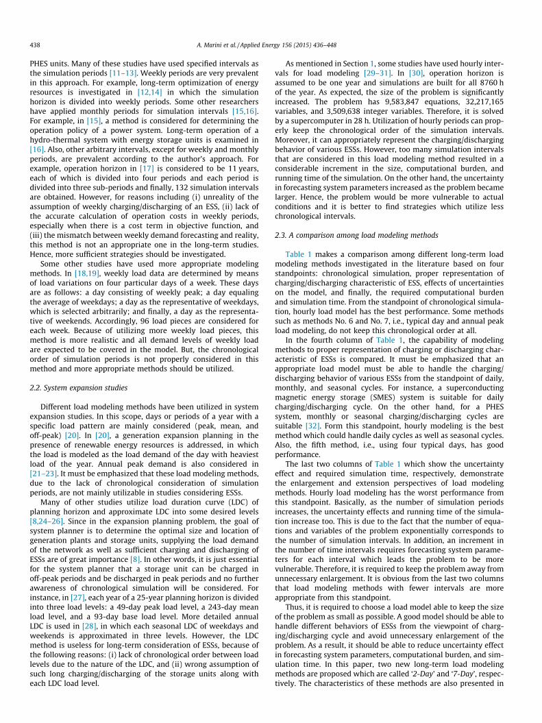
3.1. ‘2 day-14 piece’ model

In the first proposed method, each week is modeled as an equiv-alent weekend and weekday. The equivalent weekday is obtainedby averaging five weekdays, from Monday to Friday, and the equiv-alent weekend is calculated by averaging the weekends, Saturdayand Sunday. Therefore, the duration of equivalent weekday andequivalent weekend are 120 and 48 h, respectively. In the nextstep, each average day is approximated with seven chronologicalload pieces, as mentioned in previous subsection (7-piece approxi-mation). Then, the duration of each load piece is multiplied by 5 forthe equivalent weekday and by 2 for the equivalent weekend,which results in the ‘2 day-14 piece’ model.

Approximation of the week with two equivalent periods issimilar to the method used in [18,19] and considering the durationof each day is similar to the method used in [27,35]. Weekly loadcurve of ‘2 day-14 piece’ model for a typical week of the year ispresented in Fig. 3.

1 2 3 4 5 60.4

0.5

0.6

0.7

0.8

0.9

Sebp

p. u

.

"2 days-14

EquivalentWeekday

120hours

Fig. 3. Two-day model with consider

20 40 60 800.4

0.5

0.6

0.7

0.8

0.9

wee

p. u

.

"7 days-35 pie

Weekly Load Demand

Fig. 4. Weekly load model with d

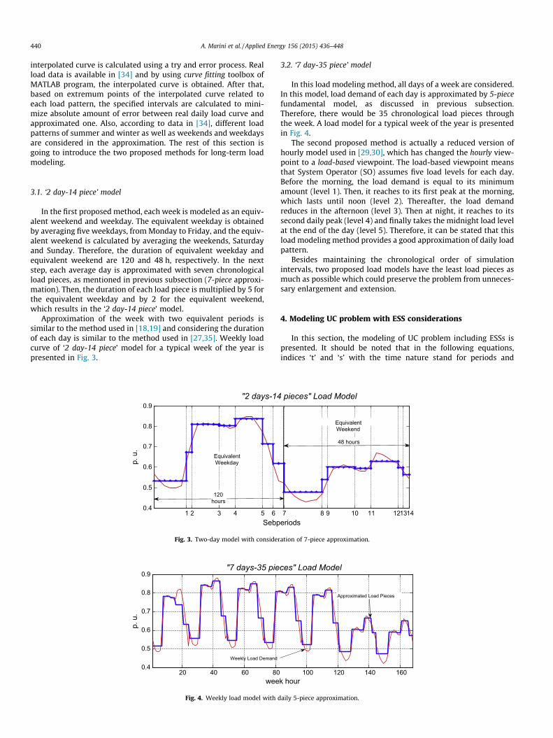
3.2. ‘7 day-35 piece’ model

In this load modeling method, all days of a week are considered.In this model, load demand of each day is approximated by 5-piecefundamental model, as discussed in previous subsection.Therefore, there would be 35 chronological load pieces throughthe week. A load model for a typical week of the year is presentedin Fig. 4.

The second proposed method is actually a reduced version ofhourly model used in [29,30], which has changed the hourly view-point to a load-based viewpoint. The load-based viewpoint meansthat System Operator (SO) assumes five load levels for each day.Before the morning, the load demand is equal to its minimumamount (level 1). Then, it reaches to its first peak at the morning,which lasts until noon (level 2). Thereafter, the load demandreduces in the afternoon (level 3). Then at night, it reaches to itssecond daily peak (level 4) and finally takes the midnight load levelat the end of the day (level 5). Therefore, it can be stated that thisload modeling method provides a good approximation of daily loadpattern.

Besides maintaining the chronological order of simulationintervals, two proposed load models have the least load pieces asmuch as possible which could preserve the problem from unneces-sary enlargement and extension.

4. Modeling UC problem with ESS considerations

In this section, the modeling of UC problem including ESSs ispresented. It should be noted that in the following equations,indices ‘t’ and ‘s’ with the time nature stand for periods and

7 8 9 10 11 121314eriods

pieces" Load Model

EquivalentWeekend

48 hours

ation of 7-piece approximation.

100 120 140 160k hour

ces" Load Model

Approximated Load Pieces

aily 5-piece approximation.

A. Marini et al. / Applied Energy 156 (2015) 436–448 441

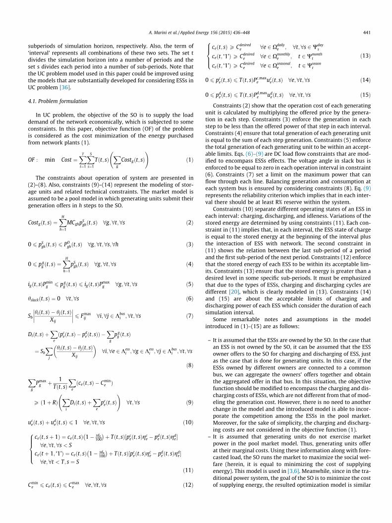
subperiods of simulation horizon, respectively. Also, the term of‘interval’ represents all combinations of these two sets. The set tdivides the simulation horizon into a number of periods and theset s divides each period into a number of sub-periods. Note thatthe UC problem model used in this paper could be improved usingthe models that are substantially developed for considering ESSs inUC problem [36].

4.1. Problem formulation

In UC problem, the objective of the SO is to supply the loaddemand of the network economically, which is subjected to someconstraints. In this paper, objective function (OF) of the problemis considered as the cost minimization of the energy purchasedfrom network plants (1).

OF : min Cost ¼XT

t¼1

XS

s¼1

Tðt; sÞX

g

Costgðt; sÞ !

ð1Þ

The constraints about operation of system are presented in(2)–(8). Also, constraints (9)–(14) represent the modeling of stor-age units and related technical constraints. The market model isassumed to be a pool model in which generating units submit theirgeneration offers in h steps to the SO.

Costgðt; sÞ ¼XH

h¼1

MCghpSghðt; sÞ 8g;8t;8s ð2Þ

0 6 pSghðt; sÞ 6 PO

ghðt; sÞ 8g;8t;8s;8h ð3Þ

0 6 p gg ðt; sÞ ¼

XH

h¼1

pSghðt; sÞ 8g;8t;8s ð4Þ

igðt; sÞPming 6 p g

g ðt; sÞ 6 igðt; sÞPmaxg 8g;8t;8s ð5Þ

hslackðt; sÞ ¼ 0 8t;8s ð6Þ

Sbhiðt; sÞ � hjðt; sÞ

Xij

�������� 6 Fmax

ij 8i;8j 2 Kbusi ;8t;8s ð7Þ

Diðt; sÞ þX

e

ðpceðt; sÞ � pd

eðt; sÞÞ �X

g

pgg ðt; sÞ

¼ Sb

Xj

hiðt; sÞ � hjðt; sÞXij

� �8i;8e 2 Kess

i ;8g 2 Kessi ;8j 2 Kbus

i ;8t;8s

ð8Þ

Xg

Pmaxg þ 1

Tðt; sÞX

e

ðceðt; sÞ � Cmine Þ

P ð1þ RÞX

i

Diðt; sÞ þX

e

pceðt; sÞ

!8t;8s ð9Þ

uceðt; sÞ þ ud

eðt; sÞ 6 1 8e;8t;8s ð10Þ

ceðt; sþ 1Þ ¼ ceðt; sÞ 1� sde100

� �þ Tðt; sÞ½pc

eðt; sÞgce � pd

eðt; sÞgde �

8e;8t;8s < S

ceðt þ 1; ‘1’Þ ¼ ceðt; sÞ 1� sde100

� �þ Tðt; sÞ½pc

eðt; sÞgce � pd

eðt; sÞgde �

8e;8t < T; s ¼ S

8>>><>>>:

ð11Þ

Cmine 6 ceðt; sÞ 6 Cmax

e 8e;8t;8s ð12Þ

ceðt; sÞP Cdesirede 8e 2 Xdaily

e ; 8t;8s 2 Wdays

ceðt; ‘1’ÞP Cdesirede 8e 2 Xmonthly

e ; t 2 Wmontht

ceðt; ‘1’ÞP Cdesirede 8e 2 Xseasonal

e ; t 2 Wseaont

8>><>>: ð13Þ

0 6 pceðt; sÞ 6 Tðt; sÞPc;max

e uceðt; sÞ 8e;8t;8s ð14Þ

0 6 pdeðt; sÞ 6 Tðt; sÞPd;max

e udeðt; sÞ 8e;8t;8s ð15Þ

Constraints (2) show that the operation cost of each generatingunit is calculated by multiplying the offered price by the genera-tion in each step. Constraints (3) enforce the generation in eachstep to be less than the offered power of that step in each interval.Constraints (4) ensure that total generation of each generating unitis equal to the sum of each step generation. Constraints (5) enforcethe total generation of each generating unit to be within an accept-able limits. Eqs. (6)–(9) are DC load flow constraints that are mod-ified to encompass ESSs effects. The voltage angle in slack bus isenforced to be equal to zero in each operation interval in constraint(6). Constraints (7) set a limit on the maximum power that canflow through each line. Balancing generation and consumption ateach system bus is ensured by considering constraints (8). Eq. (9)represents the reliability criterion which implies that in each inter-val there should be at least R% reserve within the system.

Constraints (10) separate different operating states of an ESS ineach interval: charging, discharging, and idleness. Variations of thestored energy are determined by using constraints (11). Each con-straint in (11) implies that, in each interval, the ESS state of chargeis equal to the stored energy at the beginning of the interval plusthe interaction of ESS with network. The second constraint in(11) shows the relation between the last sub-period of a periodand the first sub-period of the next period. Constraints (12) enforcethat the stored energy of each ESS to be within its acceptable lim-its. Constraints (13) ensure that the stored energy is greater than adesired level in some specific sub-periods. It must be emphasizedthat due to the types of ESSs, charging and discharging cycles aredifferent [20], which is clearly modeled in (13). Constraints (14)and (15) are about the acceptable limits of charging anddischarging power of each ESS which consider the duration of eachsimulation interval.

Some remarkable notes and assumptions in the modelintroduced in (1)–(15) are as follows:

– It is assumed that the ESSs are owned by the SO. In the case thatan ESS is not owned by the SO, it can be assumed that the ESSowner offers to the SO for charging and discharging of ESS, justas the case that is done for generating units. In this case, if theESSs owned by different owners are connected to a commonbus, we can aggregate the owners’ offers together and obtainthe aggregated offer in that bus. In this situation, the objectivefunction should be modified to encompass the charging and dis-charging costs of ESSs, which are not different from that of mod-eling the generation cost. However, there is no need to anotherchange in the model and the introduced model is able to incor-porate the competition among the ESSs in the pool market.Moreover, for the sake of simplicity, the charging and discharg-ing costs are not considered in the objective function (1).

– It is assumed that generating units do not exercise marketpower in the pool market model. Thus, generating units offerat their marginal costs. Using these information along with fore-casted load, the SO runs the market to maximize the social wel-fare (herein, it is equal to minimizing the cost of supplyingenergy). This model is used in [3,6]. Meanwhile, since in the tra-ditional power system, the goal of the SO is to minimize the costof supplying energy, the resulted optimization model is similar

Table 2Load scenarios.

Scenario Periods set Sub-period set Total intervals

Hourly t = 1, . . . , 52 s = 1, . . . , 168 8736Four s = 1, . . . , 96 4992Two s = 1, . . . , 14 728Seven s = 1, . . . , 35 1820

Table 3ESS characteristics.

No Type Bus Cmine

(MW h)Cmax

e

(MW h)Pc;max

e

(MW)sde

(%)Cdesired

e

(MW h)

1 CAES 1 5 290 10 4 502 CAES 16 2 110 4 4 353 BESS (Lead-Acid) 23 2 40 5 1 254 BESS (Lead-Acid) 15 2 40 5 1 255 BESS (NaS) 13 4 64 4.5 0.01 306 BESS (NaS) 18 4 64 4.5 0.01 307 PHESS 22 50 200 20 5 1108 PHESS 7 50 250 25 5 110

442 A. Marini et al. / Applied Energy 156 (2015) 436–448

to that of introduced in this paper. Therefore, the proposedmodel can be used in both traditional and competitiveenvironment.

– The start-up and shout-down costs as well as the minimumdown-time and minimum up-time constraints are not consid-ered in this model. However, the minimum allowable genera-tion of each generating unit is not zero (as shown in (5)). Thebinary variable ig(t) forces the power generated by a generatingunit to be zero when it is needed. Therefore, the model is able tofind the optimal decision.

– In the proposed model, incremental and decremental ramp rateconstraints of generating units are not considered. Moreover,only up-ward reserve constraint is considered in (9). Theamount of each daily load piece is generally greater than thesummation of minimum allowable generation of all generatingunits. By imposing the reserve constraint, the summation of theavailable capacities must be greater than the load piece in eachsub-period multiplied by the factor of (1 + R)%. Consequently,the summation of the available capacities is greater than thesummation of minimum allowable generation of all generatingunits. Therefore, the down-ward reserve constraint is also con-sidered inherently.

– It should be noted that considering equalities in (11) andinequalities in (13), make all the sub-periods in the study hori-zon depend on each other. In other words, these constraintswhich arise from considering ESSs in the long-term UC problem,reveal the necessity of chronological consideration ofsimulation intervals. From the optimization point of view, theoptimization problem ((1)-(15)) cannot be inherently decom-posed to independent optimization subproblems (e.g. monthlyones), due to dependent simulation intervals. Therefore,utilizing decomposition techniques to mitigate the requiredcomputational burden in solving the problem may result insome inaccuracies.

4.2. Load models

In Table 1, the hourly load model and the four day models, werementioned as the most appropriate models. In addition, two loadmodels were proposed in Section 3. Therefore, four load scenariosare considered as follows:

Hourly: In this scenario, all hours of simulation horizon areconsidered in the model. Hence, the set t which stands forsimulation periods is defined as the weeks of the year and equalsto t = 1, . . . , 52. In addition, the set of sub-periods, s, is defined asthe hours of the week and is equal to s = 1, . . . , 168. Therefore,the duration of each interval is one hour. This scenario isconsidered to be the precise model and all other scenarios wouldbe compared with this base model.

Four: This scenario is as the method No. 5 which was previouslymentioned in Table 1. Four typical days which are considered asfollows: Monday, Tuesday (containing weekly load peak), the daywhich is the average of weekdays from Monday to Friday, andfinally the day which is the average of weekends, i.e. Saturdayand Sunday. The set t is similar to that of scenario Hourly and theset s is defined as s = 1, . . . , 96, which consequently leads to 4992(=96 � 52) simulation intervals.

Two: This model is the first proposed model which was named‘2 day-14 piece’ model. The set of sub-periods in this scenario isdefined as s = 1, . . . , 14 and the set of periods is similar to that ofscenario Hourly.

Seven: This scenario is actually the second proposed methodwhich has been named ‘7 day-35 piece’ model. The set ofsub-periods in this scenario is defined as s = 1, . . . , 35 and the setof periods is similar to that of scenario Hourly. The model includes

five chronological load pieces for each day. Therefore, total numberof simulation intervals is 35 � 52 = 1820 intervals.

Table 2 provides a summary of load scenarios.

5. Case study and simulation results

This section describes case studies and provides the simulationresults. The model is tested on IEEE 24-bus RTS [34] and IEEE118-bus test system [37]. One year is considered as the operationhorizon. Generating units offer in 3 steps to the SO. Maximumamounts of offered powers and prices are calculated via data in[34]. Finally, at least 10% reserve must be available in each simula-tion interval.

Eight ESSs [38–40] are added to the system as listed in Table 3.The ESSs are owned by the SO and are dispatched according to theSO requirements. The First two ESSs are of compressed energy stor-age (CAES) type, the next four are of battery energy storage (BES)type, and the last two ones are of PHES type. The minimum storedenergy of each ESS is assumed to be a desired level at specific peri-ods and sub-periods; i.e., at the beginning of each month for CAES,at the beginning of each week for BES, and at the beginning of eachseason for PHES. The desired level of minimum stored energy ineach ESS is equal to the initial energy level at the beginning ofthe year.

Since the purpose of this paper is to make a comparison amongvarious long-term load modeling methods, no uncertainty is con-sidered in the model. The model is implemented using CPLEX[41] under GAMS [42] software on a personal computer equippedwith a core-i5 processor clocking at 2.93 GHz with 4 GB of RAM.

5.1. Results of IEEE 24-bus RTS

Table 4 shows the simulation results obtained for different loadscenarios. The first row shows the number of binary variables. Thescenario Hourly (called base scenario) has the maximum number ofbinary variables with 349,400 variables, which is mainly due to thelarge number of simulation intervals. In comparison with scenarioHourly, scenarios Four, Seven and Two have just 57%, 20%, and 8%binary variables, respectively. This reduction leads to a decreasein the simulation time, which is observed in the next row of thetable. The program requires a simulation time of more than 2 hto find the solution in the base scenario. For other scenarios, thesimulation time is just equal to 33.1%, 2.3%, and 0.5% of that of

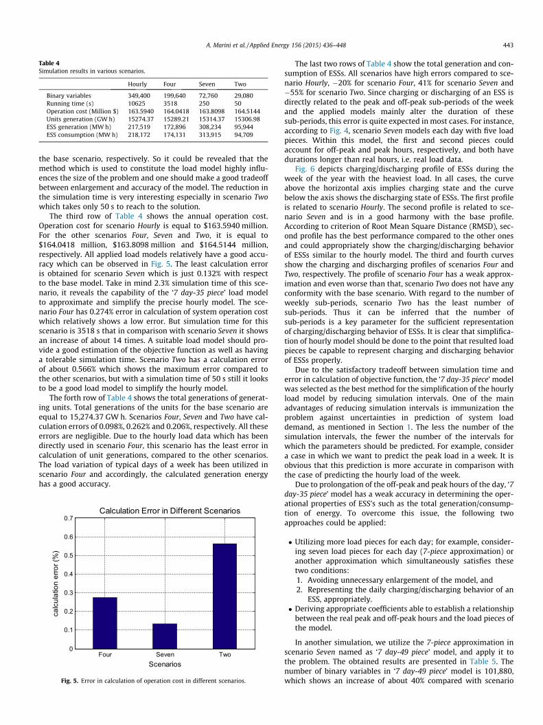
Table 4Simulation results in various scenarios.

Hourly Four Seven Two

Binary variables 349,400 199,640 72,760 29,080Running time (s) 10625 3518 250 50Operation cost (Million $) 163.5940 164.0418 163.8098 164.5144Units generation (GW h) 15274.37 15289.21 15314.37 15306.98ESS generation (MW h) 217,519 172,896 308,234 95,944ESS consumption (MW h) 218,172 174,131 313,915 94,709

A. Marini et al. / Applied Energy 156 (2015) 436–448 443

the base scenario, respectively. So it could be revealed that themethod which is used to constitute the load model highly influ-ences the size of the problem and one should make a good tradeoffbetween enlargement and accuracy of the model. The reduction inthe simulation time is very interesting especially in scenario Twowhich takes only 50 s to reach to the solution.

The third row of Table 4 shows the annual operation cost.Operation cost for scenario Hourly is equal to $163.5940 million.For the other scenarios Four, Seven and Two, it is equal to$164.0418 million, $163.8098 million and $164.5144 million,respectively. All applied load models relatively have a good accu-racy which can be observed in Fig. 5. The least calculation erroris obtained for scenario Seven which is just 0.132% with respectto the base model. Take in mind 2.3% simulation time of this sce-nario, it reveals the capability of the ‘7 day-35 piece’ load modelto approximate and simplify the precise hourly model. The sce-nario Four has 0.274% error in calculation of system operation costwhich relatively shows a low error. But simulation time for thisscenario is 3518 s that in comparison with scenario Seven it showsan increase of about 14 times. A suitable load model should pro-vide a good estimation of the objective function as well as havinga tolerable simulation time. Scenario Two has a calculation errorof about 0.566% which shows the maximum error compared tothe other scenarios, but with a simulation time of 50 s still it looksto be a good load model to simplify the hourly model.

The forth row of Table 4 shows the total generations of generat-ing units. Total generations of the units for the base scenario areequal to 15,274.37 GW h. Scenarios Four, Seven and Two have cal-culation errors of 0.098%, 0.262% and 0.206%, respectively. All theseerrors are negligible. Due to the hourly load data which has beendirectly used in scenario Four, this scenario has the least error incalculation of unit generations, compared to the other scenarios.The load variation of typical days of a week has been utilized inscenario Four and accordingly, the calculated generation energyhas a good accuracy.

Four Seven Two0

0.1

0.2

0.3

0.4

0.5

0.6

0.7

Scenarios

calc

ulat

ion

erro

r (%

)

Calculation Error in Different Scenarios

Fig. 5. Error in calculation of operation cost in different scenarios.

The last two rows of Table 4 show the total generation and con-sumption of ESSs. All scenarios have high errors compared to sce-nario Hourly, �20% for scenario Four, 41% for scenario Seven and�55% for scenario Two. Since charging or discharging of an ESS isdirectly related to the peak and off-peak sub-periods of the weekand the applied models mainly alter the duration of thesesub-periods, this error is quite expected in most cases. For instance,according to Fig. 4, scenario Seven models each day with five loadpieces. Within this model, the first and second pieces couldaccount for off-peak and peak hours, respectively, and both havedurations longer than real hours, i.e. real load data.

Fig. 6 depicts charging/discharging profile of ESSs during theweek of the year with the heaviest load. In all cases, the curveabove the horizontal axis implies charging state and the curvebelow the axis shows the discharging state of ESSs. The first profileis related to scenario Hourly. The second profile is related to sce-nario Seven and is in a good harmony with the base profile.According to criterion of Root Mean Square Distance (RMSD), sec-ond profile has the best performance compared to the other onesand could appropriately show the charging/discharging behaviorof ESSs similar to the hourly model. The third and fourth curvesshow the charging and discharging profiles of scenarios Four andTwo, respectively. The profile of scenario Four has a weak approx-imation and even worse than that, scenario Two does not have anyconformity with the base scenario. With regard to the number ofweekly sub-periods, scenario Two has the least number ofsub-periods. Thus it can be inferred that the number ofsub-periods is a key parameter for the sufficient representationof charging/discharging behavior of ESSs. It is clear that simplifica-tion of hourly model should be done to the point that resulted loadpieces be capable to represent charging and discharging behaviorof ESSs properly.

Due to the satisfactory tradeoff between simulation time anderror in calculation of objective function, the ‘7 day-35 piece’ modelwas selected as the best method for the simplification of the hourlyload model by reducing simulation intervals. One of the mainadvantages of reducing simulation intervals is immunization theproblem against uncertainties in prediction of system loaddemand, as mentioned in Section 1. The less the number of thesimulation intervals, the fewer the number of the intervals forwhich the parameters should be predicted. For example, considera case in which we want to predict the peak load in a week. It isobvious that this prediction is more accurate in comparison withthe case of predicting the hourly load of the week.

Due to prolongation of the off-peak and peak hours of the day, ‘7day-35 piece’ model has a weak accuracy in determining the oper-ational properties of ESS’s such as the total generation/consump-tion of energy. To overcome this issue, the following twoapproaches could be applied:

� Utilizing more load pieces for each day; for example, consider-ing seven load pieces for each day (7-piece approximation) oranother approximation which simultaneously satisfies thesetwo conditions:1. Avoiding unnecessary enlargement of the model, and2. Representing the daily charging/discharging behavior of an

ESS, appropriately.� Deriving appropriate coefficients able to establish a relationship

between the real peak and off-peak hours and the load pieces ofthe model.

In another simulation, we utilize the 7-piece approximation inscenario Seven named as ‘7 day-49 piece’ model, and apply it tothe problem. The obtained results are presented in Table 5. Thenumber of binary variables in ‘7 day-49 piece’ model is 101,880,which shows an increase of about 40% compared with scenario

20 40 60 80 100 120 140 160-100

0

100

Hou

rly

Charge and Discharge Profiles of ESS for Each Scenario

5 10 15 20 25 30 35-100

0100

Seve

n

10 20 30 40 50 60 70 80 90-100

0

100

Four

2 4 6 8 10 12 14-100

0

100

Subperiods

Two

Fig. 6. Charge and discharge profiles of ESSs in various scenarios.

Table 5Results for ‘7 day-49 piece’ load model.

Binary variables 101,880 Unit generations (GW h) 15307.43Simulation time (s) 750 ESS generation (MW h) 295,069Operation cost (M$) 163.5569 ESS consumption (MW h) 296,982

444 A. Marini et al. / Applied Energy 156 (2015) 436–448

Seven, and the simulation time increases by 300% as a result. Asexpected, the error in charging and discharging behavior of ESSsis reduced (an error of 35%), which is the result of using more loadpieces to approximate the hourly loads.

5.2. Different daily load pieces

It has been shown that the proposed load models have a goodcapability to simplify the precise hourly load model. But the ques-tion is that how the number of load pieces considered for each day,can affect the results? In this subsection we change the number ofdaily load pieces and provide the results.

Table 6 shows the results attained for different daily loadpieces. We bring the results for 3-piece, 5-piece, 7-piece, 9-piece,11-piece, 16-piece, 20-piece, and 24-piece (hourly) load models.These load models are demonstrated in Figs. 7–13. The 3-pieceload model is also considered in simulations to make a better com-parison among different daily load pieces. The first row of Table 6shows the objective function value, considering different loadpieces. Also, Fig. 14 provides a graphical representation of the cal-culation error of different models. The calculation error in 3-pieceload model is about 2.5% which is very high. The ‘7 day-35 piece’model determines the objective function with a good accuracyand an acceptable calculation error (about +0.132%). Of course, itcould be generally deduced from Fig. 14 that all errors are negligi-ble, but as the daily load pieces increase, the calculation error of

Table 6Output for different daily piece load models.

Daily load pieces 3-piece 5-piece 7-piece 9

OF (million $) 159.7200 163.8098 163.5569 1Binary variables 43,640 72,800 101,880 1Simulation time (s) 150 250 750 8Charge hours (h) 46,759 44,208 51,088 4Disch. hours (h) 23,129 25,680 18,800 2Power gener. (GW h) 15048.35 15314.37 15307.43 1

operation cost decreases very slightly. However, this reduction incalculation error must be evaluated while considering the simula-tion time.

The second and third rows of Table 6 shows the binary variablesand simulation time, respectively. An exponential increment in thesimulation time with respect to the number of daily load pieces isobserved in Fig. 15 in which the ratio of the simulation time ofemploying different load pieces to that of the hourly load modelis presented. A proper chronological long-term load model shouldbe able to make a compromise between the simulation time andthe computational accuracy. The ‘7 day- 35 piece’ model is the bestmodel among all, because it has an acceptable calculation error andlow simulation time. On one hand, good performance of this modelmight be a result of the fact that ‘double peak’ nature of a daily loaddemand has been modeled with five chronological daily loadpieces. On the other hand, the five-piece approximation is the loadmodel with the least pieces that could cover the two peak partsand a shoulder part in between and also two low first and last partsof daily load curve, as mentioned in Section 2. The ‘7 day-49 piece’model has also a short simulation time compared to the other loadmodels with more pieces. Furthermore, the calculation error of thisload model is very low (about 0.022%). But in comparison with ‘7day-35 piece’ model, this load model takes three times more timeto find the solution. Now, one should make a trade-off betweenthe few reduction in OF (about 0.11%) and the 300% increment inthe simulation time. In large systems, the simulation time is a moreimportant factor.

The fourth and fifth rows of Table 6 shows the charging and dis-charging hours of ESSs. Also, Fig. 16 depicts the ratio of charginghours to that of the hourly model, considering different load mod-els. The ESS interactions of 7-piece and 16-piece load models showthe closest approximation to the hourly model. The ‘7 day-35 piece’

-piece 11-piece 16-piece 20-piece 24-piece

63.3540 163.4459 164.1797 163.3286 163.594031,000 160,160 232,920 2,911,160 349,40090 1564 4680 5165 10,7568,185 47,258 42,278 46,511 43,0611,703 22,630 26,570 23,377 26,8275274.57 15276.34 15264.47 15271.68 15274.37

5 10 15 20

90

100

110

120

130

140

150

160

170

hour

typical weekday

load

dem

and

5 10 15 2080

90

100

110

120

130

hour

typical weekend

load

dem

and

Fig. 7. Three-piece daily load approximation.

5 10 15 20

90

100

110

120

130

140

150

160

170

hour

typical weekday

load

dem

and

5 10 15 20

80

90

100

110

120

130

hour

typical weekend

load

dem

and

Fig. 8. Five-piece daily load approximation.

5 10 15 20

90

100

110

120

130

140

150

160

170

hour

typical weekday

load

dem

and

5 10 15 20

80

90

100

110

120

130

hour

typical weekend

load

dem

and

Fig. 9. Seven-piece daily load approximation.

A. Marini et al. / Applied Energy 156 (2015) 436–448 445

model has the best estimation of the ESS charging and discharginghours. Finally the last row of Table 6 shows the generation of gen-erating units. All applied load models relatively have a goodapproximation of unit generations.

5.3. Results of IEEE 118-bus system

The applicability of the ‘7 day-35 piece’ model is also examinedon IEEE 188-bus system [37]. Hourly coefficients of [34] are appliedto 118-bus test system to constitute the load pattern over a one

year horizon. For the sake of simplicity, generators offer only inone step. Three simulation cases are run for the two scenariosHourly and Seven presented previously in Table 2.

Table 7 shows the obtained results for different cases. In thefirst case, the network is not taken into account and all generators,ESSs, and loads are assumed to be connected to a single bus. In thiscase, when considering hourly model, an operation cost of$376.6186 million is achieved and the simulation time is about1049 s. The ‘7 day-35 piece’ model with a simulation time of 15%of the base model, calculates the operation cost with an error of

5 10 15 20

90

100

110

120

130

140

150

160

170

hour

typical weekday

load

dem

and

5 10 15 20

80

90

100

110

120

130

hour

typical weekend

load

dem

and

Fig. 10. Nine-piece daily load approximation.

5 10 15 20

90

100

110

120

130

140

150

160

170

hour

typical weekday

load

dem

and

5 10 15 20

80

90

100

110

120

130

hour

typical weekend

load

dem

and

Fig. 11. Eleven-piece daily load approximation.

5 10 15 20

90

100

110

120

130

140

150

160

170

hour

typical weekday

load

dem

and

5 10 15 20

80

90

100

110

120

130

hour

typical weekend

load

dem

and

Fig. 12. Sixteen-piece daily load approximation.

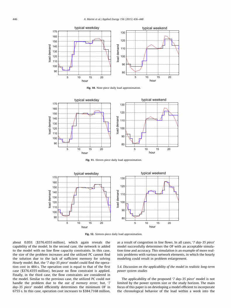
446 A. Marini et al. / Applied Energy 156 (2015) 436–448

about 0.05% ($376.4355 million), which again reveals thecapability of the model. In the second case, the network is addedto the model with no line flow capacity constraints. In this case,the size of the problem increases and the utilized PC cannot findthe solution due to the lack of sufficient memory for solvingHourly model. But, the ‘7 day-35 piece’ model could find the opera-tion cost in 484 s. The operation cost is equal to that of the firstcase ($376.4355 million), because no flow constraint is applied.Finally, in the third case, the flow constraints are considered inthe model. Similar to the previous case, the utilized PC could nothandle the problem due to the out of memory error; but, ‘7day-35 piece’ model efficiently determines the minimum OF in6755 s. In this case, operation cost increases to $384.7168 million,

as a result of congestion in line flows. In all cases, ‘7 day-35 piece’model successfully determines the OF with an acceptable simula-tion time and accuracy. This simulation is an example of more real-istic problems with various network elements, in which the hourlymodeling could result in problem enlargement.

5.4. Discussion on the applicability of the model in realistic long-termpower system studies

The applicability of the proposed ‘7 day-35 piece’ model is notlimited by the power system size or the study horizon. The mainfocus of this paper is on developing a model efficient to incorporatethe chronological behavior of the load within a week into the

5 10 15 20

90

100

110

120

130

140

150

160

170

hour

typical weekday

load

dem

and

5 10 15 20

80

90

100

110

120

130

hour

typical weekend

load

dem

and

Fig. 13. Twenty-piece daily load approximation.

5 10 15 20 250

0.5

1

1.5

2

2.5

3

3.5

4

Daily load pieces

%

Calculation Error in OF Over Daily Load Pieces

Fig. 14. Calculation error in determination of problem OF versus daily load pieces.

0 5 10 15 20 25

1000

2000

3000

4000

5000

6000

7000

8000

9000

10000

load pieces

runn

ing

time

(sec

)

Running Time in Different Load Pieces

Fig. 15. Simulation time versus daily load pieces.

0 5 10 15 20 250.8

0.85

0.9

0.95

1

1.05

1.1

1.15

daily load pieces

ratio

to h

ourly

mod

el

Ratio of Charging Hours of ESSs to The Hourly Model

Fig. 16. Charging hours of ESSs in different daily load pieces.

Table 7Output for 118-bus system.

Scenarios

Hourly Seven

Case Simulationtime (s)

OF ($) Simulationtime (s)

OF ($)

No network 1049 376.6186 165 376.4355Network in, no flow

constraintOut of memory 484 376.4355

Network in, includeflow constraint

Out of memory 8682 384.7168

A. Marini et al. / Applied Energy 156 (2015) 436–448 447

long-term power system studies. The numerical results showedthat a compromise between the simulation time and the solutionaccuracy would be available by considering ‘7 day-35 piece’ modelfor each week. Also, it was shown that over a one year horizon inwhich the weeks are in chronological order, this model can be

efficient in UC studies. In the case that a longer study horizon ora realistic power system is considered, the simulation time willincrease due to the large number of the binary variables.Moreover, considering all weeks over a long-term horizon (e.g., a10-year horizon which results in almost 520 weeks) is notjustifiable. Therefore, in such cases, the representative weeks ofthe simulation horizon can be studied, as it is prevalent in tradi-tional long-term studies. For example, every month over the studyhorizon could be modeled by a representative week (reducing thenumber of simulation weeks to 120 in a 10-year study horizon), orevery season could be modeled by a representative week (reducingthe number of simulation weeks to 40 in a 10-year study).However, the incorporation of the chronological behavior of the

448 A. Marini et al. / Applied Energy 156 (2015) 436–448

load within a week in the long-term power system studies, whichis the main goal of this paper, is still preserved. Moreover, utilizing‘7 day-35 piece’ model is practical.

6. Conclusion

Energy storage systems are new energy resources that have asignificant role in the future smart power systems. In this paper,a review of the current approaches of load modeling inlong-term system studies was presented and two new methodswere proposed which could successfully incorporate the chrono-logical behavior of the load in long-term studies. Long-term loadmodels were used in a typical UC problem and solved for standardtest systems. The ‘7 day-35 piece’ model with a reduction in thenumber of binary variables of the problem could significantlyreduce the simulation time. Furthermore, it could precisely calcu-late the operation cost of the system as well as the total generationof the generating units throughout the study horizon. A sensitivityanalysis revealed that the selection of more load pieces to studythe chronological order of the daily load pattern could notsignificantly improve the calculation accuracy and just results ina significant increase in the simulation time. Therefore, the pro-posed model provides a key approach for load modeling in powersystem studies such as operation planning, expansion planning,and maintenance scheduling, when chronological considerationof simulation intervals is needed.

References

[1] Han S, Han S, Sezaki K. Development of an optimal vehicle-to-grid aggregatorfor frequency regulation. IEEE Trans Smart Grid 2010;1:65–72.

[2] Shafie-khah M, Parsa Moghaddam M, Sheikh-El-Eslami MK, Rahmani-AndebiliM. Modeling of interactions between market regulations and behavior of plug-in electric vehicle aggregators in a virtual power market environment. Energy2012;40:139–50.

[3] Kristoffersen TK, Capion K, Meibom P. Optimal charging of electric drivevehicles in a market environment. Appl Energy 2011;88:1940–8.

[4] Luo X, Wang J, Dooner M, Clarke J. Overview of current development inelectrical energy storage technologies and the application potential in powersystem operation. Appl Energy 2015;137:511–36.

[5] Fadaeenejad M, Saberian AM, Fadaee M, Radzi MAM, Hizam H, AbKadir MZA.The present and future of smart power grid in developing countries. RenewSustain Energy Rev 2014;29:828–34.

[6] Chen S, Gooi HB, Wang M. Sizing of energy storage for microgrids. IEEE TransSmart Grid 2012;3:142–51.

[7] Nordlund P, Sjelvgren D, Pereira M, Bubenko J. Generation expansion planningfor systems with a high share of hydro power. IEEE Trans Power Syst1987;2:161–7.

[8] Finger S. Electric-power-system production costing and reliability analysisincluding hydroelectric, storage, and time-dependent power plants.Massachusetts inst of tech. Cambridge (USA). Energy Lab.; 1979.

[9] Tsoi E, Wong K. Artificial intelligence algorithms for short term scheduling ofthermal generators and pumped-storage. In: IEE Proc, gener, transm distrib;1997. IET.

[10] Das T, Krishnan V, McCalley JD. Assessing the benefits and economicsof bulk energy storage technologies in the power grid. Appl Energy 2015;139:104–18.

[11] Helseth A, Warland G, Mo B. Long-term hydro-thermal scheduling includingnetwork constraints. In: 7th Int conf Eur Energy Market (EEM); 2010. IEEE.

[12] Christoforidis M, Aganagic M, Awobamise B, Tong S, Rahimi A. Long-term/mid-term resource optimization of a hydrodominant power system using interiorpoint method. IEEE Trans Power Syst 1996;11:287–94.

[13] Siahkali H. Wind farm and pumped storage integrated in generationscheduling using PSO. In: 16th Int conf intell syst appl power syst (ISAP);2011. IEEE.

[14] Nürnberg R, Römisch W. A two-stage planning model for power scheduling ina hydro-thermal system under uncertainty. Optim Eng 2002;3:355–78.

[15] Turgeon A. A decomposition method for the long-term scheduling of reservoirsin series. Water Resour Res 1981;17:1565–70.

[16] da Cruz Jr G, Soares S. Non-uniform composite representation hydroelectricsystems for long-term hydrothermal scheduling. IEEE Trans Power Syst1996;11:702–7.

[17] Ventosa M, Denis R, Redondo C. Expansion planning in electricity markets.Two different approaches. In: Proc of 14th PSCC; 2002. Sevilla.

[18] Bernard P, Dopazo J, Stagg G. A method for economic scheduling of a combinedpumped hydro and steam generating system. IEEE Trans Power Appar Syst1964;83:23–30.

[19] Galloway C, Ringlee R. An investigation of pumped storage scheduling. IEEETrans Power Appar Syst 1966;PA S-85:459–65.

[20] Ter-Gazarian A, Kagan N. Design model for electrical distribution systemsconsidering renewable, conventional and energy storage units. In: IEE Proc,gener, transm distrib; 1992. IET.

[21] Farghal S, Abdel Aziz M. Generation expansion planning including therenewable energy sources. IEEE Trans Power Syst 1988;3:816–22.

[22] Cai Y, Huang G, Yang Z, Lin Q, Tan Q. Community-scale renewable energysystems planning under uncertainty—an interval chance-constrainedprogramming approach. Renew Sustain Energy Rev 2009;13:721–35.

[23] Celli G, Soma GG, Pilo F, Ghiani E, Cicoria R, Corti S. Comparison of planningalternatives for active distribution networks. In: Integr renew into distrib grid,CIRED Workshop; 2012. IET.

[24] Palmintier B, Webster M. Impact of unit commitment constraints ongeneration expansion planning with renewables. In: IEEE power energy socgen meet; 2011. IEEE.

[25] Foley AM, Leahy PG, Li K, McKeogh EJ, Morrison AP. A long-term analysis ofpumped hydro storage to firm wind power. Appl Energy 2015;137:638–48.

[26] Kelman MPNCR. Long-term hydro scheduling based on stochastic models.EPSOM 1998;98:23–5.

[27] Bakken BH, Skjelbred HI, Wolfgang O. ETransport: investment planning inenergy supply systems with multiple energy carriers. Energy2007;32:1676–89.

[28] Yasuda K, Nishiya K, Hasegawa J, Yokoyama R. Optimal generation expansionplanning with electric energy storage systems. In: Ind electron soc proc, 14annu conf.; 1988.

[29] Kandil M, Farghal S, Hasanin N. Economic assessment of energy storageoptions in generation expansion planning. In: IEE proc, gener, transm distrib;1990. IET.

[30] Baslis CG, Bakirtzis AG. Mid-term stochastic scheduling of a price-maker hydroproducer with pumped storage. IEEE Trans Power Syst 2011;26:1856–65.

[31] Celli G, Mocci S, Pilo F, Loddo M. Optimal integration of energy storage indistribution networks. In: PowerTech IEEE; 2009. Bucharest; IEEE.

[32] Weems C, Headington MR. Programming and problem solving with C++. Jones& Bartlett Learning; 1998.

[33] Conejo AJ, García-Bertrand R, Díaz-Salazar M. Generation maintenancescheduling in restructured power systems. IEEE Trans Power Syst2005;20:984–92.

[34] Grigg C, Wong P, Albrecht P, Allan R, Bhavaraju M, Billinton R, et al. The IEEEreliability test system-1996. A report prepared by the reliability test systemtask force of the application of probability methods subcommittee. IEEE TransPower Syst 1999;14:1010–20.

[35] Unsihuay-Vila C, Marangon-Lima J, Zambroni de Souza A, Perez-Arriaga I.Multistage expansion planning of generation and interconnections withsustainable energy development criteria: a multiobjective model. Int J ElectrPower Energy Syst 2011;33:258–70.

[36] Pozo D, Contreras J, Sauma EE. Unit commitment with ideal and generic energystorage units. IEEE Trans Power Syst 2014;29:2974–84.

[37] IEEE118bus_data.xls [Online]. Available: <http://motor.ece.iit.edu/data/>.[38] Gupta R, Nigam N, Gupta A. Application of energy storage devices in power

systems. Int J Eng Sci Technol 2011;3.[39] Divya K, Østergaard J. Battery energy storage technology for power systems—

an overview. Electr Power Syst Res 2009;79:511–20.[40] Compressed air energy storage power plants [Online]. Available: <http://www.

bine.info>.[41] I. CPLEX, 11.0 User’s Manual, G. ILOG SA, France, Editor.; 2007.[42] Rosenthal RE. GAMS–a user’s guide; 2004.