Local kriging-V2

Bayesian Local Kriging∗

Luc Pronzato and Joao Rendas

CNRS, Laboratoire I3S, UMR 7271, Universite de Nice-Sophia Antipolis/CNRS

Bat. Euclide, Les Algorithmes, 2000 route des lucioles,

06900 Sophia Antipolis cedex, France

[email protected]

[email protected]

November 24, 2014

Abstract

We consider the problem of constructing metamodels for computationally expensive sim-

ulation codes; that is, we construct interpolation/prediction of functions values (responses)

from a finite collection of evaluations (observations). We use Gaussian process modeling and

kriging, and combine a Bayesian approach, based on a finite set of covariance functions whose

weights are updated according to their marginal likelihood, with the use of localized models,

indexed by the point where the prediction is made. Our approach does not yield a single

generative model that would represent the unknown function, but by letting the weights of

the different covariance functions depend on the prediction site, it gives enough flexibility for

predictions to accommodate to non-stationarity. Contrary to kriging prediction with plug-in

parameter estimates, the resulting Bayesian predictor is constructed explicitly, without re-

quiring any numerical optimization. It inherits the smoothness properties of the covariance

∗This work was partly supported by the ANR project 2011-IS01-001-01 DESIRE (DESIgns for spatial Random

fiElds), joint with the Satistics Department of the JKU Universitat, Linz, Austria.

1

functions that are used and its superiority over the plug-in kriging predictor (sometimes also

called empirical-best-linear-unbiased predictor) is illustrated on various examples, including

the reconstruction of an oceanographic field from a small number of observations.

keywords prediction; interpolation; computer experiments; random field; non-stationary process

1 Introduction and motivation

The usual approach to Gaussian Process (GP) modeling and kriging prediction raises two major

issues: (i) stationarity is often a too strong assumption but is hardly avoidable when a single

realization of the random field is observed; (ii) the estimation of the kernel parameters that

specify the correlation between distant observations is problematic, taking the uncertainty on

these estimates into account in the construction of predictions is difficult and requires either

heavy Monte-Carlo calculations or relies on (sometimes crude) approximations based on the

asymptotic behavior of the estimators.

The classical plug-in approach, with which we shall compare, consists in predicting with a

correlation function where unknown parameters are replaced by their estimated values, usually

by Maximum Likelihood (ML). This method is simple but may face difficulties, in particular (a)

when the modeled phenomenon is strongly non-stationary, (b) when an unlucky poor sampling

wrongly suggests that the process is exaggeratedly smooth (this corresponds to the notion of

deceptive function, see Jones (2001)), or (c) far away from the design points where the process

is observed, because kriging prediction is then given by the global trend and may be locally very

inaccurate. Such situations will be considered in Section 3.

To address difficulties (i) and (ii) above, we propose a local-kriging approach that combines

two features.

First, the approach is Bayesian. It relies on a finite set of L GP models Z`(x), ` = 1, . . . , L,

for x varying in a given set X , Z`(·) having covariance function C`. We then consider that

2

f(·) is the sample path of a process Zs(·) such that s = ` with some probability w`. Starting

with prior weights w`0 (for instance uniform), we can update them into w`n after n observations

zn = (Z(x1), . . . , Z(xn))> have been collected, and hence construct a Bayesian predictor x ∈

X 7−→ ηn(x) based on the L models. This prediction and its posterior squared error can be

constructed explicitly when we assume a linear parametric trend g>(x)β, with g(·) a known

vector of functions (the usual framework for universal kriging), and a hierarchical prior β|σ2 ∼

N (β0, σ2V0) and σ2 ∼ inverse chi-squared, common to the L models. This is rather standard,

see Santner et al. (2003, Chap. 4). Notice that, due to the dependence of the w`n in zn, this

Bayesian predictor depends non linearly in zn. The method differs from the approach based on

mixture of kernels in (Ginsbourger et al., 2008), which is not Bayesian; it extends (Benassi et al.,

2011) by allowing the possible assignment of prior weights to different covariance structures.

Several examples (Section 3) will illustrate that a small number L (typically L ≈ 4) of isotropic

covariances is enough to obtain satisfactory results, at least for the two-dimensional sets X

considered.

The second feature of our construction is meant to account for non-stationarity. Instead of

proposing a unique view of the process realization, or in other words, of the phenomenon to be

modeled, we consider that observers at different locations t and t′ may contemplate different

models. We thus condition all process characteristics, in particular the covariances C`, by the

location t where prediction is made. This yields L covariance functions C`|t for each t, and a

Bayesian predictor ηn(·|t). By construction, the prediction ηn(x0|t) at x0 is only valid locally,

for x0 close to t, but the predictor t ∈ X 7−→ ηBLK,n(t) = ηn(t|t), which we call Bayesian

Local Kriging (BLK), inherits continuity and interpolating properties from the properties of

the covariances C`|t. The method differs from previously proposed local kriging approaches,

see for instance Lam et al. (2004); Sun et al. (2006); Nguyen-Tuong et al. (2009). It does not

yield a single generative model for the process, but by assigning different posterior weights

3

w`n(t) to different locations t, it gives enough flexibility for predictions to accommodate to non-

stationarity.

2 Construction

The objective is to reconstruct/predict/interpolate a function f(·): x ∈ X 7−→ f(x) ∈ R from

a collection of observations f(x1), . . . , f(xn) at sites x1, . . . , xn in X , with X a compact subset

of Rd, d ≥ 1. Real-valued GP models will be used to predict f(x0) at some unsampled x0 by

kriging. Since there is no reason to consider f(·) as the sample path of a stationary GP, we shall

use collections of local models, each of them forming a prior local representation for f(·). We

shall write Z(·) ∼ GP(µ(·), σ2C(·, ·)) when Z(·) is a GP satisfying

EZ(x) = µ(x) , ∀x ∈X , and E[Z(x)− µ(x)][Z(x′)− µ(x′)] = σ2C(x, x′) , ∀(x, x′) ∈X 2 .

2.1 Local models

For the sake of simplicity, for the moment we consider processes with zero mean; see the Ap-

pendix in Section 5 for the case where a linear parametric trend is present. At any site t ∈X , we

shall use a set of L local GP models GP(0, σ2C`|t(·, ·)) for f(·). Non stationarity is introduced by

letting C`|t(x, x′) depend on t, which makes the model local. We shall use covariance functions

C`|t(x, x′) =

k0,`(x− x′)k1/21,` (x− t)k1/21,` (x′ − t)

, (1)

where the ki,`(·), i = 0, 1, ` = 1, . . . , L, denote some classical kernel functions, continuous at

0 and such that ki,`(0) = 1. By taking k1,`(x − t) decreasing in ‖x − t‖, we obtain a prior for

f(·) which may become quite vague for x far enough from t. The covariance C`|t(x, x′) satisfies

C`|t(x, x) = k−11,` (x − t) and C`|t(t, t) = 1, whereas the corresponding correlation is k0,`(x − x′)

for any t and is thus stationary.

We shall consider in particular isotropic kernels ki,`(·) of the form ki,`(x−x′) = Kν,θ(‖x−x′‖),

4

i = 0, 1, where Kν,θ(τ) denotes a Matern covariance function, with

Kν,θ(τ) =

(θτ + 1) exp(−θτ) for ν = 3/2

(θ2τ2/3 + θτ + 1) exp(−θτ) for ν = 5/2

(2)

as special cases, see, e.g., Stein (1999, pp. 31, 48). For fixed ν and θ, Kν,θ(τ) is a decreasing

function of τ ∈ R+, with a correlation Kν,θ(τ) = 20% for τ ' 2.9943/θ when ν = 3/2 and

for τ ' 3.9141/θ when ν = 5/2. The design space X is often renormalized to [0, 1]d, so that

prior guesses on reasonable inverse correlation lengths θ can be set depending on the assumed

smoothness of the function f(·). One dimensional processes with covariance Kν,θ(τ) are m times

mean-square (and almost surely) differentiable if and only if ν > m, see Cramer and Leadbetter

(1967, p. 185), Stein (1999, p. 32), and K3/2,θ(·) (respectively K5/2,θ(·)) yields one-time (resp.

two-times) isotropic differentiable processes on Rd.

2.2 The Bayesian local kriging predictor

Consider a given site t ∈ X . With each model GP(0, σ2C`|t(·, ·)), ` = 1, . . . , L, with C`|t(·, ·)

given by (1), we associate a prior probability w`0. That is, we consider that, seen from t, f(·) is

the sample path of a stochastic process Z(·) such that

Z(·)|s(t), σ2, t ∼ GP(0, σ2Cs(t)|t(·, ·)) , with Probs(t) = ` = w`0 , ` = 1, . . . , L , (3)

with some prior distribution on σ2 (common to all components), having density ϕ0(·) with

respect to the Lebesgue measure on R+. We thus have a finite mixture of GP’s at each t, and

different mixtures at t and t′ 6= t.

Remark 1 (Linear combination of GP) Note the difference between this Bayesian construc-

tion and the more usual consideration of a linear combination of processes, that is, Z(x) =∑L`=1w

`(x)Z`(x), where Z`(·) ∼ GP(0, σ2C`(·, ·)), see, e.g., Nott and Dunsmuir (2002). In

that case, assuming that EZ`(x)Z`′(x′) = 0 for all (x, x′) ∈ X 2 when ` 6= `′, we obtain

5

that EZ(x)Z(x′) = σ2∑L

`=1w`(x)w`(x′)C`(x, x

′), which makes Z(·) non stationary also when

C`(x, x′) = C`(x− x′) for all (x, x′). This model may seem simpler to handle than the Bayesian

hierarchical one considered above. However, predictions require the estimation of the weight

functions w`(·), which is hardly possible when a single realization of Z(·) is available and no

prior parametric model is available for w`(x).

After n evaluations of f(·) at sites ξn = (x1, . . . , xn) in X , the likelihood L (zn|`, σ2, t) of

zn = (f(x1), . . . , f(xn))> for the model GP(0, σ2C`|t(·, ·)) is given by

L (zn|`, σ2, t) =1

σn(2π)n/2 det1/2 Kn(`|t)exp

[− 1

2σ2z>nK−1n (`|t)zn

],

where K−1n (`|t) is the matrix with elements Kn(`|t)i,j = C`|t(xi, xj), i, j = 1, . . . , n. Notice

that Kn(`|t) = Dn(`|t)Kn,0(`)Dn(`|t), where

Kn,0(`)i,j = k0,`(xi − xj) and Dn(`|t) = diagk−1/21,` (xi − t) , i = 1, . . . , n ,

see (1). Therefore, for suitable kernels k1,`(·), the information carried by observation zi = f(xi)

decreases with the distance from t to xi.

Using Bayes rule, the marginal likelihood L (zn|`, t) =∫R+ L (zn|`, σ2, t)ϕ0(σ

2) dσ2 is used

to update the prior weights w0` into

w`n(t) =w`0L (zn|`, t)∑L

`′=1w`′0 L (zn|`′, t)

, ` = 1, . . . , L , (4)

which gives the posterior distribution of s(t).

Remark 2 The different covariance functions C`|t(·, ·), ` = 1, . . . , L, may correspond to differ-

ent parameter values θl in a given parameterized covariance C`|t(·, ·|θ), typically different length

scales. The method can then be extended straightforwardly to the infinite mixture case, with a

continuous limit that gives some prior density π0(·) to θ. The posterior is then

πn(θ) =π0(θ)L (zn|θ, t)∫π0(θ)L (zn|θ, t) dθ

.

6

However, in general the integral on the denominator cannot be calculated analytically, and one

must resort to MCMC methods or use the Laplace approximation. Note that, besides being more

easily tractable, the finite mixture model considered here allows one to use different correlation

assumptions (isotropy, smoothness, etc.) for different C`|t(·, ·).

Let η0 denote the prediction of the unobserved value Z(x0) for the local model at site t. Its

posterior squared prediction error is

PSPE(η0) = E[Z(x0)− η0]2|zn, t ,

where the expectation is with respect to Z(x0) given zn and t, with Z(x0)|s(t), σ2, zn, t ∼

GP(0, σ2Cs(t)|t(·, ·)|zn), Probs(t) = ` = w`0, l = 1, . . . , L (which gives again a finite mixture of

GP), and σ2 ∼ ϕ0(·). Denote

ηn(x0|t) = EZ(x0)|zn, t . (5)

Then, PSPE(η0) = varZ(x0)|zn, t+ [ηn(x0|t)− η0]2, which is minimum for η0 = ηn(x0|t). The

associated posterior squared prediction error equals the posterior variance

PSPE(ηn(x0|t)) = varZ(x0)|zn, t =

L∑`=1

w`n(t)E[Z(x0)− ηn(x0|t)]2|zn, `, t

=L∑`=1

w`n(t)E[Z(x0)− ηn(x0|`, t)]2|zn, `, t+L∑`=1

w`n(t) [ηn(x0|`, t)− ηn(x0|t)]2 ,

where we have denoted ηn(x0|`, t) = EZ(x0)|zn, `, t . Since ηn(x0|t) =∑L

`=1w`n(t)ηn(x0|`, t),

we obtain

PSPE(ηn(x0|t)) =L∑`=1

w`n(t) varZ(x0)|zn, `, t+ vardn(x0|t) , (6)

where dn(x0|t) denotes the discrete distribution that allocates weight w`n(t) to ηn(x0|`, t).

Due to the use of localized covariance functions, see (1), the prediction ηn(x0|t) only makes

sense for x0 close to t. We call Bayesian Local Kriging (BLK) the predictor

t ∈X 7−→ ηBLK,n(t) = ηn(t|t) .

7

Note that it depends nonlinearly on zn even in situations where each prediction ηn(t|`, t) is linear

in zn, since the weights w`n depend on zn through the marginal likelihood L (zn|`, t), see (4).

Also note that ηn(t|t) inherits the smoothness properties of k0,`(·) and k1,`(·). The posterior

squared prediction errors, or posterior variances, PSPE(ηBLK,n(t)) = varZ(t)|zn, t, t ∈ X ,

can be used to measure the precision of predictions made after the collection of observations zn.

The preposterior variances, or mean-squared prediction errors,

MSPE(ηBLK,n(t)) = EvarZ(t)|zn, t|t , t ∈X , (7)

can be used for experimental design: one may choose a set of locations ξn = (x1, . . . , xn) ∈X n

that ensures a precise prediction of the behavior of f(·) over X by minimizing

ΦM (ξn) = maxt∈X

MSPE(ηBLK,n(t)) or ΦI(ξn) =

∫X

MSPE(ηBLK,n(t))ζ(dt) , (8)

with ζ(·) some suitable measure on X .

As shown in Section 2.3, the predictor (5) and its prediction error (6) can be expressed

explicitly when the prior density ϕ0(·) on σ2 is suitably chosen (conjugate prior).

2.3 An inverse chi-square prior for the process variance

Suppose that Z(·) satisfies (3) with σ2 having the inverse chi-squared distribution (common to

all components),

ϕ0(σ2) = ϕσ2

0 ,ν0(σ2) =

(σ20ν0/2)ν0/2

Γ(ν0/2)

exp[−ν0σ20/(2σ2)]σ2(1+ν0/2)

, (9)

so that E1/σ2 = 1/σ20, var1/σ2 = 2/(ν0σ40), Eσ2 = σ20ν0/(ν0 − 2) (for ν0 > 2) and

varσ2 = 2σ40ν20/[(ν0 − 2)2(ν0 − 4)] (for ν0 > 4). Direct calculations give

∫ ∞0

L (zn|`, t)ϕ0(σ2) dσ2 =

1

(2π)n/2 det1/2 Kn(`|t)(σ20ν0/2)ν0/2

Γ(ν0/2)

Γ(νn/2)

(σ2n|`,tνn/2)νn/2,

where νn = ν0 + n and

σ2n|`,t =ν0σ

20 + nσ2n(`|t)ν0 + n

(10)

8

Note that MSPE(ηBLK,n(t)) = Eσ2 ρ2n(t|t) when L = 1. The term

Ez>nΩn(t|t)zn|t =L∑

`′=1

w`′0 Evardn(x0|t)|`′, t ,

see (6), plays a role similar to that of the correcting term added to the kriging variance in

(Harville and Jeske, 1992; Zimmerman and Cressie, 1992; Abt, 1999; Zhu and Zhang, 2006).

The construction of an experimental design optimal in terms of ΦM (·) or ΦI(·), see (8), would

require the evaluation of Ez>nΩn(t|t)zn|t and deserves further investigations. A sequential ap-

proach facilitates the construction: suppose that n observations have already been collected,

with ηBLK,n(t) the prediction at t, see (12), and PSPE(ηBLK,n(t)) the associated posterior

squared prediction error, see (14); a reasonable choice then places next observation at xn+1

where PSPE(ηBLK,n(x)) is maximum.

In this section we have considered GP with zero mean. The presence of a linear parametric

trend (universal kriging) is considered in Section 5: expressions (12), (14) and (15) remain valid,

but with different values for νn, σ2n|`,t, cn(x0|`, t) and ρ2n(x0|`, t).

3 Examples

Example 1: average performance. We simulate various realizations of stochastic processes

on X = [0, 1]2, stationary or not, using a linear combination of processes as mentioned in

Remark 1,

Z(x) = [1− w(x)]Z1(x) + w(x)Z2(x) , (16)

where Z1(·) and Z2(·) are stationary, with respective mean, variance and covariance functions

βi, σ2i and Kνi,θi(·), i = 1, 2, see (2). For the stationary case we shall use w(x) ≡ 1, so

that Z(x) = Z2(x) for all x; realizations of a non-stationary process will be generated with

w(x) = wn−s(x) given by the product of two sigmoid functions,

wn−s(x) =exp[a(x1 − 1/2)]

exp[a(x1 − 1/2)] + exp[−a(x1 − 1/2)]

exp[a(x2 − 1/2)]

exp[a(x2 − 1/2)] + exp[−a(x2 − 1/2)],

10

x = (x1, x2) ∈ X . For a large enough (we take a = 30 in the numerical experiments below),

Z(x) is then approximately equal to Z2(x) for x1 and x2 larger than 1/2 and is approximately

equal to Z1(x) otherwise. The experimental design ξn = (x1, . . . , xn) consists of a random Latin

hypercube design with n = 20 points in X , see Figure 1.

Figure 1: Experimental design ξn in Example 1.

Two prediction methods are compared. The first one corresponds to the Empirical BLUP

(EBLUP). A stationary GP model is assumed, with unknown constant mean β, unknown vari-

ance σ2 and covariance function Kν1,θ(·) with unknown θ. The parameters β, σ and θ are

estimated by Restricted ML, see Section 5.1; these estimated values are then plugged in the or-

dinary kriging predictor (the BLUP) — it corresponds to (21) in the Appendix, with g(x) ≡ 1,

` = 1 and no conditioning on t. We denote by ηMV,n(t) this prediction at t.

The second method corresponds to the BLK predictor ηBLK,n(t) of Section 2.2, with L = 4

and covariance functions given by (1) with k0,`(x− x′) = K3/2,θ0,`(‖x− x′‖) and k1,`(x− x′) =

K3/2,θ1,`(‖x− x′‖), ` = 1, . . . , 4. We suppose that g(x) ≡ 1 and that β has a uniform prior, see

Section 5.1; we take ν0 = 2, σ0 = 1 which corresponds to a very vague prior on σ2.

We construct predictions on a regular grid of 21 × 21 = 441 points si in X and consider

different values for the parameters of the process (16): θ1 = 1, β1 = 0, σ1 = 1, ν1 = 3/2 or 5/2,

11

ν2 = 3/2, θ2 = 7, σ2 = 2, β2 = 0 or 10. Note that the EBLUP assumes that the covariance is

Kν1,θ(·). BLK uses θ0,` = 1, 5, 10, 20 and either θ1,` = 0 (i.e., it assumes stationarity) or θ1,` =

θ∗ > 0 for all ` = 1, . . . , 4 (non-stationarity). The value θ∗ is chosen according to the following

rule. Assuming that the design ξn is space-filling, we wish to ensure that, for any x ∈ X ,

k1,`(x − xi) is large enough (say, larger than 20%) for a significant set of design points xi ∈ ξn

(say, 10d/4 points). For the covariance Matern 3/2, we obtain that the hypercube with side

length τ∗ = 2.9943/θ∗ should contain 10d/4 points, which yields τ∗ = min1, [10d/(4n)]1/d. For

n = 10d and d = 2, this gives τ∗ = 0.5 and θ∗ ' 5.9886. The different configurations considered

are indicated in Table 1; Figure 2 presents realizations of the process Z(x) for configurations

corresponding to columns D and E of the table.

00.2

0.40.6

0.81

0

0.2

0.4

0.6

0.8

1−2

−1.5

−1

−0.5

0

0.5

1

1.5

Z(x), case D

−1.5

−1

−0.5

0

0.5

1

00.2

0.40.6

0.81

0

0.2

0.4

0.6

0.8

1−2

0

2

4

6

8

10

12

Z(x), case E

0

2

4

6

8

10

Figure 2: Realizations of a non-stationary process Z(x) with w(x) = wn−s(x), for configurations D (left)

and E (right) of Table 1.

For each choice of covariance structure for the process Z(·) we have repeated 1,000 indepen-

dent simulations of the 20-dimensional vector of observations zn. To compare the performances

of the two predictors without simulating realizations of Z(si) for the 21 × 21 grid points, one

may notice that, for any predictor zn(x0) which is a function of zn, we have

E2[zn(x0)] = E[zn(x0)− Z(x0)]2|zn = ∆2

n[zn(x0)] + Vn(x0) ,

12

with ∆2n[zn(x0)] = [zn(x0)− EZ(x0)|zn]2 and Vn(x0) = E[Z(x0)− EZ(x0)|zn]2|zn, where

EZ(x0)|zn and Vn(x0) can easily be calculated using the characteristics of Z(·), see Remark 1.

The values of the integrated squared errors

IE2[zn]k =1

441

441∑i=1

E2[zn(si|z(k)n )]

k

are then calculated for each vector of simulated data z(k)n , for both predictors ηMV,n and ηBLK,n.

The empirical means

IE2[zn] =1

1, 000

1,000∑k=1

IE2[zn]k

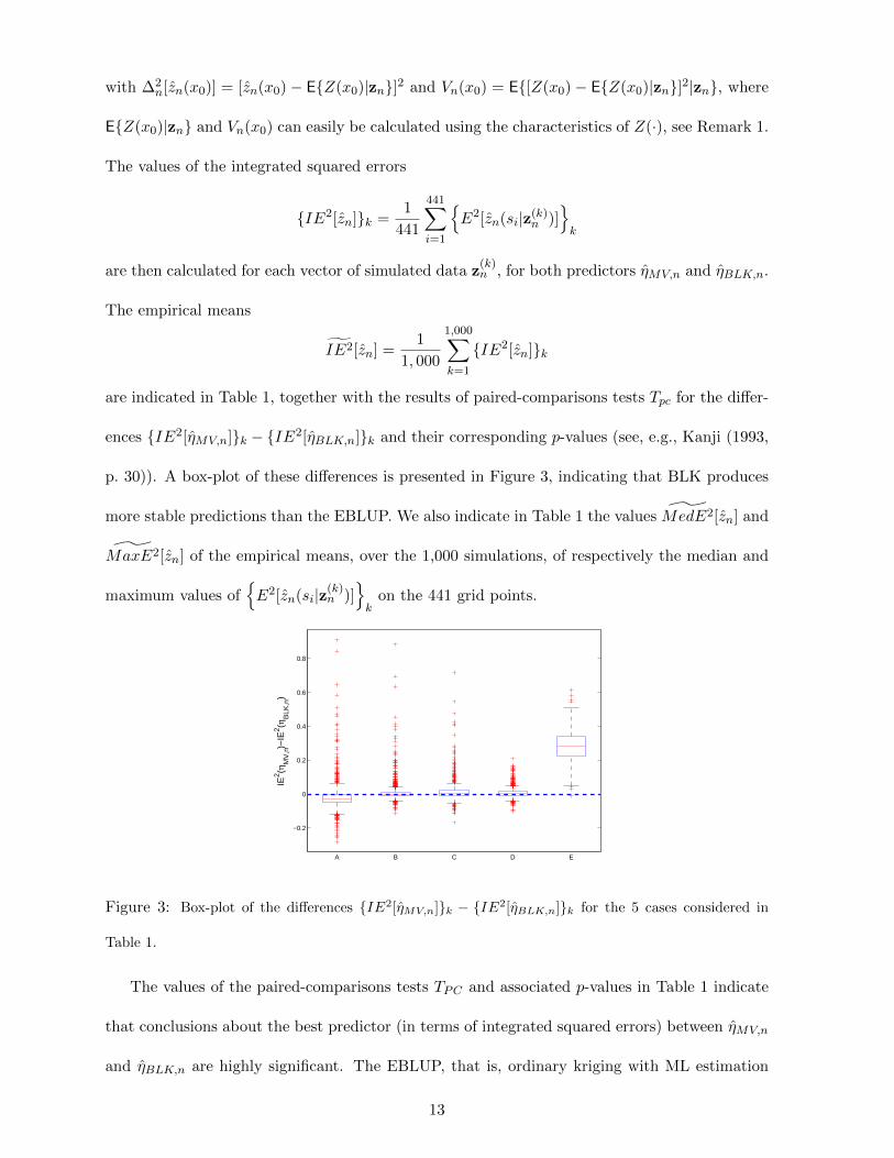
are indicated in Table 1, together with the results of paired-comparisons tests Tpc for the differ-

ences IE2[ηMV,n]k − IE2[ηBLK,n]k and their corresponding p-values (see, e.g., Kanji (1993,

p. 30)). A box-plot of these differences is presented in Figure 3, indicating that BLK produces

more stable predictions than the EBLUP. We also indicate in Table 1 the values MedE2[zn] and

MaxE2[zn] of the empirical means, over the 1,000 simulations, of respectively the median and

maximum values ofE2[zn(si|z(k)n )]

k

on the 441 grid points.

−0.2

0

0.2

0.4

0.6

0.8

A B C D E

IE2 (η

MV

,n)−

IE2 (η

BLK

,n)

Figure 3: Box-plot of the differences IE2[ηMV,n]k − IE2[ηBLK,n]k for the 5 cases considered in

Table 1.

The values of the paired-comparisons tests TPC and associated p-values in Table 1 indicate

that conclusions about the best predictor (in terms of integrated squared errors) between ηMV,n

and ηBLK,n are highly significant. The EBLUP, that is, ordinary kriging with ML estimation

13

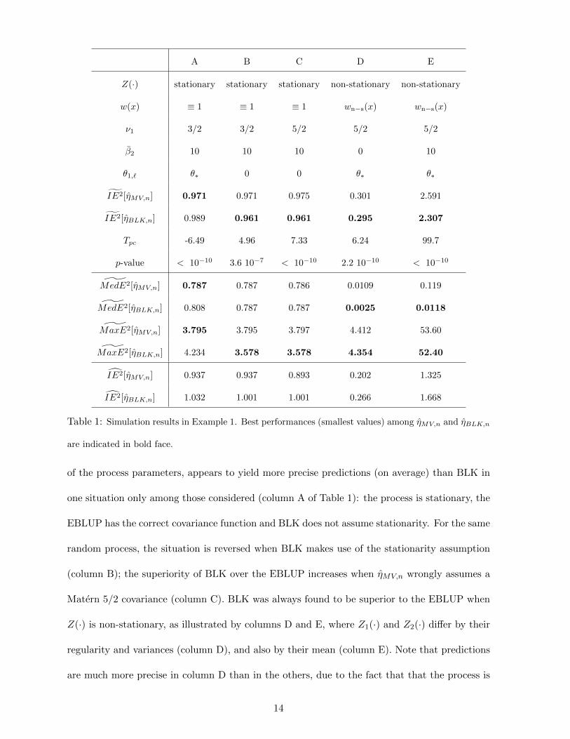
A B C D E

Z(·) stationary stationary stationary non-stationary non-stationary

w(x) ≡ 1 ≡ 1 ≡ 1 wn−s(x) wn−s(x)

ν1 3/2 3/2 5/2 5/2 5/2

β2 10 10 10 0 10

θ1,` θ∗ 0 0 θ∗ θ∗

IE2[ηMV,n] 0.971 0.971 0.975 0.301 2.591

IE2[ηBLK,n] 0.989 0.961 0.961 0.295 2.307

Tpc -6.49 4.96 7.33 6.24 99.7

p-value < 10−10 3.6 10−7 < 10−10 2.2 10−10 < 10−10

MedE2[ηMV,n] 0.787 0.787 0.786 0.0109 0.119

MedE2[ηBLK,n] 0.808 0.787 0.787 0.0025 0.0118

MaxE2[ηMV,n] 3.795 3.795 3.797 4.412 53.60

MaxE2[ηBLK,n] 4.234 3.578 3.578 4.354 52.40

IE2[ηMV,n] 0.937 0.937 0.893 0.202 1.325

IE2[ηBLK,n] 1.032 1.001 1.001 0.266 1.668

Table 1: Simulation results in Example 1. Best performances (smallest values) among ηMV,n and ηBLK,n

are indicated in bold face.

of the process parameters, appears to yield more precise predictions (on average) than BLK in

one situation only among those considered (column A of Table 1): the process is stationary, the

EBLUP has the correct covariance function and BLK does not assume stationarity. For the same

random process, the situation is reversed when BLK makes use of the stationarity assumption

(column B); the superiority of BLK over the EBLUP increases when ηMV,n wrongly assumes a

Matern 5/2 covariance (column C). BLK was always found to be superior to the EBLUP when

Z(·) is non-stationary, as illustrated by columns D and E, where Z1(·) and Z2(·) differ by their

regularity and variances (column D), and also by their mean (column E). Note that predictions

are much more precise in column D than in the others, due to the fact that that the process is

14

quite smooth (ν1 = 5/2) and has a rather large correlation length (θ1 = 1) on a big part of X ;

see in particular the small values of MedE2[ηMV,n] and MedE2[ηBLK,n] in columns D and E.

We also indicate in the table the values of the empirical errors predicted by the two modeling

approaches. For the EBLUP, the squared prediction error at x0 is given by σ2n(x0) ρ2n(x0), see

(19) and (23). For BLK with θ1,` > 0, observations that are far away from x0 have negligible

influence on the prediction of Z(x0). We thus construct an “equivalent number of observations”

n′(x0), given by n′(x0) =∑n

i=1 k1,`(x0 − xi). This value is substituted for n in (18) and (19)

for the evaluation of the posterior squared prediction error (14) (but not for the evaluation

of the marginal likelihood L (zn|`, t)). We then compute the empirical means (over the 1,000

simulations and 441 grid points) of these posterior squared prediction errors, which we denote

by IE2[ηMV,n] and IE2[ηBLK,n], to be compared respectively with IE2[ηMV,n] and IE2[ηBLK,n].

It is well known that using the plug-in mean-squared prediction error of the BLUP underes-

timates the true prediction error, the reason being that the uncertainty due to the estimation of

the covariance parameters is not accounted for, see Stein (1999, Section 6.8). The table corrobo-

rates this result. On the other hand, the error predicted by BLK slightly overestimates (columns

A and B,C) or slightly underestimates (column D) the true empirical error, with an exception

for column E where the abrupt change in the mean β yields large and hardly predictable errors

(see the values of MaxE2[ηBLK,n]).

Example 2: expected improvement and deceptive function. Kriging prediction can be

used for the global optimization of a function f(·) : x ∈ X ⊂ Rd 7−→ f(x) ∈ R, see Mockus

et al. (1978); Mockus (1989), a method which has been popularized under the name of Expected

Improvement (EI), see Jones et al. (1998). The function is considered as the realization of a

GP, whose characteristics (in particular the parameters θ of the chosen covariance function) are

estimated from observations that correspond to evaluations of the function, generally by ML.

However, when the estimated parameters are plugged into the kriging predictor and its associated

15

mean-squared prediction error, the performance of the method may be rather disappointing since

evaluation results may not contain enough information to estimate the covariance parameters in

a satisfactory manner. This may wrongly provide the sensation that the function is extremely

flat in some areas, that will thus not be explored, or on the opposite extremely wiggly, so that

all X would seem to deserve a close exploration. This phenomenon is well described in (Benassi

et al., 2011) through the concept of deceptive function, an example of which is presented below.

−1 −0.8 −0.6 −0.4 −0.2 0 0.2 0.4 0.6 0.8 1−1

−0.8

−0.6

−0.4

−0.2

0

0.2

0.4

0.6

0.8

1

x

f(x)

−1 −0.8 −0.6 −0.4 −0.2 0 0.2 0.4 0.6 0.8 1−5

−4

−3

−2

−1

0

1

2

3

4

5

x

f(x)

Figure 4: Left: a deceptive function (solid line), with the EBLUP (dashed line) and 95% credible

intervals (dotted lines). Right: the same function with BLK (dashed line) and 95% credible intervals

(dotted lines).

Consider the function in (Benassi et al., 2011, Section 5.1), f(x) = x [sin(10x + 1) +

0.1 sin(15x)], x ∈ X = [−1, 1], plotted in solid line in Figure 4. When the function is eval-

uated at the design ξn = (−0.43, −0.11, 0.515, 0.85) all observations are nearly zero, see the

stars in Figure 4. We assume that f(·) can be represented by a GP with unknown mean β and

Matern 3/2 covariance function, see (2). The EBLUP (blue solid line) and associated (approx-

imate) 95% credible intervals (dashed lines), corresponding to ηMV,n(x0)± 3.182 σn(x0)ρn(x0),

with 3.182 the critical value of the student t-distribution with n− p = 3 degrees of freedom, see

Santner et al. (2003, p. 95), are plotted in Figure 4-left. The most promising region in terms

of maximization of f(·) is around zero and several additional evaluations of f(·) are required

16

before the method starts exploring the neighborhood of the maximizer of f(·), at x∗ ' −0.9052,

see Benassi et al. (2011).

Figure 4-right presents the BLK predictor and approximate 95% credible intervals given

by ηBLK,n(x0) ± 2.571 [PSPE(ηBLK,n(x0))]1/2 (with 2.571 the critical value of the student t-

distribution with n − p + ν0 = 5 degrees of freedom), under the same setting as in Example

1 and θ0,` = 1, 5, 10, 20, θ1,` = 5 for ` = 1, . . . , L = 4. The large uncertainty on the behavior

of f(·) in the left-hand side of the domain is an incitation to put observations there. The EI

algorithm can be expected to perform much more efficiently when based on BLK, even with a

small L, than when based on the EBLUP.

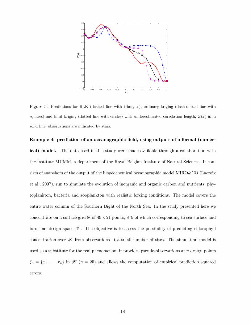
Example 3: behaviour of BLK far from design points. This example illustrates the

behavior of the BLK predictor ηBLK,n(t) when t is far enough from design points so that the

influence of the closest point xi dominates all others through k1,`(t− xi), see (1).

We consider a process Z(x) with zero mean and covariance K3/2,2(·), see (2), which is ob-

served at the 7 design points (−1, −0.9, −0.8, −0.5, −0.2, 0, 1), indicated by stars. Figure 5

shows the predictions obtained by ordinary kriging (with covariance K3/2,15(·)) and BLK (with

L = 4, k0,`(δ) = K3/2,θ0,`(|δ|) and θ0,` = 1, 5, 10, 20, k1,`(δ) = K3/2,5(|δ|) for all `), both assum-

ing that g(x) ≡ 1. The prediction by limit-kriging (Joseph, 2006), with covariance K3/2,15(·), is

also presented on the figure.

The correlation length θ being underestimated (1/15 instead of 1/2), the ordinary-kriging

prediction ηn(t) is close to the estimated mean βn given by (20) for t far enough from design

points, see the right part of the figure. On the other hand, in the same region the BLK predictor

is mainly influenced by the closest design point xi, so that ηn(t) is close to Z(xi), a reasonable

behavior that resembles that of limit-kriging with underestimated θ, see Joseph (2006, Section 3).

17

−1 −0.8 −0.6 −0.4 −0.2 0 0.2 0.4 0.6 0.8 1−1.2

−1

−0.8

−0.6

−0.4

−0.2

0

0.2

0.4

0.6

0.8

x

Z(x

)

Figure 5: Predictions for BLK (dashed line with triangles), ordinary kriging (dash-dotted line with

squares) and limit kriging (dotted line with circles) with underestimated correlation length; Z(x) is in

solid line, observations are indicated by stars.

Example 4: prediction of an oceanographic field, using outputs of a formal (numer-

ical) model. The data used in this study were made available through a collaboration with

the institute MUMM, a department of the Royal Belgian Institute of Natural Sciences. It con-

sists of snapshots of the output of the biogeochemical oceanographic model MIRO&CO (Lacroix

et al., 2007), run to simulate the evolution of inorganic and organic carbon and nutrients, phy-

toplankton, bacteria and zooplankton with realistic forcing conditions. The model covers the

entire water column of the Southern Bight of the North Sea. In the study presented here we

concentrate on a surface grid G of 49× 21 points, 879 of which corresponding to sea surface and

form our design space X . The objective is to assess the possibility of predicting chlorophyll

concentration over X from observations at a small number of sites. The simulation model is

used as a substitute for the real phenomenon; it provides pseudo-observations at n design points

ξn = x1, . . . , xn in X (n = 25) and allows the computation of empirical prediction squared

errors.

18

Experimental design. Figure 6-Left presents the model response f(x), x ∈ X . It is

manifest that variability is stronger along the French coast, so that obtaining precise predictions

there would require a denser concentration of observation sites than in other areas where the

response is more flat. However, in a realistic situation the true response is not available, and

this information cannot be used to choose ξn.

Figure 6: Left: model response over X and design points (stars). Right: shortest maritime distance

∆(x, x21) between x ∈X and the 21st design point x21.

The design ξn is thus constructed as follows. First, G is renormalized to [0, 1]2 and X is

renormalized accordingly. Then, we generate a low-discrepancy (Sobol’) sequence in G ; the

design points x1, . . . , x10 are given by the first 10 points of the sequence that fall in X . Finally,

the next 15 points are generated sequentially, according to

xk+1 = arg maxx∈X

ρk(x) , (17)

with ρk(x) the universal kriging variance (the mean-squared error of the BLUP) for a process

with unknown constant mean β and covariance function K3/2,θ(∆(x, x′)), see (2), and observa-

tions f(x1), . . . , f(xk). We take θ = 10 to ensure that ξn will be well dispersed over X . In order

to take the non-convexity of the design region into account, the “distance” ∆(x, x′) corresponds

to the shortest maritime route between x and x′, computed by Dijkstra’s algorithm (Dijkstra,

19

1959). The 25 design points xi of ξn are indicated by stars in Figure 6-Left. Figure 6-Right

presents the distance ∆(x, x21) from x ∈ X to the 21st design point x21 (with indices (15, 47),

corresponding to coordinates (0.2593, 0.9583) in the renormalized space), showing a neat differ-

ence with the Euclidean distance ‖x − x21‖. Notice that in order to compute predictions and

prediction errors over X we only need to compute distances ∆(xi, x) from the design points xi

to the x ∈X (and not all pairwise distances ∆(x, x′), (x, x′) ∈X 2).

Comparison between BLUP and BLK For this same design ξn, we compare the

predictive performance of the EBLUP and BLK. The EBLUP uses the covariance function

K3/2,θn(∆(x, x′)), with θn ' 19.2058 estimated by ML from the observations f(x1), . . . , f(xn);

BLK uses K3/2,θ(∆(x, x′)) both for k0,` and k1,`, with L = 4 and θ0,` = 5, 10, 20, 30 in k0,`,

θ1,` = θ∗ > 0 for all ` = 1, . . . , 4 in k1,`. The choice of θ∗ should make a compromise between

stepping the influence of distant points down (which means taking θ∗ large enough to obtain

local predictions) and maintaining a reasonable correlation with sufficient design points (which

means taking θ∗ not too large). Let φmM (ξn) = maxx∈X minxi∈ξn ‖x− xi‖ denote the value of

the minimax distance criterion for ξn, and denote φkNN (ξn) = maxxi∈ξn ‖xi− xj∗(i)‖ with xj∗(i)

the k-th nearest-neighbor of xi in ξn. For all x ∈X , we can then guarantee that

‖x− xi‖ ≤ δk(ξn) = φmM (ξn) + φkNN (ξn)

for k + 1 points xi of ξn. We take k = 19 and θ∗ = 2.99431/δk(ξn), which ensures that, for each

x ∈ X , k1,`(‖x − xi‖) ≥ 20% for at least 20 design points in ξn. For the design ξn plotted in

Figure 6-Left, this gives θ∗ ' 2.4202, the value we use here for BLK.

Figure 7-Left shows the BLK predictions over X , to be compared with the true responses

on Figure 6-Left. Figure 7-Right shows the squared prediction errors E2[ηBLK,n(x)], where for a

predictor zn(·) we denote E2[zn(x)] = [zn(x)− f(x)]2. Taking into account that only 25 designs

points have been used, predictions are fairly accurate, excepted at some areas along the French

20

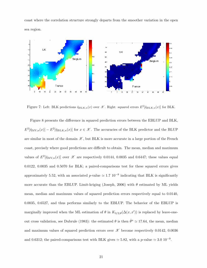
coast where the correlation structure strongly departs from the smoother variation in the open

sea region.

Figure 7: Left: BLK predictions ηBLK,n(x) over X . Right: squared errors E2[ηBLK,n(x)] for BLK.

Figure 8 presents the difference in squared prediction errors between the EBLUP and BLK,

E2[ηMV,n(x)]− E2[ηBLK,n(x)] for x ∈ X . The accuracies of the BLK predictor and the BLUP

are similar in most of the domain X , but BLK is more accurate in a large portion of the French

coast, precisely where good predictions are difficult to obtain. The mean, median and maximum

values of E2[ηMV,n(x)] over X are respectively 0.0144, 0.0035 and 0.6447; these values equal

0.0122, 0.0035 and 0.5070 for BLK; a paired-comparisons test for these squared errors gives

approximately 5.52, with an associated p-value ' 1.7 10−8 indicating that BLK is significantly

more accurate than the EBLUP. Limit-kriging (Joseph, 2006) with θ estimated by ML yields

mean, median and maximum values of squared prediction errors respectively equal to 0.0140,

0.0035, 0.6527, and thus performs similarly to the EBLUP. The behavior of the EBLUP is

marginally improved when the ML estimation of θ in K3/2,θ(∆(x, x′)) is replaced by leave-one-

out cross validation, see Dubrule (1983): the estimated θ is then θn ' 17.64, the mean, median

and maximum values of squared prediction errors over X become respectively 0.0142, 0.0036

and 0.6312; the paired-comparisons test with BLK gives ' 5.82, with a p-value ' 3.0 10−9.

21

Figure 8: Difference in squared errors between the EBLUP and BLK, E2[ηMV,n(x)]− E2[ηBLK,n(x)].

Choice of θ∗. The influence of the choice of θ∗ on the performance of BLK (with L = 4

and θ0,` = 5, 10, 10, 30 in k0,`) is illustrated in Figure 9, where the solid line (respectively dashed

line) gives the mean (respectively 1/40× the maximum) value of E2[ηBLK,n(x)] over X as a

function of θ∗ varying between 0 (stationary model) and 10 (strong non-stationarity). The choice

θ∗ = 2.99431/δ19(ξn) ' 2.4202 is not optimal but seems reasonable. Imposing that each x ∈X

has only at least 10 neighboring design points xi such that k1,`(‖x − xi‖) ≥ 20% would have

been a better choice, since 2.99431/δ9(ξn) ' 4.2531, closer to the optimum θ∗ in Figure 9. Note

that the errors E2[ηBLK,n(x)] are normally not available, and therefore cannot be used to select

θ∗. This indicates, however, that the choice of k in the construction θ∗ = 2.99431/δk(ξn) is not

critical.

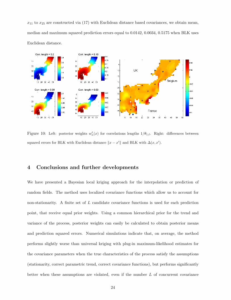
Influence of L. Increasing L does not necessarily improve the performance of BLK. For

instance, taking θ0,` = 5, 6, 7, . . . , 30 in k0,` (L = 26) and θ1,` = 2.4202 for all ` = 1, . . . , 26 in

k1,`, we obtain 0.0127, 0.0035, 0.5388, respectively for the mean, median and maximum values

of E2[ηBLK,n(x)] over X . Figure 10-Left shows the posterior weights w`n(x) associated with

the correlations lengths 1/θ1,`, ` = 1, . . . , L = 4, when θ0,` = 5, 10, 20, 30, pointing out areas

22

0 1 2 3 4 5 6 7 8 9 100.012

0.0125

0.013

0.0135

0.014

0.0145

0.015

θ*

Figure 9: Mean value (solid line) and 1/40× maximum value (dashed line) of E2[ηBLK,n(x)] over X as

functions of θ∗.

where the response exhibits strong variability and those where it is fairly smooth. It should be

stressed that the calculation of the w`n(x) only uses the 25 response values f(xi) for xi ∈ ξn.

The similarity between the maps of w3n(x) and w4

n(x) is an incitation to try reducing L to 3:

when θ0,` = 5, 10, 30 in k0,` (L = 3), we obtain 0.0122, 0.0035 and 0.5040 for the mean, median

and maximum values of E2[ηBLK,n(x)]; i.e., values that are marginally better than those with

L = 4.

Influence of the distance function. Finally, the interest of using the distance ∆(x, x′)

corresponding to the shortest maritime route between x and x′ instead of the Euclidean distance

‖x−x′‖ (in the renormalized space [0, 1]2) is illustrated for BLK in Figure 10-Right, which shows

the differences between corresponding prediction squared errors. The distance ∆(x, x′) yields

more accurate predictions along the major part of the French coast; the mean, median and

maximum values of E2[ηBLK,n(x)] over X are respectively 0.0129, 0.0030 and 0.5257 when

using Euclidean distance to compute correlations. The decrease of performance compared to

the situation where ∆(x, x′) is used is not caused to the fact that the sequential construction of

design points x11 to x25 through (17) is based on ∆(x, x′): replacing the design ξn by ξ′n where

23

x11 to x25 are constructed via (17) with Euclidean distance based covariances, we obtain mean,

median and maximum squared prediction errors equal to 0.0142, 0.0034, 0.5175 when BLK uses

Euclidean distance.

Figure 10: Left: posterior weights w`n(x) for correlations lengths 1/θ1,`. Right: differences between

squared errors for BLK with Euclidean distance ‖x− x′‖ and BLK with ∆(x, x′).

4 Conclusions and further developments

We have presented a Bayesian local kriging approach for the interpolation or prediction of

random fields. The method uses localized covariance functions which allow us to account for

non-stationarity. A finite set of L candidate covariance functions is used for each prediction

point, that receive equal prior weights. Using a common hierarchical prior for the trend and

variance of the process, posterior weights can easily be calculated to obtain posterior means

and prediction squared errors. Numerical simulations indicate that, on average, the method

performs slightly worse than universal kriging with plug-in maximum-likelihood estimates for

the covariance parameters when the true characteristics of the process satisfy the assumptions

(stationarity, correct parametric trend, correct covariance functions), but performs significantly

better when these assumptions are violated, even if the number L of concurrent covariance

24

functions is very small (L = 4 in the examples considered). Also, BLK, which does not use any

numerical optimization, is much faster and numerically more stable than universal kriging with

plug-in estimates, which requires the estimation of covariance parameters.

To summarize, our feeling is that it seems illusory in many applications to try estimate

covariance parameters from a few observations only, especially with a covariance structure not

necessarily well-adapted to the variability of the modeled phenomenon. Using a small number of

candidate processes able to reproduce a reasonable range of possible behaviors may be preferable:

it is simpler to implement, numerically more stable, and seems to often yield better predictions.

Although these results are encouraging, further numerical experimentations (in particular for

higher dimensional processes and different types and sizes of experimental designs) are needed to

confirm these preliminary observations. We have restricted our attention to the situation where

the regressor g(·) in the parametric trend g>(x)β was identical for all L models (and, moreover,

we only considered the case g(x) ≡ 1 in all examples). The same approach could be used when

different trends g`(·) are associated with different covariances C`|t(·, ·), possibly allowing for a

better consideration of uncertainty in the process trend.

The choice of the particular form of the kernels k0,`(·) and k1,`(·) seems to be less crucial

than that of the correlation length for k1,`(·), which depends on the assumed amount of non-

stationarity. Using different correlations lengths for some of the L concurrent covariances is a

possible option to investigate. Another one is to simply ensure that k1,`(x−xi) be large enough

for all points in x in X and enough design points xi, with the motivation that the more dense

the design ξn in X , the more local the models can be and the stronger the non-stationarity that

BLK can take into account. Two proposals have been made in this direction, see Examples 1 and

4. Further investigations are required to validate them, in particular concerning their asymptotic

behavior, when the number n of design points tends to infinity and ξn is space-filling.

Finally, as mentioned in Section 2.3, designing experiments adapted to BLK requires the

25

evaluation (approximation) of the second term in (15). This rather challenging problem is

under current investigation.

5 Appendix: Universal BLK in presence of a parametric trend

Here we consider that, seen from t, f(·) is the sample path of a stochastic process Z(·) such that

Z(·)|s(t), β, σ2, t ∼ GP(g>(·)β, σ2Cs(t)|t(·, ·)), with Probs(t) = ` = w`0, ` = 1, . . . , L, β|σ2 ∼

ψ0(β|σ2), σ2 ∼ ϕ0(σ2), see (9), and g(·) a known p-dimensional vector of functions defined on

X . The likelihood of zn = (f(x1), . . . , f(xn))> for the model GP(g>(·)β, σ2Cs(t)|t(·, ·)) is

L (zn|β, σ2, `, t) =1

σn(2π)n/2 det1/2 Kn(`|t)exp

[− 1

2σ2(zn −Gnβ)>K−1n (`|t)(zn −Gnβ)

],

where the i-th row of the n×pmatrix Gn equals g>(xi), i = 1, . . . , n. The weights wl0 are updated

according to (4), with now L (zn|`, t) =∫Rp

∫∞0 L (zn|β, σ2, `, t)ψ0(β|σ2)ϕ0(σ

2) dβ dσ2.

5.1 Uniform prior for β

Suppose first that β has a uniform (improper) prior on Rp. We obtain

L (zn|`, t) =1

(2π)(n−p)/2 det1/2 Kn(`|t) det1/2(G>nK−1n Gn)

(σ20ν0/2)ν0/2

Γ(ν0/2)

Γ(νn/2)

(σ2n|`,tνn/2)νn/2,

with νn = ν0 + n− p and

σ2n|`,t =ν0σ

20 + (n− p)σ2n(`|t)ν0 + n− p

, (18)

where

σ2n(`|t) =1

n− p(zn −Gnβn(`|t))>K−1n (`|t)(zn −Gnβn(`|t)) (19)

is the Restricted Maximum-Likelihood (REML) estimator of σ2, and

βn(`|t) = (G>nK−1n (`|t)Gn)−1G>nK−1n (`|t)zn (20)

is the ML estimator of β, given zn, ` and t, see, e.g., Santner et al. (2003, p. 67, 95). Moreover,

given zn, ` and t, σ2 has the inverse chi-square distribution ϕn|`,t(·) = ϕσ2n|`,t,νn

(·), see (9).

26

References

Abt, M. (1999). Estimating the prediction mean squared error in gaussian stochastic processes

with exponential correlation structure. Scandinavian Journal of Statistics, 26(4):563–578.

Benassi, R., Bect, J., and Vazquez, E. (2011). Robust Gaussian process-based global optimiza-

tion using a fully Bayesian expected improvement criterion. In Coello, C. C., editor, Learning

and Intelligent Optimization, pages 176–190, Berlin. Springer-Verlag, LNCS 6683.

Cramer, H. and Leadbetter, M. (1967). Stationary and Related Stochastic Processes. Wiley,

New York.

Dijkstra, E. (1959). A note on two problems in connexion with graphs. Numerische mathematik,

1(1):269–271.

Dubrule, O. (1983). Cross validation of kriging in a unique neighborhood. Journal of the

International Association for Mathematical Geology, 15(6):687–699.

Ginsbourger, D., Helbert, C., and Carraro, L. (2008). Discrete mixture of kernels for kriging-

based optimization. Quality and Reliability Engineering International, 24:681–691.

Harville, D. and Jeske, D. (1992). Mean squared error of estimation or prediction under a general

linear model. Journal of the American Statistical Association, 87(419):724–731.

Jones, D. (2001). A taxonomy of global optimization methods based on response surfaces.

Journal of global optimization, 21(4):345–383.

Jones, D., Schonlau, M., and Welch, W. (1998). Efficient global optimization of expensive

black-box functions. Journal of Global Optimization, 13:455–492.

Joseph, V. (2006). Limit kriging. Technometrics, 48(4):458–466.

Kanji, G. (1993). 100 Statistical Tests. Sage Pub., London.

29

Lacroix, G., Ruddick, K., Park, Y., Gypens, N., and Lancelot, C. (2007). Validation of the 3D

biogeochemical model MIRO&CO with field nutrient and phytoplankton data and MERIS-

derived surface chlorophyll α images. Journal of Marine Systems, 64:66–88.

Lam, K., Wang, Q., and Li, H. (2004). A novel meshless approach — Local kriging (LoKriging)

method with two-dimensional structural analysis. Computational Mechanics, 33:235–244.

Mockus, J. (1989). Bayesian Approach to Global Optimization, Theory and Applications. Kluwer,

Dordrecht.

Mockus, J., Tiesis, V., and Zilinskas, A. (1978). The application of Bayesian methods for seeking

the extremum. In Dixon, L. and Szego, G., editors, Towards Global Optimisation 2, pages

117–129. North Holland, Amsterdam.

Nguyen-Tuong, D., Seeger, M., and Peters, J. (2009). Model learning with local Gaussian process

regression. Advanced Robotics, 23(15):2015–2034.

Nott, D. and Dunsmuir, W. (2002). Estimation of nonstationary spatial covariance structure.

Biometrika, 89(4):819–829.

Santner, T., Williams, B., and Notz, W. (2003). The Design and Analysis of Computer Experi-

ments. Springer, Heidelberg.

Stein, M. (1999). Interpolation of Spatial Data. Some Theory for Kriging. Springer, Heidelberg.

Sun, W., Minasny, B., and McBratney, A. (2006). Analysis and prediction of soil properties

using local regression-kriging. Geoderma, 171–172:16–23.

Zhu, Z. and Zhang, H. (2006). Spatial sampling design under the infill asymptotic framework.

Environmetrics, 17(4):323–337.

Zimmerman, D. and Cressie, N. (1992). Mean squared prediction error in the spatial linear

model with estimated covariance parameters. Ann. Inst. Statist. Math., 44(1):27–43.

30

Local kriging-V2

Documents

Transcript of Local kriging-V2