
LIPIcs, Vol. 44, TQC'15 - Complete Volume - EMIS
263
10th Conference on the Theory of Quantum Computation, Communication and Cryptography TQC’15, May 20–22, 2015, Brussels, Belgium Edited by Salman Beigi Robert König LIPIcs – Vol. 44 – TQC 2015 www.dagstuhl.de/lipics
-
Upload
khangminh22 -
Category
Documents
-
view
0 -
download
0
Transcript of LIPIcs, Vol. 44, TQC'15 - Complete Volume - EMIS
10th Conference on the Theoryof Quantum Computation,Communication andCryptography
TQC’15, May 20–22, 2015, Brussels, Belgium
Edited by
Salman BeigiRobert König
LIPIcs – Vo l . 44 – TQC 2015 www.dagstuh l .de/ l ip i c s
EditorsSalman Beigi Robert KönigInstitute for Research in Institute for Advanced StudyFundamental Sciences and Zentrum MathematikTehran, Iran Technische Universität Mü[email protected] Garching, Germany
ACM Classification 1998E.3 Data Encryption, E.4 Coding and Information Theory, F Theory of Computation
ISBN 978-3-939897-96-5
Published online and open access bySchloss Dagstuhl – Leibniz-Zentrum für Informatik GmbH, Dagstuhl Publishing, Saarbrücken/Wadern,Germany. Online available at http://www.dagstuhl.de/dagpub/978-3-939897-96-5.
Publication dateNovember, 2015
Bibliographic information published by the Deutsche NationalbibliothekThe Deutsche Nationalbibliothek lists this publication in the Deutsche Nationalbibliografie; detailedbibliographic data are available in the Internet at http://dnb.d-nb.de.
LicenseThis work is licensed under a Creative Commons Attribution 3.0 Unported license (CC-BY 3.0):http://creativecommons.org/licenses/by/3.0/legalcode.In brief, this license authorizes each and everybody to share (to copy, distribute and transmit) the workunder the following conditions, without impairing or restricting the authors’ moral rights:
Attribution: The work must be attributed to its authors.
The copyright is retained by the corresponding authors.
Digital Object Identifier: 10.4230/LIPIcs.TQC.2015.i
ISBN 978-3-939897-96-5 ISSN 1868-8969 http://www.dagstuhl.de/lipics

iii
LIPIcs – Leibniz International Proceedings in Informatics
LIPIcs is a series of high-quality conference proceedings across all fields in informatics. LIPIcs volumesare published according to the principle of Open Access, i.e., they are available online and free of charge.
Editorial Board
Susanne Albers (TU München)Chris Hankin (Imperial College London)Deepak Kapur (University of New Mexico)Michael Mitzenmacher (Harvard University)Madhavan Mukund (Chennai Mathematical Institute)Catuscia Palamidessi (INRIA)Wolfgang Thomas (Chair, RWTH Aachen)Pascal Weil (CNRS and University Bordeaux)Reinhard Wilhelm (Saarland University)
ISSN 1868-8969
http://www.dagstuhl.de/lipics
TQC’15


Contents
Oracles with CostsShelby Kimmel, Cedric Yen-Yu Lin, and Han-Hsuan Lin . . . . . . . . . . . . . . . . . . . . . . . . . 1
The Resource Theory of SteeringRodrigo Gallego and Leandro Aolita . . . . . . . . . . . . . . . . . . . . . . . . . . . . . . . . . . . . . . . . . . . . . . 27
How Many Quantum Correlations Are Not Local?Carlos E. González-Guillén, C. Hugo Jiménez, Carlos Palazuelos, and IgnacioVillanueva . . . . . . . . . . . . . . . . . . . . . . . . . . . . . . . . . . . . . . . . . . . . . . . . . . . . . . . . . . . . . . . . . . . . . . . 39
The Spin-2 AKLT State on the Square Lattice is Universal for Measurement-basedQuantum Computation
Tzu-Chieh Wei and Robert Raussendorf . . . . . . . . . . . . . . . . . . . . . . . . . . . . . . . . . . . . . . . . . . 48
Quantum Capacity Can Be Greater Than Private Information for Arbitrarily Many UsesDavid Elkouss and Sergii Strelchuk . . . . . . . . . . . . . . . . . . . . . . . . . . . . . . . . . . . . . . . . . . . . . . . 64
Semidefinite Programs for Randomness ExtractorsMario Berta, Omar Fawzi, and Volkher B. Scholz . . . . . . . . . . . . . . . . . . . . . . . . . . . . . . . . 73
New Constructions for Quantum MoneyMarios Georgiou and Iordanis Kerenidis . . . . . . . . . . . . . . . . . . . . . . . . . . . . . . . . . . . . . . . . . 92
Decoherence in Open Majorana SystemsEarl T. Campbell . . . . . . . . . . . . . . . . . . . . . . . . . . . . . . . . . . . . . . . . . . . . . . . . . . . . . . . . . . . . . . . . 111
On the Closure of the Completely Positive Semidefinite Cone and Linear Approximationsto Quantum Colorings
Sabine Burgdorf, Monique Laurent, and Teresa Piovesan . . . . . . . . . . . . . . . . . . . . . . . . . 127
Making Existential-unforgeable Signatures Strongly Unforgeable in the QuantumRandom-oracle Model
Edward Eaton and Fang Song . . . . . . . . . . . . . . . . . . . . . . . . . . . . . . . . . . . . . . . . . . . . . . . . . . . 147
A Universal Adiabatic Quantum Query AlgorithmMathieu Brandeho and Jérémie Roland . . . . . . . . . . . . . . . . . . . . . . . . . . . . . . . . . . . . . . . . . . 163
Quantum Enhancement of Randomness DistributionRaul Garcia-Patron, William Matthews, and Andreas Winter . . . . . . . . . . . . . . . . . . . . 180
Implementing Unitary 2-Designs Using Random Diagonal-unitary MatricesYoshifumi Nakata, Christoph Hirche, Ciara Morgan, and Andreas Winter . . . . . . . . 191
Round Elimination in Exact Communication ComplexityJop Briët, Harry Buhrman, Debbie Leung, Teresa Piovesan, and Florian Speelman 206
On the Robustness of Bucket Brigade Quantum RAMSrinivasan Arunachalam, Vlad Gheorghiu, Tomas Jochym-O’Connor, Michele Mosca,and Priyaa Varshinee Srinivasan . . . . . . . . . . . . . . . . . . . . . . . . . . . . . . . . . . . . . . . . . . . . . . . . 226
Interferometric Versus Projective Measurement of AnyonsClaire Levaillant and Michael Freedman . . . . . . . . . . . . . . . . . . . . . . . . . . . . . . . . . . . . . . . . . 245
10th Conference on the Theory of Quantum Computation, Communication and Cryptography (TQC 2015).Editors: Salman Beigi and Robert König
Leibniz International Proceedings in InformaticsSchloss Dagstuhl – Leibniz-Zentrum für Informatik, Dagstuhl Publishing, Germany


Preface
The 10th Conference on the Theory of Quantum Computation, Communication and Cryp-tography was held at the Université libre de Bruxelles from the 20th to the 22nd of May2015. Quantum computation, quantum communication, and quantum cryptography aresubfields of quantum information processing, an interdisciplinary field of information scienceand quantum mechanics. The TQC conference series focuses on theoretical aspects of thesesubfields. The objective of the conference is to bring together researchers so that they caninteract with each other and share problems and recent discoveries.
A list of the previous editions of TQC follows:TQC 2014, National University of Singapore, SingaporeTQC 2013, University of Guelph, CanadaTQC 2012, The University of Tokyo, JapanTQC 2011, Universidad Complutense de Madrid, SpainTQC 2010, University of Leeds, UKTQC 2009, Institute for Quantum Computing, University of Waterloo, CanadaTQC 2008, University of Tokyo, JapanTQC 2007, Nara Institute of Science and Technology, Nara, JapanTQC 2006, NTT R&D Center, Atsugi, Kanagawa, Japan
The conference consisted of invited talks, contributed talks and a poster session. Theinvited talks were given by David DiVincenzo (RWTH Aachen & FZ Jülich), Sean Hallgren(Pennsylvania State University), Laura Mančinska (CQT Singapore) and Ronald de Wolf(CWI Amsterdam). The conference was possible thanks to the financial support of the BelgianFund for Scientific Research (FNRS), Visit Brussels, Journal of Physics A, Cryptoworks21,the Engineering and Physical Research Council (EPSRC), as well as the Royal Society. Wewish to thank the members of the Program Committee and all subreviewers for their precioushelp. Our warm thanks also go to the members of the Local Organizing Committee, for theirconsiderable efforts in organizing the conference. We would like to thank Marc Herbstrittand Michael Wagner (Dagstuhl Publishing) for their technical help. Finally, we would liketo thank the members of the Steering Committee for giving us the opportunity to work forTQC. And, of course, we thank all contributors and participants!
August 2015 Salman Beigi and Robert König
10th Conference on the Theory of Quantum Computation, Communication and Cryptography (TQC 2015).Editors: Salman Beigi and Robert König
Leibniz International Proceedings in InformaticsSchloss Dagstuhl – Leibniz-Zentrum für Informatik, Dagstuhl Publishing, Germany


Local Organizing Committee
Nicolas CerfUniversité libre de Bruxelles
Serge MassarUniversité libre de Bruxelles
Stefano PironioUniversité libre de Bruxelles (chair)
Jérémie RolandUniversité libre de Bruxelles (chair)
Philippe SpindelUniversité de Mons
Frank VerstraeteGhent University
10th Conference on the Theory of Quantum Computation, Communication and Cryptography (TQC 2015).Editors: Salman Beigi and Robert König
Leibniz International Proceedings in InformaticsSchloss Dagstuhl – Leibniz-Zentrum für Informatik, Dagstuhl Publishing, Germany


Program Committee
Salman Beigi, IPM (chair)Andrew Childs, University of MarylandMatthias Christandl, CopenhagenToby Cubitt, CambridgeAndrew Doherty, University of SydneyFrédéric Dupuis, AarhusSevag Gharibian, UC Berkeley and Virginia CommonwealthSaikat Guha, BBN TechnologiesMichał Horodecki, University of GdanskPeter Høyer, CalgaryIordanis Kerenidis, Paris DiderotRobert König, Technische Universität München (chair)Troy Lee, NTU & CQT SingaporeTobias Osborne, HannoverCarlos Palazuelos, UCM MadridDavid Pérez-Garcia, UCM MadridBen Reichardt, University of Southern CaliforniaKristan Temme, CaltechBarbara Terhal, RWTH AachenMarco Tomamichel, University of SydneyChristian Schaffner, University of AmsterdamTamás Vértesi, MTA AtomkiThomas Vidick, CaltechPawel Wocjan, University of Central Florida
10th Conference on the Theory of Quantum Computation, Communication and Cryptography (TQC 2015).Editors: Salman Beigi and Robert König
Leibniz International Proceedings in InformaticsSchloss Dagstuhl – Leibniz-Zentrum für Informatik, Dagstuhl Publishing, Germany


Steering Committee
Wim van DamUniversity of California, Santa Barbara, USA
Yasuhito KawanoNTT, Japan
Michele MoscaIQC and University of Waterloo, Canada
Martin RoettelerMicrosoft Research, USA
Simone SeveriniUniversity College London, UK
Vlatko VedralUniversity of Oxford, UK &National University of Singapore, Singapore
10th Conference on the Theory of Quantum Computation, Communication and Cryptography (TQC 2015).Editors: Salman Beigi and Robert König
Leibniz International Proceedings in InformaticsSchloss Dagstuhl – Leibniz-Zentrum für Informatik, Dagstuhl Publishing, Germany


Oracles with CostsShelby Kimmel1,2, Cedric Yen-Yu Lin2, and Han-Hsuan Lin2
1 Joint Center for Quantum Information and Computer Science, University ofMaryland, US
2 Center for Theoretical Physics, Massachusetts Institute of Technology, US
AbstractWhile powerful tools have been developed to analyze quantum query complexity, there are stillmany natural problems that do not fit neatly into the black box model of oracles. We create anew model that allows multiple oracles with differing costs. This model captures more of thedifficulty of certain natural problems. We test this model on a simple problem, Search with TwoOracles, for which we create a quantum algorithm that we prove is asymptotically optimal. Wefurther give some evidence, using a geometric picture of Grover’s algorithm, that our algorithmis exactly optimal.
1998 ACM Subject Classification F.2 Analysis of Algorithms and Problem Complexity
Keywords and phrases Quantum Algorithms, Query Complexity, Amplitude Amplification
Digital Object Identifier 10.4230/LIPIcs.TQC.2015.1
1 Introduction
The standard oracle model is a powerful paradigm for understanding quantum computers.Tools such as the adversary semidefinite program [12, 13], learning graphs [5, 6], and thepolynomial method [4] allow us to accurately characterize the quantum query complexity[1, 7] of many problems of interest.
However, the oracle model does not capture the full power or challenges of quantumcomputing. For example, problems such as k-SAT do not fit easily into the oracle model.Additionally, while the query complexity of the hidden subgroup problem is known to bepolynomial in the size of the problem [11], for some non-abelian groups there is no efficientalgorithm.
In this paper, we describe a variation of the oracle model. We have access to two oracles,rather than a single oracle1, but one oracle is more expensive to use. In the standard oraclemodel, the figure of merit is the query complexity, which is the minimum number of queriesneeded to an oracle to evaluate a function. In our model, the figure of merit is the costcomplexity, which is the minimum cost needed to evaluate a function using multiple oracleswith different costs.
To motivate this model, we consider the following fact: in some search problems we wantto find an element in a set that satisfies a property that is expensive to test. However, oftenanother less expensive test is available that can narrow down the search range but is notconclusive. We give three examples of problems where such less expensive, less conclusivetests are natural. In each example, Test 1 is more expensive to run but is conclusive, whileTest 2 is cheaper to run but allows some non-solutions to pass.
1 The model can easily be extended to more than two oracles, but for simplicity, we limit ourselves to two.
© Shelby Kimmel, Cedric Yen-Yu Lin, and Han-Hsuan Lin;licensed under Creative Commons License CC-BY
10th Conference on the Theory of Quantum Computation, Communication and Cryptography (TQC 2015).Editors: Salman Beigi and Robert König; pp. 1–26
Leibniz International Proceedings in InformaticsSchloss Dagstuhl – Leibniz-Zentrum für Informatik, Dagstuhl Publishing, Germany

2 Oracles with Costs
In the problem of k-SAT on n bits, we would like to find an assignment x ∈ 0, 1n suchthat all clauses are satisfied. Consider an algorithm for k-SAT that runs two types oftests on a possible assignment x:1. Check whether all clauses are satisfied.2. Check whether some subset of the clauses are satisfied.Given a graph A and a set of graphs B1, · · · , Bp, we would like to find a graph Biisomorphic to A. Consider an algorithm that runs two types of tests on a graph Bi:1. Check whether Bi is isomorphic to A (say by brute force search).2. Check whether the adjacency matrices of Bi and A have the same spectrum.In the decision variant of the traveling salesman problem, given a positively weightedN -graph G and a positive number b, we would like to find a tour of the vertices of G thatuses cost no more than b. Given a partial tour of length N/2, we can run two types oftests:1. Check whether the partial tour can be completed to an N -vertex tour that has cost at
most b, by using brute force search.2. Check whether the sum of the weights of the N/2 edges traversed in the partial tour is
bigger than b.
In all three examples, the two tests can be implemented as unitaries O1,O2 that actas Oi|x〉|y〉 = |x〉|y ⊕ fi(x)〉. Here fi(x) = 1 if assignment x passes Test i and fi(x) = 0otherwise. These two unitaries will play the role of oracles with different costs.
None of the problems listed above are typically thought of as oracle problems, becausein each problem, there is more information than can easily be incorporated into a singleoracle. However, with multiple oracles, the information can be distributed among differentoracles. Using different costs for different oracles allows us to include information aboutthe time required to access information. We see that cost complexity can capture certainaspects of a problem that can not be easily accounted for in the standard oracle model;we hope this model will provide new insight into problems previously thought beyond thetools of query algorithms. We note that we do not expect these techniques to allow us tosolve NP-complete problems in polynomial time. Rather, our goal is to potentially improveupon existing exponential time algorithms, and create connections between standard oracleproblems and problems that seem far from typical oracle problems.
Problems such as those described above can easily be recast into an oracle problem, whichwe call Search with Two Oracles (STO). In this work, we focus on the problem of STO. Wetightly characterize the quantum cost complexity of this problem, and give several techniquesfor putting lower bounds on quantum cost complexity. We also show that the cost complexityof STO is the same whether or not the oracles can be accessed using a control operation;that is, accessing the oracles in superposition gives no added power.
We also attempt to exactly bound (rather than asymptotically bound) the cost complexityof STO. Usually, one is not particularly interested in proving exact optimality, but we haveseveral reasons for wanting to explore this problem. Few quantum algorithms are known tobe exactly optimal; Grover’s algorithm and parity are two examples [10, 4]. STO is a verysimple extension of a standard search problem, so it seems like a good candidate problem forobtaining another exact lower bound. Proving that our algorithm is exactly optimal wouldprovide evidence that amplitude amplification is exactly optimal in the case of no additionalstructure (i.e. when we treat the base algorithm as a black box). Additionally, while we canobtain asymptotically tight bounds for the problem of STO, for a simple extension of STOto logN oracles (where N is the size of the search space), these techniques fail. However, if

S. Kimmel, C. Y.-Y. Lin, and H. Lin 3
we could obtain tighter bounds for STO, we should be able to get a better characterizationof the cost complexity for these more complex problems.
Finally, we compare the quantum cost complexity of STO to the classical cost complexity.We show a polynomial reduction in cost for the quantum version. Moreover, we show thatthe optimal quantum and classical algorithms behave qualitatively differently, highlightingthe power of quantum algorithms.
In Section 2, we describe cost complexity and define STO. In Section 3, we describeoptimal quantum algorithms for STO, and in Section 4, we put lower bounds on the costcomplexity of STO. Finally, we look at the classical cost complexity of STO in Section 5.
2 Cost Complexity, STO, and Relation to Previous Work
Cost complexity is very closely related to query complexity. For background on querycomplexity, see [1, 7].
We first define cost complexity. In the following, we use the notation [N ] ≡ 1, . . . , N.Given the input (f1, f2) ∈ D, which is a pair of functions f1, f2 : [N ]→ 0, 1, we want tocalculate F where F : D → 0, 1. Let f1 be associated with cost c1 and f2 be associated withcost c2. Depending on the type of algorithm (e.g. classical, quantum), these two functionsare accessed in different ways.
In the classical setting, consider a randomized classical algorithm Ac for F that makes q1queries to f1, and q2 queries to f2. Then the cost of this algorithm is
Cost(Ac) = q1c1 + q2c2. (1)
Let Ac,ε be the set of randomized classical algorithms that solve F with success probabilityat least 1− ε on all inputs in D. Then the classical randomized cost complexity (RCC) of F is
RCCε(F ) = minAc∈Ac,ε
Cost(Ac). (2)
In the quantum setting, let O1 and O2 be unitaries acting on the Hilbert space CN withstandard basis states |i〉 for i ∈ [N ] as Oj |i〉 = (−1)fj(i)|i〉 for j ∈ 1, 2. Consider a quantumalgorithm Aq that at each time step, can apply O1 or O2 or some other unitary that isindependent of f1 and f2, and which makes q1 queries to O1 and q2 queries to O2. Then thecost of the algorithm Aq is
Cost(Aq) = q1c1 + q2c2. (3)
Let Aq,ε be the set of quantum algorithms that solve F with success probability at least1− ε on all inputs in D. Then the quantum cost complexity (QCC) of F is
QCCε(F ) = minAq∈Aq,ε
Cost(Aq). (4)
Finally, we consider quantum algorithms that can access oracles in superposition. LetO1 and O2 be as above, and let O0 = I, the N × N identity matrix. We now consider aquantum algorithm that has access to a controlled operation CO that acts on the the Hilbertspace C3 ⊗ CN ⊗ CV (CV is a workspace register) with standard basis states |b〉|i〉|v〉 fori ∈ [N ], v ∈ [V ], and b ∈ 0, 1, 2 as CO|b, i〉 = |b〉Ob|i〉|v〉. Suppose the encoded functionsare f1 and f2. Then if an algorithm Aqs applies CO a total of T times over the course ofthe algorithm to states
|ηtf1,f2〉 =
2∑b=0
N∑i=1
V∑v=1
αtf1,f2(b, i, v)|b, i, v〉 (5)
TQC’15

4 Oracles with Costs
for t ∈ [T ], the cost of the algorithm is
Cost(Aqs) = maxf1,f2
T∑t=1
κ(ηtf1,f2) where
κ(ηtf1,f2) =
c1 if
∑i,v |αtf1,f2
(1, i, v)|2 6= 0,c2 if
∑i,v |αtf1,f2
(1, i, v)|2 = 0 and∑i,v |αtf1,f2
(2, i, v)|2 6= 0,0 if
∑i,v |αtf1,f2
(1, i, v)|2 = 0 and∑i,v |αtf1,f2
(2, i, v)|2 = 0.(6)
Let Aqs,ε be the set of quantum algorithms using CO that solve F with success probabilityat least 1− ε on all inputs in D. Then the controlled quantum cost complexity (ConQCC) ofF is
ConQCCε(F ) = minAqs∈Aqs,ε
Cost(Aqs). (7)
The controlled quantum cost complexity is closely related to the time required in the modelof variable times introduced by Ambainis in [2].
Note that
ConQCCε(F ) ≤ QCCε(F ) ≤ RCCε(F ). (8)
For any of the cost complexities described above, if we do not include a subscript ε, thenthe cost is assumed to apply for the case ε = 1/3.
Now that we have defined cost complexity, we introduce the problem of STO as a testbedfor tools and ideas that can hopefully be applied to more complex problems. More formally,we give the definition of STO:
I Definition 1 (Search with Two Oracles (STO)). Let N and M be known positive integersand let S ⊆ [N ] be an unknown set. There might or might not exist a special item i∗. Ifi∗ exists, then one is promised that i∗ ∈ S and |S| = M . If i∗ doesn’t exist, the size of S isarbitrary. Let f∗ and fS be two functions with domain [N ] and range 0, 1 such that
f∗(i) =
1 if i = i∗
0 if i 6= i∗ or i∗ doesn’t exist.fS(i) =
1 if i ∈ S0 if i /∈ S.
(9)
Then STO(f∗, fS) = 1 if i∗ exists, and 0 otherwise. c∗ is the cost associated with f∗ and cSis the cost associated with fS , with c∗ ≥ cS .
cS and c∗ are assumed to depend on N and M, but our results hold for any form of thatdependence, so we leave off any explicit relationship.
Cost complexity, and STO in particular, are related to several existing oracle problems.In the problem of STO, the function fS can be thought of as providing extra information oradvice about the function f∗. There have been several studies in which access to a singleoracle is supplemented with some extra information that can come in the form of anotheroracle or classical information, e.g. [14, 15]. Previous works [3, 14] have considered multipleoracles, but not with costs. Furthermore, the additional advice oracles considered in theseworks tend to be somewhat unnatural, and are tailored to the specific problems considered.As mentioned, ConQCC is related to the model of variable costs studied by Ambainis, inwhich he considered a single oracle that has different costs for querying different items [2].We also note that Cerf et al. [9] consider similar quantum algorithms in the context ofconstraint satisfaction problems, but they do not approach the problem from an oracularperspective.

S. Kimmel, C. Y.-Y. Lin, and H. Lin 5
3 Quantum Algorithms for STO
We now describe quantum algorithms for solving STO2. These algorithms use the oraclesO∗ and OS directly, rather than the controlled version (i.e. CO) of these oracles. All of ouralgorithms can be viewed as examples of amplitude amplification. Recall
I Theorem 2 (Amplitude Amplification [8]). Let T ⊂ [N ], α ∈ [0, 1], and let OT be anquantum oracle that marks the elements of T . We define
|T 〉 = 1√|T |
∑i∈T|i〉. (10)
Given an algorithm A that acts on a state |ψ0〉 and produces a state |ψA〉 such that |〈T |ψA〉| =p, one can create a new algorithm B that applies OT , A, and A−1 each
τ =⌈
arcsin√
1− α− arcsin p2 arcsin p
⌉(11)
times, and which acts on the initial state |ψ0〉 and produces a state |ψB〉 such that
|ψB〉 =√
1− α|T 〉+√α|T⊥〉, (12)
where 〈T |T⊥〉 = 0 and |T⊥〉 ∈ Span (|T 〉, |ψA〉).
This gives us the following Corollary:
I Corollary 3. Let A and τ be as in Theorem 2, and assume OT has cost cT while A andA−1 have cost cA. Then there exists a algorithm B that applies OT , A and A−1 not insuperposition, and produces the state |T 〉 with probability 1− ε such that
Cost(B) = τ (cT + 2cA) . (13)
In the following, we describe three algorithms for STO. We consider the limit thatM,N/M →∞ to simplify our analysis, but this limit still captures the essential behavior ofthe algorithms. We use the following notation:
|N〉 = 1√N
N∑i=1|i〉,
|S〉 = 1√M
∑i∈S|i〉. (14)
We have a slight abuse of notation, since |N〉 could refer either to the equal superpositionstate, or the N th standard basis state. However, whenever we write |N〉, we will alwaysmean the equal superposition state.
The first algorithm we consider ignores OS and performs a Grover search for i∗ using O∗:
2 For the purpose of describing these algorithms, we assume that i∗ exists. A single application of O∗ atthe end of the algorithm can be used to check (with appropriate probability) whether or not i∗ exists,at a cost of c∗.
TQC’15

6 Oracles with Costs
I Algorithm 1 (Grover’s Search). Prepare the state |N〉 at cost 0. Set A equal to the identity.Then by Corollary 3 there exists an algorithm B that produces the state |i∗〉 with probability1− ε with cost
c∗
⌈arcsin
√1− ε− arcsin 1√
N
2 arcsin 1√N
⌉. (15)
In the limit of N →∞, the cost becomes
c∗ arcsin√
1− ε√N. (16)
However, if OS comes to us cheaply, we would like to take advantage of it: The followingalgorithm first rotates |N〉 to |S〉 (using OS), and then rotates |S〉 to |i∗〉 (using both OSand O∗).
I Algorithm 2. Prepare the state |N〉 at cost 0. Set A equal to the identity. Since |〈N |S〉| =√M/N , by Corollary 3 there exists an algorithm B that with probability 1 produces the state|S〉 at cost
cS
(π2 − arcsin
√MN
)2 arcsin
√MN
. (17)
Now |〈i∗|S〉| =√
1/M , so using Corollary 3 again, there exists an algorithm C that withprobability 1− ε produces the state |i∗〉 at cost
⌈arcsin
√1− ε− arcsin 1√
M
2 arcsin 1√M
⌉c∗ + 2cS
(π2 − arcsin
√MN
)2 arcsin
√MN
. (18)
Dropping terms of size at most O(M−1/2) or O((M/N)1/2) of the zeroth order terms, the
cost becomes
arcsin√
1− ε4
(2c∗√M + πcS
√N). (19)
Combining Algorithms 1 and 2, we have that
QCC(STO) = O(
minc∗√N, c∗
√M + cS
√N)
= O(
maxc∗√M, cS
√N)
. (20)
In Section 4, we will show that this cost (Eq. (20)) is asymptotically optimal. This meansthat Algorithm 2 is always asymptotically optimal, although Algorithm 1 has lower costwhen c∗ ≈ cS . However, it turns out that there is an algorithm that has lower cost thaneither Algorithm 1 or 2. In Section 4, we give evidence that this final algorithm, which wecall the Hybrid Algorithm, is not just asymptotically optimal, but exactly optimal.
The two algorithms we have so far presented can be summarized as follows: Algorithm 1directly performs Grover rotations to rotate |N〉 to |i∗〉, while Algorithm 2 first rotates |N〉to |S〉, then rotates |S〉 to |i∗〉. The final algorithm we consider, the Hybrid Algorithm, firstrotates |N〉 to some superposition of |N〉 and |S〉, and then rotates to |i∗〉.

S. Kimmel, C. Y.-Y. Lin, and H. Lin 7
I Algorithm 3 (Hybrid Algorithm). Prepare the state |N〉 at cost 0. Set A equal to theidentity. Since |〈N |S〉| =
√M/N , by Theorem 2 and Corollary 3 there exists an algorithm
B that produces a state |ψB〉 at cost
cS
(
arcsin√
1− α− arcsin√
MN
)2 arcsin
√MN
. (21)
where
|ψB〉 =√
1− α|S〉+√α|S⊥〉. (22)
By Theorem 2, |S⊥〉 is a linear combination of |S〉 and |N〉 but is orthogonal to |S〉. Therefore,|S⊥〉 is a superposition of all elements not in S, and so 〈i∗|S⊥〉 = 0. Thus√
1− α√M
= 〈ψB|i∗〉. (23)
Applying Corollary 3 again, we can create an algorithm C that has costarcsin
√1− ε− arcsin
√1−α√M
2 arcsin√
1−α√M
c∗ + 2cS
(
arcsin√
1− α− arcsin√
MN
)2 arcsin
√MN
(24)
and produces the state |i∗〉 with probability 1− ε. In Appendix A, we show there is a choiceof α such that, dropping terms of size at most O(M−1/2) or O((M/N)1/4) that of the zerothorder terms, the cost is
Cost(Hybrid) = cS√N arcsin
√1− ε
2 sec(φopt +
√M
N
), (25)
where φopt is given by
φopt = max
0φ : tan
(φ+
√MN
)= φ+ c∗
cS
√MN .
(26)
When cS is close to c∗, this algorithm approximates Algorithm 1. When cS is very smallcompared to c∗, it approximates Algorithm 2. Otherwise, it, in effect, interpolates betweenthe two algorithms.
4 Lower Bound on Quantum Cost Complexity of STO
Several techniques give asymptotically tight lower bounds on the quantum cost complexityof STO. We will briefly sketch two approaches for bounding the quantum cost complexity(QCC), and then discuss a bound on controlled quantum cost complexity (ConQCC) indetail. The fact that so many approaches give good lower bounds is encouraging; this meansmany techniques from (or variations on) the standard query complexity toolbox can beapplied.
Our lower bound on ConQCC(STO) is asymptotically tight with the algorithms ofSection 3, i.e. Eq. (20), even though those algorithms do not use controlled oracles. Becausealgorithms that use controlled versions of the oracles are more powerful than oracles that
TQC’15

8 Oracles with Costs
can not access controlled versions (see Eq. (8)), this result proves that not only are ouralgorithms for STO asymptotically optimal, but having access to a controlled version of theoracles for STO does not give an advantage.
When discussing lower bounds on the cost of STO, we will often refer to the SEARCHproblem. We call SEARCH the problem in which one is given a function f∗ : [N ]→ 0, 1such that there is exactly zero or one element i∗ such that f∗(i∗) = 1, and one would liketo determine if there is such an element i∗; in other words, SEARCH is computing OR(f∗)with a promise on f∗.
Here are brief descriptions of two methods for lower bounding QCC. We describe themin the context of STO, but they could be applied more generally.
Oracle Simulation: Suppose one only has an oracle O∗. Then one could use this to simulatean oracle OS by applying O∗, and then subsequently randomly choosing M − 1 items tomark. If M N , with high probability, the chosen M − 1 items will not include O∗, andthis simulated oracle will act identically to a true OS . Now any algorithm for STO thatuses this simulated oracle will actually only use O∗ to find the marked item i∗, and so theproblem reduces to SEARCH. Well-known quantum lower bounds on SEARCH [7] then givea lower bound on the total number of queries to either O∗ or the simulated OS , which inturn can be used to put a lower bound on the cost. For more details on oracle simulation, seeSection 5, in which we use oracle simulation to bound the classical cost complexity of STO.
Adversary Method: One can create an adversary matrix whose rows and columns areindexed by pairs of oracles (f∗, fS). This matrix can be used to create a progress function,and then one can bound the progress that either oracle O∗ or OS can make. This gives lowerbounds on the queries needed to O∗ and OS to evaluate STO, which in turn can be used tolower bound the cost of STO. In Appendix C, we detail how to create this bound for STO.
4.1 Lower Bound on Controlled Quantum Cost Complexity of STOIn this section, in order to lower bound ConQCC(STO), we consider a new problem in thestandard query model, which we call Expanded Search with Two Oracles (ESTO). We showthat if we had an algorithm A which could use the control oracle CO to solve STO withcost cA, then we could create a new algorithm A′ to solve ESTO using O(cA) queries. Wethen use the adversary method to lower bound the query complexity of ESTO, which in turnputs a lower bound on ConQCC(STO). This strategy is inspired by Ambianis’s approachfor lower bounding the variable times search problem [2].
We first describe the problem ESTO. We suggest referencing Figure 1 during the de-scription of the problem for a graphical interpretation. Let N, M, c∗ and cS be as in STO.Without loss of generality, we can assume c∗, cS 1. If they are not, we can multiply bothcosts by some large factor K. Then the final cost is exactly a factor of K larger than it wouldhave been with the original costs. (If cS = 0, this approach does not work, but in that case,STO reduces to SEARCH). We define
m∗ = maxi :⌈π
4√i⌉
+ 1 ≤ c∗, i ∈ Z,
mS = maxi :⌈π
4√i⌉
+ 1 ≤ cS , i ∈ Z,
ESTO queries an unknown function f : [N(mS + m∗)] → 0, 1. We consider D1 =1, . . . , Nm∗ to be the “first part” of the domain of f , and D2 = Nm∗+1, . . . , N(m∗+mS)

S. Kimmel, C. Y.-Y. Lin, and H. Lin 9
Figure 1 A diagram of a function f for which ESTO(f) = 1. The domain of f is divided into twoparts D1 and D2. Each of these sets are further divided into N sets of size m∗ and mS respectively.These sets are labeled T 1
k for sets in D1, and T 2k for sets in D2. We see there is exactly one value of
i ∈ D1 with value 1, and it is in the set T 1k∗ . In the case shown in this figure, S = 1, k∗, so both
T 2k∗ and T 2
1 contain exactly one marked item.
to be the “second part” of the domain. We further divide D1 (D2) into N blocks of m∗ (mS)elements respectively, where the elements T 1
k = (k − 1)m∗ + 1, . . . , km∗ constitute the kthblock of D1, and the elements T 2
k = Nm∗ + (k − 1)mS + 1, . . . , Nm∗ + kmS constitutethe kth block of D2.
We are promised that there is either exactly zero or one value i∗ ∈ D1 such that f(i∗) = 1.If there is such an i∗, we label the block it is in by k∗, so i∗ ∈ T 1
k∗. Furthermore, if i∗ exists,
there is a set S ∈ [N ] such that |S| = M , k∗ ∈ S, and for each k ∈ S there is exactly onevalue of i ∈ T 2
k such that f(i) = 1. Given such a function f , ESTO(f) = 1 if there is an itemi∗ ∈ D1 such that f(i∗) = 1, and 0 otherwise.
Given an algorithm A for STO that uses the control oracle CO and has cost cA, we cancreate an algorithm A′ to solve ESTO that uses 2cA queries. Let ybj = 1 for b ∈ 1, 2 ifthere is an element i ∈ T bj such that f(i) = 1, and 0 otherwise. Then by Claim 2 in [2],there is an algorithm B that takes |b, j〉|0〉|0〉 → |b, j〉|ybj〉|ψbj〉 for some state |ψbj〉 and uses c∗queries if b = 1 and cS queries if b = 2. At the cost of doubling the number of queries, we canuncompute the final register. Thus there is an algorithm B′ that takes |b, j〉|0〉 → |b, j〉|ybj〉and uses 2c∗ queries if b = 1 and 2cS queries if b = 2. We also allow for b = 0, in which casethe algorithm B′ applies the identity.
Then we can solve ESTO using our algorithm A for STO. In STO we are searching for aspecific element i∗ ∈ [N ] with certain properties, in ESTO, the search is for a specific blockk∗ ∈ [N ] with analogous properties. We replace an application of the controlled oracle C-Oto the state |b, i〉 with b ∈ 0, 1, 2 and i ∈ [N ] with an application of the algorithm B′ to thestate |b, i〉, (which corresponds to searching the block T bi , for b ∈ 1, 2 and i ∈ [N ], or doingnothing if b = 0). The number of queries required by B′ will be twice cost of the equivalentquery made by A. Due to the specific structure of f , this algorithm will solve ESTO with anumber of queries equal to 2cA.
Now all that is left is to put a lower bound on the number of queries needed to solveESTO. We use Ambainis’s adversary bound:
I Theorem 4 (Basic Adversary Bound [1]). Let F (f(1), . . . , f(N)) be a function of N 0, 1-valued variables f(i), and let X, Y be two sets of inputs such that F (f) 6= F (g) if f ∈ X andg ∈ Y. Let R ⊂ X × Y be such that
For every f ∈ X, there exist at least µ different g ∈ Y such that (f, g) ∈ R.For every g ∈ Y , there exist at least µ′ different f ∈ X such that (f, g) ∈ R.For every f ∈ X and i ∈ [N ], there are at most l different g ∈ Y such that (f, g) ∈ Rand f(i) 6= g(i).
TQC’15
10 Oracles with Costs
For every g ∈ Y and i ∈ [N ], there exist at least l′ different f ∈ X such that (f, g) ∈ Rand f(i) 6= g(i).
Then, any quantum algorithm computing F with error at most ε on all valid inputs uses atleast
1− 2√ε(1− ε)2
√µµ′
ll′(27)
queries.
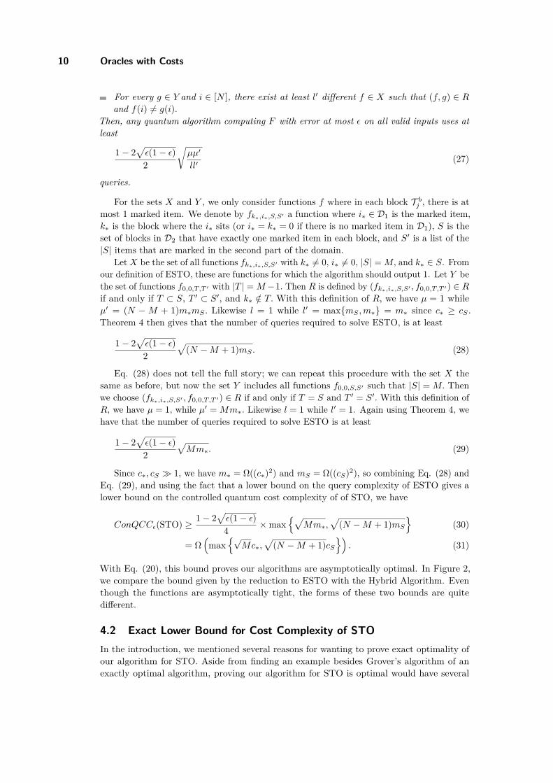
For the sets X and Y , we only consider functions f where in each block T bj , there is atmost 1 marked item. We denote by fk∗,i∗,S,S′ a function where i∗ ∈ D1 is the marked item,k∗ is the block where the i∗ sits (or i∗ = k∗ = 0 if there is no marked item in D1), S is theset of blocks in D2 that have exactly one marked item in each block, and S′ is a list of the|S| items that are marked in the second part of the domain.
Let X be the set of all functions fk∗,i∗,S,S′ with k∗ 6= 0, i∗ 6= 0, |S| = M, and k∗ ∈ S. Fromour definition of ESTO, these are functions for which the algorithm should output 1. Let Y bethe set of functions f0,0,T,T ′ with |T | = M−1. Then R is defined by (fk∗,i∗,S,S′ , f0,0,T,T ′) ∈ Rif and only if T ⊂ S, T ′ ⊂ S′, and k∗ /∈ T. With this definition of R, we have µ = 1 whileµ′ = (N −M + 1)m∗mS . Likewise l = 1 while l′ = maxmS ,m∗ = m∗ since c∗ ≥ cS .Theorem 4 then gives that the number of queries required to solve ESTO, is at least
1− 2√ε(1− ε)2
√(N −M + 1)mS . (28)
Eq. (28) does not tell the full story; we can repeat this procedure with the set X thesame as before, but now the set Y includes all functions f0,0,S,S′ such that |S| = M. Thenwe choose (fk∗,i∗,S,S′ , f0,0,T,T ′) ∈ R if and only if T = S and T ′ = S′. With this definition ofR, we have µ = 1, while µ′ = Mm∗. Likewise l = 1 while l′ = 1. Again using Theorem 4, wehave that the number of queries required to solve ESTO is at least
1− 2√ε(1− ε)2
√Mm∗. (29)
Since c∗, cS 1, we have m∗ = Ω((c∗)2) and mS = Ω((cS)2), so combining Eq. (28) andEq. (29), and using the fact that a lower bound on the query complexity of ESTO gives alower bound on the controlled quantum cost complexity of of STO, we have
ConQCCε(STO) ≥1− 2
√ε(1− ε)4 ×max
√Mm∗,
√(N −M + 1)mS
(30)
= Ω(
max√
Mc∗,√
(N −M + 1)cS)
. (31)
With Eq. (20), this bound proves our algorithms are asymptotically optimal. In Figure 2,we compare the bound given by the reduction to ESTO with the Hybrid Algorithm. Eventhough the functions are asymptotically tight, the forms of these two bounds are quitedifferent.
4.2 Exact Lower Bound for Cost Complexity of STOIn the introduction, we mentioned several reasons for wanting to prove exact optimality ofour algorithm for STO. Aside from finding an example besides Grover’s algorithm of anexactly optimal algorithm, proving our algorithm for STO is optimal would have several

S. Kimmel, C. Y.-Y. Lin, and H. Lin 11
0.2 0.4 0.6 0.8 1.0cS
10
20
30
40
50
60
70
80Cost
Figure 2 The solid line is the cost of the hybrid algorithm, while the dashed line is the lowerbound on the cost given by Eq. (30). The cost is calculated with c∗ = 1, N = 104, M = 400 andε = 0 while cS is varied.
other implications. First, the algorithms described in Section 3 are all based on amplitudeamplification, so if we can prove these approaches are optimal, that would give evidence thatamplitude amplification is an exactly optimal algorithm for certain types of unstructuredsearch problems.
Second, if we consider an extension of STO to many oracles, we can no longer proveasymptotic optimality of our amplitude amplification algorithm. Note that in amplitudeamplification, (see Theorem 2), the inner algorithm (A) is applied two times for eachapplication of the oracle that identifies the target state (if A = A−1). This factor of two isnot accounted for in our lower bound of Section 4.1. While this factor of two can be sweptunder the rug using asymptotic notation, if we consider a problem with k nested oracles,and try to apply a similar strategy as for STO and use nested amplitude amplification, theinnermost algorithm will accumulate an extra factor of 2k in the number of times it mustbe applied. Using a strategy similar to Section 4.1 to lower bound this problem will notcatch that factor of 2k, for the same reason the factor of 2 is not characterized by the oraclesimulation and adversary method. In the case of k = logN nested oracles, our bounds will nolonger be asymptotically tight. Thus, if we can find an exact bound in the case of STO, wemight be able to extend it to get asymptotically tight bounds for the case of nested oracles,providing evidence that multiple nestings of amplitude amplification are optimal for certainproblems.
We have found that proving an exactly tight lower bound for STO is a challenge, and infact we can only prove the hybrid algorithm is optimal in a limited setting. The difficulty inproving optimality even in this limited case provides insight into the difficulty of the moregeneral case.
The restricted setting we investigate is to only consider Grover-like algorithms.
I Definition 5. A Grover-like algorithm with oracles O1, . . . ,Ol that act on an N -dimensional Hilbert space must:
Use only an N -dimensional Hilbert space as its workspace,Initialize in the equal superposition state |N〉 = 1√
N
∑Ni=1 |i〉,
Use only the unitaries O1, . . . ,Ol and G = I− 2|N〉〈N | , andEnd with a measurement on the standard basis.
TQC’15
12 Oracles with Costs
If we consider Grover-like algorithms for SEARCH, the state of the system is restrictedto a 2-dimensional subspace spanned by |N〉 and |i∗〉. Since G2 = O2
∗ = I, the only possiblealgorithm is alternating G and O∗, and one can easily track the progress of the state throughthe two dimensional space towards |i∗〉, thus trivially proving that in this setting, Grover’salgorithm is exactly optimal.
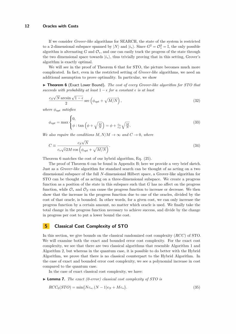
We will see in the proof of Theorem 6 that for STO, the picture becomes much morecomplicated. In fact, even in the restricted setting of Grover-like algorithms, we need anadditional assumption to prove optimality. In particular, we show
I Theorem 6 (Exact Lower Bound). The cost of every Grover-like algorithm for STO thatsucceeds with probability at least 1− ε for a constant ε is at least
cS√N arcsin
√1− ε
2 sec(φopt +
√M/N
), (32)
where φopt satisfies
φopt = max
0,φ : tan
(φ+
√MN
)= φ+ c∗
cS
√MN .
(33)
We also require the conditions M,N/M →∞ and C → 0, where
C ≡ cS√N
c∗√ε2M cos
(φopt +
√M/N
) . (34)
Theorem 6 matches the cost of our hybrid algorithm, Eq. (25).The proof of Theorem 6 can be found in Appendix B; here we provide a very brief sketch.
Just as a Grover-like algorithm for standard search can be thought of as acting on a twodimensional subspace of the full N -dimensional Hilbert space, a Grover-like algorithm forSTO can be thought of as acting on a three-dimensional subspace. We create a progressfunction as a position of the state in this subspace such that G has no affect on the progressfunction, while O∗ and OS can cause the progress function to increase or decrease. We thenshow that the increase in the progress function due to one of the oracles, divided by thecost of that oracle, is bounded. In other words, for a given cost, we can only increase theprogress function by a certain amount, no matter which oracle is used. We finally take thetotal change in the progress function necessary to achieve success, and divide by the changein progress per cost to put a lower bound the cost.
5 Classical Cost Complexity of STO
In this section, we give bounds on the classical randomized cost complexity (RCC) of STO.We will examine both the exact and bounded error cost complexity. For the exact costcomplexity, we see that there are two classical algorithms that resemble Algorithm 1 andAlgorithm 2, but whereas in the quantum case, it is possible to do better with the HybridAlgorithm, we prove that there is no classical counterpart to the Hybrid Algorithm. Inthe case of exact and bounded error cost complexity, we see a polynomial increase in costcompared to the quantum case.
In the case of exact classical cost complexity, we have:
I Lemma 7. The exact (0-error) classical cost complexity of STO is
RCC0(STO) = minNc∗, (N − 1)cS +Mc∗. (35)

S. Kimmel, C. Y.-Y. Lin, and H. Lin 13
Proof. We consider an adversarial oracle that knows in advance the queries the algorithmwill make.
Recall that for i ∈ [N ], fS identifies whether i ∈ S and f∗ identifies whether i = i∗. Wesay an item has been completely queried if it has been queried with fS , and is found to notbe an element of S, or if it has been queried with f∗. Then the adversarial oracle acts in thefollowing way:
The first M − 1 items that the algorithm queries using oracle fS are all elements of S.If all elements except one have been queried (but not necessarily completely queried)using either function f∗ or fS , the final element to be queried will be an element of S(even if this element is not queried using fS).The last element to be completely queried is the marked item, if it exists.
Any algorithm acting against this adversarial oracle that makes q queries using fS , hasworst-case cost at least
NcS +Mc∗ if q = N,
qcS + [(N − q) + (M − 1)]c∗ if N − 1 ≥ q ≥M − 1,qcS +Nc∗ if M − 1 ≥ q ≥ 0. (36)
These expressions are minimized at q = N − 1 or q = 0, and we obtain
RCC0(STO) ≥ minNc∗, (N − 1)cS +Mc∗. (37)
For the upper bound, consider the following two algorithms.
I Algorithm 4. Query all items using f∗. This algorithm will find the marked item if itexists with certainty, and has cost Nc∗.
I Algorithm 5. Query all but the last item using fS. Then:If M items of S have been found, query f∗ on these M items.If M − 1 items of S have been found, query f∗ on these M − 1 items, and also the lastitem (the item that was not queried using fS).Otherwise |S| 6= M and therefore no marked item exists.
This algorithm will find the marked item if it exists with certainty, and has cost (N − 1)cS +Mc∗.
Thus we have
RCC0(STO) ≤ minNc∗, (N − 1)cS +Mc∗. (38)
J
Algorithm 1 can be thought of as the quantum version of Algorithm 4, while Algorithm2 can be thought of as the quantum version of Algorithm 5. In the 0-error classical case,these two approaches tell the whole story. However, in the quantum case, you can do betterwith the Hybrid Algorithm. The Hybrid Algorithm works by doing something very quantum,which is to partially search for the elements of S. In the classical case, this doesn’t work.Once you’ve found an element of S, you’ve found it; there is no way to partially find anelement of S.
With Lemma 7, we’ve proven that in the 0-error case, we can obtain a polynomialreduction in cost by using a quantum algorithm for STO. Next, we show this polynomialreduction holds even in the case of bounded error algorithms. We do this by reducing STOto the problem of SEARCH. Recall that for SEARCH, we have:
TQC’15

14 Oracles with Costs
I Lemma 8. Any randomized classical algorithm that solves SEARCH with bounded probab-ility must query f∗ at least Ω(N) times.
Now we can prove the reduction of STO to standard search:
I Lemma 9. Any randomized classical algorithm that solves STO with bounded probabilityof error must use as least Ω(N) queries to either f∗ or fS, as long as M/N ≤ 1/9.
Proof. Suppose there is a randomized algorithm A that solves STO with probability 3/4and makes q∗ queries to f∗ and qS queries to fS . Then we will use A to find i∗ in the casewhen we are given f∗ but not fS . To do this, we will use f∗ to create a function that behavessimilarly to fS . We choose a subset T ∈ [N ] with |T | = M − 1 at random, and create afunction fT that acts as
fT (i) =
1 if i ∈ T0 if i /∈ T.
(39)
Then we create the function fS to simulate fS , where
fS(i) = fT (i) ∨ f∗(i). (40)
Each time we want to query fS , we must query f∗(i). Notice that fS behaves like a valid fSfunction unless i∗ exists and i∗ ∈ T (because in this case fS marks M − 1 items instead ofM .) i∗ ∈ T with probability M−1
N.
We create fS as above, and we implement A, but every time A asks us to apply fS , weinstead apply fS . This new algorithm will succeed with probability 3/4(1−(M−1)/N) ≥ 2/3,because it succeeds with probability 3/4 as long as i∗ /∈ F . This means we have createdan algorithm for standard search which uses q∗ + qS queries to f∗ and which succeeds withprobability 2/3. But by Lemma 8, we must have q∗ + qS = Ω(N). J
Finally, we note that there is an additional restriction on the number of queries to f∗:
I Lemma 10. Any randomized classical algorithm that solves STO with bounded probabilitymust use at least Ω(M) queries to f∗.
Proof. Suppose the elements of the subset S were known. Then in the worst case, thatwould still only narrow down the search to M items. (This is the worst case because if|S| 6= M , then one immediately knows there is no marked item.) One must then perform asearch for one marked item out of M , which requires Ω(M) queries via Lemma 8. J
Now we can state our lower bound on the query cost of STO:
I Theorem 11. The bounded error classical randomized cost complexity of STO is
RCC(STO) = min Ω(cSN + c∗M),Ω(c∗N) . (41)
Proof. When M/N ≤ 1/9, we solve the following linear program:
minimize: q∗c∗ + qScS
subject to: q∗ ≥ f1(M, ε)q∗ + qS ≥ f2(N,M, ε). (42)
When M/N > 1/9, from Lemma 10, we have have q∗ = Ω(M) = Ω(N), so the cost is asleast Ω(c∗M) = Ω(c∗N). J
Comparing Eq. (41) with Eq. (20), we see that there is always a separation betweenthe quantum and classical costs of STO. In particular, to get the quantum scaling from theclassical scaling, simply replace all M ’s and N ’s by
√M and
√N .

S. Kimmel, C. Y.-Y. Lin, and H. Lin 15
6 Conclusions and Open Questions
While query complexity is a well understood and powerful tool for quantifying the powerof quantum computers, there are still problems that are not easily characterized by querycomplexity. Cost complexity is one way of extending the standard query model, and we’veargued that this approach has potential applications in constraint satisfaction problems.
While we motivated STO with problems like k-SAT, graph isomorphism, and the travelingsalesman problem, it is not obvious how much of a speed-up an STO inspired algorithm forthese problems would be. The speed-up in STO depends critically on N, M, c∗, and cs. Itwould be interesting to calculate approximately what this relationship is, for example, in arandom k-SAT instance. Once this relationship is better understood, we could determine theamount of speed-up an STO algorithm would give for such a problem. However, even with abetter understanding of this relationship, it is unlikely that M would be known exactly. Inthat case, a method such as fixed point search [16] might be helpful.
STO is a very simple extension of a search problem, and thus the methods described hereall have a Grover-ish flavor to them. It would be interesting to find well motivated problemsfor the cost complexity model where other quantum algorithms could be employed.
We have also left open the question of the exact cost of STO. We believe our algorithm isoptimal, but it seems new techniques are needed to prove it.
Acknowledgments. The authors would like to thank Edward Farhi, Andrew Childs, andAram Harrow for illuminating discussions. Funding for SK provided by the Department ofDefense. HSL and CYL are supported by the ARO grant Contract Number W911NF-12-0486.CYL gratefully acknowledges support from the Natural Sciences and Engineering ResearchCouncil of Canada.
References1 Andris Ambainis. Quantum lower bounds by quantum arguments. In Proc. 32nd ACM
STOC, pages 636–643. ACM, 2000.2 Andris Ambainis. Quantum search with variable times. Theory of Computing Systems,
47(3):786–807, 2010.3 Andris Ambainis, Ansis Rosmanis, and Dominique Unruh. Quantum attacks on classical
proof systems – the hardness of quantum rewinding. arXiv preprint arXiv:1404.6898, 2014.4 Robert Beals, Harry Buhrman, Richard Cleve, Michele Mosca, and Ronald De Wolf.
Quantum lower bounds by polynomials. Journal of the ACM (JACM), 48(4):778–797,2001.
5 Aleksandrs Belovs. Learning-graph-based quantum algorithm for k-distinctness. In Proc.IEEE 53rd FOCS, pages 207–216. IEEE Computer Society, 2012.
6 Aleksandrs Belovs and Ansis Rosmanis. On the power of non-adaptive learning graphs.Computational Complexity, 23(2):323–354, 2014.
7 Charles H. Bennett, Ethan Bernstein, Gilles Brassard, and Umesh Vazirani. Strengths andweaknesses of quantum computing. SIAM Journal on Computing, 26(5):1510–1523, 1997.
8 Gilles Brassard, Peter Høyer, Michele Mosca, and Alain Tapp. Quantum amplitude ampli-fication and estimation. arXiv preprint quant-ph/0005055, 2000.
9 Nicolas J Cerf, Lov K Grover, and Colin P Williams. Nested quantum search and structuredproblems. Physical Review A, 61(3):032303, 2000.
10 Cătălin Dohotaru and Peter Høyer. Exact quantum lower bound for grover’s problem.Quantum Information and Computation, 9(5-6):533–540, 2009.
TQC’15

16 Oracles with Costs
11 Mark Ettinger, Peter Høyer, and Emanuel Knill. The quantum query complexity of thehidden subgroup problem is polynomial. Information Processing Letters, 91(1):43–48, 2004.
12 Peter Høyer, Troy Lee, and Robert Špalek. Negative weights make adversaries stronger. InProc. 39th ACM STOC, pages 526–535, 2007.
13 Troy Lee, Rajat Mittal, Ben W Reichardt, Robert Špalek, and Mario Szegedy. Quantumquery complexity of state conversion. In Proc. 52nd IEEE FOCS, pages 344–353. IEEE,2011.
14 Ashley Montanaro. Quantum search with advice. In Theory of Quantum Computation,Communication, and Cryptography, pages 77–93. Springer, 2011.
15 Aran Nayebi, Scott Aaronson, Aleksandrs Belovs, and Luca Trevisan. Quantum lowerbound for inverting a permutation with advice. arXiv preprint arXiv:1408.3193, 2014.
16 Theodore J Yoder, Guang Hao Low, and Isaac L Chuang. Fixed-point quantum searchwith an optimal number of queries. Physical review letters, 113(21):210501, 2014.
A Analysis of the Hybrid Algorithm
Throughout this section, when we are calculating something “to zeroth order”, we drop termswhose sizes are O(M−1/2) or O((M/N)1/4) multiplied by the size of the largest term.
In Section 3, Eq. (24), we showed that the cost of the Hybrid Algorithm is
Cost(Hybrid) =
arcsin
√1− ε− arcsin
√1−α√M
2 arcsin√
1−α√M
×
c∗ + 2cS
(
arcsin√
1− α− arcsin√
MN
)2 arcsin
√MN
. (43)
In this appendix, we prove that in the limit of M →∞ and N/M →∞, there is a choice ofα such that the cost is
Cost(Hybrid) = cS√N arcsin
√1− ε
2 sec(φopt +
√M
N
), (44)
where φopt is given by
φopt = max
0φ : tan
(φ+
√MN
)= φ+ c∗
cS
√MN .
(45)
We first define
t =
(
arcsin√
1− α− arcsin√
MN
)2 arcsin
√MN
, (46)
so t is a non-negative integer. Substituting t for α in Eq. (43), we obtain
Cost(Hybrid) =(2tcS + c∗)
×
arcsin√
1− ε
2 arcsin
sin(
(2t+ 1) arcsin√
MN
)√M
−1
− 1/2
.(47)

S. Kimmel, C. Y.-Y. Lin, and H. Lin 17
To zeroth order, this becomes
Cost(Hybrid) = (2tcS + c∗)√M arcsin
√1− ε
2 sin(
(2t+ 1)√
MN
) . (48)
Finally, we denote φ = 2t√M/N to obtain
Cost(Hybrid) =
(φcS +
√MN c∗
)√N arcsin
√1− ε
2 sin(φ+
√MN
) . (49)
We take the partial derivative of the cost with respect to φ, and set it to zero to find thevalue of φ that gives the smallest cost. We find the cost is minimized when φ = φopt, whereφopt satisfies
tan(φopt +
√M/N
)= φopt + c∗
c
√M/N. (50)
Notice that there is always a solution with φopt ∈ [−√M/N, π/2]. However t is non-negative,
so if φopt < 0 we set φopt = 0. This condition, along with Eq. (49) and Eq. (50), immediatelygives the cost claimed in Eq. (44).
We might not be able to exactly attain this cost, because t must be an integer, so wemight only be able to set φ close to φopt. We show that even if we can’t set φ exactly toφopt, we can still attain the cost of Eq. (44), to zeroth order.
There are two cases to consider. In the first case, we assume (M/N)1/4 ≤ φopt ≤ π/2. Werequire that t be a non-negative integer, so we choose t =
⌈(φopt
√N)/(2
√M)⌉, and hence
we set
φ =⌈φopt
2
√N
M
⌉2√M
N. (51)
For that choice, notice that
φ− φopt = O(
(M/N)1/2). (52)
This allows us to relate terms involving φ to those involving φ0:
sin(φ+
√M/N
)= sin
(φopt +
√M/N
)±O((M/N)1/2)
= sin(φopt +
√M/N
)(1±O((M/N)1/4)
)=(φopt + c∗
cS
√M/N
)cos(φopt +
√M/N
)(1±O
((M/N)1/4
))=(φ+ c∗
cS
√M/N
)cos(φopt +
√M/N
)(1±O
((M/N)1/4
)),
(53)
where in the first line, we use the angle addition formula and Eq. (52); in the second, weuse the assumption that φopt ≥ (M/N)1/4; in the third line we applied Eq. (50); and in thelast we have used Eq. (52) and the assumption on the size of φopt. Plugging Eq. (53) intoour expression for the cost in Eq. (49), we have that to zeroth order, we obtain Eq. (44), asdesired.
TQC’15

18 Oracles with Costs
We now consider the second case, when 0 ≤ φopt < (M/N)1/4. In this case, we simplyset t = 0, and hence φ = 0. Plugging φ = 0 the cost of Eq. (49), we have, to zeroth order,
Cost(Hybrid) = arcsin√
1− ε√N
2 c∗. (54)
We will show that Eq. (54) and Eq. (44) are equivalent for 0 ≤ φopt < (M/N)1/4. We have
sec(φopt +
√M/N
)= 1 +O
((M/N)1/4
). (55)
We can expand Eq. (50) to get
cS = c∗
(1−O
((M/N)1/4)
)). (56)
Plugging Eqs. (55) and (56) into Eq. (44) and keeping only zeroth order terms, we recoverEq. (54).
B Proof of Theorem 6
In this section, we prove the following theorem:
I Theorem 6 (Exact Lower Bound). The cost of every Grover-like algorithm for STO thatsucceeds with probability at least 1− ε for a constant ε is at least
cS√N arcsin
√1− ε
2 sec(φopt +
√M/N
), (32)
where φopt satisfies
φopt = max
0,φ : tan
(φ+
√MN
)= φ+ c∗
cS
√MN .
(33)
We also require the conditions M,N/M →∞ and C → 0, where
C ≡ cS√N
c∗√ε2M cos
(φopt +
√M/N
) . (34)
Proof. Throughout this section, when we say to zeroth order, we mean dropping terms ofsize at most O(M−1/2) or O
((M/N)1/2) or O(C) of the zeroth order terms.
Since we only consider the operations OS , O∗, and G, the state of the system never leavesthe three-dimensional space spanned by the orthonormal states
|i∗〉, |S−〉 = 1√M−1
∑i∈S−i∗ |i〉, |S
⊥〉 = 1√N−M
∑i/∈S |i〉
. (57)
It turns out that it is more convenient to work in a slightly shifted basis from that of Eq.(57). We instead use the orthonormal basis states:
|x〉 = cos θ0|i∗〉 − sin θ0|S−〉,|y〉 = cosφ0 sin θ0|i∗〉+ cosφ0 cos θ0|S−〉 − sinφ0|S⊥〉,|z〉 = sinφ0 sin θ0|i∗〉+ cos θ0 sinφ0|S−〉+ cosφ0|S⊥〉
= |N〉. (58)
S. Kimmel, C. Y.-Y. Lin, and H. Lin 19
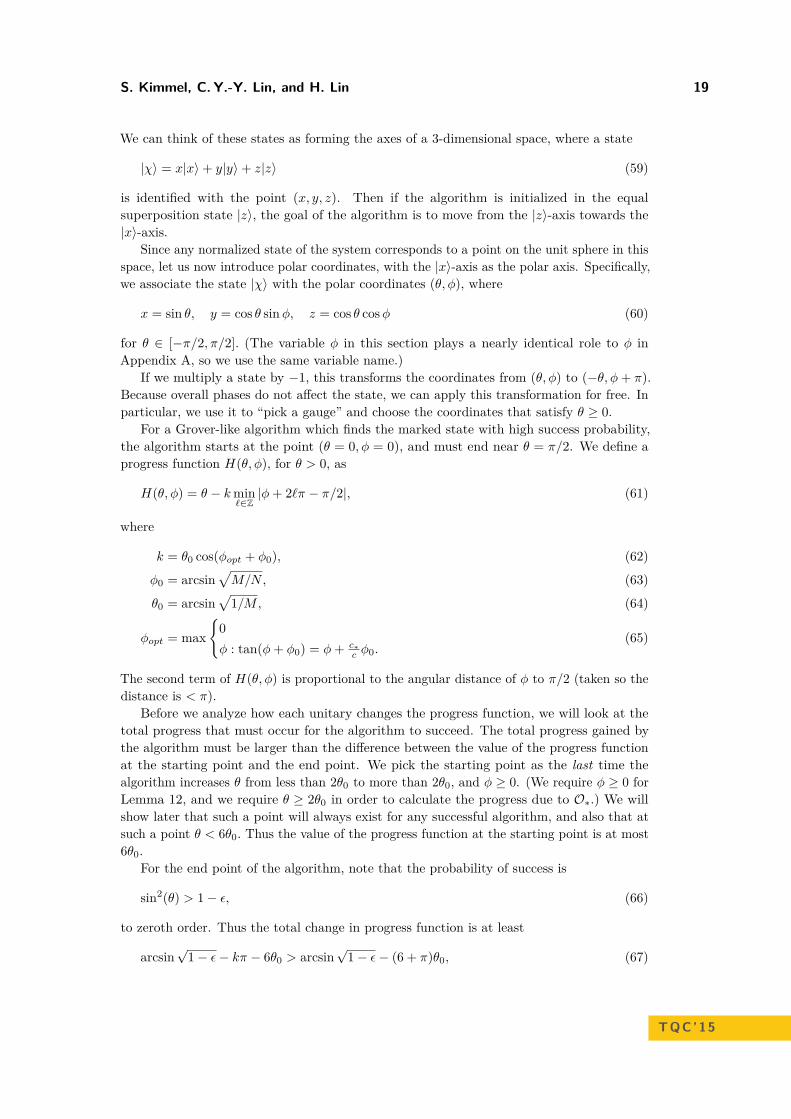
We can think of these states as forming the axes of a 3-dimensional space, where a state
|χ〉 = x|x〉+ y|y〉+ z|z〉 (59)
is identified with the point (x, y, z). Then if the algorithm is initialized in the equalsuperposition state |z〉, the goal of the algorithm is to move from the |z〉-axis towards the|x〉-axis.
Since any normalized state of the system corresponds to a point on the unit sphere in thisspace, let us now introduce polar coordinates, with the |x〉-axis as the polar axis. Specifically,we associate the state |χ〉 with the polar coordinates (θ, φ), where
x = sin θ, y = cos θ sinφ, z = cos θ cosφ (60)
for θ ∈ [−π/2, π/2]. (The variable φ in this section plays a nearly identical role to φ inAppendix A, so we use the same variable name.)
If we multiply a state by −1, this transforms the coordinates from (θ, φ) to (−θ, φ+ π).Because overall phases do not affect the state, we can apply this transformation for free. Inparticular, we use it to “pick a gauge” and choose the coordinates that satisfy θ ≥ 0.
For a Grover-like algorithm which finds the marked state with high success probability,the algorithm starts at the point (θ = 0, φ = 0), and must end near θ = π/2. We define aprogress function H(θ, φ), for θ > 0, as
H(θ, φ) = θ − kmin`∈Z|φ+ 2`π − π/2|, (61)
where
k = θ0 cos(φopt + φ0), (62)
φ0 = arcsin√M/N, (63)
θ0 = arcsin√
1/M, (64)
φopt = max
0φ : tan(φ+ φ0) = φ+ c∗
c φ0.(65)
The second term of H(θ, φ) is proportional to the angular distance of φ to π/2 (taken so thedistance is < π).
Before we analyze how each unitary changes the progress function, we will look at thetotal progress that must occur for the algorithm to succeed. The total progress gained bythe algorithm must be larger than the difference between the value of the progress functionat the starting point and the end point. We pick the starting point as the last time thealgorithm increases θ from less than 2θ0 to more than 2θ0, and φ ≥ 0. (We require φ ≥ 0 forLemma 12, and we require θ ≥ 2θ0 in order to calculate the progress due to O∗.) We willshow later that such a point will always exist for any successful algorithm, and also that atsuch a point θ < 6θ0. Thus the value of the progress function at the starting point is at most6θ0.
For the end point of the algorithm, note that the probability of success is
sin2(θ) > 1− ε, (66)
to zeroth order. Thus the total change in progress function is at least
arcsin√
1− ε− kπ − 6θ0 > arcsin√
1− ε− (6 + π)θ0, (67)
TQC’15

20 Oracles with Costs
where we bound k using Eq. (62), and the kπ term comes from the worst possible value of φwhen θ gets sufficiently large.
We note the following: from Eq. (25) and Eq. (62) we see that the cost of the optimalalgorithm is at most
cS arcsin√
1− εφ0k
, (68)
and from Eq. (67) the change in the progress function is at least arcsin√
1− ε− (6 + π)θ0;therefore the progress per unit cost must be at least φ0k/cS , to zeroth order. It thereforefollows that when calculating the change in progress function, we only need to keep track ofterms up to order O(φ0k/cS) per cost. For example, for O∗, we need only keep track of thechange in progress (not progress per cost) up to order O(φ0kc∗/cS).
The change in the progress function H(θ, φ) due to the unitaries G, OS , and O∗ can becalculated by how they change the coordinates (θ, φ) of a state. After some algebra andusing our gauge choice, we obtain
G: The unitary G is a reflection about the z-axis, and in polar coordinates is the map
G : (θ, φ)→ (θ, π − φ). (69)
Comparing with Eq. (61), we see G has no effect on the progress function.OS : The oracle OS is a reflection about the state which has polar coordinates (θ = 0, φ =−φ0).
OS : (θ, φ)→ (θ, π − φ− 2φ0) (70)
We see that OS can change the progress function by at most 2φ0k. Thus the increase inthe progress function per cost due to OS is at most
2φ0k
cS= 2φ0θ0 cos(φopt + φ0)
cS. (71)
O∗: The oracle O∗ is a reflection about the state |i∗〉, which is close to |x〉. We find O∗transforms coordinates as
θ → θ + 2θ0 sin(φ+ φ0) +O(θ20) (72)
φ→ π + φ+O
(θ0
cos θ
). (73)
Now we consider how O∗ affects the progress function; unlike the previous cases, whichwe calculated exactly, we will only analyze this case to zeroth order. We will first show thatwe can assume |φ| ≤ π/2. Suppose that |φ| > π/2 just before we would like to apply O∗.Then instead of applying O∗, we apply GO∗G. One can check that with this replacement,when O∗ is applied, |φ| ≤ π/2. Furthermore one can verify that this replacement causes θ toincrease (which can only be good for the progress function), while on the other hand, thevalue of φ changes by at most O (θ0/ cos θ) due to this replacement, resulting in a changein the progress function of size O (kθ0/
√ε) (using Eq. (66) to bound cos θ). Using our
assumption that that C = o(1), this change has order less than O(φ0kc∗/cS), and so can bediscarded using the argument following Eq. (68). We can therefore assume that O∗ is alwaysapplied at |φ| ≤ π/2.

S. Kimmel, C. Y.-Y. Lin, and H. Lin 21
Now we can examine the change in the progress function due to the action of O∗. Theincrease in the progress function is
2θ0 sin(φ+ φ0) +O(θ2
0)
− k(
min`∈Z| − φ+ 2`π − π/2| −min
`∈Z|φ+ 2`π − π/2|
)+O
(kθ0
cos θ
). (74)
Since |φ| ≤ π/2, the increase in the progress function due to O∗ is less than
2θ0 sin(φ+ φ0)− 2φθ0 cos(φopt + φ0) +O
(θ2
0√ε
), (75)
where we have used the value of k from Eq. (62) and bounded cos θ with Eq. (66).Taking the first and second derivatives of Eq. (75) with respect to φ, we see that when
φ ≥ 0, the increase in the progress function is maximized when φ = φopt. It turns out thatif one applies O∗ at φ < 0, it is sometimes possible to achieve a larger increase in progressper cost than when φ ≥ 0. However, we show at the end of this section, (Lemma 12), thatapplying O∗ when φ < 0 will always be less efficient (up to higher order terms) in terms ofthe increase in progress function per cost, than applying O∗ at φ = φopt, when viewed in thecontext of the larger algorithm. Applying the definition of φopt from Eq. (65) to Eq. (75),and using the definition of C from Eq. (34), the increase in the progress function due to O∗is less than
c∗2φ0θ0 cos(φopt + φ0)cS
(1 +O(φ2
0) +O (C)), (76)
where the O(φ20) term accounts for the case that φopt = 0.
From Eq. (71) and Eq. (76) we see that (to zeroth order) the maximum increase in theprogress function per cost is the same whether O∗ is applied or OS is applied. Dividing thetotal necessary change in progress (Eq. (67)) by the maximum change in progress per cost(Eq. (76)) gives us the minimum cost:
arcsin√
1− ε cS2φ0θ0 cos(φopt + φ0)
(1−O(C)−O(M−1/2)−O
((M/N)−1/2
)). (77)
In the limit of N,M →∞ and C → 0, (to zeroth order) we have that the cost is at least
arcsin√
1− ε cS√M
2φ0 cos(φopt + φ0) , (78)
which matches the cost of Eq. (25).We now justify why the value of the progress function must be less than 6θ0 when we start
tracking it. Immediately before we start tracking the progress function, we have θ < 2θ0, sothe bound on the increase in progress given by Eq. (75) does not necessarily apply. However,it is simple to show that the increase in the progress function due to O∗ is always boundedby 2θ0, where we have dropped terms of O(θ2
0/√ε) as before. Thus if θ < 2θ0, and then O∗
is applied, θ can increase by at most 2θ0, and so the new value of θ satisfies θ < 4θ0. At thispoint, θ > 2θ0, but φ might be negative. Notice that θ can not increase unless O∗ is applied,(and θ must increase in order to obtain a high probability of success) but O∗ flips the sign ofφ, so after applying O∗ at most one more time, we will have both the conditions θ > 2θ0and φ ≥ 0 satisfied, at which point we start tracking the progress function. This tells us thatthe value of θ will be at most 6θ0 when we start tracking the progress function. J
TQC’15

22 Oracles with Costs
I Lemma 12. Suppose there is an algorithm than applies O∗ when φ < 0. Then there isalways an alternative algorithm that achieves the same or greater increase in progress for thesame or less cost (up to zeroth order), but applies O∗ only when φ ≥ 0.
Proof. We begin by classifying the the possible sequences of O∗, OS , and G the algorithmcan take. We will use notation such that unitaries act from right to left, so GO∗ signifies O∗acts first, and then G acts.
First look at O∗. We can always assume O∗ is followed by a G; if it is not, insert a GGpair after the O∗. Note in the discussion following Eq. (73), we proved that we can assume|φ| < π/2 before applying O∗. With Eqs. (69) and (73) we have
GO∗ : φ→ −φ+O
(θ0
cos θ
). (79)
Since |φ| < π2 before GO∗ acts, we also have |φ| < π
2 after GO∗ acts, up to an additive factorof O
(θ0
cos θ), which we can ignore thanks to the discussion following Eq. (68). Therefore GO∗
maps φ inside the |φ| < π2 region.
In between applications of GO∗, there is always a sequence of one of the following forms:
(GOS)m, G(GOS)m, (OSG)m, or G(OSG)m, (80)
where m is a non-negative integer that indicates multiple applications of the unitary sequenceinside the parenthesis. These are the only possible sequences because OSOS = I and GG = I.Combining the action of G and OS in Eqs. (69) and (70) we get
(OSG)m : (θ, φ)→ (θ, φ− 2mφ0) (81)(GOS)m : (θ, φ)→ (θ, φ+ 2mφ0). (82)
Thus the 4 sequences of Eq. (80) rotate φ by some amount ±2mφ0, possibly followed by thetransformation φ→ π − φ.
Now we focus on the algorithm’s action on φ. Since the GO∗’s are mapping φ betweenpoints inside the |φ| < π
2 region, the four possible sequences of alternating G and OS inEq (80) just connect the value of φ after applying GO∗ to the value of φ before the nextapplication of GO∗. Generalizing Figure 3, one can see that the shortest path uses either(GOS)m or (OSG)m to connect points inside the |φ| < π
2 region. Therefore we do not needto consider the sequences G(OSG)m or G(GOS)m.
Next, we show that if one initially has φ > 0, it is never advantageous to again applyGO∗ when φ < 0. Since the algorithm must consist of applications of GO∗ separated bysequences of either (OSG)m or (GOS)m, we can enumerate and address the three possiblecases that lead us to apply O∗ at some φ = φneg < 0 after initially having φ ≥ 0. The threepossible cases are laid out graphically in Figure 4. In order to prove that none of the casesare optimal, we define the function
p∗(φ) = 2(θ0 sin(φ+ φ0)− kφ) (83)
as the change in progress function due to an application of O∗, dropping higher order terms.Note for φ ≥ 0, φopt optimizes Eq. (83) as discussed after Eq. (75). We proceed to treat thethree cases.

S. Kimmel, C. Y.-Y. Lin, and H. Lin 23
Figure 3 The path in the figure at left uses a sequence (GOS)m to move from φstart to φend,whereas the path in figure at right uses a sequence G(OSG)m. The path using (GOS)m is shorter,signifying that fewer uses of OS are required to move from φstart to φend, and thus this is the moreefficient path.
Sequence I. We consider the following sequence of operations (see Figure 4):(i) Start with φi > 0. Then apply GO∗ to get to −φi.(ii) Apply (GOS) some number of times to increase φ to φneg > −φi.(iii) Apply GO∗ to get to −φneg < φi.
The change in progress due only to O∗ in this sequence is
p∗(φi) + p∗(φneg) = 2(θ0 sin(φi + φ0)− kφi)+ 2(θ0 sin(φneg + φ0)− kφneg)
≤ 4[θ0 sin(φi + φneg2 + φ0)− kφneg + φi
2 ]
= 2p∗(φi + φneg)≤ 2p∗(φopt), (84)
Since φneg + φi ≥ 0, the average progress due to the two applications of O∗ is worse thanif we had applied O∗ at φopt both times. Thus this sequence cannot be optimal.
Sequence II. We consider the following sequence of operations (see Figure 4):(i) Start with φi > 0. Then apply GO∗ to get to −φi.(ii) Apply (OSG) some number of times to decrease φ to φneg < −φi.(iii) Apply GO∗ to get to −φneg > φi.Compare Sequence II to the following Sequence 2:(a) Start with φi > 0. Then apply (GOS) some number of times to increase φ to−φneg > φi.
The difference in progress between Sequence II and Sequence 2 is
(2θ0 sin(φi + φ0) + 2θ0 sin(φneg + φ0))
=4θ0 sin(φi + φneg2 + φ0) cos(φi − φneg2 )
<4θ0 sinφ0, (85)
since −π4 <φi+φneg
2 < 0 and 0 < φi−φneg2 < π
2 . Sequence II and Sequence 2 both use thesame number of applications of OS (in steps (ii) and (a) respectively). Therefore, the
TQC’15

24 Oracles with Costs
Sequence II has an additional cost 2c∗ while it only has an added increase in progress of
4θ0 sinφ0 =2p∗(0)≤2p∗(φopt). (86)
Therefore Sequence II does not attain the increase in progress per cost that one couldattain by only applying O∗ at φopt.
Sequence III. We consider the following sequence of operations (see Figure 4):(i) Start with φi ≥ 0, then apply (OSG) some number of times to decrease φ to
φneg < 0.(ii) Apply GO∗ to get to −φneg.Compare Sequence III to the following Sequence 3:(a) Start with φi ≥ 0, and then apply (OSG) some number of times to decrease φ to
φw such that 2φ0 > φw ≥ 0.(b) Apply GO∗ to get to −φw.(c) Apply (GOS) some number of times to increase φ to −φneg > 0.Note that we can always create a sequence with such a φw because (OSG) changes φ byat most 2φ0 each time. The cost of Sequence III is the same as the cost of Sequence 3.The difference in progress between Sequence III and Sequence 3 is
2θ0 sin(φneg + φ0)− 2θ0 sin(φw + φ0)
≤4θ0 cos(φneg + φw
2 + φ0
)sin(φneg − φw
2
)<0 (87)
since |φneg+φw2 + φ0| < π
2 and π2 <
φneg−φw2 < 0. Therefore Sequence III is not optimal
either.
Hence we conclude that applying O∗ at negative φ never achieves as much increase inprogress per cost as applying O∗ at φopt, and therefore we only need to consider applyingO∗ at positive φ, at φopt. J
C An Adversary Lower Bound
In this section, we will show how to apply the adversary method to the problem of costcomplexity of STO.
Suppose we are given access to an oracle O∗, which implements the function f∗, and anoracle OS , which implements the function fS . Then any algorithm which solves STO usingthese oracles, after t steps, produces a state
|ψtf∗,fS 〉 = U tOct · · ·U2Oc2U1Oc1 |ψ0〉, (88)
where cj ∈ ∗, S, and U j are fixed unitaries independent of f∗ and fS .We create an adversary matrix Γ, a matrix whose rows and columns are indexed by pairs
of functions (f∗, fS) ∈ DSTO, where DSTO is the set of valid inputs to STO. Furthermore,we have the condition that that Γ[(f∗, fS), (g∗, gS)] = 0 if STO(f∗, fS) = STO(g∗, gS). Withthis notation, we define the progress function:
W t =∑
(f∗,fS),(g∗,gS)∈DSTO×DSTO
Γ(f∗,fS),(g∗,gS)vf∗,fSv∗g∗,gS 〈ψ
tf∗,fS |ψ
tg∗,gS 〉 (89)

S. Kimmel, C. Y.-Y. Lin, and H. Lin 25
Figure 4 Possible paths that could lead to applying GO∗ at a negative value of φ, when initially,φ has positive value.
for a vector v indexed by the elements of DSTO, such that ‖v‖ = 1 and v is an eigenvectorof Γ with eigenvalue ±‖Γ‖, (where ‖ · ‖ signifies the l-2 norm for vectors or the induced l-2norm for matrices).
Then following [12]3, we have1. W 0 = ‖Γ‖.2. WT ≤
(2√ε(1− ε) + 2ε
)‖Γ‖, for any algorithm with probability of error at most ε.
3. W t−1 −W t ≤ 2 maxi ‖Γ Dcti ‖ where D
cti are |DSTO| × |DSTO| matrices satisfying
D∗i [(f∗, fS), (g∗, gS)] =
0 if f∗(i) = g∗(i),1 otherwise,
DSi [(f∗, fS), (g∗, gS)] =
0 if fS(i) = fS(i),1 otherwise.
Thus if q∗ queries are made to O∗ and qS queries are made to OS , we have
‖Γ‖g(ε) ≤ q∗maxi‖Γ D∗i ‖+ qS max
i‖Γ DS
i ‖ (90)
3 The proofs are identical, so we omit them.
TQC’15

26 Oracles with Costs
where
g(ε) =1−
(2√ε(1− ε) + 2ε
)2 . (91)
We construct the following adversary matrix for STO: Γ[(f∗, fS), (g∗, gS)] = 1 if one ofthe following conditions holds:
STO(f∗, fS) = 1, STO(g∗, gS) = 0, and fS(i) = gS(i) except if f∗(i∗) = 1, then gS(i∗) = 0,STO(g∗, gS) = 1, STO(f∗, fS) = 0, and gS(i) = fS(i) except if g∗(i∗) = 1, then fS(i∗) = 0.
Otherwise, Γ = 0.One can calculate (or it is easy to see by analogy to a standard Grover search over
N −M + 1 items) that
‖Γ‖ =√N −M + 1,
maxi‖Γ Dct
i ‖ = 1,
maxi‖Γ DS
i ‖ = 1. (92)
Plugging into Eq. (90) we have
g(ε)√N −M + 1 ≤ q∗ + qS , (93)
so for N > M/2, we have
QCC(STO) = Ω(cS√N). (94)
We also consider a second adversary matrix for STO. Let Γ[(f∗, fS), (g∗, gS)] = 1 if oneof the following conditions holds:
STO(f∗, fS) = 1, STO(g∗, gS) = 0, and fS(i) = gS(i),STO(g∗, gS) = 1, STO(f∗, fS) = 0, and gS(i) = fS(i).
Otherwise, Γ = 0.In this case, the adversary matrix only pairs instances such that OS is the same in both
pairs. Thus it is as if the set S is known ahead of time. In this case, one can calculate (or itis easy to see by analogy to a standard Grover search over M items), that
‖Γ‖ =√M
maxi‖Γ Djt
i ‖ = 1
maxi‖Γ DS
i ‖ = 0. (95)
Plugging into Eq. (90), we have
g(ε)√M ≤ q∗, (96)
so
QCC(STO) = Ω(c∗√M) (97)
Combining Eq. (94) and Eq. (97), we obtain a bound that matches Eq. (20):
QCC(STO) = Ω(
maxc∗√M, cS
√N). (98)

The Resource Theory of SteeringRodrigo Gallego and Leandro Aolita
Dahlem Center for Complex Quantum Systems, Freie Universität Berlin, 14195Berlin, Germany
AbstractWe present an operational framework for Einstein-Podolsky-Rosen steering as a physical resource.To begin with, we characterize the set of steering non-increasing operations (SNIOs) – i.e., thosethat do not create steering– on arbitrary-dimensional bipartite systems composed of a quantumsubsystem and a black-box device. Next, we introduce the notion of convex steering monotonesas the fundamental axiomatic quantifiers of steering. As a convenient example thereof, we presentthe relative entropy of steering. In addition, we prove that two previously proposed quantifiers,the steerable weight and the robustness of steering, are also convex steering monotones. Toend up with, for minimal-dimensional systems, we establish, on the one hand, necessary andsufficient conditions for pure-state steering conversions under stochastic SNIOs and prove, onthe other hand, the non-existence of steering bits, i.e., measure-independent maximally steerablestates from which all states can be obtained by means of the free operations. Our findings revealunexpected aspects of steering and lay foundations for further resource-theory approaches, withpotential implications in Bell non-locality.
1998 ACM Subject Classification J.2 Physics
Keywords and phrases Entanglement, EPR-steering, nonlocality, resource theories
Digital Object Identifier 10.4230/LIPIcs.TQC.2015.27
1 Introduction
Steering, as Schrödinger named it [38], is an exotic quantum effect by which ensembles ofquantum states can be remotely prepared by performing local measurements at a distant lab.It allows [43, 23, 34] to certify the presence of entanglement between a user with an untrustedmeasurement apparatus, Alice, and another with a trusted quantum-measurement device,Bob. Thus, it constitutes a fundamental notion between quantum entanglement [22], whosecertification requires quantum measurements on both sides, and Bell non-locality [13], whereboth users possess untrusted black-box devices. Steering can be detected through simpletests analogous to Bell inequalities [14], and has been verified in a variety of remarkableexperiments [29, 8, 37, 7, 20, 39], including steering without Bell non-locality [35] and a fullyloop-hole free steering demonstration [44]. Apart from its fundamental relevance, steeringhas been identified as a resource for one-sided device-independent quantum key-distribution(QKD), where only one of the parts has an untrusted apparatus while the other ones possesstrusted devices [9, 21]. There, the experimental requirements for unconditionally secure keysare less stringent than in fully (both-sided) device-independent QKD [4, 1, 2].
The formal treatment of a physical property as a resource is given by a resource theory.Thebasic component of this is a restricted class of operations, called the free operations, subject toa physically relevant constraint. The free operations are such that every free state, i.e., everyone without the property in question, is mapped into a free state, so that the resourceful statescan be defined as those not attainable by free operations acting on any free state. Furthermore,the quantification of the resource is also built upon the free operations: The fundamental
© R. Gallego and L. Aolita;licensed under Creative Commons License CC-BY
10th Conference on the Theory of Quantum Computation, Communication and Cryptography (TQC 2015).Editors: Salman Beigi and Robert König; pp. 27–38
Leibniz International Proceedings in InformaticsSchloss Dagstuhl – Leibniz-Zentrum für Informatik, Dagstuhl Publishing, Germany

28 The Resource Theory of Steering
necessary condition for a function to be a measure of the resource is that it is monotonous –non-increasing – under the free operations. That is, the operations that do not increase theresource on the free states do not increase it on all other states either. Entanglement theory[22] is the most popular and best understood [40, 32, 10, 11] resource theory. There, theconstrain on the operations is the unavailability of quantum communication, which yieldsthe local operations assisted by classical communication (LOCCs) [6] as the correspondingfree operations. Nevertheless, resource theories have been formulated also for states outof thermal equilibrium [12], asymmetry [3], reference frames [19], and quantum coherence[26, 5], for instance.
In steering theory, systems are described by an ensemble of quantum states, on Bob’sside, each one associated to the conditional probability of a measurement outcome (output)given a measurement setting (input), on Alice’s. Such conditional ensembles are sometimescalled assemblages [33, 36, 31]. The free operations for steering, which we call steeringnon-increasing operations (SNIOs), must thus arise from constrains native of a naturalscenario where steerable assemblages are useful for some physical task. Curiously, up to now,no attempt for an operational framework of steering as a resource has been reported.
In this submission we develop the resource theory of steering. First, we derive the explicitexpression of the most general SNIO, for arbitrarily many inputs and outputs for Alice’sblack box and arbitrary dimension for Bob’s quantum system. We show that this class offree operations emerges naturally from the basic restrictions of QKD with assemblages, i.e.,of one-side device-independent QKD [9, 21]. With the derived SNIOs, we provide a formaldefinition of steering monotones. As an example thereof, we present the relative entropy ofsteering, for which we also introduce, on the way, the notion of relative entropy betweenassemblages. In addition, we prove SNIO monotonicity for two other recently proposedsteering measures, the steerable weight [36] and the robustness of steering [31], and convexityfor all three measures. To end up with, we prove two theorems on steering conversion understochastic SNIOs for the lowest-dimensional case, i.e., qubits on Bob’s side and 2 inputs × 2outputs on Alice’s. In the first one, we show that it is impossible to transform via SNIOs,not even probabilistically, an assemblage composed of pairs of pure orthogonal states intoanother assemblage composed also of pairs of pure orthogonal states but with a differentpair overlap, unless the latter is unsteerable. This yields infinitely many inequivalent classesof steering already for systems of the lowest dimension. In the second one, we show thatthere exists no assemblage composed of pairs of pure states that can be transformed intoany assemblage by stochastic SNIOs. It follows that, in striking contrast to entanglementtheory, there exists no operationally well defined, measure-independent maximally steerableassemblage of minimal dimension.
The submission is organized as follows. In Sec. 2 we formally define assemblages andpresent their basic properties. In Sec. 3 we characterise the SNIOs. In Sec. 4 we introduce thenotion of convex steering monotones. In Sec. 5 we present the relative entropy of steering. InSec. 6 we show convexity and SNIO-monotonicity of the steerable weight and the robustnessof steering. In Sec. 7 we study, for minimal-dimensional systems, assemblage conversionsunder SNIOs and prove the in existence of pure-assemblage steering bits. Finally, in Sec. 8we present our conclusions and mention some future research directions that our results offer.
Note also, that some proofs and supplemental material can be found in the Appendix ofthe online version on which this submission is based [17], in which case it will be indicatedexplicitly.

R. Gallego and L. Aolita 29
2 Assemblages and steering
We consider two distant parties, Alice and Bob, who have each a half of a bipartite system.Alice holds a so-called black-box device, which, given a classical input x ∈ [s], generatesa classical output a ∈ [r], where s and r are natural numbers and the notation [n] ≡0, . . . , n− 1, for n ∈ N, is introduced. Bob holds a quantum system of dimension d (qudit),whose state he can perfectly characterize tomographically via trusted quantum measurements.The joint state of their system is thus fully specified by an assemblage
ρA|X ≡ PA|X(a, x), %(a, x)a∈[r],x∈[s], (1)
of normalized quantum states %(a, x) ∈ L(HB), with L(HB) the set of linear operatorson Bob’s subsystem’s Hilbert space HB, each one associated to a conditional probabil-ity PA|X(a, x) of Alice getting an output a given an input x. We denote by PA|X thecorresponding conditional probability distribution.
Equivalently, each pair PA|X(a, x), %(a, x) can be univocally represented by the unnor-malized quantum state
%A|X(a, x) ≡ PA|X(a, x)× %(a, x). (2)
In turn, an alternative representation of the assemblage ρA|X is given by the set ρA|X ≡ρA|X(x)x of quantum states
ρA|X(x) ≡∑a
|a〉〈a| ⊗ %A|X(a, x) ∈ L(HE ⊗HB), (3)
where |a〉 is an orthonormal basis of an auxiliary extension Hilbert space HE of dimensionr. The states |a〉 do not describe the system inside Alice’s box, they are just abstract flagstates to represent its outcomes with a convenient bra-ket notation. Expression (3) gives thecounterpart for assemblages of the so-called extended Hilbert space representation used forensembles of quantum states [28]. We refer to ρA|X for short as the quantum representationof ρA|X and use either notation upon convenience.
We restrict throughout to no-signaling assemblages, i.e., those for which Bob’s reducedstate %B ∈ L(HB) does not depend on Alice’s input choice x:
%B ≡∑a
%A|X(a, x) =∑a
%A|X(a, x′) ∀ x, x′. (4)
The assemblages fulfilling the no-signaling condition (4) are the ones that possess a quantumrealization. That is, they can be obtained from local quantum measurements by Alice on ajoint quantum state %AB ∈ L(HA ⊗HB) shared with Bob, where HA is the Hilbert space ofthe system inside Alice’s box. For any no-signaling assemblage ρA|X , we refer as the trace ofthe assemblage to the x-independent quantity
Tr[ρA|X ] ≡ TrEB [ρA|X ] = Tr[%B ] =∑a
PA|X(a, x), (5)
and say that the assemblage is normalized if Tr[ρA|X ] = 1 and unnormalized if Tr[ρA|X ] ≤ 1.An assemblage σA|X ≡ ςA|X(a, x)a∈[r],x∈[s], being ςA|X(a, x) ∈ L(HB) unnormalized
states, is called unsteerable if there exist a probability distribution PΛ, a conditional probabilitydistribution PA|XΛ, and normalized states ξ(λ) ∈ L(HB) such that
ςA|X(a, x) =∑λ
PΛ(λ)PA|XΛ(a, x, λ) ξ(λ) ∀ x, a. (6)
TQC’15

30 The Resource Theory of Steering
Figure 1 Schematic representation of a SNIO map M: The initial assemblage ρA|X consistsof a black-box, with inputs x and outputs a, governed by the probability distribution PA|X , inAlice’s hand, and a quantum subsystem in one of the states %(a, x)a,x, in Bob’s hands. The finalassemblage ρAf |Xf = M(ρA|X) is given by a final black-box, represented by the light-grey rectangle,of inputs xf and outputs af , and a final subsystem, represented outside the light-grey rectangle, inthe state %(af , xf ) = Eω(%(a, x)). To implement M, first, Bob applies, with a probability PΩ(ω), astochastic quantum operation Eω that leaves his subsystem in the state Eω(%(a, x)). He communicatesω to Alice. Then, Alice generates x by processing the classical bits ω and xf according to theconditional distribution PX|Xf ,Ω. She inputs x to her initial device, upon which the bit a is output.Finally, Alice generates the output af of the final device by processing xf , ω, x, and a, according tothe conditional distribution PAf |A,X,Ω,Xf .
Such assemblages can be obtained by sending a shared classical random variable λ to Alice,correlated with the state ξ(λ) sent to Bob, and letting Alice classically post-process herrandom variable according to PA|XΛ, with PX,Λ = PX ×PΛ so that condition (4) holds. Thevariable λ is called a local-hidden variable and the decomposition (6) is accordingly referredto as a local-hidden state (LHS) model. We refer to the set of all unsteerable assemblages asLHS. Any assemblage that does not admit a LHS model as in Eq. (6) is called steerable. Anassemblage is compatible with classical correlations if, and only if, it is unsteerable.
3 The operational framework
3.1 Physical constraints defining the free operations
QKD consists of the extraction of a secret key from the correlations of local-measurementoutcomes on a bipartite quantum state. The most fundamental constraint to which anygeneric QKD protocol is subject is, of course, the lack of a private safe classical-communicationchannel between distant labs. Otherwise, if such channel was available, the whole enterpriseof QKD would be pointless. This imposes restrictions on the operations allowed so as not tobreak the security of the protocol. For instance, clearly, the local-measurement outcomes

R. Gallego and L. Aolita 31
cannot be communicated, as they can be intercepted by potential eavesdroppers who could,with them, immediately crack the key. Of particular relevance for this submission arethe assumptions on the measurement devices. In non-device-independent QKD protocolsentanglement is the resource and security is proven under the assumption that the users havea specific quantum state and perfectly characterized measurement devices [16]. Knowledgeof the state by an eavesdropper does not compromise the security. Therefore, prior to themeasurements producing the key, the users are allowed to preprocess the state in any way andexchange information about it, for instance with LOCCs and even eventually disregardingthe state and aborting the protocol run. Pre-processing abortions or classical communicationcan at most provide an eavesdropper with knowledge about the state, not about the key,and therefore do not affect the security.
The situation is different in device-independent QKD (DIQKD) [4, 1, 2]. There, theresource is given by Bell non-local correlations and no assumption is made either on thequantum state or the measurement devices. The users effectively hold black-box measurementdevices, whose inputs and outputs are all to which they have access. Since such inputs andoutputs are precisely the bits with which the key is established, both classical communicationand abortions are forbidden. Communication of outputs can directly reveal the key, asmentioned, whereas abortions and communication of inputs can, due to the locality anddetection loopholes, respectively, be maliciously exploited by an eavesdropper to obtaininformation about the key too. Hence, the natural constrains of DIQKD impose thatoperations are restricted to well-known [18, 41] paradigm of shared-randomness and localclassical information processing.
Steerable assemblages are resources for one-sided DIQKD (1S-DIQKD) [9, 21]. There,while no assumption is made on the bipartite quantum state or Alice’s measurement device,Bob’s measurement device is perfectly characterized. This is effectively described by as-semblages as given in Eq. (1). Thus, it is reasonable to take the natural constrains of1S-DIQKD as the basic restrictions to define the free operations for steering. The asym-metry in the assumptions on Alice and Bob’s devices, results in an asymmetry betweenthe operations allowed to each of them. Alice is subject to the same restrictions as indevice-independent QKD, while Bob, to those of non-device-independent QKD. Hence, Alicecannot abort or transmit any information, but, prior to his key-producing measurement,Bob is allowed to implement arbitrary local quantum operations to his subsystem, includingstochastic ones with possible abortions, and send any feedback about them to Alice. Alto-gether, this gives a clear physical motivation for our operational framework: We take SNIOsas the assemblage transformations involving only deterministic classical maps on Alice’s sideand arbitrary – possibly stochastic – quantum operations on Bob’s side assisted by one-wayclassical communication only from Bob to Alice.1. Note that shared randomness, which alsodoes not introduce any security compromise in 1S-DIQKD, can always be recast as one-wayclassical communication from Bob to Alice and needs, therefore, not be considered explicitly.
1 Throughout the article, the term “deterministic” is used to refer probability (trace) preserving classical(quantum) maps. These are maps such that, given an input bit (state), generate an output bit (state),respectively, with certainty, i.e., they never cause an abortion. This does not mean that the outputcannot be chosen at random. That is, this should not be confused with classical (quantum) maps wherethe output bit (state) is a Kronecker delta function of the input bit (a unitary transformation of theinput state). In turn, the term “stochastic” is used throughout to refer to non probability-preservingclassical or non trace-preserving quantum transformations that do not occur with certainty.
TQC’15

32 The Resource Theory of Steering
3.2 The free operationsMore technically, we consider the general scenario of stochastic SNIOs, i.e., SNIOs that donot necessarily occur with certainty, which map the initial assemblage ρAf |Xf into a finalassemblage ρAf |Xf (see Fig. 1). Bob’s generic quantum operation can be represented byan incomplete generalised measurement. This is described by a completely-positive nontrace-preserving map E : L(HB)→ L(HBf ) defined by
E(·) :=∑ω
Eω(·), with Eω(·) := Kω · K†ω, (7a)
such that∑ω
K†ωKω ≤ 1, (7b)
where HBf is the final Hilbert space, of dimension df , and Kω : HB → HBf is themeasurement operator corresponding to the ω-th measurement outcome. For any normalized%B ∈ L(HB), the trace Tr[E(%B)] ≤ 1 of the map’s output E(%B) represents the probabilitythat the physical transformation %B → E(%B)/Tr[E(%B)] takes place. In turn, the map Eω(·)describes the post-selection of the ω-th outcome, which occurs with a probability
PΩ(ω) := Tr[Eω(ρB)] = Tr[Kω%BK†ω] ≤ 1. (8)
Since Alice can only process classical information, the allowed one-way communicationfrom Bob to her must be classical too. Thus, it can only consists of the outcome ω ofhis quantum operation. Classical bit processings are usually referred to as wirings [13].Alice’s wirings map a ∈ [r] and x ∈ [s] into input and out bits af ∈ [rf ] and xf ∈ [sf ],respectively, of the final assemblage, where sf and rf are natural numbers. The mostgeneral wirings respecting the above constraints are described by conditional probabilitydistributions PX|Xf ,Ω and PAf |A,X,Ω,Xf of generating x from ω and xf and af from xf ,ω, x, and a, respectively, as sketched in Fig. 1. Finally, since, as mentioned, her wiringsmust be deterministic, PX|Xf ,Ω and PAf |A,X,Ω,Xf must be normalized probability-preservingdistributions.
All in all, the general form of the resulting maps is parametrized in the following definition(see App. A in [17]).
I Definition 1 (Stochastic SNIOs). We define the class SNIO of (stochastic) SNIOs as theset of (stochastic) mapsM that take an arbitrary assemblage ρA|X into a final assemblageρAf |Xf :=M(ρA|X), where
M(ρA|X) :=∑ω
(1⊗Kω)Wω(ρA|X) (1⊗K†ω), (9)
being Wω a deterministic wiring map given by
[Wω(ρA|X)](xf ) :=∑af ,a,x
P (x|xf , ω)P (af |a, x, ω, xf )
× (|af 〉〈a| ⊗ 1) ρA|X(x) (|a〉〈af | ⊗ 1), (10)
with P (x|xf , ω) and P (af |a, x, ω, xf ) short-hand notations for the conditional probabilitiesPX|Xf ,Ω(x, xf , ω) and PAf |A,X,Ω,Xf (af , a, x, ω, xf ), respectively.
Note that the final assemblage (9) is in general not normalized: Introducing
Mω( · ) := (1⊗Kω)Wω( · ) (1⊗K†ω), (11)

R. Gallego and L. Aolita 33
such thatM( · ) =∑ωMω( · ), we obtain, using Eqs. (3), (4), (5), (8), (9), and (10), that
Tr[M(ρA|X)] =∑ω
Tr[Mω(ρA|X)] =∑ω
PΩ(ω) ≤ 1. (12)
As with quantum operations, the trace (12) ofM(ρA|X) represents the probability that thephysical transformation ρA|X →M(ρA|X)/Tr[M(ρA|X)] takes place. Analogously, the mapMω describes the assemblage transformation that takes place when Bob post-selects theω-th outcome, which occurs with probability Tr[Mω(ρA|X)] = PΩ(ω). In the particular casewhereM is trace-preserving, we refer to it as a deterministic SNIO.
Finally, we prove in App. B of Ref. [17] the following theorem.
I Theorem 2 (SNIO invariance of LHS). Any map of the class SNIO takes every unsteerableassemblage into an unsteerable assemblage.
4 Steering monotonicity
As the natural next step, we introduce an axiomatic approach to define steering measures, i.e.,a set of reasonable postulates that a bona fide quantifier of the steering of a given assemblageshould fulfill.
I Definition 3 (SNIO-monotonicity and convexity). A function S , from the space of as-semblages into R≥0, is a steering monotone if it fulfils the following two axioms:(i) S (ρA|X) = 0 for all ρA|X ∈ LHS.(ii) S does not increase, on average, under deterministic SNIOs, i.e.,
∑ω
PΩ(ω)S(
Mω(ρA|X)Tr[Mω(ρA|X)
]) ≤ S (ρA|X) (13)
for all ρA|X , with PΩ(ω) = Tr[Mω(ρA|X)
]and
∑ω PΩ = 1.
Besides, S is a convex steering monotone if it additionally satisfies the property:(iii) Given any real number 0 ≤ µ ≤ 1, and assemblages ρA|X and ρ′A|X , then
S(µ ρA|X + (1− µ)ρ′A|X
)≤ µS
(ρA|X
)+ (1− µ)S
(ρ′A|X
). (14)
Condition i) reflects the basic fact that unsteerable assemblages should have zero steering.Condition ii) formalizes the intuition that, analogously to entanglement, steering shouldnot increase – on average – under SNIOs, even if the flag information ω produced in thetransformation is available. Finally, condition iii) states the desired property that steeringshould not increase by probabilistically mixing assemblages. The first two conditions are takenas mandatory necessary conditions, the third one only as a convenient property. Importantly,there exists a less demanding definition of monotonicity. There, the left-hand side of Eq. (13)is replaced by S
(M(ρA|X)/Tr[M(ρA|X)]
). That is, ii′) it is demanded only that steering
itself, instead of its average over ω, is non-increasing under SNIOs. The latter is actually themost fundamental necessary condition for a measure. However, monotonicity ii) is in manycases (including the present submission) easier to prove and, together with condition iii),implies monotonicity ii′). Hence, we focus throughout on monotonicity as defined by Eq.(13) and refer to it simply as SNIO monotonicity. All three known quantifiers of steering,the two ones introduced in Refs. [36, 31] as well as the one we introduce next, turn out tobe convex steering monotones in the sense of Definition 3.
TQC’15

34 The Resource Theory of Steering
5 The relative entropy of steering
The first step is to introduce the notion of relative entropy between assemblages. To this end,for any two density operators % and %′, we first recall the quantum von-Neumann relativeentropy
SQ(%‖%′) := Tr [% (log %− log %′)] (15)
of % with respect to %′ and, for any two probability distributions PX and P ′X , the classicalrelative entropy, or Kullback-Leibler divergence,
SC(PX‖P ′X) :=∑x
PX(x)[logPX(x)− logP ′X(x)] (16)
of PX with respect to P ′X . The quantum and classical relative entropies (15) and (16) measurethe distinguishability of states and distributions, respectively. To find an equivalent measurefor assemblages, we note, for ρA|X(x) given by Eq. (3) and ρ′A|X(x) :=
∑a P′A|X(a, x)|a〉〈a|⊗
%′(a, x), that
SQ
(ρA|X(x)‖ρ′A|X(x)
)= SC
(PA|X(·, x)‖P ′A|X(·, x)
)+∑a
PA|X(a, x)SQ (%(a, x)‖%′(a, x)) , (17)
where PA|X(·, x) and P ′A|X(·, x) are respectively the distributions over a obtained from theconditional distributions PA|X and P ′A|X for a fixed x. That is, the distinguishability betweenthe states ρA|X(x) and ρ′A|X(x) ∈ L(HE ⊗HB) equals the sum of the distinguishabilitiesbetween PA|X(x) and P ′A|X(x) and between %(a, x) and %′(a, x) ∈ L(HB), weighted byPA|X(a, x) and averaged over a.
The entropy (17), which depends on x, does not measure the distinguishability betweenthe assemblages ρA|X and ρ′A|X . Since the latter are conditional objects, i.e., with inputs,a general strategy to distinguish them must allow for Alice choosing the input for whichthe assemblages’ outputs are optimally distinguishable. Furthermore, Bob can first apply ageneralised measurement on his subsystem and communicate the outcome γ to her, whichshe can then use for her input choice. This is the most general procedure within the allowedSNIOs. Hence, a generic distinguishing strategy under SNIOs involves probabilistically choseninputs that depend on γ. Note, in addition, that the statistics of γ generated, described bydistributions PΓ or P ′Γ, encode differences between ρA|X and ρ′A|X too and must thereforealso be accounted for by a distinguishability measure. The following definition incorporatesall these considerations.
I Definition 4 (Relative entropy between assemblages). Given any two assemblages ρA|X andρ′A|X , we define the assemblage relative entropy of ρA|X with respect to ρ′A|X as
SA(ρA|X‖ρ′A|X) := maxPX|Γ,Eγ
[SC(PΓ‖P ′Γ)
+∑γ,x
P (x|γ)PΓ(γ)SQ(1⊗ Eγ ρA|X(x)1⊗ E†γ
PΓ(γ)
∥∥∥∥ 1⊗ Eγ ρ′A|X(x)1⊗ E†γP ′Γ(γ)
)], (18)
where Eγ : HB → HB are generalised-measurement operators such that∑γ E†γEγ = 1, PX|Γ
is a conditional probability distribution of x given γ, the short-hand notation P (x|γ) :=

R. Gallego and L. Aolita 35
PX|Γ(x, γ) has been used, and
PΓ(γ) := Tr[1⊗ Eγ ρA|X(x)1⊗ E†γ ] = TrB [Eγ%BE†γ ], (19a)P ′Γ(γ) := Tr[1⊗ Eγ ρ′A|X(x)1⊗ E†γ ] = TrB [Eγ%′BE†γ ], (19b)
where %′B is Bob’s reduced state for the assemblage ρ′A|X .
In App. C of Ref. [17], we show that SA does not increase – on average – under deterministicSNIOs and, as its quantum counterpart SQ, is jointly convex. Hence, SA is a proper measure ofdistinguishability between assemblages under SNIOs.2. The first term inside the maximizationin Eq. (18) accounts for the distinguishability between the distributions of measurementoutcomes γ and the second one for that between the distributions of Alice’s outputs andBob’s states resulting from each γ, averaged over all inputs and measurement outcomes. Inturn, the maximization over Eγ and PX|Γ ensures that these output distributions andstates are distinguished using the optimal SNIO-compatible strategy.
We are now in a good position to introduce a convex steering monotone. We do it with atheorem.
I Theorem 5 (SNIO-monotonicity and convexity of SR). The relative entropy of steeringSR, defined for an assemblage ρA|X as
SR(ρA|X) := minσA|X∈LHS
SA(ρA|X ‖ σA|X), (20)
is a convex steering monotone.
The theorem is proven in App. C in Ref. [17].
6 Other convex steering monotones
Apart from SR two other quantifiers of steering have been recently proposed: the steerableweight [36] and the robustness of steering [31]. In this section, we show that these are alsoconvex steering monotones.
I Definition 6 (Steerable weight [36]). The steerable weight SW(ρA|X) of an assemblageρA|X is the minimum ν ∈ R≥0 such that
ρA|X = ν ρA|X + (1− ν)σA|X , (21)
with ρA|X an arbitrary assemblage and σA|X ∈ LHS.
I Definition 7 (Robustness of steering [31]). The robustness of steering SRob(ρA|X) of anassemblage ρA|X is the minimum ν ∈ R≥0 such that
σA|X := 11 + ν
ρA|X + ν
1 + νρA|X (22)
belongs to LHS, with ρA|X an arbitrary assemblage.
2 A natural question (which we leave open) is how to define a relative entropy between assemblages thatis non-increasing under generic assemblage transformations instead of just SNIOs, so that it can beunderstood as measure of distinguishability under fully general strategies. That is the case of SQ, forinstance, which is non-increasing under not only LOCCs but also any completely positive map. However,to introduce a steering monotone, SNIO-monotonicity of SA suffices.
TQC’15

36 The Resource Theory of Steering
In App. D in Ref. [17], we prove the following theorem.
I Theorem 8 (SNIO-monotonicity and convexity of SW and SRob). Both SW and SRob areconvex steering monotones.
To end up with, we note that a steering measure for assemblages containing continuous-variable (CV) bosonic systems in Gaussian states has very recently appeared [24]. Eventhough our formalism can be straightforwardly extended to CV systems, such extension isoutside the scope of the present submission.
7 Assemblage conversions and no steering bits
We say that ΨA|X and Ψ′A|X are pure assemblages if they are of the form
ΨA|X := PA|X(a, x), |ψ(a, x)〉〈ψ(a, x)|a,x, (23a)Ψ′A|X := P ′A|X(a, x), |ψ′(a, x)〉〈ψ′(a, x)|a,x, (23b)
where |ψ(a, x)〉 and |ψ′(a, x)〉 ∈ HB, and pure orthogonal assemblages if, in addition,〈ψ(a, x)|ψ(a, x)〉 = δa a = 〈ψ′(a, x)|ψ′(a, x)〉 for all x. Note that pure orthogonal assemblagesare the ones obtained when Alice and Bob share a pure maximally entangled state andAlice performs a von-Neumann measurement on her share. We present two theorems aboutassemblage conversions under SNIOs.
The first one, proven in App. E in Ref. [17], establishes necessary and sufficient conditionsfor stochastic-SNIO conversions between pure orthogonal assemblages, therefore playinga similar role here to the one played in entanglement theory by Vidal’s theorem [42] forstochastic-LOCC pure-state conversions.
I Theorem 9 (Criterion for stochastic-SNIO conversion). Let ΨA|X and Ψ′A|X be any twopure orthogonal assemblages with d = s = r = 2. Then, ΨA|X can be transformed into Ψ′A|Xby a stochastic SNIO iff: either Ψ′A|X ∈ LHS or P ′A|X = PA|X and
|〈ψ′(a, 0)|ψ′(a, 1)〉| = |〈ψ(a, 0)|ψ(a, 1)〉| ∀ a. (24)
In other words, no pure orthogonal assemblage of minimal dimension can be obtained via aSNIO, not even probabilistically, from a pure orthogonal assemblage of minimal dimensionwith a different state-basis overlap unless the former is unsteerable. Hence, each state-basisoverlap defines an inequivalent class of steering, there being infinitely many of them. Thisis in a way reminiscent to the inequivalent classes of entanglement in multipartite [15] orinfinite-dimensional bipartite [30] systems, but here the phenomenon is found already forbipartite systems of minimal dimension.
The second theorem, proven in App. F in [17], rules out the possibility of there beinga (non-orthogonal) minimal-dimension pure assemblage from which all assemblages can beobtained.
I Theorem 10 (Non-existence of steering bits). There exists no pure assemblage with d =s = r = 2 that can be transformed into any assemblage by stochastic SNIOs.
Hence, among the minimal-dimension assemblages there is no operationally well defined unitof steering, or steering bit, i.e., an assemblage from which all assemblages can be obtained forfree and can therefore be taken as a measure-independent maximally steerable assemblage.This is again in striking contrast to entanglement theory, where pure maximally entangledstates can be defined without the need of entanglement quantifiers and each one can betransformed into any state by deterministic LOCCs [42, 27].

R. Gallego and L. Aolita 37
8 Discussion and outlook
We have introduced the resource theory of Einstein-Podolsky-Rosen steering. The restrictedclass of free operations for the theory, which we abbreviate by SNIOs, arises naturally fromthe basic physical constraints in one-sided device-independent QKD. It is composed of all thetransformations involving deterministic bit wirings on Alice’s side and stochastic quantumoperations on Bob’s assisted by one-way classical communication from Bob to Alice. Withit, we introduced the notion of convex steering monotones, presented the relative entropyof steering as a convenient example thereof, and proved monotonicity and convexity of twoother previously proposed steering measures. In addition, for minimal-dimensional systems,we established necessary and sufficient conditions for stochastic-SNIO conversions betweenpure-state assemblages and proved the non-existence of steering bits.
It is instructive to emphasize that the derived SNIOs correspond to a combination of theoperations that do not increase the entanglement of quantum states, stochastic LOCCs, andthe ones that do not increase the Bell non-locality of correlations, local wirings assisted byshared randomness. Regarding the latter, a resource-theory approach to Bell non-locality isonly partially developed [18, 25, 41]. Hence, our findings are potentially useful also in Bellnon-locality. In addition, our submission offers a number of challenges for future research.Namely, for example, the non-existence of steering bits of minimal dimension can be seenas an impossibility of steering dilution of minimal-dimension assemblages in the single-copyregime. We leave as open questions what the rules for steering dilution and distillation are forhigher-dimensional systems, mixed-state assemblages, or in asymptotic multi-copy regimes,and what the steering classes are for mixed-state assemblages. Moreover, other fascinatingquestions are whether one can formulate a notion of bound steering or an analogue to thepositive-partial-transpose criterion for assemblages.
References1 A. Acín, N. Gisin, and L. Masanes, Phys. Rev. Lett. 97, 120405 (2006).2 A. Acín et al., Phys. Rev. Lett. 98, 230501 (2007).3 M. Ahmadi, D. Jennings and T. Rudolph, New J. Phys. 15, 013057 (2013).4 J. Barrett, L. Hardy, and A. Kent, Phys. Rev. Lett. 95, 010503 (2005).5 T. Baumgratz, M. Cramer, and M. B. Plenio, Phys. Rev. Lett. 113, 140401 (2014).6 C.H. Bennett, D. P. DiVincenzo, J. Smolin, and W.K. Wootters, Phys. Rev. A 54, 3824
(1996).7 A. J. Bennet et al., Phys. Rev. X 2, 031003 (2012).8 W.P. Bowen, R. Schnabel, and P.K. Lam, Phys. Rev. Lett. 90, 043601 (2003).9 C. Branciard, E.G. Cavalcanti, S. P. Walborn, V. Scarani and H.M. Wiseman, Phys. Rev.
A 85, 010301(R) (2012).10 F.G. S. L. Brandão and M.B. Plenio, Nature Phys. 4, 873 (2008).11 F.G. S. L. Brandão and M. B. Plenio, Comm. Math. Phys. 295, 829 (2010).12 F.G. S. L. Brandão, M. Horodecki, J. Oppenheim, J. M. Renes, and R. W. Spekkens, Phys.
Rev. Lett. 111, 250404 (2013).13 N. Brunner, D. Cavalcanti, S. Pironio, V. Scarani and S. Wehner, Rev. Mod. Phys. 86, 419
(2014).14 E.G. Cavalcanti, S. J. Jones, H. M. Wiseman and M.D. Reid, Phys. Rev. A 80, 032112
(2009).15 W. Dür, G. Vidal, and J. I. Cirac, Phys. Rev. A 62, 062314 (2000).16 A.K. Ekert, Phys. Rev. Lett. 67, 661(1991).17 R. Gallego and L. Aolita. The resource theory of steering. arXiv:1409.5804 (2014).
TQC’15

38 The Resource Theory of Steering
18 R. Gallego, L. E. Würflinger, A. Acín, and M. Navascués. Phys. Rev. Lett. 109, 070401(2012).
19 G. Gour and R.W. Spekkens, New J. Phys. 10, 033023 (2008).20 V. Händchen et al., Nat. Phot. 6, 598 (2012).21 Q.Y. He and M.D. Reid, Phys. Rev. Lett. 111, 250403 (2013).22 R. Horodecki, P. Horodecki, M. Horodecki, and K. Horodecki, Rev. Mod. Phys. 81, 865
(2009).23 S. J. Jones et al., Phys. Rev. A 76, 052116 (2007).24 I. Kogias, A.R. Lee, S. Ragy and G. Adesso, arXiv:1410.1637 (2014).25 B. Lang, T. Vertesi and M. Navascués, arXiv:1402.2850 (2014).26 F. Levi and F. Mintert, New J. Phys. 16, 033007 (2014).27 M.A. Nielsen, Phys. Rev. Lett. 83, 436 (1999).28 O. Oreshkov and J. Calsamiglia. Phys. Rev. A 79, 032336 (2009).29 Z.Y. Ou, S. F. Pereira, H. J. Kimble, and K.C. Peng, Phys. Rev. Lett. 68, 3663 (1992).30 M. Owari, K. Matsumoto, and M. Murao, Phys. Rev. A 70, 050301(R) (2004).31 M. Piani and J. Watrous, arXiv:1406.0530 (2014).32 M.B. Plenio and S. Virmani, Quant. Inf. Comput. 7, 1 (2007).33 M.F. Pusey, Phys. Rev. A 88, 032313 (2013).34 M.D. Reid, P.D. Drummond, W.P. Bowen, E.G. Cavalcanti, P.K. Lam, H.A. Bachor,
U. L. Andersen, and G. Leuchs, Rev. Mod. Phys. 81, 1727 (2009).35 D. J. Saunders, S. J. Jones, H.M. Wiseman, and G. J. Pryde, Nat. Phys. 6, 845 (2010).36 P. Skrzypczyk, M. Navascués, and D. Cavalcanti, Phys. Rev. Lett. 112, 180404 (2014).37 D.-H. Smith et al., Nat. Commun. 3, 625 (2012).38 E. Schrödinger, Proc. Camb. Phil. Soc. 31, 555 (1935).39 S. Steinlechner, J. Bauchrowitz, T. Eberle, and R. Schnabel, Phys. Rev. A 87, 022104
(2013).40 V. Vedral and M.B. Plenio, Phys. Rev. A 57, 1619 (1998).41 J. I. de Vicente, J. Phys. A: Math. Theor. 47, 424017 (2014).42 G. Vidal, Phys. Rev. Lett. 83, 1046 (1999).43 H.M. Wiseman, S. J. Jones and A.C. Doherty, Phys. Rev. Lett. 98, 140402 (2007).44 B. Wittmann, S. Ramelow, F. Steinlechner, N.K. Langford, N. Brunner, H. Wiseman, R.
Ursin, A. Zeilinger, New J. Phys. 14, 053030 (2012).
How Many Quantum Correlations Are Not Local?∗
Carlos E. González-Guillén1, C. Hugo Jiménez2, Carlos Palazuelos3,and Ignacio Villanueva4
1 Departamento de Matemáticas del Área Industrial, E.T.S.I. Industriales,UPM, 28006 Madrid, Spain;Department of Mathematics and Statistics, University of Ottawa, K1N6N5Ottawa, ON – [email protected]
2 Departamento de Matemática, Universidad Federal de Minas Gerais, 30161970Belo Horizonte, MG – [email protected]
3 Departamento de Análisis Matemático, UCM, 28040 Madrid, Spain;Instituto de Ciencias Matemáticas (ICMAT), 28049 Madrid, [email protected]
4 Departamento de Análisis Matemático and IMI, UCM, 28040 Madrid, [email protected]
AbstractWe study how generic is the property of nonlocality among the set of quantum correlations forbipartite dichotomic measurements. To do so, we consider the characterization of these quantumcorrelations as those of the form γ = (〈ui, vj〉)ni,j=1, where the vectors ui and vj are in the unitsphere of a real Hilbert space. The important parameters in this description are the number ofvectors n and the dimension of the Hilbert space m. Thus, it is natural to study the probabilityof a quantum correlation being nonlocal as a function of α = m
n , where the previous vectors areindependent and uniformly distributed in the unit sphere of Rm. In this situation, our mainresult shows the existence of two completely different regimes: There exists an α0 > 0 such thatif α ≤ α0, then γ is nonlocal with probability tending to 1 as n → ∞. On the other hand, ifα ≥ 2 then γ is local with probability tending to 1 as n→∞.
1998 ACM Subject Classification H.1.1 Systems and Information Theory
Keywords and phrases nonlocality, quantum correlations, Bell inequalities, random matrices
Digital Object Identifier 10.4230/LIPIcs.TQC.2015.39
1 Introduction
Local measurements performed by two spatially separated observers on entangled bipartitequantum states can lead to correlations which cannot be explained by Local Hidden VariableModels (LHVM) [7]. This phenomenon, known as quantum nonlocality, is one of the mostrelevant features of quantum mechanics. In fact, though initially discovered in the context offoundations of quantum mechanics, during the last decade quantum nonlocality has becomea crucial resource in many applications; some of them are quantum cryptography ([1], [2],[17]), communication complexity ([8]) and random number generators ([15], [18]).
∗ This work was partially supported by Spanish projects MTM2011-26912, MTM2012-30748, MTM2014-54240-P, QUITEMAD+ and “Ramón y Cajal” program, Mexico’s National Council for Science andTechnology postdoctoral grant 180486 and Canadian grants ER-09-06-172 and NSERC discovery grantRGPIN/341303-2010
© Carlos E. González-Guillén, C. Hugo Jiménez, Carlos Palazuelos and Ignacio Villanueva;licensed under Creative Commons License CC-BY
10th Conference on the Theory of Quantum Computation, Communication and Cryptography (TQC 2015).Editors: Salman Beigi and Robert König; pp. 39–47
Leibniz International Proceedings in InformaticsSchloss Dagstuhl – Leibniz-Zentrum für Informatik, Dagstuhl Publishing, Germany

40 How Many Quantum Correlations Are Not Local?
Both from the fundamental and the resource point of view, we are interested in quantifyingquantum nonlocality. That is, somehow measuring “how much” nonlocality is available ina given situation. The most used tool to quantify nonlocality is the violation of a Bellinequality, and by now there is an abundance of results quantifying the maximum possibleviolation in a large variety of contexts.
Another important point of view when quantifying a given resource is not only to lookat the extremal cases (that is, the maximal violations) but at the “typical” cases. That is,we would like to know not only how much quantum nonlocality we have in certain extremalsituations, but also how likely it is to find quantum nonlocality in a random situation.
This second problem is, so far, much less understood than the first. One of the first stepsin this direction is [3]. In there, the authors prove that for almost every randomly chosen(in a precisely defined way) XOR game, its quantum value will be strictly bigger than itslocal value. Put in another way, the result says that almost every such game will serve as awitness that certain quantum correlation is not local.
In this work we study the “dual problem”: if we consider a random quantum correlation,how likely is it that it is nonlocal? We state next the definitions needed for a preciseformulation of our question.
We will work in the context where two spatially separated observers, Alice and Bob,perform dichotomic (two-outcome) measurements on a bipartite quantum state ρ, each ontheir part of the system, and consider the correlations between their answers.
According to the postulates of quantum mechanics, a two-outcome measurement forAlice (resp. Bob) is given by A+, A− (resp. B+, B−), where A± (resp. B±) areprojectors acting on a Hilbert space and summing to the identity. We define the observablecorresponding to Alice’s (Bob’s) measurement as A = A+ −A− (B = B+ −B−). The jointcorrelation of Alice’s and Bob’s measurement results, denoted by a and b respectively, is〈ab〉 = tr(A⊗Bρ). Motivated by this, we say that γ = (γi,j)ni,j=1 is a quantum correlationmatrix and denote by γ ∈ Q, if there exist a density matrix ρ acting on a tensor productof Hilbert spaces H1 ⊗ H2 and two families of contractive self-adjoint operators Aini=1,Bini=1 acting on H1 and H2 respectively such that
γi,j = tr(Ai ⊗Bjρ) for every i, j = 1, · · · , n. (1)
That is, γ is a matrix whose entries are the correlations obtained in an Alice-Bob scenariowhere each of the observers can choose among n different possible dichotomic measurements.On the other hand, we say that γ = (γi,j)ni,j=1 is a local correlation matrix if it belongs tothe convex hull of deterministic correlations. That is,
L = conv
(αiβj)ni,j=1, αi = ±1, βj = ±1, i, j = 1, · · · , n. (2)
Local correlation matrices are precisely those whose entries are the correlations obtainedin an Alice-Bob scenario when the measurement procedure can be explained by means of aLHVM. It is well known ([16]) that L and Q are convex sets satisfying
L Q KGL,
where 1.67696... ≤ KG ≤ 1.78221... is the so called Grothendieck’s constant. Indeed, thefirst strict inclusion exactly means that there exist quantum correlations which cannot beexplained by means of a LHVM (what we have called quantum nonlocality above) while thesecond inclusion is a consequence of Grothendieck’s inequality (see Theorem 5 below) and aresult proved by Tsirelson ([16]) which states that γ = (γi,j)ni,j=1 is a quantum correlation

C. E. González-Guillén, C.H. Jiménez, C. Palazuelos, and I. Villanueva 41
matrix if and only if there exist a real Hilbert space H and unit vectors u1, · · · , un, v1, · · · , vnin H such that
γi,j = 〈ui, vj〉 for every i, j = 1, · · · , n. (3)
We want to choose now a probability distribution on the set of quantum correlations. Itis not obvious how to do so. One may try to use expression (1) as a guide, and choose aprobability distribution on the set of states ρ and on the set of families of self-adjoint andcontractive operators A1, · · · , An, B1, · · · , Bn. But it is not obvious how to choose a naturalcandidate for this second probability distribution.
Instead of that, we look at the equivalent reformulation (3) of a quantum correlation.In this (more mathematical, less physical) expression, there is indeed a natural probabilitydistribution: we can consider the vectors u1, · · · , un, v1, · · · , vn independently uniformlydistributed on the unit sphere of Rm. It is well known that this is exactly the same asconsidering independent normalized m-dimensional gaussian vectors. Due to the CentralLimit Theorem, this last fact makes it likely that different physically realistic models yieldprobability distributions related to this one.
Our results will depend on the relation between the dimension m and the number ofquestions n. It is simple to see that if one fixes any finite m, the probability that a quantumcorrelation matrix γ sampled according to the previous procedure is nonlocal tends to one asn tends to infinity. It is also simple to see that if n is fixed and m tends to infinity, then theprobability that γ is not local converges to 0. See [12] for details.
Remarkably, our main result says that in the “constant ratio regime”, where the ratioα = m
n remains constant as n grows, both extreme cases are possible: γ will be almost surelylocal for α big enough, whereas γ will be almost surely non local for α small enough.
Specifically, the main result of our work can be condensed as:
I Theorem 1. Let n and m be two natural numbers and α = mn . Let us consider 2n random
vectors u1, · · · , un, v1, · · · , vn independent and uniformly distributed on the unit sphere of Rmand let us denote by γ = (〈ui, vj〉)ni,j=1 the corresponding quantum correlation matrix.(a) If α ≤ α0 ≈ 0.004 then γ is nonlocal with probability tending to one as n tends to
infinity.(b) If α ≥ 2, then γ is local with probability tending to one as n tends to infinity.
This result shows clearly the need of studying the problem as a function of the parameterα = m
n . One possible way to think of this problem is the following: say that we wantto sample our vectors on a space of large dimension m. In that case, how many vectorsu1, · · · , un, v1, · · · , vn will we need to sample in order to have nonlocality with high prob-ability? Our results show that n = m
2 will be too few vectors, whereas n = mα0
will beenough.
Curiously enough, we will see below that if one considers normalized vectors whose entriesare independent Bernoulli variables, the probability of obtaining a nonlocal correlation matrixis zero, since all of them will be local. This means that, in contrast to many other contexts inrandom matrix theory, considering gaussian and Bernouilli random variables in our problemleads to completely different conclusions.
The probability distribution we consider on the random correlations arises from a mostlymathematical point of view. Despite that, in Section 5 we show a physical model whichyields that same probability distribution.
The paper is organized as follows: In Section 2 we introduce some basic results thatwill illustrate the technics used along the whole paper. The main theorem is divided in
TQC’15

42 How Many Quantum Correlations Are Not Local?
two parts, as each of them requires quite different techniques. The precise statement and asketch of the proof of part a) of the theorem, based on results from random matrix theory, isgiven in Section 3, while Section 4 states precisely part b) and sketches its proof. Here, themain tools are tensor norms in Banach space theory. In Section 5 we will discuss a physicalinterpretation of the probability distribution we consider on the set of quantum correlations.The conclusions of our work and future lines of research appear in Section 6.
2 Preliminary results
In this section we state some of the known, or essentially known, previous results which wewill need along the paper.
The following proposition can be easily deduced from [9, Lemma 2.2].
I Proposition 2. Let Gn be the gaussian measure on Rn and let L ⊂ Rn be a k-dimensionalsubspace. For a vector g = (g1, · · · , gn) ∈ Rn, let g = g
‖g‖ and let PL(g) denote the orthogonalprojection of g onto L. Then, for any 0 < ρ < 1 we have
Gn
((g1, · · · , gn) ∈ Rn : ‖PL(g)‖ ≥ 1
1− ρ
√k
n
)≤ e−
ρ2k4 ,
and
Gn
((g1, · · · , gn) ∈ Rn : ‖PL(g)‖ ≤ (1− ρ)
√k
n
)≤ e−
ρ2k4 .
I Remark. As we already mentioned in the Introduction, it is completely equivalent tosample a unit vector u ∈ Sn−1 according to the uniform measure on the sphere µn tosample normalized gaussian vectors g = 1
‖(g1,··· ,gn)‖ (g1, · · · , gn). That is, both probabilitydistributions are exactly the same (see [6, Section 3.3] for a more complete explanation). Inparticular, Proposition 2 implies an analoguous statement for unitary vectors and Theorem 1can be equivalently stated as in Theorem 6 and Theorem 9.
We say that a real random n×n matrix M is bi-orthogonally invariant if the distributionon Mn(R) of M is equal to that of O1MO2 for any orthogonal matrices O1 and O2. It iswell known and easy to check that gaussian matrices are bi-orthogonally invariant.
The following result is well known, but we have not found a reference for it. It is notdifficult to write a proof following the ideas of [13, Lemma 4.3.10].
I Proposition 3. Let A ∈ Mn(R) be an n × n random matrix in some probability space(Ξ,P). If A is bi-orthogonally invariant then there exist random matrices U and V in (Ξ,P)such that(i) U, V follow the Haar distribution in the orthogonal group O(n).(ii) U and V are independent.(iii) U and V are the matrices whose columns are respectively the left and right singular
vectors associated to the ordered singular values of A.
I Remark. We will use later the following easy consequence of Proposition 3: For everyn ∈ N there exists a probability space Ξ with three n× n random matrices A,U, V definedon it such that A is a gaussian matrix, U, V are independent and Haar distributed in O(n),and for almost every ξ ∈ Ξ, U(ξ) and V (ξ) are the right and left singular values of A(ξ)arranged in decreasing order of the singular values.
We will need the Marcenko-Pastur law, describing the distribution of the singular valuesof random matrices:

C. E. González-Guillén, C.H. Jiménez, C. Palazuelos, and I. Villanueva 43
I Theorem 4 (Marcenko-Pastur law, [14]). Let A be an n × n random matrix whose entriesaij are independent real random variables with mean 0 and variance 1. Let C ∈ [0, 2].With probability 1 − o(1), the number of singular values λ of A that satisfy λ ≥ C
√n is
(f(C)− o(1))n where
f(C) = 12π
∫ 4
x=C2
√4x− 1dx.
Here, we say that h = h(n) is o(1) if and only if limn→∞ h(n) = 0.
Finally, we state the version of Grothendieck’s inequality most useful for our purposes(see [10, Page 172]).
I Theorem 5 (Grothendieck’s inequality). There exists a universal constant KG, such thatfor every natural number n and for every real matrix (ai,j)ni,j=1 we have
sup∣∣∣ n∑
i,j=1ai,j〈xi, yj〉
∣∣∣ : xi, yj ∈ BH≤ KG sup
∣∣∣ n∑i,j=1
ai,jsitj
∣∣∣ : si, tj = ±1,
where the first supremum runs over elements x1, · · · , xn, y1, · · · , yn in the unit ball of a realHilbert space H.
The exact value of KG is still unknown but it is known that 1.67696... ≤ KG ≤ 1.78221....
3 A lower bound for α0: Part (a) of Theorem 1
The precise statement for the lower bound is the following.
I Theorem 6. Let G = (gi,j)n,mi,j=1 and H = (hi,j)n,mi,j=1 be two random matrices whoseentries are independent real normalized gaussian variables satisfying α = m
n ∈ (0, 1). Forevery i, j = 1, · · · , n, let gi = (gi,k)mk=1 and hj = (hj,k)mk=1 be the row vectors of G and Hrespectively . Let us denote gi = gi
‖gi‖ and hj = hj‖hj‖ . Then, if α ≤ α0 ≈ 0.004, the quantum
correlation matrix given by γ = (〈gi|hj〉)ni,j=1is not local with probability 1− o(1).
The starting point for its proof is the following result, which can be deduced from [3]and the Remark following Proposition 3. It provides an abundance of quantum nonlocalcorrelations when we consider the dot product of normalized truncations of orthonormalvectors.
I Proposition 7. Let U = (ui,j)ni,j=1, V = (vi,j)ni,j=1 be two independent orthogonal randommatrices distributed according to the Haar measure on the orthogonal group O(n). Letα ∈ (0, 1) and m = αn. We also denote δ = f−1(α), where f is the Marcenko-Pastur densitiyfunction as in Theorem 4. Let γi,j = 〈
√n√mui,√n√mvj〉 with ui = (ui,k)mk=1 vj = (vj,k)mk=1.
Then there exists an n× n matrix A = (ai,j)ni,j=1 such that, with probability 1− o(1),
n∑i,j=1
ai,jγi,j ≥ (δ − o(1))n 32 and ω(A) ≤ 1.6651 . . . n 3
2 .
The previous proposition implies that for certain range of α = mn , the first m properly
normalized columns of two Haar distributed orthogonal matrices generate a nonlocal quantumcorrelation with high probability. It also provides a gaussian matrix A that certifies thisnonlocality. Note that the vectors uii (resp. vjj) are dependent of each other as they
TQC’15

44 How Many Quantum Correlations Are Not Local?
are part of an orthogonal matrix. On the contrary, the vectors that we use to generate ourcorrelation matrix are independent from each other.
Now, we want to approximate this columns in the appropriate norm with the correspondingcolumns of gaussian matrices. This is achieved with the following result from [11]. Its proof,quite technical, is based on an analysis of the Gram-Schmidt orthonormalization process anda careful use of the concentration of measure phenomenon, where Proposition 2 and similarestimates are used repeatedly.
I Theorem 8 ([11, Theorem 1.1]). Let n and m be two natural numbers such that α = mn ∈
(0, 1). Then, there exist matrices Yn = (yi,j)ni,j=1 and Un = (uij)ni,j=1 whose 2n2 entries arereal random variables defined on the same probability space Ξ such that(i) yi,j ; 1 ≤ i, j ≤ n are independent normalized random gaussian variables,(ii) Un is an orthogonal matrix distributed according to the Haar measure,(iii) If we set Fmi (Yn −
√nUn) the i-th row of the matrix Yn −
√nUn truncated to its first
m entries, we have
PΞ
(sup
i=1,··· ,n
∥∥Fmi (Yn −√nUn)
∥∥ > (1 + ε)θ(α)√m)≤ KneC(ε,α)n,
where here K is a universal positive constant, C(ε, α) > 0 is a constant depending onlyon ε and α and
θ(α) =√
2− 43
(1− (1− α)3/2)α
.
Finally, Grothendieck’s inequality allows us to translate this euclidean approximationbetween gaussian and orthonormal vectors into a big value of the correlation γ when testedagainst the witness A. Details can be seen in [12].
To finish this section we mention that if we consider normalized vectors ui and vj whoseentries are independent Bernoulli variables (rather than gaussian) then we obtain localcorrelations with probability one. Indeed, if we consider such vectors ui = 1√
m(εi1, · · · , εim),
vj = 1√m
(δj1, · · · , δjm), we obtain that
(γi,j)ni,j=1 =( 1m
m∑k=1
εikδjk
)ni,j=1
.
However, for a fixed k, we have that (γki,j)ni,j=1 =(εikδ
jk
)ni,j=1 is a deterministic (so local) cor-
relation. Since (γi,j)ni,j=1 is written as a convex combination of these objects, we immediatelyconclude that (γi,j)ni,j=1 is a local correlation.
4 An upper bound for α: Part (b) of Theorem 1
The precise statement for the upper bound is the following.
I Theorem 9. Let G = (gi,j)n,mi,j=1 and H = (hi,j)n,mi,j=1 be two random matrices whose entriesare independent real normalized gaussian variables and let α = m
n . For every i, j = 1, · · · , n,let gi = (gi,k)mk=1 and hj = (hj,k)mk=1 be the row vectors of G and H respectively . Let usdenote gi = gi
‖gi‖ and hj = hj‖hj‖ . Then, if α ≥ 2, the quantum correlation matrix given by
γ = (〈gi|hj〉)ni,j=1is local with probability larger than 1− 2neC(α)n. Here, C(α) ∈ (0, 1) is aconstant depending only on α.

C. E. González-Guillén, C.H. Jiménez, C. Palazuelos, and I. Villanueva 45
The proof of Theorem 9 relies on elements from Banach space theory: Given an n×nmatrixwith real entries Γ = (γi,j)ni,j=1, we can regard this matrix as a tensor Γ =
∑ni,j=1 γi,jei⊗ej ∈
Rn ⊗Rn. It will be convenient for us to introduce two tensor norms in this space. We define
‖Γ‖`n∞⊗π`n∞ = inf N∑k=1‖xi‖∞‖yi‖∞ : Γ =
N∑i=1
xi ⊗ yi,
where in this definition, given a vector z ∈ Rn, we denote ‖z‖∞ = maxi=1,··· ,n |zi|. Thisnorm is the projective tensor norm on `n∞ ⊗ `n∞ and it can be equivalently defined (see [10,Chapter 3]) as
‖Γ‖`n∞⊗π`n∞ = inf N∑k=1
λk : λk ≥ 0,Γ =N∑k=1
λkηk
,
where here ηk denotes the matrix associated to a deterministic (so local) correlation. Thatis, for every k we have that ηk = ak ⊗ bk for certain sign vectors ak, bk ∈ Rn.I Remark. It is now clear why we are interested in this norm: For a given matrix A, wetrivially have that
‖Γ‖`n∞⊗π`n∞ ≤ 1 if and only if Γ is local (as a correlation matrix).
On the other hand, we can define another tensor norm by
‖Γ‖`n∞(`n2 ) = maxi=1,··· ,n
‖(γi,j)nj=1‖.
The following result is the starting point of our proof of Theorem 9. It is a reformulation ofthe fact, well known in Banach space theory, that π1(id : `n1 → `n2 ) ≤
√2, where π1 denotes
the 1-summing norm (see for instance [10, Ex 11.5]).
I Theorem 10. Given an n× n matrix with real entries Γ = (γi,j)ni,j=1, we have that
‖Γ‖`n∞⊗π`n∞ ≤√
2‖Γ‖`n∞(`n2 ).
To prove now Theorem 9, we use concentration of measure results to show that, with ourhypothesis, ‖Γ‖`n∞(`n2 ) ≤ 1√
2 with exponentially high probability. Details can be seen in [12].
5 A physical interpretation of the result
As we have said before, we consider the correlations arising from randomly uniformlydistributed unit vectors as in (3). In principle, this is not a physical procedure. Nevertheless,Tsirelson proved in a constructive way that all matrices given by (3) are quantum correlations.In particular, the following result holds.
I Theorem 11 ([16]). Let ui = (uik)mk=1, vl = (vjl)ml=1 ∈ Rm be unit vectors. Let γ =(〈ui, vj〉)ni,j=1. Let X1, · · · , Xm : Hr → Hr be m Hermitian operators, such that XkXl =−XlXk if l 6= k and X2
k = 11, where Hr is an r-dimensional Hilbert space. Then, for every1 ≤ i, j ≤ n,
Ai =m∑k=1
uikXk and Bj =m∑l=1
vjlXl
are Hermitian operators of norm one and
γi,j = 〈ψ|Ai ⊗Bj |ψ〉,
where |ψ〉 = 1√r
∑rs=1 |ss〉 ∈ Hr ⊗Hr.
TQC’15

46 How Many Quantum Correlations Are Not Local?
Thus, given a Hilbert space Hr and operators X1, · · · , Xm fulfilling the conditionsfrom Theorem 11, the random correlation we are considering can be obtained physically byconsidering the maximally entangled state |ψ〉 ∈ Hr⊗Hr and observables Aii, Bjj whichare independent random linear combinations of the anticommuting observables X1, · · · , Xm.
It is known that the smallest r, so that operators X1, · · · , Xm as above exist in Hr, isr = 2[(m+1)/2] (see [16]). In this case a particular choice of these operators for even m is:
X2i−1 = X⊗ i−1· · · ⊗X ⊗ Y ⊗ 11⊗ · · · ⊗ 11 for every i = 1, · · · ,m/2;
X2i = X⊗ i−1· · · ⊗X ⊗ Z ⊗ 11⊗ · · · ⊗ 11 for every i = 1, · · · ,m/2,
where X =(
0 11 0
), Y =
(0 −ii 0
)and Z =
(1 00 −1
)are the Pauli matrices.
That is, with this particular choice of X1, · · · , Xm, we can physically generate quantumcorrelations with our probability distribution by imposing the associated probability dis-tribution on those Pauli product measurements and measuring the maximally entangledstate.
Those measurements are closely related to the measurements considered in [19], but notethat in our case we increase the dimension, where in [19] the increasing parameter is thenumber of parties.
The main caveat to our model presented above is that it requires the physical dimensionof the system to be exponential in the mathematical dimension m. We expect that thereexist physical systems of much smaller dimension that give rise to quantum correlationsdistributed similarly to the ones we have consider, so that our techniques will apply.
6 Conclusions and future lines of research
We initiate the study of the probability of finding nonlocality among quantum probabilitydistributions. The dual situation, studying the probability of finding games for whichquantumness is an advantage over local resources, was initiated in [3].
We consider the simplest case, quantum correlations arising from bipartite dichotomicmeasurements. In this setting, quantum correlations can be written as the product γ =(〈ui, vj〉)ni,j=1 of unit vectors ui, vj of an m-dimensional real Hilbert space H.
In this set we consider the probability distribution in the quantum correlations inducedby considering the unit vectors u1, . . . , un, v1, . . . , vn independently uniformly distributed inthe unit sphere of Rm. This is equivalent to consider these vectors as independent normalizedgaussian vectors.
We study the situation where both m and n grow to infinity with the ratio α = mn
constant.Our main result says that in this setting two extreme situations can happen: if α is small
enough (smaller than certain α0 ≈ 0.004) then almost every such quantum correlation willbe non local. But if α is big enough (greater than 2), then almost every such correlation willbe local.
The tools needed to prove the first bound are random matrix theory and concentrationof measure. For the second bound, the main tool are tensor norms in Banach space theory.
So far, we do not know what happens when α0 < α < 2. In particular, we do not knowif a sharp threshold behaviour between both regimes exists or not. Our techniques maybecan be refined to slightly increase the bound α0, but they will never reach the relevant caseα0 = 1. From the other side, our proof of part b) suggests that a more clever argument could

C. E. González-Guillén, C.H. Jiménez, C. Palazuelos, and I. Villanueva 47
lead to replace 2 by KG, but again our present approach does not seem to allow for furtherimprovement. Along these lines, it is plausible that a relation between α and KG describesinteresting behaviors of our correlation matrices.
We provide a physical model which gives rise to our probability distribution, but itrequires of an exponential (in m) physical dimension. We expect that relevant physicalmodels of lower dimension will give rise to probability distributions close enough to ours, sothat related reasonings will apply. This line of research is also open.
Until now we have only addressed the study of bipartite dichotomic quantum correlations.The study of the full probability distribution for two or more parties, or the study of N -partitedichotomic quantum correlations is totally open.
References1 A. Acin, N. Brunner, N. Gisin, S. Massar, S. Pironio, and V. Scarani, Device-independent
security of quantum cryptography against collective attacks, Phys. Rev. Lett. 98, 230501(2007).
2 A. Acín, N. Gisin, and L. Masanes, From Bell’s Theorem to Secure Quantum Key Distri-bution, Phys. Rev. Lett. 97, 120405 (2006).
3 A. Ambainis, A. Backurs, K. Balodis, D. Kravcenko, R. Ozols, J. Smotrovs, M. Virza,Quantum strategies are better than classical in almost any XOR game, Automata, Lan-guages, and Programming Lecture Notes in Computer Science Volume 7391, 2012, 25–37.
4 A. Aspect, Bell’s inequality test: more ideal than ever, Nature 398, 189–190 (1999).5 A. Aspect, P. Grangier and G. Roger, Experimental Tests of Realistic Local Theories via
Bell’s Theorem, Phys. Rev. Lett. 47, 460 (1981).6 A. Barvinok, Measure Concentration. Math 710 Lecture Notes, Department of Mathematics,
University of Michigan (2005).7 J. S. Bell, On the einstein-podolsky-rosen paradox, Physics 1, 195–200 (1964).8 H. Buhrman, R. Cleve, S. Massar, and R. de Wolf, Nonlocality and communication com-
plexity, Rev. Mod. Phys. 82, 665 (2010).9 S. Dasgupta, A. Gupta, An elementary proof of a theorem of Johnson and Lindenstrauss,
Random Struct. Alg. 22(1), 60–65 (2003).10 A. Defant and K. Floret, Tensor Norms and Operator Ideals, North-Holland, (1993).11 C.E. González-Guillén, C. Palazuelos, I. Villanueva, Euclidean distance between Haar or-
thogonal and gaussian matrices. arXiv:1412.3743.12 C.E. González-Guillén, C.H. Jimenez, C. Palazuelos, I. Villanueva, Sampling quantum
nonlocal correlations with high probability. arXiv:1412.4010.13 F. Hiai and D. Petz, The semicircle law, free random variables and entropy, American
Mathematical Society Providence, (2000).14 V.A. Marcenko, L. A. Pastur, Distribution of eigenvalues for some sets of random matrices,
Math. USSR Sbornik, 1:457–483, (1967).15 S. Pironio, A. Acín, S. Massar, A. Boyer de la Giroday, D.N. Matsukevich, P. Maunz, S.
Olmschenk, D. Hayes, L. Luo, T.A. Manning and C. Monroe, Random numbers certifiedby Bell’s theorem, Nature (London) 464, 1021 (2010).
16 B. S. Tsirelson, Some results and problems on quantum Bell-type inequalities, Hadronic J.Supp. 8(4), 329–345 (1993).
17 U. Vazirani, T. Vidick, Fully device-independent quantum key distribution, available inarXiv:1210.1810 (2012).
18 U. Vazirani, T. Vidick, Certifiable quantum dice – Or, exponential randomness expansion,Phil. Trans. R. Soc. A, 370, 3432–3448 (2012).
19 J. J. Wallman, Y.-C. Liang, S.D. Bartlett, Generating nonclassical correlations withoutfully aligning measurements, Phys. Rev. A 83, 022110 (2011).
TQC’15

The Spin-2 AKLT State on the Square Lattice isUniversal for Measurement-based QuantumComputation∗
Tzu-Chieh Wei1 and Robert Raussendorf2
1 C. N. Yang Institute for Theoretical Physics and Department of Physics andAstronomyState University of New York at Stony Brook, Stony Brook, NY 11794-3840,[email protected]
2 Department of Physics and Astronomy, University of British ColumbiaVancouver, British Columbia, V6T 1Z1, [email protected]
AbstractOne-way quantum computation was first invented using the cluster state. Since then graph states,the generalization of the cluster state, were investigated and understood when they would enablesuch a measurement-based approach for quantum computation. Are there any other family ofstates, i.e., states with different entanglement structures, that can also serve as the universalresource for quantum computation? Recent study shows that the Affleck-Kennedy-Lieb-Tasaki(AKLT) states also provide a useful source. Here, we show that the spin-2 state on the squarelattice is a universal resource for measurement-based quantum computation. We employ a POVMon all sites that convert the local 5-level system to 2-level, and the post-POVM state is a graphstate, whose graph is in general non-planar. We then follow with another round of measurementto recover the planarity of the graphs by thinning. The resultant typical graphs are shown toreside in the supercritical phase of percolation via Monte Carlo simulations and the associatedgraph states are universal, implying the AKLT state is also universal.
1998 ACM Subject Classification F.1.1 Models of Computation
Keywords and phrases Measurement-based quantum computation, AKLT state, graph state,percolation
Digital Object Identifier 10.4230/LIPIcs.TQC.2015.48
1 Introduction and motivation
Universal quantum computation can be achieved by using local measurements on certainentangled states, such as the cluster state. This measurement-based model of quantumcomputation (MBQC) [13, 1, 14] provides equivalent power of computation as the standardcircuit model. However, not all entangled states can provide the capability for driving auniversal quantum computation. A complete classification of entanglement that enablesMBQC remains a challenging open question. The quest for more universal resource stateswill advance our knowledge towards the essential type of entanglement. The family of clusterstates or more generally graph states contains abundance supply of resource states. These
∗ This work was partially supported by NSF, NSERC, Cifar and PIMS.
© Tzu-Chieh Wei and Robert Raussendorf;licensed under Creative Commons License CC-BY
10th Conference on the Theory of Quantum Computation, Communication and Cryptography (TQC 2015).Editors: Salman Beigi and Robert König; pp. 48–63
Leibniz International Proceedings in InformaticsSchloss Dagstuhl – Leibniz-Zentrum für Informatik, Dagstuhl Publishing, Germany

T.-C. Wei and R. Raussendorf 49
states, however, cannot be unique ground states of two-body interacting Hamiltonians [12].Beyond this family of states, only a handful of other entangled states are known to beuniversal [6, 3, 2, 10].
Here, we demonstrate that the spin-2 Affleck-Kennedy-Lieb-Tasaki (AKLT) state onthe square lattice is a universal resource for measurement-based quantum computation(MBQC). This question has been open since the universality of the spin-3/2 AKLT state onthe honeycomb lattice was established [16, 11]. AKLT states can be defined on any graphand are unique ground states of two-body interacting Hamiltonians with suitable boundaryconditions. But the quantum computational universality in this family is less explored thanthe family of cluster or graph states. Together with the results here, the emerging picturefrom a series of study on the quantum computational universality in the AKLT valence-bondfamily is as follows [16, 11, 17, 15, 18]. AKLT states involving spin-2 and other lower spinentities are universal if they reside on a frustration-free lattice with any combination ofspin-2, spin-3/2, spin-1 and spin-1/2 (consistent with the lattice). Additionally, a frustratedlattice can always be decorated (by adding additional spins) such that the resultant AKLTstate is universal.
2 Overall strategy
Our goal is to show that any quantum computation that is efficiently implemented in thecircuit model can also be implemented efficiently by a sequence of adaptive local measurementson a spin-2 AKLT state. In other words, we want to show that the spin-2 AKLT state is auniversal resource for MBQC.
The overall strategy for demonstrating this is: (1) we need to find a POVM that convertsa 5-level state to a 2-level state; (2) we show that the post-POVM state is a graph state; (3)if this graph state has a planar graph then we check whether the graph is percolated; if thegraph is non-planar, we need to restore planarity by apply futher active local measurement.
However, it is not guaranteed that the POVM will convert the AKLT state a qubit graphstate. Fortunately, the POVM we found in Eq. (1) below allows us to do this. The graphsassociated with the post-POVM states are generally not planar and we indeed need to applysome procedure to restore planarity at the cost of measuring and disentangling more qubits.In order to show that the typical graphs are percolated, we need to sample from the exactdistribution. For this we manage to prove an exact weight formula for any given POVMoutcome, and this allows us to perform Monte Carlo simulations. The most pronounceddifference between the spin-3/2 and spin-2 probability weights is that for spin 3/2 all possiblecombinations of POVM outcomes do indeed occur with non-zero probability (except whenthe lattice is not bi-colorable) whereas, for the spin-2 case, certain combinations of POVMoutcomes do not occur, i.e., have probability zero.
Why our work is interesting? We investigate how particular condensed-matter spin systems(the AKLT family) can be exploited for quantum computation. The framework is the so-calledmeasurement-based quantum computation, one of several experimentally pursued approachesfor realizing a quantum computer, which uses entanglement as a resource. Proving a generalstate can be useful in measurement-based quantum computation remains a theoreticalchallenge. Our present manuscript represents a significant advancement since our paper in2011 [16], and together with our other recent works, gives a comprehensive understandingof why some generic states in the so-called AKLT family are useful. AKLT states areimportant from many perspectives: strong evidence for Haldane’s conjecture, precursor of
TQC’15

50 Spin-2 AKLT State and MBQC
(a) (b)
Figure 1 (a) AKLT state. Spin singlets |φ〉e = (|01〉 − |10〉)/√
2 of two virtual spins 1/2 arelocated on the edges of the square lattice. A projection at each lattice site onto the symmetricsubspace of four virtual spins creates the AKLT state. (b) Teleportation. A perspective of the actionof the POVM Kα in Eq. (1).
the so-called matrix product states and tensor product states (which have been developedto useful numerical tools), examples of symmetry-protected topological ordered states, andwith our contribution, quantum computation, etc. We believe our paper is of interest toresearchers in various fields, including condensed-matter physics, quantum information andcomputation, AMO physics (as possible implementation and indeed a proof-of-principledemonstration on 1D AKLT quantum computation was done with entangled photons [8]),statistical mechanics (given some of the techniques we used), and mathematics (such asrandom graph and probability theory).
3 Reduction from AKLT states to graph states
Let us define the AKLT state on the square lattice. It is useful to view the spin-2 particleon each site is consisting of four virtual qubits. Each virtual qubit forms a singlet state,|φ〉e = (|01〉 − |10〉)/
√2, with its corresponding virtual qubit on the neighboring site, with
the singlets indicated by the dotted edges; see Fig. 1a. In order to convert the local 5-levelsystem to 2-level, we shall use a POVM measurement below in Sec. 3.1. We shall see thatregardless of the POVM outcome, the post-measurement state is a graph state, with itsgraph being modified from the original square lattice, more or less, randomly. However, thegraph is not planar. But it is easier to understand such graphs as resulting from a two-stepprocess: (1) a planar random graph from the square lattice is formed (which we prove inSec. 3.2); then (2) certain Pauli measurements (due to some of the POVM elements) arethen done to change the graph further (which we illustrate in Sec. 3.3).
3.1 Reduction from spin-2 entities to qubits: the generalizedmeasurement
The POVM we shall employ consists of three rank-two elements and three additional rank-oneelements [18]:
Fα =√
23 (|Sα=2〉〈Sα=2|+ |Sα=−2〉〈Sα=−2|), Kα =
√13 |φ
−α 〉〈φ−α |, (1)
where α = x, y, z and |φ±α 〉 ≡ (|Sα=2〉 ± |Sα=−2〉)/√
2. The F ’s are straightforwardgeneralization from the spin-3/2 case [16], but they do not give rise to the completenessrelation, which is required for conservation of probabilities. By adding K’s, it can be verifiedthat the completeness relation is satisfied:
∑α F†αFα +
∑αK
†αKα = I.

T.-C. Wei and R. Raussendorf 51
Expressed in terms of the four virtual qubits representing a spin-2 particle, the aboveoperators in the POVM are
Fx =√
23 (|+⊗4〉〈+⊗4|+ |−⊗4〉〈−⊗4|), Kx =
√13 |GHZ−x 〉〈GHZ−x |, (2a)
Fy =√
23 (|i⊗4〉〈i⊗4|+ |(−i)⊗4〉〈(−i)⊗4|), Ky =
√13 |GHZ−y 〉〈GHZ−y |, (2b)
Fz =√
23 (|0⊗4〉〈0⊗4|+ |1⊗4〉〈1⊗4|), Kz =
√13 |GHZ−z 〉〈GHZ−z |, (2c)
where |ψ⊗4〉 is a short-hand notation for |ψ,ψ, ψ, ψ〉, equivalent to an eigenstate |Sα〉 of thespin-2 operator in either α = x, y, or z direction. The first three elements are similar tothose in spin-3/2 sites, except the number of virtual qubits being four, and correspond togood outcomes of type x, y and z, respectively. Associated with the last three elements,|GHZ−z 〉 ≡ (|0000〉 − |1111〉)/
√2, |GHZ−x 〉 ≡ (|+ + + +〉 − | − − −−〉)/
√2, and |GHZ−y 〉 ≡
(|i, i, i, i〉 − | − i,−i,−i,−i〉)/√
2 are the corresponding states and they will be regarded asunwanted outcomes of type x, y, and z, respectively. The effect of these GHZ outcomes isthat the neighboring four virtual qubits connected to the center site becomes GHZ entangled,as illustrated in Fig. 1b. It is these GHZ entanglement in the virtual qubits that complicatesthe measurement-based quantum computation. The reduced density matrix for a single siteof the AKLT state is a completely mixed state, and therefore, each unwanted type occurson average with a probability 1/15. An unwanted outcome associated with K thus occurswith probability perr = 3× 1/15 = 1/5. However, as we shall see below in Sec. 5 that not allPOVM outcomes associated with sets of Fα(v),Kβ(w) occur with non-zero probability, dueto the correlation present in the AKLT state.
We note that Kα can be rewritten as follows,
Kα =√
1/2|φ−α 〉〈φ−α |Fα =√
2/3KαFα. (3)
We can thus think of the POVM Eq. (1) as a two-stage process: (i) first the outcomes on allsites are F ’s, and (ii) then a number of sites are flipped to K or equivalently a projectivemeasurement is done in the basis |φ±α 〉 and the result |φ−α 〉 is post-selected.
Corresponding to step (i), we show in the next section that the post-measurement state
|G0(F)〉 ∼⊗v∈L
Fα(v)|ψAKLT〉 (4)
is an encoded graph state [16, 17]. The ‘bar’ is used to indicate that the graph state is‘encoded’, i.e., one logical qubit is formed by a few physical spins which we also can a domain.We shall omit the bar and write the state as |G0〉 instead. In the section after that, wediscuss the effect of K’s, which is either simply shrinking the size of a domain or inducing aPauli measurement.
3.2 The exact form of stabilizer generatorsIn this section we prove that |G0〉 is a graph state by deriving the form of the stabilizeroperators Kc for the domain labeled by Cc. It includes all subtle plus and minus signs. Theresult is general for all states |G0〉 ∼
⊗v∈Ω Fαv,v|ψAKLT〉, where F ’s can be of arbitrary
spins. This was already considered in the case of the spin-3/2 AKLT state [16], but theargument used there applies more generally.
Let us first explain the notation. Consider a central vertex Cc ∈ V (G0(F)) and all itsneighboring vertices Cµ ∈ V (G0); see e.g. Fig. 2 for illustration. Each vertex may contain
TQC’15

52 Spin-2 AKLT State and MBQC
Figure 2 POVM outcomes. The center domain Cc has ac = x (red), and its neighboring domains:Cµ1 and Cµ2 have aµ1 = aµ2 = y (green); Cµ3 and Cµ4 have aµ3 = aµ4 = z (black).
multiple sites that are connected and are of the same POVM outcome Fα. We shall refer tothese sites collectively as a domain. Namely, each vertex in graph G0 is physically a domain.Denote the POVM outcome for all L-sites v ∈ Cc, Cµ by ac and aµ, respectively. Denote byEµ the set of L-edges that run between Cc and Cµ. Denote by Ec the set of L-edges internalto Cc. Denote by Cc the set of all qubits in Cc, and by Cµ the set of all qubits in Cµ. (Recallthat there are 4 qubit locations per L-vertex v ∈ Cc, Cµ.) For any µ and any edge e ∈ Eµ, letu(e) [v(e)] be the endpoint of e in Cµ [Cc]. Then, for all µ and all e ∈ Eµ the Pauli operators−σ(u(e))
aµ σ(v(e))aµ are in the stabilizer of the singlet
⊗e∈E(L) |φ〉e.
Choose b ∈ x, y, z such that b 6= ac, and let, for any edge e′ ∈ Ec, v1(e′), v2(e′) ∈ Cc bequbit locations such that e′ = (v1(e′), v2(e′)). Then, for all e′ ∈ Ec, −σ(v1(e′))
b σ(v2(e′))b is in
the stabilizer of⊗
e∈E(L) |φ〉e.Thus we have the following operator as the stabilizer for
⊗e∈E(L) |φ〉e,
Kc =⊗µ
⊗e∈Eµ
(−1)σ(u(e))aµ σ(v(e))
aµ
⊗e′∈Ec
(−1)σ(v1(e′))b σ
(v2(e′))b
= (−1)|Ec|+∑
µ|Eµ|⊗
µ
⊗e∈Eµ
σ(u(e))aµ σ(v(e))
aµ
⊗e′∈Ec
σ(v1(e′))b σ
(v2(e′))b .
We now show that OCc commutes with the local POVMs and is therefore also in thestabilizer of |Ψ(A)〉. First, consider the central domain Cc. The operator OCc acts non-trivially on every qubit in Cc, OCc |l 6= Il for all qubits l ∈ Cc. Furthermore, for all qubitsl ∈ Cc, OCc |l 6= σ
(l)ac . Namely, if l ∈ Cc is connected by an edge e ∈ Eµ to Cµ, for some
µ, then OCc |l = σ(l)aµ 6= σ
(l)ac (for all µ, aµ 6= ac by construction of G(A)). Or, if l ∈ Cc is
the endpoint of an internal edge e′ ∈ Ec then OCc |l = σ(l)b 6= σ
(l)ac (ac 6= b by above choice).
Therefore, for any i, j ∈ Cc, OCc anticommutes with σ(i)ac and σ(j)
ac , and thus commutes withall σ(i)
ac σ(j)ac . Thus, OCc commutes with the local POVMs Fac in Eq. (2) on all v ∈ Cc.
Second, consider the neighboring domains Cµ. OCc∣∣Cµ =
⊗j σ
(j)aµ by construction. OC0
thus commutes with the local POVMs Fv,aµ for all v ∈ Cµ and for all µ.To give explicit form of the stabilizer operators, we shall take the following convention
for b as shown in Table 1. For POVM outcome ac = z, we take b = x; for ac = x, we takeb = z; for ac = y, we take b = z. With this choice we have
Kc = (−1)|Ec|+∑
µ|Eµ|⊗
µ
(⊗e∈Eµλu(e))Z |Eµ|µ
⊗e∈Eµ
σv(e)aµ σ
v(e)b Xc.
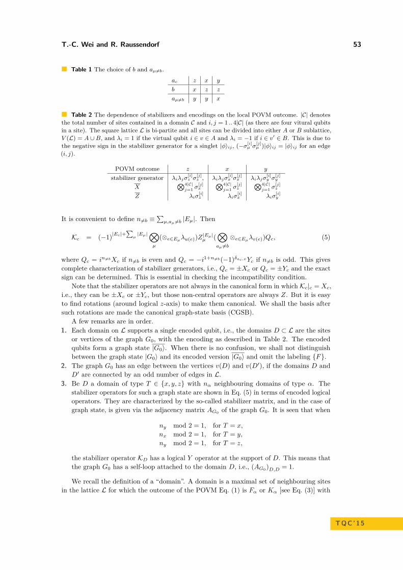
T.-C. Wei and R. Raussendorf 53
Table 1 The choice of b and aµ 6=b.
ac z x y
b x z z
aµ6=b y y x
Table 2 The dependence of stabilizers and encodings on the local POVM outcome. |C| denotesthe total number of sites contained in a domain C and i, j = 1 .. 4|C| (as there are four vitural qubitsin a site). The square lattice L is bi-partite and all sites can be divided into either A or B sublattice,V (L) = A ∪B, and λi = 1 if the virtual qubit i ∈ v ∈ A and λi = −1 if i ∈ v′ ∈ B. This is due tothe negative sign in the stabilizer generator for a singlet |φ〉ij , (−σ[i]
µ σ[j]µ )|φ〉ij = |φ〉ij for an edge
(i, j).
POVM outcome z x y
stabilizer generator λiλjσ[i]z σ
[j]z , λiλjσ
[i]x σ
[j]x λiλjσ
[i]y σ
[j]y
X⊗4|C|
j=1 σ[j]x
⊗4|C|j=1 σ
[j]z
⊗4|C|j=1 σ
[j]z
Z λiσ[i]z λiσ
[i]x λiσ
[i]y
It is convenient to define n 6=b ≡∑µ,aµ 6=b |Eµ|. Then
Kc = (−1)|Ec|+∑
µ|Eµ|⊗
µ
(⊗e∈Eµλu(e))Z |Eµ|µ (⊗aµ 6=b
⊗e∈Eµλv(e))Qc, (5)
where Qc = in 6=bXc if n 6=b is even and Qc = −i1+n 6=b(−1)δac,xYc if n 6=b is odd. This givescomplete characterization of stabilizer generators, i.e., Qc = ±Xc or Qc = ±Yc and the exactsign can be determined. This is essential in checking the incompatibility condition.
Note that the stabilizer operators are not always in the canonical form in which Kc|c = Xc,i.e., they can be ±Xc or ±Yc, but those non-central operators are always Z. But it is easyto find rotations (around logical z-axis) to make them canonical. We shall the basis aftersuch rotations are made the canonical graph-state basis (CGSB).
A few remarks are in order.1. Each domain on L supports a single encoded qubit, i.e., the domains D ⊂ L are the sites
or vertices of the graph G0, with the encoding as described in Table 2. The encodedqubits form a graph state |G0〉. When there is no confusion, we shall not distinguishbetween the graph state |G0〉 and its encoded version |G0〉 and omit the labeling F.
2. The graph G0 has an edge between the vertices v(D) and v(D′), if the domains D andD′ are connected by an odd number of edges in L.
3. Be D a domain of type T ∈ x, y, z with nα neighbouring domains of type α. Thestabilizer operators for such a graph state are shown in Eq. (5) in terms of encoded logicaloperators. They are characterized by the so-called stabilizer matrix, and in the case ofgraph state, is given via the adjacency matrix AG0 of the graph G0. It is seen that when
ny mod 2 = 1, for T = x,
nx mod 2 = 1, for T = y,
ny mod 2 = 1, for T = z,
the stabilizer operator KD has a logical Y operator at the support of D. This means thatthe graph G0 has a self-loop attached to the domain D, i.e., (AG0)D,D = 1.
We recall the definition of a “domain”. A domain is a maximal set of neighbouring sitesin the lattice L for which the outcome of the POVM Eq. (1) is Fα or Kα [see Eq. (3)] with
TQC’15

54 Spin-2 AKLT State and MBQC
the same α. That is, there are domains of x, y and z-type, and neighbouring domains mustbe of different type. The self-loop is a convenient picture to visualize the graph. But we canperform local logical rotation to transform Y to X so as to remove the self-loop, then theresulting stabilizer operators will be in the canonical form. (Such rotation will also changethe basis of logical measurement.) Moreover, we shall often not distinguish between anencoded X or Y operator from the corresponding X or Y operator, unless necessary.
3.3 POVM outcomes Kα: domain shrinking and logical Paulimeasurements
We shall denote by F,K the POVM outcomes on all sites, by JF ⊂ L the set of sites wherethe POVM outcome is of F -type, and by JK = L\JF the set of sites where POVM outcomeis of K-type. Upon obtaining F,K we can deduce the state |G〉 that the original AKLTstate is transformed to,
|G(F,K)〉 =(√
12
)|JK | ⊗u∈JK
|φ−α(u)〉〈φ−α(u)|
⊗v∈L
Fα(v)|ψAKLT〉, (6)
where the state is not normalized and the probability of the set of POVM outcomes F,Koccurs is
p(F,K) = 〈G(F,K)|G(F,K)〉. (7)
We have shown that |G0〉 is a graph state, and one can further show the normalization dueto F ’s acting on the AKLT state [16],
⊗u∈L
Fα(u)|ψAKLT〉 = c0
(1√2
)|E|−|V ||G0〉, (8)
where c0 is an outcome-independent overall normalization, V is the set of domains, E is theset of inter-domain edges (before the modulo-2 operation) and |G0〉 is properly normalizedto have unit norm [16]. For the encoding using virtual-qubit picture, see Table 2.
Summarizing the above discussion, we have
|G(F,K)〉 = c0
(√12
)|E|−|V |+|JK |(⊗u∈JK
|φ−α(u)〉〈φ−α(u)|
)|G0(F)〉, (9)
where |G0(F)〉 is assumed to be properly normalized. Without the additional operators⊗u∈JK |φ
−α(u)〉〈φ
−α(u)| the analysis of the computational universality would be the same as in
the spin-3/2 case. It is these operators that complicate the situtation. However, as we shallsee below their effect is not serious.
Then the effect of measuring in the basis |φ±α 〉 corresponds to shrinking or thinningthe domain, without affecting the entanglement of the domain with others. This can beunderstood from the following example. Suppose a two-site domain with α = x: the basisstates are |Sx = +2〉1|Sx = −2〉2 and |Sx = −2〉1|Sx = +2〉2, due to the POVM. Let us denotethe whole wavefunction of the system as |Ψ〉 = a |+2〉1|−2〉2⊗|ψ0〉R+b |−2〉1|+2〉2⊗|ψ1〉R,where |ψi〉R’s denote the corresponding state of other spins. We can rewrite the first spin in|φ±x 〉 basis: |Ψ〉 = |φ+
x 〉(a | − 2〉2 ⊗ |ψ0〉R + b |+ 2〉2 ⊗ |ψ1〉R
)/√
2 + |φ−x 〉(a | − 2〉2 ⊗ |ψ0〉R −
b | + 2〉2 ⊗ |ψ1〉R)/√
2). The measurement outcome ± gives rise the reduced state beinga | − 2〉2 ⊗ |ψ0〉R ± b |+ 2〉2 ⊗ |ψ1〉R. The only difference is that the domain is reduced to a

T.-C. Wei and R. Raussendorf 55
Figure 3 Illustration of graph transformation rules on Y measurements on a spin-2 domainsand possible follow-up Z measurement to restore planarity. The hexagon indicates a Y -measureddomain, and the diamonds indicate active Z measurements.
single site, but the quantum information remains the same (up to an inconsequential phase).But now if we continue to measure the second spin in the same way, this correponds to alogical X measurement and will change the entanglement structure for the remaining spins.In general, the effect of all |φ−α 〉〈φ−α | (associated with Kα) in multi-site domains C is thusequivalent to a logical measurement of X operator.
Thus for each domain we need to distinguish two cases: (a) Fewer then all sites in anα-domain are affected by the POVM outcome Kα. Then, the domain is simply shrunk, andthe graph G is unaffected. (b) All sites in an α-domain are affected by the POVM outcomeKα. Then, the encoded qubit residing on that domain is measured in the X-basis. If thelatter happens, in terms of CGSB, measurement can be either a logical X or a logical Ymeasurement, and the state resulting from such measurement is again a graph state, andthe new graph can be deduced from simple graph rules [7]; see Fig. 3 for illustration forY -measurement.
4 Restoring planarity
We previously established simple criteria for computational universality of random planargraph states [16, 17], namely their corresponding graphs need to have a traversing path, andthe domains need to be microscopic. The latter requirement for domains to be microscopicwas checked numerically in several trivalent lattices [16, 17, 15] and also holds here viapercolation argument. Therefore, what is needed to check is the former criterion. However,due to X- or Y -measured domains, the resultant graphs are no longer planer. After thePOVM Eq. (1) we therefore apply a further round of active measurements with the purposeof restoring planarity of the encoded graph state.
What we choose to do here, specifically, is to first remove connected POVM “measured”(regardless of whether it is X- or Y -measured) domains by actively measuring their enclos-ing/neighboring domains in the logical Z basis, so as to remove these connected “measured”domains [7] at the cost of removing the enclosing domains as well. We also remove allX-measured domains and isolated multi-site (i.e. those with more than 2 sites) Y -measureddomains by the same procedure. The non-planarity caused by these POVM “measured”domains is recovered quasi-locally; see Fig. 4.
Then we proceed to deal with the remaining isolated Y -measured domains which containeither one single or two sites (which can have at most 6 neighboring sites and hence domains).
TQC’15

56 Spin-2 AKLT State and MBQC
Figure 4 (color online) Part of a random graph for domains (solid circles). (a) The squareindicates an X-measured domain and the hexagon indicates a Y -measured domain. In this example,the two measured domains are neighbors, and the effect on the graph will induce non-planarity. Asimple approach is to apply active Z measurement on those domains (indicated by the diamonds)that enclose these connected X or Y -measured domains, similar to the game of go. (b) The upshot ofthe active Z measurements will remove these X/Y -measured domains as well as active Z-measureddomains but will restore planarity.
The effect of Y -measured domains on the graph is to apply local complementation beforeremoving the vertices corresponding to the Y -measured domains. If the Y -measured domainhas three or fewer neighboring domains, the local complentation still preserves planarity. Butwhen the nunber of neighbors is four or more, we then actively apply Z measurement onsome of the neighboring domains (see Fig. 3) to maintain local planarity of the graph.
In the end we are left with a planar graph state, whose graph may or may not be percolated.If for large enough system and with finite nonzero probability, the graphs obtained after theabove procedure are in the supercritical phase, then the resultant graph states can be usedfor universal MBQC, implying the original AKLT state is universal as well. Our simulationsindicate that we need to use L of order 80 or larger in order to show that the graphs are inthe supercritical phase with high probability such as 90%; see Fig. 5.
To carry out the simulations, we still need to sample the configuration F,K accordingto the exact distribution p(F,K) [16]. In Section 5 we describe the formula.
5 Exact weight formula and simulation results
The exact sampling is needed, as random assignment of F and K POVM outcomes doesnot correctly reflect the correlation that these outcomes must obey due to multipartiteentanglement in the AKLT state. Moreover, many of randomly chosen assignment of Fand K are not valid measurement outcomes (as see below by the incompatibility condition).This latter complication sets the spin-2 case apart from the spin-3/2 case (in addition to thePOVM itself). Employing the exact sampling also enables us to estimate the probability (atleast the lower bound) of obtaining a universal resource state from performing the reductionprocedure. We note that as long as the reduction procedure gives a finite, nonzero successprobability in the large system limit then the original state is still regarded as a universalresource state (though of probabilistic nature). The weight formula that we discuss belowwill enable the exact sampling in the numerical simulations.
The weight formula. Let us recapitulate the notations introduced in Sec. 3.3. Consider aspin-2 AKLT state on a bi-colorable lattice L (generalization to non-bicolorable lattices ispossible), and POVM elements Fα and Kα (α = x, y, z). Denote by JF ⊂ L the set of sites

T.-C. Wei and R. Raussendorf 57
0.5
0.6
0.7
0.8
0.9
1
1.1
20 60 100 140 180
Psp
an
L
0 0.1 0.2 0.3 0.4 0.5 0.6 0.7 0.8 0.9
1
0 0.05 0.1 0.15 0.2 0.25
Psp
an
Pdelete
L=120L=140L=160L=180
Figure 5 (a) Left panel: pspan vs. L (with N = L2 the total number of sites) at pdelete = 0.As L increases pspan also increases. This is obtained with exact sampling. (b) Right panel: pspan
vs. pdelete (with N = L2 the total number of sites) with L = 120, 140, 160, 180. The threshold ofpdelete is approximately 0.142(3). The crossing for these curves indicates that there is a percolationtransition from the supercritical to subcritical phase in the thermodynamic limit.
where the POVM outcome is of F -type and by JK = L\JF the set of sites where POVMoutcome is of K-type. Here additionally we denote by DK the set of domains where thenumber of K-type POVM elements is equal to the total number of sites in the domain. DenoteF,K the set of POVM outcomes corresponding to F (v)
α(v) and K(w)β(w) and the probability
for such occurrence is p(F,K).We have introduced the graph state |G0〉 in Eq. (4). Let us also label the set of all
domains (i.e. vertices of the G0) by V , the set of all inter-domain edges in L by E and theset of all edges of G0 by E. Note that E is obtained from E by a modulo-2 operation [16].
As explained in Sec. 3.3, the effect of K-type POVM elements on a strict subset of sitesin a domain only shrinks the size of a domain, whereas K-type POVM measurement on allsites in a domain in DK amounts to the measurement (on |G0〉) of an encoded logical X withrespect to the encoding in Table 2. The stablizer operators for |G0〉 in this encoding canbe either ±Xc
⊗µ∈Nb(c) Zµ or ±Yc
⊗µ∈Nb(c) Zµ (see Appendix 3.2), where Nb(c) denotes
the set of neighbors of vertex c. But one can perform local logical-qubit rotations such thatall stabilizer operators are of the canonical form Xc
⊗µ∈Nb(c) Zµ, but then the effect of
K-type POVM elements in a domain inside DK amounts to the measurement of an encodedobservable either X or Y . We have referred to this latter basis as the canonical graph-statebasis (CGSB) earlier.
TQC’15

58 Spin-2 AKLT State and MBQC
Now we introduce a |V |× |DK | binary-valued matrix H with its entries defined as follows,
Hµν = 0, if [Kµ, Oν ] = 0, (10a)Hµν = 1, if Kµ, Oν = 0, (10b)
where Kµ is the stabilizer operator associated with the vertex (or domain) µ ∈ V of thegraph G, Oν ≡ (−1)|Vµ|Xµ is proportional to a logical Pauli X operator, and ν ∈ DK ; seealso Sec. 3.2. Let dim
(ker(H)
)denote the dimension of the kernel of matrix H. We are
ready to introduce the following lemma.
I Lemma 1. If there exists a set Q (subset of DK) such that −⊗µ∈QOµ is in the stablizergroup S(|G0〉) of the state |G0〉, then p(F,K) = 0. Otherwise,
p(F,K) = c
(12
)|E|−|V |+2|JK |−dim(
ker(H)), (11)
where c is a constant.
We subsequently refer to the above condition for p(F,K) = 0 as the incompatabilitycondition. The incompatibility condition implies that not all POVM outcomes labeled byFα and Kα can occur. When there is no K outcome, Eq. (11) reduces to p = c 2|V |−|E| ofprevious results [16]. The correlation of F ’s and K’s at different sites is reflected either inthe incompatibility condition (if it is met) or else in the factor dim
(ker(H)
). The probability
distribution of F,K is thus very far from independent and random. For the proof of thelemma, see Appendix A.
Numerical simulations. With the weight formula we can sample the exact distribution ofphysically allowed POVM outcomes F,K and carry out the procedure to restore planarityof the random graphs associated with the post-POVM states. The sampling is obtained byusing the standard Metropolis algorithm for updating F,K configurations. One notabledistinction is that we will need to avoid configurations that satisfies the incompatibilitycondition. First, we check whether the random graphs after our procedure have a spannercluster by showing pspan for different L, and we see that it increases as L increases andapproaches to unity; see Fig. 5. This suggests that for L large enough, the random graphsresulting from the thinning procedure are percolated. Then, we perform site percolationnumerical experiment on these random graphs by removing each vertex with a probabilitypdelete and record the probability of a spanning cluster pspan. The crossing of curves in Fig. 5for different sizes indicates that there is a percolation transition (at p∗delete ≈ 0.142) from thesupercritical to subcritical phase in the thermodynamic limit. This shows that our randomgraph states (whose graphs are sitting at pdelete = 0) can be used to generate a network ofentanglement that is universal for measurement-based quantum computation. This showsthat the original AKLT state is also universal.
6 Concluding remarks
The family of Affleck-Kennedy-Lieb-Tasaki states provides a versatile playground for universalquantum computation. The merit of these states is that by appropriately choosing boundaryconditions they are unique ground states of two-body interacting Hamiltonians, possiblywith a spectral gap above the ground states. Here we have overcome several obstacles and

T.-C. Wei and R. Raussendorf 59
shown that the spin-2 AKLT state on the square lattice is also a universal resource formeasurement-based quantum computation. We were able to derive an exact weight formulafor any given POVM outcome. Combined with a thinning procedure to restore planarityof random graph states, we performed Monte Carlo simulations and demonstrated that theassoicated planar random graphs from the procedure are residing in the supercritical phase.
The emerging picture from our series of study on the quantum computational universalityin the two-dimensional AKLT valence-bond family is as follows. AKLT states involving spin-2and other lower spin entities are universal if they reside on a two-dimensional frustration-freeregular lattice with any combination of spin-2, spin-3/2, spin-1 and spin-1/2 (consistent withthe lattice). Additionally, the effect of frustrated lattice may not be serious and can alwaysbe decorated (by adding additional spins) such that the resultant AKLT state is universal.We conjecture that the result hold in three dimensions as well.
Another direction of generalization is to investigate the robustness of the resource undersmall perturbations, e.g., slightly away from the AKLT Hamiltonian. A slight and simplervariation [5] is to consider the AKLT deformed spin-2 AKLT state with some deformationparameters, for which we give more detail in our arXiv paper [20]. One can also considerthe frustrated kagomé lattice and deform it in a way to connect to a cluster state [4].Furthermore, how would the quantum computational power of AKLT-like states maketransition and how would they compare with the usual phases of matter [19]. We leave thesefor future consideration.
Acknowledgements. This work was supported by the National Science Foundation underGrants No. PHY 1314748 and No. PHY 1333903 (T.-C.W.) and by NSERC, Cifar andIARPA (R.R.).
References1 H. J. Briegel, D. E. Browne, W. Dür, R. Raussendorf, and M. Van den Nest, Nature Phys.
5, 19 (2009).2 J.-M. Cai, A. Miyake, W. Dür, and H. J. Briegel, Phys. Rev. A 82, 052309 (2010).3 X. Chen, B. Zeng, Z.-C. Gu, B. Yoshida, and I. L. Chuang, Phys. Rev. Lett. 102, 220501
(2009).4 A. S. Darmawan and S.D. Bartlett , New J. Phys. 16, 073013 (2014).5 A. S. Darmawan, G.K. Brennen, and S.D. Bartlett, New J. Physics, 14, 013023 (2012).6 D. Gross and J. Eisert, Phys. Rev. Lett. 98, 220503 (2007).7 M. Hein, W. Dur, J. Eisert, R. Raussendorf, M.Van den Nest, and H.-J. Briegel, in Quantum
Computers, Algorithms and Chaos, edited by G. Casati, D. Shepelyansky, P. Zoller, andG. Benenti, International School of Physics Enrico Fermi Vol. 162 (IOS Press, Amsterdam,2006); also in arXiv:quant-ph/0602096.
8 R. Kaltenbaek, J. Lavoie, B. Zeng, S.D. Bartlett, and K. J. Resch, Nature Physics 6, 850(2010).
9 Ç. K. Koç and S.N. Arachchige, J. Parallel and Distributed Computing 13, 118 (1991).10 See e.g. the review by L.C. Kwek, Z. Wei, and B. Zeng, Int. J. Mod. Phys. B 26, 1230002
(2012).11 A. Miyake, Ann. Phys. (Leipzig) 326, 1656 (2011).12 M.A. Nielsen, Rep. Math. Phys. 57, 147 (2006).13 R. Raussendorf and H. J. Briegel, Phys. Rev. Lett. 86, 5188 (2001).14 R. Raussendorf and T.-C. Wei, Annual Review of Condensed Matter Physics 3, pp.239-261
(2012).15 T.-C. Wei, Phys. Rev. A 88, 062307 (2013).
TQC’15

60 Spin-2 AKLT State and MBQC
16 T.-C. Wei, I. Affleck, and R. Raussendorf, Phys. Rev. Lett. 106, 070501 (2011).17 T.-C. Wei, I. Affleck, and R. Raussendorf, Phys. Rev. A 86, 032328 (2012).18 T.-C. Wei, P. Haghnegahdar, R. Raussendorf, Phys. Rev. A 90, 042333, (2014).19 T.-C. Wei, Y. Li, and L. C. Kwek, Phys. Rev. A 89, 052315 (2014).20 T.-C. Wei and R. Raussendorf, arXiv:1501.07571.
A Proof of the weight formula
Let us mention first the following fact that (b is chosen according to ac in Table 1),
〈G0|Orest ⊗i∈Ic σ[i]b |G0〉 = 0, (12)
if Ic is a strict subset of virtual qubits in any domain C (i.e. |Ic| < 4|C|) and σb is chosenaccording to Table 1 (Orest denotes operators not in the support of domain C). This caneasily be proved by the fact that one can choose a stabilizer Sjq ≡ λjλqσ[j]
acσ[q]ac (see Table 2),
where j ∈ Ic and q ∈ C but q /∈ Ic, so that (⊗i∈Ic(σ[i]b ) and Sjq anticommutes. Hence,
〈G0|Orest(⊗i∈Icσ[i]b )|G0〉 = 〈G0|Orest(⊗i∈Icσ
[i]b )Sjk|G0〉
= −〈G0|SjkOrest(⊗i∈Icσ[i]b )|G0〉 = −〈G0|Orest(⊗i∈Icσ
[i]b )|G0〉,
showing that the expectation value is identically zero.Let us also note the following useful relation regarding to the 4-qubit GHZ associated
with the corresponding POVM outcome Kα,
|GHZ−α 〉〈GHZ−α | = Πα
(1− σ[v;1]bα
σ[v;2]bα
σ[v;3]bα
σ[v;4]bα
)2 Πα, (13)
where Πα (α = x, y, z) is a projection to a two-dimensional subspace, equivalently anidentity operator on the code subspace and can be safely omitted when acting on thegraph state |G0〉. Specificially, Πx = | + + + +〉〈+ + + + | + | − − − −〉〈− − − − |,Πy = |i, i, i, i〉〈i, i, i, i|+ |− i,−i,−i,−i〉〈−i,−i,−i,−i| and Πz = |0000〉〈0000|+ |1111〉〈1111|.The label bα denotes the corresponding type b if ac = α; see Table 1.
For a given domain (with a given type α), the POVM outcome on any site in the domaincan be either Fα or Kα. Regarding the number nK of K outcomes, there are two scenarios:(i) nK is less than the total number |Vc| of sites in that domain C; (ii) nK = |Vc|.
For case (i), the effect of all those K in terms of the probability distribution (or theweight formula) is to multiply a factor of 2−nK , i.e., (using J ∈ C to denotes the set of thosesites with K)
〈G0|Orest
(⊗v∈J |GHZ−α(v)〉〈GHZ−α(v)|
)|G0〉 = 〈G0|Orest ⊗v∈J
(1− σ[v;1]b σ
[v;2]b σ
[v;3]b σ
[v;4]b )
2 |G0〉
=2−nK 〈G0|Orest|G0〉,
where Orest denotes operators not in the support of domain C, and we have used
〈G0|Orest ⊗v∈J (σ[v;1]b σ
[v;2]b σ
[v;3]b σ
[v;4]b )|G0〉 = 0.
For case (ii), when we expand all the 2|Vc| terms in ⊗v∈C(1− σ[v;1]b σ
[v;2]b σ
[v;3]b σ
[v;4]b )/2, the
only two nonvanishing contributions are 1/2|Vc| and (−1)|Vc|(⊗4|C|i=1σ
[i]b )/2|Vc| = (−1)|Vc|Xc/2|Vc|.

T.-C. Wei and R. Raussendorf 61
In terms of logical X, the effect of all K is equivalent to Pc = (1 + Oc)/2|Vc|, where theOc = (−1)|Vc|Xc. That is
〈G0|Orest
(⊗v∈C |GHZ−α(v)〉〈GHZ−α(v)|
)|G0〉 = 〈G0|Orest ⊗v∈C
(1− σ[v;1]b σ
[v;2]b σ
[v;3]b σ
[v;4]b )
2 |G0〉
= 2−|Vc|〈G0|Orest(1 +Oc)|G0〉.
Here we also see that the effect of all K in domain C is to measurement the logical qubit Cin the logical X, followed by a post-selection of the result corresponding to either positive (if|Vc| is even) or negative (if |Vc| is oddd) eigenvalue of X.
With the above preparation, we can move on to the proof. Now consider a spin-2 AKLTstate on a bi-colorable lattice L (generalization to non-bicolorable lattices is possible), andPOVM elements Fα and Kα (α = x, y, z). Denote by JF ⊂ L the set of sites where thePOVM outcome is of F -type and by JK = L\JF the set of sites where POVM outcome is ofK-type. We should, strictly speaking, use α(v) to denote the type of x, y, z at site v. Whenthere is no confusion, we simply write α.
Proof of Lemma 1. For simplicity let us denote the AKLT state by |ψ〉 below. The proba-bility p(F,K) for obtaining POVM measurements F,K described above is
p(F,K) = 〈ψ| ⊗v∈JF
F(v)†α(v)F
(v)α(v) ⊗
w∈JKK
(w)†α(w)K
(w)α(w)|ψ〉
=(
32
)|JK |〈ψ| ⊗
v∈JFF
(v)†α(v)F
(v)α(v) ⊗
w∈JKF
(w)†α(w)K
(w)†α(w)K
(w)α(w)F
(w)α(w)|ψ〉
=(
12
)|JK |〈ψ| ⊗
v∈LF
(v)†α(v) ⊗
w∈JK|GHZ−α(w)〉〈GHZ−α(w)| ⊗
u∈LF
(u)α(u)|ψ〉.
In the second equality we have used the fact that Kα =√
3/2KαFα, and in the thirdequality we have combined all F ’s and written explicitly Kα’s in terms of the four-qubitGHZ projectors.
Now we know from Ref. [16] that
⊗u∈L
F(u)α(u)|ψ〉 = c0
(1√2
)|E|−|V ||G0〉, (14)
where |G0〉 is an encoded graph state whose graph G0 is specified by the POVM elementsF, V is the set of domains of same-outcome POVM measurements, and E is the set ofinter-domain edges (before the modulo-2 operation) [16]. The formula (14) was originallystated for the honeycomb lattice, but holds for all bipartite lattices. (For non-bipartitelattices, an additional condition needs to be imposed relating to geometric frustration [15].Namely, if any domain contains a cycle with odd number of sites, such F will not appear.)Combining the above two results we find that
p(F,K) = |c0|2(
12
)|E|−|V |+|JK |× 〈G0|
(⊗
v∈JK|GHZ−α(v)〉〈GHZ−α(v)|
)|G0〉. (15)
Using Eq. (13) and the results in the beginning of the section, we know that for thoseGHZ-projections in a domain such that their number is less than the total number of sites inthe domain, i.e., case (i) discussed above, their contribution is to mulitiply by a factor 2−nK .For those such that the two numbers are equal, i.e., case (ii), these GHZ-projections (in a
TQC’15

62 Spin-2 AKLT State and MBQC
domain) can be replaced by Pc = (1 + Oc)/2|Vc|, where the Oc = (−1)|Vc|Xc, and c labelsthe domain. Thus,
p(F,K) = |c0|2(
12
)|E|−|V |+2|JK |× 〈G0| ⊗
c∈DK(Ic +Oc)|G0〉, (16)
where we use DK to label the domains that contain the same number of K operators as thetotal number of internal sites.
Next we demonstrate the first part of the Lemma. Assume that, for some subset Q ∈ DK ,the observable −⊗c∈QOc ∈ S(|G0〉). Then,
〈G0| ⊗µ∈DK
(Iµ +Oµ)|G0〉 = 〈G0| ⊗ν∈DK\Q
(Iν +Oν) ⊗µ∈Q
(Iµ +Oµ)(− ⊗c∈Q
Oc
)|G0〉
= −〈G0| ⊗ν∈DK\Q
(Iν +Oν) ⊗c∈Q
(Oc + Ic)|G0〉 = −〈G0| ⊗µ∈DK
(Iµ +Oµ)|G0〉 = 0.
In the third line we have used the fact O2µ = Iµ. Let us also note that being product of Pauli
operators, Oµ either commutes or anticommutes with another product of Pauli operators.Next, we demonstrate the second part of the Lemma, i.e., finding p(F,K) when it is
not identically zero. Consider a subset of domains Q ⊂ DK . If ⊗µ∈QOµ 6∈ ±S(|G0〉), then〈G0| ⊗µ∈QOµ|G0〉 = 0 (note that µ is an index for the domain, not an index for the site).Furthermore, if the incompatibility condition is not satisfied, then ⊗µ∈QOµ ∈ ±S(|G0〉)implies that ⊗µ∈QOµ ∈ S(|G0〉), and therefore 〈G0| ⊗µ∈QOµ|G0〉 = 1. We now exapnd theprojector ⊗c∈DK (Ic +Oc) in the matrix element,
〈G0| ⊗c∈DK
(Ic +Oc)|G0 = 〈G0|∑
Q⊂DK
⊗µ∈Q
Oµ|G0〉 = |M |, (17)
where the set M is defined as M = O(Q) ≡ ⊗µ∈QOw|Q ⊂ DK andO(Q) ∈ S(|G0〉).Actually M has the following equivalent formulation which will turn out to be useful,
M = O(Q) ≡ ⊗µ∈Q
Oµ|Q ⊂ DK and [O(Q), S] = 0,∀S ∈ S(|G0〉). (18)
Using this latter characterization of M , we now turn to the counting for |M |. We describeevery subset Q of DK by its characteristic vector q, defined as follows: if µ ∈ Q then qµ = 1,or if µ 6∈ Q, then qµ = 0. Furthermore we define a binary-valued matrix H of dimension|V | × |DK | (where |V | denotes total number of domains), whose entries are
Hµν = 0, if [Kµ, Oν ] = 0,Hµν = 1, if Kµ, Oν = 0,
where µ ∈ V (the set of all domains) and ν ∈ DK (the set of those domains with equalnumber of K’s and sites). Then for any Q ⊂ DK , O(Q) ∈M if and only if Hq mod 2 = 0.Therefore,
|M | = 2dim(
ker(H)). (19)
Putting everything into the expression for p(F,K) we obtain the equation (11),
p(F,K) = |c0|2(
12
)|E|−|V |+2|JK |−dim(
ker(H)),
and the lemma is proved. J

T.-C. Wei and R. Raussendorf 63
We remark that checking the kernel of a binary matrix can be done via, e.g., the Gausselimination method; see e.g. [9]. Furthermore, to check the incompatibility condition it issufficient to check the products of Oµ associated with all basis vectors q’s in the kernel. Ifnone of them satisifies it, then the incompatibility condition is not satisified.
TQC’15

Quantum Capacity Can Be Greater Than PrivateInformation for Arbitrarily Many UsesDavid Elkouss1,2 and Sergii Strelchuk3
1 Departamento de Análisis Matemático and Instituto de MatemáticaInterdisciplinar, Universidad Complutense de Madrid, 28040 Madrid, [email protected]
2 QuTech, Delft University of Technology, Lorentzweg 1, 2628 CJ Delft, [email protected]
3 Department of Applied Mathematics and Theoretical Physics,University of Cambridge, Cambridge CB3 0WA, [email protected]
AbstractThe quantum capacity of a quantum channel is always smaller than the capacity of the channelfor private communication. However, both quantities are given by the infinite regularization ofrespectively the coherent and the private information. Here, we construct a family of channelsfor which the private and coherent information can remain strictly superadditive for unboundednumber of uses. We prove this by showing that the coherent information is strictly larger thanthe private information of a smaller number of uses of the channel. It turns out that even thoughthe quantum capacity is upper bounded by the private capacity, the non-regularized quantitiescan be interleaved. From an operational point of view, the private capacity can be used forgauging the practical value of quantum channels for secure communication and, consequently, forkey distribution. We thus show that in order to evaluate the interest a channel for this task it isnecessary to optimize the private information over an unlimited number of uses of the channel.
1998 ACM Subject Classification H.1.1 Systems and Information Theory, E.4 Coding and in-formation theory.
Keywords and phrases Quantum channels, capacity, private information
Digital Object Identifier 10.4230/LIPIcs.TQC.2015.64
1 Introduction
How well is it possible to characterize the resources available to transmit information? Inclassical information theory, this proves to be fully within our computational abilities: givena description of a channel, answering the question about its capacity to convey informationto the receiver is straightforward. However, our world is inherently quantum and when oneturns to the channels which transmit quantum information – the amount of resources requiredto compute their capacities is unknown at best. To compute a number of different types ofcapacity of the quantum channel, defined as regularized quantities [15, 10, 18, 20, 5, 16, 2, 8],it is necessary to perform an unbounded optimization over the number of the copies ofthe channel. The action of a channel NA→B can be defined via an isometry V A→BE :NA→B(ρ) = trEV ρV ∗, and its complementary channel is NA→E
c (ρ) = trBV ρV ∗. In thefollowing, we will omit the register superscripts when it does not add to clarity.
© David Elkouss and Sergii Strelchuk;licensed under Creative Commons License CC-BY
10th Conference on the Theory of Quantum Computation, Communication and Cryptography (TQC 2015).Editors: Salman Beigi and Robert König; pp. 64–72
Leibniz International Proceedings in InformaticsSchloss Dagstuhl – Leibniz-Zentrum für Informatik, Dagstuhl Publishing, Germany

D. Elkouss and S. Strelchuk 65
The quantum and classical capacity of a channel [15, 10, 18, 20, 5] are given by:
Q(N ) = limn→∞
1nQ(1)(N⊗n), (1)
C(N ) = limn→∞
1nC(1)(N⊗n) (2)
where
Q(1)(N ) = maxρA
H(B)−H(E), (3)
C(1)(N ) = maxρ∈R
I(X;B). (4)
The optimization of the quantum capacity is performed over all valid states on the inputregister A while the optimization of the classical capacity is performed over R the set ofclassical-quantum states of the form ρXA =
∑x px|x〉〈x|X ⊗ ρAx . Where X is an auxiliary
classical register, H is the von Neumann entropy and I(X;B) is the quantum mutualinformation.
From the above expressions it follows that one has to optimize over an infinite number ofcopies of the channel in order to compute its capacity. Do we have to resort to the regularizedexpression in order to compute the capacity of a quantum channel? It has recently beenshown that at least in the case of the quantum capacity this is unavoidable [6, 22] even whenwe attempt to answer the question whether the channel has any capacity at all [4]. For theclassical capacity, which is known to be superadditive for two uses of the channel [9], there issome evidence that ultimately the regularization might not be required [17, 24].
Arguably, the biggest practical success of quantum information theory to date is thepossibility of quantum key distribution (QKD). QKD allows two distant parties to agree ona secret key independent of any eavesdropper. The required assumptions are: access to aquantum channel with positive private capacity and the validity of quantum physics1. Onthe other hand, key distribution is a primitive that can only be implemented with classicalresources if one is willing to constrain the power of the eavesdropper. Even though there existpractical QKD schemes which enable secure communication over large distances with highkey rates [3, 13, 11, 19], some of the fundamental questions about the capacity to transmitsecure correlations remain unanswered.
The private capacity P of a channel is used to describe the ability of the channel tosend secure messages to the receiver [5, 1]. It has a clear operational interpretation as themaximum rate at which the sender, Alice, can send private classical communication to thereceiver, Bob. It is defined as follows:
P(N ) = limn→∞
1nP(1)(N⊗n). (5)
That is the private capacity is given by the regularization of P(1)(N ), the private informationof the channel, which is given by
P(1)(N ) = maxρ∈R
I(X;B)− I(X;E). (6)
One can view private capacity as the optimal rate of reliable communication keeping Eve ina product state with Alice and Bob.
1 In order to characterize the channel and to implement a specific QKD protocol one might need a publicauthentic classical channel or a small preshared secret.
TQC’15

66 Quantum Capacity Can Be Greater Than Private Information
This capacity characterizes the optimal rates of QKD. A better understanding of thisquantity would allow to evaluate precisely the usefulness of communications channels forpractical QKD links. For instance, the private capacity of Gaussian channels [25] remainsopen. Beyond the pure loss channel [27] only lower bounds on the private information of asingle use are known.
Despite the significance of the private information, we still understand very little aboutits behaviour when the communication channel is used many times. Authors in [21, 12]provide evidence that P(1)(N ) is superadditive for two channel uses, although the magnitudeof this effect is quantitatively very small. Recently, it has been shown the existence of twoquantum channels N1,N2 with C(N1) ≤ 2,P(N2) = 0 for which P(N1 ⊗ N2) ≥ 1/2 log d,where d is the dimension of the output of the joint channel [23]. This example shows thatthe private capacity is a superadditive quantity (this was also proved in [14] using a differentconstruction).
Here we show that private information can be strictly superadditive for an arbitrarilylarge number of uses of the channel. More precisely, we prove the following theorem:
I Theorem 1. For any n there exists a quantum channel Nn such that for n > k ≥ 1:
1kP(1)(N⊗kn ) < 1
k + 1Q(1)(N⊗k+1
n ). (7)
This proves that entangled inputs increase the private information of a quantum channeland this effect persists for an arbitrary number of channel uses. As a bonus, we obtain aqualitatively different proof for the unbounded superadditivity of the coherent information [4].
The following relation holds for any channel [26]:
Q(1)(Nn) ≤ P(1)(Nn) ≤ C(1)(Nn). (8)
This means, that even though the coherent information is upper bounded by the privateinformation and the quantum capacity is upper bounded by the private capacity, Theorem 1implies that the non-regularized quantities can be interleaved.
We now introduce the key components of our construction which are required to proveTheorem 1.
2 Main construction
We first introduce switch channels:
N SA→SB(ρSA) =∑
i
PS→Si ⊗NA→Bi (ρSA). (9)
A switch channel consists of two input registers S and A of dimensions d and n respectively.Register S is measured in the standard basis and conditioned on the measurement outcomei a component channel Ni is applied to the second register. The computation of P(1)(N )when N is of the form (9) can be simplified; it suffices to restrict inputs to a special form.The equivalent result for the quantum capacity was proved in [7].
I Lemma 2. Consider a switch channel N SA→SB and let T = ρ : ρ =∑x px|x〉〈x|X ⊗
|s〉〈s|S ⊗ ρAx . Then
P(1)(N ) = max1≤s<n
P(1)(Ns), (10)
and P(1)(N ) can be achieved by some ρ ∈ T .

D. Elkouss and S. Strelchuk 67
1
S
A11A12
An1An2
B0
Bn
B0
Bn
S
RdRd
Rd
Ep,d
ED,1
Rnd
Enp,d
Figure 1 The channel has two input registers the control register S and the data register A. Thecontrol register is measured in the computational basis and depending on the output either theerasure channel En
p,d or n copies of the d-dimensional rocket channel are applied.
Proof. The channel complementary to a switch channel is also a switch channel withcomponent channels N c
i ni=1 complementary to Nini=1 [4]. We denote the output systems ofthe complementary channel by S and E. Let ρ ∈ R be the input state that maximizes P(1)(N ),then N takes ρ to
∑x,s pxps|x|x〉〈x|⊗ |s〉〈s|⊗Ns(ρs|x) and N c takes ρ to
∑x,s pxps|x|x〉〈x|⊗
|s〉〈s| ⊗ N cs (ρs|x). The following chain of inequalities holds:
I(X;BS)− I(X;ES) (11)
=∑
s
ps
(I(X;B|S = s)− I(X;E|S = s)
)(12)
≤ maxs
(I(X;B|S = s)− I(X;E|S = s)
)(13)
≤ maxsP(1)(Ns). (14)
The first equality follows because S is a classical system. The first inequality follows bychoosing the value of s which maximizes the difference between the mutual informations. Thesecond one since the difference between the between the mutual informations to the receiverand the environment is upper bounded by the private information of the channel Ns. Thisupper bound is achievable by an input state of the form σXSA =
∑x px|x〉〈x| ⊗ |s〉〈s| ⊗ ρx
where trS(σXSA) is the state that achieves the private information of channel Ns. Finallynote that σXSA ∈ T . J
There are two types of channels which we will use in place of Ni. The first channel is theerasure channel:
EA→Bp,d (ρA) = (1− p)ρB + p|e〉〈e|B (15)
where |e〉〈e| is the erasure flag and d the dimension of the input register A. For p ≤ 1/2the erasure channel is degradable and Q(Ep,d) = P(Ep,d) = max0, (1 − 2p) log d, andC(Ep,d) = (1− p) log d.
TQC’15

68 Quantum Capacity Can Be Greater Than Private Information
For any quantum channel N used alongside Ep,d the classical capacity is additive:
I Lemma 3. For all quantum channels N
C(1)(N ⊗ E⊗np,d
)= C(1)(N ) + nC(1)(Ep,d). (16)
Proof. The inequality C(1)(N ⊗ E⊗np,d
)≥ C(1)(N ) + nC(1)(Ep,d) is trivial. In order to prove
the other direction consider the following chain of inequalities:
C(1)(N ⊗ E⊗np,d ) = C(1)(M⊗Ep,d) (17)= max
ρI(X;B1B2) (18)
= maxρ
(1− p)I(X;B1A2) + pI(X;B1) (19)
≤ (1− p)C(1)(M⊗ I) + pC(1)(M) (20)= C(1)(M) + (1− p) log d (21)= C(1)(N ) + n(1− p) log d. (22)
The first equality follows by identifyingM with N ⊗E⊗n−1p,d . We let A1, A2 and B1, B2 be the
input and output ofM and Ep,d respectively. The second equality is just the definition of theclassical information (see Eq. 2). The third equality breaks the mutual information dependingon the erasure channel transmitting or erasing. The inequality follows by maximizing eachof the two mutual informations individually. The fourth inequality follows by taking intoaccount that the classical information of the identity is additive and the last one by applyingthe same argument recursively for n− 1 times. J
Intuitively, Lemma 3 states that the erasure channel cannot convey more information thanan identity channel of dimension d1−p even in the presence of other channels. Furthermore,we can use the expression for the classical capacity to obtain a trivial bound for the privateinformation. It turns out that this trivial bound is tight and is saturated by the channelconstruction that we introduce below.
The second channel that we use alongside Ep,d is a d-dimensional ‘rocket’ channel, Rd [23].It consists of two d-dimensional input registers A1 and A2 and a d-dimensional output registerB. A1 and A2 are first subject to a random unitary and then jointly decoupled with acontrolled dephasing gate. Then, the contents of A1 becomes the output of the channel andthe contents of A2 is traced out. Bob also receives the classical description of the unitarieswhich acted on A1 and A2. Since dephasing occurs after the input registers have beenscrambled by a random unitary, it is very hard for Alice to code for such channel, hence ithas a very low classical capacity: C(Rd) ≤ 2.
Our switch channel construction has the following form:
Nn,p,d = P0 ⊗Rnd + P1 ⊗ Enp,d (23)
That is, it allows Alice to choose between Rnd = R⊗nd and Enp,d = Ep,d ⊗ E1,d2n−1 – a d-dimensional erasure channel padded with a full erasure channel to match the input dimensionof Rnd .
2.1 Upper boundTo upper bound the private information of Nn,p,d we only need to optimize over all thepossible different choices of Rnd and Enp,d. Thus, the upper bound for P(1)(N⊗kn,p,d) for k ≥ 1
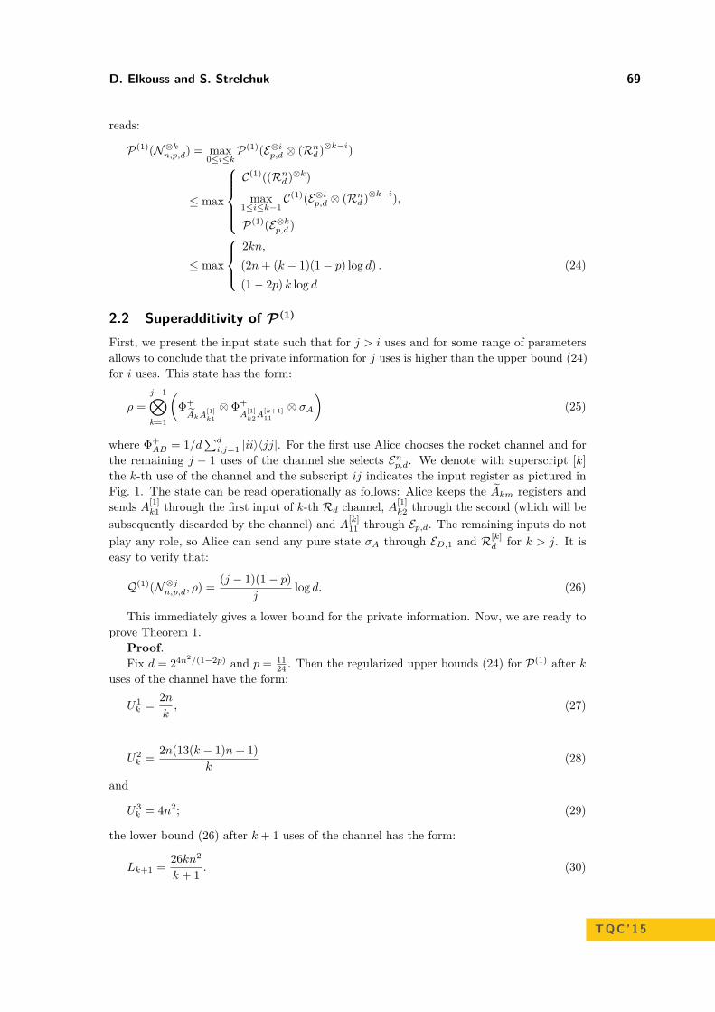
D. Elkouss and S. Strelchuk 69
reads:
P(1)(N⊗kn,p,d) = max0≤i≤k
P(1)(E⊗ip,d ⊗ (Rnd )⊗k−i)
≤ max
C(1)((Rnd )⊗k)
max1≤i≤k−1
C(1)(E⊗ip,d ⊗ (Rnd )⊗k−i),
P(1)(E⊗kp,d )
≤ max
2kn,(2n+ (k − 1)(1− p) log d) .(1− 2p) k log d
(24)
2.2 Superadditivity of P(1)
First, we present the input state such that for j > i uses and for some range of parametersallows to conclude that the private information for j uses is higher than the upper bound (24)for i uses. This state has the form:
ρ =j−1⊗
k=1
(Φ+AkA
[1]k1⊗ Φ+
A[1]k2A
[k+1]11⊗ σA
)(25)
where Φ+AB = 1/d
∑di,j=1 |ii〉〈jj|. For the first use Alice chooses the rocket channel and for
the remaining j − 1 uses of the channel she selects Enp,d. We denote with superscript [k]the k-th use of the channel and the subscript ij indicates the input register as pictured inFig. 1. The state can be read operationally as follows: Alice keeps the Akm registers andsends A[1]
k1 through the first input of k-th Rd channel, A[1]k2 through the second (which will be
subsequently discarded by the channel) and A[k]11 through Ep,d. The remaining inputs do not
play any role, so Alice can send any pure state σA through ED,1 and R[k]d for k > j. It is
easy to verify that:
Q(1)(N⊗jn,p,d, ρ) = (j − 1)(1− p)j
log d. (26)
This immediately gives a lower bound for the private information. Now, we are ready toprove Theorem 1.
Proof.Fix d = 24n2/(1−2p) and p = 11
24 . Then the regularized upper bounds (24) for P(1) after kuses of the channel have the form:
U1k = 2n
k, (27)
U2k = 2n(13(k − 1)n+ 1)
k(28)
and
U3k = 4n2; (29)
the lower bound (26) after k + 1 uses of the channel has the form:
Lk+1 = 26kn2
k + 1 . (30)
TQC’15

70 Quantum Capacity Can Be Greater Than Private Information
Consider the differences Dik = −U ik + Lk+1 for i = 1, 2, 3. Then, a simple substitution
shows that:
D1k = 26kn2
k + 1 −2nk, (31)
D2k = −2n(k − 13n+ 1)
k(k + 1) (32)
and
D3k = 2(11k − 2)n2
k + 1 . (33)
All of the differences are positive for n > k ≥ 1. JThe results of the theorem indicate that in order to compute the exact private capacity
of a channel N it is necessary to compute P(1)(N⊗n) for an arbitrary number of uses n.In addition, we found an example whereby for each n and 1 ≤ k < n having access to oneadditional copy of the channel up to n provides the parties with the largest possible gainin the capacity, proportional to the output dimension of the channel. Note, that for thechannel Nn,p,d strict superadditivity of both private and coherent information holds for allnumber of uses of the channel up to n. This is markedly different from all previously knownchannel constructions which exhibit various superadditivity effects for quantum channelcapacities. Such constructions exhibited superadditivity for some fixed number of uses of thechannel t versus t+ c for some c. Our construction above shows that the private and coherentinformation of the same channel can be strictly superadditive for an arbitrary number ofchannel uses.
3 Discussion
In this paper we have constructed a family of channels for which the private and coherentinformation can remain strictly superadditive any number of uses of the channel. We areable to prove this result by showing that the private information of k uses of the channelis smaller than the coherent information of k + 1 uses. That is, both quantities can beinterleaved use after use for the first n uses of the channel. This shows that even though thequantum capacity is upper bounded by the infinite regularization of the private information,the quantum capacity can be larger than a finite regularization of the private information.
The private capacity of a quantum channel characterizes its ability to convey classicalinformation securely. We proved that in order to compute the private capacity it is necessaryto consider regularized expressions (5).
The results shown here raise questions about the properties that a channel has to verifysuch that its different capacities can be computed exactly using only finitely many (preferablyonly a few) copies of the channel.
Acknowledgements. We thank David Perez García and Maris Ozols for many usefuldiscussions and feedback. SS acknowledges the support of Sidney Sussex College andEuropean Union under project QALGO (Grant Agreement No. 600700). DE acknowledgesfinancial support from the European CHIST-ERA project CQC (funded partially by MINECOgrant PRI-PIMCHI-2011-1071) and from Comunidad de Madrid (grant QUITEMAD+-CM,ref. S2013/ICE-2801). This work has been partially supported by STW, QuTech and by

D. Elkouss and S. Strelchuk 71
the project HyQuNet (Grant No. TEC2012-35673), funded by Ministerio de Economía yCompetitividad (MINECO), Spain. This work was made possible through the supportof grant #48322 from the John Templeton Foundation. The opinions expressed in thispublication are those of the authors and do not necessarily reflect the views of the JohnTempleton Foundation.
References1 Ning Cai, Andreas Winter, and Raymond W. Yeung. Quantum privacy and quantum
wiretap channels. Problems of Information Transmission, 40(4):318–336, 2004.2 Filippo Caruso, Vittorio Giovannetti, Cosmo Lupo, and Stefano Mancini. Quantum chan-
nels and memory effects. Reviews of Modern Physics, 86(4):1203–1259, December 2014.3 L.C. Comandar, B. Fröhlich, M. Lucamarini, K.A. Patel, A.W. Sharpe, J. F. Dynes, Z. L.
Yuan, R.V. Penty, and A. J. Shields. Room temperature single-photon detectors for highbit rate quantum key distribution. Applied Physics Letters, 104(2):021101, 2014.
4 Toby Cubitt, David Elkouss, William Matthews, Maris Ozols, David Pérez-García, andSergii Strelchuk. Unbounded number of channel uses may be required to detect quantumcapacity. Nat Commun, 6, 03 2015.
5 I. Devetak. The private classical capacity and quantum capacity of a quantum channel.Information Theory, IEEE Transactions on, 51(1):44–55, Jan 2005.
6 David P. DiVincenzo, Peter W. Shor, and John A. Smolin. Quantum-channel capacity ofvery noisy channels. Phys. Rev. A, 57(2):830–839, Feb 1998.
7 Motohisa Fukuda and Michael M. Wolf. Simplifying additivity problems using direct sumconstructions. Journal of mathematical physics, 48(7):072101, 2007.
8 Saikat Guha, Patrick Hayden, Hari Krovi, Seth Lloyd, Cosmo Lupo, Jeffrey H. Shapiro,Masahiro Takeoka, and Mark M. Wilde. Quantum enigma machines and the locking capa-city of a quantum channel. Physical Review X, 4(1):011016, 2014.
9 Matthew B. Hastings. Superadditivity of communication capacity using entangled inputs.Nature Physics, 5(4):255–257, Apr 2009.
10 A. S. Holevo. The capacity of the quantum channel with general signal states. IEEETransactions on Information Theory, 44(1):269–273, January 1998.
11 Paul Jouguet, Sébastien Kunz-Jacques, Anthony Leverrier, Philippe Grangier, and EleniDiamanti. Experimental demonstration of long-distance continuous-variable quantum keydistribution. Nature Photonics, 7(5):378–381, 2013.
12 Oliver Kern and Joseph M. Renes. Improved one-way rates for bb84 and 6-state protocols.Quantum Information & Computation, 8(8):756–772, 2008.
13 Boris Korzh, Charles Ci Wen Lim, Raphael Houlmann, Nicolas Gisin, Ming Jun Li, DanielNolan, Bruno Sanguinetti, Rob Thew, and Hugo Zbinden. Provably secure and practicalquantum key distribution over 307 km of optical fibre. Nature Photonics, 2015.
14 Ke Li, Andreas Winter, XuBo Zou, and GuangCan Guo. Private capacity of quantumchannels is not additive. Phys. Rev. Lett., 103(12):120501, Sep 2009.
15 Seth Lloyd. Capacity of the noisy quantum channel. Phys. Rev. A, 55(3):1613–1622, Mar1997.
16 Rex A.C. Medeiros and Francisco M. De Assis. Quantum zero-error capacity. InternationalJournal of Quantum Information, 3(01):135–139, 2005.
17 Ashley Montanaro. Weak multiplicativity for random quantum channels. Communicationsin Mathematical Physics, 319(2):535–555, 2013.
18 Benjamin Schumacher and Michael D. Westmoreland. Optimal signal ensembles. PhysicalReview A, 63(2):022308, January 2001.
TQC’15

72 Quantum Capacity Can Be Greater Than Private Information
19 Kaoru Shimizu, Toshimori Honjo, Mikio Fujiwara, Toshiyuki Ito, Kiyoshi Tamaki, Shige-hito Miki, Taro Yamashita, Hirotaka Terai, Zhen Wang, and Masahide Sasaki. Performanceof long-distance quantum key distribution over 90-km optical links installed in a field en-vironment of tokyo metropolitan area. Journal of Lightwave Technology, 32(1):141–151,2014.
20 Peter W. Shor. The quantum channel capacity and coherent information, 2002. LectureNotes, MSRI Workshop on Quantum Computation.
21 Graeme Smith, Joseph M. Renes, and John A. Smolin. Structured codes improve thebennett-brassard-84 quantum key rate. Phys. Rev. Lett., 100(17):170502, 2008.
22 Graeme Smith and John A. Smolin. Degenerate quantum codes for pauli channels. Phys.Rev. Lett., 98(3):030501, Jan 2007.
23 Graeme Smith and John A. Smolin. Extensive nonadditivity of privacy. Phys. Rev. Lett.,103(12):120503, Sep 2009.
24 Graeme Smith and John A. Smolin. An exactly solvable model for quantum communica-tions. Nature, 504:263–267, 2013.
25 Christian Weedbrook, Stefano Pirandola, Raúl García-Patrón, Nicolas J. Cerf, TimothyC. Ralph, Jeffrey H. Shapiro, and Seth Lloyd. Gaussian quantum information. Rev. Mod.Phys., 84:621–669, May 2012.
26 M.M. Wilde. Quantum Information Theory. Cambridge University Press, 2013.27 Michael M. Wolf, David Pérez-García, and Geza Giedke. Quantum capacities of bosonic
channels. Phys. Rev. Lett., 98:130501, Mar 2007.

Semidefinite Programs for Randomness ExtractorsMario Berta1, Omar Fawzi2,3, and Volkher B. Scholz4
1 Institute for Quantum Information and Matter, CaltechPasadena, CA 91125, USA
2 Department of Computing and Mathematical Sciences, CaltechPasadena, CA 91125, USA
3 LIP∗, École Normale Supérieure de LyonLyon, 69007, France
4 Institute for Theoretical Physics, ETH ZürichZürich, 8093, Switzerland
AbstractRandomness extractors are an important building block for classical and quantum cryptography.However, for many applications it is crucial that the extractors are quantum-proof, i.e., thatthey work even in the presence of quantum adversaries. In general, quantum-proof extractors arepoorly understood and we would like to argue that in the same way as Bell inequalities (multiprover games) and communication complexity, the setting of randomness extractors provides aoperationally useful framework for studying the power and limitations of a quantum memorycompared to a classical one.
We start by recalling how to phrase the extractor property as a quadratic program with linearconstraints. We then construct a semidefinite programming (SDP) relaxation for this programthat is tight for some extractor constructions. Moreover, we show that this SDP relaxation is evensufficient to certify quantum-proof extractors. This gives a unifying approach to understand thestability properties of extractors against quantum adversaries. Finally, we analyze the limitationsof this SDP relaxation.
1998 ACM Subject Classification E.4 Coding and Information Theory
Keywords and phrases Randomness Extractors, Quantum adversaries, Semidefinite programs
Digital Object Identifier 10.4230/LIPIcs.TQC.2015.73
1 Introduction
1.1 Randomness extractorsA randomness extractor is a procedure to distill from a weakly random system as much(almost) uniform random bits as possible. Such objects are essential in many cryptographicprotocols, in particular in quantum key distribution and device independent randomnessexpansion [3, 26, 12, 24, 35]. In this context, the process of transforming a partly privatestring into one that is almost uniformly random from the adversary’s point of view is calledprivacy amplification [5, 4]. Even though we take a cryptographic point of view in thispaper, we should mention that randomness extractors are very useful combinatorial objectsin particular in the study of the computational power of randomness (see [34] for a survey).
More precisely, a randomness extractor is described by a family of functions Ext = fss∈Dwhere fs : N →M . We use N = 2n to denote the input system (consisting of strings of n
∗ UMR 5668 LIP – ENS Lyon – CNRS – UCBL – INRIA, Université de Lyon
© Mario Berta, Omar Fawzi, and Volkher B. Scholz;licensed under Creative Commons License CC-BY
10th Conference on the Theory of Quantum Computation, Communication and Cryptography (TQC 2015).Editors: Salman Beigi and Robert König; pp. 73–91
Leibniz International Proceedings in InformaticsSchloss Dagstuhl – Leibniz-Zentrum für Informatik, Dagstuhl Publishing, Germany

74 Semidefinite Programs for Randomness Extractors
bits), M = 2m (bit-strings of length m) to denote the output system, and D = 2d (d bits) todenote the seed system that labels the functions fs. Note that in a slight abuse of notation,we use the same letter for the actual set of inputs/outputs as well as its size. We say thatExt is a (k, ε)-extractor if for any random variable X taking values in N ,
Hmin(X) := − log pguess(X) ≥ k =⇒ fUD (X) is ε-close to UM , (1)
where UD is uniformly distributed on D and independent of X and UM denotes the uniformdistribution over M . As mentioned in the equation, the min-entropy Hmin(X) is defined bythe maximum probability of success in guessing a source X with only the knowledge of thedistribution p of X. In this case, we simply have Hmin(X) = − log max p(x). To quantifythe distance between distributions, we use the total variation distance.1 Equation (1) canthus be more explicitly written as
∀x ∈ N, p(x) ≤ 2−k =⇒ 1D
∑s∈Dy∈M
∣∣∣∣∣∣∑
x:fs(x)=y
p(x)− 1M
∣∣∣∣∣∣ ≤ ε . (2)
Even though the concept was already present in [5, 4], the definition of randomness extractorswas formulated in [23]. The typical example of a family fss of functions that satisfythis condition are randomly chosen functions. In fact, one can show [29, 25] that choosingD functions fs independently at random among all the functions from N to M satisfiesequation (2) with the following parameters
m = k − 2 log(1/ε)−O(1) and d = log(n− k) + 2 log(1/ε) +O(1) . (3)
In fact, we even know that these parameters cannot be improved except for additive con-stants [25]. Probabilistic constructions are interesting, but for applications we usually wantthe functions fs to be efficiently computable. The most famous example of an explicitextractor is given by two-universal hash functions [5, 4, 17]. However, this constructionhas a seed size d that of the order of n, very far from the logn achieved by probabilisticconstructions (3). Constructing efficiently computable extractors that match the parametersof randomly chosen functions has been the subject of a large body of research. Startingwith the work of Nisan and Ta-Shma [22] and followed by Trevisan’s breakthrough res-ult [33], there has been a lot of progress in achieving polylogarithmic seed size, and there arenow many intricate constructions that come close to the parameters in (3) (see the reviewarticles [28, 34]).
1.2 Quantum-proof randomness extractorsFor applications in classical and quantum cryptography (see, e.g., [26, 20]) and for constructingdevice independent randomness amplification and expansion schemes (see, e.g., [11, 21, 13])it is important to find out if extractor constructions also work when the input source iscorrelated to another (possibly quantum) system Q. That is, we would like that for allclassical-quantum input density matrices ρQN =
∑x∈N ρ(x) ⊗ |x〉〈x| acting on QN with
conditional min-entropy
Hmin(N |Q)ρ := − log pguess(N |Q)ρ ≥ k , (4)
1 It is more convenient here to use simply the `1 norm between the distributions, ignoring the 12 factor in
the usual definition of the total variation distance.

M. Berta, O. Fawzi, and V. B. Scholz 75
where pguess(N |Q) denotes the maximal probability of guessing the system N given Q, theoutput is uniform and independent of Q,2
1D
∑s∈Dy∈M
∥∥∥∥∥∥∑
x:fs(x)=y
ρ(x)− 1M
∑x∈N
ρ(x)
∥∥∥∥∥∥1
≤ ε . (5)
As observed in [19, Proposition 1], if we restrict the system Q to be classical with respect tosome basis |e〉e∈Q then every (k, ε)-extractor as in (2) is also a
(k + log(1/ε), 2ε
)-extractor
in the sense of (5). That is, even when the input source is correlated to a classical systemQ, every extractor construction still works (nearly) equally well for extracting randomness.However, if Q is quantum no such generic reduction is known and extractor constructionsthat also work for quantum Q are called quantum-proof.3 Examples of (approximately)quantum-proof extractors include:
Spectral (k, ε)-extractors are quantum-proof (k, 2√ε)-extractors [8, Theorem 4]. This in-
cludes in particular two-universal hashing [26, 32], two-wise independent permutations [30],as well as sample and hash based constructions [18].One-bit output (k, ε)-extractors are quantum-proof (k + log(1/ε), 3
√ε)-extractors [19,
Theorem 1].(k, ε)-extractors constructed along Trevisan [33] are quantum-proof
(k + log(1/ε), 3
√ε)-
extractors [14, Theorem 4.6] (see also [2]).We emphasize that all these stability results are specifically tailored proofs that make useof the structure of the particular extractor constructions. In contrast to these findings itwas shown by Gavinsky et al. [16, Theorem 1] that there exists a valid (though contrived)extractor for which the decrease in the quality of the output randomness has to be at leastε 7→ Ω(mε).4 As put forward by Ta-Shma [31, Slide 84], this then raises the question if theseparation found by Gavinsky et al. is maximal, that is:
Is every (k, ε)-extractor a quantum-proof(O(k + log(1/ε)), O(m
√ε))-extractor or
does there exists an extractor that is not quantum-proof with a large separation, sayε 7→ (2mε)Ω(1)?
We note that such a stability result would make every extractor with reasonable parameters(approximately) quantum-proof. However, for reasons discussed later it is unclear if such ageneric quantum-proof reduction is possible and small sets of randomly chosen functions areinteresting candidates to study this possibly large classical/quantum separation.
1.3 Our resultsWe write the extractor condition (2) as a quadratic optimization program. The optimalvalue for this program denoted as C(Ext, k) is the smallest error ε such that Ext is a(k, ε)-extractor. We then construct a semidefinite programming (SDP) relaxation for thisprogram whose optimal value is denoted SDP(Ext, k). This program gives an efficientlycomputable procedure to certify that a family of functions Ext is a (k, ε)-extractor forε = SDP(Ext, k).
2 Other notions for weaker quantum adversaries have also been discussed in the literature, e.g., in thebounded storage model (see [14, Section 1] for a detailed overview).
3 Note that the dimension of Q is unbounded and that it is a priori unclear if there exist any extractorconstructions that are quantum-proof (even with arbitrarily worse parameters).
4 Since the quality of the output randomness of Gavinsky et al.’s construction is bad to start with, thedecrease ε 7→ Ω(mε) for quantum Q already makes the extractor fail completely in this case.
TQC’15

76 Semidefinite Programs for Randomness Extractors
We show that this certification procedure gives us much more: it certifies that Extis a quantum-proof (k,
√2ε)-extractor. Thus, we give a general efficient method for
proving that an extractor is quantum-proof. This technique can recover in a unified waymany of the currently known methods for constructing quantum-proof extractors. Inparticular, we can show that constructions based on two-universal hashing [27, 32] arequantum-proof, and that any extractor with entropy deficit n− k or output size m smallis quantum-proof [6] (for m = 1 this was first shown in [19]). This latter result is a basicbuilding block for showing that Trevisan based extractors are quantum-proof [14].We consider the limitations of this SDP relaxation. Even though SDP(Ext, k) is a tightbound on C(Ext, k) for many extractor constructions, there can be a large gap betweenthese two values. In particular, if Extrand is given by a small number of randomlychosen functions, then C(Extrand, k) SDP(Extrand, k). This shows that the method wepropose cannot be used to prove that a small set of randomly chosen functions definegood extractors. This means that other techniques would be needed to determine whetherExtrand is a quantum-proof extractor or not.
2 Preliminaries
2.1 Quantum informationIn quantum theory, a system is described by an inner-product space, that we denote hereby letters like N,M,Q.5 Note that we use the same symbol Q to label the system, thecorresponding inner-product space and also the dimension of the space. Let MatQ(S) be thevector space of Q×Q matrices with entries in S. Whenever S is not specified, it is assumedto be the set of complex numbers C, i.e., we write MatQ(C) =: MatQ. The state of a systemis defined by a positive semidefinite operator ρQ with trace 1 acting on Q. The set of stateson system Q is denoted by S(Q) ⊂ MatQ(C). The inner-product space of a composite systemQN is given by the tensor product of the inner-product spaces Q⊗N =: QN . From a jointstate ρQN ∈ S(QN), we can obtain marginals on the system Q by performing a partial traceof the N system ρQ := TrN [ρQN ]. The state ρQN of a system QN is called quantum-classical(with respect to some basis) if it can be written as ρQN =
∑x ρ(x)⊗ |x〉〈x| for some basis
|x〉 of N and some positive semidefinite operators ρ(x) acting on Q with∑x Tr[ρ(x)] = 1.
We denote the maximally mixed state on system N by υN .To measure the distance between two states, we use the trace norm ‖A‖1 := Tr[
√A∗A],
where A∗ is the conjugate transpose of A. In the special case when A is diagonal, ‖A‖1becomes the familiar `1 norm of the diagonal entries. Moreover, the Hilbert-Schmidt normis defined as ‖A‖2 :=
√Tr[A∗A], and when A is diagonal this becomes the usual `2 norm.
Another important norm we use is the operator norm, or the largest singular value of A,denoted by ‖A‖∞. When A is diagonal, this corresponds to the familiar `∞ norm of thediagonal entries. For a probability distribution PN on the set N , ‖PN‖`∞ corresponds to theoptimal probability with which PN can be guessed successfully. We write
Hmin(N)P := − log ‖PN‖`∞ , (6)
the min-entropy of PN . More generally, the conditional min-entropy of N given Q is used toquantify the uncertainty in the system N given the system Q. The conditional min-entropy
5 In the following all spaces are assumed to be finite-dimensional.

M. Berta, O. Fawzi, and V. B. Scholz 77
is defined as
Hmin(N |Q)ρ := − log minσQ∈S(Q)
∥∥(idN ⊗ σ−1/2Q )ρNQ(idN ⊗ σ−1/2
Q )∥∥∞ , (7)
with generalized inverses. Note that in the special case where the system Q is trivial, wehave Hmin(N)ρ = − log ‖ρN‖∞.
2.2 Semidefinite programmingSemidefinite programs (SDP) are a large class of optimization problems that can be efficientlysolved. Even if one is not explicitly interested in solving it numerically, a semidefinite programoften has appealing properties such as strong duality. Semidefinite programming has beenextensively used in various contexts in quantum information.
We use a formulation of semidefinite programs sometimes called vector programs. Forsome fixed values αx,x′ , βx,x′,k and γk, the optimization program can be written as follows:
maximize∑x,x′
αx,x′~ax · ~ax′ (8)
subject to∑x,x′
βx,x′,k~ax · ~ax′ ≤ γk for all k (9)
Here the optimization is over all vector ~ax (of arbitrary finite dimension) that satisfy theconstraints stated above. Note that we can always assume that the dimension of the vectors~ax is bounded by the number of vectors, i.e., the size of the set x runs over.
3 Quadratic programs for randomness extractors
It is useful to see the definition of extractors using the following optimization program:
Error for extractor Ext = fs
C(Ext, k) := maximize 1D
∑s,y
∑x
(δfs(x)=y −
1M
)p(x)βs,y (10)
subject to 0 ≤ p(x) ≤ 2−k (11)∑x
p(x) = 1 (12)
− 1 ≤ βs,y ≤ 1 (13)
I Definition 1. Ext is a (k, ε)-extractor if and only if C(Ext, k) ≤ ε.
To relate this to the definition given in the introduction, it suffices to observe thatthe optimal choice for βs,y is the sign of
∑x
(δfs(x)=y − 1
M
)p(x) so the objective function
becomes 1D
∑s,y
∣∣∑x
(δfs(x)=y − 1
M
)p(x)
∣∣. The conditions (11) and (12) ensure that theinput distribution has min-entropy at least k.
To simplify the program (10) we note that this function is convex in the distributionp and so the maximum is attained in the extreme points of the feasible region. These aresimply the distributions that are uniform over a set of size at least 2k. So we can equivalentlywrite
C(Ext, k) = max∑s,y
∣∣∣∣∣ 1KD
∑x∈L
δfs(x)=y −1
MD
∣∣∣∣∣ : L ⊆ N,L ≥ 2k
, (14)
TQC’15

78 Semidefinite Programs for Randomness Extractors
where again in a slight abuse of notation, we use the letter L for the actual set as well as itssize. As the expression being maximized is the `1 norm between two probability distributions,we can write it as:
C(Ext, k) = 2 ·max
1KD
∑x∈L,(y,s)∈R
δfs(x)=y −R
MD: L ⊆ N,L ≥ 2k, R ⊆M ×D
.
(15)
This allows us to interpret C(Ext, k) in graph-theoretic terms. For that we introduce abipartite graph with left vertex set N and right vertex set M × D, and there is an edgebetween vertices x and (y, s) if and only if fs(x) = y. By writing E(L,R) for the set of edgeswith one endpoint in L and the other endpoint in R, this expression is simply
C(Ext, k) = 2 ·maxE(L,R)
2kD − R
MD: L ⊆ N,L ≥ 2k, R ⊆M ×D
. (16)
Written in this way, we see that the optimization in C(Ext, k) is a kind of bipartitedensest subgraph problem. Algorithms for a slightly different problem known as the densestK-subgraph problem have been extensively studied, see e.g., [15, 9]. The best known approx-imation algorithms for this problem achieve a factor of Nα for some constant α, but evenruling out constant factor approximations is only known using quite strong assumptions [1].
We can similarly write a program for the error of Ext against potentially quantumadversaries:
Error for extractor Ext = fs against quantum adversaries
Q(Ext, k) := maximize 1D
∑s,y
∑x
(δfs(x)=y −
1M
)Tr [ρ(x)Bs,y] (17)
subject to 0 ≤ ρ(x) ≤ 2−kσ (18)∑x
Tr[ρ(x)] = 1 (19)
Tr[σ] = 1 (20)‖Bs,y‖∞ ≤ 1 (21)
Here the maximization is understood over all ρ(x) of arbitrary dimension. Unlike for SDPsfor which one can give an upper bound on the dimension of the vector of an optimal solution,no such bound is know in this setting. In fact, we do not even know if the quantity Q iscomputable.
I Definition 2. Ext is a quantum-proof (k, ε)-extractor if and only if Q(Ext, k) ≤ ε.
To see that this definition coincides with the definition given in the introduction, observethat for fixed ρ(x), the maximum over Bs,y of the quantity
∑x
(δfs(x)=y − 1
M
)Tr [ρ(x)Bs,y] is
‖∑x
(δfs(x)=y − 1
M
)ρ(x)‖1. The constraints on ρ(x) and σ ensure that the state
∑x ρ(x)⊗
|x〉〈x| has conditional min-entropy at least k.
4 Semidefinite relaxations for randomness extractors
4.1 A relaxation for the extractor conditionMotivated by the fact that the two quantities C(Ext, k) and Q(Ext, k) are generally difficultto understand, we introduce a SDP that, as we show later, provides a relaxation for both ofthese quantities. For Ext = fss∈D and fixed k, we define:

M. Berta, O. Fawzi, and V. B. Scholz 79
SDP relaxation for error of Ext = fs
SDP(Ext, k) := maximize 1D
∑s,y,x
(δfs(x)=y −
1M
)~ax ·~bs,y (22)
subject to 0 ≤ ~ax · ~ax′ ≤ 2−k · q(x) (23)q(x) ≤ 2−k (24)∑x
q(x) = 1 (25)∑x,x′
~ax · ~ax′ ≤ 1 (26)
‖bs,y‖2 ≤ 1 (27)
We maximize over all possible dimensions of the vectors ~ax and ~bx. Moreover, the Cauchy-Schwarz inequality implies that the optimal choice for ~bs,y is∑
x
(δfs(x)=y − 1
M
)~ax
‖∑x
(δfs(x)=y − 1
M
)~ax‖2
, (28)
and thus the objective function of the SDP relaxation becomes
1D
∑s,y
∥∥∥∥∥∑x
(δfs(x)=y −
1M
)~ax
∥∥∥∥∥2
, (29)
subject to the constraints on the vectors ~ax stated in (22). By simply plugging ~ax = p(x),q(x) = p(x) and ~bs,y = βs,y, we see that this SDP gives an upper bound on the extractorprogram (10).
I Proposition 3. For any Ext and k, C(Ext, k) ≤ SDP(Ext, k). In other words, ifSDP(Ext, k) ≤ ε, then Ext is a (k, ε)-extractor.
This gives a computationally efficient criterion for certifying that an extractor is good.As we show in Section 4.3, this method can certify that many important constructions aregood extractors. However, this technique does in general not give a tight characterization ofextractors and there can be a large gap between the values C(Ext, k) and SDP(Ext, k) as wewill see in Section 4.4.
4.2 A relaxation for the error against quantum adversariesA very interesting property about the SDP (22) is that it also gives an upper bound onthe error of an extractor against quantum adversaries. This means that if an extractorsatisfies the stronger property SDP(Ext, k) ≤ ε then it is not only a (k, ε)-extractor but alsoa quantum proof (k,
√2ε)-extractor.
I Theorem 4. For any Ext and k, we have
C(Ext, k) ≤ Q(Ext, k) ≤√
2 · SDP(Ext, k) . (30)
Proof. Let ρ =∑x ρ(x)⊗ |x〉〈x| be a quantum state on QN with Hmin(N |Q)ρ ≥ k. By the
definition of the conditional min-entropy, this implies that there exists σ ∈ S(Q) such thatρ(x) ≤ 2−kσ for all x ∈ N . We now define the average state ρ =
∑x ρ(x) and ω = ρ+σ
2 , aswell as the vectors ~ax as the list of entries of the matrix 1√
2ω−1/4ρ(x)ω−1/4. This is so that
TQC’15

80 Semidefinite Programs for Randomness Extractors
we have ~ax · ~ax′ = 12Tr[ω−1/2ρ(x)ω−1/2ρ(x′)]. As the trace of the product of two positive
semidefinite operators is nonnegative, we have ~ax · ~ax′ ≥ 0. Moreover, we have
~ax · ~ax′ = 12Tr[ω−1/2ρ(x)ω−1/2ρ(x′)] ≤ 1
2Tr[ω−1/2ρ(x)ω−1/22−kσ] (31)
≤ 12 · 2
−kTr[ω−1/2ρ(x)ω−1/22ω] ≤ 2−kTr[ρ(x)] . (32)
We set q(x) = Tr[ρ(x)]. Note that we have q(x) = Tr[ρ(x)] ≤ 2−kTr[σ] = 2−k and∑x q(x) ≤ 1. We can also write∑x,x′
~ax · ~ax′ = 12Tr[ω−1/2ρω−1/2ρ] ≤ 1
2Tr[ω−1/2ρω−1/22ω] ≤ 1 . (33)
We now analyze the objective function. We use the following Hölder-type inequality foroperators ‖αβγ‖1 ≤ ‖|α|4‖1/41 ‖|β|2‖
1/21 ‖|γ|4‖
1/41 , see e.g., [10, Corollary IV.2.6]. The error
the extractor makes on input ρ is given by
1D
∑s,y
∥∥∥∥∥∑x
(δfs(x)=y −
1M
)ρ(x)
∥∥∥∥∥1
≤ 1D
∑s,y
‖ω‖1/41
∥∥∥∥∥∥(∑
x
(δfs(x)=y −
1M
)ω−1/4ρ(x)ω−1/4
)2∥∥∥∥∥∥
1/2
1
‖ω‖1/41 (34)
= 1D
∑s,y
√√√√√Tr
∑x,x′
(δfs(x)=y −
1M
)(δfs(x′)=y −
1M
)ω−1/2ρ(x)ω−1/2ρ(x′)
(35)
= 1D
∑s,y
√√√√∑x,x′
(δfs(x)=y −
1M
)(δfs(x′)=y −
1M
)2 · ~ax · ~ax′ (36)
=√
2D
∑s,y
∥∥∥∥∥∑x
(δfs(x)=y −
1M
)~ax
∥∥∥∥∥2
. (37)
This proves that the error the extractor makes in the presence of quantum adversaries isupper bounded by
√2 · SDP(Ext, k). J
4.3 ApplicationsWe now give several applications of the SDP relaxation. We show that many results aboutquantum-proof extractors can be shown with the SDP quantity. First, let us consider generalresults that do not use the structure of the functions in Ext but simply the extractor’sparameters. We know the advantage obtained by a quantum adversary compared to aclassical one can by bounded by a function of the number of output bits m or the min-entropydeficit n− k [6] (for m = 1 this was first shown in [19]). In particular, if m or n− k are small,then the quantum advantage cannot be large. We show that this is actually a property ofthe SDP.
I Theorem 5. For any Ext and k, we have for any ε > 0,
SDP(Ext, k + log(1/ε)
)≤√
2m√
C(Ext, k) + ε (38)SDP(Ext, k) ≤ 3KG2n−kC(Ext, k − 1) , (39)
where KG ≤ 1.8 is Grothendieck’s constant.

M. Berta, O. Fawzi, and V. B. Scholz 81
Proof. As Ext is usually clear from the context, we use C(k) and SDP(k) for C(Ext, k)and SDP(Ext, k). To prove (38), we consider an optimal solution for SDP(k + log(1/ε)).Define p(x, x′) = ~ax · ~ax′ , with p(x) =
∑x′ p(x, x′). Now consider the set Sε = x ∈ N :
p(x) ≤ εq(x). Then∑x∈Sε p(x) ≤ ε
∑x∈Sε q(x) ≤ ε. Using the fact that ~ax define a feasible
solution for SDP(k + log(1/ε)), we have for x /∈ Sε, p(x, x′) ≤ 2−(k+log(1/ε))q(x) ≤ 2−kp(x).We can then write using the Cauchy Schwarz inequality,
1D
∑s,y
∥∥∥∥∥∑x
(δfs(x)=y − 2−m
)~ax
∥∥∥∥∥2
≤
√√√√ 1D
∑s,y
∥∥∥∥∥∑x
(δfs(x)=y − 2−m
)~ax
∥∥∥∥∥2
2
√2m . (40)
We now look at the expression 1D
∑s,y
∥∥∑x
(δfs(x)=y − 2−m
)~ax∥∥2
2 which equals
1D
∑s,y
∑x,x′
(δfs(x)=y − 2−m
)·(δfs(x′)=y − 2−m
)p(x, x′) (41)
≤ 1D
∑s,y
∑x
∣∣∣∣∣∑x′
(δfs(x)=y − 2−m
)·(δfs(x′)=y − 2−m
)p(x, x′)
∣∣∣∣∣ (42)
≤ 1D
∑s,y
∑x
∣∣∣∣∣∑x′
(δfs(x′)=y − 2−m
)p(x, x′)
∣∣∣∣∣ . (43)
We separate the sum into x ∈ Sε and x /∈ Sε and get
1D
∑s,y
∑x
∣∣∣∣∣∑x′
(δfs(x′)=y − 2−m
)p(x, x′)
∣∣∣∣∣ (44)
= 1D
∑s,y
∑x
p(x)
∣∣∣∣∣∑x′
(δfs(x′)=y − 2−m
) p(x, x′)p(x)
∣∣∣∣∣ (45)
=∑x∈Sε
p(x) 1D
∑s,y
∣∣∣∣∣∑x′
(δfs(x′)=y − 2−m
) p(x, x′)p(x)
∣∣∣∣∣ (46)
+∑x/∈Sε
p(x) 1D
∑s,y
∣∣∣∣∣∑x′
(δfs(x′)=y − 2−m
) p(x, x′)p(x)
∣∣∣∣∣ ≤ ε+ C(k) , (47)
which proves (38).We now prove the inequality (39). For that, we simply upper bound SDP(Ext, k) by
forgetting several constraints and then apply Grothendieck’s inequality (Theorem 9). Observefirst that for any feasible vectors ~ax for the SDP, we have ‖~ax‖22 ≤ 2−kq(x) ≤ 2−2k.
SDP(Ext, k) ≤ max
1D
∑s,y,x
(δfs(x)=y − 2−m
)~ax ·~bs,y : ‖~ax‖2 ≤ 2−k, ‖~bs,y‖2 ≤ 1
(48)
≤ KG max
1D
∑s,y,x
(δfs(x)=y − 2−m
)axbs,y : |ax| ≤ 2−k, |bs,y| ≤ 1
(49)
= KG max
1D
∑s,y
∣∣∣∣∣∑x
(δfs(x)=y − 2−m
)ax
∣∣∣∣∣ : |ax| ≤ 2−k
. (50)
TQC’15

82 Semidefinite Programs for Randomness Extractors
We partition the set of x ∈ N into x : ax ≥ 0 and x : ax < 0 and write∣∣∣∣∣∑x
(δfs(x)=y − 2−m
)ax
∣∣∣∣∣ ≤∣∣∣∣∣∣∑
x:ax≥0
(δfs(x)=y − 2−m
)ax
∣∣∣∣∣∣ (51)
+
∣∣∣∣∣ ∑x:ax<0
(δfs(x)=y − 2−m
)(−ax)
∣∣∣∣∣ . (52)
Let us write α+ :=∑x:ax≥0 ax. If α+ ≥ 1, then we define p+(x) = maxax,0
α+. Observing
that α+ ≤ 2n−k, we have
1D
∑s,y
∣∣∣∣∣∣∑
x:ax≥0
(δfs(x)=y − 2−m
)ax
∣∣∣∣∣∣ = α+ ·1D
∑s,y
∣∣∣∣∣∑x
(δfs(x)=y − 2−m
)p+(x)
∣∣∣∣∣ (53)
≤ α+C(k + log(α+)) ≤ 2n−kC(k) , (54)
where we have used the abbreviation C(k) = C(Ext, k). Otherwise (if α+ < 1), we definep+(x) = maxax, 0+ (1− α+)2−n. We get
1D
∑s,y
∣∣∣∣∣∣∑
x:ax≥0
(δfs(x)=y − 2−m
)ax
∣∣∣∣∣∣ (55)
= 1D
∑s,y
∣∣∣∣∣∑x
(δfs(x)=y − 2−m
)(p+(x)− (1− α+)2−n)
∣∣∣∣∣ (56)
≤ 1D
∑s,y
∣∣∣∣∣∑x
(δfs(x)=y − 2−m
)p+(x)
∣∣∣∣∣+ (1− α+) 1D
∑s,y
∣∣∣∣∣∑x
(δfs(x)=y −
1M
)2−n
∣∣∣∣∣ (57)
≤ C(k − 1) + (1− α+)C(n) . (58)
With a similar argument for the set x : ax < 0, we reach the bound
1D
∑s,y
∣∣∣∣∣∑x
(δfs(x)=y − 2−m
)ax
∣∣∣∣∣ (59)
≤ max2 · 2n−kC(k),C(k − 1) + C(n) (60)+ 2n−kC(k), 2C(k − 1) + (1− α+ − α−)C(n) ≤ 3 · 2n−kC(k − 1) . (61)
Finally, we get SDP(k) ≤ 3KG2n−kC(k − 1). J
Some specific constructions are also known to be quantum-proof, in particular construc-tions based on two-universal hash functions [26, 27, 32]. This type of construction is capturedby spectral extractors [8]. For an extractor Ext = fss∈D we define the linear maps [Ext]and τ that map vectors of dimension N to vectors of dimension DM as follows:
[Ext](∑
x
p(x)|x〉〈x|N
)= 1D·∑s,y
∑x
δfs(x)=yp(x)|y〉〈y|M ⊗ |s〉〈s|D (62)
τ
(∑x
p(x)|x〉〈x|N
)=(∑
x
p(x))vM ⊗ vD . (63)

M. Berta, O. Fawzi, and V. B. Scholz 83
Note that we used a quantum notation and identified vectors with diagonal matrices. Aspectral (k, ε)-extractor is then defined via the largest eigenvalue bound
λ1
([Ext]∗ · [Ext]− τ∗ · τ
)≤ 2k−m−dε , (64)
where ∗ refers to the adjoint of a linear map. We prove next that for spectral extractor, therecan be at most a quadratic gap between C(Ext, k) and SDP(Ext, k).
I Theorem 6. Let Extspec = fss∈D be a spectral (k, ε)-extractor as defined in (64). Then,we have
SDP(Extspec, k) ≤√ε . (65)
The proof can be found in Appendix B. Another class of extractors that are quantum-proof are Trevisan based constructions [14, 2]. These are particularly important to un-derstand because they are the only known quantum-proof constructions with short seedd = O(poly(logn)) (cf. the optimal parameters (3)). Trevisan’s construction can be thoughtof as a composition of one-bit output extractors cleverly interleaved by slightly reusing theseed. Specifically, the construction is based on a family of subsets S1, . . . , Sm ⊂ 1, . . . , dsuch that for each i we have
|Si| = l and∑j<i
2|Si∩Sj | ≤ r(m− 1) , (66)
for some r > 0. Such a family Sii∈1,...,m is also called weak (l, r)-design. Now, take aone-bit output extractor Extone = gtt∈0,1l with gt : N → 0, 1, and a weak (l, r)-designas defined in (66). Trevisan then defines a m-bit output extractor
ExtTrev = fss∈D with fs : N →M (67)fs(x) := gs|S1(x) gs|S1(x) · · · gs|Sm(x) , (68)
where s|Si denotes the l-bits of s that correspond to the position indexed by the set Si, and means concatenation.6 The basic idea of the proof is to bound the quality of ExtTrev asa function of the quality of Extone. Then (using Theorem 5) one can relate the quality ofExtone against quantum adversaries to its quality against classical adversaries. We give (inthe Appendix) a concise proof of this result using our notation in terms of the quantumprogram (17).
I Theorem 7. Let Sii∈1,...,m be a weak (l, r)-design as defined in (66), and Extone =gtt∈0,1l be a one-bit output extractor. Then, we have for Trevisan’s extractor ExtTrev =fss∈D as defined in (67)–(68),
Q(ExtTrev, k) ≤ m ·Q(Extone, k − r(m− 1)) (69)
≤ 2m ·√
C(Extone, k − r(m− 1)− log(1/ε)) + ε , (70)
for any ε > 0.
6 Actual parameters for Trevisan based extractor constructions are, e.g, discussed in detail in [14,Section 5].
TQC’15

84 Semidefinite Programs for Randomness Extractors
4.4 Gap between C and SDPIn this section, we show that there can be a large gap between the value C and SDP. Infact, we show that SDP cannot be used to prove that randomly chosen functions are goodrandomness extractors. As discussed in (3), random functions are good extractors withessentially optimal parameters. In other words, for a family of functions Extrand = fss∈Dchosen at random, we have with very high probability that
C(Extrand, k) ≤ ε for m = k − 2 log(1/ε)−O(1) (71)d = log(n− k) + 2 log(1/ε) +O(1) . (72)
In contrast to this, we find that the SDP relaxation for random constructions can becomevery large for sufficiently small min-entropy k.
I Theorem 8. Let Ext = fss∈D be a family of functions such that
γ1DN2
M≤∑x,x′,s
δfs(x)=fs(x′) ≤ γ2DN2
M, (73)
and k ≤ log(γ1
NM
). Then, we have
SDP(Ext, k) ≥ 12
√M
γ2D. (74)
When the functions fs are chosen at random, then the condition (73) is satisfied withvery high probability for constant values of γ1 and γ2 (see Proposition 11 for a proof). Hence,we find that for instance if k = n/2, m = n/4 and d = O(logn), with high probabilitySDP(Extrand, k) 2, whereas we have with very high probability C(Extrand, k) ≤ 1
n . Asclearly Q(Ext, k) ≤ 2, this also shows that Q can be much smaller than SDP.
Moreover we can show that for Trevisan’s extractor, we cannot replace Q(ExtTrev) withSDP(ExtTrev, k) in general in Theorem 7. This is because if the one-bit extractors gt inTrevisan’s construction are chosen at random, then it is possible to show that the condition(73) is satisfied with high probability for constant values of γ1 and γ2 (see Proposition 11 fora proof).
Proof of Theorem 8. Use ~ax = α−1/2 ·∑s,y δfs(x)=y|s〉|y〉, α =
∑x,x′
∑s,y δfs(x)=yδfs(x′)=y.
By definition the normalization condition∑x,x′ ~ax · ~ax′ ≤ 1 is satisfied. Moreover, for any
fixed x, x′, we have
~ax · ~ax′ = 1α
∑s,y
δfs(x)=yδfs(x′)=y ≤D
α≤ 1γ1
M
N2 ≤1γ1
M
Nq(x) , (75)
where we used the lower bound on γ1 and we choose q(x) = 1/N . Now if k ≤ log(γ1
NM
), the
min-entropy condition for the vectors is satisfied. Now let us analyze the objective functionby choosing ~bs,y = |s〉|y〉. We find
1D
∑s,y
∑x
(δfs(x)=y −
1M
)~ax ·~bs,y = 1
D
∑s,y
∑x
(δfs(x)=y −
1M
)α−1/2δfs(x)=y (76)
= 1Dα1/2
∑s,x
(1− 1
M
)= N
α1/2
(1− 1
M
)≥ 1
2
√M
γ2D, (77)
which proves the claim. J

M. Berta, O. Fawzi, and V. B. Scholz 85
5 Discussion
Theorem 8 shows limitations of the SDP relaxation presented here. In fact, even thoughthe error of the extractor C(Ext, k) and Q(Ext, k) are clearly bounded by 2, the valueSDP(Ext, k) can be much larger. In [7], we present an improved SDP relaxation that hasthe property of always being bounded by 2. In addition, we propose a converging hierarchyof SDPs that gives increasingly tight characterizations of quantum-proof extractors.
Acknowledgments. We acknowledge discussions with Matthias Christandl, Fabian Furrer,Patrick Hayden, Christopher Portmann, Renato Renner, Oleg Szehr, Marco Tomamichel,Thomas Vidick, Stephanie Wehner, Reinhard Werner, and Andreas Winter. Part of thiswork was done while OF and VBS where visiting the Institute for Quantum Informationand Matter at Caltech and we would like to thank John Preskill and Thomas Vidick fortheir hospitality. Most of this work was done while OF was at ETH Zurich supported by thethe European Research Council grant No. 258932. Additional funding was provided by theEU under the project “Randomness and Quantum Entanglement” (RAQUEL). VBS wassupported by an ETH postdoctoral fellowship.
References
1 Noga Alon, Sanjeev Arora, Rajsekar Manokaran, Dana Moshkovitz, and Omri Weinstein.Inapproximability of densest k-subgraph from average case hardness. Manuscript, availableat http://www.csc.kth.se/~rajsekar/papers/dks.pdf, 2011.
2 Avraham Ben-Aroya and Amnon Ta-Shma. Better short-seed quantum-proof extractors.Theoretical Computer Science, 419:17–25, 2012.
3 Charles H. Bennett and Gilles Brassard. Quantum cryptography: Public key distributionand coin tossing. In Proc. International Conference on Computers, Systems and SignalProcessing, 1984.
4 Charles H. Bennett, Gilles Brassard, Claude Crépeau, and Ueli M. Maurer. Generalizedprivacy amplification. Information Theory, IEEE Transactions on, 41:1915–1923, 1995.
5 Charles H. Bennett, Gilles Brassard, and Jean-Marc Robert. Privacy amplification bypublic discussion. SIAM journal on Computing, 17:210–229, 1988.
6 Mario Berta, Omar Fawzi, and Volkher B. Scholz. Quantum-proof randomness extractorsvia operator space theory. arXiv preprint arXiv:1409.3563, 2014.
7 Mario Berta, Omar Fawzi, and Volkher B. Scholz. Quantum bilinear programs. arXivpreprint arXiv:1506.08810, 2015.
8 Mario Berta, Omar Fawzi, Volkher B. Scholz, and Oleg Szehr. Variations on classical andquantum extractors. In Information Theory (ISIT), 2014 IEEE International Symposiumon, pages 1474–1478, 2014.
9 Aditya Bhaskara, Venkatesan Guruswami, Moses Charikar, Aravindan Vijayaraghavan,and Yuan Zhou. Polynomial integrality gaps for strong SDP relaxations of Densestk-subgraph. In Proc. of the 23rd Annual ACM-SIAM Symp. on Discrete Algorithms(SODA’12), 2012.
10 R. Bhatia. Matrix Analysis. Springer, 1997.11 Kai-Min Chung, Yaoyun Shi, and Xiaodi Wu. Physical randomness extractors. arXiv
preprint arXiv:1402.4797, 2014.12 Roger Colbeck and Adrian Kent. Private randomness expansion with untrusted devices.
Journal of Physics A: Mathematical and Theoretical, 44:095305, 2011.
TQC’15
86 Semidefinite Programs for Randomness Extractors
13 Matthew Coudron and Henry Yuen. Infinite randomness expansion and amplification witha constant number of devices. In Proc. of the 46th Annual ACM Symp. on Theory ofComputing, STOC’14, pages 427–436. ACM, 2014.
14 A. De, C. Portmann, T. Vidick, and R. Renner. Trevisan’s extractor in the presence ofquantum side information. SIAM Journal on Computing, 41:915–940, 2012.
15 Uriel Feige and Michael Seltser. On the densest k-subgraph problem. Algorithmica, 29:2001,1997.
16 Dmitry Gavinsky, Julia Kempe, Iordanis Kerenidis, Ran Raz, and Ronald de Wolf. Expo-nential separations for one-way quantum communication complexity, with applications tocryptography. In Proc. of the 39th Annual ACM Symp. on Theory of Computing, STOC’07,pages 516–525. ACM, 2007.
17 Johan Håstad, Russell Impagliazzo, Leonid A Levin, and Michael Luby. A pseudorandomgenerator from any one-way function. SIAM Journal on Computing, 28:1364–1396, 1999.
18 R. König and R. Renner. Sampling of min-entropy relative to quantum knowledge. Inform-ation Theory, IEEE Transactions on, 57:4760–4787, 2011.
19 R. König and B. Terhal. The bounded-storage model in the presence of a quantum adversary.Information Theory, IEEE Transactions on, 54:749–762, 2008.
20 R. König, S. Wehner, and J. Wullschleger. Unconditional security from noisy quantumstorage. Information Theory, IEEE Transactions on, 58:1962–1984, 2012.
21 Carl A. Miller and Yaoyun Shi. Robust protocols for securely expanding randomness anddistributing keys using untrusted quantum devices. arXiv preprint arXiv:1402.0489, 2014.
22 Noam Nisan and Amnon Ta-Shma. Extracting randomness: a survey and new constructions.Journal of Computer and System Sciences, 58:148–173, 1999.
23 Noam Nisan and David Zuckerman. Randomness is linear in space. Journal of Computerand System Sciences, 51:43–52, 1996.
24 Stefano Pironio, Antonio Acín, Serge Massar, A Boyer de La Giroday, Dzimitry N Mat-sukevich, Peter Maunz, Steven Olmschenk, David Hayes, Le Luo, T Andrew Manning, et al.Random numbers certified by bell’s theorem. Nature, 464:1021–1024, 2010.
25 J. Radhakrishnan and A. Ta-Shma. Bounds for dispersers, extractors, and depth-twosuperconcentrators. SIAM Journal on Discrete Mathematics, 13:2–24, 2000.
26 Renato Renner. Security of Quantum Key Distribution. PhD thesis, ETH Zurich, 2005.27 Renato Renner and Robert König. Universally composable privacy amplification against
quantum adversaries. In Joe Kilian, editor, Theory of Cryptography, volume 3378 of LectureNotes in Computer Science, pages 407–425. Springer Berlin Heidelberg, 2005.
28 Ronen Shaltiel. Recent developments in explicit constructions of extractors. Bulletin ofthe EATCS, 77:67–95, 2002.
29 Michael Sipser. Expanders, randomness, or time versus space. Journal of Computer andSystem Sciences, 36:379 – 383, 1988.
30 Oleg Szehr. Decoupling theorems. Master’s thesis, ETH Zurich, 2011.31 Amnon Ta-Shma. Extractors against classical and quantum adversaries. Tutorial QCrypt,
2013.32 M. Tomamichel, C. Schaffner, A. Smith, and R. Renner. Leftover hashing against quantum
side information. Information Theory, IEEE Transactions on, 57:5524–5535, 2011.33 Luca Trevisan. Construction of extractors using pseudo-random generators (extended ab-
stract). In Proc. of the 31st Annual ACM Symposium on Theory of Computing, STOC’99,pages 141–148. ACM, 1999.
34 Salil P. Vadhan. Pseudorandomness. Now Publishers Inc., Hanover, MA, USA, 2012.35 Umesh Vazirani and Thomas Vidick. Certifiable quantum dice: Or, true random number
generation secure against quantum adversaries. In Proc. of the 44th Annual ACM Symp.on Theory of Computing, STOC’12, pages 61–76, New York, NY, USA, 2012. ACM.

M. Berta, O. Fawzi, and V. B. Scholz 87
A Useful Lemmas
I Theorem 9 (Grothendieck’s inequality). For any real matrix Aij, we have
max
∑i,j
Aij~ai ·~bj : ‖~ai‖2 ≤ 1, ‖~bj‖2 ≤ 1
(78)
≤ KG ·max
∑i,j
Aijaibj : ai, bj ∈ R, |ai| ≤ 1, |bj | ≤ 1
. (79)
I Theorem 10 (Chernoff bound). Let Xi ∈ 0, 1 be independent and identically distributedrandom variables, and µ := E
∑iXi. Then, we have
P∑
i
Xi ≥ (1 + δ)µ≤(
eδ
(1 + δ)(1+δ)
)µfor any δ > 0 (80)
P∑
i
Xi ≤ (1− δ)µ≤(
e−δ
(1− δ)(1−δ)
)µfor any 0 < δ < 1 . (81)
B Missing Proofs
Proof of Theorem 6. We start with the expression 1D
∑s,y ‖
∑x
(δfs(x)=y − 1
M
)~ax‖2 for
the SDP, where the vectors ~ax fulfill the conditions stated in (22). Using Cauchy-Schwarz,we may bound
1D
∑s,y
∥∥∥∥∥∑x
(δfs(x)=y −
1M
)~ax
∥∥∥∥∥2
≤
1D
∑s,y
∥∥∥∥∥∑x
(δfs(x)=y −
1M
)~ax
∥∥∥∥∥2
2
1/2
2m/2 .
(82)
We now take a closer look at the expression in the brackets. Expanding the norm squaredgives rise to the expression
1D
∑s,y
(∑x
(δfs(x)=y −
1M
)~ax
)·
(∑x′
(δfs(x′)=y −
1M
)~ax′
)(83)
= 1D
∑s,y
(∑x
δfs(x)=y~ax
)·
(∑x′
δfs(x′)=y~ax′
)
− 1D
∑s,y
1M
∑x,x′
δfs(x)=y~ax · ~ax′
− 1D
∑s,y
1M
∑x,x′
δfs(x′)=y~ax · ~ax′
+ 1D
1M2
∑s,y
∑x,x′
~ax · ~ax′ . (84)
Let us examine the cross terms:1D
∑s,y
1M
∑x,x′
δfs(x)=y~ax · ~ax′ = 1D
∑s
1M
∑x,x′
~ax · ~ax′ , (85)
TQC’15

88 Semidefinite Programs for Randomness Extractors
since for each fixed pair s, x ∈ D ×N there is exactly one y ∈M such that fs(x) = y. Thesecond cross term evaluates analogously to the same value, which is also equal to the fourthterm in the expansion of the norm, and hence we are left with
1D
∑s,y
(∑x
δfs(x)=y~ax
)·
(∑x′
δfs(x′)=y~ax′
)− 1D
∑s,y
1M
(∑x
~ax
)· 1M
(∑x′
~ax′
).
(86)
Introducing the maps ψs and τ from `2(N) to `2(M),
ψs : ~ex 7→∑y
δfs(x)=y~ey and τ : ~ex 7→1M
∑y
~ey (87)
this may be written as
1D
∑s
ψs(~a) · ψs(~a)− τ(~a) · τ(~a) , (88)
where the dot now means taking the scalar product in the Hilbert space `2(M)⊗H and weset ~a =
∑x ~ex ⊗ ~ax ∈ `2(N)⊗H. However, this is up to a factor of 1
D exactly the definingexpression of a spectral extractor. Hence we may bound
1D
∑s
ψs(~a) · ψs(~a)− τ(~a) · τ(~a) ≤ 2k ε
M‖~a‖2 . (89)
The last norm evaluates to
‖~a‖2 =∑x
~ax · ~ax ≤ 2−k∑x
q(x) = 2−k , (90)
and comparison with (82) gives the desired bound. J
Proof of Theorem 7. Consider a feasible solution of (17) given by ρ(x), σ, Bs,y all actingon a Hilbert space Q. The objective function can be written as
12d∑s,y,x
(δfs(x)=y − 2−m
)Tr[ρ(x)Bs,y]
= 12d∑s,x
∑y∈0,1
(m−1∑t=0
12m−t−1
t+1∏k=1
δfs(x)k=yk −1
2m−tt∏
k=1δfs(x)k=yk
)Tr[ρ(x)Bs,y] (91)
=m−1∑t=0
12d∑s,x
∑y1,y2,...yt+1
t∏k=1
δfs(x)k=yk
(δfs(x)t+1=yt+1 −
12
)Tr[ρ(x)Cs,y1,y2,...,yt+1 ] ,
(92)
where we defined
Cs,y1,...,yt,yt+1 := 12m−t−1
∑yt+2,...,ym∈0,1
Bs,yt+2,...,ym . (93)
We now start using the particular structure of the extractor in (68). From now, we fix thevalue of t and the dependence on t of many variables are omitted to lighten the notation.The seed s can be specified by a = s|St+1 ∈ 0, 1l and b = s|Sct+1 ∈ 0, 1d−l where Sct+1 is

M. Berta, O. Fawzi, and V. B. Scholz 89
the complement on St+1 in the set 1, . . . , d. We will thus interchangeably use s and (a, b).Using this notation with the structure of fs, we obtain
12d∑s,y,x
(δfs(x)=y − 2−m
)Tr[ρ(x)Bs,y]
=m−1∑t=0
12d
∑x
a∈0,1l
b∈0,1d−l
∑y1,y2,...yt+1
δhx,b(a)=y1...yt
(δga(x)=yt+1 −
12
)Tr[ρ(x)Ca,b,y1,y2,...,yt+1 ]
(94)
=m−1∑t=0
12l
∑x
a∈0,1l
∑z∈0,1
(δga(x)=z −
12
)1
2d−l∑
b∈0,1d−lTr[ρ(x)Ca,b,hx,b(a),z] (95)
where hx,b(a) represents the first t bits of fs(x). Note that for a fixed x and b, the outcomeof this function only depends on the bits of s that belong to one of the sets S1, . . . , St. Inparticular, the first bit of hx,b only depends on the substring of a corresponding to indicesin S1 ∩ St+1. Thus, for any x, b, the function hx,b belongs to the family Ft of functionsh : 0, 1l → 0, 1t for which the j-th bit hj of h is a function hj : 0, 1Sj∩St+1 → 0, 1.Thus, for any x, b only
∑tj=1 2|Sj∩St+1| ≤ r(m − 1) bits are sufficient to fully describe the
function hx,b. As a result, |Ft| ≤ 2r(m−1).Let us define new positive operators on a larger Q⊗H ⊗G system as
ρ(x) := 12d−l
∑b∈0,1d−lh∈Ft
ρ(x)⊗ δh=hx,b |h〉〈h|H ⊗ |b〉〈b|G (96)
σ := 1|Ft|2d−l
∑b∈0,1d−lh∈Ft
σ ⊗ |h〉〈h|H ⊗ |b〉〈b|G (97)
Ca,z :=∑b,h∈Ft
Ca,b,h(a),z ⊗ |h〉〈h| ⊗ |b〉〈b| . (98)
Note that σ as well as∑x ρ(x) have unit trace and ‖Ca,z‖∞ ≤ 1. In addition,
ρx ≤1
2d−l∑
b∈0,1d−lh∈Ft
ρ(x)⊗ |h〉〈h|H ⊗ |b〉〈b|G ≤ |Ft|2−kσ ≤ 2−k+r(m−1)σ , (99)
where we used the fact that ρ(x) ≤ 2−kσ. This shows that the newly defined operatorsρ(x), σ, Ca,z satisfy the constraints of (17) for the extractor Extone with min-entropy k −r(m− 1). Looking at the value of the objective function for this solution, we obtain
12l∑a,z,x
(δga(x)=z −
12
)Tr[ρ(x)Ca,z] = 1
2l∑a,z,x
(δga(x)=z −
12
)Tr[ρ(x)Ca,z] (100)
= 12l∑a,z,x
(δga(x)=z −
12
)1
2d−l∑b
Tr[ρ(x)Ca,h(a),z] ,
(101)
which is exactly the t-th term in the sum in (95). To relate Q(Extone, k − r(m − 1)) toC(Extone, k − r(m− 1)− log(1/ε)) + ε, we use Theorem 4 and Theorem 5. J
TQC’15

90 Semidefinite Programs for Randomness Extractors
I Proposition 11. Suppose the functions fs : N →M from the family fss∈D are chosenat random with fs(x) and fs′(x′) uniformly distributed and independent whenever x 6= x′.Then, we have for N ≥ 16 that
P
∣∣∣∣∣∣∑x,x′,s
δfs(x)=fs(x′) −(DN + DN(N − 1)
M
)∣∣∣∣∣∣ ≥ 12DN(N − 1)
M
≤ 116 . (102)
This of course includes the case when the functions fs are chosen uniformly and independ-ently, but also the case of Trevisan’s construction where the one-bit extractor is a randomlychosen function.
Proof of Proposition 11. We start by separating the cases x = x′ and x 6= x′,∑x,x′,s
δfs(x)=fs(x′) = DN +∑s,x6=x′
δfs(x)=fs(x′) . (103)
We compute the expectation over the choice of f :
Ef
∑s,x6=x′
δfs(x)=fs(x′)
= DN(N − 1) 1M
, (104)
simply using the fact then for x 6= x′, fs(x) and fs(x′) are independently chosen. We nowwould like to show that with high probability this random variable is close to its expectation.For that we compute the second moment
Eg
∑s,x6=x′
δfs(x)=fs(x′)
2 (105)
=∑
s1,s2,x1 6=x2,x′1 6=x′2
P fs1(x1) = fs1(x′1), fs2(x2) = fs2(x′2) (106)
=∑
s1,s2,x1 6=x2,x′1 6=x′2,x1,x′16=x2,x′2
P fs1(x1) = fs1(x′1), fs2(x2) = fs2(x′2) (107)
+∑
s1,s2,x1 6=x2,x′1 6=x′2,x1,x′1=x2,x′2
P fs1(x1) = fs1(x′1), fs1(x2) = fs1(x′2) (108)
≤ D2N(N − 1)(N(N − 1)− 2) 1M2 (109)
+ 2∑
s1,s2,x1 6=x2
P fs1(x1) = fs1(x′1) (110)
= D2N(N − 1)(N(N − 1)− 2) 1M2 + 2D2N(N − 1) 1
M. (111)
As a result the variance is at most
Var
∑s,x6=x′
δfs(x)=fs(x′)
(112)
≤ D2N(N − 1)(N(N − 1)− 2) 1M2 + 2D2N(N − 1) 1
M−(DN(N − 1) 1
M
)2(113)
≤ 2D2N(N − 1) 1M
. (114)

M. Berta, O. Fawzi, and V. B. Scholz 91
Using Chebyshev’s inequality gives with a standard deviation σ ≤√
2D√N(N − 1)/M we
have
P
∣∣∣∣∣∣∑s,x6=x′
δfs(x)=fs(x′) −DN(N − 1)
M
∣∣∣∣∣∣ ≥ 4σ
≤ 116 . (115)
But 4σ ≤ 4√
2D√N(N − 1)/M ≤ 1
2DN(N−1)
M for N ≥ 16. J
TQC’15

New Constructions for Quantum MoneyMarios Georgiou1 and Iordanis Kerenidis2
1 The Graduate Center of the City University of New York365 5th Avenue, New York, NY 10016, [email protected]
2 CNRS-LIAFA-University Paris 7 DiderotBatiment Sophie Germain, 8 Place FM/13, Paris 75013, [email protected]
AbstractWe propose an information theoretically secure secret-key quantum money scheme in which theverification of a coin is classical and consists of only one round; namely, a classical query fromthe user to the bank and an accept/reject answer from the bank to the user. A coin can beverified polynomially (on the number of its qubits) many times before it expires. Our scheme isan improvement on Gavinsky’s scheme [5], where three rounds of interaction are needed and isbased on the notion of quantum retrieval games.
Moreover, we propose a public-key quantum money scheme which uses one-time memories asa building block and is computationally secure in the random oracle model. This construction isderived naturally from our secret-key scheme using the fact that one-time memories are a specialcase of quantum retrieval games.
1998 ACM Subject Classification F.1.1 Models of Computation
Keywords and phrases Quantum Money, Quantum Cryptography, Quantum Retrieval Games
Digital Object Identifier 10.4230/LIPIcs.TQC.2015.92
1 Introduction
Wiesner [15] in the early ’80s proposed the idea of creating money whose unforgeabilityis guaranteed by the laws of quantum mechanics. Quantum states seemed an ideal wayto encode money, since the no-cloning theorem of quantum states could possibly lead to ano-cloning theorem of money.
Informally, a quantum money scheme consists of two main processes; a process Bank thatcreates valid coins and a process Ver that verifies whether a coin is valid. The use of sucha scheme is straightforward; the authorized bank will produce valid money by running theprocess Bank and the users will be able to pay each other and verify that a coin $ is valid byrunning the process Ver($).
In Wiesner’s construction a coin consists of several BB84 states (that form a big stateρ) together with a classical identification string s. The verification of the coin (ρ, s) is asimple one round protocol in which the user of a coin sends the full coin to the bank andthe bank replies with a yes/no answer. The answer of the bank depends on its secret key(which corresponds to s) as well as the outcomes it gets by applying a measurement on thecomputational or Hadamard basis to ρ. These kinds of schemes are known as (secret-key)quantum money with quantum verification since the user has to communicate quantumlywith the bank.
Until recently, the question of whether there exist quantum money schemes where theverification protocol consists only of classical communication was open. Gavinsky [5] answered
© Marios Georgiou and Iordanis Kerenidis;licensed under Creative Commons License CC-BY
10th Conference on the Theory of Quantum Computation, Communication and Cryptography (TQC 2015).Editors: Salman Beigi and Robert König; pp. 92–110
Leibniz International Proceedings in InformaticsSchloss Dagstuhl – Leibniz-Zentrum für Informatik, Dagstuhl Publishing, Germany

M. Georgiou and I. Kerenidis 93
this question in the affirmative by creating the first secret-key quantum money scheme withclassical verification. His scheme makes use of a new quantum cryptographic idea, that ofquantum retrieval games (QRGs) and its security is information theoretic. However, a cleardrawback in contrast to Wiesner’s scheme is that the verification of a coin consists of threerounds of interaction between the user and the bank, thus forcing the bank to maintaina temporary memory for each verification session. In 2013 Molina et al. [11] proposed anew quantum money scheme with classical verification. In this scheme two rounds (fourmessages) are needed for the verification of a coin. Moreover, a drawback of the scheme isthat it requires the bank to be stateful and keep track of which coin belongs to which user.
In 2012, Aaronson and Christiano [1] proposed the idea of public-key quantum moneywhere no communication with the bank is needed in order to verify the coin. In such a scheme,although information theoretic security is impossible, computationally secure schemes maystill exist. Classically, it is impossible to create public key money schemes since, in thatcase, a coin would consist only of a bitstring and, therefore, the copy of a coin would betrivial. Public-key quantum money are essentially the optimal kind of money we could hopefor since they can be used as ordinary cash. Although some schemes have been proposedas candidates for public-key quantum money [1, 4], all of them are based on non-standardcomputational hardness conjectures. Moreover, recently one of the two schemes proposedin [1] was cryptanalyzed by Pena et al. [14].
Our contributions are twofold. First, we give the first information theoretically securequantum money scheme that requires only classical communication with the bank, tolerateserrors and the verification consists of a single round, a query to the bank and an answer.The important contribution of this scheme compared to that of Gavinsky [5] is that in thelatter, the verification requires a three-round interaction with the bank and, therefore, thebank has to maintain a temporary session memory. Moreover, we have made the proof moremodular and conceptually simpler by introducing a new cryptographic primitive as tool forthe security analysis.
Second, we create a public-key quantum money scheme from one-time memories in therandom oracle model. Considering hash functions as random oracles is a common tool forthe security proofs of cryptographic schemes which is invoked when standard properties ofhash functions (such as collision resistance) are not enough. Briefly, a hash function behavesas a random oracle if on each query it returns a uniformly random element in its range, beingin the same time consistent with the previous queries; e.i. on the same query it returns thesame answer.
One-time memories are a very natural special case of quantum retrieval games and,thus, our public-key construction is a simple modification of our secret-key scheme. In ourconstruction we also make use of the notion of a quantum money mini-scheme proposed byAaronson and Christiano [1] (see subsection 2.2). A clear advantage of this scheme comparedto other works in the literature [3, 7, 12] is the direct application of one-time memories toquantum money without going through one-time programs and this makes our scheme moreefficient. In both our schemes the number of allowed verifications is polynomial on the sizeof the coins. Our contributions, compared to previous work are summarized in Table 1.
The paper is structured as follows; in section 2 we give the definitions of secret-key andpublic-key quantum money as well as the corresponding secret-key and public-key mini-schemes. In section 3 we give the necessary tools for the security analysis of our schemes.Last, in sections 4 and 5 we present our secret-key and public-key constructions respectively.
TQC’15

94 New Constructions for Quantum Money
Table 1 Comparison between different quantum money schemes. The “Verif.” column indicateswhether the interaction of the verification protocol is Quantum or Classical, the “#Ver.” columnindicates the number of verifications allowed before the coin expires, where n is the number of qubitsof the coin and the “Rounds” column indicates the number of rounds of interaction needed in orderto verify a coin.
Scheme Key Verif. Security #Ver. Rounds
[15] Secret Quantum cryptanalyzed [13, 11] exp(n) 1[5] Secret Classical Information theoretic poly(n) 3[11] Secret Classical Information theoretic poly(n) 2Ours Secret Classical Information theoretic poly(n) 1
[1] (noise-free) Public – cryptanalyzed [14] exp(n) –[1] (noisy) Public – conj. on polynomials exp(n) –
[4] Public – conj. on knots exp(n) –Ours Public – security of OTM poly(n) –
2 Quantum Money Definitions
In this section we give the definitions for quantum money. We first define secret-key quantummoney schemes where there is a verification protocol run between a user and the bank inorder to verify a coin. We give a definition of secret-key quantum money mini-schemes, andclaim that there is a direct way to go from a mini-scheme to a full scheme [5], similar to thepublic-key case [1]. Then, we give the definition proposed by Aaronson and Christiano [1] ofa public-key quantum money scheme as well as the mini-scheme and we state their standardconstruction theorem that makes a full public-money scheme out of a mini-scheme usingsignatures.
2.1 Secret-key Quantum Money
Informally, a secret-key quantum money scheme consists of an algorithm that is used by thebank in order to create valid coins, and a protocol that is run between a holder of a coin andthe bank in order for the holder to verify that the coin is valid. The security requirementstates that it is impossible for an algorithm to create more coins than what it had in thebeginning.
I Definition 1 (Secret-key Quantum Money). A quantum money scheme with classicalverification consists of an algorithm Bank and a verification protocol Ver such that1. Bank(1n) = $ = (ρ, sn) is the algorithm that creates a quantum coin $ where ρ is a
quantum state and sn is a classical serial number.2. Ver is a protocol with classical communication, run for a coin $, between a holder H of a
number of coins and the bank B. The final message of this protocol is a bit b sent by thebank, that corresponds to whether the coin is valid or not. Denote by VerBH($) this finalbit.
Correctness: The scheme is correct if for every honest holder H, Pr[VerBH(Bank(1n)) =1] = 1− negl(n).Security: The scheme is secure if for any quantum adversary F who possesses q coins,interacts at most t times with the bank and finally produces q′ coins $1, · · · , $q′ it holds

M. Georgiou and I. Kerenidis 95
that
Pr
∧i∈[q′]
VerBH($i) = 1
∧ (q′ > q)
≤ poly(t) · negl(n)
where H is any honest holder.In general, the security parameter n corresponds to the number of qubits a valid coin consistsof. Note that, although the adversary F may deviate from the verification protocol in anattempt to create more coins, these coins will be checked for validity by an honest holderwho will correctly follow the protocol. Note that the previous definition gives informationtheoretic security; the adversary F is not restricted to be computationally efficient.
As studied by Aaronson and by Gavinsky, it is enough to prove the security of a smallerscheme (mini-scheme) in order to guarantee security of the full scheme. In the mini-scheme,the adversary F possesses only one coin $ and interacts t times with the bank in order tocreate two coins. Therefore, the security game of the mini-scheme is as before, but theadversary is allowed to run Ver only for its unique coin $. In this case where the verificationincludes interaction with the bank, note that the coin does not need to have a classical serialnumber.
I Definition 2 (Secret-key Quantum Money Mini-Scheme). A quantum money mini-schemewith classical verification consists of an algorithm Bank and a verification protocol Ver suchthat1. Bank(1n) = $ = ρ is the algorithm that creates a quantum coin $ where ρ is a quantum
state.2. Ver is a classical protocol, run between a holder H of $ and the bank B. The final
message of this protocol is a bit b ∈ 0, 1 sent by the bank, that corresponds to whetherthe coin is valid or not. Denote by VerBH($) this final bit.
Correctness: The scheme is correct if for every honest holder H, Pr[VerBH(Bank(1n)) =1] = 1− negl(n).Security: The scheme is secure if for any quantum adversary F who interacts at most ttimes with the bank and finally produces two coins $1, $2 it holds that
Pr[(
VerBH($1) = 1 ∧VerBH($2) = 1)]≤ poly(t) · negl(n)
where H is any honest holder.In order to go from a secret-key quantum money mini-scheme to a full scheme, it is enoughfor the bank to add a serial number to a coin of the mini-scheme. Then, consulting thatserial number the bank can run the verification protocol of the mini-scheme for that coin.
I Lemma 3 (Mini-scheme to full scheme [5]). There exists a secure secret-key quantum moneyfull scheme with classical verification if and only if there exists a secure secret-key quantummoney mini-scheme with classical verification.
2.2 Public-key Quantum MoneyWe now give the definition of a public-key quantum money scheme [1]. In this case we havethree algorithms; one that creates a public key and a secret key, one that uses the secret keyto create coins, and one that uses the public key to verify that a coin is valid.
I Definition 4 (Quantum Money [1]). A public-key quantum money scheme M consists ofthree algorithms:
TQC’15

96 New Constructions for Quantum Money
1. KeyGen(1n) = (sk,pk) that returns a secret key sk and a public key pk.2. Bank(sk) = $ a randomized algorithm that takes as input the secret key and returns a
coin $.3. Ver(pk, $) = 0/1 that takes as input the public key pk, and a potential coin $ and either
accepts or rejects.
Correctness: M is correct if for a pair (sk,pk) that is output of KeyGen it holds that
Ver(pk,Bank(sk)) = 1− negl(n)
Security: M is secure if for any polynomial time quantum adversary F that takes as inputthe public key pk and q valid coins $1, · · · , $q and outputs q′ potential coins $′1, · · · , $′q′it holds that
Pr
∧i∈[q′]
Ver(pk, $′i) = 1
∧ (q′ > q)
= negl(n)
Here, n is the security parameter of the scheme and corresponds to the number of bits of skas well as the number of qubits of each coin.
Now, as before, we give the notion of public key mini-schemes. A mini-scheme consistsonly of an algorithm that creates a coin and an algorithm that verifies a coin. Here thecoin is of the form (s, ρ) where s is a classical string and ρ is a quantum state. Althoughanyone can create a coin that passes the verification test (the creation algorithm is public),the security property states that no algorithm that takes a coin with serial number s cancreate an extra valid coin with the same serial s.
I Definition 5 (Quantum Money mini-scheme [1]). A public-key quantum money mini-schemeM consists of two algorithms:1. Bank(1n) = $ = (s, ρ) a randomized algorithm that returns a coin $, where s is a classical
serial number and ρ is a quantum state.2. Ver($) = 0/1 that takes as input a potential coin $ and either accepts or rejects.
Correctness: M is correct if it holds that Ver(Bank(1n)) = 1Security: M is secure if for any polynomial time quantum adversary F that takes asinput a coin (s, ρ) and outputs two quantum states ρ1, ρ2 it holds that
Pr [(Ver(s, ρ1) = 1 ∧Ver(s, ρ2) = 1)] = negl(n)
Here, n corresponds to the number of qubits of ρ.The tool that Aaronson and Christiano use in order to go from a public money mini-scheme
to a full scheme is digital signatures that are secure against quantum adversaries.
I Definition 6. A signature scheme S consists of three algorithms:1. KeyGen(1n) = (sk,pk) that returns a secret key sk and a public key pk.2. Sign(sk,m) = s that takes as input a secret key and a message m and returns its signature
s.3. Ver(pk,m, s) = 0/1 that takes as input the public key pk, a message m and a potential
signature s and either accepts or rejects.
Correctness: S is correct if for a pair (sk,pk) that is output of KeyGen it holds that
Ver(pk,m,Sign(sk,m)) = 1
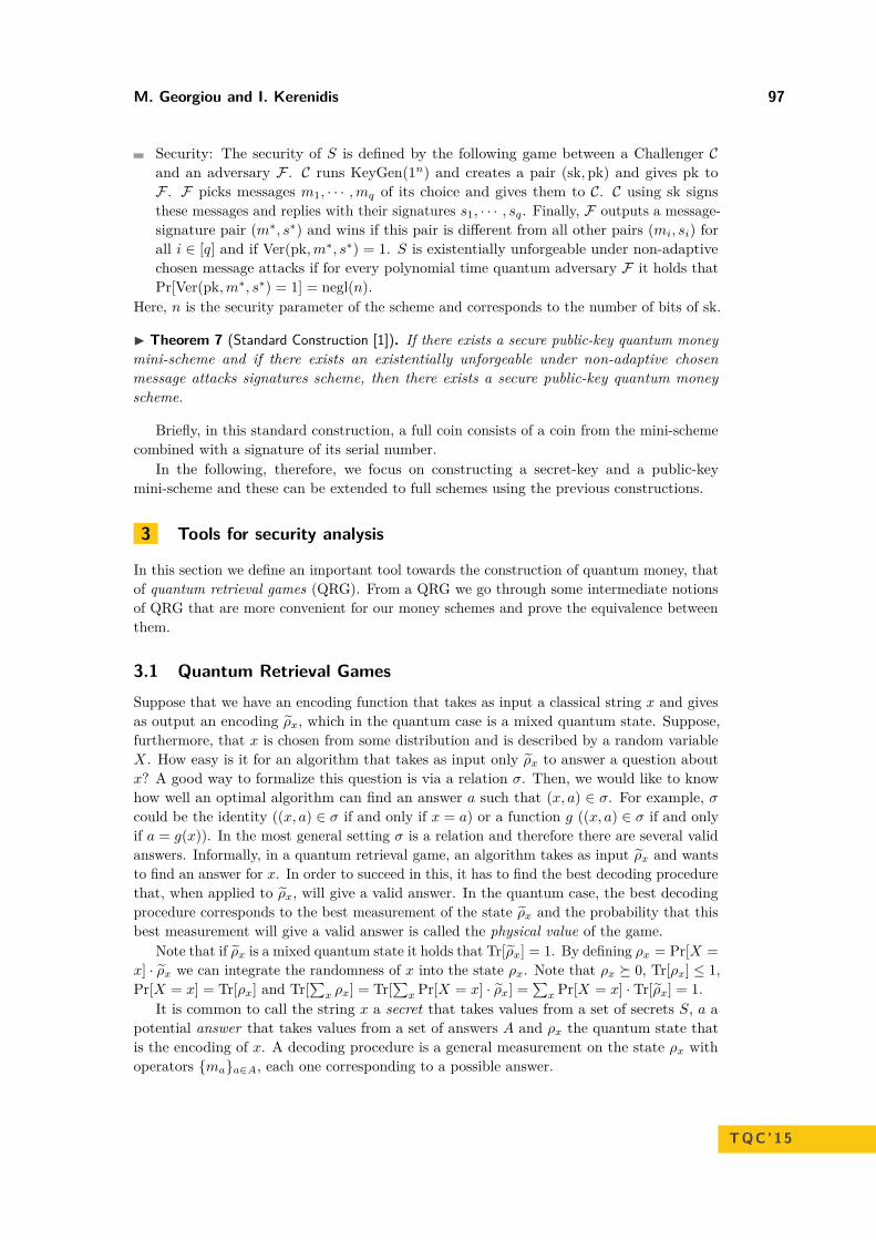
M. Georgiou and I. Kerenidis 97
Security: The security of S is defined by the following game between a Challenger Cand an adversary F . C runs KeyGen(1n) and creates a pair (sk,pk) and gives pk toF . F picks messages m1, · · · ,mq of its choice and gives them to C. C using sk signsthese messages and replies with their signatures s1, · · · , sq. Finally, F outputs a message-signature pair (m∗, s∗) and wins if this pair is different from all other pairs (mi, si) forall i ∈ [q] and if Ver(pk,m∗, s∗) = 1. S is existentially unforgeable under non-adaptivechosen message attacks if for every polynomial time quantum adversary F it holds thatPr[Ver(pk,m∗, s∗) = 1] = negl(n).
Here, n is the security parameter of the scheme and corresponds to the number of bits of sk.
I Theorem 7 (Standard Construction [1]). If there exists a secure public-key quantum moneymini-scheme and if there exists an existentially unforgeable under non-adaptive chosenmessage attacks signatures scheme, then there exists a secure public-key quantum moneyscheme.
Briefly, in this standard construction, a full coin consists of a coin from the mini-schemecombined with a signature of its serial number.
In the following, therefore, we focus on constructing a secret-key and a public-keymini-scheme and these can be extended to full schemes using the previous constructions.
3 Tools for security analysis
In this section we define an important tool towards the construction of quantum money, thatof quantum retrieval games (QRG). From a QRG we go through some intermediate notionsof QRG that are more convenient for our money schemes and prove the equivalence betweenthem.
3.1 Quantum Retrieval GamesSuppose that we have an encoding function that takes as input a classical string x and givesas output an encoding ρx, which in the quantum case is a mixed quantum state. Suppose,furthermore, that x is chosen from some distribution and is described by a random variableX. How easy is it for an algorithm that takes as input only ρx to answer a question aboutx? A good way to formalize this question is via a relation σ. Then, we would like to knowhow well an optimal algorithm can find an answer a such that (x, a) ∈ σ. For example, σcould be the identity ((x, a) ∈ σ if and only if x = a) or a function g ((x, a) ∈ σ if and onlyif a = g(x)). In the most general setting σ is a relation and therefore there are several validanswers. Informally, in a quantum retrieval game, an algorithm takes as input ρx and wantsto find an answer for x. In order to succeed in this, it has to find the best decoding procedurethat, when applied to ρx, will give a valid answer. In the quantum case, the best decodingprocedure corresponds to the best measurement of the state ρx and the probability that thisbest measurement will give a valid answer is called the physical value of the game.
Note that if ρx is a mixed quantum state it holds that Tr[ρx] = 1. By defining ρx = Pr[X =x] · ρx we can integrate the randomness of x into the state ρx. Note that ρx 0, Tr[ρx] ≤ 1,Pr[X = x] = Tr[ρx] and Tr[
∑x ρx] = Tr[
∑x Pr[X = x] · ρx] =
∑x Pr[X = x] · Tr[ρx] = 1.
It is common to call the string x a secret that takes values from a set of secrets S, a apotential answer that takes values from a set of answers A and ρx the quantum state thatis the encoding of x. A decoding procedure is a general measurement on the state ρx withoperators maa∈A, each one corresponding to a possible answer.
TQC’15
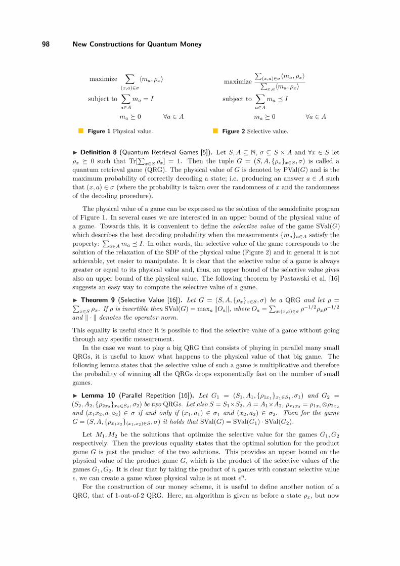
98 New Constructions for Quantum Money
maximize∑
(x,a)∈σ
〈ma, ρx〉
subject to∑a∈A
ma = I
ma 0 ∀a ∈ A
Figure 1 Physical value.
maximize∑
(x,a)∈σ〈ma, ρx〉∑x,a〈ma, ρx〉
subject to∑a∈A
ma I
ma 0 ∀a ∈ A
Figure 2 Selective value.
I Definition 8 (Quantum Retrieval Games [5]). Let S,A ⊆ N, σ ⊆ S × A and ∀x ∈ S letρx 0 such that Tr[
∑x∈S ρx] = 1. Then the tuple G = (S,A, ρxx∈S , σ) is called a
quantum retrieval game (QRG). The physical value of G is denoted by PVal(G) and is themaximum probability of correctly decoding a state; i.e. producing an answer a ∈ A suchthat (x, a) ∈ σ (where the probability is taken over the randomness of x and the randomnessof the decoding procedure).
The physical value of a game can be expressed as the solution of the semidefinite programof Figure 1. In several cases we are interested in an upper bound of the physical value ofa game. Towards this, it is convenient to define the selective value of the game SVal(G)which describes the best decoding probability when the measurements maa∈A satisfy theproperty:
∑a∈Ama I. In other words, the selective value of the game corresponds to the
solution of the relaxation of the SDP of the physical value (Figure 2) and in general it is notachievable, yet easier to manipulate. It is clear that the selective value of a game is alwaysgreater or equal to its physical value and, thus, an upper bound of the selective value givesalso an upper bound of the physical value. The following theorem by Pastawski et al. [16]suggests an easy way to compute the selective value of a game.
I Theorem 9 (Selective Value [16]). Let G = (S,A, ρxx∈S , σ) be a QRG and let ρ =∑x∈S ρx. If ρ is invertible then SVal(G) = maxa ‖Oa‖, where Oa =
∑x:(x,a)∈σ ρ
−1/2ρxρ−1/2
and ‖ · ‖ denotes the operator norm.
This equality is useful since it is possible to find the selective value of a game without goingthrough any specific measurement.
In the case we want to play a big QRG that consists of playing in parallel many smallQRGs, it is useful to know what happens to the physical value of that big game. Thefollowing lemma states that the selective value of such a game is multiplicative and thereforethe probability of winning all the QRGs drops exponentially fast on the number of smallgames.
I Lemma 10 (Parallel Repetition [16]). Let G1 = (S1, A1, ρ1x1x1∈S1 , σ1) and G2 =(S2, A2, ρ2x2x2∈S2 , σ2) be two QRGs. Let also S = S1×S2, A = A1×A2, ρx1x2 = ρ1x1⊗ρ2x2
and (x1x2, a1a2) ∈ σ if and only if (x1, a1) ∈ σ1 and (x2, a2) ∈ σ2. Then for the gameG = (S,A, ρx1x2(x1,x2)∈S , σ) it holds that SVal(G) = SVal(G1) · SVal(G2).
Let M1,M2 be the solutions that optimize the selective value for the games G1, G2respectively. Then the previous equality states that the optimal solution for the productgame G is just the product of the two solutions. This provides an upper bound on thephysical value of the product game G, which is the product of the selective values of thegames G1, G2. It is clear that by taking the product of n games with constant selective valueε, we can create a game whose physical value is at most εn.
For the construction of our money scheme, it is useful to define another notion of aQRG, that of 1-out-of-2 QRG. Here, an algorithm is given as before a state ρx, but now
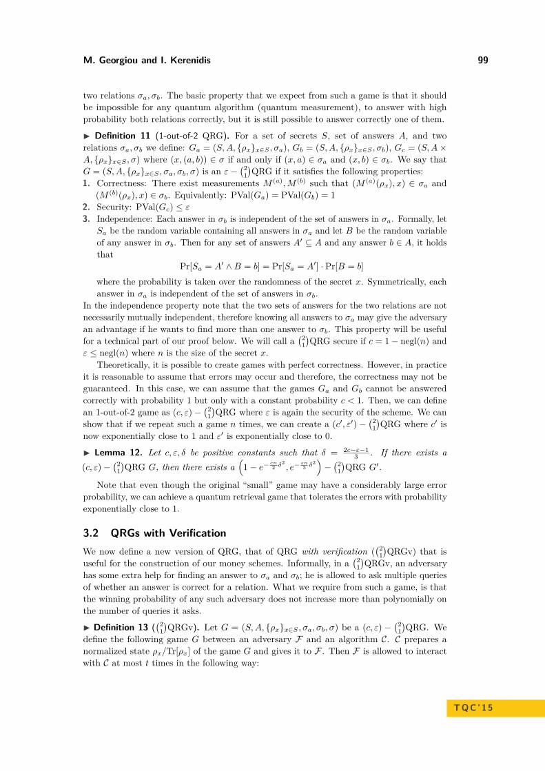
M. Georgiou and I. Kerenidis 99
two relations σa, σb. The basic property that we expect from such a game is that it shouldbe impossible for any quantum algorithm (quantum measurement), to answer with highprobability both relations correctly, but it is still possible to answer correctly one of them.
I Definition 11 (1-out-of-2 QRG). For a set of secrets S, set of answers A, and tworelations σa, σb we define: Ga = (S,A, ρxx∈S , σa), Gb = (S,A, ρxx∈S , σb), Gc = (S,A×A, ρxx∈S , σ) where (x, (a, b)) ∈ σ if and only if (x, a) ∈ σa and (x, b) ∈ σb. We say thatG = (S,A, ρxx∈S , σa, σb, σ) is an ε−
(21)QRG if it satisfies the following properties:
1. Correctness: There exist measurements M (a),M (b) such that (M (a)(ρx), x) ∈ σa and(M (b)(ρx), x) ∈ σb. Equivalently: PVal(Ga) = PVal(Gb) = 1
2. Security: PVal(Gc) ≤ ε3. Independence: Each answer in σb is independent of the set of answers in σa. Formally, let
Sa be the random variable containing all answers in σa and let B be the random variableof any answer in σb. Then for any set of answers A′ ⊆ A and any answer b ∈ A, it holdsthat
Pr[Sa = A′ ∧B = b] = Pr[Sa = A′] · Pr[B = b]where the probability is taken over the randomness of the secret x. Symmetrically, eachanswer in σa is independent of the set of answers in σb.
In the independence property note that the two sets of answers for the two relations are notnecessarily mutually independent, therefore knowing all answers to σa may give the adversaryan advantage if he wants to find more than one answer to σb. This property will be usefulfor a technical part of our proof below. We will call a
(21)QRG secure if c = 1− negl(n) and
ε ≤ negl(n) where n is the size of the secret x.Theoretically, it is possible to create games with perfect correctness. However, in practice
it is reasonable to assume that errors may occur and therefore, the correctness may not beguaranteed. In this case, we can assume that the games Ga and Gb cannot be answeredcorrectly with probability 1 but only with a constant probability c < 1. Then, we can definean 1-out-of-2 game as (c, ε)−
(21)QRG where ε is again the security of the scheme. We can
show that if we repeat such a game n times, we can create a (c′, ε′)−(2
1)QRG where c′ is
now exponentially close to 1 and ε′ is exponentially close to 0.
I Lemma 12. Let c, ε, δ be positive constants such that δ = 2c−ε−13 . If there exists a
(c, ε)−(2
1)QRG G, then there exists a
(1− e− cn
2 δ2, e−
εn3 δ
2)−(2
1)QRG G′.
Note that even though the original “small” game may have a considerably large errorprobability, we can achieve a quantum retrieval game that tolerates the errors with probabilityexponentially close to 1.
3.2 QRGs with VerificationWe now define a new version of QRG, that of QRG with verification (
(21)QRGv) that is
useful for the construction of our money schemes. Informally, in a(2
1)QRGv, an adversary
has some extra help for finding an answer to σa and σb; he is allowed to ask multiple queriesof whether an answer is correct for a relation. What we require from such a game, is thatthe winning probability of any such adversary does not increase more than polynomially onthe number of queries it asks.
I Definition 13 ((2
1)QRGv). Let G = (S,A, ρxx∈S , σa, σb, σ) be a (c, ε) −
(21)QRG. We
define the following game G between an adversary F and an algorithm C. C prepares anormalized state ρx/Tr[ρx] of the game G and gives it to F . Then F is allowed to interactwith C at most t times in the following way:
TQC’15

100 New Constructions for Quantum Money
1. F picks a σ′ ∈ σa, σb, generates an answer d and sends (σ′, d) to C.2. C returns 1 if and only if (x, d) ∈ σ′.After t interactions F outputs (a∗1, a∗2) and wins if and only if (x, (a∗1, a∗2)) ∈ σ. We say thatG is a (c, ε) −
(21)quantum retrieval game with verification (
(21)QRGv) if it satisfies the
following properties:1. Correctness: Given any state ρx/Tr[ρx] the probability of answering σa (or σb) is at least
c.2. Soundness: For any t and for any adversary F interacting the way defined above, it holds
that Pr[F wins] ≤ poly(t) · ε
We would like to argue the following: allowing such an adversary F to check whether aquery (σ′, d) is correct, does not increase considerably his probability of winning. Therefore,for an exponentially small ε an adversary would require a superpolynomial number of suchinteractions in order to have a non-negligible probability of winning. Towards this, we definebelow a more restricted version of the game and we show that this definition is equivalent tothat of a
(21)QRGv.
We now restrict the adversary F in the following manner. Suppose that F is allowed tointeract with C as previously and the i-th interaction is the first interaction when he sends toC some (σ′, a) such that (x, a) ∈ σ′ (without loss of generality we can assume that σ′ = σa).Then, for the remaining t − i interactions F is allowed to play only with σb. We call thisgame a restricted 1-out-of-2 quantum retrieval game with verification (
(21)rQRGv) and the
adversary F a restricted adversary. It can be proven that since finding an answer for σa isindependent from any answer of σb, these two games are equivalent. In other words, allowingthe adversary to succeed in more than one interaction with the same relation σ′ does nothelp him win the game more than succeeding only once for σ′.
I Lemma 14. Let G = (S,A, ρxx∈S , σa, σb, σ) be a (c, ε) −(2
1)QRGv. Then G is also a
(c, ε)−(2
1)rQRGv.
Using the previous lemma we can show that an adversary that is allowed to ask at most tqueries regarding the relations σa, σb does not increase significantly his probability of winning.More specifically, it can be shown that if the original
(21)QRG has security ε then allowing
interaction, increases the winning probability at most quadratically in t.
I Theorem 15. If there exists a (c, ε)−(2
1)QRG G′ then there exists a (c, ε)−
(21)QRGv G.
In particular, any adversary against G has winning probability of at most 4t2 · ε, where t isthe number of queries.
3.3 One-time MemoriesFor the creation of our public-key scheme we will use the notion of one-time memories (OTM)defined by Goldwasser et al in [7]. OTM are essentially devices which contain two secretsxa, xb, however, we are able to extract only one of these secrets. There is a very naturalconnection between
(21)QRG and OTMs as we will see below.
I Definition 16. A (c, ε)−one-time memory (OTM) is a device that has the followingbehavior. Suppose that the device is programmed with two n-bit messages xa, xb chosenfrom some distribution D. Then:1. Correctness: There exists an honest strategy M (a) that interacts with the device and
recovers the message xa with probability c. Likewise, there is an honest strategy M (b)
that interacts with the device and recovers the message xb with probability c.

M. Georgiou and I. Kerenidis 101
2. Security: For any strategy M , if X is the random variable corresponding to the classicaloutput of M , then Pr[X = (xa, xb)] ≤ ε.
We will call the OTM secure if c = 1− negl(n) and ε = negl(n).Note that in this paper, we deal with quantum OTM, namely the “device” is a quantum
state ρxa,xb. Although secure OTM are impossible in the plain quantum model even with
computational assumptions, Liu [8, 9, 10] has shown that OTM are possible in the isolatedqubits model, where an adversary can use only local operations and classical communication.His OTM construction is a quantum state that consists of qubits that do not need to beentangled and thus it is easier and more efficiently implementable.
It is not hard to see that OTM are equivalent to(2
1)QRG restricted so that the relations
σa, σb are, in fact, functions.
I Lemma 17. There exists a secure(2
1)QRG G = (S,A, ρxx∈S , σa, σb, σ) such that the
relations σa, σb are functions if and only if there exists a secure OTM.
Proof. Using G we can create an OTM with secrets xa = σa(x) and xb = σb(x). The OTMdevice is simply ρx. Clearly, if there exists an algorithm that can retrieve both secrets fromthe OTM then this algorithm can also break G. For the opposite direction, the role of theencoding ρx is played by the OTM device, which is a quantum state. The secret x of G isdefined as the concatenation of xa and xb and the functions σa, σb are defined such thatσa(xa|xb) = xa and σb(xa|xb) = xb. Clearly, if there exists an algorithm that can retrieveanswers for both σa and σb from the encoding ρx then this algorithm can also break theOTM. J
Similarly to the QRG with verification, we can define (c, ε)−one-time memories withverification (OTMv); where the adversary is allowed to choose d ∈ a, b and y ∈ 0, 1nand ask whether xd = y. Again, a secure OTMv means that c ≥ 1− negl(n) and ε ≤ negl(n).However, as we have shown, such a power does not really help the adversary.
Finally, a hash based OTMv (hOTM) is an OTMv where the adversary instead of beingallowed to interact in order to find an answer, it is given as input the hashes of the twoanswers H(xa), H(xb). This way, if an answer is correct, the adversary can verify that on itsown. It can be shown that if the original OTMv is secure, then the hash based OTMv isstill secure in the random oracle model.
A random oracle is essentially an oracle that behaves as follows. First, it keeps a list L ofpairs of the form (x, y) where x is an element of its domain and y is an element of its range.In the beginning L is empty. On input x0, first it searches L for a pair of the form (x0, y0),and if such a pair exists in L then it returns y0. Otherwise, it picks a uniformly randomelement y0 from its range, inserts (x0, y0) in the list L, and returns y0. Hash functions areusually assumed to have this ideal property when other properties such as one-wayness orcollision resistance are not enough for a security proof. When hash functions are used asrandom oracles in a proof that a scheme is secure, we say that the scheme is secure in therandom oracle model.
I Definition 18. A hash based one-time memory (hOTM) is a device that has the followingbehavior. Suppose that the device is programmed with two n-bit messages xa, xb chosenfrom some distribution D. Then:1. Correctness: There exists an honest strategy M (a) that interacts with the device and
recovers the message xa with probability c = 1− negl(n). Likewise, there is an honeststrategy M (b) that interacts with the device and recovers the message xb with probabilityc = 1− negl(n).
TQC’15
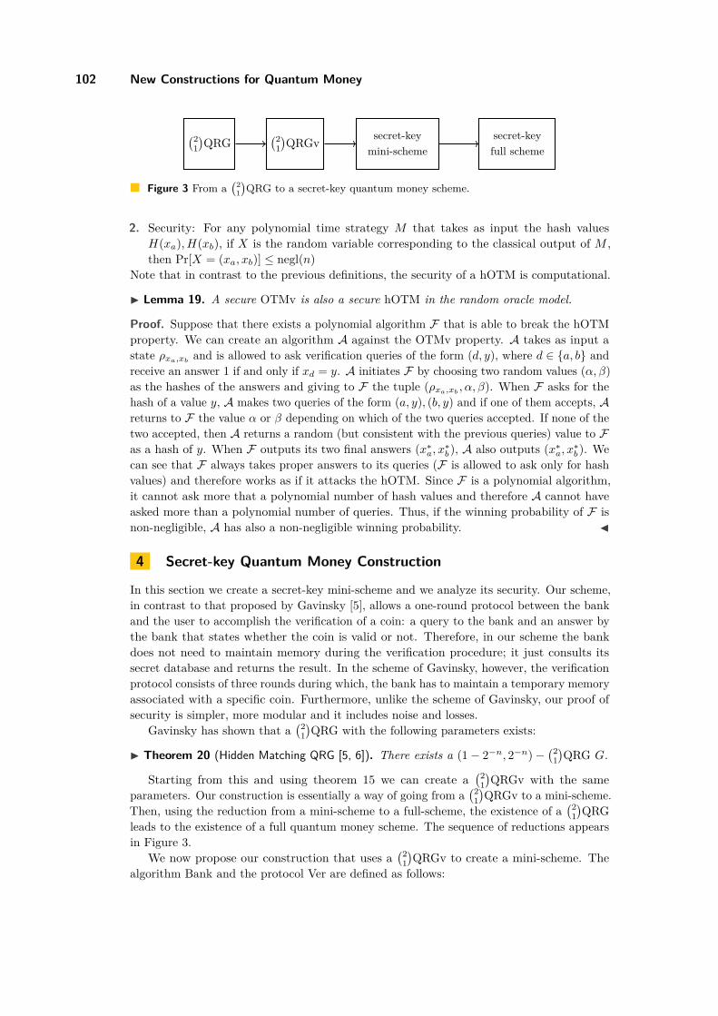
102 New Constructions for Quantum Money
(21)QRG
(21)QRGv secret-key
mini-schemesecret-keyfull scheme
Figure 3 From a(2
1
)QRG to a secret-key quantum money scheme.
2. Security: For any polynomial time strategy M that takes as input the hash valuesH(xa), H(xb), if X is the random variable corresponding to the classical output of M ,then Pr[X = (xa, xb)] ≤ negl(n)
Note that in contrast to the previous definitions, the security of a hOTM is computational.
I Lemma 19. A secure OTMv is also a secure hOTM in the random oracle model.
Proof. Suppose that there exists a polynomial algorithm F that is able to break the hOTMproperty. We can create an algorithm A against the OTMv property. A takes as input astate ρxa,xb
and is allowed to ask verification queries of the form (d, y), where d ∈ a, b andreceive an answer 1 if and only if xd = y. A initiates F by choosing two random values (α, β)as the hashes of the answers and giving to F the tuple (ρxa,xb
, α, β). When F asks for thehash of a value y, A makes two queries of the form (a, y), (b, y) and if one of them accepts, Areturns to F the value α or β depending on which of the two queries accepted. If none of thetwo accepted, then A returns a random (but consistent with the previous queries) value to Fas a hash of y. When F outputs its two final answers (x∗a, x∗b), A also outputs (x∗a, x∗b). Wecan see that F always takes proper answers to its queries (F is allowed to ask only for hashvalues) and therefore works as if it attacks the hOTM. Since F is a polynomial algorithm,it cannot ask more that a polynomial number of hash values and therefore A cannot haveasked more than a polynomial number of queries. Thus, if the winning probability of F isnon-negligible, A has also a non-negligible winning probability. J
4 Secret-key Quantum Money Construction
In this section we create a secret-key mini-scheme and we analyze its security. Our scheme,in contrast to that proposed by Gavinsky [5], allows a one-round protocol between the bankand the user to accomplish the verification of a coin: a query to the bank and an answer bythe bank that states whether the coin is valid or not. Therefore, in our scheme the bankdoes not need to maintain memory during the verification procedure; it just consults itssecret database and returns the result. In the scheme of Gavinsky, however, the verificationprotocol consists of three rounds during which, the bank has to maintain a temporary memoryassociated with a specific coin. Furthermore, unlike the scheme of Gavinsky, our proof ofsecurity is simpler, more modular and it includes noise and losses.
Gavinsky has shown that a(2
1)QRG with the following parameters exists:
I Theorem 20 (Hidden Matching QRG [5, 6]). There exists a (1− 2−n, 2−n)−(2
1)QRG G.
Starting from this and using theorem 15 we can create a(2
1)QRGv with the same
parameters. Our construction is essentially a way of going from a(2
1)QRGv to a mini-scheme.
Then, using the reduction from a mini-scheme to a full-scheme, the existence of a(2
1)QRG
leads to the existence of a full quantum money scheme. The sequence of reductions appearsin Figure 3.
We now propose our construction that uses a(2
1)QRGv to create a mini-scheme. The
algorithm Bank and the protocol Ver are defined as follows:

M. Georgiou and I. Kerenidis 103
Bank(1n2) :1. For i ∈ [n] create Gi = (S,A, ρxi
xi, σa, σb, σ), (1− 2−n, 2−n)−
(21)QRGv.
2. Create a classical binary register r of size n and initialize it to 0n.3. Return the state $ = (
⊗i ρxi
, r) as a coin for the mini-scheme.
Verification protocol for a coin $ = (⊗
i ρxi, r):
1. The holder creates an empty set L. Then, for each i ∈ [n] such that ri = 0, theholder puts i in the set L with probability 1/n1/3. For each i ∈ L the holder picks atrandom a relation σ′i ← σa, σb and applies to ρxi the measurement M (a) if σ′i = σaor M (b) if σ′i = σb, in order to retrieve an answer di. Furthermore, for all i ∈ L theholder sets ri = 1. Finally, the holder sends to the bank the i’s he has picked, therelation he has picked for each i, as well as the answers di.
2. The bank compares the answers it has received with its secret x1 · · ·xn and acceptsif all answers are correct; namely if for all i ∈ L it holds that (xi, di) ∈ σ′i.
I Remark. The coin is returned to the bank for replacement when the hamming weight of ris greater than n/4 (more than n/4 of the ρxi
are marked as used). Note that the schemeconsists of O(n2) qubits in total (there are n states ρxi
and each state consists of O(n) qubits)and that the verification protocol consists of only one round.
I Theorem 21. The scheme is secure; namely any (even computationally unbounded)adversary who interacts with the bank at most t times has winning probability of at moste−n
1/3/8 + 4t2 · n · 2−n.
Proof. Suppose there is an adversary F for the mini-scheme, namely when F receives asinput a valid coin $ and after running t verification protocols with the bank, he can producetwo coins $′ = (ρ′1, · · · , ρ′n, r′), $′′ = (ρ′′1 , · · · , ρ′′n, r′′) that can pass the verification protocolwith non-negligible probability ε greater than p(t) · 2−n, for all polynomials p. Then, onecan create an adversary A for the (1− 2−n, 2−n)−
(21)QRGv, namely when A receives from
the algorithm C as input a state ρ∗ that is the encoding of a secret x∗, and after interactingt times with the algorithm C, he can win the game with probability greater than p(t) · 2−nfor all polynomials p. By theorem 15 this also implies breaking the security of the
(21)QRG.
Let A receive as input the state ρ∗, that is the encoding of a secret x∗. He creates aninput for F in the following way:
Bank(1n2):1. Pick at random i∗ ← [n].2. For i ∈ [n]−i∗ create Gi = (S,A, ρxi
xi, σa, σb, σ) where Gi is a (1− 2−n, 2−n)−(2
1)QRGv.
3. Create a classical binary register r of size n and initialize it to 0n.4. Return to F the coin $ = (ρ, r), where ρ = ρx1 ⊗· · ·⊗ρxi∗−1 ⊗ρ∗⊗ρxi∗+1 ⊗· · ·⊗ρxn .
In other words, A creates a totally valid coin, but in the i∗-th position he puts the statehe has as input. For clarity we will denote the secret x∗ as xi∗ . Note that A is able to pretend
TQC’15

104 New Constructions for Quantum Money
to be the honest bank during the verification protocol with F , since for all i ∈ [n]− i∗ heknows the answers to the relations, whereas for the i∗-th state, he can use his own interactionwith the algorithm C in order to decide whether the query asked by F is correct. Therefore,A simulates the verification protocol between the bank and F in the following way:
1. A receives from F a set L of i’s, a set of challenges σ′i ∈ σa, σb and a set of answersdi for each i ∈ L.
2. A returns 1 if all answers are correct; namely, if (xi, di) ∈ σ′i for all i ∈ L. Note thatfor those i’s that are different from i∗, A can easily consult his own secret xi in orderto find if the answer is correct. However, for i = i∗, A can make a query (σ′i∗ , di∗) tothe algorithm C in order to find if the answer di∗ is correct.
Hence, A can provide F with a valid initial coin and simulate the bank in the t verificationprotocols with F , and in the end, he receives from F two coins $′ = (ρ′1, · · · , ρ′n, r′), $′′ =(ρ′′1 , · · · , ρ′′n, r′′) that can pass a verification protocol with an honest verifier with non-negligibleprobability ε. For the two coins $′, $′′ to be considered as valid, there must be at least 3/4n ofthe ρ′i’s denoted as valid and at least 3/4n of the ρ′′i ’s denoted as valid (a state ρ′i is denotedas valid if r′i = 0). Therefore, there are at least n/2 indices i such that r′i = r′′i = 0. We wantto argue that there must be an index i among them for which A can win the
(21)QRGv game
with probability greater than p(t) · 2−n for all polynomials p, otherwise the probability thatthe adversary F could create two valid coins is negligible.
Let I = i : r′i = r′′i = 0. Since the coins $′, $′′ are denoted as valid, it holds that|I| ≥ n/2. Assume now that two honest verifiers Ver′ and Ver′′ run the verification protocolfor the two coins respectively. Let La, Lb be the sets chosen by the honest verifiers andL′ = i ∈ La ∩ Lb : σ′i = σa ∧ σ′′i = σb, where σ′i, σ′′i are the relations chosen for the indexi by the verification protocols for the two coins. In other words, L′ contains the indicesthat where chosen by both Ver′ and Ver′′ in such a way that Ver′ chose σa for this i andVer′′ chose σb for this i. It holds that Pr[i ∈ La ∩ Lb] = 1/n2/3 and Pr[i ∈ L′] = 1/4n2/3.Therefore, Pr[∀i ∈ I : i /∈ L′] = Pr[L′ = ∅] ≤ (1 − 1/4n2/3)n/2 = e−n
1/3/8, since |I| = n/2.In other words, the probability that there exists an i with r′i = r′′i = 0 such that Ver′ choseit during the verification protocol and picked the relation σa for it and Ver′′ also chose itand picked σb for it, is exponentially close to 1. Now it holds that
Pr[F wins] = Pr[Ver′($′) = 1 ∧Ver′′($′′) = 1]= Pr[L′ = ∅] · Pr[Ver′($′) = 1 ∧Ver′′($′′) = 1|L′ = ∅]+ Pr[Ver′($′) = 1 ∧Ver′′($′′) = 1 ∧ L′ 6= ∅]
≤ e−n1/3/8 + Pr[Ver′($′) = 1 ∧Ver′′($′′) = 1 ∧ L′ 6= ∅]
≤ e−n1/3/8 + Pr[∃i ∈ L′ : (M (a)(ρ′i), xi) ∈ σa ∧ (M (b)(ρ′′i ), xi) ∈ σb]
where M (a),M (b) are the measurements applied to the states of the QRG’s in order toretrieve an answer to σa, σb respectively. The last line comes from the fact that if L′is not empty and both verifications succeed, then both verifications must succeed for alli ∈ L′. Therefore, if Pr[F wins] = ε is non-negligible then Pr[∃i ∈ L′ : (M (a)(ρ′i), xi) ∈σa ∧ (M (b)(ρ′′i ), xi) ∈ σb] ≥ ε− e−n
1/3/8 is non-negligible as well. This trivially implies thatPr[∃i ∈ [n] : (M (a)(ρ′i), xi) ∈ σa ∧ (M (b)(ρ′′i ), xi) ∈ σb] ≥ ε− e−n
1/3/8. In other words, with

M. Georgiou and I. Kerenidis 105
OTM+
random oraclehOTM
public-keymini-scheme
public-keyfull scheme
signatures [1]
Figure 4 From an OTM to a full public-key quantum money scheme. OTMs in the randomoracle model give hOTM. hOTM imply public-key mini-schemes which, together with signatures,imply public-key quantum money.
non-negligible probability there exists an index i for which both verifications succeed. At thispoint it is clear that the goal of A is just to guess that index i and put ρ∗ in that position.
Overall, the adversary A works as follows: Upon receiving as input the state ρ∗, he picksa random position i∗, creates the valid coin for F as we described above, receives the statesρ′i∗ and ρ′′i∗ from F and returns the answers
(M (a)(ρ′i∗),M (b)(ρ′′i∗)
). Now it holds that
Pr[A wins] = Pr[(M (a)(ρ′i∗), xi∗) ∈ σa ∧ (M (b)(ρ′′i∗), xi∗) ∈ σb]≥ Pr[(M (a)(ρ′i∗), xi∗) ∈ σa ∧ (M (b)(ρ′′i∗), xi∗) ∈ σb|
∃i ∈ [n] : (M (a)(ρ′i), xi) ∈ σa ∧ (M (b)(ρ′′i ), xi) ∈ σb]· Pr[∃i ∈ [n] : (M (a)(ρ′i), xi) ∈ σa ∧ (M (b)(ρ′′i ), xi) ∈ σb]
≥ 1n· Pr[∃i ∈ L′ : (M (a)(ρ′i), xi) ∈ σa ∧ (M (b)(ρ′′i ), xi) ∈ σb]
≥(ε− e−n
1/3/8)/n
which contradicts the fact that the security of the(2
1)QRGv is 2−n.
Therefore, since by theorem 15 the maximum winning probability of A is 4t2 · 2−n, themaximum winning probability of F is e−n1/3/8 + 4t2 · 2−n · n. J
5 Public-key Quantum Money Construction
In the construction of a public key scheme, it suffices to create a secure public-key mini-scheme, and this, combined with signatures, can give a full scheme [1]. The advantageof our construction is that it is a simple modification of the previous secret key one: theanswers of the bank are encoded in their hash values. Therefore, instead of requiring fromthe user to communicate with the bank in order to find out if an answer is valid, the bankannounces the hash values of the answers. It is clear that for a regular QRG there may existtoo many answers and hence giving all these hashes as part of the coin would violate thecorrectness of the scheme. Hence, for our construction, we need to use QRG with functionsor equivalently one-time memories. Despite the fact that quantum one-time memories donot exist unconditionally, they exist in the isolated qubits model.
I Theorem 22 ([8, 9, 10]). There exists a secure OTM in the isolated qubits model.
Using this, together with lemma 19, we get the following corollary.
I Corollary 23. There exists a secure hOTM in the isolated qubits-random oracle model.
Our purpose, now, is to go from hOTM to a public-key mini-scheme. The sequence ofreductions appears in Figure 4.
Since for each OTM there are only two secrets, a hashing of each answer can be given aspart of the coin. Then the verification algorithm works similarly to the secret key scheme. Itchooses each state-game with probability 1/n1/3, it chooses at random whether to retrieve
TQC’15

106 New Constructions for Quantum Money
the first (xa) or the second (xb) secret for each game, it measures the OTM (using M (a) orM (b)) in order to retrieve an answer and finally it verifies that the hash value of that answeris the same as the one given. So the two algorithms Bank and Ver of the mini-scheme arethe following:
Bank(1n2) :1. For i ∈ [n] create the OTM ρi with secrets xai , xbi ∈ 0, 1n.2. Create a classical binary register r of size n and initialize it to 0n.3. Return $ = ((h1, g1), · · · , (hn, gn), ρ1, · · · , ρn, r) as a coin for the mini-scheme, where
hi = H(xai ), gi = H(xbi ) and H is the hash function. The string (h1, g1), · · · , (hn, gn)corresponds to the classical serial number of the coin (that has to be signed in orderto give a full coin), and (ρ1, · · · , ρn, r) is the quantum state.
Ver((h1, g1), · · · , (hn, gn), ρ1, · · · , ρn, r):1. Create an empty set L. Then, for each i ∈ [n] such that ri = 0, put i in the set L
with probability 1/n1/3.2. For each i ∈ L pick at random di ← a, b and measure ρi in order to retrieve an
answer xi ∈ xai , xbi; i.e. xi = M (di)(ρi).3. For all i ∈ L set ri = 1.4. Accept if for all i ∈ L it holds that H(xi) = hi (if di = a) or H(xi) = gi (if di = b).
As before, the coin is returned to the bank for replacement when the hamming weight ofr is greater that n/4.
I Theorem 24. The scheme is secure.
Proof sketch. The proof follows the same steps as that of the secret-key scheme; a goodadversary F against the mini-scheme can lead to a good adversary A against the hOTM. Ftakes as input a coin $ = (sn, ρ), where sn = (h1, g1), · · · , (hn, gn) and ρ = (ρ1, · · · , ρn, r).At the end, F outputs two states ρ′ = (ρ′1, · · · , ρ′n, r′), ρ′′ = (ρ′′1 , · · · , ρ′′n, r′′) such that both$′ = (sn, ρ′) and $′′ = (sn, ρ′′) pass the verification test with non-negligible probability. Notethat these two states pass successfully the verification algorithm with the same serial sn andtherefore with the same hash values. As before, we can show that the number of indices thatare denoted as valid in both coins are at least n/2. Furthermore, the probability that noneof them is able to pass the two verification algorithms is negligible (otherwise the winningprobability of F would be negligible). Thus, a non-negligible counterfeiting probability ε ofF implies a non-negligible probability of A to break the hOTM. J
6 Conclusions
We created a secret-key quantum money scheme that is unconditionally secure and hasoptimal communication: a single round of classical communication. We also provided aconceptually simpler and more modular proof. Moreover, if we instantiate the
(21)QRG with
the Hidden Matching(2
1)QRG, we can tolerate an error rate of up to 12.5%; see lemma 12
in Appendix A. Note that in every verification of the coin we invalidate on average n1/3
quantum states (each consisting of n qubits) and thus the number of allowed verifications

M. Georgiou and I. Kerenidis 107
before the coin is returned to the bank is n/(4 · n1/3) = n2/3/4. Therefore, for a coin of say1012 qubits, we succeed 2,500 verifications on average. A polynomial number of verificationsis optimal for unconditionally secure schemes, nevertheless, a natural question that stillremains open is whether we can have computationally secure secret-key schemes that allowexponentially many classical verifications.
In addition, we showed how a simple extension of our secret key construction can giverise to a public-key quantum money scheme that is computationally secure against quantumadversaries in the random oracle model given one-time memories. We note that previousschemes were also based on non-standard computational assumptions. The main openquestion is to construct public-key quantum money that are provably secure based on somestandard cryptographic assumptions such as one-way functions.
Acknowledgements. We thank Jamie Sikora for bringing to our attention the semidefiniteapproach of QRG. This work was partially supported by the ERC project QCC, the ANRproject RDAM and the EU project QAlgo.
References1 Scott Aaronson and Paul Christiano. Quantum money from hidden subspaces. In Proceed-
ings of the 44th Symposium on Theory of Computing, pages 41–60. ACM, 2012.2 Ziv Bar-Yossef, Thathachar S Jayram, and Iordanis Kerenidis. Exponential separation of
quantum and classical one-way communication complexity. In Proceedings of the thirty-sixthannual ACM symposium on Theory of computing, pages 128–137. ACM, 2004.
3 Anne Broadbent, Gus Gutoski, and Douglas Stebila. Quantum one-time programs. Ad-vances in Cryptology–CRYPTO 2013, pages 344–360, 2013.
4 Edward Farhi, David Gosset, Avinatan Hassidim, Andrew Lutomirski, and Peter Shor.Quantum money from knots. In Proceedings of the 3rd Innovations in Theoretical ComputerScience Conference, pages 276–289. ACM, 2012.
5 Dmitry Gavinsky. Quantum money with classical verification. In Computational Complexity(CCC), 2012 IEEE 27th Annual Conference on, pages 42–52. IEEE, 2012.
6 Dmitry Gavinsky, Julia Kempe, Iordanis Kerenidis, Ran Raz, and Ronald de Wolf. Ex-ponential separations for one-way quantum communication complexity, with applicationsto cryptography. In Proceedings of the thirty-ninth annual ACM symposium on Theory ofcomputing, pages 516–525. ACM, 2007.
7 Shafi Goldwasser, Yael Tauman Kalai, and Guy N Rothblum. One-time programs. Advancesin Cryptology–CRYPTO 2008, pages 39–56, 2008.
8 Yi-Kai Liu. Building one-time memories from isolated qubits. In Proceedings of the 5thconference on Innovations in theoretical computer science, pages 269–286. ACM, 2014.
9 Yi-Kai Liu. Privacy amplification in the isolated qubits model. arXiv preprintarXiv:1410.3918, 2014.
10 Yi-Kai Liu. Single-shot security for one-time memories in the isolated qubits model. arXivpreprint arXiv:1402.0049, 2014.
11 Abel Molina, Thomas Vidick, and John Watrous. Optimal counterfeiting attacks andgeneralizations for wiesner’s quantum money. In Theory of Quantum Computation, Com-munication, and Cryptography, pages 45–64. Springer, 2013.
12 Michele Mosca and Douglas Stebila. Quantum coins. Error-Correcting Codes, Finite Geo-metries and Cryptography. Contemporary Mathematics, volume 523, pages 35-47. Amer-ican Mathematical Society, 2010, 2009.
13 Daniel Nagaj and Or Sattath. An adaptive attack on wiesner’s quantum money based oninteraction-free measurement. arXiv preprint arXiv:1404.1507, 2014.
TQC’15

108 New Constructions for Quantum Money
14 Marta Conde Pena, Jean-Charles Faugère, and Ludovic Perret. Algebraic cryptanalysisof a quantum money scheme the noise-free case. In Public-Key Cryptography–PKC 2015,pages 194–213. Springer, 2015.
15 Stephen Wiesner. Conjugate coding. ACM Sigact News, 15(1):78–88, 1983.16 Norman Yao, Fernando Pastawski, Liang Jiang, Mikhail Lukin, and Ignacio Cirac. Un-
forgeable noise-tolerant quantum tokens. Bulletin of the American Physical Society, 57,2012.
A Instantiating a QRG
As shown above, the existence of a (c, ε) −(2
1)QRG implies the existence of a secret-key
quantum money scheme as long as c is reasonably large and ε is any constant smaller than1. To instantiate such a quantum money scheme one has to give specific quantum retrievalgames with this property.
Hidden Matching QRG [2, 5]I Definition 25. The Hidden Matching
(21)QRG G = (S,A, ρxx∈S , σa, σb, σ) is defined the
following way: S = 0, 14, A = 0, 1 × 0, 1, |ψx〉 = 12∑i∈[4](−1)xi |i〉, ρx = 1
16 |ψx〉〈ψx|.The relation σa is defined as (x, (a, b)) ∈ σa if and only if the following holds: if a = 0 thenx1 ⊕ x2 = b; if a = 1 then x3 ⊕ x4 = b. Similarly, the relation σb is defined as (x, (a, b)) ∈ σbif and only if the following holds: if a = 0 then x1 ⊕ x3 = b; if a = 1 then x2 ⊕ x4 = b.
I Lemma 26. The Hidden Matching is a (1, 34 )−
(21)QRG.
Proof. The correctness in a noise-free environment we can be succeeded with zero errorprobability. Indeed, if we want to find an answer for the relation σa we measure in the basis |1〉+|2〉√
2 , |1〉−|2〉√2 , |3〉+|4〉√
2 , |3〉−|4〉√2 and we return the values (a, b) = (0, 0), (0, 1), (1, 0), (1, 1)
respectively. If we want to find an answer for the relation σb we measure in the basis |1〉+|3〉√
2 , |1〉−|3〉√2 , |2〉+|4〉√
2 , |2〉−|4〉√2 and we return (a, b) = (0, 0), (0, 1), (1, 0), (1, 1) respectively.
For the security of the game, we use Theorem 9. By definition, we have (x, (a1, b1), (a2, b2)) ∈σ if and only if (x, (a1, b1)) ∈ σa and (x, (a2, b2)) ∈ σb. It holds that ρ =
∑x∈0,14 ρx = 1
4I
and therefore ρ 12 = 2I. In order to find the selective value of the game (S,A×A, ρxx∈S , σ)
it is enough to consider one value of Oa for some possible answer a ∈ A×A. For example,by taking a = ((0, 0), (0, 0)) the values of x that satisfy (x, a) ∈ σ are 0000, 0001, 1110, 1111
and the corresponding density matrices are 116
14
1 1 1 11 1 1 11 1 1 11 1 1 1
, 116
14
1 1 1 −11 1 1 −11 1 1 −1−1 −1 −1 1
,
116
14
1 1 1 11 1 1 11 1 1 11 1 1 1
, 116
14
1 1 1 −11 1 1 −11 1 1 −1−1 −1 −1 1
. Therefore, O((0,0),(0,0)) = 14
1 1 1 01 1 1 01 1 1 00 0 0 1
and thus it holds that ‖O((0,0),(0,0))‖ = 3
4 = SVal(G).For the independence property, we know that for any a12, a34 ∈ 0, 1 it holds that
Pr[x1⊕x2 = a12 ∧x3⊕x4 = a34] = 1/4 and for any bit b ∈ 0, 1, it holds that Pr[x1⊕x3 =b] = 1/2. Moreover, Pr[x1 ⊕ x2 = a12 ∧ x3 ⊕ x4 = a34 ∧ x1 ⊕ x3 = b] = 1/8 and thus we seethat the event x1⊕ x3 = b is independent from the event x1⊕ x2 = a12 ∧ x3⊕ x4 = a34. Thesame of course holds for the event x2 ⊕ x4 = b. J

M. Georgiou and I. Kerenidis 109
By Lemma 12, it is enough to guarantee that c ≥ 78 + δ for some constant δ in order succeed
an exponentially good error tolerance. Thus, the hidden matching(2
1)QRG can tolerate up
to 12.5% of errors.
B Technical proofs
Proof of lemma 12. Let G = (S,A, ρxx∈S , σa, σb, σ). We create the following game G′ =(S′, A′, ρ′xx∈S′ , σ′a, σ′b, σ′) by taking the product of n games G. Then we require that(x1 · · ·xn, a1 · · · an) ∈ σ′a if at least c− δ of the (xi, ai) are in σa and (x1 · · ·xn, b1 · · · bn) ∈σ′b if at least c − δ of the (xi, bi) are in σb. Furthermore, by definition, it holds that(x1 · · ·xn, (a1 · · · an, b1 · · · bn)) ∈ σ′ if (x1 · · ·xn, a1 · · · an) ∈ σ′a and (x1 · · ·xn, b1 · · · bn) ∈ σ′b.
Since δ > 0, we have c > (1 + ε)/2 and hence c− δ > 1/2. This implies there exist at least2c− 2δ − 1 = ε+ δ common values (i’s such that (xi, ai) ∈ σa and (xi, bi) ∈ σb). Therefore,(x1 · · ·xn, (a1 · · · an, b1 · · · bn)) ∈ σ′ implies that there exist at least ε + δ of the (xi, ai, bi)that are in σ.
We then analyze its Correctness and its Security. The Correctness c′ of G′ is guaranteedvia the straightforward strategy of independently measuring each of the n states in the basisthat corresponds to σa or to σb. Let Xi be the binary random variable that equals to 1 ifand only if the i-th measurement was successful. Let X =
∑i∈[n] Xi. Then E[X] = cn and,
since the Xi’s are independent, using Chernoff bound, we have that
c′ ≥ 1− e− cn2 δ
2
For the Security ε′ of the game, we know that the selective value is always greater or equalto the physical value and that the former is equal to the product of the individual selectivevalues. Therefore, as mentioned before, the best measurement strategy that answers correctlyboth questions, cannot be better than independently playing the optimal strategy for each ofthe n small games. Let Yi be the binary random variable that equals to 1 if and only if thei-th measurement was successful. Let, also, Y =
∑i∈[n] Yi. Then, as before, E[Y ] = εn and,
since the Yi’s are independent
ε′ ≤ e− εn3 (2c−2δ−1−ε)2
= e−εn3 δ
2
which is exponentially small in n. J
Proof of lemma 14. The correctness of(2
1)QRGv and
(21)rQRGv is exactly the same. Fur-
thermore, it is clear that if a non-restricted adversary has probability ε to win, this probabilitycannot increase by restricting this adversary. In order to show the equivalence between thetwo definitions, it remains to show that a non-restricted adversary has no more power than arestricted adversary. Without loss of generality, we assume that the first successful querywas for σa. Then, one more success for σa does not help the adversary towards finding ananswer for σa (since, it already knows one). Furthermore, by the independence property, evenknowing all the answers for σa does not give the adversary extra power to find an answerto σb. Therefore, restricting the adversary to one successful query per relation, does notdecrease his winning probability. More details will appear in the full version of the paper. J
Proof of Theorem 15. The proof of correctness is straightforward. We focus on the securityof G. By lemma 14 it suffices to show that G’ implies an
(21)rQRGv. By contradiction,
assume that there exists an adversary F against the(2
1)rQRGv G, who interacts t times
with C and wins the game with probability q > p(t) · ε for all polynomials p. We can use
TQC’15

110 New Constructions for Quantum Money
F in order to create an adversary F ′ who is able to attack the original(2
1)QRG G′ with
probability greater than ε. Since F is restricted after succeeding one interaction with σa itwill continue interacting only by picking σb in its queries. Let E1, E2, E3, E4 be the eventsthat F does not succeed in any interaction, F succeeds only in a σa interaction, F succeedsonly in a σb interaction, F succeeds in both σa and σb interactions, respectively. Note that,since F is restricted, only these four events may occur. Denote the probabilities of theseevents by p1, p2, p3, p4 respectively. The idea is for F ′ to guess a priori which of the fourevents will occur and which queries will be successful. If these guesses are correct then F willnot notice any difference with a real scenario (where F is playing a real
(21)rQRGv game).
These guesses can succeed with probability proportional to an inverse polynomial and ifthey succeed then F ′ can break the QRG. Thus, F ′ can break the non-interactive game thefollowing way.1. F ′ takes as input ρx and forwards it to F .2. F ′ guesses uniformly at random i← [4] which corresponds to which of the four types of
attacks F will play.a. If i = 1 then in every interaction F ′ returns a 0 to F . When F returns its final answers
(a∗1, a∗2), F ′ returns (a∗1, a∗2).b. If i = 2 then F ′ chooses at random one of the σa queries and answers it with 1. To all
the others, F ′ answers with 0. When F returns its final answers (a∗1, a∗2), F ′ returns(a∗1, a∗2).
c. If i = 3 then F ′ chooses at random one of the σb queries and answers it with 1. To allthe others, F ′ answers with 0. When F returns its final answers (a∗1, a∗2), F ′ returns(a∗1, a∗2).
d. If i = 4 then F ′ chooses at random one of the σa and one of σb questions and answersthem with 1. After the second positive answer, F ′ stops simulating F and returns as(a∗1, a∗2) the queries that he answered with 1.
Then the winning probability of F ′ can be computed as follows
q = Pr[Fwins]= p1 Pr[Fwins|E1] + p2 Pr[Fwins|E2] + p3 Pr[Fwins|E3] + p4 Pr[Fwins|E4]≤ Pr[Fwins|E1] + Pr[Fwins|E2] + Pr[Fwins|E3] + Pr[Fwins|E4]≤ Pr[F ′wins|E1] + Pr[F ′wins|E2] · t+ Pr[F ′wins|E3] · t+ Pr[F ′wins|E4] · t2
≤ t2 ·(
Pr[F ′wins|E1] + Pr[F ′wins|E2] + Pr[F ′wins|E3] + Pr[F ′wins|E4])
= 4t2 · Pr[F ′wins]
where the third line comes from the fact that F ′ has probability 1, 1t ,
1t and 1
t2 respectivelyto correctly respond to F ’s queries. In other words, with probability 1/4t2 the view of F isidentical to a real interaction. Therefore for any polynomial p it holds that
p(t)4t2 · ε < Pr[F ′wins]
and in particular for p(t) = 4t2 it holds that ε < Pr[F ′wins] which contradicts the fact thatG′ is a (c, ε)−
(21)QRG. Hence we see that a
(21)QRG implies a
(21)QRGv. J

Decoherence in Open Majorana SystemsEarl T. Campbell
Department of Physics & Astronomy, University of SheffieldSheffield, United [email protected]
AbstractCoupling to a thermal bath leads to decoherence of stored quantum information. For a systemof Gaussian fermions, the fermionic analog of linear or Gaussian optics, these dynamics can beelegantly and efficiently described by evolution of the system’s covariance matrix. Taking bothsystem and bath to be Gaussian fermionic, we observe that decoherence occurs at a rate thatis independent of the bath temperature. Furthermore, we also consider a weak coupling regimewhere the dynamics are Markovian. We present a microscopic derivation of Markovian masterequations entirely in the language of covariance matrices, where temperature independence re-mains manifest. This is radically different from behaviour seen in other scenarios, such as whenfermions interact with a bosonic bath. Our analysis applies to many Majorana fermion systemsthat have been heralded as very robust, topologically protected, qubits. In these systems, it hasbeen claimed that thermal decoherence can be exponentially suppressed by reducing temperature,but we find Gaussian decoherence cannot be cooled away.
1998 ACM Subject Classification J.2 Physics
Keywords and phrases Majorana, Topological, Gaussian, Thermalization, Decoherence
Digital Object Identifier 10.4230/LIPIcs.TQC.2015.111
1 Introduction
Thermalization through interaction with an external bath is one of the principal mechanismsby which quantum systems lose information. In quantum technologies, rapid thermalisationdestroys their advantage over classical counterparts. By better understanding these processes,one hopes to identify and engineer physical systems that act as more robust stores of quantuminformation. In topologically ordered systems, information is stored non-locally within thedegenerate ground space of some large many-body system. The primary benefit of topologyis robustness against random adiabatic fluctuations in the system Hamiltonian. Damagefrom such noise is exponentially suppressed with system size. Topological systems also havean energy gap ∆ between the degenerate ground space and excited states, and are said tobe protected by the gap against thermal excitations. A common claim [29] is that thermalprocesses occur at a rate e−∆/T , which is sometimes called the Arrhenius law. The boldconclusion is that topology can exponentially eliminate noise merely by increasing systemsize and decreasing temperature.
Of all topological systems, Majorana zero modes have attracted the most attention.It was theorized that a so-called Kitaev wire supports Majorana zero modes at edges,which could be realised in simple solid state hetrostructures [1], for example a nanowirecoupled to a conventional s-wave superconductor [22]. This drove a series of experiments,eventually leading to observations of Majorana edge modes [27, 28, 16]. Beyond topologicalrobustness, Majorana zero-modes also possess the braiding statistics of non-Abelian Isinganyons. Though insufficient for direct quantum computation, braiding Ising anyons can
© Earl T. Campbell;licensed under Creative Commons License CC-BY
10th Conference on the Theory of Quantum Computation, Communication and Cryptography (TQC 2015).Editors: Salman Beigi and Robert König; pp. 111–126
Leibniz International Proceedings in InformaticsSchloss Dagstuhl – Leibniz-Zentrum für Informatik, Dagstuhl Publishing, Germany

112 Decoherence in Open Majorana Systems3
Bath MajoranaSystem MajoranaWeak system-bath coupling
Key
FIG. 1. A chain of cool Majorana fermions weakly coupled to a large thermal 2-dimensional bath of Majorana fermions. This provides anexample of the general paradigm we work within, though our results apply to all Gaussian systems.
2 Gaussian fermionic master equations
Here we review Gaussian fermionic master equationsfollowing Refs. [10, 11, 15]. The dynamical equation forsuch a system is
d(t)d t
= X(t) + (t)X T + Y, (13)
where, for dissipative dynamics, X is not necessarily skew-symmetric. In general, X = H P where H represents theunitary component (and is skew symmetric) and P repre-sents the dissipative part (and is symmetric and positive).Typically, dissipative systems will have one steady state ssthat satisfies Xss +ssX
T = Y , and then
(t) = eX t((0) ss)eX T t +ss. (14)
These very general dynamical equations are the covariancematrix representation of a class of Lindblad master equa-tions of the form
d(t)d t
= i[H,(t)] +Xµ
(2Lµ(t)L†µ L†
µLµ,(t)),(15)
where the Hamiltonian H must be of the quadratic formintroduced in Eq. (3) and the Lindblad operators are linearin Majorana operators
Lµ =X
j
lµ, j c j . (16)
One can prove [10, 11, 15] that such a master equationgives rise to a Gaussian quantum channel with
X = H (M +M), (17)
Y = 4i(M +M), (18)
where M has elements Mj,k =Pµ lµ, j l
µ,k. The matrices
X and Y will always be real so that X T = X † and Y T =Y †. In the literature, there is some discussion of how suchsystems decohere Majorana qubits. However, prior work hascentered on only the Kitave wire and has not considered howvariables in Lindblad equations depend on the underlyingsystem parameters.
3 Rates of thermalisation
We quantify the decoherence by the operator norm of(t) := S (t)S (t). In general, ||(t)|| 2||D(t)||2 andfrom the previous section we see that D(t) = eX t . TheoremIX.3.1 of Bhatia [23] shows that for any X , we have ||eX t ||||e(X+X †)t/2|| = ||eP t || as previously employed in this settingby Bravyi-König [15]. It entails
||(t)|| 2||eP t ||2 = 2e2P t . (19)
We know P is non-negative, so provided P does not haveany zero eigenvalues there will be exponentially rapid de-coherence. It is well known that thermalisation rates aregoverned by the spectral properties of P. Our contribu-tion is investigation of the dependence of this spectrum onmicroscopic factors.
The above statement holds for any pair of Gaussian statesand any Gaussian channel. We are also interested in themore specific scenario where the Gaussian states lie in thedegenerate groundspace of a physical Hamiltonian. Eigen-states of this Hamiltonian can be simultaneously diago-nalised, and similarly their covariance matrices can be si-multaneously brought into Williamson normal form. Thereexists a special orthogonal matrix O, such that for everypure Gaussian that is a eigenstate of the Hamiltonian wehave
= O
0B@M
j
j
1CAOT , (20)
where j 2 ±1 distinguish different eigenstates, and
=
0 11 0
. (21)
For some values of j, the numbers j tell us whether thereis an excitation present. However, for degenerate Hamiltoni-ans there are a set of degeneracy indices G, such that j canvary without creating excitations for all j 2 G. Therefore,the covariance matrices of groundstates break up into twoblocks = O[ G E]OT where E is the same for all
Figure 1 A chain of cool Majorana fermions weakly coupled to a large thermal 2-dimensionalbath of Majorana fermions. This provides an example of the general paradigm we work within,though our results apply to all Gaussian systems.
demonstrate nonlocality, teleportation and superdense coding [11]. Furthermore, Isinganyon braiding can be promoted to full quantum computing when supplemented with somenontopological (noisy) operations [6, 13].
The physics of these Majorana systems is especially tractable as their Hamiltonians arequadratic in fermion creation and annihilation operators. We say such a system is Gaussian, orquasifree fermionic, in analogy with Gaussian linear optics. Gaussian states can be describedpurely in terms of the expectation value of quadratic observables, which are captured by acovariance matrix. Furthermore, some dissipative processes can be described within thispowerful covariance matrix formalism [5, 32, 33, 34, 15, 8, 3], and allow single fermions tohop between system and bath via a†SaB. Single fermion hopping violates conservation offermion parity in the system, which is otherwise respected by unitary evolution. It is a toxicprocess that can cause errors without creating excitations, circumventing arguments thatenergy penalties suppress thermal processes to a rate e−∆/T . In particular, Majorana modesin the Kitaev wire (see Fig. 1) have been shown to decohere due to fermion hopping at ratesindependently of system size or the system gap [10, 25], and we will review these results indetail. This article considers all Gaussian fermionic systems, not just the Kitave wire, andhow they decohere as a function of temperature. A single fermion appearing in the systemwill have a partner appear in the environment, and so perhaps there is hope that a gappedbath Hamiltonian will provide an energy penalty inhibiting these processes.
We present a very general, yet simple, argument that decoherence is independent oftemperature, assuming only that the system-bath is governed by a Gaussian Hamiltonian.We extend this argument by providing a microscopic derivation of a master equation inthe weak coupling regime, and again observe temperature independent decoherence. Whenfermions couple to bosonic baths, or through quartic fermion-fermion interactions a†SaSa
†BaB ,
one would instead find a non-trivial temperature dependence. Any real physical system willexperience noise from multiple sources, mostly with temperature dependent rates. However,fermionic hopping presents a constant background noise that cannot be suppressed throughcooling. This adds to a growing body of work [18, 23, 35, 30] that shows the outlook forMajorana fermions makes them less promising quantum memories than initially supposed.Our conclusions can be avoided by going beyond Gaussian fermions, for instance by makinguse of complex many-body interactions used in the passive quantum memories reviewed inRef. [9]. We discuss how our results demonstrate a break down of the Arrhenius law, whilststill satisfying a notion of detailed balance. Decoherence of two-level systems, such as spins,has been studied when they couple to spin or fermion baths [24, 37] where a temperaturedependence is observed but at low temperatures relaxation rates plateau, similarly breaking

E. T. Campbell 113
the Arrhenius law. Throughout, we use the phrase thermalize as synonymous with equilibrateor approach steady state. The reader should not infer that the steady state is the thermalGibbs distribution with respect the system Hamiltonian and ambient temperature, as maynot be the case.
2 Covariance Matrix Formalism
Here we present standard techniques for working with Gaussian fermions [5, 32, 33, 34, 15, 8, 3],and use them to show that decoherence is independent of bath temperature. Relaxation ofGaussian fermionic open systems has be studied in detail (see e.g. Refs. [21, 38], but thesedid not include a model of the bath as also composed of Gaussian fermions. The first step isto map n Dirac fermions (e.g. electrons) with annihilation and creation operators an, a†ninto 2n Majorana operators
c2n−1 = an + a†n , c2n = i(an − a†n). (1)
They are still fermionic in anti-commutation cj , ck = δj,k, but differ from Dirac fermionsin that they satisfy c†j = cj and c2j = 1. For any quantum state ρ, the covariance matrix hasreal elements composed of second moments
Γj,k = i
2tr[(cjck − ckcj)ρ]. (2)
Due to fermion anticommutation, the covariance matrix is skew-symmetric ΓT = −Γ. Becauseof conservation of fermion parity, first moments always vanish tr(cjρ) = 0. For Gaussianstates, expectation values of higher moments are determined by the covariance matrix viaWick’s theorem. Likewise a quadratic Hamiltonian H is described by a matrix H so that
H = i
4∑j,k
Hj,kcjck. (3)
Again, H must be real for the Hamiltonian to be Hermitian, and furthermore H can alwaysbe chosen skew-symmetric H = −HT . For a closed quantum system evolving unitarily, thecovariance matrix evolves according to
dΓ(t)dt
= [Γ(t), H], (4)
where [·, ·] is the commutator. For a time independent Hamiltonian, this results in
Γ(t) = eHtΓ(0)eHT t. (5)
A joint system-bath covariance matrix has the form
Γ =(
ΓS −ΓTCΓC ΓB
), (6)
where ΓS and ΓB represent, respectively, the system and bath covariance matrices, and ΓCrecords system-bath correlations. In other words, given a state ρ with covariance matrix Γ,tracing out the bath gives a reduced density matrix trB(ρ) with covariance matrix ΓS . Wedefine · · · B to denote this process of reducing the covariance matrix, so ΓB = ΓS . Ingeneral, the reduced covariance matrix of an open quantum system will be
ΓS(t) = eHtΓ(0)eHT tB . (7)
TQC’15

114 Decoherence in Open Majorana Systems
For an uncorrelated system ΓC = 0, the covariance matrix has a direct sum form Γ = ΓS⊕ΓB .The direct sum is linear, so that uncorrelated states have the form Γ = (ΓS ⊕ 0) + (0⊕ ΓB),where 0 denotes an all zero matrices. The covariance reduction · · · B is also linear, and souncorrelated states evolve to
ΓS(t) = eHt(ΓS ⊕ 0)eHT tB + eHt(0⊕ ΓB)eH
T tB . (8)
Notice that the first term is independent of the bath variables such as temperature, and canbe more compactly written as
eHt(ΓS ⊕ 0)eHT tB = D(t)ΓSD(t)T , (9)
where D(t) := eHtB. We are interested in the rate of decoherence. How quickly willtwo states become indistinguishable? Consider two different initial covariance matricesΓρ = ΓρS ⊕ ΓB and Γρ = ΓρS ⊕ ΓB , e.g. describing logical encodings of qubit states. The timeevolved difference between these covariance matrices is
δ(t) := ΓρS(t)− ΓρS(t) = D(t)(ΓρS − ΓρS)D(t)T . (10)
We observe that this is entirely independent of the bath temperature. As δ(t)→ 0, the statesbecomes indistinguishable. Using || · · · || to denote the operator norm (the largest singularvalue) of a matrix, it is straightforward to show
tr[icj ck(ρ− ρ)] ≤ ||δ(t)||, (11)
where cj and ck are any pair of anti-commuting Majorana operators. Therefore, small ||δ(t)||entails low probability of distinguishing ρ and ρ through a single Gaussian measurement. Weshow later that this statement can be extended to completely general measurements. Theoperator norm is submultiplicative and transpose invariant so that
||δ(t)|| ≤ ||D(t)||2||(ΓρS − ΓρS)|| ≤ 2||D(t)||2, (12)
with smaller ||D(t)|| entailing more decoherence. We have used ||(ΓρS − ΓρS)|| ≤ 2 to presentan upperbound that is also independent of the initial state. Without system-bath interactionsD(t) = eHSt is unitary so that ||D(t)|| = 1, but interactions lead to dissipation and||D(t)|| < 1. Under very general conditions we have determined that Gaussian decoherenceoccurs, quite remarkably, independently of the bath temperature. In some instances ||D(t)||may decrease with time, only to revive later. However, for a sufficiently complex bath weexpect Markovian behavior lead to exponentially fast decoherence ||D(t)|| = e−λt for some λ.Next we introduce the formalism of Gaussian fermionic master equations, and then proceedto perform a microscopic derivation assuming weak-coupling. In such derivations variousapproximations are made, yet we find they respect temperature invariance.
3 Gaussian fermionic master equations
Here we review Gaussian fermionic master equations following Refs. [5, 32, 8]. The dynamicalequation for such a system is
dΓ(t)dt
= XΓ(t) + Γ(t)XT + Y, (13)
where, for dissipative dynamics, X is not necessarily skew-symmetric. In general, X = −H−Pwhere H represents the unitary component (and is skew symmetric) and P represents the

E. T. Campbell 115
dissipative part (and is symmetric and positive). Typically, dissipative systems will have onesteady state Γss that satisfies XΓss + ΓssXT = −Y , and then
Γ(t) = eXt(Γ(0)− Γss)eXT t + Γss. (14)
These very general dynamical equations are the covariance matrix representation of a classof Lindblad master equations of the form
dρ(t)dt
= i[H, ρ(t)] +∑µ
(2Lµρ(t)L†µ − L†µLµ, ρ(t)), (15)
where the Hamiltonian H must be of the quadratic form introduced in Eq. (3) and theLindblad operators are linear in Majorana operators
Lµ =∑j
lµ,jcj . (16)
One can prove [15, 8] that such a master equation gives rise to a Gaussian quantum channelwith
X = −H − (M +M∗), (17)Y = 4i(M +M∗), (18)
where M has elements Mj,k =∑µ lµ,j l
∗µ,k. The matrices X and Y will always be real so
that XT = X† and Y T = Y †. In the literature, there is some discussion of how such systemsdecohere Majorana qubits. However, prior work has centered on only the Kitave wire andhas not considered how variables in Lindblad equations depend on the underlying systemparameters.
4 Rates of thermalisation
We quantify the decoherence by the operator norm of δ(t) := ΓρS(t) − ΓρS(t). In general,||δ(t)|| ≤ 2||D(t)||2 and from the previous section we see that D(t) = eXt. Theorem IX.3.1of Bhatia [4] shows that for any X, we have ||eXt|| ≤ ||e(X+X†)t/2|| as previously employedin this setting by Bravyi-König [8]. Using the shorthand P := (X +X†)/2, this entails
||δ(t)|| ≤ 2||e−Pt||2 = 2e−2λP t. (19)
We know λP is non-negative, so provided P does not have any zero eigenvalues there willbe exponentially rapid decoherence. It is well known that decoherence rates are governedby the spectral properties of P . Our contribution is investigation of the dependence of thisspectrum on microscopic factors.
The above statement holds for any pair of Gaussian states and any Gaussian channel.We are also interested in the more specific scenario where the Gaussian states lie in thedegenerate groundspace of a physical Hamiltonian. Eigenstates of this Hamiltonian can besimultaneously diagonalised, and similarly their covariance matrices can be simultaneouslybrought into Williamson normal form. There exists a orthogonal matrix O, such that forevery pure Gaussian ψ that is a eigenstate of the Hamiltonian we have
Γψ = O
⊕j
γψj ρ
OT , (20)
TQC’15

116 Decoherence in Open Majorana Systems
where γψj ∈ ±1 distinguish different eigenstates, and
ρ =(
0 1−1 0
). (21)
For some values of j, the numbers γψj tell us whether there is an excitation present. However,for degenerate Hamiltonians there are a set of degeneracy indices G, such that γψj can varywithout creating excitations for all j ∈ G. Therefore, the covariance matrices of groundstatesbreak up into two blocks Γψ = O[ΓψG ⊕ ΓE ]OT where ΓE is the same for all groundstates,and
ΓψG =⊕j∈G
γψj ρ. (22)
Let us consider two encoded ground states |ψ〉 and |φ〉. We deduce that δ = Γψ − Γφ =O[(ΓψG − ΓφG)⊕ 0]OT where 0 is a zero matrix.
The matrix representing Hamiltonian dynamics has the same block structure as thecovariance matrices, so that H = O[HG ⊕HE ]OT . When such a system is exposed to anenvironment, its dynamics are dictated by some matrix X. In many situations (includingweakly coupled Markovian systems), X will obtain the same block structure as H, so thatX = O[HG ⊕XE ]OT . It follows that
δ(t) := Γψ(t)− Γφ(t) = O[eXGt(ΓψG − ΓφG)eXTGt ⊕ 0]OT . (23)
Defining PG = (XG +X†G)/2, and using the same arguments as earlier we find
||δ(t)|| ≤ e−2λPGt||(ΓψG − ΓφG)|| ≤ 2e−2λPG
t. (24)
Therefore, the decoherence of encoded ground states is governed by the spectrum of PG =−(XG +X†G)/2.
The above arguments tell us that two initial Gaussian states undergoing Markoviandynamics will exponentially converge towards having identical covariance matrices. There-fore, the probability of distinguishing these states through a single Gaussian measurementdecreases exponentially in time. However, a non-Gaussian measurement or multiple Gaussianmeasurements could prove more successful. In general, any strategy for distinguishing twostates can always be captured by an observable M with eigenvalues ±1, with an averagesuccess probability
Pr = 12(1 + tr[M(ρ− ρ)]). (25)
It is well known that Pr ≤ 12 ||ρ− ρ||tr where the trace norm is ||A||tr := tr[
√A†A]. Therefore,
we aim to show convergence in 1-norm. We again compare two initial pure states encoding aqubit into 4 Majorana modes, and find that the time evolved density matrices states ρ(t)and ρ(t) satisfies
||ρ− ρ||tr ≤ 2e−2λPGt, (26)
This follows quickly from Eq. (24) as we show in App. A.

E. T. Campbell 117
5 Derivation of master equation
In this section we present a weak-coupling derivation of a Gaussian master equation in thecovariance matrix formalism. Many of the steps directly mirror those made in a textbookdensity matrix derivation (see e.g. Chap 3 of Ref. [31]). We assume both the system, the heatbath and their interaction is entirely Gaussian. In addition, we make the usual assumptionsinvolved in deducing master equations, notably that system-bath coupling is weak and thatthe system-bath are effectively uncorrelated at all times. The whole system-bath dynamicsare described by a Hamiltonian with block matrix structure
H =(HS −HT
I
HI HB
), (27)
where HS and HB represent, respectively, the system and bath Hamiltonians and satisfyHx = −HT
x for x = S,B. The interaction is represented by HTI a real-valued, not necessarily
square, matrix. The initial (t = 0) system-bath convariance matrix has the form
Γ(0) =(
ΓS(0) 00 ΓB
). (28)
Before proceeding we shift to an interaction picture, defining
Γint(t) := e(HS⊕Hb)tΓ(t)e−(HS⊕Hb)t. (29)
It follows that
dΓint(t)dt
= [Γint(t), Hint(t)], (30)
where
Hint(t) = e(HS⊕HB)t(
0 −HI
HI 0
)e−(HS⊕HB)t. (31)
This simplifies to
Hint(t) =(
0 −HTI (t)
HI(t) 0
), (32)
where HI(t) = eHBtHIe−HSt. Once in the interaction picture, we integrate over time to find
Γint(t) = Γint(0) +∫ t
0[Γint(s), Hint(s)]ds. (33)
Therefore the time derivative is
dΓint(t)dt
= [Γint(0), Hint(t)] +∫ t
0[[Γint(s), Hint(s)], Hint(t)]ds. (34)
We are only interested in the system covariance matrix, which is the covariance reduction...B of the above expression. It is straightforward to verify [Γint(0), Hint(t)]B = 0, so
dΓint(t)Bdt
=∫ t
0[[Γint(s), Hint(s)], Hint(t)]Bds. (35)
Next, we assume the coupling is weak and that the system stays uncorrelated from the bath.Formally, this entails that Γint(s) → Γint(t)B ⊕ ΓB, and also that Hint(s) → Hint(t − s)
TQC’15

118 Decoherence in Open Majorana Systems
and the integral is extended to infinity. Such assumptions directly mirror those made on thelevel of Hilbert spaces and result in the expression
dΓ(t)dt
=∫ ∞
0[[Γint(t), Hint(t− s)], Hint(t)]Bds, (36)
where have made use of the shorthand Γ(t) := Γint(t)B . Next we may use our knowledgeof the block structure of the covariance matrices to evaluate the commutator, and find
[[Γint(t), Hint(t− s)], Hint(t)]B = −HTI (t)HI(t− s)Γ(t)− Γ(t)HT
I (t− s)HI(t)+ HT
I (t)ΓBHI(t − s) + HTI (t − s)ΓBHI(t).
Combining this with Eq. (36), and collecting terms to match Eq. (13) we have
dΓ(t)dt
= XΓ + ΓXT + Y, (37)
where
X = −∫ ∞
0HTI (t)HI(t− s)ds, (38)
Y =∫ ∞
0HTI (t)ΓBHI(t− s) +HT
I (t− s)ΓBHI(t)ds.
We have succeeded in deriving a form of a Gaussian quantum channel. Though to makethese equations meaningful we require that the integrals converge to finite values. Forfinite size matrices the integrands will be periodic functions and typically do not convergeto a finite value. Whereas, in the limit of infinite matrices the eigenvalue spectrum maybecome continuous and the integrand may vanish in the large s limit. Furthermore, to yieldMarkovian dynamics the resulting X and Y must be time independent. Before proceedingwe can already observe that all ΓB dependence has vanished from X.
Presently, the matrix X still carries an overt time dependence, which can be removedby making the secular approximation (SA). First we recall the explicit time dependence,HI(t) = eHBtHIe
−HSt so that
X =∫ ∞
0eHStHT
I e−HBteHB(t−s)HIe
−HS(t−s)ds,
=∫ ∞
0eHStHT
I eHBsHIe
−HS(t−s)ds. (39)
We proceed by noting that HS is real and skew-Hermitian, so it has imaginary eigenvaluesiωj , eigenvectors |j〉, and a diagonal form
HS = i∑j
ωj |j〉〈j|. (40)
This entails
X = −∑j,k
∫ ∞s
ei(ωj−ωk)t|j〉〈k|fj,k(s)eiωks,
where
fj,k(s) = 〈j|HTI e−HBsHI |k〉. (41)

E. T. Campbell 119
The SA asserts that terms with rapidly oscillating phases ei(ωj−ωk)t can be neglected, exceptof course when ωj − ωk = 0. This is valid at times longer than the reciprocal of the smallestenergy gaps, t [minωj 6=ωk
|ωj − ωk|]−1. For now, we assume this to be true, but laterwe will show that a much weaker energy gap condition entails many of the same features.Making the SA leads to:
X = −∑j
∑k;ωk=ωj
|j〉〈k|∫ ∞
0eiωksfj,k(s)ds (42)
We see that SA has removed any dependence on t making time evolution Markovian.Furthermore, the SA forces X to commute with HS , and so X has the same block-diagonalstructure as HS .
All matrices can be decomposed into X = −H − P where H† = −H and P † = P .Performing just such a decomposition of X we can show, via Bochner’s theorem, that theHermitian part P has eigenvalues that are real and nonnegative (see App. C). Furthermore,both matrices have real-valued elements, so H† = HT and P † = PT , which entails that Hhas purely imaginary eigenvalues, just as expected. In Sec. 4 we saw that decoherence ratesare governed by P . Recall that PG is the restriction of P to the kernel of HS (equivalentlythe groundspace of the associated Hamiltonian, assuming E0 = 0), and the decoherence ratesbetween groundstates are governed by the spectrum of PG. Furthermore, this restricted PGmatrix naturally emerges when one considers a relaxed SA assumption.
Recall that the validity of SA required that all energy gaps are large compared to arelevant time scale. Many interesting topological systems have a degenerate groundspacewith a large gap to the first excited state, but then the spectrum of excitations will bedense or even a continuum in the large system limit. This means that SA cannot be used toeliminate transitions between different excited states. However, provided the groundspaceis gapped from excitations, we will have a limited application of SA that decouples X intoO(XG ⊕XE)OT and with XG describing the dynamics within the ground space. AlthoughSA will not apply to the dynamics XE of the excitations, we saw in Sec. 4 that decoherencein the groundspace is governed by only XG. In particular, it is dictated by the largesteigenvalue of PG.
6 Detailed balance and the Arrhenius law
The bath temperature only influences what state we converge to, and not how quickly weget there. This conclusion is quite remarkable. So much so, that naively it seems to violatesome basic tenet of physics. Two candidates are the Arrhenius law and detailed balance.
The Arrhenius law is an empirical rule of thumb that has been successful in modelingchemical reactions. Recently, it has been suggested that it may also apply to quantummemories, though violations have been observed in various settings [24, 37, 40]. TheArrhenius law predicts that decoherence times scale as e∆/T where ∆ is the system gap.We have a gapped degenerate ground space, but quasiparticles from the environment canpoison the system without creating an excitation. From this perspective perhaps we shouldconsider ∆ = 0, and our temperature independence to be consistent with the Arrhenius law.However, although we have focused on ground space decoherence our observation apply alsoto the dynamics of excitations with a discrete spectrum. That is, the rate at which excitationpopulations equilibrate is also temperature independent! Indeed, the Arrhenius law is nota universal law and we conclude that it is absolutely violated in the domain of Gaussianfermions.
TQC’15

120 Decoherence in Open Majorana Systems
Detailed balance is a form of microscopic reversibility. It states that at thermal equilibriumthe population transfer is symmetric for each process. Consequently, the rate of transitionsmust depend on the temperature. At first this seems to imply that decoherence rates must betemperature dependent. Indeed, detailed balance has been used to study decoherence timesof spin (qubit) systems with the toric code Hamiltonian [2] and cubic code Hamiltonian [7].These results revealed an exponential temperature dependence, and so one may expect thisfeature to be generic. Though these are highly non-Gaussian systems. In the Gaussiansetting, Temme et al. [38] have rigorously proved very general bounds on thermalization rates.Their analysis appears to show an explicit temperature dependence, but closer inspectionreveals variables that depend on the specific features of the bath. These variables can beset, whilst still respecting detailed balance, to precisely cancel all temperature dependence.We have seen that when the whole system-bath is Gaussian, this is indeed what happens.To further illustrate that temperature independence is consistent with detailed balance wepresent in App. B a very simple classical Markov process where convergence rates decouplefrom temperature. Detailed balance has an esteemed history going back to Boltzmann, whoproclaimed it a key axiom of statistical mechanics and used it to great effect. However, therehas been a recent surge of interest in non-equilibrium statistical mechanics, where detailedbalance is violated, both in quantum [39, 14] and classical settings [12].
7 Comments on prior work
Mazza et al. [25] studied the effect of various noise models on the 1-dimensional Kitaevchain. Their main result is that various Hamiltonian perturbations will decohere the system,but this decoherence is suppressed by increasing the length of the Kitaev chain. Mazza etal. conclude their paper by also discussing a more destructive noise model, open systemsdynamics (see pg.4 of Ref. [25]). This model is a master equation with the Hamiltonian ofthe standard Kitaev wire (with chemical potential set to zero), and Lindblad operators
Lµ = ηa†µ = η12(c2µ−1 + ic2µ), (43)
which allows for fermions hopping to the environment and where we use η to parameterizethe strength of the hopping. They give numerical plots for decoherence of this model, but itcan also be understood analytically. We proceed by casting these master equations in thelanguage of covariance matrices, and find
M = η2
4⊕j
(1 i
−i 1
). (44)
Composing M +M∗ will cancel the imaginary parts, giving
X = −H − (M +M∗) = −H − η2
2 1, (45)
Note that the eigenvalues of H are purely imaginary so that eHt is unitary, but the dissipativecomponent adds a constant real negative component. We have that D(t) = eXt = e−η
2t/2eRt
and eXT t = e−η2t/2eH
T t. Therefore, decoherence occurs at the rate ||D(t)|| = e−η2t/2. Here
it is clear that system size and Hamiltonian gap play no role, provided η is not a function ofthese variables. Mazza et al. do not discuss how η itself might depend on the energy gap oron temperature.
Budich et al. [10] made similar observations. They considered two models where only theend of a Kitaev wire couples to the environment. In both models the system-environment

E. T. Campbell 121
coupling has the form Hint = Abathc1 where Abath is some operator acting on the bath.They also considered the standard Kitaev chain with zero chemical potential, so that theinteraction commuted with the system Hamiltonian. They observed rapid decoherence ofMajorana edge modes, with no dependence on the energy gap. These toy models are excellentways to illustrate a serious deficit in prior claims to effectiveness of topological protection ofMajorana edge modes. However, they tell us little about what to expect when the interactionand Hamiltonian do not commute. Furthermore, one may also wish to consider much moreexotic models, such as Majorana fermions in 2D systems or even higher dimensions. Thesegaps in previous work are now filled by the more general insights presented here.
8 Conclusions and acknowledgements
We have seen that decoherence of Gaussian fermionic systems cannot be reduced by cooling.For Markovian dynamics, we provided a microscopic derivation of the master equationin the weak coupling limit, leading to exponentially fast decoherence. Therefore, to useGaussian systems as a quantum memory they must be either highly non-Markovian orhave minimal tunneling with any nearby Gaussian heat baths. Eliminating tunneling ispotentially challenging when in any of the many popular proposals for acquiring topologicalorder through the proximity effect [17, 36]. In these proposals, electron hopping with anexternal s-wave superconductor is the mechanism by which topological robustness is acquired.Both electron hopping and the superconducting Hamiltonian are Gaussian, and so this opensthe door to temperature invariant decoherence. For such systems it is urgent that we acquirea better understanding of the proximity effect from an open systems perspective.
After completing this work, the author forwarded the manuscript to Leonardo Mazza whoin return kindly shared several unpublished yet interesting results [26, 19, 20]. These tacklerelated problems of interactions with fermionic baths, including various numerical simulationsof small fermionic (and bosonic) baths and numerous analytic insights. Particularly relevantis Sec. 7 of his PhD thesis [26], where Mazza makes several observations also made here,although does he not remark on the temperature independence of decoherence rates.
We thank Pieter Kok and Keith Burnett for interesting discussions on Majorana fermionsthat lead to this research. We thank Michael Kastoryano, Tomaz Prozen, Jens Eisert andLeonardo Mazza for comments on the manuscript.
References1 Jason Alicea. New directions in the pursuit of majorana fermions in solid state systems.
Reports on Progress in Physics, 75(7):076501, 2012.2 Robert Alicki, Mark Fannes, and Michal Horodecki. On thermalization in kitaev’s 2d model.
Journal of Physics A: Mathematical and Theoretical, 42(6):065303, 2009.3 H. Bernigau, M. J. Kastoryano, and J. Eisert. Mutual information area laws for thermal
free fermions. Journal of Statistical Mechanics: Theory and Experiment, 2015(2):P02008,2015.
4 Rajendra Bhatia. Matrix analysis, volume 169. Springer, 1997.5 Sergey Bravyi. Lagrangian representation for fermionic linear optics. Quant. Inf. and
Comp., 3:216, 2005.6 Sergey Bravyi. Universal quantum computation with the ν = 5/2 fractional quantum hall
state. Phys. Rev. A, 73:042313, 2006.7 Sergey Bravyi and Jeongwan Haah. Quantum self-correction in the 3d cubic code model.
Physical review letters, 111(20):200501, 2013.
TQC’15

122 Decoherence in Open Majorana Systems
8 Sergey Bravyi and Robert König. Classical simulation of dissipative fermionic linear optics.arXiv preprint arXiv:1112.2184, 2011.
9 Benjamin J. Brown, Daniel Loss, Jiannis K. Pachos, Chris N. Self, and James R. Wootton.Quantum memories at finite temperature. arXiv preprint arXiv:1411.6643, 2014.
10 Jan Carl Budich, Stefan Walter, and Björn Trauzettel. Failure of protection of majoranabased qubits against decoherence. Phys. Rev. B, 85:121405, Mar 2012.
11 Earl T. Campbell, Matty Hoban, and Jens Eisert. Majorana fermions and non-locality.Quant. Info. Comm., 14:0981, 2014.
12 T. Chou, K. Mallick, and R.K.P. Zia. Non-equilibrium statistical mechanics: from aparadigmatic model to biological transport. Reports on progress in physics, 74(11):116601,2011.
13 Fernando de Melo, Piotr Piotr Cwiklinski, and Barbara M. Terhal. The power of noisyfermionic quantum computation. New J. Phys., 15(1):013015, 2013.
14 Konstantin E. Dorfman, Dmitri V. Voronine, Shaul Mukamel, and Marlan O. Scully. Pho-tosynthetic reaction center as a quantum heat engine. Proceedings of the National Academyof Sciences, 110(8):2746–2751, 2013.
15 J. Eisert and T. Prosen. Noise-driven quantum criticality. arXiv preprint arXiv:1012.5013,2010.
16 Marcel Franz. Majorana’s wires. Nat Nano, 8(3):149–152, 03 2013.17 Liang Fu and C. L. Kane. Superconducting proximity effect and majorana fermions at the
surface of a topological insulator. Phys. Rev. Lett., 100:096407, Mar 2008.18 G. Goldstein and C. Chamon. Decay rates for topological memories encoded with majorana
fermions. Phys. Rev. B, 84:205109, Nov 2011.19 Matteo Ippoliti. Quantum recovery operations. Master’s thesis, Universita di Pisa, 2014.20 Matteo Ippoliti, Vittorio Giovannetti, Matteo Rizzi, and Leonardo Mazza. In preparation.21 Michael J Kastoryano and Jens Eisert. Rapid mixing implies exponential decay of correla-
tions. Journal of Mathematical Physics, 54(10):102201, 2013.22 A. Yu Kitaev. Unpaired majorana fermions in quantum wires. Physics-Uspekhi, 44(10S):131,
2001.23 Francois Konschelle and Fabian Hassler. Effects of nonequilibrium noise on a quantum
memory encoded in majorana zero modes. Phys. Rev. B, 88:075431, Aug 2013.24 Li-Chung Ku and Clare C. Yu. Decoherence of a josephson qubit due to coupling to two-
level systems. Phys. Rev. B, 72:024526, Jul 2005.25 L. Mazza, M. Rizzi, M.D. Lukin, and J. I. Cirac. Robustness of quantum memories based
on majorana zero modes. Phys. Rev. B, 88:205142, Nov 2013.26 Leonardo Mazza. Quantum Simulation of Topological States of Matter. PhD thesis, Tech-
nische Universität München, 2012.27 V. Mourik, K. Zuo, S.M. Frolov, S. R. Plissard, E. P.A.M. Bakkers, and L. P. Kouwenhoven.
Signatures of majorana fermions in hybrid superconductor-semiconductor nanowire devices.Science, 336(6084):1003–1007, 2012.
28 Stevan Nadj-Perge, Ilya K. Drozdov, Jian Li, Hua Chen, Sangjun Jeon, Jungpil Seo, Al-lan H. MacDonald, B. Andrei Bernevig, and Ali Yazdani. Observation of majorana fermionsin ferromagnetic atomic chains on a superconductor. Science, 346(6209):602–607, 2014.
29 Chetan Nayak, Steven H. Simon, Ady Stern, Michael Freedman, and Sankar Das Sarma.Non-abelian anyons and topological quantum computation. Reviews of Modern Physics,80(3):1083, 2008.
30 Fabio L. Pedrocchi and David P. DiVincenzo. Majorana braiding with thermal noise. arXiv1505.03712, 2015.
31 Francesco Petruccione and Heinz-Peter Breuer. The theory of open quantum systems. Ox-ford university press, 2002.

E. T. Campbell 123
32 Tomaž Prosen. Third quantization: a general method to solve master equations for quad-ratic open fermi systems. New Journal of Physics, 10(4):043026, 2008.
33 Tomaž Prosen. Spectral theorem for the lindblad equation for quadratic open fermionicsystems. Journal of Statistical Mechanics: Theory and Experiment, 2010(07):P07020, 2010.
34 Tomaž Prosen and Bojan Žunkovič. Exact solution of markovian master equations forquadratic fermi systems: thermal baths, open xy spin chains and non-equilibrium phasetransition. New Journal of Physics, 12(2):025016, 2010.
35 Diego Rainis and Daniel Loss. Majorana qubit decoherence by quasiparticle poisoning.Phys. Rev. B, 85:174533, May 2012.
36 Jay D. Sau, Roman M. Lutchyn, Sumanta Tewari, and S. Das Sarma. Robustness ofmajorana fermions in proximity-induced superconductors. Phys. Rev. B, 82:094522, Sep2010.
37 Alexander Shnirman, Gerd Schön, Ivar Martin, and Yuriy Makhlin. Low- and high-frequency noise from coherent two-level systems. Phys. Rev. Lett., 94:127002, Apr 2005.
38 Kristan Temme, Fernando Pastawski, and Michael J. Kastoryano. Hypercontractivityof quasi-free quantum semigroups. Journal of Physics A: Mathematical and Theoretical,47(40):405303, 2014.
39 Hannu Wichterich, Markus J. Henrich, Heinz-Peter Breuer, Jochen Gemmer, and MathiasMichel. Modeling heat transport through completely positive maps. Physical Review E,76(3):031115, 2007.
40 Beni Yoshida. Violation of the arrhenius law below the transition temperature. arXivpreprint arXiv:1404.0457, 2014.
A Trace norm convergence
We assume initial states of the form ρ(0) = |ψ〉〈ψ| = |ψG〉〈ψG|⊗MG⊥ and ρ(0) = |φ〉〈φ|⊗MG⊥
encoding different qubit states. These initial states differ only on 4-Majorana modes withinthe groundspace, and the evolution of the covariance matrix shows that this property holdsat later times so that
ρ(t) = ρG(t)⊗MG⊥ , ρ(t) = ρG(t)⊗MG⊥ . (46)
Therefore,
||ρ(t)− ρ(t)||tr = ||(ρG(t)− ρ′G(t))⊗MG⊥ ||tr= ||ρG(t)− ρ′G(t)||tr, (47)
where we have used ||A ⊗ B||tr = ||A||tr||B||tr and ||MG⊥ ||tr = 1. The Hilbert space of 4Majorana modes supports one qubit in the even parity subspace and one qubit in the oddparity subspace. In other words, ρG(t) = ρ
(0)G (t)⊕ρ(1)
G (t) and similarly ρG(t) = ρ(0)G (t)⊕ρ(1)
G (t).Using ||A⊕B||tr = ||A||tr + ||B||tr we have
||ρ(t)− ρ(t)||tr =∑x=0,1
||ρ(x)G (t)− ρ(x)
G (t)||tr. (48)
For a single qubit, we have ||ρ||tr = maxρ∈Btr[ρρ] where the maximum is over all single qubitHermitian unitary operators, such as the Pauli spin operators. In a Majorana encodingthe Pauli spin operators, indeed all single qubit Hermitian unitary operators, are quadraticobservables. These expectation values never exceed the operator norm of the δ(t). Therefore,
||ρ(t)− ρ(t)||tr ≤ ||δ(t)||. (49)
Finally, we make use of Eq. (24) to arrive at Eq. (26).
TQC’15

124 Decoherence in Open Majorana Systems
B Remarks on detailed balance
Here we describe the concept of detailed balance for 2-state systems. We show in this simplesetting the concept is consistent with temperature invariant decoherence rates. Furthermore,we show that Gaussian 2-mode Markov processes always obey this principle. Consider, aclassical system with two possible states, with probabilities described by a Markov chain
v =(v1v2
)=(
p
1− p
). (50)
For simplicity we consider time to be in discrete steps, with a transition matrix
P =(P1→1 P2→1P1→2 P2→2
), (51)
so that v(t) = P tv. Conserving flow of probability requires Pk→1 + Pk→2 = 1 for k = 1, 2.We say π is a stationary state of P , if Pπ = π, and where π := (α, 1−α). The process P
satisfies detailed balance if
P1→2α = P2→1(1− α). (52)
One can think of π as a thermal distribution, so α = Z exp(−E1β) and (1−α) = Z exp(−E2β),where Z = exp(−E1β) + exp(−E2β) is the partition function. As usual, β is inversetemperature. In this thermal language, detailed balance entails that
P2→1
P1→2= α
1− α = exp(∆β), (53)
where ∆ is the energy gap E2 − E1. It appears that the (ratio of) transition rates dependon the temperature of the steady state, and so one might be tempted to conclude thatconvergence rates likewise depend on temperature.
The conservation of probability and detailed balance give 3 independent linear constraintson P , out of the 4 parameters of the matrix. Therefore, the space of valid matrices is1-dimensional and includes
P1 =(
1 00 1
), Pπ =
(α α
1− α 1− α
). (54)
Both matrices satisfy Eq. (52). Furthermore, for all Markov chains v we have P1v = v andPπv = π. The whole set of suitable matrices is contained in the span of these matrices,
Pη = (1− η)P1 + ηPπ
=(ηα+ (1− η) ηα
η(1− α) η(1− α) + (1− η)
), (55)
with 0 ≤ η ≤ min[1/α, 1/(1 − α)] ≤ 2 to ensure Pi→j ∈ [0, 1]. Within these limits, η is afree parameter. We consider a general initial probability distribution it always has the formv = π + pρ for some value p, where ρ = (1,−1). It is easy to confirm P1ρ = ρ and Pπρ = 0.Therefore, Pv = (1− η)v + ηπ = π + p(1− η)ρ and for t time steps this extends to
v(t) = P tv = π + p(1− η)tρ. (56)
This clearly shows exponentially rapid convergence to the equilibrium state at a speedgoverned by η. More precisely, using any norm || . . . || to measure distance we have
||v(t)− π|| = p|1− η|t||ρ||. (57)

E. T. Campbell 125
The convergence speed is entirely independent of temperature, and only depends on thefree parameter η. The only temperature dependence lies in η ≤ min[1/α, 1/(1− α)], sinceα depends on temperature. However, α ∈ [0, 1] and so the range η ∈ [0, 1] is valid at alltemperatures. Therefore we can consider a family of Markov process with varying temperatureand constant η ∈ [0, 1]. This family is consistent with detailed balance, but has a convergencerate independent of temperature.
The convergence rate could vary with temperature if η is a non-constant function oftemperature. Although, there is no reason a piori to favour one function for η over another.Certainly, many possible temperature dependencies are consistent with detailed balance.Unless, one has a physical model of the encompassing system and can perform a microscopicderivation of the Markov process, and so derive η. This is exactly what we have performedfor the case of Gaussian fermions, showing the analogous result of temperature independent η.Lastly, we remark that this entire discussion can be recast in continuous time by consideringP to be the generator of a Markov process with transition matrix Q(t) = ePt.
It is still interesting to ask if Gaussian Markov processes obey detailed balance. Let usjust consider a pair of modes, with a 2-by-2 covariance matrix
Γ =(
0 −λλ 0
)(58)
The physical system is in one of two states (superpositions are disallowed by fermion paritysuperselection), with probability p = (1 + λ)/2 and 1− p = (1− λ)/2. A Markov processmaps Γ→ XΓXT + Y where Y is skew-symmetric. Under this process, we find some x, ysuch that λ → xλ + y. Therefore, p → px + 1
2 (1 + y − x) and the probability transitionmatrix has the form
P =( 1
2 (1 + x+ y) 12 (1− x+ y)
12 (1− x− y) 1
2 (1 + x− y)
)(59)
In the steady state pss = pssx+ 12 (1 + y − x) and so that
pss = 1− x+ y
2(1− x) ,
1− pss = 1− x− y2(1− x) .
Therefore,
pss
1− pss= 1− x+ y
1− x− y = P2→1
P1→2(60)
so that detailed balance is satisfied for all x, y.
C Application of Bochner’s theorem
Here we show that the Hermitian part of X has strictly negative eigenvalues. The proof makesuse of Bochner’s theorem, which relates properties of functions to their Fourier transform.To introduce this theorem, we first define the concept of functions of positive-type
I Definition 1. An absolutely integrable function φ : C→ C is of positive type if for all setsof complex numbers c1, c2, . . . the following summation is real-valued and positive∑
n,m
c∗ncmφ(cn − cm) ≥ 0. (61)
TQC’15

126 Decoherence in Open Majorana Systems
Note that being of positive type is very different from a function taking positive values.Now we can state
I Theorem 2. Bochner’s theorem: Let φ be an absolutely integrable function. The fouriertransformed function φ is a real-valued positive function if and only if φ is of positive type.
Returning to the problem at hand, B = (X +X†)/2 is Hermitian by construction. FromEq. (41) we already have an expression for X, and considering X† we observe that
X† = −∑j
∑k,ωk=ωj
|k〉〈j|∫ ∞
0eiωksf∗j,k(s)ds,
=∑j
∑k,ωk=ωj
|k〉〈j|∫ −∞
0eiωksf∗j,k(−s)ds, (62)
where we have made the change of variables s→ −s. Switching the order of integration,
X† = −∑j
∑k,ωk=ωj
|k〉〈j|∫ 0
−∞eiωksf∗j,k(−s)ds. (63)
Next, we use that f∗j,k(−s) = fk,j(s), which can be seen from
f∗j,k(−s) = 〈j|H†I eHBsHI |k〉†,
= 〈k|H†I e−H†
BsHI |j〉, (64)
and using H†B = HTB = −HB we have the result. Applying this to our expression for X†,
and switching the dummy variables j ↔ k gives
X† = −∑j
∑k,ωk=ωj
|j〉〈k|∫ 0
−∞eiωksfj,k(s)ds. (65)
This differs from X in only the domain of the integral and so
X† +X = −∑j
∑k,ωk=ωj
|j〉〈k|∫ ∞−∞
eiωksfj,k(s)ds.
For each set of variables, j, k, the integral is a Fourier transform of fj,k evaluated at ωk, so
X† +X = −∑j
∑k,ωk=ωj
|j〉〈k|fj,k(s)ds.
Notice, we have denoted Fourier transforms with a tilde. Next, we show that fj,k is ofpositive-type. For all c1, c2, . . .∑
n,m
c∗ncmfj,k(cn − cm) = 〈w|w〉, (66)
where
|w〉 =∑m
cmeHBcmHI |k〉. (67)
Since 〈w|w〉 ≥ 0, we can apply Bochner’s theorem and conclude that all fj,k(ωk) are positiveand real. If HS is a nondegenerate matrix, then there would be no multiplicity of eigenvectorswith the same eigenvalue and −fk,k(ωk) would represent the real-negative eigenvalues ofX +X†. However, for degenerate matrices there is a freedom of choice in the basis |k〉, butwe can always set this to be the eigenbasis of X +X†. Therefore, X +X† has real negativeeigenvalues.

On the Closure of the Completely PositiveSemidefinite Cone and Linear Approximations toQuantum ColoringsSabine Burgdorf1, Monique Laurent1,2, and Teresa Piovesan1
1 Centrum Wiskunde & Informatica (CWI)Amsterdam, The Netherlands
2 Tilburg UniversityTilburg, The Netherlands
AbstractWe investigate structural properties of the completely positive semidefinite cone CSn
+, consistingof all the n × n symmetric matrices that admit a Gram representation by positive semidefinitematrices of any size. This cone has been introduced to model quantum graph parameters asconic optimization problems. Recently it has also been used to characterize the set Q of bipartitequantum correlations, as projection of an affine section of it. We have two main results concerningthe structure of the completely positive semidefinite cone, namely about its interior and aboutits closure. On the one hand we construct a hierarchy of polyhedral cones which covers theinterior of CSn
+, which we use for computing some variants of the quantum chromatic numberby way of a linear program. On the other hand we give an explicit description of the closure ofthe completely positive semidefinite cone, by showing that it consists of all matrices admitting aGram representation in the tracial ultraproduct of matrix algebras.
1998 ACM Subject Classification G.1.2 [Mathematics in Computing] Approximation, F.2.2[Analysis of Algorithms and Problem Complexity] Nonnumerical Algorithms and Problems, F.2.1[Analysis of Algorithms and Problem Complexity] Numerical Algorithms and Problems
Keywords and phrases Quantum graph parameters, Trace nonnegative polynomials, Copositivecone, Chromatic number, Quantum Entanglement, Nonlocal games, Von Neumann algebra
Digital Object Identifier 10.4230/LIPIcs.TQC.2015.127
1 Introduction
General backgroundEntanglement, one of the most peculiar features of quantum mechanics, allows differentparties to be correlated in a non-classical way. Properties of entanglement can be studiedthrough the set of bipartite quantum correlations, commonly denoted as Q, consisting ofthe conditional probabilities that two physically separated parties can generate by perform-ing measurements on a shared entangled state. More formally, a conditional probabilitydistribution (P (a, b|x, y))a∈A,b∈B,x∈X,y∈Y is called quantum if P (a, b|x, y) = ψ†Ea
x ⊗ F byψ
for some unit vector ψ in a finite dimensional Hilbert space H and some sets of positivesemidefinite matrices (aka measurement operators) Ea
x : a ∈ A and F by : b ∈ B satisfying∑
a∈A Eax = I and
∑b∈B F
by = I for all x ∈ X, y ∈ Y . Clearly, we can equivalently assume
that the unit vector ψ is real valued and that Eax , F
by are real valued positive symmetric
operators. We will assume this throughout the paper. Here we consider the case of twoparties (aka the bipartite setting) and the sets X,Y (resp., A,B) model the possible inputs
© Sabine Burgdorf, Monique Laurent, and Teresa Piovesan;licensed under Creative Commons License CC-BY
10th Conference on the Theory of Quantum Computation, Communication and Cryptography (TQC 2015).Editors: Salman Beigi and Robert König; pp. 127–146
Leibniz International Proceedings in InformaticsSchloss Dagstuhl – Leibniz-Zentrum für Informatik, Dagstuhl Publishing, Germany

128 Completely Positive Semidefinite Cone
(resp., outputs) of the two parties, assumed throughout to be finite. While the set of classicalcorrelations (those obtained using only local and shared randomness) forms a polytope sothat membership can be decided using linear programming, the set Q of quantum correla-tions is convex but with infinitely many extreme points and its structure is much harderto characterize. An open question in quantum information is whether allowing an infiniteamount of entanglement, i.e., allowing the Hilbert space H in the above definition to beinfinite dimensional, gives rise to a probability distribution P which is not quantum [28]. Inother words, it is not known whether the set of quantum correlations Q is closed.
A setting which is frequently used to study the power of quantum correlations is theone of nonlocal games. In a nonlocal game a referee gives to each of the two cooperatingplayers a question and, without communication throughout the game, they have to answer.According to some known predicate, which depends on the two questions and on the twoanswers, the referee determines whether the players have won or lost the game. In a quantumstrategy the players can use quantum correlations to answer. The quantum coloring gameis a particular nonlocal game that has received a substantial amount of attention lately[1, 8, 25, 24, 14, 19, 23]. Here, each of the two players receives a vertex of a fixed graph G.They win if they output the same color upon receiving the same vertex or if they outputdifferent colors on pairs of adjacent vertices. The quantum chromatic number χq(G) is theminimum number of colors that the players must use as output set in order to win thecoloring game on all input pairs with a quantum strategy. It is not hard to see that if theplayers are restricted to classical strategies then the minimum number of colors they need towin the game on all input pairs is exactly the classical chromatic number χ(G).
Like its classical analog the quantum chromatic number is an NP-hard graph parame-ter [14]. Moreover, it is also lower bounded by the theta number [25], which can be efficientlycomputed with semidefinite programming. However, it appears to be hard to find non-trivialimproved upper and lower bounds to χq(G). With the intention of better understandingχq(G) and other related quantum graph parameters, two of the authors have introduced thecompletely positive semidefinite cone CSn
+ [19].Throughout Sn is the set of real symmetric n× n matrices and Sn
+ the subset of positivesemidefinite matrices; 〈X,Y 〉 = Tr(XY ) is the trace inner product and Tr(X) =
∑ni=1 Xii
for X,Y ∈ Sn. Then, CSn+ consists of all matrices A that admit a Gram representation
by positive semidefinite matrices, i.e., such that A = (〈Xi, Xj〉)ni,j=1 for some matrices
X1, . . . , Xn ∈ Sd+ and d ≥ 1. (When we do not want to specify the size of the matrices
in CSn+ we omit the superscript and write CS+.) Using an equivalent formulation of the
quantum chromatic number proven in [8], it is shown in [19] that the parameter χq(G) canbe rewritten as a feasibility program over the completely positive semidefinite cone:
χq(G) = min t ∈ N s.t. ∃A ∈ CSnt+ , A ∈ At and LG,t(A) = 0. (1.1)
Here, n is fixed and equal to the number of vertices of the graph G while t is the variablethat triggers the size of the matrix variable A in the above program. Indeed, A is indexed byV (G)× [t]. With At we represent the affine space in Snt defined by the equations∑
i,j∈[t]
Aui,vj = 1 for u, v ∈ V (G), (1.2)
and with LG,t : Snt → R we denote the linear map defined by
LG,t(A) =∑
u∈V (G),i6=j∈[t]
Aui,uj +∑
uv∈E(G),i∈[t]
Aui,vi. (1.3)
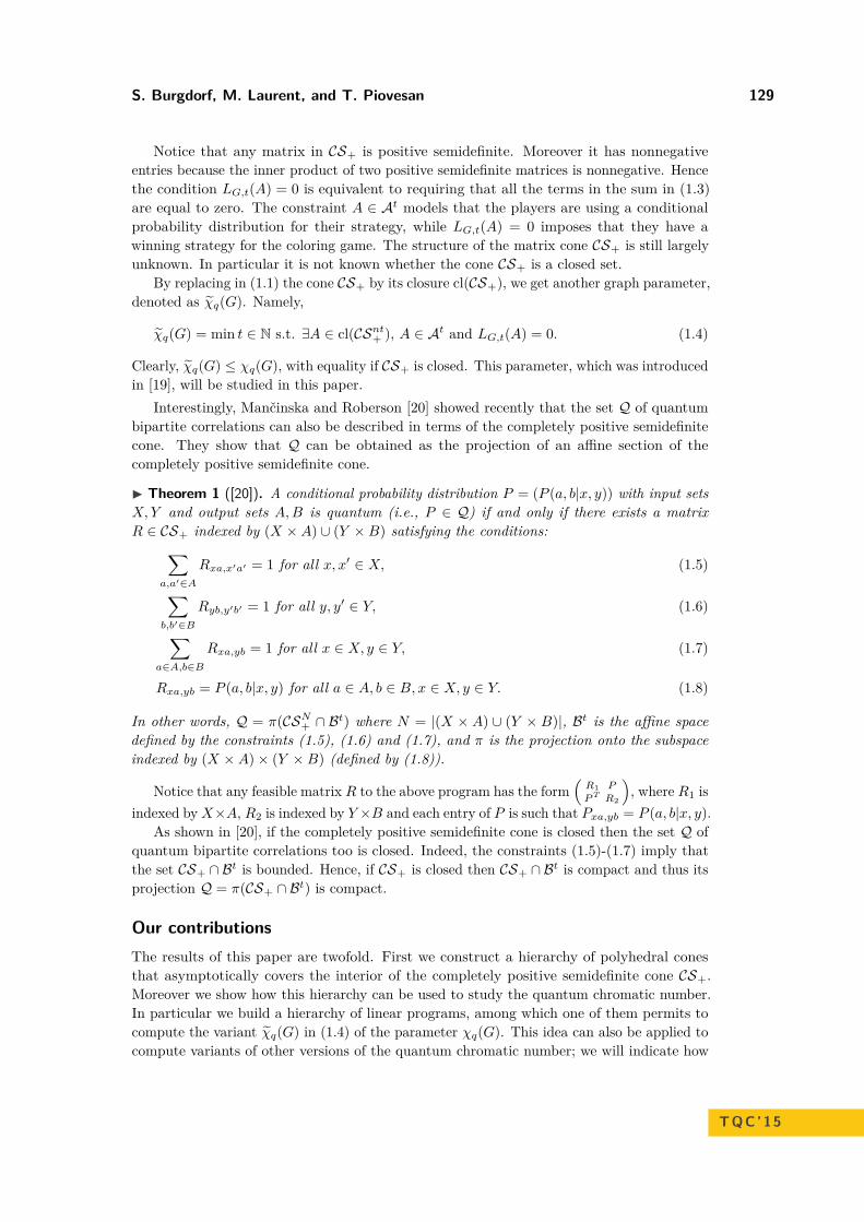
S. Burgdorf, M. Laurent, and T. Piovesan 129
Notice that any matrix in CS+ is positive semidefinite. Moreover it has nonnegativeentries because the inner product of two positive semidefinite matrices is nonnegative. Hencethe condition LG,t(A) = 0 is equivalent to requiring that all the terms in the sum in (1.3)are equal to zero. The constraint A ∈ At models that the players are using a conditionalprobability distribution for their strategy, while LG,t(A) = 0 imposes that they have awinning strategy for the coloring game. The structure of the matrix cone CS+ is still largelyunknown. In particular it is not known whether the cone CS+ is a closed set.
By replacing in (1.1) the cone CS+ by its closure cl(CS+), we get another graph parameter,denoted as χq(G). Namely,
χq(G) = min t ∈ N s.t. ∃A ∈ cl(CSnt+ ), A ∈ At and LG,t(A) = 0. (1.4)
Clearly, χq(G) ≤ χq(G), with equality if CS+ is closed. This parameter, which was introducedin [19], will be studied in this paper.
Interestingly, Mančinska and Roberson [20] showed recently that the set Q of quantumbipartite correlations can also be described in terms of the completely positive semidefinitecone. They show that Q can be obtained as the projection of an affine section of thecompletely positive semidefinite cone.
I Theorem 1 ([20]). A conditional probability distribution P = (P (a, b|x, y)) with input setsX,Y and output sets A,B is quantum (i.e., P ∈ Q) if and only if there exists a matrixR ∈ CS+ indexed by (X ×A) ∪ (Y ×B) satisfying the conditions:∑
a,a′∈A
Rxa,x′a′ = 1 for all x, x′ ∈ X, (1.5)
∑b,b′∈B
Ryb,y′b′ = 1 for all y, y′ ∈ Y, (1.6)
∑a∈A,b∈B
Rxa,yb = 1 for all x ∈ X, y ∈ Y, (1.7)
Rxa,yb = P (a, b|x, y) for all a ∈ A, b ∈ B, x ∈ X, y ∈ Y. (1.8)
In other words, Q = π(CSN+ ∩ Bt) where N = |(X × A) ∪ (Y × B)|, Bt is the affine space
defined by the constraints (1.5), (1.6) and (1.7), and π is the projection onto the subspaceindexed by (X ×A)× (Y ×B) (defined by (1.8)).
Notice that any feasible matrix R to the above program has the form(
R1 P
P T R2
), where R1 is
indexed byX×A, R2 is indexed by Y ×B and each entry of P is such that Pxa,yb = P (a, b|x, y).As shown in [20], if the completely positive semidefinite cone is closed then the set Q of
quantum bipartite correlations too is closed. Indeed, the constraints (1.5)-(1.7) imply thatthe set CS+ ∩ Bt is bounded. Hence, if CS+ is closed then CS+ ∩ Bt is compact and thus itsprojection Q = π(CS+ ∩ Bt) is compact.
Our contributionsThe results of this paper are twofold. First we construct a hierarchy of polyhedral conesthat asymptotically covers the interior of the completely positive semidefinite cone CS+.Moreover we show how this hierarchy can be used to study the quantum chromatic number.In particular we build a hierarchy of linear programs, among which one of them permits tocompute the variant χq(G) in (1.4) of the parameter χq(G). This idea can also be applied tocompute variants of other versions of the quantum chromatic number; we will indicate how
TQC’15

130 Completely Positive Semidefinite Cone
to do that for the variant χqa(G) of the parameter χqa(G) considered in [23]. See below forsome details and Sections 2 and 3 for the proofs.
As a second main contribution we provide an explicit description of the closure of thecone CS+, in terms of tracial ultraproducts of matrix algebras. Moreover we exhibit a largercone, containing CS+, which can be interpreted as an infinite dimensional analog of CS+.This cone consists of the matrices which admit a Gram representation by (a specific classof) positive semidefinite operators on a possibly infinite dimensional Hilbert space insteadof Gram representations by finite positive semidefinite matrices. We can in fact show thatthis larger cone is indeed a closed cone and that it is equal to cl(CS+) if Connes’ embeddingconjecture holds true. Since the description of these cones involve quite some notation andconcepts from operator theory we skip a preliminary description of the used methods andrefer directly to Section 4 which can be read independently of the other part.
In summary, our results give structural information about the completely positive semidef-inite cone CS+ which come in two flavors, depending whether we consider its interior or itsboundary.
We now give some more details about our first contribution. In a nutshell, the idea forbuilding the hierarchy of polyhedral cones is to discretize the set of positive semidefinitematrices by rational ones with bounded entries. Namely, given an integer r ≥ 1, we define thecone Cn
r as the conic hull of all matrices A that admit a Gram representation by r× r positivesemidefinite matrices X1, . . . , Xn whose entries are rational with denominator at most r andsatisfy
∑ni=1 Tr(Xi) = 1. We show that the cones Cn
r and their dual cones Dnr = Cn∗
r satisfythe following properties:
int(CSn+) ⊆
⋃r≥1Cn
r ⊆ CSn+ and CSn∗
+ =⋂r≥1Dn
r .
Moreover, for any fixed r, linear optimization over the cone Cnr can be performed in polynomial
time in terms of n. This discretization idea was also used in the classical (scalar) setting,where a hierarchy of polyhedral cones is constructed to approximate the completely positivecone (consisting of all matrices that admit a Gram representation by nonnegative vectors) andits dual, the copositive cone (see [29]). Our construction is in fact inspired by this classicalcounterpart. Discretization is also widely used in optimization to build good approximationsfor polynomial optimization problems over the standard simplex or for evaluating tensornorms (see e.g. [3], [17], the recent work [6] and references therein).
One of the difficulties in using the cone CS+ for studying the quantum parameter χq(G)or general quantum correlations in Q stems from the fact that the additional affine conditionsposed on the matrix A ∈ CS+ imply that it must lie on the boundary of the cone CS+. Thisis the case for instance for the conditions that A must belong to the affine space At in (1.2),or the condition LG,t(A) = 0 in (1.3), or the conditions (1.5), (1.6) and (1.7). Since wedo not know whether the cone CS+ is closed, this is why we may get different parametersdepending whether we use the cone CS+ or its closure.
In order to be able to exploit the fact that the cones Cnr asymptotically cover the full
interior of CSn+, we will relax the affine constraints (using a small perturbation) to ensure
the existence of a feasible solution in the interior of the cone CS+. In this way we will beable to get a hierarchy of parameters that can be computed through linear programmingand give the exact value of χq(G). We remark that this result is existential, we can provethe existence of a linear program permitting to compute the quantum parameter but we donot know at which stage this happens. This result should be seen in the light of a recentresult of the same flavor proved in [23]. The authors of [23] consider yet another variant

S. Burgdorf, M. Laurent, and T. Piovesan 131
χqc(G) of the quantum parameter χq(G), satisfying χqc(G) ≤ χq(G), and they show thatχqc(G) can be computed with a positive semidefinite program (also not explicitly known).The definition of χqc(G) is given below.
Link to other variants of the quantum chromatic numberIn the papers [24, 23], Paulsen and coauthors have introduced many variants of the quantumchromatic number motivated by the study of quantum correlations. We recall two of them,the parameters χqa(G) and χqc(G), in order to pinpoint the link to our parameter χq(G)and to our approach.
Recall that the quantum chromatic number χq(G) is the minimum number of colorsthat the players must use to always win the corresponding coloring game with a quantumstrategy. In other words, this is the minimum integer t for which there exists a probabilityP = (P (i, j|u, v)) ∈ Q with input sets X = Y = V (G) and output sets A = B = [t], suchthat P (i, j|u, u) = 0 for all i 6= j ∈ [t] and u ∈ V (G), and P (i, i|u, v) = 0 for all i ∈ [t] anduv ∈ E(G). For convenience, in the following paragraphs we will omit the dependence of Pon t, which should be considered as implicit. Forcing the probability of these combinations ofinputs and output to be zero imposes that the players have a winning strategy. We combinethose constraints into a single one by defining the linear map LG,t : R(nt)2 → R by
LG,t(P ) =∑
i 6=j∈[t],u∈V (G)
P (i, j|u, u) +∑
i∈[t],uv∈E(G)
P (i, i|u, v).
Then, the players have a winning strategy if and only if the probability P satisfies LG,t(P ) = 0.The following is the original definition of χq(G) in [8]:
χq(G) = min t ∈ N s.t. ∃P ∈ Q with LG,t(P ) = 0.
In [8] it is shown that in the coloring game the optimal quantum strategy is symmetric: thetwo players perform the same action upon receiving the same input. This special additionalstructure of the coloring game is the reason why χq(G) can be equivalently reformulated asin (1.1).
The parameter χqa(G) defined in [24] asks the probability P to be in the closure of Q:
χqa(G) = min t ∈ N s.t. ∃P ∈ cl(Q) with LG,t(P ) = 0.
Hence, the following relationship holds: χqa(G) ≤ χq(G).The authors of [24] (see also [23]) furthermore considered probability distributions arising
from the relativistic point of view. Roughly, instead of assuming that the measurementoperators act on different Hilbert spaces so that joint measurements have a tensor productstructure, in the relativistic model the measurement operators act on a common Hilbert spaceand the operators of the two parties commute mutually. In this case, joint measurementoperators have a product structure. More formally, a correlation P = (P (a, b|x, y)) is obtainedfrom relativistic quantum field theory if it is of the form P (a, b|x, y) = ψ†Ea
xFbyψ, where ψ is
a unit vector in a (possibly infinite dimensional) Hilbert space H, Eax and F b
y are positiveoperators on H satisfying
∑a∈A E
ax = I =
∑b∈B F
by for all x ∈ X, y ∈ Y and Ea
xFby = F b
yEax
for all a ∈ A, b ∈ B, x ∈ X, y ∈ Y . We denote by Qc the set of quantum bipartite correlationsarising from the relativistic point of view. The set Qc is closed (see e.g. [12, Proposition 3.4])and the following inclusions hold:
Q ⊆ cl(Q) ⊆ Qc. (1.9)
TQC’15

132 Completely Positive Semidefinite Cone
Deciding whether equality Qc = cl(Q) holds is known to be equivalent to Connes’ embeddingconjecture (see [22, 12, 15]) and deciding whether Qc = Q is known as Tsirelson’s problem.
In [24] the parameter χqc(G) is defined as
χqc(G) = min t ∈ N s.t. ∃P ∈ Qc with LG,t(P ) = 0.
In [23] it is shown that χqc(G) can be computed by a positive semidefinite program (afterrounding). This result is existential, meaning that the program is not explicitly known. Forthis the authors of [23] use the semidefinite programming hierarchy developed by Navascués,Pironio and Acín [21] for noncommutative polynomial optimization. This technique can beapplied since the definition of χqc(G) is in terms of products of operators. Note that thistechnique cannot be applied to the parameters χqa(G) and χq(G) whose definitions involvetensor products of operators. It is not know whether the parameters χqa(G) and χq(G) canbe written as semidefinite programs. As pointed out in [23], in view of the inclusions in (1.9),the following relationships hold between the parameters:
χqc(G) ≤ χqa(G) ≤ χq(G).
Using Theorem 1, we can reformulate the parameters χq(G) and χqa(G) as feasibilityproblems over affine sections of the cones CS+ and cl(CS+), respectively. Namely, we have
χq(G) = min t s.t. ∃P ∈ π(CS2nt+ ∩ Bt) with LG,t(P ) = 0, and
χqa(G) = min t s.t. ∃P ∈ cl(π(CS2nt+ ∩ Bt)) with LG,t(P ) = 0.
Recall that we introduced the variant χq(G) by replacing the cone CS+ by its closure in thedefinition (1.1) of χq(G). Analogously, we introduce the variant χqa(G) by replacing CS+ byits closure in the above definition of χqa(G). Namely,
χqa(G) = min t s.t. ∃P ∈ π(cl(CS2nt+ ) ∩ Bt) with LG,t(P ) = 0. (1.10)
Note that the set cl(CS+)∩Bt is bounded, thus compact, so that its projection π(cl(CS+)∩Bt)is compact too. Hence the inclusion CS+ ∩ Bt ⊆ cl(CS+) ∩ Bt implies:
cl(π(CS+ ∩ Bt)) ⊆ π(cl(CS+) ∩ Bt)
and thus the following relationship: χqa(G) ≤ χqa(G). In Section 3 we will show that χqa
can be computed with a linear program.Moreover, note that if a matrix A is feasible for the program (1.4) defining χq(G), then the
matrix R = ( A AA A ) is feasible for the program (1.10) defining χqa(G). Hence, χqa(G) ≤ χq(G)
holds.
The relationship between the parameters χq(G), χqc(G), χqa(G) and χqa(G), χq(G) canbe summarized as follows:
χqc(G) ≤ χqa(G) ≤ χq(G)
≤ ≤
χqa(G) ≤ χq(G)
2 Polyhedral approximations of CS+ and its dual cone CS∗+In this section we construct hierarchies of polyhedral cones converging asymptotically to thecompletely positive cone and its dual. We start in Section 2.1 by recalling the definition

S. Burgdorf, M. Laurent, and T. Piovesan 133
of CS+ and of CS∗+ as well as some useful properties and introduce the new hierarchy inSection 2.2. The construction of our polyhedral hierarchy is directly inspired from theclassical case where analogous hierarchies of polyhedral cones exist for approximating thecompletely positive cone CPn and the copositive cone COPn; in Appendix A we recall thisconstruction.
2.1 The completely positive semidefinite cone and its dualThe completely positive semidefinite cone was introduced in [19] to study graph parametersarising from quantum nonlocal games and quantum information theory. It has also beenconsidered implicitly in [13].
Recall that a matrix A ∈ Sn is positive semidefinite if and only if it admits a Gramrepresentation by vectors, i.e., if A = (〈xi, xj〉)n
i,j=1 for some x1, . . . , xn ∈ Rd and d ≥ 1. Wewrite A 0 (resp., A 0) when A is positive semidefinite (resp., positive definite) and Sn
+ isthe set of positive semidefinite matrices.
I Definition 2. The completely positive semidefinite cone CSn+ is the set of symmetric
matrices A which admit a Gram representation by positive semidefinite matrices, i.e.,A = (〈Xi, Xj〉)i,j for some X1, . . . , Xn ∈ Sd
+ and d ∈ N.
The completely positive cone CPn is the set of symmetric matrices that admit a Gramrepresentation by nonnegative vectors: A ∈ CPn if A = (〈xi, xj〉)i,j for some x1, . . . , xn ∈ Rd
+and d ∈ N. Hence CPn can be considered as the classical analog of CSn
+. Clearly everycompletely positive semidefinite matrix is positive semidefinite and nonnegative, and everycompletely positive matrix is completely positive semidefinite. That is, we have the followingrelationships between these cones:
CPn ⊆ CSn+ ⊆ Sn
+ ∩ Rn×n+ .
In [19] it is shown that all these inclusions are strict for n ≥ 5 (see also [13]). For n ≤ 4 it iswell known that CPn = Sn
+ ∩ Rn×n+ . For this and other properties of CP we refer the reader
to the book [5]. Both CPn and Sn+ are closed cones, while we do not know whether CSn
+ isclosed.
Moving on to the dual side, as noted in [19], the dual cone of CSn+ has a simple characteriza-
tion in terms of trace nonnegative polynomials. Given a matrixM ∈ Sn, define the polynomialpM =
∑ni,j=1 Mijxixj in n noncommutative variables. ThenM belongs to the dual cone CSn∗
+precisely when Tr(pM (X1, . . . , Xn)) ≥ 0 for all n-tuples X = (X1, . . . , Xn) ∈ ∪d≥1(Sd
+)n.If we require nonnegativity only for all X ∈ Rn
+ (i.e., the case d = 1), which amounts torequiring that the polynomial pM takes nonnegative values when evaluated at any pointin Rn
+, then the matrix M is said to be copositive; COPn denotes the cone of copositivematrices. The cones CPn and COPn are dual to each other: COPn = CPn∗ and, by duality,we have the inclusions:
Sn+ + (Sn ∩ Rn×n
+ ) ⊆ CSn∗+ ⊆ COP
n.
As will be explained in detail in Section 3, in order to be able to use our polyhedralhierarchy, we will need to have matrices that are in the interior of CS+. Recall that amatrix A ∈ CS+ lies in the interior of CS+ if and only if 〈A,M〉 > 0 for all nonzero matricesM ∈ CS∗+. Hence, A lies in the boundary of CS+ if and only if there exists a nonzero matrixM ∈ CS∗+ such that 〈A,M〉 = 0. For further reference we observe that matrices in CS+ witha zero entry, or lying in the affine spaces At or Bt, lie in the boundary of CS+.
TQC’15

134 Completely Positive Semidefinite Cone
I Lemma 3. Consider a matrix A in the cone CS+ (of appropriate size). Then A lies inthe boundary of CS+ in any of the following cases: (i) A has a zero entry; (ii) A belongs tothe affine space At defined by (1.2), or (iii) A belongs to the affine space Bt defined by theconditions (1.5), (1.6) and (1.7).
2.2 The new cones Cnr and Dn
r
We now introduce the cones Cnr , which will form a hierarchy of inner approximations for the
cone CSn+, and the cones Dn
r , which will form a hierarchy of outer approximations for thedual cone CSn∗
+ . These cones are in fact dual to each other, so it suffices to define the conesDn
r . The idea is simple and analogous to the idea used in the classical (scalar) case: insteadof requiring trace nonnegativity of the polynomial pM over the full set ∪d≥1(Sd
+)n, we onlyask trace nonnegativity over specific finite subsets. We start with defining the set
∆n = X = (X1, . . . , Xn) ∈⋃d≥1
(Sd+)n :
n∑i=1
Tr(Xi) = 1, (2.1)
which can be seen as the dimension-free matrix analog of the standard simplex ∆n in Rn.As we now observe, a matrix M belongs to CSn∗
+ if and only if its associated polynomial pM
is trace nonnegative on all n-tuples of rational matrices in ∆n (see Appendix C for a proof).
I Lemma 4. M ∈ CSn∗+ if and only if Tr(pM (X)) ≥ 0 for all X ∈∆n with rational entries.
This motivates introducing the following subset ∆(n, r) of the set ∆n, obtained byconsidering only n-tuples of rational positive semidefinite matrices with denominator at mostr. This set can be seen as a matrix analog of the rational grid point subsets of the standardsimplex ∆n and it permits to define the new cones Dn
r .
I Definition 5. Given an integer r ∈ N, define the set
∆(n, r) = X ∈∆n : each Xi has rational entries with denominator ≤ r
and define the cone
Dnr = M ∈ Sn : Tr(pM (X)) ≥ 0 ∀X ∈∆(n, r).
Next we show that the cone Dnr is a polyhedral cone. Indeed, as we observe below,
although the set ∆(n, r) is not finite, we may without loss of generality replace in thedefinition of Dn
r the set ∆(n, r) by its subset ∆(n, r), obtained by restricting to r × r
matrices X1, . . . , Xn. The next lemma is proved in Appendix C.
I Lemma 6. Define the set
∆(n, r) = X ∈ (Sr+)n :
n∑i=1
Tr(Xi) = 1, each Xi has rational entries with denominator ≤ r.
Then, equality holds:
Dnr = M ∈ Sn : Tr(pM (X)) ≥ 0 ∀X ∈∆(n, r).
I Lemma 7. For any fixed r, the cardinality of the set ∆(n, r) is polynomial in terms ofn. More precisely, let γr denote the number of r × r positive semidefinite matrices whoseentries are rational with denominator at most r and whose trace is at most one. Then,|∆(n, r)| ≤ (γr)r if n ≤ r, and |∆(n, r)| ≤
(nr
)(γr)r if n > r.

S. Burgdorf, M. Laurent, and T. Piovesan 135
Notice that Tr(pM (X)) =∑
i,j Mij〈Xi, Xj〉 for any X = (X1, . . . , Xn). Hence, the coneDn
r can be equivalently defined as the set of matrices M ∈ Sn satisfying the (finitely many)linear inequalities:
∑ni,j=1 Mij〈Xi, Xj〉 ≥ 0 for all (X1, . . . , Xn) ∈∆(n, r). This implies:
I Corollary 8. The cone Dnr is a polyhedral cone.
As ∆(n, r) ⊆∆(n, r + 1), the sets Dnr form a hierarchy of outer approximations for CSn∗
+ :
CSn∗+ ⊆ Dn
r+1 ⊆ Dnr ⊆ · · · ⊆ Dn
1 .
Hence, CSn∗+ ⊆
⋂r≥1Dn
r . In fact, as a direct application of Lemma 4, equality holds.
I Theorem 9. CSn∗+ =
⋂r≥1Dn
r .
We will also use the following property of the cones Dnr .
I Lemma 10. Consider a sequence of matrices (Mr)r≥1 in Sn converging to a matrixM ∈ Sn. If Mr ∈ Dn
r for all r, then M ∈ CSn∗+ .
We now turn to the description of the dual cone Cnr := Dn∗
r . As a direct application ofLemma 6, we can conclude that Cn
r is the set of conic combinations of matrices which have aGram representation by matrices in ∆(n, r); that is,
Cnr = coneA ∈ Sn : A = (〈Xi, Xj〉)n
i,j=1 for some (X1, . . . , Xn) ∈∆(n, r). (2.2)
By construction, the cones Cnr are polyhedral and they form a hierarchy of inner approxima-
tions of CSn+: Cn
1 ⊆ · · · ⊆ Cnr ⊆ Cn
r+1 ⊆ CSn+, with strict inclusion.
I Lemma 11. For any n ≥ 2 and r ≥ 1, we have strict inclusions: Cnr ( Cn
r+1 ( CSn+.
Proof. The only fact which needs a proof is that each inclusion is strict. It suffices to showthis for n = 2, since one can extend a matrix A in C2
r to a matrix in Cnr by adding all zero
coordinates, and the same for CS+. For this we consider a rank 1 matrix A = vvT , wherev = (1 a)T and a is a nonnegative scalar. Then A ∈ CS2
+. If we choose a to be an irrationalnumber then A cannot belong to any cone C2
r and, if we choose a = 1/(r+ 1), then A belongsto C2
r+1 but not to C2r . J
We now show that the union of the cones Cnr covers the interior of the cone CSn
+.
I Theorem 12. We have the inclusions:
int(CSn+) ⊆
⋃r≥1Cn
r ⊆ CSn+.
Proof. We only need to show the first inclusion. For this, consider a matrix A in the interiorof the cone CSn
+ and assume that A does not belong to⋃
r≥1 Cnr . Then, for each r ≥ 1, there
exists a hyperplane separating A from the (closed convex) cone Cnr . That is, there exists
a matrix Mr ∈ Dnr such that 〈Mr, A〉 < 0 and ‖Mr‖ = 1. Since all matrices Mr lie in a
compact set, the sequence (Mr)r admits a converging subsequence (Mri)i≥1 which converges
to a matrix M ∈ Sn. By Lemma 10, we know that the matrix M belongs to the cone CSn∗+
and thus 〈A,M〉 ≥ 0. On the other hand, as 〈A,Mri〉 < 0 for all i, by taking the limit as i
tends to infinity, we get that 〈A,M〉 ≤ 0. Hence we obtain 〈A,M〉 = 0, which contradictsthe assumption that A lies in the interior of CSn
+. J
It is easy to give an explicit description of the cones Cnr for small r. For example, Cn
1 isthe set of n× n diagonal nonnegative matrices and Cn
2 is the convex hull of the matrices Eii
and Eii + Eij + Ejj (for i, j ∈ [n]), where Eij denote the elementary matrices in Sn.
TQC’15

136 Completely Positive Semidefinite Cone
3 LP lower bounds to the quantum chromatic number
In this section we use the polyhedral hierarchy Cnr (r ≥ 1) to show that the parameter χq(G)
in (1.4) can be written as a linear program. We recall the definition of χq(G):
χq(G) = min t ∈ N s.t. ∃A ∈ cl(CSnt+ ), A ∈ At and LG,t(A) = 0, (3.1)
where the affine space At is defined in (1.2) and the map LG,t in (1.3). A first naturalapproach for building a linear relaxation of χq(G) is to replace the cone cl(CSnt
+ ) in thedefinition of χq(G) by the subcone Cn
r , leading to the parameter
`r(G) = min t ∈ N s.t. ∃A ∈ Cntr , A ∈ At and LG,t(A) = 0.
As Cntr ⊆ CSnt
+ , we have χq(G) ≤ χq(G) ≤ `r(G). Moreover the sequence (`r(G))r ismonotone nonincreasing and thus has a limit (it becomes stationary). However it is not clearwhether the limit is equal to χq(G). If one could claim that for t = χq(G) there is a feasiblematrix A for the program (3.1) which lies in the interior of CSnt
+ then, by Theorem 12, Awould belong to some cone Cnt
r which would imply equality χq(G) = `r(G). However, thisidea cannot work because, as observed in Lemma 3, any matrix feasible for (3.1) lies in theboundary of CSnt
+ . To go around this difficulty, our strategy is to relax the affine constraintsin (3.1) so to allow feasible solutions in the interior of CSnt
+ .More precisely, given an integer k ≥ 1, we consider the affine space At
k defined by theinequalities: |
∑i,j Aui,vj − 1 | ≤ 1
k for all u, v ∈ V (G). We define the parameter:
λk(G) = min t s.t. ∃A ∈ cl(CSnt+ ), A ∈ At
k and LG,t(A) ≤ 1k. (3.2)
In a first step we show that λk(G) = χq(G) for k large enough.
I Lemma 13. For any graph G, there exists k0 ∈ N such that χq(G) = λk(G) for all k ≥ k0.
Proof. Notice that λk(G) ≤ χq(G) holds for every k ∈ N. Indeed, any matrix solution forχq(G) is also a solution for λk(G). Moreover, as the sequence (λk(G))k∈N is a monotonenondecreasing sequence of natural numbers upper bounded by χq(G), there exists a k0 suchthat λk(G) = λk0(G) for all k ≥ k0. Let t = λk0(G). For all k ≥ k0 there exists a matrixAk ∈ cl(CSnt
+ ) with Ak ∈ Atk and LG,t(Ak) ≤ 1
k . Consider the sequence (Ak)k≥k0 , which isbounded as all Ak lie in At
k0. Therefore, the sequence has a converging subsequence to, say,
A where A ∈ cl(CSnt+ ), A ∈ At and LG,t(A) = 0. Hence, A is a feasible solution for χq(G)
and χq(G) ≤ t = λk0(G) = λk(G) for all k ≥ k0. J
In a second step we show that the new parameter λk(G) can be computed by a linearprogram. For this we replace in the definition of λk(G) the cone cl(CSnt
+ ) by the polyhedralcone Cnt
r , leading to the following parameter:
λrk(G) = min t s.t. ∃A ∈ Cnt
r , A ∈ Atk and LG,t(A) ≤ 1
k. (3.3)
Notice that this parameter λrk(G) can be computed through a linear program since Cnt
r ispolyhedral. We will show that for any graph G there exist integers k0 and r0 such thatχq(G) = λr0
k0(G). We emphasize that this is an existential result: we do not know for which
integers k0 and r0 such a convergence happens. One of the ingredients to prove the result isto show the existence of a matrix in the interior of CS+ satisfying certain constraints. Tothis end, we will use the matrix Z = I +J ∈ Snt where I and J are, respectively, the identityand the all-ones matrices. (See Appendix C for the proof of the following lemma.)

S. Burgdorf, M. Laurent, and T. Piovesan 137
I Lemma 14. The matrix Z = I + J ∈ Snt lies in the interior of CS+. Moreover, we havethat
∑i,j∈[t] Zui,uj = t2 + t for all u ∈ V (G),
∑i,j∈[t] Zui,vj = t2 for all u 6= v ∈ V (G) and
LG,t(Z) = nt2 − nt+mt, where m is the number of edges of the graph G.
I Theorem 15. For any graph G there exist k0 and r0 ∈ N such that χq(G) = λrk(G) for
all k ≥ k0 and all r ≥ r0. Moreover λr0k0
(G), and thus χq(G), can be computed via a linearprogram.
Proof. From Lemma 13 we know that there exists k0 ∈ N such that λk(G) = χq(G) for allk ≥ k0. In view of this, we just need to show that for this k0 there exists an integer r0 ∈ Nfor which λr0
k0(G) = λk0(G). Let t = λk0(G) = χq(G).
By the definitions (3.2) and (3.3) and the inclusion relationship between the cones Cntr , we
have that the sequence of natural numbers (λrk0
)r∈N is nonincreasing and it is lower boundedby λk0(G). Hence, there exists a natural number r0 such that λr
k0(G) = λr0
k0(G) for all r ≥ r0.
We are left to prove that λr0k0
(G) ≤ λk0(G) = t.
To this end, we show that there exists a matrix Yk0 ∈ int(CS+) with Yk0 ∈ Atk0
andLG,t(Yk0) ≤ 1
k0. This will suffice since then, by Theorem 12, Yk0 ∈ Cnt
r0for some r0. Therefore,
Yk0 satisfies the conditions in program (3.3) and thus λr0k0
(G) ≤ t = λk0(G). To show theexistence of such a matrix Yk0 , let A ∈ cl(CS+) be a feasible solution of the program (3.1)defining χq(G) = t and consider the matrix Z = I + J which belongs to int(CS+) (byLemma 14). Then, any convex combination Zε = (1 − ε)A + εZ (for 0 < ε < 1) lies inthe interior of CS+. If we can tune ε so that the new matrix Zε satisfies the conditionsin program (3.3), then we can choose Yk0 = Zε and we are done. We claim that selectingε := min 1
k0(t2+t−1) ,1
k0(nt2−nt+mt) will do the trick. Indeed, for this choice of ε we haveZε ∈ int(CS+) and LG,t(Zε) = εLG,t(Z) ≤ 1
k0(use Lemma 14). Moreover, Zε ∈ At
k0since
for all u, v ∈ V (G) the following holds∣∣ ∑i,j∈[t]
Yk0 (ui, vj)−1∣∣ =∣∣(1−ε)+ε
∑i,j∈[t]
Zui,vj −1∣∣ ≤∣∣−ε+ε
∑i,j∈[t]
Zui,uj
∣∣ =∣∣ε(t2 + t−1)
∣∣ ≤ 1k0.
Summarizing, from Lemma 13 we know that there exists an integer k0 ∈ N such thatλk0(G) = χq(G) and we just proved that for this k0 there exists an integer r0 ∈ N with theproperty that λr0
k0(G) = λk0(G) = χq(G). J
The same result holds for the parameter χqa(G) introduced in (1.10). For clarity werepeat its definition in the following form:
χqa(G) = min t ∈ N s.t. ∃A ∈ cl(CS2nt+ ), A ∈ Bt with LG,t(π(A)) = 0.
Note the analogy with the definition (3.1) of χq(G). The only difference is that we now workwith matrices A of size 2nt (instead of nt) lying in the affine space Bt (instead of At) andsatisfying LG,t(π(A)) = 0 (instead of LG,t(A) = 0). In analogy to the parameter λk(G) wecan define the parameter Λk(G) by doing these replacements and defining the relaxed affinespace Bt
k in the same way as Atk was defined from At. Then the analog of Lemma 13 holds:
there exists an integer k0 such that χqa(G) = Λk(G) for all k ≥ k0. Next, replacing the conecl(CS2nt
+ ) by C2ntr , we get the following parameter Λr
k(G) (the analog of λkr (G)):
Λrk(G) = min t ∈ N s.t. A ∈ C2nt
r , A ∈ Btk with LG,t(π(A)) ≤ 1
k.
The analog of Theorem 15 holds, whose proof is along the same lines and thus omitted.
I Theorem 16. For any graph G, there exist k0 and r0 ∈ N such that χqa(G) = Λrk(G) for
all k ≥ k0 and r ≥ r0. Hence the parameter χqa(G) can be computed by a linear program.
TQC’15
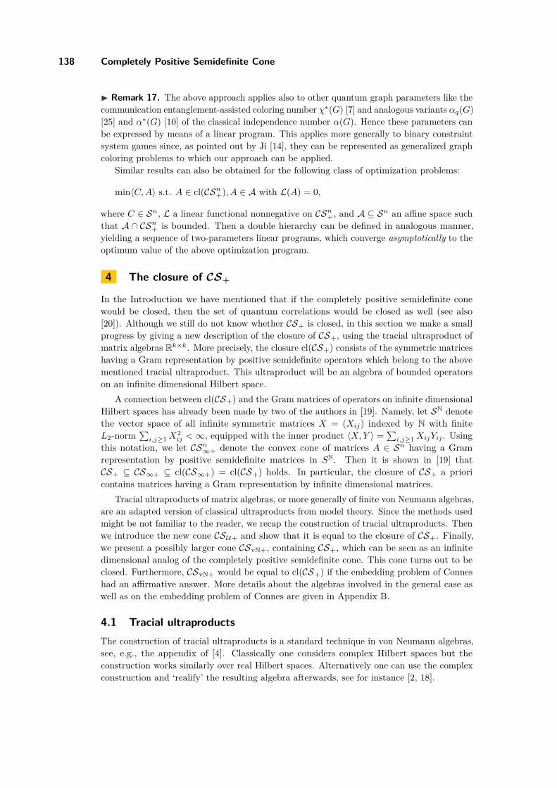
138 Completely Positive Semidefinite Cone
I Remark 17. The above approach applies also to other quantum graph parameters like thecommunication entanglement-assisted coloring number χ∗(G) [7] and analogous variants αq(G)[25] and α∗(G) [10] of the classical independence number α(G). Hence these parameters canbe expressed by means of a linear program. This applies more generally to binary constraintsystem games since, as pointed out by Ji [14], they can be represented as generalized graphcoloring problems to which our approach can be applied.
Similar results can also be obtained for the following class of optimization problems:
min〈C,A〉 s.t. A ∈ cl(CSn+), A ∈ A with L(A) = 0,
where C ∈ Sn, L a linear functional nonnegative on CSn+, and A ⊆ Sn an affine space such
that A ∩ CSn+ is bounded. Then a double hierarchy can be defined in analogous manner,
yielding a sequence of two-parameters linear programs, which converge asymptotically to theoptimum value of the above optimization program.
4 The closure of CS+
In the Introduction we have mentioned that if the completely positive semidefinite conewould be closed, then the set of quantum correlations would be closed as well (see also[20]). Although we still do not know whether CS+ is closed, in this section we make a smallprogress by giving a new description of the closure of CS+, using the tracial ultraproduct ofmatrix algebras Rk×k. More precisely, the closure cl(CS+) consists of the symmetric matriceshaving a Gram representation by positive semidefinite operators which belong to the abovementioned tracial ultraproduct. This ultraproduct will be an algebra of bounded operatorson an infinite dimensional Hilbert space.
A connection between cl(CS+) and the Gram matrices of operators on infinite dimensionalHilbert spaces has already been made by two of the authors in [19]. Namely, let SN denotethe vector space of all infinite symmetric matrices X = (Xij) indexed by N with finiteL2-norm
∑i,j≥1 X
2ij <∞, equipped with the inner product 〈X,Y 〉 =
∑i,j≥1 XijYij . Using
this notation, we let CSn∞+ denote the convex cone of matrices A ∈ Sn having a Gram
representation by positive semidefinite matrices in SN. Then it is shown in [19] thatCS+ ⊆ CS∞+ ⊆ cl(CS∞+) = cl(CS+) holds. In particular, the closure of CS+ a prioricontains matrices having a Gram representation by infinite dimensional matrices.
Tracial ultraproducts of matrix algebras, or more generally of finite von Neumann algebras,are an adapted version of classical ultraproducts from model theory. Since the methods usedmight be not familiar to the reader, we recap the construction of tracial ultraproducts. Thenwe introduce the new cone CSU+ and show that it is equal to the closure of CS+. Finally,we present a possibly larger cone CSvN+, containing CS+, which can be seen as an infinitedimensional analog of the completely positive semidefinite cone. This cone turns out to beclosed. Furthermore, CSvN+ would be equal to cl(CS+) if the embedding problem of Conneshad an affirmative answer. More details about the algebras involved in the general case aswell as on the embedding problem of Connes are given in Appendix B.
4.1 Tracial ultraproductsThe construction of tracial ultraproducts is a standard technique in von Neumann algebras,see, e.g., the appendix of [4]. Classically one considers complex Hilbert spaces but theconstruction works similarly over real Hilbert spaces. Alternatively one can use the complexconstruction and ‘realify’ the resulting algebra afterwards, see for instance [2, 18].

S. Burgdorf, M. Laurent, and T. Piovesan 139
Ultraproducts are constructions with respect to an ultrafilter. We will only considerultrafilters on N. Throughout P(N) is the collection of all subsets of N.
I Definition 18. An ultrafilter on the set N is a subset U ⊆ P(N) satisfying the condi-tions:(a) ∅ /∈ U ,(b) if A ⊆ B ⊆ N and A ∈ U then B ∈ U ,(c) if A,B ∈ U then A ∩B ∈ U ,(d) for every A ∈ P(N) either A ∈ U or N \A ∈ U .
In particular, any two elements in U need to have non-empty intersection (from (1) and(3)), which allows only two kinds of ultrafilters: Either every element of U contains a commonelement n0 ∈ N or U contains the cofinite sets of N. We are only interested in the secondkind of ultrafilters, which are called free ultrafilters. For a given free ultrafilter U on N wecan define the ultralimit limU ak of a bounded sequence (ak)k∈N of real numbers as follows:
limUak = a if k ∈ N : |ak − a| < ε ∈ U for all ε > 0. (4.1)
Let us have a look at ultralimits in a less formal way. If we have a non-free ultrafilter,i.e., U = A ∈ P(N) : k0 ∈ A for some k0 ∈ N, then limU ak = ak0 for any sequence(ak)k∈N ⊆ R. The case of a free ultrafilter is more interesting. Then the ultralimit of abounded sequence (ak)k∈N will be one of its accumulation points. For example, the sequencegiven by ak := (−1)k for all k ∈ N has two accumulation points, and both can be attained asan ultralimit depending on the choice of the ultrafilter U . In fact, considering the set 2Nof even numbers, we get by conditions (3) and (4) that any ultrafilter contains either 2Nor its complement (the odd numbers 2N + 1) but not both. Hence there is an ultrafilter U(containing 2N) with limU ak = 1 and an ultrafilter U ′ (containing 2N+1) with limU ′ ak = −1.
I Remark 19. Any bounded sequence of real numbers has an ultralimit and this is uniquefor fixed U . In particular, if limk→∞ ak = a then limU ak = a for any free ultrafilter U on N.
We can use ultralimits to construct the tracial ultraproduct of a sequence (Rdk×dk )k∈Nof matrix algebras for dk ∈ N. To simplify notation we letMk = Rk×k denote the matrixalgebra of all k × k matrices and we consider the full sequence (Mk)k∈N, but the sameconstruction would work for the sequence (Mdk
)k∈N. Here we assume that each Mk isendowed with the normalized trace trk = 1
k Tr (if the dimension k is clear we might simplywrite tr) and the corresponding inner product, so that ‖I‖2 = tr(I) = 1 for the identitymatrix. For T ∈ Mk, ‖T‖ denotes its operator norm and ‖T‖2 its L2-norm, that satisfy‖ST‖2 ≤ ‖S‖‖T‖2 for S, T ∈Mk. Define the C∗-algebra
`∞(N, (Mk)k) := (Tk)k∈N ∈∏k∈NMk : sup
k∈N‖Tk‖ <∞.
Every free ultrafilter U on N defines a two-sided ideal
IU := (Tk)k∈N ∈ `∞(N, (Mk)k) : limU‖Tk‖2 = 0,
which is well-defined since sequences in `∞(N, (Mk)k) are also bounded in the Hilbert-Schmidt norm. The ideal IU is a maximal ideal and therefore it is closed with respect to theoperator norm. The quotient algebra
MU := `∞(N, (Mk)k)/IU
TQC’15

140 Completely Positive Semidefinite Cone
is called the tracial ultraproduct of (Mk)k along U . Using the Cauchy-Schwarz inequality itis easy to show that the map
τU : MU → R, (Tk)k∈N + IU 7→ limU
trk(Tk)
is well-defined and defines a tracial state (or trace) onMU , i.e., τU is a normalized positivelinear map satisfying τU (T ∗T ) = τU (TT ∗) for any T ∈ MU . In fact, MU is a finite vonNeumann algebra of type II1 (see Appendix B for definitions). In particular, MU is asubalgebra of bounded operators on an infinite dimensional Hilbert space. As von Neumannalgebras are in particular C∗ algebras, positive semidefinite operators are exactly squares of(symmetric) operators.
4.2 Ultraproduct description of cl(CS+)We are now ready to define the new cone CSU+ which will turn out to be equal to theclosure of CS+. For this, we fix a free ultrafilter U on N and consider the tracial ultraproductMU = `∞(N, (Mk)k)/IU where again Mk denotes the full matrix algebra Rk×k for anyk ∈ N. Using this we define
CSU+ := A ∈ S+ : A = (τU (XiXj)) for some positive semidefinite X1, . . . , Xn ∈MU.
We note that the trace τU is normalized (i.e., τU (I) = 1) whereas we used the (not normalized)trace Tr in the definition of CS+. However, both descriptions agree up to rescaling of theXi’s.
To show that the closure of CS+ is a subset of CSU+ we will consider a sequence ofmatrices A(k) ∈ CSn
+ converging to some A ∈ Sn, i.e., limk→∞A(k)ij = Aij for all i, j ∈ [n].
A priori, for each k, there exist an integer dk and matrices X(k)1 , . . . , X
(k)n ∈ Sdk
+ such thatA(k) = (tr(X(k)
i X(k)j )). The next lemma says that without loss of generality we can assume
dk = k for all k ∈ N (see the Appendix C for a proof).
I Lemma 20. If (Xk)k, (Yk)k ∈∏
k∈N Sdk+ are such that the sequence (trdk
(XkYk))k∈Nconverges to some a ∈ R, then there exist (X ′k)k, (Y ′k)k ∈
∏k∈N Sk
+ with trk(X ′kY ′k) → a ask →∞.
We proceed by showing that the closure of CS+ is equal to CSU+. This is done in two steps.
I Lemma 21. For any free ultrafilter U on N, we have cl(CS+) ⊆ CSU+.
Proof. Let A ∈ cl(CS+) be given. Then there is a sequence of matrices A(k) ∈ CS+converging to A: limk→∞A
(k)ij = Aij for all i, j ∈ [n]. For each k, there exist positive
semidefinite matrices X(k)1 , . . . , X
(k)n such that A(k) = (tr(X(k)
i X(k)j )). By Lemma 20 we
can assume that X(k)1 , . . . , X
(k)n ∈ Sk
+. As the matrices A(k) are bounded the matricesX
(k)i are bounded as well. Hence the sequence (X(k)
i )k belongs to `∞(N, (Mk)) and wecan consider its image Xi in the tracial ultrapower MU . By the theorem of Łos (see e.g.[11, Prop. 4.3] and references therein) the operators Xi are positive semidefinite since allX
(k)i are positive semidefinite. It suffices now to show that A = (τU (XiXj)) since then
we can conclude that A ∈ CSU+. For this observe that, by the definition of τU , we have:τU (XiXj) = limU tr(X(k)
i X(k)j ) = limU A(k)
ij . On the other hand, as the sequence (A(k)ij )k
converges to Aij , in view of Remark 19, we have that limU A(k)ij = Aij . This concludes the
proof. J

S. Burgdorf, M. Laurent, and T. Piovesan 141
I Theorem 22. For any free ultrafilter U on N, equality cl(CS+) = CSU+ holds.
Proof. In view of Lemma 21 we only have to show the inclusion CSU+ ⊆ cl(CS+). LetA ∈ CSU+. By assumption, A = (τU (XiXj)) for some positive semidefinite operatorsX1, . . . , Xn ∈ MU . As the operators Xi are positive semidefinite, there exist operatorsYi ∈ MU such that Xi = Y 2
i for i ∈ [n], where each element Yi is given by a sequence ofsymmetric matrices (Y (k)
i )k ∈∏
kMk. Further, by definition of τU , for any s ∈ N, the indexset Is = k ∈ N : |τU (Y 2
i Y2
j )− tr((Y (k)i )2(Y (k)
j )2)| ≤ 1s for all i, j ∈ [n] belongs to U and is
therefore non-empty. Thus we find for any s ∈ N an index ks ∈ Is. Hence the operatorsX
(s)i := (Y (ks)
i )2 belong to Sks+ and satisfy∣∣∣τU (XiXj)− tr(X(s)
i X(s)j )∣∣∣ < 1
sfor all i, j ∈ [n] and all s ≥ 1. (4.2)
For each s, the matrix A(s) := (tr(X(s)i X
(s)j )) belongs to the cone CS+. Moreover it follows
from (4.2) that the sequence (A(s))s converges to the matrix A as s tends to ∞. This showsthat A belongs to the closure of CS+, which concludes the proof. J
We would like to conclude with another possible description of the closure of CS+ in thecase that Connes’ embedding conjecture turns out to be true.
As mentioned at the beginning of the section, the closure of CS+ contains the cone CS∞+,i.e., it contains symmetric matrices which have a Gram representation by some class ofpositive semidefinite infinite dimensional matrices. Also the given description of cl(CS+) asCSU+ involves Gram representations by operators on an infinite dimensional Hilbert space.In regard to the relativistic model of quantum correlations where one allows all (possiblyinfinite dimensional) Hilbert spaces one might ask for the most general infinite dimensionalversion of CS+. Since one is restricted to operators for which one can define an inner product(or a trace), a decent candidate for the infinite dimensional analog of CS+ is
CSnvN+ := A ∈ Sn
+ : A = (τN (XiXj)) for a finite vN algebra N and psd X1, . . . , Xn ∈ N,
where we allow any finite von Neumann algebra N (with trace τN ). Obviously we have thechain of inclusions CS+ ⊆ CSU+ ⊆ CSvN+.
Moreover, using the general theory of tracial ultraproducts of von Neumann algebras(instead of just matrix algebras), one can show with a similar line of reasoning as in Lemma21 that CSvN+ is closed. Indeed, take a sequence of matrices A(k) ∈ CSn
vN+ converging tosome A ∈ Sn. Then limk→∞A
(k)ij = Aij for all i, j ∈ [n] and for each k, there exist a finite
von Neumann algebra Nk with trace τk and bounded positive operators X(k)1 , . . . , X
(k)n ∈ Nk
such that A(k) = (τk(X(k)i X
(k)j )). Fixing a free ultrafilter U one can conclude that the
images Xi of the sequences (X(k)i )k in the tracial ultraproduct NU = `∞(N, (Nk)k)/IU of
the corresponding finite von Neumann algebras provide a Gram representation for A in thevon Neumann algebra NU . Hence the following statement holds.
I Theorem 23. CSvN+ is a closed cone.
Summarizing we have the inclusions:
cl(CSn+) = CSn
U+ ⊆ CSnvN+ ⊆ Sn
+ ∩ Rn×n+ .
In this context, we would like to mention that [13] shows the strict inclusion CSnvN+ (
Sn+ ∩ Rn×n
+ for any n ≥ 5. Finally, if Connes’ embedding conjecture is true, one can show,using Proposition 25 from Appendix B, that cl(CS+) = CSvN+.
TQC’15

142 Completely Positive Semidefinite Cone
Acknowledgments. We thank one of the referees for pointing out that the original proof ofTheorem 22 could be simplified to the elementary proof given above. S. B. and T. P. werefunded by the SIQS European project. S. B. was also funded by the NWO TOP project617.001.351.
References1 D. Avis, J. Hasegawa, Y. Kikuchi and Y. Sasaki. A quantum protocol to win the graph col-
oring game on all Hadamard graphs. IEICE Trans. Fundam. Electron. Commun. Comput.Sci., E89-A(5):1378–1381, 2006.
2 S. Ayupov, A. Rakhimov and S. Usmanov. Jordan, real and Lie structures in operatoralgebras. Mathematics and its Applications, 418, Kluwer Academic Publishers Group, Dor-drecht, 1997.
3 I.M. Bomze and E. de Klerk. Solving standard quadratic optimization problems via lin-ear, semidefinite and copositive programming. Journal of Global Optimization, 24:163–185,2002.
4 N.P. Brown and N. Ozawa. C∗-algebras and finite-dimensional approximations. GraduateStudies in Mathematics, 88, American Mathematical Society, Providence, RI, 2008.
5 A. Berman and N. Shaked-Monderer. Completely Positive Matrices. World Scientific, RiverEdge (NJ), London, Singapore, 2003.
6 F.G. S. L. Brandão and A. Harrow. Replacing hierarchies by nets. In preparation.7 J. Briët, H. Buhrman, M. Laurent, T. Piovesan and G. Scarpa Entanglement-assisted zero-
error source-channel coding. IEEE Transactions on Information Theory, 61(2):1–15, 2015.8 P. J. Cameron, A. Montanaro, M.W. Newman, S. Severini, and A. Winter. On the quantum
chromatic number of a graph. Electronic Journal of Combinatorics, 14(R81):1, 2007.9 B. Collins and K. J. Dykema. A linearization of Connes’ embedding problem. New York J.
Math., 14, pp. 617–641, 2008.10 T. S. Cubitt, D. Leung, W. Matthews, and A. Winter. Improving zero-error classical com-
munication with entanglement. Physical Review Letters, 104(23):230503, 2010.11 I. Farah, B. Hart, and D. Sherman. Model theory of operator algebras II: model theory.
Israel J. Math., 201(1), pp. 477–505, 2014.12 T. Fritz. Tsirelson’s problem and Kirchberg’s conjecture. Reviews in Mathematical Physics,
24(5):1250012, 2012.13 P. Frenkel and M. Weine. On vector configurations that can be realized in the cone of
positive matrices. Linear Algebra and its Applications, 459:465–474, 2014.14 Z. Ji. Binary constraint system games and locally commutative reductions. arXiv:1310:3794,
2013.15 M. Junge, M. Navascués, C. Palazuelos, D. Pérez-Garcia, V.B. Scholz and R. F. Werner.
Connes’ embedding problem and Tsirelson’s problem. Journal of Mathematical Physics,52(1):012102, 2011.
16 E. de Klerk and D.V. Pasechnik. Approximation of the stability number of a graph viacopositive programming. SIAM Journal on Optimization, 12(4):875–892, 2002.
17 E. de Klerk, M. Laurent and P. Parrilo. A PTAS for the minimization of polynomials offixed degree over the simplex. Theoretical Computer Science, 361(2-3):210–225, 2006.
18 B. Li. Real operator algebras. World Scientific Publishing Co. Inc., River Edge, NJ, 2003.19 M. Laurent and T. Piovesan. Conic approach to quantum graph parameters using linear
optimization over the completely positive semidefinite cone. arXiv:1312.6643, 2013.20 L. Mančinska and D.E. Roberson. Note on the correspondence between quantum cor-
relations and the completely positive semidefinite cone. 2014. Available online underhttp://quantuminfo.quantumlah.org/memberpages/laura/corr.pdf

S. Burgdorf, M. Laurent, and T. Piovesan 143
21 M. Navascués, S. Pironio, and A. Acín. A convergent hierarchy of semidefinite programscharacterizing the set of quantum correlations. New Journal of Physics, 10:073013, 2008.
22 N. Ozawa. About the Connes embedding conjecture. Japanese Journal of Mathematics,8(1):147–193,2013.
23 V. I. Paulsen, S. Severini, D. Stahlke, I. G. Todorov, and A. Winter. Estimating quantumchromatic numbers. arXiv:1407.6918, 2014.
24 V. I. Paulsen and I. G. Todorov. Quantum chromatic numbers via operator systems. TheQuaterly Journal of Mathematics, 66(2):677–692, 2015.
25 D.E. Roberson and L. Mančinska. Graph homomorphisms for quantum players.arXiv:1212.1724, 2012.
26 V. Scholz and R. Werner. Tsirelson’s problem. arXiv:0812.4305, 2008.27 M. Takesaki. Theory of operator algebras. II. Encyclopaedia of Mathematical Sciences 125,
Operator Algebras and Non-commutative Geometry, 6, Springer-Verlag, Berlin, 2003.28 S. Wehner, M. Christandl, and A.C. Doherty. A lower bound on the dimension of a quantum
system given measured data. Physical Review A, 78, 062112, 2008.29 E.A. Yildirim. On the Accuracy of Uniform Polyhedral Approximations of the Copositive
Cone. Optimization Methods and Software, 27(1):155–173, 2012.
A Polyhedral approximations of CPn and COPn
As mentioned above, the copositive cone COPn consists of all matrices M ∈ Sn for which thepolynomial pM =
∑ni,j=1 Mijxixj is nonnegative over Rn
+. Alternatively, a matrix M ∈ Sn
is copositive if and only if the polynomial pM is nonnegative over the standard simplex
∆n = x ∈ Rn+ :
n∑i=1
xi = 1.
The idea for constructing outer approximations of the copositive cone is simple and relieson requiring nonnegativity of the polynomial pM over all rational points in the standardsimplex with given denominator r and letting r grow. This idea is made explicit in [29]and goes back to earlier work on how to design tractable approximations for quadraticoptimization problems over the standard simplex [3, 16] and more general polynomialoptimization problems [17]. More precisely, for an integer r ≥ 1, define the sets
∆(n, r) = x ∈ ∆n : rx ∈ Zn, ∆(n, r) =r⋃
s=1∆(n, s)
where we restrict to rational points in ∆n with given denominators. The sets ∆(n, r) arenested within the standard simplex: ∆(n, r) ⊆ ∆(n, r + 1) ⊆ ∆n. Now, following Yildirim[29], define the cone:
Onr = M ∈ Sn : xTMx ≥ 0 ∀x ∈ ∆(n, r),
and its dual cone On∗r , which is the conic hull of all matrices of the form vvT for some
v ∈ ∆(n, r). By construction, the cones Onr form a hierarchy of outer approximations for
COPn and their dual cones form a hierarchy of inner approximations for CPn:
COPn ⊆ Onr+1 ⊆ On
r and On∗r ⊆ On∗
r+1 ⊆ CPn.
Yildirim [29] shows the following convergence results.
I Theorem 24 ([29]). We have: COPn =⋂
r≥1Onr . Moreover, int(CPn) ⊆
⋃r≥1On∗
r ⊆ CPn
and CPn is equal to the closure of the set⋃
r≥1On∗r .
TQC’15

144 Completely Positive Semidefinite Cone
B Von Neumann algebras and Connes’ embedding problem
We give a short overview of what is needed for our purpose; for details we refer to thebook [27].
A von Neumann algebra N is a unital ∗-subalgebra of the ∗-algebra B(H) of boundedoperators on a Hilbert space H that is closed in the weak operator topology. The weakoperator topology is the weakest topology on B(H) such that the functional B(H)→ C whichmaps T 7→ 〈Tx, y〉 is continuous for any x, y ∈ H. In other words, a sequence (Ti)i ∈ B(H)converges to T ∈ B(H) if for all x, y ∈ H the sequence (〈Tix, y〉)i converges to 〈Tx, y〉.
A factor is a von Neumann algebra with trivial center. Every von Neumann algebra on aseparable Hilbert space is isomorphic to a direct integral of factors, which is the appropriateanalog of matrix block decomposition.
A factor F is finite if it possesses a normal, faithful, tracial state τ : F → C. In particular,we can always assume that τ(I) = 1. This tracial state τ is unique and gives rise to theHilbert-Schmidt norm on F given by ‖T‖2
2 := τ(T ∗T ) for T ∈ F . A von Neumannn algebrais finite if it decomposes into finite factors. Every finite von Neumann algebra comes with atrace, which might not be unique.
Von Neumann algebras can be classified into two types depending on the behavior oftheir projections (i.e., the elements P ∈ N satisfying P = P ∗ = P 2). If for a given finitefactor F with trace τ the range of τ over all projections P ∈ F is discrete, then F is of typeI. A von Neumann algebra is of type I if it consists only of type I factors. Any finite type Ivon Neumann algebra is isomorphic to a matrix algebra over C. The only other possibilityfor a finite factor is that τ maps projections (surjectively) onto [0, 1]. Those are II1 factors,and a von Neumann algebra is of type II1 if it is finite and contains at least one II1 factor.
Connes’ embedding problem asks to which extent II1 factors are close to matrix algebras.Murray and von Neumann showed that there is a unique II1 factor R which contains anascending sequence of finite-dimensional von Neumann subalgebras, i.e. matrix algebras, withdense union. This factor R is called the hyperfinite II1 factor. There are several constructionsof R, e.g., as infinite tensor product
⊗n∈NM2(C) of the von Neumann algebras M2(C),
which is the weak closure of the algebraic tensor product⊗
n∈NM2(C). In fact, any infinitecountable sequence of matrix algebras will do.
Connes conjectured that all separable II1 factors embed (in a trace-preserving way) into anultrapower RU of the hyperfinite II1 factor R, where the ultrapower RU is just a short-handnotation for the ultraproduct `∞(N, (R)k)/IU . Since R contains ascending sequences ofmatrix algebras with dense union, any matrix algebraMk embeds into R. One can extendthese embeddings ofMk into R to an embedding of the tracial ultraproductMU into RU(using a more general construction of ultralimits), hence the finite von Neumann algebra MUsatisfies Connes’ embedding conjecture.
This conjecture is equivalent to a huge variety of other important conjectures in, e.g.,operator theory, noncommutative real algebraic geometry and quantum information theory.In particular, as we already mentioned in the introduction, it is equivalent to deciding whethercl(Q) = Qc holds.
For the alternative description of cl(CS+) in the case that Connes’ embedding conjectureis a true statement, we will use the following result on finite von Neumann algebras whichembed into RU . The claim is that tracial moments of an embeddable finite factor can beapproximated up to arbitrary precision by matricial tracial moments. This is stated moreformally in the next proposition, for a proof see e.g. [9].

S. Burgdorf, M. Laurent, and T. Piovesan 145
I Proposition 25. Let (F , τ) be a II1 factor which embeds into RU for some free ultrafilter U .Then F has matricial microstates, i.e., for any n ∈ N and given self-adjoint T1, . . . , Tn ∈ Fthe following holds: for every s ∈ N and ε > 0 there exists d ∈ N and B1, . . . , Bn ∈ Sd suchthat
|τ(Ti1 · · ·Tit)− tr(Bi1 . . . Bit))| < ε for all i1, . . . , it ∈ [n], t ≤ s.
C Additional proofs
The proofs of Lemma 3, 7 and 10 are easy and thus omitted.
Proof of Lemma 4Instead of Lemma 4 we prove the following more elaborate version.
I Lemma 26. For M ∈ Sn, the following assertions are equivalent:(i) M ∈ CSn∗
+ , i.e., Tr(pM (X)) ≥ 0 for all X ∈ ∪d≥1(Sd+)n.
(ii) Tr(pM (X)) ≥ 0 for all X ∈∆n.(iii) Tr(pM (X)) ≥ 0 for all X = (X1, . . . , Xn) ∈∆n with X1 0, . . . , Xn 0.(iv) Tr(pM (X)) ≥ 0 for all X = (X1, . . . , Xn) ∈ ∆n with X1 0, . . . , Xn 0 and with
rational entries.(v) Tr(pM (X)) ≥ 0 for all X ∈∆n with rational entries.
Proof. The implications (i) =⇒ (ii) =⇒ (iii) =⇒ (iv), (i) =⇒ (v) and (v) =⇒ (iv) areclear. We will show that (iv) =⇒ (iii) =⇒ (ii) =⇒ (i).
The implication (ii) =⇒ (i) follows by scaling: Let X ∈ (Sd+)n with λ =
∑ni=1 Tr(Xi) > 0
(else, X is identically zero and Tr(pM (X)) = 0). Then, X/λ ∈∆n and thus Tr(pM (X/λ)) ≥ 0,which implies Tr(pM (X)) ≥ 0.
The remaining implications follow using continuity arguments. Namely, for (iv) =⇒ (iii),use the fact that the set of rational positive definite matrices is dense within the set of positivedefinite matrices and, for (iii) =⇒ (ii), use the fact that the set of positive definite matricesis dense within the set of positive semidefinite matrices (combined with rescaling). J
Proof of Lemma 6We show that
Dnr = M ∈ Sn : Tr(pM (X)) ≥ 0 ∀X ∈∆(n, r).
Proof. The inclusion “⊇" is clear since ∆(n, r) ⊆∆(n, r).To show the reverse inclusion, take a matrix M such that Tr(pM (X)) ≥ 0 for all
X ∈ ∆(n, r). Consider a n-tuple X = (X1, . . . , Xn) ∈ ∆(n, r). The matrices X1, . . . , Xn
are rational with denominator at most r,∑n
i=1 Tr(Xi) = 1 and X1, . . . , Xn ∈ Sd+ with d > r
(else there is nothing to prove). For each i ∈ [n], set Ii = k ∈ [d] : Xi(k, k) 6= 0 andnotice that Tr(Xi) ≥ |Ii|/r (since each diagonal entry Xi(k, k) indexed by k ∈ Ii is atleast 1/r). Hence we have 1 =
∑ni=1 Tr(Xi) ≥
∑ni=1 |Ii|/r, implying
∑ni=1 |Ii| ≤ r. Then
we can find a set I containing I1 ∪ . . . ∪ In with cardinality |I| = r. As each matrix Xi
has only zero entries outside of its principal submatrix Xi[I] indexed by I, it follows thatTr(pM (X1, . . . , Xn)) = Tr(pM (X1[I], . . . , Xn[I])) ≥ 0, where the last inequality follows fromthe fact that (X1[I], . . . , Xn[I]) belongs to the set ∆(n, r). J
TQC’15

146 Completely Positive Semidefinite Cone
Proof of Lemma 14We will only show that the matrix Z = I + J ∈ Snt lies in the interior of CS+, the otherclaims are direct verification.
Proof. Assume that there exists a matrix M ∈ CSnt∗+ such that 〈M, I + J〉 = 0; we show
that M = 0. Indeed, as both I and J lie in CSnt+ we get that Tr(M) = 0 and 〈J,M〉 = 0.
Observe that since M is copositive its diagonal entries are nonnegative and thus equal to 0,which in turn implies that all its entries must be nonnegative. Combining with 〈J,M〉 = 0,we deduce that M is identically zero. J
Proof of Lemma 20Lemma 20 says that if we have (Xk)k, (Yk)k ∈
∏k∈N S
dk+ such that (trdk
(XkYk))k∈N convergesto some a ∈ R, then there exist (X ′k)k, (Y ′k)k ∈
∏k∈N Sk
+ with trk(X ′kY ′k)→ a as k →∞.
Proof. By possibly reordering the indices we can assume that the sequence (dk)k∈N ismonotonically nondecreasing. First, we modify the sequence (Xk)k in such a way thatdk ≤ k holds for all k ∈ N. For this, if there is some k ∈ N with dk > k we repeatthe preceding element Xk−1 exactly dk − k times before the element Xk. For instance, ifX1 ∈ R+ and X2 ∈ S3
+ (i.e., d1 = 1 and d2 = 3), we replace the sequence (X1, X2, X3, . . . )by (X1, X1, X2, X3, . . . ). Then the position of Xk is shifted by dk − k to k + dk − k = dk.If k = 1 we simply add d1 − 1 zero matrices before X1. We do the same with the sequence(Yk)k. Then the new sequence of inner products is obtained from the original sequence(trdk
(XkYk))k∈N by replacing each trdk(XkYk) by dk − k + 1 copies of it if dk > k, and thus
still converges to the limit a.Thus we can now assume that dk ≤ k for all k ∈ N. We set X ′k :=
√k
dk(Xk⊕0k−dk
) ∈ Sk+
and Y ′k :=√
kdk
(Yk ⊕ 0k−dk) ∈ Sk
+ for every k ∈ N. Then we have
trk(X ′kY ′k) = 1k
Tr(X ′kY ′k) = 1k
k
dkTr(XkYk) = trdk
(XkYk)
for every k ∈ N. Hence the final sequence (trk(X ′kY ′k))k∈N still converges to a. J

Making Existential-unforgeable SignaturesStrongly Unforgeable in the QuantumRandom-oracle ModelEdward Eaton1 and Fang Song1,2
1 Department of Combinatorics & Optimization, University of Waterloo, Canadaeeaton,[email protected]
2 Institute for Quantum Computing, University of Waterloo, Canada
AbstractStrongly unforgeable signature schemes provide a more stringent security guarantee than thestandard existential unforgeability. It requires that not only forging a signature on a new messageis hard, it is infeasible as well to produce a new signature on a message for which the adversaryhas seen valid signatures before. Strongly unforgeable signatures are useful both in practice andas a building block in many cryptographic constructions.
This work investigates a generic transformation that compiles any existential-unforgeablescheme into a strongly unforgeable one, which was proposed by Teranishi et al. [30] and was provenin the classical random-oracle model. Our main contribution is showing that the transformationalso works against quantum adversaries in the quantum random-oracle model. We develop prooftechniques such as adaptively programming a quantum random-oracle in a new setting, whichcould be of independent interest. Applying the transformation to an existential-unforgeablesignature scheme due to Cash et al. [10], which can be shown to be quantum-secure assumingcertain lattice problems are hard for quantum computers, we get an efficient quantum-securestrongly unforgeable signature scheme in the quantum random-oracle model.
1998 ACM Subject Classification E.3 Public key cryptosystems
Keywords and phrases digital signatures, strongly unforgeable, quantum random-oracle, lattices
Digital Object Identifier 10.4230/LIPIcs.TQC.2015.147
1 Introduction
Digital signature is a fundamental primitive in modern cryptography and has numerousapplications. In a signature scheme, a signer uses his/her secret key to generate a signatureon a message. Anyone who knows the corresponding public key can verify the integrity of themessage and that it comes from the genuine signer. A standard security notion for digitalsignatures is called existential-unforgeable under adaptive chosen-message-attacks (eu-acmain short). Basically it means that an adversary, without knowing the secret key of a user,cannot forge a valid signature on a new message. This should hold even if the adversaryhas seen a few signatures generated by the honest user on messages adaptively chosen bythe adversary. Another important security notion, stronger than eu-acma, is called stronglyexistential-unforgeable (su-acma). Here, in addition to eu-acma, it should be infeasible toforge a new signature on a previously signed message. Aside from applications in somepractical scenarios [26], su-acma signatures turn out to be a very powerful tool in othercryptographic constructions. For instance they are used in transforming encryption schemes
© Edward Eaton and Fang Song;licensed under Creative Commons License CC-BY
10th Conference on the Theory of Quantum Computation, Communication and Cryptography (TQC 2015).Editors: Salman Beigi and Robert König; pp. 147–162
Leibniz International Proceedings in InformaticsSchloss Dagstuhl – Leibniz-Zentrum für Informatik, Dagstuhl Publishing, Germany

148 EU to SU in QRO
that are secure under chosen-plain-text attacks into secure schemes under chosen-ciphertext-attacks [13, 6]; and in constructing identity-based blind signatures [15] and group signatureschemes [2, 5].
Strongly unforgeable signature schemes can be obtained from existential-unforgeable onesvia generic transformations [29, 18, 30]. The transformation in [30] (referred to as TOOhereafter) is particularly interesting because it only needs a mild computational assumptionand the overhead it causes to the efficiency is small. This work studies this transformation inthe quantum setting, where adversaries have the power of processing quantum information.We want to ask: does TOO transformation still hold in the presence of quantum adversaries,and furthermore can we obtain quantum-secure su-acma signatures systematically?
There is no quick answer to this question. In general a classically secure cryptographicconstruction can completely fall apart against quantum adversaries for at least two reasons.First of all, quantum computers can solve some problems efficiently which are otherwise be-lieved hard classically. This breaks the computational assumption in many constructions. Forexample, many existing eu-acma signature schemes, the starting point of the transformation,are based on factoring or discrete logarithm. The TOO transformation itself also uses thediscrete logarithm problem. They are immediately broken by Shor’s quantum algorithms [27].Naturally we may want to switch to quantum-safe assumptions. For example, we assumecertain lattice problems are hard even against quantum algorithms and then constructcrypto-systems based on them [25, 4]. However, this does not fix everything immediatelydue to another reason, which is more subtle. Security of a construction is established by asecurity reduction, which is a proof by contradiction showing that if a scheme is not secure,then one can break a computational assumption. Unfortunately, as pointed out by a line ofworks (e.g., [35, 16, 31, 28]), classical security reductions may not hold in the presence ofquantum adversaries due to technical difficulties such as quantum rewinding.
There is an additional complication, which turns out to be the main difficulty towardsmaking the TOO transformation go through in the quantum setting. Classically, TOO isproven in the random-oracle model (RO), where a hash function is treated as a truly randomfunction and all users evaluate the hash function by querying the random function. Howeveronce an adversary becomes quantum, we should naturally allow the queries to be in quantumsuperposition. This is formalized as the quantum random-oracle model (QRO) [7]. The badnews is that many classical tricks in RO become difficult to apply in QRO, if not entirelyimpossible. For starters, classically it is trivial to answer random-oracle queries on-the-fly bygenerating fresh random value for new queries while maintaining a table to keep consistency.It is not obvious that some similar trick can handle quantum superposition queries. Therehave been a host of works in recent years developing proof techniques in QRO [36, 33, 32],but many classical techniques are still missing their counterparts in QRO.
Our Contributions. Our main result is showing that the TOO transformation still worksagainst quantum adversaries in the quantum random-oracle model under reasonable compu-tational assumptions. Specifically, we first make a simple observation that classically theTOO transformation actually holds using any (generic) chameleon hash function, ratherthan the specific instantiation by the discrete log problem. As our central contribution, weprove that once the chameleon hash function and the eu-acma signature scheme are bothquantum-safe, then TOO transformation will produce a quantum-safe su-acma signaturescheme in the quantum random-oracle model. In our proof, we develop a technique thatallows for adaptively programming a quantum random-oracle in a new setting. We hope thistechnical can find applications and extensions elsewhere.

E. Eaton and F. Song 149
Once we have the transformation ready, we demonstrate instantiations of the buildingblocks to obtain concrete quantum-safe su-acma schemes. Using tools from [28], it is easy toverify that the bonsai-tree signature scheme by Cash et al. [10] is eu-acma against quantumadversaries assuming some lattice problem is quantum-safe1. In [10], a chameleon hashfunction was also proposed based on the same computational assumptions, which is easy tocheck that it is quantum-safe as well. Putting these pieces together, we can get a quantum-safesu-acma scheme.
Overview of Our Proof Techniques in QRO. As we mentioned earlier, many proof tech-niques in classical RO do not immediately go through in the QRO model. Roughly speaking,the classical proof for the TOO transformation relies on two features in the classical RO model:the history of queries that an adversary makes to the RO can the recorded, and at varioussteps one can assign a fresh random value on an input, since the response at an input needsnot to be determined before being queried. Both become difficult in the quantum setting.Copying quantum superposition queries which are unknown quantum states is generallyimpossible, and apparently a single quantum query of the form
∑|x, y〉 7→
∑|x,O(x)⊕ y〉
would “see” the function values at all inputs. It is hence unclear how to change O(x) laterwithout being caught.
The first issue turns out to be non-essential. The purpose of keeping the RO queries isto make sure some special input x∗ has not been queried by the adversary. Otherwise x∗can be used to break some assumption. In the quantum setting, we can just pick one of thequeries at random and measure it. If the overall amplitude that adversary intends to queryat x∗ is high, the probability we recover x∗ is only reduced by essentially a poly-factor (thenumber of the adversary’s RO queries).
We then come up with a technique for adaptively programming a QRO in a new setting.Namely we want to change the function value at various inputs that the adversary has partialcontrol (e.g., the prefix of these inputs are chosen by the adversary). Intuitively this ispossible when these inputs still have sufficient uncertainty to the adversary. There existtechniques previously when these input strings are information-theoretically undetermined,possessing a high min-entropy for example [32, 34]. In contrast, in our case these inputs arecomputationally difficult to decide by the adversary. Namely, these inputs remain uncertain tothe adversary unless some computational assumption is broken. We show that this is alreadysufficient freedom for programming the answers on these inputs. Being a little more specific,we show that the computational assumption implies indistinguishability of two functionswhich a distinguisher can have quantum access to: one is the all-zero function, and the othermarks a set of strings that could be used to break the computational assumption. This maybe interpreted as a computational analogue of the Grover search lower bound in quantumquery complexity. This enables us to program a quantum random-oracle adaptively. Basically,the random-oracle embeds one of the preceding functions, and programming the random-oracle roughly amounts to switching between the two functions. Since the two functions areindistinguishable, any efficient quantum algorithm querying the random-oracle cannot noticewhether we have re-programmed the quantum random-oracle. From a technical point of view,these claims may not sound very surprising. Nonetheless, we view them as an interestingconceptual shift, which is similar in spirit to [11] where the authors showed that computationalconstraints can force measurement on a quantum state and cause collapse to particular
1 Actually, we observe a tighter security reduction so that a slightly weaker assumption on the latticeproblem is sufficient.
TQC’15

150 EU to SU in QRO
subspaces. Our techniques also complements existing ones that are of information-theoreticalflavor.
Related Works. Boneh and Zhandry [8] considered a stronger type of quantum attacks onsignature schemes where an adversary can query a signing oracle in superposition. Theyproposed general transformations which amplify schemes that are secure against ordinaryquantum adversaries (i.e., those who only issue classical signing query as we consider in thiswork), to achieve security under attacks with superposition signing queries. In contrast, thetransformation in our work only considers ordinary quantum adversaries, but tries to amplifyin terms of the type of forgeries that an adversary can produce. Lyubashevsky [21, 22] appliedthe Fiat-Shamir paradigm to construct lattice-based su-acma signatures in the random-oraclemodel from identification schemes. However whether these schemes are quantum-secure isunclear, because proving quantum security of the identification schemes faces the difficulty ofquantum rewinding. More importantly, there is negative evidence that Fiat-Shamir paradigmmay not hold in general in the QRO model [12, 1]. Dagdelen et al. [12] showed that a variantof Fiat-Shamir works in the QRO model, but only for a very special form of identificationschemes. In a recent work by Unruh [34], a general transformation is proposed, which canproduce (quantum-safe) strongly-unforgeable signatures in the QRO model from generalΣ-protocols. However the overhead is much larger than the Fiat-Shamir transformation, andthe resulting signature schemes are less efficient than what can be obtained from our work.We remark that there is a generic Merkle-tree approach that produces su-acma schemes outof su-acma one-time signature schemes, which should still hold against quantum adversaries.Therefore in principle, lattice-based one-time signatures, as in [23], would suffice for full-fledged quantum-safe su-acma schemes. However the resulting scheme is usually far lessefficient and costly to manage (because it is typically stateful).
2 Preliminary
We review necessary definitions and cryptographic tools in this section.
I Definition 1 (Signature Scheme). A signature scheme is composed of a triplet ofprobabilistic polynomial-time algorithms (G,S, V ), satisfying the following:
G is the key generation algorithm. On running, it produces a pair, (pk, sk). pk is thepublic key, or verification key, while sk is the secret key, or signing key.S is the signing algorithm. Upon input of a message M from a message spaceM, as wellas a secret key sk, it produces a signature σ on that message.V is the verification algorithm. It takes in a message M , a signature σ, and a public keypk, and will output either ‘accept’ or ‘reject’.
Signature schemes must satisfy the correctness requirement, which is that for any(pk, sk) generated by G, and any M ∈M, if σ ← S(M, sk) then V (M,σ, pk) = ‘accept’.
A standard security notion for signature schemes is existential unforgeability underadaptive chosen message attack (eu-acma).
I Definition 2 (Existential Unforgeability under Adaptive Chosen Message Attack). Considerthe following game between a challenger C and a forger A:C runs G, and send the resulting pk to A.A sends up to q messages M1,M2, ...,Mq to C, one at a time. For each message C receives,she sends back σi = S(Mi, sk) to A.

E. Eaton and F. Song 151
A finally outputs a pair (M∗, σ∗) to C. We call this a valid forgery if M∗ 6= Mi∀i ∈1, ..., q and V (M∗, σ∗, pk) = ‘accept’.
If, for polynomially bounded q, it is computationally infeasible for A to come up witha valid forgery, the scheme is said to be existentially unforgeable under adaptive chosenmessage attack.
I Definition 3 (Strong Unforgeability under Adaptive Chosen Message Attack). Strong un-forgeability under Adaptive Chosen Message attack, or su-acma, is defined in thesame way as eu-acma, except that the pair (M∗, σ∗) that A eventually submits must onlyrequire that (M∗, σ∗) 6= (Mi, σi) for all i, instead of the requirement that M∗ 6= Mi. Thischange means that the forgery A submits may either be a new message, or may be a messagethat C has already signed, but with a new signature.
Note that by allowing A to submit more kinds of forgeries, if it is still computationallyinfeasible for A to succeed, then we know that this type of forgery also cannot be created,making the scheme in a sense stronger.
Chameleon hash functions. Chameleon hash functions were introduced by Krawczyk andRabin [19]. We need a slight generalization proposed in [10]. A family H of chameleonhash function is a collection of functions h that takes in a message m from a message spaceM and some randomness r from a randomness space R, and outputs to a range Y, ie,h : M× R → Y. The randomness space is associated with some efficiently sampleabledistribution. There are three properties we need for a family of chameleon hash functions:
(Chameleon property) We require an algorithm HG that samples a hash function h ∈ Htogether with trapdoor information td satisfying that for any m ∈ M and y ∈ Y, it ispossible to efficiently sample r ← h−1
td (m, y) under the distribution associated with Rsuch that h(m, r) = y.(Uniformity) For h← H and r ← R, (h, h(m, r)) is uniform over (H,Y) up to negligiblestatistical distance.(Collision resistance) For a hash function h← H, it is computationally infeasible for anadversary to find (m, r), (m′, r′), with (m, r) 6= (m′, r′) such that h(m, r) = h(m′, r′).
Quantum Random-Oracle Model. The random oracle model is a technique used in cryp-tographic proofs. In it, Hash functions are replaced with random oracles. An adversaryis given access to query this random oracle by providing an input, x, and is returned theresponse, O(x). These random oracles exist to replace hash functions in our proof. Whenwe examine the proof in the context of quantum computers, Boneh et al. [7] have pointedout that since superposition queries to hash functions are possible, to truly capture this ina model allowing quantum computers, we must allow superposition queries to the randomoracle. So we will allow superpositions of queries to our random oracle,
∑ax|x, y〉, which
will be responded to with a superposition of answers,∑ax|x, y ⊕O(x)〉.
A cryptographic scheme is said to be quantum-safe (or quantum-secure) if the securityconditions still hold once the adversaries become efficient quantum computers. We do not gointo more precise definitions. See for example [16] for details.
3 Getting SU from EU in QRO
In this section we prove our main theorem.
TQC’15

152 EU to SU in QRO
I Theorem 4. There exists a generic conversion that takes an quantum-safe eu-acma signa-ture scheme Σ = (G,S, V ) and a family of quantum-safe collision-resistant chameleon hashfunctions H and produces a quantum-safe su-acma signature scheme Σ′ = (G′, S′, V ′) in thequantum random-oracle model.
3.1 The TransformationWe first recall the TOO transformation [30] with a minor change. We use a generic chameleonhash function instead of an instantiation from the discrete log problem.
G′. On input a security parameter 1n, do the following:Run G, obtaining (pk, sk).Run HG obtaining a chameleon hash function h with trapdoor td.Set pk′ = (pk, h) and sk′ = (sk, td).
S′. On input of message M , do the following:Sample a random C from the range of h.Sign C using the signing algorithm S, obtaining σ = S(C, sk)Compute m = O(M‖σ), where O is a hash function (to be replaced with a randomoracle in the proof).Using the trapdoor information td, find an r such that h(m, r) = C.Output σ′ = (σ, r).
V ′. On input of a message M and a signature σ′ = (σ, r), do the following:Compute m = O(M‖σ) and C = h(m, r).Output ’Accept’ if and only if V (C, σ, pk) = ’Accept’ (otherwise, output ’Reject’).
The correctness of the algorithm can be seen easily. If σ′ was a signature generated onM using S′, then C will be the same C generated during the running of S′, and is preciselywhat σ is a signature for.
3.2 Main Technical Lemma: Adaptively Programming a Quantum ROTo prove the main theorem, we demonstrate a new scenario where we can adaptively programa quantum random-oracle. This extends existing works (e.g [32, 33, 34]) from information-theoretical setting to a computational setting, and we believe it is potentially useful elsewhere.We will formalize a probabilistic game which we call witness-search. It potentially capturesthe essence of numerous security definitions for cryptographic schemes (e.g. signatures).Then we show that the (computational) hardness of witness-search allows for adaptivelyprogramming a quantum random-oracle.
Let Samp be an instance-sampling algorithm. On input 1n, Samp generates publicinformation pk, description of a predicate P , and a witness w satisfying P (pk,w) = 1. Definea witness-search game WS as below.
Witness-Search Game WS
1. Challenger C generates (pk, w, P )← Samp(1n). Ignore w. Let Wpk := w : P (pk, w) =1 be the collection of valid witnesses.
2. A receives pk and produces a string w as output.3. We say A wins the game if w ∈Wpk.
We say WS(Samp) is hard, if for any poly-time A, Pr[A wins] ≤ negl(n). For instance,Samp could be the KeyGen algorithm of a signature scheme. pk consists of the public key

E. Eaton and F. Song 153
and description of the signature scheme. Predicate P is the verification algorithm and awitness consists of a valid message-signature pair. Security of the signature scheme implieshardness of WS(Samp).
I Lemma 5 (Hardness of Witness-Search to Programming QRO). Let two experiments E andE′ be as below. If WS is hard, then ADV := |PrE [b = 1]− PrE′ [b = 1]| ≤ negl(n) .
Note that E′ differs from E only in that we reprogram the random oracle at some pointin E′.
Experiment E
1. Generate (pk, w, P )← Samp(1n).2. O ← F is drawn uniformly at random from the collection of all functions F .3. A1 receives pk as input and makes at most q1 queries to O. A1 produces a classical
string x.4. Set z := O(x‖w).5. A2 gets (x,w, z) and may access the final state of A1. A2 makes at most q2 queries toO. It outputs b ∈ 0, 1 at the end.
Experiment E′
1. Generate (pk, w, P )← Samp(1n).2. O ← F is drawn uniformly at random from the collection of all functions F .3. A1 makes at most q1 queries to O. It produces a classical string x.4. Pick a random z ∈R Range(O). Reprogram O to O′: O′(y) = O(y) except thatO′(x‖w) = z.
5. A2 gets (x,w, z) and may access the final state of A1. A2 makes at most q2 queries toO′. It outputs b ∈ 0, 1 at the end.
To prove Lemma 5, we need another lemma below to pave the road. Roughly we want toargue that if witness-search is hard, then given an oracle which is either the all-zero functionor a function that marks the witness set Wpk, no efficient algorithms can distinguish them.This may be intuitively interpreted as a computational analogue of Grover search lowerbound. Its proof can be found in Appendix B.
I Lemma 6. Let f be the all-zero function, and fS be the characteristic function of a set S.Namely fS(x) = 1 iff. x ∈ S. Define two experiments G and G′ as below. If WS(Samp) is hard,then for any efficient A making q ≤ poly(n) queries, |PrG[b = 1]− PrG′ [b = 1]| ≤ negl(n).
Experiment G
1. Generate (pk, w, P )← Samp(1n).2. A is given pk and (quantum) access to f . A makes at most q queries to f and
afterwards w is given to A. It outputs b ∈ 0, 1 and aborts.
Proof of Lemma 5. We use a hybrid argument to prove the theorem. Define Ei, i = 1, . . . , 4as follows.
E1 := E. (AO1 /AO2 in short.)E2: identical to E1 except that in step 3, O is replaced by O where O(y) = O(y) butO(y) = 0 for any y = ·‖w where w ∈Wpk. (AO1 /AO2 )
TQC’15

154 EU to SU in QRO
Experiment G′
1. Generate (pk, w, P ) ← Samp(1n). Let fpk := fWpk , where Wpk = w : P (w) = 1.(i.e., fpk(x) = 1 iff. x ∈Wpk)
2. A is given pk and (quantum) access to fpk. A makes at most q queries to fpk andafterwards w is given to A. It output b ∈ 0, 1 and aborts.
E3: identical to E2 except that after step 3, we use O′ as defined in E′ instead of O.Observe that E3 can also be obtained from E′ by substitute O for O in step 3. (AO1 /AO
′
2 )E4 := E′. (AO1 /AO
′
2 )
Define ADVi :=∣∣PrEi
[b = 1]− PrEi+1 [b = 1]∣∣. We will show that ADV1 and ADV3 are
both negligible using Lemma 6. ADV2 = 0 since in both E2 and E3, the function valuesfor Wpk are assigned uniformly at random and independent of anything else. Therefore weconclude that ADV = |PrE [b = 1]− PrE′ [b = 1]| ≤
∑ADVi = negl(n).
We are only left to prove that ADV1 ≤ negl(n), and ADV3 ≤ negl(n) follows by similarargument. Suppose for contradiction that there exist (A1,A2) such that ADV1 ≥ 1/p(n)for some polynomial p(·). We show that this will lead to a contradiction to Lemma 6 that|PrG[b = 1]−PrG′ [b = 1]| ≤ negl(n), which in turn contradicts the hardness of witness-search.To see this, we construct an algorithm D from (A1,A2) that runs in G and G′ such that|PrG[b = 1 : D] − PrG′ [b = 1 : D]| ≥ 1/p(n). Let F be an oracle which ignores the firstpart of the input and then applies either all-zero function f or fpk (as defined in G′) on thesecond part. Let g be a random function. Define another oracle H := g F that implementsthe following transformation:
|x, y〉 7→|x, y〉 ⊗ |0〉 append an auxiliary register
7→|x, y〉 ⊗ |F (x)〉 compute the negation of F on aux.
7→|x, y ⊕ F (x) · g(x)〉 ⊗ |F (x)〉 controlled-g
7→|x, y ⊕ F (x) · g(x)〉 uncompute negation of F and disgard aux.
Observe that if F is induced from f then H is identical to a random function O. Whereas ifF comes from fpk then H is identical to O as in E2. For an algorithm that queries at mostq times to H, we can sample h from a family of 2q-wise independent functions and simulateH efficiently (with access to F ) without any noticeable difference.
Construction of D1. D receives pk and an oracle F (one of the two candidates above).2. D simulates oracle H = g F as defined above. D then simulates A1, for each of query
from A1, it is answered by H with (two) oracle calls to F . Let x be the output of A1.3. D receives w (from external challenger). It then simulates A2 on input (x,w, z :=
H(x‖w)) and oracle queries are answered by h.4. D outputs the output of A2.
It is easy to see that if F is induced from f , the view of A1 and A2 is identical to that ofE1. Likewise if F is induced by fpk then it is the same view as in E2. Therefore |PrG[b =1 : D]− PrG′ [b = 1 : D]| = |PrE1 [b = 1 : (A1,A2)]− PrE2 [b = 1 : (A1,A2)]| ≥ 1/p(n). Thisgives a contradiction. J

E. Eaton and F. Song 155
3.3 Proof of Theorem 4Brief Review of Classical Proof. Classical proof roughly goes as follows: consider a forgerA. If (M∗, σ′∗) is the forgery that A eventually submits, we will let C∗ = h(O(M∗‖σ∗), r∗).Similarly, for a signing query made by the forger Mi, we let Ci = h(O(Mi‖σi), ri).
We then analyze two separate cases. First the instance where C∗ 6= Ci for all i. In thiscase we show that this gives a break to the existential unforgeability of the signature schemeΣ, by way of (C∗, σ∗). Next, we examine the case where C∗ = Ci for some i. In this case weshow that (O(M∗||σ∗), r∗) and (O(Mi||σi), ri) provide a break to the collision resistance ofthe chameleon hash function.
For completeness the full classical proof is included in Appendix A. It is adapted from [30]and we use a generic chameleon hash function instead of a concrete instantiation from thediscrete logarithm problem. There are also changes which by our opinion make the proofeasier to understand.
Proof in the quantum random-oracle model. Let A be the forger making at most q queries,and let ε be the probability that A succeeds in her forgery. We construct B that either breaksexistential unforgeablity of Σ or can find collisions in H.
Case 1: We define this case as occurring when C∗ 6= Ci for all i.Firstly, B will be acting as a quantum random oracle for C. To do this, B simply choosesa 2q-wise independent hash function, O, and for any query A makes, Σαx,z|x, z〉, Bresponds with Σαx,z|x,O(x)⊕ z〉.
Construction of Existential Forger B
1. B receives a public key pk from the challenger C2. B simulates a variant of the strongly-unforgeable game with A:
(i) B generates (h, td)← HG(1n). Initiate A with pk′ = (pk, h)(ii) B simulates a random-oracle using a 2q-wise independent hash function.(iii) On the ith signing query Mi from A, B chooses a random Ci. It then signs Ci
by submitting it to C, obtaining σi. It computes mi = O(Mi||σi), and using thetrapdoor information td, finds an ri such that h(mi, ri) = Ci. It sends σ′i = (σi, ri)to A.
4. Let (M∗, (σ∗, r∗)) be the final forgery produced by A. Output (C∗, σ∗) as the forgery.
From A’s point of view, a 2q-wise independent function is identical to a random func-tion [36]. Noting that C∗ 6= Ci for all i, and the Ci’s are precisely what was submitted toC for signing queries, and finally, seeing as this is a valid forgery, so V (C∗, σ∗) =′ accept′,we can see that B submits (C∗, σ∗) as a valid new forgery, breaking the existentialunforgeability of Σ and winning his game with C. Thus in this case whenever A succeeds,so does B, and so the probability B succeeds given we are in this case is ε.Case 2: This case is defined as occurring when C∗ = Ci for some i. In this case we willshow a reduction to break the collision resistance of the chameleon hash function.It is easy to see that B finds a valid collision as long as A produces a valid forgery,with overwhelming probability. This is because if C∗ = Ci, then h(O(M∗||σ∗), r∗) =h(O(Mi||σi), ri). We simply need to ensure that this is not a trivial collision. Note thatsince this must be a new forgery, (M∗, σ∗, r∗) 6= (Mi, σi, ri). If r∗ 6= ri, we are done.Otherwise, we can see thatM∗||σ∗ 6= Mi||σi, and thus since the values for O(Mi||σi) werechosen uniformly at random, O(M∗||σ∗) 6= O(Mi||σi) with overwhelming probability.
TQC’15
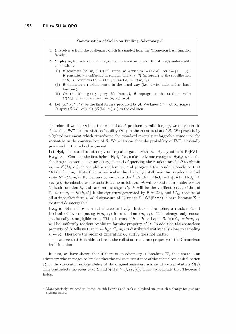
156 EU to SU in QRO
Construction of Collision-Finding Adversary B
1. B receives h from the challenger, which is sampled from the Chameleon hash functionfamily.
2. B, playing the role of a challenger, simulates a variant of the strongly-unforgeablegame with A:(i) B generates (pk, sk)← G(1n). Initialize A with pk′ = (pk, h). For i = 1, . . . , q,B generates mi uniformly at random and ri ← R (according to the specificationof h). B computes Ci := h(mi, ri) and σi := S(sk, Ci).
(ii) B simulates a random-oracle in the usual way (i.e. t-wise independent hashfunction).
(iii) On the ith signing query Mi from A, B reprograms the random-oracle:O(Mi‖σi)← mi and returns (σi, ri) to A.
4. Let (M∗, (σ∗, r∗)) be the final forgery produced by A. We know C∗ = Ci for some i.Output (O(M∗||σ∗), r∗), (O(Mi||σi), ri) as the collision.
Therefore if we let EVT be the event that A produces a valid forgery, we only need toshow that EVT occurs with probability Ω(ε) in the construction of B. We prove it bya hybrid argument which transforms the standard strongly unforgeable game into thevariant as in the construction of B. We will show that the probablity of EVT is esstiallypreserved in the hybrid argument.Let Hyd0 the standard strongly-unforgeable game with A. By hypothesis Pr[EVT :Hyd0] ≥ ε. Consider the first hybrid Hyd1 that makes only one change to Hyd0: when thechallenger answers a signing query, instead of querying the random-oracle O to obtainmi := O(Mi‖σi), it samples a random mi and programs the random oracle so thatO(Mi‖σ) = mi. Note that in particular the challenger still uses the trapdoor to findri ← h−1(Ci,mi). By Lemma 5, we claim that2 Pr[EVT : Hyd0] − Pr[EVT : Hyd1]| ≤negl(n). Specifically we instantiate Samp as follows. pk will consists of a public key forΣ, hash function h, and random messages Ci. P will be the verification algorithm ofΣ. w := σi = S(sk, Ci) is the signature generated by B in 2.i), and Wpk consists ofall strings that form a valid signature of Ci under Σ. WS(Samp) is hard because Σ isexistential-unforgeable.Hyd2 is obtained by a small change in Hyd1. Instead of sampling a random Ci, itis obtained by computing h(mi, ri) from random (mi, ri). This change only causes(statistically) a negligible error. This is because if h← H and ri ← R then Ci := h(mi, ri)will be uniformly random by the uniformity property of H. In addition the chameleonproperty of H tells us that ri ← h−1
td (Ci,mi) is distributed statistically close to samplingri ← R. Therefore the order of generating Ci and ri does not matter.Thus we see that B is able to break the collision-resistance property of the Chameleonhash function.
In sum, we have shown that if there is an adversary A breaking Σ′, then there is anadversary who manages to break either the collision resistance of the chameleon hash functionH, or the existential unforgeability of the original signature scheme Σ with probablity Ω(ε).This contradicts the security of Σ and H if ε ≥ 1/poly(n). Thus we conclude that Theorem 4holds.
2 More precisely, we need to introduce sub-hybrids and each sub-hybrid makes such a change for just onesigning query.
E. Eaton and F. Song 157
4 Discussion
Obtaining a quantum-safe su-acma signature scheme. In [10], the authors presented ascheme for generating chameleon hash functions, based off the short integer solution problemfor lattices. They also demonstrate a reduction showing an efficient algorithm to break thecollision resistance of the hash function implies an efficient algorithm to break the shortinteger solution problem for lattices. Using results from [28] this reduction can be shownto carry through to the quantum setting. As this problem is currently believed to be hardeven for quantum computers, these chameleon hash functions’ collision resistance remainseven when faced with a quantum adversary. This chameleon hash function scheme cantherefore be used in the transformation in this paper to get a quantum-secure transformation.This transformation, used with any quantum-safe eu-acma signature scheme will give aquantum-safe su-acma scheme in the quantum random-oracle model.
When implementing the scheme with the chameleon hash function from [10] we can seewhat the overhead would be in an actual realization. Let n ≥ 1, q ≥ 2, and m = O(n log q).Let k be the output length of the hash function. Then the public key, pk′ will now carrywith it a Zn×m
q matrix, so |pk′| = |pk|+ n(k+m). The secret key now includes a specializedlattice basis, which can be written as an m×m matrix over Zq, giving us |sk′| = |sk|+m2.Finally, the signature overhead is the inclusion of a vector in Zm
q , so |σ′| = |σ|+m.A signature scheme based off the Short Integer Solution problem for lattices is also
presented in [10]. Examining the proof presented there with tools from [28], we can seethat this signature scheme is quantum-safe eu-acma. Applying this transformation to thisscheme, we obtain a quantum-safe su-acma signature scheme. In fact, we can show thatthe reduction shown in [10] is not as tight as it could be, and for a message of length k
and at most Q queries, we can show that for adversary F and reduction S, we have thatADVSIS(SF ) ≥ ADV(F)eu-acma
SIG /(Q(k− logQ)). This is a small improvement over the resultof the paper, showing that ADVSIS(SF ) ≥ ADV(F)eu-acma
SIG /(Q(k − 1) + 1)
Future directions. Our work has studied a very specific transformation that gives a system-atic way of getting quantum-safe su-acma signatures. There are a few more transformationsin the plain model (i.e. without a random-oracle) [29, 20, 18, 17]. We conjecture that theyalso hold against quantum adversaries. If this is the case, it will be meaningful to evaluateall these transformations and figure out which one is preferable under specific applications.On the other hand, we chose the Bonsai-tree signature scheme [10] to instantiate the TOOtransformation. There are many recent improvements on lattice-based signatures in terms ofkey size and computational efficiency [9, 24, 14], which are shown to be eu-acma classically. Ifthey can be shown to be quantum-safe, they we can get more efficient quantum-safe su-acmaschemes in the quantum random-oracle model.
Acknowledgements. The authors are grateful to Andrew Childs for helpful discussions. EEwas supported by NSERC on an undergraduate research award at the Institute for QuantumComputing, University of Waterloo. FS acknowledges support from NSERC, CryptoWorks21,ORF and US ARO.
References1 Andris Ambainis, Ansis Rosmanis, and Dominique Unruh. Quantum attacks on classical
proof systems: The hardness of quantum rewinding. In Foundations of Computer Science(FOCS), 2014 IEEE 55th Annual Symposium on, pages 474–483. IEEE, 2014.
TQC’15

158 EU to SU in QRO
2 Giuseppe Ateniese, Jan Camenisch, Marc Joye, and Gene Tsudik. A practical and provablysecure coalition-resistant group signature scheme. In Advances in Cryptology – CRYPTO2000, pages 255–270. Springer, 2000.
3 Charles H Bennett, Ethan Bernstein, Gilles Brassard, and Umesh Vazirani. Strengths andweaknesses of quantum computing. SIAM journal on Computing, 26(5):1510–1523, 1997.
4 Daniel J. Bernstein, Johannes Buchmann, and Erik Dahmen. Post-quantum cryptography.Springer, 2009.
5 Dan Boneh, Xavier Boyen, and Hovav Shacham. Short group signatures. In Advances inCryptology – CRYPTO 2004, pages 41–55. Springer, 2004.
6 Dan Boneh, Ran Canetti, Shai Halevi, and Jonathan Katz. Chosen-ciphertext securityfrom identity-based encryption. SIAM Journal on Computing, 36(5):1301–1328, 2006.
7 Dan Boneh, Özgür Dagdelen, Marc Fischlin, Anja Lehmann, Christian Schaffner, and MarkZhandry. Random oracles in a quantum world. In Advances in Cryptology – ASIACRYPT2011, pages 41–69. Springer, 2011.
8 Dan Boneh and Mark Zhandry. Secure signatures and chosen ciphertext security in aquantum computing world. In Proceedings of CRYPTO 2013, 2013.
9 Xavier Boyen. Lattice mixing and vanishing trapdoors: A framework for fully secure shortsignatures and more. In Public Key Cryptography – PKC 2010, pages 499–517. Springer,2010.
10 David Cash, Dennis Hofheinz, Eike Kiltz, and Chris Peikert. Bonsai trees, or how todelegate a lattice basis. Journal of Cryptology, 25(4):601–639, 2012.
11 Claude Crépeau, Paul Dumais, Dominic Mayers, and Louis Salvail. Computational collapseof quantum state with application to oblivious transfer. In Theory of Cryptography (TCC),pages 374–393. Springer, 2004.
12 Özgür Dagdelen, Marc Fischlin, and Tommaso Gagliardoni. The fiat–shamir transformationin a quantum world. In Advances in Cryptology – ASIACRYPT 2013, pages 62–81. Springer,2013.
13 Danny Dolev, Cynthia Dwork, and Moni Naor. Nonmalleable cryptography. SIAM Review,45(4):727–784, 2003.
14 Léo Ducas and Daniele Micciancio. Improved short lattice signatures in the standard model.In Advances in Cryptology – CRYPTO 2014, pages 335–352. Springer, 2014.
15 David Galindo, Javier Herranz, and Eike Kiltz. On the generic construction of identity-based signatures with additional properties. In Advances in Cryptology – ASIACRYPT2006, pages 178–193. Springer, 2006.
16 Sean Hallgren, Adam Smith, and Fang Song. Classical cryptographic protocols in a quan-tum world. In Advances in Cryptology – CRYPTO 2011, pages 411–428. Springer, 2011.
17 Qiong Huang, Duncan S Wong, Jin Li, and Yi-Ming Zhao. Generic transformation fromweakly to strongly unforgeable signatures. Journal of Computer Science and Technology,23(2):240–252, 2008.
18 Qiong Huang, Duncan S. Wong, and Yiming Zhao. Generic transformation to strongly un-forgeable signatures. In Applied Cryptography and Network Security, pages 1–17. Springer,2007.
19 Hugo Krawczyk and Tal Rabin. Chameleon hashing and signatures. In Proc. of NDSS,pages 143–154, 2000.
20 Jin Li, Kwangjo Kim, Fangguo Zhang, and Duncan S. Wong. Generic security-amplifyingmethods of ordinary digital signatures. In Applied Cryptography and Network Security,pages 224–241. Springer, 2008.
21 Vadim Lyubashevsky. Fiat-Shamir with aborts: Applications to lattice and factoring-basedsignatures. In Advances in Cryptology – ASIACRYPT 2009, pages 598–616. Springer, 2009.
E. Eaton and F. Song 159
22 Vadim Lyubashevsky. Lattice signatures without trapdoors. In Advances in Cryptology –EUROCRYPT 2012, pages 738–755. Springer, 2012.
23 Vadim Lyubashevsky and Daniele Micciancio. Asymptotically efficient lattice-based digitalsignatures. In Theory of Cryptography, pages 37–54. Springer, 2008.
24 Daniele Micciancio and Chris Peikert. Trapdoors for lattices: Simpler, tighter, faster,smaller. In Advances in Cryptology – EUROCRYPT 2012, pages 700–718. Springer, 2012.
25 Daniele Micciancio and Oded Regev. Lattice-based cryptography. In Post-quantum cryp-tography, pages 147–191. Springer, 2009.
26 Markus Rückert. Strongly unforgeable signatures and hierarchical identity-based signaturesfrom lattices without random oracles. In Post-Quantum Cryptography, pages 182–200.Springer, 2010.
27 Peter W. Shor. Polynomial-time algorithms for prime factorization and discrete logarithmson a quantum computer. SIAM Journal on Computing, 26(5):1484–1509, 1997.
28 Fang Song. A note on quantum security for post-quantum cryptography. In Post-QuantumCryptography, pages 246–265. Springer, 2014.
29 Ron Steinfeld, Josef Pieprzyk, and Huaxiong Wang. How to strengthen any weakly unforge-able signature into a strongly unforgeable signature. In Topics in Cryptology – CT-RSA2007, pages 357–371. Springer, 2006.
30 Isamu Teranishi, Takuro Oyama, and Wakaha Ogata. General conversion for obtainingstrongly existentially unforgeable signatures. In Progress in Cryptology – INDOCRYPT2006, pages 191–205. Springer, 2006.
31 Dominique Unruh. Quantum proofs of knowledge. In Eurocrypt 2012, volume 7237 ofLNCS, pages 135–152. Springer, April 2012. Preprint on IACR ePrint 2010/212.
32 Dominique Unruh. Quantum position verification in the random oracle model. In Crypto2014, volume 8617 of LNCS, pages 1–18. Springer, August 2014. Preprint on IACR ePrint2014/118.
33 Dominique Unruh. Revocable quantum timed-release encryption. In Advances in Cryptol-ogy – EUROCRYPT 2014, pages 129–146. Springer, 2014.
34 Dominique Unruh. Non-interactive zero-knowledge proofs in the quantum random oraclemodel. In Advances in Cryptology – EUROCRYPT 2015, pages 755–784. Springer, 2015.
35 John Watrous. Zero-knowledge against quantum attacks. SIAM Journal on Computing,39(1):25–58, 2009.
36 Mark Zhandry. Secure identity-based encryption in the quantum random oracle model. InProceedings of CRYPTO 2012, 2012.
A Classical Proof
Let A be the forger, B the reduction, and C be the challenger. In each case, B and A will beplaying a game of strong unforgeability. Let the probability that A succeeds be ε. In Case 1,C and B will play a game of existential unforgeability on the signature scheme σ. In case 2,C and B will play a game of collision resistance on the chameleon hash function h. We showthat if the probability A succeeds in her forgery is ε, then the probability that B succeeds is≥ 1
2ε− negl(n). At the beginning of the reduction, B will flip a coin, and guess which casethe adversary’s forgery will fall under. Clearly, B will be correct with probability 1
2 .In our reduction, let the forgery that A eventually submits be (M∗, σ′∗ = (σ∗, r∗)) Let
C∗ = h(O(M∗||σ∗), r∗). Similarly, for each Mi the forger submits to the signing oracle forsigning, there is an associated σ′i and Ci.
TQC’15

160 EU to SU in QRO
Case 1: C∗ 6= Ci for all i. We show that whenever the forger succeeds in creating a validforgery of this type, the reduction succeeds in breaking the existential unforgeability ofthe original scheme Σ = (G,S, V ).C and B will be playing a game of existential unforgeability, while B and A will be playinga game of strong unforgeability. We will show that whenever A wins her game, B winshis (so long as the forgery is of the type described above).The games will play out as follows:Firstly, B will act as the random oracle for A. In the first case at least (and this willchange only slightly case to case), he can do this in the following way. Whenever Aqueries the random oracle with a query, B looks up in a maintained table if that queryhas been made before. If it has, he responds with the value he responded with before. Ifit has not, he generates a random number and responds with that.Now we discuss how the game of strong unforgeability transpires.C sends B a public key pk from the Σ scheme. B will generate a chameleon hash functionh, (with corresponding trapdoor td) and send the public key and hash function to A aspk′ = (pk, h).A will start submitting messagesMi to B for signing. For each query, B does the following:
Choose a random mi and ri and compute Ci = H(mi, ri)Sign Ci by submitting it to C as a signing query, obtaining σi
Query Mi||σi to the random oracle, obtaining mi = O(Mi||σi)Using the trapdoor information td, find an ri such that h(mi, ri) = Ci.σ′i = (σi, ri)Send σ′i to A
Eventually, A will submit a valid forgery M∗, σ′∗ = (σ∗, r∗).Then, B takes these, and computes C∗ = h(O(M∗||σ∗), r∗).Noting that C∗ 6= Ci for all i, and the Ci’s are precisely what was submitted to C forsigning queries, and finally, seeing as this is a valid forgery, so V (C∗, σ∗) =′ accept′, we cansee that B submits C∗, σ∗ as a valid new forgery, breaking the existential unforgeabilityof Σ and winning his game with C.Thus in this case whenever A succeeds, so does B, and so the probability B succeedsgiven we are in this case is ε.Case 2: This case is defined as occurring when C∗ = Ci for some i. In this case we willshow a reduction to break the collision resistance of the chameleon hash function.To start with, C sends B the description of a chameleon hash function h, which B willfind a collision for.B then runs the key generation algorithm of the signature scheme Σ, obtaining (pk, sk).He then sends pk′ = (pk, h) to A.For each signing query Mi that A sends to B, B does the following:
Choose a random mi and ri and compute C = h(mi, ri)Sign Ci using the signing algorithm S, obtaining σ = S(C, sk)Reprogram the random oracle so that O(Mi||σi) = mi.σ′i = (σi, ri)Send σ′i to A.
Note that we have now permitted B to reprogram the random oracle for the purposes ofthis proof. Thus it is necessary to show that A will still output a valid forgery.When A eventually submits her forgery, (M∗, σ∗), we can see that C∗ = Ci for somei. This implies that h(O(Mi||σi), ri) = h(O(M∗||σ∗), r∗) for that i. This shows us a
E. Eaton and F. Song 161
collision for the chameleon hash function h, which is what B is looking for. But we musttake care to ensure that it isn’t a trivial collision.Note that (Mi, σi, ri) 6= (M∗, σ∗, r∗), simply because both the message and signature ofthe forgery can’t be the same as that of one of the Mi’s. So at least one of these values isdifferent.If ri 6= r∗, we are done. Otherwise, it must be the case thatM∗||σ∗ 6= Mi||σi. In this case,since the values for the random oracle are chosen uniformly at random, with overwhelmingprobability, O(M∗||σ∗) 6= O(Mi||σi), giving B a collision for h.So in this case, B will succeed as long as A does up to a negligible probability by Lemma 7.So the probability B succeeds is ≥ ε− negl(n)
I Lemma 7. For a forger A, let B1 and B2 be as below, and have them play a game ofstrong unforgeability with A. Then
|PrB1(A wins)− PrB2(A wins)| ≤ negl(n),
as long as the underlying signature scheme is existentially unforgeable.
B1 is defined to operate exactly as the transformation dictates. B2 will operate as B wasdefined to in Case 2 above.
Proof. Say the difference in probability that A wins was not negligible. As the distributionof all values is the same, the only difference from A’s perspective was that the value ofO(Mi||σi) was changed for each i.
But clearly the only way to have the information that they changed is if A had alreadyqueried O(Mi||σi). But if A does this with non-negligible probability, then we could constructa reduction to break the existential forgeability of the signature scheme by playing strongunforgeability with A, and before submitting each Ci to the signing oracle, checking to see ifA had queried Mi||σi to the random oracle. With non-negligible probability, the reductionfinds a σi that is a valid forgery. So he submits this along with Ci and has broken theexistential unforgeability of the scheme. J
Therefore in both cases, as long as B successfully guesses which case the forgery willfall under, he manages to successfully break either the collision resistance of the chameleonhash function h, or the existential unforgeability of the original signature scheme Σ. Since Bcorrectly guesses what case he is in half of the time, his probability of success is ≥ 1
2ε−negl(n).
B Proof of Lemma 6
Proof. Let A be an arbitrary algorithm running in G (or G′). Consider another algorithmB that runs in an experiment EXT as follows:
Extraction Experiment EXT1. Generate (pk, w, P )← Samp(1n). Ignore w.2. B receives pk and picks j ∈R 1, . . . , q at random.3. B simulates A on pk and (quantum) access to f . Just before A making the jth query to
f , B measures the register that contains A’s query. Let z be the measurement outcome.
Let pB := PrEXT [z ∈ Wpk] be the probability that the output of E is a valid witness.Let ε := |PrG[b = 1]− PrG′ [b = 1]|. In both experiment G and G′, pk is selected at randomaccording to Samp. Let Ppk be the probability that pk is outputted. Then
TQC’15
162 EU to SU in QRO
ε =∣∣∣Pr
G[b = 1]− Pr
G′[b = 1]
∣∣∣=
∣∣∣∣∣∣∑pk
PrG
[b = 1|pk] · Ppk −∑pk
PrG′
[b = 1|pk] · Ppk
∣∣∣∣∣∣=∑pk
Ppk
∣∣∣PrG
[b = 1|pk]− PrG′
[b = 1|pk]∣∣∣ .
Let εpk := |PrG[b = 1|pk]− PrG′ [b = 1|pk]|. Let |φi〉 be the superposition of AG on inputpk when the i’th query is made. Then let qy(|φi〉) be the sum of squared magnitudes in Aquerying the oracle on the string y.
Let S = [q] ×Wpk. Let δpk =∑
(i,y)∈S qy(|φpki 〉). We employ a theorem by Bennet et
al. [3], that states that ‖|φpki 〉 − |φ
pki 〉‖ ≤
√q · δpk. (Here |φpk
i 〉 is defined in the same way as|φpk
i 〉 but with G′ rather than G).The same paper [3] also bounds the probability of being able to distinguish the two states,
which corresponds to our probability of distinguishing the two experiments, εpk, telling usthat
εpk ≤ 4 ·∥∥∥|φpk
i 〉 − |φpki 〉∥∥∥ ≤ 4
√q · δpk .
Now note that P pkB (that is, the probability that EXT outputs a valid witness given pk
is chosen) can be written as
P pkB =
∑i∈[0,q]
Pr[i chosen] ·∑
(j,y)∈S:j=i
qy(|φpkj 〉)
=1q
∑i∈[0,q]
∑(j,y)∈S:j=i
qy(|φpkj 〉)
=1q
∑(i,y)∈S
qy(|φpki 〉) = 1
qδpk
So we can see that εpk ≤ 4q√P pk
B . Then
ε =∑pk
Ppkεpk ≤ 4q∑pk
Ppk
√P pk
B
(∗)≤ 4q
√∑pk
PpkPpkB = 4q
√PB ,
where (*) applies Jensen’s inequality. Finally, notice that B can be viewed as an adversaryin the witness-search game WS(Samp). Therefore, we conclude that pB ≤ negl(n) by thehypothesis that WS(Samp) is hard and hence |PrG[b = 1]− PrG′ [b = 1]| ≤ negl(n). J

A Universal Adiabatic Quantum Query AlgorithmMathieu Brandeho and Jérémie Roland
Université libre de Bruxelles, Quantum Information and Communication1050 Brussels, Belgiummbrandeh,[email protected]
AbstractQuantum query complexity is known to be characterized by the so-called quantum adversarybound. While this result has been proved in the standard discrete-time model of quantumcomputation, it also holds for continuous-time (or Hamiltonian-based) quantum computation,due to a known equivalence between these two query complexity models. In this work, we revisitthis result by providing a direct proof in the continuous-time model. One originality of ourproof is that it draws new connections between the adversary bound, a modern technique oftheoretical computer science, and early theorems of quantum mechanics. Indeed, the proof ofthe lower bound is based on Ehrenfest’s theorem, while the upper bound relies on the adiabatictheorem, as it goes by constructing a universal adiabatic quantum query algorithm. Anotheroriginality is that we use for the first time in the context of quantum computation a version ofthe adiabatic theorem that does not require a spectral gap.
1998 ACM Subject Classification F.2 Analysis of Algorithms and Problem Complexity
Keywords and phrases Quantum Algorithms, Query Complexity, Adiabatic Quantum Compu-tation, Adversary Method
Digital Object Identifier 10.4230/LIPIcs.TQC.2015.163
1 Introduction
The quantum adversary method was originally introduced by Ambainis [2] for lower-boundingthe quantum query complexity Q(f) of a function f . It is based on optimizing a matrixΓ assigning weights to pairs of inputs. It was later shown by Høyer et al. [18] that usingnegative weights also provides a lower bound, which is stronger for some functions. A series ofworks [26, 27, 25] then led to the breakthrough result that this generalized adversary bound,which we will simply call adversary bound from now on, actually characterizes the quantumquery complexity of any function f with boolean output and binary input alphabet. Thisis shown by constructing a tight algorithm based on the dual of the semidefinite programcorresponding to the adversary bound1. Finally, Lee et al. [21] have generalized this resultto the quantum query complexity of state conversion, where instead of computing a functionf(x), one needs to convert a quantum state |ρx〉 into another quantum state |σx〉.
All these results where obtained in the usual discrete-time query model, where each querycorresponds to applying a unitary oracle Ox. In this model, an algorithm then consistsin a series of input-independent unitaries U1, U2, . . . , UT , interleaved with oracle calls Ox.Another natural model is the continuous-time (or Hamiltonian-based) model where theoracle corresponds to a Hamiltonian Hx, and the algorithm consists in applying a possibly
1 Note that constructing a tight algorithm for a specific problem using this method requires to find anoptimal feasible point for the semidefinite program, so that this method is not necessarily constructive.The same limitation will affect the universal adiabatic algorithm in the present article.
© Mathieu Brandeho and Jérémie Roland;licensed under Creative Commons License CC-BY
10th Conference on the Theory of Quantum Computation, Communication and Cryptography (TQC 2015).Editors: Salman Beigi and Robert König; pp. 163–179
Leibniz International Proceedings in InformaticsSchloss Dagstuhl – Leibniz-Zentrum für Informatik, Dagstuhl Publishing, Germany

164 A universal adiabatic quantum query algorithm
time-dependent, but input-independent, driver Hamiltonian HD(t), together with the oracleHamiltonian. The two models are related by the fact that the unitary oracle Ox can besimulated by applying the Hamiltonian oracle Hx for some constant amount of time. Thisimplies that the continuous-time model is at least as powerful as the discrete-time model. Inthe other direction, Cleve et al. [11] have shown that the discrete-time model can simulatethe continuous-time model up to at most a sublogarithmic overhead, which implies thatthe continuous- and discrete-time models are equivalent up to a sublogarithmic factor. Leeet al. [21] later improved this result to a full equivalence of both models, by showing thatthe fractional query model, an intermediate model proved in [11] to be equivalent to thecontinuous-time model, is also lower bounded by the adversary bound, so that all thesemodels are characterized by this same bound (in the case of functions, a similar result can beobtained by extending an earlier proof of Yonge-Mallo, originally considering the adversarybound with positive weights, to the case of negative weights [30]).
Even though these results imply that the continuous-time quantum query complexity ischaracterized by the adversary bound, they do not provide an explicit Hamiltonian-basedquery algorithm, except the one obtained from the discrete-time algorithm by replacingeach unitary oracle call by the application of the Hamiltonian oracle for a constant amountof time. The resulting Hamiltonian of this algorithm then involves many discontinuities(at all times in between unitary gates), which is not very satisfying from the point of viewof physics, where reasonable Hamiltonians are smooth. However, such discontinuities arenot unavoidable, as for some problems, continuous-time query algorithms based on smoothHamiltonians are known.
The first example is unstructured search, for which Farhi and Gutmann [15] proposeda continuous-time analogue of Grover’s algorithm based on a simple time-independentHamiltonian (later, van Dam et al. [29], as well as Roland and Cerf [28], independentlyproposed an adiabatic version of this algorithm, based on a slowly varying Hamiltonian).Algorithms were also developed in the continuous-time model for various problems suchas spatial search [8, 10, 16], oracle identification [23], or element distinctness [9]. In aseminal paper, Farhi et al. [13] proposed a quantum algorithm for the NAND-tree basedon scattering a wave incoming on the tree, using a time-independent Hamiltonian. It isprecisely this algorithm that, through successive extensions, led to the tight algorithm basedon the adversary bound for any function in [27], but most of these extensions were using thediscrete-time model.
In this article, we give a new continuous-time quantum query algorithm for any stateconversion algorithm based on a slowly varying Hamiltonian, and also provide a directproof of its optimality based on Ehrenfest’s theorem, hence proving that the quantum querycomplexity of any state conversion problem is characterized by the adversary bound. Thesoundness of the adiabatic evolution used in our algorithm relies on a lemma from Avronand Elgart [4], which does not require the usual gap condition but only weaker spectralconditions, and was originally introduced to study atoms in quantized radiation fields. Tothe best of our knowledge, it is the first time that such an adiabatic theorem without a gapcondition is used in the context of quantum computation.
The structure of the article is as follows. Section 2 is devoted to preliminaries: inSubsection 2.1, we define the necessary mathematical notions; in Subsection 2.4, we recall thequantum adiabatic evolution and quantum adiabatic theorems; in Subsection 2.2, we recallnotions of quantum query complexity; and in Section 2.3, the discrete-time adversary method.Original contributions start in Section 3, where we give a direct proof that the adversarybound remains a lower bound for continuous-time quantum query complexity (Theorem 20).

M. Brandeho and J. Roland 165
Finally, in Section 4, we present our adiabatic quantum query algorithm AdiaConvert, andshow that it is optimal, implying the characterization of the bounded-error quantum querycomplexity (Theorem 21).
2 Preliminaries
2.1 DefinitionsThroughout this article, X and Σ are finite sets and n is a positive integer. Σ represents thealphabet and X represents a subset of words of length n: x ∈ X ⊂ Σn.
I Definition 1 (Matrix norms and inner product). Let A and B be n-by-n matricesInner product: 〈A,B〉 = tr(A∗B), where A∗ is the adjoint matrix of A,Hadamard product: (A B)ij = Aij . Bij ,Operator norm: ‖A‖ = max|v〉 ‖A|v〉‖‖|v〉‖ = max|u〉,|v〉 〈u|A|v〉
‖|u〉‖.‖|v〉‖ ,Trace norm: ‖A‖tr = maxB 〈A,B〉‖B‖ .
These definitions imply the following properties:
I Lemma 2. For any n-by-n matrices A,B,C, we have〈A C,B〉 = 〈A,B C∗〉〈A,B〉 ≤ ‖A‖tr · ‖B‖
In this context, the following matrix norm will be useful:
I Definition 3 (γ2 norm). Let D be a finite set, A a |D|-square matrix. The norm γ2(A) isdefined as
γ2(A) = minm∈N
|ux〉,|vy〉∈Cm
maxx∈D
max‖ |ux〉 ‖2, ‖ |vy〉 ‖2
∣∣∣∣∣∀x, y ∈ D, Ax,y = 〈ux| vy〉,
= max|u〉,|v〉
‖|u〉‖=‖|v〉‖=1
‖A |u〉〈v|‖tr.
In particular, it is shown in [21] that the dual of the Adversary bound can be seen as avariation of the γ2 norm dubbed the filtered γ2 norm.
I Definition 4 (Filtered γ2 norm). Let D1 and D2 be two finite sets, A, Z1, . . . , Zn matriceswith |D1| rows and |D2| columns, and Z = Z1, . . . , Zn. The norm γ2(A|Z) is defined as
γ2(A|Z) = minm∈N
|ux,j〉,|vy,j〉∈Cm
max
maxx∈D1
∑j
‖ |ux,j〉 ‖2,maxy∈D2
∑j
‖ |vy,j〉 ‖2
subject to ∀(x, y) ∈ D1 ×D2, Ax,y =∑j
(Zj)x,y 〈ux,j | vy,j〉 ,
= maxΓ
‖Γ A‖ subject to ∀j ‖Γ Zj‖ ≤ 1.
I Claim 5 ([22]). For any matrices A, B where A B is defined, ‖A B‖ ≤ γ2(A).‖B‖.
The Hadamard product fidelity is introduced in [22] to characterize the output conditionof quantum query problems. Whereas the usual fidelity compares density matrices, theHadamard product fidelity compares Gram matrices (note that if ρ is a Gram matrix and|u〉 is a normalized state, then ρ |u〉〈u| is a density matrix).
TQC’15

166 A universal adiabatic quantum query algorithm
I Definition 6 (Hadamard product fidelity). The Hadamard product fidelity between twoGram matrices ρ and σ is defined as
FH(ρ, σ) = min|u〉:‖|u〉‖=1
F(ρ |u〉〈u|, σ |u〉〈u|),
where F(ρ′, σ′) is the fidelity between two density matrices ρ′ and σ′, defined as F(ρ′, σ′) =tr√√
ρ′ σ′√ρ′.
We similary define the Hadamard product distance from the trace distance.
I Definition 7 (Hadamard product distance). The Hadamard product distance between twoGram matrices ρ and σ is defined as
DH(ρ, σ) = max|u〉:‖|u〉‖=1
D(ρ |u〉〈u|, σ |u〉〈u|),
where D(ρ′, σ′) is the trace distance between two density matrices ρ′ and σ′, defined asD(ρ′, σ′) = 1
2‖ρ′ − σ′‖tr.
I Theorem 8 ([17]). For any density matrices ρ, σ, we have 1 − D(ρ, σ) ≤ F(ρ, σ) ≤√1−D2(ρ, σ).
I Corollary 9. For any Gram matrices ρ, σ, we have 1−DH(ρ, σ) ≤ FH(ρ, σ) ≤√
1−D2H(ρ, σ).
I Definition 10 (Distance between quantum states). We say that two normalized quantumstates |φ〉 , |ψ〉 ∈ H are ε-distant if ‖|φ〉 − |ψ〉‖ ≤ ε.
2.2 Quantum query complexityIn classical computation, a query algorithm computes a function f : X ⊂ Σn → B where theinput x ∈ X can only be accessed through queries to an oracle that, on input j ∈ [n], outputsxj ∈ Σ. A query algorithm can be seen as a decision tree [7] where each vertex represents adecision taken after one query. The depth of the tree then corresponds to the number ofqueries used by this algorithm to compute f in the worst case. The query complexity of f isthe minimum depth of all decision trees computing f exactly.
In quantum computation, query complexity can be generalized to state conversionproblems, where one should convert a quantum state |ρx〉 into another state |σx〉, eachdepending on the input x, which can once again only be accessed via an oracle. The evaluationof a function f is the particular case where initial states are independent of x, and final statesare orthonormal for x, y such that f(x) 6= f(y). For any set of quantum states |ρx〉x, it isenough to consider the Gram matrix ρx,y = 〈ρx| ρy〉, because if 〈ρx| ρy〉 =
⟨ρ′x∣∣ ρ′y⟩ for all
x, y, then there exists a unitary transformation U independent of x such that |ρx〉 = U |ρ′x〉for all x. This implies that a query algorithm for the set of states |ρ〉x can be convertedinto a query algorithm for the set of states |ρ′〉x without additive cost, and vice versa. Wewill therefore denote by a pair of Gram matrices (ρ, σ) the problem of converting a set ofstates |ρx〉x into another set of states |σx〉x.
In the discrete-time model of quantum query complexity, we can consider without loss ofgenerality an oracle Ox acting on an n-dimensional input register and a (|Σ|+ 1)-dimensionaloutput register as
Ox :
|j〉∣∣0⟩ 7→ |j〉 |xj〉 ∀j ∈ [n]
|j〉 |xj〉 7→ |j〉∣∣0⟩ ∀j ∈ [n]
|j〉 |y〉 7→ |j〉 |y〉 ∀j ∈ [n], y ∈ Σ \ xj(1)

M. Brandeho and J. Roland 167
where 0 is an additional output alphabet symbol, that can be seen as a blank symbol. Aquery algorithm in this model is then given by a succession of input-independent unitaries Utinterleaved with oracle calls Ox. The discrete-time quantum query complexity Qdt
0 (ρ, σ) isthe minimum number of oracle calls of any such algorithm converting ρ to σ exactly. (Notethat there exist alternative definitions for the oracle Ox, but they only affect the definitionof Qdt
0 (ρ, σ) by at most a constant factor.)In the continuous-time model, the oracle is a Hamiltonian HQ(x) of the general form
HQ(x) =n∑j=1|j〉〈j| ⊗ h(xj), (2)
where each h(y)y∈Σ is hermitian and satisfies ‖h(y)‖ ≤ 1. In particular, the choiceh(y) = |y−〉〈y−|, where∣∣y±⟩ = 1√
2(∣∣0⟩± |y〉), (3)
can be considered as the Hamiltonian analogue of the unitary oracle Ox in equation (1),since it is easy to check that Ox = e−iHQ(x)∆T for ∆T = π. A query algorithm in this modelthen corresponds to applying a Hamiltonian Hx(t) of the form
Hx(t) = HD(t) + α(t)HQ(x) (4)
where HD(t) is the driver Hamiltonian independent of the input x, and |α(t)| ≤ 1 forall t ∈ [0, T ]. The continuous-time quantum query complexity Qct
0 (ρ, σ) is the minimumcomputing time T of any such algorithm converting ρ to σ exactly.
For scenarios where we accept errors, we must distinguish two cases : coherent andnon-coherent quantum state conversion. Concretely, a computation will typically use someextra workspace and may therefore generate a state |σx, Jx〉, where |Jx〉 is the final state ofthe workspace. This might not be desirable if the state generation is used as a subroutine ina larger quantum algorithm, where we would like to use interferences between the states |σx〉for different x’s. In that case, we would like to be able to reset the state |Jx〉 to a defaultstate, so that it does not affect interferences.
We therefore define the following output conditions (both for the discrete- and continuous-time models)
I Definition 11 (Output condition). A quantum query algorithm acting as unitary Ux forinput x converts ρ to σ with error at most ε if
(coherent case) ∀x ∈ X, Re(〈σx, 0| Ux|ρx, 0〉) ≥√
1− ε,(non-coherent case) ∀x ∈ X, ∃ |Jx〉 , Re(〈σx, Jx| Ux|ρx, 0〉) ≥
√1− ε.
Note that a sufficient condition for Re(〈φ| ψ〉) ≥√
1− ε is that these states are√ε-
distant. Moreover, the output condition for the coherent case has been shown [22] tobe equivalent to FH(σ, σ′) ≥
√1− ε, where σ′ is the Gram matrix of the output states
|σ′x〉 = Ux |ρx, 0〉. Similarly, in the non-coherent case the output conditions can be rewrittenas FH(σ J, σ′) ≥
√1− ε, where J is any Gram matrix of unit vectors (corresponding
to any set of states |Jx〉). This implies that bounded-error and zero-error quantum querycomplexities are related as follows.
I Lemma 12 ([22]). For any |X|-by-|X| Gram matrices ρ, σ, we have
Q•ε(ρ, σ) = minσ′
Q•0(ρ, σ′) : FH(σ, σ′) ≥
√1− ε
(5)
Qnc,•ε (ρ, σ) = min
σ′
Q•0(ρ, σ′) : FH(σ J, σ′) ≥
√1− ε, J 1 = 1
(6)
TQC’15

168 A universal adiabatic quantum query algorithm
where the superscript nc denotes the non-coherent query complexity (otherwise we considerthe coherent case by default), and the superscript • is either dt or ct.
Computing a function f is equivalent to generating the Gram matrix Fx,y = δf(x),f(y)from the all-1 Gram matrix Jx,y = 1. In that case, it is not necessary to generate the statecoherently, but one can convert a non-coherent algorithm into a coherent algorithm, so thatwe can consider the coherent case without loss of generality.
I Lemma 13 ([22]). For any function f and associated Gram matrix Fx,y = δf(x),f(y), wehave Q•ε(f) = Qnc,•
ε (J, F ) and
Qnc,•ε (J, F ) ≤ Q•ε(J, F ) ≤ 2Qnc,•
1−√
1−ε(J, F ).
2.3 Adversary methodsThe quantum adversary method is one of main methods to prove lower bounds on quantumquery complexity (the other main method is the polynomial method [5]). Its basic principleis rather simple: it consists in defining a so-called progress function W whose value is highat the beginning of the algorithm and should be low at the end of the algorithm if it issuccessful. By bounding the change in the progress function for each oracle call, one thenbounds the minimum number of oracle calls necessary for success.
More precisely, let |φx(t)〉 be the state of the algorithm on input x after t queries, and Φtbe the Gram matrix of those states. We define a progress function
W (Φt) = 〈Γ vv∗,Φt〉 ,
where Γ is a |X|-by-|X| hermitian matrix, called the adversary matrix, and v a unit vector.We also define the matrices ∆j with entries (∆j)x,y = 1 − δxj ,yj
. The adversary methodrelies on the fact that if Γ is chosen so that it satisfies ‖Γ ∆j‖ ≤ 1 for all j ∈ [n], thenthe progress function can only increase by one after each query (see e.g. [18]), that is,|W (Φt+1)−W (Φt)| ≤ 1. The difference of the values of the progress function between Φ0 = ρ
and ΦT = σ is then given by
W (Φ0)−W (ΦT ) = 〈Γ vv∗, ρ− σ〉 = 〈Γ (ρ− σ), vv∗〉 ≤ T
By optimizing over Γ and v, we obtain the adversary bound:
I Definition 14 ([21, 22], Adversary bound).
Adv?(ρ, σ) = maxΓ‖Γ (ρ− σ)‖ subject to ∀j ∈ [n], ‖Γ ∆j‖ ≤ 1,
= γ2(ρ− σ|∆) where ∆ = ∆1, . . . ,∆n.
As shown in [21], Adv? defines a distance between Gram matrices, sometimes calledthe query distance. The following simple proposition, comparing the query distance to theHadamard product distance DH , will be used in the proof of Theorem 21.
I Proposition 15. For any Gram matrices ρ, σ of size n, DH(ρ, σ) ≤ Adv?(ρ, σ).
Proof. Since the trace distance may be written as D(ρ′, σ′) = maxP :‖P‖≤112 〈P, (ρ
′ − σ′)〉,we can reformulate the Hadamard product distance in Definition 7 as
DH(ρ, σ) = maxP :‖P‖≤1/2|u〉:‖|u〉‖=1
〈P, (ρ− σ) |u〉〈u|〉 = maxP :‖P‖≤1/2
‖P (ρ− σ)‖.

M. Brandeho and J. Roland 169
We observe that this form is similar to Adv? in Definition 14, except for the constraintson P and Γ. We conclude the proof by showing that the constraint on P is stronger, that is,if ‖P‖ ≤ 1/2 then ‖P ∆i‖ ≤ 1 for all i ∈ [n].
Let J be the all-one matrix, and i ∈ [n]. We have
‖P ∆i‖ ≤ ‖P‖+ ‖P (J−∆i)‖ ≤(
1 + γ2(J−∆i))‖P‖,
where the inequalities follows from the triangle inequality and Claim 5, respectively. Wefinally bound γ2(J −∆i) using the minimization form in Definition 3 and an appropriatechoice for |ux〉 , |vx〉x. Choosing |ux〉 = |vx〉 = |xi〉, we have 〈ux| vy〉 = (J−∆i)x,y = δxi,yi
,so that γ2(J−∆i) ≤ 1. J
2.4 Adiabatic quantum computationAdiabatic quantum computation is a quantum computational model originally proposed byFarhi et al. [14] for solving instances of the satisfiability problem. This model is based onthe quantum adiabatic theorem introduced by Born and Fock [6] and describing a physicalsystem evolving under a slowly varying Hamiltonian:
A quantum system with a time-dependent Hamiltonian remains in its instantaneouseigenstate if the Hamiltonian variation is slow enough and there is a large gap between its
eigenvalue and the rest of the spectrum of the Hamiltonian.
It was later proved that the adiabatic model is equivalent to standard quantum computation[1]. This statement, as well as the correctness of most adiabatic algorithms, rely on theexistence of a spectral gap.
In order to formally describe adiabatic quantum computation, let us first define the notionof adiabatic process.
I Definition 16. An adiabatic process on the Hilbert space H is defined by a tripletH(s), P (s), τ with s ∈ [0, 1] where(a) H(s) is a twice differentiable map from [0, 1] to the space of bounded linear self-adjoint
operators B(H), equipped with the graph norm of H(0).(b) P (s) are a family of orthogonal rank-one projections onto an eigenvector of H(s) with
continuous eigenvalue λ(s),(c) τ ∈ R+ is the time scale, which defines the time as t(s) = sτ .
For such an adiabatic process, we can define the unitary operator UA(s) correspondingto an idealized evolution, which maps the eigenvector in the range of P (0) to the eigenvectorin the range of P (s), that is, UA(s)P (0)U∗A(s) = P (s). Furthermore, the physical evolution,represented by unitary operator Uτ (s), can be obtained from the Schrödinger equation
i∂sUτ (s) = τH(s)Uτ (s). (7)
Let us note that the analytical conditions given in Definition 16 ensure the existence anduniqueness of the solution Uτ (s) of this equation with initial condition Uτ (0) = 1 [24].
The quantum adiabatic theorem can be summarized by the following statement
limτ→∞
Uτ (s)P (0) = UA(s)P (0) = P (s)UA(s).
Thus Uτ (s)P (0) converge to UA(s)P (0) for large τ , and the norm of their differencedefines the error of the adiabatic process.
TQC’15

170 A universal adiabatic quantum query algorithm
I Definition 17. The error εAP (s) of an adiabatic process H(s), P (s), τ is defined as
εAP (s) =∥∥[Uτ (s)− UA(s)
]P (0)
∥∥, with εAP = εAP (1).
This definition implies that at the end of the adiabatic evoltion, the physical state will beεAP -distant from the ideal state.
How slow should the process be, or, equivalently, how large should τ be, to ensure a smallenough adiabatic error? The folk adiabatic condition requires the following bound:
τ >>
∫ 1
0
‖∂sHτ (s)‖g(s)2 ds, (8)
where the gap g(s) represents the minimal distance between the eigenvalue λ(s) and therest of spectrum of H(s). However this folk adiabatic condition is not always sufficient, butrigorous conditions have been given e.g. by Jansen et al. [19]. Indeed, they proved thefollowing statement (where we introduce the notation A(s) = ∂sA(s)).
I Theorem 18 ([19]). Let H(s), P (s), τ be an adiabatic process with a gap g = mins∈[0,1] g(s),H, H are bounded operators, and ε > 0, if
τ ≥ 1ε
[‖H(0)‖+ ‖H(1)‖g2 + max
s∈[0,1]
‖H(s)‖2
g2 + 7‖H(s)‖2
g3
],
then εAP ≤ ε.
The adiabatic process used in our algorithm introduced in Section 4 does not necessarilyexhibit a gap, and for this reason we use another lemma from Avron and Elgart [4].
I Lemma 19 ([4]). Let H(s), P (s), τ be an adiabatic process and ε > 0. Suppose that thecommutator equation
P (s)P (s) = [H(s), X(s)] (9)
accepts as solution operator X(s) such that both X(s) and X(s) are bounded. If
τ ≥ maxs∈[0,1]
1ε
[2‖X(s)‖+ ‖X(s)P (s)‖
],
then εAP ≤ ε.
This version of the lemma is actually a special case of the statement proved by Avron andElgart, adapted to the case of continuous-time quantum computation. For completeness wereproduce a self-contained proof of this version of the lemma in Appendix A.
3 Adversary lower bound in the continuous-time model
In this section we give a direct proof that the adversary method Adv?(ρ, σ) is a lower-boundfor the zero-error quantum query complexity in the continuous-time model.
I Theorem 20. For any |X|-by-|X| Gram matrices ρ, σ, we have
Qct0 (ρ, σ) ≥ 1
2Adv?(ρ, σ),
Qctε (ρ, σ) ≥ 1
2 minσ′:FH(σ,σ′)≥
√1−ε
Adv?(ρ, σ′).
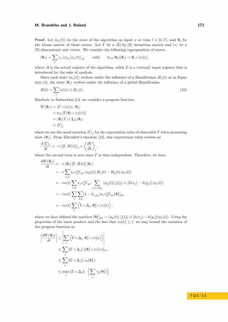
M. Brandeho and J. Roland 171
Proof. Let |φx(t)〉 be the state of the algorithm on input x at time t ∈ [0, T ], and Φt bethe Gram matrix of those states. Let Γ be a |X|-by-|X| hermitian matrix and |v〉 be a|X|-dimensional unit vector. We consider the following superposition of states:
|Φt〉 =∑x
vx |x〉I |φx(t)〉A with trA |Φt〉〈Φt| = Φt |v〉〈v|,
where A is the actual register of the algorithm, while I is a (virtual) input register that isintroduced for the sake of analysis.
Since each state |φx(t)〉 evolves under the influence of a Hamiltonian Hx(t) as in Equa-tion (4), the state |Φt〉 evolves under the influence of a global Hamiltonian
H(t) =∑x
|x〉〈x| ⊗Hx(t). (10)
Similarly to Subsection 2.3, we consider a progress function
W (Φt) = 〈Γ |v〉〈v| ,Φt〉= trI [Γ(Φt |v〉〈v|)]= 〈Φt|Γ⊗ 1A |Φt〉≡ 〈Γ〉t
where we use the usual notation 〈Γ〉t for the expectation value of observable Γ when measuringstate |Φt〉. From Ehrenfest’s theorem [12], this expectation value evolves as
d 〈Γ〉tdt
= −i 〈[Γ, H(t)]〉t +⟨∂Γ∂t
⟩t
,
where the second term is zero since Γ is time-independent. Therefore, we havedW (Φt)dt
= −i 〈Φt| [Γ, H(t)] |Φt〉
= −i∑x,y
vxv∗yΓyx 〈φy(t)|Hx(t)−Hy(t) |φx(t)〉
= −iα(t)∑x,y
vxv∗yΓyx
∑j:xj 6=yj
〈φy(t)| |j〉〈j| ⊗ [h(xj)− h(yj)] |φx(t)〉
= −iα(t)∑j
∑x,y
(1− δxjyj)vxv∗yΓyx[Φjt ]yx
= −iα(t)∑j
⟨Γ ∆j ,Φjt |v〉〈v|
⟩,
where we have defined the matrices [Φjt ]yx = 〈φy(t)| |j〉〈j| ⊗ [h(xj)− h(yj)]|φx(t)〉. Using theproperties of the inner product and the fact that |α(t)| ≤ 1, we may bound the variation ofthe progress function as∣∣∣∣dW (Φt)
dt
∣∣∣∣ ≤∣∣∣∣∣∣∑j
⟨Γ ∆j ,Φjt |v〉〈v|
⟩∣∣∣∣∣∣≤∑j
‖Γ ∆j‖.‖Φjt |v〉〈v|‖tr,
≤∑j
‖Γ ∆j‖.γ2(Φjt ),
≤ maxj‖Γ ∆j‖ ·
[∑j
γ2(Φjt )].
TQC’15

172 A universal adiabatic quantum query algorithm
We now show that∑j γ2(Φj
t ) ≤ 2. First, as |j〉〈j|j∈[n] is a set of orthogonal projectorsdefined from the orthogonal basis |j〉j∈[n], we have
∑j γ2(Φjt ) = γ2(
∑j Φjt ).
Using the minimization form in Definition 3, we show that there exist |ux〉 , |vx〉x suchthat
∑j
[Φjt]yx
= 〈uy| vx〉 and maxx
max‖ |vx〉 ‖2, ‖ |ux〉 ‖2≤ 2. Indeed, let
|ux〉 = −HQ(x) |φx(t)〉 |0〉+ |φx(t)〉 |1〉 , |vx〉 = |φx(t)〉 |0〉+HQ(x) |φx(t)〉 |1〉 .
Then, we have 〈uy| vx〉 =∑j [Φ
jt ]yx, and the upper-bound on the norms of these vectors
follows from the conditions ‖h(y)‖ ≤ 1 for all y, which imply ‖HQ(x)‖ ≤ 1 for all x.Since
∑j γ2(Φjt ) ≤ 2, the last bound then reduces to∣∣∣∣dW (Φt)
dt
∣∣∣∣ ≤ 2 maxj‖Γ ∆j‖.
Moreover, for a zero-error algorithm, we also have∣∣ 〈Γ (σ − ρ), vv∗〉∣∣ =
∣∣W (ΦT )−W (Φ0)∣∣
=
∣∣∣∣∣∫ T
0
dW (Φt)dt
∣∣∣∣∣≤ T max
t∈[0,T ]
∣∣∣∣dW (Φt)dt
∣∣∣∣≤ 2T max
j‖Γ ∆j‖.
By optimizing over Γ and |v〉, we obtain the zero-error adversary bound T ≥ 12Adv?(ρ, σ),
which proves the first part of the theorem. The second part then directly follows fromLemma 12. J
4 Adiabatic quantum query algorithm
In this section, we build an adiabatic quantum query algorithm AdiaConvert(ρ, σ, ε), forsolving the quantum state conversion problem (ρ, σ), with an error ε and a running timeτ = O(Adv?(ρ, σ)/ε). Together with Theorem 20, this implies that the adversary methodcharacterizes the quantum query complexity in the time-continuous model for bounded error.
I Theorem 21. For any |X|-by-|X| Gram matrices ρ, σ, we have
Qctε (ρ, σ) = O
(Adv?(ρ, σ)ε
).
Description of AdiaConvert
The algorithm acts on a Hilbert space H = HO ⊕HQ⊗HW where HO is the output register,HQ the query register and HW a workspace register. Without loss of generality, we canmake the initial and target states orthogonal by adding an ancilla qubit in state |0〉 for |ρx〉and |1〉 for |σx〉. We then define a continuous path from |ρx〉 |0〉 to |σx〉 |1〉:∣∣k+
x (s)⟩O = cos θ(s) |0, ρx〉O + sin θ(s) |1, σx〉O ,∣∣k−x (s)⟩O =− sin θ(s) |0, ρx〉O + cos θ(s) |1, σx〉O ,
where θ(s) = π2 s and s ∈ [0, 1].

M. Brandeho and J. Roland 173
From Definition 14, let|ux,i〉 , |vx,i〉
x,i
be vectors witnessing γ2(ρ− σ|∆) = W , with
Wdef= Adv?(ρ, σ). We use those states to define the following non-normalized states:∣∣Ψ+
x (s, ε)⟩
=∣∣k+x (s)
⟩O + ε√
W
∑i
∣∣i, x+i
⟩Q |ux,i〉W ,
∣∣Ψ−x (s, ε)⟩
=∣∣k−x (s)
⟩O + ξ(s)
√W
ε
∑i
∣∣i, x−i ⟩Q |vx,i〉W ,
where∣∣x±i ⟩ is defined by (3), and ξ(s) = 2 cos θ(s) sin θ(s). Note that we have
⟨x−i∣∣ y+
i
⟩=
12[1− δxi,yi
]. We also let |ψ±x (s, ε)〉 be their normalized versions.
The algorithm uses as driver Hamiltonian the projection Λ(s, ε) on the vector spaceV (s, ε) = span|Ψ−x (s, ε)〉 |x ∈ X, and as oracle Hamiltonian, Πx =
∑i |i, x
−i 〉〈i, x
−i |Q ⊗ 1W
(note that ‖Πx‖ ≤ 1).
AdiaConvert(ρ, σ, ε)1 Prepare the state |0, ρx〉.2 If Adv?(ρ, σ) < ε/2, do nothing.3 Otherwise apply the Hamiltonian Hx(s, ε) = Λ(s, ε)−Πx,
where s = t/τ and τ = 15Adv?(ρ,σ)ε2 , from t = 0 to t = τ .
The action of the algorithm is simple, first, if Adv?(ρ, σ) < ε/2, then we claim, usingProposition 15 and Corollary 9, that ρ and σ are closed enough, and satisfies the coherentoutput condition given in Definition 11.
Otherwise, in order to convert the initial state |0, ρx〉 into a state close enough to thetarget state |1, σx〉, we consider the state |ψ+
x (s, ε)〉, which is ε-distant to the state |k+x (s)〉
interpolating between the initial and target state. We then use the adiabatic processHx(s, ε), Px(s, ε), τ with failure ε, where Px(s, ε) is the rank-1 orthogonal projection on thestate |ψ+
x (s, ε)〉. The correctness of the adiabatic evolution is based on Lemma 19, where thesolution of Equation (9) follows from Item 5 in Proposition 22. Therefore the final state is3ε-distant from the target state since the algorithm incurs error ε at the initial state, duringthe adiabatic process, and at the target state. This implies that we solve the quantum stategeneration problem with error at most 9ε2, and in turn that Qct
9ε2(ρ, σ) ≤ 15Adv?(ρ, σ)/ε2.The proof of Theorem 21 is the consequence of the existence of the optimal quantum
query algorithm AdiaConvert. As the number of query involved are given by the time scaleτ , the demonstration relies on the derivation of an adiabatic bound linear in Adv?.
In order to prove Theorem 21, we first derive several useful properties of the algorithmAdiaConvert.
I Proposition 22. For any s, ε ∈ [0, 1] and for all x ∈ X1. Nx(ε) def= ‖ |Ψ+
x (s, ε)〉 ‖ ≤ 1 + ε2/2,2. |k+
x (s)〉 and |ψ+x (s, ε)〉 are ε-distant,
3. Λ(s, ε) |ψ+x (s, ε)〉 = 0,
4. |ψ+x (s, ε)〉 is an eigenvector of Hx(s, ε) with eigenvalue λx(s, ε) = 0,
5. 〈ψ+x (s, ε)|
(∂s |ψ+
x (s, ε)〉)
= 0,6. ∂s |Ψ+
x (s, ε)〉 = π2Hx(s, ε) |Ψ−x (s, ε)〉 ,
7. ‖ |Ψ−x (s, ε)〉 ‖2 ≤ 1 +W 2/ε2.
TQC’15

174 A universal adiabatic quantum query algorithm
Let us note that Item 5 is the key property that prevents the instantaneous state |ψ+x (s, ε)〉
from leaking to degenerate subspaces of eigenvalue 0.
Proof.1. By Definition 4, we have
∑i ‖ |ux,i〉 ‖2 ≤ γ2(ρ− σ|∆) = W , so that
N2x(ε) =
∥∥∥ ∣∣Ψ+x (s, ε)
⟩ ∥∥∥2= 1 + ε2
W
∑i
∥∥∥ |ux,i〉∥∥∥2≤ 1 + ε2.
Item 1 then follows from the inequality√
1 + δ ≤ 1 + δ/2, for δ ∈ [0, 1].2. The scalar product of these vectors gives⟨
ψ+x (s, ε)
∣∣ k+x (s)
⟩= 1Nx(ε)
⟨Ψ+x (s, ε)
∣∣ k+x (s)
⟩= 1Nx(ε) ≥ 1− ε2/2.
Since this scalar product is real, we have∥∥∣∣k+x (s)
⟩−∣∣ψ+x (s, ε)
⟩∥∥2 = 2− 2⟨ψ+x (s, ε)
∣∣ k+x (s)
⟩≤ ε2.
3. Remember Λ(s, ε) is the projection on subspace V (s, ε) = span|Ψ−x (s, ε)〉 |x ∈ X.Therefore, it suffices to show that for all x, y ∈ X,
⟨Ψ+x (s, ε)
∣∣ Ψ−y (s, ε)⟩
= 0. By definitionof |Ψ+
x (s, ε)〉 and |Ψ−x (s, ε)〉, we have⟨Ψ+x (s, ε)
∣∣ Ψ−y (s, ε)⟩
= − cos θ(s) sin θ(s)[ρx,y − σx,y −
∑j:xj 6=yj
〈ux,j | vy,j〉].
The right hand side is then zero due to the properties of|ux,i〉 , |vx,i〉
x,i
in Definition 14.4. From Item 3 we already know that Λ(s, ε) |ψ+
x (s, ε)〉 = 0. Then by the definition ofHx(s, ε), we must calculate Πx |ψ+
x (s, ε)〉,
Πy
∣∣ψ+x (s, ε)
⟩∝∑i
[1− δxi,yi]∣∣i, x+
i , ux,i⟩,
which is exactly zero for x = y.5. The property follows from
∂s∣∣ψ+x (s, ε)
⟩= 1Nx(ε)∂s
∣∣Ψ+x (s, ε)
⟩= π
2Nx(ε)∣∣k−x (s)
⟩and the fact that 〈ψ+
x (s, ε)| k−x (s)〉 ∝ 〈k+x (s)| k−x (s)〉 = 0.
6.
∂s∣∣Ψ+
x (s, ε)⟩
= π
2∣∣k−x (s)
⟩= π
2
(1−Πx
) ∣∣Ψ−x (s, ε)⟩
= π
2
[(Λ(s, ε)−Πx
)+(1− Λ(s, ε)
)] ∣∣Ψ−x (s, ε)⟩
= π
2Hx(s, ε)∣∣Ψ−x (s, ε)
⟩.
In the second line, Πx acts as the identity on∣∣i, x−i ⟩. In the third line, the second term is
zero by definition of Λ(s, ε).7. Similarly to the proof of Item 1 all vectors |vx,i〉 have their norm bounded by W∥∥∥ ∣∣Ψ−x (s, ε)
⟩ ∥∥∥2= 1 + ξ2(s)W
ε2
∑i
∥∥∥ |vx,i〉∥∥∥2≤ 1 + W 2
ε2 .
Noting that ξ(s) = sin(2θ(s)). J

M. Brandeho and J. Roland 175
Proof of Theorem 21. Let W = Adv?(ρ, σ). We show that AdiaConvert solves thequantum state conversion in time τ = 15Wε2 with error at most 9ε2. Let us first con-sider the case where W < ε/2. Then, Proposition 15 implies DH(ρ, σ) < ε/2, and Corollary 9concludes that FH(ρ, σ) > 1−ε/2 >
√1− ε, so that the coherent output condition is already
satisfied by the initial Gram matrix.We now assume that W ≥ ε/2. Before we go any further, we must justify that the
triplet Hx(s, ε), Px(s, ε), τ is an adiabatic process as defined in Definition 16. First bydefinition, the state |ψ±x (s, ε)〉 is s-smooth on [0, 1]. It follows that Hx(s, ε) and Px(s, ε) arealso s-smooth. Moreover, by Item 4 of Proposition 22, |ψ+
x (s, ε)〉 is an eigenstate of Hx(s, ε)with a constant eigenvalue λx(s, ε) = 0.
In order to bound the error of the adiabatic process εAP with Lemma 19, we define anoperator Xx(s, ε), solution of Equation (9), where Xx(s, ε) and Xx(s, ε)Px(s, ε) are bounded.
Let Xx(s, ε) = π2Nx(ε) |Ψ
−x (s, ε)〉〈ψ+
x (s, ε)|, Items 5 and 6 of Proposition 22 imply
[Hx(s, ε), Xx(s, ε)] = Hx(s, ε)Xx(s, ε) = Px(s, ε)Px(s, ε).
To obtain εAP we derive a bound for Xx(s, ε) and Xx(s, ε)Px(s, ε).First, we have
‖Xx(s, ε)‖2 =[ π
2Nx(ε)
]2∥∥∥ ∣∣Ψ−x (s, ε)⟩ ∥∥∥2
.
From Item 7 of Proposition 22 and the fact that W ≥ ε/2, we obtain
‖∣∣Ψ−x (s, ε)
⟩‖2 ≤ 1 + W 2
ε2 ≤ 5W2
ε2 ,
knowing that Nx(ε) ≥ 1 we obtain the bound : ‖Xx(s, ε)‖ ≤ π√
52
Wε .
Second, to bound ‖Xx(s, ε)Px(s, ε)‖ we derive Xx(s, ε)
Xx(s, ε) = π
2Nx(ε)∂s( ∣∣Ψ−x (s, ε)
⟩)⟨ψ+x (s, ε)
∣∣+ π2
4Nx(ε)∣∣Ψ−x (s, ε)
⟩⟨k−x (s)
∣∣ .After adding Px(s, ε) on the right, the second term disappears following Item 5 of Proposition22, and we have
‖Xx(s, ε)Px(s, ε)‖2 =[ π
2Nx(ε)
]2∥∥∥∂s ∣∣Ψ−x (s, ε)⟩ ∥∥∥2
≤[π
2
]2(π2
4 + π2 cos2(πs)Wε2
∑i
‖ |vx,i〉 ‖2)
≤[π
2
]2π2(1
4 + W 2
ε2
)≤[π
2
]22π2W
2
ε2 .
Thereby we have all the required conditions to use Lemma 19 for the adiabatic processHx(s, ε), Px(s, ε), τ, which ensures that εAP ≤ ε if
τ ≥ 15Wε2 ≥ 1
ε
[Wε
(π√
5 + π2√
2
)].
Let∣∣ψfx⟩ be the output state. Since the initial state |0, ρx〉 and the target state |1, σx〉 are
ε-distant from |ψ+x (0, ε)〉 and |ψ+
x (1, ε)〉 (Item 2 of Proposition 22) and the adiabatic process
TQC’15

176 A universal adiabatic quantum query algorithm
introduces an additional error of εAB ≤ ε, the output state∣∣ψfx⟩ and the target state |1, σx〉
are 3ε-distant, which implies that Re(⟨ψfx∣∣ 1, σx
⟩) ≥√
1− 9ε2. Therefore, we obtain
Qct9ε2(ρ, σ) ≤ 15W
ε2 ,
which implies the theorem by setting ε′ = 9ε2. J
Acknowledgements. This work was supported by the Belgian ARC project COPHYMAand the European Union Seventh Framework Programme (FP7/2007-2013) under grantagreement n. 600700 (QALGO).
References1 Dorit Aharonov, Wim van Dam, Julia Kempe, Zeph Landau, and Seth Lloyd. Adiabatic
quantum computation is equivalent to standard quantum computation. In Proceedings ofthe 45th Annual Symposium on the Foundations of Computer Science, pages 42–51, NewYork, 2004. IEEE Computer Society Press.
2 Andris Ambainis. Quantum lower bounds by quantum arguments. Journal of Computerand System Sciences, 64(4):750–767, 2002.
3 J. E. Avron, R. Seiler, and L.G. Yaffe. Adiabatic theorems and applications to the quantumHall effect. Communications in Mathematical Physics, 110(1):33–49, March 1987.
4 Joseph E. Avron and Alexander Elgart. Adiabatic Theorem without a Gap Condition.Communications in Mathematical Physics, 203(2):445–463, June 1999.
5 Robert Beals, Harry Buhrman, Richard Cleve, Michele Mosca, and Ronald de Wolf.Quantum lower bounds by polynomials. Journal of the ACM, 48:778–797, 2001.
6 M. Born and V. Fock. Beweis des adiabatensatzes. Zeitschrift für Physik, 51(3-4):165–180,1928.
7 Harry Buhrman and Ronald de Wolf. Complexity measures and decision tree complexity:A survey. Theoretical Computer Science, 288(1):21–43, 2002.
8 Andrew Childs and Jeffrey Goldstone. Spatial search by quantum walk. Physical ReviewA, 70(2):022314, August 2004.
9 Andrew M. Childs. On the Relationship Between Continuous- and Discrete-Time QuantumWalk. Communications in Mathematical Physics, 294(2):581–603, October 2009.
10 Andrew M. Childs and Jeffrey Goldstone. Spatial search and the Dirac equation. PhysicalReview A, 70(4):042312, October 2004.
11 Richard Cleve, Daniel Gottesman, Michele Mosca, Rolando D. Somma, and David Yonge-Mallo. Efficient discrete-time simulations of continuous-time quantum query algorithms. InProceedings of the 41st Annual ACM Symposium on Theory of Computing, pages 409–416.ACM, 2009.
12 P. Ehrenfest. Bemerkung über die angenäherte Gültigkeit der klassischen Mechanik inner-halb der Quantenmechanik. Zeitschrift fur Physik, 45:455–457, 1927.
13 Edward Farhi, Jeffrey Goldstone, and Sam Gutmann. A quantum algorithm for the Hamilto-nian NAND tree. Theory of Computing, 4:169–190, 2008.
14 Edward Farhi, Jeffrey Goldstone, Sam Gutmann, and Michael Sipser. Quantum computa-tion by adiabatic evolution. arXiv:0001106, 2000.
15 Edward Farhi and Sam Gutmann. An analog analogue of a digital quantum computation.arXiv:9612026, 1996.
16 Iain Foulger, Sven Gnutzmann, and Gregor Tanner. Quantum Search on Graphene Lattices.Physical Review Letters, 112(7):070504, February 2014.

M. Brandeho and J. Roland 177
17 Christopher A. Fuchs and Jeroen van De Graaf. Cryptographic distinguishability measuresfor quantum-mechanical states. In IEEE Transactions on Information Theory, volume 45,pages 1216–1227, 1999.
18 Peter Høyer, Troy Lee, and Robert Špalek. Negative weights make adversaries stronger. InProceedings of the 39th Annual ACM Symposium on Theory of Computing, pages 526–535.ACM, 2007.
19 S. Jansen, M.-B. Ruskai, and R. Seiler. Bounds for the adiabatic approximation withapplications to quantum computation. J. Math. Phys., 48(10):102111, 2007.
20 Tosio Kato. On the Adiabatic Theorem of Quantum Mechanics. Journal of the PhysicalSociety of Japan, 5(6):435–439, November 1950.
21 Troy Lee, Rajat Mittal, Ben W. Reichardt, Robert Špalek, and Mario Szegedy. Quantumquery complexity of state conversion. In Proceedings of the 52nd Annual IEEE Symposiumon Foundations of Computer Science, pages 344–353. IEEE Computer Society, 2011.
22 Troy Lee and Jérémie Roland. A strong direct product theorem for quantum query com-plexity. Computational Complexity, 22(2):429–462, 2013.
23 Carlos Mochon. Hamiltonian oracles. Physical Review A – Atomic, Molecular, and OpticalPhysics, 75(4), 2007.
24 M. Reed and B. Simon. Methods of modern mathematical physics. 2. Fourier analysis,self-adjointness. Fourier Analysis, Self-adjointness. Academic Press, 1975.
25 Ben Reichardt and Robert Špalek. Span-program-based quantum algorithm for evaluatingformulas. Theory of Computing, 8(13):291–319, 2012.
26 Ben W. Reichardt. Span programs and quantum query complexity: The general adversarybound is nearly tight for every Boolean function. In Proceedings of the 50th Annual IEEESymposium on Foundations of Computer Science, pages 544–551. IEEE Computer Society,2009.
27 Ben W. Reichardt. Reflections for quantum query algorithms. In Proceedings of the 22ndACM-SIAM Symposium on Discrete Algorithms, pages 560–569, 2011.
28 Jérémie Roland and Nicolas J. Cerf. Quantum search by local adiabatic evolution. PhysicalReview A, 65:042308, 2002.
29 W. van Dam, M. Mosca, and U. Vazirani. How powerful is adiabatic quantum computation?Proceedings 2001 IEEE International Conference on Cluster Computing, pages 279–287,2002.
30 David Yonge-Mallo. Adversary lower bounds in the Hamiltonian oracle model.arXiv:1108.2479, 2011.
A Appendix: Adiabatic theorem without a gap condition
In this section we give an adapted version of the proof of Lemma 19 in [4]. We derive anupper bound on the error εAP caused by the adiabatic process without a gap condition. Weuse the same notations as in Subsection 2.4.
I Lemma 23 ([4]). Let H(s), P (s), τ be an adiabatic process and ε > 0. Suppose that thecommutator equation
P (s)P (s) = [H(s), X(s)] (11)
accepts as solution operator X(s) such that both X(s) and X(s) are bounded. If
τ ≥ maxs∈[0,1]
1ε
[2‖X(s)‖+ ‖X(s)P (s)‖
],
then εAP ≤ ε.
TQC’15
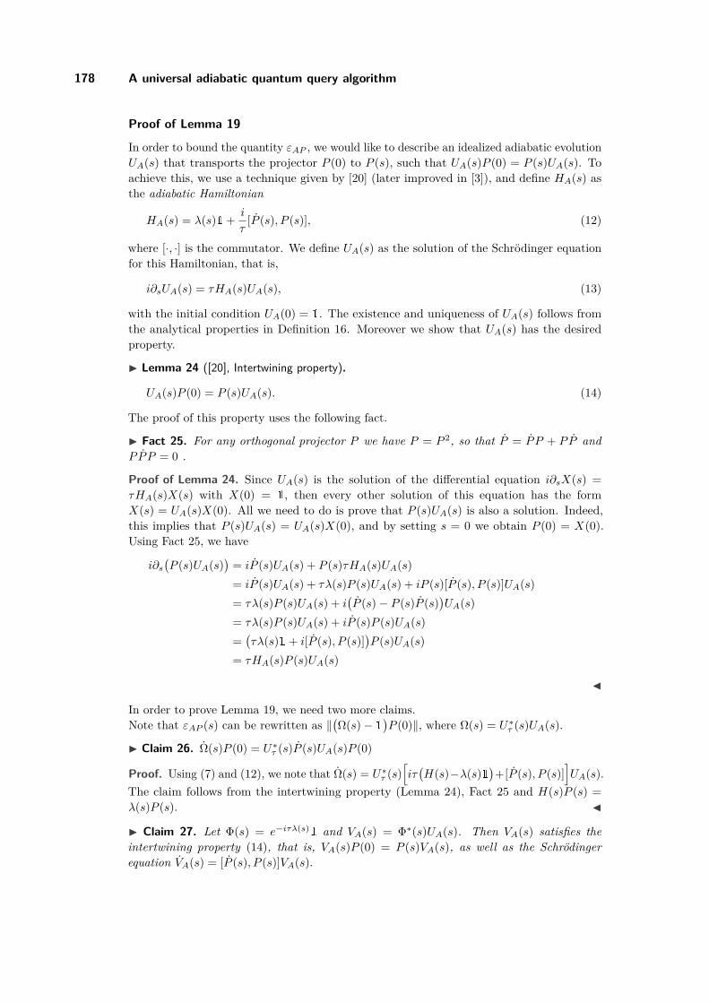
178 A universal adiabatic quantum query algorithm
Proof of Lemma 19
In order to bound the quantity εAP , we would like to describe an idealized adiabatic evolutionUA(s) that transports the projector P (0) to P (s), such that UA(s)P (0) = P (s)UA(s). Toachieve this, we use a technique given by [20] (later improved in [3]), and define HA(s) asthe adiabatic Hamiltonian
HA(s) = λ(s)1 + i
τ[P (s), P (s)], (12)
where [·, ·] is the commutator. We define UA(s) as the solution of the Schrödinger equationfor this Hamiltonian, that is,
i∂sUA(s) = τHA(s)UA(s), (13)
with the initial condition UA(0) = 1. The existence and uniqueness of UA(s) follows fromthe analytical properties in Definition 16. Moreover we show that UA(s) has the desiredproperty.
I Lemma 24 ([20], Intertwining property).
UA(s)P (0) = P (s)UA(s). (14)
The proof of this property uses the following fact.
I Fact 25. For any orthogonal projector P we have P = P 2, so that P = PP + PP andPPP = 0 .
Proof of Lemma 24. Since UA(s) is the solution of the differential equation i∂sX(s) =τHA(s)X(s) with X(0) = 1, then every other solution of this equation has the formX(s) = UA(s)X(0). All we need to do is prove that P (s)UA(s) is also a solution. Indeed,this implies that P (s)UA(s) = UA(s)X(0), and by setting s = 0 we obtain P (0) = X(0).Using Fact 25, we have
i∂s(P (s)UA(s)
)= iP (s)UA(s) + P (s)τHA(s)UA(s)= iP (s)UA(s) + τλ(s)P (s)UA(s) + iP (s)[P (s), P (s)]UA(s)= τλ(s)P (s)UA(s) + i
(P (s)− P (s)P (s)
)UA(s)
= τλ(s)P (s)UA(s) + iP (s)P (s)UA(s)=(τλ(s)1 + i[P (s), P (s)]
)P (s)UA(s)
= τHA(s)P (s)UA(s)
J
In order to prove Lemma 19, we need two more claims.Note that εAP (s) can be rewritten as ‖
(Ω(s)− 1
)P (0)‖, where Ω(s) = U∗τ (s)UA(s).
I Claim 26. Ω(s)P (0) = U∗τ (s)P (s)UA(s)P (0)
Proof. Using (7) and (12), we note that Ω(s) = U∗τ (s)[iτ(H(s)−λ(s)1
)+[P (s), P (s)]
]UA(s).
The claim follows from the intertwining property (Lemma 24), Fact 25 and H(s)P (s) =λ(s)P (s). J
I Claim 27. Let Φ(s) = e−iτλ(s)1 and VA(s) = Φ∗(s)UA(s). Then VA(s) satisfies the
intertwining property (14), that is, VA(s)P (0) = P (s)VA(s), as well as the Schrödingerequation VA(s) = [P (s), P (s)]VA(s).

M. Brandeho and J. Roland 179
Proof. The fact that VA(s) satisfies the intertwining property is immediate since UA(s)satisfies this property and Φ(s), being proportional to the identity, commutes with anyoperator. The fact that it satisfies the Schrödinger equation follows from the facts thatΦ(s) satisfies iΦ(s) = τλ(s)Φ(s), UA(s) satisfies iUA(s) = τHA(s)UA(s), and both terms ofHA(s) = λ(s)1 + i
τ [P (s), P (s)] commute. J
Let X(s) an operator solution of P (s)P (s) = [H(s), X(s)], then(Ω(s)− 1
)P (0)
=∫ s
0Ω(s′)ds′P (0)
=∫ s
0U∗τ (s′)P (s′)UA(s′)ds′P (0)
=∫ s
0U∗τ (s′)Φ(s′)P (s′)VA(s′)ds′P (0)
=∫ s
0U∗τ (s′)Φ(s′)[H(s′), X(s′)]VA(s′)ds′P (0)
=∫ s
0U∗τ (s′)Φ(s′)[H(s′)− λ(s′)]X(s′)VA(s′)ds′P (0)
= 1iτ
∫ s
0∂s′ [U∗τ (s′)Φ(s′)]X(s′)VA(s′)ds′P (0)
= 1iτ
[U∗τ (s′)Φ(s′)X(s′)VA(s′)
]s0P (0)− 1
iτ
∫ s
0U∗τ (s′)Φ(s′)∂s′ [X(s′)VA(s′)]ds′P (0)
= 1iτ
[U∗τ (s′)X(s′)UA(s′)
]s0P (0)− 1
iτ
∫ s
0U∗τ (s′)[X(s′) +X(s′)P (s′)]UA(s′)ds′P (0)
We explain line by line:(1 → 2) We use Claim 26.(2 → 3) We rearrange the expression using UA(s) = Φ(s)VA(s) and the fact that Φ(s)
commutes with any operator.(3 → 4) We use the intertwining property for VA(s) (Claim 27) and Equation (11).(6 → 7) We integrate by parts.The third term in the last line is null, because X(s) = X(s)P (s) and the intertwiningproperty (Lemma 24) yields the expression PPP , which is zero by Fact 25. Using the triangleinequality, the fact that a norm is preserved by unitary operations and can only decreaseunder projections, we finally have
εAP (s) = ‖(Ω(s)− 1
)P (0)‖
≤ 1τ
[‖X(0)‖+ ‖X(s)‖+ s max
s′∈[0,s]‖X(s′)P (s′)‖
]≤ 1τ
maxs∈[0,1]
[2‖X(s)‖+ ‖X(s)P (s)‖
]This conclude the proof. J
TQC’15

Quantum Enhancement of RandomnessDistributionRaul Garcia-Patron1, William Matthews2, and Andreas Winter3
1 Quantum Information and CommunicationEcole Polytechnique de Bruxelles, CP 165, Université Libre de Bruxelles, 1050Bruxelles, [email protected]
2 Department of Applied Mathematics and Theoretical PhysicsUniversity of Cambridge, Cambridge CB3 0WA, [email protected]
3 ICREA & Física Teòrica: Informació i Fenòmens Quàntics,Universitat Autònoma de Barcelona, ES-08193 Bellaterra (Barcelona), [email protected]
AbstractThe capability of a given channel to transmit information is, a priori, distinct from its capabilityto distribute random correlations. Despite that, for classical channels, the capacity to distributeinformation and randomness turns out to be the same, even with the assistance of auxiliarycommunication. In this work we show that this is no longer true for quantum channels whenfeedback is allowed. We prove this by constructing a channel that is noisy for the transmission ofinformation but behaves as a virtual noiseless channel for randomness distribution when assistedby feedback communication. Our result can be seen as a way of unlocking quantum randomnessinternal to the channel.
1998 ACM Subject Classification E.4 Coding and Information Theory
Keywords and phrases Quantum Shannon theory, noisy channels, capacity, randomness
Digital Object Identifier 10.4230/LIPIcs.TQC.2015.180
1 Summary
Randomness and information are different concepts. We think of information of as that whichis sent as a specific message to another person or machine. On the other hand, randomnesscan be intuitively understood as the outcome of a noisy process. Information and randomnessbeing different concepts, the capability to distribute them over a channel could, a priori, beinequivalent resources. More precisely, the capability to distribute a bit of randomness isa weaker resource than the potential to communicate a bit of information over a channel,because if Alice is capable of distributing a bit of information to Bob over a noisy channelshe can also locally generate a pair of correlated bits and transmit one to Bob, generatinga bit of shared randomness. Therefore, the capacity R(E) of randomness distribution of anoisy channel E is in principle higher than that of information communication C(E), i.e.,C(E) ≤ R(E).
We may also ask about the capacity of a channel to communicate or distribute randomnesswhen auxiliary classical communication is allowed. For communication, we thus have thecapacity of the channel assisted by feedback C←, the capacity assisted by auxiliary forwardcommunication C→ and the capacity assisted by two-way classical communication C↔. Since
© R.aul Garcia-Patron, William Matthews, and Andreas Winter;licensed under Creative Commons License CC-BY
10th Conference on the Theory of Quantum Computation, Communication and Cryptography (TQC 2015).Editors: Salman Beigi and Robert König; pp. 180–190
Leibniz International Proceedings in InformaticsSchloss Dagstuhl – Leibniz-Zentrum für Informatik, Dagstuhl Publishing, Germany

R. Garcia-Patron, W. Matthews, and A. Winter 181
the auxiliary forward communication can be used to communicate by itself, we must subtractthe amount of auxiliary forward communication from the gross communication rates inthe definitions of the later two quantities. For the distribution of shared randomness wecan similarly define rates R←, R→, R↔, but in this case we must subtract both forwardand backward auxiliary communication, as both of these may be used to establish sharedrandomness by themselves.
In the setting with feedback assistance, the tradeoff between the gross rate of randomnessdistribution and the rate of feedback allowed was characterised (among many other things)by Ahlswede and Csiszár in [2]. A corollary of their result is that R←(E) = C(E) for classicalchannels. To our knowledge the only previous work studying the generation of sharedrandomness in a quantum scenario was the work of Devetak and Winter [6] on the distillationof common randomness from bipartite quantum states. That work considered a static scenarioof distillation of randomness from a quantum state already shared between Alice and Bob,where in this manuscript we are interested on a dynamic scenario of randomness distributionover quantum channels.
In section 3 we show that, for general quantum channels E , the entanglement-assistedcapacity [12] of E , CE(E), is an upper bound on the largest of the randomness distributioncapacities, R↔(E). Since CE(E) is equal to C(E) for classical-quantum channels (whichinclude classical channels), this establishes the equality
R(E) = R←(E) = R→(E) = R↔(E) = C(E)
for such channels. A simple argument can be used to show that we also have
C(E) = C←(E) = C→(E) = C↔(E)
for such classical-quantum channels, so in this case all eight quantities are then same. Whenthe channel is classical
C(E) = maxPX
I(X : Y ), (1)
where X and Y are the input and output to a single use of the channel E with X distributedaccording to PX [1].
As opposed to the classical regime, where all capacities turn out to be equal, in thequantum scenario randomness distribution and communication remain equivalent only whenwe consider unassisted or forward assisted classical communication. That is, for generalchannels E , we have C(E) = R(E) = C→(E) = R→(E), as shown in subsection 4.1.
In section 4.2 we show that, for quantum-classical channels E , feedback allows the upperbound in terms of CE(E) to be achieved, and therefore
R←(E) = R↔(E) = CE(E).
On the other hand, since quantum-classical channels are entanglement-breaking, a resultof Bowen and Nagarajan [3] tells us that C←(E) = C(E), so any quantum-classical channelwith C(E) < CE(E) also demonstrates a separation C←(E) < R←(E). Holevo has shown thatthere are many such channels [4], and we give an explicit example, where the randomnessdistribution protocol is noiseless, in subsection 4.3.
2 Definitions
Our definitions in this section are based on those used by Ahlswede and Csiszár in [2], andDevetak and Winter [6].
TQC’15

182 Quantum Enhancement of Randomness Distribution
E E
A0 A1 A2 A3 A4 J
B0 B1 B2 B3 B4 K
X1
Y1
Z1 Z2
X2
Y2
Figure 1 An example of a two-way assisted randomness distillation protocol which makes twouses of the channel E . Time runs left to right. Classical systems are shown as double lines, quantumsystems as solid lines. Empty boxes represent local processing. We denote by Aj Alice’s system,and by Bj Bob’s system, immediately after step j of the protocol. The communication is eitherforward communication via one use of the noisy channel E , where Alice inputs Xi and Bob receivesthe output Yi, or forward/backward auxiliary noiseless classical communication Zi.
A two-way assisted randomness distribution protocol for a channel E consists of localgeneration of random variables A0 and B0 followed by a finite number of steps, each consistingof communication followed by local processing. The communication is either (i) forwardcommunication via one use of the noisy channel E , where Alice makes an input Xi and Bobreceives the output Yi; (ii) forward auxiliary noiseless classical communication; (iii) backwardauxiliary noiseless classical communication.
Suppose we have a protocol of n+m steps where n of the steps are of type (i) and theother m steps are of type (ii) or (iii). We denote by Aj Alice’s system, and by Bj Bob’ssystem, immediately after step j of the protocol. At the end of the protocol, Alice mustproduce random variable J and Bob must produce K, both of which take values in the samealphabet AK , by local processing of their respective final systems Am+n and Am+n. Anexample of such a protocol with n = m = 2 is illustrated in Figure 1.
We require that
log |AK | ≤ exp(cn) (2)
for some constant c independent of n (but depending on the channel E). We say that theprotocol is ε-good if Pr(J 6= K) ≤ ε. By Fano’s inequality and (2), an ε-good protocol has
H(K|J) ≤ εcn+ 1 (3)
We denote the data transmitted in each instance of auxiliary communication (regardlessof whether it is forward or backward) by Zk, where k ∈ 1, . . . ,m, in temporal order.
If the total auxiliary communication Z := Z(m) := (Z1, . . . , Zm) has |AZ | possible values(we require this number to be finite for any given protocol), then this alone would allow theparties to establish log |AZ | bits of perfect common randomness without using E at all! Wetherefore subtract log |AZ | from the final amount of common randomness established andhence define the net rate of the protocol is
1n
(H(K)− log |AZ |).
A forward-assisted randomness distribution protocol is one in which all steps are oftype (i) or (ii). A back-assisted randomness distribution protocol is one in which all stepsare of type (i) or (iii). An unassisted randomness distribution protocol is one in which allsteps are of type (i).

R. Garcia-Patron, W. Matthews, and A. Winter 183
I Definition 1. We say a net rate R is achieved by two-way protocols for channel E if forall ε > 0 and all sufficiently large n, there is an ε-good protocol for n noisy channel useswith net rate no less than R. We define R↔(E) to be the supremum of net rates achievedby two-way protocols; R→(E) to be the supremum of net rates achieved by forward-assistedprotocols; R←(E) to be the supremum of net rates achieved by back-assisted protocols; andR(E) to be the supremum of net rates achieved by unassisted protocols;
It follows immediately from the definitions that
R(E) ≤ R→(E) ≤ R↔(E) and R(E) ≤ R←(E) ≤ R↔(E). (4)
3 Classical equality between information and randomness distribution
In this section we will show that R↔(E) can be no larger than the entanglement-assistedcapacity of E , CE(E). Since CE(E) = C(E) for classical channels (and, more generally, forclassical-quantum channels), this establishes that
C(E) = R←(E) = R→(E) = R↔(E)
for such channels. We note that common randomness distribution via a classical channel Eand noiseless feedback was considered by Ahslwede and Csiszar in [2], and that the equalityC(E) = R←(E) is a corollary of their Theorem 4.3.
It was shown by Bennett, Shor, Smolin and Thapliyal [12], that the entanglement-assistedclassical capacity of a channel EY←X is given by
CE(E) = maxρRX
I(R : Y)EY←XρRX . (5)
We will show that the same formula is an upper bound on R↔(E).
I Theorem 2. For any channel E, R↔(E) ≤ CE(E).
Proof. Let us consider a protocol which makes n uses of the channel E and m auxiliarycommunication steps. For k ∈ 1, . . . , n, let Xk denote the input system, and Yk the outputsystem, for the k-th use of the noisy channel.
Initially, Alice and Bob have systems A0 and B0 which are uncorrelated in that I(A0 :B0) = 0. We may assume without loss of generality that any local randomness used inthe protocol is already present in the state of these systems. We may assume without lossof generality that at each step Alice and Bob have retained a full record of all auxiliarycommunication up to that step.
Suppose that at step j of the protocol, Bob sends Alice Zk by auxiliary back communica-tion. Then we may bound
I(Aj : Bj)(a)≤ I(Aj−1Zk : Bj)
(b)≤ I(Aj−1Zk : Bj−1)
=I(Aj−1 : Bj−1) +H(Zk|Aj−1)−H(Zk|Aj−1Bj−1)(c)≤I(Aj−1 : Bj−1) +H(Zk|Aj−1)
(d)≤ I(Aj−1 : Bj−1) +H(Zk|Z(k−1)) (6)
where (a) and (b) are data processing, (c) is because, since Zk is classical,H(Zk|Aj−1Bj−1) ≥0 and (d) is because Aj−1 includes Z(k−1). A similar argument establishes the same inequalitywhen Alice sends Bob Zk by auxiliary forward communication, instead.
TQC’15

184 Quantum Enhancement of Randomness Distribution
Now consider the case where Alice makes an input Xk to the noisy channel E at step j,with Bob receiving output Yk. Then
I(Aj : Bj)(a)≤ I(Aj : Bj−1Yk)=I(Aj : Yk) + I(Aj : Bj−1|Yk)=I(Aj : Yk) + I(AjYk : Bj−1)− I(Yk : Bj−1)
(b)≤I(Aj : Yk) + I(AjYk : Bj−1)(c)≤I(Aj : Yk) + I(Aj−1 : Bj−1)(d)≤CE(E) + I(Aj−1 : Bj−1). (7)
Here, (a) and (c) are by data processing, (b) is positivity of mutual information, and (d) isby the result of Bennett, Shor, Smolin and Thapliyal.
Recall that Z := Z(m) is the total record of auxiliary communication. Starting withI(An+m : Bn+m), and repeatedly invoking the inequality (6) or (7) depending on the type ofstep, we obtain
I(An+m : Bn+m) ≤I(B0 : A0) + nCE(E) +m∑k=1
H(Zk|Z(k−1))
=nCE(E) +H(Z)≤nCE(E) + log |AZ |, (8)
where the equality is by the chain rule and I(B0 : A0) = 0. Finally, we bound the net rate Rof the protocol by
R = 1n
(H(K)− log |AZ |) = 1n
(I(K : J) +H(K|J)− log |AZ |)(a)≤ 1n
(I(An+m : Bn+m) +H(K|J)− log |AZ |)(b)≤ 1n
(nCE(E) + log |AZ |+ ncε+ 1− log |AZ |)(c)=CE(E) + cε+ 1/n
where (a) is data processing, (b) is by inequalities (8) and (3), and (c) by is Shannon’s noisychannel coding theorem. Recalling the definition of R↔, we have established that
R↔(E) ≤ CE(E). (9)
J
We also claimed that C(E) = C←(E) = C→(E) = C↔(E) for classical-quantum channels.In fact, we can show that this is true of any entanglement-breaking channel. The generalequality C(E) = C←(E) is established in the next section. Now, note that we can write
C↔(E) = supmC←(E ⊗ Am)− logm
where Am is a classical identity channel with m input symbols. Since E and Am are bothentanglement-breaking, we have
C←(E ⊗ Am) = C(E ⊗ Am) = C(E) + C(Am) = C(E) + logm

R. Garcia-Patron, W. Matthews, and A. Winter 185
C = C→ <
R = R→
1 3 2
4
=
1 1
41
=
< R← ? R↔
C← < C↔<
?
Figure 2 Relations between the communication (C) and randomness distribution (R) capacities.Note that an equality means that both capacities are equal for all channels; On the other hand,an inequality means that we know of at least one channel where one is strictly higher, which doesnot preclude the possibility that for other channels they may be equal. (1) It is easy to proveC = R = C→ = R→, see Section 4.1 below. (2) Corollary of [11], using echo-correctable channels.(3) Corollary of [9], using random-phase coupling channels. (4) Our result in subsection 4.2. Therelations between R←(E), R↔(E) and C↔(E), i.e., whether they are equal for all channels or thereare some examples of strict separation between them, remains an open question.
by Bowen-Nagarajan [3], the HSW theorem [7, 8], and the fact that the Holevo informationis additive for entanglement breaking channels [10]. Therefore,
C←(E) = C↔(E) = C(E)
for entanglement-breaking E .
4 Quantum scenario
As opposed to the classical scenario, where all capacities of randomness distribution andinformation transmission, collapse into a single quantity given by Shannon’s capacity, quantumchannels have a richer behaviour depicted in Figure 2. The only similarity between thequantum and classical scenario is restricted to the unassisted and forward assisted capacitieswhere, as shown in subsection 4.1 below, one can prove the equality
C(E) = R(E) = C→(E) = R→(E). (10)
The situation changes radically for feedback and two-way assisted capacities. It was shownin [11] that by concatenating an echo-correctable channel and a depolarizing channel onecan obtain an entanglement-breaking channel exhibiting a strict separation C←(E) < C↔(E).Subsequently, in [9], the possibility of a strict separation C→(E) < C←(E) was shown usingrandom-phase coupling channels (also informally called rocket channels). In subsection 4.2below we show that there can be a separation C←(E) < R←(E). As a corollary we alsoobtain the separation R→(E) < R←(E).
4.1 Equality between unassisted and forward-assisted capacitiesIt is straightforward to see that C(E) ≤ C→(E) and R(E) ≤ R→(E) (assistance can onlyincrease the rate), C(E) ≤ R(E) (if you can send a bit of information you can also distribute
TQC’15

186 Quantum Enhancement of Randomness Distribution
E E
A0 A1 A2 A3 R J
B0
K
X1
Y1
Z1
X2
Y2
Z2
τJZYn
Figure 3 An example of a forward assisted randomness distillation protocol which makes twouses of the channel E . Without loss of generality, Bob waits until receiving all communication fromAlice to perform his local processing, and obtain K.
a bit of shared randomness) and similarly C→(E) ≤ R→(E), because in both cases weonly subtract the assisting forward communicaiton. In order to prove the equality betweenunassisted and forward-assisted capacities in eq. (10), it is sufficient to prove that thehighest of the four capacities, R→(E), is upper-bounded by the lowest of them, i.e. thatR→(E) ≤ C(E).
Since Bob does not send anything back to Alice during a forward-assisted protocol, thereis no loss of generality if Alice makes all n uses of the noisy channel, sends all auxiliaryclassical communication and computes her share of the common randomness, J , before Bobdoes anything, as illustrated in Figure 3. We denote by R all systems retained by Alice, fromwhich she computes her share of the common randomness.
Let Xn be the n input systems, and Yn the n output systems, for the n uses of thenoisy channel E⊗n. We introduce a register Z which stores the value of the auxiliaryforward communication Z, which can take one of |AZ | values. After Alice has made all hercommunication to Bob, the state of the ZYnR system is
σZYnR =∑z
p(z)|z〉〈z|Z ⊗ E⊗nYn←Xnρ(z)XnR (11)
where ρ(z)XnR is the state of the XnR, conditioned on Z = z. Now, Alice performs a measurement
E(j) (POVM of outcome j) on the system R to obtain her share J of the common randomness,which is stored in register J. At this point the state of the system is
τJZYn =∑z
q(j|z)p(z)|j〉〈j|J ⊗ |z〉〈z|Z ⊗ E⊗nYn←Xnρ(z,j)Xn , (12)
where
q(j|z)ρ(z,j)Xn := TrRE(j)Rρ
(z)XnR
defines the states ρ(z,j)Xn and conditional distribution q(j|z).
Then Bob performs a measurement on the ZYn system to obtain his share of randomnessK. We can bound the mutual information between the shares by
I(J : K)(a)≤ I(J : ZYn)τ = I(J : Yn)τ + I(J : Z|Yn)τ=I(J : Yn)τ +H(Z)τ − I(Z : Yn)τ −H(Z|J,Yn)τ
(b)≤I(J : Yn)τ +H(Z)τ
(c)≤ χ(E⊗n) + log |AZ | (13)

R. Garcia-Patron, W. Matthews, and A. Winter 187
where (a) is data processing, (b) is because τ is separable with respect to the Z/JYn
bipartition so H(Z|JYn) ≥ 0, and by positivity of mutual information, and (c) is becauseI(J : Yn) ≤ χ(E⊗n). We use this to bound the net rate R of the protocol thus
R = 1n
(H(K)− log |AZ |) = 1n
(I(K : J) +H(K|J)− log |AZ |)
≤ 1n
(χ(E⊗n) + log |AZ |+H(K|J)− log |AZ |) ≤1nχ(E⊗n) + cε+ 1/n,
and therefore R→(E) ≤ limn→∞1nχ(E⊗n) = C(E), where the equality is the Holevo-
Schumacher-Westmoreland theorem [7, 8].
4.2 Quantum-classical channels; separation C←(E) < R←(E)Suppose that EY←X is a quantum-classical channel. That is, a channel of the form
EY←X : ρX 7→∑y∈AY
|y〉〈y|Y trE(y)XρX (14)
where E(y)X : y ∈ AY is a POVM on X. In this case we can show that there is aback-assisted randomness distribution which achieves the upper-bound CE(E) for two-wayassisted protocols, and therefore:
I Theorem 3. For quantum-classical channels EY←X, R←(E) = R↔(E) = CE(E).
We just need to show achievability: One way that n uses of a quantum-classical channelcan be used to produce randomness with auxiliary back communication is as follows. Alicelocally prepares n copies of a state ψRX and applies the n uses of the channel to Xn. Thisresults in n copies of a quantum-classical state∑
y
p(y)ρ(y)R ⊗ |y〉〈y|Y = EY←XψRX (15)
being shared between Alice and Bob, with Bob holding the classical register Y , and p(y) :=trRXE(y)XψRX and ρ(y)R := trXE(y)XψRX/p(y). Now, in the proof of the classical-quantumSlepian-Wolf theorem of Devetak and Winter [5] it was shown that, for any 0 < ε < 1/2 andδ > 0, and all sufficiently large n, we can find |AZ | disjoint subsets Cz : z ∈ AZ of AnYsuch that(i) the probability that Y n fails to belong to one of the subsets is not more than 2ε,(ii) given the knowledge Y n ∈ Cz, Alice can perform a measurement on Rn which identifies
Y n with probability of error no more than ε,(iii) 1
n log |AZ | ≤ H(Y |R) + 2δ.This suggests the following protocol: Bob takes K = Y n as his share of the common
randomness (so H(K) = nH(Y )) and sends Alice the identity Z of a subset CZ containingY n (if such exists) whereupon Alice measures Rn to obtain an estimate J of Y n. Thisprotocol has Pr(K 6= J) ≤ 3ε and net rate
1n
(H(K)− log |AZ |) ≥ H(Y )−H(Y |R)− 2δ = I(Y : R)− 2δ.
Therefore, by optimising over the choice of ψXR in the protocol, we have established that
R←(E) ≥ maxψXR
I(Y : R)EY←XψXR = CE(E), (16)
TQC’15
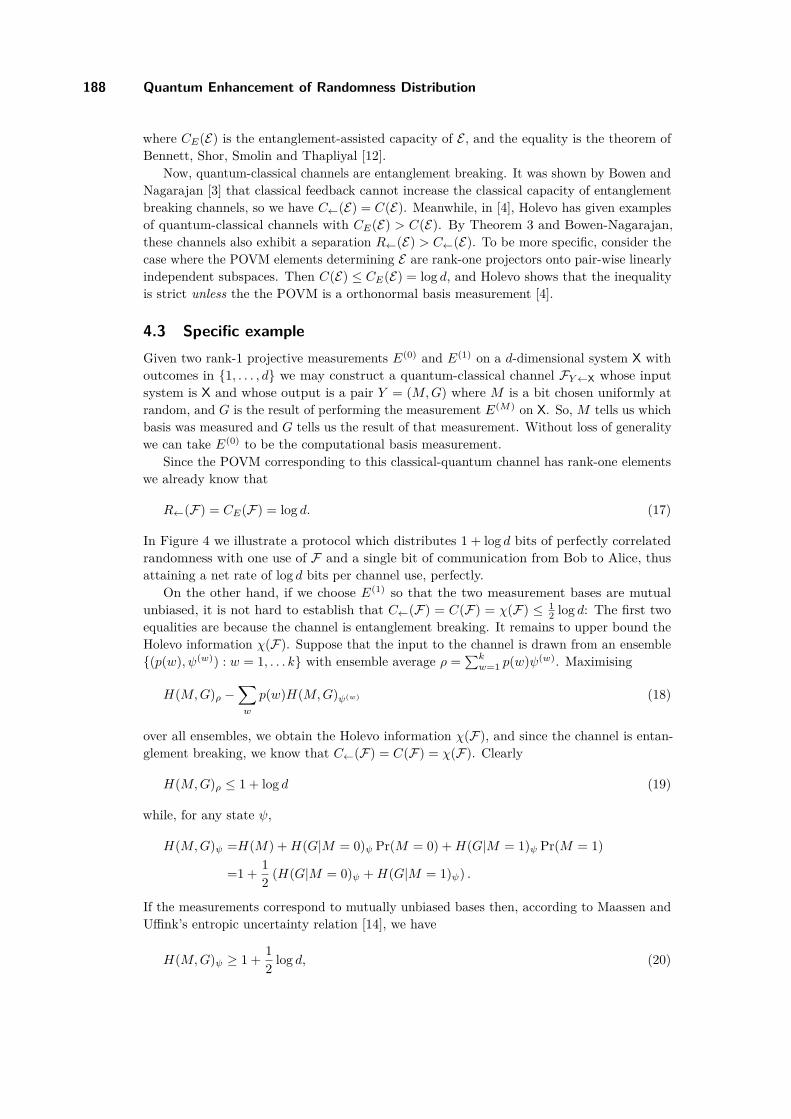
188 Quantum Enhancement of Randomness Distribution
where CE(E) is the entanglement-assisted capacity of E , and the equality is the theorem ofBennett, Shor, Smolin and Thapliyal [12].
Now, quantum-classical channels are entanglement breaking. It was shown by Bowen andNagarajan [3] that classical feedback cannot increase the classical capacity of entanglementbreaking channels, so we have C←(E) = C(E). Meanwhile, in [4], Holevo has given examplesof quantum-classical channels with CE(E) > C(E). By Theorem 3 and Bowen-Nagarajan,these channels also exhibit a separation R←(E) > C←(E). To be more specific, consider thecase where the POVM elements determining E are rank-one projectors onto pair-wise linearlyindependent subspaces. Then C(E) ≤ CE(E) = log d, and Holevo shows that the inequalityis strict unless the the POVM is a orthonormal basis measurement [4].
4.3 Specific exampleGiven two rank-1 projective measurements E(0) and E(1) on a d-dimensional system X withoutcomes in 1, . . . , d we may construct a quantum-classical channel FY←X whose inputsystem is X and whose output is a pair Y = (M,G) where M is a bit chosen uniformly atrandom, and G is the result of performing the measurement E(M) on X. So, M tells us whichbasis was measured and G tells us the result of that measurement. Without loss of generalitywe can take E(0) to be the computational basis measurement.
Since the POVM corresponding to this classical-quantum channel has rank-one elementswe already know that
R←(F) = CE(F) = log d. (17)
In Figure 4 we illustrate a protocol which distributes 1 + log d bits of perfectly correlatedrandomness with one use of F and a single bit of communication from Bob to Alice, thusattaining a net rate of log d bits per channel use, perfectly.
On the other hand, if we choose E(1) so that the two measurement bases are mutualunbiased, it is not hard to establish that C←(F) = C(F) = χ(F) ≤ 1
2 log d: The first twoequalities are because the channel is entanglement breaking. It remains to upper bound theHolevo information χ(F). Suppose that the input to the channel is drawn from an ensemble(p(w), ψ(w)) : w = 1, . . . k with ensemble average ρ =
∑kw=1 p(w)ψ(w). Maximising
H(M,G)ρ −∑w
p(w)H(M,G)ψ(w) (18)
over all ensembles, we obtain the Holevo information χ(F), and since the channel is entan-glement breaking, we know that C←(F) = C(F) = χ(F). Clearly
H(M,G)ρ ≤ 1 + log d (19)
while, for any state ψ,
H(M,G)ψ =H(M) +H(G|M = 0)ψ Pr(M = 0) +H(G|M = 1)ψ Pr(M = 1)
=1 + 12 (H(G|M = 0)ψ +H(G|M = 1)ψ) .
If the measurements correspond to mutually unbiased bases then, according to Maassen andUffink’s entropic uncertainty relation [14], we have
H(M,G)ψ ≥ 1 + 12 log d, (20)

R. Garcia-Patron, W. Matthews, and A. Winter 189
M
U
U
φRX
F
R
X
G
G
Z = M
Z
M
G
Figure 4 Sharing 1 + log d bits of perfect randomness with one use of the channel F (the contentsof the dashed rectangle) and one bit of back communication: Alice locally prepares a maximallyentangled state φRX and inputs X to the channel. We can view the channel as performing a unitarycontrolled by the bit M and then performing a computational basis measurement to yield G. Alicesets Z = M and sends Z to Bob, who performs U (the complex conjugate of U) iff Z = 1 and thenperforms a computational basis measurement on R to yield a value G. By the U ⊗ U invarianceof φ, G = G with probability one, so if Alice sets J = (G, Z) and Bob sets K = (G,M) thenPr(K = J) = 1, and K is uniformly distributed. Local operations are surrounded by dotted lines.
and substituting the bounds (19) and (20) into (18),
C←(E) = C(E) = χ(E) ≤ 12 log d.
This upper bound is indeed tight for both, C←(E) and C(E), as the channel E can betransformed with some post-processing on Bob’s side into an erasure channel (if M = 1 eraseregister G) of error probability 1/2. Therefore (feedback-assisted) error-correcting codes forthe erasure channel can be used to saturate the bound C(E) = C←(E) = 1/2 log d.
5 Conclusion
Despite being, a priori, different things, we have seen that the capacity for a classical channelto distribute shared randomness and to send information are the same, with arbitraryclassical assistance. For quantum channels, we have shown that the entanglement-assistedcapacity CE(E) is a general upper bound for R↔(E), and shown that this bound can beachieved using only back-communication for quantum-classical channels. Using this result wehave established that strict separations C←(E) < R←(E) are possible for quantum-classicalchannels. We give an explicit example for which R←(E) = log d while C←(E) = 1
2 log d.Our result shows that contrary to what is predicted by classical information theory, where
the optimal way of distributing randomness is to generate it locally and distribute it throughthe channel, quantum mechanics allows for the activation of randomness initially lockedinside the channel, which boost the amount of shared randomness generated in the process.
TQC’15

190 Quantum Enhancement of Randomness Distribution
References1 T.M. Cover and J.A. Thomas, Elements of Information Theory, (Wiley, New York, 1991).2 R. Ahlswede and I. Csiszár, IEEE Trans. Info. Theory 39, pp. 1121–1132 (1993).3 G. Bowen and R. Nagarajan, IEEE Trans. Inform. Theory 51, 320 (2005).4 A. Holevo, Problems of Information Transmission, vol. 48 (2012), pp. 1–10.5 I. Devetak and A. Winter, Phys. Rev. A 68, 042301 (2003)6 I. Devetak and A. Winter, IEEE Trans. Info. Theory 50, 3183 (2004).7 A. Holevo, IEEE Transactions on Information Theory 44(1):269–273 (1996).8 B. Schumacher, M. Westmoreland, Phys. Rev. A 56:131–138 (1997).9 G. Smith and J.A. Smolin, Phys. Rev. Lett. 103, 120503 (2009).
10 Additivity of the classical capacity of entanglement-breaking quantum channels. Journal ofMathematical Physics, 43(9):4334–4340, (2002).
11 C.H. Bennett, I. Devetak, P.W. Shor, and J.A. Smolin, Phys. Rev. Lett. 96, 150502 (2006).12 C.H. Bennett, P.W. Shor, J. A. Smolin, A.V. Thapliyal, IEEE Trans. Info. Theory 48,
2637 (2002).13 L.P. Hughston, R. Jozsa, and W.K. Wootters, Phys. Lett. A 183, 14 (1993).14 H. Maassen, and J. Uffink, Phys. Rev. Lett. 60, 1103 (1988)

Implementing Unitary 2-Designs Using RandomDiagonal-unitary MatricesYoshifumi Nakata∗1, Christoph Hirche†1, Ciara Morgan1, andAndreas Winter2
1 Institut für Theoretische Physik, Leibniz Universität Hannover,Appelstrasse 2, 30167 Hannover, Germanyyoshifumi.nakata,christoph.hirche,[email protected]
2 ICREA & Física Teòrica: Informació i Fenòmens Quàntics,Universitat Autònoma de Barcelona, ES-08193 Bellaterra (Barcelona), [email protected]
AbstractUnitary 2-designs are random unitary matrices which, in contrast to their Haar-distributed coun-terparts, have been shown to be efficiently realized by quantum circuits. Most notably, unitary2-designs are known to achieve decoupling, a fundamental primitive of paramount importance inquantum Shannon theory. Here we prove that unitary 2-designs can be implemented approxim-ately using random diagonal-unitaries.
1998 ACM Subject Classification H.1.1 Systems and Information Theory
Keywords and phrases Unitary 2-designs, commuting quantum circuits
Digital Object Identifier 10.4230/LIPIcs.TQC.2015.191
1 Introduction
With coherent implementations of quantum circuits becoming a reality, the question of thepractical realization of protocols in quantum information science has been a particular focusof the field in recent years. Indeed, quantum information theory itself is concerned withthe evolution of quantum systems and decoupling represents one of the most fundamentalprimitives [1, 2, 3, 4]. Moreover, this protocol characterizes the conditions under whichtwo, initially correlated, quantum systems will decohere completely, after evolution and theprotocol itself is achieved using so-called Haar random unitaries [5, 6].
While Haar random unitaries are a powerful theoretical tool, the number of gates requiredto achieve their implementation grows exponentially in the system size. Unitary designsrepresent finite approximations of Haar random unitaries and, unitary 2-designs in particular,have been shown to efficiently achieve the decoupling protocol [7]. Moreover, unitary designsand the analysis of their performance have been widely studied [8, 9, 10, 11, 12, 13, 14, 15,16, 17, 18]. Unitary 2-designs have been shown to be achieved using Clifford circuits [8, 9]and random quantum circuits [12, 13, 14, 15] and among the most notable of results is therecent breakthrough of Cleve et al. [18] demonstrating a “near linear” implementation of anexact unitary 2-design.
∗ Now at: Photon Science Center, Graduate School of Engineering, The University of Tokyo, Bunkyo-ku,Tokyo 113-8656, Japan – [email protected] .
† Now at: Física Teòrica: Informació i Fenòmens Quàntics, Universitat Autònoma de Barcelona, ES-08193Bellaterra (Barcelona), Spain – [email protected] .
© Yoshifumi Nakata, Christoph Hirche, Ciara Morgan, and Andreas Winter;licensed under Creative Commons License CC-BY
10th Conference on the Theory of Quantum Computation, Communication and Cryptography (TQC 2015).Editors: Salman Beigi and Robert König; pp. 191–205
Leibniz International Proceedings in InformaticsSchloss Dagstuhl – Leibniz-Zentrum für Informatik, Dagstuhl Publishing, Germany

192 Implementing Unitary 2-Designs Using Random Diagonal-unitary Matrices
This motivates the question of how simply unitary 2-designs can be achieved. In thispaper we show that unitary 2-designs can be realized to arbitrary precision by randomdiagonal-unitaries. Along with theoretical interest, the significance of this result lies inits simple implementation. Indeed, a quantum circuit for the implementation consists ofrepeating single-qubit phase gates, the controlled-Z gates, and the Hadamard gates. The firsttwo parts are commuting, and they can be applied, in principle, simultaneously. Moreover,the depth of the non-commuting part, i.e. the Hadamard gates, is O(1). These features ofour implementation leads to a vast reduction in the execution time of the overall circuit. Thiswork also provides a concrete application of commuting quantum circuits. Little is knownabout their concrete applications [19, 20] though they are known to provide a quantumadvantage in computational tasks [21, 22]. The present authors have also shown that thedecoupling theorem can be achieved by random-diagonal unitaries [23].
The article is organised as follows. We begin by introducing the necessary definitions andnotation in Section 2. The main results are presented in Section 3, with the statement thatunitary 2-designs can be achieved using random diagonal-unitary matrices given by Theorem5 and the implementation given by Corollary 6. Proofs of the main results are presented inSection 4, along with statements of the necessary lemmas. Indeed, Lemma 8 is of particularimportance in our analysis.
2 Preliminaries
2.1 NotationWe consider a system composed of N qubits and denote by H, the corresponding Hilbertspace and by d = 2N the dimension of H. The set of bounded operators and states on H aredenoted by B(H) and S(H) := ρ ∈ B(H)|ρ ≥ 0, trρ = 1, respectively.
We will make use of various norms throughout the article, defined as follows. Thep-norm of X ∈ B(H) is defined by ||X||p := (tr|X|p)1/p for p ≥ 1. For a superoperatorC : B(H) → B(H), we use a family of superoperator norms ||C||q→p (q, p ≥ 1) and thediamond norm [24] defined by
||C||q→p = supX 6=0
||C(X)||p||X||q
, ||C|| := supk||C ⊗ idk||1→1, (1)
respectively, where idk is the identity map acting on a Hilbert space of dimension k. Notethat it is known that k ≤ d is sufficient to obtain the diamond norm [24].
2.2 Random unitary matrices and their t-designsWe begin with the definition of random unitary matrices, before discussing their role inquantum information science, leading to the definition of unitary t-designs and approxima-tions.
I Definition 1 (Haar random unitary matrices [25]). Let U(d) be the unitary group of degreed, and denote the Haar measure (i.e. the unique unitarily invariant probability measure,thus often called uniform distribution) on U(d) by HU(d). A Haar random unitary matrix Uis a U(d)-valued random variable distributed according to the Haar measure, U ∼ HU(d).
I Definition 2 (Random X- and Z-diagonal-unitary matrices [19]). Let DW,diag be the set ofunitary matrices diagonal in the Pauli-W basis |n〉W
d−1n=0 (W = X,Z), given by∑d−1
n=0 eiϕn |n〉〈n|W : ϕn ∈ [0, 2π) for n ∈ [0, . . . , d − 1]
. Let DW denote a probability

Y. Nakata, C. Hirche, C. Morgan, and A. Winter 193
measure on it induced by a uniform probability measure on its parameter space [0, 2π)d.A random W -diagonal-unitary matrix DW is a DW,diag-valued random variable distributedaccording to DW , DW ∼ DW .
The random unitary matrices, defined above, have been applied to a wide variety ofproblems in quantum information science (see e.g. [16] for a summary) and have been usedto investigate typical properties in physical systems [26, 27, 28, 29]. However, they cannot beefficiently implemented by quantum circuits, since the number of random numbers needed forthe implementation scales exponentially with the number of qubits in the system. This facthas lead to the investigation of their approximation, that is, to the definition and performanceanalysis of unitary t-designs [8, 9, 10, 11, 12, 13, 14, 16, 15, 17, 18].
Indeed, a unitary t-design is a random variable taking values in the unitary group thatsimulate, up to the tth order, the statistical moments of a given random unitary matrix. Todefine a unitary t-design for a random unitary matrix U , let G(t)
U (X) be a superoperator givenby G(t)
U (X) := EU [U⊗tXU†⊗t] for any X ∈ B(H⊗t), where EU represents an expectation overU . Then, an ε-approximate unitary t-design is defined as follows.
I Definition 3 (ε-approximate unitary t-designs [9, 14]). A random unitary matrix U ∈ U(d)is called an ε-approximate unitary t-design if ||G(t)
U −G(t)UH|| ≤ ε, where UH is a Haar random
unitary matrix.
I Definition 4 (ε-approximate diagonal-unitary t-designs [19]). A random diagonal-unitarymatrix U ∈ DW,diag (W = X,Z) is called an ε-approximate W -diagonal-unitary t-design if||G(t)U − G
(t)DW || ≤ ε, where DW is a random W -diagonal unitary matrix.
In these definitions, the designs are called exact when ε = 0. Note that there arevarious definitions of ε-approximate unitary t-designs, a summary of which can be found inRef. [16]. Most definitions are equivalent in the sense that, if U is an ε-approximate unitaryt-design in one definition, it is also an ε′-approximate unitary t-design in other definitions forε′ = poly(dt)ε.
3 Main results
3.1 A unitary 2-design by random diagonal-unitary matricesWe study an implementation of a unitary 2-design using random diagonal-unitary matrices.We alternately apply independent random Z- and X-diagonal-unitary matrices, and showthat this strategy approaches a unitary 2-design, after a number of repetitions `. A randomunitary matrix obtained by this process is given by
D[`] := DZ`+1D
X` D
Z` · · ·DX
2 DZ2 D
X1 D
Z1 . (2)
where DWi are independent W -diagonal-unitary matrices (i = 1, . . . , `+ 1, W = X,Z). The
D[`] can, equivalently, be expressed as
D[`] =1∏i=`
D′Zi D
Xi D
Zi , (3)
where all random diagonal-unitary matrices are taken independently. We will use thisparticular expression of D[`] in the remainder of the article.
TQC’15

194 Implementing Unitary 2-Designs Using Random Diagonal-unitary Matrices
Note that, since a random X-diagonal-unitary matrix can be obtained by conjugating arandom Z-diagonal-unitary matrix by Hadamard gates, D[`] can equivalently be expressedas
D[`] = DZ2`+1
1∏i=2`
(H⊗NDZi ), (4)
where H⊗N is the tensor product of N Hadamard gates acting on all N qubits. From thispoint of view, the Hadamard gates are the only non-commuting part of D[`]. We will usethis expression when we consider an efficient implementation of D[`] in Subsection 3.2.
Our main result shows that D[`] quickly approaches a unitary 2-design with increasing `.The formal statement is given by Theorem 5 below.
I Theorem 5 (D[`] is an approximate unitary 2-design). A random unitary matrix D[`], actingon N qubits, is an ε-approximate unitary 2-design for ` ≥ 2 + 1
N (1 + log 1/ε). Conversely,D[`] cannot be an ε-approximate unitary 2-design if ` ≤ 1
N log 1/ε.
I Remark. The significance of Theorem 5 lies in the efficiency of its implementation. Moreover,since a random unitary matrix D[`] can be separated into commuting (random Z-diagonal-unitary matrices) and non-commuting (the Hadamard gates) parts, and the number ofnon-commuting gates for the implementation scales linearly with the system size, thisconstruction of an approximate unitary 2-design has a simple practical implementation. Weexpand upon this point in the following subsection.
3.2 Implementation of D[`] by a quantum circuitWe show that a unitary 2-design achieved by D[`] can be efficiently implemented by aquantum circuit. We do so by only considering a random Z-diagonal-unitary matrix DZ ,since D[`] is composed simply of DZ along with Hadamard matrices.
Since the exact implementation of DZ is not efficient, we replace it by a random diagonalunitary matrix that is efficiently implementable. As we only need the second moments ofDZ for the implementation of a unitary 2-design, this is achieved by an exact Z-diagonal-unitary 2-design. An efficient implementation of an exact Z-diagonal-unitary t-design by adiagonal quantum circuit for any t ∈ N is provided in Ref. [30]. As its corollary, an exactZ-diagonal-unitary 2-design is implemented in the following way.
I Corollary 6 (Exact implementation of Z-diagonal-unitary 2-designs). An exact Z-diagonal-unitary 2-design is obtained by applying single-qubit phase gates diag1, eiϕk on all qubits,where each phase ϕk is randomly and independently chosen from 0, 2π/3, 4π/3 with k ∈[1, . . . , N ], followed by probabilistic applications of the controlled-Z gate on every pair ofqubits, where each controlled-Z gate is applied with probability 1/2.
Using this implementation, an approximate unitary 2-design can be implemented byrepeating the following three steps (see also Fig. 1):1. Apply single-qubit phase gates diag(1, eiϕ), which are diagonal in the Pauli-Z basis, with
ϕ ∈ 0, 2π/3, 4π/3 a random phase on all qubits.2. Apply the controlled-phase gates diag(1, 1, 1, eiθ), diagonal in the Pauli-Z basis, with a
random phase θ ∈ 0, π on all pairs of qubits.3. Apply the Hadamard gates on all qubits.
Note that the two-qubit phase gate, applied in the second step, is equivalent to a randomapplication of the controlled-Z gate with probability 1/2 in Corollary 6, since θ is randomly

Y. Nakata, C. Hirche, C. Morgan, and A. Winter 195
ϕ1
ϕ2
ϕ3
ϕN−1
ϕN
θ1,1
θ1,2
θ1,N−1
θN−1,N
H
H
H
H
H
Step 1 Step 2 Step 3
Z-diagonal-unitary 2-design
Figure 1 The figure depicts a building block of the quantum circuit that implements a unitary2-design according to D[`], given by Eq. (4). All the gates in the implementation of a Z-diagonal-unitary 2-design are diagonal in the Pauli-Z basis and, hence, can be applied simultaneously. One-and two-qubit gates in the first and the second step are given by diag(1, eiϕk ) and diag(1, 1, 1, eiθl,r ),respectively. The phases ϕk (k = 1, · · · , N) and θl,r (l, r = 1, · · · , N , l 6= r) are chosen from0, 2π/3, 4π/3 and 0, π, respectively, uniformly at random. The one-qubit gates H represent theHadamard gates.
chosen from 0, π. We conclude from Theorem 5 and Corollary 6 that an ε-approximateunitary 2-design can be implemented with at most 3N(N + 1
2 log 1/ε) +O(N) one- or two-qubit gates, most of which are commuting. Numerical evidence for this observation haspreviously been found in Ref. [12, 13]
In terms of the number of gates, this implementation is as efficient as most of thepreviously known implementations of a unitary 2-design [9, 8, 14], but is not as efficientas a recently discovered near-linear construction of an exact unitary 2-design [18]. Ourimplementation of a unitary 2-design has another merit in view of commutativity of the gates,resulting in an instant property of the circuit in the sense that all the commuting parts of thecircuit can be, in principle, applied simultaneously. In many physical systems for a quantumcircuit, quantum gates are implemented by adding external electromagnetic fields [31]. If thecircuit is composed of non-commuting gates, each field implementing a quantum gate shouldbe applied in sequence, which results in a relatively long implementation time. In contrast,no ordering is imposed for commuting circuits and all the fields can be applied at once. Sinceour construction of a unitary 2-design uses a quantum circuit, where only the non-commutingpart is the third step and is depth one, the practical time of our implementation is drasticallyreduced compared to the implementations using non-commuting gates scattered over thecircuits. This also results in a robust implementation. Hence, our construction of a unitary2-design may be preferable to other constructions from an experimental point of view.
This construction is also preferable for measurement-based quantum computation (MBQC)[32, 33]. In MBQC, computation is performed by single-qubit measurements on a certaintype of multi-partite entangled pure states, known as cluster states. The measurementbasis for implementing quantum gates, with the exception of Clifford gates, depends onthe outcomes of previous measurements. This adaptivity of measurement basis in MBQCmakes it challenging to experimentally perform. When we implement a unitary 2-designby D[`] in MBQC, adaptive measurements are not necessary since all the gates are either
TQC’15

196 Implementing Unitary 2-Designs Using Random Diagonal-unitary Matrices
commuting (the first and the second steps) or Clifford (the third step). The implementationis also uniform in the sense that it is invariant under permutations of qubits. Hence, aunitary 2-design is obtained by simple MBQC where all the qubits in a cluster state can besimultaneously measured in prefixed bases.
4 Proofs
4.1 Auxiliary lemmasIn the following we provide the lemmas needed in the proof of Theorem 5. We begin byintroducing some additional notation.
We denote the Pauli-Z and Pauli-X bases by |i〉i=0,··· ,d−1 and |α〉α=0,··· ,d−1, respect-ively. That is, the Pauli-Z basis is always labelled by Latin alphabets and the Pauli-X basisby Greek ones. We also denote the coefficients of |α〉 in the basis of |i〉 by αi/
√d, namely,
αi =√d〈i|α〉. Similarly, we define iα :=
√d〈α|i〉. Note that they are always ±1, and αi = iα.
We also use the following quantity f ijkl ;
f ijkl = 2d3
(d−1∑α=0
αiαjαkαl
)2. (5)
The f ijkl satisfy the following relations (see Appendix A for the proof).
I Lemma 7. The quantity f ijkl is in 0, 2/d and satisfies f ijkl = fklij ,∑i>j f
ijkl = 1 and∑
s>t fijstf
stkl = f ijkl .
We use several operators in B(H⊗2). First, we denote by I, F, LZ , and LX , the identity op-erator, the swap operator defined by
∑i,j |ij〉〈ji|, LZ :=
∑i |ii〉〈ii|, and LX :=
∑α |αα〉〈αα|,
respectively. The operator LW is defined in the Pauli-W basis and is dependent on thebasis. We also denote by Psym and Panti the projection operators onto the symmetric andantisymmetric subspaces of H⊗2 , which are equal to (I + F)/2 and (I− F)/2, respectively.Using these operators, we define states Πsym, Πanti, and ΛW (W = X,Z), which are givenby Psym/trPsym, Panti/trPanti, and LW /trLW , respectively. The normalization factors aregiven by
trPsym = d(d+ 1)2 , trPanti = d(d− 1)
2 , trLW = d. (6)
The main part of the proof is concerned with the completely-positive and trace-preserving(CPTP) map R from B(H⊗2) to itself defined by R = G(2)
DZ G(2)DX G(2)
DZ , where G(2)U for a
random unitary matrix U is defined in Subsection 2.
I Lemma 8. Let B be the basis in H⊗2 given by |ii〉d−1i=0 ∪ |φij〉i>j ∪ |ψij〉i>j, where
|φij〉 := 1√2 (|ij〉 + |ji〉) and |ψij〉 := 1√
2 (|ij〉 − |ji〉). Then, for all |p〉 6= |q〉 ∈ B and allintegers `, it holds R`(|p〉〈q|) = 0, and
R`(|ii〉〈ii|) = (1− d−2`)Πsym + d−2`ΛZ (7)
R`(|φij〉〈φij |) = a`Πsym + b`ΛZ + d−`∑k>l
f ijkl |φkl〉〈φkl| (8)
R`(|ψij〉〈ψij |) = (1− d−`)Πanti + d−`∑k>l
f ijkl |ψkl〉〈ψkl| , (9)

Y. Nakata, C. Hirche, C. Morgan, and A. Winter 197
where
a` = 1− d`+1 + d` − 2d2`(d− 1) , (10)
b` = 2 d` − 1d2`(d− 1) . (11)
Proof. We first investigate R(|ii〉〈kk|), R(|φij〉〈φkl|), and R(|ψij〉〈ψkl|) (i > j and k > l).As each input state is in the Pauli-Z basis, we obtain
R(|ii〉〈kk|) = δikG(2)DZ G(2)
DX (|ii〉〈ii|) (12)
R(|φij〉〈φkl|) = δikδjlG(2)DZ G(2)
DX (|φij〉〈φij |) (13)
R(|ψij〉〈ψkl|) = δikδjlG(2)DZ G(2)
DX (|ψij〉〈ψij |). (14)
Using the relation G(2)DX (|ii〉〈ii|) = 1
d2
(I + F−LX
), and I and F are invariant under G(2)
DZ , theR(|ii〉〈kk|) is calculated to be
R(|ii〉〈kk|) = 1d2 δik
[(1− 1
d
)(I + F
)+ 1dLZ]. (15)
Note that this implies that R(|ii〉〈ii|) is independent of i. For R(|φij〉〈φkl|) and R(|ψij〉〈ψkl|),simple calculations lead to
G(2)DX (|ij〉〈ij|) = 1
d2
(I +
∑α,β
αiαjβiβj |αβ〉〈βα| − LX)
(16)
G(2)DX (|ij〉〈ji|) = 1
d2
(∑α,β
αiαjβiβj |αβ〉〈αβ|+ F− LX), (17)
and similar relations for G(2)DZ (|αβ〉〈αβ|) and G(2)
DZ (|αβ〉〈βα|). Hence, we obtain
R(|φij〉〈φkl|) = 1d2 δikδjl
[(1− 2
d
)(I + F
)+ 2dLZ + d
∑s>t
f ijst |φst〉〈φst|]
(18)
R(|ψij〉〈ψkl|) = 1d2 δikδjl
[I− F + d
∑s>t
f ijst |ψst〉〈ψst|], (19)
where we use, e.g. αi = iα for the derivation.We next show that other terms, such asR(|φij〉〈kk|), R(|ψij〉〈kk|), R(|φij〉〈ψkl|) and their
conjugates, are zero. Amongst these terms, all except R(|φij〉〈ψij |) and its conjugate vanishafter the first application of G(2)
DZ . For R(|φij〉〈ψij |), R(|φij〉〈ψij |) = G(2)DZ G(2)
DX (|φij〉〈ψij |),since |φij〉〈ψij | is not changed by G(2)
DZ . The G(2)DX (|φij〉〈ψij |) term is expanded to be
G(2)DX (|φij〉〈ψij |) = 1
2
(G(2)DX (|ij〉〈ij|)− G(2)
DX (|ij〉〈ji|) + G(2)DX (|ji〉〈ij|)− G(2)
DX (|ji〉〈ji|).)(20)
This is calculated using Eqs. (16) and (17). As the right hand sides of both Eqs. (16)and (17) are invariant under the exchange of i and j, G(2)
DX (|φij〉〈ψij |) is zero, which impliesR(|φij〉〈ψij |) = R(|ψij〉〈φij |) = 0.
Finally, we investigate R`(|ii〉〈ii|), R`(|φij〉〈φij |), and R`(|ψij〉〈ψij |). Since we have
R(LZ) = 1d
[(1− 1
d
)(I + F
)+ 1dLZ], (21)
TQC’15

198 Implementing Unitary 2-Designs Using Random Diagonal-unitary Matrices
from Eq. (15), R(I) = I, and R(F) = F, it is observed from Eq. (15) that R`(|ii〉〈ii|) is alinear combination of I + F and LZ . Using this fact, it is straightforward to obtain
R`(|ii〉〈ii|) = 1− d−2`
d(d+ 1) (I + F) + d−2`−1LZ , (22)
which is rewritten, in terms of Πsym = 1d(d+1) (I + F) and ΛZ = 1
dLZ , as
R`(|ii〉〈ii|) = (1− d−2`)Πsym + d−2`ΛZ . (23)
Similarly, R`(|φij〉〈φij |) (R`(|ψij〉〈ψij |)) is given by a linear combination of I + F, LZ ,and
∑s>t f
ijst |φst〉〈φst| (I− F and
∑s>t f
ijst |ψst〉〈ψst|). This can be seen to hold, since
R(∑s>t
f ijst |φst〉〈φst|)
= 1d2
[(1− 2
d
)(I + F
)+ 2dLZ]
+ 1d
∑s>t
∑k>l
f ijstfstkl |φkl〉〈φkl| (24)
= 1d2
[(1− 2
d
)(I + F
)+ 2dLZ]
+ 1d
∑k>l
f ijkl |φkl〉〈φkl| , (25)
where we have used∑s>t f
klst = 1 and
∑s>t f
ijstf
stkl = f ijkl due to Lemma 7, and similarly
R(∑s>t
f ijst |ψst〉〈ψst|)
= 1d2
(I− F
)+ 1d
∑k>l
f ijkl |ψkl〉〈ψkl| . (26)
Hence, to obtain R`(|φij〉〈φij |) and R`(|ψij〉〈ψij |), we set
R`(|φij〉〈φij |) = a(+)` (I + F) + b
(+)` LZ + c
(+)`
∑k>l
f ijkl |φkl〉〈φkl| (27)
R`(|ψij〉〈ψij |) = a(−)` (I− F) + c
(−)`
∑k>l
f ijkl |ψkl〉〈ψkl| , (28)
and derive the coefficients using their recurrence relations. From Eqs. (18) and (19), thecoefficients for n = 1 are given by
a(+)1 = 1
d2
(1− 2
d
), b
(+)1 = 2
d3 , c(+)1 = 1
d, (29)
a(−)1 = 1
d2 , c(−)1 = 1
d. (30)
From Eqs. (18), (19), (25), and (26), recurrence relations for a(±)` , b(+)
` , and c(±)` are given by
a(+)`+1 = a
(+)` + 1
d
(1− 1
d
)b(+)` + 1
d2
(1− 2
d
)c(+)` , b
(+)`+1 =
b(+)`
d2 +2c(+)`
d3 , c(+)`+1 =
c(+)`
d,
(31)
and
a(−)`+1 = a
(+)` +
c(−)`
d2 , c(−)`+1 =
c(−)`
d. (32)
Solving these relations, we obtain
a(+)` = 1
d(d+ 1) −d`+1 + d` − 2d2`+1(d2 − 1) , b
(+)` = 2(d` − 1)
d2`+1(d− 1) , c(+)` = d−`, (33)
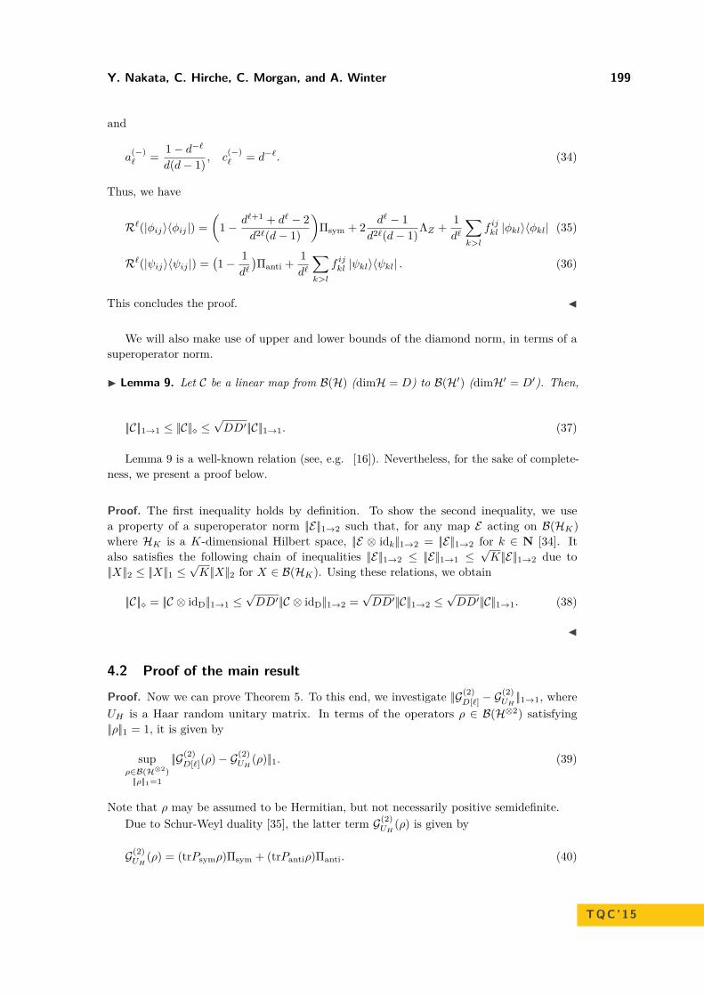
Y. Nakata, C. Hirche, C. Morgan, and A. Winter 199
and
a(−)` = 1− d−`
d(d− 1) , c(−)` = d−`. (34)
Thus, we have
R`(|φij〉〈φij |) =(
1− d`+1 + d` − 2d2`(d− 1)
)Πsym + 2 d` − 1
d2`(d− 1)ΛZ + 1d`
∑k>l
f ijkl |φkl〉〈φkl| (35)
R`(|ψij〉〈ψij |) =(1− 1
d`)Πanti + 1
d`
∑k>l
f ijkl |ψkl〉〈ψkl| . (36)
This concludes the proof. J
We will also make use of upper and lower bounds of the diamond norm, in terms of asuperoperator norm.
I Lemma 9. Let C be a linear map from B(H) (dimH = D) to B(H′) (dimH′ = D′). Then,
||C||1→1 ≤ ||C|| ≤√DD′||C||1→1. (37)
Lemma 9 is a well-known relation (see, e.g. [16]). Nevertheless, for the sake of complete-ness, we present a proof below.
Proof. The first inequality holds by definition. To show the second inequality, we usea property of a superoperator norm ||E||1→2 such that, for any map E acting on B(HK)where HK is a K-dimensional Hilbert space, ||E ⊗ idk||1→2 = ||E||1→2 for k ∈ N [34]. Italso satisfies the following chain of inequalities ||E||1→2 ≤ ||E||1→1 ≤
√K||E||1→2 due to
||X||2 ≤ ||X||1 ≤√K||X||2 for X ∈ B(HK). Using these relations, we obtain
||C|| = ||C ⊗ idD||1→1 ≤√DD′||C ⊗ idD||1→2 =
√DD′||C||1→2 ≤
√DD′||C||1→1. (38)
J
4.2 Proof of the main result
Proof. Now we can prove Theorem 5. To this end, we investigate ||G(2)D[`] − G
(2)UH||1→1, where
UH is a Haar random unitary matrix. In terms of the operators ρ ∈ B(H⊗2) satisfying||ρ||1 = 1, it is given by
supρ∈B(H⊗2)||ρ||1=1
||G(2)D[`](ρ)− G(2)
UH(ρ)||1. (39)
Note that ρ may be assumed to be Hermitian, but not necessarily positive semidefinite.Due to Schur-Weyl duality [35], the latter term G(2)
UH(ρ) is given by
G(2)UH
(ρ) = (trPsymρ)Πsym + (trPantiρ)Πanti. (40)
TQC’15

200 Implementing Unitary 2-Designs Using Random Diagonal-unitary Matrices
On the other hand, the former term G(2)D[`](ρ) is equal to R`(ρ) since
G(2)D[`](ρ) = ED[`][(D[`])⊗2ρ(D[`])†⊗2] (41)
=1∏i=`
ED′ZiEDX
iEDZ
i[(U′Zi DX
i DZi
)⊗2ρ(D′Zi D
Xi D
Zi
)†⊗2] (42)
=(G(2)DZ G(2)
DX G(2)DZ
)`(ρ) (43)
= R`(ρ), (44)
where the second line is obtained using the fact that the random diagonal-unitary matricesare independent.
Due to Lemma 8, for all ρ ∈ B(H⊗2), we have
R`(ρ) =((1− d−2`)s0 + a`s1
)Πsym + (d−2`s0 + b`s1)ΛZ + (1− d−`)s2Πanti
+ d−`∑i>j
∑k>l
f ijkl(ρφij |φkl〉〈φkl| + ρψij |ψkl〉〈ψkl|
), (45)
where a` and b` are given by Lemma 8, ρφij = trρ |φij〉〈φij |, ρψij = trρ |ψij〉〈ψij |, s0 = trρLZ ,s1 = trρ(Psym − LZ), and s2 = trρPanti. Using trPsymρ = s0 + s1, this leads to
G(2)UH
(ρ)− G(2)D[`](ρ) =
(d−2`s0 + (1− a`)s1
)Πsym − (d−2`s0 + b`s1)ΛZ + d−`s2Πanti
− d−`∑i>j
∑k>l
f ijkl(ρφij|φkl〉〈φkl| + ρψij
|ψkl〉〈ψkl|). (46)
Since Πsym = 2d(d+1)
(∑i |ii〉〈ii|+
∑i>j |φij〉〈φij |
), Πanti = 2
d(d−1)∑i>j |ψij〉〈ψij |, and ΛZ =
1d
∑i |ii〉〈ii|, Eq. (46) is already diagonal in the basis B = |ii〉d−1
i=0 ∪ |φij〉i>j ∪ |ψij〉i>j .Thus, its 1-norm is exactly calculated to be
||G(2)UH
(ρ)− G(2)D[`](ρ)||1 = d
∣∣∣∣ 2d(d+ 1)
(d−2`s0 + (1− a`)s1
)− 1d
(d−2`s0 + b`s1)∣∣∣∣
+∑k>l
(∣∣∣∣ 2d(d+ 1)
(d−2`s0+(1−a`)s1
)−d−`
∑i>j
f ijklρφij
∣∣∣∣+∣∣∣∣ 2d(d− 1)d
−`s2−d−`∑i>j
f ijklρψij
∣∣∣∣).(47)
The first term in Eq. (47) is simply equal to |2s1−(d−1)s0|d2`(d+1) , which is smaller than or equal to
2|s1|+(d−1)|s0|d2`(d+1) due to the triangle inequality. In the following, we evaluate upper and lower
bounds of the second and the third terms.The second term is bounded from above, again due to the triangle inequality, by∑k>l
(2
d(d+ 1)(d−2`|s0|+ |1− a`||s1|
)+ d−`
∑i>j
f ijkl |ρφij|), (48)
where we have used the fact that f ijkl is non-negative. Substituting a` and using Lemma 7,i.e.,
∑k>l f
ijkl = 1, it is bounded from above by
(d− 1)|trρLZ |d2`(d+ 1) + (d`+1 + d` − 2)|trρ(Psym − LZ)|
d2`(d+ 1) + 1d`
tr|ρ|(Psym − LZ). (49)

Y. Nakata, C. Hirche, C. Morgan, and A. Winter 201
Similarly, an upper bound of the third term in Eq. (47) is given by 1d` (|trρPanti|+ tr|ρ|Panti).
From these upper bounds, an upper bound of ||G(2)D[`](ρ) − G
(2)UH
(ρ)||1 is given as follows,using |s0| = |trρLZ | ≤ tr|ρ|LZ , |s1| = |trρ(Psym−LZ)| ≤ tr|ρ|(Psym−LZ), |s2| = |trρPanti| ≤tr|ρ|Panti, and Psym + Panti = I,
||G(2)D[`](ρ)− G(2)
UH(ρ)||1 ≤
2(d− 1)d2`(d+ 1)tr|ρ|LZ + 2
d`tr|ρ|(I− LZ), (50)
where we dropped the negative term − 2d2`(d+1) |trρ(Psym − LZ)|. Denoting tr|ρ|LZ and
tr|ρ|(I− LZ) by p0 and p1, respectively, we have
||G(2)D[`](ρ)− G(2)
UH(ρ)||1 ≤
2(d− 1)d2`(d+ 1)p0 + 2
d`p1. (51)
From this, we obtain an upper bound of supρ∈B(H⊗2),||ρ||1=1 ||G(2)D[`](ρ) − G
(2)UH
(ρ)||1. Since||ρ||1 = 1 implies that p0 and p1 satisfy p0 + p1 = 1, and they are positive by definition,Eq. (51) is a convex sum of 2(d−1)
d2`(d+1) and 2d` , where the latter is larger than the former. Hence,
the supremum is given by (p0, p1) = (0, 1), resulting in
supρ∈B(H⊗2),||ρ||1=1
||G(2)D[`](ρ)− G(2)
UH(ρ)||1 ≤
2d`. (52)
A lower bound of supρ∈B(H⊗2),||ρ||1=1 ||G(2)D[`](ρ)− G(2)
UH(ρ)||1 is obtained by substituting a
specific instance of ρ given by Φi0j0 := |φi0j0〉〈φi0j0 | (i0 > j0), which gives
||G(2)D[`](Φi0j0)− G(2)
UH(Φi0j0)||1 = 2
d2`(d+ 1) +∑k>l
∣∣∣∣ 2d(d+ 1)
d`+1 + d` − 2d2`(d− 1) − 1
d`f i0j0kl
∣∣∣∣, (53)
from Eq. (47). Since f i0j0kl satisfies f i0j0
kl = 0, 2/d for any k > l and∑k>l f
i0j0kl = 1 from
Lemma 7, the number of (k, l) (k > l) for which f i0j0kl is nonzero is d/2. Due to this fact, we
can exactly calculate Eq. (53) as follows:
||G(2)D[`](Φi0j0)− G(2)
UH(Φi0j0)||1 = 2
d2`(d+ 1) + d
2
∣∣∣∣ 2d(d+ 1)
d`+1 + d` − 2d2`(d− 1) − 2
d`+1
∣∣∣∣+(d(d− 1)
2 − d
2
)2
d(d+ 1)d`+1 + d` − 2d2`(d− 1) , (54)
which is simplified to be
||G(2)D[`](Φi0j0)− G(2)
UH(Φi0j0)||1 = 2
d`− 2d
`+1 + d` − 2d2`(d2 − 1) . (55)
Hence, we obtain
supρ∈B(H⊗2),||ρ||1=1
||G(2)D[`](ρ)− G(2)
UH(ρ)||1 ≥
2d`− 2d
`+1 + d` − 2d2`(d2 − 1) ≥
2d`
[1− 2d
d2 − 1
]. (56)
From these bounds, we obtain, using Lemma 9, upper and lower bounds of G(2)D[`] − G
(2)UH
in terms of the diamond norm,
2d`− 2d
`+1 + d` − 2d2`(d2 − 1) ≤ ||G
(2)D[`] − G
(2)UH|| ≤
2d`−2 . (57)
This implies that D[`] is not an ε-approximate unitary 2-design if ` ≤ log ε−1
N , as the lowerbound in Eq. (57) is strictly greater than 1/d` if d > 3, and is an ε-approximate unitary2-design if ` ≥ 2 + 1+log ε−1
N , and concludes the proof. J
TQC’15

202 Implementing Unitary 2-Designs Using Random Diagonal-unitary Matrices
5 Conclusion
We have proven that an approximate unitary 2-design can be achieved by alternately applyingindependent random Z- and X-diagonal unitary matrices. We have shown that one iterationof random Z- and X-diagonal unitary matrices is not sufficient, but it rapidly converges toan ε-approximate unitary 2-design after a number of iterations. We have also provided animplementation of our construction by a quantum circuit composed of O
(N(N+log 1/ε)
)one-
or two-qubit gates, most of which are diagonal in the Pauli-Z basis. This implementation is,in terms of the number of gates, as efficient as many of other constructions using the Cliffordcircuits and random quantum circuits. An advantage unique to our implementation is itssimple form. As the diagonal part can be applied simultaneously and the non-commutingpart is depth O(1), the practical time for the implementation will be vastly reduced comparedto other implementations. Further applications of random diagonal-unitary matrices fordecoupling can be found in Ref. [23].
Acknowledgements. The authors are grateful to Reinhard F. Werner and Omar Fawzi forinteresting and fruitful discussions. YN is a JSPS Research Fellow and is partially supportedby JSPS Postdoctoral Fellowships for Research Abroad. CM acknowledge support fromthe EU grants SIQS and QFTCMPS and by the cluster of excellence EXC 201 QuantumEngineering and Space-Time Research. CH and AW are supported by the Spanish MINECO,project FIS2013-40627-P, as well as by the Generalitat de Catalunya, CIRIT project no. 2014SGR 966. AW is further supported by the European Commission (STREP “RAQUEL”),the European Research Council (Advanced Grant “IRQUAT”) and the Spanish MINECO,project FIS2008-01236, with the support of FEDER funds.
References1 P. Hayden, M. Horodecki, A. Winter, and J. Yard. A decoupling approach to the quantum
capacity. Open Syst. Inf. Dyn., 15:7, 2008.2 A. Abeyesinghe, I. Devetak, P. Hayden, and A. Winter. The mother of all protocols :
Restructuring quantum information’s family tree. Proc. R. Soc. A, 465:2537, 2009.3 N. Datta and M.-H. Hsieh. The apex of the family tree of protocols : optimal rates and
resource inequalities. New J. Phys., 13:093042, 2011.4 C. Hirche and C. Morgan. Efficient achievability for quantum protocols using decoupling
theorems. In Proc. 2014 IEEE Int. Symp. Info. Theory, page 536, 2014.5 F. Dupuis. The decoupling approach to quantum information theory. PhD thesis, Université
de Montréal, 2010. arXiv:1004.1641.6 F. Dupuis, M. Berta, J. Wullschleger, and R. Renner. One-shot decoupling. Commun.
Math. Phys., 328:251, 2014.7 O. Szehr, F. Dupuis, M. Tomamichel, and R. Renner. Decoupling with unitary approximate
two-designs. New J. Phys., 15:053022, 2013.8 D.P. DiVincenzo, D.W. Leung, and B.M. Terhal. Quantum data hiding. IEEE Trans. Inf.
Theory, 48:580, 2002.9 C. Dankert, R. Cleve, J. Emerson, and E. Livine. Exact and approximate unitary 2-designs
and their application to fidelity estimation. Phys. Rev. A, 80:012304, 2009.10 G. Tóth and J. J. García-Ripoll. Efficient algorithm for multiqudit twirling for ensemble
quantum computation. Phys. Rev. A, 75(4):042311, 2007.11 D. Gross, K. Audenaert, and J. Eisert. Evenly distributed unitaries: On the structure of
unitary designs. J. of Math. Phys., 48(5):052104, 2007.

Y. Nakata, C. Hirche, C. Morgan, and A. Winter 203
12 W.G. Brown, Y. S. Weinstein, and L. Viola. Quantum pseudorandomness from cluster-statequantum computation. Phys. Rev. A, 77(4):040303(R), 2008.
13 Y. S. Weinstein, W.G. Brown, and L. Viola. Parameters of pseudorandom quantum circuits.Phys. Rev. A, 78(5):052332, 2008.
14 A.W. Harrow and R.A. Low. Random quantum circuits are approximate 2-designs. Com-mun. Math. Phys., 291:257, 2009.
15 I. T. Diniz and D. Jonathan. Comment on “Random quantum circuits are approximate2-designs". Commun. Math. Phys., 304:281, 2011.
16 R.A. Low. Pseudo-randomness and learning in quantum computation. PhD thesis, Univer-sity of Bristol, 2010. arXiv:1006.5227.
17 F.G. S. L. Brandao, A.W. Harrow, and M. Horodecki. Local random quantum circuits areapproximate polynomial-designs, 2012. arXiv: 1208.0692.
18 R. Cleve, D. Leung, L. Liu, and C. Wang. Near-linear constructions of exact unitary2-designs, 2015. arXiv:1501.04592.
19 Y. Nakata and M. Murao. Diagonal-unitary 2-designs and their implementations byquantum circuits. Int. J. Quant. Inf., 11:1350062, 2013.
20 Y. Nakata and M. Murao. Diagonal quantum circuits: their computational power andapplications. Eur. Phys. J. Plus, 129:152, 2014.
21 D. J. Shepherd and M. J. Bremner. Temporally unstructured quantum computation. Proc.R. Soc. A, 465:1413, 2009.
22 M. J. Bremner, R. Jozsa, and D. J. Shepherd. Classical simulation of commuting quantumcomputations implies collapse of the polynomial hierarchy. Proc. R. Soc. A, 467(2126):459,2011.
23 Y. Nakata, C. Hirche, C. Morgan, and A. Winter, 2015. In preparation.24 A. Kitaev, A. Shen, and M. Vyalyi. Classical and Quantum Computation. American
Mathematical Society Boston, MA, USA, 2002.25 M.L. Metha. Random Matrices. Academic Press, Amsterdam San Diego Oxford London,
1990.26 S. Popescu, A. J. Short, and A. Winter. Entanglement and the foundations of statistical
mechanics. Nature Physics, 2:754, 2006.27 P. Hayden and J. Preskill. Black holes as mirrors : quantum information in random
subsystems. J. High Energy Phys., 9:120, 2007.28 Y. Nakata, P. S. Turner, and M. Murao. Phase-random states: Ensembles of states
with fixed amplitudes and uniformly distributed phases in a fixed basis. Phys. Rev. A,86(1):012301, 2012.
29 L. del Rio, A. Hutter, R. Renner, and S. Wehner. Relative thermalization, 2014.arXiv:1401.7997.
30 Y. Nakata, M. Koashi, and M. Murao. Generating a state t-design by diagonal quantumcircuits. New J. Phys., 16:053043, 2014.
31 N.A. Nielsen and I. L. Chuang. Quantum Computation and Quantum Information. Cam-bridge University Press, Cambridge, UK, 2000.
32 R. Raussendorf and H. J. Briegel. A one-way quantum computer. Phys. Rev. Lett., 86:5188,2001.
33 R. Raussendorf, D. E. Browne, and H. J. Briegel. Measurement-based quantum computationwith cluster states. Phys. Rev. A, 68:022312, 2003.
34 J. Watrous. Notes on super-operator norms induced by Schatten norms, 2004. arXiv:quant-ph/0411077.
35 R. Goodman and N.R. Wallach. Representations and Invariants of the Classical Groups.Cambridge University Press, Cambridge, UK, 1999.
TQC’15

204 Implementing Unitary 2-Designs Using Random Diagonal-unitary Matrices
A Proof of Lemma 7
Proof. The statement f ijkl = fklij follows from the definition of f ijkl . We first show that
f ijkl is either 0 or 2/d. As f ijkl is defined by f ijkl = 2d3
(∑d−1α=0 αiαjαkαl
)2, we investigate∑d−1
α=0 αiαjαkαl. This is invariant even if Pauli X is applied on the m-th qubit for anym ∈ [1, · · · , N ], which we denote by Xm, since
d−1∑α=0
αiαjαkαl = d2d−1∑α=0〈α|i〉〈α|j〉〈α|k〉〈α|l〉 (58)
= d2d−1∑α=0〈α|Xm |i〉 〈α|Xm |j〉 〈α|Xm |k〉 〈α|Xm |l〉 . (59)
This is due to 〈α|Xm = ±〈α|. Hence, we assume |i〉 = |0〉⊗N without loss of generality,resulting in αi = 1 for all α. The
∑d−1α=0 αjαkαl still has another invariance, that is,
d−1∑α=0
αjαkαl = d√d
d−1∑α=0〈α|j〉〈α|k〉〈α|l〉 (60)
= d√d
d−1∑α=0〈α|Zm |j〉 〈α|Zm |k〉 〈α|Zm |l〉 , (61)
due to the summation over all α, where Zm is the Pauli-Z operator acting on the m-th qubit.We then assume αj = 1 for j = 0, · · · , d/2− 1 and αj = −1 for j = d/2, · · · , d− 1 withoutloss of generality. This leads to
d−1∑α=0
αiαjαkαl =(d/2−1∑
α=0−
d−1∑α=d/2
)αkαl. (62)
Denoting |α〉 by∣∣α1α2 · · ·αN
⟩(αm = ±), where |±〉 are the eigenbasis of the Pauli-X with
eigenvalues ±1, respectively, and similarly denoting |k〉 and |l〉 in binary such as |k1 · · · kN 〉(km = 0, 1), (
∑d/2−1α=0 −
∑d−1α=d/2)αkαl is rewritten as
∑α2,··· ,αN =±
(〈+|k1〉〈+|l1〉〈α2 · · ·αN |k1 · · · kN 〉〈α2 · · ·αN |l1 · · · lN 〉
− 〈−|k1〉〈−|l1〉〈α2 · · ·αN |k1 · · · kN 〉〈α2 · · ·αN |l1 · · · lN 〉). (63)
When k1 = l1, this is simply zero. When k1 6= l1, this is equal to 2N = d. Thus, fklij ∈ 0, 2/d.We next show
∑k>l f
ijkl = 1 for any i > j.
∑k>l
f ijkl = 2d3
∑k>l
(∑α
αiαjαkαl
)2(64)
= 1d3
∑α,β
αiαjβiβj
(∑k,l
αkαlβkβl −∑k
α2kβ
2k
). (65)

Y. Nakata, C. Hirche, C. Morgan, and A. Winter 205
As∑k α
2kβ
2k = d due to αk = ±1, we obtain
1d3
∑α,β
αiαjβiβj∑k
α2kβ
2k = 1
d2
∑α,β
αiαjβiβj (66)
=(∑
α
〈i|α〉〈α|j〉)2
(67)
= 0, (68)
where we used that i 6= j for the last line. Hence,
∑k>l
f ijkl = 1d3
∑α,β
αiαjβiβj
(∑k
αkβk
)2. (69)
As∑k αkβk is given by 1
d2
∑k |α〉〈k| |k〉〈β| =
1d2 δαβ , we obtain∑
k>l
f ijkl = 1d
∑α,β
αiαjβiβjδα,β = 1. (70)
We finally show∑s>t f
ijstf
stkl = f ijkl . To this end, we define a set Ξij for i > j by
Ξij :=
(s, t)|s, t ∈ 1, · · · , N, s > t, f ijst = 2d
. Since f ijkl ∈ 0, 2/d and
∑k>l f
ijkl = 1 for
any i > j, the number of elements in Ξij ,denoted by |Ξij |, is d/2. Due to the definitionof f ijst , Ξij is also given in terms of αi’s by Ξij =
(s, t)|s, t ∈ 1, · · · , N, s > t, ∀α ∈
[0, · · · , d− 1], αsαt = αiαj. From this, it is observed that ∀i > j and ∀k > l, Ξij is either
equal to Ξkl or has no intersection with Ξkl, i.e. Ξij ∩ Ξkl = ∅.In terms of Ξij , fklij = 2
dδkl∈Ξij, where δkl∈Ξij
= 1 if (k, l) ∈ Ξij and 0 otherwise. Notethat, as fklij = f ijkl , δkl∈Ξij
= δij∈Ξkl. Using this notation, we have
∑s>t
f ijstfstkl =
(2d
)2∑s>t
δst∈Ξklδst∈Ξij
(71)
=(
2d
)2∑s>t
δst∈Ξkl∩Ξij . (72)
When Ξkl = Ξij , this is equal to 2d as |Ξkl| = d/2. In this case, fklij = 2
dδkl∈Ξij= 2
d since(k, l) ∈ Ξkl = Ξij , implying
∑s>t f
ijstf
stkl = fklij . When Ξkl ∩ Ξij = ∅, Eq. (72) is equal to
zero, and fklij is also zero by definition. Hence,∑s>t f
ijstf
stkl = fklij holds even in this case.
Since Ξij is either Ξkl or satisfies Ξij ∩ Ξkl = ∅, this concludes the proof. J
TQC’15

Round Elimination in Exact CommunicationComplexityJop Briët1, Harry Buhrman2, Debbie Leung3, Teresa Piovesan2,and Florian Speelman2
1 Courant InstituteNew York University, 251 Mercer Street, New York NY 10012, [email protected]
2 Centrum Wiskunde & Informatica (CWI)Science Park 123, 1098 XG Amsterdam, The Netherlandsbuhrman,piovesan,[email protected]
3 University of Waterloo200 University Ave W, Waterloo, Ontario N2L3G1, [email protected]
AbstractWe study two basic graph parameters, the chromatic number and the orthogonal rank, in thecontext of classical and quantum exact communication complexity. In particular, we considertwo types of communication problems that we call promise equality and list problems. For bothof these, it was already known that the one-round classical and one-round quantum complexitiesare characterized by the chromatic number and orthogonal rank of a certain graph, respectively.
In a promise equality problem, Alice and Bob must decide if their inputs are equal or not. Weprove that classical protocols for such problems can always be reduced to one-round protocolswith no extra communication. In contrast, we give an explicit instance of a promise problemthat exhibits an exponential gap between the one- and two-round exact quantum communicationcomplexities. Whereas the chromatic number thus captures the complete complexity of promiseequality problems, the hierarchy of “quantum chromatic numbers” (starting with the orthogonalrank) giving the quantum communication complexity for every fixed number of communicationrounds thus turns out to enjoy a much richer structure.
In a list problem, Bob gets a subset of some finite universe, Alice gets an element from Bob’ssubset, and their goal is for Bob to learn which element Alice was given. The best general lowerbound (due to Orlitsky) and upper bound (due to Naor, Orlitsky, and Shor) on the classicalcommunication complexity of such problems differ only by a constant factor. We exhibit anexample showing that, somewhat surprisingly, the four-round protocol used in the bound of Naoret al. can in fact be optimal. Finally, we pose a conjecture on the orthogonality rank of a certaingraph whose truth would imply an intriguing impossibility of round elimination in quantumprotocols for list problems, something that works trivially in the classical case.
1998 ACM Subject Classification F.2 Analysis of Algorithms and Problem Complexity
Keywords and phrases Communication complexity, round elimination, quantum communication,protocols, chromatic numbers
Digital Object Identifier 10.4230/LIPIcs.TQC.2015.206
1 Introduction
The chromatic number χ(G) of a graph G is the minimum number of colors needed to colorthe vertices in such a way that adjacent vertices get different colors. This important graph
© Jop Briët, Harry Buhrman, Debbie Leung, Teresa Piovesan, and Florian Speelman;licensed under Creative Commons License CC-BY
10th Conference on the Theory of Quantum Computation, Communication and Cryptography (TQC 2015).Editors: Salman Beigi and Robert König; pp. 206–225
Leibniz International Proceedings in InformaticsSchloss Dagstuhl – Leibniz-Zentrum für Informatik, Dagstuhl Publishing, Germany

J. Briët, H. Buhrman, D. Leung, T. Piovesan, and F. Speelman 207
parameter appears frequently in computer science and mathematics; it is well-known tobe NP-hard to compute and has recently found a number of meaningful generalizationsin the context of non-local games and entanglement-assisted zero-error information theory.One of those generalizations is the orthogonal rank of a graph, denoted ξ(G) and defined asfollows. An orthogonal representation of a graph is an assignment of complex unit vectorsto the vertices such that adjacent vertices receive orthogonal vectors. The orthogonal rankis the minimum dimension of such a representation. Similar to the chromatic number,the orthogonal rank is NP-hard to compute, which follows from a result of Peeters [29,Theorem 3.1]. In this paper, we study both of these graph parameters in the context ofcommunication complexity.
Classical communication complexity. Since its introduction by Yao [34] communicationcomplexity has become a standard model in computational complexity that enjoys a widevariety of connections to other areas in theoretical computer science [22]. Here two parties,Alice and Bob, receive inputs x, y from sets X ,Y (resp.) and need to compute the value f(x, y)of a two-variable function f known to them in advance. Usually each party has insufficientinformation to solve the problem alone, meaning they have to exchange information abouteach others’ inputs. The idea that communication is expensive motivates the study ofthe communication complexity of f , which counts the minimal number of bits that theparties must exchange on worst-case inputs. Throughout this paper, we consider only exact(deterministic) communication protocols, and we will omit the word exact from now on. Ofparticular importance to this paper is the distinction between one-round protocols, where allcommunication flows from Alice to Bob, and multi-round protocols, where they take turns insending messages from one party to the other.
Quantum communication complexity. In yet another celebrated paper, Yao [35] introducedquantum communication complexity, where to compute the value f(x, y) the parties are allowedto transmit qubits back and forth. The study of this model has also become a well-establisheddiscipline in theoretical computer science and quantum information theory. The most basicquestion that arises when considering the classical and quantum models is whether they areactually substantially different. An upper bound on the possible difference between thesemodels was proved by Kremer [21, Theorem 4].1
I Theorem 1.1 (Kremer). Any quantum protocol that uses ` qubits of communication can beturned into a 2O(`)-bit one-round classical protocol for the same problem.
The first large gap between exact classical and quantum communication complexity wasdemonstrated by Buhrman, Cleve, and Wigderson [7], who gave a problem admitting a one-round quantum protocol that is exponentially more efficient than any (one- or multi-round)classical protocol.
The chromatic number and orthogonal rank naturally show up in two types of communi-cation problems that we call promise equality and list problems, discussed next.
1.1 Promise equalityIn a promise equality problem, Alice and Bob are either given equal inputs or a pair of distinctinputs from a subset D of
(X2)(D is known to them in advance). Their goal is to decide
whether they have equal or different inputs.
1 The result stated here is actually a slight generalization of Kremer’s result (which focuses on booleanfunctions) that can be proved in the same way; for completeness we give a proof in Appendix A.
TQC’15

208 Round Elimination in Exact Communication Complexity
Classical complexity of promise problems. It was shown by de Wolf [11, Theorem 8.5.1]that if G = (X ,D) is the graph with vertex set X and edge set D, then the one-round classicalcommunication of the problem equals dlogχ(G)e. Analogously, for each positive integer r onecan define a “level-r” chromatic number of the graph corresponding to the communicationcomplexity of protocols that proceed in r rounds or less. For general communication problems,using more rounds can decrease the total communication, as is the case for the generalPointer Jumping Problem for example, where for every positive integer m there is an instancefor which any m-round protocol requires exponentially more communication than the best(m + 1)-round protocol [22]. However, we show that this is not true for promise equalityproblems (Lemma 2.1 below), meaning that for such problems the chromatic number notonly gives rise to the one-round complexity, but their overall communication complexity.
Quantum complexity of promise problems. The one-round quantum communication com-plexity of promise equality problems is characterized by the orthogonal rank. It is not difficultto see that a one-round quantum protocol of a promise equality problem is equivalent to anorthogonal representation of the associated graph G = (X ,D); the vectors correspond to thestates that Alice would send to Bob and orthogonality is required for Bob’s measurement totell whether they got equal inputs or not. Viewing the orthogonal rank as the “one-roundquantum chromatic number” of the graph G naturally leads one to define a hierarchy of suchnumbers where the level-r quantum chromatic number corresponds to the communicationcomplexity of r-round quantum protocols. One might expect that, as in the classical case,this hierarchy is redundant in that the levels all carry the same number. However, one of ourmain results shows that in the quantum setting, this is not the case.
I Theorem 1.2. There exist absolute constants c, C ∈ (0,∞) and an infinite family ofpromise equality problems (Xn,Dn)n∈N such that:
The one-round quantum communication complexity of (Xn,Dn) is at least cn.There is a two-round quantum protocol for (Xn,Dn) using at most C logn qubits.
During our analysis of the particular promise problem used for Theorem 1.2 we answeran open question of Gruska, Qiu, and Zheng [18]. To explain this, we briefly elaborate onwhat goes into our result. The problem we consider is simple: Let n be a positive integermultiple of 8. Alice and Bob are given n-bit strings x and y, respectively, that are eitherequal or differ in exactly n/4 coordinates and they must distinguish between the two cases.We denote this problem by EQ-
(nn/4). Similar promise equality problems were studied before.
Buhrman, Cleve, and Wigderson [7] showed the first exponential gap between classical andquantum communication with the problem EQ-
(nn/2), where Alice and Bob get n-bit strings
that are either equal or differ in exactly half of the entries (for n a multiple of 4). Theyused a distributed version of the Deutsch–Jozsa algorithm to give a one-round O(logn)-qubitquantum protocol for this problem, while a celebrated graph-theoretic result of Frankl andRödl [14] implies that the classical communication complexity is at least Ω(n). Similarresults were shown (based on similar techniques) in the above-mentioned paper [18] for theanalogous problem EQ-
(nαn
)when α > 1/2, and the authors pose as an open problem to
determine the quantum communication complexity of EQ-(nαn
)when α < 1/2.
We show that the one-round quantum communication complexity of EQ-(nn/4)is at
least Ω(n) and we give a two-round protocol for it that uses at most O(logn) qubits. Forthe proof of the first bound we use the famous Lovász theta number, which lower boundsthe orthogonal rank and therefore the one-round quantum communication complexity. Weprove a lower bound on the theta number using the theory of association schemes and known

J. Briët, H. Buhrman, D. Leung, T. Piovesan, and F. Speelman 209
properties of the roots of the Krawtchouk polynomials. Our two-round protocol is based ona distributed version of Grover’s algorithm. With a little extra technical work our results canbe extended to any of the problems EQ-
(nαn
)with constant α < 1/2. In light of Kremer’s
Theorem and the obvious fact that the one-round classical communication complexity is atleast its quantum counterpart, we thus settle the question of [18].
1.2 The list problemIn the list problem, inputs are picked from a subset D ⊆ X × Y and the parties’ goal is forBob to learn Alice’s input. The reason for the name “list problem” is that Bob’s input ymay just as well be given to him as the list (subset) of all of Alice’s possible inputs xsatisfying (x, y) ∈ D. A list problem can thus equivalently be given by a family L ⊆ 2X oflists, where Bob gets a list L ∈ L, Alice gets an element x ∈ L, and Bob must learn x. Werefer to this communication problem as L-list.
Classical complexity of list problems. Witsenhausen [33] observed that the one-roundclassical communication complexity of the list problem is characterized by the chromaticnumber of the graph with vertex set X and whose edge set consists of the pairs of distinctelements appearing together in some list L ∈ L. Denoting this graph by GL, the one-roundcommunication complexity equals dlogχ(GL)e. The multi-round communication complexityof the list problem was also studied before. Orlitsky [28, Corollary 3 and Lemma 3] provedthe following lower bound in terms of the chromatic number of GL, and the cardinality ofthe largest list, denoted ω(L) = max|L| : L ∈ L (not to be confused with the cardinalityof the largest clique ω(GL) in the graph GL, which can be larger).
I Theorem 1.3 (Orlitsky). For every family L ⊆ 2X , the classical communication complexityof L-list is at least maxlog logχ(GL), logω(L).
The basic idea behind the above result is that Alice must send sufficient information forBob to be able to distinguish among ω(L) elements, and that any multi-round protocol can besimulated by a one-round protocol with at most an exponential difference in communication.In the same work, Orlitsky [28, Theorem 4] gave a two-round classical protocol based onperfect hashing functions that nearly achieves the above lower bound.
I Theorem 1.4 (Orlitsky). For every family L ⊆ 2X , the two-round classical communicationcomplexity of L-list is at most log logχ(GL) + 3 logω(L) + 4.
It thus follows from Witsenhausen’s observation and Theorem 1.4 that list problems haveexponentially more efficient two-round protocols than one-round protocols. But Theorem 1.3shows that—in stark contrast with the Pointer Jumping Problem—using more than tworounds cannot decrease the total amount of communication by more than a factor of 4,since obviously log logχ(GL) + 3 logω(L) ≤ 4 maxlog logχ(GL), logω(L). The naturalquestion that thus arises is if the lower bound of Theorem 1.3 can be attained by using morethan two rounds of communication. Towards answering this question, Naor, Orlitsky, andShor [27, Corollary 1] slightly improved on Theorem 1.4 and showed that the four-roundcommunication complexity gets to within a factor of about 3 of the lower bound.
I Theorem 1.5 (Naor–Orlitsky–Shor). For every family L ⊆ 2X , the four-round classicalcommunication complexity of L-list is at most log logχ(GL) + 2 logω(L) + 3 log logω(L) + 7.
As our contribution to this line of work we show that, surprisingly, for some list problemsthe four-round protocol of Naor, Orlitsky, and Shor is in fact asymptotically optimal, thusanswering the above question in the negative.
TQC’15

210 Round Elimination in Exact Communication Complexity
I Theorem 1.6. For any ε > 0 there exists a set X and a family L ⊆ 2X such that theclassical communication complexity of L-list is at least log logχ(GL) + (2 − ε) logω(L).Moreover, there exists such an (X ,L) pair for which ω(L) = logχ(GL).
In particular, our result gives a family of list problems with communication complexityat least (3− ε) maxlog logχ(GL), logω(L) for any ε > 0.
Quantum complexity of list problems and quantum round elimination. The one-roundquantum communication complexity of list problems is given by dlog ξ(GL)e, which followsfrom the same considerations as for the promise equality problems (see Lemma 3.4). Basedon a conjecture we make about the orthogonal rank of a certain family of graphs, we believethat in the context of quantum communication complexity, list problems may have theinteresting property of resisting a quantum analogue of round elimination.
In classical communication complexity, round elimination reduces the number of roundsof a given protocol by having the parties send some extra information instead. Considerthe following basic example, where we start with a two-round (logn + 1)-bit protocol inwhich Bob starts by sending Alice a single bit and Alice replies with an logn-bit string.This protocol can easily be turned into a one-round 2 logn-bit protocol by having Alicedirectly send Bob two logn-bit strings, one corresponding to the case where Bob sends a 0in the two-round protocol and another for if he sends a 1. Then Bob can just pick the stringcorresponding to the bit he would have sent based on his input and solve the problem.
A quantum analogue of the above example would turn a two-round (logn + 1)-qubitprotocol into a one-round 2 logn-qubit protocol. We conjecture that the following family oflist problems is a counterexample to the existence of such an analogue. For an even positiveinteger n and d ∈ [n], let Ld ⊆ 20,1n be the family of all lists L ⊆ 0, 1n of maximalcardinality such that all strings in L have Hamming distance exactly d. The example weconsider is given by the family K = Ln/2 ∪ · · · ∪ Ln. Similar to the classical example above,we give a simple two-round protocol for K-list.
I Theorem 1.7. For K ⊆ 20,1n as above, there exists a two-round protocol for K-listwhere Bob sends Alice a single qubit and Alice replies with a (1 + logn)-qubit message.
It is easy to see that the graph GK = (0, 1n, E) associated with K has edge set E givenby all pairs of strings with Hamming distance in n/2, . . . , n.
I Conjecture 1.8. The graph GK as above satisfies ξ(GK) ≥ nω(1).
By the relation between the one-round quantum communication complexity of list prob-lems and the orthogonal rank of their associated graphs, it follows that the validity of theabove conjecture would imply that the exact one-round quantum communication complexityof the above problem is super-logarithmic in n, in marked contrast with the classical exampleof round elimination.
1.3 Connections to other workOur work strengthens a link between communication complexity and graph theory establishedby de Wolf [11]. Orthogonal representations appear in the context of zero-error informationtheory. Indeed they were introduced by Lovász [26] to settle a famous problem of Shannonconcerning the (classical) capacity of the 5-cycle and they serve as proxies for entanglement-assisted schemes [8, 9, 24, 5, 6, 10]. They also appear in the context of non-local games [8,16, 31]. Nevertheless the orthogonal rank is poorly understood. To the best of our knowledge,

J. Briët, H. Buhrman, D. Leung, T. Piovesan, and F. Speelman 211
our result is the first time a lower bound on the dimension was used. The use of the Lovásztheta number in the context of communication complexity problems also appears to be newand we hope that it may find further applications there in the future. Finally, quantumvariants of the chromatic number that appeared in for example non-local games [8, 31]and zero-error information theory [6, 10] can be interpreted as quantum communicationcomplexities of promise equality problems in various different communication models, whichputs those parameters in a more unified framework.
Outline of the paper. In Section 2 we study the promise equality problem and in particularwe prove Theorem 1.2. In Section 3 we discuss the list problem and prove Theorem 1.6 andTheorem 1.7.
2 Promise Equality
Recall that in a promise equality problem, Alice and Bob each receive an input from a set Xwith the promise that their inputs either are equal or come from a subset D of
(X2)(known
to the players beforehand). The goal is to distinguish between the two cases. To any promiseequality problem, we associate the graph G = (X ,D).
2.1 General properties of promise equalityRecall that the one-round classical communication complexity of the problem equals dlogχ(G)e.We begin by proving that the chromatic number of the associated graph actually gives theoverall communication complexity.
I Lemma 2.1. For any promise equality problem, the classical communication complexity isattained with a single round of communication.
Proof. We show how to transform a k-round communication protocol into a one-roundprotocol that uses the same amount of bits. To summarize, the idea is that Alice mimics allthe rounds of communication assuming that her input is equal to Bob’s one, and sends themin one-round. He then checks whether the message received is consistent with his input. Ifthis is not the case, then he knows that the two strings are different, otherwise he completesthe protocol.
More formally, fix an optimal protocol P that requires k rounds, where k ≥ 2. Supposethat Alice has input x and Bob has y. We assume that the first round of communication isfrom Alice to Bob, but the same reasoning applies in the other case. For i odd, let ai be themessage that Alice would send to Bob on the i-th round of communication if she followedprotocol P and used the knowledge of the messages exchanged in the previous rounds and ofher input x. Similarly, for i even, let bi be the message that Bob would send to Alice on thei-th round of communication if he had y = x as input, followed the protocol P and used theknowledge derived by the previous rounds. Using the protocol P , Alice can mimic Bob’srounds of communication under the assumption that Bob’s input is equal to x. Alice usesher input x to produce the string a1b2a3 . . . aibi+1 . . . ak and sends it to Bob in one round.From his input y, Bob constructs the messages bi that he would have produced during theprotocol P , with the knowledge of Alice’s messages a` and his messages b` for all ` < i. Ifthere exists an index i such that bi 6= bi, then x must be different from y. Otherwise, Bobuses the transcript a1b2a3 . . . aibi+1 . . . ak to finish the protocol and either outputs x = y
or x 6= y. We have constructed a one-round communication protocol P whose worst-case
TQC’15

212 Round Elimination in Exact Communication Complexity
transcript length is at most as long as the one of the original protocol P . Since P is anoptimal protocol so must be P . J
As already mentioned, de Wolf [11, Theorem 8.5.2] showed that one-round quantumprotocols are related to orthogonal representations. We include a proof here for completeness.
I Theorem 2.2 (de Wolf). Consider a promise equality problem defined by the sets X andD, then its one-round quantum communication complexity is equal to dlog ξ(G)e, whereG = (X ,D).
The proof of the above result uses the following standard lemma (see for example [6]).
I Lemma 2.3 (Orthogonality Lemma). Let ρ1, . . . , ρ` ∈ Cd×d be a collection of Hermitianpositive semidefinite matrices. Then the following are equivalent:1. We have ρiρj = 0 for every i 6= j ∈ [`].2. There exists a measurement consisting of positive semidefinite matrices P 1, . . . , P `, P⊥ ∈
Cd×d such that Tr(P iρj) = δij Tr(ρj) and Tr(P⊥ρj) = 0 for every i, j ∈ [`].In particular, a collection of pure states |φ1〉, . . . , |φ`〉 ∈ Cd can be perfectly distinguished
with a quantum measurement if and only if they are pairwise orthogonal.
Proof of Theorem 2.2. Let P be an optimal one-round protocol for the considered promiseequality problem. Without loss of generality, Alice sends pure state |φx〉 ∈ Cd on input x ∈ X .For any pair (x, y) ∈ D, |φx〉 and |φy〉 have to be perfectly distinguishable and therefore, inview of Lemma 2.3, they must be orthogonal. Hence, the map φ : X → Cd where φ(x) = |φx〉is a d-dimensional orthonormal representation of G = (X ,D) and ξ(G) ≤ d.
On the other hand, let φ be a d-dimensional orthonormal representation of the graphG = (X ,D) and consider the one-round quantum protocol that transmits φ(x) ∈ Cd on inputx ∈ X . This uses log d-qubits of communication. From Lemma 2.3 we know that Bob can usehis input y to perform a quantum measurement that allows him to learn whether his inputis equal or not to Alice’s one. Thus, the one-round quantum communication complexity ofthis equality problem is at most dlog ξ(G)e. J
2.2 Proof of Theorem 1.2The rest of this section will be devoted to the proof of Theorem 1.2, which shows that there isa family of promise equality problems where allowing two rounds of quantum communicationis exponentially more efficient than a single round. The problem that exhibits this separationis EQ-
(nn/4), where Alice and Bob each receive a n-bit string that are either equal or differ in
exactly n/4 positions (with n multiple of 8). We denote by H(n, n/4) the graph associatedwith this problem. For any n, d ∈ N, let H(n, d) be the graph which has all the n-bit stringsas vertex set, such that two vertices are adjacent if their Hamming distance is d. We splitthe proof in two parts: in Section 2.2.1 we bound the one-round quantum communicationcomplexity and in Section 2.2.2 we give the two-round protocol.
2.2.1 One-round quantum communication complexity of EQ-(n
n/4
)The main result of this section is the following theorem.
I Theorem 2.4. The one-round quantum communication complexity of EQ-(nn/4)is at
least Ω(n).

J. Briët, H. Buhrman, D. Leung, T. Piovesan, and F. Speelman 213
To prove Theorem 2.4, we use Theorem 2.2 and thus set out to bound the orthogonalrank of the graph H(n, n/4). We prove the desired bound in three steps: first, we show thatthe Lovász theta number is a lower bound for the orthogonal rank; second, we use structuralproperties of H(n, n/4) together with known properties of the theta number to reformulatethis bound in terms of the eigenvalues of the adjacency matrix of this graph; third, we boundthe eigenvalues to get the desired result.
We remark that in the following proofs we consider a more general situation than justthe graph H(n, n/4). Indeed, the statement of Theorem 2.4 holds for any problem EQ-
(nαn
)where α ∈ (0, 1/2) and where both n and α · n are even.
Step 1: The Lovász theta number. This parameter was introduced by Lovász [26] toupper bound the Shannon capacity of a graph. Among its many equivalent definitions, wewill use the following primal and dual formulations:
ϑ(G) = max∑
i,j∈V (G)
Xij s.t. X 0, Tr(X) = 1, Xij = 0 ∀ij ∈ E(G),
ϑ(G) = min t s.t. X 0, Xii = t− 1 ∀i ∈ V (G), Xij = −1 ∀ij ∈ E(G),(1)
where X 0 means that X is a symmetric positive semidefinite matrix. The graph G, calledthe complement of a graph G, has the same vertex set as the original graph and a pair ofvertices is adjacent if and only if it is non adjacent in G.
Lovász [26] proved that ϑ lower bounds the minimum dimension of an orthonormalrepresentation where the vectors are real valued. Note that this is slightly different fromour setting where we allow the vectors to have complex entries. However, we show thatthe Lovász theta number is also a lower bound for ξ(G). The proof is an adaptation to thecomplex case of a known proof [23].
I Lemma 2.5. For any graph G, we have ξ(G) ≥ ϑ(G).
Proof. Let n = |V (G)| and label the vertices of the graph G by 1, 2, . . . , n. Supposethat the orthogonal rank of G is equal to d and that u1, . . . , un ∈ Cd are the unit vectorsforming an orthogonal representation of G. For every vertex of the graph i ∈ [n], define amatrix Ui := uiu
†i and U0 := Id. Let Z be a (n+ 1)× (n+ 1) matrix where the i, j-th entry
Zij := 〈Ui, Uj〉 = Tr(U†jUi) for every i, j ∈ 0 ∪ [n]. Notice that Z is positive semidefinitesince it is the Gram matrix of a set of complex vectors. Moreover, Z is real valued and we getthat Z00 = d, Z0i = 〈I, uiu†i 〉 = 1 and Zii = 〈uiu†i , uiu
†i 〉 = (u†iui)2 = 1 for all i ∈ V (G) and
that Zij = (u†iuj)(u†jui) ≥ 0 for all i, j ∈ V (G) with equality if ij ∈ E(G). By taking the
Schur complement2 in Z with respect to the entry Z00, we obtain a new symmetric positivesemidefinite matrix X with Xii = 1− 1/d for all i ∈ V (G) and Xij = −1/d for all ij ∈ E(G).Rescaling X by d, we get a feasible solution for the minimization program in (1) of ϑ(G)with value d. We conclude that d = ξ(G) ≥ ϑ(G). J
Step 2: Eigenvalue bound on the theta number. In the second step we show the followinguseful bound on the theta number of the graph H(n, d) in terms of the eigenvalues of its
2 Let X be a symmetric matrix of the form X =(α bT
b A
), where b ∈ Rn−1 and α > 0. X is positive
semidefinite if and only if A− bbT /α is positive semidefinite. The matrix A− bbT /α is called the Schurcomplement in X with respect to the entry α.
TQC’15

214 Round Elimination in Exact Communication Complexity
adjacency matrix. For the remainder of this step, by the eigenvalues of a graph we mean theeigenvalues of its adjacency matrix.
I Lemma 2.6. For every positive integer n and d ∈ [n], we have ϑ(H(n, d)) ≥ 1−(nd
)/λmin,
where λmin is the smallest eigenvalue of H(n, d).
The proof of the above lemma uses the fact that for graphs with certain structuralproperties, the Lovász theta number is characterized by their eigenvalues. Let us recall thefollowing standard definitions. Let G = (V,E) be a graph. A permutation π : V → V isedge preserving if for every edge u, v ∈ E, we have π(u), π(v) ∈ E. The graph G isvertex-transitive if for every pair of vertices u, v ∈ V there is an edge-preserving permutationπ : V → V such that π(u) = v. Moreover, G is edge-transitive if for every pair of edgesu1, v1, u2, v2 ∈ E, there is an edge-preserving permutation π : V → V such thatπ(u1) = u2 and π(v1) = v2. Lovász [26] showed that if a graph is both vertex- and edge-transitive, then the theta number is given by a simple formula involving its eigenvalues.
I Lemma 2.7 (Lovász). For a positive integer n let G be an n-vertex graph with eigenvaluesλ1 ≥ · · · ≥ λn. If G is both vertex- and edge-transitive, then ϑ(G) = 1− λ1/λn.
Proof of Lemma 2.6. We start by showing that H(n, d) is vertex-transitive. Given any pairof vertices u, v ∈ 0, 1n of H(n, d), consider the automorphism of the graph H(n, d) thatmaps x 7→ x ⊕ u ⊕ v where ⊕ is the bit-wise addition. This map preserves the Hammingdistance, and therefore the adjacencies, between the vertices and sends u 7→ v. Hence H(n, d)is vertex-transitive.
To show that H(n, d) is edge-transitive, fix any two edges uv and st and let p = u⊕ v,q = s ⊕ t. Noting that the n-bit strings p and q have the same Hamming weight d, let πbe a permutation of the indices such that π(p) = q. We define ν to be an automorphismthat sends a vertex x to π(x⊕ u)⊕ s. The map ν preserves the edges of H(n, d) and, sincethe permutation π maps the all-zero string to itself and p to q, we have that ν(u) = s andν(v) = t. Hence, H(n, d) is edge-transitive.
Finally, since the largest eigenvalue of a vertex-transitive graph is equal to its degree, weclearly have λ1(H(n, d)) =
(nd
). The result now follows from Lemma 2.7. J
Step 3: Bound on the smallest eigenvalue of H(n, d). Finally, we prove an upper boundon the magnitude of the smallest eigenvalue of H(n, d).
I Lemma 2.8. Let d and n be even positive integers such that d < n/2. Then, the smallesteigenvalue λmin of the graph H(n, d) is a negative number such that
|λmin| ≤
√√√√ 2n(nd
)( n
n/2−√d(n−d)
) .The proof of the lemma uses the following facts from coding theory that can be found in
the survey [12]. The eigenvalues of H(n, d) play a fundamental role in the theory of Hammingassociation schemes, where they are expressed in terms of a set of orthogonal polynomialsknown as the (binary) Krawtchouk polynomials. For a positive integer n and d = 0, 1, . . . , n,the Krawtchouk polynomial Kn
d ∈ R[x] is a degree-d polynomial that is uniquely defined by
Knd (x) =
d∑j=0
(−1)j(x
j
)(n− xd− j
), x = 0, 1, . . . , n.

J. Briët, H. Buhrman, D. Leung, T. Piovesan, and F. Speelman 215
When n and d are even, then Knd is symmetric about the point x = n/2. Moreover, these
polynomials satisfy the important orthogonality relation
n∑x=0
(n
x
)Knd (x)Kn
d′(x) = δd,d′
(n
d
)2n. (2)
The set of distinct eigenvalues of H(n, d) turns out to be Knd (0),Kn
d (1), . . . ,Knd (n). Crucial
to our proof of Lemma 2.8 then, is the following result of Levenshtein [25, Theorem 6.1]characterizing the smallest roots of the Krawtchouk polynomials.
I Theorem 2.9 (Levenshtein). Let n be a positive integer and d ∈ [n]. Then, Knd has exactly d
distinct roots and its smallest root is given by
n/2−maxz
( d−2∑i=0
zizi+1√
(i+ 1)(n− i)), (3)
where the maximum is over all vectors z = (z0, . . . , zd−1) on the real Euclidean unit sphere.
This implies the following general bound on the location of the smallest root of Knd . The
bound is stated for instance in [20], but since we were unable to find a published proof weinclude one here for completeness.
I Corollary 2.10. Let n and d be positive integers such that d < n/2. Then, the smallestroot of Kn
d lies in the interval[n/2−
√(n− d)d, n/2
].
Proof. It is clear that (3) is trivially upper bounded by n/2. We focus on the lower bound.To this end, let z = (z0, . . . , zd−1) be a real unit vector achieving the maximum in (3).For i ∈ 0, 1, . . . , d − 1 define the numbers ai = zi
√n− i and bi = zi+1
√i+ 1. By the
Cauchy-Schwarz inequality,
( d−2∑i=0
zizi+1√
(i+ 1)(n− i))2
=( d−2∑i=0
aibi
)2
≤( d−2∑i=0
a2i
)( d−2∑j=0
b2j
)
=( d−2∑i=0
a2i
)( d−1∑j=1
b2j−1
)
≤( d−1∑i=0
a2i
)( d−1∑j=0
b2j−1
)
=( d−1∑i=0
z2i (n− i)
)( d−1∑j=0
z2j j)
=(n−
d−1∑i=0
z2i i)( d−1∑
j=0z2j j), (4)
where in the last equality we used the fact that z is a unit vector. Observe that the sum∑d−1i=0 z
2i i lies in the interval [0, d− 1]. Hence, since d < n/2, (4) is at most max(n− t)t :
t ∈ [0, d− 1] = (n− (d− 1))(d− 1) ≤ (n− d)d. J
TQC’15

216 Round Elimination in Exact Communication Complexity
Proof of Lemma 2.8. Since the trace of a matrix equals the sum of its eigenvalues and thetrace of an adjacency matrix is zero, it follows that λmin < 0.
Recall that the eigenvalues of H(n, d) belong to the set Knd (x) : x = 0, 1, . . . , n.
Moreover, since by our assumption n and d are even, the polynomial Knd is symmetric
about the point n/2. Also observe that Knd (0) > 0 and hence the first time this polynomial
assumes a negative value is somewhere beyond its smallest root, i.e. the smallest x for whichKnd (x) < 0 lies in between the smallest root and n/2. It therefore follows from Corollary 2.10
and from the fact that Knd is symmetric about the point n/2 that λmin = Kn
d (x?) for someinteger x? ∈ [n/2−
√(n− d)d, n/2].
Clearly (2) implies that
n∑x=0
(n
x
)Knd (x)2 =
(n
d
)2n.
Hence,(n
x?
)Knd (x?)2 ≤
(n
d
)2n
and we can conclude that
|λmin|2 = |Knd (x?)|2 ≤
2n(nd
)(nx?
) ≤ 2n(nd
)( n
n/2−√
(n−d)d) . J
Putting everything together. To conclude this section, we combine the main lemmas ofthe above three steps to prove Theorem 2.4.
Proof of Theorem 2.4. Combining Lemmas 2.5, 2.6, and 2.8 gives
ξ(H(n, d)) ≥ ϑ(H(n, d)
)≥ 1−
(n
d
)/λmin ≥ 1 +
√(nd
)( n
n/2−√
(n−d)d)
2n . (5)
We take the logarithm and use Stirling’s approximation: log(nk
)=(H(k/n) + o(1)
)n, where
H(ε) = −ε log(ε)− (1− ε) log(1− ε) is the binary entropy function and the o(1) term goes tozero as n→∞ (see for example [32, p. 64]). Then, for α = d/n, logarithm of (5) is at least
12 log
((nd
)( n
n/2−√
(n−d)d)
2n
)= n
2
(H(α) +H
(1/2−
√(1− α)α
)− 1 + o(1)
).
A simple check gives that H(α) + H(1/2 −√
(1− α)α) − 1 > 0 for any α ∈ (0, 1/2). Inparticular, log ξ(H(n, n/4)) ≥ Ω(n). J
2.2.2 Two-round quantum communicationUsing a distributed version of Grover’s search algorithm, we find a quantum communicationprotocol that solves EQ-
(nn/4)with a logarithmic number of qubits.
I Theorem 2.11. The two-round quantum communication complexity of EQ-(nn/4)is at
most 2dlogne+ 1 qubits.

J. Briët, H. Buhrman, D. Leung, T. Piovesan, and F. Speelman 217
Proof. Let x and y be the inputs of Alice and Bob, respectively, and z = x ⊕ y be theirbit-wise addition. The promise ensures that either |z| = 0 if x = y or |z| = n/4 in the casewhere x 6= y.
If a bit string z ∈ 0, 1n is known to contain exactly n/4 entries that are 1, Grover’salgorithm [17] is able to find one of these entries without error [2], needing only a singlequery to the string z. For any string we define the query unitary Uz =
∑ni=1(−1)zi |i〉〈i|
and we define |s〉 = 1√n
∑ni=1 |i〉 to be the uniform superposition of all basis states. Then
G = 2|s〉〈s| − I is a unitary operation known as the Grover diffusion operator.The quantum communication protocol can be viewed as combining Grover’s algorithm
with a special case of the simulation theorem given by Buhrman, Cleve and Wigderson [7,Theorem 2.1]. We want to perform the algorithm on the effective string z = x⊕ y, using thefact that performing a single query Uz is the same as performing the operations Ux and Uyin sequence, i.e., Uz = UxUy = UyUx.
At the start of the protocol, Bob first creates the state Uy|s〉 and sends this state over toAlice using dlogne qubits. Alice first applies Ux to the incoming state and then applies theGrover operator G. The final state of Grover’s algorithm is 1√
n/4
∑i s.t. zi=1 |i〉 if |z| = n/4.
That is, in the case that x 6= y Grover’s algorithm has produced a superposition over allindices i such that xi 6= yi. Alice measures the state, obtaining some index i∗ such thatxi∗ 6= yi∗ if x 6= y. Then she sends i∗ and the value xi∗ over to Bob using dlogne+ 1 qubits.He outputs ‘equal’ if and only if xi∗ = yi∗ . The total communication cost of the protocol isthen 2dlogne+ 1 qubits. J
This protocol can be extended to efficiently solve the equivalent problem for other distancesthan n/4 in constant rounds, by using a more general exact version of the Grover searchalgorithm. The construction is described in Appendix B.
3 The list problem
In this section, we consider the L-list problem: Bob gets a list L ∈ L from a family L ⊆ 2Xof lists, Alice gets an element x ∈ L, and Bob must learn x.
3.1 Classical communication complexity of the list problem
Here we prove Theorem 1.6. The list problem that gives the result is simple: For positiveintegers k,N such that 2 ≤ k ≤ N , we consider the list problem L =
([N ]k
), where the family
of lists consists of all k-element subsets of [N ]. Note that for this problem, Theorem 1.5 givesa four-round protocol using at most log logN + 2 log k +O(log log k) bits of communication.
I Theorem 3.1. The classical communication complexity of([N ]k
)-list is at least
log logN + 2 log(k − 1)− log log(k − 1)−O(1).
To see that this implies Theorem 1.6 note that for L as above, we clearly have ω(L) = k
and that GL is the complete graph on N vertices, giving χ(GL) = N . Hence, the bound inthe above theorem can be written as log logχ(GL) + (2− o(1)) logω(L), where the term o(1)goes to zero as k →∞. Choosing k = logN then gives the second part of the theorem.
To prove Theorem 3.1, we use a bound on the size of cover-free families due to Dýachkovand Rykov [13]; see [30, 15] for simplified proofs (in English).
TQC’15

218 Round Elimination in Exact Communication Complexity
I Definition 3.2. Let r be a positive integer and S be a finite set. A family F ⊆ 2S of atleast r + 1 subsets is r-cover-free if every subfamily of r + 1 distinct sets F0, F1, . . . , Fr ∈ Fsatisfies F0 * F1 ∪ · · · ∪ Fr.
I Theorem 3.3 (Dýachkov–Rykov). There exists an absolute constant c > 0 such that thefollowing holds. Let N and r be positive integers such that N ≥ r + 1 and r ≥ 2. Let S be afinite set. Let F ⊆ 2S be an r-cover free family consisting of N sets. Then,
|S| ≥ cr2 logNlog r .
Proof of Theorem 3.1. For a positive integer C, suppose that the communication complexityof([N ]k
)-list is C. Fix such a protocol and for every input pair (x, L) in the
([N ]k
)-list
problem, define the transcript Tx,L ∈ 0, 1 ∪ 0, 12 ∪ · · · ∪ 0, 1C as the concatenation ofthe parties’ messages in the order they are sent during their conversation on input (x, L).Let T be the set of said transcripts.
For each transcript T ∈ T , denote by TA the sequence of Alice’s messages in T , to beunderstood as a sequence of strings indexed by her rounds in the conversation. Let F =Fxx∈X ⊆ 2T be the family where each Fx is the collection of transcripts T ∈ T thatis consistent with x being Alice’s input and that agrees on TA. We claim that F is a(k − 1)-cover free family. To see this, take any k sets of F , say Fx0 , . . . , Fxk−1 , and let L bethe corresponding k-element list x0, . . . , xk−1. Consider the transcript Tx0,L of the inputpair (x0, L). Clearly, Tx0,L ∈ Fx0 . We show that Tx0,L 6∈ Fxi
for each i ∈ 1, . . . , k − 1,which gives the claim as this implies that Fx0 6⊆ Fx1 ∪ · · · ∪ Fxk−1 . Suppose that Tx0,L ∈ Fxi
holds for some i ∈ 1, . . . , k − 1. This means that Alice sends identical message sequenceson inputs x0 and xi and therefore that Bob is not able to distinguish between these two casesfor the input pair (x0, L), contradicting our assumption that we started with a functionalprotocol.
We also claim that F consists of at least N sets. Indeed, for every pair x, y ∈ [N ], thereis a list L ∈
([N ]k
)containing both x and y. Since we must have TAx,L 6= TAy,L for Bob to be
able to distinguish x and y on input L, the inputs x and y induce distinct transcript sets.It thus follows from Theorem 3.3 that the total number of distinct transcripts is at least
|T | ≥ c(k − 1)2 logNlog(k − 1) .
Hence, since T ⊆ 0, 1 ∪ 0, 12 ∪ · · · ∪ 0, 1C , we have
2C+1 − 12− 1 =
C∑l=0
2l ≥ c(k − 1)2 logNlog(k − 1) ,
for some absolute constant c > 0. Taking logarithms now gives the claim. J
3.2 Quantum communication complexity of the list problemAnalogous to Witsenhausen’s result, the one-round quantum communication complexity of alist problem is characterized in terms of the orthogonality dimension of its associated graph.
I Lemma 3.4. For every family L ⊆ 2X , the one-round quantum communication complexityof L-list equals dlog ξ(GL)e.

J. Briët, H. Buhrman, D. Leung, T. Piovesan, and F. Speelman 219
Proof. Consider an optimal one-round protocol. Without loss of generality, we can assumethat Alice sends to Bob a pure state |φx〉 ∈ Cd on input x ∈ X . Then, given a list L ∈ L,Bob has a measurement that allows him to distinguish the states |φx〉 : x ∈ L. It thusfollows from Lemma 2.3 that these states must be orthogonal. In particular, since for everylist L ∈ L, each pair of distinct elements x, y ∈ L forms an edge in GL, the vectors |φx〉,x ∈ X , form a d-dimensional orthogonal representation. Hence, ξ(GL) ≤ d.
Conversely, let f : V (GL)→ Cd be an orthogonal representation of GL. Then, for everylist L ∈ L, the vectors f(x) : x ∈ L are pairwise orthogonal. If Bob gets a list L ∈ L andAlice gets an element x ∈ L, it follows from Lemma 2.3 that there is a quantum measurementallowing Bob to uniquely identify x when Alice sends f(x) using log d-qubits. Hence, theone-round quantum communication complexity is at most dlog ξ(GL)e. J
For multi-round protocols, a quantum analogue of Theorem 1.3 also holds.
I Lemma 3.5. For every family L ⊆ 2X , the quantum communication complexity of L-listis at least maxΩ(log logχ(GL)), logω(L).
Proof. Kremer’s Theorem (Theorem 1.1) shows that there is at most an exponential differencebetween the (multi-round) quantum and one-round classical communication complexity.Hence, by Witsenhausen’s result, the former is at least Ω(log logχ(GL)). Moreover, on theworst input Bob has to be able to distinguish among ω(L) different elements. Hence, logω(L)bits of information must be communicated and Holevo’s Theorem [19] says that to retrievelogω(L) bits of information logω(L) qubits are necessary. J
3.3 Proof of Theorem 1.7
Recall that we are considering the following family of lists. For an even positive integer nand d ∈ [n], let Ld ⊆ 20,1n be the family of all lists L ⊆ 0, 1n of maximal cardinalitysuch that all strings in L have Hamming distance exactly d. We denote by K the unionLn/2 ∪ · · · ∪ Ln.
Proof of Theorem 1.7. Let ` = dlogne and U be an (`+ 1)-qubit unitary matrix satisfying
U |0〉 |0〉⊗` = |0〉 |0〉⊗`
U |1〉 |0〉⊗` = 1√n|1〉
n∑i=1|i〉.
Moreover, for any 2`-bit string z, we define the conditional query unitary Uz which acts onthe computational basis states as Uz|0〉|i〉 = |0〉|i〉 and Uz|1〉|i〉 = (−1)zi |1〉|i〉. For a smalltechnicality, if n is not a power of 2, i.e. ` > logn, we will map any n-bit string to a 2`-bitstring obtained by padding zeros to the original string. We can now explain the protocol.
Suppose that Bob receives a list L ∈ Ld and Alice a string x ∈ L. From L, Bob computesthe distance d and he sends to Alice a single qubit γ|0〉+
√1− γ2|1〉 where γ2 = 1− n
2d > 0.Alice pads ` zero qubits to the one she received and then applies in sequence the unitaries U
TQC’15

220 Round Elimination in Exact Communication Complexity
and Ux, obtaining the state
|φx〉 := UxU(γ|0〉|0〉⊗` +
√1− γ2|1〉|0〉⊗`
)= Ux
(γ|0〉|0〉⊗` +
√1− γ2
n
n∑i=1|1〉|i〉
)
= γ|0〉|0〉⊗` +√
1− γ2
n
n∑i=1
(−1)xi |1〉|i〉
which she sends to Bob, using dlogne+ 1 qubits. Notice that if x, y ∈ 0, 1n differ in exactlyd positions, then the states |φx〉 and |φy〉 are orthogonal to each other. Hence, by Lemma 2.3,using the list L Bob can perform a measurement that allows him to learn Alice’s input x.This protocol requires a total communication of dlogne+ 2 qubits. J
Acknowledgements. Part of this work was conducted while H. B., D. L., T. P. and F. S.were at the Newton Institute of Mathematical Sciences in Cambridge, UK. J. B. was supportedby a Rubicon grant from the Netherlands Organization for Scientific Research (NWO). H. B.,T. P. and F. S. were funded in part by the EU project SIQS. D. L. is supported by NSERC,CRC, and CIFAR.
References1 Andris Ambainis. Quantum search algorithms. SIGACT News, 35(2):22–35, June 2004.2 M. Boyer, G. Brassard, P. Høyer, and A. Tapp. Tight bounds on quantum searching.
Fortschritte der Physik, 46(4-5):493–505, 1998.3 G. Brassard, P. Høyer, M. Mosca, and A. Tapp. Quantum amplitude amplification and
estimation. In Quantum computation and information (Washington, DC, 2000), volume305 of Contemp. Math., pages 53–74. Amer. Math. Soc., Providence, RI, 2002.
4 G. Brassard, P. Høyer, and A. Tapp. Quantum counting. In Proceedings of the 25thInternational Colloquium on Automata, Languages and Programming, ICALP’98, pages820–831, London, UK, 1998. Springer-Verlag.
5 J. Briët, H. Buhrman, and D. Gijswijt. Violating the Shannon capacity of metric graphswith entanglement. Proceedings of the National Academy of Sciences, 2012.
6 J. Briët, H. Buhrman, M. Laurent, T. Piovesan, and G. Scarpa. Entanglement-assisted zero-error source-channel coding. Information Theory, IEEE Transactions on, 61(2):1124–1138,2015. A previous version appeared in EuroComb 2014.
7 H. Buhrman, R. Cleve, and A. Wigderson. Quantum vs. classical communication andcomputation. In Proceedings of the 30th Annual ACM Symposium on Theory of Computing(STOC 1998), pages 63–68, 1998.
8 P. J. Cameron, A. Montanaro, M.W. Newman, S. Severini, and A. Winter. On the quantumchromatic number of a graph. The electronic journal of combinatorics, 14(R81):1, 2007.
9 T. S. Cubitt, D. Leung, W. Matthews, and A. Winter. Improving zero-error classical com-munication with entanglement. Physical Review Letters, 104(23):230503, 2010.
10 T. S. Cubitt, L. Mancinska, D. E. Roberson, S. Severini, D. Stahlke, and A. Winter. Boundson entanglement assisted source-channel coding via the lovasz theta number and its variants.IEEE Transactions of Information Theory, 60(11):7330–7344, 2014.
11 R. de Wolf. Quantum Computing and Communication Complexity. PhD thesis, Universiteitvan Amsterdam, 2001.
12 P. Delsarte and V. I. Levenshtein. Association schemes and coding theory. IEEE Transac-tions on Information Theory, 44(6):2477–2504, 1998.

J. Briët, H. Buhrman, D. Leung, T. Piovesan, and F. Speelman 221
13 A.G. Dýachkov and V.V. Rykov. Bounds on the length of disjunctive codes. ProblemyPeredachi Informatsii, 18(3):7–13, 1982. In Russian.
14 P. Frankl and V. Rödl. Forbidden intersections. Transactions of the American MathematicalSociety, 300(1):259–286, 1987.
15 Z. Füredi. On r-cover-free families. Journal of Combinatorial Theory, Series A, 73(1):172–173, 1996.
16 C.D. Godsil and M.W. Newman. Coloring an orthogonality graph. SIAM Journal onDiscrete Mathematics, 22(2):683–692, March 2008.
17 L. Grover. A fast quantum mechanical algorithm for database search. In Proceedings ofSTOC’96, pages 212–219, 1996.
18 J. Gruska, D. Qiu, and S. Zheng. Generalizations of the distributed deutsch-jozsa promiseproblem. Preprint available at arXiv:1402.7254, 2014.
19 A. S. Holevo. Bounds for the quantity of information transmitted by a quantum communi-cation channel. Problems of Information Transmission, 9:177–183, 1973.
20 I. Krasikov and S. Litsyn. Survey of binary Krawtchouk polynomials., pages 199–211. Prov-idence, RI: AMS, American Mathematical Society, 2001.
21 I. Kremer. Quantum communication. Master’s thesis, Hebrew University, Computer ScienceDepartment, 1995.
22 E. Kushilevitz and N. Nisan. Communication Complexity. Cambridge University Press,1997.
23 M. Laurent. Private communications, 2014.24 D. Leung, L. Mancinska, W. Matthews, M. Ozols, and A. Roy. Entanglement can increase
asymptotic rates of zero-error classical communication over classical channels. Communi-cations in Mathematical Physics, 311:97–111, 2012.
25 V. I. Levenshtein. Krawtchouk polynomials and universal bounds for codes and designs inhamming spaces. IEEE Trans. Inf. Theor., 41(5):1303–1321, 1995.
26 L. Lovász. On the Shannon capacity of a graph. IEEE Transactions on Information Theory,25(1):1–7, 1979.
27 M. Naor, A. Orlitsky, and P. Shor. Three results on interactive communication. IEEETransactions on Information Theory, 39:1608–1615, 1993.
28 A. Orlitsky. Worst-case interactive communication i: Two messages are almost optimal.IEEE Transactions on Information Theory, 36:1111–1126, 1990.
29 M. J. P. Peeters. Orthogonal representations over finite fields and the chromatic number ofgraphs. Combinatorica, 16(3):417–431, 1996.
30 M. Ruszinkó. On the upper bound of the size of the r-cover-free families. Journal ofCombinatorial Theory, Series A, 66(2):302–310, 1994.
31 G. Scarpa and S. Severini. Kochen-Specker Sets and the Rank-1 Quantum ChromaticNumber. IEEE Transactions on Information Theory, 58(4):2524–2529, 2012.
32 Joel Spencer. Asymptopia, volume 71 of Student Mathematical Library. American Mathe-matical Society, Providence, RI, 2014. With Laura Florescu.
33 H. S. Witsenhausen. The zero-error side information problem and chromatic numbers. IEEETransactions on Information Theory, 22(5):592–593, 1976.
34 A.C.-C. Yao. Some complexity questions related to distributive computing (preliminaryreport). In Proceedings of the 11th annual ACM symposium on Theory of computing (STOC1979), pages 209–213, 1979.
35 A.C.-C. Yao. Quantum circuit complexity. In Proceedings of the 34th Annual Symposiumon Foundations of Computer Science (FOCS 1993), pages 352–361, 1993.
TQC’15

222 Round Elimination in Exact Communication Complexity
A Kremer’s Theorem
Here we prove Kremer’s Theorem (Theorem 1.1), which we restate for convenience. Theoriginal proof by Kremer [21] applied to boolean functions; we give a slight generalization ofthe statement so that it applies to functions with arbitrary range. It is important to noticethat the statements in this section hold for general communication protocols, not only exactones.
I Theorem A.1. Let ` be a positive integer, X,Y,R be finite sets and D ⊆ X × Y . Letf : D → R be a function and suppose that f admits an `-qubit quantum protocol. Then, thereexists a one-round 2O(`)-bit classical protocol for f .
The proof uses the following lemma of Yao [35] and Kremer [21]. To reduce the amountof notation needed in the proof we assume that the parties use the following general protocol.At any point during the protocol, both Alice and Bob have a private quantum register. If it isAlice’s turn to communicate, say `-qubits, she appends a fresh `-qubit register to her existingregister, applies a unitary to both registers and sends the `-qubit register over to Bob, whothen absorbs the `-qubit register into his private register. If it’s his turn to communicate,Bob operates similarly. This assumption will allow us to deal more easily with protocols inwhich different numbers of qubits are sent in each round.
I Lemma A.2 (Yao–Kremer). Let ` be a positive integer, X,Y,R be finite sets and D ⊆ X×Y .Suppose that there exists an r-round quantum protocol for a function f : D → R, where `iqubits are communicated in round i ∈ [r]. Then, the final state of the protocol on input(x, y) ∈ D can be written as∑
αu(x)βu(y)|Au(x)〉|Bu(y)〉,
where the sum is over all u ∈ 0, 1`1 × · · · × 0, 1`r , the αu(x), βu(y) are complex numbersand the |Au(x)〉, |Bu(y)〉 are complex unit vectors.
Proof. By induction on r. The base case r = 1 is trivial, since then Alice sends Boban `-qubit state. For some i ∈ 2, 3, . . . , r, suppose that after i− 1 rounds the state is givenby ∑
αv(x)βv(y)|Av(x)〉|Bv(y)〉,
where the sum is over all v ∈ 0, 1`1 × · · ·× 0, 1`i−1 . Assume that the i-th round is Alice’sturn (the case of Bob’s turn is handled similarly). She appends a fresh `i-qubit register toher current register, causing the state to become∑
αv(x)βv(y)|Av(x)〉|01 · · · 0`i〉|Bv(y)〉.
Next, she applies a unitary over both of her registers, turning the state into
∑αv(x)βv(y)
∑w∈0,1`i
γw|Av,w(x)〉|w〉
|Bv(y)〉,
where γw is a complex number (which might depend on x) and for some unit vectors |Av,w(x)〉.Now define
αv,w(x) := αv(x)γw, βv,w(y) := βv(y) and |Bv,w(y)〉 := |w〉|Bv(y)〉,

J. Briët, H. Buhrman, D. Leung, T. Piovesan, and F. Speelman 223
so that after the ith round, after Alice has sent the `i-qubit register to Bob, the state equals∑v,w
αv,w(x)βv,w(y)|Av,w(x)〉|Bv,w(y)〉.
After r rounds the state thus looks like as claimed in the lemma. J
Proof of Theorem 1.1. Assume that the protocol proceeds in r rounds and that `i qubitsare communicated during round i ∈ [r]. By Lemma A.2 the final state of the protocol can bewritten as∑
αu(x)βu(y)|Au(x)〉|Bu(y)〉,
To produce his output, Bob performs a measurement M1, . . . ,Mk on his register. Foreach pair u,v ∈ 0, 1`1 × · · · × 0, 1`r and j ∈ [k] we define the complex numbers
au,v(x) := αu(x)αv(x)〈Au(x)|Av(x)〉bju,v(x) := βu(y)βv(y)〈Bu(y)|Mj |Bv(y)〉.
Then, the probability that Bob gets measurement outcome j equals
pj(x, y) =∑u,v
au,v(x)bju,v(y).
The classical one-round protocol works in the following way. Let ` be the total communi-cation of the protocol and define au,v(x) as an approximation of au,v(x) using 2`+ 4 bits forthe real part and 2` + 4 bits for the imaginary part, so that |au,v(x) − au,v(x)| ≤ 2−2`−3.Alice’s message consists of all 22` numbers au,v(x), making the total communication costO(`22`) bits. Bob calculates his approximation of the probability of getting outcome j as
pj(x, y) =∑u,v
au,v(x)bju,v(y).
We can bound the difference between this approximation and the acceptance probabilityof the original quantum protocol by
|pj(x, y)− pj(x, y)| =∣∣∣∑
u,v
(au,v(x)− au,v(x)
)bju,v(y)
∣∣∣≤∑u,v
∣∣au,v(x)− au,v(x)∣∣ ∣∣bju,v(y)
∣∣≤ 2−2`−322` ≤ 1
8 .
Therefore, given a quantum protocol with sufficiently high success probability, in thispaper in particular probability 1, Bob can (deterministically) choose the unique outcomej for which pj(x, y) is strictly greater than 1
2 , and this outcome j is equal to the functionvalue f(x, y), by correctness of the original quantum protocol. J
B Multi-round quantum protocols for EQ-(n
αn
)with α < 1/2
Using distributed versions of Grover’s search algorithm, we find multi-round quantumcommunication protocols that solve the EQ-
(nαn
)problem for α < 1/2 with a logarithmic
number of qubits. For α = 1/4, this statement is proven in Theorem 2.11.
TQC’15

224 Round Elimination in Exact Communication Complexity
When d = α · n where α ∈ (1/4, 1/2), we can pad zeros to the inputs such that thenew strings are either equal or differ in exactly 1/4-th of the positions and run the abovetwo-rounds protocol on the new strings. This is the simple key idea behind the followingtheorem.
I Theorem B.1. For d = α · n with α ∈ (1/4, 1/2), the two-round quantum communicationcomplexity of EQ-
(nαn
)is at most 2dlogne+ 2dlog(4α)e+ 1 qubits.
Proof. Let x and y be Alice’s and Bob’s inputs. They know that x and y are either equal orthey differ in exactly d = α · n positions where d > n/4. Suppose that Alice and Bob padtheir respective inputs with k consecutive zeros with k = 4d− n. The new bit strings x andy have length n′ = n+ k = 4d and they are either equal or differ in exactly α′ · n′ = n′/4positions.
Alice and Bob can now run the distributed Grover’s search protocol described in theproof of Theorem 2.11 on the new inputs x, y ∈ 0, 1n′ . The total communication cost is2dlogn′e+ 1 = 2dlog(4α · n)e+ 1 ≤ 2dlogne+ 2dlog(4α)e+ 1 qubits. J
For d = α · n where α ∈ (0, 1/4), we need to introduce some technicalities to ensure anexact version of Grover’s search algorithm.
I Theorem B.2. For d = α · n with α ∈ (0, 1/4), the quantum communication complexityof EQ-
(nαn
)is at most O(logn) qubits. The quantum communication protocol uses O( 1√
α)
rounds.
Proof. If a n-bit string z is known to contain exactly d entries that are 1, Grover’s algorithmcan be modified such that it finds an index for one of them with certainty [3, Theorem 16][4, 1]. The number of queries ` that the exact version of Grover’s algorithm needs in thiscase is given by
` =
π
4 arcsin√
dn
− 12
< π
4
√n
d+ 1 .
The exact version of Grover’s algorithm is the same as the original algorithm, except foran adapted final step, which uses a parametrized diffusion operator G(φ) and partial queryVz(ϕ), where φ and ϕ are angles that depend on the Hamming distance d. As these anglesdo not have a nice closed formula, we refer the reader to [3, Equation (12)] for the relationthat φ and ϕ must satisfy. Here
Vz(ϕ)|j〉 =|j〉 if zj = 0eiϕ|j〉 if zj = 1
and
G(φ) = FnV0(φ)F †n ,
where Fn is the n× n discrete quantum Fourier transform.3Take x, y ∈ 0, 1n to be the input strings of Alice and Bob and let z = x ⊕ y. As in
the proof of the n/4 case of Theorem 2.11, we turn this search algorithm into a quantumcommunication protocol by writing a single query Uz = UxUy = UyUx. We can use the
3 Note that if n is a power of 2, it is also possible to use the n× n Hadamard transform.

J. Briët, H. Buhrman, D. Leung, T. Piovesan, and F. Speelman 225
commutativity of Ux and Uy to save rounds: The exact Grover’s algorithm is performed byexecuting the operations
G(φ)Vz(ϕ)GUz . . . GUz︸ ︷︷ ︸`−1 times
on starting state |s〉 = 1√n
∑ni=1 |i〉. Since we can write two alternations as GUzGUz =
GUxUyGUyUx, alternating whether Alice or Bob executes the query first that round, only`− 1 rounds are needed for the `− 1 ordinary Grover iterations. Alice starts the protocol if` is even, and Bob sends the first message if ` is odd.
For the final step, the players need to simulate a query Vz(ϕ) by local operations thatdepend only on x or y. At this point in the protocol it is Alice’s turn to communicate. Shecurrently holds the state
|ψ〉 = GUz . . . GUz︸ ︷︷ ︸`−1 times
|s〉 .
Now Alice adds an auxiliary qubit that starts in |0〉 state. Define the unitary operationQx by its action on the computational basis states as
Qx|j〉|b〉 = |j〉|b⊕ xj〉
and the (diagonal) unitary matrix Ry(ϕ) as
Ry(ϕ)|j〉|b〉 = eiϕ(b⊕yj)|j〉|b〉 .
Now Alice first applies Qx on the state |ψ〉|0〉, sends this state to Bob who performsRy(ϕ), sending the state back to Alice who again performs Qx. It is easy to check thatQxRy(ϕ)Qx|ψ〉|0〉 = (Vz(ϕ)⊗ I)|ψ〉|0〉, therefore Alice now discards the auxiliary qubit andapplies G(φ) to finish the simulation of the exact version of Grover’s algorithm.
The final state of the exact Grover’s algorithm is 1√d
∑i s.t. zi=1 |i〉 if |z| = d. If Alice
has this state in her possession, she performs a measurement in the computational basis,obtaining an index i∗ such that xi∗ 6= yi∗ if x 6= y. Then she sends i∗ and the value xi∗ overto Bob, who outputs ‘equal’ if and only if xi∗ = yi∗ . This final message consists of dlogne+ 1qubits. By the correctness of the exact Grover’s algorithm, this protocol correctly outputs‘not equal’ if the Hamming distance between x and y is the fixed value d. Therefore weturned a `-query execution of the exact version of Grover’s algorithm into a protocol thatuses (`+ 2)dlogne+ 2 qubits of communication in `+ 2 rounds. J
TQC’15

On the Robustness of Bucket Brigade QuantumRAMSrinivasan Arunachalam1,2, Vlad Gheorghiu2,3, TomasJochym-O’Connor2,4, Michele Mosca2,3,5,6, andPriyaa Varshinee Srinivasan7,8
1 Centrum Wiskunde & Informatica (CWI), Amsterdam, The Netherlands2 Institute for Quantum Computing, University of Waterloo, Waterloo, ON,
N2L 3G1, Canada3 Department of Combinatorics & Optimization, University of Waterloo,
Waterloo, ON, N2L 3G1, Canada4 Department of Physics & Astronomy, University of Waterloo, Waterloo, ON,
N2L 3G1, Canada5 Perimeter Institute for Theoretical Physics, Waterloo, ON, N2L 6B9, Canada6 Canadian Institute for Advanced Research, Toronto, ON, M5G 1Z8, Canada7 David R. Cheriton School of Computer Science, University of Waterloo,
Waterloo, ON, N2L 3G1, Canada8 Institute for Quantum Science and Technology, University of Calgary, Calgary,
AB, T2N 1N4, Canada
AbstractWe study the robustness of the bucket brigade quantum random access memory model introducedby Giovannetti, Lloyd, and Maccone [Phys. Rev. Lett. 100, 160501 (2008)]. Due to a result ofRegev and Schiff [ICALP’08 pp. 773], we show that for a class of error models the error rate pergate in the bucket brigade quantum memory has to be of order o(2−n/2) (where N = 2n is the sizeof the memory) whenever the memory is used as an oracle for the quantum searching problem. Weconjecture that this is the case for any realistic error model that will be encountered in practice,and that for algorithms with super-polynomially many oracle queries the error rate must besuper-polynomially small, which further motivates the need for quantum error correction. Weintroduce a circuit model for the quantum bucket brigade architecture and argue that quantumerror correction for the circuit causes the quantum bucket brigade architecture to lose its primaryadvantage of a small number of “active” gates, since all components have to be actively errorcorrected.
1998 ACM Subject Classification J.2 Physical Sciences and Engineering
Keywords and phrases Quantum Mechanics, Quantum Memories, Quantum Error Correction
Digital Object Identifier 10.4230/LIPIcs.TQC.2015.226
1 Introduction
A random access memory (RAM) is a device that stores information in an array of memorycells in the form of bits. In contrast to other types of information storage devices, the accesslatency to any memory cell is constant and does not depend on the location of the informationin the RAM. Information stored in the RAM is retrieved by inputting the address of thedesired memory cell in a routing circuit. Any address in a RAM with N = 2n memory cellscan by addressed via a unique n bit input query string. The corresponding output registercontains the contents of the addressed memory location.
© Srinivasan Arunachalam, Vlad Gheorghiu, Tomas Jochym-O’Connor, Michele Mosca, andPriyaa Varshinee Srinivasan;licensed under Creative Commons License CC-BY
10th Conference on the Theory of Quantum Computation, Communication and Cryptography (TQC 2015).Eds.: Salman Beigi and Robert König; pp. 226–244
Leibniz International Proceedings in InformaticsSchloss Dagstuhl – Leibniz-Zentrum für Informatik, Dagstuhl Publishing, Germany

S. Arunachalam, V. Gheorghiu, T. Jochym-O’Connor, M. Mosca, and P. V. Srinivasan 227
The typical physical implementation of the addressing mechanism uses the fanout ar-chitecture [17, 26], in which the routing scheme corresponds to a binary tree. Each nodeconsists of a pair of transistors which routes the electronic signal down one of the two pathsto the subsequent level. In the fanout architecture, a given level has all nodes sharing thesame routing direction (left or right), set by the corresponding address bit. An n bit querystring determines a unique path in the binary tree, corresponding to the desired memorylocation. In the process, O(2n) transistors are activated.
Alternative routing schemes with O(poly(n)) activated transistors have been proposed,corresponding to exponentially lower energy consumption. One such example is the “bucketbrigade” scheme [13, 12]. However, most of the classical implementations follow the simplerfanout architecture, as the power consumption of RAM is negligible in comparison with thepower consumption of other components in the architecture.
The classical RAM addressing scheme can be generalized to a quantum RAM (which wesimply call qRAM from here on) scheme, where the input is a quantum state, the routingcomponents are inherently quantum, and the information stored can be either classical, i.e.|0〉 or |1〉 but not a superposition of both, or quantum, i.e. any arbitrary superposition of |0〉and |1〉. In the present paper we consider qRAM that stores only classical information. Suchmemory allows querying superposition of addresses∑
j
αj |j〉|0〉qRAM−→
∑j
αj |j〉|mj〉, (1)
where∑
j αj |j〉 is a superposition of queried addresses and |mj〉 represents the content ofthe j-th memory location. A memory that stores classical information but allows queriesin superposition is required for quantum algorithms such as Grover’s search on a classicaldatabase [23], collision finding [6], element distinctness [1], dihedral hidden subgroup problem[20] and various practical applications mentioned in [3]. In fact, such a quantum memoryplays the role of the oracle and is ideal in implementing any oracle-based quantum algorithm,in which the oracle is used to query classical data in superposition.
A conceptually simple physical implementation of a qRAM corresponds to a directgeneralization of the fanout architecture used in classical RAMs. However, the number offaulty components that can be tolerated by the quantum architecture is of prime importancedue to the difficulty in maintaining quantum coherence. This motivates searching for schemeswith fewer faulty components. A fundamental assumption of the qRAM architecture is that“active” gates1 are the only ones with significant errors.
In this paper we investigate the bucket brigade qRAM proposal introduced in [13, 12].Assuming one requires a constant error probability for the oracle query, then with the bucketbrigade error model it suffices to have an error rate that is on the order of O(1/n2). Inthe bucket brigade model, one assumes that each computational path only contains O(n)
1 The concept of “active” gates introduced in [13, 12] is somewhat unnatural when extended to quantumgates. At the physical level, a gate is considered active if it physically acts on its input. Since theqRAM may be in a superposition of querying many (or all) possible bit values in the memory, everygate may be in a superposition of being active or not. Implicitly, there is a physical process that ischecking whether each gate is active, and then acting in that case, and such a process will not be perfectin practice. Translated into the circuit model, such gates may be modelled as controlled-gates, i.e. gatesthat act on its input provided that the control qubit is set to |1〉. Therefore, such a gate is considered“active” if its control is set to |1〉 and “non-active” otherwise.In practice, even non-active gates will be prone to errors. The implicit assumption is that these errorsare much smaller than the errors in active gates, and the focus of the bucket brigade models is to reducethe impact of the higher order errors found in the active part of a gate.
TQC’15

228 On the Robustness of Bucket Brigade Quantum RAM
components that are faulty, and that a total of O(n2) faulty operations are performed. Onecan argue that it is optimistic to assume that the so-called “non-active” components willbe completely error-free. And, one could counter-argue that the error rates will be muchlower, and thus ignored for problem instances of appropriate size. For the purposes of thisarticle, we set aside these concerns and accept the premise of there only being O(n) faultycomponents.
In contrast to such a qRAM, if one just used a regular fanout circuit for the lookup, withno error correction, one would need to maintain quantum coherence over an exponentialnumber of components [12]. In order to achieve a constant error rate for the query in thiscase, one would need to implement a fault-tolerant version of the look-up circuit, which wouldnormally incur an overhead that is polynomial in n. One advantage of bucket brigade qRAMis thus to bypass the poly-log overhead of fault tolerant quantum error correction neededto achieve a constant error rate for a look-up. Such an error rate would be sufficient if theqRAM is used in an algorithm making a constant number of queries, for example, for certainstate generation algorithms [22, 14]. In general, for an algorithm with inverse polynomiallymany queries, it would suffice to reduce the query error rate to be inverse polynomial in n,e.g. [21, 11].
In this article, we firstly shed doubt on the usefulness of a qRAM that provides querieswith constant probability of error, when used with algorithms that make super-polynomiallymany oracle queries. As an aside, we note that if the imperfect query operation is assumedto be unitary, and if one can apply the inverse of this imperfect query, then one can applysimple amplification methods to achieve queries with arbitrarily small error δ using a numberof repetitions that is proportional to log(1/δ). It was shown that this logarithmic overheadis not necessary for quantum searching [16] and other problems [9]. However, there is noreason to expect the errors in a realistic qRAM to behave this way, and in this article weconsider incoherent errors.
We first show that a very simple model of incoherent physical errors induces an overallquery error similar to the one described by Regev and Schiff [25]. Consequently, a qRAMthat produces queries with constant error will not permit the quadratic speed-up in Grover’ssearch algorithm or any other quantum search algorithm one might design. We show thatone cannot escape achieving an error rate that is super-polynomially small. We conjecturethat this error model nullifies the asymptotic speed-ups of other quantum query algorithmsas well, and leave as open questions the extension of this result to other important queryproblems.
This negative result implies the need for some means of error reduction for the qRAM,with a look-up error rate exponential in n. For consistency we assume a physical error ratethat is inverse polynomial in n, the logarithm of the size of the database. We thus explore anatural approach, using quantum error correcting codes, to provide this error reduction, andargue that the apparent advantage of qRAM disappears in this case; in principle, one canmake the error rate arbitrarily small, however the advantage of a small number of activatedgates in the bucket brigade architecture appears to be lost when active error correction has tobe performed on each gate. The main motivation for the quantum bucket brigade approachover a straightforward binary-tree approach is that the equivalent of the active gates are theonly gates prone to error, and thus an inverse polynomial in n error rate suffices in order toachieve an overall constant error per qRAM look-up.
The remainder of this paper is organized as follows. In Sec. 2 we describe the bucketbrigade qRAM architecture and prove that for the Regev and Schiff model [25] the errorrate per gate must scale as inverse polynomial in the size of the database. In Sec. 3 we

S. Arunachalam, V. Gheorghiu, T. Jochym-O’Connor, M. Mosca, and P. V. Srinivasan 229
|•⟩
|0⟩|1⟩
Ground state
Figure 1 Representation of the energy levelsof a qutrit used at the nodes of the routing binarytree. The states |0〉 and |1〉 form a metastablesubspace since the energy difference between thestates is required to be much smaller than thedifference between the ground state |•〉 and |0〉.
|•⟩ Qutrit in wait state
|•⟩ |•⟩
|m101⟩|m000⟩ |m001⟩ |m010⟩ |m011⟩ |m100⟩ |m110⟩ |m111⟩
|•⟩
|•⟩
Input: |010⟩ |0⟩
|1⟩
|0⟩
Figure 2 (Color online) Bucket brigadescheme for a qRAM with 8 memory locations.The address register is |010〉, corresponding tothe memory location m010. The path 0→ 1→ 0is established by sequentially introducing theaddress qubits |010〉 into the root of the tree.
develop and analyze a simple error model that provides intuition for the overall behaviour ofthe memory with realistic noisy environments. In Sec. 4, in order to discuss approaches forintroducing quantum error correction inside the qRAM architecture, we introduce a circuitmodel for the bucket brigade architecture. We then argue in Sec. 5 that a fault-tolerantbucket brigade qRAM loses the advantage of small number of active components. Finally, inSec. 6 we conclude and present some open problems and directions for future research.
2 Quantum RAM Architectures
In [13, 12], Giovanetti et al. proposed a quantum bucket brigade addressing scheme requiringonly O(n) activations per memory call. The nodes of the routing binary tree are three levelquantum systems (qutrits), with an energy spectrum schematically depicted in Fig. 1.
The 2n qutrits at the nodes of the binary tree are initially prepared in the ground state|•〉, named the “wait” state, and the memory address is specified by the n-qubit state|a0a1 . . . an−1〉. At time t0, the address qubit |a0〉 is input at the root of the tree and itinteracts with the qutrit at node 0 changing its state from |•〉 to |a0〉. The states |0〉, |1〉 ofthe node qutrit are coupled to two spatial directions (paths), right and left respectively. Therole of the coupling is to route the following incoming address photon along the correct pathof the binary routing tree. At time t1, the subsequent address qubit |a1〉 is input at the rootof the tree. The address qubit |a1〉 interacts with the qutrit at node 0 and is physically routeddown the left or right path of the tree depending upon the state |a0〉 of node 0. Consequentlyit changes the state of the corresponding node at level 1 to |a1〉. The process continuesuntil all the remaining address qubits are sent through the tree, with the k-th address qubitchanging the state of the node at the k-th level from |•〉 to |ak〉. After O(n2) time steps2, arouting path is assigned from the root of the tree to the desired memory location, with onlyn nodes in the path (one node per level) having a state different from |•〉. A bucket brigaderouting scheme for an 23-address qRAM is schematically depicted in Fig. 2. The proposedphysical implementation of bucket brigade in [12] uses atoms in a cavity as routing nodesand polarization photon states as addressing qubits.
2 The k-th address qubit interacts with the first k − 1 routing nodes, followed by a single interactionwith the corresponding node at the k-th level. Considering each interaction takes a single time step,the k-th address qubit changes the state of the corresponding node at the k-th level after k time steps.Considering there are a total of n address qubits, the overall time required is O(n2).
TQC’15

230 On the Robustness of Bucket Brigade Quantum RAM
In [12], the authors claim that the bucket brigade scheme is coherent as long as the errorper gate, ε scales as O(1/n2). For this error scaling, as n increases, the overall error rate ofthe qRAM oracle asymptotically approaches a constant. Yet constant overall error rates arenot favourable for some important quantum algorithms. For example, Regev and Schiff [25]showed that the quadratic speed-up in Grover’s searching algorithm vanishes when usingoracles with a constant error rate. Namely, in order to regain the quadratic speed-up, theerror rate per oracle call should scale no worse than O(2−n/2) (therefore the error rate notonly needs to be non-constant it must vanish at a fast enough rate with increasing n).
In the next few sections, we construct a simple model of bucket brigade qRAM witherrors and show in Appendix A that Regev and Schiff error model [25] resembles the modelwe construct. Based on this resemblance and assuming O(n2) faulty operations per memorycall, we conjecture that in order to implement the qRAM for quantum searching, the overallerror rate per memory call has to be in O(2−n/2). In fact, for this to hold, the error rateper gate ε should decrease faster than 1/f(n), where f(n) ∈ ω(2n/2). Thus ε has to be ino(2−n/2) and hence much smaller than O(1/n2), since the overall error rate per memory callmust scale as
1−(
1− 1f(n)
)O(n2)∈ Ω
(n2
f(n)
), (2)
and in order to satisfy
1−(
1− 1f(n)
)O(n2)∈ O(2−n/2), (3)
it is required that
f(n) ∈ Ω(n22n/2
)=⇒ 1
f(n) ∈ O(
1n22n/2
)=⇒ ε ∈ o(2−n/2). (4)
Recently Hong et al. [15] proposed a bucket brigade qRAM scheme in which the numberof time steps required per memory call is reduced from O(n2) to O(n). While this reductiondecreases the overall error rate, the error rate per gate ε must still be in o(2−n/2).
The need for super-polynomially small (in n) error rate per gate for real world applicationsmotivates a more thorough analysis of the bucket brigade qRAM scheme and the need forquantum error correction, these topics being the subject of the following sections.
3 Errors Analysis
In this section we introduce a simple toy error model for the physical implementation proposedin [12], in which the qutrits are implemented by trapped atoms in cavities. The addressqubits are implemented by photons that propagate along the network of cavities, and excitethe corresponding qutrit to either of the states |0〉 or |1〉, depending on their polarization. Inthis way, the incoming address photons create a “path” through the binary tree of cavities,leading to the desired memory location. The readout is performed by injecting a “bus” qubit(photon) at the root of the tree that interacts with the desired memory location, copies itsvalue (the states stored by the memory are |0〉 or |1〉, and not any superposition), and finallyis sent back along the routing tree exiting through the root with the corresponding memorylocation content. For more details about the physical model an interested reader is referredto [12].

S. Arunachalam, V. Gheorghiu, T. Jochym-O’Connor, M. Mosca, and P. V. Srinivasan 231
3.1 Toy Error ModelIn the following we assume that the only source of errors in the above model is due to randomflips between the states |0〉 and |1〉 of the qutrit. We assume a typical symmetric bit-flip error,in which at each time step the state |j〉 can either flip to |j ⊕ 1〉 with probability ε or remainunchanged with probability 1− ε. The motivation for considering this error model is that,since the states |0〉, |1〉 are close together in the energy spectrum, significantly less energyis required to cause a flip between them, hence such flips are more likely to occur. In reality,there may be other sources of errors such as coupling errors, decaying of excited qutrit statesto the ground state, loss of photons during the routing process and so on. However, our toymodel illustrates the effects of an error that would naturally occur in a realistic physicalrealization of a qRAM. There is no reason to expect these other sources of errors would helpmatters (otherwise, one could seek to deliberately introduce or simulate such errors).
It is not hard to observe that any error in the routing process can propagate through thetree resulting in various possibilities. Considering all possible errors in such a model, thepossible paths that the bus photon could take in the final step termed as right path, wrongpath and no-path, respectively. For convenience, we further assume the operations used toun-compute the path information encoded in the qRAM are error-free.
1) Right path. This scenario occurs when no flips (errors) arise during the routing process.In this ideal scenario, the bus reaches the correct location in the qRAM as specified by theinput address. Fig. 2 depicts an example of a right path given an input address |010〉.
To compute the probability prp of such an event, we require that no bit flip occurs ateach of the j levels. Taking the intersection of such events for all n− 1 levels of the binarytree gives the probability of the right path
prp =n−1∏j=0
(1− ε)n−j = (1− ε)
n−1∑j=0
(n−j)
= (1− ε)n(n+1)/2. (5)
2) Wrong path. This error refers to the cases wherein the the bus reaches any other locationin the qRAM other than the location corresponding to the input address. A wrong patherror occurs at level i if the state |j〉 of the active routing qutrit at level i flips to |j ⊕ 1〉and no other errors occur subsequently (at later time steps). The scenario where anothererror occurs at a later time step in the levels preceding to the j-th level leads to a no-patherror which we discuss later. The following two figures illustrate two possible wrong paths forthe input address |010〉. In Fig. 3, the error is assumed to occur in the third time step, dueto which the bus accesses the wrong location corresponding to |011〉. In Fig. 4, the erroris assumed to occur in the second time step, with the bus wrongly accessing the locationcorresponding to |000〉.
In order to calculate the probability of a wrong path occurring, we consider the probabilityof any path occurring, regardless of whether it is the right or wrong path, we denote thisprobability by ppath. Suppose the state |ψj〉 is being routed down the qRAM circuit to thej-th level. If any of the (j − 2) first routing nodes have flipped then the state will be routeddown an unexpected branch and will not excite the j-th level of the tree, resulting in ano-path. The probability of success at this given time step is therefore (1− ε)j−1, where ε isthe probability of a node flipping, recall we must include the level-0 root node here. Thiscan only for levels 2 and above. The overall probability of success is therefore the productof each of the individual probabilities of success at each time step (including the time step
TQC’15

232 On the Robustness of Bucket Brigade Quantum RAM
|•⟩ |•⟩
|m101⟩|m000⟩ |m001⟩ |m010⟩ |m011⟩ |m100⟩ |m110⟩ |m111⟩
|•⟩
|•⟩
Input: |010⟩ |0⟩
|1⟩
|1⟩
Figure 3 (Color online) Example of a wrongpath produced by an error at the third time step,given the address |010〉.
|•⟩ |•⟩
|m101⟩|m000⟩ |m001⟩ |m010⟩ |m011⟩ |m100⟩ |m110⟩ |m111⟩
|•⟩
|•⟩
Input: |010⟩ |0⟩
|0⟩
|0⟩
Figure 4 (Color online) Example of a wrongpath produced by an error at the second timestep, given the address |010〉.
|•⟩ |•⟩
|m101⟩|m000⟩ |m001⟩ |m010⟩ |m011⟩ |m100⟩ |m110⟩ |m111⟩
|•⟩ |•⟩
Input: |010⟩
|1⟩
|1⟩
|•⟩
Figure 5 (Color online) Example of a no-pathgiven the address |010〉.
to send the bus qubit down the tree to recover the information stored in the RAM). Thisprobability is given by:
ppath = pwp + prp =n∏
j=2(1− ε)j−1 = (1− ε)
n∑j=2
(j−1)
= (1− ε)n(n−1)/2. (6)
As we computed before the probability of a right path prp in Eq. (5), the probability of awrong path is then
pwp = ppath − prp = (1− ε)n(n−1)/2 − (1− ε)n(n+1)/2. (7)
3) No-path. This error refers to the scenario where the bus never reaches any locationof the qRAM. Such an error arises when a bit flip error occurs in levels 0 to n − 3. Thesmallest such tree where this error can occur is therefore a three-level tree (corresponding toa qRAM with 23 memory cells), as shown in Fig. 5. The difference between a wrong path anda no-path is that, in the latter, the bus photon does not reach the memory address, hencedoes not read any information, whereas in the former scenario the bus reaches the wrongaddress in the qRAM and after the un-computing stage, the bus contains the information ofsome particular address in the qRAM.
We present an example of a no-path error in Fig. 5, for an input address 010. At the firsttime instant, the first address photon (i.e. |0〉) activates the switch (qutrit) in the first layerof the tree. At the second time instant, the address photon |1〉 interacts with the switch inthe first layer, now in state |0〉, to decide the direction in which it has to be routed. Assumingno error during the second time step, the second address photon is correctly routed to theleft path. Assume now that at the third time instant, a flip error occurs on the root qutrit,

S. Arunachalam, V. Gheorghiu, T. Jochym-O’Connor, M. Mosca, and P. V. Srinivasan 233
which flips its state from |0〉 to |1〉. The third address photon would then be incorrectlyrouted to the path on the right. As it can be seen from Fig. 5, at the third time instant thereare two activated switches in the second level. The readout bus photon can no longer reachany of the memory locations, and will be lost in the second level of routing tree.
The probability of a no-path event is simply
pnp = 1− pwp − prp = 1− (1− ε)n(n−1)/2. (8)
If the qRAM is used to implement a quantum oracle O, then O will be faulty, with anerror model described by
ρO→ prpOρO
† + pwpEwp(ρ) + pnpEnp(ρ), (9)
with O denoting a perfect oracle. Here Ewp(·) and Enp(·) are error channels that correspondsto the wrong path and no-path errors, respectively.
Our error model Eq. (9) is less optimistic than the one of Regev and Schiff [25] of the formρ
O→ (1− p)OρO† + pρ. The main difference is that the latter does not mix the amplitudesof the initial starting superposition state in Grover’s search algorithm, whereas our modeldecoheres the system much faster due to the non-trivial errors Ewp and Enp. Although wedo not have a proof that the quantum query complexity of our model cannot be less thanthe one considered in [25] (i.e. linear in N), we argue (based on a formal proof for a similardecoherence model, see Appendix A) that this is indeed the case.
3.2 Asymptotic BehaviourIn Figs. 6, 7 and 8 we analyze the probabilities of the three types of errors discussedin the previous subsection. The parameters of interest are the error probability per gate,denoted by ε, the overall fidelity of the addressing circuit (i.e. the probability of a right-path),denoted by prp, and the number of levels in the qRAM addressing binary tree denoted by n(corresponding to 2n memory locations).
For a fixed ε, we see that the no-path behaviour becomes the dominating term in theerror model, asymptotically with n, as depicted in Fig. 6.
For a fixed n, again the no-path term dominates when the error per gate ε becomes large,see Fig. 7.
Finally, for a fixed desired overall fidelity prp, the maximum allowed error probability pergate ε to achieve the overall fidelity prp decays exponentially as a function of n, as plotted inFig. 8.
From Fig. 8 it can be seen that, the error rate per gate of O(1/n2) (blue line in Fig. 8)as considered in Giovannetti et al. [12] is more optimistic than our error rate ε(n) (red linein Fig. 8)
For larger output fidelity prp, ε(n) will always be bounded above by 1/n2, with the gapbetween the two increasing as prp approaches towards 1. Asymptotically in n, the two graphsconverge towards zero.
Simply, the difference between our error ε(n) and the one in [12] can best be understoodby investigating the series expansion
prp = (1− ε)n2= 1 + 2 log(1− ε) 1
n(n+ 1) +O( 1n4 ). (10)
In [12] the authors considered only the first order 1/n2 as a desirable error rate per gate.However, when the output fidelity prp approaches 1, this approximation is no longer accurate,
TQC’15

234 On the Robustness of Bucket Brigade Quantum RAM
Figure 6 (Color online) Comparison of errorsfor fixed ε as a function of n.
Figure 7 (Color online) Comparison of errorsfor fixed n as a function of ε.
Figure 8 (Color online) Required ε (in di-mensionless units of 10−2) as a function of n, fora fixed circuit fidelity. GLM denotes the modelproposed in [12].
and higher order terms are important. As mentioned at the end of Sec. 2, inverse polynomialerror rates are not good enough in implementing Grover’s search with a qRAM-based oracle.In fact, overall error rates of at most O(2−n/2) are essential.
The dominant no-path error term poses a fundamental implementation problem, dueto lack of oracle information, similar (see Appendix A) to the noise model investigated byRegev and Schiff [25]. If in the future, qRAM designs could be constructed without thepresence of such a no-path term (i.e. with only wrong-path noise), one can attempt errorcorrection to efficiently reduce the error rate. We demonstrate in Appendix B a possibleerror correction scheme for a simplified wrong-path term governed by bit-flip channels, thenshow however that the scheme is not applicable to our errormodel or to the Regev and Schifferror model [25].
4 Circuit Model
In Fig. 9 we present a circuit description for an N = 23 qubit bucket brigade qRAM, inwhich the memory contains only states in the computational basis |0〉, |1〉. Our circuit isimmediately extendable to N = 2n and closely simulates the physical model proposed in [12].
The circuit description of the bucket brigade addressing scheme accounts for the temporalaspects of the bucket brigade scheme. Namely, since the address qubits are introduced into
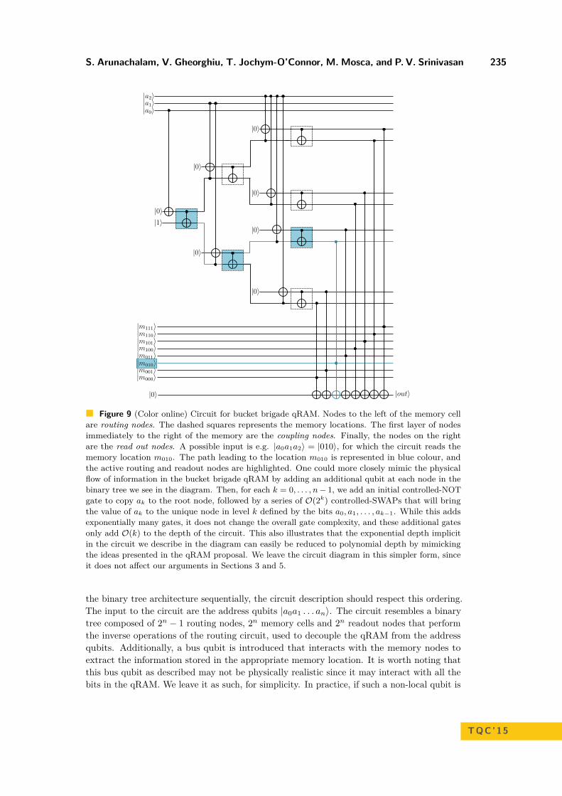
S. Arunachalam, V. Gheorghiu, T. Jochym-O’Connor, M. Mosca, and P. V. Srinivasan 235
|m100⟩
|a2⟩
|0⟩
|1⟩
|a0⟩|a1⟩
|m000⟩|m001⟩|m010⟩|m011⟩
|m110⟩|m111⟩
|0⟩
|0⟩
|0⟩
|0⟩
|0⟩
|0⟩
|0⟩
|m101⟩
|out⟩
Figure 9 (Color online) Circuit for bucket brigade qRAM. Nodes to the left of the memory cellare routing nodes. The dashed squares represents the memory locations. The first layer of nodesimmediately to the right of the memory are the coupling nodes. Finally, the nodes on the rightare the read out nodes. A possible input is e.g. |a0a1a2〉 = |010〉, for which the circuit reads thememory location m010. The path leading to the location m010 is represented in blue colour, andthe active routing and readout nodes are highlighted. One could more closely mimic the physicalflow of information in the bucket brigade qRAM by adding an additional qubit at each node in thebinary tree we see in the diagram. Then, for each k = 0, . . . , n− 1, we add an initial controlled-NOTgate to copy ak to the root node, followed by a series of O(2k) controlled-SWAPs that will bringthe value of ak to the unique node in level k defined by the bits a0, a1, . . . , ak−1. While this addsexponentially many gates, it does not change the overall gate complexity, and these additional gatesonly add O(k) to the depth of the circuit. This also illustrates that the exponential depth implicitin the circuit we describe in the diagram can easily be reduced to polynomial depth by mimickingthe ideas presented in the qRAM proposal. We leave the circuit diagram in this simpler form, sinceit does not affect our arguments in Sections 3 and 5.
the binary tree architecture sequentially, the circuit description should respect this ordering.The input to the circuit are the address qubits |a0a1 . . . an〉. The circuit resembles a binarytree composed of 2n − 1 routing nodes, 2n memory cells and 2n readout nodes that performthe inverse operations of the routing circuit, used to decouple the qRAM from the addressqubits. Additionally, a bus qubit is introduced that interacts with the memory nodes toextract the information stored in the appropriate memory location. It is worth noting thatthis bus qubit as described may not be physically realistic since it may interact with all thebits in the qRAM. We leave it as such, for simplicity. In practice, if such a non-local qubit is
TQC’15

236 On the Robustness of Bucket Brigade Quantum RAM
not feasible, one may either work with a phase shift oracle (as described in Ch. 8 of [19]), orone may use a binary-tree circuit to bring the result of the qRAM look-up to a specific qubitthat will be accessed by the quantum algorithm that performs the look-up.
The address qubit |a0〉 is used to activate the appropriate branch at the first level of therouting. The address qubit is coupled via a CNOT to an ancillary state prepared in thestate |0〉. This qubit then serves as one of the input qubits along with an additional qubitprepared in the |1〉 state for the routing node (a CNOT gate with the first qubit as control).Depending on the state of the address qubit, the resulting two-qubit output of the routingnode will have a single excited qubit in the |1〉 state, which we shall call the activated qubit.The activated branch of the tree governs the routing of the subsequent interactions withthe address qubits, playing the role of the routing atom in the case of the bucket brigadeoutlined in [12].
The two qubits at the exit of the level-0 routing node serve as inputs to the secondregister of the two level-1 routing nodes. These qubits control which of the routing nodesare activated at the next level of the qRAM binary tree architecture. Namely, the qubitthat is excited in the |1〉 state allows for the coupling between the address qubit and anintroduced |0〉 state ancilla via a Toffoli gate. Therefore the input to the active routingnode is either |01〉 or |11〉 depending on the state of the address qubit |a1〉. Effectively,the routing operation given by a CNOT gate activates a branch of the tree. For the nodethat is non-active, the state at the output of the previous level is |0〉, meaning the Toffoliis not activated and the resulting input and output state to the routing node remains |00〉.Therefore, after two routing node levels, the output of the routing qubits is composed of22 qubits, with only a single branch being excited depending on the state of the first twoaddress qubits |a0a1〉. Therefore, this corresponds to an isometry:
|00〉a0a1 → |0001〉, |01〉a0a1 → |0010〉, |10〉a0a1 → |0100〉, |11〉a0a1 → |1000〉, (11)
where the excited output qubits in the |1〉 state represent an active physical path for thesubsequent qRAM operations. This procedure is repeated for n levels, where at the k-th levelthere are 2k Toffoli gates and routing nodes. The 2k Toffoli gates are required to route of theaddress qubit |ak〉 through the previous k levels and the routing node establish the outputstates in order to route the subsequent address qubits. Since such a circuit performs theappropriate unitary mapping of the address qubits for all computational basis state inputs,by linearity it will extend to all superpositions of input address qubits. An example of therouting procedure for a three-qubit input address state |010〉 is presented in Fig. 9, wherethe blue highlighted nodes correspond to the activated nodes.
After the completion of the n routing node levels, memory readout is performed. Thereading is performed by introducing a bus qubit prepared in the |0〉 state which is the targetof 2n Toffoli gates. Each of the 2n qubits at the output of the qRAM routing nodes pair withone of the memory cells to serve as control qubits for the Toffoli gates. Since only a singleoutput qubit from the routing scheme is activated, only a single Toffoli gate couples witha memory location to the bus qubit. The bus qubit is represented by the bottom qubit inFig. 9 while the 23 memory qubits are represented between the qRAM routing architectureand the bus qubit.
Having completed the coupling of the address qubit, the state of the qRAM routing qubitsmust be decoupled from the address and bus qubits. Each of the gates from the routingcircuit are performed in reverse order, which corresponds to performing the inverse unitarycoupling transformation between the address qubits and the routing qubits. The resultingstate couples the address qubits with the corresponding memory qubit and has decouplesthe routing qubits to their input ancillary states.
S. Arunachalam, V. Gheorghiu, T. Jochym-O’Connor, M. Mosca, and P. V. Srinivasan 237
5 Error Correction
The results from Sec. 3 motivate the need for quantum error correction to be implementedat each node in order to protect against errors that may cause detrimental faults in pathinformation.
5.1 Imposing a quantum error correcting codeIn choosing a quantum error correcting code (QECC) to protect the path informationthat is stored in each node, it is essential to choose an encoding that can be implementedfault-tolerantly, to allow for the generalization to large computational systems. Moreover,the QECC should be chosen such that it can naturally be incorporated from the quantumcomputer that is accessing the qRAM. In order to analyze the desired error correctionproperties of a bucket brigade qRAM architecture we consider the circuit presented in Fig. 9.The key gate components at each site are the CNOT and Toffoli gates.
The most natural construction of a QECC that can implement such operations withminimal overhead would be the 15-qubit Reed-Muller code. The reason for choosing such acode would be that decomposing the gate operations in the routing circuit as a sequenceof CNOT and Toffoli gates has the advantage that each of these gates can be implementedin a transversal manner. Transversality is defined as the ability to implement a logicalgate by applying physical gates that have support at at most a single location per encodedcodeblock: it is the most natural way to guarantee fault-tolerance. However, if the quantumcomputing device leads more naturally to another form of quantum error correction encoding,methods such as state distillation or other schemes for universal fault-tolerance can beused [8, 24, 4, 18, 2].
The focus of many fault-tolerant implementations are through the CSS code construc-tion [28, 10, 29]. A CSS quantum code is constructed using two classical error correctingcodes, each individually used to address X and Z type errors. Given that any quantum errorcan be decomposed in terms of a linear combination of Pauli operators, developing an errorcorrecting code that can address both types of errors will be sufficient for the construction ofa QECC.
Let CX be a classical error correcting code of length n that has the associated paritycheck matrix HX , where each 0 in the parity check matrix of the classical code is replacedby the two-dimensional identity matrix I and each 1 in the classical parity check matrix isreplaced by the Pauli X operator. Similarly, let CZ be a second classical error correctingcode of length n with an associated parity check matrix HZ , where each 1 in the classicalparity check matrix has been now replaced by the Pauli Z operator. If C⊥X ⊆ CZ then bycombining the stabilizers generated from the parity check matrices of both codes, HX andHZ , the resulting stabilizer code forms a QECC. The number of physical qubits in the codeis n, the number of logical qubits is given by kX + kZ − n, where ki is the number of logicalstates in the given classical code i and the distance of the code is at least the minimum ofthe distance of the two classical codes. One of the many appealing features of the CSS codeconstruction is the transversality of the CNOT gate, a feature of the X and Z stabilizersbeing independent. A particular example of a CSS code is the 15-qubit Reed-Muller codementioned above.
5.2 Number of activations in a CSS codeIn the implementation of Giovanetti et al. [12], one of the primary advantages is the numberof gate activations that are needed per level of the bucket brigade scheme. More simply, a
TQC’15

238 On the Robustness of Bucket Brigade Quantum RAM
CNOT (Toffoli) gate in their scheme is “activated” only when the control qubit(s) is (are)in the state |1〉. Since only one register is in such a state at a given level, the total numberof activations can thus be kept low. In a physical implementation, this is relevant as anactivated path may represent the presence of a physical excitation without which no physicalprocess occurs, therefore one can think of these non-activated gates as in fact being theidentity operation. However, such an advantage vanishes when imposing a CSS code in orderto protect from errors due to the symmetry in the number of |0〉 and |1〉 states the logicalstates encoding the path information.
In the CSS code construction, two classical codes were taken to form a QECC. Therefore,given some codeword of the classical code c ∈ CZ , the equivalent quantum state written outin computation basis |c〉 must be stabilized by the Z generators of the code, by definition ofbeing a codeword of the classical code CZ . However, in order to be a logical state of the CSScode, it must also be stabilized by the elements of the group generated by the X stabilizers.Therefore, the codestate will be the superposition of the application of all X stabilizersupon |c〉,
|c+ C⊥Z 〉 =∑
x∈C⊥Z
|c+ x〉 = 12n−kX
∏i
(I⊗n + SX,i)|c〉, (12)
where SX,i are the generators of the X stabilizer group, equivalently given by the rows ofthe parity check matrix HX .
Consider the form of Eq. (12), given the state |c〉 written in the computational basis,the action of the operator (I⊗n + SX,1) will be the equally weighted superposition of thestate |c〉 and SX,1|c〉, which will differ at the location where SX,1 has a Pauli X in itsdescription. Therefore, at these locations half of the states in the superposition will have aphysical |0〉 state and half will have a physical |1〉 state. Then acting upon the state withthe operator (I⊗n + SX,2) will have the same effect on all the states in the superposition,with now an even number of physical |0〉 and |1〉 states occurring at location with Pauli Xin SX,2. Repeating this for all X generators, any location with a X operator in one of thestabilizers will necessarily have half of the states in the superposition in each of the physicalbasis states. In order for the code to protect against any arbitrary single qubit error, eachphysical qubit must be protected by at least one X stabilizer operator with support the givenlocation, otherwise it would be vulnerable to a single Z error at this location. As such, allrelevant CSS codesstate will have an equal number of each of the physical basis states whenwriting out the expansion of the state in the computational basis.
In a physical implementation, such as that of Giovanetti et al. [12], a qubit in the state |1〉represents an activated physical process, and as such the advantage of the bucket brigadescheme is that the number of such processes are kept low. However, due to the symmetryin the number of activations that must exist in both the logical ground and excited states,this advantage no longer exists when considering CSS codes. More generally, non-symmetriccodes, that is codes where the logical |0〉 state and logical |1〉 have a differing number ofphysical states in the excited state |1〉, are not desirable for the purposes of error correctionas they will be more susceptible to Z errors. The three-qubit repetition code is an extremeexample of such a property.
In principle, for the physical error model discussed in Section 3, one can envision usingthe detection of a photon lost in the routing structure as a means to correct for no-patherrors (see Fig. 5). However, detecting the exact node at which a photon was lost revealspath information about the state being read by the qRAM (since the previous node in therouting structure would have necessarily been activated by the address qubits) which leads
S. Arunachalam, V. Gheorghiu, T. Jochym-O’Connor, M. Mosca, and P. V. Srinivasan 239
to a loss of coherence in the system. Therefore, any photon detection has to identify thelevel at which the photon was lost, while not revealing exactly where. It is hard to envisagea practical means for experimentally realizing a photon detection with this property (forexample, by somehow symmetrizing the loss of the photon across the exponentially manynodes at a given level). Furthermore, even if this is achieved, one still faces the problem thatthe lost photon contained path information. Thus, destroying the photon with this pathinformation is equivalent to a dephasing error leading to a further loss of coherence.
In conclusion, if one encodes each node of the bucket brigade qRAM in an error correctingcode, then all nodes of the circuit are activated at a physical level, and essentially the qRAMarchitecture becomes equivalent to a fanout architecture. Even it the latter case, designing agood quantum error correcting code is highly non-trivial. An important issue is that thesyndrome measurement should not reveal any information whatsoever about the physicallocation of the nodes affected by errors. Otherwise, path information is being revealed, whichdecoheres the system.
6 Conclusions and open questions
We analyzed the robustness of the bucket brigade qRAM scheme introduced in [13, 12] underan optimistic error model. The primary advantage of the bucket brigade scheme is the needfor a polynomial in n (rather than exponential) number of gate activations per memoryreading. Yet, we give evidence for the hypothesis that for realistic error models, wheneverthe qRAM is used as a oracle for quantum searching, its error rate per gate has to scale aso(2−n/2). Such an error rate is exponentially smaller than the error O(1/n2) proposed in[12] (which is sufficient for algorithms with low query complexity), motivating the need forquantum error correction.
We argued that using traditional error correcting techniques offsets the main advantageof the bucket brigade scheme when used with algorithms that make super-polynomiallymany oracle queries. Since each component of the routing architecture has to be activelyerror corrected in order to protect against detrimental faults, the overall scheme requires anexponential number of physical gate activations, even if the number of logical gate activationsremains polynomial.
An interesting open question is the existence of a realistic architecture-specific errorcorrection technique that could recover the polynomial number of physical gate activationsof the routing scheme while still guaranteeing fault-tolerance. For example, if one tries touse an error correction mechanism whereby one only uses multi-qubit code states along theactive path, then one has the problem of extracting syndromes and applying corrections in away that does not identify which path has the non-trivial syndromes (since such informationwould lead to decoherence). If in this case, for example, one attempts to extract the syndromewithout leaving a trace of which node in a given level it came from, then the problem seemsat least as challenging as implementing a reliable qRAM.
Moreover, it would be interesting to investigate whether the requirement for a super-polynomial suppression of the error rate is a characteristic of quantum searching algorithmsor a more general feature of query complexity with faulty oracles.
Acknowledgements. We thank Daniel Gottesman, Stacey Jeffery, Seth Lloyd, LorenzoMaccone and Matteo Mariantoni for numerous insightful discussions and suggestions. Wethank Seth Lloyd for pointing out to us nice examples of important algorithms that onlyuse polynomially many queries. The authors were supported in part by NSERC, CIFAR,
TQC’15

240 On the Robustness of Bucket Brigade Quantum RAM
FQRNT, OGS, CryptoWorks21 and Industry Canada. IQC and PI are supported in part bythe Government of Canada and the Province of Ontario. S.A. is grateful to Ronald de Wolf’sERC Consolidator Grant QPROGRESS and Michele Mosca for support from NSERC.
References1 Andris Ambainis. Quantum walk algorithm for element distinctness. SIAM J. Comput.,
37(1):210–239, April 2007.2 Jonas T. Anderson, Guillaume Duclos-Cianci, and David Poulin. Fault-tolerant conversion
between the steane and reed-muller quantum codes. Phys. Rev. Lett., 113:080501, Aug2014.
3 Srinivasan Arunachalam. Quantum speed-ups for boolean satisfiability and derivative-freeoptimization. Master’s Thesis, University of Waterloo, 2014.
4 H. Bombin. Optimal transversal gates under geometric constraints. e-print arXiv:1311.0879[quant-ph].
5 H. Bombin and M.A. Martin-Delgado. Topological quantum distillation. Phys. Rev. Lett.,97:180501, Oct 2006.
6 Gilles Brassard, Peter Høyer, and Alain Tapp. Quantum cryptanalysis of hash and claw-freefunctions. SIGACT News, 28(2):14–19, June 1997.
7 Sergey Bravyi and Jeongwan Haah. Magic-state distillation with low overhead. Phys. Rev.A, 86:052329, Nov 2012.
8 Sergey Bravyi and Alexei Kitaev. Universal quantum computation with ideal clifford gatesand noisy ancillas. Phys. Rev. A, 71:022316, Feb 2005.
9 Harry Buhrman, Ilan Newman, Hein Roehrig, and Ronald de Wolf. Robust polynomialsand quantum algorithms. e-print arXiv:quant-ph/0309220.
10 A.R. Calderbank and Peter W. Shor. Good quantum error-correcting codes exist. Phys.Rev. A, 54:1098–1105, Aug 1996.
11 Andrew M. Childs, Richard Cleve, Enrico Deotto, Edward Farhi, Sam Gutmann, andDaniel A. Spielman. Exponential algorithmic speedup by a quantum walk. In Proceedingsof the Thirty-fifth Annual ACM Symposium on Theory of Computing, STOC’03, pages59–68, New York, NY, USA, 2003. ACM.
12 Vittorio Giovannetti, Seth Lloyd, and Lorenzo Maccone. Architectures for a quantumrandom access memory. Phys. Rev. A, 78:052310, Nov 2008.
13 Vittorio Giovannetti, Seth Lloyd, and Lorenzo Maccone. Quantum random access memory.Phys. Rev. Lett., 100:160501, Apr 2008.
14 Lov Grover and Terry Rudolph. Creating superpositions that correspond to efficientlyintegrable probability distributions. e-print arXiv:quant-ph/0208112.
15 Fang-Yu Hong, Yang Xiang, Zhi-Yan Zhu, Li-zhen Jiang, and Liang-neng Wu. Robustquantum random access memory. Phys. Rev. A, 86:010306, Jul 2012.
16 Peter Høyer, Michele Mosca, and Ronald de Wolf. Quantum search on bounded-errorinputs. In JosC.M. Baeten, JanKarel Lenstra, Joachim Parrow, and GerhardJ. Woeginger,editors, Automata, Languages and Programming, volume 2719 of Lecture Notes in ComputerScience, pages 291–299. Springer Berlin Heidelberg, 2003.
17 R.C. Jaeger and T.N. Blalock. Microelectronic Circuit Design. McGraw-Hill, Dubuque,2003.
18 Tomas Jochym-O’Connor and Raymond Laflamme. Using concatenated quantum codes foruniversal fault-tolerant quantum gates. Phys. Rev. Lett., 112:010505, Jan 2014.
19 Phillip Kaye, Raymond Laflamme, and Michele Mosca. An Introduction to Quantum Com-puting. Oxford University Press, 2007.
20 Greg Kuperberg. A subexponential-time quantum algorithm for the dihedral hidden sub-group problem. SIAM J. Comput., 35(1):170–188, July 2005.
S. Arunachalam, V. Gheorghiu, T. Jochym-O’Connor, M. Mosca, and P. V. Srinivasan 241
21 Seth Lloyd, Masoud Mohseni, and Patrick Rebentrost. Quantum algorithms for supervisedand unsupervised machine learning. e-print arXiv:1307.0411 [quant-ph].
22 Michele Mosca and Phillip Kaye. Quantum networks for generating arbitrary quantumstates. In Optical Fiber Communication Conference and International Conference onQuantum Information, page PB28. Optical Society of America, 2001.
23 Michael A. Nielsen and Isaac L. Chuang. Quantum Computation and Quantum Information(Cambridge Series on Information and the Natural Sciences). Cambridge University Press,1 edition, January 2004.
24 Adam Paetznick and Ben W. Reichardt. Universal fault-tolerant quantum computationwith only transversal gates and error correction. Phys. Rev. Lett., 111:090505, Aug 2013.
25 Oded Regev and Liron Schiff. Impossibility of a quantum speed-up with a faulty oracle. InProceedings of the 35th International Colloquium on Automata, Languages and Program-ming, Part I, ICALP’08, pages 773–781, Berlin, Heidelberg, 2008. Springer-Verlag.
26 A. S. Sedra and K.C. Smith. Microelectronic Circuits. Oxford Press, New York, 1998.27 Peter W. Shor. Scheme for reducing decoherence in quantum computer memory. Phys.
Rev. A, 52:R2493–R2496, Oct 1995.28 A.M. Steane. Error correcting codes in quantum theory. Phys. Rev. Lett., 77(5):793–797,
Jul 1996.29 Andrew M. Steane. Multiple-particle interference and quantum error correction. Proceed-
ings of the Royal Society of London. Series A: Mathematical, Physical and EngineeringSciences, 452(1954):2551–2577, 1996.
A A simple decoherence model
Let us consider the error model considered in [25],
Rp(ρ) := (1− p)OρO† + pρ, (13)
with O denoting the perfect oracle for quantum searching and let us define
Dq(ρ) := (1− q)ρ+ q ~Xρ ~X† (14)
as the multi-qubit bit-flip channel where ~X is a shorthand notation for a tensor product ofσX bit-flip operators acting on some fixed subset of the oracle qubits. The proof techniquepresented below for Dq also applies to the case of multi-qubit dephasing channels).
The error model proposed in this paper (see Eq. (9)) is
O(ρ) := prpOρO† + pwpEwp(ρ) + pnpEnp(ρ). (15)
We show that the composition Rp Dq resembles (although it is not exactly the same) ourerror model Eq. (9), for suitable chosen p and q. It follows immediately that Ω(N) lowerbound for the searching algorithm considered in [25] is also a lower bound for the compositionRp Dq, since channel composition cannot decrease the query complexity (one can simplyincorporate Dq into an appropriate unitary for the Rp algorithm).
A simple calculation yields:
Rp Dq(ρ) = (1− p)ODq(ρ)O† + pDq(ρ)
= (1− p)(1− q)OρO† + (1− p)qO( ~Xρ ~X†)O† + p(1− q)ρ+ pq ~Xρ ~X†
= (1− p)(1− q)OρO† + (1− p)qO( ~Xρ ~X†)O† + pDq(ρ). (16)
TQC’15

242 On the Robustness of Bucket Brigade Quantum RAM
We now identify the coefficients in Eq. (15) and Eq. (16)
prp = (1− p)(1− q)pwp = (1− p)qpnp = p, (17)
and note that for any given probabilities prp, pwp, pnp satisfying prp + pwp + pnp = 1, thesystem of equations Eq. (17) has the solution
p = pnp
q = pwp
pwp + prp. (18)
We can therefore write
Rp Dq(ρ) = prpOρO† + pwpO( ~Xρ ~X†)O† + pnpDq(ρ). (19)
Comparing Eq. (15) and Eq. (19), we observe that the term O( ~Xρ ~X†)O† is very similar toour wrong path term Ewp(ρ) (the error that corresponds to reading out an incorrect memorylocation). The last term term Dq(ρ) in Eq. (19) is not of the form of our no-path error termEnp(ρ), as the latter consists of depolarizing channels of different strengths depending on theposition of the address qubit (i.e., the qubits are affected in decreasing order of significance,that is, the first qubit is affected the most, whilst the last one the least). However, Dq(ρ) is adecohering term, which seems to be a “weaker” form of noise than Enp(ρ). We showed abovethat even with this weaker decoherence term the quadratic speedup of any searching algorithmis lost. Therefore we have strong reasons to believe that adding a stronger decoherence termwill not lower the quantum query complexity for the quantum searching problem. A rigorousproof of this conjecture remains an open problem.
B Error correction schemes
B.1 Correcting simple bit-flip errorsWe show below that for a qRAM governed by a toy error model of the form
O(ρ) = (1− p)OρO† + pO( ~Xρ ~X†)O†, (20)
the query error rate can be made arbitrarily small by using quantum error correction. Here Odenotes the perfect oracle and ~X represents a multi-qubit bit-flip channel (a tensor productof individual bit-flip operators acting on an arbitrary subset of qubits). While such errormodels are not realistic for the architecture presented in this work, it may be that futuredesigns allow for simpler error propagation. Such schemes could benefit from quantum errorcorrection to sufficiently reduce their error rate to enable Grover search.
As Grover’s algorithm requires O(√N) steps, one desires a target logical error rate of
δ = O(1/√N). Since the faulty oracle has an error model that consists of a bit flip channel
followed by the perfect oracle call, one can use a quantum error correcting code and applythe oracle in parallel along the qubits composing the code. The parallelism of the oracle callsmimics majority counting and allows for error correction to be performed between logicaloracle call steps. For simplicity, we provide an example that corrects against bit flip errorsonly using the repetition code, however such an analysis could be extended to correct for

S. Arunachalam, V. Gheorghiu, T. Jochym-O’Connor, M. Mosca, and P. V. Srinivasan 243
phase flips using code families such as the color codes [5], higher dimensional Shor codes [27],or triorthogonal codes [7].
For example, consider an oracle of the form |a〉|b〉 → |a〉|b⊕ f(a)〉, where a, b ∈ 0, 1. Alogical oracle call that uses an n-qubit repetition code behaves as follows for states in thecomputational basis:
|a〉|b〉 V→ |a〉⊗n|b〉⊗n O⊗n
−→ |a〉⊗n|b⊕ f(a)〉⊗n, (21)
where V denotes the isometric encoding. Therefore, given a repetition code of length d,the code corrects for all errors up to d/2− 1 physical bit flips by majority counting, usingnon-destructive Z-type stabilizer measurements. Therefore, the logical error rate becomespL = pd/2. Choosing d large enough allows the logical error rate to satisfy pL = pd/2 < δ,where δ is the desired target fidelity. Therefore
d >2 log δlog p =
2 log(
1/√N)
log p = n
log (1/p) . (22)
Each of the n address qubits that serve as input to the oracle call must be encoded intoa repetition code of length d. Hence, the total number of oracle calls for the completeGrover search algorithm is O(nd
√N) = O(n2
√N) = O(
√N(logN)2). As such, there is a
logarithmic penalty for error correction, yet the scaling is not linear as in the error model ofRegev and Schiff [25].
B.2 The failure of repetition codes for Regev and Schiff error modelThe above error correction scheme is not applicable to the error model presented in [25],described by Rp(ρ) = (1 − p)OρO† + pρ, since the failure of an oracle call can lead to anuncorrectable error, as demonstrated below. Consider the following example of the 3-qubitrepetition code, where rather than all three oracles calls succeeding, the oracle call on thefirst set of qubits fails. The computational states evolve as:
|000〉|000〉 O2O3−→ |000〉|0f(0)f(0)〉 (23)
|111〉|000〉 O2O3−→ |111〉|0f(1)f(1)〉. (24)
Consider the action of such a faulty oracle on the encoded state (|000〉 + |111〉)/√
2, forf(0) = 0 and f(1) = 1 . The resulting mapping is
1√2
(|000〉+ |111〉)⊗ |000〉 O2O3−→ 1√2
(|000〉|000〉+ |111〉|011〉). (25)
The syndrome check operators for the repetition code are the parity check operatorsZ1Z2, Z2Z3. They are used to determine if an oracle call has failed by measuring the ancillaqubits. However, the measurement collapses the state to either |000〉|000〉 or |111〉|011〉.Upon applying the appropriate correction based on the measured syndromes, the resultingstate becomes either |000〉|000〉 or |111〉|111〉. Therefore, the logical oracle call has failed,since the correct result must yield the superposition (|000〉|000〉+ |111〉|111〉)/
√2.
As expected, the error correction properties of the repetition code are not in violation ofthe results of Ref. [25], which state that a linear number of noisy black-box oracle calls arerequired, even with the addition of error correction.
TQC’15

244 On the Robustness of Bucket Brigade Quantum RAM
B.3 The failure of repetition codes for our error modelConsider the oracle error model:
O(ρ) := prpOρO† + pwpEwp(ρ) + pnpEnp(ρ), (26)
where O is the perfect oracle call while Ewp(ρ) and Enp(ρ) are the wrong path and no-pathterms, respectively. We model the wrong path term as a convex combinations of bit-flipchannels followed by perfect oracle calls. An example of one of those terms is the secondterm in Equation 20. We model the no-path term as taking any input state and mapping itto a fixed state |g〉, which represents the loss of a qubit to be replaced by any fixed ancillarystate. It should be noted that in the no-path case, the readout ancilla state does not change.Consider the action of the noisy channel on the five-qubit repetition code. Each instance ofthe channel has a certain probability of failure given by the associated weights. Focusing onone particular instance where the first address photon is lost and the second is affected by abit flip, the resulting mapping on the computational basis states is given by:
|00000〉|00000〉−→|g1000〉|0f(1)f(0)f(0)f(0)〉 (27)|11111〉|00000〉−→|g0111〉|0f(0)f(1)f(1)f(1)〉. (28)
Again choosing f(0) = 0 and f(1) = 1, a superposition of input states in the computationalbasis evolves as
12P [(|00000〉+ |11111〉)⊗ |00000〉]−→1
2 (P [|g1000〉 ⊗ |01000〉] + P [|g0111〉 ⊗ |00111〉]) ,(29)
where P[•] denotes the projector onto its argument. The measurement of the stabilizers ofthe 5-qubit code on the ancillary states results in the collapse of the state into one of twoterms depending on the syndrome measured. Note that the no-path term is the term thatdestroys coherence, similarly to the error term in the Regev and Schiff model [25].
Interferometric Versus Projective Measurement ofAnyonsClaire Levaillant1 and Michael Freedman2
1 Department of Mathematics, South Hall Room 6607, University of California,Santa Barbara, CA 93106, USA
2 Station Q, Microsoft Research, Santa Barbara, CA 93106-6105, USA
AbstractTwo distinct methods for measuring topological charge in a nonabelian anyonic system have beendiscussed in the literature: projective measurement of a single point-like quasiparticle and inter-ferometric measurement of the total topological charge of a group of quasiparticles. Projectivemeasurement by definition is only applied near a point and will project to a topological chargesector near that point. Thus, if it is to be applied to a group of anyons to project to a total charge,then the anyons must first be fused one by one to obtain a single anyon carrying the collectivecharge. We show that interferometric measurement is strictly stronger: Any protocol involvingprojective measurement can be simulated at low overhead by another protocol involving onlyinterferometric measurement.
1998 ACM Subject Classification J.2 Physical Sciences and Engineering
Keywords and phrases anyons, measurement, interferometry, physics
Digital Object Identifier 10.4230/LIPIcs.TQC.2015.245
1 Introduction
We clarify a foundational issue regarding the relative power of two computational schemeswhich have been long proposed for nonabelian anyons. The two are projective measurement[8] and interferometric measurement; abstractly [11, 10, 5, 4, 1] and in a physical system, [7].
The discussion is restricted to the basic case: unitary modular tensor categories (UMTC)[13]. This is a mathematical idealization of a (2 + 1)-dimension topological quantum fieldtheory (TQFT). The unitary requirement is necessary for the system to be a legitimate modelof the non-dissipative physics of the low energy states of a gapped quantum mechanical system.The modularity assumption is a nonsingularity requirement. Abstractly this condition assuresus that the quantum system can be consistently defined on a physical torus (and this impliesall surfaces [12]) – the system is not tied to the plane. Concretely it tells us that everytopologically nontrivial excitation (or equivalently “quasiparticle” or “anyon”) of the theorya is detected by its braiding with some other anyon b (see page 29 of [1]). For example, whenanyons a and b are mutually abelian, i.e., have a unique fusion channel c, braiding assumesthe form:
b a
OO OO= Mb,a
b a
OO OO, Mb,a a nontrivial phase.
Modularity implies that for each nontrivial particle a, there is a (possibly composite) b sothat not only is Mb,a 6= 1 but Mb,a 6= Mb,a′ , a′ = a, a′ an anyon of the theory. Even fornon-abelian theories, modularity implies that particles are distinguished via braiding.
© Claire Levaillant and Michael Freedman;licensed under Creative Commons License CC-BY
10th Conference on the Theory of Quantum Computation, Communication and Cryptography (TQC 2015).Editors: Salman Beigi and Robert König; pp. 245–249
Leibniz International Proceedings in InformaticsSchloss Dagstuhl – Leibniz-Zentrum für Informatik, Dagstuhl Publishing, Germany

246 Interferometric Versus Projective Measurement of Anyons
Figure 1
This distinguishability was exploited in [1, 4] to give a full analysis of anyonic interfero-meters of Mach-Zehnder and Fabry-Perot designs. We note that much of the applied andeven experimental literature on measuring topological charge, e.g. [14], has focused on Fabry-Perot geometries. In the low tunnelling (single pass) limit, the Fabry-Perot interferometerdetermines the same evolution of the system density matrix ρ as the simpler Mach-Zehnderinterferometer. Even so, the evolution of ρ under operation of the interferometer is quitecomplicated. Fortunately, and this is the main conclusion of [1, 4], there is an easy topologicalinterpretation of the asymptotic action of an interferometer, Inta, which has converged to ameasurement “a”, meaning the total topological charge within the interferometric loop hasbeen measured to be that of an anyon of type a. See Figure 1. Furthermore, convergence tothis limit is efficient – exponentially fast.
In contrast, a projective measurement Proja to particle type a is the Hermitian orthogonalprojection to that particle sector. It is visualized as occurring by bringing some externalprob, such as an STM tip, up to an isolated point-like anyon and directly detecting some,perhaps non-universal, signature of that particular particle type in that particular system.For example, even for an electrically neutral ψ, in ν = 5
2 fractional quantum Hall effect(FQHE), higher moments of the electric field might provide a signature. In any case, it isthis hope which has led to the projective measurement model.
We now show that within the UMTC formalism, any protocol using projective measure-ment can be efficiently simulated by a protocol which instead uses interferometric measure-ment.
To do this we first need to define, through a density matrix diagram, the asymptotictopological action of Inta. The diagrams, Figure 2b and on, have a |ket〉〈bra| aspect whenread from top to bottom. The diagrams in |ket〉〈bra| format, of course, represent operators(density matrices), and Figure 2a represents a state vector (|ket〉). It should be noted thatsuch representations of operators and states obey topological rules [13] and may or may notcorrespond bit by bit to a physical process.
We start with a vacuum and create a, perhaps complex, system of anyons which we divideinto two halves “inside” and “outside” the interferometer. In Figure 2 these two halves atany given time are depicted simply as points, but they may represent composite anyons, indual groups, drawn out of the vacuum.

C. Levaillant and M. Freedman 247
Figure 2
Figure 3
From [1, 4], Inta asymptotically transforms from Figure 2b to Figure 3, assuming thatthe measurement outcome a, indeed, has nonzero probability. In Figure 3 and below, wedrop overall nonzero scalars from the diagrams.
Notation: ωa is the ath row of the normalized S-matrix which operates as a projectoronto the a particle:
b
ωa = δa,b
b
.
The presence of ωa is expected – it projects onto the a-particle type sector. The ω0 loophas long been regarded as an unfortunate but unavoidable consequence of running theinterferometer. ω0 encodes a kind of decoherence between inside and outside caused by theintervening stream of prob particles b. In [4], this severing of charge lines k running fromthe inside to the outside of the interferometer was called anyonic charge line decoherence.Topologically, ω0 surgers the a-lines (Figure 3c) so that a and a have forgotten that theycame out of the vacuum together – they are no longer correlated.
The presence of this ω0-loop leads to a general supposition in the community that Inta
and Proja were incomparable: Inta permits non-demolition measurement, as the internalcorrelations within the two groups of quasiparticles, inside and outside, are not disturbed,whereas in order to obtain a localized particle on which to apply Proja, the internal structureof the quasiparticle group to be measured would first need to be destroyed by a series offusions (which produces decoherence even if the fusion outcomes are presumed not to beobserved). In contrast, Proja does not cause anyonic charge line decoherence between themeasured subsystem from its complement. Each seemed to have its own peculiar advantagesand disadvantages with respect to the preservation of quantum information.
However, we will now show that the anyonic charge line decoherence of a and a can bereversed (oddly, this oximoron is possible in a topological system) by additional interferometricmeasurements. The key observation is that if after Inta we interferometrically measure thecollective state of a ∪ a, there is still a nonzero probability of observing the outcome 0, thetrivial particle. This is because if the two lines in Figure 3c are recoupled, the F -symbol,
TQC’15

248 Interferometric Versus Projective Measurement of Anyons
Figure 4
F a,aa,a;0,0 6= 0, reflecting the fact that a particle and its uncorrelated antiparticle may fuse into
the vacuum. (This, in fact, is the definition of an antiparticle.) Suppose we measure a ∪ aand observe 0, so that Int0 is applied to the system. The result is given in Figure 4.
We see that Int0 has restored us to the situation we would have been in if the ω0 loopassociated to the initial Inta had not been present. The decoherence has been reversed.
Of course it is not certain that the second measurement will result in Int0; other outcomesIntk are also possible. But now there is an easy “ping-pong” strategy (referred to as “forcedmeasurement” in [3]): Bounce back and forth between measuring the initial inside – which willalways return outcome a, Inta will be applied on the odd steps of this cycle, and measuringthe entire system a ∪ a. Each of the odd steps decoheres the inside and outside of the initialinterferometer and returns the density matrix to that shown in Figure 3c. Actually, sinceon the odd steps 3, 5, 7, . . ., there is no doubt that topological charge a will be measured,it is not necessary to read the output of the interferometer, but merely to run the probeparticles around the initial loop, thus producing anyonic charge line decoherence. Each ofthese even step measurements on the entire system constitute an independent chance toapply Int0. Because of independence, the tail event that after 2t measurements Int0 has notbeen applied decays exponentially in t. The exact exponential rate is easily calculated fromthe data of any particular UMTC. Since F a,a
a,a;0,0 = 1da, charge 0 is observed at each step 2t
with probability p =(
1da
)2, so the exponential rate of decay in t is 2 loge
(1− 1
d2a
).
2 Conclusion and outlook
We have shown how to “projectively”1 measure the total topological charge with repeatedinterferometric measurements of groups of anyons without decohering the group from itscomplement. In contrast, projective measurement of anyonic charge is in the usual model [8]limited to projecting to the topological charge of a single anyon. A priori, this looks like astrictly weaker operation.
It should be remarked, though, that as with all issues of complexity, at this point inhistory there are no “lower bounds.”
Any proof that it is impossible to simulate interferometric measurement by projectivemeasurement would necessarily rely on complexity assumptions. We regard this as an areafor future work.
However, evidence of the enhanced strength of interferometric measurement is presentedin a series of papers [2, 9] on universal gate systems for qubit and qutrit systems withinSU(2)4 and its Jones-Kauffman partner. Previously a universal protocol for a certain qutrit
1 We place “projectively” in quotes because unlike the usual usage in the arena of anyonic systems, thismeasurement is both nonlocal and nondemolitional. It is projective in the usual quantum mechanicalsense of Hermitian orthogonal projection onto an eigenbasis, in this case the eigenbasis of total topologicalcharge.

C. Levaillant and M. Freedman 249
within SU(2)4 was found [6] using projective measurement but the argument appears quitespecial and not applicable to qubits.
We call attention to a shortcut for graphically exploring interferometry protocols. Becauseof the iterative process we have just described for eliminating the decohering ω0-loopsassociated to interferometric measurement, one may proceed – in the manner of a personwriting computer code in a higher order language – only to manipulate the |ket〉 whichdescribes the current state of the system of anyons. The |ket〉 is used at any given time todescribe the state that has been pulled out of the vacuum. It is not necessary to double thediagram by adding the dual bra (and the linking |ket〉〈bra| by ω0-loops). Any ω0-loop willeventually be removed by some even numbered step of our protocol. Thus it is not reallynecessary to draw the ω0-loops, or even the 〈bra|, but merely to keep track of the |ket〉. Inthe end, if a density matrix ρ is desired, one may obtain ρ as the outer product of the final|ket〉final with its dual 〈bra|final, ρ = |ket〉final〈bra|final.
References1 Bonderson, P. Non-abelian anyons and interferometry. PhD thesis, Caltech, 2007. Physics.2 Bonderson, P., Freedman, M., Lutchyn, R., Nayak, C., and Wang, Z. Unpublished.3 Bonderson, P., Freedman, M., and Nayak, C. Measurement-only topological quantum
computation via anyonic interferometry. Annals of Physics 324 (2009), 787.4 Bonderson, P., Shtengel, K., and Slingerland, J.K. Decoherence of anyonic charge in
interferometry measurements. Phys. Rev. Lett. 98 (2007), 070401.5 Bonderson, P., Shtengel, K., and Slingerland, J.K. Interferometry of non-Abelian Anyons.
Annals of Physics 323 (2008), 2709.6 Cui, S.X., and Wang, Z. Universal quantum computation with metaplectic anyons.
arXiv:1405.7778, April 2014.7 Das Sarma, S., Freedman, M., and Nayak, C. Topologically-protected qubits from a possible
non-abelian fractional quantum hall state. Phys. Rev. Lett. 94 (2005), 166802.8 Kitaev, A. Fault-tolerant computation by anyons. Ann. Phys. 303 (2003), 2–111.9 Levaillant, C. 2014, to appear.
10 Overbosch, B., and Bais, F. Inequivalent classes of interference experiements with non-abelian anyons. Phys. Rev. A 64 (2001), 062107.
11 Preskill, J. Fault-tolerant quantum computation. In Introduction to Quantum Computation,H.-K. Lo, S. Popescu, and T. P. Spiller, Eds. World Scientific, 1998.
12 Turaev, V.G. Quantum invariants of knots and 3-manifolds, vol. 18 of Studies in Mathem-atics. Walter de Gruyter, 1994.
13 Wang, Z. Topological quantum computation, vol. 112 of Regional Conference Series inMathematics. Conference Board of the Mathematical Sciences, 2010.
14 Willet, R., Pfeiffer, L., West, K., and Manfra, M. Aharonov-bohm effect and coherencelength of charge e
4 quasiparticles at 52 filling factor measured in multiple small fabry-perot
interferometers. arXiv:1301.2594, January 2013.
TQC’15