Links between observed micrometeorological variability and land-use patterns in the highveld ...

1 23

Meteorology and AtmosphericPhysics ISSN 0177-7971Volume 118Combined 3-4 Meteorol Atmos Phys (2012)118:129-142DOI 10.1007/s00703-012-0218-4

Links between observed micro-meteorological variability and land-usepatterns in the highveld priority area ofSouth Africa

Igor Esau, Philbert Luhunga, GeorgeDjolov, C. J. de W. Rautenbach & SergejZilitinkevich

1 23

Your article is protected by copyright and

all rights are held exclusively by Springer-

Verlag Wien. This e-offprint is for personal

use only and shall not be self-archived in

electronic repositories. If you wish to self-

archive your work, please use the accepted

author’s version for posting to your own

website or your institution’s repository. You

may further deposit the accepted author’s

version on a funder’s repository at a funder’s

request, provided it is not made publicly

available until 12 months after publication.

ORIGINAL PAPER

Links between observed micro-meteorological variabilityand land-use patterns in the highveld priority area of South Africa

Igor Esau • Philbert Luhunga • George Djolov •

C. J. de W. Rautenbach • Sergej Zilitinkevich

Received: 10 March 2012 / Accepted: 24 September 2012 / Published online: 12 October 2012

� Springer-Verlag Wien 2012

Abstract Links between spatial and temporal variability

of Planetary Boundary Layer meteorological quantities and

existing land-use patterns are still poorly understood due to

the non-linearity of air–land interaction processes. This

study describes the results of a statistical analysis of

meteorological observations collected by a network of

ten Automatic Weather Stations. The stations were in

operation in the highveld priority area of the Republic

of South Africa during 2008–2010. The analysis revealed

localization, enhancement and homogenization in the inter-

station variability of observed meteorological quantities

(temperature, relative humidity and wind speed) over

diurnal and seasonal cycles. Enhancement of the meteo-

rological spatial variability was found on a broad range of

scales from 20 to 50 km during morning hours and in the

dry winter season. These spatial scales are comparable to

scales of observed land-use heterogeneity, which suggests

links between atmospheric variability and land-use patterns

through excitation of horizontal meso-scale circulations.

Convective motions homogenized and synchronized

meteorological variability during afternoon hours in the

winter seasons, and during large parts of the day during the

moist summer season. The analysis also revealed that tur-

bulent convection overwhelms horizontal meso-scale cir-

culations in the study area during extensive parts of the

annual cycle.

1 Introduction

It has been recognized (Pielke 2001; Patton et al. 2005;

Horlacher et al. 2012) that heterogeneity of land use has a

significant impact on land–air interaction and atmospheric

dynamics in the planetary boundary layer (PBL). Several

studies (Esau and Lyons 2002; Sogalla et al. 2006; Scanlon

et al. 2007) have found strong connections between land-

use patterns and the largest scales of atmospheric turbulent

convection. For instance, Scanlon et al. (2007) revealed a

positive feedback to the atmospheric meso-scale and

PBL dynamics linked to the clustering of vegetation in

arid areas of the Kalahari Desert in southern Africa.

Starting from homogeneously and randomly distributed

vegetation, they arrived to strongly localized vegetation

clusters in their model. The process has been attributed to

Responsible editor: J.-F. Miao.

I. Esau (&) � S. Zilitinkevich

Nansen Environmental and Remote Sensing Center, G.C. Rieber

Climate Institute, Thormohlensgt. 47, 5006 Bergen, Norway

e-mail: [email protected]

S. Zilitinkevich


I. Esau

Centre for Climate Dynamics (SKD), Bergen, Norway

I. Esau � S. Zilitinkevich

Department of Radiophysics, University of Nizhny Novgorod,

Nizhny Novgorod, Russia

P. Luhunga � G. Djolov � C. J. de W. Rautenbach

Department of Geography, Geoinformatics and Meteorology,

Faculty of Natural and Agricultural Sciences,

University of Pretoria, Pretoria 0002, South Africa


S. Zilitinkevich

Finnish Meteorological Institute, Erik Palmenin aukio 1, PL 503,

00101 Helsinki, Finland

S. Zilitinkevich

Division of Atmospheric Sciences, University of Helsinki,

Helsinki, Finland

123

Meteorol Atmos Phys (2012) 118:129–142

DOI 10.1007/s00703-012-0218-4

Author's personal copy

a redistribution of atmospheric convective motions, and

therefore, precipitation.

A major deficiency of such modeling studies is that the

links between the atmospheric dynamics and land-use

types are implicitly incorporated into the corresponding

(e.g. atmospheric convection and dynamical vegetation)

model parameterizations. Hence, independent observa-

tionally based validation and calibration are required. A

better understanding of the atmospheric dynamics on a

multitude of spatial and temporal scales over a realistic

heterogeneous landscape could be gained through the

analysis of synchronous high-resolution meteorological

observations collected by a dense network of Automatic

Weather Stations (AWSs).

Statistical analysis of observations and their associated

meteorological modeling is often disclosing non-linear and

climatologically significant effects caused by turbulence

self-organization and excitation of meso-scale circulations

(land breezes) over different types of surface heterogeneity.

For instance, Van Heerwaarden and Vila-Guerau de Arel-

lano (2008) studied the sensitivity of PBL turbulent

dynamics to surface heterogeneities with the aid of turbu-

lence-resolving models, where the transport of specific

humidity was varied. Their results clearly indicated that

despite the higher temperature and lower surface relative

humidity of warm land patches, the heterogeneity-induced

convection facilitate the penetration of air parcels to higher

elevations where additional condensation enhanced cloud

formation. Horlacher et al. (2012) performed a combined

statistical analysis on meteorological observations and the

simulated output by two meso-scale models, and demon-

strated greatly enhanced spatial variability of screen-level

variables under stably stratified boundary layer conditions.

This variability decreases with height, but at low levels (up

to 10 m) it manifested local temperature differences as

large as 5 �C, which are significant and therefore important

for agricultural and other social economic activities.

This study describes unique high-resolution synchro-

nous observational data sets that were collected from

February 2008 to December 2010 by two independent

dense AWS networks deployed in the highveld priority

area (HPA) of the Republic of South Africa (Fig. 1). This

network of stations is significantly larger, and more

diverse, than networks used in previous studies (Taylor

et al. 2007; Washington et al. 2005; Laakso et al. 2010;

Horlacher et al. 2012). The statistical data analysis focuses

on the study of micro-meteorological spatial and temporal

variability of surface air temperature, relative humidity and

wind speed. Using co-variability as a characteristic of the

impact of land use and other heterogeneities on the atmo-

spheric turbulent dynamics, this study attempts to reveal

patterns of homogenization, localization and enhancement

of the near-surface atmospheric dynamics. These patterns

are still poorly studied and therefore not accounted for in

the PBL parameterizations used in many meteorological

models.

Since the HPA is a highly industrialized area accounting

for about 75 % of South Africa’s industrial output, the

region is the source of significant atmospheric pollution

(Tyson et al. 1988; Laakso et al. 2010). Sources of about

90 % of the South African nitrogen oxide emission are

located in the HPA. The concentration of such pollutants

depends on the micro-meteorological variability, which

could be used as a proxy characteristic for turbulent dis-

persion and meso-scale meteorological transport of

admixtures. Human health in the HPA, especially the

health of children, has been found to be already signifi-

cantly affected by atmospheric pollution (Alberts 2011).

Alberts (2011) has, however, concluded that a quantifica-

tion of the effect of ambient air pollution on human health

was problematic due to the lack of proper high-resolution

meteorological information. This study could provide such

information for future health risk assessment and life

quality research.

The manuscript is structured in five sections. Section 2

describes the study area and the data collected. Section 3

describes the methodology of analysis, while results of the

study are discussed in Sect. 4. In it the applications and

limitations of the results are also considered. Conclusions

from the study are summarized in Sect. 5.

2 Description of the study area and observations

2.1 Geography

The HPA has been intensively studied during several

decades (Von Gogh et al. 1982; Tyson et al. 1988; Jury and

Tosen 1989; Held et al. 1996; Freiman and Tyson 2000;

Tyson and Gatebe 2001; Freiman and Piketh 2003; Collett

et al. 2010; Laakso et al. 2010). The HPA is located in the

South Africa highveld region (25�–27�S; 28�–30�E). It

extends across the eastern parts of the urbanized Gauteng

Province and the country’s largest cities (Pretoria and

Johannesburg), and falls also in the Free State and

Mpumalanga Provinces where it occupies an plateau of

about 30,000 km2 with an altitude of about 1,400–1,700 m

above mean sea level. In general, the surface of the plateau

is rather flat but surface morphology is very heterogeneous.

About 70 % of the HPA is covered by grassland, while the

rest is utilized for agricultural (maize, cattle and sheep,

crop production, dairy farming), urban and industrial

activities. Figure 2 exemplifies surface heterogeneity in the

HPA. It shows the Normalized Digital Vegetation Index

(NDVI) for a 20 km by 20 km patch within the HPA

obtained from the Landsat platform 7 satellite on 3 July

130 I. Esau et al.

123


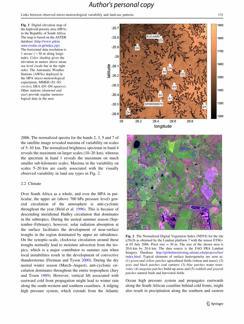
2006. The normalized spectra for the bands 2, 3, 5 and 7 of

the satellite image revealed maxima of variability on scales

of 5–10 km. The normalized brightness spectrum in band 4

reveals the maximum on larger scales (10–20 km), whereas

the spectrum in band 1 reveals the maximum on much

smaller sub-kilometer scales. Maxima in the variability on

scales 5–20 km are easily associated with the visually

observed variability in land use types in Fig. 2.

2.2 Climate

Over South Africa as a whole, and over the HPA in par-

ticular, the upper air (above 700 hPa pressure level) gen-

eral circulation of the atmosphere is anti-cyclonic

throughout the year (Held et al. 1996). This is because of

descending meridional Hadley circulation that dominates

in the subtropics. During the austral summer season (Sep-

tember–February), however, solar radiation absorption at

the surface facilitates the development of near-surface

troughs in the region dominated by upper air subsidence.

On the synoptic-scale, clockwise circulation around these

troughs normally lead to moisture advection from the tro-

pics, which is a major contributor to summer rain when

local instabilities result in the development of convective

thunderstorms (Freiman and Tyson 2000). During the dry

austral winter season (March–August), anti-cyclonic cir-

culation dominates throughout the entire troposphere (Jury

and Tosen 1989). However, vertical lift associated with

eastward cold front propagation might lead to winter rain

along the south-western and southern coastlines. A ridging

high pressure system, which extends from the Atlantic

Ocean high pressure system and propagates eastwards

along the South African coastline behind cold fronts, might

also result in precipitation along the southern and eastern

Fig. 1 Digital elevation map of

the highveld priority area (HPA)

in the Republic of South Africa.

The map is based on the ASTER

database (http://www.gdem.

aster.ersdac.or.jp/index.jsp).

The horizontal data resolution is

1 arcsec (*30 m along longi-

tude). Color shading gives the

elevation in meters above mean

sea level (scale bar at the right

side). The Automatic Weather

Stations (AWSs) deployed in

the HPA micro-meteorological

experiment, MMEH (S1–S5:

circles), DEA (D1–D4 squares).

Other stations (diamond andstar) provide regular meteoro-

logical data in the area

Fig. 2 The Normalized Digital Vegetation Index (NDVI) for the tile

e29s26 as obtained by the Landsat platform 7 with the sensor ETM?

at 03 July 2006. Pixel size = 30 m. The size of the shown area is

20.6 km by 20.6 km. The data source is the FAO FRA Landsat

Imagery Database http://globalmonitoring.sdstate.edu/projects/fao/

index.html. Typical elements of surface heterogeneity are seen as:

(1) green and yellow patches agricultural fields (wheat and maze); (2)

gray and black patches coal carriers; (3) blue patches water reser-

voirs; (4) magenta patches build-up areas and (5) reddish and grayishpatches natural bush and harvested fields

Links between observed micro-meteorological variability and land-use patterns 131

123


http://www.gdem.aster.ersdac.or.jp/index.jsp

http://www.gdem.aster.ersdac.or.jp/index.jsp

http://globalmonitoring.sdstate.edu/projects/fao/index.html

http://globalmonitoring.sdstate.edu/projects/fao/index.html

coastlines. This creates favorable conditions for cloud

development against the eastern escarpment.

The HPA climate is found to be cooler than the climate of

other areas of similar latitude, which is mainly due to the high

altitude of the HPA. The weather is characterized by hot

summer daytime temperatures (25–32 �C), and spectacular

late afternoon thundershowers. Winter daytime average

temperatures are cooler (15–19 �C), while night time tem-

peratures often drop below freezing point, which often leads

to morning frost. During winter, temperature inversions

occur almost every night at the surface, while elevated

inversions are occurring with high frequency (Von Gogh

et al. 1982; Freiman and Tyson 2000; Becker 2005). As a

matter of fact, elevated inversions occur on 60 % of all days

at a mean altitude of 1,700 m above ground level, and with a

depth and strength of just under 200 m and 1.5 �C, respec-

tively. In winter, the depth of the surface inversion varies

from 300 to 500 m at around sunrise, which is the time of

maximum depth and when the average strength of the

inversion is about 5–6 �C. In summer, surface inversions are

of approximately the same depth, but with strength of less

than 2 �C. Tyson et al. (1988) presented climatological data

on the PBL stability regime at the city of Bloemfontein,

which reveals the following frequency appearance at mid-

day: stable (25 %), unstable (74 %) and inversion (1 %), and

the following frequency appearance during midnight: stable

(19 %), unstable (2 %), inversion (79 %).

Highveld priority area precipitation, which ranges from

600 to 800 mm per annum, has its maximum during

December to January (the mid-austral summer season).

Frost occurs regularly during winter months and ranges

from about 30 days in the Mpumalanga Province, to about

70 days in the southern Free State Province. Winds are

highly variable but easterly and westerly winds are more

prevalent. Closer to the mountain ranges along the eastern

escarpment the incidence of frost is probably even higher.

Over higher lying areas snow events are not uncommon.

2.3 Micro-meteorological experiment in the highveld

priority area (MMEH)

The HPA is relatively densely covered with measurements

stations. However, a large part of the observational data is

proprietary and cannot easily be obtained. A part of the

available data are scattered over a larger area, and there-

fore, are less useful for the characterization of micro-

meteorological variability on spatial scales of up to 20 km.

In order to overcome these difficulties related to the

homogenization of the available data sets, five AWSs were

deployed in the HPA during a Norway–South Africa

bilateral research project. The data collected by these sta-

tions constitute the Micro-Meteorological Experiment in

the Highveld (MMEH) data set that is used in this study.

The MMEH AWSs (identified by the symbol ‘‘S’’) have

been deployed in rural and agricultural areas. In addition,

the South African Department of Environmental Affairs

(DEA) provided data collected from another five AWSs

(identified by the symbol ‘‘D’’) that were placed over a

wider area as the MMEH AWSs in the HPA (Fig. 1). The

DEA data set is very similar to the MMEH data set,

although some systematic differences could be observed

due to the preferable location of the DEA AWSs near

settlements. Table 1 lists the 10 meteorological stations

with their geographic coordinates. Table 2 gives the geo-

desic distances between the stations.

The MMEH AWSs made use of Davis Vantage Pro 2

instrumentation (see Application Note N�30 for technical

information), and were equipped with a pressure sensor,

temperature and humidity sensors, a wind anemometer, a rain

collection gauge and a solar radiation sensor. The Davis

Vantage Pro 2 instruments were chosen due to their low price

and relatively high accuracy in a regime of autonomous data

collection. This type of equipment has already successfully

been used in African conditions (e.g. during the Bodele

Experiment: BodEx-2005) conducted in Chad (Giles 2005;

Washington et al. 2005), and elsewhere in the world [e.g. the

Bergen municipality (Norway) installed and operates 55

Davis Vantage Pro 2 AWSs to monitor weather conditions].

The DEA AWSs were based on a more permanent installation

in a 3 m 9 2 m 9 2.4 m shelter and a 10 m mast for wind

measurements on a concrete plinth with 1.8 m palisade for

security. The DEA AWSs are equipped with RM Young

instrumentation (RM Young, Traverse City, USA) measuring

wind speed and direction, ambient air temperature, relative

humidity, rainfall, solar radiation and barometric pressure.

The MMEH and DEA data were collected from the

beginning of February 2008 through to the end of

December 2010. Data samples were recorded every 10 min

(144 samples per day when the completeness was 100 %).

As commonly experienced with unattended AWS obser-

vations, the collected data sometimes had significant gaps,

mostly due to technical problems with the stations

(Table 1). Therefore, the joint use of both data sets could

be beneficial as it would greatly improve the data coverage

during the considered period. There are two periods con-

tinuously covered with observations: (1) the austral winter

during June and July 2009; (2) the austral summer during

January and February 2009. In addition, there are a period

during August and December 2008 when all MMEH AWSs

were recording without any problems.

3 Methodology

Data sets collected from a dense network of synchronous

AWSs only very recently became accessible for statistical

132 I. Esau et al.

123


analysis, and there are therefore no commonly used methods

or procedures available to provide a complete and unam-

biguous statistical interpretation of inter-AWS relationships.

Literature surveys, however, revealed a large diversity of

suggested methods and routines, but many of these cannot be

used consistently for informative analyses of the data of this

study. This study will therefore be confined to a multi-scale

variability analysis using a convenient modification of the

approach followed by Harzallah and Sadourny (1995) and

Ting et al. (2009). The method seeks to quantify contribu-

tions of externally forced variability as well as internal var-

iability in the total data variance. The externally forced

variability is defined as variability of an observed meteoro-

logical parameter, e.g. u, synchronized in the data from all

stations in a data set. Correspondingly, the internal vari-

ability is associated with variability in data specific to the

given station, and can therefore be obtained from inter-AWS

variability at any given time. If there exists any significant

effect of land use heterogeneity on the PBL, it should be

reflected as enhanced internal variability as compared to the

forced variability.

Data collected by the spatially distributed network of

AWSs in the HPA are beneficial for studying external

versus internal variability, as they can be processed with

two variants of the multi-scale analysis, conventionally

called spatial scale analysis and Root Mean Square (RMS)

analysis.

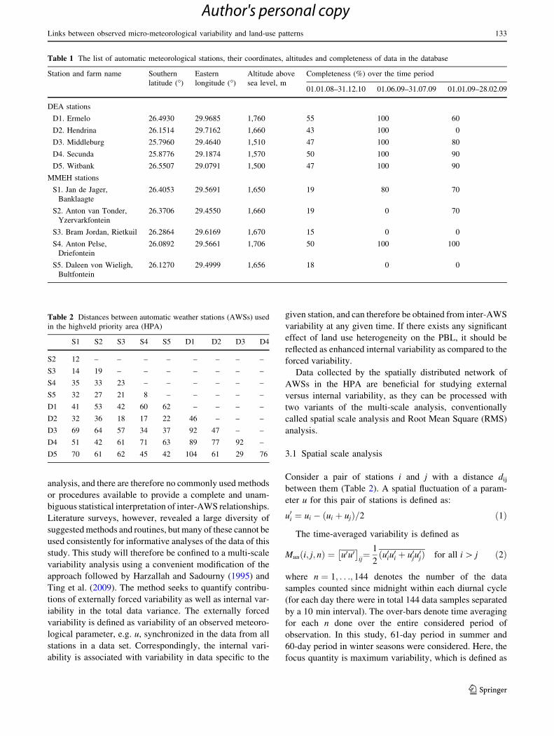
3.1 Spatial scale analysis

Consider a pair of stations i and j with a distance dij

between them (Table 2). A spatial fluctuation of a param-

eter u for this pair of stations is defined as:

u0i ¼ ui � ðui þ ujÞ=2 ð1Þ

The time-averaged variability is defined as

Muuði; j; nÞ ¼ u0u0� �

ij¼ 1

2ðu0iu0i þ u0ju

0jÞ for all i [ j ð2Þ

where n ¼ 1; . . .; 144 denotes the number of the data

samples counted since midnight within each diurnal cycle

(for each day there were in total 144 data samples separated

by a 10 min interval). The over-bars denote time averaging

for each n done over the entire considered period of

observation. In this study, 61-day period in summer and

60-day period in winter seasons were considered. Here, the

focus quantity is maximum variability, which is defined as

Table 1 The list of automatic meteorological stations, their coordinates, altitudes and completeness of data in the database

Station and farm name Southern

latitude (�)

Eastern

longitude (�)

Altitude above

sea level, m

Completeness (%) over the time period

01.01.08–31.12.10 01.06.09–31.07.09 01.01.09–28.02.09

DEA stations

D1. Ermelo 26.4930 29.9685 1,760 55 100 60

D2. Hendrina 26.1514 29.7162 1,660 43 100 0

D3. Middleburg 25.7960 29.4640 1,510 47 100 80

D4. Secunda 25.8776 29.1874 1,570 50 100 90

D5. Witbank 26.5507 29.0791 1,500 47 100 90

MMEH stations

S1. Jan de Jager,

Banklaagte

26.4053 29.5691 1,650 19 80 70

S2. Anton van Tonder,

Yzervarkfontein

26.3706 29.4550 1,660 19 0 70

S3. Bram Jordan, Rietkuil 26.2864 29.6169 1,670 15 0 0

S4. Anton Pelse,

Driefontein

26.0892 29.5661 1,706 50 100 100

S5. Daleen von Wieligh,

Bultfontein

26.1270 29.4999 1,656 18 0 0

Table 2 Distances between automatic weather stations (AWSs) used

in the highveld priority area (HPA)

S1 S2 S3 S4 S5 D1 D2 D3 D4

S2 12 – – – – – – – –

S3 14 19 – – – – – – –

S4 35 33 23 – – – – – –

S5 32 27 21 8 – – – – –

D1 41 53 42 60 62 – – – –

D2 32 36 18 17 22 46 – – –

D3 69 64 57 34 37 92 47 – –

D4 51 42 61 71 63 89 77 92 –

D5 70 61 62 45 42 104 61 29 76


123


U0T 0 ði; jÞ ¼ maxn¼1...144

MUTði; j; nÞð Þ ð3Þ

It characterizes the maximum variability of the horizontal

temperature flux (U0T 0). Variability of the horizontal relative

humidity flux (U0R0) and the horizontal momentum flux

(U0U0) are obtained in the same manner. It is reasonable to

expect that the flux given by Eq. (3) maximize on certain

spatial scales, as fluctuations defined by Eq. (1) might

increase with an increase in the distance dij, while

correlations between observed data from such stations

might decay.

At a large scale, only the external forced variability,

which is the same for all stations in the area, will determine

residual horizontal flux values. The decay of these fluxes

with increasing dij is, however, not necessarily monotonic.

If there are significant interactions between the land use

scales and the scales of the atmospheric dynamics, the

fluxes may level off or even enhance for a certain range of

scales. The next section will demonstrate that this is in fact

the case for the MMEH, as well as for DEA data recorded

in the HPA. Such an enhancement of turbulent exchange

over heterogeneous surface was previously referred to as a

resonant response (Roy et al. 2003; Patton et al. 2005; Esau

2007; Robinson et al. 2008). Such response is expected

within the range of normalized scales 1\dij=h\9, where h

denotes the PBL depth. The lower limit of scales is more

relevant to initial stages of the PBL convection, whereas

the upper limit is more relevant to well-developed con-

vection (Robinson et al. 2008). Taking h = 2–3 km in the

HPA (Freiman and Tyson 2000), fluxes should peak at

distances of dij = 5–30 km. These spatial scales are rather

similar to the typical land use heterogeneity scales in

Fig. 2b. Unfortunately, the scales smaller than 10 km are

only marginally resolved in the available data sets.

3.2 RMS analysis

In RMS analysis, the mean variability of a parameter u,

which is determined for each station over all time intervals,

is compared with the mean variability of u, which is

determined at each time interval over all stations. Mathe-

matically, if u ði; tÞ is a matrix at each sampling interval,

where the row index i ¼ 1; . . .;N runs over stations and the

column index t ¼ 1; . . .; T runs over time intervals, the

temporal and spatial RMS could be defined as

rtimeu ðnÞ ¼

ffiffiffiffiffiffiffiffiffiffiffiffiffiffiffiffiffiffiffiffiffiffiffi

u� �uð Þ2D Er

ð4Þ

rstationu ðnÞ ¼

ffiffiffiffiffiffiffiffiffiffiffiffiffiffiffiffiffiffiffiffiffiffiffiffiffiffi

u� uh ið Þ2D Er

ð5Þ

where uh iðt; nÞ ¼ 1N

Pi uði; t; nÞand �uði; nÞ ¼ 1

T

Pt uði; t; nÞ.

In order to study diurnal cycle of interactions between

land use and PBL dynamics, time averaging was achieved

independently for each of the data sampling moments n

across all days available in each data set (60 or 61 days for

100 % completeness of a station’s data).

Both measures, rstationu and rtime

u , may rise and fall within

the diurnal cycle. Moreover, one may be consistently

smaller or larger than the other. Useful information could

be extracted from their relative change within the diurnal

cycle as defined by the following measures:

RuðnÞ ¼rstation

u ðnÞrstation

u ðnÞ þ rtimeu ðnÞ ð6Þ

DuðnÞ ¼ rstationu ðnÞ � rstation

u ðnÞ� �

� rtimeu ðnÞ � rtime

u ðnÞ� �

ð7Þ

Here, the over-bar denotes averaging over all the diurnal

sampling intervals n. The ratio, Ru, indicates the relative

significance of the internal (local) variability at the stations

versus total variability. It should not be confused with the

fraction of total variability, which is explained by the internal

variability. For small ensembles of data sets (N\20) with

large internal variability, such a fraction would be estimated

with a significant error (Ting et al. 2009). The difference of

the normalized RMS, Du, indicates the relative importance of

changes in the external and internal variability across the

diurnal cycle. A reduction of Du, in particular to negative

values, indicates spatial homogenization, and therefore

diminishing internal variability. Vice versa, an increase of

Du indicates that the internal variability become more

pronounced, which suggests an increased coupling between

local land surface features and atmospheric PBL dynamics

and a decreasing coupling to the large scale dynamics of the

free troposphere, correspondingly.

4 Results

4.1 Externally forced variability versus internal

variability

In this study, the methods proposed for spatial scale and

RMS analyses mutually complement each other. The for-

mer select the horizontal scale of the optimal land-use–

atmosphere coupling while the latter show the change of

the coupling strength within a typical diurnal cycle for both

winter and summer seasons.

Figure 3 denotes results of the spatial scale analysis as

applied to the available data sets. Previously published

works (Patton et al. 2005; Esau 2007; Robinson et al. 2008)

suggested that the horizontal flux given in Eq. (3) should

be enhanced on the scales 5–30 km, in the event of PBL

134 I. Esau et al.

123


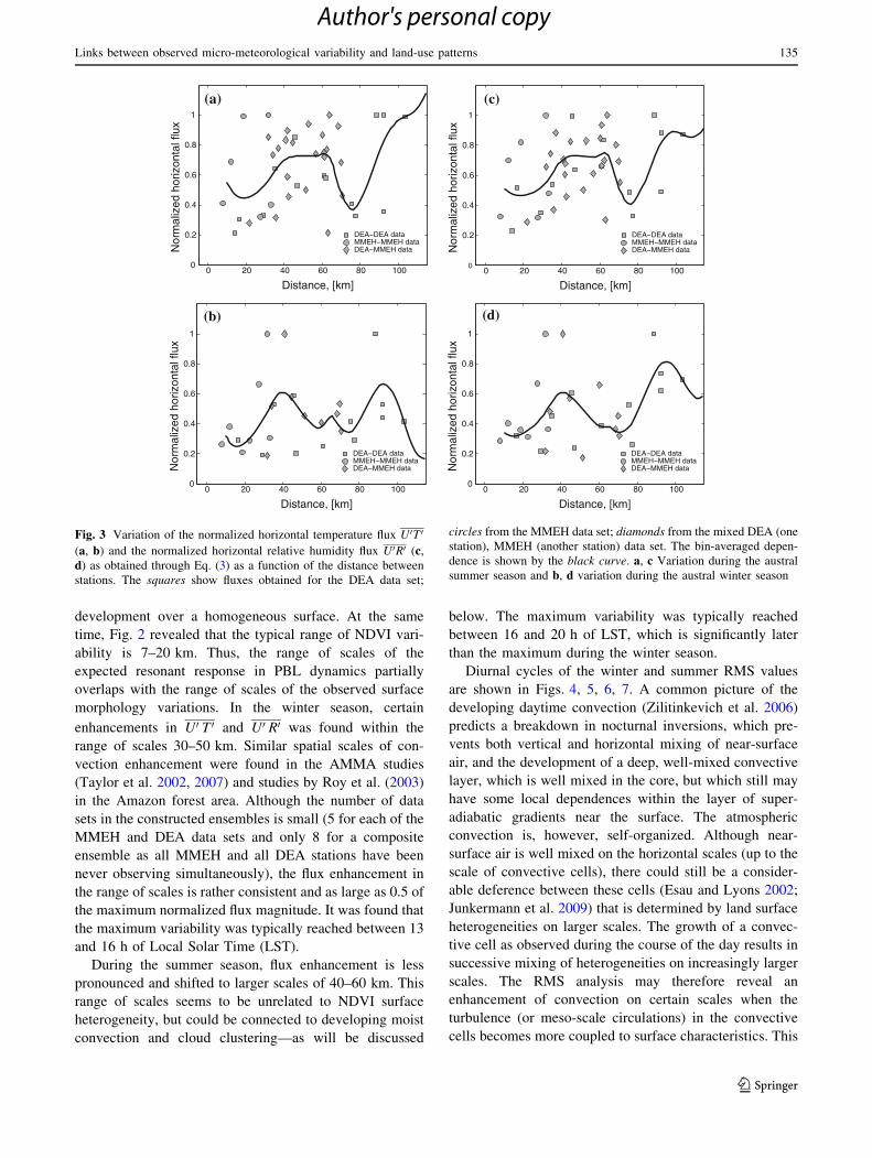
development over a homogeneous surface. At the same

time, Fig. 2 revealed that the typical range of NDVI vari-

ability is 7–20 km. Thus, the range of scales of the

expected resonant response in PBL dynamics partially

overlaps with the range of scales of the observed surface

morphology variations. In the winter season, certain

enhancements in U0 T 0 and U0 R0 was found within the

range of scales 30–50 km. Similar spatial scales of con-

vection enhancement were found in the AMMA studies

(Taylor et al. 2002, 2007) and studies by Roy et al. (2003)

in the Amazon forest area. Although the number of data

sets in the constructed ensembles is small (5 for each of the

MMEH and DEA data sets and only 8 for a composite

ensemble as all MMEH and all DEA stations have been

never observing simultaneously), the flux enhancement in

the range of scales is rather consistent and as large as 0.5 of

the maximum normalized flux magnitude. It was found that

the maximum variability was typically reached between 13

and 16 h of Local Solar Time (LST).

During the summer season, flux enhancement is less

pronounced and shifted to larger scales of 40–60 km. This

range of scales seems to be unrelated to NDVI surface

heterogeneity, but could be connected to developing moist

convection and cloud clustering—as will be discussed

below. The maximum variability was typically reached

between 16 and 20 h of LST, which is significantly later

than the maximum during the winter season.

Diurnal cycles of the winter and summer RMS values

are shown in Figs. 4, 5, 6, 7. A common picture of the

developing daytime convection (Zilitinkevich et al. 2006)

predicts a breakdown in nocturnal inversions, which pre-

vents both vertical and horizontal mixing of near-surface

air, and the development of a deep, well-mixed convective

layer, which is well mixed in the core, but which still may

have some local dependences within the layer of super-

adiabatic gradients near the surface. The atmospheric

convection is, however, self-organized. Although near-

surface air is well mixed on the horizontal scales (up to the

scale of convective cells), there could still be a consider-

able deference between these cells (Esau and Lyons 2002;

Junkermann et al. 2009) that is determined by land surface

heterogeneities on larger scales. The growth of a convec-

tive cell as observed during the course of the day results in

successive mixing of heterogeneities on increasingly larger

scales. The RMS analysis may therefore reveal an

enhancement of convection on certain scales when the

turbulence (or meso-scale circulations) in the convective

cells becomes more coupled to surface characteristics. This

0 20 40 60 80 1000

0.2

0.4

0.6

0.8

1

DEA−DEA dataMMEH−MMEH dataDEA−MMEH data

Distance, [km]

Nor

mal

ized

hor

izon

tal f

lux

0 20 40 60 80 1000

0.2

0.4

0.6

0.8

1


Distance, [km]

Nor

mal

ized

hor

izon

tal f

lux

0 20 40 60 80 1000

0.2

0.4

0.6

0.8

1


Distance, [km]

Nor

mal

ized

hor

izon

tal f

lux

0 20 40 60 80 1000

0.2

0.4

0.6

0.8

1


Distance, [km]

Nor

mal

ized

hor

izon

tal f

lux

(a) (c)

(d)(b)

Fig. 3 Variation of the normalized horizontal temperature flux U0T 0

(a, b) and the normalized horizontal relative humidity flux U0R0 (c,

d) as obtained through Eq. (3) as a function of the distance between

stations. The squares show fluxes obtained for the DEA data set;

circles from the MMEH data set; diamonds from the mixed DEA (one

station), MMEH (another station) data set. The bin-averaged depen-

dence is shown by the black curve. a, c Variation during the austral

summer season and b, d variation during the austral winter season


123


coupling will occur at certain hours of LST, as horizontal

scales increase as l / t 1=2.

In this study, the ensemble of all MMEH and DEA

station data is considered. Inspection of the individual

MMEH and DEA data sets revealed an acceptable quali-

tative and quantitative similarity to this ensemble, and

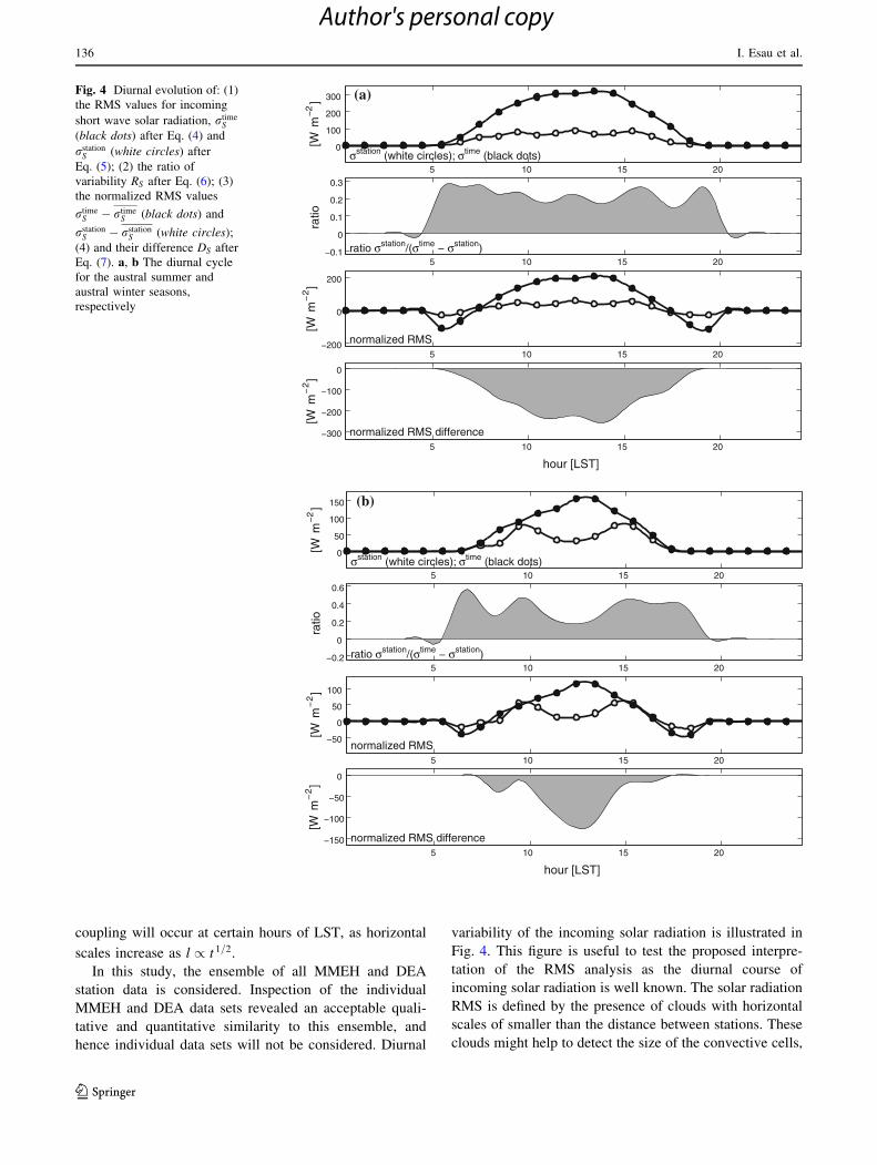
hence individual data sets will not be considered. Diurnal

variability of the incoming solar radiation is illustrated in

Fig. 4. This figure is useful to test the proposed interpre-

tation of the RMS analysis as the diurnal course of

incoming solar radiation is well known. The solar radiation

RMS is defined by the presence of clouds with horizontal

scales of smaller than the distance between stations. These

clouds might help to detect the size of the convective cells,

5 10 15 20

0

100

200

300

σstation (white circles); σtime (black dots)

[W m

−2]

5 10 15 20−0.1

0

0.1

0.2

0.3

ratio σstation/(σtime − σstation)

ratio

5 10 15 20−200

0

200

normalized RMS

[W m

−2]

5 10 15 20

−300

−200

−100

0

normalized RMS difference

[W m

−2]

hour [LST]

5 10 15 20

0

50

100

150


[W m

−2]

5 10 15 20−0.2

0

0.2

0.4

0.6


ratio

5 10 15 20

−50

0

50

100

normalized RMS

[W m

−2]

5 10 15 20−150

−100

−50

0


[W m

−2]

hour [LST]

(a)

(b)

Fig. 4 Diurnal evolution of: (1)

the RMS values for incoming

short wave solar radiation, rtimeS

(black dots) after Eq. (4) and

rstationS (white circles) after

Eq. (5); (2) the ratio of

variability RS after Eq. (6); (3)

the normalized RMS values

rtimeS � rtime

S (black dots) and

rstationS � rstation

S (white circles);

(4) and their difference DS after

Eq. (7). a, b The diurnal cycle

for the austral summer and

austral winter seasons,

respectively

136 I. Esau et al.

123


although convection might not create clouds in a dry

atmosphere. At sunset and sunrise, the solar radiation RMS

will also be defined by local surface properties such as

trees, houses and the orientation of the terrain slope.

Figure 4 suggests that local surface properties and clouds

have little effect on the RMS during summer, as cloud

clusters would typically occupy the whole HPA area.

During winter, the effect is more pronounced, indicating

5 10 15 200

1

2

3


[oC

]

5 10 15 20

0.2

0.3

0.4


ratio

5 10 15 20

− 1

0

1

normalized RMS

[oC

]

5 10 15 20− 3

− 2

− 1

0


[oC

]

hour [LST]

(a)

5 10 15 200

1

2


[oC

]

5 10 15 20

0.2

0.4


ratio

5 10 15 20

− 1

0

1

normalized RMS

[oC

]

5 10 15 20

− 2

− 1

0


[oC

]

hour [LST]

(b)


the RMS values of near-surface

air temperature, rtimeS (black

dots) after Eq. (4) and rstationS

(white circles) after Eq. (5); (2)

the ratio of variability RS after

Eq. (6); (3) the normalized RMS

values rtimeS � rtime

S (black dots)

and rstationS � rstation

S (whitecircles); (4) and their difference

DS after Eq. (7). a, b The

diurnal cycle for the austral

summer and austral winter

seasons, respectively


123


smaller cloud sizes and longer periods associated with low

sun angles.

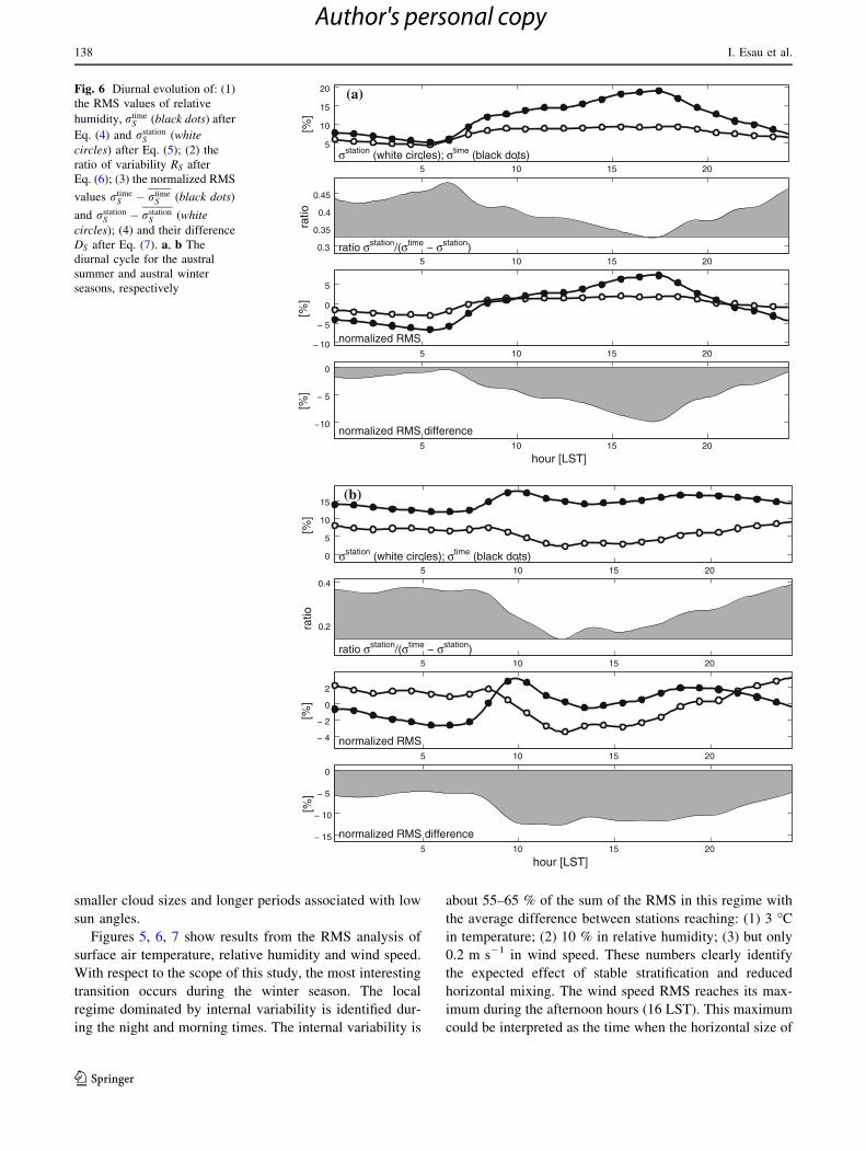
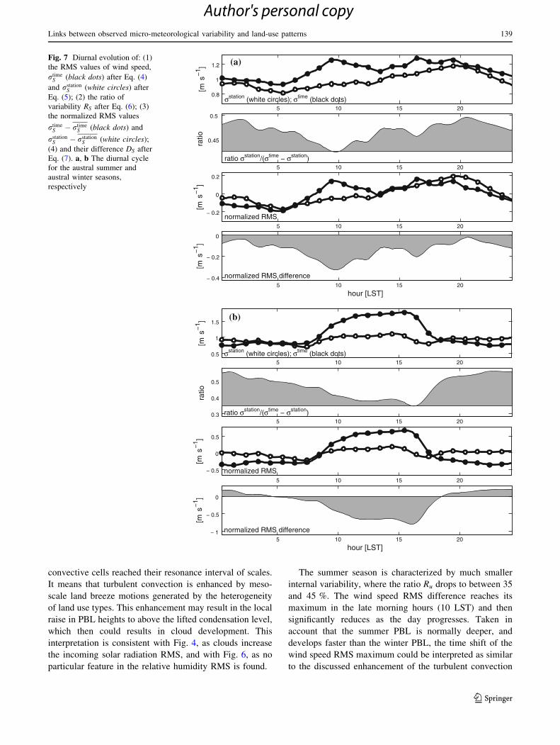
Figures 5, 6, 7 show results from the RMS analysis of

surface air temperature, relative humidity and wind speed.

With respect to the scope of this study, the most interesting

transition occurs during the winter season. The local

regime dominated by internal variability is identified dur-

ing the night and morning times. The internal variability is

about 55–65 % of the sum of the RMS in this regime with

the average difference between stations reaching: (1) 3 �C

in temperature; (2) 10 % in relative humidity; (3) but only

0.2 m s-1 in wind speed. These numbers clearly identify

the expected effect of stable stratification and reduced

horizontal mixing. The wind speed RMS reaches its max-

imum during the afternoon hours (16 LST). This maximum

could be interpreted as the time when the horizontal size of

5 10 15 20

5

10

15

20


[%]

5 10 15 20

0.3

0.35

0.4

0.45


ratio

5 10 15 20− 10

− 5

0

5

normalized RMS

[%]

5 10 15 20

−10

− 5

0


[%]

hour [LST]

(a)

5 10 15 20

0

5

10

15


[%]

5 10 15 20

0.2

0.4


ratio

5 10 15 20

− 4

− 2

0

2

normalized RMS

[%]

5 10 15 20− 15

− 10

− 5

0


[%]

hour [LST]

(b)


the RMS values of relative

humidity, rtimeS (black dots) after

Eq. (4) and rstationS (white

circles) after Eq. (5); (2) the

ratio of variability RS after

Eq. (6); (3) the normalized RMS

values rtimeS � rtime

S (black dots)

and rstationS � rstation

S (whitecircles); (4) and their difference

DS after Eq. (7). a, b The

diurnal cycle for the austral

summer and austral winter

seasons, respectively

138 I. Esau et al.

123


convective cells reached their resonance interval of scales.

It means that turbulent convection is enhanced by meso-

scale land breeze motions generated by the heterogeneity

of land use types. This enhancement may result in the local

raise in PBL heights to above the lifted condensation level,

which then could results in cloud development. This

interpretation is consistent with Fig. 4, as clouds increase

the incoming solar radiation RMS, and with Fig. 6, as no

particular feature in the relative humidity RMS is found.

The summer season is characterized by much smaller

internal variability, where the ratio Ru drops to between 35

and 45 %. The wind speed RMS difference reaches its

maximum in the late morning hours (10 LST) and then

significantly reduces as the day progresses. Taken in

account that the summer PBL is normally deeper, and

develops faster than the winter PBL, the time shift of the

wind speed RMS maximum could be interpreted as similar

to the discussed enhancement of the turbulent convection

5 10 15 20

0.8

1

1.2


[m s

−1 ]

5 10 15 20

0.45

0.5


ratio

5 10 15 20

− 0.2

0

0.2

normalized RMS

[m s

−1 ]

5 10 15 20− 0.4

− 0.2

0


[m s

−1 ]

hour [LST]

5 10 15 200.5

1

1.5


[m s

−1 ]

5 10 15 200.3

0.4

0.5


ratio

5 10 15 20

− 0.5

0

0.5

normalized RMS

[m s

−1 ]

5 10 15 20− 1

− 0.5

0


[m s

−1 ]

hour [LST]

(a)

(b)


the RMS values of wind speed,

rtimeS (black dots) after Eq. (4)

and rstationS (white circles) after

Eq. (5); (2) the ratio of

variability RS after Eq. (6); (3)

the normalized RMS values

rtimeS � rtime

S (black dots) and

rstationS � rstation

S (white circles);

(4) and their difference DS after

Eq. (7). a, b The diurnal cycle

for the austral summer and

austral winter seasons,

respectively


123


that was observed at 16 LST in wintertime. The subsequent

growth of the PBL destroys the resonance between turbu-

lent and breeze circulations, which then might lead to

smaller wind speed RMS values.

4.2 Discussion

One of the most important criteria for the quality of statistical

analysis is the number of independent samples and data sets

considered, which then constitutes the statistical ensemble.

The MMEH and DEA data sets covered the temporal vari-

ability of the HPA climate relatively well. In this study, 144

time samples were considered at each station for each day

with a 100 % completeness in observation records—there

were 60 (or 61) continues days of observations. There were

two periods during the summer seasons, and one period

during the winter season with observations representing the

majority of stations. In contrast to the temporal variability,

the spatial variability of the HPA climate was covered much

worse. There were only three stations in the MMEH data set,

and five stations in the DEA data set, that have been recorded

simultaneously. Thus, the ensemble consisted only of eight

members. This is not enough for quantifying the statistical

confidence of the derived dependences and to running more

sophisticated variants of the analysis (e.g. the principal

orthogonal decomposition analysis or the Bayesian proba-

bility analysis). This objective limitation of the study is

unlikely to be addressed in the near future since a dense

network of AWSs is expensive to erect and maintained.

Similar problems are encountered by the climate model

community where the number of model ensembles is of the

same order of magnitude.

To overcome these limitations in rigorous statistical

analysis, the focus of discussion is shifted from quantitative

dependences to qualitative measures. As common in the

climate model community (Ting et al. 2009), this study

considers dissimilarity of temporal variations in the

ensemble members. With respect to the spatial scale

analysis, one could observe that the scattered data reach the

maximum (or minimum) of horizontal flux in the same

range of scales for each data set, as well as in the blending

of these data sets. Although it is difficult to quantify the

degree of enhancement of atmospheric motions in the PBL,

it is very likely that scales of the enhancement were in-

dentified correctly in this study, and that these enhance-

ments are not random. Future work on this will necessarily

involve high-resolution numerical modeling as it has

already been applied elsewhere (Esau and Lyons 2002).

The enhancement of variability found in this study has

been interpreted as a strengthening of the turbulent con-

vection by meso-scale breeze motions. Another physically

plausible cause of enhancement could be linked to the

cloud system development. According to Blamey and

Reason (2012), the meso-scale convective storms that

develop in the HPA during summer have a general initia-

tion time of 13–19 LST. It corresponds well to this study’s

afternoon maxima in temperature rtimeT , DT and similar

maxima in the relative humidity. It was also found that the

wind speed RMS consistently increases as convection

developed. The horizontal scale of storms was found to be

200–300 km, which covers the entire area of observations.

Hence, convective storms did not generate internal vari-

ability in meteorological quantities, with the exception for

wind speed, which is affected by sub-cloud micro-fronts.

This is different to the RMS behavior found during win-

tertime when all quantities exhibit coherent fluctuations

within the diurnal cycle.

5 Conclusions

An analysis of observational data collected from two

independent networks of AWSs in the HPA of South

Africa, are presented. Meteorological quantities were

recorded with a high time frequency (sampling every

10 min) in a synchronous mode of operation. This allowed

for the utilization of the ensemble of data sets, not only to

characterize time series variability, but also spatial micro-

meteorological variability and their mutual interference.

Although the ensemble consists of only eight members

placed at distances of 10–100 km from each other, it is still

comparable with typical previously used ensembles from

regional and climate model simulations and even superior

to them if the horizontal resolution of AWS distribution is

considered.

In this study, the statistical analysis of the prepared

ensemble obtained from AWS data sets was aimed at

investigating variability at different time and spatial scales.

The analysis was seeking for an enhancement in PBL

dynamics through increased meso-scale circulation under

conditions of surface heterogeneity in the HPA. Such an

enhancement was indeed found in the data on scales of

30–50 km (during winter seasons) and 40–60 km (during

summer seasons). These scales, however, are somewhat

larger than scales visually identified on the NDVI Landsat

images. Hence, although the links between atmospheric

circulation enhancement and surface heterogeneity were

identified qualitatively, quantification of such links still

requires high-resolution numerical model studies.

The strongest evidence of land use–atmosphere resonant

coupling at certain scales was derived from the diurnal

evolution of the RMS transition from internal (local) to

externally forced variability regimes. The results suggest

that nocturnal, and especially wintertime, variability is

shaped by local surface properties. The development of a

deeper convective PBL homogenized internal variability

140 I. Esau et al.

123


forcing synchronous variations of the meteorological quan-

tities across the stations. As the growing convective cell

increases in size to the scale of meso-scale circulations a kind

of resonance interaction between the convective and meso-

scale motions occurred that enhanced the horizontal fluxes.

It is known that interactions between the surface layer’s

atmospheric dynamics and land use heterogeneity are

strongly non-linear and complex. This is one of the reasons

why these interactions are not satisfactory included in

meteorological or climate models. Results from this study

provide solid and sound observational material for further

model development, as well as for a more accurate inter-

pretation of regional climate change. A more applied utility

of the analysis is seen in the optimization of land use, the

calibration of satellite remote sensing data and the facili-

tation of climate adaptation.

Acknowledgments The authors would like to acknowledge the

bilateral Norway–South Africa project 180343/S50 ‘‘Analysis and the

Possibility for Control of Atmospheric Boundary Layer Processes to

Facilitate Adaptation to Environmental Changes’’ co-funded by the

South African National Research Foundation (NRF) and the Norwe-

gian Research Council (NRC). A significant part of this work has

been developed under the NRC project 191516/V30 ‘‘Planetary

boundary layer feedback in the Earth’s Climate System’’, under the

European Research Council Advanced Grant, FP7-IDEAS, 227915

‘‘Atmospheric planetary boundary layers: physics, modeling and its

role in the Earth system’’, and under a grant from the Government of

the Russian Federation (project code 11.G34.31.0048). The Authors

are grateful to the DEA, and in particular to Xolile Ncipha, for

making the DEA data available. The authors are also grateful to all

farmers who gave permission for the deployment of AWSs on their

land and who assisted in the collection of data.

References

Alberts PN (2011) Baseline assessment of child respiratory health in

the Highveld Priority Area. Dissertation at School of Health

Systems and Public Health, University of Pretoria, p 80

Application Note, N�30 (2011) Reporting quality observations to

NOAA and other weather observation groups, Rev B 3/4/08.

http://www.davisnet.com/product_documents/weather/app_notes/

apnote_30.pdf. Accessed 21 Mar 2011

Becker S (2005) Thermal structure of the atmospheric boundary layer

over the South African Mpumalanga Highveld. Clim Res

29:129–137

Blamey RC, Reason CJC (2012) Mesoscale convective complexes

over Southern Africa. J Clim 25:753–766

Collett KS, Piketh SJ, Ross KE (2010) An assessment of the

atmospheric nitrogen budget on the South African Highveld.

South Afr J Sci 106(5–6):1–9

Esau I (2007) Amplification of turbulent exchange over wide Arctic

leads: large-eddy simulation study. J Geophys Res 112:D08109.

doi:10.1029/2006JD007225

Esau I, Lyons TJ (2002) Effect of sharp vegetation boundary on the

convective atmospheric boundary layer. Agric For Meteorol

114(1–2):3–13

Freiman MT, Piketh SJ (2003) Air transport into and out of the

industrial Highveld region in South Africa. J Appl Meteorol

42:994–1005

Freiman MT, Tyson PD (2000) The thermodynamic structure of the

atmosphere over South Africa: implications for water vapour

transport. Water SA 26(2):152–158

Giles J (2005) Climate science: the dustiest place on Earth. Nature

434:816–819

Harzallah A, Sadourny R (1995) Internal versus SST-forced atmo-

spheric variability as simulated by an atmospheric general

circulation model. J Clim 8:474–495

Held G, Scheifinger H, Snyman GM, Tosen GR, Zunckel M (1996)

The climatology and meteorology of the Highveld. In: Held G,

Gore BJ, Surridge AD, Tosen GR, Turner CR, Walmsley RD

(eds) Air pollution and its impacts on the South African

Highveld, 60–71. Environmental Scientific Association, Cleve-

land, p 144

Horlacher V, Osborne S, Price JD (2012) Comparison of two closely

located meteorological measurement sites and consequences for

their areal representability. Boundary-Layer Meteorol 142:469–493

Junkermann W, Hacker J, Lyons T, Nair U (2009) Land use change

suppress precipitation. Atmos Chem Phys 9:6531–6539

Jury MR, Tosen GR (1989) Characteristics of the winter boundary

layer over the African Plateau: 26 S. Boundary-Layer Meteorol

49(1–2):53–76

Laakso L, Vakkari V, Laakso H et al (2010) South African

EUCAARI-measurements: a site with high atmospheric vari-

ability. Atmos Chem Phys Discuss 10:30691–30729

Patton EG, Sullivan PP, Moeng C-H (2005) Influence of idealized

heterogeneity on wet and dry planetary boundary layers coupled

to the land surface. J Atmos Sci 62:2078–2097

Pielke RA (2001) Influence of the special distribution of vegetation

and soils on the prediction of cumulus convective rainfall. Rev

Geophys 39:151–178

Robinson FJ, Sherwood SC, Li Y (2008) Resonant response of deep

convection to surface hot spots. J Atmos Sci 65:276–286

Roy SB, Weaver CP, Nolan DS, Avissar R (2003) A preferred scale

for landscape forced mesoscale circulations? J Geophys Res

108(D22):8854. doi:10.1029/2002JD003097

Scanlon TM, Caylor KK, Levin SA, Rodriguez-Iturbe I (2007)

Positive feedbacks promote power-law clustering of Kalahari

vegetation. Nature 449:209–212

Sogalla M, Kruger A, Kerschgens M (2006) Mesoscale modelling of

interactions between rainfall and the land surface in West Africa.

Meteorol Atmos Phys 91:211–221

Taylor CM, Lambin EF, Stephenne N, Harding RJ, Essery RLH

(2002) The influence of land use change on climate in the Sahel.

J Clim 15:3615–3629

Taylor CM, Parker DJ, Harris PP (2007) An observational case study

of mesoscale atmospheric circulations induced by soil moisture.

Geophys Res Lett 34:L15801. doi:10.1029/2007GL030572

Ting M, Kushnir Y, Seager R, Li C (2009) Forced and internal

twentieth-century SST trends in the North Atlantic. J Clim

22:1469–1481

Tyson PD, Gatebe CK (2001) The atmosphere, aerosols, trace gases

and biogeochemical change in southern Africa: a regional

integration. South Afr J Sci 97:106–118

Tyson PD, Kruger FJ, Louw CW (1988) Atmospheric pollution and

its implications in the Eastern Transvaal Highveld. National

Scientific Programmes Unit: CSIR, SANSP Report 150, p 123

Van Heerwaarden CC, Vila-Guerau de Arellano J (2008) Relative

humidity as an indicator for cloud formation over heterogeneous

land surfaces. J Atmos Sci 65(10):3263–3277

Von Gogh RG, Landenberg H, Brassel K, Danford I (1982)

Dispersion climatology and characteristics of sulphur dioxide

pollution in Eastern Transvaal Highveld. ATMOS/82/3, Atmo-

spheric Science Division, CSIR, Pretoria, p 117

Washington R, Todd MC, Engelstaedter S, Mbainayel S, Mitchell F

(2005) Dust and the low level circulation over the Bodele


123


http://www.davisnet.com/product_documents/weather/app_notes/apnote_30.pdf

http://www.davisnet.com/product_documents/weather/app_notes/apnote_30.pdf

http://dx.doi.org/10.1029/2006JD007225

http://dx.doi.org/10.1029/2002JD003097

http://dx.doi.org/10.1029/2007GL030572

Depression, Chad: observations from BoDEx 2005. J Geophys

Res 111(D3):D03201

Zilitinkevich SS, Hunt JCR, Grachev AA, Esau I, Lalas DP, Akylas E,

Tombrou M, Fairall CW, Fernando HJS, Baklanov A, Joffre SM

(2006) The influence of large convective eddies on the

surface layer turbulence. Quart J Roy Meteorol Soc 132:1423–

1456

142 I. Esau et al.

123


Links between observed micrometeorological variability and land-use patterns in the highveld ...

Documents

Transcript of Links between observed micrometeorological variability and land-use patterns in the highveld ...