Linear Systems and Signals, Second EditionB. P. Lathi

Oxford University Press2005

Published by Oxford University Press, Inc.198 Madison Avenue, New York, New York 10016http://www.oup.com

© 2005 Oxford University Press, Inc.

Oxford is a registered trademark of Oxford University Press

All rights reserved. No part of this publication may be reproduced, stored in a retrieval system, or transmitted, in any form or byany means, electronic, mechanical, photocopying, recording, or otherwise, without the prior permission of Oxford UniversityPress.

Library of Congress Cataloging-in-Publication Data

Lathi, B. P. (Bhagwandas Pannalal)Linear systems and signals/B. P. Lathi.—2nd ed.p. cm.0-19-515833-4

1. Signal processing—Mathematics. 2. System analysis. 3. Linear time invariant systems. 4. Digital filters (Mathematics) I. Title.

TK5102.5L298 2004621.382′2—dc22 2003064978

9 8 7 6 5 4 3 2 1

PrefaceThis book, Linear Systems and Signals, presents a comprehensive treatment of signals and linear systems at an introductorylevel. Like all my other books, it emphasizes physical appreciation of concepts through heuristic reasoning, and the use ofmetaphors, analogies, and creative explanations. Such an approach is much different from a purely deductive technique thatuses mere mathematical manipulation of symbols. There is a temptation to treat engineering subjects as a branch of appliedmathematics. Such an approach is a perfect match to the public image of engineering as a dry and dull discipline. It ignoresthe physical meaning behind various derivations and deprives a student of intuitive grasp and the enjoyable experience oflogical uncovering of the subject matter. Here I have used mathematics not so much to prove axiomatic theory as to supportand enhance physical and intuitive understanding. Wherever possible, theoretical results are interpreted heuristically and areenhanced by carefully chosen examples and analogies.

This second edition, which closely follows the organization of the first edition, has been refined by incorporating suggestionsand changes provided by various reviewers. The added topics include Bode plots, use of digital filters in an impulse-invariancemethod of designing analog systems, convergence of infinite series, bandpass systems, group and phase delay, and Fourierapplications to communication systems. A significant and sizable addition in the area of MATLAB® (a registered trademark ofThe Math Works, Inc.) has been provided by Dr. Roger Green of North Dakota State University. Dr. Green discusses hiscontribution at the conclusion of this preface.

ORGANIZATION

The book may be conceived as divided into five parts:

1. Introduction (Background and Chapter 1).

2. Time-domain analysis of linear time-invariant (LTI) systems (Chapters 2 and 3).

3. Frequency-domain (transform) analysis of LTI systems (Chapters 4 and 5).

4. Signal analysis (Chapters 6, 7, 8, and 9).

5. State-space analysis of LTI systems (Chapter 10).

The organization of the book permits much flexibility in teaching the continuous-time and discrete-time concepts. The naturalsequence of chapters is meant to integrate continuous-time and discrete-time analysis. It is also possible to use a sequentialapproach in which all the continuous-time analysis is covered first (Chapters 1, 2, 4, 6, 7, and 8), followed by discrete-timeanalysis (Chapters 3, 5, and 9).

SUGGESTIONS FOR USING THIS BOOKThe book can be readily tailored for a variety of courses spanning 30 to 45 lecture hours. Most of the material in the first eightchapters can be covered at a brisk pace in about 45 hours. The book can also be used for a 30-lecture-hour course bycovering only analog material (Chapters 1, 2, 4, 6, 7, and possibly selected topics in Chapter 8). Alternately, one can alsoselect Chapters 1 to 5 for courses purely devoted to systems analysis or transform techniques. To treat continuous- anddiscrete-time systems by using an integrated (or parallel) approach, the appropriate sequence of Chapters is 1, 2, 3, 4, 5, 6, 7,and 8. For a sequential approach, where the continuous-time analysis is followed by discrete-time analysis, the proper chaptersequence is 1, 2, 4, 6, 7, 8, 3, 5, and possibly 9 (depending on the time availability).

Logically, the Fourier transform should precede the Laplace transform. I have used such an approach in the companionvolume, Signal Processing and Linear Systems (Oxford, 1998). However, a sizable number of instructors feel that it is easier forstudents to learn Fourier after Laplace. Such an approach has an appeal because of the gradual progression of difficulty, in thesense that the relatively more difficult concepts of Fourier are treated after the simpler area of Laplace. This book is written toaccommodate that viewpoint. For those who wish to see Fourier before Laplace, there is Signal Processing and LinearSystems.

NOTABLE FEATURESThe notable features of this book include the following:

1. Intuitive and heuristic understanding of the concepts and physical meaning of mathematical results areemphasized throughout. Such an approach not only leads to deeper appreciation and easier comprehension ofthe concepts, but also makes learning enjoyable for students.

2. Many students are handicapped by an inadequate background in basic material such as complex numbers,sinusoids, quick sketching of functions, Cramer's rule, partial fraction expansion, and matrix algebra. I have addeda chapter that addresses these basic and pervasive topics in electrical engineering. Response by students hasbeen unanimously enthusiastic.

3. There are more than 200 worked examples in addition to exercises (usually with answers) for students to test theirunderstanding. There is also a large number of selected problems of varying difficulty at the end of each chapter.

4. For instructors who like to get students involved with computers, several examples are worked out by means ofMATLAB, which is becoming a standard software package in electrical engineering curricula. There is also aMATLAB session at the end of each chapter. The problem set contains several computer problems. Workingcomputer examples or problems, though not essential for the use of this book, is highly recommended.

5. The discrete-time and continuous-time systems may be treated in sequence, or they may be integrated by usinga parallel approach.

6. The summary at the end of each chapter proves helpful to students in summing up essential developments in thechapter.

7. There are several historical notes to enhance student's interest in the subject. This information introduces studentsto the historical background that influenced the development of electrical engineering.

ACKNOWLEDGMENTSSeveral individuals have helped me in the preparation of this book. I am grateful for the helpful suggestions of the severalreviewers. I am most grateful to Prof. Yannis Tsividis of Columbia University, who provided his comprehensively thorough andinsightful feedback for the book. I also appreciate another comprehensive review by Prof. Roger Green. I thank Profs. JoeAnderson of Tennessee Technological University, Kai S. Yeung of the University of Texas at Arlington, and AlexanderPoularikis of the University of Alabama at Huntsville for very thoughtful reviews. Thanks for helpful suggestions are also due toProfs. Babajide Familoni of the University of Memphis, Leslie Collins of Duke University, R. Rajgopalan of the University of

Arizona, and William Edward Pierson from the U.S. Air Force Research Laboratory. Only those who write a book understandthat writing a book such as this is an obsessively time-consuming activity, which causes much hardship for the familymembers, where the wife suffers the most. So what can I say except to thank my wife, Rajani, for enormous but invisiblesacrifices.

B. P. Lathi

MATLABMATLAB is a sophisticated language that serves as a powerful tool to better understand a myriad of topics, including controltheory, filter design, and, of course, linear systems and signals. MATLAB's flexible programming structure promotes rapiddevelopment and analysis. Outstanding visualization capabilities provide unique insight into system behavior and signalcharacter. By exploring concepts with MATLAB, you will substantially increase your comfort with and understanding of coursetopics.

As with any language, learning MATLAB is incremental and requires practice. This book provides two levels of exposure toMATLAB. First, short computer examples are interspersed throughout the text to reinforce concepts and perform variouscomputations. These examples utilize standard MATLAB functions as well as functions from the control system, signalprocessing, and symbolic math toolboxes. MATLAB has many more toolboxes available, but these three are commonlyavailable in many engineering departments.

A second and deeper level of exposure to MATLAB is achieved by concluding each chapter with a separate MATLAB session.Taken together, these eleven sessions provide a self-contained introduction to the MATLAB environment that allows evennovice users to quickly gain MATLAB proficiency and competence. These sessions provide detailed instruction on how to useMATLAB to solve problems in linear systems and signals. Except for the very last chapter, special care has been taken toavoid the use of toolbox functions in the MATLAB sessions. Rather, readers are shown the process of developing their owncode. In this way, those readers without toolbox access are not at a disadvantage.

All computer code is available online (http://www.mathworks.com/support/books). Code for the computer examples in a givenchapter, say Chapter xx, is named CExx.m. Program yy from MATLAB Session xx is named MSxxPyy.m. Additionally, completecode for each individual MATLAB session is named MSxx.m.

Roger Green

Chapter B: BackgroundThe topics discussed in this chapter are not entirely new to students taking this course. You have already studied many of these topics in earliercourses or are expected to know them from your previous training. Even so, this background material deserves a review because it is so pervasive inthe area of signals and systems. Investing a little time in such a review will pay big dividends later. Furthermore, this material is useful not only forthis course but also for several courses that follow. It will also be helpful later, as reference material in your professional career.

B.1 COMPLEX NUMBERS

Complex numbers are an extension of ordinary numbers and are an integral part of the modern number system. Complex numbers, particularlyimaginary numbers, sometimes seem mysterious and unreal. This feeling of unreality derives from their unfamiliarity and novelty rather than theirsupposed nonexistence! Mathematicians blundered in calling these numbers "imaginary," for the term immediately prejudices perception. Had thesenumbers been called by some other name, they would have become demystified long ago, just as irrational numbers or negative numbers were.Many futile attempts have been made to ascribe some physical meaning to imaginary numbers. However, this effort is needless. In mathematics weassign symbols and operations any meaning we wish as long as internal consistency is maintained. The history of mathematics is full of entities thatwere unfamiliar and held in abhorrence until familiarity made them acceptable. This fact will become clear from the following historical note.

B.1-1 A Historical Note

Among early people the number system consisted only of natural numbers (positive integers) needed to express the number of children, cattle, andquivers of arrows. These people had no need for fractions. Whoever heard of two and one-half children or three and one-fourth cows!

However, with the advent of agriculture, people needed to measure continuously varying quantities, such as the length of a field and the weight of aquantity of butter. The number system, therefore, was extended to include fractions. The ancient Egyptians and Babylonians knew how to handlefractions, but Pythagoras discovered that some numbers (like the diagonal of a unit square) could not be expressed as a whole number or a fraction.Pythagoras, a number mystic, who regarded numbers as the essence and principle of all things in the universe, was so appalled at his discovery thathe swore his followers to secrecy and imposed a death penalty for divulging this secret.[1] These numbers, however, were included in the numbersystem by the time of Descartes, and they are now known as irrational numbers.

Until recently, negative numbers were not a part of the number system. The concept of negative numbers must have appeared absurd to early man.However, the medieval Hindus had a clear understanding of the significance of positive and negative numbers.[2], [3] They were also the first torecognize the existence of absolute negative quantities.[4] The works of Bhaskar (1114-1185) on arithmetic (Līlāvatī) and algebra (Bījaganit) not onlyuse the decimal system but also give rules for dealing with negative quantities. Bhaskar recognized that positive numbers have two square roots.[5]

Much later, in Europe, the men who developed the banking system that arose in Florence and Venice during the late Renaissance (fifteenth century)are credited with introducing a crude form of negative numbers. The seemingly absurd subtraction of 7 from 5 seemed reasonable when bankersbegan to allow their clients to draw seven gold ducats while their deposit stood at five. All that was necessary for this purpose was to write thedifference, 2, on the debit side of a ledger.[6]

Thus the number system was once again broadened (generalized) to include negative numbers. The acceptance of negative numbers made itpossible to solve equations such as x + 5 = 0, which had no solution before. Yet for equations such as x2 + 1 = 0, leading to x2 = −1, the solutioncould not be found in the real number system. It was therefore necessary to define a completely new kind of number with its square equal to −1.During the time of Descartes and Newton, imaginary (or complex) numbers came to be accepted as part of the number system, but they were stillregarded as algebraic fiction. The Swiss mathematician Leonhard Euler introduced the notation i (for imaginary) around 1777 to represent √−1.Electrical engineers use the notation j instead of i to avoid confusion with the notation i often used for electrical current. Thus

and

This notation allows us to determine the square root of any negative number. For example,

When imaginary numbers are included in the number system, the resulting numbers are called complex numbers.

ORIGINS OF COMPLEX NUMBERSIronically (and contrary to popular belief), it was not the solution of a quadratic equation, such as x2 + 1 = 0, but a cubic equation with real roots thatmade imaginary numbers plausible and acceptable to early mathematicians. They could dismiss √−1 as pure nonsense when it appeared as asolution to x2 + 1 = 0 because this equation has no real solution. But in 1545, Gerolamo Cardano of Milan published Ars Magna (The Great Art), themost important algebraic work of the Renaissance. In this book he gave a method of solving a general cubic equation in which a root of a negativenumber appeared in an intermediate step. According to his method, the solution to a third-order equation[†]

is given by

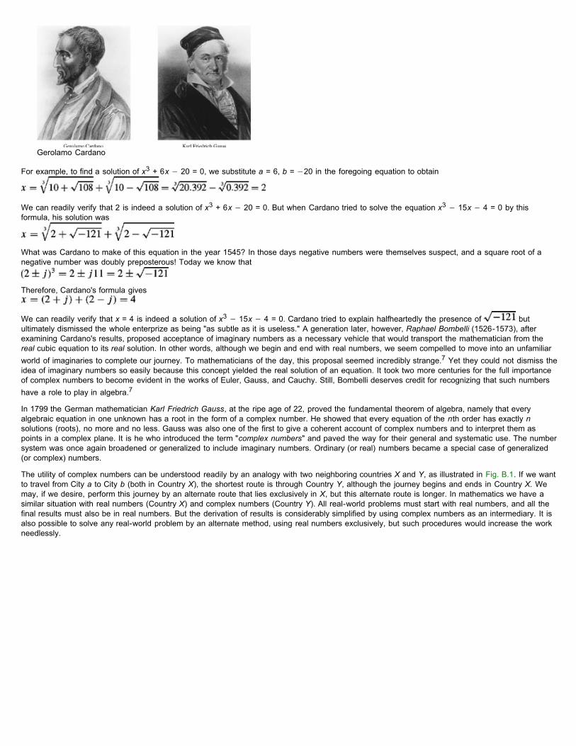
Gerolamo Cardano

For example, to find a solution of x3 + 6x − 20 = 0, we substitute a = 6, b = −20 in the foregoing equation to obtain

We can readily verify that 2 is indeed a solution of x3 + 6x − 20 = 0. But when Cardano tried to solve the equation x3 − 15x − 4 = 0 by thisformula, his solution was

What was Cardano to make of this equation in the year 1545? In those days negative numbers were themselves suspect, and a square root of anegative number was doubly preposterous! Today we know that

Therefore, Cardano's formula gives

We can readily verify that x = 4 is indeed a solution of x3 − 15x − 4 = 0. Cardano tried to explain halfheartedly the presence of butultimately dismissed the whole enterprize as being "as subtle as it is useless." A generation later, however, Raphael Bombelli (1526-1573), afterexamining Cardano's results, proposed acceptance of imaginary numbers as a necessary vehicle that would transport the mathematician from thereal cubic equation to its real solution. In other words, although we begin and end with real numbers, we seem compelled to move into an unfamiliarworld of imaginaries to complete our journey. To mathematicians of the day, this proposal seemed incredibly strange.7 Yet they could not dismiss theidea of imaginary numbers so easily because this concept yielded the real solution of an equation. It took two more centuries for the full importanceof complex numbers to become evident in the works of Euler, Gauss, and Cauchy. Still, Bombelli deserves credit for recognizing that such numbershave a role to play in algebra.7

In 1799 the German mathematician Karl Friedrich Gauss, at the ripe age of 22, proved the fundamental theorem of algebra, namely that everyalgebraic equation in one unknown has a root in the form of a complex number. He showed that every equation of the nth order has exactly nsolutions (roots), no more and no less. Gauss was also one of the first to give a coherent account of complex numbers and to interpret them aspoints in a complex plane. It is he who introduced the term "complex numbers" and paved the way for their general and systematic use. The numbersystem was once again broadened or generalized to include imaginary numbers. Ordinary (or real) numbers became a special case of generalized(or complex) numbers.

The utility of complex numbers can be understood readily by an analogy with two neighboring countries X and Y, as illustrated in Fig. B.1. If we wantto travel from City a to City b (both in Country X), the shortest route is through Country Y, although the journey begins and ends in Country X. Wemay, if we desire, perform this journey by an alternate route that lies exclusively in X, but this alternate route is longer. In mathematics we have asimilar situation with real numbers (Country X) and complex numbers (Country Y). All real-world problems must start with real numbers, and all thefinal results must also be in real numbers. But the derivation of results is considerably simplified by using complex numbers as an intermediary. It isalso possible to solve any real-world problem by an alternate method, using real numbers exclusively, but such procedures would increase the workneedlessly.

Figure B.1: Use of complex numbers can reduce the work.

B.1-2 Algebra of Complex Numbers

A complex number (a, b) or a + jb can be represented graphically by a point whose Cartesian coordinates are (a, b) in a complex plane (Fig. B.2).Let us denote this complex number by z so that

The numbers a and b (the abscissa and the ordinate) of z are the real part and the imaginary part, respectively, of z. They are also expressed as

Note that in this plane all real numbers lie on the horizontal axis, and all imaginary numbers lie on the vertical axis.

Complex numbers may also be expressed in terms of polar coordinates. If (r, θ) are the polar coordinates of a point z = a + jb (see Fig. B.2), then

and

Figure B.2: Representation of a number in the complex plane.

The Euler formula states that

To prove the Euler formula, we use a Maclaurin series to expand ejθ, cos θ, and sin θ:

Hence, it follows that[†]

Using Eq. (B.3) in (B.2) yields

Thus, a complex number can be expressed in Cartesian form a + jb or polar form rejθ with

and

Observe that r is the distance of the point z from the origin. For this reason, r is also called the magnitude (or absolute value) of z and is denoted by|z|. Similarly, θ is called the angle of z and is denoted by ∠z. Therefore

and

Also

CONJUGATE OF A COMPLEX NUMBER

We define z*, the conjugate of z = a + jb, as

The graphical representation of a number z and its conjugate z* is depicted in Fig. B.2. Observe that z* is a mirror image of z about the horizontalaxis. To find the conjugate of any number, we need only replace j by −j in that number (which is the same as changing the sign of its angle).

The sum of a complex number and its conjugate is a real number equal to twice the real part of the number:

The product of a complex number z and its conjugate is a real number |z|2, the square of the magnitude of the number:

UNDERSTANDING SOME USEFUL IDENTITIESIn a complex plane, rejθ represents a point at a distance r from the origin and at an angle θ with the horizontal axis, as shown in Fig. B.3a. Forexample, the number − 1 is at a unit distance from the origin and has an angle π or − π (in fact, any odd multiple of ± π), as seen from Fig. B.3b.Therefore,

Figure B.3: Understanding some useful identities in terms of rejθ.

In fact,

The number 1, on the other hand, is also at a unit distance from the origin, but has an angle 2π (in fact, ±2nπ for any integer value of n). Therefore,

The number j is at unit distance from the origin and its angle is π/2 (see Fig. B.3b). Therefore,

Similarly,

Thus

In fact,

This discussion shows the usefulness of the graphic picture of rej. This picture is also helpful in several other applications. For example, to determinethe limit of e(α+ jw)t as t → ∞, we note that

Now the magnitude of ejwt is unity regardless of the value of ω or t because ejwt = rejθ with r = 1. Therefore, eαt determines the behavior of e(α+ jω)t

as t → ∞ and

In future discussions you will find it very useful to remember rejθ as a number at a distance r from the origin and at an angle θ with the horizontalaxis of the complex plane.

A WARNING ABOUT USING ELECTRONIC CALCULATORS IN COMPUTING ANGLESFrom the Cartesian form a + jb we can readily compute the polar form rejθ [see Eq. (B.6)]. Electronic calculators provide ready conversion ofrectangular into polar and vice versa. However, if a calculator computes an angle of a complex number by using an inverse trigonometric function θ =tan−1 (b/a), proper attention must be paid to the quadrant in which the number is located. For instance, θ corresponding to the number −2 − j3 istan−1 (−3/−2). This result is not the same as tan−1 (3/2). The former is −123.7°, whereas the latter is 56.3°. An electronic calculator cannot makethis distinction and can give a correct answer only for angles in the first and fourth quadrants. It will read tan−1(−3/−2) as tan−1 (3/2), which isclearly wrong. When you are computing inverse trigonometric functions, if the angle appears in the second or third quadrant, the answer of thecalculator is off by 180°. The correct answer is obtained by adding or subtracting 180° to the value found with the calculator (either adding orsubtracting yields the correct answer). For this reason it is advisable to draw the point in the complex plane and determine the quadrant in which thepoint lies. This issue will be clarified by the following examples.

EXAMPLE B.1Express the following numbers in polar form:

a. 2 + j3

b. −2 + j3

c. −2 − j3

d. 1 − j3

a.

In this case the number is in the first quadrant, and a calculator will give the correct value of 56.3°. Therefore (see Fig. B.4a), we can

write

b.

Figure B.4: From Cartesian to polar form.

In this case the angle is in the second quadrant (see Fig. B.4b), and therefore the answer given by the calculator, tan−1 (1/−2) =−26.6°, is off by 180°. The correct answer is (−26.6 ± 180)° = 153.4° or −206.6°. Both values are correct because they represent thesame angle.

It is a common practice to choose an angle whose numerical value is less than 180°. Such a value is called the principal value of theangle, which in this case is 153.4°. Therefore,

c.

In this case the angle appears in the third quadrant (see Fig. B.4c), and therefore the answer obtained by the calculator (tan−1 (−3/−2)= 56.3°) is off by 180°. The correct answer is (56.3° 180)° = 236.3° or −123.7°. We choose the principal value −123.7° so that (seeFig. B.4c).

d.

In this case the angle appears in the fourth quadrant (see Fig. B.4d), and therefore the answer given by the calculator, tan−1 (−3/1) =−71.6°, is correct (see Fig. B.4d):

COMPUTER EXAMPLE CB.1Using the MATLAB function cart2pol, convert the following numbers from Cartesian form to polar form:

a. z = 2 + j3

b. z = −2 + j1

b. Therefore, z = 2 + j3 = 3.6056ej0.98279 + 3.6056ej56.3099°

Therefore, z = −2 + j1 = 2.2361ej2.6779 = 2.2361ej153.4349°.

>> [z_rad, z_mag] = cart2pol(2, 3);>> z_deg = z_rad* (180/pi);>> disp(['(a) z_mag = ',num2str(z_mag),'; z_rad = ',num2str(z_rad), ...>> '; z_deg = ',num2str(z_deg)]);(a) z mag = 3.6056; z rad = 0.98279; z deg = 56.3099

>> [z_rad, z_mag] = cart2pol(-2, 1);>> z_deg = z_rad* (180/pi);>> disp(['(b) z_mag = ',num2str(z_mag),'; z_rad = ',num2str(z_rad), ...>> '; z_deg = ',num2str(z_deg)]);(b) z mag = 2.2361; z rad = 2.6779; z deg = 153.4349

EXAMPLE B.2Represent the following numbers in the complex plane and express them in Cartesian form:

a. 2ejπ/3

b. 4e−j3π/4

c. 2ejπ/2

d. 3e−j3π

e. 2ej4π

f. 2e−j4π

a. 2ejπ/3 = 2(cos π/3 + j sin π/3) = 1 + j √3 (See Fig. B.5b)

Figure B.5: From polar to Cartesian form.

b. 4e−j3π/4 = 4(cos 3π/4 − j sin π/4) = −2√2 − j2 √2 (See Fig. B.5b)

c. 2ejπ/2 = 2(cos π/2 + j sin π/2) = 2(0 + j 1) = j2 (See Fig. B.5c)

d. 3e−j3π = 2(cos 3π − j sin 3π) = 3(−1 + j0) = −3 (See Fig. B.5d)

e. 2ej4π = 2(cos 4π + j sin 4π) = 2(1 − j0) = 2 (See Fig. B.5e)

f. 2e−j4π = 2(cos 4π − j sin 4π) = 2(1 − j0) = 2 (See Fig. B.5f)

COMPUTER EXAMPLE CB.2Using the MATLAB function pol2cart, convert the number z = 4e−j(3π/4) from polar form to Cartesian form.

Therefore, z = 4e−j(3π/4) = −2.8284 − j2.8284.

ARITHMETICAL OPERATIONS, POWERS, AND ROOTS OF COMPLEX NUMBERSTo perform addition and subtraction, complex numbers should be expressed in Cartesian form. Thus, if

>> [z_real, z_imag] = pol2cart(-3*pi/4,4);>> disp (['z_real = ',num2str(z_real),'; z_imag = ',num2str(z_imag)]);z real = -2.8284; z imag = -2.8284

and

then

If z1 and z2 are given in polar form, we would need to convert them into Cartesian form for the purpose of adding (or subtracting). Multiplication anddivision, however, can be carried out in either Cartesian or polar form, although the latter proves to be much more convenient. This is because if z1and z2 are expressed in polar form as

then

and

Moreover,

and

This shows that the operations of multiplication, division, powers, and roots can be carried out with remarkable ease when the numbers are in polarform.

Strictly speaking, there are n values for z1/n (the nth root of z). To find all the n roots, we reexamine Eq. (B.15d).

The value of z1/n given in Eq. (B.15d) is the principal value of z1/n, obtained by taking the nth root of the principal value of z, which corresponds tothe case k = 0 in Eq. (B.15e).

EXAMPLE B.3Determine z1z2 and z1/z2 for the numbers

We shall solve this problem in both polar and Cartesian forms.

MULTIPLICATION: CARTESIAN FORM

MULITPLICATION: POLAR FORM

DIVISION: CARTESIAN FORM

To eliminate the complex number in the denominator, we multiply both the numerator and the denominator of the right-hand side by 2 − j3, thedenominator's conjugate. This yields

DIVISION: POLAR FORM

It is clear from this example that multiplication and division are easier to accomplish in polar form than in Cartesian form.

EXAMPLE B.4For z1 = 2ejπ/4 and z2 = 8ejπ/3, find the following:

a. 2z1 − z2

b. 1/z1

c. z1/z22

d.

a. Since subtraction cannot be performed directly in polar form, we convert z1 and z2 to Cartesian form:

Therefore,

b.

c.

d. There are three cube roots of 8ej(π/3) = 8e jj(π/3+2k), k = 0, 1, 2.

The principal value (value corresponding to k = 0) is 2ejπ/9.

COMPUTER EXAMPLE CB.3Determine z1z2 and z1/z2 if z1 = 3 + j4 and z2 = 2 + j3

Therefore, z1z2 = (3 + j4)(2 + j3) = −6 + j17 and z1/z2 = (3 + j4)/(2 + j3) = 1.3486 − j0.076923.

EXAMPLE B.5Consider X(ω), a complex function of a real variable ω:

a. Express X(ω) in Cartesian form, and find its real and imaginary parts.

b. Express X(ω) in polar form, and find its magnitude |X(ω)| and angle ∠X(ω).

a. To obtain the real and imaginary parts of X (ω), we must eliminate imaginary terms in the denominator of X (ω). This is readily done bymultiplying both the numerator and the denominator of X(ω) by 3 − j4ω, the conjugate of the denominator 3 + j4ω so that

This is the Cartesian form of X(ω). Clearly the real and imaginary parts Xr(ω) and Xi(ω) are given by

b.

This is the polar representation of X(ω). Observe that

>> z_1 = 3+j*4; z_2 = 2+j*3;>> z_1z_2 = z_1*z_2;>> z_1divz_2 = z_1/z_2;>> disp(['z_1*z_2 = ',num2str(z_1 z_2),'; z_1/z_2 = ',num2str(z_1divz_2)]);z 1*z 2 = -6+17i; z 1/z 2 = 1.3846-0.076923i

LOGARITHMS OF COMPLEX NUMBERS

We have

if

then

The value of In z for k = 0 is called the principal value of In z and is denoted by Ln z.

In all these expressions, the case of k = 0 is the principal value of that expression.

[1]Calinger, R., ed. Classics of Mathematics. Moore Publishing, Oak Park, IL, 1982.

[2]Hogben, Lancelot. Mathematics in the Making. Doubleday, New York, 1960.

[3]Cajori, Florian. A History of Mathematics, 4th ed. Chelsea, New York, 1985.

[4]Encyclopaedia Britannica. Micropaedia IV, 15th ed., vol. 11, p. 1043. Chicago, 1982.

[5]Singh, Jagjit. Great Ideas of Modern Mathematics. Dover, New York, 1959.

[6]Dunham, William. Journey Through Genius. Wiley, New York, 1990.

[†]This equation is known as the depressed cubic equation. A general cubic equation

can always be reduced to a depressed cubic form by substituting y = x − (p/3). Therefore any general cubic equation can be solved if we know thesolution to the depressed cubic. The depressed cubic was independently solved, first by Scipione del Ferro (1465-1526) and then by Niccolo Fontana(1499-1557). The latter is better known in the history of mathematics as Tartaglia ("Stammerer"). Cardano learned the secret of the depressed cubicsolution from Tartaglia. He then showed that by using the substitution y = x − (p/3), a general cubic is reduced to a depressed cubic.

[†]It can be shown that when we impose the following three desirable properties on an exponential ez where z = x + jy, we come to conclusion thatejy = cos y + j sin y (Euler equation). These properties are

1. ez is a single-valued and analytic function of z.

2. dez/dz = ez

3. ez reduces to ex if y = 0.

B.2 SINUSOIDSConsider the sinusoid

We know that

Therefore, cos φ repeats itself for every change of 2π in the angle φ. For the sinusoid in Eq. (B.18), the angle 2πf0t + θ changes by 2π when tchanges by 1/f0. Clearly, this sinusoid repeats every 1/f0 seconds. As a result, there are f0 repetitions per second. This is the frequency of thesinusoid, and the repetition interval T0 given by

is the period. For the sinusoid in Eq. (B.18), C is the amplitude, f0 is the frequency (in hertz), and θ is the phase. Let us consider two special casesof this sinusoid when θ = 0 and θ = −π/2 as follows:

a. x(t) = C cos 2πf0t (θ = 0)

b. x(t) = C cos (2πf0t − π/2) = C sin 2πf0t (θ = −π/2)

The angle or phase can be expressed in units of degrees or radians. Although the radian is the proper unit, in this book we shall often use thedegree unit because students generally have a better feel for the relative magnitudes of angles expressed in degrees rather than in radians. Forexample, we relate better to the angle 24° than to 0.419 radian. Remember, however, when in doubt, use the radian unit and, above all, beconsistent. In other words, in a given problem or an expression do not mix the two units.

It is convenient to use the variable ω0 (radian frequency) to express 2π/f0:

With this notation, the sinusoid in Eq. (B.18) can be expressed as

in which the period T0 is given by [see Eqs. (B.19) and (B.20)]

and

In future discussions, we shall often refer to ω0 as the frequency of the signal cos (ω0t + θ), but it should be clearly understood that the frequencyof this sinusoid is f0 Hz (f0 = ω0/2π), and ω0 is actually the radian frequency.

The signals C cos ω0t and C sin ω0t are illustrated in Fig. B.6a and B.6b, respectively. A general sinusoid C cos (ω0t + θ) can be readily sketchedby shifting the signal C cos ω0t in Fig. B.6a by the appropriate amount. Consider, for example,

Figure B.6: Sketching a sinusoid.

This signal can be obtained by shifting (delaying) the signal C cos ω0t (Fig. B.6a) to the right by a phase (angle) of 60°. We know that a sinusoidundergoes a 360° change of phase (or angle) in one cycle. A quarter-cycle segment corresponds to a 90° change of angle. We therefore shift (delay)the signal in Fig. B.6a by two-thirds of a quarter-cycle segment to obtain C cos (ω0t − 60°), as shown in Fig. B.6c.

Observe that if we delay C cos ω0t in Fig. B.6a by a quarter-cycle (angle of 90° or π/2 radians), we obtain the signal C sin ω0t, depicted in Fig.B.6b. This verifies the well-known trigonometric identity

Alternatively, if we advance C sin ω0t by a quarter-cycle, we obtain C cos ω0t. Therefore,

This observation means sin ω0t lags cos ω0t by 90°(π/2 radians), or cos ω0t leads sin ω0t by 90°.

B.2-1 Addition of Sinusoids

Two sinusoids having the same frequency but different phases add to form a single sinusoid of the same frequency. This fact is readily seen from thewell-known trigonometric identity

in which

Therefore,

Equations (B.23b) and (B.23c) show that C and θ are the magnitude and angle, respectively, of a complex number a − jb. In other words, a − jb =Cejθ. Hence, to find C and θ, we convert a − jb to polar form and the magnitude and the angle of the resulting polar number are C and θ,respectively.

To summarize,

in which C and θ are given by Eqs. (B.23b) and (B.23c), respectively. These happen to be the magnitude and angle, respectively, of a − jb.

The process of adding two sinusoids with the same frequency can be clarified by using phasors to represent sinusoids. We represent the sinusoid Ccos (ω0t + θ) by a phasor of length C at an angle θ with the horizontal axis. Clearly, the sinusoid a cos ω0t is represented by a horizontal phasor oflength a (θ = 0), while b sin ω0t = b cos (ω0t − π/2) is represented by a vertical phasor of length b at an angle − π/2 with the horizontal (Fig. B.7).Adding these two phasors results in a phasor of length C at an angle θ, as depicted in Fig. B.7. From this figure, we verify the values of C and θfound in Eqs. (B.23b) and (B.23c), respectively.

Figure B.7: Phasor addition of sinusoids.

Proper care should be exercised in computing θ, as explained on page 8 ("A Warning About Using Electronic Calculators in Computing Angles").

EXAMPLE B.6In the following cases, express x(t) as a single sinusoid:

a. x(t) = cos ω0t − √3 sin ω0t

b. x(t) = −3 cos ω0t + 4 sin ω0t

a. In this case, a = 1, b = −√3, and from Eqs. (B.23)

Therefore,

We can verify this result by drawing phasors corresponding to the two sinusoids. The sinusoid cos ω0t is represented by a phasor ofunit length at a zero angle with the horizontal. The phasor sin ω0t is represented by a unit phasor at an angle of −90° with thehorizontal, Therefore, −√3 sin ω0t is represented by a phasor of length √2 at 90° with the horizontal, as depicted in Fig. B.8a. The twophasors added yield a phasor of length 2 at 60° with the horizontal (also shown in Fig. B.8a).

Figure B.8: Phasor addition of sinusoids.

Alternately, we note that a − jb = 1 + j√3 = 2ejπ/3. Hence, C = 2 and θ = π/3.

Observe that a phase shift of ±π amounts to multiplication by −1. Therefore, x(t) can also be expressed alternatively as

In practice, the principal value, that, is, −120°, is preferred.

b. In this case, a = −3, b = 4, and from Eqs. (B.23) we have

Observe that

Therefore,

This result is readily verified in the phasor diagram in Fig. B.8b. Alternately, a − jb = −3 −j4 = 5e−j126.9°. Hence, C = 5 and θ =−126.9°.

COMPUTER EXAMPLE CB.4Express f(t) = −3 cos (ω0t) + 4 sin (ω0t) as a single sinusoid.

Notice that a cos (ω0t) + b sin (ω0t) = C cos [ω0t + tan−1 (−b/a)]. Hence, the amplitude C and the angle θ of the resulting sinusoid are themagnitude and angle of a complex number a − jb.

Therefore, f(t) = −3 cos (ω0t) + 4 sin (ω0t) = 5 cos (ω0t − 2.2143) = 5 cos (ω0t − 126.8699°).

We can also perform the reverse operation, expressing

in terms of cos ω0t and sin ω0t by means of the trigonometric identity

>> a= -3; b = 4;>> [theta,C] = cart2pol(a,-b);>> theta_deg = (180/pi)*theta;>> disp(['C = ',num2str(C),'; theta = ',num2str(theta),...>> '; theta_deg = ',nu,2str(theta_deg)]);C = 5; theta = -2.2143; theta deg = -126.8699

For example,

B.2-2 Sinusoids in Terms of Exponentials: Euler's Formula

Sinusoids can be expressed in terms of exponentials by using Euler's formula [see Eq. (B.3)]

Inversion of these equations yields

B.3 SKETCHING SIGNALSIn this section we discuss the sketching of a few useful signals, starting with exponentials.

B.3-1 Monotonic Exponentials

The signal e−at decays monotonically, and the signal eat grows monotonically with t (assuming a > 0) as depicted in Fig. B.9. For the sake ofsimplicity, we shall consider an exponential e−at starting at t = 0, as shown in Fig. B.10a.

Figure B.9: Monotonic exponentials.

Figure B.10: (a) Sketching e−at. (b) Sketching e−2t.

The signal e−at has a unit value at t = 0. At t = 1/a, the value drops to 1/e (about 37% of its initial value), as illustrated in Fig. B.10a. This timeinterval over which the exponential reduces by a factor e (i.e., drops to about 37% of its value) is known as the time constant of the exponential.Therefore, the time constant of e−at is 1/a. Observe that the exponential is reduced to 37% of its initial value over any time interval of duration 1/a.This can be shown by considering any set of instants t1 and t2 separated by one time constant so that

Now the ratio of e−at2 to e−at1 is given by

We can use this fact to sketch an exponential quickly. For example, consider

The time constant in this case is 0.5. The value of x(t) at t = 0 is 1. At t = 0.5 (one time constant) it is 1/e (about 0.37). The value of x(t) continuesto drop further by the factor 1/e (37%) over the next half-second interval (one time constant). Thus x(t) at t = 1 is (1/e)2. Continuing in this manner,we see that x(t) = (1/e)3 at t = 1.5, and so on. A knowledge of the values of x(t) at t = 0, 0.5, 1, and 1.5 allows us to sketch the desired signal asshown in Fig. B.10b.[†]

For a monotonically growing exponential eat, the waveform increases by a factor e over each interval of 1/a seconds.

B.3-2 The Exponentially Varying Sinusoid

We now discuss sketching an exponentially varying sinusoid

Let us consider a specific example:

We shall sketch 4e−2t and cos (6t − 60°) separately and then multiply them:

i. Sketching 4e−2t. This monotonically decaying exponential has a time constant of 0.5 second and an initial value of 4 at t = 0.Therefore, its values at t = 0.5, 1, 1.5, and 2 are 4/e, 4/e2, 4/e3, and 4/e4, or about 1.47, 0.54, 0.2, and 0.07, respectively. Using thesevalues as a guide, we sketch 4e−2t, as illustrated in Fig. B.11a.

ii. Sketching cos (6t − 60°). The procedure for sketching cos (6t − 60°) is discussed in Section B.2 (Fig. B.6c). Here the period of thesinusoid is T0 = 2π/6 ≈ 1, and there is a phase delay of 60°, or two-thirds of a quarter-cycle, which is equivalent to a delay of about(60/360)(1) ≈ 1/6 second (see Fig. B.11b).

Figure B.11: Sketching an exponentially varying sinusoid.

iii. Sketching 4e−2t cos (6t − 60°). We now multiply the waveforms in steps i and ii. This multiplication amounts to forcing the sinusoid 4cos (6t − 60°) to decrease exponentially with a time constant of 0.5. The initial amplitude (at t = 0) is 4, decreasing to 4/e (= 1.47) at t =0.5, to 1.47/e (= 0.54) at t = 1, and so on. This is depicted in Fig. B.11c. Note that when cos (6t − 60°) has a value of unity (peakamplitude),

Therefore, 4e−2t cos (6t − 60°) touches 4e−2t at the instants at which the sinusoid cos (6t − 60°) is at its positive peaks. Clearly 4e−2t is anenvelope for positive amplitudes of4e−2t cos (6t − 60°). Similar argument shows that 4e−2t cos (6t − 60°) touches −4e−2t at its negative peaks.Therefore, −4e−2t is an envelope for negative amplitudes of 4e−2t cos (6t − 60°). Thus, to sketch 4e−2t cos (6t − 60°), we first draw the envelopes4e−2t and −4e−2t (the mirror image of 4e−2t about the horizontal axis), and then sketch the sinusoid cos (6t − 60°), with these envelopes acting asconstraints on the sinusoid's amplitude (see Fig. B.11c).

In general, Ke−at cos (ω0t + θ) can be sketched in this manner, with Ke−at and −Ke−at constraining the amplitude of cos (ω0t + θ).

[†]If we wish to refine the sketch further, we could consider intervals of half the time constant over which the signal decays by a factor 1/√e. Thus,at t = 0.25, x(t) = 1/√e, and at t = 0.75, x(t) = 1/e√e, and so on.

B.4 CRAMER'S RULECramer's rule offers a very convenient way to solve simultaneous linear equations. Consider a set of n linear simultaneous equations in n unknownsx1, x2,..., xn:

These equations can be expressed in matrix form as

We denote the matrix on the left-hand side formed by the elements aij as A. The determinant of A is denoted by |A|. If the determinant |A| is notzero, the set of equations (B.29) has a unique solution given by Cramer's formula

where |Dk| is obtained by replacing the kth column of |A| by the column on the right-hand side of Eq. (B.30) (with elements y1, y2,..., yn).

We shall demonstrate the use of this rule with an example.

EXAMPLE B.7Use Cramer's rule to solve the following simultaneous linear equations in three unknowns:

In matrix form these equations can be expressed as

Here,

Since |A| = 4 ≠ 0, a unique solution exists for x1, x2, and x3. This solution is provided by Cramer's rule [Eq. (B.31)] as follows:

B.5 PARTIAL FRACTION EXPANSIONIn the analysis of linear time-invariant systems, we encounter functions that are ratios of two polynomials in a certain variable, say x. Such functionsare known as rational functions. A rational function F(x) can be expressed as

The function F(x) is improper if m ≧ n and proper if m < n. An improper function can always be separated into the sum of a polynomial in x and aproper function. Consider, for example, the function

Because this is an improper function, we divide the numerator by the denominator until the remainder has a lower degree than the denominator.

Therefore, F(x) can be expressed as

A proper function can be further expanded into partial fractions. The remaining discussion in this section is concerned with various ways of doing this.

B.5-1 Method of Clearing Fractions

A rational function can be written as a sum of appropriate partial fractions with unknown coefficients, which are determined by clearing fractions andequating the coefficients of similar powers on the two sides. This procedure is demonstrated by the following example.

EXAMPLE B.8Expand the following rational function F(x) into partial fractions:

This function can be expressed as a sum of partial fractions with denominators (x + 1), (x + 2), (x + 3), and (x + 3)2, as follows:

To determine the unknowns k1, k2, k3, and k4 we clear fractions by multiplying both sides by (x + 1)(x + 2)(x + 3)2 to obtain

Equating coefficients of similar powers on both sides yields

Solution of these four simultaneous equations yields

Therefore,

Although this method is straightforward and applicable to all situations, it is not necessarily the most efficient. We now discuss other methods thatcan reduce numerical work considerably.

B.5-2 The Heaviside "Cover-Up" Method

Distinct Factors Of Q(x)

We shall first consider the partial fraction expansion of F(x) = P(x)/Q(x), in which all the factors of Q(x) are distinct (not repeated). Consider theproper function

We can show that F(x) in Eq. (B.35a) can be expressed as the sum of partial fractions

To determine the coefficient k1, we multiply both sides of Eq. (B.35b) by x − λ1 and then let x = λ1. This yields

On the right-hand side, all the terms except k1 vanish. Therefore,

Similarly, we can show that

This procedure also goes under the name method of residues.

EXAMPLE B.9Expand the following rational function F(x) into partial fractions:

To determine k1, we let x = −1 in (x + 1) F(x). Note that (x + 1)F(x) is obtained from F(x) by omitting the term (x + 1) from its denominator.Therefore, to compute k1 corresponding to the factor (x + 1), we cover up the term (x + 1) in the denominator of F(x) and then substitute x = −1 inthe remaining expression. [Mentally conceal the term (x + 1) in F(x) with a finger and then let x = −1 in the remaining expression.] The steps incovering up the function

are as follows.

Step 1. Cover up (conceal) the factor (x + 1) from F(x):

Step 2. Substitute x = −1 in the remaining expression to obtain k1:

Similarly, to compute k2, we cover up the factor (x − 2) in F(x) and let x = 2 in the remaining function, as follows:

and

Therefore,

Complex Factors Of Q(x)

The procedure just given works regardless of whether the factors of Q(x) are real or complex. Consider, for example,

where

Similarly,

Therefore,

The coefficients k2 and k3 corresponding to the complex conjugate factors are also conjugates of each other. This is generally true when thecoefficients of a rational function are real. In such a case, we need to compute only one of the coefficients.

Quadratic Factors

Often we are required to combine the two terms arising from complex conjugate factors into one quadratic factor. For example, F(x) in Eq. (B.38) canbe expressed as

The coefficient k1 is found by the Heaviside method to be 2. Therefore,

The values of c1 and c2 are determined by clearing fractions and equating the coefficients of similar powers of x on both sides of the resultingequation. Clearing fractions on both sides of

Eq. (B.40) yields

Equating terms of similar powers yields c1 = 2, c2 = −8, and

SHORTCUTS

The values of c1 and c2 in Eq. (B.40) can also be determined by using shortcuts. After computing k1 = 2 by the Heaviside method as before, we letx = 0 on both sides of Eq. (B.40) to eliminate c1. This gives us

Therefore,

To determine c1, we multiply both sides of Eq. (B.40) by x and then let x → ∞. Remember that when x → ∞, only the terms of the highest powerare significant. Therefore,

and

In the procedure discussed here, we let x = 0 to determine c2 and then multiply both sides by x and let x → ∞ to determine c1. However, nothing issacred about these values (x = 0 or x = ∞). We use them because they reduce the number of computations involved. We could just as well use

other convenient values for x, such as x = 1. Consider the case

We find k = 1 by the Heaviside method in the usual manner. As a result,

To determine c1 and c2, if we try letting x = 0 in Eq. (B.43), we obtain ∞ on both sides. So let us choose x = 1. This yields

or

We can now choose some other value for x, such as x = 2, to obtain one more relationship to use in determining c1 and c2. In this case, however, asimple method is to multiply both sides of Eq. (B.43) by x and then let x → ∞. This yields

so that

Therefore,

B.5-3 Repeated Factors of Q(x)

If a function F(x) has a repeated factor in its denominator, it has the form

Its partial fraction expansion is given by

The coefficients k1, k2,..., kj corresponding to the unrepeated factors in this equation are determined by the Heaviside method, as before [Eq.

(B.37)]. To find the coefficients a0, a1, a2,..., ar−1, we multiply both sides of Eq. (B.45) by (x − λ)r. This gives us

If we let x = λ on both sides of Eq. (B.46), we obtain

Therefore, a0 is obtained by concealing the factor (x − λ)r in F(x) and letting x = λ in the remaining expression (the Heaviside "cover-up" method). Ifwe take the derivative (with respect to x) of both sides of Eq. (B.46), the right-hand side is a1 + terms containing a factor (x − λ) in their numerators.Letting x = λ on both sides of this equation, we obtain

Thus, a1 is obtained by concealing the factor (x − λ)r in F(x), taking the derivative of the remaining expression, and then letting x = λ. Continuing inthis manner, we find

Observe that (x − λ)r F(x) is obtained from F(x) by omitting the factor (x − λ)r from its denominator. Therefore, the coefficient aj is obtained by

concealing the factor (x − λ)r in F(x), taking the jth derivative of the remaining expression, and then letting x = λ (while dividing by j!).

EXAMPLE B.10Expand F(x) into partial fractions if

The partial fractions are

The coefficient k is obtained by concealing the factor (x + 2) in F(x) and then substituting x = −2 in the remaining expression:

To find a0, we conceal the factor (x + 1)3 in F(x) and let x = −1 in the remaining expression:

To find a1, we conceal the factor (x + 1)3 in F(x), take the derivative of the remaining expression, and then let x = −1:

Similarly,

Therefore,

B.5-4 Mixture of the Heaviside "Cover-Up" and Clearing Fractions

For multiple roots, especially of higher order, the Heaviside expansion method, which requires repeated differentiation, can become cumbersome. Fora function that contains several repeated and unrepeated roots, a hybrid of the two procedures proves to be the best. The simpler coefficients aredetermined by the Heaviside method, and the remaining coefficients are found by clearing fractions or shortcuts, thus incorporating the best of thetwo methods. We demonstrate this procedure by solving Example B.10 once again by this method.

In Example B.10, coefficients k and a0 are relatively simple to determine by the Heaviside expansion method. These values were found to be k1 = 1and a0 = 2. Therefore,

We now multiply both sides of this equation by (x + 1)3 (x + 2) to clear the fractions. This yields

Equating coefficients of the third and second powers of x on both sides, we obtain

We may stop here if we wish because the two desired coefficients, a1 and a2, are now determined. However, equating the coefficients of the two

remaining powers of x yields a convenient check on the answer. Equating the coefficients of the x1 and x0 terms, we obtain

These equations are satisfied by the values a1 = 1 and a2 = 3, found earlier, providing an additional check for our answers. Therefore,

which agrees with the earlier result.

A MIXTURE OF THE HEAVISIDE "Cover-Up" AND SHORTCUTS

In Example B.10, after determining the coefficients a0 = 2 and k = 1 by the Heaviside method as before, we have

There are only two unknown coefficients, a1 and a2. If we multiply both sides of this equation by x and then let x → ∞, we can eliminate a1. Thisyields

Therefore,

There is now only one unknown a1, which can be readily found by setting x equal to any convenient value, say x = 0. This yields

which agrees with our earlier answer.

There are other possible shortcuts. For example, we can compute a0 (coefficient of the highest power of the repeated root), subtract this term fromboth sides, and then repeat the procedure.

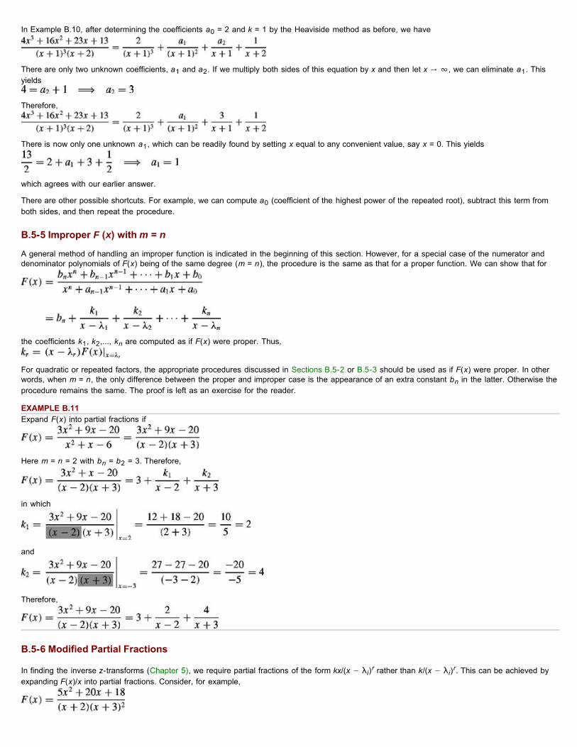
B.5-5 Improper F (x) with m = n

A general method of handling an improper function is indicated in the beginning of this section. However, for a special case of the numerator anddenominator polynomials of F(x) being of the same degree (m = n), the procedure is the same as that for a proper function. We can show that for

the coefficients k1, k2,..., kn are computed as if F(x) were proper. Thus,

For quadratic or repeated factors, the appropriate procedures discussed in Sections B.5-2 or B.5-3 should be used as if F(x) were proper. In otherwords, when m = n, the only difference between the proper and improper case is the appearance of an extra constant bn in the latter. Otherwise theprocedure remains the same. The proof is left as an exercise for the reader.

EXAMPLE B.11Expand F(x) into partial fractions if

Here m = n = 2 with bn = b2 = 3. Therefore,

in which

and

Therefore,

B.5-6 Modified Partial Fractions

In finding the inverse z-transforms (Chapter 5), we require partial fractions of the form kx/(x − λi)r rather than k/(x − λi)r. This can be achieved byexpanding F(x)/x into partial fractions. Consider, for example,

Dividing both sides by x yields

Expansion of the right-hand side into partial fractions as usual yields

Using the procedure discussed earlier, we find a1 = 1, a2 = 1, a3 = −2, and a4 = 1. Therefore,

Now multiplying both sides by x yields

This expresses F(x) as the sum of partial fractions having the form kx/(x − λi)r.

B.6 VECTORS AND MATRICESAn entity specified by n numbers in a certain order (ordered n-tuple) is an n-dimensional vector. Thus, an ordered n-tuple (x1, x2,..., xn) representsan n-dimensional vector x. A vector may be represented as a row (row vector):

or as a column (column vector):

Simultaneous linear equations can be viewed as the transformation of one vector into another. Consider, for example, the n simultaneous linearequations

If we define two column vectors x and y as

then Eqs. (B.48) may be viewed as the relationship or the function that transforms vector x into vector y. Such a transformation is called the lineartransformation of vectors. To perform a linear transformation, we need to define the array of coefficients aij appearing in Eqs. (B.48). This array iscalled a matrix and is denoted by A for convenience:

A matrix with m rows and n columns is called a matrix of the order (m, n) or an (m × n) matrix. For the special case of m = n, the matrix is called asquare matrix of order n.

It should be stressed at this point that a matrix is not a number such as a determinant, but an array of numbers arranged in a particular order. It isconvenient to abbreviate the representation of matrix A in Eq. (B.50) with the form (aij) m x n, implying a matrix of order m x n with aij as its ijthelement. In practice, when the order m x n is understood or need not be specified, the notation can be abbreviated to (aij). Note that the first index iof aij indicates the row and the second index j indicates the column of the element aij in matrix A.

The simultaneous equations (B.48) may now be expressed in a symbolic form as

or

Equation (B.51) is the symbolic representation of Eq. (B.48). Yet we have not defined the operation of the multiplication of a matrix by a vector. Thequantity Ax is not meaningful until such an operation has been defined.

B.6-1 Some Definitions and Properties

A square matrix whose elements are zero everywhere except on the main diagonal is a diagonal matrix. An example of a diagonal matrix is

A diagonal matrix with unity for all its diagonal elements is called an identity matrix or a unit matrix, denoted by I. This is a square matrix:

The order of the unit matrix is sometimes indicated by a subscript. Thus, In represents the n − n unit matrix (or identity matrix). However, we shallomit the subscript. The order of the unit matrix will be understood from the context.

A matrix having all its elements zero is a zero matrix.

A square matrix A is a symmetric matrix if aij = aij (symmetry about the main diagonal).

Two matrices of the same order are said to be equal if they are equal element by element. Thus, if

then A = B only if aij = bij for all i and j.

If the rows and columns of an m × n matrix A are interchanged so that the elements in the ith row now become the elements of the ith column (for i= 1, 2,..., m), the resulting matrix is called the transpose of A and is denoted by AT. It is evident that AT is an n x m matrix. For example, if

Thus, if

then

Note that

B.6-2 Matrix Algebra

We shall now define matrix operations, such as addition, subtraction, multiplication, and division of matrices. The definitions should be formulated sothat they are useful in the manipulation of matrices.

ADDITION OF MATRICESFor two matrices A and B, both of the same order (m × n),

we define the sum A + B as

or

Note that two matrices can be added only if they are of the same order.

MULTIPLICATION OF A MATRIX BY A SCALAR

We multiply a matrix A by a scalar c as follows:

We also observe that the scalar c and the matrix A commute, that is,

MATRIX MULTIPLICATIONWe define the product

in which cij, the element of C in the ith row and jth column, is found by adding the products of the elements of A in the ith row with thecorresponding elements of B in the jth column. Thus,

This result is expressed as follows:

Note carefully that if this procedure is to work, the number of columns of A must be equal to the number of rows of B. In other words, AB, theproduct of matrices A and B, is defined only if the number of columns of A is equal to the number of rows of B. If this condition is not satisfied, theproduct AB is not defined and is meaningless. When the number of columns of A is equal to the number of rows of B, matrix A is said to beconformable to matrix B for the product AB. Observe that if A is an m × n matrix and B is an n × p matrix, A and B are conformable for the product,and C is an m × p matrix.

We demonstrate the use of the rule in Eq. (B.56) with the following examples.

In both cases, the two matrices are conformable. However, if we interchange the order of the matrices as follows,

the matrices are no longer conformable for the product. It is evident that in general,

Indeed, AB may exist and BA may not exist, or vice versa, as in our examples. We shall see later that for some special matrices, AB = BA. When

this is true, matrices A and B are said to commute. We reemphasize that in general, matrices do not commute.

In the matrix product AB, matrix A is said to be postmultiplied by B or matrix B is said to be premultiplied by A. We may also verify the followingrelationships:

We can verify that any matrix A premultiplied or postmultiplied by the identity matrix I remains unchanged:

Of course, we must make sure that the order of I is such that the matrices are conformable for the corresponding product.

We give here, without proof, another important property of matrices:

where |A| and |B| represent determinants of matrices A and B.

MULTIPLICATION OF A MATRIX BY A VECTORConsider the matrix Eq. (B.52), which represents Eq. (B.48). The right-hand side of Eq. (B.52) is a product of the m × n matrix A and a vector x. If,for the time being, we treat the vector x as if it were an n × 1 matrix, then the product Ax, according to the matrix multiplication rule, yields the right-hand side of Eq. (B.48). Thus, we may multiply a matrix by a vector by treating the vector as if it were an n × 1 matrix. Note that the constraint ofconformability still applies. Thus, in this case, xA is not defined and is meaningless.

MATRIX INVERSION

To define the inverse of a matrix, let us consider the set of equations represented by Eq. (B.52):

We can solve this set of equations for x1,x2,...,xn in terms of y1, y2,..., yn, by using Cramer's rule [see Eq. (B.31)]. This yields

in which |A| is the determinant of the matrix A and |Dij| is the cofactor of element aij in the matrix A. The cofactor of element aij is given by (−1)i+j

times the determinant of the (n − 1) × (n − 1) matrix that is obtained when the ith row and the jth column in matrix A are deleted.

We can express Eq. (B.62a) in matrix form as

We now define A−1, the inverse of a square matrix A, with the property

Then, premultiplying both sides of Eq. (B.63) by A−1, we obtain

or

A comparison of Eq. (B.65) with Eq. (B.62b) shows that

One of the conditions necessary for a unique solution of Eq. (B.62a) is that the number of equations must equal the number of unknowns. This

implies that the matrix A must be a square matrix. In addition, we observe from the solution as given in Eq. (B.62b) that if the solution is to exist, |A|≠ 0.[†] Therefore, the inverse exists only for a square matrix and only under the condition that the determinant of the matrix be nonzero. A matrixwhose determinant is nonzero is a nonsingular matrix. Thus, an inverse exists only for a nonsingular, square matrix. By definition, we have

Postmultiplying this equation by A−1 and then premultiplying by A, we can show that

Clearly, the matrices A and A−1 commute.

The operation of matrix division can be accomplished through matrix inversion.

EXAMPLE B.12Let us find A−1 if

Here

and |A| = −4. Therefore,

B.6-3 Derivatives and Integrals of a Matrix

Elements of a matrix need not be constants; they may be functions of a variable. For example, if

then the matrix elements are functions of t. Here, it is helpful to denote A by A(t). Also, it would be helpful to define the derivative and integral ofA(t).

The derivative of a matrix A(t) (with respect to t) is defined as a matrix whose ijth element is the derivative (with respect to t) of the ijth element ofthe matrix A. Thus, if

then

or

Thus, the derivative of the matrix in Eq. (B.68) is given by

Similarly, we define the integral of A(t) (with respect to t) as a matrix whose ijth element is the integral (with respect to t) of the ijth element of thematrix A:

Thus, for the matrix A in Eq. (B.68), we have

We can readily prove the following identities:

The proofs of identities (B.71a) and (B.71b) are trivial. We can prove Eq. (B.71c) as follows. Let A be an m x n matrix and B an n x p matrix. Then, if

from Eq. (B.56), we have

and

or

Equation (B.72) along with the multiplication rule clearly indicate that dik is the ikth element of matrix and eik is the ikth element of matrix Equation (B.71c) then follows.

If we let B = A−1 in Eq. (B.71c), we obtain

But since

we have

B.6-4 The Characteristic Equation of a Matrix: The Cayley-Hamilton Theorem

For an (n − n) square matrix A, any vector x (x ≠ 0) that satisfies the equation

is an eigenvector (or characteristic vector), and λ is the corresponding eigenvalue (or characteristic value) of A. Equation (B.74) can be expressed as

The solution for this set of homogeneous equations exists if and only if

or

Equation (B.76a) [or (B.76b)] is known as the characteristic equation of the matrix A and can be expressed as

Q(λ) is called the characteristic polynomial of the matrix A. The n zeros of the characteristic polynomial are the eigenvalues of A and, correspondingto each eigenvalue, there is an eigenvector that satisfies Eq. (B.74).

The Cayley-Hamilton theorem states that every n × n matrix A satisfies its own characteristic equation. In other words, Eq. (B.77) is valid if λ. isreplaced by A:

FUNCTIONS OF A MATRIX

We now demonstrate the use of the Cayley-Hamilton theorem to evaluate functions of a square matrix A.

Consider a function f(λ) in the form of an infinite power series:

Since λ, being an eigenvalue (characteristic root) of A, satisfies the characteristic equation [Eq. (B.77)], we can write

If we multiply both sides by λ, the left-hand side is λn+1, and the right-hand side contains the terms λn, λn-1, ..., λ. Using Eq. (B.80), we substituteλn, in terms of λn−1, ?n-2,..., λ so that the highest power on the right-hand side is reduced to n − 1. Continuing in this way, we see that λn+k canbe expressed in terms of λn-1, ?n-2,...,λ for any k. Hence, the infinite series on the right-hand side of Eq. (B.79) can always be expressed in terms ofλn−1, λn−2,λ,λ and a constant as

If we assume that there are n distinct eigenvalues ?1, ?2,..., λn, then Eq. (B.81) holds for these n values of λ. The substitution of these values in Eq.(B.81) yields n simultaneous equations

and

Since A also satisfies Eq. (B.80), we may advance a similar argument to show that if f(A) is a function of a square matrix A expressed as an infinitepower series in A, then

and, as argued earlier, the right-hand side can be expressed using terms of power less than or equal to n − 1,

in which the coefficients βis are found from Eq. (B.82b). If some of the eigenvalues are repeated (multiple roots), the results are somewhat modified.

We shall demonstrate the utility of this result with the following two examples.

B.6-5 Computation of an Exponential and a Power of a Matrix

Let us compute eAt defined by

From Eq. (B.83b), we can express

in which the βis are given by Eq. (B.82b), with f(λi) = eλit.

EXAMPLE B.13Let us consider

The characteristic equation is

Hence, the eigenvalues are λ1 = −1, λ2 = −2, and

in which

and

COMPUTATION OF Ak

As Eq. (B.83b) indicates, we can express Ak as

in which the βis are given by Eq. (B.82b) with f(λi) = λki. For a completed example of the computation of Ak by this method, see Example 10.12.

[†]These two conditions imply that the number of equations is equal to the number of unknowns and that all the equations are independent.

B.7 MISCELLANEOUS

B.7-1 L'Hôpital's Rule

If lim f(x)/g(x) results in the indeterministic form 0/0 or ∞/∞, then

B.7-2 The Taylor and Maclaurin Series

B.7-3 Power Series

B.7-4 Sums

B.7-5 Complex Numbers

B.7-6 Trigonometric Identities

B.7-7 Indefinite Integrals

B.7-8 Common Derivative Formulas

B.7-9 Some Useful Constants

B.7-10 Solution of Quadratic and Cubic Equations

Any quadratic equation can be reduced to the form

The solution of this equation is provided by

A general cubic equation

may be reduced to the depressed cubic form

by substituting

This yields

Now let

The solution of the depressed cubic is

and

REFERENCES1. Asimov, Isaac. Asimov on Numbers. Bell Publishing, New York, 1982.

2. Calinger, R., ed. Classics of Mathematics. Moore Publishing, Oak Park, IL, 1982.

3. Hogben, Lancelot. Mathematics in the Making. Doubleday, New York, 1960.

4. Cajori, Florian. A History of Mathematics, 4th ed. Chelsea, New York, 1985.

5. Encyclopaedia Britannica. Micropaedia IV, 15th ed., vol. 11, p. 1043. Chicago, 1982.

6. Singh, Jagjit. Great Ideas of Modern Mathematics. Dover, New York, 1959.

7. Dunham, William. Journey Through Genius. Wiley, New York, 1990.

MATLAB SESSION B: ELEMENTARY OPERATIONS

MB.1 MATLAB OVERVIEW

Although MATLAB(r) (a registered trademark of The Math Works, Inc.) is easy to use, it can be intimidating to new users. Over the years, MATLABhas evolved into a sophisticated computational package with thousands of functions and thousands of pages of documentation. This section providesa brief introduction to the software environment.

When MATLAB is first launched, its command window appears. When MATLAB is ready to accept an instruction or input, a command prompt (>>) isdisplayed in the command window. Nearly all MATLAB activity is initiated at the command prompt.

Entering instructions at the command prompt generally results in the creation of an object or objects. Many classes of objects are possible, including

functions and strings, but usually objects are just data. Objects are placed in what is called the MATLAB workspace. If not visible, the workspace canbe viewed in a separate window by typing workspace at the command prompt. The workspace provides important information about each object,including the object's name, size, and class.

Another way to view the workspace is the whos command. When whos is typed at the command prompt, a summary of the workspace is printed inthe command window. The who command is a short version of whos that reports only the names of workspace objects.

Several functions exist to remove unnecessary data and help free system resources. To remove specific variables from the workspace, the clearcommand is typed, followed by the names of the variables to be removed. Just typing clear removes all objects from the workspace. Additionally,the clc command clears the command window, and the clf command clears the current figure window.

Often, important data and objects created in one session need to be saved for future use. The save command, followed by the desired filename,saves the entire workspace to a file, which has the .mat extension. It is also possible to selectively save objects by typing save followed by thefilename and then the names of the objects to be saved. The load command followed by the filename is used to load the data and objectscontained in a MATLAB data file (.mat file).

Although MATLAB does not automatically save workspace data from one session to the next, lines entered at the command prompt are recorded inthe command history. Previous command lines can be viewed, copied, and executed directly from the command history window. From the commandwindow, pressing the up or down arrow key scrolls through previous commands and redisplays them at the command prompt. Typing the first fewcharacters and then pressing the arrow keys scrolls through the previous commands that start with the same characters. The arrow keys allowcommand sequences to be repeated without retyping.

Perhaps the most important and useful command for new users is help. To learn more about a function, simply type help followed by the functionname. Helpful text is then displayed in the command window. The obvious shortcoming of help is that the function name must first be known. This isespecially limiting for MATLAB beginners. Fortunately, help screens often conclude by referencing related or similar functions. These references arean excellent way to learn new MATLAB commands. Typing help help, for example, displays detailed information on the help command itself andalso provides reference to relevant functions such as the lookfor command. The lookfor command helps locate MATLAB functions based on akeyword search. Simply type lookfor followed by a single keyword, and MATLAB searches for functions that contain that keyword.

MATLAB also has comprehensive HTML-based help. The HTML help is accessed by using MATLAB's integrated help browser, which also functionsas a standard web browser. The HTML help facility includes a function and topic index as well as full text-searching capabilities. Since HTMLdocuments can contain graphics and special characters, HTML help can provide more information than the command-line help. With a little practice,MATLAB makes it very easy to find information.

When MATLAB graphics are created, the print command can save figures in a common file format such as postscript, encapsulated postscript,JPEG, or TIFF. The format of displayed data, such as the number of digits displayed, is selected by using the format command. MATLAB helpprovides the necessary details for both these functions. When a MATLAB session is complete, the exit command terminates MATLAB.

MB.2 Calculator Operations

MATLAB can function as a simple calculator, working as easily with complex numbers as with real numbers. Scalar addition, subtraction,multiplication, division, and exponentiation are accomplished using the traditional operator symbols +, −, ×, ÷, and ⁁. Since MATLAB predefines i = j= √−1, a complex constant is readily created using cartesian coordinates. For example,

assigns the complex constant −3 − j4 to the variable z.

The real and imaginary components of z are extracted by using the real and imag operators. In MATLAB, the input to a function is placedparenthetically following the function name.

When a line is terminated with a semicolon, the statement is evaluated but the results are not displayed to the screen. This feature is useful whenone is computing intermediate results, and it allows multiple instructions on a single line. Although not displayed, the results z_real = −3 andz_imag = −4 are calculated and available for additional operations such as computing |z|.

There are many ways to compute the modulus, or magnitude, of a complex quantity. Trigonometry confirms that z = −3 − j4, which corresponds to a

3-4-5 triangle, has modulus . The MATLAB sqrt command provides one way to compute therequired square root.

In MATLAB, most commands, include sqrt, accept inputs in a variety of forms including constants, variables, functions, expressions, andcombinations thereof.

The same result is also obtained by computing . In this case, complex conjugation is performed by using the conj command.

More simply, MATLAB computes absolute values directly by using the abs command.

>> z = -3-j*4z = -3.0000 - 4.0000i

>> z_real = real(z); z_imag = imag(z);

>> z_mag = sqrt(z_real^2 + z_imag^2)z_mag = 5

>> z_mag = sqrt(z*conj(z))z_mag = 5

In addition to magnitude, polar notation requires phase information. The angle command provides the angle of a complex number.

MATLAB expects and returns angles in a radian measure. Angles expressed in degrees require an appropriate conversion factor.

Notice, MATLAB predefines the variable pi = π.

It is also possible to obtain the angle of z using a two-argument arc-tangent function, atan2.

Unlike a single-argument arctangent function, the two-argument arctangent function ensures that the angle reflects the proper quadrant. MATLABsupports a full complement of trigonometric functions: standard trigonometric functions cos, sin, tan; reciprocal trigonometric functions sec, csc,cot; inverse trigonometric functions acos, asin, atan, asec, acsc, acot; and hyperbolic variations cosh, sinh, tanh, sech, csch, coth,acosh, asinh, atanh, asech, acsch, and acoth. Of course, MATLAB comfortably supports complex arguments for any trigonometric function. Aswith the angle command, MATLAB trigonometric functions utilize units of radians.

The concept of trigonometric functions with complex-valued arguments is rather intriguing. The results can contradict what is often taught inintroductory mathematics courses. For example, a common claim is that |cos(x)| ≤ 1. While this is true for real x, it is not necessarily true forcomplex x. This is readily verified by example using MATLAB and the cos function.

Problem B.19 investigates these ideas further.

Similarly, the claim that it is impossible to take the logarithm of a negative number is false. For example, the principal value of ln(−1) is jπ, a facteasily verified by means of Euler's equation. In MATLAB, base-10 and base-e logarithms are computed by using the log10 and log commands,respectively.

MB.3 Vector Operations

The power of MATLAB becomes apparent when vector arguments replace scalar arguments. Rather than computing one value at a time, a singleexpression computes many values. Typically, vectors are classified as row vectors or column vectors. For now, we consider the creation of rowvectors with evenly spaced, real elements. To create such a vector, the notation a: b: c is used, where a is the initial value, b designates the stepsize, and c is the termination value. For example, 0: 2: 11 creates the length-6 vector of even-valued integers ranging from 0 to 10.

In this case, the termination value does not appear as an element of the vector. Negative and noninteger step sizes are also permissible.

If a step size is not specified, a value of one is assumed.

Vector notation provides the basis for solving a wide variety of problems.

For example, consider finding the three cube roots of minus one, w3 = −1 = ej(π + 2πk) for integer k. Taking the cube root of each side yields w =ej(π/3+2πk/3) To find the three unique solutions, use any three consecutive integer values of k and MATLAB's exp function.

The solutions, particularly w = − 1, are easy to verify.

Finding the 100 unique roots of w100 = −1 is just as simple.

A semicolon concludes the final instruction to suppress the inconvenient display of all 100 solutions. To view a particular solution, the user must

>> z_mag = abs(z)z_mag = 5

>> z_rad = angle(z)z_πad = -2.2143

>> z_deg = angle(z)*180/piz_πad = 126.8699

>> z_deg = atan(z_imag,z_real)z_rad = -2.2143

>> cos(j)ans = 1.5431

>> log(-1)ans = 0 + 3.1416i

>> k = 0:2:11k = 0 2 4 6 8 10

>> k = 11:-10/3:00k = 11.0000 7.6667 4.3333 1.0000

>> k = 0:11k = 0 1 2 3 4 5 6 7 8 9 10 11

>> k = 0:2;>> w = exp(j*(pi/3 + 2*pi*k/3))w = 0.5000 + 0.8660i -1.0000 + 0.0000i 0.5000 - 0.8660i

>> k = 0:99;>> w = exp(j*(pi/100 + 2*pi*k/100));

specify an index. In MATLAB, ascending positive integer indices specify particular vector elements. For example, the fifth element of w is extractedusing an index of 5.

Notice that this solution corresponds to k = 4. The independent variable of a function, in this case k, rarely serves as the index. Since k is also avector, it can likewise be indexed. In this way, we can verify that the fifth value of k is indeed 4.

It is also possible to use a vector index to access multiple values. For example, index vector 98:100 identifies the last three solutions correspondingto k = [97,98,99].

Vector representations provide the foundation to rapidly create and explore various signals. Consider the simple 10 Hz sinusoid described by f(t) =sin(2π 10t + π/6). Two cycles of this sinusoid are included in the interval 0 ≤ t < 0.2. A vector t is used to uniformly represent 500 points over thisinterval.

Next, the function f(t) is evaluated at these points.

The value of f(t) at t = 0 is the first element of the vector and is thus obtained by using an index of one.

Unfortunately, MATLAB's indexing syntax conflicts with standard equation notation.[†] That is, the MATLAB indexing command f(1) is not the sameas the standard notation f(1) = f(t)|t = 1. Care must be taken to avoid confusion; remember that the index parameter rarely reflects the independentvariable of a function.

MB.4 Simple Plotting

MATLAB's plot command provides a convenient way to visualize data, such as graphing f(t) against the independent variable t.

Axis labels are added using the xlabel and ylabel commands, where the desired string must be enclosed by single quotation marks. The result isshown in Fig. MB.1.

Figure MB.1: f(t) = sin (2π 10t + π/6).

The title command is used to add a title above the current axis.

By default, MATLAB connects data points with solid lines. Plotting discrete points, such as the 100 unique roots of w100 = −1, is accommodated bysupplying the plot command with an additional string argument. For example, the string 'o' tells MATLAB to mark each data point with a circlerather than connecting points with lines. A full description of the supported plot options is available from MATLAB's help facilities.

>> w(5)ans = 0.9603 + 0.2790i

>> k(5)ans = 4

>> w(98:100)ans = 0.9877 - 0.1564i 0.9956 - 0.0941i 0.9995 - 0.0314i

>> t = 0:0.2/500:0.2-0.2/500;

>> f = sin(2*pi*10*t+pi/6);

>> f(1)ans = 0.5000

>> plot(t, f);

>> xlabel('t'); ylabel('f(t)')

>> plot(real(w),imag(w),'o');

The axis equal command ensures that the scale used for the horizontal axis is equal to the scale used for the vertical axis. Without axisequal, the plot would appear elliptical rather than circular. Figure MB.2 illustrates that the 100 unique roots of w100 = −1 lie equally spaced on theunit circle, a fact not easily discerned from the raw numerical data.

Figure MB.2: Unique roots of w100 = −1.

MATLAB also includes many specialized plotting functions. For example, MATLAB commands semilogx, semilogy, and loglog operate like theplot command but use base-10 logarithmic scales for the horizontal axis, vertical axis, and the horizontal and vertical axes, respectively.Monochrome and color images can be displayed by using the image command, and contour plots are easily created with the contour command.Furthermore, a variety of three-dimensional plotting routines are available, such as plot3, contour3, mesh, and surf. Information about theseinstructions, including examples and related functions, is available from MATLAB help.

MB.5 Element-by-Element Operations

Suppose a new function h(t) is desired that forces an exponential envelope on the sinusoid f(t), h(t) = f(t)g(t) where g(t) = e−10t. First, row vector g(t)is created.

Given MATLAB's vector representation of g(t) and f(t), computing h(t) requires some form of vector multiplication. There are three standard ways tomultiply vectors: inner product, outer product, and element-by-element product. As a matrix-oriented language, MATLAB defines the standardmultiplication operator * according to the rules of matrix algebra: the multiplicand must be conformable to the multiplier. A 1 × N row vector times anN × 1 column vector results in the scalar-valued inner product. An N × 1 column vector times a 1 × M row vector results in the outer product, whichis an N × M matrix. Matrix algebra prohibits multiplication of two row vectors or multiplication of two column vectors. Thus, the * operator is not usedto perform element-by-element multiplication.[†]

Element-by-element operations require vectors to have the same dimensions. An error occurs if element-by-element operations are attemptedbetween row and column vectors. In such cases, one vector must first be transposed to ensure both vector operands have the same dimensions. InMATLAB, most element-by-element operations are preceded by a period. For example, element-by-element multiplication, division, andexponentiation are accomplished using. *,. /, and .ˇ, respectively. Vector addition and subtraction are intrinsically element-by-element operations andrequire no period. Intuitively, we know h(t) should be the same size as both g(t) and f(t). Thus, h(t) is computed using element-by-elementmultiplication.

The plot command accommodates multiple curves and also allows modification of line properties. This facilitates side-by-side comparison ofdifferent functions, such as h(t) and f(t). Line characteristics are specified by using options that follow each vector pair and are enclosed in singlequotes.

Here, '-k' instructs MATLAB to plot f(t) using a solid black line, while ':k' instructs MATLAB to use a dotted black line to plot h(t). A legend and axislabels complete the plot, as shown in Fig. MB.3. It is also possible, although more cumbersome, to use pull-down menus to modify line propertiesand to add labels and legends directly in the figure window.

>> xlabel('Re(w); ylabel('Im(w)');>> axis equal

>> g = exp(-10*t);

>> h = f.*g;

>> plot(t, f,'-k',t,h,':k');>> xlabel('t'); ylabel('Amplitude');>> legend('f(t)','h(t)');

Figure MB.3: Graphical comparison of f(t) and h(t).

MB.6 Matrix Operations

Many applications require more than row vectors with evenly spaced elements; row vectors, column vectors, and matrices with arbitrary elements aretypically needed.

MATLAB provides several functions to generate common, useful matrices. Given integers m, n, and vector x, the function eye(m) creates the m × midentity matrix; the function ones(m,n) creates the m × n matrix of all ones; the function zeros (m,n) creates the m × n matrix of all zeros; and thefunction diag(x) uses vector x to create a diagonal matrix. The creation of general matrices and vectors, however, requires each individual elementto be specified.

Vectors and matrices can be input spreadsheet style by using MATLAB's array editor. This graphical approach is rather cumbersome and is not oftenused. A more direct method is preferable.

Consider a simple row vector r,

The MATLAB notation a: b: c cannot create this row vector. Rather, square brackets are used to create r.

Square brackets enclose elements of the vector, and spaces or commas are used to separate row elements.

Next, consider the 3 × 2 matrix A,

Matrix A can be viewed as a three-high stack of two-element row vectors. With a semicolon to separate rows, square brackets are used to create thematrix.

Each row vector needs to have the same length to create a sensible matrix.

In addition to enclosing string arguments, a single quote performs the complex conjugate transpose operation. In this way, row vectors becomecolumn vectors and vice versa. For example, a column vector c is easily created by transposing row vector r.

Since vector r is real, the complex-conjugate transpose is just the transpose. Had r been complex, the simple transpose could have beenaccomplished by either r. 'or (conj (r)) '.

More formally, square brackets are referred to as a concatenation operator. A concatenation combines or connects smaller pieces into a larger whole.Concatenations can involve simple numbers, such as the six-element concatenation used to create the 3 × 2 matrix A. It is also possible toconcatenate larger objects, such as vectors and matrices. For example, vector c and matrix A can be concatenated to form a 3 × 3 matrix B.

Errors will occur if the component dimensions do not sensibly match; a 2 × 2 matrix would not be concatenated with a 3 × 3 matrix, for example.

Elements of a matrix are indexed much like vectors, except two indices are typically used to specify row and column.[†] Element (1, 2) of matrix B,for example, is 2.

>> r = [1 0 0]r = 1 0 0

>> A = [2 3; 4 5; 0 6]A = 2 34 50 6

>> c = r'c = 100

>> B = [c A]B = 1 2 30 4 50 0 6

Indices can likewise be vectors. For example, vector indices allow us to extract the elements common to the first two rows and last two columns ofmatrix B.

One indexing technique is particularly useful and deserves special attention. A colon can be used to specify all elements along a specified dimension.For example, B(2,:) selects all column elements along the second row of B.

Now that we understand basic vector and matrix creation, we turn our attention to using these tools on real problems. Consider solving a set of threelinear simultaneous equations in three unknowns.

This system of equations is represented in matrix form according to Ax = y, where

Although Cramer's rule can be used to solve Ax = y, it is more convenient to solve by multiplying both sides by the matrix inverse of A. That is, x =A−1Ax = A−1y. Solving for x by hand or by calculator would be tedious at best, so MATLAB is used. We first create A and y.

The vector solution is found by using MATLAB's inv function.

It is also possible to use MATLAB's left divide operator x = A\y to find the same solution. The left divide is generally more computationally efficientthan matrix inverses. As with matrix multiplication, left division requires that the two arguments be conformable.

Of course, Cramer's rule can be used to compute individual solutions, such as x1, by using vector indexing, concatenation, and MATLAB's detcommand to compute determinants.

Another nice application of matrices is the simultaneous creation of a family of curves. Consider hα(t) = e−αt sin(2π10t + π/6) over 0 ≤ t ≤ 0.2.Figure MB.3 shows hα(t) for α = 0 and α = 10. Let's investigate the family of curves hα(t) for a = [0, 1,..., 10].

An inefficient way to solve this problem is create hα(t) for each α of interest. This requires 11 individual cases. Instead, a matrix approach allows all11 curves to be computed simultaneously. First, a vector is created that contains the desired values of α.

By using a sampling interval of one millisecond, Δt = 0.001, a time vector is also created.

The result is a length-201 column vector. By replicating the time vector for each of the 11 curves required, a time matrix T is created. This replicationcan be accomplished by using an outer product between t and a 1 × 11 vector of ones.[†]

The result is a 201 × 11 matrix that has identical columns. Right multiplying T by a diagonal matrix created from α, columns of T can be individuallyscaled and the final result is computed.

Here, H is a 201 × 11 matrix, where each column corresponds to a different value of α. That is, H = [h0, h1,..., h10], where hα are column vectors.As shown in Fig. MB.4, the 11 desired curves are simultaneously displayed by using MATLAB's plot command, which allows matrix arguments.

>> B(1, 2)ans = 2

>> B(1:2,2:3)ans = 2 34 5

>> B(2,:)ans = 0 4 5

>> A = [1 -2 3;-sqrt(3) 1 -sqrt(5);3 -sqrt(7) 1];>> y = [1;pi;exp(1)];

>> x = inv(A)*yx = -1.9999-3.8998-1.5999

>> x1 = det([y,A(:,2:3)])/det(A)x1 = -1.9999

>> alpha = (0:10);

>> t = (0:0.001:0.2)';

>> T = t*ones(1,11);

>> H = exp(-T*diag(alpha)).*sin(2*pi*10*T+pi/6);

Figure MB.4: hα(t) for α = [0,1,..., 10].

This example illustrates an important technique called vectorization, which increases execution efficiency for interpretive languages such asMATLAB.[‡] Algorithm vectorization uses matrix and vector operations to avoid manual repetition and loop structures. It takes practice and effort tobecome proficient at vectorization, but the worthwhile result is efficient, compact code.

MB.7 Partial Fraction Expansions

There are a wide variety of techniques and shortcuts to compute the partial fraction expansion of rational function F(x) = B(x)/A(x), but few are moresimple than the MATLAB residue command. The basic form of this command is

The two input vectors B and A specify the polynomial coefficients of the numerator and denominator, respectively. These vectors are ordered indescending powers of the independent variable. Three vectors are output. The vector R contains the coefficients of each partial fraction, and vector Pcontains the corresponding roots of each partial fraction. For a root repeated r times, the r partial fractions are ordered in ascending powers. Whenthe rational function is not proper, the vector K contains the direct terms, which are ordered in descending powers of the independent variable.

To demonstrate the power of the residue command, consider finding the partial fraction expansion of

By hand, the partial fraction expansion of F(x) is difficult to compute. MATLAB, however, makes short work of the expansion.

Written in standard form, the partial fraction expansion of F(x) is

The signal processing toolbox function residuez is similar to the residue command and offers more convenient expansion of certain rationalfunctions, such as those commonly encountered in the study of discrete-time systems. Additional information about the residue and residuezcommands are available from MATLAB's help facilities.

[†]Advanced structures such as MATLAB inline objects are an exception.

[†]While grossly inefficient, element-by-element multiplication can be accomplished by extracting the main diagonal from the outer product of two N-length vectors.

[†]Matrix elements can also be accessed by means of a single index, which enumerates along columns. Formally, the element from row m andcolumn n of an M × N matrix may be obtained with a single index (n − 1)M + m. For example, element (1, 2) of matrix B is accessed by using theindex (2 − 1)3 + 1 = 4. That is, B (4) yields 2.

[†]The repmat command provides a more flexible method to replicate or tile objects. Equivalently, T = repmat(t,1,11).

[‡]The benefits of vectorization are less pronounced in recent versions of MATLAB.

>> plot(t,H); xlabel('t'); ylabel('h(t)');

>> [R,P,K] = residue(B,A)

>> [R,P,K] = residue( [1 0 0 0 0 pi], [1 -sqrt(8) 0 sqrt(32) -4])R = 7.8888 5.9713 3.1107 0.1112P = 1.4142 1.4142 1.4142 -1.4142K = 1.0000 2.8284

PROBLEMSb.1 Given a complex number w = x + jy, the complex conjugate of w is defined in rectangular coordinates as w* = x − jy. Use this fact to

derive complex conjugation in polar form. b.2 Express the following numbers in polar form:

a. 1 + j

b. −4 + j3

c. (1 + j)(−4 + j3)

d. ejπ/4 + 2e−jπ/4

e. ej + 1

f. (1 + j)/(04 + j3) b.3 Express the following numbers in Cartesian form:

a. 3ejπ/4

b. 1/ej

c. (1 + j)(−4 + j3)

d. ejπ/4 + 2e−jπ/4

e. ej + 1

f. 1/2 j

b.4 For complex constant w, prove:

a. Re(w) = (w + w*)/2

b. Im(w) = (w − w*)/2j b.5 Given w = x − jy, determine:

a. Re(ew)

b. Im(ew) b.6 For arbitrary complex constants w1 and w2, prove or disprove the following:

a. Re(jw1) = −Im(w1)

b. Im(jw1) = Re(w1)

c. Re(w1) + Re(w2) = Re(w1 + w2)

d. Im(w1) + Im(w2) = Im(w1 + w2)

e. Re(w1)Re(w2) = Re(w1, w2)

f. Im(w1)/Im(w2) = Im(w1/w2) b.7 Given w1 = 3 + j4 and w2 = 2ejπ/4.

a. Express w1 in standard polar form.

b. Express w2 in standard rectangular form.

c. Determine |w1|2 and |w2|2.

d. Express w1 + w2 in standard rectangular form.

e. Express w1 − w2 in standard polar form.

f. Express w1w2 in standard rectangular form.

g. Express w1/w2 in standard polar form. b.8 Repeat Prob. B.7 using w = (3 + j4)2 and w = 2.5 je−j40π.

1 2 b.9 Repeat Prob. B.7 using w1 = j + eπ/4 and w2 = cos (j). b.10 Use Euler's identity to solve or prove the following:

a. Find real, positive constants c and φ for all real t such that 2.5 cos (3t) − 1.5 sin (3t + π/3) = c cos(3t + φ)

b. Prove that cos (θ ± φ) = cos (θ) cos (φ) ∓ sin (θ) sin (φ).

c. Given real constants a, b, and α, complex constant w, and the fact that

evaluate the integral

b.11 In addition to the traditional sine and cosine functions, there are the hyperbolic sine and cosine functions, which are defined by sinh (w)

= (ew − e−w)/2 and cosh (w) = (ew + e−w)/2. In general, the argument is a complex constant w = x + jy.

a. Show that cosh (w) = cosh (x) cos (y) + j sinh (x) sin (y).

b. Determine a similar expression for sinh (w) in rectangular form that only uses functions of real arguments, such as sin (x),cosh (y), and so on.

b.12 Using the complex plane:

a. Evaluate and locate the distinct solutions to (w)4 = −1.

b. Evaluate and locate the distinct solutions to (w − (1 + j2))5 = (32/√2) (1 + j).

c. Sketch the solution to |w − 2j| = 3.

d. Graph w(t) = (1 + t)ejt for (−10 ≤ t ≤ 10). b.13 The distinct solutions to (w − w1)n = w2 lie on a circle in the complex plane, as shown in Fig. PB.13. One solution is located on the

real axis at √3 + 1 = 2.732, and one solution is located on the imaginary axis at √3 − 10.732. Determine w1, w2, and n.

Figure PB.13: Distinct solutions to (w − w1)n = w2.

b.14 Find the distinct solutions to (j − w)1.5 = 2 + j2. Use MATLAB to graph the solution set in the complex plane. b.15 If j = √−1, what is √j? b.16 Find all the values of ln(−e), expressing your answer in Cartesian form. b.17 Determine all values of log10(−1), expressing your answer in Cartesian form. Notice that the logarithm has base 10, not e. b.18 Express the following in standard rectangular coordinates:

a. ln(1/(1+j))

b. cos(1 + j)

c. (1 − j)j

b.19 By constraining w to be purely imaginary, show that the equation cos (w) = 2 can be represented as a standard quadratic equation.

Solve this equation for w. b.20 Determine an expression for an exponentially decaying sinusoid that oscillates three times per second and whose amplitude envelope

decreases by 50% every 2 seconds. Use MATLAB to plot the signal over −2 ≤ t ≤ 2. b.21 By hand, sketch the following against independent variable t:

a. x1(t) = Re(2e(−1 +j2π)t)

b. x2(t) = Im(3 − e(1 − j2π)t)

c. x3(t) = 3 − Im(e(1 − j2π)t) b.22 Use MATLAB to produce the plots requested in Prob. B.21. b.23 Use MATLAB to plot x(t) = cos (t) sin (20t) over a suitable range of t. b.24 Use MATLAB to plot x(t) = Σ10

k=1 cos (2πkt) over a suitable range of t. The MATLAB command sum may prove useful. b.25 When a bell is struck with a mallet, it produces a ringing sound. Write an equation that approximates the sound produced by a small,

light bell. Carefully identify your assumptions. How does your equation change if the bell is large and heavy? You can assess thequality of your models by using the MATLAB sound command to listen to your "bell."

b.26 Certain integrals, although expressed in relatively simple form, are quite difficult to solve. For example, ∫ e-x2 dx cannot be evaluated

in terms of elementary functions; most calculators that perform integration cannot handle this indefinite integral. Fortunately, you aresmarter than most calculators.

a. Express e−x2 using a Taylor series expansion.

b. Using your series expansion for e−x2, determine ∫ e−x2 dx.

c. Using a suitably truncated series, evaluate the definite integral ∫10 e−x2 dx.

b.27 Repeat Prob. B.26 for ∫ e−x3 dx. b.28 Repeat Prob. B.26 for ∫ cos x2 dx. b.29 For each function, determine a suitable series expansion.

a. f1(x) = (2 −x2)−1

b. f2(x) = (0.5)x b.30 You are working on a digital quadrature amplitude modulation (QAM) communication receiver. The QAM receiver requires a pair of

quadrature signals: cos Ωn and sin Ωn. These can be simultaneously generated by following a simple procedure: (1) choose a point won the unit circle, (2) multiply w by itself and store the result, (3) multiply w by the last result and store, and (4) repeat step 3.

a. Show that this method can generate the desired pair of quadrature sinusoids.

b. Determine a suitable value of w so that good-quality, periodic, 2π × 100,000 rad/s signals can be generated. How muchtime is available for the processing unit to compute each sample?

c. Simulate this procedure by using MATLAB and report your results.

d. Identify as many assumptions and limitations to this technique as possible. For example, can your system operatecorrectly for an indefinite period of time?

b.31 Consider the following system of equations.

Use Cramer's rule to determine:

a. x1

b. x2

c. x3

Matrix determinants can be computed by using MATLAB's det command. b.32 A system of equations in terms of unknowns x1 and x2 and arbitrary constants a, b, c, d, e, and f is given by

a. Represent this system of equations in matrix form.

b. Identify specific constants a, b, c, d, e, and f such that x1 = 3 and x2 = −2. Are the constants you selected unique?

c. Identify nonzero constants a, b, c, d, e, and f such that no solutions x1 and x2 exist.

d. Identify nonzero constants a, b, c, d, e, and f such that an infinite number of solutions x1 and x2 exist. b.33 Solve the following system of equations:

b.34 Solve the following system of equations:

b.35 Compute by hand the partial fraction expansions of the following rational functions:

a. H1(s) = (s2 + 5s + 6)/(s3 + s2 + s + 1), which has denominator poles at s = ± j and s = −1

b. H2(s) = 1/H1(s) = (s3 + s2 + s + 1)/(s2 + 5s + 6)

c. H2(s) = 1/((s + 1)2(s2 + 1))

d. H4(s) = (s2 + 5s + 6)/(3s2 + 2s + 1) b.36 Using MATLAB's residue command,

a. Verify the results of Prob. B.35a.

b. Verify the results of Prob. B.35b.

c. Verify the results of Prob. B.35c.

d. Verify the results of Prob. B.35d. b.37 Determine the constants a0, a1, and a2 of the partial fraction expansion F(s) = s/(s + 1)3 = a0/(s + 1)3 + a1/(s + 1)2 + a2/(s + 1). b.38 Let N = [n7, n6, n5,...,n2, n1] represent the seven digits of your phone number. Construct a rational function according to

Use MATLAB's residue command to compute the partial fraction expansion of HN(s). b.39 When plotted in the complex plane for −π ≤ ω ≤ π, the function f (ω) = cos(ω) + j0.1 sin(2ω) results in a so-called Lissajous figure

that resembles a two-bladed propeller.

a. In MATLAB, create two row vectors fr and fi corresponding to the real and imaginary portions of f (ω), respectively,over a suitable number N samples of ω. Plot the real portion against the imaginary portion and verify the figureresembles a propeller.

b. Let complex constant w = x + jy be represented in vector form

Consider the 2 × 2 rotational matrix R:

Show that Rw rotates vector w by θ radians.

c. Create a rotational matrix R corresponding to 10° and multiply it by the 2 × N matrix f = [f r; f i];. Plot the resultto verify that the "propeller" has indeed rotated counterclockwise.

d. Given the matrix R determined in part c, what is the effect of performing RRf? How about RRRf? Generalize the result.

e. Investigate the behavior of multiplying f (ω) by the function ejθ.

Chapter 1: Signals and Systems

OVERVIEW

In this chapter we shall discuss certain basic aspects of signals. We shall also introduce important basic concepts and qualitativeexplanations of the hows and whys of systems theory, thus building a solid foundation for understanding the quantitative analysis in theremainder of the book.

SIGNALS

A signal is a set of data or information. Examples include a telephone or a television signal, monthly sales of a corporation, or dailyclosing prices of a stock market (e.g., the Dow Jones averages). In all these examples, the signals are functions of the independentvariable time. This is not always the case, however. When an electrical charge is distributed over a body, for instance, the signal is thecharge density, a function of space rather than time. In this book we deal almost exclusively with signals that are functions of time. Thediscussion, however, applies equally well to other independent variables.

SYSTEMS

Signals may be processed further by systems, which may modify them or extract additional information from them. For example, anantiaircraft gun operator may want to know the future location of a hostile moving target that is being tracked by his radar. Knowing theradar signal, he knows the past location and velocity of the target. By properly processing the radar signal (the input), he canapproximately estimate the future location of the target. Thus, a system is an entity that processes a set of signals (inputs) to yieldanother set of signals (outputs). A system may be made up of physical components, as in electrical, mechanical, or hydraulic systems(hardware realization), or it may be an algorithm that computes an output from an input signal (software realization).

1.1 SIZE OF A SIGNALThe size of any entity is a number that indicates the largeness or strength of that entity. Generally speaking, the signal amplitude varieswith time. How can a signal that exists over a certain time interval with varying amplitude be measured by one number that will indicatethe signal size or signal strength? Such a measure must consider not only the signal amplitude, but also its duration. For instance, if weare to devise a single number V as a measure of the size of a human being, we must consider not only his or her width (girth), but alsothe height. If we make a simplifying assumption that the shape of a person is a cylinder of variable radius r (which varies with theheight h) then one possible measure of the size of a person of height H is the person's volume V, given by

1.1-1 Signal Energy

Arguing in this manner, we may consider the area under a signal x(t) as a possible measure of its size, because it takes account notonly of the amplitude but also of the duration. However, this will be a defective measure because even for a large signal x(t), itspositive and negative areas could cancel each other, indicating a signal of small size. This difficulty can be corrected by defining thesignal size as the area under x2(t), which is always positive. We call this measure the signal energy Ex, defined (for a real signal) as

This definition can be generalized to a complex valued signal x(t) as

There are also other possible measures of signal size, such as the area under |x(t)|. The energy measure, however, is not only moretractable mathematically but is also more meaningful (as shown later) in the sense that it is indicative of the energy that can beextracted from the signal.

1.1-2 Signal Power

The signal energy must be finite for it to be a meaningful measure of the signal size. A necessary condition for the energy to be finite isthat the signal amplitude → 0 as |t| → ∞ (Fig. 1.1a). Otherwise the integral in Eq. (1.2a) will not converge.

Figure 1.1: Examples of signals: (a) a signal with finite energy and (b) a signal with finite power.

When the amplitude of x(t) does not → 0 as |t| → ∞ (Fig. 1.1b), the signal energy is infinite. A more meaningful measure of the signalsize in such a case would be the time average of the energy, if it exists. This measure is called the power of the signal. For a signalx(t), we define its power Px as

We can generalize this definition for a complex signal x(t) as

Observe that the signal power Px is the time average (mean) of the signal amplitude squared, that is, the mean-squared value of x(t).Indeed, the square root of Px is the familiar rms (root-mean-square) value of x(t).

Generally, the mean of an entity averaged over a large time interval approaching infinity exists if the entity either is periodic or has astatistical regularity. If such a condition is not satisfied, the average may not exist. For instance, a ramp signal x(t) = t increasesindefinitely as |t| → ∞, and neither the energy nor the power exists for this signal. However, the unit step function, which is not periodicnor has statistical regularity, does have a finite power.

When x(t) is periodic, |x(t)|2 is also periodic. Hence, the power of x(t) can be computed from Eq. (1.3b) by averaging |x(t)|2 over oneperiod.

Comments. The signal energy as defined in Eqs. (1.2) does not indicate the actual energy (in the conventional sense) of the signalbecause the signal energy depends not only on the signal, but also on the load. It can, however, be interpreted as the energydissipated in a normalized load of a 1-ohm resistor if a voltage x(t) were to be applied across the 1-ohm resistor (or if a current x(t)were to be passed through the 1 -ohm resistor). The measure of "energy" is, therefore indicative of the energy capability of the signal,not the actual energy. For this reason the concepts of conservation of energy should not be applied to this "signal energy." Parallelobservation applies to "signal power" defined in Eqs. (1.3). These measures are but convenient indicators of the signal size, whichprove useful in many applications. For instance, if we approximate a signal x(t) by another signal g(t), the error in the approximation ise(t) = x(t) − g(t). The energy (or power) of e(t) is a convenient indicator of the goodness of the approximation. It provides us with aquantitative measure of determining the closeness of the approximation. In communication systems, during transmission over a channel,message signals are corrupted by unwanted signals (noise). The quality of the received signal is judged by the relative sizes of thedesired signal and the unwanted signal (noise). In this case the ratio of the message signal and noise signal powers (signal to noisepower ratio) is a good indication of the received signal quality.

Units of Energy and Power. Equations (1.2) are not correct dimensionally. This is because here we are using the term energy not inits conventional sense, but to indicate the signal size. The same observation applies to Eqs. (1.3) for power. The units of energy andpower, as defined here, depend on the nature of the signal x(t). If x(t) is a voltage signal, its energy Ex has units of volts squared-

seconds (V2 s), and its power Px has units of volts squared. If x(t) is a current signal, these units will be amperes squared-seconds (A2

s) and amperes squared, respectively.

EXAMPLE 1.1Determine the suitable measures of the signals in Fig. 1.2.

Figure 1.2

In Fig. 1.2a, the signal amplitude → 0 as |t| → ∞. Therefore the suitable measure for this signal is its energy Ex given by

In Fig. 1.2b, the signal amplitude does not → 0 as |t| → ∞. However, it is periodic, and therefore its power exists. We can use Eq.(1.3a) to determine its power. We can simplify the procedure for periodic signals by observing that a periodic signal repeats regularlyeach period (2 seconds in this case). Therefore, averaging x2(t) over an infinitely large interval is identical to averaging this quantityover one period (2 seconds in this case). Thus

Recall that the signal power is the square of its rms value. Therefore, the rms value of this signal is 1/√3.

EXAMPLE 1.2Determine the power and the rms value of

a. x(t) = C cos (ω0t + θ)

b. x(t) = C1 cos (ω1t + θ1) + C2 cos (ω2t + θ2) ω1 ≠ ω2

c. x(t) = Dejω0 t

a. This is a periodic signal with period T0 = 2π/ω0. The suitable measure of this signal is its power. Because it is a periodicsignal, we may compute its power by averaging its energy over one period T0 = 2π/ω0. However, for the sake ofdemonstration, we shall solve this problem by averaging over an infinitely large time interval using Eq. (1.3a).

The first term on the right-hand side is equal to C2/2. The second term, however, is zero because the integral appearingin this term represents the area under a sinusoid over a very large time interval T with T → ∞. This area is at most equalto the area of half the cycle because of cancellations of the positive and negative areas of a sinusoid. The second term isthis area multiplied by C2/2T with T → ∞. Clearly this term is zero, and

This shows that a sinusoid of amplitude C has a power C2/2 regardless of the value of its frequency ω0 (ω0 ≠ 0) andphase θ. The rms value is C/√2. If the signal frequency is zero (dc or a constant signal of amplitude C), the reader canshow that the power is C2.

b. In Chapter 6, we shall show that a sum of two sinusoids may or may not be periodic, depending on whether the ratioω1/ω2 is a rational number. Therefore, the period of this signal is not known. Hence, its power will be determined byaveraging its energy over T seconds with T → ∞. Thus,

The first and second integrals on the right-hand side are the powers of the two sinusoids, which are C21/2 and C2

2/2 asfound in part (a). The third term, the product of two sinusoids, can be expressed as a sum of two sinusoids cos [(ω1 +

ω2)t + (θ1 + θ2)] and cos [(ω1 − ω2)t + (θ1 − θ2)], respectively. Now, arguing as in part (a), we see that the third term

is zero. Hence, we have[†]

and the rms value is .

We can readily extend this result to a sum of any number of sinusoids with distinct frequencies. Thus, if

assuming that none of the two sinusoids have identical frequencies and ωn ≠ 0, then

If x(t) also has a dc term, as

then

c. In this case the signal is complex, and we use Eq. (1.3b) to compute the power.

Recall that |ejω0 t| = 1 so that |Dejω0 t|2 = |D|2, and

The rms value is |D|.

Comment. In part (b) of Example 1.2, we have shown that the power of the sum of two sinusoids is equal to the sum of the powers ofthe sinusoids. It may appear that the power of x1(t) + x2(t) is Px1 + Px2. Unfortunately, this conclusion is not true in general. It is trueonly under a certain condition (orthogonality), discussed later (Section 6.5-3).

EXERCISE E1.1Show that the energies of the signals in Fig. 1.3a, 1.3b, 1.3c, and 1.3d are 4, 1, 4/3, and 4/3, respectively. Observe that doubling asignal quadruples the energy, and time-shifting a signal has no effect on the energy. Show also that the power of the signal in Fig. 1.3eis 0.4323. What is the rms value of signal in Fig. 1.3e?

Figure 1.3

EXERCISE E1.2Redo Example 1.2a to find the power of a sinusoid C cos (ω0t + θ) by averaging the signal energy over one period T0 = 2π/ω0

(rather than averaging over the infinitely large interval). Show also that the power of a dc signal x(t) = C0 is C20, and its rms value is

C0.

EXERCISE E1.3Show that if ω1 = ω2, the power of x(t) = C1 cos (ω1t + θ1) + C2 cos (ω2t + θ2) is [C2

1 + C22 + 2C1C2 cos (θ1 − θ2)]/2, which is

not equal to (C21 + C2

2)/2.

[†]This is true only if ω1 ≠ ω2. If ω1 = ω2, the integrand of the third term contains a constant cos (θ1 − θ2), and the third term →2C1C2 cos (θ1 − θ2) as T → ∞.

1.2 SOME USEFUL SIGNAL OPERATIONSWe discuss here three useful signal operations: shifting, scaling, and inversion. Since the independent variable in our signal descriptionis time, these operations are discussed as time shifting, time scaling, and time reversal (inversion). However, this discussion is valid forfunctions having independent variables other than time (e.g., frequency or distance).

1.2-1 Time Shifting

Consider a signal x(t) (Fig. 1.4a) and the same signal delayed by T seconds (Fig. 1.4b), which we shall denote by φ(t). Whateverhappens in x(t) (Fig. 1.4a) at some instant t also happens in φ(t) (Fig. 1.4b) T seconds later at the instant t + T. Therefore

and

Figure 1.4: Time-shifting a signal.

Therefore, to time-shift a signal by T, we replace t with t − T. Thus x(t − T) represents x(t) time-shifted by T seconds. If T is positive,the shift is to the right (delay), as in Fig. 1.4b. If T is negative, the shift is to the left (advance), as in Fig. 1.4c. Clearly, x(t − 2) is x(t)delayed (right-shifted) by 2 seconds, and x(t + 2) is x(t) advanced (left-shifted) by 2 seconds.

EXAMPLE 1.3An exponential function x(t) = e−2t shown in Fig. 1.5a is delayed by 1 second. Sketch and mathematically describe the delayedfunction. Repeat the problem with x(t) advanced by 1 second.

Figure 1.5: (a) Signal x(t). (b) Signal x(t) delayed by 1 second. (c) Signal x(t) advanced by 1 second.

The function x(t) can be described mathematically as

Let xd(t) represent the function x(t) delayed (right-shifted) by 1 second as illustrated in Fig. 1.5b. This function is x(t − 1); itsmathematical description can be obtained from x(t) by replacing t with t − 1 in Eq. (1.7). Thus

Let xa(t) represent the function x(t) advanced (left-shifted) by 1 second as depicted in Fig. 1.5c. This function is x(t + 1); itsmathematical description can be obtained from x(t) by replacing t with t + 1 in Eq. (1.7). Thus

EXERCISE E1.4Write a mathematical description of the signal x3(t) in Fig. 1.3c. This signal is delayed by 2 seconds. Sketch the delayed signal. Showthat this delayed signal xd(t) can be described mathematically as xd(t) = 2(t − 2) for 2 ≤ t ≤ 3, and equal to 0 otherwise. Now repeatthe procedure with the signal advanced (left-shifted) by 1 second. Show that this advanced signal xa(t) can be described as xa(t) = 2(t+ 1) for − 1 ≤ t ≤ 0, and equal to 0 otherwise.

1.2-2 Time Scaling

The compression or expansion of a signal in time is known as time scaling. Consider the signal x(t) of Fig. 1.6a. The signal φ(t) in Fig.1.6b is x(t) compressed in time by a factor of 2. Therefore, whatever happens in x(t) at some instant t also happens to φ(t) at theinstant t/2, so that

and

Figure 1.6: Time scaling a signal.

Observe that because x(t) = 0 at t = T1 and T2, we must have φ(t) = 0 at t = T1/2 and T2/2, as shown in Fig. 1.6b. If x(t) wererecorded on a tape and played back at twice the normal recording speed, we would obtain x(2t). In general, if x(t) is compressed intime by a factor a (a > 1), the resulting signal φ(t) is given by

Using a similar argument, we can show that x(t) expanded (slowed down) in time by a factor a (a > 1) is given by

Figure 1.6c shows x(t/2), which is x(t) expanded in time by a factor of 2. Observe that in a time-scaling operation, the origin t = 0 is theanchor point, which remains unchanged under the scaling operation because at t = 0, x(t) = x(at) = x(0).

In summary, to time-scale a signal by a factor a, we replace t with at. If a > 1, the scaling results in compression, and if a < 1, thescaling results in expansion.

EXAMPLE 1.4Figure 1.7a shows a signal x(t). Sketch and describe mathematically this signal time-compressed by factor 3. Repeat the problem forthe same signal time-expanded by factor 2.

Figure 1.7: (a) Signal x(t),(b) signal x(3t), and (c) signal x(t/2).

The signal x(t) can be described as

Figure 1.7b shows xc(t), which is x(t) time-compressed by factor 3; consequently, it can be described mathematically as x(3t), which isobtained by replacing t with 3t in the right-hand side of Eq. (1.14). Thus

Observe that the instants t = −1.5 and 3 in x(t) correspond to the instants t = −0.5, and 1 in the compressed signal x(3t).

Figure 1.7c shows xe(t), which is x(t) time-expanded by factor 2; consequently, it can be described mathematically as x(t/2), which isobtained by replacing t with t/2 in x(t). Thus

Observe that the instants t = −1.5 and 3 in x(t) correspond to the instants t = −3 and 6 in the expanded signal x(t/2).

EXERCISE E1.5Show that the time compression by a factor n (n > 1) of a sinusoid results in a sinusoid of the same amplitude and phase, but with thefrequency increased n-fold. Similarly, the time expansion by a factor n (n > 1) of a sinusoid results in a sinusoid of the same amplitudeand phase, but with the frequency reduced by a factor n. Verify your conclusion by sketching a sinusoid sin 2t and the same sinusoidcompressed by a factor 3 and expanded by a factor 2.

1.2-3 Time Reversal

Consider the signal x(t) in Fig. 1.8a. We can view x(t) as a rigid wire frame hinged at the vertical axis. To time-reverse x(t), we rotatethis frame 180° about the vertical axis. This time reversal [the reflection of x(t) about the vertical axis] gives us the signal φ(t) (Fig.1.8b). Observe that whatever happens in Fig. 1.8a at some instant t also happens in Fig. 1.8b at the instant −t, and vice versa.Therefore

Figure 1.8: Time reversal of a signal.

Thus, to time-reverse a signal we replace t with −t, and the time reversal of signal x(t) results in a signal x(−t). We must rememberthat the reversal is performed about the vertical axis, which acts as an anchor or a hinge. Recall also that the reversal of x(t) about thehorizontal axis results in −x(t).

EXAMPLE 1.5For the signal x(t) illustrated in Fig. 1.9a, sketch x(−t), which is time-reversed x(t).

Figure 1.9: Example of time reversal.

The instants −1 and −5 in x(t) are mapped into instants 1 and 5 in x(−t). Because x(t) = et /2, we have x(-t) = e1/2. The signal x(−t)

is depicted in Fig. 1.9b. We can describe x(t) and x(−t) as

and its time reversed version x(−t) is obtained by replacing t with −t in x(t) as

1.2-4 Combined Operations

Certain complex operations require simultaneous use of more than one of the operations just described. The most general operationinvolving all the three operations is x(at − b), which is realized in two possible sequences of operation:

1. Time-shift x(t) by b to obtain x(t − b). Now time-scale the shifted signal x(t − b) by a (i.e., replace t with at) to obtain x(at− b).

2. Time-scale x(t) by a to obtain x(at). Now time-shift x(at) by b/a (i.e., replace t with t − (b/a)) to obtain x[a(t − b/a)] = x(at− b). In either case, if a is negative, time scaling involves time reversal.

For example, the signal x(2t − 6) can be obtained in two ways. We can delay x(t) by 6 to obtain x(t − 6), and then time-compress thissignal by factor 2 (replace t with 2t) to obtain x(2t − 6). Alternately, we can first time-compress x(t) by factor 2 to obtain x(2t), thendelay this signal by 3 (replace t with t − 3) to obtain x(2t − 6).

1.3 CLASSIFICATION OF SIGNALSThere are several classes of signals. Here we shall consider only the following classes, which are suitable for the scope of this book:

1. Continuous-time and discrete-time signals

2. Analog and digital signals

3. Periodic and aperiodic signals

4. Energy and power signals

5. Deterministic and probabilistic signals

1.3-1 Continuous-Time and Discrete-Time Signals

A signal that is specified for a continuum of values of time t (Fig. 1.10a) is a continuous-time signal, and a signal that is specified only atdiscrete values of t (Fig. 1.10b) is a discrete-time signal. Telephone and video camera outputs are continuous-time signals, whereas thequarterly gross national product (GNP), monthly sales of a corporation, and stock market daily averages are discrete-time signals.

Figure 1.10: (a) Continuous-time and (b) discrete-time signals.

1.3-2 Analog and Digital Signals

The concept of continuous time is often confused with that of analog. The two are not the same. The same is true of the concepts ofdiscrete time and digital. A signal whose amplitude can take on any value in a continuous range is an analog signal. This means that ananalog signal amplitude can take on an infinite number of values. A digital signal, on the other hand, is one whose amplitude can takeon only a finite number of values. Signals associated with a digital computer are digital because they take on only two values (binarysignals). A digital signal whose amplitudes can take on M values is an M-ary signal of which binary (M = 2) is a special case. The termscontinuous time and discrete time qualify the nature of a signal along the time (horizontal) axis. The terms analog and digital, on theother hand, qualify the nature of the signal amplitude (vertical axis). Figure 1.11 shows examples of signals of various types. It is clearthat analog is not necessarily continuous-time and digital need not be discrete-time. Figure 1.11c shows an example of an analogdiscrete-time signal. An analog signal can be converted into a digital signal [analog-to-digital (A/D) conversion] through quantization(rounding off), as explained in Section 8.3.

Figure 1.11: Examples of signals: (a) analog, continuous time, (b) digital, continuous time, (c) analog, discrete time, and (d) digital,discrete time.

1.3-3 Periodic and Aperiodic Signals

A signal x(t) is said to be periodic if for some positive constant T0

The smallest value of T0 that satisfies the periodicity condition of Eq. (1.17) is the fundamental period of x(t). The signals in Figs. 1.2band 1.3e are periodic signals with periods 2 and 1, respectively. A signal is aperiodic if it is not periodic. Signals in Figs. 1.2a, 1.3a,1.3b, 1.3c, and 1.3d are all aperiodic.

By definition, a periodic signal x(t) remains unchanged when time-shifted by one period. For this reason a periodic signal must start at t= − ∞: if it started at some finite instant, say t = 0, the time-shifted signal x(t + T0) would start at t = −T0 and x(t + T0) would not bethe same as x(t). Therefore a periodic signal, by definition, must start at t = − ∞ and continue forever, as illustrated in Fig. 1.12.

Figure 1.12: A periodic signal of period T0.

Another important property of a periodic signal x(t) is that x(t) can be generated by periodic extension of any segment of x(t) of durationT0 (the period). As a result we can generate x(t) from any segment of x(t) having a duration of one period by placing this segment andthe reproduction thereof end to end ad infinitum on either side. Figure 1.13 shows a periodic signal x(t) of period T0 = 6. The shadedportion of Fig. 1.13a shows a segment of x(t) starting at t = −1 and having a duration of one period (6 seconds). This segment, whenrepeated forever in either direction, results in the periodic signal x(t). Figure 1.13b shows another shaded segment of x(t) of duration T0starting at t = 0. Again we see that this segment, when repeated forever on either side, results in x(t). The reader can verify that thisconstruction is possible with any segment of x(t) starting at any instant as long as the segment duration is one period.

Figure 1.13: Generation of a periodic signal by periodic extension of its segment of one-period duration.

An additional useful property of a periodic signal x(t) of period T0 is that the area under x(t) over any interval of duration T0 is thesame; that is, for any real numbers a and b

This result follows from the fact that a periodic signal takes the same values at the intervals of T0. Hence, the values over any segmentof duration T0 are repeated in any other interval of the same duration. For convenience, the area under x(t) over any interval of durationT0 will be denoted by

It is helpful to label signals that start at t = − ∞ and continue forever as everlasting signals. Thus, an everlasting signal exists over theentire interval − ∞ < t < ∞. The signals in Figs. 1.1b and 1.2b are examples of everlasting signals. Clearly, a periodic signal, bydefinition, is an everlasting signal.

A signal that does not start before t = 0 is a causal signal. In other words, x(t) is a causal signal if

Signals in Fig. 1.3a-1.3c are causal signals. A signal that starts before t = 0 is a noncausal signal. All the signals in Fig. 1.1 and 1.2 arenoncausal. Observe that an everlasting signal is always noncausal but a noncausal signal is not necessarily everlasting. The everlastingsignal in Fig. 1.2b is noncausal; however, the noncausal signal in Fig. 1.2a is not everlasting. A signal that is zero for all t ≥ 0 is calledan anticausal signal.

Comment. A true everlasting signal cannot be generated in practice for obvious reasons. Why should we bother to postulate such asignal? In later chapters we shall see that certain signals (e.g., an impulse and an everlasting sinusoid) that cannot be generated inpractice do serve a very useful purpose in the study of signals and systems.

1.3-4 Energy and Power Signals

A signal with finite energy is an energy signal, and a signal with finite and nonzero power is a power signal. Signals in Fig. 1.2a and1.2b are examples of energy and power signals, respectively. Observe that power is the time average of energy. Since the averaging isover an infinitely large interval, a signal with finite energy has zero power, and a signal with finite power has infinite energy. Therefore, asignal cannot both be an energy signal and a power signal. If it is one, it cannot be the other. On the other hand, there are signals thatare neither energy nor power signals. The ramp signal is one such case.

Comments. All practical signals have finite energies and are therefore energy signals. A power signal must necessarily have infiniteduration; otherwise its power, which is its energy averaged over an infinitely large interval, will not approach a (nonzero) limit. Clearly, itis impossible to generate a true power signal in practice because such a signal has infinite duration and infinite energy.

Also, because of periodic repetition, periodic signals for which the area under |x(t)|2 over one period is finite are power signals;however, not all power signals are periodic.

EXERCISE E1.6Show that an everlasting exponential e−at is neither an energy nor a power signal for any real value of a. However, if a is imaginary, itis a power signal with power Px = 1 regardless of the value of a.

1.3-5 Deterministic and Random Signals

A signal whose physical description is known completely, either in a mathematical form or a graphical form, is a deterministic signal. A

signal whose values cannot be predicted precisely but are known only in terms of probabilistic description, such as mean value ormean-squared value, is a random signal. In this book we shall exclusively deal with deterministic signals. Random signals are beyondthe scope of this study.

1.4 SOME USEFUL SIGNAL MODELSIn the area of signals and systems, the step, the impulse, and the exponential functions play very important role. Not only do they serveas a basis for representing other signals, but their use can simplify many aspects of the signals and systems.

1.4-1 Unit Step Function u(t)

In much of our discussion, the signals begin at t = 0 (causal signals). Such signals can be conveniently described in terms of unit stepfunction u(t) shown in Fig. 1.14a. This function is defined by

Figure 1.14: (a) Unit step function u(t). (b) Exponential e−atu(t).

If we want a signal to start at t = 0 (so that it has a value of zero for t < 0), we need only multiply the signal by u(t). For instance, thesignal e−at represents an everlasting exponential that starts at t = − ∞. The causal form of this exponential (Fig. 1.14b) can bedescribed as e−at u(t).

The unit step function also proves very useful in specifying a function with different mathematical descriptions over different intervals.Examples of such functions appear in Fig. 1.7. These functions have different mathematical descriptions over different segments of timeas seen from Eqs. (1.14), (1.15a), and (1.15b). Such a description often proves clumsy and inconvenient in mathematical treatment. Wecan use the unit step function to describe such functions by a single expression that is valid for all t.

Consider, for example, the rectangular pulse depicted in Fig. 1.15a. We can express such a pulse in terms of familiar step functions byobserving that the pulse x(t) can be expressed as the sum of the two delayed unit step functions as shown in Fig. 1.15b. The unit stepfunction u(t) delayed by T seconds is u(t − T). From Fig. 1.15b, it is clear that

Figure 1.15: Representation of a rectangular pulse by step functions.

EXAMPLE 1.6Describe the signal in Fig. 1.16a.

Figure 1.16: Representation of a signal defined interval by interval.

The signal illustrated in Fig. 1.16a can be conveniently handled by breaking it up into the two components x1(t) and x2(t), depicted inFig. 1.16b and 1.16c, respectively. Here, x1(t) can be obtained by multiplying the ramp t by the gate pulse u(t) − u(t − 2), as shown inFig. 1.16b. Therefore

The signal x2(t) can be obtained by multiplying another ramp by the gate pulse illustrated in Fig. 1.16c. This ramp has a slope −2;hence it can be described by −2t + c. Now, because the ramp has a zero value at t = 3, the constant c = 6, and the ramp can bedescribed by −2(t − 3). Also, the gate pulse in Fig. 1.16c is u(t − 2) − u(t − 3). Therefore

and

EXAMPLE 1.7Describe the signal in Fig. 1.7a by a single expression valid for all t.

Over the interval from −1.5 to 0, the signal can be described by a constant 2, and over the interval from 0 to 3, it can be described by2e−t /2. Therefore

Compare this expression with the expression for the same function found in Eq. (1.14).

EXERCISE E1.7Show that the signals depicted in Fig. 1.17a and 1.17b can be described as u(−t) and e−atu(−t), respectively.

Figure 1.17

EXERCISE E1.8Show that the signal shown in Fig. 1.18 can be described as

Figure 1.18

1.4-2 The Unit Impulse Function δ(t)

The unit impulse function δ(t) is one of the most important functions in the study of signals and systems. This function was first definedby P. A. M. Dirac as

We can visualize an impulse as a tall, narrow, rectangular pulse of unit area, as illustrated in Fig. 1.19b. The width of this rectangularpulse is a very small value ε → 0. Consequently, its height is a very large value 1/ε → ∞. The unit impulse therefore can be regardedas a rectangular pulse with a width that has become infinitesimally small, a height that has become infinitely large, and an overall areathat has been maintained at unity. Thus δ(t) = 0 everywhere except at t = 0, where it is undefined. For this reason a unit impulse isrepresented by the spearlike symbol in Fig. 1.19a.

Figure 1.19: A unit impulse and its approximation.

Other pulses, such as the exponential, triangular, or Gaussian types, may also be used in impulse approximation. The important featureof the unit impulse function is not its shape but the fact that its effective duration (pulse width) approaches zero while its area remains atunity. For example, the exponential pulse αe−αt u(t) in Fig. 1.20a becomes taller and narrower as α increases. In the limit as α → ∞,the pulse height → ∞, and its width or duration → 0. Yet, the area under the pulse is unity regardless of the value of α because

The pulses in Fig. 1.20b and 1.20c behave in a similar fashion. Clearly, the exact impulse function cannot be generated in practice; itcan only be approached.

Figure 1.20: Other possible approximations to a unit impulse.

From Eq. (1.21), it follows that the function kδ(t) = 0 for all t ≠ 0, and its area is k. Thus, kδ(t) is an impulse function whose area is k

(in contrast to the unit impulse function, whose area is 1).

MULTIPLICATION OF A FUNCTION BY AN IMPULSELet us now consider what happens when we multiply the unit impulse δ(t) by a function φ(t) that is known to be continuous at t = 0.Since the impulse has nonzero value only at t = 0, and the value of φ(t) at t = 0 is φ(0), we obtain

Thus, multiplication of a continuous-time function φ(t) with an unit impulse located at t = 0 results in an impulse, which is located at t =0 and has strength φ(0) (the value of φ(t) at the location of the impulse). Use of exactly the same argument leads to the generalizationof this result, stating that provided φ(t) is continuous at t = T, φ(t) multiplied by an impulse δ(t − T) (impulse located at t = T) results inan impulse located at t = T and having strength φ(T) [the value of φ(t) at the location of the impulse].

SAMPLING PROPERTY OF THE UNIT IMPULSE FUNCTIONFrom Eq. (1.23a) it follows that

provided φ(t) is continuous at t = 0. This result means that the area under the product of a function with an impulse δ(t) is equal to thevalue of that function at the instant at which the unit impulse is located. This property is very important and useful and is known as thesampling or sifting property of the unit impulse.

From Eq. (1.23b) it follows that

Equation (1.24b) is just another form of sampling or sifting property. In the case of Eq. (1.24b), the impulse δ(t − T) is located at t = T.Therefore, the area under φ(t)δ(t − T) is φ(T), the value of φ(t) at the instant at which the impulse is located (at t = T). In thesederivations we have assumed that the function is continuous at the instant where the impulse is located.

UNIT IMPULSE AS A GENERALIZED FUNCTIONThe definition of the unit impulse function given in Eq. (1.21) is not mathematically rigorous, which leads to serious difficulties. First, theimpulse function does not define a unique function: for example, it can be shown that δ(t) + δ(t) also satisfies Eq. (1.21).[1] Moreover,δ(t) is not even a true function in the ordinary sense. An ordinary function is specified by its values for all time t. The impulse function iszero everywhere except at t = 0, and at this, the only interesting part of its range, it is undefined. These difficulties are resolved bydefining the impulse as a generalized function rather than an ordinary function. A generalized function is defined by its effect on otherfunctions instead of by its value at every instant of time.

In this approach the impulse function is defined by the sampling property [Eqs. (1.24)]. We say nothing about what the impulse functionis or what it looks like. Instead, the impulse function is defined in terms of its effect on a test function φ(t). We define a unit impulse asa function for which the area under its product with a function φ(t) is equal to the value of the function φ(t) at the instant at which theimpulse is located. It is assumed that φ(t) is continuous at the location of the impulse. Therefore, either Eq. (1.24a) or (1.24b) can serveas a definition of the impulse function in this approach. Recall that the sampling property [Eqs. (1.24)] is the consequence of theclassical (Dirac) definition of impulse in Eq. (1.21). In contrast, the sampling property [Eqs. (1.24)] defines the impulse function in thegeneralized function approach.

We now present an interesting application of the generalized function definition of an impulse. Because the unit step function u(t) isdiscontinuous at t = 0, its derivative du/dt does not exist at t = 0 in the ordinary sense. We now show that this derivative does exist inthe generalized sense, and it is, in fact, δ(t). As a proof, let us evaluate the integral of (du/dt)φ(t), using integration by parts:

This result shows that du/dt satisfies the sampling property of δ(t). Therefore it is an impulse δ(t) in the generalized sense-that is,

Consequently

These results can also be obtained graphically from Fig. 1.19b. We observe that the area from − ∞ to t under the limiting form of δ(t)in Fig. 1.19b is zero if t < −ε/2 and unity if t ≥ ε/2 with ε → 0. Consequently

This result shows that the unit step function can be obtained by integrating the unit impulse function. Similarly the unit ramp function x(t)= tu(t) can be obtained by integrating the unit step function. We may continue with unit parabolic function t2/2 obtained by integratingthe unit ramp, and so on. On the other side, we have derivatives of impulse function, which can be defined as generalized functions(see Prob. 1.4-9). All these functions, derived from the unit impulse function (successive derivatives and integrals) are called singularityfunctions.[†]

EXERCISE E1.9Show that

a. (t3 + 3)δ(t) = 3δ(t)

b.

c. e−2t δ(t) = δ(t)

d.

EXERCISE E1.10Show that

a. ∫∞−∞ δ(t)e-jωt dt = 1

b.

c. ∫∞−∞ δ e−2(x−t)δ(2−t dt =e−2(x− 2)

1.4-3 The Exponential Function est

Another important function in the area of signals and systems is the exponential signal est, where s is complex in general, given by

Therefore

Since s* = σ − jω (the conjugate of s), then

and

Comparison of this equation with Euler's formula shows that est is a generalization of the function ejωt, where the frequency variable jω

is generalized to a complex variable s = σ + jω. For this reason we designate the variable s as the complex frequency. From Eqs.(1.30) it follows that the function est encompasses a large class of functions. The following functions are either special cases of or canbe expressed in terms of est:

1. A constant k = ke0t (s = 0)

2. A monotonic exponential eσt (ω = 0, s = σ)

3. A sinusoid cos ωt (σ = 0, s = ±jω)

4. An exponentially varying sinusoid eσt cos ωt (s = σ ± jω)

These functions are illustrated in Fig. 1.21.

Figure 1.21: Sinusoids of complex frequency σ + jω.

The complex frequency s can be conveniently represented on a complex frequency plane (s plane) as depicted in Fig. 1.22. Thehorizontal axis is the real axis (σ axis), and the vertical axis is the imaginary axis (jω axis). The absolute value of the imaginary part ofs is |ω| (the radian frequency), which indicates the frequency of oscillation of est; the real part σ (the neper frequency) givesinformation about the rate of increase or decrease of the amplitude of est. For signals whose complex frequencies lie on the real axis(σ axis, where ω = 0), the frequency of oscillation is zero. Consequently these signals are monotonically increasing or decreasingexponentials (Fig. 1.21a). For signals whose frequencies lie on the imaginary axis (jω axis where σ = 0), eσt = 1. Therefore, thesesignals are conventional sinusoids with constant amplitude (Fig. 1.21b). The case s = 0 (σ = ω = 0) corresponds to a constant (dc)signal because e0t = 1. For the signals illustrated in Fig. 1.21c and 1.21d, both σ and ω are nonzero; the frequency s is complex anddoes not lie on either axis. The signal in Fig. 1.21c decays exponentially. Therefore, σ is negative, and s lies to the left of the imaginaryaxis. In contrast, the signal in Fig. 1.21d grows exponentially. Therefore, σ is positive, and s lies to the right of the imaginary axis. Thusthe s plane (Fig. 1.21) can be separated into two parts: the left half-plane (LHP) corresponding to exponentially decaying signals andthe right half-plane (RHP) corresponding to exponentially growing signals. The imaginary axis separates the two regions andcorresponds to signals of constant amplitude.

Figure 1.22: Complex frequency plane.

An exponentially growing sinusoid e2t cos 5t, for example, can be expressed as a linear combination of exponentials e(2+ j5)t ande(2− j5)t with complex frequencies 2 + j5 and 2 − j5, respectively, which lie in the RHP. An exponentially decaying sinusoid e−2t cos 5tcan be expressed as a linear combination of exponentials e(−2+j5)t and e(−2−j5)t with complex frequencies −2 + j5 and-2 − j5,respectively, which lie in the LHP. A constant amplitude sinusoid cos 5t can be expressed as a linear combination of exponentials ej5t

and e−j5t with complex frequencies ±j5, which lie on the imaginary axis. Observe that the monotonic exponentials e±2t are alsogeneralized sinusoids with complex frequencies ±2.

[1]Papoulis, A. The Fourier Integral and Its Applications. McGraw-Hill, New York, 1962.

[†]Singularity functions were defined by late Prof. S. J. Mason as follows. A singularity is a point at which a function does not possess aderivative. Each of the singularity functions (or if not the function itself, then the function differentiated a finite number of times) has asingular point at the origin and is zero elsewhere.[2]

[†]Mason, S. J. Electronic Circuits, Signals, and Systems. Wiley, New York, 1960.

1.5 EVEN AND ODD FUNCTIONS

A real function xe(t) is said to be an even function of t if[†]

and a real function x0(t) is said to be an odd function of t if

An even function has the same value at the instants t and-t for all values of t. Clearly, xe(t) is symmetrical about the vertical axis, asshown in Fig. 1.23a. On the other hand, the value of an odd function at the instant t is the negative of its value at the instant -t.Therefore, x0(t) is antisymmetrical about the vertical axis, as depicted in Fig. 1.23b.

Figure 1.23: Functions of t: (a) even and (b) odd.

1.5-1 Some Properties of Even and Odd Functions

Even and odd functions have the following properties:

The proofs are trivial and follow directly from the definition of odd and even functions [Eqs. (1.31) and (1.32)].

AREA

Because xe(t) is symmetrical about the vertical axis, it follows from Fig. 1.23a that

It is also clear from Fig. 1.23b that

These results are valid under the assumption that there is no impulse (or its derivatives) at the origin. The proof of these statements isobvious from the plots of the even and the odd function. Formal proofs, left as an exercise for the reader, can be accomplished byusing the definitions in Eqs. (1.31) and (1.32).

Because of their properties, study of odd and even functions proves useful in many applications, as will become evident in laterchapters.

1.5-2 Even and Odd Components of a Signal

Every signal x(t) can be expressed as a sum of even and odd components because

From the definitions in Eqs. (1.31) and (1.32), we can clearly see that the first component on the right-hand side is an even function,while the second component is odd. This is apparent from the fact that replacing t by -t in the first component yields the same function.The same maneuver in the second component yields the negative of that component.

Consider the function

Expressing this function as a sum of the even and odd components xe(t) and x0(t), we obtain

where [from Eq. (1.34)]

and

The function e−atu(t) and its even and odd components are illustrated in Fig. 1.24.

Figure 1.24: Finding even and odd components of a signal.

EXAMPLE 1.8Find the even and odd components of ejt.

From Eq. (1.34)

where

and

[†]A complex signal x(t) is said to be conjugate symmetrical if x(t) = x*(−t). A real conjugate symmetrical signal is an even signal. Asignal is conjugate antisymmetrical if x(t) = −x*(−t). A real conjugate antisymmetrical signal is an odd signal.

1.6 SYSTEMSAs mentioned in Section 1.1, systems are used to process signals to allow modification or extraction of additional information from thesignals. A system may consist of physical components (hardware realization) or of an algorithm that computes the output signal from theinput signal (software realization).

Roughly speaking, a physical system consists of interconnected components, which are characterized by their terminal (input-output)relationships. In addition, a system is governed by laws of interconnection. For example, in electrical systems, the terminal relationshipsare the familiar voltage-current relationships for the resistors, capacitors, inductors, transformers, transistors, and so on, as well as thelaws of interconnection (i.e., Kirchhoff's laws). Using these laws, we derive mathematical equations relating the outputs to the inputs.These equations then represent a mathematical model of the system.

A system can be conveniently illustrated by a "black box" with one set of accessible terminals where the input variables x1(t), x2(t),...,xj(t) are applied and another set of accessible terminals where the output variables y1(t), y2(t),..., yk(t) are observed (Fig. 1.25).

Figure 1.25: Representation of a system.

The study of systems consists of three major areas: mathematical modeling, analysis, and design. Although we shall be dealing withmathematical modeling, our main concern is with analysis and design. The major portion of this book is devoted to the analysisproblem-how to determine the system outputs for the given inputs and a given mathematical model of the system (or rules governingthe system). To a lesser extent, we will also consider the problem of design or synthesis-how to construct a system that will produce adesired set of outputs for the given inputs.

DATA NEEDED TO COMPUTE SYSTEM RESPONSETo understand what data we need to compute a system response, consider a simple RC circuit with a current source x(t) as its input(Fig. 1.26). The output voltage y(t) is given by

Figure 1.26: Example of a simple electrical system.

The limits of the integral on the right-hand side are from − ∞ to t because this integral represents the capacitor charge due to thecurrent x(t) flowing in the capacitor, and this charge is the result of the current flowing in the capacitor from − ∞. Now, Eq. (1.36a) canbe expressed as

The middle term on the right-hand side is vC(0), the capacitor voltage at t = 0. Therefore

This equation can be readily generalized as

From Eq. (1.36a), the output voltage y(t) at an instant t can be computed if we know the input current flowing in the capacitorthroughout its entire past (− ∞ to t). Alternatively, if we know the input current x(t) from some moment t0 onward, then, using Eq.

(1.36d), we can still calculate y(t) for t ≥ t0 from a knowledge of the input current, provided we know vC(t0), the initial capacitor voltage(voltage at t0). Thus vC(t0) contains all the relevant information about the circuit's entire past (− ∞ to t0) that we need to compute y(t)for t ≥ t0. Therefore, the response of a system at t ≥ t0 can be determined from its input(s) during the interval t0 to t and from certaininitial conditions at t = t0.

In the preceding example, we needed only one initial condition. However, in more complex systems, several initial conditions may benecessary. We know, for example, that in passive RLC networks, the initial values of all inductor currents and all capacitor voltages[†]

are needed to determine the outputs at any instant t ≥ 0 if the inputs are given over the interval [0, t].

[†]Strictly speaking, this means independent inductor currents and capacitor voltages.

1.7 CLASSIFICATION OF SYSTEMSSystems may be classified broadly in the following categories:

1. Linear and nonlinear systems

2. Constant-parameter and time-varying-parameter systems

3. Instantaneous (memoryless) and dynamic (with memory) systems

4. Causal and noncausal systems

5. Continuous-time and discrete-time systems

6. Analog and digital systems

7. Invertible and noninvertible systems

8. Stable and unstable systems

Other classifications, such as deterministic and probabilistic systems, are beyond the scope of this text and are not considered.

1.7-1 Linear and Nonlinear Systems

THE CONCEPT OF LINEARITYA system whose output is proportional to its input is an example of a linear system. But linearity implies more than this; it also impliesthe additivity property: that is, if several inputs are acting on a system, then the total effect on the system due to all these inputs can bedetermined by considering one input at a time while assuming all the other inputs to be zero. The total effect is then the sum of all thecomponent effects. This property may be expressed as follows: for a linear system, if an input x1 acting alone has an effect y1, and ifanother input x2, also acting alone, has an effect y2, then, with both inputs acting on the system, the total effect will be y1 + y2. Thus, if

then for all x1 and x2

In addition, a linear system must satisfy the homogeneity or scaling property, which states that for arbitrary real or imaginary number k,if an input is increased k-fold, the effect also increases k-fold. Thus, if

then for all real or imaginary k

Thus, linearity implies two properties: homogeneity (scaling) and additivity.[†] Both these properties can be combined into one property(superposition), which is expressed as follows: If

then for all values of constants k1 and k2,

This is true for all x1 and x2.

It may appear that additivity implies homogeneity. Unfortunately, homogeneity does not always follow from additivity. Exercise E1.11

demonstrates such a case.

EXERCISE E1.11Show that a system with the input x(t) and the output y(t) related by y(t) = Re{x(t)} satisfies the additivity property but violates thehomogeneity property. Hence, such a system is not linear.

[Hint: Show that Eq. (1.39) is not satisfied when k is complex.]

RESPONSE OF A LINEAR SYSTEMFor the sake of simplicity, we discuss only single-input, single-output (SISO) systems. But the discussion can be readily extended tomultiple-input, multiple-output (MIMO) systems.

A system's output for t ≥ 0 is the result of two independent causes: the initial conditions of the system (or the system state) at t = 0and the input x(t) for t ≥ 0. If a system is to be linear, the output must be the sum of the two components resulting from these twocauses: first, the zero-input response component that results only from the initial conditions at t = 0 with the input x(t) = 0 for t ≥ 0, andthen the zero-state response component that results only from the input x(t) for t ≥ 0 when the initial conditions (at t = 0) are assumedto be zero. When all the appropriate initial conditions are zero, the system is said to be in zero state. The system output is zero whenthe input is zero only if the system is in zero state.

In summary, a linear system response can be expressed as the sum of the zero-input and the zero-state component:

This property of linear systems, which permits the separation of an output into components resulting from the initial conditions and fromthe input, is called the decomposition property.

For the RC circuit of Fig. 1.26, the response y(t) was found to be [see Eq. (1.36c)]

From Eq. (1.42), it is clear that if the input x(t) = 0 for t ≥ 0, the output y(t) = vC(0). Hence vC(0) is the zero-input component of theresponse y(t). Similarly, if the system state (the voltage vC in this case) is zero at t = 0, the output is given by the second componenton the right-hand side of Eq. (1.42). Clearly this is the zero-state component of the response y(t).

In addition to the decomposition property, linearity implies that both the zero-input and zero-state components must obey the principleof superposition with respect to each of their respective causes. For example, if we increase the initial condition k-fold, the zero-inputcomponent must also increase k-fold. Similarly, if we increase the input k-fold, the zero-state component must also increase k-fold.These facts can be readily verified from Eq. (1.42) for the RC circuit in Fig. 1.26. For instance, if we double the initial condition vC(0),the zero-input component doubles; if we double the input x(t), the zero-state component doubles.

EXAMPLE 1.9Show that the system described by the equation

is linear.[†]

Let the system response to the inputs x1(t) and x2(t) be y1(t) and y2(t), respectively. Then

and

Multiplying the first equation by k1, the second with k2, and adding them yields

But this equation is the system equation [Eq. (1.43)] with

and

Therefore, when the input is k1x1(t) + k2x2(t), the system response is k1y1(t) + k2y2(t). Consequently, the system is linear. Using thisargument, we can readily generalize the result to show that a system described by a differential equation of the form

is a linear system. The coefficients ai and bi in this equation can be constants or functions of time. Although here we proved only zero-state linearity, it can be shown that such systems are also zero-input linear and have the decomposition property.

EXERCISE E1.12Show that the system described by the following equation is linear:

EXERCISE E1.13Show that the system described by the following equation is nonlinear:

MORE COMMENTS ON LINEAR SYSTEMSAlmost all systems observed in practice become nonlinear when large enough signals are applied to them. However, it is possible toapproximate most of the nonlinear systems by linear systems for small-signal analysis. The analysis of nonlinear systems is generallydifficult. Nonlinearities can arise in so many ways that describing them with a common mathematical form is impossible. Not only iseach system a category in itself, but even for a given system, changes in initial conditions or input amplitudes may change the natureof the problem. On the other hand, the superposition property of linear systems is a powerful unifying principle that allows for a generalsolution. The superposition property (linearity) greatly simplifies the analysis of linear systems. Because of the decomposition property,we can evaluate separately the two components of the output. The zero-input component can be computed by assuming the input to bezero, and the zero-state component can be computed by assuming zero initial conditions. Moreover, if we express an input x(t) as asum of simpler functions,

then, by virtue of linearity, the response y(t) is given by

where yk(t) is the zero-state response to an input xk(t). This apparently trivial observation has profound implications. As we shall seerepeatedly in later chapters, it proves extremely useful and opens new avenues for analyzing linear systems.

For example, consider an arbitrary input x(t) such as the one shown in Fig. 1.27a. We can approximate x(t) with a sum of rectangularpulses of width Δt and of varying heights. The approximation improves as Δt → 0, when the rectangular pulses become impulsesspaced Δt seconds apart (with Δt → 0).[†] Thus, an arbitrary input can be replaced by a weighted sum of impulses spaced Δt (Δt → 0)seconds apart. Therefore, if we know the system response to a unit impulse, we can immediately determine the system response to anarbitrary input x(t) by adding the system response to each impulse component of x(t). A similar situation is depicted in Fig. 1.27b,where x(t) is approximated by a sum of step functions of varying magnitude and spaced Δt seconds apart. The approximation improvesas Δt becomes smaller. Therefore, if we know the system response to a unit step input, we can compute the system response to anyarbitrary input x(t) with relative ease. Time-domain analysis of linear systems (discussed in Chapter 2) uses this approach.

Figure 1.27: Signal representation in terms of impulse and step components.

Chapters 4 through 7 employ the same approach but instead use sinusoids or exponentials as the basic signal components. We showthat any arbitrary input signal can be expressed as a weighted sum of sinusoids (or exponentials) having various frequencies. Thus aknowledge of the system response to a sinusoid enables us to determine the system response to an arbitrary input x(t).

1.7-2 Time-Invariant and Time-Varying Systems

Systems whose parameters do not change with time are time-invariant (also constant-parameter) systems. For such a system, if the

input is delayed by T seconds, the output is the same as before but delayed by T (assuming initial conditions are also delayed by T).This property is expressed graphically in Fig. 1.28. We can also illustrate this property, as shown in Fig. 1.29. We can delay the outputy(t) of a system S by applying the output y(t) to a T second delay (Fig. 1.29a). If the system is time invariant, then the delayed outputy(t − T) can also be obtained by first delaying the input x(t) before applying it to the system, as shown in Fig. 1.29b. In other words, thesystem S and the time delay commute if the system S is time invariant. This would not be true for time-varying systems. Consider, forinstance, a time-varying system specified by y(t) = e−tx(t). The output for such a system in Fig. 1.29a is e−(t−T)x(t − T). In contrast,the output for the system in Fig. 1.29b is e−tx(t − T).

Figure 1.28: Time-invariance property.

Figure 1.29: Illustration of time-invariance property.

It is possible to verify that the system in Fig. 1.26 is a time-invariant system. Networks composed of RLC elements and other commonlyused active elements such as transistors are time-invariant systems. A system with an input-output relationship described by a lineardifferential equation of the form given in Example 1.9 [Eq. (1.44)] is a linear time-invariant (LTI) system when the coefficients ai and biof such equation are constants. If these coefficients are functions of time, then the system is a linear time-varying system.

The system described in Exercise E1.12 is linear time varying. Another familiar example of a time-varying system is the carbonmicrophone, in which the resistance R is a function of the mechanical pressure generated by sound waves on the carbon granules ofthe microphone. The output current from the microphone is thus modulated by the sound waves, as desired.

EXERCISE E1.14Show that a system described by the following equation is time-varying-parameter system:

[Hint: Show that the system fails to satisfy the time-invariance property.]

1.7-3 Instantaneous and Dynamic Systems

As observed earlier, a system's output at any instant t generally depends on the entire past input. However, in a special class ofsystems, the output at any instant t depends only on its input at that instant. In resistive networks, for example, any output of thenetwork at some instant t depends only on the input at the instant t. In these systems, past history is irrelevant in determining theresponse. Such systems are said to be instantaneous or memoryless systems. More precisely, a system is said to be instantaneous (ormemoryless) if its output at any instant t depends, at most, on the strength of its input(s) at the same instant t, and not on any past orfuture values of the input(s). Otherwise, the system is said to be dynamic (or a system with memory). A system whose response at t iscompletely determined by the input signals over the past T seconds [interval from (t − T) to t] is a finite-memory system with a memoryof T seconds. Networks containing inductive and capacitive elements generally have infinite memory because the response of such

networks at any instant t is determined by their inputs over the entire past (− ∞, t). This is true for the RC circuit of Fig. 1.26.

In this book we will generally examine dynamic systems. Instantaneous systems are a special case of dynamic systems.

1.7-4 Causal and Noncausal Systems

A causal (also known as a physical or nonanticipative) system is one for which the output at any instant to depends only on the value ofthe input x(t) for t ≤ to. In other words, the value of the output at the present instant depends only on the past and present values ofthe input x(t), not on its future values. To put it simply, in a causal system the output cannot start before the input is applied. If theresponse starts before the input, it means that the system knows the input in the future and acts on this knowledge before the input isapplied. A system that violates the condition of causality is called a noncausal (or anticipative) system.

Any practical system that operates in real time[†] must necessarily be causal. We do not yet know how to build a system that canrespond to future inputs (inputs not yet applied). A noncausal system is a prophetic system that knows the future input and acts on it inthe present. Thus, if we apply an input starting at t = O to a noncausal system, the output would begin even before t = O. For example,consider the system specified by

For the input x(t) illustrated in Fig. 1.30a, the output y(t), as computed from Eq. (1.46) (shown in Fig. 1.30b), starts even before theinput is applied. Equation (1.46) shows that y(t), the output at t, is given by the sum of the input values 2 seconds before and 2seconds after t (at t − 2 and t + 2, respectively). But if we are operating the system in real time at t, we do not know what the value ofthe input will be 2 seconds later. Thus it is impossible to implement this system in real time. For this reason, noncausal systems areunrealizable in real time.

Figure 1.30: A noncausal system and its realization by a delayed causal system.

WHY STUDY NONCAUSAL SYSTEMS?

The foregoing discussion may suggest that noncausal systems have no practical purpose. This is not the case; they are valuable in thestudy of systems for several reasons. First, noncausal systems are realizable when the independent variable is other than "time" (e.g.,space). Consider, for example, an electric charge of density q(x] placed along the x axis for x ≥ O. This charge density produces anelectric field E(x) that is present at every point on the x axis from x = − ∞ to ∞. In this case the input [i.e., the charge density q(x)]starts at x = O, but its output [the electric field E(x)] begins before x = O. Clearly, this space-charge system is noncausal. Thisdiscussion shows that only temporal systems (systems with time as independent variable) must be causal to be realizable. The terms"before" and "after" have a special connection to causality only when the independent variable is time. This connection is lost forvariables other than time. Nontemporal systems, such as those occurring in optics, can be noncausal and still realizable.

Moreover, even for temporal systems, such as those used for signal processing, the study of noncausal systems is important. In suchsystems we may have all input data prerecorded. (This often happens with speech, geophysical, and meteorological signals, and withspace probes.) In such cases, the input's future values are available to us. For example, suppose we had a set of input signal recordsavailable for the system described by Eq. (1.46). We can then compute y(t) since, for any t, we need only refer to the records to findthe input's value 2 seconds before and 2 seconds after t. Thus, noncausal systems can be realized, although not in real time. We maytherefore be able to realize a noncausal system, provided we are willing to accept a time delay in the output. Consider a system whoseoutput Ŷ(t) is the same as y(t) in Eq. (1.46) delayed by 2 seconds (Fig 1.30c), so that

Here the value of the output Ŷ at any instant t is the sum of the values of the input x at t and at the instant 4 seconds earlier [at (t −4)]. In this case, the output at any instant t does not depend on future values of the input, and the system is causal. The output of this

system, which is Ŷ(t), is identical to that in Eq. (1.46) or Fig. 1.30b except for a delay of 2 seconds. Thus, a noncausal system may berealized or satisfactorily approximated in real time by using a causal system with a delay.

Noncausal systems are realizable with time delay!

A third reason for studying noncausal systems is that they provide an upper bound on the performance of causal systems. For example,if we wish to design a filter for separating a signal from noise, then the optimum filter is invariably a noncausal system. Althoughunrealizable, this noncausal system's performance acts as the upper limit on what can be achieved and gives us a standard forevaluating the performance of causal filters.

At first glance, noncausal systems may seem to be inscrutable. Actually, there is nothing mysterious about these systems and theirapproximate realization through physical systems with delay. If we want to know what will happen one year from now, we have twochoices: go to a prophet (an unrealizable person) who can give the answers instantly, or go to a wise man and allow him a delay of oneyear to give us the answer! If the wise man is truly wise, he may even be able, by studying trends, to shrewdly guess the future veryclosely with a delay of less than a year. Such is the case with noncausal systems-nothing more and nothing less.

EXERCISE E1.15Show that a system described by the following equation is noncausal:

Show that this system can be realized physically if we accept a delay of 5 seconds in the output.

1.7-5 Continuous-Time and Discrete-Time Systems

Signals defined or specified over a continuous range of time are continuous-time signals, denoted by symbols x(t), y(t), and so on.Systems whose inputs and outputs are continuous-time signals are continuous-time systems. On the other hand, signals defined only atdiscrete instants of time to, t1, t,... are discrete-time signals, denoted by the symbols x(tn), y(tn), and so on, where n is some integer.Systems whose inputs and outputs are discrete-time signals are discrete-time systems. A digital computer is a familiar example of thistype of system. In practice, discrete-time signals can arise from sampling continuous-time signals. For example, when the sampling isuniform, the discrete instants to, t1, t2,... are uniformly spaced so that

In such case, the discrete-time signals represented by the samples of continuous-time signals x(t), y(t), and so on can be expressed asx(nT), y(nT), and so on; for convenience, we further simplify this notation to x[n], y[nT],..., where it is understood that x[n] = x(nT) andthat n is some integer. A typical discrete-time signal is shown in Fig. 1.31. A discrete-time signal may also be viewed as a sequence ofnumbers..., x[− 1], x[0], x[1], x[2],.... Thus a discrete-time system may be seen as processing a sequence of numbers x[n] and yieldingas an output another sequence of numbers y[n].

Figure 1.31: A discrete-time signals.

Discrete-time signals arise naturally in situations that are inherently discrete time, such as population studies, amortization problems,national income models, and radar tracking. They may also arise as a result of sampling continuous-time signals in sampled datasystems, digital filtering, and the like. Digital filtering is a particularly interesting application in which continuous-time signals areprocessed by using discrete-time systems as shown in Fig. 1.32. A continuous-time signal x(t) is first sampled to convert it into adiscrete-time signal x[n], which then is processed by the discrete-time system to yield a discrete-time output y[n]. A continuous-timesignal y(t) is finally constructed from y[n]. In this manner we can process a continuous-time signal with an appropriate discrete-time

system such as a digital computer. Because discrete-time systems have several significant advantages over continuous-time systems.

Figure 1.32: Processing contiuous-time signals by discrete-time system.

1.7-6 Analog and Digital Systems

Analog and digital signals are discussed in Section 1.3-2. A system whose input and output signals are analog is an analog system; asystem whose input and output signals are digital is a digital system. A digital computer is an example of a digital (binary) system.Observe that a digital computer is digital as well as a discrete-time system.

1.7-7 Invertible and Noninvertible Systems

A system S performs certain operation(s) on input signal(s). If we can obtain the input x(t) back from the corresponding output y(t) bysome operation, the system S is said to be invertible. When several different inputs result in the same output (as in a rectifier), it isimpossible to obtain the input from the output, and the system is noninvertible. Therefore, for an invertible system, it is essential thatevery input have a unique output so that there is a one-to-one mapping between an input and the corresponding output. The systemthat achieves the inverse operation [of obtaining x(t) from y(t)] is the inverse system for S. For instance, if S is an ideal integrator, thenits inverse system is an ideal differentiator. Consider a system S connected in tandem with its inverse Si, as shown in Fig. 1.33. Theinput x(t) to this tandem system results in signal y(t) at the output of S, and the signal y(t), which now acts as an input to Si, yieldsback the signal x(t) at the output of Si, Thus, Si, undoes the operation of S on x(t), yielding back x(t). A system whose output is equalto the input (for all possible inputs) is an identity system. Cascading a system with its inverse system, as shown in Fig. 1.33, results inan identity system.

Figure 1.33: A cascade of a system with its inverse results in an identity system.

In contrast, a rectifier, specified by an equation y(t) = |x(t)|, is noninvertibe because the rectification operation cannot be undone.

Inverse systems are very important in signal processing. In many applications, the signals are distorted during the processing, and it isnecessary to undo the distortion. For instance, in transmission of data over a communication channel, the signals are distorted owing tononideal frequency response and finite bandwidth of a channel. It is necessary to restore the signal as closely as possible to its originalshape. Such equalization is also used in audio systems and photographic systems.

1.7-8 Stable and Unstable Systems

Systems can also be classified as stable or unstable systems. Stability can be internal or external. If every bounded input applied at theinput terminal results in a bounded output, the system is said to be stable externally. The external stability can be ascertained bymeasurements at the external terminals (input and output) of the system. This type of stability is also known as the stability in the BIBO(bounded-input/bounded-output) sense. The concept of internal stability is postponed to Chapter 2 because it requires someunderstanding of internal system behavior, introduced in that chapter.

EXERCISE E1.16Show that a system described by the equation y(t) = x2(t) is noninvertible but BIBO stable.

[†]A linear system must also satisfy the additional condition of smoothness, where small changes in the system's inputs must result insmall changes in its outputs.[3]

[†]Kailath, T. Linear Systems. Prentice-Hall, Englewood Cliffs, NJ, 1980.

[†]Equations such as (1.43) and (1.44) are considered to represent linear systems in the classical definition of linearity. Some authorsconsider such equations to represent incrementally linear systems. According to this definition, linear system has only a zero-statecomponent. The zero-input component is absent. Hence, incrementally linear system response can be represented as a response of a

linear system (linear in this new definition) plus a zero-input component. We prefer the classical definition to this new definition. It is justa matter of definition and makes no difference in the final results.

[†]Here, the discussion of a rectangular pulse approaching an impulse at Δt → 0 is somewhat imprecise. It is explained in Section 2.4with more rigor.

[†]In real-time operations, the response to an input is essentially simultaneous (contemporaneous) with the input itself.

1.8 SYSTEM MODEL: INPUT-OUTPUT DESCRIPTIONA system description in terms of the measurements at the input and output terminals is called the input-output description. Asmentioned earlier, systems theory encompasses a variety of systems, such as electrical, mechanical, hydraulic, acoustic,electromechanical, and chemical, as well as social, political, economic, and biological. The first step in analyzing any system is theconstruction of a system model, which is a mathematical expression or a rule that satisfactorily approximates the dynamical behavior ofthe system. In this chapter we shall consider only continuous-time systems. (Modeling of discrete-time systems is discussed in Chapter3.)

1.8-1 Electrical Systems

To construct a system model, we must study the relationships between different variables in the system. In electrical systems, forexample, we must determine a satisfactory model for the voltage-current relationship of each element, such as Ohm's law for a resistor.In addition, we must determine the various constraints on voltages and currents when several electrical elements are interconnected.These are the laws of interconnection-the well-known Kirchhoff laws for voltage and current (KVL and KCL). From all these equations,we eliminate unwanted variables to obtain equation(s) relating the desired output variable(s) to the input(s). The following examplesdemonstrate the procedure of deriving input-output relationships for some LTI electrical systems.

EXAMPLE 1.10For the series RLC circuit of Fig. 1.34, find the input-output equation relating the input voltage x(t) to the output current (loop current)y(t).

Figure 1.34

Application of Kirchhoff's voltage law around the loop yields

By using the voltage-current laws of each element (inductor, resistor, and capacitor), we can express this equation as

Differentiating both sides of this equation, we obtain

This differential equation is the input-output relationship between the output y(t) and the input x(t).

It proves convenient to use a compact notation D for the differential operator d/dt. Thus

and so on. With this notation, Eq. (1.49) can be expressed as

The differential operator is the inverse of the integral operator, so we can use the operator 1/D to represent integration.[†]

Consequently, the loop equation (1.48) can be expressed as

Multiplying both sides by D, that is, differentiating Eq. (1.54), we obtain

which is identical to Eq. (1.52).

Recall that Eq. (1.55) is not an algebraic equation, and D2 + 3D + 2 is not an algebraic term that multiplies y(t); it is an operator thatoperates on y(t). It means that we must perform the following operations on y(t): take the second derivative of y(t) and add to it 3 timesthe first derivative of y(t) and 2 times y(t). Clearly, a polynomial in D multiplied by y(t) represents a certain differential operation on y(t).

EXAMPLE 1.11Find the equation relating the input to output for the series RC circuit of Fig. 1.35 if the input is the voltage x(t) and output is

a. the loop current i(t)

b. the capacitor voltage y(t)

Figure 1.35

a. The loop equation for the circuit is

or

With operational notation, this equation can be expressed as

b. Multiplying both sides of Eqs. (1.58) by D (i.e., differentiating the equation), we obtain

or

Moreover,

Substitution of this result in Eq. (1.59a) yields

or

EXERCISE E1.17

For the RLC circuit in Fig. 1.34, find the input-output relationship if the output is the inductor voltage vL(t).

Answers

(D2 + 3D + 2)vL(t) = D2x(t)

EXERCISE E1.18

For the RLC circuit in Fig. 1.34, find the input-output relationship if the output is the capacitor voltage vc(t).

Answers

(D2 + 3D + 2)vc(t) = 2x(t)

1.8-2 Mechanical Systems

Planar motion can be resolved into translational (rectilinear) motion and rotational (torsional) motion. Translational motion will beconsidered first. We shall restrict ourselves to motions in one dimension.

Translational Systems

The basic elements used in modeling translational systems are ideal masses, linear springs, and dashpots providing viscous damping.The laws of various mechanical elements are now discussed.

For a mass M (Fig. 1.36a), a force x(t) causes a motion y(t) and acceleration ÿ(t). From Newton's law of motion,

Figure 1.36: Some elements in translational mechanical systems.

The force x(t) required to stretch (or compress) a linear spring (Fig. 1.36b) by an amount y(t) is given by

where K is the stiffness of the spring.

For a linear dashpot (Fig. 1.36c), which operates by virtue of viscous friction, the force moving the dashpot is proportional to the relativevelocity y(t) of one surface with respect to the other. Thus

where B is the damping coefficient of the dashpot or the viscous friction.

EXAMPLE 1.12Find the input-output relationship for the translational mechanical system shown in Fig. 1.37a or its equivalent in Fig. 1.37b. The inputis the force x(t), and the output is the mass position y(t).

In mechanical systems it is helpful to draw a free-body diagram of each junction, which is a point at which two or more elements areconnected. In Fig. 1.37, the point representing the mass is a junction. The displacement of the mass is denoted by y(t). The spring isalso stretched by the amount y(t), and therefore it exerts a force-Ky(t) on the mass. The dashpot exerts a force-By(t) on the mass asshown in the free-body diagram (Fig. 1.37c). By Newton's second law, the net force must be Mÿ(t). Therefore

or

Figure 1.37

Rotational Systems

In rotational systems, the motion of a body may be defined as its motion about a certain axis. The variables used to describe rotationalmotion are torque (in place of force), angular position (in place of linear position), angular velocity (in place of linear velocity), andangular acceleration (in place of linear acceleration). The system elements are rotational mass or moment of inertia (in place of mass)and torsional springs and torsional dashpots (in place of linear springs and dashpots). The terminal equations for these elements areanalogous to the corresponding equations for translational elements. If J is the moment of inertia (or rotational mass) of a rotating bodyabout a certain axis, then the external torque required for this motion is equal to J (rotational mass) times the angular acceleration. If θis the angular position of the body, is its angular acceleration, and

Similarly, if K is the stiffness of a torsional spring (per unit angular twist), and θ is the angular displacement of one terminal of the springwith respect to the other, then

Finally, the torque due to viscous damping of a torsional dashpot with damping coefficient B is

EXAMPLE 1.13The attitude of an aircraft can be controlled by three sets of surfaces (shown shaded in Fig. 1.38): elevators, rudder, and ailerons. Bymanipulating these surfaces, one can set the aircraft on a desired flight path. The roll angle φ can be controlled by deflecting in theopposite direction the two aileron surfaces as shown in Fig. 1.38. Assuming only rolling motion, find the equation relating the roll angle

φ to the input (deflection) θ.

Figure 1.38: Attitude control of an airplane.

The aileron surfaces generate a torque about the roll axis proportional to the aileron deflection angle θ. Let this torque be cθ, where cis the constant of proportionality. Air friction dissipates the torque . The torque available for rolling motion is then

. If J is the moment of inertia of the plane about the x axis (roll axis), then

and

or

This is the desired equation relating the output (roll angle φ) to the input (aileron angle θ).

The roll velocity ω is . If the desired output is the roll velocity ω rather than the roll angle φ, then the input-output equation wouldbe

or

EXERCISE E1.19

Torque (t) is applied to the rotational mechanical system shown in Fig. 1.39a. The torsional springstiffness is K; the rotational mass (the cylinder's moment of inertia about the shaft) is J; the viscous dampingcoefficient between the cylinder and the ground is B. Find the equation relating the output angle θ to theinput torque . [Hint: A free-body diagram is shown in Fig. 1.39b.]

Figure 1.39: Rotational system.

Answers

or

1.8-3 Electromechanical Systems

A wide variety of electromechanical systems convert electrical signals into mechanical motion (mechanical energy) and vice versa. Herewe consider a rather simple example of an armaturecontrolled dc motor driven by a current source x(t), as shown in Fig. 1.40a. Thetorque (t) generated in the motor is proportional to the armature current x(t). Therefore

Figure 1.40: Armature-controlled dc motor.

where KT is a constant of the motor. This torque drives a mechanical load whose free-body diagram is shown in Fig. 1.40b. The

viscous damping (with coefficient B) dissipates a torque . If J is the moment of inertia of the load (including the rotor of the

motor), then the net torque must be equal to :

Thus

which in conventional form can be expressed as

[†]Use of operator 1/D for integration generates some subtle mathematical difficulties because the operators D and 1/D do notcommute. For instance, we know that D(1/D) = 1 because

However, (1/D)D is not necessarily unity. Use of Cramer's rule in solving simultaneous integro-differential equations will always result incancellation of operators 1/D and D. This procedure may yield erroneous results when the factor D occurs in the numerator as well asin the denominator. This happens, for instance, in circuits with all-inductor loops or all-capacitor cut sets. To eliminate this problem,avoid the integral operation in system equations so that the resulting equations are differential rather than integro-differential. Inelectrical circuits, this can be done by using charge (instead of current) variables in loops containing capacitors and choosing currentvariables for loops without capacitors. In the literature this problem of commutativity of D and 1/D is largely ignored. As mentionedearlier, such procedure gives erroneous results only in special systems, such as the circuits with all-inductor loops or all-capacitor cutsets. Fortunately such systems constitute a very small fraction of the systems we deal with. For further discussion of this topic and acorrect method of handling problems involving integrals, see Ref. 4.

1.9 INTERNAL AND EXTERNAL DESCRIPTION OF A SYSTEMThe input-output relationship of a system is an external description of that system. We have found an external description (not theinternal description) of systems in all the examples discussed so far. This may puzzle the reader because in each of these cases, wederived the input-output relationship by analyzing the internal structure of that system. Why is this not an internal description? Whatmakes a description internal? Although it is true that we did find the input-output description by internal analysis of the system, we didso strictly for convenience. We could have obtained the input-output description by making observations at the external (input andoutput) terminals, for example, by measuring the output for certain inputs such as an impulse or a sinusoid. A description that beobtained from measurements at the external terminals (even when the rest of the system is sealed inside an inaccessible black box) isan external description. Clearly, the input-output description is an external description. What, then, is an internal description? Internal

description is capable of providing the complete information about all possible signals in the system. An external description may notgive such complete information. An external description can always be found from an internal description, but the converse is notnecessarily true. We shall now give an example to clarify the distinction between an external and an internal description.

Let the circuit in Fig. 1.41a with the input x(t) and the output y(t) be enclosed inside a "black box" with only the input and the outputterminals accessible. To determine its external description, let us apply a known voltage x(t) at the input terminals and measure theresulting output voltage y(t).

Figure 1.41: A system that cannot be described by external measurements.

Let us also assume that there is some initial charge Qo present on the capacitor. The output voltage will generally depend on both, theinput x(t) and the initial charge Qo. To compute the output resulting because of the charge Qo, assume the input x(t) = O (short acrossthe input).

In this case, the currents in the two 2 Ω resistors in the upper and the lower branches at the output terminals are equal and oppositebecause of the balanced nature of the circuit. Clearly, the capacitor charge results in zero voltage at the outpu.[†]

Now, to compute the output y(t) resulting from the input voltage x(t), we assume zero initial capacitor charge (short across the capacitorterminals). The current i(t) (Fig. 1.41a), in this case, divides equally between the two parallel branches because the circuit is balanced.Thus, the voltage across the capacitor continues to remain zero. Therefore, for the purpose of computing the current i(t), the capacitormay be removed or replaced by a short. The resulting circuit is equivalent to that shown in Fig. 1.41b, which shows that the input x(t)sees a load of 5 Ω, and

Also, because y(t) = 2i(t),

This is the total response. Clearly, for the external description, the capacitor does not exist. No external measurement or externalobservation can detect the presence of the capacitor. Furthermore, if the circuit is enclosed inside a "black box" so that only theexternal terminals are accessible, it is impossible to determine the currents (or voltages) inside the circuit from external measurementsor observations. An internal description, however, can provide every possible signal inside the system. In Example 1.15, we shall findthe internal description of this system and show that it is capable of determining every possible signal in the system.

For most systems, the external and internal descriptions are equivalent, but there are a few exceptions, as in the present case, wherethe external description gives an inadequate picture of the systems. This happens when the system is uncontrollable and/orunobservable.

Figure 1.42 shows structural representations of simple uncontrollable and unobservable systems. In Fig. 1.42a, we note that part of thesystem (subsystem S2) inside the box cannot be controlled by the input x(t). In Fig. 1.42b, some of the system outputs (those insubsystem S2) cannot be observed from the output terminals. If we try to describe either of these systems by applying an external inputx(t) and then measuring the output y(t), the measurement will not characterize the complete system but only the part of the system(here S1) that is both controllable and observable (linked to both the input and output). Such systems are undesirable in practice andshould be avoided in any system design. The system in Fig. 1.41a can be shown to be neither controllable nor observable. It can berepresented structurally as a combination of the systems in Fig. 1.42a and 1.42b.

Figure 1.42: Structures of uncontrollable and unobservable systems.

[†]The output voltage y(t) resulting because of the capacitor charge [assuming x(t) = O] is the zero-input response, which, as arguedabove, is zero. The output component due to the input x(t) (assuming zero initial capacitor charge) is the zero-state response.Complete analysis of this problem is given later in Example 1.15.

1.10 INTERNAL DESCRIPTION: THE STATE-SPACE DESCRIPTIONWe shall now introduce the state-space description of a linear system, which is an internal description of a system. In this approach, weidentify certain key variables, called the state variables, of the system. These variables have the property that every possible signal inthe system can be expressed as a linear combination of these state variables. For example, we can show that every possible signal in apassive RLC circuit can be expressed as a linear combination of independent capacitor voltages and inductor currents, which, therefore,are state variables for the circuit.

To illustrate this point, consider the network in Fig. 1.43. We identify two state variables; the capacitor voltage q1 and the inductorcurrent q2. If the values of q1, q2, and the input x(t) are known at some instant t, we can demonstrate that every possible signal(current or voltage) in the circuit can be determined at t. For example, if q1 = 10, q2 = 1, and the input x = 20 at some instant, theremaining voltages and currents at that instant will be

Thus all signals in this circuit are determined. Clearly, state variables consist of the key variables in a system; a knowledge of the statevariables allows one to determine every possible output of the system. Note that the state-variable description is an internal descriptionof a system because it is capable of describing all possible signals in the system.

Figure 1.43: Choosing suitable initial conditions in a network.

EXAMPLE 1.14This example illustrates how state equations may be natural and easier to determine than other descriptions, such as loop or nodeequations. Consider again the network in Fig. 1.43 with q1 and q2 as the state variables and write the state equations.

This can be done by simple inspection of Fig. 1.43. Since is the current through the capacitor,

Also , the voltage across the inductor, is given by

or

Thus the state equations are

This is a set of two simultaneous first-order differential equations. This set of equations is known as the state equations. Once theseequations have been solved for q1 and q2, everything else in the circuit can be determined by using Eqs. (1.79). The set of outputequations (1.79) is called the output equations. Thus, in this approach, we have two sets of equations, the state equations and theoutput equations. Once we have solved the state equations, all possible outputs can be obtained from the output equations. In theinput-output description, an Nth-order system is described by an Nth-order equation. In the state-variable approach, the same systemis described by N simultaneous first-order state equations.[†]

EXAMPLE 1.15In this example, we investigate the nature of state equations and the issue of controllability and observability for the circuit in Fig. 1.41a.This circuit has only one capacitor and no inductors. Hence, there is only one state variable, the capacitor voltage q(t). Since C = 1 F,the capacitor current is q. There are two sources in this circuit: the input x(t) and the capacitor voltage q(t). The response due to x(t),assuming q(t) = 0, is the zero-state response, which can be found from Fig. 1.44a, where we have shorted the capacitor [q(t) = 0]. Theresponse due to q(t) assuming x(t) = 0, is the zero-input response, which can be found from Fig. 1.44b, where we have shorted x(t) toensure x(t) = 0. It is now trivial to find both the components.

Figure 1.44a shows zero-state currents in every branch. It is clear that the input x(t) sees an effective resistance of 5 Ω, and, hence,the current through x(t) is x/5 A, which divides in the two parallel branches resulting in the current x/10 through each branch.

Figure 1.44: Analysis of a system that is neither controllable nor observable.

Examining the circuit in Fig. 1.44b for the zero-input response, we note that the capacitor voltage is q and the current is q. We alsoobserve that the capacitor sees two loops in parallel, each with resistance 4 Ω and current q/2. Interestingly, the 3 Ω branch iseffectively shorted because the circuit is balanced, and thus the voltage across the terminals cd is zero. The total current in any branchis the sum of the currents in that branch in Fig. 1.44a and 1.44b (principle of superposition).

To find the state equation, we note that the current in branch ca is (x/10) + q/2 and the current in branch cb is (x/10) − q/2. Hence, theequation around the loop acba is

or

This is the desired state equation.

Substitution of q = −0.5q in Eqs. (1.81) shows that every possible current and voltage in the circuit can be expressed in terms of thestate variable q and the input x, as desired. Hence, the set of Eqs. (1.81) is the output equation for this circuit. Once we have solvedthe state equation (1.82) for q, we can determine every possible output in the circuit.

The output y(t) is given by

A little examination of the state and the output equations indicates the nature of this system. The state equation (1.82) shows that thestate q(t) is independent of the input x(t), and hence, the system state q cannot be controlled by the input. Moreover, Eq. (1.83) showsthat the output y(t) does not depend on the state q(t). Thus, the system state cannot be observed from the output terminals. Hence,the system is neither controllable nor observable. Such is not the case of other systems examined earlier. Consider, for example, thecircuit in Fig. 1.43. The state equation (1.80) shows that the states are influenced by the input directly or indirectly. Hence, the systemis controllable. Moreover, as the output Eqs. (1.79) show, every possible output is expressed in terms of the state variables and theinput. Hence, the states are also observable.

State-space techniques are useful not just because of their ability to provide internal system description, but for several other reasons,including the following.

1. State equations of a system provide a mathematical model of great generality that can describe not just linear systems,but also nonlinear systems; not just time-invariant systems, but also time-varying parameter systems; not just SISO(single-input/single-output) systems, but also multiple-input/multiple-output (MIMO) systems. Indeed, state equations areideally suited for the analysis, synthesis, and optimization of MIMO systems.

2. Compact matrix notation and the powerful techniques of linear algebra greatly facilitates complex manipulations. Withoutsuch features, many important results of the modern system theory would have been difficult to obtain. State equationscan yield a great deal of information about a system even when they are not solved explicitly.

3. State equations lend themselves readily to digital computer simulation of complex systems of high order, with or withoutnonlinearities, and with multiple inputs and outputs.

4. For second-order systems (N = 2), a graphical method called phase-plane analysis can be used on state equations,whether they are linear or nonlinear.

The real benefits of the state-space approach, however, are realized for highly complex systems of large order. Much of the book isdevoted to introduction of the basic concepts of linear systems analysis, which must necessarily begin with simpler systems withoutusing the state-space approach. Chapter 10 deals with the state-space analysis of linear, time invariant, continuous-time, and discrete-time systems.

EXERCISE E1.20

Write the state equations for the series RLC circuit shown in Fig. 1.45, using the inductor current q1 (t) andthe capacitor voltage q2(t) as state variables. Express every voltage and current in this circuit as a linearcombination of q1, q2, and x.

Figure 1.45

Answers

[†]This assumes the system to be controllable and observable. If it is not, the input-output description equation will be of an order lowerthan the corresponding number of state equations.

1.11 SUMMARYA signal is a set of data or information. A system processes input signals to modify them or extract additional information from them toproduce output signals (response). A system may be made up of physical components (hardware realization), or it may be an algorithmthat computes an output signal from an input signal (software realization).

A convenient measure of the size of a signal is its energy, if it is finite. If the signal energy is infinite, the appropriate measure is itspower, if it exists. The signal power is the time average of its energy (averaged over the entire time interval from − ∞ to ∞). Forperiodic signals the time averaging need be performed only over one period in view of the periodic repetition of the signal. Signal poweris also equal to the mean squared value of the signal (averaged over the entire time interval from t = − ∞ to ∞).

Signals can be classified in several ways.

1. A continuous-time signal is specified for a continuum of values of the independent variable (such as time t). A discrete-time signal is specified only at a finite or a countable set of time instants.

2. An analog signal is a signal whose amplitude can take on any value over a continuum. On the other hand, a signal whoseamplitudes can take on only a finite number of values is a digital signal. The terms discrete-time and continuous-timequalify the nature of a signal along the time axis (horizontal axis). The terms analog and digital, on the other hand, qualifythe nature of the signal amplitude (vertical axis).

3. A periodic signal x(t) is defined by the fact that x(t) = x(t + T0) for some T0. The smallest value of T0 for which thisrelationship is satisfied is called the fundamental period. A periodic signal remains unchanged when shifted by an integermultiple of its period. A periodic signal x (t) can be generated by a periodic extension of any contiguous segment of x(t) ofduration T0. Finally, a periodic signal, by definition, must exist over the entire time interval − ∞ < t < ∞. A signal isaperiodic if it is not periodic.

An everlasting signal starts at t = − ∞ and continues forever to t = ∞. Hence, periodic signals are everlasting signals. Acausal signal is a signal that is zero for t < 0.

4. A signal with finite energy is an energy signal. Similarly a signal with a finite and nonzero power (mean square value) is apower signal. A signal can be either an energy signal or a power signal, but not both. However, there are signals that areneither energy nor power signals.

5. A signal whose physical description is known completely in a mathematical or graphical form is a deterministic signal. A

random signal is known only in terms of its probabilistic description such as mean value or mean-square value, rather thanby its mathematical or graphical form.

A signal x(t) delayed by T seconds (right-shifted) can be expressed as x(t − T); on the other hand, x(t) advanced by T (left-shifted) is x(t+ T). A signal x(t) time-compressed by a factor a (a > 1) is expressed as x(at); on the other hand, the same signal time-expanded byfactor a (a > 1) is x(t/a). The signal x(t) when time reversed can be expressed as x(−t).

The unit step function u(t) is very useful in representing causal signals and signals with different mathematical descriptions over differentintervals.

In the classical (Dirac) definition, the unit impulse function δ(t) is characterized by unit area and is concentrated at a single instant t = 0.The impulse function has a sampling (or sifting) property, which states that the area under the product of a function with a unit impulseis equal to the value of that function at the instant at which the impulse is located (assuming the function to be continuous at theimpulse location). In the modern approach, the impulse function is viewed as a generalized function and is defined by the samplingproperty.

The exponential function eST, where s is complex, encompasses a large class of signals that includes a constant, a monotonicexponential, a sinusoid, and an exponentially varying sinusoid.

A real signal that is symmetrical about the vertical axis (t = 0) is an even function of time, and a real signal that is antisymmetrical aboutthe vertical axis is an odd function of time. The product of an even function and an odd function is an odd function. However, theproduct of an even function and an even function or an odd function and an odd function is an even function. The area under an oddfunction from t = −a to a is always zero regardless of the value of a. On the other hand, the area under an even function from t = −ato a is two times the area under the same function from t = 0 to a (or from t = −a to 0). Every signal can be expressed as a sum of oddand even function of time.

A system processes input signals to produce output signals (response). The input is the cause, and the output is its effect. In general,the output is affected by two causes: the internal conditions of the system (such as the initial conditions) and the external input.

Systems can be classified in several ways.

1. Linear systems are characterized by the linearity property, which implies superposition; if several causes (such as variousinputs and initial conditions) are acting on a linear system, the total output (response) is the sum of the responses fromeach cause, assuming that all the remaining causes are absent. A system is nonlinear if superposition does not hold.

2. In time-invariant systems, system parameters do not change with time. The parameters of time-varying-parametersystems change with time.

3. For memoryless (or instantaneous) systems, the system response at any instant t depends only on the value of the inputat t. For systems with memory (also known as dynamic systems), the system response at any instant t depends not onlyon the present value of the input, but also on the past values of the input (values before t).

4. In contrast, if a system response at t also depends on the future values of the input (values of input beyond t), the systemis noncausal. In causal systems, the response does not depend on the future values of the input. Because of thedependence of the response on the future values of input, the effect (response) of noncausal systems occurs before thecause. When the independent variable is time (temporal systems), the noncausal systems are prophetic systems, andtherefore, unrealizable, although close approximation is possible with some time delay in the response. Noncausalsystems with independent variables other than time (e.g., space) are realizable.

5. Systems whose inputs and outputs are continuous-time signals are continuous-time systems; systems whose inputs andoutputs are discrete-time signals are discrete-time systems. If a continuous-time signal is sampled, the resulting signal is adiscrete-time signal. We can process a continuous-time signal by processing the samples of the signal with a discrete-timesystem.

6. Systems whose inputs and outputs are analog signals are analog systems; those whose inputs and outputs are digitalsignals are digital systems.

7. If we can obtain the input x(t) back from the output y(t) of a system S by some operation, the system S is said to beinvertible. Otherwise the system is noninvertible.

8. A system is stable if bounded input produces bounded output. This defines the external stability because it can beascertained from measurements at the external terminals of the system. The external stability is also known as the stabilityin the BIBO (bounded-input/bounded-output) sense. The internal stability, discussed later in Chapter 2, is measured interms of the internal behavior of the system.

The system model derived from a knowledge of the internal structure of the system is its internal description. In contrast, an externaldescription is a representation of a system as seen from its input and output terminals; it can be obtained by applying a known inputand measuring the resulting output. In the majority of practical systems, an external description of a system so obtained is equivalent to

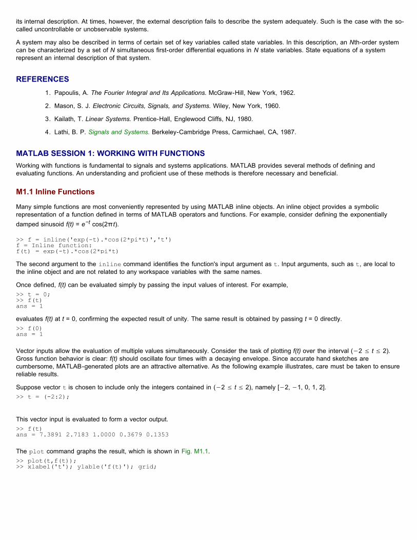
its internal description. At times, however, the external description fails to describe the system adequately. Such is the case with the so-called uncontrollable or unobservable systems.

A system may also be described in terms of certain set of key variables called state variables. In this description, an Nth-order systemcan be characterized by a set of N simultaneous first-order differential equations in N state variables. State equations of a systemrepresent an internal description of that system.

REFERENCES1. Papoulis, A. The Fourier Integral and Its Applications. McGraw-Hill, New York, 1962.

2. Mason, S. J. Electronic Circuits, Signals, and Systems. Wiley, New York, 1960.

3. Kailath, T. Linear Systems. Prentice-Hall, Englewood Cliffs, NJ, 1980.

4. Lathi, B. P. Signals and Systems. Berkeley-Cambridge Press, Carmichael, CA, 1987.

MATLAB SESSION 1: WORKING WITH FUNCTIONSWorking with functions is fundamental to signals and systems applications. MATLAB provides several methods of defining andevaluating functions. An understanding and proficient use of these methods is therefore necessary and beneficial.

M1.1 Inline Functions

Many simple functions are most conveniently represented by using MATLAB inline objects. An inline object provides a symbolicrepresentation of a function defined in terms of MATLAB operators and functions. For example, consider defining the exponentiallydamped sinusoid f(t) = e−t cos(2πt).

The second argument to the inline command identifies the function's input argument as t. Input arguments, such as t, are local tothe inline object and are not related to any workspace variables with the same names.

Once defined, f(t) can be evaluated simply by passing the input values of interest. For example,

evaluates f(t) at t = 0, confirming the expected result of unity. The same result is obtained by passing t = 0 directly.

Vector inputs allow the evaluation of multiple values simultaneously. Consider the task of plotting f(t) over the interval (−2 ≤ t ≤ 2).Gross function behavior is clear: f(t) should oscillate four times with a decaying envelope. Since accurate hand sketches arecumbersome, MATLAB-generated plots are an attractive alternative. As the following example illustrates, care must be taken to ensurereliable results.

Suppose vector t is chosen to include only the integers contained in (−2 ≤ t ≤ 2), namely [−2, −1, 0, 1, 2].

This vector input is evaluated to form a vector output.

The plot command graphs the result, which is shown in Fig. M1.1.

>> f = inline('exp(-t).*cos(2*pi*t)','t')f = Inline function:f(t) = exp(-t).*cos(2*pi*t)

>> t = 0;>> f(t)ans = 1

>> f(0)ans = 1

>> t = (-2:2);

>> f(t)ans = 7.3891 2.7183 1.0000 0.3679 0.1353

>> plot(t,f(t));>> xlabel('t'); ylable('f(t)'); grid;

Figure M1.1: f(t) = e−t cos (2πt) for t = (-2:2).

Grid lines, added by using the grid command, aid feature identification. Unfortunately, the plot does not illustrate the expectedoscillatory behavior. More points are required to adequately represent f(t).

The question, then, is how many points is enough?[†] If too few points are chosen, information is lost. If too many points are chosen,memory and time are wasted. A balance is needed. For oscillatory functions, plotting 20 to 200 points per oscillation is normallyadequate. For the present case, t is chosen to give 100 points per oscillation.

Again, the function is evaluated and plotted.

The result, shown in Fig. M1.2, is an accurate depiction of f(t).

Figure M1.2: f(t) = e−t cos(2πt) for t = (-2:0.01:2).

M1.2 Relational Operators and the Unit Step Function

The unit step function u(t) arises naturally in many practical situations. For example, a unit step can model the act of turning on asystem. With the help of relational operators, inline objects can represent the unit step function.

In MATLAB, a relational operator compares two items. If the comparison is true, a logical true (1) is returned. If the comparison isfalse, a logical false (0) is returned. Sometimes called indicator functions, relational operators indicates whether a condition is true. Sixrelational operators are available: <, >, <=, >=, ==, and ~=.

>> t = (-2:0.01:2);

>> plot (t,f(t));>> xlabel('t'); ylabel('f(t)'); grid;

The unit step function is readily defined using the >= relational operator.

Any function with a jump discontinuity, such as the unit step, is difficult to plot. Consider plotting u(t) by using t = (−2:2).

Two significant problems are apparent in the resulting plot, shown in Fig. M1.3. First, MATLAB automatically scales plot axes to tightlybound the data. In this case, this normally desirable feature obscures most of the plot. Second, MATLAB connects plot data with lines,making a true jump discontinuity difficult to achieve. The coarse resolution of vector t emphasizes the effect by showing an erroneoussloping line between t = − 1 and t − 0.

Figure M1.3: u(t) for t = (−2:2).

The first problem is corrected by vertically enlarging the bounding box with the axis command. The second problem is reduced, but noteliminated, by adding points to vector t.

The four-element vector argument of axis specifies x-axis minimum, x-axis maximum, y-axis minimum, and y-axis maximum,respectively. The improved results are shown in Fig. M1.4.

Figure M1.4: u(t) for t = (−2:0.01:2) with axis modification.

Relational operators can be combined using logical AND, logical OR, and logical negation: &, |, and ~, respectively. For example,(t>0)&(t<1) and ~((t<=0) | (t>=1)) both test if 0 < t < 1. To demonstrate, consider defining and plotting the unit pulse p(t) =u(t) − u(t − 1), as shown in Fig. M1.5:

>> u = inline('(t>=0)','t')u = Inline function:u(t) = (t>=0)

>> t = (-2:2);>> plot (t,u(t));>> xlable('t'); ylabel('u(t)');

>> t = (-2:0.01:2);>> plot (t,u(t));>> xlable('t'); ylabel('u(t)');>> axis ([-2 2 -0.1 1.1]);

Figure M1.5: p(t) = u(t) − u(t − 1) over (−1 ≤ t ≤ 2).

For scalar operands, MATLAB also supports two short-circuit logical constructs. A short-circuit logical AND is performed by using &&,and a short-circuit logical OR is performed by using | |. Short-circuit logical operators are often more efficient than traditional logicaloperators because they test the second portion of the expression only when necessary. That is, when scalar expression A is found falsein (A&&B), scalar expression B is not evaluated, since a false result is already guaranteed. Similarly, scalar expression B is notevaluated when scalar expression A is found true in (A | |B), since a true result is already guaranteed.

M1.3 Visualizing Operations on the Independent Variable

Two operations on a function's independent variable are commonly encountered: shifting and scaling. Inline objects are well suited toinvestigate both operations.

Consider g(t) = f(t)u(t) = e−t cos(2πt)u(t) a realizable version of f(t).[†] Unfortunately, MATLAB cannot multiply inline objects. That is,MATLAB reports an error for g = f*u when f and u are inline objects. Rather, g(t) needs to be explicitly defined.

A combined shifting and scaling operation is represented by g(at + b), where a and b are arbitrary real constants. As an example,consider plotting g(2t + 1) over (−2 ≤ t ≤ 2). With a = 2, the function is compressed by a factor of 2, resulting in twice the oscillationsper unit t. Adding the condition b > 0, the waveform shifts to the left. Given inline function g, an accurate plot is nearly trivial to obtain.

Figure M1.6 confirms the expected waveform compression and left shift. As a final check, realize that function g(·) turns on when theinput argument is zero. Therefore, g(2t + 1) should turn on when 2t + 1 = 0 or at t = −0.5, a fact again confirmed by Fig. M1.6.

>> p = inline('(t>=0) & (t<1)','t');>> t = (-1:0.01:2); plot(t,p(t));>> xlabel('t'); ylabel('p(t) = u(t)-u(t-1)');>> axis ([-1 2 -.1 1.1]);

>> g = inline('exp(-t).*cos(2*pi*t).*(t>=0)','t')g = Inline function:g(t) = exp(-t).*cos(2*pi*t).*(t>=0)

>> t = (-2:0.01:2);>> plot(t,g(2*t+1)); xlabel('t'); ylabel('g(2t+1)')'; grid;

Figure M1.6: g(2t + 1) over (−2 ≤ t ≤ 2).

Next, consider plotting g(−t + 1) over (−2 ≤ t ≤ 2). Since a < 0, the waveform will be reflected. Adding the condition b > 0, the finalwaveform shifts to the right

Figure M1.7 confirms both the reflection and the right shift.

Figure M1.7: g(−t + 1) over (−2 ≤ t ≤ 2).

Up to this point, Figs. M1.6 and M1.7 could be reasonably sketched by hand. Consider plotting the more complicated function h(t) =g(2t + 1) + g(−t + 1) over (−2 ≤ t ≤ 2) (Fig. M1.8). In this case, an accurate hand sketch is quite difficult. With MATLAB, the work ismuch less burdensome.

>> plot(t,g(-t+1)); xlabel('t'); ylabel('g(-t+1)')'; grid;

>> plot(t,g(2*t+1) +g(-t+1)); xlabel('t'); ylabel('h(t)')'; grid;

Figure M1.8: h(t) = g(2t + 1) + g(−t + 1) over (−2 ≤ t ≤ 2).

M1.4 Numerical Integration and Estimating Signal Energy

Interesting signals often have nontrivial mathematical representations. Computing signal energy, which involves integrating the square ofthese expressions, can be a daunting task. Fortunately, many difficult integrals can be accurately estimated by means of numericalintegration techniques. Even if the integration appears simple, numerical integration provides a good way to verify analytical results.

To start, consider the simple signal x(t) = e−t(u(t) − u(t − 1)). The energy of x(t) is expressed as Ex = ∫∞−∞ |x(t)|2 dt = ∫1

0 e−2t dt.

Integrating yields Ex = 0.5(1 − e−2) ≈ 0.4323. The energy integral can also be evaluated numerically. Figure 1.27 helps illustrate thesimple method of rectangular approximation: evaluate the integrand at points uniformly separated by Δt, multiply each by Δt to computerectangle areas, and then sum over all rectangles. First, we create function x(t).

Letting Δt = 0.01, a suitable time vector is created.

The final result is computed by using the sum command.

The result is not perfect, but at 1% relative error it is close. By reducing Δt, the approximation is improved. For example, Δt = 0.001yields E_x = 0.4328, or 0.1% relative error.

Although simple to visualize, rectangular approximation is not the best numerical integration technique. The MATLAB function quadimplements a better numerical integration technique called recursive adaptive Simpson quadrature.[†] To operate, quad requires afunction describing the integrand, the lower limit of integration, and the upper limit of integration. Notice, that no Δt needs to bespecified.

To use quad to estimate Ex, the integrand must first be described.

Estimating Ex immediately follows.

In this case, the relative error is -0.0026%.

The same techniques can be used to estimate the energy of more complex signals. Consider g(t), defined previously. Energy isexpressed as Eg = ∫∞

0 e−2t cos2 (2πt) dt. A closed-form solution exists, but it takes some effort. MATLAB provides an answer morequickly.

>> x = inline('exp(-t).*((t>=0)&(t<1))','t');

>> t = (0:0.01:1);

>> E_x =sum(x(t).*x(t)*0.01)E_x = 0.4367

>> x_squared = inline('exp(-2*t).*((t>=0)&(t>1))','t');

>> E_x = quad(x_squared,0,1)E_x = 0.4323

>> g_squared = inline('exp(-2*t).*(cos(2*pi*t).*^2).*(t>=0)','t');

Although the upper limit of integration is infinity, the exponentially decaying envelope ensures g(t) is effectively zero well before t = 100.Thus, an upper limit of t = 100 is used along with Δt = 0.001.

A slightly better approximation is obtained with the quad function.

As an exercise, confirm that the energy of signal h(t), defined previously, is Eh = 0.3768.

[†]Sampling theory, presented later, formally addresses important aspects of this question.

[†]The function f(t) = e−t cos(2πt) can never be realized in practice; it has infinite duration and, as t → −∞, infinite magnitude.

[†]A comprehensive treatment of numerical integration is outside the scope of this text. Details of this particular method are notimportant for the current discussion; it is sufficient to say that it is better than the rectangular approximation.

PROBLEMS1.1.1 Find the energies of the signals illustrated in Fig. P1.1-1. Comment on the effect on energy of sign change, time shifting,

or doubling of the signal. What is the effect on the energy if the signal is multiplied by k?

Figure P1.1-1

1.1.2 Repeat Prob. 1.1-1 for the signals in Fig. P1.1-2.

Figure P1.1-2

1.1.3

a. Find the energies of the pair of signals x(t) and y(t) depicted in Fig. P1.1-3a and P1.1-3b. Sketch and findthe energies of signals x(t) + y(t) and x(t) − y(t).

>> t = (0:0.001:100);>> E_g = sum(g_squared(t)*0.001)E g = 0.2567

>> E_g = quad(g_squared, 0,100)E_g = 0.2562

Figure P1.1-3

Can you make any observation from these results?

b. Repeat part (a) for the signal pair illustrated in Fig. P1.1-3c. Is your observation in part (a) still valid? 1.1.4 Find the power of the periodic signal x(t) shown in Fig. P1.1-4. Find also the powers and the rms values of:

a. −x(t)

b. 2x(t)

c. cx(t).

Figure P1.1-4

Comment. 1.1.5 Determine the power and the rms value for each of the following signals:

a. 5 + 10 cos(100t + π/3)

b. 10 cos(100t + π/3) + 16sin(150t + π/5)

c. (10 + 2sin 3t)cos 10t

d. 10 cos5t cos 10t

e. 10 sin 5t cos 10t

f. ejαt cos ω0t

1.1.6 Figure P1.1-6 shows a periodic 50% duty cycle dc-offset sawtooth wave x(t) with peak amplitude A. Determine the

energy and power of x(t).

Figure P1.1-6: 50% duty cycle dc-offset sawtooth wave x(t). 1.1.7

a. There are many useful properties related to signal energy. Prove each of the following statements. In eachcase, let energy signal x1(t) have energy E|x2 (t)], let energy signal x2(t) have energy E[x2(t)], and let T bea nonzero, finite, real-valued constant.

i. Prove E[Tx1(t)] = T2E[x1(t)]. That is, amplitude scaling a signal by constant T scales the

signal energy by T2.

ii. Prove E[x1(t)] = E[x1 (t − T)]. That is, shifting a signal does not affect its energy.

iii. If (x1(t) ≠ 0) ⇒ x2(t) = 0) and (x2(t) ≠ 0) ⇒ (x1(t) = 0), then prove E[x1(t) + x2(t)] = E[x1(t)]+ E[x2(t)]. That is, the energy of the sum of two nonoverlapping signals is the sum of the twoindividual energies.

iv. Prove E[x1(Tt)] = (1/|T|)E[x1(t)]. That is, time-scaling a signal by T reciprocally scales thesignal energy by 1/|7|.

b. Consider the signal x(t) shown in Fig. P1.1-7. Outside the interval shown, x(t) is zero. Determine the signalenergy E[x(t)].

Figure P1.1-7: Energy signal x(t).

1.1.8

a. Show that the power of a signal

assuming all frequencies to be distinct, that is, ωi ≠ ωk for all i ≠ k.

b. Using the result in part (a) determine the power of each of the signals in Prob. 1.1-5. 1.1.9 A binary signal x(t) = 0 for t < 0. For positive time, x(t) toggles between one and zero as follows: one for 1 second, zero

for 1 second, one for 1 second, zero for 2 seconds, one for 1 second, zero for 3 seconds, and so forth. That is, the "on"time is always one second but the "off" time successively increases by one second between each toggle. A portion of x(t)is shown in Fig. P1.1-9. Determine the energy and power of x(t).

Figure P1.1-9: Binary signal x(t).

1.2.1 For the signal x(t) depicted in Fig. P1.2-1, sketch the signals

a. x(−t)

b. x(t + 6)

c. x(3t)

d. x(t/2)

Figure P1.2-1

1.2.2 For the signal x(t) illustrated in Fig. P1.2-2, sketch

a. x(t−4)

b. x(t/1.5)

c. x(−t)

d. x(2t − 4)

e. x(2 − t)

Figure P1.2-2

1.2.3 In Fig. P1.2-3, express signals x1(t), x3(t) x3(t), x4(t), and x5(t) in terms of signal x(t) and its time-shifted, time-scaled, or

time-reversed versions.

Figure P1.2-3

1.2.4 For an energy signal x(t) with energy Ex, show that the energy of any one of the signals −x(t), x(−t), and x(t − T) is Ex.

Show also that the energy of x(at) as well as x(at − b) is Ex/a, but the energy of ax(t) is a2Ex. This shows that timeinversion and time shifting do not affect signal energy. On the other hand, time compression of a signal (a > 1) reducesthe energy, and time expansion of a signal (a < 1) increases the energy. What is the effect on signal energy if the signalis multiplied by a constant a?

1.2.5 Define 2x(−3t+1) = t(u(−t−1)−u(−t+1)), where u(t) is the unit step function.

a. Plot 2x(−3t + 1) over a suitable range of t.

b. Plot x(t) over a suitable range of t. 1.2.6 Consider the signal x(t) = 2−tu(t) where u(t) is the unit step function.

a. Accurately sketch x(t) over (−1 ≤ t ≤ 1).

b. Accurately sketch y(t) = 0.5x(1 − 2t) over (−1 ≤ t ≤ 1).

1.3.1 Determine whether each of the following statements is true or false. If the statement is false, demonstrate this by proofor example.

a. Every continuous-time signal is analog signal.

b. Every discrete-time signal is digital signal.

c. If a signal is not an energy signal, then it must be a power signal and vice versa.

d. An energy signal must be of finite duration.

e. A power signal cannot be causal.

f. A periodic signal cannot be anticausal. 1.3.2 Determine whether each of the following statements is true or false. If the statement is false, demonstrate by proof or

example why the statement is false.

a. Every bounded periodic signal is a power signal.

b. Every bounded power signal is a periodic signal.

c. If an energy signal x(t) has energy E, then the energy of x(at) is E/a. Assume a is real and positive.

d. If a power signal x(t) has power P, then the power of x(at) is P/a. Assume a is real and positive. 1.3.3 Given x1(t) = cos(t), x2(t) = sin(πt), and x3(t) = x1(t) + x2(t).

a. Determine the fundamental periods T1 and T2 of signals x1(t) and x2(t).

b. Show that x3(t) is not periodic, which requires T3 = k1T1 = k2T2 for some integers k1 and k2.

c. Determine the powers Px1, Px2, and Px3 of signals x1(t), x2(t), and x3(t). 1.3.4 For any constant ω, is the function f(t) = sin (ωt) a periodic function of the independent variable t? Justify your answer. 1.3.5 The signal shown in Fig. P1.3-5 is defined as

Figure P1.3-5: Energy signal x(t).

The energy of x(t) is E ≈ 1.0417.

a. What is the energy of y1(t) = (⅓)x(2t)?

b. A periodic signal y2(t) is defined as

What is the power of y2(t)?

c. What is the power of y3(t) = (⅓)y2(2t)? 1.3.6 Let y1(t) = y2(t) = t2 over 0 ≤ t ≤ 1. Notice, this statement does not require y1(t) = y2(t) for all t.

a. Define y1(t) as an even, periodic signal with period T1 = 2. Sketch y1(t) and determine its power.

b. Design an odd, periodic signal y2(t) with period T2 = 3 and power equal to unity. Fully describe y2(t) andsketch the signal over at least one full period. [Hint: There are an infinite number of possible solutions tothis problem-you need to find only one of them!]

c. We can create a complex-valued function y3(t) = y1(t) + jy2(t). Determine whether this signal is periodic. Ifyes, determine the period T3. If no, justify why the signal is not periodic.

d. Determine the power of y3(t) defined in part (c). The power of a complex-valued function z(t) is

1.4.1 Sketch the following signal:

a. u(t − 5) − u(t − 7)

b. u(t − 5) − u(t − 7)

c. t2[u(t − 1) − u(t − 2)]

d. (t − 4)[u(t − 2) − u(t − 4)] 1.4.2 Express each of the signals in Fig. P1.4-2 by a single expression valid for all t.

Figure P1.4-2

1.4.3 Simplify the following expressions:

a.

b.

c. [e−t cos(3t − 60°)]δ(t)

d.

e.

f.

[Hint: Use Eq. (1.23). For part (f) use L'Hôpital's rule.] 1.4.4 Evaluate the following integrals:

a. ∫∞−∞δ(τ)x(t−τ)dτ

b. ∫∞−∞x(τ)δ(t−τ)dτ

c. ∫∞−∞ δ(t)e −jωtdt

d. ∫∞−∞ δ(2t−3)πtdt

e. ∫∞−∞ δ (t + 3)ee−1dt

f. ∫∞−∞ (t3 +4) δ (1−t) dt

g. ∫∞−∞ x (2−t)δ (3−t)dt

h.

1.4.5

a. Find and sketch dx/dt for the signal x(t) shown in Fig. P1.2-2.

b. Find and sketch d2x/dt2 for the signal x(t) depicted in Fig. P1.4-2a. 1.4.6 Find and sketch ∫t

−∞ x(t) dt for the signal x(t) illustrated in Fig. P1.4-6.

Figure P1.4-6

1.4.7 Using the generalized function definition of impulse [Eq. (1.24a)], show that δ(t) is an even function of t. 1.4.8 Using the generalized function definition of impulse [Eq. (1.24a)], show that

1.4.9 Show that

where φ(t) and are continuous at t = 0, and φ(t) → 0 as t → ±∞. This integral defines as a generalizedfunction. [Hint: Use integration by parts.]

1.4.10 A sinusoid eσt cos ωt can be expressed as a sum of exponentials est and est [Eq. (1.30c)] with complex frequencies s

= σ + jω and s = σ − jω. Locate in the complex plane the frequencies of the following sinusoids:

a. cos 3t

b. e−3t cos 3t

c. e2t cos 3t

d. e−2t

e. e2t

f. 5

1.5.1 Find and sketch the odd and the even components of the following:

a. u(t)

b. tu(t)

c. sin ω0t

d. cos ω0t

e. cos (ω0t + θ)

f. sin ω0tu(t)

g. cos ω0tu(t)

1.5.2

a. Determine even and odd components of the signal x(t) = e−2tu(t).

b. Show that the energy of x(t) is the sum of energies of its odd and even components found in part (a).

c. Generalize the result in part (b) for any finite energy signal. 1.5.3

a. If xe(t) and x0(t) are even and the odd components of a real signal x(t), then show that

b. Show that

1.5.4 An aperiodic signal is defined as x(t) = sin (πt)u(t), where u(t) is the continuous-time step function. Is the odd portion of

this signal, x0(t), periodic? Justify your answer. 1.5.5 An aperiodic signal is defined as x(t) = cos (πt)u(t), where u(t) is the continuous-time step function. Is the even portion

of this signal, xe(t), periodic? Justify your answer. 1.5.6 Consider the signal x(t) shown in Fig. P1.5-6.

a. Determine and carefully sketch v(t) = 3x(-(1/2)(t + 1).

b. Determine the energy and power of v(t).

c. Determine and carefully sketch the ever portion of v(t), ve(t).

d. Let a = 2 and b = 3, sketch v(at + b), v(at) + b, av(t + b), and av(t) + b.

e. Let a = −3 and b = −2, sketch v(at + b), v(at) + b, av(t + b), and av(t) + b.

Figure P1.5-6: Input x(t).

1.5.7 Consider the signal y(t) = ( )x(−2t − 3) shown in Figure P1.5-7.

a. Does y(t) have an odd portion, y0(t)? If so, determine and carefully sketch y0(t). Otherwise, explain whyno odd portion exists.

b. Determine and carefully sketch the original signal x(t).

Figure P1.5-7: y(t) = x(−2t − 3).

1.5.8 Consider the signal -(1/2)x(−3t + 2) show in Fig. P1.5-8.

a. Determine and carefully sketch the original signal x(t).

b. Determine and carefully sketch the even portion of the original signal x(t).

c. Determine and carefully sketch the odd portion of the original signal x(t).

Figure P1.5-8: -1/2x(−3t + 2).

1.5.9 The conjugate symmetric (or Hermitian) portion of a signal is defined as wcs(t) = (w(t) + w*(−t))/2. Show that the real

portion of wcs(t) is even and that the imaginary portion of wcs(t) is odd. 1.5.10 The conjugate antisymmetric (or skew-Hermitian) portion of a signal is defined as wcs(t) = (w(t) + w*(−t))/2. Show that

the real portion of wca(t) is even and that the imaginary portion of wcs(t) is even. 1.5.11 Figure P1.5-11 plots a complex signal w(t) in the complex plane over the time range (0 ≤ t ≤ 1). The time t = 0

corresponds with the origin, while the time t = 1 corresponds with the point (2,1).

a. In the complex plane, plot w(t) over (−1 ≤ t ≤ 1) if:

i. w(t) is an even signal.

ii. w(t) is an odd signal.

iii. w(t) is a conjugate symmetric signal.

[Hint: See Prob. 1.5-9.]

iv. w(t) is a conjugate antisymmetric signal. [Hint: See Prob. 1.5-10.]

b. In the complex plane, plot as much of w(3t) as possible.

Figure P1.5-11: w(t) for (0 ≤ t ≤ 1).

1.5.12 Define complex signal x(t) = t2(1 + j) over interval (1 ≤ t ≤ 2). The remaining portion is defined such that x(t) is a

minimum-energy, skew-Hermitian signal.

a. Fully describe x(t) for all t.

b. Sketch y(t) = Re{x(t)} versus the independent variable t.

c. Sketch z(t) = Re{jx(−2t + 1)} versus the independent variable t.

d. Determine the energy and power of x(t).

1.6.1 Write the input-output relationship for an ideal integrator. Determine the zero-input and zero-state components of theresponse.

1.6.2 A force x(t) acts on a ball of mass M (Fig. P1.6-2). Show that the velocity v(t) of the ball at any instant t > 0 can be

determined if we know the force x(t) over the interval from 0 to t and the ball's initial velocity v(0).

Figure P1.6-2

1.7.1 For the systems described by the following equations, with the input x(t) and output y(t), determine which of thesystems are linear and which are nonlinear.

a.

b.

c. 3 y(t) +2 = x(t)

d.

e.

f.

g.

h. y(t) = ∫t−∞ x (τ) d τ

1.7.2 For the systems described by the following equations, with the input x(t) and output y(t), explain with reasons which of

the systems are time-invariant parameter systems and which are time-varying-parameter systems.

a. y(t) = x(t − 2)

b. y(t) = x(−t)

c. y(t) = x(at)

d. y(t) = tx(t−2)

e. y(t) = ∞ 5−5x(τ)dτ

f.

1.7.3 For a certain LTI system with the input x(t), the output y(t) and the two initial conditions q1(0) and q2(0), following

observations were made:

Open table as spreadsheetx(t) q1(0) q2(0) y(t)

0 1 −1 e−tu(t)

0 2 1 e−t(3t + 2)u(t)

u(t) −1 −1 2u(t)

Determine y(t) when both the initial conditions are zero and the input x(t) is as shown in Fig. P1.7-3. [Hint: There arethree causes: the input and each of the two initial conditions. Because of the linearity property, if a cause is increasedby a factor k, the response to that cause also increases by the same factor k. Moreover, if causes are added, thecorresponding responses add.]

Figure P1.7-3

1.7.4 A system is specified by its input-output relationship as

Show that the system satisfies the homogeneity property but not the additivity property. 1.7.5 Show that the circuit in Fig. P1.7-5 is zero-state linear but not zero-input linear. Assume all diodes to have identical

(matched) characteristics. The output is the current y(t).

Figure P1.7-5

1.7.6 The inductor L and the capacitor C in Fig. P1.7-6 are nonlinear, which makes the circuit nonlinear. The remaining three

elements are linear. Show that the output y(t) of this nonlinear circuit satisfies the linearity conditions with respect to theinput x(t) and the initial conditions (all the initial inductor currents and capacitor voltages).

Figure P1.7-6

1.7.7 For the systems described by the following equations, with the input x(t) and output y(t), determine which are causal

and which are noncausal.

a. y(t) = x(t − 2)

b. y(t) = x(− t)

c. y(t) = x(at) a > 1

d. y(t) = x(at) a < 1 1.7.8 For the systems described by the following equations, with the input x(t) and output y(t), determine which are invertible

and which are noninvertible. For the invertible systems, find the input-output relationship of the inverse system.

a. y(t) = ∫t−∞ x (τ) d τ

b. y(t) = xn (t) x(t) real and n integer

c.

d. y(t) = x (3t−6)

e. y(t) = cos [x(t)]

f. y(t)= e x(t) x(t) real 1.7.9 Consider a system that multiplies a given input by a ramp function, r(t) = tu(t). That is, y(t) = x(t)r(t).

a. Is the system linear? Justify your answer.

b. Is the system memoryless? Justify your answer.

c. Is the system causal? Justify your answer.

d. Is the system time invariant? Justify your answer. 1.7.10 A continuous-time system is given by

Recall that δ(t) designates the Dirac delta function.

a. Explain what this system does.

b. Is the system BIBO stable? Justify your answer.

c. Is the system linear? Justify your answer.

d. Is the system memoryless? Justify your answer.

e. Is the system causal? Justify your answer.

f. Is the system time invariant? Justify your answer. 1.7.11 A system is given by

a. Is the system BIBO stable? [Hint: Let system input x(t) be a square wave.]

b. Is the system linear? Justify your answer.

c. Is the system memoryless? Justify your answer.

d. Is the system causal? Justify your answer.

e. Is the system time invariant? Justify your answer. 1.7.12 A system is given by

a. Is the system BIBO stable? Justify your answer.

b. Is the system linear? Justify your answer.

c. Is the system memoryless? Justify your answer.

d. Is the system causal? Justify your answer.

e. Is the system time invariant? Justify your answer. 1.7.13 Figure P1.7-13 displays an input x1(t) to a linear time-invariant (LTI) system H, the corresponding output y1(t), and a

second input x2(t).

a. Bill suggests that x2(t) = 2x1(3t) − x1(t − 1). Is Bill correct? If yes, prove it. If not, correct his error.

b. Hoping to impress Bill, Sue wants to know the output y2(t) in response to the input x2(t). Provide her withan expression for y2(t) in terms of y1(t). Use MATLAB to plot y2(t).

Figure P1.7-13: and x2(t).

1.8.1 For the circuit depicted in Fig. P1.8-1, find the differential equations relating outputs y1(t) and y2(t) to the input x(t).

Figure P1.8-1

1.8.2 Repeat Prob. 1.8-1 for the circuit in Fig. P1.8-2.

Figure P1.8-2

1.8.3 A simplified (one-dimensional) model of an automobile suspension system is shown in Fig. P1.8-3. In this case, the input

is not a force but a displacement x(t) (the road contour). Find the differential equation relating the output y(t) (auto bodydisplacement) to the input x(t) (the road contour).

Figure P1.8-3

1.8.4 A field-controlled dc motor is shown in Fig. P1.8-4. Its armature current ia is maintained constant. The torque generated

by this motor is proportional to the field current ij (torque = Kfif). Find the differential equation relating the output positionθ to the input voltage x(t). The motor and load together have a moment of inertia J.

Figure P1.8-4

1.8.5 Water flows into a tank at a rate of qi units/s and flows out through the outflow valve at a rate of q0 units/s (Fig. P1.8-5).

Determine the equation relating the outflow q0 to the input qi. The outflow rate is proportional to the head h. Thus q0 =Rh, where R is the valve resistance. Determine also the differential equation relating the head h to the input qi. [Hint: Thenet inflow of water in time Δt is (qi − q0)Δt. This inflow is also AΔh where A is the cross section of the tank.]

Figure P1.8-5

1.8.6 Consider the circuit shown in Fig. P1.8-6, with input voltage x(t) and output currents y1(t), y2(t), and y3(t).

a. What is the order of this system? Explain your answer.

b. Determine the matrix representation for this system.

c. Use Cramer's rule to determine the output current y3(t) for the input voltage x(t) = (2 − | cos(t)|)u(t − 1).

Figure P1.8-6: Resistor circuit.

1.10.1 Write state equations for the parallel RLC circuit in Fig. P1.8-2. Use the capacitor voltage q1 and the inductor currentq2 as your state variables. Show that every possible current or voltage in the circuit can be expressed in terms of q1,q2 and the input x(t)

1.10.2 Write state equations for the third-order circuit shown in Fig. P1.10-2, using the inductor currents q1, q2 and the

capacitor voltage q3 as state variables. Show that every possible voltage or current in this circuit can be expressed as alinear combination of q1, q2, q3, and the input x(t). Also, at some instant t it was found that q1 = 5, q2 = 1, q3 = 2, andx = 10. Determine the voltage across and the current through every element in this circuit.

Figure P1.10-2

Chapter 2: Time-Domain Analysis of Continuous-Time SystemsIn this book we consider two methods of analysis of linear time-invariant (LTI) systems: the time-domain method and the frequency-domain method.In this chapter we discuss the time-domain analysis of linear, time-invariant, continuous-time (LTIC) systems.

2.1 INTRODUCTION

For the purpose of analysis, we shall consider linear differential systems. This is the class of LTIC systems introduced in Chapter 1, for which theinput x(t) and the output y(t) are related by linear differential equations of the form

where all the coefficients ai and bi are constants. Using operational notation D to represent d/dt, we can express this equation as

or

where the polynomials Q(D) and P(D) are

Theoretically the powers M and N in the foregoing equations can take on any value. However, practical considerations make M > N undesirable fortwo reasons. In Section 4.3-2, we shall show that an LTIC system specified by Eq. (2.1) acts as an (M − N)th-order differentiator.

A differentiator represents an unstable system because a bounded input like the step input results in an unbounded output, δ (t). Second, the noiseis enhanced by a differentiator. Noise is a wideband signal containing components of all frequencies from 0 to a very high frequency approaching∞[†]. Hence, noise contains a significant amount of rapidly varying components. We know that the derivative of any rapidly varying signal is high.Therefore, any system specified by Eq. (2.1) in which M > N will magnify the high-frequency components of noise through differentiation. It is entirelypossible for noise to be magnified so much that it swamps the desired system output even if the noise signal at the system's input is tolerably small.Hence, practical systems generally use M ≤ N. For the rest of this text we assume implicitly that M ≤ N. For the sake of generality, we shall assumeM = N in Eq. (2.1).

In Chapter 1, we demonstrated that a system described by Eq. (2.1) is linear. Therefore, its response can be expressed as the sum of twocomponents: the zero-input component and the zero-state component (decomposition property).[‡] Therefore,

The zero-input component is the system response when the input x(t) = 0, and thus it is the result of internal system conditions (such as energystorages, initial conditions) alone. It is independent of the external input x(t). In contrast, the zero-state component is the system response to theexternal input x(t) when the system is in zero state, meaning the absence of all internal energy storages: that is, all initial conditions are zero.

[†]Noise is any undesirable signal, natural or man-made, that interferes with the desired signals in the system. Some of the sources of noise are theelectromagnetic radiation from stars, the random motion of electrons in system components, interference from nearby radio and television stations,transients produced by automobile ignition systems, and fluorescent lighting.

[‡]We can verify readily that the system described by Eq. (2.1) has the decomposition property. If y0(t) is the zero-input response, then, by definition,

If y(t) is the zero-state response, then y(t) is the solution of

subject to zero initial conditions (zero-state). Adding these two equations, we have

Clearly, y0(t)+y(t) is the general solution of Eq. (2.1).

2.2 SYSTEM RESPONSE TO INTERNAL CONDITIONS: THE ZERO-INPUT RESPONSEThe zero-input response y0(t) is the solution of Eq. (2.1) when the input x(t) = 0 so that

or

A solution to this equation can be obtained systematically.[1] However, we will take a shortcut by using heuristic reasoning. Equation (2.4b) showsthat a linear combination of y0(t) and its N successive derivatives is zero, not at some values of t, but for all t. Such a result is possible if and only ify0(t) and all its N successive derivatives are of the same form. Otherwise their sum can never add to zero for all values of t. We know that only an

exponential function eλt has this property. So let us assume that

is a solution to Eq. (2.4b). Then

Substituting these results in Eq. (2.4b), we obtain

For a nontrivial solution of this equation,

This result means that ceλt is indeed a solution of Eq. (2.4), provided λ satisfies Eq. (2.5a). Note that the polynomial in Eq. (2.5a) is identical to thepolynomial Q(D) in Eq. (2.4), with λ replacing D. Therefore, Eq. (2.5a) can be expressed as

When Q (λ) is expressed in factorized form, Eq. (2.5b) can be represented as

Clearly, λ has N solutions: λ1, λ2,..., λN, assuming that all λi, are distinct. Consequently, Eq. (2.4) has N possible solutions: c1eλ1 t, c2e?2 t,...,

cNeλNt, with c1, c2,..., cN as arbitrary constants. We can readily show that a general solution is given by the sum of these N solutions,[†]

so that

where c1, c2,..., cN are arbitrary constants determined by N constraints (the auxiliary conditions) on the solution.

Observe that the polynomial Q(λ), which is characteristic of the system, has nothing to do with the input. For this reason the polynomial Q(λ) iscalled the characteristic polynomial of the system. The equation

is called the characteristic equation of the system. Equation (2.5c) clearly indicates that ?1, ?2,...,λN are the roots of the characteristic equation;consequently, they are called the characteristic roots of the system. The terms characteristic values, eigenvalues, and natural frequencies are alsoused for characteristic roots.[†] The exponentials eλit (i = 1, 2,..., n) in the zero-input response are the characteristic modes (also known as naturalmodes or simply as modes) of the system. There is a characteristic mode for each characteristic root of the system, and the zero-input response is alinear combination of the characteristic modes of the system.

An LTIC system's characteristic modes comprise its single most important attribute. Characteristic modes not only determine the zero-input responsebut also play an important role in determining the zero-state response. In other words, the entire behavior of a system is dictated primarily by itscharacteristic modes. In the rest of this chapter we shall see the pervasive presence of characteristic modes in every aspect of system behavior.

REPEATED ROOTSThe solution of Eq. (2.4) as given in Eq. (2.6) assumes that the N characteristic roots ?1, ?2,..., λN are distinct. If there are repeated roots (same rootoccurring more than once), the form of the solution is modified slightly. By direct substitution we can show that the solution of the equation

is given by

In this case the root λ repeats twice. Observe that the characteristic modes in this case are eλt and teλt. Continuing this pattern, we can show thatfor the differential equation

the characteristic modes are eλt, teλt, t2e?t,..., tr−1eλt, and that the solution is

Consequently, for a system with the characteristic polynomial

the characteristic modes are eλ1 t, te?1 t,..., tr−1eλ1 t, eλr+1t,..., eλNt and the solution is

COMPLEX ROOTSThe procedure for handling complex roots is the same as that for real roots. For complex roots the usual procedure leads to complex characteristicmodes and the complex form of solution. However, it is possible to avoid the complex form altogether by selecting a real form of solution, asdescribed next.

For a real system, complex roots must occur in pairs of conjugates if the coefficients of the characteristic polynomial Q(λ) are to be real. Therefore, ifα + jβ is a characteristic root, α − jβ must also be a characteristic root. The zero-input response corresponding to this pair of complex conjugateroots is

For a real system, the response y0(t) must also be real. This is possible only if c1 and c2 are conjugates. Let

This yields

Therefore, the zero-input response corresponding to complex conjugate roots α ± jβ can be expressed in a complex form (2.10a) or a real form(2.10b).

EXAMPLE 2.1

a. Find y0(t), the zero-input component of the response for an LTIC system described by the following differential equation:

when the initial conditions are . Note that y0(t), being the zero-input component (x(t) = 0), is the solution of

(D2 + 3D + 2)y0(t) = 0.

The characteristic polynomial of the system is λ2 + 3λ + 2. The characteristic equation of the system is therefore λ2 + 3λ + 2 = (λ + 1)(λ + 2) = 0. The characteristic roots of the system are λ1 = −1 and λ2 = −2, and the characteristic modes of the system are e−t and

e−2t. Consequently, the zero-input response is

To determine the arbitrary constants c1 and c2, we differentiate Eq. (2.11a) to obtain

Setting t = 0 in Eqs. (2.11a) and (2.11b), and substituting the initial conditions y0(0) = 0 and we obtain

Solving these two simultaneous equations in two unknowns for c1 and c2 yields

Therefore

This is the zero-input component of y(t). Because y0(t) is present at t = 0−, we are justified in assuming that it exists for t ≥ 0.[†]

b. A Similar procedure may be followed for repeated roots. For instance, for a system specified by

let us determine y0(t), the zero-input component of the response if the initial conditions are y0(0) = 3 and .

The characteristic polynomial is λ2 + 6λ + 9 = (λ + 3)2, and its characteristic roots are λ1 = −3, λ2 = −3 (repeated roots).

Consequently, the characteristic modes of the system are e−3t and te3t. The zero-input response, being a linear combination of thecharacteristic modes, is given by

We can find the arbitrary constants c1 and c2 from the initial conditions y0(0) = 3 and following the procedure in part (a).The reader can show that c1 = 3 and c2 = 2. Hence,

c. For the case of complex roots, let us find the zero-input response of an LTIC system described by the equation

with initial conditions y0(0) = 2 and .

The characteristic polynomial is λ2 + 4λ + 40 = (λ + 2 − j6)(λ + 2 + j6). The characteristic roots are −2 ± j6.[†] The solution can bewritten either in the complex form [Eq. (2.10a)] or in the real form [Eq. (2.10b)]. The complex form is y0(t) = c1eλ1 t + c2eλ2 t, where λ1= −2 + j6 and λ2 = −2 − j6. Since α = −2 and β = 6, the real form solution is [see Eq. (2.10b)]

where c and θ are arbitrary constants to be determined from the initial conditions y0(0) = 2 and Differentiation of Eq.(2.12a) yields

Setting t = 0 in Eqs. (2.12a) and (2.12b), and then substituting initial conditions, we obtain

Solution of these two simultaneous equations in two unknowns c cos θ and c sin θ yields

Squaring and then adding the two sides of Eqs. (2.13) yields

Next, dividing Eq. (2.13b) by Eq. (2.13a), that is, dividing c sin θ, by c cos θ, yields

and

Therefore

For the plot of y0(t), refer again to Fig. B.11c.

COMPUTER EXAMPLE C2.1Find the roots λ1 and λ2 of the polynomial λ2 + 4λ + k for three values of k :

a. k = 3

b. k = 4

c. k = 40

For k = 3, the polynomial roots are therefore λ1 = −3 and λ2 = −1.

For k = 4, the polynomial roots are therefore λ1 = λ2 = −2.

>> r = roots ([1 4 3]);>> disp (['Case (k=3): roots = [',num2str(r.'),']']);Case (k=3): roots = [-3 -1]

>> r = roots ([1 4 4]);>> disp (['Case (k=4): roots = [',num2str(r.'),']']);Case (k=4): roots = [-2 -2]

For k = 40, the polynomial roots are therefore λ1 = −2 + j6 and λ2 = −2 − j6.

COMPUTER EXAMPLE C2.2Consider an LTIC system specified by the differential equation

Using initial conditions y0(0) = 3 and , determine the zero-input component of the response for three values of k :

a. k = 3

b. k = 4

c. k = 40

For k = 3, the zero-input response is therfore y0(t) = 2e−3t + e−1.

For k = 4, the zero-input response is therfore y0(t) = 3e−2t − te−2t.

For k = 40, the zero-input response is therfore

EXERCISE E2.1

Find the zero-input response of an LTIC system described by (D + 5) y (t) = x(t) if the initial condition is y(0) = 5.

Answers

y0(t) = 5e−5t t ≥ 0

EXERCISE E2.2

Solve

(D2 + 2D)y0 (t) = 0

if y0(0) = 1 and

Answers

y0(t) = 3 −2e−2t t ≥ 0

PRACTICAL INITIAL CONDITIONS AND THE MEANING OF 0− AND 0+

In Example 2.1 the initial conditions y0(0) and were supplied. In practical problems, we must derive such conditions from the physical situation.For instance, in an RLC circuit, we may be given the conditions (initial capacitor voltages, initial inductor currents, etc.).

From this information, we need to derive y0(0) , for the desired variable as demonstrated in the next example.

In much of our discussion, the input is assumed to start at t = 0, unless otherwise mentioned. Hence, t = 0 is the reference point. The conditionsimmediately before t = 0 (just before the input is applied) are the conditions at t = 0-, and those immediately after t = 0 (just after the input is applied)are the conditions at t = 0+ (compare this with the historical time frame B.C. and A.D.). In practice, we are likely to know the initial conditions at t =0− rather than at t = 0+. The two sets of conditions are generally different, although in some cases they may be identical.

>> r = roots ([1 4 40]);>> disp (['Case (k=40): roots = [',num2str(r.',' %0.5g'),']']);Case (k=40): roots = [-2+6i -2-6i]

>> y_0 = dsolve('D2y + 4*Dy + 3*y = 0','y(0) = 3','Dy(0) = -7','t');>> disp(['(a) k = 3; y_0 = ',char(y_0)])(a) k = 3; y 0 = 2*exp(-3*t) + exp(-t)

>> y_0 = dsolve('D2y + 4*Dy + 4*y = 0','y(0) = 3','Dy(0) = -7','t');>> disp(['(b) k = 4; y_0 = ',char(y_0)])(b) k = 4; y 0 = 3*exp(-2*t) -exp(-2*t)*t

>> y_0 = dsolve('D2y + 4*Dy + 40*y = 0','y(0) = 3','Dy(0) = -7','t');>> disp(['(c) k = 40; y_0 = ',char(y_0)])(c) k = 40; y 0 = -1/6*exp(-2*t) *sin(6*t) + 3*exp(-2*t)*cos(6*t)

The total response y(t) consists of two components: the zero-input component y0(t) [response due to the initial conditions alone with x(t) = 0] and

the zero-state component resulting from the input alone with all initial conditions zero. At t = 0−, the total response y(t) consists solely of the zero-input component y0(t) because the input has not started yet. Hence the initial conditions on y(t) are identical to those of y0(t). Thus, y(0−) = y0(0−),

, and so on. Moreover, y0(t) is the response due to initial conditions alone and does not depend on the input x(t). Hence,

application of the input at t = 0 does not affect y0(t). This means the initial conditions on y0(t) at t = 0− and 0+ are identical; that is y0(0-),

are identical to y0(0+), , respectively. It is clear that for y0(t), there is no distinction between the initial conditions at t = 0−, 0 and 0+. They areall the same. But this is not the case with the total response y(t), which consists of both the zero-input and the zero-state components. Thus, ingeneral, y(0−) ≠ y(0+) , and so on.

EXAMPLE 2.2A voltage x(t) = 10e−3t u(t) is applied at the input of the RLC circuit illustrated in Fig. 2.1a. Find the loop current y(t) for t ≥ 0 if the initial inductorcurrent is zero; that is, y(0−) = 0 and the initial capacitor voltage is 5 volts; that is, υc(0−) = 5.

Figure 2.1

The differential (loop) equation relating y(t) to x(t) was derived in Eq. (1.55) as

The zero-state component of y(t) resulting from the input x(t), assuming that all initial conditions are zero, that is, y(0−) = υc(0−) = 0, will be obtainedlater in Example 2.6. In this example we shall find the zero-input component y0(t). For this purpose, we need two initial conditions y0(0) and .

These conditions can be derived from the given initial conditions, y(0−) = 0 and υc(0−) = 5, as follows. Recall that y0(t) is the loop current when theinput terminals are shorted so that the input x(t) = 0 (zero-input) as depicted in Fig. 2.1b.

We now compute y0(0) and , the values of the loop current and its derivative at t = 0, from the initial values of the inductor current and thecapacitor voltage. Remember that the inductor current cannot change instantaneously in the absence of an impulsive voltage. Similarly, the capacitorvoltage cannot change instantaneously in the absence of an impulsive current. Therefore, when the input terminals are shorted at t = 0, the inductorcurrent is still zero and the capacitor voltage is still 5 volts. Thus,

To determine , we use the loop equation for the circuit in Fig. 2.1b. Because the voltage across the inductor is L(dy0/dt) or , this equationcan be written as follows:

Setting t = 0, we obtain

But y0(0) = 0 and vc(0) = 5. Consequently,

Therefore, the desired initial conditions are

Thus, the problem reduces to finding y0(t), the zero-input component of y(t) of the system specified by the equation (D2 + 3D + 2)y(t) = Dx(t), whenthe initial conditions are y0(0) = 0 and . We have already solved this problem in Example 2.1a, where

we found

This is the zero-input component of the loop current y(t).

It will be interesting to find the initial conditions at t = 0− and 0+ for the total response y(t). Let us compare y(0−) and with y(0+) and .The two pairs can be compared by writing the loop equation for the circuit in Fig. 2.1a at t = 0− and t = 0+. The only difference between the twosituations is that at t = 0−, the input x(t) = 0, whereas at t = 0+, the input x(t) = 10 [because x(t) = 10e−3t]. Hence, the two loop equations are

The loop current y(0+) = y0−) = 0 because it cannot change instantaneously in the absence of impulsive voltage. The same is true of the capacitor

voltage. Hence, υc(0+) = υc(0−) = 5. Substituting these values in the foregoing equations, we obtain and Thus

EXERCISE E2.3In the circuit in Fig. 2.1a, the inductance L = 0 and the initial capacitor voltage vc(0) = 30 volts. Show that the zero-input component of the loop

current is given by y0(t) = −10e−2t /3 for t ≥ 0.

INDEPENDENCE OF ZERO-INPUT AND ZERO-STATE RESPONSEIn Example 2.2 we computed the zero-input component without using the input x(t). The zero-state component can be computed from theknowledge of the input x(t) alone; the initial conditions are assumed to be zero (system in zero state). The two components of the system response(the zero-input and zero-state components) are independent of each other. The two worlds of zero-input response and zero-state response coexistside by side, neither one knowing or caring what the other is doing. For each component, the other is totally irrelevant.

ROLE OF AUXILIARY CONDITIONS IN SOLUTION OF DIFFERENTIAL EQUATIONSSolution of a differential equation requires additional pieces of information (the auxiliary conditions). Why? We now show heuristically why adifferential equation does not, in general, have a unique solution unless some additional constraints (or conditions) on the solution are known.

Differentiation operation is not invertible unless one piece of information about y(t) is given. To get back y(t) from dy/dt, we must know one piece ofinformation, such as y(0). Thus, differentiation is an irreversible (noninvertible) operation during which certain information is lost. To invert thisoperation, one piece of information about y(t) must be provided to restore the original y(t). Using a similar argument, we can show that, givend2y/dt2, we can determine y(t) uniquely only if two additional pieces of information (constraints) about y(t) are given. In general, to determine y(t)uniquely from its Nth derivative, we need N additional pieces of information (constraints) about y(t). These constraints are also called auxiliaryconditions. When these conditions are given at t = 0, they are called initial conditions.

2.2-1 Some Insights into the Zero-Input Behavior of a System

By definition, the zero-input response is the system response to its internal conditions, assuming that its input is zero. Understanding thisphenomenon provides interesting insight into system behavior. If a system is disturbed momentarily from its rest position and if the disturbance isthen removed, the system will not come back to rest instantaneously. In general, it will come back to rest over a period of time and only through aspecial type of motion that is characteristic of the system.[†] For example, if we press on an automobile fender momentarily and then release it at t =0, there is no external force on the automobile for t > 0.[‡] The auto body will eventually come back to its rest (equilibrium) position, but not throughany arbitrary motion. It must do so by using only a form of response that is sustainable by the system on its own without any external source, sincethe input is zero. Only characteristic modes satisfy this condition. The system uses a proper combination of characteristic modes to come back to therest position while satisfying appropriate boundary (or initial) conditions.

If the shock absorbers of the automobile are in good condition (high damping coefficient), the characteristic modes will be monotonically decayingexponentials, and the auto body will come to rest rapidly without oscillation. In contrast, for poor shock absorbers (low damping coefficients), thecharacteristic modes will be exponentially decaying sinusoids, and the body will come to rest through oscillatory motion. When a series RC circuitwith an initial charge on the capacitor is shorted, the capacitor will start to discharge exponentially through the resistor. This response of the RCcircuit is caused entirely by its internal conditions and is sustained by this system without the aid of any external input. The exponential currentwaveform is therefore the characteristic mode of the RC circuit.

Mathematically we know that any combination of characteristic modes can be sustained by the system alone without requiring an external input. Thisfact can be readily verified for the series RL circuit shown in Fig. 2.2. The loop equation for this system is

Figure 2.2: Modes always get a free ride.

It has a single characteristic root λ = −2, and the characteristic mode is e−2t. We now verify that a loop current y(t) = ce-2t can be sustained throughthis circuit without any input voltage.

The input voltage x(t) required to drive a loop current y(t) = ce−2t is given by

Clearly, the loop current y(t) = ce−2t is sustained by the RL circuit on its own, without the necessity of an external input.

THE RESONANCE PHENOMENONWe have seen that any signal consisting of a system's characteristic mode is sustained by the system on its own; the system offers no obstacle tosuch signals. Imagine what would happen if we were to drive the system with an external input that is one of its characteristic modes. This would belike pouring gasoline on a fire in a dry forest or hiring an alcoholic to taste liquor. An alcoholic would gladly do the job without pay. Think what wouldhappen if he were paid by the amount of liquor he tasted! He would work overtime. He would work day and night, until he is burned out. The samething happens with a system driven by an input of the form of characteristic mode. The system response grows without limit, until it burns out.[†] Wecall this behavior the resonance phenomenon. An intelligent discussion of this important phenomenon requires an understanding of the zero-stateresponse; for this reason we postpone this topic until Section 2.7-7.

[1]Lathi, B. P. Signals and Systems. Berkeley-Cambridge Press, Carmichael, CA, 1987.

[†]To prove this assertion, assume that y1(t), y2(t) ... yN(t) are all solutions of Eq. (2.4). Then

Multiplying these equations by c1, c2,..., cN, respectively, and adding them together yields

This result shows that c1y1(t) + c2y2(t) + ... λ cNyn(t) is also a solution of the homogeneous equation [Eq. (2.4)].

[†]Eigenvalue is German for "characteristic value."

[†]y0(t) may be present even before t = 0−. However, we can be sure of its presence only from t = 0− onward.

[†]The complex conjugate roots of a second-order polynomial can be determined by using the formula in Section B.7-10 or by expressing thepolynomial as a sum of two squares. The latter can be accomplished by completing the square with the first two terms, as follows:

[†]This assumes that the system will eventually come back to its original rest (or equilibrium) position.

[‡]We ignore the force of gravity, which merely causes a constant displacement of the auto body without affecting the other motion.

[†]In practice, the system in resonance is more likely to go in saturation because of high amplitude levels.

2.3 THE UNIT IMPULSE RESPONSE h(t)In Chapter 1 we explained how a system response to an input x(t) may be found by breaking this input into narrow rectangular pulses, as illustratedearlier in Fig. 1.27a, and then summing the system response to all the components. The rectangular pulses become impulses in the limit as theirwidths approach zero. Therefore, the system response is the sum of its responses to various impulse components. This discussion shows that if weknow the system response to an impulse input, we can determine the system response to an arbitrary input x(t). We now discuss a method ofdetermining h(t), the unit impulse response of an LTIC system described by the Nth-order differential equation [Eq. (2.1a)]

where Q(D) and P(D) are the polynomials shown in Eq. (2.2). Recall that noise considerations restrict practical systems to M ≤ N. Under thisconstraint, the most general case is M = N. Therefore, Eq. (2.16a) can be expressed as

Before deriving the general expression for the unit impulse response h(t), it is illuminating to understand qualitatively the nature of h(t). The impulseresponse h(t) is the system response to an impulse input δ(t) applied at t = 0 with all the initial conditions zero at t = 0−. An impulse input δ(t) is likelightning, which strikes instantaneously and then vanishes. But in its wake, in that single moment, objects that have been struck are rearranged.Similarly, an impulse input δ(t) appears momentarily at t = 0, and then it is gone forever. But in that moment it generates energy storages; that is, itcreates nonzero initial conditions instantaneously within the system at t = 0+. Although the impulse input δ(t) vanishes for t > 0 so that the systemhas no input after the impulse has been applied, the system will still have a response generated by these newly created initial conditions. Theimpulse response h(t), therefore, must consist of the system's characteristic modes for t ≥ 0+. As a result

This response is valid for t > 0. But what happens at t = 0? At a single moment t = 0, there can at most be an impulse,[†] so the form of thecomplete response h(t) is

because h(t) is the unit impulse response, setting x(t) = δ(t) and y(t) = h(t) in Eq. (2.16b) yields

In this equation we substitute h(t) from Eq. (2.17) and compare the coefficients of similar impulsive terms on both sides. The highest order of thederivative of impulse on both sides is N, with its coefficient value as A0 on the left-hand side and b0 on the right-hand side. The two values must bematched. Therefore, A0 = b0 and

In Eq. (2.16b), if M < N, b0 = 0. Hence, the impulse term b0δ(t) exists only if M = N. The unknown coefficients of the N characteristic modes in h(t)in Eq. (2.19) can be determined by using the technique of impulse matching, as explained in the following example.

EXAMPLE 2.3Find the impulse response h(t) for a system specified by

In this case, b0 = 0. Hence, h(t) consists of only the characteristic modes. The characteristic polynomial is λ2 + 5λ + 6 = (λ + 2)(λ + 3). The rootsare −2 and −3. Hence, the impulse response h(t) is

letting x(t) = δ(t) and y(t) = h(t) in Eq. (2.20), we obtain

Recall that initial conditions h(0−) and are both zero. But the application of an impulse at t = 0 creates new initial conditions at t = 0+. Let

h(0+) = K1 and . These jump discontinuities in h(t) and at t = 0 result in impulse terms and

on the left-hand side. Matching the coefficients of impulse terms on both sides of Eq. (2.22) yields

We now use these values h(0+) = K1 = 1 and in Eq. (2.21) to find c1 and c2. Setting t = 0+ in Eq. (2.21), we obtain c1 + c2 =

1. Also setting t = 0+ in , we obtain −2c1 −3c1 = −4. These two simultaneous equations yield c1 = −1 and c2 = 2. Therefore

Although, the method used in this example is relatively simple, we can simplify it still further by using a modified version of impulse matching.

SIMPLIFIED IMPULSE MATCHING METHODThe alternate technique we present now allows us to reduce the procedure to a simple routine to determine h(t). To avoid the needless distraction,the proof for this procedure is placed in Section 2.8. There, we show that for an LTIC system specified by Eq. (2.16), the unit impulse response h(t)

is given by

where yn(t) is a linear combination of the characteristic modes of the system subject to the following initial conditions:

where y(k)n(0) is the value of the kth derivative of yn(t) at t = 0. We can express this set of conditions for various values of N (the system order) as

follows:

and so on.

As stated earlier, if the order of P(D) is less than the order of Q(D), that is, if M < N, then b0 = 0, and the impulse term b0δ(t) in h(t) is zero.

EXAMPLE 2.4Determine the unit impulse response h(t) for a system specified by the equation

This is a second-order system (N = 2) having the characteristic polynomial

The characteristic roots of this system are λ = −1 and λ = −2. Therefore

Differentiation of this equation yields

The initial conditions are [see Eq. (2.24b) for N = 2]

Setting t = 0 in Eqs. (2.26a) and (2.26b), and substituting the initial conditions just given, we obtain

Solution of these two simultaneous equations yields

Therefore

Moreover, according to Eq. (2.25), P(D) = D, so that

Also in this case, b0 = 0 [the second-order term is absent in P(D)]. Therefore

Comment. In the above discussion, we have assumed M ≤ N, as specified by Eq. (2.16b). Appendix 2.1 (i.e., Section 2.8) shows that theexpression for h(t) applicable to all possible values of M and N is given by

where yn(t) is a linear combination of the characteristic modes of the system subject to initial conditions (2.24). This expression reduces to Eq. (2.23)when M ≤ N.

Determination of the impulse response h(t) using the procedure in this section is relatively simple. However, in Chapter 4 we shall discuss another,even simpler method using the Laplace transform.

EXERCISE E2.4

Determine the unit impulse response of LTIC systems described by the following equations:

a. (D + 2)y(t) = (3D + 5)x(t)

b. D(D + 2)y(t) = (D + 4)x(t)

c. (D2 + 2D + 1)y(t) = Dx(t)

Answers

a. 3δ(t) − e−2tu(t)

b. (2 − e−2t)u(t)

c. (1 − t)e−1u(t)

COMPUTER EXAMPLE C2.3Determine the impulse response h(t) for an LTIC system specified by the differential equation

This is a second-order system with b0 = 0. First we find the zero-input component for initial conditions y(0−) = 0, and . Since P(D) = D,the zero-input response is differentiated and the impulse response immediately follows.

Therefore, h(t) = b0δ(t) + [Dy0(t)]u(t) = (−e−1 + 2e−2t)u(t).

SYSTEM RESPONSE TO DELAYED IMPULSEIf h(t) is the response of an LTIC system to the input δ(t), then h(t − T) is the response of this same system to the input δ(t − T). This conclusionfollows from the time-invariance property of LTIC systems. Thus, by knowing the unit impulse response h(t), we can determine the system responseto a delayed impulse δ(t − T).

[†]It might be possible for the derivatives of δ(t) to appear at the origin. However, if M ≤ N, it is impossible for h(t) to have any derivatives of δ(t).This conclusion follows from Eq. (2.16b) with x(t) = δ(t) and y(t) = h(t). The coefficients of the impulse and all its derivatives must be matched onboth sides of this equation. If h(t) contains δ(1)(t), the first derivative of δ(t), the left-hand side of Eq. (2.16b) will contain a term δ(N+1)(t). But thehighest-order derivative term on the right-hand side is δ(N)(t). Therefore, the two sides cannot match. Similar arguments can be made against thepresence of the impulse's higher-order derivatives in h(t).

2.4 SYSTEM RESPONSE TO EXTERNAL INPUT: ZERO-STATE RESPONSEThis section is devoted to the determination of the zero-state response of an LTIC system. This is the system response y(t) to an input x(t) when thesystem is in the zero state, that is, when all initial conditions are zero. We shall assume that the systems discussed in this section are in the zerostate unless mentioned otherwise. Under these conditions, the zero-state response will be the total response of the system.

We shall use the superposition property for finding the system response to an arbitrary input x(t). Let us define a basic pulse p(t) of unit height andwidth Δτ, starting at t = 0 as illustrated in (Fig. 2.3a). Figure 2.3b shows an input x(t) as a sum of narrow rectangular pulses. The pulse starting at t= nΔτ in Fig. 2.3b has a height x(nΔτ), and can be expressed as x(nΔτ)p(t − nΔτ). Now, x(t) is the sum of all such pulses. Hence

>> y_n = desolve ('D2y+3*Dy+2*y=0','y (0)=0','Dy (0)=1','t');>> Dy_n = diffy (y_n);>> disp(['h(t) = (',char (Dy_n),') u (t)']);h(t) = (-exp(-t)+2*exp (-2*t))u(t)

Figure 2.3: Finding the system response to an arbitrary input x(t).

The term [x(nΔτ)/Δτ]p(t − nΔτ) represents a pulse p(t − nΔτ) with height [x(nΔτ)/Δτ]. As Δτ → 0, the height of this strip →∞, but its arearemains x(nΔτ). Hence, this strip approaches an impulse x(nΔτ)δ(t − nΔτ) as Δτ → 0 (Fig. 2.3e). Therefore

To find the response for this input x(t), we consider the input and the corresponding output pairs, as shown in Fig. 2.3c-2.3f and also shown bydirected arrow notation as follows:

Therefore[†]

This is the result we seek. We have obtained the system response y(t) to an arbitrary input x(t) in terms of the unit impulse response h(t). Knowingh(t), we can determine the response y(t) to any input. Observe once again the all-pervasive nature of the system's characteristic modes. The systemresponse to any input is determined by the impulse response, which, in turn, is made up of characteristic modes of the system.

It is important to keep in mind the assumptions used in deriving Eq. (2.29). We assumed a linear, time-invariant (LTI) system. Linearity allowed us touse the principle of superposition, and time invariance made it possible to express the system's response to δ(t − nΔτ) as h(t − nΔτ).

2.4-1 The Convolution Integral

The zero-state response y(t) obtained in Eq. (2.29) is given by an integral that occurs frequently in the physical sciences, engineering, andmathematics. For this reason this integral is given a special name: the convolution integral. The convolution integral of two functions x1(t) and x2(t)is denoted symbolically by x1 (t) * x2(t) and is defined as

Some important properties of the convolution integral follow.

THE COMMUTATIVE PROPERTYConvolution operation is commutative; that is, x1 (t) * x2(t) = x2(t) * x1 (t). This property can be proved by a change of variable. In Eq. (2.30), if welet z = t − τ so that τ = t − z and dτ = −dz, we obtain

THE DISTRIBUTIVE PROPERTYAccording to the distributive property,

THE ASSOCIATIVE PROPERTYAccording to the associative property,

The proofs of Eqs. (2.32) and (2.33) follow directly from the definition of the convolution integral. They are left as an exercise for the reader.

THE SHIFT PROPERTYif

then

and

Proof. We are given

Therefore

Equation (2.34b) follows from Eq. (2.34a).

CONVOLUTION WITH AN IMPULSEConvolution of a function x(t) with a unit impulse results in the function x(t) itself. By definition of convolution

Because δ(t − τ) is an impulse located at τ = t, according to the sampling property of the impulse [Eq. (1.24)], the integral in Eq. (2.35) is the valueof x(τ) at τ = t, that is, x(t). Therefore

Actually this result was derived earlier [Eq. (2.28)].

THE WIDTH PROPERTYIf the durations (widths) of x1 (t) and x2(t) are finite, given by T1 and T2, respectively, then the duration (width) of x1 (t) * x2(t) is T1 + T2 (Fig. 2.4).The proof of this property follows readily from the graphical considerations discussed later in Section 2.4-2.

Figure 2.4: Width property of convolution.

ZERO-STATE RESPONSE AND CAUSALITY

The (zero-state) response y(t) of an LTIC system is

In deriving Eq. (2.37), we assumed the system to be linear and time invariant. There were no other restrictions either on the system or on the inputsignal x(t). In practice, most systems are causal, so that their response cannot begin before the input. Furthermore, most inputs are also causal,which means they start at t = 0.

Causality restriction on both signals and systems further simplifies the limits of integration in Eq. (2.37). By definition, the response of a causalsystem cannot begin before its input begins. Consequently, the causal system's response to a unit impulse δ(t) (which is located at t = 0) cannotbegin before t = 0. Therefore, a causal system's unit impulse response h(t) is a causal signal.

It is important to remember that the integration in Eq. (2.37) is performed with respect to τ (not t). If the input x(t) is causal, x(τ) = 0 for τ < 0.Therefore, x(τ) = 0 for τ < 0, as illustrated in Fig. 2.5a. Similarly, if h(t) is causal, h(t − τ) = 0 for t − τ < 0; that is, for τ > t, as depicted in Fig.2.5a. Therefore, the product x(t)h(t − τ) = 0 everywhere except over the nonshaded interval 0 ≤ τ ≤ t shown in Fig. 2.5a (assuming t ≥ 0).Observe that if f is negative, x(τ)h(t − τ) = 0 for all τ as shown in Fig. 2.5b. Therefore, Eq. (2.37) reduces to

Figure 2.5: Limits of the convolution integral.

The lower limit of integration in Eq. (2.38a) is taken as 0− to avoid the difficulty in integration that can arise if x(t) contains an impulse at the origin.This result shows that if x(t) and h(t) are both causal, the response y(t) is also causal.

Because of the convolution's commutative property [Eq. (2.31)], we can also express Eq. (2.38a) as [assuming causal x(t) and h(t)]

Hereafter, the lower limit of 0- will be implied even when we write it as 0. As in Eq. (2.38a), this result assumes that both the input and the systemare causal.

EXAMPLE 2.5For an LTIC system with the unit impulse response h(t) = e−2tu(t), determine the response y(t) for the input

Here both x(t) and h(t) are causal (Fig. 2.6). Hence, from Eq. (2.38a), we obtain

Figure 2.6: Convolution of x(t) and h(t).

Because x(t) = e−tu(t) and h(t) = e−2tu(t)

Remember that the integration is performed with respect to τ (not t), and the region of integration is 0 ≤ τ ≤ t. Hence, ≤ 0 and t − τ ≥ 0.Therefore, u(t) = 1 and u(t − τ) = 1; consequently

Because this integration is with respect to τ, we can pull e−2t outside the integral, giving us

Moreover, y(t) = 0 when t < 0 [see Eq. (2.38a)]. Therefore

The response is depicted in Fig. 2.6c.

EXERCISE E2.5

For an LTIC system with the impulse response h(t) = 6e−tu(t), determine the system response to theinput:

a. 2u(t)

b. 3e−3tu(t)

Answers

a. 12(1−e−t)u(t)

b. 9(e−t − e−3t)u(t)

EXERCISE E2.6

Repeat Exercise E2.5 for the input x(t) =e−tu(t).

Answers

6te−tu(t)

THE CONVOLUTION TABLEThe task of convolution is considerably simplified by a ready-made convolution table (Table 2.1). This table, which lists several pairs of signals andtheir convolution, can conveniently determine y (t), a system response to an input x(t), without performing the tedious job of integration. For instance,we could have readily found the convolution in Example 2.5 by using pair 4 (with λ = − 1 and λ = −2) to be (e−t − e−2t)u(t). The following example

demonstrates the utility of this table.

Table 2.1: Convolution Table Open table as spreadsheet

No. x1(t) x2(t) x1(t)*x2(t) = x2(t)*x1(t)

1 x(t) δ(t − T) x(t − T)

2 eλtu(t) u(t)

3 u(t) u(t) tu(t)

4 eλ1 tu(t) eλ2 tu(t)

5 eλtu(t) eλtu(t) teλtu(t)

6 teλtu(t) eλtu(t)

7 tNu(t) eλtu(t)

8 tMu(t) tNu(t)

9 teλ1 tu(t) eλ2 tu(t)

10 tMeλtu(t) tNeλtu(t)

11 tMeλ1 tu(t)λ1 ≠ λ2

tNeλ2 tu(t)

12 e−αt cos (βt + θ)u(t) eλ1 tu(t)

13 eλ1 tu(t) eλ2 tu(−t)

14 eλ1 tu(−t) eλ2 tu(−t)

EXAMPLE 2.6Find the loop current y(t) of the RLC circuit in Example 2.2 for the input x(t) = 10e-3tu(t), when all the initial conditions are zero.

The loop equation for this circuit [see Example 1.10 or Eq. (1.55)] is

The impulse response h(t) for this system, as obtained in Example 2.4, is

The input is x(t) = 10e−3 t x u(t), and the response y(t) is

Using the distributive property of the convolution [Eq. (2.32)], we obtain

Now the use of pair 4 in Table 2.1 yields

EXERCISE E2.7Rework Exercises E2.5 and E2.6 using the convolution table.

EXERCISE E2.8

Use the convolution table to determine

Answers

(1/2 - e-t + 1/2e−2t)u(t)

EXERCISE E2.9

For an LTIC system with the unit impulse response h(t) = e-2tu(t), determine the zero-state response y(t) if the inputx(t) = sin 3t u(t). [Hint: Use pair 12 from Table 2.1.]

Answers

or

RESPONSE TO COMPLEX INPUTSThe LTIC system response discussed so far applies to general input signals, real or complex. However, if the system is real, that is, if h(t) is real,then we shall show that the real part of the input generates the real part of the output, and a similar conclusion applies to the imaginary part.

If the input is x (t) = xr (t) + jxi (t), where xr (t) and xi (t) are the real and imaginary parts of x(t), then for real h(t)

where yr(t) and yi(t) are the real and the imaginary parts of y(t). Using the right-directed arrow notation to indicate a pair of the input and thecorresponding output, the foregoing result can be expressed as follows. If

then

MULTIPLE INPUTSMultiple inputs to LTI systems can be treated by applying the superposition principle. Each input is considered separately, with all other inputsassumed to be zero. The sum of all these individual system responses constitutes the total system output when all the inputs are appliedsimultaneously.

2.4-2 Graphical Understanding of Convolution Operation

Convolution operation can be grasped readily by examining the graphical interpretation of the convolution integral. Such an understanding is helpful inevaluating the convolution integral of more complex signals. In addition, graphical convolution allows us to grasp visually or mentally the convolutionintegral's result, which can be of great help in sampling, filtering, and many other problems. Finally, many signals have no exact mathematicaldescription, so they can be described only graphically. If two such signals are to be convolved, we have no choice but to perform their convolutiongraphically.

We shall now explain the convolution operation by convolving the signals x(t) and g(t), illustrated in Fig. 2.7a and 2.7b, respectively. If c(t) is theconvolution of x(t) with g(t), then

Figure 2.7: Graphical explanation of the convolution operation.

One of the crucial points to remember here is that this integration is performed with respect to τ, so that t is just a parameter (like a constant). Thisconsideration is especially important when we sketch the graphical representations of the functions x(τ) and g(t − τ) appearing in the integrand ofEq. (2.41). Both these functions should be sketched as functions of τ, not of t.

The function x(τ) is identical to x(t), with τ replacing t (Fig. 2.7c). Therefore, x(t) and x(τ) will have the same graphical representations. Similarremarks apply to g(t) and g(τ) (Fig. 2.7d).

To appreciate what g(t − τ) looks like, let us start with the function g(τ) (Fig. 2.7d). Time reversal of this function (reflection about the vertical axis τ= 0 yields g(− τ) (Fig. 2.7e). Let us denote this function by φ(τ)

Now φ(τ) shifted by t seconds is φ(τ − 1), given by

Therefore, we first time-reverse g(− τ) to obtain g(− τ) and then time-shift g(− τ) by t to obtain g(t− τ). For positive t, the shift is to the right (Fig.2.7f); for negative t, the shift is to the left (Fig. 2.7g, 2.7h).

The preceding discussion gives us a graphical interpretation of the functions x(τ) and g(t − τ). The convolution c(t) is the area under the product ofthese two functions. Thus, to compute c(t) at some positive instant t = t1, we first obtain g(−τ) by inverting g(τ) about the vertical axis. Next, weright-shift or delay g(−τ) by t1 to obtain g(t1 − τ) (Fig. 2.7f), and then we multiply this function by x(τ), giving us the product x(τ)g(t1 − τ) (shadedportion in Fig. 2.7f). The area A1 under this product is c(t1), the value of c(t) at t = t1. We can therefore plot c(t1) = A1 on a curve describing c(t), asshown in Fig. 2.7i. The area under the product x(τ)g(τ) in Fig. 2.7e is c(0), the value of the convolution for t = 0 (at the origin).

A similar procedure is followed in computing the value of c(t) at t = t2, where t2 is negative (Fig. 2.7g). In this case, the function g(− τ) is shifted bya negative amount (that is, left-shifted) to obtain g(t2 − τ). Multiplication of this function with x(τ) yields the product x(τ)g(t2 − τ). The area underthis product is c(t2) = A2, giving us another point on the curve c(t) at t = t2 (Fig. 2.7i). This procedure can be repeated for all values of t, from − ∞to ∞. The result will be a curve describing c(t) for all time t. Note that when t ≤ −3, g(τ) and g(t − τ) do not overlap (see Fig. 2.7h); therefore, c(t)= 0 for t ≤ −3.

SUMMARY OF THE GRAPHICAL PROCEDURE

The procedure for graphical convolution can be summarized as follows

1. Keep the function x(τ) fixed.

2. Visualize the function g(τ) as a rigid wire frame, and rotate (or invert) this frame about the vertical axis (τ = 0) to obtain g(− τ).

3. Shift the inverted frame along the τ axis by t0 seconds. The shifted frame now represents g(t0 − τ).

4. The area under the product of x(τ) and g(t0 − τ) (the shifted frame) is c(t0), the value of the convolution at t = t0.

5. Repeat this procedure, shifting the frame by different values (positive and negative) to obtain c(t) for all values of t.

The graphical procedure discussed here appears very complicated and discouraging at first reading. Indeed, some people claim that convolution hasdriven many electrical engineering undergraduates to contemplate theology either for salvation or as an alternative career (IEEE Spectrum, March1991, p. 60).[†] Actually, the bark of convolution is worse than its bite. In graphical convolution, we need to determine the area under the productx(τ)g(t − τ) for all values of t from −∞ to ∞. However, a mathematical description of x(τ)g(t −τ) is generally valid over a range of t. Therefore,repeating the procedure for every value of t amounts to repeating it only a few times for different ranges of t.

Convolution: its bark is worse than its bite!

We can also use the commutative property of convolution to our advantage by computing x(t) * g(t) or g(t) * x(t), whichever is simpler. As a rule ofthumb, convolution computations are simplified if we choose to invert (time-reverse) the simpler of the two functions. For example, if the mathematicaldescription of g(t) is simpler than that of x(t), then x(t) * g(t) will be easier to compute than g(t) * x(t). In contrast, if the mathematical description ofx(t) is simpler, the reverse will be true.

We shall demonstrate graphical convolution with the following examples. Let us start by using this graphical method to rework Example 2.5.

EXAMPLE 2.7Determine graphically y(t) = x(t) * h(t) for x(t) = e−tu(t) and h(t) = e−2tu(t).

In Fig. 2.8a and 2.8b we have x(t) and h(t), respectively; and Fig. 2.8c shows x(τ) and h (−τ) as functions of τ. The function h(t − τ) is nowobtained by shifting h(− τ) by t. If t is positive, the shift is to the right (delay); if t is negative, the shift is to the left (advance). Figure 2.8d shows thatfor negative t, h(t − τ) [obtained by left-shifting h(− τ)] does not overlap x(τ), and the product x(τ)h(t − τ) = 0, so that

Figure 2.8: Convolution of x(t) and h(t).

Figure 2.8e shows the situation for t ≥ 0. Here x(τ) and h(t − τ) do overlap, but the product is nonzero only over the interval 0 ≤ τ ≤ t (shadedinterval). Therefore

All we need to do now is substitute correct expressions for x(τ) and h(t − τ) in this integral. From Fig. 2.8a and 2.8b it is clear that the segments ofx(t) and g(t) to be used in this convolution (Fig. 2.8e) are described by

Therefore

Consequently

Moreover, y(t) = 0 for t ≤ 0, so that

EXAMPLE 2.8Find c(t) = x(t) * g(t) for the signals depicted in Fig. 2.9a and 2.9b.

Since x(t) is simpler than g(t), it is easier to evaluate g(t) * x(t) than x(t) * g(t). However, we shall intentionally take the more difficult route andevaluate x(t) * g(t).

From x(t) and g(t) (Fig. 2.9a and 2.9b, respectively), observe that g(t) is composed of two segments. As a result, it can be described as

Figure 2.9: Convolution of x(t) and g(t).

Therefore

The segment of x(t) that is used in convolution is x(t) = 1, so that x(τ) = 1. Figure 2.9c shows x(τ) and g(−τ).

To compute c(t) for t ≥ 0, we right-shift g(−τ) to obtain g(t − τ), as illustrated in Fig. 2.9d. Clearly, g(t − τ) overlaps with x(τ) over the shadedinterval, that is, over the range ≥ 0; segment A overlaps with x(τ) over the interval (0, t), while segment B overlaps with x(τ) over (t, ∞).Remembering that x(τ) = 1, we have

Figure 2.9e shows the situation for t ≤ 0. Here the overlap is over the shaded interval, that is, over the range τ > 0, where only the segment B ofg(t) is involved. Therefore

Therefore

Figure 2.9f shows a plot of c(t).

EXAMPLE 2.9Find x(t) * g(t) for the functions x(t) and g(t) shown in Fig. 2.10a and 2.10b.

Figure 2.10: Convolution of x(t) and g(t).

Here, x(t) has a simpler mathematical description than that of g(t), so it is preferable to time-reverse x(t). Hence, we shall determine g(t) * x(t) ratherthan x(t) * g(t). Thus

First, we determine the expressions for the segments of x(t) and g(t) used in finding c(t). According to Fig. 2.10a and 2.10b, these segments can beexpressed as

so that

Figure 2.10c shows g(τ) and x(− τ), whereas Fig. 2.10d shows g(τ) and x(t − τ), which is x(τ) shifted by t. Because the edges of x(− τ) are at τ =− 1 and 1, the edges of x(t − τ) are at − 1 + t and 1 + t. The two functions overlap over the interval (0,1 + t)(shaded interval), so that

This situation, depicted in Fig. 2.10d, is valid only for − 1 ≤ t ≤ 1. For t ≤ 1 but ≤ 2, the situation is as illustrated in Fig. 2.10e. The two functionsoverlap only over the range − 1+ t to 1 + t (shaded interval). Note that the expressions for g(τ) and x(t − τ) do not change; only the range ofintegration changes. Therefore

Also note that the expressions in Eqs. (2.42a) and (2.42b) both apply at t = 1, the transition point between their respective ranges. We can readilyverify that both expressions yield a value of 2/3 at t = 1, so that c(1) = 2/3. The continuity of c(t) at transition points indicates a high probability of a

right answer. Continuity of c(t) at transition points is assured as long as there are no impulses at the edges of x(t) and g(t).

For t ≥ 2 but ≤ 4 the situation is as shown in Fig. 2.10f. The functions g(τ) and x(t − τ) overlap over the interval from − 1 + t to 3 (shadedinterval), so that

Again, both Eqs. (2.42b) and (2.42c) apply at the transition point t = 2. We can readily verify that c(2) = 4/3 when either of these expressions is used.

For t ≥ 4, x(t − τ) has been shifted so far to the right that it no longer overlaps with g(τ) as depicted in Fig. 2.10g. Consequently

We now turn our attention to negative values of t. We have already determined c(t) up to t = − 1. For t < − 1 there is no overlap between the twofunctions, as illustrated in Fig. 2.10h, so that

Figure 2.10i plots c(t) according to Eqs. (2.42a) through (2.42e).

WIDTH OF THE CONVOLVED FUNCTIONThe widths (durations) of x(t), g(t), and c(t) in Example 2.9 (Fig. 2.10) are 2, 3, and 5, respectively. Note that the width of c(t) in this case is the sumof the widths of x(t) and g(t). This observation is not a coincidence. Using the concept of graphical convolution, we can readily see that if x(t) andg(t) have the finite widths of T1 and T2 respectively, then the width of c(t) is equal to T1 + T2. The reason is that the time it takes for a signal ofwidth (duration) T1 to completely pass another signal of width (duration) T2 so that they become nonoverlapping is T1 + T2. When the two signalsbecome nonoverlapping, the convolution goes to zero.

EXERCISE E2.10Rework Example 2.8 by evaluating g(t) * x(t)

EXERCISE E2.11Use graphical convolution to show that x(t) * g(t) = g(t) * x(t) = c(t) in Fig. 2.11.

Figure 2.11: Convolution of x(t) and g(t).

EXERCISE E2.12Repeat Exercise E2.11 for the functions in Fig. 2.12.

Figure 2.12: Convolution of x(t) and g(t).

EXERCISE E2.13Repeat Exercise E2.11 for the functions in Fig. 2.13.

Figure 2.13: Convolution of x(t) and g(t).

THE PHANTOM OF THE SIGNALS AND SYSTEMS OPERAIn the study of signals and systems we often come across some signals such as an impulse, which cannot be generated in practice and have neverbeen sighted by anyone.[†] One wonders why we even consider such idealized signals. The answer should be clear from our discussion so far in thischapter. Even if the impulse function has no physical existence, we can compute the system response h(t) to this phantom input according to theprocedure in Section 2.3, and knowing h(t), we can compute the system response to any arbitrary input. The concept of impulse response, therefore,provides an effective intermediary for computing system response to an arbitrary input. In addition, the impulse response h(t) itself provides a greatdeal of information and insight about the system behavior. In Section 2.7 we show that the knowledge of impulse response provides much valuableinformation, such as the response time, pulse dispersion, and filtering properties of the system. Many other useful insights about the system behavior

can be obtained by inspection of h(t).

Similarly, in frequency-domain analysis (discussed in later chapters), we use an everlasting exponential (or sinusoid) to determine system response.An everlasting exponential (or sinusoid) too is a phantom, which no-body has ever seen and which has no physical existence. But it provides anothereffective intermediary for computing the system response to an arbitrary input. Moreover, the system response to everlasting exponential (or sinusoid)provides valuable information and insight regarding the system's behavior. Clearly, idealized impulse and everlasting sinusoids are friendly and helpfulspirits.

Interestingly, the unit impulse and the everlasting exponential (or sinusoid) are the dual of each other in the time-frequency duality, to be studied inChapter 7. Actually, the time-domain and the frequency-domain methods of analysis are the dual of each other.

WHY CONVOLUTION? AN INTUITIVE EXPLANATION OF SYSTEM RESPONSEOn the surface, it appears rather strange that the response of linear systems (those gentlest of the gentle systems) should be given by such atortuous operation of convolution, where one signal is fixed and the other is inverted and shifted. To understand this odd behavior, consider ahypothetical impulse response h(t) that decays linearly with time (Fig. 2.14a). This response is strongest at t = 0, the moment the impulse is applied,and it decays linearly at future instants, so that one second later (at t = 1 and beyond), it ceases to exist. This means that the closer the impulseinput is to an instant t, the stronger is its response at t.

Figure 2.14: Intuitive explanation of convolution.

Now consider the input x(t) shown in Fig. 2.14b. To compute the system response, we break the input into rectangular pulses and approximatethese pulses with impulses. Generally the response of a causal system at some instant t will be determined by all the impulse components of theinput before t. Each of these impulse components will have different weight in determining the response at the instant t, depending on its proximity tot. As seen earlier, the closer the impulse is to t, the stronger is its influence at t. The impulse at t has the greatest weight (unity) in determining theresponse at t. The weight decreases linearly for all impulses before t until the instant t − 1. The input before t − 1 has no influence (zero weight).Thus, to determine the system response at t, we must assign a linearly decreasing weight to impulses occurring before t, as shown in Fig. 2.14b.This weighting function is precisely the function h(t − τ). The system response at t is then determined not by the input x(τ) but by the weightedinput x(τ)h(t − τ), and the summation of all these weighted inputs is the convolution integral.

2.4-3 Interconnected Systems

A larger, more complex system can often be viewed as the interconnection of several smaller subsystems, each of which is easier to characterize.Knowing the characterizations of these subsystems, it becomes simpler to analyze such large systems. We shall consider here two basicinterconnections, cascade and parallel. Figure 2.15a shows S1 and S2, two LTIC subsystems connected in parallel, and Fig. 2.15b shows the sametwo systems connected in cascade.

Figure 2.15: Interconnected systems.

In Fig. 2.15a, the device depicted by the symbol Σ inside a circle represents an adder, which adds signals at its inputs. Also the junction from whichtwo (or more) branches radiate out is called the pickoff node. Every branch that radiates out from the pickoff node carries the same signal (the signalat the junction). In Fig. 2.15a, for instance, the junction at which the input is applied is a pickoff node from which two branches radiate out, each ofwhich carries the input signal at the node.

Let the impulse response of S1 and S2 be h1 (t) and h2(t), respectively. Further assume that interconnecting these systems, as shown in Fig. 2.15,does not load them. This means that the impulse response of either of these systems remains unchanged whether observed when these systems areunconnected or when they are interconnected.

To find hp(t), the impulse response of the parallel system Sp in Fig. 2.15a, we apply an impulse at the input of Sp. This results in the signal δ(t) atthe inputs of S1 and S2, leading to their outputs h1(t) and h2(t), respectively. These signals are added by the adder to yield h1 (t) + h2(t) as theoutput of Sp. Consequently

To find hc(t), the impulse response of the cascade system Sc in Fig. 2.15b, we apply the input δ(t) at the input of Sc, which is also the input to S1.Hence, the output of S1 is h1(t), which now acts as the input to S2. The response of S2 to input h1(t) is h1(t) * h2(t). Therefore

Because of commutative property of the convolution, it follows that interchanging the systems S1 and S2, as shown in Fig. 2.15c, results in the sameimpulse response h1(t)*h2(t). This means that when several LTIC systems are cascaded, the order of systems does not affect the impulse responseof the composite system. In other words, linear operations, performed in cascade, commute. The order in which they are performed is not important,at least theoretically.[†]

We shall give here another interesting application of the commutative property of LTIC systems. Figure 2.15d shows a cascade of two LTIC systems:a system S with impulse response h(t), followed by an ideal integrator. Figure 2.15e shows a cascade of the same two systems in reverse order; anideal integrator followed by S. In Fig. 2.15d, if the input x(t) to S yields the output y(t), then the output of the system 2.15d is the integral of y(t). InFig. 2.15e, the output of the integrator is the integral of x(t). The output in Fig. 2.15e is identical to the output in Fig. 2.15d. Hence, it follows that ifan LTIC system response to input x(t) is y(t), then the response of the same system to integral of x(t) is the integral of y(t). In other words,

Replacing the ideal integrator with an ideal differentiator in Fig. 2.15d and 2.15e, and following a similar argument, we conclude that

If we let x(t) = δ(t) and y(t) = h(t) in Eq. (2.44a), we find that g(t), the unit step response of an LTIC system with impulse h(t), is given by

We can also show that the system response to is dh(t)/dt. These results can be extended to other singularity functions. For example, the unitramp response of an LTIC system is the integral of its unit step response, and so on.

INVERSE SYSTEMSIn Fig. 2.15b, if S1 and S2 are inverse systems with impulse response h(t and hi(t), respectively, then the impulse response of the cascade of thesesystems is h(t) * hi(t). But, the cascade of a system with its inverse is an identity system, whose output is the same as the input. In other words, theunit impulse response of the cascade of inverse systems is also an unit impulse δ(t). Hence

We shall give an interesting application of the commutivity property. As seen from Eq. (2.45), a cascade of inverse systems is an identity system.Moreover, in a cascade of several LTIC subsystems, changing the order of the subsystems in any manner does not affect the impulse response ofthe cascade system. Using these facts, we observe that the two systems, shown in Fig. 2.15f, are equivalent. We can compute the response of thecascade system on the right-hand side, by computing the response of the system inside the dotted box to the input . The impulse response ofthe dotted box is g(t), the integral of h(t), as given in Eq. (2.44c). Hence, it follows that

Recall that g(t) is the unit step response of the system. Hence, an LTIC response can also be obtained as a convolution of x(t) (the derivative of theinput) with the unit step response of the system. This result can be readily extended to higher derivatives of the input. An LTIC system response isthe convolution of the nth derivative of the input with the nth integral of the impulse response.

2.4-4 A Very Special Function for LTIC Systems: The Everlasting Exponential est

There is a very special connection of LTIC systems with the everlasting exponential function est, where s is a complex variable, in general. We nowshow that the LTIC system's (zero-state) response to everlasting exponential input est is also the same everlasting exponential (within a multiplicativeconstant). Moreover, no other function can make the same claim. Such an input for which the system response is also of the same form is called thecharcteristic function (also eigenfunction) of the system. Because a sinusoid is a form of exponential (s = ±jω), everlasting sinusoid is also acharacteristic function of an LTIC system. Note that we are talking here of an everlasting exponential (or sinusoid), which starts at t = −∞

If h(t) is the system's unit impulse response, then system response y(t) to an everlasting exponential est is given by

The integral on the right-hand side is a function of a complex variable s. Let us denote it by H(s), which is also complex, in general. Thus

where

Equation (2.47) is valid only for the values of s for which H(s) exists, that is, if ∫∞− ∞ h(τ)e−sτ dτ exists (or converges). The region in the s plane for

which this integral converges is called the region of convergence for H(s). Further elaboration of the region of convergence is presented in Chapter4.

Note that H(s) is a constant for a given s. Thus, the input and the output are the same (within a multiplicative constant) for the everlastingexponential signal.

H(s), which is called the transfer function of the system, is a function of complex variable s. An alternate definition of the transfer function H(s) of anLTIC system, as seen from Eq. (2.47), is

The transfer function is defined for, and is meaningful to, LTIC systems only. It does not exist for nonlinear or time-varying systems in general.

We repeat again that in this discussion we are talking of the everlasting exponential, which starts at t = − ∞, not the causal exponential estu(t),which starts at t = 0.

For a system specified by Eq. (2.1), the transfer function is given by

This follows readily by considering an everlasting input x(t) = est. According to Eq. (2.47), the output is y(t) = H(s)est. Substitution of this x(t) andy(t) in Eq. (2.1) yields

Moreover

Hence

Consequently,

EXERCISE E2.14Show that the transfer function of an ideal integrator is H(s) = 1/s and that of an ideal differentiator is H(s) = s. Find the answer in two ways: usingEq. (2.48) and Eq. (2.50). [Hint: Find h(t) for the ideal integrator and differentiator. You also may need to use the result in Prob. 1.4-9.]

A FUNDAMENTAL PROPERTY OF LTI SYSTEMSWe can show that Eq. (2.47) is a fundamental property of LTI systems and it follows directly as a consequence of linearity and time invariance. Toshow this let us assume that the response of an LTI system to an everlasting exponential est is y(s, t). If we define

then

Because of the time-invariance property, the system response to input es(t−T) is H(s, t−T) es(t−T), that is,

The delayed input es(t−T) represents the input est multiplied by a constant e−sT. Hence, according to the linearity property, the system response toes(t−T) must be y(s, t) e−sT. Hence

Comparison of this result with Eq. (2.51) shows that

This means H(s, t) is independent of t, and we can express H(s, t) = H(s). Hence

2.4-5 Total Response

The total response of a linear system can be expressed as the sum of its zero-input and zero-state components:

assuming distinct roots. For repeated roots, the zero-input component should be appropriately modified.

For the series RLC circuit in Example 2.2 with the input x(t) = 10e-3tu(t) and the initial conditions y(0-) = 0, vc(0-) = 5, we determined the zero-input

component in Example 2.1a [Eq. (2.11c)]. We found the zero-state component in Example 2.6. From the results in Examples 2.1a and 2.6, weobtain

Figure 2.16a shows the zero-input, zero-state, and total responses.

Figure 2.16: Total response and its components.

NATURAL AND FORCED RESPONSE

For the RLC circuit in Example 2.2, the characteristic modes were found to be e−1 and e−2t. As we expected, the zero-input response is composedexclusively of characteristic modes. Note, however, that even the zero-state response [Eq. (2.52a)] contains characteristic mode terms. Thisobservation is generally true of LTIC systems. We can now lump together all the characteristic mode terms in the total response, giving us acomponent known as the natural response yn(t). The remainder, consisting entirely of noncharacteristic mode terms, is known as the forced responseyφ(t). The total response of the RLC circuit in Example 2.2 can be expressed in terms of natural and forced components by regrouping the terms inEq. (2.52a) as

Figure 2.16b shows the natural, forced, and total responses.

[†]In deriving this result we have assumed a time-invariant system. If the system is time varying, then the system response to the input δ(t − nΔτ)cannot be expressed as h(t − nΔτ) but instead has the form h(t, nΔτ). Use of this form modifies Eq. (2.29) to

where h(t, τ) is the system response at instant t to a unit impulse input located at τ.

[†]Strange that religious establishments are not agitating for compulsory "convolution education" in schools and colleges!

[†]The late Prof. S. J. Mason, the inventor of signal flow graph techniques, used to tell a story of a student frustrated with the impulse function. Thestudent said, "The unit impulse is a thing that is so small you can't see it, except at one place (the origin), where it is so big you can't see it. In otherwords, you can't see it at all; at least I can't!"[2]

[†]Mason, S. J. Electronic Circuits, Signals, and Systems. Wiley, New York, 1960.

[†]Change of order, however, could affect performance because of physical limitations and sensitivities to changes in the subsystems involved.

2.5 CLASSICAL SOLUTION OF DIFFERENTIAL EQUATIONSIn the classical method we solve differential equation to find the natural and forced components rather than the zero-input and zero-state componentsof the response. Although this method is relatively simple compared with the method discussed so far, as we shall see, it also has several glaringdrawbacks.

As Section 2.4-5 showed, when all the characteristic mode terms of the total system response are lumped together, they form the system's naturalresponse yn (t) (also known as the homogeneous solution or complementary solution). The remaining portion of the response consists entirely ofnoncharacteristic mode terms and is called the system's forced response yφ(t) (also known as the particular solution). Equation (2.52b) showed thesetwo components for the loop current in the RLC circuit of Fig. 2.1a.

The total system response is y(t) = yn(t) + yφ(t). Since y(t) must satisfy the system equation [Eq. (2.1)],

or

But yn(t) is composed entirely of characteristic modes. Therefore

so that

The natural response, being a linear combination of the system's characteristic modes, has the same form as that of the zero-input response; only itsarbitrary constants are different. These constants are determined from auxiliary conditions, as explained later. We shall now discuss a method ofdetermining the forced response.

2.5-1 Forced Response: The Method of Undetermined Coefficients

It is a relatively simple task to determine yφ(t), the forced response of an LTIC system, when the input x(t) is such that it yields only a finite number

of independent derivatives. Inputs having the form eζt or tr fall into this category. For example, the repeated differentiation of eζt yields the same formas this input; that is, eζt. Similarly, the repeated differentiation of tr yields only r independent derivatives. The forced response to such an input can beexpressed as a linear combination of the input and its independent derivatives. Consider, for example, the input has at2 + bt + c. The successivederivatives of this input are 2at + b and 2a. In this case, the input has only two independent derivatives. Therefore, the forced response can beassumed to be a linear combination of x(t) and its two derivatives. The suitable form for yφ(t) in this case is, therefore

The undetermined coefficients β0,β1 and β2 are determined by substituting this expression for yφ(t)in Eq. (2.53)

and then equating coefficients of similar terms on both sides of the resulting expression.

Although this method can be used only for inputs with a finite number of derivatives, this class of inputs includes a wide variety of the mostcommonly encountered signals in practice. Table 2.2 shows a variety of such inputs and the form of the forced response corresponding to eachinput. We shall demonstrate this procedure with an example.

Table 2.2: Forced Response Open table as spreadsheet

No. Input x(t) Forced Response

1 eζt ζ ? ? i(i = 1,2,...,N) βeζt

2 eζt ζ = λi βtζt

3 k (a constant) β (a constant)

4 cos (ωt + θ) βcos (ωt + θ)

5 (tr + ar-1tr-1 + ... + α1t + α0)eζt) (βrtr + βr-1tr-1 + ... + β1t + β0)eζt)

Note: By definition, yφ(t) cannot have any characteristic mode terms. If any term appearing in the right-hand column for the forced response is

also a characteristic mode of the system, the correct form of the forced response must be modified to tiyφ(t), where i is the smallest possible

integer that can be used and still can prevent tiyφ (t) from having a characteristic mode term. For example, when the input is eζt, the forced

response (right-hand column) has the form βeζt. But if eζt happens to be a characteristic mode of the system, the correct form of the forcedresponse is βteζt (see pair 2). If teζt also happens to be a characteristic mode of the system, the correct form of the forced response is βt2eζt,

and so on.

EXAMPLE 2.10Solve the differential equation

if the input

and the initial conditions are y(0+) = 2 and y(0+) = 3.

The characteristic polynomial of the system is

Therefore, the characteristic modes are e−t and e-2t. The natural response is then a linear combination of these modes, so that

Here the arbitrary constants K1 and K2 must be determined from the system's initial conditions.

The forced response to the input t2 + 5t + 3, according to Table 2.2 (pair 5 with ζ = 0), is

Moreover, yφ(t) satisfies the system equation [Eq. (2.53)]; that is,

Now

and

Substituting these results in Eq. (2.54) yields

or

Equating coefficients of similar powers on both sides of this expression yields

Solution of these three simultaneous equations yields β0 = 1, β1 = 1, and β2 = 0. Therefore

The total system response y(t) is the sum of the natural and forced solutions. Therefore

so that

Setting t = 0 and substituting y(0) = 2 y(0) = 3 in these equations, we have

The solution of these two simultaneous equations is K1 = 4 and K2 = −3. Therefore

COMMENTS ON INTIAL CONDITIONSIn the classical method, the initial conditions are required at t = 0+. The reason is that because at t = 0−, only the zero-input component exists, andthe initial conditions at t = 0− can be applied to the zero-input component only. In the classical method, the zero-input and zero-state componentscannot be separated Consequently, the initial conditions must be applied to the total response, which begins at t = 0+.

EXERCISE E2.15

An LTIC system is specified by the equation

The input is x(t) = 6t2. Find the following:

a. The forced response yφ(t)

b. The total response y(t) if the initial conditions are y(0+) = 25/18 and y(0+) = −2/3

Answers

a.

b.

THE EXPONENTIAL INPUT eζ(t)

The exponential signal is the most important signal in the study of LTIC systems. Interestingly, the forced response for an exponential input signalturns out to be very simple. From Table 2.2 we see that the forced response for the input eζt has the form βeζt. We now show that β = Q(ζ)/P(ζ).[†]

To determine the constant β, we substitute yφt in the system equation [Eq. (2.53)] to obtain

Now observe that

Consequently

Therefore, Eq. (2.53) becomes

and

Thus, for the input x(t) = eζtu(t), the forced response is given by

where

This is an interesting and significant result. It states that for an exponential input eζt the forced response yζ(t) is the same exponential multiplied by

H(ζ) = P(ζ)/Q(ζ). The total system response y(t) to an exponential input eζt is then given by[‡]

where the arbitrary constants K1, K2,..., KN are determined from auxiliary conditions. The form of Eq. (2.57) assumes N distinct roots. If the roots arenot distinct, proper form of modes should be used.

Recall that the exponential signal includes a large variety of signals, such as a constant (ζ = 0), a sinusoid (ζ = ± jω), and an exponentially growingor decaying sinusoid (ζ = σ ± jω). Let us consider the forced response for some of these cases.

THE CONSTANT INPUT x(t) = CBecause C = Ce

0t, the constant input is a special case of the exponential input Ceζt with ζ = 0. The forced response to this input is then given by

THE EXPONENTIAL INPUT ejωt

Here ζ = jω and

THE SINUSOIDA INPUT x(t) = cos ωtWe know that the forced response for the input e± jwt is H(±jw)e± jwt. Since cos ωt = (ejωt + e−jwt)/2, the forced response to cos ωt is

Because the two terms on the right-hand side are conjugates,

But

so that

This result can be generalized for the input x(t) = cos (ωt + θ). The forced response in this case is

EXAMPLE 2.11Solve the differential equation

if the initial conditions are y(0+) = 2 and and the input is

a. 10e−3t

b. 5

c. e−2t

d. 10 cos(3t + 30°)

According to Example 2.10, the natural response for this case is

For this case

a. For input x(t) = 10e−3tζ = −3, and

The total solution (the sum of the forced and the natural response) is

and

The initial conditions are y(0+) = 2 and . Setting t = 0 in the foregoing equations and then substituting the initial conditionsyields

Solution of these equations yields K1 = −8 and K2 = 25. Therefore

b. For input x (t) = 5 = 5e0t, ζ = 0, and

The complete solution is K1e−t + K2e−2t + 2te − t. Using the initial conditions, we determine K1 and K2 as in part (a).

c. Here ζ = −2, which is also a characteristic root of the system. Hence (see pair 2, Table 2.2, or the note at the bottom of the table).

To find β, we substitute yφ,(t) in the system equation to obtain

or

But

Consequently

or

Therefore, β = 2 so that

The complete solution is Ke−t + K2e−2u. Using the initial conditions, we determine K1 and K2 as in part (a).

d. For the input x(t) = 10cos (3t + 30°), the forced response [see Eq. (2.61)] is

where

Therefore

and

The complete solution is K1e−1 + K2e−2t + 2.63cos (3t − 7.9°). We then use the initial conditions to determine K1 and K2 as in part (a).

EXAMPLE 2.12Use the classical method to find the loop current y(t) in the RLC circuit of Example 2.2 (Fig. 2.1) if the input voltage x(t) = 10e

−3t and the initial

conditions are y(0−) = 0 and υc(0−) = 5.

The zero-input and zero-state responses for this problem are found in Examples 2.2 and 2.6, respectively. The natural and forced responses appearin Eq. (2.52b). Here we shall solve this problem by the classical method, which requires the initial conditions at t = 0+. These conditions, alreadyfound in Eq. (2.15), are

The loop equation for this system [see Example 2.2 or Eq. (1.55)] is

The characteristic polynomial is λ2 + 3λ + 2 = (λ + 1)(λ + 2) Therefore, the natural response is

The forced response, already found in part (a) of Example 2.11, is

The total response is

Differentiation of this equation yields

Setting t = 0+ and substituting y(0+) = 0, y(0+) = 5 in these equations yields

Therefore

which agrees with the solution found earlier in Eq. (2.52b).

COMPUTER EXAMPLE C2.4Solve the differential equation

Therefore,

ASSESSMENT OF THE CLASSICAL METHODThe development in this section shows that the classical method is relatively simple compared with the method of finding the response as a sum ofthe zero-input and zero-state components. Unfortunately, the classical method has a serious drawback because it yields the total response, whichcannot be separated into components arising from the internal conditions and the external input. In the study of systems it is important to be able toexpress the system response to an input x(t) as an explicit function of x(t). This is not possible in the classical method. Moreover, the classical

using the input x(t) = 5t + 3 and initial conditions y0(0) = 2 and y0(0) = 3.>>y = dsolve('D2y+3*Dy+2*y=5*t+3', y(0)=2', 'Dy(0)=3', 't');>>disp (['y(t) = (',char(y), ')u(t) ' ]);y(t) = (-9/4+5/2*t+9*exp(-t)-19/4*exp(-2*t))u(t)

method is restricted to a certain class of inputs; it cannot be applied to any input. Another minor problem is that because the classical method yieldstotal response, the auxiliary conditions must be on the total response which exists only for t ≥ 0+. In practice we are most likely to know theconditions at t = 0− (before the input is applied). Therefore, we need to derive a new set of auxiliary conditions at t = 0+ from the known conditions att = 0−.

If we must solve a particular linear differential equation or find a response of a particular LTIC system, the classical method may be the best. In thetheoretical study of linear systems, however, the classical method is not so valuable.

Caution We have shown in Eq. (2.52a) that the total response of an LTI system can be expressed as a sum of the zero-input and the zero-state components. In Eq. (2.52b), we showed that the same response can also be expressed as a sum of the natural and the forcedcomponents. We have also seen that generally the zero-input response is not the same as the natural response (although both aremade of natural modes). Similarly, the zero-state response is not the same as the forced response. Unfortunately, such erroneousclaims are often encountered in the literature.

[†]This result is valid only if ζ is not a characteristic root of the system.

[‡]Observe the closeness of Eqs. (2.57) and (2.47). Why is there a difference between the two equations? Equation (2.47) is the response to anexponential that started at −∞, while Eq. (2.57) is the response to an exponential that starts at t = 0. As t → ∞, Eq. (2.57) approaches Eq. (2.47). InEq. (2.47), the term yn(t), which starts at t = −∞, has already decayed at t = 0, and hence, is missing.

2.6 SYSTEM STABILITYTo understand the intuitive basis for the BIBO (bounded-input/bounded-output) stability of a system introduced in Section 1.7, let us examine thestability concept as applied to a right circular cone. Such a cone can be made to stand forever on its circular base, on its apex, or on its side. For thisreason, these three states of the cone are said to be equilibrium states. Qualitatively, however, the three states show very different behavior. If thecone, standing on its circular base, were to be disturbed slightly and then left to itself, it would eventually return to its original equilibrium position. Insuch a case, the cone is said to be in stable equilibrium. In contrast, if the cone stands on its apex, then the slightest disturbance will cause the coneto move farther and farther away from its equilibrium state. The cone in this case is said to be in an unstable equilibrium. The cone lying on its side, ifdisturbed, will neither go back to the original state nor continue to move farther away from the original state. Thus it is said to be in a neutralequilibrium. Clearly, when a system is in stable equilibrium, application of a small disturbance (input) produces a small response. In contrast, whenthe system is in unstable equilibrium, even a minuscule disturbance (input) produces an unbounded response. BIBO stability definition can beunderstood in the light of this concept. If every bounded input produces bounded output, the system is (BIBO) stable.[†] In contrast, if even onebounded input results in unbounded response, the system is (BIBO) unstable.

For an LTIC system

Therefore

Moreover, if x(t) is bounded, then |(x − τ)t < K1 < ∞, and

Hence for BIBO stability

This is a sufficient condition for BIBO stability. We can show that this is also a necessary condition (see Prob. 2.6-4). Therefore, for an LTIC system,if its impulse response h(t) is absolutely integrale, the system is (BIBO) stable. Otherwise it is (BIBO) unstable. In addition, we shall show in Chapter4 that a necessary (but not sufficient) condition for an LTIC system described by Eq. (2.1) to be BIBO stable is M ≤ N. If M > N, the system isunstable. This is one of the reasons to avoid systems with M > N.

Because the BIBO stability of a system can be ascertained by measurements at the external terminals (input and output), this is an external stabilitycriterion. It is no coincidence that the BIBO criterion in (2.64) is in terms of the impulse response, which is an external description of the system.

As observed in Section 1.9, the internal behavior of a system is not always ascertainable from the external terminals. Therefore, the external (BIBO)stability may not be correct indication of the internal stability. Indeed, some systems that appear stable by the BIBO criterion may be internallyunstable. This is like a room inside a house on fire: no trace of fire is visible from outside, but the entire house will be burned to ashes.

The BIBO stability is meaningful only for systems in which the internal and the external description are equivalent (controllable and observablesystems). Fortunately, most practical systems fall into this category, and whenever we apply this criterion, we implicitly assume that the system in factbelongs to this category. The internal stability is all-inclusive, and the external stability can always be determined from the internal stability. For this

reason, we now investigate the internal stability criterion.

2.6-1 Internal (Asymptotic) Stability

Because of the great variety of possible system behaviors, there are several definitions of internal stability in the literature. Here we shall consider adefinition that is suitable for causal, linear, time-invariant (LTI) systems.

If, in the absence of an external input, a system remains in a particular state (or condition) indefinitely, then that state is said to be an equilibriumstate of the system. For an LTI system, zero state, in which all initial conditions are zero, is an equilibrium state. Now suppose an LTI system is inzero state and we change this state by creating small nonzero initial conditions (small disturbance). These initial conditions will generate signalsconsisting of characteristic modes in the system. By analogy with the cone, if the system is stable it should eventually return to zero state. In otherwords, when left to itself, every mode in a stable system arising as a result of nonzero initial conditions should approach 0 as t → ∞. However, ifeven one of the modes grows with time, the system will never return to zero state, and the system would be identified as unstable. In the borderlinecase, some modes neither decay to zero nor grow indefinitely, while all the remaining modes decay to zero. This case is like the neutral equilibriumin the cone. Such a system is said to be marginally stable. The internal stability is also called asymptotic stability or stability in the sense ofLyapunov.

For a system characterized by Eq. (2.1), we can restate the internal stability criterion in terms of the location of the N characteristic roots λ1, ?2,...,

λN of the system in a complex plane. The characteristic modes are of the form eλkt or tr eλkt. Location of roots in the complex plane and the

corresponding modes are shown in Fig. 2.17. These modes → 0 as t → ∞ if Re λk < 0 In contrast, the modes → ∞* ∞ if Ra λk≥0 [†] Hence, asystem is (asymptotically) stable if all its characteristic roots lie in the LHP, that is, if Re λk <0 for all k. If even a single characteristic root lies in the

RHP, the system is (asymptotically) unstable. Modes due to roots on the imaginary axis (λ = ±jω0) are of the form e± jω0 t. Hence, if some roots areon the imaginary axis, and all the remaining roots are in the LHP, the system is marginally stable (assuming that the roots on the imaginary axis arenot repeated). If the imaginary axis roots are repeated, the characteristic modes are of the form tr e± jωkt, which do grow with time indefinitely.Hence, the system is unstable. Figure 2.18 shows stability regions in the complex plane.

Figure 2.17: Location of characteristic roots and the corresponding characteristic modes.

Figure 2.18: Characteristic roots location and system stability.

To summarize:

1. An LTIC system is asymptotically stable if, and only if, all the characteristic roots are in the LHP. The roots may be simple (unrepeated)or repeated.

2. An LTIC system is unstable if, and only if, one or both of the following conditions exist: (i) at least one root is in the RHP; (ii) there arerepeated roots on the imaginary axis.

3. An LTIC system is marginally stable if, and only if, there are no roots in the RHP, and there are some unrepeated roots on theimaginary axis.

2.6-2 Relationship Between BIBO and Asymptotic Stability

The external stability is determined by applying the external input with zero initial conditions, while the internal stability is determined by applying thenonzero initial conditions and no external input. This is why these stabilities are also called the zero-state stability and the zero-input stability,respectively.

Recall that h(t), the impulse response of an LTIC system, is a linear combination of the system characteristic modes. For an LTIC system, specifiedby Eq. (2.1), we can readily show that when a characteristic root λk is in the LHP, the corresponding mode eλkt is absolutely integrable. In contrast, if

λk is in the RHP or on the imaginary axis, eλkt is not absolutely integrable.[†] This means that an asymptotically stable system is BIBO stable.Moreover, a marginally stable or asymptotically unstable system is BIBO unstable. The converse is not necessarily true; that is, BIBO stability doesnot necessarily inform us about the internal stability of the system. For instance, if a system is uncontrollable and/or unobservable, some modes ofthe system are invisible and/or uncontrollable from the external terminals.[3] Hence, the stability picture portrayed by the external description is ofquestionable value. BIBO (external) stability cannot assure internal (asymptotic) stability, as the following example shows.

EXAMPLE 2.13An LTID systems consists of two subsystems S1 and S2 in cascade (Fig. 2.19). The impulse response of these systems are h1(t) and h2(t),respectively, given by

Figure 2.19: BIBO and asymptotic stability.

The composite system impulse response h(t) is given by

If the composite cascade system were to be enclosed in a black box with only the input and the output terminals accessible, any measurement fromthese external terminals would show that the impulse response of the system is e-tu(t), without any hint of the dangerously unstable system thesystem is harboring within.

The composite system is BIBO stable because its impulse response, e−tu(t), is absolutely integrable. Observe, however, the subsystem S2 has acharacteristic root 1, which lies in the RHP. Hence, S2 is asymptotically unstable. Eventually, S2 will burn out (or saturate) because of theunbounded characteristic response generated by intended or unintended initial conditions, no matter how small. We shall show in Example 10.11 thatthis composite system is observable, but not controllable. If the positions of S1 and S2 were interchanged S2 followed by S1), the system is stillBIBO stable, but asymptotically unstable. In this case, the analysis in Example 10.11 shows that the composite system is controllable, but notobservable.

This example shows that BIBO stability does not always imply asymptotic stability. However, asyptotic stability always implies BIBO stability

Fortunately, uncontrollable and/or unobservable systems are not commonly observed in practice. Henceforth, in determining system stability, we shallassume that unless otherwise mentioned, the internal and the external descriptions of a system are equivalent, implying that the system iscontrollable and observable

EXAMPLE 2.14Investigate the asymptotic and the BIBO stability of LTIC system described by the following equations, assuming that the equations are internalsystem description.

a. (D + 1)(D2 + 4D + 8)y(t) = (D-3)x(t)

b. (D − 1)(D2 + 4D + 8)y(t) = (D+2)x(t)

c. (D + 2)(D2 + 4)y(t) = (D2 + D + 1)x(t)

d. (D + 1)(D2 + 4)2y(t) = (D2 + 2D + 8)x(t)

The characteristic polynomials of these systems are

a. (λ + 1)(λ2 + 4λ + 8) = (λ + 1)(λ + 2 − j2)(λ + 2 + j2)

b. (λ − 1)(λ2 + 4λ + 8) = (λ − 1)(λ + 2 − j2)(λ + 2 + j2)

c. (λ + 2)(λ2 + 4) = (λ + 2)(λ − j2)(λ + j2)

d. (λ + 1)(λ2 + 4)2 = (λ + 2)(λ − j2)2(λ + j2)2

Consequently, the characteristic roots of the systems are (see Fig. 2.20):

a. −1,−2±j2

b. 1,−2 ±j2

c. −2 ±j2

d. 1,−±j2,±j2

Figure 2.20: Location of characteristic roots for the systems.

System (a) is asymptotically stable (all roots in LHP), system (b) is unstable (one root in RHP), system (c) is marginally stable (unrepeated roots onimaginary axis) and no roots in RHP, and system (d) is unstable (repeated roots on the imaginary axis). BIBO stability is readily determined from theasymptotic stability. System (a) is BIBO stable, system (b) is BIBO unstable, system (c) is BIBO unstable, and system (d) is BIBO unstable. We haveassumed that these systems are controllable and observable.

EXERCISE E2.16

For each of the systems specified by the equations that follow, plot its characteristic roots in the complex plane anddetermine whether it is asymptotically stable, marginally stable, or unstable, assuming that the equations describe itsinternal system. Also, determine BIBO stability for each system.

a. D(D + 2)y(t) = 3x(t)

b. D2(D + 3)y(t) = (D + 5)x(t)

c. (D + 1)(D + 2)y(t) = (2D + 3)x(t)

d. (D2 + 1)(D2 + 9)y(t) = (D2 + 2D + 4)x(t)

e. (D + 1)(D2 −4D + 9)y(t) = (D + 7)x(t)

Answers

a. Marginally stable, but BIBO unstable

b. Unstable in both senses

c. Stable in both senses

d. Marginally stable, but BIBO unstable

e. Unstable in both senses.

IMPLICATIONS OF STABILITYAll practical signal processing systems must be asymptotically stable. Unstable systems are useless from the viewpoint of signal processing becauseany set of intended or unintended initial conditions leads to an unbounded response that either destroys the system or (more likely) leads it to somesaturation conditions that change the nature of the system. Even if the discernible initial conditions are zero, stray voltages or thermal noise signalsgenerated within the system will act as initial conditions. Because of exponential growth of a mode or modes in unstable systems, a stray signal, nomatter how small, will eventually cause an unbounded output.

Marginally stable systems, though BIBO unstable, do have one important application in the oscillator, which is a system that generates a signal on itsown without the application of an external input. Consequently, the oscillator output is a zero-input response. If such a response is to be a sinusoidof frequency ωo, the system should be marginally stable with characteristic roots at ±jωo. Thus, to design an oscillator of frequency ωo, we should

pick a system with the characteristic polynomial (λ − jωo)(λ + jωo) + λ2 − jω02). A system described by the differential equation

will do the job. However, practical oscillators are invariably realized using nonlinear systems.

[†]The system is assumed to be in zero state.

[†]This may be seen from the fact that if α and β are the real and the imaginary parts of a root λ, then

This conclusion is also valid for the terms of the form treλt.

[†]Consider a mode of the form eλt, where λ = α + jβ. Hence, eλt ext and |eλt| = eαt. Therefore

This conclusion is also valid when the integrand is of the form |tkeλtu(t)|.

[3]Kailath, T. Linear System. Prentice-Hall, Englewood Cliffs, NJ, 1980.

2.7 INTUITIVE INSIGHTS INTO SYSTEM BEHAVIORThis section attempts to provide an understanding of what determines system behavior. Because of its intuitive nature, the discussion is more or lessqualitative. We shall now show that the most important attributes of a system are its characteristic roots or characteristic modes because theydetermine not only the zero-input response but also the entire behavior of the system.

2.7-1 Dependence of System Behavior on Characteristic Modes

Recall that the zero-input response of a system consists of the system's characteristic modes. For a stable system, these characteristic modes decayexponentially and eventually vanish. This behavior may give the impression that these modes do not substantially affect system behavior in generaland system response in particular. This impression is totally wrong! We shall now see that the system's characteristic modes leave their imprint onevery aspect of the system behavior. We may compare the system's characteristic modes (or roots) to a seed that eventually dissolves in theground; however, the plant that springs from it is totally determined by the seed. The imprint of the seed exists on every cell of the plant.

To understand this interesting phenomenon, recall that the characteristic modes of a system are very special to that system because it can sustainthese signals without the application of an external input. In other words, the system offers a free ride and ready access to these signals. Nowimagine what would happen if we actually drove the system with an input having the form of a characteristic mode! We would expect the system torespond strongly (this is, in fact, the resonance phenomenon discussed later in this section). If the input is not exactly a characteristic mode but isclose to such a mode, we would still expect the system response to be strong. However, if the input is very different from any of the characteristicmodes, we would expect the system to respond poorly. We shall now show that these intuitive deductions are indeed true.

Intuition can cut the math jungle instantly!

Although we have devised a measure of similarity of signals later, in Chapter 6, we shall take a simpler approach here. Let us restrict the system'sinputs to exponentials of the form eζt, where ζ is generally a complex number. The similarity of two exponential signals eζt and eζt will then bemeasured by the closeness of ζ and λ. If the difference ζ − λ is small, the signals are similar; if ζ − λ is large, the signals are dissimilar.

Now consider a first-order system with a single characteristic mode eλt and the input eζt. The impulse response of this system is then given by Aeλt,where the exact value of A is not important for this qualitative discussion. The system response y(t) is given by

From the convolution table (Table 2.1), we obtain

Clearly, if the input eζt is similar to eλt, ζ − λ is small and the system response is large. The closer the input x(t) to the characteristic mode, thestronger the system response. In contrast, if the input is very different from the natural mode, ζ − λ is large and the system responds poorly. This isprecisely what we set out to prove.

We have proved the foregoing assertion for a single-mode (first-order) system. It can be generalized to an Nth-order system, which has Ncharacteristic modes. The impulse response h(t) of such a system is a linear combination of its N modes. Therefore, if x(t) is similar to any one of themodes, the corresponding response will be high; if it is similar to none of the modes, the response will be small. Clearly, the characteristic modes arevery influential in determining system response to a given input.

It would be tempting to conclude on the basis of Eq. (2.66) that if the input is identical to the characteristic mode, so that ζ = λ, then the responsegoes to infinity. Remember, however, that if ζ = λ, the numerator on the right-hand side of Eq. (2.66) also goes to zero. We shall study this complexbehavior (resonance phenomenon) later in this section.

We now show that mere inspection of the impulse response h(t) (which is composed of characteristic modes) reveals a great deal about the systembehavior.

2.7-2 Response Time of a System: The System Time Constant

Like human beings, systems have a certain response time. In other words, when an input (stimulus) is applied to a system, a certain amount of timeelapses before the system fully responds to that input. This time lag or response time is called the system time constant. As we shall see, a system'stime constant is equal to the width of its impulse response h(t).

An input δ(t) to a system is instantaneous (zero duration), but its response h(t) has a duration Th. Therefore, the system requires a time Th torespond fully to this input, and we are justified in viewing Th as the system's response time or time constant. We arrive at the same conclusion viaanother argument. The output is a convolution of the input with h(t). If an input is a pulse of width Tx, then the output pulse width is Tx + Thaccording to the width property of convolution.

This conclusion shows that the system requires Th seconds to respond fully to any input. The system time constant indicates how fast the system is.A system with a smaller time constant is a faster system that responds quickly to an input. A system with a relatively large time constant is asluggish system that cannot respond well to rapidly varying signals.

Strictly speaking, the duration of the impulse response h(t) is ∞ because the characteristic modes approach zero asymptotically as t → ∞. However,beyond some value of t, h(t) becomes negligible. It is therefore necessary to use some suitable measure of the impulse response's effective width.

There is no single satisfactory definition of effective signal duration (or width) applicable to every situation. For the situation depicted in Fig. 2.21, areasonable definition of the duration h(t) would be Th, the width of the rectangular pulse ĥ(t). This rectangular pulse ĥ(t) has an area identical to thatof h(t) and a height identical to that of h(t) at some suitable instant t = to. In Fig. 2.21, to is chosen as the instant at which h(t) is maximum.

According to this definition,[†]

or

Figure 2.21: Effective duration of an impulse response.

Now if a system has a single mode

with λ negative and real, then h(t) is maximum at t = 0 with value h(0) = A. Therefore, according to Eq. (2.67),

Thus, the time constant in this case is simply the (negative of the) reciprocal of the system's characteristic root. For the multimode case, h(t) is aweighted sum of the system's characteristic modes, and Th is a weighted average of the time constants associated with the N modes of the system.

2.7-3 Time Constant and Rise Time of a System

Rise time of a system, defined as the time required for the unit step response to rise from 10% to 90% of its steady-state value, is an indication ofthe speed of response.[†] The system time constant may also be viewed from a perspective of rise time. The unit step response y(t) of a system isthe convolution of u(t) with h(t). Let the impulse response h(t) be a rectangular pulse of width Th, as shown in Fig. 2.22. This assumption simplifiesthe discussion, yet gives satisfactory results for qualitative discussion. The result of this convolution is illustrated in Fig. 2.22. Note that the outputdoes not rise from zero to a final value instantaneously as the input rises; instead, the output takes Th seconds to accomplish this. Hence, the risetime Tr of the system is equal to the system time constant

Figure 2.22: Rise time of a system.

This result and Fig. 2.22 show clearly that a system generally does not respond to an input instantaneously. Instead, it takes time Th for the systemto respond fully.

2.7-4 Time Constant and Filtering

A larger time constant implies a sluggish system because the system takes longer to respond fully to an input. Such a system cannot respondeffectively to rapid variations in the input. In contrast, a smaller time constant indicates that a system is capable of responding to rapid variations inthe input. Thus, there is a direct connection between a system's time constant and its filtering properties.

A high-frequency sinusoid varies rapidly with time. A system with a large time constant will not be able to respond well to this input. Therefore, sucha system will suppress rapidly varying (high-frequency) sinusoids and other high-frequency signals, thereby acting as a lowpass filter (a filter allowingthe transmission of low-frequency signals only). We shall now show that a system with a time constant Th, acts as a lowpass filter having a cutofffrequency of fc = 1/Th hertz, so that sinusoids with frequencies below fc hertz are transmitted reasonably well, while those with frequencies above fcHz are suppressed.

To demonstrate this fact, let us determine the system response to a sinusoidal input x(t) by convolving this input with the effective impulse responseh(t) in Fig. 2.23a. From Fig. 2.23b and 2.23c we see the process of convolution of h(t) with the sinusoidal inputs of two different frequencies. Thesinusoid in Fig. 2.23b has a relatively high frequency, while the frequency of the sinusoid in Fig. 2.23c is low. Recall that the convolution of x(τ) andh(t) is equal to the area under the product x(τ)h(t − τ). This area is shown shaded in Fig. 2.23b and 2.23c for the two cases. For the high-frequency sinusoid, it is clear from Fig. 2.23b that the area under x(τ)h(t − τ) is very small because its positive and negative areas nearly canceleach other out. In this case the output y(t) remains periodic but has a rather small amplitude. This happens when the period of the sinusoid is muchsmaller than the system time constant Th. In contrast, for the low-frequency sinusoid, the period of the sinusoid is larger than Th, rendering thepartial cancellation of area under x(τ)h(t-τ) less effective. Consequently, the output y(t) is much larger, as depicted in Fig. 2.23c.

Figure 2.23: Time constant and filtering.

Between these two possible extremes in system behavior, a transition point occurs when the period of the sinusoid is equal to the system timeconstant Th. The frequency at which this transition occurs is known as the cutoff frequency fc of the system. Because Th is the period of cutofffrequency fc,

The frequency fc is also known as the bandwidth of the system because the system transmits or passes sinusoidal components with frequenciesbelow fc while attenuating components with frequencies above fc. Of course, the transition in system behavior is gradual. There is no dramaticchange in system behavior at fc = 1/Th. Moreover, these results are based on an idealized (rectangular pulse) impulse response; in practice theseresults will vary somewhat, depending on the exact shape of h(t). Remember that the "feel" of general system behavior is more important than exactsystem response for this qualitative discussion.

Since the system time constant is equal to its rise time, we have

Thus, a system's bandwidth is inversely proportional to its rise time. Although Eq. (2.71a) was derived for an idealized (rectangular) impulseresponse, its implications are valid for lowpass LTIC systems in general. For a general case, we can show that1

where the exact value of k depends on the nature of h(t). An experienced engineer often can estimate quickly the bandwidth of an unknown systemby simply observing the system response to a step input on an oscilloscope.

2.7-5 Time Constant and Pulse Dispersion (Spreading)

In general, the transmission of a pulse through a system causes pulse dispersion (or spreading). Therefore, the output pulse is generally wider thanthe input pulse. This system behavior can have serious consequences in communication systems in which information is transmitted by pulseamplitudes. Dispersion (or spreading) causes interference or overlap with neighboring pulses, thereby distorting pulse amplitudes and introducingerrors in the received information.

Earlier we saw that if an input x(t) is a pulse of width Tx, then Ty, the width of the output y(t), is

This result shows that an input pulse spreads out (disperses) as it passes through a system. Since Th is also the system's time constant or rise time,the amount of spread in the pulse is equal to the time constant (or rise time) of the system.

2.7-6 Time Constant and Rate of Information Transmission

In pulse communications systems, which convey information through pulse amplitudes, the rate of information transmission is proportional to the rateof pulse transmission. We shall demonstrate that to avoid the destruction of information caused by dispersion of pulses during their transmissionthrough the channel (transmission medium), the rate of information transmission should not exceed the bandwidth of the communications channel.

Since an input pulse spreads out by Th seconds, the consecutive pulses should be spaced Th seconds apart to avoid interference between pulses.Thus, the rate of pulse transmission should not exceed 1/Th, pulses/second. But 1/Th, = fc, the channel's bandwidth, so that we can transmit pulsesthrough a communications channel at a rate of fc pulses per second and still avoid significant interference between the pulses. The rate of

information transmission is therefore proportional to the channel's bandwidth (or to the reciprocal of its time constant).[†]

This discussion (Sections 2.7-2-2.7-6) shows that the system time constant determines much of a system's behavior-its filtering characteristics, risetime, pulse dispersion, and so on. In turn, the time constant is determined by the system's characteristic roots. Clearly the characteristic roots andtheir relative amounts in the impulse response h(t) determine the behavior of a system.

2.7-7 The Resonance Phenomenon

Finally, we come to the fascinating phenomenon of resonance. As we have already mentioned several times, this phenomenon is observed when theinput signal is identical or is very close to a characteristic mode of the system. For the sake of simplicity and clarity, we consider a first-order systemhaving only a single mode, eλt. Let the impulse response of this system be[‡]

and let the input be

The system response y(t) is then given by

From the convolution table we obtain

Now, as ε → 0, both the numerator and the denominator of the term in the parentheses approach zero. Applying L'H∘pital's rule to this term yields

Clearly, the response does not go to infinity as ε → 0, but it acquires a factor t, which approaches ∞ as t → ∞ If λ has a negative real part (so thatit lies in the LHP), eλt decays faster than t and y(t) → 0 as t → ∞. The resonance phenomenon in this case is present, but its manifestation isaborted by the signal's own exponential decay.

This discussion shows that resonance is a cumulative phenomenon, not instantaneous. It builds up linearly[§] with t. When the mode decaysexponentially, the signal decays too fast for resonance to counteract the decay; as a result, the signal vanishes before resonance has a chance tobuild it up. However, if the mode were to decay at a rate less than 1/t, we should see the resonance phenomenon clearly. This specific conditionwould be possible if Re λ ≥ 0. For instance, when Re λ = 0, so that λ lies on the imaginary axis of the complex plane, and therefore

and Eq. (2.75) becomes

Here, the response does go to infinity linearly with t.

For a real system, if λ = jω is a root, λ* = −jω must also be a root; the impulse response is of the form Aejωt+ Ae−jωt = 2A cos ωt. The responseof this system to input A cos ωt is 2A cos ωt * cos ωt. The reader can show that this convolution contains a term of the form At cos θt. Theresonance phenomenon is clearly visible. The system response to its characteristic mode increases linearly with time, eventually reaching ∞, asindicated in Fig. 2.24.

Figure 2.24: Buildup of system response in resonance.

Recall that when λ = jω, the system is marginally stable. As we have indicated, the full effect of resonance cannot be seen for an asymptoticallystable system; only in a marginally stable system does the resonance phenomenon boost the system's response to infinity when the system's input isa characteristic mode. But even in an asymptotically stable system, we see a manifestation of resonance if its characteristic roots are close to theimaginary axis, so that Re λ is a small, negative value. We can show that when the characteristic roots of a system are σ ± jω0, then, the system

response to the input ejωt or the sinusoid cos ωot is very large for small σ[†]. The system response drops off rapidly as the input signal frequencymoves away from ωo. This frequency-selective behavior can be studied more profitably after an understanding of frequency-domain analysis hasbeen acquired. For this reason we postpone full discussion of this subject until Chapter 4.

IMPORTANCE OF THE RESONANCE PHENOMENONThe resonance phenomenon is very important because it allows us to design frequency-selective systems by choosing their characteristic rootsproperly. Lowpass, bandpass, highpass, and bandstop filters are all examples of frequency-selective networks. In mechanical systems, theinadvertent presence of resonance can cause signals of such tremendous magnitude that the system may fall apart. A musical note (periodicvibrations) of proper frequency can shatter glass if the frequency is matched to the characteristic root of the glass, which acts as a mechanicalsystem. Similarly, a company of soldiers marching in step across a bridge amounts to applying a periodic force to the bridge. If the frequency of thisinput force happens to be nearer to a characteristic root of the bridge, the bridge may respond (vibrate) violently and collapse, even though it wouldhave been strong enough to carry many soldiers marching out of step. A case in point is the Tacoma Narrows Bridge failure of 1940. This bridge wasopened to traffic in July 1940. Within four months of opening (on November 7, 1940), it collapsed in a mild gale, not because of the wind's brute forcebut because the frequency of wind-generated vortices, which matched the natural frequency (characteristic roots) of the bridge, causing resonance.

Because of the great damage that may occur, mechanical resonance is generally to be avoided, especially in structures or vibrating mechanisms. Ifan engine with periodic force (such as piston motion) is mounted on a platform, the platform with its mass and springs should be designed so thattheir characteristic roots are not close to the engine's frequency of vibration. Proper design of this platform can not only avoid resonance, but also

attenuate vibrations if the system roots are placed far away from the frequency of vibration.

[†]This definition is satisfactory when h(t) is a single, mostly positive (or mostly negative) pulse. Such systems are lowpass systems. This definitionshould not be applied indiscriminately to all systems.

[†]Because of varying definitions of rise time, the reader may find different results in the literature. The qualitative and intuitive nature of thisdiscussion should always be kept in mind.

[†]Theoretically, a channel of bandwidth fc can transmit correctly up to 2fc pulse amplitudes per second.[4] Our derivation here, being very simple andqualitative, yields only half the theoretical limit. In practice it is not easy to attain the upper theoretical limit.

[†]Lathi, B. P. Modern Digital and Analog Communication Systems, 3rd ed. Oxford University Press, New York, 1998.

[‡]For convenience we omit multiplying x(t) and h(t) by u(t). Throughout this discussion, we assume that they are causal.

[§]If the characteristic root in question repeats r times, resonance effect increases as tr−1. However, tr−1 eλt → 0 as t → ∞ for any value of r,provided Re λ < 0 (λ in the LHP).

[†]This follows directly from Eq. (2.74) with λ = σ + jωo and ∊σ.

2.8 APPENDIX 2.1: DETERMINING THE IMPULSE RESPONSEIn Eq. (2.19), we showed that for an LTIC system S specified by Eq. (2.16), the unit impulse response h(t) can be expressed as

To determine the characteristic mode terms in Eq. (2.77), let us consider a system So whose input x(t) and the corresponding output w(t) are relatedby

Observe that both the systems S and So have the same characteristic polynomial; namely, Q(λ), and, consequently, the same characteristic modes.Moreover, So is the same as S with P(D) = 1, that is, bo = 0. Therefore, according to Eq. (2.77), the impulse response of So consists of characteristicmode terms only without an impulse at t = 0. Let us denote this impulse response of So by yn(t). Observe that y n(t) consists of characteristic modesof S and therefore may be viewed as a zero-input response of S. Now yn(t) is the response of So to input δ(t). Therefore, according to Eq. (2.78)

or

or

where y(k)n(t) represents the kth derivative of yn(t). The right-hand side contains a single impulse term, δ(t). This is possible only if y(N−1)

n(t) has a

unit jump discontinuity at t = 0, so that y(N)n(t) = δ(t). Moreover, the lower-order terms cannot have any jump discontinuity because this would mean

the presence of the derivatives of δ(t). Therefore yn(0) = y(1)n (0) = ... = y(N−2)

n(0) = 0 (no discontinuity at t = 0), and the N initial conditions on yn(t)are

This discussion means that yn(t) is the zero-input response of the system S subject to initial conditions (2.80).

We now show that for the same input x(t) to both systems, S and So, their respective outputs y(t) and w(t) are related by

To prove this result, we operate on both sides of Eq. (2.78) by P(D) to obtain

Comparison of this equation with Eq. (2.1c) leads immediately to Eq. (2.81).

Now if the input x(t) = δ(t), the output of So is yn(t), and the output of S, according to Eq. (2.81), is P(D)yn(t). This output is h(t), the unit impulseresponse of S. Note, however, that because it is an impulse response of a causal system So, the function yn(t) is causal. To incorporate this fact wemust represent this function as yn(t)u(t). Now it follows that h(t), the unit impulse response of the system S, is given by

where yn(t) is a linear combination of the characteristic modes of the system subject to initial conditions (2.80).

The right-hand side of Eq. (2.82) is a linear combination of the derivatives of yn(t)u(t). Evaluating these derivatives is clumsy and inconvenientbecause of the presence of u(t). The derivatives will generate an impulse and its derivatives at the origin. Fortunately when M ≤ N [Eq. (2.16)], wecan avoid this difficulty by using the observation in Eq. (2.77), which asserts that at t = 0 (the origin), h(t) = b0δ(t). Therefore, we need not bother tofind h(t) at the origin. This simplification means that instead of deriving P(D)[yn(t)u(t)], we can derive P(D)yn(t) and add to it the term b0δ(t), so that

This expression is valid when M ≤ N [the form given in Eq. (2.16b)]. When M > N, Eq. (2.82) should be used.

2.9 SUMMARYThis chapter discusses time-domain analysis of LTIC systems. The total response of a linear system is a sum of the zero-input response and zero-state response. The zero-input response is the system response generated only by the internal conditions (initial conditions) of the system, assumingthat the external input is zero; hence the adjective "zero-input." The zero-state response is the system response generated by the external input,assuming that all initial conditions are zero, that is, when the system is in zero state.

Every system can sustain certain forms of response on its own with no external input (zero input). These forms are intrinsic characteristics of thesystem; that is, they do not depend on any external input. For this reason they are called characteristic modes of the system. Needless to say, thezero-input response is made up of characteristic modes chosen in a combination required to satisfy the initial conditions of the system. For an Nth-order system, there are N distinct modes.

The unit impulse function is an idealized mathematical model of a signal that cannot be generated in practice.[†] Nevertheless, introduction of such asignal as an intermediary is very helpful in analysis of signals and systems. The unit impulse response of a system is a combination of thecharacteristic modes of the system[‡] because the impulse δ(t) = 0 for t > 0. Therefore, the system response for t > 0 must necessarily be a zero-input response, which, as seen earlier, is a combination of characteristic modes.

The zero-state response (response due to external input) of a linear system can be obtained by breaking the input into simpler components and thenadding the responses to all the components. In this chapter we represent an arbitrary input x(t) as a sum of narrow rectangular pulses [staircaseapproximation of x(t)]. In the limit as the pulse width → 0, the rectangular pulse components approach impulses. Knowing the impulse response ofthe system, we can find the system response to all the impulse components and add them to yield the system response to the input x(t). The sum ofthe responses to the impulse components is in the form of an integral, known as the convolution integral. The system response is obtained as theconvolution of the input x(t) with the system's impulse response h(t). Therefore, the knowledge of the system's impulse response allows us todetermine the system response to any arbitrary input.

LTIC systems have a very special relationship to the everlasting exponential signal est because the response of an LTIC system to such an inputsignal is the same signal within a multiplicative constant. The response of an LTIC system to the everlasting exponential input est is H(s)est, whereH(s) is the transfer function of the system.

Differential equations of LTIC systems can also be solved by the classical method, in which the response is obtained as a sum of natural and forcedresponse. These are not the same as the zero-input and zero-state components, although they satisfy the same equations respectively. Althoughsimple, this method is applicable to a restricted class of input signals, and the system response cannot be expressed as an explicit function of theinput. These limitations make it useless in the theoretical study of systems.

If every bounded input results in a bounded output, the system is stable in the bounded-input/bounded-output (BIBO) sense. An LTIC system isBIBO stable if and only if its impulse response is absolutely integrable. Otherwise, it is BIBO unstable. BIBO stability is a stability seen from externalterminals of the system. Hence, it is also called external stability or zero-state stability.

In contrast, the internal stability (or the zero-input stability) examines the system stability from inside. When some initial conditions are applied to asystem in zero state, then, if the system eventually returns to zero state, the system is said to be stable in the asymptotic or Lyapunov sense. If thesystem's response increases without bound, it is unstable. If the system does not go to zero state and the response does not increase indefinitely,the system is marginally stable. The internal stability criterion, in terms of the location of a system's characteristic roots, can be summarized asfollows.

1. An LTIC system is asymptotically stable if, and only if, all the characteristic roots are in the LHP. The roots may be repeated orunrepeated.

2. An LTIC system is unstable if, and only if, either one or both of the following conditions exist: (i) at least one root is in the RHP; (ii)there are repeated roots on the imaginary axis.

3. An LTIC system is marginally stable if, and only if, there are no roots in the RHP, and there are some unrepeated roots on theimaginary axis.

It is possible for a system to be externally (BIBO) stable but internally unstable. When a system is controllable and observable, its external andinternal descriptions are equivalent. Hence, external (BIBO) and internal (asymptotic) stabilities are equivalent and provide the same information. Sucha BIBO-stable system is also asymptotically stable, and vice versa. Similarly, a BIBO-unstable system is either marginally stable or asymptoticallyunstable system.

The characteristic behavior of a system is extremely important because it determines not only the system response to internal conditions (zero-inputbehavior), but also the system response to external inputs (zero-state behavior) and the system stability. The system response to external inputs is

determined by the impulse response, which itself is made up of characteristic modes. The width of the impulse response is called the time constantof the system, which indicates how fast the system can respond to an input. The time constant plays an important role in determining such diversesystem behavior as the response time and filtering properties of the system, dispersion of pulses, and the rate of pulse transmission through thesystem.

[†]However, it can be closely approximated by a narrow pulse of unit area and having a width that is much smaller than the time constant of an LTICsystem in which it is used.

[‡]There is the possibility of an impulse in addition to the characteristic modes.

REFERENCES1. Lathi, B. P. Signals and Systems. Berkeley-Cambridge Press, Carmichael, CA, 1987.

2. Mason, S. J. Electronic Circuits, Signals, and Systems. Wiley, New York, 1960.

3. Kailath, T. Linear System. Prentice-Hall, Englewood Cliffs, NJ, 1980.

4. Lathi, B. P. Modern Digital and Analog Communication Systems, 3rd ed. Oxford University Press, New York, 1998.

MATLAB SESSION 2: M-FILESM-files are stored sequences of MATLAB commands and help simplify complicated tasks. There are two types of M-file: script and function. Bothtypes are simple text files and require a.m filename extension.

Although M-files can be created by using any text editor, MATLAB's built-in editor is the preferable choice because of its special features. As withany program, comments improve the readability of an M-file. Comments begin with the % character and continue through the end of the line.

An M-file is executed by simply typing the filename (without the .m extension). To execute, M-files need to be located in the current directory or anyother directory in the MATLAB path. New directories are easily added to the MATLAB path by using the addpath command.

M2.1 Script M-Files

Script files, the simplest type of M-file, consist of a series of MATLAB commands. Script files record and automate a series of steps, and they areeasy to modify. To demonstrate the utility of a script file, consider the operational amplifier circuit shown in Fig. M2.1.

Figure M2.1: Operation amplifier circuit.

The system's characteristic modes define the circuit's behavior and provide insight regarding system behavior. Using ideal, infinite gain differenceamplifier characteristics, we first derive the differential equation that relates output y(t) to input x(t). Kirchhoff's current law (KCL) at the node sharedby R1 and R3 provides

KCL at the inverting input of the op amp gives

Combining and simplifying the KCL equations yields

which is the desired constant coefficient differential equation. Thus, the characteristic equation is given by

The roots λ1 and λ2 of Eq. (M2.1) establish the nature of the characteristic modes eλ1 t and eλ2 t.

As a first case, assign nominal component values of R = R = R = 10k Ω and C = C = 1 μF. A series of MATLAB commands allows convenient

1 2 3 1 2computation of the roots λ = [λ1;λ2]. Although λ can be determined using the quadratic equation, MATLAB's roots command is more convenient.The roots command requires an input vector that contains the polynomial coefficients in descending order. Even if a coefficient is zero, it must still beincluded in the vector.

A script file is created by placing these commands in a text file, which in this case is named MS 2 P1. m. While comment lines improve programclarity, their removal does not affect program functionality. The program is executed by typing:

After execution, all the resulting variables are available in the workspace. For example, to view the characteristic roots, type:

Thus, the characteristic modes are simple decaying exponentials: e−261.8034t and e−38.1966t.

Script files permit simple or incremental changes, thereby saving significant effort. Consider what happens when capacitor C1 is changed from 1.0 μFto 1.0 μF. Changing MS2PI.m so that C = [1e−9, 1e−6] , allows computation of the new characteristic roots:

Perhaps surprisingly, the characteristic modes are now complex exponentials capable of supporting oscillations. The imaginary portion of λ dictatesan oscillation rate of 3158.7 rad/s or about 503 Hz. The real portion dictates the rate of decay. The time expected to reduce the amplitude to 25% isapproximately t = In 0.25/Re≈ λ0.01 second.

M2.2 Function M-Files

It is inconvenient to modify and save a script file each time a change of parameters is desired. Function M-files provide a sensible alternative. Unlikescript M-files, function M-files can accept input arguments as well as return outputs. Functions truly extend the MATLAB language in ways that scriptfiles cannot.

Syntactically, a function M-file is identical to a script M-file except for the first line. The general form of the first line is:

For example, consider modification of MS2P1. m to make function MS2P2.m. Component values are passed to the function as two separate inputs: alength-3 vector of resistor values and a length-2 vector of capacitor values. The characteristic roots are returned as a 2 × 1 complex vector.

As with script M-files, function M-files execute by typing the name at the command prompt. However, inputs must also be included. For example,MS2P2 easily confirms the oscillatory modes of the preceding example.

Although scripts and functions have similarities, they also have distinct differences that are worth pointing out. Scripts operate on workspace data;functions must either be supplied data through inputs or create their own data. Unless passed as an output, variables and data created by functions

% MS2P1.m : MATLAB Session 2, Program 1% Script M-file determines characteristic roots of op-amp circuit.

% Set component values:R = [le4, le4, le4];C = [le-6, le-6];% Determine coefficients for characteristic equation:a0 = 1;a1 = (1/R (1) + 1/R (2) + 1/R (3)) /C (2);a2 = 1/R(1) *R (2) *C(1) *C(2));A = [a0 a1 a2];% Determine characteristic roots:lambda = roots (A);

>> MS2P1

>> lambdalambda = -261.8034-38.1966

>> MS2P1>> lambdalambada = 1.0e+003 *-0.1500 + 3.1587i-0.1500 - 3.1587i

function [output1, output2, ...,outputN] = filename(input1, input2,...,inputM)

function [lambda] = MS2P2 (R, C)% MS2P2.m : MATLAB Session 2, Program 2% Function M-file determines characteristic roots of% op-amp circuit.% INPUTS: R =length-3 vector of resistances% C = length-2 vector of capacitances% OUTPUTS: lambda = characteristic roots

% Determine coefficients for characteristic equation:a0 = 1;a1 = (1/R(1) + 1/R(2) + 1/R (3))/C(2);a2 = 1/(R(1) *R (2) *C(1) *C(2));A = [a0 a1 a2];% Determine characteristic roots:lambda = roots (A);

>> lambda = MS2P2([le4, le4, le4], [le-9, le-6])lambda = 1.0e + 003 *-0.1500 + 3.1587i-0.1500 - 3.1587i

remain local to the function; variables or data generated by scripts are global and are added to the workspace. To emphasize this point, considerpolynomial coefficient vector A, which is created and used in both MS2P1.m and MS2P2.m. Following execution of function MS2P2, the variable A isnot added to the workspace. Following execution of script MS2P1, however, A is available in the workspace. Recall, the workspace is easily viewedby typing either who or whos.

M2.3 For-Loops

Real resistors and capacitors never exactly equal their nominal values. Suppose that the circuit components are measured as R1 = 10.322 k, R2 =9.952 k, R3 = 10.115 k C1 = 1.120nF, and C2 = 1.320 μF. These values are consistent with the 10 and 25% tolerance resistor and capacitor valuescommonly and readily available. MS2P2.m uses these component values to calculate the new values of λ.

Now the natural modes oscillate at 2611.3 rad/s or about 416 Hz. Decay to 25% amplitude is expected in t = In 0.25/(−113.6) ≈ 0.012 second.These values, which differ significantly from the nominal values of 503 Hz and t ≈ 0.01 second, warrant a more formal investigation of the effect ofcomponent variations on the locations of the characteristic roots.

It is sensible to look at three values for each component: the nominal value, a low value, and a high value. Low and high values are based oncomponent tolerances. For example, a 10% 1k Ω resistor could have an expected low value of 1000(1 − 0.1) = 900Ω and an expected high value of1000(1 + 0.1) = 1100 Ω. For the five passive components in the design, 35 = 243 permutations are possible.

Using either MS2 PI.m or MS2 P2 .m to solve each of the 243 cases would be very tedious and boring. For-loops help automate repetitive taskssuch as this. In MATLAB, the general structure of a for statement is:

Five nested for-loops, one for each passive component, are required for the present example.

The command lambda = zeros (2,243) preallocates a 2 × 243 array to store the computed roots. When necessary, MATLAB performs dynamicmemory allocation, so this command is not strictly necessary. However, preallocation significantly improves script execution speed. Notice also that itwould be nearly useless to call script MS2P1 from within the nested loop; script file parameters cannot be changed during execution.

The plot instruction is quite long. Long commands can be broken across several lines by terminating intermediate lines with three dots (...). The threedots tell MATLAB to continue the present command to the next line. Black x's locate roots of each permutation. The command lambda (:)vectorizes the 2 × 243 matrix lambda into a 486 × 1 vector. This is necessary in this case to ensure that a proper legend is generated. Because ofloop order, permutation p = 1 corresponds to the case of all components at the smallest values and permutation p = 243 corresponds to the case ofall components at the largest values. This information is used to separately highlight the minimum and maximum cases using down-triangles (∇) andup-triangles (Δ), respectively. In addition to terminating each for loop, end is used to indicate the final index along a particular dimension, whicheliminates the need to remember the particular size of a variable. An overloaded function, such as end, serves multiple uses and is typicallyinterpreted based on context.

The graphical results provided by MS2P3 are shown in Fig. M2.2. Between extremes, root oscillations vary from 365 to 745 Hz and decay times to25% amplitude vary from 6.2 to 12.7 ms. Clearly, this circuit's behavior is quite sensitive to ordinary component variations.

>> lambda = MS2P2 ([10322, 9592, 10115], [1.12e-9, 1.32e-6])lambda = 1.0e+003 *-0.1136 + 2.6113i-0.1136 - 2.6113i

for variable = expression, statement,..., statement, end

% MS2P3.m : MATLAB Session 2, Program 3% Script M-file determines characteristic roots over% a range of component values.

% Pre-allocate memory for all computed roots:lambda = zeros(2, 243);% Initialize index to identify each permutation:p=0;for R1 = le4* [0.9, 1.0, 1.1],for R2 = le4* [0.9, 1.0, 1.1],for R3 = le4* [0.9, 1.0, 1.1],for C1 = le-9* [0.75, 1.0, 1.25],for C2 = le-6*[0.75,1.0,1.25],p = p+1;lambda (:, p) = MS2P2 ([R1 R2 R3], [C1 C2]);endendendendendplot (real(lambda(:)), imag(lambda(:)), 'kx',...real (lambda(:, 1)), image (lambda(:, 1)), 'kv',...real (lambda(:, end)), imag(lambda(:, end)), 'k^')xlabel ('Real'), ylabel ('Imaginary')legend('Characteristic Roots', 'Min-Component Values Roots',...'Max-Component Values Roots', 0);

Figure M2.2: Effect of component values on characteristic root locations.

M2.4 Graphical Understanding of Convolution

MATLAB graphics effectively illustrate the convolution process. Consider the case of y(t) = x(t) * h(t), where x(t) = sin (πt)(u(t) − u(t − 1)) and h(t)=1.5(u(t) − u(t − 1.5)) −u(t − 2) + u(t − 2.5). Program MS2P4 steps through the convolution over the time interval (−0.25 ≤ t ≤ 3.75).

At each step, the program plots h(τ), x(t − τ), and shades the area h(τ)x(t − τ) gray. This gray area, which reflects the integral of h(τ)x(t − τ) isalso the desired result, y(t). Figures M2.3, M2.4, and M2.5 display the convolution process at times t of 0.75, 2.25, and 2.85 seconds, respectively.These figures help illustrate how the regions of integration change with time. Figure M2.3 has limits of integration from 0 to (t = 0.75). Figure M2.4has two regions of integration, with limits (t − 1 = 1.25) to 1.5 and 2.0 to (t = 2.25). The last plot, Fig. M2.5, has limits from 2.0 to 2.5.

Figure M2.3: Graphical convolution at step t = 0.75 seconds.

% MS2p4.m : MATLAB Session 2, Program 4% Script M-file graphically demonstrates the convolution process.

figure (1) % Create figure window and make visible on screenx = inline('1.5*sin(pi*t).*(t>=0 & t<1)');h = inline('1.5*(t>=0&t<1.5) - (t>=2&t<2.5)');dtau = 0.005; tau = -1:dtau:4;ti = 0; tvec = -.25:.1:3.75;y = NaN*xeros(1, length (tvec)); % Pre-allocate memoryfor t = tvec,ti = ti+1; % Time indexxh = x(t-tau).*h(tau); lxh = length (xh);y(ti) = sum(xh.*dtau); % Trapezoidal approximation of interalsubplot (2,1,1), plot(tau, h(tau), 'k-', tau, x(t-tau), 'k- -', t, 0, 'ok');axis ([tau (1) tau(end) -2.0 2.5]);patch([tau(1:end-1); tau(1:end-1); tau (2:end); tau (2:end)],...[zeros(1,lxh-1);xh(1:end-1);xh(2:end);zeros(1,lxh-1)],...[.8 .8 .8], 'edgecolor', 'none');

(xlabel'\tau'); legend('h(\tau)', 'x(t-\tau);'t ', 'h(\tau) x (t-\tau)', 3);c = get(gca, 'children'); set (gca, 'children', [c(2); c(3); c(4); c(1)]);subplot (2, 1, 2), plot (tvec, y, 'k', tvec (ti), y(ti), 'ok');xlabel ('t'); ylabel ('y(t) = \int h(\tau)x(t-\tau) d\tau');axis ([tau(1) tau(end) -1.0 2.0]); grid;drawnow;end

Figure M2.4: Graphical convolution at step t = 2.25 seconds.

Figure M2.5: Graphical convolution at step t = 2.85 seconds.

Several comments regarding MS2P4 are in order. The command figure (1) opens the first figure window and, more important, makes sure it isvisible. Inline objects are used to represent the functions x(t) and h(t). NaN, standing for not-a-number, usually results from operations such as 0/0 or∞ − ∞. MATLAB refuses to plot NaN values, so preallocating y(t) with NaNs ensures that MATLAB displays only values of y(t) that have beencomputed. As its name suggests, length returns the length of the input vector. The subplot (a, b, c) command partitions the current figurewindow into an a-by-b matrix of axes and selects axes c for use. Subplots facilitate graphical comparison by allowing multiple axes in a single figurewindow. The patch command is used to create the gray-shaded area for h(τ)x(t − τ). In MS2P4, the get and set commands are used to reorderplot objects so that the gray area does not obscure other lines. Details of the patch, get, and set commands, as used in MS2P4, are somewhatadvanced and are not pursued here.[†] MATLAB also prints most Greek letters if the Greek name is preceded by a backslash (/) character. Forexample, /tau in the xlabel command produces the symbol τ in the plot's axis label. Similarly, an integral sign is produced by /int. Finally, thedrawnow command forces MATLAB to update the graphics window for each loop iteration. Although slow, this creates an animation-like effect.Replacing drawnow with the pause command allows users to manually step through the convolution process. The pause command still forces thegraphics window to update, but the program will not continue until a key is pressed.

[†]Interested students should consult the MATLAB help facilities for further information. Actually, the get and set commands are extremely powerfuland can help modify plots in almost any conceivable way.

PROBLEMS2.2.1 An LTIC system is specified by the equation

a. Find the characteristic polynomial, characteristic equation, characteristic roots, and characteristic modes of this system.

b. Find y0(t) the zero-input component of the response y(t) for t ≥ 0, if the initial conditions are y0(0−) = 2 and .

2.2.2 Repeat Prob. 2.2-1 for

and . 2.2.3 Repeat Prob. 2.2-1 for

and . 2.2.4 Repeat Prob. 2.2-1 for

and .

2.2.5 Repeat Prob. 2.2-1 for

with . 2.2.6 Repeat Prob. 2.2-1 for

with . 2.2.7 Repeat Prob. 2.2-1 for

with . 2.2.8 A system is described by a constant-coefficient linear differential equation and has zero-input response given by y0(t) = 2e−t + 3.

a. Is it possible for the system's characteristic equation to be λ + 1 = 0? Justify your answer.

b. Is it possible for the system's characteristic equation to be √3 (λ2 + λ) = 0? Justify your answer.

c. Is it possible for the system's characteristic equation to be λ(λ + 1)2 = 0? Justify your answer.

2.3.1 Find the unit impulse response of a system specified by the equation

2.3.2 Repeat Prob. 2.3-1 for

2.3.3 Repeat Prob. 2.3-1 for the first-order allpass filter specified by the equation

2.3.4 Find the unit impulse response of an LTIC system specified by the equation

2.4.1 If c(t) = x(t) * g(t), then show that Ac = AxAg, where Ax, Ag, and Ac are the areas under x(t), g(t), and c(t), respectively. Verify thisarea property of convolution in Examples 2.7 and 2.9.

2.4.2 If x(t) * g(t) = c(t), then show that x(at) * g(at) = |1/a|c(at). This time-scaling property of convolution states that if both x(t) and g(t)

are time-scaled by a, their convolution is also time-scaled by a (and multiplied by |1/a|). 2.4.3 Show that the convolution of an odd and an even function is an odd function and the convolution of two odd or two even functions is

an even function. [Hint: Use time-scaling property of convolution in Prob. 2.4-2.] 2.4.4 Using direct integration, find e−atu(t) * e−bt u(t). 2.4.5 Using direct integration, find u(t) * u(t), e−atu(t) *e−atu(t), and tu(t) *u(t). 2.4.6 Using direct integration, find sin t u(t) *u(t) and cos t u(t) *u(t). 2.4.7 The unit impulse response of an LTIC system is

Find this system's (zero-state) response y(t) if the input x(t) is:

a. u(t)

b. e−tu(t)

c. e−2tu(t)

d. sin 3t u(t)

Use the convolution table (Table 2.1) to find your answers. 2.4.8 Repeat Prob. 2.4-7 for

and if the input x(t) is:

a. u(t)

b. e−tu(t)

c. e−2tu(t)

2.4.9 Repeat Prob. 2.4-7 for

and input x(t) = u(t). 2.4.10 Repeat Prob. 2.4-7 for

and each of the following inputs x(t):

a. u(t)

b. e-tu(t) 2.4.11 Repeat Prob. 2.4-7 for

and each of the following inputs x(t):

a. e−2tu(t)

b. e2(t−3)u(t)

c. e−2tu(t − 3)

d. The gate pulse depicted in Fig. P2.4-11-and provide a sketch of y(t).

Figure P2.4-11

2.4.12 A first-order allpass filter impulse response is given by

a. Find the zero-state response of this filter for the input etu(−t).

b. Sketch the input and the corresponding zero-state response. 2.4.13 Figure P2.4-13 shows the input x(t) and the impulse response h(t) for an LTIC system. Let the output be y(t).

Figure P2.4-13

a. By inspection of x(t) and h(t), find y(-1), y(0), y(1), y(2), y(3), y(4), y(5), and y(6). Thus, by merely examining x(t) andh(t), you are required to see what the result of convolution yields at t = −1, 0, 1, 2, 3, 4, 5, and 6.

b. Find the system response to the input x(t). 2.4.14 The zero-state response of an LTIC system to an input x(t) = 2e−2tu(t) is y(t) = [4e-2t + 6e-3t]u(t). Find the impulse response of the

system. [Hint: We have not yet developed a method of finding h(t) from the knowledge of the input and the corresponding output.Knowing the form of x(t) and y(t), you will have to make the best guess of the general form of h(t).]

2.4.15 Sketch the functions x(t) − 1/(t2 + 1) and u(t). Now find x(t) * u(t) and sketch the result. 2.4.16 Figure P2.4-16 shows x(t) and g(t). Find and sketch c(t) = x(t) * g(t).

Figure P2.4-16

2.4.17 Find and sketch c(t) = x(t) * g(t) for the functions depicted in Fig. P2.4-17.

Figure P2.4-17

2.4.18 Find and sketch c(t) = x1(t) * x2(t) for the pairs of functions illustrated in Fig. P2.4-18.

Figure P2.4-18

2.4.19 Use Eq. (2.46) to find the convolution of x(t) and w(t), shown in Fig. P2.4-19.

Figure P2.4-19

2.4.20 Determine H(s), the transfer function of an ideal time delay of T seconds. Find your answer by two methods: using Eq. (2.48) and

using Eq. (2.49). 2.4.21 Determine y(t) = x(t)*h(t) for the signals depicted in Fig. P2.4-21.

Figure P2.4-21: Analog signals x(t) and h(t).

2.4.22 Two linear time-invariant systems, each with impulse response h(t), are connected in cascade. Refer to Fig. P2.4-22. Given input x(t)

= u(t), determine y(1). That is, determine the step response at time t = 1 for the cascaded system shown.

Figure P2.4-22: Impulse response and cascade system.

2.4.23 Consider the electric circuit shown in Fig. P2.4-23.

a. Determine the differential equation that relates the input x(t) to output y(t). Recall

that

b. Find the characteristic equation for this circuit, and express the root(s) of the characteristic equation in terms of L andC.

c. Determine the zero-input response given an initial capacitor voltage of one volt and an initial inductor current of zeroamps. That is, find y0(t) given vc(0) = 1 V and iL(0) = 0 A. [Hint: The coefficient(s) in y0(t) are independent of L and C.]

d. Plot y0(t) for t ≥ 0. Does the zero-input response, which is caused solely by initial conditions, ever "die" out?

e. Determine the total response y(t) to the input x(t) = e−1u(t). Assume an initial inductor current of iL (0−) = 0 A, an initial

capacitor voltage of vc(0−) = 1 V, L = 1 H, and C = 1 F.

Figure P2.4-23: LC circuit.

2.4.24 Two LTIC systems have impulse response functions given by h1(t) = (1 − t)[u(t) − u(t − 1)] and h2(t) = t[u(t + 2) − u(t − 2)].

a. Carefully sketch the functions h1(t) and h2(t).

b. Assume that the two systems are connected in parallel as shown in Fig. P2.4-24a. Carefully plot the equivalent impulseresponse function, hp(t).

Figure P2.4-24: (a) Parallel and (b) series connections.

c. Assume that the two systems are connected in cascade as shown in Fig. P2.4-24a. Carefully plot the equivalentimpulse response function, hs(t).

2.4.25 Consider the circuit shown in Fig. P2.4-25.

a. Find the output y(t) given an initial capacitor voltage of y(0) = 2 V and an input x(t) = u(t).

b. Given an input x(t) = u(t − 1), determine the initial capacitor voltage y(0) so that the output y(t) is 0.5 volt at t = 2seconds.

Figure P2.4-25: RCcircuit.

2.4.26 An analog signal is given by x(t) = t[u(t) − u(t − 1)], as shown in Fig. P2.4-26. Determine and plot y(t) = x(t) * x(2t)

Figure P2.4-26: Short-duration ramp signal x(t).

2.4.27 Consider the electric circuit shown in Fig. P2.4-27.

a. Determine the differential equation that relates the input current x(t) to output current y(t). Recall that

b. Find the characteristic equation for this circuit, and express the root(s) of the characteristic equation in terms of L1, L2,and R.

c. Determine the zero-input response given initial inductor currents of one ampere each. That is, find y0(t) given iL1 (0) =iL2(0) = 1 A.

Figure P2.4-27: RLL circuit.

2.4.28 An LTI system has step response given by g(t) = e−1u(t) − e−2tu(t). Determine the output of this system y(t) given an input x(t) =

δ(t − π) − cos(√3)u(t). 2.4.29 The periodic signal x(t) shown in Fig. P2.4-29 is input to a system with impulse response function h(t) = t[u(t) − u(t − 1.5)], also

shown in Fig. P2.4-29. Use convolution to determine the output y(t) of this system. Plot y(t) over (−3 ≤ t ≤ 3).

Figure P2.4-29: Periodic input x(t).

2.4.30 Consider the electric circuit shown in Fig. P2.4-30.

a. Determine the differential equation relating input x(t) to output y(t).

b. Determine the output y(t) in response to the input x(t) = 4te−3t /2u(t). Assume component values of R = 1 Ω, C1 = 1 F,and C2 = 2 F, and initial capacitor voltages of VC1 = 2 V and VC2 = 1 V.

Figure P2.4-30: RCC circuit.

2.4.31 A cardiovascular researcher is attempting to model the human heart. He has recorded ventricular pressure, which he believes

corresponds to the heart's impulse response function h(t), as shown in Fig. P2.4-31. Comment on the function h(t) shown in Fig.P2.4-31. Can you establish any system properties, such as causality or stability? Do the data suggest any reason to suspect that themeasurement is not a true impulse response?

Figure P2.4-31: Measured impulse response function. 2.4.32 The autocorrelation of a function x(t) is given by rxx(t) = ∫∞

−∞ x(τ)x(τ − t)dτ. This equation is computed in a manner nearlyidentical to convolution.

a. Show rxx(t) = x(t) * x(−t)

b. Determine and plot rxx(t) for the signal x(t) depicted in Fig. P2.4-32. [Hint: rxx(t) = rxx(−t).]

Figure P2.4-32: Analog signal x(t).

2.4.33 Consider the circuit shown in Fig. P2.4-33. This circuit functions as an integrator. Assume ideal op-amp behavior and recall that

a. Determine the differential equation that relates the input x(t) to the output y(t).

b. This circuit does not behave well at dc. Demonstrate this by computing the zero-state response y(t) for a unit step inputx(t) = u(t).

Figure P2.4-33: Integrator op-amp circuit.

2.4.34 Derive the result in Eq. (2.46) in another way. As mentioned in Chapter 1 (Fig. 1.27b), it is possible to express an input in terms of

its step components, as shown in Fig. P2.4-34. Find the system response as a sum of the responses to the step components of theinput.

Figure P2.4-34

2.4.35 Show that an LTIC system response to an everlasting sinusoid cos w0t is given by

where

assuming the integral on the right-hand side exists. 2.4.36 A line charge is located along the x axis with a charge density Q(x) coulombs per meter. Show that the electric field E(x) produced

by this line charge at a point x is given by

where h(x) = 1/4πεx2. [Hint: The charge over an interval Δτ located at τ = nΔτ is Q(nΔτ) Δτ. Also by Coulomb's law, the electricfield E(r) at a distance r from a charge q coulombs is given by E(r) = q/4πεr2.]

2.4.37 Consider the circuit shown in Fig. P2.4-37. Assume ideal op-amp behavior and recall that

Figure P2.4-37: Lossy integrator op-amp circuit.

Without a feedback resistor Rf, the circuit functions as an integrator and is unstable, particularly at dc. A feedback resistor Rf correctsthis problem and results in a stable circuit that functions as a "lossy" integrator.

a. Determine the differential equation that relates the input x(t) to the output y(t). What is the corresponding characteristicequation?

b. To demonstrate that this "lossy" integrator is well behaved at dc, determine the zero-state response y(t) given a unitstep input x(t) = u(t).

c. Investigate the effect of 10% resistor and 25% capacitor tolerances on the system's characteristic root(s). 2.4.38 Consider the electric circuit shown in Fig. P2.4-38. Let C1 = C2 = 10 μF, R1 = R2 = 100 kΩ, and R3 = 50 kΩ.

a. Determine the corresponding differential equation describing this circuit. Is the circuit BIBO stable?

b. Determine the zero-input response y0(t) if the output of each op amp initially reads one volt.

c. Determine the zero-state response y(t) to a step input x(t) = u(t).

d. Investigate the effect of 10% resistor and 25% capacitor tolerances on the system's characteristic roots.

Figure P2.4-38: Op-amp circuit.

2.4.39 A system is called complex if a real-valued input can produce a complex-valued output. Suppose a linear, time-invariant complex

system has impulse response h(t) = j[u(−t + 2) − u(−t)].

a. Is this system causal? Explain.

b. Use convolution to determine the zero-state response y1(t) of this system in response to the unit-duration pulse x1(t) =u(t) − u(t − 1).

c. Using the result from part b, determine the zero-state response y2(t) in response to x2(t) = 2u(t − 1) − u(t − 2) −u(t− 3).

2.5.1 Use the classical method to solve

for initial conditions of ,

and input x(t) of

a. u(t)

b. e−1u(t)

c. e−2tu(t) 2.5.2 Using the classical method, solve

for the initial conditions of y(0+) = 0, Z and input x(t) = u(t). 2.5.3 Using the classical method, solve

for initial conditions of of

a. e−3tu(t)

b. e−tu(t) 2.5.4 Using the classical method, solve

for initial conditions of . 2.5.5 Repeat Prob. 2.5-1 for the input

2.6.1 Explain, with reasons, whether the LTIC systems described by the following equations are (i) stable or unstable in the BIBO sense; (ii)asymptotically stable, unstable, or marginally stable. Assume that the systems are controllable and observable.

a. (D2 + 8D + 12)y(t) = (D − 1)x(t)

b. D(D2 + 3D + 2)y(t) = (D + 5)x(t)

c. D2(D2 + 2)y(t) = x(t)

d. (D + 1)(D2 − 6D + 5)y(t) = (3 D + 1)x(t) 2.6.2 Repeat Prob. 2.6-1 for the following.

a. (D + 1)(D2 + 2D + 5)2y(t) = x(t)

b. (D + 1)(D2 + 9)y(t) = (2D + 9)x(t)

c. (D + 1)(D2 + 9)2y(t) = (2D + 9)x(t)

d. (D2 + 1)(D2 + 4)(D2 + 9)y(t) = 3Dx(t) 2.6.3 For a certain LTIC system, the impulse response h(t) = u(t).

a. Determine the characteristic root(s) of this system.

b. Is this system asymptotically or marginally stable, or is it unstable?

c. Is this system BIBO stable?

d. What can this system be used for? 2.6.4 In Section 2.6 we demonstrated that for an LTIC system, condition (2.64) is sufficient for BIBO stability. Show that this is also a

necessary condition for BIBO stability in such systems. In other words, show that if condition (2.64) is not satisfied, then there exists abounded input that produces an unbounded output. [Hint: Assume that a system exists for which h(t) violates condition (2.64) and yetproduces an output that is bounded for every bounded input. Establish the contradiction in this statement by considering an input x(t)defined by x(t1 − τ) = 1 when h(τ) ≥ 0 and x(t1 − τ) = − 1 when h(τ) < 0, where t1 is some fixed instant.]

2.6.5 An analog LTIC system with impulse response function h(t) = u(t + 2) − u(t − 2) is presented with an input x(t) = t(u(t) − u(t − 2)).

a. Determine and plot the system output y(t) = x(t) * h(t).

b. Is this system stable? Is this system causal? Justify your answers.

2.6.6 A system has an impulse response function shaped like a rectangular pulse, h(t) = u(t) − u(t − 1). Is the system stable? Is thesystem causal?

2.6.7 A continuous-time LTI system has impulse response function h(t) = Σ∞

i=0(0.5)i∞(t−i).

a. Is the system causal? Prove your answer.

b. Is the system stable? Prove your answer.

2.7.1 Data at a rate of 1 million pulses per second are to be transmitted over a certain communications channel. The unit step response g(t)for this channel is shown in Fig. P2.7-1.

a. Can this channel transmit data at the required rate? Explain your answer.

b. Can an audio signal consisting of components with frequencies up to 15 kHz be transmitted over this channel withreasonable fidelity?

Figure P2.7-1

2.7.2 A certain communication channel has a bandwidth of 10 kHz. A pulse of 0.5 ms duration is transmitted over this channel.

a. Determine the width (duration) of the received pulse.

b. Find the maximum rate at which these pulses can be transmitted over this channel without interference between thesuccessive pulses.

2.7.3 A first-order LTIC system has a characteristic root λ = −104.

a. Determine Tr, the rise time of its unit step input response.

b. Determine the bandwidth of this system.

c. Determine the rate at which the information pulses can be transmitted through this system. 2.7.4 Consider a linear, time-invariant system with impulse response h(t) shown in Fig. P2.7-4. Outside the interval shown, h(t) = 0.

a. What is the rise time Tr of this system? Remember, rise time is the time between the application of a unit step and themoment at which the system has "fully" responded.

b. Suppose h(t) represents the response of a communication channel. What conditions might cause the channel to havesuch an impulse response? What is the maximum average number of pulses per unit time that can be transmitted withoutcausing interference? Justify your answer.

c. Determine the system output y(t) = x(t) * h(t) for x(t) = [u(t − 2) − u(t)]. Accurately sketch y(t) over (0 ≤ t ≤ 10).

Figure P2.7-4: Impulse responseh(t).

Chapter 3: Time-Domain Analysis of Discrete-Time SystemsIn this chapter we introduce the basic concepts of discrete-time signals and systems. We shall study convolution method of analysis of linear, time-invariant, discrete-time (LTID) systems. Classical methods of analysis of these systems will also be examined.

3.1 INTRODUCTION

Discrete-time signal is basically a sequence of numbers. Such signals arise naturally in inherently discrete-time situations such as populationstudies, amortization problems, national income models, and radar tracking. They may also arise as a result of sampling continuous-time signals insampled data systems and digital filtering. Such signals can be denoted by x[n], γ[n], and so on, where the variable n takes integer values, andx[n] denotes the nth number in the sequence labeled x. In this notation, the discrete-time variable n is enclosed in square brackets instead ofparentheses, which we have reserved for enclosing continuous-time variable, such as t.

Systems whose inputs and outputs are discrete-time signals are called discrete-time systems. A digital computer is a familiar example of this type ofsystem. A discrete-time signal is a sequence of numbers, and a discrete-time system processes a sequence of numbers x[n] to yield anothersequence γ[n] as the output.[†]

A discrete-time signal, when obtained by uniform sampling of a continuous-time signal x(t), can also be expressed as x(nT), where T is thesampling interval and n, the discrete variable taking on integer values. Thus, x(nT) denotes the value of the signal x(t) at t = nT. The signal x(nT)is a sequence of numbers (sample values), and hence, by definition, is a discrete-time signal. Such a signal can also be denoted by the customarydiscrete-time notation x[n], where x[n] = x(nT). A typical discrete-time signal is depicted in Fig. 3.1, which shows both forms of notation. By way ofan example, a continuous-time exponential x(t) = e−t, when sampled every T = 0.1 second, results in a discrete-time signal x(nT) given by

Figure 3.1: A discrete-time signal.

Clearly, this signal is a function of n and may be expressed as x[n]. Such representation is more convenient and will be followed throughout thisbook even for signals resulting from sampling continuous-time signals.

Digital filters, can process continuous-time signals by discrete-time systems, using appropriate interfaces at the input and the output, as illustratedin Fig. 3.2. A continuous-time signal x(t) is first sampled to convert it into a discrete-time signal x[n], which is then processed by a discrete-timesystem to yield the output γ[n]. A continuous-time signal γ(t) is finally constructed from γ[n]. We shall use the notations C/D and D/C forconversion from continuous to discrete-time and from discrete to continuous time. By using the interfaces in this manner, we can use an appropriatediscrete-time system to process a continuous-time signal. As we shall see later in our discussion, discrete-time systems have several advantagesover continuous-time systems. For this reason, there is an accelerating trend toward processing continuous-time signals with discrete-time systems.

Figure 3.2: Processing a continuous-time signal by means of a discrete-time system.

3.1-1 Size of a Discrete-Time Signal

Arguing along the lines similar to those used for continuous-time signals, the size of a discrete-time signal x[n] will be measured by its energy Ex,defined by

This definition is valid for real or complex x[n]. For this measure to be meaningful, the energy of a signal must be finite. A necessary condition forthe energy to be finite is that the signal amplitude must → 0 as |n| → ∞. Otherwise the sum in Eq. (3.1) will not converge. If Ex is finite, the signalis called an energy signal.

In some cases, for instance, when the amplitude of x[n] does not → 0 as |n| → ∞, then the signal energy is infinite, and a more meaningfulmeasure of the signal in such a case would be the time average of the energy (if it exists), which is the signal power Px, defined by

In this equation, the sum is divided by 2N + 1 because there are 2N + 1 samples in the interval from - N to N. For periodic signals, the timeaveraging need be performed over only one period in view of the periodic repetition of the signal. If Px is finite and nonzero, the signal is called apower signal. As in the continuous-time case, a discrete-time signal can either be an energy signal or a power signal, but cannot be both at thesame time. Some signals are neither energy nor power signals.

EXAMPLE 3.1Find the energy of the signal x[n] = n, shown in Fig. 3.3a and the power for the periodic signal γ[n] in Fig. 3.3b.

Figure 3.3: (a) Energy and (b) power computation for a signal.

By definition

A periodic signal x[n] with period N0 is characterized by the fact that

The smallest value of N0 for which the preceding equation holds is the fundamental period. Such a signal is called N0 periodic. Figure 3.3b showsan example of a periodic signal γ[n] of period N0 = 6 because each period contains 6 samples. Note that if the first sample is taken at n = 0, thelast sample is at n = N0 − 1 = 5, not at n = N0 = 6. Because the signal γ[n] is periodic, its power Py can be found by averaging its energy overone period. Averaging the energy over one period, we obtain

EXERCISE E3.1Show that the signal x[n] = an u[n] is an energy signal of energy Ex = 1/(1 − |a|2) if |a| < 1. It is a power signal of power Px = 0.5 if |a| = 1. It isneither an energy signal nor a power signal if |a| > 1.

[†]There may be more than one input and more than one output.

3.2 USEFUL SIGNAL OPERATIONSSignal operations for shifting, and scaling, as discussed for continuous-time signals also apply to discrete-time signals with some modifications.

SHIFTING

Consider a signal x[n] (Fig. 3.4a) and the same signal delayed (right-shifted) by 5 units (Fig. 3.4b), which we shall denote by xs [n].[†] Using theargument employed for a similar operation in continuous-time signals (Section 1.2), we obtain

Figure 3.4: Shifting and time reversal of a signal.

Therefore, to shift a sequence by M units (M integer), we replace n with n − M. Thus x[n − M] represents x[n] shifted by M units. If M is positive,the shift is to the right (delay). If M is negative, the shift is to the left (advance). Accordingly, x[n − 5] is x[n] delayed (right-shifted) by 5 units, andx[n + 5] is x[n] advanced (left-shifted) by 5 units.

TIME REVERSALTo time-reverse x[n] in Fig. 3.4a, we rotate x[n] about the vertical axis to obtain the time reversed signal xr[n] shown in Fig. 3.4c. Using theargument employed for a similar operation in continuous-time signals (Section 1.2), we obtain

Therefore, to time-reverse a signal, we replace n with − n so that x[−n] is the time reversed x[n]. For example, if x[n] = (0.9)−n for 3 ≤ n ≤ 10,then x,[n] = (0.9)−n for 3 ≤ −n ≤ 10; that is, −3 ≤ n ≤ −10, as shown in Fig. 3.4c.

The origin n = 0 is the anchor point, which remains unchanged under time-reversal operation because at n = 0, x[n] = x[−n] = x[0]. Note that whilethe reversal of x[n] about the vertical axis is x[−n], the reversal of x[n] about the horizontal axis is −x[n].

EXAMPLE 3.2In the convolution operation, discussed later, we need to find the function x[k − n] from x[n].

This can be done in two steps: (i) time-reverse the signal x[n] to obtain x[−n]; (ii) now, right-shift x[−n] by k. Recall that right-shifting isaccomplished by replacing n with n − k. Hence, right-shifting x[−n]by k units is x[−(n−k] = x[k−n]. Figure 3.4d shows x[5 − n], obtained thisway. We first time-reverse x[n] to obtain x[−n] in Fig. 3.4c. Next, we shift x[−n] by k = 5 to obtain x[k − n] = x[5 − n], as shown in Fig. 3.4d.

In this particular example, the order of the two operations employed is interchangeable. We can first left-shift x[k] to obtain x[n + 5]. Next, we time-reverse x[n + 5] to obtain x[−n + 5] = x[5 −n]. The reader is encouraged to verify that this procedure yields the same result, as in Fig. 3.4d.

SAMPLING RATE ALTERATION: DECIMATION AND INTERPOLATION

Alteration of the sampling rate is somewhat similar to time-scaling in continuous-time signals. Consider a signal x[n] compressed by factor M.Compressing a signal x[n] by factor M yields xd[n] given by

Because of the restriction that discrete-time signals are defined only for integer values of the argument, we must restrict M to integer values. Thevalues of x[Mn] at n = 0, 1, 2, 3,... are x[0], x[M], x[2M], x[3M],.... This means x[Mn] selects every Mth sample of x[n] and deletes all the samplesin between. For this reason, this operation is called decimation. It reduces the number of samples by factor M. If x[n] is obtained by sampling acontinuous-time signal, this operation implies reducing the sampling rate by factor M. For this reason, decimation is also called downsampling.Figure 3.5a shows a signals x[n] and Fig. 3.5b shows the signal x[2n], which is obtained by deleting odd numbered samples of x[n].[†]

Figure 3.5: Compression (decimation) and expansion (interpolation) of a signal.

In the continuous-time case, time compression merely speeds up the signal without loss of any data. In contrast, decimation of x[n] generallycauses loss of data. Under certain conditions-for example, if x[n] is the result of oversampling some continuous-time signal-then xd[n] may stillretain the complete information about x[n].

An interpolated signal is generated in two steps; first, we expand x[n] by an integer factor L to obtain the expanded signal xe[n], as

To understand this expression, consider a simple case of expanding x[n] by a factor 2 (L = 2). The expanded signal xe[n] = x[n/2]. When n is odd,n/2 is noninteger. But x[n] is defined only for integer values of n and is zero otherwise. Therefore, xe[n] = 0, for odd n, that is, xe[1] = xe[3] =xe[5],... are all zero, as depicted in Fig. 3.5c. Moreover, n/2 is integer for even n, and the values of xe[n] = x[n/2] for n = 0, 2, 4, 6,..., are x[0], x[1],x[2], x[3],..., as shown in Fig. 3.5c. In general, for n = 0, 1, 2,..., xe[n] is given by the sequence

Thus, the sampling rate of xe[n] is L times that of x[n]. Hence, this operation is called expanding. The expanded signal xe[n] contains all the dataof x[n], although in an expanded form.

In the expanded signal in Fig. 3.5c, the missing (zero-valued) odd-numbered samples can be reconstructed from the non-zero-valued samples byusing some suitable interpolation formula. Figure 3.5d shows such an interpolated signal xi[n], where the missing samples are constructed by usingan interpolating filter. The optimum interpolating filter is usually an ideal lowpass filter, which is realizable only approximately. In practice, we mayuse an interpolation that is nonoptimum but realizable. Further discussion of interpolation is beyond our scope. This process of filtering to interpolatethe zero-valued samples is called interpolation. Since the interpolated data are computed from the existing data, interpolation does not result ingain of information.

EXERCISE E3.2Show that x[n] in Fig. 3.4a left-shifted by 3 units can be expressed as 0.729(0.9)n for 0 ≤ n ≤ 7, and zero otherwise. Sketch the shifted signal.

EXERCISE E3.3Sketch the signal x[n] = e−0.5n for −3 ≤ n ≤ 2, and zero otherwise. Sketch the corresponding time-reversed signal and show that it can beexpressed as xr[n] = e0.5n for −2 ≤ n ≤ 3.

EXERCISE E3.4Show that x[−k − n] can be obtained from x[n] by first right-shifting x[n] by k units and then time-reversing this shifted signal.

EXERCISE E3.5A signal x[n] is expanded by factor 2 to obtain signal x[n/2]. The odd-numbered samples (n odd) in this signal have zero value. Show that thelinearly interpolated odd-numbered samples are given by xi[n] = (1/2){x[n − 1] + x[n + 1]}.

[†]The terms "delay" and "advance" are meaningful only when the independent variable is time. For other independent variables, such as frequencyor distance, it is more appropriate to refer to the "right shift" and "left shift" of a sequence.

[†]Odd-numbered samples of x[n] can be retained (and even numbered samples deleted) by using the transformation xd[n] = x[2n + 1].

3.3 SOME USEFUL DISCRETE-TIME SIGNAL MODELSWe now discuss some important discrete-time signal models that are encountered frequently in the study of discrete-time signals and systems.

3.3-1 Discrete-Time Impulse Function δ[n]

The discrete-time counterpart of the continuous-time impulse function δ(t) is δ[n], a Kronecker delta function, defined by

This function, also called the unit impulse sequence, is shown in Fig. 3.6a. The shifted impulse sequence δ[n − m] is depicted in Fig. 3.6b. Unlikeits continuous-time counterpart δ(t) (the Dirac delta), the Kronecker delta is a very simple function, requiring no special esoteric knowledge ofdistribution theory.

Figure 3.6: Discrete-time impulse function: (a) unit impulse sequence and (b) shifted impulse sequence.

3.3-2 Discrete-Time Unit Step Function u[n]

The discrete-time counterpart of the unit step function u(t) is u[n] (Fig. 3.7a), defined by

Figure 3.7: (a) A discrete-time unit step function u[n] and (b) its application.

If we want a signal to start at n = 0 (so that it has a zero value for all n < 0), we need only multiply the signal by u[n].

EXAMPLE 3.3Describe the signal x[n] shown in Fig. 3.7b by a single expression valid for all n.

There are many different ways of viewing x[n]. Although each way of viewing yields a different expression, they are all equivalent. We shallconsider here just one possible expression.

The signal x[n] can be broken into three components: (1) a ramp component x1 [n] from n = 0 to 4, (2) a step component x2[n] from n = 5 to 10,and (3) an impulse component x3[n] represented by the negative spike at n = 8. Let us consider each one separately.

We express x1[n] = n(u[n] −3.4 EXAMPLES OF DISCRETE-TIME SYSTEMSWe shall give here four examples of discrete-time systems. In the first two examples, the signals are inherently of the discrete-time variety. In thethird and fourth examples, a continuous-time signal is processed by a discrete-time system, as illustrated in Fig. 3.2, by discretizing the signalthrough sampling.

EXAMPLE 3.4: (Savings Account)A person makes a deposit (the input) in a bank regularly at an interval of T (say, 1 month). The bank pays a certain interest on the accountbalance during the period T and mails out a periodic statement of the account balance (the output) to the depositor. Find the equation relating theoutput y[n] (the balance) to the input x[n] (the deposit).

In this case, the signals are inherently discrete time. Let

The balance y[n] is the sum of (i) the previous balance y[n − 1], (ii) the interest on y[n − 1] during the period T, and (iii) the deposit x[n]

or

In this example the deposit x[n] is the input (cause) and the balance y[n] is the output (effect).

A withdrawal from the account is a negative deposit. Therefore, this formulation can handle deposits as well as withdrawals. It also applies to a loanpayment problem with the initial value y[0] = −M, where M is the amount of the loan. A loan is an initial deposit with a negative value. Alternately,we may treat a loan of M dollars taken at n = 0 as an input of −M at n = 0 (see Prob. 3.8-16).

We can express Eq. (3.9a) in an alternate form. The choice of index n in Eq. (3.9a) is completely arbitrary, so we can substitute n + 1 for n toobtain

We also could have obtained Eq. (3.9b) directly by realizing that y[n + 1], the balance at the (n + 1)st instant, is the sum of y[n] plus ry[n] (theinterest on y[n]) plus the deposit (input) x[n + 1] at the (n + 1)st instant.

The difference equation in (3.9a) uses delay operation, whereas the form in Eq. (3.9b) uses advance operation. We shall call the form (3.9a) thedelay operator form and the form (3.9b) the advance operator form. The delay operator form is more natural because operation of delay is acausal, and hence realizable. In contrast, advance operation, being noncausal, is unrealizable. We use the advance operator form primarily for itsmathematical convenience over the delay form.[†]

We shall now represent this system in a block diagram form, which is basically a road map to hardware (or software) realization of the system. Forthis purpose, the causal (realizable) delay operator form in Eq. (3.9a) will be used. There are three basic operations in this equation: addition,scalar multiplication, and delay. Figure 3.11 shows their schematic representation. In addition, we also have a pickoff node (Fig. 3.11d), which isused to provide multiple copies of a signal at its input.

Figure 3.11: Schematic representations of basic operations on sequences.

Equation (3.9a) can be rewritten as

Figure 3.12 shows in block diagram form a system represented by Eq. (3.9c). To understand this realization, assume that the output y[n] isavailable at the pickoff node N. Unit delay of y[n] results in y[n − 1], which is multiplied by a scalar of value a to yield ay[n − 1]. Next, we generatey[n] by adding the input x[n] and ay[n − 1] according to Eq. (3.9c).[‡] Observe that the node N is a pickoff node, from which two copies of theoutput signal flow out; one as the feedback signal, and the other as the output signal.

Figure 3.12: Realization of the savings account system.

EXAMPLE 3.5: (Sales Estimate)In an nth semester, x[n] students enroll in a course requiring a certain textbook. The publisher sells y[n] new copies of the book in the nthsemester. On the average, one-quarter of students with books in salable condition resell the texts at the end of the semester, and the book life isthree semesters. Write the equation relating y[n], the new books sold by the publisher, to x[n], the number of students enrolled in the nth semester,assuming that every student buys a book.

In the nth semester, the total books x[n] sold to students must be equal to y[n] (new books from the publisher) plus used books from studentsenrolled in the preceding two semesters (because the book life is only three semesters). There are y[n − 1] new books sold in the (n − 1)stsemester, and one-quarter of these books, that is, (1/4)y[n − 1], will be resold in the nth semester. Also, y[n − 2] new books are sold in the (n −2)nd semester, and one-quarter of these, that is, (1/4)y[n − 2], will be resold in the (n − 1)st semester. Again a quarter of these, that is, (1/16)y[n− 2], will be resold in the nth semester. Therefore, x[n] must be equal to the sum of y[n], (1/4)y[n − 1], and (1/16)y[n − 2].

Equation (3.10a) can also be expressed in an alternative form by realizing that this equation is valid for any value of n. Therefore, replacing n by n +2, we obtain

This is the alternative form of Eq. (3.10a).

For a realization of a system with this input-output equation, we rewrite the delay form Eq. (3.10a) as

Figure 3.13 shows a hardware realization of Eq. (3.10c) using two unit delays in cascade.[†]

Figure 3.13: Realization of the system representing sales estimate in Example 3.5.

EXAMPLE 3.6: (Digital Differentiator)Design a discrete-time system, like the one in Fig. 3.2, to differentiate continuous-time signals. This differentiator is used in an audio system havingan input signal bandwidth below 20 kHz.

In this case, the output y(t) is required to be the derivative of the input x(t). The discrete-time processor (system) G processes the samples of x(t)to produce the discrete-time output y[n]. Let x[n] and y[n] represent the samples T seconds apart of the signals x(t) and y(t), respectively, that is,

The signals x[n] and y[n] are the input and the output for the discrete-time system G. Now, we require that

Therefore, at t = nT (see Fig. 3.14a)

Figure 3.14: Digital differentiator and its realization.

By using the notation in Eq. (3.11), the foregoing equation can be expressed as

This is the input-output relationship for G required to achieve our objective. In practice, the sampling interval T cannot be zero. Assuming T to besufficiently small, the equation just given can be expressed as

The approximation improves as T approaches 0. A discrete-time processor G to realize Eq. (3.12) is shown inside the shaded box in Fig. 3.14b.The system in Fig. 3.14b acts as a differentiator. This example shows how a continuous-time signal can be processed by a discrete-time system.The considerations for determining the sampling interval T are discussed in Chapters 5 and 8, where it is shown that to process frequencies below20 kHz, the proper choice is

To see how well this method of signal processing works, let us consider the differentiator in Fig. 3.14b with a ramp input x(t) = t, depicted in Fig.3.14c. If the system were to act as a differentiator, then the output y(t) of the system should be the unit step function u(t). Let us investigate howthe system performs this particular operation and how well the system achieves the objective.

The samples of the input x(t) = t at the interval of T seconds act as the input to the discrete-time system G. These samples, denoted by a compactnotation x[n], are, therefore,

Figure 3.14d shows the sampled signal x[n]. This signal acts as an input to the discrete-time system G. Figure 3.14b shows that the operation of Gconsists of subtracting a sample from the preceding (delayed) sample and then multiplying the difference with 1/T. From Fig. 3.14d, it is clear thatthe difference between the successive samples is a constant nT − (n − 1)T = T for all samples, except for the sample at n = 0 (because there isno preceding sample at n = 0). The output of G is 1/T times the difference T, which is unity for all values of n, except n = 0, where it is zero.Therefore, the output y[n] of G consists of samples of unit values for n ≥ 1, as illustrated in Fig. 3.14e. The D/C (discrete-time to continuous-time)converter converts these samples into a continuous-time signal y(t), as shown in Fig. 3.14f. Ideally, the output should have been y(t) = u(t). Thisdeviation from the ideal is due to our use of a nonzero sampling interval T. As T approaches zero, the output y(t) approaches the desired outputu(t).

The digital differentiator in Eq. (3.12) is an example of what is known as the backward difference system. The reason for calling it so is obviousfrom Fig. 3.14a. To compute the derivative of y(t), we are using the difference between the present sample value and the preceding (backward)sample value. If we use the difference between the next (forward) sample at t = (n + 1)T and the present sample at t = nT, we obtain the forwarddifference form of differentiator as

EXAMPLE 3.7: (Digital Integrator)Design a digital integrator along the same lines as the digital differentiator in Example 3.6.

For an integrator, the input x(t) and the output y(t) are related by

Therefore, at t = nT (see Fig. 3.14a)

Using the usual notation x(kT) = x[k], y(nT) = y[n], and so on, this equation can be expressed

Assuming that T is small enough to justify the assumption T → 0, we have

This equation represents an example of accumulator system. This digital integrator equation can be expressed in an alternate form. From Eq.(3.14a), it follows that

This is an alternate description for the digital integrator. Equations (3.14a) and (3.14b) are equivalent; the one can be derived from the other.Observe that the form of Eq. (3.14b) is similar to that of Eq. (3.9a). Hence, the block diagram representation of the digital differentiator in the form(3.14b) is identical to that in Fig. 3.12 with a = 1 and the input multiplied by T.

RECURSIVE AND NONRECURSIVE FORMS OF DIFFERENCE EQUATIONIf Eq. (3.14b) expresses Eq. (3.14a) in another form, what is the difference between these two forms? Which form is preferable? To answer thesequestions, let us examine how the output is computed by each of these forms. In Eq. (3.14a), the output y[n] at any instant n is computed byadding all the past input values till n. This can mean a large number of additions. In contrast, Eq. (3.14b) can be expressed as y[n] = y[n − 1] +Tx[n]. Hence, computation of y[n] involves addition of only two values; the preceding output value y[n − 1] and the present input value x[n]. Thecomputations are done recursively by using the preceding output values. For example, if the input starts at n = 0, we first compute y[0]. Then weuse the computed value y[0] to compute y[1]. Knowing y[1], we compute y[2], and so on. The computations are recursive. This is why the form(3.14b) is called recursive form and the form (3.14a) is called nonrecursive form. Clearly, "recursive" and "nonrecursive" describe two different waysof presenting the same information. Equations (3.9), (3.10), and (3.14b) are examples of recursive form, and Eqs. (3.12) and (3.14a) are examplesof nonrecursive form.

KINSHIP OF DIFFERENCE EQUATIONS TO DIFFERENTIAL EQUATIONSWe now show that a digitized version of a differential equation results in a difference equation. Let us consider a simple first-order differentialequation

Consider uniform samples of x(t) at intervals of T seconds. As usual, we use the notation x[n] to denote x(nT), the nth sample of x(t). Similarly,y[n] denotes y[nT], the nth sample of y(t). From the basic definition of a derivative, we can express Eq. (3.15a) at t = nT as

Clearing the fractions and rearranging the terms yields (assuming nonzero, but very small T)

where

We can also express Eq. (3.15b) in advance operator form as

It is clear that a differential equation can be approximated by a difference equation of the same order. In this way, we can approximate an nth-orderdifferential equation by a difference equation of nth order. Indeed, a digital computer solves differential equations by using an equivalent differenceequation, which can be solved by means of simple operations of addition, multiplication, and shifting. Recall that a computer can perform only thesesimple operations. It must necessarily approximate complex operation like differentiation and integration in terms of such simple operations. Theapproximation can be made as close to the exact answer as possible by choosing sufficiently small value for T.

At this stage, we have not developed tools required to choose a suitable value of the sampling interval T. This subject is discussed in Chapter 5and also in Chapter 8. In Section 5.7, we shall discuss a systematic procedure (impulse invariance method) for finding a discrete-time system withwhich to realize an Nth-order LTIC system.

ORDER OF A DIFFERENCE EQUATIONEquations (3.9), (3.10), (3.13), (3.14b), and (3.15) are examples of difference equations. The highest-order difference of the output signal or theinput signal, whichever is higher represents the order of the difference equation. Hence, Eqs. (3.9), (3.13), (3.14b), and (3.15) are first-orderdifference equations, whereas Eq. (3.10) is of the second order.

EXERCISE E3.8Design a digital integrator in Example 3.7 using the fact that for an integrator, the output y(t) and the input x(t) are related by dy/dt = x(t).Approximation (similar to that in Example 3.6) of this equation at t = nT yields the recursive form in Eq. (3.14b).

ANALOG, DIGITAL, CONTINUOUS-TIME, AND DISCRETE-TIME SYSTEMS

The basic difference between continuous-time systems and analog systems, as also between discrete-time and digital systems, is fully explained inSections 1.7-5 and 1.7-6.[†] Historically, discrete-time systems have been realized with digital computers, where continuous-time signals areprocessed through digitized samples rather than unquantized samples. Therefore, the terms digital filters and discrete-time systems are usedsynonymously in the literature. This distinction is irrelevant in the analysis of discrete-time systems. For this reason, we follow this loose conventionin this book, where the term digital filter implies a discrete-time system, and analog filter means continuous-time system. Moreover, the terms C/D(continuous-to-discrete-time) and D/C will occasionally be used interchangeably with terms A/D (analog-to-digital) and D/A, respectively.

ADVANTAGES OF DIGITAL SIGNAL PROCESSING

1. Digital systems operation can tolerate considerable variation in signal values, and, hence, are less sensitive to changes in thecomponent parameter values caused by temperature variation, aging and other factors. This results in greater degree of precision andstability. Since they are binary circuits, their accuracy can be increased by using more complex circuitry to increase word length,subject to cost limitations.

2. Digital systems do not require any factory adjustment and can be easily duplicated in volume without having to worry about precisecomponent values. They can be fully integrated, and even highly complex systems can be placed on a single chip by using VLSI(very-large-scale integrated) circuits.

3. Digital filters are more flexible. Their characteristics can be easily altered simply by changing the program. Digital hardwareimplementation permits the use of microprocessors, miniprocessors, digital switching, and large-scale integrated circuits.

4. A greater variety of filters can be realized by digital systems.

5. Digital signals can be stored easily and inexpensively on magnetic tapes or disks without deterioration of signal quality. It is alsopossible to search and select information from distant electronic storehouses.

6. Digital signals can be coded to yield extremely low error rates and high fidelity, as well as privacy. Also, more sophisticated signalprocessing algorithms can be used to process digital signals.

7. Digital filters can be easily time-shared and therefore can serve a number of inputs simultaneously. Moreover, it is easier and moreefficient to multiplex several digital signals on the same channel.

8. Reproduction with digital messages is extremely reliable without deterioration. Analog messages such as photocopies and films, forexample, lose quality at each successive stage of reproduction and have to be transported physically from one distant place toanother, often at relatively high cost.

One must weigh these advantages against such disadvantages, as increased system complexity due to use of A/D and D/A interfaces,limited range of frequencies available in practice (about tens of megahertz), and use of more power than is needed for the passiveanalog circuits. Digital systems use power-consuming active devices.

3.4-1 Classification of Discrete-Time Systems

Before examining the nature of discrete-time system equations, let us consider the concepts of linearity, time invariance (or shift invariance), andcausality, which apply to discrete-time systems also.

LINEARITY AND TIME INVARIANCE

For discrete-time systems, the definition of linearity is identical to that for continuous-time systems, as given in Eq. (1.40). We can show that thesystems in Examples 3.4, 3.5, 3.6, and 3.7 are all linear.

Time invariance (or shift invariance) for discrete-time systems is also defined in a way similar to that for continuous-time systems. Systems whoseparameters do not change with time (with n) are time-invariant or shift-invariant (also constant-parameter) systems. For such a system, if the inputis delayed by k units or samples, the output is the same as before but delayed by k samples (assuming the initial conditions also are delayed by k).Systems in Examples 3.4, 3.5, 3.6, and 3.7 are time invariant because the coefficients in the system equations are constants (independent of n). Ifthese coefficients were functions of n (time), then the systems would be linear time-varying systems. Consider, for example, a system described by

For this system, let a signal x1[n] yield the output y1[n], and another input x2[n] yield the output y2[n]. Then

If we let x2[n] = x1[n − N0], then

Clearly, this is a time-varying parameter system.

CAUSAL AND NONCAUSAL SYSTEMSA causal (also known as a physical or nonanticipative) system is one for which the output at any instant n = k depends only on the value of theinput x[n] for n ≤ k. In other words, the value of the output at the present instant depends only on the past and present values of the input x[n],not on its future values. As we shall see, the systems in Examples 3.4, 3.5, 3.6, and 3.7 are all causal.

INVERTIBLE AND NONINVERTIBLE SYSTEMSA discrete-time system S is invertible if an inverse system Si exists such that the cascade of S and Si results in an identity system. An identitysystem is defined as one whose output is identical to the input. In other words, for an invertible system, the input can be uniquely determined fromthe corresponding output. For every input there is a unique output. When a signal is processed through such a system, its input can bereconstructed from the corresponding output. There is no loss of information when a signal is processed through an invertible system.

A cascade of a unit delay with a unit advance results in an identity system because the output of such a cascaded system is identical to the input.Clearly, the inverse of an ideal unit delay is ideal unit advance, which is a noncausal (and unrealizable) system. In contrast, a compressor y[n] =x[Mn] is not invertible because this operation loses all but every Mth sample of the input, and, generally, the input cannot be reconstructed.Similarly, an operations, such as, y[n] = cos x[n] or y[n] = |x[n]| are not invertible.

EXERCISE E3.9Show that a system specified by equation y[n] = ax[n] + b is invertible, but the system y[n] = |x[n]|2 is noninvertible.

STABLE AND UNSTABLE SYSTEMSThe concept of stability is similar to that in continuous-time systems. Stability can be internal or external. If every bounded input applied at the inputterminal results in a bounded output, the system is said to be stable externally. The external stability can be ascertained by measurements at theexternal terminals of the system. This type of stability is also known as the stability in the BIBO (bounded-input/bounded-output) sense. Both,internal and external stability are discussed in greater detail in Section 3.10.

MEMORYLESS SYSTEMS AND SYSTEMS WITH MEMORYThe concepts of memoryless (or instantaneous) systems and those without memory (or dynamic) are identical to the corresponding concepts of thecontinuous-time case. A system is memoryless if its response at any instant n depends at most on the input at the same instant n. The output atany instant of a system with memory generally depends on the past, present, and future values of the input. For example, y[n] = sin x[n] is anexample of instantaneous system, and y[n] − y[n − 1] = x[n] is an example of a dynamic system or a system with memory.

[†]Use of the advance operator form results in discrete-time system equations that are identical in form to those for continuous-time systems. Thiswill become apparent later. In the transform analysis, use of the advance operator permits the use of more convenient variable z instead of theclumsy z−1 needed in the delay operator form.

[‡]A unit delay represents one unit of time delay. In this example one unit of delay in the output corresponds to period T for the actual output.

[†]The comments in the preceding footnote apply here also. Although one unit of delay in this example is one semester, we need not use this valuein the hardware realization. Any value other than one semester results in a time-scaled output.

[†]The terms discrete-time and continuous-time qualify the nature of a signal along the time axis (horizontal axis). The terms analog and digital, incontrast, qualify the nature of the signal amplitude (vertical axis).

3.5 DISCRETE-TIME SYSTEM EQUATIONSIn this section we discuss time-domain analysis of LTID (linear time-invariant, discrete-time systems). With minor differences, the procedure isparallel to that for continuous-time systems.

DIFFERENCE EQUATIONSEquations (3.9), (3.10), (3.12), and (3.15) are examples of difference equations. Equations (3.9), (3.12), and (3.15) are first-order differenceequations, and Eq. (3.10) is a second-order difference equation. All these equations are linear, with constant (not time-varying) coefficients.[†]

Before giving a general form of an Nth-order linear difference equation, we recall that a difference equation can be written in two forms; the firstform uses delay terms such as y[n − 1], y[n − 2], x[n − 1], x[n − 2], and so on, and the alternate form uses advance terms such as y[n + 1], y[n+ 2], and so on. Although the delay form is more natural, we shall often prefer the advance form, not just for the general notational convenience,but also for resulting notational uniformity with the operational form for differential equations. This facilitates the commonality of the solutions andconcepts for continuous-time and discrete-time systems.

We start here with a general difference equation, using the advance operator form

This is a linear difference equation whose order is Max(N, M). We have assumed the coefficient of y[n + N] to be unity (a0 = 1) without loss ofgenerality. If a0 ≠ 1, we can divide the equation throughout by a0 to normalize the equation to have a0 = 1.

CAUSALITY CONDITION

For a causal system the output cannot depend on future input values. This means that when the system equation is in the advance operator form(3.16), the causality requires M ≤ N. If M were to be greater than N, then y[n + N], the output at n + N would depend on x[n + M], which is theinput at the later instant n + M. For a general causal case, M = N, and Eq. (3.16) can be expressed as

where some of the coefficients on either side can be zero. In this Nth-order equation, a0, the coefficient of y[n + N], is normalized to unity.Equation (3.17a) is valid for all values of n. Therefore, it is still valid if we replace n by n − N throughout the equation [see Eqs. (3.9a) and (3.9b)].Such replacement yields the alternative form (the delay operator form) of Eq. (3.17a):

3.5-1 Recursive (Iterative) Solution of Difference Equation

Equation (3.17b) can be expressed as

In Eq. (3.17c), y[n] is computed from 2N + 1 pieces of information; the preceding N values of the output: y[n - 1], y[n - 2], ..., y[n − N], and thepreceding N values of the input: x[n − 1], x[n − 2], ..., x[n − N], and the present value of the input x[n]. Initially, to compute y[0], the N initialconditions y[-1], y[-2],..., y[−N] serve as the preceding N output values. Hence, knowing the N initial conditions and the input, we can determinethe entire output y[0], y[1], y[2], y[3],...recursively, one value at a time. For instance, to find y[0] we set n = 0 in Eq. (3.17c). The left-hand side isy[0], and the right-hand side is expressed in terms of N initial conditions y[−1], y[-2],..., y[−N] and the input x[0] if x[n] is causal (because ofcausality, other input terms x[−n] = 0). Similarly, knowing y[0] and the input, we can compute y[1] by setting n = 1 in Eq. (3.17c). Knowing y[0] andy[1], we find y[2], and so on. Thus, we can use this recursive procedure to find the complete response y[0], y[1], y[2],.... For this reason, thisequation is classed as a recursive form. This method basically reflects the manner in which a computer would solve a recursive difference equation,given the input and initial conditions. Equation (3.17) is nonrecursive if all the N - 1 coefficients ai = 0 (i = 1,2,..., N − 1). In this case, it can beseen that y[n] is computed only from the input values and without using any previous outputs. Generally speaking, the recursive procedure appliesonly to equations in the recursive form. The recursive (iterative) procedure is demonstrated by the following examples.

EXAMPLE 3.8Solve iteratively

with initial condition y[−1] = 16 and causal input x[n] = n2 (starting at n = 0). This equation can be expressed as

If we set n = 0 in this equation, we obtain

Now, setting n = 1 in Eq. (3.18b) and using the value y[0] = 8 (computed in the first step) and x[1] = (1)2 = 1, we obtain

Next, setting n = 2 in Eq. (3.18b) and using the value y[1] = 5 (computed in the previous step) and x[2] = (2)2, we obtain

Continuing in this way iteratively, we obtain

The output y[n] is depicted in Fig. 3.15.

Figure 3.15: Iterative solution of a difference equation.

We now present one more example of iterative solution-this time for a second-order equation. The iterative method can be applied to a differenceequation in delay or advance operator form. In Example 3.8 we considered the former. Let us now apply the iterative method to the advanceoperator form.

EXAMPLE 3.9Solve iteratively

with initial conditions y[−1] = 2, y[−2] = 1 and a causal input x[n] = n (starting at n = 0). The system equation can be expressed as

Setting n = −2 and then substituting y[−1] = 2, y[−2] = 1, x[0] = x[−1] = 0 (recall that x[n] = n starting at n = 0), we obtain

Setting n = −1 in Eq. (3.20) and then substituting y[0] = 1.76, y[−1] = 2, x[1] = 1, x[0] = 0, we obtain

Setting n = 0 in Eq. (3.20) and then substituting y[0] = 1.76, y[1] = 2.28, x[2] = 2 and x[1] = 1 yields

and so on.

Note carefully the recursive nature of the computations. From the N initial conditions (and the input) we obtained y[0] first. Then, using this value ofy[0] and the preceding N − 1 initial conditions (along with the input), we find y[1]. Next, using y[0], y[1] along with the past N − 2 initial conditionsand input, we obtained y[2], and so on. This method is general and can be applied to a recursive difference equation of any order. It is interestingthat the hardware realization of Eq. (3.18a) depicted in Fig. 3.12 (with a = 0.5) generates the solution precisely in this (iterative) fashion.

EXERCISE E3.10

Using the iterative method, find the first three terms of y[n] for

The initial condition is y[−1] = 10 and the input x[n] = 2 starting at n =0.

Answers

COMPUTER EXAMPLE C3.3Use MATLAB to solve Example 3.9.

Figure C3.3

We shall see in the future that the solution of a difference equation obtained in this direct (iterative) way is useful in many situations. Despite themany uses of this method, a closed-form solution of a difference equation is far more useful in study of the system behavior and its dependence onthe input and the various system parameters. For this reason we shall develop a systematic procedure to analyze discrete-time systems along linessimilar to those used for continuous-time systems.

OPERATIONAL NOTATIONIn difference equations it is convenient to use operational notation similar to that used in differential equations for the sake of compactness. Incontinuous-time systems we used the operator D to denote the operation of differentiation. For discrete-time systems we shall use the operator E todenote the operation for advancing a sequence by one time unit. Thus

The first-order difference equation of the savings account problem was found to be [see Eq. (3.9b)]

Using the operational notation, we can express this equation as

or

>> n = (-2:10)'; y=[1;2;zeros(length(n)-2,1)]; x=[0;0;n(3:end)];>> for k = 1:length(n)-2,>> y(k + 2) = y(k+1) - 0.24*y(k) + x(k+2) - 2*x(k+1);>> end;>> clf; stem(n,y,'k'); xlabel('n'); ylabel('y[n]');>> disp(' n y'); disp([num2str([n,y])]);n y-2 1-1 20 1.761 2.282 1.85763 0.31044 -2.135425 -5.209926 -8.697427 -12.4478 -16.35979 -20.372410 -24.4461

The second-order difference equation (3.10b)

can be expressed in operational notation as

A general Nth-order difference Eq. (3.17a) can be expressed as

or

where Q[E] and P[E] are Nth−order polynomial operators

RESPONSE OF LINEAR DISCRETE-TIME SYSTEMSFollowing the procedure used for continuous-time systems, we can show that Eq. (3.24) is a linear equation (with constant coefficients). A systemdescribed by such an equation is a linear time-invariant, discrete-time (LTID) system. We can verify, as in the case of LTIC systems (see thefootnote on page 152), that the general solution of Eq. (3.24) consists of zero-input and zero-state components.

[†]Equations such as (3.9), (3.10), (3.12), and (3.15) are considered to be linear according to the classical definition of linearity. Some authors labelsuch equations as incrementally linear. We prefer the classical definition. It is just a matter of individual choice and makes no difference in the finalresults.

3.6 SYSTEM RESPONSE TO INTERNAL CONDITIONS: THE ZERO-INPUT RESPONSEThe zero-input response y0[n] is the solution of Eq. (3.24) with x[n] = 0; that is

or

or

We can solve this equation systematically. But even a cursory examination of this equation points to its solution. This equation states that a linearcombination of y0[n] and advanced y0[n] is zero, not for some values of n, but for all n. Such situation is possible if and only if y0[n] and advanced

y0[n] have the same form. Only an exponential function γn has this property, as the following equation indicates.

Equation (3.28) shows that γn advanced by k units is a constant (γk) times γn. Therefore, the solution of Eq. (3.27) must be of the form[†]

To determine c and γ, we substitute this solution in Eq. (3.27b). Equation (3.29) yields

Substitution of this result in Eq. (3.27b) yields

For a nontrivial solution of this equation

or

Our solution cγn [Eq. (3.29)] is correct, provided γ satisfies Eq. (3.32). Now, Q[γ] is an Nth−order polynomial and can be expressed in the factoredform (assuming all distinct roots):

Clearly, γ has N solutions γ1, ?2,...,γN and, therefore, Eq. (3.27) also has N solutions c1γn1, c2?n

2,..., cnγnN. In such a case, we have shown that

the general solution is a linear combination of the N solutions (see the footnote on page 153). Thus

where ?1, ?2,...,γn are the roots of Eq. (3.32) and c1, c2,..., cn are arbitrary constants determined from N auxiliary conditions, generally given inthe form of initial conditions. The polynomial Q[γ] is called the characteristic polynomial of the system, and

is the characteristic equation of the system. Moreover, ?1, ?2,...,γn, the roots of the characteristic equation, are called characteristic roots or

characteristic values (also eigenvalues) of the system. The exponentials γni(i = 1, 2,..., N) are the characteristic modes or natural modes of the

system. A characteristic mode corresponds to each characteristic root of the system, and the zero-input response is a linear combination of thecharacteristic modes of the system.

REPEATED ROOTSSo far we have assumed the system to have N distinct characteristic roots γ1, γ2,...,γN with corresponding characteristic modes γn

1, ?n2,...,γn

N. Iftwo or more roots coincide (repeated roots), the form of characteristic modes is modified. Direct substitution shows that if a root γ repeats r times(root of multiplicity r), the corresponding characteristic modes for this root are γn, nγn,n2?n..., nr−1γn. Thus, if the characteristic equation of asystem is

the zero-input response of the system is

COMPLEX ROOTS

As in the case of continuous-time systems, the complex roots of a discrete-time system will occur in pairs of conjugates if the system equationcoefficients are real. Complex roots can be treated exactly as we would treat real roots. However, just as in the case of continuous-time systems,we can also use the real form of solution as an alternative.

First we express the complex conjugate roots γ and γ * in polar form. If |γ| is the magnitude and β is the angle of γ, then

The zero-input response is given by

For a real system, c1 and c2 must be conjugates so that y0[n] is a real function of n. Let

Then

where c and θ are arbitrary constants determined from the auxiliary conditions. This is the solution in real form, which avoids dealing with complexnumbers.

EXAMPLE 3.10

a. For an LTID system described by the difference equation

find the total response if the initial conditions are y[−1] = 0 and y[−2] = 25/4, and if the input x[n] = 4−nu[n]. In this example we shalldetermine the zero-input component y0[n] only. The zero-state component is determined later, in Example 3.14.

The system equation in operational notation is

The characteristic polynomial is

The characteristic equation is

The characteristic roots are γ1 = −0.2 and γ2 = 0.8. The zero-input response is

To determine arbitrary constants c1 and c2, we set n = −1 and −2 in Eq. (3.40), then substitute y0[−1] = 0 and y0[−2] = 25/4 to

obtain[†]

Therefore

The reader can verify this solution by computing the first few terms using the iterative method (see Examples 3.8 and 3.9).

b. A similar procedure may be followed for repeated roots. For instance, for a system specified by the equation

Let us determine y0[n], the zero-input component of the response if the initial conditions are y0[−1] = −1/3 and y0[−2] = −2/9.

The characteristic polynomial is γ2 + 6γ + 9 = (γ + 3)2, and we have a repeated characteristic root at γ = −3. The characteristic

modes are (−3)n and n(−3)n. Hence, the zero-input response is

We can determine the arbitrary constants c1 and c2 from the initial conditions following the procedure in part (a). It is left as anexercise for the reader to show that c1 = 4 and c2 = 3 so that

c. For the case of complex roots, let us find the zero-input response of an LTID system described by the equation

when the initial conditions are y0[−1] = 2 and y0[−2] = 1.

The characteristic polynomial is (γ2 − 1.56γ + 0.81) = (γ − 0.78 − j0.45)(γ − 0.78 + j0.45). The characteristic roots are 0.78 ± j0.45;that is, 0.9e± j(π/6). We could immediately write the solution as

Setting n = −1 and −2 and using the initial conditions y0[−1] = 2 and y0[−2] = 1, we find c = 2.34e−j0.17 and c* = 2.34e j0.17.

Alternately, we could also find the solution by using the real form of solution, as given in Eq. (3.37b). In the present case, the rootsare 0.9e± j(π/6). Hence, |γ| = 0.9 and β = π/6, and the zero-input response, according to Eq. (3.37b), is given by

To determine the arbitrary constants c and θ, we set n = −1 and −2 in this equation and substitute the initial conditions y0[−1] = 2,y0[−2] = 1 to obtain

or

These are two simultaneous equations in two unknowns c cos θ and c sin θ. Solution of these equations yields

Dividing c sin θ by c cos θ yields

Substituting θ = −0.17 radian in c cos θ = 2.308 yields c = 2.34 and

Observe that here we have used radian unit for both β and θ. We also could have used the degree unit, although this practice is notrecommended. The important consideration is to be consistent and to use the same units for both β and θ.

EXERCISE E3.11

Find and sketch the zero-input response for the systems described by the following equations:

a. y[n + 1] − 0.8y[n] = 3x[n + 1]

b. y[n + 1] + 0.8y[n] = 3x[n + 1]

In each case the initial condition is y[−1] = 10. Verify the solutions by computing the first three terms using the iterativemethod.

Answers

a. 8(0.8)n

b. −8(−0.8)n

EXERCISE E3.12

Find the zero-input response of a system described by the equation

The initial conditions are y0[−1] = 1 and y0[−2] = 33. Verify the solution by computing the first three termsiteratively.

Answers

y0[n] = (0.2)n + 2(−0.5)n

EXERCISE E3.13

Find the zero-input response of a system described by the equation

The initial conditions are y0[−1] = −1/(2√2) and y0[−2] = 1/(4√2). Verify the solution by computing the first threeterms iteratively.

Answers

COMPUTER EXAMPLE C3.4Using the initial conditions y[−1] = 2 and y[−2] = 1, find and sketch the zero-input response for the system described by (E2 − 1.56E + 0.81)y[n]= (E + 3)x[n].>> n = (-2:20)'; y=[1;2;zeros(length(n)-2,1)];>> for k = 1:length(n)-2>> y(k+2) = 1.56*y(k+1) -0.81*y(k);>> end>> clf; stem(n,y,'k'); xlabel('n'); ylabel(y[n]');

Figure C3.4

[†]A signal of the form nmγn also satisfies this requirement under certain conditions (repeated roots), discussed later.

[†]The initial conditions y[−1] and y[−2] are the conditions given on the total response. But because the input does not start until n = 0, the zero-state response is zero for n < 0. Hence, at n = −1 and −2 the total response consists of only the zero-input component, so that y[−1] = y0[−1]and y[−2] = y0[−2].

3.7 THE UNIT IMPULSE RESPONSE h[n]Consider an nth-order system specified by the equation

or

The unit impulse response h[n] is the solution of this equation for the input δ[n] with all the initial conditions zero; that is,

subject to initial conditions

Equation (3.43) can be solved to determine h[n] iteratively or in a closed form. The following example demonstrates the iterative solution.

EXAMPLE 3.11: (Iterative Determination of h[n])Find h[n], the unit impulse response of a system described by the equation

To determine the unit impulse response, we let the input x[n] = δ[n] and the output y[n] = h[n] in Eq. (3.45) to obtain

subject to zero initial state; that is, h[−1] = h[−2] = 0.

Setting n = 0 in this equation yields

Next, setting n = 1 in Eq. (3.46) and using h[0] = 5, we obtain

Continuing this way, we can determine any number of terms of h[n]. Unfortunately, such a solution does not yield a closed-form expression for h[n].Nevertheless, determining a few values of h[n] can be useful in determining the closed-form solution, as the following development shows.

THE CLOSED-FORM SOLUTION OF h[n]Recall that h[n] is the system response to input δ[n], which is zero for n > 0. We know that when the input is zero, only the characteristic modescan be sustained by the system. Therefore, h[n] must be made up of characteristic modes for n > 0. At n = 0, it may have some nonzero value A0,

so that a general form of h[n] can be expressed as[†]

where yc[n] is a linear combination of the characteristic modes. We now substitute Eq. (3.47) in Eq. (3.43) to obtain Q[E] (A0δ[n] + yc[n]u[n] =P[E]δ[n]). Because yc[n] is made up of characteristic modes. Q[E]yc [n]u[n] = 0, and we obtain A0Q[E]δ[n] = P[E]δ[n], that is,

Setting n = 0 in this equation and using the fact that δ[m] = 0 for all m ≠ 0, and δ[0] = 1, we obtain

Hence[‡]

The N unknown coefficients in yc[n] (on the right-hand side) can be determined from a knowledge of N values of h[n]. Fortunately, it is astraightforward task to determine values of h[n] iteratively, as demonstrated in Example 3.11. We compute N values h[0], h[1], h[2],..., h[N - 1]iteratively. Now, setting n = 0,1,2,..., N − 1 in Eq. (3.49), we can determine the N unknowns in yc[n]. This point will become clear in the followingexample.

EXAMPLE 3.12Determine the unit impulse response h[n] for a system in Example 3.11 specified by the equation

This equation can be expressed in the advance operator form as

or

The characteristic polynomial is

The characteristic modes are (−0.2)n and (0.8)n. Therefore

Also, from Eq. (3.51), we have aN = −0.16 and bN = 0. Therefore, according to Eq. (3.49)

To determine c1 and c2, we need to find two values of h[n] iteratively. This step is already taken in Example 3.11, where we determined that h[0] =5 and h[1] = 3. Now, setting n = 0 and 1 in Eq. (3.53) and using the fact that h[0] = 5 and h[1] = 3, we obtain

Therefore

COMPUTER EXAMPLE C3.5Use MATLAB to solve Example 3.12.

There are several ways to find the impulse response using MATLAB. In this method, we first specify the input as a unit impulse function. Vectors aand b are created to specify the system. The filter command is then used to determine the impulse response. In fact, this method can be usedto determine the zero-state response for any input.>> n = (0: 19); x = inline ('n==0');>> a = [1 -0.6 -0.16]; b = [5 0 0];>> h = filter (b,a,x(n));>> clf; stem(n,h,'k'); xlabel ('n'); ylabel('h[n]');

Figure C3.5

Comment. Although it is relatively simple to determine the impulse response h[n] by using the procedure in this section, in Chapter 5 we shalldiscuss the much simpler method of the z−transform.

EXERCISE E3.14

Find h[n], the unit impulse response of the LTID systems specified by the followingequations:

a. y[n + 1] − y[n] = x[n]

b. y[n] − 5y[n − 1] + 6y[n − 2] = 8x[n − 1] − 19x[n − 2]

c. y[n + 2] − 4y[n + 1] + 4y[n] = 2x[n + 2] − 2x[n + 1]

d. y[n] = 2x[n] − 2x[n − 1]

Answers

a. h[n] = u[n − 1]

b.

c. h[n] = (2 + n)2nu[n]

d. h[n] = 2δ[n] − 2δ[n − 1]

[†]We assumed that the term yc[n] consists of characteristic modes for n > 0 only. To reflect this behavior, the characteristic terms should be

expressed in the form γnju[n − 1]. But because u[n − 1] = u[n] − δ[n], cjγn

ju[n − 1] = cjγnju[n] − cjδ[n], and yc[n] can be expressed in terms of

exponentials δnju[n] (which start at n = 0), plus an impulse at n = 0.

[‡]If aN = 0, then A0 cannot be determined by Eq. (3.48). In such a case, we show in Section 3.12 that h[n] is of the form A0δ[n] + A1δ[n − 1] +yc[n]u[n]. We have here N + 2 unknowns, which can be determined from N + 2 values h[0], h[1],..., h[N + 1] found iteratively.

3.8 SYSTEM RESPONSE TO EXTERNAL INPUT: THE ZERO-STATE RESPONSEThe zero-state response y[n] is the system response to an input x[n] when the system is in the zero state. In this section we shall assume thatsystems are in the zero state unless mentioned otherwise, so that the zero-state response will be the total response of the system. Here we followthe procedure parallel to that used in the continuous-time case by expressing an arbitrary input x[n] as a sum of impulse components. A signal x[n]in Fig. 3.16a can be expressed as a sum of impulse components such as those depicted in Fig. 3.16b-3.16f. The component of x[n] at n = m isx[m]δ[n − m], and x[n] is the sum of all these components summed from m = −∞ to ∞. Therefore

Figure 3.16: Representation of an arbitrary signal x[n] in terms of impulse components.

For a linear system, knowing the system response to impulse δ[n], the system response to any arbitrary input could be obtained by summing thesystem response to various impulse components. Let h[n] be the system response to impulse input δ[n]. We shall use the notation

to indicate the input and the corresponding response of the system. Thus, if

then because of time invariance

and because of linearity

and again because of linearity

The left-hand side is x[n] [see Eq. (3.55)], and the right-hand side is the system response y[n] to input x[n]. Therefore[†]

The summation on the right-hand side is known as the convolution sum of x[n] and h[n], and is represented symbolically by x[n] * h[n]

PROPERTIES OF THE CONVOLUTION SUMThe structure of the convolution sum is similar to that of the convolution integral. Moreover, the properties of the convolution sum are similar tothose of the convolution integral. We shall enumerate these properties here without proof. The proofs are similar to those for the convolutionintegral and may be derived by the reader.

The Commutative Property.

The Distributive Property.

The Associative Property.

The Shifting Property. If

then

The Convolution with an Impulse.

The Width Property. If x1[n] and x2[n] have finite widths of W1 and W2, respectively, then the width of x1[n] * x2[n] is W1 + W2. The width of asignal is one less than the number of its elements (length). For instance, the signal in Fig. 3.17h has six elements (length of 6) but a width of only5. Alternately, the property may be stated in terms of lengths as follows: if x1[n] and x2[n] have finite lengths of L1 and L2 elements, respectively,then the length of x1[n] * x2[n] is L1 + L2 − 1 elements.

CAUSALITY AND ZERO-STATE RESPONSEIn deriving Eq. (3.56), we assumed the system to be linear and time invariant. There were no other restrictions on either the input signal or thesystem. In our applications, almost all the input signals are causal, and a majority of the systems are also causal. These restrictions further simplifythe limits of the sum in Eq. (3.56). If the input x[n] is causal, x[m] = 0 for m < 0. Similarly, if the system is causal (i.e., if h[n] is causal), then h[x] =0 for negative x, so that h[n − m] = 0 when m > n. Therefore, if x[n] and h[n] are both causal, the product x[m]h[n − m] = 0 for m < 0 and for m >n, and it is nonzero only for the range 0 ≤ m ≤ n. Therefore, Eq. (3.56) in this case reduces to

We shall evaluate the convolution sum first by an analytical method and later with graphical aid.

EXAMPLE 3.13Determine c[n] = x[n] * g[n] for

We have

Note that

Both x[n] and g[n] are causal. Therefore, [see Eq. (3.63)]

In this summation, m lies between 0 and n (0 ≤ m ≤ n). Therefore, if n ≥ 0, then both m and n − m ≤ 0, so that u[m] = u[n − m] = 1. If n < 0, mis negative because m lies between 0 and n, and u[m] = 0. Therefore, Eq. (3.64) becomes

and

This is a geometric progression with common ratio (0.8/0.3). From Section B.7-4 we have

EXERCISE E3.15Show that (0.8)nu[n] * u[n] = 5[1 − (0.8)n+1]u[n].

CONVOLUTION SUM FROM A TABLEJust as in the continuous-time case, we have prepared a table (Table 3.1) from which convolution sums may be determined directly for a variety ofsignal pairs. For example, the convolution in Example 3.13 can be read directly from this table (pair 4) as

Table 3.1: Convolution Sums

We shall demonstrate the use of the convolution table in the following example.

EXAMPLE 3.14Find the (zero-state) response y[n] of an LTID system described by the equation

If the input x[n] = 4−nu[n].

The input can be expressed as x[n] = 4−nu[n] = (1/4)nu[n] = (0.25)nu[n]. The unit impulse response of this system was obtained in Example 3.12.

Therefore

We use pair 4 (Table 3.1) to find the foregoing convolution sums.

Recognizing that

We can express y[n] as

EXERCISE E3.16Show that

EXERCISE E3.17Show that

EXERCISE E3.18Show that

COMPUTER EXAMPLE C3.6Find and sketch the zero-state response for the system described by (E2 + 6E + 9)y[n] = (2E2 + 6E)x[n] for the input x[n] = 4−nu[n].

Although the input is bounded and quickly decays to zero, the system itself is unstable and an unbounded output results.

Figure C3.6

RESPONSE TO COMPLEX INPUTSAs in the case of real continuous-time systems, we can show that for an LTID system with real h[n], if the input and the output are expressed interms of their real and imaginary parts, then the real part of the input generates the real part of the response and the imaginary part of the inputgenerates the imaginary part. Thus, if

using the right-directed arrow to indicate the input-output pair, we can show that

The proof is similar to that used to derive Eq. (2.40) for LTIC systems.

MULTIPLE INPUTS

Multiple inputs to LTI systems can be treated by applying the superposition principle. Each input is considered separately, with all other inputsassumed to be zero. The sum of all these individual system responses constitutes the total system output when all the inputs are appliedsimultaneously.

3.8-1 Graphical Procedure for the Convolution Sum

The steps in evaluating the convolution sum are parallel to those followed in evaluating the convolution integral. The convolution sum of causalsignals x[n] and g[n] is given by

We first plot x[m] and g[n − m] as functions of m (not n), because the summation is over m. Functions x[m] and g[m] are the same as x[n] andg[n], plotted respectively as functions of m (see Fig. 3.17). The convolution operation can be performed as follows:

1. Invert g[m] about the vertical axis (m = 0) to obtain g[−m] (Fig. 3.17d). Figure 3.17e shows both x[m] and g[−m].

2. Shift g[−m] by n units to obtain g[n − m]. For n > 0, the shift is to the right (delay); for n < 0, the shift is to the left (advance). Figure3.17f shows g[n − m] for n > 0; for n < 0, see Fig. 3.17g.

>> n = (0:11); x = inline('(4.^(-n)).*(n>=0)');>> a = [1 6 9]; b = [2 6 0];>> y = filter (b,a,x(n));>> clf; stem(n,y,'k'); xlabel ('n'); ylabel('y[n]');

3. Next we multiply x[m] and g[n − m] and add all the products to obtain c[n]. The procedure is repeated for each value of n over therange −∞ to ∞.

We shall demonstrate by an example the graphical procedure for finding the convolution sum. Although both the functions in this example arecausal, this procedure is applicable to general case.

EXAMPLE 3.15Find

where x[n] and g[n] are depicted in Fig. 3.17a and 3.17b, respectively.

Figure 3.17: Graphical understanding of convolution of x[n] and g[n].

We are given

Therefore

Figure 3.17f shows the general situation for n ≥ 0. The two functions x[m] and g[n − m] overlap over the interval 0 ≤ m ≤ n. Therefore

For n < 0, there is no overlap between x[m] and g[n − m], as shown in Fig. 3.17g so that

and

which agrees with the earlier result in Eq. (3.65).

EXERCISE E3.19

Find (0.8)nu[n] * u[n] graphically and sketch the result.

Answers

AN ALTERNATIVE FORM OF GRAPHICAL PROCEDURE: THE SLIDING-TAPE METHODThis algorithm is convenient when the sequences x[n] and g[n] are short or when they are available only in graphical form. The algorithm isbasically the same as the graphical procedure in Fig. 3.17. The only difference is that instead of presenting the data as graphical plots, we display itas a sequence of numbers on tapes. Otherwise the procedure is the same, as will become clear in the following example.

EXAMPLE 3.16Use the sliding-tape method to convolve the two sequences x[n] and g[n] depicted in Fig. 3.18a and 3.18b, respectively.

Figure 3.18: Sliding-tape algorithm for discrete-time convolution.

In this procedure we write the sequences x[n] and g[n] in the slots of two tapes: x tape and g tape (Fig. 3.18c). Now leave the x tape stationary (tocorrespond to x[m]). The g[−m] tape is obtained by inverting the g[m] tape about the origin (m = 0) so that the slots corresponding to x[0] and g[0]remain aligned (Fig. 3.18d). We now shift the inverted tape by n slots, multiply values on two tapes in adjacent slots, and add all the products tofind c[n]. Figure 3.18d-3.18i shows the cases for n = 0-5. Figure 3.18j-3.18k, and 3.181 shows the cases for n = −1, −2, and −3, respectively.

For the case of n = 0, for example (Fig. 3.18d)

For n = 1 (Fig. 3.18e)

Similarly,

Figure 3.18i shows that c[n] = 7 for n ≥ 4

Similarly, we compute c[n] for negative n by sliding the tape backward, one slot at a time, as shown in the plots corresponding to n = −1, −2, and−3, respectively (Fig. 3.18j, 3.18k, and 3.181).

Figure 3.181 shows that c[n] = 0 for n ≤ 3. Figure 3.18m shows the plot of c[n].

EXERCISE E3.20Use the graphical procedure of Example 3.16 (sliding-tape technique) to show that x[n]*g[n] = c[n] in Fig. 3.19. Verify the width property ofconvolution.

Figure 3.19

COMPUTER EXAMPLE C3.7For the signals x[n] and g[n] depicted in Fig. 3.19, use MATLAB to compute and plot c[n] = x[n] * g[n].

Figure C3.7

3.8-2 Interconnected Systems

As with continuous-time case, we can determine the impulse response of systems connected in parallel (Fig. 3.20a) and cascade (Fig. 3.20b,3.20c). We can use arguments identical to those used for the continuous-time systems in Section 2.4-3 to show that if two LTID systems S1 andS2 with impulse response h1[n] and h2[n], respectively, are connected in parallel, the composite parallel system impulse response is h1[n] + h2[n].Similarly, if these systems are connected in cascade (in any order), the impulse response of the composite system is h1[n] *h2[n]. Moreover,because h1[n] *h2[n] = h2[n] *h1[n], linear systems commute. Their orders can be interchanged without affecting the composite system behavior.

>> x = [0 1 2 3 2 1]; [1 1 1 1 1 1];>> n= (0:1:length(x)+length(g)-2);>> c=conv(x,g);>> clf; stem(n, c, 'k'); xlabel('n'); ylabel('c[n]');

Figure 3.20: Interconnected systems.

INVERSE SYSTEMSIf the two systems in cascade are inverse of each other, with impulse responses h[n] and hi[n], respectively, then the impulse response of thecascade of these systems is h[n] * hi[n]. But, the cascade of a system with its inverse is an identity system, whose output is the same as the input.

Hence, the unit impulse response of an identity system is δ[n]. Consequently

As an example, we show that an accumulator system and a backward difference system are inverse of each other. An accumulator system isspecified by[†]

The backward difference system is specified by

From Eq. (3.68a), we find hacc[n], the impulse response of the accumulator, as

Similarly, from Eq. (3.68b), hbdf[n], the impulse response of the backward difference system is given by

We can verify that

Roughly speaking, in discrete-time systems, an accumulator is analogous to an integrator in continuous-time systems, and a backward differencesystem is analogous to a differentiator. We have already encountered examples of these systems in Examples 3.6 and 3.7 (digital differentiator andintegrator).

SYSTEM RESPONSE TO ∑nk=−∞ x[k]

Figure 3.20d shows a cascade of two LTID systems: a system S with impulse response h[n], followed by an accumulator. Figure 3.20e shows acascade of the same two systems in reverse order: an accumulator followed by S. In Fig. 3.20d, if the input x[n] to S results in the output y[n], thenthe output of the system 3.20d is the ∑ y[k]. In Fig. 3.20e, the output of the accumulator is the sum ∑ x[k]. Because the output of the system inFig. 3.20e is identical to that of system Fig. 3.20d, it follows that

If we let x[n] = δ[n] and y[n] = h[n] in Eq. (3.70a), we find that g[n], the unit step response of an LTID system with impulse response h[n], is givenby

The reader can readily prove the inverse relationship

3.8-3 A Very Special Function for LTID Systems: The Everlasting Exponential zn

In Section 2.4-4, we showed that there exists one signal for which the response of an LTIC system is the same as the input within a multiplicativeconstant. The response of an LTIC system to an everlasting exponential input est is H(s)est, where H(s) is the system transfer function. We nowshow that for an LTID system, the same role is played by an everlasting exponential zn. The system response y[n] in this case is given by

For causal h[n], the limits on the sum on the right-hand side would range from 0 to ∞. In any case, this sum is a function of z. Assuming that thissum converges, let us denote it by H[z]. Thus,

where

Equation (3.71a) is valid only for values of z for which the sum on the right-hand side of Eq. (3.71b) exists (converges). Note that H[z] is aconstant for a given z. Thus, the input and the output are the same (within a multiplicative constant) for the everlasting exponential input zn.

H[z], which is called the transfer function of the system, is a function of the complex variable z. An alternate definition of the transfer function H[z]of an LTID system from Eq. (3.71a) as

The transfer function is defined for, and is meaningful to, LTID systems only. It does not exist for nonlinear or time-varying systems in general.

We repeat again that in this discussion we are talking of the everlasting exponential, which starts at n = −∞, not the causal exponential znu[n],which starts at n = 0.

For a system specified by Eq. (3.24), the transfer function is given by

This follows readily by considering an everlasting input x[n] = zn. According to Eq. (3.72), the output is y[n] = H[z]zn. Substitution of this x[n] andy[n] in Eq. (3.24b) yields

Moreover

Hence

Consequently,

EXERCISE E3.21Show that the transfer function of the digital differentiator in Example 3.6 (big shaded block in Fig. 3.14b) is given by H[z] = (z − 1)/Tz, and thetransfer function of an unit delay, specified by y[n] = x[n − 1], is given by 1/z.

3.8-4 Total Response

The total response of an LTID system can be expressed as a sum of the zero-input and zero-state components:

In this expression, the zero-input component should be appropriately modified for the case of repeated roots. We have developed procedures todetermine these two components. From the system equation, we find the characteristic roots and characteristic modes. The zero-input response isa linear combination of the characteristic modes. From the system equation, we also determine h[n], the impulse response, as discussed in Section3.7. Knowing h[n] and the input x[n], we find the zero-state response as the convolution of x[n] and h[n]. The arbitrary constants c1, c2,..., cn inthe zero-input response are determined from the n initial conditions. For the system described by the equation

with initial conditions y[−1] = 0, y[−2] = 25/4 and input x[n] = (4)−nu[n], we have determined the two components of the response in Examples3.10a and 3.14, respectively. From the results in these examples, the total response for n ≥ 0 is

NATURAL AND FORCED RESPONSEThe characteristic modes of this system are (−0.2)n and (0.8)n. The zero-input component is made up of characteristic modes exclusively, asexpected, but the characteristic modes also appear in the zero-state response. When all the characteristic mode terms in the total response arelumped together, the resulting component is the natural response. The remaining part of the total response that is made up of noncharacteristicmodes is the forced response. For the present case, Eq. (3.74) yields

[†]In deriving this result, we have assumed a time-invariant system. The system response to input δ[n − m] for a time-varying system cannot beexpressed as h[n − m], but instead has the form h[n, m]. Using this form, Eq. (3.56) is modified as follows:

[†]Equations (3.68a) and (3.68b) are identical to Eqs. (3.14a) and (3.12), respectively, with T = 1.

3.9 CLASSICAL SOLUTION OF LINEAR DIFFERENCE EQUATIONSAs in the case of LTIC systems, we can use the classical method, in which the response is obtained as a sum of natural and forced components ofthe response, to analyze LTID systems.

FINDING NATURAL AND FORCED RESPONSEAs explained earlier, the natural response of a system consists of all the characteristic mode terms in the response. The remainingnoncharacteristic mode terms form the forced response. If yc[n] and yφ[n] denote the natural and the forced response respectively, then the totalresponse is given by

Because the total response yc[n] + yφ[n] is a solution of the system equation (3.24b), we have

But since yc[n] is made up of characteristic modes,

Substitution of this equation in Eq. (3.77) yields

The natural response is a linear combination of characteristic modes. The arbitrary constants (multipliers) are determined from suitable auxiliaryconditions usually given as y[0], y[1],..., y[n − 1]. The reasons for using auxiliary instead of initial conditions are explained later. If we are giveninitial conditions y[-1], y[-2],..., y[−N], we can readily use iterative procedure to derive the auxiliary conditions y[0], y[1],..., y[N − 1]. We now turnour attention to the forced response.

Table 3.2: Forced Response Open table as spreadsheet

No. Input x[n] Forced response yφ[n]

1 rn r ? ? i (i = 1, 2,..., N) crn

2 rn r = γi cnrn

3 cos (βn + θ) c cos (βn + φ)

4

Note: By definition, yφ[n] cannot have any characteristic mode terms. Should any term shown in the right-hand column for the forced responsebe a characteristic mode of the system, the correct form of the forced response must be modified to ni yφ[n], where i is the smallest integerthat will prevent ni yφ[n] from having a characteristic mode term. For example, when the input is rn, the forced response in the right-handcolumn is of the form crn. But if rn happens to be a natural mode of the system, the correct form of the forced response is cnrn(see pair 2).

The forced response yφ[n] satisfies Eq. (3.79) and, by definition, contains only nonmode terms. To determine the forced response, we shall usethe method of undetermined coefficients, the same method used for the continuous-time system. However, rather than retracing all the steps of thecontinuous-time system, we shall present a table (Table 3.2) listing the inputs and the corresponding forms of forced function with undeterminedcoefficients. These coefficients can be determined by substituting yφ[n] in Eq. (3.79) and equating the coefficients of similar terms.

EXAMPLE 3.17Solve

if the input x[n] = (3n + 5)u[n] and the auxiliary conditions are y[0] = 4, y[1] = 13.

The characteristic equation is

Therefore, the natural response is

To find the form of forced response yφ[n], we use Table 3.2, pair 4, with r = 1, m = 1. This yields

Therefore

Also

and

Substitution of these results in Eq. (3.79) yields

or

Comparison of similar terms on the two sides yields

Therefore

The total response is

To determine arbitrary constants B1 and B2 we set n = 0 and 1 and substitute the auxiliary conditions y[0] = 4, y[1] = 13 to obtain

Therefore

and

COMPUTER EXAMPLE C3.8Use MATLAB to solve Example 3.17.

Figure C3.8

EXAMPLE 3.18Find the sum y[n] if

Such problems can be solved by finding an appropriate difference equation that has y[n] as the response. From Eq. (3.83), we observe that y[n +1] = y[n] + (n + 1)2. Hence

This is the equation we seek. For this first-order difference equation, we need one auxiliary condition, the value of y[n] at n = 0. From Eq. (3.83), itfollows that y[0] = 0. Thus, we seek the solution of Eq. (3.83) subject to an auxiliary condition y[0] = 0.

>> n = (-0:10)'; y=[4;13;zeros(length(n)-2,1); x = [3*n+5).*(n>=0);>> for k = 1:length(n)-2>> y(k+2) = 5*y(k+1) - 6*y(k) + x(k+1) - 5*x(k);>> end;>> clf; stem(n,y,'k'); xlabel('n'); ylabel('y[n]');>> disp(' n y'); disp([num2str([n,y])]);n y0 41 132 243 134 −1205 −7316 −30007 −106918 −355449 −11367510 −355224

The characteristic equation of Eq. (3.83) is γ − 1 = 0, the characteristic root is γ = 1, and the characteristic mode is c(1)n = cu[n], where c is anarbitrary constant. Clearly, the natural response is cu[n].

The input, x[n] = (n + 1)2 = n2 + 2n + 1, is of the form in pair 4 (Table 3.2) with r = 1 and m = 2. Hence, the desired forced response is

Note, however, the term β0 in yφ[n] is of the form of characteristic mode. Hence, the correct form is yφ[n] = β3n3 + β1n2 + β0n. Therefore

From Eq. (3.79), we obtain

or

Equating the coefficients of similar powers, we obtain

Hence

Setting n = 0 in this equation and using the auxiliary condition y[0] = 0, we find c = 0 and

COMMENTS ON AUXILIARY CONDITIONSThis (classical) method requires auxiliary conditions y[0], y[1],..., y[N - 1]. This is because at n = -1, -2,..., −N, only the zero-input componentexists, and these initial conditions can be applied to the zero-input component only. In the classical method, the zero-input and zero-statecomponents cannot be separated. Consequently, the initial conditions must be applied to the total response, which begins at n = 0. Hence, weneed the auxiliary conditions y[0], y[1],..., y[N - 1]. If we are given the initial conditions y[-1], y[-2],..., y[-N], we can use iterative procedure to derivethe auxiliary conditions y[0], y[1],..., y[n − 1].

AN EXPONENTIAL INPUT

As in the case of continuous-time systems, we can show that for a system specified by the equation

the forced response for the exponential input x[n] = rn is given by

where

The proof follows from the fact that if the input x[n] = rn, then from Table 3.2 (pair 4), yφ[n] = crn. Therefore

so that Eq. (3.85) reduces to

which yields c = P[r]/Q[r] = H[r].

This result is valid only if r is not a characteristic root of the system. If r is a characteristic root, then the forced response is cnrn where c isdetermined by substituting yφ[n] in Eq. (3.79) and equating coefficients of similar terms on the two sides. Observe that the exponential rn includesa wide variety of signals such as a constant C, a sinusoid cos (βn + θ), and an exponentially growing or decaying sinusoid |γ|n cos (βn + θ).

A Constant Input x[n] = C. This is a special case of exponential Crn with r = 1. Therefore, from Eq. (3.86), we have

A Sinusoidal Input. The input ejΩn is an exponential rn with r = ejΩ. Hence

−jΩn

Similarly, for the input e

Consequently, if the input x[n] = cos Ωn = 1/2(ejΩn + e−jΩn), then

Since the two terms on the right-hand side are conjugates,

If

then

Using a similar argument, we can show that for the input

EXAMPLE 3.19For a system specified by the equation

find the forced response for the input x[n] = (3)n u[n].

In this case

and the forced response to input (3)n u[n] is H[3](3)n u[n]; that is,

EXAMPLE 3.20For an LTID system described by the equation

determine the forced response yφ[n] if the input is

Here

For the input cos (2n + (π/3))u[n], the forced response is

where

Therefore

so that

ASSESSMENT OF THE CLASSICAL METHODThe remarks in Chapter 2 concerning the classical method for solving differential equations also apply to difference equations.

3.10 SYSTEM STABILITY: THE EXTERNAL (BIBO) STABILITY CRITERION

Concepts and criteria for the BIBO (external) stability and the internal (asymptotic) stability for discrete-time systems are identical to thosecorresponding to continuous-time systems. The comments in Section 2.6 for LTIC systems concerning the distinction between the external and theinternal stability are also valid for LTID systems.

Recall that

and

If x[n] is bounded, then |x[n − m]| < K1 < ∞, and

Clearly the output is bounded if the summation on the right-hand side is bounded; that is, if

This is a sufficient condition for BIBO stability. We can show that this is also a necessary condition (see Prob. 3.10-1). Therefore, for an LTIDsystem, if its impulse response h[n] is absolutely summable, the system is (BIBO) stable. Otherwise it is unstable.

All the comments about the nature of the external and the internal stability in Chapter 2 apply to discrete-time case. We shall not elaborate themfurther.

3.10-1 Internal (Asymptotic) Stability

For LTID systems, as in the case of LTIC systems, the internal stability, called the asymptotical stability or the stability in the sense of Lyapunov(also the zero-input stability) is defined in terms of the zero-input response of a system.

For an LTID system specified by a difference equation of the form (3.17) [or (3.24)], the zero-input response consists of the characteristic modes ofthe system. The mode corresponding to a characteristic root γ is γn. To be more general, let γ be complex so that

Since the magnitude of enβn is always unity regardless of the value of n, the magnitude of γn is |γ|n. Therefore

Figure 3.21 shows the characteristic modes corresponding to characteristic roots at various locations in the complex plane

Figure 3.21: Characteristic roots location and the corresponding characteristic modes.

These results can be grasped more effectively in terms of the location of characteristic roots in the complex plane. Figure 3.22 shows a circle of unitradius, centered at the origin in a complex plane. Our discussion shows that if all characteristic roots of the system lie inside the unit circle, |γi| < 1for all i and the system is asymptotically stable. On the other hand, even if one characteristic root lies outside the unit circle, the system is unstable.If none of the characteristic roots lie outside the unit circle, but some simple (unrepeated) roots lie on the circle itself, the system is marginallystable. If two or more characteristic roots coincide on the unit circle (repeated roots), the system is unstable. The reason is that for repeated roots,the zero-input response is of the form nr−1γn, and if |γ| = 1, then |nr−1γn| = nr−1 → ∞ as n → ∞.[†]

Figure 3.22: Characteristic root locations and system stability.

Note, however, that repeated roots inside the unit circle do not cause instability. To summarize:

1. An LTID system is asymptotically stable if and only if all the characteristic roots are inside the unit circle. The roots may be simple orrepeated.

2. An LTID system is unstable if and only if either one or both of the following conditions exist: (i) at least one root is outside the unitcircle; (ii) there are repeated roots on the unit circle.

3. An LTID system is marginally stable if and only if there are no roots outside the unit circle and there are some unrepeated roots on theunit circle.

3.10-2 Relationship Between BIBO and Asymptotic Stability

For LTID systems, the relation between the two types of stability is similar to those in LTIC systems. For a system specified by Eq. (3.17), we canreadily show that if a characteristic root γk is inside the unit circle, the corresponding mode γn

k is absolutely summable. In contrast, if γk lies

outside the unit circle, or on the unit circle, γnk is not absolutely summable.[†]

This means that an asymptotically stable system is BIBO stable. Moreover, a marginally stable or asymptotically unstable system is BIBO unstable.The converse is not necessarily true. The stability picture portrayed by the external description is of questionable value. BIBO (external) stabilitycannot ensure internal (asymptotic) stability, as the following example shows.

EXAMPLE 3.21An LTID systems consists of two subsystems S1 and S2 in cascade (Fig. 3.23). The impulse response of these systems are h1[n] and h2[n],respectively, given by

Figure 3.23: BIBO and asymptotic stability.

The composite system impulse response h[n] is given by

If the composite cascade system were to be enclosed in a black box with only the input and the output terminals accessible, any measurementfrom these external terminals would show that the impulse response of the system is (0.5)n u[n], without any hint of the unstable system shelteredinside the composite system.

The composite system is BIBO stable because its impulse response (0.5)nu[n] is absolutely summable. However, the system S2 is asymptoticallyunstable because its characteristic root, 2, lies outside the unit circle. This system will eventually burn out (or saturate) because of the unboundedcharacteristic response generated by intended or unintended initial conditions, no matter how small.

The system is asymptotically unstable, though BIBO stable. This example shows that BIBO stability does not necessarily ensure asymptotic stabilitywhen a system is either uncontrollable, or unobservable, or both. The internal and the external descriptions of a system are equivalent only whenthe system is controllable and observable. In such a case, BIBO stability means the system is asymptotically stable, and vice versa.

Fortunately, uncontrollable or unobservable systems are not common in practice. Henceforth, in determining system stability, we shall assume thatunless otherwise mentioned, the internal and the external descriptions of the system are equivalent, implying that the system is controllable andobservable.

EXAMPLE 3.22Determine the internal and external stability of systems specified by the following equations. In each case plot the characteristic roots in thecomplex plane.

a. y[n + 2] + 2.5y[n + 1] + y[n] = x[n + 1] − 2x[n]

b. y[n] − y[n − 1] + 0.21y[n − 2] = 2x[n − 1] + 3x[n − 2]

c.

d. (E2 − E + 1)2y[n] = (3E + 1)x[n]

a. The characteristic polynomial is

The characteristic roots are −0.5 and −2. Because |−2| > 1 (−2 lies outside the unit circle), the system is BIBO unstable and alsoasymptotically unstable (Fig. 3.24a).

Figure 3.24: Location of characteristic roots for the systems.

b. The characteristic polynomial is

The characteristic roots are 0.3 and 0.7, both of which lie inside the unit circle. The system is BIBO stable and asymptotically stable(Fig. 3.24b).

c. The characteristic polynomial is

The characteristic roots are −1, −0.5 ± j0.5 (Fig. 3.24c). One of the characteristic roots is on the unit circle and the remaining tworoots are inside the unit circle. The system is BIBO unstable but marginally stable.

d. The characteristic polynomial is

The characteristic roots are (1/2) ± j(√3/2) = 1e± j(π/3) repeated twice, and they lie on the unit circle (Fig. 3.24d). The system is BIBOunstable and asymptotically unstable.

EXERCISE E3.22

Find and sketch the location in the complex plane of the characteristic roots of the system specified by the followingequation:

Determine the external and the internal stability of the system.

Answers

BIBO and asymptotically unstable

EXERCISE E3.23

Repeat Exercise E3.22 for

Answers

BIBO and asymptotically unstable

[†]If the development of discrete−time systems is parallel to that of continuous-time systems, we wonder why the parallel breaks down here. Why,for instance, are LHP and RHP not the regions demarcating stability and instability? The reason lies in the form of the characteristic modes. Incontinuous-time systems, we chose the form of characteristic mode as eλit. In discrete-time systems, for computational convenience, we choose theform to be γn

i. Had we chosen this form to be eλin where γi = eλi, then the LHP and RHP (for the location of λi) again would demarcate stability

and instability. The reason is that if γ = eλ |γ| = 1 implies |eλ| = 1, and therefore λ = jω. This shows that the unit circle in γ plane maps into theimaginary axis in the λ plane.

[†]This conclusion follows from the fact that (see Section B.7-4)

Moreover, if |γ| ≥ 1, the sum diverges and goes to ∞. These conclusions are valid also for the modes of the form nrγnk

3.11 INTUITIVE INSIGHTS INTO SYSTEM BEHAVIORThe intuitive insights into the behavior of continuous-time systems and their qualitative proofs, discussed in Section 2.7, also apply to discrete-timesystems. For this reason, we shall merely mention here without discussion some of the insights presented in Section 2.7.

The system's entire (zero-input and zero-state) behavior is strongly influenced by the characteristic roots (or modes) of the system. The systemresponds strongly to input signals similar to its characteristic modes and poorly to inputs very different from its characteristic modes. In fact, whenthe input is a characteristic mode of the system, the response goes to infinity, provided the mode is a nondecaying signal. This is the resonancephenomenon. The width of an impulse response h[n] indicates the response time (time required to respond fully to an input) of the system. It is thetime constant of the system.[†] Discrete-time pulses are generally dispersed when passed through a discrete-time system. The amount ofdispersion (or spreading out) is equal to the system time constant (or width of h[n]). The system time constant also determines the rate at whichthe system can transmit information. Smaller time constant corresponds to higher rate of information transmission, and vice versa.

[†]This part of the discussion applies to systems with impulse response h[n] that is a mostly positive (or mostly negative) pulse.

3.12 APPENDIX 3.1: IMPULSE RESPONSE FOR A SPECIAL CASEWhen aN = 0, A0 = bN/aN becomes indeterminate, and the procedure needs to be modified slightly. When aN = 0, Q[E] can be expressed as

and Eq. (3.43) can be expressed as

Hence

In this case the input vanishes not for n ≥ 1, but for n ≥ 2. Therefore, the response consists not only of the zero-input term and an impulse A0δ[n](at n = 0), but also of an impulse A1 δ[n − 1] (at n = 1). Therefore

We can determine the unknowns A0, A1, and the N − 1 coefficients in yc[n] from the N + 1 number of initial values h[0], h[1],..., h[N], determined

as usual from the iterative solution of the equation Q[E]h[n] = P[E]δ[n].[‡] Similarly, if aN = aN−1 = 0, we need to use the form h[n] = A0δ[n] +A1δ[n − 1] + A2δ[n − 2] + yc[n]u[n]. The N + 1 unknown constants are determined from the N + 1 values h[0], h[1],..., h[N], determinediteratively, and so on.

[‡] is now an (N − 1)-order polynomial. Hence there are only N − 1 unknowns in yc[n].

3.13 SUMMARYThis chapter discusses time-domain analysis of LTID (linear, time-invariant, discrete-time) systems. The analysis is parallel to that of LTIC systems,with some minor differences. Discrete-time systems are described by difference equations. For an Nth-order system, N auxiliary conditions must bespecified for a unique solution. Characteristic modes are discrete-time exponentials of the form γn corresponding to an unrepeated root γ, and themodes are of the form n i γn corresponding to a repeated root γ.

The unit impulse function δ[n] is a sequence of a single number of unit value at n = 0. The unit impulse response h[n] of a discrete-time system isa linear combination of its characteristic modes.[†]

The zero-state response (response due to external input) of a linear system is obtained by breaking the input into impulse components and thenadding the system responses to all the impulse components. The sum of the system responses to the impulse components is in the form of a sum,known as the convolution sum, whose structure and properties are similar to the convolution integral. The system response is obtained as theconvolution sum of the input x[n] with the system's impulse response h[n]. Therefore, the knowledge of the system's impulse response allows us todetermine the system response to any arbitrary input.

LTID systems have a very special relationship to the everlasting exponential signal zn because the response of an LTID system to such an inputsignal is the same signal within a multiplicative constant. The response of an LTID system to the everlasting exponential input zn is H[z]zn, whereH[z] is the transfer function of the system.

Difference equations of LTID systems can also be solved by the classical method, in which the response is obtained as a sum of the natural andthe forced components. These are not the same as the zero-input and zero-state components, although they satisfy the same equations,respectively. Although simple, this method is applicable to a restricted class of input signals, and the system response cannot be expressed as an

explicit function of the input. These limitations diminish its value considerably in the theoretical study of systems.

The external stability criterion, the bounded-input/bounded-output (BIBO) stability criterion, states that a system is stable if and only if everybounded input produces a bounded output. Otherwise the system is unstable.

The internal stability criterion can be stated in terms of the location of characteristic roots of the system as follows:

1. An LTID system is asymptotically stable if and only if all the characteristic roots are inside the unit circle. The roots may be repeatedor unrepeated.

2. An LTID system is unstable if and only if either one or both of the following conditions exist: (i) at least one root is outside the unitcircle; (ii) there are repeated roots on the unit circle.

3. An LTID system is marginally stable if and only if there are no roots outside the unit circle and some unrepeated roots on the unitcircle.

An asymptotically stable system is always BIBO stable. The converse is not necessarily true.

[†]There is a possibility of an impulse δ[n] in addition to characteristic modes.

MATLAB SESSION 3: DISCRETE-TIME SIGNALS AND SYSTEMSMATLAB is naturally and ideally suited to discrete-time signals and systems. Many special functions are available for discrete-time data operations,including the stem, filter, and conv commands. In this session, we investigate and apply these and other commands.

M3.1 Discrete-Time Functions and Stem Plots

Consider the discrete-time function f[n] = e−n/5 cos (πn/5)u[n]. In MATLAB, there are many ways to represent f[n] including M-files or, forparticular n, explicit command line evaluation. In this example, however, we use an inline object

A true discrete-time function is undefined (or zero) for noninteger n. Although inline object f is intended as a discrete-time function, its presentconstruction does not restrict n to be integer, and it can therefore be misused. For example, MATLAB dutifully returns 0.8606 to f (0.5) when aNaN (not-a-number) or zero is more appropriate. The user is responsible for appropriate function use.

Next, consider plotting the discrete-time function f[n] over (−10 ≤ n ≤ 10). The stem command simplifies this task.

Here, stem operates much like the plot command: dependent variable f (n) is plotted against independent variable n with black lines. Thestem command emphasizes the discrete-time nature of the data, as Fig. M3.1 illustrates.

Figure M3.1: f[n] over (−10 ≤ n ≤ 10).

For discrete-time functions, the operations of shifting, inversion, and scaling can have surprising results. Compare f[−2n] with f[−2n + 1]. Contraryto the continuous case, the second is not a shifted version of first. We can use separate subplots, each over (−10 ≤ n ≤ 10), to help illustrate thisfact. Notice that unlike the plot command, the stem command cannot simultaneously plot multiple functions on a single axis; overlapping stemlines would make such plots difficult to read anyway.

The results are shown in Fig. M3.2. Interestingly, the original function f[n] can be recovered by interleaving samples of f[−2n] and f[−2n + 1] and

>> f = inline('exp(-n/5).*cos(pi*n/5).*(n>=0)','n');

>> n = (-10:10)';>> stem(n, f(n),'k');>> xlabel ('n'); ylabel('f[n]');

>> subplot (2,1,1); stem(n, f(-2*n), 'k'); ylabel('f[-2n]');>> subplot(2,1,2); stem(n, f(-2*n+1),'k'); ylabel('f[-2n+1]'); xlabel('n');

then time-reflecting the result.

Figure M3.2: f[−2n] and f[−2n + 1] over (−10 ≤ n ≤ 10).

Care must always be taken to ensure that MATLAB performs the desired computations. Our inline function f is a case in point: although it correctlydownsamples, it does not properly upsample (see Prob. 3.M-1). MATLAB does what it is told, but it is not always told how to do everythingcorrectly!

M3.2 System Responses Through Filtering

MATLAB's filter command provides an efficient way to evaluate the system response of a constant coefficient linear difference equationrepresented in delay form as

In the simplest form, filter requires three input arguments: a length−(N + 1) vector of feedforward coefficients [b0, b1,..., bN], a length-(N + 1)

vector of feedback coefficients [a0, a1,..., aN], and an input vector.[†] Since no initial conditions are specified, the output corresponds to thesystem's zero-state response.

To serve as an example, consider a system described by y[n] − y[n − 1] + y[n − 2] = x[n]. When x[n] = δ[n], the zero-state response is equal tothe impulse response h[n], which we compute over (0 ≤ n ≤ 30).

As shown in Fig. M3.3, h[n] appears to be (N0 = 6)−periodic for n ≥ 0. Since periodic signals are not absolutely summable, ∑∞n = −∞ |h[n]| is not

finite and the system is not BIBO stable. Furthermore, the sinusoidal input x[n] = cos (2πn/6)u[n], which is (N0 = 6)−periodic for n ≥ 0, shouldgenerate a resonant zero-state response.

Figure M3.3: h[n] for y[n] − y[n − 1] + y[n − 2] = x[n].

>> b = [1 0 0]; a = [1 -1 1];>> n = (0:30)'; delta = inline('n==0','n');>> h = filter(b,a,delta(n));>> stem(n,h,'k'); axis([-.5 30.5 -1.1 1.1]);>> xlabel ('n'); ylabel('h[n]');

>> x = inline('cos(2*pi*n/6).*(n>=0)','n');>> y = filter(b,a,x(n));>> stem(n,y,'k'); xlabel('n'); ylabel('y[n]');

The response's linear envelope, shown in Fig. M3.4, confirms a resonant response. The characteristic equation of the system is γ2 − γ + 1, whichhas roots γ = e± jπ/3. Since the input x[n] = cos (2πn/6)u[n] = (1/2)(ejπn/3 + e−jπn/3)u[n] coincides with the characteristic roots, a resonantresponse is guaranteed.

Figure M3.4: Resonant zero-state response y[n] for x[n] = cos(2πn/6)u[n].

By adding initial conditions, the filter command can also compute a system's zero-input response and total response. Continuing the precedingexample, consider finding the zero-input response for y[−1] = 1 and y[−2] = 2 over (0 ≤ n ≤ 30).

There are many physical ways to implement a particular equation. MATLAB implements Eq. (M3.1) by using the popular direct form II transposedstructure.[†] Consequently, initial conditions must be compatible with this implementation structure. The signal processing toolbox function filticconverts the traditional y[-1], y[-2],..., y[−N] initial conditions for use with the filter command. An input of zero is created with the zeroscommand. The dimensions of this zero input are made to match the vector n by using the size command. Finally, −{ } forces subscript text inthe graphics window, and ^{ } forces superscript text. The results are shown in Fig. M3.5.

Figure M3.5: Zero-input response y0[n] for y[−1] = 1 and y[−2] = 2.

Given y[−1] = 1 and y[−2] = 2 and an input x[n] = cos (2πn/6)u[n], the total response is easy to obtain with the filter command.

Summing the zero-state and zero-input response gives the same result. Computing the total absolute error provides a check.

Within computer round-off, both methods return the same sequence.

M3.3 A Custom Filter Function

The filtic command is only available if the signal processing toolbox is installed. To accommodate installations without the signal processingtoolbox and to help develop your MATLAB skills, consider writing a function similar in syntax to filter that directly uses the ICS y[-1], y[-2]....y[−N]. Normalizing a0 = 1 and solving Eq. (M3.1) for y[n] yields

>> z_i = filtic(b,a,[1 2]);>> y_0 = filter(b,a,zeros(size(n)),z_i);>> stem(n,y_0,'k'); xlabel('n'); ylabel('y_{0} [n]');>> axis([-0.5 30.5 -2.1 2.1]);

>> y_total = filter(b,a,x(n),z_i);

>> sum(abs(y_total-(y + y_0)))ans = 1.8430e-014

This recursive form provides a good basis for our custom filter function.

Most instructions in MS3P1 have been discussed; now we turn to the flipud instruction. The flip up-down command flipud reverses the order ofelements in a column vector. Although not used here, the flip left-right command fliplr reverses the order of elements in a row vector. Note thattyping help filename displays the first contiguous set of comment lines in an M-file. Thus, it is good programming practice to document M-files,as in MS3P1, with an initial block of clear comment lines.

As an exercise, the reader should verify that MS3P1 correctly computes the impulse response h[n], the zero-state response y[n], the zero-inputresponse y0[n], and the total response y[n] + y0[n].

M3.4 Discrete-Time Convolution

Convolution of two finite-duration discrete-time signals is accomplished by using the conv command. For example, the discrete-time convolution oftwo length-4 rectangular pulses, g[n] = (u[n] − u[n − 4]) * (u[n] − u[n − 4]), is a length-(4 + 4 − 1 = 7) triangle. Representing u[n] − u[n − 4] bythe vector [1, 1, 1, 1], the convolution is computed by:

Notice that (u[n+4] − u[n])*(u[n] − u[n−4]) is also computed by conv ([1 1 1 1], [1 1 1 1]) and obviously yields the same result. Thedifference between these two cases is the regions of support: (0 ≤ n ≤ 6) for the first and (−4 ≤ n ≤ 2) for the second. Although the convcommand does not compute the region of support, it is relatively easy to obtain. If vector w begins at n = nw and vector v begins at n = nν, thenconv (w, v) begins at n = nw + nν.

In general, the conv command cannot properly convolve infinite-duration signals. This is not too surprising, since computers themselves cannotstore an infinite-duration signal. For special cases, however, conv can correctly compute a portion of such convolution problems. Consider thecommon case of convolving two causal signals. By passing the first N samples of each, conv returns a length-(2N − 1) sequence. The first Nsamples of this sequence are valid; the remaining N − 1 samples are not.

To illustrate this point, reconsider the zero-state response y[n] over (0 ≤ n ≤ 30) for system y[n] − y[n − 1] + y[n − 2] = x[n] given input x[n] =cos (2πn/6)u[n]. The results obtained by using a filtering approach are shown in Fig. M3.4.

The response can also be computed using convolution according to y[n] = h[n]*x[n]. The impulse response of this system is[†]

Both h[n] and x[n] are causal and have infinite duration, so conv can be used to obtain a portion of the convolution.

The conv output is fully displayed in Fig. M3.6. As expected, the results are correct over (0 ≤ n ≤ 30). The remaining values are clearly incorrect;the output envelope should continue to grow, not decay. Normally, these incorrect values are not displayed.

function [y] = MS3P1(b, a, x, yi);% MS3P1.m : MATLAB Session 3, Program 1% Function M-file filters data x to create y% INPUTS: b = vector of feedforward coefficients% a = vector of veedback coefficients% x = input data vector% yi = vector of initial conditions [y[-1], y[-2], ...]% OUTPUTS: y = vector of filtered output data

yi = flipud(yi(:)); % Properly format IC's.y = [yi;zeros(length(x),1)]; % Preinitialize y, beginning with IC'sx = [zeros(length(yi),1);x(:)]; % Append x with zeros to match size of y.b = b/a(1);a = a/a(1); % Normalize coefficients.for n = length(yi)+1:length(y),for nb = 0:length(b)-1,y(n) = y(n) + b(nb+1)*x(n-na); % Feedforward terms.endfor na = 1:length(a)-1y(n) = y(n) − a(na+1)*y(n-na); % Feedback terms.endendy = y(length)(yi)+1:end); % Strip of IC's for final output.

>> conv ( [1 1 1 1], [1 1 1 1])ans = 1 2 3 4 3 2 1

>> h = inline('(cos(pi*n/3)+sin(pi*n/3)/sqrt(3)).*(n>=0)','n');>> y = conv(h(n), x(n));>> stem([0:60],y,'k'); xlabel('n'); ylabel('y[n]');

>> stem(n,y(1:31),'k'); xlabel('n'); ylabel('y[n]');

Figure M3.6: y[n] for x[n] = cos (2ダn/6)u[n] computed with conv.

The resulting plot is identical to Fig. M3.4.

[†]It is important to pay close attention to the inevitable notational differences found throughout engineering documents. In MATLAB helpdocuments, coefficient subscripts begin at 1 rather than 0 to better conform with MATLAB indexing conventions. That is, MATLAB labels a0 as a(1), b0 as b (1), and so forth.

[†]Implementation structures, such as direct form II transposed, are discussed in Chapter 4.

[†]Techniques to analytically determine h[n] are presented in Chapter 5.

PROBLEMS3.1.1 Find the energy of the signals depicted in Figs. P3.1-1.

Figure P3.1-1

3.1.2 Find the power of the signals illustrated in Figs. P3.1-2.

Figure P3.1-2

3.1.3 Show that the power of a signal Dej(2π/N0)n is |D|2. Hence, show that the power of a signal

Use the fact that

3.1.4

a. Determine even and odd components of the signal x[n] = (0.8)nu[n].

b. Show that the energy of x[n] is the sum of energies of its odd and even components found in part (a).

c. Generalize the result in part (b) for any finite energy signal. 3.1.5

a. If xe[n] and x0[n] are the even and the odd components of a real signal x[n], then show that Exe = Ex0

= 0.5Ex.

b. Show that the cross-energy of xe and x0 is zero, that is,

3.2.1 If the energy of a signal x[n] is Ex, then find the energy of the following:

a. x[−n]

b. x[n − m]

c. x[m − n]

d. Kx[n] (m integer and K constant) 3.2.2 If the power of a periodic signal x[n] is Px, find and comment on the powers and the rms values of the following:

a. −x[n]

b. x[−n]

c. x[n − m] (m integer)

d. cx[n]

e. x[m − n] (m integer) 3.2.3 For the signal shown in Fig. P3.1-1b, sketch the following signals:

a. x[−n]

b. x[n + 6]

c. x[n − 6]

d. x[3n]

e.

f. x[3 − n] 3.2.4 Repeat Prob. 3.2-3 for the signal depicted in Fig.P3.1-1c.

3.3.1 Sketch, and find the power of, the following signals:

a. (1)n

b. (−1)n

c. u[n]

d. (−1)nu[n]

e. 3.3.2 Show that

a. δ[n] + δ[n − 1] = u[n] − u[n − 2]

b.

c. n(n − 1)γnu[n] = n(n − 1)γnu[n − 2]

d.

e. 3.3.3 Sketch the following signals:

a. u[n − 2] − u[n − 6]

b. n{u[n] − u[n − 7]}

c. (n − 2) {u[n − 2] − u[n − 6]}

d. (−n + 8){u[n − 6] − u[n − 9]}

e. (n − 2){u[n − 2] − u[n − 6]} + (− n + 8){u[n − 6] − u[n − 9]} 3.3.4 Describe each of the signals in Fig. P3.1-1 by a single expression valid for all n. 3.3.5 The following signals are in the form eλn. Express them in the form γn:

a. e−0.5n

b. e0.5n

c. e−jπn

d. ejπn

In each case show the locations of λ and γ in the complex plane. Verify that an exponential is growing if γ lies outsidethe unit circle (or if λ lies in the RHP), is decaying if γ lies within the unit circle (or if λ lies in the LHP), and has aconstant amplitude if γ lies on the unit circle (or if λ lies on the imaginary axis).

3.3.6 Express the following signals, which are in the form eλn, in the form n:

a. e−(1+jπ)n

b. e−(1−jπ)n

c. e(1+ jπ)n

d. e(1− jπ)n

e. e−[1+ j(π/3)]n

f. e[1−j(π/3)]n

3.3.7 The concepts of even and odd functions for discrete-time signals are identical to those of the continuous-time signals discussed in

Section 1.5. Using these concepts, find and sketch the odd and the even components of the following:

a. u[n]

b. nu[n]

c.

d.

3.4.1 A cash register output y[n] represents the total cost of n items rung up by a cashier. The input x[n] is the cost of the nth item.

a. Write the difference equation relating y[n] to x[n].

b. Realize this system using a time-delay element. 3.4.2 Let p[n] be the population of a certain country at the beginning of the nth year. The birth and death rates of the population during

any year are 3.3 and 1.3%, respectively. If i[n] is the total number of immigrants entering the country during the nth year, write thedifference equation relating p[n + 1], p[n], and i[n]. Assume that the immigrants enter the country throughout the year at a uniformrate.

3.4.3 A moving average is used to detect a trend of a rapidly fluctuating variable such as the stock market average. A variable may

fluctuate (up and down) daily, masking its long-term (secular) trend. We can discern the long-term trend by smoothing or averagingthe past N values of the variable. For the stock market average, we may consider a 5-day moving average y[n] to be the mean ofthe past 5 days' market closing values x[n], x[n - 1],..., x[n − 4].

a. Write the difference equation relating y[n] to the input x[n].

b. Use time-delay elements to realize the 5-day moving-average filter. 3.4.4 The digital integrator in Example 3.7 is specified by

If an input u[n] is applied to such an integrator, show that the output is (n + 1)Tu[n], which approaches the desired ramp nTu[n] asT → 0.

3.4.5 Approximate the following second-order differential equation with a difference equation.

3.4.6 The voltage at the nth node of a resistive ladder in Fig. P3.4-6 is v[n]

Figure P3.4-6

(n = 0, 1, 2,..., N). Show that ν[n] satisfies the second-order difference equation

[Hint: Consider the node equation at the nth node with voltage ν[n].] 3.4.7 Determine whether each of the following statements is true or false. If the statement is false, demonstrate by proof or example why

the statement is false. If the statement is true, explain why.

a. A discrete-time signal with finite power cannot be an energy signal.

b. A discrete-time signal with infinite energy must be a power signal.

c. The system described by y[n] = (n+1)x[n] is causal.

d. The system described by y[n − 1] = x[n] is causal.

e. If an energy signal x[n] has energy E, then the energy of x[an] is E/|a|. 3.4.8 A linear, time-invariant system produces output y1[n] in response to input x1[n], as shown in Fig. P3.4-8. Determine and sketch the

output y2[n] that results when input x2[n] is applied to the same system.

Figure P3.4-8: Input-output plots.

3.4.9 A system is described by

a. Explain what this system does.

b. Is the system BIBO stable? Justify your answer.

c. Is the system linear? Justify your answer.

d. Is the system memoryless? Justify your answer.

e. Is the system causal? Justify your answer.

f. Is the system time invariant? Justify your answer. 3.4.10 A discrete-time system is given by

a. Is the system BIBO stable? Justify your answer.

b. Is the system memoryless? Justify your answer.

c. Is the system causal? Justify your answer. 3.4.11 Explain why the continuous-time system y(t) = x(2t) is always invertible and yet the corresponding discrete-time system y[n] =

x[2n] is not invertible. 3.4.12 Consider the input-output relationships of two similar discrete-time systems:

and

Explain why x[n] can be recovered from y1[n] yet x[n] cannot be recovered from y2[n]. 3.4.13 Consider a system that multiplies a given input by a ramp function, r[n]. That is, y[n] = x[n]r[n].

a. Is the system BIBO stable? Justify your answer.

b. Is the system linear? Justify your answer.

c. Is the system memoryless? Justify your answer.

d. Is the system causal? Justify your answer.

e. Is the system time invariant? Justify your answer. 3.4.14 A jet-powered car is filmed using a camera operating at 60 frames per second. Let variable n designate the film frame, where n = 0

corresponds to engine ignition (film before ignition is discarded). By analyzing each frame of the film, it is possible to determine thecar position x[n], measured in meters, from the original starting position x[0] = 0.

From physics, we know that velocity is the time derivative of position,

Furthermore, we know that acceleration is the time derivative of velocity,

We can estimate the car velocity from the film data by using a simple difference equation ν[n] = k(x[n] − x[n − 1])

a. Determine the appropriate constant k to ensure ν[n] has units of meters per second.

b. Determine a standard-form constant coefficient difference equation that outputs an estimate of acceleration, a[n],using an input of position, x[n]. Identify the advantages and shortcomings of estimating acceleration a(t) with a[n].What is the impulse response h[n] for this system?

3.4.15 Do part (a) of Prob. 3.M-2.

3.5.1 Solve recursively (first three terms only):

a. y[n + 1] − 0.5y[n] = 0, with y[−1] = 10

b. y[n + 1] + 2y[n] = x[n + 1], with x[n] = e−nu[n] and y[−1] = 0 3.5.2 Solve the following equation recursively (first three terms only):

with

3.5.3 Solve recursively the second-order difference Eq. (3.10b) for sales estimate (first three terms only), assuming y[−1] = y[−2] = 0 and

x[n] = 100u[n]. 3.5.4 Solve the following equation recursively (first three terms only):

with x[n] = (3)nu[n], y[−1] = 3, and y[−2] = 2 3.5.5 Repeat Prob. 3.5−4 for

with x[n] = (3)−nu[n], y[−1] = 2, and y[−2] = 3.

3.6.1 Solve

3.6.2 Solve

3.6.3 Solve

3.6.4 For the general Nth-order difference Eq. (3.17b), letting

results in a general causal Nth-order LTI nonrecursive difference equation

Show that the characteristic roots for this system are zero, and hence, the zero-input response is zero. Consequently, the totalresponse consists of the zero-state component only.

3.6.5 Leonardo Pisano Fibonacci, a famous thirteenth-century mathematician, generated the sequence of integers {0, 1, 1, 2, 3, 5, 8, 13,

21, 34,....} while addressing, oddly enough, a problem involving rabbit reproduction. An element of the Fibonacci sequence is thesum of the previous two.

a. Find the constant-coefficient difference equation whose zero-input response f[n] with auxiliary conditions f[1] = 0 andf[2] = 1 is a Fibonacci sequence. Given f[n] is the system output, what is the system input?

b. What are the characteristic roots of this system? Is the system stable?

c. Designating 0 and 1 as the first and second Fibonacci numbers, determine the fiftieth Fibonacci number. Determine thethousandth Fibonacci number.

3.6.6 Find ν[n], the voltage at the nth node of the resistive ladder depicted in Fig. P3.4-6, if V = 100 volts and a = 2. [Hint 1: Consider the

node equation at the nth node with voltage ν[n]. Hint 2: See Prob. 3.4-6 for the equation for ν[n]. The auxiliary conditions are ν[0] =100 and ν[N] = 0.]

3.6.7 Consider the discrete-time system y[n] + y[n − 1] + 0.25y[n − 2] = √x[n − 8]. Find the zero input response, y0[n], if y0[−1] = 1

and y0[1] = 1

3.7.1 Find the unit impulse response h[n] of systems specified by the following equations:

a. y[n + 1] + 2y[n] = x[n]

b. y[n] + 2y[n − 1] = x[n] 3.7.2 Repeat Prob. 3.7−1 for

3.7.3 Repeat Prob. 3.7−1 for

3.7.4

a. For the general Nth-order difference Eq. (3.17), letting

results in a general causal Nth-order LTI nonrecursive difference equation

Find the impulse response h[n] for this system. [Hint: The characteristic equation for this case is γn = 0. Hence, all thecharacteristic roots are zero. In this case, yc[n] = 0, and the approach in Section 3.7 does not work. Use a directmethod to find h[n] by realizing that h[n] is the response to unit impulse input.]

b. Find the impulse response of a nonrecursive LTID system described by the equation

Observe that the impulse response has only a finite (N) number of nonzero elements. For this reason, such systemsare called finite-impulse response (FIR) systems. For a general recursive case [Eq. (3.24)], the impulse response hasan infinite number of nonzero elements, and such systems are called infinite-impulse response (IIR) systems.

3.8.1 Find the (zero-state) response y[n] of an LTID system whose unit impulse response is

and the input is x[n] = e−nu[n + 1]. Find your answer by computing the convolution sum and also by using the convolution table(Table 3.1).

3.8.2 Find the (zero-state) response y[n] of an LTID system if the input is x[n] = 3n−1u[n + 2] and

3.8.3 Find the (zero-state) response y[n] of an LTID system if the input x[n] = (3)n+2u[n + 1], and

3.8.4 Find the (zero-state) response y[n] of an LTID system if the input x[n] = (3)−n+2u[n + 3], and

3.8.5 Find the (zero-state) response y[n] of an LTID system if its input x[n] = (2)nu[n − 1], and

Find your answer using only Table 3.1, the convolution table. 3.8.6 Derive the results in entries 1, 2 and 3 in Table 3.1. [Hint: You may need to use the information in Section B.7-4.] 3.8.7 Derive the results in entries 4, 5, and 6 in Table 3.1. 3.8.8 Derive the results in entries 7 and 8 in Table 3.1. [Hint: You may need to use the information in Section B.7-4.] 3.8.9 Derive the results in entries 9 and 11 in Table 3.1. [Hint: You may need to use the information in Section B.7-4.]

3.8.10 Find the total response of a system specified by the equation

if y[−1] = 10, and the input x[n] = e−nu[n]. 3.8.11 Find an LTID system (zero-state) response if its impulse response h[n] = (0.5)nu[n], and the input x[n] is

a. 2nu[n]

b. 2n−3u[n]

c. 2nu[n − 2]

[Hint: You may need to use the shift property (3.61) of the convolution.] 3.8.12 For a system specified by equation

Find the system response to input x[n] = u[n]. What is the order of the system? What type of system (recursive or nonrecursive) isthis? Is the knowledge of initial condition(s) necessary to find the system response? Explain.

3.8.13

a. A discrete-time LTI system is shown in Fig. P3.8-13. Express the overall impulse response of the system, h[n], interms of h1[n], h2[n], h3[n], h4[n], and h5[n].

b. Two LTID systems in cascade have impulse response h1[n] and h2[n], respectively. Show that if h1[n] = (0.9)nu[n] −0.5(0.9)n−1u[n −1] and h2[n] = (0.5)nu[n] − 0.9(0.5)n−1u[n − 1], the cascade system is an identity system.

Figure P3.8-13

3.8.14

a. Show that for a causal system, Eq. (3.70b) can also be expressed as

b. How would the expressions in part (a) change if the system is not causal? 3.8.15 In the savings account problem described in Example 3.4, a person deposits $500 at the beginning of every month, starting at n =

0 with the exception at n = 4, when instead of depositing $500, she withdraws $1000. Find y[n] if the interest rate is 1% per month(r = 0.01).

3.8.16 To pay off a loan of M dollars in N number of payments using a fixed monthly payment of P dollars, show that

where r is the interest rate per dollar per month. [Hint: This problem can be modeled by Eq. (3.9a) with the payments of P dollarsstarting at n = 1. The problem can be approached in two ways (1) Consider the loan as the initial condition y0[0] = −M, and theinput x[n] = Pu[n − 1]. The loan balance is the sum of the zero-input component (due to the initial condition) and the zero-statecomponent h[n] * x[n]. (2) Consider the loan as an input −M at n = 0 along with the input due to payments. The loan balance isnow exclusively a zero-state component h[n] * x[n]. Because the loan is paid off in N payments, set y[N] = 0.]

3.8.17 A person receives an automobile loan of $10,000 from a bank at the interest rate of 1.5% per month. His monthly payment is $500,

with the first payment due one month after he receives the loan. Compute the number of payments required to pay off the loan.Note that the last payment may not be exactly $500. [Hint: Follow the procedure in Prob. 3.8−16 to determine the balance y[n]. Todetermine N, the number of payments, set y[N] = 0. In general, N will not be an integer. The number of payments K is the largestinteger ≤ N. The residual payment is |y[K]|.]

3.8.18 Using the sliding-tape algorithm, show that

a. u[n] * u[n] = (n + 1)u[n]

b. (u[n] − u[n − m]) * u[n] = (n + 1)u[n] − (n − m + 1)u[n − m]

3.8.19 Using the sliding-tape algorithm, find x[n] * g[n] for the signals shown in Fig. P3.8-19.

Figure P3.8-19

3.8.20 Repeat Prob. 3.8-19 for the signals shown in Fig. P3.8-20.

Figure P3.8-20

3.8.21 Repeat Prob. 3.8-19 for the signals depicted in Fig. P3.8-21.

Figure P3.8-21

3.8.22 The convolution sum in Eq. (3.63) can be expressed in a matrix form as

or

and

Knowing h[n] and the output y[n], we can determine the input x[n]. This operation is the reverse of the convolution and is known asthe deconvolution. Moreover, knowing x[n] and y[n], we can determine h[n]. This can be done by expressing the foregoing matrixequation as n + 1 simultaneous equations in terms of n + 1 unknowns h[0], h[1],..., h[n]. These equations can readily be solvediteratively. Thus, we can synthesize a system that yields a certain output y[n] for a given input x[n].

a. Design a system (i.e., determine h[n]) that will yield the output sequence (8, 12, 14, 15, 15.5, 15.75,...) for the inputsequence (1, 1, 1, 1, 1, 1,...).

b. For a system with the impulse response sequence (1, 2, 4,...), the output sequence was (1, 7/3, 43/9,...). Determinethe input sequence.

3.8.23 A second-order LTID system has zero-input response

a. Determine the characteristic equation of this system, a0γ2 + a1γ + a2 = 0.

b. Find a bounded, causal input with infinite duration that would cause a strong response from this system. Justify yourchoice.

c. Find a bounded, causal input with infinite duration that would cause a weak response from this system. Justify yourchoice.

3.8.24 An LTID filter has an impulse response function given by h1[n] = δ[n + 2] − δ[n − 2]. A second LTID system has an impulse

response function given by h2[n] = n(u[n + 4] − u[n − 4]).

a. Carefully sketch the functions h1[n] and h2[n] over (−10 ≤ n ≤ 10).

b. Assume that the two systems are connected in parallel as shown in Fig. P3.8-24. Determine the impulse responsehp[n] for the parallel system in terms of h1[n] and h2[n]. Sketch hp[n] over (−10 ≤ n ≤ 10).

Figure P3.8-24: Parallel and series system connections.

c. Assume that the two systems are connected in cascade as shown in Fig. P3.8-24. Determine the impulse responsehs[n] for the cascade system in terms of h1[n] and h2[n]. Sketch hs[n] over (−10 ≤ n ≤ 10).

3.8.25 This problem investigates an interesting application of discrete-time convolution: the expansion of certain polynomial expressions.

a. By hand, expand (z3 + z2 + z + 1)2. Compare the coefficients to [1, 1, 1, 1] * [1, 1, 1, 1].

b. Formulate a relationship between discrete-time convolution and the expansion of constant-coefficient polynomialexpressions.

c. Use convolution to expand (z−4 − 2z−3 + 3z−2)4.

d. Use convolution to expand (z5 + 2z4 + 3z2 + 5)2(z−4 − 5z−2 + 13). 3.8.26 Joe likes coffee, and he drinks his coffee according to a very particular routine. He begins by adding two teaspoons of sugar to his

mug, which he then fills to the brim with hot coffee. He drinks 2/3 of the mug's contents, adds another two teaspoons of sugar, andtops the mug off with steaming hot coffee. This refill procedure continues, sometimes for many, many cups of coffee. Joe has notedthat his coffee tends to taste sweeter with the number of refills.

Let independent variable n designate the coffee refill number. In this way, n = 0 indicates the first cup of coffee, n = 1 is the firstrefill, and so forth. Let x[n] represent the sugar (measured in teaspoons) added into the system (a coffee mug) on refill n. Let y[n]designate the amount of sugar (again, teaspoons) contained in the mug on refill n.

a. The sugar (teaspoons) in Joe's coffee can be represented using a standard second-order constant coefficientdifference equation y[n] + a1y[n − 1] + a2y[n − 2] = b0x[n] + b1x[n − 1] + b2x[n − 2]. Determine the constants a1,a2, b0, b1, and b2.

b. Determine x[n], the driving function to this system.

c. Solve the difference equation for y[n]. This requires finding the total solution. Joe always starts with a clean mug fromthe dishwasher, so y[−1] (the sugar content before the first cup) is zero.

d. Determine the steady-state value of y[n]. That is, what is y[n] as n → ∞? If possible, suggest a way of modifying x[n]so that the sugar content of Joe's coffee remains a constant for all nonnegative n.

3.8.27 A system is called complex if a real-valued input can produce a complex-valued output. Consider a causal complex system

described by a first-order constant coefficient linear difference equation:

a. Determine the impulse response function h[n] for this system.

b. Given input x[n] = u[n − 5] and initial condition y0[−1] = j, determine the system's total output y[n] for n ≥ 0. 3.8.28 A discrete-time LTI system has impulse response function h[n] = n(u[n − 2] − u[n + 2]).

a. Carefully sketch the function h[n] over (−5 ≤ n ≤ 5).

b. Determine the difference equation representation of this system, using y[n] to designate the output and x[n] todesignate the input.

3.8.29 Do part (a) of Prob. 3.M-3. 3.8.30 Consider three discrete-time signals: x[n], y[n], and z[n]. Denoting convolution as *, identify the expression(s) that is(are)

equivalent to x[n](y[n] * z[n]):

a. (x[n] * y[n])z[n]

b. (x[n]y[n]) * (x[n]z[n])

c. (x[n]y[n]) * z[n]

d. none of the above

Justify your answer!

3.9.1 Use the classical method to solve

with the input x[n] = e−nu[n], and the auxiliary condition y[0] = 1. 3.9.2 Use the classical method to solve

with the input x[n] = e−nu[n] and the auxiliary condition y[−1] = 0. [Hint: You will have to determine the auxiliary condition y[0] byusing the iterative method.]

3.9.3

a. Use the classical method to solve

with the input x[n] = (3)n and the auxiliary conditions y[0] = 1, y[1] = 3.

b. Repeat part (a) for auxiliary conditions y[−1] = y[−2] = 1. [Hint: Use the iterative method to determine to y[0] and y[1].] 3.9.4 Use the classical method to solve

with the input x[n] = 3−nu[n] and the auxiliary conditions y[0] = 2 and y[1] = −13/3. 3.9.5 Use the classical method to find the following sums:

a.

b. 3.9.6 Repeat Prob. 3.9-5 to find ∑n

k=0krk. 3.9.7 Use the classical method to solve

with the input x[n] = (0.2)nu[n] and the auxiliary conditions y[0] = 1, y[1] = 2. [Hint: The input is a natural mode of the system.] 3.9.8 Use the classical method to solve

with the input

and the initial conditions y[−1] = y[−2] = 0. [Hint: Find y[0] and y[1] iteratively.]

3.10.1 In Section 3.10 we showed that for BIBO stability in an LTID system, it is sufficient for its impulse response h[n] to satisfy Eq.(3.90). Show that this is also a necessary condition for the system to be BIBO stable. In other words, show that if Eq. (3.90) is notsatisfied, there exists a bounded input that produces unbounded output. [Hint: Assume that a system exists for which h[n] violatesEq. (3.90), yet its output is bounded for every bounded input. Establish the contradiction in this statement by considering an inputx[n] defined by x[n1 − m] = 1 when h[m] > 0 and x[n1 − m] = −1 when h[m] < 0, where n1 is some fixed integer.]

3.10.2 Each of the following equations specifies an LTID system. Determine whether each of these systems is BIBO stable or unstable.

Determine also whether each is asymptotically stable, unstable, or marginally stable.

a. y[n+2]+0.6y[n+1]−0.16y[n] = x[n+1]−2x[n]

b. y[n]+3y[n−1]+2y[n−2] = x[n−1]+2x[n−2]

c. (E − 1)2 (E + 1/2) y[n] = x[n]

d. y[n]+2y[n−1]+0.96y[n−2] = x[n]

e. y[n]+y[n−1]−2y[n−2] = x[n] + 2x[n−1]

f. (E2 − 1)(E2 + 1)y[n] = x[n] 3.10.3 Consider two LTIC systems in cascade, as illustrated in Fig. 3.23. The impulse response of the system S1 is h1[n] = 2n u[n] and

the impulse response of the system S2 is h2[n] = δ[n] − 2δ[n − 1]. Is the cascaded system asymptotically stable or unstable?Determine the BIBO stability of the composite system.

3.10.4 Figure P3.10-4 locates the characteristic roots of nine causal, LTID systems, labeled A through I. Each system has only two roots

and is described using operator notation as Q(E)y[n] = P(E)x[n]. All plots are drawn to scale, with the unit circle shown forreference. For each of the following parts, identify all the answers that are correct.

a. Identify all systems that are unstable.

b. Assuming all systems have P(E) = E2, identify all systems that are real. Recall that a real system always generates areal-valued response to a real-valued input.

c. Identify all systems that support oscillatory natural modes.

d. Identify all systems that have at least one mode whose envelop decays at a rate of 2−n.

e. Identify all systems that have only one mode.

Figure P3.10-4: Characteristic roots for systems A through I.

3.10.5 A discrete-time LTI system has impulse response given by

a. Is the system stable? Is the system causal? Justify your answers.

b. Plot the signal x[n] = u[n − 3] − u[n + 3].

c. Determine the system's zero-state response y[n] to the input x[n] = u[n − 3] − u[n + 3]. Plot y[n] over (−10 ≤ n ≤10).

3.10.6 An LTID system has impulse response given by

a. Is the system causal? Justify your answer.

b. Compute ∑∞n = −∞ |h[n]|. Is this system BIBO stable?

c. Compute the energy and power of input signal x[n] = 3u[n − 5].

d. Using input x[n] = 3u[n − 5], determine the zero-state response of this system at time n = 10. That is, determineyzs[10].

3.m.1 Consider the discrete-time function f[n] = e−n/5cos(πn/5)u[n]. MATLAB Session 3 uses an inline object in describing this function.

While this inline object operates correctly for a downsampling operation such as f[2n], it does not operate correctly for an

>> f = inline('exp(-n/5).* cos(pi*n/5).* (n>=0)','n');

upsampling operation such as f[n/2]. Modify the inline object f so that it also correctly accommodates upsampling operations. Testyour code by computing and plotting f[n/2] over (−10 ≤ n ≤ 10).

3.m.2 An indecisive student contemplates whether he should stay home or take his final exam, which is being held 2 miles away. Starting at

home, the student travels half the distance to the exam location before changing his mind. The student turns around and travels half thedistance between his current location and his home before changing his mind again. This process of changing direction and travelinghalf the remaining distance continues until the student either reaches a destination or dies from exhaustion.

a. Determine a suitable difference equation description of this system.

b. Use MATLAB to simulate the difference equation in part (a). Where does the student end up as n → ∞? How do youranswer change if the student goes two-thirds the way each time, rather than halfway?

c. Determine a closed-form solution to the equation in part (a). Use this solution to verify the results in part (b). 3.m.3 The cross-correlation function between x[n] and y[n] is given as

Notice that rxy[k] is quite similar to the convolution sum. The independent variable k corresponds to the relative shift between the twoinputs.

a. Express rxy[k] in terms of convolution. Is rxy[k] = ryx[k]?

b. Cross-correlation is said to indicate similarity between two signals. Do you agree? Why or why not?

c. If x[n] and y[n] are both finite duration, MATLAB's conv command is well suited to compute rxy[k].

i. Write a MATLAB function that computes the cross-correlation function using the conv command. Fourvectors are passed to the function (x, y, nx, and ny) corresponding to the inputs x[n], y[n], and theirrespective time vectors. Notice that, x and y are not necessarily the same length. Two outputs should becreated (rxy and k) corresponding to rxy[k] and its shift vector.

ii. Test your code from part c(i), using x[n] = u[n − 5] − u[n − 10] over (0≤n = nx ≤ 20) and y[n] = u[−n −15] − u[−n − 10] + δ[n − 2] over (−20 ≤ n = ny ≤ 10). Plot the result rxy as a function of the shift vectork. What shift k gives the largest magnitude of rxy[k]? Does this make sense?

3.m.4 A causal N-point max filter assigns y[n] to the maximum of {x[n],..., x[n − (N − 1)]}.

a. Write a MATLAB function that performs N-point max filtering on a length-M input vector x. The two function inputs arevector x and scalar N. To create the length-M output vector Y, initially pad the input vector with N − 1 zeros. TheMATLAB command max may be helpful.

b. Test your filter and MATLAB code by filtering a length-45 input defined as x[n] = cos(πn/5) + δ[n − 30] − δ[n − 35].Separately plot the results for N = 4, N = 8, and N = 12. Comment on the filter behavior.

3.m.5 A causal N-point min filter assigns y[n] to the minimum of {x[n],..., x[n − (N − 1)]}.

a. Write a MATLAB function that performs N-point min filtering on a length-M input vector x. The two function inputs arevector x and scalar N. To create the length-M output vector Y, initially pad the input vector with N − 1 zeros. TheMATLAB command min may be helpful.

b. Test your filter and MATLAB code by filtering a length-45 input defined as x[n] = cos(πn/5) + δ[n − 30] − δ[n − 35].Separately plot the results for N = 4, N = 8, and N = 12. Comment on the filter behavior.

3.m.6 A causal N-point median filter assigns y[n] to the median of {x[n],..., x[n − (N - 1)]}. The median is found by sorting sequence {x[n],...,

x[n − (N − 1)]} and choosing the middle value (odd N) or the average of the two middle values (even N).

a. Write a MATLAB function that performs N-point median filtering on a length-M input vector x. The two function inputs arevector x and scalar N. To create the length-M output vector Y, initially pad the input vector with N − 1 zeros. TheMATLAB command sort or median may be helpful.

b. Test your filter and MATLAB code by filtering a length-45 input defined as x[n] = cos(πn/5) + δ[n − 30] − δ[n − 35].Separately plot the results for N = 4, N = 8, and N = 12. Comment on the filter behavior.

3.m.7 Recall that y[n] = x[n/N] represents an up-sample by N operation. An interpolation filter replaces the inserted zeros with more realistic

values. A linear interpolation filter has impulse response

a. Determine a constant coefficient difference equation that has impulse response h[n].

b. The impulse response h[n] is noncausal. What is the smallest time shift necessary to make the filter causal? What is the

effect of this shift on the behavior of the filter?

c. Write a MATLAB function that will compute the parameters necessary to implement an interpolation filter usingMATLAB's filter command. That is, your function should output filter vectors b and a given an input scalar N.

d. Test your filter and MATLAB code. To do this, create x[n] = cos(n) for (0 ≤ n ≤ 9). Upsample x[n] by N = 10 to create anew signal xup[n]. Design the corresponding N = 10 linear interpolation filter, filter xup[n] to produce y[n], and plot theresults.

3.m.8 A causal N-point moving-average filter has impulse response h[n] = (u[n]−u[n−N])/N.

a. Determine a constant coefficient difference equation that has impulse response h[n].

b. Write a MATLAB function that will compute the parameters necessary to implement an N-point moving-average filter usingMATLAB's filter command. That is, your function should output filter vectors b and a given a scalar input N.

c. Test your filter and MATLAB code by filtering a length-45 input defined as x[n] = cos(πn/5) + δ[n − 30] − δ[n − 35].Separately plot the results for N = 4, N = 8, and N = 12. Comment on the filter behavior.

d. Problem 3.M-7 introduces linear interpolation filters, for use following an up-sample by N operation. Within a scale factor,show that a cascade of two N−point moving-average filters is equivalent to the linear interpolation filter. What is the scalefactor difference? Test this idea with MATLAB. Create x[n] = cos(n) for (0 ≤ n ≤ 9). Upsample x[n] by N = 10 to create anew signal xup[n]. Design an N = 10 moving-average filter. Filter xup[n] twice and scale to produce y[n]. Plot the results.Does the output from the cascaded pair of moving-average filters linearly interpolate the upsampled data?

Chapter 4: Continuous-Time System Analysis Using the Laplace Transform

OVERVIEW

Because of the linearity (superposition) property of linear time-invariant systems, we can find the response of these systems by breaking the input x(t)into several components and then summing the system response to all the components of x(t). We have already used this procedure in time-domainanalysis, in which the input x(t) is broken into impulsive components. In the frequency-domain analysis developed in this chapter, we break up theinput x(t) into exponentials of the form est, where the parameter s is the complex frequency of the signal est, as explained in Section 1.4-3. Thismethod offers an insight into the system behavior complementary to that seen in the time-domain analysis. In fact, the time-domain and thefrequency-domain methods are duals of each other.

The tool that makes it possible to represent arbitrary input x(t) in terms of exponential components is the Laplace transform, which is discussed in thefollowing section.

4.1 THE LAPLACE TRANSFORMFor a signal x(t), its Laplace transform X(s) is defined by

The signal x(t) is said to be the inverse Laplace transform of X(s). It can be shown that[1]

where c is a constant chosen to ensure the convergence of the integral in Eq. (4.1), as explained later.

This pair of equations is known as the bilateral Laplace transform pair, where X(s) is the direct Laplace transform of x(t) and x(t) is the inverseLaplace transform of X(s). Symbolically,

Note that

It is also common practice to use a bidirectional arrow to indicate a Laplace transform pair, as follows:

The Laplace transform, defined in this way, can handle signals existing over the entire time interval from −∞ to ∞ (causal and noncausal signals).For this reason it is called the bilateral (or two-sided) Laplace transform. Later we shall consider a special case-the unilateral or one-sided Laplacetransform-which can handle only causal signals.

LINEARITY OF THE LAPLACE TRANSFORMWe now prove that the Laplace transform is a linear operator by showing that the principle of superposition holds, implying that if

then

The proof is simple. By definition

This result can be extended to any finite sum.

THE REGION OF CONVERGENCE (ROC)The region of convergence (ROC), also called the region of existence, for the Laplace transform X(s), is the set of values of s (the region in thecomplex plane) for which the integral in Eq. (4.1) converges. This concept will become clear in the following example.

EXAMPLE 4.1For a signal x(t) = e−atu(t), find the Laplace transform X(s) and its ROC.

By definition

Because u(t) = 0 for t < 0 and u(t) = 1 for t ≥ 0,

Note that s is complex and as t → ∞, the term e−(s+a)t does not necessarily vanish. Here we recall that for a complex number z = α + jβ,

Now |e−jβt| = 1 regardless of the value of βt. Therefore, as t → ∞, e−zt → 0 only if α > 0, and ezt → if α < 0. Thus

Clearly

Use of this result in Eq. (4.5) yields

or

The ROC of X(s) is Re s > −a, as shown in the shaded area in Fig. 4.1a. This fact means that the integral defining X(s) in Eq. (4.5) exists only forthe values of s in the shaded region in Fig. 4.1 a. For other values of s, the integral in Eq. (4.5) does not converge. For this reason the shadedregion is called the ROC (or the region of existence) for X(s).

Figure 4.1: Signals (a) e−atu(t) and (b) −eatu(−t) have the same Laplace transform but different regions of convergence.

REGION OF CONVERGENCE FOR FINITE-DURATION SIGNALSA finite-duration signal xf(t) is a signal that is nonzero only for t1 ≤ t ≤ t2, where both t1 and t2 are finite numbers and t2 > t1. For a finite-duration,absolutely integrable signal, the ROC is the entire s plane. This is clear from the fact that if xf(t) is absolutely integrable and a finite-duration signal,

then x(t)e−σt is also absolutely integrable for any value of σ because the integration is over only finite range of t. Hence, the Laplace transform ofsuch a signal converges for every value of s. This means that the ROC of a general signal x(t) remains unaffected by addition of any absolutelyintegrable, finite-duration signal xf(t) to x(t). In other words, if represents the ROC of a signal x(t), then the ROC of a signal x(t) + xf(t) is also .

ROLE OF THE REGION OF CONVERGENCEThe ROC is required for evaluating the inverse Laplace transform x(t) from X(s), as defined by Eq. (4.2). The operation of finding the inversetransform requires an integration in the complex plane, which needs some explanation. The path of integration is along c + jω, with ω varying from−∞ to ∞.[†] Moreover, the path of integration must lie in the ROC (or existence) for X(s). For the signal e−atu(t), this is possible if c > −a. Onepossible path of integration is shown (dotted) in Fig. 4.1a. Thus, to obtain x(t) from X(s), the integration in Eq. (4.2) is performed along this path.When we integrate [1/(s + a)]est along this path, the result is e−atu(t). Such integration in the complex plane requires a background in the theory offunctions of complex variables. We can avoid this integration by compiling a table of Laplace transforms (Table 4.1), where the Laplace transformpairs are tabulated for a variety of signals. To find the inverse Laplace transform of, say, 1/(s + a), instead of using the complex integral of Eq. (4.2),we look up the table and find the inverse Laplace transform to be e−atu(t) (assuming that the ROC is Re s > −a). Although the table given here israther short, it comprises the functions of most practical interest. A more comprehensive table appears in Doetsch.[2]

Table 4.1: A Short Table of (Unilateral) Laplace Transforms Open table as spreadsheet

No. x(t) X(s)

1 δ(t) 1

2 u(t)

3 tu(t)

4 tnu(t)

5 eλtu(t)

6 teλtu(t)

7 tneλtu(t)

8a cos bt u(t)

8b sin bt u(t)

9a e−at cos bt u(t)

9b e−at sin bt u(t)

10a re−at cos (bt + θ)u(t)

10b re−at cos (bt + θ)u(t)

10c re−at cos (bt + θ)u(t)

10d

THE UNILATERAL LAPLACE TRANSFORMTo understand the need for defining unilateral transform, let us find the Laplace transform of signal x(t) illustrated in Fig. 4.1b:

The Laplace transform of this signal is

Because u(−t) = 1 for t < 0 and u(−t) = 0 for t > 0,

Equation (4.6) shows that

Hence

The signal −e−atu(−t) and its ROC (Re s < −a) are depicted in Fig. 4.1b. Note that the Laplace transforms for the signals e−atu(t) and −e−atu(−t)are identical except for their regions of convergence. Therefore, for a given X(s), there may be more than one inverse transform, depending on theROC. In other words, unless the ROC is specified, there is no one-to-one correspondence between X(s) and x(t). This fact increases the complexityin using the Laplace transform. The complexity is the result of trying to handle causal as well as noncausal signals. If we restrict all our signals to thecausal type, such an ambiguity does not arise. There is only one inverse transform of X(s) = 1/(s + a), namely, e−atu(t). To find x(t) from X(s), weneed not even specify the ROC. In summary, if all signals are restricted to the causal type, then, for a given X(s), there is only one inverse transformx(t).[†]

The unilateral Laplace transform is a special case of the bilateral Laplace transform in which all signals are restricted to being causal; consequentlythe limits of integration for the integral in Eq. (4.1) can be taken from 0 to ∞. Therefore, the unilateral Laplace transform X(s) of a signal x(t) isdefined as

We choose 0− (rather than 0+ used in some texts) as the lower limit of integration. This convention not only ensures inclusion of an impulse functionat t = 0, but also allows us to use initial conditions at 0− (rather than at 0+) in the solution of differential equations via the Laplace transform. Inpractice, we are likely to know the initial conditions before the input is applied (at 0−), not after the input is applied (at 0+). Indeed, the very meaningof the term "initial conditions" implies conditions at t = 0− (conditions before the input is applied). Detailed analysis of desirability of using t = 0−

appears in Section 4.3.

The unilateral Laplace transform simplifies the system analysis problem considerably because of its uniqueness property, which says that for a givenX(s), there is a unique inverse transform. But there is a price for this simplification: we cannot analyze noncausal systems or use noncausal inputs.However, in most practical problems, this restriction is of little consequence. For this reason, we shall first consider the unilateral Laplace transformand its application to system analysis. (The bilateral Laplace transform is discussed later, in Section 4.11.)

Basically there is no difference between the unilateral and the bilateral Laplace transform. The unilateral transform is the bilateral transform that dealswith a subclass of signals starting at t = 0 (causal signals). Therefore, the expression [Eq. (4.2)] for the inverse Laplace transform remainsunchanged. In practice, the term Laplace transform means the unilateral Laplace transform.

EXISTENCE OF THE LAPLACE TRANSFORMThe variable s in the Laplace transform is complex in general, and it can be expressed as s = σ + jω. By definition

Because |ejωt| = 1, the integral on the right-hand side of this equation converges if

Hence the existence of the Laplace transform is guaranteed if the integral in expression (4.9) is finite for some value of σ. Any signal that grows nofaster than an exponential signal Meσ0 t for some M and σ0 satisfies the condition (4.9). Thus, if for some M and σ0,

we can choose σ > σ0 to satisfy (4.9).[†] The signal et2, in contrast, grows at a rate faster than eσ0 t, and consequently not Laplace transformable.[‡]

Fortunately such signals (which are not Laplace transformable) are of little consequence from either a practical or a theoretical viewpoint. If σ0 is thesmallest value of σ for which the integral in (4.9) is finite, σ0 is called the abscissa of convergence and the ROC of X(s) is Re s > σ0. The abscissa

of convergence for e−atu(t) is −a (the ROC is Re s > −a).

EXAMPLE 4.2Determine the Laplace transform of the following:

a. δ(t)

b. u(t)

0

c. cos ω t u(t)

a.

Using the sampling property [Eq. (1.24a)], we obtain

that is,

b. To find the Laplace transform of u(t), recall that u(t) = 1 for t ≥ 0. Therefore

We also could have obtained this result from Eq. (4.7b) by letting a = 0.

c. Because

From Eq. (4.7), it follows that

For the unilateral Laplace transform, there is a unique inverse transform of X(s); consequently, there is no need to specify the ROC explicitly. For thisreason, we shall generally ignore any mention of the ROC for unilateral transforms. Recall, also, that in the unilateral Laplace transform it isunderstood that every signal x(t) is zero for t < 0, and it is appropriate to indicate this fact by multiplying the signal by u(t).

EXERCISE E4.1

By direct integration, find the Laplace transform X(s) and the region of convergence of X (s) for the signals shown in Fig.4.2.

Figure 4.2

Answers

a.

for all s

b.

for all s

4.1-1 Finding the Inverse Transform

Finding the inverse Laplace transform by using the Eq. (4.2) requires integration in the complex plane, a subject beyond the scope of this book (butsee, e.g., Ref. 3). For our purpose, we can find the inverse transforms from the transform table (Table 4.1). All we need is to express X(s) as a sumof simpler functions of the forms listed in the table. Most of the transforms X(s) of practical interest are rational functions, that is, ratios of polynomialsin s. Such functions can be expressed as a sum of simpler functions by using partial fraction expansion (see Section B.5).

Values of s for which X(s) = 0 are called the zeros of X(s); the values of s for which X(s) → ∞ are called the poles of X(s). If X(s) is a rationalfunction of the form P(s)/Q(s), the roots of P(s) are the zeros and the roots of Q(s) are the poles of X(s).

EXAMPLE 4.3Find the inverse Laplace transforms of

a.

b.

c.

d.

In no case is the inverse transform of these functions directly available in Table 4.1. Rather, we need to expand these functions into partial fractions,as discussed in Section B.5-1. In this computer age, it is very easy to find partial fractions on a computers. However, just as the availability of ahandheld computer does not obviate the need for learning the mechanics of arithmetical operations (addition, multiplication, etc.), the widespreadavailability of computers does not eliminate the need to learn the mechanics of partial fraction expansion.

a.

To determine k1, corresponding to the term (s + 2), we cover up (conceal) the term (s + 2) in X(s) and substitute s = −2 (the value of sthat makes s + 2 = 0) in the remaining expression (see Section B.5-2):

Similarly, to determine k2 corresponding to the term (s − 3), we cover up the term (s − 3) in X(s) and substitute s = 3 in the remainingexpression

Therefore

CHECKING THE ANSWER

It is easy to make a mistake in partial fraction computations. Fortunately it is simple to check the answer by recognizing that X(s) and itspartial fractions must be equal for every value of s if the partial fractions are correct. Let us verify this assertion in Eq. (4.15a) for someconvenient value, say s = 0. Substitution of s = 0 in Eq. (4.15a) yields[†]

We can now be sure of our answer with a high margin of confidence. Using pair 5 of Table 4.1 in Eq. (4.15a), we obtain

b.

Observe that X(s) is an improper function with M = N. In such a case we can express X(s) as a sum of the coefficient of the highestpower in the numerator plus partial fractions corresponding to the poles of X(s) (see Section B.5-5). In the present case the coefficientof the highest power in the numerator is 2. Therefore

where

and

Therefore

From Table 4.1, pairs 1 and 5, we obtain

Note that the coefficients (k2 and k*2) of the conjugate terms must also be conjugate (see Section B.5). Now

Therefore

To use pair 10b of Table 4.1, we need to express k2 and k*2 in polar form.

Observe that tan−1(4/−3) ≠ tan−1(−4/3). This fact is evident in Fig. 4.3. For further discussion of this topic, see Example B.1.

Figure 4.3: tan−1 (−4/3) ≠ tan−1 (4/−3).

From Fig. 4.3, we observe that

so that

Therefore

From Table 4.1 (pairs 2 and 10b), we obtain

ALTERNATIVE METHOD USING QUADRATIC FACTORS

The foregoing procedure involves considerable manipulation of complex numbers. Pair 10c (Table 4.1) indicates that the inversetransform of quadratic terms (with complex conjugate poles) can be found directly without having to find first-order partial fractions. Wediscussed such a procedure in Section B.5-2. For this purpose, we shall express X(s) as

We have already determined that k1 = 6 by the (Heaviside) "cover-up" method. Therefore

Clearing the fractions by multiplying both sides by s(s2 + 10s + 34) yields

Now, equating the coefficients of s2 and s on both sides yields

and

We now use pairs 2 and 10c to find the inverse Laplace transform. The parameters for pair 10c are A = −6, B = −54, a = 5, c −34, b =√c − a2 = 3, and

Therefore

which agrees with the earlier result.

SHORTCUTS

The partial fractions with quadratic terms also can be obtained by using shortcuts. We have

We can determine A by eliminating B on the right-hand side. This step can be accomplished by multiplying both sides of the equationfor X(s) by s and then letting s → ∞. This procedure yields

Therefore

To find B, we let s take on any convenient value, say s = 1, in this equation to obtain

a result that agrees with the answer found earlier.

c.

where

Therefore

and

ALTERNATIVE METHOD: A HYBRID OF HEAVISIDE AND CLEARING FRACTIONS

In this method, the simpler coefficients k1 and a0 are determined by the Heaviside "cover-up" procedure, as discussed earlier. Todetermine the remaining coefficients, we use the clearing-fraction method. Using the values k1 = 2 and a0 = 6 obtained earlier by theHeaviside "cover-up" method, we have

We now clear fractions by multiplying both sides of the equation by (s + 1)(s + 2)[3]. This procedure yields[†]

Equating coefficients of s3 and s2 on both sides, we obtain

We can stop here if we wish, since the two desired coefficients a1 and a2 have already been found. However, equating the coefficients

of s1 and s0 serves as a check on our answers. This step yields

Substitution of a1 = a2 = −2, obtained earlier, satisfies these equations. This step assures the correctness of our answers.

ANOTHER ALTERNATIVE: A HYBRID OF HEAVISIDE AND SHORTCUTS

In this method, the simpler coefficients k1 and a0 are determined by the Heaviside "cover-up" procedure, as discussed earlier. Theusual shortcuts are then used to determine the remaining coefficients. Using the values k1 = 2 and a0 = 6, determined earlier by theHeaviside method, we have

There are two unknowns, a1 and a2. If we multiply both sides by s and then let s → ∞, we elminate a1. This procedure yields

Therefore

There is now only one unknown, a1. This value can be determined readily by setting s equal to any convenient value, say s = 0. Thisstep yields

COMPUTER EXAMPLE C4.1

Using the MATLAB residue command, determine the inverse Laplace transform of each of the following functions:

a.

b.

c.

Therefore, Xa(s) = −13/(s + 2) + 7/(s + 1)+2 and xa(t) = (−13e−2t +7e−t)u(t)+2δ(t).

Therefore, Xb(s) = 3/(s + 2) + 2/(s + 2)2 − 1/(s + 1) and xb(t) = (3e−2t + 2te−2t −e−t)u(t).

Thus,

and

COMPUTER EXAMPLE C4.2Using MATLAB 's symbolic math toolbox, determine the following:

a. the direct Laplace transform of xa(t) = sin (at) + cos (bt)

b. the inverse Laplace transform of Xb(s) = as2/(s2 + b2)

Therefore, Xa = (s3 + as2 + a2s + b2a)/(s2 + a2)(s2 + b2)

Therefore, xb(t) = aδ(t) − ab sin (bt)u(t).

EXERCISE E4.2

>> num = [2 0 5]; den = [1 3 2];>> [r, p, k] = residue(num,den);>> disp([ '(a) r = [ ',num2str(r. ', ' %0.5g '), '] ']);...>> disp([ ' p = [ ',num2str(p. ', ' %0.5g '), '] ']);...>> disp([ ' k = [ ',num2str(k. ', ' %0.5g '), '] ']);...(a) r = [-13 7]p [-2 -1]k = [2]

>> num = [2 7 4]; den = [conv([1 1],conv([1 2], [1 2])]);>> [r, p, k] = residue(num,den);>> disp([ '(b) r = [ ',num2str(r. ', ' %0.5g '), '] ']);...>> disp([ ' p = [ ',num2str(p. ', ' %0.5g '), '] ']);...>> disp([ ' k = [ ',num2str(k. ', ' %0.5g '), '] ']);...(b) r = [3 2 -1]p [-2 -2 -1]k = []

>> num = [8 21 19]; den = [conv([1 2], ([1 1 7])];>> [r, p, k] = residue(num,den);>> disp([ '(c) r = [ ',num2str(r. ', ' %0.5g '), '] ']);...>> disp([ ' p = [ ',num2str(p. ', ' %0.5g '), '] ']);...>> disp([ ' k = [ ',num2str(k. ', ' %0.5g '), '] ']);...>> disp([ ' rad = [ ',num2str(rad. ', ' %0.5g '), '] ']);...>> disp([ ' mag = [ ',num2str(mag. ', ' %0.5g '), '] ']);

(c) r = [3.5-0.48113i 3.5+0.48113i 1+0i]p [-0.5+2.5981i -0.5-2.5981i -2+0i]k = []rad = [-0.13661 0.13661 0]mag = [3.5329 3.5329 1]

***

***

i. Show that the Laplace transform of 10e−3t cos (4t + 53.13°) is (6s − 14)/ (s2 + 6s + 25). Use pair 10afrom Table 4.1.

ii. Find the inverse Laplace transform of the following:

a.

b.

c.

Answers

a. (3et − 2e−5t)u(t)

b.

c. [3e2t + (t − 3)e−3t]u{t)

A HISTORICAL NOTE:MARQUIS PIERRE-SIMON DE LAPLACE (1749-1827)

The Laplace transform is named after the great French mathematician and astronomer Laplace, who first presented the transform and its applicationsto differential equations in a paper published in 1779.

Pierre-Simon de Laplace

Laplace developed the foundations of potential theory and made important contributions to special functions, probability theory, astronomy, andcelestial mechanics. In his Exposition du système du monde (1796), Laplace formulated a nebular hypothesis of cosmic origin and tried to explain theuniverse as a pure mechanism. In his Traité de mécanique céleste (celestial mechanics), which completed the work of Newton, Laplace usedmathematics and physics to subject the solar system and all heavenly bodies to the laws of motion and the principle of gravitation. Newton had beenunable to explain the irregularities of some heavenly bodies; in desperation, he concluded that God himself must intervene now and then to preventsuch catastrophes as Jupiter eventually falling into the sun (and the moon into the earth) as predicted by Newton 's calculations. Laplace proposed toshow that these irregularities would correct themselves periodically and that a little patience -in Jupiter 's case, 929 years -would see everythingreturning automatically to order; thus there was no reason why the solar and the stellar systems could not continue to operate by the laws of Newtonand Laplace to the end of time.[4]

Laplace presented a copy of Mécanique céleste to Napoleon, who, after reading the book, took Laplace to task for not including God in his scheme:"You have written this huge book on the system of the world without once mentioning the author of the universe." "Sire," Laplace retorted, "I had noneed of that hypothesis." Napoleon was not amused, and when he reported this reply to another great mathematician-astronomer, Louis deLagrange, the latter remarked, "Ah, but that is a fine hypothesis. It explains so many things."[5]

Napoleon, following his policy of honoring and promoting scientists, made Laplace the minister of the interior. To Napoleon 's dismay, however, thenew appointee attempted to bring "the spirit of infinitesimals" into administration, and so Laplace was transferred hastily to the senate.

OLIVER HEAVISIDE (1850-1925)

Although Laplace published his transform method to solve differential equations in 1779, the method did not catch on until a century later. It was

rediscovered independently in a rather awkward form by an eccentric British engineer, Oliver Heaviside (1850-1925), one of the tragic figures in thehistory of science and engineering. Despite his prolific contributions to electrical engineering, he was severely criticized during his lifetime and wasneglected later to the point that hardly a textbook today mentions his name or credits him with contributions. Nevertheless, his studies had a majorimpact on many aspects of modern electrical engineering. It was Heaviside who made transatlantic communication possible by inventing cableloading, but no one ever mentions him as a pioneer or an innovator in telephony. It was Heaviside who suggested the use of inductive cable loading,but the credit is given to M. Pupin, who was not even responsible for building the first loading coil.[†] In addition, Heaviside was[6]

The first to find a solution to the distortionless transmission line.

The innovator of lowpass filters.

The first to write Maxwell 's equations in modern form.

The codiscoverer of rate energy transfer by an electromagnetic field.

An early champion of the now-common phasor analysis.

An important contributor to the development of vector analysis. In fact, he essentially created the subject independently of Gibbs.[7]

An originator of the use of operational mathematics used to solve linear integro-differential equations, which eventually led torediscovery of the ignored Laplace transform.

The first to theorize (along with Kennelly of Harvard) that a conducting layer (the Kennelly-Heaviside layer) of atmosphere exists, whichallows radio waves to follow earth 's curvature instead of traveling off into space in a straight line.

The first to posit that an electrical charge would increase in mass as its velocity increases, an anticipation of an aspect of Einstein 'sspecial theory of relativity.[8] He also forecast the possibility of superconductivity.

Heaviside was a self-made, self-educated man. Although his formal education ended with elementary school, he eventually became a pragmaticallysuccessful mathematical physicist. He began his career as a telegrapher, but increasing deafness forced him to retire at the age of 24. He thendevoted himself to the study of electricity. His creative work was disdained by many professional mathematicians because of his lack of formaleducation and his unorthodox methods.

Heaviside had the misfortune to be criticized both by mathematicians, who faulted him for lack of rigor, and by men of practice, who faulted him forusing too much mathematics and thereby confusing students. Many mathematicians, trying to find solutions to the distortionless transmission line,failed because no rigorous tools were available at the time. Heaviside succeeded because he used mathematics not with rigor, but with insight andintuition. Using his much maligned operational method, Heaviside successfully attacked problems that the rigid mathematicians could not solve,problems such as the flow of heat in a body of spatially varying conductivity. Heaviside brilliantly used this method in 1895 to demonstrate a fatalflaw in Lord Kelvin 's determination of the geological age of the earth by secular cooling; he used the same flow of heat theory as for his cableanalysis. Yet the mathematicians of the Royal Society remained unmoved and were not the least impressed by the fact that Heaviside had found theanswer to problems no one else could solve. Many mathematicians who examined his work dismissed it with contempt, asserting that his methodswere either complete nonsense or a rehash of known ideas.[6]

Sir William Preece, the chief engineer of the British Post Office, a savage critic of Heaviside, ridiculed Heaviside 's work as too theoretical and,therefore, leading to faulty conclusions. Heaviside 's work on transmission lines and loading was dismissed by the British Post Office and might haveremained hidden, had not Lord Kelvin himself publicly expressed admiration for it.[6]

Heaviside 's operational calculus may be formally inaccurate, but in fact it anticipated the operational methods developed in more recent years.[9]

Although his method was not fully understood, it provided correct results. When Heaviside was attacked for the vague meaning of his operationalcalculus, his pragmatic reply was, "Shall I refuse my dinner because I do not fully understand the process of digestion?"

Heaviside lived as a bachelor hermit, often in near-squalid conditions, and died largely unnoticed, in poverty. His life demonstrates the persistentarrogance and snobbishness of the intellectual establishment, which does not respect creativity unless it is presented in the strict language of theestablishment.

[1]Lathi, B. P. Signal Processing and Linear Systems, 1st ed. Oxford University Press, New York, 1998.

[†]The discussion about the path of convergence is rather complicated, requiring the concepts of contour integration and understanding of the theoryof complex variables. For this reason, the discussion here is somewhat simplified.

[2]Doetsch, G. Introduction to the Theory and Applications of the Laplace Transformation with a Table of Laplace Transformations. Springer-Verlag,New York, 1974.

[†]Actually, X(s) specifies x(t), within a null function n(t), which has the property that the area under |n(t)|2 is zero over any finite interval 0 to t (t >0) (Lerch 's theorem). For example, if two functions are identical everywhere except at finite number of points, they differ by a null function.

[†]Condition (4.10) is sufficient but not necessary for the existence of the Laplace transform. For example x(t) = 1/√t is infinite at t = 0 and, (4.10)cannot be satisfied, but the transform of 1/√t exists and is given by √π/s.

[‡]However, if we consider a truncated (finite duration) signal et2, the Laplace transform exists.

[†]Because X(s) = ∞ at its poles, we should avoid the pole values (−2 and 3 in the present case) for checking. The answers may check even if

partial fractions are wrong. This situation can occur when two or more errors cancel their effects. But the chances of this problem arising for randomlyselected values of s are extremely small.

[3]LePage, W. R. Complex Variables and the Laplace Transforms for Engineers. McGraw-Hill, New York, 1961.

[†]We could have cleared fractions without finding k1 and a0. This alternative, however, proves more laborious because it increases the number ofunknowns to 4. By predetermining k1 and a0, we reduce the unknowns to 2. Moreover, this method provides a convenient check on the solution. Thishybrid procedure achieves. the best of both methods.

[4]Durant, Will, and Ariel Durant. The Age of Napoleon, Part XI in The Story of Civili ation Series. Simon & Schuster, New York, 1975.

[5]Bell, E. T. Men of Mathematics. Simon & Schuster, New York, 1937.

[†]Heaviside developed the theory for cable loading, George Campbell built the first loading coil, and the telephone circuits using Campbell 's coilswere in operation before Pupin published his paper. In the legal fight over the patent, however, Pupin won the battle because of his shrewd self-promotion and the poor legal support for Campbell.

[6]Nahin, P. J. "Oliver Heaviside: Genius and Curmudgeon." IEEE Spectrum, vol. 20, pp. 63 -69, July 1983.

[7]Berkey, D. Calculus, 2nd ed. Saunders, Philadelphia, 1988.

[8]Encyclopaedia Britannica. Micropaedia IV, 15th ed., p. 981, Chicago, 1982.

[9]Churchill, R. V. Operational Mathematics, 2nd ed. McGraw-Hill, New York, 1958.

4.2 SOME PROPERTIES OF THE LAPLACE TRANSFORMProperties of the Laplace transform are useful not only in the derivation of the Laplace transform of functions but also in the solutions of linearintegro-differential equations. A glance at Eqs. (4.2) and (4.1) shows that there is a certain measure of symmetry in going from x(t) to X(s), and viceversa. This symmetry or duality is also carried over to the properties of the Laplace transform. This fact will be evident in the following development.

We are already familiar with two properties; linearity [Eq. (4.4)] and the uniqueness property of the Laplace transform discussed earlier.

4.2-1 Time Shifting

The time-shifting property states that if

then for t0 ≥ 0

Observe that x(t) starts at t = 0, and, therefore, x(t − t0) starts at t = t0. This fact is implicit, but is not explicitly indicated in Eq. (4.19a). This oftenleads to inadvertent errors. To avoid such a pitfall, we should restate the property as follows. If

then

Proof.

Setting t − t0 = τ, we obtain

Because u(τ) = 0 for τ < 0 and u(τ) = 1 for τ ≥ 0, the limits of integration can be taken from 0 to ∞. Thus

Note that x(t − t0)u(t − t0) is the signal x(t)u(t) delayed by t0 seconds. The time-shifting property states that delaying a signal by t0 seconds

amounts to multiplying its transform e−st0.

This property of the unilateral Laplace transform holds only for positive t0 because if t0 were negative, the signal x(t − t0)u(t − t0) may not becausal.

We can readily verify this property in Exercise E4.1. If the signal in Fig. 4.2a is x(t)u(t), then the signal in Fig. 4.2b is x(t − 2)u(t − 2). The Laplacetransform for the pulse in Fig. 4.2a is (1/s)(1 − e−2s). Therefore, the Laplace transform for the pulse in Fig. 4.2b is (1/s)(1 − e−2s)e−2s.

The time-shifting property proves very convenient in finding the Laplace transform of functions with different descriptions over different intervals, asthe following example demonstrates.

EXAMPLE 4.4Find the Laplace transform of x(t) depicted in Fig. 4.4a.

Figure 4.4: Finding a mathematical description of a function x(t).

Describing mathematically a function such as the one in Fig. 4.4a is discussed in Section 1.4. The function x(t) in Fig. 4.4a can be described as asum of two components shown in Fig. 4.4b. The equation for the first component is t − 1 over 1 ≤ t ≤ 2, so that this component can be describedby (t − 1)[u(t − 1) − u(t − 2)]. The second component can be described by u(t − 2) − u(t − 4). Therefore

The first term on the right-hand side is the signal tu(t) delayed by 1 second. Also, the third and fourth terms are the signal u(t) delayed by 2 and 4seconds, respectively. The second term, however, cannot be interpreted as a delayed version of any entry in Table 4.1. For this reason, werearrange it as

We have now expressed the second term in the desired form as tu(t) delayed by 2 seconds plus u(t) delayed by 2 seconds. With this result, Eq.(4.20a) can be expressed as

Application of the time-shifting property to tu(t) 1/s2 yields

Also

Therefore

EXAMPLE 4.5Find the inverse Laplace transform of

Observe the exponential term e−2s in the numerator of X(s), indicating time delay. In such a case we should separate X(s) into terms with andwithout delay factor, as

where

Therefore

Also, because

We can write

EXERCISE E4.3

Find the Laplace transform of the signal illustrated in Fig. 4.5.

Figure 4.5

Answers

EXERCISE E4.4

Find the inverse Laplace transform of

Answers

[et−2 − e−2(t−2)]u(t−2)

4.2-2 Frequency Shifting

The frequency-shifting property states that if

then

Observe the symmetry (or duality) between this property and the time-shifting property (4.19a).

Proof.

EXAMPLE 4.6Derive pair 9a in Table 4.1 from pair 8a and the frequency-shifting property.

Pair 8a is

From the frequency-shifting property [Eq. (4.23)] with s0 = −a we obtain

EXERCISE E4.5Derive pair 6 in Table 4.1 from pair 3 and the frequency-shifting property.

We are now ready to consider the two of the most important properties of the Laplace transform: time differentiation and time integration.

4.2-3 The Time-Differentiation Property[†]

The time-differentiation property states that if

then

Repeated application of this property yields

where x(r)(0−) is dr x/dtr at t = 0−.

Proof.

Integrating by parts, we obtain

For the Laplace integral to converge [i.e., for X (s) to exist], it is necessary that x(t)e−st → 0 as t → ∞ for the values of s in the ROC for X(s). Thus,

Repeated application of this procedure yields Eq. (4.24c).

EXAMPLE 4.7Find the Laplace transform of the signal x(t) in Fig. 4.6a by using Table 4.1 and the time-differentiation and time-shifting properties of the Laplacetransform.

Figure 4.6: Finding the Laplace transform of a piecewise-linear function by using the time-differentiation property.

Figures 4.6b and 4.6c show the first two derivatives of x(t). Recall that the derivative at a point of jump discontinuity is an impulse of strength equalto the amount of jump [see Eq. (1.27)]. Therefore

The Laplace transform of this equation yields

Using the time-differentiation property Eq. (4.24b), the time-shifting property (4.19a), and the facts that , and δ(t) 1, we obtain

Therefore

which confirms the earlier result in Exercise E4.3.

4.2-4 The Time-Integration Property

The time-integration property states that if

then[†]

and

Proof. We define

so that

Now, if

then

Therefore

or

To prove Eq. (4.26), observe that

Note that the first term on the right-hand side is a constant for t ≥ 0. Taking the Laplace transform of the foregoing equation and using Eq. (4.25),we obtain

Scaling

The scaling property states that if

then for a > 0

The proof is given in Chapter 7. Note that a is restricted to positive values because if x(t) is causal, then x(at) is anticausal (is zero for t ≥ 0) fornegative a, and anticausal signals are not permitted in the (unilateral) Laplace transform.

Recall that x(at) is the signal x(t) time-compressed by the factor a, and is X(s) expanded along the s-scale by the same factor a (see Section1.2-2). The scaling property states that time compression of a signal by a factor a causes expansion of its Laplace transform in the s-scale by thesame factor. Similarly, time expansion x(t) causes compression of X(s) in the s-scale by the same factor.

4.2-5 Time Convolution and Frequency Convolution

Another pair of properties states that if

then (time-convolution property)

and (frequency-convolution property)

Observe the symmetry (or duality) between the two properties. Proofs of these properties are postponed to Chapter 7.

Equation (2.48) indicates that H(s), the transfer function of an LTIC system, is the Laplace transform of the system's impulse response h(t); that is,

If the system is causal, h(t) is causal, and, according to Eq. (2.48), H(s) is the unilateral Laplace transform of h(t). Similarly, if the system isnoncausal, h(t) is noncausal, and H(s) is the bilateral transform of h(t).

We can apply the time-convolution property to the LTIC input-output relationship y(t) = x(t) * h(t) to obtain

The response y(t) is the zero-state response of the LTIC system to the input x(t). From Eq. (4.31), it follows that

This may be considered to be an alternate definition of the LTIC system transfer function H(s). It is the ratio of the transform of zero-state responseto the transform of the input.

EXAMPLE 4.8Using the time-convolution property of the Laplace transform to determine c(t) = eatu(t)*ebtu(t).

From Eq. (4.28), it follows that

The inverse transform of this equation yields

Table 4.2: The Laplace Transform Properties Open table as spreadsheet

Operation x(t) X(s)

Addition x1(t) + x2(t) X1(s) + X2(s)

Scalar multiplication kx(t) kX(s)

Time differentiation sX(s) − x(0−)

Time integration

Time shifting x(t − t0)u(t − t0) X(s)e−st0 t0 ≥ 0

Frequency shifting x(t)es0 t X(s − s0)

Frequency differentiation −tx(t)

Frequency integration

Scaling x(at), a ≥ 0

Time convolution x1(t)x2(t) X1(s) X2(s)

Frequency convolution x1(t)x2(t)

Initial value x(0+)

Final value x(∞)

Initial and Final Values

In certain applications, it is desirable to know the values of x(t) as t → 0 and t → ∞ [initial and final values of x(t)] from the knowledge of its Laplacetransform X(s). Initial and final value theorems provide such information.

The initial value theorem states that if x(t) and its derivative dx/dt are both Laplace transformable, then

provided the limit on the right-hand side of Eq. (4.33) exists.

The final value theorem states that if both x(t) and dx/dt are Laplace transformable, then

provided sX(s) has no poles in the RHP or on the imaginary axis. To prove these theorems, we use Eq. (4.24a)

Therefore

and

Comment. The initial value theorem applies only if X(s) is strictly proper (M < N), because for M ≥ N, lims→∞ sX(s) does not exist, and the theoremdoes not apply. In such a case, we can still find the answer by using long division to express X(s) as a polynomial in s plus a strictly proper fraction,where M ≤ N. For example, by using long division, we can express

The inverse transform of the polynomial in s is in terms of δ(t), and its derivatives, which are zero at t = 0+. In the foregoing case, the inverse

transform of s + 1 is . Hence, the desired x(0+) is the value of the remainder (strictly proper) fraction, for which the initial value theoremapplies. In the present case

To prove the final value theorem, we let s → 0 in Eq. (4.24a) to obtain

a deduction that leads to the desired result, Eq. (4.34).

Comment. The final value theorem applies only if the poles of X(s) are in the LHP (including s = 0). If X(s) has a pole in the RHP, x(t) contains anexponentially growing term and x(∞) does not exist. If there is a pole on the imaginary axis, then x(t) contains an oscillating term and x(∞) does notexist. However, if there is a pole at the origin, then x(t) contains a constant term, and hence, x(∞) exists and is a constant.

EXAMPLE 4.9Determine the initial and final values of y(t) if its Laplace transform Y(s) is given by

Equations (4.33) and (4.34) yield

[†]The dual of the time-differentiation property is the frequency-differentiation property, which states that

[†]The dual of the time-integration property is the frequency-integration property, which states that

4.3 SOLUTION OF DIFFERENTIAL AND INTEGRO-DIFFERENTIAL EQUATIONSThe time-differentiation property of the Laplace transform has set the stage for solving linear differential (or integro-differential) equations withconstant coefficients. Because dky/dtk skY(s), the Laplace transform of a differential equation is an algebraic equation that can be readily solvedfor Y(s). Next we take the inverse Laplace transform of Y(s) to find the desired solution y(t). The following examples demonstrate the Laplacetransform procedure for solving linear differential equations with constant coefficients.

EXAMPLE 4.10Solve the second-order linear differential equation

for the initial conditions y(0−) = 2 and and the input x(t) = e−4tu(t).

The equation is

Let

Then from Eqs. (4.24)

and

Moreover, for x(t) = e−4tu(t),

Taking the Laplace transform of Eq. (4.35b), we obtain

Collecting all the terms of Y(s) and the remaining terms separately on the left-hand side, we obtain

Therefore

and

Expanding the right-hand side into partial fractions yields

The inverse Laplace transform of this equation yields

Example 4.10 demonstrates the ease with which the Laplace transform can solve linear differential equations with constant coefficients. The methodis general and can solve a linear differential equation with constant coefficients of any order.

Zero-Input and Zero-State Components of Response

The Laplace transform method gives the total response, which includes zero-input and zero-state components. It is possible to separate the twocomponents if we so desire. The initial condition terms in the response give rise to the zero-input response. For instance, in Example 4.10, the termsattributable to initial conditions y(0−) = 2 and in Eq. (4.36a) generate the zero-input response. These initial condition terms are −(2s +11), as seen in Eq. (4.36b). The terms on the right-hand side are exclusively due to the input. Equation (4.36b) is reproduced below with the properlabeling of the terms.

so that

Therefore

Taking the inverse transform of this equation yields

COMMENTS ON INITIAL CONDITIONSAT 0− AND AT 0+

The initial conditions in Example 4.10 are y(0−) = 2 and . If we let t = 0 in the total response in Eq. (4.37), we find y(0) = 2 and , which is at odds with the given initial conditions. Why? Because the initial conditions are given at t = 0− (just before the input is applied),

when only the zero-input response is present. The zero-state response is the result of the input x(t) applied at t = 0. Hence, this component doesnot exist at t = 0−. Consequently, the initial conditions at t = 0− are satisfied by the zero-input response, not by the total response. We can readilyverify in this example that the zero-input response does indeed satisfy the given initial conditions at t = 0−. It is the total response that satisfies theinitial conditions at t = 0+, which are generally different from the initial conditions at 0−.

There also exists a version of the Laplace transform, which uses the initial conditions at t = 0+ rather than at 0− (as in our present version).The version, which was in vogue till the early 1960s, is identical to the version except the limits of Laplace integral [Eq. (4.8)] are from 0+ to∞. Hence, by definition, the origin t = 0 is excluded from the domain. This version, still used in some math books, has some serious difficulties. Forinstance, the Laplace transform of δ(t) is zero because δ(t) = 0 for t ≥ 0+. Moreover, this approach is rather clumsy in the theoretical study of linearsystems because the response obtained cannot be separated into zero-input and zero-state components. As we know, the zero-state componentrepresents the system response as an explicit function of the input, and without knowing this component, it is not possible to assess the effect of theinput on the system response in a general way. The version can separate the response in terms of the natural and the forced components,which are not as interesting as the zero-input and the zero-state components. Note that we can always determine the natural and the forcedcomponents from the zero-input and the zero-state components [see Eqs. (2.52)], but the converse is not true. Because of these and some otherproblems, electrical engineers (wisely) started discarding the version in the early sixties.

It is interesting to note the time-domain duals of these two Laplace versions. The classical method is the dual of the method, and the convolution

(zero-input/zero-state) method is the dual of the method. The first pair uses the initial conditions at 0+, and the second pair uses those at t = 0−.The first pair (the classical method and the version) is awkward in the theoretical study of linear system analysis. It was no coincidence that the

version was adopted immediately after the introduction to the electrical engineering community of state-space analysis (which uses zero-input/zero-state separation of the output).

EXERCISE E4.6

Solve

for the input x(t) = u(t). The initial conditions are y(0−) = 1 and .

Answers

y(t) = (1 + 9e−t − 7e−3t)u(t)u(t)

EXAMPLE 4.11In the circuit of Fig. 4.7a, the switch is in the closed position for a long time before t = 0, when it is opened instantaneously. Find the inductor currenty(t) for t ≥ 0.

Figure 4.7: Analysis of a network with a switching action.

When the switch is in the closed position (for a long time), the inductor current is 2 amperes and the capacitor voltage is 10 volts. When the switch isopened, the circuit is equivalent to that depicted in Fig. 4.7b, with the initial inductor current y(0−) = 2 and the initial capacitor voltage vC(0−) = 10.The input voltage is 10 volts, starting at t = 0, and, therefore, can be represented by 10u(t).

The loop equation of the circuit in Fig. 4.7b is

If

then

and [see Eq. (4.26)]

Because y(t) is the capacitor current, the integral ∫0−−∞ y(τ)dτ is qc(0−), the capacitor charge at t = 0−, which is given by C times the capacitor

voltage at t = 0−. Therefore

From Eq. (4.39c) it follows that

Taking the Laplace transform of Eq. (4.38) and using Eqs. (4.39a), (4.39b), and (4.40), we obtain

or

and

To find the inverse Laplace transform of Y(s), we use pair 10c (Table 4.1) with values A = 2, B = 0, a = 1, and c = 5. This yields

Therefore

This response is shown in Fig. 4.7c.

Comment. In our discussion so far, we have multiplied input signals by u(t), implying that the signals are zero prior to t = 0. This is needlesslyrestrictive. These signals can have any arbitrary value prior to t = 0. As long as the initial conditions at t = 0 are specified, we need only theknowledge of the input for t ≥ 0 to compute the response for t ≥ 0. Some authors use the notation 1(t) to denote a function that is equal to u(t) for t≥ 0 and that has arbitrary value for negative t. We have abstained from this usage to avoid needless confusion caused by introduction of a newfunction, which is very similar to u(t).

4.3-1 Zero-State Response

Consider an Nth-order LTIC system specified by the equation

or

We shall now find the general expression for the zero-state response of an LTIC system. Zero-state response y(t), by definition, is the systemresponse to an input when the system is initially relaxed (in zero state). Therefore, y(t) satisfies the system equation (4.41) with zero initial conditions

Moreover, the input x(t) is causal, so that

Let

Because of zero initial conditions

Therefore, the Laplace transform of Eq. (4.41) yields

or

But we have shown in Eq. (4.31) that Y(s) = H(s)X(s). Consequently,

This is the transfer function of a linear differential system specified in Eq. (4.41). The same result has been derived earlier in Eq. (2.50) using an

alternate (time-domain) approach.

We have shown that Y(s), the Laplace transform of the zero-state response y(t), is the product of X(s) and H(s), where X(s) is the Laplacetransform of the input x(t) and H(s) is the system transfer function [relating the particular output y(t) to the input x(t)].

INTUITIVE INTERPRETATION OF THE LAPLACE TRANSFORMSo far we have treated the Laplace transform as a machine, which converts linear integro-differential equations into algebraic equations. There is nophysical understanding of how this is accomplished or what it means. We now discuss a more intuitive interpretation and meaning of the Laplacetransform.

In Chapter 2, Eq. (2.47), we showed that LTI system response to an everlasting exponential est is H (s)est. If we could express every signal as alinear combination of everlasting exponentials of the form est, we could readily obtain the system response to any input. For example, if

The response of an LTIC system to such input x(t) is given by

Unfortunately, a very small class of signals can be expressed in this form. However, we can express almost all signals of practical utility as a sum ofeverlasting exponentials over a continuum of frequencies. This is precisely what the Laplace transform in Eq. (4.2) does.

Invoking the linearity property of the Laplace transform, we can find the system response y(t) to input x(t) in Eq. (4.44) as[†]

Clearly

We can now represent the transformed version of the system, as depicted in Fig. 4.8a. The input X(s) is the Laplace transform of x(t), and the outputY(s) is the Laplace transform of (the zero-input response) y(t). The system is described by the transfer function H(s). The output Y(s) is the productX(s)H(s).

Figure 4.8: Alternate interpretation of the Laplace transform.

Recall that s is the complex frequency of est. This explains why the Laplace transform method is also called the frequency-domain method. Note thatX(s), Y(s), and H(s) are the frequency-domain representations of x(t), y(t), and h(t), respectively. We may view the boxes marked and in Fig.4.8a as the interfaces that convert the time-domain entities into the corresponding frequency-domain entities, and vice versa. All real-life signalsbegin in the time domain, and the final answers must also be in the time domain. First, we convert the time-domain input(s) into the frequency-domain counterparts. The problem itself is solved in the frequency domain, resulting in the answer Y(s), also in the frequency domain. Finally, weconvert Y(s) to y(t). Solving the problem is relatively simpler in the frequency domain than in the time domain. Henceforth, we shall omit the explicitrepresentation of the interface boxes and , representing signals and systems in the frequency domain, as shown in Fig. 4.8b.

THE DOMINANCE CONDITIONIn this intuitive interpretation of the Laplace transform, one problem should have puzzled the reader. In Section 2.5 (classical solution of differentialequations), we showed in Eq. (2.57) that an LTI system response to input est is H(s) est plus characteristic mode terms. In the intuitive interpretation,an LTI system response is found by adding the system responses to all the infinite exponential components of the input. These components areexponentials of the form est starting at t = −∞. We showed in Eq. (2.47) that the response to everlasting input est is also an everlasting exponentialH(s) est. Does this result not conflict with the result in Eq. (2.57)? Why are there no characteristic mode terms in Eq. (2.47), as predicted by Eq.(2.57)? The answer is that the mode terms are also present. The system response to an everlasting input est is indeed an everlasting exponentialH(s) est plus mode terms. All these signals start at t = −∞. Now, if a mode eλit is such that it decays faster than (or grows slower than) est, that is, ifRe λi < Re s, then after some time interval, est will be overwhelmingly stronger than eλit, and hence will completely dominate such a mode term. Insuch a case, at any finite time (which is long time after the start at t = −∞), we can ignore the mode terms and say that the complete response is

st

H(s) e . Hence, we can reconcile Eq. (2.47) to Eq. (2.57) only if the dominance condition is satisfied, that is, if Re λi < Re s for all i. If the

dominance condition is not satisfied, the mode terms dominate est and Eq. (2.47) does not hold.[10]

Careful examination shows that the dominance condition is implied in Eq. (2.47). This is because of the caviat in Eq. (2.47) that the response of anLTIC system to everlasting est is H(s) est, provided H(s) exists (or converges). We can show that this condition amounts to dominance condition. If asystem has characteristic roots ?1, ?2, ..., λN, then h(t) consists of exponentials of the form eλit (i = 1, 2, ..., N) and the convergence of H (s)requires that Re s > Re λi for i = 1, 2, ..., N, which precisely is the dominance condition. Clearly, the dominance condition is implied in Eq. (2.47),and also in the entire fabric of the Laplace transform. It is interesting to note that the elegant structure of convergence in Laplace transform is rootedin such a lowly, mundane origin, as Eq. (2.57).

EXAMPLE 4.12Find the response y(t) of an LTIC system described by the equation

if the input x(t) = 3e−5tu(t) and all the initial conditions are zero; that is, the system is in the zero state.

The system equation is

Therefore

Also

and

The inverse Laplace transform of this equation is

EXAMPLE 4.13Show that the transfer function of

a. an ideal delay of T seconds is e−sT

b. an ideal differentiator is s

c. an ideal integrator is 1/s

a. Ideal Delay. For an ideal delay of T seconds, the input x(t) and output y(t) are related by

or

Therefore

b. Ideal Differentiator. For an ideal differentiator, the input x(t) and the output y(t) are related by

The Laplace transform of this equation yields

and

c. Ideal Integrator. For an ideal integrator with zero initial state, that is, y(0−) = 0,

and

Therefore

EXERCISE E4.7

For an LTIC system with transfer function

a. Describe the differential equation relating the input x(t) and output y(t).

b. Find the system response y(t) to the input x(t) = e−2tu(t) if the system is initially in zerostate.

Answers

a.

b. y(t) = (2e−t − 3e−2t − 3e−2t + e−3t)u(t)

4.3-2 Stability

Equation (4.43) shows that the denominator of H(s) is Q(s), which is apparently identical to the characteristic polynomial Q(λ) defined in Chapter 2.Does this mean that the denominator of H(s) is the characteristic polynomial of the system? This may or may not be the case, since if P(s) andQ(s) in Eq. (4.43) have any common factors, they cancel out, and the effective denominator of H(s) is not necessarily equal to Q(s). Recall also thatthe system transfer function H(s), like h(t), is defined in terms of measurements at the external terminals. Consequently, H(s) and h(t) are bothexternal descriptions of the system. In contrast, the characteristic polynomial Q(s) is an internal description. Clearly, we can determine only externalstability, that is, BIBO stability, from H(s). If all the poles of H(s) are in LHP, all the terms in h(t) are decaying exponentials, and h(t) is absolutelyintegrable [see Eq. (2.64)].[†] Consequently, the system is BIBO stable. Otherwise the system is BIBO unstable.

Beware of the RHP poles!

So far, we have assumed that H(s) is a proper function, that is, M ≥ N. We now show that if H(s) is improper, that is, if M > N, the system is BIBOunstable. In such a case, using long division, we obtain H(s) = R(s) + H′(s), where R(s) is an (M − N)th-order polynomial and H′(s) is a propertransfer function. For example,

As shown in Eq. (4.47), the term s is the transfer function of an ideal differentiator. If we apply step function (bounded input) to this system, theoutput will contain an impulse (unbounded output). Clearly, the system is BIBO unstable. Moreover, such a system greatly amplifies noise becausedifferentiation enhances higher frequencies, which generally predominate in a noise signal. These are two good reasons to avoid improper systems(M > N). In our future discussion, we shall implicitly assume that the systems are proper, unless stated otherwise.

If P(s) and Q(s) do not have common factors, then the denominator of H(s) is identical to Q(s), the characteristic polynomial of the system. In thiscase, we can determine internal stability by using the criterion described in Section 2.6. Thus, if P(s) and Q(s) have no common factors, theasymptotic stability criterion in Section 2.6 can be restated in terms of the poles of the transfer function of a system, as follows:

1. An LTIC system is asymptotically stable if and only if all the poles of its transfer function H(s) are in the LHP. The poles may be simpleor repeated.

2. An LTIC system is unstable if and only if either one or both of the following conditions exist: (i) at least one pole of H(s) is in the RHP;(ii) there are repeated poles of H(s) on the imaginary axis.

3. An LTIC system is marginally stable if and only if there are no poles of H(s) in the RHP and some unrepeated poles on the imaginaryaxis.

Location of zeros of H(s) have no role in determining the system stability.

EXAMPLE 4.14Figure 4.9a shows a cascade connection of two LTIC systems followed by . The transfer functions of these systems are H1 (s) = 1/(s − 1) andH2(s) = (s − 1)/(s + 1), respectively. We shall find the BIBO and asymptotic stability of the composite (cascade) system.

Figure 4.9: Distinction between BIBO and asymptotic stability.

If the impulse response of and are h1(t) and h2(t), respectively, then the impulse response of the cascade system is h(t) = h1(t) * h2(t).Hence, H(s) = H1(s)H2(s). In the present case,

The pole of at s = 1 cancels with the zero at s = 1 of . This results in a composite system having a single pole at s = − 1. If the compositecascade system were to be enclosed inside a black box with only the input and the output terminals accessible, any measurement from theseexternal terminals would show that the transfer function of the system is 1/(s + 1), without any hint of the fact that the system is housing an unstablesystem (Fig. 4.9b).

The impulse response of the cascade system is h(t) = e−tu(t), which is absolutely integrable. Consequently, the system is BIBO stable.

To determine the asymptotic stability, we note that has one characteristic root at 1, and also has one root at − 1. Recall that the two systemsare independent (one does not load the other), and the characteristic modes generated in each subsystem are independent of the other. Clearly, themode et will not be eliminated by the presence of . Hence, the composite system has two characteristic roots, located at ±1, and the system isasymptotically unstable, though BIBO stable.

Interchanging the positions of and makes no difference in this conclusion. This example shows that BIBO stability can be misleading. If asystem is asymptotically unstable, it will destroy itself (or, more likely, lead to saturation condition) because of unchecked growth of the response dueto intended or unintended stray initial conditions. BIBO stability is not going to save the system. Control systems are often compensated to realizecertain desirable characteristics. One should never try to stabilize an unstable system by canceling its RHP pole(s) by RHP zero(s). Such amisguided attempt will fail, not because of the practical impossibility of exact cancellation but for the more fundamental reason, as just explained.

EXERCISE E4.8Show that an ideal integrator is marginally stable but BIBO unstable.

4.3-3 Inverse Systems

If H(s) is the transfer function of a system , then , its inverse system has a transfer function Hi(s) given by

This follows from the fact the cascade of with its inverse system is an identity system, with impulse response δ(t), implying H(s)Hi(s) = 1. Forexample, an ideal integrator and its inverse, an ideal differentiator, have transfer functions 1/s and s, respectively, leading to H(s)Hi(s) = 1.

[†]Recall that H(s) has its own region of validity. Hence, the limits of integration for the integral in Eq. (4.44) are modified in Eq. (4.45) toaccommodate the region of existence (validity) of X(s) as well as H(s).

[10]Lathi, B. P. Signals, Systems, and Communication. Wiley, New York, 1965.

[†]Values of s for which H(s) is ∞ are the poles of H(s). Thus poles of H(s) are the values of s for which the denominator of H(s) is zero.

4.4 ANALYSIS OF ELECTRICAL NETWORKS: THE TRANSFORMED NETWORKExample 4.10 shows how electrical networks may be analyzed by writing the integro-differential equation(s) of the system and then solving theseequations by the Laplace transform. We now show that it is also possible to analyze electrical networks directly without having to write the integro-differential equations. This procedure is considerably simpler because it permits us to treat an electrical network as if it were a resistive network. Forthis purpose, we need to represent a network in the "frequency domain" where all the voltages and currents are represented by their Laplacetransforms.

For the sake of simplicity, let us first discuss the case with zero initial conditions. If v(t) and i(t) are the voltage across and the current through aninductor of L henries, then

The Laplace transform of this equation (assuming zero initial current) is

Similarly, for a capacitor of C farads, the voltage-current relationship is i(t) = C(dv/dt) and its Laplace transform, assuming zero initial capacitorvoltage, yields I(s) = CsV(s); that is,

For a resistor of R ohms, the voltage-current relationship is v(t) = Ri(t), and its Laplace transform is

Thus, in the "frequency domain," the voltage-current relationships of an inductor and a capacitor are algebraic; these elements behave like resistorsof "resistance" Ls and 1/Cs, respectively. The generalized "resistance" of an element is called its impedance and is given by the ratio V(s)/I(s) for theelement (under zero initial conditions). The impedances of a resistor of R ohms, an inductor of L henries, and a capacitance of C farads are R, Ls,and 1/Cs, respectively.

Also, the interconnection constraints (Kirchhoff's laws) remain valid for voltages and currents in the frequency domain. To demonstrate this point, letvj(t) (j = 1, 2, ..., k) be the voltages across k elements in a loop and let ij(t)(j = 1, 2, ..., m) be the j currents entering a node. Then

Now if

then

This result shows that if we represent all the voltages and currents in an electrical network by their Laplace transforms, we can treat the network as ifit consisted of the "resistances" R, Ls, and 1/Cs corresponding to a resistor R, an inductor L, and a capacitor C, respectively. The system equations(loop or node) are now algebraic. Moreover, the simplification techniques that have been developed for resistive circuits-equivalent series and parallelimpedances, voltage and current divider rules, Thevenin and Norton theorems-can be applied to general electrical networks. The following examplesdemonstrate these concepts.

EXAMPLE 4.15Find the loop current i(t) in the circuit shown in Fig. 4.10a if all the initial conditions are zero.

Figure 4.10: (a) A circuit and (b) its transformed version.

In the first step, we represent the circuit in the frequency domain, as illustrated in Fig. 4.10b. All the voltages and currents are represented by theirLaplace transforms. The voltage 10u(t) is represented by 10/s and the (unknown) current i(t) is represented by its Laplace transform I(s). All thecircuit elements are represented by their respective impedances. The inductor of 1 henry is represented by s, the capacitor of 1/2 farad isrepresented by 2/s, and the resistor of 3 ohms is represented by 3. We now consider the frequency-domain representation of voltages and currents.The voltage across any element is I(s) times its impedance. Therefore, the total voltage drop in the loop is I(s) times the total loop impedance, and itmust be equal to V(s), (transform of) the input voltage. The total impedance in the loop is

The input "voltage" is V(s) = 10/s. Therefore, the "loop current" I(s) is

The inverse transform of this equation yields the desired result:

INITIAL CONDITION GENERATORSThe discussion in which we assumed zero initial conditions can be readily extended to the case of nonzero initial conditions because the initialcondition in a capacitor or an inductor can be represented by an equivalent source. We now show that a capacitor C with an initial voltage v(0−) (Fig.4.11a) can be represented in the frequency domain by an uncharged capacitor of impedance 1/Cs in series with a voltage source of value v(0−)/s(Fig. 4.11b) or as the same uncharged capacitor in parallel with a current source of value Cv(0−) (Fig. 4.11c). Similarly, an inductor L with an initialcurrent i(0−) (Fig. 4.11d) can be represented in the frequency domain by an inductor of impedance Ls in series with a voltage source of value Li(0−)(Fig. 4.11e) or by the same inductor in parallel with a current source of value i(0−)/s (Fig. 4.11f). To prove this point, consider the terminalrelationship of the capacitor in Fig. 4.11a

Figure 4.11: Initial condition generators for a capacitor and an inductor.

The Laplace transform of this equation yields

This equation can be rearranged as

Observe that V(s) is the voltage (in the frequency domain) across the charged capacitor and I(s)/Cs is the voltage across the same capacitor withoutany charge. Therefore, the charged capacitor can be represented by the uncharged capacitor in series with a voltage source of value v(0−)/s, asdepicted in Fig. 4.11b. Equation (4.51a) can also be rearranged as

This equation shows that the charged capacitor voltage V(s) is equal to the uncharged capacitor voltage caused by a current I(s) + Cv(0−). This

result is reflected precisely in Fig. 4.11c, where the current through the uncharged capacitor is I(s) + Cv(0−).[†]

For the inductor in Fig. 4.11d, the terminal equation is

and

We can verify that Fig. 4.11e satisfies Eq. (4.52a) and that Fig. 4.11f satisfies Eq. (4.52b).

Let us rework Example 4.11 using these concepts. Figure 4.12a shows the circuit in Fig. 4.7b with the initial conditions y(0−) = 2 and vc(0−) = 10.Figure 4.12b shows the frequency-domain representation (transformed circuit) of the circuit in Fig. 4.12a. The resistor is represented by itsimpedance 2; the inductor with initial current of 2 amperes is represented according to the arrangement in Fig. 4.11e with a series voltage sourceLy(0−) = 2. The capacitor with initial voltage of 10 volts is represented according to the arrangement in Fig. 4.11b with a series voltage source v(0−)/s= 10/s. Note that the impedance of the inductor is s and that of the capacitor is 5/s. The input of 10u(t) is represented by its Laplace transform 10/s.

Figure 4.12: A circuit and its transformed version with initial condition generators.

The total voltage in the loop is (10/s) + 2 − (10/s) = 2, and the loop impedance is (s + 2 + (5/s)). Therefore

which confirms our earlier result in Example 4.11.

EXAMPLE 4.16The switch in the circuit of Fig. 4.13a is in the closed position for a long time before t = 0, when it is opened instantaneously. Find the currents y1 (t)and y2(t) for t ≥ 0.

Figure 4.13: Using initial condition generators and Thévenin equivalent representation.

Inspection of this circuit shows that when the switch is closed and the steady-state conditions are reached, the capacitor voltage vc = 16 volts, and

the inductor current y2 = 4 amperes. Therefore, when the switch is opened (at t = 0), the initial conditions are vc(0−) = 16 and y2(0−) = 4. Figure4.13b shows the transformed version of the circuit in Fig. 4.13a. We have used equivalent sources to account for the initial conditions. The initialcapacitor voltage of 16 volts is represented by a series voltage of 16/s and the initial inductor current of 4 amperes is represented by a source ofvalue Ly2(0−) = 2

From Fig. 4.13b, the loop equations can be written directly in the frequency domain as

Application of Cramer 's rule to this equation yields

and

Similarly, we obtain

and

We also could have used Thévenin's theorem to compute Y1(s) and Y2(s) by replacing the circuit to the right of the capacitor (right of terminals ab)with its Thévenin equivalent, as shown in Fig. 4.13c. Figure 4.13b shows that the Thévenin impedance Z(s) and the Thévenin source V(s) are

According to Fig. 4.13c, the current Y1(s) is given by

which confirms the earlier result. We may determine Y2(s) in a similar manner.

EXAMPLE 4.17The switch in the circuit in Fig. 4.14a is at position a for a long time before t = 0, when it is moved instantaneously to position b. Determine thecurrent y1(t) and the output voltage v0(t) for t ≥ 0.

Figure 4.14: Solution of a coupled inductive network by the transformed circuit method.

Just before switching, the values of the loop currents are 2 and 1, respectively, that is, y1(0−) = 2 and y2(0−) = 1.

The equivalent circuits for two types of inductive coupling are illustrated in Fig. 4.14b and 4.14c. For our situation, the circuit in Fig. 4.14c applies.Figure 4.14d shows the transformed version of the circuit in Fig. 4.14a after switching. Note that the inductors L1 + M, L2 + M, and − M are 3,4, and

−1 henries with impedances 3s, 4s, and −s respectively. The initial condition voltages in the three branches are (L1 + M)y1 (0−) = 6, (L2 +

M)y2(0−) = 4, and −M[y1 (0−) − y2(0−)] = − 1, respectively. The two loop equations of the circuit are[†]

or

and

Therefore

Similarly

and

The output voltage

EXERCISE E4.9

For the RLC circuit in Fig. 4.15, the input is switched on at t = 0. The initial conditions are y(0−) = 2 amperes and vc(0−)

= 50 volts. Find the loop current y(t) and the capacitor voltage vc(t) for ≥ 0.

Figure 4.15

Answers

y(t) = 10√2e−t cos (2t + 81.8°)u(t)vC(t) = [24 + 31.62e−t cos (2t − 34.7°)]u(t)

4.4-1 Analysis of Active Circuits

Although we have considered examples of only passive networks so far, the circuit analysis procedure using the Laplace transform is also applicableto active circuits. All that is needed is to replace the active elements with their mathematical models (or equivalent circuits) and proceed as before.

The operational amplifier (depicted by the triangular symbol in Fig. 4.16a) is a well-known element in modern electronic circuits. The terminals withthe positive and the negative signs correspond to noninverting and inverting terminals, respectively. This means that the polarity of the output voltagev2 is the same as that of the input voltage at the terminal marked by the positive sign (noninverting). The opposite is true for the inverting terminal,marked by the negative sign.

Figure 4.16: Operational amplifier and its equivalent circuit.

Figure 4.16b shows the model (equivalent circuit) of the operational amplifier (op amp) in Fig. 4.16a. A typical op amp has a very large gain. Theoutput voltage v2 = −Av1, where A is typically 105 to 106. The input impedance is very high, of the order of 1012 Ω and the output impedance isvery low (50-100 Ω). For most applications, we are justified in assuming the gain A and the input impedance to be infinite and the output impedanceto be zero. For this reason we see an ideal voltage source at the output.

Consider now the operational amplifier with resistors Ra and Rb connected, as shown in Fig. 4.16c. This configuration is known as the noninvertingamplifier. Observe that the input polarities in this configuration are inverted in comparison to those in Fig. 4.16a. We now show that the outputvoltage v2 and the input voltage v1 in this case are related by

First, we recognize that because the input impedance and the gain of the operational amplifier approach infinity, the input current ix and the inputvoltage vx in Fig. 4.16c are infinitesimal and may be taken as zero. The dependent source in this case is Avx instead of −Avx because of the inputpolarity inversion. The dependent source Avx (see Fig. 4.16b) at the output will generate current io, as illustrated in Fig. 4.16c. Now

also

Therefore

or

The equivalent circuit of the noninverting amplifier is depicted in Fig. 4.16d.

EXAMPLE 4.18The circuit in Fig. 4.17a is called the Sallen-Key circuit, which is frequently used in filter design. Find the transfer function H(s) relating the outputvoltage vo(t) to the input voltage vi(t).

Figure 4.17: (a) Sallen-Key circuit and (b) its equivalent.

We are required to find

assuming all initial conditions to be zero.

Figure 4.17b shows the transformed version of the circuit in Fig. 4.17a. The noninverting amplifier is replaced by its equivalent circuit. All the voltagesare replaced by their Laplace transforms and all the circuit elements are shown by their impedances. All the initial conditions are assumed to be zero,as required for determining H(s).

We shall use node analysis to derive the result. There are two unknown node voltages, Va(s) and Vb(s) requiring two node equations.

At node a, IR1(s), the current in R1 (leaving the node a), is [Va(s) − Vj(s)]/R2], Similarly, IR2

(s), the current in R2 (leaving the node a), is [Va(s) −Vb(s)]R2, and Ic, (s), the current in capacitor C1 (leaving the node a), is [Va(s) − Va(s)]C1s = [Va(s) − KVb(s)]C1s.

The sum of all the three currents is zero. Therefore

or

Similarly, the node equation at node b yields

or

The two node equations (4.55a) and (4.55b) in two unknown node voltages Va(s) and Vb(s) can be expressed in matrix form as

where

Application of Cramer 's rule to Eq. (4.56) yields

where

Now

Therefore

[†]In the time domain, a charged capacitor C with initial voltage v(0−) can be represented as the same capacitor uncharged in series with a voltagesource v(0−)u(t) or in parallel with a current source Cv(0−)δ(t). Similarly, an inductor L with initial current i(0−) can be represented by the sameinductor with zero initial current in series with a voltage source Li(0−)δ(t) or with a parallel current source i(0−)u(t).

[†]The time domain equations (loop equations) are

The Laplace transform of these equations yields Eq. (4.53).

4.5 BLOCK DIAGRAMSLarge systems may consist of an enormous number of components or elements. As anyone who has seen the circuit diagram of a radio or atelevision receiver can appreciate, analyzing such systems all at once could be next to impossible. In such cases, it is convenient to represent asystem by suitably interconnected subsystems, each of which can be readily analyzed. Each subsystem can be characterized in terms of its input-output relationships. A linear system can be characterized by its transfer function H(s). Figure 4.18a shows a block diagram of a system with atransfer function H(s) and its input and output X(s) and Y(s), respectively.

Subsystems may be interconnected by using cascade, parallel, and feedback interconnections (Fig. 4.18b, 4.18c, 4.18d), the three elementary types.When transfer functions appear in cascade, as depicted in Fig. 4.18b, then, as shown earlier, the transfer function of the overall system is theproduct of the two transfer functions. This result can also be proved by observing that in Fig. 4.18b

Figure 4.18: Elementary connections of blocks and their equivalents.

We can extend this result to any number of transfer functions in cascade. It follows from this discussion that the subsystems in cascade can beinterchanged without affecting the overall transfer function. This commutation property of LTI systems follows directly from the commutative (andassociative) property of convolution. We have already proved this property in Section 2.4-3. Every possible ordering of the subsystems yields thesame overall transfer function. However, there may be practical consequences (such as sensitivity to parameter variation) affecting the behavior ofdifferent ordering.

Similarly, when two transfer functions, H(s) and H2(s), appear in parallel, as illustrated in Fig. 4.18c, the overall transfer function is given by H1(s) +H2(s), the sum of the two transfer functions. The proof is trivial. This result can be extended to any number of systems in parallel.

When the output is fed back to the input, as shown in Fig. 4.18d, the overall transfer function Y(s)/X(s) can be computed as follows. The inputs tothe adder are X(s) and −H(s)Y(s). Therefore, E(s), the output of the adder, is

But

Therefore

so that

Therefore, the feedback loop can be replaced by a single block with the transfer function shown in Eq. (4.59) (see Fig. 4.18d).

In deriving these equations, we implicitly assume that when the output of one subsystem is connected to the input of another subsystem, the latterdoes not load the former. For example, the transfer function H1 (s) in Fig. 4.18b is computed by assuming that the second subsystem H2(s) was notconnected. This is the same as assuming that H2 (s) does not load H1 (s). In other words, the input-output relationship of H1(s) will remainunchanged regardless of whether H2(s) is connected. Many modern circuits use op amps with high input impedances, so this assumption is justified.When such an assumption is not valid, H1 (s) must be computed under operating conditions [i.e., with H2(s) connected].

COMPUTER EXAMPLE C4.3Using the feedback system ofFig 4.18d with G(s) = K/(s(s + 8)) and H(s) = 1, determine the transfer function for each of the following cases:

a. K = 7

b. K = 16

c. K = 80

>> H = tf(1, 1); K = 7; G = tf([0 0 K], [1 8 0]);>> disp(['(a) K = ',num2str(K)]); TFa = feedback(G,H)(a) K = 7

Transfer function:7-------------s^2 + 8 s + 7

Thus, Ha(s) = 7/s2 + 8s + 7).

Thus, HB(s) = 16/(s2 + 8s+ 16).

Thus, Hc(s) = 80/(s2 + 8s + 80).

4.6 SYSTEM REALIZATIONWe now develop a systematic method for realization (or implementation) of an arbitrary Nth-order transfer function. The most general transferfunction with M = N is given by

Since realization is basically a synthesis problem, there is no unique way of realizing a system. A given transfer function can be realized in manydifferent ways. A transfer function H(s) can be realized by using integrators or differentiators along with adders and multipliers. We avoid use ofdifferentiators for practical reasons discussed in Sections 2.1 and 4.3-2. Hence, in our implementation, we shall use integrators along with scalarmultipliers and adders. We are already familiar with representation of all these elements except the integrator. The integrator can be represented by abox with integral sign (time-domain representation, Fig. 4.19a) or by a box with transfer function 1/s (frequency-domain representation, 4.19b).

Figure 4.19: (a) Time-domain and (b) frequency-domain representations of an integrator.

4.6-1 Direct Form I Realization

Rather than realize the general Nth-order system described by Eq. (4.60), we begin with a specific case of the following third-order system and thenextend the results to the Nth-order case

We can express H (s) as

We can realize H(s) as a cascade of transfer function H1(s) followed by H2(s), as depicted in Fig. 4.20a, where the output of H1(s) is denoted byW(s). Because of the commutative property of LTI system transfer functions in cascade, we can also realize H(s) as a cascade of H2(s) followed byH1(s), as illustrated in Fig. 4.20b, where the (intermediate) output of H2(s) is denoted by V(s).

Figure 4.20: Realization of a transfer function in two steps.

The output of H1(s) in Fig. 4.20a is given by W(s) = H1(s)X(s). Hence

>> H = tf(1, 1); K = 16; G = tf([0 0 K], [1 8 0]);>> disp(['(b) K = ',num2str(K)]); TFa = feedback(G,H)(b) K = 16

Transfer function:16-------------s^2 + 8 s + 16

>> H = tf(1, 1); K = 80; G = tf([0 0 K], [1 8 0]);>> disp(['(c) K = ',num2str(K)]); TFa = feedback(G,H)(c) K = 80

Transfer function:80-------------s^2 + 8 s + 80

Also, the output Y(s) and the input W(s) of H2(s) in Fig. 4.20a are related by Y(s) = H2(s)W(s). Hence

We shall first realize H1(s). Equation (4.63) shows that the output W(s) can be synthesized by adding the input b0X(s) to b1(X(s)/s), b2(X(s)/s2),

and b3(X(s)/s3). Because the transfer function of an integrator is 1/s, the signals X(s)/s, X(s)/s2, and X(s)/s3 can be obtained by successiveintegration of the input x(t). The left-half section of Fig. 4.21a shows how W(s) can be synthesized from X(s), according to Eq. (4.63). Hence, thissection represents a realization of H1(s).

Figure 4.21: Direct form I realization of an LTIC system: (a) third-order and (b) Nth-order.

To complete the picture, we shall realize H2(s), which is specified by Eq. (4.64). We can rearrange Eq. (4.64) as

Hence, to obtain Y(s), we subtract a1Y(s)/s, a2Y(s)/s2, and a3Y(s)/s3 from W(s). We have already obtained W(s) from the first step [output of

H1(s)]. To obtain signals Y(s)/s, Y(s)/s2, and Y(s)/s3, we assume that we already have the desired output Y(s). Successive integration of Y(s) yields

the needed signals Y(s)/s, Y(s)/s2, and Y(s)/s3. We now synthesize the final output Y(s) according to Eq. (4.65), as seen in the right-half section ofFig. 4.21a.[†] The left-half section in Fig. 4.21a represents H1(s) and the right-half is H2(s). We can generalize this procedure, known as the directform I (DFI) realization, for any value of N. This procedure requires 2N integrators to realize an Nth-order transfer function, as shown in Fig. 4.21b.

4.6-2 Direct Form II Realization

In the direct form I, we realize H(s) by implementing H1(s) followed by H2(s), as shown in Fig. 4.20a. We can also realize H(s), as shown in Fig.4.20b, where H2(s) is followed by H1(s). This procedure is known as the direct form II realization. Figure 4.22a shows direct form II realization, where

we have interchanged sections representing H1(s) and H2(s) in Fig. 4.21b. The output of H2(s) in this case is denoted by V(s).[†]

Figure 4.22: Direct form II realization of an Nth-order LTIC system.

An interesting observation in Fig. 4.22a is that the input signal to both the chains of integrators is V(s). Clearly, the outputs of integrators in the left-side chain are identical to the corresponding outputs of the right-side integrator chain, thus making the right-side chain redundant. We can eliminatethis chain and obtain the required signals from the left-side chain, as shown in Fig. 4.22b. This implementation halves the number of integrators to N,and, thus, is more efficient in hardware utilization than either Fig. 4.21b or 4.22a. This is the direct form II (DFII) realization.

An Nth-order differential equation with N = M has a property that its implementation requires a minimum of N integrators. A realization is canonic ifthe number of integrators used in the realization is equal to the order of the transfer function realized. Thus, canonic realization has no redundantintegrators. The DFII form in Fig. 4.22b is a canonic realization, and is also called the direct canonic form. Note that the DFI is noncanonic.

The direct form I realization (Fig. 4.21b) implements zeros first [the left-half section represented by H1(s)] followed by realization of poles [the right-half section represented by H2(s)] of H(s). In contrast, canonic direct implements poles first followed by zeros. Although both these realizations resultin the same transfer function, they generally behave differently from the viewpoint of sensitivity to parameter variations.

EXAMPLE 4.19

Find the canonic direct form realization of the following transfer functions:

a.

b.

c.

d.

All four of these transfer functions are special cases of H(s) in Eq. (4.60).

a. The transfer function 5/(s + 7) is of the first order (N = 1); therefore, we need only one integrator for its realization. The feedback andfeedforward coefficients are

The realization is depicted in Fig. 4.23a. Because N = 1, there is a single feedback connection from the output of the integrator to theinput adder with coefficient a1 = 7. For N = 1, generally, there are N + 1 = 2 feedforward connections. However, in this case, b0 = 0,and there is only one feedforward connection with coefficient b1 = 5 from the output of the integrator to the output adder. Because thereis only one input signal to the output adder, we can do away with the adder, as shown in Fig. 4.23a.

Figure 4.23: Realization of H(s).

b.

In this first-order transfer function, b1 = 0. The realization is shown in Fig. 4.23b. Because there is only one signal to be added at theoutput adder, we can discard the adder.

c.

The realization appears in Fig. 4.23c. Here H(s) is a first-order transfer function with a1 = 7 and b0 = 1, b1 = 5. There is a singlefeedback connection (with coefficient 7) from the integrator output to the input adder. There are two feedforward connections (Fig.4.23c).[†]

d.

This is a second-order system with b0 = 0, b1 = 4, b2 = 28, a1 = 6, and a2 = 5. Figure 4.23d shows a realization with two feedback connections andtwo feedforward connections.

EXERCISE E4.10Give canonic direct realization of

4.6-3 Cascade and Parallel Realizations

An Nth-order transfer function H(s) can be expressed as a product or a sum of N first-order transfer functions. Accordingly, we can also realize H(s)as a cascade (series) or parallel form of these N first-order transfer functions. Consider, for instance, the transfer function in part (d) of the Example4.19.

We can express H(s) as

We can also express H(s) as a sum of partial fractions as

Equations (4.66) give us the option of realizing H(s) as a cascade of H1(s) and H2(s), as shown in Fig. 4.24a, or a parallel of H3(s) and H4(s), asdepicted in Fig. 4.24b. Each of the first-order transfer functions in Fig. 4.24 can be implemented by using canonic direct realizations, discussedearlier.

Figure 4.24: Realization of (4s + 28)/((s + 1)(s + 5)): (a) cascade form and (b) parallel form.

This discussion by no means exhausts all the possibilities. In the cascade form alone, there are different ways of grouping the factors in thenumerator and the denominator of H(s), and each grouping can be realized in DFI or canonic direct form. Accordingly, several cascade forms arepossible. In Section 4.6-4, we shall discuss yet another form that essentially doubles the numbers of realizations discussed so far.

From a practical viewpoint, parallel and cascade forms are preferable because parallel and certain cascade forms are numerically less sensitive thancanonic direct form to small parameter variations in the system. Qualitatively, this difference can be explained by the fact that in a canonic realizationall the coefficients interact with each other, and a change in any coefficient will be magnified through its repeated influence from feedback andfeedforward connections. In a parallel realization, in contrast, the change in a coefficient will affect only a localized segment; the case with a cascaderealization is similar.

In the examples of cascade and parallel realization, we have separated H(s) into first-order factors. For H(s) of higher orders, we could group H(s)into factors, not all of which are necessarily of the first order. For example, if H(s) is a third-order transfer function, we could realize this function as acascade (or a parallel) combination of a first-order and a second-order factor.

REALIZATION OF COMPLEXCONJUGATE POLES

The complex poles in H(s) should be realized as a second-order (quadratic) factor because we cannot implement multiplication by complex numbers.Consider, for example,

We cannot realize first-order transfer functions individually with the poles −2 ± j3 because they require multiplication by complex numbers in thefeedback and the feedforward paths. Therefore, we need to combine the conjugate poles and realize them as a second-order transfer function.[†] Inthe present case, we can express H(s) as

Now we can realize H(s) in cascade form by using Eq. (4.67a) or in parallel form by using Eq. (4.67b).

REALIZATION OF REPEATED POLESWhen repeated poles occur, the procedure for canonic and cascade realization is exactly the same as before. In parallel realization, however, theprocedure requires special handling, as explained in Example 4.20.

EXAMPLE 4.20Determine the parallel realization of

This third-order transfer function should require no more than three integrators. But if we try to realize each of the three partial fractions separately,we require four integrators because of the one second-order term. This difficulty can be avoided by observing that the terms 1 / (s + 3) and 1 / (s +3)2 can be realized with a cascade of two subsystems, each having a transfer function 1 / (s + 3), as shown in Fig. 4.25. Each of the three first-order transfer functions in Fig. 4.25 may now be realized as in Fig. 4.23.

Figure 4.25: Parallel realization of (7s2 + 37s + 51)/((s + 2)(s + 3)2).

EXERCISE E4.11Find the canonic, cascade, and parallel realization of

4.6-4 Transposed Realization

Two realizations are said to be equivalent if they have the same transfer function. A simple way to generate an equivalent realization from a givenrealization is to use its transpose. To generate a transpose of any realization, we change the given realization as follows:

1. Reverse all the arrow directions without changing the scalar multiplier values.

2. Replace pickoff nodes by adders and vice versa.

3. Replace the input X(s) with the output Y(s) and vice versa.

Figure 4.26a shows the transposed version of the canonic direct form realization in Fig. 4.22b found according to the rules just listed. Figure 4.26b isFig. 4.26a reoriented in the conventional form so that the input X(s) appears at the left and the output Y(s) appears at the right. Observe that thisrealization is also canonic.

Figure 4.26: Realization of an Nth-order LTI transfer function in the transposed form.

Rather than prove the theorem on equivalence of the transposed realizations, we shall verify that the transfer function of the realization in Fig. 4.26bis identical to that in Eq. (4.60).

Figure 4.26b shows that Y(s) is being fed back through N paths. The fed-back signal appearing at the input of the top adder is

The signal X(s), fed to the top adder through N + 1 forward paths, contributes

The output Y(s) is equal to the sum of these two signals (feed forward and feed back). Hence

Transporting all the Y(s) terms to the left side and multiplying throughout by sN, we obtain

Consequently

Hence, the transfer function H(s) is identical to that in Eq. (4.60).

We have essentially doubled the number of possible realizations. Every realization that was found earlier has a transpose. Note that the transpose ofa transpose results in the same realization.

EXAMPLE 4.21Find the transpose of the canonic direct realization found in parts (a) and (d) of Example 4.19 (Fig. 4.23c and 4.23d).

The transfer functions are

a.

b.

Both these realizations are special cases of the one in Fig. 4.26b.

a. In this case, N = 1 with a1 = 7, b0 = 1, b1 = 5. The desired realization can be obtained by transposing Fig. 4.23c. However, we alreadyhave the general model of the transposed realization in Fig. 4.26b. The desired solution is a special case of Fig. 4.26b with N = 1 anda1 = 7, b0 = 1, b1 = 5, as shown in Fig. 4.27a.

Figure 4.27: Transposed form realization of (a) (s + 5)/(s + 7) and (b) (4s + 28)/(s2 + 6s + 5).

b. In this case N = 2 with b0 = 0, b1 = 4, b2 = 28, a1 = 6, a2 = 5. Using the model of Fig. 4.26b, we obtain the desired realization, asshown in Fig. 4.27b.

EXERCISE E4.12Find the realization that is the transposed version of (a) DFI realization and (b) canonic direct realization of H(s) in Exercise E4.10.

4.6-5 Using Operational Amplifiers for System Realization

In this section, we discuss practical implementation of the realizations described in Section 4.6-4. Earlier we saw that the basic elements required forthe synthesis of an LTIC system (or a given transfer function) are (scalar) multipliers, integrators, and adders. All these elements can be realized byoperational amplifier (op-amp) circuits.

OPERATIONAL AMPLIFIER CIRCUITSFigure 4.28 shows an op-amp circuit in the frequency domain (the transformed circuit). Because the input impedance of the op amp is infinite (veryhigh), all the current I (s) flows in the feedback path, as illustrated. Moreover Vx(s), the voltage at the input of the op amp, is zero (very small)because of the infinite (very large) gain of the op amp. Therefore, for all practical purposes,

Moreover, because vx ≈ 0,

Substitution of the second equation in the first yields

Therefore, the op-amp circuit in Fig. 4.28 has the transfer function

Figure 4.28: A basic inverting configuration op-amp circuit.

By properly choosing Z(s) and Zf(s), we can obtain a variety of transfer functions, as the following development shows.

THE SCALAR MULTIPLIERIf we use a resistor Rf in the feedback and a resistor R at the input (Fig. 4.29a), then Zf(s) = Rf, Z(s) = R, and

Figure 4.29: (a) Op-amp inverting amplifier. (b) Integrator.

The system acts as a scalar multiplier (or an amplifier) with a negative gain Rf/R. A positive gain can be obtained by using two such multipliers incascade or by using a single noninverting amplifier, as depicted in Fig. 4.16c. Figure 4.29a also shows the compact symbol used in circuit diagramsfor a scalar multiplier.

THE INTEGRATORIf we use a capacitor C in the feedback and a resistor R at the input (Fig. 4.29b), then Zf(s) = 1/Cs, Z(s) = R, and

The system acts as an ideal integrator with a gain −1/RC. Figure 4.29b also shows the compact symbol used in circuit diagrams for an integrator.

THE ADDERConsider now the circuit in Fig. 4.30a with r inputs X1(s), X2(s),..., Xr(s). As usual, the input voltage Vx(s) ≈ 0 because the gain of op amp → ∞.Moreover, the current going into the op amp is very small (≈0) because the input impedance → ∞. Therefore, the total current in the feedbackresistor Rf is I1(s) + I2(s) +...+ Ir(s). Moreover, because Vx(s) = 0,

Figure 4.30: Op-amp summing and amplifying circuit.

Also

where

Clearly, the circuit in Fig. 4.30 serves a adder and an amplifier with any desired gain for each of the input signals. Figure 4.30b shows the compactsymbol used in circuit diagrams for a adder with r inputs.

EXAMPLE 4.22Use op-amp circuits to realize the canonic direct form of the transfer function

The basic canonic realization is shown in Fig. 4.31a. The same realization with horizontal reorientation is shown in Fig. 4.31b. Signals at variouspoints are also indicated in the realization. For convenience, we denote the output of the last integrator by W(s). Consequently, the signals at theinputs of the two integrators are sW(s) and s2W(s), as shown in Fig. 4.31a and 4.31b. Op-amp elements (multipliers, integrators, and adders)change the polarity of the output signals. To incorporate this fact, we modify the canonic realization in Fig. 4.31b to that depicted in Fig. 4.31c. In Fig.4.31b, the successive outputs of the adder and the integrators are s2W(s), sW(s), and W(s) respectively. Because of polarity reversals in opampcircuits, these outputs are −s2W(s), sW(s), and −W(s), respectively, in Fig. 4.31c. This polarity reversal requires corresponding modifications in thesigns of feedback and feedforward gains. According to Fig. 4.31b

Figure 4.31: Op-amp realization of a second-order transfer function (2s + 5)/(s2 + 4s + 10).

Therefore

Because the adder gains are always negative (see Fig. 4.30b), we rewrite the foregoing equation as

Figure 4.31c shows the implementation of this equation. The hardware realization appears in Fig. 4.31d. Both integrators have a unity gain whichrequires RC = 1. We have used R = 100 kΩ and C = 10 μF. The gain of 10 in the outer feedback path is obtained in the adder by choosing thefeedback resistor of the adder to be 100 kΩ and an input resistor of 10 kΩ. Similarly, the gain of 4 in the inner feedback path is obtained by usingthe corresponding input resistor of 25 kΩ. The gains of 2 and 5, required in the feedforward connections, are obtained by using a feedback resistor of100 kΩ and input resistors of 50 and 20 kΩ, respectively.[†]

The op-amp realization in Fig. 4.31 is not necessarily the one that uses the fewest op amps. This example is given just to illustrate a systematicprocedure for designing an op-amp circuit of an arbitrary transfer function. There are more efficient circuits (such as Sallen-Key or biquad) that usefewer op amp to realize a second-order transfer function.

EXERCISE E4.13Show that the transfer functions of the op-amp circuits in Fig. 4.32a and 4.32b are H1(s) and H2(s), respectively, where

Figure 4.32

[†]It may seem odd that we first assumed the existence of Y(s), integrated it successively, and then in turn generated Y(s) from W(s) and the three

successive integrals of signal Y(s). This procedure poses a dilemma similar to "Which came first, the chicken or the egg?" The problem here issatisfactorily resolved by writing the expression for Y(s) at the output of the right-hand adder (at the top) in Fig. 4.21a and verifying that thisexpression is indeed the same as Eq. (4.64).

[†]The reader can show that the equations relating X(s), V(s), and Y(s) in Fig. 4.22a are

and

[†]When M = N (as in this case), H(s) can also be realized in another way by recognizing that

We now realize H(s) as a parallel combination of two transfer functions, as indicated by this equation.

[†]It is possible to realize complex, conjugate poles indirectly by using a cascade of two first-order transfer functions and feedback. A transferfunction with poles −a ±jb can be realized by using a cascade of two identical first-order transfer functions, each having a pole at −a. (See Prob.4.6-13.)

[†]It is possible to avoid the two inverting op amps (with gain −1) in Fig. 4.31d by adding signal sW(s) to the input and output adders directly, usingthe noninverting amplifier configuration in Fig. 4.16d.

4.7 APPLICATION TO FEEDBACK AND CONTROLSGenerally, systems are designed to produce a desired output y(t) for a given input x(t). Using the given performance criteria, we can design asystem, as shown in Fig. 4.33a. Ideally, such an open-loop system should yield the desired output. In practice, however, the system characteristicschange with time, as a result of aging or replacement of some components or because of changes in the environment in which the system isoperating. Such variations cause changes in the output for the same input. Clearly, this is undesirable in precision systems.

Figure 4.33: (a) Open-loop and (b) closed-loop (feedback) systems.

A possible solution to this problem is to add a signal component to the input that is not a predetermined function of time but will change to counteractthe effects of changing system characteristics and the environment. In short, we must provide a correction at the system input to account for theundesired changes just mentioned. Yet since these changes are generally unpredictable, it is not clear how to preprogram appropriate corrections tothe input. However, the difference between the actual output and the desired output gives an indication of the suitable correction to be applied to thesystem input. It may be possible to counteract the variations by feeding the output (or some function of output) back to the input.

We unconsciously apply this principle in daily life. Consider an example of marketing a certain product. The optimum price of the product is the valuethat maximizes the profit of a merchant. The output in this case is the profit, and the input is the price of the item. The output (profit) can becontrolled (within limits) by varying the input (price). The merchant may price the product too high initially, in which case, he will sell too few items,reducing the profit. Using feedback of the profit (output), he adjusts the price (input), to maximize his profit. If there is a sudden or unexpectedchange in the business environment, such as a strike-imposed shutdown of a large factory in town, the demand for the item goes down, thusreducing his output (profit). He adjusts his input (reduces price) using the feedback of the output (profit) in a way that will optimize his profit in thechanged circumstances. If the town suddenly becomes more prosperous because of a new factory opens, he will increase the price to maximize theprofit. Thus, by continuous feedback of the output to the input, he realizes his goal of maximum profit (optimum output) in any given circumstances.We observe thousands of examples of feedback systems around us in everyday life. Most social, economical, educational, and political processes

are, in fact, feedback processes. A block diagram of such a system, called the feedback or closed-loop system is shown in Fig. 4.33b.

A feedback system can address the problems arising because of unwanted disturbances such as random-noise signals in electronic systems, a gustof wind affecting a tracking antenna, a meteorite hitting a spacecraft, and the rolling motion of antiaircraft gun platforms mounted on ships or movingtanks. Feedback may also be used to reduce nonlinearities in a system or to control its rise time (or bandwidth). Feedback is used to achieve, with agiven system, the desired objective within a given tolerance, despite partial ignorance of the system and the environment. A feedback system, thus,has an ability for supervision and self-correction in the face of changes in the system parameters and external disturbances (change in theenvironment).

Consider the feedback amplifier in Fig. 4.34. Let the forward amplifier gain G = 10,000. One-hundredth of the output is fed back to the input (H =0.01). The gain T of the feedback amplifier is obtained by [see Eq. (4.59)]

Figure 4.34: Effects of negative and positive feedback.

Suppose that because of aging or replacement of some transistors, the gain G of the forward amplifier changes from 10,000 to 20,000. The new gainof the feedback amplifier is given by

Surprisingly, 100% variation in the forward gain G causes only 0.5% variation in the feedback amplifier gain T. Such reduced sensitivity to parametervariations is a must in precision amplifiers. In this example, we reduced the sensitivity of gain to parameter variations at the cost of forward gain,which is reduced from 10,000 to 99. There is no dearth of forward gain (obtained by cascading stages). But low sensitivity is extremely precious inprecision systems.

Now, consider what happens when we add (instead of subtract) the signal fed back to the input. Such addition means the sign on the feedbackconnection is + instead of − (which is same as changing the sign of H in Fig. 4.34). Consequently

If we let G = 10,000 as before and H = 0.9 × 10−4, then

Suppose that because of aging or replacement of some transistors, the gain of the forward amplifier changes to 11,000. The new gain of thefeedback amplifier is

Observe that in this case, a mere 10% increase in the forward gain G caused 1000% increase in the gain T (from 100,000 to 1,100,000). Clearly,the amplifier is very sensitive to parameter variations. This behavior is exactly opposite of what was observed earlier, when the signal fed back wassubtracted from the input.

What is the difference between the two situations? Crudely speaking, the former case is called the negative feedback and the latter is the positivefeedback. The positive feedback increases system gain but tends to make the system more sensitive to parameter variations. It can also lead toinstability. In our example, if G were to be 111,111, then GH = 1, T = ∞, and the system would become unstable because the signal fed back wasexactly equal to the input signal itself, since GH = 1. Hence, once a signal has been applied, no matter how small and how short in duration, it comesback to reinforce the input undiminished, which further passes to the output, and is fed back again and again and again. In essence, the signalperpetuates itself forever. This perpetuation, even when the input ceases to exist, is precisely the symptom of instability.

Generally speaking, a feedback system cannot be described in black and white terms, such as positive or negative. Usually H is a frequency-dependent component, more accurately represented by H(s), varies with frequency. Consequently, what was negative feedback at lower frequenciescan turn into positive feedback at higher frequencies and may give rise to instability. This is one of the serious aspects of feedback systems, whichwarrants careful attention of a designer.

4.7-1 Analysis of a Simple Control System

Figure 4.35a represents an automatic position control system, which can be used to control the angular position of a heavy object (e.g., a trackingantenna, an antiaircraft gun mount, or the position of a ship). The input θi is the desired angular position of the object, which can be set at any givenvalue. The actual angular position θo of the object (the output) is measured by a potentiometer whose wiper is mounted on the output shaft. Thedifference between the input θi (set at the desired output position) and the output θo (actual position) is amplified; the amplified output, which isproportional to θi − θo, is applied to the motor input. If θi − θo = 0 (the output being equal to the desired angle), there is no input to the motor, andthe motor stops. But if θo ≠ θi, there will be a nonzero input to the motor, which will turn the shaft until θo = θi. It is evident that by setting the input

potentiometer at a desired position in this system, we can control the angular position of a heavy remote object.

Figure 4.35: (a) An automatic position control system. (b) Its block diagram. (c) The unit step response. (d) The unit rampresponse.

The block diagram of this system is shown in Fig. 4.35b. The amplifier gain is K, where K is adjustable. Let the motor (with load) transfer functionthat relates the output angle θo to the motor input voltage be G(s) [see Eq. (1.77)]. This feedback arrangement is identical to that in Fig. 4.18d withH(s) = 1. Hence, T(s), the (closed-loop) system transfer function relating the output θo to the input θi, is

From this equation, we shall investigate the behavior of the automatic position control system in Fig. 4.35a for a step and a ramp input.

STEP INPUTIf we desire to change the angular position of the object instantaneously, we need to apply a step input. We may then want to know how long thesystem takes to position itself at the desired angle, whether it reaches the desired angle, and whether it reaches the desired position smoothly(monotonically) or oscillates about the final position. If the system oscillates, we may want to know how long it takes for the oscillations to settledown. All these questions can be readily answered by finding the output θo(t) when the input θi(t) = u(t). A step input implies instantaneous changein the angle. This input would be one of the most difficult to follow; if the system can perform well for this input, it is likely to give a good account ofitself under most other expected situations. This is why we test control systems for a step input.

For the step input θi(t) = u(t), θi(s) = 1/s and

Let the motor (with load) transfer function relating the load angle θo(t) to the motor input voltage be G(s) = 1/(s(s + 8)) [see Eq. (1.77)]. This yields

Let us investigate the system behavior for three different values of gain K.

For K = 7,

and

This response, illustrated in Fig. 4.35c, shows that the system reaches the desired angle, but at a rather leisurely pace. To speed up the response letus increase the gain to, say, 80.

For K = 80,

and

This response, also depicted in Fig. 4.35c, achieves the goal of reaching the final position at a faster rate than that in the earlier case (K = 7).Unfortunately the improvement is achieved at the cost of ringing (oscillations) with high overshoot. In the present case the percent overshoot (PO) is21%. The response reaches its peak value at peak time tp = 0.393 second. The rise time, defined as the time required for the response to rise from

10% to 90% of its steady-state value, indicates the speed of response.[†] In the present case tp = 0.175 second. The steady-state value of theresponse is unity so that the steady-state error is zero. Theoretically it takes infinite time for the response to reach the desired value of unity. Inpractice, however, we may consider the response to have settled to the final value if it closely approaches the final value. A widely accepted measureof closeness is within 2% of the final value. The time required for the response to reach and stay within 2% of the final value is called the settlingtime ts.[‡] In Fig. 4.35c, we find ts ≈ 1 second (when K = 80). A good system has a small overshoot, small tr and ts and a small steady-state error.

A large overshoot, as in the present case, may be unacceptable in many applications. Let us try to determine K (the gain) that yields the fastestresponse without oscillations. Complex characteristic roots lead to oscillations; to avoid oscillations, the characteristic roots should be real. In thepresent case the characteristic polynomial is s2+8s+K. For K > 16, the characteristic roots are complex; for K < 16, the roots are real. The fastestresponse without oscillations is obtained by choosing K = 16. We now consider this case.

For K = 16,

and

This response also appears in Fig. 4.35c. The system with K > 16 is said to be underdamped (oscillatory response), whereas the system with K < 16is said to be overdamped. For K = 16, the system is said to be critically damped.

There is a trade-off between undesirable overshoot and rise time. Reducing overshoots leads to higher rise time (sluggish system). In practice, asmall overshoot, which is still faster than the critical damping, may be acceptable. Note that percent overshoot PO and peak time tp are meaninglessfor the overdamped or critically damped cases. In addition to adjusting gain K, we may need to augment the system with some type of compensatorif the specifications on overshoot and the speed of response are too stringent.

RAMP INPUTIf the antiaircraft gun in Fig. 4.35a is tracking an enemy plane moving with a uniform velocity, the gun-position angle must increase linearly with t.Hence, the input in this case is a ramp; that is, θi(t) = tu(t). Let us find the response of the system to this input when K = 80. In this case, θi(s) =

1/s2, and

Use of Table 4.1 yields

This response, sketched in Fig. 4.35d, shows that there is a steady-state error er = 0.1 radian. In many cases such a small steady-state error maybe tolerable. If, however, a zero steady-state error to a ramp input is required, this system in its present form is unsatisfactory. We must add someform of compensator to the system.

COMPUTER EXAMPLE C4.4Using the feedback system of Fig. 4.18d with G(s) = K/(s(s + 8)) and H(s) = 1, determine the step response for each of the following cases:

a. K = 7

b. K = 16

c. K = 80

Additionally,

d. Find the unit ramp response when K = 80.

Computer Example C4.3 computes the transfer functions of these feedback systems in a simple way. In this example, the conv command is used todemonstrate polynomial multiplication of the two denominator factors of G(s). Step responses are computed by using the step command.

(a-c)

Figure C4.4-1

The unit ramp response is equivalent to the derivative of the unit step response.

Figure C4.4-2

Design Specifications

Now the reader has some idea of the various specifications a control system might require. Generally, a control system is designed to meet giventransient specifications, steady-state error specifications, and sensitivity specifications. Transient specifications include overshoot, rise time, andsettling time of the response to step input. The steady-state error is the difference between the desired response and the actual response to a testinput in steady-state. The system should also satisfy a specified sensitivity specifications to some system parameter variations, or to certaindisturbances. Above all, the system must remain stable under operating conditions. Discussion of design procedures used to realize givenspecifications is beyond the scope of this book.

[†]Delay time td, defined as the time required for the response to reach 50% of its steady-state value, is another indication of speed. For the presentcase, td = 0.141 second.

[‡]Typical percentage values used are 2 to 5% for ts.

4.8 FREQUENCY RESPONSE OF AN LTIC SYSTEMFiltering is an important area of signal processing. Filtering characteristics of a system are indicated by its response to sinusoids of various

>> H = tf(1,1); K = 7; G = tf([0 0 K], conv([0 1 0], [0 1 8]));>> TFa = feedback(G, H);>> H = tf(1,1); K = 16; G = tf([0 0 K]. conv([0 1 0], [0 1 8]));>> TFb = feeback (G,H);>> H = tf(1,1); K = 80; G = tf([0 0 K]. conv([0 1 0], [0 1 8]));>> TFc = feeback (G,H);>> figure(1); clf; step(TFa, 'k-',TFb, 'k - ',TFc, 'k-. ');>> legend( '(a) K = 7 ', '(b) K = 16 ', ' (c) K = 80 ',0);

>> TFd = series(TFc, tf([0 1], [1 0]));>> figure(2); clf; step(TFd, 'k-'); legend( '(d) k = 80 ', 0);>> title( 'Unit Ramp Response ')

frequencies varying from 0 to ∞. Such characteristics are called the frequency response of the system. In this section, we shall find the frequencyresponse of LTIC systems.

In Section 2.4-4 we showed that an LTIC system response to an everlasting exponential input x(t) = est is also an everlasting exponential H(s)est.As before, we use an arrow directed from the input to the output to represent an input -output pair:

Setting s = jω in this relationship yields

Noting that cos ωt is the real part of ejωt, use of Eq. (2.40) yields

We can express H(jω) in the polar form as

With this result, the relationship (4.73) becomes

In other words, the system response y(t) to a sinusoidal input cos ωt is given by

Using a similar argument, we can show that the system response to a sinusoid cos (ωt + θ) is

This result is valid only for BIBO-stable systems. The frequency response is meaningless for BIBO-unstable systems. This follows from the fact thatthe frequency response in Eq. (4.72) is obtained by setting s = jω in Eq. (4.71). But, as shown in Section 2.4-4 [Eqs. (2.47) and (2.48)], therelationship (4.71) applies only for the values of s for which H(s) exists. For BIBO-unstable systems, the ROC for H(s) does not include the jω axiswhere s = jω [see Eq. (4.14)]. This means that H(s) when s = jω, is meaningless for BIBO-unstable systems.[†]

Equation (4.75b) shows that for a sinusoidal input of radian frequency ω, the system response is also a sinusoid of the same frequency ω. Theamplitude of the output sinusoid is |H(jω)| times the input amplitude, and the phase of the output sinusoid is shifted by ∠H(jω) with respect to theinput phase (see later Fig. 4.36 in Example 4.23). For instance, a certain system with |H(j10)| = 3 and ∠H(j10) = −30° amplifies a sinusoid offrequency ω = 10 by a factor of 3 and delays its phase by 30°. The system response to an input 5 cos (10t + 50°) is 3 × 5 cos (10t + 50° − 30°) =15 cos (10t + 20°).

Figure 4.36: Frequency responses of the LTIC system.

Clearly |H(jω)| is the amplitude gain of the system, and a plot of |H(jω)| versus ω shows the amplitude gain as a function of frequency ω. We shallcall ∠H(jω) the amplitude response. It also goes under the name magnitude response in the literature.[‡] Similarly, ∠H(jω) is the phase responseand a plot of ∠H(jω) versus ω shows how the system modifies or changes the phase of the input sinusoid. Observe that H(jω) has the informationof |H(jω)| and ∠H(jω). For this reason, H(jω) is also called the frequency response of the system. The frequency response plots |H(jω)| and∠H(jω) show at a glance how a system responds to sinusoids of various frequencies. Thus, the frequency response of a system represents itsfiltering characteristic.

EXAMPLE 4.23Find the frequency response (amplitude and phase response) of a system whose transfer function is

Also, find the system response y(t) if the input x(t) is

a. cos 2t

b. cos (10t − 50°)

In this case

Therefore

Both the amplitude and the phase response are depicted in Fig. 4.36a as functions of ω. These plots furnish the complete information about thefrequency response of the system to sinusoidal inputs.

a. For the input x(t) = cos 2t, ω = 2, and

We also could have read these values directly from the frequency response plots in Fig. 4.36a corresponding to ω = 2. This resultmeans that for a sinusoidal input with frequency ω = 2, the amplitude gain of the system is 0.372, and the phase shift is 65.3°. In otherwords, the output amplitude is 0.372 times the input amplitude, and the phase of the output is shifted with respect to that of the inputby 65.3°. Therefore, the system response to an input cos 2t is

The input cos 2t and the corresponding system response 0.372 cos (2t + 65.3°) are illustrated in Fig. 4.36b.

b. For the input cos (10t − 50°), instead of computing the values |H(jω)| and ∠H(jω) as in part (a), we shall read them directly from thefrequency response plots in Fig. 4.36a corresponding to ω = 10. These are:

Therefore, for a sinusoidal input of frequency ω = 10, the output sinusoid amplitude is 0.894 times the input amplitude, and the outputsinusoid is shifted with respect to the input sinusoid by 26°. Therefore, y(t), the system response to an input cos (10t = 50°), is

If the input were sin (10t − 50°), the response would be 0.894 sin (10t − 50° + 26°) = 0.894 sin (10t − 24°).

The frequency response plots in Fig. 4.36a show that the system has highpass filtering characteristics; it responds well to sinusoids ofhigher frequencies (ω well above 5), and suppresses sinusoids of lower frequencies (ω well below 5).

COMPUTER EXAMPLE C4.5Plot the frequency response of the transfer function H(s) = (s + 5)/(s2 + 3s + 2).

Figure C4.5

EXAMPLE 4.24

>> H = tf([1 5], [1 3 2]);>> bode(H, 'k-',{0.1 100});

Find and sketch the frequency response (amplitude and phase response) for the following.

a. an ideal delay of T seconds

b. an ideal differentiator

c. an ideal integrator

a. Ideal delay of T seconds. The transfer function of an ideal delay is [see Eq. (4.46)]

Therefore

Consequently

These amplitude and phase responses are shown in Fig. 4.37a. The amplitude response is constant (unity) for all frequencies. Thephase shift increases linearly with frequency with a slope of −T. This result can be explained physically by recognizing that if a sinusoidcos ωt is passed through an ideal delay of T seconds, the output is cos ω(t − T). The output sinusoid amplitude is the same as that ofthe input for all values of ω. Therefore, the amplitude response (gain) is unity for all frequencies. Moreover, the output cos ω(t − T) =cos (ωt − ωT) has a phase shift − ωT with respect to the input cos ωt. Therefore, the phase response is linearly proportional to thefrequency ω with a slope −T.

Figure 4.37: Frequency response of an ideal (a) delay, (b) differentiator, and (c) integrator.

b. An ideal differentiator. The transfer function of an ideal differentiator is [see Eq. (4.47)]

Therefore

Consequently

This amplitude and phase response are depicted in Fig. 4.37b. The amplitude response increases linearly with frequency, and phaseresponse is constant (π/2) for all frequencies. This result can be explained physically by recognizing that if a sinusoid cos ωt is passedthrough an ideal differentiator, the output is −ω sin ωt = ωcos[ωt + (π/2)]. Therefore, the output sinusoid amplitude is ω times theinput amplitude; that is, the amplitude response (gain) increases linearly with frequency ω. Moreover, the output sinusoid undergoes aphase shift π/2 with respect to the input cos ωt. Therefore, the phase response is constant (π/2) with frequency.

In an ideal differentiator, the amplitude response (gain) is proportional to frequency [|H(jω)| = ω], so that the higher-frequencycomponents are enhanced (see Fig. 4.37b). All practical signals are contaminated with noise, which, by its nature, is a broadband(rapidly varying) signal containing components of very high frequencies. A differentiator can increase the noise disproportionately to thepoint of drowning out the desired signal. This is why ideal differentiators are avoided in practice.

c. An ideal integrator. The transfer function of an ideal integrator is [see Eq. (4.48)]

Therefore

Consequently

These amplitude and the phase responses are illustrated in Fig. 4.37c. The amplitude response is inversely proportional to frequency,and the phase shift is constant (−π/2) with frequency. This result can be explained physically by recognizing that if a sinusoid cos ωt ispassed through an ideal integrator, the output is (1/ω) sin ωt = (1/ω) cos [ωt − (π/2)]. Therefore, the amplitude response is inverselyproportional to ω, and the phase response is constant (−π/2) with frequency.[†] Because its gain is 1/ω, the ideal integratorsuppresses higher-frequency components but enhances lower-frequency components with ω < 1. Consequently, noise signals (if theydo not contain an appreciable amount of very-low-frequency components) are suppressed (smoothed out) by an integrator.

EXERCISE E4.14

Find the response of an LTIC system specifiedby

if the input is a sinusoid 20 sin (3t + 35°).

Answers

10.23 sin (3t −61.91°)

4.8-1 Steady-State Response to Causal Sinusoidal Inputs

So far we have discussed the LTIC system response to everlasting sinusoidal inputs (starting at t = −∞). In practice, we are more interested incausal sinusoidal inputs (sinusoids starting at t = 0). Consider the input ejωtu(t), which starts at t = 0 rather than at t = −∞. In this case X(s) = 1/(s+ jω). Moreover, according to Eq. (4.43), H(s) = P(s)/Q(s), where Q(s) is the characteristic polynomial given by Q(s) = (s − λ1)(s − λ2) (s −λN).[‡] Hence,

In the partial fraction expansion of the right-hand side, let the coefficients corresponding to the N terms (s -?1), (s -?2), ..., (s - ?N) be k1, k2,..., kN.The coefficient corresponding to the last term (s − jω) is P(s)/Q(s)|s=jω = H(jω). Hence,

and

For an asymptotically stable system, the characteristic mode terms ejωt decay with time, and, therefore, constitute the so-called transient componentof the response. The last term H(jω)ejωt persists forever, and is the steady-state component of the response given by

This result also explains why an everlasting exponential input ejωt results in the total response H(jω)ejωt for BIBO systems. Because the inputstarted at t = −∞, at any finite time the decaying transient component has long vanished, leaving only the steady-state component. Hence, the totalresponse appears to be H(jω)ejωt.

From the argument that led to Eq. (4.75a), it follows that for a causal sinusoidal input cos ωt, the steady-state response yss(t) is given by

In summary, |H(jω)|cos[ωt + ∠H(jω)] is the total response to everlasting sinusoid cos ωt. In contrast, it is the steady-state response to the sameinput applied at t = 0.

[†]This may also be argued as follows. For BIBO-unstable systems, the zero-input response contains nondecaying natural mode terms of the formcos ω0t or eat cos ω0t (a > 0). Hence, the response of such a system to a sinusoid cos ωt will contain not just the sinusoid of frequency ω, butalso nondecaying natural modes, rendering the concept of frequency response meaningless. Alternately, we can argue that when s = jω, a BIBO-unstable system violates the dominance condition Re λi < Re jω for all i, where λi, represents ith characteristic root of the system (see Section 4.3-1).

[‡]Strictly speaking, |H(ω)| is magnitude response. There is a fine distinction between amplitude and magnitude. Amplitude A can be positive andnegative. In contrast, the magnitude |A| is always nonnegative. We refrain from relying on this useful distinction between amplitude and magnitude inthe interest of avoiding proliferation of essentially similar entities. This is also why we shall use the "amplitude" (instead of "magnitude") spectrum for|H(ω)|.

[†]A puzzling aspect of this result is that in deriving the transfer function of the integrator in Eq. (4.48), we have assumed that the input starts at t = 0.In contrast, in deriving its frequency response, we assume that the everlasting exponential input ejωt starts at t = −∞. There appears to be afundamental contradiction between the everlasting input, which starts at t = −∞, and the integrator, which opens its gates only at t = 0. What use iseverlasting input, since the integrator starts integrating at t = 0? The answer is that the integrator gates are always open, and integration beginswhenever the input starts. We restricted the input to start at t = 0 in deriving Eq. (4.48) because we were finding the transfer function using theunilateral transform, where the inputs begin at t = 0. So the integrator starting to integrate at t = 0 is restricted because of the limitations of theunilateral transform method, not because of the limitations of the integrator itself. If we were to find the integrator transfer function using Eq. (2.49),where there is no such restriction on the input, we would still find the transfer function of an integrator as 1/s. Similarly, even if we were to use thebilateral Laplace transform, where t starts at −∞, we would find the transfer function of an integrator to be 1/s. The transfer function of a system isthe property of the system and does not depend on the method used to find it.

[‡]For simplicity, we have assumed nonrepeating characteristic roots. The procedure is readily modified for repeated roots, and the same conclusionresults.

4.9 BODE PLOTSSketching frequency response plots (|H(jω)| and ∠H(jω) versus ω) is considerably facilitated by the use of logarithmic scales. The amplitude andphase response plots as a function of ω on a logarithmic scale are known as Bode plots. By using the asymptotic behavior of the amplitude and thephase responses, we can sketch these plots with remarkable ease, even for higher-order transfer functions.

Let us consider a system with the transfer function

where the second-order factor (s2 + b2s + b3) is assumed to have complex conjugate roots.[†] We shall rearrange Eq. (4.81a) in the form

and

This equation shows that H(jω) is a complex function of ω. The amplitude response |H(jω)) and the phase response ∠H(jω) are given by

and

From Eq. (4.82b) we see that the phase function consists of the addition of only three kinds of term: (i) the phase of jω), which is 90° for all values ofω, (ii) the phase for the first-order term of the form 1 + jω/a, and (iii) the phase of the second-order term

We can plot these three basic phase functions for ω in the range 0 to ∞ and then, using these plots, we can construct the phase function of anytransfer function by properly adding these basic responses. Note that if a particular term is in the numerator, its phase is added, but if the term is inthe denominator, its phase is subtracted. This makes it easy to plot the phase function ∠H(jω) as a function of ω. Computation of |H(jω)|, unlike thatof the phase function, however, involves the multiplication and division of various terms. This is a formidable task, especially when, we have to plotthis function for the entire range of ω (0 to ∞).

We know that a log operation converts multiplication and division to addition and subtraction. So, instead of plotting |H(jω)|, why not plot log |H(jω)|to simplify our task? We can take advantage of the fact that logarithmic units are desirable in several applications, where the variables consideredhave a very large range of variation. This is particularly true in frequency response plots, where we may have to plot frequency response over arange from a very low frequency, near 0, to a very high frequency, in the range of 1010 or higher. A plot on a linear scale of frequencies for such a

large range will bury much of the useful information at lower frequencies. Also, the amplitude response may have a very large dynamic range from alow of 10−6 to a high of 106. A linear plot would be unsuitable for such a situation. Therefore, logarithmic plots not only simplify our task of plotting,but, fortunately, they are also desirable in this situation.

There is another important reason for using logarithmic scale. The Weber-Fechner law (first observed by Weber in 1834) states that human senses(sight, touch, hearing, etc.) generally respond in logarithmic way. For instance, when we hear sound at two different power levels, we judge onesound twice as loud when the ratio of the two sound powers is 10. Human senses respond to equal ratios of power, not equal increments inpower.[11] This is clearly a logarithmic response.[†]

The logarithmic unit is the decibel and is equal to 20 times the logarithm of the quantity (log to the base 10). Therefore, 20 log10 |H(jω)| is simply the

log amplitude in decibels (dB).[‡] Thus, instead of plotting |H(jω)|, we shall plot 20 log10 |H(jω)| as a function of ω. These plots (log amplitude andphase) are called Bode plots. For the transfer function in Eq. (4.82a), the log amplitude is

The term 20 log(Ka1a2/b1b3) is a constant. We observe that the log amplitude is a sum of four basic terms corresponding to a constant, a pole or

zero at the origin (20 log |jω|), a first-order pole or zero (20 log |1 + jω/a|), and complex-conjugate poles or zeros (20 log |1 + jωb2/b3 + (jω)2/b3|).We can sketch these four basic terms as functions of ω and use them to construct the log-amplitude plot of any desired transfer function. Let usdiscuss each of the terms.

4.9-1 Constant ka1a2/b1b3

The log amplitude of the constant ka1a2/b1b2 term is also a constant, 20 log(Ka1a2/b1b3). The phase contribution from this term is zero for positivevalue and π for negative value of the constant.

4.9-2 Pole (or Zero) at the Origin

LOG MAGNITUDE

A pole at the origin gives rise to the term −20 log |jω|, which can be expressed as

This function can be plotted as a function of ω. However, we can effect further simplification by using the logarithmic scale for the variable ω itself.Let us define a new variable u such that

Hence

The log-amplitude function −20u is plotted as a function of u in Fig. 4.38a. This is a straight line with a slope of −20. It crosses the u axis at u = 0.The ω-scale (u = log ω) also appears in Fig. 4.38a. Semilog graphs can be conveniently used for plotting, and we can directly plot ω on semilogpaper. A ratio of 10 is a decade, and a ratio of 2 is known as an octave. Furthermore, a decade along the ω-scale is equivalent to 1 unit along theu-scale. We can also show that a ratio of 2 (an octave) along the ω-scale equals to 0.3010 (which is log10 2) along the u-scale.[†]

Figure 4.38: (a) Amplitude and (b) phase responses of a pole or a zero at the origin.

Note that equal increments in u are equivalent to equal ratios on the ω-scale. Thus, one unit along the u-scale is the same as one decade along theω-scale. This means that the amplitude plot has a slope of −20 dB/decade or −20(0.3010) = −6.02 dB/octave (commonly stated as −6 dB/octave).Moreover, the amplitude plot crosses the ω axis at ω = 1, since u = log10 ω = 0 when ω = 1.

For the case of a zero at the origin, the log-amplitude term is 20 log ω. This is a straight line passing through ω = 1 and having a slope of 20

dB/decade (or 6 dB/octave). This plot is a mirror image about the ω axis of the plot for a pole at the origin and is shown dashed in Fig. 4.38a.

PHASE

The phase function corresponding to the pole at the origin is −∠jω [see Eq. (4.82b)]. Thus

The phase is constant (−90°) for all values of ω, as depicted in Fig. 4.38b. For a zero at the origin, the phase is ∠jω = 90°. This is a mirror imageof the phase plot for a pole at the origin and is shown dotted in Fig. 4.38b.

4.9-3 First-Order Pole (or Zero)

THE LOG MAGNITUDEThe log amplitude of a first-order pole at -a is −20 log |1 + jω/a|. Let us investigate the asymptotic behavior of this function for extreme values of ω(ω ≪ a and ω >> a).

a. For ω ≪ a,

Hence, the log-amplitude function → 0 asymptotically for ω ≪ a (Fig. 4.39a).

Figure 4.39: (a) Amplitude and (b) phase responses of a first-order pole or zero at s = −a.

b. For the other extreme case, where ω >> a,

This represents a straight line (when plotted as a function of u, the log of ω) with a slope of −20 dB/decade (or −6 dB/octave). When ω = a, the logamplitude is zero [Eq. (4.84b)].

Hence, this line crosses the ω axis at ω = a, as illustrated in Fig. 4.39a. Note that the asymptotes in (a) and (b) meet at ω = a.

The exact log amplitude for this pole is

This exact log magnitude function also appears in Fig. 4.39a. Observe that the actual and the asymptotic plots are very close. A maximum error of 3dB occurs at ω = a. This frequency is known as the corner frequency or break frequency. The error everywhere else is less than 3 dB. A plot of theerror as a function of ω is shown in Fig. 4.40a. This figure shows that the error at one octave above or below the corner frequency is 1 dB and theerror at two octaves above or below the corner frequency is 0.3 dB. The actual plot can be obtained by adding the error to the asymptotic plot.

Figure 4.40: Errors in asymptotic approximation of a first-order pole at s = −a.

The amplitude response for a zero at −a (shown dotted in Fig. 4.39a) is identical to that of the pole at −a with a sign change and therefore is themirror image (about the 0 dB line) of the amplitude plot for a pole at −a.

PHASE

The phase for the first-order pole at −a is

Let us investigate the asymptotic behavior of this function. For ω ≪ a,

and, for >> a,

The actual plot along with the asymptotes is depicted in Fig. 4.39b. In this case, we use a three-line segment asymptotic plot for greater accuracy.The asymptotes are a phase angle of 0° for ω ≤ a/10, a phase angle of −90° for ω ≥ 10a, and a straight line with a slope −45°/decade connectingthese two asymptotes (from ω = a/10 to 10a) crossing the ω axis at ω = a/10. It can be seen from Fig. 4.39b that the asymptotes are very close tothe curve and the maximum error is 5.7°. Figure 4.40b plots the error as a function of ω; the actual plot can be obtained by adding the error to theasymptotic plot.

The phase for a zero at −a (shown dotted in Fig. 4.39b) is identical to that of the pole at −a with a sign change, and therefore is the mirror image(about the 0° line) of the phase plot for a pole at −a.

4.9-4 Second-Order Pole (or Zero)

Let us consider the second-order pole in Eq. (4.81a). The denominator term is s2 + b2s + b3. We shall introduce the often-used standard form s2 +

2ζωns + ω2n instead of s2 + b2s + b3. With this form, the log amplitude function for the second-order term in Eq. (4.83) becomes

and the phase function is

THE LOG MAGNITUDEThe log amplitude is given by

For ω ≪ ωn, the log amplitude becomes

For ω >> ωn, the log amplitude is

The two asymptotes are zero for ω < ωn and − 40u − 40 logωn for ω > ωn. The second asymptote is a straight line with a slope of −40dB/decade (or −12 dB/octave) when plotted against the log ω scale. It begins at ω = ωn [see Eq. (4.87b)]. The asymptotes are depicted in Fig.4.41a. The exact log amplitude is given by [see Eq. (4.86)]

Figure 4.41: Amplitude and phase response of a second-order pole.

The log amplitude in this case involves a parameter ζ, resulting in a different plot for each value of ζ. For complex-conjugate poles,[†] ζ < 1. Hence,we must sketch a family of curves for a number of values of ζ in the range 0 to 1. This is illustrated in Fig. 4.41a. The error between the actual plotand the asymptotes is shown in Fig. 4.42. The actual plot can be obtained by adding the error to the asymptotic plot.

Figure 4.42: Errors in the asymptotic approximation of a second-order pole.

For second-order zeros (complex-conjugate zeros), the plots are mirror images (about the 0dB line) of the plots depicted in Fig. 4.41a. Note theresonance phenomenon of the complex-conjugate poles. This phenomenon is barely noticeable for ζ > 0.707 but becomes pronounced as ζ → 0.

PHASE

The phase function for second-order poles, as apparent in Eq. (4.85b), is

For ω ≪ ωn,

For ω >> ωn,

Hence, the phase → −180° as ω → ∞. As in the case of amplitude, we also have a family of phase plots for various values of ζ, as illustrated inFig. 4.41b. A convenient asymptote for the phase of complex-conjugate poles is a step function that is 0° for ω < ωn and −180° for ω > ωn. Anerror plot for such an asymptote is shown in Fig. 4.42 for various values of ζ. The exact phase is the asymptotic value plus the error.

For complex-conjugate zeros, the amplitude and phase plots are mirror images of those for complex conjugate-poles.

We shall demonstrate the application of these techniques with two examples.

EXAMPLE 4.25Sketch Bode plots for the transfer function

First, we write the transfer function in normalized form

Here, the constant term is 100; that is, 40 dB (20 log 100 = 40). This term can be added to the plot by simply relabeling the horizontal axis (fromwhich the asymptotes begin) as the 40 dB line (see Fig. 4.43a). Such a step implies shifting the horizontal axis upward by 40 dB. This is preciselywhat is desired.

Figure 4.43: (a) Amplitude and (b) phase responses of the second-order system.

In addition, we have two first-order poles at −2 and −10, one zero at the origin, and one zero at −100.

Step 1. For each of these terms, we draw an asymptotic plot as follows (shown in Fig. 4.43a by dotted lines):

i. For the zero at the origin, draw a straight line with a slope of 20 dB/decade passing through ω = 1.

ii. For the pole at −2, draw a straight line with a slope of −20 dB/decade (for ω > 2) beginning at the corner frequency ω = 2

iii. For the pole at −10, draw a straight line with a slope of −20 dB/decade beginning at the corner frequency ω = 10.

iv. For the zero at −100, draw a straight line with a slope of 20 dB/decade beginning at the corner frequency ω = 100.

Step 2. Add all the asymptotes, as depicted in Fig. 4.43a by solid line segments.

Step 3. Apply the following corrections (see Fig. 4.40a):

i. The correction at ω = 1 because of the corner frequency at ω = 2 is −1 dB. The correction at ω = 1 because of the corner frequenciesat ω − 10 and ω = 100 are quite small (see Fig. 4.40a) and may be ignored. Hence, the net correction at ω = 1 is −1 dB.

ii. The correction at ω = 2 because of the corner frequency at ω = 2 is − 3 dB, and the correction because of the corner frequency at ω= 10 is −0.17 dB. The correction because of the corner frequency ω = 100 can be safely ignored. Hence the net correction at ω = 2 is−3.17 dB.

iii. The correction at ω = 10 because of the corner frequency at ω = 10 is −3 dB, and the correction because of the corner frequency atω = 2 is −0.17 dB. The correction. because of ω = 100 can be ignored. Hence the net correction at ω = 10 is − 3.17dB.

iv. The correction at ω = 100 because of the corner frequency at ω = 100 is 3 dB, and the corrections because of the other cornerfrequencies may be ignored.

v. In addition to the corrections at corner frequencies, we may consider corrections at intermediate points for more accurate plots. Forinstance, the corrections at ω = 4 because of corner frequencies at ω = 2 and 10 are −1 and about −0.65, totaling − 1.65 dB. In thesame way the correction at ω = 5 because of corner frequencies at ω = 2 and 10 are −0.65 and −1, totaling −1.65 dB.

With these corrections, the resulting amplitude plot is illustrated in Fig. 4.43a.

PHASE PLOTS

We draw the asymptotes corresponding to each of the four factors:

i. The zero at the origin causes a 90° phase shift.

ii. The pole at s = − 2 has an asymptote with a zero value for − ∞ < ω < 0.2 and a slope of −45°/decade beginning at ω = 0.2 andgoing up to ω = 20. The asymptotic value for ω > 20 is −90°.

iii. The pole at s = −10 has an asymptote with a zero value for − ∞ < ω < 1 and a slope of − 45°/decade beginning at ω = 10 and goingup to ω = 100. The asymptotic value for ω > 100 is −90°.

iv. The zero at s = −100 has an asymptote with a zero value for − ∞ < ω < 10 and a slope of −45°/decade beginning at ω = 10 andgoing up to ω = 1000. The asymptotic value for ω > 1000 is 90°. All the asymptotes are added, as shown in Fig. 4.43b. Theappropriate corrections are applied from Fig. 4.40b, and the exact phase plot is depicted in Fig. 4.43b.

EXAMPLE 4.26Sketch the amplitude and phase response (Bode plots) for the transfer function

Here, the constant term is 10: that is, 20 dB(20 log 10 = 20). To add this term, we simply label the horizontal axis (from which the asymptotes begin)as the 20 dB line, as before (see Fig. 4.44a).

Figure 4.44: (a) Amplitude and (b) phase responses of the second-order system.

In addition, we have a real zero at s = −100 and a pair of complex conjugate poles. When we express the second-order factor in standard form,

we have

Step 1. Draw an asymptote of −40 dB/decade (−12 dB/octave) starting at ω = 10 for the complex conjugate poles, and draw another asymptote of20 dB/decade, starting at ω = 100 for the (real) zero.

Step 2. Add both asymptotes.

Step 3. Apply the correction at ω = 100, where the correction because of the corner frequency ω = 100 is 3 dB. The correction because of thecorner frequency ω = 10, as seen from Fig. 4.42a for ζ =0.1, can be safely ignored. Next, the correction at ω = 10, because of the corner frequencyω = 10 is 13.90 dB (see Fig. 4.42a for ζ = 0.1). The correction because of the real zero at −100 can be safely ignored at ω = 10. We may findcorrections at a few more points. The resulting plot is illustrated in Fig. 4.44a.

PHASE PLOT

The asymptote for the complex conjugate poles is a step function with a jump of −90° at ω = 10. The asymptote for the zero at s = −100 is zero forω > 10 and is a straight line with a slope of 45°/decade, starting at ω = 10 and going to ω = 1000. For ω ≥ 1000, the asymptote is 90°. The twoasymptotes add to give the sawtooth shown in Fig. 4.44b. We now apply the corrections from Figs. 4.42b and 4.40b to obtain the exact plot.

Comment. These two examples demonstrate that actual frequency response plots are very close to asymptotic plots, which are so easy to construct.Thus, by mere inspection of H(s) and its poles and zeros, one can rapidly construct a mental image of the frequency response of a system. This isthe principal virtue of Bode plots.

COMPUTER EXAMPLE C4.6Use MATLAB function bode to solve Examples 4.25 and 4.26.

Figure C4.6

>> bode(tf(conv([20 0],[1 100]), conv([1 2],[1 10])), 'k-',...>> tf([10 1000], [1 2 100]), 'k: ');>> legend( 'Ex. 4.25 ', 'Ex. 4.26 ',0)

POLES AND ZEROS IN THE RIGHT-HAND PLANEIn our discussion so far, we have assumed the poles and zeros of the transfer function to be in the left-hand plane. What if some of the poles and/orzeros of H(s) lie in the RHP? If there is a pole in the RHP, the system is unstable. Such systems are useless for any signal processing application.For this reason, we shall consider only the case of the RHP zero. The term corresponding to RHP zero at s = a is (s/a) − 1, and the correspondingfrequency response is (jω/a) − 1. The amplitude response is

This shows that the amplitude response of an RHP zero at s = a is identical to that of an LHP zero or s = −a. Therefore, the log amplitude plotsremain unchanged whether the zeros are in the LHP or the RHP. However, the phase corresponding to the RHP zero at s = a is

whereas the phase corresponding to the LHP zero at s = −a is tan−1(ω/a).

The complex-conjugate zeros in the RHP give rise to a term s2 − 2ζωns + ω2n, which is identical to the term s2 + 2ζωns + ω2

n with a signchange in ζ. Hence, from Eqs. (4.88) and (4.89) it follows that the amplitudes are identical, but the phases are of opposite signs for the two terms.

Systems whose poles and zeros are restricted to the LHP are classified as minimum phase systems

4.9-5 The Transfer Function from the Frequency Response

In the preceding section we were given the transfer function of a system. From a knowledge of the transfer function, we developed techniques fordetermining the system response to sinusoidal inputs. We can also reverse the procedure to determine the transfer function of a minimum phasesystem from the system 's response to sinusoids. This application has significant practical utility. If we are given a system in a black box with only theinput and output terminals available, the transfer function has to be determined by experimental measurements at the input and output terminals. Thefrequency response to sinusoidal inputs is one of the possibilities that is very attractive because the measurements involved are so simple. One onlyneeds to apply a sinusoidal signal at the input and observe the output. We find the amplitude gain |H(jω)| and the output phase shift ∠H(jω) (withrespect to the input sinusoid) for various values of ω over the entire range from 0 to ∞. This information yields the frequency response plots (Bodeplots) when plotted against log ω. From these plots we determine the appropriate asymptotes by taking advantage of the fact that the slopes of allasymptotes must be multiples of ±20 dB/decade if the transfer function is a rational function (function that is a ratio of two polynomials in s). Fromthe asymptotes, the corner frequencies are obtained. Corner frequencies determine the poles and zeros of the transfer function. Because of theambiguity about the location of zeros since LHP and RHP zeros (zeros at s = ±a) have identical magnitudes, this procedure works only for minimumphase systems.

[†]Coefficients a1, a2 and b1, b2, b3 used in this section are not to be confused with those used in the representation of Nth-order LTIC systemequations given earlier [Eqs. (2.1) or (4.41)].

[11]Truxal, J. G. The Age of Electronic Messages. McGraw-Hill, New York, 1990.

[†]Observe that that the frequencies of musical notes are spaced logarithmically (not linearly). The octave is a ratio of 2. The frequencies of the samenote in the successive octaves have a ratio of 2. On the Western musical scale, there are 12 distinct notes in each octave. The frequency of eachnote is about 6% higher than the frequency of the preceding note. Thus, the successive notes are separated not by some constant frequency, but byconstant ratio of 1.06.

[‡]Originally, the unit bel (after the inventor of telephone, Alexander Graham Bell) was introduced to represent power ratio as log10, P2/P1 bels. Atenth of this unit is a decibel, as in 10 log10 P2/P2 decibels. Since, the power ratio of two signals is proportional to the amplitude ratio squared, or

|H(jω)|2, we have 10 log10 P2/P1 = 10 log10 |H(jω)|2 = 20 log10|H(jω)| dB.

[†]This point can be shown as follows. Let ω1 and ω2 along the ω-scale correspond to u1 and u2 along the u-scale so that log ω1 = u1, and logω2 = u2. Then

Thus, if

then

and if

then

[†]For ζ ≥ 1, the two poles in the second-order factor are no longer complex but real, and each of these two real poles can be dealt with as a

separate first-order factor.

4.10 FILTER DESIGN BY PLACEMENT OF POLES AND ZEROS OF H(s)In this section we explore the strong dependence of frequency response on the location of poles and zeros of H(s). This dependence points to asimple intuitive procedure to filter design.

4.10-1 Dependence of Frequency Response on Poles and Zeros of H(s)

Frequency response of a system is basically the information about the filtering capability of the system. A system transfer function can be expressedas

where 1, 2, N are ?1, ?2,..., λN are the poles of H(s). Now the value of the transfer function H(s) at some frequency s = p is

This equation consists of factors of the form p − i and p − λi. The factor p − i is a complex number represented by a vector drawn from point to thepoint p in the complex plane, as illustrated in Fig. 4.45a. The length of this line segment is | p − i| the magnitude of p − i. The angle of this directedline segment (with the horizontal axis) is ∠(p − i). To compute H(s) at s = p, we draw line segments from all poles and zeros of H(s) to the point p,as shown in Fig. 4.45b. The vector connecting a zero i to the point p is p − i. Let the length of this vector be rj, and let its angle with the horizontal

axis be φ i. Then p − i = riejφi. Similarly, the vector connecting a pole λi to the point p is p − λi = deejθi, where di and θi, are the length and theangle (with the horizontal axis), respectively, of the vector p − λi Now from Eq. (4.90b) it follows that

Figure 4.45: Vector representations of (a) complex numbers and (b) factors of H(s).

Therefore

and

Here, we have assumed positive b0. If b0 is negative, there is an additional phase π. Using this procedure, we can determine H(s) for any value ofs. To compute the frequency response H(jω), we use s = jω (a point on the imaginary axis), connect all poles and zeros to the point jω, anddetermine |H(jω)| and ∠H(jω) from Eqs. (4.91). We repeat this procedure for all values of ω from 0 to ∞ to obtain the frequency response.

GAIN ENHANCEMENT BY A POLETo understand the effect of poles and zeros on the frequency response, consider a hypothetical case of a single pole −α + jω0, as depicted in Fig.4.46a. To find the amplitude response |H(jω)| for a certain value of ω, we connect the pole to the point jω (Fig. 4.46a). If the length of this line is d,then |H(jω)| is proportional to 1/d,

where the exact value of constant K is not important at this point. As ω increases from zero, d decreases progressively until ω reaches the valueω0. As ω increases beyond ω0, d increases progressively. Therefore, according to Eq. (4.92), the amplitude response |H(jω)| increases from ω − 0until ω = ω0, and it decreases continuously as ω increases beyond ω0, as illustrated in Fig. 4.46b. Therefore, a pole at −α + jω0 results in afrequency-selective behavior that enhances the gain at the frequency ω0 (resonance). Moreover, as the pole moves closer to the imaginary axis (asα is reduced), this enhancement (resonance) becomes more pronounced. This is because α, the distance between the pole and jω0 (dcorresponding to jω0), becomes smaller, which increases the gain K/d. In the extreme case, when α = 0 (pole on the imaginary axis), the gain at α0goes to infinity. Repeated poles further enhance the frequency-selective effect. To summarize, we can enhance a gain at a frequency ω0 by placinga pole opposite the point jω0. The closer the pole is to jω0, the higher is the gain at ω0, and the gain variation is more rapid (more frequencyselective) in the vicinity of frequency ω0- Note that a pole must be placed in the LHP for stability.

Figure 4.46: The role of poles and zeros in determining the frequency response of an LTIC system.

Here we have considered the effect of a single complex pole on the system gain. For a real system, a complex pole −α + jω0 must accompany itsconjugate −α − jω0. We can readily show that the presence of the conjugate pole does not appreciably change the frequency-selective behavior inthe vicinity of ω0. This is because the gain in this case is K/dd′, where d′ is the distance of a point jω from the conjugate pole −α − jω0. Becausethe conjugate pole is far from jω0, there is no dramatic change in the length d′ as ω varies in the vicinity of ω0. There is a gradual increase in thevalue of d′ as ω increases, which leaves the frequency-selective behavior as it was originally, with only minor changes.

GAIN SUPPRESSION BY A ZEROUsing the same argument, we observe that zeros at −α ±jω0 (Fig. 4.46d) will have exactly the opposite effect of suppressing the gain in the vicinityof ω0, as shown in Fig. 4.46e). A zero on the imaginary axis at jω0 will totally suppress the gain (zero gain) at frequency ω0. Repeated zeros willfurther enhance the effect. Also, a closely placed pair of a pole and a zero (dipole) tend to cancel out each other 's influence on the frequencyresponse. Clearly, a proper placement of poles and zeros can yield a variety of frequency-selective behavior. We can use these observations todesign lowpass, highpass, bandpass, and bandstop (or notch) filters.

Phase response can also be computed graphically. In Fig. 4.46a, angles formed by the complex conjugate poles −α ± jω0), at ω − 0 (the origin)are equal and opposite. As ω increases from 0 up, the angle θ1 (due to the pole −α + jω0), which has a negative value at ω = 0,is reduced inmagnitude; the angle θ2 because of the pole −α − jω0, which has a positive value at ω = 0, increases in magnitude. As a result, θ1 + θ2, the sumof the two angles, increases continuously, approaching a value π as ω → ∞. The resulting phase response ∠H(jω)) = −(θ1 + θ2) is illustrated inFig. 4.46c. Similar arguments apply to zeros at −α ± jω0. The resulting phase response ∠H(jω) = (φ1 + φ2) is depicted in Fig. 4.46f.

We now focus on simple filters, using the intuitive insights gained in this discussion. The discussion is essentially qualitative.

4.10-2 Lowpass Filters

A typical lowpass filter has a maximum gain at ω = 0. Because a pole enhances the gain at frequencies in its vicinity, we need to place a pole (orpoles) on the real axis opposite the origin (jω = 0), as shown in Fig. 4.47a. The transfer function of this system is

Figure 4.47: Pole-zero configuration and the amplitude response of a lowpass (Butterworth) filter.

We have chosen the numerator of H(s) to be ωc to normalize the dc gain H(0) to unity. If d is the distance from the pole −ωc to a point jω (Fig.4.47a), then

with H(0) = 1. As ω to increases, d increases and |H (jω)| decreases monotonically with ω, as illustrated in Fig. 4.47d with label N = 1. This isclearly a lowpass filter with gain enhanced in the vicinity of ω = 0.

WALL OF POLESAn ideal lowpass filter characteristic (shaded in Fig. 4.47d) has a constant gain of unity up to frequency ωc. Then the gain drops suddenly to 0 for ω> ω. To achieve the ideal lowpass characteristic, we need enhanced gain over the entire frequency band from 0 to ωc. We know that to enhance again at any frequency ω, we need to place a pole opposite ω. To achieve an enhanced gain for all frequencies over the band (0 to ωc), we need toplace a pole opposite every frequency in this band. In other words, we need a continuous wall of poles facing the imaginary axis opposite thefrequency band 0 to ωc (and from 0 to − ωc for conjugate poles), as depicted in Fig. 4.47b. At this point, the optimum shape of this wall is notobvious because our arguments are qualitative and intuitive. Yet, it is certain that to have enhanced gain (constant gain) at every frequency over thisrange, we need an infinite number of poles on this wall. We can show that for a maximally flat[†] response over the frequency range (0 to ωc), the

wall is a semicircle with an infinite number of poles uniformly distributed along the wall.[12]. In practice, we compromise by using a finite number (N)of poles with less-than-ideal characteristics. Figure 4.47c shows the pole configuration for a fifth-order (N = 5) filter. The amplitude response forvarious values of N are illustrated in Fig. 4.47d. As N → ∞, the filter response approaches the ideal. This family of filters is known as the Butterworthfilters. There are also other families. In Chebyshev filters, the wall shape is a semiellipse rather than a semicircle. The characteristics of a Chebyshevfilter are inferior to those of Butterworth over the passband (0, ωc), where the characteristics show a rippling effect instead of the maximally flatresponse of Butterworth. But in the stopband (ω > ωc), Chebyshev behavior is superior in the sense that Chebyshev filter gain drops faster than thatof the Butterworth.

4.10-3 Bandpass Filters

The shaded characteristic in Fig. 4.48b shows the ideal bandpass filter gain. In the bandpass filter, the gain is enhanced over the entire passband.Our earlier discussion indicates that this can be realized by a wall of poles opposite the imaginary axis in front of the passband centered at ω0.(There is also a wall of conjugate poles opposite −ω0) Ideally, an infinite number of poles is required. In practice, we compromise by using a finitenumber of poles and accepting less-than-ideal characteristics (Fig. 4.48).

Figure 4.48: (a) Pole-zero configuration and (b) the amplitude response of a bandpass filter.

4.10-4 Notch (Bandstop) Filters

An ideal notch filter amplitude response (shaded in Fig. 4.49b) is a complement of the amplitude response of an ideal bandpass filter. Its gain is zeroover a small band centered at some frequency ω0 and is unity over the remaining frequencies. Realization of such a characteristic requires aninfinite number of poles and zeros. Let us consider a practical second-order notch filter to obtain zero gain at a frequency ω = ω0. For this purposewe must have zeros at ±jω0. The requirement of unity gain at ω = ∞ requires the number of poles to be equal to the number of zeros (M = N). Thisensures that for very large values of ω, the product of the distances of poles from ω will be equal to the product of the distances of zeros from ω.Moreover, unity gain at ω = 0 requires a pole and the corresponding zero to be equidistant from the origin. For example, if we use two (complex-conjugate) zeros, we must have two poles; the distance from the origin of the poles and of the zeros should be the same. This requirement can bemet by placing the two conjugate poles on the semicircle of radius ω0, as depicted in Fig. 4.49a. The poles can be any where on the semicircle tosatisfy the equidistance condition. Let the two conjugate poles be at angles ±θ with respect to the negative real axis. Recall that a pole and a zero inthe vicinity tend to cancel out each other's influences. Therefore, placing poles closer to zeros (selecting θ closer to π/2) results in a rapid recoveryof the gain from value 0 to 1 as we move away from ω0 in either direction. Figure 4.49b shows the gain |H(jω)| for three different values of θ.

Figure 4.49: (a) Pole-zero configuration and (b) the amplitude response of a bandstop (notch) filter.

EXAMPLE 4.27Design a second-order notch filter to suppress 60 Hz hum in a radio receiver.

We use the poles and zeros in Fig. 4.49a with ω0 = 120π. The zeros are at s = ±jω0. The two poles are at −ω0 cos θ ± jω0 sin θ. The filtertransfer function is (with ω0 = 120π)

and

The closer the poles are to the zeros (the closer θ is to π/2), the faster the gain recovery from 0 to 1 on either side of ω0 = 120π. Figure 4.49bshows the amplitude response for three different values of θ. This example is a case of very simple design. To achieve zero gain over a band, weneed an infinite number of poles as well as of zeros.

COMPUTER EXAMPLE C4.7The transfer function of a second-order notch filter is

Using ω0 = 2π60, plot the magnitude response for the following cases:

a. θa = 60°

b. θb = 80°

c. θc = 87°>> omega_0 = 2*pi*60; theta = [60 80 87]*(pi/180);>> omega = (0:.5:1000) '; mag = zeros(3,length(omega));>> for m=1:length (theta)>> H = tf([1 0 omega_0^2],{1 2*omega_0*cos (theta(m)) omega_0^2]);>> [mag(m,:),phase] = bode (H,omega);>> end>> f = omega/(2*pi); plot (f,mag (1,:) ,'k-',f,mag (2,:),'k--',f,mag(3,:),'k-.');>> xlabel ('f [Hz] '); ylabel ('|H(j2\pi f)|');>> legend (\theta = 60^\circ','\theta = 80^\circ','\theta = 87^\circ',0)

Figure C4.7

EXERCISE E4.15Use the qualitative method of sketching the frequency response to show that the system with the pole-zero configuration in Fig. 4.50a is a highpassfilter and the configuration in Fig. 4.50b is a bandpass filter.

Figure 4.50: Pole-zero configuration of (a) a highpass filter and (b) a bandpass filter.

4.10-5 Practical Filters and Their Specifications

For ideal filters, everything is black and white; the gains are either zero or unity over certain bands. As we saw earlier, real life does not permit sucha worldview. Things have to be gray or shades of gray. In practice, we can realize a variety of filter characteristics that can only approach idealcharacteristics.

An ideal filter has a passband (unity gain) and a stopband (zero gain) with a sudden transition from the passband to the stopband. There is notransition band. For practical (or realizable) filters, on the other hand, the transition from the passband to the stopband (or vice versa) is gradual andtakes place over a finite band of frequencies. Moreover, for realizable filters, the gain cannot be zero over a finite band (Paley-Wiener condition). Asa result, there can no true stopband for practical filters. We therefore define a stopband to be a band over which the gain is below some smallnumber Gs, as illustrated in Fig. 4.51. Similarly, we define a passband to be a band over which the gain is between 1 and some number Gp (Gp <1), as shown in Fig. 4.51. We have selected the passband gain of unity for convenience. It could be any constant. Usually the gains are specified interms of decibels. This is simply 20 times the log (to base 10) of the gain. Thus

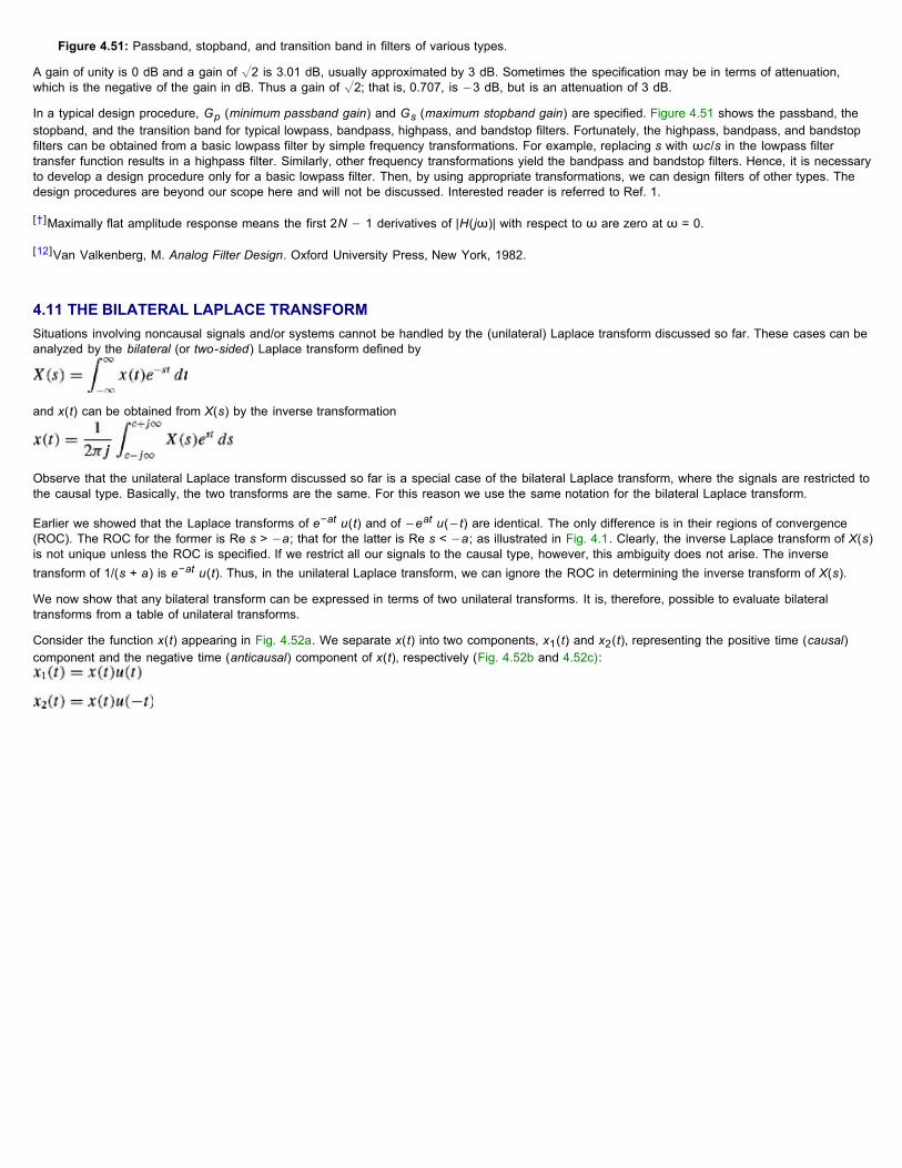
Figure 4.51: Passband, stopband, and transition band in filters of various types.

A gain of unity is 0 dB and a gain of √2 is 3.01 dB, usually approximated by 3 dB. Sometimes the specification may be in terms of attenuation,which is the negative of the gain in dB. Thus a gain of √2; that is, 0.707, is −3 dB, but is an attenuation of 3 dB.

In a typical design procedure, Gp (minimum passband gain) and Gs (maximum stopband gain) are specified. Figure 4.51 shows the passband, thestopband, and the transition band for typical lowpass, bandpass, highpass, and bandstop filters. Fortunately, the highpass, bandpass, and bandstopfilters can be obtained from a basic lowpass filter by simple frequency transformations. For example, replacing s with ωc/s in the lowpass filtertransfer function results in a highpass filter. Similarly, other frequency transformations yield the bandpass and bandstop filters. Hence, it is necessaryto develop a design procedure only for a basic lowpass filter. Then, by using appropriate transformations, we can design filters of other types. Thedesign procedures are beyond our scope here and will not be discussed. Interested reader is referred to Ref. 1.

[†]Maximally flat amplitude response means the first 2N − 1 derivatives of |H(jω)| with respect to ω are zero at ω = 0.

[12]Van Valkenberg, M. Analog Filter Design. Oxford University Press, New York, 1982.

4.11 THE BILATERAL LAPLACE TRANSFORMSituations involving noncausal signals and/or systems cannot be handled by the (unilateral) Laplace transform discussed so far. These cases can beanalyzed by the bilateral (or two-sided) Laplace transform defined by

and x(t) can be obtained from X(s) by the inverse transformation

Observe that the unilateral Laplace transform discussed so far is a special case of the bilateral Laplace transform, where the signals are restricted tothe causal type. Basically, the two transforms are the same. For this reason we use the same notation for the bilateral Laplace transform.

Earlier we showed that the Laplace transforms of e−at u(t) and of −eat u(−t) are identical. The only difference is in their regions of convergence(ROC). The ROC for the former is Re s > −a; that for the latter is Re s < −a; as illustrated in Fig. 4.1. Clearly, the inverse Laplace transform of X(s)is not unique unless the ROC is specified. If we restrict all our signals to the causal type, however, this ambiguity does not arise. The inversetransform of 1/(s + a) is e−at u(t). Thus, in the unilateral Laplace transform, we can ignore the ROC in determining the inverse transform of X(s).

We now show that any bilateral transform can be expressed in terms of two unilateral transforms. It is, therefore, possible to evaluate bilateraltransforms from a table of unilateral transforms.

Consider the function x(t) appearing in Fig. 4.52a. We separate x(t) into two components, x1(t) and x2(t), representing the positive time (causal)component and the negative time (anticausal) component of x(t), respectively (Fig. 4.52b and 4.52c):

Figure 4.52: Expressing a signal as a sum of causal and anticausal components.

The bilateral Laplace transform of x(t) is given by

where X1(s) is the Laplace transform of the causal component x1(t) and X2(s) is the Laplace transform of the anticausal component x2(t). ConsiderX2(S), given by

Therefore

If x(t) has any impulse or its derivative(s) at the origin, they are included in x1 (t). Consequently, x2(t) = 0 at the origin; that is, x2(0) = 0. Hence, the

lower limit on the integration in the preceding equation can be taken as 0− instead of 0+. Therefore

Because x2(−t) is causal (Fig. 4.52d), X2(−s) can be found from the unilateral transform table. Changing the sign of s in X2(−s) yields X2(s).

To summarize, the bilateral transform X(s) in Eq. (4.93) can be computed from the unilateral transforms in two steps:

1. Split x(t) into its causal and anticausal components, x1 (t) and x2(t), respectively.

2. The signals x1(t) and x2(−t) are both causal. Take the (unilateral) Laplace transform of x1(t) and add to it the (unilateral) Laplacetransform of x2(−t), with s replaced by −s. This procedure gives the (bilateral) Laplace transform of x(t).

Since x1(t) and x2(−t) are both causal, X1(s) and X2(−s) are both unilateral Laplace transforms. Let σc1 and σc2 be the abscissas of convergence

of X1(s) and X2(−s), respectively. This statement implies that X1 (s) exists for all s with Re s > σc1, and X2(−s) exists for all s with Re s > σc2.

Therefore, X2 (s) exists for all s with Res < σc2[†]. Therefore, X (s) = X1(s)+X2(s) exists for all s such that

The regions of convergence (or existence) of X1 (s), X2(s), and X(s) are shown in Fig. 4.53. Because X(s) is finite for all values of s lying in the stripof convergence (σc1 < Re s < −σc2), poles of X (s) must lie outside this strip. The poles of X(s) arising from the causal component x1(t) lie to theleft of the strip (region) of convergence, and those arising from its anticausal component x2(t) lie to its right (see Fig. 4.53). This fact is of crucialimportance in finding the inverse bilateral transform.

Figure 4.53

This result can be generalized to left-sided and right-sided signals. We define a signal x(t) as a right-sided signal if x(t) = 0 for t < T1 for some finitepositive or negative number T1. A causal signal is always a right-sided signal, but the converse is not necessarily true. A signal is said to left sided ifit is zero for t > T2 for some finite, positive, or negative number T2.

An anticausal signal is always a left-sided signal, but the converse is not necessarily true. A two-sided signal is of infinite duration on both positiveand negative sides of t and is neither right sided nor left sided.

We can show that the conclusions for ROC for causal signals also hold for right-sided signals, and those for anticausal signals hold for left-sidedsignals. In other words, if x(t) is causal or right-sided, the poles of X(s) lie to the left of the ROC, and if x(t) is anticausal or left-sided, the poles ofX(s) lie to the right of the ROC.

To prove this generalization, we observe that a right-sided signal can be expressed as x(t) + x(t), where x(t) is a causal signal and xf(t) is somefinite-duration signal. ROC of any finite-duration signal is the entire s-plane (no finite poles). Hence, the ROC of the right-sided signal x(t) + x(t) isthe region common to the ROCs of x(t) and xf(t), which is same as the ROC for x(t). This proves the generalization for right-sided signals. We canuse a similar argument to generalize the result for left-sided signals.

Let us find the bilateral Laplace transform of

We already know the Laplace transform of the causal component

For the anticausal component, x2(t) = ebtu(−t), we have

so that

Therefore

and the Laplace transform of x(t) in Eq. (4.94) is

Figure 4.54 shows x(t) and the ROC of X(s) for various values of a and b. Equation (4.97) indicates that the ROC of X(s) does not exist if a > b,which is precisely the case in Fig. 4.54g.

Figure 4.54

Observe that the poles of X (s) are outside (on the edges) of the ROC. The poles of X (s) because of the anticausal component of x(t) lie to theright of the ROC, and those due to the causal component of x(t) lie to its left.

When X(s) is expressed as a sum of several terms, the ROC for X(s) is the intersection of (region common to) the ROCs of all the terms. In general,if x(t) = ∑k

i=1 xi(t), then the ROC for X(s) is the intersection of the ROCs (region common to all ROCs) for the transforms X1(s), X2(s),...,Xk(s).

EXAMPLE 4.28Find the inverse Laplace transform of

if the ROC is

a. −2 < Re s < 1

b. Re s > 1

c. Re s < −2

a.

Now, X(s) has poles at −2 and 1. The strip of convergence is −2 < Re s < 1. The pole at −2, being to the left of the strip ofconvergence, corresponds to the causal signal. The pole at 1, being to the right of the strip of convergence, corresponds to theanticausal signal. Equations (4.95) and (4.96) yield

b. Both poles lie to the left of the ROC, so both poles correspond to causal signals. Therefore

c. Both poles lie to the right of the region of convergence, so both poles correspond to anticausal signals, and

Figure 4.55 shows the three inverse transforms corresponding to the same X (s) but with different regions of convergence.

Figure 4.55: Three possible inverse transforms of −3/((s + 2)(s −1)).

4.11-1 Properties of Bilateral Laplace Transform

Properties of the bilateral Laplace transform are similar to those of the unilateral transform. We shall merely state the properties here without proofs.Let the ROC of X(s) be a < Re s < b. Similarly, let the ROC of Xi (s) is ai < Re s < bi for (i = 1, 2).

LINEARITY

The ROC for a1 X1 (s) + a2X2(s) is the region common to (intersection of) the ROCs for X1 (s) and X2(s).

TIME SHIFT

The ROC for X(s)e−sT is identical to the ROC for X(s).

FREQUENCY SHIFT

The ROC for X(s − s0) is a + c < Re s < b + c, where c = Re s0.

TIME DIFFERENTIATION

The ROC for sX (s) contains the ROC for X(s) and may be larger than that of X(s) under certain conditions [e.g., if X(s) has a first-order pole at s =0 that is canceled by the factor s in sX(s)].

TIME INTEGRATION

The ROC for sX(s) is max (a, 0) < Re s < b.

TIME SCALING

The ROC for X (s/β) is βa < Re s < βb. For β > 1, x(βt) represents time compression and the corresponding ROC expands by factor β. For 0 > β >1, x(βt) represents time expansion and the corresponding ROC is compressed by factor β.

TIME CONVOLUTION

The ROC for X1(s)X2(s) is the region common to (intersection of) the ROCs for X1(s) and X2(s).

FREQUENCY CONVOLUTION

The ROC for X1 (s) * X2(s) is a1 + a2 < Re s < b1 + b2.

TIME REVERSAL

The ROC for X(−s) is −b < Re s < −a.

4.11-2 Using the Bilateral Transform for Linear System Analysis

Since the bilateral Laplace transform can handle noncausal signals, we can analyze noncausal LTIC systems using the bilateral Laplace transform.We have shown that the (zero-state) output y(t) is given by

This expression is valid only if X(s)H(s) exists. The ROC of X(s)H(s) is the region in which both X (s) and H (s) exist. In other words, the ROC ofX(s)H (s) is the region common to the regions of convergence of both X(s) and H(s). These ideas are clarified in the following examples.

EXAMPLE 4.29Find the current y(t) for the RC circuit in Fig. 4.56a if the voltage x(t) is

Figure 4.56: Response of a circuit to a noncausal input.

The transfer function H(s) of the circuit is given by

Because h(t) is a causal function, the ROC of H(s) is Re s > −1. Next, the bilateral Laplace transform of x (t) is given by

The response y(t) is the inverse transform of X(s)H(s)

The ROC of X(s)H(s) is that ROC common to both X(s) and H(s). This is 1 < Re s < 2. The poles s = ±1 lie to the left of the ROC and, therefore,correspond to causal signals; the pole s = 2 lies to the right of the ROC and thus represents an anticausal signal. Hence

Figure 4.56c shows y(t). Note that in this example, if

then the ROC of X(s) is −4 < Re s < −2. Here no region of convergence exists for X(s)H(s). Such a situation means that the dominance conditioncannot be satisfied by any permissible value of s in the range (1 < Re s < 2). Hence, the response y(t) goes to infinity.

EXAMPLE 4.30Find the response y(t) of a noncausal system with the transfer function

to the input x(t) = e−2t u(t).

We have

and

The ROC of X(s)H(s) is the region −2 < Re s < 1. By partial fraction expansion

and

Note that the pole of H(s) lies in the RHP at 1. Yet the system is not unstable. The pole(s) in the RHP may indicate instability or noncausality,depending on its location with respect to the region of convergence of H(s). For example, if H(s) = −1/(s − 1) with Re s > 1, the system is causaland unstable, with h(t) = −et u(t). In contrast, if H(s) = −1/(s −1) with Re s < 1, the system is noncausal and stable, with h(t) = etu(−t).

EXAMPLE 4.31Find the response y(t) of a system with the transfer function

and the input

The input x(t) is of the type depicted in Fig. 4.54g, and the region of convergence for X(s) does not exist. In this case, we must determine separatelythe system response to each of the two input components, x1(t) = e−1u(t) and x2(t) = e−2tu(−t).

If y1 (t) and y2(t) are the system responses to x1 (t) and x2(t), respectively, then

so that

and

so that

Therefore

[†]For instance, if x(t) exists for all t > 10, then x(−t), its time-inverted form, exists for t < −10.

4.12 SUMMARYThis chapter discusses analysis of LTIC (linear, time-invariant, continuous-time) systems by the Laplace transform, which transforms integro-differential equations of such systems into algebraic equations. Therefore solving these integro-differential equations reduces to solving algebraicequations. The Laplace transform method cannot be used for time-varying-parameter systems or for nonlinear systems in general.

The transfer function H(s) of an LTIC system is the Laplace transform of its impulse response. It may also be defined as a ratio of the Laplacetransform of the output to the Laplace transform of the input when all initial conditions are zero (system in zero state). If X(s) is the Laplacetransform of the input x(t) and Y(s) is the Laplace transform of the corresponding output y(t) (when all initial conditions are zero), then Y(s) =

X(s)H(s). For an LTIC system described by an Nth-order differential equation Q(D)y(t) = P(D)x(t), the transfer function H(s) = P(s)/Q(s). Like theimpulse response h(t), the transfer function H(s) is also an external description of the system.

Electrical circuit analysis can also be carried out by using a transformed circuit method, in which all signals (voltages and currents) are representedby their Laplace transforms, all elements by their impedances (or admittances), and initial conditions by their equivalent sources (initial conditiongenerators). In this method, a network can be analyzed as if it were a resistive circuit.

Large systems can be depicted by suitably interconnected subsystems represented by blocks. Each subsystem, being a smaller system, can bereadily analyzed and represented by its input-output relationship, such as its transfer function. Analysis of large systems can be carried out with theknowledge of input-output relationships of its subsystems and the nature of interconnection of various subsystems.

LTIC systems can be realized by scalar multipliers, adders, and integrators. A given transfer function can be synthesized in many different ways,such as canonic, cascade, and parallel. Moreover, every realization has a transpose, which also has the same transfer function. In practice, all thebuilding blocks (scalar multipliers, adders, and integrators) can be obtained from operational amplifiers.

The system response to an everlasting exponential est is also an everlasting exponential H(s)est. Consequently, the system response to aneverlasting exponential ejωt is H(jω)ejωt. Hence, H(jω) is the frequency response of the system. For a sinusoidal input of unit amplitude and havingfrequency ω, the system response is also a sinusoid of the same frequency (ω) with amplitude |H(jω)|, and its phase is shifted by ∠H(jω) withrespect to the input sinusoid. For this reason |H(jω)| is called the amplitude response (gain) and ∠H(jω) is called the phase response of the system.Amplitude and phase response of a system indicate the filtering characteristics of the system. The general nature of the filtering characteristics of asystem can be quickly determined from a knowledge of the location of poles and zeros of the system transfer function.

Most of the input signals and practical systems are causal. Consequently we are required most of the time to deal with causal signals. When allsignals must be causal, the Laplace transform analysis is greatly simplified; the region of convergence of a signal becomes irrelevant to the analysisprocess. This special case of the Laplace transform (which is restricted to causal signals) is called the unilateral Laplace transform. Much of thechapter deals with this variety of Laplace transform. Section 4.11 discusses the general Laplace transform (the bilateral Laplace transform), whichcan handle causal and noncausal signals and systems. In the bilateral transform, the inverse transform of X(s) is not unique but depends on theregion of convergence of X(s). Thus the region of convergence plays a very crucial role in the bilateral Laplace transform.

REFERENCES1. Lathi, B. P. Signal Processing and Linear Systems, 1st ed. Oxford University Press, New York, 1998.

2. Doetsch, G. Introduction to the Theory and Applications of the Laplace Transformation with a Table of Laplace Transformations.Springer-Verlag, New York, 1974.

3. LePage, W. R. Complex Variables and the Laplace Transforms for Engineers. McGraw-Hill, New York, 1961.

4. Durant, Will, and Ariel Durant. The Age of Napoleon, Part XI in The Story of Civili ation Series. Simon & Schuster, New York, 1975.

5. Bell, E. T. Men of Mathematics. Simon & Schuster, New York, 1937.

6. Nahin, P. J. "Oliver Heaviside: Genius and Curmudgeon." IEEE Spectrum, vol. 20, pp. 63 -69, July 1983.

7. Berkey, D. Calculus, 2nd ed. Saunders, Philadelphia, 1988.

8. Encyclopaedia Britannica. Micropaedia IV, 15th ed., p. 981, Chicago, 1982.

9. Churchill, R. V. Operational Mathematics, 2nd ed. McGraw-Hill, New York, 1958.

10. Lathi, B. P. Signals, Systems, and Communication. Wiley, New York, 1965.

11. Truxal, J. G. The Age of Electronic Messages. McGraw-Hill, New York, 1990.

12. Van Valkenberg, M. Analog Filter Design. Oxford University Press, New York, 1982.

MATLAB SESSION 4: CONTINUOUS-TIME FILTERSContinuous-time filters are essential to many if not most engineering systems, and MATLAB is an excellent assistant for filter design and analysis.Although a comprehensive treatment of continuous-time filter techniques is outside the scope of this book, quality filters can be designed and realizedwith minimal additional theory.

A simple yet practical example demonstrates basic filtering concepts. Telephone voice signals are often lowpass-filtered to eliminate frequenciesabove a cutoff of 3 kHz, or ωc = 3000(2π) ≈ 18.850 rad/s. Filtering maintains satisfactory speech quality and reduces signal bandwidth, therebyincreasing the phone company 's call capacity. How, then, do we design and realize an acceptable 3 kHz lowpass filter?

M4.1 Frequency Response and Polynomial Evaluation

Magnitude response plots help assess a filter 's performance and quality. The magnitude response of an ideal filter is a brick-wall function with unitypassband gain and perfect stopband attenuation. For a lowpass filter with cutoff frequency ωc, the ideal magnitude response is

Unfortunately, ideal filters cannot be implemented in practice. Realizable filters require compromises, although good designs will closely approximatethe desired brick-wall response.

A realizable LTIC system often has a rational transfer function that is represented in the s-domain as

Frequency response H(jω) is obtained by letting s = jω, where frequency ω is in radians per second.

MATLAB is ideally suited to evaluate frequency response functions. Defining a length-(N + 1) coefficient vector A = [a0, a1,...,aN] and a length-(M +1) coefficient vector B = [bN-M, bN-M+1,...,bN], program MS4P1 computes H(jω) for each frequency in the input vector ω.

The function polyval efficiently evaluates simple polynomials and makes the program nearly trivial. For example, when A is the vector ofcoefficients [a0,a1,...,aN), polyval (A, j * omega) computes

for each value of the frequency vector omega. It is also possible to compute frequency responses by using the signal processing toolbox functionfreqs.

M4.2 Design and Evaluation of a Simple RC Filter

One of the simplest lowpass filters is realized by using the RC circuit shown in Fig. M4.1. This one-pole system has transfer function HRC(s) = (RCs

+ 1)−1 and magnitude response . Independent of component values R and C, thismagnitude function possesses many desirable characteristics such as a gain that is unity at ω = 0 and that monotonically decreases to zero as ω →∞.

Figure M4.1: An RC filter.

Components R and C are chosen to set the desired 3 kHz cutoff frequency. For many filter types, the cutoff frequency corresponds to the half-powerpoint, or |HRC (jωc) | = 1/√2. Assigning C a realistic capacitance of 1 nF, the required resistance is computed by

.

The root of this first-order RC filter is directly related to the cutoff frequency, λ = −1/RC = −18,850 = −ωc.

To evaluate the RC filter performance, the magnitude response is plotted over the mostly audible frequency range (0 ≤ f 20 kHz).

The linspace (XI, X2, N) command generates an N-length vector of linearly spaced points between X1 and X2.

As shown in Fig. M4.2, the first-order RC response is indeed lowpass with a half-power cutoff frequency equal to 3 kHz. It rather poorlyapproximates the desired brick-wall response: the passband is not very flat, and stopband attenuation increases very slowly to less than 20 dB at 20kHz.

function [H] = MS4P1(B,A,omega);%MS4P1.m : MATLAB Session 4, Program 1% Function M-file computers frequency response for LTIC system% INPUTS: B = vector of feedforward coefficients% A = vector of feedback coefficients% omega =vector of frequencies [rad/s].% OUTPUTS: H = frequency response

H = polyval (B,j*omega)./polyval(A,j*omega);

>> omega_c = 2-pi*3000;>> C = 1e-9;>> R = 1/sqrt(C^2*omega_c^2)R = 5.3052e+004

>> f = linspace(0,20000,200);>> B = 1; A = [R*C 1]; Hmag_RC = abs(MS4P1(B,A,f*2*pi));>> plot(f,abs(f*2*pi)<=omega_c, 'k-', f, Hmag_RC, 'k00 ');>> xlabel ( 'f [Hz] '); ylabel( '|H_{RC} (j2/pi f)| ');>> axis([0 20000 - 0.05 1.05]); legend( 'Ideal ',, 'First-Order RC ');

Figure M4.2: First-order RC magnitude response |HRC(j2πf)|.

M4.3 A Cascaded RC Filter and Polynomial Expansion

A first-order RC filter is destined for poor performance; one pole is simply insufficient to obtain good results. A cascade of RC circuits increases thenumber of poles and improves the filter response. To simplify the analysis and prevent loading between stages, op-amp followers buffer the output ofeach section as shown in Fig. M4.3. A cascade of N stages results in an Nth-order filter with transfer function given by

Figure M4.3: A cascaded RC filter.

Upon choosing a cascade of 10 sections and C = 1 nF, a 3 kHz cutoff frequency is obtained by setting

.

This cascaded filter has a 10th-order pole at λ = −1/RC and no finite zeros. To compute the magnitude response, polynomial coefficient vectors Aand B are needed. Setting B = [1] ensures there are no finite zeros or, equivalently, that all zeros are at infinity. The poly command, which expandsa vector of roots into a corresponding vector of polynomial coefficients, is used to obtain A.

Notice that scaling a polynomial by a constant does not change its roots. Conversely, the roots of a polynomial specify a polynomial within a scalefactor. The command A = A/A (end) properly scales the denominator polynomial to ensure unity gain at ω = 0.

The magnitude response plot of the cascaded RC filter is included in Fig. M4.4. The passband remains relatively unchanged, but stopbandattenuation is greatly improved to over 60 dB at 20 kHz.

Figure M4.4: Lowpass filter comparison.

M4.4 Butterworth Filters and the Find Command

The pole location of a first-order lowpass filter is necessarily fixed by the cutoff frequency. There is little reason, however, to place all the poles of a10th-order filter at one location. Better pole placement will improve our filter 's magnitude response. One strategy, discussed in Section 4.10, is toplace a wall of poles opposite the passband frequencies. A semicircular wall of poles leads to the Butterworth family of filters, and a semiellipticalshape leads to the Chebyshev family of filters. Butterworth filters are considered first.

To begin, notice that a transfer function H(s) with real coefficients has a squared magnitude response given by |H(jω)|2 = H(jω)H*(jω) =H(jω)H(−jω) = H(s)−s)|s=jω. Thus, half the poles of |H(jω)|2 correspond to the filter H(s) and the other half correspond to H(−s). Filters that areboth stable and causal require H(s) to include only left-half-plane poles.

>> R = sqrt(2^(1/10)-1)/(C*omega_c)R = 1.4213e+004

>> B = 1; A = poly(-1/(R*C)*ones(10,1));A = A/A(end);>> Hmag_cascade = abs (MS4P1(B,A,f*2*pi));

The squared magnitude response of a Butterworth filter is

This function has the same appealing characteristics as the first-order RC filter: a gain that is unity at ω = 0 and monotonically decreases to zero asω → ∞. By construction, the half-power gain occurs at ωc. Perhaps most importantly, however, the first 2N − 1 derivatives of |HB(jω)| with respectto ω are zero at ω = 0. Put another way, the passband is constrained to be very flat for low frequencies. For this reason, Butterworth filters aresometimes called maximally flat filters.

As discussed in MATLAB Session B, the roots of minus one must lie equally spaced on a circle centered at the origin. Thus, the 2N poles of|HB(jω)|2 naturally lie equally spaced on a circle of radius ωc centered at the origin. Figure M4.5 displays the 20 poles corresponding to the case N

= 10 and ωc = 3000(2π) rad/s. An Nth-order Butterworth filter that is both causal and stable uses the N left-half-plane poles of |HB(jω)|2.

Figure M4.5: Roots of |HB(jω)|2 for N = 10 and ωc = 3000(2π).

To design a 10th-order Butterworth filter, we first compute the 20 poles of |HB(jω)|2:

The find command is an extremely powerful function that returns the indices of a vector 's nonzero elements. Combined with relational operators,the find command allows us to extract the 10 left-half-plane roots that correspond to the poles of our Butterworth filter.

To compute the magnitude response, these roots are converted to coefficient vector A.

The magnitude response plot of the Butterworth filter is included in Fig. M4.4. The Butterworth response closely approximates the brick-wall functionand provides excellent filter characteristics: flat passband, rapid transition to the stopband, and excellent stopband attenuation (>40dB at 5kHz).

M4.5 Using Cascaded Second-Order Sections for Butterworth Filter Realization

For our RC filters, realization preceded design. For our Butterworth filter, however, design has preceded realization. For our Butterworth filter to beuseful, we must be able to implement it.

Since the transfer function HB(s) is known, the differential equation is also known. Therefore, it is possible to try to implement the design by usingop-amp integrators, summers, and scalar multipliers. Unfortunately, this approach will not work well. To understand why, consider the denominatorcoefficients a0 = 1.766 × 10−43 and a10 = 1. The smallest coefficient is 43 orders of magnitude smaller than the largest coefficient! It is practicallyimpossible to accurately realize such a broad range in scale values. To understand this, skeptics should try to find realistic resistors such that Rf/R =

1.766 × 10−43. Additionally, small component variations will cause large changes in actual pole location.

A better approach is to cascade five second-order sections, where each section implements one complex conjugate pair of poles. By pairing poles incomplex conjugate pairs, each of the resulting second-order sections have real coefficients. With this approach, the smallest coefficients are onlyabout nine orders of magnitude smaller than the largest coefficients. Furthermore, pole placement is typically less sensitive to component variationsfor cascaded structures.

>> N=10;>> poles = roots([(j*omega_c)^(-2*N), zeros(1,2*N-1),1]);

>> B_poles = poles (find(real(poles) <0));

>> A = poly (B_poles); A = A/A (end);>> Hmag_B = abs (MS4P1 (B,A,f*2*pi));

The Sallen-Key circuit shown in Fig. M4.6 provides a good way to realize a pair of complex-conjugate poles.[†] The transfer function of this circuit is

Figure M4.6: Sallen-Key filter stage.

Geometrically, ω0 is the distance from the origin to the poles and Q = 1/2 cos ψ, where ψ is the angle between the negative real axis and the pole.Termed the "quality factor" of a circuit, Q provides a measure of the peakedness of the response. High-Q filters have poles close to the ω axis,which boost the magnitude response near those frequencies.

Although many ways exist to determine suitable component values, a simple method is to assign R1 a realistic value and then let R2 = R1, C1 =2Q/ω0R1 and C2 = 1/2Qω0R2. Butter-worth poles are a distance ωc from the origin, so ω0 = ωc. For our 10th-order Butterworth filter, the anglesψ are regularly spaced at 9, 27, 45, 63, and 81 degrees. MATLAB program MS4P2 automates the task of computing component values andmagnitude responses for each stage.

The disp command displays a character string to the screen. Character strings must be enclosed in single quotation marks. The num2strcommand converts numbers to character strings and facilitates the formatted display of information. The prod command multiplies along the columnsof a matrix; it computes the total magnitude response as the product of the magnitude responses of the five stages.

Executing the program produces the following output:

Since all the component values are practical, this filter is possible to implement. Figure M4.7 displays the magnitude responses for all five stages(solid lines). The total response (dotted line) confirms a 10th-order Butterworth response. Stage 5, which has the largest Q and implements the pairof conjugate poles nearest the ω axis, is the most peaked response. Stage 1, which has the smallest Q and implements the pair of conjugate polesfurthest from the ω axis, is the least peaked response. In practice, it is best to order high-Q stages last; this reduces the risk of the high gainssaturating the filter hardware.

% MS4P2.m : MATLAB Session 4, Program 2% Script M-file computes Sallen---Key component values and magnitude% responses for each of the five cascaded second-order filter sections.

omega_0 = 3000*2*pi; % Filter cut---off frequencypsi = [9 27 45 63 81]*pi/180; % Butterworth pole anglesf = linspace(0, 6000, 200); % Frequency range for magnitude response calculationsHmag_SK = zeros(5,200); % Pre-allocate array for magnitude responsesfor stage = 1:5,Q = 1/(2* cos(psi(stage))); % Compute Q for current stage% Compute and display filter components to the screen:disp([ 'Stage ',num2str(stage),...' (Q = ',num2str(Q),...'): R1 = R2 = ',num2str(56000),...', C1 = ' ,num2str (2*Q/(omega_0*56000) ), ...', C2 = ' ,num2str (1/(2*Q*omega_0*56000) ) ] ) ;B = omega_0^2; A = [1 omega_0/Q omega_0^2] ; % Compute filter coefficientsHmag_SK(stage,:) = abs(MS4P1(B, A, 2*pi*f)); % Compute magnitude responseendplot (f, Hmag_SK, 'k ', f, prod (Hmag_SK), 'k: ')xlabel ( 'f [Hz] '); ylabel ( 'Magnitude Response ')

>> MS4P2Stage 1 (Q = 0.50623): R1 = R2 = 56000, C1 = 9.5916e-010, C2 = 9.3569e-010Stage 2 (Q = 0.56116): R1 = R2 = 56000, C1 = 1.0632e-009, C2 = 8.441e-010Stage 3 (Q = 0.70711): R1 = R2 = 56000, C1 = 1.3398e-009, C2 = 6.6988e-010Stage 4 (Q = 1.1013): R1 = R2 = 56000, C1 = 2.0867e-009, C2 = 4.3009e-010Stage 5 (Q = 3.1962): R1 = R2 = 56000, C1 = 6.0559e-009, C2 = 1.482e-010

Figure M4.7: Magnitude responses for Sallen-Key filter stages.

M4.6 Chebyshev Filters

Like an order-N Butterworth lowpass filter (LPF), an order-N Chebyshev LPF is an all-pole filter that possesses many desirable characteristics.Compared with an equal-order Butterworth filter, the Chebyshev filter achieves better stopband attenuation and reduced transition band width byallowing an adjustable amount of ripple within the passband.

The squared magnitude response of a Chebyshev filter is

where ∊ controls the passband ripple, CN(ω/ωc) is a degree-N Chebyshev polynomial, and ωc is the radian cutoff frequency. Several characteristicsof Chebyshev LPFs are noteworthy:

An order-N Chebyshev LPF is equiripple in the passband (|ω| ≤ ωc), has a total of N maxima and minima over (0 ≤ ω ≤ ωc), and ismonotonic decreasing in the stopband (|ω| > ωc).

In the passband, the maximum gain is 1 and the minimum gain is . For oddvalued N, |H(j0)| = 1. For even-valued

.

Ripple is controlled by setting , where R is the allowable passband ripple expressed in decibels. Reducing ∊adversely affects filter performance (see Prob. 4.M-8).

Unlike Butterworth filters, the cutoff frequency ωc rarely specifies the 3 dB point. For ∊ ≠ 1, |H(jωc)|2 = 1/(1 + ∊2) ≠ 0.5. The cutoff

frequency ωc simply indicates the frequency after which .

The Chebyshev polynomial CN(x) is defined as

In this form, it is difficult to verify that CN(x) is a degree-N polynomial in x. A recursive form of CN(x) makes this fact more clear (see Prob. 4.M-11).

With C0(x) = 1 and C1(x) = x, the recursive form shows that any CN is a linear combination of degree-N polynomials and is therefore a degree-Npolynomial itself. For N ≥ 2, MATLAB program MS4P3 generates the (N + 1) coefficients of Chebyshev polynomial CN(x).

As examples, consider C2(x) = 2xC1(x) − C0(x) = 2x(x) − 1 = 2x2 − 1 and C3(x) = 2xC2(x) − C1(x) = 2x(2x2 − 1) − x = 4x3 = 3x. MS4P3easily confirms these cases.

function [C_N] = MS4P3 (N);% MS4P3 .m : MATLAB Session 4, Program 3% Function M-file computes Chebyshev polynomial coefficients% using the recursion relation C_N(x) = 2xC_{N- 1} (x) - C_{N-2} (x)% INPUTS: N = degree of Chebyshev polynomial% OUTPUTS: C_N = vector of Chebyshev polynomial coefficients

C_Nm2 = 1; C_Nm1 = [1 0]; % Initial polynomial coefficients:for t = 2:N;C_N =2*conv([1 0], C_Nm1) - [zeros (1, length (C_Nm1) - length(C_Nm2) + 1), C_Nm2];C_Nm2 = C_Nm1; C_Nm1 = C_N;end

>> MS4P3 (2)ans = 2 0 -1>> MS4P3(3)ans = 4 0 -3 0

Since CN(ω/ωc) is a degree-N polynomial, |H(jω)|2 is an all-pole rational function with 2N finite poles. Similar to the Butterworth case, the N poles

specifying a causal and stable Chebyshev filter can be found by selecting the N left-half plane roots of 1 + ∊2C2N[s/(jωc)].

Root locations and dc gain are sufficient to specify a Chebyshev filter for a given N and ∊. To demonstrate, consider the design of an order-8Chebyshev filter with cutoff frequency fc = 1 kHz and allowable passband ripple R = 1 dB. First, filter parameters are specified.

The coefficients of CN (s/(jωc)) are obtained with the help of MS4P3, and then the coefficients of (1 + ∊2C2N(s/(jωc)) are computed by using

convolution to perform polynomial multiplication.

Next, the polynomial roots are found, and the left-half-plane poles are retained and plotted.

As shown in Fig. M4.8, the roots of a Chebyshev filter lie on an ellipse[†] (see Prob. 4.M-12).

Figure M4.8: Pole-zero plot for an order-8 Chebyshev LPF with fc = 1 kHz and r = 1 dB.

To compute the filter's magnitude response, the poles are expanded into a polynomial, the dc gain is set based on the even value of N, and MS4P1is used.

As seen in Fig. M4.9, the magnitude response exhibits correct Chebyshev filter characteristics: passband ripples are equal in height and neverexceed R = 1 dB; there are a total of N = 8 maxima and minima in the passband; and the gain rapidly and monotonically decreases after the cutofffrequency of fc = 1 kHz.

>> omega_c = 2*pi*1000; R = 1; N = 8;>> epsilon = sqrt (10^(R/10)-1);

>> CN = MS4P3 (N).* ((1/(j*omega_c)).^ [N:-1:0]);>> CP = epsilon^2*conv(CN, CN); CP(end) = CP (end) +1;

>> poles = roots(CP); i = find (real (poles) < 0); C_poles = poles(i);>> plot(real (C_poles),imag(C_poles), 'kx '); axis equal;>> axis(omega_c* [-1.1 1.1 -1.1 1.1]);>> xlabel ( ' \sigma '); ylabel ( '\omega ');

>> A = poly (C_poles);>> B = A (end)/sqrt (1+epsilon^2) ;>> omega = linspace(0,2*pi*2000,2001);>> H = MS4P1 (B, A, omega);>> plot (omega/2/pi,abs(H), 'k '); grid>> xlabel ( 'f [Hz] '); ylabel ( '|H (j2\pi f)| ');>> axis([0 2000 0 1.1]);

Figure M4.9: Magnitude responses for an order-8 Chebyshev LPF with fc = 1 kHz and r = 1 dB.

For higher-order filters, polynomial rooting may not provide reliable results. Fortunately, Chebyshev roots can also be determined analytically. For

the Chebyshev poles are

Continuing the same example, the poles are recomputed and again plotted. The result is identical to Fig. M4.8.

As in the case of high-order Butterworth filters, a cascade of second-order filter sections facilitates practical implementation of Chebyshev filters.Problems 4.M-3 and 4.M-6 use second-order Sallen-Key circuit stages to investigate such implementations.

[†]A more general version of the Sallen-Key circuit has a resistor Ra from the negative terminal to ground and a resistor Rb between the negativeterminal and the output. In Fig. M4.6, Ra = ∞ and Rb = 0.

[†]E. A. Guillemin demonstrates a wonderful relationship between the Chebyshev ellipse and the Butterworth circle in his book, Synthesis of PassiveNetworks (Wiley, New York, 1957).

PROBLEMS4.1.1 By direct integration [Eq. (4.1)] find the Laplace transforms and the region of convergence of the following functions:

a. u(t) − u(t − 1)

b. te−tu(t)

c. t cos ω0t u(t)

d. (e2t − 2e−t)u(t)

e. cos ω1t cos ω2t u(t)

f. cosh (at)u(t)

g. sinh (at)u(t)

h. e−2t cos (5t + θ)u(t) 4.1.2 By direct integration find the Laplace transforms of the signals shown in Fig. P4.1-2.

Figure P4.1-2

>> k = [1:N]; xi = 1/N*asinh(1/epsilon); phi = (k*2-1)/(2*N)*pi;>> C_poles = omega_c*(-sinh(xi)*sin(phi)+j*cosh(xi)*cos(phi));>> plot(real(C_poles),imag(C_poles), 'kx '); axis equal;>> axis(omega_c*[-1.1 1.1 -1.1 1.1]);>> xlabel( '\sigma '); ylabel( '\omega ');

4.1.3 Find the inverse (unilateral) Laplace transforms of the following functions:

a.

b.

c.

d.

e.

f.

g.

h.

i.

4.2.1 Find the Laplace transforms of the following functions using only Table 4.1 and the time-shifting property (if needed) of the unilateralLaplace transform:

a. u(t) − u(t − 1)

b. e−(t− τ)u(t − τ)

c. e−(t− τ)u(t)

d. e−tu(t − τ)

e. te−tu(t − τ)

f. sin [ω0(t − τ)] u(t − τ)

g. sin [ω0(t − τ)] u(t)

h. sin ω0t u(t − τ) 4.2.2 Using only Table 4.1 and the time-shifting property, determine the Laplace transform of the signals in Fig. P4.1-2. [Hint: See Section

1.4 for discussion of expressing such signals analytically.] 4.2.3 Find the inverse Laplace transforms of the following functions:

a.

b.

c.

d.

4.2.4 The Laplace transform of a causal periodic signal can be determined from the knowledge of the Laplace transform of its first cycle

(period).

a. If the Laplace transform of x(t) in Fig. P4.2-4a is X (s), then show that G(s), the Laplace transform of g(t) (Fig. P4.2-4b),is

Figure P4.2-4

b. Use this result to find the Laplace transform of the signal p(t) illustrated in Fig. P4.2-4c. 4.2.5 Starting only with the fact that δ(t) 1, build pairs 2 through 10b in Table 4.1, using various properties of the Laplace transform. 4.2.6

a. Find the Laplace transform of the pulses in Fig. 4.2 in the text by using only the time-differentiation property, the time-shifting property, and the fact that δ(t) 1.

b. In Example 4.7, the Laplace transform of x(t) is found by finding the Laplace transform of d2x/dt2. Find the Laplacetransform of x(t) in that example by finding the Laplace transform of dx/dt and using Table 4.1, if necessary.

4.2.7 Determine the inverse unilateral Laplace transform of

4.2.8 Since 13 is such a lucky number, determine the inverse Laplace transform of X(s) = 1/(s+1)13 given region of convergence σ > − 1.

[Hint: What is the nth derivative of 1/(s + a)?] 4.2.9 It is difficult to compute the Laplace transform X(s) of signal

by using direct integration. Instead, properties provide a simpler method.

a. Use Laplace transform properties to express the Laplace transform of tx(t) in terms of the unknown quantity X(s).

b. Use the definition to determine the Laplace transform of y(t) = tx(t).

c. Solve for X(s) by using the two pieces from a and b. Simplify your answer.

4.3.1 Using the Laplace transform, solve the following differential equations:

a. and x(t) = u(t)

b. and x(t) = e−1u(t)

c. and x(t) = 25u(t)

4.3.2 Solve the differential equations in Prob. 4.3-1 using the Laplace transform. In each case determine the zero-input and zero-state

components of the solution. 4.3.3 Solve the following simultaneous differential equations using the Laplace transform, assuming all initial conditions to be zero and the

input x(t) = u(t):

a. (D + 3)y1(t) − 2y2(t)=x(t) − 2y1(t) + (2D + 4)y2(t) = 0

b. (D + 2)y1(t) − (D + 1)y2(t) = 0 − (D + 1)y1(t) + (2D + 1)y2(t)= x(t)

Determine the transfer functions relating outputs y1(t) and y2(t) to the input x(t). 4.3.4 For the circuit in Fig. P4.3-4, the switch is in open position for a long time before t = 0, when it is closed instantaneously.

a. Write loop equations (in time domain) for t ≥ 0.

b. Solve for y1(t) and y2(t) by taking the Laplace transform of loop equations found in part (a). 4.3.5 For each of the systems described by the following differential equations, find the system transfer function:

a.

b.

c.

d.

Figure P4.3-4

4.3.6 For each of the systems specified by the following transfer functions, find the differential equation relating the output y(t) to the input

x(t) assuming that the systems are controllable and observable:

a.

b.

c.

4.3.7 For a system with transfer function

a. Find the (zero-state) response for input x(t) of (i) 10u(t) and (ii) u(t − 5).

b. For this system write the differential equation relating the output y(t) to the input x(t) assuming that the systems arecontrollable and observable.

4.3.8 For a system with transfer function

a. Find the (zero-state) response if the input x(t) = (1 −e−1)u(t)

b. For this system write the differential equation relating the output y(t) to the input x(t) assuming that the systems arecontrollable and observable.

4.3.9 For a system with transfer function

a. Find the (zero-state) response for the following values of input x(t):

i. e−3tu(t)

ii. e−4tu(t)

iii. e−4(t−5)u(t − 5)

iv. e−4(t−5)u(t)

v. e−4tu(t − 5)

b. For this system write the differential equation relating the output y(t) to the input x(t) assuming that the systems arecontrollable and observable.

4.3.10 An LTI system has a step response given by s(t) = e−1u(t) − e−2u(t). Determine the output of this system y(t) given an input x(t) =

δ(t−π)−cos (√3)u(t). 4.3.11 For an LTIC system with zero initial conditions (system initially in zero state), if an input x(t) produces an output y(t), then using the

Laplace transform show the following.

a. The input dx/dt produces an output dy/dt.

b. The input ∫t0 x(τ) dτ produces an output ∫t

0 y(τ) dτ. Hence, show that the unit step response of a system is an

integral of the impulse response; that is, ∫t0 h(τ) dτ.

4.3.12

a. Discuss asymptotic and BIBO stabilities for the systems described by the following transfer functions assuming that thesystems are controllable and observable:

i.

ii.

iii.

iv.

v.

b. Repeat part (a) for systems described by the following differential equations. Systems may be uncontrollable and/orunobservable.

i. (D2 + 3D + 2)y(t) = (D + 3)x(t)

ii. (D2 + 3D + 2)y(t) = (D + 1)x(t)

iii. (D2 + D − 2)y(t) = (D − 1)x(t)

iv. (D2 − 3D + 2)y(t) = (D − 3)x(t)

4.4.1 Find the zero-state response y(t) of the network in Fig. P4.4-1 if the input voltage x(t) = te−tu(t). Find the transfer function relatingthe output y(t) to the input x(t). From the transfer function, write the differential equation relating y(t) to x(t).

Figure P4.4-1

4.4.2 The switch in the circuit of Fig. P4.4-2 is closed for a long time and then opened instantaneously at t = 0. Find and sketch the

current y(t).

Figure P4.4-2

4.4.3 Find the current y(t) for the parallel resonant circuit in Fig. P4.4-3 if the input is

a. x(t) = A cos ω0t u(t)

b. x(t) = A sin ω0t u(t)

Assume all initial conditions to be zero and, in both cases, ω20 = 1/LC.

Figure P4.4-3

4.4.4 Find the loop currents y1 (t) and y2(t) for t≥ 0 in the circuit of Fig. P4.4-4a for the input x(t) in Fig. P4.4-4b.

Figure P4.4-4

4.4.5 For the network in Fig. P4.4-5 the switch is in a closed position for a long time before t = 0, when it is opened instantaneously. Find

y1(t) and vs(t) for t ≥ 0.

Figure P4.4-5

4.4.6 Find the output voltage v0(t) for t ≥ 0 for the circuit in Fig. P4.4-6, if the input x(t) = 100u(t). The system is in the zero state initially.

Figure P4.4-6

4.4.7 Find the output voltage y(t) for the network in Fig. P4.4-7 for the initial conditions iL(0) = 1 A and vc(0) = 3 V.

Figure P4.4-7

4.4.8 For the network in Fig. P4.4-8, the switch is in position a for a long time and then is moved to position b instantaneously at t = 0.

Determine the current y(t) for t > 0.

Figure P4.4-8

4.4.9 Show that the transfer function that relates the output voltage y(t) to the input voltage x(t) for the op-amp circuit in Fig. P4.4-9a is

given by

and that the transfer function for the circuit in Fig. P4.4-9b is given by

Figure P4.4-9

4.4.10 For the second-order op-amp circuit in Fig. P4.4-10, show that the transfer function H(s) relating the output voltage y(t) to the input

voltage x(t) is given by

Figure P4.4-10

4.4.11

a. Using the initial and final value theorems, find the initial and final value of the zero-state response of a system with thetransfer function

and the input (i) u(t) and (ii) e−tu(t).

b. Find y(0+) and y(∞) if Y(s) is given by

i.

ii.

4.5.1 Figure P4.5-1a shows two resistive ladder segments. The transfer function of each segment (ratio of output to input voltage) is 1/2.Figure P4.5-1b shows these two segments connected in cascade.

a. Is the transfer function (ratio of output to input voltage) of this cascaded network (1/2)(1/2) = 1/4?

b. If your answer is affirmative, verify the answer by direct computation of the transfer function. Does this computationconfirm the earlier value 1/4? If not, why?

c. Repeat the problem with R3 = R4 = 20 kΩ. Does this result suggest the answer to the problem in part (b)?

Figure P4.5-1

4.5.2 In communication channels, transmitted signal is propagated simultaneously by several paths of varying lengths. This causes the signal

to reach the destination with varying time delays and varying gains. Such a system generally distorts the received signal. For error-freecommunication, it is necessary to undo this distortion as much as possible by using the system that is inverse of the channel model.

For simplicity, let us assume that a signal is propagated by two paths whose time delays differ by τ seconds. The channel over theintended path has a delay of T seconds and unity gain. The signal over the unintended path has a delay of T + τ seconds and gain a.Such a channel can be modeled, as shown in Fig. P4.5-2. Find the inverse system transfer function to correct the delay distortion andshow that the inverse system can be realized by a feedback system. The inverse system should be causal to be realizable. [Hint: Wewant to correct only the distortion caused by the relative delay τ seconds. For distortionless transmission, the signal may be delayed.What is important is to maintain the shape of x(t). Thus a received signal of the form c x(t − T) is considered to be distortionless.]

Figure P4.5-2

4.5.3 Discuss BIBO stability of the feedback systems depicted in Fig. P4.5-3. For the case in Fig. P4.5-3b, consider three cases:

i. K = 10

ii. K = 50

iii. K = 48

Figure P4.5-3

4.6.1 Realize

by canonic direct, series, and parallel forms. 4.6.2 Realize the transfer function in Prob. 4.6-1 by using the transposed form of the realizations found in Prob. 4.6-1. 4.6.3 Repeat Prob. 4.6-1 for

a.

b.

4.6.4 Realize the transfer functions in Prob. 4.6-3 by using the transposed form of the realizations found in Prob. 4.6-3. 4.6.5 Repeat Prob. 4.6-1 for

4.6.6 Realize the transfer function in Prob. 4.6-5 by using the transposed form of the realizations found in Prob. 4.6-5. 4.6.7 Repeat Prob. 4.6-1 for

4.6.8 Realize the transfer function in Prob. 4.6-7 by using the transposed form of the realizations found in Prob. 4.6-7. 4.6.9 Repeat Prob. 4.6-1 for

4.6.10 Realize the transfer function in Prob. 4.6-9 by using the transposed form of the realizations found in Prob. 4.6-9. 4.6.11 Repeat Prob. 4.6-1 for

4.6.12 Realize the transfer function in Prob. 4.6-11 by using the transposed form of the realizations found in Prob. 4.6-11. 4.6.13 In this problem we show how a pair of complex conjugate poles may be realized by using a cascade of two first-order transfer

functions and feedback. Show that the transfer functions of the block diagrams in Fig. P4.6-13a and P4.6-13b are

a.

b.

Hence, show that the transfer function of the block diagram in Fig. P4.6-13c is

c.

Figure P4.6-13

4.6.14 Show op-amp realizations of the following transfer functions:

i.

ii.

iii.

4.6.15 Show two different op-amp circuit realizations of the transfer function

4.6.16 Show an op-amp canonic direct realization of the transfer function

4.6.17 Show an op-amp canonic direct realization of the transfer function

4.7.1 Feedback can be used to increase (or decrease) the system bandwidth. Consider the system in Fig. P4.7-1a with transfer functionG(s) = ωc/(s + ωc).

a. Show that the 3 dB bandwidth of this system is ωc and the dc gain is unity, that is, |H(j0)| = 1.

b. To increase the bandwidth of this system, we use negative feedback with H(s) = 9, as depicted in Fig. P4.7-1b. Showthat the 3 dB bandwidth of this system is 10ωc. What is the dc gain?

c. To decrease the bandwidth of this system, we use positive feedback with H(s) = −0.9, as illustrated in Fig. P4.7-1c.Show that the 3 dB bandwidth of this system is ωc/10. What is the dc gain?

d. The system gain at dc times its 3 dB bandwidth is the gain-bandwidth product of a system. Show that this product is thesame for all the three systems in Fig. P4.7-1. This result shows that if we increase the bandwidth, the gain decreasesand vice versa.

Figure P4.7-1

4.8.1 For an LTIC system described by the transfer function

find the response to the following everlasting sinusoidal inputs:

a. 5 cos (2t + 30°)

b. 10 sin (2t + 45°)

c. 10 cos (3t + 40°)

Observe that these are everlasting sinusoids. 4.8.2 For an LTIC system described by the transfer function

find the steady-state system response to the following inputs:

a. 10u(t)

b. cos (2t + 60°)u(t)

c. sin (3t − 45°)u(t)

d. ej3t u(t) 4.8.3 For an allpass filter specified by the transfer function

find the system response to the following (everlasting) inputs:

a. ejωt

b. cos (ωt + θ)

c. cos t

d. sin 2t

e. cos 10t

f. cos 100t

Comment on the filter response. 4.8.4 The pole-zero plot of a second-order system H(s) is shown in Fig. P4.8-4. The dc response of this system is minus one, H(j0) = −1.

a. Letting H(s) = k(s2 + b1s + b2)/(s2 + a1s + a2), determine the constants k, b1, b2, a1, and a2.

b. What is the output y(t) of this system in response to the input x(t) = 4 + cos (t/2 + π/3)?

Figure P4.8-4: System pole-zero plot.

4.9.1 Sketch Bode plots for the following transfer functions:

a.

b.

c.

4.9.2 Repeat Prob. 4.9-1 for

a.

b.

c.

4.9.3 Using the lowest order possible, determine a system function H(s) with real-valued roots that matches the frequency response in Fig.

P4.9-3 Verify your answer with MATLAB.

Figure P4.9-3: Bode plot and frequency response for H(s).

4.9.4 A graduate student recently implemented an analog phase lock loop (PLL) as part of his thesis. His PLL consists of four basic

components: a phase/frequency detector, a charge pump, a loop filter, and a voltage-controlled oscillator. This problem considers onlythe loop filter, which is shown in Fig. P4.9-4a. The loop filter input is the current x(t), and the output is the voltage y(t).

a. Derive the loop filter 's transfer function H(s). Express H(s) in standard form.

b. Figure P4.9-4b provides four possible frequency response plots, labeled A through D. Each log-log plot is drawn to thesame scale, and line slopes are either 20 dB/decade, 0 dB/decade, or −20 dB/decade. Clearly identify which plot(s), if

any, could represent the loop filter.

c. Holding the other components constant, what is the general effect of increasing the resistance R on the magnituderesponse for low-frequency inputs?

d. Holding the other components constant, what is the general effect of increasing the resistance R on the magnituderesponse for high-frequency inputs?

Figure P4.9-4: (a) Circuit diagram for PLL loop filter. (b) Possible magnitude response plots for PLL loop filter.

4.10.1 Using the graphical method of Section 4.10-1, draw a rough sketch of the amplitude and phase response of an LTIC systemdescribed by the transfer function

What kind of filter is this? 4.10.2 Using the graphical method of Section 4.10-1, draw a rough sketch of the amplitude and phase response of LTIC systems whose

polezero plots are shown in Fig. P4.10-2.

Figure P4.10-2 4.10.3 Design a second-order bandpass filter with center frequency ω = 10. The gain should be zero at ω = 0 and at ω = ∞. Select poles

at −a ± j10. Leave your answer in terms of a. Explain the influence of a on the frequency response. 4.10.4 The LTIC system described by H(s) = (s − 1)/(s + 1) has unity magnitude response |H(jω)| = 1. Positive Pat claims that the output

y(t) of this system is equal the input x(t) since the system is allpass. Cynical Cynthia doesn 't think so. "This is signals and systemsclass," she complains. "It has to be more complicated!" Who is correct, Pat or Cynthia? Justify your answer.

4.10.5 Two students, Amy and Jeff, disagree about an analog system function given by H1(s) = s. Sensible Jeff claims the system has a

zero at s = 0. Rebellious Amy, however, notes that the system function can be rewritten as H1(s) = 1/s−1 and claims that thisimplies a system pole at s = ∞. Who is correct? Why? What are the poles and zeros of the system H2(s) = 1/s?

4.10.6 A rational transfer function H(s) is often used to represent an analog filter. Why must H(s) be strictly proper for lowpass and

bandpass filters? Why must H(s) be proper for highpass and bandstop filters? 4.10.7 For a given filter order N, why is the stopband attenuation rate of an all-pole lowpass filter better than filters with finite zeros? 4.10.8 Is it possible, with real coefficients ( ), for a system

to function as a lowpass filter? Explain your answer. 4.10.9 Nick recently built a simple second-order But-terworth lowpass filter for his home stereo. Although the system performs pretty well,

Nick is an overachiever and hopes to improve the system performance. Unfortunately, Nick is pretty lazy and doesn 't want todesign another filter. Thinking "twice the filtering gives twice the performance," he suggests filtering the audio signal not once buttwice with a cascade of two identical filters. His overworked, underpaid signals professor is skeptical and states, "If you are usingidentical filters, it makes no difference whether you filter once or twice!" Who is correct? Why?

4.10.10 An LTIC system impulse response is given by h(t) = u(t)-u(t − 1).

a. Determine the transfer function H(s). Using H(s), determine and plot the magnitude response |H(jω)|. Which type offilter most accurately describes the behavior of this system: lowpass, highpass, bandpass, or bandstop?

b. What are the poles and zeros of H(s)? Explain your answer.

c. Can you determine the impulse response of the inverse system? If so, provide it. If not, suggest a method that couldbe used to approximate the impulse response of the inverse system.

4.10.11 An ideal lowpass filter HLP(s) has magnitude response that is unity for low frequencies and zero for high frequencies. An ideal

highpass filter HHP(s) has an opposite magnitude response: zero for low frequencies and unity for high frequencies. A studentsuggests a possible lowpass-to-highpass filter transformation: HHP(s) = 1 − HLP(s). In general, will this transformation work?Explain your answer.

4.10.12 An LTIC system has a rational transfer function H(s). When appropriate, assume that all initial conditions are zero.

a. Is is possible for this system to output y(t) = sin (100πt) u(t) in response to an input x(t) = cos (100πt)u(t)? Explain.

b. Is is possible for this system to output y(t) = sin (100πt)u(t) in response to an input x(t) = sin (50πt)u(t)? Explain.

c. Is is possible for this system to output y(t) = sin (100πt) in response to an input x(t) = cos (100πt)? Explain.

d. Is is possible for this system to output y(t) = sin (100πt) in response to an input x(t) = sin (50πt)? Explain.

4.11.1 Find the ROC, if it exists, of the (bilateral) Laplace transform of the following signals:

a. etu(t)

b. e−tu(t)

c.

d.

e. e−kt2

4.11.2 Find the (bilateral) Laplace transform and the corresponding region of convergence for the following signals:

a. e−|t |

b. e−|t | cos t

c. etu(t) + e2tu(−t)

d. e−tu(t)

e. e−tu(−t)

f. cos ω0t u(t) + et u(−t) 4.11.3 Find the inverse (bilateral) Laplace transforms of the following functions:

a.

b.

c.

d.

e.

4.11.4 Find

if the ROC is

a. Re s > 1

b. Re s < −2

c. −1 < Re s < 1

d. −2 < Re s < −1 4.11.5 For a causal LTIC system having a transfer function H(s) = 1/(s + 1), find the output y(t) if the input x(t) is given by

a. e−|t |/2

b. etu(t) + e2tu(−t)

c. e−t /2u(t) + e−t /4u(−t)

d. e2tu(t) + etu(−t)

e. e−t /4u(t) + e−t /2u(−t)

f. e−3tu(t) + e−2tu(−t) 4.11.6 The autocorrelation function rxx(t) of a signal x(t) is given by

Derive an expression for in terms of X(s), where . 4.11.7 Determine the inverse Laplace transform of

given that the region of convergence is σ < 0. 4.11.8 An absolutely integrable signal x(t) has a pole at s = π. It is possible that other poles may be present. Recall that an absolutely

integrable signal satisfies

a. Can x(t) be left sided? Explain.

b. Can x(t) be right sided? Explain.

c. Can x(t) be two sided? Explain.

d. Can x(t) be of finite duration? Explain. 4.11.9 Using the definition, compute the bilateral Laplace transform, including the region of convergence (ROC), of the following complex-

valued functions:

a. x1(t) = (j + ejt)u(t)

b. x2(t) = j cosh (t)u(−1)

c.

d. x4(t) = jtu(−t) + δ(t − π) 4.11.10 A bounded-amplitude signal x(t) has bilateral Laplace transform X(s) given by

a. Determine the corresponding region of convergence.

b. Determine the time-domain signal x(t).

4.m.1 Express the polynomial C20(x) in standard form. That is, determine the coefficients ak of C20(x) = ∑20k=0 akx20−k.

4.m.2 Design an order-12 Butterworth lowpass filter with a cutoff frequency of ωc = 2π5000 by completing the following.

a. Locate and plot the filter 's poles and zeros in the complex plane. Plot the corresponding magnitude response |HLP(jω)|to verify proper design.

b. Setting all resistor values to 100,000, determine the capacitor values to implement the filter using a cascade of sixsecondorder Sallen-Key circuit sections. The form of a Sallen-Key stage is shown in Fig. P4.M-2. On a single plot, plotthe magnitude response of each section as well as the overall magnitude response. Identify the poles that correspond toeach section 's magnitude response curve. Are the capacitor values realistic?

Figure P4.M-2: Sallen-Key filter stage.

c. Rather than a Butterworth filter, repeat Prob. P4.M-2 for a Chebyshev LPF with R = 3 dB of passband ripple. Sinceeach Sallen-Key stage is constrained to have unity gain at dc, an overall gain error of 1/√1 + ∊2 is acceptable.

d. An analog lowpass filter with cutoff frequency ωc can be transformed into a highpass filter with cutoff frequency ωc byusing an RCCR transformation rule: each resistor Ri is replaced by a capacitor C 'i = 1/Riωc and each capacitor Ci′ =1/Riωc and each capacitor Ci is replaced by a resistor Ri′ = 1/Ciωc.

Use this rule to design an order-8 Butterworth highpass filter with ωc = 2π4000 by completing the following.

a. Design an order-8 Butterworth lowpass filter with ωc = 2π4000 by using four second-order Sallen-Keycircuit stages, the form of which is shown in Fig. P4.M-2. Give resistor and capacitor values for each stage.Choose the resistors so that the RC-CR transformation will result in 1 nF capacitors. At this point, are thecomponent values realistic?

b. Draw an RC-CR transformed Sallen-Key circuit stage. Determine the transfer function H(s) of thetransformed stage in terms of the variables R′1, R′2, C′1, and C′2.

c. Transform the LPF designed in part a by using an RC-CR transformation. Give the resistor and capacitorvalues for each stage. Are the component values realistic?

Using H(s) derived in part b, plot the magnitude response of each section as well as the overall magnituderesponse. Does the overall response look like a highpass Butterworth filter?

Plot the HPF system poles and zeros in the complex s plane. How do these locations compare with thoseof the Butterworth LPF?

e. Repeat Prob. P4.M-4, using ωc = 2π1500 and an order-16 filter. That is, eight second-order stages need to bedesigned.

f. Rather than a Butterworth filter, repeat Prob. P4.M-4 for a Chebyshev LPF with R = 3 dB of passband ripple. Since

each transformed Sallen-Key stage is constrained to have unity gain at ω = ∞, an overall gain error of isacceptable.

g. The MATLAB signal processing toolbox function butter helps design analog Butter-worth filters. Use MATLAB help tolearn how butter works. For each of the following cases, design the filter, plot the filter's poles and zeros in thecomplex s plane, and plot the decibel magnitude response 20 log10 |H(jω)|.

a. Design a sixth-order analog lowpass filter with ωc = 2π3500.

b. Design a sixth-order analog highpass filter with ωc = 2π3500.

c. Design a sixth-order analog bandpass filter with a passband between 2 and 4 kHz.

d. Design a sixth-order analog bandstop filter with a stopband between 2 and 4 kHz.

h. The MATLAB signal processing toolbox function cheby1 helps design analog Chebyshev type I filters. A Chebyshevtype I filter has a passband ripple and a smooth stopband. Setting the passband ripple to Rp = 3 dB, repeat Prob. P4.M-7 using the cheby1 command. With all other parameters held constant, what is the general effect of reducing Rp, theallowable passband ripple?

i. The MATLAB signal processing toolbox function cheby2 helps design analog Chebyshev type II filters. A Chebyshevtype II filter has a smooth passband and ripple in the stopband. Setting the stopband ripple Rs = 20 dB down, repeatProb. P4.M-7 using the cheby2 command. With all other parameters held constant, what is the general effect ofincreasing Rs, the minimum stopband attenuation?

j. The MATLAB signal processing toolbox function ellip helps design analog elliptic filters. An elliptic filter has ripple inboth the passband and the stopband. Setting the passband ripple to Rp = 3 dB and the stopband ripple Rs = 20 dBdown, repeat Prob. P4.M-7 using the ellip command.

k. Using the definition CN(x) = cosh(N cosh−1(x)), prove the recursive relation CN(x) = 2xCN−1(x) − CN−2(x).

l. Prove that the poles of a Chebyshev filter, which are located at pk = ωc sinh (ξ) sin (φk) + jωc cosh(ξ) cos(φk), lie on

an ellipse. [Hint: The equation of an ellipse in the x−y plane is (x/a)2 + (y/b)2 = 1, where constants a and b define themajor and minor axes of the ellipse.]

Chapter 5: Discrete-Time System Analysis Using the z-Transform

OVERVIEW

The counterpart of the Laplace transform for discrete-time systems is the z-transform. The Laplace transform converts integro-differential equations into algebraic equations. In the same way, the z-transforms changes difference equations into algebraic equations,thereby simplifying the analysis of discrete-time systems. The z-transform method of analysis of discrete-time systems parallels theLaplace transform method of analysis of continuous-time systems, with some minor differences. In fact, we shall see that the z-transform is the Laplace transform in disguise.

The behavior of discrete-time systems is similar to that of continuous-time systems (with some differences). The frequency-domainanalysis of discrete-time systems is based on the fact (proved in Section 3.8-3) that the response of a linear, time-invariant, discrete-time (LTID) system to an everlasting exponential zn is the same exponential (within a multiplicative constant) given by H [z]zn. We thenexpress an input x [n] as a sum of (everlasting) exponentials of the form zn. The system response to x [n] is then found as a sum ofthe system's responses to all these exponential components. The tool that allows us to represent an arbitrary input x [n] as a sum of(everlasting) exponentials of the form zn is the z-transform.

5.1 THE z-TRANSFORMWe define X[z], the direct z-transform of x[n], as

where z is a complex variable. The signal x [n], which is the inverse z-transform of X [z], can be obtained from X[z] by using thefollowing inverse z-transformation:

The symbol ∮ indicates an integration in counterclockwise direction around a closed path in the complex plane (see Fig. 5.1). We derivethis z-transform pair later, in Chapter 9, as an extension of the discrete-time Fourier transform pair.

Figure 5.1: γnu[n] and the region of convergence of its z-transform.

As in the case of the Laplace transform, we need not worry about this integral at this point because inverse z-transforms of manysignals of engineering interest can be found in a z-transform table. The direct and inverse z-transforms can be expressed symbolicallyas

or simply as

Note that

LINEARITY OF THE z-TRANSFORMLike the Laplace transform, the z-transform is a linear operator. If

then

The proof is trivial and follows from the definition of the z-transform. This result can be extended to finite sums.

THE UNILATERAL z-TRANSFORMFor the same reasons discussed in Chapter 4, we find it convenient to consider the unilateral z-transform. As seen for the Laplacecase, the bilateral transform has some complications because of nonuniqueness of the inverse transform. In contrast, the unilateraltransform has a unique inverse. This fact simplifies the analysis problem considerably, but at a price: the unilateral version can handleonly causal signals and systems. Fortunately, most of the practical cases are causal. The more general bilateral z-transform isdiscussed later, in Section 5.9. In practice, the term z-transform generally means the unilateral z-transform.

In a basic sense, there is no difference between the unilateral and the bilateral z-transform. The unilateral transform is the bilateraltransform that deals with a subclass of signals starting at n = 0 (causal signals). Hence, the definition of the unilateral transform is thesame as that of the bilateral [Eq. (5.1)], except that the limits of the sum are from 0 to ∞

The expression for the inverse z-transform in Eq. (5.2) remains valid for the unilateral case also.

THE REGION OF CONVERGENCE (ROC) OF X[z]The sum in Eq. (5.1) [or (5.4)] defining the direct z-transform X [z] may not converge (exist) for all values of z. The values of z (theregion in the complex plane) for which the sum in Eq. (5.1) converges (or exists) is called the region of existence, or more commonlythe region of convergence (ROC), for X[z]. This concept will become clear in the following example.

EXAMPLE 5.1Find the z-transform and the corresponding ROC for the signal γnu[n].

By definition

Since u[n] = 1 for all n ≥ 0,

It is helpful to remember the following well-known geometric progression and its sum:

Use of Eq. (5.6) in Eq. (5.5) yields

Observe that X [z] exists only for |z| > |γ|. For |z| < |γ|, the sum in Eq. (5.5) may not converge; it goes to infinity. Therefore, the ROCof X [z] is the shaded region outside the circle of radius |γ|, centered at the origin, in the z-plane, as depicted in Fig. 5.1b.

Later in Eq. (5.85), we show that the z-transform of another signal −γnu[−(n + 1)] is also z/(z − γ). However, the ROC in this case is|z| < |γ|. Clearly, the inverse z-transform of z/(z − γ) is not unique. However, if we restrict the inverse transform to be causal, then theinverse transform is unique, namely, γnu [n].

The ROC is required for evaluating x [n] from X[z], according to Eq. (5.2). The integral in Eq. (5.2) is a contour integral, implyingintegration in a counterclockwise direction along a closed path centered at the origin and satisfying the condition |z| > |γ|. Thus, anycircular path centered at the origin and with a radius greater than |γ| (Fig. 5.1b) will suffice. We can show that the integral in Eq. (5.2)along any such path (with a radius greater than |γ|) yields the same result, namely x[n].[†] Such integration in the complex planerequires a background in the theory of functions of complex variables. We can avoid this integration by compiling a table of z-transforms(Table 5.1), where z-transform pairs are tabulated for a variety of signals. To find the inverse z-transform of say, z/(z − γ), instead of

using the complex integration in Eq. (5.2), we consult the table and find the inverse z-transform of z/(z − γ) as γnu[n]. Because ofuniqueness property of the unilateral z-transform, there is only one inverse for each X[z]. Although the table given here is rather short,it comprises the functions of most practical interest.

Table 5.1: (Unilateral) z-Transform Pairs Open table as spreadsheet

No. X[n] X[z]

1 delta[n−n] z−k

2 u[n]

3 nu[n]

4 n2u[n]

5 n3u[n]

6 ynu[n]

7 yn−1u[n−1]

8 nynu[n]

9 n2ynu[n]

10

11a |γn| cosβn u[n]

11b |γ|nsinβn u[n]

12a r|γ|n cos(βn+ θ)u[n]

12b r|γ|n cos(γn+ θ)u[n] γ=|γ|e jγ

12c r|γ|ncos(γn+θ)u[n]

The situation of the z-transform regarding the uniqueness of the inverse transform is parallel to that of the Laplace transform. For thebilateral case, the inverse z-transform is not unique unless the ROC is specified. For the unilateral case, the inverse transform is

unique; the region of convergence need not be specified to determine the inverse z-transform. For this reason, we shall ignore the ROCin the unilateral z-transform Table 5.1.

EXISTENCE OF THE z-TRANSFORMBy definition

The existence of the z-transform is guaranteed if

for some |z|. Any signal x[n] that grows no faster than an exponential signal rn0, for some r0, satisfies this condition. Thus, if

then

Therefore, X[z] exists for |z| > r0. Almost all practical signals satisfy condition (5.8) and are therefore z-transformable. Some signal

models (e.g., γn2) grow faster than the exponential signal rn

0 (for any r0) and do not satisfy Eq. (5.8) and therefore are not z-transformable. Fortunately, such signals are of little practical or theoretical interest. Even such signals over a finite interval are z-transformable.

EXAMPLE 5.2Find the z-transforms of

a. δ[n]

b. u[n]

c. cos βn u[n]

d. The signal shown in Fig. 5.2

Figure 5.2

Recall that by definition

a. For x[n] = δ[n], x[0] = 1 and x[2] = x[3] = x[4] = ... = 0. Therefore

b. For x[n] = u[n], x[0] = x[1] = x[3] = ... = 1. Therefore

From Eq. (5.6) it follows that

Therefore

c. Recall that cos βn = (ejβn + e−jβn)/2. Moreover, according to Eq. (5.7),

Therefore

d. Here x[0] = x[1] = x[2] = x[3] = x[4] = 1 and x[5] = x[6] = ... = 0. Therefore, according to Eq. (5.9)

We can also express this result in a more compact form by summing the geometric progression on the right-hand side ofthe foregoing equation. From the result in Section B.7-4 with r = 1/z, m = 0, and n = 4, we obtain

EXERCISE E5.1

1. Find the z-transform of a signal shown in Fig. 5.3.

Figure 5.3

2. Use pair 12a (Table 5.1) to find the z-transform of x[n] = 20.65(√2)n cos ((π/4)n − 1.415)u[n].

Answers

1.

2.

5.1-1 Finding the Inverse Transform

As in the Laplace transform, we shall avoid the integration in the complex plane required to find the inverse z-transform [Eq. (5.2)] byusing the (unilateral) transform table (Table 5.1). Many of the transforms X[z] of practical interest are rational functions (ratio ofpolynomials in z), which can be expressed as a sum of partial fractions, whose inverse transforms can be readily found in a table oftransform. The partial fraction method works because for every transformable x[n] defined for n ≥ 0, there is a corresponding uniqueX[z] defined for |z| > r0 (where r0 is some constant), and vice versa.

EXAMPLE 5.3Find the inverse z-transform of

a.

b.

c.

a. Expanding X[z] into partial fractions yields

From Table 5.1, pair 7, we obtain

If we expand rational X[z] into partial fractions directly, we shall always obtain an answer that is multiplied by u[n − 1]because of the nature of pair 7 in Table 5.1. This form is rather awkward as well as inconvenient. We prefer the form thatcontains u[n] rather than u[n − 1]. A glance at Table 5.1 shows that the z-transform of every signal that is multiplied byu[n] has a factor z in the numerator. This observation suggests that we expand X[z] into modified partial fractions, whereeach term has a factor z in the numerator. This goal can be accomplished by expanding X[z]/z into partial fractions andthen multiplying both sides by z. We shall demonstrate this procedure by reworking part (a). For this case

Multiplying both sides by z yields

From pairs 1 and 6 in Table 5.1, it follows that

The reader can verify that this answer is equivalent to that in Eq. (5.12a) by computing x[n] in both cases for n = 0, 1, 2,3, ..., and comparing the results. The form in Eq. (5.12b) is more convenient than that in Eq. (5.12a). For this reason, weshall always expand X[z]/z rather than X[z] into partial fractions and then multiply both sides by z to obtain modified partialfractions of X[z], which have a factor z in the numerator.

b.

and

where

Therefore

We can determine a1 and a2 by clearing fractions. Or we may use a shortcut. For example, to determine a2, we multiplyboth sides of Eq. (5.13) by z and let z → ∞. This yields

This result leaves only one unknown, a1, which is readily determined by letting z take any convenient value, say z = 0, onboth sides of Eq. (5.13). This step yields

which yields a1 = −1. Therefore

and

Now the use of Table 5.1, pairs 6 and 10, yields

c. Complex Poles.

Poles of X[z] are 1,3 + j4, and 3 − j4. Whenever there are complex conjugate poles, the problem can be worked out intwo ways. In the first method we expand X[z] into (modified) first-order partial fractions. In the second method, rather thanobtain one factor corresponding to each complex conjugate pole, we obtain quadratic factors corresponding to each pair ofcomplex conjugate poles. This procedure is explained next.

METHOD OF FIRST-ORDER FACTORS

We find the partial fraction of X[z]/z using the Heaviside "cover-up" method:

and

The inverse transform of the first term on the right-hand side is 2u[n]. The inverse transform of the remaining two terms(complex conjugate poles) can be obtained from pair 12b (Table 5.1) by identifying r/2 = 1.6, θ = −2.246 rad, γ = 3 + j4 =5ej0.927, so that |γ| = 5, β = 0.927. Therefore

METHOD OF QUADRATIC FACTORS

Multiplying both sides by z and letting z → ∞, we find

and

To find B, we let z take any convenient value, say z = 0. This step yields

Therefore

and

We now use pair 12c, where we identify A = −2, B = 16, |γ| = 5, and a = −3. Therefore

and

so that

EXERCISE E5.2Find the inverse z-transform of the following functions:

1.

2.

3.

4.

[Hint: √0.8 = 2/√5.]

Answers

1. 2. 3. 18δ[n] − [0.72(−2)n + 17.28(0.5)n − 14.4n(0.5)n]u[n]4.

INVERSE TRANSFORM BY EXPANSION OF X[z] IN POWER SERIES OF z−1

By definition

This result is a power series in z−1. Therefore, if we can expand X[z] into the power series in z−1, the coefficients of this power seriescan be identified as x[0], x[1], x[2], x[3],.... A rational X[z] can be expanded into a power series of z−1 by dividing its numerator by thedenominator. Consider, for example,

To obtain a series expansion in powers of z−1, we divide the numerator by the denominator as follows:

Thus

Therefore

Although this procedure yields x[n] directly, it does not provide a closed-form solution. For this reason, it is not very useful unless wewant to know only the first few terms of the sequence x[n].

EXERCISE E5.3Using long division to find the power series in z−1, show that the inverse z-transform of z/(z − 0.5) is (0.5)n u[n] or (2)−n u[n].

RELATIONSHIP BETWEEN h[n] AND H[z]

For an LTID system, if h[n] is its unit impulse response, then from Eq. (3.71b), where we defined H[z], the system transfer function, wewrite

For causal systems, the limits on the sum are from n = 0 to ∞. This equation shows that the transfer function H[z] is the z-transform ofthe impulse response h[n] of an LTID system; that is,

This important result relates the time-domain specification h[n] of a system to H[z], the frequency-domain specification of a system.The result is parallel to that for LTIC systems.

EXERCISE E5.4

Redo Exercise E3.14 by taking the inverse z-transform of H[z], as given by Eq. (3.73).

[†]Indeed, the path need not even be circular. It can have any odd shape, as long as it encloses the pole(s) of X[z] and the path ofintegration is counterclockwise.

5.2 SOME PROPERTIES OF THE z-TRANSFORMThe z-transform properties are useful in the derivation of z-transforms of many functions and also in the solution of linear differenceequations with constant coefficients. Here we consider a few important properties of the z-transform.

In our discussion, the variable n appearing in signals, such as x[n] and y[n], may or may not stand for time. However, in mostapplications of our interest, n is proportional to time. For this reason, we shall loosely refer to the variable n as time.

In the following discussion of the shift property, we deal with shifted signals x[n]u[n], x[n − k]u[n − k], x[n − k]u[n], and x[n + k]u[n].Unless we physically understand the meaning of such shifts, our understanding of the shift property remains mechanical rather thanintuitive or heuristic. For this reason using a hypothetical signal x[n], we have illustrated various shifted signals for k = 1 in Fig. 5.4.

Figure 5.4: A signal x[n] and its shifted versions.

RIGHT SHIFT (DELAY)

If

then

In general,

Moreover,

Repeated application of this property yields

In general, for integer value of m

A look at Eqs. (5.15a) and (5.16a) shows that they are identical except for the extra term x[−1] in Eq. (5.16a). We see from Fig. 5.4cand 5.4d that x[n − 1]u[n] is the same as x[n − 1]u[n − 1] plus x[−1]δ[n]. Hence, the difference between their transforms is x[−1].

Proof. For integer value of m

Recall that x[n − m]u[n − m] = 0 for n < m, so that the limits on the summation on the right-hand side can be taken from n = m to ∞.Therefore

To prove Eq. (5.16c), we have

LEFT SHIFT (ADVANCE)If

then

Repeated application of this property yields

and for integer value of m

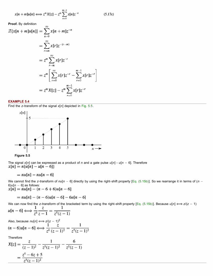
Proof. By definition

EXAMPLE 5.4Find the z-transform of the signal x[n] depicted in Fig. 5.5.

Figure 5.5

The signal x[n] can be expressed as a product of n and a gate pulse u[n] - u[n − 6]. Therefore

We cannot find the z-transform of nu[n − 6] directly by using the right-shift property [Eq. (5.15b)]. So we rearrange it in terms of (n −6)u[n − 6] as follows:

We can now find the z-transform of the bracketed term by using the right-shift property [Eq. (5.15b)]. Because u[n] z/(z − 1)

Also, because nu[n] z/(z − 1)2

Therefore

EXERCISE E5.5

Using only the fact that u[n] z/(z − 1) and the right-shift property [Eq. (5.15)], find the z-transforms ofthe signals in Figs. 5.2 and 5.3.

Answers

See Example 5.2d and Exercise E5.1a.

CONVOLUTION

The time-convolution property states that if[†]

then (time convolution)

Proof. This property applies to causal as well as noncausal sequences. We shall prove it for the more general case of noncausalsequences, where the convolution sum ranges from −∞ to ∞.

We have

Interchanging the order of summation, we have

LTID SYSTEM RESPONSE

It is interesting to apply the time-convolution property to the LTID input-output equation y[n] = x[n] * h[n]. Since from Eq. (5.14b), weknow that h[n] H[z], it follows from Eq. (5.18) that

EXERCISE E5.6Use the time-convolution property and appropriate pairs in Table 5.1 to show that u[n] * u[n − 1] = nu[n].

MULTIPLICATION BY γn (SCALING IN THE z-DOMAIN)If

then

Proof.

EXERCISE E5.7Use Eq. (5.20) to derive pairs 6 and 8 in Table 5.1 from pairs 2 and 3, respectively.

MULTIPLICATION BY nIf

then

Proof.

EXERCISE E5.8Use Eq. (5.21) to derive pairs 3 and 4 in Table 5.1 from pair 2. Similarly, derive pairs 8 and 9 from pair 6.

TIME REVERSALIf

then[†]

Proof.

Changing the sign of the dummy variable n yields

The region of convergence is also inverted, that is, if ROC of x[n] is |z| > |γ|, then, the ROC of x[−n] is |z| < 1/|γ|.

EXERCISE E5.9Use the time-reversal property and pair 2 in Table 5.1 to show that u[−n] −1/(z − 1) with the ROC |z| < 1.

INITIAL AND FINAL VALUES

For a causal x[n],

This result follows immediately from Eq. (5.9).

We can also show that if (z − 1) X (z) has no poles outside the unit circle, then[†]

All these properties of the z-transform are listed in Table 5.2.

Table 5.2: z-Transform Operations Open table as spreadsheet

Operation x[n] X[z]

Addition x1[n] + x2[n] X1[z] + X2[z]

Scalar multiplication ax[n] aX[z]

Right-shifting x[n − m]u[n − m]

x[n − m]u[n]

x[n − 1]u[n]

x[n − 2]u[n]

x[n − 3]u[n]

Left-shifting x[n + m]u[n]

x[n + 1]u[n] zmX[z] − zx[0]

x[n + 2]u[n] zmX[z] − zx[0] − zx[1]

x[n + 2]u[n] zmX[z] − zx[0] − zx[1] −zx[2]

Multiplication by γn γn x[n]u[n]

Multiplication by n nx[n]u[n]

Time convolution x1[n]*x2[n] X1[z] X2[z]

Time reversal x[−n] X[1/z]

Initial value x[0]

Final value

[†]There is also the frequency-convolution property, which states that if

[†]For complex signal x[n], the time-reversal property is modified as follows:

[†]This can be shown from the fact that

and

and

5.3 z-TRANSFORM SOLUTION OF LINEAR DIFFERENCE EQUATIONSThe time-shifting (left-shift or right-shift) property has set the stage for solving linear difference equations with constant coefficients. Asin the case of the Laplace transform with differential equations, the z-transform converts difference equations into algebraic equationsthat are readily solved to find the solution in the z domain. Taking the inverse z-transform of the z-domain solution yields the desiredtime-domain-solution. The following examples demonstrate the procedure.

EXAMPLE 5.5Solve

if the initial conditions are y[−1] = 11/6, y[−2] = 37/36, and the input x[n] = (2)−n u[n].

As we shall see, difference equations can be solved by using the right-shift or the left-shift property. Because the difference equation,Eq. (5.24), is in advance operator form, the use of the left-shift property in Eqs. (5.17a) and (5.17b) may seem appropriate for itssolution. Unfortunately, as seen from Eqs. (5.17a) and (5.17b), these properties require a knowledge of auxiliary conditions y[0], y[1],...,y[N − 1] rather than of the initial conditions y[-1], y[-2],..., y[−n], which are generally given. This difficulty can be overcome byexpressing the difference equation (5.24) in delay operator form (obtained by replacing n with n − 2) and then using the right-shiftproperty.[†] Equation (5.24) in delay operator form is

We now use the right-shift property to take the z-transform of this equation. But before proceeding, we must be clear about the meaningof a term like y[n − 1] here. Does it mean y[n − 1]u[n − 1] or y[n − 1]u[n]? In any equation, we must have some time reference n = 0,and every term is referenced from this instant. Hence, y[n − k] means y[n − k]u[n]. Remember also that although we are consideringthe situation for n ≥ 0, y[n] is present even before n = 0 (in the form of initial conditions). Now

Noting that for causal input x[n],

We obtain

In general

Taking the z-transform of Eq. (5.25) and substituting the foregoing results, we obtain

or

from which we obtain

so that

and

Therefore

and

This example demonstrates the ease with which linear difference equations with constant coefficients can be solved by z-transform.This method is general; it can be used to solve a single difference equation or a set of simultaneous difference equations of any orderas long as the equations are linear with constant coefficients.

Comment. Sometimes, instead of initial conditions y[- 1], y[-2],..., y[−n], auxiliary conditions y[0], y[1],..., y[N − 1] are given to solve adifference equation. In this case, the equation can be solved by expressing it in the advance operator form and then using the left-shiftproperty (see later: Exercise E5.11).

EXERCISE E5.10

Solve the following equation if the initial conditions y[−1] = 2, y[−2] = 0, and the input x[n] = u[n]:

Answers

EXERCISE E5.11

Solve the following equation if the auxiliary conditions are y[0] = 1, y[1] = 2, and the input x[n] = u[n]:

Answers

ZERO-INPUT AND ZERO-STATE COMPONENTS

In Example 5.5 we found the total solution of the difference equation. It is relatively easy to separate the solution into zero-input andzero-state components. All we have to do is to separate the response into terms arising from the input and terms arising from initialconditions. We can separate the response in Eq. (5.26b) as follows:

Therefore

Multiplying both sides by z2 yields

and

We expand both terms on the right-hand side into modified partial fractions to yield

and

which agrees with the result in Eq. (5.28).

EXERCISE E5.12

Solve

if the initial conditions are y[−1] = 2, y[−2] = 0, and the input x[n] = u[n]. Separate the response into zero-input and zero-state components.

Answers

5.3-1 Zero-State Response of LTID Systems: The Transfer Function

Consider an Nth-order LTID system specified by the difference equation

or

or

We now derive the general expression for the zero-state response: that is, the system response to input x[n] when all the initialconditions y[-1] = y[-2] = ... = y[−N] = 0 (zero state). The input x[n] is assumed to be causal so that x[−1] = x[-2] = ... = x[−N] = 0.

Equation (5.31c) can be expressed in the delay operator form as

Because y[−r] = x[−r] = 0 for r = 1, 2, ..., N

Now the z-transform of Eq. (5.31d) is given by

Multiplication of both sides by zN yields

Therefore

We have shown in Eq. (5.19) that Y[z] = X[z]H[z]. Hence, it follows that

As in the case of LTIC systems, this result leads to an alternative definition of the LTID system transfer function as the ratio of Y[z] toX[z] (assuming all initial conditions zero).

ALTERNATE INTERPRETATION OF THE z-TRANSFORMSo far we have treated the z-transform as a machine, which converts linear difference equations into algebraic equations. There is nophysical understanding of how this is accomplished or what it means. We now discuss more intuitive interpretation and meaning of thez-transform.

In Chapter 3, Eq. (3.71a), we showed that LTID system response to an everlasting exponential zn is H[z]zn. If we could express everydiscrete-time signal as a linear combination of everlasting exponentials of the form zn, we could readily obtain the system response toany input. For example, if

the response of an LTID system to this input is given by

Unfortunately, a very small class of signals can be expressed in the form of Eq. (5.36a). However, we can express almost all signals ofpractical utility as a sum of everlasting exponentials over a continuum of values of z. This is precisely what the z-transform in Eq. (5.2)does.

Figure 5.6: The transformed representation of an LTID system.

Invoking the linearity property of the z-transform, we can find the system response y[n] to input x[n] in the Eq. (5.37) as[†]

Clearly

This viewpoint of finding the response of LTID system is illustrated in Fig. 5.6a. Just as in continuous-time systems, we can modeldiscrete-time systems in the transformed manner by representing all signals by their z-transforms and all system components (orelements) by their transfer functions, as shown in Fig. 5.6b.

The result Y[z]=H[z]X[z] greatly facilitates derivation of the system response to a given input. We shall demonstrate this assertion by anexample.

EXAMPLE 5.6Find the response y[n] of an LTID system described by the difference equation

or

for the input x [n]=(−2)−n u[n] and with all the initial conditions zero (system in the zero state).

From the difference equation we find

For the input x[n]=(−2)−n u[n]=[(−2)−1]nu(n)=(−0.5)nu[n]

and

Therefore

so that

and

EXAMPLE 5.7: (The Transfer Function of a Unit Delay)Show that the transfer function of a unit delay is 1/z.

If the input to the unit delay is x[n]u[n], then its output (Fig. 5.7) is given by

Figure 5.7: Ideal unit delay and its transfer function.

The z-transform of this equation yields [see Eq. (5.15a)]

It follows that the transfer function of the unit delay is

EXERCISE E5.13

A discrete-time system is described by the following transfer function:

a. Find the system response to input x [n]=3-(n+1)u[n] if all initial conditions arezero.

b. Write the difference equation relating the output y[n] to input x[n] for this system.

Answers

a.

b.

5.3-2 Stability

Equation (5.34) shows that the denominator of H[z] is Q[z], which is apparently identical to the characteristic polynomial Q[γ] defined inChapter 3. Does this mean that the denominator of H[z] is the characteristic polynomial of the system? This may or may not be thecase: if P[z] and Q[z] in Eq. (5.34) have any common factors, they cancel out, and the effective denominator of H[z] is not necessarilyequal to Q[z]. Recall also that the system transfer function H[z], like h[n], is defined in terms of measurements at the externalterminals. Consequently, H[z] and h[n] are both external descriptions of the system. In contrast, the characteristic polynomial Q[z] is aninternal description. Clearly, we can determine only external stability, that is, BIBO stability, from H[z]. If all the poles of H[z] are within

the unit circle, all the terms in h[z] are decaying exponentials, and as shown in Section 3.10, h[n] is absolutely summable.Consequently, the system is BIBO stable. Otherwise the system is BIBO unstable.

If P[z] and Q[z] do not have common factors, then the denominator of H[z] is identical to Q[z].[†] The poles of H[z] are thecharacteristic roots of the system. We can now determine internal stability. The internal stability criterion in Section 3.10-1 can berestated in terms of the poles of H[z], as follows.

1. An LTID system is asymptotically stable if and only if all the poles of its transfer function H[z] are within the unit circle. Thepoles may be repeated or simple.

2. An LTID system is unstable if and only if either one or both of the following conditions exist: (i) at least one pole of H[z] isoutside the unit circle; (ii) there are repeated poles of H[z] on the unit circle.

3. An LTID system is marginally stable if and only if there are no poles of H[z] outside the unit circle, and there are somesimple poles on the unit circle.

EXERCISE E5.14Show that an accumulator whose impulse response is h[n]=u[n] is marginally stable but BIBO unstable.

5.3-3 Inverse Systems

If H[z] is the transfer function of a system S, then Si, its inverse system has a transfer function Hi[z] given by

This follows from the fact the inverse system Si undoes the operation of S. Hence, if H[z] is placed in cascade with Hi[z], the transferfunction of the composite system (identity system) is unity. For example, an accumulator, whose transfer function is H[z]=z/(z − 1) anda backward difference system whose transfer function is Hi[z]=(z − 1)/z are inverse of each other. Similarly if

its inverse system transfer function is

as required by the property H[z]Hi[z]=1. Hence, it follows that

EXERCISE E5.15Find the impulse response of an accumulator and the backward difference system. Show that the convolution of the two impulseresponses yields δ[n].

[†]Another approach is to find y[0], y[1], y[2],..., y[N − 1] from y[−1], y[-2],..., y[−n] iteratively, as in Section 3.5-1, and then apply theleft-shift property to Eq. (5.24).

[†]In computing y[n], the contour along which the integration is performed is modified to consider the ROC of X[z] as well as H[z]. Weignore this consideration in this intuitive discussion.

[†]There is no way of determining whether there were common factors in P[z] and Q[z] that were canceled out because in ourderivation of H[z], we generally get the final result after the cancellations are already effected. When we use internal description of thesystem to derive Q[z], however, we find pure Q[z] unaffected by any common factor in P[z].

5.4 SYSTEM REALIZATIONBecause of the similarity between LTIC and LTID systems, conventions for block diagrams and rules of interconnection for LTID areidentical to those for continuous-time (LTIC) systems. It is not necessary to rederive these relationships. We shall merely restate them torefresh the reader's memory.

The block diagram representation of the basic operations such as an adder a scalar multiplier, unit delay, and pick off points wereshown in Fig. 3.11. In our development, the unit delay, which was represented by a box marked D in Fig. 3.11, will be represented byits transfer function 1/z. All the signals will also be represented in terms of their z-transforms. Thus, the input and the output will belabeled X[z] and Y[z], respectively.

When two systems with transfer functions H1[z] and H2[z] are connected in cascade (as in Fig. 4.18b), the transfer function of thecomposite system is H1[z]H2[z]. If the same two systems are connected in parallel (as in Fig. 4.18c), the transfer function of thecomposite system is H1[z]H2[z]. For a feedback system (as in Fig. 4.18d), the transfer function is G[z]/(1 + G[z]H[z]).

We now consider a systematic method for realization (or simulation) of an arbitrary Nth-order LTID transfer function. Since realization isbasically a synthesis problem, there is no unique way of realizing a system. A given transfer function can be realized in many differentways. We present here the two forms of direct realization. Each of these forms can be executed in several other ways, such as cascadeand parallel. Furthermore, a system can be realized by the transposed version of any known realization of that system. This artificedoubles the number of system realizations. A transfer function H[z] can be realized by using time delays along with adders andmultipliers.

We shall consider a realization of a general Nth-order causal LTID system, whose transfer function is given by

This equation is identical to the transfer function of a general Nth-order proper LTIC system given in Eq. (4.60). The only difference isthat the variable z in the former is replaced by the variable s in the latter. Hence, the procedure for realizing an LTID transfer functionis identical to that for the LTIC transfer function with the basic element 1/s (integrator) replaced by the element 1/z (unit delay). Thereader is encouraged to follow the steps in Section 4.6 and rederive the results for the LTID transfer function in Eq. (5.41). Here weshall merely reproduce the realizations from Section 4.6 with integrators (1/s) replaced by unit delays (1/z). The direct form I (DFI) isshown in Fig. 5.8a, the canonic direct form (DFII) is shown in Fig. 5.8b and the transpose of canonic direct is shown in Fig. 5.8c. TheDFII and its transpose are canonic because they require N delays, which is the minimum number needed to implement an Nth-orderLTID transfer function in Eq. (5.41). In contrast, the form DFI is a noncanonic because it generally requires 2N delays. The DFIIrealization in Fig. 5.8b is also called a canonic direct form.

Figure 5.8: Realization of an Nth-order causal LTID system transfer function by using (a) DFI, (b) canonic direct (DFII), and (c) thetranspose form of DFII.

EXAMPLE 5.8Find the canonic direct and the transposed canonic direct realizations of the following transfer functions.

i.

ii.

iii.

iv.

All four of these transfer functions are special cases of H[z] in Eq. (5.41).

i.

For this case, the transfer function is of the first order (N=1); therefore, we need only one delay for its realization. Thefeedback and feedforward coefficients are

We use Fig. 5.8 as our model and reduce it to the case of N=1. Figure 5.9a shows the canonic direct (DFII) form, and Fig.5.9b its transpose. The two realizations are almost the same. The minor difference is that in the DFII form, the gain 2 isprovided at the output, and in the transpose, the same gain is provided at the input.

Figure 5.9: Realization of transfer function 2/(z + 5): (a) canonic direct form and (b) its transpose.

In a similar way, we realize the remaining transfer functions.

ii.

In this case also, the transfer function is of the first order (N=1); therefore, we need only one delay for its realization. Thefeedback and feedforward coefficients are

Figure 5.10 illustrates the canonic direct and its transpose for this case.[†]

Figure 5.10: Realization of (4z + 28)/(z + 1): (a) canonic direct form and (b) its transpose.

iii.

Here N=1 and b0=1, b1=0 and a1=7. Figure 5.11 shows the direct and the transposed realizations. Observe that therealizations are almost alike.

Figure 5.11: Realization of z/(z + 7): (a) canonic direct form and (b) its transpose.

iv.

This is a second-order system (N = 2) with b0 = 0, b1 = 4, b2 = 28, a1 = 6, a2 = 5. Figure 5.12 shows the canonic directand transposed canonic direct realizations.

Figure 5.12: Realization of (4z + 28)/(z2 + 6z + 5): (a) canonic direct form and (b) its transpose.

EXERCISE E5.16Realize the transfer function

CASCADE AND PARALLEL REALIZATIONS, COMPLEX AND REPEATED POLES

The considerations and observations for cascade and parallel realizations as well as complex and multiple poles are identical to thosediscussed for LTIC systems in Section 4.6-3.

EXERCISE E5.17Find canonic direct realizations of the following transfer function by using the cascade and parallel forms. The specific cascadedecomposition is as follows:

REALIZATION OF FINITE IMPULSE RESPONSE (FIR) FILTERS

So far we have been quite general in our development of realization techniques. They can be applied to infinite impulse response (IIR)or FIR filters. For FIR filters, the coefficients ai = 0 for all i ≠ 0.[†] Hence, FIR filters can be readily implemented by means of theschemes developed so far by eliminating all branches with ai coefficients. The condition ai = 0 implies that all the poles of a FIR filterare at z = 0.

EXAMPLE 5.9Realize H [z] = (z3 + 4z2 + 5z + 2)/z3 using canonic direct and transposed forms.

We can express H[z] as

For H[z], b0 = 1, b1 = 4, b2 = 5, and b3 = 2. Hence, we obtain the canonic direct realization, shown in Fig. 5.13a. We have shown thehorizontal orientation because it is easier to see that this filter is basically a tapped delay line. That is why this structure is also knownas a tapped delay line or transversal filter. Figure 5.13b shows the corresponding transposed implementation.

Figure 5.13: Realization of (z3 + 4z2 + 5z + 2)/z3.

DO ALL REALIZATIONS LEAD TO THE SAME PEREORMANCE?

For a given transfer function, we have presented here several possible different realizations (DFI, canonic form DFII, and its transpose).There are also cascade and parallel versions, and there are many possible grouping of the factors in the numerator and thedenominator of H[z], leading to different realizations. We can also use various combinations of these forms in implementing differentsubsections of a system. Moreover, the transpose of each version doubles the number. However, this discussion by no means exhaustsall the possibilities. Transforming variables affords limitless potential realizations of the same transfer function.

Theoretically, all these realizations are equivalent; that is, they lead to the same transfer function. This, however, is true only when weimplement them with infinite precision. In practice, finite wordlength restriction causes each realization to behave differently in terms ofsensitivity to parameter variation, stability, frequency response distortion error, and so on. These effects are serious for higher-ordertransfer functions, which require correspondingly higher numbers of delay elements. The finite wordlength errors that plague theseimplementations are coefficient quantization, overflow errors, and round-off errors. From a practical viewpoint, parallel and cascadeforms using low-order filters minimize the effects of finite wordlength. Parallel and certain cascade forms are numerically less sensitivethan the canonic direct form to small parameter variations in the system. In the canonic direct form structure with large N, a smallchange in a filter coefficient due to parameter quantization results in a large change in the location of the poles and the zeros of thesystem. Qualitatively, this difference can be explained by the fact that in a direct form (or its transpose), all the coefficients interact witheach other, and a change in any coefficient will be magnified through its repeated influence from feedback and feedforward connections.In a parallel realization, in contrast, a change in a coefficient will affect only a localized segment; the case of a cascade realization issimilar. For this reason, the most popular technique for minimizing finite wordlength effects is to design filters by using cascade orparallel forms employing low-order filters. In practice, high-order filters are realized by using multiple second-order sections in cascade,because second-order filters are not only easier to design but are less susceptible to coefficient quantization and round-off errors andtheir implementations allow easier data word scaling to reduce the potential overflow effects of data word size growth. A cascadedsystem using second-order building blocks usually requires fewer multiplications for a given filter frequency response.[1]

There are several ways to pair the poles and zeros of an Nth-order H[z] into a cascade of second-order sections, and several ways toorder the resulting sections. Quantizing error will be different for each combination. Although several papers published provideguidelines in predicting and minimizing finite wordlength errors, it is advisable to resort to computer simulation of the filter design. Thisway, one can vary filter hardware characteristic, such as coefficient wordlengths, accumulator register sizes, sequencing of cascadedsections, and input signal sets. Such an approach is both reliable and economical.[1]

[†]Transfer functions with N=M may also be expressed as a sum of a constant and a strictly proper transfer function. For example,

Hence, this transfer function can also be realized as two transfer functions in parallel.

[†]This statement is true for all i ≠ 0 because a0 is assumed to be unity.

[1]Lyons, R. G. Understanding Digital Signal Processing. Addison-Wesley, Reading, MA, 1997.

5.5 FREQUENCY RESPONSE OF DISCRETE-TIME SYSTEMS

For (asymptotically or BIBO-stable) continuous-time systems, we showed that the system response to an input ejωt is H(jω)ejωt and

that the response to an input cos ωt is |H(jω)| cos [ωt + ∠H(jω)]. Similar results hold for discrete-time systems. We now show that foran (asymptotically or BIBO-stable) LTID system, the system response to an input ejΩn is H[ejΩ]ejΩn and the response to an input cosΩn is |H[ejΩ]| cos (Ωn + ∠H[ejΩ]).

The proof is similar to the one used for continuous-time systems. In Section 3.8-3, we showed that an LTID system response to an(everlasting) exponential zn is also an (everlasting) exponential H[z]zn. This result is valid only for values of z for which H[z], as definedin Eq. (5.14a), exists (converges). As usual, we represent this input-output relationship by a directed arrow notation as

Setting z = ejΩ in this relationship yields

Noting that cos Ωn is the real part of ejΩn, use of Eq. (3.66b) yields

Expressing H[ejΩ] in the polar form

Eq. (5.44) can be expressed as

In other words, the system response y[n] to a sinusoidal input cos Ωn is given by

Following the same argument, the system response to a sinusoid cos (Ωn + θ) is

This result is valid only for BIBO-stable or asymptotically stable systems. The frequency response is meaningless for BIBO-unstablesystems (which include marginally stable and asymptotically unstable systems). This follows from the fact that the frequency response inEq. (5.43) is obtained by setting z = ejΩ in Eq. (5.42). But, as shown in Section 3.8-3 [Eqs. (3.71)], the relationship (5.42) applies onlyfor values of z for which H[z] exists. For BIBO unstable systems, the ROC for H[z] does not include the unit circle where z = ejΩ. Thismeans, for BIBO-unstable systems, that H[z] is meaningless when z = ejΩ[†]

This important result shows that the response of an asymptotically or BIBO-stable LTID system to a discrete-time sinusoidal input offrequency Ω is also a discrete-time sinusoid of the same frequency. The amplitude of the output sinusoid is |H[ejΩ]| times the inputamplitude, and the phase of the output sinusoid is shifted by ∠H[ejΩ] with respect to the input phase. Clearly |H[ejΩ]| is the amplitudegain, and a plot of |H[ejΩ]| versus Ω is the amplitude response of the discrete-time system. Similarly, ∠H[ejΩ] is the phase response ofthe system, and a plot of ∠H[ejΩ] versus Ω shows how the system modifies or shifts the phase of the input sinusoid. Note that H[ejΩ]incorporates the information of both amplitude and phase responses and therefore is called the frequency responses of the system.

STEADY-STATE RESPONSE TO CAUSAL SINUSOIDAL INPUT

As in the case of continuous-time systems, we can show that the response of an LTID system to a causal sinusoidal input cos Ωn u[n]is y[n] in Eq. (5.46a), plus a natural component consisting of the characteristic modes (see Prob. 5.5-6). For a stable system, all themodes decay exponentially, and only the sinusoidal component in Eq. (5.46a) persists. For this reason, this component is called thesinusoidal steady-state response of the system. Thus, yss[n], the steady-state response of a system to a causal sinusoidal input cosΩn u[n], is

SYSTEM RESPONSE TO SAMPLED CONTINUOUS-TIME SINUSOIDS

So far we have considered the response of a discrete-time system to a discrete-time sinusoid cos Ωn (or exponential ejΩn). In practice,the input may be a sampled continuous-time sinusoid cos ωt (or an exponential ejωt). When a sinusoid cos ωt is sampled withsampling interval T, the resulting signal is a discrete-time sinusoid cos ωnT, obtained by setting t = nT in cos ωt. Therefore, all theresults developed in this section apply if we substitute ωT for Ω:

EXAMPLE 5.10

For a system specified by the equation

find the system response to the input

a. 1n = 1

b.

c. a sampled sinusoid cos 1500t with sampling interval T = 0.001

The system equation can be expressed as

Therefore, the transfer function of the system is

The frequency response is

Therefore

and

The amplitude response |H[ejΩ]| can also be obtained by observing that |H|2=HH*. Therefore

From Eq. (5.48) it follows that

which yields the result found earlier in Eq. (5.49a)

Figure 5.14 shows plots of amplitude and phase response as functions of Ω. We now compute the amplitude and the phase responsefor the various inputs.

a. x[n] = 1n = 1

Since 1n=(ejΩ)n with Ω = 0, the amplitude response is H[ej0]. From Eq. (5.49a) we obtain

Therefore

These values also can be read directly from Fig. 5.14a and 5.14b, respectively, corresponding to Ω = 0. Therefore, thesystem response to input 1 is

b. x[n] = cos[(π/6)n −0.2]

Here Ω = π/6. According to Eqs. (5.49)

These values also can be read directly from Fig. 5.14a and 5.14b, respectively, corresponding to Ω=π/6. Therefore

Figure 5.15 shows the input x[n] and the corresponding system response.

Figure 5.15: Sinusoidal input and the corresponding output of the LTID system.

c. A sinusoid cos 1500t sampled every T seconds (t = nT) results in a discrete-time sinusoid

For T = 0.001, the input is

In this case, Ω =1.5. According to Eqs. (5.49a) and (5.49b),

These values also could be read directly from Fig. 5.14 corresponding to Ω =1.5. Therefore

Figure 5.14: Frequency response of the LTID system.

COMPUTER EXAMPLE C5.1Using MATLAB, find the frequency response of the system in Example 5.10.

Figure C5.1

Comment. Figure 5.14 shows plots of amplitude and phase response as functions of Ω. These plots as well as Eqs. (5.49) indicate thatthe frequency response of a discrete-time system is a continuous (rather than discrete) function of frequency Ω. There is nocontradiction here. This behavior is merely an indication of the fact that the frequency variable Ω is continuous (takes on all possiblevalues) and therefore the system response exists at every value of Ω.

EXERCISE E5.18

For a system specified by the equation

find the amplitude and the phase response. Find the system response to sinusoidal input cos (100t − (π/3))sampled every T = 0.5 ms.

Answers

>> Omega = linspace(-pi,pi,400);>> H = tf ( [1 0], [1 -0.8],-1);>> H_Omega = squeeze (freqresp (H,Omega));>> subplot (2,1,1); plot (Omega, abs(H_Omega), 'k'); axis tight;>> xlabel ('\Omega'); ylabel('|H[e^{j \Omega}]|');>> subplot (2,1,2); plot (Omega, angle (H_Omega) * 180/pi, 'k'); axis tight;>> xlabel ('\Omega'); ylabel ('\angle H[e^{j \Omega}] [deg]');

EXERCISE E5.19Show that for an ideal delay (H[z]=1/z), the amplitude response |H[ejπ]|=1, and the phase response ∠H[ejΩ]= −Ω. Thus, a pure timedelay does not affect the amplitude gain of sinusoidal input, but it causes a phase shift (delay) of Ω radians in a discrete sinusoid offrequency Ω. Thus, for an ideal delay, the phase shift of the output sinusoid is proportional to the frequency of the input sinusoid (linearphase shift).

5.5-1 The Periodic Nature of the Frequency Response

In Example 5.10 and Fig. 5.14, we saw that the frequency response H[ejΩ] is a periodic function of Ω. This is not a coincidence. Unlikecontinuous-time systems, all LTID systems have periodic frequency response. This is seen clearly from the nature of the expression ofthe frequency response of an LTID system. Because e± j2πm=1 for all integer values of m [see Eq. (B.12)],

Therefore the frequency response H[ejΩ] is a periodic function of Ω with a period 2π. This is the mathematical explanation of theperiodic behavior. The physical explanation that follows provides a much better insight into the periodic behavior.

NONUNIQUENESS OF DISCRETE-TIME SINUSOID WAVEFORMS

A continuous-time sinusoid cos ωt has a unique waveform for every real value of ω in the range 0 to ∞. Increasing ω results in asinusoid of ever increasing frequency. Such is not the case for the discrete-time sinusoid cos Ωn because

and

This shows that the discrete-time sinusoids cos Ωn (and exponentials ejΩn) separated by values of Ω in integral multiples of 2π areidentical. The reason for the periodic nature of the frequency response of an LTID system is now clear. Since the sinusoids (orexponentials) with frequencies separated by interval 2π are identical, the system response to such sinusoids is also identical and,hence, is periodic with period 2π.

This discussion shows that the discrete-time sinusoid cos Ωn has a unique waveform only for the values of Ω in the range −π to π.This band is called the fundamental band. Every frequency Ω, no matter how large, is identical to some frequency, Ωa, in thefundamental band (− π ≤ Ωa < π), where

The integer m can be positive or negative. We use Eq. (5.58) to plot the fundamental band frequency Ωa versus the frequency Ω of asinusoid (Fig. 5.16a). The frequency Ωa is modulo 2π value of Ω.

All these conclusions are also valid for exponential ejΩn.

ALL DISCRETE-TIME SIGNALS ARE INHERENTLY BANDLIMITEDThis discussion leads to the surprising conclusion that all discrete-time signals are inherently bandlimited, with frequencies lying in therange −π to π radians per sample. In terms of frequency where is in cycles per sample, all frequencies separatedby an integer number are identical. For instance, all discrete-time sinusoids of frequencies 0.3, 1.3, 2.3, ...cycles per sample areidentical. The fundamental range of frequencies is −0.5 to 0.5 cycles per sample.

Any discrete-time sinusoid of frequency beyond the fundamental band, when plotted, appears and behaves, in every way, like asinusoid having its frequency in the fundamental band. It is impossible to distinguish between the two signals. Thus, in a basic sense,discrete-time frequencies beyond |Ω| = π or do not exist. Yet, in a "mathematical" sense, we must admit the existence ofsinusoids of frequencies beyond Ω = π. What does this mean?

A MAN NAMED ROBERTTo give an analogy, consider a fictitious person Mr. Robert Thompson. His mother calls him Robby; his acquaintances call him Bob, hisclose friends call him by his nickname, Shorty. Yet, Robert, Robby, Bob, and Shorty are one and the same person. However, we cannotsay that only Mr. Robert Thompson exists, or only Robby exists, or only Shorty exists, or only Bob exists. All these four persons exist,although they are one and the same individual. In a same way, we cannot say that the frequency π/2 exists and frequency 5π/2 doesnot exist; they are both the same entity, called by different names.

It is in this sense that we have to admit the existence of frequencies beyond the fundamental band. Indeed, mathematical expressionsin frequency-domain automatically cater to this need by their built-in periodicity. As seen earlier, the very structure of the frequencyresponse is 2π periodic. We shall also see later, in Chapter 9, that discrete-time signal spectra are also 2π periodic.

Admitting the existence of frequencies beyond π also serves mathematical and computational convenience in digital signal processingapplications. Values of frequencies beyond π may also originate naturally in the process of sampling continuous-time sinusoids.Because there is no upper limit on the value of ω, there is no upper limit on the value of the resulting discrete-time frequency Ω = ωTeither.[†]

The highest possible frequency is π and the lowest frequency is 0 (dc or constant). Clearly, the high frequencies are those in thevicinity of Ω = (2m + 1)π and the low frequencies are those in the vicinity of Ω = 2πm for all positive or negative integer values of m.

FURTHER REDUCTION IN THE FREQUENCY RANGEBecause cos (−Ωn + θ) = cos (Ωn − θ), a frequency in the range −π to 0 is identical to the frequency (of the same magnitude) in therange 0 to π (but with a change in phase sign). Consequently the apparent frequency for a discrete-time sinusoid of any frequency isequal to some value in the range 0 to π. Thus, cos (8.7πn + θ) = cos (0.7πn + θ), and the apparent frequency is 0.7π. Similarly,

Hence, the frequency 9.6π is identical (in every respect) to frequency −0.4π, which, in turn, is equal (within the sign of its phase) tofrequency 0.4π. In this case, the apparent frequency reduces to |Πa|=0.4π. We can generalize the result to say that the apparentfrequency of a discrete-time sinusoid Ω is |Ωa|, as found from Eq. (5.58), and if Ωa < 0, there is a phase reversal. Figure 5.16b plots Ωversus the apparent frequency |Ωa|. The shaded bands represent the ranges of Ω for which there is a phase reversal, whenrepresented in terms of |Ωa|. For example, the apparent frequency for both the sinusoids cos (2.4π + θ) and cos (3.6π + θ) is |Ωa| =0.4π, as seen from Fig. 5.16b. But 2.4π is in a clear band and 3.6π is in a shaded band. Hence, these sinusoids appear as cos (0.4π+ θ) and cos (0.4π − θ), respectively.

Figure 5.16: (a) Actual frequency versus (b) apparent frequency.

Although every discrete-time sinusoid can be expressed as having frequency in the range from 0 to π, we generally use the frequencyrange from −π to π instead of 0 to π for two reasons. First, exponential representation of sinusoids with frequencies in the range 0 toπ requires a frequency range −π to π. Second, even when we are using trigonometric representation, we generally need thefrequency range −π to π to have exact identity (without phase reversal) of a higher-frequency sinusoid.

For certain practical advantages, in place of the range −π to π, we often use other contiguous ranges of width 2π. The range 0 to 2π,for instance, is used in many applications. It is left as an exercise for the reader to show that the frequencies in the range from π to2π are identical to those in the range from −π to 0.

EXAMPLE 5.11Express the following signals in terms of their apparent frequencies.

a. cos (0.5πn + θ)

b. cos (1.6πn + θ)

c. sin (1.6πn + θ)

d. cos (2.3πn + θ)

e. cos (34.699n + θ)

a. Ω = 0.5π is in the reduced range already. This is also apparent from Fig. 5.16a or 5.16b. Because Ωa = 0.5π, and thereis no phase reversal, and the apparent sinusoid is cos (0.5πn + θ).

b. We express 1.6π = −0.4π + 2π so that Ωa = −0.4 and |Ωa| = 0.4. Also, Ωa is negative, implying sign change for thephase. Hence, the apparent sinusoid is cos (0.4πn − ΰ). This fact is also apparent from Fig. 5.16b.

c. We first convert the sine form to cosine form as sin (1.6πn + θ) = cos (1.6πn − (π/2) θ). In part (b) we found Ωa =−0.4π. Hence, the apparent sinusoid is cos (0.4πn + (π/2) + θ) = −sin (0.4πn − θ). In this case, both the phase andthe amplitude change signs.

d. 2.3π = 0.3π + 2π so that Ωa = 0.3π. Hence, the apparent sinusoid is cos (0.3π n + θ).

e. We have 34.699 = -3 + 6(2π). Hence, Ωa = −3, and the apparent frequency |Ωa| = 3 rad/sample. Because Ωa isnegative, there is a sign change of the phase. Hence, the apparent sinusoid is cos (3n − θ).

EXERCISE E5.20Show that the sinusoids having frequencies Ω of

a. 2π

b. 3π

c. 5π

d. 3.2π

e. 22.1327

f. π + 2

can be expressed, respectively, as sinusoids of frequencies

a. 0

b. π

c. π

d. 0.8π

e. 3

f. π - 2

Show that in cases (d), (e), and (f), phase changes sign.

5.5-2 Aliasing and Sampling Rate

The nonuniqueness of discrete-time sinusoids and the periodic repetition of the same waveforms at intervals of 2π may seeminnocuous, but in reality it leads to a serious problem for processing continuous-time signals by digital filters. A continuous-time sinusoidcos ωt sampled every T seconds (t=nT) results in a discrete-time sinusoid cos ωnT, which is cos Ωn with Ω=ωT. The discrete-timesinusoids cos Ωn have unique waveforms only for the values of frequencies in the range ω < π or ωT < π. Therefore samples ofcontinuous-time sinusoids of two (or more) different frequencies can generate the same discrete-time signal, as shown in Fig. 5.17. Thisphenomenon is known as aliasing because through sampling, two entirely different analog sinusoids take on the same "discrete-time"identity.[†]

Figure 5.17: Demonstration of aliasing effect.

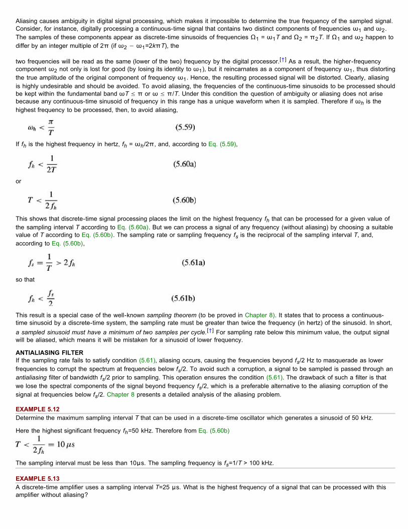
Aliasing causes ambiguity in digital signal processing, which makes it impossible to determine the true frequency of the sampled signal.Consider, for instance, digitally processing a continuous-time signal that contains two distinct components of frequencies ω1 and ω2.The samples of these components appear as discrete-time sinusoids of frequencies Ω1 = ω1T and Ω2 = π2T. If Ω1 and ω2 happen todiffer by an integer multiple of 2π (if ω2 − ω1=2kπT), the

two frequencies will be read as the same (lower of the two) frequency by the digital processor.[†] As a result, the higher-frequencycomponent ω2 not only is lost for good (by losing its identity to ω1), but it reincarnates as a component of frequency ω1, thus distortingthe true amplitude of the original component of frequency ω1. Hence, the resulting processed signal will be distorted. Clearly, aliasingis highly undesirable and should be avoided. To avoid aliasing, the frequencies of the continuous-time sinusoids to be processed shouldbe kept within the fundamental band ωT ≤ π or ω ≤ π/T. Under this condition the question of ambiguity or aliasing does not arisebecause any continuous-time sinusoid of frequency in this range has a unique waveform when it is sampled. Therefore if ωh is thehighest frequency to be processed, then, to avoid aliasing,

If fh is the highest frequency in hertz, fh = ωh/2π, and, according to Eq. (5.59),

or

This shows that discrete-time signal processing places the limit on the highest frequency fh that can be processed for a given value ofthe sampling interval T according to Eq. (5.60a). But we can process a signal of any frequency (without aliasing) by choosing a suitablevalue of T according to Eq. (5.60b). The sampling rate or sampling frequency fs is the reciprocal of the sampling interval T, and,according to Eq. (5.60b),

so that

This result is a special case of the well-known sampling theorem (to be proved in Chapter 8). It states that to process a continuous-time sinusoid by a discrete-time system, the sampling rate must be greater than twice the frequency (in hertz) of the sinusoid. In short,a sampled sinusoid must have a minimum of two samples per cycle.[†] For sampling rate below this minimum value, the output signalwill be aliased, which means it will be mistaken for a sinusoid of lower frequency.

ANTIALIASING FILTERIf the sampling rate fails to satisfy condition (5.61), aliasing occurs, causing the frequencies beyond fs/2 Hz to masquerade as lowerfrequencies to corrupt the spectrum at frequencies below fs/2. To avoid such a corruption, a signal to be sampled is passed through anantialiasing filter of bandwidth fs/2 prior to sampling. This operation ensures the condition (5.61). The drawback of such a filter is thatwe lose the spectral components of the signal beyond frequency fs/2, which is a preferable alternative to the aliasing corruption of thesignal at frequencies below fs/2. Chapter 8 presents a detailed analysis of the aliasing problem.

EXAMPLE 5.12Determine the maximum sampling interval T that can be used in a discrete-time oscillator which generates a sinusoid of 50 kHz.

Here the highest significant frequency fh=50 kHz. Therefore from Eq. (5.60b)

The sampling interval must be less than 10μs. The sampling frequency is fs=1/T > 100 kHz.

EXAMPLE 5.13A discrete-time amplifier uses a sampling interval T=25 μs. What is the highest frequency of a signal that can be processed with thisamplifier without aliasing?

From Eq. (5.60a)

[†]This may also be argued as follows. For BIBO-unstable systems, the zero-input response contains nondecaying natural mode termsof the form cos Ωn or γ n cos Ωn (γ > 1). Hence, the response of such a system to a sinusoid cos Ωn will contain not just the sinusoidof frequency Ω but also nondecaying natural modes, rendering the concept of frequency response meaningless. Alternately, we canargue that when z = ejΩ, a BIBO-unstable system violates the dominance condition |γi| < |ejΩ| for all i, where γi represents ithcharacteristic root of the system (see Section 4.3).

[†]However, if Ω goes beyond π, the resulting aliasing reduces the apparent frequency to Ωa < π.

[†]Figure 5.17 shows samples of two sinusoids cos 12πt and cos 2πt taken every 0.2 second. The corresponding discrete-timefrequencies (Ω=ωT=0.2ω) are cos 2.4π and cos 0.4π. The apparent frequency of 2.4π is 0.4π, identical to the discrete-timefrequency corresponding to the lower sinusoid. This shows that the samples of both these continuous-time sinusoids at 0.2-secondintervals are identical, as verified from Fig. 5.17.

[†]In the case shown in Fig. 5.17, ω1=12π, ω2=2π, and T=0.2. Hence, ω2 − ω1=10πT=2π, and the two frequencies are read as thesame frequency Ω=0.4π by the digital processor.

[†]Strictly speaking, we must have more than two samples per cycle.

5.6 FREQUENCY RESPONSE FROM POLE-ZERO LOCATIONThe frequency responses (amplitude and phase responses) of a system are determined by pole-zero locations of the transfer functionH[z]. Just as in continuous-time systems, it is possible to determine quickly the amplitude and the phase response and to obtainphysical insight into the filter characteristics of a discrete-time system by using a graphical technique. The general Nth-order transferfunction H[z] in Eq. (5.34) can be expressed in factored form as

We can compute H[z] graphically by using the concepts discussed in Section 4.10. The directed line segment from zi to z in thecomplex plane (Fig. 5.18a) represents the complex number z − zi. The length of this segment is |z − zi| and its angle with thehorizontal axis is ∠(z − zi).

Figure 5.18: Vector representations of (a) complex numbers and (b) factors of H[z].

To compute the frequency response H[ejΩ] we evaluate H[z] at z = ejΩ. But for z = ejΩ, |z| = 1 and ∠z = Ω so that z = ejΩ representsa point on the unit circle at an angle Ω with the horizontal. We now connect all zeros (z1, z2, ..., zN) and all poles (y1, y2, ..., yN) to

the point ejΩ, as indicated in Fig. 5.18b. Let r1,r2,...,rN be the lengths and f1 f2, ..., φN be the angles, respectively, of the straight lines

connecting z1, z2, ..., zN to the point ejΩ. Similarly, let d1, d2,..., dN be the lengths and ?1, ?2,..., θN be the angles, respectively, of the

lines connecting y1, y2,...,yN to ejΩ. Then

Therefore (assuming b0 < 0)

and

In this manner, we can compute the frequency response H[ejΩ] for any value of Ω by selecting the point on the unit circle at an angleΩ. This point is ejΩ. To compute the frequency response H[ejΩ], we connect all poles and zeros to this point and use the foregoingequations to determine |H[ejΩ]| and ∠H[ejΩ]. We repeat this procedure for all values of Ω from 0 to π to obtain the frequencyresponse.

CONTROLLING GAIN BY PLACEMENT OF POLES AND ZEROSThe nature of the influence of pole and zero locations on the frequency response is similar to that observed in continuous-time systems,with minor differences. In place of the imaginary axis of the continuous-time systems, we have the unit circle in the discrete-time case.The nearer the pole (or zero) is to a point ejΩ (on the unit circle) representing some frequency Ω, the more influence that pole (or zero)wields on the amplitude response at that frequency because the length of the vector joining that pole (or zero) to the point ejΩ is small.The proximity of a pole (or a zero) has similar effect on the phase response. From Eq. (5.65a), it is clear that to enhance the amplituderesponse at a frequency Ω, we should place a pole as close as possible to the point ejΩ (which is on the unit circle).[†] Similarly, tosuppress the amplitude response at a frequency Ω, we should place a zero as close as possible to the point ejΩ on the unit circlePlacing repeated poles or zeros will further enhance their influence.

Total suppression of signal transmission at any frequency can be achieved by placing a zero on the unit circle at a point correspondingto that frequency. This observation is used in the notch (bandstop) filter design.

Placing a pole or a zero at the origin does not influence the amplitude response because the length of the vector connecting the originto any point on the unit circle is unity. However, a pole (or a zero) at the origin adds angle −Ω (or Ω) to ∠H[ejΩ]. Hence, the phasespectrum −Ω (or Ω) is a linear function of frequency and therefore represents a pure time delay (or time advance) of T seconds (seeExercise E5.19). Therefore, a pole (a zero) at the origin causes a time delay (or a time advance) of T seconds in the response. There isno change in the amplitude response.

For a stable system, all the poles must be located inside the unit circle. The zeros may lie anywhere. Also, for a physically realizablesystem, H[z] must be a proper fraction, that is, N ≥ M. If, to achieve a certain amplitude response, we require M > N, we can still makethe system realizable by placing a sufficient number of poles at the origin to make N = M. This will not change the amplitude response,but it will increase the time delay of the response.

In general, a pole at a point has the opposite effect of a zero at that point. Placing a zero closer to a pole tends to cancel the effect ofthat pole on the frequency response.

LOWPASS FILTERSA lowpass filter generally has a maximum gain at or near Ω = 0, which corresponds to point ej0 = 1 on the unit circle. Clearly, placing apole inside the unit circle near the point z = 1 (Fig. 5.19a) would result in a lowpass response.[†] The corresponding amplitude andphase response appear in Fig. 5.19a. For smaller values of Ω, the point ejΩ (a point on the unit circle at an angle Ω) is closer to thepole, and consequently the gain is higher. As Ω increases, the distance of the point ejω from the pole increases. Consequently the gaindecreases, resulting in a lowpass characteristic. Placing a zero at the origin does not change the amplitude response but it does modifythe phase response, as illustrated in Fig. 5.19b. Placing a zero at z = −1, however, changes both the amplitude and the phaseresponse (Fig. 5.19c). The point z = −1 corresponds to frequency Ω = π(z = ejΩ = ejπ = 1). Consequently, the amplitude responsenow becomes more attenuated at higher frequencies, with a zero gain at Ω = π. We can approach ideal lowpass characteristics byusing more poles staggered near z = 1 (but within the unit circle). Figure 5.19d shows a third-order lowpass filter with three poles nearz = 1 and a third-order zero at z = −1, with corresponding amplitude and phase response. For an ideal lowpass filter we need anenhanced gain at every frequency in the band (0, Ωc). This can be achieved by placing a continuous wall of poles (requiring an infinitenumber of poles) opposite this band.

Figure 5.19: Various pole-zero configurations and the corresponding frequency responses.

HIGHPASS FILTERSA highpass filter has a small gain at lower frequencies and a high gain at higher frequencies. Such a characteristic can be realized byplacing a pole or poles near z = −1 because we want the gain at Ω = π to be the highest. Placing a zero at z = 1 further enhancessuppression of gain at lower frequencies. Figure 5.19e shows a possible pole-zero configuration of the third-order highpass filter withcorresponding amplitude and phase responses.

In the following two examples, we shall realize analog filters by using digital processors and suitable interface devices (C/D and D/C),as shown in Fig. 3.2. At this point we shall examine the design of a digital processor with the transfer function H[z] for the purpose ofrealizing bandpass and bandstop filters in the following examples.

As Fig. 3.2 showed, the C/D device samples the continuous-time input x(t) to yield a discrete-time signal x[n], which serves as theinput to H[z]. The output y[n] of H[z] is converted to a continuous-time signal y(t) by a D/C device. We also saw in Eq. (5.47) that acontinuous-time sinusoid of frequency Ω, when sampled, results in a discrete-time sinusoid Ω = ωT.

EXAMPLE 5.14: (Bandpass Filter)By trial and error, design a tuned (bandpass) analog filter with zero transmission at 0 Hz and also at the highest frequency fh = 500 Hz.The resonant frequency is required to be 125 Hz.

Because fh = 500, we require T < 1/1000 [see Eq. (5.60b)]. Let us select T = 10−3.[†] Recall that the analog frequencies ωcorresponds to digital frequencies Ω = ωt. Hence, analog frequencies ω = 0 and 1000π correspond to Ω = 0 and π, respectively. Thegain is required to be zero at these frequencies. Hence, we need to place zeros at ejΩ corresponding to Ω = 0 and Ω = π. For Ω = 0, z= ejΩ = 1; for Ω = π, ejΩ = −1. Hence, there must be zeros at z = ± 1. Moreover, we need enhanced response at the resonantfrequency ω = 250π, which corresponds to Ω = π /4, which, in turn, corresponds to z = ejΩ = ejπ/4. Therefore, to enhance thefrequency response at ω = 250π, we place a pole in the vicinity of ejπ/4. Because this is a complex pole, we also need its conjugatenear e−jπ/4, as indicated in Fig. 5.20a. Let us choose these poles γ1 and γ2 as

where |γ| < 1 for stability. The closer the γ is to the unit circle, the more sharply peaked is the response around ω = 250π. We alsohave zeros at ± 1. Hence

For convenience we shall choose K = 1. The amplitude response is given by

Now, by using Eq. (5.50), we obtain

Figure 5.20b shows the amplitude response as a function of ω, as well as Ω = ωT = 10−3ω for values of |γ| = 0.83, 0.96, and 1. Asexpected, the gain is zero at ω = 0 and at 500 Hz (ω =1000π). The gain peaks at about 125 Hz (ω =250π). The resonance (peaking)becomes pronounced as |γ| approaches 1. Figure 5.20c shows a canonical realization of this filter [see Eq. (5.66)].

Figure 5.20: Designing a bandpass filter.

COMPUTER EXAMPLE C5.2Use MATLAB to compute and plot the frequency response of the bandpass filter in Example 5.14 for the following cases:

a. |γ| = 0.83

b. |γ| = 0.96

c. |γ| = 0.99>> Omega = linspace(-pi,pi,4097); g_mag = [0.83 0.96 0.99];>> H = zeros(length(g_mag),length(Omega));>> for m = 1:length(g_mag),>> H(m,:) = freqz ( [1 0 -1], [1 -sqrt (2) *g_mag (m) g_mag (m) ^2], Omega);>> end>> subplot(2,1,1); plot(Omega,abs(H(1,:)),'k-',...>> Omega,abs(H(2,:)),'k--',Omega,abs(H(3,:)),'k-.');>> axis tight; xlabel('\Omega'); ylabel('|H[e^(j \Omega)]|');>> legend('(a) | \gammal| = 0.83','(b) | \gammal| = 0.96','(c) |\gammal| = 0.99',0)>> subplot(2,1,2); plot(Omega,angle(H(1,:)),'k-',...>> Omega,angle(H(2,:)),'k--',Omega,angle(H(3,:)),'k-.');>> axis tight; xlabel('\Omega'); ylabel('\angle H[e^(j \Omega)] [rad]');>> legend('(a) |\gamma| = 0.83','(b) |\gamma| = 0.96','(c) |\gamma | = 0.99',0)

Figure C5.2

EXAMPLE 5.15: [Notch (Bandstop) Filter]Design a second-order notch filter to have zero transmission at 250 Hz and a sharp recovery of gain to unity on both sides of 250 Hz.The highest significant frequency to be processed is fh = 400 Hz.

In this case, T < 1/2fh = 1.25 × 10−3. Let us choose T = 10−3. For the frequency 250 Hz, Ω = 2π(250)T = π/2. Thus, the frequency

250 Hz is represented by a point ejΩ = ejπ/2 = j on the unit circle, as depicted in Fig. 5.21a. Since we need zero transmission at thisfrequency, we must place a zero at z = ejπ/2 = j and its conjugate at z = e−jπ/2 = −j. We also require a sharp recovery of gain on bothsides of frequency 250 Hz. To accomplish this goal, we place two poles close to the two zeros, to cancel out the effect of the two zerosas we move away from the point j (corresponding to frequency 250 Hz). For this reason, let us use poles at ±ja with a < 1 for stability.The closer the poles are to zeros (the closer the a to 1), the faster is the gain recovery on either side of 250 Hz. The resulting transferfunction is

The dc gain (gain at Ω = 0, or z = 1) of this filter is

Because we require a dc gain of unity, we must select K = (1 + a2)/2. The transfer function is therefore

and according to Eq. (5.50)

Figure 5.21b shows |H[ejΩ]| for values of a = 0.3, 0.6, and 0.95. Figure 5.21c shows a realization of this filter.

Figure 5.21: Designing a notch (bandstop) filter.

EXERCISE E5.21Use the graphical argument to show that a filter with transfer function

acts like a highpass filter. Make a rough sketch of the amplitude response.

[†]The closest we can place a pole is on the unit circle at the point representing Ω. This choice would lead to infinite gain, but shouldbe avoided because it will render the system marginally stable (BIBO unstable). The closer the point to the unit circle, the moresensitive the system gain to parameter variations.

[†]Placing the pole at z = 1 results in maximum (infinite) gain, but renders the system BIBO unstable and hence should be avoided.

[†]Strictly speaking, we need T < 0.001. However, we shall show in Chapter 8 that if the input does not contain a finite amplitudecomponent of 500 Hz, T = 0.001 is adequate. Generally practical signals satisfy this condition.

5.7 DIGITAL PROCESSING OF ANALOG SIGNALSAn analog (meaning continuous-time) signal can be processed digitally by sampling the analog signal and processing the samples by adigital (meaning discrete-time) processor. The output of the processor is then converted back to analog signal, as shown in Fig. 5.22a.We saw some simple cases of such processing in Examples 3.6, 3.7, 5.14, and 5.15. In this section, we shall derive a criterion fordesigning such a digital processor for a general LTIC system.

Suppose that we wish to realize an equivalent of an analog system with transfer function Ha(s), shown in Fig. 5.22b. Let the digitalprocessor transfer function in Fig. 5.22a that realizes this desired Ha(s) be H[z]. In other words, we wish to make the two systems inFig. 5.22 equivalent (at least approximately).

By "equivalence" we mean that for a given input x(t), the systems in Fig. 5.22 yield the same output y(t). Therefore y(nT), the samples

of the output in Fig. 5.22b, are identical to y[n], the output of H[z] in Fig. 5.22a.

Figure 5.22: Analog filter realization with a digital filter.

For the sake of generality, we are assuming a noncausal system. The argument and the results are also valid for causal systems. Theoutput y(t) of the system in Fig. 5.22b is

For our purpose, it is convenient to use the notation T for δ τ in Eq. (5.69a). Assuming T (the sampling interval) to be small enough,such a change of notation yields

The response at the nth sampling instant is y(nT) obtained by setting t = nT in the equation is

In Fig. 5.22a, the input to H[z] is x(nT) = x[n]. If h[n] is the unit impulse response of H[z], then y[n], the output of H[z], is given by

If the two systems are to be equivalent, y(nT) in Eq. (5.69c) must be equal to y[n] in Eq. (5.70). Therefore

This is the time-domain criterion for equivalence of the two systems.[†] According to this criterion, h[n], the unit impulse response ofH[z] in Fig. 5.22a, should be T times the samples of ha(t), the unit impulse response of the system in Fig. 5.22b. This is known as theimpulse invariance criterion of filter design.

Strictly speaking, this realization guarantees the output equivalence only at the sampling instants, that is, y(nT) = y[n], and that alsorequires the assumption that T → 0. Clearly, this criterion leads to an approximate realization of Ha(s). However, it can be shown that

when the frequency response of |Ha(jω)| is bandlimited, the realization is exact,[2] provided the sampling rate is high enough to avoidany aliasing (T < 1/2fh).

REALIZATION OF RATIONAL H(S)If we wish to realize an analog filter with transfer function

The impulse response h(t), given by the inverse Laplace transform of Ha(s), is

The corresponding digital filter unit impulse response h[n], per Eq. (5.71), is

Figure 5.23 shows ha(t) and h[n] The corresponding H[z], the z-transform of h[n], as found from Table 5.1, is

Figure 5.23: Impulse response for analog and digital systems in the impulse invariance method of filter design.

The procedure of finding H[z] can be systematized for any Nth-order system. First we express an Nth-order analog transfer functionHa(s) as a sum of partial fractions as[†]

Then the corresponding H[z] is given by

This transfer function can be readily realized as explained in Section 5.4. Table 5.3 lists several pairs of Ha(s) and their correspondingH[z]. For instance, to realize a digital integrator, we examine its Ha(s) = 1/s. From Table 5.3, corresponding to Ha(s) = 1/s (pair 2), wefind H[z] = Tz/(z − 1). This is exactly the result we obtained in Example 3.7 using another approach.

Note that Ha(jω) in Eq. (5.72a) [or (5.74)] is not bandlimited. Consequently, all these realizations are approximate.

CHOOSING THE SAMPLING INTERVAL TThe impulse invariance criterion (5.71) was derived under the assumption that T → 0. Such an assumption is neither practical nornecessary for satisfactory design. Avoiding of aliasing is the most important consideration for the choice of T. In Eq. (5.60a), we showedthat for a sampling interval T seconds, the highest frequency that can be sampled without aliasing is 1/2T Hz or π/T radians persecond. This implies that Ha(jω), the frequency response of the analog filter in Fig. 5.22b should not have spectral components beyondfrequency π/T radians per second. In other words, to avoid aliasing, the frequency response of the system Ha(s) must be bandlimitedto π/T radians per second. We shall see later in Chapter 7 that frequency response of a realizable LTIC system cannot be bandlimited;that is, the response generally exists for all frequencies up to ∞. Therefore, it is impossible to digitally realize an LTIC system exactlywithout aliasing. The saving grace is that the frequency response of every realizable LTIC system decays with frequency. This allowsfor a compromise in digitally realizing an LTIC system with an acceptable level of aliasing. The smaller the value of T, the smaller thealiasing, and the better the approximation. Since it is impossible to make |Ha(jω)| zero, we are satisfied with making it negligible beyond

the frequency π/T. As a rule of thumb,[3] we choose T such that |Ha(jω)| at the frequency ω = π/T is less than a certain fraction(often taken as 1%) of the peak value of |Ha(jω)|. This ensures that aliasing is negligible. The peak |Ha(jω)| usually occurs at ω = 0for lowpass filters and at the band center frequency ωc for bandpass filters.

Table 5.3: (Unilateral) z-Transform Pairs Open table as spreadsheet

No. ha(t) h[n] H[z] Ha(s)

1 K Kδ(t) TKδ[n] TK

2 u(t) Tu[n]

3 t nT2

4

5 λt λnT

e Te

6 teλt nT2eλnT

7 Tre−atcos(bt + θ) Tre−anTcos(bnT + θ)

EXAMPLE 5.16Design a digital filter to realize a first-order lowpass Butterworth filter with the transfer function

For this filter, we find the corresponding H[z] according to Eq. (5.73)(or pair 5 in Table 5.3) as

Next, we select the value of T by means of the criterion according to which the gain at ω =/T drops to 1% of the maximum filter gain.However, this choice results in such a good design that aliasing is imperceptible. The resulting amplitude response is so close to thedesired response that we can hardly notice the aliasing effect in our plot. For the sake of demonstrating the aliasing effect, we shalldeliberately select a 10% criterion (instead of 1%). We have

In this case |Ha(jω)|max = 1, which occurs at ω = 0. Use of 10% criterion leads to |Ha(π/T)| = 0.1. Observe that

Hence,

Thus, the 10% criterion yields T = 10−6π. The 1% criterion would have given T = 10−7π. Substitution of T = 10−6π in Eq. (5.76) yields

A canonical realization of this filter is shown in Fig. 5.24a. To find the frequency response of this digital filter, we rewrite H[z] as

Therefore

Consequently

Figure 5.24: An example of filter design by the impulse invariance method: (a) filter realization, (b) amplitude response, and (c)phase response.

This frequency response differs from the desired response Ha(jω) because aliasing causes frequencies above π/T to appear asfrequencies below π/T. This generally results in increased gain for frequencies below π/T. For instance, the realized filter gain at ω=0is H[ej0]=H[1]. This value, as obtained from Eq. (5.77), is 1.1654 instead of the desired value 1. We can partly compensate for thisdistortion by multiplying H[z] or H[ejωt] by a normalizing constant K=Ha(0)/H[1] = 1/1.1654 = 0.858. This forces the resulting gain of

H[ejωt] to be equal to 1 at ω = 0. The normalized Hn[z] = 0.858H[z] = 0.858(0.1πz/(z − 0.7304)). The amplitude response in Eq.

(5.78a) is multiplied by K = 0.858 and plotted in Fig. 5.24b over the frequency range 0 ≤ ω ≤ π/T = 106. The multiplying constant Khas no effect on the phase response in Eq. (5.78b), which is shown in Fig. 5.24c.

Also, the desired frequency response, according to Eq. (5.75) with ωc = 105, is

Therefore

This desired amplitude and phase response are plotted (dotted) in Fig. 5.24b and 5.24c for comparison with realized digital filterresponse. Observe that the amplitude response behavior of the analog and the digital filter is very close over the range ω ≤ ωc = 105.However, for higher frequencies, there is considerable aliasing, especially in the phase spectrum. Had we used the 1% rule, therealized frequency response would have been closer over another decade of the frequency range.

COMPUTER EXAMPLE C5.3Using the MATLAB impinvar command, find the impulse invariance digital filter to realize the first-order analog Butterworth filterpresented in Example 5.16.

The analog filter transfer function is 105/(s + 105) and the sampling interval is T = 10−6π.>> num=[0 10^5]; den=[1 10^5];

EXERCISE E5.22

Design a digital filter to realize an analog transferfunction

Answers

[†]Because T is a constant, some authors ignore the factor T, which yields a simplified criterion h[n]=ha(nT). Ignoring T merely scalesthe amplitude response of the resulting filter.

[2]Oppenheim, A. V., and R. W. Schafer. Discrete-Time Signal Processing, 2nd ed. Prentice-Hall, Upper Saddle River, NJ, 1999.

[†]Assuming Ha(s) has simple poles. For repeated poles, the form changes accordingly. Entry 6 in Table 5.3 is suitable for repeatedpoles.

[3]Mitra, S. K. Digital Signal Processing, 2nd ed. McGraw-Hill, New York, 2001.

5.8 CONNECTION BETWEEN THE LAPLACE TRANSFORM AND THE z-TRANSFORMWe now show that discrete-time systems also can be analyzed by means of the Laplace transform. In fact, we shall see that the z-transform is the Laplace transform in disguise and that discretetime systems can be analyzed as if they were continuous-time systems.

So far we have considered the discrete-time signal as a sequence of numbers and not as an electrical signal (voltage or current).Similarly, we considered a discrete-time system as a mechanism that processes a sequence of numbers (input) to yield anothersequence of numbers (output). The system was built by using delays (along with adders and multipliers) that delay sequences ofnumbers. A digital computer is a perfect example: every signal is a sequence of numbers, and the processing involves delayingsequences of numbers (along with addition and multiplication).

Now suppose we have a discrete-time system with transfer function H[z] and input x[n]. Consider a continuous-time signal x(t) suchthat its nth sample value is x[n], as shown in Fig. 5.25.[†] Let the sampled signal be x (t), consisting of impulses spaced T secondsapart with the nth impulse of strength x[n]. Thus

Figure 5.25 shows x[n] and the corresponding x (t). The signal x[n] is applied to the input of a discrete-time system with transferfunction H[z], which is generally made up of delays, adders, and scalar multipliers. Hence, processing x[n] through H[z] amounts tooperating on the sequence x[n] by means of delays, adders, and scalar multipliers. Suppose for x (t) samples, we perform operationsidentical to those performed on the samples of x[n] by H[z]. For this purpose, we need a continuous-time system with transfer functionH(s) that is identical in structure to the discrete-time system H[z] except that the delays in H[z] are replaced by elements that delaycontinuous-time signals (such as voltages or currents). There is no other difference between realizations of H[z] and H(s). If acontinuous-time impulse δ(t) is applied to such a delay of T seconds, the output will be δ(t − T). The continuous-time transfer functionof such a delay is e−sT [see Eq. (4.46)]. Hence the delay elements with transfer function 1/z in the realization of H[z] will be replacedby the delay elements with transfer function esT in the realization of the corresponding H(s). This is same as z being replaced by esT.Therefore H(s)=H[esT]. Let us now apply x[n] to the input of H[z] and apply x (t) at the input of H[esT]. Whatever operations are

>> T = pi/10^6; Fs = 1/T;>> [b,a] = impinvar(num,den,Fs);>> tf(b,a,T)

Transfer function:0.3142 z---------z - 0.7304

Sampling time: 3.1416e-006

performed by the discrete-time system H[z] on x[n] (Fig. 5.25a) are also performed by the corresponding continuous-time systemH[esT] on the impulse sequence x (t) (Fig. 5.25b). The delaying of a sequence in H[z] would amount to delaying of an impulse train inH[esT]. Adding and multiplying operations are the same in both cases. In other words, one-to-one correspondence of the two systemsis preserved in every aspect. Therefore if y[n] is the output of the discrete-time system in Fig. 5.25a, then y (t), the output of thecontinuous-time system in Fig. 5.25b, would be a sequence of impulse whose nth impulse strength is y[n]. Thus

Figure 5.25: Connection between the Laplace transform and the z-transform.

The system in Fig. 5.25b, being a continuous-time system, can be analyzed via the Laplace transform. If

then

Also

Now because the Laplace transform of δ(t − nT) is e−snT

and

Substitution of Eqs. (5.82) and (5.83) in Eq. (5.81) yields

By introducing a new variable z=esT, this equation can be expressed as

or

where

It is clear from this discussion that the z-transform can be considered to be the Laplace transform with a change of variable z=esT ors=(1/T) In z. Note that the transformation z=esT transforms the imaginary axis in the s plane (s=jω) into a unit circle in the z plane(z=esT=ejωT, or |z|=1) The LHP and RHP in the s plane map into the inside and the outside, respectively, of the unit circle in the zplane.

[†]We can construct such x(t) from the sample values, as explained in Chapter 8.

5.9 THE BILATERAL z-TRANSFORMSituations involving noncausal signals or systems cannot be handled by the (unilateral) z-transform discussed so far. Such cases canbe analyzed by the bilateral (or two-sided) z-transform defined in Eq. (5.1), as

As in Eq. (5.2), the inverse z-transform is given by

These equations define the bilateral z-transform. Earlier, we showed that

In contrast, the z-transform of the signal − γn u[−(n + 1)], illustrated in Fig. 5.26a, is

Figure 5.26: (a) −γnu[ −(n + 1)] and (b) the region of convergence (ROC) of its z-transform.

Therefore

A comparison of Eqs. (5.84) and (5.85) shows that the z-transform of γnu[n] is identical to that of −γnu[−(n + 1)]. The regions ofconvergence, however, are different. In the former case, X[z] converges for |z| > |γ|;in the latter, X[z] converges for |z| < |γ|(see Fig.5.26b). Clearly, the inverse transform of X[z] is not unique unless the region of convergence is specified. If we add the restriction thatall our signals be causal, however, this ambiguity does not arise. The inverse transform of z/(z − γ) is γnu[n] even without specifyingthe ROC. Thus, in the unilateral transform, we can ignore the ROC in determining the inverse z-transform of X[z].

As in the case the bilateral Laplace transform, if x[n]=Σki=1 xi[n], then the ROC for X[z] is the intersection of the ROCs (region

common to all ROCs) for the transforms X1[z], X2[z],...,Xk[z].

The preceding results lead to the conclusion (similar to that for the Laplace transform) that if z=β is the largest magnitude pole for acausal sequence, its ROC is |z| > |β|. If z=α is the smallest magnitude nonzero pole for an anticausal sequence, its ROC is |z| < |α|.

REGION OF CONVERGENCE FOR LEFT-SIDED AND RIGHT-SIDED SEQUENCESLet us first consider a finite duration sequence xf[n], defined as a sequence that is nonzero for N1 ≤ n ≤ N2, where both N1 and N2are finite numbers and N2 > N1. Also

For example, if N1=−2 and N2=1, then

Assuming all the elements in xf[n] are finite, we observe that Xf[z] has two poles at z=∞ because of terms xf[−2]z2 + xf[−1]z and onepole at z=0 because of term xf[1]/z. Thus, a finite duration sequence could have poles at z=0 and z=∞. Observe that Xf[z] convergesfor all values of z except possibly z=0 and z = ∞.

This means that the ROC of a general signal x[n] + xf[n] is the same as the ROC of x[n] with the possible exception of z=0 and z=∞.

A right-sided sequence is zero for n < N2 < ∞ and a left-sided sequence is zero for n > N1 > − ∞. A causal sequence is always aright-sided sequence, but the converse is not necessarily true. An anticausal sequence is always a left-sided sequence, but theconverse is not necessarily true. A two-sided sequence is of infinite duration and is neither right sided nor left sided.

A right-sided sequence xr[n] can be expressed as xr[n]=xc[n] + xf[n], where xc[n] is a causal signal and xf [n] is a finite duration signal.Therefore, the ROC for xr[n] is the same as the ROC for xc[n] except possibly z=∞. If z=β is the largest magnitude pole for a right-sided sequence xr[n], its ROC is |β| < |z| ≤ ∞. Similarly, a left-sided sequence can be expressed as x1[n]=xa[n] + xf[n], where xa[n]is an anticausal sequence and xf[n] is a finite duration signal. Therefore, the ROC for x1[n] is the same as the ROC for xa[n] exceptpossibly z=0. Thus, if z=α is the smallest magnitude nonzero pole for a left-sided sequence, its ROC is 0 ≤ |z| <|α|.

EXAMPLE 5.17Determine the z-transform of

From the results in Eqs. (5.84) and (5.85), we have

The common region where both X1[z] and X2[z] converge is 0.9 < |z| < 1.2 (Fig. 5.27b).

Figure 5.27: (a) Signal x[n] and (b) ROC of X[z].

Hence

The sequence x[n] and the ROC of X[z] are depicted in Fig. 5.27.

EXAMPLE 5.18Find the inverse z-transform of

if the ROC is

a. |z| > 2

b. |z| < 0.8

c. 0.8 < |z| < 2

(a)

and

Since the ROC is |z| > 2, both terms correspond to causal sequences and

This sequence appears in Fig. 5.28a.

Figure 5.28: Three possible inverse transforms of X[z].

(b) In this case, |z| < 0.8, which is less than the magnitudes of both poles. Hence, both terms correspond to anticausal sequences, and

This sequence appears in Fig. 5.28b.

(c) In this case, 0.8 < |z| < 2; the part of X[z] corresponding to the pole at 0.8 is a causal sequence, and the part corresponding to thepole at 2 is an anticausal sequence:

This sequence appears in Fig. 5.28c.

EXERCISE E5.23

Find the inverse z-transform of

Answers

INVERSE TRANSFORM BY EXPANSION OF X[Z] IN POWER SERIES OF Z

We have

For an anticausal sequence, which exists only for n ≤ −1, this equation becomes

We can find the inverse z-transform of X[z] by dividing the numerator polynomial by the denominator polynomial, both in ascendingpowers of z, to obtain a polynomial in ascending powers of z. Thus, to find the inverse transform of z/(z − 0.5) (when the ROC is |z| <0.5), we divide z by −0.5 + z to obtain −2z - 4z2 - 8z3 - ... Hence, x[−1]=−2, x[−2]=−4, x[−3]=−8, and so on.

5.9-1 Properties of the Bilateral z-Transform

Properties of the bilateral z-transform are similar to those of the unilateral transform. We shall merely state the properties here, withoutproofs, for xi[n] Xi[z]

LINEARITY

The ROC for a1X1[z] + a2X2[z] is the region common to (intersection of) the ROCs for X1[z] and X2[z]

SHIFT

The ROC for X[z]/zm is the ROC for X[z] (except for the addition or deletion of z=0 or z=∞ caused by the factor 1/zm.

CONVOLUTION

The ROC for X1[z]X2[z] is the region common to (intersection of) the ROCs for X1[z] and X2[z].

MULTIPLICATION BY γn

If the ROC for X[z] is |γ1| < |z| < |γ2|, then the ROC for X[z/γ] is |γγ1| < |z| < |γγ2|, indicating that the ROC is scaled by the factor |γ|.

MULTIPLICATION BY n

The ROC for −z(dX/dz) is the same as the ROC for X[z].

TIME REVERSAL[†]

If the ROC for X[z]is |γ| < |z| < |γ|2| then the ROC for X[1/z] is 1/γ1 > |z| > |1/γ2|

5.9-2 Using the Bilateral z-Transform for Analysis of LTID Systems

Because the bilateral z-transform can handle noncausal signals, we can use this transform to analyze noncausal linear systems. Thezero-state response y[n] is given by

provided X[z]H[z] exists. The ROC of X[z]H[z] is the region in which both X[z] and H[z] exist, which means that the region is thecommon part of the ROC of both X[z] and H[z].

EXAMPLE 5.19For a causal system specified by the transfer function

find the zero-state response to input

The ROC corresponding to the causal term is |z| > 0.8, and that corresponding to the anticausal term is |z| < 2. Hence, the ROC forX[z] is the common region, given by 0.8 < |z| < 2. Hence

Therefore

Since the system is causal, the ROC of H[z] is |z| > 0.5. The ROC of X[z] is 0.8 < |z| < 2.

The common region of convergence for X[z] and H[z] is 0.8 < |z| < 2. Therefore

Expanding Y[z] into modified partial fractions yields

Since the ROC extends outward from the pole at 0.8, both poles at 0.5 and 0.8 correspond to causal sequence. The ROC extends inward from the pole at 2. Hence, the pole at 2 corresponds to anticausal sequence. Therefore

EXAMPLE 5.20For the system in Example 5.19, find the zero-state response to input

The z-transforms of the causal and anticausal components x1[n] and x2[n] of the output are

Observe that a common ROC for X1[z] and X2[z] does not exist. Therefore X[z] does not exist. In such a case we take advantage ofthe superposition principle and find y1[n] and y2[n], the system responses to x1[n] and x2[n], separately. The desired response y[n] isthe sum of y1[n] and y2[n]. Now

Expanding Y1[z] and Y2[z] into modified partial fractions yields

Therefore

and

EXERCISE E5.24

For a causal system in Example 5.19, find the zero-state response to input

Answers

[†]For complex signal x[n], the property is modified, as follows:

5.10 SUMMARYIn this chapter we discussed the analysis of linear, time-invariant, discrete-time (LTID) systems by means of the z-transform. The z-transform changes the difference equations of LTID systems into algebraic equations. Therefore, solving these difference equationsreduces to solving algebraic equations.

The transfer function H[z] of an LTID system is equal to the ratio of the z-transform of the output to the z-transform of the input whenall initial conditions are zero. Therefore, if X[z] is the z-transform of the input x[n] and Y[z] is the z-transform of the correspondingoutput y[n] (when all initial conditions are zero), then Y[z]=H[z]X[z]. For an LTID system specified by the difference equationQ[E]y[n]=P[E]x[n], the transfer function H[z]=P[z]/Q[z]. Moreover, H[z] is the z-transform of the system impulse response h[n]. Weshowed in Chapter 3 that the system response to an everlasting exponential zn is H[z]zn.

We may also view the z-transform as a tool that expresses a signal x[n] as a sum of exponentials of the form zn over a continuum ofthe values of z. Using the fact that an LTID system response to zn is H[z]zn, we find the system response to x[n] as a sum of thesystem's responses to all the components of the form zn over the continuum of values of z.

LTID systems can be realized by scalar multipliers, adders, and time delays. A given transfer function can be synthesized in manydifferent ways. We discussed canonical, transposed canonical, cascade, and parallel forms of realization. The realization procedure isidentical to that for continuous-time systems with 1/s (integrator) replaced by 1/z (unit delay).

In Section 5.8, we showed that discrete-time systems can be analyzed by the Laplace transform as if they were continuous-timesystems. In fact, we showed that the z-transform is the Laplace transform with a change in variable.

The majority of the input signals and practical systems are causal. Consequently, we are required to deal with causal signals most ofthe time. Restricting all signals to the causal type greatly simplifies z-transform analysis; the ROC of a signal becomes irrelevant to theanalysis process. This special case of z-transform (which is restricted to causal signals) is called the unilateral z-transform. Much of thechapter deals with this transform. Section 5.9 discusses the general variety of the z-transform (bilateral z-transform), which can handlecausal and noncausal signals and systems. In the bilateral transform, the inverse transform of X[z] is not unique, but depends on theROC of X[z]. Thus, the ROC plays a crucial role in the bilateral z-transform.

REFERENCES1. Lyons, R. G. Understanding Digital Signal Processing. Addison-Wesley, Reading, MA, 1997.

2. Oppenheim, A. V., and R. W. Schafer. Discrete-Time Signal Processing, 2nd ed. Prentice-Hall, Upper Saddle River, NJ,1999.

3. Mitra, S. K. Digital Signal Processing, 2nd ed. McGraw-Hill, New York, 2001.

MATLAB SESSION 5: DISCRETE-TIME IIR FILTERSRecent technological advancements have dramatically increased the popularity of discrete-time filters. Unlike their continuous-timecounterparts, the performance of discrete-time filters is not affected by component variations, temperature, humidity, or age.Furthermore, digital hardware is easily reprogrammed, which allows convenient change of device function. For example, certain digitalhearing aids are individually programmed to match the required response of a user.

Typically, discrete-time filters are categorized as infinite-impulse response (IIR) or finiteimpulse response (FIR). A popular method toobtain a discrete-time IIR filter is by transformation of a corresponding continuous-time filter design. MATLAB greatly assists thisprocess. Although discrete-time IIR filter design is the emphasis of this session, methods for discrete-time FIR filter design areconsidered in MATLAB Session 9.

M5.1 Frequency Response and Pole-Zero PlotsFrequency response and pole-zero plots help characterize filter behavior. Similar to continuoustime systems, rational transfer functionsfor realizable LTID systems are represented in the z-domain as

When only the first (N1 + 1) numerator coefficients are nonzero and only the first (N2 + 1) denominator coefficients are nonzero, Eq.(M5.1) simplifies to

The form of Eq. (M5.2) has many advantages. It can be more efficient than Eq. (M5.1); it still works when N1=N2=N; and it more closelyconforms to the notation of built-in MATLAB discrete-time signal processing functions.

The right-hand side of Eq. (M5.2) is a form that is convenient for MATLAB computations. The frequency response H(ejΩ) is obtained byletting z=ejΩ, where Ω. has units of radians. Often, Ω=ωT, where ω is the continuous-time frequency in radians per second and T isthe sampling period in seconds. Defining length-(N2 + 1) coefficient vector A=[a0, a1,...,aN2] and length-(N1 + 1) coefficient vector

B=[b0, b1,..., bN1], program MS 5P1 computes H(ejΩ) by using Eq. (M5.2) for each frequency in the input vector Ω.

Note that owing to MATLAB's indexing scheme, A(k) corresponds to coefficient ak−1 and B(k) corresponds to coefficient bk−1. It isalso possible to use the signal processing toolbox function freqz to evaluate the frequency response of a system described by Eq.(M5.2). Under special circumstances, the control system toolbox function bode can also be used.

Program MS5P2 computes and plots the poles and zeros of an LTID system described by Eq. (M5.2) again using vectors B and A.

The right-hand side of Eq. (M5.2) helps explain how the roots are computed. When N1 ≠ N2, the term z N2−N1 implies additional rootsat the origin. If N1 > N2, the roots are poles, which are added by concatenating A with zeros (N_1-N_2, 1); since N2 − N2 N1 ≤0, zeros (N_2-N_1,1) produces the empty set and B is unchanged. If N2 > N1, the roots are zeros, which are added byconcatenating B with zeros (N_2-N_1,1); since N1 − N2 ≤ 0, zeros (N_1-N_2,1) produces the empty set and A is unchanged.Poles and zeros are indicated with black x's and o's, respectively. For visual reference, the unit circle is also plotted. The last line inMS5P2 expands the plot axis box so that root locations are not obscured.

M5.2 Transformation BasicsTransformation of a continuous-time filter to a discrete-time filter begins with the desired continuous-time transfer function

As a matter of convenience, H(s) is represented in factored form as

where zk and pk are the system poles and zeros, respectively.

A mapping rule converts the rational function H(s) to a rational function H[z]. Requiring that the result be rational ensures that thesystem realization can proceed with only delay, sum, and multiplier blocks. There are many possible mapping rules. For obviousreasons, good transformations tend to map the ω axis to the unit circle, ω=0 to z=1, ω=∞ to z=−1, and the left half-plane to theinterior of the unit circle. Put another way, sinusoids map to sinusoids, zero frequency maps to zero frequency, high frequency maps tohigh frequency, and stable systems map to stable systems.

Section 5.8 suggests that the z-transform can be considered to be a Laplace transform with a change of variable z=esT or s=(1/T) In z,where T is the sampling interval. It is tempting, therefore, to convert a continuous-time filter to a discrete-time filter by substituting

function [H]=MS5P1 (B,A,Omega);% MS5P1.m : MATLAB Session 5, Program 1% Function M-file computes frequency response for LTID systems% INPUTS: B=vector of feedforward coefficients% A=vector of feedback coefficients% Omega=vector of frequencies [rad], typically - pi<=Omega>=pi% OUTPUTS: H=frequency responseN_1=length(B)-1; N_2=length(A)-1;H=polyval(B,exp(j*Omega))./polyval(A,exp(j*Omega)).*exp(j*Omega*(N 2-N 1));

function [p,z]=MS5P2(B,A);% MS5P2.m : MATLAB Session 5, Program 2% Function M-file computes and plots poles and zeros for LTID systems% INPUTS: B=vector of feedforward coefficients% A=vector of feedback coefficientsN_1=length(B)-1; N_2=length(A)-1;p=roots ([A, zeros (1,N_1-N_2)]); z=roots([B, zeros(1,N_2-N_1)]);ucirc=exp(j*linspace(0,2*pi,200)); % Compute unit circle for pole-zero plotplot(real(p),imag(p), 'xk',real (z),imag(z), 'ok',real(ucirc), imag(ucirc),'k:');xlabel('Real'); ylabel('Imaginary');ax=axis; dx=0.05*(ax(2)-ax(1)); dy=0.05*(ax(4)-ax (3));axis(ax+[-dx,dx,-dy,dy]);

s=(1/T) In z into H(s), or H[z]=H(s)|s=1/T)ln z. Unfortunately, this approach is impractical since the resulting H[z] is not rational andtherefore cannot be implemented by using standard blocks. Although not considered here, the so-called matched-z transformation relieson the relationship z=esT to transform system poles and zeros, so the connection is not completely without merit.

M5.3 Transformation by First-Order Backward DifferenceConsider the transfer function H(s)=Y(s)/X(s)=s, which corresponds to the first-order continuous-time differentiator

An approximation that resembles the fundamental theorem of calculus is the first-order backward difference

For sampling interval T and t=nT, the corresponding discrete-time approximation is

which has transfer function

This implies a transformation rule that uses the change of variable s=(1 − z−1)/T or z=1/(1 − sT). This transformation rule is appealingsince the resulting H[z] is rational and has the same number of poles and zeros as H(s). Section 3.4 discusses this transformationstrategy in a different way in describing the kinship of difference equations to differential equations.

After some algebra, substituting s=(1 − z−1)/T into Eq. (M5.3) yields

The discrete-time system has M zeros at 1/(1 − Tzk) and N poles at 1/(1 − Tpk). This transformation rule preserves system stabilitybut does not map the ω axis to the unit circle (see Prob. 5.7-9).

MATLAB program MS5P3 uses the first-order backward difference method of Eq. (M5.4) to convert a continuous-time filter described bycoefficient vectors A=[a0, a1,...,aN] and B=[bN-M, bN-M+1,...,bN] into a discrete-time filter. The form of the discrete-time filter followsEq. (M5.2).

M5.4 Bilinear TransformationThe Bilinear transformation is based on a better approximation than first-order backward differences. Again, consider the continuous-time integrator

Represent signal x(t) as

Letting t=nT and replacing the integral with a trapezoidal approximation yields

function [Bd,Ad]=MS5P3(B,A,T);% MS5P3.m : MATLAB Session 5, Program 3% Function M-file first-order backward difference transformation% of a continuous-time filter described by B and A into a discrete-time filter.% INPUTS: B=vector of continuous-time filter feedforward coefficients% A=vector of continuous-time filter feedback coefficients% T=sampling interval% OUTPUTS: Bd=vector of discrete-time filter feedforward coefficients% Ad=vector of discrete-time filter feedback coefficientsz=roots(B); p=roots(A); % s-domain rootsgain=B(1)/A(1)*prod(1/T-z)/prod(1/T-p);zd=1./(1-T*z); pd=1./(1-T*p); % z-domain rootsBd=gain*poly(zd); Ad=poly(pd);

Substituting y(t) for (d/dt)x(t), the equivalent discrete-time system is

From z-transforms, the transfer function is

The implied change of variable s=2(1 − z−1)/T(1 + z−1) or z=(1 + sT/2)/(1 − sT/2) is called the bilinear transformation. Not only doesthe bilinear transformation result in a rational function H[z], the ω-axis is correctly mapped to the unit circle (see Prob. 5.6-11a).

After some algebra, substituting s=2(1 − z−1)/T(1 + z−1) into Eq. (M5.3) yields

In addition to the M zeros at (1 + zkT/2)/(1 − zkT/2) and N poles at (1 + pkT/2)/(1 − pkT/2), there are N − M zeros at minus one. Sincepractical continuous-time filters require M ≤ N for stability, the number of added zeros is thankfully always nonnegative.

MATLAB program MS5P4 converts a continuous-time filter described by coefficient vectors A=[a0, a1,...,aN] and B=[bN-MbN-M+1,...,bN]into a discrete-time filter by using the bilinear transformation of Eq. (M5.5). The form of the discrete-time filter follows Eq. (M5.2). Ifavailable, it is also possible use the signal processing toolbox function bilinear to perform the bilinear transformation.

As with most high-level languages, MATLAB supports general if-structures:

In this program, the if statement tests M > N. When true, an error message is displayed and the return command terminatesprogram execution to prevent errors.

M5.5 Bilinear Transformation with Prewarping

The bilinear transformation maps the entire infinite-length ω axis onto the finite-length unit circle (z=eiΩ) according to ω=(2/T) tan(Ω/2) (see Prob. 5.6-11b). Equivalently, Ω=2 arctan (ωT/2). The nonlinearity of the tangent function causes a frequency compression,commonly called frequency warping, that distorts the transformation.

To illustrate the warping effect, consider the bilinear transformation of a continuous-time lowpass filter with cutoff frequency ωc=2π3000rad/s. If the target digital system uses a sampling rate of 10kHz, then T=1/(10,000) and ωc maps to Ωc=2 arctan (ωcT/2)=1.5116.Thus, the transformed cutoff frequency is short of the desired Ωc=ωcT=0.6π=1.8850.

Cutoff frequencies are important and need to be as accurate as possible. By adjusting the parameter T used in the bilinear transform,one continuous-time frequency can be exactly mapped to one discrete-time frequency; the process is called prewarping. Continuing the

function [Bd,Ad]=MS5P4(B,A,T);% MS5P4.m : MATLAB Session 5, Program 4% Function M-file bilinear transformation of a continuous-time filter% described by vectors B and A into a discrete-time filter.% Length of B must not exceed A.% INPUTS: B=vector of continuous-time filter feedforward coefficients% A=vector of continuous-time filter feedback coefficients% T=sampling interval% OUTPUTS: Bd=vector of discrete-time filter feedforward coefficients% Ad=vector of discrete-time filter feedback coefficientsif (length(B) > length(A)),disp ('Numerator order must not exceed denominator order.);returnendz=roots(B); p=roots(A); % s-domain rootsgain=real (B(1)/A(1)*prod(2/T-z)/prod(2/T-p));zd=(1+z*T/2)./(1-z*T/2); pd=(1+p*T/2)./(1-p*T/2); % z-domain rootsBd=gain*poly([zd;-ones(length(A)-length(B),1)]); Ad=poly(pd);

if expression,statements;elseif expression,statements;else,statements;end

last example, adjusting T=(2/ωc) tan (Ωc/2) ≈ 1/6848 achieves the appropriate prewarping to ensure ωc=2π3000 maps to Ωc=0.6π.

M5.6 Example: Butterworth Filter TransformationTo illustrate the transformation techniques, consider a continuous-time 10th-order Butterworth lowpass filter with cutoff frequencyωc=2π3000, as designed in MATLAB Session 4. First, we determine continuous-time coefficient vectors A and B.

Programs MS5P3 and MS5P4 are used to perform first-order forward difference and bilinear transformations, respectively.

Magnitude responses are computed by using MS5P1 and then plotted.

The result of each transformation method is shown in Fig. M5.1.

Figure M5.1: Comparison of various transformation techniques.

Although the first-order backward difference results in a lowpass filter, the method causes significant distortion that makes the resultingfilter unacceptable with regard to cutoff frequency. The bilinear transformation is better, but, as predicted, the cutoff frequency falls shortof the desired value. Bilinear transformation with prewarping properly locates the cutoff frequency and produces a very acceptable filterresponse.

M5.7 Problems Finding Polynomial RootsNumerically, it is difficult to accurately determine the roots of a polynomial. Consider, for example, a simple polynomial that has a root atminus one repeated four times, (s + 1)4=s4 + 4s3 + 6s2 + 4s + 1. The MATLAB roots command returns a surprising result:

Even for this low-degree polynomial, MATLAB does not return the true roots.

The problem worsens as polynomial degree increases. The bilinear transformation of the 10th-order Butterworth filter, for example,should have 10 zeros at minus one. Figure M5.2 shows that the zeros, computed by MS5P2 with the roots command, are not correctlylocated.

>> omega.c=2*pi*3000; N=10;>> poles=roots([(j*omega.c)^(-2*N), zeros(1,2*N-1),1]);>> poles=poles(find(poles<0));>> B=1; A=poly(poles); A=A/A(end);

>> Omega=linspace(0,pi,200); T=1/10000; Omega.c=omega=c*T;>> [B1,A1]=MS5P3(B,A,T); % First-order backward difference transformation>> [B2,A2]=MS5P4(B,A,T); % Bilinear transformation>> [B3,A3]=MS5P4 (B,A,2/omega=c*tan (Omega=c/2)) ; % Bilinear with prewarping

>> Hlmag=abs(MS5P1(B1,A1,Omega));>> H2mag=abs(MS5P1(B2,A2,Omega));>> H3mag=abs(MS5P1(B3,A3,Omega));>> plot(Omega,(Omega<=Omega_c),'k',Omega,Hlmag,'k-.',...Omega,H2mag,'k--',Omega,H3mag,'k:');>> axis([0 pi -.05 1.5]);>> xlabel('/Omega [rad]'); ylabel('Magnitude Response');>> legend('Ideal','First-Order Backward Difference',...'Bilinear','Bilinear with Prewarping');

>> roots ([1 4 6 4 1])ans= -1.0002 -1.0000 -0.0002i -1.0000 + 0.0002i -0.9998

Figure M5.2: Pole-zero plot computed by using roots.

When possible, programs should avoid root computations that may limit accuracy. For example, results from the transformationprograms MS5P3 and MS5P4 are more accurate if the true transfer function poles and zeros are passed directly as inputs rather thanthe polynomial coefficient vectors. When roots must be computed, result accuracy should always be verified.

M5.8 Using Cascaded Second-Order Sections to Improve DesignThe dynamic range of high-degree polynomial coefficients is often large. Adding the difficulties associated with factoring a high-degreepolynomial, it is little surprise that high-order designs are difficult.

As with continuous-time filters, performance is improved by using a cascade of second-order sections to design and realize a discrete-time filter. Cascades of second-order sections are also more robust to the coefficient quantization that occurs when discrete-time filtersare implemented on fixed-point digital hardware.

To illustrate the performance possible with a cascade of second-order sections, consider a 180th-order transformed Butterworthdiscrete-time filter with cutoff frequency Ωc=0.6 π ≈ 1.8850. Program MS5P5 completes this design, taking care to initially locate polesand zeros without root computations.

The figure command preceding each plot command opens a separate window for each plot.

The filter's pole-zero plot is shown in Fig. M5.3, along with the unit circle, for reference. All 180 zeros of the cascaded design areproperly located at minus one. The wall of poles provides an amazing approximation to the desired brick-wall response, as shown bythe magnitude response in Fig. M5.4. It is virtually impossible to realize such high-order designs with continuous-time filters, which addsanother reason for the popularity of discrete-time filters. Still, the design is not trivial; even functions from the MATLAB signalprocessing toolbox fail to properly design such a high-order discrete-time Butterworth filter!

% MS5P5.m : MATLAB Session 5, Program 5% Script M-file designs a 180th-order Butterworth lowpass discrete-time filter% with cutoff Omega.c=0.6*pi using 90 cascaded second-order filter sections.omega_0=1; % Use normalized cutoff frequency for analog prototypepsi=[0.5:1:90]*pi/180; % Butterworth pole anglesOmega.c=0.6*pi; % Discrete-time cutoff frequencyOmega=linspace(0,pi,1000); % Frequency range for magnitude responseHmag=zeros(90,1000); p=zeros(1,180); z=zeros(1,180); % Pre-allocationfor stage=1:90,Q=1/(2*cos (psi (stage))); % Compute Q for stageB = omega_0^2; A=[1 omega_0/Q omega_0^2]; % Compute stage coefficients[B1,A1]=MS5P4 (B,A, 2/omega_0*tan(0.6*pi/2)); % Transform stage to DTp(stage*2-1:stage*2)=roots(A1); % Compute z-domain poles for stagez(stage*2-1:stage*2)=roots(B1); % Compute z-domain zeros for stageHmag(stage,:)=abs(MS5P1(B1,A1,Omega)); % Compute stage mag responseenducirc=exp(j*linspace(0,2*pi,200)); % Compute unit circle for pole-zero plotfigure;plot(real(p),imag(p),'kx',real(z),imag(z),'ok',real(ucirc),imag(ucirc), 'k:');axis equal; xlabel('Real'); ylabel('Imaginary');figure; plot(Omega,Hmag,'k'); axis tightxlabel('\Omega [rad]'); ylabel('Magnitude Response');figure; plot(Omega,prod(Hmag),'k'); axis([0 pi -0.05 1.05]);xlabel('\Omega [rad]'); ylabel('Magnitude Response');

Figure M5.3: Pole-zero plot for 180th-order discrete-time Butterworth filter.

Figure M5.4: Magnitude response for a 180th-order discrete-time Butterworth filter.

PROBLEMS5.1.1 Using the definition, compute the z-transform of x[n] = (−1)n(u[n] − u[n − 8]). Sketch the poles and zeros of X(z) in the

z plane. No calculator is needed to do this problem! 5.1.2 Using the definition of the z-transform, find the z-transform and the ROC for each of the following signals.

a. u[n − m]

b. γnsin π nu[n]

c. γncos π nu[n]

d.

e.

f.

g. γn−1 u[n−1]

h. nγnu[n]

i. nu[n]

j.

k. [2n−1 − (−2)n−1]u[n]

l.

5.1.3 Showing all work, evaluate Σ∞

n=0 n(3/2)−n

5.1.4 Using only the z-transforms of Table 5.1, determine the z-transform of each of the following signals.

a. u[n] − u[n − 2]

b. γn−2 u[n−2]

c. 2n+1 u[n − 1] + en−1u[n]

d.

e. nγn u[n − 1]

f. n(n − 1)(n − 2) 2n −3u[n − m] for m = 0,1,2,3

g. (− 1)nnu[n]

h. 5.1.5 Find the inverse z-transform of the following:

a.

b.

c.

d.

e.

f.

g.

h.

i.

j.

k.

l.

5.1.6

a. Expanding X[z] as a power series in z−1, find the first three terms of x[n] if

b. Extend the procedure used in part (a) to find the first four terms of x[n] if

5.1.7 Find x[n] by expanding

as a power series in z−1. 5.1.8

a. In Table 5.1, if the numerator and the denominator powers of X[z] are M and N, respectively, explain why insome cases N − M = 0, while in others N − M − 1 or N − M = m (m any positive integer).

b. Without actually finding the z-transform, state what is N − M for X[z] corresponding to x[n] = ynu[n − 4]

5.2.1 For a discrete-time signal shown in Fig. P5.2-1 show that

Figure P5.2-1

Find your answer by using the definition in Eq. (5.1) and by using Table 5.1 and an appropriate property of the z-transform.

5.2.2 Find the z-transform of the signal illustrated in Fig. P5.2-2. Solve this problem in two ways, as in Examples 5.2d and 5.4.

Verify that the two answers are equivalent.

Figure P5.2-2

5.2.3 Using only the fact that ynu[n] z/(z − y) and properties of the z-transform, find the z-transform of each of thefollowing:

a. n2u[n]

b. n2ynu[n]

c. n3u[n]

d. an[u[n] − u[n − m]]

e. ne−2nu[n − m]

f. (n − 2) (0.5)n−3u[n − 4] 5.2.4 Using only pair 1 in Table 5.1 and appropriate properties of the z-transform, derive iteratively pairs 2 through 9. In other

words, first derive pair 2. Then use pair 2 (and pair 1, if needed) to derive pair 3, and so on. 5.2.5 Find the z-transform of cos (πn/4) u[n] using only pairs 1 and 1 lb in Table 5.1 and a suitable property of the z-

transform. 5.2.6 Apply the time-reversal property to pair 6 of Table 5.1 to show that ynu[/(n + 1)] −z/(z-y) and the ROC is given by

|z| < |y|. 5.2.7

a. If x[n] X[z], then show that (−1)nx[n] X[−z].

b. Use this result to show that (−y)nu[n] z/(z + y).

c. Use these results to find the z-transform of

i. [2n−1 − (−2)n−1]u[n]

ii. yn cos πnu[n] 5.2.8

a. If x[n] X[z], then show that

b. Use this result to derive pair 2 from pair 1 in Table 5.1. 5.2.9 A number of causal time-domain functions are shown in Fig. P5.2-9.

Figure P5.2-9: Various causal time-domain functions.

List the function of time that corresponds to each of the following functions of z. Few or no calculations are necessary! Becareful, the graphs may be scaled differently.

a.

b.

c.

d.

e.

f.

g.

h.

i.

j.

5.3.1 Solve Prob. 3.8-16 by the z-transform method. 5.3.2

a. Solve

when y[0] = 1 and x[n] = e−(n−1)u[n]

b. Find the zero-input and the zero-state components of the response. 5.3.3

a. Find the output y[n] of an LTID system specified by the equation

if the initial conditions are y[−1] = 0, y[−2] = 1, and the input x[n] = (4)−n=u[n].

b. Find the zero-input and the zero-state components of the response.

c. Find the transient and the steady-state components of the response. 5.3.4 Solve Prob. 5.3-3 if instead of initial conditions y[−1], y[−2] you are given the auxiliary conditions y[0] = 3/2 and y[1] =

35/4. 5.3.5

a. Solve

with y[−1] = 0, y[−2] = 1, and x[n] = u[n].

b. Find the zero-input and the zero-state components of the response.

c. Find the transient and the steady-state components of the response. 5.3.6 Solve

if y[−1] = 2y[−2] = 3, and x[n] = (3)nu[n]. 5.3.7 Solve

with y[−1] = 1, y[−2] = 0, and x[n] = u[n]. 5.3.8 Solve

with y[0] = 0, y[1] = 1, and x[n] = enu[n]. 5.3.9 A system with impulse response h[n] = 2(⅓)nu[n − 1] produces an output y[n] = (−2)nu[n − 1]. Determine the

corresponding input x[n]. 5.3.10 Sally deposits $100 into her savings account on the first day of every month except for each December, when she uses

her money to buy holiday gifts. Define b[m] as the balance in Sally's account on the first day of month m. Assume Sallyopens her account in January (m = 0), continues making monthly payments forever (except each December!), and thather monthly interest rate is 1%. Sally's account balance satisfies a simple difference equation b[m] = (1.01)b[m − 1] +p[m], where p[m] designates Sally's monthly deposits. Determine a closed-form expression for b[m] that is only afunction of the month m.

5.3.11 For each impulse response, determine the number of system poles, whether the poles are real or complex, and

whether the system is BIBO stable.

a. h1[n] = (−1 + (0.5)n)u[n]

b. h2[n] = (j)n(u[n] − u[n−10]) 5.3.12 Find the following sums:

[Hint: Consider a system whose output y[n] is the desired sum. Examine the relationship between y[n] and y[n - 1].Note also that y[0] = 0.]

5.3.13 Find the following sum:

[Hint: See the hint for Prob. 5.3-12.] 5.3.14 Find the following sum:

[Hint: See the hint for Prob. 5.3-12.] 5.3.15 Redo Prob. 5.3-12 using the result in Prob. 5.2-8a. 5.3.16 Redo Prob. 5.3-13 using the result in Prob. 5.2-8a. 5.3.17 Redo Prob. 5.3-14 using the result in Prob. 5.2-8a. 5.3.18

a. Find the zero-state response of an LTID system with transfer function

and the input x[n] = e(n+1)u[n].

b. Write the difference equation relating the output y[n] to input x[n]. 5.3.19 Repeat Prob. 5.3-18 for x[n] = u[n] and

5.3.20 Repeat Prob. 5.3-18 for

and the input x[n] is

a. (4)−n[n]

b. (4)−(n−2)u[n−2]

c. (4)−(n−2)u[n]

d. (4)−nu[n−2] 5.3.21 Repeat Prob. 5.3-18 for x[n] = u[n] and

5.3.22 Find the transfer functions corresponding to each of the systems specified by difference equations in Probs. 5.3-2, 5.3-

3, 5.3-5, and 5.3-8. 5.3.23 Find h[n], the unit impulse response of the systems described by the following equations:

a. y[n] + 3y[n − 1] + 2y[n − 2] = x[n] + 3x[n − 1] + 3x[n − 2]

b. y[n + 2] + 2y[n + 1] + y[n] = 2x[n + 2] − x[n + 1]

c. y[n] − y[n − 1] + 0.5y[n − 2] = x[n] + 2x[n − 1] 5.3.24 Find h[n], the unit impulse response of the systems in Probs. 5.3-18, 5.3-19, and 5.3-21. 5.3.25 A system has impulse response h[n] = u[n − 3].

a. Determine the impulse response of the inverse system h−1[n].

b. Is the inverse stable? Is the inverse causal?

c. Your boss asks you to implement h−1[n] to the best of your ability. Describe your realizable design, takingcare to identify any deficiencies.

5.4.1 A system has impulse response given by

This system can be implemented according to Fig. P5.4-1.

a. Determine the coefficients A1 and A2 to implement h[n] using the structure shown in Fig. P5.4-1.

b. What is the zero-state response y0[n] of this system, given a shifted unit step input x[n] = u[n + 3]?

Figure P5.4-1: Structure to implement h[n].

5.4.2

a. Show the canonic direct form, a cascade and, a parallel realization of

b. Find the transpose of the realizations obtained in part (a). 5.4.3 Repeat Prob. 5.4-2 for

5.4.4 Repeat Prob. 5.4-2 for

5.4.5 Repeat Prob. 5.4-2 for

5.4.6 Repeat Prob. 5.4-2 for

5.4.7 Realize a system whose transfer function is

5.4.8 Realize a system whose transfer function is given by

5.4.9 This problem demonstrates the enormous number of ways of implementing even a relatively low-order transfer function.

A second-order transfer function has two real zeros and two real poles. Discuss various ways of realizing such a transferfunction. Consider canonic direct, cascade, parallel, and the corresponding transposed forms. Note also that interchangeof cascaded sections yields a different realization.

5.5.1 Find the amplitude and phase response of the digital filters depicted in Fig. P5.5-1.

Figure P5.5-1

5.5.2 Find the amplitude and the phase response of the filters shown in Fig. P5.5-2. [Hint: Express H[ejΩ] as e−j2.5Ω

Ha[ejΩ].]

Figure P5.5-2

5.5.3 Find the frequency response for the moving-average system in Prob. 3.4-3. The input-output equation of this system is

given by

5.5.4

a. Input-output relationships of two filters are described by

i. y[n] = −0.9y[n − 1] + x[n]

ii. y[n] = 0.9y[n − 1] + x[n]

For each case, find the transfer function, the amplitude response, and the phase response.Sketch the amplitude response, and state the type (highpass, lowpass, etc.) of each filter.

b. Find the response of each of these filters to a sinusoid x[n] = cosΩn for Ω = 0.01π and 0.99π. In generalshow that the gain (amplitude response) of the filter (i) at frequency Ω0 is the same as the gain of thefilter (ii) at frequency π − Ω0

5.5.5 For an LTID system specified by the equation

a. Find the amplitude and the phase response.

b. Find the system response y[n] for the input x[n] = cos (0.5k − (π/3)). 5.5.6 For an asymptotically stable LTID system, show that the steady-state response to input ejΩnu[n] is H[ejΩ]e jΩnu[n]. The

steady-state response is that part of the response which does not decay with time and persists forever.

5.5.7 Express the following signals in terms of apparent frequencies.

a. cos(0.8πn + θ)

b. sin(1.2πn + θ)

c. cos(6.9n + θ)

d. cos(2.8πn + θ) + 2 sin (3.7πn + θ)

e. sinc(πn/2)

f. sinc(3πn/2)

g. sinc(2πn) 5.5.8 Show that cos (0.6πn + (π/6)) + √3 cos (1.4πn + (π/3)) = 2 cos (0.6πn − (π/6)). 5.5.9

a. A digital filter has the sampling interval T = 50 μs. Determine the highest frequency that can be processedby this filter without aliasing.

b. If the highest frequency to be processed is 50 kHz, determine the minimum value of the samplingfrequency and the maximum value of the sampling interval T that can be used.

5.5.10 Consider the discrete-time system represented by

a. Determine and plot the magnitude response |H(ejΩ)| of the system.

b. Determine and plot the phase response ∠H(ejΩ) of the system.

c. Find an efficient block representation that implements this system.

5.6.1 Pole-zero configurations of certain filters are shown in Fig. P5.6-1. Sketch roughly the amplitude response of thesefilters.

Figure P5.6-1

5.6.2 The system y[n] − y[n − 1] = x[n] − x[n − 1] is an all-pass system that has zero phase response. Is there any

difference between this system and the system y[n] = x[n]? Justify your answer. 5.6.3 The magnitude and phase responses of a real, stable, LTI system are shown in Fig. P5.6-3.

a. What type of system is this: lowpass, high-pass, bandpass, or bandstop?

b. What is the output of this system in response to

c. What is the output of this system in response to

Figure P5.6-3: Frequency response of a real, stable, LTI system.

5.6.4 Do Prob. 5.M-1 by graphical procedure. Do the sketches approximately, without using MATLAB. 5.6.5 Do Prob. 5.M-4 by graphical procedure. Do the sketches approximately, without using MATLAB. 5.6.6

a. Realize a digital filter whose transfer function is given by

b. Sketch the amplitude response of this filter, assuming |a| < 1.

c. The amplitude response of this lowpass filter is maximum at Ω = 0. The 3 dB bandwidth is the frequencyat which the amplitude response drops to 0.707 (or 1 /√2) times its maximum value. Determine the 3 dBbandwidth of this filter when a = 0.2.

5.6.7 Design a digital notch filter to reject frequency 5000 Hz completely and to have a sharp recovery on either side of 5000

Hz to a gain of unity. The highest frequency to be processed is 20 kHz . [Hint: See Example 5.15.The zeros should be at e±jωT for ω corresponding to 5000 Hz, and the poles are at ae±jωT with a < 1. Leave youranswer in terms of a. Realize this filter using the canonical form. Find the amplitude response of the filter.]

5.6.8 Show that a first-order LTID system with a pole at z = r and a zero at z = 1/r (r ≤ 1) is an allpass filter. In other words,

show that the amplitude response |H[ejΩ]| of a system with the transfer function

is constant with frequency. This is a first-order allpass filter. [Hint: Show that the ratio of the distances of any point onthe unit circle from the zero (at z = 1/r) and the pole (at z = r) is a constant 1/r.]

Generalize this result to show that an LTID system with two poles at z = re±jθ and two zeros at z = (1/r)e±jθ (r ≤ 1) isan allpass filter. In other words, show that the amplitude response of a system with the transfer function

is constant with frequency. 5.6.9

a. If h1[n] and h2[n], the impulse responses of two LTID systems are related by h2[n] = (−1)nh1,[n], thenshow that

How are the frequency response spectrum H2[e jΩ] related to the H1[ejΩ].

b. If H1 [z] represents an ideal lowpass filter with cutoff frequency Ωc, sketch H2[ejΩ]. What type of filter is

H2[ejΩ]? 5.6.10 Mappings such as the bilinear transformation are useful in the conversion of continuous-time filters to discrete-time

filters. Another useful type of transformation is one that converts a discrete-time filter into a different type of discrete-time filter. Consider a transformation that replaces z with −z.

a. Show that this transformation converts lowpass filters into highpass filters and highpass filters into lowpassfilters.

b. If the original filter is an FIR filter with impulse response h[n], what is the impulse response of thetransformed filter?

5.6.11 The bilinear transformation is defined by the rules s = 2(1 -z−)T(1+z-1).

a. Show that this transformation maps the ω axis in the s plane to the unit circle z = ejΩ in the z plane.

b. Show that this transformation maps Ω to 2 arctan(ωT/2).

5.7.1 In Chapter 3, we used another approximation to find a digital system to realize an analog system. We showed that ananalog system specified by Eq. (3.15a) can be realized by using the digital system specified by Eq. (3.15c). Comparethat solution with the one resulting from the impulse invariance method. Show that one result is a close approximation ofthe other and that the approximation improves as T → 0.

5.7.2

a. Using the impulse invariance criterion, design a digital filter to realize an analog filter with transfer function

b. Show a canonical and a parallel realization of the filter. Use the 1% criterion for the choice of T. 5.7.3 Use the impulse invariance criterion to design a digital filter to realize the second-order analog Butterworth filter with

transfer function

Use the 1% criterion for the choice of T. 5.7.4 Design a digital integrator using the impulse invariance method. Find and give a rough sketch of the amplitude response,

and compare it with that of the ideal integrator. If this integrator is used primarily for integrating audio signals (whosebandwidth is 20 kHz), determine a suitable value for T.

5.7.5 An oscillator by definition is a source (no input) that generates a sinusoid of a certain frequency ω0. Therefore an

oscillator is a system whose zero-input response is a sinusoid of the desired frequency. Find the transfer function of adigital oscillator to oscillate at 10 kHz by the methods described in parts a and b. In both methods select T so that thereare 10 samples in each cycle of the sinusoid.

a. Choose H [z] directly so that its zero-input response is a discrete-time sinusoid of frequency Ω = ωTcorresponding to 10 kHz.

b. Choose Ha(s) whose zero-input response is an analog sinusoid of 10 kHz. Now use the impulse invariancemethod to determine H[z].

c. Show a canonical realization of the oscillator. 5.7.6 A variant of the impulse invariance method is the step invariance method of digital filter synthesis. In this method, for a

given Ha(s), we design H[z] in Fig. 5.22a such that y(nT) in Fig. 5.22b is identical to y[n] in Fig. 5.22a when x(t) = u(t).

a. Show that in general

b. Use this method to design H[z] for

c. Use the step invariant method to synthesize a discrete-time integrator and compare its amplitude responsewith that of the ideal integrator.

5.7.7 Use the ramp-invariance method to synthesize a discrete-time differentiator and integrator. In this method, for a given

Ha(s), we design H[z] such that y(nT) in Fig. 5.22b is identical to y[n] in Fig. 5.22a when x(t) = tu(t).

5.7.8 In an impulse invariance design, show that if Ha(s) is a transfer function of a stable system, the corresponding H[z] isalso a transfer function of a stable system.

5.7.9 First-order backward differences provide the transformation rule s = (1− z−1)/T

a. Show that this transformation maps the ω axis in the s plane to a circle of radius 1/2 centered at (1/2, 0) inthe z plane.

b. Show that this transformation maps the left-half s plane to the interior of the unit circle in the z plane, whichensures that stability is preserved.

5.9.1 Find the z-transform (if it exists) and the corresponding ROC for each of the following signals:

a. (0.8)nu[n] + 2nu[−(n + 1)]

b. 2nu[n]−3nu[−(n + 1)]

c. (0.8)nu[n] + (0.9)nu[−(n + 1)]

d. [(0.8)n + 3(0.4)nu[−(n + 1)]

e. [(0.8)n + 3(0.4)n]u[n]

f. (0.8)nu[n] + 3(0.4)nu[−n + 1)]

g. (0.5)|n |

h. n u[-(n + 1)] 5.9.2 Find the inverse z-transform of

when the ROC is

a. |z > 2

b. e−2 < |z| < 2

c. |z| < e-2

5.9.3 Use partial fraction expansions, z-transform tables, and a region of convergence (|z| < 1/2) to determine the inverse z-

transform of

5.9.4 Consider the system

a. Draw the pole-zero diagram for H(z) and identify all possible regions of convergence.

b. Draw the pole-zero diagram for H−1(z) and identify all possible regions of convergence. 5.9.5 A discrete-time signal x[n] has a rational z-transform that contains a pole at z = 0.5. Given x1[n] = (⅓)nx[n] is absolutely

summable and x2[n] = (1/4)nx[n] is NOT absolutely summable, determine whether x[n] is left sided, right sided, or twosided. Justify your answer!

5.9.6 Let x[n] be an absolutely summable signal with rational z-transform X(z). X(z) is known to have a pole at z = (0.75 +

0.75j), and other poles may be present. Recall that an absolutely summable signal satisfies Σ∞−∞ |x[n]| < ∞.

a. Can x[n] be left sided? Explain.

b. Can x[n] be right sided? Explain.

c. Can x[n] be two sided? Explain.

d. Can x[n] be of finite duration? Explain. 5.9.7 Consider a causal system that has transfer function

When appropriate, assume initial conditions of zero.

a. Determine the output y1 [n] of this system in response to x1[n]=(3/4)nu[n].

b. Determine the output y2[n] of this system in response to x2=(3/4)n. 5.9.8 Letx[n]=(−1)nu[n−n0]+αnu[−n]. Determine the constraints on the complex number α and the integer n0 so that the z-

transform X(z) exists with region of convergence 1 < |z| < 2. 5.9.9 Using the definition, compute the bilateral z-transform, including the region of convergence (ROC), of the following

complex-valued functions:

a. x1[n] = (− j)− n u[−n] + δ[−n]

b. x2[n] = (j)n cos (n + 1)u[n]

c. x3[n] = j sinh[n] u[−n+1]

d. x4[n] = Σ0 k=−∞(2j)nδ[n −2k] 5.9.10 Use partial fraction expansions, z-transform tables, and a region of convergence (0.5 < |z| < 2) to determine the inverse

z-transform of

a.

b.

5.9.11 Use partial fraction expansions, z-transform tables, and the fact that the systems are stable to determine the inverse z-

transform of

a.

b.

5.9.12 By inserting N zeros between every sample of a unit step, we obtain a signal

Determine H(z), the bilateral z-transform of h[n]. Identify the number and location(s) of the poles of H(z). 5.9.13 Determine the zero-state response of a system having a transfer function

and an input x[n] given by

a. xn[n]= enu[n]

b. xn[n]= 2nu[−(n+1)]

c. xn[n]=enu[n]+2n[−(n+1)]] 5.9.14 For the system in Prob. 5.9-13, determine the zero-state response for the input

5.9.15 For the system in Prob. 5.9-13, determine the zero-state response for the input

5.m.1 Consider an LTID system described by the difference equation 4y[n + 2] − y[n] = x[n + 2]+x[n].

a. Plot the pole-zero diagram for this system.

b. Plot the system's magnitude response |H(ejΩ)|over-π≤Ω≤π.

c. What type of system is this: lowpass, high-pass, bandpass, or bandstop?

d. Is this system stable? Justify your answer.

e. Is this system real? Justify your answer.

f. If the system input is of the form x[n]=cos (Ωn), what is the greatest possible amplitude of the output?Justify your answer.

g. Draw an efficient, causal implementation of this system using only add, scale, and delay blocks. 5.m.2 One interesting and useful application of discrete systems is the implementation of complex (rather than real) systems.

A complex system is one in which a real-valued input can produce a complex-valued output. Complex systems that aredescribed by constant coefficient difference equations require at least one complex-valued coefficient, and they arecapable of operating on complex-valued inputs.

Consider the complex discrete time system

a. Determine and plot the system zeros and poles.

b. Sketch the magnitude response |H(e jω)| of this system over −2π ≤ ω ≤ 2π. Comment on the system'sbehavior.

5.m.3 Consider the complex system

Refer to Prob. 5.M-2 for an introduction to complex systems.

a. Plot the pole-zero diagram for H(z).

b. Plot the system's magnitude response |H(ejΩ)|over-π≤Ω≤π.

c. Explain why H(z) is a noncausal system. Do not give a general definition of causality; specifically identifywhat makes this system noncausal.

d. One way to make this system causal is to add two poles to H(z). That is,

Find poles a and b such that |Hcasual(ejΩ)|=|H(ejΩ)|.

e. Draw an efficient block implementation of Hcausal(z).

5.m.4 A discrete-time LTI system is shown in Fig. P5.M-4.

a. Determine the difference equation that describes this system.

b. Determine the magnitude response |H(ejΩ)| for this system and simplify your answer. Plot the magnituderesponse over − π ≤ Ω ≤ π. What type of standard filter (lowpass, highpass, bandpass, or bandstop)best describes this system?

c. Determine the impulse response h[n] of this system.

Figure P5.M-4: Second-order discrete-time system.

5.m.5 Determine the impulse response h[n] for the system shown in Fig. P5.M-5. Is the system stable? Is the system

causal?

Figure P5.M-5: Third-order discrete-time system.

5.m.6 An LTID filter has an impulse response function given by h[n]=δ[n − 1] + δ[n + 1].

Determine and carefully sketch the magnitude response |H(e jΩ)| over the range −π ≤ Ω ≤ π. For this range offrequencies, is this filter lowpass, highpass, bandpass, or bandstop?

5.m.7 A causal, stable discrete system has the rather strange transfer function H(z)=cos(z−1).

a. Write MATLAB code that will compute and plot the magnitude response of this system over anappropriate range of digital frequencies Ω. Comment on the system.

b. Determine the impulse response h[n]. Plot h[n] over (0 ≤ n ≤ 10).

c. Determine a difference equation description for an FIR filter that closely approximates the systemH(z)=cos(z-1). To verify proper behavior, plot the FIR filter's magnitude response and compare it with themagnitude response computed in Prob. 5.M-7a.

5.m.8 The MATLAB signal processing toolbox function butter helps design digital Butterworth filters. Use MATLAB help to

learn how butter works. For each of the following cases, design the filter, plot the filter's poles and zeros in thecomplex z plane, and plot the decibel magnitude response 20 log10 |H(eΩ)|.

a. Design an eighth-order digital lowpass filter with Ωc = π/3.

b. Design an eighth-order digital highpass filter with Ωc = π/3.

c. Design an eighth-order digital bandpass filter with passband between 5π/24 and 11π/24.

d. Design an eighth-order digital bandstop filter with stopband between 5π/24 and 11π/24. 5.m.9 The MATLAB signal processing toolbox function cheby1 helps design digital Chebyshev type I filters. A Chebyshev

type I filter has passband ripple and smooth stopband. Setting the passband ripple to Rp=3 dB, repeat Prob. 5.M-8using the cheby1 command. With all other parameters held constant, what is the general effect of reducing Rp, theallowable passband ripple?

5.m.10 The MATLAB signal processing toolbox function cheby2 helps design digital Chebyshev type II filters. A Chebyshev

type II filter has smooth passband and ripple in the stopband. Setting the stopband ripple Rs=20 dB down, repeat Prob.5.M-8 using the cheby2 command. With all other parameters held constant, what is the general effect of increasingRs, the minimum stopband attenuation?

5.m.11 The MATLAB signal processing toolbox function ellip helps design digital elliptic filters. An elliptic filter has ripple in

both the passband and the stopband. Setting the passband ripple to Rp=3 dB and the stopband ripple Rs=20 dB down,repeat Prob. 5.M-8 using the ellip command.

Chapter 6: Continuous-Time Signal Analysis-The Fourier Series

OVERVIEW

Electrical engineers instinctively think of signals in terms of their frequency spectra and think of systems in terms of their frequencyresponse. Even teenagers know about audible portion of audio signals having a bandwidth of about 20 kHz and the need for good-quality speakers to respond up to 20 kHz. This is basically thinking in frequency domain. In Chapters 4 and 5 we discussed extensivelythe frequency-domain representation of systems and their spectral response (system response to signals of various frequencies). InChapters 6, 7, 8, and 9 we discuss spectral representation of signals, where signals are expressed as a sum of sinusoids orexponentials. Actually, we touched on this topic in Chapters 4 and 5. Recall that the Laplace transform of a continuous-time signal is itsspectral representation in terms of exponentials (or sinusoids) of complex frequencies. Similarly the z-transform of a discrete-time signalis its spectral representation in terms of discrete-time exponentials. However, in the earlier chapters we were concerned mainly withsystem representation, and the spectral representation of signals was incidental to the system analysis. Spectral analysis of signals isan important topic in its own right, and now we turn to this subject.

In this chapter we show that a periodic signal can be represented as a sum of sinusoids (or exponentials) of various frequencies. Theseresults are extended to aperiodic signals in Chapter 7 and to discrete-time signals in Chapter 9. The fascinating subject of sampling ofcontinuous-time signals is discussed in Chapter 8, leading to A/D (analog-to-digital) and D/A conversion. Chapter 8 forms the bridgebetween the continuous-time and the discrete-time worlds.

6.1 PERIODIC SIGNAL REPRESENTATION BY TRIGONOMETRIC FOURIER SERIESAs seen in Section 1.3-3 [Eq. (1.17)], a periodic signal x(t) with period T0 (Fig. 6.1) has the property

Figure 6.1: A periodic signal of period T0.

The smallest value of T0 that satisfies the periodicity condition (6.1) is the fundamental period of x(t). As argued in Section 1.3-3, thisequation implies that x(t) starts at −∞ and continues to ∞. Moreover, the area under a periodic signal x(t) over any interval of durationT0 is the same; that is, for any real numbers a and b

This result follows from the fact that a periodic signal takes the same values at the intervals of T0. Hence, the values over any segmentof duration T0 are repeated in any other interval of the same duration. For convenience, the area under x(t) over any interval of durationT0 will be denoted by

The frequency of a sinusoid cos 2πf0t or sin 2πf0t is f0 and the period is T0 = 1/f0. These sinusoids can also be expressed as cosω0t or sin ω0t where ω0 = 2πf0 is the radian frequency, although for brevity, it is often referred to as frequency (see Section B.2). Asinusoid of frequency nf0 is said to be the nth harmonic of the sinusoid of frequency f0.

Let us consider a signal x(t) made up of a sines and cosines of frequency ω0 and all of its harmonics (including the zeroth harmonic;

i.e., dc) with arbitrary amplitudes:[†]

The frequency ω0 is called the fundamental frequency.

We now prove an extremely important property: x(t) in Eq. (6.3) is a periodic signal with the same period as that of the fundamental,regardless of the values of the amplitudes an and bn. Note that the period T0 of the fundamental is

and

To prove the periodicity of x(t), all we need is to show that x(t) = x(t + T0). From Eq. (6.3)

From Eq. (6.5), we have nω0T0 = 2π n, and

We could also infer this result intuitively. In one fundamental period T0, the nth harmonic executes n complete cycles. Hence, everysinusoid on the right-hand side of Eq. (6.3) executes a complete number of cycles in one fundamental period T0. Therefore, at t = T0,every sinusoid starts as if it were the origin and repeats the same drama over the next T0 seconds, and so on ad infinitum. Hence, thesum of such harmonics results in a periodic signal of period T0.

This result shows that any combination of sinusoids of frequencies 0, f0, 2f0,..., kf0 is a periodic signal of period T0 = 1/f0 regardless ofthe values of amplitudes ak and bk of these sinusoids. By changing the values of ak and bk in Eq. (6.3), we can construct a variety ofperiodic signals, all of the same period T0(T0 = 1/f0 or 2π/ω0).

The converse of this result is also true. We shall show in Section 6.5-4 that a periodic signal x(t) with a period T0 can be expressed as

a sum of a sinusoid of frequency f0(f0 = 1/T0) and all its harmonics, as shown in Eq. (6.3).[†] The infinite series on the right-hand sideof Eq. (6.3) is known as the trigonometric Fourier series of a periodic signal x(t).

COMPUTING THE COEFFICIENTS OF A FOURIER SERIESTo determine the coefficients of a Fourier series, consider an integral I defined by

where ∫T0 stands for integration over any contiguous interval of T0 seconds. By using a trigonometric identity (see Section B.7-6), Eq.(6.6a) can be expressed as

Because cos ω0t executes one complete cycle during any interval of duration T0, cos(n + m)ω0t executes (n + m) complete cyclesduring any interval of duration T0. Therefore the first integral in Eq. (6.6b), which represents the area under n + m complete cycles of asinusoid, equals zero. The same argument shows that the second integral in Eq. (6.6b) is also zero, except when n = m. Hence I in Eq.(6.6) is zero for all n ≠ m. When n = m, the first integral in Eq. (6.6b) is still zero, but the second integral yields

Thus

Using similar arguments, we can show that

and

To determine a0 in Eq. (6.3) we integrate both sides of Eq. (6.3) over one period T0 to yield

Recall that T0 is the period of a sinusoid of frequency ω0. Therefore functions cos nω0t and sin nω0t execute n complete cycles overany interval of T0 seconds, so that the area under these functions over an interval T0 is zero, and the last two integrals on the right-hand side of the foregoing equation are zero. This yields

and

Next we multiply both sides of Eq. (6.3) by cos mω0t and integrate the resulting equation over an interval T0:

The first integral on the right-hand side is zero because it is an area under m integral number of cycles of a sinusoid. Also, the lastintegral on the right-hand side vanishes because of Eq. (6.7c). This leaves only the middle integral, which is also zero for all n ≠ m,because of Eq. (6.7a). But n takes on all values from 1 to ∞, including m. When n = m, this integral is T0/2, according to Eq. (6.7a).Therefore, from the infinite number of terms on the right-hand side, only one term survives to yield anT0 /2 = amT0 /2 (recall that n =m). Therefore

and

Similarly, by multiplying both sides of Eq. (6.3) by sin nω0t and then integrating over an interval T0, we obtain

To sum up our discussion, which applies to real or complex x(t), we have shown that a periodic signal x(t) with period T0 can beexpressed as a sum of a sinusoid of period T0 and its harmonics:

where

COMPACT FORM OF FOURIER SERIESThe results derived so far are general and apply whether x(t) is a real or a complex function of t. However, when x(t) is real,coefficients an and bn are real for all n, and the trigonometric Fourier series can be expressed in a compact form, using the results inEqs. (B.23)

where Cn and θn are related to an and bn, as [see Eqs. (B.23b) and (B.23c)]

These results are summarized in Table 6.1.

Table 6.1: Fourier Series Representation of a Periodic Signal of Period T0 (ω0 = 2π /T0) Open table as spreadsheet

Series Form Coefficient Computation Conversion Formulas

Trigonometric a0 = c0 = D0

an − jbn = Cnejθn = 2Dn

an + jbn = Cne−jθn = 2D−n

Compact trigonometric C0 = a0 C0 = D0

Cn = 2|Dn| n≥1

θn = ∠Dn

Exponential

The compact form in Eq. (6.12) uses the cosine form. We could just as well have used the sine form, with terms sin (nω0t + θn)instead of cos (nω0t + θn). The literature overwhelmingly favors the cosine form, for no apparent reason except possibly that the cosinephasor is represented by the horizontal axis, which happens to be the reference axis in phasor representation.

Equation (6.11a) shows that a0 (or C0) is the average value of x(t) (averaged over one period). This value can often be determined byinspection of x(t).

Because an and bn are real, Cn and θn are also real. In the following discussion of trigonometric Fourier series, we shall assume realx(t), unless mentioned otherwise.

6.1-1 The Fourier Spectrum

The compact trigonometric Fourier series in Eq. (6.12) indicates that a periodic signal x(t) can be expressed as a sum of sinusoids offrequencies 0 (dc), ?0, 2?0, ..., n?0, ..., whose amplitudes are C0, C1, C2, ..., Cn, ..., and whose phases are 0, θ1, ?2, ..., ?n, ...,

respectively. We can readily plot amplitude Cn versus n (the amplitude spectrum) and θn versus n (the phase spectrum).[†] Because nis proportional to the frequency nω0, these plots are scaled plots of Cn versus ω and θn versus ω. The two plots together are thefrequency spectra of x(t). These spectra show at a glance the frequency contents of the signal x(t) with their amplitudes and phases.Knowing these spectra, we can reconstruct or synthesize the signal x(t) according to Eq. (6.12). Therefore frequency spectra, which arean alternative way of describing a periodic signal x(t), are in every way equivalent to the plot of x(t) as a function of t. The frequencyspectra of a signal constitute the frequency-domain description of x(t), in contrast to the time-domain description, where x(t) is specifiedas a function of time.

In computing θn, the phase of the nth harmonic from Eq. (6.13c), the quadrant in which θn lies should be determined from the signs ofan and bn. For example, if an = −1 and bn = 1, θn lies in the third quadrant, and

Observe that

Although Cn, the amplitude of the nth harmonic as defined in Eq. (6.13b), is positive, we shall find it convenient to allow Cn to take onnegative values when bn = 0. This will become clear in later examples.

EXAMPLE 6.1Find the compact trigonometric Fourier series for the periodic signal x(t) shown in Fig. 6.2a. Sketch the amplitude and phase spectrafor x(t).

Figure 6.2: A periodic signal and (b,c) its Fourier spectra.

In this case the period T0 = π and the fundamental frequency f0 = 1/T0 = 1/π Hz, and

Therefore

where

In this example the obvious choice for the interval of integration is from 0 to χ. Hence

and

Table 6.2 Open table as

spreadsheet

n Cn θn

0 0.504 0

1 0.244 −75.96

2 0.125 −82.87

3 0.084 −85.24

4 0.063 −86.42

5 0.0504 −87.14

6 0.042 −87.61

7 0.036 −87.95

Therefore

Also from Eqs. (6.13)

Amplitude and phases of the dc and the first seven harmonics are computed from the above equations and displayed in Table 6.2. Wecan use these numerical values to express x(t) as

COMPUTER EXAMPLE C6.1Following Example 6.1, compute and plot the Fourier coefficients for the periodic signal in Fig. 6.2a.

In this example, T0 = π and ω0 = 2. The expressions for a0, an, bn, Cn, and θn are derived in Example 6.1.>> n = 1:10; a_n(1) = 0.504; a_n(n+1) = 0.504*2./(1+16*n.^2);>> b_n(1) = 0; b_n(n+1) = 0.504*8*n./(1+16*n.^2);>> c_n(1) = a_n(1); c_n(n+1) = sqrt (a_n(n+1).^2+b_n(n+1),^2);>> theta_n(1) = 0; theta_n(n+1) = atan2(-b_n(n+1),a_n(n+1));>> n = [0,n];>> clf; subplot(2,2,1); stem(n,a_n,'k'); ylabel('a_n'); xlabel('n');>> subplot(2,2,2); stem(n,b_n,'k'); ylabel('b_n'); xlabel('n');>> subplot(2,2,3); stem(c_n,'k'); ylabel('c_n'); xlabel('n');>> subplot(2,2,4); stem(n,theta n,'k'); ylabel('\theta n [rad]'); xlabel('n');

Figure C6.1

The amplitude and phase spectra for x(t), in Fig. 6.2b and 6.2c, tell us at a glance the frequency composition of x(t), that is, theamplitudes and phases of various sinusoidal components of x(t). Knowing the frequency spectra, we can reconstruct x(t), as shown onthe right-hand side of Eq. (6.15b). Therefore the frequency spectra (Fig. 6.2b, 6.2c) provide an alternative description-the frequency-domain description of x(t). The time-domain description of x(t) is shown in Fig. 6.2a. A signal, therefore, has a dual identity: the time-domain identity x(t) and the frequency-domain identity (Fourier spectra). The two identities complement each other; taken together, theyprovide a better understanding of a signal.

An interesting aspect of Fourier series is that whenever there is a jump discontinuity in x(t), the series at the point of discontinuityconverges to an average of the left-hand and right-hand limits of x(t) at the instant of discontinuity.[†] In the present example, forinstance, x(t) is discontinuous at t = 0 with x(0+) = 1 and x(0−) = x(π) = e−π/2 = 0.208. The corresponding Fourier series converges toa value (1 + 0.208)/2 = 0.604 at t = 0. This is easily verified from Eq. (6.15b) by setting t = 0.

EXAMPLE 6.2Find the compact trigonometric Fourier series for the triangular periodic signal x(t) shown in Fig. 6.3a, and sketch the amplitude andphase spectra for x(t).

Figure 6.3: (a) A triangular periodic signal and (b, c) its Fourier spectra.

In this case the period T0 = 2. Hence

and

where

Here it will be advantageous to choose the interval of integration from −1/2 to 3/2 rather than 0 to 2.

A glance at Fig. 6.3a shows that the average value (dc) of x(t) is zero, so that a0 = 0. Also

Detailed evaluation of these integrals shows that both have a value of zero. Therefore

Detailed evaluation of these integrals yields, in turn,

Therefore

To plot Fourier spectra, the series must be converted into compact trigonometric form as in Eq. (6.12). In this case this is readily doneby converting sine terms into cosine terms with a suitable phase shift. For example,

By using these identities, Eq. (6.16) can be expressed as

In this series all the even harmonics are missing. The phases of the odd harmonics alternate from −90° to 90°. Figure 6.3 showsamplitude and phase spectra for x(t).

EXAMPLE 6.3A periodic signal x(t) is represented by a trigonometric Fourier series

Express this series as a compact trigonometric Fourier series and sketch amplitude and phase spectra for x(t).

In compact trigonometric Fourier series, the sine and cosine terms of the same frequency are combined into a single term and all termsare expressed as cosine terms with positive amplitudes. Using Eqs. (6.12), (6.13b), and (6.13c), we have

Also

and

Therefore

In this case only four components (including dc) are present. The amplitude of dc is 2. The remaining three components are offrequencies ω = 2, 3, and 7 with amplitudes 5, 2, and 1 and phases −53.13°, −60°, and −30°, respectively. The amplitude and phasespectra for this signal are shown in Fig. 6.4a and 6.4b, respectively.

Figure 6.4: Fourier spectra of the signal.

EXAMPLE 6.4Find the compact trigonometric Fourier series for the square-pulse periodic signal shown in Fig. 6.5a and sketch its amplitude andphase spectra.

Figure 6.5: (a) A square pulse periodic signal and (b) its Fourier spectra.

Here the period is T0 = 2π and ω0 = 2π/T0 = 1. Therefore

where

From Fig. 6.5a, it is clear that a proper choice of region of integration is from −π to π. But since x(t) = 1 only over (−π/2, π/2) andx(t) = 0 over the remaining segment,

We could have found a0, the average value of x(t), to be 1/2 merely by inspection of x(t) in Fig. 6.5a. Also,

Therefore

Observe that bn = 0 and all the sine terms are zero. Only the cosine terms appear in the trigonometric series. The series is thereforealready in the compact form except that the amplitudes of alternating harmonics are negative. Now by definition, amplitudes Cn arepositive [see Eq. (6.13b)]. The negative sign can be accommodated by associating a proper phase, as seen from the trigonometricidentity[†]

Using this fact, we can express the series in (6.17) as

This is the desired form of the compact trigonometric Fourier series. The amplitudes are

We might use these values to plot amplitude and phase spectra. However, we can simplify our task in this special case if we allowamplitude Cn to take on negative values. If this is allowed, we do not need a phase of −π to account for the sign as seen from Eq.(6.17). This means that phases of all components are zero, and we can discard the phase spectrum and manage with only theamplitude spectrum, as shown in Fig. 6.5b. Observe that there is no loss of information in doing so and that the amplitude spectrum inFig. 6.5b has the complete information about the Fourier series in Eq. (6.17). Therefore, whenever all sine terms vanish (bn = 0), it is

convenient to allow Cn to take on negative values. This permits the spectral information to be conveyed by a single spectrum.[†]

Let us investigate the behavior of the series at the points of discontinuities. For the discontinuity at t = π/2, the values of x(t) on eithersides of the discontinuity are x((π/2)−) = 1 and x((π/2)+) = 0. We can verify by setting t = π/2 in Eq. (6.17) that x(π/2) = 0.5, which isa value midway between the values of x(t) on the either sides of the discontinuity at t = π/2.

6.1-2 The Effect of Symmetry

The Fourier series for the signal x(t) in Fig. 6.2a (Example 6.1) consists of sine and cosine terms, but the series for the signal x(t) inFig 6.3a (Example 6.2) consists of sine terms only and the series for the signal x(t) in Fig. 6.5a (Example 6.4) consists of cosine termsonly. This is no accident. We can show that the Fourier series of any even periodic function x(t) consists of cosine terms only and the

series for any odd periodic function x(t) consists of sine terms only. Moreover, because of symmetry (even or odd), the information ofone period of x(t) is implicit in only half the period, as seen in Figs. 6.3a and 6.5a. In these cases, knowing the signal over a half-periodand knowing the kind of symmetry (even or odd), we can determine the signal waveform over a complete period. For this reason, theFourier coefficients in these cases can be computed by integrating over only half the period rather than a complete period. To prove thisresult, recall that

Recall also that cos nω0t is an even function and sin nω0t is an odd function of t. If x(t) is an even function of t, then x(t) cos nω0t isalso an even function and x(t) sin nω0t is an odd function of t (see Section 1.5-1). Therefore, following from Eqs. (1.33a) and (1.33b),

Similarly, if x(t) is an odd function of t, then x(t) cos nω0t is an odd function of t and x(t) sin nω0t is an even function of t. Therefore

Observe that because of symmetry, the integration required to compute the coefficients need be performed over only half the period.

If a periodic signal x(t) shifted by half the period remains unchanged except for a sign-that is, if

the signal is said to have a half-wave symmetry. It can be shown that for a signal with a half-wave symmetry, all the even-numberedharmonics vanish (see Prob. 6.1-5). The signal in Fig. 6.3a is an example of such a symmetry. The signal in Fig. 6.5a also has thissymmetry, although it is not obvious owing to a dc component. If we subtract the dc component of 0.5 from this signal, the remainingsignal has a half-wave symmetry. For this reason this signal has a dc component 0.5 and only the odd harmonics.

EXERCISE E6.1

Find the compact trigonometric Fourier series for periodic signals shown in Fig. 6.6. Sketch their amplitudeand phase spectra. Allow Cn to take on negative values if bn = 0 so that the phase spectrum can beeliminated. [Hint: Use Eqs. (6.18) and (6.19) for appropriate symmetry conditions.]

Figure 6.6: Periodic signals.

Answers

a.

b.

6.1-3 Determining the Fundamental Frequency and Period

We have seen that every periodic signal can be expressed as a sum of sinusoids of a fundamental frequency ω0 and its harmonics.One may ask whether a sum of sinusoids of any frequencies represents a periodic signal. If so, how does one determine the period?Consider the following three functions:

Recall that every frequency in a periodic signal is an integer multiple of the fundamental frequency ω0. Therefore the ratio of any twofrequencies is of the form m/n, where m and n are integers. This means that the ratio of any two frequencies is a rational number.When the ratio of two frequencies is a rational number, the frequencies are said to be harmonically related.

The largest number of which all the frequencies are integer multiples is the fundamental frequency. In other words, the fundamentalfrequency is the greatest common factor (GCF) of all the frequencies in the series. The frequencies in the spectrum of x1(t) are 1/2,2/3, and 7/6 (we do not consider dc). The ratios of the successive frequencies are 3:4 and 4:7, respectively. Because both thesenumbers are rational, all the three frequencies in the spectrum are harmonically related, and the signal x1(t) is periodic. The GCF, that

is, the greatest number of which 1/2, 2/3, and 7/6 are integer multiples, is 1/6.[†] Moreover, 3(1/6) = 1/2, 4(1/6) = 2/3, and 7(1/6) = 7/6.Therefore the fundamental frequency is 1/6, and the three frequencies in the spectrum are the third, fourth, and seventh harmonics.Observe that the fundamental frequency component is absent in this Fourier series.

The signal x2(t) is not periodic because the ratio of two frequencies in the spectrum is 2/π, which is not a rational number. The signalx3(t) is periodic because the ratio of frequencies 3√2 and 6√2 is 1/2, a rational number. The greatest common factor of 3√2 and 6√2is 3√2. Therefore the fundamental frequency ω0 = 3√2, and the period

EXERCISE E6.2

Determine whether the signal

is periodic. If it is periodic, find the fundamental frequency and the period. What harmonics are present inx(t)?

Answers

Periodic with ω0 = 2/15 and period T0 = 15π. The fifth and sixth harmonics.

A HISTORICAL NOTE: BARON JEAN-BAPTISTE-JOSEPH FOURIER (1768-1830)The Fourier series and integral comprise a most beautiful and fruitful development, which serves as an indispensable instrument in the

treatment of many problems in mathematics, science, and engineering. Maxwell was so taken by the beauty of the Fourier series thathe called it a great mathematical poem. In electrical engineering, it is central to the areas of communication, signal processing, andseveral other fields, including antennas, but its initial reception by the scientific world was not enthusiastic. In fact, Fourier could not gethis results published as a paper.

Fourier, a tailor's son, was orphaned at age 8 and educated at a local military college (run by Benedictine monks), where he excelled inmathematics. The Benedictines prevailed upon the young genius to choose the priesthood as his vocation, but revolution broke outbefore he could take his vows. Fourier joined the people's party. But in its early days, the French Revolution, like most such upheavals,liquidated a large segment of the intelligentsia, including prominent scientists such as Lavoisier. Observing this trend, many intellectualsdecided to leave France to save themselves from a rapidly rising tide of barbarism. Fourier, despite his early enthusiasm for theRevolution, narrowly escaped the guillotine twice. It was to the everlasting credit of Napoleon that he stopped the persecution of theintelligentsia and founded new schools to replenish their ranks. The 26-year-old Fourier was appointed chair of mathematics at thenewly created École Normale in 1794.[1]

Napoleon was the first modern ruler with a scientific education, and he was one of the rare persons who are equally comfortable withsoldiers and scientists. The age of Napoleon was one of the most fruitful in the history of science. Napoleon liked to sign himself as"member of Institut de France" (a fraternity of scientists), and he once expressed to Laplace his regret that "force of circumstances hasled me so far from the career of a scientist."[2] Many great figures in science and mathematics, including Fourier and Laplace, werehonored and promoted by Napoleon. In 1798 he took a group of scientists, artists, and scholars-Fourier among them-on his Egyptianexpedition, with the promise of an exciting and historic union of adventure and research. Fourier proved to be a capable administrator ofthe newly formed Institut d'Égypte, which, incidentally, was responsible for the discovery of the Rosetta stone. The inscription on thisstone in two languages and three scripts (hieroglyphic, demotic, and Greek) enabled Thomas Young and Jean-François Champollion, aprotégé of Fourier, to invent a method of translating hieroglyphic writings of ancient Egypt-the only significant result of Napoleon'sEgyptian expedition.

Back in France in 1801, Fourier briefly served in his former position as professor of mathematics at the École Polytechnique in Paris. In1802 Napoleon appointed him the prefect of Isère (with its headquarters in Grenoble), a position in which Fourier served with distinction.Fourier was created Baron of the Empire by Napoleon in 1809. Later, when Napoleon was exiled to Elba, his route was to take himthrough Grenoble. Fourier had the route changed to avoid meeting Napoleon, which would have displeased Fourier's new master, KingLouis XVIII. Within a year, Napoleon escaped from Elba and returned to France. At Grenoble, Fourier was brought before him inchains. Napoleon scolded Fourier for his ungrateful behavior but reappointed him the prefect of Rhône at Lyons. Within four monthsNapoleon was defeated at Waterloo and was exiled to St. Helena, where he died in 1821. Fourier once again was in disgrace as aBonapartist and had to pawn his effects to keep himself alive. But through the intercession of a former student, who was now a prefectof Paris, he was appointed director of the statistical bureau of the Seine, a position that allowed him ample time for scholarly pursuits.Later, in 1827, he was elected to the powerful position of perpetual secretary of the Paris Academy of Science, a section of the Institutde France.[3].

While serving as the prefect of Grenoble, had Fourier carried on his elaborate investigation of the propagation of heat in solid bodies,which led him to the Fourier series and the Fourier integral. On December 21, 1807, he announced these results in a prize paper onthe theory of heat. Fourier claimed that an arbitrary function (continuous or with discontinuities) defined in a finite interval by anarbitrarily capricious graph can always be expressed as a sum of sinusoids (Fourier series). The judges, who included the great Frenchmathematicians Laplace, Lagrange, Legendre, Monge, and LaCroix, admitted the novelty and importance of Fourier's work but criticizedit for lack of mathematical rigor and generality. Lagrange thought it incredible that a sum of sines and cosines could add up to anythingbut an infinitely differentiable function. Moreover, one of the properties of an infinitely differentiable function is that if we know itsbehavior over an arbitrarily small interval, we can determine its behavior over the entire range (the Taylor-Maclaurin series). Such afunction is far from an arbitrary or a capriciously drawn graph.[4] Laplace had additional reason to criticize Fourier's work. Laplace andhis students had already approached the problem of heat conduction by a different angle, and Laplace was reluctant to accept thesuperiority of Fourier's method.[5] Fourier thought the criticism unjustified but was unable to prove his claim because the tools requiredfor operations with infinite series were not available at the time. However, posterity has proved Fourier to be closer to the truth than hiscritics. This is the classic conflict between pure mathematicians and physicists or engineers, as we saw earlier (Chapter 4) in the life ofOliver Heaviside. In 1829 Dirichlet proved Fourier's claim concerning capriciously drawn functions with a few restrictions (Dirichletconditions).

Although three of the four judges were in favor of publication, Fourier's paper was rejected because of vehement opposition byLagrange. Fifteen years later, after several attempts and disappointments, Fourier published the results in expanded form as a text,Théorie analytique de la chaleur, which is now a classic.

[†]In Eq. (6.3), the constant term a0 corresponds to the cosine term for n = 0 because cos (0 x ω0)t = 1. However, sin (0 x ω0)t = 0.Hence, the sine term for n = 0 is nonexistent.

[†]Strictly speaking, this statement applies only if a periodic signal x(t) is a continuous function of t. However, Section 6.5-4 shows thatit can be applied even for discontinuous signals, if we interpret the equality in Eq. (6.3), not in the ordinary sense, but in the mean-square sense. This means that the power of the difference between the periodic signal x(t) and its Fourier series on the right-hand sideof Eq. (6.3) approaches zero as the number of terms in the series approach infinity.

[†]The amplitude Cn, by definition here, is nonnegative. Some authors define amplitude An that can take positive or negative values andmagnitude Cn = |An| that can only be nonnegative. Thus, what we call amplitude spectrum becomes magnitude spectrum. Thedistinction between amplitude and magnitude, although useful, is avoided in this book in the interest of keeping definitions of essentiallysimilar entities to a minimum.

[†]This behavior of the Fourier series is dictated by its convergence in the mean, discussed later in Sections 6.2 and 6.5.

[†]Because cos (x ± π) = − cos x, we could have chosen the phase π or −π. In fact, cos (x ± Nπ) = − cos x for any odd integralvalue of N. Therefore the phase can be chosen as ± Nπ, where N is any convenient odd integer.

[†]Here, the distinction between amplitude An and magnitude Cn = |An| would have been useful. But, for the reason mentioned in thefootnote on page 600, we refrain from this distinction formally.

[†]The greatest common factor of a1/b1, a2/b2, ..., am/bm is the ratio of the GCF of the numerators set (a1, a2,..., am) to the LCM(least common multiple) of the denominator set (b1, b2, ..., bm). For instance, for the set (2/3, 6/7, 2), the GCF of the numerator set (2,6, 2) is 2; the LCM of the denominator set (3, 7, 1) is 21. Therefore 2/21 is the largest number of which 2/3, 6/7, and 2 are integermultiples.

[1]Bell, E. T. Men of Mathematics. Simon & Schuster, New York, 1937.

[2]Durant, Will, and Ariel Durant. The Age of Napoleon, Part XI in The Story of Civilization Series. Simon & Schuster, New York, 1975.

[3]Calinger, R. Classics of Mathematics, 4th ed. Moore Publishing, Oak Park, IL, 1982.

[4]Lanczos, C. Discourse on Fourier Series. Oliver Boyd, London, 1966.

[5]Körner, T. W. Fourier Analysis. Cambridge University Press, Cambridge, UK, 1989.

6.2 EXISTENCE AND CONVERGENCE OF THE FOURIER SERIESFor the existence of the Fourier series, coefficients a0, an, and bn in Eqs. (6.11) must be finite. It follows from Eqs. (6.11a), (6.11b),and (6.11c) that the existence of these coefficients is guaranteed if x(t) is absolutely integrable over one period; that is,

However, existence, by itself, does not inform us about the nature and the manner in which the series converges. We shall first discussthe notion of convergence.

6.2-1 Convergence of a Series

The key to many puzzles lies in the nature of the convergence of the Fourier series. Convergence of infinite series is a complexproblem. It took mathematicians several decades to understand the convergence aspect of the Fourier series. We shall barely scratchthe surface here.

Nothing annoys a student more than the discussion of convergence. Have we not proved, they ask, that a periodic signal x(t) can beexpressed as a Fourier series? Then why spoil the fun by this annoying discussion? All we have shown so far is that a signalrepresented by a Fourier series in Eq. (6.3) is periodic. We have not proved the converse, that every periodic signal can be expressedas a Fourier series. This issue will be tackled later, in Section 6.5-4, where it will be shown that a periodic signal can be represented bya Fourier series, as in Eq. (6.3), where the equality of the two sides of the equation is not in the ordinary sense, but in the mean-square sense (explained later in this discussion). But the astute reader should have been skeptical of the claims of the Fourier series torepresent discontinuous functions in Figs. 6.2a and 6.5a. If x(t) has a jump discontinuity, say at t = 0, then x(0+), x(0), and x(0−) aregenerally different. How could a series consisting of the sum of continuous functions of the smoothest type (sinusoids) add to one valueat t = 0− and a different value at t = 0 and yet another value at t = 0+? The demand is impossible to satisfy unless the math involvedexecutes some spectacular acrobatics. How does a Fourier series act under such conditions? Precisely for this reason, the greatmathematicians Lagrange and Laplace, two of the judges examining Fourier's paper, were skeptical of Fourier's claims and votedagainst publication of the paper that later became a classic.

There are also other issues. In any practical application, we can use only a finite number of terms in a series. If, using a fixed number ofterms, the series guarantees convergence within an arbitrarily small error at every value of t, such a series is highly desirable, and is

called an uniformly convergent series. If a series converges at every value of t, but to guarantee convergence within a given errorrequires different number of terms at different t, then the series is still convergent, but is less desirable. It goes under the namepointwise convergent series.

Finally, we have the case of a series that refuses to converge at some t, no matter how many terms are added. But the series mayconverge in the mean, that is, the energy of the difference between x(t) and the corresponding finite term series approaches zero asthe number of terms approaches infinity.[†]. To explain this concept, let us consider representation of a function x(t) by an infinite series

Let the partial sum of the first N terms of the series on the right-hand side be denoted by xN (t), that is,

If we approximate x(t) by xN (t) (the partial sum of the first N terms of the series), the error in the approximation is the difference x(t) −xN(t). The series converges in the mean to x(t) in the interval (0, T0) if

Hence, the energy of the error x(t) − xN(t) approaches zero as N → ∞. This form of convergence does not require for the series to be

equal to x(t) for all t. It just requires the energy of the difference (area under |x(t) − xN (t)|2) to vanish as N → ∞. Superficially it mayappear that if the energy of a signal over an interval is zero, the signal (the error) must be zero everywhere. This is not true. The signalenergy can be zero even if there are nonzero values at finite number of isolated points. This is because although the signal is nonzeroat a point (and zero everywhere else), the area under its square is still zero. Thus, a series that converges in the mean to x(t) need notconverge to x(t) at a finite number of points. This is precisely what happens to the Fourier series when x(t) has jump discontinuities.This is also what makes Fourier series convergence compatible with the Gibbs phenomenon, to be discussed later in this section.

There is a simple criterion for ensuring that a periodic signal x(t) has a Fourier series that converges in the mean. The Fourier seriesfor x(t) converges to x(t) in the mean if x(t) has a finite energy over one period, that is,

Thus, the periodic signal x(t), having a finite energy over one period, guarantees the convergence in the mean of its Fourier series. Inall the examples discussed so far, condition (6.26) is satisfied, and hence the corresponding Fourier series converges in the mean.Condition (6.26), like condition (6.22), guarantees that the Fourier coefficients are finite.

We shall now discuss an alternate set of criteria, due to Dirichlet, for convergence of the Fourier series.

DIRICHLET CONDITIONSDirichlet showed that if x(t) satisfies certain conditions (Dirichlet conditions), its Fourier series is guaranteed to converge pointwise at allpoints where x(t) is continuous. Moreover, at the points of discontinuities, x(t) converges to the value midway between the two valuesof x(t) on either sides of the discontinuity. These conditions are:

1. The function x(t) must be absolutely integrable; that is, it must satisfy Eq. (6.22).

2. The function x(t) must have only a finite number of finite discontinuities in one period.

3. The function x(t) must contain only a finite number of maxima and minima in one period.

All practical signals, including those in Examples 6.1-6.4, satisfy these conditions.

6.2-2 The Role of Amplitude and Phase Spectra in Waveshaping

The trigonometric Fourier series of a signal x(t) shows explicitly the sinusoidal components of x(t). We can synthesize x(t) by addingthe sinusoids in the spectrum of x(t). Let us synthesize the square-pulse periodic signal x(t) of Fig. 6.5a by adding successiveharmonics in its spectrum step by step and observing the similarity of the resulting signal to x(t). The Fourier series for this function asfound in Eq. (6.17) is

We start the synthesis with only the first term in the series (n = 0), a constant 1/2 (dc); this is a gross approximation of the squarewave, as shown in Fig. 6.7a. In the next step we add the dc (n = 0) and the first harmonic (fundamental), which results in a signalshown in Fig. 6.7b. Observe that the synthesized signal somewhat resembles x(t). It is a smoothed-out version of x(t). The sharpcorners in x(t) are not reproduced in this signal because sharp corners mean rapid changes, and their reproduction requires rapidlyvarying (i.e., higher-frequency) components, which are excluded. Figure 6.7c shows the sum of dc, first, and third harmonics (evenharmonics are absent). As we increase the number of harmonics progressively, as shown in Fig. 6.7d (sum up to the fifth harmonic) and6.7e (sum up to the nineteenth harmonic), the edges of the pulses become sharper and the signal resembles x(t) more closely.

ASYMPTOTIC RATE OF AMPLITUDE SPECTRUM DECAYFigure 6.7 brings out one interesting aspect of the Fourier series. Lower frequencies in the Fourier series affect the large-scale behaviorof x(t), whereas the higher frequencies determine the fine structure such as rapid wiggling. Hence, sharp changes in x(t), being a partof fine structure, necessitate higher frequencies in the Fourier series. The sharper the change [the higher the time derivative x(t)], thehigher are the frequencies needed in the series.

Figure 6.7: Synthesis of a square-pulse periodic signal by successive addition of its harmonics.

The amplitude spectrum indicates the amounts (amplitudes) of various frequency components of x(t). If x(t) is a smooth function, itsvariations are less rapid. Synthesis of such a function requires predominantly lower-frequency sinusoids and relatively small amounts ofrapidly varying (higher-frequency) sinusoids. The amplitude spectrum of such a function would decay swiftly with frequency. Tosynthesize such a function we require fewer terms in the Fourier series for a good approximation. On the other hand, a signal withsharp changes, such as jump discontinuities, contains rapid variations, and its synthesis requires relatively large amount of high-frequency components. The amplitude spectrum of such a signal would decay slowly with frequency, and to synthesize such a function,we require many terms in its Fourier series for a good approximation. The square wave x(t) is a discontinuous function with jumpdiscontinuities, and therefore its amplitude spectrum decays rather slowly, as 1/n [see Eq. (6.17)]. On the other hand, the triangularpulse periodic signal in Fig. 6.3a is smoother because it is a continuous function (no jump discontinuities). Its spectrum decays rapidlywith frequency as 1/n2 [see Eq. (6.16)].

We can show that[6] that if the first k − 1 derivatives of a periodic signal x(t) are continuous and the kth derivative is discontinuous,then its amplitude spectrum cn decays with frequency at least as rapidly as 1/nk+1. This result provides a simple and useful means forpredicting the asymptotic rate of convergence of the Fourier series. In the case of the square-wave signal (Fig. 6.5a), the zerothderivative of the signal (the signal itself) is discontinuous, so that k = 0. For the triangular periodic signal in Fig. 6.3a, the first derivativeis discontinuous; that is, k = 1. For this reason the spectra of these signals decay as 1/n and 1/n2, respectively.

PHASE SPECTRUM: THE WOMAN BEHIND A SUCCESSFUL MAN[†]

The role of the amplitude spectrum in shaping the waveform x(t) is quite clear. However, the role of the phase spectrum in shaping thiswaveform is less obvious. Yet, the phase spectrum, like the woman behind a successful man, plays an equally important role inwaveshaping. We can explain this role by considering a signal x(t) that has rapid changes such as jump discontinuities. To synthesizean instantaneous change at a jump discontinuity, the phases of the various sinusoidal components in its spectrum must be such that all(or most) of the harmonic components will have one sign before the discontinuity and the opposite sign after the discontinuity. This willresult in a sharp change in x(t) at the point of discontinuity. We can verify this fact in any waveform with jump discontinuity. Consider,for example, the sawtooth waveform in Fig. 6.6b. This waveform has a discontinuity at t = 1. The Fourier series for this waveform, asgiven in Exercise E6.1b, is

Figure 6.8 shows the first three components of this series. The phases of all the (infinite) components are such that all the componentsare positive just before t = 1 and turn negative just after t = 1, the point of discontinuity. The same behavior is also observed at t = −1,where a similar discontinuity occurs. This sign change in all the harmonics adds up to produce very nearly a jump discontinuity. Therole of the phase spectrum is crucial in achieving a sharp change in the waveform. If we ignore the phase spectrum when trying toreconstruct this signal, the result will be a smeared and spread-out waveform. In general, the phase spectrum is just as crucial as theamplitude spectrum in determining the waveform. The synthesis of any signal x(t) is achieved by using a proper combination ofamplitudes and phases of various sinusoids. This unique combination is the Fourier spectrum of x(t).

Figure 6.8: Role of the phase spectrum in shaping a periodic signal.

FOURIER SYNTHESIS OF DISCONTINUOUS FUNCTIONS: THE GIBBS PHENOMENONFigure 6.7 showed the square function x(t) and its approximation by a truncated trigonometric Fourier series that includes only the firstN harmonics for N = 1, 3, 5, and 19. The plot of the truncated series approximates closely the function x(t) as N increases, and weexpect that the series will converge exactly to x(t) as N→ ∞. Yet the curious fact, as seen from Fig. 6.7, is that even for large N, thetruncated series exhibits an oscillatory behavior and an overshoot approaching a value of about 9% in the vicinity of the discontinuity atthe nearest peak of oscillation.[†] Regardless of the value of N, the overshoot remains at about 9%. Such strange behavior certainlywould undermine anyone's faith in the Fourier series. In fact, this behavior puzzled many scholars at the turn of the century. JosiahWillard Gibbs, an eminent mathematical physicist who was the inventor of vector analysis, gave a mathematical explanation of thisbehavior (now called the Gibbs phenomenon).

We can reconcile the apparent aberration in the behavior of the Fourier series by observing from Fig. 6.7 that the frequency ofoscillation of the synthesized signal is N f0, so the width of the spike with 9% overshoot is approximately 1/2Nf0. As we increase N, thefrequency of oscillation increases and the spike width 1/2Nf0 diminishes. As N → ∞, the error power → 0 because the error consistsmostly of the spikes, whose widths → 0. Therefore, as N → ∞, the corresponding Fourier series differs from x(t) by about 9% at theimmediate left and right of the points of discontinuity, and yet the error power → 0. The reason for all this confusion is that in this case,the Fourier series converges in the mean. When this happens, all we promise is that the error energy (over one period) → 0 as N →∞. Thus, the series may differ from x(t) at some points and yet have the error signal power zero, as verified earlier. Note that theseries, in this case also converges pointwise at all points except the points of discontinuity. It is precisely at the discontinuities that theseries differs from x(t) by 9%.[†]

When we use only the first N terms in the Fourier series to synthesize a signal, we are abruptly terminating the series, giving a unitweight to the first N harmonics and zero weight to all the remaining harmonics beyond N. This abrupt termination of the series causesthe Gibbs phenomenon in synthesis of discontinuous functions. Section 7.8 offers more discussion on the Gibbs phenomenon, its

ramifications, and cure.

The Gibbs phenomenon is present only when there is a jump discontinuity in x(t). When a continuous function x(t) is synthesized byusing the first N terms of the Fourier series, the synthesized function approaches x(t) for all t as N → ∞. No Gibbs phenomenonappears. This can be seen in Fig. 6.9, which shows one cycle of a continuous periodic signal being synthesized from the first 19harmonics. Compare the similar situation for a discontinuous signal in Fig. 6.7.

Figure 6.9: Fourier synthesis of a continuous signal using first 19 harmonics.

EXERCISE E6.3

By inspection of signals in Figs. 6.2a, 6.6a, and 6.6b, determine the asymptotic rate of decay of theiramplitude spectra.

Answers

1/n, 1/n2, and 1/n, respectively.

COMPUTER EXAMPLE C6.2Analogous to Fig. 6.7, demonstrate the synthesis of the square wave of Fig. 6.5a by successively adding its Fourier components.

Figure C6.2

A HISTORICAL NOTE ON THE GIBBS PHENOMENON

Normally speaking, troublesome functions with strange behavior are invented by mathematicians; we rarely see such oddities inpractice. In the case of the Gibbs phenomenon, however, the tables were turned. A rather puzzling behavior was observed in amundane object, a mechanical wave synthesizer, and then well-known mathematicians of the day were dispatched on the scent of it todiscover its hideout.

Albert Michelson (of Michelson-Morley fame) was an intense, practical man who developed ingenious physical instruments of

>>x = inline ('mod(t+pi/2,2*pi)< =pi'); t = linspace (-2*pi, 2*pi,1000);>>sumterms = zeros(16, length(t)); sumterms(1,:) = 1/2;>>for n = 1:size(sumterms,1)-1;>>sumterms(n+1,:) = (2/(pi*n)*sin(pi*n/2))*cos(n*t);>>end>>x_N = cumsum (sumterms); figure(1); clf; ind = 0;>>for N = [0,1:2:size(sumterms, 1)-1],>>ind = ind+1; subplot (3,3,ind);>>plot (t,x_N(N+1),:), 'k',t,x(t), 'k--'); axis ([-2*pi 2*pi -0.2 1.2]);>>xlabel ('t'); ylabel (['x_{',num2str (N),'} (t)']);>>end

extraordinary precision, mostly in the field of optics. His harmonic analyzer, developed in 1898, could compute the first 80 coefficients ofthe Fourier series of a signal x(t) specified by any graphical description. The instrument could also be used as a harmonic synthesizer,which could plot a function x(t) generated by summing the first 80 harmonics (Fourier components) of arbitrary amplitudes and phases.This analyzer, therefore, had the ability of self-checking its operation by analyzing a signal x(t) and then adding the resulting 80components to see whether the sum yielded a close approximation of x(t).

Michelson found that the instrument checked very well with most of signals analyzed. However, when he tried a discontinuous function,such as a square wave,[†] a curious behavior was observed. The sum of 80 components showed oscillatory behavior (ringing), with anovershoot of 9% in the vicinity of the points of discontinuity. Moreover, this behavior was a constant feature regardless of the number ofterms added. A larger number of terms made the oscillations proportionately faster, but regardless of the number of terms added, theovershoot remained 9%. This puzzling behavior caused Michelson to suspect some mechanical defect in his synthesizer. He wroteabout his observation in a letter to Nature (December 1898). Josiah Willard Gibbs, who was a professor at Yale, investigated andclarified this behavior for a sawtooth periodic signal in a letter to Nature.[7] Later, in 1906, Bôcher generalized the result for any functionwith discontinuity.[8] It was Bôcher who gave the name Gibbs phenomenon to this behavior. Gibbs showed that the peculiar behavior inthe synthesis of a square wave was inherent in the behavior of the Fourier series because of nonuniform convergence at the points ofdiscontinuity.

This, however, is not the end of the story. Both Bôcher and Gibbs were under the impression that this property had remainedundiscovered until Gibbs's work published in 1899. It is now known that what is called the Gibbs phenomenon had been observed in1848 by Wilbraham of Trinity College, Cambridge, who clearly saw the behavior of the sum of the Fourier series components in theperiodic sawtooth signal later investigated by Gibbs.[9] Apparently, this work was not known to most people, including Gibbs andBôcher.

[†]The reason for calling this behavior "convergence in the mean" is that minimizing the error energy over a certain interval isequivalent to minimizing the mean-squared value of the error over the same interval.

[6]Guillemin, E. A. Theory of Linear Physical Systems. Wiley, New York, 1963.

[†]Or, to keep up with times, "the man behind a successful woman".

[†]There is also an undershoot of 9% at the other side [at t = (π/2)+] of the discontinuity.

[†]Actually, at discontinuities, the series converges to a value midway between the values on either side of the discontinuity. The 9%overshoot occurs at t = (π/2)− and 9% undershoot occurs at t = (π/2)+.

[†]Actually it was a periodic sawtooth signal.

[7]Gibbs, W. J. Nature, vol. 59, p. 606, April 1899.

[8]Bôcher, M. Annals of Mathematics, vol. 7, no. 2, 1906.

[9]Carslaw, H. S. Bulletin of the American Mathematical Society, vol. 31, pp. 420-424, October 1925.

6.3 EXPONENTIAL FOURIER SERIES

By using Euler's equality, we can express cos nω0t and sin nω0t in terms of exponentials ejnω0 t and e−jnω0 t. Clearly, we should be

able to express the trigonometric Fourier series in Eq. (6.9) in terms of exponentials of the form ejnω0 t with the index n taking on allinteger values from −∞ to ∞, including zero. Derivation of the exponential Fourier series from the results already derived for thetrigonometric Fourier series is straightforward, involving conversion of sinusoids to exponentials. We shall, however, derive them hereindependently, without using the prior results of the trigonometric series.

This discussion shows that the exponential Fourier series for a periodic signal x(t) can be expressed as

To derive the coefficients Dn, we multiply both sides of this equation by e−jmω0t (m integer) and integrate over one period. This yields

Here we use the orthogonality property of exponentials (proved in the footnote below)[†]

Using this result in Eq. (6.27), we obtain

from which we obtain

To summarize, the exponential Fourier series can be expressed as

where

Observe the compactness of expressions (6.29a) and (6.29b) and compare them with expressions corresponding to the trigonometricFourier series. These two equations demonstrate very clearly the principal virtue of the exponential Fourier series. First, the form of theseries is most compact. Second, the mathematical expression for deriving the coefficients of the series is also compact. It is much moreconvenient to handle the exponential series than the trigonometric one. For this reason we shall use exponential (rather thantrigonometric) representation of signals in the rest of the book.

We can now relate Dn to trigonometric series coefficients an and bn. Setting n = 0 in Eq. (6.29b), we obtain

Moreover, for n ≠ 0

and

These results are valid for general x(t), real or complex. When x(t) is real, an and bn are real, and Eqs. (6.30b) and (6.30c) show thatDn and D−n are conjugates.

Moreover, from Eqs. (6.13), we observe that

Hence

and

Therefore

Note that |Dn| are the amplitudes and ∠Dn are the angles of various exponential components. From Eqs. (6.33) it follows that when x(t)

is real, the amplitude spectrum (|Dn| versus ω) is an even function of ω and the angle spectrum (∠Dn versus ω) is an odd function ofω. For complex x(t), Dn and D−n are generally not conjugates.

EXAMPLE 6.5Find the exponential Fourier series for the signal in Fig. 6.2a (Example 6.1).

In this case T0 = π, ω0 = 2π/T0 = 2, and

where

and

Observe that the coefficients Dn are complex. Moreover, Dn and D−n are conjugates, as expected.

COMPUTER EXAMPLE C6.3Following Example 6.5, compute and plot the exponential Fourier spectra for the periodic signal x(t) shown in Fig. 6.2a.

The expression for Dn is derived in Example 6.5.>> n = (-10:10); D_n = 0.504./(1+j*4*n);>> clf; subplot (2,1,1); stem(n,abs(D_n),'k');>> xlabel('n'); ylabel ('|D_n|');>> subplot (2,1,2); stem(n,angle(D_n),'k');>> xlabel ('n'); ylabel('\angle D n [rad]');

Figure C6.3

6.3-1 Exponential Fourier Spectra

In exponential spectra, we plot coefficients Dn as a function of ω. But since Dn is complex in general, we need both parts of one of twosets of plots: the real and the imaginary parts of Dn, or the magnitude and the angle of Dn. We prefer the latter because of its closeconnection to the amplitudes and phases of corresponding components of the trigonometric Fourier series. We therefore plot |Dn|

versus ω and ∠Dn versus ω. This requires that the coefficients Dn be expressed in polar form as |Dn|e∠Dn, where |Dn| are theamplitudes and ∠Dn are the angles of various exponential components. Equations (6.33) show that for real x(t), the amplitude spectrum(|Dn| versus ω) is an even function of ω and the angle spectrum (ωDn versus ω) is an odd function of ω.

For the series in Example 6.5 [Eq. (6.35b)], for instance,

and

and so on. Note that Dn and D−n are conjugates, as expected [see Eqs. (6.33)].

Figure 6.10 shows the frequency spectra (amplitude and angle) of the exponential Fourier series for the periodic signal x(t) in Fig. 6.2a.

Figure 6.10: Exponential Fourier spectra for the signal in Fig. 6.2a.

We notice some interesting features of these spectra. First, the spectra exist for positive as well as negative values of ω (thefrequency). Second, the amplitude spectrum is an even function of ω and the angle spectrum is an odd function of ω.

At times it may appear that the phase spectrum of a real periodic signal fails to satisfy the odd symmetry: for example, when Dk = D−k

= −10. In this case, Dk = 10ejπ, and therefore, D−k = 10e−jπ. Recall that e±jπ = −1. Here, although Dk = D−k, their phases should betaken as π and −π.

WHAT IS A NEGATIVE FREQUENCY?The existence of the spectrum at negative frequencies is somewhat disturbing because, by definition, the frequency (number ofrepetitions per second) is a positive quantity. How do we interpret a negative frequency? We can use a trigonometric identity to expressa sinusoid of a negative frequency −ω0 as

This equation clearly shows that the frequency of a sinusoid cos(ω0t + θ) is |ω0|, which is a positive quantity. The same conclusion isreached by observing that

Thus, the frequency of exponentials e±jω0 t is indeed |ω0|. How do we then interpret the spectral plots for negative values of ω? Amore satisfying way of looking at the situation is to say that exponential spectra are a graphical representation of coefficients Dn as a

function of ω. Existence of the spectrum at ω = −nω0 is merely an indication that an exponential component e−jnω0t exists in the

series. We know that a sinusoid of frequency nω0 can be expressed in terms of a pair of exponentials ejnω0t and e−jnω0t.

We see a close connection between the exponential spectra in Fig. 6.10 and the spectra of the corresponding trigonometric Fourierseries for x(t) (Fig. 6.2b, 6.2c). Equations (6.33) explain the reason for close connection, for real x(t), between the trigonometric spectra(Cn and ∠n) with exponential spectra (|Dn| and ∠Dn). The dc components D0 and C0 are identical in both spectra. Moreover, theexponential amplitude spectrum |Dn| is half the trigonometric amplitude spectrum Cn for n ≥ 1. The exponential angle spectrum ∠Dn isidentical to the trigonometric phase spectrum θn for n ≥ 0. We can therefore produce the exponential spectra merely by inspection oftrigonometric spectra, and vice versa. The following example demonstrates this feature.

EXAMPLE 6.6The trigonometric Fourier spectra of a certain periodic signal x(t) are shown in Fig. 6.11a. By inspecting these spectra, sketch thecorresponding exponential Fourier spectra and verify your results analytically.

Figure 6.11

The trigonometric spectral components exist at frequencies 0, 3, 6, and 9. The exponential spectral components exist at 0, 3, 6, 9, and−3, −6, −9. Consider first the amplitude spectrum. The dc component remains unchanged: that is, D0 = C0 = 16. Now |Dn| is an evenfunction of ω and |Dn| = |D−n| = Cn/2. Thus, all the remaining spectrum |Dn| for positive n is half the trigonometric amplitude spectrumCn, and the spectrum |Dn| for negative n is a reflection about the vertical axis of the spectrum for positive n, as shown in Fig. 6.11b.

The angle spectrum ∠Dn = θn for positive n and is −θn for negative n, as depicted in Fig. 6.11b. We shall now verify that both sets ofspectra represent the same signal.

Signal x(t), whose trigonometric spectra are shown in Fig. 6.11a, has four spectral components of frequencies 0, 3, 6, and 9. The dccomponent is 16. The amplitude and the phase of the component of frequency 3 are 12 and −π/4, respectively. Therefore, thiscomponent can be expressed as 12 cos (3t − π/4). Proceeding in this manner, we can write the Fourier series for x(t) as

Consider now the exponential spectra in Fig. 6.11b. They contain components of frequencies 0 (dc), ±3, ±6, and ±9. The dc componentis D0 = 16. The component ej3t (frequency 3) has magnitude 6 and angle −π/4. Therefore, this component strength is 6ejπ/4 and it can

be expressed as (6e−jπ/4)ej3t. Similarly, the component of frequency −3 is (6ejπ/4)e−j3t. Proceeding in this manner, the signalcorresponding to the spectra in Fig. 6.11b, is

Clearly both sets of spectra represent the same periodic signal.

BANDWIDTH OF A SIGNALThe difference between the highest and the lowest frequencies of the spectral components of a signal is the bandwidth of the signal.The bandwidth of the signal whose exponential spectra are shown in Fig. 6.11b is 9 (in radians). The highest and lowest frequenciesare 9 and 0, respectively. Note that the component of frequency 12 has zero amplitude and is nonexistent. Moreover, the lowestfrequency is 0, not −9. Recall that the frequencies (in the conventional sense) of the spectral components at ˉ = −3, −6, and −9 inreality are 3, 6, and 9.[†] The bandwidth can be more readily seen from the trigonometric spectra in Fig. 6.11a.

EXAMPLE 6.7Find the exponential Fourier series and sketch the corresponding spectra for the impulse train δT0(t) depicted in Fig. 6.12a. From thisresult sketch the trigonometric spectrum and write the trigonometric Fourier series for δT0(t).

Figure 6.12: (a) Impulse train and (b, c) its Fourier spectra.

The unit impulse train shown in Fig. 6.12a can be expressed as

Following Papoulis, we shall denote this function as δT0(t) for the sake of notational brevity.

The exponential Fourier series is given by

where

Choosing the interval of integration (−T0/2, T0/2) and recognizing that over this interval δT0(t) = δ(t),

In this integral the impulse is located at t = 0. From the sampling property (1.24a), the integral on the right-hand side is the value ofe−jnω0 t at t = 0 (where the impulse is located). Therefore

Substitution of this value in Eq. (6.36) yields the desired exponential Fourier series

Equation (6.37) shows that the exponential spectrum is uniform (Dn=1/T0) for all the frequencies, as shown in Fig. 6.12b. Thespectrum, being real, requires only the amplitude plot. All phases are zero.

To sketch the trigonometric spectrum, we use Eq. (6.33) to obtain

Figure 6.12c shows the trigonometric Fourier spectrum. From this spectrum we can express δT0(t) as

EFFECT OF SYMMETRY IN EXPONENTIAL FOURIER SERIESWhen x(t) has an even symmetry, bn=0, and from Eq. (6.30b), Dn=an/2, which is real (positive or negative). Hence, ∠Dn can only be 0or ±π. Moreover, we may compute Dn=an/2 by using Eq. (6.18b), which requires integration over a half-period only. Similarly, whenx(t) has an odd symmetry, an=0, and Dn=−jbn/2 is imaginary (positive or negative). Hence, ∠Dn can only be 0 or ±π/2. Moreover, wemay compute Dn=/jbn/2 by using Eq. (6.19b), which requires integration over a half-period only. Note, however, that in the exponentialcase, we are using the symmetry property indirectly by finding the trigonometric coefficients. We cannot apply it directly to Eq. (6.29b).

EXERCISE E6.4

The exponential Fourier spectra of a certain periodic signal x(t) are shown in Fig. 6.13. Determine andsketch the trigonometric Fourier spectra of x(t) by inspection of Fig. 6.13. Now write the (compact)trigonometric Fourier series for x(t).

Figure 6.13

Answers

EXERCISE E6.5

Find the exponential Fourier series and sketch the corresponding Fourier spectrum Dn versus ω for the full-wave rectified sine wave depicted in Fig. 6.14.

Figure 6.14

Answers

EXERCISE E6.6

Find the exponential Fourier series and sketch the corresponding Fourier spectra for the periodic signalsshown in Fig. 6.6.

Answers

a.

b.

6.3-2 Parseval's Theorem

The trigonometric Fourier series of a periodic signal x(t) is given by

Every term on the right-hand side of this equation is a power signal. As shown in Example 1.2, Eq. (1.4d), the power of x(t) is equal tothe sum of the powers of all the sinusoidal components on the right-hand side.

The result is one form of the Parseval's theorem, as applied to power signals. It states that the power of a periodic signal is equal to thesum of the powers of its Fourier components.

We can apply the same argument to the exponential Fourier series (see Prob. 1.1-8). The power of a periodic signal x(t) can beexpressed as a sum of the powers of its exponential components. In Eq. (1.4e), we showed that the power of an exponential Dejω0 t is|D2|. We can use this result to express the power of a periodic signal x t) in terms; of its exponential Fourier series coefficients as

For a real (t), |D−n|=|Dn|. Therefore

EXAMPLE 6.8The input signal to an audio amplifier of gain 100 is given by x (t)=0.1 cos ω0t. Hence, the output is a sinusoid 10 cos ω0t. However,the amplifier, being nonlinear at higher amplitude levels, clips all amplitudes beyond ±8 volts as shown in Fig. 6.15a. We shall determinethe harmonic distortion incurred in this operation.

Figure 6.15: (a) A clipped sinusoid cos. ω0t (b) The distortion component xd(t) of the signal in (a).

The output y(t) is the clipped signal in Fig. 6.15a. The distortion signal yd(t), shown in Fig. 6.15b, is the difference between theundistorted sinusoid 10 cos ω0t and the output signal y(t). The signal yd(t), whose period is T0 [the same as that of y(t) can bedescribed over the first cycle as

Observe that yd(t) is an even function of t and its mean value is zero. Hence, a0=C0=0, and bn=0. Thus, Cn=an and the Fourier seriesfor yd(t) can be expressed as

As usual, we can compute the coefficients Cn (which is equal to an) by integrating yd (t) cos nω0 t over one cycle (and then dividing by2/T0). Because yd (t) has even symmetry, we can find an by integrating the expression over a half-cycle only using Eq. (6.18b). The

straightforward evaluation of the appropriate integral yields[†]

Computing the coefficients C1C2C3,... from this expression, we can write

COMPUTING HARMONIC DISTORTION

We can compute the amount of harmonic distortion in the output signal by computing the power of the distortion component yd(t).Because yd(t) is an even function of t and because the energy in the first half-cycle is identical to the energy in the second half-cycle,we can compute the power by averaging the energy over a quarter-cycle. Thus

The power of the desired signal 10 cos ω0t is (10)2/2=50. Hence, the total harmonic distortion is

The power of the third harmonic components of yy(t) is (0.733)2/2=0.2686. The third harmonic distortion is[‡]

[†]We can readily prove this property as follows. For the case of m = n, the integrand in Eq. (6.28) is unity and the integral is T0. Whenm ≠ n, the integral on the left-hand side of Eq. (6.28) can be expressed as

Both the integrals on the right-hand side represent area under n − m number of cycles. Because n − m is an integer, both the areasare zero. Hence follows Eq. (6.28).

[†]Some authors do define bandwidth as the difference between the highest and the lowest (negative) frequency in the exponentialspectrum. The bandwidth according to this definition is twice that defined here. In reality, this phrasing defines not the signal bandwidthbut the spectral width (width of the exponential spectrum of the signal).

[†]In addition, yd(t) exhibits half-wave symmetry (see Prob. 6.1-5), where the second half-cycle is the negative of the first. Because ofthis property, all the even harmonics vanish, and the odd harmonics can be computed by integrating the appropriate expressions overthe first half-cycle only (from − T0/4 to T0/4) and doubling the resulting values. Moreover, because of even symmetry, we can integratethe appropriate expressions over 0 to T0/4 (instead of from /T0/4 to T0/4) and double the resulting values. In essence, this allows us tocompute Cn integrating the expression over the quarter-cycle only and then quadrupling the resulting values. Thus

[‡]In the literature, the harmonic distortion often refers to the rms distortion rather than the power distortion. The rms values are thesquare-root values of the corresponding powers. Thus, the third harmonic distortion in this sense is .Alternately, we may also compute this value directly from the amplitudes of the third harmonic 0.733 and that of the fundamental as 10.The ratio of the rms values is (0.733/√2). (10/√2) = 0.0733 and the percentage distortion is 7.33%.

6.4 LTIC SYSTEM RESPONSE TO PERIODIC INPUTSA periodic signal can be expressed as a sum of everlasting exponentials (or sinusoids). We also know how to find the response of an

LTIC system to an everlasting exponential. From this information we can readily determine the response of an LTIC system to periodicinputs. A periodic signal x(t) with period T0 can be expressed as an exponential Fourier series

In Section 4.8, we showed that the response of an LTIC system with transfer function H(s) to an everlasting exponential input e jωt is aneverlasting exponential H(jω)e jωt. This input-output pair can be displayed as[†]

Therefore, from the linearity property

The response y (t) is obtained in the form of an exponential Fourier series and is therefore a periodic signal of the same period as thatof the input.

We shall demonstrate the utility of these results by the following example.

EXAMPLE 6.9A full-wave rectifier (Fig. 6.16a) is used to obtain a dc signal from a sinusoid sin t. The rectified signal x(t), depicted in Fig. 6.14, isapplied to the input of a lowpass RC filter, which suppresses the time-varying component and yields a dc component with someresidual ripple. Find the filter output y(t). Find also the dc output and the rms value of the ripple voltage.

Figure 6.16: (a) Full-wave rectifier with a lowpass filter and (b) its output.

First, we shall find the Fourier series for the rectified signal x(t), whose period is T0=π Consequently, ω=2, and

where

Therefore

Next, we find the transfer function of the RC filter in Fig. 6.16a. This filter is identical to the RC circuit in Example 1.11 (Fig. 1.35) forwhich the differential equation relating the output(capacitor voltage) to the input x(t) was found to be [Eq. (1.60)]

The transfer function H(s) for this system is found from Eq. (2.50) as

and

From Eq. (6.42), the filter output y(t) can be expressed as (with ω 0=2)

Substituting Dn and H(j2n) from Eqs. (6.43) and (6.44) in the foregoing equation, we obtain

Note that the output y(t) is also a periodic signal given by the exponential Fourier series on the right-hand side. The output isnumerically computed from Eq. (6.45) and plotted in Fig. 6.16b.

The output Fourier series coefficient corresponding to n=0 is the dc component of the output, given by 2/π. The remaining terms in theFourier series constitute the unwanted component called the ripple. We can determine the rms value of the ripple voltage by using Eq.(6.41) to find the power of the ripple component. The power of the ripple is the power of all the components except the dc (n=0). Note

that , the exponential Fourier coefficient for the output y(t) is

Therefore, from Eq. (6.41b), we have

Numerical computation of the right-hand side yields Pripple=0.0025, and the ripple rms value . This shows that the rmsripple voltage is 5% of the amplitude of the input sinusoid.

WHY USE EXPONENTIALS?

The exponential Fourier series is just another way of representing trigonometric Fourier series (or vice versa). The two forms carryidentical information-no more no less. The reasons for preferring the exponential form have already been mentioned: this form is morecompact, and the expression for deriving the exponential coefficients is also more compact, than those in the trigonometric series.Furthermore, the LTIC system response to exponential signals is also simpler (more compact) than the system response to sinusoids. Inaddition, the exponential form proves to be much easier than the trigonometric form to manipulate mathematically and otherwise handlein the area of signals as well as systems. Moreover, exponential representation proves much more convenient for analysis of complexx(t). For these reasons, in our future discussion we shall use the exponential form exclusively.

A minor disadvantage of the exponential form is that it cannot be visualized as easily as sinusoids. For intuitive and qualitativeunderstanding, the sinusoids have the edge over exponentials. Fortunately, this difficulty can be overcome readily because of the closeconnection between exponential and Fourier spectra. For the purpose of mathematical analysis, we shall continue to use exponentialsignals and spectra; but to understand the physical situation intuitively or qualitatively, we shall speak in terms of sinusoids andtrigonometric spectra. Thus, although all mathematical manipulation will be in terms of exponential spectra, we shall now speak ofexponential and sinusoids interchangeably when we discuss intuitive and qualitative insights in attempting to arrive at an understandingof physical situations. This is an important point; readers should make an extra effort to familiarize themselves with the two forms ofspectra, their relationships, and their convertibility.

DUAL PERSONALITY OF A SIGNAL

The discussion so far shows that a periodic signal has a dual personality-the time domain and the frequency domain. It can bedescribed by its waveform or by its Fourier spectra. The time and frequency-domain descriptions provide complementary insights into asignal. For in-depth perspective, we need to understand both these identities. It is important to learn to think of a signal from bothperspectives. In the next chapter, we shall see that aperiodic signals also have this dual personality. Moreover, we shall show that evenLTI systems have this dual personality, which offers complementary insights into the system behavior.

LIMITATIONS OF THE FOURIER SERIES METHOD OF ANALYSIS

We have developed here a method of representing a periodic signal as a weighted sum of everlasting exponentials whose frequencieslie along the jω axis in the s plane. This representation (Fourier series) is valuable in many applications. However, as a tool foranalyzing linear systems, it has serious limitations and consequently has limited utility for the following reasons:

1. The Fourier series can be used only for periodic inputs. All practical inputs are aperiodic (remember that a periodic signal

starts at t=−∞).

2. The Fourier methods can be applied readily to BIBO-stable (or asymptotically stable) systems. It cannot handle unstableor even marginally stable systems.

The first limitation can be overcome by representing a periodic signals in terms of everlasting exponentials. This representation can beachieved through the Fourier integral, which may be considered to be an extension of the Fourier series. We shall therefore use theFourier series as a stepping stone to the Fourier integral developed in the next chapter. The second limitation can be overcome byusing exponentials est, where s is not restricted to the imaginary axis but is free to take on complex values. This generalization leads tothe Laplace integral, discussed in Chapter 4 (the Laplace transform).

[†]This result applies only to the asymptotically stable systems. This is because when s=jω, the integral on the right-hand side of Eq.(2.48) does not converge for unstable systems. Moreover, for marginally stable systems also, that integral does not converge in theordinary sense, and H(jω) cannot be obtained from H(s) by replacing s with jω.

6.5 GENERALIZED FOURIER SERIES: SIGNALS AS VECTORS[†]

We now consider a very general approach to signal representation with far-reaching consequences. There is a perfect analogy betweensignals and vectors; the analogy is so strong that the term analogy understates the reality. Signals are not just like vectors. Signals arevectors! A vector can be represented as a sum of its components in a variety of ways, depending on the choice of coordinate system. Asignal can also be represented as a sum of its components in a variety of ways. Let us begin with some basic vector concepts and thenapply these concepts to signals.

6.5-1 Component of a Vector

A vector is specified by its magnitude and its direction. We shall denote all vectors by boldface. For example, x is a certain vector withmagnitude or length |x|. For the two vector x and y shown in Fig. 6.17, we define their dot (inner or scalar) product as

Figure 6.17: Component (projection) of a vector along another vector.

where θ is the angle between these vectors. Using this definition we can express |x|, the length of a vector x, as

Let the component of x along y be c y as depicted in Fig. 6.17. Geometrically, the component of x along y is the projection of x on yand is obtained by drawing a perpendicular from the tip of x on the vector y, as illustrated in Fig. 6.17. What is the mathematicalsignificance of a component of a vector along another vector? As seen from Fig. 6.17, the vector x can be expressed in terms of vectory as

However, this is not the only way to express x in terms of y. From Fig. 6.18, which shows two of the infinite other possibilities, we have

Figure 6.18: Approximation of a vector in terms of another vector.

In each of these three representations, x is represented in terms of y plus another vector called the error vector, If we approximate x byc y

the error in the approximation is the vector e=x − c y. Similarly, the errors in approximations in these drawing are e1 (Fig. 6.18a) ande2 (Fig. 6.18b). What is unique about the approximation in Fig. 6.17 is that the error vector is the smallest. We can now definemathematically the component of a vector x along vector y to be c y where c is chosen to minimize the length of the error vectore=x−c y. Now, the length of the component of x along y is |x| cos θ. But its is also c|y| as seen from Fig. 6.17. Therefore

Multiplying both sides by |y| yields

Therefore

From Fig. 6.17, it is apparent that when x and y and are perpendicular, or orthogonal, then x has a zero component along y;consequently, c=0. Keeping an eye on Eq. (6.51), we therefore define x and y to be orthogonal if the inner (scalar or dot) product of thetwo vector is zero, that is, if

6.5-2 Signal Comparison and Component of a Signal

The concept of a vector component and orthogonality can be extended to signals. Consider the problem of approximating a real signalx(t) in terms of another real signal y(t) over an interval (t1, t2):

The error e(t) in this approximation is

We now select a criterion for the "best approximation." We know that the signal energy is one possible measure of a signal size. Forbest approximation, we shall use the criterion that minimizes the size or energy of the error signal e(t) over the interval (t1, t2). Thisenergy Ee is given by

Note that the right-hand side is a definite integral with t as the dummy variable. Hence, Ee is a function of the parameter c (not t) andEe is minimum for some choice of c. To minimize Ee, a necessary condition is

or

Expanding the squared term inside the integral, we obtain

From which we obtain

and

We observe a remarkable similarity between the behavior of vectors and signals, as indicated by Eqs. (6.51) and (6.56). It is evidentfrom these two parallel expressions that the area under the product of two signals corresponds to the inner (scalar or dot) product oftwo vectors. In fact, the area under the product of x(t) and y(t) is called the inner product of x(t) and y(t), and is denoted by (x, y). Theenergy of a signal is the inner product of a signal with itself, and corresponds to the vector length square (which is the inner product ofthe vector with itself).

To summarize our discussion, if a signal x(t) is approximated by another signal y(t) as

then the optimum value of c that minimizes the energy of the error signal in this approximation is given by Eq. (6.56).

Taking our clue from vectors, we say that a signal x(t) contains a component cy(t), where c is given by Eq. (6.56). Note that in vectorterminology, cy(t) is the projection of x(t) on y(t). Continuing with the analogy, we say that if the component of a signal x(t) of the formy(t) is zero (i.e., c=0), the signals x(t) and y(t) are orthogonal over the interval (t1, t2). Therefore, we define the real signals x(t) and

y(t) to be orthogonal over the interval (t1, t2) if[†]

EXAMPLE 6.10For the square signal x(t) shown in Fig. 6.19 find the component in x(t) of the form sin t. In other words, approximate x(t) in terms ofsin t

Figure 6.19: Approximation of a square signal in terms of a single sinusoid.

so that the energy of the error signal is minimum.

In this case

From Eq. (6.56), we find

Thus

represents the best approximation of x(t) by the function sin t, which will minimize the error energy. This sinusoidal component of x(t) isshown shaded in Fig. 6.19. By analogy with vectors, we say that the square function x(t) depicted in Fig. 6.19 has a component ofsignal sin t and that the magnitude of this component is 4/π.

EXERCISE E6.7Show that over an interval (−π < t < π), the "best" approximation of the signal x(t)=t in terms of the function sin t is 2 sin t. Verify thatthe error signal e(t)=t − 2 sin t is orthogonal to the signal sin t over the interval −π < t < π. Sketch the signals t and 2 sin t over theinterval −π < t < π.

6.5-3 Extension to Complex Signals

So far we have restricted ourselves to real functions of t. To generalize the results to complex functions of t, consider again the problemof approximating a signal x(t) by a signal y(t) over an interval (t1 < t < t2):

where x(t) and y(t) now can be complex functions of t. Recall that the energy Ey of the complex signal y(t) over an interval (t1, t2) is

In this case, both the coefficient c and the error

are complex (in general). For the "best" approximation, we choose c so that Ee, the energy of the error signal e(t) is minimum. Now,

Recall also that

After some manipulation, we can use this result to rearrange Eq. (6.62) as

Since the first two terms on the right-hand side are independent of c, it is clear that Ee is minimized by choosing c so that the third termon the right-hand side is zero. This yields

In light of this result, we need to redefine orthogonality for the complex case as follows: two complex functions x1(t) and x2(t) areorthogonal over an interval (t1 < t < t2) if

Either equality suffices. This is a general definition of orthogonality, which reduces to Eq. (6.57) when the functions are real.

EXERCISE E6.8Show that over an interval (0 < t < 2π), the "best" approximation of the square signal x(t) in Fig. 6.19 in terms of the signal ejt is givenby (2/jπ)ejt. Verify that the error signal e(t)=x(t) − (2/jπ)ejt is orthogonal to the signal ejt.

ENERGY OF THE SUM OF ORTHOGONAL SIGNALS

We know that the square of the length of a sum of two orthogonal vectors is equal to the sum of the squares of the lengths of the twovectors. Thus, if vectors x and y are orthogonal, and if z=x + y, then

We have a similar result for signals. The energy of the sum of two orthogonal signals is equal to the sum of the energies of the two

signals. Thus, if signals x(t) and y(t) are orthogonal over an interval (t1, t2), and if z(t)=x(t) + y(t), then

We now prove this result for complex signals of which real signals are a special case. From Eq. (6.63) it follows that

The last result follows from the fact that because of orthogonality, the two integrals of the products x(t)y*(t) and x*(t)y(t) are zero [seeEq. (6.65)]. This result can be extended to the sum of any number of mutually orthogonal signals.

6.5-4 Signal Representation by an Orthogonal Signal Set

In this section we show a way of representing a signal as a sum of orthogonal signals. Here again we can benefit from the insightgained from a similar problem in vectors. We know that a vector can be represented as a sum of orthogonal vectors, which form thecoordinate system of a vector space. The problem in signals is analogous, and the results for signals are parallel to those for vectors.So, let us review the case of vector representation.

ORTHOGONAL VECTOR SPACELet us investigate a three-dimensional Cartesian vector space described by three mutually orthogonal vectors x1, x2, and x3, asillustrated in Fig. 6.20. First, we shall seek to approximate a three-dimensional vector x in terms of two mutually orthogonal vectors x1and x2:

Figure 6.20: Representation of a vector in three-dimensional space.

The error e in this approximation is

or

As in the earlier geometrical argument, we see from Fig 6.20 that the length of e is minimum when e is perpendicular to the x1-x2plane, and c1x1 and c2x2 are the projections (components) of x on x1 and x2, respectively. Therefore, the constants c1 and c2 aregiven by Eq. (6.51). Observe that the error vector is orthogonal to both the vectors x1 and x2.

Now, let us determine the "best" approximation to x in terms of all three mutually orthogonal vectors x1, x2, and x3:

Figure 6.20 shows that a unique choice of c1, c2, and c3 exists, for which Eq. (6.68) is no longer an approximation but an equality

In this case, c1x1, c2x2, and c3x3 are the projections (components) of x on x1, x2, and x3, respectively; that is,

Note that the error in the approximation is zero when x is approximated in terms of three mutually orthogonal vectors: x1, x2, and x3.The reason is that x is a three-dimensional vector, and the vectors x1, x2, and x3 represent a complete set of orthogonal vectors inthree-dimensional space. Completeness here means that it is impossible to find another vector x4 in this space, which is orthogonal toall three vectors, x1, x2, and x3. Any vector in this space can then be represented (with zero error) in terms of these three vectors.Such vectors are known as basis vectors. If a set of vectors {x i} is not complete, the error in the approximation will generally not bezero. Thus, in the three-dimensional case discussed earlier, it is generally not possible to represent a vector x in terms of only twobasis vectors without an error.

The choice of basis vectors is not unique. In fact, a set of basis vectors corresponds to a particular choice of coordinate system. Thus, athree-dimensional vector x may be represented in many different ways, depending on the coordinate system used.

ORTHOGONAL SIGNAL SPACEWe start with real signals first and then extend the discussion to complex signals. We proceed with our signal approximation problem,using clues and insights developed for vector approximation. As before, we define orthogonality of a real signal set x1(t), x2(t), ..., xN(t)over interval (t1, t2) as

If the energies En=1 for all n, then the set is normalized and is called an orthonormal set. An orthogonal set can always be normalizedby dividing xn(t) by √En for all n.

Now, consider approximating a signal x(t) over the interval (t1, t2) by a set of N real, mutually orthogonal signals x1(t), x2(t), ..., xN(t)as

In the approximation of Eqs. (6.72) the error e(t) is

and Ee, the error signal energy is

According to our criterion for best approximation, we select the values of ci that minimize Ee.

Hence, the necessary condition is ∂Ee/dci=0 for i=1, 2, ..., N, that is,

When we expand the integrand, we find that all the cross-multiplication terms arising from the orthogonal signals are zero by virtue oforthogonality: that is, all terms of the form ∮xm(t)xn(t) dt with m ≠ n vanish. Similarly, the derivative with respect to ci of all terms thatdo not contain ci is zero. For each i, this leaves only two nonzero terms in Eq. (6.75):

or

Therefore

A comparison of Eqs. (6.76) with Eqs. (6.70) forcefully brings out the analogy of signals with vectors.

Finality Property. Equation (6.76) shows one interesting property of the coefficients of c1, c2, ..., cN: the optimum value of anycoefficient in approximation (6.72a) is independent of the number of terms used in the approximation. For example, if we used only oneterm (N=1) or two terms (N=2) or any number of terms, the optimum value of the coefficient c1 would be the same [as given by Eq.(6.76)]. The advantage of this approximation of a signal x(t) by a set of mutually orthogonal signals is that we can continue to add termsto the approximation without disturbing the previous terms. This property of finality of the values of the coefficients is very importantfrom a practical point of view.[†]

ENERGY OF THE ERROR SIGNAL

When the coefficients ci in the approximation (6.72) are chosen according to Eqs. (6.76), the error signal energy in the approximation(6.72) is minimized. This minimum value of Ee is given by Eq. (6.74):

Substitution of Eqs. (6.71) and (6.76) in this equation yields

Observe that because the term ck2Ek is nonnegative, the error energy Ee generally decreases as N, the number of terms, is increased.

Hence, it is possible that the error energy → 0 as N →∞. When this happens, the orthogonal signal set is said to be complete. In thiscase, Eq. (6.72b) is no more an approximation but an equality

where the coefficients cn are given by Eq. (6.76b). Because the error signal energy approaches zero, it follows that the energy of x(t) isnow equal to the sum of the energies of its orthogonal components c1x1(t), c2x2(t), c3x3(t), ...

The series on the right-hand side of Eq. (6.78) is called the generalized Fourier series of x(t) with respect to the set {xn(t)}. When theset {xn(t)} is such that the error energy Ee → 0 as N → ∞ for every member of some particular class, we say that the set {xn(t)} iscomplete on (t1, t2) for that class of x(t), and the set {xn(t)} is called a set of basis functions or basis signals. Unless otherwisementioned, in future we shall consider only the class of energy signals.

Thus, when the set {xn(t)} is complete, we have the equality (6.78). One subtle point that must be understood clearly is the meaning ofequality in Eq. (6.78). The equality here is not an equality in the ordinary sense, but in the sense that the error energy, that is, theenergy of the difference between the two sides of Eq. (6.78), approaches zero. If the equality exists in the ordinary sense, the errorenergy is always zero, but the converse is not necessarily true. The error energy can approach zero even though e(t), the differencebetween the two sides, is nonzero at some isolated instants. The reason is that even if e(t) is nonzero at such instants, the area under

e2(t) is still zero; thus the Fourier series on the right-hand side of Eq. (6.78) may differ from x(t) at a finite number of points.

In Eq. (6.78), the energy of the left-hand side is Ex, and the energy of the right-hand side is the sum of the energies of all the

orthogonal components.[†] Thus

This is the Parseval's theorem applicable to energy signals. In Eqs. (6.40) and (6.41), we have already encountered the form of theParseval theorem suitable for power signals. Recall that the signal energy (area under the squared value of a signal) is analogous tothe square of the length of a vector in the vector-signal analogy. In vector space, we know that the square of the length of a vector isequal to the sum of the squares of the lengths of its orthogonal components. The Parseval theorem in Eq. (6.79) is the statement of thisfact as it applies to signals.

GENERALIZATION TO COMPLEX SIGNALSThe foregoing results can be generalized to complex signals as follows: a set of functions x1(t), x2(t), ..., xN(t) is mutually orthogonalover the interval (t1, t2) if

If this set is complete for a certain class of functions, then a function x(t) in this class can be expressed as

where

EXAMPLE 6.11As an example, we shall consider again the square signal x(t) in Fig. 6.19. In Example 6.10 this signal was approximated by a singlesinusoid sin t. Actually the set sin t, sin 2t, ..., sin nt, ... is orthogonal over the interval over any interval of duration 2π.[†] The readercan verify this fact by showing that for any real number a

Let us approximate the square signal in Fig. 6.19, using this set, and see how the approximation improves with number of terms

where

Therefore

Note that coefficients of terms sin kt are zero for even values of k. Figure 6.21 shows how the approximation improves as we increasethe number of terms in the series. Let us investigate the error signal energy as N → ∞. Form Eq. (6.77)

Figure 6.21: Approximation of a square signal by a sum of sinusoids.

Note that

and from Eq. (6.83)

Therefore

For a single-term approximation (N=1),

For a two-term approximation (N=3)

Table 6.3 shows the error energy Ee for various values of N.

Table 6.3 Open table as

spreadsheet

N Ee

1 1.1938

3 0.6243

5 0.4206

7 0.3166

99 0.02545

∞ 0

Clearly, x(t) can be represented by the infinite series

The equality exists in the sense that the error signal energy → 0 as N → ∞. In this case, the error energy decreases rather slowly withN, indicating that the series converges slowly. This is to be expected because x(t) has jump discontinuities and consequently, accordingto discussion in Section 6.2-2, the series converges asymptotically as 1/n.

EXERCISE E6.9

Approximate the signal x(t)=t − π (Fig. 6.22) over the interval (0, 2p) in terms of the set of sinusoids {sin nt},n=0, 1, 2, ..., used in Example 6.11. Find Ee, the error energy. Show that Ee → 0 as N → ∞.

Figure 6.22

Answers

SOME EXAMPLES OF GENERALIZED FOURIER SERIESSignals are vectors in every sense. Like a vector, a signal can be represented as a sum of its components in a variety of ways. Just asvector coordinate systems are formed by mutually orthogonal vectors (rectangular, cylindrical, spherical), we also have signal coordinatesystems (basis signals) formed by a variety of sets of mutually orthogonal signals. There exist a large number of orthogonal signal setsthat can be used as basis signals for generalized Fourier series. Some well-known signal sets are trigonometric (sinusoid) functions,exponential functions, Walsh functions, Bessel functions, Legendre polynomials, Laguerre functions, Jacobi polynomials, Hermitepolynomials, and Chebyshev polynomials. The functions that concern us most in this book are the trigonometric and the exponentialsets discussed earlier in this chapter.

LEGENDRE FOURIER SERIESA set of Legendre polynomials Pn(t) (n=0, 1, 2, 3, ...) forms a complete set of mutually orthogonal functions over an interval (−1 < t <1). These polynomials can be defined by the Rodrigues formula:

It follows from this equation that

and so on.

We may verify the orthogonality of these polynomials by showing that

We can express a function x(t) in terms of Legendre polynomials over an interval (−1 < t < 1) as

where

Note that although the series representation is valid over the interval (−1, 1), it can be extended to any interval by the appropriate timescaling (see Prob. 6.5-8).

EXAMPLE 6.12Let us consider the square signal shown in Fig. 6.23. This function can be represented by Legendre Fourier series:

Figure 6.23

The coefficients c0, c1, c2, ..., cr may be found from Eq. (6.89). We have

and

This result follows immediately from the fact that the integrand is an odd function of t. In fact, this is true of all cr for even values of r,that is,

Also,

In a similar way, coefficients c5, c7, ... can be evaluated. We now have

TRIGONOMETRIC FOURIER SERIES

We have already proved [see Eqs. (6.7)] that the trigonometric signal set

is orthogonal over any interval of duration T0, where T0=1/ƒ0 is the period of the sinusoid of frequency ƒ0. This is a complete set for a

class of signals with finite energies.[11], [12] Therefore we can express a signal x(t) by a trigonometric Fourier series over any intervalof duration T0 seconds as

or

where

We can use Eq. (6.76) to determine the Fourier coefficients a0, an, and bn. Thus

The integral in the denominator of Eq. (6.93) has already been found to be T0/2 when n ≠ 0 [Eq. (6.7a) with m=n]. For n=0, thedenominator is T0. Hence

and

Similarly, we find that

Note that the Fourier series in Eq. (6.85) of Example 6.11 is indeed the trigonometric Fourier series with T0=2π and ω0=2π/T0. In thisparticular example, it is easy to verify from Eqs. (6.94a) and (6.94b) that an=0 for all n, including n=0. Hence the Fourier series in thatexample consisted only of sine terms.

EXPONENTIAL FOURIER SERIES

As shown in the footnote on page 624, the set of exponentials ej?0 t (n=0, ±1, ±2, ...) is a set of functions orthogonal over any intervalof duration T0=2π/ω0. An arbitrary signal x(t) can now be expressed over an interval (t1, t1 + T0) as

where [see Eq. (6.82)]

WHY USE THE EXPONENTIAL SET?

If x(t) can be represented in terms of hundreds of different orthogonal sets, why do we exclusively use the exponential (or trigonometric)set for the representation of signals or LTI systems? It so happens that the exponential signal is an eigenfunction of LTI systems. Inother words, for an LTI system, only an exponential input est yields the response that is also an exponential of the same form, given byH(s)est. The same is true of the trigonometric set. This fact makes the use of exponential signals natural for LTI systems in the sensethat the system analysis using exponentials as the basis signals is greatly simplified.

[†]This section closely follows the material from the author's earlier book[10]. Omission of this section will not cause any discontinuity inunderstanding the rest of the book. Derivation of Fourier series through the signal-vector analogy provides an interesting insight intosignal representation and other topics such as signal correlation, data truncation, and signal detection.

[†]Lathi, B. P. Signals, Systems, and Communication. Wiley, New York, 1965.

[†]For complex signals the definition is modified as in Eq. (6.65), in Section 6.5-3.

[†]Contrast this situation with polynomial approximation of x(t). Suppose we wish to find a two-point approximation of x(t) by apolynomial in t; that is, the polynomial is to be equal to x(t) at two points t1 and t2. This can be done by choosing a first-orderpolynomial a0 + a1t with

Solution of these equations yields the desired values of a0 and a1. For a three-point approximation, we must choose the polynomial a0

+ a1t + a2t2 with

The approximation improves with larger number of points (higher-order polynomial), but the coefficients a0, a1, a2, ..., do not have thefinality property. Every time we increase the number of terms in the polynomial, we need to recalculate the coefficients.

[†]Note that the energy of a signal cx(t) is c2Ex.

[†]This sine set, along with the cosine set cos 0 t, cos 2t, ..., cos nt, ..., forms a complete set. In this case, however, the coefficients cicorresponding to the cosine terms are zero. For this reason, we have omitted cosine terms in this example. This composite sine andcosine set is the basis set for the trigonometric Fourier series.

[11]Walker P. L. The Theory of Fourier Series and Integrals. Wiley, New York, 1986.

[12]Churchill, R. V., and J. W. Brown. Fourier Series and Boundary Value Problems, 3rd ed. McGraw-Hill, New York, 1978.

6.6 NUMERICAL COMPUTATION OF Dn

We can compute Dn numerically by using the DFT (the discrete Fourier transform discussed in Section 8.5), which uses the samples ofa periodic signal x(t) over one period. The sampling interval is T seconds. Hence, there are N0=T0/T number of samples in one periodT0. To find the relationship between Dn and the samples of x(t), consider Eq. (6.29b)

where x(kT) is the kth sample of x(t) and

In practice, it is impossible to make T → 0 in computing the right-hand side of Eq. (6.96). We can make T small, but not zero, which willcause the data to increase without limit. Thus, we shall ignore the limit on T in Eq. (6.96) with the implicit understanding that T isreasonably small. Nonzero T will result in some computational error, which is inevitable in any numerical evaluation of an integral. Theerror resulting from nonzero T is called the aliasing error, which is discussed in more detail in Chapter 8. Thus, we can express Eq.(6.96) as

Now, from Eq. (6.97), Ω0N0=2π. Hence, ejΩ0(k+N 0)=ejΩ0 k and from Eq. (6.98a), it follows that

The periodicity property Dn+N0=Dn means that beyond n=N0/2, the coefficients represent the values for negative n. For instance, when

N0=32, D17=D−15, D18=D-14, ..., D31=D−1. The cycle repeats again from n=32 on.

We can use the efficient FFT (the fast Fourier transform discussed in Section 8.6) to compute the right-hand side of Eq. (6.98b). Weshall use MATLAB to implement the FFT algorithm. For this purpose, we need samples of x(t) over one period starting at t = 0. In thisalgorithm, it is also preferable (although not necessary) that N0 be a power of 2, that is N0=2m, where m is an integer.

COMPUTER EXAMPLE C6.4Numerically compute and then plot the trigonometric and exponential Fourier spectra for the periodic signal in Fig. 6.2a (Example 6.1).

The samples of x(t) start at t =0 and the last (N0th) sample is at t=T0 − T. At the points of discontinuity, the sample value is taken as

the average of the values of the function on two sides of the discontinuity. Thus, the sample at t =0 is not 1 but (e−π/2 + 1)/2 =0.604.To determine N0, we require that Dn for n ≥ N0/2 to be negligible. Because x(t) has a jump discontinuity, Dn decays rather slowly as1/n. Hence, a choice of N0=200 is acceptable because the (N0/2)nd (100th) harmonic is about 1% of the fundamental. However, we

also require N0 to be power of 2. Hence, we shall take N0=256=2.[8]

First, the basic parameters are established.

Next, the DFT, computed by means of the fft function, is used to approximate the exponential Fourier spectra over −M ≤ n ≤ M.

The approximate trigonometric Fourier spectra over 0 ≤ n ≤ M immediately follow.

>> T_0 = pi; N_0 = 256; T = T_0/N_0; t = (0:T:T*(N_0-1))'; M = 10;>> x = exp(-t/2); x(1) = (exp(-pi/2) + 1)/2;

>> D_n = fft (x)/N_0; n = [-N_0/2:N_0/2-1]';>> clf; subplot (2, 2, 1); stem(n, abs(fftshift (D_n)),'k');>> axis ([-M M -.1 .6]); xlabel('n'); ylabel('|D_n|');>> subplot (2, 2, 2); stem(n, angle(fftshift(D_n)),'k');>> axis([-M M -pi pi]); xlabel ('n'); ylabel('\angle D n [rad]');

>> n = [0:M]; C_n(1) = abs(D_n(1)); C_n(2:M+1) = 2*abs (D_n(2:M+1));>> theta_n(1) = angle(D_n(1)); theta_n(2:M+1) = angle(D_n(2:M+1));>> subplot (2, 2, 3); stem(n,C_n,'k');

Figure C6.4

[8]Bôcher, M. Annals of Mathematics, vol. 7, no. 2, 1906.

6.7 SUMMARYIn this chapter we showed how a periodic signal can be represented as a sum of sinusoids or exponentials. If the frequency of aperiodic signal is ƒ0, then it can be expressed as a weighted sum of a sinusoid of frequency ƒ0 and its harmonics (the trigonometricFourier series). We can reconstruct the periodic signal from a knowledge of the amplitudes and phases of these sinusoidal components(amplitude and phase spectra).

If a periodic signal x(t) has an even symmetry, its Fourier series contains only cosine terms (including dc). In contrast, if x(t) has an oddsymmetry, its Fourier series contains only sine terms. If x(t) has neither type of symmetry, its Fourier series contains both sine andcosine terms.

At points of discontinuity, the Fourier series for x(t) converges to the mean of the values of x(t) on either sides of the discontinuity. Forsignals with discontinuities, the Fourier series converges in the mean and exhibits Gibbs phenomenon at the points of discontinuity. Theamplitude spectrum of the Fourier series for a periodic signal x(t) with jump discontinuities decays slowly (as 1/n) with frequency. Weneed a large number of terms in the Fourier series to approximate x(t) within a given error. In contrast, smoother periodic signalamplitude spectrum decays faster with frequency and we require a fewer number of terms in the series to approximate x(t) within agiven error.

A sinusoid can be expressed in terms of exponentials. Therefore the Fourier series of a periodic signal can also be expressed as a sumof exponentials (the exponential Fourier series). The exponential form of the Fourier series and the expressions for the seriescoefficients are more compact than those of the trigonometric Fourier series. Also, the response of LTIC systems to an exponentialinput is much simpler than that for a sinusoidal input. Moreover, the exponential form of representation lends itself better tomathematical manipulations than does the trigonometric form. For these reasons, the exponential form of the series is preferred inmodern practice in the areas of signals and systems.

The plots of amplitudes and angles of various exponential components of the Fourier series as functions of the frequency are theexponential Fourier spectra (amplitude and angle spectra) of the signal. Because a sinusoid cos ω0t can be represented as a sum of

two exponentials, ejω0 t and ejω0 t, the frequencies in the exponential spectra range from π =−∞ to ∞. By definition, frequency of asignal is always a positive quantity. Presence of a spectral component of a negative frequency −nω0 merely indicates that the Fourier

series contains terms of the form ejnω0t. The spectra of the trigonometric and exponential Fourier series are closely related, and onecan be found by the inspection of the other.

In Section 6.5 we discuss a method of representing signals by the generalized Fourier series, of which the trigonometric andexponential Fourier series are special cases. Signals are vectors in every sense. Just as a vector can be represented as a sum of itscomponents in a variety of ways, depending on the choice of the coordinate system, a signal can be represented as a sum of itscomponents in a variety of ways, of which the trigonometric and exponential Fourier series are only two examples. Just as we havevector coordinate systems formed by mutually orthogonal vectors, we also have signal coordinate systems (basis signals) formed bymutually orthogonal signals. Any signal in this signal space can be represented as a sum of the basis signals. Each set of basis signalsyields a particular Fourier series representation of the signal. The signal is equal to its Fourier series, not in the ordinary sense, but in

>> xlabel ('n'); ylabel('C_n');>> subplot (2, 2, 4); stem(n,theta_n,'k');>> xlabel ('n'); ylabel('\theta n [rad]');

the special sense that the energy of the difference between the signal and its Fourier series approaches zero. This allows for the signalto differ from its Fourier series at some isolated points.

REFERENCES1. Bell, E. T. Men of Mathematics. Simon & Schuster, New York, 1937.

2. Durant, Will, and Ariel Durant. The Age of Napoleon, Part XI in The Story of Civilization Series. Simon & Schuster, NewYork, 1975.

3. Calinger, R. Classics of Mathematics, 4th ed. Moore Publishing, Oak Park, IL, 1982.

4. Lanczos, C. Discourse on Fourier Series. Oliver Boyd, London, 1966.

5. Körner, T. W. Fourier Analysis. Cambridge University Press, Cambridge, UK, 1989.

6. Guillemin, E. A. Theory of Linear Physical Systems. Wiley, New York, 1963.

7. Gibbs, W. J. Nature, vol. 59, p. 606, April 1899.

8. Bôcher, M. Annals of Mathematics, vol. 7, no. 2, 1906.

9. Carslaw, H. S. Bulletin of the American Mathematical Society, vol. 31, pp. 420-424, October 1925.

10. Lathi, B. P. Signals, Systems, and Communication. Wiley, New York, 1965.

11. Walker P. L. The Theory of Fourier Series and Integrals. Wiley, New York, 1986.

12. Churchill, R. V., and J. W. Brown. Fourier Series and Boundary Value Problems, 3rd ed. McGraw-Hill, New York, 1978.

MATLAB SESSION 6: FOURIER SERIES APPLICATIONSComputational packages such as MATLAB simplify the Fourier-based analysis, design, and synthesis of periodic signals. MATLABpermits rapid and sophisticated calculations, which promote practical application and intuitive understanding of the Fourier series.

M6.1 Periodic Functions and the Gibbs Phenomenon

It is sufficient to define any T0-periodic function over the interval (0 ≤ t < T0). For example, consider the 2π-periodic function given by

Although similar to a square wave, x(t) has a linearly rising edge of width A, where (0 < A < π). As A → 0,x(t) approaches a squarewave; as A → π, x(t) approaches a type of sawtooth wave.

In MATLAB, the mod command helps represent periodic functions such as x(t).

Sometimes referred to as the signed remainder after division, mod (t,2*pi) returns the value t modulo 2π. Thought of another way,the mod operator appropriately shifts t into [0, T0), where x(t) is conveniently defined. When an inline object is a function of multiplevariables, the variables are simply listed in the desired order following the function expression.

The exponential Fourier series coefficients for x(t) (see Prob. 6.3-2) are given by

Since x(t) is real, D-n=Dn*. Truncating the Fourier series at |n|=N yields the approximation

>> x = inline (['mod(t,2*pi)/A.*(mod(t,2*pi)<A) +',...'((mod(t,2*pi) > =A) & (mod(t,2*pi) < pi))'], 't', 'A');

Program MS 6 P1 uses Eq. (M6.2) to compute xN(t) for (0 ≤ N ≤ 100), each over (− π/4 ≤ t < 2π + π/4).

Although theoretically not required, the real command ensures that small computer round-off errors do not cause a complex-valuedresult. For a matrix input, the cumsum command cumulatively sums along rows: the first output row is identical to the first input row, thesecond output row is the sum of the first two input rows, the third output row is the sum of the first three input rows, and so forth. Thus,row (N + 1) of x_N corresponds to the truncation of the exponential Fourier series at |n|=N.

Setting A=π/2, Fig. M6.1 compares x(t) and x20(t).

Figure M6.1: Comparison of x20(t) and x(t) using A=π/2.

As expected, the falling edge is accompanied by the overshoot that is characteristic of the Gibbs phenomenon.

Increasing N to 100, as shown in Fig. M6.2, improves the approximation but does not reduce the overshoot.

Figure M6.2: Comparison of x100(t) and x(t) using A=π/2.

Reducing A to π/64 produces a curious result. For N=20, both the rising and falling edges are accompanied by roughly 9% of

function [x_N,t]=MS6P1(A);% MS6P1. m : MATLAB Session 6, Program 1% Function M-file approximates x(t) using Fourier series% truncated at |n| = N for (0 < = N < = 100).% INPUTS: A = width of rising edge% OUTPUTS: x_N = output matrix, where x_N(N+1,:) is the |n| = N truncation% t=time vector for x_N

t=linspace (-pi/4,2*pi+pi/4, 1000); % Time vector exceeds one period.sumterms = zeros (101, length (t)); % Pre-allocate memorysumterms (1,:) = (2*pi-A)/(4*pi); % Compute DC termfor n = 1:100, % Compute N remaining termsD_n=1/(2*pi*n)*((exp(-j*n*A)-1)/(n*A) + j*exp(-j*n*pi));sumterms (1+n,:)=real (D_n*exp(j*n*t) + conj(D_n)*exp(-j*n*t));endx N = cumsum (sumterms);

>> A = pi/2; [x_N,t] = MS6P1(A);>> plot (t,x_N(21,:),'k',t,x(t,A),'k:'); axis([-pi/4,2*pi+pi/4,-0.1,1.1]);>> xlabel ('t'); ylabel ('Amplitude'); legend ('x 20(t)','x(t)',0);

>> plot(t,x_N(101,:),'k',t,x(t,A),'k:'); axis([-pi/4,2*pi+pi/4,-0.1,1.1]);>> xlabel('t'); ylabel('Amplitude'); legend('x_100(t)','x(t)',0);

overshoot, as shown in Fig. M6.3. As the number of terms is increased, overshoot persists only in the vicinity of jump discontinuities.For xN(t), increasing N decreases the overshoot near the rising edge but not near the falling edge. Remember that it is a true jumpdiscontinuity that causes the Gibbs phenomenon. A continuous signal, no matter how sharply it rises, can always be represented by aFourier series at every point within any small error by increasing N. This is not the case when a true jump discontinuity is present.Figure M6.4 illustrates this behavior using N=100.

Figure M6.3: Comparison of x20(t) and x(t) using A=π/64.

Figure M6.4: Comparison of x100(t) and x(t) using A=π/64.

M6.2 Optimization and Phase Spectra

Although magnitude spectra typically receive the most attention, phase spectra are critically important in some applications. Considerthe problem of characterizing the frequency response of an unknown system. By applying sinusoids one at a time, the frequencyresponse is empirically measured one point at a time. This process is tedious at best. Applying a superposition of many sinusoids,however, allows simultaneous measurement of many points of the frequency response. Such measurements can be taken by aspectrum analyzer equipped with a transfer function mode or by applying Fourier analysis techniques, which are discussed in laterchapters.

A multitone test signal m(t) is constructed using a superposition of N real sinusoids

where Mn and θn establish the relative magnitude and phase of each sinusoidal component. It is sensible to constrain all gains to beequal, Mn=M for all n. This ensures equal treatment at each point of the measured frequency response. Although the value M isnormally chosen to set the desired signal power, we set M=1 for convenience.

While not required, it is also sensible to space the sinusoidal components uniformly in frequency,

Another sensible alternative, which spaces components logarithmically in frequency, is treated in Prob. 6.M-1.

Equation (M6.4) is now a truncated compact-form Fourier series with a flat magnitude spectrum. Frequency resolution and range areset by w0 and N, respectively. For example, a 2 kHz range with a resolution of 100 Hz requires w0=2π 100 and N=20. The onlyremaining unknowns are the θn.

While it is tempting to set θn=0 for all n, the results are quite unsatisfactory. MATLAB helps demonstrate the problem by using Ω0=2π100 and N=20 sinusoids, each with a peak-to-peak voltage of one volt.

As shown in Fig. M6.5, θn=0 causes each sinusoid to constructively add. The resulting 20-volt peak can saturate system components,such as operational amplifiers operating with ±12-volt rails. To improve signal performance, the maximum amplitude of m(t) over tneeds to be reduced.

Figure M6.5: Test signal m(t) with θn=0.

One way to reduce maxt (|m(t)|) is to reduce M, the strength of each component. Unfortunately, this approach reduces the system'ssignal-to-noise ratio and ultimately degrades measurement quality. Therefore, reducing M is not a smart decision. The phases θn,however, can be adjusted to reduce maxt (|m(t)|) while preserving signal power. In fact, since ΰn=0 maximizes maxt (|m(t)|), just aboutany other choice of θn will improve the situation. Even a random choice should improve performance.

As with any computer, MATLAB cannot generate truly random numbers. Rather, it generates pseudo-random numbers. Pseudo-randomnumbers are deterministic sequences that appear to be random. The particular sequence of numbers that is realized depends entirely onthe initial state of the pseudo-random-number generator. Setting the generator's initial state to a known value allows a "random"experiment with reproducible results. The command rand ('state', 0) initializes the state of the pseudorandom number generatorto a known condition of zero, and the MATLAB command rand (a, b) generates an a-by-b matrix of pseudo-random numbers thatare uniformly distributed over the interval (0, 1). Radian phases occupy the wider interval (0, 2π), so the results from rand need to beappropriately scaled.

By using the randomly chosen θn, m(t) is computed, the maximum magnitude is identified, and the results are plotted as shown in Fig.M6.6.

>> m = inline('sum(cos(omega*t+theta*ones(size(t))))','theta','t','omega');>> N = 20; omega = 2*pi*100*[1:N]'; theta = zeros(size(omega));>> t = linspace(-0.01,0.01,1000);>> plot(t,m(theta,t,omega),'k'); xlabel('t [sec]'); ylabel('m(t) [volts]');

>> rand ('statr' 0); theta_rand0 =2*pi*rand(N, 1);

>> m_rand0 = m (theta_rand0,t,omega);>> [max_mag,max_ind] = max(abs(m_rand0(1:end/2)));>> plot (t,m_rand0,'k'); axis([-0.01,0.01,-10,10]);>> xlabel('t [sec]'); ylabel ('m(t) [volts]');>> text (t(max_ind),m_rand0(max_ind,...['\leftarrow max = ',num2str(m rand0(max ind))]);

Figure M6.6: Test signal m(t) with random θn found by using rand ('state', 0).

For a vector input, the max command returns the maximum value and the index corresponding to the first occurrence of the maximum.Similarly, although not used here, the MATLAB command min determines and locates minima. The text (a, b, c) commandannotates the current figure with the string c at the location (a, b). MATLAB's help facilities describe the many properties availabel toadjust the appearance and format delivered by the text command. The /leftarrow command produces the symbol ←. Similarly,/rightarrow, /uparrow, and /downarrow produce the symbols →↑, and ↓, respectively.

Randomly chosen phases suffer a fatal fault: there is little guarantee of optimal performance. For example, repeating the experimentwith rand ('state', 1) produces a maximum magnitude of 9.1 volts, as shown in Fig. M6.7. This value is significantly higher thanthe previous maximum of 7.2 volts. Clearly, it is better to replace a random solution with an optimal solution.

Figure M6.7: Test signal m(t) with random θn found by using rand ('state', 1).

What constitutes "optimal"? Many choices exist, but desired signal criteria naturally suggest that optimal phases minimize the maximummagnitude of m(t) over all t. To find these optimal phases, MATLAB's fminsearch command is useful. First, the function to beminimized, called the objective function, is defined.

The inline argument order is important; fminsearch uses the first input argument as the variable of minimization. To minimize overθ, as desired, θ must be the first argument of the objective function maxmagm.

Next, the time vector is shortened to include only one period of m(t).

A full period ensures that all values of m(t) are considered; the short length of t helps ensure that functions execute quickly. An initialvalue of t is randomly chosen to begin the search.

>> maxmagm = inline('max (abs(sum(cos(omega*t+theta*ones(size(t))))))',...'theta','t','omega');

>> t = linespace(0, 0.01, 201) ;

Notice that fminsearch finds the minimizer to maxmagm over θ by using an initial value theta_init. Most numerical minimizationtechniques are capable of finding only local minima, and fminsearch is no exception. As a result, fminsearch does not alwaysproduce a unique solution. The empty square brackets indicate no special options are requested, and the remaining ordered argumentsare secondary inputs for the objective function. Full format details for fminsearch are available from MATLAB's help facilities.

Figure M6.8 shows the phase-optimized test signal. The maximum magnitude is reduced to a value of 5.4 volts, which is a significantimprovement over the original peak of 20 volts.

Figure M6.8: Test signal m(t) with optimized phases.

Although the signals shown in Figs. M6.5 through M6.8 look different, they all possess the same magnitude spectra. They differ only inphase spectra. It is interesting to investigate the similarities and differences of these signals in ways other than graphs andmathematics. For example, is there an audible difference between the signals? For computers equipped with sound capability, theMATLAB sound command can be used to find out.

Since the sound command clips magnitudes that exceed one, the input vector is scaled by 1/20. The remaining signals are createdand played in a similar fashion. How well does the human ear discern the differences in phase spectra?

PROBLEMS6.1.1 For each of the periodic signals shown in Fig. P6.1-1, find the compact trigonometric Fourier series and sketch the

amplitude and phase spectra. If either the sine or cosine terms are absent in the Fourier series, explain why.

>> rand('state', 0); theta_init = 2*pi*rand(N,1);>> theta_opt = fminsearch(maxmagm,theta_int, [], t, omega);

>> Fs = 8000; t = [0:1/Fs:2]; % Two second records at a sampling rate of 8kHz>> m_0 = m(theta,t,omega); % m(t) using zero phases>> sound(m 0/20,Fs);

Figure P6.1-1

6.1.2

a. Find the trigonometric Fourier series for y(t) shown in Fig. P6.1-2.

Figure P6.1-2

b. The signal y(t) can be obtained by time reversal of x(t) shown in Fig. 6.2a. Use this fact to obtain theFourier series for y(t) from the results in Example 6.1. Verify that the Fourier series thus obtained isidentical to that found in part (a).

c. Show that, in general, time reversal of a periodic signal does not affect the amplitude spectrum, and thephase spectrum is also unchanged except for the change of sign.

6.1.3

a. Find the trigonometric Fourier series for the periodic signal y(t) depicted in Fig. P6.1-3.

Figure P6.1-3

b. The signal y(t) can be obtained by time compression of x(t) shown in Fig. 6.2a by a factor 2. Use this factto obtain the Fourier series for y(t) from the results in Example 6.1. Verify that the Fourier series thusobtained is identical to that found in part (a).

c. Show that, in general, time-compression of a periodic signal by a factor a expands the Fourier spectraalong the Ω axis by the same factor a. In other words C0, Cn, and θn remain unchanged, but thefundamental frequency is increased by the factor a, thus expanding the spectrum. Similarly time expansionof a periodic signal by a factor a compresses its Fourier spectra along the Ω axis by the factor a.

6.1.4

a. Find the trigonometric Fourier series for the periodic signal g(t) in Fig. P6.1-4. Take advantage of thesymmetry.

Figure P6.1-4

b. Observe that g(t) is identical to x(t) in Fig. 6.3a left-shifted by 0.5 second. Use this fact to obtain theFourier series for g(t) from the results in Example 6.2. Verify that the Fourier series thus obtained isidentical to that found in part (a).

c. Show that, in general, a time shift of T seconds of a periodic signal does not affect the amplitude spectrum.However, the phase of the nth harmonic is increased or decreased nw0T depending on whether the signalis advanced or delayed by T seconds.

6.1.5 If the two halves of one period of a periodic signal are identical in shape except that one is the negative of the other, the

periodic signal is said to have a half-wave symmetry. If a periodic signal x(t) with a period T0 satisfies the half-wavesymmetry condition, then

In this case, show that all the even-numbered harmonics vanish and that the odd-numbered harmonic coefficients aregiven by

and

Using these results, find the Fourier series for the periodic signals in Fig. P6.1-5.

Figure P6.1-5

6.1.6 Over a finite interval, a signal can be represented by more than one trigonometric (or exponential) Fourier series. For

instance, if we wish to represent x(t)=t over an interval 0 < t < 1 by a Fourier series with fundamental frequency w0=2,we can draw a pulse x(t)=t over the interval 0 < t < 1 and repeat the pulse every π seconds so that T0=π and Ω0=2(Fig. P6.1-6a). If we want the fundamental frequency Ω0 to be 4, we repeat the pulse every π/2 seconds. If we want theseries to contain only cosine terms with w0=2, we construct a pulse x(t)=|t| over − 1 < t < 1, and repeat it every πseconds (Fig. P6.1-6b). The resulting signal is an even function with period π. Hence, its Fourier series will have onlycosine terms with w0=2. The resulting Fourier series represents x(t)=t over 0 < t < 1, as desired. We do not care what itrepresents outside this interval.

Figure P6.1-6

Sketch the periodic signal x(t) such that x(t)=t for 0 < t < 1 and the Fourier series for x(t) satisfies the followingconditions.

a. ω0=π/2 and contains all harmonics, but cosine terms only

b. ω0=2 and contains all harmonics, but sine terms only

c. ω0=π/2 and contains all harmonics, which are neither exclusively sine nor cosine

d. ω0=1 and contains only odd harmonics and cosine terms

e. ω0=π/2 and contains only odd harmonics and sine terms

f. ω0=1 and contains only odd harmonics, which are neither exclusively sine nor cosine.

[Hint: For parts (d), (e), and (f), you need to use half-wave symmetry discussed in Prob. 6.1-5. Cosine terms implypossible dc component.] You are asked only to sketch the periodic signal x(t) satisfying the given conditions. Do not findthe values of the Fourier coefficients.

6.1.7 State with reasons whether the following signals are periodic or aperiodic. For periodic signals, find the period and state

which of the harmonics are present in the series.

a. 3 sin t + 2 sin 3t

b. 2 + 5 sin 4t + 4 cos 7t

c. 2 sin 3t + 7 cos πt

d. 7 cos πt + 5 sin 2πt

e. 3 cos √2t + 5 cos 2t

f.

g.

h. (3 sin 2t + sin 5t)2

i. (5 sin 2t)3

6.3.1 For each of the periodic signals in Fig. P6.1-1, find exponential Fourier series and sketch the corresponding spectra. 6.3.2 A 2π-periodic signal x(t) is specified over one period as

Sketch x(t) over two periods from t=0 to 4π. Show that the exponential Fourier series coefficients Dn for this series aregiven by

6.3.3 A periodic signal x(t) is expressed by the following Fourier series:

a. Sketch the amplitude and phase spectra for the trigonometric series.

b. By inspection of spectra in part (a), sketch the exponential Fourier series spectra.

c. By inspection of spectra in part (b), write the exponential Fourier series for x(t).

d. Show that the series found in part (c) is equivalent to the trigonometric series for x(t). 6.3.4 The trigonometric Fourier series of a certain periodic signal is given by

a. Sketch the trigonometric Fourier spectra.

b. By inspection of spectra in part (a), sketch the exponential Fourier series spectra.

c. By inspection of spectra in part (b), write the exponential Fourier series for x(t).

d. Show that the series found in part (c) is equivalent to the trigonometric series for x(t). 6.3.5 The exponential Fourier series of a certain function is given as

a. Sketch the exponential Fourier spectra.

b. By inspection of the spectra in part (a), sketch the trigonometric Fourier spectra for x(t). Find the compacttrigonometric Fourier series from these spectra.

c. Show that the trigonometric series found in part (b) is equivalent to the exponential series for x(t).

d. Find the signal bandwidth. 6.3.6 Figure P6.3-6 shows the trigonometric Fourier spectra of a periodic signal x(t).

a. By inspection of Fig. P6.3-6, find the trigonometric Fourier series representing x(t).

b. By inspection of Fig. P6.3-6, sketch the exponential Fourier spectra of x(t).

c. By inspection of the exponential Fourier spectra obtained in part (b), find the exponential Fourier series forx(t).

d. Show that the series found in parts (a) and (c) are equivalent.

Figure P6.3-6

6.3.7 Figure P6.3-7 shows the exponential Fourier spectra of a periodic signal x(t).

a. By inspection of Fig. P6.3-7, find the exponential Fourier series representing x(t).

b. By inspection of Fig. P6.3-7, sketch the trigonometric Fourier spectra for x(t).

c. By inspection of the trigonometric Fourier spectra found in part (b), find the trigonometric Fourier series forx(t).

d. Show that the series found in parts (a) and (c) are equivalent.

Figure P6.3-7

6.3.8 a. Find the exponential Fourier series for the signal in Fig. P6.3-8a.

Figure P6.3-8

b. Using the results in part (a), find the Fourier series for the signal in Fig. P6.3-8b, which is a time-shifted version of the signal ○(t).

c. Using the results in part (a), find the Fourier series for the signal in Fig. P6.3-8c, which is a time-scaled version of the signal x(t).

6.3.9 If a periodic signal x(t) is expressed as an exponential Fourier series

a. Show that the exponential Fourier series for is given by

in which

This result shows that time-shifting of a periodic signal by T seconds merely changes the phase spectrumby nw0T. The amplitude spectrum is unchanged.

b. Show that the exponential Fourier series for is given by

This result shows that time compression of a periodic signal by a factor a expands its Fourier spectraalong the w axis by the same factor a. Similarly, time expansion of a periodic signal by a factor acompresses its Fourier spectra along the w axis by the factor a. Can you explain this result intuitively?

6.3.10

a. The Fourier series for the periodic signal in Fig. 6.6a is given in Exercise E6.1. Verify Parseval's theoremfor this series, given that

b. If x(t) is approximated by the first N terms in this series, find N so that the power of the error signal is lessthan 1% of Px.

6.3.11

a. The Fourier series for the periodic signal in Fig. 6.6b is given in Exercise E6.1. Verify Parseval's theoremfor this series, given that

b. If x(t) is approximated by the first N terms in this series, find N so that the power of the error signal is lessthan 10% of Px.

6.3.12 The signal x(t) in Fig. 6.14 is approximated by the first 2N + 1 terms (from n=-N to N) in its exponential Fourier series

given in Exercise E6.5. Determine the value of N if this (2N + 1)-term Fourier series power is to be no less than99.75% of the power of x(t).

6.4.1 Find the response of an LTIC system with transfer function

to the periodic input shown in Fig. 6.2a. 6.4.2

a. Find the exponential Fourier series for a signal x(t)=cos 5t sin 3t. You can do this without evaluating anyintegrals.

b. Sketch the Fourier spectra.

c. The signal x(t) is applied at the input of an LTIC system with frequency response, as shown in Fig. P6.4-2.Find the output y(t).

Figure P6.4-2

6.4.3

a. Find the exponential Fourier series for a periodic signal x(t) shown in Fig. P6.4-3a.

Figure P6.4-3

b. The signal x(t) is applied at the input of an LTIC system shown in Fig. P6.4-3b. Find the expression for theoutput y(t).

6.5.1 Derive Eq. (6.51) in an alternate way by observing that e=(x − c y) and |e|2=(x − c y) · (x − c y)=|x|2 + c2|y|2 − 2c x· y.

6.5.2 A signal x(t) is approximated in terms of a signal y(t) over an interval (t1, t2):

where c is chosen to minimize the error energy.

a. Show that y(t) and the error e(t)=x(t) − cy(t) are orthogonal over the interval (t1, t2).

b. Can you explain the result in terms of the signal-vector analogy?

c. Verify this result for the square signal x(t) in Fig. 6.19 and its approximation in terms of signal sin t. 6.5.3 If x(t) and y(t) are orthogonal, then show that the energy of the signal x(t) + y(t) is identical to the energy of the signal

x(t) − y(t) and is given by E + E . Explain this result by using the vector analogy. In general, show that for orthogonal

x ysignals x(t) and y(t) and for any pair of arbitrary real constants c1 and c2, the energies of c1x(t) + c2y(t) and c1x(t) −c2y(t) are identical, given by c1

2Ex + c22Ey.

6.5.4

a. For the signals x(t) and y(t) depicted in Fig. P6.5-4, find the component of the form y(t) contained in x(t). Inother words find the optimum value of c in the approximation x(t) ≈ cy(t) so that the error signal energy isminimum.

b. Find the error signal e(t) and its energy Ee. Show that the error signal is orthogonal to y(t), and that

Ex=c2Ey + Ee. Can you explain this result in terms of vectors. 6.5.5 For the signals x(t) and y(t) shown in Fig. P6.5-4, find the component of the form x(t) contained in y(t). In other words,

find the optimum value of c in the approximation y(t) ≈ cx(t) so that the error signal energy is minimum. What is theerror signal energy?

6.5.6 Represent the signal x(t) shown in Fig. P6.5-4a over the interval from 0 to 1 by a trigonometric Fourier series of

fundamental frequency Ω0=2π. Compute the error energy in the representation of x(t) by only the first N terms of thisseries for N=1, 2, 3, and 4.

6.5.7 Represent x(t)=t over the interval (0, 1) by a trigonometric Fourier series that has

a. ω0=2π and only sine terms

b. ω0=π and only sine terms

c. ω0=π and only cosine terms

You may use a dc term in these series if necessary. 6.5.8 In Example 6.12, we represented the function in Fig. 6.23 by Legendre polynomials.

a. Use the results in Example 6.12 to represent the signal g(t) in Fig. P6.5-8 by Legendre polynomials.

Figure P6.5-8

b. Compute the error energy for the approximations having one and two-(nonzero) terms. 6.5.9 Walsh functions, which can take on only two amplitude values, form a complete set of orthonormal functions and are of

great practical importance in digital applications because they can be easily generated by logic circuitry and becausemultiplication with these functions can be implemented by simply using a polarity-reversing switch. Figure P6.5-9 showsthe first eight functions in this set. Represent x(t) in Fig. P6.5-4a over the interval (0, 1) by using a Walsh Fourier serieswith these eight basis functions. Compute the energy of e(t), the error in the approximation, using the first N nonzeroterms in the series for N=1, 2, 3, and 4. We found the trigonometric Fourier series for x(t) in Prob. 6.5-6. How does theWalsh series compare with the trigonometric series in Prob. 6.5-6 from the viewpoint of the error energy for a given N?

Figure P6.5-9

6.m.1 MATLAB Session 6 discusses the construction of a phase-optimized multitone test signal with linearly spaced frequencycomponents. This problem investigates a similar signal with logarithmically spaced frequency components.

A multitone test signal m(t) is constructed by using a superposition of N real sinusoids

where θn establishes the relative phase of each sinusoidal component.

a. Determine a suitable set of N=10 frequencies πn that logarithmically spans [(2π) ≤ π ≤ 100(2π)] yet stillresults in a periodic test signal m(t). Determine the period T0 of your signal. Using θn=0. plot the resulting(T0)-periodic signal over-T0/2 ≤ t ≤ T0/2.

b. Determine a suitable set of phases θn that minimize the maximum magnitude of m(t). Plot the resultingsignal and identify the maximum magnitude that results.

c. Many systems suffer from what is called one-over-f noise. The power of this undesirable noise isproportional to 1/f. Thus, low-frequency noise is stronger than high-frequency noise. What modifications tom(t) are appropriate for use in environments with 1/f noise? Justify your answer.

Chapter 7: Continuous-Time Signal Analysis-The Fourier Transform

OVERVIEW

We can analyze linear systems in many different ways by taking advantage of the property of linearity, where by the input is expressedas a sum of simpler components. The system response to any complex input can be found by summing the system's response to thesesimpler components of the input. In time-domain analysis, we separated the input into impulse components. In the frequency-domainanalysis in Chapter 4, we separated the input into exponentials of the form est (the Laplace transform), where the complex frequency s=σ + jω. The Laplace transform, although very valuable for system analysis, proves somewhat awkward for signal analysis, where weprefer to represent signals in terms of exponentials ejωt instead of est. This is accomplished by the Fourier transform. In a sense, theFourier transform may be considered to be a special case of the Laplace transform with s=jω. Although this view is true most of thetime, it does not always hold because of the nature of convergence of the Laplace and Fourier integrals.

In Chapter 6, we succeeded in representing periodic signals as a sum of (everlasting) sinusoids or exponentials of the form ejωt. TheFourier integral developed in this chapter extends this spectral representation to aperiodic signals.

7.1 APERIODIC SIGNAL REPRESENTATION BY FOURIER INTEGRALApplying a limiting process, we now show that an aperiodic signal can be expressed as a continuous sum (integral) of everlastingexponentials. To represent an aperiodic signal x(t) such as the one depicted in Fig. 7.1a by everlasting exponentials, let us construct anew periodic signal xT0(t) formed by repeating the signal x(t) at intervals of T0 seconds, as illustrated in Fig. 7.1b. The period T0 ismade long enough to avoid overlap between the repeating pulses. The periodic signal xT0(t) can be represented by an exponentialFourier series. If we let T0 → ∞, the pulses in the periodic signal repeat after an infinite interval and, therefore

Figure 7.1: Construction of a periodic signal by periodic extension of x(t).

Thus, the Fourier series representing xT0(t) will also represent x(t) in the limit T0 → ∞. The exponential Fourier series for xT0(t) isgiven by

where

and

Observe that integrating xT0(t) over (−T0/2, T0/2) is the same as integrating x(t) over (−∞, ∞). Therefore, Eq. (7.2a) can beexpressed as

It is interesting to see how the nature of the spectrum changes as T0 increases. To understand this fascinating behavior, let us define

X(ω), a continuous function of ω, as

A glance at Eqs. (7.2c) and (7.3) shows that

Figure 7.2: Change in the Fourier spectrum when the period T0 in Fig. 7.1 is doubled.

This means that the Fourier coefficients Dn are 1/T0 times the samples of X(ω) uniformly spaced at intervals of ω0, as depicted in Fig.

7.2a.[†] Therefore, (1/T0)X(ω) is the envelope for the coefficients Dn. We now let T0 → ∞ by doubling T0 repeatedly. Doubling T0halves the fundamental frequency ω0 [Eq. (7.2b)], so that there are now twice as many components (samples) in the spectrum.However, by doubling T0, the envelope (1/T0)X(ω) is halved, as shown in Fig. 7.2b. If we continue this process of doubling T0repeatedly, the spectrum progressively becomes denser while its magnitude becomes smaller. Note, however, that the relative shape ofthe envelope remains the same [proportional to X(ω) in Eq. (7.3)]. In the limit as T0 → ∞, ω0 → 0 and Dn → 0. This result makes fora spectrum so dense that the spectral components are spaced at zero (infinitesimal) intervals. At the same time, the amplitude of eachcomponent is zero (infinitesimal). We have nothing of everything, yet we have something! This paradox sounds like Alice inWonderland, but as we shall see, these are the classic characteristics of a very familiar phenomenon.[‡]

Substitution of Eq. (7.4) in Eq. (7.1) yields

As T0 → ∞, ω0 becomes infinitesimal (ω0 → 0). Hence, we shall replace ω0 by a more appropriate notation, Δω. In terms of this newnotation, Eq. (7.2b) becomes

and Eq. (7.5) becomes

Equation (7.6a) shows that xT0(t) can be expressed as a sum of everlasting exponentials of frequencies 0, ±Δω, ±2Δω, ±3Δω,... (theFourier series). The amount of the component of frequency nΔω is [X(nΔω)Δω]/2π. In the limit as T0 → ∞, Δω → 0 and xT0(t) →x(t). Therefore

The sum on the right-hand side of Eq. (7.6b) can be viewed as the area under the function X(ω),ejωt, as illustrated in Fig. 7.3.Therefore

Figure 7.3: The Fourier series becomes the Fourier integral in the limit as T0 → ∞.

The integral on the righteqnhand side is called the Fourier integral. We have now succeeded in representing an aperiodic signal x(t) bya Fourier integral (rather than a Fourier series).[†]This integral is basically a Fourier series (in the limit) with fundamental frequency Δω→ 0, as seen from Eq. (7.6). The amount of the exponential ejnΔωt is X (nΔω)Δω/2π. Thus, the function X(ω) given by Eq. (7.3) actsas a spectral function.

We call X (ω) the direct Fourier transform of x(t), and x(t) the inverse Fourier transform of X(ω). The same information is conveyed bythe statement that x(t) and X(ω) are a Fourier transform pair. Symbolically, this statement is expressed as

or

To recapitulate,

and

It is helpful to keep in mind that the Fourier integral in Eq. (7.8b) is of the nature of a Fourier series with fundamental frequency Δωapproaching zero [Eq. (7.6b)]. Therefore, most of the discussion and properties of Fourier series apply to the Fourier transform as well.The transform X (ω) is the frequency-domain specification of x(t).

We can plot the spectrum X(ω) as a function of ω. Since X(ω)is complex, we have both amplitude and angle (or phase) spectra

in which |X(ω)| is the amplitude and ∠X(ω) is the angle (or phase) of X(ω). According to Eq. (7.8a),

Taking the conjugates of both sides yields

This property is known as the conjugation property. Now, if x(t) is a real function of t, then x(t)=x*(t), and from the conjugation property,we find that

This is the conjugate symmetry property of the Fourier transform, applicable to real x(t). Therefore, for real x(t)

Thus, for real x(t), the amplitude spectrum |X(ω)| is an even function, and the phase spectrum ∠X(ω) is an odd function of ω. Theseresults were derived earlier for the Fourier spectrum of a periodic signal (Eq. (6.33)] and should come as no surprise.

EXAMPLE 7.1Find the Fourier transform of e−atu(t).

By definition [Eq. (7.8a)],

But |e−jωt| = 1. Therefore, as t → ∞,e−(a+jω)t = e−at e−jωt = ∞ if a < 0, but it is equal to 0 if a > 0. Therefore

Expressing a + jω in the polar form as , we obtain

Therefore

The amplitude spectrum |X(ω)| and the phase spectrum ∠X(ω) are depicted in Fig. 7.4b. Observe that |X(ω)| is an even function ofω, and ∠X(ω) is an odd function of ω, as expected.

Figure 7.4: e−at(t) and its Fourier spectra.

EXISTENCE OF THE FOURIER TRANSFORMIn Example 7.1 we observed that when a < 0, the Fourier integral for e−atu(t) does not converge. Hence, the Fourier transform fore−atu(t) does not exist if a < 0 (growing exponential). Clearly, not all signals are Fourier transformable.

Because the Fourier transform is derived here as a limiting case of the Fourier series, it follows that the basic qualifications of theFourier series, such as equality in the mean, and convergence conditions in suitably modified form apply to the Fourier transform aswell. It can be shown that if x(t) has a finite energy, that is if

then the Fourier transform X(ω) is finite and converges to x(t) in the mean. This means, if we let

then Eq. (7.8b) implies

In other words, x(t) and its Fourier integral [the right-hand side of Eq. (7.8b)] can differ at some values of t without contradicting Eq.

(7.14). We shall now discuss an alternate set of criteria due to Dirichlet for convergence of the Fourier transform.

As with the Fourier series, if x(t) satisfies certain conditions (Dirichlet conditions), its Fourier transform is guaranteed to convergepointwise at all points where x(t) is continuous. Moreover, at the points of discontinuity, x(t) converges to the value midway betweenthe two values of x(t) on either side of the discontinuity. The Dirichlet conditions are as follows:

1. x(t) should be absolutely integrable, that is,

If this condition is satisfied, we see that the integral on the right-hand side of Eq. (7.8a) is guaranteed to have a finitevalue.

2. x(t) must have only finite number of finite discontinuities within any finite interval.

3. x(t) must contain only finite number of maxima and minima within any finite interval.

We stress here that although the Dirichlet conditions are sufficient for the existence and pointwise convergence of the Fourier transform,they are not necessary. For example, we saw in Example 7.1 that a growing exponential, which violates Dirichlet's first condition in(7.15) does not have a Fourier transform. But the signal of the form (sin at)/t, which does violate this condition, does have a Fouriertransform.

Any signal that can be generated in practice satisfies the Dirichlet conditions and therefore has a Fourier transform. Thus, the physicalexistence of a signal is a sufficient condition for the existence of its transform.

LINEARITY OF THE FOURIER TRANSFORM

The Fourier transform is linear; that is, if

then

The proof is trivial and follows directly from Eq. (7.8a). This result can be extended to any finite number of terms. It can be extended toan infinite number of terms only if the conditions required for interchangeability of the operations of summation and integration aresatisfied.

7.1-1 Physical Appreciation of the Fourier Transform

In understanding any aspect of the Fourier transform, we should remember that Fourier representation is a way of expressing a signalin terms of everlasting sinusoids (or exponentials). The Fourier spectrum of a signal indicates the relative amplitudes and phases ofsinusoids that are required to synthesize that signal. A periodic signal Fourier spectrum has finite amplitudes and exists at discretefrequencies (ω0 and its multiples). Such a spectrum is easy to visualize, but the spectrum of an aperiodic signal is not easy to visualizebecause it has a continuous spectrum. The continuous spectrum concept can be appreciated by considering an analogous, moretangible phenomenon. One familiar example of a continuous distribution is the loading of a beam. Consider a beam loaded with weightsD1, D2, D3, ..., Dn units at the uniformly spaced points y1, y2, ..., yn, as shown in Fig. 7.5a. The total load WT on the beam is given bythe sum of these loads at each of the n points:

Consider now the case of a continuously loaded beam, as depicted in Fig. 7.5b. In this case, although there appears to be a load atevery point, the load at any one point is zero. This does not mean that there is no load on the beam. A meaningful measure of load inthis situation is not the load at a point, but rather the loading density per unit length at that point. Let X(y) be the loading density perunit length of beam. It then follows that the load over a beam length Δy(Δy → 0), at some point y, is X(y)Δy.To find the total load onthe beam, we divide the beam into segment of interval Δy(Δy → 0). The load over the nth such segment of length Δy is X(nΔy)Δy.The total load WT is given by

Figure 7.5: Weight-loading analogy for the Fourier transform.

The load now exists at every point, and y is now a continuous variable. In the case of discrete loading (Fig. 7.5a), the load exists only atthe n discrete points. At other points there is no load. On the other hand, in the continuously loaded case, the load exists at everypoint, but at any specific point y, the load is zero. The load over a small interval Δy however, is [X(nΔy)] Δy (Fig. 7.5b). Thus, eventhough the load a point y is zero, the relative load at that point is X(y).

An exactly analogous situation exists in the case of a signal spectrum. When x(t) is periodic, the spectrum is discrete, and x(t) can beexpressed as a sum of discrete exponentials with finite amplitudes:

For an aperiodic signal, the spectrum becomes continuous; that is, the spectrum exists for every value of ω, but the amplitude of eachcomponent in the spectrum is zero. The meaningful measure here is not the amplitude of component of some frequency but thespectral density per unit bandwidth. From Eq. (7.6b) it is clear that x(t) is synthesized by adding exponentials of the form ejnΔωt, inwhich the contribution by any one exponential component is zero. But the contribution by exponentials in an infinitesimal band Δωlocated at ω = nΔω is (1/2π) X(nΔω)Δω, and the addition of all these components yields x(t) in the integral form:

Thus, nΔω approaches a continuous variable ω. The spectrum now exists at every ω. The contribution by components within a banddω is (1/2π)X(ω) dω = X(ω)df, where df is the bandwidth in hertz. Clearly, X(ω) is the spectral density per unit bandwidth (inhertz).[†]It also follows that even if the amplitude of any one component is infinitesimal, the relative amount of a component offrequency ω is X(ω). Although X(ω) is spectral density, in practice it is customarily called spectrum of x(t) rather than the spectraldensity of x(t). Deferring to this convention, we shall call X(ω) the Fourier spectrum (or Fourier transform) of x(t).

A MARVELOUS BALANCING ACTAn important point to remember here is that x(t) is represented (or synthesized) by exponentials or sinusoids that are everlasting (notcausal). Such conceptualization leads to rather fascinating picture when we try to visualize the synthesis of time limited pulse signal x(t)[Fig. 7.6] by the sinusoidal components in its Fourier spectrum. The signal x(t) exists only over an interval (a, b) and is zero outside thisinterval. The spectrum x(t) contains an infinite number of exponentials (or sinusoids), which start at t= −∞ and continue forever. Theamplitudes and phases of these components add up exactly to x(t) over the finite interval (a, b) and the zero everywhere outside thisinterval. Juggling the amplitudes and phases of an infinite number of components to achieve such a perfect and delicate balanceboggles the human imagination. Yet the Fourier transform accomplishes it routinely, without much thinking on our part. Indeed, webecome so involved in mathematical manipulations that we fail to notice this marvel.

Figure 7.6: The marvel of the Fourier transform.

[†]For the sake of simplicity, we assume Dn, and therefore X(ω), in Fig. 7.2, to be real. The argument, however, is also valid forcomplex Dn [or X(ω)].

[‡]If nothing else, the reader now has irrefutable proof of the proposition that 0% ownership of everything is better than 100% ownershipof nothing.

[†]This derivation should not be considered to be a rigorous proof of Eq. (7.7). The situation is not as simple as we have made itappear.[1]

[†]Churchill, R. V., and J. W. Brown, Fourier Series and Boundary Value Problems, 3rd ed. McGraw-Hill, New York, 1978.

[†]To stress that the signal spectrum is a density function we shall shade the plot of |X(ω)| (as in Fig. 7.4b). The representation of∠X(ω). however, will be a by a line plot, primarily to avoid confusion.

7.2 TRANSFORMS OF SOME USEFUL FUNCTIONSFor convenience, we now introduce a compact notation for the useful gate, triangle, and interpolation functions.

UNIT GATE FUNCTIONWe define a unit gate function rect (x) as a gate pulse of unit height and unit width, centered at the origin, as illustrated in Fig. 7.7a:[†]:

The gate pulse in Fig. 7.7b is unit gate pulse rect (x) expended by a factor τ along the horizontal axis and therefore can be expressedas rect (x/τ) (see section 1.2-2). Observe that τ, the denominator of the argument of rect (x/τ), indicates the width of the pulse.

Figure 7.7: A gate pulse.

UNIT TRIANGLE FUNCTIONWe define a unit triangle function Δ(x) as triangular pulse of unit height and unit width, centered at the origin, as shown in Fig. 7.8a

The pulse in Fig. 7.8b is Δ(x/τ). Observe that here, as for the gate pulse, the denominator τ of the argument of Δ(x/τ) indicates thepulse width.

Figure 7.8: A triangle pulse.

INTERPOLATION FUNCTION sinc (x)

The function sin x/x is the "sine over argument" function denoted by sinc (x)[†]. This function plays an important role in signalprocessing. It is also known as the filtering or interpolating function. We define

Inspection of Eq. (7.20) shows the following:

1. sinc (x) is an even function of x.

2. sinc (x) = 0 when sin x = 0 except at x = 0, where it appears to be indeterminate. This means that sinc x = 0 for x = ±p,±2p,±3p,....

3. Using L'Hôpital's rule, we find sinc (0) = 1.

4. sinc (x) is the product of an oscillating signal sin x (of period 2π) and a monotonically decreasing function 1/x. Therefore,sinc (x) exhibits damped oscillations of period 2π, with amplitude decreasing continuously as 1/x.

Figure 7.9a shows sinc (x). Observe that sinc (x) = 0 for values of x that are positive and negative integer multiples of π. Figure 7.9ashows sinc (3ω/7). The argument 3ω/7 = π when ω = 7π/3. Therefore, the first zero of this function occurs at ω = 7π/3.

Figure 7.9: A sinc pulse.

EXERCISE E7.1Sketch:

a. rect (x/8)

b. Δ(ω/10)

c. sinc (3πω/2)

d. sinc (t) rect (t/4π)

EXAMPLE 7.2Find the Fourier transform of x(t) = rect (t/τ) (fig. 7.10a).

Figure 7.10: (a) A gate pulse x(t), (b) its Fourier spectrum X(ω), (c) its amplitude spectrum |X(ω)|, and (d) its phase spectrum∠X(ω).

Sinc rect (t/τ) = 1 for |t| < τ/2, and since it is zero for |t| > τ/2,

Therefore

Recall that sinc(x) = 0 when x = ±nπ. Hence, sinc (ωτ/2) = 0 when ωτ/2 = ±nπ; that is, when ω = ±2nπ/τ, (n = 1, 2, 3, ...) asdepicted in Fig. 7.10b. The Fourier transforms X(ω) shown in Fig. 7.10b exhibits positive and negative values. A negative amplitudecan be considered to be a positive amplitude with a phase of −π or π. We use this observation to plot the amplitude spectrum |X(ω)|= |sinc (ωτ/2)| (Fig. 7.10c) and the phase spectrum ∠X(ω) (Fig. 7.10d). The phase spectrum, which is required to be an odd functionof ω, may be draen is several other ways because a negative sign can be accounted for by a phase of ±nπ, where n is any oddinteger. All such representations are equivalent.

BANDWIDTH OF rect (t/τ)

The spectrum X(ω) in fig. 7.10 peaks at ω = 0 and decays at higher frequencies. Therefore, rect (t/τ) is a lowpass signal with most ofthe signal energy in lower-frequency components. Strictly speaking, because the spectrum extends from 0 to ∞. The bandwidth is ∞.However, must of the spectrum is concentrated within first lobe (from ω = 0 to ω = 2π/τ). Therefore, a rough estimate of thebandwidth of a rectangular pulse of width τ seconds is 2π/τ rad/s, or 1/tau Hz[†]. Note the reciprocal relationship of the pulse widthwith its bandwidth. We shall observe later that this result is true in general.

EXAMPLE 7.3Find the Fourier transform of the unit impulse δ(t).

Using the sampling property of the impulse [Eq. (1.24)], we obtain

or

Figure 7.11 shows δ(t) and its spectrum.

Figure 7.11: (a) Unit impulse and (b) its Fourier spectrum.

EXAMPLE 7.4Find the inverse Fourier transform of δ(ω).

On the basis of Eq. (7.8b) and the sampling property of the function,

Therefore

or

Figure 7.12: (a) A constant (dc) signal and (b) its Fourier spectrum.

This result shows that the spectrum of a constant signal x(t) = 1 is an impulse 2πδ(ω), as illustrated in Fig. 7.12.

The result [Eq. (7.23b)] could have been anticipated on qualitative grounds. Recall that the Fourier transform of x(t) is a spectralrepresentation of x(t) in term of everlasting exponential components of the form ejωt. Now, to represent a constant signal x(t) = 1 weneed a single everlasting exponential ejωt with ω = 0.[†]. This result in spectrum at a single frequency ω = 0. Another way of looking atthe situation is that x(t) = 1 is a dc signal which has a single frequency ω = 0 (dc).

If an impulse at ω = 0 is a spectrum of a dc signal, what does an impulse at ω = ω0 represent? We shall answer this question in thenext example.

EXAMPLE 7.5Find the inverse Fourier transform of δ(ω − ω0).

Using the sampling property of the impulse function, we obtain

Therefore

or

This result shows that the spectrum of an everlasting exponential ejωt is signal impulse at ω = ω0. We reach the same conclusion by

qualitative reasoning. To represent the everlasting exponential ejω0t, we need a single everlasting exponentials ejωt with ω = ω0.

Therefore, the spectrum consists of a single component at frequency ω = ω0.

From Eq. (7.24a) it follows that

EXAMPLE 7.6Find the Fourier transforms of the everlasting sinusoid cos ω0t (Fig. 7.13a).

Figure 7.13: (a) A cosine signal and (b) its Fourier spectrum.

Recall the Euler formula

Adding Eqs. (7.24a) and (7.24b), and using the foregoing result, we obtain

The spectrum of cos ω0t consists of two impulses at ω0 and −ω0, as shown in Fig. 7.13b. The result also follows from qualitative

reasoning. An everlasting sinusoid cos ω0t can be synthesized by two everlasting exponentials, ejω0 t and e−jω0 t. Therefore the Fourierspectrum consists of only two components of frequencies ω0 and −ω0.

EXAMPLE 7.7: (Fourier Transform of a Periodic Signal)We can use a Fourier series to express a periodic signal as a sum of a sum of exponentials of the form ejnω0 t, whose Fourier transformis found in Eq. (7.24a). Hence, we can readily find the Fourier transform of a periodic signal by using the linearity property in Eq. (7.16).

The Fourier series of a periodic signal x(t) with period T0 is given by

Taking the Fourier transform of both sides, we obtain[†]

EXAMPLE 7.8: (Fourier Transform of a Unit Impulse Train)The Fourier series for the unit impulse train δT0

(t), shown in Fig. 7.14a, was found in Example 6.7. The Fourier coefficient Dn for thissignal, as seen from Eq. (6.37), is a constant Dn = 1/T0.

Figure 7.14: (a) The uniform impulse train and (b) its Fourier transform.

From Eq. (7.26), the Fourier transform for the unit impulse train is

The corresponding spectrum is shown in Fig. 7.14b.

EXAMPLE 7.9Find the Fourier transform of the unit step function u(t).

Trying to find the Fourier transform of u(t) by direct integration leads to an indeterminate result because

The upper limit of e−jωt as t → ∞ yields an indeterminate answer. So we approach this problem by considering u(t) to be a decayingexponential e−atu(t) in the limit as a → 0 (Fig. 7.15a). Thus

and

Figure 7.15: Derivation of the Fourier transform of the step function.

Expressing the right-hand side in terms of its real and imaginary parts yields

The function a/(a2 + ω2) has interesting properties. First, the area under this function (Fig. 7.15b) is π regardless of the value of a:

Second, when a → 0, this function approaches zero for all ω ≠ 0, and all its area (π) is concentrated at a single point ω = 0. Clearly,as a → 0, this function approaches an impulse of strength π[†]. Thus

Note that u(t) is not a "true" dc signal because it is not constant over the interval − ∞ to ∞. To synthesize a "true" dc, we require onlyone everlasting exponential with ω = 0 (impulse at ω = 0). The signal u(t) has a jump discontinuity at t = 0. It is impossible tosynthesize such a signal with a single everlasting exponential ejωt. To synthesize this signal from everlasting exponentials, we need, inaddition to an impulse at ω = 0, all the frequency components, as indicated by the term 1/jω in Eq. (7.29).

EXAMPLE 7.10Find the Fourier transform of the sign function sgn (t) [pronounced signum (t)], depicted in Fig. 7.16.

Figure 7.16

Observe that

Using the results in Eqs. (7.23b), (7.29), and the linearity property, we obtain

EXERCISE E7.2Show that the inverse Fourier transform of X(ω) illustrated in Fig. 7.17 is x(t) = (ω0/π) sinc (ω0t). Sketch x(t).

Figure 7.17

EXERCISE E7.3Show that cos (ω0t + θ) π[δ(ω + ω0)e−jθ + δ(ω − ω0)ejθ].

7.2-1 Connection Between the Fourier and Laplace Transforms

The general (bilateral) Laplace transform of a signal x(t), according to Eq. (4.1) is

Setting s = jω in this equation yields

where X(jω) = X(s)|s = jω. But, the right-hand-side integral defines X(ω), the Fourier transform of x(t). Does this mean that the Fouriertransform can be obtained from the corresponding Laplace transform by setting s = jω? In other words, is it true that X(jω) = X(ω)?Yes and no. Yes, it is true in most cases. For example, when x(t) = e−at u(t), its Laplace transform is 1/(s + a), and X(jω) = 1/(jω + a),which is equal to X(ω) (assuming a < 0). However, for the unit step function u(t), the Laplace transform is

The Fourier transform is given by

Clearly, X(jω) ≠ X(ω) in this case.

To understand this puzzle, consider the fact that we obtain X(jω) by setting s = jω in Eq. (7.31a). This implies that the integral on theright-hand side of Eq. (7.31a) converges for s = jω, meaning that s = jω (the imaginary axis) lies in the ROC for X(s). The general ruleis that only when the ROC for X(s) includes the jω axis, does setting s = jω in X(s) yield the Fourier transform X(ω), that is, X(jω) =X(ω). This is the case of absolutely integrable x(t). If the ROC of X(s) excludes the jω axis, X(jω) ≠ X(ω). This is the case forexponentially growing x(t) and also x(t) that is constant or is oscillating with constant amplitude.

The reason for this peculiar behavior has something to do with the nature of convergence of the Laplace and the Fourier integrals whenx(t) is not absolutely integrable.[†]

This discussion shows that although the Fourier transform may be considered as a special case of the Laplace transform, we need tocircumscribe such a view. This fact can also be seen from the fact that a periodic signal has the Fourier transform, but the Laplacetransform does not exist.

[†]At |x| = 0.5, we require rect (x) = 0.5 because the inverse Fourier transform of a discontinuous signal converges to the mean of itstwo values at the discontinuity.

[†]sinc(x) is also denoted by Sa (x) in the literature. Some authors define sinc (x) as

[†]To compute bandwidth, we must consider the spectrum only for positive values of ω. See discussion in Section 6.3.

[†]The constant multiple 2π in the spectrum [X(ω) = 2πδ(ω))] may be a bit puzzling. Since 1 = ejωt with ω = 0, it appears that the

Fourier transform of x(t) = 1 should be an impulse of strength unity rather than 2π. Recall, however, that in the Fourier transform x(t) issynthesized by exponentials not of amplitude X(nΔω)Δω but of amplitude 1/2π times X(nΔω)Δω, as seen from Eq. (7.66b). Had weused variable f (hertz) instead of ω, the spectrum would have been the unit impulse.

[†]We assume here that the linearity property can be extended to an infinite sum.

[†]The second term on the right-hand side of Eq. (7.28b), being an odd function of ω, has zero area regardless of the value of a. As a→ 0, the second term approaches 1/ω.

[†]To explain this point, consider the unit step function and its transforms. Both the Laplace and the Fourier transform synthesize x(t),using everlasting exponentials of the form est. The frequency s can be anywhere in the complex plane for the Laplace transform, but itmust be restricted to the jω axis in the case of the Fourier transform. The unit step function is readily synthesized in the Laplacetransform by a relatively simple spectrum X(s) = 1 /s, in which the frequencies s are chosen in the RHP [the region of convergence foru(t) is Re s > 0]. In the Fourier transform, however, we are restricted to values of s only on the jω axis. The function u(t) can still besynthesized by frequencies along the jω axis, but the spectrum is more complicated than it is when we are free to choose thefrequencies in the RHP. In contrast, when x(t) is absolutely integrable, the region of convergence for the Laplace transform includes thejω axis, and we can synthesize x(t) by using frequencies along the jω axis in both transforms. This leads to X(jω) = X(ω).

We may explain this concept by an example of two countries, X and Y. Suppose these countries want to construct similar dams in theirrespective territories. Country X has financial resources but not much manpower. In contrast, Y has considerable manpower but fewfinancial resources. The dams will still be constructed in both countries, although the methods used will be different. Country X will useexpensive but efficient equipment to compensate for its lack of manpower, whereas Y will use the cheapest possible equipment in alabor-intensive approach to the project. Similarly, both Fourier and Laplace integrals converge for u(t), but the make-up of thecomponents used to synthesize u(t) will be very different for two cases because of the constraints of the Fourier transform, which arenot present for the Laplace transform.

7.3 SOME PROPERTIES OF THE FOURIER TRANSFORMWe now study some of the important properties of the Fourier transform and their implications as well as applications. We have alreadyencountered two important properties, linearity [Eq. (7.16)] and the conjugation property [Eq. (7.10)].

Before embarking on this study, we shall explain an important and pervasive aspect of the Fourier transform: the time-frequency duality.

Figure 7.18: A near symmetry between the direct and the inverse Fourier transforms.

TIME-FREQUENCY DUALITY IN THE TRANSFORM OPERATIONS

Equations (7.8) show an interesting fact: the direct and the inverse transform operations are remarkably similar. These operations,required to go from x(t) to X(ω) and then from X(ω) to x(t), are depicted graphically in Fig. 7.18. The inverse transform equation can beobtained from the direct transform equation by replacing x(t) with X(ω), t with ω, and ω with t. In a similar way, we can obtain thedirect from the inverse. There are only two minor differences in these operations: the factor 2π appears only in the inverse operator,and the exponential indices in the two operations have opposite signs. Otherwise the two equations are duals of each other.[†] Thisobservation has far-reaching consequences in the study of the Fourier transform. It is the basis of the so-called duality of time andfrequency. The duality principle may be compared with a photograph and its negative. A photograph can be obtained from its negative,and by using an identical procedure, a negative can be obtained from the photograph. For any result or relationship between x(t) andX(ω), there exists a dual result or relationship, obtained by interchanging the roles of x(t) and X(ω) in the original result (along withsome minor modifications arising because of the factor 2π and a sign change). For example, the time-shifting property, to be provedlater, states that if x(t) X(ω), then

The dual of this property (the frequency-shifting property) states that

Observe the role-reversal of time and frequency in these two equations (with the minor difference of the sign change in the exponentialindex). The value of this principle lies in the fact that whenever we derive any result, we can be sure that it has a dual. This possibilitycan give valuable insights about many unsuspected properties or results in signal processing.

The properties of the Fourier transform are useful not only in deriving the direct and inverse transforms of many functions, but also inobtaining several valuable results in signal processing. The reader should not fail to observe the ever-present duality in this discussion.

LINEARITY

The linearity property [Eq. (7.16)] has already been introduced.

CONJUGATION AND CONJUGATE SYMMETRYThe conjugation property, which has already been introduced, states that if x(t) X(ω), then

From this property follows the conjugate symmetry property, also introduced earlier, which states that if x(t) is real, then

DUALITY

The duality property states that if

then

Proof. From Eq. (7.8b) we can write

Hence

Changing t to ω yields Eq. (7.32).

EXAMPLE 7.11In this example we apply the duality property [Eq. (7.32)] to the pair in Fig. 7.19a.

Figure 7.19: The duality property of the Fourier transform.

From Eq. (7.21) we have

Also, X(t) is the same as X(ω) with ω replaced by t, and x(−ω) is the same as x(t) with t replaced by −ω. Therefore, the dualityproperty (7.32) yields

In Eq. (7.33) we used the fact that rect (−x) = rect (x) because rect is an even function. Figure 7.19b shows this pair graphically.Observe the interchange of the roles of t and ω (with the minor adjustment of the factor 2π). This result appears as pair 18 in Table7.1 (with τ/2 = W).

As an interesting exercise, the reader should generate the dual of every pair in Table 7.1 by applying the duality property.

Table 7.1: Fourier Transforms Open table as spreadsheet

No. x(t) X(ω)

1 e−atu(t) a > 0

2 eatu(−t) a > 0

3 e−a |t | a > 0

4 te−atu(t) a > 0

5 tne−atu(t) a > 0

6 δ(t) 1

7 1 2πδ(ω)

8 ejω0 t 2πδ(ω−ω0)

9 cos ω0t π[δ(ω − ω0) + δ(ω + ω0)]

10 sin ω0t jπ[δ(ω + ω0) − δ (ω − ω0)]

11 u(t)

12 sgn t

13 cos ω0t u(t)

14 sin ω0t u(t)

15 e−atsin ω0t u(t) a > 0

16 e−atcos ω0t u(t) a > 0

17

18

19

20

21

22 e−t2/2σ2

EXERCISE E7.4Apply the duality property to pairs 1, 3, and 9 (Table 7.1) to show that

a. 1/(jt + a) 2πeaω u(−ω)

b. 2a/(t2 + a2) 2π e−a |ω|

c. δ(t + t0) + δ(t − t0) 2 cos t0ω

THE SCALING PROPERTY

If

then, for any real constant a,

Proof. For a positive real constant a,

Similarly, we can demonstrate that if a < 0,

Hence follows Eq. (7.34).

SIGNIFICANCE OF THE SCALING PROPERTY

The function x(at) represents the function x(t) compressed in time by a factor a (see Section 1.2-2). Similarly, a function X(ω/a)represents the function X(ω) expanded in frequency by the same factor a. The scaling property states that time compression of a signalresults in its spectral expansion, and time expansion of the signal results in its spectral compression. Intuitively, compression in time byfactor a means that the signal is varying faster by factor a.[†] To synthesize such a signal, the frequencies of its sinusoidal componentsmust be increased by the factor a, implying that its frequency spectrum is expanded by the factor a. Similarly, a signal expanded intime varies more slowly; hence the frequencies of its components are lowered, implying that its frequency spectrum is compressed. Forinstance, the signal cos 2 ω0t is the same as the signal cos ω0t time-compressed by a factor of 2. Clearly, the spectrum of the former(impulse at ±2ω0) is an expanded version of the spectrum of the latter (impulse at ±ω0). The effect of this scaling is demonstrated inFig. 7.20.

Figure 7.20: The scaling property of the Fourier transform.

RECIPROCITY OF SIGNAL DURATION AND ITS BANDWIDTH

The scaling property implies that if x(t) is wider, its spectrum is narrower, and vice versa. Doubling the signal duration halves itsbandwidth, and vice versa. This suggests that the bandwidth of a signal is inversely proportional to the signal duration or width (inseconds).[†] We have already verified this fact for the gate pulse, where we found that the bandwidth of a gate pulse of width τseconds is 1/τ Hz. More discussion of this interesting topic can be found in the literature.[2]

By letting a = −1 in Eq. (7.34), we obtain the inversion property of time and frequency:

EXAMPLE 7.12Find the Fourier transforms of eatu(−t) and e−a |t |.

Application of Eq. (7.35) to pair 1 (Table 7.1) yields

Also

Therefore

The signal e−a |t | and its spectrum are illustrated in Fig. 7.21.

Figure 7.21

(a) e−a|t| and (b) its Fourier spectrum.

THE TIME-SHIFTING PROPERTYIf

then

Proof. By definition,

Letting t − t0 = u, we have

This result shows that delaying a signal by t0 seconds does not change its amplitude spectrum. The phase spectrum, however, ischanged by − ωt0.

PHYSICAL EXPLANATION OF THE LINEAR PHASETime delay in a signal causes a linear phase shift in its spectrum. This result can also be derived by heuristic reasoning. Imagine x(t)being synthesized by its Fourier components, which are sinusoids of certain amplitudes and phases. The delayed signal x(t − t0) canbe synthesized by the same sinusoidal components, each delayed by t0 seconds. The amplitudes of the components remainunchanged. Therefore, the amplitude spectrum of x(t − t0) is identical to that of x(t). The time delay of t0 in each sinusoid, however,does change the phase of each component. Now, a sinusoid cos ωt delayed by t0 is given by

Figure 7.22: Physical explanation of the time-shifting property.

Therefore a time delay t0 in a sinusoid of frequency ω manifests as a phase delay of ωt0. This is a linear function of ω, meaning thathigher-frequency components must undergo proportionately higher phase shifts to achieve the same time delay. This effect is depictedin Fig. 7.22 with two sinusoids, the frequency of the lower sinusoid being twice that of the upper. The same time delay t0 amounts to aphase shift of π/2 in the upper sinusoid and a phase shift of π in the lower sinusoid. This verifies the fact that to achieve the same timedelay, higher-frequency sinusoids must undergo proportionately higher phase shifts. The principle of linear phase shift is very important,and we shall encounter it again in distortionless signal transmission and filtering applications.

EXAMPLE 7.13Find the Fourier transform of e−a |t−t

0|.

This function, shown in Fig. 7.23a, is a time-shifted version of e−a |t | (depicted in Fig. 7.21a). From Eqs. (7.36) and (7.37) we have

The spectrum of e−a |t−t0| (Fig. 7.23b) is the same as that of e−a |t | (Fig. 7.21b), except for an added phase shift of −ωt0.

Observe that the time delay t0 causes a linear phase spectrum −ωt0. This example clearly demonstrates the effect of time shift.

Figure 7.23: Effect of time-shifting on the Fourier spectrum of a signal.

EXAMPLE 7.14Find the Fourier transform of the gate pulse x(t) illustrated in Fig. 7.24a.

The pulse x(t) is the gate pulse rect (t/τ) in Fig. 7.10a delayed by 3τ/4 second. Hence, according to Eq. (7.37a), its Fourier transformis the Fourier transform of rect (t/τ) multiplied by e−jω(3τ/4). Therefore

The amplitude spectrum |X(ω)| (depicted in Fig. 7.24b) of this pulse is the same as that indicated in Fig. 7.10c. But the phase spectrumhas an added linear term −3ωτ/4. Hence, the phase spectrum of x(t) (Fig. 7.24a) is identical to that in Fig. 7.10d plus a linear term−3ωτ/4, as shown in Fig. 7.24c.

PHASE SPECTRUM USING PRINCIPAL VALUES

There is an alternate way of spectral representation of ∠X(ω). The phase angle computed on a calculator or by using a computersubroutine is generally the principal value (modulo 2π value) of the phase angle, which always lies in the range −π to π. For instance,the principal value of angle 3π/2 is −π/2, and so on. The principal value differs from the actual value by ±2π radians (and its integermultiples) in a way that ensures that the principal value remains within −π to π. Thus, the principal value will show jumpdiscontinuities of ±2π whenever the actual phase crosses +π. The phase plot in Fig. 7.24c is redrawn in Fig. 7.24d using principalvalue for the phase. This phase pattern, which contains phase discontinuities of magnitudes 2π and π, becomes repetitive at intervalsof ω = 8π/τ.

Figure 7.24: Another example of time-shifting and its effect on the Fourier spectrum of a signal.

EXERCISE E7.5Use pair 18 of Table 7.1 and the time-shifting property to show that the Fourier transform of sinc[ω0(t − T)] is (πω0) rect

(ω/2ω0)e−jωT. Sketch the amplitude and phase spectra of the Fourier transform.

THE FREQUENCY-SHIFTING PROPERTY

If

then

Proof. By definition,

According to this property, the multiplication of a signal by a factor ejω0 t shifts the spectrum of that signal by ω = ω0. Note the dualitybetween the time-shifting and the frequency-shifting properties.

Changing ω0 to − ω0 in Eq. (7.39) yields

Because ejω0 t is not a real function that can be generated, frequency shifting in practice is achieved by multiplying x(t) by a sinusoid.Observe that

From Eqs. (7.39) and (7.40), it follows that

This result shows that the multiplication of a signal x(t) by a sinusoid of frequency ω0 shifts the spectrum X(ω) by ±ω0, as depicted inFig. 7.25.

Figure 7.25: Amplitude modulation of a signal causes spectral shifting.

Multiplication of a sinusoid cos ω0t by x(t) amounts to modulating the sinusoid amplitude. This type of modulation is known asamplitude modulation. The sinusoid cos ω0t is called the carrier, the signal x(t) is the modulating signal, and the signal x(t) cos ω0t isthe modulated signal. Further discussion of modulation and demodulation appears in Section 7.7.

To sketch a signal x(t) cos ω0t, we observe that

Therefore, x(t) cos ω0t touches x(t) when the sinusoid cos ω0t is at its positive peaks and touches −x(t) when cos ω0t is at itsnegative peaks. This means that x(t) and −x(t) act as envelopes for the signal x(t) cos ω0t (see Fig. 7.25). The signal −x(t) is a mirrorimage of x(t) about the horizontal axis. Figure 7.25 shows the signals x(t) and x(t) cos ω0t and their spectra.

EXAMPLE 7.15Find and sketch the Fourier transform of the modulated signal x(t) cos 10t in which x(t) is a gate pulse rect (t/4) as illustrated in Figure7.26a.

Figure 7.26: An example of spectral shifting by amplitude modulation.

From pair 17 (Table 7.1) we find rect (t/4) 4 sinc (2ω), which is depicted in Fig. 7.26b. From Eq. (7.41) it follows that

In this case, X(ω) = 4 sinc (2ω). Therefore

The spectrum of x(t) cos 10t is obtained by shifting X(ω) in Fig. 7.26b to the left by 10 and also to the right by 10, and then multiplying

it by 0.5, as depicted in Fig. 7.26d.

EXERCISE E7.6Show that

EXERCISE E7.7

1. Sketch signal e−|t | cos 10t. Find the Fourier transform of this signal and sketch its spectrum.

Answers

1.

X(ω) = See Fig. 7.21b for the spectrum of e−a |t |.

APPLICATION OF MODULATIONModulation is used to shift signal spectra. Some of the situations that call for spectrum shifting are presented next.

1. If several signals, all occupying the same frequency band, are transmitted simultaneously over the same transmissionmedium, they will all interfere; it will be impossible to separate or retrieve them at a receiver. For example, if all radiostations decide to broadcast audio signals simultaneously, a receiver will not be able to separate them. This problem issolved by using modulation, whereby each radio station is assigned a distinct carrier frequency. Each station transmits amodulated signal. This procedure shifts the signal spectrum to its allocated band, which is not occupied by any otherstation. A radio receiver can pick up any station by tuning to the band of the desired station. The receiver must nowdemodulate the received signal (undo the effect of modulation). Demodulation therefore consists of another spectral shiftrequired to restore the signal to its original band. Note that both modulation and demodulation implement spectral shifting;consequently, demodulation operation is similar to modulation (see Section 7.7).

This method of transmitting several signals simultaneously over a channel by sharing its frequency band is known asfrequency-division multiplexing (FDM).

Old is gold, but sometimes it is fool's gold.

2. For effective radiation of power over a radio link, the antenna size must be of the order of the wavelength of the signal tobe radiated. Audio signal frequencies are so low (wavelengths are so large) that impracticably large antennas would berequired for radiation. Here, shifting the spectrum to a higher frequency (a smaller wavelength) by modulation solves theproblem.

CONVOLUTION

The time-convolution property and its dual, the frequency-convolution property, state that if

then

and

Proof. By definition

The inner integral is the Fourier transform of x2(t − τ), given by [time-shifting property in Eq. (7.37)] X2(ω)e−jωτ. Hence

Let H(ω) be the Fourier transform of the unit impulse response h(t), that is

Application of the time-convolution property to y(t) = x(t)*h(t) yields (assuming that both x(t) and h(t) are Fourier transformable)

The frequency-convolution property (7.43) can be proved in exactly the same way by reversing the roles of x(t) and X(ω).

EXAMPLE 7.16Use the time-convolution property to show that if

then

Because

it follows that

Now, from the time-convolution property [Eq. (7.42)], it follows that

In deriving the last result, we used Eq. (1.23a).

EXERCISE E7.8Use the time-convolution property to show that x(t)* δ(t) = x(t).

EXERCISE E7.9Use the time-convolution property to show that

TIME DIFFERENTIATION AND TIME INTEGRATIONIf

then

[†]

and

Proof. Differentiation of both sides of Eq. (7.8b) yields

This result shows that

Repeated application of this property yields

Table 7.2: Fourier Transform Operations Open table as spreadsheet

Operation x(t) X(ω)

Scalar multiplication kx(t) kX(ω)

Addition x1(t) + x2(t) X1(ω) + X2(ω)

Conjugation x*(t) X*(−ω)

Duality X(t) 2πx(−ω)

Scaling (a real) x(at)

Time shifting x(t − t0) X(ω)e−jωt0

Frequency shifting (ω0 real) x(t)ejω0 t X(ω − ω0)

Time convolution x1(t)* x2(t) X1(ω)X2(ω)

Frequency convolution x1(t)x2(t)

Time differentiation (jω)nX(ω)

Time integration ∫t−∞x(u)du

The time-integration property [Eq. (7.47)] has already been proved in Example 7.16.

The Fourier transform properties are summarized in Table 7.2.

EXAMPLE 7.17Use the time-differentiation property to find the Fourier transform of the triangle pulse Δ(t/τ) illustrated in Fig. 7.27a.

Figure 7.27: Finding the Fourier transform of a piecewise-linear signal using the time-differentiation property.

To find the Fourier transform of this pulse we differentiate the pulse successively, as illustrated in Fig. 7.27b and 7.27c. Because dx/dtis constant everywhere, its derivative, d2x/dt2, is zero everywhere. But dx/dt has jump discontinuities with a positive jump of 2/τ at t =τ/2, and a negative jump of 4/τ at t = 0. Recall that the derivative of a signal at a jump discontinuity is an impulse at that point ofstrength equal to the amount of jump. Hence, d2x/dt2, the derivative of dx/dt, consists of a sequence of impulses, as depicted in Fig.7.27c; that is,

From the time-differentiation property [Eq. (7.46)]

Also, from the time-shifting property [Eq. (7.37b)]

Taking the Fourier transform of Eq. (7.49) and using the results in Eqs. (7.50), we obtain

and

The spectrum X(ω) is depicted in Fig. 7.27d. This procedure of finding the Fourier transform can be applied to any function x(t) madeup of straight-line segments with x(t) → 0 as |t| → ∞. The second derivative of such a signal yields a sequence of impulses whoseFourier transform can be found by inspection. This example suggests a numerical method of finding the Fourier transform of an arbitrarysignal x(t) by approximating the signal by straight-line segments.

EXERCISE E7.10Use the time-differentiation property to find the Fourier transform of rect (t/τ).

[†]Of the two differences, the former can be eliminated by change of variable from ω to f (in hertz). In this case ω = 2π f and dω = 2πdf.

Therefore, the direct and the inverse transforms are given by

This leaves only one significant difference, that of sign change in the exponential index.

[†]We are assuming a > 1, although the argument still holds if a < 1. In the latter case, compression becomes expansion by factor 1/a,and vice versa.

[†]When a signal has infinite duration, we must consider its effective or equivalent duration. There is no unique definition of effectivesignal duration. One possible definition is given in Eq. (2.67).

[2]Bracewell, R. N. Fourier Transform and Its Applications, rev. 2nd ed. McGraw-Hill, New York, 1986.

[†]Valid only if the transform of dx/dt exists. In other words, dx/dt must satisfy the Dirichlet conditions. The first Dirichlet condition implies

We also require that x(t) → 0 as t → ±∞. Otherwise, x(t) has a dc component, which gets lost in differentiation, and there is no one-to-one relationship between x(t) and dx/dt.

7.4 SIGNAL TRANSMISSION THROUGH LTIC SYSTEMSIf x(t) and y(t) are the input and output of an LTIC system with impulse response h(t), then, as demonstrated in Eq. (7.44b)

This equation does not apply to (asymptotically) unstable systems because h(t) for such systems is not Fourier transformable. It appliesto BIBO stable as well as most of the marginally stable systems.[†] Also the input x(t) itself must be Fourier transformable if we are touse Eq. (7.52).

In Chapter 4, we saw that the Laplace transform is more versatile and capable of analyzing all kinds of LTIC systems whether stable,unstable, or marginally stable. Laplace transform can also handle exponentially growing inputs. In comparison to the Laplace transform,the Fourier transform in system analysis is not just clumsier, but also very restrictive. Hence, the Laplace transform is preferable to theFourier transform in LTIC system analysis. We shall not belabor the application of the Fourier transform to LTIC system analysis. Weconsider just one example here.

EXAMPLE 7.18Find the zero-state response of a stable LTIC system with frequency response[‡]

and the input is x(t) = e−tu(t).

In this case

Moreover, because the system is stable, the frequency response H(jω) = H(ω). Hence

Therefore

Expanding the right-hand side in partial fractions yields

and

EXERCISE E7.11For the system in Example 7.18, show that the zero-input response to the input etu(−t) is y(t) = ⅓[etu(−t) + e−2tu(t)] [Hint: Use pair 2

t

(Table 7.1) to find the Fourier transform of e u(−t).]

HEURISTIC UNDERSTANDING OF LINEAR SYSTEM RESPONSEIn finding the linear system response to arbitrary input, the time-domain method uses convolution integral and the frequency-domainmethod uses the Fourier integral. Despite the apparent dissimilarities of the two methods, their philosophies are amazingly similar. Inthe time-domain case we express the input x(t) as a sum of its impulse components; in the frequency-domain case, the input isexpressed as a sum of everlasting exponentials (or sinusoids). In the former case, the response y(t) obtained by summing the system'sresponses to impulse components results in the convolution integral; in the latter case, the response obtained by summing the system'sresponse to everlasting exponential components results in the Fourier integral. These ideas can be expressed mathematically asfollows:

1. For the time-domain case,

and

2. For the frequency-domain case,

and

The frequency-domain view sees a system in terms of its frequency response (system response to various sinusoidal components). Itviews a signal as a sum of various sinusoidal components. Transmission of an input signal through a (linear) system is viewed astransmission of various sinusoidal components of the input through the system.

It was not by coincidence that we use the impulse function in time-domain analysis and the exponential ejωt in studying the frequencydomain. The two functions happen to be duals of each other. Thus, the Fourier transform of an impulse δ(t − τ) is e−jωτ, and theFourier transform of ejω0 t is an impulse 2πδ(ω − ω0). This time-frequency duality is a constant theme in the Fourier transform andlinear systems.

7.4-1 Signal Distortion During Transmission

For a system with frequency response H(ω), if X(ω) and Y(ω) are the spectra of the input and the output signals, respectively, then

The transmission of the input signal x(t) through the system changes it into the output signal y(t). Equation (7.53) shows the nature ofthis change or modification. Here X(ω) and Y(ω) are the spectra of the input and the output, respectively. Therefore, H(ω) is thespectral response of the system. The output spectrum is obtained by the input spectrum multiplied by the spectral response of thesystem. Equation (7.53), which clearly brings out the spectral shaping (or modification) of the signal by the system, can be expressed inpolar form as

Therefore

During the transmission, the input signal amplitude spectrum |X(ω)| is changed to |X(ω)| |H(ω)|. Similarly, the input signal phasespectrum ∠X(ω) is changed to ∠X(ω) + ∠H(ω). An input signal spectral component of frequency ω is modified in amplitude by afactor |H(ω)| and is shifted in phase by an angle ∠H(ω). Clearly, |H(ω)| is the amplitude response, and ∠H(ω) is the phase responseof the system. The plots of |H(ω)| and ∠H(ω) as functions of ω show at a glance how the system modifies the amplitudes and phases

of various sinusoidal inputs. This is the reason why H(ω) is also called the frequency response of the system. During transmissionthrough the system, some frequency components may be boosted in amplitude, while others may be attenuated. The relative phases ofthe various components also change. In general, the output waveform will be different from the input waveform.

DISTORTIONLESS TRANSMISSIONIn several applications, such as signal amplification or message signal transmission over a communication channel, we require that theoutput waveform be a replica of the input waveform. In such cases we need to minimize the distortion caused by the amplifier or thecommunication channel. It is, therefore, of practical interest to determine the characteristics of a system that allows a signal to passwithout distortion (distortionless transmission).

Transmission is said to be distortionless if the input and the output have identical wave-shapes within a multiplicative constant. Adelayed output that retains the input waveform is also considered to be distortionless. Thus, in distortionless transmission, the input x(t)and the output y(t) satisfy the condition

The Fourier transform of this equation yields

But

Therefore

This is the frequency response required of a system for distortionless transmission. From this equation it follows that

This result shows that for distortionless transmission, the amplitude response |H(ω)| must be a constant, and the phase response∠H(ω) must be a linear function of ω with slope −td, where td is the delay of the output with respect to input (Fig. 7.28).

Figure 7.28: LTIC system frequency response for distortionless transmission.

MEASURE OF TIME DELAY VARIATION WITH FREQUENCY

The gain |H(ω)| = G0 means that every spectral component is multiplied by a constant G0. Also as seen in connection with Fig. 7.22, alinear phase ∠H(ω) = −ωtd means that every spectral component is delayed by td seconds. This results in the output equal to G0times the input delayed by td seconds. Because each spectral component is attenuated by the same factor (G0) and delayed by exactlythe same amount (td), the output signal is an exact replica of the input (except for attenuating factor G0 and delay td).

For distortionless transmission, we require a linear phase characteristic. The phase is not only linear function of ω, but it should alsopass through the origin ω = 0. In practice, many systems have a phase characteristic that may be only approximately linear. Aconvenient way of judging phase linearity is to plot the slope of ∠H(ω) as a function of frequency. This slope, which is constant for anideal linear phase (ILP) system, is a function of ω in the general case and can be expressed as

If tg(ω) is constant, all the components are delayed by the same time interval tg. But if the slope is not constant, the time delay tgvaries with frequency. This variation means that different frequency components undergo different amounts of time delay, andconsequently the output waveform will not be a replica of the input waveform. As we shall see, tg(ω) plays an important role inbandpass systems and is called the group delay or envelope delay. Observe that constant td [Eq. (7.56b)] implies constant tg. Note that

∠H(ω) = φ0− ωtg also has a constant tg. Thus, constant group delay is a more relaxed condition.

It is often thought (erroneously) that flatness of amplitude response |H(ω)| alone can guarantee signal quality. However, a system thathas a flat amplitude response may yet distort a signal beyond recognition if the phase response is not linear (td not constant).

THE NATURE OF DISTORTION IN AUDIO AND VIDEO SIGNALSGenerally speaking, the human ear can readily perceive amplitude distortion but is relatively insensitive to phase distortion. For thephase distortion to become noticeable, the variation in delay [variation in the slope of ∠H(ω)] should be comparable to the signalduration (or the physically perceptible duration, in case the signal itself is long). In the case of audio signals, each spoken syllable canbe considered to be an individual signal. The average duration of a spoken syllable is of a magnitude of the order of 0.01 to 0.1 second.The audio systems may have nonlinear phases, yet no noticeable signal distortion results because in practical audio systems, maximumvariation in the slope of ∠H(ω) is only a small fraction of a millisecond. This is the real truth underlying the statement that "the humanear is relatively insensitive to phase distortion.[3]" As a result, the manufacturers of audio equipment make available only |H(ω)|, theamplitude response characteristic of their systems.

For video signals, in contrast, the situation is exactly the opposite. The human eye is sensitive to phase distortion but is relativelyincensitive to amplitude distortion. The amplitude distortion in television signals manifests itself as a partial destruction of the relativehalf-tone values of the resulting picture, but this effect is not readily apparent to the human eye. The phase distortion (nonlinear phase),on the other hand, causes different time delays in different picture elements. The result is a smeared picture, and this effect is readilyperceived by the human eye. Phase distortion is also very important in digital communication systems because the nonlinear phasecharacteristic of a channel causes pulse dispersion (spreading out), which in turn causes pulses to interfere with neighboring pulses.Such interference between pulses can cause an error in the pulse amplitude at the receiver: a binary 1 may read as 0, and vice versa.

7.4-2 Bandpass Systems and Group Delay

The distortionless transmission conditions [Eqs. (7.56)] can be relaxed slightly for bandpass systems. For lowpass systems, the phasecharacteristics not only should be linear over the band of interest but should also pass through the origin. For bandpass systems, thephase characteristics must be linear over the band of interest but need not pass through the origin.

Consider an LTI system with amplitude and phase characteristics as shown in Fig. 7.29, where the amplitude spectrum is a constantG0 and the phase is φ0 − ωtg over a band 2W centered at frequency ωc. Over this band, we can describe H(ω) as[†]

Figure 7.29: Generalized linear phase characteristics.

The phase of H(ω) in Eq. (7.58), shown dotted in Fig. 7.29b, is linear but does not pass through the origin.

Consider a modulated input signal z(t) = x(t) cos ωct. This is a bandpass signal, whose spectrum is centered at ω = ωc. The signal

cos ωct is the carrier, and the signal x(t), which is a lowpass signal of bandwidth W (see Fig. 7.25), is the envelope of z(t).[‡] We shallnow show that the transmission of z(t) through H(ω) results in distortionless transmission of the envelope x(t). However, the carrierphase changes by φ0. To show this, consider an input and the corresponding output . From Eq. (7.39),

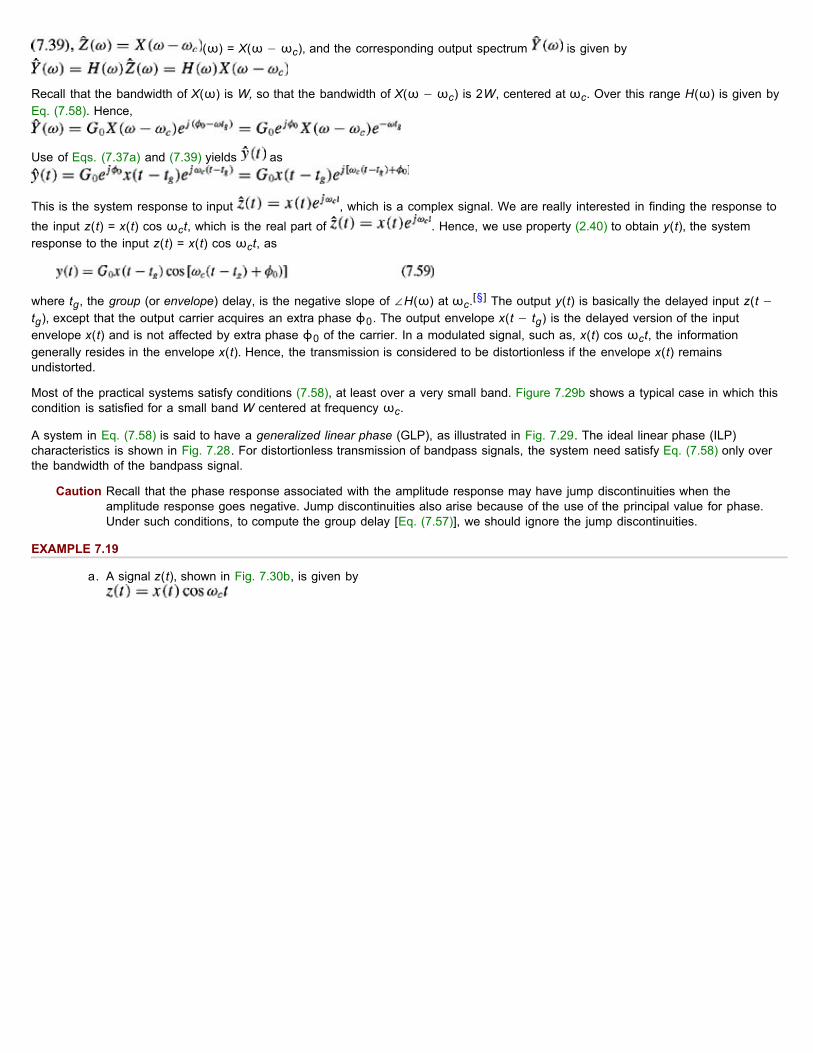
(ω) = X(ω − ωc), and the corresponding output spectrum is given by

Recall that the bandwidth of X(ω) is W, so that the bandwidth of X(ω − ωc) is 2W, centered at ωc. Over this range H(ω) is given byEq. (7.58). Hence,

Use of Eqs. (7.37a) and (7.39) yields as

This is the system response to input , which is a complex signal. We are really interested in finding the response tothe input z(t) = x(t) cos ωct, which is the real part of . Hence, we use property (2.40) to obtain y(t), the systemresponse to the input z(t) = x(t) cos ωct, as

where tg, the group (or envelope) delay, is the negative slope of ∠H(ω) at ωc.[§] The output y(t) is basically the delayed input z(t −tg), except that the output carrier acquires an extra phase φ0. The output envelope x(t − tg) is the delayed version of the inputenvelope x(t) and is not affected by extra phase φ0 of the carrier. In a modulated signal, such as, x(t) cos ωct, the informationgenerally resides in the envelope x(t). Hence, the transmission is considered to be distortionless if the envelope x(t) remainsundistorted.

Most of the practical systems satisfy conditions (7.58), at least over a very small band. Figure 7.29b shows a typical case in which thiscondition is satisfied for a small band W centered at frequency ωc.

A system in Eq. (7.58) is said to have a generalized linear phase (GLP), as illustrated in Fig. 7.29. The ideal linear phase (ILP)characteristics is shown in Fig. 7.28. For distortionless transmission of bandpass signals, the system need satisfy Eq. (7.58) only overthe bandwidth of the bandpass signal.

Caution Recall that the phase response associated with the amplitude response may have jump discontinuities when theamplitude response goes negative. Jump discontinuities also arise because of the use of the principal value for phase.Under such conditions, to compute the group delay [Eq. (7.57)], we should ignore the jump discontinuities.

EXAMPLE 7.19

a. A signal z(t), shown in Fig. 7.30b, is given by

Figure 7.30

where ωc = 2000π. The pulse x(t) (Fig. 7.30a) is a lowpass pulse of duration 0.1 second and has a bandwidth of about10 Hz. This signal is passed through a filter whose frequency response is shown in Fig. 7.30c (shown only for positive ω).Find and sketch the filter output y(t).

b. Find the filter response if ωc = 4000π.

a. The spectrum Z(ω) is a narrow band of width 20 Hz, centered at frequency f0 = 1 kHz. The gain at the center frequency(1 kHz) is 2. The group delay, which is the negative of the slope of the phase plot, can be found by drawing tangents atωc, as shown in Fig. 7.30c. The negative of the slope of the tangent represents tg, and the intercept along the verticalaxis by the tangent represents φ0 at that frequency. From the tangents at ωc, we find tg, the group delay, as

The vertical axis intercept is φ0 = −0.4π. Hence, by using Eq. (7.59) with gain G0 = 2, we obtain

Figure 7.30d shows the output y(t), which consists of the modulated pulse envelope x(t) delayed by 1 ms and the phaseof the carrier changed by −0.4π. The output shows no distortion of the envelope x(t), only the delay. The carrier phasechange does not affect the shape of envelope. Hence, the transmission is considered distortionless.

b. Figure 7.30c shows that when ωc = 4000π, the slope of ∠H(ω) is zero, so that tg = 0. Also the gain G0 = 1.5, and theintercept of the tangent with the vertical axis is φ0 = −3.1π. Hence

This too is a distortionless transmission for the same reasons as for case (a).

[†]For marginally stable systems, if the input x(t) contains a finite amplitude sinusoid of the system's natural frequency, which leads toresonance, the output is not Fourier transformable. It does, however, apply to marginally stable systems if the input does not contain afinite amplitude sinusoid of the system's natural frequency.

[‡]Stability implies that the region of convergence of H(s) includes the jω axis.

[3]Guillemin, E. A. Theory of Linear Physical Systems. Wiley, New York, 1963.

[†]Because the phase function is an odd function of ω, if ∠H(ω) = ω0 − ωtg for ω ≥ 0, over the band 2W (centered at ωc), then∠H(ω) = −φ0 − ωtg for ω < 0 over the band 2W (centered at − ωc), as shown in Fig. 7.29a.

[‡]The envelope of a bandpass signal is well defined only when the bandwidth of the envelope is well below the carrier ωc (W ≪ ωc).

[§]Equation (7.59) can also be expressed as

where tph, called the phase delay at ωc, is given by tph(ωc) = (ωctg − φ0)/ωc. Generally, tph varies with ω, and we can write

Recall also that tg itself may vary with ω.

7.5 IDEAL AND PRACTICAL FILTERSIdeal filters allow distortionless transmission of a certain band of frequencies and completely suppress the remaining frequencies. Theideal lowpass filter (Fig. 7.31), for example, allows all components below ω = W rad/s to pass without distortion and suppresses allcomponents above ω = W. Figure 7.32 illustrates ideal highpass and bandpass filter characteristics.

Figure 7.31: Ideal lowpass filter: (a) frequency response and (b) impulse response.

Figure 7.32: Ideal (a) highpass and (b) bandpass filter frequency responses.

The ideal lowpass filter in Fig. 7.31a has a linear phase of slope −td, which results in a time delay of td seconds for all its inputcomponents of the frequencies below W rad/s. Therefore, if the input is a signal x(t) bandlimited to W rad/s, the output y(t) is x(t)delayed by td: that is,

The signal x(t) is transmitted by this system without distortion, but with time delay td. For this filter |H(ω)| = rect (ω/2W) and ∠H(ω) =

e−jωtd, so that

The unit impulse response h(t) of this filter is obtained from pair 18 (Table 7.1) and the time-shifting property

Recall that h(t) is the system response to impulse input δ(t), which is applied at t = 0. Figure 7.31b shows a curious fact: the responseh(t) begins even before the input is applied (at t = 0). Clearly, the filter is noncausal and therefore physically unrealizable. Similarly, onecan show that other ideal filters (such as the ideal highpass or ideal bandpass filters depicted in Fig. 7.32) are also physicallyunrealizable.

For a physically realizable system, h(t) must be causal: that is,

In the frequency domain, this condition is equivalent to the well-known Paley-Wiener criterion, which states that the necessary andsufficient condition for the amplitude response |H(ω)| to be realizable is[†]

If H(ω) does not satisfy this condition, it is unrealizable. Note that if |H(ω)| = 0 over any finite band, | In |H(ω)‖ = ∞ over that band,and condition (7.61) is violated. If, however, H(ω) = 0 at a single frequency (or a set of discrete frequencies), the integral in Eq. (7.61)may still be finite even though the integrand is infinite at those discrete frequencies. Therefore, for a physically realizable system, H(ω)may be zero at some discrete frequencies. Therefore, for a physically realizable system, H(ω) may be zero at some discretefrequencies, but it cannot be zero over any finite band. In addition, if |H(ω)| decays exponentially (or at a higher rate) with ω, theintegral in (7.61) goes to infinity, and |H(ω)| cannot be realized. Clearly, |H(ω)| cannot decay too fast with ω. According to thiscriterion, ideal filter characteristics (Figs. 7.31 and 7.32) are unrealizable.

The impulse response h(t) in Fig. 7.31 is not realizable. One practical approach to filter design is to cut off the tail of h(t) for t < 0. The

resulting causal impulse response , given by

is physically realizable because it is causal (Fig. 7.33). If td is sufficiently large, will be a close approximation of h(t), and the

resulting filter will be a good approximation of an ideal filter. This close realization of the ideal filter is achieved because of theincreased value of time delay td. This observation means that the price of close realization is higher delay in the output; this situation iscommon in noncausal systems. Of course, theoretically, a delay td = ∞ is needed to realize the ideal characteristics. But a glance at

Fig. 7.31b shows that a delay td of three or four times will make ĥ(t) a reasonable close version of h(t − td). For instance, an audio

filter is required to handle frequencies of up to 20 kHz (W = 40,000π). In this case, a td of about 10−4 (0.1 ms) would be a reasonablechoice. The truncation operation [cutting the tail of h(t) to make it causal], however, creates some unsuspected problems. We discussthese problems and their cure in Section 7.8.

Figure 7.33: Approximate realization of an ideal low-pass filter by truncation of its impulse response.

In practice, we can realize a variety of filter characteristics that approach the ideal. Practical (realizable) filter characteristics are gradual,without jump discontinuities in amplitude response.

EXERCISE E7.12

Show that a filter with Gaussian frequency response H(ω) = e−αω2 is unrealizable. Demonstrate this fact in two ways: first by showing

that its impulse response is noncausal, and then by showing that |H(ω)| violates the Paley-Wiener criterion. [Hint: Use pair 22 in Table7.1.]

THINKING IN THE TIME AND FREQUENCY DOMAINS: A TWO-DIMENSIONAL VIEW OF SIGNALS AND SYSTEMSBoth signals and systems have dual personalities, the time domain and the frequency domain. For a deeper perspective, we shouldexamine and understand both these identities because they offer complementary insights. An exponential signal, for instance, can be

specified by its time-domain description such as e−2tu(t) or by its Fourier transform (its frequency-domain description) 1/(jω + 2). Thetime-domain description depicts the waveform of a signal. The frequency-domain description portrays its spectral composition (relativeamplitudes of its sinusoidal (or exponential) components and their phases). For the signal e−2t, for instance, the time-domain descriptionportrays the exponentially decaying signal with a time constant 0.5. The frequency-domain description characterizes it as a lowpasssignal, which can be synthesized by sinusoids with amplitudes decaying with frequency roughly as 1/ω.

An LTIC system can also be described or specified in the time domain by its impulse response h(t) or in the frequency domain by itsfrequency response H(ω). In Section 2.7, we studied intuitive insights in the system behavior offered by the impulse response, whichconsists of characteristic modes of the system. By purely qualitative reasoning, we saw that the system responds well to signals that aresimilar to the characteristic modes and responds poorly to signals that are very different from those modes. We also saw that the shapeof the impulse response h(t) determines the system time constant (speed of response), and pulse dispersion (spreading), which, in turn,determines the rate of pulse transmission.

The frequency response H(ω) specifies the system response to exponential or sinusoidal input of various frequencies. This is preciselythe filtering characteristic of the system.

Experienced electrical engineers instinctively think in both domains (the time and frequency) whenever possible. When they look at asignal, they consider, its waveform, the signal width (duration), and the rate at which the waveform decays. This is basically a time-domain perspective. They also think of the signal in terms of its frequency spectrum, that is, in terms of its sinusoidal components andtheir relative amplitudes and phases, whether the spectrum is lowpass, bandpass, highpass and so on. This is the frequency-domainperspective. When they think of a system, they think of its impulse response h(t). The width of h(t) indicates the time constant(response time): that is, how fast the system is capable of responding to an input, and how much dispersion (spreading) it will cause.This is the time-domain perspective. From the frequency-domain perspective, these engineers view a system as a filter, whichselectively transmits certain frequency components and suppresses the others [frequency response H(ω)]. Knowing the input signalspectrum and the frequency response of the system, they create a mental image of the output signal spectrum. This concept isprecisely expressed by Y(ω) = X(ω)H(ω).

We can analyze LTI systems by time-domain techniques or by frequency-domain techniques. Then why learn both? The reason is thatthe two domains offer complementary insights into system behavior. Some aspects are easily grasped in one domain; other aspectsmay be easier to see in the other domain. Both the time-domain and frequency-domain methods are as essential for the study ofsignals and systems as two eyes are essential to a human being for correct visual perception of reality. A person can see with eithereye, but for proper perception of three-dimensional reality, both eyes are essential.

It is important to keep the two domains separate, and not to mix the entities in the two domains. If we are using the frequency domainto determine the system response, we must deal with all signals in terms of their spectra (Fourier transforms) and all systems in termsof their frequency responses. For example, to determine the system response y(t) to an input x(t), we must first convert the input signalinto its frequency-domain description X(ω). The system description also must be in the frequency domain, that is, the frequencyresponse H(ω). The output signal spectrum Y(ω) = X(ω)H(ω). Thus, the result (output) is also in the frequency domain. To determinethe final answer y(t), we must take the inverse transform of Y(ω).

[†]We are assuming that |H(ω)| is square integrable, that is,

Note that the Paley-Wiener criterion is a criterion for the realizability of the amplitude response |H(ω)|.

7.6 SIGNAL ENERGYThe signal energy Ex of a signal x(t) was defined in Chapter 1 as

Signal energy can be related to the signal spectrum X(ω) by substituting Eq. (7.8b) in Eq. (7.62):

Here we used the fact that x*(t), being the conjugate of x(t), can be expressed as the conjugate of the right-hand side of Eq. (7.8b).Now, interchanging the order of integration yields

Consequently,

This is the statement of the well-known Parseval's theorem (for the Fourier transform). A similar result was obtained in Eqs. (6.40) and(6.41) for a periodic signal and its Fourier series. This result allows us to determine the signal energy from either the time-domainspecification x(t) or the corresponding frequency-domain specification X(ω).

Equation (7.63) can be interpreted to mean that the energy of a signal x(t) results from energies contributed by all the spectralcomponents of the signal x(t). The total signal energy is the area under |X(ω)2| (divided by 2π). If we consider a small band Δω(Δω→ 0), as illustrated in Fig. 7.34, the energy ΔEx of the spectral components in this band is the area of |X(ω)|2 under this band dividedby 2π):

Figure 7.34: Interpretation of energy spectral density of a signal.

Therefore, the energy contributed by the components in this band of Δf (in hertz) is |X(ω)|2Δf. The total signal energy is the sum ofenergies of all such bands and is indicated by the area under |X(ω)|2 as in Eq. (7.63). Therefore, |X(ω)|2 is the energy spectral density(per unit bandwidth in hertz).

For real signals, X(ω) and X(−ω) are conjugates, and |X(ω)|2 is an even function of ω because

Therefore, Eq. (7.63) can be expressed as[†]

The signal energy Ex, which results from contributions from all the frequency components from ω = 0 to ∞, is given by (1 / π times)

the area under |X(ω)|2 from ω = 0 to ∞. It follows that the energy contributed by spectral components of frequencies between ω1 andω2 is

EXAMPLE 7.20Find the energy of signal x(t) = e−atu(t). Determine the frequency W (rad/s) so that the energy contributed by the spectral componentsof all the frequencies below W is 95% of the signal energy Ex.

We have

We can verify this result by Parseval's theorem. For this signal

and

The band ω = 0 to ω = W contains 95% of the signal energy, that is, 0.95/2a. Therefore, from Eq. (7.67) with ω1 = 0 and ω2 = W, weobtain

or

This result indicates that the spectral components of x(t) in the band from 0 (dc) to 12.706a rad/s (2.02a Hz) contribute 95% of the totalsignal energy; all the remaining spectral components (in the band from 12.706a rad/s to ∞) contribute only 5% of the signal energy.

EXERCISE E7.13Use Parseval's theorem to show that the energy of the signal x(t) = 2a/(t2 + a2) is 2π/a. [Hint: Find X(ω) using pair 3 of Table 7.1 andthe duality property.]

THE ESSENTIAL BANDWIDTH OF A SIGNALThe spectra of all practical signals extend to infinity. However, because the energy of any practical signal is finite, the signal spectrummust approach 0 as ω → ∞. Most of the signal energy is contained within a certain band of B Hz, and the energy contributed by thecomponents beyond B Hz is negligible. We can therefore suppress the signal spectrum beyond B Hz with little effect on the signalshape and energy. The bandwidth B is called the essential bandwidth of the signal. The criterion for selecting B depends on the errortolerance in a particular application. We may, for example, select B to be that band which contains 95% of the signal energy.[†] Thisfigure may be higher or lower than 95%, depending on the precision needed. Using such a criterion, we can determine the essentialbandwidth of a signal. The essential bandwidth B for the signal e−atu(t), using 95% energy criterion, was determined in Example 7.20to be 2.02a Hz.

Suppression of all the spectral components of x(t) beyond the essential bandwidth results in a signal (t), which is a closeapproximation of x(t). If we use the 95% criterion for the essential bandwidth, the energy of the error (the difference)

(t) is 5% of Ex.

[†]In Eq. (7.66) it is assumed that X(ω) does not contain an impulse at ω = 0. If such an impulse exists, it should be integratedseparately with a multiplying factor of 1/2π rather than 1/π.

[†]For lowpass signals, the essential bandwidth may also be defined as a frequency at which the value of the amplitude spectrum is asmall fraction (about 1%) of its peak value. In Example 7.20, for instance, the peak value, which occurs at ω = 0, is 1/a.

7.7 APPLICATION TO COMMUNICATIONS: AMPLITUDE MODULATIONModulation causes a spectral shift in a signal and is used to gain certain advantages mentioned in our discussion of the frequency-shifting property. Broadly speaking, there are two classes of modulation: amplitude (linear) modulation and angle (nonlinear) modulation.In this section, we shall discuss some practical forms of amplitude modulation.

7.7-1 Double-Sideband, Suppressed-Carrier (DSB-SC) Modulation

In amplitude modulation, the amplitude A of the carrier A cos (ωct + θc) is varied in some manner with the baseband (message)[‡]

signal m(t) (known as the modulating signal). The frequency ωc and the phase θc are constant. We can assume θc = 0 without loss ofgenerality. If the carrier amplitude A is made directly proportional to the modulating signal m(t), the modulated signal is m(t) cos ωct(Fig. 7.35). As was indicated earlier [Eq. (7.41)], this type of modulation simply shifts the spectrum of m(t) to the carrier frequency (Fig.7.35c). Thus, if

then

Figure 7.35: DSB-SC modulation.

Recall that M(ω − ωc) is M(ω)-shifted to the right by ωc and M(ω + ωc) is M(ω)-shifted to the left by ωc. Thus, the process ofmodulation shifts the spectrum of the modulating signal to the left and the right by ωc. Note also that if the bandwidth of m(t) is B Hz,then, as indicated in Fig. 7.35c, the bandwidth of the modulated signal is 2B Hz. We also observe that the modulated signal spectrumcentered at ωc is composed of two parts: a portion that lies above ωc, known as the upper sideband (USB), and a portion that liesbelow ωc, known as the lower sideband (LSB). Similarly, the spectrum centered at −ωc has upper and lower sidebands. This form ofmodulation is called double sideband (DSB) modulation for obvious reason.

The relationship of B to ωc is of interest. Figure 7.35c shows that ωc ≥ 2πB to avoid the overlap of the spectra centered at ±c. If ωc <2π B, the spectra overlap and the information of m(t) is lost in the process of modulation, a loss that makes it impossible to get backm(t) from the modulated signal m(t) cos ωct.[†]

EXAMPLE 7.21For a baseband signal m(t) = cos ωmt, find the DSB signal, and sketch its spectrum. Identify the upper and lower sidebands.

We shall work this problem in the frequency domain as well as the time domain to clarify the basic concepts of DSB-SC modulation. Inthe frequency-domain approach, we work with the signal spectra. The spectrum of the baseband signal m(t) = cos ωmt is given by

The spectrum consists of two impulses located at ±ωm, as depicted in Fig. 7.36a. The DSB-SC (modulated) spectrum, as indicated byEq. (7.70), is the baseband spectrum in Fig. 7.36a shifted to the right and the left by ωc (times 0.5), as depicted in Fig. 7.36b. Thisspectrum consists of impulses at ±(ωc − ωm) and ±(ωc + ωm). The spectrum beyond ωc is the upper sideband (USB), and the onebelow ωc is the lower sideband (LSB). Observe that the DSB-SC spectrum does not have as a component the carrier frequency ωc.This is why the term double-sideband, suppressed carrier (DSB-SC) is used for this type of modulation.

Figure 7.36: An example of DSB-SC modulation.

In the time-domain approach, we work directly with signals in the time domain. For the baseband signal m(t) = cos ωmt, the DSB-SCsignal φDSB-SC(t) is

This result shows that when the baseband (message) signal is a single sinusoid of frequency ωm, the modulated signal consists of twosinusoids: the component of frequency ωc + ωm (the upper sideband), and the component of frequency ωc − ωm (the lowersideband). Figure 7.36b illustrates precisely the spectrum of φDSB-SC(t). Thus, each component of frequency ωm in the modulatingsignal results into two components of frequencies ωc + ωm and ωc − ωm in the modulated signal. This being a DSB-SC (suppressed

carrier) modulation, there is no component of the carrier frequency ωc on the right-hand side of Eq. (7.71).[†]

DEMODULATION OF DSB-SC SIGNALSThe DSB-SC modulation translates or shifts the frequency spectrum to the left and the right by ωc (i.e., at + ωc and −ωc), as seenfrom Eq. (7.70). To recover the original signal m(t) from the modulated signal, we must retranslate the spectrum to its original position.The process of recovering the signal from the modulated signal (retranslating the spectrum to its original position) is referred to asdemodulation, or detection. Observe that if the modulated signal spectrum in Fig. 7.35c is shifted to the left and to the right by ωc (andhalved), we obtain the spectrum illustrated in Fig. 7.37b, which contains the desired baseband spectrum in addition to an unwantedspectrum at ±2ωc. The latter can be suppressed by a lowpass filter. Thus, demodulation, which is almost identical to modulation,consists of multiplication of the incoming modulated signal m(t) cos ωct by a carrier cos ωct followed by a lowpass filter, as depicted inFig. 7.37a. We can verify this conclusion directly in the time domain by observing that the signal e(t) in Fig. 7.37a is

Figure 7.37: Demodulation of DSB-SC: (a) demodulator and (b) spectrum of e(t).

Therefore, the Fourier transform of the signal e(t) is

Hence, e(t) consists of two components (1/2)m(t) and (1/2)m(t) cos 2ωct, with their spectra, as illustrated in Fig. 7.37b. The spectrumof the second component, being a modulated signal with carrier frequency 2ωc, is centered at ±2ωc. Hence, this component issuppressed by the lowpass filter in Fig. 7.37a. The desired component (1/2)M(ω), being a lowpass spectrum (centered at ω = 0),passes through the filter unharmed, resulting in the output (1/2)m(t).

A possible form of lowpass filter characteristics is depicted (dotted) in Fig. 7.37b. In this method of recovering the baseband signal,called synchronous detection, or coherent detection, we use a carrier of exactly the same frequency (and phase) as the carrier used formodulation. Thus, for demodulation, we need to generate a local carrier at the receiver in frequency and phase coherence(synchronism) with the carrier used at the modulator. We shall demonstrate in Example 7.22 that both phase and frequencysynchronism are extremely critical.

EXAMPLE 7.22Discuss the effect of lack of frequency and phase coherence (synchronism) between the carriers at the modulator (transmitter) and thedemodulator (receiver) in DSB-SC.

Let the modulator carrier be cos ωct (Fig. 7.35a). For the demodulator in Fig. 7.37a, we shall consider two cases: with carrier cos (ωct+ θ) (phase error of θ) and with carrier cos (ωc + Δω)t (frequency error Δω).

a. With the demodulator carrier cos (ωct + θ) (instead of cos ωct) in Fig. 7.37a, the multiplier output is e(t) = m(t) cos ωct

cos (ωct + θ) instead of m(t) cos2 ωct. From the trigonometric identity, we obtain

The spectrum of the component (1/2)m(t) cos (2ωct + θ) is centered at ± 2ωc. Consequently, it will be filtered out by thelowpass filter at the output. The component (1/2)m(t) cos θ is the signal m(t) multiplied by a constant (1/2) cos θ. Thespectrum of this component is centered at ω = 0 (lowpass spectrum) and will pass through the lowpass filter at the output,yielding the output (1/2)m(t) cos θ.

If θ is constant, the phase asynchronism merely yields an output that is attenuated (by a factor cos θ). Unfortunately, inpractice, θ is often the phase difference between the carriers generated by two distant generators and varies randomlywith time. This variation would result in an output whose gain varies randomly with time.

b. In the case of frequency error, the demodulator carrier is cos (ωc + Δω)t. This situation is very similar to the phase errorcase in part (a) with θ replaced by (Δω)t. Following the analysis in part (a), we can express the demodulator product e(t)as

The spectrum of the component (1/2)m(t) cos (2ω + Δω)t is centered at ±(2ωc + Δω). Consequently, this component willbe filtered out by the lowpass filter at the output. The component (1/2)m(t) cos (Δω)t is the signal m(t) multiplied by alow-frequency carrier of frequency Δω. The spectrum of this component is centered at ±Δω. In practice, the frequencyerror (Δω) is usually very small. Hence, the signal (1/2)m(t) cos (Δω)t (whose spectrum is centered at ±Δω) is alowpass signal and passes through the lowpass filter at the output, resulting in the output (1/2)m(t) cos (Δω)t. The outputis the desired signal m(t) multiplied by a very-low-frequency sinusoid cos (Δω)t. The output in this case is not merely anattenuated replica of the desired signal m(t), but represents m(t) multiplied by a time-varying gain cos (Δω)t. If, forinstance, the transmitter and the receiver carrier frequencies differ just by 1 Hz, the output will be the desired signal m(t)multiplied by a time-varying signal whose gain goes from the maximum to 0 every half-second. This is like a restless childfidding with the volume control knob of a receiver, going from maximum volume to zero volume every half-second. Thiskind of distortion (called the beat effect) is beyond repair.

7.7-2 Amplitude Modulation (AM)

For the suppressed-carrier scheme just discussed, a receiver must generate a carrier in frequency and phase synchronism with thecarrier at a transmitter that may be located hundreds or thousands of miles away. This situation calls for a sophisticated receiver, whichcould be quite costly. The other alternative is for the transmitter to transmit a carrier A cos ωct [along with the modulated signal m(t)cos ωct] so that there is no need to generate a carrier at the receiver. In this case the transmitter needs to transmit much larger power,a rather expensive procedure. In point-to-point communications, where there is one transmitter for each receiver, substantial complexityin the receiver system can be justified, provided there is a large enough saving in expensive high-power transmitting equipment. On theother hand, for a broadcast system with a multitude of receivers for each transmitter, it is more economical to have one expensive high-power transmitter and simpler, less expensive receivers. The second option (transmitting a carrier along with the modulated signal) isthe obvious choice in this case. This is amplitude modulation (AM), in which the transmitted signal φAM(t) is given by

Recall that the DSB-SC signal is m(t) cos ωct. From Eq. (7.73b) it follows that the AM signal is identical to the DSB-SC signal with A +m(t) as the modulating signal [instead of m(t)]. Therefore, to sketch φAM(t), we sketch A +m(t) and −[A + m(t)] as the envelopes andfill in between with the sinusoid of the carrier frequency. Two cases are considered in Fig. 7.38. In the first case, A is large enough sothat A + m(t) ≥ 0 (is nonnegative) for all values of t. In the second case, A is not large enough to satisfy this condition. In the first case,the envelope (Fig. 7.38d) has the same shape as m(t) (although riding on a dc of magnitude A). In the second case the envelope shapeis not m(t), for some parts get rectified (Fig. 7.38e). Thus, we can detect the desired signal m(t) by detecting the envelope in the firstcase. In the second case, such a detection is not possible. We shall see that envelope detection is an extremely simple andinexpensive operation, which does not require generation of a local carrier for the demodulation. But as just noted, the envelope of AMhas the information about m(t) only if the AM signal [A + m(t)] cos ωct satisfies the condition A + m(t) > 0 for all t. Thus, the conditionfor envelope detection of an AM signal is

If mp is the peak amplitude (positive or negative) of m(t) then condition (7.74) is equivalent to[†]

Thus the minimum carrier amplitude required for the viability of envelope detection is mp. This point is clearly illustrated in Fig. 7.38.

Figure 7.38: An AM signal (a) for two values of A (b, c) and the respective envelopes (d, e)

We define the modulation index μ as

where A is the carrier amplitude. Note that mp is a constant of the signal m(t). Because A ≥ mp and because there is no upper boundon A, it follows that

as the required condition for the viability of demodulation of AM by an envelope detector.

When A < mp, Eq. (7.76) shows that μ > 1 (overmodulation, shown in Fig. 7.38e). In this case, the option of envelope detection is nolonger viable. We then need to use synchronous demodulation. Note that synchronous demodulation can be used for any value of μ(see Prob. 7.7-6). The envelope detector, which is considerably simpler and less expensive than the synchronous detector, can be usedonly when μ ≤ 1.

EXAMPLE 7.23Sketch φAM for modulation indices of μ = 0.5 (50% modulation) and μ = 1 (100% modulation), when m(t) = B cos ωmt. This case isreferred to as tone modulation because the modulating signal is a pure sinusoid (or tone).

In this case, mp = B and the modulation index according to Eq. (7.76) is

Hence, B = μ A and

Therefore

The modulated signals corresponding to μ = 0.5 and μ = 1 appear in Fig. 7.39a and 7.39b, respectively.

Figure 7.39: Tone-modulated AM: (a) μ = 0.5 and (b) μ = 1.

DEMODULATION OF AM: THE ENVELOPE DETECTORThe AM signal can be demodulated coherently by a locally generated carrier (see Prob. 7.7-6). Since, however, coherent, orsynchronous, demodulation of AM (with μ ≤ 1) will defeat the very purpose of AM, it is rarely used in practice. We shall consider hereone of the noncoherent methods of AM demodulation, envelope detection.[†]

In an envelope detector, the output of the detector follows the envelope of the (modulated) input signal. The circuit illustrated in Fig.7.40a functions as an envelope detector. During the positive cycle of the input signal, the diode conducts and the capacitor C chargesup to the peak voltage of the input signal (Fig. 7.40b). As the input signal falls below this peak value, the diode is cut off, because thecapacitor voltage (which is very nearly the peak voltage) is greater than the input signal voltage, a circumstance causing the diode toopen. The capacitor now discharges through the resistor R at a slow rate (with a time constant RC). During the next positive cycle, thesame drama repeats. When the input signal becomes greater than the capacitor voltage, the diode conducts again. The capacitor againcharges to the peak value of this (new) cycle. As the input voltage falls below the new peak value, the diode cuts off again and thecapacitor discharges slowly during the cutoff period, a process that changes the capacitor voltage very slightly.

Figure 7.40: Demodulation by means of envelope detector.

In this manner, during each positive cycle, the capacitor charges up to the peak voltage of the input signal and then decays slowly untilthe next positive cycle. Thus, the output voltage υc(t) follows closely the envelope of the input. The capacitor discharge betweenpositive peaks, however, causes a ripple signal of frequency ωc in the output. This ripple can be reduced by increasing the timeconstant RC so that the capacitor discharges very little between the positive peaks (RC >> 1/ωc). Making RC too large, however, wouldmake it impossible for the capacitor voltage to follow the envelope (see Fig. 7.40b). Thus, RC should be large in comparison to 1/c butsmall in comparison to 1/2π B, where B is the highest frequency in m(t). Incidentally, these two conditions also require that ωc >> 2πB, a condition necessary for a well-defined envelope.

The envelope-detector output υc(t) is A + m(t) plus a ripple of frequency ωc. The dc term A can be blocked out by a capacitor or asimple RC highpass filter. The ripple is reduced further by another (lowpass) RC filter. In the case of audio signals, the speakers alsoact as lowpass filters, which further enhances suppression of the high-frequency ripple.

7.7-3 Single-Sideband Modulation (SSB)

Now consider the baseband spectrum M(ω) (Fig. 7.41a) and the spectrum of the DSB-SC modulated signal m(t) cos ωct (Fig. 7.41b).The DSB spectrum in Fig. 7.41b has two sidebands: the upper and the lower (USB and LSB), both containing complete information onM(ω) [see Eqs. (7.11)]. Clearly, it is redundant to transmit both sidebands, a process that requires twice the bandwidth of the basebandsignal. A scheme in which only one sideband is transmitted is known as single-sideband (SSB) transmission, which requires only halfthe bandwidth of the DSB signal. Thus, we transmit only the upper sidebands (Fig. 7.41c) or only the lower sidebands (Fig. 7.41d).

Figure 7.41: Spectra for single-sideband transmission: (a) baseband, (b) DSB, (c) USB, (d) LSB, and (e) synchronouslydemodulated signal.

An SSB signal can be coherently (synchronously) demodulated. For example, multiplication of a USB signal (Fig. 7.41c) by 2 cos ωctshifts its spectrum to the left and to the right by ωc, yielding the spectrum in Fig. 7.41e. Lowpass filtering of this signal yields thedesired baseband signal. The case is similar with an LSB signal. Hence, demodulation of SSB signals is identical to that of DSB-SCsignals, and the synchronous demodulator in Fig. 7.37a can demodulate SSB signals. Note that we are talking of SSB signals withoutan additional carrier. Hence, they are suppressed-carrier signals (SSB-SC).

EXAMPLE 7.24Find the USB (upper sideband) and LSB (lower sideband) signals when m(t) = cos ωmt. Sketch their spectra, and show that theseSSB signals can be demodulated using the synchronous demodulator in Fig. 7.37a.

The DSB-SC signal for this case is

As pointed out in Example 7.21, the terms (1/2) cos (ωc + ωm)t and (1/2) cos (ωc − ωm)t represent the upper and lower sidebands,respectively. The spectra of the upper and lower sidebands are given in Fig. 7.42a and 7.42b. Observe that these spectra can beobtained from the DSB-SC spectrum in Fig. 7.36b by using a proper filter to suppress the undesired sidebands. For instance, the USBsignal in Fig. 7.42a can be obtained by passing the DSB-SC signal (Fig. 7.36b) through a highpass filter of cutoff frequency ωc.Similarly, the LSB signal in Fig. 7.42b can be obtained by passing the DSB-SC signal through a lowpass filter of cutoff frequency ωc.

If we apply the LSB signal (1/2) cos (ωc − ωm) to the synchronous demodulator in Fig. 7.37a, the multiplier output is

The term (1/4) cos (2ωc − ωm) is suppressed by the lowpass filter, producing the desired output (1/4) cos ωmt [which is m(t)/4]. Thespectrum of this term is π[δ(ω + ωm) + δ)(ω − ωm)]/4, as depicted in Fig. 7.42c. In the same way we can show that the USB signalcan be demodulated by the synchronous demodulator.

Figure 7.42: Single-sideband spectra for m(t) = cos ωmt: (a) USB, (b) LSB, and (c) synchronously demodulated LSBsignal.

In the frequency domain, demodulation (multiplication by cos ωt) amounts to shifting the LSB spectrum (Fig. 7.42b) to the left and theright by ωc (times 0.5) and then suppressing the high frequency, as illustrated in Fig. 7.42c. The resulting spectrum represents thedesired signal (1/4)m(t).

GENERATION OF SSB SIGNALSTwo methods are commonly used to generate SSB signals. The selective-filtering method uses sharp cutoff filters to eliminate theundesired sideband, and the second method uses phase-shifting networks[4] to achieve the same goal.[†] We shall consider here onlythe first method.

Selective filtering is the most commonly used method of generating SSB signals. In this method, a DSB-SC signal is passed through asharp cutoff filter to eliminate the undesired sideband.

To obtain the USB, the filter should pass all components above ωc, unattenuated and completely suppress all components below ωc.Such an operation requires an ideal filter, which is unrealizable. It can, however, be realized closely if there is some separation betweenthe passband and the stopband. Fortunately, the voice signal provides this condition, because its spectrum shows little power content atthe origin (Fig. 7.43). Moreover, articulation tests show that for speech signals, frequency components below 300 Hz are not important.In other words, we may suppress all speech components below 300 Hz without appreciably affecting intelligibility.[†] Thus, filtering of theunwanted sideband becomes relatively easy for speech signals because we have a 600 Hz transition region around the cutoff frequencyωc. For some signals, which have considerable power at low frequencies (around ω = 0), SSB techniques cause considerabledistortion. Such is the case with video signals. Consequently, for video signals, instead of SSB, we use another technique, the vestigialsideband (VSB), which is a compromise between SSB and DSB. It inherits the advantages of SSB and DSB but avoids theirdisadvantages at a cost of slightly increased bandwidth. VSB signals are relatively easy to generate, and their bandwidth is only slightly(typically 25%) greater than that of the SSB signals. In VSB signals, instead of rejecting one sideband completely (as in SSB), weaccept a gradual cutoff from one sideband[4].

Figure 7.43: Voice Spectrum.

7.7-4 Frequency-Division Multiplexing

Signal multiplexing allows transmission of several signals on the same channel. Later, in Chapter 8 (Section 8.2-2), we shall discusstime-division multiplexing (TDM), where several signals time-share the same channel, such as a cable or an optical fiber. In frequency-division multiplexing (FDM), the use of modulation, as illustrated in Fig. 7.44, makes several signals share the band of the samechannel. Each signal is modulated by a different carrier frequency. The various carriers are adequately separated to avoid overlap (orinterference) between the spectra of various modulated signals. These carriers are referred to as subcarriers. Each signal may use adifferent kind of modulation, for example, DSB-SC, AM, SSB-SC, VSB-SC, or even other forms of modulation, not discussed here [suchas FM (frequency modulation) or PM (phase modulation)]. The modulated-signal spectra may be separated by a small guard band toavoid interference and to facilitate signal separation at the receiver.

Figure 7.44: Frequency-division multiplexing: (a) FDM spectrum (b) transmitter, and (c) receiver.

When all the modulated spectra are added, we have a composite signal that may be considered to be a new baseband signal.Sometimes, this composite baseband signal may be used to further modulate a high-frequency (radio frequency, or RF) carrier for thepurpose of transmission.

At the receiver, the incoming signal is first demodulated by the RF carrier to retrieve the composite baseband, which is then bandpass-filtered to separate the modulated signals. Then each modulated signal is individually demodulated by an appropriate subcarrier toobtain all the basic baseband signals.

[‡]The term baseband is used to designate the band of frequencies of the signal delivered by the source or the input transducer.

[†]Practical factors may impose additional restriction on ωc. For instance, in broadcast applications, a radiating antenna can radiate onlya narrow band without distortion. This restriction implies that to avoid distortion caused by the radiating antenna, ωc/2π B >> 1. Thebroadcast band AM radio, for instance, with B = 5 kHz and the band of 550-1600 kHz for carrier frequency give a ratio of ωc/2π Broughly in the range of 100-300.

[†]The term suppressed carrier does not necessarily mean absence of the spectrum at the carrier frequency. "Suppressed carrier"merely implies that there is no discrete component of the carrier frequency. Since no discrete component exists, the DSB-SC spectrumdoes not have impulses at ±ωc, which further implies that the modulated signal m(t) cos ωct does not contain a term of the form k cosωct [assuming that m(t) has a zero mean value].

[†]In case the negative and the positive peak amplitudes are not identical, mp in condition (7.75) is the absolute negative peakamplitude.

[†]There are also other methods of noncoherent detection. The rectifier detector consists of a rectifier followed by a lowpass filter. Thismethod is also simple and almost as inexpensive as the envelope detector.[4] The nonlinear detector, although simple and inexpensive,results in a distorted output.

[†]Lathi, B. P. Modern Digital and Analog Communication Systems, 3rd ed. Oxford University Press, New York, 1998.

[†]Yet another method, known as Weaver's method, is also used to generate SSB signals.

[†]Similarly, suppression of components of a speech signal above 3500 Hz causes no appreciable change in intelligibility.

7.8 DATA TRUNCATION: WINDOW FUNCTIONSWe often need to truncate data in diverse situations from numerical computations to filter design. For example, if we need to computenumerically the Fourier transform of some signal, say e−1u(t), we will have to truncate the signal e−1u(t) beyond a sufficiently largevalue of t (typically five time constants and above). The reason is that in numerical computations, we have to deal with date of finiteduration. Similarly, the impulse response h(t) of an ideal lowpass filter is noncausal and approaches zero asymptotically as |t| → ∞. Fora practical design, we may want to truncate h(t) beyond a sufficiently large value of |t| to make h(t) causal and of finite duration. Insignal sampling, to eliminate aliasing, we must use an antialiasing filter to truncate the signal spectrum beyond the half-samplingfrequency ωs/2. Again, we may want to synthesize a periodic signal by adding the first n harmonics and truncating all the higherharmonics. These examples show that data truncation can occur in both time and frequency domains. On the surface, truncationappears to be a simple problem of cutting off the data at a point at which values are deemed to be sufficiently small. Unfortunately, thisis not the case. Simple truncation can cause some unsuspected problems.

WINDOW FUNCTIONSTruncation operation may be regarded as multiplying a signal of a large width by a window function of a smaller (finite) width. Simpletruncation amounts to using a rectangular window ωR(t) (shown later in Fig. 7.47a) in which we assign unit weight to all the data withinthe window width (|t| < T/2), and assign zero weight to all the data lying outside the window (|t| > T/2). It is also possible to use awindow in which the weight assigned to the data within the window may not be constant. In a triangular window ωT(t), for example, theweight assigned to data decreases linearly over the window width (shown later in Fig. 7.47b).

Consider a signal x(t) and a window function ω(t). If x(t) X(ω) and ω(t) ω W(ω), and if the windowed function xω(t) Xω(ω),then

According to the width property of convolution, it follows that the width of Xω (ω) equals the sum of the widths of X (ω) and W(ω).Thus, truncation of a signal increases its bandwidth by the amount of bandwidth of ω(t). Clearly, the truncation of a signal causes itsspectrum to spread (or smear) by the amount of the bandwidth of ω(t). Recall that the signal bandwidth is inversely proportional to thesignal duration (width). Hence, the wider the window, the smaller its bandwidth, and the smaller the spectral spreading. This result ispredictable because a wider window means that we are accepting more data (closer approximation), which should cause smallerdistortion (smaller spectral spreading). Smaller window width (poorer approximation) causes more spectral spreading (more distortion).In addition, since W (ω) is really not strictly bandlimited and its spectrum → 0 only asymptotically, the spectrum of Xω (ω) → 0asymptotically also at the same rate as that of W (ω), even if the X (ω) is in fact strictly bandlimited. Thus, windowing causes thespectrum of X (ω), to spread into the band where it is supposed to be zero. This effect is called leakage. The following example clarifiesthese twin effects, the spectral spreading and the leakage.

Let us consider x(t) = cos ω0t and a rectangular window ωR(t) = rect(t/T), illustrated in Fig. 7.45b. The reason for selecting a sinusoidfor x(t) is that its spectrum consists of spectral lines of zero width (Fig. 7.45a). Hence, this choice will make the effect of spectralspreading and leakage easily discernible. The spectrum of the truncated signal xω(t) is the convolution of the two impulses of X (ω)with the sinc spectrum of the window function. Because the convolution of any function with an impulse is the function itself (shifted atthe location of the impulse), the resulting spectrum of the truncated signal is 1/2π times the two sinc pulses at ±ω0, as depicted in Fig.7.45c (also see Fig. 7.26). Comparison of spectra X (ω) and Xω (ω) reveals the effects of truncation. These are:

1. The spectral lines of X (ω) have zero width. But the truncated signal is spread out by 2πT about each spectral line. Theamount of spread is equal to the width of the mainlobe of the window spectrum. One effect of this spectral spreading (orsmearing) is that if x(t) has two spectral components of frequencies differing by less than 4π/T rad/s (2/T Hz), they will beindistinguishable in the truncated signal. The result is loss of spectral resolution. We would like the spectral spreading[mainlobe width of W (ω)] to be as small as possible.

2. In addition to the mainlobe spreading, the truncated signal has sidelobes, which decay slowly with frequency. Thespectrum of x(t) is zero everywhere except at ±ω0. On the other hand, the truncated signal spectrum Xω(ω) is zeronowhere because of the sidelobes. These sidelobes decay asymptotically as 1/ω. Thus, the truncation causes spectralleakage in the band where the spectrum of the signal x(t) is zero. The peak sidelobe magnitude is 0.217 times themainlobe magnitude (13.3 dB below the peak mainlobe magnitude). Also, the sidelobes decay at a rate 1/ω, which is −6dB/octave (or /20 dB/decade). This is the sidelobes rolloff rate. We want smaller sidelobes with a faster rate of decay (highrolloff rate). Figure 7.45d, which plots |WR(ω)| as a function of ω, clearly shows the mainlobe and sidelobe features, withthe first sidelobe amplitude −13.3 dB below the mainlobe amplitude and the sidelobes decaying at a rate of −6 dB/octave(or −20 dB/decade).

Figure 7.45: Windowing and its effects.

So far, we have discussed the effect on the signal spectrum of signal truncation (truncation in the time domain). Because of the time-frequency duality, the effect of spectral truncation (truncation in frequency domain) on the signal shape is similar.

REMEDIES FOR SIDE EFFECTS OF TRUNCATION

For better results, we must try to minimize the twin side effects of truncations: spectral spreading (mainlobe width) and leakage(sidelobe). Let us consider each of these ills.

1. The spectral spread (mainlobe width) of the truncated signal is equal to the bandwidth of the window function ω(t). Weknow that the signal bandwidth is inversely proportional to the signal width (duration). Hence, to reduce the spectralspread (mainlobe width), we need to increase the window width.

2. To improve the leakage behavior, we must search for the cause of the slow decay of sidelobes. In Chapter 6, we saw thatthe Fourier spectrum decays as 1/ω for a signal with jump discontinuity, decays as 1/ω2 for a continuous signal whosefirst derivative is discontinuous, and so on.[†] Smoothness of a signal is measured by the number of continuousderivatives it possesses. The smoother the signal, the faster the decay of its spectrum. Thus, we can achieve a givenleakage behavior by selecting a suitably smooth (tapered) window.

3. For a given window width, the remedies for the two effects are incompatible. If we try to improve one, the otherdeteriorates. For instance, among all the windows of a given width, the rectangular window has the smallest spectralspread (mainlobe width), but its sidelobes have high level and they decay slowly. A tapered (smooth) window of the samewidth has smaller and faster decaying sidelobes, but it has a wider mainlobe.[†] But we can compensate for the increasedmainlobe width by widening the window. Thus, we can remedy both the side effects of truncation by selecting a suitablysmooth window of sufficient width.

There are several well-known tapered-window functions, such as Bartlett (triangular), Hanning (von Hann), Hamming, Blackman, andKaiser, which truncate the data gradually. These windows offer different trade-offs with respect to spectral spread (mainlobe width), thepeak sidelobe magnitude, and the leakage rolloff rate as indicated in Table 7.3.[5], [6] Observe that all windows are symmetrical aboutthe origin (even functions of t). Because of this feature, W (ω) is a real function of ω; that is, ∠W(ω) is either 0 or π. Hence, thephase function of the truncated signal has a minimal amount of distortion.

Figure 7.46 shows two well-known tapered-window functions, the von Hann (or Hanning) window ωHAN(x) and the Hamming windowωHAM(x). We have intentionally used the independent variable x because windowing can be performed in the time domain as well as inthe frequency domain; so x could be t or ω, depending on the application.

Figure 7.46: (a) Hanning and (b) Hamming windows.

There are hundreds of windows, all with different characteristics. But the choice depends on a particular application. The rectangularwindow has the narrowest mainlobe. The Bartlett (triangle) window (also called the Fejer or Cesaro) is inferior in all respects to theHanning window. For this reason it is rarely used in practice. Hanning is preferred over Hamming in spectral analysis because it hasfaster sidelobe decay. For filtering applications, on the other hand, the Hamming window is chosen because it has the smallest sidelobemagnitude for a given mainlobe width. The Hamming window is the most widely used general-purpose window. The Kaiser window,which uses I0(α), the modified zero-order Bessel function, is more versatile and adjustable. Selecting a proper value of α (0 ≤ α ≤ 10)allows the designer to tailor the window to suit a particular application. The parameter α controls the mainlobe-sidelobe tradeoff. Whenα = 0, the Kaiser window is the rectangular window. For α = 5.4414, it is the Hamming window, and when α = 8.885, it is theBlackman window. As α increases, the mainlobe width increases and the sidelobe level decreases.

Table 7.3: Some Window Functions and Their Characteristics Open table as spreadsheet

No. Window ω(t) MainlobeWidth

Rolloff Rate(dB/oct)

Peak Sidelobe level(dB)

1 −6 −13.3

2 −12 −26.5

3 −18 −31.5

4 −6 −42.7

5 −18 −58.1

6 −6 −59.9 (α = 8.168)

7.8-1 Using Windows in Filter Design

We shall design an ideal lowpass filter of bandwidth W rad/s, with frequency response H(ω), as shown in Fig. 7.47e or 7.47f. For thisfilter, the impulse response h(t) = (W/π) sinc (Wt) (Fig. 7.47c) is noncausal and, therefore, unrealizable. Truncation of h(t) by asuitable window (Fig. 7.47a) makes it realizable, although the resulting filter is now an approximation to the desired ideal filter.[†] Weshall use a rectangular window WR(t) and a triangular (Bartlett) window ωT(t) to truncate h(t), and then examine the resulting filters.The truncated impulse responses hR(t) = h(t)ωR(t) and hT(t) = h(t)ωT(t) are depicted in Fig. 7.47d. Hence, the windowed filterfrequency response is the convolution of H(ω) with the Fourier transform of the window, as illustrated in Fig. 7.47e and 7.47f. We makethe following observations.

1. The windowed filter spectra show spectral spreading at the edges, and instead of a sudden switch there is a gradualtransition from the passband to the stopband of the filter. The transition band is smaller (2π/T rad/s) for the rectangularcase than for the triangular case (4π/T rad/s).

2. Although H(ω) is bandlimited, the windowed filters are not. But the stopband behavior of the triangular case is superior tothat of the rectangular case. For the rectangular window, the leakage in the stopband decreases slowly (as 1/ω) incomparison to that of the triangular window (as 1/ω2). Moreover, the rectangular case has a higher peak sidelobeamplitude than that of the triangular window.

Figure 7.47

[†]This result was demonstrated for periodic signals. However, it applies to aperiodic signals also. This is because we showed in thebeginning of this chapter that if xT0(t) is a periodic signal formed by periodic extension of an aperiodic signal x(t), then the spectrum ofxT0(t) is (1/T0 times) the samples of X (ω). Thus, what is true of the decay rate of the spectrum of xT0(t) is also true of the rate ofdecay of X (ω).

[†]A tapered window yields a higher mainlobe width because the effective width of a tapered window is smaller than that of therectangular window; see Section 2.7-2 [Eq. (2.67)] for the definition of effective width. Therefore, from the reciprocity of the signal widthand its bandwidth, it follows that the rectangular window mainlobe is narrower than a tapered window.

[5]Hamming, R. W. Digital Filters, 2nd ed. Prentice-Hall, Englewood Cliffs, NJ, 1983.

[6]Harris. F. J. On the use of windows for harmonic analysis with the discrete Fourier transform. Proceedings of the IEEE, vol. 66, no.1, pp. 51-83, January 1978.

[†]In addition to truncation, we need to delay the truncated function by T/2 to render it causal. However, the time delay only adds alinear phase to the spectrum without changing the amplitude spectrum. Thus, to simplify our discussion, we shall ignore the delay.

7.9 SUMMARYIn Chapter 6, we represented periodic signals as a sum of (everlasting) sinusoids or exponentials (Fourier series). In this chapter weextended this result to aperiodic signals, which are represented by the Fourier integral (instead of the Fourier series). An aperiodicsignal x(t) may be regarded as a periodic signal with period T0 → ∞, so that the Fourier integral is basically a Fourier series with afundamental frequency approaching zero. Therefore, for aperiodic signals, the Fourier spectra are continuous. This continuity meansthat a signal is represented as a sum of sinusoids (or exponentials) of all frequencies over a continuous frequency interval. The Fouriertransform X(ω), therefore, is the spectral density (per unit bandwidth in hertz).

An ever present aspect of the Fourier transform is the duality between time and frequency, which also implies duality between thesignal x(t) and its transform X(ω). This duality arises because of near-symmetrical equations for direct and inverse Fourier transforms.The duality principle has far-reaching consequences and yields many valuable insights into signal analysis.

The scaling property of the Fourier transform leads to the conclusion that the signal bandwidth is inversely proportional to signalduration (signal width). Time-shifting of a signal does not change its amplitude spectrum, but it does add a linear phase component toits spectrum. Multiplication of a signal by an exponential ejω0 t shifts the spectrum to the right by ω0. In practice, spectral shifting isachieved by multiplying a signal by a sinusoid such as cos ω0t (rather than the exponential ejω

0t). This process is known as amplitudemodulation. Multiplication of two signals results in convolution of their spectra, whereas convolution of two signals results inmultiplication of their spectra.

For an LTIC system with the frequency response H(ω), the input and output spectra X(ω) are Y(ω) are related by the equation Y(ω) =X(ω)H(ω). This is valid only for asymptotically stable systems. It also applies to marginally stable systems if the input does not containa finite amplitude sinusoid of the natural frequency of the system. For asymptotically unstable systems, the frequency response H(ω)does not exist. For distortionless transmission of a signal through an LTIC system, the amplitude response |H(ω)| of the system mustbe constant, and the phase response ∠H(ω) should be a linear function of ω over a band of interest. Ideal filters, which allowdistortionless transmission of a certain band of frequencies and suppress all the remaining frequencies, are physically unrealizable

(noncausal). In fact, it is impossible to build a physical system with zero gain [H(ω) = 0] over a finite band of frequencies. Such systems(which include ideal filters) can be realized only with infinite time delay in the response.

The energy of a signal x(t) is equal to 1/2π times the area under |X(ω)2| (Parseval's theorem). The energy contributed by spectralcomponents within a band Δf (in hertz) is given by |X(ω)2|Δf. Therefore, |X(ω)|2 is the energy spectral density per unit bandwidth (inhertz).

The process of modulation shifts the signal spectrum to different frequencies. Modulation is used for many reasons: to transmit severalmassages simultaneously over the same channel for the sake of utilizing channel's high bandwidth, to effectively radiate power over aradio link, to shift a signal spectrum at higher frequencies to overcome the difficulties associated with signal processing at lowerfrequencies, and to effect the exchange of transmission bandwidth and transmission power required to transmit data at a certain rate.Broadly speaking there are two types of modulation, amplitude and angle modulation. Each class has several subclasses.

In practice, we often need to truncate data. Truncating is like viewing data through a window, which permits only certain portions of thedata to be seen and hides (suppresses) the remainder.

Abrupt truncation of data amounts to a rectangular window, which assigns a unit weight to data seen from the window and zero weightto the remaining data. Tapered windows, on the other hand, reduce the weight gradually from 1 to 0. Data truncation can cause someunsuspected problems. For example, in computation of the Fourier transform, windowing (data truncation) causes spectral spreading(spectral smearing) that is characteristic of the window function used. A rectangular window results in the least spreading, but it does soat the cost of a high and oscillatory spectral leakage outside the signal band, which decays slowly as 1/ω. In comparison to arectangular window, tapered windows in general have larger spectral spreading (smearing), but the spectral leakage is smaller anddecays faster with frequency. If we try to reduce spectral leakage by using a smoother window, the spectral spreading increases.Fortunately, spectral spreading can be reduced by increasing the window width. Therefore, we can achieve a given combination ofspectral spread (transition bandwidth) and leakage characteristics by choosing a suitable tapered window function of a sufficiently longwidth T.

REFERENCES1. Churchill, R. V., and J. W. Brown, Fourier Series and Boundary Value Problems, 3rd ed. McGraw-Hill, New York, 1978.

2. Bracewell, R. N. Fourier Transform and Its Applications, rev. 2nd ed. McGraw-Hill, New York, 1986.

3. Guillemin, E. A. Theory of Linear Physical Systems. Wiley, New York, 1963.

4. Lathi, B. P. Modern Digital and Analog Communication Systems, 3rd ed. Oxford University Press, New York, 1998.

5. Hamming, R. W. Digital Filters, 2nd ed. Prentice-Hall, Englewood Cliffs, NJ, 1983.

6. Harris. F. J. On the use of windows for harmonic analysis with the discrete Fourier transform. Proceedings of the IEEE,vol. 66, no. 1, pp. 51-83, January 1978.

MATLAB SESSION 7: FOURIER TRANSFORM TOPICSMATLAB is useful for investigating a variety of Fourier transform topics. In this session, a rectangular pulse is used to investigate thescaling property, Parseval's theorem, essential bandwidth, and spectral sampling. Kaiser window functions are also investigated.

M7.1 The Sinc Function and the Scaling Property

As shown in Example 7.2, the Fourier transform of x(t) = rect (t/τ) is X(ω) = τ sinc (ωτ/2). To represent X(ω) in MATLAB, a sincfunction is first required.[†]

The computational simplicity of sinc (x) = sin (x)/x is somewhat deceptive: sin (0)/0 results in a divide-by-zero error. Thus, programMS7P1 assigns sinc (0) = 1 and computes the remaining values according to the definition. Notice that MS7P1 cannot be directlyreplaced by an inline object. Inline objects prohibit the defining expression from having multiple lines, using other inline objects, andusing certain commands such as = , if, or for. M-files, however, can be used to define an inline object. For example, MS7P1 helpsrepresent X(ω) as an inline object.

function [y] = MS7P1 (x);% MS7P1 .m : MATLAB Session 7, Program 1% Function M-file computes the sinc function, y = sin (x)/x.

y = ones (size(x)); i = find(x ~ = 0);y (i) = sin (x(i))./x(i);

>> X = inline ('tau*MS7P1(omega*tau/2)', 'omega', 'tau');

Once we have defined X(ω), it is simple to investigate the effects of scaling the pulse width τ. Consider the three cases τ = 1.0, τ =0.5, and τ = 2.0.

Figure M7.1 confirms the reciprocal relationship between signal duration and spectral bandwidth: time compression causes spectralexpansion, and time expansion causes spectral compression. Additionally, spectral amplitudes are directly related to signal energy. As asignal is compressed, signal energy and thus spectral magnitude decrease. The opposite effect occurs when the signal is expanded.

Figure M7.1: Pulse spectra for τ = 1.0, τ = 0.5, and τ = 2.0.

M7.2 Parseval's Theorem and Essential Bandwidth

Parseval's theorem concisely relates energy between the time domain and the frequency domain:

This too is easily verified with MATLAB. For example, a unit amplitude pulse x(t) with duration τ has energy Ex = τ. Thus,

Letting τ = 1, the energy of X(ω) is computed by using the quad function.

Although not perfect, the result of the numerical integration is consistent with the expected value of 2π ≈ 6.2832. For quad, the firstargument is the function to be integrated, the next two arguments are the limits of integration, the empty square brackets indicatedefault values for special options, and the last argument is the secondary input τ for the inline function X_squared. Full format detailsfor quad are available from MATLAB's help facilities.

A more interesting problem involves computing a signal's essential bandwidth. Consider, for example, finding the essential bandwidth W,in radians per second, that contains fraction β of the energy of the square pulse x(t). That is, we want to find W such that

Program MS7P2 uses a guess-and-check method to find W.

>> omega = linspace(-4*pi,4*pi,200);>> plot (omega,X(omega,1),'k-'omega, X(omega,0.5),'k:',omega,X(omega,2),'k--');>> grid; axis tight; xlabel ('\omega'); ylabel('X(\omega)');>> legend('Baseline (\tau = 1)','Compressed (\tau = 0.5)',...'Expanded (\tau = 2.0)');

>> X_squared = inline('(tau*MS7P1 (omega*tau/2)). ^2','omega','tau');>> quad (X_squared,-1e6,1e6, [], [], 1)ans = 6.2817

function [W,E_W] = MS7P2 (tau,beta,tol)% MS7P2.m : MATLAB Session 7, Program 2% Function M-file computes essential bandwidth W for square pulse.% INPUTS: tau = pulse width% beta = fraction of signal energy desired in W% tol = tolerance of relative energy error% OUTPUTS: W = essential bandwidth [rad/s]% E_W = Energy contained in bandwidth WW = 0; step = 2*pi/tau; % Initial guess and step valuesX_squared = inline('(tau*MS7P1 (omega*tau/2)).^2','omega','tau');E = beta*tau; % Desired energy in Wrelerr = (E-0)/E; % Initial relative error is 100 percentwhile(abs(relerr) > tol),if (relerr>0), % W too smallW=W + step; % Increase W by stepelseif (relerr<0), % W too largestep = step/2; W = W-step; % Decrease step size and then W.endE W = 1/(2*pi)*quad(X squared,-W,W, [], [],tau);

Although this guess-and-check method is not the most efficient, it is relatively simple to understand: MS7P2 sensibly adjusts W until therelative error is within tolerance. The number of iterations needed to converge to a solution depends on a variety of factors and is notknown beforehand. The while command is ideal for such situations:

While the expression is true, the statements are continually repeated.

To demonstrate MS7p2, consider the 90% essential bandwidth W for a pulse of one second duration. Typing [W, E_W] = MS7p2(1,0.9,0.001) returns an essential bandwidth W = 5.3014 that contains 89.97% of the energy. Reducing the error toleranceimproves the estimate. MS7P2 (1,0.9, 0.00005) returns an essential bandwidth W = 5.3321 that contains 90.00% of the energy.These essential bandwidth calculations are consistent with estimates presented after Example 7.2.

M7.3 Spectral Sampling

Consider a signal with finite duration τ. A periodic signal xT0(t) is constructed by repeating x(t) every T0 seconds, where T0 ≥ τ. FromEq. (7.4) we can write the Fourier coefficients of xT0(t) as Dn = (1/T0)X(n2π/T0). Put another way, the Fourier coefficients areobtained by sampling the spectrum X(ω).

By using spectral sampling, it is simple to determine the Fourier series coefficients for an arbitrary duty-cycle square-pulse periodicsignal. The square pulse x(t) = rect (t/τ) has spectrum X(ω) = τ sinc (ωτ/2). Thus, the nth Fourier coefficient of the periodic extensionxT0(t) is Dn = (τ/T0) sinc (nπτ/T0). As in Example 6.4, τ = π and T0 = 2 π provide a square-pulse periodic signal. The Fouriercoefficients are determined by

The results, shown in Fig. M7.2, agree with Fig. 6.5b. Doubling the period to T0 = 4π effectively doubles the spectral sampling, asshown in Fig. M7.3.

Figure M7.2: Fourier spectra for τ = π and T0 = 2π.

relerr = (E - E_W)/E;end

while expression,statements;end

>> tau = pi; T_0 = 2*pi; n = [0:10];>> D_n = tau/T_0*MS7P1 (n*pi*tau/T_0);>> stem (n, D_n); xlabel ('n'); ylabel ('D_n');>> axis ([-0.5 10.5 -0.2 0.55]);

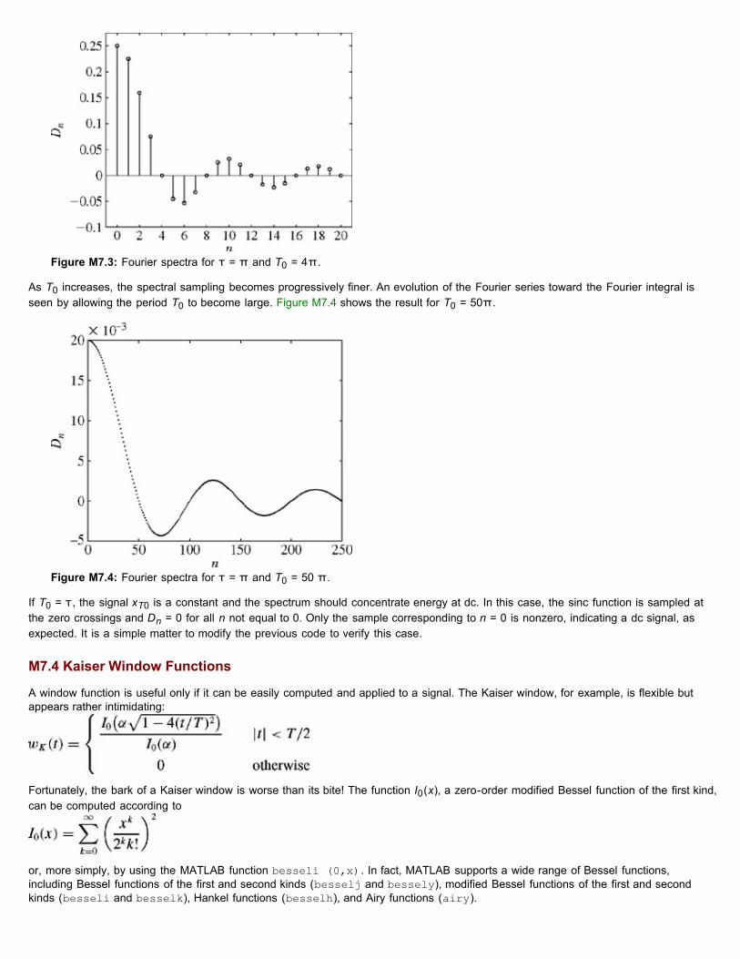
Figure M7.3: Fourier spectra for τ = π and T0 = 4π.

As T0 increases, the spectral sampling becomes progressively finer. An evolution of the Fourier series toward the Fourier integral isseen by allowing the period T0 to become large. Figure M7.4 shows the result for T0 = 50π.

Figure M7.4: Fourier spectra for τ = π and T0 = 50 π.

If T0 = τ, the signal xT0 is a constant and the spectrum should concentrate energy at dc. In this case, the sinc function is sampled atthe zero crossings and Dn = 0 for all n not equal to 0. Only the sample corresponding to n = 0 is nonzero, indicating a dc signal, asexpected. It is a simple matter to modify the previous code to verify this case.

M7.4 Kaiser Window Functions

A window function is useful only if it can be easily computed and applied to a signal. The Kaiser window, for example, is flexible butappears rather intimidating:

Fortunately, the bark of a Kaiser window is worse than its bite! The function I0(x), a zero-order modified Bessel function of the first kind,can be computed according to

or, more simply, by using the MATLAB function besseli (0,x). In fact, MATLAB supports a wide range of Bessel functions,including Bessel functions of the first and second kinds (besselj and bessely), modified Bessel functions of the first and secondkinds (besseli and besselk), Hankel functions (besselh), and Airy functions (airy).

Program MS7P3 computes Kaiser windows at times t by using parameters T and α.

Recall that α = 0, α = 5.4414, and α = 8.885 correspond to rectangular, Hamming, and Blackman windows, respectively. MS7P3 iswritten to allow these special-case Kaiser windows to be identified by name rather than by α value. While unnecessary, this convenientfeature is achieved with the help of the strncmpi command.

The strncmpi (S1, S2, N) command compares the first N characters of strings S1 and S2, ignoring case. More completely,MATLAB has four variants of string comparison: strcmp, strcmpi, strncmp, and strncmpi. Comparisons are restricted to the firstN characters when n is present; case is ignored when i is present. Thus, MS7P3 identifies any string alpha that starts with the letter ror R as a rectangular window. To prevent confusion with a Hanning window, the first three characters must match to identify a Hammingwindow. The isa (alpha, 'char') command determines whether alpha is a character string. MATLAB help documents the manyother classes that isa can identify. In MS7P3, isa is used to terminate execution if a string identifier alpha has not been recognizedas one of the three special cases.

Figure M7.5 shows the three special-case, unit duration Kaiser windows generated by

Figure M7.5: Special-case, unit duration Kaiser windows.

[†]The signal processing toolbox function sinc (x), which computes (sin (πx))/πx, also works provided that inputs are scaled by 1/π.

PROBLEMS7.1.1 Show that if x(t) is an even function of t, then

and if x(t) is an odd function of t, then

Hence, prove that if x(t) is a real and even function of t, then X(ω) is a real and even function of ω. In addition, if x(t) isa real and odd function of t, then X(ω) is an imaginary and odd function of ω.

function [w_K] = MS7P3 (t, T, alpha)% MS7P3.m : MATLAB Session 7, Program 3% Function M-file computes a width-T Kaiser window using parameter alpha,% Alpha can also be a string identifier: 'rectangular', 'Hamming', or% 'Blackman'.% INPUTS: t = independent variable of the window function% T = window width% alpha = Kaiser parameter or string identifier% OUTPUTS: w_K = Kaiser window functionif strncmpi (alpha, 'rectangular', 1),alpha = 0;elseif strncmpi (alpha, 'Hamming', 3),alpha = 5.4414;elseif strncmpi (alpha, 'Blackman', 1),alpha = 8.885;elseif isa(alpha, 'char')disp ('Unrecognized string identifier.'); returnendw_K = zeros (size (t)); i = find (abs (t) <T/2);w K(i) = besseli (0, alpha*sqrt (1-4*t(i). ^2/(T^2)))/besseli (0,alpha);

>> t = [-0.6:.001:0.6]; T = 1;>> plot (t, MS7P3 (t, T, 'r'), 'k-', t, MS7P3 (t, T, 'ham'), 'k:', t,MS7P3 (t, T, 'b'), 'k--');>> axis ([-0.6 0.6 -.1 1.1]); xlabel ('t'); ylabel ('w_K(t)');>> legend ('Rectangular', 'Hamming', 'Blackman');

7.1.2 Show that for a real x(t), Eq. (7.8b) can be expressed as

This is the trigonometric form of the Fourier integral. Compare this with the compact trigonometric Fourier series. 7.1.3 A signal x(t) can be expressed as the sum of even and odd components (see Section 1.5-2):

a. If x(t) X(ω), show that for real x(t),

and

b. Verify these results by finding the Fourier transforms of the even and odd components of the followingsignals: (i) u(t) and (ii) e−atu(t).

7.1.4 From definition (7.8a), find the Fourier transforms of the signals x(t) in Fig. P7.1-4.

Figure P7.1-4

7.1.5 From definition (7.8a), find the Fourier transforms of the signals depicted in Fig. P7.1-5.

Figure P7.1-5

7.1.6 Use Eq. (7.8b) to find the inverse Fourier transforms of the spectra in Fig. P7.1-6.

Figure P7.1-6

7.1.7 Use Eq. (7.8b) to find the inverse Fourier transforms of the spectra in Fig. P7.1-7.

Figure P7.1-7

7.1.8 If x(t) X(ω), then show that

and

Also show that

7.2.1 Sketch the following functions:

a. rect (t/2)

b. Δ(3ω/100)

c. rect ((t− 10)/8)

d. sinc (πω/5)

e. sinc ((ω/5) − 2π)

f. sinc (t/5) rect (t/10π) 7.2.2 From definition (7.8a), show that the Fourier transform of rect (t − 5) is sinc (ω/2)e−j5ω. Sketch the resulting amplitude

and phase spectra. 7.2.3 From definition (7.8b), show that the inverse Fourier transform of rect ((ω − 10)/2π) is sinc (πt)ej10t. 7.2.4 Find the inverse Fourier transform of Xω) for the spectra illustrated in Fig. P7.2-4. [Hint: X(ω) = |X(ω)| ej∠x(ω). This

problem illustrates how different phase spectra (both with the same amplitude spectrum) represent entirely differentsignals.]

a. Can you find the Fourier transform of eatu(t) when a > 1 by setting s = j ω in its Laplace transform ofeatu(t)? Explain.

b. Find the Laplace transform of x(t) shown in Fig. P7.2-5. Can you find the Fourier transform of x(t) bysetting s = jω in its Laplace transform? Explain. Verify your answer by finding the Fourier and the Laplacetransforms of x(t).

Figure P7.2-5

Figure P7.2-4

7.3.1 Apply the duality property to the appropriate pair in Table 7.1 to show that

a. 1/2[δ(t) + j/πt] u(ω)

b. δ(t + T) + δ(t − T) 2cos Tω

c. δ(t + T) + δ(t − T) 2j sin Tω 7.3.2 The Fourier transform of the triangular pulse x(t) in Fig. P7.3-2 is expressed as

Use this information, and the time-shifting and time-scaling properties, to find the Fourier transforms of the signals xi(t)(i= 1, 2, 3, 4, 5) shown in Fig. P7.3-2.

Figure P7.3-2

7.3.3 Using only the time-shifting property and Table 7.1, find the Fourier transforms of the signals depicted in Fig. P7.3-3.

Figure P7.3-3

7.3.4 Use the time-shifting property to show that if x(t) X(ω), then

This is the dual of Eq. (7.41). Use this result and Table 7.1 to find the Fourier transforms of the signals shown in Fig.P7.3-4.

Figure P7.3-4

7.3.5 Prove the following results, which are duals of each other:

Use the latter result and Table 7.1 to find the Fourier transform of the signal in Fig. P7.3-5.

Figure P7.3-5

7.3.6 The signals in Fig. P7.3-6 are modulated signals with carrier cos 10t. Find the Fourier transforms of these signals by

using the appropriate properties of the Fourier transform and Table 7.1. Sketch the amplitude and phase spectra forFig. P7.3-6a and P7.3-6b.

Figure P7.3-6

7.3.7 Use the frequency-shifting property and Table 7.1 to find the inverse Fourier transform of the spectra depicted in Fig.

P7.3-7.

Figure P7.3-7

7.3.8 Use the time convolution property to prove pairs 2, 4, 13, and 14 in Table 2.1 (assume λ < 0 in pair 2, λ1 and λ2 < 0 in

pair 4, λ1 < 0 and λ2 > 0 in pair 13, and λ1 and λ2 > 0 in pair 14). These restrictions are placed because of theFourier transformability issue for the signals concerned. For pair 2, you need to apply the result in Eq. (1.23).

7.3.9 A signal x(t) is bandlimited to B Hz. Show that the signal xn(t) is bandlimited to nB Hz. 7.3.10 Find the Fourier transform of the signal in Fig. P7.3-3a by three different methods:

a. By direct integration using the definition (7.8a).

b. Using only pair 17 (Table 7.1) and the time-shifting property.

c. Using the time-differentiation and time-shifting properties, along with the fact that δ(t) 1. 7.3.11

a. Prove the frequency-differentiation property (dual of the time-differentiation property):

b. Use this property and pair 1 (Table 7.1) to determine the Fourier transform of te−atu(t).

7.4.1 For a stable LTIC system with transfer function

find the (zero-state) response if the input x(t) is

a. e−2tu(t)

b. e−tu(t)

c. etu(−t)

d. u(t) 7.4.2 A stable LTIC system is specified by the frequency response

Find the impulse response of this system and show that this is a noncausal system. Find the (zero-state)response of this system if the input x(t) is

−t

a. e u(t)

b. etu(−t) 7.4.3 Signals x1(t) = 104rect (104t) and x2(t) = δ(t) are applied at the inputs of the ideal low-pass filters

H1(ω) = rect (ω/40,000π) and H2(ω) = rect(ω/20,000π) (Fig. P7.4-3). The outputs y1(t) and y2(t) ofthese filters are multiplied to obtain the signal y(t) = y1(t)y2(t).

a. Sketch X1(ω) and X2(ω).

b. Sketch H1(ω) and H2(ω).

c. Sketch Y1(ω) and Y2(ω).

d. Find the bandwidths of y1(t), y2(t), and y(t).

Figure P7.4-3

7.4.4 A lowpass system time constant is often defined as the width of its unit impulse response h(t) (see

Section 2.7-2). An input pulse p(t) to this system acts like an impulse of strength equal to the area ofp(t) if the width of p(t) is much smaller than the system time constant, and provided p(t) is a lowpasspulse, implying that its spectrum is concentrated at low frequencies. Verify this behavior by considering asystem whose unit impulse response is h(t) = rect(t/10−3). The input pulse is a triangle pulse p(t) =Δ(t/10−6). Show that the system response to this pulse is very nearly the system response to the inputAδ(t), where A is the area under the pulse p(t).

7.4.5 A lowpass system time constant is often defined as the width of its unit impulse response h(t) (see

Section 2.7-2). An input pulse p(t) to this system passes practically without distortion if the width of p(t)is much greater than the system time constant, and provided p(t) is a lowpass pulse, implying that itsspectrum is concentrated at low frequencies. Verify this behavior by considering a system whose unitimpulse response is h(t) = rect (t/10−3). The input pulse is a triangle pulse p(t) = Δ(t). Show that thesystem output to this pulse is very nearly kp(t), where k is the system gain to a dc signal, that is, k =H(0).

7.4.6 A causal signal h(t) has a Fourier transform H(ω). If R(ω) and X(ω) are the real and the imaginary parts

of H(ω), that is, H(ω) = R(ω) + jX(ω), then show that

and

assuming that h(t) has no impulse at the origin. This pair of integrals defines the Hilbert transform. [Hint:Let he(t) and ho(t) be the even and odd components of h(t). Use the results in Prob. 7.1-3. See Fig.1.24 for the relationship between he(t) and ho(t).]

This problem states one of the important properties of causal systems: that the real and imaginary partsof the frequency response of a causal system are related. If one specifies the real part, the imaginarypart cannot be specified independently. The imaginary part is pre-determined by the real part, and viceversa. This result also leads to the conclusion that the magnitude and angle of H(ω) are related providedall the poles and zeros of H(ω) lie in the LHP.

7.5.1 Consider a filter with the frequency response

Show that this filter is physically unrealizable by using the time-domain criterion [noncausal h(t)] and thefrequency-domain (Paley-Wiener) criterion. Can this filter be made approximately realizable by choosing

t0 sufficiently large? Use your own (reasonable) criterion of approximate realizability to determine t0.[Hint: Use pair 22 in Table 7.1.]

7.5.2 Show that a filter with frequency response

is unrealizable. Can this filter be made approximately realizable by choosing a sufficiently large t0? Useyour own (reasonable) criterion of approximate realizability to determine t0.

7.5.3 Determine whether the filters with the following frequency response H(ω) are physically realizable. If

they are not realizable, can they be realized approximately by allowing a finite time delay in theresponse?

a. 10−6 sinc (10−6ω)

b. 10−4 Δ (ω/40,000π)

c. 2πδ(ω)

7.6.1 Show that the energy of a Gaussian pulse

is . Verify this result by using Parseval's theorem to derive the energy Ex from X(ω). [Hint:

See pair 22 in Table 7.1. Use the fact that . 7.6.2 Use Parseval's theorem (7.64) to show that

7.6.3 A lowpass signal x(t) is applied to a squaring device. The squarer output x2(t) is applied to a lowpass

filter of bandwidth Δf (in hertz) (Fig. P7.6-3). Show that if Δf is very small (Δf → 0), then the filter outputis a dc signal y(t) ≈ 2ExΔf. [Hint: if x2(t) A(ω), then show that Y(ω) ≈ [4πA(0)Δf] δ(ω) if Δf → 0.Now, show that A(0) = Ex.]

Figure P7.6-3

7.6.4 Generalize Parseval's theorem to show that for real, Fourier-transformable signals x1(t) and x2(t)

7.6.5 Show that

[Hint: Recognize that

Use this fact and the result in Prob. 7.6-4.] 7.6.6 For the signal

determine the essential bandwidth B (in hertz) of x(t) such that the energy contained in the spectralcomponents of x(t) of frequencies below B Hz is 99% of the signal energy Ex.

7.7.1 For each of the following baseband signals (i) m(t) = cos 1000t, (ii) m(t) = 2cos 1000t + cos 2000t, and(iii) m(t) = cos 1000t cos 3000t:

a. Sketch the spectrum of m(t).

b. Sketch the spectrum of the DSB-SC signal m(t) cos 10,000t.

c. Identify the upper sideband (USB) and the lower sideband (LSB) spectra.

d. Identify the frequencies in the baseband, and the corresponding frequencies in the DSB-SC, USB, and LSB spectra. Explain the nature of frequency shifting in each case.

7.7.2 You are asked to design a DSB-SC modulator to generate a modulated signal km(t) cos ωct, where m(t)

is a signal bandlimited to B Hz (Fig. P7.7-2a). Figure P7.7-2b shows a DSB-SC modulator available inthe stockroom. The bandpass filter is tuned to ωc and has a bandwidth of 2B Hz. The carrier generator

available generates not cos ωct, but cos3 ωct.

a. Explain whether you would be able to generate the desired signal using only thisequipment. If so, what is the value of k?

b. Determine the signal spectra at points b and c, and indicate the frequency bands occupiedby these spectra.

c. What is the minimum usable value of ωc?

d. Would this scheme work if the carrier generator output were cos2 ωct? Explain.

e. Would this scheme work if the carrier generator output were cosn ωct for any integer n ≥2?

Figure P7.7-2

7.7.3 In practice, the analog multiplication operation is difficult and expensive. For this reason, in amplitude

modulators, it is necessary to find some alternative to multiplication of m(t) with cos ωct. Fortunately, forthis purpose, we can replace multiplication with switching operation. A similar observation applies todemodulators. In the scheme depicted in Fig. P7.7-3a, the period of the rectangular periodic pulse x(t)shown in Fig. P7.7-3b is T0 = 2π/ωc. The bandpass filter is centered at ±ωc and has a bandwidth of 2BHz. Note that multiplication by a square periodic pulse x(t) in Fig. P7.7-3b amounts to periodic on-offswitching of m(t), which is bandlimited to B Hz. Such a switching operation is relatively simple andinexpensive.

Show that this scheme can generate an amplitude-modulated signal k cos ωct. Determine the value of k.Show that the same scheme can also be used for demodulation, provided the bandpass filter in Fig.P7.7-3a is replaced by a lowpass (or baseband) filter.

Figure P7.7-3

7.7.4 Figure P7.7-4a shows a scheme to transmit two signals m1(t) and m2(t) simultaneously on the same

channel (without causing spectral interference). Such a scheme, which transmits more than one signal, isknown as signal multiplexing. In this case, we transmit multiple signals by sharing an available spectralband on the channel, and, hence, this is an example of the frequency-division multiplexing. The signal atpoint b is the multiplexed signal, which now modulates a carrier of frequency 20,000 rad/s. Themodulated signal at point c is now transmitted over the channel.

a. Sketch the spectra at points a, b, and c.

b. What must be the minimum bandwidth of the channel?

c. Design a receiver to recover signals m1(t) and m2(t) from the modulated signal at point c.

Figure P7.7-4

7.7.5 The system shown in Fig. P7.7-5 is used for scrambling audio signals. The output y(t) is the scrambled

version of the input m(t).

a. Find the spectrum of the scrambled signal y(t).

b. Suggest a method of descrambling y(t) to obtain m(t).

A slightly modified version of this scrambler was first used commercially on the 25-mile radio-telephonecircuit connecting Los Angeles and Santa Catalina Island.

Figure P7.7-5

7.7.6 Figure P7.7-6 presents a scheme for coherent (synchronous) demodulation. Show that this scheme can

demodulate the AM signal [A + m(t)]cos ωct regardless of the value of A.

Figure P7.7-6

7.7.7 Sketch the AM signal [A + m(t)] cos ωct for the periodic triangle signal m(t) illustrated in Fig. P7.7-7

corresponding to the following modulation indices:

a. μ = 0.5

b. μ = 1

c. μ = 2

d. μ = ∞

How do you interpret the case μ = ∞?

Figure P7.7-7

7.m.1 Consider the signal x(t) = e−atu(t). Modify MS7P2 to compute the following essential bandwidths.

a. Setting a = 1, determine the essential bandwidth W1 that contains 95% of the signalenergy. Compare this value with the theoretical value presented in Example 7.20.

b. Setting a = 2, determine the essential bandwidth W2 that contains 90% of the signalenergy.

c. Setting a = 3, determine the essential bandwidth W3 that contains 75% of the signalenergy.

7.m.2 A unit amplitude pulse with duration τ is defined as

a. Determine the duration τ1 that results in a 95% essential bandwidth of 5 Hz.

b. Determine the duration τ2 that results in a 90% essential bandwidth of 10 Hz.

c. Determine the duration τ3 that results in a 75% essential bandwidth 20 Hz. 7.m.3 Consider the signal x(t) = e−atu(t).

a. Determine the decay parameter a1 that results in a 95% essential bandwidth of 5 Hz.

b. Determine the decay parameter a2 that results in a 90% essential bandwidth of 10 Hz.

c. Determine the decay parameter a3 that results in a 75% essential bandwidth 20 Hz. 7.m.4 Use MATLAB to determine the 95, 90, and 75% essential bandwidths of a one-second triangle function

with a peak amplitude of one. Recall that a triangle function can be constructed by the convolution oftwo rectangular pulses.

7.m.5 A ⅓ duty-cycle square-pulse T0-periodic signal x(t) is described as

a. Use spectral sampling to determine the Fourier series coefficients Dn of x(t) for T0 = 2π.Evaluate and plot Dn for (0 ≤ n ≤ 10).

b. Use spectral sampling to determine the Fourier series coefficients Dn of x(t) for T0 = π.Evaluate and plot Dn for (0 ≤ n ≤ 10). How does this result compare with your answer topart a? What can be said about the relation of T0 to Dn for signal x(t), which has fixed dutycycle of 1/3?

7.m.6 Determine the Fourier transform of a Gaussian pulse defined as x(t) = e−t2

. Plot both x(t) and X(ω).How do the two curves compare? [Hint:

for any real or imaginary a.]

Chapter 8: Sampling-The Bridge From Continuous to Discrete

OVERVIEW

A continuous-time signal can be processed by processing its samples through a discrete-time system. For this purpose, it is important tomaintain the signal sampling rate high enough to permit the reconstruction of the original signal from these samples without error (orwith an error within a given tolerance). The necessary quantitative framework for this purpose is provided by the sampling theoremderived in Section 8.1.

The sampling theory is the bridge between the continuous-time and the discrete-time worlds. The information inherent in a sampledcontinuous-time signal is equivalent to that of a discrete-time signal. A sampled continuous-time signal is a sequence of impulses, whilea discrete-time signal presents the same information as a sequence of numbers. These are basically two different ways of presentingthe same data. Clearly, all the concepts in the analysis of sampled signals apply to discrete-time signals. We should not be surprised tosee that the Fourier spectra of the two kinds of signal are also the same (within a multiplicative constant).

8.1 THE SAMPLING THEOREMWe now show that a real signal whose spectrum is bandlimited to B Hz [X (ω)= 0 for |ω| > 2πB] can be reconstructed exactly (withoutany error) from its samples taken uniformly at a rate f s > 2B samples per second. In other words, the minimum sampling frequency is f

s= 2B Hz.[†]

Figure 8.1: Sampled signal and its Fourier spectrum.

To prove the sampling theorem, consider a signal x (t) (Fig. 8.1a) whose spectrum is band-limited to B Hz (Fig. 8.1b).[‡] Forconvenience, spectra are shown as functions of ω as well as of f (hertz). Sampling x (t) at a rate of f s Hz (f s samples per second) canbe accomplished by multiplying x (t) by an impulse train δT (t)(Fig. 8.1c), consisting of unit impulses repeating periodically every Tseconds, where T= 1/f s. The schematic of a sampler is shown in Fig. 8.1d. The resulting sampled signal x (t) is shown in Fig. 8.1e.

The sampled signal consists of impulses spaced every T seconds (the sampling interval). The nth impulse, located at t= nT, has astrength x (nT), the value of x (t) at t= nT.

Because the impulse train δT (t) is a periodic signal of period T, it can be expressed as a trigonometric Fourier series like that alreadyobtained in Example 6.7 [Eq. (6.39)]

Therefore

To find X (ω), the Fourier transform of x (t), we take the Fourier transform of the right-hand side of Eq. (8.3), term by term. The

transform of the first term in the brackets is X (ω). The transform of the second term 2x (t) cos ωst is X (ω − ωs) + X (ω + ωs) [seeEq. (7.41)]. This represents spectrum X (ω) shifted to ωs and −ωs. Similarly, the transform of the third term 2x (t) cos 2ωst is X (ω −2ωs) + X (ω + 2ωs), which represents the spectrum X (ω) shifted to 2ωs and −2ωs, and so on to infinity. This result means that thespectrum X (ω) consists of X (ω) repeating periodically with period ωs= 2π/T rad/s, or f s= 1/T Hz, as depicted in Fig. 8.1f. There isalso a constant multiplier 1/T in Eq. (8.3). Therefore

If we are to reconstruct x (t) from x (t), we should be able to recover X (ω) from X (ω). This recovery is possible if there is no overlapbetween successive cycles of X (ω). Figure 8.1f indicates that this requires

Also, the sampling interval T= 1/f s. Therefore

Thus, as long as the sampling frequency f s is greater than twice the signal bandwidth B (in hertz), X (ω) consists of nonoverlappingrepetitions of X (ω). Figure 8.1f shows that the gap between the two adjacent spectral repetitions is f s − 2B Hz, and x (t) can berecovered from its samples x (t) by passing the sampled signal x (t) through an ideal lowpass filter having a bandwidth of any valuebetween B and f s − B Hz. The minimum sampling rate f s= 2B required to recover x (t) from its samples x (t) is called the Nyquist ratefor x (t), and the corresponding sampling interval T= 1/2B is called the Nyquist interval for x (t). Samples of a signal taken at its Nyquistrate are the Nyquist samples of that signal.

We are saying that the Nyquist rate 2B Hz is the minimum sampling rate required to preserve the information of x (t). This contradictsEq. (8.5), where we showed that to preserve the information of x (t), the sampling rate f s needs to be greater than 2B Hz. Strictlyspeaking, Eq. (8.5) is the correct statement. However, if the spectrum X (ω) contains no impulse or its derivatives at the highestfrequency B Hz, then the minimum sampling rate 2B Hz is adequate. In practice, it is rare to observe X (ω) with an impulse or itsderivatives at the highest frequency. If the contrary situation were to occur, we should use Eq. (8.5).[†]

The sampling theorem proved here uses samples taken at uniform intervals. This condition is not necessary. Samples can be takenarbitrarily at any instants as long as the sampling instants are recorded and there are, on average, 2B samples per second.[2] Theessence of the sampling theorem was known to mathematicians for a long time in the form of the interpolation formula [see later, Eq.(8.11)]. The origin of the sampling theorem was attributed by H. S. Black to Cauchy in 1841. The essential idea of the samplingtheorem was rediscovered in the 1920s by Carson, Nyquist, and Hartley.

EXAMPLE 8.1In this example, we examine the effects of sampling a signal at the Nyquist rate, below the Nyquist rate (undersampling), and above theNyquist rate (oversampling). Consider a signal x (t)= sin2 (5πt) (Fig. 8.2a) whose spectrum is X (ω)= 0.2 Δ (ω/20π) (Fig. 8.2b). Thebandwidth of this signal is 5 Hz (10π rad/s). Consequently, the Nyquist rate is 10 Hz; that is, we must sample the signal at a rate noless than 10 samples/s. The Nyquist interval is T= 1/2B= 0.1 second.

Figure 8.2: Effects of undersampling and oversampling.

Recall that the sampled signal spectrum consists of (1/T) X (ω) = (0.2/T) Δ (ω/20π) repeating periodically with a period equal to thesampling frequency f s Hz. We present this information in Table 8.1 for three sampling rates: f s= 5 Hz (undersampling), 10 Hz (Nyquistrate), and 20 Hz (oversampling).

Table 8.1 Open table as spreadsheet

Sampling Frequency f s (Hz) Sampling Interval T (second) Comments

5 0.2 Undersampling

10 0.1 Nyquist rate

20 0.05 Oversampling

In the first case (undersampling), the sampling rate is 5 Hz (5 samples/s), and the spectrum (1/T) X (ω) repeats every 5 Hz (10πrad/s). The successive spectra overlap, as depicted in Fig. 8.2d, and the spectrum X (ω) is not recoverable from X (ω); that is, x (t)cannot be reconstructed from its samples x (t) in Fig. 8.2c. In the second case, we use the Nyquist sampling rate of 10 Hz (Fig. 8.2e).The spectrum X (ω) consists of back-to-back, nonoverlapping repetitions of (1/T) X (ω) repeating every 10 Hz. Hence, X (ω) can berecovered from X (ω) using an ideal lowpass filter of bandwidth 5 Hz (Fig. 8.2f). Finally, in the last case of oversampling (sampling rate20 Hz), the spectrum X (ω) consists of nonoverlapping repetitions of (1/T) X (ω) (repeating every 20 Hz) with empty bands betweensuccessive cycles (Fig. 8.2h). Hence, X (ω) can be recovered from X (ω) by using an ideal lowpass filter or even a practical lowpassfilter (shown dashed in Fig. 8.2h).[†]

EXERCISE E8.1

Find the Nyquist rate and the Nyquist interval for the signals sinc (100πt) and sinc (100πt) + sinc (50πt).

Answers

The Nyquist interval is 0.01 second and the Nyquist sampling rate is 100 Hz for both the signals.

FOR SKEPTICS ONLYRare is a reader, who, at first encounter, is not skeptical of the sampling theorem. It seems impossible that Nyquist samples can definethe one and the only signal that passes through those sample values. We can easily picture infinite number of signals passing througha given set of samples. However, among all these (infinite number of) signals, only one has the minimum bandwidth B ≤ 1/2T Hz,where T is the sampling interval. See Prob. 8.2−9.

To summarize, for a given set of samples taken at a rate of f s Hz, there is only one signal of bandwidth B ≤ f s/2 that passes throughthose samples. All other signals that pass through those samples have bandwidth higher than f s/2, and the samples are sub-Nyquistrate samples for those signals.

8.1-1 Practical Sampling

In proving the sampling theorem, we assumed ideal samples obtained by multiplying a signal x (t) by an impulse train that is physicallyunrealizable. In practice, we multiply a signal x (t) by a train of pulses of finite width, depicted in Fig. 8.3c. The sampler is shown in Fig.8.3d. The sampled signal x (t) is illustrated in Fig. 8.3e. We wonder whether it is possible to recover or reconstruct x (t) from this x (t).Surprisingly, the answer is affirmative, provided the sampling rate is not below the Nyquist rate. The signal x (t) can be recovered bylowpass filtering x (t) as if it were sampled by impulse train.

Figure 8.3: Effect of practical sampling.

The plausibility of this result becomes apparent when we consider the fact that reconstruction of x (t) requires the knowledge of theNyquist sample values. This information is available or built in the sampled signal x (t) in Fig. 8.3e because the nth sampled pulsestrength is x (nT). To prove the result analytically, we observe that the sampling pulse train p T (t) depicted in Fig. 8.3c, being aperiodic signal, can be expressed as a trigonometric Fourier series

and

The sampled signal x (t) consists of C0x (t), C1x (t) cos (ωst + θ1), C2 x (t) cos(2ωs t θ2),.... Note that the first term C0x (t) is thedesired signal and all the other terms are modulated signals with spectra centered at ±ωs, ±ωs, ±ωs, ..., as illustrated in Fig. 8.3f.Clearly the signal x (t) can be recovered by lowpass filtering of x (t), as shown in Fig. 8.3d. As before, it is necessary that ωs > 4π B

(orfs > 2B).

EXAMPLE 8.2To demonstrate practical sampling, consider a signal x (t)= sinc2 (5πt) sampled by a rectangular pulse sequence p T (t) illustrated inFig. 8.4c. The period of p T (t) is 0.1 second, so that the fundamental frequency (which is the sampling frequency) is 10 Hz. Hence,ωs= 20π.

The Fourier series for p T (t) can be expressed as

Figure 8.4: An example of practical sampling.

Hence

Use of Eqs. (6.18) yields Consequently, we have

and

where C n= (2/nπ) sin (nπ/4). The spectrum consists of X (ω) repeating periodically at the interval of 20π rad/s (10 Hz). Hence, thereis no overlap between cycles, and X (ω) can be recovered by using an ideal lowpass filter of bandwidth 5 Hz. An ideal lowpass filter ofunit gain (and bandwidth 5 Hz) will allow the first term on the right hand side of the foregoing equation to pass fully and suppress all theother terms. Hence, the output y (t) is

EXERCISE E8.2Show that the basic pulse p (t) used in the sampling pulse train in Fig. 8.4c cannot have zero area if we wish to reconstruct x (t) bylowpass-filtering the sampled signal.

[†]The theorem stated here (and proved subsequently) applies to lowpass signals. A bandpass signal whose spectrum exists over afrequency band f c − (B/2) < |f| < f c + (B/2) has a bandwidth of B Hz. Such a signal is uniquely determined by 2B samples persecond. In general, the sampling scheme is a bit more complex in this case. It uses two interlaced sampling trains, each at a rate of Bsamples per second. See, for example, Linden.[1]

[†]Linden, D. A. A discussion of sampling theorem. Proceedings of the IRE, vol. 47, pp. 1219-1226, July 1959.

[‡]The spectrum X (ω) in Fig. 8.1b is shown as real, for convenience. However, our arguments are valid for complex X (ω) as well.

[†]An interesting observation is that if the impulse is because of a cosine term, the sampling rate of 2B Hz is adequate. However, if theimpulse is because of a sine term, then the rate must be greater than 2B Hz. This may be seen from the fact that samples of sin 2π Btusing T= 1/2B are all zero because sin 2π BnT= sin πn= 0. But, samples of cos 2π Bt are cos 2π BnT= cos πn= (−1)n. We canreconstruct cos 2π Bt from these samples. This peculiar behavior occurs because in the sampled signal spectrum corresponding to thesignal cos 2π Bt, the impulses, which occur at frequencies (2n±1) B Hz (n= 0, ±1, ±2, ...), interact constructively, whereas in the caseof sin 2πBt, the impulses, because of their opposite phases (e±jπ/2, interact destructively and cancel out in the sampled signalspectrum. Hence, sin 2π Bt cannot be reconstructed from its samples at a rate of 2B Hz. A similar situation exists for signal cos(2π Bt+ θ), which contains a component of the form sin 2π Bt. For this reason, it is advisable to maintain sampling rate above 2B Hz if afinite amplitude component of a sinusoid of frequency B Hz is present in the signal.

[2]Siebert, W. M. Circuits, Signals, and Systems. MIT-McGraw-Hill, New York, 1986.

[†]The filter should have a constant gain between 0 and 5 Hz and zero gain beyond 10 Hz. In practice, the gain beyond 10 Hz can bemade negligibly small, but not zero.

8.2 SIGNAL RECONSTRUCTIONThe process of reconstructing a continuous-time signal x (t) from its samples is also known as interpolation. In Section 8.1, we saw thata signal x (t) bandlimited to B Hz can be reconstructed (interpolated) exactly from its samples if the sampling frequency f s exceeds 2BHz or the sampling interval T is less than 1/2B. This reconstruction is accomplished by passing the sampled signal through an ideallowpass filter of gain T and having a bandwidth of any value between B and f s − B Hz. From a practical viewpoint, a good choice isthe middle value f s/2= 1/2T Hz or π/T rad/s. This value allows for small deviations in the ideal filter characteristics on either side of thecutoff frequency. With this choice of cutoff frequency and gain T, the ideal lowpass filter required for signal reconstruction (orinterpolation) is

The interpolation process here is expressed in the frequency domain as a filtering operation. Now we shall examine this process fromthe time-domain viewpoint.

TIME-DOMAIN VIEW: A SIMPLE INTERPOLATION

Consider the interpolation system shown in Fig. 8.5a. We start with a very simple interpolating filter, whose impulse response is rect(t/T), depicted in Fig. 8.5b. This is a gate pulse centered at the origin, having unit height, and width T (the sampling interval). We shallfind the output of this filter when the input is the sampled signal x (t) consisting of an impulse train with the nth impulse at t= nT withstrength x (nT). Each sample in x (t), being an impulse, produces at the output a gate pulse of height equal to the strength of thesample. For instance, the nth sample is an impulse of strength x (nT) located at t= nT and can be expressed as x (nT)δ(t − nT). Whenthis impulse passes through the filter, it produces at the output a gate pulse of height x (nT), centered at t= nT (shaded in Fig. 8.5c).Each sample in x (t) will generate a corresponding gate pulse, resulting in the filter output that is a staircase approximation of x (t),shown dotted in Fig. 8.5c. This filter thus gives a crude form of interpolation.

Figure 8.5: Simple interpolation by means of a zero-order hold (ZOH) circuit. (a) ZOH interpolator. (b) Impulse response of a ZOHcircuit. (c) Signal reconstruction by ZOH, as viewed in the time domain. (d) Frequency response of a ZOH.

The frequency response of this filter H (ω) is the Fourier transform of the impulse response rect (t/T).

and

The amplitude response |H (ω)| for this filter, illustrated in Fig. 8.5d, explains the reason for the crudeness of this interpolation. Thisfilter, also known as the zero-order hold (ZOH) filter, is a poor form of the ideal lowpass filter (shaded in Fig. 8.5d) required for exactinterpolation.[†]

We can improve on the ZOH filter by using the first-order hold filter, which results in a linear interpolation instead of the staircaseinterpolation. The linear interpolator, whose impulse response is a triangle pulse Δ(t/2T), results in an interpolation in which successivesample tops are connected by straight-line segments (see Prob. 8.2-3).

TIME-DOMAIN VIEW: AN IDEAL INTERPOLATION

The ideal interpolation filter frequency response obtained in Eq. (8.8) is illustrated in Fig. 8.6a. The impulse response of this filter, theinverse Fourier transform of H (ω) is

Figure 8.6: Ideal interpolation for Nyquist sampling rate.

For the Nyquist sampling rate, T= 1/2B, and

This h (t) is depicted in Fig. 8.6b. Observe the interesting fact that h (t)= 0 at all Nyquist sampling instants (t= ±n/2B) except at t= 0.When the sampled signal x (t) is applied at the input of this filter, the output is x (t). Each sample in x (t), being an impulse, generatesa sinc pulse of height equal to the strength of the sample, as illustrated in Fig. 8.6c. The process is identical to that depicted in Fig.8.5c, except that h (t) is a sinc pulse instead of a gate pulse. Addition of the sinc pulses generated by all the samples results in x (t).The nth sample of the input x (t) is the impulse x (nT)δ(t−nT); the filter output of this impulse is x (nT)h (t−nT). Hence, the filteroutput to x (t), which is x (t), can now be expressed as a sum

For the case of Nyquist sampling rate, T= 1/2B, and Eq. (8.11a) simplifies to

Equation (8.11b) is the interpolation formula, which yields values of x (t) between samples as a weighted sum of all the sample values.

EXAMPLE 8.3Find a signal x (t) that is bandlimited to B Hz, and whose samples are

where the sampling interval T is the Nyquist interval for x (t), that is, T= 1/2B.

Because, we are given the Nyquist sample values, we use the interpolation formula (8.11b) to construct x (t) from its samples. Since allbut one of the Nyquist samples are zero, only one term (corresponding to n= 0) in the summation on the right-hand side of Eq. (8.11b)survives. Thus

This signal is illustrated in Fig. 8.6b. Observe that this is the only signal that has a bandwidth B Hz and the sample values x (0)= 1 andx (nT)= 0 (n ≠ 0). No other signal satisfies these conditions.

8.2-1 Practical Difficulties in Signal Reconstruction

Consider the signal reconstruction procedure illustrated in Fig. 8.7a. If x (t) is sampled at the Nyquist rate f s= 2B Hz, the spectrum X(ω) consists of repetitions of X (ω) without any gap between successive cycles, as depicted in Fig. 8.7b. To recover x (t) from x (t), weneed to pass the sampled signal x (t) through an ideal lowpass filter, shown dotted in Fig. 8.7b. As seen in Section 7.5, such a filter isunrealizable; it can be closely approximated only with infinite time delay in the response. In other words, we can recover the signal x (t)from its samples with infinite time delay. A practical solution to this problem is to sample the signal at a rate higher than the Nyquist rate(f s >2B or ωs > 4πB). The result is X (ω), consisting of repetitions of X (ω) with a finite band gap between successive cycles, asillustrated in Fig. 8.7c. Now, we can recover X (ω) from X (ω) using a lowpass filter with a gradual cutoff characteristic, shown dottedin Fig. 8.7c. But even in this case, if the unwanted spectrum is to be suppressed, the filter gain must be zero beyond some frequency(see Fig. 8.7c). According to the Paley-Wiener criterion [Eq. (7.61)], it is impossible to realize even this filter. The only advantage in thiscase is that the required filter can be closely approximated with a smaller time delay. All this means that it is impossible in practice torecover a bandlimited signal x (t) exactly from its samples, even if the sampling rate is higher than the Nyquist rate. However, as thesampling rate increases, the recovered signal approaches the desired signal more closely.

Figure 8.7: (a) Signal reconstruction from its samples. (b) Spectrum of a signal sampled at the Nyquist rate. (c) Spectrum of asignal sampled above the Nyquist rate.

THE TREACHERY OF ALIASINGThere is another fundamental practical difficulty in reconstructing a signal from its samples. The sampling theorem was proved on theassumption that the signal x (t) is bandlimited. All practical signals are timelimited; that is, they are of finite duration or width. We candemonstrate (see Prob. 8.2-14) that a signal cannot be timelimited and bandlimited simultaneously. If a signal is timelimited, it cannotbe bandlimited, and vice versa (but it can be simultaneously nontimelimited and nonbandlimited). Clearly, all practical signals, which arenecessarily timelimited, are nonbandlimited, as shown in Fig. 8.8a; they have infinite bandwidth, and the spectrum X (ω) consists ofoverlapping cycles of X (ω) repeating every f s Hz (the sampling frequency), as illustrated in Fig. 8.8b.[†] Because of infinite bandwidthin this case, the spectral overlap is unavoidable, regardless of the sampling rate. Sampling at a higher rate reduces but does noteliminate overlapping between repeating spectral cycles. Because of the overlapping tails, X (ω) no longer has complete informationabout X (ω), and it is no longer possible, even theoretically, to recover x (t) exactly from the sampled signal x (t). If the sampled signalis passed through an ideal lowpass filter of cutoff frequency f s/2 Hz, the output is not X (ω) but X n (ω) (Fig. 8.8c), which is a versionof X (ω) distorted as a result of two separate causes:

Figure 8.8: Aliasing effect. (a) Spectrum of a practical signal x (t). (b) Spectrum of sampled x (t). (c) Reconstructed signalspectrum. (d) Sampling scheme using antialiasing filter. (e) Sampled signal spectrum (dotted) and the reconstructed signalspectrum (solid) when antialiasing filter is used.

1. The loss of the tail of X (ω) beyond |f| > f s/2 Hz.

2. The reappearance of this tail inverted or folded onto the spectrum. Note that the spectra cross at frequency f s/2= 1/2THz. This frequency is called the folding frequency. The spectrum may be viewed as if the lost tail is folding back onto itselfat the folding frequency. For instance, a component of frequency (f s/2) + f z shows up as or "impersonates" as acomponent of lower frequency (f s/2) − f z in the reconstructed signal. Thus, the components of frequencies above f s/2reappear as components of frequencies below f s/2. This tail inversion, known as spectral folding or aliasing, is shownshaded in Fig. 8.8b and also in Fig. 8.8c. In the process of aliasing, not only are we losing all the components offrequencies above the folding frequency f s/2 Hz, but these very components reappear (aliased) as lower-frequencycomponents, as shown in Fig. 8.8b or 8.8c. Such aliasing destroys the integrity of the frequency components below thefolding frequency f s/2, as depicted in Fig. 8.8c.

The aliasing problem is analogous to that of an army with a platoon that has secretly defected to the enemy side. The platoon is,however, ostensibly loyal to the army. The army is in double jeopardy. First, the army has lost this platoon as a fighting force. Inaddition, during actual fighting, the army will have to contend with the sabotage by the defectors and will have to find another loyalplatoon to neutralize the defectors. Thus, the army has lost two platoons in nonproductive activity.

DEFECTORS ELIMINATED: THE ANTIALIASING FILTERIf you were the commander of the betrayed army, the solution to the problem would be obvious. As soon as the commander got wind ofthe defection, he would incapacitate, by whatever means, the defecting platoon before the fighting begins. This way he loses only one(the defecting) platoon. This is a partial solution to the double jeopardy of betrayal and sabotage, a solution that partly rectifies theproblem and cuts the losses to half.

We follow exactly the same procedure. The potential defectors are all the frequency components beyond the folding frequency f s/2=1/2T Hz. We should eliminate (suppress) these components from x (t) before sampling x (t). Such suppression of higher frequenciescan be accomplished by an ideal lowpass filter of cutoff f s/2 Hz, as shown in Fig. 8.8d. This is called the antialiasing filter. Figure 8.8dalso shows that antialiasing filtering is performed before sampling. Figure 8.8e shows the sampled signal spectrum (dotted) and thereconstructed signal X aa (ω) when antialiasing scheme is used. An antialiasing filter essentially bandlimits the signal x (t) to f s/2 Hz.

This way, we lose only the components beyond the folding frequency f s/2 Hz. These suppressed components now cannot reappear tocorrupt the components of frequencies below the folding frequency. Clearly, use of an antialiasing filter results in the reconstructedsignal spectrum X aa (ω)= X (ω) for |f| < f s/2. Thus, although we lost the spectrum beyond f s/2 Hz, the spectrum for all thefrequencies below f s/2 remains intact. The effective aliasing distortion is cut in half owing to elimination of folding. We stress again thatthe antialiasing operation must be performed before the signal is sampled.

An antialiasing filter also helps to reduce noise. Noise, generally, has a wideband spectrum, and without antialiasing, the aliasingphenomenon itself will cause the noise lying outside the desired band to appear in the signal band. Antialiasing suppresses the entirenoise spectrum beyond frequency f s/2.

The antialiasing filter, being an ideal filter, is unrealizable. In practice, we use a steep cutoff filter, which leaves a sharply attenuatedspectrum beyond the folding frequency f s/2.

SAMPLING FORCES NONBANDLIMITED SIGNALS TO APPEAR BANDLIMITEDFigure 8.8b shows the spectrum of a signal x (t) consists of overlapping cycles of X (ω). This means that x (t) are sub-Nyquist samplesof x (t). However, we may also view the spectrum in Fig. 8.8b as the spectrum X a (ω) (Fig. 8.8c), repeating periodically every f s Hzwithout overlap. The spectrum X a (ω) is bandlimited to f sω Hz. Hence, these (sub-Nyquist) samples of x (t) are actually the Nyquistsamples for signal x a (t). In conclusion, sampling a nonbandlimited signal x (t) at a rate f s Hz makes the samples appear to be theNyquist samples of some signal x a (t), bandlimited to f s Hz. In other words, sampling makes a nonbandlimited signal appear to be abandlimited signal x a (t) with bandwidth f s/2 Hz. A similar conclusion applies if x (t) is bandlimited but sampled at a sub-Nyquist rate.

VERIFICATION OF ALIASING IN SINUSOIDSWe showed in Fig. 8.8b how sampling a signal below the Nyquist rate causes aliasing, which makes a signal of higher frequency (f s/2)+ f z Hz masquerade as a signal of lower frequency (f s/2) − f z Hz. Figure 8.8b demonstrates this result in the frequency domain. Letus now verify it in the time domain to gain a deeper appreciation of aliasing.

We can prove our proposition by showing that samples of sinusoids of frequencies (ωs/2) + ωz and (ωs/2 − ωz are identical when thesampling frequency is f s= ωs/2π Hz.

For a sinusoid x (t)= cos ωt, sampled at intervals of T seconds, x (nT), its nth sample (at t= nT) is

Hence, samples of sinusoids of frequency ω= (ωs/2) ± ωz are[†]

Recognizing that ωsT= 2π f sT= 2π, and sin (ωs/2)nT= sin πn= 0 for all integer n, we obtain

Clearly, the samples of a sinusoid of frequency (f s/2) + f z are identical to the samples of a sinusoid (f s/2) − f z.[‡] For instance, whena sinusoid of frequency 100 Hz is sampled at a rate of 120 Hz, the apparent frequency of the sinusoid that results from reconstructionof the samples is 20 Hz. This follows from the fact that here, 100= (f s/2) + f z= 60 + f z so that f z= 40. Hence, (f s/2) − f z= 20. Suchwould precisely be the conclusion arrived at from Fig. 8.8b.

This discussion again shows that sampling a sinusoid of frequency f aliasing can be avoided if the sampling rate f s > 2f Hz.

Violating this condition leads to aliasing, implying that the samples appear to be those of a lower-frequency signal. Because of this lossof identity, it is impossible to reconstruct the signal faithfully from its samples.

GENERAL CONDITION FOR ALIASING IN SINUSOIDSWe can generalize the foregoing result by showing that samples of a sinusoid of frequency f 0 are identical to those of a sinusoid offrequency f 0 + mf s Hz (integer m), where f s is the sampling frequency. The samples of cos 2π (f 0 + mf s) t are

The result follows because mn is an integer and f sT= 1. This result shows that sinusoids of frequencies that differ by integer multiple off s result in identical set of samples. In other words, samples of sinusoids separated by frequency f s Hz are identical. This implies thatsamples of sinusoids in any frequency band of f s Hz are unique; that is, no two sinusoids in that band have the same samples (when

sampled at a rate f s Hz). For instance, frequencies in the band from − f s/2 to f s/2 have unique samples (at the sampling rate f s).This band is called the fundamental band. Recall also that f s/2 is the folding frequency.

From the discussion thus far, we conclude that if a continuous-time sinusoid of frequency f Hz is sampled at a rate of f s Hz(samples/s), the resulting samples would appear as samples of a continuous-time sinusoid of frequency f a in the fundamental band,where

The frequency f a lies in the fundamental band from − f s/2 to f s/2. Figure 8.9a shows the plot of f a versus f, where f is the actualfrequency and f a is the corresponding fundamental band frequency, whose samples are identical to those of the sinusoid of frequencyf, when sampling rate is f s Hz.

Figure 8.9: Apparent frequencies of a sampled sinusoid: (a) f a versus f and (b) |f a| versus f.

Recall, however, that the sign change of a frequency does not alter the actual frequency of the waveform. This is because

Clearly the apparent frequency of a sinusoid of frequency − f a is also f a. However, its phase undergoes a sign change. This meansthe apparent frequency of any sampled sinusoid lies in the range from 0 to f s/2 Hz. To summarize, if a continuous-time sinusoid offrequency f Hz is sampled at a rate of f s Hz (samples/second), the resulting samples would appear as samples of a continuous-timesinusoid of frequency |f a| that lies in the band from 0 to f s/2. According to Eq. (8.15a)

The plot of the apparent frequency |f a| versus f is shown in Fig. 8.9b.[†] As expected, the apparent frequency |f a| of any sampledsinusoid, regardless of its frequency, is always in the range of 0 to f s/2 Hz. However, when f a is negative, the phase of the apparentsinusoid undergoes a sign change. The frequency belts in which such phase changes occur are shown shaded in Fig. 8.9b.

Consider, for example, a sinusoid cos (2π ft + θ) with f= 8000 Hz sampled at a rate f s= 3000 Hz. Using Eq. (8.15a), we obtain f a=8000 − 3 × 3000= −1000. Hence, |f a|= 1000. The samples would appear to have come from a sinusoid cos (2000ω t ω θ). Observe

the sign change of the phase because f a is negative.[‡]

In the light of the foregoing development, let us consider a sinusoid of frequency f = (f s/2) + f z, sampled at a rate of f s Hz. Accordingto Eq. (8.15a).

Hence, the apparent frequency is |f a|= (f s/2) − f z, confirming our earlier result. However, the phase of the sinusoid will suffer a signchange because f a is negative.

Figure 8.10 shows how samples of sinusoids of two different frequencies (sampled at the same rate) generate identical sets of samples.Both the sinusoids are sampled at a rate f s= 5 Hz (T= 0.2 second). The frequencies of the two sinusoids, 1 Hz (period 1) and 6 Hz(period 1/6), differ by f s= 5 Hz.

Figure 8.10: Demonstration of aliasing.

The reason for aliasing can be clearly seen in Fig. 8.10. The root of the problem is the sampling rate, which may be adequate for thelower-frequency sinusoid but is clearly inadequate for the higher-frequency sinusoid. The figure clearly shows that between thesuccessive samples of the higher-frequency sinusoid, there are wiggles, which are bypassed or ignored, and are unrepresented in thesamples, indicating a sub-Nyquist rate of sampling. The frequency of the apparent signal X a (t) is always the lowest possible frequencythat lies within the band |f| ≤ f s/2. Thus, the apparent frequency of the samples in this example is 1 Hz. If these samples are chosento reconstruct a signal using a lowpass filter of bandwidth f s/2, we shall obtain a sinusoid of frequency 1 Hz.

EXAMPLE 8.4A continuous-time sinusoid cos (2π ft + θ) is sampled at a rate f s= 1000 Hz. Determine the apparent (aliased) sinusoid of the resultingsamples if the input signal frequency f is:

a. 400 Hz

b. 600 Hz

c. 1000 Hz

d. 2400 Hz

The folding frequency is f s/2 = 500. Hence, sinusoids below 500 Hz (frequency within the fundamental band) will not be aliased andsinusoids of frequency above 500 Hz will be aliased.

a. f= 400 Hz is less than 500 Hz, and there is no aliasing. The apparent sinusoid is cos (2π ft + θ) with f= 400.

b. f= 600 Hz can be expressed as 600= −400 + 1000 so that f a= −400. Hence, the aliased frequency is 400 Hz and thephase changes sign. Hence, the apparent (aliased) sinusoid is cos (2π ft − θ) with f= 400.

c. f= 1000 Hz can be expressed as 1000= 0 + 1000 so that f a= 0. Hence, the aliased frequency is 0 Hz (dc), and there is nophase sign change. Hence, the apparent sinusoid is y (t)= cos (0πt ± θ)= cos (θ). This is a dc signal with constantsample values for all n.

d. f= 2400 Hz can be expressed as 2400= 400 + (2 × 1000) so that f a= 400. Hence, the aliased frequency is 400 Hz andthere is no sign change for the phase. The apparent sinusoid is cos (2π ft + θ) with f= 400.

We could have found these answers directly from Fig. 8.9b. For example, for case b, we read |f a|= 400 corresponding to f= 600.Moreover, f= 600 lies in the shaded belt. Hence, there is a phase sign change.

EXERCISE E8.3Show that samples of 90 Hz and 110 Hz sinusoids of the form cos ωt are identical when sampled at a rate 200 Hz.

EXERCISE E8.4

A sinusoid of frequency f 0 Hz is sampled at a rate of 100 Hz. Determine the apparent frequency of thesamples if f 0 is

a. 40 Hz

b. 60 Hz

c. 140 Hz

d. 160 Hz

Answers

40 Hz for all four cases

8.2-2 Some Applications of the Sampling Theorem

The sampling theorem is very important in signal analysis, processing, and transmission because it allows us to replace a continuous-time signal with a discrete sequence of numbers. Processing a continuous-time signal is therefore equivalent to processing a discretesequence of numbers. Such processing leads us directly into the area of digital filtering. In the field of communication, the transmissionof a continuous-time message reduces to the transmission of a sequence of numbers by means of pulse trains. The continuous-timesignal x (t) is sampled, and sample values are used to modify certain parameters of a periodic pulse train. We may vary the amplitudes(Fig. 8.11b), widths (Fig. 8.11c), or positions (Fig. 8.11d) of the pulses in proportion to the sample values of the signal x (t). Accordingly,we may have pulse-amplitude modulation (PAM), pulse-width modulation (PWM), or pulse-position modulation (PPM) The mostimportant form of pulse modulation today is pulse-code modulation (PCM), discussed in Section 8.3 in connection with Fig. 8.14b. In allthese cases, instead of transmitting x (t), we transmit the corresponding pulse-modulated signal. At the receiver, we read theinformation of the pulse-modulated signal. At the receiver, we read the information of the pulse-modulated signal and reconstruct theanalog signal x (t).

Figure 8.11: Pulse-modulated signals. (a) The signal. (b) The PAM signal. (c) The PWM (PDM) signal. (d) The PAMsignal.

One advantage of using pulse modulation is that it permits the simultaneous transmission of several signals on a time-sharingbasis-time-division multiplexing (TDM). Because a pulse-modulated signal occupies only a part of the channel time, we can transmitseveral pulse-modulated signals on the same channel by interweaving them. Figure 8.12 shows the TDM of two PAM signals. In thismanner, we can multiplex several signals on the same channel by reducing pulse widths.[†]

Figure 8.12: Time-division multiplexing of two signals.

Digital signals also offer an advantage in the area of communications, where signals must travel over distances. Transmission of digitalsignals is more rugged than that of analog signals because digital signals can withstand channel noise and distortion much better aslong as the noise and the distortion are within limits. An analog signal can be converted to digital binary form through sampling andquantization (rounding off), as explained in the next section. The digital (binary) message in Fig. 8.13a is distorted by the channel, asillustrated in Fig. 8.13b. Yet if the distortion remains within a limit, we can recover the data without error because we need only make asimple binary decision: Is the received pulse positive or negative? Figure 8.13c shows the same data with channel distortion and noise.

Here again the data can be recovered correctly as long as the distortion and the noise are within limits. Such is not the case withanalog messages. Any distortion or noise, no matter how small, will distort the received signal.

Figure 8.13: Digital signal transmission: (a) at the transmitter, (b) received distorted signal (without noise), (c) received distortedsignal (with noise), and (d) regenerated signal at the receiver.

The greatest advantage of digital communication over the analog counterpart, however, is the viability of regenerative repeaters in theformer. In an analog transmission system, a message signal grows progressively weaker as it travels along the channel (transmissionpath), whereas the channel noise and the signal distortion, being cumulative, become progressively stronger. Ultimately the signal,overwhelmed by noise and distortion, is mutilated. Amplification is of little help because it enhances the signal and the noise in thesame proportion. Consequently, the distance over which an analog message can be transmitted is limited by the transmitted power. If atransmission path is long enough, the channel distortion and noise will accumulate sufficiently to overwhelm even a digital signal. Thetrick is to set up repeaters along the transmission path at distances short enough to permit detection of signal pulses before the noiseand distortion have a chance to accumulate sufficiently. At each repeater, the pulses are detected, and new, clean pulses aretransmitted to the next repeater, which, in turn, duplicates the same process. If the noise and distortion remain within limits (which ispossible because of the closely spaced repeaters), pulses can be detected correctly.[†] This way the digital messages can betransmitted over longer distances with greater reliability. In contrast, analog messages cannot be cleaned up periodically, and theirtransmission is therefore less reliable. The most significant error in digitized signals comes from quantizing (rounding off). This error,discussed in Section 8.3, can be reduced as much as desired by increasing the number of quantization levels, at the cost of anincreased bandwidth of the transmission medium (channel).

[†]Figure 8.5b shows that the impulse response of this filter is noncausal, and this filter is not realizable. In practice, we make itrealizable by delaying the impulse response by T/2. This merely delays the output of the filter by T/2.

[†]Figure 8.8b shows that from the infinite number of repeating cycles, only the neighboring spectral cycles overlap. This is a somewhatsimplified picture. In reality, all the cycles overlap and interact with every other cycle because of the infinite width of all practical signalspectra. Fortunately, all practical spectra also must decay at higher frequencies. This results in insignificant amount of interference fromcycles other than the immediate neighbors. When such an assumption is not justified, aliasing computations become little moreinvolved.

[†]Here we have ignored the phase aspect of the sinusoid. Sampled versions of a sinusoid x (t)= cos (ωt + θ) with two differentfrequencies (ωs/2) ωz have identical frequency, but the phase signs may be reversed depending on the value of ωz.

[‡]The reader is encouraged to verify this result graphically by plotting the spectrum of a sinusoid of frequency (ωs/2) + ωz, (impulsesat ± [ωs/2) +ωz] and its periodic repetition at intervals ωs. Although the result is valid for all values of ωz, consider the case of ωz<ωs/2 to simplify the graphics.

[†]The plots in Figs. 8.9 and Fig. 5.16 are identical. This is because a sampled sinusoid is basically a discrete-time sinusoid.

[‡]For phase sign change, we are assuming the signal of the form cos (2π ft + θ). If the form is sin (2π ft + θ), the rule changesslightly. It is left as an exercise for the reader to show that when f a < 0, this sinusoid appears as −sin (2π|f a|t−θ). Thus, in additionto phase change, the amplitude also changes sign.

[†]Another method of transmitting several beaseband signals simultaneously is frequency-division multiplexing (FDM) discussed inSection 7.7-4. In FDM various signals are multiplexed by sharing the channel bandwidth. The spectrum of each message is shifted to aspecific band not occupied by any other signal. The information of various signals is located in nonoverlapping frequency bands of thechannel (Fig. 7.44). In a way. TDM and FDM are duals of each other.

[†]The error in pulse detection can be made negligible.

8.3 ANALOG-TO-DIGITAL (A/D) CONVERSIONAn analog signal is characterized by the fact that its amplitude can take on any value over a continuous range. Hence, analog signalamplitude can take on an infinite number of values. In contrast, a digital signal amplitude can take on only a finite number of values. Ananalog signal can be converted into a digital signal by means of sampling and quantizing (rounding off). Sampling and analog signalalone will not yield a digital signal because a sample of analog signal can still take on any value in a continuous range. It is digitized byrounding off its value to one of the closest permissible numbers (or quantized levels), as illustrated in Fig. 8.14a, which represents onepossible quantizing scheme. The amplitudes of the analog signal x (t) lie in the range (−V, V). This range is partitioned into Lsubintervals, each of magnitude Δ= 2V/L. Next, each sample amplitude is approximated by the midpoint value of the subinterval inwhich the sample falls (see Fig. 8.14a for L= 16). It is clear that each sample is approximated to one of the L numbers. Thus, the signalis digitized with quantized samples taking on any one of the L values. This is an L-ary digital signal (see Section 1.3-2). Each samplecan now be represented by one of L distinct pulses.

Figure 8.14: Analog-to-digital (A/D) conversion of a signal: (a) quantizing and (b) pulse coding.

From a practical viewpoint, dealing with a large number of distinct pulses is difficult. We prefer to use the smallest possible number ofdistinct pulses, the very smallest number being two. A digital signal using only two symbols or values is the binary signal. A binarydigital signal (a signal that can take on only two values) is very desirable because of its simplicity, economy, and ease of engineering.We can convert an L-ary signal into a binary signal by using pulse coding. Figure 8.14b shows one such code for the case of L= 16.This code, formed by binary representation of the 16 decimal digits from 0 to 15, is known as the natural binary code (NBC). For Lquantization levels, we need a minimum of b binary code digits, where 2b= L or b= log2 L.

Each of the 16 levels is assigned one binary code word of four digits. Thus, each sample in this example is encoded by four binarydigits. To transmit or digitally process the binary data, we need to assign a distinct electrical pulse to each of the two binary states. Onepossible way is to assign a negative pulse to a binary 0 and a positive pulse to a binary 1 so that each sample is now represented by agroup of four binary pulses (pulse code), as depicted in Fig. 8.14b. The resulting binary signal is a digital signal obtained from theanalog signal x (t) through A/D conversion. In communications jargon, such a signal is known as a pulse-code-modulated (PCM) signal.

The convenient contraction of "binary digit" to bit has become an industry standard abbreviation.

The audio signal bandwidth is about 15 kHz, but subjective tests show that signal articulation (intelligibility) is not affected if all thecomponents above 3400 Hz are suppressed.[3] Since the objective in telephone communication is intelligibility rather than high fidelity,the components above 3400 Hz are eliminated by a lowpass filter.[†] The resulting signal is then sampled at a rate of 8000 samples/s

(8 kHz). This rate is intentionally kept higher than the Nyquist sampling rate of 6.8 kHz to avoid unrealizable filters required for signalreconstruction. Each sample is finally quantized into 256 levels (L= 256), which requires a group of eight binary pulses to encode eachsample (28= 256). Thus, a digitized telephone signal consists of data amounting to 8 × 8000= 64,000 or 64 kbit/s, requiring 64,000binary pulses per second for its transmission.

The compact disc (CD), a recent high-fidelity application of A/D conversion, requires the audio signal bandwidth of 20 kHz. Although theNyquist sampling rate is only 40 kHz, an actual sampling rate of 44.1 kHz is used for the reason mentioned earlier. The signal isquantized into a rather large number of levels (L= 65,536) to reduce quantizing error. The binary-coded samples are now recorded onthe CD.

A HISTORICAL NOTE

The binary system of representing any number by using 1s and 0s was invented by Pingala (ca. 200 B.C.) in India. It was again workedout independently in the West by Gottfried Wilhelm Leibniz (1646-1716). He felt a spiritual significance in this discovery, reasoning that1 representing unity was clearly a symbol for God, while 0 represented the nothingness. He reasoned that if all numbers can berepresented merely by the use of 1 and 0, this surely proves that God created the universe out of nothing!

EXAMPLE 8.5

A signal x (t) bandlimited to 3 kHz is sampled at a rate higher than the Nyquist rate. The maximum acceptable error in thesample amplitude (the maximum error due to quantization) is 0.5% of the peak amplitude V. The quantized samples are binary-coded.Find the required sampling rate, the number of bits required to encode each sample, and the bit rate of the resulting PCM signal.

The Nyquist sampling rate is fNyq= 2 × 3000= 6000 Hz (samples/s). The actual sampling rate is .

The quantization step is Δ, and the maximum quantization error is ±Δ/2, where Δ = 2V/L. The maximum error due to quantization, Δ/2,should be no greater than 0.5% of the signal peak amplitude V. Therefore

For binary coding, L must be a power of 2. Hence, the next higher value of L that is a power of 2 is L= 256. Because log2 256= 8, weneed 8 bits to encode each sample. Therefore the bit rate of the PCM signal is

EXERCISE E8.5The American Standard Code for Information Interchange (ASCII) has 128 characters, which are binary coded. A certain computergenerates 100,000 characters per second. Show that

a. 7 bits (binary digits) are required to encode each character

b. 700,000 bits/s are required to transmit the computer output.

[3]Bennett, W. R. Introduction to Signal Transmission. McGraw-Hill, New York, 1970.

[†]Components below 300 Hz may also be suppressed without affecting the articulation.

8.4 DUAL OF TIME SAMPLING: SPECTRAL SAMPLINGAs in other cases, the sampling theorem has its dual. In Section 8.1, we discussed the time-sampling theorem and showed that a signalbandlimited to B Hz can be reconstructed from the signal samples taken at a rate of f s > 2B samples/s. Note that the signal spectrumexists over the frequency range (in hertz) of −B to B. Therefore, 2B is the spectral width (not the bandwidth, which is B) of the signal.This fact means that a signal x (t) can be reconstructed from samples taken at a rate f s > the spectral width of X (ω) in hertz (f s >2B).

We now prove the dual of the time-sampling theorem. This is the spectral sampling theorem, that applies to timelimited signals (thedual of bandlimited signals). A timelimited signal x (t) exists only over a finite interval of τ seconds, as shown in Fig. 8.15a. Generally, atimelimited signal is characterized by x (t)= 0 for t < T 1 and t > T 2 (assuming T 2 > T 1). The signal width or duration is τ = T 2 − T 1seconds.

Figure 8.15: Periodic repetition of a signal amounts to sampling its spectrum.

The spectral sampling theorem states that the spectrum X (ω) of a signal x (t) timelimited to a duration of τ seconds can bereconstructed from the samples of X (ω) taken at a rate R samples/Hz, where R > τ (the signal width or duration) in seconds.

Figure 8.15a shows a timelimited signal x (t) and its Fourier transform X (ω). Although X (ω) is complex in general, it is adequate forour line of reasoning to show X (ω) as a real function.

We now construct x T0 (t), a periodic signal formed by repeating x (t) every T 0 seconds (T 0 > τ), as depicted in Fig. 8.15b. Thisperiodic signal can be expressed by the exponential Fourier series

where (assuming T 0 > τ)

From Eq. (8.16) it follows that

This result indicates that the coefficients of the Fourier series for x T0 (t) are (1/T 0) times the sample values of the spectrum X (ω)taken at intervals of ω0. This means that the spectrum of the periodic signal x T0 (t) is the sampled spectrum X (ω), as illustrated inFig. 8.15b. Now as long as T 0 > τ, the successive cycles of x (t) appearing in x T0 (t) do not overlap, and x (t) can be recovered fromx T0 (t). Such recovery implies indirectly that X (ω) can be reconstructed from its samples. These samples are separated by thefundamental frequency f 0= 1/T 0 Hz of the periodic signal x T0 (t). Hence, the condition for recovery is T 0 > τ; that is,

Therefore, to be able to reconstruct the spectrum X (ω) from the samples of X (ω), the samples should be taken at frequency intervalsf 0 < 1/τ Hz. If R is the sampling rate (samples/Hz), then

SPECTRAL INTERPOLATIONConsider a signal timelimited to τ seconds and centered at T c. we now show that the spectrum X (ω) of x (t) can be reconstructedfrom the samples of X (ω). For this case, using the dual of the approach employed to derive the signal interpolation formula in Eq.(8.11b), we obtain the spectral interpolation formula[†]

For the case in Fig. 8.15, T c = T 0/2. If the pulse x (t) were to be centered at the origin, then T c = 0, and the exponential term at theextreme right in Eq. (8.18) would vanish. In such a case Eq. (8.18) would be the exact dual of Eq. (8.11b).

EXAMPLE 8.6The spectrum X (ω) of a unit duration signal x (t), centered at the origin, is sampled at the intervals of 1 Hz or 2π rad/s (the Nyquistrate). The samples are:

Find x (t).

We use the interpolation formula (8.18) (with T c= 0) to construct X (ω) from its samples. Since all but one of the Nyquist samples arezero, only one term (corresponding to n = 0) in the' summation on the right-hand side of Eq. (8.18) survives. Thus, with X (0)= 1 and τ= T 0= 1, we obtain

For a signal of unit duration, this is the only spectrum with the sample values X (0)= 1 and X (2πn)= 0 (n ≠ 0). No other spectrumsatisfies these conditions.

[†]This can be obtained by observing that the Fourier transform of x T0 (t) is 2π ΣnD n δ(ω−nω0) [see Eq. (7.26)]. We can recover x

(t) from x T 0 (t) by multiplying the latter with rect (t − T c)/T 0, whose Fourier transform is T 0 sinc (ωT 0/2)e−jωtc. Hence, X (ω) is1/2π times the convolution of these two Fourier transforms, which yields Eq. (8.18).

8.5 NUMERICAL COMPUTATION OF THE FOURIER TRANSFORM: THE DISCRETE FOURIERTRANSFORM (DFT)Numerical computation of the Fourier transform of x (t) requires sample values of x (t) because a digital computer can work only withdiscrete data (sequence of numbers). Moreover, a computer can compute X (ω) only at some discrete values of ω [samples of X (ω)].We therefore need to relate the samples of X (ω) to samples of x (t). This task can be accomplished by using the results of the twosampling theorems developed in Sections 8.1 and 8.4.

We begin with a timelimited signal x (t) (Fig. 8.16a) and its spectrum X (ω) (Fig. 8.16b). Since x (t) is timelimited, X (ω) isnonbandlimited. For convenience, we shall show all spectra as functions of the frequency variable f (in hertz) rather than ω. Accordingto the sampling theorem, the spectrum X (ω) of the sampled signal x (t) consists of X (ω) repeating every f s Hz, where f s = 1/T, as

depicted in Fig. 8.16d.[†] In the next step, the sampled signal in Fig. 8.16c is repeated periodically every T 0 seconds, as illustrated inFig. 8.16e. According to the spectral sampling theorem, such an operation results in sampling the spectrum at a rate of T 0 samples/Hz.This sampling rate means that the samples are spaced at f 0 = 1/T 0 Hz, as depicted in Fig. 8.16f.

Figure 8.16: Relationship between samples of x (t) and X (ω).

The foregoing discussion shows that when a signal x (t) is sampled and then periodically repeated, the corresponding spectrum is alsosampled and periodically repeated. Our goal is to relate the samples of x (t) to the samples of X (ω).

NUMBER OF SAMPLESOne interesting observation from Fig. 8.16e and 8.16f is that N 0, number of samples of the signal in Fig. 8.16e in one period T 0 isidentical to N′0, the number of samples of the spectrum in Fig. 8.16f in one period f s. The reason is

But, because

ALIASING AND LEAKAGE IN NUMERICAL COMPUTATIONFigure 8.16f shows the presence of aliasing in the samples of the spectrum X (ω). This aliasing error can be reduced as much asdesired by increasing the sampling frequency f s (decreasing the sampling interval T = 1/f s). The aliasing can never be eliminated fortimelimited x (t), however, because its spectrum X (ω) is nonbandlimited. Had we started out with a signal having a bandlimitedspectrum X (ω), there would be no aliasing in the spectrum in Fig. 8.16f. Unfortunately such a signal is nontimelimited, and its repetition(in Fig. 8.16e) would result in signal overlapping (aliasing in the time domain). In this case we shall have to contend with errors in signalsamples. In other words, in computing the direct or inverse Fourier transform numerically, we can reduce the error as much as we wish,but the error can never be eliminated. This is true of numerical computation of direct and inverse Fourier transforms, regardless of themethod used. For example, if we determine the Fourier transform by direct integration numerically, by using Eq. (7.8a), there will be anerror because the interval of integration Δt can never be made zero. Similar remarks apply to numerical computation of the inversetransform. Therefore, we should always keep in mind the nature of this error in our results. In our discussion (Fig. 8.16), we assumed x(t) to be a timelimited signal. If x (t) were not timelimited, we would need to timelimit it because numerical computations can work onlywith finite data. Further, this data truncation causes error because of spectral spreading (smearing) and leakage, as discussed inSection 7.8. The leakage also causes aliasing. Leakage can be reduced by using a tapered window for signal truncation. But this choiceincreases spectral spreading or smearing. Spectral spreading can be reduced by increasing the window width (i.e., more data), whichincreases T 0, and reduces f 0 (increases spectral or frequency resolution).

PICKET FENCE EFFECTThe numerical computation method yields only the uniform sample values of X (ω). The major peaks or valleys of X (ω) can liebetween two samples and may remain hidden, giving a false picture of reality. Viewing samples is like viewing the signal and itsspectrum through a "picket fence" with upright posts that are very wide and placed close together. What is hidden behind the pickets ismuch more than what we can see. Such misleading results can be avoided by using a sufficiently large N 0, the number of samples, toincrease resolution. We can also use zero padding (discussed later) or the spectral interpolation formula [Eq. (8.18)] to determine thevalues of X (ω) between samples.

POINTS OF DISCONTINUITYIf x (t) or X (ω) has a jump discontinuity at a sampling point, the sample value should be taken as the average of the values on the twosides of the discontinuity because the Fourier representation at a point of discontinuity converges to the average value.

DERIVATION OF THE DISCRETE FOURIER TRANSFORM (DFT)

If x (nT) and X (rω0) are the nth and rth samples of x (t) and X (ω), respectively, then we define new variables x n and X r as

and

where

We shall now show that x n and X r are related by the following equations[†]:

These equations define the direct and the inverse discrete Fourier transforms, with X r the direct discrete Fourier transform (DFT) of x n,and x n the inverse discrete Fourier transform (IDFT) of X r. The notation

is also used to indicate that x n and X r are a DFT pair. Remember that x n is T 0/N 0 times the nth sample of x (t) and X r is the rthsample of X (ω). Knowing the sample values of x (t), we can use the DFT to compute the sample values of X (ω)-and vice versa. Note,however, that x n is a function of n (n = 0, 1, 2, ...,N 0 − 1) rather than of t and that X r is a function of r (r = 0, 1, 2, ..., N 0 − 1) ratherthan of ω. Moreover, both x n and X r are periodic sequences of period N 0 (Fig. 8.16e, 8.16f). Such sequences are called N 0-periodicsequences. The proof of the DFT relationships in Eqs. (8.22) follows directly from the results of the sampling theorem.

The sampled signal x (t) (Fig. 8.16c) can be expressed as

Since , the Fourier transform of Eq. (8.23) yields

But from Fig. 8.1f [or Eq. (8.4)], it is clear that over the interval |ω|≤ ωs/2,X (ω), the Fourier transform of x (t) is X (ω)/T, assumingnegligible aliasing. Hence

and

If we let ω0T = Ω0, then from Eqs. (8.20a) and (8.20b)

Also, from Eq. (8.21a),

Therefore, Eq. (8.25) becomes

The inverse transform relationship (8.22b) could be derived by using a similar procedure with the roles of t and ω reversed, but herewe shall use a more direct proof. To prove the inverse relation in Eq. (8.22b), we multiply both sides of Eq. (8.27) by ejmΩ0r and sumover r as

By interchanging the order of summation on the right-hand side, we have

We can readily show that the inner sum on the right-hand side is zero for n ≠ m, and that the sum is N 0 when n = m. To avoid a

break in the flow, the proof is placed in the footnote below.[†]

Therefore the outer sum will have only one nonzero term when n = m, and it is N 0x n = N 0x m.

Therefore

Because X r is N 0 periodic, we need to determine the values of X r over any one period. It is customary to determine X r over the

range (0, N 0 − 1) rather than over the range (−N 0/2, (N 0/2) − 1).[†]

CHOICE OF T AND T 0In DFT computation, we first need to select suitable values for N 0 and T or T 0. For this purpose we should first decide on B, theessential bandwidth (in hertz) of the signal. The sampling frequency f s must be at least 2B, that is,

Moreover, the sampling interval T = 1/f s [Eq. (8.20b)], and

Once we pick B, we can choose T according to Eq. (8.29b). Also,

where f 0 is the frequency resolution [separation between samples of X (ω)]. Hence, if f 0 is given, we can pick T 0 according to Eq.(8.30). Knowing T 0 and T, we determine N 0 from

ZERO PADDINGRecall that observing X r is like observing the spectrum X (ω) through a picket fence. If the frequency sampling interval f 0 is notsufficiently small, we could miss out on some significant details and obtain a misleading picture. To obtain a higher number of samples,we need to reduce f 0. Because f 0 = 1/T 0, a higher number of samples requires us to increase the value of T 0, the period ofrepetition for x (t). This option increases N 0, the number of samples of x (t), by adding dummy samples of 0 value. This addition ofdummy samples is known as zero padding. Thus, zero padding increases the number of samples and may help in getting a better ideaof the spectrum X (ω) from its samples X r. To continue with our picket fence analogy, zero padding is like using more, and narrower,pickets.

ZERO PADDING DOES NOT IMPROVE ACCURACY OR RESOLUTION

Actually, we are not observing X (ω) through a picket fence. We are observing a distorted version of X (ω) resulting from the truncationof x (t). Hence, we should keep in mind that even if the fence were transparent, we would see a reality distorted by aliasing. Seeingthrough the picket fence just gives us an imperfect view of the imperfectly represented reality. Zero padding only allows us to look atmore samples of that imperfect reality. It can never reduce the imperfection in what is behind the fence. The imperfection, which iscaused by aliasing, can only be lessened by reducing the sampling interval T. Observe that reducing T also increases N 0, the numberof samples and is also like increasing the number of pickets while reducing their width. But in this case, the reality behind the fence isalso better dressed and we see more of it.

EXAMPLE 8.7A signal x (t) has a duration of 2 ms and an essential bandwidth of 10 kHz. It is desirable to have a frequency resolution of 100 Hz inthe DFT (f 0 = 100). Determine N 0.

To have f 0 = 100 Hz, the effective signal duration T 0 must be

Since the signal duration is only 2 ms, we need zero padding over 8 ms. Also, B = 10,000. Hence, f s = 2B = 20,000 and T = 1/f s = 50μs. Further,

The fast Fourier transform (FFT) algorithm (discussed later: see Section 8.6) is used to compute DFT, where it proves convenient(although not necessary) to select N 0 as a power of 2; that is, N 0 = 2n (n, integer). Let us choose N 0 = 256. Increasing N 0 from 200to 256 can be used to reduce aliasing error (by reducing T), to improve resolution (by increasing T 0 using zero padding), or acombination of both:

i. Reducing Aliasing Error. We maintain the same T 0 so that f 0 = 100. Hence

Thus, increasing N 0 from 200 to 256 permits us to reduce the sampling interval T from 50 μs to 39 μs while maintainingthe same frequency resolution (f 0 = 100).

ii. Improving Resolution. Here we maintain the same T = 50 μs, which yields

Thus, increasing N 0 from 200 to 256 can improve the frequency resolution from 100 to 78.125 Hz while maintaining thesame aliasing error (T = 50 μs).

iii. Combination of These Two Options. We could choose T = 45 μs and T 0 = 11.5 ms so that f 0 = 86.96 Hz.

EXAMPLE 8.8Use DFT to compute the Fourier transform of e−2tu (t). Plot the resulting Fourier spectra.

We first determine T and T 0. The Fourier transform of e−2tu (t) is 1/(jω + 2). This lowpass signal is not bandlimited. In Section 7.6, weused the energy criterion to compute the essential bandwidth of a signal. Here, we shall present a simpler, but workable alternative tothe energy criterion. The essential bandwidth of a signal will be taken as the frequency at which |X (ω)| drops to 1% of its peak value(see the footnote on page 732). In this case, the peak value occurs at ω = 0, where |X (0)| = 0.5. Observe that

Also, 1% of the peak value is 0.01 × 0.5 = 0.005. Hence, the essential bandwidth B is at ω = 2πB, where

and from Eq. (8.29b),

Had we used 1% energy criterion to determine the essential bandwidth, following the procedure in Example 7.20, we would haveobtained B = 20.26 Hz, which is somewhat smaller than the value just obtained by using the 1% amplitude criterion.

The second issue is to determine T 0. Because the signal is not timelimited, we have to truncate it at T 0 such that x (T 0) ≪ 1. A

reasonable choice would be T 0 = 4 because x (4) = e−8 = 0.000335 ≪ 1. The result is N 0 = T 0/T = 254.6, which is not a power of 2.Hence, we choose T 0 = 4, and T = 0.015625 = 1/64, yielding N 0 = 256, which is a power of 2.

Note that there is a great deal of flexibility in determining T and T 0, depending on the accuracy desired and the computational capacityavailable. We could just as well have chosen T = 0.03125, yielding N 0 = 128, although this choice would have given a slightly higheraliasing error.

Because the signal has a jump discontinuity at t = 0, the first sample (at t = 0) is 0.5, the averages of the values on the two sides of thediscontinuity. We compute X r (the DFT) from the samples of e−2tu (t) according to Eq. (8.22a). Note that X r is the rth sample of X(ω), and these samples are spaced at f 0 = 1/T 0 = 0.25 Hz. (ω0 = π/2 rad/s.)

Because X r is N 0 periodic, X r = X(r+256) so that X 256 = X 0. Hence, we need to plot X r over the range r = 0 to 255 (not 256).Moreover, because of this periodicity, X −r = X(−r+256), and the values of X r over the range r = −127 to −1 are identical to those overthe range r = 129 to 255. Thus, X −127 = X 129, X -126 = X 130,...,X −1 = X 255. In addition, because of the property of conjugatesymmetry of the Fourier transform, X −r = X r*, it follows that X −1 = X 1*, X -2 = X 2*, ..., X −128 = X 128*. Thus, we need X r only overthe range r = 0 to N 0/2 (128 in this case).

Figure 8.17 shows the computed plots of |X r| and ∠X r. The exact spectra are depicted by continuous curves for comparison. Note thenearly perfect agreement between the two sets of spectra. We have depicted the plot of only the first 28 points rather than all 128points, which would have made the figure very crowded, resulting in loss of clarity. The points are at the intervals of 1/T 0 = 1/4 Hz orω0 = 1.5708 rad/s. The 28 samples, therefore, exhibit the plots over the range ω = 0 to ω = 28(1.5708) ≈ 44 rad/s or 7 Hz.

Figure 8.17: Discrete Fourier transform of an exponential signal e−2tu (t).

In this example, we knew X (ω) beforehand and hence could make intelligent choices for B (or the sampling frequency f s). In practice,we generally do not know X (ω) beforehand. In fact, that is the very thing we are trying to determine. In such a case, we must make anintelligent guess for B or f s from circumstantial evidence. We should then continue reducing the value of T and recomputing thetransform until the result stabilizes within the desired number of significant digits. The MATLAB program, which implements the DFTusing the FFT algorithm, is presented in Computer Example C8.1.

COMPUTER EXAMPLE C8.1Using MATLAB, repeat Example 8.8.

First, MATLAB's fft command is used to compute the DFT.

The true Fourier transform is also computed for comparison.

For clarity, we display spectrum over a restricted frequency range.

Figure C8.1

EXAMPLE 8.9Use DFT to compute the Fourier transform of 8 rect (t).

>> T_0 = 4; N_0 = 256;>> T = T_0/N_0; t = (0:T:T*(N_0-1))';>> x = T*exp(-2*t); x(1) = T*(exp(-2*T_0)+1)/2;>> X r = fft(x); r = [-N 0/2:N 0/2-1]'; omega r = r*2*pi/T 0;

>> omega = linspace (-pi/T,pi/T,4097); X = 1./(j*omega+2);

>> subplot (211);>> plot (omega, abs (X), 'k', omega_r, fftshift (abs(X_r)), 'ko');>> xlabel ('\omega'); ylabel ('|X(\omega)|')>> axis ([-0.01 40 -0.01 0.51]);>> legend ('True FT', ['DFT with T_0 = ',num2str (T_0), . . .>> ', N_0 = ',num2str(N_0)],0);>> subplot (212);>> plot (omega, angle (X), 'k', omega_r, fftshift (angle(X_r)), 'ko');>> xlabel ('\omega'); ylabel ('\angle X(\omega)')>> axis ([-0.01 40 -pi/2-0.01 0.01]);>> legend ('True FT', ['DFT with T_0 = ', num2str (T_0),. . .>> ', N 0 = ',num2str(N 0)], 0);

This gate function and its Fourier transform are illustrated in Fig. 8.18a and 8.18b. To determine the value of the sampling interval T, wemust first decide on the essential bandwidth B. In Fig. 8.18b, we see that X (ω) decays rather slowly with ω. Hence, the essentialbandwidth B is rather large. For instance, at B = 15.5 Hz (97.39 rad/s), X (ω) = −0.1643, which is about 2% of the peak at X (0).Hence, the essential bandwidth is well above 16 Hz if we use the 1% of the peak amplitude criterion for computing the essentialbandwidth. However, we shall deliberately take B = 4 for two reasons: to show the effect of aliasing and because the use of B > 4would give an enormous number of samples, which could not be conveniently displayed on the page without losing sight of theessentials. Thus, we shall intentionally accept approximation to clarify the concepts of DFT graphically.

The choice of B = 4 results in the sampling interval T = 1/2B = 1/8. Looking again at the spectrum in Fig. 8.18b, we see that the choiceof the frequency resolution f 0 = 1/4 Hz is reasonable. Such a choice gives us four samples in each lobe of X (ω). In this case T 0 = 1/f0 = 4 seconds and N 0 = T 0/T = 32. The duration of x (t) is only 1 second. We must repeat it every 4 seconds (T 0 = 4), as depicted inFig. 8.18c, and take samples every ⅛ second. This choice yields 32 samples (N 0 = 32). Also,

Figure 8.18: Discrete Fourier transform of a gate pulse.

Since x (t) = 8 rect (t), the values of x n are 1, 0, or 0.5 (at the points of discontinuity), as illustrated in Fig. 8.18c, where x n is depictedas a function of t as well as n, for convenience.

In the derivation of the DFT, we assumed that x (t) begins at t = 0 (Fig. 8.16a), and then took N 0 samples over the interval (0, T 0). Inthe present case, however, x (t) begins at −1/2. This difficulty is easily resolved when we realize that the DFT obtained by thisprocedure is actually the DFT of x n repeating periodically every T 0 seconds. Figure 8.18c clearly indicates that periodic repeating thesegment of x n over the interval from −2 to 2 seconds yields the same signal as the periodic repeating the segment of x n over theinterval from 0 to 4 seconds. Hence, the DFT of the samples taken from −2 to 2 seconds is the same as that of the samples takenfrom 0 to 4 seconds. Therefore, regardless of where x (t) starts, we can always take the samples of x (t) and its periodic extension overthe interval from 0 to T 0. In the present example, the 32 sample values are

Observe that the last sample is at t = 31/8, not at 4, because the signal repetition starts at t = 4, and the sample at t = 4 is the same asthe sample at t = 0. Now, N 0 = 32 and Ω0 = 2π/32 = π/16. Therefore [see Eq. (8.22a)]

Values of X r are computed according to this equation and plotted in Fig. 8.18d.

The samples X r are separated by f 0 = 1/T 0 Hz. In this case T 0 = 4, so the frequency resolution f 0 is 1/4 Hz, as desired. The foldingfrequency f s/2 = B = 4 Hz corresponds to r = N 0/2 = 16. Because X r is N 0 periodic (N 0 = 32), the values of X r for r = −16 to n =−1 are the same as those for r = 16 to n = 31. For instance, X 17 = X −15, X 18 = X −14, and so on. The DFT gives us the samples ofthe spectrum X (ω).

For the sake of comparison, Fig. 8.18d also shows the shaded curve 8 sinc (ω/2), which is the Fourier transform of 8 rect (t). Thevalues of X r computed from the DFT equation show aliasing error, which is clearly seen by comparing the two superimposed plots. Theerror in X 2 is just about 1.3%. However, the aliasing error increases rapidly with r. For instance, the error in X 6 is about 12%, and theerror in X 10 is 33%. The error in X 14 is a whopping 72%. The percent error increases rapidly near the folding frequency (r = 16)because x (t) has a jump discontinuity, which makes X (ω) decay slowly as 1/ω. Hence, near the folding frequency, the inverted tail(due to aliasing) is very nearly equal to X (ω) itself. Moreover, the final values are the difference between the exact and the foldedvalues (which are very close to the exact values). Hence, the percent error near the folding frequency (r = 16 in this case) is very high,although the absolute error is very small. Clearly, for signals with jump discontinuities, the aliasing error near the folding frequency willalways be high (in percentage terms), regardless of the choice of N 0. To ensure a negligible aliasing error at any value r, we mustmake sure that N 0 >> r. This observation is valid for all signals with jump discontinuities.

COMPUTER EXAMPLE C8.2Using MATLAB, repeat Example 8.9.

First, MATLAB's fft command is used to compute the DFT.

The true Fourier transform is also computed for comparison.

Next, the spectrum is displayed.

Notice that the DFT approximation does not perfectly follow the true Fourier transform, especially at high frequencies. As in Example8.9, this is because the parameter B is deliberately set too small.

>> T_0 = 4; N_0 = 32; T = T_0/N_0;>> x_n = [ones(1,4) 0.5 zeros(1,23) 0.5 ones(1,3)]';>> X r = fft(x n); r = [-N 0/2:N 0/2-1]'; omega r = r*2*pi/T 0;

>> omega = linspace(-pi/T,pi/T,4097); X = 8*sinc(omega/(2*pi));

>> figure(1); subplot (2,1,1);>> plot(omega, abs(X),'k', omega_r,fftshift(abs(X_r)),'ko');>> xlabel('\omega'); ylabel('|X(\omega)|'); axis tight>> legend('True FT',['T_0 = ',num2str(T_0), . . .>> ', N_0 = ',num2str(N_0)],0);>> subplot(2,1,2);>> plot(omega,angle(X),'k',omega_r,fftshift(angle(X_r)),'ko');>> xlabel('\omega'); ylabel('\angle X(\omega)'); axis([-25 25 -.5 3.5]);

Figure C8.2

8.5-1 Some Properties of the DFT

The discrete Fourier transform is basically the Fourier transform of a sampled signal repeated periodically. Hence, the properties derivedearlier for the Fourier transform apply to the DFT as well.

LINEARITY

If and , then

The proof is trivial.

CONJUGATE SYMMETRY

From the conjugation property , we have

From this equation and the time-reversal property, we obtain

When x (t) is real, then the conjugate symmetry property states that X*(ω) = X (−ω). Hence, for real x n

Moreover, X r is N 0 periodic. Hence

Because of this property, we need compute only half the DFTs for real x n. The other half are the conjugates.

TIME SHIFTING (CIRCULAR SHIFTING)[†]

Proof. We use Eq. (8.22b) to find the inverse DFT of X r e−jrΩ0kas

FREQUENCY SHIFTING

Proof. This proof is identical to that of the time-shifting property except that we start with Eq. (8.22a).

PERIODIC CONVOLUTION

and

For two N 0-periodic sequences x n and g n, the periodic convolution is defined by

To prove condition (8.35a), we find the DFT of periodic convolution x n g n as

Equation (8.35b) can be proved in the same way.

For periodic sequences, the convolution can be visualized in terms of two sequences, with one sequence fixed and the other invertedand moved past the fixed sequence, one digit at a time. If the two sequences are N 0 periodic, the same configuration will repeat afterN 0 shifts of the sequence. Clearly the convolution x n g n becomes N 0 periodic. Such convolution can be convenientlyvisualized in terms of N 0 sequences, as illustrated in Fig. 8.19, for the case of N 0 = 4. The inner N 0-point sequence x n is clockwiseand fixed. The outer N 0-point sequence g n is inverted so that it becomes counterclockwise. This sequence is now rotated clockwiseone unit at a time. We multiply the overlapping numbers and add. For example, the value of x n g n at n = 0 (Fig. 8.19) is

Figure 8.19: Graphical depictions of periodic convolution.

and the value of x n g n at n = 1 is (Fig. 8.19)

and so on.

8.5-2 Some Applications of the DFT

The DFT is useful not only in the computation of direct and inverse Fourier transforms, but also in other applications such asconvolution, correlation, and filtering. Use of the efficient FFT algorithm, discussed shortly (Section 8.6), makes it particularly appealing.

LINEAR CONVOLUTION

Let x (t) and g (t) be the two signals to be convolved. In general, these signals may have different time durations. To convolve them byusing their samples, they must be sampled at the same rate (not below the Nyquist rate of either signal). Let x n (0 ≪ n ≪ N 1 − 1)and g n (0 ≪ n ≪ N 2 − 1) be the corresponding discrete sequences representing these samples. Now,

and if we define three sequences as x n − Tx (nT), g n − Tg (nT), and c n − Tc (nT), then[†]

where we define the linear convolution sum of two discrete sequences x n and g n as

Because of the width property of the convolution, c n exists for 0 ≪ n ≪ N 1 + N 2 − 1. To be able to use the DFT periodic

convolution technique, we must make sure that the periodic convolution will yield the same result as the linear convolution. In otherwords, the signal resulting from the periodic convolution must have the same length (N 1 + N 2 − 1) as that of the signal resulting fromlinear convolution. This step can be accomplished by adding N 2 − 1 dummy samples of zero value to x n and N 1 − 1 dummysamples of zero value to g n (zero padding). This procedure changes the length of both x n and g n to N 1 + N 2 − 1. The periodicconvolution now is identical to the linear convolution except that it repeats periodically with period N 1 + N 2 − 1. A little reflection willshow that in such a case the circular convolution procedure in Fig. 8.19 over one cycle (0 ≪ n ≪ N 1 + N 2 − 1) is identical to thelinear convolution of the two sequences x n and g n. We can use the DFT to find the convolution x n * g n in three steps, as follows:

1. Find the DFTs X r and G r corresponding to suitable padded x n and g n.

2. Multiply X r by G r.

3. Find the IDFT of X rG r. This procedure of convolution, when implemented by the fast Fourier transform algorithm(discussed later), is known as the fast convolution.

FILTERING

We generally think of filtering in terms of some hardware-oriented solution (namely, building a circuit with RLC components andoperational amplifiers). However, filtering also has a software-oriented solution [a computer algorithm that yields the filtered output y (t)for a given input x (t)]. This goal can be conveniently accomplished by using the DFT. If x (t) is the signal to be filtered, then X r, theDFT of x n, is found. The spectrum X r is then shaped (filtered) as desired by multiplying X r by H r, where H r are the samples of H(ω) for the filter [H r = H (rω0)]. Finally, we take the IDFT of X rH r to obtain the filtered output y n[y n = Ty (nT)]. This procedure isdemonstrated in the following example.

EXAMPLE 8.10The signal x (t) in Fig. 8.20a is passed through an ideal lowpass filter of frequency response H (ω) depicted in Fig. 8.20b. Use the DFTto find the filter output.

Figure 8.20: DFT solution for filtering x (t) through H (ω).

We have already found the 32-point DFT of x (t) (see Fig. 8.18d). Next we multiply X r by H r. To find H r, we recall using f 0 = 1/4 incomputing the 32-point DFT of x (t). Because X r is 32-periodic, H r must also be 32-periodic with samples separated by 1/4 Hz. Thisfact means that H r must be repeated every 8 Hz or 16π rad/s (see Fig. 8.20c). The resulting 32 samples of H r over (0 ≪ ω≪ 16π)are as follows:

We multiply X r with H r. The desired output signal samples y n are found by taking the inverse DFT of X rH r. The resulting output

signal is illustrated in Fig. 8.20d. Table 8.2 gives a printout of x n, X r, H r, Y r, and y n.

Table 8.2 Open table as spreadsheet

No. xk Xr Hr XrHr yk

0 1 8.000 1 8.000 0.9285

1 1 7.179 1 7.179 1.009

2 1 5.027 1 5.027 1.090

3 1 2.331 1 2.331 0.9123

4 0.5 0.000 1 0.000 0.4847

5 0 −1.323 1 −1.323 0.08884

6 0 −1.497 1 −1.497 −0.05698

7 0 −0.8616 1 −0.8616 −0.01383

8 0 0.000 0.5 0.000 0.02933

9 0 0.5803 0 0.000 0.004837

10 0 0.6682 0 0.000 −0.01966

11 0 0.3778 0 0.000 −0.002156

12 0 0.000 0 0.000 0.01534

13 0 −0.2145 0 0.000 0.0009828

14 0 −0.1989 0 0.000 −0.01338

15 0 −0.06964 0 0.000 −0.0002876

16 0 0.000 0 0.000 0.01280

17 0 −0.06964 0 0.000 −0.0002876

18 0 −0.1989 0 0.000 −0.01338

19 0 −0.2145 0 0.000 0.0009828

20 0 0.000 0 0.000 0.01534

21 0 0.3778 0 0.000 −0.002156

22 0 0.6682 0 0.000 −0.01966

23 0 0.5803 0 0.000 0.004837

24 0 0.000 0.5 0.000 0.03933

25 0 −0.8616 1 −0.8616 −0.01383

26 0 −1.497 1 −1.497 −0.05698

27 0 −1.323 1 −1.323 0.08884

28 0.5 0.000 1 0.000 0.4847

29 1 2.331 1 2.331 0.9123

30 1 5.027 1 5.027 1.090

31 1 7.179 1 7.179 1.009

COMPUTER EXAMPLE C8.3Solve Example 8.10 using MATLAB.>> T_0 = 4; N_0 = 32; T = T_0/N_0; n = (0:N_0-1); r = n;>> x_n = [ones(1,4) 0.5 zeros(1,23) 0.5 ones(1,3)]'; X_r = fft(x_n);>> H_r = [ones(1,8) 0.5 zeros(1,15) 0.5 ones(1,7)]';>> Y_r = H_r.*X_r; y_n = iffft(Y_r);>> figure(1); subplot(2,2,1); stem(n,x_n,'k');>> xlabel('n'); ylabel('x_n'); axis([0 31 -.1 1.1]);>> subplot(2,2,2); stem(r,real(X_r),'k');>> xlabel('r'); ylabel('X_r'); axis([0 31 -2 8]);>> subplot(2,2,3); stem(n, real(y_n),'k');>> xlabel('n'); ylabel('y_n'); axis([0 31 -.1 1.1]);>> subplot(2,2,4); stem(r, X_r.*H_r,'k');>> xlabel('r'); ylabel('Y r = X RH r'); axis ([0 31 -2 8]);

Figure C8.3

[†]There is a multiplying constant 1/T for the spectrum in Fig. 8.16d [see Eq. (8.4)], but this is irrelevant to our discussion here.

[†]In Eqs. (8.22a) and (8.22b), the summation is performed from 0 to N 0 − 1. It is shown in Section 9.1-2 [Eqs. (9.12) and (9.13)] thatthe summation may be performed over any successive N 0 values of n or r.

[†]We show that

Recall that Ω0N 0=2π. So e jkω0

n = 1 when k = 0, ± N 0, ±2N 0,... Hence, the sum on the left-hand side of Eq. (8.28) is N 0. Tocompute the sum for other values of k, we note that the sum on the left-hand side of Eq. 8.28) is a geometric progression with commonratio α = ejkΩ

0. Therefore, (see Section B.7-4)

[†]The DFT equations (8.22) represent a transform in their own right, and they are exact. There is no approximation. However, x n andX r, thus obtained, are only approximations to the actual samples of a signal x (t) and of its Fourier transform X (ω).

[†]Also known as circular shifting because such a shift can be interpreted as a circular shift of the N 0 samples in the first cycle 0 ≪ n≪ N 0 − 1.

[†]We can show that[4] c n = limT → 0x n*g n. Because T ≠ 0 in practice, there will be some error in this equation. This error is inherentin any numerical method used to compute convolution of continuous-time signals.

[†]Lathi, B. P. Linear Systems and Signals. Berkeley-Cambridge Press, Carmichael, CA, 1992.

8.6 THE FAST FOURIER TRANSFORM (FFT)The number of computations required in performing the DFT was dramatically reduced by an algorithm developed by Cooley and Tukeyin 1965.[5]. This algorithm, known as the fast Fourier transform (FFT), reduces the number of computations from something on theorder of N 02 to N 0 log N 0. To compute one sample X r from Eq. (8.22a), we require N 0 complex multiplications and N 0 − 1

complex additions. To compute N 0 such values (X r for r = 0, 1, ..., N 0 − 1), we require a total of N 02 complex multiplications and N0 (N 0 − 1) complex additions. For a large N 0, these computations can be prohibitively time-consuming, even for a high-speedcomputer. The FFT algorithm is what made the use of Fourier transform accessible for digital signal processing.

HOW DOES FFT REDUCE NUMBER OF COMPUTATIONS?It is easy to understand the magic of FFT. The secret is in the linearity of the Fourier transform, and also of the DFT. Because of

linearity, we can compute the Fourier transform of a signal x (t) as a sum of the Fourier transforms of segments of x (t) of shorterduration. The same principle applies to computation of DFT. Consider a signal of length N 0 = 16 samples. As seen earlier, DFT

computation of this sequence requires N 02 = 256 multiplications and N 0 (N 0 − 1) = 240 additions. We can split this sequence in twoshorter sequences, each of length 8. To compute DFT of each of these segments, we need 64 multiplications and 56 additions. Thus,we need a total of 128 multiplications and 112 additions. Suppose, we split the original sequence in four segments of length 4 each. Tocompute the DFT of each segment, we require 16 multiplications and 12 additions. Hence, we need a total of 64 multiplications and 48additions. If we split the sequence in eight segments of length 2 each, we need 4 multiplications and 2 additions for each segment,resulting in a total of 32 multiplications and 8 additions. Thus, we have been able to reduce the number of multiplications from 256 to 32and the number of additions from 240 to 8. Moreover, some of these multiplications turn out to be multiplications by 1 or −1. All thisfantastic economy in number of computations is realized by the FFT without any approximation! The values obtained by the FFT areidentical to those obtained by DFT. In this example, we considered a relatively small value of N 0 = 16. The reduction in number ofcomputations is much more dramatic for higher values of N 0.

The FFT algorithm is simplified if we choose N 0 to be a power of 2, although such a choice is not essential. For convenience, wedefine

so that

and

Although there are many variations of the Tukey-Cooley algorithm, these can be grouped into two basic types: decimation in time anddecimation in frequency.

THE DECIMATION-IN-TIME ALGORITHMHere we divide the N 0-point data sequence x n into two (N 0/2)-point sequences consisting of even-and odd-numbered samples,respectively, as follows:

Then, from Eq. (8.38a),

Also, since

we have

where G r and H r are the (N 0/2)-point DFTs of the even-and odd-numbered sequences, g n and h n, respectively. Also, G r and H r,being the (N 0/2)-point DFTs, are (N 0/2) periodic. Hence

Moreover,

From Eqs. (8.41), (8.42), and (8.43), we obtain

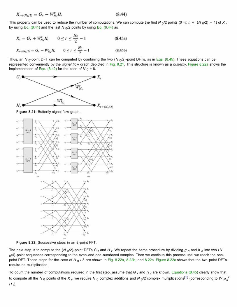
This property can be used to reduce the number of computations. We can compute the first N 0/2 points (0 ≪ n ≪ (N 0/2) − 1) of X rby using Eq. (8.41) and the last N 0/2 points by using Eq. (8.44) as

Thus, an N 0-point DFT can be computed by combining the two (N 0/2)-point DFTs, as in Eqs. (8.45). These equations can berepresented conveniently by the signal flow graph depicted in Fig. 8.21. This structure is known as a butterfly. Figure 8.22a shows theimplementation of Eqs. (8.42) for the case of N 0 = 8.

Figure 8.21: Butterfly signal flow graph.

Figure 8.22: Successive steps in an 8-point FFT.

The next step is to compute the (N 0/2)-point DFTs G r and H r. We repeat the same procedure by dividing g n and h n into two (N0/4)-point sequences corresponding to the even-and odd-numbered samples. Then we continue this process until we reach the one-point DFT. These steps for the case of N 0 / 8 are shown in Fig. 8.22a, 8.22b, and 8.22c. Figure 8.22c shows that the two-point DFTsrequire no multiplication.

To count the number of computations required in the first step, assume that G r and H r are known. Equations (8.45) clearly show that

to compute all the N 0 points of the X r, we require N 0 complex additions and N 0/2 complex multiplications[†] (corresponding to W N 0r

H r).

In the second step, to compute the (N 0/2)-point DFT G r from the (N 0/4)-point DFT, we require N 0/2 complex additions and N 0/4complex multiplications. We require an equal number of computations for H r. Hence, in the second step, there are N 0 complexadditions and N 0/2 complex multiplications. The number of computations required remains the same in each step. Since a total of log2N 0 steps is needed to arrive at a one-point DFT, we require, conservatively, a total of N 0 log2 N 0 complex additions and (N 0/2) log2N 0 complex multiplications, to compute the N 0-point DFT. Actually, as Fig. 8.22c shows, many multiplications are multiplications by 1or −1, which further reduces the number of computations.

The procedure for obtaining IDFT is identical to that used to obtain the DFT except that W N 0 = ej (2π/N 0) instead of e−j (2π/N 0) (inaddition to the multiplier 1/N 0). Another FFT algorithm, the decimation-in-frequency algorithm, is similar to the decimation-in-timealgorithm. The only difference is that instead of dividing x n into two sequences of even-and odd-numbered samples, we divide x n intotwo sequences formed by the first N 0/2 and the last N 0/2 digits, proceeding in the same way until a single-point DFT is reached inlog2 N 0 steps. The total number of computations in this algorithm is the same as that in the decimation-in-time algorithm.

[5]Cooley, J. W., and J. W. Tukey. An algorithm for the machine calculation of complex fourier series.

[†]Actully N0/2 is a conservative figure because some multiplications corresponding to the cases of WrN0

= 1,j, and so on, areeliminated.

8.7 SUMMARYA signal bandlimited to B Hz can be reconstructed exactly from its samples if the sampling rate f s> 2B Hz (the sampling theorem).Such a reconstruction, although possible theoretically, poses practical problems such as the need for ideal filters, which are unrealizableor are realizable only with infinite delay. Therefore, in practice, there is always an error in reconstructing a signal from its samples.Moreover, practical signals are not bandlimited, which causes an additional error (aliasing error) in signal reconstruction from itssamples. When a signal is sampled at a frequency f s Hz, samples of a sinusoid of frequency (f s/2) + x Hz appear as samples of alower frequency (f s/2) − x Hz. This phenomenon, in which higher frequencies appear as lower frequencies, is known as aliasing.Aliasing error can be reduced by bandlimiting a signal to f s/2 Hz (half the sampling frequency). Such bandlimiting, done prior tosampling, is accomplished by an antialiasing filter that is an ideal lowpass filter of cutoff frequency f s/2 Hz.

The sampling theorem is very important in signal analysis, processing, and transmission because it allows us to replace a continuous-time signal with a discrete sequence of numbers. Processing a continuous-time signal is therefore equivalent to processing a discretesequence of numbers. This leads us directly into the area of digital filtering (discrete-time systems). In the field of communication, thetransmission of a continuous-time message reduces to the transmission of a sequence of numbers. This opens doors to many newtechniques of communicating continuous-time signals by pulse trains.

The dual of the sampling theorem states that for a signal timelimited to τ seconds, its spectrum X (ω) can be reconstructed from thesamples of X (ω) taken at uniform intervals not greater than 1/τ Hz. In other words, the spectrum should be sampled at a rate not lessthan τ samples/Hz.

To compute the direct or the inverse Fourier transform numerically, we need a relationship between the samples of x (t) and X (ω). Thesampling theorem and its dual provide such a quantitative relationship in the form of a discrete Fourier transform (DFT). The DFTcomputations are greatly facilitated by a fast Fourier transform (FFT) algorithm, which reduces the number of computations fromsomething on the order of N 02 to N 0 log N 0.

REFERENCES1. Linden, D. A. A discussion of sampling theorem. Proceedings of the IRE, vol. 47, pp. 1219-1226, July 1959.

2. Siebert, W. M. Circuits, Signals, and Systems. MIT-McGraw-Hill, New York, 1986.

3. Bennett, W. R. Introduction to Signal Transmission. McGraw-Hill, New York, 1970.

4. Lathi, B. P. Linear Systems and Signals. Berkeley-Cambridge Press, Carmichael, CA, 1992.

5. Cooley, J. W., and J. W. Tukey. An algorithm for the machine calculation of complex fourier series. Mathematics ofComputation, vol. 19, pp. 297-301, April 1965.

MATLAB SESSION 8: THE DISCRETE FOURIER TRANSFORMAs an idea, the discrete Fourier transform (DFT) has been known for hundreds of years. Practical computing devices, however, areresponsible for bringing the DFT into common use. MATLAB is capable of DFT computations that would have been impractical not too

many years ago.

M8.1 Computing the Discrete Fourier Transform

The MATLAB command fft(x) computes the DFT of a vector x that is defined over (0 ≪ n ≪ N 0 − 1) (Problem 8.M−1 considershow to scale the DFT to accommodate signals that do not begin at n = 0.) As its name suggests, the function fft uses thecomputationally more efficient fast Fourier transform algorithm when it is appropriate to do so. The inverse DFT is easily computed byusing the ifft function.

To illustrate MATLAB's DFT capabilities, consider 50 points of a 10 Hz sinusoid sampled at f s = 50 Hz and scaled by T 1/f s.

In this case, the vector x contains exactly 10 cycles of the sinusoid. The fft command computes the DFT.

Figure M8.1: |X (f)| computed over (0 ≤ f < 50) by using fft.

Since the DFT is both discrete and periodic, fft needs to return only the N 0 discrete values contained in the single period (0 ≤ f < fs).

While X r can be plotted as a function of r, it is more convenient to plot the DFT as a function of frequency f. A frequency vector, inhertz, is created by using N 0 and T.

As expected, Fig. M8.1 shows content at a frequency of 10 Hz. Since the time-domain signal is real, X (f) is conjugate symmetric. Thus,content at 10 Hz implies equal content at −10 Hz. The content visible at 40 Hz is an alias of the −10 Hz content.

Often, it is preferred to plot a DFT over the principal frequency range (−f s/2 ≤ f < f s/2). The MATLAB function fftshift properlyrearranges the output of fft to accomplish this task.

When we use fftshift, the conjugate symmetry that accompanies the DFT of a real signal becomes apparent, as shown in Fig.M8.2.

>> T = 1/50; N_0 = 50; n = (0:N_0-1);>> X = T*cos (2*pi*10*n*T);

>> X = fft (x);

>> f = (0:N_0-1) / (T*N_0);>> stem (f, abs (X), 'k'); axis ([0 50 -0.05 0.55]);>> xlabel ('f [Hz]'); ylabel ('|X(f)|');

>> stem (f-1/(T*2), fftshift (abs (X)), 'k'); axis ([-25 25 -0.05 0.55]);>> xlabel ('f [Hz]'); ylabel ('|X(f)|');

Figure M8.2: |X (f)| displayed over (−25 ≪ f < 25) by using fftshift.

Figure M8.3: ∠X (f) displayed over (−25 ≪ f < 25).

Since DFTs are generally complex valued, the magnitude plots of Figs. M8.1 and M8.2 offer only half the picture; the signal's phasespectrum, shown in Fig. M8.3, completes it.

Since the signal is real, the phase spectrum necessarily has odd symmetry. Additionally, the phase at ±10 Hz is zero, as expected for azero-phase cosine function. More interesting, however, are the phase values found at the remaining frequencies. Does a simple cosinereally have such complicated phase characteristics? The answer, of course, is no. The magnitude plot of Fig. M8.2 helps identify theproblem: there is zero content at frequencies other than ±10 Hz. Phase computations are not reliable at points where the magnituderesponse is zero. One way to remedy this problem is to assign a phase of zero when the magnitude response is near or at zero.

M8.2 Improving the Picture with Zero Padding

DFT magnitude and phase plots paint a picture of a signal's spectrum. At times, however, the picture can be somewhat misleading.Given a sampling frequency f s = 50 Hz and a sampling interval T = 1/f s, consider the signal

This complex-valued, periodic signal contains a single positive frequency at 10 ⅓ Hz. Let us compute the signal's DFT using 50samples.

In this case, the vector Y contains a noninteger number of cycles. Figure M8.4 shows the significant frequency leakage that results.Since y[n] is not real, also notice that the DFT is not conjugate symmetric.

>> stem (f-1/(T*2), fftshift (angle (X)), 'k'); axis ([-25 25 -1.1*pi 1.1*pi]);>> xlabel ('f [Hz]'); ylabel (' X(f)');

>> y = T*exp(j*2*pi*(10+1/3)*n*T); Y = fft (y);>> stem (f-25, fftshift (abs (Y)), 'k'); axis ([-25 25 -0.05 1.05]);>> xlabel ('f [Hz]'); ylabel ('|Y(f)|');

Figure M8.4: |Y (f)| using 50 data points.

Figure M8.5: |Y zp (f)| using 50 data points padded with 550 zeros.

In this example, the discrete DFT frequencies do not include the actual 10 ⅓ Hz frequency of the signal. Thus, it is difficult to determinethe signal's frequency from Fig. M8.4. To improve the picture, the signal is zero-padded to 12 times its original length.

Figure M8.5 correctly shows the peak frequency at 10 ⅓ Hz and better represents the signal's spectrum.

It is important to keep in mind that zero padding does not increase the resolution or accuracy of the DFT. To return to the picket fenceanalogy, zero padding increases the number of pickets in our fence but cannot change what is behind the fence. More formally, thecharacteristics of the sinc function, such as main beam width and sidelobe levels, depend on the fixed width of the pulse, not on thenumber of zeros that follow. Adding zeros cannot change the characteristics of the sinc function and thus cannot change the resolutionor accuracy of the DFT. Adding zeros simply allows the sinc function to be sampled more finely.

M8.3 Quantization

A b-bit analog-to-digital converter (ADC) samples an analog signal and quantizes amplitudes by using 2b discrete levels. Thisquantization results in signal distortion that is particularly noticeable for small b. Typically, quantization is classified as symmetric orasymmetric. As discussed earlier, asymmetric quantization uses zero as a quantization level, which can help suppress low-level noise.

Program MS8P1 quantizes a signal using either symmetric quantization or asymmetric quantization. If available, the signal processingtoolbox functions uencode and udecode can also be used for symmetric quantization, but not for asymmetric quantization.

>> Y_zp = [y, zeros (1, 11*length (y))]; Y_zp = fft (y_zp);>> f_zp = (0:12*N_0-1) / (T*12*N_0);>> stem (f_zp-25, fftshift (abs (Y_zp)), 'k.'); axis ([-25 25 -0.05 1.05]);>> xlabel ('f [Hz]'); ylabel ('|Y {zp} (f) |');

function [xq] = MS8P1 (x, xmax, b, method);% MS8P1.m : MATLAB Session 8, Program 1% Function M-file quantizes x over (-xmax, xmax) using 2^b levels.% Both symmetric and asymmetric quantization are supported.% INPUTS: x = input signal

Several MATLAB commands require discussion. First, the nargin function returns the number of input arguments. In this program,nargin is used to ensure that a correct number of inputs is supplied. If the number of inputs supplied is incorrect, an error message isdisplayed and the function terminates. If only three input arguments are detected, the quantization type is not explicitly specified and theprogram assigns the default symmetric method.

As with many high-level languages such as C, MATLAB supports general switch/case structures:[†]

MS8P1 switches among cases of the string method. In this way, method-specific parameters are easily set. The command lower isused to convert a string to all lowercase characters. In this way, strings such as SYM, Sym, and sym are all indistinguishable. Similar tolower, the MATLAB command upper converts a string to all uppercase.

Quantization is accomplished by appropriately scaling and shifting the input and then rounding the result. The floor (q) commandrounds elements of q to the nearest integer toward minus infinity. Mathematically, it computes ⌊q⌋. To accommodate different types ofrounding, MATLAB supplies three other rounding commands: ceil, round, and fix. The command ceil (q) rounds elements ofq to the nearest integers toward infinity, (⌈q⌉); the command round (q) rounds elements of q toward the nearest integer; the commandfix(q) rounds elements of q to the nearest integer toward zero. For example, if q = [-0.5 0.5];, floor (q) yields [−1 0],ceil (q) yields [0 1], round (q) yields [−1 1], and fix(q) yields [0 0]. The final aspect of quantization in MS8P1 isaccomplished by means of the find command, which is used to identify values outside the maximum allowable range for saturation.

To verify operation, MS8P1 is used to determine the transfer characteristics of a symmetric 3-bit quantizer operating over (−10, 10).

Figure M8.6 shows the results. Figure M8.7 shows the transfer characteristics of an asymmetric 3-bit quantizer. The asymmetricquantizer includes zero as a quantization level, but at a price: quantization errors exceed Δ/2 = 1.25 for input values greater than 8.75.

% xmax = maximum magnitude of signal to be quantized% b = number of quantization bits% method = default 'sym' for symmetrical, 'asym' for asymmetrical% OUTPUTS: xq = quantized signalif (nargin<3),disp('Insufficient number of inputs.'); returnelseif (nargin==3),method = 'sym';elseif (nargin>4),disp ('Too many inputs.'); returnendswitch lower (method)case 'asym'offset = 1/2;case 'sym'offset = 0;otherwisedisp ('Unrecognized quantization method.'); returnendq = floor (2^b* ((x+xmax) / (2*max)) + offset);i = find(q>2^b-1); q(i) = 2^b-1;i = find (q<0); q(i) = 0;xq = (q- (2^(b-1) - (1/2-offset))) * 2*xmax / (2^b));

switch switch_expr,case case_expr,statements;. . .otherwise,statements;end

>> x = (-10: .0001: 10);>> xsq = MS8P1 (x, 10, 3, 'sym');>> plot (x, xsq, 'k'); grid;>> xlabel ('Quantizer input'); ylabel ('Quantizer output');

Figure M8.6: Transfer characteristics of a symmetric 3-bit quantizer.

Figure M8.7: Transfer characteristics of an asymmetric 3-bit quantizer.

There is no doubt that quantization can change a signal. It follows that the spectrum of a quantized signal can also change. While thesechanges are difficult to characterize mathematically, they are easy to investigate by using MATLAB. Consider a 1 Hz cosine sampled atf s = 50 Hz over 1 second.

Upon quantizing by means of a 2-bit asymmetric quantizer, both the signal and spectrum are substantially changed.

The results are shown in Fig. M8.8. The original signal x[n] appears sinusoidal and has pure spectral content at ±1 Hz. Theasymmetrically quantized signal x aq[n] is significantly distorted. The corresponding magnitude spectrum |X aq (f)| is spread over abroad range of frequencies.

>> x = cos (2*pi*n*T); X = fft (x);

>> xaq = MS8P1 (x, 1, 2, 'asym'); Xaq = fft (xaq);>> subplot (2, 2, 1); stem (n, x, 'k'); axis ([0 49 -1.1 1.1]);>> xlabel ('n'); ylabel ('x[n]');>> subplot (2, 2, 2); stem (f-25, fftshift (abs (X)), 'k'); axis ([-25, 25 -1 26])>> xlabel ('f'); ylabel ('|X(f)|');>> subplot (2, 2, 3); stem (n, xaq, 'k'); axis ([0 49 -1.1 1.1]);>> xlabel ('n'); ylabel ('x_{aq} [n]');>> subplot (2, 2, 4); stem (f-25, fftshift (abs(fft (xaq))), 'k'); axis ([-25, 25 -1 26]);>> xlabel ('f'); ylabel ('|X {aq} (f)|');

Figure M8.8: Signal and spectrum effects of quantization.

[†]A functionally equivalent structure can be written by using if, else if, and else statements.

PROBLEMSNote In many problems, the plots of spectra are shown as functions of frequency f Hz for convenience, although we have labeled

them as function of ω as X (ω), Y (ω), etc.]

8.1.1 Figure P8.1-1 shows Fourier spectra of signals x 1 (t) and x 2 (t). Determine the Nyquist sampling rates for signals x 1(t), x 2 (t), x 12 (t), x 23 (t), and x 1 (t)x 2 (t).

Figure P8.1-1

8.1.2 Determine the Nyquist sampling rate and the Nyquist sampling interval for the signals.

a. sinc2 (100πt)

b. 0.01 sinc2 (100πt)

c. sinc(100πt) + 3 sinc2 (60πt)

d. sinc(50πt) sinc (100πt) 8.1.3

a. Sketch |X (ω)|, the amplitude spectrum of a signal x (t) = 3 cos 6πt + sin 18πt + 2 cos(28 − ∉)πt,where ∉ is a very small number → 0. Determine the minimum sampling rate required to be able toreconstruct x (t) from these samples.

b. Sketch the amplitude spectrum of the sampled signal when the sampling rate is 25% above the Nyquistrate (show the spectrum over the frequency range ±50 Hz only). How would you reconstruct x (t) fromthese samples?

8.1.4

a. Derive the sampling theorem by considering the fact that the sampled signal x (t) = x (t)δT (t), and usingthe frequency-convolution property in Eq. (7.43).

b. For a sampling train consisting of shifted unit impulses at instants nT + τ instead of at nT (for all positiveand negative integer values of n), find the spectrum of the sampled signal.

8.1.5 A signal is bandlimited to 12 kHz. The band between 10 and 12 kHz has been so corrupted by excessive noise that the

information in this band is nonrecoverable. Determine the minimum sampling rate for this signal so that the uncorruptedportion of the band can be recovered. If we were to filter out the corrupted spectrum prior to sampling, what would bethe minimum sampling rate?

8.1.6 A continuous-time signal x (t) = Δ((t = 1)/2) is sampled at three rates: 10, 2, and 1 Hz. Sketch the resulting sampled

signals. Because x (t) is timelimited, its bandwidth is infinite. However, most of its energy is concentrated in a smallband. Can you determine the reasonable minimum sampling rate that will allow reconstruction of this signal with a smallerror? The answer is not unique. Make a reasonable assumption of what you define as a "negligible" or "small" error.

8.1.7

a. A signal x (t) = 5 sinc2 (5πt) + cos 20πt is sampled at a rate of 10 Hz. Find the spectrum of the sampledsignal. Can x (t) be reconstructed by lowpass filtering the sampled signal?

b. Repeat part (a) for a sampling frequency of 20 Hz. Can you reconstruct the signal from this sampledsignal? Explain.

c. If x (t) = 5 sinc2 (5πt)+sin 20πt, can you reconstruct x (t) from the samples of x (t) at a rate of 20 Hz?Explain your answer with spectral representations(s).

d. For x (t) = 5 sinc2 (5πt) + sin 20πt, can you reconstruct x (t) from the samples of x (t) at a rate of 21Hz? Explain your answer with spectral representation(s). Comment on your results.

8.1.8

a. The highest frequency in the spectrum X (ω) (Fig. P8.1-8a) of a bandpass signal x (t) is 30 Hz. Hence,the minimum sampling frequency needed to sample x (t) is 60 Hz. Show the spectrum of the signalsampled at a rate of 60 Hz. Can you reconstruct x (t) from these samples? How?

Figure P8.1-8

b. A certain busy student looks at X (ω), concludes that its bandwidth is really 10 Hz, and decides that thesampling rate 20 Hz is adequate for sampling x (t). Sketch the spectrum of the signal sampled at a rate of20 Hz. Can she reconstruct x (t) from these samples?

c. The same student, using the same reasoning, looks at Y (ω) in Fig. P8.1-8b, the spectrum of anotherbandpass signal y (t), and concludes that she can use sampling rate of 20 Hz to sample y (t). Sketch thespectrum of the signal y (t) sampled at a rate of 20 Hz. Can she reconstruct y (t) from these samples?

8.1.9 A signal x (t) whose spectrum X (ω), as shown in Fig. P8.1-9, is sampled at a frequency f s = f 1 + f 2 Hz. Find all the

sample values of x (t) merely by inspection of X (ω).

Figure P8.1-9

8.1.10 In digital data transmission over a communication channel, it is important to know the upper theoretical limit on the rate

of digital pulses that can be transmitted over a channel of band-width B Hz. In digital transmission, the relative shape ofthe pulse is not important. We are interested in knowing only the amplitude represented by the pulse. For instance, inbinary communication, we are interested in knowing whether the received pulse amplitude is 1 or −1 (positive ornegative). Thus, each pulse represents one piece of information. Consider one independent amplitude value (notnecessarily binary) as one piece of information. Show that 2B independent pieces of information per second can betransmitted correctly (assuming no noise) over a channel of bandwidth B Hz. This important principle in communicationtheory states that one hertz of bandwidth can transmit two independent pieces of information per second. It representsthe upper rate of pulse transmission over a channel without any error in reception in the absence of noise. [Hint:According to the interpolation formula [Eq. (8.11)], a continuous-time signal of bandwidth B Hz can be constructed from2B pieces of information/second.]

8.1.11 This example is one of those interesting situations leading to a curious result in the category of defying gravity. The sinc

function can be recovered from its samples taken at extremely low frequencies in apparent defiance of the samplingtheorem.

Consider a sinc pulse x (t) = sinc (4πt) for which X (ω) = (1/4) rect (ω/8π). The bandwidth of x (t) is B = 2Hz, and itsNyquist rate is 4 Hz.

a. Sample x (t) at a rate 4 Hz and sketch the spectrum of the sampled signal.

b. To recover x (t) from its samples, we pass the sampled signal through an ideal lowpass filter of bandwidthB = 2 Hz and gain G = T = 1/4. Sketch this system and show that for this system H (ω) = (1/4) rect(ω/8π). Show also that when the input is the sampled x (t) at a rate 4 Hz, the output of this system isindeed x (t), as expected.

c. Now sample x (t) at half the Nyquist rate, at 2 Hz. Apply this sampled signal at the input of the lowpassfilter used part (b). Find the output.

d. Repeat part (c) for the sampling rate 1 Hz.

e. Show that the output of the lowpass filter in part (b) is x (t) to the sampled x (t) if the sampling rate is 4/N,where N is any positive integer. This means that we can recover x (t) from its samples taken at arbitrarilysmall rate by letting N →∞.

f. The mystery may be clarified a bit by examining the problem in the time domain. Find the samples of x (t)when the sampling rate is 2/N (N integer).

8.2.1 A signal x (t) = sinc (200πt) is sampled (multiplied) by a periodic pulse train p T (t) represented in Fig. P8.2-1. Findand sketch the spectrum of the sampled signal. Explain whether you will be able to reconstruct x (t) from thesesamples. Find the filter output if the sampled signal is passed through an ideal lowpass filter of bandwidth 100 Hz andunit gain. What is the filter output if its bandwidth B Hz is between 100 and 150 Hz? What happens if the bandwidthexceeds 150 Hz?

Figure P8.2-1

8.2.2 Show that the circuit in Fig. P8.2-2 is a realization of the causal ZOH (zero-order hold) circuit. You can do this by

showing that the unit impulse response h (t) of this circuit is indeed equal to that in Eq. (8.9a) delayed by T/2 secondsto make it causal.

Figure P8.2-2

8.2.3

a. A first-order hold circuit (FOH) can also be used to reconstruct a signal x (t) from its samples. The impulseresponse of this circuit is h (t) = Δ(t/2T), where T is the sampling interval. Consider a typical sampledsignal x (t) and show that this circuit performs the linear interpolation. In other words, the filter outputconsists of sample tops connected by straight-line segments. Follow the procedure discussed in Section8.2 (Fig. 8.5c).

b. Determine the frequency response of this filter, and its amplitude response, and compare it with

i. the ideal filter required for signal reconstruction

ii. the ZOH circuit

c. This filter, being noncausal, is unrealizable. By delaying its impulse response, the filter can be maderealizable. What is the minimum delay required to make it realizable? How would this delay affect thereconstructed signal and the filter frequency response?

d. Show that the causal FOH circuit in part (c) can be realized by the ZOH circuit depicted in Fig. P8.2-2followed by an identical filter in cascade.

8.2.4 In the text, for sampling purposes, we used timelimited narrow pulses such as impulses or rectangular pulses of widthless than the sampling interval T. Show that it is not necessary to restrict the sampling pulse width. We can usesampling pulses of arbitrarily large duration and still be able to reconstruct the signal x (t) as long as the pulse rate isno less than the Nyquist rate for x (t).

Consider x (t) to be bandlimited to B Hz. The sampling pulse to be used is an exponential e−atu (t). We multiply x (t)by a periodic train of exponential pulses of the form e−atu (t) spaced T seconds apart. Find the spectrum of thesampled signal, and show that x (t) can be reconstructed from this sampled signal provided the sampling rate is no lessthan 2B Hz or T < 1/2B. Explain how you would reconstruct x (t) from the sampled signal.

8.2.5 In Example 8.2, the sampling of a signal x (t) was accomplished by multiplying the signal by a pulse train p T (t),

resulting in the sampled signal depicted in Fig. 8.4d. This procedure is known as the natural sampling. Figure P8.2-5shows the so-called flat-top sampling of the same signal x (t) = sinc2 (5πt).

Figure P8.2-5: Flat-top sampling.

a. Show that the signal x (t) can be recovered from flat-top samples if the sampling rate is no less than theNyquist rate.

b. Explain how you would recover x (t) from the flat-top samples.

c. Find the expression for the sampled signal spectrum X (ω) and sketch it roughly. 8.2.6 A sinusoid of frequency f 0 Hz is sampled at a rate f s = 20 Hz. Find the apparent frequency of the sampled signal if f 0

is

a. 8 Hz

b. 12 Hz

c. 20 Hz

d. 22 Hz

e. 32 Hz 8.2.7 A sinusoid of unknown frequency f 0 is sampled at a rate 60 Hz. The apparent frequency of the samples is 20 Hz.

Determine f 0 if it is known that f 0 lies in the range

a. 0-30 Hz

b. 30-60 Hz

c. 60-90 Hz

d. 90-120 Hz 8.2.8 A signal x (t) = 3 cos 6πt + cos 16πt + 2 cos 20πt is sampled at a rate 25% above the Nyquist rate. Sketch the

spectrum of the sampled signal. How would you reconstruct x (t) from these samples? If the sampling frequency is 25%below the Nyquist rate, what are the frequencies of the sinusoids present in the output of the filter with cutoff frequencyequal to the folding frequency? Do not write the actual output; give just the frequencies of the sinusoids present in theoutput.

8.2.9

a. Show that the signal x (t), reconstructed from its samples x (nT), using Eq. (8.11a) has a bandwidth B ≪1/2T Hz.

b. Show that x (t) is the smallest bandwidth signal that passes through samples x (nT). [Hint: Use thereductio ad absurdum method.]

8.2.10 In digital communication systems, the efficient use of channel bandwidth is ensured by transmitting digital data encoded

by means of bandlimited pulses. Unfortunately, bandlimited pulses are nontimelimited; that is, they have infinite duration,which causes pulses representing successive digits to interfere and cause errors in the reading of true pulse values.This difficulty can be resolved by shaping a pulse p (t) in such a way that it is bandlimited, yet causes zero interferenceat the sampling instants. To transmit R pulses per second, we require a minimum bandwidth R/2 Hz (see Prob. 8.1-10).The bandwidth of p (t) should be R/2 Hz, and its samples, in order to cause no interference at all other samplinginstants, must satisfy the condition

Because the pulse rate is R pulses per second, the sampling instants are located at intervals of 1/R seconds. Hence,the foregoing condition ensures that any given pulse will not interfere with the amplitude of any other pulse at its center.Find p (t). Is p (t) unique in the sense that no other pulse satisfies the given requirements?

8.2.11 The problem of pulse interference in digital data transmission was outlined in Prob. 8.2-10, where we found a pulse

shape p (t) to eliminate the interference. Unfortunately, the pulse found is not only noncausal, (and unrealizable) butalso has a serious drawback: because of its slow decay (as 1/t), it is prone to severe interference due to smallparameter deviation. To make the pulse decay rapidly, Nyquist proposed relaxing the bandwidth requirement from R/2Hz to kR/2 Hz with 1 ≪ k ≪ 2. The pulse must still have a property of noninterference with other pulses, for example,

Show that this condition is satisfied only if the pulse spectrum P (ω) has an odd symmetry about the set of dotted axesas shown in Fig. P8.2-11. The bandwidth of P (ω) is kR/2 Hz (1 ≤ k ≤ 2).

Figure P8.2-11

8.2.12 The Nyquist samples of a signal x (t) bandlimited to B Hz are

Show that

This pulse, known as the duobinary pulse, is used in digital transmission applications. 8.2.13 A signal bandlimited to B Hz is sampled at a rate f s = 2B Hz. Show that

[Hint: Use the orthogonality property of the sinc function in Prob. 7.6-5.] 8.2.14 Prove that a signal cannot be simultaneously timelimited and bandlimited. [Hint: Show that contrary assumption leads to

contradiction. Assume a signal to be simultaneously time-limited and bandlimited so that X (ω) = 0 for |ω| ≥ 2πB. In

this case X (ω) = X (ω)rect (ω/4πB′) for B′ > B. This fact means that x (t) is equal to x (t) * 2B′ sinc (2πB′t). Thelatter cannot be timelimited because the sinc function tail extends to infinity.]

8.3.1 A compact disc(CD) records audio signals digitally by means of a binary code. Assume an audio signal bandwidth of 15kHz.

a. What is the Nyquist rate?

b. If the Nyquist samples are quantized into 65,536 levels (L = 65,536) and then binary coded, what numberof binary digits is required to encode a sample.

c. Determine the number of binary digits per second (bits/s) required to encode the audio signal.

d. For practical reasons discussed in the text, signals are sampled at a rate well above the Nyquist rate.Practical CDs use 44,100 samples/s. If L = 65,536, determine the number of pulses per second required toencode the signal.

8.3.2 A TV signal (video and audio) has a bandwidth of 4.5 MHz. This signal is sampled, quantized, and binary coded.

a. Determine the sampling rate if the signal is to be sampled at a rate 20% above the Nyquist rate.

b. If the samples are quantized into 1024 levels, what number of binary pulses is required to encode eachsample?

c. Determine the binary pulse rate (bits/s) of the binary-coded signal. 8.3.3

a. In a certain A/D scheme, there are 16 quantization levels. give one possible binary code and one possiblequaternary (4-ary) code. For the quaternary code use 0, 1, 2, and 3 as the four symbols. Use the minimumnumber of digits in your code.

b. To represent a given number of quantization levels L, we require a minimum of b M digits for an M-arycode. Show that the ratio of the number of digits in a binary code to the number of digits in a quaternary(4-ary) code is 2, that is, b 2/b 4 = 2.

8.3.4 Five telemetry signals, each of bandwidth 1 kHz, are quantized and binary coded. These signals are time-division

multiplexed (signal bits interleaved). Choose the number of quantization levels so that the maximum error in sampleamplitudes is no greater than 0.2% of the peak signal amplitude. The signals must be sampled at least 20% above theNyquist rate. Determine the data rate (bits per second) of the multiplexed signal.

8.4.1 The Fourier transform of a signal x (t), bandlimited to B Hz, is X (ω). The signal x (t) is repeated periodically at intervalsT, where T = 1.25/B. The resulting signal y (t) is

Show that y (t) can be expressed as

where

and

Recall that a bandlimited signal is not time limited, and hence has infinite duration. The periodic repetitions are alloverlapping.

8.5.1 For a signal x (t) that is timelimited to 10 ms and has an essential bandwidth of 10 kHz, determine N 0, the number ofsignal samples necessary to compute a power-of-2 FFT with a frequency resolution f 0 of at least 50 Hz. Explain whetherany zero padding is necessary.

8.5.2 To compute the DFT of signal x (t) in Fig. P8.5-2, write the sequence x n (for n = 0 to N 0 − 1) if the frequency

resolution f 0 must be at least 0.25 Hz. Assume the essential bandwidth (the folding frequency) of x (t) to be at least 3

Hz. Do not compute the DFT; just write the appropriate sequence x n.

Figure P8.5-2

8.5.3 Choose appropriate values for N 0 and T and compute the DFT of the signal e−t u (t). Use two different criteria for

determining the effective bandwidth of e−t u (t). As the bandwidth, use the frequency at which the amplitude responsedrops to 1% of its peak value (at ω = 0). Next, use the 99% energy criterion for determining the bandwidth (see Example7.20).

8.5.4 Repeat Prob. 8.5-3 for the signal

8.5.5 For the signals x (t) and g (t) represented in Fig. P8.5-5, write the appropriate sequences x n and g n necessary for the

computation of the convolution of x (t) and g (t) using DFT. Use T = 1/8.

Figure P8.5-5

8.5.6 For this problem, interpret the N-point DFT as an N-periodic function of r. To stress this fact, we shall change the

notation X r to X (r). Are the following frequency domain signals valid DFTs? Answer yes or no. For each valid DFT,determine the size N of the DFT and whether the time-domain signal is real.

a. X (r) = j − π

b. X (r) = sin (r/10)

c. X (r) = sin (πr/10)

d. X (r) = [(1 + j)/√2]r

e. X (r) = 〈r + π〉10 where, 〈·〉10 denotes the modulo-N operation.

8.m.1 MATLAB's fft command computes the DFT of a vector x assuming the first sample occurs at time n = 0. Given that X= fft (x) has already been computed, derive a method to correct X to reflect an arbitrary starting time n = n 0.

8.m.2 Consider a complex signal composed of two closely spaced complex exponentials: x1[n]= ej2πn30/100 + ej2πn33/100. For

each of the following cases, plot the length-N DFT magnitude as a function of frequency f r, where f r = r/N.

a. Compute and plot the DFT of x 1[n] using 10 samples (0 ≪ n ≪ 9). From the plot, can both exponentialsbe identified? Explain.

b. Zero-pad the signal from part (a) with 490 zeros and then compute and plot the 500-point DFT. Does thisimprove the picture of the DFT? Explain.

c. Compute and plot the DFT of x 1[n] using 100 samples (0 ≪ n ≪ 99). From the plot, can bothexponentials be identified? Explain.

d. Zero-pad the signal from part (c) with 400 zeros and then compute and plot the 500-point DFT. Does thisimprove the picture of the DFT? Explain.

8.m.3 Repeat Prob. 8.M-2, using the complex signal x 2 [n] = e j2πn30/100 + e j2πn31.5/100.

8.m.4 Consider a complex signal composed of a dc term and two complex exponentials: y1[n] = 1+e jπn30/100+0.5*ej2πn43/100.For each of the following cases, plot the length-N DFT magnitude as a function of frequency f r, where f r / r/N.

a. Use MATLAB to compute and plot the DFT of y 1[n] with 20 samples (0 ≪ n ≪ 19). From the plot, canthe two nondc exponentials be identified? Given the amplitude relation between the two, the lower-frequency peak should be twice as large as the higher-frequency peak. Is this the case? Explain.

b. Zero-pad the signal from part (a) to a total length of 500. Does this improve locating the two non-dcexponential components? Is the lower-frequency peak twice as large as the higher-frequency peak?Explain.

c. MATLAB's signal processing toolbox function window allows window functions to be easily generated.Generate a length-20 Hanning window and apply it to y 1[n]. Using this windowed function, repeat parts (a)and (b). Comment on whether the window function helps or hinders the analysis.

8.m.5 Repeat Prob. 8.M-4, using the complex signal y 2 [n] = 1+e j2πn30/100+0.5e j2πn38/100. 8.m.6 This problem investigates the idea of zero padding applied in the frequency domain. When asked, plot the length-N DFT

magnitude as a function of frequency f r, where f r = r/N.

a. In MATLAB, create a vector x that contains one period of the sinusoid x[n] = cos((π/2)n). Plot the result.How "sinusoidal" does the signal appear?

b. Use the fft command to compute the DFT X of vector x. Plot the magnitude of the DFT coefficients. Dothey make sense?

c. Zero-pad the DFT vector to a total length of 100 by inserting the appropriate number of zeros in the middleof the vector X. Call this zero-padded DFT sequence Y. Why are zeros inserted in the middle rather thanthe end? Take the inverse DFT of Y and plot the result. What similarities exist between the new signal yand the original signal x? What are the differences between x and y? What is the effect of zero padding inthe frequency domain? How is this type of zero padding similar to zero padding in the time domain?

d. Derive a general modification to the procedure of zero padding in the frequency domain to ensure that theamplitude of the resulting time-domain signal is left unchanged.

e. Consider one period of a square wave described by the length-8 vector [1 1 1 1 −1 −1 −1 −1]. Zero-padthe DFT of this vector to a length of 100, and call the result S. Scale S according to part (d), take theinverse DFT, and plot the result. Does the new time-domain signal s[n] look like a square wave? Explain.

Chapter 9: Fourier Analysis of Discrete-Time SignalsIn Chapters 6 and 7, we studied the ways of representing a continuous-time signal as a sum of sinusoids or exponentials. In thischapter we shall discuss similar development for discrete-time signals. Our approach is parallel to that used for continuous-time signals.We first represent a periodic x[n] as a Fourier series formed by a discrete-time exponential (or sinusoid) and its harmonics. Later weextend this representation to an aperiodic signal x[n] by considering x[n] as a limiting case of a periodic signal with the periodapproaching infinity.

9.1 DISCRETE-TIME FOURIER SERIES (DTFS)

A continuous-time sinusoid cos ωt is a periodic signal regardless of the value of ω. Such is not the case for the discrete-time sinusoidcos Ωn (or exponential ejΩn). A sinusoid cos Ωn is periodic only if Ω/2π is a rational number. This can be proved by observing that ifthis sinusoid is N0 periodic, then

This is possible only if

Here, both m and N0 are integers. Hence, Ω/2π = m/N0 is a rational number. Thus, a sinusoid cos Ωn (or exponential ejΩn) is periodiconly if

When this condition (Ω/2π a rational number) is satisfied, the period N0 of the sinusoid cos Ωn is given by [Eq. (9.1a)]

To compute N0, we must choose the smallest value of m that will make m(2π/Ω) an integer. For example, if Ω = 4π/17, then thesmallest value of m that will make m(2π/Ω) = m (17/2) an integer is 2. Therefore

However, a sinusoid cos(0.8n) is not a periodic signal because 0.8/2π is not a rational number.

9.1-1 Periodic Signal Representation by Discrete-time Fourier Series

A continuous-time periodic signal of period T0 can be represented as a trigonometric Fourier series consisting of a sinusoid of the

fundamental frequency ω0 = 2π/T0, and all its harmonics. The exponential form of the Fourier series consists of exponentials ej0t,

e± jω0t, e± j2ω0t, e± j3?0t....

A discrete-time periodic signal can be represented by a discrete-time Fourier series using a parallel development. Recall that a periodicsignal x[n] with period N0 is characterized by the fact that

The smallest value of N0 for which this equation holds is the fundamental period. The fundamental frequency is Ω0 ... 2π/N0rad/sample. An N0-periodic signal x[n] can be represented by a discrete-time Fourier series made up of sinusoids of fundamentalfrequency Ω0 2π/N0 and its harmonics. As in the continuous-time case, we may use a trigonometric or an exponential form of theFourier series. Because of its compactness and ease of mathematical manipulations, the exponential form is preferable to thetrigonometric. For this reason we shall bypass the trigonometric form and go directly to the exponential form of the discrete-time Fourierseries.

The exponential Fourier series consists of the exponentials ej0n, e± jΩ0n, e± j2Ω0n, ..., e± jnO0n, ..., and so on. There would be an infinitenumber of harmonics, except for the property proved in Section 5.5-1, that discrete-time exponentials whose frequencies are separatedby 2π (or integer multiples of 2π) are identical because

The consequence of this result is that the rth harmonic is identical to the (r + N0)th harmonic. To demonstrate this, let gn denote the

nth harmonic ejnωn0n. Then

and

Thus, the first harmonic is identical to the (N0 + 1)st harmonic, the second harmonic is identical to the (N0 + 2)nd harmonic, and so on.In other words, there are only N0 independent harmonics, and their frequencies range over an interval 2π (because the harmonics areseparated by Ω0 = 2π/N0). This means, unlike the continuous-time counterpart, that the discrete-time Fourier series has only a finitenumber (N0) of terms. This result is consistent with our observation in Section 5.5-1 that all discrete-time signals are bandlimited to aband from −π to π. Because the harmonics are separated by Ω0 = 2π/N0, there can only be N0 harmonics in this band. We also sawthat this band can be taken from 0 to 2π or any other contiguous band of width 2π. This means we may choose the N0 independent

harmonics ejrΩ0n over 0 ≤ r ≤ N0 − 1, or over −1 ≤ r ≤ N0 − 2, or over 1 ≤ r ≤ N0, or over any other suitable choice for thatmatter. Every one of these sets will have the same harmonics, although in different order.

Let us consider the first choice, which corresponds to exponentials ejrO0n for r = 0,1,2,..., N0 − 1. The Fourier series for an N0-periodicsignal x[n] consists of only these N0 harmonics, and can be expressed as

To compute coefficients in the Fourier series (9.4), we multiply both sides of (9.4) by e−jmΩ0n and sum over n from n = 0 to (N0 −1).

The right-hand sum, after interchanging the order of summation, results in

The inner sum, according to Eq. (8.28) in Section 8.5, is zero for all values of r ≠ m. It is nonzero with a value N0 only when r = m.This fact means the outside sum has only one term DmN0 (corresponding to r = m). Therefore, the right-hand side of Eq. (9.5) is equalto DmN0, and

and

We now have a discrete-time Fourier series (DTFS) representation of an N0-periodic signal x[n] as

where

Observe that DTFS equations (9.8) and (9.9) are identical (within a scaling constant) to the DFT equations (8.22b) and (8.22a).[†]

Therefore, we can use the efficient FFT algorithm to compute the DTFS coefficients.

9.1-2 Fourier Spectra of a Periodic Signal x[n]

The Fourier series consists of N0 components

The frequencies of these components are 0, Ω0, 2O0, ..., (N0 − 1)Ω0 where Ω0 = 2π/N0. The amount of the rth harmonic is . Wecan plot this amount (the Fourier coefficient) as a function of index r or frequency Ω. Such a plot, called the Fourier spectrum ofx[n], gives us, at a glance, the graphical picture of the amounts of various harmonics of x[n].

In general, the Fourier coefficients are complex, and they can be represented in the polar form as

The plot of | | versus Ω is called the amplitude spectrum and that of ∟ versus Ω is called the angle (or phase) spectrum. Thesetwo plots together are the frequency spectra of x[n]. Knowing these spectra, we can reconstruct or synthesize x[n] according to Eq.(9.8). Therefore, the Fourier (or frequency) spectra, which are an alternative way of describing a periodic signal x[n], are in every wayequivalent (in terms of the information) to the plot of x[n] as a function of n. The Fourier spectra of a signal constitute the frequency-domain description of x[n], in contrast to the time-domain description, where x[n] is specified as a function of index n (representingtime).

The results are very similar to the representation of a continuous-time periodic signal by an exponential Fourier series except that,generally, the continuous-time signal spectrum bandwidth is infinite and consists of an infinite number of exponential components(harmonics). The spectrum of the discrete-time periodic signal, in contrast, is bandlimited and has at most N0 components.

PERIODIC EXTENSION OF FOURIER SPECTRUMWe now show that if Φ[r] is an N0-periodic function of r, then

where r = 〈N0〉 indicates summation over any N0 consecutive values of r. Because Φ[r] is N0 periodic, the same values repeat withperiod N0. Hence, the sum of any set of N0 consecutive values of Φ[r] must be the same no matter the value of r at which we startsumming. Basically it represents the sum over one cycle.

To apply this result to the DTFS, we observe that e−jrΩ0n is N0 periodic because

Therefore, if x[n] is N0 periodic, x[n]e−Ω0n is also N0 periodic. Hence, from Eq. (9.9) it follows that is also N0 periodic, as is

DrejrΩ0n. Now, because of the property (9.11), we can express Eqs. (9.8) and (9.9) as

and

If we plot for all values of r (rather than only 0 ≤ r ≤ N0 − 1), then the spectrum is N0 periodic. Moreover, Eq. (9.12) shows thatx[n] can be synthesized by not only the N0 exponentials corresponding to 0 ≤ r ≤ N0 − 1, but by any successive N0 exponentials inthis spectrum, starting at any value of r (positive or negative). For this reason, it is customary to show the spectrum for all values ofr (not just over the interval 0 ≤ r ≤ N0 − 1). Yet we must remember that to synthesize x[n] from this spectrum, we need to add only N0consecutive components. All these observations are consistent with our discussion in Chapter 5, where we showed that a sinusoid of agiven frequency is equivalent to multitudes of sinusoids, all separated by integer multiple of 2π in frequency.

Along the Ω scale, repeats every 2π intervals, and along the r scale, repeats at intervals of N0. Equations (9.12) and (9.13)show that both x[n] and its spectrum are N0 periodic and both have exactly the same number of components (N0) over one period.

Equation (9.13) shows that is complex in general, and D−r is the conjugate of if x[n] is real. Thus

so that the amplitude spectrum | | is an even function, and ∟ is an odd function of r (or Ω). All these concepts will be clarified bythe examples to follow. The first example is rather trivial and serves mainly to familiarize the reader with the basic concepts of DTFS.

EXAMPLE 9.1Find the discrete-time Fourier series (DTFS) for x[n] = sin 0.1 πn (Fig. 9.1a). Sketch the amplitude and phase spectra.

Figure 9.1: Discrete-time sinusoid sin 0.1π n and its Fourier spectra.

In this case the sinusoid sin 0.1 πn is periodic because Ω/2π = 1/20 is a rational number and the period N0 is [see Eq. (9.1b)]

The smallest value of m that makes 20m an integer is m = 1. Therefore, the period N0 = 20, so that Ω0 = 2π/N0 = 0.1 π, and from Eq.(9.12)

where the sum is performed over any 20 consecutive values of r. We shall select the range −10 < r < 10 (values of r from −10 to 9).This choice corresponds to synthesizing x[n] using the spectral components in the fundamental frequency range (−≤Ω<π). Thus,

where, according to Eq. (9.13),

In these sums, r takes on all values between −10 and 9. From Eq. (8.28) it follows that the first sum on the right-hand side is zero forall values of r except r = 1, when the sum is equal to N0 = 20. Similarly, the second sum is zero for all values of r except r = −1, whenit is equal to N0 = 20. Therefore

and all other coefficients are zero. The corresponding Fourier series is given by

Here the fundamental frequency Ω0 = 0.1π, and there are only two nonzero components:

Therefore

Sketches of for the interval (−10 ≤ r < 10) appear in Fig. 9.1b and 9.1c. According to Eq. (9.15), there are only two componentscorresponding to r = 1 and −1. The remaining 18 coefficients are zero. The rth component is the amplitude of the frequency rΩ0 =0.1rπ. Therefore, the frequency interval corresponding to −10 ≤ r < 10 is −π≤<π, as depicted in Fig. 9.1b and 9.1c. This spectrumover the range −10 ≤ r < 10 (or −π) is sufficient to specify the frequency-domain description (Fourier series), and we can synthesizex[n] by adding these spectral components. Because of the periodicity property discussed in Section 9.1-2, the spectrum is a periodicfunction of r with period N0 = 20. For this reason, we repeat the spectrum with period N0 = 20 (or Ω = 2π), as illustrated in Fig. 9.1band 9.1c, which are periodic extensions of the spectrum in the range −10 ≤ r < 10. Observe that the amplitude spectrum is an evenfunction and the angle or phase spectrum is an odd function of r (or Ω) as expected.

The result (9.15) is a trigonometric identity and could have been obtained immediately without the formality of finding the Fouriercoefficients. We have intentionally chosen this trivial example to introduce the reader gently to the new concept of the discrete-timeFourier series and its periodic nature. The Fourier series is a way of expressing a periodic signal x[n] in terms of exponentials of theform ejrΩ0n and its harmonics. The result in Eq. (9.15) is merely a statement of the (obvious) fact that sin 0.1π n can be expressed asa sum of two exponentials ej0.1πn and e−j0.1πn.

Because of the periodicity of the discrete-time exponentials ejrΩ0n, the Fourier series components can be selected in any range oflength N0 = 20 (or Ω = 2π). For example, if we select the frequency range 0 ≤ Ω < 2π (or 0 ≤ r < 20), we obtain the Fourier series as

This series is equivalent to that in Eq. (9.15) because the two exponentials ej1.9πn and e−j.0.1πn are equivalent. This follows from thefact that ej1.9πn=ej1.9πn ×e−j2πn = e−j0πn.

We could have selected the spectrum over any other range of width Ω = 2π in Fig. 9.1b and 9.1c as a valid discrete-time Fourierseries. The reader may verify this by proving that such a spectrum starting anywhere (and of width Ω = 2π) is equivalent to the sametwo components on the right-hand side of Eq. (9.15).

EXERCISE E9.1From the spectra in Fig. 9.1 write the Fourier series corresponding to the interval −10 ≥ r > −30 (or−π≥Ω>−3π). Show that thisFourier is equivalent to that in Eq. (9.15).

EXERCISE E9.2

Find the period and the DTFS for

over the interval 0 ≤ r ≤ 19. Use Eq. (9.9) to compute .

Answers

N0 = 20

EXERCISE E9.3

Find the fundamental periods N0, if any, for the following sinusoids.

a. sin(301πn/4)

b. cos 1.3n

Answers

a. N0 = 8

b. N0 does not exist because the sinusoid is not periodic.

EXAMPLE 9.2Find the discrete-time Fourier series for the periodic sampled gate function shown in Fig. 9.2a.

Figure 9.2: (a) Periodic sampled gate pulse and (b) its Fourier spectrum.

In this case N0 = 32 and Ω0 = 2π/32 = π/16. Therefore

where

For our convenience, we shall choose the interval −16 ≤ n ≤ 15 for the summation (9.18a), although any other interval of the samewidth (32 points) would give the same result.[†]

Now x[n] = 1 for −4 ≤ n ≤ 4 and is zero for all other values of n. Therefore

This is a geometric progression with a common ratio e−j(π/16)r. Therefore [see Sec. (B.7-4)],

This spectrum (with its periodic extension) is depicted in Fig. 9.2b.[†]

COMPUTER EXAMPLE C9.1Repeat Example 9.2 using MATLAB.

Figure C9.1

[†]If we let x[n] = N0xk and = Xr, Eqs. (9.8) and (9.9) are identical to Eqs. (8.22b) and (8.22a), respectively.

[†]In this example we have used the same equations as those for DFT in Example 8.9, within a scaling constant. In the presentexample, the values of x[n] at n = 4 and −4 are taken as 1 (full value), whereas in Example 8.9 these values are 0.5 (half the value).This is the reason for the slight difference in spectra in Fig. 9.2b and Fig. 8.18d. Unlike continuous-time signals, discontinuity is ameaningless concept in discrete-time signals.

[†]Strictly speaking, geometric progression sum formula applies only if the common ratio e−1j(π/16)r ≠ 1. When r = 0, this ratio is unity.Hence, Eq. (9.19) is valid for values of r ≠ 0. For the case r = 0, the sum in Eq. (9.18b) is given by

Fortunately, the value of D0, as computed from Eq. (9.19) also happens to be 9/32. Hence, Eq. (9.19) is valid for all r.

9.2 APERIODIC SIGNAL REPRESENTATION BY FOURIER INTEGRALIn Section 9.1 we succeeded in representing periodic signals as a sum of (everlasting) exponentials. In this section we extend thisrepresentation to aperiodic signals. The procedure is identical conceptually to that used in Chapter 7 for continuous-time signals.

Applying a limiting process, we now show that an aperiodic signal x[n] can be expressed as a continuous sum (integral) of everlastingexponentials. To represent an aperiodic signal x[n] such as the one illustrated in Fig. 9.3a by everlasting exponential signals, let usconstruct a new periodic signal xN0[n] formed by repeating the signal x[n] every N0 units, as shown in

>> N_0 = 32; n = (0: N_0-1);>> x_n = [ones(1,5) zeros(1,23) ones(1,4)];>> for r = 0:31,>> X_r(r+1) = sum(x_n.*exp(-j*r*2*pi/N_0*n))/32;>> end>> subplot (2,1,1); r = n; stem (r,real(X_r),'k');>> xlable('r'); ylabel('X_r'); axis([0 31 -.1 0.3]);>> legend('DTFS by direct computation',0);>> X_r = fft(x_n)/N_0;>> subplot(2,1,2); stem(r,real(X_r),'k');>> xlabel('x'); ylabel('X_r'); axis ([0 31 - .1 0.3]);>> legend('DTFS by FFT',0);

Figure 9.3: Generation of a periodic signal by periodic extension of a signal x[n].

Fig. 9.3b. The period N0 is made large enough to avoid overlap between the repeating cycles (N0 ≥ 2N + 1). The periodic signalxN0[n] can be represented by an exponential Fourier series. If we let N0 →, the signal x[n] repeats after an infinite interval, andtherefore

Thus, the Fourier series representing xN0[n] will also represent x[n] in the limit N0 →∞. The exponential Fourier series for xN0 [n] isgiven by

where

The limits for the sum on the right-hand side of Eq. (9.21) should be from − N to N. But because x[n] = 0 for |n| > N, it does not matterif the limits are taken from − ∞ to ∞.

It is interesting to see how the nature of the spectrum changes as N0 increases. To understand this behavior, let us define X(Ω), acontinuous function of Ω, as

From this definition and Eq. (9.21), we have

This result shows that the Fourier coefficients are 1/N0 times the samples of X(Ω) taken every Ω0 rad/s.[†] Therefore, (1/N0)X(Ω) isthe envelope for the coefficients . We now let N0 →∞ by doubling N0 repeatedly. Doubling N0 halves the fundamental frequencyΩ0, with the result that the spacing between successive spectral components (harmonics) is halved, and there are now twice as manycomponents (samples) in the spectrum. At the same time, by doubling N0, the envelope of the coefficients is halved, as seen fromEq. (9.23). If we continue this process of doubling N0 repeatedly, the number of components doubles in each step; the spectrumprogressively becomes denser while its magnitude becomes smaller. Note, however, that the relative shape of the envelope remainsthe same [proportional to X (Ω) in Eq. (9.22)]. In the limit, as N0 →∞, the fundamental frequency Ω0 → 0, and → 0. The separationbetween successive harmonics, which is Ω0, is approaching zero (infinitesimal), and the spectrum becomes so dense that it appears tobe continuous. But as the number of harmonics increases indefinitely, the harmonic amplitudes become vanishingly small(infinitesimal). We discussed an identical situation in Section 7.1.

We follow the procedure in Section 7.1 and let N0 →∞. According to Eq. (9.22)

Using Eqs. (9.23), we can express Eq. (9.20) as,

In the limit as N0 →∞ 0 Ω→ 0 and xN0 [n] → x[n]. Therefore

Because Ω0 is infinitesimal, it will be appropriate to replace Ω0 with an infinitesimal notation ΔΩ:

Equation (9.26) can be expressed as

The range r = 〈N0〉 implies the interval of N0 number of harmonics, which is N0ΔΩ = 2π according to Eq. (9.27). In the limit, theright-hand side of Eq. (9.28) becomes the integral

where ∫2π indicates integration over any continuous interval of 2π. The spectrum X(Ω) is given by [Eq. (9.22)]

The integral on the right-hand side of Eq. (9.29) is called the Fourier integral. We have now succeeded in representing an aperiodicsignal x[n] by a Fourier integral (rather than a Fourier series). This integral is basically a Fourier series (in the limit) with fundamentalfrequency Δ→ 0, as seen in Eq. (9.28). The amount of the exponential ejrΔΩn is X(r ΔΩ)Δ/2π. Thus, the function X(Ω) given by Eq.(9.30) acts as a spectral function, which indicates the relative amounts of various exponential components of x[n].

We call X(Ω) the (direct) discrete-time Fourier transform (DTFT) of x[n], and x[n] the inverse discrete-time Fourier transform (IDTFT) ofX(Ω). This nomenclature can be represented as

The same information is conveyed by the statement that x[n] and X(Ω) are a (discrete-time) Fourier transform pair. Symbolically, this isexpressed as

The Fourier transform X(Ω) is the frequency-domain description of x[n].

9.2-1 Nature of Fourier Spectra

We now discuss several important features of the discrete-time Fourier transform and the spectra associated with it.

THE FOURIER SPECTRA ARE CONTINUOUS FUNCTIONS OF ΩAlthough x[n] is a discrete-time signal, X(Ω), its DTFT is a continuous function of Ω for the simple reason that Ω is a continuousvariable, which can take any value over a continuous interval from −∞ to ∞.

THE FOURIER SPECTRA ARE PERIODIC FUNCTIONS OF Ω WITH PERIOD 2πFrom Eq. (9.30) it follows that

Clearly, the spectrum X(Ω) is a continuous, periodic function of Ω with period 2π. We must remember, however, that to synthesizex[n], we need to use the spectrum over a frequency interval of only 2π, starting at any value of Ω [see Eq. (9.29)]. As a matter ofconvenience, we shall choose this interval to be the fundamental frequency range (−ππ,). It is, therefore, not necessary to show

discrete-time -signal spectra beyond the fundamental range, although we often do so.

The reason for periodic behavior of X(Ω) was discussed in Chapter 5, where we showed that, in a basic sense, the discrete-timefrequency Ω is bandlimited to |Ω|≥π. However, all discrete-time sinusoids with frequencies separated by an integer multiple of 2π areidentical. This is why the spectrum is 2π periodic.

CONJUGATE SYMMETRY OF X(Ω)From Eq. (9.30), we obtain the DTFT of x*[n] as

In other words,

For real x[n], Eq. (9.32b) reduces to x[n] ⇔ X*(−Ω), which implies that for real x[n]

Therefore, for real x[n], X(Ω) and X(−Ω) are conjugates. Since X(Ω) is generally complex, we have both amplitude and angle (orphase) spectra

Because of conjugate symmetry of X(Ω), it follows that for real x[n]

Therefore, the amplitude spectrum |X(Ω)| is an even function of Ω and the phase spectrum ∟X(Ω) is an odd function of Ω for real x[n].

PHYSICAL APPRECIATION OF THE DISCRETE-TIME FOURIER TRANSFORMIn understanding any aspect of the Fourier transform, we should remember that Fourier representation is a way of expressing a signalx[n] as a sum of everlasting exponentials (or sinusoids). The Fourier spectrum of a signal indicates the relative amplitudes and phasesof the exponentials (or sinusoids) required to synthesize x[n].

A detailed explanation of the nature of such sums over a continuum of frequencies is provided in Section 7.1-1.

EXISTENCE OF THE DTFTBecause |e−jΩn| = 1, from Eq. (9.30), it follows that the existence of X(Ω) is guaranteed if x[n] is absolutely summable: that is,

This shows that the condition of absolute summability is a sufficient condition for the existence of the DTFT representation. Thiscondition also guarantees its uniform convergence. The inequality

shows that the energy of an absolutely summable sequence is finite. However, not all finite-energy signals are absolutely summable.Signal x[n] = sinc (n) is such an example. For such signals, the DTFT converges, not uniformly, but in the mean.[†]

To summarize, X(Ω) exists under a weaker condition

The DTFT under this condition is guaranteed to converge in the mean. Thus, the DTFT of the exponentially growing signal γnu[n] doesnot exist when |γ|> 1 because the signal violates conditions (9.33a) and (9.33b). But the DTFT exists for the signal sinc(n), whichviolates (9.33a) but does satisfy (9.33b) (see later: Example 9.6). In addition, if the use of γ(Ω), the continuous-time impulse function, ispermitted, we can even find the DTFT of some signals that violate both (9.33a) and (9.33b). Such signals are not absolutely summable,nor do they have finite energy. For example, as seen from pairs 11 and 12 of Table 9.1, the DTFT of x[n] = 1 for all n and x[n] = ejΩ0n

exist, although they violate conditions (9.33a) and (9.33b).

Table 9.1: A Short Table of Discrete-Time Fourier Transforms

Open table as spreadsheet

No. x[n] X(Ω)

1 δ[n − k] e−jkΩ Integer k

2 γnu[n] |γ|<1

3 −γnu([−n + 1)] |γ|>1

4 γ|n| |γ|<1

5 nγnu[n] |γ|<1

6 γn cos (Ω0n + θ)u[n] |γ|<1

7 u[n]−u[n−M]

8 Ωc≤π

9 Ω≥π

10 u[n]

11 1 for all n

12 ejΩ0 n

13 cosΩ0n

14 sin Ω0n

15 (cos Ω0n) u[n]

16 (sin Ω0n) u[n]

EXAMPLE 9.3Find the DTFT of x[n] = γn u[n].

This is an infinite geometric series with a common ratio γe−jΩ. Therefore (see Section B.7-4)

−jΩ −jΩ

provided that |γe | < 1. But because |e | = 1, this condition implies |γ| < 1. Therefore

If |γ| > 1, X (Ω) does not converge. This result is in conformity with condition (9.33). From Eq. (9.34a)

so that

Figure 9.4 shows x[n] = γn u[n] and its spectra for γ = 0.8. Observe that the frequency spectra are continuous and periodic functions ofΩ with the period 2π. As explained earlier, we need to use the spectrum only over the frequency interval of 2π. We often select thisinterval to be the fundamental frequency range (−π,π).

Figure 9.4: Exponential γn u[n] and its frequency spectra.

The amplitude spectrum |X(Ω)| is an even function and the phase spectrum ∟X(Ω) is an odd function of Ω.

EXAMPLE 9.4Find the DTFT of γn u[−(n + 1)] depicted in Fig. 9.5.

Figure 9.5: Exponential γnu[−(n + 1)].

Setting n = −m yields

This is a geometric series with a common ratio ejΩ/γ. Therefore, from Section B.7-4,

Therefore

Except for the change of sign, this Fourier transform (and the corresponding frequency spectra) is identical to that of x[n] = γnu[n]. Yetthere is no ambiguity in determining the IDTFT of X(Ω) = 1/(γe−jΩ −1) because of the restrictions on the value of γ in each case. If|γ|< 1, then the inverse transform is x[n] = −γn u[n]. If |γ| > 1, it is x[n] = γn[−(n + 1)].

EXAMPLE 9.5Find the DTFT of the discrete-time rectangular pulse illustrated in Fig. 9.6a. This pulse is also known as the 9-point rectangular windowfunction.

Figure 9.6: (a) Discrete-time gate pulse and (b) its Fourier spectrum.

This is a geometric progression with a common ratio e−jΩ and (see Section B.7-4)

Figure 9.6b shows the spectrum X(Ω) for M = 9.

COMPUTER EXAMPLE C9.2Repeat Example 9.5 using MATLAB.

Figure C9.2

EXAMPLE 9.6Find the inverse DTFT of the rectangular pulse spectrum described over the fundamental band (|Ω| ≤π) by X(Ω) = rect (Ω/2Ωc) for Ωc≤π. Because of the periodicity property, X(Ω) repeats at the intervals of 2π, as shown in Fig. 9.7a.

Figure 9.7: Inverse discrete-time Fourier transform of a periodic gate spectrum.

According to Eq. (9.29)

The signal x[n] is depicted in Fig. 9.7b (for the case Ωc = π/4).

EXERCISE E9.4

Find and sketch the amplitude and phase spectra of the DTFT of the signal x[n] = γ|k| with |γ| | 1.

>> syms Omega n M>> X = simplify(symsum(exp(-j*Omega*n),n,-(M-1)/2,(M-1)/2))X =1/(-1+exp(i*Omega))*(-exp(-1/2*i*Omega*(M-1))+exp(1/2*i*Omega*(M+1)))% Evaluate symbolic expression X(Omega) for M = 9:>> Omega = linspace(-pi,pi,1000); M = 9*ones(size(Omega)); X = subs(X);>> subplot(2,1,1); plot(Omega,abs(X),'k'); axis([-pi pi 0 9]);>> xlabel('\Omega'); ylabel('X(\Omega)');>> legend('DTFT by symbolic computation',0);% Compute samples of X(Omega) using the FFT:>> N = 512; M = 9;>> x = [ones(1,(M+1)/2) zeros(1,N-M) ones(1,(M-1)/2)];>> X = fft(x); Omega = (-N/2:N/2-1)*2*pi/N;>> subplot(2,1,2); plot(Omega,fftshift(abs(X)),'k.'); axis([-pi pi 0 9]);>> xlabel('\Omega'); ylabel('X(\Omega)');>> legend('DTFT samples by FFT',0);

Answers

EXERCISE E9.5

Find and sketch the amplitude and phase spectra of the DTFT of the signal x[n] = δ[n + 1] − δ[n − 1].

Answers

9.2.2 Connection Between the DTFT and the z-Transform

The connection between the (bilateral) -transform and the DTFT is similar to that between the Laplace transform and the Fouriertransform. The -transform of x[n], according to Eq. (5.1) is

Setting = ejΩ in this equation yields

The right-hand side sum defines X(Ω), the DTFT of x[n]. Does this mean that the DTFT can be obtained from the corresponding -transform by setting = ejΩ? In other words, is it true that X[ejΩ] = X(Ω)? Yes, it is true in most cases. For example, when x[n] =anu[n], its -transform is /( −a), and X[ejΩ] = ejΩ/(ejΩ − a), which is equal to X(Ω) (assuming |a| < 1). However, for the unit stepfunction u[n], the -transform is /(−1), and X[ejΩ] = ejΩ/(ejΩ − 1). As seen from Table 9.1, pair 10, this is not equal to X(Ω) in thiscase.

We obtained X[ejΩ] by setting = ejΩ in Eq. (9.42a). This implies that the sum on the right-hand side of Eq. (9.42a) converges for = ejΩ,which means the unit circle (characterized by = ejΩ) lies in the region of convergence for X[ ]. Hence, the general rule is that only whenthe ROC for X[ ] includes the unit circle, setting = ejΩ in X[ ] yields the DTFT X(Ω). This applies for all x[n] that are absolutelysummable. If the ROC of X[ ] excludes the unit circle, X[ejΩ] ≠ X(Ω). This applies to all exponentially growing x[n] and also x[n], whicheither is constant or oscillates with constant amplitude.

The reason for this peculiar behavior has something to do with the nature of convergence of the -transform and the DTFT.[†]

This discussion shows that although the DTFT may be considered to be a special case of the -transform, we need to circumscribe sucha view. This cautionary note is supported by the fact that a periodic signal has the DTFT, but its -transform does not exist.

[†]For the sake of simplicity we assume and therefore X(Ω) to be real. The argument, however, is also valid for complex [orX(Ω)].

[†]This means

[†]To explain this point, consider the unit step function u[n] and its transforms. Both the -transform and the DTFT synthesize x[n], usingeverlasting exponentials of the form n. The value of can be anywhere in the complex -plane for the -transform, but it must be restrictedto the unit circle ( = ejΩ) in the case of the DTFT. The unit step function is readily synthesized in the -transform by a relatively simple

spectrum X[ ] = /( − 1), by choosing outside the unit circle (the ROC for u[n] is | | > 1). In the DTFT, however, we are restricted tovalues of only on the unit circle ( = ejΩ). The function u[n] can still be synthesized by values of on the unit circle, but the spectrum ismore complicated than when we are free to choose anywhere including the region outside the unit circle. In contrast, when x[n] isabsolutely summable, the region of convergence for the -transform includes the unit circle, and we can synthesize x[n] is absolutelysummable, the region of convergence for the -transform includes the unit circle, and we can synthesize x[n] by using along the unitcircle in both the transforms. This leads to X[ejΩ] = X(Ω).

9.3 PROPERTIES OF THE DTFTIn the next section, we shall see a close connection between the DTFT and the CTFT (continuous-time Fourier transform). For thisreason, the properties of the DTFT are very similar to those of the CTFT, as the following discussion shows.

LINEARITY OF THE DTFTIf

then

The proof is trivial. The result can be extended to any finite sums.

CONJUGATE SYMMETRY OF X(Ω)

In Eq. (9.32b), we proved the conjugation property

We also showed that as a consequence of this, when x[n] is real, X(Ω) and X(−Ω) are conjugates, that is,

This is the conjugate symmetry property. Since X(Ω) is generally complex, we have both amplitude and angle (or phase) spectra

Hence, for real x[n], it follows that

Therefore, for real x[n], the amplitude spectrum |X(Ω)| is an even function of Ω and the phase spectrum ∟X(Ω) is an odd function ofΩ.

TIME AND FREQUENCY REVERSAL

From Eq. (9.30), the DTFT of x[−n] is

EXAMPLE 9.7Use the time-frequency reversal property (9.48) and pair 2 in Table 9.1 to derive pair 4 in Table 9.1.

Pair 2 states that

Hence, from Eq. (9.48)

Moreover, γn could be expressed as a sum of γn u[n] and γ−nu[−n], except that the impulse at n = 0 is counted twice (once from

each of the two exponentials). Hence

Therefore, using Eqs. (9.49a) and (9.49b), and invoking the linearity property, we can write

which agrees with pair 4 in Table 9.1.

EXERCISE E9.6In Table 9.1, derive pair 13 from pair 15 by using the time-reversal property (9.48).

MULTIPLICATION BY n: FREQUENCY DIFFERENTIATION

The result follows immediately by differentiating both sides of Eq. (9.30) with respect to Ω.

EXAMPLE 9.8Use the property in Eq. (9.50) [multiplication by n] and pair 2 in Table 9.1 to derive pair 5 in Table 9.1.

Pair 2 states that

Hence, from Eq. (9.50)

which agrees with pair 5 in Table 9.1.

TIME-SHIFTING PROPERTY

If

then

This property can be proved by direct substitution in the equation defining the direct transform. From Eq. (9.30) we obtain

This result shows that delaying a signal by k samples does not change its amplitude spectrum. The phase spectrum, however, ischanged by −kΩ. This added phase is a linear function of Ω with slope -k.

PHYSICAL EXPLANATION OF THE LINEAR PHASE

Time delay in a signal causes a linear phase shift in its spectrum. The heuristic explanation of this result is exactly parallel to that forcontinuous-time signals given in Section 7.3 (see Fig. 7.22).

EXAMPLE 9.9Find the DTFT of x[n] = (1/4) sinc (π(n − 2)/4), shown in Fig. 9.8a.

Figure 9.8: Shifting x[n] by k units changes the phase of X(Ω) by kΩ.

In Example 9.6, we found that

Use of the time-shifting property [Eq. (9.52)] yields (for integer k)

The spectrum of the shifted signal is shown in Fig. 9.8b.

EXERCISE E9.7Verify the result in Eq. (9.40) from pair 7 In Table 9.1, and the time-shifting property of the DTFT.

FREQUENCY-SHIFTING PROPERTY

If

then

This property is the dual of the time-shifting property. To prove the frequency-shifting property, we have from Eq. (9.30)

From this result, it follows that

Adding this pair to the pair in Eq. (9.54), we obtain

This is the modulation property.

Multiplying both sides of pair (9.54) by ejθ, we obtain

Using this pair, we can generalize the modulation property as

EXAMPLE 9.10A signal x[n] = sinc (πn/4) modulates a carrier cos Ωcn. Find and sketch the spectrum of the modulated signal x[n] cos Ωcn for

a. Ωc = π/2

b. Ωc = 7π/8 = 0.875π

a. For x[n] = sinc (πn/4), we find (Table 9.1, pair 8)

Figure 9.9a shows the DTFT X(Ω). From the modulation property (9.55), we obtain

Figure 9.9b shows half the X(Ω) shifted by π/2 and Fig. 9.9c shows half the X(Ω) shifted by −π/2. The spectrum of themodulated signal, is obtained by adding these two shifted spectra and multiplying by half, as shown in Fig. 9.9d.

Figure 9.9: Instance of modulation for Example 9.10a.

b. Figure 9.10a shows X(Ω), which is the same as that in part a. For Ωc = 7π/8 = 0.875π, the modulation property (9.55)yields

Figure 9.10b shows X(Ω) shifted by 7π/8 and Fig. 9.10c shows X(Ω) shifted by −7π/8. The spectrum of the modulatedsignal, is obtained by adding these two shifted spectra and multiplying by half, as shown in Fig. 9.10d. In this case, thetwo shifted spectra overlap. Since, the operation of modulation thus causes aliasing, it does not achieve the desired effectof spectral shifting. In this example, to realize spectral shifting without aliasing requires Ωc ≤ 3π/4.

Figure 9.10: Instance of modulation for Example 9.10b

EXERCISE E9.8In Table 9.1, derive pairs 12 and 13 from pair 11 and the frequency-shifting/modulation property.

TIME-AND FREQUENCY-CONVOLUTION PROPERTY

If

then

and

where

For two continuous, periodic signals, we define the periodic convolution, denoted by symbol as[†]

The convolution here is not the linear convolution used so far. This is a periodic (or circular) convolution applicable to convolution of twocontinuous, periodic functions with the same period. The limit of integration in the convolution extends only to one period.

Proof of the time convolution property is identical to that given in Section 5.2 [Eq. (5.18)]. All we have to do is replace with e jΩ. Toprove the frequency-convolution property (9.58b), we have

Interchanging the order of summation and integration, we obtain

EXAMPLE 9.11If , then show that

Recognize that the sum on the left-hand side of (9.59) is x[n] * u[n] because

In deriving this result, we have used the fact that

Hence, from the time-convolution property (9.58a) and pair 10 in Table 9.1, it follows that

Because of 2π periodicity, X(0) = X(2πk). Moreover,X (Ω)δ(Ω−2πk)=X(2πk)δ(Ω−2πk)=X(0)δ(Ω−2πk). Hence

EXERCISE E9.9

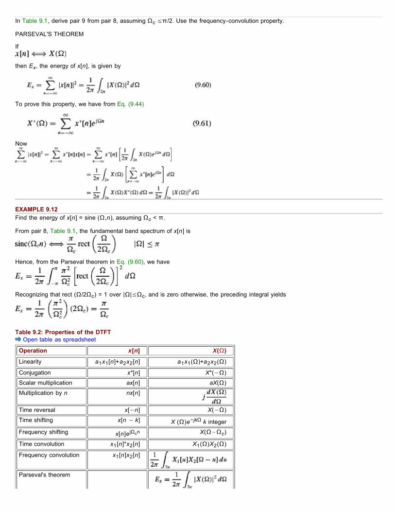
In Table 9.1, derive pair 9 from pair 8, assuming Ωc ≤π/2. Use the frequency-convolution property.

PARSEVAL'S THEOREM

If

then Ex, the energy of x[n], is given by

To prove this property, we have from Eq. (9.44)

Now

EXAMPLE 9.12Find the energy of x[n] = sine (Ω,n), assuming Ωc < π.

From pair 8, Table 9.1, the fundamental band spectrum of x[n] is

Hence, from the Parseval theorem in Eq. (9.60), we have

Recognizing that rect (Ω/2Ωc) = 1 over |Ω|≤Ωc, and is zero otherwise, the preceding integral yields

Table 9.2: Properties of the DTFT Open table as spreadsheet

Operation x[n] X(Ω)

Linearity a1x1[n]+a2x2[n] a1x1(Ω)+a2x2(Ω)

Conjugation x*[n] X*(−Ω)

Scalar multiplication ax[n] aX(Ω)

Multiplication by n nx[n]

Time reversal x[−n] X(−Ω)

Time shifting x[n − k] X (Ω)e−jkΩ k integer

Frequency shifting x[n]e jΩcn X(Ω−Ωc)

Time convolution x1[n]*x2[n] X1(Ω)X2(Ω)

Frequency convolution x1[n]x2[n]

Parseval's theorem

[†]In Eq. (8.36), we defined periodic convolution for two discrete, periodic sequences in a different way. Although, we are using thesame symbol for both discrete and continuous cases, the meaning will be clear from the context.

9.4 LTI DISCRETE-TIME SYSTEM ANALYSIS BY DTFTConsider a linear, time-invariant, discrete-time system with the unit impulse response h[n]. We shall find the (zero-state) systemresponse y[n] for the input x[n]. Let

Because

According to Eq. (9.58a) it follows that

This result is similar to that obtained for continuous-time systems. Let us examine the role of H(Ω), the DTFT of the unit impulseresponse h[n].

Equation (9.63) holds only for BIBO-stable systems and also for marginally stable systems if the input does not contain the system'snatural mode(s). In other cases, the response grows with n and is not Fourier transformable. [†] Moreover, the input x[n] also has to beDTF transformable. For cases where Eq. (9.63) does not apply, we use the -transform for system analysis.

Equation (9.63) shows that the output signal frequency spectrum is the product of the input signal frequency spectrum and thefrequency response of the system. From this equation, we obtain

and

This result shows that the output amplitude spectrum is the product of the input amplitude spectrum and the amplitude response of thesystem. The output phase spectrum is the sum of the input phase spectrum and the phase response of the system.

We can also interpret Eq. (9.63) in terms of the frequency-domain viewpoint, which sees a system in terms of its frequency response(system response to various exponential or sinusoidal components). The frequency domain views a signal as a sum of variousexponential or sinusoidal components. The transmission of a signal through a (linear) system is viewed as transmission of variousexponential or sinusoidal components of the input signal through the system. This concept can be understood by displaying the input-output relationships by a directed arrow as follows:

which shows that the system response to ejΩn is H(Ω)ejΩn, and

which shows x[n] as a sum of everlasting exponential components. Invoking the linearity property, we obtain,

which gives y[n] as a sum of responses to all input components and is equivalent to Eq. (9.63). Thus, X(Ω) is the input spectrum andY(Ω) is the output spectrum, given by X(Ω)H(Ω).

EXAMPLE 9.13An LTID system is specified by the equation

Find H(Ω), the frequency response of this system. Determine the (zero-stable) response y[n] if the input x[n] = (0.8)nu[n].

Let x[n] ⇔ X(Ω) and y[n] ⇔ Y(Ω). The DTFT of both sides of Eq. (9.66) yields

According to Eq. (9.63)

Also, x[n] = (0.8)nu[n]. Hence,

and

We can express the right-hand side as a sum of two first-order terms (modified partial fraction expansion as discussed in Section B.5-6) as follows:[†]

Consequently

According to Eq. (9.34a), the inverse DTFT of this equation is

This example demonstrates the procedure for using DTFT to determine an LTID system response. It is similar to the Fourier transformmethod in the analysis of LTIC systems. As in the case of the Fourier transform, this method can be used only if the system isasymptotically or BIBO stable and if the input signal is DTF-transformable.[†] We shall not belabor this method further because it isclumsier and more restrictive than the -transform method discussed in Chapter 5.

9.4-1 Distortionless Transmission

In several applications, digital signals are passed through LTI systems, and we require that the output waveform be a replica of theinput waveform. As in the continuous-time case, transmission is said to be distortionless if the input x[n] and the output y[n] satisfy thecondition

Here nd, the delay (in samples) is assumed to be integer. The Fourier transform of Eq. (9.68) yields

But

Therefore

This is the frequency response required for distortionless transmission. From this equation it follows that

Thus, for distortionless transmission, the amplitude response |H(Ω)| must be a constant, and the phase response ∠H(Ω) must be a

linear function of Ω with slope −nd, where nd is the delay in number of samples with respect to input (Fig. 9.11). These are preciselythe characteristics of an ideal delay of nd samples with a gain of G0 [see Eq. (9.52)].

Figure 9.11: LTI system frequency response for distortionless transmission.

MEASURE OF DELAY VARIATIONFor distortionless transmission, we require a linear phase characteristic. In practice, many systems have a phase characteristic that maybe only approximately linear. A convenient way of judging phase linearity is to plot the slope of ∠H(Ω) as a function of frequency. Thisslope is constant for ideal linear phase (ILP) system, but it may vary with Ω in general case. The slope can be expressed as

If ng(Ω) is constant, all the components are delayed by ng samples. But if the slope is not constant, the delay ng varies with frequency.This variation means that different frequency components undergo different amounts of delay, and consequently the output waveformwill not be a replica of the input waveform. As in the case of LTIC systems, ng(Ω), as defined in Eq. (9.70), plays an important role inbandpass systems and is called the group delay or envelope delay. Observe that constant nd implies constant ng. Note that ∠H(Ω) =Φ0 −Ωnd also has a constant ng. Thus, constant group delay is a more relaxed condition.

DISTORTIONLESS TRANSMISSION OVER BANDPASS SYSTEMSAs in the case of continuous-time systems, the distortionless transmission conditions can be relaxed for discrete-time bandpasssystems. For lowpass systems, the phase characteristic should not only be linear over the band of interest, but should also passthrough the origin [condition (9.69b)]. For bandpass systems, the phase characteristic should be linear over the band of interest, but itneed not pass through the origin (ng should be constant). The amplitude response is required to be constant over the passband. Thus,

for distortionless transmission over a bandpass system, the frequency response for positive range of Ω is of the form [†]

The proof is identical to that for the continuous-time case in Section 7.4-2 and will not be repeated. In using Eq. (9.70) to compute ng,we should ignore jump discontinuities in the phase function.

9.4-2 Ideal and Practical Filters

Ideal filters allow distortionless transmission of a certain band of frequencies and suppress all the remaining frequencies. The generalideal lowpass filter shown in Fig. 9.12 for |Ω|≤π allows all components below the cutoff frequency Ω=Ωc to pass without distortion andsuppresses all components above Ωc. Figure 9.13 illustrates ideal highpass and bandpass filter characteristics.

Figure 9.12: Ideal lowpass filter: its frequency response and impulse response.

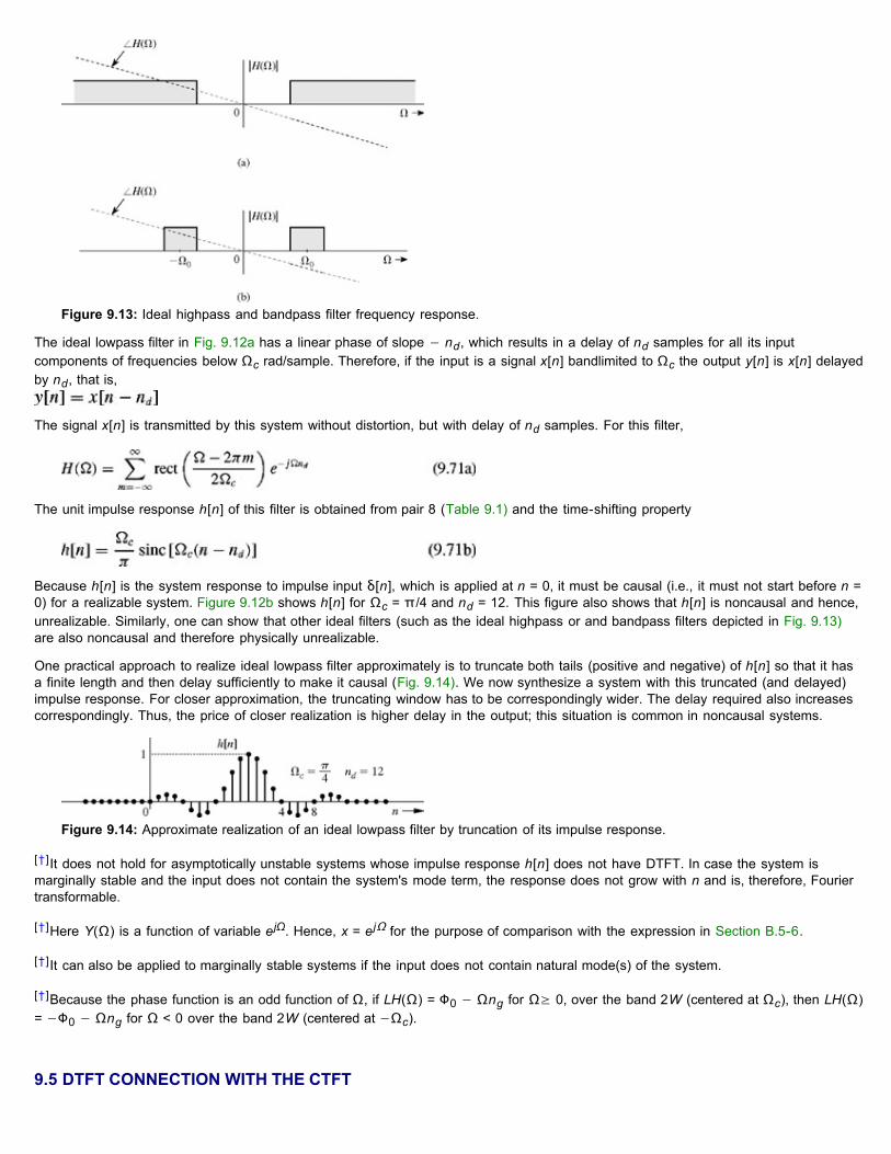
Figure 9.13: Ideal highpass and bandpass filter frequency response.

The ideal lowpass filter in Fig. 9.12a has a linear phase of slope − nd, which results in a delay of nd samples for all its inputcomponents of frequencies below Ωc rad/sample. Therefore, if the input is a signal x[n] bandlimited to Ωc the output y[n] is x[n] delayedby nd, that is,

The signal x[n] is transmitted by this system without distortion, but with delay of nd samples. For this filter,

The unit impulse response h[n] of this filter is obtained from pair 8 (Table 9.1) and the time-shifting property

Because h[n] is the system response to impulse input δ[n], which is applied at n = 0, it must be causal (i.e., it must not start before n =0) for a realizable system. Figure 9.12b shows h[n] for Ωc = π/4 and nd = 12. This figure also shows that h[n] is noncausal and hence,unrealizable. Similarly, one can show that other ideal filters (such as the ideal highpass or and bandpass filters depicted in Fig. 9.13)are also noncausal and therefore physically unrealizable.

One practical approach to realize ideal lowpass filter approximately is to truncate both tails (positive and negative) of h[n] so that it hasa finite length and then delay sufficiently to make it causal (Fig. 9.14). We now synthesize a system with this truncated (and delayed)impulse response. For closer approximation, the truncating window has to be correspondingly wider. The delay required also increasescorrespondingly. Thus, the price of closer realization is higher delay in the output; this situation is common in noncausal systems.

Figure 9.14: Approximate realization of an ideal lowpass filter by truncation of its impulse response.

[†]It does not hold for asymptotically unstable systems whose impulse response h[n] does not have DTFT. In case the system ismarginally stable and the input does not contain the system's mode term, the response does not grow with n and is, therefore, Fouriertransformable.

[†]Here Y(Ω) is a function of variable ejΩ. Hence, x = ejΩ for the purpose of comparison with the expression in Section B.5-6.

[†]It can also be applied to marginally stable systems if the input does not contain natural mode(s) of the system.

[†]Because the phase function is an odd function of Ω, if LH(Ω) = Φ0 − Ωng for Ω≥ 0, over the band 2W (centered at Ωc), then LH(Ω)= −Φ0 − Ωng for Ω < 0 over the band 2W (centered at −Ωc).

9.5 DTFT CONNECTION WITH THE CTFT

Consider a continuous-time signal xc(t) (Fig. 9.15a) with the Fourier transform Xc(ω) bandlimited to B Hz (Fig. 9.15b). This signal issampled with a sampling interval T. The sampling rate is at least equal to the Nyquist rate; that is, T = 1/2B. The sampled signal xBc(t)(Fig. 9.15c) can be expressed as

The continuous-time Fourier transform of the foregoing equation yields

In Section 8.1 (Fig. 8.1f), we showed that Xc(ω) is Xc(ω)/T repeating periodically with a period ωs = 2π/T, as illustrated in Fig. 9.15d.Let us construct a discrete-time signal x[n] such that its nth sample value is equal to the value of the nth sample of xc(t), as depicted inFig. 9.15e, that is,

Figure 9.15: Connection between the DTFT and the Fourier transform

Now, X(Ω), the DTFT of x[n], is given by

Comparison of Eqs. (9.74) and (9.72) shows that letting ωT = Ω in Xc(ω) yields X(Ω), that is,

Alternately, X(Ω) can be obtained from Xc(ω) by replacing ω with Ω/T, that is,

Therefore, X(Ω) is identical to Xc(ω), frequency-scaled by factor T, as shown in Fig. 9.15f. Thus, ω = 2π/T in Fig. 9.15d correspondsto Ω = 2π in Fig. 9.15f.

9.5-1 Use of DFT and FFT for Numerical Computation of DTFT

The discrete Fourier transform (DFT), as discussed in Chapter 8, is a tool for computing the samples of continuous-time Fouriertransform (CTFT). Because of the close connection between CTFT and DTFT, as seen in Eq. (9.76), we can also use this same DFT tocompute DTFT samples.

In Chapter 8, Eqs. (8.22a) and (8.22b) relate an N0-point sequence xn to another N0-point sequence Xr. Changing the notation xn tox[n], in these equations, we obtain

Comparing Eq. (9.30) with Eq. (9.77a), we recognize that Xr is the sample of X(Ω) at Ω = rΩ0, that is,

Hence, the pair of DFT equations (9.77) relates an N0-point sequence x[n] to the N0-point samples of corresponding X(Ω). We cannow use the efficient algorithm FFT (discussed in Chapter 8) to compute Xr from x[n], and vice versa.

If x[n] is not timelimited, we can still find the approximate values of Xr by suitably windowing x[n]. To reduce the error, the windowshould be tapered and should have sufficient width to satisfy error specifications. In practice, numerical computation of signals, whichare generally nontimelimited, is performed in this manner because of the computational economy of the DFT, especially for signals oflong duration.

COMPUTATION OF DISCRETE-TIME FOURIER SERIES (DTFS)The discrete-time Fourier series (DTFS) equations (9.8) and (9.9) are identical to the DFT equations (8.22b) and (8.22a) within ascaling constant N0. If we let x[n] = N0xn and = Xr in Eqs. (9.9) and (9.8), we obtain

This is precisely the DFT pair in Eqs. (8.22). For instance, to compute the DTFS for the periodic signal in Fig. 9.2a, we use the valuesof xn = x[n]/N0 as

Numerical computations in modern digital signal processing are conveniently performed with the discrete Fourier transform, introducedin Section 8.5. The DFT computations can be very efficiently executed by using the fast Fourier transform (FFT) algorithm discussed inSection 8.6. The DFT is indeed the workhorse of modern digital signal processing. The discrete-time Fourier transform (DTFT) and theinverse discrete-time Fourier transform (IDTFT) can be computed by using the DFT. For an N0-point signal x[n], its DFT yields exactlyN0 samples of X(Ω) at frequency intervals of 2π/N0. We can obtain a larger number of samples of X(Ω) by padding a sufficientnumber of zero-valued samples to x[n]. the N0-point DFT of x[n] gives exact values of the DTFT samples if x[n] has a finite length N0.If the length of x[n] is infinite, we need to use the appropriate window function to truncate x[n].

Because of the convolution property, we can use DFT to compute the convolution of two signals x[n] and h[n], as discussed in Section8.5. This procedure, known as fast convolution, requires padding both signals by a suitable number of zeros, to make the linearconvolution of the two signals identical to the circular (or periodic) convolution of the padded signals. Large blocks of data may beprocessed by sectioning the data into smaller blocks and processing such smaller blocks in sequence. Such a procedure requiressmaller memory and reduces the processing time.[1]

[1]Mitra, S. K. Digital Signal Processing: A Computer-Based Approach, 2nd ed. McGraw-Hill, New York, 2001.

9.6 GENERALIZATION OF THE DTFT TO THE z-TRANSFORMLTID systems can be analyzed by using the DTFT. This method, however, has the following limitations:

1. Existence of the DTFT is guaranteed only for absolutely summable signals. The DTFT does not exist for exponentially oreven linearly growing signals. This means that the DTFT method is applicable only for a limited class of inputs.

2. Moreover, this method can be applied only to asymptotically or BIBO stable systems; it cannot be used for unstable oreven marginally stable systems.

These are serious limitations in the study of LTID system analysis. Actually it is the first limitation that is also the cause of the secondlimitation. Because the DTFT is incapable of handling growing signals, it is incapable of handling unstable or marginally stable

systems.[†] Our goal is, therefore, to extend the DTFT concept so that it can handle exponentially growing signals.

We may wonder what causes this limitation on DTFT so that it is incapable of handling exponentially growing signals. Recall that inDTFT, we are using sinusoids or exponentials of the form ejΩn to synthesize an arbitrary signal x[n]. These signals are sinusoids withconstant amplitudes. They are incapable of synthesizing exponentially growing signals no matter how many such components we add.Our hope, therefore, lies in trying to synthesize x[n] by using exponentially growing sinusoids or exponentials. This goal can beaccomplished by generalizing the frequency variable jΩ to σ + jΩ, that is, by using exponentials of the form e(σ + jΩ)n instead ofexponentials ejΩn. The procedure is almost identical to that used in extending the Fourier transform to the Laplace transform.

Let us define a new variable . Hence

and

Consider now the DTFT of x[n]e−σn (σ real)

It follows from Eq. (9.79) that the sum in Eq. (9.82) is .Thus

Hence, the inverse DTFT of is x[n]e−σn. Therefore

Multiplying both sides of Eq. (9.84) by eσn yields

Let us define a new variable as

Because = eσ+ jΩ is complex, we can express it as = rejΩ, where r = eσ. Thus, lies on a circle of radius r, and as Ω varies from −σ toσ, circumambulates along this circle, completing exactly one counterclockwise rotation, as illustrated in Fig. 9.16. Changing to variable inEq. (9.85) yields

Figure 9.16: Contour of integration for the -transform.

and form Eq. (9.83) we obtain

where the integral ∡ indicates a contour integral around a circle of radius r in the counterclockwise direction.

Equations (9.87a) and (9.87b) are the desired extensions. They are, however, in a clumsy form. For the sake of convenience, we makeanother notational change by observing that (In ) is a function of .Let us denote it by a simpler notation X[ ]. Thus, Eqs. (9.87)become

and

This is the (bilateral) transform pair. Equation (9.88) expresses x[n] as a continuous sum of exponentials of the form n = e(σ+ jΩ)n = rn

ejΩ)n. Thus, by selecting a proper value for r (or σ), we can make the exponential grow (or decay) at any exponential rate we desire.

If we let σ = 0, we have = ejΩ and

Thus, the familiar DTFT is just a special case of the -transform X[ ] obtained by letting = ejΩ and assuming that the sum on the right-hand side of Eq. (9.89) converges when = ejΩ. This also implies that the ROC for X[ ] includes the unit circle.

[†]Recall that the output of an unstable system grows exponentially. Also, the output of a marginally stable system to characteristicmode input grows with time.

9.7 SUMMARYThis chapter deals with the analysis and processing of discrete-time signals. For analysis, our approach is parallel to that used incontinuous-time signals. We first represent a periodic x[n] as a Fourier series formed by a discrete-time exponential and its harmonics.Later we extend this representation to an aperiodic signal x[n] by considering x[n] to be a limiting case of a periodic signal with periodapproaching infinity.

Periodic signals are represented by discrete-time Fourier series (DTFS); aperiodic signals are represented by the discrete-time Fourierintegral. The development, although similar to that of continuous-time signals, also reveals some significant differences. The basic

jωt

difference in the two cases arises because a continuos-time exponential e has a unique waveform for every value of ω in the range−∞ to ∞. In contrast, a discrete-time exponential ejΩn has a unique waveform only for values of Ω in a continuous interval of 2π.Therefore, if Ω0 is the fundamental frequency, then at most 2π/Ω0 exponentials in the Fourier series are independent. Consequently,the discrete-time exponential Fourier series has only N0 = 2π/Ω0 terms.

The discrete-time Fourier transform (DTFT) of an aperiodic signal is a continuous function of Ω and is periodic with period 2π. We cansynthesize x[n] from spectral components of X(Ω) in any band of width 2π. In a basic sense, the DTFT has a finite spectral width of2π, which makes it bandlimited to π radians.

Linear, time-invariant, discrete-time (LTID) systems can be analyzed by means of the DTFT if the input signals are DTF transformableand if the system is stable. Analysis of unstable (or marginally stable) systems and/or exponentially growing inputs can be handled bythe -transform, which is a generalized DTFT. The relationship of the DTFT to the - transform is similar to that of the Fourier transform tothe Laplace transform. Whereas the - transform is superior to the DTFT for analysis of LTID systems, the DTFT is preferable in signalanalysis.

If H(Ω) is the DTFT of the system's impulse response h[n], then |H(Ω)| is the amplitude response, and ∠H(Ω) is the phase responseof the system. Moreover, if X(Ω) and Y(Ω) are the DTFTs of the input x[n] and the corresponding output y[n], then Y(Ω) = H(Ω)X(Ω).Therefore the output spectrum is the product of the input spectrum and the system's frequency response.

Because of the similarity between the DFT and DTFT relationships, numerical computations of the DTFT of finite-length signals can behandled by using the DFT and the FFT, introduced in Sections 8.5 and 8.6. For signals of infinite length, we use a window of suitablelength to truncate the signal so that the final results are within a given error tolerance.

REFERENCE1. Mitra, S. K. Digital Signal Processing: A Computer-Based Approach, 2nd ed. McGraw-Hill, New York, 2001.

MATLAB SESSION 9: WORKING WITH THE DTFS AND THE DTFTThis session investigates various methods to compute the discrete-time Fourier series (DTFS). Performance of these methods isassessed by using MATLAB's stopwatch and profiling functions. Additionally, the discrete-time Fourier transform (DTFT) is applied to theimportant topic of finite impulse response (FIR) filter design.

M9.1 Computing the Discrete-Time Fourier Series

Within a scale factor, the DTFS is identical to the DFT. Thus, methods to compute the DFT can be readily used to compute the DTFS.Specifically, the DTFS is the DFT scaled by 1/N0. As an example, consider a 50 Hz sinusoid sampled at 1000 Hz over one-tenth of asecond.

The DTFS is obtained by scaling the DFT.

Figure M9.1 shows a peak magnitude of 0.5 at ±50 Hz. This result is consistent with Euler's representation

>> T = 1/1000; N_0 = 100; n = (0:N_0-1)';>> X = cos(2*pi*50*n*T);

>> X = fft (x) /N_0; f = (0:N_0-1) / (T*N_0);>> stem (f-500, fftshift (abs (X)), 'k'); axis ([-500 500 -0.1 0.6]);>> xlabel ('f [Hz]'); ylabel ('|X (f)|');

Figure M9.1: DTFS computed by scaling the DFT.

Lacking the 1/N0 scale factor, the DFT would have a peak amplitude 100 times larger.

The inverse DTFS is obtained by scaling the inverse DFT by N0.

Figure M9.2 confirms that the sinμ soid x[n] is properly recovered. Although the result is theoretically real, computer round-off errorsproduce a small imaginary component, which the real command removes.

Figure M9.2: Inverse DTFS computed by scaling the inverse DFT.

Although the fft provides an efficient method to compute the DTFS, other important computational methods exist. A matrix-basedapproach is one popular way to implement Eq. (9.9). Although not as efficient as an FFT-based algorithm, matrix-based approachesprovide insight into the DTFS and serve as an excellent model for solving similarly structured problems.

To begin, define WN0 = ejΩ0, which is a constant for a given N0. Substituting WN0 into Eq. (9.9) yields

An inner product of two vectors computes .

>> x_hat = real (ifft (X) *N_0);>> stem (n, x_hat, 'k'); axis ([0 99 -1.1 1.1]);>> xlabel ('n'); ylabel ('x {hat} [n]');

Stacking the results for all r yields:

In matrix notation, Eq. (M9.1) is compactly written as

Since it is also used to compute the DFT, matrix WN0 is often called a DFT matrix.

Program MS9P1 computes the N0-by-N0 DFT matrix WN0. Although not used here, the signal processing toolbox function dftmtxcomputes the same DFT matrix, although in a less obvious but more efficient fashion.

While less efficient than FFT-based methods, the matrix approach correctly computes the DTFS.

The resulting plot is indistinguishable from Fig. M9.1. Problem 9.M-1 investigates a matrix-based approach to compute Eq. (9.8), theinverse DTFS.

M9.2 Measuring Code Performance

Writing efficient code is important, particularly if the code is frequently used, requires complicated operations, involves large data sets,or operates in real time. MATLAB provides several tools for assessing code performance. When properly used, the profile functionprovides detailed statistics that help assess code performance. MATLAB help thoroughly describes the use of the sophisticatedprofile command.

A simpler method of assessing code efficiency is to measure execution time and compare it with a reference. The MATLAB commandtic starts a stopwatch timer. The toc command reads the timer. Sandwiching instructions between tic and toc returns the elapsedtime. For example, the execution time of the 100-point matrix-based DTFS computation is:

Different machines operate at different speeds with different operating systems and with different background tasks. Therefore, elapsedtime measurements can very considerably from machine to machine and from execution to execution. In this particular case, however, aresult other than zero is reported only by relatively slow machines. Execution times are so brief that MATLAB reports unreliable times orfails to register an elapsed time at all.

To increase the elapsed time and therefore the accuracy of the time measurement, a loop is used to repeat the calculation.

This elapsed time suggests that each 100-point DTFS calculation takes around one-half millisecond. What exactly does this mean,however? Elapsed time is only meaningful relative to some reference. Consider the time it takes to compute the same DTFS using theFFT-based approach.

With this as a reference, the matrix-based computations appear to be several times slower than the FFT-based computations. This

function [W] = MS9P1 (N_0);% MS9P1.m : MATLAB Session 9, Program 1% Function M-file computes the N_0 -by -N_0 DFT matrix W.W = (exp (-j*2*pi/N 0)). ^ ((0: N 0-1)' * (0: N 0-1));

>> W = MS9P1 (100); X = W*x/N_0;>> stem (f-500, fftshift (abs (X)), 'k'); axis ([-500 500 -0.1 0.6]);>> xlabel ('f [Hz]'); ylabel ('|X(f)|');

>> tic; W*x/N_0; tocelapsed_time = 0

>> tic; for i = 1: 1000, W*x/N_0; end; tocelapsed_time = 0.4400

>> tic; for i = 1: 1000, fft (x) /N_0; end; tocelapsed_time = 0.1600

difference is more dramatic as N0 is increased. Since the two methods provide identical results, there is little incentive to use the slowermatrix-based approach, and the FFT-based algorithm is generally preferred. Even so, the FFT can exhibit curious behavior: adding afew data points, even the artificial smaples introduced by zero padding, can dramatically increase or decrease execution times. The ticand toc commands illustrate this strange result. Consider computing the DTFS of 1015 random data points 1000 times.

Next, pad the sequence with four zeros.

The ratio of the two elapsed times indicates that adding four points to an already long sequence increases the computation time by afactor of 4. Next, the sequence is zero-padded to a length of N0 = 1024.

In this case, the added data decrease the original execution time by a factor of 2 and the second execution time by a factor of 8! Theseresults are particularly surprising when it is realized that the lengths of y1, y2, and y3 differ by less than 1%.

As it turns out, the efficiency of the fft command depends on the factorability of N0. With the factor command, 1015 = (5)(7)(29),

1019 is prime, and 1024 = (2)10. The most factorable length, 1024, results in the fastest execution, while the least factorable length,1019, results in the slowest execution. To ensure the greatest factorability and fastest operation, vector lengths are ideally a power of 2.

M9.3 FIR Filter Design by Frequency Sampling

Finite impulse response (FIR) digital filters are flexible, always stable, and relatively easy to implement. These qualities make FIR filtersa popular choice among digital filter designers. The difference equation of a length-N causal FIR filter is conveniently expressed as

The filter coefficients, or tap weights as they are sometimes called, are expressed using the variable h to emphasize that thecoefficients themselves represent the impulse response of the filter.

The filter's frequency response is

Since H(Ω) is a 2π -periodic function of the continuous variable Ω, it is sufficient to specify H(Ω) over a single period (0 ≤Ω < 2π).

In many filtering applications, the desired magnitude response |Hd(Ω)| is known but not the filter coefficients h[n]. The question, then, isone of determining the filter coefficients from the desired magnitude response.

Consider the design of a lowpass filter with cutoff frequency Ωc = π/4. An inline function represents the desired ideal frequencyresponse.

Since the inverse DTFT of Hd(Ω) is a sampled sinc function, it is impossible to perfectly achieve the desired response with a causal,finite-length FIR filter. A realizable FIR filter is necessarily an approximation, and an infinite number of possible solutions exist. Thoughtof another way, Hd(Ω) specifies an infinite number of points, but the FIR filter only has N unknown tap weights. In general, we expect alength-N filter to match only N points of the desired response over (0 ≤Ω < 2π). Which frequencies should be chosen?

A simple and sensible method is to select N frequencies uniformly spaced on the interval (0≤Ω<2π),(0,2π/N,0,4p/N,0,6p/N,...(N−1)2π/N). By choosing uniformly spaced frequency samples, the N-point inverse DFT can beused to determine the tap weights h[n]. Program MS9P2 illustrates this procedure.

>> y1 = rand (1015,1);>> tic; for i=1: 1000; fft (y1)/1015; end; T1 = tocT1 = 1.9800

>> y2 = [y1; zeros (4, 1)];>> tic; for i = 1:1000; fft (y2)/1019; end; T2 = tocT2 = 8.3000

>> y3 = [y2; zeros (5, 1)];>> tic; for i = 1:1000; fft (y3)/1024; end; T3 = tocT3 = 0.9900

>> H_d = inline ('mod (Omega, 2*pi)<pi/4) + (mod (Omega, 2*pi) < 2*pi-pi/4)');

function [h] = MS9P2 (N,H_d);% MS9P2.m : MATLAB Session 9, Program 2% Function M-file designs a length-N FIR filter by sampling the desired% magnitude response H. Phase of magnitude samples is left as zero.% INPUTS: N = desired FIR filter length% H_d = inline function that defines the desired magnitude response% OUTPUTS: h = impulse response (FIR filter coefficients)

% Create N equally spaced frequency samples:

To complete the design, the filter length must be specified. Small values of N reduce the filter's complexity but also reduce the quality ofthe filter's response. Large values of N improve the approximation of Hd(Ω) but also increase complexity. A balance is needed. Wechoose an intermediate value of N = 21 and use MS9P2 to design the filter.

To assess the filter quality, the frequency response is computed by means of program MS5P1.

As shown in Fig. M9.3, the filter's frequency response intersects the desired response at the sampled values of Hd(Ω). The overallresponse, however, has significant ripple between sample points that renders the filter practically useless. Increasing the filter lengthdoes not alleviate the ripple problems. Figure M9.4 shows the case N = 41.

Figure M9.3: Length-21 FIR lowpass filter using zero phase.

Figure M9.4: Length-41 FIR lowpass filter using zero phase.

To understand the poor behavior of filters designed with MS9P2, remember that the impulse response of an ideal lowpass filter is a sincfunction with the peak centered at zero. Thought of another way, the peak of the sinc is centered at n = 0 because the phase of Hd(Ω)is zero. Constrained to be causal, the impulse response of the designed filter still has a peak at n = 0 but it cannot include values fornegative n. As a result, the sinc function is split in an unnatural way with sharp discontinuities on both ends of h[n]. Sharpdiscontinuities in the time domain appear as high-frequency oscillations in the frequency domain, which is why H(Ω) has significantripple.

To improve the filter behavior, the peak of the sinc is moved to n = (N − 1)/2, the center of the length-N filter response. In this way,the peak is not split, no large discontinuities are present, and frequency-response ripple is consequently reduced. With DFT properties,a cyclic shift of (N − 1)/2 in the time domain requires a scale factor of e−jΩ(N−1)/2 in the frequency domain.[†] Notice that the scalefactor e−jΩ(N−1)/2 affects only phase, not magnitude, and results in a linear phase filter. Program MS9P3 implements the procedure.

Omega = linspace (0,2*pi*(1-1/N), N)';% Sample the desired magnitude response and create h[n]:H = 1.0*H d(Omega); h = real (ifft (H));

>> N = 21; h = MS9P2 (N, H_d);

>> Omega = linspace (0, 2*pi, 1000); samples = linspace (0,2*pi*(1-1/N),N)';>> H = MS5P1 (h,1, Omega);>> subplot (2,1,1); stem ([0:N-1],h,'k'); xlabel ('n'); ylabel ('h[n]');>> subplot (2,1,2);>> plot (samples, H_d (samples),'ko', Omega, H_d(Omega), 'k:',Omega,abs (H),'k');>> axis ([0 2*pi -0.1 1.6]); xlabel ('\Omega'); ylabel ('|H(\Omega)|');>> legend('Samples','Desired','Actual',0);

Figure M9.5 shows the results for the N = 21 case using MS9P3 to compute h[n]. As hoped, the impulse response looks like a sincfunction with the peak centered at n = 10. Additionally, the frequency-response ripple is greatly reduced. With MS9P3, increasing Nimproves the quality of the filter, as shown in Fig. M9.6 for the case N = 41. While the magnitude response is needed to establish thegeneral shape of the filter response, it is the proper selection of phase that ensures the acceptability of the filter's behavior.

Figure M9.5: Length-21 FIR lowpass filter using linear phase.

Figure M9.6: Length-41 FIR lowpass filter using linear phase.

To illustrate the flexibility of the design method, consider a bandpass filter with passband (π/4<|Ω|<π/2).

Figure M9.7 shows the results for N = 50. Notice that this even-length filter uses a fractional shift and is symmetric about n = 24.5.

function [h] = MS9P3 (N,H_d);% MS9P3.m : MATLAB Session 9, Program 3% Function M-file designs a length-N FIR filter by sampling the desired% magnitude response H. Phase is defined to shift h[n] by (N-1)/2.% INPUTS: N = desired FIR filter length% H_d = inline function that defines the desired magnitude response

% OUTPUTS: h = impulse response (FIR filter coefficients)% Create N equally spaced frequency samples:Omega = linspace (0,2*pi* (1-1/N),N)';% Sample the desired magnitude response:H = H_d (Omega);% Define phase to shift h[n] by (N - 1)/2:H = H.*exp(-j*Omega*( (N-1) / 2));H(fix (N/2) + 2:N,1) = H(fix(N/2) +2:N, 1) * ((-1)^(N-1));h = real (ifft (H));

>> H_d = inline(['(mod (Omega, 2*pi)>pi/4) & (mod(Omega, 2*pi)<pi/2) +',. . .'(mod(Omega,2*pi)>3*pi/2)&(mod(Omega,2*pi)<7*pi/4)']);

Figure M9.7: Length-50 FIR bandpass filter using linear phase.

Although FIR filter design by means of frequency sampling is very flexible, it is not always appropriate. Extreme care is needed forfilters, such as digital differentiators and Hilbert transformers, that require special phase characteristics for proper operation. Additionally,if frequency samples occur near jump discontinuities of Hd(Ω), rounding errors may, in rare cases, disrupt the desired symmetry of thesampled magnitude response. Such cases are corrected by slightly adjusting the location of problematic jump discontinuities or bychanging the value of N.

[†]Technically, the shift property requires (N − 1)/2 to be an integer, which occurs only for odd-length filters. The next-to-last line ofprogram MS9P3 implements a correction factor, of sorts, that is required to accommodate the fractional shifts desired for even-lengthfilters. The mathematical derivation of this correction is nontrivial and is not included here. Those hesitant to use this correction factorhave an alternative: simply round (N − 1)/2 to the nearest integer. Although the rounded shift is slightly off center for even-length filters,there is usually little or no appreciable difference in the characteristics of the filter. Even so, true centering is desirable because theresulting impulse response is symmetric, which can reduce by half the number of multiplies required to implement the filter.

PROBLEMS9.1.1 Find the discrete-time Fourier series (DTFS) and sketch their spectra | | and ∠ for 0 ≤ r ≤ N0 − 1 for the following

periodic signal:

9.1.2 Repeat Prob. 9.1-1 for x[n] = cos2.2πn cos3.3πn. 9.1.3 Repeat Prob. 9.1-1 for x[n] = 2 cos 3.2π(n −3). 9.1.4 Find the discrete-time Fourier series and the corresponding amplitude and phase spectra for the x[n] shown in Fig. P9.1-

4.

Figure P9.1-4

9.1.5 Repeat Prob. 9.1-4 for the x[n] depicted in Fig. P9.1-5.

Figure P9.1-5

9.1.6 Repeat Prob. 9.1-4 for the x[n] illustrated in Fig. P9.1-6.

Figure P9.1-6

9.1.7 An N0-periodic signal x[n] is represented by its DTFS as in Eq. (9.8). Prove Parseval's theorem (for the DTFS), which

states that

In the text [Eq. (9.60)], we obtain the Pareseval's theorem for DTFT. [Hint: If ω is complex, then |ω|2 = ωω*, and useEq. (8.28).]

9.1.8 Answer yes or no, and justify your answers with an appropriate example or proof.

a. Is a sum of aperiodic discrete-time sequences ever periodic?

b. Is a sum of periodic discrete-time sequences ever aperiodic?

9.2.1 Show that for a real x[n], Eq. (9.29) can be expressed as

This is the trigonometric form of the DTFT. 9.2.2 A signal x[n] can be expressed as the sum of even and odd components (Section 1.5-1):

a. If x[n] ⇔ X(Ω), show that for real x[n],

and

b. Verify these results by finding the DTFT of the even and odd components of the signal (0.8)nu[n]. 9.2.3 For the following signals, find the DTFT directly, using the definition in Eq. (9.30). Assume |γ| < 1.

a. δ[n]

b. δ[n − k]

c. γnu[n − 1]

d. γnu[n + 1]

e. (−γ)nu[n]

f. γ|n |

9.2.4 Use Eq. (9.29) to find the inverse DTFT for the following spectra, given only over the interval |Ω|≤π. Assume Ωc and

Ω0 < π.

a. ejkΩ integer k

b. cos k Ω integer k

c. cos2(Ω/2)

d.

e. 2πδ(Ω−Ω0)

f. π[δ(Ω−Ω0)+δ(Ω+Ω0)]

9.2.5 Using Eq. (9.29), show that the inverse DTFT of rect ((Ω−/4)π) is 0.5 sinc (πn/2)ejπn/4. 9.2.6 From definition (9.30), find the DTFT of the signals x[n] in Fig. P9.2-6.

Figure P9.2-6

9.2.7 From definition (9.30), find the DTFT of the signals depicted in Fig. P9.2-7.

Figure P9.2-7

9.2.8 Use Eq. (9.29) to find the inverse DTFT of the spectra (shown only for |Ω| ≤) in Fig. P9.2-8.

Figure P9.2-8

9.2.9 Use Eq. (9.29) to find the inverse DTFT of the spectra (shown only for |Ω|≤π) in Fig. P9.2-9.

Figure P9.2-9

9.2.10 Find the DTFT for the signals shown in Fig. P9.2-10.

Figure P9.2-10

9.2.11 Find the inverse DTFT of X(Ω) (shown only for |Ω|≤ π) for the spectra illustrated in Fig. P9.2-11. [Hint: X(Ω) =|X(Ω)|ej∟X(Ω). This problem illustrates how different phase spectra (both with the same amplitude spectrum) represententirely different signals.]

Figure P9.2-11

9.2.12

a. Show that time-expanded signal xe[n] in Eq. (3.4) can also be expressed as

b. Find the DTFT of xe[n] by finding the DTFT of the right-hand side of the equation in part (a).

c. Use the result in part (b) and Table 9.1 to find the DTFT of [n], shown in Fig. P9.2-12.

Figure P9.2-12

9.2.13

a. A glance at Eq. (9.29) shows that the inverse DTFT equation is identical to the inverse (continuous-time)Fourier transform Eq. (7.8b) for a signal x(t) bandlimited to π rad/s. Hence, we should be able to use thecontinuous-time Fourier transform Table 7.1 to find DTFT pairs that correspond to continuous-timetransform pairs for bandlimited signals. Use this fact to derive DTFT pairs 8, 9, 11, 12, 13, and 14 inTable 9.1 by means of the appropriate pairs in Table 7.1.

b. Can this method be used to derive pairs 2, 3, 4, 5, 6, 7, 10, 15, and 16 in Table 9.1? Justify your answerwith specific reason(s).

9.2.14 Are the following frequency domain signals valid DTFT's? Answer yes or no, and justify your answers.

a. X(Ω) = Ω+π

b. X(Ω) = j + π

c. X(Ω) = sin(10Ω)

d. X(Ω) = sin(Ω/10)

e. X(Ω) = δ(Ω)

9.3.1 Using only pairs 2 and 5 (Table 9.1) and the time-shifting property (9.52), find the DTFT of the following signals,assuming |a| < 1

a. u[n] − u[n − 9]

b. an−mu[n − m]

c. an−3(u[n] − u[n −10])

d. an−mu[n]

e. anu[n − m]

f. (n − m)an−mu[n − m]

g. (n − m)anu[n]

h. nan−mu[n−m] 9.3.2 The triangular pulse x[n] shown in Fig. P9.3-2a is given by

Figure P9.3-2

Use this information and the DTFT properties to find the DTFT of the signals x1[n], x2[n], x3[n], and x4[n] shown inFig. P9.3-2b, P9.3-2c, P9.3-2d, and P9.3-2e, respectively.

9.3.3 Show that periodic convolution X if

and

where ak is a set of arbitrary constants. 9.3.4 Using only pair 2 (Table 9.1) and properties of DTFT, find the DTFT of the following signals, assuming |a| < 1 and Ω0

<π.

a. an cos Ω0 nu [n]

b. n2 an u [n]

c. (n − k) a2n u [n − m] 9.3.5 Use pair 10 in Table 9.1, and some suitable property or properties of the DTFT, to derive pairs 11, 12, 13, 14, 15, and

16. 9.3.6 Use the time-shifting property to show that

Use this result to find the DTFT of the signals shown in Fig. P9.3-6.

Figure P9.3-6

9.3.7 Use the time-shifting property to show that

Use this result to find the DTFT of the signal shown in Fig. P9.3-7.

Figure P9.3-7

9.3.8 Using only pair 2 in Table 9.1 and the convolution property, find the inverse DTFT of X(Ω) = e2 jΩ/(ejΩ − γ)2. 9.3.9 In Table 9.1, you are given pair 1. From this information and using some suitable property or properties of the DTFT,

derive pairs 2, 3, 4, 5, 6, and 7 of Table 9.1. For example, starting with pair 1, derive pair 2. From pair 2, use suitableproperties of the DTFT to derive pair 3. From pairs 2 and 3, derive pair 4, and so on.

9.3.10 From the pair over the fundamental band, and the frequency-convolution property,

find the DTFT of e jΩ0n. Assume Ω0 > π/2. 9.3.11 From the definition and properties of the DTFT, show that

a.

b.

c.

d.

e.

f. 9.3.12 Show that the energy of signal xc(t) specified in Eq. (9.73) is identical to T times the energy of the discrete-time signal

x[n], assuming xc(t) is bandlimited to B = 1/2T Hz. [Hint: Recall that sinc functions are orthogonal, that is,

9.4.1 Use the DTFT method to find the zero-state response y[n] of a causal system with frequency response

and the input

9.4.2 Repeat Prob. 9.4-1 for

and input

9.4.3 Repeat Prob. 9.4-1 for

and

x[n] = 0.8nu[n] + 2(2)nu[−(n + 1)] 9.4.4 An accumulator system has the property that an input x[n] results in the output

a. Find the unit impulse response h[n] and the frequency response H(Ω) for the accumulator.

b. Use the results in part a to find the DTFT of u[n]. 9.4.5 An LTID system frequency response over |Ω|

Find the output y[n] of this system, if the input x[n] is given by

a. sinc (πn/2)

b. sinc (πn)

c. sinc2 (πn/4) 9.4.6

a. If x[n] ⇔ X(Ω), then, show that (−1)nx[n] ⇔ X(Ω − π).

b. Sketch γnu[n] and (−γ)nu[n] for γ = 0.8; see the spectra for γnu[n] in Fig. 9.4b and 9.4c. From thesespectra, sketch the spectra for (−γ)nu[n].

Figure P9.4-7

Figure P9.4-9

c. An ideal lowpass filter of cutoff frequency Ωc is specified by the frequency response H(Ω) = rect (Ω/2Ωc).Find its impulse response h[n]. Find the frequency response of a filter whose impulse response is

(−1)nh[n]. Sketch the frequency response of this filter. What kind of filter is this? 9.4.7 A filter with impulse response h[n] is modified as shown in Fig. P9.4-7. Determine the resulting filter impulse response

h1[n]. Find also the resulting filter frequency response H1(Ω) in terms of the frequency response H(Ω). How are H(Ω)and H1(Ω) related?

9.4.8

a. Consider an LTID system S1, specified by a difference equation of the form of Eqs. (3.17a) or (3.17b) or(3.24) in Chapter 3. We construct another system S2 by replacing coefficients ai (i = 0, 1, 2, ..., N) by

coefficients (−1)iai and replacing all coefficients bi (i = 0, 1, 2, ...,N) with coefficients (−1)ibi. How are thefrequency responses of the two systems related?

b. If S1 represents a lowpass filter, what kind of filter is specified by S2?

c. What type of filter (lowpass, high-pass, etc.) is specified by the difference equation

What kind of filter is specified by the difference equation

9.4.9

a. The system shown in Fig. P9.4-9 contains two identical LTID filters with frequency response H0(Ω) andcorresponding impulse response h0[n]. It is easy to see that the system is linear. Show that this system isalso time invariant. Do this by finding the response of the system to input δ[n − k] in terms of h0[n].

b. If H0(Ω) = rect (Ω/2W) over the fundamental band, and Ωc + W ≤, find H(Ω), the frequency response ofthis system. What kind of filter is this?

9.m.1 This problem uses a matrix-based approach to investigate the computation of the inverse DTFS.

a. Implement Eq. (9.8), the inverse DTFS, using a matrix-based approach.

b. Compare the execution speed of the matrix-based approach to the IFFT-based approach for input vectorsof sizes 10, 100, and 1000.

c. What is the result of multiplying the DFT matrix WN0 by the inverse DTFS matrix? Discuss your result. 9.m.2 A stable, first-order highpass IIR digital filter has transfer function

a. Derive an expression relating α to the 3 dB cutoff frequency Ωc.

b. Test your expression from part a in the following manner. First, compute α to achieve a 3 dB cutofffrequency of 1 kHz, assuming a sampling rate of Fs = 5 kHz. Determine a difference equation descriptionof the system, and verify that the system is stable. Next, compute and plot the magnitude response of theresulting filter. Verify that the filter is highpass and has the correct cutoff frequency.

c. Holding α constant, what happens to the cutoff frequency Ωc as Fs is increased to 50 kHz? What happensthe cutoff frequency fc as Fs is increased to 50 kHz?

d. Is there a well-behaved inverse filter to H( )? Explain.

e. Determine α for Ωc = π/2. Comment on the resulting filter, particularly h[n]. 9.m.3 Figure P9.M-3 provides the desired magnitude response |H(Ω)| of a real filter. Mathematically,

Figure P9.M-3: Desired magnitude response |H(Ω)|.

Since the digital filter is real, |H(Ω)| = |H(−Ω)| and |H(Ω)| = |H(Ω + 2π)| for all Ω.

a. Can a realizable filter have this exact magnitude response? Explain your answer.

b. Use the frequency sampling method to design an FIR filter with this magnitude response (or a reasonableapproximation). Use MATLAB to plot the magnitude response of your filter.

9.m.4 A real FIR comb filter is needed that has magnitude response |H(Ω)| = [0, 3, 0, 3, 0, 3, 0, 3] for Ω = [0, π/4, π/2, 3π/4,

π, 5π/4, 3π/2, 7π/4], respectively. Provide the impulse response h[n] of a filter that accomplishes these specifications. 9.m.5 A permutation matrix P has a single one in each row and column with the remaining elements all zero. Permutation

matrices are useful for reordering the elements of a vector; the operation Px reorders the elements of a column vector xbased on the form of P.

a. Fully describe an N0 × N0 permutation matrix named RN0 that reverses the order of the elements of acolumn vector x.

b. Given DFT matrix WN0, verify that (WN0)(WN0) = WN02 produces a scaled permutation matrix. How does

WN02x reorder the elements of x?

c. What is the result of (WN02)(WN0

2)x = WN04x?

Chapter 10: State-Space Analysis

OVERVIEW

In Section 1.10, basic notions of state variables were introduced. In this chapter, we shall discuss state variables in more depth.

Most of this book deals with external (input-output) description of systems. As noted in Chapter 1, such a description may be inadequate in somecases, and we need a systematic way of finding a system's internal description. State-space analysis of systems meets this need. In this method, wefirst select a set of key variables, called the state variables, in the system. Every possible signal or variable in the system at any instant t can beexpressed in terms of the state variables and the input(s) at that instant t. If we know all the state variables as a function of t, we can determineevery possible signal or variable in the system at any instant with a relatively simple relationship. The system description in this method consists oftwo parts:

1. A set of equations relating the state variables to the inputs (the state equation).

2. A set of equations relating outputs to the state variables and the inputs (the output equation).

The analysis procedure, therefore, consists of solving the state equation first, and then solving the output equation. The state-space description iscapable of determining every possible system variable (or output) from knowledge of the input and the initial state (conditions) of the system. For thisreason, it is an internal description of the system.

By its nature, state variable analysis is eminently suited for multiple-input, multiple-output (MIMO) systems. A single-input, single output (SISO)system is a special case of MIMO systems. In addition, the state-space techniques are useful for several other reasons, mentioned in Section 1.10,and repeated here:

1. The state equations of a system provide a mathematical model of great generality that can describe not just linear systems, but alsononlinear systems; not just time-invariant systems, but also time-varying-parameter systems; not just SISO systems, but also MIMOsystems. Indeed, state equations are ideally suited for analysis, synthesis, and optimization of MIMO systems.

2. Compact matrix notation along with powerful techniques of linear algebra greatly facilitate complex manipulations. Without suchfeatures, many important results of modern system theory would have been difficult to obtain. State equations can yield a great deal ofinformation about a system even when they are not solved explicitly.

3. State equations lend themselves readily to digital computer simulation of complex systems of high order, with or without nonlinearities,and with multiple inputs and outputs.

4. For second-order systems (N = 2), a graphical method called phase-plane analysis can be used on state equations, whether they arelinear or nonlinear.

This chapter requires some understanding of matrix algebra. Section B.6 is a self-contained treatment of matrix algebra, which should be more thanadequate for the purposes of this chapter.

10.1 INTRODUCTIONFrom the discussion in Chapter 1, we know that to determine a system's response(s) at any instant t, we need to know the system's inputs during itsentire past, from (tm)∞ to t. If the inputs are known only for t > t0, we can still determine the system output(s) for any t > t0, provided we knowcertain initial conditions in the system at t = t0. These initial conditions collectively are called the initial state of the system (at t = t0).

The state variables q1(t), q2(t), ..., qN(t) are the minimum number of variables of a system such that their initial values at any instant t0 are sufficientto determine the behavior of the system for all time t ≥ t0 when the input(s) to the system is known for t ≥ t0. This statement implies that an outputof a system at any instant is determined completely from a knowledge of the values of the system state and the input at that instant.

Initial conditions of a system can be specified in many different ways. Consequently, the system state can also be specified in many different ways.This means that state variables are not unique.

This discussion is also valid for multiple-input, multiple-output (MIMO) systems, where every possible system output at any instant t is determinedcompletely from a knowledge of the system state and the input(s) at the instant t. These ideas should become clear from the following example of anRLC circuit.

EXAMPLE 10.1Find a state-space description of the RLC circuit shown in Fig. 10.1. Verify that all possible system outputs at some instant t can be determined fromknowledge of the system state and the input at that instant t.

Figure 10.1

It is known that inductor currents and capacitor voltages in an RLC circuit can be used as one possible choice of state variables. For this reason, weshall choose q1 (the capacitor voltage) and q2 (the inductor current) as our state variables.

The node equation at the intermediate node is

but . Hence

or

This is the first state equation. To obtain the second state equation, we sum the voltages in the extreme right loop formed by C, L, and the 2 Ωresistor so that they are equal to zero:

or

Thus, the two state equations are

Every possible output can now be expressed as a linear combination of q1, q2, and x. From Fig. 10.1, we have

This set of equations is known as the output equation of the system. It is clear from this set that every possible output at some instant t can bedetermined from knowledge of q1(t), q2(t), and x(t), the system state, and the input at the instant t. Once we have solved the state equations (10.3)to obtain q1(t) and q2(t), we can determine every possible output for any given input x(t).

For continuous-time systems, the state equations are N simultaneous first-order differential equations in N state variables q1, q2, ..., qN of the form

where x1, x2, ..., xj are the j system inputs. For a linear system, these equations reduce to a simpler linear form

If there are k outputs y1, y2, ..., yk, the k output equations are of the form

The N simultaneous first-order state equations are also known as the normal-form equations.

These equations can be written more conveniently in matrix form:

and

or

Equation (10.8a) is the state equation and Eq. (10.8b) is the output equation; q, y, and x are the state vector, the output vector, and the inputvector, respectively.

For discrete-time systems, the state equations are N simultaneous first-order difference equations. Discrete-time systems are discussed in Section10.6.

10.2 A SYSTEMATIC PROCEDURE FOR DETERMINING STATE EQUATIONSWe shall discuss here a systematic procedure for determining the state-space description of linear time-invariant systems. In particular, we shallconsider systems of two types: (1) RLC networks and (2) systems specified by block diagrams or Nth-order transfer functions.

10.2-1 Electrical Circuits

The method used in Example 10.1 proves effective in most of the simple cases. The steps are as follows:

1. Choose all independent capacitor voltages and inductor currents to be the state variables.

2. Choose a set of loop currents; express the state variables and their first derivatives in terms of these loop currents.

3. Write loop equations, and eliminate all variables other than state variables (and their first derivatives) from the equations derived insteps 2 and 3.

EXAMPLE 10.2Write the state equations for the network shown in Fig. 10.2.

Figure 10.2

Step 1. There is one inductor and one capacitor in the network. Therefore, we shall choose the inductor current q1 and the capacitor voltage q2 asthe state variables.

Step 2. The relationship between the loop currents and the state variables can be written by inspection:

Step 3. The loop equations are

Now we eliminate i1, i2, and i3 from Eqs. (10.9) and (10.10) as follows. From Eq. (10.10b), we have

We can eliminate i1 and i2 from this equation by using Eqs. (10.9a) and (10.10a) to obtain

The substitution of Eqs. (10.9a) and (10.10c) in Eq. (10.9b) yields

These are the desired state equations. We can express them in matrix form as

The derivation of state equations from loop equations is facilitated considerably by choosing loops in such a way that only one loop current passesthrough each of the inductors or capacitors.

AN ALTERNATIVE PROCEDUREWe can also determine the state equations by the following procedure:

1. Choose all independent capacitor voltages and inductor currents to be the state variables.

2. Replace each capacitor by a voltage source equal to the capacitor voltage, and replace each inductor by a current source equal to theinductor current. This step will transform the RLC network into a network consisting only of resistors, current sources, and voltagesources.

3. Find the current through each capacitor and equate it to , where qi is the capacitor voltage. Similarly, find the voltage across each

inductor and equate it to , where qj is the inductor current.

EXAMPLE 10.3Use the three-step alternative procedure just outlined to write the state equations for the network in Fig. 10.2.

In the network in Fig. 10.2, we replace the inductor by a current source of current q1 and the capacitor by a voltage source of voltage q2, as shownin Fig. 10.3. The resulting network consists of four resistors, two voltage sources, and one current source. We can determine the voltage vL acrossthe inductor and the current ic through the capacitor by using the principle of superposition. This step can be accomplished by inspection. Forexample, vL has three components arising from three sources. To compute the component due to x, we assume that q1 = 0 (open circuit) and q2 = 0(short circuit). Under these conditions, the entire network to the right of the 2 Ω resistor is opened, and the component of vL due to x is the voltageacross the 2 O resistor. This voltage is clearly (1/2)x. Similarly, to find the component of vL due to q1, we short x and q2. The source q1 sees anequivalent resistor of 1 Ω across it, and hence vL = −q1. Continuing the process, we find that the component of vL due to q2 is −q2. Hence

Figure 10.3: Equivalent circuit of the network in Fig. 10.2.

Using the same procedure, we find

These equations are identical to the state equations (10.11) obtained earlier.[†]

10.2-2 State Equations from a Transfer Function

It is relatively easy to determine the state equations of a system specified by its transfer function.[•] Consider, for example, a first-order system withthe transfer function

The system realization appears in Fig. 10.4. The integrator output q serves as a natural state variable since, in practical realization, initial conditionsare placed on the integrator output. The integrator input is naturally . From Fig. 10.4, we have

Figure 10.4

In Section 4.6 we saw that a given transfer function can be realized in several ways. Consequently, we should be able to obtain different state-spacedescriptions of the same system by using different realizations. This assertion will be clarified by the following example.

EXAMPLE 10.4Determine the state-space description of a system specified by the transfer function

We shall use the procedure developed in Section 4.6 to realize H(s) in Eq. (10.15) in four ways: (i) the direct form II (DFII), and (ii) the transpose ofDFII [Eq. (10.15a)], (iii) the cascade realization [Eq. (10.15b)], and (iv) the parallel realization [Eq. (10.15c)]. These realizations are depicted in Fig.10.5. As mentioned earlier, the output of each integrator serves as a natural state variable.

Figure 10.5: (a) Canonical, (b) transpose, (c) cascade, and (d) parallel realizations of the system.

DIRECT FORM II AND ITS TRANSPOSE

Here we shall realize the system using the canonical form (direct form II and its transpose) discussed in Section 4.6. If we choose the state variablesto be the three integrator outputs q1, q2, and q3, then, according to Fig. 10.5a,

Also, the output y is given by

Equations (10.16a) are the state equations, and Eq. (10.16b) is the output equation. In matrix form we have

and

We can also realize H(s) by using the transpose of the DFII form, as shown in Fig. 10.5b. If we label the output of the three integrators as the statevariables υ1, υ2, and υ3, then, according to Fig. 10.5b,

and the output y is given by

Hence

and

Observe closely the relationship between the state-space description of H(s) by means of the DFII realization [Eqs. (10.17)] and that from thetranspose of DFII realization [Eqs. (10.19)]. The A matrices in these two cases are the transpose of each other; also, the B of one is the transposeof C in the other, and vice versa. Hence

This is no coincidence. This duality relation is generally true.[1]

CASCADE REALIZATIONThe three integrator outputs w1, w2, and w3 in Fig. 10.5c are the state variables. The state equations are

and the output equation is

Upon eliminating from Eq. (10.21c) by means of Eq. (10.21b), we convert these equations into the desired state form

and

PARALLEL REALIZATION (DIAGONAL REPRESENTATION)The three integrator outputs z1, z2, and z3 in Fig. 10.5d are the state variables. The state equations are

and the output equation is

Therefore, the equations in the matrix form are

COMPUTER EXAMPLE C10.1Use MATLAB to determine the first canonical form (DFI) for the system given in Example 10.4.

Caution [MATLAB's convention for labeling state variables q1, q2, ..., qn in a block diagram, such as shown in Fig. 10.5a, is reversed. That is,MATLAB labels q1 as qn, q2 and qn−1, and so on.]

It is also possible to determine the transfer function from the state space representation.

>> num = [2 10]; den = [1 8 19 12];>> [A,B,C,D] = tf2ss (num,den)

A = -8 -19 -121 0 00 1 0

B = 100

C = 0 2 10

D = 0

>> [num, den] = ss2tf(A,B,C,D);>> tf(num, den)

Transfer function:4.441e-015 s^2 + 2 s + 10

-------------------------s^3 + 8 s^2 + 19 s + 12

A GENERAL CASE

It is clear that a system has several state-space descriptions. Notable among these are the variables obtained from the DFII, its transpose, and thediagonalized variables (in the parallel realization). State equations in these forms can be written immediately by inspection of the transfer function.Consider the general Nth-order transfer function

The realizations of H(s) found by using direct form II [Eq. (10.26a)] and the parallel form [Eq. (10.26b)] appear in Fig. 10.6a and 10.6b, respectively.

Figure 10.6: (a) Direct form II and (b) parallel realizations for an Nth-order LTIC system.

The N integrator outputs q1, q2, ...,qN in Fig. 10.6a are the state variables. By inspection of this figure, we obtain

and output y is

We can eliminate by using the last equation in the set (10.27a) to yield

where ,

or

and

In Fig. 10.6b, the N integrator outputs z1, z2, ...,zN are the state variables. By inspection of this figure, we obtain

and

or

and

Observe that the diagonalized form of the state matrix [Eq. (10.30a)] has the transfer function poles as its diagonal elements. The presence ofrepeated poles in H(s) will modify the procedure slightly. The handling of these cases is discussed in Section 4.6.

It is clear from the foregoing discussion that a state-space description is not unique. For any realization of H(s) obtained from integrators, scalarmultipliers, and adders, a corresponding state-space description exists. Since there are uncountable possible realizations of H(s), there areuncountable possible state-space descriptions.

The advantages and drawbacks of various types of realization were discussed in Section 4.6.

[†]This procedure requires modification if the system contains all-capacitor and voltage-source tie sets or all-inductor and current-source cut sets. Inthe case of all-capacitor and voltage-source tie sets, all capacitor voltages cannot be independent. One capacitor voltage can be expressed in termsof the remaining capacitor voltages and the voltage source(s) in that tie set. Consequently, one of the capacitor voltages should not be used as astate variable, and that capacitor should not be replaced by a voltage source. Similarly, in all-inductor current-source tie sets, one inductor should notbe replaced by a current source. If there are all-capacitor tie sets or all-inductor cut sets only, no further complications occur. In all-capacitor voltage-source tie sets and/or all-inductor current-source cut sets, we have additional difficulties in that the terms involving derivatives of the input mayoccur. This problem can be solved by redefining the state variables. The final state variables will not be capacitor voltages and inductor currents.

[•]We implicitly assume that the system is controllable and observable. This implies that there are no pole-zero cancellations in the transfer function.If such cancellations are present, the state variable description represents only the part of the system that is controllable and observable (the part ofthe system that is coupled to the input and the output). In other words, the internal description represented by the state equations is no better thanthe external description represented by the input-output equation.

[1]Kailath, Thomas. Linear Systems. Prentice-Hall, Englewood Cliffs, NJ, 1980.

10.3 SOLUTION OF STATE EQUATIONSThe state equations of a linear system are N simultaneous linear differential equations of the first order. We studied the techniques of solving lineardifferential equations in Chapters 2 and 4. The same techniques can be applied to state equations without any modification. However, it is moreconvenient to carry out the solution in the framework of matrix notation.

These equations can be solved in both the time and frequency domains (Laplace transform). The latter is relatively easier to deal with than the time-domain solution. For this reason, we shall first consider the Laplace transform solution.

10.3-1 Laplace Transform Solution of State Equations

The ith state equation [Eq. (10.6a)] is of the form

We shall take the Laplace transform of this equation. Let

so that

Also, let

The Laplace transform of Eq. (10.31a) yields

Taking the Laplace transforms of all N state equations, we obtain

Defining the vectors, as indicated, we have

or

and

where I is the N × N identity matrix. From Eq. (10.32b), we have

where

Thus, from Eq. (10.33b),

and

Equation (10.35b) gives the desired solution. Observe the two components of the solution. The first component yields q(t) when the input x(t) = 0.Hence the first component is the zero-input component. In a similar manner, we see that the second component is the zero-state component.

EXAMPLE 10.5Find the state vector q(t) for the system whose state equation is given by

where

and the initial conditions are q1(0) = 2, q2(0) = 1.

From Eq. (10.33b), we have

Let us first find Φ (s). We have

and

Now, q(0) is given as

Also, X(s) = 1/s, and

Therefore

and

The inverse Laplace transform of this equation yields

COMPUTER EXAMPLE C10.2Repeat Example 10.5 using MATLAB. [Caution: See the caution in Computer Example C10.1.]

Next, a plot is generated of the state vector.

The plot is shown in Fig. C10.2.

>> syms s>> A = [-12 2/3;-36 -1]; B = [1/3; 1]; q0 = [2;1]; X = 1/s;>> q = ilaplace (inv(s*eye(2)-A)*(q0+B*X))q =

[ 136/45*exp(-9*t) -21/20*exp(-4*t) +1/36][ 68/5*exp(-9*t)-63/5*exp(-4*t)]

>> t = (0:.01:2)'; q = subs (q);>> q1 = q(1:length (t)); q2 = q(length (t) + 1:end);>> plot (t, q1, 'k', t, q2, 'k--'); xlabel ('t'); ylabel ('Amplitude');>> legend ('q 1(t)', 'q 2(t)');

Figure C10.2

THE OUTPUTThe output equation is given by

and

Upon substituting Eq. (10.33b) into this equation, we have

The zero-state response [i.e., the response Y(s) when q(0) = 0] is given by

Note that the transfer function of a system is defined under the zero-state condition [see Eq. (4.32)]. The matrix CΦ(s) B + D is the transfer functionmatrix H(s) of the system, which relates the responses y1, y2,...,yk to the inputs x1, x2,...,xj:

and the zero-state response is

The matrix H(s) is a k x j matrix (k is the number of outputs and j is the number of inputs). The ijth element Hij(s) of H(s) is the transfer function thatrelates the output yi(t) to the input xj(t).

EXAMPLE 10.6Let us consider a system with a state equation

and an output equation

In this case,

and

Hence, the transfer function matrix H(s) is given by

and the zero-state response is

Remember that the ijth element of the transfer function matrix in Eq. (10.42) represents the transfer function that relates the output yi(t) to the input

xj(t). For instance, the transfer function that relates the output y3 to the input x2 is H32(s), where

COMPUTER EXAMPLE C10.3Repeat Example 10.6 using MATLAB.

Transfer functions relating particular inputs to particular outputs can be obtained using the ss2tf function.

CHARACTERISTIC ROOTS (EIGENVALUES) OF A MATRIXIt is interesting to observe that the denominator of every transfer function in Eq. (10.42) is (s + 1)(s + 2) except for H21(s) and H22(s), where the

factor (s + 1) is canceled. This is no coincidence. We see that the denominator of every element of Φ(s) is |s I − A| because Φ(s) = (s I − A)−1,and the inverse of a matrix has its determinant in the denominator. Since C, B, and D are matrices with constant elements, we see from Eq. (10.38b)that the denominator of Φ(s) will also be the denominator of H(s). Hence, the denominator of every element of H(s) is |s I − A|, except for thepossible cancellation of the common factors mentioned earlier. In other words, the zeros of the polynomial |s I − A| are also the poles of all transferfunctions of the system. Therefore, the zeros of the polynomial |s I − A| are the characteristic roots of the system. Hence, the characteristic roots ofthe system are the roots of the equation

Since |s I − A| is an Nth-order polynomial in s with N zeros λ1, λ2, ..., λN, we can write Eq. (10.43a) as

For the system in Example 10.6,

Hence

Equation (10.43a) is known as the characteristic equation of the matrix A, and λ1, ?2, ..., λN, are the characteristic roots of A. The term eigenvalue,meaning "characteristic value" in German, is also commonly used in the literature. Thus, we have shown that the characteristic roots of a system arethe eigenvalues (characteristic values) of the matrix A.

At this point, the reader will recall that if ?1, ?2, ..., λN, are the poles of the transfer function, then the zero-input response is of the form

This fact is also obvious from Eq. (10.37). The denominator of every element of the zero-input response matrix CΦ(s)q(0) is |s I − A| = (s − λ1)(s -?2) ...(s − λN). Therefore, the partial fraction expansion and the subsequent inverse Laplace transform will yield a zero-input component of the formin Eq. (10.45).

10.3-2 Time-Domain Solution of State Equations

The state equation is

>> A = [0 1; -2 -3]; B = [1 0; 1 1];>> C = [1 0; 1 1; 0 2]; D = [0 0;1 0;0 1];>> syms s; H = simplify (C*inv (s*eye (2) -A) *B+D)

H =

[ (s+4) / (s^2+3*s+2), 1/(s^2+3*s+2)][ (s+4) / (s+2), 1/(s+2)][ 2*(-2+s) / (s^2+3*s+2), (5*s+s^2+2) / (s^2+3*s+2)]

>> disp ('Transfer function relating y_3 and x_2:')>> [num, den] = ss2tf(A, B, C, D, 2); tf (num (3,:), den)

Transfer function relating y_3 and x_2:

Transfer function:s^2 + 5 s + 2-------------s^2 + 3 s + 2

We now show that the solution of the vector differential Equation (10.46) is

Before proceeding further, we must define the exponential of the matrix appearing in Eq. (10.47). An exponential of a matrix is defined by an infiniteseries identical to that used in defining an exponential of a scalar. We shall define

For example, if

then

and

and so on.

We can show that the infinite series in Eq. (10.48a) is absolutely and uniformly convergent for all values of t. Consequently, it can be differentiated orintegrated term by term. Thus, to find (d/dt)eA t, we differentiate the series on the right-hand side of Eq. (10.48a) term by term:

The infinite series on the right-hand side of Eq. (10.51a) also may be expressed as

Hence

Also note that from the definition (10.48a), it follows that

where

If we premultiply or postmultiply the infinite series for eA t [Eq. (10.48a)] by an infinite series for e−A t, we find that

In Section B.6-3, we showed that

Using this relationship, we observe that

We now premultiply both sides of Eq. (10.46) by e−A t to yield

or

A glance at Eq. (10.54) shows that the left-hand side of Eq. (10.55b) is

Hence

The integration of both sides of this equation from 0 to t yields

or

Hence

Premultiplying Eq. (10.56c) by eA t and using Eq. (10.53b), we have

This is the desired solution. The first term on the right-hand side represents q(t) when the input x(t) = 0. Hence it is the zero-input component. Thesecond term, by a similar argument, is seen to be the zero-state component.

The results of Eq. (10.57a) can be expressed more conveniently in terms of the matrix convolution. We can define the convolution of two matrices ina manner similar to the multiplication of two matrices, except that the multiplication of two elements is replaced by their convolution.

For example,

By using this definition of matrix convolution, we can express Eq. (10.57a) as

Note that the limits of the convolution integral [Eq. (10.57a)] are from 0 to t. Hence, all the elements of eA t in the convolution term of Eq. (10.57b)are implicitly assumed to be multiplied by u(t).

The result of Eqs. (10.57) can be easily generalized for any initial value of t. It is left as an exercise for the reader to show that the solution of thestate equation can be expressed as

DETERMINING eAt

The exponential eA t required in Eqs. (10.57) can be computed from the definition in Eq. (10.48a). Unfortunately, this is an infinite series, and itscomputation can be quite laborious. Moreover, we may not be able to recognize the closed-form expression for the answer. There are severalefficient methods of determining eA t in closed form. It was shown in Section B.6-5 that for an N × N matrix A.

where

and λ1, λ2, ..., λN, are the N characteristic values (eigenvalues) of A.

We can also determine eA t by comparing Eqs. (10.57a) and (10.35b). It is clear that

Thus, eA t and Φ(s) are a Laplace transform pair. To be consistent with Laplace transform notation, eAt is often denoted by Φ(t), the state transitionmatrix (STM):

EXAMPLE 10.7Use the time-domain method to find the solution to the problem in Example 10.5.

For this case, the characteristic roots are given by

The roots are λ1 = −4 and λ2 = −9, so

and

The zero-input component is given by [see Eq. (10.57a)]

Note the presence of u(t) in Eq. (10.61a), indicating that the response begins at t = 0.

The zero-state component is eA t * Bx = [see Eq. (10.57b)], where

and

Note again the presence of the term u(t) in every element of eA t. This is the cast because the limits of the convolution integral run from 0 to t [Eqs.(10.56)]. Thus

Substitution for the preceding convolution integrals from the convolution table (Table 2.1) yields

The sum of the two components [Eq. (10.61a) and Eq. (10.61b)] now gives the desired solution for q(t):

This result confirms the solution obtained by using the frequency-domain method [see Eq. (10.36b)]. Once the state variables q1 and q2 have beenfound for t ≥ 0, all the remaining variables can be determined from the output equation.

THE OUTPUTThe output equation is given by

The substitution of the solution for q [Eq. (10.57b)] in this equation yields

Since the elements of B are constants,

With this result, Eq. (10.62a) becomes

Now recall that the convolution of x(t) with the unit impulse δ(t) yields x(t). Let us define a j × j diagonal matrix δ(t) such that all its diagonal termsare unit impulse functions. It is then obvious that

and Eq. (10.62b) can be expressed as

With the notation φ(t) for eA t, Eq. (10.63b) may be expressed as

The zero-state response, that is, the response when q(0) = 0, is

where

The matrix h(t) is a k × j matrix known as the impulse response matrix. The reason for this designation is obvious. The ij th element of h(t) is hij(t),which represents the zero-state response yi when the input xj(t) = δ(t) and when all other inputs (and all the initial conditions) are zero. It can alsobe seen from Eq. (10.39) and (10.64b) that

EXAMPLE 10.8For the system described by Eqs. (10.40a) and (10.40b), use Eq. (10.59b) to determine eA t:

This problem was solved earlier with frequency-domain techniques. From Eq. (10.41), we have

The same result is obtained in Example B.13 (Section B.6-5) by using Eq. (10.59a) [see Eq. (B.84)].

Also, δ(t) is a diagonal j × j or 2 × 2 matrix:

Substituting the matrices φ(t), δ(t), C,D, and B [Eq. (10.40c)] into Eq. (10.65), we have

The reader can verify that the transfer function matrix H(s) in Eq. (10.42) is the Laplace transform of the unit impulse response matrix h(t) in Eq.(10.66).

10.4 LINEAR TRANSFORMATION OF STATE VECTORIn Section 10.1 we saw that the state of a system can be specified in several ways. The sets of all possible state variables are related-in otherwords, if we are given one set of state variables, we should be able to relate it to any other set. We are particularly interested in a linear type ofrelationship. Let q1, q2, ...,qN and w1, w2, ..., wN be two different sets of state variables specifying the same system. Let these sets be related bylinear equations as

or

Defining the vector w and matrix P as just shown, we can write Eq. (10.67b) as

and

Thus, the state vector q is transformed into another state vector w through the linear transformation in Eq. (10.67c).

If we know w, we can determine q from Eq. (10.67d), provided P−1 exists. This is equivalent to saying that P is a nonsingular matrix[†] (|P| ≠ 0).Thus, if P nonsingular matrix, the vector w defined by Eq. (10.67c) is also a state vector. Consider the state equation of a system

If

then

and

Hence the state equation (10.68a) now becomes

or

where

and

Equation (10.68d) is a state equation for the same system, but now it is expressed in terms of the state vector w.

The output equation is also modified. Let the original output equation be

In terms of the new state variable w, this equation becomes

where

EXAMPLE 10.9The state equations of a certain system are given by

Find the state equations for this system when the new state variables w1 and w2 are

or

According to Eq. (10.68d), the state equation for the state variable w is given by

where [see Eqs. (10.69)]

and

Therefore

This is the desired state equation for the state vector w. The solution of this equation requires a knowledge of the initial state w(0). This can beobtained from the given initial state q(0) by using Eq. (10.70b).

COMPUTER EXAMPLE C10.4Repeat Example 10.9 using MATLAB.

Therefore,

INVARIANCE OF EIGENVALUESWe have seen that the poles of all possible transfer functions of a system are the eigenvalues of the matrix A. If we transform a state vector from qto w, the variables w1, w2, ..., wN are linear combinations of q1, q2, ..., qN and therefore may be considered to be outputs. Hence, the poles of thetransfer functions relating w1, w2, ..., wN to the various inputs must also be the eigenvalues of matrix A. On the other hand, the system is alsospecified by Eq. (10.68d). This means that the poles of the transfer functions must be the eigenvalues of Â. Therefore, the eigenvalues of matrix Aremain unchanged for the linear transformation of variables represented by Eq. (10.67), and the eigenvalues of matrix A and matrix Â( = PAP−1)are identical, implying that the characteristic equations of A and  are also identical. This result also can be proved alternately as follows.

Consider the matrix P(s I − A)P−1. We have

Taking the determinants of both sides, we obtain

The determinants |P| and |P−1| are reciprocals of each other. Hence

This is the desired result. We have shown that the characteristic equations of A and  are identical. Hence the eigenvalues of A and  are identical.

In Example 10.9, matrix A is given as

The characteristic equations is

Also

and

This result verifies that the characteristic equations of A and  are identical.

10.4-1 Diagonalization of Matrix A

For several reasons, it is desirable to make matrix A diagonal. If A is not diagonal, we can transform the state variables such that the resulting matrix is diagonal.[†] One can show that for any diagonal matrix A, the diagonal elements of this matrix must necessarily be ?1, ?2, ..., λN (theeigenvalues) of the matrix. Consider the diagonal matrix A:

>> A = [0 1; -2 -3]; B = [1; 2];>> P = [1 1;1 -1];>> Ahat = P*A*inv (P), Bhat = P*B

Ahat = -2 03 -1

Bhat = 3-1

The characteristic equation is given by

or

Hence, the eigenvalues of A are a1, a2, ..., aN. The nonzero (diagonal) elements of a diagonal matrix are therefore its eigenvalues λ1, ?2, ..., λN.We shall denote the diagonal matrix by a special symbol, A:

Let us now consider the transformation of the state vector A such that the resulting matrix  is a diagonal matrix Λ.

Consider the system

We shall assume that λ1, ?2, ..., λN, the eigenvalues of A, are distinct (no repeated roots). Let us transform the state vector q into the new statevector z, using the transformation

Then, after the development of Eq. (10.68c), we have

We desire the transformation to be such that PAP−1 is a diagonal matrix Λ given by Eq. (10.72), or

Hence

or

We know Λ and A. Equation (10.74b) therefore can be solved to determine P.

EXAMPLE 10.10Find the diagonalized form of the state equation for the system in Example 10.9.

In this case,

We found λ1 = −1 and λ2 = −2. Hence

and Eq. (10.74b) becomes

Equating the four elements on two sides, we obtain

The reader will immediately recognize that Eqs. (10.75a) and (10.75b) are identical. Similarly, Eqs. (10.75c) and (10.75d) are identical. Hence twoequations may be discarded, leaving us with only two equations [Eqs. (10.75a) and (10.75c)] and four unknowns. This observation means that thereis no unique solution. There is, in fact, an infinite number of solutions. We can assign any value to p11 and p21 to yield one possible solution.[†]If p11= k1 and p21 = k2, then from Eqs. (10.75a) and (10.75c) we have p12 = k1/2 and p22 = k2:

We may assign any values to k1 and k2. For convenience, let k1 = 2 and k2 = 1. This substitution yields

The transformed variables [Eq. (10.73a)] are

Thus, the new state variables z1 and z2 are related to q1 and q2 by Eq. (10.76). The system equation with z as the state vector is given by [see Eq.(10.73c)]

where

Hence

or

Note the distinctive nature of these state equations. Each state equation involves only one variable and therefore can be solved by itself. A generalstate equation has the derivative of one state variable equal to a linear combination of all state variables. Such is not the case with the diagonalizedmatrix Λ. Each state variable zi is chosen so that it is uncoupled from the rest of the variables; hence a system with N eigenvalues is split into Ndecoupled systems, each with an equation of the form

This fact also can be readily seen from Fig. 10.7a, which is a realization of the system represented by Eq. (10.77). In contrast, consider the originalstate equations [see Eq. 10.70a)]

Figure 10.7: Two realizations of the second-order system.

A realization for these equations is shown in Fig. 10.7b. It can be seen from Fig. 10.7a that the states z1 and z2 are decoupled, whereas the states

q1 and q2 (Fig. 10.7b) are coupled. It should be remembered that Fig. 10.7a and 10.7b are realizations of the same system.[†]

COMPUTER EXAMPLE C10.5Repeat Example 10.10 using MATLAB. [Caution: Neither P nor is unique.]

Therefore,

and

[†]This condition is equivalent to saying that all N equations in Eq. (10.67a) are linearly independent; that is, none of the N equations can beexpressed as a linear combination of the remaining equations.

[†]In this discussion we assume distinct eigenvalues. If the eigenvalues are not distinct, we can reduce the matrix to a modified diagonalized (Jordan)form.

[†]If, however, we want the state equations in diagonalized form, as in Eq. (10.30a), where all the elements of matrix are unity, there is uniquesolution. The reason is that the equation = PB, where all the elements of are unity, imposes additional constraints. In the present example,this condition will yield p11 = 1/2, p12 = 1/4, p21 = ⅓, and p22 = ⅓. The relationship between z and q is then

[†]Here we only have a simulated state equation; the outputs are not shown. The outputs are linear combinations of state variables (and inputs).Hence, the output equation can be easily incorporated into these diagrams.

10.5 CONTROLLABILITY AND OBSERVABILITYConsider a diagonalized state-space description of a system

and

We shall assume that all N eigenvalues ?1, ?2, ..., λN are distinct. The state equations (10.78a) are of the form

If (the mth row in matrix ) are all zero, then

and the variable zm is uncontrollable because zm is not coupled to any of the inputs. Moreover, zm is decoupled from all the remaining (N − 1) statevariables because of the diagonalized nature of the variables. Hence, there is no direct or indirect coupling of zm with any of the inputs, and the

system is uncontrollable. In contrast, if at least one element in the mth row of is nonzero, zm is coupled to at least one input and is therefore

controllable. Thus, a system with a diagonalized state [Eqs. (10.78)] is completely controllable if and only if the matrix has no row of zeroelements.

The outputs [Eq. (10.78b)] are of the form

If ĉim = 0, then the state zm will not appear in the expression for yi. Since all the states are decoupled because of the diagonalized nature of the

equations, the state zm cannot be observed directly or indirectly (through other states) at the output yi. Hence the mth mode eλmt will not beobserved at the output yi. If c1m, c2m, ..., ĉkm (the mth column in matrix Ĉ) are all zero, the state zm will not be observable at any of the k outputs,and the state, zm is observable. In contrast, if at least one element in the mth column of Ĉ is nonzero, zm is observable at least at one output. Thus,

>> A = [0 1; -2 -3]; B = [1; 2];>> [V, Lambda] = eig (A);>> P = inv (V), Lambda, Bhat = P*B

P = 2.8284 1.41422.2361 2.2361

Lambda = -1 00 -2

Bhat = 5.65696.7082

a system with diagonalized equations of the form in Eqs. (10.78) is completely observable if and only if the matrix Ĉ has no column of zero elements.In this discussion, we assumed distinct eigenvalues; for repeated eigenvalues, the modified criteria can be found in the literature.[1], [2]

If the state-space description is not in diagonalized form, it may be converted into diagonalized form using the procedure in Example 10.10. It is alsopossible to test for controllability and observability even if the state-space description is in undiagonalized form.[1], [2]

EXAMPLE 10.11Investigate the controllability and observability of the systems in Fig. 10.8.

Figure 10.8

In both cases, the state variables are identified as the two integrator outputs, q1 and q2. The state equations for the system in Fig. 10.8a are

and

Hence

Therefore

and

We shall now use the procedure in Section 10.4-1 to diagonalize this system. According to Eq. (10.74b), we have

The solution of this equation yields

Choosing p11 = 1 and p21 = 1, we have

and

All the rows of are nonzero. Hence the system is controllable. Also,

and

The first column of Ĉ is zero. Hence the mode z1 (corresponding to λ1 = 1) is unobservable. The system is therefore controllable but not observable.We come to the same conclusion by realizing the system with the diagonalized state variables z1 and z2, whose state equations are

According to Eqs. (10.80) and (10.81), we have

and

Figure 10.9a shows a realization of these equations. It is clear that each of the two modes is controllable, but the first mode (corresponding to λ = 1)is not observable at the output.

Figure 10.9: Equivalents of the systems in Fig. 10.8.

The state equations for the system in Fig. 10.8b are

and

Hence

so that λ1 = −1, λ2 = 1, and

Diagonalizing the matrix, we have

The solution of this equation yields p11 = −p12 and p22 = 0. Choosing p11 = −1 and p21 = 1, we obtain

and

The first row of is zero. Hence the mode corresponding to λ1 = 1 is not controllable. However, since none of the columns of Ĉ vanish, both modesare observable at the output. Hence the system is observable but not controllable.

We reach the same conclusion by realizing the system with the diagonalized state variables z1 and z2. The two state equations are

From Eqs. (10.83) and (10.84), we have

and thus

Figure 10.9b shows a realization of these equations. Clearly, each of the two modes is observable at the output, but the mode corresponding to λ1 =1 is not controllable.

COMPUTER EXAMPLE C10.6Repeat Example 10.11 using MATLAB.

a. System from Fig. 10.8a.

Since all the rows of Bhat are nonzero, the system is controllable. However, one column of Chat (Ĉ) is zero, so one made isunobservable.

b. System from Fig. 10.8b.

One of the rows of Bhat is zero, so one mode is uncontrollable. Since all of the columns of Chat (Ĉ) are nonzero, the system isobservable.

10.5-1 Inadequacy of the Transfer Function Description of a System

Example 10.11 demonstrates the inadequacy of the transfer function to describe an LTI system in general. The systems in Fig. 10.8a and 10.8b both

>> A = [1 0;1 -1]; B = [1; 0]; C = [1 -2];>> [V, Lambda] = eig(A); P=inv(V);>> disp('Part (a):'), Bhat = P*B, Chat = C*inv(P)Part (a):

Bhat = -0.50001.1180

Chat = -2 0

>> A = [-1 0;-2 1]; B = [1; 1]; C = [0 1];>> [V, Lambda] = eig(A); P=inv(V);>> disp('Part (b):'), Bhat = P*B, Chat = C*inv(P),Part (b):

Bhat = 01.4142

Chat = 1.0000 0.7071

have the same transfer function

Yet the two systems are very different. Their true nature is revealed in Fig. 10.9a and 10.9b, respectively. Both the systems are unstable, but theirtransfer function H(s) = 1/(s + 1) does not give any hint of it. Moreover, the systems are very different from the viewpoint of controllability andobservability. The system in Fig. 10.8a is controllable but not observable, whereas the system in Fig. 10.8b is observable but not controllable.

The transfer function description of a system looks at a system only from the input and output terminals. Consequently, the transfer functiondescription can specify only the part of the system that is coupled to the input and the output terminals. From Fig. 10.9a and 10.9b we see that inboth cases only a part of the system that has a transfer function H(s) = 1/(s + 1) is coupled to the input and the output terminals. This is why bothsystems have the same transfer function H(s) = 1/(s + 1).

The state variable description (Eqs. 10.79 and 10.82), on the other hand, contains all the information about these systems to describe themcompletely. The reason is that the state variable description is an internal description, not the external description obtained from the system behaviorat external terminals.

Apparently, the transfer function fails to describe these systems completely because the transfer functions of these systems have a common factor s− 1 in the numerator and denominator; this common factor is canceled out in the systems in Fig. 10.8, with a consequent loss of the information.Such a situation occurs when a system is uncontrollable and/or unobservable. If a system is both controllable and observable (which is the case withmost of the practical systems) the transfer function describes the system completely. In such a case the internal and external descriptions areequivalent.

[2]Zadeh, L., and C. Desoer. Linear System Theory. McGraw-Hill, New York, 1963.

10.6 STATE-SPACE ANALYSIS OF DISCRETE-TIME SYSTEMSWe have shown that an Nth-order differential equation can be expressed in terms of N first-order differential equations. In the following analogousprocedure, we show that a general Nth-order difference equation can be expressed in terms of N first-order difference equations.

Consider the z-transfer function

The input x[n] and the output y[n] of this system are related by the difference equation

The DFII realization of this equation is illustrated in Fig. 10.10. Signals appearing at the outputs of N delay elements are denoted by q1[n], q2[n], ...,qN[n]. The input of the first delay is qN[n + 1]. We can now write N equations, one at the input of each delay:

Figure 10.10: Direct form II realization of an Nth-order, discrete-time system.

and

We can eliminate qN + 1[n] from this equation by using the last equation in the set (10.87) to yield

where .

Equations (10.87) are N first-order difference equations in N variables q1[n], q2[n], ..., qN[n]. These variables should immediately be recognized asstate variables, since the specification of the initial values of these variables in Fig. 10.10 will uniquely determine the response y[n] for a given x[n].Thus, Eqs. (10.87) represent the state equations, and Eq. (10.88) is the output equation. In matrix form we can write these equations as

and

In general,

Here we have represented a discrete-time system with state equations for DFII form. There are several other possible representations, as discussedin Section 10.2. We may, for example, use the cascade, parallel, or transpose of DFII forms to realize the system, or we may use some lineartransformation of the state vector to realize other forms. In all cases, the output of each delay element qualifies as a state variable. We then writethe equation at the input of each delay element. The N equations thus obtained are the N state equations.

10.6-1 Solution in State-Space

Consider the state equation

From this equation it follows that

and

Substituting Eq. (10.92b) in Eq. (10.92a), we obtain

Substituting Eq. (10.92c) in this equation, we obtain

Continuing in this way, we obtain

The upper limit on the summation in Eq. (10.93a) is nonnegative. Hence n ≥ 1, and the summation is recognized as the convolution sum

Consequently

and

In Section B.6-5, we showed that

where (assuming N distinct eigenvalues of A)

and ?1, ?2, ...,λN are the N eigenvalues of A.

We can also determine An from the z-transform formula, which will be derived later, in Eq. (10.102):

EXAMPLE 10.12Give a state-space description of the system in Fig. 10.11. Find the output y[n] if the input x[n] = u[n] and the initial conditions are q1[0] = 2 andq2[0] = 3.

Figure 10.11

Recognizing that q2[n] = q1[n + 1], the state equations are [see Eq. (10.89)]

and

To find the solution [Eq. (10.94)], we must first determine An. The characteristic equation of A is

Hence, λ1 = ⅓ and ?2 = 1/2 are the eigenvalues of A and [see Eq. (10.95a)]

where [see Eq. (10.95b)]

and

We can now determine the state vector q[n] from Eq. (10.93b). Since we are interested in the output y[n], we shall use Eq. (10.94b) directly. Notethat

and the zero-input response is CAnq[0], with

Hence, the zero-input response is

The zero-state component is given by the convolution sum of CAn−1u[n − 1] and Bx[n]. We can use the shifting property of the convolution sum[Eq. (9.46)] to obtain the zero-state component by finding the convolution sum of CAnu[n] and Bx[n] and then replacing n with n − 1 in the result.We use this procedure because the convolution sums are listed in Table 3.1 for functions of the type x[n]u[n] rather than x[n]u[n − 1].

Using Table 3.1 (pair 4), we obtain

Now the desired (zero-state) response is obtained by replacing n by n − 1. Hence

It follows that

This is the desired answer. We can simplify this answer by observing that 12 + 6(3)−n − 18(2)−n = 0 for n = 0. Hence, u[n − 1] may be replaced byu[n] in Eq. (10.99b), and

COMPUTER EXAMPLE C10.7Use MATLAB to find a graphical solution for Example 10.12.

Figure C10.7

COMPUTER EXAMPLE C10.8Use MATLAB to plot the zero-state response of the system in Example 10.12.

Similar to Computer Example C10.7, it is also possible to compute the output by using:

>> A = [0 1;-1/6 5/6]; B = [0; 1]; C = [-1 5]; D = 0;>> sys = ss(A,B,C,D,-1); % Discrete-time state space model>> N = 25; x = ones(1,N+1); n = (0:N); q0 = [2;3];>> [y,q] = lsim(sys,x,n,q0); % Simulate output and state vector>> clf; stem(n,y,'k'); xlabel('n'); ylabel('y[n]'); axis([-.5 25.5 11.5 13.5]);

>> A = [0 1;-1/6 5/6]; B = [0; 1]; C = [-1 5]; D = 0;>> N = 25; x = ones(1,N+1); n = (0:N);>> [num,den] = ss2tf(A,B,C,D);>> y = filter(num,den,x);>> clf; stem(n,y,'k'); xlabel('n'); ylabel('y[n] (ZSR)');>> axis([-.5 25.5 -0.5 12.5]);

>> A = [0 1;-1/6 5/6]; B = [0; 1]; C = [-1 5]; D = 0;>> N = 25; x = ones(1,N+1); n = (0:N);>> sys = ss(A,B,C,D,-1); y = lsim(sys,x,n);>> clf; stem(n,y,'k'); xlabel('n'); ylabel('y[n] (ZSR)');>> axis([-.5 25.5 -0.5 12.5]);

Figure C10.8

10.6-2 The z-Transform Solution

The z-transform of Eq. (10.91) is given by

Therefore

and

Hence

A comparison of Eq. (10.101b) with Eq. (10.93b) shows that

The output equation is given by

where

Note that H[z] is the transfer function matrix of the system, and Hij[z], the ijth element of H[z], is the transfer function relating the output yi[n] to theinput xj[n]. If we define h[n] as

then h[n] represents the unit impulse function response response matrix of the system. Thus, hij[n], the ijth element of h[n], represents the zero-stateresponse yi[n] when the input xj[n] = δ[n] and all other inputs are zero.

EXAMPLE 10.13Use the z-transform to, find the response y[n] for the system in Example 10.12.

According to Eq. (10.103a)

Therefore

LINEAR TRANSFORMATION, CONTROLLABILITY, AND OBSERVABILITYThe procedure for linear transformation is parallel to that in the continuous-time case (Section 10.4). If w is the transformed-state vector given by

then

and

Controllability and observability may be investigated by diagonalizing the matrix, as explained in Section 10.4-1.

10.7 SUMMARYAn Nth-order system can be described in terms of N key variables-the state variables of the system. The state variables are not unique; rather, theycan be selected in a variety of ways. Every possible system output can be expressed as a linear combination of the state variables and the inputs.Therefore the state variables describe the entire system, not merely the relationship between certain input(s) and output(s). For this reason, the statevariable description is an internal description of the system. Such a description is therefore the most general system description, and it contains theinformation of the external descriptions, such as the impulse response and the transfer function. The state variable description can also be extendedto time-varying-parameter systems and nonlinear systems. An external description of a system may not characterize the system completely.

The state equations of a system can be written directly from knowledge of the system structure, from the system equations, or from the blockdiagram representation of the system. State equations consist of a set of N first-order differential equations and can be solved by time-domain orfrequency-domain (transform) methods. Suitable procedures exist to transform one given set of state variables into another. Because a set of statevariables is not unique, we can have an infinite variety of state-space descriptions of the same system. The use of an appropriate transformationallows us to see clearly which of the system states are controllable and which are observable.

REFERENCES1. Kailath, Thomas. Linear Systems. Prentice-Hall, Englewood Cliffs, NJ, 1980.

2. Zadeh, L., and C. Desoer. Linear System Theory. McGraw-Hill, New York, 1963.

MATLAB SESSION 10: TOOLBOXES AND STATE-SPACE ANALYSISThe preceding MATLAB sessions provide a comprehensive introduction to the basic MATLAB environment. However, MATLAB also offers a widerange of toolboxes that perform specialized tasks. Once installed, toolbox functions operate no differently from ordinary MATLAB functions. Althoughtoolboxes are purchased at extra cost, they save time and offer the convenience of predefined functions. It would take significant effort to duplicate atoolbox's functionality by using custom user-defined programs.

Three toolboxes are particularly appropriate in the study of signals and systems: the control system toolbox, the signal processing toolbox, and thesymbolic math toolbox. Functions from these toolboxes have been utilized throughout the text in the Computer Exercises as well as certain homeworkproblems. This session provides a more formal introduction to a selection of functions, both standard and toolbox, that are appropriate for state-space problems.

M10.1 z-Transform Solutions to Discrete-Time State-Space Systems

As with continuous-time systems, it is often more convenient to solve discrete-time systems in the transform domain rather than in the time domain.As given in Example 10.12, consider the state-space description of the system shown in Fig. 10.11.

and

We are interested in the output y[n] in response to the input x[n] = u[n] with initial conditions q1[0] = 2 and q2[0] = 3.

To describe this system, the state matrices A, B, C, and D are first defined.

Additionally, the vector of initial conditions is defined.

In the transform domain, the solution to the state equation is

The solution is separated into two parts: the zero-input component and the zero-state component.

MATLAB's symbolic toolbox makes possible a symbolic representation of Eq. (M10.1). First, a symbolic variable z needs to be defined.

The sym command is used to construct symbolic variables, objects, and numbers. Typing whos confirms that z is indeed a symbolic object. Thesyms command is a shorthand command for constructing symbolic objects. For example, syms z s is equivalent to the two instructions z = sym('z'); and s = sym ('s');.

Next, a symbolic expression for X[z] needs to be constructed for the unit step input, x[n] = u[n]. The z-transform is computed by means of theztrans command.

Several comments are in order. First the ztrans command assumes a causal signal. For n ≥ 0, u[n] has a constant value of one. Second, theargument of ztrans needs to be a symbolic expression, even if the expression is a constant. Thus, a symbolic one sym ('1') is required. Alsonote that continuous-time systems use Laplace transforms rather than z-transforms. In such cases, the laplace command replaces the ztranscommand.

Construction of Q[z] is now trivial.

Unfortunately, not all MATLAB functions work with symbolic objects. Still, the symbolic toolbox overloads many standard MATLAB functions, such asinv, to work with symbolic objects. Recall that overloaded functions have identical names but different behavior; proper function selection is typicallydetermined by context.

The expression Q is somewhat unwieldy. The simplify command uses various algebraic techniques to simplify the result.

The resulting expression is mathematically equivalent to the original but notationally more compact.

Since D = 0, the output Y[z] is given by Y[z] = CQ[z].

The corresponding time-domain expression is obtained using the inverse z-transform command iztrans.

Like ztrans, the iztrans command assumes a causal signal so the result implies multiplication by a unit step. That is, the system output is y[n] =(12+3(1/2)n − 2(⅓)n)u[n], which is equivalent to Eq. (10.100b) derived in Example 10.12. Continuous-time systems use inverse Laplace transformsrather than inverse z-transforms. In such cases, the ilaplace command therefore replaces the iztrans command.

Following a similar procedure, it is a simple matter to compute the zero-input response y0[n]:

>> A = [0 1; -1/6 5/6]; B = [0; 1]; C = [-1 5]; D = 0;

>> q_0 = [2; 3];

>> z = sym ('z');

>> X = ztrans (sym ('1'))X = z/(z-1)

>> Q = inv (eye (2) -z^ (-1)*A) *q_0 + inv (z*eye(2) -A) *B*XQ =[ 2 * (6*z-5) *z/(6*z^2-5*z+1)+18*z/(6*z^2-5*z+1)+6*z/(z-1)/(6*z^2-5*z+1)][ -2*z/(6*z^2-5*z+1)+18/(6*z^2-5*z+1)*z^2+6*z^2/(z-1)/(6*z^2-5*z+1)]

>> Q = simplify(Q)Q =[ 2*z*(6*z^2-2*z-1)/(z-1)/(6*z^2-5*z+1)][ 2*z*(-7*z+1+9*z^2)/(z-1)/(6*z^2-5*z+1)]

>> Y = simplify(C*Q)Y = 6*z*(13*z^2-11*z+2)/(z-1)/(6*z^2-5*z+1)

>> y = iztrans(Y)y = 12+3*(1/2)^n-2*(1/3)^n

>> y_0 = iztrans(simplify(C*inv(eye(2) -z^(-1)*A)*q_0))y_0 = 21*(1/2)^n-8*(1/3)^n

The zero-state response is given by

Typing iztrans(simplify(C*inv(z*eye(2) − A)*B*X)) produces the same result.

MATLAB plotting functions, such as plot and stem, do not directly support symbolic expressions. By using the subs command, however, it is easyto replace a symbolic variable with a vector of desired values.

Figure M10.1 shows the results, which are equivalent to the results obtained using program CE10(7). Although there are plotting commands in thesymbolic math toolbox such as ezplot that plot symbolic expression, these plotting routines lack the flexibility needed to satisfactorily plot discrete-time functions.

Figure M10.1: Output y[n] computed by using the symbolic math toolbox.

M10.2 Transfer Functions from State-Space Representations

A system's transfer function provides a wealth of useful information. From Eq. (10.103b), the transfer function for the system described in Example10.12 is:

It is also possible to determine the numerator and denominator transfer function coefficients from a state-space model by using the signal processingtoolbox function ss2tf.

The denominator of H[z] provides the characteristic polynomial

Equivalently, the characteristic polynomial is the determinant of (z I − A).

Here, the subs command replaces the symbolic variable z with the desired symbolic variable gamma.

The roots command does not accommodate symbolic expressions. Thus, the sym2poly command converts the symbolic expression into apolynomial coefficient vector suitable for the roots command.

Taking the inverse z-transform of H[z] yields the impulse response h[n].

As suggested by the characteristic roots, the characteristic modes of the system are (1/2)n and (⅓)n. Notice that the symbolic math toolboxrepresents δ[n] as charfcn[0] (n). In general, δ[n − a] is represented as charfnc[a] (n). This notation is frequently encountered. Consider,for example, delaying the input x[n] = u[n] by 2, x[n − 2] = u[n − 2]. In the transform domain, this is equivalent to z−2X[z]. Taking the inverse z-transform of z-2X[z] yields:

>> y-y_0ans = 12-18*(1/2)^n+6*(1/3)^n

>> n = [0:25]; stem(n, subs(y,n),'k'); xlabel('n'); ylabel('y[n]');

>> H = simplify(C*inv(z*eye(2)-A)*B+D)H = 6*(-1+5*z)/(6*z^2-5*z+1)

>> [num,den] = ss2tf (A,B,C,D)num = 0 5.0000 -1.0000den = 1.0000 -0.8333 0.1667

>> syms gamma; char_poly = subs(det(z*eye(2)-A),z,gamma)char_poly = gamma^2-5/6*gamma+1/6

>> roots(sym2poly(char_poly))ans = 0.50000.3333

>> h = iztrans(H)h = -6*charfcn[0](n)+18*(1/2)^n-12*(1/3)^n

That is, MATLAB represents the delayed unit step u[n − 2] as (−δ[n − 1] − δ[n − 0] + 1)u[n].

The transfer function also permits convenient calculation of the zero-state response.

The result agrees with previous calculations.

M10.3 Controllability and Observability of Discrete-Time systems

In their controllability and observability, discrete-time systems one analogous to continuous-time systems. For example, consider the LTID systemdescribed by the constant coefficient difference equation

Figure M10.2 illustrates the direct form II (DFII) realization of this system. The system input is x[n], the system output is y[n], and the outputs of thedelay blocks are designated as state variables q1[n] and q2[n].

Figure M10.2: Direct form II realization of y[n]+( )y[n - 1]+(?)y[n - 2] = x[n]+(1/2)x[n − 1].

The corresponding state and output equations (see Prob. 10.M-1) are

and

To describe this system in MATLAB, the state matrices A, B, C, and D are first defined.

To assess the controllability and observability of this system, the state matrix A needs to be diagonalized.[†] As shown in Eq. (10.74b), this requiresa transformation matrix P such that

where Λ is a diagonal matrix containing the unique eigenvalues of A. Recall, the transformation matrix P is not unique.

To determine a matrix P, it is helpful to review the eigenvalue problem. Mathematically, an eigendecomposition of A is expressed as

where V is a matrix of eigenvectors and Λ is a diagonal matrix of eigenvalues. Pre-and post-multiplying both sides of Eq. (M10.3) by V−1 yields

Simplification yields

Comparing Eqs. (M10.2) and (M10.4), we see that a suitable transformation matrix P is given by an inverse eigenvector matrix V−1.

The eig command is used to verify that A has the required distinct eigenvalues as well as compute the needed eigenvector matrix V.

>> iztrans(z^(-2)*X)ans = -charfcn[1] (n)-charfcn[0](n)+1

>> iztrans(H*X)ans = -18*(1/2)^n+6*(1/3)^n+12

>> A = [0 1;-1/6 -5/6]; B = [0; 1]; C = [-1/6 -1/3]; D = 1;

>> [V,Lambda] = eig(A)V =0.9487 -0.8944-0.3162 0.4472

Since the diagonal elements of Lambda are all unique, a transformation matrix P is given by:

The transformed state matrices and Ĉ = CP−1 are easily computed by using transformation matrix P. Notice that matrix Dis unaffected by state variable transformations.

The proper operation of P is verified by the correct diagonalization of A, Â = Λ. Since no row of is zero, the system is controllable.Since, however, at least one column of Ĉ is zero, the system is not observable. These characteristics are no coincidence. The DFII realization, whichis more descriptively called the controller canonical form, is always controllable but not always observable.

As a second example, consider the same system realized using the transposed direct form II structure (TDFII), as shown in Fig. M10.3. The systeminput is x[n], the system output is y[n], and the outputs of the delay blocks are designated as state variables v1[n] and v2[n].

Figure M10.3: Transposed direct form II realization of y[n] + ( )y[n − 1] + ( )y[n − 2] = x[n] + (1/2)x[n − 1].

The corresponding state and output equations (see Prob. 10.M-2) are

and

To describe this system in MATLAB, the state matrices A, B, C, and D are defined.

To diagonalize A, a transformation matrix P is created.

Lambda =-0.3333 00 -0.5000

>> P = inv(V);

>> Ahat = P*A*inv(P), Bhat = P*B, Chat = C*inv(P)Ahat =-0.3333 -0.00000.0000 -0.5000Bhat =

6.32466.7082

Chat =-0.0527 -0.0000

>> A = [0 -1/6;1 -5/6]; B = [-1/6; -1/3]; C = [0 1]; D = 1;

>> [V,Lambda] = eig(A)V =

0.4472 0.31620.8944 0.9487

Lambda =-0.3333 00 -0.5000

The characteristic modes of a system do not depend on implementation, so the eigenvalues of the DFII and TDFII realizations are the same.However, the eigenvectors of the two realizations are quite different. Since the transformation matrix P depends on the eigenvectors, differentrealizations can possess different observability and controllability characteristics.

Using transformation matrix P, the transformed state matrices and Ĉ = CP−1 are computed.

Again, the proper operation of P is verified by the correct diagonalization of A, Â = Λ. Since no column of Ĉ is zero, the system is observable.However, at least one row of is zero, and therefore the system is not controllable. The TDFII realization, which is more descriptively called theobserver canonical form, is always observable but not always controllable. It is interesting to note that the properties of controllability and observabilityare influenced by the particular realization of a system.

M10.4 Matrix Exponentiation and the Matrix Exponential

Matrix exponentiation is important to many problems, including the solution of discrete-time state-space equations. Equation (10.93b), for example,shows that the state response requires matrix exponentiation, An. For a square A and specific n, MATLAB happily returns An by using the ^operator. From the system in Example 10.12 and n = 3, we have

The same result is also obtained by typing A*A*A.

Often, it is useful to solve An symbolically. Noting An = Z−1[(I − z−1A)−1], the symbolic toolbox can produce a symbolic expression for An.

Notice that this result is identical to Eq. (10.97), derived earlier. Substituting the case n = 3 into An provides a result that is identical to the oneelicited by the previous A^n command.

For continuous-time systems, the matrix exponential eAt is commonly encountered. The expm command can compute the matrix exponentialsymbolically. Using the system from Example 10.7 yields:

This result is identical to the result given in Eq. (10.60). Similar to the discrete-time case, an identical result is obtained by typing syms s;simplify(ilaplace(inv(s*eye(2)−A))).

For a specific t, the matrix exponential is also easy to compute, either through substitution or direct computation. Consider the case t = 3.

The command expm(A*3) produces the same result.

[†]This approach requires that the state matrix A have unique eigenvalues. systems with repeated roots require that state matrix A be transformedinto a modified diagonal form, also called the Jordan form. The MATLAB function jordan is used in these cases.

PROBLEMS10.1.1 Convert each of the following second-order differential equations into a set of two first-order differential equations (state equations).

State which of the sets represent nonlinear equations.

>> P = inv(V);>> Ahat = P*A*inv(P), Bhat = P*B, Chat = C*inv(P)Ahat =-0.3333 0

0.0000 -0.5000

Bhat =-0.3727-0.0000

Chat =0.8944 0.9487

>> A = [0 1;-1/6 5/6]; n = 3; A^nans =-0.1389 0.5278-0.0880 0.3009

>> syms z n; An = simplify (iztrans (inv(eye(2) -z^(-1)*A)))An =[ -2^(1-n)+3^(1-n), 6*2^(-n)-6*3^(-n)][ -2^(-n)+3^(-n), 3*2^(-n)-2*3^(-n)]

>> subs(An,n,3)ans =-0.1389 0.5278-0.0880 0.3009

>> syms t; A = [-12 2/3;-36 -1]; eAt = simplify(expm(A*t))eAt =[ -3/5*exp(-4*t)+8/5*exp(-9*t), -2/15*exp(-9*t)+2/15*exp(-4*t)][ 36/5*exp(-9*t) -36/5*exp(-4*t), 8/5*exp(-4*t)-3/5*exp(-9*t)]

>> subs (eAt,t,3)ans = 1.0e-004 *-0.0369 0.0082-0.4424 0.0983

a.

b.

c.

10.2.1 Write the state equations for the RLC network in Fig. P10.2-1.

Figure P10.2-1

10.2.2 Write the state and output equations for the network in Fig. P10.2-2.

Figure P10.2-2

10.2.3 Write the state and output equations for the network in Fig. P10.2-3.

Figure P10.2-3

10.2.4 Write the state and output equations for the electrical network in Fig. P10.2-4.

Figure P10.2-4

10.2.5 Write the state and output equations for the network in Fig. P10.2-5.

Figure P10.2-5

10.2.6 Write the state and output equations of the system shown in Fig. P10.2-6.

Figure P10.2-6

10.2.7 Write the state and output equations of the system shown in Fig. P10.2-7.

Figure P10.2-7

10.2.8 For a system specified by the transfer function

write sets of state equations for DFII and its transpose, cascade, and parallel forms. Also write the corresponding output equations. 10.2.9 Repeat Prob. 10.2-8 for

a.

b.

10.3.1 Find the state vector q(t) by using the Laplace transform method if

where

10.3.2 Repeat Prob. 10.3-1 for

10.3.3 Repeat Prob. 10.3-1 for

10.3.4 Repeat Prob. 10.3-1 for

10.3.5 Use the Laplace transform method to find the response y for

where

and

10.3.6 Repeat Prob. 10.3-5 for

10.3.7 The transfer function H(s) in Prob. 10.2-8 is realized as a cascade of H1(s) followed by H2(s), where

Let the outputs of these subsystems be state variables q1 and q2, respectively. Write the state equations and the output equationfor this system and verify that H(s) = Cφ(s)B + D.

10.3.8 Find the transfer function matrix H(s) for the system in Prob. 10.3-5. 10.3.9 Find the transfer function matrix H(s) for the system in Prob. 10.3-6. 10.3.10 Find the transfer function matrix H(s) for the system

where

10.3.11 Repeat Prob. 10.3-1, using the time-domain method. 10.3.12 Repeat Prob. 10.3-2, using the time-domain method. 10.3.13 Repeat Prob. 10.3-3, using the time-domain method. 10.3.14 Repeat Prob. 10.3-4, using the time-domain method. 10.3.15 Repeat Prob. 10.3-5, using the time-domain method. 10.3.16 Repeat Prob. 10.3-6, using the time-domain method. 10.3.17 Find the unit impulse response matrix h(t) for the system in Prob. 10.3-7, using Eq. (10.65). 10.3.18 Find the unit impulse response matrix h(t) for the system in Prob. 10.3-6. 10.3.19 Find the unit impulse response matrix h(t) for the system in Prob. 10.3-10.

10.4.1 The state equations of a certain system are given as

Define a new state vector w such that

Find the state equations of the system with w as the state vector. Determine the characteristic roots (eigenvalues) of the matrix A inthe original and the transformed state equations.

10.4.2 The state equations of a certain system are

a. Determine a new state vector w (in terms of vector q) such that the resulting state equations are in diagonalized form.

b. For output y given by

where

determine the output y in terms of the new state vector w. 10.4.3 Given a system

determine a new state vector w such that the state equations are diagonalized. 10.4.4 The state equations of a certain system are given in diagonalized form as

The output equation is given by

Determine the output y for

10.5.1 Write the state equations for the systems depicted in Fig. P10.5-1. Determine a new state vector w such that the resulting stateequations are in diagonalized form. Write the output y in terms of w. Determine in each case whether the system is controllable andobservable.

Figure P10.5-1

10.6.1 An LTI discrete-time system is specified by

and

a. Find the output y[n], using the time-domain method.

b. Find the output y[n], using the frequency-domain method. 10.6.2 An LTI discrete-time system is specified by the difference equation

a. Show the DFII, its transpose, cascade, and parallel realizations of this system.

b. Write the state and the output equations from these realizations, using the output of each delay element as a statevariable.

10.6.3 Repeat Prob. 10.6-2 for

10.m.1 Verify the state and output equations for the LTID system shown in Fig. M.10-2. 10.m.2 Verify the state and output equations for the LTID system shown in Fig. M.10-3.

A

Abscissa of convergence, 346Accumulator systems, 266, 301, 524Active circuits, 393-96Adders, 411-12Addition

of complex numbers, 12of matrices, 39of sinusoids, 18-21

Additivity, 101, 102Algebra

of complex numbers, 5-16matrix, 39-43

Aliasing, 541-43, 782-89, 800, 821defined, 541general condition for in sinusoids, 786-89treachery of, 782-83verification of in sinusoids, 785-86

Aliasing error, 659, 804Amplitude, 16Amplitude modulation, 710, 732, 737-42, 753Amplitude response, 424, 425, 427-29, 430-32Amplitude spectrum, 600, 603, 617-18, 660, 705, 840Analog filters, 268Analog signals, 129

defined, 82digital processing of, 553-59properties of, 82-83

Analog systems, 111, 131, 267-68Analog-to-digital (A/D) conversion, 790-91, 792-95Angle modulation, 732, 753Angles

electronic calculators in computing, 8-12principal value of, 10

Angular acceleration, 119Angular position, 118-19Angular velocity, 118Antialiasing filters, 543, 783-85, 821Anticausal signals, 85Anticipative systems. See Noncausal systemsAperiodic signals, 129

discrete-time Fourier integral and, 847-59Fourier integral and, 678-87, 753properties of, 83-86

Apparent frequency, 539, 540, 787-88Ars Magna (Cardano), 2-4Associative property, 172, 288Asymptotic stability. See Internal stability

Audio signals, 721-22, 744-45Automatic position control system, 417Auxiliary conditions, 154

difference equations and, 308differential equation solution and, 162-63, 199, 203, 207

B

Backward difference system, 265, 301, 524, 574-75Bandlimited signals, 538, 782-83, 785, 821Bandpass filters, 455, 456, 548-50, 745, 873-74

group delay and, 722-24ideal, 726, 727, 875poles and zeros of H(s) and, 451

Bandstop filters, 455, 456, 548. See also Notch filtersBandwidth, 630

continuous-time systems and, 219-21data truncation and, 747, 749essential, 732, 755-57Fourier transform and, 690, 704, 753

Bartlett window, 750, 751Baseband signals, 732-35, 742-43Basis signals, 650, 661Basis vectors, 648Beat effect, 737Bhaskar, 2BIBO stability. See Bounded-input/bounded-output stabilityBilateral Laplace transform, 341, 345, 346, 456-66, 468

in linear system analysis, 463-66properties of, 462-63

Bilateral Laplace transform pair, 340-41Bilateral z-transform, 495, 497, 562-71, 572

in discrete-time system analysis, 569properties of, 568-69

Bilinear transformation, 576-78Binary digital signals, 793-95Black box, 99, 122, 123Blackman window, 750, 759Block diagrams, 397-99, 416, 419, 525Bôcher, M., 623Bode plots, 430-46

constant of, 432first-order pole and, 434-37pole at the origin and, 433-34second-order pole and, 437-46

Bombelli, Raphael, 4Bonaparte, Napoleon, 358, 613-14Bounded-input/bounded-output (BIBO) stability, 112, 131, 270

of continuous-time systems, 207-9, 211-14, 226of discrete-time systems, 311-12, 314-17, 319, 531, 532

frequency response and, 423-24internal stability relationship to, 211-14, 314-17of the Laplace transform, 382-84signal transmission and, 717steady-state response and, 430of the z-transform, 523

Butterfly signal flow graph, 819Butterworth filters, 451, 556-59

MATLAB on, 472-75transformation of, 578-79

C

Canonic direct realization, See Direct form II realizationCardano, Gerolamo, 2-4Cartesian form, 5, 6, 8-15Cascaded RC filters, 470-71Cascade realization, 404-7, 525, 529, 905, 908Cascade systems, 192, 194, 397Causal signals, 85, 129Causal sinusoidal input

in continuous-time systems, 429-30in discrete-time systems, 532

Causal systems, 108-10, 130, 269properties of, 108zero-state response and, 173-74, 289

Cayley-Hamilton theorem, 45-47Characteristic equations

of continuous-time systems, 154, 155of discrete-time systems, 279of a matrix, 45-47, 919

Characteristic functions, 195Characteristic modes

of continuous-time systems, 154, 155, 156, 163, 164, 165, 167, 171, 198, 209-10, 215-16, 217, 221, 222, 223, 225of discrete-time systems, 277-78, 283-84, 285, 304, 312, 318, 319

Characteristic polynomialsof continuous-time systems, 154, 155, 156, 157, 223of discrete-time systems, 277, 279, 280, 284, 316, 317of the Laplace transform, 381-82of a matrix, 45of the z-transform, 523

Characteristic rootsof continuous-time systems, 154, 155-56, 157, 209-10, 211, 215, 217, 221, 222, 223, 226of discrete-time systems, 277-78, 279, 309, 312, 314, 315-17, 318, 319invariance of, 929-30of a matrix, 45, 46, 918-19

Characteristic values. See Characteristic rootsCharacteristic vectors, 45Chebyshev filters, 451, 475-78Circular convolution. See Periodic convolutionClearing fractions, 27-28, 34, 353-54Closed-loop systems. See Feedback systems

Coherent demodulation. See Synchronous demodulationColumn vectors, 37Commutative property

of the convolution integral, 172, 174, 183, 193-94of the convolution sum, 288

Compact disc (CD), 793Complex factors of Q(x), 30Complex frequency, 94-96Complex inputs, 179, 293Complex numbers, 1-16, 49

algebra of, 5-16arithmetical operations for, 12-15conjugates of, 7historical note, 1-2logarithms of, 16origins of, 2-5useful identities, 7-8

Complex poles, 406, 503, 529Complex roots, 155, 157, 278, 280Conjugate symmetry

of the discrete Fourier transform, 812of the discrete-time Fourier transform, 850-51, 860of the Fourier transform, 682, 700

Conjugation, 682, 700Constant input, 203, 309Constant-parameter systems. See Time-invariant systemsConstants, 52, 94, 130, 432Continuous functions, 850Continuous-time filters, 468-78Continuous-time Fourier transform (CTFT), 859, 875-78Continuous-time signals, 129

defined, 82discrete-time systems and, 246Fourier series and, 594-677Fourier transform and, 678-769

Continuous-time systems, 130, 151-244analog systems compared with, 267-68differential equations of, 162-63, 198-207, 225discrete-time systems compared with, 246external input, response to, 169-98frequency response of, 423-29, 728, 729internal conditions, response to, 152-64intuitive insights into, 191-92, 215-23Laplace transform analysis of, 340-493periodic inputs and, 637-40properties of, 110-11signal transmission through, 717-25stability of, 207-14state equations for, 901

Controllability/observability, 123-24, 126-27, 131of continuous-time systems, 209, 211, 212, 226of discrete-time systems, 315, 953-56in state-space analysis, 934-40, 948

Control systems, 415-23

analysis of, 417-23design specifications, 423step input and, 419-21

Convergenceabscissa of, 346of Fourier series, 615-16to the mean, 615, 616region of. See Region of convergence

Convolutionof the bilateral z-transform, 568discrete-time, 324-25fast, 814, 878of the Fourier transform, 712-14frequency. See Frequency convolutionwith an impulse, 289linear, 814periodic, 812-13, 814, 867table of, 176-77time. See Time convolution

Convolution integral, 171-95, 225, 288, 319, 718explanation for use, 191-92graphical understanding of, 179-92, 232-34properties of, 172-74

Convolution sum, 288-92, 319graphical procedure for, 294-99properties of, 288-89from a table, 290-91

Cooley, J.W., 817, 818Corner frequency, 436Cramer's rule, 24-26, 42, 390, 396Critically damped systems, 420, 421Cubic equations, 2-4, 52Cutoff frequency, 219

D

Damping coefficient, 117Dashpots

linear, 117torsional, 118, 119

Data truncations, 746-51, 753-54Decades, 433Decibels, 432Decimation, 250Decimation-in-frequency algorithm, 818, 821Decimation-in-time algorithm, 818-21Decomposition, 102-3, 105, 152Delayed impulse, 169Demodulation, 711

of amplitude modulation, 740-42of DSB-SC signals, 735-37synchronous, 736, 739, 740, 743-44

Depressed cubic equation, 52Derivative formulas, 51-52Descartes, René, 2Detection. See DemodulationDeterministic signals, 86, 129Diagonal matrices, 38Difference equations, 266-67, 270-76

causality condition in, 271classical solution of, 304-11, 319differential equation kinship with, 266-67order of, 267recursive and nonrecursive forms of, 266recursive solution of, 271-75z-transform solution of, 494, 515-24, 571

Differential equations, 162-63classical solution of, 198-207, 225difference equation kinship with, 266-67dominance condition in, 379Laplace transform solution of, 371-84

Differentiatorsdigital, 263-65ideal, 381, 382, 427-28

Digital differentiator example, 263-65Digital filters, 111, 246, 267-68Digital integrators, 265-66Digital processing of analog signals, 553-59Digital signals, 129, 790-92

advantages of, 268binary, 793-95defined, 82L-ary, 793properties of, 82-83See also Analog-to-digital conversion

Digital systems, 111, 131, 267-68Dirac, P.A.M., 90Dirac definition of an impulse, 92, 130Direct discrete Fourier transform (DFT), 801, 849Direct form I (DFI) realization

Laplace transform and, 400-401, 402, 405z-transform and, 525

Direct form II (DFII) realization, 905, 907-8, 910, 940-42, 953, 955-56Laplace transform and, 402-4, 405z-transform and, 525, 526-28, 529-30See also Transposed direct form II realization

Direct Fourier transform, 681, 699-700, 753Direct z-transform, 494-95Dirichlet conditions, 614, 616, 684Discrete Fourier transform (DFT), 658, 798-817, 818, 819, 821

aliasing and leakage and, 800applications of, 813-17derivation of, 801-3direct, 801, 849discrete-time Fourier transform and, 876-78, 881

inverse, 801, 821, 849MATLAB on, 822-29picket fence effect and, 800points of discontinuity, 800properties of, 811-13zero padding and, 803-4, 824-25

Discrete-time complex exponentials, 259Discrete-time exponentials, 254-56Discrete-time Fourier integral, 847-59Discrete-time Fourier series (DTFS), 837-47

computation of, 877-78MATLAB on, 881-89periodic signals and, 838-39, 880

Discrete-time Fourier transform (DTFT), 850-80continuous-time Fourier transform and, 875-78existence of, 851inverse, 877MATLAB on, 881-89physical appreciation of, 851properties of, 859-69table of, 852z-transform connection with, 858-59, 878-80, 881

Discrete-time signals, 129, 245-59defined, 82Fourier analysis of,

E

Eigenfunctions, 195Eigenvalues. See Characteristic rootsEigenvectors, 45Einstein, Albert, 359Electrical systems, 113-16

Laplace transform analysis of, 384-96, 467state equations for, 902-4

Electromechanical systems, 121Electronic calculators, 8-12Energy signals, 86, 129, 246-48. See also Signal energyEnergy spectral density, 730Envelope delay. See Group delayEnvelope detector, 738-39, 740-42Equilibrium states, 208, 209Error signals, 650-51Error vectors, 642Essential bandwidth, 732, 755-57Euler, Leonhard, 2, 4Euler's formula, 5-6, 21, 259Even functions, 96-99, 130Everlasting exponentials

continuous-time systems and, 191, 195-97, 225discrete-time systems and, 302-3, 319Fourier series and, 637, 640Fourier transform and, 685

Laplace transform and, 377-78, 379Everlasting signals, 85, 129Exponential Fourier series, 623-36, 661, 796-97

periodic inputs and, 637-40reasons for using, 639-40, 658symmetry effect on, 632-33

Exponential Fourier spectra, 627-34, 661Exponential functions, 94-96, 130Exponential input, 202-3, 309-11Exponentials

computation of matrix, 47-48discrete-time, 254-56discrete-time complex, 259everlasting. See Everlasting exponentialsmatrix, 956-57monotonic, 22-23, 94, 95, 96, 130sinusoids expressed in, 21sinusoid varying, 23-24, 94, 130

Exposition du système du monde (Laplace), 358External description of a system, 122-24, 131External input

continuous-time system response to, 169-98discrete-time system response to, 286-304

External stability. See Bounded-input/bounded-output stability

F

Fast convolution, 814, 878Fast Fourier transform (FFT), 659, 804, 814, 817-21, 822

computations reduced by, 818discrete-time Fourier series and, 839discrete-time Fourier transform and, 876-78, 881

Feedback systemsLaplace transform and, 397, 405, 406, 415-23z-transform and, 525

Feedward connections, 405, 406Filtering

discrete Fourier transform and, 814-16MATLAB on, 321-24selective, 744-45time constant and, 218-20

Filtersanalog, 268antialiasing, 543, 783-85, 821bandpass. See Bandpass filtersbandstop, 455, 456, 548Butterworth. See Butterworth filterscascaded RC, 470-71Chebyshev, 451, 475-78continuous-time, 468-78digital, 111, 246, 267-68finite impulse response, 529, 885-89first-order hold, 780frequency response of, 423-24

highpass, 455, 456, 546, 726, 727, 875ideal. See Ideal filtersimpulse invariance criterion of, 554infinite impulse response, 529, 572-81lowpass. See Lowpass filtersnotch, 451-54, 545, 51-52poles and zeros of H (s) and, 446-56practical, 454-56, 874-75sharp cutoff, 744windows in design of, 751zero-order hold, 780

Final value theorem, 369-71, 515Finite-duration signals, 343Finite impulse response (FIR) filters, 529, 885-89Finite-memory systems, 107First-order factors, method of, 503-4First-order hold filters, 780Folding frequency, 783, 787Forced response

difference equations and, 304-8, 309-11, 319differential equations and, 198, 199-203, 225

For-loops, 230-32Forward amplifiers, 416-17Fourier, Baron Jean-Baptiste-Joseph, 612-14, 615Fourier integral, 718

aperiodic signal and, 678-87, 753discrete-time, 847-59

Fourier series, 594-677compact form of, 599, 600, 604-8computing the coefficients of, 596-98discrete-time. See Discrete-time Fourier seriesexistence of, 614-15exponential. See Exponential Fourier seriesgeneralized, 641-58, 661Legendre, 655-56limitations of analysis method, 640trigonometric. See Trigonometric Fourier serieswaveshaping in, 617-23

Fourier spectrum, 600-609, 770exponential, 627-34, 661nature of, 850-51of a periodic signal, 840-47

Fourier transform, 678-769, 772, 796continuous-time, 859, 875-78direct, 681, 699-700, 753discrete. See Discrete Fourier transformdiscrete-time. See Discrete-time Fourier transformexistence of, 683-84fast. See Fast Fourier transforminterpolation and, 779inverse, 681, 699-700, 753, 780physical appreciation of, 685-87properties of, 698-716useful functions of, 687-98

Fourier transform pair, 681

Fractions, 1clearing, 27-28, 34, 353-54partial. See Partial fractions

Frequencyapparent, 539, 540, 787-88complex, 94-96corner, 436cutoff, 219folding, 783, 787fundamental, 595, 611-12, 838negative, 628-29neper, 94radian, 17, 94, 595reduction in range, 539of sinusoids, 16time delay variation with, 721

Frequency convolutionof the bilateral Laplace transform, 463of the discrete-time Fourier transform, 866-68of the Fourier transform, 712-14of the Laplace transform, 368

Frequency differentiation, 861Frequency-division multiplexing (FDM), 711, 745Frequency domain analysis, 340, 378-79, 718-19, 840

of electrical networks, 384-85, 386-87, 388of the Fourier series, 600, 603two-dimensional view and, 728-29See also Laplace transform

Frequency inversion, 704Frequency resolution, 800, 803Frequency response, 720

Bode plots and, 431-32of continuous-time systems, 423-29, 728, 729of discrete-time systems, 531-43MATLAB on, 468-69, 572-74periodic nature of, 537-41poles and zeros of H (s) and, 447-50from pole-zero location, 544-53pole-zero plots and, 572-74transfer function from, 446

Frequency reversal, 860-61Frequency shifting,

of the bilateral Laplace transform, 462of the discrete Fourier transform, 812of the discrete-time Fourier transform, 863-66of the Fourier transform, 709-10of the Laplace transform, 363-64

Frequency spectra, 600, 603Function M-files, 229-30Functions

characteristic, 195continuous, 850even, 96-99, 130exponential, 94-96, 130improper, 26-27, 35inline, 131-33

interpolation, 688MATLAB on, 131-38matrix, 46-47odd, 96-99, 130periodic. See Periodic functionsproper, 26, 27, 28rational, 26, 27, 29, 348singularity, 93of square matrices, 46-47unit impulse. See Unit impulse functionunit step. See Unit step function

Fundamental band, 538, 539, 542, 787Fundamental frequency, 595, 611-12, 838Fundamental period, 83, 129, 248, 594, 596, 838

G

Gauss, Karl Friedrich, 4Generalized Fourier series, 641-58, 661Generalized linear phase (GLP), 724Gibbs, Josiah Willard, 620, 623Gibbs phenomenon, 616, 620-23, 661, 662-64Graphical interpretation

of convolution integral, 179-92, 232-34of convolution sum, 294-99

Greatest common factor of frequencies, 611-12Group delay, 721, 722-24, 873

H

Half-wave symmetry, 610Hamming window, 750, 759Hanning window, 750Hardware realization, 68, 99, 129Harmonically related frequencies, 611Harmonic distortion, 635-36Heaviside, Oliver, 358-59, 614Heaviside "cover-up" method, 28-32, 34-35, 352, 353-54, 503Highpass filters, 455, 456, 546, 726, 727, 875Homogeneity. See ScalingH(s)

filter design and, 446-56realization of, 554-55See also Transfer functions

I-J

Ideal delay, 380, 427

Ideal differentiators, 381, 382, 427-28Ideal filters, 726-29, 753, 778, 780, 782, 783, 874-75Ideal integrators, 381, 428-29Ideal interpolation, 780-81Ideal linear phase (ILP), 721, 724Ideal masses, 117Identity matrices, 38Identity systems, 112, 194, 269Imaginary numbers, 1, 2, 4, 5Impedance, 385, 386-87, 388, 393Improper functions, 26-27, 35Impulse invariance criterion of filter design, 554Impulse matching, 166-68Impulse response matrix, 925Indefinite integrals, 50-51Indicator functions. See Relational operatorsIntertia, moment of, 118, 121Infinite impulse response (IIR) filters, 529, 572-81Information transmission rate, 220-21Initial conditions, 100-101, 345

at 0− and 0+, 373-74classical solution and, 201continuous-time systems and, 160-62, 163generators of, 386-93

Initial value theorem, 369-71, 515Inline functions, 131-33Input, 68

complex, 179, 293constant, 203, 309exponential, 202-3, 309-11external. See External inputin linear systems, 101multiple, 179, 294sinusoidal. See Sinusoidal inputstep, 419-21

Input-output description, 113-21Instantaneous systems, 107, 130, 270Integrals

convolution. See Convolution integraldiscrete-time Fourier, 847-59Fourier. See Fourier integralindefinite, 50-51of matrices, 43-45

Integratorsdigital, 265-66ideal, 381, 428-29system realization and, 411

Integro-differential equations, 371-84, 467, 494Interconnected systems

continuous-time, 192-95discrete-time, 300-302

Internal conditionscontinuous-time system response to, 152-64discrete-time system response to, 276-82

Internal description of a system, 122-24, 131, 898. See also State-space description of a systemInternal stability, 112, 131, 270

BIBO relationship to, 211-14, 314-17of continuous-time systems, 209-14, 222, 226of discrete-time systems, 311, 312-17, 319, 531, 532of the Laplace transform, 382-84of the z-transform, 524

Interpolation, 778-81of discrete-time signals, 250-52ideal, 780-81simple, 779-80spectral, 797

Interpolation formula, 773, 781Interpolation function, 688Intuitive insights

into continuous-time systems, 191-92, 215-23into discrete-time systems, 317-18into the Laplace transform, 377-79

Inverse continuous-time systems, 194-95Inverse discrete Fourier transform (IDFT), 801, 821, 849Inverse discrete-time Fourier transform (IDTFT), 877Inverse discrete-time systems, 300-301Inverse Fourier transform, 681, 699-700, 753, 780Inverse Laplace transform, 340, 343, 345, 384, 554

finding, 348-57Inverse z-transform, 494-95, 497, 524, 568

finding, 501-6Inversion

frequency, 704matrix, 42-43

Invertible systems, 112, 131, 269-70Irrational numbers, 1, 2

K

Kaiser window, 750, 758-59Kelvin, Lord, 359Kennelly-Heaviside atmosphere layer, 359Kirchhoff's laws, 99

current (KCL), 113, 227-28, 385voltage (KVL), 113, 385

Kronecker delta functions, 252-53

L

Lagrange, Louis de, 358, 614, 615Laplace, Marquis Pierre-Simon de, 357-58, 613, 614, 615

Laplace transform, 168, 340-493, 717bilateral. See Bilateral Laplace transformdifferential equation solutions and, 371-84electrical network analysis and, 384-96, 467existence of, 346-47Fourier transform connection with, 697-98, 858intuitive interpretation of, 377-79inverse. See Inverse Laplace transformproperties of, 360-71stability of, 381-84state equation solutions by, 912-19system realization and, 399-414, 467unilateral, 341, 343-46, 347, 456-58, 467z-transform connection with, 494, 495, 497, 560-62, 572

Laplace transform pairs, 340-41, 343L-ary digital signals, 793Leakage, 747, 749-50, 751, 754, 800Left half plane (LHP), 96, 209, 210, 446Left shift, 76, 129, 509, 515, 516, 517Left-sided sequences, 564Legendre Fourier series, 655-56Leibniz, Gottfried Wilhelm, 795L'Hôpital's rule, 48, 221, 688Linear convolution, 814Linear dashpots, 117Linearity

of the bilateral Laplace transform, 462of the bilateral z-transform, 568concept of, 101-2of the discrete Fourier transform, 811, 818of the discrete-time Fourier transform, 859of discrete-time systems, 269of the Fourier transform, 684-85, 818of the Laplace transform, 341of the z-transform, 495

Linear phasedistortionless transmission and, 721, 873generalized, 724ideal, 721, 724physical description of, 705-7physical explanation of, 862

Linear springs, 117Linear systems, 101-6, 130

heuristic understanding of, 718-19response of, 102-4

Linear time-invariant continuous-time (LTIC) systems. See Continuous-time systemsLinear time-invariant discrete-time (LTID) systems. See Discrete-time systemsLinear time-invariant (LTI) systems, 107, 196-97Linear time-varying systems, 107Linear transformation of vectors, 37, 926-34, 948Log magnitude, 433, 434-38Loop currents

continuous-time systems and, 160-62, 163-64, 198, 206Laplace transform and, 386

Lower sideband (LSB), 734, 735, 742-44Lowpass filters, 455, 456, 546

ideal, 726, 778, 780, 782, 783, 874-75poles and zeros of H(s) and, 450-51

M

Maclaurin series, 6, 48Magnitude response. See Amplitude responseMarginally stable systems,

continuous-time, 209, 210, 211, 214, 222, 226discrete-time, 312, 314, 319Laplace transform, 383signal transmission and, 717z-transform, 524

Mathematical models of systems, 99MATLAB

calculator operations in, 54-56on continuous-time filters, 468-78on discrete Fourier transform, 822-29on discrete-time Fourier series and transform, 881-89on discrete-time systems/signals, 320-25elementary operations in, 53-64Fourier series applications in, 662-68Fourier transform topics in, 754-60on functions, 131-38on infinite-impulse response filters, 572-81matrix operations in, 60-63M-files in, 227-34partial fraction expansion in, 63-64simple plotting in, 57-59state-space analysis in, 949-57vector operations in, 56-57

Matrices, 37-48algebra of, 39-43characteristic equation of, 45-47, 919characteristic roots of, 918-19definitions and properties of, 38-39derivatives and integrals of, 43-45diagonal, 38diagonalization of, 930-31equal, 38functions of, 46-47identity, 38impulse response, 925inversion of, 42-43MATLAB operations, 60-63nonsingular, 43square 37, 38, 42-43, 45, 46-47state transition, 922symmetric, 38transpose of, 39zero, 38

Matrix exponentials, 956-57Matrix exponentiation, 956-57

Mechanical systems, 117-21Memoryless systems. See Instantaneous systemsMethod of residues, 28M-files, 227-34

function, 229-30script, 227-29, 230

Michelson, Albert, 622-23Minimum phase systems, 446Modified partial fractions, 36-37, 501-3Modulation, 711-12, 732-46

amplitude, 710, 732, 737-42, 753angle, 732, 753of the discrete-time Fourier transform, 864-66double-sideband, suppressed-carrier, 732-37, 738, 742-44pulse-amplitude, 790pulse-code, 790, 793pulse-position, 790pulse-width, 790single-sideband, 742-45

Moment of inertia, 118, 121Monotonic exponentials, 22-23, 94, 95, 96, 130Multiple-input, multiple-output (MIMO) systems, 102, 128, 898Multiple inputs, 179, 294Multiplication

bilateral z-transform and, 568, 569of complex numbers, 12-14discrete-time Fourier transform and, 861of a function by an impulse, 91matrix, 40-41scalar, 40, 410-11, 512z-transform and, 512-13

N

Natural binary code (NBC), 793Natural modes. See Characteristic modesNatural numbers, 1Natural response

difference equations and, 304-8, 319differential equations and, 198-99, 225

Negative feedback, 417Negative frequency, 628-29Negative numbers, 1, 2-4Neper frequency, 94Neutral equilibrium, 208, 209Newton, Sir Isaac, 2, 358Noise, 70, 165, 382, 428, 785, 792Nonanticipative systems. See Causal systemsNonbandlimited signals, 785Noncausal signals, 85

Noncausal systems, 108-10, 130, 269properties of, 108reasons for studying, 109-10

Noninvertible systems, 112, 131, 269-70Noninverting amplifiers, 393Nonlinear systems, 101-6, 130Nonsingular matrices, 43Nonuniqueness, 538Normal-form equations, 901Norton theorem, 385Notch filters, 451-54, 545, 551-52. See also Bandstop filtersNyquist interval, 772, 773Nyquist rate, 772, 773, 774, 780-81, 782, 785, 789, 793, 814Nyquist samples, 772, 785

O

Observability. See Controllability/observabilityOctave, 433Odd functions, 96-99, 130Operational amplifiers, 393-94, 410-14, 467Ordinary numbers, 4-5Orthogonality, 624Orthogonal signals, 642, 661

energy of the sum of, 646signal representation by set, 646-58

Orthogonal signal space, 648-49Orthogonal vector space, 647-48Orthonormal sets, 648Oscillators, 214Output, 68, 101Output equations, 125, 127, 898, 900, 901, 916, 924-25, 927Overdamped systems, 420, 421

P

Paley-Wiener criterion, 455, 727, 782Parallel realization, 404-7, 525, 529, 905, 908-9, 910Parallel systems, 192, 397Parseval's theorem, 634, 651, 730, 753, 755-57, 868-69Partial fractions

expansion of, 26-37, 63-64Laplace transform and, 349, 352-53modified, 36-37, 501-3z-transform and, 501-3

Passbands, 451, 455, 744Peak time, 420, 421

Percent overshoot (PO), 420, 421Periodic convolution

of the discrete Fourier transform, 812-13, 814of the discrete-time Fourier transform, 867

Periodic extensionof the Fourier spectrum, 840-46properties of, 84-85

Periodic functionsFourier spectra as, 850MATLAB on, 662-64

Periodic signals, 129continuous-time system and, 637-40discrete-time Fourier series and, 838-39, 880exponential Fourier series and, 637-40Fourier spectra of, 840-47Fourier transform of, 693-94properties of, 83-86trigonometric Fourier series and, 594-612, 660

Periodsfundamental, 83, 129, 248, 594, 596, 838sinusoid, 16, 17

Phase-plane analysis, 128, 899Phase response, 425, 427-29, 430-32, 433-34, 437, 438-45Phase spectrum, 600, 603, 619-20, 660, 705, 840

MATLAB on, 664-68using principal values, 707-8

Phasors, 19-20Physical systems, See Causal systemsPicket fence effect, 800Pickoff nodes, 192, 261, 407Pingala, 795Pointwise convergent series, 615Polar coordinates, 5-6Polar form, 8-15

arithmetical operations in, 12-15sinusoids and, 19

Polescomplex, 406, 503, 529controlling gain by, 545-46first-order, 434-37gain enhancement by, 448-49H(s), filter design and, 446-56at the origin, 433-34repeated, 406-7, 529, 912in the right half plane, 445-46second-order, 437-46wall of, 451, 546

Pole-zero location, 544-53Pole-zero plots, 572-74Polynomial expansion, 470-71Polynomial roots, 579Positive feedback, 417Powers

complex number, 12-15matrix, 47-48

Power series, 48Power signals, 86, 129, 247-48, See also Signal powerPractical filters, 726-29, 874-75Preece, Sir William, 359Prewarping, 577-78Principal values

of the angle, 10phase spectrum using, 707-8

Proper functions, 26, 27, 28Pulse-amplitude modulation (PAM), 790Pulse-code modulation (PCM), 790, 793Pulse dispersion, 220Pulse-position modulation (PPM), 790Pulse-width modulation (PWM), 790Pupin, M., 358Pythagoras, 1-2

Q

Quadratic equations, 52Quadratic factors, 30-31

for the Laplace transform, 351-52for the z-transform, 504

Quantization, 793, 826-29Quantized levels, 793

R

Radian frequency, 17, 94, 595Random signals, 86, 129Rational functions, 26, 27, 29, 348Real numbers, 4-5Real time, 108Rectangular windows, 747, 751, 754, 759Region of convergence (ROC)

for continous-time systems, 195-96for finite-duration signals, 343for the Laplace transform, 341-43, 345, 346-47, 456, 458, 459-65for the z-transform, 495-97, 563-66, 568, 569-70

Relational operators, 133-35Repeated factors of Q(x), 32-33Repeated poles, 406-7, 529, 912Repeated roots

of continuous-time systems, 154-55, 156, 197, 211, 226of discrete-time systems, 278, 279, 303, 312, 314

Resonance phenomenon, 164, 215, 216, 221-23, 318

Right half plane (RHP), 96, 209, 211, 445-46Right shift, 76, 129, 508-9, 515, 516Right-sided sequences, 564Rise time, 218, 420, 423RLC networks, 899-900, 901, 902-3Rolloff rate, 749, 750Roots

complex, 155, 157, 278, 280of complex numbers, 12-15polynomial, 579repeated. See Repeated rootsunrepeated, 211, 226, 312, 314

Rotational mass. See Moment of inertiaRotational systems, 117, 118-21Row vectors, 37

S

Sales estimate example, 262Sallen-Key circuit, 394, 473Sampled continuous-time sinusoids, 533-36Sampling, 770-836

practical, 775-78properties of, 91-92, 130signal reconstruction and, 778-92spectral, 757-58, 795-98See also Discrete Fourier transform; Fast Fourier transform

Sampling interval, 555-59Sampling rate, 250-52, 541-43Sampling theorem, 543, 770-78, 821

applications of, 790-92spectral, 796

Savings account example, 260-61Scalar multiplication, 40, 410-11, 512Scaling, 101-2

of the Fourier transform, 703-4, 753, 754-55of the Laplace transform, 367See also Time scaling

Script M-files, 227-29, 230Selective-filtering method, 744-45Sharp cutoff filter, 744Shifting

of the bilateral z-transform, 568of the convolution integral, 172-73of the convolution sum, 288of discrete-time signals, 248See also Frequency shifting; Time shifting

Sideband, 745Sifting, See SamplingSignal distortion, 719-22

Signal energy, 69, 71, 129, 137-38, 729-32, 753. See also Energy signalsSignal power, 69-75, 71, 129. See also Power signalsSignal reconstruction, 778-92. See also InterpolationSignals, 68-99, 129-30

analog. See Analog signalsanticausal, 85aperiodic. See Aperiodic signalsaudio, 721-22, 744-45bandlimited, 538, 782-83, 785, 821baseband, 732-35, 742-43basis, 650, 661causal, 85, 129classification of, 82-86, 129comparison and components of, 642-44continuous-time. See Continuous-time signalsdefined, 68deterministic, 86, 129digital. See Digital signalsdiscrete-time. See Discrete-time signalsenergy, 86, 129, 246-48error, 650-51everlasting, 85, 129finite-duration, 343modulating, 710, 732-35nonbandlimited, 785noncausal, 85orthogonal. See Orthogonal signalsperiodic. See Periodic signalsphantoms of, 191power, 86, 129, 247-48random, 86, 129size of, 68-75, 129sketching, 22-24timelimited, 782-83, 798, 800two-dimensional view of, 728-29useful models, 86-96useful operations, 75-82as vectors, 641-58video, 721-22, 745

Signal to noise power ratio, 70Signal transmission, 717-25Sinc function, 754-55Single-input, single-output (SISO) systems, 102, 128, 898Single-sideband (SSB) modulation, 742-45Singularity functions, 93Sinusoidal input,

causal. See Causal sinusoidal inputcontinuous-time systems and, 203, 218-20discrete-time systems and, 309frequency response and, 423-27

Sinusoids, 16-21, 94, 95, 96, 130continuous-time, 258, 541-43discrete-time, 257-58, 538, 539, 541exponentially varying, 23-24, 94, 130in exponential terms, 21general condition for aliasing in, 786-89sampled continuous-time, 533-36

verification of aliasing in, 785-86Sketching signals, 22-24Sliding-tape method, 296-99Software realization, 68, 99, 129Spectral density, 686Spectral folding. See AliasingSpectral interpolation, 797Spectral resolution, 800Spectral sampling, 757-58, 795-98Spectral sampling theorem, 796Spectral spreading, 747, 748-50, 751, 754, 800Springs

linear, 117torsional, 118, 119

Square matrices, 37, 38, 42-43, 45, 46-47Square roots of negative numbers, 2-4Stability

BIBO. See Bounded-input/bounded-output stabilityof continuous-time systems, 207-14of descrete-time systems, 270, 311-17, 319internal. See Internal stabilityof the Laplace transform, 381-84marginal. See Marginally stable systemsof the z-transform, 523-24

Stable equilibrium, 208Stable systems, 112, 270State equations, 125, 126-127, 128, 898, 900, 949

solution of, 912-26for the state vector, 928systematic procedure for determining, 901-12

State-space analysis, 898-961controllability/observability in, 934-40, 948of discrete-time systems, 940-48, 949-51in MATLAB, 949-57

State-space description of a system, 124-28State variables, 124-125, 131, 898, 899, 948-49State vectors, 926-34, 948Steady-state error, 420, 421, 423Steady-state response

in continuous-time systems, 429-30in discrete-time systems, 532

Stem plots, 320-21Step input, 419-21Stiffness

of linear springs, 117of torsional springs, 119

Stopbands, 451, 455, 744Subcarriers, 745Sum. See Convolution sumSuperpositon, 102, 103, 105, 130

continuous-time systems and, 169, 171

discrete-time systems and, 294Symmetric matrices, 38Symmetry

conjugate. See Conjugate symmetryexponential Fourier series and, 632-33trigonometric Fourier series and, 609-10

Synchronous demodulation, 736, 739, 740, 743-44System realization, 399-414, 467, 525-31, 572

cascade, 404-7, 525, 529, 905, 908of complex conjugate poles, 406differences in performance, 530-31direct. See Direct form I realization; Direct form II realizationhardware, 68, 99, 129parallel. See Parallel realizationsoftware, 68, 99, 129

Systems, 99-128, 129accumulator, 266, 301, 524analog, 111, 131, 267-68backward difference, 265, 301, 524, 574-75cascade, 192, 194, 397causal. See Causal systemsclassification of, 101-12, 130-31continuous-time. See Continuous-time systemscontrol. See Control systemscritically damped, 420, 421data for computing response, 100-101defined, 68digital, 111, 131, 267-68discrete-time. See Discrete-time systemsdynamic, 107, 130, 270electrical.See Electrical systemselectromechanical, 121feedback. See Feedback systemsfinite-memory, 107identity, 112, 194, 269input-output description, 113-21instantaneous, 107, 130, 270interconnected. See Interconnected systemsinvertible, 112, 131, 269-70linear. See Linear systemsmathematical models of, 99mechanical, 117-21minimum phase, 446multiple-input, multiple-output, 102, 128, 898noncausal, 108-10, 130, 269noninvertible, 112, 131nonlinear, 101-6, 130overdamped, 420, 421parallel, 192, 397phantoms of, 191rotational, 117, 118-21single-input, single-output, 102, 128, 898stable, 112, 270time-invariant. See Time-invariant systemstime-varying. See Time-varying systemstranslational, 117-18two-dimensional view of, 728-29underdamped, 420unstable, 112, 270

T

Tacoma Narrows Bridge failure, 223Tapered windows, 750, 754, 800Taylor series, 48Théorie analytique de la chaleur (Fourier), 614Thevenin's theorem, 385, 390Time constant

of continuous-time systems, 216-21, 226of the exponential, 22-23filtering and, 218-20information transmission rate and, 220-21pulse dispersion and, 220rise time and, 218

Time convolutionof the bilateral Laplace transform, 463of the discrete-time Fourier transform, 866-68of the Fourier transform, 712-14of the Laplace transform, 368of the z-transform, 511-12

Time delay, variation with frequency, 721Time differentiation

of the bilateral Laplace transform, 463of the Fourier transform, 714-16of the Laplace transform, 364-66

Time-division multiplexing (TDM), 745, 790Time-domain analysis, 718-19

of continuous-time systems, 151-244of discrete-time systems, 245-339of the Fourier series, 600, 603of interpolation, 779-81state equation solution in, 919-25two-dimensional view and, 728-29

Time-frequency duality, 699-700, 719, 753Time integration

of the bilateral Laplace transform, 463of the Fourier transform, 714-16of the Laplace transform, 366-67

Time-invariant systems, 130discrete-time, 269linear, See Linear time-invariant systemsproperties of, 106-7

Time inversion, 704Timelimited signals, 782-83, 798, 800Time reversal, 129

of the bilateral Laplace transform, 463of the bilateral z-transform, 569of the convolution integral, 180, 183described, 80-81of the discrete-time Fourier transform, 860-61of discrete-time signals, 248-49of the z-transform, 513-14

Time scaling, 82of the bilateral Laplace transform, 463described, 77-80

Time shifting, 82, 129of the bilateral Laplace transform, 462of the convolution integral, 180described, 75-77of the discrete Fourier transform, 812of the discrete-time Fourier transform, 862of the Fourier transform, 705of the Laplace transform, 360-62of the z-transform, 507-11, 515

Time-varying systems, 130discrete-time, 269linear, 107properties of, 106-7

Torque, 118, 119, 121Torsional dashpots, 118, 119Torsional springs, 118, 119Total response

of continuous-time systems, 197-98of discrete-time systems, 303-4

Traité de mécanique céleste (Laplace), 358Transfer functions

analog filter realization with, 554-55block diagrams and, 397-99of continuous-time systems, 195-96, 225of discrete-time systems, 302-3, 519-23, 571from the frequency response, 446inadequacy for system description, 939-40realization of, 399-401, 402, 403, 404-5, 407, 408, 410, 525, 527state equations from, 901, 904-12from state-space representations, 952-53

Translational systems, 117-18Transposed direct from II (TDFII) realization, 407-9, 955, 956

state equations and, 905, 907-8, 910z-transform and, 525, 526-28, 529-30

Transpose of a matrix, 39Triangular windows, 747. See also Bartlett windowTrigonometric Fourier series, 629-30, 631, 634, 639, 657-58, 661

periodic signals and, 594-612, 660sampling and, 771, 776symmetry effect on, 609-10

Trigonometric identities, 49-50Tukey, J. W., 817, 818

U

Underdamped systems, 420Undetermined coefficients, method of, 199-203Uniformly convergent series, 615Unilateral Laplace transform, 341, 343-46, 347, 456-58, 467Unilateral z-transform, 495, 497, 572

Uniqueness, 346Unit delay, 522-23, 525Unit gate function, 687Unit impulse function, 130

of discrete-time systems, 252-53, 319as a generalized function, 92-94properties of, 90-94

Unit impulse responseof continuous-time systems, 164-69, 171, 191-95, 223-24, 225, 728convolution with, 173determining, 223-24of discrete-time systems, 282-86, 300-301, 318

Unit impulse train, 694Unit matrices, 38Unit step function, 87-90

of discrete-time systems, 253relational operators and, 133-35

Unit triangle function, 687Unrepeated roots, 211, 226, 312, 314Unstable equilibrium, 208Unstable systems, 112, 270Upper sideband (USB), 734, 735, 742-44

V

Vectors, 37-38basis, 648characteristic, 45column, 37components of, 641-42error, 642MATLAB operations, 56-57matrix multiplication by, 41orthogonal space, 647-48row, 37signals as, 641-58state, 926-34, 948

Vestigial sideband (VSB), 745Video signals, 721-22, 745

W-Y

Weber-Fechner law, 432Width

of the convolution integral, 173, 189of the convolution sum, 289

Window functions, 746-51, 753-54

Z

Zero-input response, 105of continuous-time systems, 152-64, 197-98, 215, 225described, 102-4of discrete-time systems, 276-82, 308, 312insights into behavior of, 163-64of the Laplace transform, 373, 374in oscillators, 214zero-state response independence from, 162of the z-transform, 518-19

Zero matrices, 38Zero-order hold (ZOH) filters, 780Zero padding, 803-4, 824-25Zeros

controlling gain by, 545-46first-order, 434-37gain suppression by, 449-50H(s), filter design and, 446-56at the origin, 433-34second-order, 437-46

Zero-state response, 105causality and, 173-74of continuous-time systems, 152, 162, 169-98, 225, 519-23described, 102-4of discrete-time systems, 286-304, 308, 319of the Laplace transform, 373, 374, 376-77zero-input response independence from, 162of the z-transform, 518-19

z-transform, 494-593bilateral. See Bilateral z-transformdifference equation solutions of, 494, 515-24, 571direct, 494-95discrete-time Fourier transform and, 858-59, 878-80, 881existence of, 497-99inverse. See Inverse z-transformproperties of, 506-15stability of, 523-24state-space analysis and, 943, 947-48system realization and, 525-31, 572unilateral, 495, 497, 572