arX

iv:h

ep-e

x/99

1203

3v2

7 J

un 2

000

Limits on Anomalous WWγ and WWZ Couplings from

WW/WZ → eνjj Production

B. Abbott,47 M. Abolins,44 V. Abramov,19 B.S. Acharya,13 D.L. Adams,54 M. Adams,30

S. Ahn,29 V. Akimov,17 G.A. Alves,2 N. Amos,43 E.W. Anderson,36 M.M. Baarmand,49

V.V. Babintsev,19 L. Babukhadia,49 A. Baden,40 B. Baldin,29 S. Banerjee,13 J. Bantly,53

E. Barberis,22 P. Baringer,37 J.F. Bartlett,29 U. Bassler,9 A. Belyaev,18 S.B. Beri,11

G. Bernardi,9 I. Bertram,20 V.A. Bezzubov,19 P.C. Bhat,29 V. Bhatnagar,11

M. Bhattacharjee,49 G. Blazey,31 S. Blessing,27 A. Boehnlein,29 N.I. Bojko,19

F. Borcherding,29 A. Brandt,54 R. Breedon,23 G. Briskin,53 R. Brock,44 G. Brooijmans,29

A. Bross,29 D. Buchholz,32 V. Buescher,48 V.S. Burtovoi,19 J.M. Butler,41 W. Carvalho,3

D. Casey,44 Z. Casilum,49 H. Castilla-Valdez,15 D. Chakraborty,49 K.M. Chan,48

S.V. Chekulaev,19 L.-P. Chen,22 W. Chen,49 D.K. Cho,48 S. Choi,26 S. Chopra,27

B.C. Choudhary,26 J.H. Christenson,29 M. Chung,30 D. Claes,45 A.R. Clark,22

W.G. Cobau,40 J. Cochran,26 L. Coney,34 B. Connolly,27 W.E. Cooper,29 D. Coppage,37

D. Cullen-Vidal,53 M.A.C. Cummings,31 D. Cutts,53 O.I. Dahl,22 K. Davis,21 K. De,54

K. Del Signore,43 M. Demarteau,29 D. Denisov,29 S.P. Denisov,19 H.T. Diehl,29

M. Diesburg,29 G. Di Loreto,44 P. Draper,54 Y. Ducros,10 L.V. Dudko,18 S.R. Dugad,13

A. Dyshkant,19 D. Edmunds,44 J. Ellison,26 V.D. Elvira,49 R. Engelmann,49 S. Eno,40

G. Eppley,56 P. Ermolov,18 O.V. Eroshin,19 J. Estrada,48 H. Evans,46 V.N. Evdokimov,19

T. Fahland,25 S. Feher,29 D. Fein,21 T. Ferbel,48 H.E. Fisk,29 Y. Fisyak,50 E. Flattum,29

F. Fleuret,22 M. Fortner,31 K.C. Frame,44 S. Fuess,29 E. Gallas,29 A.N. Galyaev,19

P. Gartung,26 V. Gavrilov,17 R.J. Genik II,20 K. Genser,29 C.E. Gerber,29 Y. Gershtein,53

B. Gibbard,50 R. Gilmartin,27 G. Ginther,48 B. Gobbi,32 B. Gomez,5 G. Gomez,40

P.I. Goncharov,19 J.L. Gonzalez Solıs,15 H. Gordon,50 L.T. Goss,55 K. Gounder,26

A. Goussiou,49 N. Graf,50 P.D. Grannis,49 D.R. Green,29 J.A. Green,36 H. Greenlee,29

S. Grinstein,1 P. Grudberg,22 S. Grunendahl,29 G. Guglielmo,52 A. Gupta,13

S.N. Gurzhiev,19 G. Gutierrez,29 P. Gutierrez,52 N.J. Hadley,40 H. Haggerty,29

S. Hagopian,27 V. Hagopian,27 K.S. Hahn,48 R.E. Hall,24 P. Hanlet,42 S. Hansen,29

J.M. Hauptman,36 C. Hays,46 C. Hebert,37 D. Hedin,31 A.P. Heinson,26 U. Heintz,41

T. Heuring,27 R. Hirosky,30 J.D. Hobbs,49 B. Hoeneisen,6 J.S. Hoftun,53 F. Hsieh,43

A.S. Ito,29 S.A. Jerger,44 R. Jesik,33 T. Joffe-Minor,32 K. Johns,21 M. Johnson,29

A. Jonckheere,29 M. Jones,28 H. Jostlein,29 S.Y. Jun,32 S. Kahn,50 E. Kajfasz,8

D. Karmanov,18 D. Karmgard,34 R. Kehoe,34 S.K. Kim,14 B. Klima,29 C. Klopfenstein,23

B. Knuteson,22 W. Ko,23 J.M. Kohli,11 D. Koltick,35 A.V. Kostritskiy,19 J. Kotcher,50

A.V. Kotwal,46 A.V. Kozelov,19 E.A. Kozlovsky,19 J. Krane,36 M.R. Krishnaswamy,13

S. Krzywdzinski,29 M. Kubantsev,38 S. Kuleshov,17 Y. Kulik,49 S. Kunori,40

G. Landsberg,53 A. Leflat,18 F. Lehner,29 J. Li,54 Q.Z. Li,29 J.G.R. Lima,3 D. Lincoln,29

S.L. Linn,27 J. Linnemann,44 R. Lipton,29 J.G. Lu,4 A. Lucotte,49 L. Lueking,29

C. Lundstedt,45 A.K.A. Maciel,31 R.J. Madaras,22 V. Manankov,18 S. Mani,23 H.S. Mao,4

R. Markeloff,31 T. Marshall,33 M.I. Martin,29 R.D. Martin,30 K.M. Mauritz,36 B. May,32

A.A. Mayorov,33 R. McCarthy,49 J. McDonald,27 T. McKibben,30 T. McMahon,51

H.L. Melanson,29 M. Merkin,18 K.W. Merritt,29 C. Miao,53 H. Miettinen,56 A. Mincer,47

1

C.S. Mishra,29 N. Mokhov,29 N.K. Mondal,13 H.E. Montgomery,29 M. Mostafa,1

H. da Motta,2 E. Nagy,8 F. Nang,21 M. Narain,41 V.S. Narasimham,13 H.A. Neal,43

J.P. Negret,5 S. Negroni,8 D. Norman,55 L. Oesch,43 V. Oguri,3 B. Olivier,9 N. Oshima,29

D. Owen,44 P. Padley,56 A. Para,29 N. Parashar,42 R. Partridge,53 N. Parua,7 M. Paterno,48

A. Patwa,49 B. Pawlik,16 J. Perkins,54 M. Peters,28 R. Piegaia,1 H. Piekarz,27

Y. Pischalnikov,35 B.G. Pope,44 E. Popkov,34 H.B. Prosper,27 S. Protopopescu,50 J. Qian,43

P.Z. Quintas,29 R. Raja,29 S. Rajagopalan,50 N.W. Reay,38 S. Reucroft,42 M. Rijssenbeek,49

T. Rockwell,44 M. Roco,29 P. Rubinov,32 R. Ruchti,34 J. Rutherfoord,21

A. Sanchez-Hernandez,15 A. Santoro,2 L. Sawyer,39 R.D. Schamberger,49 H. Schellman,32

A. Schwartzman,1 J. Sculli,47 N. Sen,56 E. Shabalina,18 H.C. Shankar,13 R.K. Shivpuri,12

D. Shpakov,49 M. Shupe,21 R.A. Sidwell,38 H. Singh,26 J.B. Singh,11 V. Sirotenko,31

P. Slattery,48 E. Smith,52 R.P. Smith,29 R. Snihur,32 G.R. Snow,45 J. Snow,51 S. Snyder,50

J. Solomon,30 X.F. Song,4 V. Sorın,1 M. Sosebee,54 N. Sotnikova,18 M. Souza,2

N.R. Stanton,38 G. Steinbruck,46 R.W. Stephens,54 M.L. Stevenson,22 F. Stichelbaut,50

D. Stoker,25 V. Stolin,17 D.A. Stoyanova,19 M. Strauss,52 K. Streets,47 M. Strovink,22

L. Stutte,29 A. Sznajder,3 J. Tarazi,25 M. Tartaglia,29 T.L.T. Thomas,32 J. Thompson,40

D. Toback,40 T.G. Trippe,22 A.S. Turcot,43 P.M. Tuts,46 P. van Gemmeren,29 V. Vaniev,19

N. Varelas,30 A.A. Volkov,19 A.P. Vorobiev,19 H.D. Wahl,27 J. Warchol,34 G. Watts,57

M. Wayne,34 H. Weerts,44 A. White,54 J.T. White,55 J.A. Wightman,36 S. Willis,31

S.J. Wimpenny,26 J.V.D. Wirjawan,55 J. Womersley,29 D.R. Wood,42 R. Yamada,29

P. Yamin,50 T. Yasuda,29 K. Yip,29 S. Youssef,27 J. Yu,29 Y. Yu,14 M. Zanabria,5

H. Zheng,34 Z. Zhou,36 Z.H. Zhu,48 M. Zielinski,48 D. Zieminska,33 A. Zieminski,33

V. Zutshi,48 E.G. Zverev,18 and A. Zylberstejn10

(DØ Collaboration)

1Universidad de Buenos Aires, Buenos Aires, Argentina2LAFEX, Centro Brasileiro de Pesquisas Fısicas, Rio de Janeiro, Brazil

3Universidade do Estado do Rio de Janeiro, Rio de Janeiro, Brazil4Institute of High Energy Physics, Beijing, People’s Republic of China

5Universidad de los Andes, Bogota, Colombia6Universidad San Francisco de Quito, Quito, Ecuador

7Institut des Sciences Nucleaires, IN2P3-CNRS, Universite de Grenoble 1, Grenoble, France8Centre de Physique des Particules de Marseille, IN2P3-CNRS, Marseille, France

9LPNHE, Universites Paris VI and VII, IN2P3-CNRS, Paris, France10DAPNIA/Service de Physique des Particules, CEA, Saclay, France

11Panjab University, Chandigarh, India12Delhi University, Delhi, India

13Tata Institute of Fundamental Research, Mumbai, India14Seoul National University, Seoul, Korea

15CINVESTAV, Mexico City, Mexico16Institute of Nuclear Physics, Krakow, Poland

17Institute for Theoretical and Experimental Physics, Moscow, Russia18Moscow State University, Moscow, Russia

19Institute for High Energy Physics, Protvino, Russia20Lancaster University, Lancaster, United Kingdom

2

21University of Arizona, Tucson, Arizona 8572122Lawrence Berkeley National Laboratory and University of California, Berkeley, California 94720

23University of California, Davis, California 9561624California State University, Fresno, California 93740

25University of California, Irvine, California 9269726University of California, Riverside, California 9252127Florida State University, Tallahassee, Florida 32306

28University of Hawaii, Honolulu, Hawaii 9682229Fermi National Accelerator Laboratory, Batavia, Illinois 60510

30University of Illinois at Chicago, Chicago, Illinois 6060731Northern Illinois University, DeKalb, Illinois 6011532Northwestern University, Evanston, Illinois 6020833Indiana University, Bloomington, Indiana 47405

34University of Notre Dame, Notre Dame, Indiana 4655635Purdue University, West Lafayette, Indiana 47907

36Iowa State University, Ames, Iowa 5001137University of Kansas, Lawrence, Kansas 66045

38Kansas State University, Manhattan, Kansas 6650639Louisiana Tech University, Ruston, Louisiana 71272

40University of Maryland, College Park, Maryland 2074241Boston University, Boston, Massachusetts 02215

42Northeastern University, Boston, Massachusetts 0211543University of Michigan, Ann Arbor, Michigan 48109

44Michigan State University, East Lansing, Michigan 4882445University of Nebraska, Lincoln, Nebraska 6858846Columbia University, New York, New York 1002747New York University, New York, New York 10003

48University of Rochester, Rochester, New York 1462749State University of New York, Stony Brook, New York 11794

50Brookhaven National Laboratory, Upton, New York 1197351Langston University, Langston, Oklahoma 73050

52University of Oklahoma, Norman, Oklahoma 7301953Brown University, Providence, Rhode Island 02912

54University of Texas, Arlington, Texas 7601955Texas A&M University, College Station, Texas 77843

56Rice University, Houston, Texas 7700557University of Washington, Seattle, Washington 98195

Abstract

Limits on anomalous WWγ and WWZ couplings are presented from a study

of WW/WZ → eνjj events produced in pp collisions at√

s = 1.8 TeV. Results

from the analysis of data collected using the DØ detector during the 1993–

3

1995 Tevatron collider run at Fermilab are combined with those of an earlier

study from the 1992–1993 run. A fit to the transverse momentum spectrum of

the W boson yields direct limits on anomalous WWγ and WWZ couplings.

With the assumption that the WWγ and WWZ couplings are equal, we

obtain −0.34 < λ < 0.36 (with ∆κ = 0) and −0.43 < ∆κ < 0.59 (with λ = 0)

at the 95% confidence level for a form-factor scale Λ = 2.0 TeV.

Typeset using REVTEX

4

I. INTRODUCTION

The Tevatron pp collider at Fermilab offers one of the best opportunities to test trilineargauge boson couplings [1–3], which are a direct consequence of the non-Abelian SU(2) ×U(1) gauge structure of the standard model (SM). The trilinear gauge boson couplings canbe measured directly from gauge boson pair (diboson) production. Production of WWand WZ pairs in pp collisions at

√s = 1.8 TeV can proceed through s-channel boson

intermediaries, or a t- or u-channel quark exchange processes as shown in Fig. 1. There areimportant cancellations between the t- or u-diagrams, which involve only couplings of thebosons to fermions, and the s-channel diagrams which contain three-boson couplings. Thesecancellations are essential for making calculations of SM diboson production unitary andrenormalizable. Since the fermionic couplings of the γ and W and Z bosons have been welltested [4], we may regard diboson production as primarily a test of the three-boson vertex.Production of WW pairs is sensitive to both WWγ and WWZ couplings; WZ productionis sensitive only to WWZ couplings.

FIG. 1. Feynman diagrams for WW and WZ production at leading order. a) and c): t- and

u-channel quark exchange diagrams; b) and d): s-channel diagrams with three-boson couplings.

A generalized effective Lagrangian has been developed to describe the couplings of threegauge bosons [5]. The Lorentz-invariant effective Lagrangian for the gauge boson self-interactions contains fourteen dimensionless coupling parameters, λV , κV , gV

1 , λV , κV , gV4 ,

and gV5 (V = Z or γ), seven for WWZ interactions and another seven for WWγ interac-

tions, and two overall couplings, gWWγ = −e and gWWZ = −e cot θW , where e and θW arethe positron charge and the weak mixing angle. The couplings λV and κV conserve chargeC and parity P . The couplings gV

4 are odd under CP and C, gV5 are odd under C and P ,

5

and κV and λV are odd under CP and P . To first order in the SM (tree level), all of thecouplings vanish except gV

1 and κV (gγ1 = gZ

1 = κγ = κZ = 1). For real photons, gaugeinvariance in electromagnetic interactions does not allow deviations of gγ

1 , gγ4 , and gγ

5 fromtheir SM values of 1, 0, and 0, respectively. The CP -violating WWγ couplings λγ and κγ

are tightly constrained by measurements of the neutron electric dipole moment [6]. In thepresent study, we assume C, P and CP symmetries are conserved, reducing the independentcoupling parameters to κγ , κZ , λγ, λZ and gZ

1 .

Cross sections for gauge boson pair production increase for couplings with non-SM values,because the cancellation between the t- and u-channel diagrams and the s-channel diagramsis destroyed. This can yield large cross sections at high energies, eventually violating tree-level unitarity. A consistent description therefore requires anomalous couplings with a formfactor that causes them to vanish at very high energies. We will use dipole form factors,e.g., λV (s) = λV /(1+ s/Λ2)2, where s is the square of the invariant mass of the gauge-bosonpair. Given a form-factor scale Λ, the anomalous-coupling parameters are restricted by S-matrix unitarity. Assuming that the independent coupling parameters are κ = κγ = κZ andλ = λγ = λZ , tree-level unitarity is satisfied if Λ ≤ [6.88/((κ− 1)2 + 2λ2]1/4 TeV [2,7]. Theexperimental limits on anomalous couplings can be compared with the bounds derived fromS-matrix unitarity, and constrain the trilinear gauge-boson couplings only if the limits aremore stringent than the bounds from unitarity for any given value of Λ.

For both WW and WZ production processes, the effect of anomalous values of λV onthe helicity amplitudes is enhanced for large s. On the other hand, terms containing ∆κV

(= κV − 1) grow as√s in the WZ production process, and as s in the WW production

process. Limits on ∆κV from the study of WW production are therefore expected to betighter than those from WZ production.

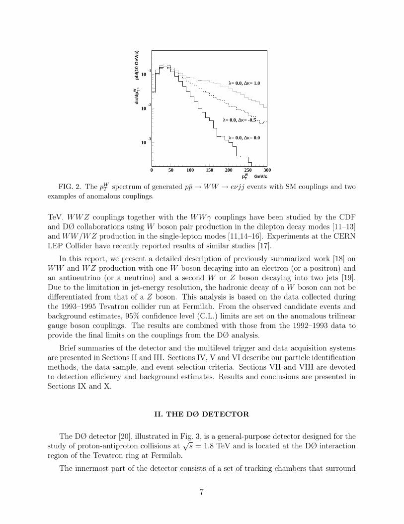
Since anomalous couplings contribute only via s-channel photon or W or Z boson in-termediaries, their effects are expected mainly in the region of small vector boson rapidi-ties, and the transverse momentum distribution of the vector boson is therefore partic-ularly sensitive to anomalous trilinear gauge-boson couplings. This is demonstrated inFig. 2, which shows the distribution of the W boson transverse momentum pW

T in simu-lated pp → WW + X → eνjj + X events for anomalous trilinear gauge boson couplings,using a dipole form factor with a scale Λ = 1.5 TeV, and with the couplings for WWγ andWWZ assumed to be equal.

Trilinear gauge-boson couplings can therefore be measured by comparing the shapes ofthe pT distributions of the final state gauge bosons with theoretical predictions. Even ifthe background is much larger than the expected gauge-boson pair production signal as isthe case for the WW/WZ → eνjj process, limits on anomalous couplings can still be setusing a kinematic region where the effects of anomalous trilinear gauge boson couplings areexpected to dominate.

Trilinear gauge-boson couplings have been studied in several experiments. WWγ cou-plings have been studied in pp collisions by the UA2 [8], CDF [9], and DØ [10,11] collabo-rations using Wγ events. The UA2 results are based on data taken during the 1988–1990CERN pp collider run at

√s = 630 GeV with an integrated luminosity of 13 pb−1 and the

CDF and DØ data are from the 1992–1993 and 1993–1995 Fermilab pp runs at√s = 1.8

6

10-3

10-2

10-1

0 50 100 150 200 250 300

λ= 0.0, ∆κ= 0.0

λ= 0.0, ∆κ= -0.5

λ= 0.0, ∆κ= 1.0

pWT GeV/c

dσ/

dp

W T,

p

b/(

10 G

eV/c

)

FIG. 2. The pWT spectrum of generated pp → WW → eνjj events with SM couplings and two

examples of anomalous couplings.

TeV. WWZ couplings together with the WWγ couplings have been studied by the CDFand DØ collaborations using W boson pair production in the dilepton decay modes [11–13]and WW/WZ production in the single-lepton modes [11,14–16]. Experiments at the CERNLEP Collider have recently reported results of similar studies [17].

In this report, we present a detailed description of previously summarized work [18] onWW and WZ production with one W boson decaying into an electron (or a positron) andan antineutrino (or a neutrino) and a second W or Z boson decaying into two jets [19].Due to the limitation in jet-energy resolution, the hadronic decay of a W boson can not bedifferentiated from that of a Z boson. This analysis is based on the data collected duringthe 1993–1995 Tevatron collider run at Fermilab. From the observed candidate events andbackground estimates, 95% confidence level (C.L.) limits are set on the anomalous trilineargauge boson couplings. The results are combined with those from the 1992–1993 data toprovide the final limits on the couplings from the DØ analysis.

Brief summaries of the detector and the multilevel trigger and data acquisition systemsare presented in Sections II and III. Sections IV, V and VI describe our particle identificationmethods, the data sample, and event selection criteria. Sections VII and VIII are devotedto detection efficiency and background estimates. Results and conclusions are presented inSections IX and X.

II. THE DØ DETECTOR

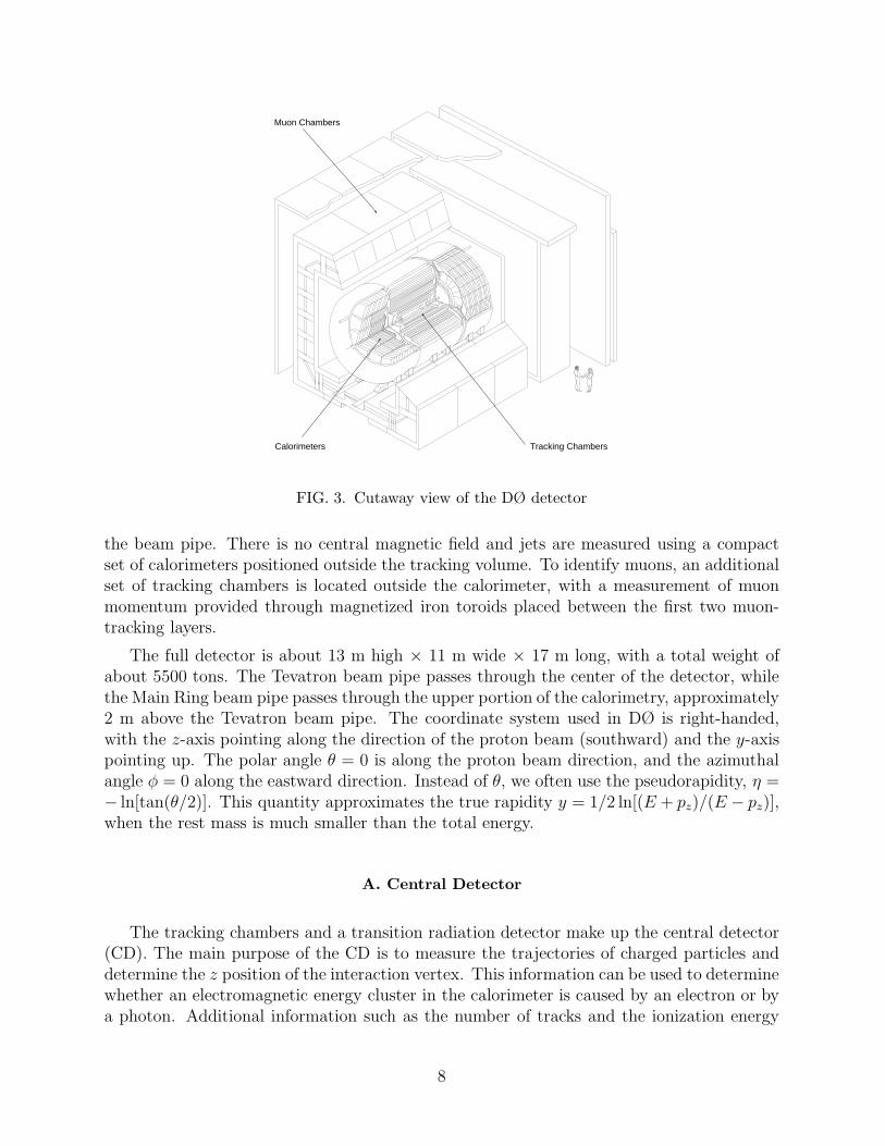
The DØ detector [20], illustrated in Fig. 3, is a general-purpose detector designed for thestudy of proton-antiproton collisions at

√s = 1.8 TeV and is located at the DØ interaction

region of the Tevatron ring at Fermilab.

The innermost part of the detector consists of a set of tracking chambers that surround

7

D0 Detector

Muon Chambers

Calorimeters Tracking Chambers

FIG. 3. Cutaway view of the DØ detector

the beam pipe. There is no central magnetic field and jets are measured using a compactset of calorimeters positioned outside the tracking volume. To identify muons, an additionalset of tracking chambers is located outside the calorimeter, with a measurement of muonmomentum provided through magnetized iron toroids placed between the first two muon-tracking layers.

The full detector is about 13 m high × 11 m wide × 17 m long, with a total weight ofabout 5500 tons. The Tevatron beam pipe passes through the center of the detector, whilethe Main Ring beam pipe passes through the upper portion of the calorimetry, approximately2 m above the Tevatron beam pipe. The coordinate system used in DØ is right-handed,with the z-axis pointing along the direction of the proton beam (southward) and the y-axispointing up. The polar angle θ = 0 is along the proton beam direction, and the azimuthalangle φ = 0 along the eastward direction. Instead of θ, we often use the pseudorapidity, η =− ln[tan(θ/2)]. This quantity approximates the true rapidity y = 1/2 ln[(E + pz)/(E − pz)],when the rest mass is much smaller than the total energy.

A. Central Detector

The tracking chambers and a transition radiation detector make up the central detector(CD). The main purpose of the CD is to measure the trajectories of charged particles anddetermine the z position of the interaction vertex. This information can be used to determinewhether an electromagnetic energy cluster in the calorimeter is caused by an electron or bya photon. Additional information such as the number of tracks and the ionization energy

8

along the track (dE/dx) can be used to determine whether a track is caused by one or severalclosely spaced charged particles, such as a photon conversion.

The CD consists of four separate subsystems: the vertex drift chamber (VTX), thetransition radiation detector (TRD), the central drift chamber (CDC), and two forwarddrift chambers (FDC). The full set of CD detectors fits within the inner cylindrical apertureof the calorimeters in a volume of radius r = 78 cm and length l = 270 cm. The systemprovides charged-particle tracking over the region |η| < 3.2. The trajectories of chargedparticles are measured with a resolution of 2.5 mrad in φ and 28 mrad in θ. From thesemeasurements, the position of the interaction vertex along the z direction is determinedwith a resolution of 6 mm.

The VTX is the innermost tracking chamber in the DØ detector, occupying the regionr = 3.7 cm to 16.2 cm. It is made of three mechanically independent concentric layers ofcells parallel to the beam pipe. The innermost layer has sixteen cells while the outer twolayers have thirty-two cells each.

The TRD occupies the space between the VTX and the CDC; it extends from r = 17.5cm to 49 cm. The TRD consists of three separate units, each containing a radiator (393 foilsof 18 µm thick polypropylene in a volume filled with nitrogen gas) and an X-ray detectionchamber filled with Xe gas. The TRD information is not used in this analysis.

The CDC is a cylindrical drift chamber, 184 cm along z, located between r = 49.5 andr = 74.5 cm, and provides coverage for |η| < 1.2. It is made up of four concentric rings of 32azimuthal cells per ring. Each cell contains seven sense wires (staggered by 200 µm relativeto each other to help resolve left-right ambiguities), and two delay lines. The rφ positionof a hit is determined via the drift time measured for the hit wire and the z position of ahit is measured using inductive delay lines embedded in the module-walls of the sense wireplanes.

The FDC consists of two sets of drift chambers located at the ends of the CDC. Theyperform the same function as the CDC, but for 1.4 < |η| < 3.1. Each FDC package consistsof three separate chambers: a Φ module, whose sense wires are radial and measure theφ coordinate, sandwiched between a pair of Θ modules whose sense wires measure the θcoordinate.

B. Calorimeters

The DØ calorimeters are sampling calorimeters, with liquid argon as the sensitive ioniza-tion medium. The primary absorber material is depleted uranium, with copper and stainlesssteel used in the outer regions. There are three separate units, each contained in separatecryostats: the Central Calorimeter (CC), the North End Calorimeter (ECN), and the SouthEnd Calorimeter (ECS). The readout cells are arranged in a pseudo-projective geometrypointing to the interaction region.

The calorimeters are subdivided in depth into three distinct types of modules: electro-magnetic sections (EM) with relatively thin uranium absorber plates, fine-hadronic sections

9

(FH) with thicker uranium plates, and coarse-hadronic sections (CH) with thick copper orstainless steel plates. There are four separate layers for the EM modules in both the CCand EC that are readout separately. The first two layers are 2 radiation lengths thick inthe CC and 0.3 and 2.6 radiation lengths thick in the EC, and measure the initial longi-tudinal shower development, where photons and π0s differ somewhat on a statistical basis.The third layer spans the region of maximum EM shower energy deposition and the fourthcompletes the EM coverage of approximately 20 total radiation lengths. The fine-hadronicmodules are typically segmented into three or four layers. Typical transverse sizes of towersin both EM and hadronic modules are ∆η = 0.1 and ∆φ = 2π/64 ≈ 0.1. The third sectionof the EM modules is segmented twice as finely in both η and φ to provide more precisedetermination of centroids of EM showers.

The CC has a length of 2.6 m, covering the pseudorapidity region |η| < 1.2, and consistsof three concentric cylindrical rings. There are 32 EM modules in the inner ring, 16 FHmodules in the surrounding ring, and 16 CH modules in the outer ring. The EM, FH andCH module boundaries are rotated with respect to each other so as to prevent having morethan one intermodular gap intercepting a trajectory from the origin of the detector.

The two end calorimeters (ECN and ECS) are mirror-images, and contain four types ofmodules. To avoid the dead spaces in a multi-module design, there is just a single large EMmodule and one inner hadronic (IH) module. Outside the EM and IH, there are concentricrings of 16 middle and outer hadronic modules (MH and OH). The azimuthal boundariesof the MH and OH modules are also offset to prevent cracks through which particles couldpenetrate the calorimeter. This makes the DØ detector almost completely hermetic and pro-vides an accurate measurement of missing transverse energy. Due to increase in backgroundand loss of tracking efficiency for |η| > 2.5, electron and photon candidates are restricted to1.5 < |η| < 2.5 in the EC.

In the transition region between the CC and EC (0.8 ≤ |η| ≤ 1.4), there is a largeamount of uninstrumented material in the form of cryostat walls, stiffening rings, and moduleendplates. To correct for energy deposited in the uninstrumented material, we use twosegmented (0.1 × 0.1 in η×φ) arrays of scintillation counters, called intercryostat detectors.In addition, separate single-cell structures called “massless gaps” are mounted on the endplates of the CC-FH modules and on the front plates of EC-MH and EC-OH modules, andare used to correct showers in this region of the detector.

The Main Ring beam pipe passes through the outer layers of the CC, ECN and ECS.Beam losses from the Main-Ring cause energy deposition in the calorimeter that can biasthe energy measurement. The data acquisition system either stops recording data duringperiods of Main-Ring activity near the DØ detector, or flags such events.

C. Muon Detectors

The DØ muon detector is designed to identify muons and to determine their trajectoriesand momenta. It is located outside of the calorimeter, and is divided in two subsystems:the Wide Angle Muon Spectrometer and the Small Angle Muon Spectrometer. Since the

10

calorimeter is thick enough to absorb most of the debris from electromagnetic and hadronicshowers, muons can be identified with great confidence. The muon system is not used inthis analysis, and is therefore not discussed any further.

III. MULTILEVEL TRIGGER AND DATA ACQUISITION SYSTEMS

The DØ trigger system is a multilayer hierarchical system. Increasingly complex testsare applied to the data at each successive stage to reduce background.

The first stage, called Level 0 (L0), consists of two scintillator arrays mounted on the frontsurfaces of the EC cryostats, perpendicular to the beam direction. Each array covers a partialregion of pseudorapidity for 1.9 < |η| < 4.3, with nearly complete coverage over the range2.2 < |η| < 3.9. The L0 system is used to detect the occurrence of an inelastic pp collision,and serves as the luminosity monitor for the experiment. In addition, it provides fastinformation on the z-coordinate of the primary collision vertex, by measuring the differencein arrival time between particles hitting the north and south L0 arrays; this is used in makingpreliminary trigger decisions. A slower, more accurate measurement of the position of theinteraction vertex, and an indication of the possible occurrence of multiple interactions, arealso made available for subsequent trigger decisions. The L0 trigger is ≈ 99% efficient fornon-diffractive inelastic collisions. The output rate from L0 is on the order of 150 kHz at atypical luminosity of 1.6 × 1031cm−2 s−1.

The next stage of the trigger is called Level 1 (L1). It combines the results from individualL1 components into a set of global decisions that command the readout of the digitizationcrates. It also interacts with the Level 2 trigger (L2). Most of the L1 components, such asthe calorimeter triggers and the muon triggers, operate within the 3.5 µs interval betweenbeam crossings, so that all events are examined. However, other components, such as theTRD trigger and several components of the calorimeter and muon triggers, called Level 1.5trigger (L1.5), can require more time. The goal of the L1 trigger is to reduce the event rateto 100–200 Hz. The primary input for the L1 trigger consists of 256 trigger terms, each ofwhich corresponds to a single bit, indicating that some specific requirement is met. These256 terms are reduced to a set of 32 L1 trigger bits by a two-dimensional AND-OR logicnetwork. An event is said to pass L1 if at least one of these 32 bits is set. The L1 trigger alsouses information based on Main Ring activity. To prevent saturation of the trigger systemby processes with large cross sections, such as QCD multijet production, any particularcontributor to the L1 trigger can be prescaled.

The L1 calorimeter trigger covers the region up to |η| < 4.0 in trigger towers of 0.2 × 0.2in η−φ space. These towers are subdivided longitudinally into electromagnetic and hadronictrigger sectors. The output of the L1 calorimeter trigger corresponds to the transverse energydeposited in these sectors and towers.

For the 1993–1995 collider run, an L1.5 trigger for the calorimeter was implementedusing the L1 calorimeter trigger data and filters based on neighbor sums and ratios of theEM and total transverse energies.

When an event satisfies the L1 trigger, the data are passed on the DØ data acquisition

11

pathways to a farm of 48 parallel microprocessors, which serve as event builders as well asthe L2 trigger system. The L2 system collects the digitized data from all elements of thedetector and trigger blocks for events that successfully pass Level 1. It applies sophisticatedalgorithms to the data to reduce the event rate to about 2 Hz before passing the acceptedevents on to the host computer for monitoring and recording. The data for a specific eventare sent over parallel paths to memory modules in specific selected nodes. The accepteddata are collected and formatted in final form in the nodes, and the L2 filter algorithms arethen executed.

The L2 filtering process in each node is built around a series of filter tools. Each toolhas a specific function related to the identification of a type of particle or event character-istic. There are tools to recognize jets, muons, calorimeter EM clusters, tracks associatedwith calorimeter clusters,

∑

ET (sum of transverse energies of jets), and /ET (imbalance intransverse energy). Other tools recognize specific noise or background conditions. There are128 L2 filters available. If all of the L2 requirements (for at least one of these 128 filters)are satisfied, the event is said to pass L2 and it is temporarily stored on disk before beingtransferred to an 8 mm magnetic tape.

Once an event is passed by an L2 node, it is transmitted to the host cluster, where it isreceived by the data logger, a program running on one of the host computers. This programand others associated with it are responsible for receiving data from the L2 system andcopying it to magnetic tape, while performing all necessary bookkeeping tasks (e.g., timestamping, recording the run number, an event number, etc.). Part of the data is sent to anevent pool for online monitoring.

A. Electron Trigger

To trigger on electrons, L1 requires the transverse energy in the EM section of a triggertower to be above a programmable threshold. The L2 electron algorithm then uses the fullsegmentation of the EM calorimeter to identify electron showers. Using the trigger towersthat are above threshold at L1 as seeds, the algorithm forms clusters that include all cells inthe four EM layers and the first FH layer in a region of ∆η × ∆φ = 0.3 × 0.3, centered onthe tower with the highest ET . The longitudinal and transverse energy profile of the clustermust satisfy the following requirements: (i) the fraction of the cluster energy in the EMsection (the EM fraction) must be above a threshold, which depends on energy and detectorposition; and (ii) the difference between the energy depositions in two regions of the thirdEM layer, covering ∆η × ∆φ = 0.25 × 0.25 and 0.15 × 0.15, and centered on the cell withthe highest ET , must be within a window that depends on the total cluster energy.

B. Jet Trigger

The L1 jet triggers require the sum of the transverse energy in the EM and FH sectionsof a trigger tower (∆η × ∆φ = 0.2 × 0.2) to be above a programmable threshold. The L2

12

jet algorithm begins with an ET -ordered list of towers that are above threshold at L1. AtL2, a jet is formed by placing a cone of given radius R, where R =

√∆η2 + ∆φ2, around

the seed tower from L1. If another seed tower lies within the jet cone, it is passed over andnot allowed to seed a new jet. The summed ET in all of the towers included in the jet conedefines the jet ET . If any two jets overlap, then the towers in the overlap region are addedinto the jet candidate that is formed first. To filter out events, requirements on quantitiessuch as the minimum transverse energy of a jet, the minimum transverse size of a jet, theminimum number of jets, and the pseudorapidity of jets, can be imposed at this point.

C. Missing Transverse Energy Trigger

Rare and interesting physics processes often involve production of weakly interactingparticles such as neutrinos. These particles usually can not be detected directly. However,assuming momentum conservation in a collision allows the momenta of such particles to beinferred from the vector sum of the momenta of the observed particles. Since the energyflow near the beamline is largely undetected, such calculations are realistic only in the planetransverse to the beam. The negative of the vector sum of the momenta of the detectedparticles is referred to as missing ET and denoted by /ET ; it is used as an indicator of thepresence of weakly interacting particles. At L2, /ET is computed using the vector sum ofall calorimeter and intercryostat detector cell energies with respect to the z position of theinteraction vertex, which is determined from the timing of the hits in the L0 counters.

IV. PARTICLE IDENTIFICATION

A. Electron

Electrons and photons are identified by the properties of the shower in the calorimeter.The algorithm loops over all EM towers (∆η × ∆φ = 0.1 × 0.1) with energy E > 50 MeV,and connects the neighboring tower with the next highest energy. The cluster energy is thendefined as the sum of the energies of the EM towers and the energies in the corresponding firstFH layer. The ratio of the energy in the EM cluster to the total energy (EM energy summedwith the corresponding hadronic layers), defined as the EM fraction, is used to discriminateelectrons and photons from hadronic showers. A cluster must pass the following criteria tobe an electron/photon candidate: (i) the EM fraction must be greater than 90% and (ii)at least 40% of the energy must be contained in a single 0.1 × 0.1 tower. To distinguishelectrons from photons, we search for a track in the central detector that extrapolates tothe EM cluster from the primary interaction vertex within a window of |∆η| ≤ 0.1, and|∆φ| ≤ 0.1. If one or more tracks are found, the object is classified as an electron candidate.Otherwise, it is classified as a photon candidate.

13

1. Selection Requirements

The spatial development of EM showers is quite different from that of hadronic showersand the shower shape information can be used to differentiate electrons and photons fromhadrons. The following variables are used for final electron selection:

(i) Electromagnetic energy fraction. This quantity is based on the observation that electronsdeposit almost all of their energy in the EM section of the calorimeter, while hadron jetsare far more penetrating (typically only 10% of their energy is deposited in the EM sectionof the calorimeter). It is defined as the ratio of EM energy to the total shower energy.Electrons are required to have at least 95% of their total energy in the EM calorimeter.This requirement loses only about 1% of all electrons.

(ii) Covariance matrix (H-matrix) χ2. The shape of any shower can be characterized by thefraction of the cluster energy deposited in each layer and tower of the calorimeter. Thesefractions are correlated, i.e., an electron shower deposits energies according to the expectedtransverse and longitudinal shapes of an EM shower and a hadron shower following thetypical development of a hadronic shower. To obtain good discrimination against hadrons,we use a covariance matrix technique. The observables in this method are the fractionalenergies in Layers 1, 2, and 4 of the EM sector and the fractional energy in each cell of a 6×6array of cells in Layer 3 centered on the most energetic tower in the EM cluster. To takeaccount of the dependence of the shower shape on energy and on the position of the primaryinteraction vertex, we use the logarithm of the shower energy and the z-position of the eventvertex as the remaining input observables. The event vertex is determined by extrapolatingCDC tracks to the z axis, and for more than one possibility, the vertex associated with thehighest number of tracks is chosen as the event vertex. Using these 41 variables, covariancematrices are constructed for each of the 37 detector towers (at different values of η) basedon Monte Carlo generated electrons. The Monte Carlo showers are tuned to make themagree with our test beam measurements of the shower shapes. The 41 observables for anygiven shower can be compared with the parameters of the appropriate covariance matrix todefine a χ2, which is to be be less than 100 for electron candidates in the CC and less than200 for the EC. This requirement loses about 5% of all true electrons.

(iii) Isolation. The decay electron from a W boson should not be close to any other object inthe event. This is quantified by the isolation fraction. If E(0.4) is the energy deposited in allcalorimeter cells within the cone R < 0.4 around the direction of the electron, and EM(0.2)is the energy deposited in only the EM calorimeter in the cone R < 0.2, the isolation variableis then defined as the ratio I = [E(0.4) − EM(0.2)]/EM(0.2). The requirement I < 0.1loses only 3% of the electrons from W boson decays.

(iv) Track-match significance. An important source of background for electrons is the photonfrom the decay of π0 or η mesons. Such photons do not produce tracks, but their trajecto-ries can overlap with those of nearby charged particles, thereby simulating electrons. Thisbackground can be reduced by demanding a good spatial match between the energy clusterin the calorimeter and nearby charged tracks. The significance S of the mismatch betweenthese quantities is given by S = [(∆φ/δ∆φ)

2 + (∆z/δ∆z)2]1/2, where ∆φ is the azimuthal

mismatch, ∆z the mismatch along the beam axis, and the δ are the resolutions of these vari-

14

ables. This form for S is appropriate for the central calorimeter. For the end calorimeter, rreplaces z. Requiring S < 5 accepts 95(78)% of the CC(EC) electrons reconstructed in thecentral tracker.

(v) Track-in-road. All electrons from W → eν decays are required to have a partiallyreconstructed track along the trajectory between the energy cluster in the calorimeter andthe interaction vertex. This requirement is found to reject 16(14)% of CC(EC) electronsfrom W boson decay.

In our analysis, we combine the above quantities to form the electron identificationcriteria. A summary of the selection requirements and their acceptance efficiencies is listedin Table I (See SectVII).

TABLE I. Electron selection requirements and their acceptance efficiencies for W → eν events.

Selection CC EC

requirement ε ε

H-matrix χ2 < 100 0.946±0.005 < 200 0.950±0.008

EM fraction > 0.95 0.991±0.003 > 0.95 0.987±0.006

Isolation < 0.10 0.970±0.004 < 0.10 0.976±0.007

Track match < 5 0.948±0.005 < 5 0.776±0.012

Track-in-road 0.835±0.009 0.858±0.006

2. Electromagnetic Energy Corrections

The energy scales of the calorimeters were originally set through calibration in a test-beam. However, due to differences in conditions between the test beam and the DØ envi-ronment, additional corrections had to be implemented.

The EM energy scales for the calorimeters were determined by comparing the measuredmasses of π0 → γγ, J/ψ → ee, and Z → ee to their known values. If the electron energymeasured in the calorimeter and the true energy are related by Emeas = αEtrue + δ, themeasured and true mass values are, to first order, related by mmeas = αmtrue + δf , wherethe calculable variable f reflects the topology of the decay. To determine α and δ, we fit theMonte Carlo prediction to the observed resonances, with α and δ as free parameters [21].The values of α and δ are found to be α = 0.9533± 0.0008 and δ = −0.16+0.03

−0.21 GeV for theCC and α = 0.952 ± 0.002 and δ = −0.1 ± 0.7 GeV for the EC.

3. Energy Resolution

The relative energy resolution for electrons and photons in the CC is expressed by the

empirical relation(

σE

)2= C2+ S2

ET

+N2

E2 , where E and ET are the energy and transverse energy

15

of the incident electron/photon, C is a constant term from uncertainties in calibration, Sreflects the sampling fluctuation of the liquid argon calorimeter, and N corresponds to acontribution from noise. For the EC, the ET in the relation is replaced by E. The samplingand noise terms are based on results from the test beam. The noise term measured at thetest beam agrees with the one obtained in the collider environment (based on the width ofpedestal distributions). The constant term is tuned to match the mass resolution of bothobserved and simulated Z → ee events. Table II lists these parameters.

TABLE II. Parameters for describing the energy resolution of electrons and photons.

Quantity CC EC

C 0.017 0.009

S (√

GeV) 0.14 0.157

N (GeV) 0.49 1.140

B. Jets

In our analysis, jets are reconstructed using a fixed-cone algorithm with radius R =√∆η2 + ∆φ2 = 0.5. The algorithm forms preclusters of contiguous cells using a radius of

Rprecluster = 0.3 centered on the tower with highest ET . Only towers with ET > 1 GeV areincluded in preclusters. These preclusters serve as the starting points for jet reconstruction.An ET -weighted center of gravity is then formed using the ET of all towers within a radiusR of the center of the cluster, and the process is repeated until the jet becomes stable. Ajet must have ET > 8 GeV. If two jets share energy, they are combined or split, based onthe fraction of overlapping energy relative to the ET of the lesser jet. If this shared fractionexceeds 50%, the jets are combined.

Although the R = 0.3 cone algorithm is more efficient for jet finding than our largercone size, which leads to undesired merging of jets for high-pT W or Z bosons, the relativelylarge uncertainties in the measurement of jet-energy for the R = 0.3 cones negate theiradvantage, and we therefore choose to use the R = 0.5 cone algorithm for our studies.

1. Selection Requirements

To remove jets produced by cosmic rays, calorimeter noise, and interactions in the MainRing, we developed a set of requirements based on Monte Carlo studies of jets in suchenvironments and on data on noise taken with and without colliding beams. The variablesused are:

(i) Electromagnetic energy fraction (emf). As for electrons, this quantity is defined as thefraction of the total energy deposited in the electromagnetic section of the calorimeter. A

16

requirement on this quantity removes electrons, photons and false jets from the jet sample.Electrons and photons typically have a high EM fraction. False jets are caused mainlyby background from the Main Ring or by noisy or “hot” cells, and therefore generallydo not contain energy in the EM section, thereby yielding very low EM fractions. Jetswith 0.05 < emf < 0.95 are defined as acceptable in this analysis. The efficiency of thisrequirement is 99.9% at ET = 20 GeV and decreases to 99.6% at 100 GeV.

(ii) Hot cell energy fraction (hcf). The hcf is defined as the ratio of the energy in the cellof second highest ET to that of the cell with highest ET within a jet. A requirement onthis quantity is imposed to remove events with a large amount of noise in the calorimeter.Hot cells can appear when a discharge occurs between electrodes within a cell; often thisdoes not affect neighboring cells. In this case, hcf is small, which signals a problem, sincethe hcf for a jet should not be small because the energy is expected to be distributed overcells. If most of the energy is concentrated in a single cell, it is very likely to be a false jetreconstructed from discharge noise. For good jets, hcf is found to be greater than 0.1. Theefficiency of this requirement is 97.3% at ET = 20 GeV and decreases to 96.9% at 100 GeV.

(iii) Coarse hadronic energy fraction (chf). This quantity is defined as the fraction of jetenergy deposited in the coarse hadronic section of the calorimeter. The Main Ring at DØpasses through the CH modules, and any energy deposition related to the Main Ring willbe concentrated in this section of the calorimeter. Such jets tend to have more than 40% oftheir energy in the CH region, while standard jets have less than 10% of their energy in thissection of the calorimeter. All acceptable jets are therefore required to have chf < 0.4. Theefficiency of this requirement is 99.6% at ET = 20 GeV and decreases to 99.3% at 100 GeV.

2. Hadronic Energy Corrections

Since the measured jet energy is usually not equal to the energy of the original partonthat formed the jet, corrections are needed to minimize any systematic bias. Jet energyresponse affected by non-uniformities in the calorimeter, non-linearities in the response tohadrons, emission of particles outside of the R = 0.5 cone (often referred to as out-of-coneshowering), noise due to the radioactivity of uranium, and energy overlap from the productsof soft interactions of spectator partons within the proton and the antiproton (“underlyingevent”). The first two effects are estimated using a method called Missing-ET ProjectionFraction (MPF) [22].

The MPF method is based on events that contain a single isolated EM cluster (dueto a photon or a jet that fragmented mostly into neutral mesons), and one hadronic jetlocated opposite in φ, and no other objects in the event. It is assumed that such eventsdo not have energetic neutrinos so that any missing transverse energy can be attributedto a mismeasurement of the hadronic jet. The EM-cluster energy is corrected using theelectromagnetic energy corrections described above. Projecting the corrected /ET along thejet axis determines corrections to the jet energy. This correction is averaged over manyevents in the sample to obtain a correction as a function of jet ET , η, and electromagneticcontent of the jet. The hadronic energy correction is 20% at E = 20 GeV and 15% at

17

E = 100 GeV, and gradually approaches 10% at high E.

The impact of out-of-cone showering is estimated using Monte Carlo jet events. Effectsdue to the underlying events and uranium noise are determined in separate studies usingminimum-bias event data. (Minimum-bias data corresponds to inclusive inelastic collisionscollected using only the L0 trigger.)

3. Energy Resolution

The jet energy resolution has been studied by examining momentum balance in dijet

events [23]. The formula used for parametrizing the relative jet energy resolution is(

σE

)2=

C2 + S2

E+ N2

E2 . Table III shows the values of the parameters for different η regions of thecalorimeter.

TABLE III. Jet energy resolution for different regions of the calorimeter.

η Region C S (√

GeV) N (GeV)

|η| < 0.5 0.00±0.01 0.81±0.02 7.07±0.09

0.5 < |η| < 1.0 0.00±0.01 0.91±0.02 6.92±0.09

1.0 < |η| < 1.5 0.05±0.01 1.45±0.02 0.00±1.40

1.5 < |η| < 2.0 0.00±0.01 0.48±0.07 8.15±0.21

2.0 < |η| < 3.0 0.01±0.58 1.64±0.13 3.15±2.50

C. Neutrinos: Missing Transverse Energy

The presence of neutrinos in an event is inferred from the /ET . In this analysis we assumethat the /ET in each candidate event corresponds to the neutrino from the decay W → eν.

1. Missing ET

The missing transverse energy in the calorimeter is defined as /ET = ( /ET2x+ /ET

2y)

1/2, where

/ET x = −∑

iEi sin(θi) cos(φi) −∑

j ∆Ejx and /ET y = −∑

iEi sin(θi) sin(φi) −∑

j ∆Ejy. The

first sum (over i) is over all cells in the calorimeters, intercryostat detectors and masslessgaps (see Sec. II B). The second sum (over j) is over the ET corrections applied to allelectrons and jets in the event. This can be used to estimate the transverse momentum ofany neutrinos in an event that does not contain muons, which deposit only a small portionof their energy in the calorimeter. The total missing ET is missing ET from the calorimetercorrected for the transverse momenta of any observed muon tracks. Since this analysis doesnot use muons, we will refer to the /ET based on the calorimeters as the true /ET .

18

2. Resolution in /ET

For an ideal calorimeter, the magnitude of the components of the /ET vector wouldsum to zero for events with no true source of /ET . However, detector noise and energyresolution in the measurement of jets, photons, and electrons contribute to the /ET . Inaddition, non-uniform response in the detector also results in /ET . The /ET resolution for ourcandidate events is parameterized as σ = 1.08GeV+0.019(

∑

ET ), and is based on studies ofminimum-bias data [23]. The

∑

ET used in the parameterization is quite reasonable becausethe greater the total amount of transverse energy in the event, the larger the possibility forits mismeasurement.

V. DATA SAMPLE

The analysis of the WW/WZ → eνjj process is based on data taken during the 1993–1995 Tevatron Collider run (called Run 1b). The L0 trigger is used to check the presence ofan inelastic collision, but is not included in the trigger conditions for W -boson data. Thiswas done to allow studies of diffractive W -boson production. Our analysis uses the collectedW → eν data sample, with the L0 trigger requirement imposed offline. The L1 trigger usedin this analysis (called the EM1 1 HIGH trigger) requires the presence of an electromagnetictrigger tower with ET > 10 GeV. The L1.5 trigger then requires the L1 trigger tower to haveET > 15 GeV and checks that the electromagnetic fraction is greater than 85%. The L2component of the trigger (called the EM1 EISTRKCC MS trigger) requires an isolated electroncandidate with ET > 20 GeV that has a shower shape consistent with that of an electronand /ET > 15 GeV.

Additional conditions are imposed on the data to further reduce background. Triggersthat occur at the times when a proton bunch in the Main Ring passes through the detectorare not used in this analysis. Similarly, triggers that occur during the first 0.4 seconds of the2.4-second antiproton production cycle are rejected. Data taken during periods when thedata acquisition system or the detector sub-systems malfunctioned are also discarded. Withthese trigger requirements, the integrated luminosity of the data sample is estimated to be82.3± 4.4 pb−1 [24]. The efficiency and turn-on of the L2 trigger are described in Ref. [25].The trigger efficiency for signal is (98.1 ± 1.9)%.

Data samples that satisfy two other L2 triggers, the EM1 ELE MON and ELE 1 MON triggers,are used for background studies. These triggers select events that have an electron candidatewith ET > 20 GeV and ET > 16 GeV, respectively. The electron candidates in these samplesmust pass the standard shower-shape requirements, but not the isolation requirement. Thesetriggers use the same L1 and L1.5 conditions as the trigger used for signal.

19

VI. EVENT SELECTION

WW/WZ → eνjj candidates are selected by searching for events with an isolated high-ET electron, large /ET , and at least two high-ET jets. Electrons in the candidate samplemust be in the |η| < 1.1 region but away from the boundaries between calorimeter modulesin φ (∆φ > 0.01), or within the region 1.5 < |η| < 2.5. Jets in the candidate sample mustbe in the region |η| < 2.5.

The W → eν decay is defined through the presence of only a single isolated electronwith Ee

T > 25 GeV and /ET > 25 GeV in the event. The transverse mass of the electron andneutrino ( /ET ) system is required to be MT > 40 GeV/c2, where MT = {2Ee

T /ET [1− cos(φe−φν)]}1/2. The requirement on the electron ET is sufficiently high to provide an efficiencythat is independent of ET (the hardware threshold of 20 GeV). Requiring only one electronreduces background from Z → ee production. The requirements on /ET and MT reduce thebackground contribution from misidentified electrons.

The W/Z → jj decay is defined by requiring at least two jets with EjT > 20 GeV and an

invariant mass of the two-jet system consistent with that of the W or Z boson (50 < Mjj <110 GeV/c2). The dijet invariant mass (Mjj) is calculated via Mjj = {2Ej1

T Ej2T [cosh(ηj1 −

ηj2)− cos(φj1 − φj2)]}1/2. If there are more than two jets in the event, the two jets with thehighest dijet invariant mass are chosen to represent the W (or Z) decay.

The difference between the pT values of the eν and the two-jet systems is used to reducebackgrounds. For WW or WZ production, the pT (eν) − pT (jj) distribution should bepeaked near zero and have a symmetric Gaussian shape, with the width of the Gaussiandistribution determined primarily by the jet energy resolution. On the other hand, forbackground such as tt production (see Sec. VIII), the distribution should be broader andasymmetric (shifted to positive values) due to additional b-quark jets in the events. Ouranalysis therefore requires |pT (eν) − pT (jj)| < 40 GeV/c.

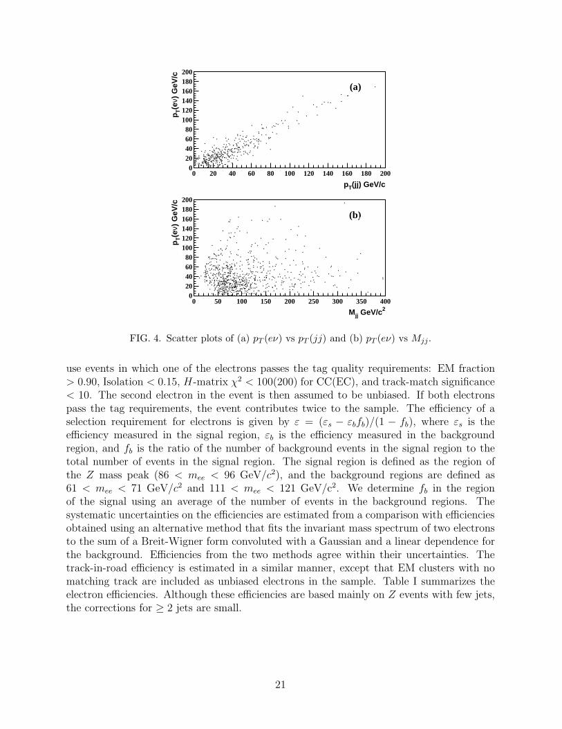
The data satisfying the above selection criteria yield 399 events. Figure 4a shows a scatterplot of pT (eν) vs pT (jj) for candidate events that satisfy the two-jet mass requirement. Thewidth of the band reflects both the resolution and the true spread in the pT values. Figure 4bshows a scatter plot of pT (eν) vs Mjj without the imposition of the two-jet mass requirement.

VII. DETECTION EFFICIENCY

A. Electron Selection Efficiency

The efficiency of electron selection is studied using the Z → ee event sample from the1993–1995 Tevatron collider run using the EM2 EIS HI trigger. Z → ee events were selectedat L1 and L1.5 by requiring two EM towers with ET > 7 GeV at L1, and at least one towerwith ET > 12 GeV with more than 85% of its energy in the EM section of the calorimeter. AtL2, the trigger required two electron candidates with ET > 20 GeV that satisfied electronshower-shape and isolation requirements. To select an unbiased sample of electrons, we

20

(a)

020406080

100120140160180200

0 20 40 60 80 100 120 140 160 180 200

pT(jj) GeV/cp

T(e

ν) G

eV/c

(b)

020406080

100120140160180200

0 50 100 150 200 250 300 350 400

Mjj GeV/c2

pT(e

ν) G

eV/c

FIG. 4. Scatter plots of (a) pT (eν) vs pT (jj) and (b) pT (eν) vs Mjj.

use events in which one of the electrons passes the tag quality requirements: EM fraction> 0.90, Isolation < 0.15, H-matrix χ2 < 100(200) for CC(EC), and track-match significance< 10. The second electron in the event is then assumed to be unbiased. If both electronspass the tag requirements, the event contributes twice to the sample. The efficiency of aselection requirement for electrons is given by ε = (εs − εbfb)/(1 − fb), where εs is theefficiency measured in the signal region, εb is the efficiency measured in the backgroundregion, and fb is the ratio of the number of background events in the signal region to thetotal number of events in the signal region. The signal region is defined as the region ofthe Z mass peak (86 < mee < 96 GeV/c2), and the background regions are defined as61 < mee < 71 GeV/c2 and 111 < mee < 121 GeV/c2. We determine fb in the regionof the signal using an average of the number of events in the background regions. Thesystematic uncertainties on the efficiencies are estimated from a comparison with efficienciesobtained using an alternative method that fits the invariant mass spectrum of two electronsto the sum of a Breit-Wigner form convoluted with a Gaussian and a linear dependence forthe background. Efficiencies from the two methods agree within their uncertainties. Thetrack-in-road efficiency is estimated in a similar manner, except that EM clusters with nomatching track are included as unbiased electrons in the sample. Table I summarizes theelectron efficiencies. Although these efficiencies are based mainly on Z events with few jets,the corrections for ≥ 2 jets are small.

21

B. W/Z → jj Selection Efficiency

The W/Z → jj selection efficiency is estimated using Monte Carlo WW/WZ → eνjjevents generated with the isajet [26] and pythia [27] programs, followed by a detailedsimulation of the DØ detector, and parametrized as a function of pW

T . Figure 5 showsthe W/Z → jj detection efficiency ǫ(W → jj) calculated as the ratio of events after theimposition of the two-jet selection requirements relative to the initial number of events. Atlow pT , the detection efficiency is artificially elevated due to the presence of additional jetsfrom initial- and final-state gluon radiation (ISR/FSR) that are mislabeled as being decaysof W or Z bosons. The decrease in the efficiency at high pT is due to the merging of thetwo jets from a W or a Z boson. The results obtained from isajet are used to estimate theefficiencies for identifying the WW/WZ process.

0

0.2

0.4

0.6

0.8

0 50 100 150 200 250 300 350 400 450 500

ISAJETPYTHIA

PT(W→ jj) GeV/c

Eff

icie

ncy(

W→

jj)

FIG. 5. Efficiency for W → jj selection as a function of pWT . The decrease in the efficiency at

high pT is due to the merging of the two jets from the decay of a W boson.

The estimated W/Z → jj efficiency is affected by the jet energy scale, the accuracyof the ISR/FSR simulation, the accuracy of the parton fragmentation mechanism, and thestatistics of the Monte Carlo samples.

The energy-scale correction has an uncertainty that decreases from 5% at jet ET = 20GeV to 2% at 80 GeV, and then increases to 5% at 350 GeV. The effect of this uncertaintyhas been studied by recalculating the efficiency with the jet energy scale changed by onestandard deviation. The largest relative change in the accepted number of events is foundto be 3%.

To estimate the uncertainty due to the accuracy of the ISR/FSR simulation and of theparton fragmentation mechanism, we use the W/Z → jj efficiency based on Monte Carlosamples generated with pythia. The efficiency obtained using isajet is lower than that forpythia, but by less than 10%. We use the efficiencies from isajet because they providesmaller yields of WW/WZ events and therefore weaker limits on anomalous couplings. Wedefine one-half of the largest difference in isajet/pythia efficiency estimations (5%) as thesystematic uncertainty attributable to the choice of event generator.

C. Overall Selection Efficiency

The overall detection efficiency for WW/WZ → eνjj events assuming SM couplings iscalculated using two MC methods, coupled with electron-selection and trigger efficiencies

22

measured from data. The first MC method uses the isajet event generator followed by adetailed simulation of the DØ detector. The second MC method uses the event generator ofRef. [2] and a fast simulation program to characterize the response of the detector. isajetused the CTEQ2L [28] parton distribution functions to simulate 2500 WW → eνjj eventsand 1000 WZ → eνjj events with SM couplings. The event selection efficiency for forthe WW → eνjj signal is estimated as ǫWW = (13.4 ± 0.8)%, and ǫWZ = (15.7 ± 1.4)%for the WZ → eνjj signal, where the errors are statistical. The combined efficiency forWW/WZ → eνjj is given by [ǫWW · σ · B(WW → eνjj) + ǫWZ · σ · B(WZ → eνjj)]/[σ ·B(WW → eνjj)+σ ·B(WZ → eνjj)] = (13.7±0.7)%, where the theoretical cross sectionsof 9.5 pb for WW and 2.5 pb for WZ production [29], and the W and Z boson branchingfractions from the Particle Data Group [4], are used in the calculation (σ ·B(WW → eνjj) =1.38 ± 0.05 pb and σ · B(WZ → eνjj) = 0.188 ± 0.006 pb).

For the fast simulation, we generated over 30,000 events, with approximately four timesmore for WW production thanWZ production, reflecting the sizes of their expected produc-tion cross sections. The overall detection efficiencies for the SM couplings were calculatedas [14.7 ± 0.2(stat) ± 1.2(sys)]% for WW → eνjj and [14.6 ± 0.4(stat) ± 1.1(sys)]% forWZ → eνjj. The 7.8% systematic uncertainty includes statistics of the fast MC (1%),efficiency of trigger and electron identification (1%), /ET smearing and modeling of the pT ofthe WW/WZ system (5%), difference in W → jj detection efficiencies from the two eventgenerators (5%), and the effect of the jet energy scale (3%). The combined efficiency is[14.7 ± 0.2(stat) ± 1.2(sys)]%. The combined efficiency estimated using the fast simulationis consistent with the value obtained using isajet.

D. Expected Number of Signal Events

Using the fast detector simulation and the cross section times branching ratio from theevent generator of Ref. [2] (σ · B(WW → eνjj) = 1.26 ± 0.18 pb, and σ · B(WZ → eνjj)= 0.18 ± 0.03 pb), we estimate the number of expected WW/WZ → eνjj events to be17.5 ± 3.0 (15.3 ± 3.0 WW events and 2.2 ± 0.5 WZ events), with the uncertainty (17.1%)given by the sum in quadrature of the uncertainty in the efficiency, the uncertainty in theluminosity (5.4%), and that in the NLO calculation (14%).

VIII. BACKGROUND

The sources of background to the WW/WZ → eνjj process can be divided into twocategories. The first is instrumental background due to misidentified or mismeasured parti-cles, and the other is inherent irreducible background consisting of physical processes withthe same signature as the events of interest.

23

A. Instrumental Background

The major source of instrumental background is QCD multijet production in which oneof the jets showers (mainly) in the electromagnetic calorimeter and is misidentified as anelectron, and the energies of the remaining jets fluctuate to produce /ET . Although theprobability for a jet to be misidentified as an electron is small, the large cross section forQCD multijet events makes this background significant.

This background is estimated using samples of “good” and “bad” electrons. A “good”electron has the quality requirements described in Sec. IVA1, while a “bad” electron has anEM cluster with EM fraction > 0.95, Isolation ≤ 0.15, and eitherH-matrix χ2 ≥ 250 or track-match significance ≥ 10. We assume that the shape of the /ET spectrum of the events with abad electron is identical to the /ET spectrum of the QCD multijet background. Furthermore,with the assumption that the contribution of signal events at low /ET is negligible, the bad-electron sample can be normalized to the good-electron data in the low- /ET region and the/ET distribution of the bad-electron events can then be extrapolated to the signal region ofthe good-electron sample.

To estimate the multijet background, we use triggers that do not require /ET . SeveralL2 triggers in Run 1b meet this requirement, in particular the triggers EM1 ELE MON andELE 1 MON described in Sec. V. To avoid biases, we add a condition that the EM object inthese triggers pass the same L2 requirements as the signal. We then extract two samplesfrom these data, based on the electron quality. The /ET distribution for the bad-electronsample is then normalized to agree with the /ET distribution for the good-electron sample atlow /ET ( /ET < 15 GeV). Figure 6 shows these two distributions. The normalization factorNF is calculated as the ratio of the number of bad-electron events to the number of good-electron events with 0 ≤ /ET ≤ 15 GeV. After imposing the jet selection requirements onthe events, we find NF = 1.870 ± 0.060 (stat) ± 0.003 (sys). The systematic uncertainty onthe normalization factor is obtained by varying the range of /ET used for the normalizationprocedure from 0–12 GeV to 0–18 GeV.

Missing ET

1

10

10 2

10 3

10 4

0 10 20 30 40 50 60 70 80 90 100

Good electron sample

Bad electron sample

GeV

Nev

ts /

(2 G

eV)

FIG. 6. /ET distributions for the good-electron (histogram) and bad-electron (solid circles)

samples selected from data taken with the EM1 ELE MON and ELE 1 MON triggers (see text). The

bad-electron sample is normalized to the good electron sample for /ET < 15 GeV.

In the next step, we select two samples from the data taken with the trigger for signalevents, one containing background and signal (“good” electrons obtained through our se-

24

lection procedure) and the other containing only background events (“bad” electrons). Thenormalization factor NF is then applied to the background sample. Figure 7 shows thedistributions of /ET for the candidates and the estimated QCD multijet background basedon the bad-electron events after the imposition of jet requirements.

Missing ET

0

20

40

60

80

0 10 20 30 40 50 60 70 80 90 100

GeV

Nev

t/ 2

GeV

Good electron sample

Bad electron sample

FIG. 7. Distributions of /ET of the good-electron (sum of signal and background) and

bad-electron (background only) samples selected from data taken with the trigger used for sig-

nal events.

From the above procedure, we estimate 104.3 ± 8.2 (stat) ± 9.1 (sys) background eventsfor /ET > 25 GeV. The systematic uncertainty (8.7%) includes the uncertainty on the nor-malization factor (1%), the difference when an alternative method is used to estimate themultijet background (5.2%), and the difference for events with /ET > 25 GeV when the /ET

region 15–25 GeV is used for normalization (6.9%). In the alternative method, the probabil-ity of a jet to be misidentified as an electron is multiplied by the number of multijet eventsthat satisfy selection criteria when one of the jets in the event is treated as an electron.When more than one jet in an event satisfies the kinematic requirements, all are consideredin estimating the background from multijet production.

B. Inherent Background

The background contribution from processes with similar event topology (i.e., with final-state objects identical to those of the signal) is estimated using Monte Carlo events.

1. W+ ≥ 2 jets

W+ ≥ 2 jets production is the dominant background to the WW and WZ sig-nals. This background is estimated using the Monte Carlo program vecbos [30], fol-lowed by herwig [31] for the hadronization of the partons generated in vecbos andthen by the detailed simulation of the DØ detector. The cross section from vecbos hasa large uncertainty, and the generated W+ ≥ 2 jets sample is therefore normalized tothe candidate event sample after subtraction of the QCD multijet background. To avoidthe inclusion of WW and WZ events in this normalization procedure, we use only theevents whose two-jet invariant mass lies outside of the mass peak of the W boson (i.e.,

25

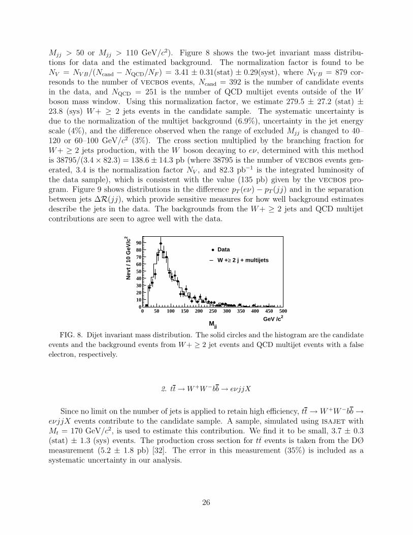
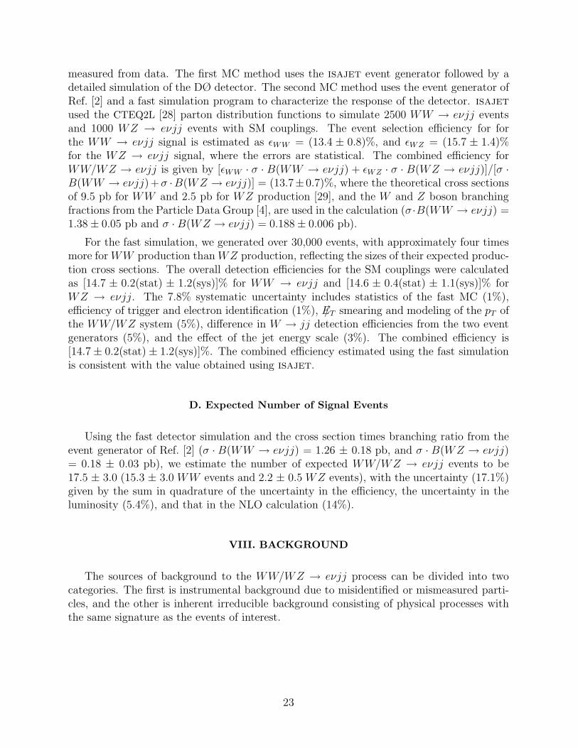
Mjj > 50 or Mjj > 110 GeV/c2). Figure 8 shows the two-jet invariant mass distribu-tions for data and the estimated background. The normalization factor is found to beNV = NV B/(Ncand − NQCD/NF ) = 3.41 ± 0.31(stat) ± 0.29(syst), where NV B = 879 cor-resonds to the number of vecbos events, Ncand = 392 is the number of candidate eventsin the data, and NQCD = 251 is the number of QCD multijet events outside of the Wboson mass window. Using this normalization factor, we estimate 279.5 ± 27.2 (stat) ±23.8 (sys) W+ ≥ 2 jets events in the candidate sample. The systematic uncertainty isdue to the normalization of the multijet background (6.9%), uncertainty in the jet energyscale (4%), and the difference observed when the range of excluded Mjj is changed to 40–120 or 60–100 GeV/c2 (3%). The cross section multiplied by the branching fraction forW+ ≥ 2 jets production, with the W boson decaying to eν, determined with this methodis 38795/(3.4× 82.3) = 138.6 ± 14.3 pb (where 38795 is the number of vecbos events gen-erated, 3.4 is the normalization factor NV , and 82.3 pb−1 is the integrated luminosity ofthe data sample), which is consistent with the value (135 pb) given by the vecbos pro-gram. Figure 9 shows distributions in the difference pT (eν) − pT (jj) and in the separationbetween jets ∆R(jj), which provide sensitive measures for how well background estimatesdescribe the jets in the data. The backgrounds from the W+ ≥ 2 jets and QCD multijetcontributions are seen to agree well with the data.

Mjj

0102030405060708090

0 50 100 150 200 250 300 350 400 450 500

Data

W +≥ 2 j + multijets

GeV /c2

Nev

t / 1

0 G

eV/c

2

FIG. 8. Dijet invariant mass distribution. The solid circles and the histogram are the candidate

events and the background events from W+ ≥ 2 jet events and QCD multijet events with a false

electron, respectively.

2. tt → W+W−bb → eνjjX

Since no limit on the number of jets is applied to retain high efficiency, tt →W+W−bb →eνjjX events contribute to the candidate sample. A sample, simulated using isajet withMt = 170 GeV/c2, is used to estimate this contribution. We find it to be small, 3.7 ± 0.3(stat) ± 1.3 (sys) events. The production cross section for tt events is taken from the DØmeasurement (5.2 ± 1.8 pb) [32]. The error in this measurement (35%) is included as asystematic uncertainty in our analysis.

26

pT(eν)-pT(jj)

(a)

0

10

20

30

40

50

60

70

-100 -80 -60 -40 -20 0 20 40 60 80 100

Data

W+≥2j + multijets

GeV/cN

evt/

2 G

eV/c

∆R(jj)

(b)

0

20

40

60

80

100

0 1 2 3 4 5 6 7 8 9 10

Data

W+≥2j + multijets

Nev

t/0.

2

FIG. 9. (a) Distributions in pT (eν)−pT (jj) before imposition of the mass window on Mjj. (b)

Distributions for the separation of two jets in η − φ space.

3. WW/WZ → τνjj → eννjj

Since the contribution from WW/WZ → τνjj → eννjj is small, and no separatesimulation of the signal is available, we treat it as background. We use the isajet eventgenerator and the detailed detector simulation program to estimate this source. The WWand WZ production cross sections are assumed to be 9.5 pb and 2.5 pb, respectively. Afterevent selection, we find 0.15 +0.16

−0.08 (stat) ± 0.01 (sys) events. The systematic uncertainty onthe background estimate is assigned to have the larger value of the asymmetric errors onthe theoretical cross section (8.4%) [29].

4. ZX → e+e−X

The ZX → eeX processes can produce events that can be misidentified as signal. Theseevents can be included in the candidate sample if one electron goes through a boundary ina calorimeter module and is measured as /ET in the event. From a sample of 10,000 isajetZX → e+e−X events generated, none survive the selection procedure. The backgroundfrom events of this type is therefore negligible.

27

5. ZX → τ+τ−X → eνjjX

The ZX → ττX processes can also produce events that can be mistaken for signal if,due to shower fluctuation, one or two jets from ISR or FSR are observed in the detector.From a sample of 10,000 pythia-generated ZX → ττX events, none survive our selection.The background from this source is therefore also negligible.

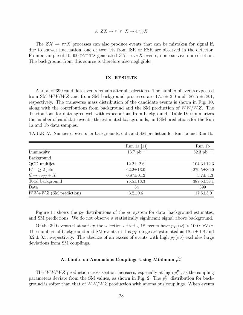
IX. RESULTS

A total of 399 candidate events remain after all selections. The number of events expectedfrom SM WW/WZ and from SM background processes are 17.5 ± 3.0 and 387.5 ± 38.1,respectively. The transverse mass distribution of the candidate events is shown in Fig. 10,along with the contributions from background and the SM production of WW/WZ. Thedistributions for data agree well with expectations from background. Table IV summarizesthe number of candidate events, the estimated backgrounds, and SM predictions for the Run1a and 1b data samples.

TABLE IV. Number of events for backgrounds, data and SM prediction for Run 1a and Run 1b.

Run 1a [11] Run 1b

Luminosity 13.7 pb−1 82.3 pb−1

Background

QCD multijet 12.2± 2.6 104.3±12.3

W+ ≥ 2 jets 62.2±13.0 279.5±36.0

tt → eνjj + X 0.87±0.12 3.7± 1.3

Total background 75.5±13.3 387.5±38.1

Data 84 399

WW+WZ (SM prediction) 3.2±0.6 17.5±3.0

Figure 11 shows the pT distributions of the eν system for data, background estimates,and SM predictions. We do not observe a statistically significant signal above background.

Of the 399 events that satisfy the selection criteria, 18 events have pT (eν) > 100 GeV/c.The numbers of background and SM events in this pT range are estimated as 18.5± 1.8 and3.2 ± 0.5, respectively. The absence of an excess of events with high pT (eν) excludes largedeviations from SM couplings.

A. Limits on Anomalous Couplings Using Minimum pWT

The WW/WZ production cross section increases, especially at high pWT , as the coupling

parameters deviate from the SM values, as shown in Fig. 2. The pWT distribution for back-

ground is softer than that of WW/WZ production with anomalous couplings. When events

28

MT(eν)

0

20

40

60

80

100

120

0 20 40 60 80 100 120 140 160 180 200

Data

W +≥ 2 j + multijets

ISAJET WW/WZ SMx10

GeV /c2N

evt

/ 5 G

eV/c

2

FIG. 10. Transverse-mass distributions of the electron and ν ( /ET ) system. The solid circles,

solid histogram, and dotted histogram are, respectively, the candidate events, the background from

QCD multijet events with false electrons and W+ ≥ 2 jet events, and the expected SM production

of WW/WZ events scaled up by a factor of ten.

0

20

40

60

80

100

0 50 100 150 200 250pT(W→eν) GeV/c

Nev

ts/1

0 G

eV/c

FIG. 11. The pT distributions of the eν system from the 1993–1995 (Run 1b) data. The solid

circles are data. The light-shaded histogram is the SM prediction for the background, including

the dark-shaded histogram, which represents the SM prediction for WW/WZ processes.

are selected with pWT above some large minimum value, almost all background events are

rejected, but a good fraction of signal with anomalous couplings remains, providing bettersensitivity to such couplings. This kind of selection eliminates most of SM production, andtherefore does not have sensitivity to the SM couplings. Moreover the 95% C.L. upper limiton the number of signal events (N95%C.L.) can be obtained from the observed number ofcandidate events and the expected background beyond some minimum pW

T cutoff, using themethod described in the report by the Particle Data Group [4]. To do this, Monte Carloevents are generated for pairs of anomalous couplings in grid points of ∆κ and λ. We as-sume that the couplings for WWγ and WWZ are equal. The expected number of eventsfor each pair of anomalous couplings is calculated using the integrated luminosity of thedata sample, and entered into a two-dimensional density plot with ∆κ and λ as coordinateaxes. The results are fitted with a two-dimensional parabolic function, and limits on anoma-lous couplings are calculated at the 95% C.L. from the intersection of the two-dimensionalparabolic surface for the predicted number of events with a plane of N95%C.L. values. Theresulting contour of constant probability is an ellipse in the ∆κ − λ plane. The numericalvalues for the “one-dimensional” 95% C.L. limits (setting one of the coordinates to zero) are

29

summarized in Table V for different minimum values of pWT .

TABLE V. Limits on λ and ∆κ at the 95% C.L. as a function of minimum pWT , for Λ = 1.5

TeV. The number of candidates (Ncand), background (NBG), and the SM WW/WZ predictions

(NSM) are also listed.

pWT (GeV/c) Ncand NBG NSM λ ∆κ

events events events (∆κ = 0) (λ = 0)

150 4 2.8 1.9 (−0.66, 0.67) (−0.96, 1.08)

160 1 2.1 1.8 (−0.54, 0.54) (−0.79, 0.89)

170 0 1.5 0.9 (−0.52, 0.52) (−0.76, 0.86)

180 0 1.2 0.2 (−0.59, 0.58) (−0.87, 0.96)

190 0 0.7 0.1 (−0.64, 0.64) (−0.96, 1.05)

200 0 0.3 0.1 (−0.74, 0.73) (−1.13, 1.20)

B. Limits on Anomalous Couplings from the pWT Spectrum

The limits obtained for some cutoff minimum pWT do not take into account information

that is available in the full pWT spectrum, and depend on the chosen minimum pT value as

well as on the overall normalization factors for background and predictions for signal. Analternative way to proceed is to fit the shape of kinematical distributions that are sensitiveto anomalous couplings. This usually provides tighter limits, since it uses all the informationcontained in the differential distributions, and it is also less sensitive to overall normalizationfactors.

As described in Sec. I, the differential distribution that is most sensitive to anomalouscouplings is the p

W (Z)T distribution. Our analysis relies on the pT (W → eν) spectrum rather

than pT (W → jj) or pT (Z → jj) because the resolution on pT (eν) (12.5 GeV/c) is betterthan on pT (jj) (16.7 GeV/c). This is primarily due to the ambiguity in assigning jets to theW (Z) boson.

The differential cross sections have been exploited by previous publications[9–11,13–16,18,19] for extracting limits on trilinear gauge boson couplings. We use a mod-ified fit to the binned pW

T distribution to obtain limits, with the modification consisting ofadding an extra bin in pW

T with no observed events, thereby improving the sensitivity toanomalous couplings [33].

Based on the number of expected WW/WZ → eνjj events, we choose two 25 GeV/cbins between 0 and 50 GeV/c, five 10 GeV/c bins from 50 to 100 GeV/c, two 20 GeV/c binsfrom 100 to 140 GeV/c, one 30 GeV/c bin from 140 to 170 GeV/c, and a single bin from 170GeV/c to 500 GeV/c. The cross section for pW

T > 500 GeV/c is negligible for any anomalouscouplings allowed by unitarity. For each bin i of pW

T , the probability Pi for observing Ni

30

events is given by the Poisson distribution:

Pi =(bi + Lǫiσi(λ,∆κ))

Ni

Ni!e−(bi+Lǫiσi(λ,∆κ)),

where L is the luminosity, and bi, ǫi, and and σi are the expected background, the totaldetection efficiency, and the cross section, respectively, for bin i. Our fast Monte Carlo isused to calculate ǫiσi(λ,∆κ). The joint probability for all pW

T bins is the product of theindividual probabilities Pi, P =

∏Nbin

i=1 Pi. Since the values L, bi, and ǫi are measured valueswith their respective uncertainties, we assign them Gaussian prior distributions of meanµ = 1 and standard deviation σx:

P ′ =∫

Gfndfn

∫

Gfbdfb

Nbin∏

i=1

efnni+fbbi(fnni + fbbi)Ni

Ni!,

where ni = Lǫiσi is the predicted number of signal events, and Gfnand Gfb

are Gaussiandistributions for the fractions of signal and background events. The integrals are calculatedusing 50 evenly spaced points between ±3 standard deviations. For convenience, the log ofthe likelihood L = logP ′ is used in the fit and the set of couplings that best describes thedata is given by the point in the λ − ∆κ plane that maximizes the likelihood given in theabove equation.

It is conventional to quote the limits on one coupling when all the others are set to theirSM values. These “one-dimensional” limits at the 95% C.L., assuming that the WWγ andWWZ couplings are equal, are shown in Table VI. The limits are more stringent than thoseobtained using the minimum pW

T method.

TABLE VI. Limits on anomalous trilinear gauge boson couplings at the 95% C.L. for three

values of Λ obtained using the fit to pWT for data from the Run 1b.

Couplings Λ = 1.0 TeV Λ = 1.5 TeV Λ = 2.0 TeV

λγ = λZ (∆κγ = ∆κZ = 0) −0.50, 0.53 −0.42, 0.45 −0.39, 0.42

∆κγ = ∆κZ (λγ = λZ = 0) −0.66, 0.90 −0.56, 0.75 −0.52, 0.70

λγ (HISZ) (∆κγ = 0) −0.50, 0.53 −0.42, 0.45 −0.39, 0.42

∆κγ (HISZ) (λγ = 0) −0.78, 1.15 −0.68, 0.98 −0.63, 0.91

λγ (SM WWZ) (∆κγ = 0) −1.54, 1.58 −1.53, 1.56

∆κγ (SM WWZ) (λγ = 0) −2.03, 2.45 −1.79, 2.12

λZ (SM WWγ) (∆κZ = ∆gZ1 = 0) −0.58, 0.62 −0.49, 0.51 −0.45, 0.48

∆κZ (SM WWγ) (λZ = ∆gZ1 = 0) −0.86, 1.12 −0.72, 0.93 −0.67, 0.87

We have assumed thus far that the couplings ∆κ and λ for WWZ and WWγ are equal.However, this is not the only possibility. Another common assumption leads to the HISZrelations [34]. These relations specify λZ , κZ , and gZ

1 in terms of the independent variablesλγ and κγ , thereby reducing the number of independent couplings from five to two: ∆κZ =

31

12∆κγ(1 − tan2 θW ), ∆gZ

1 = 12∆κγ/ cos2 θW , and λZ = λγ. These one-dimensional limits at

the 95% C.L. are also shown in Table VI.

Since the WWZ and WWγ couplings are independent, it is interesting to find the limitson one when the other is set to its SM values. Table VI includes the one-dimensional limitsat the 95% C.L. for both assumptions: limits on ∆κγ and λγ when the WWZ couplingsare assumed to be standard, and limits on ∆κZ and λZ when the WWγ couplings areassumed to be standard. These results indicate that our analysis is more sensitive to WWZcouplings, as should be expected from the larger overall SM couplings for WWZ than forWWγ, and that our analysis is complementary to studies of the Wγ production processwhich is sensitive only to the WWγ couplings.

C. Combined Results for Run 1 on WW/WZ → eνjj

The limits on anomalous couplings presented in this paper are significantly tighter thanthose in our previous publications [11,15]. The primary reason for this is the increase in theamount of data (about a factor of six). We can obtain even stronger limits by combiningthe results from Run 1a and 1b. The analysis based on the Run 1a data is described inRefs [11,15]. A summary of the signal and backgrounds for the two analyses [18] is given inTable IV.

The two analyses can be treated as different experiments. However, because both ex-periments used the same detector, there are certain correlated uncertainties, such as theuncertainties on the luminosity, lepton reconstruction and identification, and the theoreticalprediction. Also, the background estimate is common to each experiment. The uncertaintyon the W/Z → jj selection efficiency is assumed to be uncorrelated, since we use differ-ent cone sizes for jet reconstruction in the two analyses. (This hypothesis does not affectthe results in any significant way.) The uncertainties for both analyses are summarized inTables VII and VIII. Each uncertainty is weighted by the integrated luminosity for therespective data sample. Figure 12 shows the combined pW

T spectrum.

TABLE VII. Common systematic uncertainties for Run 1a and Run 1b analyses.

Source of Uncertainty

Luminosity 5.4%

QCD corrections 14%

Electron and trigger efficiency 1.2%

Statistics of fast MC 1%

/ET smearing 5.1%

Jet energy scale 3.4%

Total 16%

To set limits on anomalous couplings, we combine the results of the two analyses by calcu-lating a combined likelihood function. The individual uncertainties on signal and background

32

TABLE VIII. Uncorrelated systematic uncertainties for Run 1a and Run 1b analyses.

Source of Uncertainty Run 1a Run 1b

isajet vs pythia 9% 4%

Stat. uncertainties of ǫ(W → jj) 4% 2%

Parametrization of ǫiσi(λ,∆κ) 4% 5%

Total (added in quadrature) 11% 7%

Background 13% 7%

020406080

100

0 50 100 150 200 250pT(W→eν) GeV/c

Nev

ts/1

0 G

eV/c

FIG. 12. The pWT spectrum for eνjj candidates for the full Run 1 data sample. The solid circles

are data. The light-shaded histogram is the sum of predictions from the SM and background, and

the dark-shaded histogram is the SM prediction for WW/WZ processes alone.

for each analysis are taken into account as in the previous section. Common systematic un-certainties are taken into account by introducing a common Gaussian prior distribution forthe two data samples.

Combining results from Run 1a and Run 1b yields the 95% C.L. contours of constantprobability shown in Fig. 13. The one and two dimensional 95% C.L. contour limits (corre-sponding to log-likelihood values of 1.92 and 3.00 units below the maximum, respectively)are shown as the inner contours, along with the unitarity limits from the S-matrix, shownas the outermost contours. Figure 13(a) shows the contour limits when couplings for WWγare assumed to be equal to those for WWZ. Figure 13(b) shows contour limits assuming theHISZ relations. In Figs. 13(c) and 13(d), SM WWγ couplings are assumed and the limitsare shown for WWZ couplings. Assuming SM WWγ couplings, the U(1) point that corre-sponds to the condition in which there is no WWZ couplings (κZ = 0, λZ = 0, gZ

1 = 0) isexcluded at the 99% C.L. This is direct evidence for the existence of WWZ couplings. Theselimits are slightly stronger than those from the 1993–1995 data alone. The one-dimensional95% C.L. limits for four assumptions on the relation between WWγ and WWZ couplings:(i) ∆κ ≡ ∆κγ = ∆κZ , λ ≡ λγ = λZ , (ii) HISZ relations, (iii) SM WWγ couplings, and (iv)SM WWZ couplings are listed in Table IX.

33

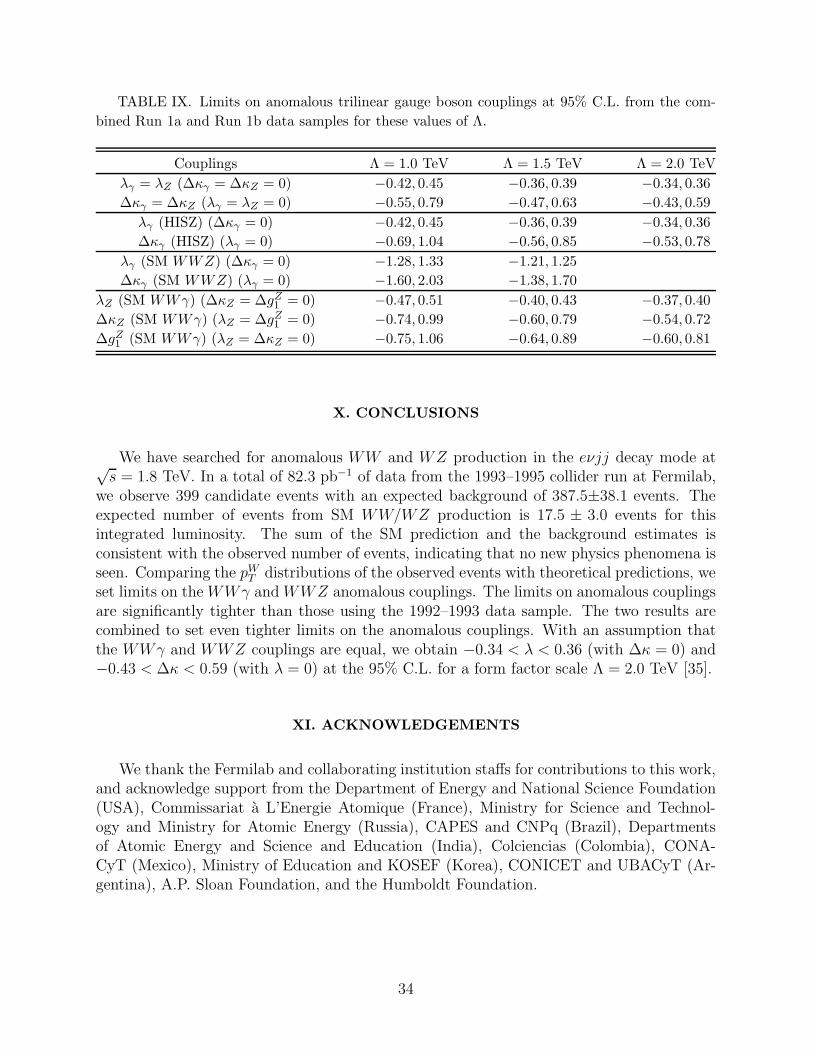
TABLE IX. Limits on anomalous trilinear gauge boson couplings at 95% C.L. from the com-

bined Run 1a and Run 1b data samples for these values of Λ.

Couplings Λ = 1.0 TeV Λ = 1.5 TeV Λ = 2.0 TeV

λγ = λZ (∆κγ = ∆κZ = 0) −0.42, 0.45 −0.36, 0.39 −0.34, 0.36

∆κγ = ∆κZ (λγ = λZ = 0) −0.55, 0.79 −0.47, 0.63 −0.43, 0.59

λγ (HISZ) (∆κγ = 0) −0.42, 0.45 −0.36, 0.39 −0.34, 0.36

∆κγ (HISZ) (λγ = 0) −0.69, 1.04 −0.56, 0.85 −0.53, 0.78

λγ (SM WWZ) (∆κγ = 0) −1.28, 1.33 −1.21, 1.25

∆κγ (SM WWZ) (λγ = 0) −1.60, 2.03 −1.38, 1.70

λZ (SM WWγ) (∆κZ = ∆gZ1 = 0) −0.47, 0.51 −0.40, 0.43 −0.37, 0.40

∆κZ (SM WWγ) (λZ = ∆gZ1 = 0) −0.74, 0.99 −0.60, 0.79 −0.54, 0.72

∆gZ1 (SM WWγ) (λZ = ∆κZ = 0) −0.75, 1.06 −0.64, 0.89 −0.60, 0.81

X. CONCLUSIONS

We have searched for anomalous WW and WZ production in the eνjj decay mode at√s = 1.8 TeV. In a total of 82.3 pb−1 of data from the 1993–1995 collider run at Fermilab,

we observe 399 candidate events with an expected background of 387.5±38.1 events. Theexpected number of events from SM WW/WZ production is 17.5 ± 3.0 events for thisintegrated luminosity. The sum of the SM prediction and the background estimates isconsistent with the observed number of events, indicating that no new physics phenomena isseen. Comparing the pW

T distributions of the observed events with theoretical predictions, weset limits on the WWγ and WWZ anomalous couplings. The limits on anomalous couplingsare significantly tighter than those using the 1992–1993 data sample. The two results arecombined to set even tighter limits on the anomalous couplings. With an assumption thatthe WWγ and WWZ couplings are equal, we obtain −0.34 < λ < 0.36 (with ∆κ = 0) and−0.43 < ∆κ < 0.59 (with λ = 0) at the 95% C.L. for a form factor scale Λ = 2.0 TeV [35].

XI. ACKNOWLEDGEMENTS

We thank the Fermilab and collaborating institution staffs for contributions to this work,and acknowledge support from the Department of Energy and National Science Foundation(USA), Commissariat a L’Energie Atomique (France), Ministry for Science and Technol-ogy and Ministry for Atomic Energy (Russia), CAPES and CNPq (Brazil), Departmentsof Atomic Energy and Science and Education (India), Colciencias (Colombia), CONA-CyT (Mexico), Ministry of Education and KOSEF (Korea), CONICET and UBACyT (Ar-gentina), A.P. Sloan Foundation, and the Humboldt Foundation.

34

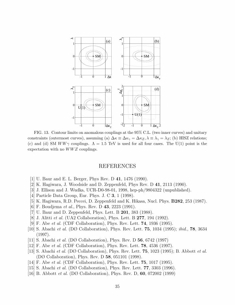
-1

0

1

-1 0 1

SM

(a)

∆κλ

-1

0

1

-1 0 1

SM

(b)

∆κγ

λ γ

-1

0

1

-1 0 1

SMU(1)

(c)

∆κZ

λ Z

-2

-1

0

1

2

-2 -1 0 1 2

SM

U(1)

(d)

∆κZ

∆gZ 1

FIG. 13. Contour limits on anomalous couplings at the 95% C.L. (two inner curves) and unitary

constraints (outermost curves), assuming (a) ∆κ ≡ ∆κγ = ∆κZ , λ ≡ λγ = λZ ; (b) HISZ relations;

(c) and (d) SM WWγ couplings. Λ = 1.5 TeV is used for all four cases. The U(1) point is the

expectation with no WWZ couplings.

REFERENCES

[1] U. Baur and E. L. Berger, Phys Rev. D 41, 1476 (1990).[2] K. Hagiwara, J. Woodside and D. Zeppenfeld, Phys Rev. D 41, 2113 (1990).[3] J. Ellison and J. Wudka, UCR-D0-98-01, 1998, hep-ph/9804322 (unpublished).[4] Particle Data Group, Eur. Phys. J. C 3, 1 (1998).[5] K. Hagiwara, R.D. Peccei, D. Zeppenfeld and K. Hikasa, Nucl. Phys. B282, 253 (1987).[6] F. Boudjema et al., Phys. Rev. D 43, 2223 (1991).[7] U. Baur and D. Zeppenfeld, Phys. Lett. B 201, 383 (1988).[8] J. Alitti et al. (UA2 Collaboration), Phys. Lett. B 277, 194 (1992).[9] F. Abe et al. (CDF Collaboration), Phys. Rev. Lett. 74, 1936 (1995).

[10] S. Abachi et al. (DØ Collaboration), Phys. Rev. Lett. 75, 1034 (1995); ibid., 78, 3634(1997).

[11] S. Abachi et al. (DØ Collaboration), Phys. Rev. D 56, 6742 (1997)[12] F. Abe et al. (CDF Collaboration), Phys. Rev. Lett. 78, 4536 (1997).[13] S. Abachi et al. (DØ Collaboration), Phys. Rev. Lett. 75, 1023 (1995); B. Abbott et al.

(DØ Collaboration), Phys. Rev. D 58, 051101 (1998).[14] F. Abe et al. (CDF Collaboration), Phys. Rev. Lett. 75, 1017 (1995).[15] S. Abachi et al. (DØ Collaboration), Phys. Rev. Lett. 77, 3303 (1996).[16] B. Abbott et al. (DØ Collaboration), Phys. Rev. D, 60, 072002 (1999)

35

[17] P. Abreu et al. (DELPHI Collaboration), Phys. Lett. B 459, 382 (1999); G. Abbiendiet al. (OPAL Collaboration), Eur. Phys. J. C 8, 191 (1999); M. Acciarri et al. (L3Collaboration), Phys. Lett. B 467, 171 (1999); B. Barate et al. (ALEPH Collaboration),CERN-EP-98-178, 1998, submitted to Phys. Lett. B.

[18] B. Abbott et al. (DØ Collaboration), Phys. Rev. Lett. 79, 1441 (1997).[19] A. Sanchez-Hernandez, Ph.D. Dissertation, CINVESTAV, Mexico City, Mexico (1997),

http://www-d0.fnal.gov/results/publications talks/thesis/thesis.html, un-published.

[20] S. Abachi et al. (DØ Collaboration), Nucl. Instrum. Methods in Phys. Res. A 338, 185(1994).

[21] S. Abachi et al. (DØ Collaboration), Phys. Rev. Lett. 77, 3309 (1996); B. Abbott et al.

(DØ Collaboration), Phys. Rev. Lett. 80, 3008 (1998); Phys. Rev. D 58, 12002 (1998);ibid., 58, 092003 (1998); B. Abbott et al. (DØ Collaboration), FERMILAB-Pub-99/237-E, hep-ex/9908057 (submitted to Phys. Rev. D); B. Abbott et al. (DØ Collaboration),Phys. Rev. Lett. 84, 222 (2000).

[22] DØ Collaboration, R. Kehoe, in Proceedings of the Sixth International Conference on

Calorimetry in High Energy Physics, Frascati, Italy (World Scientific, River Edge, NJ,1996), FERMILAB-Conf-96/284-E.

[23] S. Abachi et al. (DØ Collaboration), Phys. Rev. D 52, 4877 (1995).[24] J. Bantly et al., FERMILAB-TM-1995 (unpublished). To facilitate combination with

previously published results, this analysis uses the older DØ luminosity of Ref. [18].The recently updated 3.2% increase in luminosity, B. Abbott et al. (DØ Collaboration),hep-ex/990625, Sec. VII, pp. 21–22 (submitted to Phys. Rev. D), has little impact onthese results.

[25] M. L. Kelly, Ph.D. Thesis, Notre Dame (1996),http://www-d0.fnal.gov/results/publications talks/thesis/thesis.html, un-published.

[26] F. Paige and S. Protopopescu, BNL Report BNL38034 (1986), unpublished. We usedversion 7.22.

[27] T. Sjostrand, Comput. Phys. Commun. 82, 74 (1994).[28] H. L. Lai et al. Phys. Rev. D 51, 4763 (1995).[29] J. Ohnemus, Phys. Rev. D 44, 1403 (1991); ibid., 44, 3477 (1991).[30] F.A. Berends et al., Nucl. Phys. B357, 32 (1991). We used version 3.0.[31] G. Marchesini et al., Comput. Phys. Commun. 67, 465 (1992). We used version 5.7.[32] B. Abbott et al. (DØ Collaboration), Phys. Rev. Lett. 79, 1203 (1997).[33] G. L. Landsberg, Ph.D. Thesis, State University of New York at Stony Brook (1994),

http://www-d0.fnal.gov/results/publications talks/thesis/thesis.html, un-published.

[34] K. Hagiwara, S. Ishihara, R. Szalapski and D. Zeppenfeld, Phys. Rev. D 48, 2182 (1993);Phys. Lett. B 283, 353 (1992). They parametrize the WWZ couplings in terms of theWWγ couplings: ∆κZ = ∆κγ(1 − tan2 θW )/2, ∆gZ

1 = ∆κγ/2 cos2 θW and λZ = λγ .[35] Subsequent to the publication of Ref. [18] which summarized this analysis, these re-

sults were combined with the other DØ measurements of anomalous WWγ and WWZcouplings, using the method described in B. Abbott et al. (DØ Collaboration), Phys.Rev. D 58 31102 (1998), to provide the experiment’s most restrictive limits which were

36

reported in Ref. [16].

37