Limits and advantages of Good Practice Guide to NoiseMapping

G. Licitraa and G. Memolib

aARPAT - Dept. Firenze, Via Porpora, 22, 50144 Firenze, ItalybImperial College London, Department of Chemical Engineering, Exhibition road, SW7 2AZ

London, UKg.licitra@arpat.toscana.it

Acoustics 08 Paris

771

The Pisa Noise Mapping Project has recently presented to the public what turned out to be the first noise map for road traffic in Italy, developed taking into account the Good Practice Guide version 2 (GPG2) of WG-AEN and the main results of the IMAGINE project. This paper will discuss the results of this noise map, relative to road traffic, in terms of Lden and Lnight and their uncertainties, obtained by comparing the calculated values with a set of noise measurements taken across the territory. The uncertainties so defined were compared with the ones predicted by GPG2 considering, in particular, two different ways to model the source. To do this, input traffic flows were assigned first by taking direct measurements and performing a road classification and then, at a second stage, using a static traffic model (the latter method should give less uncertainty, according to GPG2). The expected change in uncertainty will be discussed, together with advantages and disadvantages of the two different choices. A comparison of exposed population with other EU realities will be also presented.

1 Introduction

The European Noise Directive 2002/49/EC (END) has introduced two new instruments for urban planning and noise management: strategic noise maps and action plans. The declared aim of the Directive is “to define a common approach intended to avoid, prevent or reduce on a prioritized basis the harmful effects, including annoyance, due to exposure to environmental noise” [1]. Action plans are due in five years intervals, with the first deadline in July 2008 for major infrastructures and agglomerates over 250,000 inhabitants. Action plans should take the results noise maps as input data to manage noise issues and effects, including noise reduction where necessary (in particular where exposure levels may be harmful for health) and preservation of environmental noise quality where it is good (quiet areas). A strategic noise map, relative to each type of source (road and rail infrastructures, aircraft and industrial noise), is an acoustical photo of the territory, to be confronted with the noise limits decided by the competent authorities to identify, with a strategic view, the areas where actions are needed (conflict maps). The END prescribes a 5 years cadence also for noise maps: for agglomerates, for instance, the first deadline was in June 2007 (population greater than 250,000 inhabitants) and the second will be in 2012 (agglomerates > 100,000 inhabitants). A noise map, however, is above all an instrument to inform the citizens about the number of people exposed to the different noise levels, with the aim to involve the general public into the development of action plans [2], but also promoting the conscience of problems and the knowledge of the health risks related to noise. In this sense, the purpose of a noise map goes beyond its utility for an action plan. In addition to this, in order to unify the results on the EU scale, the END has introduced Lden and Lnight as main indicators for the preparation and revision of strategic noise maps where most Member States used different ones (in Italy this was the case of Lday, IT assessed on the period 6:00-22:00): new methodologies are needed to assess the exposed population. In this context, the municipality of Pisa decided to draw up a noise map of the noise due to road traffic using the new methodologies, even if not under the obligation to do it (Pisa had slightly more than 90,000 inhabitants in 2007). The Pisa Noise Mapping project for mapping road traffic, presented for the first time to the public in April 2007, represents a practical example of the problems encountered and of the solutions taken. It was completed taking into

account the Good Practice Guide of WG-AEN in its version of January 2006 (GPG2, [3]), the guidelines of the Italian Environmental Protection Agency (APAT, [4][5][6]) and the main results of the IMAGINE project [7][8][9]. This paper presents the efforts to reduce the average uncertainty on the assessed noise levels with a cost/effectiveness approach. In this sense, it contributes to reports like [10]. In particular, this paper addresses the characterization of the traffic source. can be completed in two ways, after measuring traffic fluxes in a selection of areas: extending these values with a classification of roads or using a traffic model [3]. The differences between the two methods, in terms of uncertainty, will be highlighted here by presenting a comparison with noise measurements taken on the territory.

2 Road classification

The determination of traffic fluxes is among the main causes of uncertainty, while determining the noise emission with the French method NMPB (ad interim method recommended in [1] in absence of a unified model on the European scale). The final uncertainty on the assessed levels, to be intended on the scale of the map, has many different causes but, according to the GPG2, it is possible to identify the contribution of traffic fluxes in terms of how precisely they are known [3]. As an example, Toolkit 2 of the GPG2, • to use default values depending on road use (like the

ones in [3]) should cause a 4 dB uncertainty; • to complete a classification of the roads for the specific

territory should reduce uncertainty to 2 dB. A further reduction of uncertainty to 1 dB should be observed by using a well defined traffic model. These statements simply point out that the more precise are input data, the less uncertainty should be expected on the final noise map. On the other hand, the solution chosen in practice is always a compromise between two different needs: on one side the requirements of END to report exposed population in discrete 5 dB wide bands; on the other side the necessity of the stakeholders to keeps costs of realization and verification under control. Practical considerations tend to imply that absolute accuracy within 2 dB(A) of the actual value should be sought.

Acoustics 08 Paris

772

2.1 Determination of the classes

In a first phase of the project, fluxes have been assigned to roads, according to their function, as follows:

• roads where direct measurements of fluxes were present, had these used as input data for the model;

• roads where no measurements were available received the average value of their class (as reported in Table 1), rounded to the next 5 units.

This means that the flow of 40 light vehicles and 25 motorbikes, assigned to ZTL roads (roads where the traffic is limited to residents owing a special permit), is the average value of all the measurements available in such roads. This average value has been assigned to all the ZTL roads where traffic flux was unknown. Where a “real” measurement was available, instead, the latter was assigned to the road in order to favour the comparison with measured noise levels. In this way, in fact, it is possible to verify immediately whether the measured flux can predict the assessed noise level. Table 1 also reports the traffic composition suggested by the GPG2 (in terms of the NMPB model). For the town of Pisa, measurements of traffic composition were available for extra-urban roads. For urban roads, instead, the only heavy vehicles considered were busses, whose travel paths were known. Also in Table 1 are the factors for obtaining night values from daily ones. These values, averaged on the ratios measured in the roads of a fixed type, are more detailed then the single default value of 0.143 reported in GPG2 and similar to those suggested by APAT [5] on the Italian scale. Another important factor is the acoustic weight of the different vehicles. Recent studies demonstrated that the two theoretical vehicles (“light” and “heavy” vehicles) of the NMPB model overestimate the emission of Italian equivalents [11]. Also important is the necessity to consider 2-wheelers as a stand-alone vehicle. To take this into account, the assigned fluxes have been accurately weighted with coefficients that depend on

velocity. Fig. 1 reports such coefficients, as calculated from the data presented in [11]and [12]. Fig. 1 shows, for instance, that 1.6 typical Italian cars, travelling at 50 km/h in urban environment, were needed to have the same emission as one NMPB light vehicle (this corresponds to 2 dB less on the average). Last but not least, travel speeds in Table 1 were assumed to be the maximum allowed ones according to existing limits. Fig. 2 shows an extract from the Pisa noise map, relatively at the indicators Lday and Lnight: these were converted in Lden and Lnight using the correlations reported in [5] which contribute for 1 dB to the total uncertainty (all the contributions are add up as statistically independent).

3 Comparison with measurements

More than 100 geo-referenced measurements were used for the comparison: 54 continuous measurements of at least 48 hours’ duration and 106 spot measurements lasting between 45 minutes and 1 hour, all taken between December 2004 and January 2007. In both types of measurements the microphone was at 4 m height and at 3 m from reflecting façades. Simultaneous measurements of traffic fluxes and

Table 1 Comparison of the average values and classes used in this work with GPG2’s recommendations.

Fig. 1: Corrective factors to NMPB light vehicles to match emission measurements taken in [11] and [12].

Acoustics 08 Paris

773

composition were conducted when possible (in particular, for the spot measurements), if not already available. These measurements were taken and analyzed to obtain an adequate representation of the traffic source, distinguishing the different types of road, like in Table 1.

Fig. 3 shows the comparison between the measured and the calculated values: almost all the calculated values for the day period were within a band of ± 5 dB from the measured ones. The calculated values for the night period appear to be more disperse. In both cases, more than 80% of the calculated values can be found in a band of 4.6 dB from the measurements (this percentage is 95% in the Lday case). It is worth noticing that 4.6 dB correspond to the expected uncertainty according to GPG2, calculated by adding up all the different contributions and relatively to a 95% level of confidence. The greater uncertainty registered in the case of Lnight, with a light trend to overestimate the measurements, is probably due to the smaller values of the traffic fluxes: these values were calculated at the limits of validity of the NMPB model. These results say that, within the approximations taken so far and according to what is reported in the GPG2, it would have been difficult to obtain a better agreement. This is a very difficult conclusion to accept, in terms of the bands required by the END. On the other hand, the GPG2 suggests that it is theoretically possible to increase accuracy with a better characterization of the source, especially working on the characteristics that contribute more to the overall uncertainty. For this reason, ARPAT and the municipality of Pisa invested in the development of a traffic model.

4 The traffic model

The term “traffic model” refers to a description of traffic on a grid (made by road axes and nodes). The fluxes are obtained by applying demand/offer criteria (input data, supposed to be known) to a matrix of weighting factors, one for each road, that take into account time of travel and cost. In case of Pisa, the input data were obtained from the local authorities (e.g. the Municipality conducted a relevant study in 2001), while the weighting factors have been elaborated to describe even recent actions on traffic (like the introduction of new round-abouts). The model used is of the “static” type [9] and calculations were performed using TransCAD, producing a photo of fluxes and average velocities for the main roads in a short computing time. Like all the models of this kind, there are many underlying assumptions: • in many cases the traffic is assigned to an area, inside

which roads are not distinguished; • “roads” in the model are often only connectors

between zones, so that a large amount of manual work may be needed to transfer the data on the territory, to avoid the consequent loss of precision;

• there are some areas completely neglected in the demand/offer model, which may be affected by large traffic in some period of the year (for Pisa, this is the case of the seaside);

• the resulting fluxes are in “equivalent light vehicles”, calculated weighting heavy vehicle with an “road occupation factor” which is not related to the acoustic difference between “heavy vehicles” or busses and cars (see Fig. 1).

Fig. 2: Extract from Pisa’s noise map: Lday and Lnight

40

45

50

55

60

65

70

75

80

40,0 50,0 60,0 70,0 80,0

Calculated value, dB(A)

Measured value, dB(A)

Lday

Reference

Ltheo=Lmeas+5dBLtheo=Lmeas-5dB

Lnight

Fig. 3: Comparison between the calculated levels and the measured ones for the case of Lday and Lnight. Also in the graph are the reference lines relative to a difference of 0 and ± 5 dB.

Acoustics 08 Paris

774

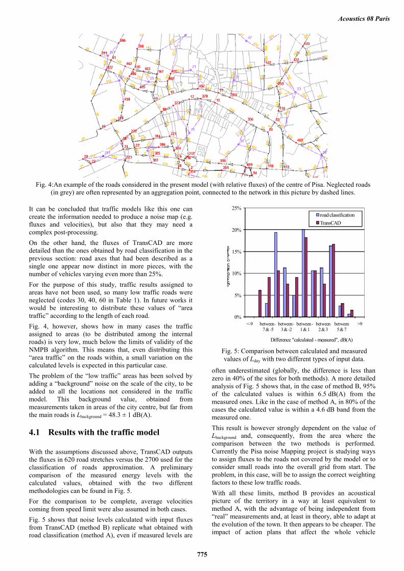
It can be concluded that traffic models like this one can create the information needed to produce a noise map (e.g. fluxes and velocities), but also that they may need a complex post-processing. On the other hand, the fluxes of TransCAD are more detailed than the ones obtained by road classification in the previous section: road axes that had been described as a single one appear now distinct in more pieces, with the number of vehicles varying even more than 25%. For the purpose of this study, traffic results assigned to areas have not been used, so many low traffic roads were neglected (codes 30, 40, 60 in Table 1). In future works it would be interesting to distribute these values of “area traffic” according to the length of each road. Fig. 4, however, shows how in many cases the traffic assigned to areas (to be distributed among the internal roads) is very low, much below the limits of validity of the NMPB algorithm. This means that, even distributing this “area traffic” on the roads within, a small variation on the calculated levels is expected in this particular case. The problem of the “low traffic” areas has been solved by adding a “background” noise on the scale of the city, to be added to all the locations not considered in the traffic model. This background value, obtained from measurements taken in areas of the city centre, but far from the main roads is Lbackground = 48.3 ± 1 dB(A).

4.1 Results with the traffic model

With the assumptions discussed above, TransCAD outputs the fluxes in 620 road stretches versus the 2700 used for the classification of roads approximation. A preliminary comparison of the measured energy levels with the calculated values, obtained with the two different methodologies can be found in Fig. 5. For the comparison to be complete, average velocities coming from speed limit were also assumed in both cases. Fig. 5 shows that noise levels calculated with input fluxes from TransCAD (method B) replicate what obtained with road classification (method A), even if measured levels are

often underestimated (globally, the difference is less than zero in 40% of the sites for both methods). A more detailed analysis of Fig. 5 shows that, in the case of method B, 95% of the calculated values is within 6.5 dB(A) from the measured ones. Like in the case of method A, in 80% of the cases the calculated value is within a 4.6 dB band from the measured one. This result is however strongly dependent on the value of Lbackground and, consequently, from the area where the comparison between the two methods is performed. Currently the Pisa noise Mapping project is studying ways to assign fluxes to the roads not covered by the model or to consider small roads into the overall grid from start. The problem, in this case, will be to assign the correct weighting factors to these low traffic roads. With all these limits, method B provides an acoustical picture of the territory in a way at least equivalent to method A, with the advantage of being independent from “real” measurements and, at least in theory, able to adapt at the evolution of the town. It then appears to be cheaper. The impact of action plans that affect the whole vehicle

Fig. 4:An example of the roads considered in the present model (with relative fluxes) of the centre of Pisa. Neglected roads

(in grey) are often represented by an aggregation point, connected to the network in this picture by dashed lines.

0%

5%

10%

15%

20%

25%

<-9 between -7 & -5

between -3 & -2

between -1 & 1

between 2 & 3

between 5 & 7

>9

Percentage of sites

Difference "calculated - measured", dB(A)

road classificationTransCAD

Fig. 5: Comparison between calculated and measured values of Lday with two different types of input data.

Acoustics 08 Paris

775

circulation may in fact be described with a static traffic model. It must not be forgotten, however, that the management of a traffic model requires a periodical update of the offer/demand model. The expense for this activity might eventually be more onerous than effective noise measurements.

5 Conclusion

This paper reports the final results of the Pisa Noise Mapping Project that has delivered, on January 2007 and at least five years before the deadlines, the noise map for road traffic in the Municipality of Pisa, according to the European noise Directive. In particular, this paper presents the comparison between two different ways to characterize the source in terms of traffic fluxes, taking into account the recommendations of WG-AEN [3]. The Good Practice Guide (version 2), in fact, proposes a traffic model to reduce the uncertainty on calculated noise levels. Results confirm that even a very simple traffic model produces fluxes (and consequently noise levels) comparable with the ones obtained from a more “classical” method (e.g. the classification of roads), leaving a lot of space for improvement. More accurate studies will be needed, especially on low traffic roads, to further reduce the uncertainty. The assessment of noise due to low traffic roads will also require more detailed and accurate acoustical models (like Harmonoise), as the existing ad interim models were designed for much larger numbers of vehicles. It is expected, however, that those new generation models will need a conscious cost/benefits analysis before being implemented for the common user.

The main output of a noise mapping process, according to the END, is however the assessment of the exposed population to different noise levels. The data presented so far, after further processing, were compared with some of

the other experiences mentioned in [10], in a workshop open to the public (see Fig. 6), so fulfilling the object of promoting the population’s conscience and favouring an exchange of experiences on the EU scale [2] for the design of action plans.

Acknowledgement

This work has been partially funded by the Regional Authority of Tuscany through a consultancy contract with the Institute of Chemical and Physical Processes of CNR in Pisa. Thanks are due to the Municipality of Pisa and in particular to the office for Environmental policies.

References

[1] “Directive 2002/49/EC of the European Parliament and of the Council of 25th June 2002, relating to the assessment and management of environmental noise”, Official Journal of the European Communities (2002)

[2] Working Group on the Assessment of Environmental Noise (WG-AEN), “Position paper on Presenting Noise Mapping Information to the Public”, March (2008)

[3] Working Group on the Assessment of Environmental Noise (WG-AEN), “Good Practice Guide for Strategic Noise Mapping and the Production of Associated Data on Noise Exposure” - version 2 (2006)

[4] APAT, “Review, aimed at the application of the END, of the methodologies used in the different EU Members to collect data on the noise due to urban road traffic” – in Italian, Report CTN-AGF nr. 1/04 (2004)

[5] APAT, “Procedure to convert existing data on environmental noise in the indicators required by the European Directive 2002/49/EC” – in Italian, Report CTN-AGF nr. AGF-T-LGU-04-05 (2005)

[6] APAT, “Operative indications to construct the indicator “Population exposed to noise” required by the European Directive 2002/49/EC” – in Italian, Report CTN-AGF nr. AGF-T-MAN-04-01 (2004)

[7] IMAGINE website, www.imagine-project.org

[8] Licitra G., Chiari C., Iacoponi A., Paviotti M. and Memoli G., “Input data prepa-ration for noise mapping according to the european directive on environmental noise”, Proceedings of the 13th International Congress on Sound and Vibration (ICSV13), Wien (A) (2006)

[9] Documents presented at the IMAGINE-WP2 workshop “Demand and traffic flow modelling” during Forum Acusticum, Budapest (2005)

[10] Ripoll A., Bäckman A., “State of the art of noise mapping in Europe”, available online from http://terrestrial.eionet.europa.eu/ (2005)

[11] Moran L., Casini D., Poggi A., “Corrective factors to the emission data to be used in predictive models for road traffic in urban sites” – in Italian, Proceedings of the Annual meeting of the Italian Society of Acoustics (2005).

[12] Steven H., “Noise Emission of Road Transport”, presented at “Noise Research Strategies for a Quieter Europe”, Brussels (B) in (2004) (downloadable from http://www.calm-network.com/)

Fig. 6: Percentage of exposed population in different cities across Europe.

Acoustics 08 Paris

776