LightWave 3D 7 Manual

This publication, or parts thereof, may not bereproduced in any form, by any method, for anypurpose without prior written consent ofNewTek.

© 2001 NewTek. All rights reserved.

NewTek5131 BeckwithSan Antonio, TX 78249

Manual version: 1.1

LLiigghhttWWaavvee 33DD 77

Software License and Limited WarrantyPLEASE READ CAREFULLY BEFORE INSTALLING THIS

SOFTWARE. BY INSTALLING THIS SOFTWARE, YOU AGREE TOBECOME BOUND BY THE TERMS OF THIS LICENSE. IF YOU DO NOTAGREE TO THE TERMS OF THIS LICENSE, RETURN THIS PACKAGETO THE PLACE WHERE YOU OBTAINED IT WITHIN 15 DAYS FOR AFULL REFUND.

1. Grant of License

The enclosed computer program(s) (the “Software”) is licensed,not sold, to you by NewTek for use only under the terms of thisLicense, and NewTek reserves any rights not expressly granted toyou. You own the disk(s) on which the Software is recorded or fixed,but the Software is owned by NewTek or its suppliers and isprotected by United States copyright laws and international treatyprovisions.

The copyright restrictions of this license extend to any furtherupdates, software patches, or bug fixes made available to you byNewTek, whether distributed by floppy disc, CD-ROM, or in anelectronic format via BBS, ftp, e-mail, etc.

This License allows you to use one copy of the Software on asingle computer at a time. To “use” the Software means that theSoftware is either loaded in the temporary memory (i.e., RAM) of acomputer, or installed on the permanent memory of a computer (i.e.,hard disk, CD-ROM, etc.).

You may use at one time as many copies of the Software as youhave licenses for. You may install the Software on a common storagedevice shared by multiple computers, provided that if you havemore computers having access to the common storage device thanthe number of licensed copies of the Software, you must have somesoftware mechanism which locks out any concurrent user in excessof the number of licensed copies of the Software (an additionallicense is not needed for the one copy of Software stored on thecommon storage device accessed by multiple computers).

You may make one copy of the Software in machine readableform solely for backup purposes. The Software is protected bycopyright law. As an express condition of this License, you mustreproduce on the backup copy the NewTek copyright notice in thefollowing format “© 2001 NewTek”

You may permanently transfer all your rights under this Licenseto another party by providing such party all copies of the Softwarelicensed under this License together with a copy of this License andall written materials accompanying the Software, provided that theother party reads and agrees to accept the terms and conditions ofthis License.

2. Restrictions

The Software contains trade secrets in its human perceivableform and, to protect them, YOU MAY NOT REVERSE ENGINEER,DECOMPILE, DISASSEMBLE, OTHERWISE REDUCE THE SOFTWARETO ANY HUMAN PERCEIVABLE FORM. YOU MAY NOT MODIFY,ADAPT, TRANSLATE, RENT, LEASE, LOAN, RESELL FOR PROFIT, ORCREATE DERIVATIVE WORKS BASED UPON THE SOFTWARE OR ANYPART THEREOF.

3. Termination

This License is effective until terminated. This License willterminate immediately without notice from NewTek or judicialresolution if you fail to comply with any provision of this License.Upon such termination you must destroy the Software, allaccompanying written materials and all copies thereof. You may alsoterminate this License at any time by destroying the Software, allaccompanying written materials and all copies thereof.

4. Export Law Assurances

You agree that neither the Software nor any direct productthereof is being or will be shipped, transferred or re-exported,directly or indirectly, into any country prohibited by the UnitedStates Export Administration Act and the regulations thereunder orwill be used for any purpose prohibited by the Act.

5. Limited Warranty and Disclaimer, Limitation of Remedies andDamages.

YOU ACKNOWLEDGE THAT THE SOFTWARE MAY NOT SATISFYALL YOUR REQUIREMENTS OR BE FREE FROM DEFECTS. NEWTEKWARRANTS THE MEDIA ON WHICH THE SOFTWARE IS RECORDEDTO BE FREE FROM DEFECTS IN MATERIALS AND WORKMANSHIPUNDER NORMAL USE FOR 90 DAYS FROM PURCHASE, BUT THESOFTWARE AND ACCOMPANYING WRITTEN MATERIALS ARELICENSED “AS IS.” ALL IMPLIED WARRANTIES AND CONDITIONS

(INCLUDING ANY IMPLIED WARRANTY OF MERCHANTABILITY ORFITNESS FOR A PARTICULAR PURPOSE) ARE DISCLAIMED AS TO THESOFTWARE AND ACCOMPANYING WRITTEN MATERIALS ANDLIMITED TO 90 DAYS AS TO THE MEDIA. YOUR EXCLUSIVE REMEDYFOR BREACH OF WARRANTY WILL BE THE REPLACEMENT OF THEMEDIA OR REFUND OF THE PURCHASE PRICE. IN NO EVENT WILLNEWTEK OR ITS DEVELOPERS, DIRECTORS, OFFICERS, EMPLOYEESOR AFFILIATES BE LIABLE TO YOU FOR ANY CONSEQUENTIAL,INCIDENTAL OR INDIRECT DAMAGES (INCLUDING DAMAGES FORLOSS OF BUSINESS PROFITS, BUSINESS INTERRUPTION, LOSS OFBUSINESS INFORMATION, AND THE LIKE), WHETHER FORESEEABLEOR UNFORESEEABLE, ARISING OUT OF THE USE OR INABILITY TOUSE THE SOFTWARE OR ACCOMPANYING WRITTEN MATERIALS,REGARDLESS OF THE BASIS OF THE CLAIM AND EVEN IF NEWTEKOR AN AUTHORIZED NEWTEK REPRESENTATIVE HAS BEEN ADVISEDOF THE POSSIBILITY OF SUCH DAMAGES.

The above limitations will not apply in case of personal injuryonly where and to the extent that applicable law requires suchliability. Because some jurisdictions do not allow the exclusion orlimitation of implied warranties or liability for consequential orincidental damages, the above limitations may not apply to you.

6. General

This License will be construed under the laws of the State ofTexas, except for that body of law dealing with conflicts of law. If anyprovision of this License shall be held by a court of competentjurisdiction to be contrary to law, that provision will be enforced tothe maximum extent permissible, and the remaining provisions ofthis License will remain in full force and effect. If you are a USGovernment end-user, this License of the Software conveys only“RESTRICTED RIGHTS,” and its use, disclosure, and duplication aresubject to Federal Acquisition Regulations, 52.227-7013 (c)(1)(ii).(See the US Government Restricted provision below.)

7. Trademarks

LightWave 3D, LightWave, Video Toaster and Aura aretrademarks of NewTek. All other brand names, product names, ortrademarks belong to their respective holders.

8. US Government Restricted Provision

If this Software was acquired by or on behalf of a unit or agencyof the United States Government this provision applies. ThisSoftware:

(a) Was developed at private expense, and no part of it wasdeveloped with government funds,

(b) Is a trade secret of NewTek for all purposes of the Freedomof Information Act,

(c) Is “commercial computer software” subject to limitedutilization as provided in the contract between the vendor and thegovernment entity, and

(d) In all respects is proprietary data belonging solely toNewTek.

For units of the Department of Defense (DoD), this Software issold only with “Restricted Rights” as that term is defined in the DoDSupplement to the Federal Acquisition Regulations, 52.227-7013 (c)(1) (ii).

Use, duplication or disclosure is subject to restrictions as setforth in subdivision (c) (l) (ii) of the Rights in Technical Data andComputer Software clause at 52.227-7013. Manufacturer: NewTek,5131 Beckwith, San Antonio, TX 78249.

If this Software was acquired under a GSA Schedule, the USGovernment has agreed to refrain from changing or removing anyinsignia or lettering from the software or the accompanying writtenmaterials that are provided or from producing copies of manuals ordisks (except one copy for backup purposes) and:

(e) Title to and ownership of this Software and documentationand any reproductions thereof shall remain with NewTek,

(f) Use of this Software and documentation shall be limited tothe facility for which it is required, and,

(g) If use of the Software is discontinued to the installationspecified in the purchase/delivery order and the US Governmentdesires to use it at another location, it may do so by giving priorwritten notice to NewTek, specifying the type of computer and newlocation site. US Governmental personnel using this Software, otherthan under a DoD contract or GSA Schedule, are hereby on noticethat use of this Software is subject to restrictions which are thesame as or similar to those specified.

Product MarketingRob “Bubba” HoffmannKriss SchreinerDavid Tracy

Special Thanks to:Tim Jenison, Brad Peebler, Jason Linhart,Robin Hastings, Sandi Spires, John Gross, PaulDavies, Michael Sherak, Taron, TerrenceWalker, Christian Aubert, Sébastien Hudon,Frédéric Hébert, Michel Langlois, LeeStranahan, John Teska, Danny Braet, ForiOwurowa, Shaan Pruden, David Herrington,Paul Debevec, Apple Computers, HollieWendt, James Jones, DStorm, Yoshiaki Tazaki,Andy Frerking, David Warner, the students of3D Exchange, and, of course, all the BetaTeam members. A very special thank you toJacqueline Nakakihara, Taylor Nakakihara,Lexy, the Palm, the Minstrel, VB6, the Net,Bruce Winter and Misterhouse, Josie and thePCs, CZ Jones, J Alba, dougworld.com, TacoTaco, ICQ and many more—you know whoyou are. Also, you can't learn English byreading a dictionary.

CREDITS ANDACKNOWLEDGEMENTS

Lead ProgrammersAllen HastingsStuart Ferguson

Senior ProgrammersArnie CachelinMatt CraigGregory DuquesneJamie FinchDaisuke InoRyan MapesErnie Wright

Additional ProgrammingJoe AngellChristian AubertNeil BarnesRobert GougherJames JonesMarvin LandisMike ReedJon Tindall Steve Worley

Build and IntegrationsManagementJason Craig

Product Design and TestingKenneth WoodruffRich HurreyAristomenis “Meni” Tsirbas

InstallerKris Debolt

DocumentationDouglas J. NakakiharaStephanie BartonBrian Marshall

Product ManagementArt Howe

All rendering speed tests rated in cowmarks (basedon the average unladen cow). No cows were permanentlyharmed in the creation of this product—with theexception of one contumacious individual—although I’msure the Twist and Pole Evenly tools hurt a bit. Cowsequences, featuring a herd of thousands (Texaslonghorns), choreographed by someone who shouldknow better than to morph a cow into a sphere.Anysimilarities between the cow object and someone youknow is a tragic coincidence, we would hope.

Chapter 1: Introduction

About the Manual . . . . . . . . . . . . . . . . . . . . . . . .1.1

LightWave Overview . . . . . . . . . . . . . . . . . . . . . .1.1

Hardware Lock Installation . . . . . . . . . . . . . . . . .1.2

Parallel Port Lock (PC) . . . . . . . . . . . . . . . . . .1.2

Upgrading From a Prior Version . . . . . . . . . . . . . .1.2

Software Installation . . . . . . . . . . . . . . . . . . . . . .1.2

Registering Your Software . . . . . . . . . . . . . . . . . .1.3

Contact Information for Registration . . . . . . . .1.3

Licensing Your Software . . . . . . . . . . . . . . . . . .1.3

Running the Program . . . . . . . . . . . . . . . . . . . . . .1.4

Optimizing RAM Usage . . . . . . . . . . . . . . . . . . . .1.4

LightWave 3D Resources . . . . . . . . . . . . . . . . . . .1.4

Internet Resources . . . . . . . . . . . . . . . . . . . . . .1.4

NewTek Web and FTP Sites . . . . . . . . . . . . . . .1.4

Community . . . . . . . . . . . . . . . . . . . . . . . . . . .1.5

Technical Support . . . . . . . . . . . . . . . . . . . . . .1.5

Chapter 2: Conventions

Typographic Conventions . . . . . . . . . . . . . . . . . .2.1

Directory Structure . . . . . . . . . . . . . . . . . . . . .2.1

Typefaces . . . . . . . . . . . . . . . . . . . . . . . . . . . . .2.1

Keystroke Combinations . . . . . . . . . . . . . . . . . .2.1

Mouse Operations . . . . . . . . . . . . . . . . . . . . . .2.1

Attenti-cons . . . . . . . . . . . . . . . . . . . . . . . . . . .2.2

Key LightWave Terms & Concepts . . . . . . . . . . . .2.2

Working with the Interface . . . . . . . . . . . . . . . . .2.8

Chapter 3: Common Interface Items

The Hub . . . . . . . . . . . . . . . . . . . . . . . . . . . . . . .3.1

Properties . . . . . . . . . . . . . . . . . . . . . . . . . . . .3.2

The Image Viewer . . . . . . . . . . . . . . . . . . . . . . . .3.3

The File Menu . . . . . . . . . . . . . . . . . . . . . . . . .3.4

Image Control Panel . . . . . . . . . . . . . . . . . . . . . .3.4

File Saving . . . . . . . . . . . . . . . . . . . . . . . . . . . . . .3.6

L I G H T W A V E 3 D 7 5

TABLE OF CONTENTS

The Magnify Menu . . . . . . . . . . . . . . . . . . . . .3.6

The Visual Browser . . . . . . . . . . . . . . . . . . . . . . .3.7

VIPER:The Interactive Preview Window . . . . . . . .3.8

Surface Previews . . . . . . . . . . . . . . . . . . . . . .3.10

When Used With Surface Previews . . . . . . . . . .3.11

Non-Surface Preview Uses . . . . . . . . . . . . . . .3.11

The Preset Shelf . . . . . . . . . . . . . . . . . . . . . . . .3.11

LScript . . . . . . . . . . . . . . . . . . . . . . . . . . . . . . . .3.13

LightWave Panels and Dialogs . . . . . . . . . . . . . .3.13

Math in Input Fields . . . . . . . . . . . . . . . . . . . .3.13

Enter/Tab Keys with Input Fields . . . . . . . . . . .3.14

Yes and No . . . . . . . . . . . . . . . . . . . . . . . . . . .3.14

Color Selection . . . . . . . . . . . . . . . . . . . . . . . .3.14

Color Pickers . . . . . . . . . . . . . . . . . . . . . . . . .3.15

Standard List Windows . . . . . . . . . . . . . . . . . .3.15

Reorganizing Lists . . . . . . . . . . . . . . . . . . . . . .3.16

Context Pop-up Menus . . . . . . . . . . . . . . . . .3.16

Chapter 4: Plug-ins

Add Plug-ins Command . . . . . . . . . . . . . . . . . . . .4.1

Edit Plug-ins Command (Modeler) . . . . . . . . . . .4.3

File Grouping Method . . . . . . . . . . . . . . . . . . .4.4

Plug-ins Configuration File . . . . . . . . . . . . . . . . .4.4

Legacy Plug-ins . . . . . . . . . . . . . . . . . . . . . . . . . .4.4

Chapter 5: Customizing Your Interface

First-Level Menu Items . . . . . . . . . . . . . . . . . . . .5.2

Top Menu Group . . . . . . . . . . . . . . . . . . . . . . . . .5.3

Adding New Groups . . . . . . . . . . . . . . . . . . . . . .5.3

Divider Line . . . . . . . . . . . . . . . . . . . . . . . . . . . . .5.3

Renaming Menu Items . . . . . . . . . . . . . . . . . . . .5.4

Automatic More Buttons . . . . . . . . . . . . . . . . . . .5.4

Adding Commands . . . . . . . . . . . . . . . . . . . . . . .5.4

Reorganizing Menus . . . . . . . . . . . . . . . . . . . . . .5.5

Default Menu Locations for Plug-in Commands .5.5

Finding Assignments and Commands . . . . . . . .5.5

Deleting Menu Items . . . . . . . . . . . . . . . . . . . . . .5.6

Window Pop-up . . . . . . . . . . . . . . . . . . . . . . . . .5.6

6 T A B L E O F C O N T E N T S

Maintaining Menu Sets . . . . . . . . . . . . . . . . . . . .5.6

Arranging Menu Tabs . . . . . . . . . . . . . . . . . . . . . .5.7

Keyboard Shortcuts . . . . . . . . . . . . . . . . . . . . . . .5.7

Panel-Specific Shortcuts . . . . . . . . . . . . . . . . . .5.7

Customizing Keyboard Shortcuts . . . . . . . . . . . . .5.7

Finding Assignments and Commands . . . . . . . .5.8

Maintaining Key Mapping Sets . . . . . . . . . . . .5.9

Generic Plug-ins . . . . . . . . . . . . . . . . . . . . . . . . .5.9

Middle Mouse Button Menu . . . . . . . . . . . . . . . .5.9

Chapter 6: Layout: General Functions

The Toolbar Menus . . . . . . . . . . . . . . . . . . . . . . .6.2

Modeler Access . . . . . . . . . . . . . . . . . . . . . . . . . .6.3

LightWave’s Virtual World . . . . . . . . . . . . . . . . . .6.3

World and Local Axes . . . . . . . . . . . . . . . . . . . .6.4

Your Point of View . . . . . . . . . . . . . . . . . . . . . . . .6.5

Changing Your Point of View . . . . . . . . . . . . . . .6.7

Taking Aim . . . . . . . . . . . . . . . . . . . . . . . . . . . . .6.8

Resetting Views . . . . . . . . . . . . . . . . . . . . . . . . . .6.9

Viewport Display Mode . . . . . . . . . . . . . . . . . .6.9

Bone Weight Shade . . . . . . . . . . . . . . . . . . . . . .6.10

The Schematic View . . . . . . . . . . . . . . . . . . . . . .6.11

Parenting in Schematic View . . . . . . . . . . . . . .6.11

Other Schematic View Options . . . . . . . . . . . .6.12

The Grid . . . . . . . . . . . . . . . . . . . . . . . . . . . . . .6.12

The Grid and Relative Camera/Light Sizes . . .6.12

The Grid Square Size Effect on Positioning . .6.13

Grid Square Size Auto-Adjustment . . . . . . . . .6.13

Content Directory . . . . . . . . . . . . . . . . . . . . . . .6.14

Relative Links . . . . . . . . . . . . . . . . . . . . . . . . .6.14

Object File Links . . . . . . . . . . . . . . . . . . . . . . .6.15

Ways to Use the Content Directory . . . . . . . .6.15

Production Data Files . . . . . . . . . . . . . . . . . . .6.16

Scene File Management . . . . . . . . . . . . . . . . . .6.16

Saving a Copy . . . . . . . . . . . . . . . . . . . . . . . .6.17

Recipe for a Scene . . . . . . . . . . . . . . . . . . . . . .6.17

Scene Statistics . . . . . . . . . . . . . . . . . . . . . . . .6.17

Selecting an Item in Layout . . . . . . . . . . . . . . . .6.18


Selecting Multiple Items . . . . . . . . . . . . . . . . .6.19

Selecting by Name . . . . . . . . . . . . . . . . . . . . .6.20

Unselecting Items . . . . . . . . . . . . . . . . . . . . . .6.20

Layout List Item Pop-up Menu . . . . . . . . . . . . .6.20

General Options . . . . . . . . . . . . . . . . . . . . . . . .6.21

Alert Level . . . . . . . . . . . . . . . . . . . . . . . . . . .6.21

Content Directory . . . . . . . . . . . . . . . . . . . . .6.22

Toolbar . . . . . . . . . . . . . . . . . . . . . . . . . . . . . .6.22

Input Device . . . . . . . . . . . . . . . . . . . . . . . . . .6.22

File Dialog and Color Selection . . . . . . . . . . .6.22

Automatically Creating Keyframes . . . . . . . . .6.22

Parent in Place . . . . . . . . . . . . . . . . . . . . . . . .6.23

Left Mouse Button Item Select . . . . . . . . . . .6.23

Frame Slider Label . . . . . . . . . . . . . . . . . . . . .6.23

Frames Per Second . . . . . . . . . . . . . . . . . . . . .6.23

Frame 0 Time Code . . . . . . . . . . . . . . . . . . . .6.24

Frames Per Foot . . . . . . . . . . . . . . . . . . . . . . .6.24

Allow Fractional Current Frame . . . . . . . . . . .6.24

Show Keys in Slider . . . . . . . . . . . . . . . . . . . .6.24

Play at Exact Rate . . . . . . . . . . . . . . . . . . . .6.24

Measurement Unit System . . . . . . . . . . . . . . .6.24

Setting the Default Unit . . . . . . . . . . . . . . . . .6.25

Generic Plug-ins . . . . . . . . . . . . . . . . . . . . . . . .6.25

Comments . . . . . . . . . . . . . . . . . . . . . . . . . . .6.25

Content Manager . . . . . . . . . . . . . . . . . . . . . .6.26

Export Scene Mode . . . . . . . . . . . . . . . . . . . . .6.26

Consolidate Only Mode . . . . . . . . . . . . . . . . . .6.27

FX_... . . . . . . . . . . . . . . . . . . . . . . . . . . . . . . .6.28

ImageLister . . . . . . . . . . . . . . . . . . . . . . . . . .6.28

MD_Controller . . . . . . . . . . . . . . . . . . . . . . . .6.28

Schematic View Tools . . . . . . . . . . . . . . . . . . .6.28

SelectGroup . . . . . . . . . . . . . . . . . . . . . . . . . .6.29

Skelegons To Nulls . . . . . . . . . . . . . . . . . . . . .6.29

Other Generics . . . . . . . . . . . . . . . . . . . . . . . .6.30

Scene Master Plug-Ins . . . . . . . . . . . . . . . . . . . .6.30

ItemPicker . . . . . . . . . . . . . . . . . . . . . . . . . . .6.30

MasterChannel . . . . . . . . . . . . . . . . . . . . . . .6.31

ProxyPick . . . . . . . . . . . . . . . . . . . . . . . . . . .6.32


Global Display Options . . . . . . . . . . . . . . . . . . .6.33

Viewport Layouts . . . . . . . . . . . . . . . . . . . . . .6.34

Grid Settings . . . . . . . . . . . . . . . . . . . . . . . . .6.34

Fixed Near Clip Distance . . . . . . . . . . . . . . . .6.34

Dynamic Update . . . . . . . . . . . . . . . . . . . . . .6.35

Bounding Box Threshold . . . . . . . . . . . . . . . . .6.35

Display Characteristic Settings . . . . . . . . . . . .6.35

Overlay Color . . . . . . . . . . . . . . . . . . . . . . . . .6.38

Shaded Display Options . . . . . . . . . . . . . . . . .6.38

Camera View Tab . . . . . . . . . . . . . . . . . . . . . .6.40

Camera View Background . . . . . . . . . . . . . . . . .6.40

Show Safe Areas . . . . . . . . . . . . . . . . . . . . . . . .6.41

Alternate Aspect Overlay . . . . . . . . . . . . . . . . .6.41

OpenGL Fog . . . . . . . . . . . . . . . . . . . . . . . . . . .6.42

Show Field Chart . . . . . . . . . . . . . . . . . . . . . . .6.42

OpenGL Lens Flares . . . . . . . . . . . . . . . . . . . . .6.43

Schematic View Tabs . . . . . . . . . . . . . . . . . . . .6.43

Layout Commands . . . . . . . . . . . . . . . . . . . . . .6.44

LScripts Menu Tab . . . . . . . . . . . . . . . . . . . . . . .6.45

LScript Commander . . . . . . . . . . . . . . . . . . . .6.45

Select Hierarchy . . . . . . . . . . . . . . . . . . . . . . .6.47

Select Children . . . . . . . . . . . . . . . . . . . . . . . .6.47

Shockwave3D Exporter . . . . . . . . . . . . . . . . . . .6.47

Export Selection . . . . . . . . . . . . . . . . . . . . . .6.48

Quality Controls . . . . . . . . . . . . . . . . . . . . . . .6.49

Preview Options . . . . . . . . . . . . . . . . . . . . . . .6.49

Objects . . . . . . . . . . . . . . . . . . . . . . . . . . . . . .6.49

Animating Objects . . . . . . . . . . . . . . . . . . . . .6.50

Animating Bones . . . . . . . . . . . . . . . . . . . . . .6.51

Surfacing and Texturing . . . . . . . . . . . . . . . . .6.51

Cameras . . . . . . . . . . . . . . . . . . . . . . . . . . . . .6.52

Lighting . . . . . . . . . . . . . . . . . . . . . . . . . . . . .6.53

VRML97 Exporter . . . . . . . . . . . . . . . . . . . . . . .6.53

Accurate Translation . . . . . . . . . . . . . . . . . . . .6.53

High-Performance Output . . . . . . . . . . . . . . .6.54

VRML Creation Settings . . . . . . . . . . . . . . . . .6.54

So What is VRML? . . . . . . . . . . . . . . . . . . . . . .6.57

Animation . . . . . . . . . . . . . . . . . . . . . . . . . . .6.58


Surfaces . . . . . . . . . . . . . . . . . . . . . . . . . . . . .6.58

LightWave VRML Implementation . . . . . . . . .6.59

Performance Notes . . . . . . . . . . . . . . . . . . . .6.60

Scene Tags . . . . . . . . . . . . . . . . . . . . . . . . . . .6.60

Spreadsheet Scene Manager . . . . . . . . . . . . . . .6.62

Workspaces . . . . . . . . . . . . . . . . . . . . . . . . . .6.62

Options . . . . . . . . . . . . . . . . . . . . . . . . . . . . .6.63

Filters . . . . . . . . . . . . . . . . . . . . . . . . . . . . . . .6.64

Mouse Functions . . . . . . . . . . . . . . . . . . . . . .6.65

The Item List . . . . . . . . . . . . . . . . . . . . . . . . .6.65

The Property Cells . . . . . . . . . . . . . . . . . . . . .6.67

Editing Cells . . . . . . . . . . . . . . . . . . . . . . . . . .6.67

Envelopes . . . . . . . . . . . . . . . . . . . . . . . . . . . .6.69

Timeline . . . . . . . . . . . . . . . . . . . . . . . . . . . . .6.69

Column Sorting . . . . . . . . . . . . . . . . . . . . . . .6.70

Chapter 7: Objects in Layout

Loading an Object into Layout . . . . . . . . . . . . . .7.1

Loading from Modeler . . . . . . . . . . . . . . . . . . .7.3

Loading a Single Layer . . . . . . . . . . . . . . . . . . .7.3

The Null Object:The Star of Objects . . . . . . . . . .7.3

Saving an Object . . . . . . . . . . . . . . . . . . . . . . . . .7.4

Saving a Copy . . . . . . . . . . . . . . . . . . . . . . . . .7.4

Object vs. Scene File . . . . . . . . . . . . . . . . . . . . . .7.5

Saving a Transformed Object . . . . . . . . . . . . . . . .7.5

Cloning Items . . . . . . . . . . . . . . . . . . . . . . . . . . .7.6

Replacing, Renaming, and Clearing Items . . . . . .7.6

Replacing a Multi-layer Object . . . . . . . . . . . .7.6

Tools and Commands . . . . . . . . . . . . . . . . . . . . .7.6

Moving an Item . . . . . . . . . . . . . . . . . . . . . . . . . .7.6

Local Axis Adjustments . . . . . . . . . . . . . . . . . . .7.7

Rotating an Item . . . . . . . . . . . . . . . . . . . . . . . . .7.8

Coordinate System . . . . . . . . . . . . . . . . . . . . . . .7.9

Avoiding Gimbal Lock . . . . . . . . . . . . . . . . . . .7.10

Scaling Objects . . . . . . . . . . . . . . . . . . . . . . . . .7.10

Squashing Objects . . . . . . . . . . . . . . . . . . . . . . .7.11

Additive Changes . . . . . . . . . . . . . . . . . . . . . . . .7.11

Item Handles . . . . . . . . . . . . . . . . . . . . . . . . . . .7.11


Numerical adjustments . . . . . . . . . . . . . . . . . . .7.13

Protecting from Changes . . . . . . . . . . . . . . . .7.14

Pivot Point . . . . . . . . . . . . . . . . . . . . . . . . . . . .7.14

Moving the Pivot Point . . . . . . . . . . . . . . . . . .7.15

Layout or Modeler . . . . . . . . . . . . . . . . . . . . .7.16

Why Move the Pivot Point? . . . . . . . . . . . . . . . .7.16

Rotating the Pivot Point . . . . . . . . . . . . . . . . . .7.17

Resetting Position, Rotation, and Size . . . . . . . .7.18

Chapter 8: Keyframing

The Frame Slider . . . . . . . . . . . . . . . . . . . . . . . . .8.2

Navigating the Scene . . . . . . . . . . . . . . . . . . . . .8.2

Keyboard Shortcuts . . . . . . . . . . . . . . . . . . . . .8.2

Going to a Specific Frame . . . . . . . . . . . . . . . .8.2

Playing the Scene . . . . . . . . . . . . . . . . . . . . . . . .8.3

Creating Keyframes . . . . . . . . . . . . . . . . . . . . . . .8.3

Creating and Modifying Keys Automatically . . .8.4

Editing Motion Paths Directly in a Viewport . .8.5

Deleting Keyframes . . . . . . . . . . . . . . . . . . . . . . .8.5

Delete Motion Key Generic Plug-in . . . . . . . . .8.5

Delete Mode . . . . . . . . . . . . . . . . . . . . . . . . . . . .8.7

Threshold . . . . . . . . . . . . . . . . . . . . . . . . . . . . . .8.7

Protection . . . . . . . . . . . . . . . . . . . . . . . . . . . . . .8.8

Saving and Loading Motion Files . . . . . . . . . . . . .8.8

Creating a Preview Animation . . . . . . . . . . . . . . .8.8

Preview Options . . . . . . . . . . . . . . . . . . . . . . . .8.9

Undo/Redo Changes . . . . . . . . . . . . . . . . . . . . .8.10

The Graph Editor . . . . . . . . . . . . . . . . . . . . . . .8.10

Frame Range . . . . . . . . . . . . . . . . . . . . . . . . .8.12

The Time Slider . . . . . . . . . . . . . . . . . . . . . . .8.13

Panel Layout Adjustments . . . . . . . . . . . . . . .8.14

Using the Channel Bin . . . . . . . . . . . . . . . . . .8.14

The Channels Pop-up . . . . . . . . . . . . . . . . . . .8.15

Editing Curves . . . . . . . . . . . . . . . . . . . . . . . .8.16

Edit Mode Selection . . . . . . . . . . . . . . . . . . . .8.17

Copying Keys . . . . . . . . . . . . . . . . . . . . . . . . .8.20

Editing Color Channels . . . . . . . . . . . . . . . . . .8.21

Adjusting the Curve Edit Window . . . . . . . . . .8.22

L I G H T W A V E 3 D 7 11

Zooming and Panning . . . . . . . . . . . . . . . . . .8.22

The Graph Editor Toolbar . . . . . . . . . . . . . . . .8.23

Toolbar Selection Menu . . . . . . . . . . . . . . . . .8.23

Add Layout Selected . . . . . . . . . . . . . . . . . . . . .8.23

Get Layout Selected . . . . . . . . . . . . . . . . . . . . .8.23

Clear Unselected Channels . . . . . . . . . . . . . . . .8.24

Clear Channel Bin . . . . . . . . . . . . . . . . . . . . . . .8.24

Remove Channel from Bin . . . . . . . . . . . . . . . .8.24

Invert Channel Section . . . . . . . . . . . . . . . . . . .8.24

Select All Curves in Bin . . . . . . . . . . . . . . . . . . .8.24

Reset Bin Selection . . . . . . . . . . . . . . . . . . . . . .8.24

Filter Curves . . . . . . . . . . . . . . . . . . . . . . . . . . .8.24

Filter Position Channels . . . . . . . . . . . . . . . . . .8.24

Filter Rotation Channels . . . . . . . . . . . . . . . . . .8.24

Filter Scale Channels . . . . . . . . . . . . . . . . . . . . .8.24

Toolbar Keys Menu . . . . . . . . . . . . . . . . . . . .8.24

Create Key . . . . . . . . . . . . . . . . . . . . . . . . . . . .8.24

Delete Selected Keys . . . . . . . . . . . . . . . . . . . .8.24

Lock Selected Keys . . . . . . . . . . . . . . . . . . . . . .8.25

Unlock Selected Keys . . . . . . . . . . . . . . . . . . . .8.25

Invert Selected Keys . . . . . . . . . . . . . . . . . . . . .8.25

Snap Keys to Frames . . . . . . . . . . . . . . . . . . . . .8.25

Set Key Values . . . . . . . . . . . . . . . . . . . . . . . . . .8.25

Bake Selected Curves . . . . . . . . . . . . . . . . . . . .8.25

Copy Time Slice . . . . . . . . . . . . . . . . . . . . . . . .8.26

Copy Footprint Time Slice . . . . . . . . . . . . . . . .8.26

Paste Time Slice . . . . . . . . . . . . . . . . . . . . . . . .8.26

Match Footprint Time Slice . . . . . . . . . . . . . . . .8.26

Copy Selected Keys . . . . . . . . . . . . . . . . . . . . .8.26

Add to Key Bin . . . . . . . . . . . . . . . . . . . . . . . . .8.26

Numeric Move . . . . . . . . . . . . . . . . . . . . . . . . .8.27

Numeric Scale . . . . . . . . . . . . . . . . . . . . . . . . . .8.27

Roll Keys Left . . . . . . . . . . . . . . . . . . . . . . . . . .8.27

Roll Keys Right . . . . . . . . . . . . . . . . . . . . . . . . .8.27

Reduce Keys . . . . . . . . . . . . . . . . . . . . . . . . . . .8.27

Toolbar Footprints Menu . . . . . . . . . . . . . . . .8.28

Toolbar Autofit Menu . . . . . . . . . . . . . . . . . . .8.28

Autofit . . . . . . . . . . . . . . . . . . . . . . . . . . . . . . .8.28


Autofit Selected . . . . . . . . . . . . . . . . . . . . . . . .8.28

Autofit By Type . . . . . . . . . . . . . . . . . . . . . . . . .8.28

Fit Values By Type . . . . . . . . . . . . . . . . . . . . . . .8.28

Toolbar Display Menu . . . . . . . . . . . . . . . . . .8.28

Numeric Limits . . . . . . . . . . . . . . . . . . . . . . . . .8.28

Go To Frame . . . . . . . . . . . . . . . . . . . . . . . . . . .8.29

Reset Graph . . . . . . . . . . . . . . . . . . . . . . . . . . .8.29

Edit Keyboard Shortcuts . . . . . . . . . . . . . . . . . .8.29

Edit Menu Layout . . . . . . . . . . . . . . . . . . . . . . .8.29

Insert Overwrites Keys . . . . . . . . . . . . . . . . . . .8.30

Filter Static Envelopes . . . . . . . . . . . . . . . . . . . .8.30

Large Autosize Margins . . . . . . . . . . . . . . . . . . .8.30

Allow Fractional Keyframes . . . . . . . . . . . . . . . .8.30

Lazy Layout Update . . . . . . . . . . . . . . . . . . . . . .8.30

Track Layout Time . . . . . . . . . . . . . . . . . . . . . . .8.30

Allow Passthrough Keys . . . . . . . . . . . . . . . . . .8.31

Lock Motion Keys in Time . . . . . . . . . . . . . . . .8.31

Move No Keys Sel . . . . . . . . . . . . . . . . . . . . . . .8.31

Track Item Selections . . . . . . . . . . . . . . . . . . . .8.31

Fit Values when Selected . . . . . . . . . . . . . . . . . .8.31

Show Modifiers . . . . . . . . . . . . . . . . . . . . . . . . .8.32

Show Tangents . . . . . . . . . . . . . . . . . . . . . . . . . .8.32

AntiAlias Curves . . . . . . . . . . . . . . . . . . . . . . . .8.32

Show Key Info . . . . . . . . . . . . . . . . . . . . . . . . . .8.32

Hide Background Curves . . . . . . . . . . . . . . . . .8.32

Large Keyframe Points . . . . . . . . . . . . . . . . . . .8.32

Custom Point Color . . . . . . . . . . . . . . . . . . . . .8.32

Collapse/Show All . . . . . . . . . . . . . . . . . . . . . . .8.33

Collapse/Show Tabs . . . . . . . . . . . . . . . . . . . . . .8.33

Collapse/Show Trees . . . . . . . . . . . . . . . . . . . . .8.33

Other Commands . . . . . . . . . . . . . . . . . . . . . .8.33

Graph Editor Options . . . . . . . . . . . . . . . . . . . .8.33

Undo Last Action . . . . . . . . . . . . . . . . . . . . . . .8.33

Cancel Changes . . . . . . . . . . . . . . . . . . . . . . . .8.33

Graph Editor Options . . . . . . . . . . . . . . . . . . .8.33

Channel Bin Pop-up Menu . . . . . . . . . . . . . . .8.34

Curve Edit Window Pop-up Menu . . . . . . . . .8.36

Key Pop-up Menu . . . . . . . . . . . . . . . . . . . . .8.36

L I G H T W A V E 3 D 7 13

Curve Controls . . . . . . . . . . . . . . . . . . . . . . . .8.37

Multiple Values . . . . . . . . . . . . . . . . . . . . . . . . .8.37

Pre and Post Behaviors . . . . . . . . . . . . . . . . . . .8.38

Incoming Curves . . . . . . . . . . . . . . . . . . . . . . .8.39

TCB Spline . . . . . . . . . . . . . . . . . . . . . . . . . . . .8.39

Interactive TCB Adjustments . . . . . . . . . . . . . . .8.41

Hermite Spline . . . . . . . . . . . . . . . . . . . . . . . . .8.41

Bezier Spline . . . . . . . . . . . . . . . . . . . . . . . . . . .8.42

Linear . . . . . . . . . . . . . . . . . . . . . . . . . . . . . . . .8.42

Stepped Transition . . . . . . . . . . . . . . . . . . . . . . .8.43

Dual-handled Control Points . . . . . . . . . . . . .8.43

Integrated Expressions . . . . . . . . . . . . . . . . . .8.44

Additive Expression . . . . . . . . . . . . . . . . . . . . .8.44

Libraries . . . . . . . . . . . . . . . . . . . . . . . . . . . . . .8.45

Expression Syntax . . . . . . . . . . . . . . . . . . . . . . .8.45

Bad Expressions . . . . . . . . . . . . . . . . . . . . . . . .8.47

Subexpressions . . . . . . . . . . . . . . . . . . . . . . . . .8.47

Vector References . . . . . . . . . . . . . . . . . . . . . . .8.47

Expressions Tree . . . . . . . . . . . . . . . . . . . . . . . .8.47

Graph Editor Exercises . . . . . . . . . . . . . . . . . .8.48

Channel Motion Modifiers . . . . . . . . . . . . . . . .8.58

AudioChannel . . . . . . . . . . . . . . . . . . . . . . . . .8.59

ChannelFollower . . . . . . . . . . . . . . . . . . . . . .8.59

Cycler . . . . . . . . . . . . . . . . . . . . . . . . . . . . . . .8.59

Expressions . . . . . . . . . . . . . . . . . . . . . . . . . . .8.60

Object References . . . . . . . . . . . . . . . . . . . . . .8.61

Sample Expressions . . . . . . . . . . . . . . . . . . . . . .8.66

Oscillator . . . . . . . . . . . . . . . . . . . . . . . . . . . .8.66

NoisyChannel . . . . . . . . . . . . . . . . . . . . . . . . .8.67

SetDrivenKey . . . . . . . . . . . . . . . . . . . . . . . . .8.67

TextureChannel . . . . . . . . . . . . . . . . . . . . . . .8.68

Chapter 9: Object Properties

Custom Objects . . . . . . . . . . . . . . . . . . . . . . . . . .9.2

Camera Mask . . . . . . . . . . . . . . . . . . . . . . . . . .9.2

Effector . . . . . . . . . . . . . . . . . . . . . . . . . . . . . .9.4

Frame Rate Meter . . . . . . . . . . . . . . . . . . . . . .9.5

Item Shape . . . . . . . . . . . . . . . . . . . . . . . . . . . .9.5


Level-of-Detail Mesh Refinement . . . . . . . . . . .9.6

Protractor . . . . . . . . . . . . . . . . . . . . . . . . . . . .9.7

Ruler . . . . . . . . . . . . . . . . . . . . . . . . . . . . . . . .9.8

ShowCurve . . . . . . . . . . . . . . . . . . . . . . . . . . . .9.8

SockMonkey . . . . . . . . . . . . . . . . . . . . . . . . . . .9.9

Speedometer . . . . . . . . . . . . . . . . . . . . . . . . .9.10

VRML97 Custom Object . . . . . . . . . . . . . . . . .9.10

Object Replacement . . . . . . . . . . . . . . . . . . . . .9.11

Level-of-Detail Object Replacement . . . . . . .9.11

ObjList . . . . . . . . . . . . . . . . . . . . . . . . . . . . . .9.12

ObjectSequence . . . . . . . . . . . . . . . . . . . . . . .9.12

Using SubPatch objects in Layout . . . . . . . . . . .9.13

SubPatch Display and Render Levels . . . . . . .9.14

Meta-primitive Display and Render Levels . . . .9.15

Morph Targets . . . . . . . . . . . . . . . . . . . . . . . . . .9.15

Multiple Target/Single Envelope . . . . . . . . . . .9.16

Animating Endomorphs . . . . . . . . . . . . . . . . . . .9.16

Saving Morph Mix . . . . . . . . . . . . . . . . . . . . .9.19

Displacement Maps . . . . . . . . . . . . . . . . . . . . . .9.19

Differences from Surface Textures . . . . . . . . .9.20

Displacement Mapped Objects . . . . . . . . . . .9.26

Displacement Mapping Versus Bump Mapping 9.26

Bump Displacement . . . . . . . . . . . . . . . . . . . .9.27

Displacement Plug-ins . . . . . . . . . . . . . . . . . . . .9.27

CurveConform . . . . . . . . . . . . . . . . . . . . . . . .9.27

Deform Displacement Plug-ins . . . . . . . . . . . .9.29

Deform:Bend . . . . . . . . . . . . . . . . . . . . . . . . . .9.29

Deform:Pole . . . . . . . . . . . . . . . . . . . . . . . . . . .9.29

Deform:Shear . . . . . . . . . . . . . . . . . . . . . . . . . .9.30

Deform:Taper . . . . . . . . . . . . . . . . . . . . . . . . . .9.30

Deform:Twist . . . . . . . . . . . . . . . . . . . . . . . . . .9.31

Deform:Vortex . . . . . . . . . . . . . . . . . . . . . . . . .9.31

DisplacementTexture . . . . . . . . . . . . . . . . . . .9.32

Effector . . . . . . . . . . . . . . . . . . . . . . . . . . . . .9.32

Expression . . . . . . . . . . . . . . . . . . . . . . . . . . .9.33

HyperVoxelsParticles . . . . . . . . . . . . . . . . . . .9.33

Inertia . . . . . . . . . . . . . . . . . . . . . . . . . . . . . .9.34

Joint Morph . . . . . . . . . . . . . . . . . . . . . . . . . .9.34

L I G H T W A V E 3 D 7 15

Morph Mixer . . . . . . . . . . . . . . . . . . . . . . . . .9.35

NormalDisplacement . . . . . . . . . . . . . . . . . . .9.35

Serpent . . . . . . . . . . . . . . . . . . . . . . . . . . . . .9.37

SockMonkey . . . . . . . . . . . . . . . . . . . . . . . . . .9.38

Control Item Tab . . . . . . . . . . . . . . . . . . . . . . . .9.40

Display Options . . . . . . . . . . . . . . . . . . . . . . . .9.40

Batch Operations . . . . . . . . . . . . . . . . . . . . . . .9.40

Disabling Deformations . . . . . . . . . . . . . . . . . . .9.41

Clip Mapping . . . . . . . . . . . . . . . . . . . . . . . . . .9.41

Object Dissolve . . . . . . . . . . . . . . . . . . . . . . . . .9.43

Distance Dissolve . . . . . . . . . . . . . . . . . . . . . . .9.44

Sizing Object Polygons . . . . . . . . . . . . . . . . . . .9.44

Particle and Line Objects . . . . . . . . . . . . . . . . .9.45

Size and Aspect Scaling . . . . . . . . . . . . . . . . .9.46

Unseen by Rays . . . . . . . . . . . . . . . . . . . . . . . . .9.46

Unaffected by Fog . . . . . . . . . . . . . . . . . . . . . . .9.46

Unseen By Camera . . . . . . . . . . . . . . . . . . . . . .9.46

Object Shadow Options . . . . . . . . . . . . . . . . . .9.47

Receive Shadows and HyperVoxels . . . . . . . . .9.48

Object Exclusions . . . . . . . . . . . . . . . . . . . . . . .9.48

Polygon Edges . . . . . . . . . . . . . . . . . . . . . . . . . .9.49

Edge Z Scale . . . . . . . . . . . . . . . . . . . . . . . . .9.50

Sasquatch Lite . . . . . . . . . . . . . . . . . . . . . . . . . .9.51

Designing Fur and Grass . . . . . . . . . . . . . . . . .9.52

Rendering . . . . . . . . . . . . . . . . . . . . . . . . . . . .9.54

Long Hair . . . . . . . . . . . . . . . . . . . . . . . . . . . .9.55

Chapter 10: Bones and Skelegons

Bone-friendly Objects . . . . . . . . . . . . . . . . . . . .10.2

Selecting a Bone . . . . . . . . . . . . . . . . . . . . . . . .10.2

Bones from Another Object . . . . . . . . . . . . . . . .10.4

Activating and Recording Rest Position . . . . . . .10.4

Skelegons . . . . . . . . . . . . . . . . . . . . . . . . . . . . . .10.5

Drawing Skelegons . . . . . . . . . . . . . . . . . . . . .10.6

Bank Rotation Handle . . . . . . . . . . . . . . . . . .10.8

Make Skelegon . . . . . . . . . . . . . . . . . . . . . . . .10.9

Editing Skelegons . . . . . . . . . . . . . . . . . . . . .10.10

Changing Skelegon Direction . . . . . . . . . . . .10.11


Splitting Skelegons . . . . . . . . . . . . . . . . . . . .10.11

The Skelegon Tree Panel . . . . . . . . . . . . . . . .10.11

Converting Skelegons to Bones . . . . . . . . . . .10.12

Bone Strength . . . . . . . . . . . . . . . . . . . . . . . . .10.13

Scaling the Strength . . . . . . . . . . . . . . . . . . .10.14

Using Weight Maps . . . . . . . . . . . . . . . . . . . . .10.14

Bone Weight Help . . . . . . . . . . . . . . . . . . . .10.16

Weight Normalization . . . . . . . . . . . . . . . . .10.17

Auto Weight Maps with Skelegon . . . . . . . . .10.18

Area of Influence . . . . . . . . . . . . . . . . . . . . . . .10.18

Falloff Type and Limited Range . . . . . . . . . . . .10.19

Joints and Muscles . . . . . . . . . . . . . . . . . . . . . .10.20

Chapter 11: Item Motion Options

Parenting . . . . . . . . . . . . . . . . . . . . . . . . . . . . . .11.1

Unparenting . . . . . . . . . . . . . . . . . . . . . . . . . .11.7

Local Axis Rotation . . . . . . . . . . . . . . . . . . . .11.7

Parent in Place . . . . . . . . . . . . . . . . . . . . . . . .11.8

Targeting . . . . . . . . . . . . . . . . . . . . . . . . . . . . . .11.8

Where Does It Point? . . . . . . . . . . . . . . . . . .11.10

Inverse Kinematics . . . . . . . . . . . . . . . . . . . . . .11.11

Full or Part-time? . . . . . . . . . . . . . . . . . . . . .11.12

Pointing the End of a Chain . . . . . . . . . . . . .11.14

Mix and Match . . . . . . . . . . . . . . . . . . . . . .11.14

Setting Your Goals . . . . . . . . . . . . . . . . . . . .11.16

Dueling Goals . . . . . . . . . . . . . . . . . . . . . . . . .11.17

Goal Orientation . . . . . . . . . . . . . . . . . . . . . .11.18

Breaking the Chain . . . . . . . . . . . . . . . . . . . .11.19

Stiff Stuff . . . . . . . . . . . . . . . . . . . . . . . . . . .11.19

Item Motion Modifiers . . . . . . . . . . . . . . . . . .11.25

CurveConstraint . . . . . . . . . . . . . . . . . . . . . .11.25

Cyclist . . . . . . . . . . . . . . . . . . . . . . . . . . . . .11.26

Effector . . . . . . . . . . . . . . . . . . . . . . . . . . . .11.28

Expression . . . . . . . . . . . . . . . . . . . . . . . . . .11.29

Follower . . . . . . . . . . . . . . . . . . . . . . . . . . . .11.29

Gravity . . . . . . . . . . . . . . . . . . . . . . . . . . . . .11.31

Motion Baker . . . . . . . . . . . . . . . . . . . . . . . .11.31

Jolt! . . . . . . . . . . . . . . . . . . . . . . . . . . . . . . .11.32

L I G H T W A V E 3 D 7 17

Global Options . . . . . . . . . . . . . . . . . . . . . . . .11.33

Keyframes Tab . . . . . . . . . . . . . . . . . . . . . . . . .11.34

Randomizing Keys . . . . . . . . . . . . . . . . . . . . . .11.34

Jolting Effect . . . . . . . . . . . . . . . . . . . . . . . . . .11.35

Using Preset Values . . . . . . . . . . . . . . . . . . . . .11.35

Applying Turbulence . . . . . . . . . . . . . . . . . . . .11.35

Key Settings . . . . . . . . . . . . . . . . . . . . . . . . . .11.36

Events Tab . . . . . . . . . . . . . . . . . . . . . . . . . . . .11.36

Oscillator . . . . . . . . . . . . . . . . . . . . . . . . . . .11.37

Sun Spot . . . . . . . . . . . . . . . . . . . . . . . . . . . .11.38

TextureMotion . . . . . . . . . . . . . . . . . . . . . . .11.39

Rotational Limits . . . . . . . . . . . . . . . . . . . . . . .11.40

Align to Path . . . . . . . . . . . . . . . . . . . . . . . . . .11.41

Chapter 12:The Scene Editor

Basic Functions . . . . . . . . . . . . . . . . . . . . . . . . .12.1

Pop-up Menu . . . . . . . . . . . . . . . . . . . . . . . . . .12.4

Keyframes . . . . . . . . . . . . . . . . . . . . . . . . . . . . .12.4

Adjusting Channels . . . . . . . . . . . . . . . . . . . . . .12.5

Adjusting Hierarchy . . . . . . . . . . . . . . . . . . . . . .12.5

Effects of Selection . . . . . . . . . . . . . . . . . . . . . .12.6

Buttons . . . . . . . . . . . . . . . . . . . . . . . . . . . . . . .12.6

Adding Audio . . . . . . . . . . . . . . . . . . . . . . . . . . .12.7

Chapter 13: Camera Basics

Multiple Cameras . . . . . . . . . . . . . . . . . . . . . . .13.2

Resolution . . . . . . . . . . . . . . . . . . . . . . . . . . . . .13.2

Pixel Aspect Ratio . . . . . . . . . . . . . . . . . . . . . . .13.3

Frame Aspect Ratio . . . . . . . . . . . . . . . . . . . . . .13.3

Lens Settings . . . . . . . . . . . . . . . . . . . . . . . . . . .13.4

Aperture Height . . . . . . . . . . . . . . . . . . . . . . .13.4

Camera Settings in a Viewport . . . . . . . . . . . . .13.5

Rendering a Limited Region . . . . . . . . . . . . . . .13.6

Memory Considerations . . . . . . . . . . . . . . . . .13.6

Masking Out a Region . . . . . . . . . . . . . . . . . . . .13.6

Segment Memory Limit . . . . . . . . . . . . . . . . . . .13.7

Antialiasing . . . . . . . . . . . . . . . . . . . . . . . . . . . .13.7

Antialiasing Using Edge Detection . . . . . . . . .13.8


Applying a Soft Filter Effect . . . . . . . . . . . . . . .13.9

Motion Blur effects . . . . . . . . . . . . . . . . . . . . .13.10

Blur Length and Real Cameras . . . . . . . . . . .13.11

Rendering Video Fields . . . . . . . . . . . . . . . . .13.12

Stereoscopic Rendering . . . . . . . . . . . . . . . . . .13.13

Depth of Field . . . . . . . . . . . . . . . . . . . . . . . . .13.13

Chapter 14: Backdrops and Image Processing

Gradient Backdrops . . . . . . . . . . . . . . . . . . . . . .14.2

Background Image . . . . . . . . . . . . . . . . . . . . . . .14.3

Background Plate . . . . . . . . . . . . . . . . . . . . . . .14.5

Environments . . . . . . . . . . . . . . . . . . . . . . . . . . .14.7

Image World . . . . . . . . . . . . . . . . . . . . . . . . . .14.7

SkyTracer2 . . . . . . . . . . . . . . . . . . . . . . . . . . .14.8

The Atmosphere Panel . . . . . . . . . . . . . . . . . . .14.9

The Clouds Panel . . . . . . . . . . . . . . . . . . . . . .14.10

The Texture Editor Panel . . . . . . . . . . . . . . . . .14.13

The Suns Panel . . . . . . . . . . . . . . . . . . . . . . . .14.14

Sun Position . . . . . . . . . . . . . . . . . . . . . . . . . .14.15

The Sky Baker Panel . . . . . . . . . . . . . . . . . . . .14.15

Texture Environment . . . . . . . . . . . . . . . . . .14.16

Compositing . . . . . . . . . . . . . . . . . . . . . . . . . .14.17

Foreground Images . . . . . . . . . . . . . . . . . . . .14.17

Alpha Images . . . . . . . . . . . . . . . . . . . . . . . .14.18

Creating Alpha Images . . . . . . . . . . . . . . . . . . .14.18

Foreground Fader Alpha . . . . . . . . . . . . . . . . .14.19

Foreground Key . . . . . . . . . . . . . . . . . . . . . . .14.20

Processing Effects . . . . . . . . . . . . . . . . . . . . . .14.20

Limit Dynamic Range . . . . . . . . . . . . . . . . . .14.21

Dither Intensity . . . . . . . . . . . . . . . . . . . . . .14.21

Animated Dither . . . . . . . . . . . . . . . . . . . . . .14.21

Color Saturation . . . . . . . . . . . . . . . . . . . . . .14.22

Glow Settings . . . . . . . . . . . . . . . . . . . . . . . .14.22

Pixel Filters . . . . . . . . . . . . . . . . . . . . . . . . . . .14.22

Halftone . . . . . . . . . . . . . . . . . . . . . . . . . . . .14.22

SasLite . . . . . . . . . . . . . . . . . . . . . . . . . . . . .14.23

Image Filters . . . . . . . . . . . . . . . . . . . . . . . . . .14.23

Anaglyph Stereo: Compose . . . . . . . . . . . . . .14.23

L I G H T W A V E 3 D 7 19

Anaglyph Stereo: Simulate . . . . . . . . . . . . . .14.24

Bloom . . . . . . . . . . . . . . . . . . . . . . . . . . . . . .14.24

Render Buffer View (Post-processing only) . .14.24

Chroma Depth (Post-processing only) . . . . .14.25

Corona . . . . . . . . . . . . . . . . . . . . . . . . . . . . .14.26

Input Settings . . . . . . . . . . . . . . . . . . . . . . . . .14.26

Effect Settings . . . . . . . . . . . . . . . . . . . . . . . . .14.27

Other Settings . . . . . . . . . . . . . . . . . . . . . . . .14.27

Depth-Of-Field Blur (Post-processing only) .14.28

Digital Confusion (Post-processing only) . . .14.28

Extended RLA Export (Post-processing only) 14.31

Full Precision Blur . . . . . . . . . . . . . . . . . . . . .14.31

Full Precision Gamma . . . . . . . . . . . . . . . . . .14.32

HDR Exposure . . . . . . . . . . . . . . . . . . . . . . .14.32

Soften Reflections (Post-processing only) . . .14.33

Render Buffer Export (Post-processing only) 14.34

TextureFilter . . . . . . . . . . . . . . . . . . . . . . . . .14.35

Vector Blur (Post-processing only) . . . . . . . .14.36

Overlapping Objects . . . . . . . . . . . . . . . . . . . .14.37

High Quality Blur . . . . . . . . . . . . . . . . . . . . . .14.37

Limits . . . . . . . . . . . . . . . . . . . . . . . . . . . . . . .14.37

Video Legalize . . . . . . . . . . . . . . . . . . . . . . .14.38

Video Tap (Post-processing only) . . . . . . . . . .14.39

Virtual Darkroom . . . . . . . . . . . . . . . . . . . . .14.39

Basic Settings Tab . . . . . . . . . . . . . . . . . . . . . .14.40

Spectral Sensitivity Tab . . . . . . . . . . . . . . . . . .14.40

Film, Paper, and MTF Curve Tabs . . . . . . . . . . .14.41

WaterMark . . . . . . . . . . . . . . . . . . . . . . . . . .14.42

WaveFilterImage . . . . . . . . . . . . . . . . . . . . . . .14.42

Image Filters . . . . . . . . . . . . . . . . . . . . . . . . .14.43

Blur Image . . . . . . . . . . . . . . . . . . . . . . . . . . . .14.44

Sharpen . . . . . . . . . . . . . . . . . . . . . . . . . . . . . .14.44

Edge Blend . . . . . . . . . . . . . . . . . . . . . . . . . . .14.44

Multi-Pass Edge Blend . . . . . . . . . . . . . . . . . . .14.45

Using on Rendered images . . . . . . . . . . . . . . .14.45

Saturation . . . . . . . . . . . . . . . . . . . . . . . . . . . .14.45

Negative . . . . . . . . . . . . . . . . . . . . . . . . . . . . .14.45

Limit High/Low Color . . . . . . . . . . . . . . . . . . .14.45


Posterize . . . . . . . . . . . . . . . . . . . . . . . . . . . . .14.46

Palette Reduce . . . . . . . . . . . . . . . . . . . . . . . .14.46

Film Grain . . . . . . . . . . . . . . . . . . . . . . . . . . . .14.46

Flip Frame . . . . . . . . . . . . . . . . . . . . . . . . . . . .14.46

Color Filters . . . . . . . . . . . . . . . . . . . . . . . . .14.47

Contrast . . . . . . . . . . . . . . . . . . . . . . . . . . . . .14.47

MidPoint . . . . . . . . . . . . . . . . . . . . . . . . . . . . .14.47

Gamma . . . . . . . . . . . . . . . . . . . . . . . . . . . . . .14.47

Luminance . . . . . . . . . . . . . . . . . . . . . . . . . . . .14.48

Brightness . . . . . . . . . . . . . . . . . . . . . . . . . . . .14.48

Adjust Color . . . . . . . . . . . . . . . . . . . . . . . . . .14.48

Matte Filters . . . . . . . . . . . . . . . . . . . . . . . .14.48

The Affect Tab . . . . . . . . . . . . . . . . . . . . . . .14.49

Affected Areas . . . . . . . . . . . . . . . . . . . . . . . . .14.49

Preset Shelf . . . . . . . . . . . . . . . . . . . . . . . . . . .14.49

Enable/Disable . . . . . . . . . . . . . . . . . . . . . . . . .14.49

Preview Window . . . . . . . . . . . . . . . . . . . . . .14.50

Chapter 15:Volumetrics

Background . . . . . . . . . . . . . . . . . . . . . . . . . . . .15.1

Computational Issues . . . . . . . . . . . . . . . . . . .15.2

About Particles . . . . . . . . . . . . . . . . . . . . . . . .15.3

Normal Fog . . . . . . . . . . . . . . . . . . . . . . . . . . . .15.3

Volumetric Antialiasing . . . . . . . . . . . . . . . . . . .15.5

Volumetric Plug-ins . . . . . . . . . . . . . . . . . . . . . .15.5

GroundFog . . . . . . . . . . . . . . . . . . . . . . . . . . . . .15.5

HyperVoxels . . . . . . . . . . . . . . . . . . . . . . . . . . . .15.7

HyperVoxels and Transparent Surfaces . . . . . .15.9

Jump-starting with HyperVoxels . . . . . . . . . .15.10

Exercise: HyperVoxels basics . . . . . . . . . . . . . .15.10

Exercise: HyperVoxel volumetrics . . . . . . . . . .15.13

Exercise: blending HyperVoxel objects . . . . . . .15.15

Preview Options . . . . . . . . . . . . . . . . . . . . . .15.17

Use Z-Buffer . . . . . . . . . . . . . . . . . . . . . . . . .15.18

Sprite Texture Resolution . . . . . . . . . . . . . . .15.18

HyperVoxels Setting Management . . . . . . . .15.18

Object Type . . . . . . . . . . . . . . . . . . . . . . . . .15.19

Sprites . . . . . . . . . . . . . . . . . . . . . . . . . . . . . . .15.19

L I G H T W A V E 3 D 7 21

Geometry Tab . . . . . . . . . . . . . . . . . . . . . . . .15.20

Stretching and Rotating HyperVoxels . . . . . . .15.21

Align to Path . . . . . . . . . . . . . . . . . . . . . . . . . .15.21

Blending HyperVoxels . . . . . . . . . . . . . . . . . . .15.21

Show Particles . . . . . . . . . . . . . . . . . . . . . . . . .15.23

Use ParticleStorm Color . . . . . . . . . . . . . . . .15.23

Shading Tab: Surface Mode . . . . . . . . . . . . . .15.24

Shading Tab:Volume Mode . . . . . . . . . . . . . .15.24

Baking HyperVoxels . . . . . . . . . . . . . . . . . . . . .15.25

Volume Mode Advanced Sub-tab . . . . . . . . . . .15.26

Shading Tab: Sprite Mode . . . . . . . . . . . . . . .15.27

Sprite Clip Frame Offset . . . . . . . . . . . . . . . . .15.29

HyperTexture Tab . . . . . . . . . . . . . . . . . . . . .15.30

Gradient Input Parameters . . . . . . . . . . . . . .15.31

Chapter 16: Rendering Options

Render Frames . . . . . . . . . . . . . . . . . . . . . . . . . .16.1

Automatic Advance . . . . . . . . . . . . . . . . . . . . . .16.2

Render Complete Notification . . . . . . . . . . . . .16.2

Monitoring Progress . . . . . . . . . . . . . . . . . . . . .16.2

Viewing the Finished Image . . . . . . . . . . . . . . . .16.3

VIPER . . . . . . . . . . . . . . . . . . . . . . . . . . . . . . . .16.3

Rendering . . . . . . . . . . . . . . . . . . . . . . . . . . . . .16.3

Rendering Tab . . . . . . . . . . . . . . . . . . . . . . . . . .16.4

Ray Tracing Options . . . . . . . . . . . . . . . . . . . .16.6

Ray Trace Optimization . . . . . . . . . . . . . . . . . . .16.8

Ray Recursion Limit . . . . . . . . . . . . . . . . . . . . .16.9

Multiple CPU Systems . . . . . . . . . . . . . . . . . .16.9

Data Overlay . . . . . . . . . . . . . . . . . . . . . . . . .16.9

Output Files . . . . . . . . . . . . . . . . . . . . . . . . . .16.10

Special Animation Types . . . . . . . . . . . . . . . .16.11

QuickTime Virtual Reality Object Saver . . . .16.12

What is a QuickTime VR Object? . . . . . . . . . .16.12

Object Settings Tab . . . . . . . . . . . . . . . . . . . . .16.12

Animation Settings Tab . . . . . . . . . . . . . . . . . .16.13

Saving Individual Frame Files . . . . . . . . . . . .16.16

Using 32-bit RGB Formats . . . . . . . . . . . . . . . .16.16

Selecting a Filename Format . . . . . . . . . . . .16.16


Fader Alpha . . . . . . . . . . . . . . . . . . . . . . . . .16.17

Recording Images to Tape . . . . . . . . . . . . . . . .16.17

Chapter 17: Particle FX

Partigons . . . . . . . . . . . . . . . . . . . . . . . . . . . . . .17.1

Particle FX Panels . . . . . . . . . . . . . . . . . . . . . . .17.1

The Start Button . . . . . . . . . . . . . . . . . . . . . .17.3

The Save Button . . . . . . . . . . . . . . . . . . . . . .17.3

Options Dialog . . . . . . . . . . . . . . . . . . . . . . . .17.3

Real-time Display . . . . . . . . . . . . . . . . . . . . . . .17.4

Loading/Saving Controllers . . . . . . . . . . . . . . . .17.5

Controller Groups . . . . . . . . . . . . . . . . . . . . . . .17.5

Emitter Controller . . . . . . . . . . . . . . . . . . . . . . .17.6

Emitter Types . . . . . . . . . . . . . . . . . . . . . . . . .17.6

Generator Tab . . . . . . . . . . . . . . . . . . . . . . . .17.7

Particle Tab . . . . . . . . . . . . . . . . . . . . . . . . . .17.10

Motion Tab . . . . . . . . . . . . . . . . . . . . . . . . . .17.11

Etc Tab . . . . . . . . . . . . . . . . . . . . . . . . . . . . .17.12

Interaction Tab . . . . . . . . . . . . . . . . . . . . . . .17.13

File Tab . . . . . . . . . . . . . . . . . . . . . . . . . . . .17.14

Using an Object as an Emitter . . . . . . . . . . .17.15

Wind Controller . . . . . . . . . . . . . . . . . . . . . . . .17.15

Mode Tab . . . . . . . . . . . . . . . . . . . . . . . . . . .17.16

Vector Tab . . . . . . . . . . . . . . . . . . . . . . . . . . .17.18

Gravity Controller . . . . . . . . . . . . . . . . . . . . . .17.19

Collision Controller . . . . . . . . . . . . . . . . . . . . .17.20

Using an Object for Collisions . . . . . . . . . . .17.24

Item Motion Modifiers . . . . . . . . . . . . . . . . . .17.24

FX_Link . . . . . . . . . . . . . . . . . . . . . . . . . . . .17.25

FX_Linker . . . . . . . . . . . . . . . . . . . . . . . . . . . .17.26

FX_Motion . . . . . . . . . . . . . . . . . . . . . . . . . .17.27

The Mode Tab . . . . . . . . . . . . . . . . . . . . . . . . .17.28

The Vector Tab . . . . . . . . . . . . . . . . . . . . . . . .17.28

FX_Link Channel Motion Modifier . . . . . . . . .17.29

Getting Started . . . . . . . . . . . . . . . . . . . . . . . .17.30

Emitter and Wind . . . . . . . . . . . . . . . . . . . . .17.30

Collision Detection . . . . . . . . . . . . . . . . . . . .17.34

More Tutorials . . . . . . . . . . . . . . . . . . . . . . .17.35

L I G H T W A V E 3 D 7 23

Chapter 18: Motion Designer

Elastic Body Models . . . . . . . . . . . . . . . . . . . . .18.1

Operating Motion Designer . . . . . . . . . . . . . . . .18.1

Setting Parameters . . . . . . . . . . . . . . . . . . . . . .18.2

Property Panel: Object Tab . . . . . . . . . . . . . . . .18.3

Group . . . . . . . . . . . . . . . . . . . . . . . . . . . . . . .18.3

Target . . . . . . . . . . . . . . . . . . . . . . . . . . . . . . .18.3

Collision Select . . . . . . . . . . . . . . . . . . . . . . . .18.3

Collision-Detection . . . . . . . . . . . . . . . . . . . . .18.4

Pressure Effect . . . . . . . . . . . . . . . . . . . . . . . .18.4

Fiber Structure . . . . . . . . . . . . . . . . . . . . . . . .18.4

DumpFileName . . . . . . . . . . . . . . . . . . . . . . .18.4

Collision . . . . . . . . . . . . . . . . . . . . . . . . . . . . .18.4

MddFileName . . . . . . . . . . . . . . . . . . . . . . . .18.5

Motion Files . . . . . . . . . . . . . . . . . . . . . . . . . .18.5

Property Panel: Surface Tab . . . . . . . . . . . . . . . .18.5

Basic Settings . . . . . . . . . . . . . . . . . . . . . . . . .18.5

Weight . . . . . . . . . . . . . . . . . . . . . . . . . . . . . . .18.5

Weight +- . . . . . . . . . . . . . . . . . . . . . . . . . . . . .18.6

Spring . . . . . . . . . . . . . . . . . . . . . . . . . . . . . . . .18.6

Viscosity . . . . . . . . . . . . . . . . . . . . . . . . . . . . . .18.6

Resistance . . . . . . . . . . . . . . . . . . . . . . . . . . . . .18.6

Parallel Resistance . . . . . . . . . . . . . . . . . . . . . . .18.7

Back-resistance . . . . . . . . . . . . . . . . . . . . . . . . .18.7

Structure Settings . . . . . . . . . . . . . . . . . . . . . .18.7

Fixed . . . . . . . . . . . . . . . . . . . . . . . . . . . . . . . . .18.7

Sub-Structure . . . . . . . . . . . . . . . . . . . . . . . . . .18.7

Hold-Structure . . . . . . . . . . . . . . . . . . . . . . . . .18.9

Smoothing . . . . . . . . . . . . . . . . . . . . . . . . . . . . .18.9

Stretch-limit . . . . . . . . . . . . . . . . . . . . . . . . . . .18.9

Compress Stress . . . . . . . . . . . . . . . . . . . . . . .18.10

Shrink . . . . . . . . . . . . . . . . . . . . . . . . . . . . . . .18.10

Collision Settings . . . . . . . . . . . . . . . . . . . . .18.10

Self Collision . . . . . . . . . . . . . . . . . . . . . . . . . .18.10

Collision Detection . . . . . . . . . . . . . . . . . . . . .18.11

Single-sided . . . . . . . . . . . . . . . . . . . . . . . . . . .18.11

Skin Thickness . . . . . . . . . . . . . . . . . . . . . . . . .18.11

Friction . . . . . . . . . . . . . . . . . . . . . . . . . . . . . .18.12


Bound Force . . . . . . . . . . . . . . . . . . . . . . . . . .18.12

Action Force . . . . . . . . . . . . . . . . . . . . . . . . . .18.13

Bind Force . . . . . . . . . . . . . . . . . . . . . . . . . . .18.13

Other Surface Controls . . . . . . . . . . . . . . . .18.13

Hide . . . . . . . . . . . . . . . . . . . . . . . . . . . . . . . .18.13

COPY/PASTE . . . . . . . . . . . . . . . . . . . . . . . . .18.14

SAVE/LOAD . . . . . . . . . . . . . . . . . . . . . . . . . .18.14

Material Library . . . . . . . . . . . . . . . . . . . . . . . .18.14

Property Panel: Environment tab . . . . . . . . . . .18.14

Gravity . . . . . . . . . . . . . . . . . . . . . . . . . . . . . .18.14

Wind1/Wind2 . . . . . . . . . . . . . . . . . . . . . . . . .18.14

Turbulence . . . . . . . . . . . . . . . . . . . . . . . . . . .18.14

Wavelength . . . . . . . . . . . . . . . . . . . . . . . . . . .18.15

Wind Mode . . . . . . . . . . . . . . . . . . . . . . . . . . .18.15

SAVE/LOAD . . . . . . . . . . . . . . . . . . . . . . . . . .18.15

Helpful Tips . . . . . . . . . . . . . . . . . . . . . . . . . . .18.15

Options Panel . . . . . . . . . . . . . . . . . . . . . . . . .18.16

Supplemental MD Displacement Plug-ins . . . .18.17

MD_Plug . . . . . . . . . . . . . . . . . . . . . . . . . . .18.17

Setting Options . . . . . . . . . . . . . . . . . . . . . . . .18.17

MD_MetaPlug . . . . . . . . . . . . . . . . . . . . . . .18.18

Setting Options . . . . . . . . . . . . . . . . . . . . . . . .18.18

MD_MetaPlug_Morph . . . . . . . . . . . . . . . . .18.18

MD_Scan . . . . . . . . . . . . . . . . . . . . . . . . . . .18.19

Tutorials . . . . . . . . . . . . . . . . . . . . . . . . . . . . .18.20

Waving a Flag . . . . . . . . . . . . . . . . . . . . . . . .18.20

Collision Detection . . . . . . . . . . . . . . . . . . . .18.24

More Tutorials . . . . . . . . . . . . . . . . . . . . . . .18.26

Chapter 19: Distributed Rendering

Rendering Modes . . . . . . . . . . . . . . . . . . . . . . . .19.1

ScreamerNet Classic . . . . . . . . . . . . . . . . . . . . .19.1

ScreamerNet II . . . . . . . . . . . . . . . . . . . . . . . . .19.2

Using Screamernet II . . . . . . . . . . . . . . . . . . .19.2

ScreamerNet Rendering Requirements . . . . . . .19.3

Getting the Nodes Going . . . . . . . . . . . . . . . . .19.3

Scene Saving Info . . . . . . . . . . . . . . . . . . . . . . . .19.5

Host Machine Setup . . . . . . . . . . . . . . . . . . . . .19.5

L I G H T W A V E 3 D 7 25

Controlling the Network Rendering . . . . . . . . .19.6

Shutting Down Nodes . . . . . . . . . . . . . . . . . . .19.7

Aborting a Rendering Session . . . . . . . . . . . . . .19.7

Changing the Number of Nodes . . . . . . . . . . . .19.7

ScreamerNet II Syntax . . . . . . . . . . . . . . . . . . .19.8

Batch Render on One Computer . . . . . . . . . . . .19.8

Troubleshooting . . . . . . . . . . . . . . . . . . . . . . . . .19.8

Rendering Without LightWave . . . . . . . . . . . . . .19.9

Chapter 20: LightWave 3D Modeling

Components of a 3D Object . . . . . . . . . . . . . . .20.1

Modeling in 3D . . . . . . . . . . . . . . . . . . . . . . . . .20.2

Points and Polygons . . . . . . . . . . . . . . . . . . . . .20.2

Editing Objects . . . . . . . . . . . . . . . . . . . . . . . . .20.3

Have a Plan . . . . . . . . . . . . . . . . . . . . . . . . . . . .20.3

The Modeler Interface . . . . . . . . . . . . . . . . . . . .20.3

Viewport Titlebar . . . . . . . . . . . . . . . . . . . . . .20.4

Modeler Menus . . . . . . . . . . . . . . . . . . . . . . .20.5

Other Interface Areas . . . . . . . . . . . . . . . . . . .20.5

Resetting Tools . . . . . . . . . . . . . . . . . . . . . . . . . .20.6

Four Viewports . . . . . . . . . . . . . . . . . . . . . . . . . .20.6

Multi-layer Object Standard . . . . . . . . . . . . . . .20.8

Multi-document Environment . . . . . . . . . . . . .20.8

Layout Communication . . . . . . . . . . . . . . . . .20.9

Layer Navigation . . . . . . . . . . . . . . . . . . . . . .20.9

Layer Browser Panel . . . . . . . . . . . . . . . . . . .20.10

Hiding Panels . . . . . . . . . . . . . . . . . . . . . . . . . .20.12

Loading an existing object from disk . . . . . . . .20.12

Encapsulated PostScript Loader . . . . . . . . . .20.13

Starting a New Object . . . . . . . . . . . . . . . . . . .20.13

Saving Object Files . . . . . . . . . . . . . . . . . . . . .20.14

Exporting Objects . . . . . . . . . . . . . . . . . . . . . .20.14

Export Encapsulated Postscript . . . . . . . . . .20.14

Closing Object Files . . . . . . . . . . . . . . . . . . . . .20.15

Custom Preferences . . . . . . . . . . . . . . . . . . . . .20.15

User Commands . . . . . . . . . . . . . . . . . . . . . . .20.15

Maintaining User Command Sets . . . . . . . . .20.17

Execute Command . . . . . . . . . . . . . . . . . . . .20.17


Defining a Startup Command . . . . . . . . . . . . .20.17

General Options . . . . . . . . . . . . . . . . . . . . . . .20.17

Content Directory . . . . . . . . . . . . . . . . . . . .20.18

Default Polygon Type . . . . . . . . . . . . . . . . . .20.18

Flatness Limit . . . . . . . . . . . . . . . . . . . . . . . .20.18

The Default Surface Name . . . . . . . . . . . . . .20.18

Curve Divisions . . . . . . . . . . . . . . . . . . . . . . .20.19

Patch Divisions . . . . . . . . . . . . . . . . . . . . . . .20.19

Metaball Resolution . . . . . . . . . . . . . . . . . . .20.19

Undoing Operations . . . . . . . . . . . . . . . . . . .20.19

Undoing the Undo . . . . . . . . . . . . . . . . . . . . .20.19

Chapter 21: Points and Polygons

Point Selection . . . . . . . . . . . . . . . . . . . . . . . . .21.1

Polygons . . . . . . . . . . . . . . . . . . . . . . . . . . . . . .21.3

Non-planar Polygons . . . . . . . . . . . . . . . . . . .21.4

Flatness . . . . . . . . . . . . . . . . . . . . . . . . . . . . .21.5

Polygon Efficiency . . . . . . . . . . . . . . . . . . . . . . .21.5

Special-Use Polygons . . . . . . . . . . . . . . . . . . . . .21.5

Polygon Selection . . . . . . . . . . . . . . . . . . . . . . .21.6

Selection With In-line Points/Polygons . . . . . . . .21.9

Symmetrical Selection . . . . . . . . . . . . . . . . . . . .21.9

Volume Selection Mode . . . . . . . . . . . . . . . . . .21.10

Lasso Volume Select . . . . . . . . . . . . . . . . . . .21.11

Selection by Criteria . . . . . . . . . . . . . . . . . . . .21.12

Surface Normal . . . . . . . . . . . . . . . . . . . . . . . .21.14

Surface Normal Functions . . . . . . . . . . . . . .21.14

Numeric Panel . . . . . . . . . . . . . . . . . . . . . . . . .21.15

Chapter 22: Creating Geometry

The Primitive Tools . . . . . . . . . . . . . . . . . . . . . .22.1

Tools and the Right Mouse Button . . . . . . . . .22.3

Creating in Perspective . . . . . . . . . . . . . . . . .22.3

Using the Arrow Keys . . . . . . . . . . . . . . . . . . .22.4

Using the Numeric Panel . . . . . . . . . . . . . . . . . .22.4

Actions Pop-up Menu . . . . . . . . . . . . . . . . . . .22.4

Box Tool Fields . . . . . . . . . . . . . . . . . . . . . . . .22.5

Ball Tool Fields . . . . . . . . . . . . . . . . . . . . . . . .22.6

L I G H T W A V E 3 D 7 27

Disc/Cone Tool Fields . . . . . . . . . . . . . . . . . . .22.7

Make UVs Option . . . . . . . . . . . . . . . . . . . . .22.8

Other Primitive Tools and Functions . . . . . . . . .22.8

The Capsule Tool . . . . . . . . . . . . . . . . . . . . . .22.8

The Platonic Solid Tool . . . . . . . . . . . . . . . . . .22.9

The SuperQuadric Tool . . . . . . . . . . . . . . . . . .22.9

The Gemstone Tool . . . . . . . . . . . . . . . . . . . .22.10

The Equilateral Function . . . . . . . . . . . . . . .22.11

The Gear Function . . . . . . . . . . . . . . . . . . . .22.11

The Wedge Function . . . . . . . . . . . . . . . . . . .22.12

The Toroid Function . . . . . . . . . . . . . . . . . . .22.13

The Parametric Surface Object Function . . .22.14

The Plot1D Function . . . . . . . . . . . . . . . . . .22.14

The Plot2D Function . . . . . . . . . . . . . . . . . .22.15

Using the Pen Tool . . . . . . . . . . . . . . . . . . . . . .22.16

Using the Pen Numeric Panel . . . . . . . . . . . .22.17

The Text Tool . . . . . . . . . . . . . . . . . . . . . . . . . .22.17

The Edit Font List Panel . . . . . . . . . . . . . . . .22.17

Interactively Creating Text . . . . . . . . . . . . . .22.18

Modifying the Template . . . . . . . . . . . . . . . .22.19

The Text Numeric Panel . . . . . . . . . . . . . . . .22.19

The Sketch Tool . . . . . . . . . . . . . . . . . . . . . . . .22.20

Sketching Curves . . . . . . . . . . . . . . . . . . . . .22.21

The Bezier Tool . . . . . . . . . . . . . . . . . . . . . . . .22.22

Spline Curves . . . . . . . . . . . . . . . . . . . . . . . . . .22.23

The Spline Draw Tool . . . . . . . . . . . . . . . . . .22.23

Creating from Points . . . . . . . . . . . . . . . . . .22.24

Curve Direction . . . . . . . . . . . . . . . . . . . . . .22.25

Using Control Points . . . . . . . . . . . . . . . . . .22.25

Smoothing Two Overlapping Curves . . . . . . .22.26

Turning Curves into Polygons . . . . . . . . . . . .22.27

Using Modeling Tools on Curves . . . . . . . . . .22.27

MetaBalls and Skelegons . . . . . . . . . . . . . . . . .22.28

The Point Tool . . . . . . . . . . . . . . . . . . . . . . . . .22.28

The Spray Points Tool . . . . . . . . . . . . . . . . . . .22.29

Making a Polygon . . . . . . . . . . . . . . . . . . . . . .22.29

Single-Point Polygons . . . . . . . . . . . . . . . . . . .22.30

Random Points . . . . . . . . . . . . . . . . . . . . . . . .22.30


Random Pricks . . . . . . . . . . . . . . . . . . . . . . . . .22.31

Stipple . . . . . . . . . . . . . . . . . . . . . . . . . . . . . . .22.31

Triangles . . . . . . . . . . . . . . . . . . . . . . . . . . . . .22.32

Cage . . . . . . . . . . . . . . . . . . . . . . . . . . . . . . . .22.32

Other Creation Functions . . . . . . . . . . . . . . . .22.33

Platonic Solid . . . . . . . . . . . . . . . . . . . . . . . .22.33

Primitives . . . . . . . . . . . . . . . . . . . . . . . . . . .22.34

Teapot . . . . . . . . . . . . . . . . . . . . . . . . . . . . .22.34

Chapter 23: Modifying Geometry

The Numeric Panel . . . . . . . . . . . . . . . . . . . . . .23.1

Falloff Mode . . . . . . . . . . . . . . . . . . . . . . . . . . .23.1

Falloff Meanings . . . . . . . . . . . . . . . . . . . . . . .23.2

Setting Linear Falloff . . . . . . . . . . . . . . . . . . . . .23.3

Defining a Specific Range . . . . . . . . . . . . . . .23.3

Setting the Falloff Shape . . . . . . . . . . . . . . . .23.5

Flexing an Object on an Arbitrary Axis . . . . . .23.6

Setting Radial Falloff . . . . . . . . . . . . . . . . . . . . .23.7

Setting the Falloff Shape . . . . . . . . . . . . . . . .23.7

Defining a Specific Range . . . . . . . . . . . . . . .23.7

The Numeric Panel . . . . . . . . . . . . . . . . . . . . . .23.9

Symmetrical Editing . . . . . . . . . . . . . . . . . . . . . .23.9

Action Center Control . . . . . . . . . . . . . . . . . . .23.10

The Move Group . . . . . . . . . . . . . . . . . . . . . . .23.11

The Move Tool . . . . . . . . . . . . . . . . . . . . . . .23.11

The Snap Tool . . . . . . . . . . . . . . . . . . . . . . . .23.11

The Drag Tool . . . . . . . . . . . . . . . . . . . . . . . .23.12

The DragNet Tool . . . . . . . . . . . . . . . . . . . . .23.12

The Magnet Tool . . . . . . . . . . . . . . . . . . . . .23.14

The Shear Tool . . . . . . . . . . . . . . . . . . . . . . .23.15

The Rove Tool . . . . . . . . . . . . . . . . . . . . . . . .23.16

Center Data . . . . . . . . . . . . . . . . . . . . . . . . .23.16

Center1D . . . . . . . . . . . . . . . . . . . . . . . . . . .23.16

Rest_On_Ground . . . . . . . . . . . . . . . . . . . . .23.16

Aligner . . . . . . . . . . . . . . . . . . . . . . . . . . . . .23.17

The Rotate Group . . . . . . . . . . . . . . . . . . . . . .23.18

The Rotate Tool . . . . . . . . . . . . . . . . . . . . . .23.18

The Rotate Numeric Panel . . . . . . . . . . . . . . .23.18

L I G H T W A V E 3 D 7 29

The Bend Tool . . . . . . . . . . . . . . . . . . . . . . .23.19

The Twist Tool . . . . . . . . . . . . . . . . . . . . . . . .23.19

The Vortex Tool . . . . . . . . . . . . . . . . . . . . . . .23.20

Dangle . . . . . . . . . . . . . . . . . . . . . . . . . . . . .23.21

RotateAnyAxis . . . . . . . . . . . . . . . . . . . . . . .23.23

RotateHPB . . . . . . . . . . . . . . . . . . . . . . . . . .23.23

Rotate-About-Normal . . . . . . . . . . . . . . . . .23.23

Rotate-Arbitrary-Axis . . . . . . . . . . . . . . . . . .23.23

Rotate-To-Ground . . . . . . . . . . . . . . . . . . . .23.23

Rotate-To-Object . . . . . . . . . . . . . . . . . . . . .23.24

The Stretch Group . . . . . . . . . . . . . . . . . . . . . .23.24

The Size Tool . . . . . . . . . . . . . . . . . . . . . . . .23.24

The Size Numeric Panel . . . . . . . . . . . . . . . . .23.25

The Stretch Tool . . . . . . . . . . . . . . . . . . . . . .23.25

The Stretch Numeric Panel . . . . . . . . . . . . . . .23.25

Tapering Objects . . . . . . . . . . . . . . . . . . . . .23.26

Taper Take 2 . . . . . . . . . . . . . . . . . . . . . . . . .23.27

The Pole Evenly Tool . . . . . . . . . . . . . . . . . .23.28

The Pole Tool . . . . . . . . . . . . . . . . . . . . . . . .23.28

Absolute Size . . . . . . . . . . . . . . . . . . . . . . . .23.29

Smooth Scaling . . . . . . . . . . . . . . . . . . . . . . .23.30

The Spline Guide Tool . . . . . . . . . . . . . . . . . .23.31

Other Stretching Commands . . . . . . . . . . . . . .23.33

CenterScale . . . . . . . . . . . . . . . . . . . . . . . . .23.33

CenterStretch . . . . . . . . . . . . . . . . . . . . . . . .23.34

The Deform Group . . . . . . . . . . . . . . . . . . . . .23.34

The Jitter Command . . . . . . . . . . . . . . . . . . .23.34

The Smooth Command . . . . . . . . . . . . . . . .23.35

The Quantize Command . . . . . . . . . . . . . . .23.36

Chapter 24: Multiplying Geometry

Make UVs Option . . . . . . . . . . . . . . . . . . . . . . .24.1

The Extend Group . . . . . . . . . . . . . . . . . . . . . . .24.1

The Bevel Tool . . . . . . . . . . . . . . . . . . . . . . . .24.1

Other Numeric Options . . . . . . . . . . . . . . . . . .24.3

Beveling Tips . . . . . . . . . . . . . . . . . . . . . . . . . . .24.4

The Extrude Tool . . . . . . . . . . . . . . . . . . . . . .24.6

The Lathe Tool . . . . . . . . . . . . . . . . . . . . . . . .24.7


The Rail Bevel Tool . . . . . . . . . . . . . . . . . . . . .24.8

The Smooth Shift Tool . . . . . . . . . . . . . . . . . .24.9

The Path Extrude Command . . . . . . . . . . . .24.11

The Rail Extrude Command . . . . . . . . . . . . .24.12

Single Curve . . . . . . . . . . . . . . . . . . . . . . . . . .24.12

Multiple Curves . . . . . . . . . . . . . . . . . . . . . . . .24.13

The Extender Command . . . . . . . . . . . . . . .24.15

The SeaShellTool . . . . . . . . . . . . . . . . . . . . .24.15

The Spikey Tool . . . . . . . . . . . . . . . . . . . . . .24.16

The Create Skin Command . . . . . . . . . . . . .24.17

The Morph Polygons Command . . . . . . . . . .24.18

The Combine Group . . . . . . . . . . . . . . . . . . . .24.18

The Boolean Command . . . . . . . . . . . . . . . .24.18

Single vs. Double-sided Polygons . . . . . . . . . . .24.21

The Drill Tools . . . . . . . . . . . . . . . . . . . . . . .24.23

The Solid Drill Tool . . . . . . . . . . . . . . . . . . . .24.26

Faster and Better Drills and Booleans . . . . .24.26

Patches Menu . . . . . . . . . . . . . . . . . . . . . . . .24.26

The Duplicate Group . . . . . . . . . . . . . . . . . . . .24.27

The Mirror Tool . . . . . . . . . . . . . . . . . . . . . .24.27

Paste Tool . . . . . . . . . . . . . . . . . . . . . . . . . . .24.28

The Array Command . . . . . . . . . . . . . . . . . .24.29

Array Type: Rectangular . . . . . . . . . . . . . . . . . .24.29

Array Type: Radial . . . . . . . . . . . . . . . . . . . . . .24.30

Radial Array . . . . . . . . . . . . . . . . . . . . . . . . .24.30

The Clone Command . . . . . . . . . . . . . . . . . .24.30

The Path Clone Command . . . . . . . . . . . . . .24.32

The Rail Clone Command . . . . . . . . . . . . . .24.33

The Symmetrize Command . . . . . . . . . . . . .24.33

Point-Clone-Plus . . . . . . . . . . . . . . . . . . . . . .24.34

Chapter 25: Constructing Geometry

Basic Point and Polygon Maintenance . . . . . . .25.1

The Remove Polygons Command . . . . . . . . . . .25.2

The Remove Points Command . . . . . . . . . . . . . .25.2

The Merge Polygons Command . . . . . . . . . . . . .25.3

The Merge Points Command . . . . . . . . . . . . . . .25.3

Collapse Polygons . . . . . . . . . . . . . . . . . . . . . . .25.5

L I G H T W A V E 3 D 7 31

The Unify Polygons Command . . . . . . . . . . . . .25.5

The qemLOSS2 Function . . . . . . . . . . . . . . . . . .25.5

Introduction . . . . . . . . . . . . . . . . . . . . . . . . . .25.6

Terminology . . . . . . . . . . . . . . . . . . . . . . . . . .25.6

Using qemLOSS2 . . . . . . . . . . . . . . . . . . . . . .25.8

The Reduce-Points Command . . . . . . . . . . . . .25.11

The Reduce-Polygons Command . . . . . . . . . . .25.11

Adding Polygon Points . . . . . . . . . . . . . . . . . . .25.12

The Knife Tool . . . . . . . . . . . . . . . . . . . . . . . . .25.12

The Subdivide Polygons Panel . . . . . . . . . . . . .25.13

Randomizing Options . . . . . . . . . . . . . . . . . .25.13

Faceted Subdivide . . . . . . . . . . . . . . . . . . . . .25.14

Smooth Subdivide . . . . . . . . . . . . . . . . . . . . .25.14

Smooth Subdivide . . . . . . . . . . . . . . . . . . . . .25.15

The BandSaw Command . . . . . . . . . . . . . . . . .25.16

The Split Polygons Command . . . . . . . . . . . . .25.17

The Triple Command . . . . . . . . . . . . . . . . . . . .25.17

The Julienne Command . . . . . . . . . . . . . . . . . .25.18

The Split Skelegon Command . . . . . . . . . . . . .25.19

The Triple Fan Command . . . . . . . . . . . . . . . . .25.19

The Triple Traverse Command . . . . . . . . . . . . .25.19

SubPatches . . . . . . . . . . . . . . . . . . . . . . . . . . .25.20

The Freeze Command . . . . . . . . . . . . . . . . . . .25.20

Make... Commands . . . . . . . . . . . . . . . . . . . . .25.20

The Toggle Metamesh Command . . . . . . . . . . .25.20

Judging Distance and Angles . . . . . . . . . . . . . .25.20

The BoundingBox Command . . . . . . . . . . . .25.21

The PointCenter Command . . . . . . . . . . . . .25.22

LScript . . . . . . . . . . . . . . . . . . . . . . . . . . . . . . .25.22

Additional . . . . . . . . . . . . . . . . . . . . . . . . . . . .25.22

Chapter 26: Detailing Geometry

The Pivot Point Tool . . . . . . . . . . . . . . . . . . . . .26.1

Layer Settings . . . . . . . . . . . . . . . . . . . . . . . . . .26.1

Flatten Layers . . . . . . . . . . . . . . . . . . . . . . . . . .26.1

Change Surface . . . . . . . . . . . . . . . . . . . . . . . . .26.1

Flip Polygons . . . . . . . . . . . . . . . . . . . . . . . . . . .26.2

Spin Quads . . . . . . . . . . . . . . . . . . . . . . . . . . . .26.2


Aligning Polygons . . . . . . . . . . . . . . . . . . . . . . . .26.3

Make 2 Sided . . . . . . . . . . . . . . . . . . . . . . . . . .26.4

Change Sketch Color . . . . . . . . . . . . . . . . . . . . .26.5

Set Value . . . . . . . . . . . . . . . . . . . . . . . . . . . . . .26.5

Welding Commands . . . . . . . . . . . . . . . . . . . . . .26.5

Unwelding Points . . . . . . . . . . . . . . . . . . . . . . .26.6

Curve Commands . . . . . . . . . . . . . . . . . . . . . . .26.6

Skelegon and Metaball Commands . . . . . . . . . .26.6

Chapter 27: Display Menu

Viewports Menu Group . . . . . . . . . . . . . . . . . . .27.1

Zooming . . . . . . . . . . . . . . . . . . . . . . . . . . . . .27.1

OpenGL Display Clipping . . . . . . . . . . . . . . . . .27.1

Panning . . . . . . . . . . . . . . . . . . . . . . . . . . . . .27.2

Automatic Pan and Zoom . . . . . . . . . . . . . . .27.2

View Options . . . . . . . . . . . . . . . . . . . . . . . . . . .27.3

Display Options Panel, Layout Tab . . . . . . . . .27.3

Texture Resolution . . . . . . . . . . . . . . . . . . . . . .27.4

Perspective Amount . . . . . . . . . . . . . . . . . . . . .27.4

Background Color . . . . . . . . . . . . . . . . . . . . . . .27.5

Show Options . . . . . . . . . . . . . . . . . . . . . . . . . .27.5

Display Options Panel,Viewports Tab . . . . . . .27.8

Perspective . . . . . . . . . . . . . . . . . . . . . . . . . . . .27.9

Rendering Style . . . . . . . . . . . . . . . . . . . . . . . .27.10

Upright Rotation . . . . . . . . . . . . . . . . . . . . . . .27.12

Titlebar Shortcuts . . . . . . . . . . . . . . . . . . . . . .27.12

Independent Options . . . . . . . . . . . . . . . . . . .27.12

Independent Visibility . . . . . . . . . . . . . . . . . . . .27.13

Display Options Panel, Backdrop Tab . . . . . .27.13

Aspect and Video images . . . . . . . . . . . . . . . . .27.15

Display Options Panel, Interface Tab . . . . . .27.16

Display Options Panel, Units Tab . . . . . . . . .27.17

Default Unit . . . . . . . . . . . . . . . . . . . . . . . . . .27.18

Grid Units . . . . . . . . . . . . . . . . . . . . . . . . . . . .27.18

Grid Snap . . . . . . . . . . . . . . . . . . . . . . . . . . . .27.18

Time Format . . . . . . . . . . . . . . . . . . . . . . . . . .27.19

Presetting Views . . . . . . . . . . . . . . . . . . . . . . . .27.19

Full-screen Toggle Feature . . . . . . . . . . . . . . .27.20

L I G H T W A V E 3 D 7 33

Selection Menu Group . . . . . . . . . . . . . . . . . . .27.20

Point Information . . . . . . . . . . . . . . . . . . . . .27.20

Polygon Information . . . . . . . . . . . . . . . . . . .27.22

Expanding and Shrinking Selection . . . . . . . .27.23

Groupings . . . . . . . . . . . . . . . . . . . . . . . . . . . .27.24

Polygon Parts . . . . . . . . . . . . . . . . . . . . . . . .27.24

Updating Old Objects . . . . . . . . . . . . . . . . . . .27.24

Point Selection Sets . . . . . . . . . . . . . . . . . . .27.25

Selection By VMaps . . . . . . . . . . . . . . . . . . . . .27.26

Select by Map . . . . . . . . . . . . . . . . . . . . . . .27.26

Select By Map Influence . . . . . . . . . . . . . . .27.26

Select Polygons from Selection Set . . . . . . . .27.27

Per-Polygon UV Map Selection Commands .27.27

Skelegon Selection Commands . . . . . . . . . . . .27.27

Radial Select . . . . . . . . . . . . . . . . . . . . . . . . . .27.27

Visibility Menu Group . . . . . . . . . . . . . . . . . . .27.28

Swap Layer States . . . . . . . . . . . . . . . . . . . . . .27.28

Chapter 28:Vertex Maps

VMap List Window . . . . . . . . . . . . . . . . . . . . . .28.2

VMap Selection . . . . . . . . . . . . . . . . . . . . . . .28.3

General VMap Commands . . . . . . . . . . . . . . . . .28.4

Setting Map Values . . . . . . . . . . . . . . . . . . . . .28.4

Copy, Delete, and Rename Commands . . . . . .28.5

Clearing Maps from Points . . . . . . . . . . . . . . .28.5

CullMap . . . . . . . . . . . . . . . . . . . . . . . . . . . . .28.5

Normalizing Values . . . . . . . . . . . . . . . . . . . . .28.5

Normal Baker . . . . . . . . . . . . . . . . . . . . . . . .28.6

Weight Maps . . . . . . . . . . . . . . . . . . . . . . . . . . .28.6

Weight Tool Falloff . . . . . . . . . . . . . . . . . . . . .28.8

The Airbrush Tool . . . . . . . . . . . . . . . . . . . . . .28.8

Using Weight Maps with Modeling Tools . . . .28.10

Vertex Color Maps . . . . . . . . . . . . . . . . . . . . .28.11

Vertex Color Alpha . . . . . . . . . . . . . . . . . . . .28.13

Vertex Paint . . . . . . . . . . . . . . . . . . . . . . . . .28.14

ColorMap Adjust Tool . . . . . . . . . . . . . . . . . .28.14

UV to Weight . . . . . . . . . . . . . . . . . . . . . . . .28.15

UV Map Jitter . . . . . . . . . . . . . . . . . . . . . . . .28.16


Texture VMap . . . . . . . . . . . . . . . . . . . . . . . .28.16

Bone Weights . . . . . . . . . . . . . . . . . . . . . . . .28.17

Point Color Command . . . . . . . . . . . . . . . . .28.17

UV Texture Maps . . . . . . . . . . . . . . . . . . . . . . .28.17

UVs and Projection . . . . . . . . . . . . . . . . . . .28.18

Guess Viewport UV Image Command . . . . . . .28.24

Atlas Map Type . . . . . . . . . . . . . . . . . . . . . . .28.24

Texture Guide . . . . . . . . . . . . . . . . . . . . . . .28.25

The Make UVs Command . . . . . . . . . . . . . . .28.25

Creating from Command Panels . . . . . . . . . .28.26

Automatic UV Making . . . . . . . . . . . . . . . . .28.26

Set UV Value . . . . . . . . . . . . . . . . . . . . . . . . .28.28

Transform UV Values Command . . . . . . . . . .28.28

Flip UVs . . . . . . . . . . . . . . . . . . . . . . . . . . . .28.29

Spread UVs . . . . . . . . . . . . . . . . . . . . . . . . . .28.29

Quantize UVs . . . . . . . . . . . . . . . . . . . . . . . .28.30

Discontinuous UVs . . . . . . . . . . . . . . . . . . . . . .28.30

That Dreaded Seam Problem . . . . . . . . . . . .28.30

Enter Discontinuous UVs . . . . . . . . . . . . . . .28.32

Unweld Command . . . . . . . . . . . . . . . . . . . .28.35

Merge and Weld Commands . . . . . . . . . . . . .28.36

UVs Outside the Box . . . . . . . . . . . . . . . . . .28.36

UV Mapping in Everyday Modeling . . . . . . . . .28.36

Per-Polygon UV Mapping . . . . . . . . . . . . . . . .28.38

Select UV Seam . . . . . . . . . . . . . . . . . . . . . .28.39

Editing Polymaps . . . . . . . . . . . . . . . . . . . . .28.40

Using Separate Editing UV Maps . . . . . . . . .28.41

Quad Polygon Maps . . . . . . . . . . . . . . . . . . .28.42

EndoMorphs . . . . . . . . . . . . . . . . . . . . . . . . . .28.42

Inserting a Layer into a Morph Map . . . . . .28.46

Merging Morph Maps . . . . . . . . . . . . . . . . .28.47

Rotate Morph Function . . . . . . . . . . . . . . . .28.47

Scale Morph Function . . . . . . . . . . . . . . . . .28.48

VertexPaint . . . . . . . . . . . . . . . . . . . . . . . . . . .28.50

Component and Blend Display . . . . . . . . . . .28.51

Rendering Modes . . . . . . . . . . . . . . . . . . . . .28.52

Preferences . . . . . . . . . . . . . . . . . . . . . . . . . .28.54

Default Keyboard/Mouse Operations . . . . . . .28.55

L I G H T W A V E 3 D 7 35

Customizing Keyboard/Mouse Operations . . .28.56

Modifying Modes . . . . . . . . . . . . . . . . . . . . .28.57

Setting the Morph Map . . . . . . . . . . . . . . . .28.57

Color Mode Tab . . . . . . . . . . . . . . . . . . . . . .28.57

Baking the Color . . . . . . . . . . . . . . . . . . . . . . .28.58

Point Color . . . . . . . . . . . . . . . . . . . . . . . . . . .28.58

Painting a Point . . . . . . . . . . . . . . . . . . . . . . .28.59

Painting a Polygon Point Index . . . . . . . . . . . .28.59

Painting a Polygon . . . . . . . . . . . . . . . . . . . . . .28.60

Weight Mode Tab . . . . . . . . . . . . . . . . . . . . .28.60

Rotating Bones . . . . . . . . . . . . . . . . . . . . . . . .28.61

Renaming Bones . . . . . . . . . . . . . . . . . . . . . . .28.61

Renaming Weight Maps . . . . . . . . . . . . . . . . . .28.62

Copying and Pasting Weight . . . . . . . . . . . . . .28.62

Clearing Weight . . . . . . . . . . . . . . . . . . . . . . . .28.62

Normalizing Weight . . . . . . . . . . . . . . . . . . . . .28.62

Trimming Weight . . . . . . . . . . . . . . . . . . . . . . .28.63

Painting Weight Values . . . . . . . . . . . . . . . . . . .28.65

Calculating Weight . . . . . . . . . . . . . . . . . . . . . .28.65

Scaling Weight . . . . . . . . . . . . . . . . . . . . . . . . .28.66

Clamping Weight . . . . . . . . . . . . . . . . . . . . . . .28.67

Status of Weight . . . . . . . . . . . . . . . . . . . . . . .28.68

Lights Mode Tab . . . . . . . . . . . . . . . . . . . . . .28.68

Show Mode Tab . . . . . . . . . . . . . . . . . . . . . .28.69

Selecting Polygons . . . . . . . . . . . . . . . . . . . . . .28.69

Show and Hide . . . . . . . . . . . . . . . . . . . . . . . .28.70

Frequently Asked Questions . . . . . . . . . . . . .28.70

Chapter 29: Organic Modeling Tools

SubPatches . . . . . . . . . . . . . . . . . . . . . . . . . . . .29.1

Creating a SubPatch Object . . . . . . . . . . . . . . .29.2

Using Weight Maps . . . . . . . . . . . . . . . . . . . . . .29.4

Adding More Details . . . . . . . . . . . . . . . . . . . . .29.4

Specific Display Options . . . . . . . . . . . . . . . . . .29.5

Meta-primitive Objects . . . . . . . . . . . . . . . . . . .29.6

Metaedges and Metafaces . . . . . . . . . . . . . . .29.7

Radius and Influence Settings . . . . . . . . . . . . .29.9

Converting to Metaballs and Metaedges . . . .29.9


Metaball Appearance . . . . . . . . . . . . . . . . . .29.10

Animating Meta-primitives . . . . . . . . . . . . . .29.10

Editing Meta-primitives . . . . . . . . . . . . . . . .29.10

Patch Level and Conversion to Polygons . . . . .29.11

Spline Patching . . . . . . . . . . . . . . . . . . . . . . . .29.12

AutoPatcherMK . . . . . . . . . . . . . . . . . . . . . . . .29.14

Why Spline Patch? . . . . . . . . . . . . . . . . . . . . . .29.14

Chapter 30: Image Editor

Quick Access to Image Editor . . . . . . . . . . . . . .30.2

The Image Editor File List Window . . . . . . . . . .30.2

File-handling Options . . . . . . . . . . . . . . . . . . . .30.3

The Preview Window . . . . . . . . . . . . . . . . . . . . .30.4

Source Tab . . . . . . . . . . . . . . . . . . . . . . . . . . . . .30.4

Loading a Sequence . . . . . . . . . . . . . . . . . . . .30.5

Alpha Channel . . . . . . . . . . . . . . . . . . . . . . . .30.5

Interlace . . . . . . . . . . . . . . . . . . . . . . . . . . . . .30.5

Sequence Digits . . . . . . . . . . . . . . . . . . . . . . .30.5

Frame Rate . . . . . . . . . . . . . . . . . . . . . . . . . .30.6

Image Sequence Settings . . . . . . . . . . . . . . . .30.6

Edit Tab . . . . . . . . . . . . . . . . . . . . . . . . . . . . . . .30.7

Processing Tab . . . . . . . . . . . . . . . . . . . . . . . . . .30.7

Chapter 31: Surface Editor

Surfacing Objects . . . . . . . . . . . . . . . . . . . . . . .31.1

The Surface Editor Panel . . . . . . . . . . . . . . . . . .31.3

Surface Edit Modes . . . . . . . . . . . . . . . . . . . .31.4

Object Edit Mode . . . . . . . . . . . . . . . . . . . . . . .31.5

Scene Edit Mode . . . . . . . . . . . . . . . . . . . . . . . .31.5

Surface List . . . . . . . . . . . . . . . . . . . . . . . . . .31.6

Mass Surface Changes . . . . . . . . . . . . . . . . . .31.6

Preset Shelf and VIPER . . . . . . . . . . . . . . . . . .31.7

Preview Window . . . . . . . . . . . . . . . . . . . . . . .31.8

Basic Surface Parameters . . . . . . . . . . . . . . . . .31.9

Color . . . . . . . . . . . . . . . . . . . . . . . . . . . . . . .31.9

Luminosity . . . . . . . . . . . . . . . . . . . . . . . . . . .31.9

Diffuse . . . . . . . . . . . . . . . . . . . . . . . . . . . . .31.10

Specularity . . . . . . . . . . . . . . . . . . . . . . . . . .31.10

L I G H T W A V E 3 D 7 37

Glossiness . . . . . . . . . . . . . . . . . . . . . . . . . . .31.11

Reflection . . . . . . . . . . . . . . . . . . . . . . . . . . .31.11

Transparency . . . . . . . . . . . . . . . . . . . . . . . .31.11

Refraction Chart Index . . . . . . . . . . . . . . . . . .31.12

Translucency . . . . . . . . . . . . . . . . . . . . . . . . .31.13

Bump Map . . . . . . . . . . . . . . . . . . . . . . . . . .31.13

Surface Smoothing . . . . . . . . . . . . . . . . . . . .31.14

Smooth Threshold . . . . . . . . . . . . . . . . . . . . . .31.14

Sharing Points . . . . . . . . . . . . . . . . . . . . . . . . .31.15

Using Separation . . . . . . . . . . . . . . . . . . . . . . .31.15

Double Sided . . . . . . . . . . . . . . . . . . . . . . . .31.16

Comment . . . . . . . . . . . . . . . . . . . . . . . . . . .31.16

Numerical Settings . . . . . . . . . . . . . . . . . . . . .31.16

Envelopes and Textures . . . . . . . . . . . . . . . . . .31.17

Texture Editor . . . . . . . . . . . . . . . . . . . . . . . . .31.17

Texture Layers . . . . . . . . . . . . . . . . . . . . . . .31.19

Copy and Paste . . . . . . . . . . . . . . . . . . . . . .31.19

Layer Order . . . . . . . . . . . . . . . . . . . . . . . . .31.19

Blending Layers . . . . . . . . . . . . . . . . . . . . . .31.20

Layer Type: Image Mapping . . . . . . . . . . . . . . .31.22

Image Map Projection . . . . . . . . . . . . . . . . .31.22

Planar Projection . . . . . . . . . . . . . . . . . . . . . . .31.23

Cylindrical Projection . . . . . . . . . . . . . . . . . . .31.23

Spherical Projection . . . . . . . . . . . . . . . . . . . .31.24

Cubic Projection . . . . . . . . . . . . . . . . . . . . . . .31.24

Front Projection . . . . . . . . . . . . . . . . . . . . . .31.25

Fixed Projection . . . . . . . . . . . . . . . . . . . . . . .31.28

Image Properties . . . . . . . . . . . . . . . . . . . . .31.30

Texture Placement . . . . . . . . . . . . . . . . . . . .31.33

Surface Size, Position, and Rotation . . . . . . . . .31.33

Falloff . . . . . . . . . . . . . . . . . . . . . . . . . . . . . . .31.34

Using the Reference Object . . . . . . . . . . . . . .31.35

Freezing Reference Object/Camera . . . . . . . . .31.35

World Coordinates . . . . . . . . . . . . . . . . . . . . .31.35

Texture Guide Tool . . . . . . . . . . . . . . . . . . . . . .31.36

Layer Type: Procedural Texture . . . . . . . . . . . . .31.37

Texture Color and Texture Value . . . . . . . . . .31.38

Texture Scale . . . . . . . . . . . . . . . . . . . . . . . .31.38


Procedural Texture Settings . . . . . . . . . . . . .31.39

Brick . . . . . . . . . . . . . . . . . . . . . . . . . . . . . . .31.39

Bump Array . . . . . . . . . . . . . . . . . . . . . . . . .31.39

Checkerboard . . . . . . . . . . . . . . . . . . . . . . . .31.39

Crumple . . . . . . . . . . . . . . . . . . . . . . . . . . . .31.40

Crust . . . . . . . . . . . . . . . . . . . . . . . . . . . . . .31.40

Dots . . . . . . . . . . . . . . . . . . . . . . . . . . . . . . .31.41

FBM . . . . . . . . . . . . . . . . . . . . . . . . . . . . . . .31.41

Fractal Noise . . . . . . . . . . . . . . . . . . . . . . . .31.42

Grid . . . . . . . . . . . . . . . . . . . . . . . . . . . . . . .31.43

HoneyComb . . . . . . . . . . . . . . . . . . . . . . . . .31.43

Marble . . . . . . . . . . . . . . . . . . . . . . . . . . . . .31.44

Ripples . . . . . . . . . . . . . . . . . . . . . . . . . . . . .31.44

Looping Wave Ripples . . . . . . . . . . . . . . . . . . .31.45

Smoky1, 2, and 3 . . . . . . . . . . . . . . . . . . . . . .31.45

Turbulence . . . . . . . . . . . . . . . . . . . . . . . . . .31.45

Underwater . . . . . . . . . . . . . . . . . . . . . . . . .31.45

Looping Wave Ripples . . . . . . . . . . . . . . . . . . .31.46

Value . . . . . . . . . . . . . . . . . . . . . . . . . . . . . .31.46

Veins . . . . . . . . . . . . . . . . . . . . . . . . . . . . . . .31.46

Wood . . . . . . . . . . . . . . . . . . . . . . . . . . . . . .31.47

Additional Procedural Textures . . . . . . . . . . .31.47

Coriolis . . . . . . . . . . . . . . . . . . . . . . . . . . . . .31.48

Cyclone . . . . . . . . . . . . . . . . . . . . . . . . . . . .31.49

Dented . . . . . . . . . . . . . . . . . . . . . . . . . . . . .31.49

FBM Noise . . . . . . . . . . . . . . . . . . . . . . . . . .31.50

Hetero Terrain . . . . . . . . . . . . . . . . . . . . . . .31.50

Hybrid Multi-fractal . . . . . . . . . . . . . . . . . . .31.50

Multi-fractal . . . . . . . . . . . . . . . . . . . . . . . . .31.50

Puffy Clouds . . . . . . . . . . . . . . . . . . . . . . . .31.51

Ridged Multi-fractal . . . . . . . . . . . . . . . . . . .31.51

Turbulent Noise . . . . . . . . . . . . . . . . . . . . . .31.51

Layer Type: Gradient . . . . . . . . . . . . . . . . . . . .31.51

The Gradient Bar . . . . . . . . . . . . . . . . . . . . .31.53

The Current Key . . . . . . . . . . . . . . . . . . . . . .31.54

Changing Key Values . . . . . . . . . . . . . . . . . . .31.55

Changing Key Positions . . . . . . . . . . . . . . . .31.55

Smoothing Between Keys . . . . . . . . . . . . . . .31.55

L I G H T W A V E 3 D 7 39

Scale and Shift . . . . . . . . . . . . . . . . . . . . . . .31.55

Surface Editor:Advanced Tab . . . . . . . . . . . . . .31.56

Surface Editor: Environment Tab . . . . . . . . . . .31.58

Surface Editor: Shaders Tab . . . . . . . . . . . . . . .31.59

BRDF . . . . . . . . . . . . . . . . . . . . . . . . . . . . . .31.60

Edge Transparency . . . . . . . . . . . . . . . . . . . .31.62

Fast Fresnel . . . . . . . . . . . . . . . . . . . . . . . . . .31.63

Halftone . . . . . . . . . . . . . . . . . . . . . . . . . . . .31.65

Interference . . . . . . . . . . . . . . . . . . . . . . . . .31.66

RealFresnel . . . . . . . . . . . . . . . . . . . . . . . . . .31.67

SuperCelShader . . . . . . . . . . . . . . . . . . . . . .31.68

Defining Color Zones . . . . . . . . . . . . . . . . . . .31.68

Brightness . . . . . . . . . . . . . . . . . . . . . . . . . . . .31.69

Colored Lights . . . . . . . . . . . . . . . . . . . . . . . .31.69

Specular Highlights . . . . . . . . . . . . . . . . . . . . .31.69

Surface Baker . . . . . . . . . . . . . . . . . . . . . . . .31.70

Baking Tips . . . . . . . . . . . . . . . . . . . . . . . . . . .31.71

Image Mode . . . . . . . . . . . . . . . . . . . . . . . . . .31.72

Object Mode . . . . . . . . . . . . . . . . . . . . . . . . . .31.73

Instant Radiosity . . . . . . . . . . . . . . . . . . . . . . .31.75

ThinFilm . . . . . . . . . . . . . . . . . . . . . . . . . . . .31.77

ZShader . . . . . . . . . . . . . . . . . . . . . . . . . . . .31.77

Surfacing Ideas . . . . . . . . . . . . . . . . . . . . . . . .31.78

Surface Management . . . . . . . . . . . . . . . . . . .31.78

Chapter 32: Shadow and Light

Not the Real World . . . . . . . . . . . . . . . . . . . . . .32.1

Display Size . . . . . . . . . . . . . . . . . . . . . . . . . . . .32.2

Exclusions . . . . . . . . . . . . . . . . . . . . . . . . . . . . .32.3

Saving Lights . . . . . . . . . . . . . . . . . . . . . . . . . . .32.3

Light Types . . . . . . . . . . . . . . . . . . . . . . . . . . . . .32.4

The Distant Light . . . . . . . . . . . . . . . . . . . . . .32.4

The Point Light . . . . . . . . . . . . . . . . . . . . . . .32.4

Intensity Falloff . . . . . . . . . . . . . . . . . . . . . . . . .32.5

The Spotlight . . . . . . . . . . . . . . . . . . . . . . . . .32.5

Virtual Projector . . . . . . . . . . . . . . . . . . . . . . . .32.7

Spotlight Viewport Display . . . . . . . . . . . . . . . .32.7

Linear and Area Lights . . . . . . . . . . . . . . . . . .32.8


The Cow Light . . . . . . . . . . . . . . . . . . . . . . .32.10

Light Color and Intensity . . . . . . . . . . . . . . . . .32.10

Light Intensity Tool . . . . . . . . . . . . . . . . . . . .32.10

Negative Lights . . . . . . . . . . . . . . . . . . . . . . .32.11

The Envelope Please . . . . . . . . . . . . . . . . . . .32.11

Other Light Attributes . . . . . . . . . . . . . . . . . . .32.11

Me and My Shadow . . . . . . . . . . . . . . . . . . . .32.11

Shadow Type . . . . . . . . . . . . . . . . . . . . . . . . .32.12

Shadow Mapping . . . . . . . . . . . . . . . . . . . . .32.13

Transparent Objects . . . . . . . . . . . . . . . . . . . .32.13

Cache Shadow Map . . . . . . . . . . . . . . . . . . .32.13

Shadow Map Size . . . . . . . . . . . . . . . . . . . . .32.14

Shadow Map Area . . . . . . . . . . . . . . . . . . . .32.14

Smoothing Out an Edge . . . . . . . . . . . . . . . .32.14

Lightening Shadows . . . . . . . . . . . . . . . . . . .32.15

Lens Flares . . . . . . . . . . . . . . . . . . . . . . . . . . . .32.15

Lens Flare Options . . . . . . . . . . . . . . . . . . . .32.16

Lens Flare Viewport Preview . . . . . . . . . . . . . .32.17

Fade and Dissolve Options . . . . . . . . . . . . . . .32.18

Glow Options . . . . . . . . . . . . . . . . . . . . . . . . .32.19

Central Ring . . . . . . . . . . . . . . . . . . . . . . . . . .32.19

Anamorphic Distort . . . . . . . . . . . . . . . . . . . .32.19

Streaks . . . . . . . . . . . . . . . . . . . . . . . . . . . . . .32.20

Lens Reflections . . . . . . . . . . . . . . . . . . . . . . .32.21

Volumetric Lights . . . . . . . . . . . . . . . . . . . . . . .32.25

Light Textures . . . . . . . . . . . . . . . . . . . . . . . .32.28

The VIPER Window and Presets . . . . . . . . . .32.30

Volumetric Shadows within Lights . . . . . . . . .32.30

Global Illumination Panel . . . . . . . . . . . . . . . .32.31

Ambient Light . . . . . . . . . . . . . . . . . . . . . . . .32.31

Shading Noise Reduction . . . . . . . . . . . . . . .32.32

Radiosity . . . . . . . . . . . . . . . . . . . . . . . . . . .32.32

How Radiosity Is Calculated . . . . . . . . . . . . . .32.35

The Radiosity Settings . . . . . . . . . . . . . . . . . . .32.37

Lighting Considerations . . . . . . . . . . . . . . . . . .32.38

VolumetricRadiosity command . . . . . . . . . . . .32.38

Radiosity and High Dynamic Range Images . . .32.38

Ambient Light . . . . . . . . . . . . . . . . . . . . . . . . .32.39

L I G H T W A V E 3 D 7 41

Using Radiosity . . . . . . . . . . . . . . . . . . . . . . . .32.40

Caustics . . . . . . . . . . . . . . . . . . . . . . . . . . . .32.41

Radiosity and Caustic Caching Considerations 32.42

Appendix

Macintosh Information . . . . . . . . . . . . . . . . . .App.1

Right Mouse Button Action . . . . . . . . . . . . .App.1

Memory Allocation . . . . . . . . . . . . . . . . . . .App.1

Command Line Files . . . . . . . . . . . . . . . . . .App.1

Your Display . . . . . . . . . . . . . . . . . . . . . . . . . .App.1

Filenames and Extensions . . . . . . . . . . . . . . . .App.2

Foreign Object Support . . . . . . . . . . . . . . . . .App.2

Imported Formats . . . . . . . . . . . . . . . . . . . .App.2

Exported Formats . . . . . . . . . . . . . . . . . . . .App.3

Image and Animation Types . . . . . . . . . . . . . . .App.4

Images and Memory . . . . . . . . . . . . . . . . . .App.4

High Dynamic Range Images (HDRI) . . . . . .App.5

Import/Export . . . . . . . . . . . . . . . . . . . . . . . .App.6

Internal Compositing . . . . . . . . . . . . . . . . . . .App.7

Preview Compression Codec . . . . . . . . . . . . . .App.7

Configuration Files . . . . . . . . . . . . . . . . . . . . .App.7

Custom Configuration Files . . . . . . . . . . . . .App.7

Layout Startup Command . . . . . . . . . . . . . .App.8

Customizing Layout Viewport Navigation . .App.8

Customizing Camera Presets . . . . . . . . . . . .App.8

LightWave Limits . . . . . . . . . . . . . . . . . . . . . . .App.8

Measurement Units . . . . . . . . . . . . . . . . . . . .App.9

Do the Math . . . . . . . . . . . . . . . . . . . . . . . . . .App.9

Math Functions . . . . . . . . . . . . . . . . . . . . .App.10

Functions . . . . . . . . . . . . . . . . . . . . . . . . . .App.10

Constants . . . . . . . . . . . . . . . . . . . . . . . . .App.10

Other . . . . . . . . . . . . . . . . . . . . . . . . . . . . .App.12

Index


cchhaapptteerr1Introduction

Chapter 1:Introduction

Congratulations on your acquisition of LightWave 3D, a truly powerfulpiece of software. This program represents over 12 years of research anddevelopment from a team of insanely dedicated programmers, artistsand visionaries.

ABOUT THE MANUALThe opening chapters of this manual give you an overview of

LightWave 3D, and cover the functions that are common to both theanimation and modeling aspects of LightWave. Following that, there arechapters that cover how to move your objects, how to set lighting andrender options, and other information on how to create your animations.The final set of chapters go over how to build your 3-D objects, applysurface textures, add lighting to your scene, and more.

LightWave 3D is generally divided into two separate environments:LightWave Layout and LightWave Modeler. (It is a common convention torefer to the animation and rendering toolset as LightWave, or just Layout,and to refer to the object creation toolset as Modeler.)

For Layout, the buttons on the toolbar are often shortcuts to controlsthat can also be accessed from one of Layout’s many panels. The manualgenerally takes a panel and topic-based approach to explaining Layout,since many controls for certain tasks are grouped together on panels.

Modeler is a little different. All of its tools are accessed from thetoolbar, and panels are used to execute more focused tasks. As such, theModeler portion of the manual is generally organized by the order oftools in the toolbar.

LIGHTWAVE OVERVIEWWith LightWave, you are the producer, art director, cinematographer

and director, all rolled into one. Your actors consist of objects that youbuild in Modeler or import from another program. You place lights toilluminate them, assign surface colors and values to clothe them, and

L I G H T W A V E 3 D 7 1.1

then choreograph their movement to animate them. Once you have youractors in place, a camera records all of their movements, creating imagesof their movements that you can compile into animations.

LightWave can create animations and still images for virtually anyuse, from tiny 16 x 16 pixel Web graphics, all the way up to a resolutionof 16,000 x 16,000 pixels, and anywhere in between. A multitude of presetresolutions are also provided, including industry standard D1 and D2(NTSC and PAL) video resolutions.

You create animations by generating a single frame at a time, thenrecording each frame to some type of playback device, like videotape ora hard-disk playback device, or even film. Frames can also be saved incomputer animation format, like AVI.

HARDWARE LOCK INSTALLATIONIf you have a USB hardware lock, you can install it with your machine

running. If you have a Mac ADB hardware lock (from a prior version),install it with your machine turned off.

Parallel Port Lock (PC)1 Turn off your computer.

2 Remove any peripherals from the parallel port on which you want toinstall the hardware lock. If possible, install the hardware lock on anunused parallel port.

3 Plug the hardware lock into the parallel port.

4 Plug any removed peripherals into the hardware lock.

5 Restart your system.

UPGRADING FROM A PRIOR VERSIONIf you already have a version of LightWave 3D on your computer, you

may follow the same installation instructions as new users. Theinstallation will not delete any objects, scenes, images, etc. unless a fileon your system has the same name as a file installed by the installer inthe same subdirectory, in which case it will be overwritten.

WARNINGWe strongly recommend you backup your system before you installLightWave 3D.

SOFTWARE INSTALLATIONTo install LightWave 3D on your system, insert the LightWave 3D CD-

ROM in the appropriate drive. On the PC, run SETUP.EXE and on the Mac,run the LightWave installer program.

1.2 C H A P T E R O N E : I N T R O D U C T I O N

Follow the instructions for installation as presented. You will be givenoptions for what to install. A full installation includes optional “content”data, such as objects, scenes, and images that you can install accordingto your interests and available hard drive space—you can delete thesefiles later if you need to. Note that content data is not required to runLightWave 3D; however, some files will be required for many of theexercises and tutorials in the manual.

When the installation is complete, reboot your computer.

REGISTERING YOUR SOFTWAREInitially, LightWave will only run a certain number of days until you

register the software. Run LightWave to get your hardware lock serialnumber—a dialog will appear telling you this information. Write thisnumber down.

A registration folder should have been installed in the LightWavestart-up menu group. There will be links to a form that must becompleted and sent to NewTek. You must provide your hardware lockserial number.

Registration is important since it allows you to receive technicalsupport, upgrades, special offers, new product information, and yourpermanent license key.

Contact Information for Registration1-800-TOASTER (862-7837)International: 1-210-370-8000Fax: 1-210-370-8030

Hours (Central time): Mon-Thur: 9:00 AM to 6:00 PM, Friday: 9:00 AMto 5:30 PM

On-line registration: www.newtek.comE-mail: [email protected]

Mail:

NewTek Inc.Attn: Customer Service5131 Beckwith Blvd.San Antonio, TX 78249

Licensing Your SoftwareOnce you obtain your licensing code number, edit the LICENSE.KEY file

using a text editor (e.g., Notepad (PC), Simple Text (MacOS 9.x), TextEdit (MacOS X), etc.) and add your code. LICENSE.KEY should be located inyour PROGRAMS\LIGHTWAVE_SUPPORT directory. You can have multiple codenumbers in the file, but each one needs to be on its own line.

L I G H T W A V E 3 D 7 1.3

NOTEMake sure you save LICENSE.KEY as a plain text file, not RTF or other fileformat.

RUNNING THE PROGRAMLightWave 3D is started the same way as any other program on the

particular platform on which it’s installed. Start LightWave (to startLayout) or Modeler by double-clicking their respective icons, or byclicking their icons and selecting Open from the menu. Each program canbe started independently; however, you may also access them byclicking the appropriate button on their respective interfaces.

OPTIMIZING RAM USAGEIf your computer is accessing virtual memory frequently during

rendering, you may find a substantial increase in performance byinstalling more RAM on your machine or reducing the amount of RAMLightWave needs to store the render information.

One of the best ways to minimize the need for RAM is to reduce thecolor of the images used for texture mapping effects. Except for thoseused as a Surface Color, texture maps usually need to be only 256-levelgray-scale images.

Other ways to reduce RAM usage are to render your animation inmultiple passes or decrease Segment Memory Limit on Layout’s CameraProperties panel.

LIGHTWAVE 3D RESOURCES

Internet ResourcesA LightWave-specific newsgroup and mailing list are maintained on

the Internet. Here you can find new users asking questions about usingLightWave and experts answering them. Also, many topics related tocomputer animation are discussed in these groups, such as theperformance of various accelerators, CPU speeds, animation recordingdevices, and many more. The newsgroup’s Internet address is:comp.graphics.apps.lightwave.

Internet mailing list information can be found at www.tv3d.com.

NewTek Web and FTP SitesIn addition to information about NewTek products, upgrades, and the

latest releases of LightWave software, our World Wide Web sites(www.LightWave3D.com and www.newtek.com) have tutorials, LightWaveimages and animations, technical support FAQs, tech support e-mail link,and links to related sites.


NewTek maintains an FTP site (ftp.newtek.com) on the Internet. Hereyou can find objects, scene files, images, and other items of interest toLightWave users.

CommunityA unique attribute of LightWave 3D is the LightWave community. It is

rare to find such a fun-loving bunch of hooligans that are so talented andyet so willing to share their secrets, ideas, and creations. Make certainyou also take a look into the available resources such as local usersgroups, training videos (www.DesktopImages.com), and NewTek specificmagazines (www.keyframemag.com and www.newtekpro.com).

Technical SupportThe best source for help with installing or configuring software or

hardware is the retailer from whom you purchased your NewTekproduct. While we have made every effort to keep your software andhardware trouble-free and easy to use, you may occasionally need helpright from the source. If you have problems with NewTek suppliedhardware or LightWave doesn’t seem to be functioning as it should,please contact technical support in one of the following ways:

• By email: [email protected]

• By fax: (210) 370-8030

• By telephone: (210) 341-8444. Technicians are available to answerquestions from 8:00 a.m. to 8:00 p.m. Central Time, Monday throughThursday, and Friday from 8:00 a.m. to 5:30 p.m. Central Time.

Please supply in your communication or have the followinginformation handy when calling:

• Your computer’s operating system and version

• The version of LightWave you are using

• The amount of RAM in your computer

• Any relevant specifics about your system (display card type, memorymanagers, accelerator type, etc.)

• Your product serial number

NOTEYour product must be registered before you can receive support.

L I G H T W A V E 3 D 7 1.5

cchhaapptteerr2Conventions

Chapter 2:Conventions

TYPOGRAPHIC CONVENTIONSThe following conventions will be used throughout this manual.

Directory StructureExcept for a few system files, all of the software will be installed in a

single subdirectory on the drive you specified during the installationprocess. Therefore, subdirectories referred to in this documentation arelocated in this main subdirectory. (For example, if the discussion refersto the Images drawer, the actual path might be C:\LIGHTWAVE\IMAGES.)

TypefacesALL CAPS Computer keys, directories, device names (e.g., ENTER,

C:\LIGHTWAVE\OBJECTS, CTRL+P, etc.).

Bold Names of interface menus, fields, buttons, etc. are set inbold type.

Keystroke CombinationsKEY1 + KEY2 Simultaneous keystrokes. Hold the first key and press the

second key.

Mouse OperationsLMB Left mouse button

MMB Middle mouse button (if applicable)

RMB Right mouse button

Selecting Single-clicking an element with the LMB so that itbecomes active or selected.

Deselecting Single-clicking an element with the LMB so that itbecomes inactive or unselected.

Activating Selecting an option by clicking on its toggle button.

L I G H T W A V E 3 D 7 2.1

Deactivating Unselecting an option by clicking on its toggle button.

Clicking Placing your mouse pointer over something and thenpressing a mouse button. This nearly always means theLMB.

Right-clicking Clicking an element with your RMB.

Double-clicking Rapidly clicking an element twice.

Dragging Selecting an element with your mouse pointer andcontinuing to hold the mouse button down as you moveyour mouse. This nearly always means with the LMB.

Attenti-consThe warning symbol will highlight a discussion thatwarns the user about something. You should pay specialattention to text marked with this symbol.

The note symbol will highlight a discussion that isparticularly noteworthy.

The hint symbol will highlight tips and suggestions thatare usually of a time-saving nature.

KEY LIGHTWAVE TERMS & CONCEPTSThe following are some common terms and concepts used with

LightWave that you should familiarize yourself with:

Alpha matte/image Alpha matte/image generally refers to an imagewhere the brightness of each pixel is used to cutor partially dissolve out another image. Theseare generally grayscale or black-and-whiteimages, but the brightness values can also beextracted from a color image.

Animation Channel Animation Channel refers to the differentposition, rotation, and scaling settings an itemcan have in Layout. It can also refer to otherenvelopeable elements like light intensity. Seealso motion channel.

Axis Axis refers to the XYZ coordinates used as thebasis for positioning elements in LightWave’s 3Dspace. It is somewhat like the concept ofleft/right, up/down, and near/far.

Bone For any object, you can define a skeletal systemcomposed of bones. By moving bones around,you can change the shape of an object.

2.2 C H A P T E R T W O : C O N V E N T I O N S

Bounding Box A Bounding Box is a six-sided box conforming tothe outer dimensions of an object. It is commonlyused as a quickly drawn stand-in for a morecomplex object.

Camera As in real life, a camera records events. Lookingthrough LightWave’s camera shows you the viewas it will be generated.

Cattiwompus Weird. Mixed up. Unusual. Distorted.

Channel See Animation Channel.

Child See Parenting.

Control Mesh A Control Mesh is a cage of points used to shapeSubPatches.

Default unit The Default unit is the unit of measure (e.g.,meter, feet, etc.) that is assumed, usually whenno unit of measure is entered with the numericdata. In Layout, it is determined by the setting onthe General Options tab of the Preferences panel.In Modeler, the setting is on the Display Optionspanel.

Endomorph An EndoMorph is an object containing one ormore morph maps.

Envelope An envelope is a way of setting a particular valuethat usually changes over time using a graphicalinput mode.

Flatness Flatness is used as a threshold in determining if apolygon is non-planar. A flatness of 0 percentmeans the polygon is absolutely flat.

Flatness is computed as percentage deviationfrom a triangle (the “ideal plane”) formed fromthe first two and last vertices of a polygon. All ofthe other points are measured relative to thisplane. The largest deviation is divided by thetotal size of the polygon to get a percentage thatis the flatness value.

For example, if a polygon is 1 meter wide, a .5percent flatness means that no point will beoutside the ideal plane of the polygon by morethan 5 millimeters. (1 x .005)

Frames LightWave works with frames. A frame is oneimage out of many that define an animation.There are approximately 30 frames per second inNTSC video, 25 frames per second in PAL video,and 24 frames per second in film.

L I G H T W A V E 3 D 7 2.3

GCore Short for Geometry Core, the engine that sitsunderneath all animation and modeling tools.

Geometry Geometry refers to the positional layout of pointsand polygons for an object.

High Dynamic Range Image HDRI is an image with a very large intensitydifference between the brightest and darkestpixels. In typical 8/24-bit images, the maximumpossible intensity range is 255 times brighterthan the darkest gray pixel (with a value of 1).Natural scenes and images rendered withradiosity can have dynamic ranges from 10 to10,000 times greater than this. Recording thisinformation requires use of an image format withhigher precision.

Hub, the The Hub is a message board that LightWavemodules use to synchronize information.

HyperVoxel HyperVoxels are volumetric rendering effects.

Item An item in Layout refers to an object, bone, light,or camera.

Intelligentities Intelligentities refer to LightWave’s object format.

Keyframe (Also known as just a key.) A keyframe is a framefor which you define an animation channel(s)(e.g., position or rotation) for an item in Layout.Animations are composed of a beginningkeyframe, an ending keyframe and usually somenumber of keyframes in between. See also tween.

Light A light in LightWave is generally used just like alight in real life. Lights illuminate a scene andallow you to see the objects within it.

LScript This is LightWave’s built-in scripting language.LScripts can be installed and used just like plug-ins.

Meta-primitive A Metaball, Metaedge or Metaface object.

Modal/Non-modal A modal panel must be closed before you cancontinue working with the rest of the application.A non-modal panel lets you shift the focusbetween it and another part of the applicationwithout having to close the panel—you cancontinue to work elsewhere in the currentapplication while the panel is displayed.Modeler’s Numeric panel is non-modal becauseyou can do other things while it is open. In


contrast, Modeler’s Display Options panel ismodal because you must close it before you cancontinue working.

Motion Channel Motion Channel is generally the same asAnimation Channel, but refers only to position,rotation, and scale. (i.e., not light intensity.)

Non-planar Non-planar refers generally to a polygon whereall points do not reside in the same plane andcan occur only with polygons using more thanthree points. Non-planar polygons can causeerratic rendering errors.

Normal A polygon normal is the imaginary line projectingout perpendicular to a surface at any pointindicating the direction of the polygon. A polygonsurface normal is represented as dashed lines onselected polygons in Modeler. LightWave seespolygons or faces of an object only from thesurface normal side. A single-sided polygon (likea piece of paper) with its normal facing awayfrom the camera will be invisible to the camerafrom that viewpoint (unless the surface is usingthe Double Sided option).A vertex normal’s direction is the average of thepolygon normals it is connected to.

Null Object A null object is an object that contains nogeometry and will not show up in a renderedimage. Nulls are useful for tracking, grouping(parenting), and using with inverse kinematicsfunctions. They are also commonly used tocontrol plug-ins.

NURBS NURBS are Non-uniform Rational B-Splines.

Object An object is composed of points and faces.Points connected together to form a polygondefine a face. Faces joined together form anobject.

Origin The world Origin is the absolute center of theLightWave universe. A local Origin is the centerof an object. Both are defined by the XYZcoordinates of 0, 0, 0.

Orthogonal Orthogonal usually refers to a display that hasonly two axes at right angles from each other inthe same flat plane.

Parenting Parenting refers to LightWave’s ability to sethierarchical associations between items in aScene. Generally, the parent item will have some

L I G H T W A V E 3 D 7 2.5

level of influence on its child, whether it isposition, rotation, size, etc. The child can also bea parent to another item.

Particles Usually refers to animated points used forsparks, fire, and even liquid. LightWave’s particleengine is called Particle FX.

Phong Shading Phong Shading is a computer process wherebyfaceted object faces are shaded and renderedwith a smoothed over appearance. LightWaveuses a Phong shading algorithm in its renderingcalculations.

Pivot Point The position in an object that acts as the centerof rotation and position reference.

Pixel A pixel is the smallest unit of measurement in animage and is used to describe the image’s widthand height.

Plane A plane refers to a two-dimensional (i.e., flat andlevel) surface. You might want to think of a planeas a piece of glass that is infinitely large, but hasno depth.

Plug-in A plug-in is a program that works with andextends the functionality of LightWave.

POV POV refers to Point of view.

Radiosity Radiosity refers to the reflection of light off ofdiffuse surfaces.

Ray Tracing Ray tracing is a process whereby a “ray” from alight source is followed as it interacts withobjects in a scene and travels into the camera.Ray tracing allows for such realistic events asshadows, refraction, and reflection.

Render Rendering is the computer’s process ofcalculating and generating an image based on thevalues you have selected for the different optionsin LightWave.

Scene A Scene is a LightWave project defining theobjects loaded and their motions, the number oflights and their values/motions, the resolution ofthe final image, special effects, camera settings,and so on. This ASCII text file is generally savedfrom Layout.

Scrub Scrubbing usually refers to the action of dragginga slider and seeing/listening to its effect onvideo/audio.


Session A session is a single use of an application. Asession starts when you first boot the applicationand ends when you exit.

Shaded mode Shaded mode generally refers to a viewport thathas its Rendering Style (Display Options panel orviewport titlebar) set to something other thanwireframe. These modes show polygon surfaceswith some level of shading.

Spline (Curves) LightWave uses splines or curved paths betweenkeys while moving items about. When modeling,splines refer to open or closed curves.

Spline Cage A spline cage is usually a three-dimensionalobject made up of connected spline curves.

Spline Patching Spline patching is the process of adding polygonsto fill in areas outlined by splines.

Subdivided Subdivided generally refers to the result ofincreasing the number of polygons by dividingexisting ones. The overall shape of thesubdivided polygons may or may not changedepending on the method of subdivision.

SubPatch SubPatch is a modeling mode where polygonsbecome a cage that controls an underlying meshof NURBS.

Surface Essentially, the surface is the skin of an object. Asingle object can have multiple surface names,each with its own independent attributes (e.g.,color), and multiple objects can share the samesurface name(s).

Tangent A tangent is a straight line that makes contactwith a single point along a curve.

Texture A texture is an attribute of a defined surface, oran entire object, in the case of displacement andclip maps.

Tween Tween is the internal process of calculating theanimation channel values between keys.

Vertex A vertex is the point at which the sides of apolygon intersect.

V (Vertex) Maps V Maps is an abbreviation for vertex maps. VMaps provide additional information associatedwith object points (vertices), like weight, UV andmorph maps.

VIPER Versatile Interactive Preview Render window thatprovides the user with an interactive previewingsystem.

L I G H T W A V E 3 D 7 2.7

Volumetric Lights Volumetric Lights offer a special light propertythat allows you to see the beam of light.

Weights See V Maps.

Wacky Crazy. Zany. Mixed-up. Cool.

WORKING WITH THE INTERFACEIn no time, you’ll find yourself mastering LightWave’s intuitive

interface. LightWave uses very few picture-icons that may confuse you.Instead, most functions are listed on the interface panels in plain text.Listed below are a few other conventions involved with the LightWaveinterface:

Button A button refers to an area on the screen that youclick on with your mouse to cause some functionto occur. Generally, only a single click is required.There are also special types of buttons, liketoggle, pop-up menu, and envelope buttons.Some buttons become highlighted, indicating achosen or active status.

Contextual Pop-ups This refers to context-sensitive pop-up menus.Such menus appear when you SHIFT+CTRL+LMBand are aware of the area the mouse pointer isover.

Dialog See Requester

Drag Button A drag button is similar in effect to a slider,except the button does not move. To use, justclick on it and hold the mouse button, then dragthe mouse. Depending on the parameter beingadjusted, the direction and mouse button usedwill have different specific effects.

Envelope Button An envelope button is a small button markedwith an E. Selecting this button will display theGraph Editor where you can create an envelopefor the setting. A highlighted envelope buttonindicates a value has an envelope applied. Toturn off (i.e., remove) an envelope, hold the SHIFT

key and click on the Envelope button.

Ghosted Item LightWave will ghost out parameters that are notavailable to you. This is usually the result of acertain option not being activated. Selecting aghosted item will display a message informingyou why it cannot be used.

Information Field/DisplayInformation Fields/Displays are text displays


found throughout the different panels. Thesedisplays cannot be changed directly and simplyprovide information and feedback.

Input Field Input fields are areas on the screen where youcan enter data.

Mini-Slider A mini-slider is a button with two arrows on it,pointing right and left. Clicking on one andholding the LMB, then dragging to the right orleft will raise or lower the value of the parameternext to it. In many cases, however, the sliderdoes not encompass the entire spectrum ofpossible values.

Panels Panels are any one of the windows that openwhen you click on a button in LightWave. Manypanels have additional tabbed sections that areselected when you click on a tab.

Pop-up Menu Pop-up menu buttons have a downward facingarrow on their right edge. To use, click on it andhold the LMB. The menu will pop up and as youmove your pointer over the menu, each item willbecome highlighted. When the desired selectionis highlighted, release the LMB.

If you decide not to select an item, simply movethe pointer off the menu and release the LMB.

Certain pop-up menus contain lists of objects,images, and lights, which are normally listed inthe order they were loaded or created.

Requester A requester is also known as a dialog box. Theseappear on the screen for operations like fileloading and saving. This also refers to smallerwindows that appear requesting the user inputdata into various fields.

Reset Area The reset area is a non-active open area (e.g., nota button) on the Modeler toolbar that acts as areset button, much like you might use the ESC keyon other applications.

Scrollbar See Slider

Shaded Display See Solid-Shaded Display.

Slider A slider allows you to modify a setting bydragging the slider’s button along the bar.Alternatively, you can click to the right or left ofthe button or use the arrow buttons at either endto incrementally change the setting value. (Alsoknown as a scrollbar.)

L I G H T W A V E 3 D 7 2.9

Solid Shaded Display Solid shaded display refers to a non-wireframedisplay mode where some level of surface texturedetail is visible.

Texture Button A texture button is a small button marked with aT. Selecting this button will present a texturepanel allowing you to define a texture for thechosen parameter. A highlighted texture buttonindicates a texture in use for the given parameter.To turn off (i.e., remove) a texture, hold the SHIFT

key and click on the Texture button.

Toggle Button A toggle button is a small button that becomeshighlighted with a check mark when clicked. Thisindicates the adjacent feature is active.


cchhaapptteerr3Common Interface Items

Chapter 3:Common Interface Items

This chapter covers common interface items as well as panels anddialogs that are shared between modules, panels, plug-ins, and so on.

THE HUBThe Hub is essentially a message board that LightWave modules use

to synchronize information. It contains entries like synced objectfilenames and configuration memory blocks. When the same object isloaded into both Layout and Modeler, changes made to the object areautomatically synchronized. If the object appears in Layout, but notModeler, you can quickly load it into Modeler by selecting it from theobject pop-up menu—initially, the name will be ghosted.

NOTEIf you have modified an object in Modeler (without saving) and thenload the object file into Layout, the modified version will appear—sinceit is synced—not the data from the object file.

The Hub runs automatically when you run LightWave. Basically, it is abackground process and you shouldn’t need to directly interact with it.However, you can bring up its interface by clicking its icon (whenrunning).

L I G H T W A V E 3 D 7 3.1

The Hub interface window

If you expand the Launch Processes menu, you should seeapplications that the HUB is aware of (e.g., LWLayout, LWModeler). Youcan launch the application by double-clicking it. If you single-click (toselect it) and then press the L key, you will also launch the application. Ifyou press the DELETE key instead, you will delete the application from thelaunch list. (This has no effect on the program files on your hard drive.)

NOTEThe Launch Processes menu will be empty initially. However, once yourun Layout or Modeler, entries will be added.

Under Windows, the Hub icon will appear in the System tray. You canright-click on it to access a small menu:

Open Open Hub window

Close Close Hub window

Launch Launch applications that the Hub knows about

Properties Set options to quit the Hub after you exit LightWave

Exit Close the Hub program

PropertiesYou can set the Automatic Shutdown to various time intervals, after

which the Hub will shutdown when there is no activity. Note that evenwhen Layout and Modeler are idle, there is still some minimalcommunication activity which will keep the Hub from shutting down.

When Layout or Modeler are running, the Hub will periodicallyrequest that the applications write their recent changes to temporaryfiles. The frequency of this Automatic Save is set by the Hub option. Thetemporary files are located in a LWHUB directory inside your normal

3.2 C H A P T E R T H R E E : C O M M O N I N T E R F A C E I T E M S

system temporary directory. The files have names that include the basename of the object with a numeric prefix. So, if you are editing an objectcalled MYOBJECT.LWO and you crash after an editing session, you can stillfind an auto-saved version of your edits in the temporary directory witha name like 0012.MYOBJECT.LWO.

NOTEIf you would like to run Layout and/or Modeler independently, append-0 to the command (e.g., Lightwav.exe -0.That’s a zero, by the way.) Youwill have to load and save objects manually.

THE IMAGE VIEWERThe Image Viewer is used throughout LightWave (Render Display,

Image Editor, etc.) to show an image using colors up to the capabilitiesof your computer’s display. Once open, you do not need to close theImage Viewer window. In fact, if you do, any unsaved images may be lost.

From Render Display (Render Options panel)

The Image Viewer can sometimes hold multiple images, depending onhow it is used by LightWave. In such a case, you can select those imagesusing the Layer pop-up menu.

You can choose to see the regular image or the alpha image, ifapplicable, using the pop-up menu in the upper-right corner.

L I G H T W A V E 3 D 7 3.3

If you drag your mouse pointer over the image, information about thepixel beneath the pointer will appear in the titlebar. The first set ofvalues is the X and Y position. This is followed by RGBA colorinformation where 100% equals 255 for non-floating-point images. Forfloating-point images, 100% equals 1.

Titlebar pixel information

You can adjust the size of the window by dragging the lower-rightcorner. Anytime the entire image is not fully visible in the viewerwindow, hold the ALT key to scroll around.

The File MenuUsing the File pop-up menu, you can save the current image to a file.

Once you select the format type, a file dialog will appear. Make sure youadd the appropriate filename extension, if necessary (e.g., PICTURE.TGA).The commands to clear layers are accessed from this menu.

Image Control PanelA Image Controls menu item also appears on the File menu.

Image Controls


On the Controls dialog, you can select a foreground image by clickingin the FG column. You can also blend a foreground and backgroundimage in real-time using the Blend Mode pop-up menu and then draggingthe Blend slider.

Left to right: Horizontal,Vertical and Dissolve blend

Left to right:Alpha and Difference blend

Most of the modes are self-explanatory. The Difference mode showsthe difference between the foreground and background pixels (i.e.,foreground minus background). If the Blend slider is all the way to theleft, the actual difference is shown. Increasing the Blend scales up thedifference to make it more noticeable. If the foreground and backgroundpixels are very close, the result looks black.

NOTEThe Blend slider will have no effect when using the Alpha blendmode.

If you are displaying a high dynamic range image, you can accessspecial parameters if you activate the Exposure option. This allows youto adjust HDR data much like the HDRExpose image filter, but in real-time.

The White Point is the input intensity considered to be the hottestwhite. Anything above this will be the same white in the output. TheBlack Point, expressed as a percentage of the nominal black point(1/255), is the darkest non-black pixel level in the input image that willbe preserved. Anything darker will come out black. This control isoverridden by the Auto option, which uses the image data to compute ablack point.

NOTEWhen the Image Viewer is the active window, pressing the P key willdisplay/hide the Control panel.

L I G H T W A V E 3 D 7 3.5

File SavingIf you are viewing a high-dynamic-range image, and you use the

previously described exposure controls to adjust the appearance of the24-bit display, choosing a file format from the Save Exposed sub-menusaves the adjusted image as a 24/32-bit image. The normal saveRGBAsub-menu preserves all the color information without any adjustments.The full precision of the image (i.e., 24/32-bit, floating-point) is saved (upto the capabilities of the file format).

The Save Resampled submenu allows you to save a 24/32-bit scaledversion of the image. You can set the Width and Height independently orif Lock Aspect is checked, changing either setting automatically adjuststhe other to maintain the same image aspect ratio.

The Magnify MenuThe Magnify menu has several settings that will affect the

magnification level of the image. You may also press the plus (+) orminus (-) key to increase or decrease the level of magnification. If theentire image is not visible in the window, holding the ALT key down asyou drag on the window will scroll the image around.


Magnified image

THE VISUAL BROWSERYou can make the LightWave visual browser the default file dialog for

Layout and/or Modeler by choosing VBFileRequester on the File Dialogpop-up menu. This appears on the Interface tab of Modeler’s DisplayOptions panel (Display > Viewport: View Options) and Layout’s GeneralOptions tab of the Preferences panel (Display > Options: GeneralOptions).

L I G H T W A V E 3 D 7 3.7

The Visual Browser

Most of its features should be self-explanatory. The button above thelist window will toggle between Show Icons and Show Filelist, allowingyou to switch between an icon or list view. Right-click on the list windowor an item in the directory window to display the options pop-up menu.The Add to Favorites option will add the current directory to the driveselect pop-up button in the top-left corner.

VIPER:THE INTERACTIVE PREVIEW WINDOWThe VIPER system (Versatile Interactive Preview Render) is

LightWave’s sophisticated internal preview engine. VIPER lets youpreview HyperVoxels, volumetric lights, and surface settings withincredible speed and accuracy. It is accessed using the VIPER button onLayout’s toolbar or from some plug-in panels.

Basically, the VIPER window updates are nearly instantaneous as youmake changes to settings. This provides valuable feedback to theanimator. When used on surface previews, VIPER uses the internalrender data buffers to make changes to what are typically render-intensive elements in the scene.


VIPER

The Draft Mode option will use a lower resolution for faster updates.Click the Render button to force a refresh. You can press the ESC key toabort the render. Use the Preview Options pop-up menu to accessdisplay options—these will vary depending on what feature is used inthe window. You can select from various window sizes using the PreviewSize pop-up menu.

For certain features, like surfaces, volumetric lights and HyperVoxels,clicking Add Preset (or double-clicking the image) will add it to thePreset Shelf, discussed next.

The Preview pop-up menu operates in a manner similar to its cousinon the main interface. You can use this function to preview things likeanimated procedural textures, volumetric light textures, HyperVoxels,and so on. Note that objects will not move like they would with astandard preview animation and pressing the ESC key will abort thepreview creation process. (See Chapter 8 for more information onmaking preview animations.) The playback controls will appear when apreview animation is available. Choose Free Preview from the Previewpop-up menu and the controls will disappear.

L I G H T W A V E 3 D 7 3.9

Playing a VIPER preview

Surface PreviewsWhen LightWave renders an image, it generates much more

information than the red, green, and blue components of the pixels yousee in your images. The color components represent only a smallfraction of the data that is generated during a render. LightWave alsogenerates, alpha (transparency), z-buffer (depth), luminosity, diffuse,specular, mirror, shading, shadow, geometry, object, diffuse shading,specular shading, and even custom surface buffers.

As a result, VIPER can determine not only what color a pixel is, butalso how far back on the z axis a pixel is, what surface it relates to, andso on. By manipulating this extra data, VIPER can change a surface coloror specularity setting and show the result amongst the rest of the scenewithout requiring another full frame render. This will even show theappropriate shading, scene lighting changes, as well as backdrop colorchanges.

NOTEBecause VIPER requires rendering data, it is available for surfacesamples only when the Surface Editor is launched from Layout.

VIPER uses information from the last rendered image when displayingcertain things. This includes surface previews and when Use Z-Buffer inPreview is active on the HyperVoxels panel. However, this information isnormally dumped after a render. To preserve it, the Enable VIPER option(Render Options) needs to be activated before you render a frame.


NOTEIf needed, you will be asked if you want LightWave to activate theEnable VIPER option for you. However, when rendering, you shoulddisable this option, since it increases rendering time and memoryconsumption.

When Used With Surface PreviewsIf you click on the VIPER image, the visible surface will become the

current surface in the Surface Editor.

Since VIPER does not do a full-scene evaluation, there are some thingsthat are not accounted for, like vertex maps (weight, UV, etc.) onSubPatch objects, ray-traced effects (reflections, refractions, shadows),shadow maps, fog, double-sided polygons, radiosity, light falloff, etc. Assuch, it is not a replacement for the render preview window. Also, VIPERwill not be affected by moving geometry.

Non-Surface Preview UsesWhen using VIPER to preview non-surface preview items, like

hypervoxels and volumetric lights, generally it does not use the internalrender buffers. Thus, there is no need to activate the Enable VIPERoption nor render a frame.

THE PRESET SHELFThe Preset Shelf is a sizable floating window that holds a list of

previews along with all of the associated settings. It can be used forsettings with surfaces, volumetric lights, hypervoxels, etc. It is accessedusing the Presets button on the toolbar or from some plug-in panels. Youadd to the shelf by double-clicking on the VIPER window or previewwindow, if one exists on the panel (e.g., Surface Editor). The shelfsurvives from session to session.

The shelf can be resized by dragging an edge of the window

L I G H T W A V E 3 D 7 3.11

The window is context sensitive, so if you are working on surfaces,surface presets are displayed, if you are working on hypervoxels, thosepresets are shown, and so on.

Each editor has a default library named Workspace—a library is agrouping of presets for a particular editor. You can create a customlibrary by right-clicking over a preview and choosing Library > Create.For example, using the Surface Editor, you might make a library of Woodpresets, a library of Stone, etc. The Library > Discard Presets menuclears all of the presets from the displayed library.

To apply one of the presets:1 Double-click on a preview or select Preset > Open from the RMB pop-

up menu.

2 Click the Yes button on the confirmation dialog.

NOTEPreset > Open w/Parameters works with certain preset groups, likehypervoxels, and allows you to pick which part of the settings you wantto use.

Right-click menu

Choose Set Name to open a dialog box where you can set a Name tobe used for the sample, it appears underneath the sample image. Youcan add a longer string of text in the Description field, which appears atthe bottom of the panel when your mousepointer is over a preview.

There are also options to move/copy presets between libraries. TheDelete option removes the sample from the shelf.


LSCRIPTLScript is a high-level wrapper for the LightWave plug-in Application

Programming Interface (API). It encapsulates the complex underpinningsof the API away from the plug- in developer, allowing them toconcentrate more fully on the task to be accomplished. LScript alsoprovides added features not available in the plug-in API, making plug-indevelopment faster.

Because LScript has its roots in the C language, the transitionbetween scripting and native-language (binary) plug-in development iseased a great deal. Scripts written in LScript can often be ported into Cwith far less effort. This makes it possible to use LScript as a rapidprototyping tool for plug-in development.

Nearly all of the LightWave plug-in architectures have scriptingcapabilities through LScript.

LScripts can be installed in the same way plug-ins are. The LScriptsthen become commands that can be added to menus or assigned tokeyboard shortcuts.

LScript also provides a run-time system, allowing scripts to becompiled into an encrypted binary form that prevents modification orreverse engineering. Facilities for timed or counted execution are alsoprovided by the run-time system.

Most important, LScript is a virtual machine system. Scripts writtenon one platform should work directly and immediately on any otherplatform supported by LightWave. This differs from traditional plug-indevelopment in that each platform must have its own compiler, and eachplug-in must be compiled and maintained on that platform. LScripts areplatform independent.

See the on-line documentation for more information.

LIGHTWAVE PANELS AND DIALOGSLightWave’s panels and requesters are generally non-modal and can

be left open even while you interact, say, with the Layout window and itscontrols.

Math in Input FieldsNumeric input fields support basic math operations (+, -, *, /, and ^)

and algebraic equations. You can even mix units. Here is an example:(12ft+14m)^2+(3/5). The result, 312.3908 m, would appear after you pressthe ENTER key. Note that the result is shown using the default unit; here,it is meters. Also, since we didn’t specify the unit of measure for the 3and 5, the default is used.

L I G H T W A V E 3 D 7 3.13

ENTER/TAB Keys with Input FieldsWhen your enter values into dialogs that have multiple input fields,

the TAB and ENTER keys have special functions to save you time. Pressingthe TAB key stores the entered/current value and automatically advancesyou to the next input field. SHIFT + TAB moves to the previous field. TheENTER key also stores value, but dismisses dialog, if appropriate.

Yes and NoWhenever a requester asks you a Yes or No question, pressing the

ENTER key is the same as selecting Yes, while pressing the ESC key is thesame as selecting No. Likewise, an Error, Warning or Reminder requesterwith a choice of Continue or Cancel can use ESC for Cancel and ENTER forContinue. For those requesters with only a Continue, pressing either ESC

or ENTER will close the panel.

Color SelectionWhere you must select a certain color (e.g., surface color), there will

be a three-number color component display and a color swatch box. Youcan also drag your mouse on each color component to change its value.By default, the standard RGB color space is displayed; however, if youright-click on the display, you may also use the Hue, Saturation, andValue (HSV) color space, if that is more familiar to you. HSV is based onthe artist concepts of tint, shade, and tone. There are 16.7 millionpossible color combinations.

NOTEUnlike RGB, HSV color components are not independent. Forexample, if Value is 0 (i.e., brightness is 0), you will not be able tochange Hue (color) nor Saturation. Similarly, if Saturation is 0, you willnot be able to change Hue. Moreover, reducing one component maycause another component to decrease.

NOTELightWave will attempt to display the selected color to the best ofyour display’s capabilities.This will generally result in an approximationof the color if you are using less than a 24-bit display mode.


Color PickersClicking the color swatch box will open a color selection requester

that is standard for your specific platform or the built-in color picker.

Windows color picker

The LW_ColrPikr color picker is a color selector with more features,such as a wavelength and temperature-guided layout of color. ForLayout, select this on the General Options tab of the Preferences panel(Layout > Options > General Options). For Modeler, go to the Interfacetab of the Display Options panel (Modeler > Options > GeneralOptions).

LightWave color picker

Standard List WindowsWindows that contain lists of items (surfaces, scene items, menu

items, etc.) all have a slider bar to scroll through the list. If the list ishierarchical in nature, there will be arrowheads to the left of item names.If the arrowhead is facing to the right, then they are subordinate items tothis parent item. Clicking the arrowhead will make it face down and alsoreveal the subordinate items.

L I G H T W A V E 3 D 7 3.15

Left: List is collapsed for both entries. Right: Light entry is uncollapsed

If selection is appropriate, you can click on an item to select it. CTRL +click will select non-contiguous items and SHIFT + Click will select a rangeof items.

List windows that are hierarchical in nature can be reorganized bydragging items around in the list. Where appropriate, multiple selectionis supported.

Reorganizing ListsIn some list windows (e.g., menu configuration), you can reorganize

entries by just dragging them in the window. Place your pointer over theentry and drag it up or down. You will see a thin line appear as you drag.This is the insert point. Releasing the mouse button will drop the entryhere.

Now, if your pointer is at a position where the dropped item could be,say, a sub-item of an entry, the same level as the entry, or even the samelevel as the next entry, you will see the line change its length as youdrag. The position of the left end of the line determines the level of thedrop.

Left: Same level drop. Right: Sub-level drop

Context Pop-up MenusBoth Layout and Modeler have special “context” pop-up menus that

you display by holding CTRL + SHIFT and clicking your LMB, MMB, or RMBwith your mousepointer over a viewport—there are different menus foreach mousebutton. These can be customized as discussed later in thismanual.


Left: Modeler LMB menu. Right: Layout LMB menu

L I G H T W A V E 3 D 7 3.17

cchhaapptteerr4Plug-ins

Chapter 4:Plug-ins

Plug-ins can greatly increase the available features in LightWave 3D. Asingle plug-in file can contain multiple commands. Some plug-incommands are tools, and as such, they can be active or inactive just likea standard built-in tool. All of the plug-ins that come with LightWaveshould already be installed and available. However, you may sometimesneed to re-add one because of an update or just to add a new third-partyplug-in.

Generally, plug-in files are stored in various subdirectories in theLIGHTWAVE6_5\PROGRAMS\PLUGINS subdirectory. Some plug-ins work only inLayout or Modeler, while others work in both. You can even install anLScript as a plug-in! It becomes a command that can be used like anyother command and assigned to a menu or keyboard shortcut.

ADD PLUG-INS COMMANDTo add plug-ins from Modeler, choose Modeler > Plug-ins >

Add Plug-ins. From Layout, choose Layout > Plug-ins > Add Plug-ins.(Hold the SHIFT key to select a range. Hold CTRL to select multiple non-contiguous files.) Generally, it doesn’t matter from which application youadd the plug-ins.

In Layout, an informational dialog will appear telling you how manyplug-in (commands) were added. In Modeler, the Add Plug-ins panelappears after you select the .p file(s).

The number of individual plug-ins found will appear in aninformational dialog. Then, the added plug-ins, their type and related .pfilenames are listed in the window.

L I G H T W A V E 3 D 7 4.1

Add Plug-ins Panel

NOTERe-adding a plug-in that is already added will not do any harm.

To add additional plug-ins from the Add Plug-ins panel:Click the Add Plug-ins button and select one or more .p plug-in files

from a directory.

NOTEA single plug-in file can have many functions, some internal and notdirectly accessible by the user.Thus, when you add one, it may reportback that it has added more than one plug-in.This is normal.

To add a directory of plug-ins:You can quickly add all of the plug-ins in a directory (including

subdirectories) using the Scan Directory button. (It may take a fewseconds to scan all of your plug-in files. Be patient!)

NOTEYou can get immediate access to the Scan Directory feature on theEdit Plug-ins panel, discussed next.

4.2 C H A P T E R F O U R : P L U G - I N S

EDIT PLUG-INS COMMAND (MODELER)Use the Edit Plug-ins command to review and delete plug-ins that

have been added. In Modeler, choose Modeler > Plug-ins > Edit Plug-ins.In Layout, choose Layout > Plug-ins > Edit Plug-ins.

Category Grouping Method

To delete a plug-in command:You can delete a plug-in command by selecting it and clicking the

Delete button. (Other commands from the plug-in will continue to exist.)Click Clear to delete all plug-ins listed. These operations have no effecton the actual files stored on your hard drives.

To rename a plug-in command:You can rename a plug-in command’s name by selecting it, clicking

the Rename button and entering a new name.

NOTEYou can also add plug-ins on this panel.The Add Plug-ins and ScanDirectory buttons operate the same as they do for the Add Plug-inspanel, discussed earlier.

L I G H T W A V E 3 D 7 4.3

File Grouping MethodIf desired, you can list the plug-in commands by their .p plug-in

filenames. Just select the File Grouping Method button at the bottom ofthe Edit Plug-ins panel.

File Grouping Method

PLUG-INS CONFIGURATION FILEPlug-ins configuration information is centralized and shared between

applications. The file is named LWEXT3.CFG. Adding plug-ins from Layoutor Modeler automatically makes them available to all LightWaveapplications.

LEGACY PLUG-INSSome plug-ins are included in the LEGACY_PLUGINS folder for

transitional purposes. These should be used only when needed for thesupport of older scene files. Generally, the functionality of these toolshas been integrated into the new system and, as such, the LightWavenative tools should be used for any new content creation.

4.4 C H A P T E R F O U R : P L U G - I N S

cchhaapptteerr5Customizing Your Interface

Chapter 5:Customizing Your

Interface

WARNINGWe strongly suggest that you keep the default menu organizationintact. Otherwise, technical support and using the documentation maybecome difficult.A better solution is to create a new menu tab and/orgroups and place your frequently used tools in them.

NOTESome custom menu configurations have been included on the CD.Trythem.You might like ‘em!

LightWave menus are customizable. You can add, remove, group, andreorganize commands.

Choose Layout > Interface > Edit Menu Layout or Modeler >Interface > Edit Menu Layout to open the Configure Menus panel. In the(left) Command window, a list of available commands will appear. Thesewill be grouped by type.

In the (right) Menus window, several main sections have sub-items,which are indented to show the hierarchical relationships. Top MenuGroup contains the items that are always visible no matter which tab isselected. Main Menu items are the main tabs and related buttons for themain interface toolbar. Bottom Edge is for Modeler only and relates tothe controls along the bottom edge of the screen. Left, Middle, and RightMouse Button Menu (when available) are the menus that appear whenthe SHIFT + CTRL keys are held down along with the corresponding mousebutton. There may be other menu sections defined.

L I G H T W A V E 3 D 7 5.1

Layout Configure Menus panel

In the Menus window, dots indicate commands while arrowsindicate groups of commands/sub-groups beneath it. If the arrow pointsto the right , the group’s sub-menu items are collapsed and notvisible. To reveal the sub-menu items for a collapsed group, simply clickon its right-facing arrow. To collapse an open group, click on itsdownward-facing arrow .

FIRST-LEVEL MENU ITEMSMenu items on the first-level must always be a group. Commands and

sub-groups may exist on the second menu level. On the toolbar, a MainMenu group’s name will appear as a heading above the groupedcommand buttons. If the group name is blank, no heading will appear. Onthe next menu level, commands or sub-groups can also be used. If a sub-group is used, it will appear as a pop-up menu on the interface.

The hierarchy would look like this:

• Section Type (e.g., Main Menu)• Group (Group name appears on row of horizontal tabs on the

main interface)• Command/Sub-group (If a group, its name, if any, appears as a

header above the next group of commands)• Command/Sub-group (If a group, its name appears on pop-

up button)

5.2 C H A P T E R F I V E : C U S T O M I Z I N G Y O U R I N T E R F A C E

TOP MENU GROUPNote that top items of the toolbar are constant no matter which menu

tab is selected. These are contained in the Top Menu Group. This givesyou immediate access to basic file operations, global settings, majoreditors, and so on.

Constant menus for Layout (left) and Modeler (right)

ADDING NEW GROUPSIf you select a collapsed group when you click the New Group button,

it will be added at the same level as the group. If you select anuncollapsed group when you click the New Group button, it will beadded inside the group.

Group added to collapsed group

Group added to uncollapsed group

DIVIDER LINEClicking the New Divider button will add a dashed line below the

selected menu item. This is displayed as a dividing line between menuitems when it appears in a pop-up menu group.

Left: Divider line added. Right: Divider line visible in pop-up menu

L I G H T W A V E 3 D 7 5.3

RENAMING MENU ITEMSYou can rename any menu item (including commands) by selecting it

with your mouse and then clicking the Rename button.

NOTEThe command name is not always what is displayed on a button. If thecommand uses a shorter name, the button may use the exact or asimilar name. However, the button name can be very different in somecases. Of course, you can always rename the displayed name.

AUTOMATIC MORE BUTTONSIf an interface (e.g., Layout or Modeler) is sized too small to fit all

toolbar buttons, a More pop-up button will appear at the end of menugroups and contain the hidden buttons. Note that sometimes the menunames can be different depending on whether they are listed on thetoolbar or listed in a pop-up menu.

ADDING COMMANDSTo add a command, select it in the (left) Command window and select

the target position in the (right) Menus window. Then click the Addbutton. The command will be added under the selected target—insidethe group if a group was selected. Alternatively, you may drag thecommand to the Menus window.

Command and menu location selected


Command added to menu

Commands that are already added to a menu appear ghosted in theCommand window. That just indicates that the command alreadyappears somewhere in your menus. However, the same command canstill be added more than one time. Since Modeler plug-in commands areautomatically added to the Middle Mouse Button Menu, their commandswill always be ghosted.

REORGANIZING MENUSSee Chapter 3, “Reorganizing Lists” for information on how to

reorganize entries.

HINTTo place the group/command at a specific point in a group, make surethe group is uncollapsed before you begin dragging.

DEFAULT MENU LOCATIONS FOR PLUG-IN COMMANDSThe plug-ins that come with LightWave have default (Layout or

Modeler) menu locations for their commands. However, when you addplug-ins, the commands will be placed in their default menu locationsonly if you are using the default menu. (You are using the default menu, ifyou have never customized the menu configuration or have chosenDefault from the Presets pop-up menu.)

Modeler places commands without default menu locations in theConstruct > Utility: Additional pop-up menu. For Layout, you mustmanually assign such commands to menus.

Finding Assignments and CommandsIf you have a command selected in the left window and click Find, the

command, if any, on the right will become selected. Selecting a commandin the right window and clicking Find will select the matching commandin the left window.

Since a command can be assigned to more than one menu location,successive Find clicks will show the next assignment, if more than oneexists.

L I G H T W A V E 3 D 7 5.5

Clicking Search allows you to type in a search phrase to find acommand. Note that this will only find the first instance and it is casesensitive.

HINTIf you know the keyboard shortcut, but want to find thecorresponding menu location, use the Find function on the ConfigureKeys panel to determine the command name.Then, use the Findfunction on the Configure Menus panel to see where it is assigned.

DELETING MENU ITEMSTo delete a command/group, select it and click the Delete button.

WINDOW POP-UPThe Window pop-up menu lets you select different menus to edit

(e.g., Graph Editor), if available.

MAINTAINING MENU SETSThe Load and Save buttons let you retrieve and store menu sets that

you develop. To restore the default menu configuration, choose Defaultfrom the Presets pop-up menu. If you’d like to have a menu set similar toLightWave 6.0, choose 6.0 Style. (For Layout, you can even choose 5.6Style.)

Menu presets


NOTEIn Modeler, you can use Modeler > Preferences > Revert toStartup Preferences to restore your initial settings; however, anychanges since you first ran the application will not be reflected.

ARRANGING MENU TABSYou can reorganize the main menu tabs by simply dragging them left

or right on the main interface. Before you release the mouse button youwill see an insertion point market appear.

KEYBOARD SHORTCUTSKeyboard shortcuts are displayed on the right side of buttons, if

applicable. Keystrokes that need the SHIFT key are displayed in uppercaseif they are letters. (e.g., A) Unshifted keystrokes are displayed inlowercase. (e.g., a) For example, M is SHIFT + M and & would be SHIFT + 7.This manual, however, always explicitly indicates when the SHIFT keyshould be used.

WARNINGYou need to be aware of the state of your CAPS LOCK. If this is active,it can affect upper and lowercase keyboard shortcuts.

Panel-Specific ShortcutsSome panels have their own special keyboard shortcuts. To use them,

you must have that panel active. (Click on it, if it isn’t already active.) Ifthe panel is not active and that shortcut has another meaning forLightWave in general, the general function will be run. Moreover, if thepanel is active, but doesn’t use the keyboard shortcut, it will be passedto the main interface.

CUSTOMIZING KEYBOARD SHORTCUTS

WARNINGWe strongly suggest that you keep the default keyboard mappingassignments and make new assignments only to unmapped keys. (Mostof the function keys are open.) Otherwise, technical support and usingthe documentation may become difficult.

Like the menus, keyboard shortcuts can be configured to suit yourown needs. To display the Configure Keys panel, choose Layout /Modeler > Interface > Edit Keyboard Shortcuts.

L I G H T W A V E 3 D 7 5.7

Modeler Configure Keys panel

The window on the left contains a complete list of all assignablecommands grouped by type. The right window shows a complete list ofall keystrokes and assigned commands, if applicable.

To assign a command to key:1 Select a command in the left window.

2 Select the target key in the right window. (You can hit the desired keyor keystroke combo to quickly select the key.)

3 Click the Assign button. This will overwrite any existing assignment.Alternatively, you may drag the command to the right window.

To unassign a command to key:1 Select the target key in the right window.

2 Click the Unassign button.

Finding Assignments and CommandsIf you have a command selected in the left window and click Find, the

command, if any, on the right will become selected. Selecting a commandin the right window and clicking Find will select the matching commandin the left window.

Clicking Search allows you to type in a search phrase to find acommand. Note that this will only find the first instance and it is casesensitive.


NOTEKeyboard shortcuts can be assigned to only one command.Assigning acommand that is already assigned to a different key will assign it to thenew key, but remove it from the old one.

Maintaining Key Mapping SetsThe Load and Save buttons let you retrieve and store key mapping

sets that you develop. The Clear button clears out all assignments, souse with caution.

NOTEIn Modeler, you can use Modeler > Preferences > Revert toStartup Preferences to restore your initial settings; however, anychanges since you first ran the application will not be reflected.

Any available preset key mapping sets can be chosen from thePresets pop-up menu. The Window pop-up menu lets you select differentmenus to edit (e.g., Graph Editor), if available.

GENERIC PLUG-INSGeneric Layout plug-ins (Scene > Utilities: Generics) will appear in

the Plug-in commands group. Thus, they can be added to menus ormapped to keyboard shortcuts.

MIDDLE MOUSE BUTTON MENUThe context menu for the middle mouse button exactly mirrors the

group structure for commands, as found in the menu and key editingdialogs—including any plug-in commands added to the system. If youknow where a command is located in the master groupings, you can findit in the middle button menu.

L I G H T W A V E 3 D 7 5.9

cchhaapptteerr6Layout: General Functions

L I G H T W A V E 3 D 7 6.1

Chapter 6:Layout: General

FunctionsLightWave’s Layout has been designed to provide the most efficient

interface possible for your 3-D animation work. By default, there is asingle large viewport, but you can display multiple viewports if youdesire. A viewport provides you with visual feedback about the virtualworld you are creating. How well this corresponds to what the finaloutput will look like is completely configurable by the user. This canrange from bounding box stand-ins to wireframe representations, all theway to textured and solid-shaded displays. How you view your creationswill vary depending on their complexity, your machine’s capabilities, andother factors.

Default single viewport layout

1 Top, 3 Bottom viewport layout

THE TOOLBAR MENUSThe vertical menu along the left is the toolbar. The toolbar contains a

set of buttons, and each button can bring up control panels, tools,activate settings, and so on. The buttons can also be pop-up menus. Theactive tab along the top of the interface determines which set of buttonsis visible on the toolbar.

Many of the buttons are shortcuts to controls that can also beaccessed from one of Layout’s many panels.

NOTEAn option on the Preference panel’s General Options tab (Display >Options: General Options) lets you place the vertical menu on theright or left side of the interface, or hide it altogether.

You can select several predefined menus by clicking on the tabsabove the viewports.

NOTEYou have absolute control over these menus. See Chapter 5 forinformation on how to customize your menus.

6.2 C H A P T E R S I X : L A Y O U T : G E N E R A L F U N C T I O N S

Major Layout interface functions

MODELER ACCESSIf the Hub is running (and connected), a Modeler button will appear

in the upper-right corner of the Layout interface.

LIGHTWAVE’S VIRTUAL WORLDLightWave’s world is defined using three axes: X, Y, and Z. Here we’ve

loaded the ANIMALS\COW.LWO object and haven’t rotated it. At its defaultposition, from front to back, the cow’s body is aligned along the Z axisand is facing the the positive Z direction. The X axis runs left to right,with right as the positive side. The Y axis runs up and down, with up asthe positive side.

L I G H T W A V E 3 D 7 6.3

Viewing from different angles

It is common to see objects that have a front and back (e.g., vehicles,spaceships and animals) facing in the positive Z direction. As you willunderstand later, this orientation works best with LightWave’s motionfeatures.

The center of the world, called the Origin, is defined by the XYZcoordinates 0, 0, 0 and represents the intersection of all three axes. Anyposition in LightWave’s virtual world can be defined by positive andnegative XYZ values. The cow is standing right over the Origin. (The Sizeand Stretch tools also use XYZ (scaling) values along those axes.)

The Origin and world axes

World and Local AxesObjects in a scene also have axes and, thus, an Origin, called the local

Origin. When an object is first loaded, its local Origin is lined up with theworld Origin. Moreover, its local axes are lined up with the world axes.


However, once you move or rotate the object, this is no longer the case.LightWave provides functions that let you move and rotate items usingglobal or local axes. Now, most of the time you’ll use World, butsometimes using local will be invaluable.

Local axes vs. world axes

To illustrate the difference, let’s say you are standing in the middle ofa one-room house facing the front door. If you held your right armstraight out, it would point to the right side of the house, and your leftarm would point to the left side of the house.

Now, let’s say you turned 90 degrees clockwise. (You’d be facing theright side of the house.) If I told you to point your right arm towards thehouse’s right side (global axes), you’d move it straight out in front ofyou. However, if I told you to point your right arm to your right (localaxes), you would point to the back of the house. Get it? Now sit down atyour PC before someone sees you.

YOUR POINT OF VIEWBy default, Layout uses a single viewport. Later on in this chapter,

you’ll learn how to use up to four simultaneous viewports! Anyway, youcan choose between several different points of view (POV) for eachviewport using the View Type pop-up menu at each viewport’s top-leftcorner. Manipulating items in virtual 3-D space on a 2-D display (i.e., yourmonitor) can be difficult at times, so you will switch between nearly allof these as you edit your scene.

L I G H T W A V E 3 D 7 6.5

View Type pop-up menu on titlebar

It is sometimes easier to work in just two dimensions at a time. Theoptions with the axis notations (e.g., Top (XZ)) are the “orthogonal”views, which let you move items in only two dimensions (horizontally orvertically), along the XY, XZ, or ZY axes. The (none) setting blanks outthe viewport. Note that there are two options for each axis set. Thisallows you to look in either direction along the perpendicular axis (e.g.,Top (XZ) and Bottom (XZ). For these, Y is the perpendicular axis.)

The Perspective view is a forced-perspective view. That is, it gives youa three-dimensional look at your scene.

NOTEThe orthogonal and the Perspective views are dependent on eachother. Changing the position of one will affect the other.

Left: Back. Right:Top

Left: Right. Right: Perspective


There are also pseudo-physical POVs. When setting up a light, you’lloften want to look through it to see exactly what it points at. In such acase, you’ll use the Light view to look through the current light. You’llalways want to see your scene from the Camera view at some point sincethat is the perspective used in your rendered images.

Left: Light View. Right: Camera View

Changing Your Point of ViewWith the View Control drag buttons located on the upper-right edge

of a viewport, you can interactively alter the orthogonal and perspectivePOVs. The buttons obviously have no effect when you use the Light orCamera views, since those are based on their respective item’s POV inthe scene itself.

Center Continuously centers the viewport on the selected item.You may also activate the Center Current Item option onthe pop-up menu next to the view selector.

For an object, the centering is based on its pivot point,which is discussed later. This is not always the center ofan object. If you deactivate this mode, the existing POVposition will remain until changed. As such, you can usethis feature to establish a starting point if the needarises.

Move Orthogonal view: Moves your POV horizontally when youdrag left or right and vertically when you drag up ordown.

L I G H T W A V E 3 D 7 6.7

Perspective view: Moves your POV horizontally when youdrag left or right and farther/closer when you drag up ordown with the LMB. Moves your POV vertically whenyou drag up or down with the RMB.

Keyboard shortcut: SHIFT + ALT

NOTESince you are changing your POV, the scene items will appear to movein the opposite direction of your mouse movements.

Rotate Orthogonal views: not applicable.

Perspective view: Rotates your POV’s heading when youdrag left or right and its pitch when you drag up or downwith the LMB. Rotates your POV’s bank when you dragleft or right with the RMB.

Keyboard shortcut: ALT

NOTEALT is the same as SHIFT + ALT (i.e., Move) when used in an orthogonalview.

Zoom All views: Zooms in and out when you drag left and right.(You can also use the < and > keys.)

Keyboard shortcut: CTRL + ALT

Taking AimBoth the orthogonal and perspective views are based on a single

aimpoint. In other words, you are always looking at the same point in 3Dspace no matter which of the views you use (except Light and Cameraview, of course.) It is also the center of the view rotation. That’s why, ifyou move around in the Back view, it also affects the other views, likePerspective.


The position, rotation (affects only Perspective mode), and zoom ofeach viewport can now be specified numerically using the Set View...menu items in the viewport titlebar.

NOTEIf you are using multiple viewports, each has its own independent setof position, rotation, and zoom values.

Resetting ViewsAlso on the pop-up menu, above, are options to reset a view’s

position (Move), rotation, and zoom to default values.

Viewport Display ModeYou can also set the display mode used by the viewport using the

Viewport Options pop-up menu next to the View Type selector. This ismuch faster than using the Scene Editor panel, discussed in Chapter 12.

Maximum Render Level menu

Left to right: Bounding Box,Vertices, and Wireframe

L I G H T W A V E 3 D 7 6.9

Left to right: Front Face Wireframe, Shaded Solid,Textured Shaded Solid

BONE WEIGHT SHADEActivating Bone Weight Shade in the Viewport Options pop-up menu

will show the selected bone’s influence range in any shaded viewport.The influence coloring is based on each bone’s color, which can bechanged in the Scene Editor. A bright yellow is used for the currentlyselected bone. Note that the bone must be active to see this effect. Thismode will override the normal texture display.

Bone Weight Shade menu item

Bone Weight Shade


THE SCHEMATIC VIEWThe Schematic viewport type is a two-dimensional view showing all

items in the scene as rectangles that can be selected and moved into anyarrangement. You access this mode by selecting Schematic from theViewport Options pop-up menu on a viewport’s titlebar.

The Schematic view

Each rectangle appears in the associated item's wireframe color, andhidden items are shown as outlined instead of filled rectangles. Solidlines link children to their parents and end effectors are connected totheir goals with dashed lines.

NOTEAlso see the display options and Schematic View Tool generic plug-in,discussed later.

Navigation is consistent with other 2-D viewports (e.g., ALT/ALT+SHIFT

=move, CTRL+ALT=zoom, Center Current Item, etc.). Press the A key to fillall items into view or G key to center.

Parenting in Schematic ViewParent items can be assigned by holding your CTRL key down and

clicking on the desired parent for the current item. CTRL-clicking in ablank area unparents the item.

L I G H T W A V E 3 D 7 6.11

Other Schematic View OptionsWhen you right-click an item, it displays a pop-up menu. This menu

can clear, clone, rename, open the properties panel for the item, and setthe item's wireframe color.

THE GRIDA grid of squares—cleverly known as the grid—is visible in any of the

orthogonal views, as well as the Perspective view. The grid serves as avisual reference when you move items around, but it will never render ina final image (no matter how much you wish it to). The grid lines aredarker every tenth square for visual reference. The Origin is located atthe center of the grid.

You can find the current size of the grid squares in the informationfield at the very lower-left corner of the screen. The size of each gridsquare is adjustable as is its overall size on the Display Options tab ofthe Preferences panel (Display > Options: Display Options).

The Grid and Relative Camera/Light SizesThe size of lights and cameras (that is, how they appear in the

viewport) are relative to the size of the grid squares. If you have verylarge grid squares, you will also have very large lights/camera comparedto objects, and vice versa.


Left: 1m grid. Right: 5m grid

NOTEThe size of the lights/cameras do not affect their functionality.

The Grid Square Size Effect on PositioningThe Grid Square Size (Display > Options: Display Options) also

determines the incremental change as you drag your mouse. Thus, asmaller size lets you edit your object’s position with greater accuracythan using a larger one. If you find that you can’t edit an object with theaccuracy required, try lowering the Grid Square Size. However, this willalso affect the orthogonal and Perspective view modes.

Grid Square Size Auto-AdjustmentWhen you start creating a new scene, your Grid Square Size will

automatically adjust itself upwards only, if necessary. This can beproblematic when you use objects that differ significantly in relative size,like planets and spaceships. Objects may seem to disappear, when inreality they are just too small or too big to see in the viewport.

5m grid

L I G H T W A V E 3 D 7 6.13

500m grid

Once you manually set the Grid Square Size or save and reload ascene, the automatic sizing adjustment is deactivated. As such, you maywant to load the smaller objects first and then manually change the GridSquare Size to the same value. Then, load the larger objects.

CONTENT DIRECTORYBefore we get into how you create a LightWave scene, you need to

understand an important concept called the Content Directory. LightWavedefaults to looking in certain directories under the Content Directorywhen you load scenes, objects, surfaces, images, envelopes, motions,previews, etc. This is usually the directory you installed the LightWavesoftware into. The Content Directory is LightWave’s master directory;LightWave expects to find all of the appropriate subdirectories withinthis master directory.

The Content Directory allows you to create a truly portableLightWave scene, including all object and image files. It essentially actsas a pseudo root directory. By saving all your object and image files insubdirectories below the Content Directory, your LightWave scene andrelated files can be moved from drive to drive, from system to system,and even platform to platform, and still load properly.

Portability is important because LightWave scenes are often renderedon multiple machines or shared for education or fun.

WARNINGIf you use LightWave in a network environment, it is imperative thatyou use the Content Directory correctly.

Relative LinksWhen you save a scene, LightWave tries to save only a relative link to

image and object files. So an object stored on your hard drive asC:\MYPROJECTS\STRETCHPRINCESS\OBJECTS\JO.LWO where the ContentDirectory was C:\MYPROJECTS\STRETCHPRINCESS, would be saved in thescene file as only OBJECTS\STRETCHPRINCESS.LWO.


If you use objects/images outside of the Content Directory, those linksare hard-coded (e.g., F:\STRETCH\PRINCESS\JO.LWO). If you never move thescene and support files to another computer, the scene will load fine, butthis isn’t the way you should do it.

NOTEIf you load a scene where an object/image file cannot be found, a filedialog will appear, letting you manually locate the file.

Let’s say your weird carnival-ride-operator-friend had this screamingrendering monster that you could use. Well, you just copy all of the filesin the STRETCHPRINCESS directory to your zippy removable disk and trudgeover to your friend’s place next to the fun house. All you do is insert thedisk, set the Content Directory to his zippy removable disk, seamlesslyload the scene, and render the scene. Now that’s portability!

Object File LinksLike scenes, objects can also have linked files. These are usually

image maps used for surface textures. The Content Directory concept isalso relevant here. Using image files below the Content Directory willavoid loading problems.

If you make any changes to object surfaces, you must save the objectfile—a step separate from saving a scene.

To set the Content Directory:Open the General Options tab of the Preferences panel (Display >

Options: General Options) and click the Content Directory button. Youcan also change it in Modeler, on the General Options panel. (If the Hubis active, Layout and Modeler will sync any changes to this setting.)

Ways to Use the Content DirectoryHere are a few ways you might utilize the Content Directory feature:

• Use a separate directory as the Content Directory for every project.You’ll need to create subdirectories for OBJECTS, IMAGES, and SCENES

beneath it. All files relevant to the project would be stored here. Asyou change from project to project, you must also change yourContent Directory. (Note that your project could contain a multitudeof scenes.)

L I G H T W A V E 3 D 7 6.15

• Create subdirectories called MYPROJECTS in the OBJECTS, IMAGES, andSCENES subdirectories that are created when you installed LightWave.(e.g., C:\LIGHTWAVE\OBJECTS\MYPROJECTS, C:\LIGHTWAVE\IMAGES

\MYPROJECTS, etc.). Then, for each project, create identically namedsubdirectories in each of the MYPROJECTS subdirectories and storeyour files accordingly.

Production Data FilesSubdirectories other than IMAGES, OBJECTS, and SCENES (e.g., SURFACES,

MOTIONS, etc.) are generally important only during the production stage.The information from these files is incorporated in the scene or objectfiles and is not tracked independently. For example, when you apply thatcromulent silver surface file to your spaceship’s skin, the settings aresaved in the object file. The surface is not referred to again, unless youuse it again.

NOTEThe generic plug-in Content Manager, discussed later in the chapter,can be used to collect a scene’s supporting files and ensure correctcompliance with your content directory.

SCENE FILE MANAGEMENT

To load an existing scene:1 Make sure the Content Directory is set properly.

2 Choose File > Load > Load Scene and use the file dialog to navigate tothe desired scene file. When the scene is loading, a progress dialogwill appear. You may abort the load operation by clicking the Abortbutton; however, this may result in a partially loaded scene.


To save a scene:1 Make sure your Content Directory is properly set.

2 Choose File > Save > Save Scene to save a scene. Save Scene As letsyou save the current scene using a different name.

NOTERemember that this operation does not save any loaded object files.That must be done as a separate step.

Saving a CopyChoosing File > Save > Save Scene Copy will let you save a copy of

the current scene using a different name, without affecting the currentscene.

RECIPE FOR A SCENELightWave animations (or still images) always start as a Scene—

basically, a collection of objects, lights, cameras, and images, which canmove and change over some specified length of time. Creating a basicLightWave scene involves the following steps:

• Adding items (e.g., objects and lights) to a scene

• Setting the starting position for all items in the scene

• Setting the length of the scene

• Placing items in key positions at certain points in time

• Previewing the motions of the items

• Setting and testing render settings

• Rendering the final animation

Scene StatisticsPressing the w key will display the Scene Statistics panel, which

provides various information about the current scene.

Scene Stats

L I G H T W A V E 3 D 7 6.17

SELECTING AN ITEM IN LAYOUTUsually, you work on one item at a time, the current item, and you

need to tell LightWave which item it is. But before you learn how to dothat, you need to know that Layout items are grouped into four differenttypes: objects, bones, lights, and cameras. When you work on any item,the edit mode buttons along the bottom (i.e., Objects, Bones, Lights orCameras) are set to the current item’s type.

To select an item:There are several ways to select an item in Layout:

• Click on the item in a viewport;

• Click on the item’s name in the Scene Editor panel (Scene Editor); or

• Manually select the edit mode and then select the item from theCurrent Item pop-up menu. Note that you cannot select a locked item(a little lock icon appears next to name). (See Chapter 12 forinformation on locking items.)

• Use the ItemPicker master plug-in, discussed later.

NOTEYou can use your UP and DOWN ARROWKEYS to cycle through theCurrent Item list.

All items, except objects, are highlighted in yellow when selected.When an object is selected, a dotted-yellow bounding box will appeararound it.

Cow is selected


NOTEYou can select a bone by clicking near its midpoint, rather than itspivot point, making it possible to pick different bones that branch fromthe same point in a hierarchy.

Selecting Multiple ItemsYou can select multiple items of the same type, like all objects or all

lights, and perform edits on them simultaneously.

To select multiple items:Holding the SHIFT (or CTRL) key will allow you to select multiple items

of the same type.

If you select multiple items, many operations will be applied to all ofthem. This can save a lot of time under the right circumstances. Suchoperations include Move, Rotate, and Size, as well as certain itemproperties, like Unseen by Rays, Unseen by Camera, Self Shadow, CastShadow, Receive Shadow, Bone Active, Affect Diffuse, Affect Specular,Affect Caustics, Affect OpenGL, and so on.

Of course, these aren’t the fingers that were bent when this was shown to me.

L I G H T W A V E 3 D 7 6.19

If the toolbar command is a state-type command and the selecteditems have mixed settings, the button will be shaded diagonally. Clickingthe button will toggle the state of the current item and make all otherselected items the same. Clicking again will toggle the state of all items.

Bone Active button showing mixed selections

Selecting by NamePressing the apostrophe (‘) key launches a special selector dialog.

Simply type-in a few characters that uniquely identify the desired itemand click OK. You can select any type of item.

Unselecting ItemsIn Layout, one item is always selected. It becomes unselected when

you select a different object.

LAYOUT LIST ITEM POP-UP MENUFor lists in Layout like surface shaders, image filters, etc., a special

pop-up menu appears when you right-click on an item in the list. Hereyou can bring up its options panel, as well as remove the item from thelist. (Note that choosing Options is the same as double-clicking theitem.) The Copy option copies the selected item along with its settingsto a memory buffer. The Paste option will add the item to the list. Thismemory buffer is independent for each list window.

Layout List pop-up menu


GENERAL OPTIONSChoose Display > General Options to bring up the General Options

tab on the Preferences panel.

General Options tab

Alert LevelThe Alert Level setting controls how error, warning and informational

messages are displayed. When set to Beginner, these messages aredisplayed as dialog boxes, which the user needs to manually dismiss.The Intermediate level moves warning and information messages to aninformation line near the bottom of the interface and Expert moves allmessages.

Layout information line

NOTEModeler has its own Alert Level setting on the Interface tab of theDisplay Options panel.

L I G H T W A V E 3 D 7 6.21

Modeler information line

Content DirectoryUse the Content Directory button to set this previously discussed

and very important setting.

ToolbarThe Left or Right settings determine on which side of the interface

the toolbar appears. (If you are left-handed, select Right.) If you are akeyboard shortcut god, you can activate the Hide Toolbar option, whichmakes the toolbar invisible.

NOTETo redisplay the toolbar, press the letter O key to bring up the GeneralOptions tab of the Preferences panel.

Input DeviceThe Input Device pop-up menu lets you select either a Mouse or

Tablet as the primary input device. When you choose the input device,the default system drivers for the appropriate device are used.

File Dialog and Color SelectionThe File Dialog and Color Picker pop-up menus let you use custom

LightWave dialogs for file loading/saving and picking colors. (SeeChapter 3 for more information.) Selecting Default will use your standardsystem dialogs.

The Color Format setting determines the scale used where the colorselector appears. Integer uses values 000 to 255, Float uses .00 to 1.00,and Percentage uses 0% to 100%.

Automatically Creating KeyframesThe Auto Key button on the lower part of the main interface turns

the overall auto key mode on or off. When active, existing keys areautomatically adjusted if an item is modified. The pop-up menu on theGeneral Options tab has three settings:

Off Off will modify only the settings of an existingkeyframe for the current item.


All Modified Channels All Modified Channels creates a keyframe, butfor only the modified motion channel group(e.g., XYZ or HPB). So, for example, if youchange only an item’s heading, a key is createdonly for the current item’s heading, pitch, andbank at the current frame.

All Motion Channels All Motion Channels creates a keyframe for allmotion channels.

This feature can be a nice time-saver when composing still images orinitial keyframes, but can be a detriment when changing a feature like aposition, as a test to see if you like it.

Parent in PlaceWhen Parent in Place is active, an item will maintain a constant

position, size, and orientation when it is parented or unparented. (SeeChapter 11, “Parent in Place.”)

Left Mouse Button Item SelectWhen Left Mouse Button Item Select is active, you may click on an

item with the LMB to select it in a viewport. (Those of you with three-button mouses can always use the MMB.)

Frame Slider LabelThe Frame Slider Label pop-up menu lets you choose a type of

measurement on the frame slider, which is the ruler-like control on themain interface. You can select between Frame Number (the default),SMPTE Time Code (HH:MM:SS:FF, where HH is hours, MM is minutes, SSis seconds and FF is frames), Film Key Code, or Time in Seconds.

Left: Frame. Right: SMPTE Time code

Left: Film Key Code. Right:Time in Seconds

Frames Per SecondThe Frames Per Second rate is specific to the calculation of texture

velocities and other internal information that can be accessed byLightWave’s plug-in architecture. If you had based a moving texturevelocity so that it appeared to repeat every 30 frames, but your outputwas going to film (at the film rate of 24 frames per second), you would

L I G H T W A V E 3 D 7 6.23

want to set this value to 24 so that the repeating nature of the patternrepeated properly. Change this frame rate if you are working on film oranother medium that has a frame rate different than video (30 fps).

Frame 0 Time CodeEnter a starting SMPTE time code for frame 0 in this input field if it is

other than 00:00:00:00. This can be important, even if you are not usingSMPTE Time Code as your Frame Slider Label, but are using it in theData Overlay setting on the Render Options panel (Rendering > RenderOptions).

Frames Per FootWhen using Film Key Code, you can specify the Frames Per Foot.

Allow Fractional Current FrameWhen Allow Fractional Current Frame (formerly Allow Fractional

Frames) is turned on, the frame slider can be placed at non-integralframe values, either by adjusting the frame slider, jumping to theprevious or next key, or typing into the Go to Frame requester.

NOTEKeyframes are based on time so they're always allowed to lie onfractional frames.

Show Keys in SliderWhen Show Keys in Slider is active, a white line will appear in the

slider where a keyframe exists for the selected item(s).

Play at Exact Rate Play at Exact Rate causes forward and reverse playing of the scene to

ignore the frame step and instead play in real-time, waiting or skippingframes as needed. It has no effect on preview animation playback.

Measurement Unit SystemLightWave supports several units of measurement. You can choose to

work in different notations; however, you may input a value using a unitof measurement other than the default, and it will be converted on thefly. For example, you may be using meters, but if you type in “5 ft”LightWave converts it to 1.524 m. (Metric is basically the same as SIexcept that it also uses centimeters.) The Unit System settingdetermines what units of measurement Layout uses and displays.


SI SI is the International System of Units. (SI is the abbreviationof the French “Le Système International d’Unites.”) Unitmeasurements in Layout will now use a base system ofmeters. Grid sizes and distances can be measured inmegameters, kilometers, meters, millimeters, micrometers,and nanometers.

Metric Metric is the same as SI with the addition of centimeters.

English The English system refers to measurements in miles, feet,and inches.

NOTEWe strongly suggest that you use SI or Metric since that measurementtype is generally assumed for exercises and tutorials.

Setting the Default UnitIf a unit is not specified in an input field, the default is used. You can

select the default unit using the Default Unit pop-up menu.

WARNINGWe strongly suggest that you use the SI or Metric Unit System andmeters as the default unit. Use other settings only for specialsituations. Both systems are based on 10, which will make yourmodeling and animation life easier.The Default Unit of meters isassumed for exercises.

GENERIC PLUG-INSGeneric plug-ins are miscellaneous type plug-ins that more or less

stand on their own. These can range from small utility modules to full-blown applications. They are selected on the Scene > Utilities: Genericsmenu.

Generic plug-ins have the unique ability (among Layout plug-incommands) to be added to menus and keyboard shortcuts (they appearin the Plug-in command group when configuring menus and keyboardshortcuts). See Chapter 5 for more information.

CommentsThe Comments panel lets you add several lines of comments to an

item in the Scene. The comment text is saved with the scene file.

L I G H T W A V E 3 D 7 6.25

Comments panel

Content ManagerContent Manager lets you collect a scene and its support files (i.e.,

object and images) and copy them to another location. It also has anoption to just pull support files into the Content Directory (for those rareoccasions, right?).

Export Scene ModeWhen the Mode pop-up menu is set to Export Scene, Content

Manager will copy the scene and support files to the New Content Dir.You may edit the scene name in the Scene Name field if you want tochange the name. You may reload the exported scene when theprocessing is finished by activating the Load Exported Scene option.Otherwise, the current scene will remain untouched.

Export Scene mode

When you close the initial Options panel, the main interface willappear. The list window will show all of the objects and images in yourscene. The Status column will show Local (the exported file will bewithin the content directory) or External (the exported file will beoutside the content directory).


Content Manager interface

The Source column shows the location of the objects and images. Ifthe files are local, only the path relative to the content directory (e.g.,OBJECT\JOEY.LWO) is shown. If the files are external, the full path (e.g.,C:\PICS\DC\PACEY.JPG) is shown.

The Destination column shows where those files will be copied. Thedestination and source are the same for local files. The destination willbe blank for external files and needs to be specified by the user. You canchange the destination of local files, if you desire.

Consolidate Only ModeThe Consolidate Only mode moves files in the current scene into the

current content directory. If you activate the Allow Overwrite option,Content Manager will automatically save the scene and objects.

Consolidate Only mode

To change the destination:1 Select the file(s) with your mouse. (Note: The Externals button will

select all external files.)

2 Click the Set Path button.

3 Enter the path in the dialog or use the pop-up menu to selectstandard directory names.

4 The destination will be local and show a relative path.

L I G H T W A V E 3 D 7 6.27

Click the OK button to execute Content Manager based on yoursettings.

FX_...See Chapter 17 for information on the FX_Browser, FX_Linker, and

FX_Property commands.

ImageListerImageLister outputs a text file with a list of the currently loaded

images.

MD_ControllerSee Chapter 18 for information on MD_Controller.

Schematic View ToolsThis panel contains some tools to help you organize the scene items

when using the Schematic View.

Schematic View Tools panel

The Tree View button will organize a hierarchy in a “tree” fashion.You must select the parent item before clicking the button. If MoveParent is active, the parent will be repositioned along with the children.If inactive, only the children are moved.

After using Tree View

The Skeleton View button will organize a hierarchy based on thepositions of the items at frame 0, from the perspective set on theProjection pop-up menu. You must select the root item before clickingthe button.


After using Skeleton View with Front Projection on a walking robot

Snap Selection to Grid will snap the selected items to the specifiedGrid Size. Snap Hierarchy to Grid is similar, but only works on thehierarchy from the selected root item. Snap All Items to Grid snapseverything.

Before (left) and after (right) using Snap All Items to Grid

SelectGroupSelectGroup selects all child items of currently selected scene items.

Skelegons To NullsSkelegons2Nulls converts skelegons from the object selected on the

Object to Convert pop-up menu into null objects. It can optionallygenerate a hierarchy based on the skelegon relationships if ApplySkelegon Hierarchy is active. If Apply Skelegon Hierarchy is inactive,the nulls will be positioned relative to the Origin.

If you activate Place near object (Apply Skelegon Hierarchy must beinactive), the nulls are created in place. That is, wherever the object is

L I G H T W A V E 3 D 7 6.29

located in 3D space. The object should also be positioned off the Originand un-rotated for this option to make a difference.

Use this plug-in if you want to use SockMonkey instead of bones,based on your skelegon set-up.

Other GenericsSasquatch Lite, Shockwave3D Export, Spreadsheet, and Export Scene

as VRML97 are discussed at the end of this chapter.

SCENE MASTER PLUG-INSChoose Display > Utilities: Master Plug-ins to display the Master Plug-

ins panel. Use the Add Layout or Scene Master pop-up button to addglobal-type plug-ins.

Master Plug-ins panel.The ProxyPick plug-in’s options are visible on the lower portion of the panel

NOTEIn some cases, plug-ins will be listed on the pop-up menu that are notmeant for direct use, but are used internally.

ItemPickerItemPicker displays the Quick Pick panel. You can instantly select

frequently used items in your scene by just clicking on the item’s namein the list.


ItemPicker interface

Use the Add Item pop-up menu to add an item from the scene to thelist. To delete an entry, select it and click Remove.

NOTEThe Scene Editor can also be used as an item picker. See Chapter 12.

MasterChannelThe MasterChannel lets you create a user-defined channel, which will

appear in the Scene list of the Graph editor under the entry MC. You cankeyframe the channel and use it as you would any channel.

MasterChannel dialog

To create the master channel, add the plug-in and enter a name intothe Channel Name field of its options dialog. The Type settingdetermines the units of measure for the channel. You can add the plug-inmore than once to create multiple master channels.

L I G H T W A V E 3 D 7 6.31

Custom channel added to MC group

ProxyPick ProxyPick translates the selection of one object, known as the

“proxy”, into the selection of another, known as the “target.” This isuseful for picking small but crucial items out of complex, crowdedscenes.

The Apply Label button uses the selected Proxy Object and TargetItem to apply the ItemShape custom object to the proxy. The name ofthe target is used in ItemShape’s Label setting and its Draw Line Tooption is set to the target. If a previous proxy was used, this button willclean up the settings. This is an optional step.

Remember to disable this plug-in when you want to actually selectthe proxy rather than the target, as it is not yet telepathic.

ProxyPick


ProxyPick using null as proxy and cow as target

GLOBAL DISPLAY OPTIONSThe Display Options tab on the Preferences panel (Display > Options:

Display Options) controls the settings for display options that are globalin nature.

Display Options tab

L I G H T W A V E 3 D 7 6.33

NOTEThe display always uses OpenGL; it is not an option.Also, many of thedisplay options are approximations and your actual rendered resultsmay be different.

Viewport LayoutsYou can display more than one viewport by changing the Viewport

Layout pop-up menu. All of the normal viewport options can be setindependently and all viewports will update simultaneously.

Click the Save as Default button to use the selected Viewport Layoutfor future sessions. Otherwise, it will affect only the current session.

You can customize the relative sizes of multiple viewports bydragging the borders between them.

Grid SettingsUse the Grid Type pop-up menu to set the size of the overall grid or

turn it off. Adjust the Grid Square Size to change the size of eachsquare. The Grid Antialiasing option will smooth out jaggies whenactive.

Fixed Near Clip DistanceThe near clipping distance is the point at which surfaces disappear in

your OpenGL display. Normally, the distance to the near clipping plane is


set automatically to one-tenth of the grid size, multiplied by the camerazoom factor. You may change the base value by activating the FixedNear Clip Distance option and entering a value in the input field.

If near clipping becomes a problem for you, you may find it easier tojust adjust the grid size using the [ and ] keyboard shortcuts.

NOTEThe near clipping distance only affects your OpenGL display and hasno impact on your rendered images.

NOTEThere is also a far clipping distance that is always set to 10,000 timesthe near clipping distance. Normally you never see its effects unlessyou zoom out extremely far or have very distant objects, like stars.

Dynamic UpdateThe Dynamic Update pop-up menu affects how the Layout window is

updated with respect to changes on various panels. Interactive willcontinuously update the Layout window while changes are made.Delayed will update the Layout window when you release the mousebutton. Off will update the window only when you close the panel.

Which setting you use will depend on many factors, like yourprocessor speed, available processing resources, scene complexity, andso on. You may want to try Interactive and then back off to a lowersetting, if updates become too sluggish.

Bounding Box ThresholdThis value is an absolute limit for the number of points or polygons

an object must have for it to automatically change to a bounding boxduring editing (move, rotate, size, etc.). For example, if the value is set to5000, any object that has fewer than 5000 points or polygons will remainin solid or wireframe mode even as the object is manipulated. This canresult in jerky movements depending on the speed of your computer andthe quality of the video card. Any object with more points or polygonsthan the limit will automatically switch to bounding box mode so thatthe object can be manipulated smoothly. You should experiment and finda level that your computer can display at a decent rate and then leavethat as your default.

Display Characteristic SettingsThe Show Motion Paths option toggles the visibility of the motion

path and keyframes for the current active item in Layout.

A motion path looks like a line with small white (+) symbols at eachkeyframe. Motion paths are subdivided into smaller segments

L I G H T W A V E 3 D 7 6.35

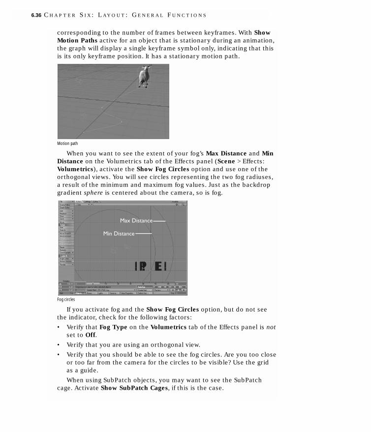
corresponding to the number of frames between keyframes. With ShowMotion Paths active for an object that is stationary during an animation,the graph will display a single keyframe symbol only, indicating that thisis its only keyframe position. It has a stationary motion path.

Motion path

When you want to see the extent of your fog’s Max Distance and MinDistance on the Volumetrics tab of the Effects panel (Scene > Effects:Volumetrics), activate the Show Fog Circles option and use one of theorthogonal views. You will see circles representing the two fog radiuses,a result of the minimum and maximum fog values. Just as the backdropgradient sphere is centered about the camera, so is fog.

Fog circles

If you activate fog and the Show Fog Circles option, but do not seethe indicator, check for the following factors:

• Verify that Fog Type on the Volumetrics tab of the Effects panel is notset to Off.

• Verify that you are using an orthogonal view.

• Verify that you should be able to see the fog circles. Are you too closeor too far from the camera for the circles to be visible? Use the gridas a guide.

When using SubPatch objects, you may want to see the SubPatchcage. Activate Show SubPatch Cages, if this is the case.


SubPatch cages

The Show Handles option will display reference handles for thecurrent item when you are moving, rotating, or stretching. These arebased on the item’s local axes at its pivot point. (See Chapter 7 for moreinformation.)

Rotation handles

The Show IK Chains option will display a solid line for the IK chainand a dotted line for the direction of the item reaching for the goalobject.

IK chains

The Show Target Lines option turns on/off the line that connects totargeted items.

L I G H T W A V E 3 D 7 6.37

Overlay ColorThe color of the overlays for the field chart, limited region, fog

circles, and so on, can be set to any of the standard wireframe colorsusing the Overlay Color pop-up menu.

Shaded Display OptionsThe following options affect the shaded OpenGL display

characteristics.

In the Max OpenGL Lights field, enter the maximum number, up toeight, of light sources you want used in the display. This lets you seetheir effect right in the viewport in real-time.

OpenGL light

Activate OpenGL Textures to show image-mapped textures (notprocedural) in the viewports. Use the size pop-up menu to select thepixel resolution (e.g., 128 x 128). Lower settings will update faster anduse fewer system resources.

Left: 64 x 64. Right 512 x 512

Usually the first Color or Diffuse image map layer is shown in theTexture mode viewports. Enable Show Current Texture Editor Layer toshow the Texture Editor's current layer instead, if applicable.

The OpenGL Pixel Blending option will activate a smoothing displayfunction.


OpenGL Pixel Blending. Left: Off. Right: On

The OpenGL Reflections option lets you see the effects of image-mapped reflections (not ray-traced) in a Layout window.

OpenGL reflection

NOTEThe reflection mapping will be visible only when the surface Reflectionvalue is greater than 50 percent.

The Faster Highlights option makes the display of (specular)highlights faster, but less accurate. Note that the difference may notalways be visible and will vary depending on circumstances.

The OpenGL Transparency option activates a surface transparencyfeature in viewports. This lets you see through transparent surfaces inshaded viewports! (Of course, this is only an approximation of youractual rendered result.) This setting also controls Modeler’s display oftransparent surfaces, if the Hub is running. Modeler will remember thelast used setting, if you aren’t using the Hub.

L I G H T W A V E 3 D 7 6.39

Camera View Tab

Camera View tab

Camera View BackgroundLightWave lets you choose how you want the Layout interface

background to appear when using the Camera view (only).

Blank is the default choice and will show nothing but the normalblank gray background. Backdrop Color uses the color selected as theBackdrop Color on the Backdrop tab of the Effects panel (Scene >Effects: Backdrop).

NOTEThis setting is independent of how the background will appear in arendered image.That is, if the Backdrop Color is orange and there isa Background Image set, the viewport background will still appearorange if this option is set to Backdrop Color.

Background Image lets you see the image set as the BackgroundImage on the Compositing tab of the Effects panel (Scene > Effects:Compositing) in the Camera view. You can use it to help you alignobjects that need to be positioned properly with respect to thebackground image. It will also show when you make preview animationsusing the Camera view.

Background image


LightWave also allows you to use a preview animation as abackground, if use the Preview option. This requires that you to have apreview animation loaded into memory of course. This can be one thatwas just generated or one that was loaded.

NOTECreating and loading a preview animation is discussed in Chapter 8.

The preview animation will load starting at the upper-left corner ofthe Layout window. Make sure to use the same size interface as you didwhen you generated the preview for easy reference. It will also loadbeginning at frame 0 no matter what the frame was originally when theanimation was created.

This feature is invaluable for creating moving composite shots andmattes. Using an image sequence composed of live footage as thebackground image, create a preview animation of that sequence with noobjects or grid. Save the preview and load it in later when you need it.The preview animation will update much faster than using the originalimages as a background.

Show Safe AreasIf your animation will be viewed on a television, be aware that

viewers will not see the entire image. Select Show Safe Areas to toggleoutlines in a Camera view that indicate the safe text (the inner border)and safe action areas (the outer border) for television. To allow for thedisplay differences of different brands and designs of television sets, youshould use this guide to ensure that text and action elements in youranimations remain on screen when it is important that they be seen.

Safe areas

NOTEThese are reference guidelines and are not absolute positions.

Alternate Aspect OverlayThe Alternate Aspect Overlay setting lets you overlay the borders of

an alternate frame aspect ratio, within the normal frame in camera

L I G H T W A V E 3 D 7 6.41

viewports. This information-only display mode can be used tosimultaneously compose shots for both film and television, for example.The default alternate aspect ratio is 1.85.

Alternate Aspect Overlay

OpenGL FogIf you have the OpenGL Fog option active, you can see an

approximation of your fog settings from the Camera View as well.

OpenGL fog

Show Field ChartThe Show Field Chart option turns on a crosshair chart similar to a

12-field chart as used in the film industry. It divides the camera view intoquadrants, with each quadrant having 12 segments.


Field chart

OpenGL Lens FlaresThe OpenGL Lens Flares option lets you see lens flares right in a

viewport while you use the Camera view. If you have the Lens FlaresOptions panel open you can interactively make changes to the settings.

OpenGL lens flares

Schematic View TabsSeveral display options for the Schematic view appear on the

Schematic View tab.

Schematic View tab

Link Style. Left: Straight. Right: Right Angle

L I G H T W A V E 3 D 7 6.43

Link Direction. Left:Vertical. Right: Horizontal

Show Goal Links active

If the Drag Descendants option is active, moving a parent will moveall its children as well.

If the Show Plug-in Links option is active, motion dependencies frommotion and channel modifier plug-ins are shown as dotted black lines.

Here, Cyclist has been added to Talk on Corner.The Cycle Controller for the plug-in is ControllerNull.Thus,Talk on Corner’smotion is dependent on ControllerNull.

LAYOUT COMMANDSThe Layout interface is built on a command system. Buttons, keyboard

shortcuts, plug-ins, etc., essentially submit commands to the underlyingLayout engine, which performs the actual operation. You can view a listof the last commands that were executed by choosing Layout >Commands > Command History.

Command History window


You can execute a single command by entering it—with any requiredparameters—in the input field at the bottom of the Command Historypanel. Clicking an entry in the list will automatically copy it to the inputfield—you can edit the command before hitting the ENTER key.

Click an entry to select it

Alternatively, you can choose Layout > Commands > Command Inputand enter a command into the dialog that appears.

You can save a list of commands to a file by choosing Layout >Commands > Save Command List.

Obviously, using the user interface to execute commands is far easier,and most users do not need to use these functions. However, you mightuse the information from command history to reproduce or documentthe exact operations you made interactively. Moreover, some commandsare not available to menus and keyboard shortcuts, thus, running themdirectly is the only way to execute them.

To execute commands in a programmatic fashion, use LScript. Thedocumentation for LScript is included on the LightWave CD.

LSCRIPTS MENU TABThe LScript menu tab contains tools for creating and running

LScripts. as well as some actual LScripts that you can use in Layout. Seethe on-line LScript documentation for more information.

LScript CommanderLScript Commander can be used to create a command sequence or an

actual LScript for Layout. A command sequence is merely a list of

L I G H T W A V E 3 D 7 6.45

commands that can be executed in order from top to bottom. An LScriptis similar, but more powerful. In an LScript, for example, you can haveprogramming type commands like loops and so on.

The LScript Command panel

The top black area is the session window and can contain either acommand sequence or an LScript. You can type directly into this windowor copy commands from either of the bottom two tabs.

The Events tab contains a list of commands from operations thathave occurred in Layout. The Command Sequence tab contains a list ofall available commands. You can copy commands from either list byselecting them (multiple selection is supported) and then right clickingon the list. Once copied to the session window, you can edit the lines asneeded.

You can execute single commands by entering them in the Commandfield.

You can define and use multiple sessions. The left Session pop-upmenu contains controls to start a new session, load an existing one, savethe current session to file, and close the current session. The ClearSession option erases all of the commands in the current session. Alsoon this menu are options to convert a command sequence into anLScript and convert an LScript into a command sequence.

The pop-up menu to the right is used to choose the current session, ifthere are more than one.

Click the Execute button to run the current command sequence orLScript.


Clicking the Install button will add the script to the Macros group onthe LScript menu tab.

Select HierarchyThis LScript will select the entire hierarchy that the currently

selected item belongs to.

Select ChildrenThis LScript will select all of the children (and their children) of the

currently selected item.

SHOCKWAVE3D EXPORTERThe Shockwave3D Exporter (Scene menu tab) allows the user to

export Layout's current scene as a Macromedia® Shockwave® file (.W3D).This encapsulated file contains all of the information needed to recreateobjects, surfaces, and animation, as well as the image files used in thescene. The exported file can then be integrated into Macromedia®Director® as a Cast Member. With this exporter, the user can combinethe content creation toolset of LightWave with the interactivefunctionality of Macromedia Director, creating an integrated solution fordistributing multimedia content.

NOTEAlthough the exported file can be previewed in LightWave, you musthave Macromedia Director in order to create files for distribution.More information on Shockwave and Director can be found atMacromedia's website: http://www.macromedia.com/software/director/.Also, be sure to check out NewTek's Shockwave3D discussion in theNewTek discussion forum at http://www.newtek.com/discuss.

L I G H T W A V E 3 D 7 6.47

The Shockwave3D Exporter Interface.

The top portion of the panel contains controls for the exportselections, quality controls and preview options for the exported file.The options for these items can be found on the tabs located on thelower portion of the panel labeled Objects, Animation, Textures, andCameras. The file location is determined when the Ok button is pressedand the file dialog appears.

Some things should be considered when modeling and animating ascene that will be exported with Shockwave3D. Because this media ismeant for distributing large multimedia files, many of the exporter'sfeatures and options keep performance issues in mind. Please take amoment to read through this section and familiarize yourself on howLightWave and Shockwave3D are compatible with each other. It couldsave you a considerable amount of time on your next Shockwave3Dproject.

Export SelectionThis list of items determines which portion of the scene will be

exported into the .w3d file. The Scene Structure option preserves theparenting hierarchy of your scene, while Cameras, Lights, Surfaces,Objects, Animations, and Texture Maps all control which elements ofthe scene will actually be exported. Simply activating these checkboxeswill include these items in the file.


Selecting which items to be exported.

Quality ControlsFor three of the item export parameters, Objects, Animations, and

Texture Maps, there are additional controls to adjust the quality of theassets used in the .W3D file. Since the .W3D file is encapsulated, theseadjustments will have no effect on the items or settings within yourLightWave scene. Only the data within the exported file will be affected.If you are concerned about download times, or performance issues,modify these parameters to create smaller or faster playing files.

Adjusting the quality levels.

Preview OptionsOn the Microsoft Windows platform, the Shockwave3D Exporter has

the option of playing a Shockwave-enabled preview window. You cansimply choose the resolution of the preview window, and on export, aseparate window will open displaying the exported file. Thisrepresentation of the exported scene is how it will appear as a CastMember in Macromedia Director.

Selecting the Preview window size.

ObjectsThe Shockwave3D Exporter exports polygonal models and frozen

SubPatch objects from the scene into a .W3D file. To increaseperformance, Shockwave3D also creates multiple Level Of Detail (LOD's)objects. These features are automatically enabled and their parameterscan be controlled in Macromedia Director. Unfortunately, objectmorphing is not supported in Shockwave3D.

L I G H T W A V E 3 D 7 6.49

The options tab for Objects

By activating the Enable Toons and SDS (cel shading and subdivisionsurfaces) feature, the objects are exported with the neighboring meshinformation needed by these features in Director. Since this optionincreases the size of the exported file, deactivate Enable Toons and SDSif these features won't be utilized in Director. (Note that the SDS modifiermust be added in Lingo.)

The Crease Angle determines how much of an angle is allowedbetween neighboring normals before polygons are joined together. Thisparameter is used as a geometric smoothing angle when objects arebeing optimized. Normal Deviation sets a limit that normals can deviatefrom when the exporter creates any LOD's. The smaller the number, theless likely the reduced model's normals will be drastically different thanthe original object.

The Shockwave3D Exporter will remove very small triangles fromyour models and does not support 1 or 2 point polygons. Base verticesare points that will be removed last during any compression or polygonreduction during the export. To use the base vertices feature, create aPoint Selection Set in Modeler named base verts. Any points includedwithin this set will be given priority when the exporter does any of itsoptimization functions, and will be reduced last.

Animating ObjectsAll items (lights, cameras, objects, and surfaces) should have unique

names. Also, only two of LightWave's scene items are capable of beinganimated with Shockwave3D, objects and bones. Thus, you cannotdirectly animate cameras or lights. However, you can animate a nullobject and parent the camera or light to the null object and achieve thesame effect. Hierarchy controls exported from LightWave include bothitem parenting and pivot point manipulation.

The options tab for Animation.

The user can select the range of the animation to be exported bydefining the Start and End fields located on the Animation tab. By


default, these initial values will match the start time and end time of thecurrent scene. These options are not available if Force Sampling is notactivated.

In LightWave, animation is created using keyframes. The exportertakes the motion defined by these keyframes and all the motion'smodifiers from a single frame and creates what is called a Sample. This ismuch like freezing the motion curves of an item, but for that singleframe.

These samples are then used in Shockwave as the keyframes of theanimation. By adjusting the sample Interval, you control how often theexporter samples the animation. For example, a value of five will exporta sample every fifth frame. This is very similar to LightWave's FrameStep parameter.

The smaller the Interval is, the more samples the exporter willcreate. In order to store this information, a larger file is created and willtake longer to download and store in memory. Having the sampleInterval set as high as possible will reduce the overhead needed to playthe animation. However, having an incredibly high value won't solve allyour problems either.

The Shockwave3D Exporter will rotate an item based on the fastestroute from angle A to angle B. Obviously this is not how LightWaveworks. For this reason, it may be necessary to export a scene using amuch smaller sample Interval. This will give the Shockwave player morekeyframes to rotate an item with and will match the LightWave scenemore accurately.

Animating BonesAnimating bones is one of the more advanced features of the

Shockwave3D Exporter. However, one thing to keep in mind is thatShockwave uses a different bones system than LightWave. The majordifference between the two systems is how points get bone influencesassigned to them. The animator should make all influence adjustments inweight maps as opposed to LightWave's bone setup options. For thisreason, all bones must have a weight map assigned to them. Any pointnot assigned to a weight map is assigned to a null bone located at theroot of the hierarchy. Also, unlike LightWave, a Bone's rest position isdetermined on frame 0.

Surfacing and TexturingSurfacing is converted from LightWave to Shockwave as closely as

possible. This includes, Color, Luminosity, Diffuse, Specularity,Glossiness, Reflection and Transparency. However, because therendering methods (rendering vs. OpenGL) used in these twoapplications are setup differently, some tweaking may be needed to thesesettings in order to get the desired effect.

L I G H T W A V E 3 D 7 6.51

All surface mapping is converted to UV mapping when exported.However, Shockwave does not support the use of layered textures.Therefore, any surface channels that use layered textures must beflattened and turned into a single texture by using LightWave's surfacebaker. Texture mapping in the diffuse, glossiness, reflection, orspecularity channels also works a little differently than LightWave. Anymaps used in these channels are projected environmentally inShockwave3D, thus ignoring any user-defined mapping.

Double-sided surfaces are not supported in Shockwave and must becreated using actual double-sided geometry.

The options tab for Textures.

The image resolution values.

By overriding the texture size, you can force the Shockwave3DExporter to globally reduce the image size of the textures in the .W3D file.For example, if you had 512 x 512 images, you could reduce them downto 64 x 64 by simply selecting Override Size and choosing 64. DisableAlphas simply disables the alpha channels on all the images.

Cameras

The options tab for Cameras.

The Selected Camera values.


The Camera pop-up menu lets the user decide which camera shouldbe exported. If All cameras is selected, the camera data for all thecameras will be embedded within the exported file. Switching betweencameras is handled within Macromedia Director.

The Fog pop-up menu lets the user choose which camera will havethe fog settings attached to them. Fog settings exported include, FogType, Fog Color, and Fog Falloff.

The Backdrop drop-down menu lets you determine which camera willhave the scene's backdrop color setting attached to them.

NOTETake note of the aforementioned animation limitation when animatingCameras.

LightingShockwave3D supports many of LightWave's internal Light types,

Distant, Spot, and Point, as well as ambient light. The lighting parameterssupported by Shockwave3D include Light Color, Light Intensity, and SpotAngle.

NOTETake note of the aforementioned animation limitation when animatinglights.

VRML97 EXPORTERThe VRML97 Exporter plug-in (File > Export > Export Scene as

VRML97) creates a VRML97 World based on the current scene. The VRMLoutput complies with the ISO-VRML97 specification. The objects in thescene may be saved as separate files into the Content Directory or analternate path. The following list shows some highlights:

Accurate Translation• Keyframed hierarchical animation

• Light intensity envelopes, including ambient

• Non-linear fog

• Color image texture mapping using projection or UV maps

• Solid, non-linear gradient and image backgrounds

• Support for SkyTracer warp image environments

• Particle animation with single-point-polygon object to PointSet nodeconversion

• Two-point-polygon object to IndexedLineSet node conversion

L I G H T W A V E 3 D 7 6.53

• SubPatch object morph capture (for capturing morph, displacementmap and bone effects on SubPatch objects).

High-Performance Output• 3-D Sounds

• Level-of-detail object replacement animation

• Object instancing

• Vertex color and lighting support

• Multiple custom viewpoints

• Custom VRML nodes

• Touch activated behaviors

• Viewer proximity activated behaviors

• Object visibility activated behaviors

• Objects output as prototypes (PROTO) definitions (optional)

• Scene object ignore

• Standard object viewpoints (optional)

• Optional embedded objects for single file scene output!

• Optional lowercase conversion for embedded object/image filenames

• Direct avatar navigation speed control

• Improved compliance for export to VRML97 editors, includingconversion of illegal VRML97 names (like 2LEGS or MY LIGHT), andreflection of illegal negative scaling

VRML Creation Settings

Output .wrl is the file path for the VRML97 World.

Author is comment text to embed in the file.

Use Prototypes is used to define and use objects in the VRML scenemore efficiently. Some older importers may not like this, but it isrequired for morph capture.


When Lowercase Filenames is enabled, the filenames used in the filecan all be converted to lowercase. This can be helpful on UNIX-basedWeb servers, where filenames are case sensitive, and links withmismatched cases will fail.

Use Embed Objects to include the geometry for all meshes in themain VRML97 World file. This may be more convenient, but for complexworlds, or reusing objects, it is less efficient. Using external object filesallows the main world to load faster, and display bounding boxes whilethe objects are loaded. This option must be off for morphing objects aswell as LOD objects (loading them all at once would defeat theirpurpose!)

If Overwrite Objects is enabled and the Embed Objects option is notused, external object files will be created for objects in the scene. If theobjects already exist, this option must be enabled to overwrite theobjects, thus updating surface or morph changes.

Local .wrl Path is the file path on your machine where external VRMLobjects will be found and/or saved. This will default to the currentLightWave Content Directory.

VRML Object URL is the URL where browsers will search for externalobjects, this should be the web equivalent of the local path (e.g.,HTTP:\\WWW.SOMEPLACE.NET\VRML_OBJECTS\).

Text entered into the Texture URN field will be pre-pended to texturemap image filenames, as an alternate texture location. This shouldfacilitate work with libraries like the Universal Media textures. Thisinformation, when specified, will appear in addition to the regular URLelements.

On the Scene Item pop-up menu, select a scene element to which youwant to apply the settings on this tab.

The Sensor Type is the sensor used to start the item's animation.

For some sensor types, like Proximity, a distance range is required.When the viewer approaches the item within the Range, the animation istriggered.

L I G H T W A V E 3 D 7 6.55

Alternate Trigger is an alternate item to serve as the animationtrigger for this item.

On the Object pop-up menu select an object whose settings will beedited on this tab.

The Ignore Object option will exclude a selected object and itschildren objects from export.

Use Attach Sound to add a sound effect, triggered with the selectedobject's animation. Enter the URL for the audio file triggered in the URLfield. You can also set the volume and whether the sound should belooped once it has started.

The Record Morph option saves a Morph Object—a special animatedProto object—in place of the standard external object files. This requiresthat the exporter step through the animation and capture the deformedmesh at different times. The deformed positions are used in aCoordinateInterpolator node hidden in the morph object. This currentlyworks for SubPatch objects.

First Frame is the starting frame for the Morph Object animation. LastFrame is the final frame in the morph capture for this object. Frame Stepis the number of frames between captured morph keys. Making this toosmall results in huge objects; making it too large results in an animationthat is not smooth or points with motion that is too linear.

Enable Loop to repeat the morph animation, once it has beentriggered.

Enable the AutoStart option to make the animation start as soon asthe world is loaded.


Use the Navigation Mode pop-up menu to set the initial navigationmode for Web browsers.

Enable Headlight for good defaults in dark places.

Standard Viewpoints creates extra ViewPoint nodes (top, left, etc.)for scene and external objects.

Avatar Size lets the browser set appropriate movement for thedimensions of your world.

Global Light Scale globally scales all light intensities.

Environment Images are warp images generated by SkyTracer. Thesemap nicely to VRML's idea of environment mapping. Enter only thebasename portion of the image files. (For example, if you hadSKYWARP__BACK.JPG, SKYWARP__FRONT.JPG, etc., you would enter SKYWARP.)Note that any panoramic images should be compatible, provided theyare renamed to match the SkyTracer filenaming convention.

The text in the Image URN field will be pre-pended to the imagefilename and added to the list of URLs for the environment image.

So What is VRML?VRML, also known as ISO-VRML97 (ISO/IEC 14772-1:1997), stands for

Virtual Reality Modeling Language. It is a standard for describing 3Dobjects and scenes via the Internet.

Like HTML-based web pages, VRML worlds can contain links toremote files. However, rather than using text or images for links, VRMLuses 3D objects. As a result, the Web browser for VRML resembles a 3Danimation program or video game more than a word processingprogram.

VRML worlds can be embedded in HTML pages and vice versa. VRMLmodels are based on either primitives, like spheres, cubes, and cones, or,more likely, sets of points and polygons. Since the latter is basically theapproach used by LightWave 3D's polygonal models, there is a prettygood match between LightWave scenes and VRML worlds.

Before you can view any of your VRML creations, you'll need to get aVRML 97 Browser. The VRML files produced by LightWave are text files

L I G H T W A V E 3 D 7 6.57

that follow LightWave's style of separate object and scene files. This isnot a requirement of VRML, but a powerful feature that lets a VRMLscene include objects from different files, even from some remote library.

These external objects in the scene file consist of a file URL, abounding box, and a set of position, rotation and scalingtransformations. The bounding box information is used by browsers torender stand-ins while the objects are loaded.

VRML scenes also include multiple point lights, directional lights, andspot lights with adjustable cones. The VRML equivalent of the LightWavecamera is a viewpoint. The exporter will add a named viewpoint for eachcamera in the LightWave scene, which browsers can use to jumpbetween points of interest or standard views. In addition, VRML objectscreated by LightWave may include a set of standard viewpoints for theobject.

AnimationObjects in your LightWave scene that have keyframes in any motion

channels will be given linear motion keys in the VRML file, throughPositionInterpolator and OrientationInterpolator nodes.

The Pre Behavior and Post Behavior set for the channels in theLightWave motion has a critical influence on the VRML behavior of anobject. If the Pre behavior is set to Repeat, the motion will begin whenthe world is loaded and keep on playing. Otherwise the motion will beginwhen the item is triggered. If the Post behavior is set to Repeat, theanimation will loop until re-triggered, otherwise it will stop after playing.

The default triggering is a click (TouchSensor) on the object thatcauses the animation to run from the beginning. Currently, theTouchSensor switch is placed on the highest-level animated object in ahierarchy, and triggers the animation of all the children simultaneously(as one would expect).

Morphing in VRML uses a CoordinateInterpolator node. The node ispart of the Proto in the object file, if morph data has been captured. Forthis reason, Prototypes should be enabled and embedded objectsdisabled for morphing worlds.

SurfacesCurrently, double-sided surfaces are not supported in VRML97. Thus

LightWave 3D objects with polygons whose surfaces are double-sided aretranslated as if they weren't double-sided. VRML objects that seem to bemissing polygons may actually have double-sided surfaces that need tobe either flipped or aligned in Modeler. If the surface is truly meant to bedouble-sided, you will need to model the geometry with double-sidedpolygons.

If your model has a texture map image associated with it (color only,not diffuse, specular, etc.), there are a few tricks that can minimize the


nuisance of hand-editing your VRML models. Since some browsers willhave to load the image named in the object, that image name, saved inthe LightWave object, is critical.

It pays to use LightWave's Content Directory system properly, so thatthe image path will be relative to that content directory (i.e.,IMAGES\WOOD.JPG rather than C:\NEWTEK\IMAGES\WOOD.JPG). You may alsowant to move the image to the Content Directory so that the name in theobject will have no path, and browsers will seek the image in the samedirectory as the object.

In any event, wherever the VRML object finally resides, you will wanta matching directory hierarchy where the browser will find the image oryou can just edit the VRML file.

Another image issue is that of file format. JPEG and GIF images arealmost universally supported on the Web, but the PNG format is gainingacceptance as a modernized, yet unencumbered, replacement for GIF.JPEG images are nice and small, and compression artifacts should bevirtually invisible at Web/VRML resolutions. If you have nice high qualitytexture images for your rendering work and want VRML versions, makesmaller JPEG versions of the images for the Web. Large textures may belimited by the browser's rendering engine in most cases anyway. Whenyou install the VRML model, just use the smaller JPEG image or edit theVRML file.

LightWave VRML ImplementationThe organization of LightWave's VRML object output follows that of

LightWave's own object format. A list of XYZ coordinate triples describethe vertices in the object. For each surface, there is also anIndexedFaceSet node that holds the polygons with that surface,described as a number for each point in the polygon, which refers to anentry in the main list of point coordinates. There may also be anIndexedLineSet node or a PointSet node containing any two-point andone-point polygons.

If the original LightWave object had a color texture map image, therewill be an image file name and a set of texture coordinates. Texturecoordinates, also known as UV coordinates, are 2-D pixel positions in animage. They describe how the image lies on the 3-D surface by pinningcertain pixels to each polygon's vertices. These values can be calculatedfrom LightWave's mapping and texture size settings.

In the case of planar UV mapping, U and V are simply x and y, (for Z-axis planar). Spherical UV mapping yields U and V coordinatessomewhat analogous to longitude and latitude, with the U's all bunchingup at the poles. Cylindrical mapping uses U's from the spherical case,then the V's are the coordinate lying along the texture axis. If the

L I G H T W A V E 3 D 7 6.59

LightWave texturing is using UV mapping already, then these coordinatesare used, since VRML texture coordinates are defined in a per-polygonfashion (i.e. discontinuous UVs).

The entire object may be embedded in a VRML Anchor, which makesit an active link on the Web. If you supply a URL for the object when youcreate it, then anytime that object appears in a scene, it will act as aclickable link to some other page. This should be used sparingly, as itcan be quite annoying to keep jumping around the web when you're justinspecting an object.

The uses for URLs in your objects can range from booby traps or adsfor your favorite Web site, to inventory data for some widget. A very niceexample is a VRML origami site, where each step in the folding of apaper menagerie has a simple model with a link to the next stage. This issimilar to the VRML level-of-detail mode, where multiple models aregrouped together and the viewer's distance determines which model, ifany, is actually rendered.

Performance NotesAlthough the VRML format is capable of describing complex scenes,

current 3-D browsers are limited by the real-time rendering capabilitiesof their underlying computers. Thus, exquisitely crafted models withpainstaking detail, suitable for those print-res close-ups, may failpainfully when they enter the realm of VRML renderers. To avoid thetwin perils of long download times and slow rendering, remember: thefirst key to VRML success is efficient, low-polygon count modeling.

Similarly, elaborate layers of diffuse, specular, and luminositytextures, whether images or algorithmic, will not survive any conversionto VRML. Don't even ask about bump maps, displacement maps, orsurface shaders. Love it or leave it, VRML supports a single image mapfor a color texture, as well as diffuse color, specular, and transparencyvalues. Since that texture image may very well have to fly through amodem, you'll probably want to keep it small.

Elaborate textures and lighting can be baked into a model's 'imagemap however, and lighting effects and coloring can also be baked intovertex color maps.

PointSet objects are stored most efficiently if there is only one surfaceper object. Otherwise, duplicate references to the vertices are required.For large scenes, this could be significant.

Scene TagsMany of the VRML attributes set in the exporter UI are stored in the

Lightwave scene file as comments. These comments can be viewed andedited on an item-by-item basis with the Comments (Layout Generic)plug-in. These Comments should be formatted as <Tag>=<value> wherethe Tag is one of the following:


Item Tag Name/Usage Description

URL URL=<url> (URL="http://etc.")Item URL, overrides object and children's URLs.

SOUND SOUND=<url> [<volume> <loop?>]Sounds can be added to objects. Currently these aretriggered with any animation.

TOUCH TOUCH=Trigger when mouse is over object (mouse grope).

PROXIMITY PROXIMITY=W H DTrigger if viewer enters active region (WxHxD).

VISIBILITY VISIBILITY=Trigger when viewer sees object.

INCLUDE INCLUDE=<filename>Dump contents of file directly into output.

IGNORE IGNORE=Skip this object and its children.

TRIGGER TRIGGER=<object>Other object for sensor.

VRML VRML=nodeName{node fields}Node creator, dump node from comment into file.

LABEL LABEL=<text>Create text node.

MORPH MORPH= <start> <end> <step> <loop?>Morph animation capture. Creates externalMorphObject.

LOD LOD=<objectfilename> [<range>]Level of Detail node. Use multiple tags in order ofdecreasing complexity (increasing range).

Camera Tag Name/Usage Description (stored in firstcamera in scene)

NAVIGATE NAVIGATE=<type> [<speed>]NavigationInfo Type is one of NONE, WALK,EXAMINE, FLY, or ANY. Browsers may restrict usernavigation with this.

ENVIRONMENT ENVIRONMENT=<basename>Override scene background image with URLs forfront, back, left, right, and top images named likebasename__front.jpg, etc.

HEADLIGHT HEADLIGHT=NavigationInfo Headlight on, if present.

L I G H T W A V E 3 D 7 6.61

SPREADSHEET SCENE MANAGEROften you want to edit certain properties of an item, and luckily,

changing the values and properties of items is simple in Layout. Butwhat if you need to change the properties for 20 objects? TheSpreadsheet Scene Manager (Scene > Utilities: Generics > Spreadsheet)organizes these properties and lets you edit a wide range of valuesquickly and easily.

The Spreadsheet Scene Manager interface.

The Spreadsheet Scene Manager has six sections: Workspaces, Filters,Items, Properties, Timeline, and the Edit Controls. Many of these areashave Expand and Collapse controls, so you can adjust which sections arecurrently displayed. A message bar above the Edit Controls informs youabout the tasks performed.

WorkspacesYou can use the Spreadsheet to customize settings and options that

are displayed in the Manager’s panel.

Whether creating a workspace makes editing easier for you or savesyou time, you can configure almost every aspect of the display with thisplug-in.

Customizing the Workspace.

Settings are defined in the Spreadsheet as a Workspace. You create alibrary of commonly-used displays by using the Create Workspace andDelete Workspace commands. These two commands are found in thedrop-list beside the Workspace name.

The Workspace drop-list.


Creating a workspace:1 Customize the Workspace to fit your display needs.

2 Apply a Name to the Workspace by entering text in the Workspacename field.

3 Select the Create Workspace command in the drop-list menu.

Once a Workspace is created, the name of the Workspace appears inthe top portion of this drop-list menu. To revert to the settings saved inthis Workspace, simply select its name from the drop-list. This will loadthe settings for the selected Workspace and reconfigure the interface tomatch the saved parameters.

To remove the current Workspace from the drop-list, select the DeleteWorkspace command from the drop-list. A confirmation dialog will askwhether you want to delete the Workspace from the scene file. Once youdelete it, the Workspace name is also removed from the drop-list.

NOTEWorkspaces are saved with the scene file.

OptionsThe Spreadsheet Scene Manager has options for customizing how the

Spreadsheet tools function and how information is displayed. A check-list contains a list of General, Display, and Workspace options for theSpreadsheet.

The Options drop-list menu.

You can use this check-list (shown above), or you can access thetabbed interface by selecting the first item in the list, labeled Options.

L I G H T W A V E 3 D 7 6.63

FiltersA complex animation might have dozens, if not hundreds, of items

within the scene. Searching through this almost endless list to find aparticular group of items can often be frustrating.

Using the Spreadsheet’s filtering options, you can narrow the listdown to make it easier to navigate, so you can get to your items faster.

You activate the Spreadsheet’s filtering tools with the Filter checkbox. Then you enter the characters for your search in a text field so thatyou can search through the item names in your scene. The filterparameters determine how the search is conducted.

The Filter’s parameters drop-list

To use a Filter:1 Create a scene with three nulls named leftLeg, leftArm, and rightArm.

2 Select Scene > Generics > Spreadsheet.

3 Activate the Filter option.

4 Enter the word “Left” in the text field.

5 Select the Containing filter parameter.

The Manager then searches through the items listed in your scene,looking for names with the word “Left.” The resulting list of items reads,leftLeg and leftArm. Because the item rightArm doesn’t contain the word“Left,” it is omitted from the filtered list.

Activate the Case option to refine the search parameters; Caseincludes the upper or lowercase characters of your entry in the search.In the example above, activating the Case option results in no items inthe filtered list because the search characters contain an uppercase “L”in the word “Left.” The item names use a lowercase “l” and since theydon’t match, they are omitted from the filtered list.

NOTEThe filtering tools are not available in the Hierarchy listing mode.

After you create a working filter, you can add it to a favorites list byselecting the Create Favorite… command in the Favorites drop-list.


The “left” Favorite in the Favorites drop-list.

This command prompts a dialog window that requests a name foryour search parameters. Later, you can quickly reselect the filter and itssettings by name. The new filter is placed at the top of the drop-list,above the Favorite commands.

Replacing and Deleting Favorites from this menu is as easy asselecting a filter name from a list. This list of Favorite filters is savedwithin the animation’s scene file.

NOTEThe section of the Spreadsheet Scene Manager that contains the filtercontrols can be minimized by using the expand and collapse button.

Mouse FunctionsThe mouse has several different functions in the Spreadsheet Scene

Manager.

LMB: Selects and highlights a field.

SHIFT + LMB: Range selection.

CTRL + LMB: Non-continuous selection.

RMB: Opens the cell’s Options menu.

In the Items List:

Double-click: Selects the object in Layout

The Item ListItems in a scene are displayed in the Spreadsheet Scene Manager’s

Item list window.

The Items list portion of the Panel.

L I G H T W A V E 3 D 7 6.65

Items in this list are determined by any active filters and by thecurrent Display Mode. Use the plus (+) and minus (-) icons to open andclose an item’s channel lists.

The Display Mode drop-list.

By selecting a Display Mode you specify the items for theSpreadsheet to include and also how the Spreadsheet is displayed. TheHierarchy display mode lists the items by creating collapsible trees ofparent and sibling items. The All Items mode lists every item in thescene, while the Objects Only, Bones Only, Lights Only and CamerasOnly modes refine the list to include only certain types of items.

The Sort Order mode determines how the items are actually listed inthe window.

The Sort Order drop-list.

The Natural and Reverse Natural modes list the items in either theorder or the reverse order that they were loaded or created in the scene.Alphabetical and Reverse Alphabetical will display the items in afashion that is easy to locate individual items.

In the Selected Items display mode, you have two additional sortingmodes: Selected and Reverse Selected. These modes refer to how theitems were selected in Layout.

The Item Selection options menu.


The Property CellsThe Property Editor is where you find most of the Spreadsheet’s

functionality. Here you can select and edit an item’s individual value orgroups of values for multiple objects. This list of cells is organized usingrows and columns, much like a spreadsheet used in businessapplications. That is why this plug-in is called the Spreadsheet SceneManager.

The Property Editor.

Listed in the columns, left to right, are the item properties supportedby the Spreadsheet Scene Manager. These properties are organized inlists of related attributes called Banks. You can select which banks arecurrently displayed by selecting them from the Banks drop-list.

The Banks drop-list.

You can view more than one Bank at a time. You can add and deletedifferent Banks from the Property Cells by using the plus (+) and minus(-) button located by the Banks drop-list. Use the slider-bar at thebottom of the Property Cells to adjust which bank(s) are currentlydisplayed in the viewing area.

Editing CellsThe Property cells contain the values for each of the properties, for

all items. The values range from numerical values to file names,depending on which property you are editing. Because the Spreadsheet

L I G H T W A V E 3 D 7 6.67

is a non-modal interface, when a value displayed in a cell is changed, theitem’s property is updated instantly. This lets you interactively changethe properties of each item and see their results in Layout’s viewport.

You can define this level of interaction from the Options check-list.Enable Apply Quick Edits Immediately to make changes as soon as themouse button is released. Otherwise changes are delayed until you hitthe Apply button.

There are two ways to edit the values displayed in an item’s propertycell. The first method is to edit the values directly in the cell.

1 Select a cell or group of cells to edit. This can include cells frommultiple columns, as long as they are of the same type. The interfacewill not allow you to mix value types.

2 Using the LMB, edit a selected cell. Once you let go of the mousebutton, the values for all selected cells will adjust accordingly.

The second method is to use Edit controls.

1 Select a cell as you did above.

2 Use the Edit controls located at the bottom of the interface to adjustthe values in the cells. These controls reflect the type of value youare editing, so they vary from cell to cell. The image below showsnumerical data (integers, percents, distances, angles, time and floats)but it gives you an idea of how the editing controls work.

Controls for numerical data:

The Edit controls used for numerical data.

The Edit controls allow you to edit the property cell’s values inabsolute or relative mode. You enter a value in the Change Value To fieldand choose an edit effect from the Effect drop-list. The effect selects howthe cell’s value will be altered when the edit is applied.

The available Effect options.

The Replace edit mode lets you make absolute changes to the cell’svalues. That is, when you apply the edit to the selected cells, the newvalue will replace the current values. For example, you select ten cellswith various values in each cell, and in the Change Value To field youenter a value of 2.0. When the edit is Previewed or Applied, the cells willnow all read 2.0.

The Add, Subtract, Multiply, and Divide functions are all relativeediting modes. They adjust the cell’s values relative to their originalvalues. In the example above, if you select the Add edit mode, all cellswill add the value 2.0 to their original values when you apply the effect.


By pressing the Apply button, you commit to the edit. You cannotundo these edits. For that reason, you can use the Preview and Resetbuttons to view the effect of the edit without actually applying the edit. Ifyou like the results of the previewed changes, simply press the Applybutton and the changes are made to the item’s properties.

NOTEThe Spreadsheet Scene Manager will notify you when you are editingin Preview mode by highlighting the Items, Property Cells, and Timelinepanels.

The Use Step field lets you increase the values in the selected cells byan exact increment. Simply put the increment in the field, select an editmode, and Preview or Apply the changes.

EnvelopesThe Spreadsheet Scene Manager also lets you edit any parameters

that can support envelopes. Like in Layout, these parameters areindicated by a small E button in the cell itself.

Envelopes can be edited in cells using the E button.

You can add envelopes by group selecting the cells and pressing the Ebutton. You can also use the SHIFT+E combination to remove envelopesfrom properties.

If the cell has envelope information stored in the channel, a keyframedivot appears on the left edge. If a keyframe is located at the currentframe, the divot turns yellow, and the value becomes editable. Otherwisethis value is ghosted.

Clicking this divot will create a key, and SHIFt+clicking will remove akey.

TimelineThe Spreadsheet’s timeline has much of the same functionality as

LightWave’s Scene Editor. You can edit an object’s motions by simplyadjusting an animation bar located on the timeline.

L I G H T W A V E 3 D 7 6.69

The Timeline Editor.

The long bars let you adjust the first and last frame for both theRender and Preview ranges. The fifth bar in the image above shows theposition of the current frame. By sliding these bars around, theSpreadsheet updates the settings in Layout dynamically.

You can adjust the Start Time and End Time by dragging the blackarrows beneath the frame hash marks.

The different colored bars display the frame range of the item’smotion. Small plus signs (+) within the bars represent the keyframes formotion. To change the start and end time of the motion, you must selectthe middle of the bar; you can then slide the bar to the left and right. Toscale the motion, you drag the left or right handles of the bar.

The slider located at the bottom of the Timeline both zooms andscrolls the viewable area.

Column SortingYou can change a column’s sort order by selecting the area under the

column’s header name.

The flags lets you determine the new sort order.

As you select columns, numbered flags appear that reflect the sortingorder. By defining this order, you can sort the item list according to itsproperties. For example, you can sort by an object’s Subpatch level,which will put all the items at level three at the top, and everything atlevel one at the bottom.


cchhaapptteerr7Objects in Layout

Chapter 7:Objects in Layout

LOADING AN OBJECT INTO LAYOUTWhen you set up a new scene, you will need to load the appropriate

objects into the scene. There are several ways to load objects into ascene.

To load an object file into a scene:1 Make sure your Content Directory is properly set. This will help with

any images that are referenced in the object file.

2 Select Items > Add > Objects > Load Object (or File > Load > LoadObject) and use the file dialog to navigate to the desired object file.(Note: Multiple objects may be loaded when more than one isselected in the file dialog.)

HINTAlternatively, you can press the + (plus) key on your numeric keypad,which adds the appropriate item based on the active edit modeselected at the bottom of the screen (i.e., Object, Bones, Lights orCameras).

If the object contains multiple layers of geometry, each layer will beloaded as a separate editable item in Layout. (See Chapter 20, “Multi-layer Object Standard.”)

L I G H T W A V E 3 D 7 7.1

As discussed in the prior chapter, an object is initially loaded so thatits local Origin is at the global Origin and its local axes line up with theworld axes.

Object loaded at Origin

When you move an object, you are repositioning its local Originrelative to the world Origin. The local Origin provides a single point ofreference for an object’s position in 3-D space. The object’s geometry isthen applied relatively to the local Origin’s new position.

NOTEActually, an object’s (numerical) position is first determined by its pivotpoint, discussed later, which can provide an offset amount to the localOrigin’s position. However, the pivot point is usually located at thelocal Origin, by default.

Object moved off the Origin

7.2 C H A P T E R S E V E N : O B J E C T S I N L A Y O U T

An object’s local Origin is established when it is modeled and is mosteasily seen when the object is viewed in Modeler—the local Origin is atthe point where all axes meet (i.e., equal to 0).

The location of the origin

Loading from ModelerFor information on how to load an object directly from Modeler, see

Chapter 20, “Layout Communication.”

Loading a Single LayerChoose Items > Add > Objects > Load Object Layer to load a specific

layer from a multi-layer object. A dialog will appear allowing you todefine which layer to load.

THE NULL OBJECT:THE STAR OF OBJECTSNull objects are special objects that can be used for many different

purposes in LightWave. Generally, they are used any time you need a 3-Dpoint that can be referenced. Nulls can act as a spot for lights or thecamera to watch, or a handle to help in manipulating a group of objects.They are often used with object/bone hierarchies to group majorcomponents and with Inverse Kinematics to act as goals for items toreach for.

Null objects appear in the Layout window as six-pointed stars orjacks; however, they never render in an image. Null objects, like thecamera and lights, will appear to grow or shrink in relation to objects asthe grid size is changed. They can be moved, rotated, scaled, and so on,just like any regular object.

L I G H T W A V E 3 D 7 7.3

A null object

To add a null object:1 Select Items > Add > Objects > Add Null.

2 Enter the name you wish to use for the null object in the dialog thatappears or accept the default name of “Null.”

NOTEWhen there are multiple items of the same type with the same name,a numerical suffix is added automatically (e.g., Null (1), Null (2), etc.).

Null objects are created by LightWave on a scene-by-scene basis andare not real objects that can be saved to disk. They remain part of thescene file, however, and will reload with the scene.

SAVING AN OBJECTYou should always save objects after you have altered their surface

settings.

To save an object:1 Make sure your Content Directory is properly set.

2 Select the object you want to save.

3 Select File > Save > Save Current Object to save...you guessed it...thecurrent object.

You can also use the File > Save > Save All Objects function to saveall objects in the current scene.

WARNINGUse Save All Objects with caution. Be sure it is what you reallywant to do!

Saving a CopyChoosing File > Save > Save Object Copy will allow you to save a

copy of an object using a new name, without affecting the object used bythe scene.


OBJECT VS. SCENE FILEThe important difference between loading an object directly versus

loading from a scene lies in what is stored in an object file versus what isstored in a scene file. The object file contains only the object geometryand surface settings—what the object looks like in its most basic state.There is no movement information in an object file. Loading objects froma scene is accomplished using File > Load > Load Items From Scene.Note that this will load all of the objects (and optionally the lights) in thescene.

Movement information is saved in the scene file. However, this is notonly movement in the normal sense, like moving an object from point Ato point B, but also includes movement of the points in their positionalrelationship to each other.

Moving points can change the shape of an object, sometimesdramatically. However, generally, the number of points and polygons, aswell as their relationship, remains the same.

WARNINGUnderstanding object and scene files is fundamental to understandingLightWave.

For example, say we had a flag object that was really just a flat-subdivided rectangle. In Layout, we could make the flag wave usingsomething called a displacement map—essentially this animates thepoints in the object. The displacement map settings are saved in thescene file. The underlying flag geometry and surface settings are storedin the flag object file.

SAVING A TRANSFORMED OBJECTChoose File > Save > Save Transformed Object to save an object with

any changes of location, rotation, scale, morph, skeletal deformation,displacement map, and so on. The new object is also saved relative tothe Origin. The current frame in Layout controls the state of the savedobject.

NOTEThere is a unique quality to an object that uses displacement mappingwith an image (planar, cylindrical, or spherical) as well as surface colormapped with an image.With the displacement map altering the object’sshape, the color map is also bent to follow the contours of thetransformed object. However, if you save this reshaped object withSave Transformed Object, it will now be permanently reshaped andthe surface color mapping will no longer match.

L I G H T W A V E 3 D 7 7.5

CLONING ITEMSIf you want to use an item that is already in your scene, you can just

choose Items > Add > Clone Current Item. The new item will inherit allof the source items properties and motion. As such, this can be a realtime saver.

REPLACING, RENAMING, AND CLEARING ITEMSThe command in the Items > Replace menu lets you replace the

current object with another object or a null object. You might use thisfeature to animate a very complex object by inserting a stand-in objectwith a low-polygon count and then replacing it when it is time to render.

You can rename items, like cameras, bones, and lights, but notobjects, using Items > Replace > Rename Current Item.

You can use commands on the Items > Clear menu to removeselected items or all of the items of a specified type from a scene.

Replacing a Multi-layer ObjectWhen replacing a multi-layer object, select the first layer before

replacing. The first layer will be replaced with the first layer from thenew object file. Subsequent layers—belonging to the same originalobject—will be replaced if their layer numbers match those found in thenew object file.

You can also use Items > Replace > Replace With Object Layer toreplace an object with a single layer from a multi-layered object. A dialogwill appear to let you specify the layer.

TOOLS AND COMMANDSIn Layout, tools operate in a manner similar to Modeler tools. Once

they are selected, you need to select another tool to stop using it.However, unlike Modeler, one tool is always selected. You are familiarwith the Move and Rotate tools, but there are many others like theAdjust Limited Region tool. You can use the SPACEBAR to cycle throughthe main tools.

NOTEYou can see a list of tools in the Tool group when setting up shortcutsand menus.

MOVING AN ITEMWhen you move an (unparented and unrotated) item in Layout,

generally your mouse movements have the following effects:


Movement MoveLeft/Right LMB Left/RightUp/Down LMB Fwd/Back(3D*); Up/Dn(orthogonal)Left/Right RMB Up/Down

*3D=Perspective, Light, and Camera views

NOTEFor parented and rotated items, see also the subsequent discussion onCoordinate System.

You generally use a viewport’s arbitrary horizontal and vertical axesto adjust an item’s position (Move tool). As such, no matter how muchyou have rotated a Perspective view, dragging your mouse left or rightwill always move the item left or right on your display. Dragging yourLMB left/right in the Right view would move an object along the Z axis.The same mouse movement in the Back view would move it along the Xaxis.

To move an item in a scene:1 Select the item(s).

2 Click Items > Tools: Move.

3 Drag your mouse as described previously.

Local Axis AdjustmentsSometimes you may want to move an item using its local axes

instead. You can do this by simply holding the CTRL key as you drag. Themovement will be along the object’s local axis, no matter what view isyou use (or how much you rotate the item).

Movement (Ctrl) Move

Left/Right LMB X axisUp/Down LMB Z axisLeft/Right RMB Y axis

L I G H T W A V E 3 D 7 7.7

ROTATING AN ITEMWhen you adjust rotation, in contrast to adjusting position, the action

is relative to the global axes around the item’s pivot point (discussedlater). By default, the pivot point is at the item’s local Origin.

Rotation uses a similar three-coordinate system: Heading, Pitch, andBank. (These are rotations around each of the axes: Y, X, and Z,respectively.) You can think of heading as the movement in shaking yourhead “no.” Pitch is like the movement in shaking your head “yes.” Bankis like the movement of tilting your head left and right (and sticking yourtongue out. Nyaa nyaa!).

Rotation coordinate names and related axes

NOTEParenting (see Chapter 11) can dramatically impact the results ofrotation.

When you rotate an item, your mouse movements have the followingeffects:

Movement Rotate

Left/Right LMB HeadingUp/Down LMB PitchLeft/Right RMB Bank

To rotate an item in a scene:1 Select the item.

2 Click Items > Tools: Rotate.



COORDINATE SYSTEMThe Coordinate System setting (Items > Motions: Coord System)

affects the Move, Rotate, and Move Pivot Pt tools. World allows easymovement based on the world axes, even for items deep within ahierarchy that contains rotated parents. Parent is for movement basedon the axes of an item's parent(s). If an item has no parent then thissetting is equivalent to World. Local is for movement based on an item'sown axes (such as dollying a rotated camera along its view direction).For unrotated items it is equivalent to Parent. Local, which can still betemporarily activated by holding CTRL, as discussed previously.

Below, we have rotated a null and then parented a spotlight to it. TheShow Handles option, discussed later, is also active for illustrationpurposes. The handles will line up with the movement axes that wouldbe used if you dragged your mouse.

Left:World. Right: Parent

Local

Note how with World, the handles line up with the lines on the grid.With Parent, the handles line up with the rotated (parented) null. Finally,with Local, the handles line up with the spotlight’s rotation.

NOTEThe position and rotation coordinate system settings are independent.To change the system, select either the Move or Rotate tool first.

L I G H T W A V E 3 D 7 7.9

NOTEOne thing to remember about Local and World rotation is that theyare only for interactive manipulation. Internally, the Parent system isalways used since it's the only one that can encode absolute rotationvalues.This will affect how an item's orientation is interpolatedbetween two keyframes.As such, rotating the pivot point might still beuseful in some situations.

Avoiding Gimbal LockGimbal lock normally occurs after you rotate an item 90 degrees on

its pitch using the Parent coordinate system. Once this has occurred,rotating the object about either its heading or its bank axis gives you thesame result—you have lost the ability to rotate about the object’s localheading.

Two rotation handles lined up resulting in Gimbal lock

Gimbal lock is commonly a problem with bones in a hierarchy. Bynature, bones have a starting position that is often rotated 90 degrees ontheir pitch, like bones in the arm of a human figure. You can avoidGimbal lock by rotating using the Local coordinate system.

SCALING OBJECTSYou can scale an object (but not lights or cameras) using the Size and

Stretch functions. The difference between the two is that Size scales yourobject proportionately along all axes, while Stretch lets you scale eachaxis independently. Both operations happen around its pivot point(discussed later).

When you Size an object, it is scaled equally along all axes. Draggingleft will make it smaller and dragging right will make it bigger. When youStretch an object, your mouse movements affect the following axes:

Movement Stretch

Left/Right LMB X axisUp/Down LMB Z axisLeft/Right RMB Y axis


To size and stretch an object:1 Select the item(s).

2 Click Items > Tools: Size or Stretch.


SQUASHING OBJECTSThe Squash tool is similar to the Stretch tool; however, when one of

the scale channels is modified, the other two channels are automaticallyadjusted to preserve the object's volume.

After using the Squash tool

ADDITIVE CHANGESYou can numerically add to Position, Rotation, and Scale values by

using the functions in the Items > Tools: Additive menu group. Theywork like editing the input fields in the lower-left corner of Layout, butadd to the existing values instead of replacing them.

Add to Position dialog

ITEM HANDLESIf you have Show Handles active on the Display Options tab of the

Preferences panel (Display > Options: Display Options), special handleswill be available when the Move, Rotate, or Stretch tool is active. Thehandles can be dragged (anywhere along their axis lines) to edit itemsalong the chosen axis. This can be a quicker alternative to usingstandard mouse dragging; moreover, movement along all three axes canbe performed with just one mouse button and no qualifier keys.

L I G H T W A V E 3 D 7 7.11

NOTEHandles are drawn at a constant size relative to the viewports theyappear in, regardless of the item's scale or distance, the viewport'szoom factor, or the grid square size.

When moving, three arrows will appear that point toward the positiveside of the X (red), Y (green), and Z (blue) axes.

Move handles

Stretch handles (for objects) are similar but appear as cubes insteadof arrowheads.

Stretch handles

When you rotate an item, heading (red), pitch (green), and bank(blue) rings will appear. You can manipulate the rotation discs bydragging anywhere on their circumference. The arrowheads—onlyvisible using the Parent coordinate system—provide a reference for therelated rotation value.

Rotate handles


Below, you can see how the rotation limit values on the MotionOptions panel (Items > Motions: Motion Options), if any, are also visibleon the discs (like a piece of pie) in the Parent coordinate system.

Pie area indicates rotation limits

Love handles

NOTEIf Show Handles is active on the Display Options tab of thePreferences panel and you click on an item to move it, you may haveto move your pointer away from the object, before you start dragging.

NUMERICAL ADJUSTMENTSYou can also change position and rotation settings numerically by

entering the desired values in the XYZ or HPB fields, located in the lowerleft corner. The function of these fields change depending on the editingbeing done.

Numeric position fields displayed

L I G H T W A V E 3 D 7 7.13

Protecting from ChangesWhether you are moving, rotating, or stretching an item, or moving its

pivot point, Layout lets you independently deactivate any of the threecomponents used for those settings. You deactivate the components onthe information display in the lower-left corner of the screen. Thisprotects the deactivated component(s) from changing as you move yourmouse.

Left:Y inactive. Right: pitch and bank inactive

NOTEYou can also confine changes by using any of the orthogonal views (i.e.,Front,Top, and Side). In these views, you can generally make changesonly along the display’s horizontal and vertical axes using your mouse.

PIVOT POINT

WARNINGUnderstanding pivot points is fundamental to understandingLightWave.

The pivot point is a point of reference used for all objects and doesnot correspond to any point used in an object’s geometry. The pivotpoint is the center of position, rotation, and scaling. By default, it islocated at the object’s local Origin. The pivot point, a small yellow star,becomes visible when you select an object.

NOTEYou cannot animate the pivot point.

The pivot point


Rotation with pivot point at default location.

Rotation with pivot point moved behind the cow. Note the difference in the center of rotation.

Moving the Pivot PointYou can modify the pivot point from its default position in Layout or

Modeler. Think of this as giving an offset amount from the object’s localOrigin. When you move the pivot point, the object will appear to stay inthe same position. On the face of it, this should seem confusing to you; ifthe pivot point is the point used to reference position, the object shouldmove if the pivot point is moved. The reason the object doesn’t move isbecause LightWave automatically adjusts the object’s position by thesame amount the pivot point is moved.

To move the pivot point in Modeler:Select Items > Tools: Pivot > Move Pivot Point Tool to activate the

Pivot Point tool and move the crosshairs to a new position in anyviewport. It is just like moving a point.

L I G H T W A V E 3 D 7 7.15

Moving the pivot point in Modeler

To move the pivot point in Layout:1 Select the object.

2 Select Items > Tools: Pivot > Move Pivot Point Tool

3 Move the pivot point as you would any item in the Layout. (If youselect the Move tool and look at the object’s position settings, youwill see that they have been changed to compensate for themovement in the pivot point—the object will not visibly move.)

NOTEWe strongly suggest that you leave an object at its default rotation andscale before you move its pivot point in Layout or you may getunpredictable results.

Layout or ModelerSetting the pivot point in Modeler saves its position in the object file.

Setting it in Layout only saves the data in the scene file. As such, it isusually best to set your pivot point position in Modeler.

Why Move the Pivot Point?You might be wondering why you might want to move the pivot point.

Why not just model all objects so that the Origin is the desired center ofrotation? Well, you certainly could do this and should probably try to dothis as much as possible. However, there are often circumstances whenmultiple objects are just parts of a larger element. You want theindividual parts to be positioned in their respective locations by default.But you may want to rotate them individually, around their own centerpoint.

Let’s take puzzle pieces for example, where all of the pieces fly in toform the complete puzzle. If you modeled each piece centered aroundthe Origin, it would be a real pain to move each piece perfectly into itsfinal resting place. It would be much easier to load each piece by default


at its resting position and then set arbitrary starting positions androtations. To do the latter, you need to move the pivot points to thecenter of each piece.

A robot is another good example. The arms, legs, feet, torso, etc., areall separate objects, each modeled in their natural resting position inModeler. However, all parts must be rotatable around a unique axis. Thisis possible only by moving the pivot points of each object.

Left: Left ankle object. Right: Pivot point moved so rotation is at the knee

Rotating the Pivot PointYou can also rotate the pivot point. This sets a starting point for

rotation that is different from the default rotation, which is in alignmentwith world coordinates.

HINTPivot rotation is most useful when used with bones, as discussed later.You may want to stick with normal item rotation for other rotationalneeds.

To rotate the pivot point in Layout:1 Select the object.

2 Select Items > Tools: Pivot > Rotate Pivot Point Tool.

3 Rotate the pivot point as you would any item in Layout.

NOTEUnlike the Move Pivot tool, which changes the position values, whenyou use the Rotate Pivot tool, it does not compensate with changes torotation values.

If you have rotated an object and wish to transfer its currentrotational state to the pivot rotation, choose Items > Tools: Pivot >Record Pivot Rotation, which runs the Record Pivot Rotation command.Then you can start all over as far as rotating the item is concerned. Itwill add the rotations to any existing values for pivot rotation.

L I G H T W A V E 3 D 7 7.17

RESETTING POSITION, ROTATION, AND SIZEYou can quickly reset position and rotation to their initial states by

selecting the item, activating the channel you wish to reset (i.e., Move,Rotate, Size, and other tools), and then clicking Items > Tools: Reset.Each function must be reset individually.

NOTEIf you plan to move a pivot point, you should reset the item’s positionand rotation first.

Reset is not an undo feature, although it can sometimes worksimilarly. Resetting restores the state for the selected channels to what itwas when the item was first loaded or created.

NOTEIf you have Position or Rotation axes deactivated, Reset will have noeffect on those settings.


cchhaapptteerr8Keyframing

Chapter 8:Keyframing

In order for the items (cameras, objects, lights and bones) to moveabout, you must tell them where they must be located at any given frameduring the course of an animation. You do this by creating key poses,known as keyframes (or simply keys), at strategic points in timethroughout an animation. Once keyframes are created, LightWaveautomatically calculates the in-between (tweens) frames in smooth (orabrupt) movements.

For instance, you could create an animation where a coffee cup jumpsup and down and spins around. This could be done easily by creatingone keyframe at the point where the coffee cup begins to jump up;moving and/or rotating the coffee cup to the top of its leap and creatinganother key; then, creating a third key after you move it back to where itlands.

A cup at different keyframes

All items in a LightWave scene can have independent keyframes. Thecamera can do a slow truck in on a scene while the lights move up anddown and the objects fly about. The keyframes for each of these itemsare independent of the keyframes for every other item. Moreover, youcan even independently control each individual animation channel (e.g.,XYZ positions and HPB rotations). Thus, an item’s X position can changewhile the Y and Z positions remain constant, or Y and Z positions maymove using totally different keys.

Generally, LightWave works in frames. A certain number of framesmake up animations when played back on video (30 fps for NTSC and 25fps for PAL) or film (24 frames per second). Of course, a single frame willmake a still image such as those used for print.

L I G H T W A V E 3 D 7 8.1

By now, you should be fairly comfortable with positioning, rotating,and scaling objects in Layout. However, all of your efforts tweaking yourobjects just so will be wasted if you forget to keyframe the object onceyou are done—freezing the pose of the item at a point in time.

THE FRAME SLIDERThe Frame Slider, located beneath the viewport area can be dragged

to change the current frame or shuttle through your scene. The inputfield to the left of the slider is the first frame in your scene and the inputfield to the right is the last frame. You can change these settings bysimply changing the values in either field.

The frame slider

If you hold the ALT key while you drag, you can pan the current rangeof frames. The first and last frames will change, but the total number offrames between the first and last will remain constant.

NOTEFor additional information on frame slider options, see Chapter 6.

NAVIGATING THE SCENEBesides dragging the frame slider to navigate through your scene, you

can also use the transport controls.

Keyboard ShortcutsThere are also some keyboard shortcuts that can be used:

• Previous frame (LEFT ARROW key)

• Next frame (RIGHT ARROW key)

• Previous keyframe (SHIFT + LEFT ARROW key)

• Next keyframe (SHIFT + RIGHT ARROW key)

Going to a Specific FrameIf you press the F key, a dialog will appear. Enter the frame you want

to go to.

8.2 C H A P T E R E I G H T : K E Y F R A M I N G

PLAYING THE SCENEYou can also play your scene backward (left arrow) or forward (right

arrow) from the current frame using the playback controls. The Stepfield, in the bottom-right corner, determines the frame increment. Asetting of 1 will play all frames; 2 will play every other frame, and so on.

The Step input field

NOTEAlso see the Play at Exact Rate option on the General Options tabof the Preferences panel discussed in Chapter 6.

NOTEYour playback speed will vary depending on the complexity of yourscene, object display mode, system capabilities and so on. Reducing thesize of your Layout window can dramatically increase playback speed.

HINTTo take advantage of Play, you can modify an object in Modeler while itis animated in Layout (Note that the HUB must be activate.) Howcool is that?!

CREATING KEYFRAMESAs we’ve already learned, objects are always loaded at the Origin.

This is the center of Layout’s grid, 0, 0, 0, and every new item will have adefault keyframe for frame 0 here. If you never create another keyframefor an item, it will stay at this default location throughout the animation(if you want to call it that).

NOTEFrame 0 is the default starting point, but you can create keys at framesat less than 0, if you need to.

To create a keyframe:1 Select the item(s) and pose (move, rotate, size, etc.) it.

2 Click the Create Key button or press the ENTER key.

3 The Create Motion Key dialog will appear.

L I G H T W A V E 3 D 7 8.3

Create Motion Key dialog

By default the Create Key At field will contain the current frame. Youcan change the frame number to create the key—using the animationchannel values for the current frame—at a different frame by entering adifferent frame number here. This is a good way to copy a keyframe. Youcan also re-pose your item and create a new key over an old one.

The For pop-up menu has several options. You can create keys for:

Selected Items All items that are selected, which will alwaysinclude the current item. Generally, this will bethe one you use the most.

Current Item Only Only the current item, even if others are selected.

Current Item and DescendantsThe current item and any child items.

All Items All items in the scene. Beware that this is notlimited to just items of the same type. A key willbe created using the current animation channelsettings for all objects, bones, lights, andcameras.

The dialogs for creating motion keyframes for scene items have threerows of toggle buttons. This lets you create animation channel keysindependently. The Position, Rotation and Scale buttons allow a row tobe turned on or off with one click. All channels are enabled by defaultand their state is remembered.

NOTEKeys created using the Create Motion Key dialog use the GraphEditor's Default Incoming Curve type, discussed later. Generally, wesuggest you use TCB Splines and not Bezier splines. Bezier tangents aredetermined at the moment of creation and don't automatically adjustas new keys are created.This can cause awkward movement throughkeys.

Creating and Modifying Keys AutomaticallyTo automatically create or modify keys you must activate the Auto

Key option on the main interface. This is the global on/off switch forautomatically creating keyframes. It works in conjunction with the AutoKey Create setting (General Options tab of the Preferences panel). (SeeChapter 6 for more information.)


Auto Key is a time-saving feature for advanced users and can be veryuseful for quickly roughing out a motion path; however, beginners maywant to stick with creating keys manually. Most of the exercises in themanuals assume that Auto Key is not active.

Make sure you are always aware of the status of Auto Key and AutoKey Create. These options can result in an animation with extraneouskeyframes.

HINTA good way to get familiar with this feature is to set Auto KeyCreate to Off and leave Auto Key active.This will affect onlyexisting keys.You can use the Undo function if you make a mistake, butremember that it is only a single-level undo.

Editing Motion Paths Directly in a ViewportYou can also move an item’s motion path directly in a viewport using

the Move Motion Path tool (Items > Motions: Move Path).

DELETING KEYFRAMESYou delete keyframes in much the same way your create them.

To delete a keyframe:1 Select the item. Normally, you will also go to the keyframe you wish

to delete.

2 Click the Delete Key button or press the DEL key.

3 The Delete Motion Key dialog will appear. It uses all of the samecontrols previously described for the Create Motion Key dialog.

Delete Motion Key dialog

Delete Motion Key Generic Plug-inUse the Delete Motion Key generic plug-in (Scene > Utilities:

Generics) to delete keyframes, clear motions, delete ranges of keys,delete keys within a threshold, and more. Delete Motion Key can be usedto completely replace the built-in Delete Key dialog. In fact, you maywant to remap the DEL key to this plug-in.

L I G H T W A V E 3 D 7 8.5

Delete Motion Key dialog

To use Delete Motion Key:1 Select the item(s) you want to delete keyframes from. Normally, you

will also go to the keyframe you wish to delete.

2 Run Delete Motion Key

3 Choose a Delete Mode.

4 Enter a range of keys in the Delete Keys From and Through inputfields.

5 Enter a Threshold.

6 Choose a For mode.

7 Enable or disable channels

8 Click OK.

Note that many of the above steps are optional. For example, tosimply delete a keyframe at the current time (using the previous Formode), run Delete Motion Key and click OK.

The For pop-up menu determines which objects will have their keysdeleted and has several options. You can delete keys for:

Selected Items All items that are selected, which will alwaysinclude the current item. Generally, this will bethe option you use the most.

Selected Items and DescendantsThe selected items and any child items.

Current Item Only Only the current item, even if others are selected.

Current Item and DescendantsThe current item and any child items.

All Items All items in the scene. Beware that this is notlimited to just items of the same type.

The Position, Rotation and Scale buttons allow a row to be turnedon or off with one click. Only the selected channels will be processed.You can SHIFT+click to invert a group's selection state.

The All Other Channels button is a very powerful feature, but cancause a lot of damage to your scene if used incorrectly. All non-motionchannels will also be processed (the Position, Rotation and Scalebuttons still determine if the motion channels are processed). Thisincludes all envelopes applied to those items (like Camera Zoom Factor


and Light Intensity), envelopes for applied plug-ins (such as MorphMixer channels), and surface envelopes applied in the Surface Editor.Use this feature carefully, especially when deleting keys on multipleitems at once

The About button will open an informational dialog, including a list ofkeyboard shortcuts.

Delete ModeThe Delete Mode determines what is done to the item's motion. The

default mode, Delete Key, deletes the key at the frame entered in the(Delete Keys) From field. Both integer and fractional keyframe valuescan be entered.

The Threshold field can be used to determine how close a keyframehas to be to the defined frame to be deleted. This is useful for deletingfractional keyframes when Allow Fractional Current Frame is disabledon the General Options tab of the Preferences panel.

Delete Keys Within Range will delete all keyframes between andincluding the From and Through frames. The Threshold setting, in thiscase, will extend the range lower and higher—all keys within the rangewill be deleted.

Delete Keys Outside Range will delete all keyframes outside, but notincluding, the From and Through frames. Threshold is not used in thismode, as it only applies when the end frames are also deleted.

Delete Keys Before Range deletes all keyframes before, but notincluding, the From frame. Similarly, Delete Keys After Range deletes allkeys after, but not including, the Through frame.

With Clear Motion, all existing keyframes will be deleted. This willonly clear the channels marked at the bottom of the dialog.

If all keyframes become deleted in any of these modes, a new defaultkeyframe is created at frame 0 with a position and rotation of 0.0 on allaxes, and a scale of 1.0.

ThresholdThreshold determines how close a keyframe has to be to the From

and Through frame numbers in order to be deleted. The default value of0.0 means that the key must exactly match the frame numbers entered. Avalue of 0.1 mean that any keyframe within 0.1 frames will be deleted.For example, if the you are trying to delete keyframe 20 with a Thresholdof 0.1, all keys between the range of 19.9 through 20.1 will be deleted. Avalue of 0.5 can be used to ensure that any fractional keys between thecurrent frame and the next or previous frames are deleted without goinginto the domain of the the next keyframe. The small pop-up menu to theright of the Threshold input field contains a number of reasonablepresets values.

L I G H T W A V E 3 D 7 8.7

ProtectionThe Protection pop-up menu can be used to ensure that certain

important keyframes are not deleted. This is especially useful whenusing the Delete Keys Outside Range or Clear Motion modes, wheredeleting all keyframes could ruin your scene or destroy your character'sbone setup and IK poses. Yikes!

No Protection means that no keyframes will be protected fromdeletion. This allows you to delete any keyframe.

Protect Frame 0 will ensure that no keys at frame 0 are deleted.Similarly, Protect Neg & 0 will protect frame 0 and all negativekeyframes.

Protect First Key and Protect Last Key will keep you from deletingthe first or last key in the channel, respectively.

SAVING AND LOADING MOTION FILESTo save the selected item’s motion path to a file, choose File > Save >

Save Motion File. Likewise, you may load a saved motion file into theselected item by choosing File > Load > Load Motion File.

NOTEModeler’s Path Extrude and Path Clone commands use these files toexecute their operations.

CREATING A PREVIEW ANIMATIONIn addition to playing a scene using the transport controls, you can

also create special preview animations. In most cases, these will give youa more accurate preview of your final animation.

To Create a Preview Animation:1 If you are using multiple viewports, the top-left viewport is used for

the preview, so make sure it shows the view you want.

2 Make sure the viewport’s Maximum Render Level is set as desired.

3 Select Make Preview from the Preview pop-up menu. A dialog willappear asking you for first and last frame settings, as well as Step.This initially defaults to the scene settings, but may be setindependently. Click OK and the preview animation will be created.

4 When the preview is complete, the Preview Playback Controls panelwill appear.

NOTEYou can press the ESC key to stop creating the preview animation.Theanimation will still be playable up to the point of termination.

Here’s a rundown of the Preview Playback Controls:


HINTTo save time creating a preview animation for a complex scene, do theTexas Two Step: use a Step of 2 and playback using a frame rate one-half the desired rate.

Preview OptionsAlso from the the Preview pop-up menu, you can replay the preview

currently in memory, free it from memory, and load/save a previewanimation file. Selecting Preview Options from the Preview pop-upmenu will display a dialog.

Here, you can select a compression level for preview animations, aswell as select the format and codec used when you save them.Compressed previews use much less memory, thus you can have a lotmore frames before virtual memory starts being used, which bogs downplayback. Compressed preview files are also smaller when saved to disk.You can also set whether or not to use virtual memory for previewanimations.

Using the Make Preview Buffer option, you can choose to record theOpenGL back (offscreen) or front (on screen) display buffer. Otheroptions may be available (e.g., Direct Draw). You may get betterperformance with different settings, depending on your video card.

When Virtual Memory is set to Disabled, LightWave attempts to useonly RAM for storage and playback. (Your operating system can stillultimately swap the data to virtual memory, however.)

L I G H T W A V E 3 D 7 8.9

Setting Screen Size to Stretch to Fit causes the image to fit thewindow, even if its a different size than what was used when the previewwas made.

UNDO/REDO CHANGESThe undo function will undo the last motion change (Move, Rotate,

Size, or Stretch tool). The button description will change, letting youknow what will be undone (e.g., Undo Move) or redone (e.g., RedoRotate).

HINTIf you are not using the Auto Key feature, you can quickly reset allaspects of a frame (i.e., position, rotation, etc.) if you haven’t createdthe key yet. Just press the RIGHT ARROW key and then the LEFT ARROW

key.This advances the current frame and then goes back to theoriginal frame.The frame will return to the last keyframed state, or ifthe frame is not a keyframe, to its in-between state.

NOTEUndo is not the same as using Reset, discussed previously.

THE GRAPH EDITORWhen you create keyframes for items, you specify a set of keys for the

item’s animation channels (generally position, rotation, and scale, butalso light intensity, etc.). The Graph Editor provides both a more globaland more detailed way to alter the settings that govern an item’sanimation channels. You have all of Layout’s keyframe editingcapabilities, plus some others like dragging keyframes to differentframes, or graphically adjusting keyframe attributes. Use it to visuallyfine-tune or dramatically change an item’s animation characteristics.

NOTEThe Graph Editor also controls all envelopes for options like lightintensity, color, camera zoom, etc.

Each animation channel is displayed on a two-dimensional graph.Time is constant along the bottom and the channel value or setting isequal to the vertical position. Because time is constant, you can visuallyjudge things like where an item slows down or speeds up based on theslope of the curve. The Graph Editor is a great way to identify and fixthose annoying hiccups, which can occur from time to time, in whatshould be a smooth animation .


The Graph Editor has four major interface areas: the Channel (Curve)bin, the Curve Edit Window, the Curve/Expressions controls, and theScene/Expressions list.

You can click the Collapse buttons to hide the left side and bottomareas of the panel. This will increase the screen real estate used by theCurve Edit window. When the left side is collapsed, the primary selectedcurve is shown in the information field.

Collapse Trees active

L I G H T W A V E 3 D 7 8.11

Collapse Tabs active

Collapse Trees and Collapse Tabs both active

Frame RangeIf frames outside the range of frames in your scene (i.e., less than your

first frame or greater than your last frame) are visible in the Curve EditWindow, those areas will be slightly darkened. There will also be a smallhandle at the very bottom of each border. You can drag these tointeractively adjust your scene’s first and last frame.


First and last frame handles and corresponding fields on the main Layout interface

The Time SliderYou can grab the time slider in the Curve Edit Window by its base and

drag to change Layout’s current frame. The current frame is displayedbelow the slider handle.

The time slider

Clicking at the bottom of the graph—where the frame slider handlewould be—moves the frame slider to that frame.

L I G H T W A V E 3 D 7 8.13

Panel Layout AdjustmentsYou can drag the border between the Scene list and Channel Bin, and

between the Channel Bin and Curve Edit Window to change the spacingbetween the two sides (if the Graph Editor is not at its minimum overallsize).

Draggable borders

Using the Channel BinWhen you first open the Graph Editor, the appropriate curves for the

currently selected item are displayed in the Channel Bin. The ChannelBin is merely a repository to show the user which curves are availablefor display and edit. Deleting curves from this window will not affectyour scene. This system makes it very simple to edit multiple curvesfrom several different items.

To replace/add channels to the Channel Bin:1 Locate the desired item in the Scene list.

2 Double-click on an individual channel or an item name (for all itschannels). These will replace any existing channels in the bin. To addthe channels to the Channel Bin hold the SHIFT key as you click ordrag it into the bin. If you use the drag method, you can drag multiplechannels/items into the bin by selecting multiple items in the Scenelist (SHIFT key for range and CTRL for non-contiguous selection).


Adding channels to the bin

Once you add channels to the bin, you can rearrange the order bydragging and dropping.

The Channels Pop-upThe Channels pop-up menu, above the Channel Bin, has a few

functions. You may select Filter to filter out channels from the ChannelBin that do not match a pattern. The pattern is case sensitive.*.POSITION.* would remove any channel that wasn’t a Position channel.You could use *.Y to show only Y channels.

Channel pop-up menu

Choose Create Favorite Set to manage curve sets. It lets you createsets of editable curves so that you can easily switch between differentcombinations of curves to manipulate during a session.

To create a favorites entry:1 Make sure the desired curves appear in the Channel Bin.

2 Select Create Set from the Channels pop-up menu.

L I G H T W A V E 3 D 7 8.15

3 Enter an appropriate Name in the input field that appears and clickOK.

You can revert to any saved favorite set of curves by selecting it fromthe bottom of the Channels pop-up menu.

Choosing Replace favorite set lets you replace an existing favorite setwith the curves currently in the bin. Choosing Delete favorite set letsyou remove an existing favorite set from the Channels pop-up menu.

Editing CurvesWith the Graph Editor, you can easily edit multiple curves

simultaneously or use curves from different items as references. Sinceyou can mix curves of different types in the bin, you can do wacky thingslike compare the curve of light intensity with the X position of anobject—any curve in LightWave can be compared or edited together!

Editing the Cow.Position.X and Light.Position.Y channels

You can interactively cut and paste key frames from one curve toanother as well as simply replace an entire curve. This is also a goodway to lock areas of curves together. By selecting multiple curves whenyou create keys the curves can be identical at those segments of theanimation.

Creating identical keys on different curves

If you put your cursor over a key you will see a data label pop up toinform you of that point’s Curve, Value, and Frame.


A key’s data label

Edit Mode SelectionYou can select from the edit modes by clicking one of the buttons

beneath the Curve Edit Window. From left to right, the mode buttons aremove, add, stretch, roll, and zoom. Pressing your SPACEBAR cycles youthrough the modes.

The information display, just to the right of the buttons, will displaythe name of the selected mode button, the shortcut key, and mouseoperation information.

Mode buttons

To select curves for editing:Click on the channels in the Channel Bin to select their curves for

editing. (Hold the SHIFT key for range and CTRL for non-contiguousselection.) Selected curves will become highlighted, but unselectedcurves will still be visible as a reference.

You can also ALT+RMB on a curve in the Curve Edit window to make itthe (only) selected curve. Use ALT+SHIFT+RMB to add the curve to thecurrent curve selection.

Your keyboard up and down arrow keys will cycle the selected keythrough the curves in the curve bin. Hold the SHIFT key as you press thearrow keys to increase or decrease the curves selected.

When multiple curves are selected, one will be the “primary” selectedcurve and its selection color will be a little brighter. Some commands,like Fit Values by Type, use the primary selected curve when more thanone is selected.

L I G H T W A V E 3 D 7 8.17

Selecting curves

To select/unselect keys for editing:In the Move mode, select keys by clicking on them with your LMB. In

any mode, except Roll, you can drag out a bounding box with your RMB.This will toggle the state of the bounded group of keys. To add to orsubtract from a selection, hold the SHIFT key. To unselect all selectedkeys, just click in the graph border. To select all, SHIFT+double-click.

If only a single key is selected, you can use your keyboard left andright arrowkeys to cycle the selection of keys along curves.

To add keys to curves:1 Select the channel curve(s).

2 Click the Add mode button.

3 Click on the graph at the desired frame (horizontal) and value(vertical) position. Before you release the mousebutton, you can dragup and down to adjust the value. Hold the CTRL key to adjust theframe.


Adding key to curve

To delete keys from curves:1 Select the channel curve(s) and then the key(s).

2 Press the DELETE key.

In the Add mode, you can delete keys with CTRL + LMB.

To change key value/time:1 Select the key(s) and click the Move mode button.

2 Drag with your LMB to change the value. Hold the CTRL key to changetime.

To scale selected keys:1 Select the key(s) and click the Stretch mode button.

2 Place your mouse pointer at the position you want to use as thecenter of the scaling.

3 Drag using your LMB to scale value. Hold the CTRL key to scale time.

To roll a range of keys:1 Select the Roll mode.

2 Drag out the time range using your RMB.

L I G H T W A V E 3 D 7 8.19

3 Drag your LMB to roll the keys—as keys go past the end of the range,they reappear at the other end of the range.

Copying KeysYou may copy keys using your mouse or keyboard.

To copy selected keys with a mouse:1 Select the keys for editing. Any mode except Roll can be used. Drag

using CTRL+RMB.

2a When you copy a single curve, an insertion point marker (and pastetime display) will appear as your pointer moves over the curve.Release the mouse button to insert. Move your pointer off the curveto abort the paste.

2b When you copy multiple curves, color-coded insertion marks willappear. With your mousepointer not directly over a curve, release topaste. Selected keys may be on different curves, but they can becopied only onto the same curve.

NOTEExisting keys will be shifted over if you paste in more than one key(unless the Insert Overwrites Keys option is enabled).

See also the Copy Time Slice command (Keys > Copy Time Slice),discussed later.


Editing Color ChannelsYou can also animate color channels. If you add an envelope for, say,

a surface color, you can edit the related RGB channels on the grapheditor.

Clicking the Color Envelope button

Color envelope in the Graph Editor

When a color channel is selected in the Channel Bin, a color bar willappear at the bottom of the graph. The bar shows you the color for thecombined red, green, and blue values at any particular point in time—even if you don’t have all three color components in the bin.

L I G H T W A V E 3 D 7 8.21

Color bar is a mixture of all three color curves

NOTEYou can adjust any color channel beyond the normal maximum andminimum—creating a high dynamic range color.This may have novisible effect on the color bar, but could affect how the color isinterpreted by other factors.

You can use a color requester to set the key values by right-clickingon a key and selecting Open Color Picker. Note that the selected colorwill only set the color component for the selected channel(s). If otherchannels are selected, keys will be created as needed.

Adjusting the Curve Edit WindowLike other LightWave viewports, you can pan around the graph by

holding the ALT key as you drag around the Curve Edit Window.Alternatively, you can use the drag-window drag button in the upper-right corner. You can change the zoom by holding CTRL+ALT while youdrag or by dragging on the zoom-window drag button in the upper-rightcorner.

The drag and zoom drag button

Zooming and PanningThe Zoom Box tool button is the right-most Mode button. Click it and

you can drag out a box on the graph and zoom in on that area.


The Zoom Box tool button

Dragging out the zoom box

After using the Zoom Box tool

You can get a 2X zoom out by clicking your RMB with the Zoom Boxtool selected. The zoom out will be centered at the point you click.

If you have a mouse wheel, scrolling it over the Curve Edit windowwill affect the zoom. Hold the CTRL key to pan horizontally and useCTRL+ALT to pan vertically.

The Graph Editor ToolbarThe Toolbar contains a slew of commands for the Graph Editor. Many

of these are also available on the various Curve Bin and Curve EditWindow pop-up menus, described later.

Toolbar Selection MenuThe Selection menu contains commands that affect curves in the

Curve Bin.

Add Layout SelectedThis command will add the channels for the currently selected

item(s) in Layout to the Channel Bin.

Get Layout SelectedThis command will replace the contents of the Channel Bin with the

channels for the currently selected item(s) in Layout.

L I G H T W A V E 3 D 7 8.23

Clear Unselected ChannelsThis command will remove any unselected curves from the Channel

Bin.

Clear Channel BinThis command will empty the Channel Bin.

Remove Channel from BinThis command will remove all selected curves from the Channel Bin.

Invert Channel SectionThis command will invert the selection state of curves in the Channel

Bin.

Select All Curves in BinThis command selects all of the curves in the Channel Bin.

Reset Bin SelectionThis command leaves only the first curve in the Channel Bin selected.

Filter CurvesUse this command to filter out channels from the Channel Bin that do

not match a pattern. The pattern is case sensitive. *.POSITION.* wouldremove any channel that wasn’t a Position channel. You could use *.Y toshow only Y channels.

Filter Position ChannelsUse this to filter out everything but Position channels from the

Channel Bin.

Filter Rotation ChannelsUse this to filter out everything but Rotation channels from the

Channel Bin.

Filter Scale ChannelsUse this to filter out everything but Scale channels from the Channel

Bin.

Toolbar Keys MenuThe Keys menu contains commands that manipulate the selection,

creation, deletion, frame setting, and value of keys.

Create KeyThis allows you to create a key, Layout-style. A dialog will appear

where you can enter the Frame and Value.

Delete Selected KeysThis command will delete any selected keys.


Lock Selected KeysThis locks the selected keys so they are uneditable. Locked keys are

gray.

Unlock Selected KeysUnlocks selected keys.

Invert Selected KeysThis flips the order of selected keys in time.

Before and after inverting keys

Snap Keys to FramesThis command causes every selected key that falls on a fractional

frame to snap to the nearest whole frame.

Set Key ValuesThis command will bring up a dialog where you can enter a new

Value for the selected keys.

Bake Selected CurvesThis “bakes” the state of selected curves by creating keys at every

frame. Curves do not necessarily need to be affected by a Modifier, buttheir effects will be taken into account.

Single-key curve being modified by the Oscillator modifier

L I G H T W A V E 3 D 7 8.25

After Bake Selected Curves command

Copy Time SliceYou can copy values of selected curves at the current frame (even if

there are no existing source keys) and paste them elsewhere. Thiscommand will copy the values. These values may be pasted at any framewith Paste Time Slice, but only onto the same curve(s).

Copy Footprint Time SliceThis works like Copy Time Slice, but uses the value(s) from the

curve’s footprint instead of the actual curve. Use Paste Time Slice topaste.

Paste Time SlicePastes in values copied with Copy Time Slice or Copy Footprint Time

Slice at the current frame. Keys will be created (or modified, if theyalready exist) at the new frame with the new values.

Match Footprint Time SliceThis creates a key on the curve that matches the footprint value at

the current time. Essentially, its like doing a Copy Footprint Time Sliceoperation and immediate paste.

Copy Selected KeysThis copies selected keys to a memory buffer. To paste the buffer, you

must have your mouse pointer over a curve and use the Paste Keyscommand on the Curve Edit Window pop-up menu (CTRL+SHIFT+LMB),discussed later.

Add to Key BinThis creates a named set of keys that you can insert into a curve

later. To paste the set, you must have your mouse pointer over a curveand use the Insert From Bin item on the Curve Edit Window pop-upmenu (CTRL+SHIFT+LMB), discussed later.


Numeric MoveWith this command you can shift the selected keys. Frame Offset is

the number of frames to use for the shift. Value Offset is a number toadd to or subtract from the value for each keyframe.

Numeric ScaleThis command lets you scale the key times and values for selected

keys. A Time Scale Factor of 1 means no change. A value of 2 woulddouble the time and .5 would halve it. The Time Scale Origin is thecenter of the scaling. Thus, if you place this at one selected key, thescaling will happen around it and not affect that particular key. Thissetting uses the units displayed on the graph. Value Scale Factor andValue Scale Origin work similarly except they affect the selected keyvalues.

Roll Keys LeftShifts the values of the selected keys to the left without affecting their

time. This command works only with contiguously selected keys.

Roll Keys RightShifts the values of the selected keys to the right without affecting

their time. This command works only with contiguously selected keys.

Reduce KeysThe Reduce functions let you remove consecutive keys that are

within a certain threshold value of one another. The threshold is set byselecting Set Key Reduction Threshold.

There are two modes: Reduce Keys and Reduce Keys ( Recursive). Asan example, assume consecutive keys A B C D E all have values withinthe threshold. Choosing Reduce Keys would remove keys leaving A C E.Selecting Reduce Keys again would leave A E and a final Reduce Keyswould leave only A. Reduce Keys (Recursive) would go directly from A BC D E to A in one step.

If you set the threshold to a negative number, Reduce Keys willeliminate every other key. Reduce Keys (Recursive) will remove all butthe first key.

L I G H T W A V E 3 D 7 8.27

Toolbar Footprints MenuThe Footprints feature lets you create an imprint of the current

curve(s) to use as a reference and as a state you can revert back to.Leave Footprint creates the imprint that will be visible as a shade of thereal curve’s color (once you make a change). Pickup Footprint erasesthe footprint for the current curve(s). Backtrack Footprint will restorethe curve to its footprinted state.

Lighter curve is footprint

Toolbar Autofit MenuThis group of commands affect the range of frames and values shown

in the Curve Edit Window.

AutofitYou can automatically scale the graph display to show all of the

selected curves with this command.

Autofit SelectedYou can automatically scale the graph display to show all of the

selected keys with this command.

Autofit By TypeAutofit By Type will scale the graph to fit the values for the primary

selected curve’s type (i.e. position, rotation, scale, and so on).

Fit Values By TypeThis works like Autofit By Type, but only scales the graph vertically,

retaining the current frame range.

Toolbar Display MenuThe Display menu contains commands that affect the graph display,

as well as global options.

Numeric LimitsThis will display a small dialog. The Min Frame and Max Frame

values set the range of frames you want to see on the graph. The MinValue determines the value of the bottom boundary of the graph and theMax Value sets the upper boundary.


Numeric Limits dialog

Go To FrameThis action sets the current frame to the entered value. It also centers

the Curve Edit Window around that frame.

Reset GraphThis simply resets the graph to default frame and value ranges.

Edit Keyboard ShortcutsThis command will bring up the standard Configure Keys panel.

However, it will list shortcuts for the Graph Editor. (Note that theWindow pop-up menu will be set to Graph Editor.) See Chapter 5 forinformation on how to set keyboard shortcuts.

Graph Editor Keyboard Shortcuts

Edit Menu LayoutThe Graph Editor has its own set of menus. These can be customized

using the normal Configuring Menus panel. (Note that you are editing theGraph Editor menus when Graph Editor is selected in the Window pop-up menu on the Configuring Menus panel.)

Beneath the Main Menu group is the Graph Editor group. This is thegroup used for the Graph Editor’s (now famous) toolbar. It can containits own group for pull-down style menus. In the Popup Menu group arethe commands that will appear when you press Ctrl+Shift+LMB over theCurve Edit window.

L I G H T W A V E 3 D 7 8.29

Edit Graph Editor menus

Insert Overwrites KeysNormally, when you paste in more than one key, existing keys may be

shifted over. Enable this option to replace the paste range and not shiftover keys.

Filter Static EnvelopesThis option will keep envelopes that have fewer than two keys from

being displayed in the Channel Bin when selecting groups (both from thescene list, as well as from other Layout panels.)

Large Autosize MarginsThis option will add an extra amount of outside space when you use

autofit commands.

Allow Fractional KeyframesThis option keeps frame adjustments to whole numbers. This is

linked to Layout's Allow Fractional Current Frame setting (GeneralOptions tab of the Preferences panel).

Lazy Layout UpdateWhen active, the Graph Editor will not update in Layout until after

you release the mouse button. This can allow smoother adjustments incomplex situations. When inactive, Layout will update as you makeadjustments.

Track Layout TimeThis option will scroll the Curve Edit window to keep the frame slider

centered. This is useful for watching the curves scroll by as Layout isplaying.


Allow Passthrough KeysThis option lets you drag keys through each other in time. Normally,

you stop at a neighboring key.

Lock Motion Keys in TimeThis option causes keys to be created for all motion channels of the

selected channel(s). Only Position, Rotation and Scale channels areaffected. For example, Position.Y, Position.Z, Rotation.H, etc. would all beaffected if Position.X was selected.)

Here we have added a single key to Camera.Position.X

With all motion channels selected, you can see that keys were added to all of the siblings, locking them in place

Move No Keys SelBy default, if no keys are selected, no editing will occur when using

tools like Move or Stretch. Activate this option to change this so that allkeys are considered selected when none are selected (like in Modeler).

Track Item SelectionsThis is a mode that will automatically bring the channels for the

currently selected Layout item into the Graph Editor.

Fit Values when SelectedWhen this option is active, your view will automatically fit the values

of the selected curve. This will not affect the visible range of frames,however.

L I G H T W A V E 3 D 7 8.31

Show ModifiersActivate this to always make the modified curve (i.e., after the effects

of motion Modifier plug-ins) visible as a dotted line.

Modified curve shown as dotted line

Show TangentsThis command will activate or deactivate tangent handle display.

AntiAlias CurvesThis command will activate or deactivate the feature that smooths

the display of curves.

HINTIf you are working with a lot of curves and keys, turning off theAntiAlias Curves and Show Tangents options can help speed up displayrefreshing.

Show Key InfoThis turns the pop-up display of key information off or on. This

appears when your mouse pointer is directly over a key.

Hide Background CurvesNormally, non-selected curves in the Curve Bin are visible in the

graph. This display option will toggle their visibility state.

Large Keyframe PointsActivate this option to increase the display size of keys.

Custom Point ColorThis turns on the user-defined (unselected) point color. Selected

points are always yellow.


Collapse/Show AllThis collapses or shows the Tabs and Trees areas of the Graph Editor.

Collapse/Show TabsThis is the same as clicking the Collapse Tabs button.

Collapse/Show TreesThis is the same as clicking the Collapse Trees button.

Other Commands

Graph Editor OptionsThis brings up the Graph Editor Options panel. Note that most of

these options can be set from the Display menu.

Undo Last ActionUse this command for a single level undo/redo of the last edit.

HINTAlso see the discussion on the Footprints feature.

Cancel ChangesThis command restores all envelopes to their state at the time the

Graph Editor panel was last activated (i.e., making it the top window).

Graph Editor OptionsMost of the options on this panel can also be set from the Display

menu and have been described previously. There are a few that can onlybe set here, however. On the General tab, you can change the DefaultIncoming Curve. On the Display tab, you can set the color used whenthe Custom Point Color option is active.

Graph Editor Options panel, General tab

L I G H T W A V E 3 D 7 8.33

Graph Editor Options panel, Display tab

Channel Bin Pop-up MenuThe Channel Bin has a pop-up menu that appears when you right-

click a curve:

Channel Bin Pop-up Menu

Replace Use to load a curve from a file.

Save Saves a single curve to a file.

Copy Copies the curve under your mouse pointer whenyou open the menu to the curve memory buffer.

Paste Pastes the curve stored in the memory buffer. Yourmousepointer must be over the curve you wish toreplace before you opening the menu.

Remove from Bin Removes the selected curve(s) from the Channel Bin.

Footprints See previous discussion on Footprints.


Show Velocity Adds a non-editable background curve representingthe velocity of the selected curve. Velocity is definedas the time rate of change for a single curve includinga vector. In other words, a velocity curve defines howmuch the value of the current single channel changedat that time.

Show Speed Adds a non-editable background curve representingthe speed of the current curve. Speed is defined asthe magnitude of the velocity vector. This means theSpeed curve represents the time rate of change of allthree position, rotation, or scale curves.

Show Modified If the Show Modifiers option (Display menu) isinactive and your curve is being modified, like from amodifier plug-in, this will let you see the actualmodified motion curve.

L I G H T W A V E 3 D 7 8.35

Curve Edit Window Pop-up MenuAnother pop-up menu is available when you work in the Curve Edit

Window. It appears when you CTRL+SHIFT+LMB click over the graph. Thisgives you quick access to many commonly used commands.

Curve Edit Window Pop-up Menu

Most of the commands have been discussed earlier; however, someonly appear on this menu because they require your mousepointer to bedirectly over a curve.

Copy Selected KeysThis copies selected keys to a memory buffer.

Paste Keys Inserts the keys stored in a memory buffer with theCopy Selected Keys command—existing keys may bemoved over if the buffer has multiple keys. Yourmousepointer must be over the pasting point on acurve before opening the menu (pointer willhighlight).

Add to Key Bin Creates named set of keys that you can insert into acurve later.

Insert Works like Paste Keys, but gets data from specifiedkey set.

Options Displays the Graph Editor Options panel.

Key Pop-up MenuAnother contextual pop-up is available when you work in the Curve

Edit Window. It appears when you right-click directly over a key: theoperations affect that key only.


Key Pop-up Menu

Key Locked Locks/unlocks the key so it is uneditable; locked keysare gray

Copy Key Value Copies the key value to memory buffer

Paste Key Value Pastes the value stored in memory to the key

Ease In/Out Sets the Incoming Curve for the key to TCB Splineand sets the Tension to 1.

Incoming Curves Quickly change the Incoming Curve type for the keyby selecting it from the list at the bottom of themenu.

NOTEOther customizable menus will appear when you Ctrl+Shift+RMB andCtrl+Shift+MMB.

Curve ControlsThe Curves tab in the Curve Controls area contains specific values

for a selected key(s). The Frame field contains the frame number and theValue field holds the related value.

Curves tab

Multiple ValuesIf you select multiple keys, input fields will show (mixed) if the keys

have different settings. You can still edit the fields, which will change all

L I G H T W A V E 3 D 7 8.37

selected keys to match the entered value. You can use this method toflatten a portion of a curve(s) or to match key times across multiplecurves.

Mixed values

Pre and Post BehaviorsThe Pre Behavior setting determines what happens before the first

keyframe. The Post Behavior determines what happens after the lastkeyframe. The available settings are:

With Reset, the motion value is reset to zero.

Post Behavior set to Reset

With Constant, the values beyond the ends are constant, that is,equal to the first or last keyframe value.

Post Behavior set to Constant

With Repeat, the motion repeats from the first to last keyframe.


Post Behavior set to Repeat

With Oscillate, the motion is mirrored over and over.

Post Behavior set to Oscillate

With Offset Repeat, the motion repeats, but it is offset by thedifference between the first and last keyframe values.

Post Behavior set to Offset Repeat

With Linear, the curve receives a linear angle consistent with theangle at the start or end points.

Post Behavior set to Linear

Incoming CurvesThe type of curve that precedes a key can be set using the Incoming

Curve pop-up menu.

TCB SplineTCB Spline (tension, continuity, and bias) curves have three controls

that determine the shape of a curve as it passes through a key.

L I G H T W A V E 3 D 7 8.39

Tension causes an object in motion to slow down, or move a little bitless in each frame, as it nears the keyframe, and to accelerate as itpasses the keyframe (-1 = low tension, 0 = normal tension, 1 = hightension). Without Tension (i.e., value of 0), the object would passthrough the keyframe position at a constant speed. Positive values slowan item through a keyframe (ease-in) while negative values speed it up(ease-out).

Left to Right: Tension -1, 0 and 1

A high Tension value (1.0) is often used at the end of a flying logomove in order to make the logo come to a gradual stop. High Tension atthe beginning of this move would have the logo start slowly, while anegative value would have the logo start quickly.

NOTEIf you right-click on a key, choosing Ease In/Out from the pop-upmenu will set the Tension to 1 for all selected keys using TCB Spline.

Continuity accentuates a break or change in an object’s graph (-1 = sharp , 0 = normal , 1 = smooth). Negative Continuity gives asharper transition in the spline path at a keyframe, while positiveContinuity gives a broader transition (sometimes over-continuous)through a keyframe. Negative Continuity is usually used to replicate asharp change in motion such as that of a falling ball striking a floor andquickly reversing direction.

Left to Right: Continuity -1, 0 and 1

You would rarely want to use a positive continuity—this will cause anobject to overcompensate as it passes through the keyframe and appearto stutter or roller coaster at the frame.

Bias determines whether an item’s spline path leans to one side of akeyframe or the other (-1 = more slack incoming, 0 = equal slack, 1 = more slack outgoing). You accomplish this effect by moving the slack


in the spline path to one side or the other of a keyframe. This serves toaccentuate motion—the incoming motion by undershooting thekeyframe and creating a feeling of anticipation, or the outgoing motionby overshooting the keyframe. For example, a race car moving through aturn could use either a negative or a positive Bias setting to a) anticipate the turn with a negative Bias, or b) overshoot the turn witha positive Bias.

Negative Bias values place the slack before the keyframe whilepositive Bias values place it after the keyframe.

Left to Right: Bias -1, 0 and 1

Interactive TCB AdjustmentsYou can interactively adjust TCB keys with your mouse. Simply press

F1 for tension, F2 for continuity, or F3 for bias and then drag your mouseleft to decrease or right to increase the value. You will see a smallindicator in the lower-left corner of the graph.

This only works in the Move edit mode and for the first mouse drag.The tool stops when you release the mouse button.

Interactive TCB adjustment display

Hermite SplineIf you use Hermite Spline, a tangent control handle will appear,

emanating left from the key. This type of curve is an extension of the

L I G H T W A V E 3 D 7 8.41

standard TCB Spline, but allows a wider range of results. Drag thehandle (at the end) up or down to change the angle of the tangent andthus the shape of the curve.

Hermite spline incoming curve

NOTENote that TCB Splines generally limit you to more realistic results.

Bezier SplineSplines using Bezier Spline operate like bezier curves do in many

industry-standard paint and illustration packages. When you create akey, you must drag before releasing your mouse button to edit thehandles. (See note below.) Otherwise, bezier keys have handles thatcoincide with the key. For an existing key, select it and then click-drag onit to pull out the handles.

Drag the handles to change the angle of the tangent and thus theshape of the curve. If you are curious, Bezier splines are indeed a variantof Hermite splines, and thus the results will be very similar.

FUN FACTSBezier curves were developed by Pierre Bezier for designing Renaultautomobile bodies.

LinearLinear removes the gradual, smooth nature of a spline curve change

and replaces it with more direct, sudden change. Linear affects thechanges between the current keyframe to the previous keyframe only. Byturning Linear on or off at different keyframes, graphs may contain bothgradual and sudden changes.

Linear incoming curve


Stepped TransitionStepped transition holds the preceding keyframe value and then

abruptly jumps to the next keyframe value at that frame.

Stepped transition incoming curve

Dual-handled Control PointsWhen a Hermite or Bezier (incoming curve) key is followed by

another key with the same incoming curve type, the (outgoing) tangenton the right side will affect the outgoing curve as well. Normally, theoutgoing tangent will be unified with the incoming tangent. That is, theywill operate as though there is only one tangent.

Unified tangents

You can break the tangents, that is, make them operate separately byholding the ALT key and then dragging either side.

Broken tangents

To reunite the tangents, just double-click on either control handle.The opposite side will line back up.

L I G H T W A V E 3 D 7 8.43

Integrated ExpressionsExpressions are built right into the Expressions tab on the Graph Editor.

This implementation has several advantages over the channel expressionmodifier. First, expressions are not an attribute for a single channel. Instead,the expressions stand alone and channels are attached to them. This allowsyou to attach multiple channels to a single expression! Moreover, you cansave and load libraries of expressions you create.

NOTETo get interactive updates in Layout for expressions, make sure youhave Auto Key active.

To create an expression:1 Click the New expression button. No channels need to exist in the

Channel Bin nor does any channel need to be selected—expressionsstand alone.

2 Enter a name for your expression in the Name field.

3 Enter your expression in the Value field.

You may also copy the selected expression by clicking the Clonebutton. This creates an independent copy that you can alter.

Additive ExpressionYou can use the Value variable to make an additive expression. Value

is equal to the (base) keyframed value. For example, if the camera’skeyframed X position was 2m and the Light’s keyframed X position was3m, the expression VALUE + [LIGHT.POSITION.X], placed on the camera’s Xposition, would move it to 5m.

Note that editing an item in Layout with an additive expressionattached (e.g., VALUE + [NULL.POSITION.X]) can cause recursive updates,since you’re changing the Value. There are a few work-arounds:

1 Do the edit in the Graph Editor;

2 Turn off the expression in the Graph Editor. Perform the edit and thenturn it back on; or

3 Add a null and animate it the same way as the item itself (exceptwithout the expression). Then, replace Value in the expression withthe null's corresponding channel (e.g., if Value was the item'sY position, then use the null's Y position instead).

To rename an expression:1 Make sure the expression is selected. Its name will appear in the

Name field. To select a different expression, choose it from theExpressions... pop-up menu.

2 Type a new name into the Name field. This will have no effect on anyof the expressions channels.


To attach an expression on a channel:1 Make sure the expression is selected. Its name will appear in the


2 Select the channel(s) in the Channel Bin.

3 Click the Apply button. The modified dot (•) will appear to the left ofthe channel name in the Channel Bin. The expression must be legal,of course.

NOTEIt is possible to attach multiple expressions to a single channel, but thisis not recommended.The expressions will be evaluated in the orderthey were attached; however, there is no way to determine that order.

To determine what channels are attached to an expression:1 Make sure the expression is selected. Its name will appear in the


2 Click the Get Channels button. The contents of the Channel Bin willbe replaced with the channels attached to the current expression.

NOTEThe name of an expression on the Expressions... pop-up menu willlist the number of channels attached to it in parentheses.

To remove a channel from an expression:1 Select the channel(s) in the Channel Bin.

2 Click the Remove button.

LibrariesYou can save all of the existing expressions to a file on your hard

drive by choosing Expressions... > Save Library. To load a previouslysaved library, choose Expressions... > Load Library. If an expressionexists with the same name, it will be replaced. Otherwise, the library ofexpressions will be added to the list.

You can clear all unused expressions by choosing Expressions... >Clear Used. This clears out any expressions that do not have anychannels attached.

Expression SyntaxLightWave supports two types of expression syntax. The first is

identical to the Channel Expression syntax (e.g., the x position of a lightat time t is given by LIGHT.POS(TIME).X). This works normally, as does all ofthe control syntax ( x < 5 ? y : -y).

L I G H T W A V E 3 D 7 8.45

With integrated expressions, you can also use a bracket notationsyntax to reference any channel in the system. By placing squarebrackets ([]) around a full channel name, you may access any channel inthe system. This includes MorphMixer channels, envelopes, and so on(e.g., [CAMERA.ROTATION.H]). You can freely mix and match the twomethods of referencing item information ([LIGHT.POSITION.X] andLIGHT.POS(TIME).X).

Channels referenced in this way will be evaluated in a dependency-conscious way. In other words, if channel X references channel Y, whichhas an expression that follows channel Z, then the bracket notationinsures that the Y channel’s expression (referencing Z) is evaluatedbefore computing channel X.

Bracket notation expressions may also take an optional timeargument. The syntax is [CHANNEL,TIME_ARG] where TIME_ARG may be anylegal expression, but cannot include anything using the bracket notationsyntax. An example of a bracket notation expression that follows thecamera’s X position, but lags by half a second, would be[CAMERA.POSITION.X,TIME - 0.5]. To make it lag by four frames, it would be[CAMERA.POSITION.X,FRAME - 4].

To use bracket notation expressions:1 Add two null objects named Control and Action to an empty scene.

2 Animate the Control null on its Y axis.

3 Attach the expression [CONTROL.POSITION.Y] to the Action null. Thiswould lock the two together on the Y axis; wherever Control goes,Action follows.

4 Change the expression to [CONTROL.POSITION.Y,TIME]. This has the exactsame result. As such, unless you want to modify Time, you do notneed to use the time argument.

5 The expression [CONTROL.POSITION.Y,TIME - 1] would lock Action toControl, but give it a one second delay.

6 The expression [CONTROL.POSITION.Y,FRAME] also has the same result asthe original expression, but differs in that it feeds the time of thecurrent frame to the expression. This lets you do something like:[CONTROL.POSITION.Y,FRAME - 30].

[CONTROL.POSITION.Y,TIME - 1] and [CONTROL.POSITION.Y,FRAME - 30] yieldthe exact same results (assuming 30 fps). One expression is workingwith seconds and the other is working with frames.

NOTEMake sure you use spaces around math operators, like the minus signused above. Not doing so may confuse the expressions parser, whichallows some of those characters in scene item names.


NOTELoops are not allowed and the system will report an error if any aredetected.

Bad ExpressionsIf an integrated expression is erroneous, an error dialog will appear

when you attempt to apply it or otherwise exit the input field (e.g., usingTAB key, ENTER key, mouse click, etc.). Also, the Apply button will showUncompiled instead of Apply.

SubexpressionsAn expression may reference another expression (subexpression). The

format is identical to other bracket notation calls, except that in place ofa channel name, you supply an expression name. Time may still bespecified, just as if it was a channel reference.

So [MYCENTER, FRAME - 5] would cause the system to evaluate theexpression MYCENTER at the current FRAME - 5 and return that value.

If the subexpression contains a reference to the Value variable, thenthe current value of the channel—whose expression is using thesubexpression—will be used. In other words, all expressions within anexpression are using the same Value variable.

Also, subexpressions may not themselves contain subexpressions.There will be no error, but any sub-subexpression will always return 0.0upon evaluation.

Vector ReferencesBracket notation references to channels may also reference a vector

for position, rotation, or scale. This works with the built-in expressionfunctions that take vectors as parameters.

For example, this expression shows how you could find the center Xcoordinate of two items using scalar values:

([LEFT.POSITION.X] + [RIGHT.POSITION.X]) / 2.0

Here is an expression that performs the same feat, but using vectors:

CENTER ([LEFT.POSITION], [RIGHT.POSITION]).X

An advantage to the second method is that items with spaces in thenames can now be referenced by vector functions.

Expressions TreeThe Scene list area for the Graph Editor has an Expressions tab. The

Expressions tree shows all the expressions in the system. The firstcolumn reflects the active state of an expression. You may toggle theexpression on and off by clicking in the On column. All attachedchannels will be affected.

L I G H T W A V E 3 D 7 8.47

Expressions tab

The Attached column shows the number of channels attached to theexpression.

Double-click an expression name and the contents of the Channel Binwill be replaced with the channels attached to that expression. You alsowill select the expression. Hold the SHIFT key and double-click to add thechannels without removing any.

If you right-click an expression name, a pop-up menu appears,allowing you to delete the expression. This will detach any channels thatmay be using it.

Graph Editor ExercisesHere are some exercises to help you learn the Graph Editor:

Exercise: Creating Curves1 Clear the scene and click the Graph Editor button.

2 Locate the Light’s Position.X and double-click on it to move it into theChannel Bin by itself. Hold the SHIFT key and double-click on theCamera’s Position.Y curve to add it to the Channel Bin.

3 Hold the SHIFT key and click on both curves to select them in theChannel Bin. You will see they are both active in the Curve EditWindow.


4 Choose the Add mode and randomly create two more keys to theright of the first key frame. You will notice that the new keys arecreated for both curves so that they match as closely as possible.

5 With both curves selected you can also select key frames from bothcurves and edit them. This can be very useful for making relativechanges to multiple curves simultaneously.

6 Click on Light.Position.X, which will automatically deselectCamera.Position.Y. Create more keys for the Light.Position.X. Now,you can see how to create portions of a curve that match and usebackground curves as reference.

Exercise: Setting Values1 Clear the scene and click the Graph Editor button.

2 Add Light.Position.X to the bin and create four or five random keyframes. Change to the Move mode and unselect all keys by clicking inthe graph border.

L I G H T W A V E 3 D 7 8.49

3 Use the bounding box (RMB) to select two or more of the keys. Noticethat the Frame and Value fields have changed to (mixed) because youhave selected multiple keys that also have different values.

4 Double-click in the Value field and enter 0. You will see that allselected keys are now set to a value of zero.

5 Experiment with multiple curves selected. You can set Frame orValue to match across curves.

Exercise: Footprints1 Clear the scene and click the Graph Editor button.

2 Choose all Camera channels by double-clicking on the Camera in theScene List.


3 Choose the Camera.Position.X and make about five random keys.

4 Since we plan to edit this curve, let's save its current state. SelectFootprints > Leave Footprint from the toolbar.

5 In the Move mode, edit some points on the graph; you will see a newcurve appear underneath that is lighter than the selected curve. Thisis the footprint of the original curve.

6 Select Footprint > Backtrack Footprint to restore the original curve. Ifyou liked your changes, you would select Pickup Footprint, whichwould delete the footprint altogether, or you could use LeaveFootprint, which would update the footprint to the new curve.

Exercise: Locking KeysNow that you know how to create a fail-safe for a curve, let's take a

look at another way to protect curves or keys from editing.

1 Clear the scene and click the Graph Editor button.

2 Add Camera.Position.X to the bin and make about five random keys.

L I G H T W A V E 3 D 7 8.51

3 Unselect all keys and then using the bounding box, select three keysin the middle.

4 From the toolbar, choose Keys > Lock Selected Keys. The selectedkeys will now appear gray. Any attempt to edit these keys will befutile. This is a great way to protect keys from being accidentallybumped. It also lets you experiment with keys around an area thatshould be locked.

5 In the Move mode, select all keys. Now choose Keys > UnlockSelected Keys.


6 Now try Keys > Invert Selected Keys from the toolbar. This willreverse the order of all of the selected keys. You can invert themagain to get them back into place (or press the U key to undo theedit).

Exercise:The Channel Bin1 Clear the scene and click the Graph Editor button. Place the

Camera.Position.X and the Light.Position.Y into the Channel Bin.

2 Select both curves and create five keys.

3 Select just Camera.Position.X and move the keys around randomly soyou can see both curves.

4 Select all keys for just Camera.Position.X and choose Keys > Add toKey Bin. Create a bin named CAM MOVE CURVE.

L I G H T W A V E 3 D 7 8.53

5 Select the Light.Position.Y curve. Move your mousepointer over thecurve and notice the change in the pointer. The little X indicates thisis an insertion point. Your cursor must be over a curve to insert thekeys, since there may be multiple curves active.

6 Place your pointer at the end of the Light.Position.Y, open the CurveEdit Window pop-up (CTRL+SHIFT+LMB) and choose Insert > CamMove Curve.

You have now appended the Light.Position.Y motion curve with thekeys from the Camera.Position.X curve! Press the A key to “autofit”the two curves into the display.

Exercise: Favorites1 Clear the scene and click the Graph Editor button. Place some of the

individual Camera curves into the Channel Bin.


2 Choose Create Set from the Channels pop-up menu just above theChannel Bin.

3 Type the name of your set, perhaps MY FIRST SET.

4 Now, in the Scene List, double-click on the Light. This should replacethe contents of the Channel Bin with only the Light curves.

5 Select MY FIRST SET from the Channels pop-up. Your previous Cameracurves will now appear back in the Channel Bin.

Exercise: Color Channels1 Clear the scene and add the COW.LWO object.

2 Open the Surface Editor, select the first surface, CowEyes, and clickthe E button next to the Color attribute.

L I G H T W A V E 3 D 7 8.55

3 The Graph Editor will appear with the surface’s three color channelsin the Channel Bin.

4 Create three random keys for each color channel. Note how the colorbar appears when a color channel is selected, but doesn’t changewhen different color channels are selected. This is because itrepresents all three color channels whether or not all three areselected.

5 In the Move mode, try dragging one of the lower value keys up andnote the change in the color bar. It is reflecting the overall colorchange based on the change in this one channel.


6 Now, select just the red channel and right-click on one of the keys.Choose Open Color Picker from the pop-up menu.

7 Your color requester will appear. Select pure white (RGB 255, 255,255) and click OK.

This is the standard Windows color requester.Yours may differ.

8 Notice that only the red channel was affected and the curve flies offthe graph.

9 Undo the operation by pressing the U key. Select all three channelsand select the white color again. Now all three channels are affectedand collectively create the color white. Note that keys wereautomatically created for the other curves. (A quick way to getgrayscales is to just select all channels and create keys.)

L I G H T W A V E 3 D 7 8.57

All three channels set using white.

CHANNEL MOTION MODIFIERSChannel motion modifiers are added on the Modifiers tab of the

Graph Editor. These modifiers control the motion at the channel level, asopposed to the (scene) item level, where motion is handled by itemmotion modifiers (see Chapter 11).

To use a channel motion modifier, select the target curve in the GraphEditor’s Channel Bin. Then select the modifier from the Add Modifierpop-up menu on the Modifier tab. Once added, click on its name in thelist to access its settings, if any. Channels with modifiers will have asmall dot to the left of their names in the Channel Bin.

NOTEModifiers that do not have an explicit additive option are generallyadditive in nature.

NOTEAlso see the MasterChannel Scene Master plug-in discussed in Chapter6.This lets you create custom user-defined channels.


AudioChannelThe AudioChannel modifier modifies a curve based on an audio file.

Click the Name button to select the file you want to use. The ValueOffset lets you move the entire motion up or down. (The units are theones used on the graph.) Waveform Scale is a multiplier. Thus, a value of1 will have no effect. A value of 2 will double the values of the effect and.5 will halve it. Use the Start Time to enter a frame number when theaudio should begin. The Filter Strength value will determine thesampling frequency used to convert the audio into a curve. A highervalue will cause the curve to more closely follow the contours of theaudio’s sound wave.

ChannelFollowerSee “SetDrivenKey.”

CyclerThis is a channel-oriented version of the Cyclist item motion modifier

discussed in Chapter 11.

L I G H T W A V E 3 D 7 8.59

Select the controlling channel in the list window. The Controller LowValue and Controller High Value settings define how much change isrequired to equal one full animation cycle. The unit of measure for thisparameter depends on the selected control channel.

ExpressionsExpressions are an advanced LightWave 3D feature that uses

mathematical formulas to modify the value of any animation channel.Expressions let you make the motion of scene items dependent on otheritem motions or factors in a scene. You could, for example, force anobject to stay between two other objects, keep feet from going throughthe floor, or even control the entire posture of a character based on itsfeet! The possibilities are endless.

NOTEMany motion modifiers can be duplicated using appropriateexpressions. Since we at NewTek don't want to force you to hire a TD,or learn calculus, we have wrapped some of the most common anduseful expressions into preset plug-ins—optimized for theirpurposes—like Cyclist, Oscillator, Gravity, and so on.

The Channel Expressions panel

The Expressions panel has four buttons: Copy, Paste, Load and Save.The Copy and Paste functions work on a per-screen basis—if you type inyour full expression, you may click on Copy, open another channel up,and then click on Paste and the entire expression is pasted in, includingscratch variables. Click on Save if you create an expression that youwant to use again in the future, and then you may Load it in to otherchannels at your convenience.

The A, B, C, and D fields are scratch variables for the expressions.Each of these can have an expression, which is evaluated before themain expression. This means that the main expression can use thevariable A, B, C, and D for some other calculated value. The scratchvariables are evaluated in alphabetical order, so B can use A, C can referto A and B, and the D expression can contain A, B, and C.


Scratch variables are useful both for breaking up massive expressionsand for logically separating the functional elements of an expression. Forexample, driving a ball's pitch based on its Z-distance can simulaterolling, if the ball rotates once for every pi*diameter it moves. Thisexpression (pitch = pi*Z/Diameter) fits on a line, but you need to includethe model's diameter. If you apply it to another ball, the expression mustchange. If you include the diameter in A, then changing the expression ismore obvious; when you scale up the ball, A can be more complex.

WARNINGUsing Expressions requires a strong background in mathematics andcomputer programming.Transferring such skills in sufficient quantitiesto your brain is well beyond the scope of this user documentation.Check our web site and LScript documentation for more information.

Object ReferencesAn objects is referenced by its name (e.g., myBox, NULL (1),

Object:Layer1, etc.). Bones are addressed as an item of their parentobject in expressions, which allows bones with the same name indifferent objects. Here is an example: NULL2.BONE1.WPOS(TIME).X.

The Scene object is the only pre-defined object in the system. Allother object references must equate to an object in the current scene.

Data Type Command Syntax

Built-in Functionsdouble sqrt(double)double exp(double)double log(double)double sin(double)double cos(double)double tan(double)double asin(double)double acos(double)double atan(double)int random(int,int)double vmag(vector | double,double,double)(int | double | vector) abs(int | double | vector)double ceil(double | vector)double floor(double)double cosh(double)double sinh(double)double tanh(double)double mod(double | vector,double | vector)double pow(double,double)double rad(double | vector)double deg(double | vector)

L I G H T W A V E 3 D 7 8.61

(double | int | vector) max(double | int | vector,double | int |vector)

(double | int | vector) min(double | int | vector,double | int |vector)

double range(double,double,double)double selector(double,double,double,double)double step(double,double,double)double round(double,int)double frac(double)double fac(double)double cot(double)double sec(double)double csc(double)vector cross3d(vector,vector)double dot3d(vector,vector)double cross2d(double,double,double,double)double dot2d(double,double,double,double)vector normalize(vector)vector center(vector,vector)vector extent(vector,vector)string parse(string,string)double number(string)vector vector(string)string string(double + int + string + vector)int integer(double | string)string strleft(string,int)string strright(string,int)string strsub(string,int,int)string strupper(string)string strlower(string)double randu([double | int])string hex(int[,int[,int | "true" ]])string octal(int[,int[,int | "true" ]])double angle(vector,vector,int)

Common Object Methods and Data (all objects respond)vector pos(double)vector position(double)vector rot(double)vector rotation(double)vector right(double)vector up(double)vector forward(double)vector pivot(double)vector wpos(double)vector wposition(double)vector wright(double)


vector wup(double)vector wforward(double)vector scale(double)vector limits.pos.minvector limits.pos.maxvector limits.position.minvector limits.position.maxvector limits.rot.minvector limits.rot.maxvector limits.rotation.minvector limits.rotation.maxvector limits.right.minvector limits.right.maxvector limits.up.minvector limits.up.maxvector limits.forward.minvector limits.forward.maxvector limits.pivot.minvector limits.pivot.maxvector limits.wpos.minvector limits.wpos.maxvector limits.wposition.minvector limits.wposition.maxvector limits.wright.minvector limits.wright.maxvector limits.wup.minvector limits.wup.maxvector limits.wforward.minvector limits.wforward.max

Mesh Object Methods and Datadouble dissolve(double)int pointsint polygons

Light Object Methods and Datavector color(double)int pointsint polygonsdouble coneangle.raddouble coneangle.radiusdouble coneangle.edgeCamera Object Methods and Datadouble zoom(double)double zoomfactor(double)double focallength(double)double focaldistance(double)double fstop(double)

L I G H T W A V E 3 D 7 8.63

double blurlength(double)double fovhor(double)double fovhorizontal(double)double fovver(double)double fovvertical(double)

Scene Object Methods and Dataint pointsint polygonsint renderstartint renderendint renderstepdouble fpsint widthint renderwidthint heightint renderheightdouble aspectdouble pixelaspectdouble aspectratioint minsppint maxsppint recursionint maxrecurseint recursedepthint usingTraceShadowsint usingTraceReflectionint usingTraceRefractionint usingFieldsint usingEvenFieldsint usingMotionBlurint usingDOFint usingLRint usingLimitedRegionint lr.x1int lr.leftint lr.x2int lr.rightint lr.y1int lr.topint lr.y2int lr.bottomint limitedregion.x1int limitedregion.leftint limitedregion.x2int limitedregion.rightint limitedregion.y1


int limitedregion.topint limitedregion.y2int limitedregion.bottom

Selector/Converter itemsdouble x (selects the first element of a multiple-

data type)double y (selects the second element of a multiple-

data type)double z (selects the third element of a multiple-

data type)double h (selects the first element of a multiple-

data type)double p (selects the second element of a multiple-

data type)double b (selects the third element of a multiple-

data type)int r (selects the first element of a multiple-data

type)int g (selects the first element of a multiple-

data type)int b (selects the first element of a multiple-

data type)vector rbg (converts a vector data into color-

normalized data)string asStr (converts int, double, vector to

string)string asStringint asInt (converts string, double to integer)int asIntegerdouble asNum (converts string, int to double)double asNumbervector asVec (converts int, double, string to

vector)vector asVector

NOTEA vector is a group of related values.They could relate to position(x,y,z), rotation (h,p,b), color (r,g,b), etc.To get only one component,use a selector as demonstrated below.

NOTEExpressions react to interactively moved items, even if Auto Key isturned off.

L I G H T W A V E 3 D 7 8.65

NOTEYou may use XS,YS, and ZS as aliases for Scale.X, Scale.Y, and Scale.Z.

Sample ExpressionsHeadLight.rot(Time).h returns the heading rotation value of the

HeadLight item at the current time.

Left.pos(Time).x + Right.pos(Time).x returns the sum of the Left andRight items positions on the x axis.

<1,2,3>.y returns 2

<1,1,1>.rgb returns <255,255,255>

<.5,.25,1>.rgb returns <127,63,255>

BackLight.color(frame / Scene.fps).rgb returns RGB vector value forcolor BackLight at a user-defined frame converted to a time index usingthe Scene object's fps setting. The frame variable is returned to the callerand can have its value explicitly set before each evaluation of theexpression.

2 * "1 2 3".asVec.y returns 4

((Scene.usingLR ? (Scene.lr.right - Scene.lr.left) : Scene.width) / 2).asIntfinds the horizontal center of the frame.

OscillatorThis is a channel-oriented version of the Oscillator item motion

modifier discussed in Chapter 11. The settings are identical, except thechannel is determined by which channel the modifier is added to in theGraph Editor. The effect is always additive.


NoisyChannelThis modifier randomizes a channel.

The Offset lets you move the entire motion up or down. (The unitsare the ones used on the graph.) The Scale parameter multiplies thenoise amount added in to the channel, so a factor of 1 will have a noiseeffect, a factor of 0 will have no effect, 2 will double the effect, .5 wouldhalve it, and so on. Speed is the rate of change of the noise, basically likea texture velocity. Phase shifts the effect in time.

The formula is: channel value = old value + scale * fractal noise(phase+ speed*time )

SetDrivenKeyUsing SetDrivenKey (aka ChannelFollower) is similar to parenting an

object to another, except you have control over which motion channels

L I G H T W A V E 3 D 7 8.67

you wish to inherit. You can also modify and delay the inherited value.Moreover, the motion can be inherited from the camera, a light, a bone,or any object in the scene.

Select the channel you wish to follow in the list window.

The amount of seconds entered into the Time Lag field is added tothe current time. This number may be negative.

The value can be scaled by inputting a factor other than 100% in thecorresponding Scale field.

The Start Frame and End Frame parameters specify when themodifier is applied.

TextureChannelThis is a channel-oriented version of the TextureMotion item motion

modifier discussed in Chapter 11. It works exactly the same except thatyou apply it directly to the channel you wish to modify. Since texturesare three dimensional, particularly procedurals, use the Axis setting touse the X, Y or Z of the texture. (Note: The differences between the Axisselection can be subtle.) You can also move the texture with the Offsetsetting and change the size of the texture using the Scale setting.


cchhaapptteerr9Object Properties

Chapter 9:Object Properties

The Object Properties panel controls the settings for the currentobject—the object last selected in Layout. It will be shown on theCurrent Object pop-up menu on the Object Properties panel andchanged here as well.

The Object Properties panel

NOTEThe Properties panel for the current editing mode (i.e., Objects, Bones,Lights, etc.) can be displayed by clicking the Item Properties buttonon the main Layout interface.

L I G H T W A V E 3 D 7 9.1

CUSTOM OBJECTSUse the Custom Object pop-up menu on the Geometry tab of the

Object Properties panel to apply a Custom Object plug-in to the currentobject. Custom objects are usually used to change the look of a null andgive you additional visual feedback features. Like null objects, customobjects do not render.

Many custom objects are used internally by other plug-ins, so youmay see some that are not listed below. ParticleFX, for example, usescustom objects to create its emitters, winds, and so on.

Custom Object pop-up menu

Camera MaskIt is sometimes necessary to use a textured object for the background

instead of using a Background Image (Effects panel, Compositing tab)for effects like casting shadows onto the background or when you wantto move the background around. The Camera Mask custom object can beused to compute the exact Z distance needed to fill your camera view.

To use Camera Mask:1 Model a flat Z-facing rectangle object with the proper aspect ratio. For

example, 640 mm x 480 mm for a 4:3 aspect ratio. Apply your surfacetexture.

2 Load the object into Layout and parent it to the camera.

3 Add the Camera Mask custom object plug-in to the object. Enter theobject’s size into its options dialog and then close it. You will then seea rectangle that represents the exact Z position where the objectwould fill the camera view. The numeric value of this magic distance isalso displayed.

9.2 C H A P T E R N I N E : O B J E C T P R O P E R T I E S

4 Now, adjust the Z position of the object. You will see a representationof the camera view extend from the object with your texturedrectangle attached to the end. If you have a Camera Mask set on theCamera Properties panel, it will be visible.

Note that when the object is selected, the camera’s mask will appearas dotted lines. Otherwise, the mask will be the mask’s set color.(Note: That you may see OpenGL display errors when the mask issolid.)

5 Adjust the object’s Z Position to the magic distance. The object willnow fill the camera view.

You might also use a background plane with parts cut out, inconjunction with a Background Image, so you can position thingsbetween the plane and Background Image.

A cross (+) also appears, which marks the camera's Focal Distancesetting from the Camera Properties panel (see Chapter 13, “Depth ofField”).

L I G H T W A V E 3 D 7 9.3

EffectorThe Effector custom object can be used with the Effector

Displacement plug-in, discussed later in this chapter. This custom objectis designed to give you better visual feedback in Layout about youreffector. Note that it does not directly communicate with the relatedDisplacement plug-in, so all settings must be set manually.

It has two modes to match the shape of the effector: Point and Plane.

When Effector Shape is set to Point, set the Solid Core Radius andFalloff Distance to match those settings on the Displacement plug-in’spanel. The arrows and dotted-lines indicate the falloff area. The solid-lineball in the center is the solid core.

The Effector custom object in Point mode used with the Effector Displacement plug-in

When Effector Shape is set to Plane, the effector will look like a four-sided plane. The Axis settings will become available, which you can setaccordingly. The other settings have no effect in this mode.


The Effector custom object in Plane mode used with the Effector Displacement plug-in

Frame Rate MeterAdding Frame Rate Meter to a null object will display frames-per-

second information when you play a scene or drag the frame slider.

Item ShapeItem Shape lets you add a custom object where you can specify its

shape and look. The settings should be fairly obvious.

L I G H T W A V E 3 D 7 9.5

Level-of-Detail Mesh RefinementAdding the Level-Of-Detail Mesh Refinement custom object plug-in

allows you to independently change the display and rendering resolutionof SubPatch and Meta-primitives based on their distance from thecamera. This can save you rendering time when those types of objectsare sometimes close to the camera and sometimes far, during youranimation.

From top to bottom, the entry groups must be in near-to-far order, sothe furthest group is last. When the distance from the camera to theobject is within each range, the corresponding display/render settingsare used.

A value of -1 disables that (display/render) parameter. It is likedeactivating the Enable option for a group, but lets you control itdifferently for individual items in that group.

Level-of-Detail Mesh Refinement

In your viewport, concentric rings are displayed around the objectshowing the defined distance ranges.


Concentric rings

ProtractorProtractor sets up a custom object you can use to measure angles.

With the Shape setting you can make it a Full or Half circle. The Labeloption places numerical labels at set intervals. Use the Show Markoption to place a tick mark at a set angle. Use Show Range to highlight aset range.

Protractor settings

Range Finder

Adding Range Finder to an object will display the distance in metersfrom the selected item in the scene. The Draw Link option will draw adotted line between the items.

L I G H T W A V E 3 D 7 9.7

Range Finder in action

Null objects work best. However, if you add this to a regular object,you may want to use the Bounding Box rendering level (selected on theviewport’s titlebar). Otherwise, the object’s surface may obscure thenumeric display.

RulerAdding Ruler to a null object provides a measurement device. You

can change the length of the ruler by stretching the object along theselected Axis. The units of measure can be 1/10 of a meter orfeet/inches. The Draw Numbers option controls the display of thenumbers.

ShowCurveShowCurve displays an object curve in Layout—normally curve

objects are a modeling tool and cannot be seen in Layout. (If there ismore than one curve in the object, the first curve is used.) The color ofthe curve can be adjust using the Curve Color setting on the optionspanel. The Draw Cage option, when active, displays the “cage” of thecurve by connecting the vertices with dashed lines in a color of yourchoice. The Draw Points option, when active, adds arrowheads to eachof the vertices to indicate the direction of the curve.


The ShowCurve options panel

ShowCurve was designed to be used with the CurveConformdisplacement plug-in, discussed later in this chapter.

A curve with ShowCurve applied

SockMonkeyThe SockMonkey custom object plug-in draws bounding boxes for

links created in the main SockMonkey displacement plug-in, discussedlater. However, if you use the Auto-add Control Item button on the maininterface, this custom object plug-in is automatically added to thecreated control item, so you don’t need to worry about adding thismanually. If instead, you use the Add Relationship option—where youmanually define the Control Item—, you can add this custom objectplug-in to get the bounding box.

The Parent Object is the main SockMonkey object. The PendingRelationship is the related Vertex Group defined on the main interface.Once assigned, this dialog will no longer appear when you try to accessthe options. Instead, you will get the following dialog:

If not assigned to a link, adding this plug-in does nothing.

L I G H T W A V E 3 D 7 9.9

SpeedometerAdding Speedometer to a null object allows you to measure the

speed of an item in meters per second. Choose the item whose speedyou wish to measure with the Item pop-up menu. Activate the WorldCoords option to measure the actual speed based on world coordinates.(You’ll probably want to do this if the item is parented to moving item.)

The Max Speed setting determines the value when the pointer ispegged all the way to the right. Select Auto-Range to have the plug-indetermine the maximum. Note that the pointer can go past the maximumif the speed exceeds it.

Speedometer

VRML97 Custom ObjectThe VRML97 custom object can be applied to an object to make its

VRML attributes visible in Layout. It will display URLs, the Proximity-Sensor bounding box, LOD ranges, sound nodes, and links to alternatetriggers.


OBJECT REPLACEMENTYou can use special plug-ins to replace objects during the course of

an animation.

Level-of-Detail Object ReplacementAdding Level-Of-Detail Object Replacement lets you replace the

object with another object based on its distance from the camera. Thiscan be a great time-saver for objects that are sometimes close to thecamera and sometimes far, during your animation. There is no reason towaste rendering power on a gazillion-polygon battle cruiser that is toosmall to make out any of its details. If it’s far enough away, you might beable to get away with a simple box or sphere!

Level-of-Detail Object Replacement panel

From top to bottom, the entries must be in near-to-far order, so thefurthest entry is last. When the distance from the camera to the object iswithin each range, the corresponding object is loaded. The Base Objectsetting defaults to the object the plug-in is added to; however, you candefine a different one if you like.

L I G H T W A V E 3 D 7 9.11

ObjListObjList replaces the current object with those listed in a text file. The

file is defined using a file requester that appears when you click theOptions button. ObjList works much like ObjectSequence, discussedlater, but the object replacement list lets you use objects in differentdirectories or even across a network. The file must be formatted asfollows:

#LW Object Replacement List<replacement frame number><replacement object file><replacement frame number><replacement object file><replacement frame number><replacement object file>

The replacement object information is defined in pairs of lines. Thefirst line of the pair is the frame number at which the object is to bereplaced. The second line of the pair is the filename of the replacementobject, using a full path.

For example, to sequence through a series of box objects, this listwould be used:

#LW Object Replacement List0c:\Newtek\Objects\terrihendrix.lwo10c:\Newtek\Objects\lloydmaines.lwo20c:\Newtek\Objects\willoryfarm.lwo

The sequence of objects don’t need to be similar copies of the samething. You can replace the cow with a chrome teapot if you want to (andyou probably do by now).

The first paired lines must be the object you want at frame 0.LightWave will assume this even if you enter a different frame number.As such, if you used:

#LW Object Replacement List35c:\Newtek\Objects\box2.lwo

The Box2 object would still be loaded at frame 0.

ObjectSequenceObjectSequence replaces an object with another one at a certain

frame of the animation. This replacement is like choosing Items >Replace > Replace With Object File except that it happens during theanimation. ObjectSequence is to objects, what an image sequence is toimages.


To perform an object replacement, you must have multiple objectswith names that differ only by a three-digit number. For example, if youwant to change between a series of box objects, you would name thefirst object box000.lwo. If you want that object replaced by a secondobject at frame 10, name the second object box010.lwo. This would bereplaced by box027.lwo at frame 27, and so on. These objects don’t needto have anything in common except their names.

To use ObjectSequence, load the first object normally. Then, selectObjectSequence as the Object Replacement plug-in. All of the object filesmust be in the same subdirectory.

Object geometry is normally created in Modeler and object animationis accomplished in Layout. However, you can also animate objectgeometry, that is, change the relative positioning of points in an objectand thus change its shape. A simple example of this is sending a ripplethrough a flag, which might be a simple segmented flat box. LightWave’sbones feature lets you bend and distort object geometry using an objectskeleton. Often the bones are set up in a hierarchy using InverseKinematics (IK) to help animate a complex structure, but IK can just aseasily be applied to a hierarchy of objects. Geometry can also beinfluenced by morphing.

USING SUBPATCH OBJECTS IN LAYOUTThe Subdivision Order setting controls the order in which LightWave

meshes and deforms a SubPatch object (using bones, endomorphs,displacement maps, etc.). This can have a huge impact on what therendered object will look like. LightWave subdivides the SubPatch object,converting it into a polygon mesh (i.e., meshing) on the fly. First is thedefault and should be used whenever possible since it allows anydeformation to affect an object in detail. For example, you can't adddisplacement wrinkles to skin with Last, since the wrinkles would affectonly the low-resolution cage. Moreover, choices other than First taketwice as long. This is because LightWave actually does the meshingcomputation first regardless, to get the undistorted point positions thatare later used for surface texture mapping purposes. Thus, choices otherthan First require a second meshing computation.

However, if the meshing is performed first and then bones bend theheck out of the object, you may get unwanted pinching in your object. Inthis case, Last may work better since the conversion is not done untilafter the SubPatch cage is deformed. Also, if you are morphing aSubPatch object, you will want meshing to occur after the morphingoccurs (using After Morphing, Last, etc.). This is because the SubPatch

L I G H T W A V E 3 D 7 9.13

object is really a control-point cage. If you mesh before the morph, youare actually changing the shape of the control cage and unexpectedresults will likely occur.

If you use a displacement map on a SubPatch object, you probablywant the subdivision to occur before the displacement (using First, etc.).This will give the displacement more points to displace.

If you need to choose one of the in-between settings, here is the orderin which LightWave performs object deformations:

1 Morphing

2 Before-bones plug-in displacements

3 Bones

4 Object coordinate plug-in and built-in displacements

5 Motion (scale, rotate, move)

6 World coordinate plug-in and built-in displacements

SubPatch Display and Render LevelsSubPatch objects may be used in Layout the same as any other

object. In Layout, the Object Properties panel includes two settings thatare important when you use SubPatch objects. The Display SubPatchLevel and Render SubPatch Level settings determine the level ofsubdivision smoothing needed for display and rendering purposes,respectively. These values, generally, have an effect similar to Modeler’sPatch Divisions (General Options panel) setting, discussed next.

The SubPatch levels may be set to zero. This is similar to a level ofone, except that the patches are not continually remeshed, even ifSubdivision Order is not set to First. In other words, a level of zeromakes patches act like normal polygons, and this allows fasterinteraction.

Treat Subpatch objects just like polygonal objects. You can use all ofthe normal Layout features, like bones, to animate and deform theSubPatch object.

NOTEFor an object to be a SubPatch object, it must be saved with theSubPatch mode active. See Chapter 29 for more information onSubPatch objects.


NOTESee also the Level_Of_Detail Custom Object plug-in discussed earlierin the chapter.

META-PRIMITIVE DISPLAY AND RENDER LEVELSThe Display Metaball Resolution value represents the number of

subdivisions. To get a smoother surface, increase the value. There is nolimit. There is also a companion setting, Render Metaball Resolution,that controls the resolution used for rendering, which can be different.

NOTESee also the Level-Of-Detail Mesh Refinement custom object plug-indiscussed earlier in the chapter.

MORPH TARGETSMetamorphosing, or Morphing, causes a 3-D metamorphosis from one

object into the shape of another object. Morphing requires a minimum oftwo objects: a beginning object and a target object. These controls areon the Deformations tab of the Object Properties panel.

Deformations tab selected

The number of points in each object must be equal. You cannotmorph successfully between objects that have a different number ofpoints. Point order also needs to be the same.

L I G H T W A V E 3 D 7 9.15

NOTEUsing Endomorph objects, discussed later, simplifies the process bykeeping all target data within a single object file.This guarantees thesame number of points and helps to maintain point order.

When you enter a Morph Amount, the object will be transformed bythat percentage into the Morph Target object. However, you will almostalways animate the amount of morphing over time using a standardLightWave envelope to control the morphing of an object’s shape,surface colors, or both, during an animation.

NOTEIf you use an envelope, the Morph Amount will have no effect on theresult.

The Morph Target is the destination object (the object that thecurrent object will morph into). The target object itself can have its owntarget and you may create a chain of up to forty targets. (Any number ofobjects may be morphing within a scene.)

With Morph Surfaces you can cause the surface attributes (color,texture, etc.) of the first object in a morph chain to convert to thesurface attributes of the second object. Even if additional objects aremorphing, only the first and second objects may use Morph Surfaces.

Multiple Target/Single EnvelopeTo morph a single object through a chain of multiple targets using

only one envelope you can use the Multi Target/Single Env option.Themorph chain should be set so that object A has target B, object B hastarget C, object C has target D, and so on. Once that is set up a morphvalue from 0 to 100 morphs the A object into the B object. Morph valuesfrom 101 to 200 will morph object A into object C. Values of 201 to 300morph to D, and so on.

NOTEMulti Target/Single Env with surface morphing will reflect only a surfacechange during the first morph.

ANIMATING ENDOMORPHSUsing LightWave’s vertex map feature, all of your morph targets can

be wrapped up neatly into a single object, with point offset information.This type of object is called an endomorph and the targets are referred toas morph maps. (See Chapter 28 for information on creating endomorphobjects.)


Another advantage of endomorphs is that a morphed pose can be amixture of multiple targets. With normal object morphing, discussedpreviously, you are limited to the morphed states between the beginningand target objects only.

What’s more, animating an endomorph is simple because you justkeyframe your poses using the MorphMixer Displacement plug-in.

To animate an endomorph:1 In Layout, add the MorphMixer displacement plug-in to your

endomorph object on the Object Properties panel’s Deformations tab.

2 Open the plug-in’s option panel (double-click it in the list).

3 Now, move your Layout frame slider to the frame where you want topose your object and set the morph maps as desired on theMorphMixer panel.

L I G H T W A V E 3 D 7 9.17

NOTEIf you do not have Dynamic Update set to Interactive (Display Optionstab of the Preferences panel), you can get Layout to update as you dragby holding the ALT key while you drag a MorphMixer slider.

MorphMixer automatically creates keys at the current frame for anymorph channel you adjust. It is like using the normal Auto KeyCreate function (General Options tab of the Preferences panel). If akey exists for a morph channel at the current frame, a key icon willappear to the right of the slider. You can also use the arrow buttonsto jump from key to key—this also changes the current frame.

You can create keys for all morphs on the current tab—at the currentframe—by holding CTRL+SHIFT down while dragging any slider.

The Reset button creates keys at 0% for all channels in the group.

4 Repeat the previous step for all of the keys you want to create.

5 Since the MorphMixer plug-in adds the morph maps as animationchannels, just like XYZ position, you can also use the Graph Editor tomanipulate values. If you click the Graph Editor button on theMorphMixer panel, it will appear with the group’s channels already inthe curve bin.

The maximum number of morph targets in a group is 32. For largersets of morph targets, create additional groups. Use the Load and Savefunctions to retrieve and save MorphMixer data from and to files on yourhard drive.

NOTEIf you use the Graph Editor, you must still add the MorphMixerdisplacement plug-in to make the animation channels available, althoughyou do not have to open the MorphMixer options panel.


If you are lip syncing to audio, you can load an audio file (SceneEditor panel) as a reference for setting your keys.

Saving Morph MixYou can save the current “mix” of your morphs back into the

endomorph by choosing File > Save > Save Endomorph. The morph willappear on a new “Miscellaneous” tab on MorphMixer. (Note that youmay need to remove and then re-add MorphMixer.) Don’t forget to saveyour object if you want to keep the new morph.

DISPLACEMENT MAPSDisplacement maps are similar to surface maps, which add color and

texture to object surfaces. (In fact, you can refer to Chapter 31 fordescriptions of the various displacement map settings.) However,instead of affecting the way an object’s surface looks, displacement mapsmove the points in an object, which changes its shape. The change canbe subtle or dramatic, making it look like a totally different object.

L I G H T W A V E 3 D 7 9.19

Displacement Map button

Displacement map on flag object

NOTERemember that displacement mapping is saved in the scene file not inthe object file. If you want to load an object with its displacement mapinformation, choose File > Load > Load Items From Scene.

You can easily make blowing curtains, rippling water surfaces, andbumpy terrain by applying a displacement map to an object. Althoughthe object’s points move around, the polygon relationships remain and,thus, surfacing information follows the displaced polygons.

Differences from Surface TexturesFor the most part, textures for displacement maps are set up in the

same way as textures for surfaces. You will, however, notice a fewdifferences.


One difference is that 3-D textures (i.e., procedural and gradients)have an option that lets you select the Displacement Axis.

You can also factor the effect you would normally get from an imagemap displacement using the Texture Amplitude setting. Use a value lessthan 1 to lessen the effect or more than 1 to increase it.

Exercise: displacement map1 Load the USFLAG2.LWO object (TUTORIALS folder) into Layout.

2 Press P to open the Object Properties panel.

L I G H T W A V E 3 D 7 9.21

3 Click the Displacement Map Texture button on the Deformations tab.When the Texture editor appears, change the default Layer Type toProcedural Texture. Select Turbulence as the Procedural Type andset the Displacement Axis to Z since we want the flag to move alongthat axis.

4 Study the effect of the displacement map on the object.

Interesting, but a little too exaggerated. Essentially, the size andamount of the displacement is out of proportion for our object. It’slike dropping a boulder into a wading pool. What we really need is asmall stone.

5 Go back to the Texture editor and change the Texture Value to .2.This will reduce the general amount of displacement.


6 Now, our object is only one meter wide. So to get smaller ripples,change the texture’s Scale to 400mm for all axes.

7 Click the Play button in the lower right corner of the main interface.The display updates automatically and we get better feedback as weanimate the texture. (Note: the flag won’t move yet.)

NOTEIf you don’t see anything, stop playback and choose Display >Options: Display Options to open the Display Options tab of thePreferences panel. Make sure the Bounding Box Threshold is atleast 5000 (a little more than the number of polygons in the object).Start Play again.

8 You can animate the wave by animating the texture’s Position, whichis the center of the texture. Click on the Envelope button for the XPosition.

L I G H T W A V E 3 D 7 9.23

9 The Graph Editor will appear. Select only the Position X for thetexture and add a key at frame 60 (the last frame in the scene) with avalue of about 2m. (You may need to adjust the graph zoom a little.Just drag on the magnifying glass icon.)

If your scene is still playing, you should see your flag waving. We aremoving the texture two meters over 60 frames.

10 Now of course, if this were a real flag, it would be attached to a poleand the left side would not wave as much as the right. We cansimulate this by moving the center of the texture and applying falloffto the effect.

Set the texture’s Falloff to X = 100%. This sets the amount to reducethe displacement per default unit, which should be one meter(General Options tab of the Preferences panel). Now, the effect is infull force at its center and reduced 100% at one meter from the center(the left edge, since the flag is 1 meter wide). If you want a little moremovement towards the left side of the flag, reduce the Falloff value.

11 The flag is one meter wide, but its local Origin is at its center—youcould figure this out by looking at it in Modeler or where it loads bydefault in Layout. Thus, the right edge is at 500mm. This should bethe starting point for the texture’s X Position.


Back in the Graph Editor, switch to the Move mode and drag the firstkey (at frame 0) up, but not past 500mm.

As you drag, look at the layout viewport. You should see the texturemove to the right (along the X axis). Since you have falloff, as youmove the key, the falloff will begin at a different point—eventually theright edge of the flag—and fall off completely at the left.

NOTEWhen you animate the Position values, the Falloff center is based onthe Position at frame 0.

L I G H T W A V E 3 D 7 9.25

12 To add a little more variance to the wave, you could add keys to the Zposition of the displacement map.

Displacement Mapped ObjectsGenerally, when you construct objects in Modeler, you try to

minimize the number of polygons that are used. However, if you knowyou will use the object with a displacement map, you may need tosubdivide certain or all areas of an object into a greater number ofpolygons to create more bendable areas. All polygons should also betriangles. Displacement mapping can cause four-plus sided polygons tobecome non-planar, which may result in rendering errors.

Displacement Mapping Versus Bump MappingDisplacement mapping is different from surface bump mapping in that

the object’s geometry actually changes, where bump mapping fakes thechange with shading.

Left: Ripple Bump map. Right: Ripple Displacement map.

If you use an image map as a displacement map (instead of aprocedural texture), pure white areas will displace an object’s points 100percent of the value of the Texture Amplitude. Pure black areas will notdisplace at all, and in-between values will be applied relatively.

Note that the Texture Amplitude value has an enveloping option,which can animate a displacement over time.


HINTThe Ripples displacement texture will not actually raise the surface,but rather it spreads the points out across the surface. If you need tocreate water ripples that appear to rise when you view the surfaceedge closely, try using the Fractal Noise texture instead. Fractal Noisewill actually displace points out from the surface.

Bump DisplacementThe Bump Displacement option uses the bump texture on a polygon

and vertex, and applies it as a displacement texture. The direction of thedisplacement is set by the vertex normal, and the amount ofdisplacement is set by the Dist value.

Bump Displacement is great because it creates actual geometrydeformations from bump shading. (Remember, bump shading by itselfdoes not affect the geometry.) The result is better looking bumpcontours, shading, and shadows.

This feature is especially good on SubPatch objects because theirdetailed geometry allows the displacement to more closely match thebumps and surface contours, particularly when Render SubPatch Level(Object Properties) is set to high values.

DISPLACEMENT PLUG-INSIn addition to the MorphMixer Displacement plug-in, several other

plug-ins let you deform the object in various ways.

CurveConformCurveConform uses a curve object to deform an object’s mesh. In

order to determine what part of the curve applies to what part of themesh, you must define an axis and a range of distances along that axis.The axis is the direction in the mesh which will be transformed to liealong the curve. The Range Start and Range End values define wherethe beginning and end of the curve match up with the selected Axis.

L I G H T W A V E 3 D 7 9.27

The CurveConform options panel

When CurveConform is first added, it scans the mesh to compute abounding box. The range and axis are set to match the longest side ofthis bounding box. The Auto-Range button can be used to rescan themesh and set the range based on the bounds of the currently selectedaxis.

The curve object is set on the Curve pop-up. If there is more than onecurve in the object, the first curve is used.

CurveConform deforms the cow. Stretch option is active.The ShowCurve custom object plug-in has been applied to the curveobject to make it visible.

The Flip option reverses the influence direction of the curve. WorldCoordinates leaves the curve’s position fixed in 3-D space, deformingonly that part of the mesh that moves into its range.

Stretch alters the mapping of the range to the curve's arclength (thelength of the curve), so that the entire range exactly fits into the lengthof the curve. This can cause stretching or compression of the meshalong its axis.

When Align is enabled, the vertices are rotated, as well as translated,so the mesh's “thickness” along the axis is preserved, like a bend


operation. This mode maps the range directly to the curve, so the Flipoption has the effect of flipping the mesh, but leaving the basic shapethe same.

The Curve Influence percentage blends the deformed shape with theoriginal un-deformed shape

Deform Displacement Plug-insThe Deform Displacement plug-ins let you deform objects much like

Modeler’s Flex and Deform tools. Each needs two null objects to operate.

Deform:BendThe Effect Base object defines the start of the bending point along

the selected Axis. The Effect Handle object determines the direction ofthe bending.

Deform: Bend

Deform:PoleThe Effect Center is the center of the effect and scaling it will distort

the geometry. The Effect Corner defines the corner of the influencedarea. Use the sliders to shape the influence area.

Deform: Pole

L I G H T W A V E 3 D 7 9.29

Deform:ShearThe setup for Deform:Shear is nearly the same as Deform:Bend. You

can also control how the effect is applied from the base to the handle byusing the two tension sliders. The top slider controls the beginning andthe bottom one controls the end. Use the Preset pop-up to select fromsome common settings.

Deform: Shear

Deform:TaperDeform:Taper works just like Deform:Shear, except that you size the

handle instead of moving it.

Deform:Taper


Deform:TwistDeform:Twist works just like Deform:Shear, except that you rotate the

handle instead of moving it. The center of the twisting is defined by thebase object.

Deform:Twist

Deform:VortexThe Effect Center is the center of the effect and rotating it around the

selected Axis will distort the geometry. As such, if you select the X axis,you rotate the object’s pitch; for Y, you rotate heading; and for Z, yourotate bank. The Effect Corner defines the corner of the influenced area.Use the sliders to shape the influence area.

Deform:Vortex

HINTAdd Deform:Vortex three times using a different Axis setting on eachto have full rotational influence.

L I G H T W A V E 3 D 7 9.31

DisplacementTextureUse Displacement Texture to use a texture as a displacement map.

Ah, so you say you can already do this with the Displacement Mapfunction. Well, smarty-pants-brain-boy, using the plug-in lets you orderthe deformation when you use multiple displacement plug-ins. Forexample, Motion Designer totally overrides any effect the DisplacementMap function has. With Displacement Texture, you could place it afterMotion Designer.

EffectorEffector causes effector objects to repel or attract the points of the

affected object. The effector objects may be any objects you wish, butNull objects work best.

The Effector Object(s) Prefix is a name prefix with the default ofEffector, and any object that begins with this name will be an effector.This lets you have more than one effector based simply on their name.

Solid Core Radius defines a spherical area, within which all pointsare equally affected. There is a gradual falloff of the effect between theSolid Core Radius and Falloff Distance. Points outside the FalloffDistance are not affected at all.

You can also choose the Effector Shape: it can be a Point or Plane. Ifit is a Plane, you need to specify the Axis. Plane can make animpenetrable plane that begins at the negative side of the axis based onthe effector position (like keeping feet squashed against the floor).Falloff Distance and Solid Core Radius will have no effect.

The impact of the effector object is set and animated by keyframingits XYZ Size channels. Positive values repel and negative values attract.

Effector in action


ExpressionExpression is a sister plug-in to the Expression channel modifier (see

Chapter 8). You use it in the same way.

You can set independent expressions for the XYZ point displacementsusing the Channel pop-up menu.

Some global options are available that are not on the channelmodifier version. The After Bones option will cause the displacement tooccur after bone displacement. With World Coordinates checked, theXYZ variables in the expression are in world space, not local space.

HyperVoxelsParticlesThe HyperVoxelsParticles Displacement plug-in lets you set the base

color for a hypervoxels particle to the color of the vertex color map, ifone exists.

L I G H T W A V E 3 D 7 9.33

InertiaInertia creates lazy points. It will delay the point positions in an

object, and cause them to catch up over a period of time.

Lag Rate (s/m) is the amount of delay (in seconds) for points that areone meter away from the pivot point of the object—points closer orfarther will be adjusted accordingly. If you had the pivot point for thecow object at the tip of her nose and moved her forward, her nose wouldmove with the pivot point; however, the rest of her would be delayed. Ifyou set Lag Rate to 1, then the portion of the cow that is one meter fromher nose would be one second (30 frames) behind.

Normally, the object’s movement triggers the effect; however, you canpoint at a different object instead by using Inertia Pivot Object. Then,the object doesn’t even need to move to get the effect. Inertia PivotObject replaces the item's pivot point, and becomes the center fromwhich the inertia acts. Points farther away from this center have a largerdelay in their animation—they are delayed by a time equal to thedistance multiplied by the Lag Rate. Activating Local Pivot uses thepivot point’s local coordinates rather than world coordinates.

You can also specify a weight map. Zero weighting will result in nodelay for those points. Using 100% is the same as not using a weight mapon those points.

Joint MorphJointMorph drives an endomorph based on the angle of a bone. This

displacement function replaces the common, but cumbersome, use ofMorph Mixer in combination with an expression or plug-in to control the


morph channel based on a bone angle. This would allow you to, say,bend an arm using bones, but also control a morph map that might bulgemuscles.

Joint Morph panel

To use, just choose a Bone from the endomorph. This will be thebone whose rotation will affect morphing. Next, activate which rotationsshould influence which morph maps. They can be different, so changingthe heading would morph to a different morph map than changing thepitch.

The Angle Minimum and Angle Maximum angles correspond to theMorph Minimum and Morph Maximum morph percentages. So when thebone heading is at the Angle Minimum, the morph will be applied at theMorph Minimum percentage. As the angle increases to the AngleMaximum, the morph increases to the Morph Maximum. There is nolimit applied to the morphing, so going beyond the range of anglesresults in morph percentages beyond the range of morphs.

Morph MixerFor information on Morph Mixer, see “Animating Endomorphs” earlier

in the chapter.

NormalDisplacementNormalDisplacement can displace each vertex either along its normal

or using morph maps. NormalDisplacement differs from regulardisplacement in that with regular displacement, the direction is fixed bythe user (or texture). With NormalDisplacement, the displacement is setby the geometry, an effect similar to using Smooth Shift in Modeler.

L I G H T W A V E 3 D 7 9.35

NOTEA vertex’s normal direction is the average of the polygon normals it isconnected to.

The Displacement Amplitude sets the amount of displacement.Displacement Direction lets you choose whether the direction of thedisplacement is along the vertex Normals or using Morph Maps. TheTexture button brings up the Texture Editor, where you can add atexture (like in a regular displacement texture).

If you are displacing along morph maps, set the MorphMap pop-upmenu to the target morph map.

The Detail Attenuation option reduces the displacement in highlydetailed areas, preventing the geometry from intersecting itself. This isaccomplished by weighting each displacement by the neighboringpolygons area, so vertices in small polygon areas are displaced less thanin large polygon areas. You can adjust this weighting with theAttenuation Bias parameter. A bias of 0 percent will attenuate mostpolygons and 100 percent will affect only very small polygons.

The Cache Normals option causes the normals to be calculated onlyonce. These results are used for later evaluations, making theevaluations much faster. This option is recommended for solid objects,but not for objects that are being deformed (e.g., with bones).

Cache Normals. Left: Off. Right: On (Hmmm Cow becomes a sheep!)


NOTEPlay your scene while tweaking the settings to get real-time feedback.

Remember that textures are three-dimensional and generally havedifferent values for any point in 3-D space (assuming your texture issomething dynamic, like Turbulence). The value of the texture at eachvertex acts as a multiplier against the Displacement Amplitude value. Soif a texture was at 50 percent for a particular vertex and theDisplacement Amplitude was 500mm, that vertex would be displaced250mm (500mm x 50 percent). Each vertex would have its ownevaluation.

Because each vertex gets its own texture value, when using morphmaps, the amount of morphing is usually different for each vertex. If thetexture is animated, you will see the amount of morphing change overtime.

A cool trick would be to use a gradient texture with Distance toCamera or Distance to Object set as the Input Parameter. The gradientcould just be a ramp from 100 percent to 0 percent. Then, you can causea morph to occur based on the distance to the object or camera.

SerpentSerpent is a displacement plug-in that deforms an object so that it

hugs its path. The object is expected to travel along some axis ofalignment.

Serpent in action

Alignment Axis sets the axis along which the object will be aligned.The Start Frame and End Frame parameters turn the deformation onand off at those frames, respectively.

Object deformation is usually not pretty when the object slides pastthe Start Frame and End Frame. To get around this glitch, give theobject a nice straight lead-in, possibly with a linear keyframe. The length

L I G H T W A V E 3 D 7 9.37

of this segment should be about the length the object extends past itscenter (0,0,0 in Modeler). Also, let the motion path and end frame extendbeyond the end of your intended animation, or end with a nice straightsegment along the Alignment Axis. Don't make the bends in the curvetoo sharp relative to the thickness and subdivision level of the object.

Serpent is computationally intensive. Using the following steps willmaximize your efforts:

• Set up the motion path (i.e. keyframes) before applying the plug-in tothe object.

• Apply the plug-in to a low-polygon-count stand-in object and refineyour Scene.

• Use Items > Replace > Replace With Object File to replace the stand-in object with the finished version.

NOTESerpent does not work well with Align To Path controllers (MotionOptions panel) activated for the object.

SockMonkeySockMonkey is an animation plug-in that uses scene items—typically

null objects—to deform an object's mesh. You can deform an object likeit is a puppet.

SockMonkey parallels bones in many respects. You may want to use itif it matches your animation style. One big difference, however, fromusing bones is that the control objects are external to the object.


SockMonkey panel

Basic SockMonkey Setup:1 Create an object in Modeler using selection sets or weight maps.

These will define the regions of the mesh to be deformed (e.g., chest,upper arm, lower arm, hand, etc.). Using weight maps lets you varythe influence based on the vertex weighting.

2 Load the object into Layout and add the SockMonkey displacementplug.

3 Open the SockMonkey options panel. On the Relationship Setup tab,set Vertex Group Types to the type you used in step 1.

4 Click the Auto Setup Object button. Control items (objects) will beadded to the scene and a relationship with each vertex group will beset up. (If you are using weight maps, select each group and activatethe Use Weight Values option (Control Item tab).)

To manually add a control item, select the selection set or weightmap from the Vertex Group pop-up menu. Then, click the Auto-AddControl Item button. If the item already exists in the scene, select it fromthe Control Item pop-up menu and click the Add Relationship button.

Instead of using Auto-Add Control Item, which creates the controlitems, Auto Assoc. w/Existing will add relationships to existing sceneitems. Just make sure the scene items have the same name as the groupsbefore running. In other words, if you have a weight map called Shoulder,

L I G H T W A V E 3 D 7 9.39

you must have, say, a null object called Shoulder. Note that thisoperation will not position the scene items like Auto-Add Control Itemdoes.

NOTEControl items don’t have to be null objects, although this is usually thecase.They can be lights or even cameras.

Control Item TabThe settings on the Control Item tab affect the selected group in the

list. Use Rotation will cause the control item’s rotation to influence thegroup. When using weight maps, you’ll probably want to activate UseWeight Values so the weighting of vertices will affect influence.

Like bones, control items have rest positions that provide the startingpoint of their influence. To change a control item’s rest position, activatethe Edit Rest Position option, move the item and then deactivate theoption.

Display OptionsUse the settings on the Display Options tab to change how (or if) the

group bounding box is displayed in viewports.

Batch OperationsUse Enable All Relationships and Disable All Relationships to

activate or deactivate all of the group/control item relationships.

The Edit All Rest Positions option allows you to edit the rest positionfor all control items.

The Remove Relationship button removes the group/control itemrelationship for the selected group. You can also remove all relationshipsin one step.


WARNINGExcessive use of this plug-in has caused certain side-effects inlaboratory animals, including dry-mouth and bloating.

Courtesy of Ashbury Designs. (www.temecula-usa.com/Adesigns)

DISABLING DEFORMATIONSThe Enable Deformations On/Off command (Motion group) can be

used to temporarily disable deformations (i.e., morphing, bones,displacement plug-ins, and displacement maps) in order to improveinteractivity when editing other aspects of a scene. Assign this to a menuor keyboard shortcut for easy access, if you need it.

CLIP MAPPINGThe Clip mapping function, located on the Rendering tab of the

Object Properties panel, offers a way to quickly alter an object. Basically,it allows you to cut away portions of an object using a texture. This is agreat way of creating 2D pop-ups, as well as holes, tears, or grids inobjects without having to model them.

Left: Flat plane object in Layout. Right: Clip-map image

L I G H T W A V E 3 D 7 9.41

Rendered image

Left: Object cloned 19 times. Right:Army of kids!

There is one important distinction between a clip map and normaltexturing options: there is no partial clip. The information in the clip mapeither cuts the relevant area away or leaves it intact.

HINTIf you need a partial-clip effect, try using a surface transparency mapinstead.

If an image is used as a clip map, any value of 50% luminance(brightness) or higher will clip the corresponding part of the object,while a value below 50% will not. Using Procedural Textures workssimilarly, except LightWave calculates the image data instead ofproviding it in a picture. A two-color image will give you the most controlover the results of a clip map.

Like displacement maps, clip maps are also saved as part of the scenefile and not as part of the object. In order to load an object and its clipmap, use File > Load > Load Items From Scene.

HINTPlace a clip-mapped flat polygon outside the camera view to fakeshadows through grids, trees, or a window, using shadow maps. Usethis where a shadow-mapped light source doesn’t result in the correctshadow due to features like a transparent surface.


OBJECT DISSOLVEEntering a value for Object Dissolve on the Rendering tab of the

Object Properties panel will cause LightWave to render the object in asemi-dissolved state. If you enter 100 percent, LightWave will not renderit at all. Since the value supports envelopes, you can change the dissolveamount over time. For example, you may wish to slowly dissolve cloudsin on a rainy day, or replace one object with another by dissolving themin and out in the same frame.

NOTEThe appropriate properties panel will appear based on the current editmode (Objects, Bones, Lights, or Cameras) when you press the P keyor click the Item Properties button.

Don’t confuse Object Dissolve with surface transparency.Transparency is applied on a surface-by-surface basis. Moreover, a 100-percent transparent surface can still have specular highlights. A 100-percent dissolved object just doesn’t exist. However, in some instancesyou may want to use Object Dissolve as a global transparency effect.

The object above is shown at 100% Object Dissolve. (It’s also a polar bear eating an ice cream cone in a snow storm.)

L I G H T W A V E 3 D 7 9.43

NOTEWireframe objects that are 100-percent dissolved will be visible in theLayout window only if they are selected.

NOTEYou can deactivate an object on the Scene Editor which is effectivelythe same as 100% Dissolve.

DISTANCE DISSOLVEActivating Distance Dissolve lets you automatically dissolve the

current object out after it has moved a certain distance from the camera.The Max Dist value determines the distance at which the object shouldbe totally dissolved. The dissolve is gradual, thus the object willgenerally have some amount of dissolve any time it is between thecamera and the Max Dist.

HINTUnderwater particles and moving stars often benefit from DistanceDissolve.

SIZING OBJECT POLYGONSEntering a percentage value for Polygon Size lets you shrink or

expand an object’s polygons. They will expand or shrink from the centerof each polygon, creating gaps between them or overlapping. Thisfeature is often used with enveloping to simulate objects exploding orcollapsing in on themselves.

HINTFor explosions, you might want to further cut up your object with theKnife tool.Also try enveloping object sizing so that the polygons movequickly at first and then slow down as they dissolve.Adding somecarefully timed lens flares would be a nice touch, too.


PARTICLE AND LINE OBJECTSParticles are objects that are composed of single-point polygons.

Lines are objects composed of two points connected into line segments(line segments may be a string of more than two points, as long as eachsegment is a two-point polygon). These are special objects that arealways rendered at a defined size no matter how close they are to thecamera.

Particles are most often used for star fields, but they can also be usedto simulate smoke, jet exhaust, and sparkles, particularly when used inconjunction with some special surface shaders. Lines can be used foritems like brush bristles, a field of wheat, and hair.

The Particle/Line Thickness value tells LightWave how big to makethe particle or line in pixels. There is a pop-up menu to select from somepre-defined sizes.

L I G H T W A V E 3 D 7 9.45

Size and Aspect ScalingThe size and aspect of particles and lines are scaled automatically by

the Resolution Multiplier (Camera Properties). Also accurate widthcompensation is made for any Pixel Aspect Ratio (Camera Properties)other than 1.0.

NOTEThe Particle/Line Thickness setting has no effect on objects that arenot particles or lines.

HINTTo create starfields, use some of the provided starfield objects, whichare really just single-point polygons arranged in the shape of a hugehollow ball.You can even use the same object a few times, each with adifferent rotation and Particle/Line Thickness value. Place thecamera in the center of the point balls.

UNSEEN BY RAYSSelecting Unseen by Rays for an object tells LightWave to ignore the

object in its ray-tracing calculations when reflection and refraction areinvolved. This means that the object will not appear in the reflections orrefraction of another object. It will, however, render normally in thescene. This is especially handy for objects that are front projection-mapped; you probably do not wish them to show up in the reflectionswithin other objects. Unseen by Rays will not affect the shadow optionsof a given object.

UNAFFECTED BY FOGObjects that have Unaffected by Fog selected will be excluded from

the fog effect. Also, the fog Level setting, to the right of the Unaffectedby Fog option, will let you apply an amount less than or greater thannormal. Normal is 100%.

UNSEEN BY CAMERAAn alternative to making an object 100-percent dissolved is to activate

Unseen by Camera. This makes the object invisible to the camera whenyou render; however, you will still be able to see it and work with it inthe Layout window.

Although the camera won’t see these objects, lights will. You can usethis option to cast fake shadows into your scene from off-screen objects,like window pane frames.


Invisible cow casts shadow

OBJECT SHADOW OPTIONSIf a light casts shadows, any objects illuminated by it will generally

cast shadows on themselves or onto other objects. However, you havecomplete control over this. LightWave lets you decide exactly whichshadow options an object should employ. For example, you may wish forsome objects not to cast shadows and others not to receive shadows. Bydefault, all shadow options are on.

All shadow options active

Judicious use of the Self Shadow, Cast Shadow, and Receive Shadowoptions (Rendering tab) for the objects in your scene can greatly speedup rendering times for both ray-traced and shadow-mapped lights.

Deactivate Self Shadow if you do not want or need an object to castshadows on itself. An egg is a good example of an object that cannot castshadows on itself. A tree on the other hand is a prime candidate for SelfShadow.

Self Shadow inactive

L I G H T W A V E 3 D 7 9.47

Do not confuse Self Shadow with shading. An egg under a solitarylight source may be shaded so that one side is darker, but this is shadingand not casting a shadow on itself.

Deactivate Cast Shadow if you do not want an object to cast ashadow onto other objects. A spaceship orbiting a planet would be agood example of an object that usually should not cast a shadow.

Cast Shadow (and Self Shadow) inactive

Deactivate Receive Shadow if you do not wish an object to receiveshadows from other objects. In the spaceship orbiting a planet scenario,perhaps a better option would be to turn off Receive Shadow for theplanet as opposed to turning off Cast Shadow for the spaceship. Youmay want the spaceship to cast shadows onto nearby asteroids or otherships.

Shadow options apply whether LightWave is using ray-tracedshadows or shadow maps. However, when you use shadow maps andyou do not wish an object to receive a shadow, you need to deactivateboth Receive Shadow and Self Shadow. Likewise, for an object that youdo not wish to cast a shadow-mapped shadow, deactivate Cast Shadowand Self Shadow.

Receive Shadows and HyperVoxelsCurrently, plug-ins do not have access to all lighting information. As a

result, hypervoxels, for example, will continue to receive shadows, evenif the Receive Shadows option is disabled.

OBJECT EXCLUSIONSYou can exclude any set of lights, as well as radiosity and caustics,

from the shading of any object. Simply click in the Exclude column toactivate the exclusion.

If for some reason you need the excluded lights to continue to castshadows, deactivate the Shadow Exclusion option. When this globalsetting is not activate, all lights will cast shadows even if they are


excluded. You will need to add the Shadow Exclusion command (Lightscommand group) to a keyboard shortcut or menu to access it. Note thatadding to a menu may be preferable so you can see its current state.

POLYGON EDGESNormally, the actual edges of polygons do not appear in a rendered

image. However, in some instances you may want the edges to show. Thepolygons themselves are still rendered with all surface characteristics,and outlines are added. Edge Color sets the color of visible polygonedges.

For example, you might want the finished animation to be done inwireframe with respect for hidden lines. (To see the full outline, use theRender Outlines on the Surfaces Editor’s Advanced tab. LightWave alsolets you add a cel look to your rendered images, like the look you see incartoons.

Polygon and surface edges are broken down into edge types that youcan activate independently. You may also define a pixel width. You havegreat control over how cel-look objects are outlined.

The images from left to right are examples of different polygon edgeeffects:

L I G H T W A V E 3 D 7 9.49

• Silhouette Edges outlines the outer contours of the object.

• Unshared Edges are the places where two different surfaces meet,but do not share the edge of a polygon.

• Sharp Creases outlines places that have abrupt folds or wrinkles inthe surface.

• Surface Borders is similar to Unshared Edges, but where thepolygons share the edge.

• Other Edges are all polygon edges, except those where two surfacesmeet.

HINTTo create a solid-wireframe animation, use the same Surface Color(Surface Editor) as the Backdrop Color (Effects panel) and select allEdges with a contrasting Edge Color.

Edges can also get smaller as they move away from the Camera byactivating the Shrink Edges with Distance option. The Nominal Distancesetting determines the arbitrary distance from the Camera at which theedges are at their defined width. As the object gets farther away, theedges will get smaller.

The far left image shows how the object looks with Silhouette Edges.The Shrink Edges with Distance option is active in the middle pictureand the Nominal Distance is set to 3.6m, which coincidentally happensto be the same distance the Camera is away from the object. Moving theobject away from the Camera, you can see the edges getting smaller. Thepicture on the right shows how the frame looks if the Shrink Edges withDistance option is inactive.

Edge Z ScaleWhen pixels of a polygon edge are rendered, they will have depths

that are approximately equal to those of the polygon that they belong to.This means that some of the pixels will be visible while others will behidden, which could result in broken-looking edges.


To prevent this, LightWave multiplies polygon-edge depth (i.e. Zbuffer) values by a scaling factor, the Edge Z Scale, which is, by default,slightly less than one to ensure that the edges are always drawn on topof their polygons.

The default value, .998, should work in nearly all cases. However, incertain circumstances, like camera zoom factors that are extremely high,you may need to adjust this value. However, if the value is too high (i.e.,too close to 1.0), the edges start to submerge into the polygon and breakup. On the other hand, if the scale factor is too low, the edges will comein toward the camera too much and may even start to appear in front ofother polygons that they should be behind. If either of these problemsoccurs, adjust the Z scale in the appropriate direction; otherwise, leaveit alone.

NOTEIt is unlikely Edge Z Scale values outside the range of .95 to 1.0would ever be necessary.

SASQUATCH LITESasquatch Lite allows you to quickly and easily create a variety of

effects such as grass, fur, and hair on your objects. Sasquatch Lite usesits own rendering engine to render the hairs quickly and combine theresults seamlessly with your LightWave objects. Sasquatch Lite is a verysimplified version of the commercial plugin Sasquatch from WorleyLaboratories.

To use Sasquatch Lite to create fur effects, you need to apply twoplugins to your scene: the SasLite displacement plug-in (added on theObject Properties panel) and the SasLite pixel filter (added on theProcessing tab of the Effects panel).

You “teach” Sasquatch Lite about what object(s) grow hair by addingthe displacement plug-in on those objects. The hair attributes like color,length, and density are defined in the displacement plug-in's interface.Each object can have its own hair with its own style. You can even addmultiple copies of the displacement plug-in to an object to add layers ofhair.

The rendering engine is controlled by the single pixel panel interface.This panel allows you to set global options such as antialiasing, andshadow control.

L I G H T W A V E 3 D 7 9.51

Default settings turn the cow into a sheepdog!

Designing Fur and GrassThe easiest effects to apply are fur and grass. The default settings of

Sasquatch Lite will cause your objects to grow short brown fur all overthe surface of your object. The fur itself is quite customizable, allowingyou to make a huge variety of appearances.

The SasLite displacement plug-in panel

The large radio buttons in the upper left of the interface allow you torestrict the fur to appear only on certain surface(s) by entering the name


in the Surface Name(s) field. You can use the wildcard character "*" toselect multiple similar surfaces, so "Fur*" will select surface names like"Fur_back" and "Furry head". The entry is not case sensitive.

The basic color of the fur is selected with the Fiber Color setting.Real fur and hair have a range of hues, and you can approximate some ofthis variation with the Hue Vary and Bright Vary controls. These willvary the color shade and brightness of each hair randomly to give amore natural range.

The fur will react to the lights in your scene. Fur is usually muchmore sensitive to lighting direction than normal solid surfaces, so youoften need to spend extra time to get the effects you're looking for. Thissensitivity is inherent in real hair and fur too; we're used to looking atsolid surfaces like wood and stone, but the thin fibers of hair react verydifferently. SasLite's shading captures these differences, but it does meanthat you have to learn to understand the lighting more carefully thannormal LightWave shading.

Like normal surfaces, SasLite fibers have Diffuse, Specular, andGlossiness attributes. These allow you to change the way the hairs reactto light. Specularity is particularly important, but is also very sensitive.

The thickness of individual fibers is controlled by Coarseness. Humanhair is very thin, but you can create much wider strands, even thickporcupine quills or grass stalks by using large enough values.

Fur and hair fibers are rarely completely straight. You can make thefibers “wiggle” more by using the Frizz control.

Fur Density determines how many fibers are added to your objectsurface. Length is the maximum length of each fiber. Both of thesecontrols are relative to the basic size of your object. This makes settingvalues much easier, since you don't have to think about the size of yourobject as much. Both Length and Density are non-linear, so doubling thevalue will give you much more than double the amount of fur or length.This makes adjustments easier overall, since it eliminates extreme caseswhich might require bizarre settings like 100,000 percent!

The length of each fiber is partially randomized to give a more naturalvariation The length you specify in the interface is the maximum length.

Drooping controls the way fibers bend downwards from gravity.

Clumping makes the fibers cluster together in groups. This controlsets the number of fibers in each group, and Clump Size sets the widthof each clump.

The direction of the fibers can be biased in a “combing” direction.This combing is in object coordinates, so it is safe to move and rotateyour object in Layout without worrying about the fibers changing theirorientation. The Comb X, Y, and Z controls let you specify this combingdirection and strength.

L I G H T W A V E 3 D 7 9.53

RenderingThe SasLite pixel filter controls control the rendering engine used to

generate the final fur effects. This engine is independent of LightWave's,so it has its own controls for antialiasing and shadowing.

The SasLite pixel filter

Higher Antialiasing Level values will make SasLite work harder toproduce a smoother output image, though rendering may take longer.This setting is independent of LightWave's antialiasing controls.

SasLite speeds up most fur rendering by skipping the fibers on thebackside of your object which are probably hidden by the object itself.This can increase rendering speed considerably, but if the fibers are verylong, you may find that even the backside fibers should be visible. Youcan set the quality of the “backside” fibers with the Reward PolygonQuality setting. If your scene appears to be missing any fibers, you canincrease this value to tell SasLite to work harder and be moreconservative when rendering.

You can also speed up fiber rendering by telling SasLite to ignore theeffect of LightWave geometry shadows. This means that objects won'tcast shadows onto fibers, but your rendering speed will be considerablyfaster. The Receive LightWave Shadows control toggles this option.When active, the fibers will be affected by shadows.

Self-shadowing is the very important ability for fibers to cast ashadow onto themselves. It's important because the deep complexity offur is very sensitive to self shadowing. Without it, fur and hair looks flatand doesn't “feel” natural. (Sparser effects like grass still look goodthough, since it's not as dense and there are fewer shadows).

SasLite uses shadow maps (similar to LightWave's) to allow the fibersto cast shadows onto themselves. This means that any shadow castinglights must be spotlights. You'll get the best quality if you adjust thecone angle of the spotlights to be as narrow and focused on your objectas possible. You can choose to use all spotlights as shadow casters, orjust the ones LightWave uses as shadows itself.


Long HairSasLite has a very simplified version of Sasquatch's system for

rendering long hair. The shape and path of the hair is defined andanimated by the use of “guide geometry,” which are chains of two-pointpolygons. When you render, SasLite adds bundles of hair which followthese guides. The advantage to this method is that you can create, style,and animate the hair using all of LightWave's tools.

You can create guides easily in Modeler. Just make some points. Then,select the first two points and hit the P key to make the polygon. Selectthe next set of two and hit P again. Do this for the length of your guide.This creates the proper kind of guide that SasLite needs. You can clonethe chain, or load pre-made chains, to define the hair shape. (Use thePolygon Statistics panel to select and delete any non-two-pointpolygons.)

You can make the guide as simple or complex as you like (includingmaking knots, bows, or even braids), but it has to be a chain of two-pointpolygons. The root end of the chain must have a different surface namethan the chain itself. SasLite needs this marked end so that it knowswhich end of the chain to grow from.

This end surface can be as simple as an extra one-point polygonplaced at the root end of the chain. In practice, it's easiest to make oneextra point at the end of the chain, then name the last two-point polygonsomething like “Root”. You can then move the first point on top of thesecond point to hide this extra link if you don't want it to show. Youmight name the surface of the rest of the chain “Hair”.

To use guides, enable the Make long hair using guide chains optionon the displacement plug-in. Enter in the surface name of the “hair”guide in the Surface Name(s) field. Remember that the hair needs to beattached at the root to another surface (any surface) so SasLite knowswhich direction to grow from.

Lock Width specifies how wide the bundle of hair is relative to thelength of the guide. Fiber Density controls how many fibers are createdalong the guide you create. This may be a low number if you have manyguides, but you can make thick ropes by using a high enough setting.Clumping is still active with long hair, so adjusting Clump Size canchange the way the fibers cluster together. Smaller values tend to lookbest.

If your first trials with hair create “explosions” of hair, you shoulddecrease the Clump Size and Lock Width of the hair until it's undercontrol and following the guide more closely. You can then increase thevalues (slowly) until you get the volume and thickness you want.SasLite’s settings are also greatly influenced by the scale of your objects.You may find that you have more control using smaller objects.

Also, often your guides will be hidden in the hair. If they are visible,just dissolve them out as you would any object.

L I G H T W A V E 3 D 7 9.55

Field of hair guides

SasLite long hairs (object dissolved out)

A lone strand of hair


Gnarly hair from single guide

L I G H T W A V E 3 D 7 9.57

cchhaapptteerr10Bones and Skelegons

Chapter 10:Bones and Skelegons

Bones isn’t a reference to a certain doctor on a certain sci-fi TV show.Adding bones to an object lets you animate the object by deforming itsshape in a very controlled manner. Dancing gas pumps and credit cards,beating hearts, and undulating ghosts can all be animated with bones. Inmany respects, LightWave bones operate just like the bones (andmuscles) in your own body, which when moved, change your ownphysical shape. In fact, bones are referred to as an object’s skeleton.They are often set up like an actual skeleton, particularly when usedinside an object that might have a bone skeleton in real life, like aperson. Here all of the bones have parent/child relationships. This workswell because when you, for example, rotate the bone in the upper arm,all of its children (farther down the chain) rotate with it.

However, a skeletal setup is not required. Here, we have just twobones in this soda can with no bone parenting. The lower bone acts asan anchor here, while moving and rotating the upper bone deforms theupper portion of the can.

L I G H T W A V E 3 D 7 10.1

Two bones deforming a soda can

Bones function by first holding a default rest position and rest rotation.After this, anytime a bone is moved, rotated, or sized away from its restsettings, the object will deform. How much the object deforms is basedon the number of bones, their ranges of influence, and their relativestrengths. It helps to think of bones as magnets that attract parts of anobject (those closest to the bone) as the bone is moved, rotated, orsized away from its rest settings. Bones play against each other, so youusually need at least two. A single bone will affect every point within anobject (unless an influence range is used).

NOTEBecause bones are generally set up in a hierarchy, they are often usedwith LightWave’s Inverse Kinematics system.

NOTEAs with displacement and clip maps, bone information is saved as partof a scene file and not as part of an object. In order to load an objectand its bones into a scene, use Load From Scene.

BONE-FRIENDLY OBJECTSSince objects can be greatly deformed by bones, it is a good idea to

get into the practice of using three-sided polygons in order to keeprendering errors from appearing. Tripled polygons, by their very nature,cannot be non-planar and therefore will render correctly.

SELECTING A BONEYou can select a bone to edit as you would any item in layout. The

Bones panel can be displayed by selecting a bone and then pressing theP key. From this panel you can switch between different object skeletons(i.e., bone hierarchies).

10.2 C H A P T E R T E N : B O N E S A N D S K E L E G O N S

NOTEIt is very important to understand that each object in a scene can haveits own independent bone hierarchy.

To add a default bone to your object:Select the object and then choose Items > Add > Bones > Add Bone.

The bone will be added with its base at the object’s local Origin, alongits positive Z axis.

To add a child bone to an existing bone:Choose Items > Add > Bones > Add Child Bone and an identical bone

will be added with its base at the tip of the selected bone. The selectedbone is automatically the parent. As you create bones, the last createdone is always selected. Thus, you can quickly add child after child. Ifthere is no bone selected, this is the same as just adding a bone.

HINTSince you are often adding multiple child bones, remember theshortcut (=) to immediately add a child bone.

NOTEYou will be prompted for a name when adding bones. Click OK toaccept the default.

L I G H T W A V E 3 D 7 10.3

To draw a bone in a viewport:1 In any Layout orthogonal-view viewport, select the object, or existing

bone if you are drawing a child bone.

2 Select Items > Add > Bones > Draw Bones. (Since this is the initialbone, you can alternatively choose Draw Child Bones.)

3 Place your mousepointer where you want to place the base of thebone.

4 Drag your mouse to create the bone.

To open the Bones panel:Select a bone and press the P key or click Item Properties.

BONES FROM ANOTHER OBJECTYou can borrow the bones from another object by selecting the

lending object in the Use Bones From Object pop-up menu.

ACTIVATING AND RECORDING REST POSITIONOnce a bone is placed and keyframed in the desired rest position you

must set its rest position and activate it. Usually, you will use thekeyboard shortcut for the Record Bone Rest Position command, whichis the R key. This does two things: records the rest position and activatesthe bone. From then on, any changes to the bone will deform the object.


To change only the activation state of a bone (and not adjust the restposition), you can: use CTRL+R to toggles the state, use the Bone Activeoption on the Bones Properties panel, or use the activation checkbox onthe Scene Editor.

NOTEWhen adjusting a chain of bones individually you’ll need to keyframeeach bone (or use Auto Key Create on the General Options tab ofthe Preferences panel) before moving on to the next bone.

When you use the Record Bone Rest Position command, LightWavesets the rest position by copying the bone’s current position androtation values to the Rest Position and Rest Direction values (Bonespanel). This creates a point of reference, so if you later move the bone(not the object), it can influence the object’s shape.

If you need to reset the rest position, you may want to deactivate thebone before reapplying the Record Bone Rest Position command.Alternatively, you could manually edit the Rest Position and RestDirection values.

SKELEGONSAnother way to create a bone hierarchy is to use LightWave’s

skelegon feature in Modeler. Skelegons are a polygon type that can beadded to your object in Modeler; they look like bones. You can create acomplete skeletal structure out of polygons, hence the name skelegons.Skelegons set up only placeholders for the bones. When you load anobject with skelegons into Layout, the skelegons must first be convertedto bones before you can use them for skeletal deformation.

There are several advantages to this system. First, you can useexisting points in a character to create the skelegons, if you wish, or youcan draw your own skelegons manually. Having this function as amodeling tool makes the creation process much easier, as building a

L I G H T W A V E 3 D 7 10.5

skeleton is inherently a modeling task. Since the skelegons areconsidered polygons, you can use any of the modeling tools to createand modify the skeleton.

Another benefit is that the skelegons are saved in the object file itself.This means that you no longer need to create a separate scene file tohold bone positions.

One of the most beneficial features of this system is that when youmodify the shape of the model, the bone structure can be modified atthe same time, so you do not need to make secondary modifications tothat skeleton.

Imagine building a character and spending the time to create thebone structure. Now the client decides they would rather have thecharacter with shorter legs and really long arms. Typically, the modelingchanges would be simple but recreating the skeletal system would be anarduous task at best. With skelegons the process becomes one simplestep of modifying the geometry.

With skelegons it is also feasible to have a series of base skeletonsthat you store and use as templates. The rubber band editing style of theskelegons makes it very simple to modify an existing skeleton to fit alltypes of characters.

NOTERemember that skelegons are only placeholders for bones.Also, thereis no way to convert bones back into skelegons.

Drawing SkelegonsLike drawing bones in Layout, you can use the Draw Skelegons tool to

draw skelegons directly into a Modeler layer. Just choose Create >Elements: Skelegons and drag your mouse. When you release the mousebutton a skelegon is created. With the tool still active, you can drag yourmouse again to create yet another skelegon attached to the first. Selectthe tool again to turn it off.


Drawing Skelegons

You can customize the Name used for each skelegon, as well as theWeight Map name, on the numeric panel. When Digits is active on thenumeric panel, bone names are incremented, like Bone01, Bone02, andso on. You can specify the initial number in the Start At field. If the PartTag option is active, the bone name will also be used as a Part nameautomatically. Click the Delete Last button to delete the last skelegonbeing created.

Draw Skelegon numeric panel

The lower portion of the dialog combines the functions of the BoneWeights plug-in (Map > Weight & Color: Bone Weights), discussed later.Activate Fill Weight Map to gain access to these functions. Rememberthat weight maps are part of geometry, not skelegons. Thus, you needsome geometry in the foreground to use this feature. The weight mapswill be automatically created for the geometry.

L I G H T W A V E 3 D 7 10.7

Note that you can also activate the Fill Weight Map option after youhave finished drawing your Skelegons or even toggle it on and off. This,however, must be done prior to making the Skelegons, by dropping orswitching the tool.

Creating weight maps with Draw Skelegons tool

Define the base weight map name in the Weight Map field. The mapswill be named sequentially (e.g., Bone01, Bone02, and so on). The Falloffsetting corresponds to the falloff that you can use on bones normallywhen you are not using weight maps. (See “Falloff Type and LimitedRange”, later in the chapter). The resulting weight maps will give you anice starting point for modifying bone influences.

The Threshold Value is a distance from the bone that defines acapsule-shaped region.

The Use Threshold pop-up has several settings. This will take theweight value at the Threshold Value distance and either: ignore it (Off);set all weights outside the distance to 0 (Clip); subtract the thresholdweight from all weights, so the weights go smoothly to 0 at thethreshold, then start to become negative (Subtract); or subtract thethreshold weight value as above, then clip the negative weights to 0(Blend).

Bank Rotation HandleWhen you edit skelegons, a bank rotation handle will appear. The

default angle for the handle is perpendicular to the viewport theskelegon is first drawn in. Drag it to change the bank rotation to applywhen it’s converted into a bone.


The mousepointer is over the bank rotation handle

NOTEThe resulting bones will have only a 0 degree bank if they are drawn inthe Top view, assuming you do not adjust the skelegon rotation handle.

Make SkelegonAnother way to create skelegons is to create curves first. You can

then convert the curves into skelegons, which will be placed betweenthe curve knots (points). With Make Skelegon, you can even use pointsfrom the object to create the curves.

To use Make Skelegon:1 In an open Modeler layer, create points that will correspond to the

bases and tips of the bones you want to eventually create. (You’llprobably want the object to be boned in the background forreference.)

2 Select points, working from the (theoretical) base of the first childbone to the tip of the last bone in the chain. Then choose Create >Elements: Make Curve > Make Open Curve to create an open-endedcurve with your points.

L I G H T W A V E 3 D 7 10.9

3 Repeat the previous step for all chains, if you have more than one.You can use the same point in multiple chains.

4 Choose Construct > Convert: Make Skelegons to create the skelegonfrom the curves. You can edit the base/tip of the bones usingstandard modeling tools. The skelegon bones will stay attached toeach other.

If you desire, you can select and delete the curve afterward.

5 If you want, you can optionally cut and paste the skelegons into thelayer with the normal object geometry.

Editing SkelegonsYou can edit existing skelegon (chains) by simply selecting the lowest

skelegon in the chain you wish to edit. Then, choose Detail > Other: EditSkelegons. You can also edit skelegons along with an object’s normalpolygons by selecting them at the same time.

If you want the skelegons to use the same points as your object, copythe points you want to use as beginning and end points for the skelegonsto an empty layer. Use the Make Skelegons command. Then cut andpaste the skelegons into the normal object layer. Finally, merge points.


Changing Skelegon DirectionThe Flip command (Detail > Polygons: Flip) will flip the direction of

selected skelegons. (This command also flips the direction of a polygon’snormal.)

Splitting SkelegonsYou can split selected skelegons in two using the Split Skelegon

command (Construct > Subdivide: Split Skelegon).

The Skelegon Tree PanelIf you open the Skelegon Tree panel (Detail > Other: Skelegon Tree),

you can view the hierarchy of skelegons. Skelegons will be automaticallyparented if Draw Skelegons was used, for example.

The Weight Map column lists associated weight map names. Double-click in the Weight Map column to specify a weight map.

L I G H T W A V E 3 D 7 10.11

You can also change the hierarchy by dragging and droppingindividual skelegons in the list.

The same points will be used, but the connections will change toreflect the revised hierarchy.

You can rename a skelegon by double-clicking its name in the list andentering the new name in the dialog that appears. The names you assignbecome bone names when the skelegons are converted to bones inLayout.

You can also rename a skelegon by selecting it in the viewport andthen executing the SkelegonRename command.

Converting Skelegons to BonesSkelegons cannot be used directly in Layout. They must be converted

into bones first.

To convert skelegons into bones:1 In Layout, select the skelegon object.


2 Choose Items > Add > Bones > Convert Skelegons into Bones. Thisconverts the skelegons, which are only placeholders, into actualbones. Note that the bones are immediately ready for action. Restpositions are set automatically and bones are activated.

3 If your skelegons were in a Modeler layer by themselves, you need topoint the regular object to the newly created bones. Select the regularobject and then open its Bone panel. Select the skelegon object in theUse Bones from Object pop-up menu.

NOTEIf you want, you can simplify the process by cutting and pasting theskelegons into the same layer as the object before saving.Then you canavoid the Use Bones from Object feature.

BONE STRENGTHBones work against each other. Thus having only one bone with

unlimited range in an object is the same as having no bones—the entireobject is affected by the changes to the bone. The real power of bonesappears when you have more than one bone in an object.

When you have more than one bone present, each bone will affect thepoints closest to it more strongly (again, assuming unlimited range foreach bone). For this reason, it is common to place strategic anchor bonesthat do not move, to keep selected parts of objects from being deformedby other bones in the object.

Whenever two or more bones are present, Strength (Bones panel) willdetermine the influence one bone has over another when ranges ofinfluence intersect. If the option to limit the bones range is inactive, allpoints within the object are considered completely within the influencerange of each bone.

A bone with a Strength value double that of another has twice asmuch influence over points than the weaker bone. Pulling these twobones equally in opposite directions would cause the object to movetoward the bone with greater Strength. The object, however, won’t move

L I G H T W A V E 3 D 7 10.13

completely with the stronger bone because the weaker bone still exertssome influence. If the bones had equal Strength, the object would notmove at all, as each exerts the same amount of Strength on the object.

L-R:All bones equal; Middle bone stronger; and Middle bone weaker

Scaling the StrengthThe Multiply Strength by Rest Length option (Bones panel) causes a

bone to multiply its Strength by its Rest Length to determine theinfluence of the bone. Bones with larger rest lengths will exert greaterinfluence over other bones with equal Strength values, but smaller restlengths.

USING WEIGHT MAPSWeight maps scale falloff-based bone effects rather than completely

replace them. Boned characters can then be easily cleaned up withweight maps to eliminate unwanted influences. (See Chapter 28 for moreinformation on weight maps.)

NOTERemember that weight maps are created in Modeler.The maps areassigned to bones in Layout.

Each bone affects each point according to a weight, which is either afunction of distance or a weight map value. Here is a nice hand object.The middle finger weight map is shown—actually each finger has its ownweight map.


Weight map on finger

A simple bones hierarchy was added to this object in Layout.Normally, if we tried to bend the bones in one finger, we would still getsome movement in other fingers.

Bones added to hand

Below, the appropriate weight maps have been assigned to each boneusing the Bone Weight Map pop-up menu on the Bones panel. So now ifyou bend the bones in the middle finger, they affect only points withnon-zero weights in the weight map for the middle finger.

Below, three different weight maps have been applied to a finger; onefor each bone. Since the screenshots are not in color, it is difficult to see

L I G H T W A V E 3 D 7 10.15

the true falloff of the weight map; however, you can see that the differentweight maps will allow deformation more in some areas and less inothers.

With SubPatch objects, you should set the Subdivision Order toAfter Bones on the Object Properties panel to avoid weird polygons afterthe bend.

Bone Weight HelpModeler’s BoneWeights plug-in (Map > Weight & Color: Bone

Weights) uses a Falloff algorithm to fill a weight map when you use theSkelegons in the foreground. The BoneWeights correspond to the falloffthat you can use on bones when you are not using weight maps. (See“Falloff Type and Limited Range”, later in the chapter). This plug-in givesa handy starting point for modifying bone influences. The weight mapsmatch the bone names.


Remember that weight maps are part of geometry, not skelegons.Thus, you need some geometry in the foreground to use this feature. Theweight maps will be automatically created for the geometry.

The Additive option adds the weight to any existing value. So if bothleft and right arm bones were named armbone.01, the weight map wouldshow the effects from both arms. The Threshold Value is a distance fromthe bone that defines a capsule-shaped region. Using Threshold Valuewill take the weight value at this threshold distance and either: ignore it(Off); set all weights outside the distance to 0 (Clip); subtract thethreshold weight from all weights, so the weights go smoothly to 0 at thethreshold, then start to become negative (Subtract); or subtract thethreshold weight value as above, then clip the negative weights to 0(Blend).

Weight NormalizationIf for some reason you want weight maps to be the sole control for

influence, activate the Use Weight Map Only option. You should alsoactivate the Weight Normalization option, and your bone influences willnormally be scaled based on distances and weight map. If you deactivateWeight Normalization, only the bone’s weight map is used, which cancause wild influences unless the map is made of precise values.

Weight map on flat subdivided plane

L I G H T W A V E 3 D 7 10.17

Left: Normal effect lifting a center bone. Right: Using the weight map

Left: Use Weight Map Only active. Right: Weight Normalization inactive

Auto Weight Maps with SkelegonIf you have created a skelegon hierarchy in Modeler, you can

automatically create the weight map names, one for each skelegon, byrunning the Set Skelegon Weight command (Detail > Other:Set Skelegon Weight). Note that this merely sets up the association tomap names. You still need to create and edit the weighting values as youwould normally. The associated map names are automatically assignedto the bones and will appear as the Bone Weight Map setting on theBones panel.

The previously described SkelegonTree panel will list mapassignments.

AREA OF INFLUENCEBones are represented in Layout as pyramids that connect at the

base. Although it appears as if a bone has a specific base and tip (and forrotational purposes, it does), the area of influence of a bone is equalaround it. The length of a bone is adjusted by changing its Rest Length.You can use either the Bone Rest Length Tool (Objects > Bones: RestLength) or adjust it numerically on the Bones panel.


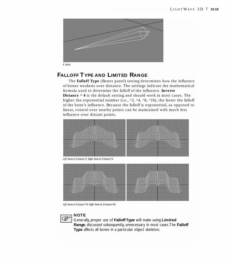
A bone

FALLOFF TYPE AND LIMITED RANGEThe Falloff Type (Bones panel) setting determines how the influence

of bones weakens over distance. The settings indicate the mathematicalformula used to determine the falloff of the influence. InverseDistance ^ 4 is the default setting and should work in most cases. Thehigher the exponential number (i.e., ^2, ^4, ^8, ^16), the faster the falloffof the bone’s influence. Because the falloff is exponential, as opposed tolinear, control over nearby points can be maintained with much lessinfluence over distant points.

Left: Inverse Distance^2. Right: Inverse Distance^4

Left: Inverse Distance^16. Right: Inverse Distance^64

NOTEGenerally, proper use of Falloff Type will make using LimitedRange, discussed subsequently, unnecessary in most cases.The FalloffType affects all bones in a particular object skeleton.

L I G H T W A V E 3 D 7 10.19

When Limited Range (Bones panel) is active, the Min valuedetermines the sharp cutoff point of a bone’s influence. Any pointswithin this range are 100 percent affected by movement or sizing of thebone. Any points outside of this range are affected less or not at alldepending on whether they fall within the Max. In an orthogonal view,the Max setting is visible in the viewport. A short bone will exert aspherical influence, while longer bones exert a more oblong influence.

Min is very powerful and points within this range are greatlyinfluenced by the bone, following the bone movements exactly (unlessan extremely small bone Strength is applied to the bone). Maxdetermines the gradual falling off point of a bone’s influence. Thestrength of the influence falls off from the edge of the Min down to 0 atthe Max. Any points falling outside of this range are not affected at all bythe bone.

Generally, to get the best effects from using bones, you should eitheruse bones that all have unlimited range, or that all have limited ranges.Character animation is generally easier using limited ranges on all bones.

Often you will want your Min and Max to be equal. Typing in a Minthat is bigger than the Max will increase the Max to the same size.Likewise, typing in a Max smaller than the Min will force the Min down.

JOINTS AND MUSCLESSometimes bones used to create joints can cause pinching or

unwanted bunching, much like a folded garden hose. JointCompensation (Bones panel) will remedy this effect by making theaffected points tend to maintain the original volume inside the joint. Theresult is a more realistic-looking joint. You can modify the compensationamount to increase or decrease the effect.

Joint Compensation for Parent (Bones panel) shears the pointsaffected by the parent bone during the child bone’s rotation. Thiscompensation also alleviates the pinching effect often caused by bones.At the same time the point shear occurs, the bone will also try tomaintain the volume inside the joint.

The default value of 100% was chosen as a value that is applicable formost instances. Negative values can also be used, which will increase thepinching effect.


NOTEThe joint is always located at the base of the current bone.AdjustingJoint Compensation for Parent is not the same as adjusting theparent bone’s Joint Compensation.

L-R: Off; Joint Compression 100%; Joint Comp for Parent 100% added

LightWave also makes it easy to create realistic flexing muscles whenyou use bone structures in the object. When you activate Muscle Flexing(Bones panel), the points affected by the bone will flare out as the boneis rotated. The effect simulates muscles bulging under the skin.

Muscle Flexing for Parent (Bones panel) is generally more commonthan Muscle Flexing. For example, when your forearm rotates yourbiceps flex. The forearm is the child and the bicep is the parent. It wouldnot look natural for the forearm to bulge as it rotated, but it looksperfectly natural when the biceps flex.

NOTEJoint Compensation and Muscle Flexing react only to pitch rotations.To react to other rotations (or just for more precise control), youcould model a muscle Endomorph object and use ChannelFollower (oran expression) on the morph target’s MorphMixer channel (on theGraph Editor) to follow the bone’s rotation.You’ll need to setChannelFollower’s Scale down to something like one percent or less.

L I G H T W A V E 3 D 7 10.21

Exercise: using bones1 Load the ARM_LOWPOLY.LWO object (TUTORIALS folder) into a clear scene

in Layout. Use the Side view. Note that it just happens to be modeledalong the positive Z axis. Just what we need. What a coincidence!

2 Select the arm object and choose Items > Add > Bones > Add Bone.

3 If you are using a shaded display, you probably won’t see the addedbone. You can make it visible by making it the current item, but sincewe plan to add several bones, using a wireframe display works best.So, change the viewport’s Maximum Render Level to Front FaceWireframe. You will see the bone inside the arm—try looking at theobject using different views to see that the bone is indeed inside thearm.

4 Notice that the tip of the bone is not quite at the elbow. Since weneed it to bend there, we must increase the bone’s Rest Length.Activate the Bone edit mode button at the bottom of the interfaceand then click Objects > Bones: Rest Length.

The arm was the current item, so activating the Bone edit mode letsus edit its bones. If other objects were in the scene, we would need toselect the bone directly in the viewport or select the appropriateobject first.


5 Drag your mouse to the right until the Rest Length is about 1.13 (theindicator is in the lower-left corner). The bone’s tip should be justabout at the elbow. Note that we don’t need to keyframe this change.

6 Next, let’s add a child bone and for fun, we’ll draw it. Choose Items >Add > Bones > Draw Child Bone and drag your mousepointer to thethe wrist.

7 Now add another child bone, but don’t draw it. Choose Items > Add >Bones > Add Child Bone.

8 The last bone will extend past the tip of the fingers but that’s okay.However, select Items > Tools: Rotate and change its Pitch a little (-2.4 degrees) to align the bone with the hand a little better. You doneed to re-keyframe changes to position and rotation, so re-create akeyframe for this bone after the rotation change.

As you can see, you position bones the same way you positionobjects.

L I G H T W A V E 3 D 7 10.23

9 Press the R key to set the rest position and activate the current bone.Notice that the bone’s outline becomes solid and bright. Press the UP

ARROW key to select the middle bone and activate it. Do the same forthe first bone.

10 Now for the fun part! Select the middle bone and rotate its Pitch.(Switch the viewport back to Textured Shaded Solid.)

Cool!

Select the last bone and rotate its Pitch.

OK. Now walk like an Egyptian... (stop whistling!)

11 Select the middle bone and play with the Joint Compensation andMuscle Flexing options (Bones panel) to see their effects.

12 Try varying the bone Strength for different bones and observe theeffects.


cchhaapptteerr11Item Motion Options

Chapter 11:Item Motion Options

Generally, the Motions Options panel controls the overall motion ofan item in your scene, as opposed to individual channel control, which isaccomplished using the Graph Editor.

PARENTINGParenting refers to LightWave’s ability to create hierarchical

relationships between items, much like files use directories. Theserelationships can grow into a complex hierarchy with multiple itemsparented to an item and the child items being parents themselves ofother items.

You can parent just about anything to anything. That is, lights can beparented to objects, objects can be parented to a camera, and so on. Youcan also parent items to bones; however, bones must remain under theobject they relate to. Generally, you’ll restrict parenting to the same typeof item (e.g., objects to objects); however, there are often times when,say, parenting a camera or light to an object can be very handy.

Scene Editor List showing indented hierarchical relationships

When you initially parent an object to another, you align its localOrigin with the local Origin of the parent object. The child inherits theposition, rotation, and scale of its parent. You can also animate the childindependently, but its movement will be added on to the parent’s.

A simple example involves a camera parented to a car object. As thecar moves throughout the animation, the camera follows its movements,

L I G H T W A V E 3 D 7 11.1

thus providing the look of a camera mounted to the car. Additionally, thecamera may have its own motion, so it could go up and over the carwhile still moving along with it.

Camera parented to car

A more complex example involves a robot walking. The hands of therobot are parented to their respective forearms, which in turn areparented to their respective upper arms and so on. As the main parent ismoved (in this case, perhaps the torso of the robot), all the child objectsfollow. Of course, all objects can have their own motions, which lets youflail the robot’s arms about as it runs.

Left: Solid textured display. Right: Bounding boxes show individual objects

HINTIf possible, try to set up your hierarchical relationships before youanimate the individual items.Then work from the top down (i.e., parentto child).

To change hierarchical relationships:Use the Scene Editor to quickly change hierarchical relationships by

dragging items. (See Chapter 12 for more information.)

To use the Motion Options panel to change an item’s parent:1 Select the item to be parented (i.e., future child).

2 Choose Items > Motions: Motions Options (or M key).

11.2 C H A P T E R E L E V E N : I T E M M O T I O N O P T I O N S

3 Select the parent item from the Parent Item pop-up menu. (Yes, in theLightWave world, children can pick their parents. And what awonderful world it is too...)

HINTUse File > Load Items From Scene to load in an entire chain ofparented objects.This way, you can have default scenes set up with allof the objects parented and in place.You can even have motions set upso you could load in a walking woman or a police car with revolvinglights atop. If you do load a scene that has motion for certain objects,it may be a good idea to have the items in the loaded scene parentedto a null object that you can easily reposition once it’s loaded in thenew scene.

L I G H T W A V E 3 D 7 11.3

Exercise: parenting:1 Load the COW.LWO object (ANIMALS subdirectory).

2 Parent the light to cow. (You can just drag it under the cow.)

3 Drag the cow around and notice how the light moves right along withit.


Example: complex parenting:For a good example of parenting, let’s look at the Mechwalk scene

that comes with LightWave.

1 Load the MECHWALK.LWS scene (ROBOTS subdirectory). This machine iscomposed of many objects linked together in a hierarchy.

2 Open up the Scene Editor panel (Scene Editor) and look at the objecthierarchy. The Control object—really just a null object—is the masterparent. Repositioning it would move all of the children objects.

L I G H T W A V E 3 D 7 11.5

3 Select all objects (Select pop-up) and set their visibility to boundingbox (Visibility pop-up). This lets you see the individual objects moreeasily in the viewport.

4 Select the Light edit mode to avoid displaying all objects as selected.All of the different objects in the viewport should be different colors.


5 Try moving and rotating various objects and see their effect on theirchildren.

NOTEGenerally, the way a scene like this is created is that the individualobjects are created in a standing position in Modeler.After all objectsare loaded into Layout, the pivot points are then moved to the properpositions. Remember, pivot points should always be set prior to anyrotating or moving.

UnparentingYou can unparent an item by:

• clicking the Unparent button,

• selecting (none) from the Parent Item pop-up menu, or

• dragging in the Scene Editor.

Local Axis RotationWe stated earlier that rotation generally occurs relative to the global

axes. However, remember that child items inherit their parent’s rotation.This, in effect, lets you use parenting to rotate an item relative tosomething other than the global axes. To do this, add a null and parent itto the object. Rotate the null to the initial rotation you want the object tohave. Now, you can rotate the object itself and it will all happen relativeto the null’s rotational values.

L I G H T W A V E 3 D 7 11.7

For example, let’s say you wanted a satellite to orbit a planet at a 20-degree angle. Simply add a null and rotate its bank to 20 degrees. Loadthe satellite and move its pivot point away from the object, a distanceequal to the radius of the orbit. Set the satellite’s position back to 0, 0, 0(remember it gets moved because of the pivot point move). Parent thesatellite to the null and rotate the satellite’s heading.

Orbiting satellite

Parent in PlaceIf the Parent in Place option is active on the General Options tab of

the Preferences panel (Display > General Options), an item will maintaina constant position, size, and orientation when it is parented orunparented. Adjusted position keyframes for the child will be created atthe current time, but its position at other times may still change. It isbest to be at frame 0 and to perform parenting before animating whenthis option is active.

TARGETINGSometimes you will want an item to continually point to or follow

something. A common example is when a stationary camera tracks a carspeeding down a street. Obviously, you could keyframe the necessarycamera rotations, but wouldn’t it be easier to just say, “camera, followthat car.” Well, in LightWave, this is called targeting. Any scene item canbe targeted by another item.


Car targeted by light and camera

Targeting automatically controls an item’s heading and pitchrotational values based on the position of a specified object. Banking isunrelated to the targeted object, so you can still control that channel.

A dashed line will appear connecting any item with its target. There isa display option to turn this off or on (Display > Display Options).

NOTETargeting overrides any actual heading and/or pitch channel values.

To target an item:1 Select the item to be targeted toward something.

2 Open the Motion Options panel (Items > Motions: Motion Options).

3 Set the Target Item pop-up menu to the desired object you want topoint to.

L I G H T W A V E 3 D 7 11.9

4 Both the Heading Controller and Pitch Controller (Controller andLimits tab) will automatically set themselves to Point At Target. Ifyou desire, you can set either back to Key Frames for manual control.

Where Does It Point?A targeted item always points towards an object’s pivot point. This

may not always be the exact location you want to point to. There are twosolutions. You could move the item’s pivot point, but this might causeother undesirable ramifications. Another method is to parent a nullobject to the target and move it to the desired target location. Then,select the null as the target.


Light is targeted at cow, but cow’s pivot has been moved off the object

INVERSE KINEMATICSKinematics describes motion, or the study of motion. It is motion in

the most abstract sense, without regard to force, mass, velocity,acceleration, or the positional values that produced the motion. Incomputer animation, you employ kinematics when you animate links ofparented objects such as those used to make up a robot’s arm or leg, orwhen you work with a chain of parented bones inside a one-piece limb.With these types of joints between objects/bones, we generally deal withrotational values for the individual objects/bones in the chain.

Forward kinematics is the standard type of motion generated inLightWave when you rotate/move any parents in a chain. The animatordecides what will be the motion of all the joints. The motion of the lastitem in the chain is determined indirectly by the accumulation of allmotion of any parent items up (i.e., forward) through the chain. (Like ifyou move your upper arm, your forearm and hand also move with it.)

L I G H T W A V E 3 D 7 11.11

Motion accumulates forward through the chain of bones

LightWave also features inverse kinematics (IK), sometimes calledgoal-directed motion. IK occurs when you have a hierarchy of two ormore objects/bones and a goal object selected for an object or bone inthe chain. LightWave can calculate (solve for) the motion of the chainbased on the goal’s position. Usually, the last item in the chain (i.e., thelast child) is the one that receives the goal, but this is not necessarily so,as you can have multiple goals for a chain. (Like if Billy P’s mom grabshis ear, his head, neck, and body must usually follow.)

Motion is computed from goal back up through the chain of bones

You can even use forward kinematics (normal keyframing) and IKsimultaneously for an incredible hybrid motion system. You can setkinematics independently for each item and rotational setting!

Full or Part-time?By default, LightWave does not compute IK continuously. Thus,

animating the goal object will not do anything. You position the goal topose your chain and then keyframe all of the items in the chain. Thismethod uses LightWave’s IK as an animation aid. In effect, you are usingIK to pose your chain, but forward kinematics when you render youranimation.

Alternatively, you can use Full-time IK for any item in the chain with agoal. When active, LightWave continuously computes the chain’s motionbased on the goal. Thus, you can animate the goal object, and the chainwill react accordingly. Full-time IK also works well with multiple active


goals. This means you can have an active knee goal (middle of the chain)as well as an active foot goal (end of the chain). When you move onegoal, LightWave takes into account the position of the other goal.

IK and Modifiers tab

Creating key frames for all items in the chain can become tedious ifyou make a lot of changes and must keep deleting and re-creating keyframes for all items in the chain. Thus, you may want to use LightWave’sFull-time IK option.

Because you can have multiple goals, you can activate Full-time IKfor some goals and not for others. A full-time IK item further down thechain will always override a non-full-time IK item further up the chain. Inpractice, however, you’ll generally have Full-time IK on or off for allitems in the chain.

NOTEIf you are not using Full-time IK, you do not need to create keyframes for the goal object, but it can be useful to help remember yourplace.

HINTAn easy way to create keys for all items in a chain is to select theparent of the chain and create the key frame using the Current Itemand Descendants option (Create Motion Key requester).

LightWave also provides a global IK on/off switch: Items > IK: EnableIK. Use this to toggle IK solving off or on for all IK chains in the scene.

L I G H T W A V E 3 D 7 11.13

Pointing the End of a ChainA bone rotates at its base. So, to get the tip of a bone to point

towards something, you need to add an extra child bone whose baseacts as a pointer (or you could parent a null). For aesthetic reasons,you’ll probably want to reduce this pointing bone’s Rest Length tosomething really small. If it is a chain of objects, parent a null object tothe end of the chain.

Selected bone is “pointing” at goal (null object) using its base

Mix and MatchTo have an entire chain solve for IK goals, you should set each item’s

Heading Controller and Pitch Controller to Inverse Kinematics (MotionOptions panel). As such, you can also have any of the controllers (or theitem) not use IK by setting the controller to something other thanInverse Kinematics. This is how you can mix IK with forward kinematics!

Mixing IK and Key Frames

Here is a basic scene with three bones attached to a null object and asecond null object that will be the goal object for our IK chain. (Note: thethird bone, which is small and nearly invisible, is at the tip on the rightside.)


Three-bone chain.Tip bone is very small

Below are the Motion Options for the bones.

Left: Bone (1). Right: Bone (2)

Bone (3)

Bone (1)’s Heading Controller is set to Inverse Kinematics, but itsPitch Controller is set to KeyFrame. This means that only its headingwill be affected by IK influences. Bone (2)’s Heading Controller andPitch Controller are both set to Inverse Kinematics. This means thatboth its heading and pitch will be affected by IK influences.

L I G H T W A V E 3 D 7 11.15

Bone (3) doesn’t use any IK controllers because it merely acts as apointer to the goal object. Note that it does have Null (2) selected as theGoal Object and Full-time IK is also activated.

Now, as the Goal object is moved around, Bone (1) moves only on itsheading, while Bone (2) moves along both heading and pitch. (Note thatthe Show IK Chain option on the Display Options tab of the Preferencespanel (Display > Options: Display Options) and Keep Goal WithinReach option on the Motion Options panel’s IK and Modifiers tab, arealso active. Enable IK is also on, but you knew that, right?)

Left: Side view. Right:Top view.

Finally, if you rotate Bone (1)’s pitch (as you would normally), youcan see it change. This shows how you can now use a hybrid of forwardand inverse kinematics.

Forward and inverse kinematics in one chain

Setting Your GoalsSetting a goal object is similar to targeting a camera to an object: the

item in the chain with the goal will try to point at the goal object. This iscalled reaching for the goal. Items up the chain will move and rotate tokeep the chain connected.

If physically possible, the goal object will be stuck to the goaled item.Moving it beyond its reach will detach the goal object. You can use theKeep Goal Within Reach option to affix the goal object to the item, ifdesired. This may make monitoring multiple goals easier, but it is up toyou.


Keep Goal Within Reach is active

Moreover, let’s say you build an arm and instead of parenting thehand to the forearm, you just make the hand a goal for the arm. WithKeep Goal Within Reach, you can insure that the hand stays locked tothe forearm. (According to Paul, doing this manually would be a pain andyou’d end up adding a lot of extra keyframes.)

NOTEIf you move the IK object with goals that have Keep Goal WithinReach active and you are using Full-time IK, those goals will bedragged along for the ride.Wheeeeee!

Although any object can be a goal, null objects are used most oftenbecause they do not render. However, you can also use a visible objecteffectively as a goal. Let’s say that you have a searchlight object that youalways want to point at a blimp flying overhead. By modeling thesearchlight with its origin at one end (or simply moving the pivot pointto the end) and parenting a null object at the other end, you can selectthe blimp as the null object’s goal. The searchlight will now follow themovement of the blimp.

Dueling GoalsWhen you create an IK chain with multiple goals that may compete,

you must set strengths for these goals. The strength will determine therelative magnetism that goal has for the shared objects in the chain. Toincrease the strength of a particular goal, raise the Goal Strength value.

L I G H T W A V E 3 D 7 11.17

Multiple goals on one chain

Goal Strength comes into play when the distance between thecompeting goals becomes too great to solve the IK calculation, or whenthe distance exceeds the length of the object chain. As the goals movepast this distance, the objects will move away from their originalpositions. The distance they move from both goals is equal as long asthe strength values are equal. If the strengths are not equal, thedifference in distance is equal to the ratio of the two strength values. Ifone goal’s strength is set to 1 and the other is 10, the object’s distancefrom the weaker goal is ten times that of the stronger goal.

Goal OrientationItems in an IK chain that have a goal assigned can match the

orientation of the goal. You do this by activating the Match GoalOrientation option.

Note:The rest length for the bone with the goal has been increased for illustration

You should note that this option also matches the goal object’sscaling, overriding the (goaled) item’s scale setting. If this adverselyaffects your animation, one solution is to copy the (goaled) item’s scalechannels to the goal object. Another solution may be to add a null objectto the IK chain and use that as the goaled item instead.


HINTUse Match Goal Orientation to prevent a character’s feet from goingthrough the ground plane.

Breaking the ChainWhen you activate the Unaffected by IK of Descendants option for

an item in an IK chain, the selected item is locked from the effects of anIK goal. This, in effect, makes that item the new base of the IK chain, andonly items farther down the chain are affected by any IK operations.

Chain broken with Unaffected by IK of Descendants

A good example of using Unaffected by IK of Descendants is waggingthe tail of a dog. Imagine a string of bones inside a solid dog object,extending down its tail. You want the tail to follow the dog as it movesabout, but you do not want the dog’s body to wag as the tail bones areaffected by a goal object (i.e., the “tail wagging the dog”). You activateUnaffected by IK of Descendants for the bone at the base of the tail toaccomplish this.

Stiff StuffYou may also add a Stiffness value to items in the IK chain. Items with

a higher stiffness value will tend to be more resistant to bending causedby IK.

L I G H T W A V E 3 D 7 11.19

The third bone has a high stiffness setting (for heading in this case). Note how it barely flexes.

HINTWhen you use IK, you will often want to set rotation limits, asdiscussed later in the chapter.

Exercise: setting up a bone IK hierarchy1 Bones must be added to an object, so add a null object to a clear

scene and call it BASENULL. Add another null object and call itGOALNULL.

HINTNaming nulls is a good habit to get into.Although not necessary, it canavoid confusion when you use them later.

2 Change to the Top view and move it so that the nulls are at thebottom of the Layout window.

3 Choose Items > Add > Bones > Add Bone to add a bone to the nullobject.


4 Add three child bones using the shortcut (=).

5 With the last bone (4) still selected, open the Motion Options panel(M). Select the GOALNULL as the Goal Object and set all of theControllers to Inverse Kinematics.

6 Using the Current Item in the main interface, select each of the otherbones and set all of their Controllers to Inverse Kinematics, too.

L I G H T W A V E 3 D 7 11.21

7 Now, select the GOALNULL and drag it around the viewport. You shouldnotice that the chain follows the object; however, the last bone doesnot seem to point to it and just hangs there.

8 To create the illusion that the tip of the bone (4) is pointing to thegoal, you need to add another child bone, whose base will act as apointer. Select the last bone and add a child (=). Size the new bone’sRest Length down so that it is more or less a point.

9 Now, set Bone (4)’s Goal Object to (none) and set the new bone’s (5)Goal Object to GOALNULL.

10 Now move GOALNULL in the viewport. That’s more like it. You shouldnow see the bones bend around like a snake with the end pointing tothe goal. Notice how the GoalNull tends to stick to the base of Bone(5).


Exercise: bone stiffness1 Continue on from the previous exercise.

2 Select Bone (2) and set the Heading Stiffness, Pitch Stiffness, andBank Stiffness (Motion Options panel) all to 100. This makes thebone very inflexible and is probably a much higher value than you’duse normally.

3 Move the GOALNULL around. Notice that the stiffened bone’s joint(base) is much more resistant to bending compared to the others.

Exercise: limiting chain movement1 Continue from the prior exercise.

2 Reset Bone (2)’s Stiffness values to 1 (Motion Options panel).

3 Activate Unaffected by IK of Descendants for Bone (2) (MotionOptions panel).

4 Now move the GOALNULL around. Bone (1) through Bone (2) should bestationary and the snake should bend beginning with Bone (3).

Exercise:To match goal object orientation:1 Continue on from the previous exercise.

2 Deactivate Unaffected by IK of Descendants for Bone (2) (MotionOptions panel).

L I G H T W A V E 3 D 7 11.23

3 Select Bone (5), click Objects > Bones: Rest Length and then clickItems > Tools: Reset to restore its size.

4 Activate Bone (5)’s Match Goal Orientation (Motion Options panel)option.

5 Move and rotate the GOALNULL around. Notice how the orientation ofthe goaled bone matches the orientation of the goal object.

6 Size the GOALNULL object up and see how the bone sizes up too.

7 Set the Keep Goal Within Reach option for Bone (5).

8 Move GOALNULL again. Notice how it is now permanently attached tothe goaled object and can no longer be moved off it.


ITEM MOTION MODIFIERSItem motion modifiers are added on the IK and Modifiers tab of the

Motion Options panel. These generally control the motion at the itemlevel, as opposed to strictly the channel level, which are handled byGraph Editor modifiers (see Chapter 8). However, they often haveindividual motion channel control. Item motion modifiers can also getmotion data after IK is applied, which is not possible with channelmotion modifiers.

To display this panel for the current scene item, choose Items >Motions: Motions Options or just press M.

Motions Options panel

To use an item motion modifier, select the modifier from the AddModifier pop-up menu on IK and Modifier tab. Once added, click on itsname in the list to access its settings, if any.

NOTEModifiers that do not have an explicit additive option are generallyadditive in nature.

CurveConstraintCurveConstraint moves an item along a curve object, similar to a

motion path. The curve object is selected on the Curve pop-up menu. (Ifthere is more than one curve in the object, the first curve is used.)

Enabling Align will rotate the object so it faces along the curve in thetraditional “Z axis” manner. The Start Time and End Time valuesdetermine how long the item takes to traverse the curve. The CurveInfluence percentage blends the curve motion in or out.

L I G H T W A V E 3 D 7 11.25

CurveConstraint options

CurveConstraint does not remain locked to the curve, but adds thecurve's position to its own keyframed motion. To lock the item to thecurve, simply parent the item to the curve, reset the item's position, andeliminate all its keyframes.

You might use CurveConstraint to move an object along the samecurve used to create the geometry (or create the curve from thegeometry), like with a roller coaster.

CyclistCyclist will associate the action of one item with a repeatable action

(an animation cycle) of another item.

All activated channels will have their values replaced by theanimation-cycle values of that same channel, but at the time determinedby the Cycle Controller. Channels that are not enabled will retain theirnormal value at the particular frame.

The Cycle Frames define the action that you want repeated (i.e., theanimation cycle).

The Cycle Controller controls the item based on the selected controlparameter, defined on the pop-up menu just to the right. The controlparameters can be an item's position, rotation, scale, speed, or thedistance it has traveled along its actual path length. The ForwardProgress, Side Slip, and Climb parameters take into account the item'sorientation and tell how far the item has been moving forward (Z axis),to the right (X axis), or up (Y axis), respectively. Speed looks at theitem's velocity.


Essentially, Controller Range defines how much change is required toequal one full animation cycle. The unit of measure for this parameterdepends on the selected control parameter. For position and otherdistance-type settings the unit of measure is in the LightWave DefaultUnit defined on the General Options tab of the Preferences panel.Rotation uses degrees and scale is a factor where 1 equals 100 percent.Speed is in default units per second.

Similar to motion graphs, End Behavior determines what happensafter the first cycle is completed.

Activate the World Coordinates button to use the Cycle Controller'sactual (world) coordinates, rather than its relative coordinates. Thesecould be different if, for example, the object is parented to anotherobject.

Although the motion of the item will always come from keyframes, themotion can be used to move an IK goal, if After IK is off.

Exercise: Cyclist1 Add a Null object.

2 Load the WHEEL.LWO from the TUTORIAL folder into Layout.

3 Parent the Wheel to the Null. Create a keyframe for the Wheel atframe 0.

4 Go to frame 60 and rotate the wheel's pitch 360 degrees and create akeyframe.

5 Open the Graph Editor and set the Pre Behavior to Linear for thewheel’s pitch channel. This sets up the Wheel's cycle (frames 1 to 60).

6 Set the Last Frame to 180 and go to frame 0.

7 Move the Null to 0m, 19.5cm, 1.4325m, and create a keyframe.

8 Go to frame 103, move the Null to 0m, 19.5cm, -21.1209cm, and createa keyframe.

9 Go to frame 126, move the Null to 0m, 19.5cm, 35.175cm, and create akeyframe.

10 Copy this keyframe to 140. To do this, while still at frame 126, pressthe ENTER key to bring up the Create Motion Key dialog. Enter 140 inthe Create Key At input field and click OK. This copies the keyframeinfo from 126 to 140.

11 Go to frame 180, move the Null to 0m, 19.5cm, -1.44m, and create akeyframe. Adjust your Perspective view so you can see the null'sentire motion path.

L I G H T W A V E 3 D 7 11.27

12 Select the Wheel and open its Motion Options panel. Add the Cyclistmodifier and set the settings as shown. (Note: Since the wheel isabout .194m in diameter, the circumference is about 1.22m (2 * pi *.194).)

13 Close the Cyclist panel and drag the time slider. You will see thewheel turn backward and forward as it moves.

EffectorEffector causes effector objects to repel or attract the motion path of

the affected object. The effector objects may be any objects you wish,but Null objects work best.

The Effector Object(s) Prefix, with the default of Effector, is a nameprefix, as such, any object that begins with this name will be an effector,allowing you to have more than one based simply on their names.

Solid Core Radius defines a spherical area, within which all objectsare equally affected. There is a gradual falloff of the effect between theSolid Core Radius and Falloff Distance. Objects outside the FalloffDistance are not affected at all.

You also have a choice for the Effector Shape. It can be a Point orPlane. If it is a Plane, you need to specify the Axis.

The impact of the effector object is set and animated by keyframingits XYZ Size channels. Positive values repel and negative values attract.

NOTESee also the Effector custom object plug-in discussed in Chapter 9.


ExpressionThis is a motion-modifier version of expressions, which can get the

results of other motion modifiers, as well as IK. This is not possible witha channel modifier. (See Chapter 8 for more information.)

You can select multiple channels on the Channel pop-up menu andapply different settings for each (i.e., you don't just pick one). They canall share scratch variables (A through Z) and the expressions can beaware of other components of the item's motion. Thus, H can depend onZ, for example, without trying to reference the item's object.

FollowerUsing the Follower item motion modifier is similar to parenting an

object to another, except you have control over which motion channelsyou wish to inherit. You can also modify and delay the inherited value.Moreover, the motion can be inherited from the camera, a light, a bone,or any object in the scene.

L I G H T W A V E 3 D 7 11.29

Use the Item To Follow pop-up menu to define the item whosemotion you want to use. This is the leader.

Activate the World Coordinates option to use the leader's actual(world) coordinates, rather than its relative coordinates. These could bedifferent if, for example, the object is parented to another object.

The amount of seconds entered into the Time Delay field is added tothe current time. This number may be negative.

Randomize is a maximum amount of time (in seconds) to be added tothe delay. The actual amount will be between 0 and the Randomizevalue. This number may be negative or even larger than the Time Delay.(The latter would cause the item to sometimes anticipate the leader'smoves and lag at other times.) The overall delay amount for each item isfixed over the course of the animation, so this is useful for basic flockingeffects.

NOTEThe random number seed is taken from the object ID, which should bethe same among ScreamerNet nodes and, thus, will cause items to havedifferent delay amounts.The delay stays the same from frame to frame.

The Path Delay parameter specifies a fixed following distance alongthe path of motion of the leader, which is helpful for keeping cars in atrain following correctly through accelerations.

The Align to Path option will align the follower object to its newpath.

The After IK option allows you to apply this modifier taking (or nottaking) into account changes from IK.

Select a Source for any of the leader object's motion channels youwish to use. Generally, the type of motion channels will match. That is,the follower object's, say, X Position will be determined from the leader'sX Position. However, the settings can be different. For example, thefollower object's Bank Angle might be derived from the leader's ZPosition. Select none to disregard that channel.

The value can be scaled by inputting a factor other than 1 in thecorresponding Multiply By field. The value may be offset by inputting avalue other than 0 in the Add field.


GravityGravity simulates the effects of the Earth’s gravity on an item’s

motion, making it fall naturally and even bounce with varying degrees ofelasticity.

Strength is the acceleration due to gravity in units of ‘g’, the Earth’sstandard gravity. The object’s position will be altered along the specifiedAxis. The Ground Level value determines at what height the objectbounces. This is measured in the Default Unit (General Options tab ofthe Preferences panel)

Elasticity describes the amount of energy lost on each bounce, whichequates to the relative height of the bounces. Thus, 100% Elasticity iscompletely bouncy, and bounces forever, 0% doesn’t bounce at all.

The Start Frame and End Frame parameters specify when the effectis applied.

NOTEThe most natural results will occur if all the keyframed motion withinthe range of frames is a single linear path. In particular, the trajectory isdetermined by an object's initial speed and direction of motion.

NOTEYour object must start in a positive position along the selected Axis.

Motion BakerMotion Baker (formerly IKCapture) will freeze the motion of an item

into individual keys. Motion Baker takes into account not only IK, butalso motion/channel modifiers, align to path, and so on. Thecomputation is executed by dragging your frame slider or playing thescene.

L I G H T W A V E 3 D 7 11.31

Motion Baker panel

Selecting the Use Existing mode will create normal keys for theselected position or rotation channels. The Extra Channels mode placesthe keys in a special AfterIK channel group—you might use these withexpressions, for example.

AfterIK group shown in ChannelFollower channels window

If Overwrite Keys is active, any existing key data will be overwritten.Note that the existing key data will include the effect of Motion Bakerrecorded on a previous pass.

Motion Baker’s position in a list of item motion modifiers does notmatter unless another modifier has an AfterIK option and it is active.

Jolt!Jolt! is an item motion modifier that simulates the chaotic and

uncontrolled movements that occur when physical impacts have enoughweight and velocity to cause jarring vibrations. For example, thecollision of a celestial body striking another, the impact of a robot's footwith the earth, the collision of a laser beam with a passing spaceship,and so on. All of these events are good candidates for Jolt!


Jolt! panel

Jolt! also lets you specify vibration events using keyframes thatindicate when a vibration will begin—and be at its most intense. You canalso specify the duration of the vibration and its initial intensity.Intensities can be set based on the object’s position (X, Y, and Z axis)and its rotational values (heading, pitch, and bank).

NOTEJolt! does not provide the basic motion of an item, but rather modifiesan existing motion. Jolt! does not modify existing motion except toradically deviate from it temporarily at specified intervals.

Global OptionsThe Save Keys and Load Keys buttons let you save and restore Jolt!

settings. The Save Motion and Load Motion buttons save and load,respectively, standard LightWave motion files based on the keyframedata. The Save Motion button is ghosted if no keyframes are set, andboth buttons are ghosted when the Events tab is selected. Motion filessaved with the Linear button active have their keyframes set to the(spline control) linear mode.

Activating Intensity Ramp tells Jolt! to track the movement of aLightWave item (i.e., Camera, light, object, or bone) and based upon itsdistance from the Jolt! object, increase or decrease the effect of thevibration proportionally. Minimum Range is the radius in meters of theeffect range. LightWave items outside of this range will not create a

L I G H T W A V E 3 D 7 11.33

visible effect. If you forget to set this value when you leave the Jolt!interface panel, you will be reminded and Jolt! will disable IntensityRamp (with a minimum range of 0.0, it is ineffective anyway).

If you activate Shock Wave, vibration keyframes are adjustedinternally to offset for the distance of the ramp object. In effect, thefurther away the ramp item is, the longer it will take for the vibrationevent to actually trigger, and the later it will trigger from its indicatedstart time. This option is useful if you use Jolt! on items in your sceneother than the Camera. Items using Jolt! that are closer to the ramp itembegin their vibration events sooner than items that are further away.With items positioned correctly, this option can produce a visible shockwave effect from the ramp item's location.

If you select an item that is part of a parental hierarchy, Jolt! alertsyou and—if it isn't selected already—suggests that you turn on theWorld Coordinates option. This option ensures that you get propermovement information from the child item.

The NonLin2 button activates an alternate calculation for Jolt!'smotion calculations. It creates motions that are less harsh.

Keyframes TabThe Keyframes section houses the Jolt! key controls. When you want

the jolting to occur on specific keyframes, you will utilize this tab. (If youwant the effect to occur based on the position, rotation, and/or scale ofan item, this is set on the Events tab. You can set both.) The Jolt Keysslider selects the current frame. The range of the slider will exactlycoincide with the number of render frames that have been specified onLightWave's Render Options panel—not necessarily the same value thatis used in the Preview settings. The << and >> buttons will jump to theprevious or next keyframe, if any exist.

Clicking the Create Key button makes a keyframe at the currentframe. Use Delete Key to remove an existing keyframe. Note that thecurrent frame must be a keyframe to do this.

Clicking the Populate Key will take the settings for the currentkeyframe and copy them to every existing keyframe. In other words, itpopulates all keyframes with the current settings and saves you from thetedious task of copying and pasting settings, frame by frame.

Randomizing KeysRandomizing (or jittering, if you prefer) provides a means of breaking

up potentially monotonous key settings. Although Jolt! will internallyrandomize settings to some degree as it applies them to the item, unlessyou are using intensity ramping, the actual key values themselves willnot be altered. By using the Randomize button, you can generatevariances such that the motion of subsequent keys does not look sosimilar.


The randomizing process requires two or more keys in order tofunction. The settings of the first key are never altered (nor is there anyreason to alter them because no other key will look exactly like themafter the effect is applied). The degree of variance can be altered byusing the Threshold control input field to the immediate right of theRandomize button. This control lets you specify, as a percentage, themaximum amount that each altered key will deviate from its currentvalue.

Jolting EffectThe bottom half of this tab sets the actual jolting effect. Clicking

Light, Medium, or Heavy will update a keyframe's Position and Rotationvalues to reflect preset values for a light, medium, or heavy vibration.This feature can be used for starting points or final settings.

WARNINGPlease be aware that when you press any of these buttons, anyexisting keyframe settings will be destroyed.

Clicking the Copy Key button will copy all of the Jolting effectsettings to an internal memory buffer. Clicking the Paste Key button willpaste the settings into the fields currently visible. Note that this canaffect either the Keyframe or Events tab interchangeably.

Using Preset ValuesYou can alter preset values. If you press the D button to the

immediate right of any of the presets, then you store the current settingsfor the key as the default values for that preset. These new default valueswill persist between sessions with LightWave 3D. (Jolt! stores its presetdefaults in a file called JOLT.PRE. You can restore the built-in Jolt! presetvalues at anytime by deleting this file; however, it can be stored invarious places depending on the system configuration. You will need tosearch your hard drive to find it.)

Applying TurbulenceJolt! can apply turbulence to your item's motion path in several ways.

When you select Falloff, the turbulence applied will gradually decreasethroughout the duration of the event. In other words, at the first frame ofthe event, the position and rotation values you have entered for theevent will be at their strongest, while at the last frame of the event theywill be at their weakest. If you do not select Falloff, then Jolt! applies theevent values at their full strength at each frame throughout the eventduration.

If you select Spring, Jolt! applies turbulence uniformly, and makes itappear as though your item is supported and buffered by springs.Without Spring, Jolt! applies turbulence more chaotically or randomly,which produces more of a true vibration effect.

L I G H T W A V E 3 D 7 11.35

Key SettingsA Duration value must be specified, in terms of the number of frames,

within which Jolt! must complete the effect. Because the you can specifyduration and location of vibration events, keyframe data may overlap.Jolt! handles this situation by warning you about the overlap condition.The overlapping key will start before the preceding key ends. If akeyframe is deleted, Jolt! will recalculate all keys to ensure that anyoverlapped keys are corrected.

The Position controls let you to define the maximum deviation oneach of the three axes for the item at the current frame. These values areall specified in meters. The higher the number, the more dramatic theinitial movement in that direction. A value of zero (0.0) in any positionwill prevent the item from deviating in that direction. The Rotationcontrols work similarly, but set deviation values for heading, pitch, andbank (in degrees).

Events TabOn the Events tab, you can cause jolting based on the position,

rotation, or scale of items. (If you want the effect to occur on specifickeyframes, this is set on the Keyframes tab. You can set both.) TheWatch pop-up menu gives you a list of all the items currently in yourLightWave scene. You may select any available item from this list as thewatched item, that is, the item that triggers the event.

With the watched item selected, click on the Position, Rotation,and/or Scale button to activate the watched attributes. Click either the


< (less than) or > (greater than) button next to the input field you wishto set. The Position and Scale fields correspond to X, Y, and Z, from topto bottom and the Rotation fields correspond to H, P, and B.

The << and >> buttons let you watch more than one item. To addanother watched item, simply click the >> button. The informationaldisplay to the left will tell you what item is currently selected and howmany there are in total (e.g., 01 of 03). The << and >> buttons are alsoused to navigate through existing watched items. If you add a watcheditem by mistake, set Watch to (none). You also cannot add anotherwatched item if the last existing item is set to (none).

Activate the Re-arm button if the item repeats its motion and youwant it to trigger the event again. If Cascade is active, Jolt! will ignore theevent (i.e., not evaluate it) until the event immediately preceding it hasoccurred at least once.

The settings on the lower half of the tab work as described for theKeyframes tab (see Jolting Effect, above).

OscillatorOscillator applies damped harmonic oscillator motions (i.e.,

decreasing waves) to selected animation channels of an object's motion.Examples of this effect are everywhere, from springs and guitar stringsto a grandfather clock pendulum.

Use the Channel pop-up menu to select an animation channel to beaffected. Activate the Enable button to turn on the selected channel. Theoscillator value will replace the normal channel value. You mayindependently enable multiple channels and each channel may have itsown independent group of settings.

Additive adds the oscillator value to the channel rather thanreplacing it. If this setting is active, a plus sign (+) will appear next to thechannel name. If Additive is off, an asterisk (*) will appear next to eachenabled channel name.

Cycle Time is the period of the oscillation (i.e., wave), that is, thenumber of seconds between successive crests.

L I G H T W A V E 3 D 7 11.37

Wave Size refers to amplitude; the oscillator adds/subtracts thisamount at its positive/negative crests.

The Offset value is also added to the oscillator value on each frame.Essentially, this sets the value of the horizontal axis that runs throughthe wave. By default it is zero.

Phase sets where the wave crests with respect to the beginning of thecycle, it ranges from 0 to 360 degrees. Essentially, the wave is shiftedhorizontally.

If Damping is applied, the crests will fall or grow over time, as isappropriate for harmonic oscillators. Damping units are a percent percycle.

The Start Frame and End Frame parameters specify when theoscillator is applied.

Copy and Paste use an internal clipboard to move oscillator settingsbetween channels or Layout items.

The formula is: channel value = old value + size * sin( phase +2*pi*time/cycle time ) * exp(-t*damping factor).

Where the damping factor is a special number computed from theDamping percentage.

Sun SpotSun Spot is a motion modifier that will rotate an item, usually a

Distant light, to match the sun’s angle at the specified date and time.

Distance is the radial distance from the rotation center, at which thelight is pointing.


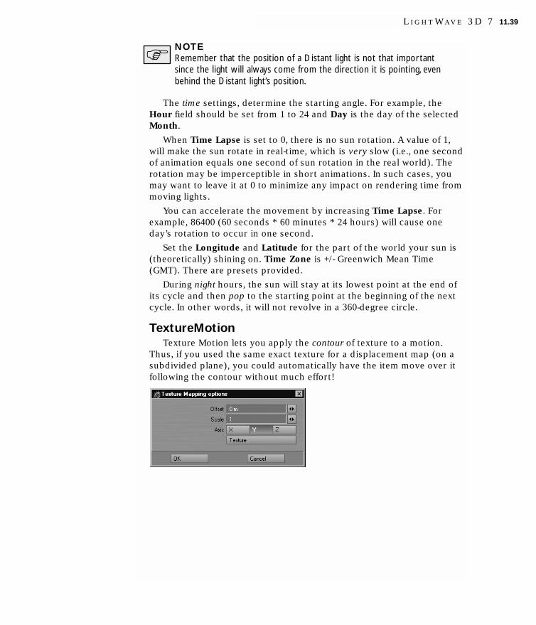
NOTERemember that the position of a Distant light is not that importantsince the light will always come from the direction it is pointing, evenbehind the Distant light’s position.

The time settings, determine the starting angle. For example, theHour field should be set from 1 to 24 and Day is the day of the selectedMonth.

When Time Lapse is set to 0, there is no sun rotation. A value of 1,will make the sun rotate in real-time, which is very slow (i.e., one secondof animation equals one second of sun rotation in the real world). Therotation may be imperceptible in short animations. In such cases, youmay want to leave it at 0 to minimize any impact on rendering time frommoving lights.

You can accelerate the movement by increasing Time Lapse. Forexample, 86400 (60 seconds * 60 minutes * 24 hours) will cause oneday’s rotation to occur in one second.

Set the Longitude and Latitude for the part of the world your sun is(theoretically) shining on. Time Zone is +/- Greenwich Mean Time(GMT). There are presets provided.

During night hours, the sun will stay at its lowest point at the end ofits cycle and then pop to the starting point at the beginning of the nextcycle. In other words, it will not revolve in a 360-degree circle.

TextureMotionTexture Motion lets you apply the contour of texture to a motion.

Thus, if you used the same exact texture for a displacement map (on asubdivided plane), you could automatically have the item move over itfollowing the contour without much effort!

L I G H T W A V E 3 D 7 11.39

The Axis determines the perpendicular mapping axis, just like with animage map. The Offset lets you move the motion in the positive ornegative direction along the selected Axis. Scale acts as a multiplier forthe motion. A value of 1 has no effect.

Here a simple Checkerboard texture has been applied

ROTATIONAL LIMITSYou can independently limit heading, pitch, and bank rotations

between maximum and minimum values. You can prevent actions likebending a leg backwards at the knee (unless you’re animating a footballinjury). To use the limiting feature, activate the desired Limit option(s)and set the related Min and Max values on the Motion Options panel (M)for the particular item. Setting rotation limits can be particularlyimportant when using inverse kinematics. (Note that the maximum valuemust be greater than the minimum.)

You can interactively set the Min and Max values by rotating the itemto the desired minimum direction and choosing Items > IK: Limits >Record Minimum Joint Angles. This will activate minimum limits forany rotational parameters (heading, pitch, or bank) that are currentlyactive for the chosen item. Similarly, rotating the item to the desiredmaximum range limit and choosing Items > IK: Limits > Record


Maximum Joint Angles will automatically input the values into themaximum limits for the active rotational parameters. You can deactivateHeading, Pitch, and/or Bank to avoid setting limits for the deactivatedsetting.

If any of the rotational limits are active on the Motion Options panel,you can access angle limit dialogs from the Items > IK: Limits menu.

Heading Angle Limit dialog

ALIGN TO PATHAnother way to automatically control the rotation of an item is to

align itself to the motion path that it is traveling. This feature aligns thelocal Z axis of the item (through its pivot point). A classic example ofthis is when you have a car speeding down a curvy road. Sure, you couldkeyframe the rotational changes, but its much easier to have LightWavealign the car to its path.

NOTEThis is one reason most vehicles (and other objects) are modeledalong the Z axis, facing the positive side.

This feature automatically controls an item’s heading and pitchrotational values based on its motion path. Banking is still independent,so you can still control that channel manually.

NOTEAlign-to-path overrides any actual heading and/or pitch channel values.

To apply align-to-path to an item:1 Select the item to be aligned.

2 Open the Motion Options panel (Items > Motions: Motion Options).

L I G H T W A V E 3 D 7 11.41

3 Generally, you’ll want to set both the Heading Controller and PitchController (Controller and Limits tab) to Align to Path. If you desire,you can set either back to Key Frames for manual control.

The Align to Path Look-ahead value on the IK and Modifiers tabdetermines how far ahead of itself an item looks as it travels a path,when Align to Path is activated. Like a racecar driver, the item cananticipate the turn and begin turning before the motion path actuallycurves. An object looking three frames ahead will smoothly round acorner as it travels through the turn, whereas as an object looking fifteenframes ahead may appear to turn out of the corner before it has actuallytraveled through the turn itself.


cchhaapptteerr12The Scene Editor

L I G H T W A V E 3 D 7 12.1

Chapter 12:The Scene Editor

The Scene Editor gives you the big picture. Here you can see a list ofall of the items in your scene arranged hierarchically. You can see all ofthe individual enveloped channels, perform global edits on keyframes,and change hierarchy. Here, you also set the wireframe colors, changevisibility modes, and even load a reference sound file.

Scene Editor

BASIC FUNCTIONSThe scene list is a standard LightWave list window. You can expand

and collapse groups as well as subordinate items (e.g., child objects) byclicking the arrow icon that appears to the left of the item name.

The plus/minus sign icon will display or hide the individual channelsfor the item. Most of the time, these are the position, rotation, and scalechannels; however, other enveloped channels can also be included, likelight intensity.

Expanded channels

The item type icon indicates the type of item and the color usedwhen the item appears in wireframe. You can change this by right-clicking on the item name and selecting a color from the pop-up menu.When working with complex scenes with overlapping objects, it can bebeneficial to use different colors for certain items in the scene.

Changing item color

Double-clicking an item’s name will bring up the related propertiespanel.

If you drag the right edge of the panel, you can shrink the size of theScene Editor and hide the keys display. Use in this mode as a scene itempicker!

12.2 C H A P T E R T W E L V E : T H E S C E N E E D I T O R

Shrunken Scene Editor become item picker

The checkmark column activates or deactivates items. Deactivatingan object is like setting its Object Dissolve (Object Properties) to 100%,and deactivating a light is like setting its Light Intensity (LightProperties) to 0%. For a bone, this toggles its Bone Active state (BoneProperties). This option has no effect on cameras.

The “eye” column is the visibility column. For objects, clicking on thisicon will display a pop-up menu where you can select how the object isdisplayed. This can range from making the object hidden all the way upto showing it as a textured shaded solid.

The visibility setting can dramatically affect not only how an object isdisplayed, but also how fast the display is updated. Moving a 200,000-polygon 100-surface spacecraft around the screen using a textureddisplay surely requires greater computing power than a wireframe six-sided bounding box. There are other reasons as well. Often, in a verycomplex scene, you may need to play with object visibility options inorder to concentrate on certain aspects of the scene.

Most of the visibility settings are self-explanatory. Front FaceWireframe will show only polygons that face the camera. The TexturedShaded Solid adds image-mapped surface textures.

NOTEYou can override the visibility setting somewhat using the viewport’sMaximum Render Level pop-up menu located on the top left edgeof a viewport.

NOTEThe color and visibility options affect only the appearance of items inthe Layout view.They do not affect the final rendered image.

For lights, cameras, and bones, you can make them visible or hiddenby clicking in the visibility column.

L I G H T W A V E 3 D 7 12.3

Light is hidden and camera is visible

Clicking in the “lock” column will toggle the locking function on forthat item. Locked items cannot be selected in the viewports. The lockicon will also appear on the Current Item pop-up menu (on the maininterface) next to the item’s name.

The lock icon indicates a locked item

POP-UP MENUWhen you right-click an item, it displays a pop-up menu. This menu

can set the item's wireframe color, clear the item, clone the item, renamethe item, and open its properties or motion panels.

KEYFRAMESThe colored bars to the right indicate the length of the keyframed

channel. The bar starts at its first keyframe and ends at the last one.(Note that the ends may be past the end of the visible display area.) Theplus signs indicate keyframes.


The line with the item’s name is the master channel and will show acomposite of all of the keyframes in any of the underlying channels.

ADJUSTING CHANNELSYou can move individual keyframes by dragging them with your

mouse. The affected key is highlighted when you initially click on it.Dragging on the bar, off any key, will move the entire bar forward orbackward in time.

Key becomes highlighted as you drag one key

Move all keys for channel by dragging bar

NOTEYou can also drag keys on the master channel, which will affect onlythe appropriate underlying channels.

There are square handles at the beginning and end of every bar. Youcan drag these to scale all of the keys in the bar.

Drag handle at end to scale

HINTFor more precise adjustments, use the Shift Keys and/or Scale Keysfunctions.

ADJUSTING HIERARCHYYou can drag item names up and down to change the order and

hierarchy (i.e., parent/child relationships). As you drag, a yellow insertline will appear. You insert the item by releasing your mouse button atthe line’s position. The line will cycle between different lengths as youdrag; the different lengths indicate different levels of hierarchy. Therelative length indicates the level the line becomes when you release themouse button.

L I G H T W A V E 3 D 7 12.5

Unparenting object by dragging

For more information on parenting, see Chapter 11.

NOTEAn item inserted between a parent and child will always becomeanother child.

EFFECTS OF SELECTIONYou can select a contiguous range of (same type) items by holding

the SHIFT key down as you select. Hold the CTRL key down toselect/unselect non-contiguous items.

You can then drag the entire selected range of items to a newhierarchical position. Most of the editing functions can be limited toselected items only. These items will also be highlighted in theviewports.

BUTTONSUse the Favorites pop-up menu to create (or delete) selection sets for

items that you want to access quickly. For example, if you always movethe same five lights, you could multi-select them and make a favorite.Then, the next time you want to move them, you just select the favoritesset you created and all five lights are selected automatically.

The Select pop-up menu lets you quickly select all items based ontheir type. To unselect a group of items, just click on any item. (One itemis always selected.)

The Visibility pop-up menu will show/hide selected or all items.

The Colors pop-up menu will apply the selected color to all of theselected items. You can also set the default colors and apply them to thescene.

The Channels pop-up menu will expand/collapse selected or all items.


With Shift Keys you can shift keyframes for all or just selected itemsforward or backward in time. The Low Frame and High Frame values setthe range of frames to be affected. This function lets you fine-tune theanimation without making individual changes for each item in the scene(a potentially tedious task). Enter a negative Shift Frames by value toshift backwards in time.

Some operations can affect frames outside the specified range. Forexample, shifting a range of frames in the middle of a motion path willcause keyframes after the range to shift so they are not overlapped bythe newly shifted keyframes.

With Scale Keys you can extend or shorten either the duration of allor just selected items. The Low Frame and High Frame values set therange of frames to be affected. The result is that events occur eithermore slowly or more quickly, as they have been scaled to take place overa longer or shorter period of time. Scale Keys enables you to fine-tunethe animation, allowing certain events or the entire animation to takeplace within a specified time frame so that you do not need to alterspecific keyframes manually. The Scale Time by value represents thescaling factor with 1 being equal to 100 percent.

NOTETime-related elements of the scene other than motions and envelopeswill not change with the use of either Shift Keys or Scale Keys.Therefore, image sequence loop lengths and texture motion will notbe affected.

ADDING AUDIOYou can sync your animation to sound: from the Audio pop-up menu,

load a reference audio file (WAV format) that you can hear when you playthe scene. A simple waveform is shown behind the time slider on themain interface. You can scrub though the audio by dragging the timelineslider or preview the audio by selecting Play Audio. Use the Clear Audiooption to clear the audio from the scene.

L I G H T W A V E 3 D 7 12.7

Audio graph visible behind frame slider

The Fixed Frequency option keeps the audio from changing pitchwhen you scrub the frame slider.

You can delay the start time of a loaded audio file by selecting AudioStart Time from the Audio pop-up menu. The value you enter into thedialog is the delay amount in seconds (e.g., if Frames Per Second, on theGeneral Options tab of the Preferences panel, is set at 30, entering 1.0starts your audio at frame 30).


cchhaapptteerr13Camera Basics

Chapter 13:Camera Basics

When you create a LightWave animation or still image, you will have adisplay device in mind. In the case of video, it’s probably a TV set ormonitor. You might also be creating something that will appear only on acomputer screen. Other possibilities include film or print media.

Whatever the ultimate destination of your images, two things willbecome very important before you can render your images: pixel aspectratio and resolution. Essentially, these are the shape of the pixel andnumber of pixels, respectively.

Whenever you render a frame in LightWave, you render it from thecamera’s point of view. LightWave’s Camera Properties panel lets youchange any and all settings of the camera. To open it, just select acamera and press the P key. Among other things, you can control theresolution of the rendered output, the antialiasing amount, motion blur,and the depth of field settings.

L I G H T W A V E 3 D 7 13.1

Camera Properties panel

MULTIPLE CAMERASYou can add additional cameras by choosing Items > Add > Add

Camera; however, only the Current Camera is used to render a scene. Ifyou have more than one camera in the scene, use the Current Camerapop-up menu on the Camera Properties panel (or Layout’s Current Itempop-up menu) to select the currently active camera.

RESOLUTIONThe Resolution pop-up menu contains several standard resolution

presets. Selecting one will automatically set the Width and Height fields,and the Pixel Aspect Ratio field (more on this parameter later).

Width and Height fields determine the precise number of horizontaland vertical pixels, respectively. Any values between 16 x 16 and 16,000 x 16,000 are acceptable.

The Resolution Multiplier scales the underlying selected Resolutionup or down, with 100% as the default full resolution. This feature letsyou quickly reduce or enlarge the resolution of your rendered images.You will often want to render test animations at a smaller resolution fortest purposes. Particle, line, and edge thickness, as well as the glowradius, are scaled by the Resolution Multiplier during rendering.

13.2 C H A P T E R T H I R T E E N : C A M E R A B A S I C S

Manually entering values directly into the Width or Height fields willoverride any selected Resolution (which will then display the wordCustom). The Resolution Multiplier will continue to operate,automatically scaling these values if you alter its setting.

Deciding on a resolution is generally a matter of output quality andintended use. If you are rendering for video, there is no reason to useanything other than the appropriate NTSC or PAL settings. If you arerendering for film or print, you’ll want to use a higher resolution. Forcomputer animations, lower resolutions may be adequate.

PIXEL ASPECT RATIOA pixel is a pixel, right? Wrong. Although pixels are generally square

on your computer monitor, some display devices, like televisiondisplays, use rectangular pixels.

The Pixel Aspect Ratio refers to the shape of the pixels on the targetdisplay device. It is calculated by dividing the width of the pixel by itsheight. For instance, a square pixel will give you a Pixel Aspect Ratio of1.0, and this is nearly always used for images that are viewed exclusivelyon computer monitors. For NTSC video, Pixel Aspect Ratio is about .86to .9.

So why do you have to worry about this? Well, remember that a pixelis just a dot with some color information. So let’s say you had a ball thatwas exactly 50 pixels high and 50 pixels wide. Generally, the ball wouldbe perfectly round if you displayed it on a computer monitor. However, ifyou showed this same image on an NTSC video display (e.g., a TV set),the ball would appear vertically elongated. That’s because NTSC video’sPixel Aspect Ratio is about .9. Conversely, if the ball appeared round onan NTSC monitor, it would appear squashed on a computer monitor.

Left: .9 Pixel Aspect Ratio on video monitor. Right: Same image on computer monitor.

Fortunately, selecting one of the Resolution settings will also set thedefault Pixel Aspect Ratio to the proper value. If you are working on ananimation that will be shown on video, you’ll have to get used to thestretched/squashed imagery when viewing it on your computer display.

FRAME ASPECT RATIODo not confuse Pixel Aspect Ratio with the more common term frame

aspect ratio (sometimes just referred to as aspect ratio). Frame aspectratio is the pixel width divided by the pixel height times the Pixel Aspect

L I G H T W A V E 3 D 7 13.3

Ratio, usually rounded to whole numbers. For example: a standardcomputer resolution is 640 x 480, which would have a frame aspect ratioof 4:3 or 1.333 in decimal form. (640/480 reduces down to 4/3, whichequals 1.333) The frame aspect ratio is displayed for informationalpurposes on the Camera Properties panel.

LENS SETTINGSThe zoom factor pop-up menu lets you set the equivalent real world

camera lens using Zoom Factor, Lens Focal Length, or Horizontal FOV(Field of View), and Vertical FOV values. The default, Zoom Factor of 3.2,is equal to a 24 mm camera lens, a mildly wide angle lens. Users familiarwith camera lenses may find the Lens Focal Length the easiest to use.Long-time LightWave users will be more comfortable with Zoom Factor.The FOV settings set this parameter using the degrees of view, whichtake into account the Width and Height settings.

Smaller Zoom Factor and Lens Focal Length values produce a wideangle lens effect, while larger settings produce a narrow (telephoto) lenseffect.

A close-up using an 8mm lens

Create an envelope for special effects such as quick zooms in and out,or zooming in on a subject while pulling the camera back.

Aperture HeightIn LightWave, you can change the size of the virtual film that the

camera uses by selecting the Aperture Height button. Changing thissetting affects only the strength of the Depth of Field effect (see below)and the Lens Focal Length. When you generate LightWave imagery forfilm photography, use the same film size used for the project’s real worldcamera, so you match the optical characteristics of that camera.


NOTEAperture Height is always listed in inches, even if you are using ametric unit system.

CAMERA SETTINGS IN A VIEWPORTWhen you use the Camera view, the areas of the viewport outside of

the frame are shaded with the overlay color, marking the edges of thecamera frame. Items (or portions of items) in the shaded areas will notbe seen when you render the frame.

These areas can be either horizontally or vertically orienteddepending upon the resolution and pixel aspect you choose (and theshape of your interface screen).

If you aren’t using the Camera view, the camera representationincludes a camera pyramid, with its tip lying on its side. The camerapyramid shows the frame aspect of the image that will be generated.

Camera pyramid

L I G H T W A V E 3 D 7 13.5

RENDERING A LIMITED REGIONYou can use a limited region to mark off a specific rectangular area to

be rendered. This is a great feature when you wish to test render an areaof the frame without rendering the entire image.

Two controls are available for using limited region. If you activate theAdjust Limited Region Tool in the Camera view, a yellow dotted-linebounding box will appear. This is the limited region rendering area. Tochange the area, drag either the corners or the sides of the rectangle.Place the cursor inside the rectangle to move the entire rectanglearound. Choose a new tool, like Move, to stop editing the limited region.

The second control is the Limited Region option on the CameraProperties panel and if you activate it, only the limited region will render.Pressing CTRL+L will toggle the state of this setting.

Memory ConsiderationsLimited Region allocates only enough memory to render the

horizontal limited region area. If you stitch parts of an image together,you can effectively render images that are much larger than those youcould render one pass. This is especially useful for high resolution printimages or in low memory situations. However, note that some post-processing filters require a full-sized image. In such cases, you may beable to apply those filters to the "stitched" image in an additional step.

MASKING OUT A REGIONThe Use Mask is similar to Limited Region, but masks the outer areas

with a color instead of cropping them out. The mask size, defined by theLeft, Top, Width, and Height settings, are pixel accurate and consideredpart of the camera setup (along with the resolution, pixel aspect ratio,etc.). The outside area can be set to any color using the Mask Coloroption. Use this feature to get a letterbox effect.


Camera mask and resulting rendered image

SEGMENT MEMORY LIMITWhen LightWave renders an image, it can render the image in

segments. Segmental rendering saves memory but usually takes longer.Select Segment Memory Limit to input a value (in megabytes) todetermine the maximum amount of memory LightWave can devote tosegments. If the value is lower than that required to render an entireframe, based on camera settings, images will be rendered in multiplesegments. The default is 8MB and the minimum is 1MB.

NOTEThe segment memory value should be considered an upper bound(only the exact amount of memory needed will actually be used).

Ideally, you would want to use a large enough value so the number ofsegments is reduced to one. This is not always possible (especially whenusing lots of image maps), but can speed up rendering a great deal whenusing features such as Motion Blur.

NOTEOn platforms that support virtual memory, you may get better resultsusing smaller segments that fit within available RAM. (Using onesegment that may not fit entirely in RAM forces you to page to thehard disk and slow down rendering).You may need to experiment withsegment values to find a useful setting.

After changing the Segment Memory Limit, a requester will appearthat lets you save the new value as the default (which is stored in theconfig file).

ANTIALIASINGAliasing is a common computer artifact and occurs when a line is

seen diagonally. Because a computer’s pixels are rectangular in shape, aline seen at a diagonal angle will appear to stair step or alias. LightWavecan antialias an image by comparing the RGB values of two neighboringedge pixels and then adding an RGB value between the two. This foolsthe eye into seeing a smooth edge.

L I G H T W A V E 3 D 7 13.7

Antialiasing set to Enhanced Low

Without (left) and with (right) antialiasing

The level of antialiasing performed by LightWave is based on thenumber of antialiasing passes you tell LightWave to make. Each highersetting performs more passes.

For most video work, low or medium antialiasing is acceptable. Forprint work, sometimes rendering a higher resolution with no antialiasingis faster and looks as good as or better than a lower resolution with lowantialiasing.

All antialiasing levels have an enhanced option. This greatly improvesantialiasing quality by using almost twice as many samples for each pixeland filtering them more intelligently, yielding a better rendered image.Selecting an enhanced antialiasing level will add to render time, althoughwith Motion Blur or Depth of Field activated, this increase is small.

NOTEThe Extreme antialiasing settings are beneficial only if Motion Blur orDepth of Field is being used.

HINTTry rendering in lower resolution with a high antialiasing level andthen scaling the image up in an image processing program to obtain avery soft look (works well for underwater scenes).

Antialiasing Using Edge DetectionBy default, LightWave uses Adaptive Sampling (edge detection) to

determine which areas of an image should be antialiased. This focusesthe antialiasing process primarily on the edges of objects. With Adaptive


Sampling active, you can tell LightWave which areas to antialias byentering a sampling Threshold value. If the Adaptive Sampling option isinactive, LightWave will antialias the entire frame.

Adaptive Sampling active

The adaptive sampling Threshold functions by comparing thebrightness of two neighboring pixels. A value of 0 will antialiaseverything in the scene, but values between .0314 and .1255 work well inmost situations—the higher the level, the less edges are detected and,thus, the lower the rendering time.

A value of 1 is the maximum brightness difference in a 24-bit colorspace; however, internally LightWave can work with pixels brighter thanRGB 255, 255, 255. Since you might want antialiasing only when nearbypixels differ by more than 1, the adaptive sampling Threshold can be sethigher than 1. If you want to ensure that extra antialiasing is neverperformed, use a large Threshold value.

When Adaptive Sampling and the Show Rendering in Progress(Render Options panel, Rendering > Render Options) options are active,you can see the area where LightWave has detected edges highlighted inwhite on the rendering screen. By adjusting the sampling Threshold, youcan increase or decrease the amount of white areas (and thus theantialiasing) to correspond to areas you know contain prominent edges.

HINTWhen you turn off Adaptive Sampling, images take longer torender, but you will achieve better antialiasing results. If usingAdaptive Sampling does not give you the results you wish or finelines are being missed (even at a low or zero sampling Thresholdlevel), disable Adaptive Sampling.

APPLYING A SOFT FILTER EFFECTSelecting Soft Filter instructs LightWave to render objects with a

slightly softened look. This is handy to recreate the soft look of film.

NOTESoft Filter affects only objects.Any background images will not beaffected by the softening effect.

L I G H T W A V E 3 D 7 13.9

MOTION BLUR EFFECTSYour eyes naturally blur fast-moving objects. A film camera recording

objects that move faster than the camera’s shutter will also producemotion blur. In order to simulate this effect in LightWave, use some ofthe options on the Motion Effects tab on the Camera Properties panel.Using Motion Blur can help overcome the unnaturally sharp computerfeel inherent in many computer generated animations.

Motion Blur set to Normal

Motion blurred moving car

LightWave’s motion blur system handles everything that changesover time, like surface changes, shadows, light intensities, etc. It evenaccounts for curved motion and does not just perform the blur in alinear fashion.

HINTTry to render with one segment (see Segment Memory) to greatlyspeed up rendering with Motion Blur.

LightWave simulates Motion Blur by producing a number of semi-dissolved images of a moving object. In the Normal mode, the number ofimages is determined by the number of Antialiasing passes. In fact, youmust have some level of Antialiasing in order to use Motion Blur. TheDithered mode greatly enhances the quality of the effect by doubling thenumber of images.

HINTDithered Motion Blur will give you better results than using thenext higher Antialiasing setting, but will take only about one-third ofthe amount of extra time the higher Antialiasing would require.

HINTUsing Soft Filter in combination with Dithered Motion Blurcreates an even better effect.


Because Dithered Motion Blur uses a process related to fieldrendering to compute its effect, you may not use it and Field Renderingsimultaneously.

If Particle Blur is active, LightWave will blur the movement ofparticles (single point polygons) during the course of an animation(whether they are moving or the camera is moving). This helps simulatethe effect of moving quickly through star fields or simulating underwaterparticles, rain, and fireworks. The blur of a particle will appear as astreak emanating from the particle itself.

Notice the blurring of the star particles

HINTSometimes when you use particles in an animation, you may need tomove them on or off screen or move them some distanceinstantaneously (i.e. over one frame). If you don’t want the blurringeffect to happen during this move, use Linear for the IncomingCurve (Graph Editor) on the particles over that one frame.

Blur Length and Real CamerasThe shutter in a real camera usually uses a rotating mechanism,

making one complete revolution each frame. Thus, the amount of timethe film is exposed is actually expressed as an angle (in degrees). (Ashutter angle of 360 degrees would be one full rotation.) The exposuretime for a single frame can, therefore, be calculated as follows:

Exposure time = 1 / (360 degrees / Shutter angle x Frame rate)

Now, even though a (feature) film camera takes 24 pictures everysecond, the film is exposed for a much shorter time than 1/24 second toallow for the camera mechanism to advance the film. In fact, usually it isabout one-half (i.e., 50%) that amount: in this case, 1/48 second or a 180-degree rotation (i.e., shutter angle). This is why the Blur Length valuedefaults to 50%. Perceptible movement during this exposure time is whatcauses motion blur in the real world.

L I G H T W A V E 3 D 7 13.11

NOTEIn LightWave you can go beyond what is possible in the real world andset the Blur Length beyond 100 percent.

A Blur Length of 100 percent will streak the distance of its currentlocation back to the previous frame. Likewise, 50 percent will streak itback half the distance between the two frames and 200 percent willspread it back the distance of the last two frames. A negative value willstreak a particle forward.

On the Motion Effects tab, there is an information display for ShutterAngle and Exposure Time. The Shutter Angle is the Blur Lengthmultiplied by 360 degrees. The Exposure Time is computed using theformula mentioned previously.

NOTEAlso see the VectorBlur image filter in Chapter 14.

Rendering Video FieldsLightWave normally renders in frames. However, a frame of video is

actually composed of two interlaced fields—one consisting of the odd-numbered scan lines and one consisting of the even-numbered scanlines. If you ever freeze a frame of fast-moving video on a VCR, you maynotice a flicker in the image. This is because you are seeing the twoindividual fields. In LightWave, with normal rendering, each field of videois rendered identically and you will see no flickering.

Field Rendering option

NOTEField Rendering is designed for animations going to video tape. It doesnot work well with images going to film or other non-video playback.

When selecting Field Rendering, you instruct LightWave to rendereach frame as two distinct fields. The motion of an object is divided inhalf for each frame of its movement. The first half is rendered to onefield and the second half is rendered to the other field. LightWave theninterlaces the two fields and displays it as a single frame. The FieldRendering pop-up menu lets you set whether the even or odd field iscreated first.

The result is that instead of 30 distinct images per second (normalvideo rate), you actually see 60 distinct images per second. This makesfor much smoother motion and prevents strobe-like effects that thehuman eye can pick up. (Note that the two fields are still combined intoa single file.)


Using Field Rendering does not greatly increase rendering times.

NOTESome video display devices/recorders require even lines to berecorded first while others require odd lines first. If you noticeincorrect strobing in your recorded video output, simply select theother Field Rendering menu option. NewTek’s VideoToaster requireseven fields first for 480-line images and odd fields first for 486-lineimages.

STEREOSCOPIC RENDERINGLightWave offers a Stereoscopic Rendering option on the Stereo and

DOF tab. Rendering with this option active will result in two images foreach frame, which depict the scene as viewed from positions to the leftand right of the single camera that would normally be used. The framenumbers in the filenames of the saved images will be followed by either"L" or "R" to distinguish these views. The Eye Separation input fielddefaults to 60mm, which is about the average distance between ahuman's eyes. We suggest that you use a null object as a Camera targetand place it at the point where you want eyes to converge.

NOTEAlso see the Anaglyph Stereo: Compose filter, discussed inChapter 14, which will create red-blue glasses style images.

NOTEFor an in-depth look at stereography, get out your red-blue glasses andhead over to HTTP://WWW.AIFX.COM/3D_LW_A.HTML.Tony Aldersonprovides some insightful information.

DEPTH OF FIELDNormally, everything in a LightWave scene is completely in focus, no

matter what the distance is to the camera. When rendering withAntialiasing greater than Low, you have the added ability to use theDepth of Field option, which will render images with some objects out offocus.

L I G H T W A V E 3 D 7 13.13

Depth of Field in action!

NOTESee also the Digital Confusion image filter in Chapter 14.

Depth of Field refers to the area of acceptable sharpness in front ofand behind the actual area in focus. When you enable Depth of Field youcan change two settings. The first setting, Focal Distance, refers to thedistance from the camera to the object that you would like to be infocus.

The second option is Lens F-Stop. Camera focus typicallyencompasses a range, from near to far, that we call in focus. Objectsnearer than this, or farther than this, appear out of focus. The Lens F-Stop value determines the range of focus around the Focal Distance (thenear and far distances from the camera in which objects still appear infocus).

If you are familiar with real world cameras, you know that the f-stopsets the diameter of the lens aperture. An f-stop of f/4 (whichcorresponds to a LightWave Lens F-Stop of 4) indicates an aperturediameter that is 1/4 the lens focal length (LightWave’s Lens FocalLength). Higher f-stop numbers refer to a smaller aperture, because thenumber is the denominator of a fraction. The aperture (f-stop) control ona real camera affects both the brightness and sharpness of an image. Inthe LightWave world, the Lens F-Stop works in the context of Depth ofField where it affects only sharpness.

The larger the Lens F-Stop value, the larger the depth of field, that is,the greater the distance between the near and far distances whereobjects appear in focus. Conversely, the smaller the Lens F-Stop, thesmaller the range of focused area.

In general, remember that the Depth of Field becomes progressivelygreater as the Lens F-Stop setting increases, the Focal Distance valueincreases and/or the Zoom Factor (and therefore the Lens Focal Length)setting becomes smaller.


When starting to experiment with Depth of Field, try using a shortFocal Distance setting (shorter than the distance to the object you wishto be in focus) so the depth of field is more pronounced.

HINTUse the Quickshade Rendering Mode (Render Options panel) tocheck out depth of field renderings quickly.

If Depth of Field is active, the focal distance is shown in orthogonalviewports as a dashed circle around the camera.

Depth of Field circle around camera

Exercise: depth of field1 Load the DOF.LWS scene from the BENCHMARK subdirectory.

2 Switch to the Top view and adjust your view. Use the Front FaceWireframe for the viewport’s Maximum Render Level.

If you use the Grid’s size of 10 as a gauge, the camera appears to be alittle less than 10 meters from the object farthest away along the Zaxis. (Remember the camera’s position point is actually near itscenter.) Note the position of the DOF ring.

3 Switch to the Camera view. You should see two objects, aptly namedFuzzy and Sharp.

L I G H T W A V E 3 D 7 13.15

4 Select the camera and open the Camera Properties panel.Antialiasing should be set to High. Depth of Field should also beactive with a Focal Distance of 9.2632. This should make the Sharpobject in focus, since it is about that distance away from the camera,and the Fuzzy object out of focus, since it is much closer to thecamera. The small Lens F-Stop setting constricts the in focus range toa very small area, effectively limiting it to just the Sharp object.

5 Do a quick render (F9).

HINTYou can get an accurate measure of the distance between the cameraand your selected object using the Ruler or Range Finder customobjects discussed in Chapter 9.


cchhaapptteerr14Backdrops and Image Processing

Chapter 14: Backdrops and

Image ProcessingLightWave lets you change the colors of the backdrop behind all of

the objects in a scene. The settings are on the Backdrop tab of theEffects panel (Scene > Effects: Backdrop). You can elect to have a solidcolor using the Backdrop Color setting or a gradient color backdrop. Bydefault, the backdrop is solid black.

NOTEIf you have any reflective surfaces and you want the backdrop includedin the reflection, set the Reflection Options on the Surface Editor’sEnvironment tab to one of the backdrop options.

L I G H T W A V E 3 D 7 14.1

GRADIENT BACKDROPSLightWave’s Gradient Backdrop settings essentially provide a quick

earth-like environment background. Note that no shadows can be cast onthe backdrop since it really isn’t there. Although you’ll likely not use itmuch for real-life imagery, it is great for faking a sky behind mountainobjects, instructional animations, and logo animations. Use it when youneed something to stick in the background.

Gradient Backdrop active

There are actually two gradient areas. Think of it as a huge sphere cutinto two halves. One half rests on top of the Y axis plane, and the otherhalf sits directly beneath it.

The Sky Color begins all around the edge of the top half of the sphereand gradually turns into the Zenith Color moving towards the top. TheGround Color begins all around the edge of the bottom half of thesphere and gradually turns into the Nadir Color moving towards thebottom. Note that there is no gradual change of color between the SkyColor and Ground Color.

HINTIf you want the Gradient Backdrop to blend everywhere with nosharp color change, make the Sky Color and Ground Color thesame.

The camera is always positioned right in the center of the sphere.Thus, if you move the camera, the Gradient Backdrop will always lookthe same. However, if you rotate the camera, you will see the variouscolors.

14.2 C H A P T E R F O U R T E E N : B A C K D R O P S A N D I M A G E P R O C E S S I N G

Gradient areas

The Sky Squeeze value determines how the Zenith and Sky colors areblended. The Ground Squeeze value determines how the Ground andNadir colors are blended. The default value of 2.0 yields a nice spreadbetween the various colors. A lower value will spread the change incolors over a greater area and a higher value will compress the change.

Left: Normal squeeze. Right: Sky Squeeze and Ground Squeeze both at 20.0

HINTThe default gradient colors are useful when simulating a reflectivechrome surface.

BACKGROUND IMAGEThe Background Image is similar to the gradient backdrop; however,

it is always registered to the camera. That is, it will always appear inexactly the same position/location no matter which way you tilt or movethe camera. You set this option on the Compositing tab of the Effectspanel. Background images are considered infinitely distant from thecamera. You can never have an object behind a background image, norcan you light a background image or cast shadows upon it.

L I G H T W A V E 3 D 7 14.3

Background Image loaded

Background images stretch to fit the Camera resolution and frameaspect that you are using. Make sure to use similar-sized backgroundimages if you wish them to match.

You often use background images to merge live action and 3Delements, like creating the illusion that a UFO crashed into the EmpireState building. An image of the New York skyline would be thebackground image and the UFO would be a LightWave object.

NOTEBackground images are visible only through the Camera View.

HINTIf you actually need your background image to interact with objects,use the image as a Surface Color Texture mapped on a flat planeobject and place the plane at the back of your scene.

If you set Camera View Background on the Display Options tab ofthe Preferences panel (Display > Display Options) to BackgroundImage, you will see the set Background Image in Layout’s Camera View.Of course, actually seeing the background in the Layout window isoptional. The background image will always appear in the renderedframe.


Cow object stands in front of Background Image

NOTEDisplaying background in the Layout window, particularly a color one,is processor intensive, so use this feature sparingly.

BACKGROUND PLATESometimes you will want a flat plane to act as your background

instead of using the Background Image option, described above. Thiswill allow you to do things like cast shadows on the background or flythings behind it. To create a flat box object that exactly fills your screen,use the following steps:

1 In Layout, open the Camera Properties panel. Make sure all settingsare set as desired. Note the Frame Aspect Ratio and Zoom Factorvalues.

Frame Aspect Ratio and Zoom Factor on Camera Properties panel

2 In Modeler, select the Box tool and open the numeric panel. To makesure you are starting from the default settings, select Reset from theActions pop-up menu. Then select Activate to gain access to theinput fields.

Set Width to the Frame Aspect Ratio value you noted in the previousstep and Depth to 0 m. Leave all other settings at their default values.

L I G H T W A V E 3 D 7 14.5

Make a box in Modeler

3 Deselect the Box tool to make the box. The polygon may be facing thewrong direction, so use the Flip command (Detail > Polygons: Flip) toface it in the negative Z direction. Save it and load into Layout.

4 Finally, the distance between the camera and background plate objectmust be one-half the Zoom Factor value, noted in Step 1. You caneither move the camera or object. After that, the plate will nowprecisely fill the camera view.

NOTESee also the Camera Mask custom object in Chapter 9.


The Distance between the camera and object is one-half the Zoom Factor

ENVIRONMENTSSeveral plug-ins may be used to create exciting backgrounds for your

animations. You access these plug-ins by adding them on the AddEnvironment pop-up menu on the Backdrop tab of the Effects panel.

Image WorldThe Image World Environment lets you apply an image as a spherical

environment wrap; this approach is perfect for high dynamic rangeimages. You can offset the heading and pitch of the image, as well asadjust its brightness.

ImageWorld

L I G H T W A V E 3 D 7 14.7

SkyTracer2The SkyTracer2 Environment was designed to create sophisticated

atmospheric effects using real-world parameters. You can adjust theatmospheric, cloud, and sun settings within the interface to create avariety of beautifully rendered sky images. These skies can be rendered(volumetrically or as a 2-D effect) within an existing scene, or saved asimage files to be composited or used as texture maps.

Sample skies created by Gregory Duquesne.

SkyTracer2 simulates light scattering and light absorption in theatmosphere. The settings for this simulation are real-life parameterssuch as atmosphere thickness, cloud altitude, sun position and so on.Because SkyTracer2 uses volumetric lighting techniques, you can evenget spectacular effects like the sun casting light rays through the clouds.You can adjust both the current time and location settings to accuratelysimulate the sun rising or setting, anywhere in this world or another.

The interface is split into two sections: global controls are at the topof the panel and controls to adjust atmospheric effects are at the bottomof the panel.

The top portion of the panel contains the settings for SkyTracer2’s global parameters.

The SkyBaker button brings up the SkyBaker panel (see below).


The Dissolve setting adjusts the transparency of the SkyTracer2 effectand the Planet Radius adjusts the size of the planet, and thus the size ofthe atmosphere. The default value of 6.3Mm represents the size of theEarth.

The Atmosphere PanelThink of the sky as a stack of two layers, Atmosphere and Haze.

These layers have identical controls, but each can have different valuesfor scattering, absorption, and density distribution.

Atmosphere and Haze settings are adjusted in the Atmosphere panel.

Quality is the level of sampling performed along the camera’s viewingdirection. Higher Quality levels give more accurate renders, however,this setting also affects rendering times. Therefore, the High settingshould be reserved for very precise effects.

An atmospheric Thickness value of 100% and 50%.

The Thickness setting controls the thickness of the atmosphere andhaze layers. Thickness is measured in kilometers and metersrespectively, with 100km and 1000m as default values.

An atmospheric Luminosity value of 100% and 0%.

L I G H T W A V E 3 D 7 14.9

The Luminosity parameter adjusts the percentage of light thatscatters within the layer. This scattering intensity is greatest in front ofthe sun and lower elsewhere.

An atmospheric Opacity value of 50% and 200%.

Opacity measures the percentage of light absorbed within the layer.High values attenuate light, and objects disappear at the horizon. Whenyou use opacity with haze, you can create pollution-like effects. Howeverwhen you adjust the opacity within the atmosphere panel, you cancreate strange, out-of-this world skies.

An atmospheric Fall Off of 75% and 200%.

Fall Off modifies how density is distributed throughout the layer.Values higher than 100% decrease density rapidly with altitude, while avalue of 0% has no decrease at all. Negative values in the Haze Falloffsetting will invert the density distribution.

The Clouds PanelNo sky would be complete without some clouds! By controlling the

clouds’ altitude, density, luminosity, opacity, and contrast parameters,SkyTracer2 can create an incredible range of cloud effects. The twolayers in SkyTracer2, low and high-altitude clouds, have identicalparameters; you can enable these layers separately for drasticallydifferent effects or together for complex sky patterns.


The Low and High Altitude Cloud panels.

Use the Enable Clouds switch to turn the two cloud layers on or off.

The Texture button opens the Texture Editor panel, which is whereyou specify the type of cloud to render and adjust its coverageparameters. (see below)

Altitude sets the height in the sky where the cloud layer will start.

A low-altitude cloud setting Density of 20% and 200%.

The Density setting controls how dense the cloud layer is. Think ofthis setting as adjusting the probability of rainfall for the area. A Densityvalue of 10% means that the clouds are fairly devoid of water. This givesa much thinner cloud layer, which allows more light to travel through it.A value of 75% has a much thicker appearance, and shows a higherprobability of rain.

A low-altitude cloud Luminosity setting of 10% and 100%.

Luminosity controls the scattering intensity of light through theclouds. With high values, you create bright clouds. The light scatteredfrom the cloud is attenuated by the atmospheric and haze settings.

L I G H T W A V E 3 D 7 14.11

A low-altitude cloud Opacity of 10% and 50%.

Opacity controls how much light is allowed through the layer. Asetting of 100% renders a completely dark sky, while a value of 0%renders a much brighter sky.

A low-altitude cloud Contrast setting of 100% and 200%.

The Contrast setting affects the coverage of the cloud layer. A valueof 10% gives a constant sheet of clouds, with little variation within thelayer. While the default value of 200% shows subtle variation within thecloud, it also reduces the cloud’s coverage.

Volume Rendering activated and deactivated.

Enable the Volumetric Rendering option to specify how SkyTracer2will render the layer. When Volumetric Rendering is enabled, SkyTracer2renders the clouds as a volume that has both density and mass. WhenVolumetric Rendering is disabled, SkyTracer2 renders the layer like animage projected on a piece of geometry in the sky. Disabling this effectwill greatly reduce rendering time, but it will also generate a lessconvincing cloud layer.

If enabled, Volumetric Rendering also makes the cloud quality,height, shadow strength, and ambient light parameters available. Theseoptions do not apply to a cloud layer when you disable VolumetricRendering.

The Textured Shadows option activated and deactivated.


Textured Shadows activates the cloud layer’s self-shadowing option,which generates more accurate shadows within the layer, but increasesrendering times. Textured Shadows is similar to HyperVoxel’s self-shadowing feature.

Like in reality, you can get an under-lit effect when the sun is very lowon the horizon. In this case, the clouds are lit from beneath, creatingspectacular red lighting effects. The effect is best accomplished by usingvolumetric clouds with textured shadows.

The Texture Editor PanelSkyTracer2 uses a texture defined in Lightwave’s Texture Editor to

control the style, coverage, and placement of the cloud layers. Althoughyou can use a Procedural, Image, or Gradient texture layer, the mostcommon texture used will be the STClouds procedural texture. Thisprocedural texture is specifically designed to work with SkyTracer2 andcontains many of the settings needed to create realistic clouds.

Use the procedural preview window in Texture Editor to quickly seeresults when you adjust settings for cloud style and coverage. Simplyadjust one of the procedural’s settings and watch how it affects thecomputed fractal.

The procedural texture STClouds’ portion of the Texture Editor panel.

The Texture Value controls the strength of the cloud layer. Thehigher the percentage, the more cloud coverage in this layer.

The Small Scale and Big Scale values are two fractal scale parametersfor the appearance of the clouds.

Lacunarity sets the turbulence within the cloud layer. A value of 1renders the clouds nice and smooth, while a value of 5 or higher breaksup and distorts the cloud to give it a much more natural appearance.

The Octaves setting controls the amount of frequencies or detail yourfractal receives. The higher the value, the more frequencies are usedwhen rendering. This will create more details within the cloud, but it alsocauses longer rendering times.

Cloud Type lets you select from cloud styles. Cumulus clouds are bigand puffy low-altitude clouds; Cirrus clouds are long and thin and aregenerally found at higher altitudes. You can even simulate the streamingeffect that jets create when flying at high altitudes by selecting the JetTrails Cloud Type.

L I G H T W A V E 3 D 7 14.13

SkyTracer2 applies textures to an imaginary cloud layer that isparallel to the XZ plane. Therefore when you apply textures with a planarprojection, you should use the Y axis. You can create realistic cloudeffects like attenuating the clouds in the distance using X and Z Falloff,or create pyramid-shaped clouds (as in Cumulus) by using a textureFalloff on the Y axis.

NOTEThe SkyTracer2 default texture has a Falloff setting already applied.

Instead of using a procedural approach, you can specify the cloudsexact coverage by loading a fractal-like image on the Y axis. To get aconvincing effect, you should use a smoothly repeating texture.

For example, try the image DARKFRACTAL.TGA in the IMAGES\TUTORIAL

FOLDER.

Use a gradient in any layer to modify previous layer’s effect. Thegradient Input Parameters are Heading (ray heading angle), Pitch (raypitch angle), and Height. The height is the height inside the cloud layer.

NOTEThat is 0 in the bottom and 1 at the top.

The Suns PanelSkyTracer2 uses one or two lights to render the clouds and

atmospheric effects. You can use either your own lights or the SKT_Sunlights added by SkyTracer2. An added bonus: you can also set up theselights to render as either a sun or a moon flare.

NOTEBy default only one Sun light is added.

The Suns Panel adjusts the flare parameters used as the sun.

You can select which light(s) SkyTracer2 uses to calculate theappearance of the clouds in the Sun1 and Sun2 Light drop-down list. The


Type lets you choose to render the light as a sun or a moon. You canchange the appearance of the sun or moon by adjusting the flare’s Size,Flare Intensity, Flare Boost, Streaks, and Color Shift values.

Sun PositionBy pressing the Sun Position button you access the Sun Spot motion

modifier. You adjust the sun’s position by specifying the exact day andtime for the light to be positioned. The Sun Spot motion modifier isdetailed in chapter 11.

The Sun Spot motion modifier

Although you may never see it, the position of the SKT_Sun lightrotates properly as time passes. To increase the speed of the animatingsun, edit the Time Lapse field. To complete the time lapse effect, animatethe cloud’s texture parameters.

The Sky Baker PanelOnce you create your sky, you can either render it on every frame

along with your scene or Sky Baker can generate image files to map itonto geometry and fake the effect. Several reasons are listed below forwhy you would want to bake a sky:

1 You can see your sky in real-time using OpenGL.

2 The sky is saved as an image, so you can edit it with the image editorcontrols (e.g., hue, saturation, gamma, etc.).

3 The solution is already figured out, so the sky renders extremely fast.

The Sky Baker Panel.

L I G H T W A V E 3 D 7 14.15

The Sky Baker panel lets you select the resolution of the images, theirimage type, mapping projection style and a file prefix name. TheAntialiasing option activates and deactivates the Antialiasing pass whenrendering the images.

NOTEThe spherical projection has the advantage of being more compact andnot distorted when compared to the cubic projection.

By pressing the OK button Sky Baker will start to render all images. Aprogress bar shows you how much Sky Baker has completed. Once SkyBaker completes the job, you can choose to generate, position, and mapthe geometry needed to complete the effect.

Texture EnvironmentThe Texture Environment Environment lets you use a LightWave

texture as a background.

You can access the standard Texture editor, letting you mix images,procedurals, and gradients. You can create turbulent multi-colored skieswith procedural textures, or manipulate images for incredible effects.

The texture is not stuck to the camera background, like a normalbackground image, so as you move the camera, you will pan over theenvironment.

An interesting application would be to use a gradient and select the(camera) Heading or Pitch as the Input Parameter. This lets you vary aglorious sunset sky based on the rotation of the camera. You might alsouse this to add a cool nebula behind your starfield using a simpleTurbulence or Fractal Noise procedural texture.

NOTEFor information on the Volumetrics tab, see Chapter 15.


COMPOSITINGThe whole idea behind traditional image compositing is quite simple:

take two or more images, and merge them into a new composite image.LightWave lets you do this, but also takes it one step further by lettingyou throw objects into the mix.

The images can also be a sequence of pictures, so you may usecaptured video footage as a background for your objects. A simpleexample would be a modeled UFO moving against a real sky and trees.Images can appear behind all objects, in front of all objects, or acombination of the two with objects showing in between.

Compositing can be a render time-saver. If you set up a scene withmany objects, but only a few are moving, you could render one framewith only the inanimate objects, and then remove all of those objectsand render the animated objects against the single frame saved earlier.This is especially useful when the still objects are complicated or involveray-traced shadows, refraction, and/or reflection.

Foreground ImagesPlacing an image in front of everything may seem like a silly thing to

do. However, some options let you cut parts of the image away so youcan see through it. You can also make the image partially dissolved oreven envelope the dissolve. Dissolving in a black image in the foregroundwill produce the common fade-to-black effect, or reverse the dissolve tofade in from black.

You can make holes in the foreground image based on a defined colorrange in the image. However, the biggest drawback to simply clipping outportions of the foreground image is that you will have hard edges. Acolor is either clipped or it isn’t, so you see either the foreground imageor the background image.

Use the Foreground Image pop-up to set the foreground image.

L I G H T W A V E 3 D 7 14.17

Foreground and alpha images loaded

Alpha ImagesYou may also use a special alpha image to merge the background and

foreground images. This type of alpha image is very different from thetype you use to set up a transparency surface texture. LightWavecomposites the foreground image over any objects or background byadding their colors to the foreground image. How much background isadded is determined by the alpha image. The darker the area of an alphaimage, the more the background is added to the foreground. The pseudomathematical equation might look like:

Foreground + (1 - Alpha) * Background

If you used the same exact image for both the background andforeground images, plus a solid black image as the alpha image, you willreceive a final rendered image where every pixel is twice the color valueit was. This results from the background image being completely addedto the foreground image.

Creating Alpha ImagesGenerally, alpha images will be generated when you render a scene to

create the foreground images. When you select Save Alpha on theRender Options panel’s Output Files tab (Rendering > Render Options),LightWave will generate and save an alpha image in addition to thenormal RGB output. The alpha image will be composed of grayscalevalues representing the opacity of any objects that were rendered in thescene.

An object that contains no transparent surfaces will be rendered assolid white. Transparent surfaces will render in some shade of gray


depending on how transparent they are. One hundred percenttransparent surfaces render as black. A 50-percent transparent surfacewill render as 50-percent gray. Using object dissolve, antialiasing, motionblur, and so on. will also give you values other than white in an alphaimage. Any background (image or colors) will be black in the alphaimage, as will any additive effects such as glow or lens flare.

Left: RGB image of three balls will differing transparency. Right:Associated alpha image

Since glows and lens flares are additive effects and are assigned avalue of black in an alpha image, glows and lens flares in the actualforeground image will simply have the background values added, so theywill appear brighter where the background is a value other than black.

HINTGenerally, due to LightWave’s additive compositing method,foreground images are created using a solid black backdrop.Thisallows the composited background to show through unaltered when itis mixed 100 percent with the foreground.

Foreground Fader AlphaWhat happens if you want to composite a foreground element on top

of objects or a background, but the foreground image was not renderedover black? In this case, LightWave provides a Foreground Fader Alphabutton that can be selected. In this mode, LightWave will ignore anyareas of the foreground image corresponding to black areas in the alphaImage. These areas of the foreground image will be faded away tonothing so you see 100 percent of the background instead.

When using Foreground Fader Alpha, glows and lens flares will notbe added to the final rendered image (their corresponding alpha isblack) unless you are using a different alpha image containing non-blackareas in those locations. Additionally, antialiased object edges mostlikely will stand out because they contain bits of color from the originalnon-black background.

L I G H T W A V E 3 D 7 14.19

Foreground KeyActivate Foreground Key when you want to key out (i.e., not render

or see) a color (or range of colors) from the foreground image. Use thesame color value for both Low Clip Color and High Clip Color if youwish to key out one color only. Use different values to key out the LowClip Color and High Clip Color values, and all those in between.

Foreground Key option active

The Low Clip Color is the color value for the darkest color value thatwill be keyed out. High Clip Color is the brightest color value that willbe keyed out.

HINTIf you want to create a giant space battle and lack the RAM to hold allof the objects and image files, you could composite layers of ships andachieve the same results.This is, in fact, how some broadcast TV shotswere done using machines with only 32MB of RAM in the early daysof LightWave.

PROCESSING EFFECTSThe Processing tab on the Effects panel contains functions that apply

effects to the rendered image. Choose Scene > Effects: Image Process todirectly bring up the Processing tab of the Effects panel.


Processing tab of the Effects panel

Limit Dynamic RangeLimit Dynamic Range clips the pixel color components of each

rendering pass at 1.0, improving the antialiasing of extremely brightareas. This option should not be used with filters or image savers thatexpect high dynamic range data.

Dither IntensityDithering blends two colors to simulate a third color between them,

forming a more realistic blend. Dither Intensity lets you set the amountof color blending used by LightWave when rendering an image. Even with24-bits of color data, it is possible to perceive color banding wheredistinct changes in color or brightness occur within otherwise smoothlyramped colors. Off removes all dithering, and you will probablyexperience some color banding. Normal, the default setting, reducesbanding to the point where it nearly disappears. 2x Normal increasesthe dithering even further, which may be useful for high-end systemsthat still retain some appearance of banding in the final image. 4xNormal boosts dithering so that the resulting image looks more grainy,like film, which may be a desirable effect (especially when used withAnimated Dither, below).

Animated DitherSelect Animated Dither to change the dithering pattern used from

one frame to the next. This ensures that dithering is randomly placed, so

L I G H T W A V E 3 D 7 14.21

there is no apparent pattern to the dither blend. With a 2x Normal or 4xNormal Dither Intensity, this can be used to approximate therandomness of film grain moving through an image.

Color SaturationColor Saturation lets you control the amount of color in a scene (or

in an animation, if using an envelope). Saturation at 100% is a normal,full-color setting, while saturation at 0% is a black and white setting.

Glow SettingsWhen Enable Glow is turned active, LightWave can add a glow

around surfaces with a (surface) Glow Intensity above 0%. Use thecontrols below to set up the amount of glow you wish to add to all suchsurfaces.

Glow Intensity sets the brightness of the glow, starting from the edgeof the surface itself and fading away from there. Glow Radius sets thedistance (in pixels) that the glow extends from the edge of a glowingsurface. Note that different resolution settings will cause dramaticallydifferent results.

PIXEL FILTERSPixel filters let external applications affect LightWave’s rendering

engine. Filters in this class can be affected by motion blur and other sub-frame operations during the render rather than as a post process, asimage filters are.

HalftoneIn print, halftone screens are made up of dots that control how much

ink is deposited at a specific location. Varying the resulting dots’ sizeand proximities creates the illusion of variations of grey or continuouscolor.

Halftone panel

The X Tiles and Y Tiles values determine the number of possiblehorizontal and vertical dots. If you would like to randomize either ofthese settings (throughout your animation), use the corresponding Jitterfields.


In the photography world, this type of effect is achieved with a(physical) screen that breaks up the image into dots. Think of the ScreenAngle setting as the rotation of that screen. It controls the angle of thedots.

You can control the overall amount of effect by adjusting the EffectStrength setting. Settings below and above the default of 100% areallowed.

You can change the pattern by changing the Spot Type. Specify andanimate a Screen Tack Object to animate the pattern position. The OKbutton stands for Ocular Kinesthetics. It lets the filter change pixels thatwill then be perceived by the ocular nerves.

Halftone effect

SasLiteSee the discussion on the “Sasquatch Lite” displacement plug-in at

the end of Chapter 9.

IMAGE FILTERSImage filters post-process rendered images. All pre-processor (image

filters added on the Image Editor) and post-processors (image filtersadded on the Effects panel) are the same plug-in class. However, someimage filters require post-process data and cannot be used on the ImageEditor.

Anaglyph Stereo: ComposeWhen you use this filter in conjunction with the Stereoscopic

Rendering option (Camera panel, Stereo and DOF tab), it saves out theleft and right channels stitched together as the right channel (red-blueglasses style), and the normal RGB image as the left channel.

This can be used with the QuickTime Stereo animation Type (RenderOptions panel) (Mac and Intel only) to save out a stereo QuickTimemovie.

L I G H T W A V E 3 D 7 14.23

Anaglyph Stereo: SimulateThis filter fakes having the Stereoscopic Rendering option turned on

in the Camera panel by making the image a stereo image. The optionsdefault to 1.1 (meters) in the Eye Separation field. In many cases, youmay want to increase this value, to exaggerate the effect.

NOTEYou must render in one segment to use this filter, so you may have toadjust your Segment Memory Limit (Camera panel) accordingly.

BloomSometimes light reflections in the real world are so bright that too

much light will enter a camera lens, over-saturate areas, and create aglare or a glowing halo. Shiny metallic objects like cars and water oftenexhibit this phenomenon. Bloom will mimic this effect.

Bloom

Threshold determines how bright a pixel must be before it blooms.Strength is the strength of the bloom brush compared to the pixel itblooms. Size is the radius in pixels of the brush at a 640 by 480resolution. If the resolution is different, the brush will be adjusted sothat the effect always looks the same at different resolutions.

NOTEUse Bloom for a simple over-exposure bleed effect. For a morefeature-rich version, use Corona.

Render Buffer View (Post-processing only)This filter makes the selected internal buffers visible as separate

images when you use the Image Viewer.

Render Buffer View dialog


Viewing the buffer images with Image Viewer Layer pop-up menu

Chroma Depth (Post-processing only)The ChromaDepth filter makes a stereo image for use with

ChromaDepthTM glasses (see www.chromatek.com). Basically, colordetermines the apparent depth in the image. This filter re-colors thescene based on the Z-depth; it spreads the spectrum of colors from theNear Z Distance to the Far Z Distance. Blend dissolves theChromaDepth image in with the regular colors to make the depth effectmore subtle. Auto-Scale finds the actual near and far for you when itrenders—you can render once with this option on and the calculatedvalues will appear in the fields.

Chroma Depth settings

L I G H T W A V E 3 D 7 14.25

CoronaCorona is an extension of Bloom. Essentially, it scans the Input

Channel and whenever the input value exceeds the Input Threshold,Corona applies some effect.

Input SettingsInput Basis lets you choose which internal buffer to read for the

bloom effect, so you can bloom on specularity, bloom on diffuse, and soon. The Input Basis acts like a trigger: when its value exceeds the InputThreshold, the effect is applied to that pixel.

Color uses raw pixel values—essentially any pixel on screen that isbright enough gets bloomed. Alpha uses alpha’s pixel values—0 to 100%for the image. Specular Shading uses 0 to 100% of surface specularity asshaded during the rendering. This varies over a given surface and isdifferent from the Specular surface channel, which is uniform over asurface. Diffuse Shading is similar, but uses the diffuse surface property.

Geometry uses the normal of object surfaces, where 100% indicatesthat the normal points at the camera. Inverse Geometry is similar, but100% indicates that the normal points perpendicular to the camera.These are easily demonstrated using a sphere. For Geometry, the centerof the ball would trigger Corona, while Inverse Geometry would result inthe effect along the edges.

Special uses the surface Special Buffer feature on the Surface Editor.The value of the Special Buffer is compared against the threshold andwhen it exceeds that value, the Corona filter is applied.

The input can also be masked to skip areas of the input altogether.Threshold Mask is basically an alpha channel. Brighter areas will besusceptible to the mask, while darker areas will not.


Effect SettingsThe Effect pop-up menu selects your blending mode. Additive yields

very hot (white) results where triggering pixels are closely grouped. Thisis useful for, say, obtaining the look of metal being heated. The center ofa block of metal will become super hot while the edges do not. Normal issimilar to Additive, except in the case of heated metal, the effect at thecenter and the edges tends to grow more evenly. Maximum takes themaximum of contributive pixels. This yields an effect like applying ballsof cotton to brightly colored particles, whose effects start to merge asthe particles become closer to each other.

The Falloff pop-up menu lets you select how the bloom brush fallsoff. The preview window will give you an idea of what the falloff will looklike.

Strength is the strength of the brush compared to the source pixel.Size is the radius in pixels of the brush at a 640 by 480 resolution. If theresolution is different, the brush will be adjusted so that the effectalways looks the same at different resolutions.

The Edit Texture button can modulate the color of the bloom brushwith a texture.

When Texture Only is inactive and Edit Texture is off, the effect usesthe color of the original image. If texture color is available, the effectuses the color of the original image plus the contribution of the texture.When Texture Only is active and there is also a texture color, the effectuses the value of the texture only.

Other SettingsThe Corona filter will affect your alpha channel if you activate the

Contribute to Alpha option.

Use the Save Effect to File option to save just the corona effect to animage file when rendering. Note you must also choose a file format anddefine a filespec.

When you use gradients with Corona, you will have additional optionsfor the Input Parameter. These options let you customize how thecorona effect is applied. For example, the size or intensity of the effectcan grow or diminish based on an object’s proximity to another object,center of the image, and so on.

You can use the standard Preset Shelf if you want to save and recallsettings.

L I G H T W A V E 3 D 7 14.27

Left:Without Corona. Right:With Corona (Note:Applied as a post-processing filter)

Depth-Of-Field Blur (Post-processing only)This filter lets you add a depth of field effect that is based on a fast

image filter, without requiring multi-pass antialiasing like normal depth offield does (Camera panel). You can adjust the overall strength of theblur, as well as independently choose whether to blur the alpha channeland background.

See the discussion on normal Depth of field (DOF) in Chapter 13 forinformation on the Focal Distance and Lens F-Stop settings. You can alsoactivate the Use Layout Lens option to use the Camera Properties DOFsettings.

Digital Confusion (Post-processing only)Lightwave's built-in Depth of Field effect (Camera Properties panel)

adjusts which pixels the rendering camera considers in and out of focus.The Digital Confusion image filter creates the same effect using thesimilar controls, but offers several extra features. Adjusting the FocalDistance and Lens F-Stop still easily controls the range of focus, butadded options include camera lens parameters, auto-focusing, and waysto fine-tune surface properties.

Since Digital Confusion is added during the anti-aliasing renderingpass, it will respect and can actually improve oversampling methods likemotion blur and Depth of Field effects. However, Adaptive Sampling(Camera Properties panel) may not function correctly with this filter. Inthis case, you should use an Enhanced Antialiasing setting (CameraProperties panel).


The Digital Confusion interface.

The four Diaphragm Shape settings, Hexagon, Octagon, Disc, andCut Disc, determine which pattern Digital Confusion will use when“defocusing” the rendered image. These settings correspond to theactual shape of the camera lens used during this effect. The Aspect Ratioand Rotation angle of the camera lens can also be adjusted to createeven more specialized effects.

Controlling the Blur Effect

When using Lightwave's built-in Depth of Field controls, it issometimes difficult to keep a moving object in focus. Now, instead ofusing envelopes to animate the focal distance, with Digital Confusion youcan simply select a reference object from the Autofocus pop-up menuand the proper focal distance will be computed automatically. Thisreference object can be either the (target) geometry in the scene, or anull object used to dynamically adjust the focus. When an object isselected, the Focal Distance field becomes disabled.

The Focal Distance setting represents the distance from the camerato the point in space that is in focus. Objects that fall either in front of orbehind this area will be rendered out of focus. Just how far out of focusis determined by adjusting Digital Confusion's Lens F-Stop setting. Bychanging this value, you are adjusting the radius of the area that is infocus. For this value, the smaller the Lens F-Stop size, the smaller the in-focus area will be.

L I G H T W A V E 3 D 7 14.29

NOTEFor more information on using the Depth of Field controls, refer toChapter 13, "Depth of Field."

The Blur Size setting acts as a multiplier to Digital Confusion's“defocusing” effect. Adjusting this control is similar to adjusting the LensF-Stop setting, but instead of changing the size of the in-focus area, itdetermines the amount of blur these pixels will receive. By entering aBlur Size value of 50%, the area out of focus, defined by the FocalDistance and Lens F-Stop setting, will receive only half the computedblur.

Digital Confusion's miscellaneous features

If a background image is used in your scene, you may want to activateBlur Background to blur it. However, because the background image isat an infinite distance from the camera, it will always receive themaximum blur amount and will result in much longer rendering times. Amore efficient solution is to simply blur the background image in a paintprogram.

The Render Hidden Geometry feature forces LightWave to ray traceany geometry behind objects in case they go transparent when beingblurred. This is a much more accurate representation of the depth offield effect, but can increase rendering times. In multi-pass rendering andcompositing, it may be acceptable to not activate this feature, butnormally it should be activated.

NOTEDouble-Sided geometry will not work correctly with the RenderHidden Geometry activated.

Fine-tuning surface properties

Sometimes defocusing the rendered image can cause the effect ofsurface specularity or luminosity to diminish unacceptably. To offset thiseffect you can adjust the Luminosity Boost or Specular Boost multiplierslocated at the bottom of the panel. Any pixels rendered with thesesurface properties will have their intensity adjusted accordingly.


Digitally confused cow

Extended RLA Export (Post-processing only)This filter saves images in the Extended RLA format, popular for

2D/3D compositing work. The image includes optional depth buffers, aswell as masks for which object or surface (material) a pixel came from.Enter the Image Base Name in the field or use the file requester button.

Full Precision BlurThis filter will soften an image by blurring it. Change the Size values

to increase the amount of blur horizontally or vertically. The Strengthsettings determine the amount of the effect. You can also choosewhether to affect the RGB (color) and/or alpha data.

L I G H T W A V E 3 D 7 14.31

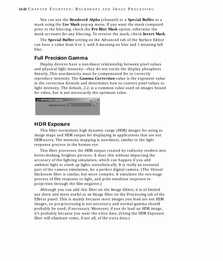
You can use the Rendered Alpha (channel) or a Special Buffer as amask using the Use Mask pop-up menu. If you want the mask computedprior to the blurring, check the Pre-Blur Mask option, otherwise themask accounts for any blurring. To reverse the mask, check Invert Mask.

The Special Buffer setting on the Advanced tab of the Surface Editorcan have a value from 0 to 1, with 0 meaning no blur and 1 meaning fullblur.

Full Precision GammaDisplay devices have a non-linear relationship between pixel values

and physical light intensity—they do not excite the display phosphorslinearly. This non-linearity must be compensated for to correctlyreproduce intensity. The Gamma Correction value is the exponent valuein the correction formula and determines how to convert pixel values tolight intensity. The default, 2.2, is a common value used on images boundfor video, but is not necessarily the optimum value.

HDR ExposureThis filter normalizes high dynamic range (HDR) images for using as

image maps and HDR output for displaying in applications that are notHDR-savvy. The intensity mapping is non-linear, similar to the lightresponse process in the human eye.

This filter processes the HDR output created by radiosity renders intobetter-looking, brighter pictures. It does this without impacting theaccuracy of the lighting simulation, which can happen if you addambient light or crank up lights unrealistically. It is really an essentialpart of the camera simulation, for a perfect digital camera. (The VirtualDarkroom filter is similar, but more complex. It simulates the two-stageprocess of film response to light, and print emulsion response toprojection through the film negative.)

Although you can add this filter on the Image Editor, it is of limiteduse there and more useful as an Image filter on the Processing tab of theEffects panel. This is mainly because most images you load are not HDRimages, so pre-processing is not necessary and normal gamma shouldprobably be used, if necessary. Moreover, if you do load an HDR image,it’s probably because you want the extra data. (Using the HDR Exposurefilter will eliminate some, if not all, of the extra data.)


HDR Exposure

The Input Dynamic Range is an informational display showing theHigh and Low pixel-intensity values encountered in the last processedimage. Note that when the panel first appears, this information is not yetknown.

If you do not want the filter applied to the Full Image, set theExposure Apply pop-up menu to Foreground to apply it only to sceneitems or Background to affect only the background (i.e., where youralpha would be black).

The White Point is the input intensity considered to be the hottestwhite. Anything above this will be the same white in the output. Thiscontrol is overridden by the Auto-Iris option, which sets the white pointbased on the actual input image data. Adjusting the white point is similarto cranking down an iris on a film camera to limit how bright parts blowout in a photograph.

The Black Point, expressed as a percentage of the nominal blackpoint (1/255), is the darkest non-black pixel level in the input image thatwill be preserved. Anything darker will come out black. The Auto-Exposure option overrides Black Point by using the actual image data todetermine a black point in the incoming data. Lowering the black point issimilar to increasing the exposure time for a photograph.

Once these values are set, the filter translates the incoming imageintensity—in a process very similar to gamma correction—so that thedarker colors get more of the output range than the brighter colors. Inother words, the filter changes the spacing of intensity levels so morelevels are devoted to low intensity, darker details.

Soften Reflections (Post-processing only)This filter will blur reflections. The Blend control will Replace the

reflection with a blurred version, Average them together, which is moresubtle, or use the Maximum of the replace result and the original, whichavoids a dark halo, at the cost of a lighter image. You can also blendbased on the Alpha channel or the intensity of the reflection(LumaBlend).

L I G H T W A V E 3 D 7 14.33

Soften Reflections

Soften Reflections can scale the blur based on the surface’s value inSpecial Buffer 1 (Advanced tab of the Surface Editor), if you check theScale By Surface Buffer option. (A value of 1 means 100 percent.)

Left to right: SoftReflections off, Replace,Average and Maximum

Left:Alpha. Right: LumaBlend

Render Buffer Export (Post-processing only)This filter lets you save images from one of LightWave’s internal

buffers (Source). The Surface Custom option on the Source pop-upmenu will create a grayscale image, where each object surface can havea unique grayscale value. This was designed to allow post-processingeffects to be applied on a surface-by-surface basis. A surface’s grayscalevalue (0-255) is assigned using the Special Buffer option on theAdvanced tab of the Surface Editor.

To invert the image data, check the Negative option. The Normalizeoption is available only for certain Source selections that don’t normallyprovide image data, like X Motion. Normalize scales the values to be 0to 1.


With the Destination pop-up menu, you can save the selected bufferimage as a separate Image File, or replace the Rendered RGB orRendered Alpha image data. (If you choose Image File, set the ImageType and enter the full path and filename in the File Name input field.)

TextureFilterUse TextureFilter to add the selected texture to the image before use.

You could use this filter to add, say, an animated Fractal Noise pattern toa simple black image. Since textures are three-dimensional, particularlyprocedurals, use the Axis setting to use the X, Y, or Z of the texture.(Note: The differences between the Axis selection can be subtle.)

To see procedurals in viewports:You can use TextureFilter to see procedural textures in your Layout

viewport! Basically, you apply the procedural texture(s) to the imageusing TextureFilter and then map the image to the surface. Here’s howyou do it:

1 First, you need to load an image into the Image Editor. It reallydoesn’t matter what image you use since it will be obscured by thetextures.

2 On the Image Editor’s Processing tab, add TextureFilter. Double-clickit in the list window to access its options. Click the Texture button toaccess the Texture Editor.

3 Change the default initial Layer Type to Gradient. This provides theunderlying color. You can leave it white or change it.

4 Add one or more procedural texture layers and set as you wouldnormally.

5 Load your object and open the Surface Editor.

6 Click the Color attribute’s Texture button. Leave Layer Type set toImage Map on the Texture Editor that appears.

7 Set Projection as you would normally and select your image from theImage pop-up menu. The procedural will now appear in yourviewport.

L I G H T W A V E 3 D 7 14.35

Dots and Crumple textured on cow’s hide

This operation requires a lot of computations and Layout may seemsluggish as it computes the texture.

NOTEThe image preview window on the Image Editor will show the textureas well.Thus, you can double-click the window to bring up the ImageViewer, from which you can save this compiled image.This can then beimage mapped back onto the surface without all of the calculationsrequired with TextureFilter.

If you use an image sequence instead of a still image, you can evensee an animated texture! Note that if an animated texture is applied to astill image, it will not appear animated.

Vector Blur (Post-processing only)LightWave’s normal motion blur (Camera properties) may need long

render times because of multi-pass antialiasing. Vector Blur, on the otherhand, can achieve great-looking motion blur in a fraction of the rendertime.

The two modes, Vector and Blur, use motion data that identifies eachpixel’s immediate motion in the horizontal and vertical directions. TheVector mode smears the pixel out based on the motion information,while the Blur mode uses the horizontal and vertical data to smush


together the surrounding pixels with that pixel. Blur affects the pixelsaround it including backgrounds, while Vector alters only the pixels ofthe moving object.

The Blur mode should be used in conjunction with the normal motionblur; however, the Vector mode can be used by itself—you don’t evenneed to use antialiasing! The result can be drastically reduced renderingtime.

Below is a comparison between regular motion blur and the twomodes of Vector Blur.

Left: Regular. Middle: Blur mode. Right:Vector mode

Overlapping ObjectsSince objects become transparent with motion blur, the filter needs

something in the background of the blur. When Compensate Backgroundis active, the filter does not use the backdrop and attempts tocompensate for this absence. This works in most cases, but may not givea very realistic motion blur.

When Compensate Background is not active, the filter uses thebackdrop. However, it will not show an object behind another object.

Left: Compensate Background is off. Right: Compensate Background is on

If you have overlapping objects, you may want to do some testrenders to see if Vector Blur will provide acceptable results. If not, useLightWave’s normal motion blur.

High Quality BlurIf you uncheck Compensate Background, you can activate the High

Quality Blur setting. This provides better quality, but takes longer torender. In this mode, you will only be able to set the Vector Lengthsetting.

LimitsThe important thing to understand about using Vector Blur is that it

is a post process. As such, hidden geometry can't be blurred and you

L I G H T W A V E 3 D 7 14.37

may see problems with motion blur on shadows and moving textures.However, it can be a great help when used in conjunction with normalmotion blur, by giving you better quality with lower antialiasing settings(Camera panel).

Video LegalizeThe Video Legalize filter might be more appropriately named Hot

Video, since it assumes that pure black, RGB 0, 0, 0, is mapped to theproper pedestal by the encoding device (e.g., 7.5 IRE for NTSC). Theencoding device may not, however, correct hot pixels—that is, colorsthat exceed certain video specifications. This is where VideoLegalizesteps in.

Pixel values are generally scaled into IRE units using the Black Point,White Point and Pedestal settings as follows: Level = Pedestal + (100 -Pedestal) * (pixel - Black) / (White - Black). White is always 100 IRE andNTSC black is 7.5 IRE. Thus, for NTSC, the level would be computed:Level = 7.5 + 92.5 * (pixel - Black) / (White - Black).

Normally, an RGB level of 0.0 is black and 1.0 is white. If those areused for the Black Point and White Point settings, the level will be 7.5 +92.5 * (pixel - 0.0) / (1.0 - 0.0) or just 7.5 + 92.5 * pixel. When the pixel is1.0, the level is 100 IRE, and when the pixel is 0.0, the level is 7.5 IRE.

NOTENote that the actual computation is more complex than the abovesince other operations, like gamma correction, can happen.

The settings default to NTSC encoding, but you may also select PALfrom the Encoding pop-up menu. (Note that you also need to click theDefault button after selecting a new Encoding item.) You may changethe individual settings from their defaults, if desired.

The Correct pop-up menu determines how the image is corrected tofall within the specified limits.


NOTEIt is highly recommended that you use VideoLegalize (as a post-processimage filter) if you plan to use your images for video.

Video Tap (Post-processing only)

The Video Tap filter will save a second image using different cameraand render option settings. This is perfect for times when you render afilm resolution scene, but you want to preview a video resolution versionon your Video Toaster or other digital disk recorder.

FUN FACTSMovie-makers often attach a video camera to a film camera, so theycan watch dailies without developing the film—saving time and money.This filter’s namesake is the video tap on the film camera. (Clever ideaby Brad. More clever name by Arnie.)

Virtual DarkroomThe Virtual Darkroom filter simulates the photographic capture of

images. It is based on A Model for Simulating the PhotographicDevelopment Process on Digital Images, by Joe Geigel and F. KentonMusgrave in the SIGGRAPH ’97 conference proceedings.

L I G H T W A V E 3 D 7 14.39

Virtual Darkroom

Global settings are the four controls located at the top. Output Typespecifies whether the output image is Black and White (single-planegrayscale) or Color (three-plane RGB). Use Reset to Default to reset allcontrols to default values. You can save and load settings using the SaveCurrent Settings and Load New Settings buttons.

Basic Settings TabBasic Settings control everything except for those settings on other

tabs. Negative LUX is the illumination value for the negative pass—analogous to scene capture with a camera—which will affect overallbrightness. Negative Time is the exposure time for negative pass,essentially the exposure setting on the virtual camera. Positive LUX isthe illumination value for the positive (printing) pass. Think of this asthe brightness of the bulb in the enlarger or printing mechanism.Positive Time is the exposure time during the printing pass of virtualenlarger.

Enable Scattering will activate the internal scattering effect. NegativeWidth and Negative Height are the width and height, respectively, inmillimeters, of the virtual negative. These values are used in scatteringand grain calculations. Enable Grain will activate the grain effect.Selwyn Granularity controls the intensity of the grain. Increasing thisvalue increases grain, decreasing it will decrease grain.

Spectral Sensitivity TabIf Output Type is set to Color, there will be six sets of RGB

percentage controls. Each RGB trio specifies the percentage of the blackand white output plane that is contributed by the input image plane


named in the control. For example, the RGB trio in the upper-middledefines how the output from the negative passes on the spectralsensitivity module creates the green plane.

If Output Type is set to Black & White, you specify what percentageof the red, green, and blue planes of the input image are used when theyare combined into a single black and white image. This transition takesplace in the negative (first) pass. During the printing (second) pass,there is only a single input plane, so spectral sensitivity is not used.

Film, Paper, and MTF Curve TabsYou can enter up to 21 pairs that define the characteristic curve of

the film and paper, and the function for modulation transfer used forscattering calculations. For each pair, the first value represents log(exposure) and the second value represents the density.

For all Curve tab entries, points should be entered in order startingwith Pt. 01. If Output Type is set to Color, curves must be set for eachoutput plane by selecting the appropriate Red Plane, Green Plane, orBlue Plane sub-tab.

Original image.

Left: Processing with TMax 100/PolyMax with scattering of a 3.2 mm x 2.4 mm. Right: Same with Grain enabled

L I G H T W A V E 3 D 7 14.41

Left: . Right: Processing with TMax 100/PolyMax with scattering of a .32 mm x .24 mm. Right: Same as above with Grain enabled

WaterMarkThe WaterMark filter embosses an image in the lower-right quarter of

the image. You can select any loaded image; however, grayscale imagesusing a black background work best. The Light Angle field determinesthe direction of the implied light source.

NOTEOther filters, like Pixel filters, may appear on the Image Editor in thelist of image filters.

WAVEFILTERIMAGEThe WaveFilter Image image filter allows you to apply and adjust

image filters, color filters, grain and matte filters to the entire image, thebackground, objects only, shadows only, a special buffer, or a user-definable color range. A powerful interface with color preview providesthe control you need to tweak your image to perfection.

Image filters include blur, sharpen, edge blend, saturation, negative,high/low limit, palette, film grain, and flip frame. The edge blend filterprovides additional and faster anti-aliasing control, allowing a possible30% to 50% savings on rendering times.

Color filters controls for RGB values, as well as the contrast, midtone,gamma, luminosity and brightness of the image. The filters work on apercentage scale, but values above 100% can be entered to create allsorts of interesting effects.


Matte filters are used to create images for compositing. Portions ofyour images can be set to black or white for matte creation. If you do alot of image compositing, you will find Matte filter to be an invaluabletool.

For even more control, WaveFilter Image can be added more thanonce to allow for multiple passes over an image, with each pass applyingdifferent settings to different parts of an image and creating differenteffects.

WaveFilter Image allows you to move many pre- and post-renderingoperations directly into LightWave. It fully supports network rendering,animated settings and has batch processing capabilities.

NOTESpecial thanks to Mike Reed for his work on this plug-in.

Image FiltersImage Filters can be used individually or in combination with other

filters to apply interesting effects. These filters use simple mathematicalformulas for faster image rendering. Several adjustable presets areincluded for quick effects.

L I G H T W A V E 3 D 7 14.43

WaveFilter Image Image tab selected

Blur ImageBlur Image simulates out-of-focus effect and is applied equally across

your image. This filter is commonly used on the background to helpcontrast your sharply focused objects in the foreground.

SharpenSharpen is an edge-seeking (low-pass) detail-enhancing filter that will

increase the sharpness between surface colors by exaggerating thedifference in color between the two edges.

Edge BlendEdge Blend is a softening tool that will smooth the edges between

sharply contrasting surfaces. This helps to tone down the stair-stepedges or jaggies found in computer graphics.

You may control the Number of Passes this filter makes. Highervalues provide finer detailed blending of the edges. Tolerance allows youcontrol the amount of edge affected. You may also limit the edgedetection to Object Edges Only.


Multi-Pass Edge BlendSome images with single-pixel details, like stars or highly detailed

objects, lose desired details when the Edge Blend filter is set strongenough to remove unwanted jaggies. Increasing the Number of Passescan help to minimize this loss of detail. (Note that normally only a singlepass is needed.)

When you select more than one pass, the filter searches for edgesand applies the blend at a power equal to the percent you select dividedby the Number of Passes. For example, if are using four passes at 100%,the filter will apply a blend of only 25% on each pass.

Once the first pass is completed, the edges are detected again, butthis time fewer edges will be found—edges that needed only the light25% blend will not be selected. This process is repeated for all passes.This results in the pixels that needed the least blending only getting a25% blend, while those that needed a bit more get 50%, and so on. Onlythe worst jaggies get the full 100% blend.

Adding WaveFilter Image plug-in multiple times can also help inremoving really bad jaggies. Just like using multiple Number of Passes,each instance of the filter will only select the jaggies that remain afterprocessing in any previous instance. However, remember that the blendpercentage will be applied fully for each instance, so you may want tokeep the value as low as possible to avoid overly blurring the edges.

Using on Rendered imagesIf you render a large number of frames and find you should have used

a higher antialiasing setting, you can simply apply the Edge Blend filterto them—WaveFilter Image does not require geometry to work. Thiscould save you from re-rendering the original scene.

To do this, simply load the images as an image sequence and set thesequence as the background image. Then, set the camera to exactly thesame resolution as used for the original images and turn off any normalantialiasing. Set the images to render to a new filename and you’re readyto post process.

SaturationSaturation allows you to control the saturation of the image’s color.

NegativeNegative gives control of the amount of negative applied to an image.

50% negative is equivalent to RGB 128/128/128.

Limit High/Low ColorThe Limit High Color and Limit Low Color settings limits the colors

in your image to levels which are NTSC compliant. Only highlights areaffected.

L I G H T W A V E 3 D 7 14.45

PosterizeThe Posterize filter reduces the colors used causing a poster-like

effect. Lower values allow more colors.

Palette ReduceThe Palette Reduce filter limits the colors in your image to smaller,

evenly distributed, color palettes. Palette reduction method can bespecified as a preference by choosing either Average (the default),NTSC/PAL Luminance, HDTV Luminance, Nearest Red, Nearest Green,or Nearest Blue.

Several palettes are available on the Use Palette pop-up menu. IfCustom is selected, the Palette button and input field will be available.Here you can specify a Photoshop *.act file or an ASCII file that defineseach color in the desired palette.

Film GrainCheck Add Film Grain to add a random noise effect. of selectable

density to your image. The Color setting defines the grain color.Checking Greyscale Grain causes the grain to be various levels of gray.

Flip FrameFlip Frame provides a quick method to vertically and/or horizontally

flip the image.


Color FiltersColor filters allow global control of general color attributes.

WaveFilter Image Color tab selected

ContrastThe Contrast value sets the mid-tones of the selected part of the

image either towards the highlight or shadow range. The Center settingcontrols the contrast tonal range.

MidPointThe MidPoint value is similar to the Brightness setting, except it

affects only the mid-tones within the selected part of the image. Use inconjunction with Brightness for a good overall lighting effect. The Centersetting controls the MidPoint tonal range.

GammaGamma allows control of the range between the darkest and lightest

areas of your image.

L I G H T W A V E 3 D 7 14.47

LuminanceLuminance adds overall brightness or darkness to the frame.

Shadows, mid-tones, and highlights will all be affected.

BrightnessBrightness multiplies the amount of light within the selected part of

the image. Mid-tones and highlights are affected, while dark shadows arenot affected. Use Brightness to adjust the lighting within your imagewithout resetting the scene’s lights or raising the ambient light level.

Adjust ColorThe Adjust Color options provide different options for adjusting

colors.

Mult: Pixel x Percentage looks at the color information in each RGBchannel and multiplies the base color by the selected Color.

Add: Pixel + Color adjusts the color information by increasing theamount of R, G and B color in the image.

Sub: Pixel - Color adjusts the color information by decreasing theamount of R, G and B color in the image.

Replace: Pixel = Color replace will change the RGB color from thecurrent base color to the new selected Color.

Matte FiltersThe Matte tab contains options that affect the image’s alpha channel.

You can see the results in the Image Viewer when you render a frame(F9) by simply selecting Alpha from the pop-up menu in the upper-rightcorner.

WaveFilter Image Matte tab selected

Choosing Custom will set the alpha channel for the affected area to agrayscale value defined in the Custom Value input field.

Choosing All Black sets the alpha channel for the affected area toblack. Choosing All White sets the alpha channel for the affected area towhite. Generally, with these, you will want Affected Areas (Affect tab)set to something other than Full Frame.

Invert reverses the alpha channel for the affected area.


The Affect Tab

WaveFilter Image Affect tab selected

Affected AreasWaveFilter can apply most filters to a scene’s images, surfaces,

channels or objects. Often, when multiple WaveFilter passes areinstalled, you will select a different portion of the image to effect in eachpass.

Objects applies the effect to all objects, including an image mappedpolygon background.

Background applies the effect to the background only.

Shadows applies the effect to the shadow channel only.

Full Frame applies the effect to the entire frame.

High/Low Color Range applies the effect to a selected color range inall three color channels (RGB). The range is defined by the Lower Boundand Upper Bound colors.

Selected Surfaces applies the effect to selected surfaces. Surfaces areconsidered selected if they have a Special Buffer value greater than zero.To access, click the Special Buffers button on the Advanced tab of theSurface Editor.

Preset ShelfClick Use Shelf to access the standard Preset shelf to save and load

presets. You can save WaveFilter settings to the shelf by double-clickingon the preview image.

Enable/DisableYou can quickly enable and disable all filters by clicking the Enable

All Filters and Disable All Filters buttons.

L I G H T W A V E 3 D 7 14.49

Preview WindowThe preview window will give you an idea of what the current settings

will do. This can take a little time to compute so you can disable thepreview. You may also use the last rendered image instead of the defaultimage.

WaveFilter Image preview window and settings


cchhaapptteerr15Volumetrics

L I G H T W A V E 3 D 7 15.1

Chapter 15:Volumetrics

LightWave features volumetric effects—essentially lighting andparticle effects with physical volume. These effects are common ineveryday life and can play a key role in creating dramatic realisticenvironments. However, they are difficult to reproduce using standardpolygonal models.

BACKGROUNDA very common example of volumetric lighting is the atmosphere: the

color of the sky comes from the scattering and absorption of light in thedifferent layers of the atmosphere.

NOTEVolumetric light effects, like a cone of light from a flashlight, arediscussed in Chapter 32.

The combination of light scattering and absorption is the very core ofvolumetric lighting effects. Additionally, other parameters must also betaken into account, like volume size and shape, density distributioninside the volume, lighting conditions, and behavior of light inside themedium. Adjusting these parameters lets you create a wide range ofnatural effects.

The sky, for example, is usually blue because light attenuationdepends on wavelength and distance. When the sun is at the zenith, itslight crosses fewer layers of atmosphere than when the sun is on thehorizon. Blue light is stronger at the zenith than at sunset because thethinner atmosphere does not interfere with its shorter wavelength. InRed sunsets, the thicker layers of atmosphere attenuate blue light, butthe longer wavelength of red light passes through the atmosphericlayers.

Fog is another good example. It is a medium composed of vaporizedwater where density is distributed in a non-homogeneous manner. Thewater particles in the fog cause a dispersion/absorption phenomenon

that causes the lighting effect, while the density distribution gives theglobal appearance of the fog. If you want a thick fog lying on the groundand fading with altitude, you will have to use a density distribution thatmakes the density high at lower altitudes and low at higher altitudes. Ifyou want to add turbulence in the fog (to have a more cloudyappearance), you can add fractal noise, which creates a 3D density field.

Computational IssuesVolumetrics are calculated by integrating all the scattering/absorption

contributions along a ray (which comes from the camera). When you usea 3D fractal density field, the integration must be made numerically witha limited number of sampling points. In this case, the values will becalculated at each sampling point, which means that for 50 samplingpoints, the algorithm calculates 50 density field values, 50 lightingvalues, and 50 scattering/absorption values. All those values can take alot of time to compute. Using fewer sampling points will result in a fasterrendering but will introduce numerical errors: this is volumetric aliasing.Volumetric shadows can be obtained this way by measuring the lightingconditions at each sampling point along the ray.

When you work with a normal density distribution, you can make theintegration literally, which gives a much faster rendering. But in thismodel (which we call fast model), it is not possible to measure lightingconditions along the ray, and as a consequence it is not possible to getvolumetric shadows.

Another important note about numerical issues is how to adjustvalues to get the desired effect. The intensity of the effect is alwaysrelated to the length of the medium crossed by the ray. This is obvious ifyou compare cigarette smoke to smoke from a large fire—the size of thevolume has a big influence on the result. The behavior of light may alsochange completely when the volume size changes, because absorptionmay overpower scattering, and vice versa. A good example of this isclouds.

When you look at clouds, you see that small thin clouds are brightand totally white, while big clouds have dark gray areas and a thin whiteborder. The dark gray color comes from the absorption of light insidethe cloud. Even the scattering of light emitted inside the cloud isabsorbed from the point of scattering to the boundaries of the cloud. Inthis example, absorption takes precedence over scattering whenthickness gets bigger. However, under other circumstances, the oppositecould occur. When you use high absorption and scattering values, youcan create explosion-like effects, where there is very high contrastbetween bright and dark areas. In conclusion, when adjustingparameters, you must be aware of the scale of the object you areworking on.

15.2 C H A P T E R F I F T E E N : V O L U M E T R I C S

About ParticlesWhen you work with particles, a sphere of gas is associated with each

particle. As a result, a particle cloud is really just a union of spheres.Computing the effect for every particle can be computationally intensive,particularly when their spheres overlap one another. The solution is theautomatic particle sizing option, which evaluates a particle size so thateach particle is close to another. The result is a dense cloud optimizedfor numerical integration and lower rendering times.

NORMAL FOGLightWave can generate a quick fog effect that is useful for many

special effects. Just as objects seem to blend into real fog with distance,the effect fades the objects away into the fog color you set. Fogsurrounds the camera in all directions, as though the camera were in themiddle of a huge spherical fog bank extending in all directions.

The fog settings are on the Volumetric tab of the Effects panel (Scene> Effects: Volumetrics). In setting up fog, you will set a minimum andmaximum distance from the camera. Within and beyond this range,objects will take on some amount of the Fog Color. You can also specifythe percent of fog color that objects take on at the minimum andmaximum distances.

The Fog Type pop-up menu sets the characteristics of your fog. Off,obviously, turns off the fog effect. The other fog types differ in how theeffect falls off toward the camera. Linear falls off in a linear manner.Nonlinear 1 is somewhat more realistic in appearance, since the fog willappear to grow thicker with distance. Nonlinear 2 has a steeper falloffcurve.

It’s important to realize that the Fog feature doesn’t actually calculatea wispy volumetric fog around objects, but rather changes the color ofthe objects to that color chosen as the Fog Color. As such, the backdropwill receive no amount of fog. For volumetric 3D fog, use the GroundFogvolumetric, discussed later.

L I G H T W A V E 3 D 7 15.3

A negative Minimum Distance will start the fog behind the camera.You can even enter a larger minimum amount than the MaximumDistance amount, which results in an effect whereby objects will renderin more of the fog when closer to the camera.

By default, fog is applied linearly between the Minimum Distance andMaximum Distance. Non-linear options are also available, which applythe fog amount more rapidly as they are moved away from the camera,then less so as they approach the maximum distance. The small graph tothe left of the setting gives you an indication of the fog application overdistance.

The Use Backdrop Color option causes an object to blend in withwhatever backdrop you have set, including a background image. Thiscan have the effect of making objects appear slightly transparent. Usethis option to simulate the effects of an underwater environment or ahazy, foggy day with an appropriate Backdrop Color like bluish green forunderwater and grayish white for a foggy day.

If you add the Texture Environment environment (Scene > Effects:Backdrop) and also activate Use Backdrop Color, your fog (andbackdrop) can use a texture.

Textured fog

NOTEThe rendering speed of the Fast Fog Render Type for the Ground Fogvolumetric comes at a price. Because it is not a full volumetric effect, itwill not always blend accurately with other volumetric effects, likevolumetric lights.This may result in visible artifacts in your renderedimages.


NOTEAlso see the discussion on the Unaffected by Fog option in Chapter9 and the special display options for fog in Chapter 6.

VOLUMETRIC ANTIALIASINGThe Volumetric Antialiasing option activates or deactivates the

antialiasing of volumetric plug-ins and volumetric lights. If this option isoff, the volumetric effects from the first rendering pass are stored andreused in later passes, instead of being re-rendered in each pass.Obviously, this can save rendering time, but will require more memoryand may cause problems when used in conjunction with motion blur ordepth of field.

VOLUMETRIC PLUG-INSVolumetric Plug-ins are added on the Volumetrics tab of the Effects

panel.

GROUNDFOGUse the GroundFog volumetric plug-in to add three-dimensional fog to

your scene. The fog has actual physical size so, for example, the cameracan move in and out of the fog. This differs fundamentally from normalfog, discussed previously, where the camera is always within the fog.

L I G H T W A V E 3 D 7 15.5

GroundFog panel

With the Render Type pop-up menu, you can choose between twodifferent types of GroundFog. Fast Fog is a quick-rendering fog with auniform thickness. It is basically the three-dimensional version of normalfog. Ray Marcher adds an uneven fog, particularly when you use atexture. Since this fog varies by precise physical position, like real fog, itis computationally intensive, but generally yields a more accurate andrealistic result.

When using Ray Marcher, you can throttle the amount ofcomputations using the Quality pop-up menu at the bottom of the panel.Add a texture by activating the Use Texture option. Clicking the EditTexture button will bring up the standard Texture Editor. A fog texturewill make your fog more interesting and less flat.

The Top and Bottom settings control the altitude of the fog, that is,where your fog starts and stops vertically. Falloff determines how thefog decreases to zero, from the Bottom to the Top. The higher the value,the more the fog will decrease its density. Note that the Ray Marchermode tends to fall off quickly at the fog’s edges, while Fast Fog has auniform linear fall off.

NOTEMake sure you know where your camera is when using GroundFog.The effect is really best seen from outside of the fog. If your camera isinside the fog, changing settings may appear to have little effect. In fact,if your camera is always within the fog, you may want to just use the(faster) normal fog.

The Luminosity and Opacity values are the values where the fog is atits thickest.


Nominal Distance is the distance at which the fog has a mediumeffect—it is not like standard Fog’s Minimum Distance. You will want touse small values for small-scale scenes. Large-scale scenes may requirehigher values to keep close objects from getting too affected by the fog.

You can set the color of the fog with the Color setting or you can justuse the backdrop color.

Without fog

Left: Fast Fog. Right: Ray Marcher fog using a texture

HYPERVOXELSWith ordinary polygonal objects, realistic effects like liquids, smoke,

clouds, and fire are difficult, if not impossible, to achieve withoutHyperVoxels. It simplifies the creation of volumetric rendering effectssuch as photo-realistic clouds, flames, explosions, dust, nebulas,contrails, fluids, smoke, ash, pyroclastics, gelatin, electromicroscopicimages, rusted materials, detailed solid and rocky surfaces, and much,much more.

L I G H T W A V E 3 D 7 15.7

Example HyperVoxels

HyperVoxels have computed mass, as opposed to the modeled massof normal LightWave objects. This opens the door to effects an order ofmagnitude greater in complexity. You can now transform objectsdynamically, like merging and slicing objects, without modeling multiplegeometries. A common example of this is the action of the substanceinside lava lamps.

HyperVoxel cow

HyperVoxels can be a surface, volume, or sprite. Surface HyperVoxelsare similar to standard LightWave objects. They have a defined surface,but no interior. If you go inside such an object, there is nothing. VolumeHyperVoxels, on the other hand, have computed volume. You would usethis option to create effects like gases, flames, clouds, explosions, oreven short hair or fur. Your camera can go inside these HyperVoxels andstill see the texture. The Sprite mode is a “slice” of a volume HyperVoxel.It renders quicker, but lacks much of the volume mode’s 3-D quality.


HyperVoxel fog

The HyperVoxels volumetric filter is usually applied to a points-onlyobject or a null object. The reason is that polygons may be visible afterrendering and usually this is not desired. However, having polygons maymake the object easier to see in Layout. In such cases, you can use theUnseen by Camera object property.

HyperVoxel textures are 3-D algorithmic textures, unlike normalsurface bump maps, which only appear to have depth. This means youcan actually get very close to the surface and the textures will look threedimensional. HyperVoxels feature sub-pixel displacement, which results insurface details no matter how close you get.

You can determine the position of HyperVoxels by using a null objector an object’s points. Moving the object will move the HyperVoxel object.Changing the position of an object’s internal points will also change thelook of a HyperVoxel object. HyperVoxels will appear around each pointand their proximity to each other affects how the object appears on thewhole.

A particle animation system is not required. You can achieve manyspectacular effects using null objects or points animated by conventionalmeans. However, to achieve realistic dynamic liquid effects, you willprobably need a LightWave particle system, like Particle FX.

NOTEHyperVoxel objects exist just as normal objects do.Thus, they castshadows, are reflected, and so on. However, currently, plug-ins do nothave access to all lighting information.As a result, HyperVoxels willcontinue to receive shadows, even if the Receive Shadows option onthe Object Properties panel is disabled.

HyperVoxels and Transparent SurfacesBecause volumetrics are ray-traced, to see a HyperVoxel behind a

transparent surface, you must ray trace transparent surfaces. You can dothis by simply activating the Ray Trace Transparency option on theRender Options panel. However, this is not necessary if the Refraction

L I G H T W A V E 3 D 7 15.9

Index of the object’s transparent surface (Surface Editor) is set greaterthan 1.0 (even 1.001) and Ray Trace Refraction on the Render Optionspanel is enabled.

Also, if you want to see an object behind a transparent HyperVoxelsurface, you need to set the Refraction Option to Ray Tracing +Backdrop on the HyperVoxels Shading, Environment tab.

Jump-starting with HyperVoxelsHere are some short exercises to jump-start you with HyperVoxels—

more complex tutorials are included later.

Exercise: HyperVoxels basicsThis exercise gives you a quick hands-on feel for how to use

HyperVoxels.

1 Add a null object to an empty Scene in Layout.

2 Add the HyperVoxelsFilter on the Volumetrics tab of the Effects panel(Scene > Effects: Volumetrics).

3 Double-click its name in the list to bring up its settings panel.

4 On the HyperVoxels panel, double-click on the null in the list window.This will activate HyperVoxels for this object. A check will appear tothe left of its name. (You could also select the object and click theActivate button.)


5 Object Type should be set to Surface. When you activate an object,the automatic size function is performed. The value 1m shouldappear in the Particle Size field.

6 Make sure the Automatic Preview options are active so we can seethe results of your efforts. Automatic Preview updates the preview asyou make changes, so you don’t have to keep clicking Render. OpenVIPER (the button is on the main Layout toolbar). You should alreadysee a rather dull ball in the VIPER window—of course it’s a lot moreinteresting than a rendered null.

L I G H T W A V E 3 D 7 15.11

NOTEYou can preview animated textures with VIPER. See Chapter 3 formore information. Remember that VIPER uses the camera view, somake sure the camera can see your particles.

7 Change the Particle size to 2. The ball should be larger now. (Wouldyou believe twice as big?) Activate the Draft Mode to speed VIPER up.

8 Click on the HyperTexture tab. This is where you define the surfacetexture—essentially the terrain of the surface. Select FBM from theTexture pop-up. Notice that this is similar to setting a surfaceprocedural texture.

9 Go ahead and play around with the various settings on this tab andwatch the HyperVoxel change.


10 You can actually apply all of the standard surface attributes toHyperVoxels on the Shading tab. All of the settings should be familiarto you since they are identical in name and operation to the normalLightWave surface settings. Try changing the various values and seetheir effects on VIPER.

Exercise: HyperVoxel volumetricsThis exercise will give you a flavor for some of the volumetric

features.

1 Using the HyperVoxel from the previous exercise, change the ObjectType from Surface to Volume.

2 Go to the HyperTexture tab and select Turbulence as the Texture.You should now see a nice wispy volumetric cloud. This object istotally three dimensional. You could fly the camera into it andcontinue to see all of the details. How cool is that?!

3 Let’s add some color. Go to Shading tab > Basic tab and click theColor Texture button.

4 Change the default Layer Type to a Gradient and use Local Densityas the Input Parameter. This will apply the gradient based on thedensity of the cloud.

L I G H T W A V E 3 D 7 15.13

5 Create three keys: blue, yellow, and red, top to bottom. You will seeVIPER updating the preview as you make changes. Click Use Textureto close the panel when you are done.

6 The options on the Shading tab > Basic tab control the basic look ofyour volumetric HyperVoxel. You can adjust the color, opacity, anddensity. The lower half of the tab controls the fractal look of theobject. Try playing with the settings to see their effects.


7 Click on the Advanced subtab. As you might expect, this tab containsmore advanced options. Included are options to define how theHyperVoxel object is lit, as well as self-shadow options.

8 Try messin’ with the various setting, including the Sprite mode.

Exercise: blending HyperVoxel objectsThis exercise shows how different HyperVoxel objects can interact

with one another.

1 Add three null objects to an empty Scene in Layout.

2 Move and keyframe Null (1) to Y = 1m and Null (3) to Y = -1m.

Camera view of three nulls

3 Choose Scene > Effects: Volumetrics and add the HyperVoxelsFilterand open its panel.

L I G H T W A V E 3 D 7 15.15

4 Activate HyperVoxels for all three objects.

5 Open VIPER and set Preview Options to Scene Preview. This willgive us a preview of all of the HyperVoxel objects in the scene.

6 Select Null (1) and choose New Group from the Blending Group pop-up menu on Geometry tab. Accept the default name Blend Group (1)by clicking OK.


7 For each HyperVoxel set the Blending Group to Blend Group (1) andthe Blending Mode to Additive (Geometry tab). By placing all of theHyperVoxels in the same group, they can interact with each other.

8 Try changing the Color (Shading tab > Basic tab) of each null andgiving them Texture (HyperTexture tab).

Notice how the texture surfaces blend together.

Preview OptionsWhen used with HyperVoxels, the Preview Options pop-up menu on

the VIPER window has some options. Object Preview gives you apreview of the selected HyperVoxel object only from the camera’sperspective. Scene Preview will show you all HyperVoxel objects visible

L I G H T W A V E 3 D 7 15.17

from the camera’s perspective. Particle Preview will give you anenlarged view of a single particle, which is particularly helpful if yourHyperVoxel object consists of many particles.

Use Z-BufferThe Use Z-Buffer in Preview option (on the main HyperVoxel panel)

allows you to preview your HyperVoxels in the last rendered frame.(Note: Object Preview or Scene Preview modes only.) This requires thatthe Enable VIPER option be active on the Render Options panel.

The Use Z-Buffer in Preview option in action

Sprite Texture ResolutionThe Sprite Texture Resolution setting (on the main HyperVoxel

panel) is a display setting and does not affect your renderedHyperVoxels nor VIPER. It allows you to set the quality of textures usedon HyperVoxel particles in Layout.

HyperVoxels Setting ManagementLoad/Save buttons allows you to retrieve and store HyperVoxels

setting files. This can be used to create a library of attributes.

HyperVoxels Setting Management


Use the Copy button to copy the settings for the selected HyperVoxelobject to a memory buffer. These can be pasted to the currently selectedHyperVoxel object using the Paste button.

You can enable/disable HyperVoxels for an activated object byclicking in the checkmark column and you will not lose your settings.The Activate button will activate the selected object and set all settingsto their defaults. The Deactivate button places the object in an inactivedefault state. With Activate and Deactivate, you will lose any existingsettings.

If the Show pop-up menu is set to All Objects, then all objects in thescene will be listed. HyperVoxels Only will list only HyperVoxel objects;however, this includes disabled HyperVoxel objects.

Object TypeThe Object Type pop-up menu lets you choose between the

previously demonstrated Surface, Volume, and Sprite HyperVoxelmodes. Use it for testing purposes when you are developing yourHyperVoxel animation.

Dissolve lets you individually set an opacity value for each activeHyperVoxel object: 0% is totally opaque and 100% is completelytransparent.

Object Type pop-up menu

SpritesThe Sprite mode is a simplified two-dimensional slice (or slices) of a

HyperVoxel, so it can quickly produce results to give the user a fastsketch of the HyperVoxel’s rendered appearance. You might think of it asa slice of a Volume that has been mapped on a polygon that always facesthe camera.

You may want to use Sprite to accelerate the setup process forSurface or Volume modes. It’s even great for instances where you don’tneed a full 3-D volumetric effect, like a smokestack in the distance.

L I G H T W A V E 3 D 7 15.19

Sprite with hypertexture

Although Sprites are two-dimensional in nature, you can still fly acamera through them. The sprite will begin to dissolve when the cameragets into it and eventually fully dissolve when the camera hits the slice.

Geometry TabEnter a specific radius for the individual particles in the Particle Size

field. Click Automatic Sizing to compute an average size—this is a handyway to find a starting point. The average particle size is based on theshape of the entire object—HyperVoxels surfaces will not intersect atthis setting.

NOTEWhen you first activate an object, automatic sizing is performed foryou.

The Geometry tab


Rendering time is related to how much the particles intersect eachother—the more intersections you have, the longer the rendering time.For fastest rendering, always try to use the fewest number of particlesand the smallest Particle Size that achieves acceptable results.

Size Variation sets the maximum percent that the particle size canvary. For example, a particle size of 1m with a variation of 100% can beas small as 1m and as large as 2m. Using a variation of 50% would yieldparticles ranging from 1m to 1.5m in size. Use this setting to createrandom disturbances in the surface.

Stretching and Rotating HyperVoxelsYou can stretch HyperVoxels on a selected axis or based on velocity

(Stretch Direction). The amount of stretching is determined by theStretch Amount setting, which may be animated. When using nulls, youmay stretch HyperVoxels by animating normal Layout XYZ size values.

Sprite stretched using Velocity

Hypervoxels also respect the rotation of the object.

The Maintain Volume option on the HyperVoxel panel Geometry tab,will cause the HyperVoxels to maintain their volume. This means thatwhen they get squashed, they will maintain the same area.

Align to PathAlign to Path causes the HyperVoxels to rotate as they follow a path.

This can be particularly important when using particles.

Blending HyperVoxelsSeparate HyperVoxel items can interact with one another. You can

individually set how the selected object interacts with other HyperVoxelobjects. In order for HyperVoxels to interact:

• All must belong to the same Blending Group

• All must have a Blending Mode selected

• To view with VIPER, you must have Scene Preview set as thePreview Options

Here, the two objects are shown separately

L I G H T W A V E 3 D 7 15.21

Left: Object 1. Right: Object 2

(none) means it will not interact with other HyperVoxel items.

no blending

Additive will smoothly blend HyperVoxels.

Additive on both objects

Negative will make the object push away portions of otherHyperVoxel items that it comes in contact with—sort of like an animatedboolean effect.


Negative on object 1 and Additive on object 2

Effector is kind of a cross between Additive and Negative.

Effector on object 1 and Additive on object 2

A Blending Group is the group of HyperVoxel objects that you wantto interact with each other. You can select an existing group or create anew one.

Show ParticlesThe Show Particles option will display a bounding sphere in

viewports.

Left: Show Particles off. Right: Show Particles on

Use ParticleStorm ColorThe HyperVoxels will use the color from ParticleStorm particles, if

available.

L I G H T W A V E 3 D 7 15.23

NOTEThe HyperVoxelsParticles Displacement plug-in lets you set theHyperVoxels particle base color to that of the vertex color map, if oneexists.

Shading Tab: Surface ModeThe parameters on the Shading tab work just like their cousins on the

Surface Editor. (See Chapter 31 for more information.)

Shading Tab: Surface Mode

Self Shadows lets the HyperVoxel cast shadows on itself. (TheHyperVoxel will cast shadows on other objects in the normal way.) FullRefraction forces rays to bounce each time a new refracting (i.e.,transparent) surface is found. If this option is inactive, one refractionbounce is computed, which is enough most of the time. Full Refractionwill, of course, increase render time, but will result in more sophisticatedeffects.

HINTYou might try the (faster-rendering) corresponding bump textures onthe Shading tab without HyperTextures, if you don’t need the truesurface details. Remember this: “Don’t get hyper if bumping will do” or“A bump in the night is not worth getting hyper over.”

Shading Tab:Volume ModeThe options on the Shading tab are different for Volume HyperVoxels,

which are gas- or cloud-type effects. Use the Color, Luminosity, Opacity,and Density settings to change those parameters for the volumetricobject.


Shading Tab:Volume Mode

The Thickness setting, which defaults to 50%, lets you adjust thegeneral heaviness of the volume. Higher Smoothing values yield less of ahard-edged look and volumes will appear more wispy.

Baking HyperVoxelsThe baking feature subdivides HyperVoxels into a 3-D grid of

subvolumes (a space subdivision). This dramatically reduces thenecessary computations and allows preprocessing of the HyperVoxeleffect, including shadows, textures, and so on. The result is essentially astack of image maps.

Click the Options button to display the baking options. The size ofthe “image map stack” is set on the Resolution pop-up menu. The firsttwo numbers define the size of the images and the third defines thenumber of frames.

Enter the name of the file to save in the Filename field. The animationcodec (File Type) used when saving the volume data is very important.By default it uses QuickTime uncompressed because this formatpreserves the alpha channel. This is important because the alphachannel encodes the volume opacity information. Many codecs don'thandle the alpha channel properly and the opacity information will becompromised. (Note that you could edit the file externally in anotherprogram or even create one from scratch.)

Baking options dialog

L I G H T W A V E 3 D 7 15.25

Click Bake Object to execute the baking computation. Whencomplete, you should notice that most of the normal settings will beghosted except for some basic ones like Color, Luminosity, and so on.These can be adjusted to change the look of the baked object.

Volume Mode Advanced Sub-tabThe various items on the Render Quality pop-up menu determine the

level of detail HyperVoxels uses to render the volume. The default isMedium and should be adequate for most situations. Near Clip is thedistance from the camera where the rendering starts. The default valueis normally fine. A lower value will render finer details, but take longer torender. You might adjust this setting if the camera was inside a cloud. Itreally depends on the scale of the HyperVoxel objects and the scale ofthe details you want to see.

Volume Mode Advanced sub-tab

The Volumetric Shadows option creates shadows within the volume,which add detail and realism. However, it can increase render timesignificantly, especially when you are trying to simulate very denseclouds, like volcanic smoke. The Texture shadows option yields a veryrealistic shading of the hypertexture, but increases rendering timesignificantly. If you disable this option, you will miss all of thehypertexture shadow details.

Use the Shadow Quality pop-up menu to choose the render quality ofthe shadows. The Shadow Strength sets the darkness of the shadows.

The Illumination pop-up menu determines how the HyperVoxelsvolume is lighted. Self acts as if the light comes from the viewer. It canbe useful to see more details on the object. With Constant, the scatteringof light is constant, that is, the amount of light scattered at one point isproportional to the amount of light received at that point.


Rayleigh simulates a strong forward scattering of light within thevolume. Light scatters in the direction of the light relative to the viewer,which means that illumination will be at its maximum when the lightfaces the viewer. This is perfect for back-lit clouds, smoke, and so on.

Beer uses the pattern’s sample density amount as the illuminationvalue, dramatically reducing contrast between lighted areas. The settinguses the physical model for scattering of light inside a gas, and is a goodsetting for clouds. For a more “cartoony” look, try CelShade.

You can choose to have all lights affect the HyperVoxel with Use AllLights, or choose one or two specific lights.

HINTTry to avoid using these Light options, if you are ray tracing shadows.Ray-traced shadows on volumetrics is incredibly computationallyintensive and will often result in unacceptable rendering times.A singlepixel in volumetrics requires 20 or more samples and a shadow is raytraced for every sample.Try to fake lighting with Ambient Intensityand surface Luminosity or use shadow map Spotlights.

Ambient Color lets you specify the ambient light color of the volume.This setting works hand-in-hand with the Color setting on the Shadertab. Ambient Color is similar to ambient light in Layout, except it appliesonly to the selected HyperVoxel object. Basically, the shading process isvery similar to what happens with regular object surfaces.

Because of the way illumination is calculated inside volumetricsobjects, Ambient Intensity can be higher than 100% withoutoverexposing the image.

Shading Tab: Sprite ModeThe options on the Sprite mode Basic subtab are similar to the

options available for the Volume mode. This makes sense since the

L I G H T W A V E 3 D 7 15.27

Sprite mode is just a slice of a Volume mode HyperVoxel. Density onsprites is a multiplier for both Opacity and Luminosity. It is essentiallythe opposite of Dissolve.

Shading Tab: Sprite Mode

With the Number of Slices setting, you can “thicken up” the effect byincreasing the number of slices used for sprites from the default settingof 1. This allows you to get something a little closer to the Volume modewhile still retaining the speed of the Sprite mode.

Left to Right: 1-slice sprite, 5-slice sprite, and Volume mode

You may choose to light the Sprite using all lights in your scene or upto two specific lights.

On the Clips subtab, you can map an image directly onto a spriteusing the Add Clip button. Any image available to the scene may beselected. Use the Image Editor to load an image not already available.


Clips subtab

Clips are added to the HyperTexture. If you want to see only the clip,set the Texture option to (none) on the HyperTexture tab.

Some options on the Alpha pop-up menu let you cut away parts of theimage you don’t want to use. If the image file includes an alpha channel,choose Embedded to use the alpha channel. Use Luminosity to leavebrighter parts of the image. The Black mode will cut away black areas.The Threshold level lets you increase the range for what is consideredblack.

The Rotation setting sets a rotation speed for your clips. This isperfect for effects like billowing smoke and explosions. The higher thesetting, the faster the rotation. Positive values make the clip rotateclockwise. Rotation always faces the camera.

If you do not want to use the color information in the image, uncheckUse Color. Then, only the grayscale information will be used.

AntiAliasing will yield better-looking edges, but it significantlyincreases render time and memory requirements.

When Solid is checked, the sprite is rendered as a solid object,preventing the normal additive result of overlapping sprites.

Sprite Clip Frame OffsetIf you use HyperVoxels with particles, you can use multiple clips. The

Frame Offset setting determines how you want to map an imagesequence to a given particle. Particle Age starts the sequence for aparticle at birth. Thus, the image will likely be different for particles at agiven frame. Uniform will use the layout time as the time in the

L I G H T W A V E 3 D 7 15.29

sequence. Thus, the image used is the same at each frame. When thebottom of the list is reached, it starts again from the top. Random willassign a random offset to each particle.

Frame Offset is an important control for sprite animations. It allowsyou to decide how to attach images to particles. Particle Age isprobably the most useful. You can have literally hundreds of particles,each mapped with distinct image sequences. For example, you couldhave particles with independent water-splash image sequences, creatinga complex and rich visual effect.

HyperTexture TabThe Texture pop-up menu determines what the texture will look like.

The textures in this menu correspond to the identically namedprocedural textures, although not all of them will be available here. (SeeChapter 31 for more information.)

HyperTexture Tab

The big difference is when you are using a Volume (Object Type)HyperVoxel. In this case, you can animate the texture effect.

Texture animation settings

In the Texture Effect pop-up menu you have several options.Turbulence makes the texture move towards the viewer. It is likeanimating a texture with the texture velocity parameter. Billowinganimates the texture by rotating outward along a velocity vector (à laDante's Peak). It is very good for explosions. Displace adds variations tothe texture. The effect is best seen when the texture is moving. Dissolvegradually lowers density, making particles disintegrate.


Velocity Translate moves the texture in the direction of the particlevelocity. Since each particle has a different velocity, this can result in acool and complex texture motion. Dissolve & Expand might be used onexplosions. It dissolves the effect as it expands.Some trial and error maybe necessary to get the desired look.

The Effect Speed setting is the duration of the looping cycle. Thevalue is equal to a percentage of Layout’s Default units, on the GeneralOptions tab of the Preferences panel, per frame.

NOTEAnimated textures can be previewed with VIPER. See Chapter 3 formore information.

Gradient Input ParametersSpecial Input Parameters will be available for texture gradients on

HyperVoxel parameters. Particle Age is simply the age of (Particle FX)particles, in frames. Particle Speed is the particle speed in defaultLightWave units (usually meters) per second. Use Time to change thesetting over a range of frames.

Gradient Input Parameters

The Particle Weight Input Parameter is used with regular objects thatuse HyperVoxels and requires them to have a weight map. The objectmust also have the HyperVoxelsParticles Displacement plug-in added.Set Particle Weight should be checked and the weight map selected.

L I G H T W A V E 3 D 7 15.31

Object Properties panel

To use the Particle Weight Input Parameter:1 Create an object in Modeler.

2 Create a weight map and add some random weighting to the points.

3 Load the object into Layout.

4 Choose Scene > Effects: Volumetrics and add the HyperVoxelsFilter.

5 Open the HyperVoxels panel and activate the object.

6 Open the object’s Properties panel, add the HyperVoxelsParticlesDisplacement plug-in. Open its options, activate Set Particle Weightand choose the weight map.


7 On the HyperVoxels panel, add a texture to the Particle Size and setthe Layer Type to Gradient. Choose Particle Weight as the InputParameter. Create some keys.

The ball.Your results will vary depending on your weight map

For HyperTexture and Shading settings, gradient textures can use adistance to particle (along a specific axis) input parameter. This is thesurface distance from the actual particle position along the selected axis.

L I G H T W A V E 3 D 7 15.33

cchhaapptteerr16Rendering Options

Chapter 16:Rendering Options

The Render Options panel (Rendering > Render Options) contains allof the settings that control your output. Generally speaking, it is herethat you set how realistic you want your images to look. They can rangefrom wireframe test versions to full ray-traced final images. You will alsospecify the file format for your output, ranging from single frames to ananimation.

Render Options panel

RENDER FRAMESThe Render First Frame, Render Last Frame, Render Frame Step

fields determine the range of frames you want to render as well as theframe increment. These are independent from the similar fields in themain interface, which control the playback of scene and PreviewAnimation creation.

L I G H T W A V E 3 D 7 16.1

AUTOMATIC ADVANCEBy default, LightWave will render only one frame at a time, even if you

have set a range of frames to render. After each frame is rendered, youcan click the Continue button on the Render Status panel (or press theENTER key) to continue rendering the next frame in the range.

This would likely get tedious in a 900 frame animation, so selectingAutomatic Frame Advance will continuously render all of the frames inthe defined range without stopping after each frame.

WARNINGWhen rendering, make sure you check the state of AutomaticFrame Advance before you grab some shut-eye!

RENDER COMPLETE NOTIFICATIONBy selecting Frame End Beep, you can instruct LightWave to have

your computer beep whenever a frame has been rendered or a wireframepreview has been generated. This can be a handy feature to inform youthat a process is finished. The status of Frame End Beep is saved as adefault when you quit LightWave.

MONITORING PROGRESSA watched pot does indeed eventually boil: when you activate the

Show Rendering in Progress option, you add a preview window to theRender Status panel that displays the image as it is generated. Thenumber of colors used in the window is determined by your computer’sdisplay setting. Of course, this is only a representation of the final image,which will be rendered in full color at the proper resolution.

16.2 C H A P T E R S I X T E E N : R E N D E R I N G O P T I O N S

NOTEUsing the Show Rendering in Progress option adds to renderingtimes.As such, this feature is best used for test rendering.You shoulddeactivate it for the final rendering process.

If the Show Rendering in Progress option is not active, a similardialog will appear, sans preview image.

You can close the Render Status window by clicking the Abort buttonor pressing the ESC key. You can also render the next frame (if you aren’tusing Auto Frame Advance) by clicking Continue or pressing ENTER.

VIEWING THE FINISHED IMAGEOnce LightWave finishes rendering a frame, the image is displayed

using the selected Render Display. The Image Viewer option isdescribed in Chapter 3.

NOTEThe FP (floating point) version of the Image viewer maintains thefloating point image data. Use it if you want to save files from theviewer and need the FP data. Note that it uses more memory than theregular Image Viewer.

VIPERVIPER (see Chapter 3) can use information from the internal render

buffers to perform tasks like surface previews. When used in thismanner, you must activate the Enable VIPER option. However, when yourender you should disable this option, since it increases rendering timeand memory consumption.

RENDERINGTo render the current frame—determined by the position of the frame

slider—choose Rendering > Render Current Frame or press F9. SelectRender Scene to render the entire scene using the defined range offrames on the Render Options panel, or press F10. Make sure AutoFrame Advance is set as desired!

L I G H T W A V E 3 D 7 16.3

NOTEColors on your computer monitor will not match actual NTSC/PALcolors. If possible, always test frames from LightWave on a videomonitor prior to final rendering.

You can also render only the selected object(s) at the current frameby choosing Rendering > Render Selected Objects. Unselected objectscan still cast shadows or be seen in reflections on the rendered objects.

NOTEThe Render Status window is a modal window.Thus, you may beprecluded from accessing options on other windows until it is closed.

RENDERING TABDepending upon your needs, LightWave can produce different types

of output. Select a Rendering Mode to output images best suited foryour project.

Selecting Quickshade will render the objects with no smoothing,textures, transparency settings, or object dissolve levels. It gives a betterrepresentation of the camera’s view than Wireframe and can be handyfor checking out rough lighting and object placement. Because of itsspeed, using Quickshade is a good idea for testing out CPU-intensivefeatures such as Motion Blur and Depth of Field (Camera Propertiespanel).


Quickshade mode

Selecting Wireframe will produce wireframe representations of all ofthe objects in your scene. This will show all polygons of an object in thecolor chosen for Surface Color on the Surface Editor’s Basic tab. Theadvantage of Wireframe is that it renders quickly and is ideal forshowing the motions of objects in your scene without any of the detail.

Wireframe mode

HINTTo produce a solid wireframe animation, Use the Unshared Edges,Surface Borders, and Other Edges options on the ObjectProperties panel’s Edges tab, and render in Quickshade mode.

Realistic is the mode you will use most for final rendering. It rendersimages with full photo-realistic quality. Plus, you can use all ray tracingfunctions.

L I G H T W A V E 3 D 7 16.5

Realistic mode

Ray Tracing OptionsWhen Realistic is selected as the Render Mode, you can also select

any of LightWave’s ray tracing functions. Ray tracing lets you renderrealistic shadows, reflections, and refractions.

Ray Trace Shadows causes illuminated objects to cast ray-tracedshadows onto themselves or other objects.

Ray Trace Shadows

NOTELights must have Ray Trace selected as their Shadow Type (LightProperties panel).

HINTJudicious use of the Self Shadow, Cast Shadow, and ReceiveShadow options (Object Properties panel, Rendering tab) forindividual objects can speed up rendering times dramatically when raytracing shadows.

Choosing Ray Trace Reflection allows objects that contain surfaceswith some degree of surface reflectivity to reflect any other objectsaround them.


Ray Trace Reflections

NOTEThe surfaces must have one of the Ray Tracing options selected as theReflection Options (Surface Editor’s Environment tab) in order toray trace reflections.

Ray Trace Refraction instructs LightWave to calculate refractions forsurfaces that have some degree of Transparency, and a RefractionIndex (Surface Editor, Basic tab) higher than 1. Any objects seen throughthese surfaces will be distorted, such as a straw that appears bent in aglass that is half full of water.

Ray Trace Refraction

NOTEAlso see the discussion on the Unseen by Rays option in Chapter 9.

Ray Trace Transparency causes all transparent surfaces, not justrefracting surfaces, to be ray traced. This allows volumetric effects (e.g.,HyperVoxels) to appear behind such surfaces without forcing refractionray tracing. Only use when necessary since this option will add torendering time.

L I G H T W A V E 3 D 7 16.7

Ray Trace OptimizationRay tracing in its simplest form must determine which polygon each

ray hits. However, if all polygons were individually tested for every ray,ray tracing would be impractical for all but the simplest scene. Somesort of acceleration strategy is needed to make ray tracing practical.

LightWave's primary acceleration strategy is to compute a hierarchyof bounding volumes before doing any ray tracing. This involves someextra work initially, but it usually pays off when rays are actually traced.For example, if 1,024 polygons are contained within a box and aparticular ray misses that box, there is no need to individually testwhether the ray hits any of those 1,024 polygons, and the program canimmediately try the next box. Moreover, if the ray does hit the box, itmight still miss a smaller box within the first box, allowing it to skip thepolygons in the smaller box, and so on. Obviously, such techniques canresult in huge timesavings.

There are many ways to construct bounding volume hierarchies,some allowing much faster ray tracing than others. LightWave uses asimple and fast method by default. The Extra Ray Trace Optimizationoption activates a more sophisticated method, one that takes longer tocompute but generates "tighter" volumes that can be ray traced moreefficiently.

In scenes with heavy ray tracing, Extra Ray Trace Optimization cansignificantly reduce rendering time. However, in scenes with lots ofgeometry, but not much ray tracing, the extra preprocessing time mightexceed any rendering timesavings. If there is no ray tracing at all in thescene, this option is ignored, even if active. However, it is not alwaysobvious whether ray tracing is present. For example, surface shaders,volumetrics, pixel filters, and lens flares can sometimes trace rays even ifall of the ray tracing options are inactive. In such cases, thepreprocessing is still performed if Extra Ray Trace Optimization isactive.

Here are some factors to consider in predicting whether Extra RayTrace Optimization will help or hurt total rendering time:

• Bounding volumes are recomputed whenever time changes, so ifmotion blur is used, the preprocessing cost is multiplied by thenumber of passes and the number of segments, as opposed to beingdone only once per frame.

• The preprocessing cost depends roughly on the number of polygonsin each object, but heavy geometry slows down ray tracing too, sothat's not necessarily a reason to turn the option off.

• The benefits of using Extra Ray Trace Optimization depend on theamount of ray tracing needed, which is often proportional to thenumber of pixels that involve shadows, reflection, or refraction. Assuch, the benefit increases as the resolution goes up. Conversely, the


cost is still there even when rendering a 50% test image or a limitedregion, so any experiments to determine whether or not to use theoption should be done at full image size.

Ray Recursion LimitRay Recursion is the maximum number of times you want light

reflected off reflective surfaces. In the real world, things can be reflectedan infinite number of times, like when you have two mirrors facing eachother—you see an infinite number of reflections. In the world of 3Danimation, you must set a limit for the number of reflections. The defaultvalue is 16, but you can set this field from 0 to 24. Lower numbers willyield faster rendering times.

HINTIf you do not have a lot of reflective surfaces in your scene, try usinglow values (even a value of 1).

Multiple CPU SystemsThe Multithreading setting is used for systems with multiple CPUs.

Normally, you should set this to the number of processors on yoursystem; however, there are times when you will get faster rendering withthis set at a greater number. You may want to test a few frames beforebeginning your final render.

WARNINGA potential for problems exists with some plug-ins that were notdesigned with multithreading in mind. If problems occur, try using the1 Thread setting).

When Multithreading is set to 1 and Show Rendering in Progress isenabled, you can watch the image being built. If a higher setting is used,the window will not update until the segment or frame is totally finishedrendering.

Data OverlayThe Data Overlay option lets you place a descriptive title (of up to 20

characters) along with a frame reference in the lower portion of therendered image. This is useful when you generate large numbers ofanimations for others to review and approve before final rendering. Itcan serve to identify the scene being rendered, and the specific framesyou may wish to change. The Data Overlay pop-up menu settingdetermines the format for the frame reference. Enter the text in theLabel field. If Data Overlay is not set to Off and the Label field is blank,the scene name will be used automatically.

L I G H T W A V E 3 D 7 16.9

NOTEIf you have Data Overlay active, when you save your scene you canchoose to have the scene name automatically set as the Label.

Data Overlay

OUTPUT FILESAnimations can be saved in two ways: as a single animation file (e.g.,

AVI) or as separate individual frame files. The two are not mutuallyexclusive.

Output Files tab

To save an animation file:1 Click the Save Animation option to activate it.

2 If an acceptable animation file is not already defined (see the displayto the right of the Animation File button), a file dialog will appear.Choose a location and a filename for the animation. Be sure to addthe proper filename extension. (e.g., COOLANIM.AVI)

If you wish to change the defined animation file, click the SaveAnimation button and define a new one.

3 Choose the type of animation you would like to save with the relatedType pop-up menu. The available options will vary depending on theplatform you are using.


4 If the animation type has options, click the Options button to displaya dialog with the available options.

You can activate and deactivate Save Animation without losing thedefined animation file.

Special Animation TypesFilmExpand converts an animation from 24 fps (film speed) to 30 fps

(NTSC video speed) by rendering 30 frames for every 24 of the originalanimation. The interpolation works best when you use Field Rendering(Camera Properties panel). When you select Field Rendering, an optionspanel appears where you can select the type of image to save and set thefield dominance.

4XStoryboard creates JPEG images of the rendered animation framesat four times the camera resolution. You use this option when theResolution Multiplier (Camera Properties) is set to 25% for testrendering of a scene.

Storyboard creates JPEG images that contain small versions of therendered animation frames. The images are a five by six grid ofthumbnails of the rendered frames. Every fifth frame is skipped.

QuickTime_Stereo is used with the AnaglyphStereoCompose filter,discussed in Chapter 14, for creating animations in the red-blue glassesstyle.

L I G H T W A V E 3 D 7 16.11

QuickTime Virtual Reality Object SaverQuickTimeVR_Object is a QuickTime Virtual RealityTM object saver,

which adds the ability to pan and tilt the camera inside the animationitself.

QuickTime Virtual Reality Object Saver

What is a QuickTime VR Object?QuickTime VR Objects are QuickTime movies that display an object

from multiple views. Special data embedded in an otherwise ordinarymovie tells QuickTime how to play through the frames of a movie as aviewer moves the mouse across the image. When the viewer moves themouse down, the player skips a large number of frames to find one thatcorresponds to a view of the same side of the object, from a lowerposition. This can simulate rotating the object in space, if the views areright.

Once a scene with the appropriate camera and/or object movement iscreated, open up the Render Options panel and selectQuickTimeVR_Object(.mov) under the Type pop-up menu. Click theOptions button to set the critical parameters for your animation.

Object Settings TabThe image below shows the Object Settings tab.

Columns (Pan Frames) is the number of frames of horizontal views inthe animation. If your view is from 0 degrees at frame 0 to a full 360


degrees at frame 20 (the same view as 0°), then you will have 20 columns(frames 000 to 019). In a typical movie, the row angle will step up afterthis many frames.

The Start Pan and End Pan values set the angle range of thehorizontal views.

Flip Horizontal Control reverses the object's direction of rotationwith regard to horizontal mouse movement. In other words, if you dragthe object left and it turns to the right, you need to change this setting(or reverse your entire animation!).

Rows (Tilt Frames) is the number of frames of vertical views in theanimation. In a QTVR Object Movie, the animation moves through all thepan frames in a row before moving to the next tilt frame, and does all thepan views again with that tilt.

If there are 20 pan frames (000 to 019, as above), the tilt angle willchange every 20 frames, so sequential tilt values will be at frames 000,020, 040, 060, etc. This means that your entire animation must be (tiltframes)*(pan frames) long.

HINTThe default Columns and Rows settings (20 x 20 = 400 frames) aremore than enough for most uses and you may be able to use lowervalues to reduce the size of the file.

The Start Tilt and End Tilt values set the angle range of the verticalviews.

NOTEThe Start and End settings may not seem to change simple viewing ofthe objects, but may be critical if the object is embedded in a largerQTVR world.

Flip Vertical Control reverses the direction of rotation of the objectwith regard to vertical mouse movement. If you drag the object up, andit rotates down, you need to change this setting.

Animation Settings TabThis tab sets some advanced QTVR options.

Frames Per View sets the animation loop size that will run from eachview. If this value is greater than one, then your animation should hold

L I G H T W A V E 3 D 7 16.13

each pan view for this many frames, as the loop happens. This alsomeans that your animation length must be multiplied by this number.You should not alter the pan or tilt frame counts; QTVR will handle that.

The QTVR object format features an alternate state that can bedisplayed based on some user input, for example, when the user clicksthe mouse. The View States value supports this alternate state, but willalso multiply your animation frame count. These extra frames take theform of an entire identical animation of the object in an alternate state,appended onto the first. Currently, the QuickTime player appears tosupport only two usable states, not clicked and clicked. In theory, highervalues could be used.

The Compression Options button will invoke the standard QuickTimeCompressor selection dialog. The choices are many and the differencessubtle. The only relevant warning for QTVR is that you should set thecompression to use keyframes at every frame, since these movies arenot played in a linear fashion.

To set up a basic QTVR scene:1 Add three null objects to an empty scene, named PAN, TILT, and

TARGET.

2 Parent Tilt to Pan and parent the camera and light to Tilt.

3 Set the camera's position to 0m, 0m, -2m.

4 Unselect the X and Y motion channels, as well as all the rotationchannels. Moving the camera on Z will determine its distance fromthe actual object—necessary for proper framing. All other cameramotion is done with the Pan and Tilt nulls.

5 Parent Pan to Target, for future convenience.

At this point, you should decide how many rows, columns, viewstates, and animation loop frames you want. Here, we will use thedefaults.

It is best to start on the innermost loop first. Since we're usingdefaults, with no extra animation loop frames (Frames Per View is 1),the inner loop is the pan motion.

6 Create a keyframe for the Pan object at frame 20, with the Heading at -360 degrees.


7 In the Graph Editor, select both keys and set their Incoming Curve,Pre Behavior and Post Behavior to Linear. This should give aconstant heading rotation of one cycle every twenty frames.

If we had chosen to use only one Tilt Frame, our work would be done.We chose, however, to create twenty Tilt Frames, ranging over 180degrees. This means that each tilt frame should increase enough thatthe last row is at -90 degrees.

If we simply used, 180 degrees/20 or 9 degrees, the Tilt's pitch wouldreach -90 degrees at precisely 400, the first frame after our render!Using 180 degrees/19 = 9.47 degrees will get the tilt to -90 degrees atthe end of the 19th row, so our animation will include a pan fromdirectly below as well as directly above. Since there are 20 Panframes, we must hold each tilt angle for that many frames.

In short, our motion curve should look more like stairsteps than theperfect line of the Pan Heading curve. To be more specific, Tilt's PitchAngle curve should be stairs of a height of 9.47 degrees, and a widthof 20 frames, going from 90 to -90 degrees. Fortunately for us, this iseasily achieved.

8 In the Graph Editor, set the key at frame 0 in Tilt's Pitch channel to avalue of 90 degrees and create a key at frame 20, with a value of 80.53degrees (90-9.47). Set the Incoming Curve to Stepped, and the PostBehavior to Offset Repeat. The camera motion should now becomplete.

9 You can save the scene as a basic QTVR template.

In order to create an interesting QTVR Object, you need something torender. If you load an object that is too large or too small you can movethe camera along the Z axis (use the Local Coordinate System).

L I G H T W A V E 3 D 7 16.15

If the object is off-center, it should be moved. The object should fit inthe frame of all the views, so it is important to check the ends andmiddle of the animation, but only set the Z keyframe position at frame 0.

Try loading the cow object and follow the preceding steps to createyour own QTVR animation.

NOTEThere are many ways to set up a LightWave scene to render a QTVRObject Movie.The above procedure is only one method of many.

Saving Individual Frame FilesYou can also save each frame as an individual file.

To save each frame as an individual file when rendering:1 Activate the Save RGB or Save Alpha option.

2 Choose a location and a base filename (described below) in the filedialog that appears when you click the RGB Files or Alpha Filesbutton. Using different names for RGB and alpha files is encouragedto avoid overwriting—no, let’s make that a rule!

3 Choose the file format you would like to use with the related Typepop-up menu.

NOTESee the Appendix for information on image types.

Using 32-bit RGB FormatsWhen a 32-bit RGB image format is selected, 8-bit alpha image data is

automatically embedded in the same image file along with the 24-bit RGBdata. Alpha channels are useful for creating masks to key an animationinto another animation or to use with a video switcher to key theanimation over live video.

Using 32-bit RGB image formats can cause unexpected results, likesome or all of the image not appearing on surfaces when rendered, dueto the alpha channel masking—the alpha channel will not be taken intoaccount in OpenGL. (Of course, you can always disable the alphachannel in the Image Editor.)

Selecting a Filename FormatWhen you save an RGB or alpha image, LightWave will append a

numbered extension to the “base name,” based upon the frame rendered.The filenaming convention is determined by the Output FilenameFormat pop-up menu setting. “Name” will be replaced with the base


name. The number one with the leading zeros (e.g., 0001) indicates thenumber of digits used for the numerical sequence. The standard PC fileextension will replace “.xxx”.

For example, with Name001, frame 34 of an animation using the basename EXPLODE would save out as EXPLODE034. Using Name001.xxx,EXPLODE as the base name, and a Targa file format, the 56th frame wouldsave an image named EXPLODE056.TGA.

NOTEThe .xxx formats are recommended for general use, since mostapplications require that you use the proper filename extension.

A filename example appears to the right of the save buttons. The lastused Output Filename Format is saved as the default for the next timeyou start LightWave.

WARNINGIf the images may be used on a platform that supports only “8+3”filenames, make sure to keep your base names to a maximum of fouror five characters (depending on whether you select a Name001 orName0001 Output Filename Format).

Fader AlphaIf you plan to use an alpha channel generated by LightWave along

with an external video fader or linear keyer, or a different compositingprogram, you may need to activate Fader Alpha Mode. Certain switcherscan use an alpha image as a fade control. When you select this mode,LightWave computes the saved RGB images and alpha images a bitdifferently. Transparent items in an RGB image render in a moreintensified manner, with rough, aliased edges. Lens flares appearoverblown. In alpha images, however, the transparency levels renderproperly so that the appropriate transparency levels are used when youcombine the RGB images with the alpha channel.

WARNINGDo not use this mode if you plan to digitally composite images inLightWave or another digital compositing package that allows foradditive compositing.

RECORDING IMAGES TO TAPEWith the Serial Port Recording option active, you can instruct

LightWave to send record commands to a single-frame controller,enabling it to control a VTR deck to record frames. These recordcommands are sent after each frame is rendered.

L I G H T W A V E 3 D 7 16.17

The name of your serial port needs to be entered into the Serial PortName field. On a PC, for example, you may use COM1: or COM2:. Thename of your serial port is saved as a default when you quit LightWave.

Enter the appropriate commands into the Setup Command 1, SetupCommand 2, and Frame Record Command fields. (These varydepending on the recording equipment’s manufacturer: see itsdocumentation for instructions and proper commands to use.) There arebuttons to send the setup commands manually.

The Frame Record Command delays the playback of frames enoughto give the VTR time to rewind and cue up for a single frame edit. FrameRecord Delay, if needed, gives a deck enough time to pre-roll to theselected edit point before a frame is laid down. You can also add someadditional time for the first frame.

Many single frame control devices need to know a starting positionvalue (this is usually a time code number). To give a starting value, pressthe S key. The Starting Position requester will appear where you caninput a value for the starting position. (Note: a Starting Position appliesonly when your Frame Record Command uses the # control code.)

To save wear and tear on your VTR, first render all of the frames toyour hard drive. Then set up a new scene using the resulting imagesequence as a Background Image (Effects panel, Compositing tab).Render the new scene and record the images.


cchhaapptteerr17Particle FX

Chapter 17:Particle FX

With LightWave’s integrated particle system, Particle FX, you cancreate scintillating effects like sparks, explosions, liquids, smoke, andmuch more. Because the system is integrated, there is no need for asecondary viewing interface or duplication of existing items likecameras. Everything is handled within the normal Layout interface,reducing the learning curve tremendously.

Particle FX features several basic controllers: Emitters, Wind,Collision, and Gravity. You can add one or more of these controllers toyour scene. Then, each can be set with its own parameter settings tocreate just the effect you are looking for.

PARTIGONS“Partigons” are a special object type for particles. Partigons provide a

means for particle systems (like Particle FX) to automatically generatesingle-point polygons as needed. You can apply surface attributes tosingle-point polygons and, thus, make them visible when they render.

PARTICLE FX PANELSThe Particle FX Browser panel is where you add the various

controllers. From here, you can also open the property panels for thecontrollers that you add. To open this panel, choose Scene >FX_Browser.

.ParticleFX Browser panel

L I G H T W A V E 3 D 7 17.1

HINTKeep this non-modal panel out while you use particles; it will save youa lot of time adding controllers and changing properties.

To add a Particle FX controller:From the Add pop-up menu, choose the controller you wish to add.

Generally, the first controller you will add is an Emitter.

Adding a controller

NOTEWhen you add a controller from the Particle FX Browser, what reallyhappens is an object, usually a null object, is added to the scene.Then, aParticle FX custom object plug-in is added (e.g., FX_Emitter, FX_Wind,etc.). Just check out the Geometry tab of the Object Properties panel.

To delete a Particle FX controller:Select and clear, just as you would any other Layout item (Items >

Clear > Clear Selected Item).

To open a controller’s property panel:1 Choose the controller from the Item pop-up menu.

2 Click the Property button.

17.2 C H A P T E R S E V E N T E E N : P A R T I C L E F X

NOTEYou can also display the property panel for the currently selectedcontroller by choosing Scene > FX_Property.

The Start ButtonSome effects require a “pre-calculation” before they can be previewed

in your animations. These are instances where you have particlesinteracting or have post-deformed geometry. By activating the Startbutton, Particle FX will begin solving any simulations that are currentlysetup in the scene. The progress of the simulation is displayed in theoutput pane located at the bottom of the Particle FX Browser. A shortcutto this is on Layout’s toolbar at Scene > FX_Start.

NOTEMany scenes don’t need this step, but clicking Start won’t do anyharm if you are unsure.

The Save ButtonClicking the Save button saves all emitter motions, using individual

files, to your PFX directory (defined on the Option dialog). These can beloaded using the Load Motion option on the Emitter panel’s File tab.

Options DialogThe Options dialog has some options that affect the manner in which

LightWave computes particles.

Options button

Options panel

The Background Job option activates multithreading. The update byBackground Job option will update Layout when background tasks arecomplete. In most cases, you should leave these options in their defaultstate of off.

L I G H T W A V E 3 D 7 17.3

The Resolution setting adjusts the parameter used when performingthe physics simulations. The smaller the Resolution setting is, the moreaccurate the simulation will be. However, this also has a direct effect onthe rendering times.

In this dialog you can also set the PFX Directory. This is the defaultdirectory used when saving controller settings.

Real-time DisplayJust click the Play button in Layout and as you tweak the various

controller parameters, you get real-time updates of how your changesaffect the particles.

NOTEScenes with particles interacting or with post-deformed geometryrequire you to click the Start button first to pre-compute somemotions. Clicking Start won’t do any harm if you are unsure.

You can control how emitters are updated using the UpdateModepop-up menu.

UpdateMode pop-up menu on PFX Options panel

Auto updates all emitters as parameters are modified. Use this forfast systems or in low-particle count simulations.

If you have multiple emitters and are using the Select update, thenonly the emitter showing in the Select pop-up menu, if any, will beupdated.

Adaptive dynamically scales the number of visible particles based onyour CPU performance. This setting attempts to keep interactiveperformance at a useful level.

User turns off particle updating completely. You may force an updateby either clicking the Start button on the Particle FX Browser, or theupdate button on the File tab of the Emitter controller panel. This settingis useful in situations with heavy particle counts.


LOADING/SAVING CONTROLLERSAll of the individual controller panels sport save buttons that let you

save the controller’s settings to a file. If you wish to add a new controllerusing the same settings, choose Add > Load Item on the Particle FXBrowser panel. If you wish to use those settings on an existing controller,use the load button on that controller’s panel.

Controllers also have copy and paste buttons, which let you copysettings between like-kind controllers.

CONTROLLER GROUPSWhen you work with multiple controllers, you may want to isolate

specific groups. That is, perhaps you want Emitter (1) affected by Wind(1), but you want Emitter (2) to be affected only by Wind (2). This iseasily accomplished by using groups.

The <default> group is a special global group that disregardsindependent groupings. Thus, if an emitter is set to a defined group (e.g.,new_group), a wind controller set to <default> will still affect it.

To create a group:Choose <new_group> from the Group pop-up menu on the Browser

panel or the individual controller panels. A dialog will appear that asksyou to input a group name.

Make Group dialog

When you add a new controller, it uses the group selected on theBrowser panel Group pop-up menu.

Once you add a new group, it appears in the Group pop-up menu,where you can select it, as desired, to associate groups of controllers.

Groups appear on Group button. Emitter properties panel shown.

L I G H T W A V E 3 D 7 17.5

NOTEThe Group feature works in conjunction with Motion Designer! Thus,if you add an emitter, a wind controller, and a soft body (MotionDesigner) element to the same group, they are all affected by the wind!

NOTEYou can use the Group feature to disable a controller by simply settingit to a group not associated with an emitter.

EMITTER CONTROLLERThe Emitter controller is the main controller and the source for

particles. The settings for this controller determine the make up of theparticles, factors like how many particles are created, how they moveinitially, how long they last, and so on.

If you have multiple emitters, you can select a specific emitter fromthe Current Item pop-up menu at the top of the panel.

Emitter TypesOn the Add menu for the Particle FX Browser panel, there are two

emitter selections: HVEmitter and PolygonEmitter. Either typeautomatically uses the FX_Emitter custom object plug-in to create theparticles. The difference between the two selections is the type of objectthat each uses in Layout, which affects how they render.

HVEmitters use null objects that are invisible by themselves. Torender particles from HVEmitters, you must add the HyperVoxelsvolumetric plug-in on the Volumetrics tab of the Effects panel. Then, onthe HyperVoxels panel, activate the HVEmitter object. If you usegradients with HyperVoxels parameters, special particle-related InputParameters will be available.

PolygonEmitters, on the other hand, use partigon objects—specialobjects designed specifically for use by particle systems. Essentially,they generate single-point polygons on the fly. Single-point polygonshave a surface and you can use normal surfacing techniques. Thesurface will even be visible in shaded OpenGL viewports.

You can achieve many effects, like fireworks and sparks, by usingPolygonEmitters alone (i.e., without HyperVoxels). You can savesignificant rendering time compared to HVEmitters, which requireHyperVoxels for rendering.


NOTEPolygonEmitters can use HyperVoxels just like an HVEmitter can.Assuch, you may want to use PolygonEmitters exclusively to avoidconfusion. If you do not wish to see the particles (e.g., whenHyperVoxels are transparent), just deactivate the object on the SceneEditor.This will not affect the rendering of the hypervoxels.

Generator TabOn the Generator tab, you set parameters relating to the creation of

the particles.

Generator tab of Emitter Properties

The Birth rate works in conjunction with the Generate by setting.Essentially, it determines how many particles are born per the Generateby setting. The texture T option generates particles where the textureexists.

Using Brick texture

L I G H T W A V E 3 D 7 17.7

Generate by has several possible settings. With the frame and secoptions, every new frame or second, the number of particles set as theBirth rate are created.

When Generate by is set to speed, it creates the particles based onthe speed of the emitter, caused by moving it. You need to keyframesome movement for the emitter to use this setting. The faster themovement, the faster the particles are created. The effect is sort of likesalt coming out of a salt shaker—the harder you shake it, the more saltcomes out.

When Generate by is set to collision event, the particles are createdwhen a collision event occurs. You need to use a collision controllerwhose Mode is set to event.

When Generate by is set to wind, particles are created if the windspeed exceeds the threshold1 setting (Motion tab). (Threshold2 has noimpact here.) The force of the wind has no effect on the birth rate. Thewindspeed setting is similar, but the birth rate is affected by the windforce. The greater the wind force, the greater the number of particlesborn.

The Nozzle setting determines the shape of the emitting source. Withbox, particles are emitted from inside a box. With sphere, particles areemitted from inside a sphere. With cone, particles are emitted frominside a cone.

You can use geometry as an emitter, by adding the FX_Emittercustom object to any loaded object. This will allow you to use theObject-vertices, Object-normal, Object-surface, and Object-line nozzletypes. When you use these nozzles, you can offset the center position bychanging the Center Position values on the Misc tab.

Left: Object-vertices. Right: Object-normal

When you use the parent-emitter, parent-emitter(end), parent-collision, and child-pivots nozzle types, they use one controller’srelationship to another in order to create multiple or cascading effects.

To use parent-emitter, you need to create two emitters and parentone to the other. Then, set the child’s Nozzle to parent-emitter. Theparent’s particles will spawn particles, essentially becoming emitters


themselves. Parent-emitter(end) is similar, but emits the particles afterthe parent’s particles die—perfect for exploding fireworks. Parent-collision doesn’t emit the particles until the parent particle has acollision. (Make sure you click Start to compute the motion.)

Firework-like effects can be created using the parent-emitter nozzle type.

Child-pivots aligns the emitter’s particles with the pivot point of childobjects (i.e., objects parented to the emitter). The child objects musthave the FX_Link motion modifier added. This allows you to use particlecollision detection to move (e.g., break up) a group of objects.

HINTUsually, you use the object modes in conjunction with an Explosionvalue (Motion tab).

The Size effect setting determines how keyframing a Size change forthe emitter affects the particles.

The Key effect option causes particles to be created when a keyframeis encountered. The key setting differs from key-env, in that key-envcreates them in a smoothed non-linear fashion. Set to none to turn thisoption off.

The XYZ Generator size fields set the default size of the emitter.

Particle limit sets an overall limit for the number of particles that areemitted.

The Start frame field is normally an informational field that indicatesthe frame the particles will start being born. By default, this is the firstframe setting in Layout. You can manually change this starting frame bychecking the Fixed option and entering the desired frame in the Startframe field.

L I G H T W A V E 3 D 7 17.9

Particle TabOn the Particle tab, you set parameters that describe the created

particles.

Emitter Particle tab

Particle weight sets an arbitrary weighting value that will influencehow properties like gravity affect the particles.

The plus(+) and minus(-) fields randomize the preceding field byadding or subtracting a value between 0 and the number entered. So ifParticle weight was 1 and its randomize value was .1, the Particleweights would range from .9 to 1.1.

Particle size affects the outer boundary used for collision detection.It can also be used by volumetric plug-ins like HyperVoxels.

Particle resistance adds an air resistance effect. Particles will moveslower as you increase this value.

Life time (frame) sets the life of the particles in frames. Once aparticle is born, it lasts only this long.

If you activate Fixed Random, random calculations are constant, sothey yield more predictable results.

By activating the Show Id option, each particle will display a numberin the Layout viewport indicating the index number of the particle.

The Show Size option draws a wireframe sphere around each particlerepresenting the particle’s current size.


Motion TabOn the Motion tab, you set how the particles are placed into motion.

Emitter Motion tab

Use the Velocity setting to scale the overall speed of the particles. Asetting of 100% is normal. Lower values will slow down your particlesand higher values will speed them up.

Honeycomb texture applied to velocity

The XYZ Vector settings determine the initial direction and speed ofthe particle motion. Other factors, like gravity, wind, and so on, willimpact the actual result, however. You may override the Vector settingsand point the particles to an object in the scene by selecting it in theTarget pop-up menu.

If you want the Vector settings to relate to World coordinates insteadof the emitter’s local coordinates, activate the World coordinates option.

The Explosion setting makes the particles move out from the centerof the nozzle with an initial velocity equal to the value that you set.

L I G H T W A V E 3 D 7 17.11

Vibration(m/s) randomizes the initial trajectory of each particle. Youcan achieve a fountain-like effect by reducing the size of your nozzle(e.g., XYZ=.1), adding some vector speed and increasing the Vibrationvalue.

Vibration(min) sets a minimum vibration amount.

A fountain of particles

The threshold1 and threshold2 values set up a vibration effect range.If a particle’s initial speed is under the threshold1 value, no vibrationwill occur. If it exceeds the threshold2 value, the vibration is applied.The vibration is phased in for speeds between threshold1 andthreshold2. Use this for effects like water coming from a garden hose,where the water tends to fan out as more water comes out.

Threshold1 is also used when particles are generated by wind. Whenthe wind speed exceeds the threshold1 value, particles are generated.

Etc TabOn the Etc tab, you set miscellaneous parameters for the emitter.

Emitter Etc tab


In most cases, if you want gravity, you set the Gravity Y value tosomething like -1. However, you can set up inverse gravity by usingpositive values, and you can apply gravity on other axes.

The Center Position XYZ values set the center for particle effects likeExplosion (Motion tab). Sometimes you may not want the particlesexploding from the center of the emitter.

The Position blur value randomizes the initial particle position byusing velocity. If you set this option to 0%, the particles are created sideby side.

Use the Parent motion setting to control how much of the emitter’smotion is applied to the particles. If it is set to 0, the particles areemitted the same no matter how the emitter may be moving.

The three emitters are moving up in unison. Note how the 100% Parent motion particles also move up.

Setting the Max Speed (m/s) field regulates the top speed of the aparticle.

The Loop Frame setting is used to repeat the particle generation andmotion in the set number of frames. For example, if you enter a LoopFrame value of 30 frames, in a two second animation 2 particles will begenerated with the same birth location and motion.

Interaction TabThe settings on this tab affect the way particles interact with other

particles from both the same and other emitters of the group.

Emitter Interaction tab

L I G H T W A V E 3 D 7 17.13

The Self Interaction drop-list determines how particles react to otherparticles of the same emitter. The Interaction drop-list determines howparticles react to other particles from different emitters (within the samegroup). Options include having colliding particles push emitters, bounceoff, drag, and crowd around each other.

The Force setting adjusts the strength of the interaction effect. Adjustthe Viscosity setting to change the amount of resistance particles receivewhen they interact with each other. This setting is useful when creatingdifferent types of liquid effects.

Turning on and off the interaction effects is done by activating anddeactivating the Interaction Detect option.

File Tab The File Tab contains options for handling the clipboard and file

commands.

Emitter File tab

You can save the particle motion of an emitter using the save motionbutton. The motion will take into account wind, gravity, and otheroptions. It effectively freezes the particle motion; the particles will movejust as they did when the motion was saved. Changing the emittersettings, clearing/adding wind and gravity controllers, and so on, all willhave no impact.

Save motion is a great time-saver for scenes that will be network-rendered or scenes that require heavy calculations for collisions. Onceyou’ve saved the motion, it doesn't need to be calculated again.

To use this feature, first, get your particles moving the way you want.Then, make sure your scene plays back without any pauses—this meansthat Particle FX has finished its calculations. Now, you can click the savemotion button to save out the .PFX file. (If you look at the emitter’sObject Properties panel, you’ll see the .PFX file referenced in the FXemitter custom object entry.) Now save the scene and you're done.Remember, you can even clear wind, collision, and gravity controllerswithout affecting particle motion.


When this feature is active, the save motion button will be ghosted.To clear a loaded motion, click clear motion. You can also load themotion file into another emitter using load motion.

The playback mode works with the motion and determines how itwill playback. The Normal mode indicates that it will playback normally,starting at frame zero. With Key the motion will be started every time akeyframe is encountered for the emitter. Parent-Key is similar, but usesthe parent item’s keyframes.

Parent Particles and Parent Particles (end) work like the identicallynamed Nozzle options. Of course, the particles come from the motionfile instead of emitter settings. Make sure that the parent’s Particle sizeis set greater than 0.

Parent Recoded CP uses the Recode CP option on the Collisioncontroller, which must be the parent of the emitter. Playback will occurwhen collisions are detected. Use this for effects like splashes in waterfrom rain drops, where one emitter provides the rain and anotheremitter (with this option set) creates the splashes from the detectedcollisions with a ground plane.

The copy and paste clipboard buttons allow you to copy the settingsof a controller and apply them to another. Use the save and load buttonsto add custom saved Particle FX controllers to your scene.

Using an Object as an EmitterYou can use a LightWave object as an emitter by adding FX_Emitter as

a Custom Object plug-in on the Object Properties panel, Geometry tab.You must also use one of the object Nozzle settings discussed belowunder Emitter Controller.

NOTEThe custom object bounding box will continue to appear.

WIND CONTROLLERThe Wind controller lets you add wind to blow your particles around.

The Wind controller appears in a Layout viewport as a cloud of windindicators—a bunch of short lines with pivot point dots at one end. Thethe length of the lines indicates the force of the wind: the longer the line,the more powerful the wind. The angle of the line indicates the directionof the wind at the line’s location.

L I G H T W A V E 3 D 7 17.15

Wind object

Mode TabOn the Mode tab, you set the basic characteristics of the Wind

controller.

Wind Mode tab

The Wind mode setting determines the type of wind and how itchanges over time. You can get a feel for what the setting does bylooking at the wind indicators. There are a few special indicators,however. If you select Turbulence, you can set the size of the effect anddirection using the turbulence settings on the Vector tab. If you selectDirection as the Wind mode, you can use a texture map (Texture buttonon Vector tab) to control the wind power and turbulence. Animate thetexture to animate the wind. If you select rotation(y) or doughnut, usethe Spiral setting at the bottom of the panel to adjust the intensity of therotation.


Left: rotation(y). Right: doughnut

The Blend mode sets how the wind blends with other overlappingwinds. Add is additive. Max means the highest wind controls. Withoverwrite, the wind is replaced with itself. Heavy-wind disregardsparticle weight.

If winds have different Blend mode settings, obviously only one cancontrol the blend. The priority order from highest to lowest is:overwrite, max, add, and heavy-wind. So, if Wind1 is set to add andWind2 is set to max, the overlapping area will use max blend because ithas the highest priority.

The Size effect setting determines how scaling the Wind controller inLayout affects the wind. Setting it to Wind scales the wind power. Settingit to Region scales the overall size of the effect area.

The Falloff mode setting determines how the wind’s effect tapers offat its region borders, if at all. Linear means the wind is the samethroughout its borders. The Inverse Distance setting tapers off thewind’s power from its center. The Distance setting makes the wind fallofftowards its center. OFF means no falloff. With this setting, the particlesdo not need to be within a controller region to be affected.

The Radius setting sets the radius of the controller region.

Use the Power setting to scale the overall force of the wind.

The Spiral Amount setting is used for the rotation(y) or doughnutWind modes.

L I G H T W A V E 3 D 7 17.17

The Spiral Thickness setting controls the thickness of the doughnutwind.

Spiral Thickness. Left: 10%. Middle: 50%. Right: 100%

Vector TabOn the Vector tab, you set the direction and force characteristics of

the wind controller.

Wind Vector tab

The Wind XYZ settings determine the basic direction and force ofyour wind.


If you are using the Direction, Rotation, Cylinder-Explosion, orHemisphere Wind mode, use the envelope E button to animate the winddirection and force. To remove the envelope, SHIFT+ click the E button.

If you are using the Direction Wind mode, use the texture T button toadd a 3D texture that affects wind direction and force. Note that thetexture is added to the base Wind XYZ settings. To remove the texture,SHIFT + click the T button.

NOTETextures are three-dimensional.Thus, adding a texture adds it to allchannels.Also, for envelopes, make sure you have the correct channelin the channel bin.

If you are using the Turbulence Wind mode, the Turbulence Vectorsets the direction and power of wind turbulence. Turbulence size setsthe wavelength of the turbulence.

GRAVITY CONTROLLERAdd a Gravity controller to add gravity-like effects to your particle

motions.

Gravity Controller

Size effect determines how scaling the Gravity controller in Layoutaffects the gravity. The Gravity option scales the gravity effect. Regionscales the overall size of the effect area.

The Direction Gravity mode applies the gravity in a single directionusing the Gravity XYZ values. The Point mode causes the center of theGravity controller to attract/repel the particles. Negative values attractand positive values repel.

L I G H T W A V E 3 D 7 17.19

Point mode with Power = -100. Note how particles continue past center

The 2Pole Gravity mode creates two attraction points, one meter oneither side of the center. It can create magnetic or electric field effects.

The Falloff mode setting determines how the gravity’s effect tapersoff at its region borders. Linear means the effect is linear throughout thecontroller’s region. The Inverse distance setting uses a one divided bythe radius of the controller region to taper off the gravity’s power fromthe center of the region. Off means no falloff. With this setting, theparticles do not need to be within a controller region to be affected.

The Radius setting sets the radius of the controller region.

The Power setting scales the overall force of the gravity.

The Gravity XYZ settings determine the direction and force of yourgravity when Gravity mode is set to Direction. Normally, you’ll want toset Y to something like -1.

COLLISION CONTROLLERThe Collision controller lets you add an element for the particles to

bump into.

Collision Controller


The Type setting controls the shape of the collision object. TheSphere, Box, and Plane options can be used for basic primitive collisionshapes. The object, object-subdiv, and object-advanced settings areused when you use a LightWave object for collisions, which is discussedlater. Use the Infinite setting for an infinite-sized collision area. This isparticularly useful with the Scatter and Attract modes. (Note that theBound and Stick modes will continue to respect the Radius/Levelsetting.)

Use the Recode CP option to set up an event-like trigger to be read bya child emitter’s Playback Mode, discussed earlier. As particles cross thecollision plane created by the collision item, this event triggers theplayback of a saved motion.

The InSide option causes the collision to occur inside the collisionobject.

Using InSide

The Noshift option disables any offset the particles may generate inthe collision process. This ensures that the particles will collide directlyon the collision surface.

By activating the Change option, particles passing through thecollision item can switch to a different group, to be affected by adifferent controller. The New Group defines which group the particleswill switch to.

The Mode setting determines what happens when a collision occurs.The Bound option causes the collision to change the direction andvelocity of the particles. With Stick, the particles simply adhere to thesurface. Erase kills the particle upon contact. The event mode is usedwhen the emitter has its Generate by option set to collision event: itcreates particles at the time of collision. In Scatter mode, the collisionsoccur within the interior of the collision object and not at its surface.This causes the particles to scatter. The Attract mode causes theparticles to be attracted to the center of the collision object.

L I G H T W A V E 3 D 7 17.21

Left to right: Bound, Stick, Diffuse and Target modes

The Radius/Level setting sets the size of the collision object based onthis radius. If Type is set to Plane, this setting controls the level of theplane. If you are using a LightWave object, this setting controls thedistance from the surface where the collision occurs.

Left: Radius = .3. Right: Radius = 0

The Bound/Bind power setting controls how particles bound off ofthe surface, when Mode is set to Bound. The Stick mode controls theamount of attachment the particles have.

Bound/Bind power using Bound mode. Left: 0%. Right: 200%


Bound/Bind power using Stick mode. Left: 75%. Right: 125%

Friction power adds friction to the collision surface when you use theStick mode, which slows the momentum of particles sliding over thesurface.

Friction power. Left: 0. Right: 2

Fix power causes the particles to stick to the surface and not slidearound.

Left: Fix power = 0. Right: Fix power = .1

Increasing the Roughness setting roughens up the collision surface.Roughness changes particle motion after collisions, but it also dependson the Mode setting.

L I G H T W A V E 3 D 7 17.23

Using Bounding mode. Left: Roughness = 0%. Right: Roughness = 200%

If you reduce the Probability setting below 100%, you reduce thechance of a particle being treated as having collided with the collisionobject.

Left: Probability = 100%. Right: Probability = 10%

Using an Object for CollisionsYou can use a LightWave object as a Collision object by adding

FX_Collision as a Custom Object plug-in on the Object Properties panel,Geometry tab. You must set the Type to object on the object’s Collisioncontroller panel. If you use a SubPatch object, you set the Type toobject-subdiv to use the subdivided mesh instead of the base polygonalobject. Use the object-advanced type to get even more accurate collisiondetection.

ITEM MOTION MODIFIERSParticle FX features a few item motion modifiers that let Layout items

move along with or instead of particles. You add these plug-ins to aLayout item by clicking the Add Modifier button on the item’s MotionOptions panel. After you add the modifiers, you can open an optionspanel by clicking the modifier’s name in the list.


NOTEGenerally, these modifiers are applied to objects, but they will alsowork on cameras, lights, bones, and so on.

FX_LinkThe FX_Link motion modifier links the motion of the particles with an

object. To use FX_Link, just add the modifier on the item’s MotionOptions panel (IK and Modifiers tab)

.FX_Link panel

Select the emitter on the Particles pop-up menu. The Node setting isthe specific particle, and 0 is the first emitted. By activating the Show Idoption in the emitter’s particle tab, you can determine exactly whichparticle you want to use.

The Rotation drop-list determines which rotation method the particlewill have when emitted. The default value, Non, has no rotation added.The Random option gives the item a random starting rotation. Align toPath(h) and Align to Path(hp) will rotate the item according to theparticle’s path.

Time shift moves the start of the item’s sizing/rotation motionaccording to the settings in the drop-list. The Non value doesn’t alter thetiming of the item’s motion, it plays as it was originally keyframed. TheStart Shift and End Shift options move the item’s motion to thebeginning or end of the particle’s life. The Start Adjust (distance) andEnd Adjust (distance) settings will alter the frame rate of the motionaccording to the value in the Distance/Sec field. As the particle travels acertain distance, a percentage of the motion is animated.

The Pre and Post Behavior settings indicate what the item’srotation/scaling state will be when the motion isn’t being animated. Thisrepresents the time before the particle is born and after it dies.

The Stay behavior will hold the first frame of the motion for the PreBehavior and the last frame with the Post Behavior. The Original settingreturns the object to its original state in either the beginning or ending ofthe animation. The Size Dissolve setting will dissolve the item in either

L I G H T W A V E 3 D 7 17.25

the beginning or ending of the particles life. So in the Pre Behavior,while the particle is waiting to be generated, it’s not visible. Then for thePost Behavior, after the particle dies, it becomes invisible.

Size effect applies the particle size to the object. The object’s normallayout size becomes a factor where 0 = 0% and 1 = 100%. You cananimate an overall size of particles using normal layout sizing functions.

NOTEMake sure your particles have some Particle Size on the Particle tab ofthe Emitter property panel. By default, Particle Size is 0.

Make key will make a keyframe of the related particle motion onevery frame—take care using this option because created keyframesdon’t go away when you uncheck this option. You sometimes need Makekey because the movement of the linked object is only apparent.Internally, the object is still at its keyframed position.

In the top figure below, you can see that the linked object (an emitter)is on the right. However, its keyframed position is on the left as indicatedby the emitted particles. In the bottom figure below, Make key is active.Thus, the keyframed position follows the motion of the linked object.

Top: Make key off. Bottom: Make key on

Make key is important for features like collision detection. Thekeyframed position will cause the collision event, not the linked object’sapparent position.

FX_LinkerFX_Linker is a Generic plug-in that automates FX_Link setup on

multiple particles. It basically clones the specified object and adds theFX_Link motion modifier using the settings you specify.


FX_Linker panel

To use FX_Linker:1 Save your scene!

2 Load the target object.

3 If you plan to use the Size effect option, keyframe the size on thisobject. Also, make sure your particles have some amount of size(Emitter properties).

4 Choose Scene > FX_Linker and set the copy field to the number ofinstances you want to create.

5 The Random, Time Shift, Pre/Post Behavior, Distance/Sec, Sizeeffect, and Make key options correspond to the same options onFX_Link, see above. Check them if you want those options set.

6 If you are using Random or Size effect, you may set maximum andminimum values in the provided fields.

7 Click OK. Depending on how many copies you make, it may take awhile before FX_Linker finishes.

WARNINGUsing FX_Linker is a one-way shot.You can’t undo what it does afteryou click OK.Therefore, you should definitely save your scene beforerunning this modifier.

FX_MotionWhen you add the FX_Motion motion modifier to an item, you can

control it in a manner similar to particles.

L I G H T W A V E 3 D 7 17.27

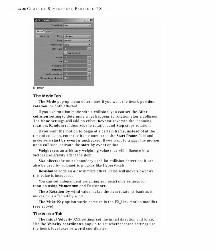
FX_Motion

The Mode TabThe Mode pop-up menu determines if you want the item’s position,

rotation, or both affected.

If you use rotation mode with a collision, you can set the Aftercollision setting to determine what happens to rotation after a collision.The None settings will add no effect; Reverse reverses the incomingrotation; Random randomizes the rotation; and Stop stops rotation.

If you want the motion to begin at a certain frame, instead of at thetime of collision, enter the frame number in the Start Frame field andmake sure start by event is unchecked. If you want to trigger the motionupon collision, activate the start by event option.

Weight sets an arbitrary weighting value that will influence howfactors like gravity affect the item.

Size affects the outer boundary used for collision detection. It canalso be used by volumetric plug-ins like HyperVoxels.

Resistance adds an air resistance effect. Items will move slower asthis value is increased.

You can set independent weighting and resistance settings forrotation using Momentum and Resistance.

The z-Rotation by wind value makes the item rotate its bank as itmoves or is affected by wind.

The Make Key option works same as in the FX_Link motion modifier(see above).

The Vector TabThe initial Velocity XYZ settings set the initial direction and force.

Use the Velocity coordinates pop-up to set whether these settings usethe item’s local axes or world coordinates.


The initial Rotation(deg/s) HPB settings set the initial rotation. If youwant the rotation to begin at a random point, activate the Randomrotation start option.

FX_Motion Vector tab

NOTEThe Mode setting on the Mode tab determines whether or not theseinitial settings have any effect. In other words, if you aren’t using arotation mode, the initial rotation settings don’t matter.

FX_LINK CHANNEL MOTION MODIFIERThe FX_Link channel modifier has two functions. First, it can be used

to dissolve out the object when the particles die.

FX_Link Channel motion modifier

To dissolve an object based on particle life:1 Open the Object Properties panel for the object to be dissolved.

(You’ll also need an existing emitter controller.)

2 On the Rendering tab, click the Object Dissolve Envelope button.This adds a Dissolve channel for the object and opens the GraphEditor.

3 On the Modifiers tab of the Graph Editor, add the FX_Link modifier.Open its options panel by double-clicking its name in the list after ithas been added.

L I G H T W A V E 3 D 7 17.29

4 Set the mode to Particles dissolve and select the emitter from theParticles pop-up menu. Enter the particle number in theNode/numbers field; 0 is the first emitted.

5 Click OK. When that particle dies, the object will be dissolved to100%.

FX_Link can also be used to vary a channel based on the number ofparticles at the emitter.

To control a channel based on the number of particles:1 Open the Graph Editor and select the desired channel in the Curve

bin.

2 On the Modifiers tab of the Graph Editor, add the FX_Link modifier.Open its options panel by double-clicking its name in the list after ithas been added.

3 Set the mode to Particles numbers and select the emitter from theParticles pop-up menu.

4 Click OK to close the panel and play your scene. The channel youselected will be changed based on the number of particles in thatparticular frame.You can scale the value by entering a number in theNode/numbers field. The number of particles will be divided by thisvalue.

GETTING STARTEDHere are some very basic tutorials to get you started with particles.

Emitter and Wind1 In Layout, choose Scene > FX_Browser. This brings up the Particle FX

Browser panel.


2 Let’s use the new partigon object type. From the Add pop-up menu,choose PolygonEmitter. This will add a PolygonEmitter controller toyour scene. It will also list this emitter in the Item pop-up menu onthe Particle FX Browser panel.

3 Click the Property button. This brings up the property panel for thecontroller shown on the Item pop-up menu, in this case, the emitter’s.

4 Click the play button on the main Layout interface. This is the right-facing triangle in the lower-right corner—changes you make tocontrollers are updated in real-time. Right now, all you will see are theparticles being created inside the emitter; there is no movement.

5 Open the Surface Editor. The PolygonEmitter object will have adefault surface called Partigons. Just change the Color to a deep red.You should see the particles change color.

L I G H T W A V E 3 D 7 17.31

6 Click the Motion tab on the emitter’s property panel. Set the Vector Yvalue to 2 to give the particles some vertical movement.

The particles at frame 41

7 On the Generator tab, decrease the Generator size values to .1, .1 , .1.Notice the effect of changing the size of the emitter.


8 On the Motion tab, try different values for the Explosion andVibration settings and note the results. When you are done foolingaround, leave Vibration(m/s) at 1, Vibration(min) at 100%, andExplosion at 0.

9 Go back to the FX Browser panel and from the Add pop-up menu,choose Wind. This adds a wind controller to your scene. Thecontroller name, Wind, should appear on the Item pop-up menu, soclick the Property button to bring up its property panel.

L I G H T W A V E 3 D 7 17.33

10 In Layout, stop playback and go to frame 0. Move the wind controllerup a little (to about Y=700mm). Also, on the wind’s property panel,change the Wind X setting on the Vector tab to 2m. Leave Wind Y at1. You will see the little wind vectors change directions.

11 Play the scene again and see the particles change direction due to thewind.

Go ahead and play with the wind and emitter settings. It’s very easy.Try adding HyperVoxels to the emitter object. Remember, if you don’twant to see the (partigon) particles when using HyperVoxels, use ObjectDissolve on the emitter’s Object Properties panel.

Collision Detection1 Start with the emitter from the preceding tutorial, but clear the wind

controller. (The wind controller can be cleared from the scene justlike any object using Items > Clear > Clear Selected Items.)

2 On the FX Browser panel, choose Collision from the Add pop-upmenu. This adds a collision controller to your scene. The controllername, Collision, should appear on the Item pop-up menu, so click theProperty button to bring up its property panel.


3 At frame 0, move the Collision object up to about Y=1.725m. Play thescene and notice how the particles bounce off.

4 Play around with the Collision properties and note the effects. Also,adjust the emitter properties, like Vibration(m/s).

More TutorialsObviously, these tutorials barely get your feet wet. However, because

of the real-time feedback, you can mess around with the settings and geta good feel for how everything works. There are several example ParticleFX scenes included on the CD. They will give you great insight as to howyou can use ParticleFX. Also, please visit LightWave3D.com for additionaltutorials.

L I G H T W A V E 3 D 7 17.35

cchhaapptteerr18Motion Designer

Chapter 18: Motion Designer

Motion Designer is a soft body dynamics engine that reshapesobjects according to wind, gravity, and object motions, by using elasticbody models to create animation data. You can easily achieve realisticeffects like draping cloth over objects, material flapping in the wind, orjiggling jello, with Motion Designer. Because it is integrated intoLightWave, Motion Designer can automatically take into account motionscaused by displacement, bones, IK, and so on.

WARNINGYour Bounding Box Threshold (Display Options tab of the Preferencespanel) must be set high enough to display your Motion Designertargets. If not, you may encounter a can’t scan objects... message dialog.

ELASTIC BODY MODELSA standard LightWave object normally consists of points, polygons

and surfaces. Motion Designer adds other properties to create its elasticbody models. Points can be influenced by gravity and air resistance,proportional to speed. Polygon edges are deemed springs that alsoinfluence points. Surfaces have additional parameters that further definethe elastic body model. The spring force is calculated continuously toreproduce its motions.

OPERATING MOTION DESIGNERYou begin using Motion Designer by choosing Scene > Dynamics:

MD_Controller to access the MD_Controller. The following panel isdisplayed.

L I G H T W A V E 3 D 7 18.1

Click Start to apply your MD settings to your LightWave scene. Thisbutton is used after you have set all of the MD properties to yoursatisfaction. Press your CTRL key to abort the calculation.

Click Property to bring up the MotionDesigner Property panel. Hereyou set the details of how MD affects the items in your scene.

Click the Option button to set various global options, which arediscussed later.

Click Save to manually save the MD data to a MDD file.

SETTING PARAMETERSTo change a parameter, select it in the list. The selected parameter’s

name will appear in the field beneath the list window. You change therelated value by entering a number in the input field to the right.

You can click some parameters in the list to toggle their state on oroff. For filename parameters, you can double-click or press ENTER tobring up a file dialog.

NOTEFor On/Off parameters, a value of 1 means On and 0 means off.

18.2 C H A P T E R E I G H T E E N : M O T I O N D E S I G N E R

PROPERTY PANEL: OBJECT TABThe Object Tab is where you specify which objects to use and how

Motion Designer treats them. Select the object from the object list pop-up menu and click the Activate button. You can then apply MDparameters to it. Click Deactivate to deactivate an MD item.

NOTEActivate and Deactivate essentially add and remove the MD_Plugdisplacement map plug-in automatically for you.

Initially you’ll want the ALL option active so that all objects are listedin the pop-up menu. Once you have defined the MD objects, you canuncheck ALL to list only defined objects. This may be useful if you havea lot of objects loaded into Layout.

GroupYou can group MD objects with a user-defined name to prevent

unwanted interaction. This also works with Particle FX controllers.

TargetTarget On means the object is an elastic body model and can be

influenced by other Target or Collision objects.

Collision SelectNormally, MD executes the collision calculation among all target and

collision objects. The Collision Select function lets you specify which

L I G H T W A V E 3 D 7 18.3

object the target collides with. Double-clicking the setting displays adialog where you select the collision object. This function will improvethe calculation speed.

Collision-DetectionUse the Collision-Detection function to specify collision detection on

an object-by-object basis instead of surface-by-surface. If this parameteris OFF, all of the object’s surfaces are treated as if the (Surface tab)Collision-detection setting was OFF.

Pressure EffectPressure effect causes the object to maintain its volume during a

motion, as if it is filled with a stiffer gel, instead of, say, water. This worksbest when the object is a closed volume and spherical in shape.

Fiber StructureWhen Fiber structure is set to a value other than zero, the object

seems to be made of a fiber material. This function essentially weakensthe force when the motion direction is different from that of the virtualfiber. When the value is 100%, the force is zero, except along the fiber.This setting also weakens the force from the sub-structure.

Left: Fiber structure = 0%. Right: Fiber structure = 100%

DumpFileNameDumpFileName is a special file that sets up an initial pose for the

target object. This file is discussed below.

CollisionCollision On means the object is a collision object that will influence

target objects, if it collides with one.

NOTEYou cannot have Target and Collision both set to ON for the sameobject.


MddFileNameGenerally, this setting is for backwards compatibility with prior

versions of MD, which required you to manually specify motion datafiles.

Motion FilesFor Target objects, click SAVE MDD to save the generated motion to a

file, which will be used subsequently to deform the object.

Click DUMP to save the final pose (position, speed) of a Target objectto a file, based on the last frame calculated. In a subsequent session, youcan specify this file as the DumpFileName parameter for a Target objectand set a starting pose for the target. This is useful to have a realisticbeginning state for the target.

To use a dump file:1 Set your Last Frame in Layout to the pose you want to start with.

2 Start the calculation.

3 After the calculation, click DUMP and save the Dump file.

4 Specify the saved Dump file for the DumpFileName parameter of theTarget object. The Target object will not begin in this state.

NOTEIf you do not want to use the Dump file, make sure you clear it fromDumpFileName.

PROPERTY PANEL: SURFACE TABApply physical characteristics to the surfaces of Target objects or

Collision objects on the Surface tab. To specify characteristics, select thesurface from the surface list and assign parameters.

Basic Settings

WeightWeight defines the weight of the material. The flags below are the

same except for the Weight parameter. The flag on the right hangs downmore due to its weight and also will not flap as much.

Left:Weight = 1. Right:Weight = 2

L I G H T W A V E 3 D 7 18.5

Weight +-Use the Weight +- parameter to add randomness to the Weight

parameter.

Left:Weight+- = 0. Right:Weight+- = 1

SpringThe Spring coefficient controls the springiness or stiffness of the

material. The flags below are the same except for the Spring parameter.An extremely large Spring value on the right flag makes its cloth stiffer.

Left: Spring = 1000. Right: Spring = 10000

ViscosityViscosity controls the impact of a collision. The pieces of cloth below

are the same except for the Viscosity parameter. Here, a ball is movingup, pushing the piece of a cloth. The cloth with the higher Viscosityvalue tends to keep its shape more.

Left:Viscosity = 1. Right:Viscosity = 10

If an object bounces, a higher Viscosity value will have less bouncemotion because the bouncing force is absorbed by the Viscosity.

ResistanceResistance controls the amount of air resistance. The flags below are

the same except for the Resistance parameter. The flag on the rightstretches more due to its greater air resistance.

.Left: Resistance = 1. Right: Resistance = 2


Parallel ResistanceParallel Resistance controls the amount of air resistance parallel to

the surface. An object, such as a floor tile, will fall quicker if turned onits edge. The default value of 100% for parallel resistance yields normalresults and should be used for items like falling leaves and flags. If forsome reason you do not desire this effect, reduce the setting.

Two falling tiles. Left: Parallel-resistance = 100%. Right: Parallel-resistance = 0%

Back-resistanceBack-resistance specifies the air resistance for the back of a surface

(i.e., opposite the surface normal’s direction). At 100%, the back side isaffected by wind the same as the front. At a value lower than 100%, theback side is affected more by wind. This function can be effective whenyour wind becomes weak due to overlapped objects.

The back side for these objects is the side closest to the center of this image.

Structure Settings

FixedThe shape of polygons with Fixed On remains intact. The flag pole

below, for example, has Fixed On and the flag has it off.

Sub-StructureThe surface of a pure, elastic body model has a high degree of

freedom, which causes the object to easily distort. To prevent distortion,you can apply an auxiliary MD form, called a Sub-structure, to restrictthe instability of the surface. This can improve your results with a two-dimensional object (i.e., one with no thickness) making it act as if it hassome thickness. However, this reinforcement can require a high Sub-structure setting that can take longer to calculate.

L I G H T W A V E 3 D 7 18.7

The flag below is made up of square polygons. Due to distortedpolygons, the flag appears to be abnormally stretched as if it is made ofa net.

The problem can be corrected (partially) by tripling the geometry inModeler to eliminate the abnormal stretching. Unfortunately, triangleshave a tendency to bend in one direction and cause wrinkles. They alsoresist bending in the other direction, which may result in an unnaturalmotion.

When Sub-structure is used on a square mesh, it creates somethingthat looks like two triangular polygons placed on top of each other inopposite directions. The sub-structure mitigates the tendencies to bendand to resist bending in certain directions. Notice below that the clothappears smoother now than it did with tripled polygons, above.


When the Sub-structure value is non-zero, the auxiliary form isapplied. The higher the value, the more the form will have a tendency tokeep its shape.

Hold-StructureBecause a pure elastic body model simulates only the surface

structure, it can be limited to two-dimensional motions, like with a bedsheet. In order to simulate elastic three-dimensional motions, such assome gelatin, a Hold-structure needs to be used. This parameter causes asurface to tend to maintain its original shape, like gelatin does when itjiggles.

NOTEThe effect of Hold-structure is uniform throughout the surface, whilewith Sub-structure it is non-linear, which will often result in a morenatural look.You can use a combination of both to achieve just the rightresult.

SmoothingTo smooth out the transition between, say, a Fixed surface and Hold-

structure, apply some level of Smoothing to both surfaces. This can helpprevent unwanted creases and wrinkles occurring between the twoareas.

Stretch-limitTo prevent a surface from stretching like rubber, lower the Stretch-

limit below the default value of 100%. This restricts the amount of thesurface to be stretched.

Left: Stretch-limit = 100%. Right: Stretch-limit = 20%

NOTEAlthough you could also increase the Spring value to reducestretching, increasing that value can make the surface too complex andcause other problems, like weird folds.

L I G H T W A V E 3 D 7 18.9

Compress StressCompress Stress controls the amount of compression a surface

exhibits as a result of stress. A soft fabric like cotton can be made usinga large Spring value and a low Compress stress setting. A stiffer fabricwould use a higher Compress stress setting.

Left: Compress stress = 100%. Right: Compress stress = 0%

You can easily adjust the apparent thickness of a drape by adjustingCompress Stress, as shown below. (The drape object also uses thesesettings: Weight = 1, Spring = 200, Resistance = 2 and Viscosity = 1.)

Left: Compress Stress = 100%. Middle: Compress Stress = 10%. Right: Compress Stress = 1%.

ShrinkShrink reduces the surface to a specified size. For example, a value of

90% reduces the size of the surface to 90%. Use Shrink to reduce thelooseness of a dress or to create frills.

Collision Settings

HINTTry to use Self Collision and Collision Detection only onnecessary surfaces to minimize calculation time.

Self CollisionThe Self Collision setting can prevent an object from crossing itself

when the object is transformed. Self Collision is calculated based on apoint on the target object and a polygon on the collision object. If asurface has Self Collision and Collision Detection active, Self Collisionis computed on the same surface.

Self Collision works in much the same way Collision Detection does,and there is no collision detection for polygon edges. As such, you mayalso want to adjust Skin Thickness to avoid errant point penetrations.Note that unlike Collision Detection, Self Collision is detected even ifthe motion is from behind the polygon.


Collision DetectionCollision Detection reflects the influence of other objects upon the

motion of an object. This lets you create complex motions caused byobstacles. The simulation is performed by taking an object that collides(the collision object) with the elastic body model (the target object) intothe calculation.

Left: No collision detection. Right:With collision detection

The direction of the surface normal plays an important part incollision detection. The target object must collide with the surface of thecollision object. If it contacts the surface from the rear (i.e., away fromthe surface normal), the target object will simply pass through, as shownbelow.

As such, if you need collision detection inside a container, forexample, you’ll need to have interior facing surface normals.

Single-sidedWhen Single-sided is ON, surfaces with normals facing the same

direction will not collide. If the collision is between surfaces withopposing normals, you can reduce calculation time by turning this ON. Ifyou will have collisions between surface normals facing the samedirection, you should turn this OFF.

Left: Surface normals with the same direction. Middle: Single-sided = ON. Right: Single-sided = OFF

Skin ThicknessYou should understand that the collision is detected using a point on

the target object (elastic body model) and a polygon of the collisionobject. As a result, a polygon of the target object can possibly penetratethe collision object—usually an undesirable result.

L I G H T W A V E 3 D 7 18.11

NOTEIn the picture below, you can see the points on the cloth do notpenetrate the ball, but the surface between the points does.

Use the Skin Thickness (Surface tab) setting to avoid undesiredsurface penetration like the example below. Skin Thickness, set inmeters, creates a gap between the collision and target objects, withinwhich a collision is deemed to have occurred. Make sure you specifySkin Thickness for the surface of the collision object, not the surface ofthe target object.

Left: Skin Thickness = 0. Right: Skin Thickness = 0.1(m)

FrictionLike real world friction, the Friction parameter makes the surface less

slippery. So if you want the target object to tend to slip off the collisionobject, set Friction to 0. If you want it to stick more, increase the value.

Left: Friction = 0. Right: Friction = 3

Bound ForceBound force adds a rebounding speed change at collision, if set

greater than 0. At 1, the speed is the same as the collision object. At 2, itrebounds at the collision speed.

Particles dropped on a ball. Left: Bound force = 1. Right: Bound force = 2


Action ForceAction force decides whether the colliding object receives the

reaction force at the time of the collision, or not. This function does notaffect the reaction force that the collision object receives.

Object on left is stationary and object on right is moving left

After collision. Left:Action force = OFF. Right:Action force = ON

Bind ForceBind force causes the target to adhere to the collision surface.

Particles dropped on a ball. Left: Bind force = 0. Right: Bind force = 1

If you have some level of Bind force, Fix Force will also be available.Fix Force causes the target object to stick to the surface and not slidearound.

Left: Fix force = 0. Right: Fix force = 100

Other Surface Controls

HideWhen Hide is unchecked, MD displays all of the Surface parameters

that you can specify. When Hide is checked, MD hides all parameters attheir default values. This display mode helps you zero in on just thesettings you have tweaked.

L I G H T W A V E 3 D 7 18.13

COPY/PASTEUse the COPY and PASTE buttons to copy and paste the current

settings between surfaces.

SAVE/LOADUse the SAVE button to save the current surface settings to a file on

your hard drive. Use the LOAD button to load the settings from apreviously saved file.

If you save the files to the SURFACES subdirectory in your Contentdirectory, they will appear in the Material Library pop-up menu,discussed below.

Material LibraryThis pop-up menu (located near the Hide button) contains pre-

defined sets of surface parameters.

PROPERTY PANEL: ENVIRONMENT TABThe gravity and wind settings are specified on the Environment tab.

All of these settings affect Target objects.

GravitySpecify the direction and intensity of gravity along the world axes.

Wind1/Wind2Specify the direction and intensity of two winds along the world axes.

TurbulenceSpecify the direction and intensity of turbulence along the world axes.

Left:Turbulence = 0,0,1. Right:Turbulence = 0,1,0

The strength of turbulence is affected by the wind, as shown in theexamples below.

Left:Wind = 0,2.0,0. Middle:Wind = 0,5.0,0. Right:Wind = 0,8.0,0


WavelengthSpecify the wavelength of the turbulence.

Left:Wavelength = 0,0.25,0. Middle:Wavelength = 0,0.5,0. Right:Wavelength = 0,1.0,0

Wind ModeThe Wind Mode controls the repeating pattern for Wind1 and Wind2.

Random randomizes the pattern according to the specified Random-ratio. The Cycle setting swaps Wind1 and Wind2 every Cycle-lengthperiod, specified in seconds. Gust uses Wind2 only for the durationbeginning with Gust-start (in seconds) for the Gust-length (in seconds).Wind1 is used at other times. Default ignores the Wind1 setting and usesonly Wind2.

SAVE/LOADUse the SAVE button to save the current environment settings to a file

on your hard drive. Use the LOAD button to load the settings from apreviously saved file.

HELPFUL TIPSWith Motion Designer, you can adjust motions intuitively since MD is

based on physical models. You can achieve heavy motions by increasingthe Weight value, and you can create light motions by decreasingWeight.

Reducing the Spring coefficient creates soft motions, while raisingSpring produces motions with a stronger repelling force. Setting thecoefficient to an extremely large value creates stiff motions.

Since Motion Designer uses elastic body models as calculationmodels, based on mass, spring, and resistance, unexpected vibrationmay appear in the calculated motions. One of the following adjustmentsmay help correct the problem:

• Increase Resistance to make moving more difficult.

• Reduce the Spring coefficient. This will reduce the force that causesvibration.

• Increase the Weight to stabilize the surface.

Abnormal motion, including vibration, may be the result of (gasp!)calculation errors. Remember, the motion is approximated based only onnumeric values. This problem may be solved by adjusting the accuracyof the calculations using the Calculate resolution setting on the MotionDesigner Options panel, discussed below.

L I G H T W A V E 3 D 7 18.15

OPTIONS PANELThe Motion Designer Options panel is displayed when you click on

the Option button on the main Motion Designer panel.

The Calculate resolution setting controls the accuracy of the motioncalculations. The default is 10. Increasing this value improves theaccuracy of calculation, but as you might expect, it also increases theamount of calculation. Extremely large values will result in unusuallylong calculation times.

If you are using a multi-processor machine, specify the number ofCPUs in Thread max field.

When the Safe Mode option is unchecked, some internal calculationrestrictions are eased. This allows faster calculations, but may result inunwanted vibrations, as well as different results for calculations basedon the same parameter values.

You can control how MD updates by using the Update Mode pop-upmenu. Auto updates only targets that have had parameters changed. Useselect only if you have multiple targets, then only the selected targetswill be updated. All targets updates all targets. Use this if your system isfast.

If Update in calculation is checked, Layout is updated while MDcalculates.

Step is a great time-saving feature. It sets the frame increment for MDcalculations. Since LightWave will obviously interpolate movementbetween frames, it is usually not necessary to set this to 1. You mayoften get away with 3, 5, or even higher settings, depending on the scene.


SUPPLEMENTAL MD DISPLACEMENT PLUG-INS

MD_PlugMD_Plug is the displacement map plug-in that applies the motion data

created by MD (MDD file) to the object in Layout.

NOTEMD_Plug is automatically added to the Target when you click theActivate button on the MD Property, Objects tab. It is removed ifDeactivate is clicked.As such, you will normally not need to add oradjust this plug-in manually.

Setting OptionsDouble-click MD_Plug after it has been added on the Deformations

tab of the Object Properties panel to display its options panel.

The MDD Filename field specifies the Target’s MDD file.

The Action Start field indicates the time (in seconds) at which themotions from the MDD file should start. This lets you delay the start ofthe effect.

The End Behavior setting determines what happens after the motionfinishes. Stop holds the last state. Repeat repeats the motion from thebeginning. Use Composite if you wish to stack multiple instances ofMD_Plug and add the motions together.

If Key-Move is ON, keyframed motion is applied along with the MDdisplacement motion. Since the motion data created with MotionDesigner (including MD_Scan) contains displacement of shapes using thekeyframes, setting this ON can cause a doubling up of the keyframedmotion. To prevent this problem, set Key-Move to OFF.

NOTEWhen using MD with other displacement plug-ins (which should beloaded after MD) be sure Key-Move is ON. Motion Designer ignoresany plug-ins loaded above MD_Plug.

L I G H T W A V E 3 D 7 18.17

MD_MetaPlugMD_MetaPlug is a displacement map plug-in for extending MD_Plug

and applying a MDD file to the object in Layout without restricting theshape or the number of points. This lets you create the animation, andlets you completely separate the object for animation and the object forrendering. For example, you might use this to add buttons on a dressafter the MD calculation.

Setting OptionsSpecify the target MDD file in the MDD Filename field. The details

include the number of MDD frames, recorded time, and the number ofpoints on the plug-in button. Verify the information.

Specify the object used for the calculation of the MDD file as CageObject. This object should be made up of triangles and quads. Thesmooth reshaping is executed based on the lattice by polygons.

NOTEYou may run into problems if the Cage Object is too rough.Subdividing the Cage Object may help.

In the ActionStart field, specify the time (in seconds) at whichmotions based on the MDD should start.

Use the EndBehavior pop-up menu to specify what happens at theend of the motion based on the MDD. Stop maintains the last state,Repeat repeats the motion, and Composite plays back the MDD filesuccessively.

Key-Move is used to specify whether or not to displace the shapeusing the standard keyframe. Since the MDD already containsdisplacement information, setting Key-Move to ON can duplicate thedisplacement of shapes. As such, you will usually set this to OFF.However, this will also disable any movement in Layout.

The Smoothing option attempts to smooth the reshaping. Ifunchecked, the reshaping will pass through the vertex of the CageObject.

Activate Disable to turn the plug-in off without losing your settings.

MD_MetaPlug_MorphMD_MetaPlug_Morph is a displacement plug-in that enhances the

functions of MD_MetaPlug. By itself, MD_MetaPlug cannot use normalmorphing information because it ignores bones, morph mapping, anddisplacement maps. However, if you use MD_Plug withMD_MetaPlug_Morph, you can use normal morphing data with MotionDesigner.


L I G H T W A V E 3 D 7 18.19

The MD_MetaPlug_Morph plug-in can be added before or afterMD_Plug. Make sure MD_Plug’s Key-Move is set to OFF.

MD_MetaPlug_Morph has one pop-up menu called Morph Mode. Setthis to One time morph to execute morphing only one time. This modeis appropriate when the morphing is from morph mapping. Use Everytime morph to execute morphing for each displacement process. Thismode is appropriate when the morphing varies, like the displacementmap of waves. The Non morph setting simply disables this plug-in.

NOTEUsing MD_Metaplug_Morph is CPU intensive, so be sure to select theappropriate Morph Mode.

MD_ScanMD_Scan is a displacement map plug-in that incorporates motion data

from Layout into Motion Designer. MD_Scan can handle motions, such asthose of bones affected by displacement map plug-ins. The resulting databecomes an MDD file to be used with the main Motion Designer plug-in.

The MDD Filename field specifies the MDD filename.

Scan Points displays the number of points in the object to be saved.

Specify the frame where you want to begin recording in the FirstFrame field and the frame you want to end recording in the Last Framefield.

Specify the number of frames for which data should be saved in theMDD file in the Frame Rate field. Data for skipped frames isautomatically interpolated. Increasing this number can reduce the datasize when you save motions that are long but relatively slow.

Scanned Frame displays the fetched frame.

NOTEWhen you use MD_Scan with other displacement map plug-ins, besure to add MD_Scan last.

To use MD_Scan:1 Add MD_Scan to the Deformations tab of the Object Properties panel

for the object whose motion you wish to incorporate.

2 Double-click the added plug-in to open its Options panel.

3 Define the desired MDD filename and set the parameters. Click OK.

4 Click OK for the next dialog that appears.

5 Make a preview animation. (Yes, this is necessary!)

6 Open the MD_Scan Options panel again. This time a different versionof the panel will appear. Click OK to save the MDD file data.

7 Remove MD_Scan or deactivate it.

8 Load the file into MD_Plug.

TUTORIALSHere are a few basic tutorials to get you started with Motion Designer.

Waving a Flag1 In Modeler make a flag pole using the Disc tool. Use two Segments.

Name the surface Pole.

2 Using the Box tool, make the flag. It should use lots of X and YSegments and line up with the top and middle of the pole. Triple thepolygons (Construct > Subdivide: Triple). Select the flag polygonsand name the surface Flag. Make sure the polygons face towards you.If they do not, flip them.


3 Zoom in and select the top-left point on the flag and then the nearestpoint on the pole. Make sure only two points are selected and chooseDetail > Points: Weld.

Left: Before welding. Right:After welding

4 Weld the bottom-left corner of the flag to the pole in the same manneras above.

5 Save your object as MDFLAG.LWO and load it into Layout.

6 Choose Scene > Dynamics: MD_Controller. This brings up theMotionDesigner Controller panel.

HINTFor easy access, you may want to assign the MD_Controller commandto a menu or keyboard shortcut.

7 Click the Property button on the panel to bring up theMotionDesigner Property panel. With only one object in the scene,our flag object will already be selected on the pop-up menu. Click theActivate button to use it with MotionDesigner.

L I G H T W A V E 3 D 7 18.21

8 Next, double-click the Target line to turn this option on. Additionaloptions will appear, but you can leave them at their default state.

NOTEThat is one click to select the option and another to toggle its setting.This is the way all of MD’s On/Off settings work. If the item is alreadyselected, you need to click only once.

9 Click the Surface tab and then the MDFlag entry to display the twosurfaces: Pole and Flag.

10 Choose the Pole surface and turn On the Fixed setting.


11 Choose the Flag surface and click the Spring setting. This settingrequires a numerical input. Enter 1000 in the input field beneath thelist of settings. A value of 1000 will make the surface resist stretchinglike a piece of cloth.

12 Click the Environment tab. Each setting has three fields that are forthe X, Y, and Z axes, from left to right. Set Gravity to 0, -1, 0; Wind1 to1, 0, -1; and Wind2 to 1, 0, 1. Cycle-length should default to twoseconds; this value makes the environment settings repeat every twoseconds.

L I G H T W A V E 3 D 7 18.23

13 Click the Continue button to close the MD Property panel.

14 In Layout, set your last frame to 300. Go to the Display Options tab ofthe Preferences panel (D) and make sure Bounding Box Threshold ishigh enough to display your MotionDesigner target.

15 Click the Start button on the MotionDesigner Controller panel andwatch the magic!

Go ahead and play with the surface settings to change the effect.

Collision DetectionIn this tutorial, we will show you how to do basic collision detection.

1 Here we have a simple flat segmented box with tripled polygons and abasic ball. The objects were modeled in these positions. The boxobject is called mdcloth and has a surface named cloth. The ballobject is called mdball and has a surface named ball. (Clever naming,eh?)


2 Choose Scene > Dynamics: MD_Controller. From the MotionDesignerController panel, click the Property button. Activate the mdclothobject and turn the Target option on.

3 Activate the mdball object and turn the Collision option on.

4 Go to the Environment tab and set Gravity to 0, -1, 0.

5 In Layout, set the last frame to 300 and click Start on theMotionDesigner Controller panel. You will see the cloth float down,due to the gravity, and deform around the ball.

L I G H T W A V E 3 D 7 18.25

6 You should notice that some parts of the cloth surface go inside theball. We can easily fix this by increasing the thickness of the ballsurface for calculation purposes only.

Select the ball surface and increase the Skin thickness to about .02.

7 Click Start again and the cloth surface should no longer go inside theball. If it still does, increase Skin thickness some more.

You should see your cloth slide off the ball towards the end of theanimation. Play with the surface settings to change the effect.

More TutorialsPlease visit LightWave3D.com for additional tutorials.


cchhaapptteerr19Distributed Rendering

Chapter 19:Distributed Rendering

LightWave allows you to use the processing power of othercomputers on a network to render scenes. This is called distributedrendering or sometimes a rendering farm. There are a few basicapproaches to distributed rendering with LightWave.

ScreamerNet uses Layout’s Network Rendering panel (Rendering >Network Rendering) to control submitting scenes to networkedcomputers running the ScreamerNet process. ScreamerNet can controlup to 1,000 CPUs (Note: A single machine can have more than one CPU.Each CPU is counted as one). Each will render a frame from theanimation until the scene is rendered.

NOTEYou can also use LightWave’s distributed rendering feature to batch-render multiple scenes on a single machine.

RENDERING MODESYou can choose from two distributed rendering modes: Original

ScreamerNet and ScreamerNet II.

WARNINGScenes, objects, and images should not have any spaces in their savednames; use an underscore ‘_’ instead (e.g., MY_3DCAR.LWO insteadof MY 3DCAR.LWO).This is vital for dependable ScreamerNetoperation. If there are spaces in these names, ScreamerNet andLightWave may read them as corrupt files.

SCREAMERNET CLASSICOriginal ScreamerNet is designed to be used with networked CPUs

that do not share directories. Original ScreamerNet has the disadvantageof requiring you to load the scene to be rendered on the control machineand sending the scene file, object files, and image files to each connected

L I G H T W A V E 3 D 7 19.1

CPU. When a frame is rendered by a remote CPU, it is sent back to thecontrol machine whereby it is saved to a selected directory. Thisprocess, while it works, is often slow due to the constant file transfers.

NOTEOriginal ScreamerNet is included primarily for backward compatibilitywith older rendering engines.

Since the Original ScreamerNet rendering method is somewhatoutdated, those still using it will find little change in the controls for thismethod. Changes will be noted below. The majority of this chapter dealswith the new ScreamerNet II rendering method.

SCREAMERNET IIScreamerNet II does not require the scene be loaded on the control

machine. As long as the scene, object, and image files, (as well as thesave-to directories) are all accessible to each CPU on the network, eachindividual node machine can load the scene and save images directly tothe shared drive(s). Additionally, ScreamerNet II can “batch render” upto 100 separate scene files.

The process of using ScreamerNet II is basically to run the renderingmodule (i.e., LWSN) on all of the computers that will be rendering. Thisincludes the designated control computer. You then run LightWave onthe control computer and identify the scene or scenes you want torender.

Since ScreamerNet communicates by writing files, NetBEUI andTCP/IP are not required. As long as each machine can see each other andwrite files across the network, ScreamerNet should function properly.

The LWSN program is supplied with LightWave. However, you willonly receive the version appropriate for the platform for which youbought LightWave. For example, if you purchase the Intel version ofLightWave, you will receive the Intel version of LWSN.

WARNINGAll of the rendering nodes need not have the same architecture (i.e.,Intel, Mac, etc.). However you must run the proper LWSN version oneach type of machine. In addition, plug-ins used in the scene must alsoreside on each node. If not, some images would render using the plug-in and others wouldn’t because they couldn’t.

Using Screamernet IIThe Host is the machine with Lightwave installed on it. Nodes are the

other machines on the network used for rendering. Node machines donot need to have any NewTek software or hardware on them.

19.2 C H A P T E R N I N E T E E N : D I S T R I B U T E D R E N D E R I N G

The key to understanding ScreamerNet is network drive mapping andsharing. There are a variety of ways to configure a network and thus avariety of ways to set up ScreamerNet.

ScreamerNet Rendering RequirementsTo set up a ScreamerNet rendering farm you need to set up the

following:

1 A common directory that the Host (controlling PC) and all renderingnodes can access. This could be physically located on the Host, but isnot necessarily.

2 Each rendering node must be able to load a plug-in configuration file(e.g., LWEXT3.CFG) that has the plug-in files mapped with a path thatthe rendering node can access.

Now, if all rendering nodes are on the same platform (e.g., IntelWindows), you could map the same drive letter to another commondirectory and place the plug-in, LWSN.EXE and configuration filesthere. The paths in the configuration file would obviously also usethis drive letter.

If you don’t use the common configuration file route, you’ll need tostore a set of all of the files locally on each rendering node.

3 All of the rendering nodes need access to a Content Directory. Ideallythis can be stored in one common directory since you want to makesure all of the rendering nodes are using the same objects andimages.

NOTEThe Host machine can be a rendering node as well. It may be easiestto use the same mapping technique described above, although youcould map everything locally if you want.

Getting the Nodes GoingThe ScreamerNet utility is executed on each rendering node using a

lengthy command. The following is an example. Note that the commandhas been broken up into separate lines for clarity. In reality, the entirecommand must be entered on a single line.

L:\SCREAMERNET\LWSN.EXE -2-CL:\SCREAMERNET

-DL:\SCREAMERNET\CONTENT

L:\SCREAMERNET\COMMON\JOB1L:\SCREAMERNET\COMMON\ACK1

In the above example, we’ve assumed the following:

• All of the rendering nodes are Intel Windows machines.

• The drive letter L: has been mapped to the same network drive for allnodes.

L I G H T W A V E 3 D 7 19.3

• The LWSN.EXE and configuration files are all stored in L:\SCREAMERNET.

• The plug-in files are stored in L:\SCREAMERNET\PLUGINS and that is thepath used in the LWEXT3.CFG file. (Note: that the plug-in files couldstill be in subdirectories (L:\SCREAMERNET\PLUGINS\ANIMATE).

The -C parameter defines the directory where the configuration filesare stored. The -D parameter defines the content directory to be used. (Ifthis is not defined, the content directory defined in the scene file isused.)

The command for subsequent rendering nodes must increment theJob and Ack number. For example, node 2 would use JOB2 and ACK2, node3 would use JOB3 and ACK3 and so on. The Job/Ack number equates tothe CPU number used by ScreamerNet to identify the node and goesfrom 1 to the number set as your Maximum CPU Number on theNetwork Rendering panel, discussed next. (You must include the path forJob and Ack.)

To save time in the future, you will want to set these commands up asicon shortcuts.

NOTEMac users should use a command-line file, discussed in the Appendix,to set LWSN’s parameters.

NOTEAfter you execute LWSN.EXE you may see a message like Can’t openL:\ScreamerNet\Common\Job1.This will be normal until Lightwaveinitializes ScreamerNet.

MS-DOS console window output


Scene Saving Info1 When setting up your scene, you must use your content directory

properly. Otherwise, some nodes may not be able to render thescene.

2 Set up all of your render options (e.g., file-saving) before saving thescene. You will probably want to save the rendered frames to acommon directory, like L:\SCREAMERNET\FRAMES. Alternatively, theycould be saved locally, but remember all rendering nodes will begetting the path to save the files from the same scene file.

NOTEScreamerNet does not render out animations. It renders onlyindividual files.

Host Machine Setup1 Start LightWave. Open the Network Rendering panel (Rendering >

Network Rendering) and click the Command Directory button.Change this to Z:\LIGHTWAVE\PROGRAMS. You will get a requester thatasks you to re-initialize; choose NO.

2 Set the Maximum CPU Number to your number of nodes/CPUs.

3 In the General Options tab of the Preferences panel, confirm that theContent Directory is set to the proper directory.

4 Quit LightWave and then start it up again to save changes to theconfiguration file.

L I G H T W A V E 3 D 7 19.5

Controlling the Network Rendering1 On the Host, open the Network Rendering panel (Rendering >

Network Rendering) and click the Screamer Init button. At thispoint, all of your CPUs that are running ScreamerNet should appear inthe window. (The job/ack number assigned to each node machine willcorrespond to the CPU number in the SN window.)

Network Rendering panel

2 Click Add Scene To List and add a scene(s).

Scene added for rendering


3 Click on Screamer Render. This will now render your scene(s).

ScreamerNet now rendering the scene

Shutting Down NodesWhen all CPUs are finished rendering, selecting the Screamer

Shutdown button will close all windows on all ScreamerNet nodes andstop them. In order to start a new session, you must restart ScreamerNeton each CPU and re-initialize the CPUs from the control machine.

Aborting a Rendering SessionPress the ESC key to abort a ScreamerNet session. There may be a

long pause before all of the ScreamerNet nodes are ready again, whileeach finishes up the current task. This is especially true when they areworking on a complex scene. Note: ScreamerNet rendering is onlyabortable when the ScreamerNet panel reads Waiting for CPUs to finishrendering.

WARNINGIf you close the DOS shell on any of the render nodes, you may haveto restart all nodes and re-initialize them.

Changing the Number of NodesBy changing the value in the Maximum CPU Number field from the

default eight, you can tell the control machine how many nodes it shouldcheck for. The maximum number is 1000, but setting the number to theactual CPU’s available nodes will save time. This number is written to theconfiguration file upon exiting LightWave.

L I G H T W A V E 3 D 7 19.7

ScreamerNet II SyntaxThe command line parameters for LWSN.EXE -2 are:

LWSN -2 [-C<CONFIG FILE DIR>] [-D<CONTENT DIR>] [-Q] [-T<CHECK INTERVAL>] <JOB FILE> <REPLY FILE>

The check interval is defined in seconds. It specifies how often tocheck for commands during rendering. If the -T parameter is not used,rendering is uninterrupted and LWSN won't check the job file until itscurrent render job is done. With -T, it will check every so often duringrendering for only two commands: status and abort. (All othercommands are ignored). (The actual check interval may be longer thanspecified, depending on what is currently being processed.)

BATCH RENDER ON ONE COMPUTERYou do not actually need a network in order to use the ScreamerNet.

Just follow the network instructions as if the computer was the node andcontrol machine. It’s a little easier since you won’t have to worry aboutshared directories and volume names. ScreamerNet is useful forrendering a series of scene files unattended, and it is most beneficial ifyou are using a dual-processor system—each processor could be treatedas a separate CPU for rendering.

TROUBLESHOOTINGIf clicking the Screamer Init button doesn't find the other CPUs, go

back and start at the Host Machine Setup section.

If images seem to render unrealistically fast and no images are saved:

1 Check to make sure that you have full sharing access across thenetwork. This is done through Windows NT Explorer. You can checkthis by copying a file at random back and forth across the network.

2 If the scene and/or objects were created without taking intoconsideration the new drive path names, rendering may occur ononly the host machine.

The most common cause of ScreamerNet crashing is when too manycomputers try to write or read their information to/from the Hostcomputers while the host renders.

• Do not use ScreamerNet to render on the host machine, but ratheruse it only as a server where the hard drives are found.

• Map a drive from a different computer as drive Y:, for example, andset your scene to save the animations to that drive. The computersdon’t know that drive Y: is not on the host, just that it’s present.

Another problem occurs when the hard drive where you save theimages or animation is full. This problem creates an error in LightWaveand each ScreamerNet node.


RENDERING WITHOUT LIGHTWAVEThe LWSN program has a third option that lets you render a scene

without running LightWave. There is no control machine and thus it isnot a distributed rendering situation. You must tell the programspecifically what to render. The method is run from a DOS prompt usingthe following syntax (one line):

LWSN -3 [-C<CONFIG FILE>] [-D<CONTENT DIR>] <SCENE FILE> <FIRST FRAME><LAST FRAME> [<FRAME STEP>]

As you can see, you basically supply the program with the basicinformation needed to render a scene. An example would be:

LWSN -3 -CD:\LIGHTWAVE\LW.CFG -D M:\NEWTEK SPICEGIRLS.LWS 1 900 1

In the example, the program would render frames 1 through 900 ofthe Spicegirls.lws scene using the Lw.cfg file stored in the D:\Lightwaveand using M:\Newtek as the Content Directory.

The configuration file specification is optional, if the Lw.cfg file is inthe current directory. Likewise, if the Content Directory is correctlyspecified in the configuration file, you do not need to give thatparameter.

HINTYou can get the syntax for ScreamerNet by simply typing LWSN withno arguments.

L I G H T W A V E 3 D 7 19.9

cchhaapptteerr20LightWave 3D Modeling

Chapter 20:LightWave 3D Modeling

LightWave Modeler lets you create objects from scratch or editexisting objects. Object modeling is the design and creation of wireframeobjects from a simple shape, like an apple, to a complex shape, like afinely-detailed sports car. In Layout, you are the interior designer movingfurniture and putting up pictures. In Modeler, you are the furniture makerand the builder of the house.

COMPONENTS OF A 3D OBJECTWhat makes up the 3D object? It has two traits: its physical shape and

its visual appearance. The physical shape of an object comprises pointsjoined by lines to form faces that we call polygons. The form that thepolygons present to us makes up an object’s shape.

The visual appearance of an object consists of color and texturequalities that connote realism to the eye, which are called surfaceattributes or material properties. When you enter a room and look atyour chair you see a certain shape (that of a chair) and a certain surface(maybe wood or metal), so you think, “chair”. In LightWave 3D you havethe tools to create simple or complex objects and define their surfacequalities with great precision and detail.

L I G H T W A V E 3 D 7 20.1

MODELING IN 3DHow would you make a mug? It depends; if you were a sculptor, you

would mold a lump of clay. If you were a designer, you would draft it withpaper and a mechanical pencil. If you were an artist, you would probablysketch it. But suppose you were using a computer. How would you makea mug then? What tools would you use?

You want to portray the mug with realistic color, depth, and shading.You need drawing tools, yes, but also power tools! With the computer,you can create the mug in a variety of ways. LightWave recreates draftingand workshop tools on screen so that people who are neither sculptorsnor traditional artists can use them just as easily. In fact, LightWave’stools do more than their real-life counterparts. There are severalbonuses to computer design also. You can undo a mistake, somethingthat is difficult to do in many of the arts. And there’s no mess to cleanup.

POINTS AND POLYGONSGenerally, 3D modeling is based on two simple elements: the point

and the polygon. A point is a location in space, just as a point in a dot-to-dot coloring book represents a location on the page. Points are used asanchors to create polygons. Since points alone do not have height,width, or depth, they cannot be seen or rendered. However, you can loadthem into Layout and use points as invisible influences on other objects:as a center of rotation, or to play an invisible role of influence in anobject hierarchy, for example.

The process of creating 3D objects is a lot like drawing in dot-to-dotcoloring books—of course, with 3D modeling, the dots can also beplaced in a third dimension (i.e., depth). Once placed, the dots can beconnected with lines to form polygons. That collection of polygons formsa recognizable shape that the computer can draw and animate. Polygonsare usually three-sided triangles or four-sided quadrangles (althoughthey can consist of more sides).

20.2 C H A P T E R T W E N T Y : L I G H T W A V E 3 D M O D E L I N G

You create or edit all objects using the same XYZ coordinate systemused in Layout. The difference is that in Layout you are usuallypositioning an entire object, whereas in Modeler you are positioning thepoints that make up an object. Modeler also uses the XYZ coordinates 0,0, 0 as the Origin.

NOTEThe Origin is the default rotation center (called the pivot point) forobjects in Layout. Keeping this in mind as you model your objects willmake the objects load into Layout properly without having to movethe pivot point.

EDITING OBJECTSGenerally, to build a 3D object, you create, combine, and modify

simple shapes into more complex shapes. This is known as editing. Thebasic building blocks (i.e., primitives) include cubes, spheres, cylinders,and other shapes. Using tools not unlike those found in a wood or metalshop, you form a realistic representation of the envisioned object.

HAVE A PLANIf you were building a desk, you would work from a sketch, a

photograph, plans, or a small model of the desk you intended to build.This approach also works well for modeling 3D objects. Having theactual shape or a representation of the object in front of you while youdesign is invaluable, and it will aid you in determining size, shape, angle,color, and more. Whenever possible, work from pictures or small-scalemodels. Picture books, magazines, blueprints, and visual dictionaries areuseful companions to have nearby.

As in any project, you either begin from scratch or modify an existingobject. If you’re new to 3D, building from scratch will appear tedious atfirst. The Modeler exercises start off by using existing objects so you canget the hang of how modeling tools work.

THE MODELER INTERFACEModeler’s screen is divided into several areas. By default, the

workspace of the screen consists of four viewports. Modeler displaysfour simultaneous points of view (Top, Back, Right, and a forced-

L I G H T W A V E 3 D 7 20.3

perspective view), each looking at the same portion of the workspacefrom a different angle. These are not unlike Layout’s viewports. Changesmade in one view are immediately updated in the others.

The toolbar sits at the side of the screen. The buttons presented willvary depending on which menu tab you select along the top. You cancompletely hide (or unhide) the toolbar by pressing ALT+F2 (or choosingModeler > Interface > Hide Toolbar On/Off).

Without Toolbar

Viewport TitlebarYou can change the View Type and Rendering Style of a viewport

without going to the Display Options panel by using the pop-up menuson the left side of each viewport titlebar. The buttons on the right sideaffect panning, rotating and zooming your view. See Chapter 27 for moreinformation.


Viewport titlebar controls

Modeler MenusMost of the menus should be fairly obvious. The Construct menu

contains commands that perform large-scale operations, grouped byaction type. The Detail menu contains commands that change theproperties of objects, grouped by object type.

Generally, menu group names that are verbs contain commandsbased on the type of action they perform. Menu group names that arenouns contain commands based on the type of object they affect. Themenu tab names are all intended to be read as verbs. So, to create yourobject you would start on the Create menu tab; to detail your object,you would move to the Detail menu tab, and so on.

The Utility group, at the bottom of the Construct menu, containsmiscellaneous commands that do not fit elsewhere on the menus. TheAdditional pop-up menu resides here for unclassified commands.

Make particular note of the Mode menu along the bottom border. It’sgot some important stuff on it and is easily missed.

Other Interface AreasAbove the workspace on the right are the current object pop-up menu

and the layer buttons. (More on this later.) In the bottom-left corner ofthe screen you can see the grid size information display. As in Layout,this tells you how big each square is in the Modeler workspace. Just

L I G H T W A V E 3 D 7 20.5

above the grid display is an information display. Most of the time thisgives you feedback on the position of your mouse. However, dependingon what you are doing, it can also display a variety of other information.

To the right of the grid display are the three mode buttons. These aremutually exclusive buttons, so only one can be active at any one time.These determine when you are editing points, polygons, or a user-defined area. Above them is the selection info display, which normallytells you how may points/polygons you have selected.

Along the bottom-right are the cut-and-paste buttons, as well as theundo/redo buttons. In the row of controls above this is the tool tipsdisplay and the Vertex map mode (W, T, and M) controls.

RESETTING TOOLSNon-interactive areas (e.g., not a button) on the toolbar and bottom

border (including the left-corner information display and grid size) act asa reset button, much like you might use the ESC key on otherapplications. What happens when you click in a reset area depends onthe current state of tools. For example, if you have points/polygonsselected and you are in the Point/Polygon Selection mode, they becomeunselected.

All built-in tools (i.e., primitive and modifying) maintain their state, ifthey are used, unselected, and then used again. The default state of thetool can be recovered by dropping (clicking in a reset area or choosingModes > Drop Current Tool when a tool is selected, but inactive. If thetool is active, the first drop deactivates the tool, keeping the currentsettings. The second drop would then reset to the default settings.

You can also choose Modes > Deselect Tool. This is just like clickingthe active tool button, making it inactive.

FOUR VIEWPORTSThe largest part of the interface consists (by default) of four

viewports. You can edit in any viewport. The default three viewportsstarting in the top left and moving counter-clockwise are labeled Top,Back, Right, and Perspective. The Top view is an overhead point of viewlooking down on the object. The Back view looks directly at the objectfrom the rear. The Right view is positioned as if you stood to the object’sright. Perspective is a forced perspective view that you can rotate byholding the ALT key and dragging your mouse on it.


Default four viewports

You can change the relative sizes of the windows by dragging anyborder between the viewports.

Drag border to change viewport spacing

As you grow familiar and gain experience with Modeler, you will findyourself switching back and forth among these viewports, changing theirsize, position, and function, and even changing the number, to get thebest view from which to use a particular tool. You can adjust the screento see as much or as little detail as you want, by using various options.

L I G H T W A V E 3 D 7 20.7

Various viewport setups

NOTESee Chapter 27 for information on how the viewports operate andoptions that allow you to change them.

MULTI-LAYER OBJECT STANDARDEvery object can be a “MultiMesh,” that is, consist of an unlimited

number of layers, similar to layers in many paint programs. TheMultiMesh lets you work independently on specific parts of an object.During modeling operations, you can set layers independently to be inthe foreground or background, so you can work on a combination oflayers as if they were in the same layer. Background layers can be usedas a reference, but are often required when using certain modeling tools.

When you save an object, you save all layers with it. When you loadan object, all of the individual layers remain intact; however, you mayspecify that certain layers be hidden when you use the object in Layout.You can thus save things like scratch objects—which you would notwant rendered—in the same object file.

NOTEWhen loaded into Layout, individual layers of a MultiMesh are treatedas individual objects.

Multi-document EnvironmentLike files in your wordprocessor, multiple object files can be loaded

simultaneously. The Current Object pop-up button to the left of the layerbuttons switches from object to object. Object names listed with anasterisk (*) have been changed and may need to be saved. Attempting toclose the application triggers a request to save all changed objects.Ghosted objects are ones that have been loaded into Layout, but not intoModeler. Choosing a ghosted object from the pop-up menu will load it.


Current Object pop-up menu

Layout CommunicationIf the Hub (see Chapter 3) is running, a small pop-up menu button

appears in the top-right corner of the interface, just to the right of thelayer buttons.

Layout communication commands

Switch to Layout switches to your Layout window if it is open oropens up Layout if you do not already have it open.

Changes to objects in Modeler are reflected automatically in Layoutwhen you select the Layout interface. You can force this synchronizationby choosing Synchronize Layout.

Send Object to Layout sends the current object to Layout. Actually, itsends a pointer to the current object’s file. As such, the object must besaved to your hard drive first.

If you load an object in Layout only, its name is ghosted in theCurrent Object pop-up menu. Selecting a ghosted item will load it intoModeler and initiate the syncing process.

Layer NavigationYou can use the layer buttons in the top-right corner of the main

interface to work with layers in banks of ten. You can apply mostmodeling functions across multiple layers simultaneously by placingthem in the foreground. You do this by clicking the top part of a layerbutton; all other layers are unselected, whether they are in the

L I G H T W A V E 3 D 7 20.9

foreground or background. You can add foreground layers by holding theSHIFT key as you click. You can unselect a foreground layer by holding theSHIFT key as you click on a selected foreground layer button.

To place a layer in the background, click on the bottom part of a layerbutton. Selecting a background layer will unselect all other backgroundlayers. You can add background layers by holding the SHIFT key as youclick. You can unselect a background layer by holding the SHIFT key asyou click on a selected background layer button.

NOTEYou can quickly swap the state of foreground and background layers bypressing the apostrophe key (‘).

You can change which bank of layers—ten layers per bank—arecontrolled by these buttons. Just click the < or > buttons. Bank 1controls layers 1 through 10, bank 2 controls layers 11 through 20, andso forth. The bank selection buttons are mapped to your PAGEUP andPAGEDN keys by default. The highest bank number is 99, but you canaccess higher layers using the Layer Browser panel.

Layer Browser PanelYou can also use the Layers Browser window (Modeler > Windows >

Layer Browser Open/Close) to do the following:

• Access more than ten layers at a time

• Set foreground/background state, even between objects

• Navigate between objects

• Name layers

• Set layer visibility flag

• Parent object layers

The Layer Browser window has a pop-up menu that lets you switchbetween List and Hierarchy views.


The List view just lists the layers. In the Hierarchy view, the layers ofan object are shown in their parental relationship, and that can be alteredby dragging and dropping layers. Layers cannot be moved betweenobjects and all children at the same level are shown in numeric order.

Parenting layers

When in Hierarchy view, the layer list shows non-existent layers atthe root level, and lists two more than the current max. This makes itmatch the list mode behavior more closely.

List/Hierarchy View pop-up menu

The ALT+# (1 through 0) keyboard shortcut will place a layer into thebackground. Note that if only one layer is active, it cannot be placed intothe background.

All of the currently loaded objects will be listed. Click on the whitetriangle to expand or contract the layer listing for a particular object.Layers in the foreground will have a checkmark in the corresponding Fcolumn. Clicking in the F column for a different layer will place that layerby itself in the foreground. To add to the current selection, hold the SHIFT

key as you click. The B column works similarly on background layers.

L I G H T W A V E 3 D 7 20.11

The Visibility flag can be toggled on/off for each layer by clicking inthe column. A layer is invisible to Layout when the (Visibility flag) dotdoes not appear. You may want to use this on scratch layers and cuttingobjects used for booleans. This setting has no effect on Modeler.

NOTEA few empty layers are always listed after the last occupied layer.

Double-click on a layer name (unnamed by default) or choose Detail >Layers: Layer Settings to bring up the dialog to set the layer name andparent.

Layout Properties dialog

HIDING PANELSSince your screen can often get cluttered with open panels, you can

quickly hide/show these floating windows by pressing the ALT+F1.

LOADING AN EXISTING OBJECT FROM DISKObjects can be created, loaded into Layout, or loaded directly into

Modeler.

To load an object into Modeler:Select File > Load Object. The object becomes the current object and

all of its layers are loaded.

NOTEYou may select multiple objects, if supported by your platform’s filedialog, or select VBFileRequester as your File Dialog on theInterface tab of the Display Options panel (Display > Viewports: ViewOptions).

Choose File > Load Object into Layer to load an object file into thecurrently selected layer. If the file contains multiple layers, they will allbe loaded into the same layer.

Choose File > Revert Current Object to put the current object in itslast-saved state. Essentially, this is like closing and reloading the object.


Encapsulated PostScript LoaderThe EPSF_Loader command (File > Import > EPSF_Loader) converts

Illustrator (.ai) and encapsulated PostScript (.eps) files into two-dimensional LightWave objects, by converting bezier curves intotessellated polygons.

NOTEIf the EPS uses a gradient fill, you will need to convert it to a solid fill(e.g., using Illustrator) before using this loader.

The Curve Division Level option sets the desired level of detail.

The Convert to pop-up menu sets the type of object that will becreated.

The EPS file is defined by either typing the full path in the EPSF Fileinput field or using the requester button to bring up a file requester.

Auto Axis Drill will attempt to automatically drill holes in faces,where appropriate. (e.g., the two holes in the number 8).

Auto Centering will center the resulting geometry.

NOTEDue to the inherent differences between 2D structured drawings and3D objects, there will usually be some amount of cleanup required.

NOTEThis command has been tested with Illustrator files up to version 8.

STARTING A NEW OBJECTUse the current object pop-up menu to select which object you are

editing.

To start editing a new object from scratch:Select File > New Object. A new object called UNNAMED is created with

a nice set of fresh empty layers.

L I G H T W A V E 3 D 7 20.13

SAVING OBJECT FILESWhen you save an object, all layers are saved and preserved. You

have several options, all available from the File menu:

Save Object This option saves the current object using itsfilename. If the object has never been saved before,this is the same as using Save Object As.

Save Object As This option opens a file dialog letting you name (orrename) the object before saving.

Save Layers As ObjectUse this to save a foreground layer to its own objectfile. If multiple layers are selected, they will be savedin a single layer. Make sure you add the .LWO filenameextension to your object name when saving.

Save All Objects This option saves all files using their filenames. If anynew objects haven’t been saved before, you arealerted and given the option of naming them.

NOTEAn asterisk will appear next to the names (on the current pop-upmenu) of objects that have been modified since their last save.

EXPORTING OBJECTSThe File > Export menu has several options to export your LightWave

object into different formats. They are discussed in the Appendix underthe heading Foreign Object Support.

Export Encapsulated PostscriptThis plug-in will allow you to save your object as an encapsulated

postscript file (.EPS). In the View pop-up menu, select which of yourviewports you want included in the file. If you want the grid or pointsincluded, activate Draw Grid or Draw Points.

Enter the path and filename in the file input field or click the ExportFile button to bring up a file dialog. Define the size in inches of theresulting drawing using the W and H field.


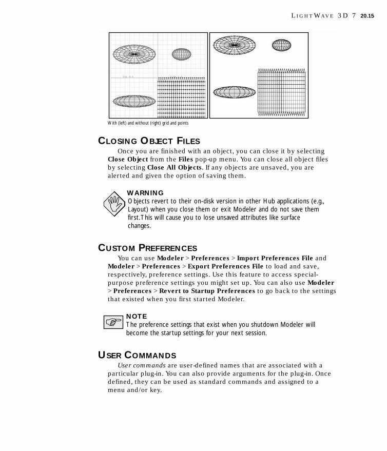
With (left) and without (right) grid and points

CLOSING OBJECT FILESOnce you are finished with an object, you can close it by selecting

Close Object from the Files pop-up menu. You can close all object filesby selecting Close All Objects. If any objects are unsaved, you arealerted and given the option of saving them.

WARNINGObjects revert to their on-disk version in other Hub applications (e.g.,Layout) when you close them or exit Modeler and do not save themfirst.This will cause you to lose unsaved attributes like surfacechanges.

CUSTOM PREFERENCESYou can use Modeler > Preferences > Import Preferences File and

Modeler > Preferences > Export Preferences File to load and save,respectively, preference settings. Use this feature to access special-purpose preference settings you might set up. You can also use Modeler> Preferences > Revert to Startup Preferences to go back to the settingsthat existed when you first started Modeler.

NOTEThe preference settings that exist when you shutdown Modeler willbecome the startup settings for your next session.

USER COMMANDSUser commands are user-defined names that are associated with a

particular plug-in. You can also provide arguments for the plug-in. Oncedefined, they can be used as standard commands and assigned to amenu and/or key.

L I G H T W A V E 3 D 7 20.15

NOTEYou can set up multiple user commands using the same plug-in withdifferent arguments.

NOTEThe command arguments can be derived from the LScriptdocumentation on the LightWave CD.

To add a user command:1 Choose Modeler > Commands > Edit User Commands. This will

display the Edit User Commands dialog.

2 Enter the name you want to use. We suggest you also use the prefixCMD (e.g., CMDSTRETCHPRINCESS). This will keep all of your defined usercommands together when they appear in a list together with standardcommands.

3 Select the command you want to use on the Action pop-up menu.

4 If the plug-in requires arguments, enter them in the Argument field.

5 Click the Add button. Your command will appear on the UserCommand pop-up, along with any other user commands you havecreated.

Click Delete to delete the selected User Command. Selecting theClear All button will delete all defined user commands, but don’tclick this unless you really mean it! There is no implicit undo for this.You will have to either re-add commands manually or use Modeler >Preferences > Revert to Startup Preferences.


6 Click OK to close the dialog. The user command will now appear inany command lists.

NOTEIf you need to change the plug-in associated with a user command, youmust delete it and then re-add it.

Maintaining User Command SetsAlthough the user commands are a part of the main preferences, the

Load and Save buttons let you retrieve and store user command sets thatyou develop.

Execute CommandThe XCommand function (Construct > Utility: LScript) lets you

directly enter a user command to be executed.

DEFINING A STARTUP COMMANDYou may define any plug-in (with arguments) to run automatically

when you first run Modeler. Simply choose Modeler > Commands > EditStartup Command and define the command and argument, if applicable.

GENERAL OPTIONSYou can access the General Options panel by choosing Modeler >

Options > General Options.

L I G H T W A V E 3 D 7 20.17

Modeler General Options panel

Content DirectoryThe Content Directory (see Chapter 6) is a central file path for

loading objects, images, and scenes. Note that this setting is shared byall LightWave applications.

Default Polygon TypeSome operations in Modeler create many polygons in one operation.

As such, the computer must decide whether to generate triangles (three-point polygons) or quadrangles (four-point polygons), depending on theshape’s requirements.

To force the computer to use Triangles or Quadrangles, select eitherfor the Polygon setting. Choose Automatic to let the computer createthe most appropriate polygon type for each given operation.

HINTTo create optimal objects, your goal is to keep the polygon countdown.They will load and render faster than bloated objects, with novisible difference.As such, Quadrangles is the suggested setting formost cases.This lets you manually choose the areas that requiretriangles.

Flatness LimitThe Flatness Limit setting determines whether Modeler regards a

polygon as planar or not. Note that a non-flat polygon within this settingcan still cause rendering errors. (See Chapter 21, “Non-Planar Polygons.”)

The Default Surface NameAll polygons must have a surface name. When geometry is created,

polygons are given the default surface name of DEFAULT. You can changethe default name by changing the Surface field. This will affect onlygeometry created from that point on, however. Use the pop-up to theright of the field to select from existing surface names.


NOTEWhen you create a surface using the Change Surface dialog (Detail >Polygons: Surface), the option (Make Default) automatically sets thedefault surface name.

Curve DivisionsThe Curve Divisions setting determines how smoothly a curve (e.g.,

spline curves, text, etc.) should be interpolated. The finer the setting,the greater the number of polygons used, and the smoother the resultingcurve division.

Patch DivisionsWhen a SubPatch object is frozen with the Freeze command, it is

converted into a polygonal object. The Patch Division settingdetermines the level of detail used in the resulting object. The numberentered in the Patch Division field must be 1 or greater and is restrictedto whole numbers. (See Chapter 29, “Patch Level and Conversion toPolygons.”)

The number of polygons per SubPatch surface will be equal to thesquare of the Patch Division number. For example, if set to 4, eachSubPatch surface will be converted into 16 polygons arranged in a 4 by 4array. A setting of 2 would result in 4 polygons arranged in a 2 by 2 array.

The higher the setting, the higher the number of polygons used.Because of LightWave’s surface smoothing capabilities, you can often getaway with a setting of 2 and sometimes even 1, which will keep thepolygon count of your objects to a minimum.

Metaball ResolutionThe Metaball Resolution setting determines the amount of detail

used to display metaballs. (See Chapter 29, “Metaball Resolution.”)

Undoing OperationsLightWave Modeler offers an undo function that lets you take back

the last change you made while working on an object. The Undo button(U) is located along the lower edge of the interface. The number of undosis determined by the Undo Levels setting. The maximum value is 128,but you can also be limited by your computer system RAM. However,minimally-configured systems should be able to go back several steps ifnecessary. Even power-users should find 10 undo levels sufficient.

Undoing the UndoIt’s possible to go too far unintentionally and undo too many steps.

To correct for this error, click the Redo button located next to the Undobutton. As long as you have made no editing changes, you can redo allthe way back to your last modeling operation.

L I G H T W A V E 3 D 7 20.19

The combination of Undo and Redo is a powerful one, allowing you tostep backward and forward through the evolution of a model. This isespecially useful when you use some of the more advanced modelingtools, where you may need to make a series of subtle changes to a modelas you design it, undoing and redoing as needed, until you achieve thedesired shape.

WARNINGIf you undo back five steps, then use a new tool, you will no longer beable to redo those steps. Undo is a kind of history that unfolds as youmodel. If you go back and change the model, then you have changedthe course of history in a fundamental way.The structure of the model isnow different, and redo will be unable to restore it. (You aren’t MartyMcFly.)


cchhaapptteerr21Points and Polygons

Chapter 21:Points and Polygons

The process of object editing involves manipulating points andpolygons. It will include selecting some portion of an existing object,choosing the operation to perform, adjusting any parameters for thatoperation, then carrying out the operation.

The concept of selecting is very important to Modeler. Selection is theact of specifying either the object itself, or a portion of it, that you intendto edit next. The most basic elements you can modify include points andpolygons—the dots and multi-sided shapes that make up all objects. Anynumber of points, polygons, or objects, in any combination, may beselected for a specific operation.

NOTEEverything in a layer is considered selected when nothing is selected.

NOTEWhen selecting and unselecting, make sure that no modeling tool iscurrently active.You can usually tell if a tool is active based on themouse pointer.You can quickly deactivate any tool by pressing theSPACEBAR; however, if no tool was active, you will change the edit mode.You can also choose Modes > Deselect Tool.

POINT SELECTIONPoints generally appear in two ways on screen, selected and

unselected. Selected points are highlighted, while unselected pointsremain small dots.

L I G H T W A V E 3 D 7 21.1

To select points:1 Use Point Selection mode (Point button or CTRL+G). The mode

selection buttons are located at the bottom-left of the screen.

Point Selection mode button selected

2 Drag your LMB over points in an object and then release the mousebutton to select those points.

NOTEOnce you have selected points and released the mouse button, youcannot select additional points in the same manner.

HINTIf you know the number of points you want to select, check theinformation display above the Point (Selection mode) button. It showsyou the number of selected items.

21.2 C H A P T E R T W E N T Y - O N E : P O I N T S A N D P O L Y G O N S

To add more points to a selection:Hold the SHIFT key while you select with your LMB to add points to

the existing selection or just click your MMB.

To lasso a group of points:With the RMB, drag out a circle around points to select a group. As

you might expect, you can add more points to a selection by holding theSHIFT key as you drag.

To unselect points:If selected points exist (and you have released the mouse button),

dragging over them with your LMB will unselect them. You can also usethe lasso by dragging with your RMB.

To unselect all points:Click in any non-active (i.e., not a button) area on the toolbar to

unselect all points. You can also use the Drop Current Tool command (/).

NOTESee Chapter 27 for additional selection commands.

POLYGONSAs discussed briefly in the prior chapter, a polygon is some number of

points joined by lines to form a solid face. A triangular polygon is athree-point polygon. A quadrangular polygon is a four-point polygon. Amulti-sided polygon (some programs call these n-gons) is a complexpolygon, one with many points. As long as the points that make up apolygon remain in one (flat) plane, the polygon will render properly. Ifnot, polygons can fall victim to unpredictable rendering errors. Even if apolygon is flat when modeled, it can become “unflat” (non-planar) if adisplacement map, bones, or other effects that move points non-uniformly are applied to the object during an animation.

L I G H T W A V E 3 D 7 21.3

Polygon illustrations

Non-planar PolygonsNon-planar rendering errors can be eliminated by using triangles.

Why use triangles? Well, say you had a square piece of glass laying on atable. It’s physically impossible to lift just one corner without also liftingat least one of the other corners, right? However, if the glass istriangular, we can easily lift one corner and leave the other two stillresting on the table. A non-planar polygon is like our square piece ofglass with just one corner lifted in the air—impossible for you andLightWave’s renderer. Although you can make objects with non-planarpolygons, they will likely cause sporadic rendering errors.

Example rendering error due to non-planar polygon

If we split the glass square in half from one corner to another, we endup with two triangles sharing a single side. (In Modeler speak, this is calledtripling polygons.) We can then, in effect, lift one corner without a problembecause the shared side would act like a hinge.


Tripled polygons

FlatnessWhether Modeler regards a polygon as planar or not depends on its

flatness value and the Flatness Limit on the General Options panel(Modeler > Options > General Options) setting. If a polygon’s flatnessexceeds the limit, then it is considered non-planar. A polygon’s flatnesscan be determined by selecting the polygon and opening the PolygonInfo panel (Display > Selection: Info). It is unlikely that you will everneed to adjust the Flatness Limit default setting of .05%.

NOTEIf a polygon is non-planar, but within the Flatness Limit, it may stillcause rendering errors.

POLYGON EFFICIENCYSo why not just use triangles exclusively? Well, the more polygons

your object has, the longer it takes to render. Polygons with more thanthree points are still useful when they will not be bent or twisted—bending or twisting these types of polygons usually results in non-planarpolygons, which cause rendering errors. It is best to use a combinationof polygons when you model, using three-, four-, and greater-sidedpolygons where necessary. Use the type of polygon that best fits theneeds of the animation and model.

SPECIAL-USE POLYGONSA few types of polygons are useful for very specific purposes. Single-

point polygons appear to be normal points, except that you can selectthem and assign them surface qualities like any polygon. However,unless single-point polygons are assigned luminous or motion blurattributes (or are used with HyperVoxels), generally they are not visiblewhen rendered. With luminosity and/or motion blur, they appear as apinpoints or streaks of lights in images or animations. This is highlyuseful for emulating rain, stars, fireworks effects, and more.

L I G H T W A V E 3 D 7 21.5

Fireworks with single-point polygons

Two-point polygons, or lines, are useful for strings, such as onstringed instruments, fields of wheat, and so on. Technically, a line hasno measurable thickness, but LightWave lets you render at an adjustablesize.

A field of wheat with two-point polygons

NOTESee the discussion on Particle/Line Thickness; this feature is onLayout’s Rendering tab on the Object Properties panel, see Chapter 9for more information.

POLYGON SELECTIONPolygons generally appear in two ways on screen, selected and

unselected. A selected polygon will appear highlighted with outlines inyellow. You will see that selecting polygons is very similar to selectingpoints.


To select polygons in a viewport:1 Use Polygon selection mode (CTRL+H). The mode selection buttons

are located at the bottom-left of the screen.

Polygon Selection mode button selected

2 If you are using a viewport set to a non-shaded Rendering Style(Display Options), like wireframe, drag your LMB over the edge ofpolygons and then release the mouse button. This selects polygonsthat share that edge. With a shaded Rendering Style like Texture orSmooth Shade, you can click directly on the polygon’s face.

As polygons become selected, they will become highlighted and youwill see the surface normal indicator (the perpendicular dotted line)appear. (The Normal display option must be active.)

L I G H T W A V E 3 D 7 21.7

NOTEOnce you have selected polygons and released the mouse button, youcannot select additional polygons in the same manner.

HINTIf you know the number of polygons you want to select, check theinformation display above the Point Selection mode button. It showsyou the number of selected items.

To add more polygons to a selection:Hold the SHIFT key while you select with LMB to add more polygons to

the existing selection or just click your MMB.

To lasso a group of polygons:With the RMB, drag out a circle around polygons to select a group.

Only the polygons completely within the outline are selected. Of course,you can add more polygons to a selection by holding the SHIFT key as youdrag.

To unselect polygons:If selected polygons exist (and you have released the mouse button),

dragging over them with your LMB will unselect them. You can also usethe lasso by dragging with your RMB.

NOTESelecting a group of polygons and then deselecting the ones you don’twant is often the only way to select the ones you do want.

To unselect all polygons:Click in any non-active (i.e., not a button) area on the toolbar to unselect

all polygons. You can also use the Drop Current Tool command (/).


NOTESee Chapter 27 for additional selection commands.

SELECTION WITH IN-LINE POINTS/POLYGONSIf there are points/polygons in-line (on top of each other) in a

viewport using a non-shaded Rendering Style (i.e., Wireframe), you selectall of the points/polygons when you select with your mouse. However,shaded viewports respect polygons facing away from you and thoseobscured by other polygons. Thus, you can select by clicking on apolygon’s face without worrying about what’s behind or on the otherside. You can change the Rendering Style from the pop-up menu on theviewport titlebar or on the Viewport tab of the Display Options panel.

Polygon selected in shaded mode

SYMMETRICAL SELECTIONWhen you select polygons/points on the positive X axis and

Symmetry mode (Symmetry button) is active, polygons/points on thenegative X axis are also selected (or deselected). Polygons/points mustbe exactly opposite each other on the positive and negative sides of theX axis for this command to work properly.

L I G H T W A V E 3 D 7 21.9

Selecting polygons in Symmetry mode

NOTEGenerally, you should perform all of your edits on the positive side ofthe X axis when using Symmetry. Using the negative side may lead tounpredictable results.

NOTESymmetry also affects polygon editing.

VOLUME SELECTION MODEYou may also select a portion of an object using a definable bounding

box (i.e., a volume). The Volume Selection mode (CTRL + J) button is nextto the Polygon Selection mode button at the bottom of the interface.Polygons/points selected in this manner do not become highlighted.

To use Volume selection:1 Click the Volume selection mode button.


Volume Selection mode button selected

2 The initial state of the Volume select is usually Exclude. This meanspolygons touching the bounding box are excluded. Clicking theVolume button again will toggle to the Include state where polygonstouching the bounding box are included in the selection. You can alsojudge the state by looking at the small text field right above the PointSelection mode button.

3 Drag out a bounding box in a viewport with your LMB. If one alreadyexists, you can drag it around from the center or drag the edges andcorners to re-size. You can reset the bounding box by clicking in aninactive part of the interface.

The selection is infinite along the axis perpendicular to the viewportyou dragged the bounding box in.

If you open the Volume Statistics panel (Modeler > Windows >Statistics Open/Close), you can also use the + and - buttons to formallyselect/unselect the listed points/polygons.

Lasso Volume SelectYou can also lasso-select a volume by dragging your RMB in a

viewport. A big difference between this and normal volume selection is

L I G H T W A V E 3 D 7 21.11

that in a perspective viewport, the lassoed area is perpendicular to theviewport. Moreover, the angle will be retained even when the viewport issubsequently rotated.

HINTIf you are selecting from among many items within a cluttered space,it’s probably easier to use the lasso tool for Polygon Selection mode(i.e., RMB).

HINTPress the SPACEBAR to cycle through the Selection modes (Point,Polygon, and Volume). Note that it will also first drop any modelingtool that may be active.

SELECTION BY CRITERIAThe Polygon Statistics panel (Modeler > Windows > Statistics

Open/Close) includes some tools that simplify your life when you selectpolygons.


Polygon Statistics panel. Pop-up button for surface, part, and sketch color selection are circled

The Polygon Statistics panel lists polygons by type, includingskelegons, metaballs, and SubPatches, as well as the number of eachtype. 1 Vertex polygons are those that consist of a single point; 2Vertices polygons are those with two points, and so on.

You can select all of the polygons in a particular group by clicking onthe corresponding plus (+) symbol. You can unselect the entire group byclicking the minus (-) sign.

You can also select by surface name (Surf), part name (Part), andsketch color (Col). First, select a name by clicking on the pop-up menu(down-arrow button). Then click on the plus or minus signs as needed.

Left: Selecting surface. Right: Surface now available for polygon selection

NOTEThe information presented on the Statistics panel will vary dependingon the editing mode (i.e., Points, Polygons, or Volume).

L I G H T W A V E 3 D 7 21.13

HINTLeave the Statistics panel open all the time for easy access.

SURFACE NORMALThe surface normal—admittedly an unusual-sounding name—has

great importance in 3D. Here’s why: A feature of polygons is that theycan be one-sided or double-sided. They have the unique ability to beinvisible from one side while visible from the other, or they can bevisible from both sides. The surface normal, which appears whenever apolygon is selected, projects away from the visible side of a polygon.

Since LightWave needs to calculate the appearance of all polygonsthat make up an object, it helps for you to determine beforehandwhether the polygons you need for an object will actually be seen fromboth sides. Why is this important? Because it takes LightWave longer tocalculate both sides of the polygon. If LightWave knows that a polygon isonly one-sided, it can render images more quickly.

How can you determine whether to use a one-sided or double-sidedpolygon? Easy. Suppose you’re making an apple. Will the scene requirethat the viewer see the inside of the apple? If not, then you model onlythe outside of the apple. There’s a simple rule of thumb for modeling:build only what your animation requires. The author of LightWave oncecreated a model of San Francisco’s famed Golden Gate Bridge. However,since the back side of the bridge would not be seen in the animation, hedid not model it. It wasn’t needed.

NOTEEven if you have not modeled double-sided polygons, you can still usethe Double Sided surface attribute when rendering.

Surface Normal FunctionsSee Chapter 26 for information on special functions to change the

direction of surface normals.


NUMERIC PANELThe Numeric panel is a multi-functional non-modal window. Its

contents and abilities change depending on what tool is selected. Whenyou create primitives, it lets you refine graphically set values. When youuse modifying tools, it lets you change various settings that affect howthe tool performs. It is displayed by choosing Modeler > Windows >Numeric Options or by just pressing the N key. It may be left opencontinuously.

Use the Actions pop-up menu to Reset the fields to their defaultsettings or to Activate the tool. (You can also press the N key to activatethe tool.) Generally, activating a tool turns on its interactive handles, ifany, in the viewports. This can be for primitive shape, influence range,and so on. It will also activate the numeric fields, if they are ghosted.

Activate option

NOTEYou can also reset to defaults by clicking a reset area when a tool isselected, but not activated.

L I G H T W A V E 3 D 7 21.15

cchhaapptteerr22Creating Geometry

Chapter 22:Creating Geometry

As you might expect, no one is going to create a starship byindividually creating each and every point and polygon. You create mostof your objects with primitives, that is, boxes, balls, discs, and cones.

Look around the room. Nearly everything in it can be broken downinto one or more of these primitive shapes. Your monitor is basically abox, your desk is made up of several boxes, your trash can is anextruded disc, and so on.

The modeling process normally starts with a primitive and you justmodify and add to it. So, the better you get at breaking down objectsinto primitives, the better modeler you will become.

THE PRIMITIVE TOOLSOn the Create menu, there are several basic primitive tools in the

Object group in the toolbar. Generally, most of the tools are used in thesame way. First, you drag out a two-dimensional shape and then adddepth to your object by expanding it in a different viewport. Forexample, with the Box tool you begin by creating a square and adddepth, making it a box. The Ball, Disc, and Cone tools all start off thesame, with a circle. It is really the second step that differentiates thosetools.

L I G H T W A V E 3 D 7 22.1

Dragging out a ball

You’ll probably use the Box tool most often, because most objects arebox-like in general form. The Ball tool is great for creating anything froma tiny pea to a giant planet. The Disc tool is used to form cylinder-shaped objects like coins or tubes. The Cone tool is perfect for makingdelicious ice cream cones...mmmmmm.

To create a primitive:1 Select the primitive tool button on the Create menu (i.e., Box, Ball,

Disc, or Cone).

2 Drag out the initial 2D shape in any viewport with your LMB. Thisactivates the tool. Pressing the CTRL key before you click and holdingit while you drag will symmetrically constrain the shape. Thedimensions of your outline are shown in the lower left corner.

3 After you release the mouse button, you can adjust the shape bydragging any of the sides or corners. You can reposition it bydragging the center.

22.2 C H A P T E R T W E N T Y - T W O : C R E A T I N G G E O M E T R Y

4 Go to another viewport and drag to extend the shape into the thirddimension. Release the mouse button.

5 You can continue to adjust the primitive’s size and position.

NOTEIf you find you need to start over from scratch, just click in an inactivetoolbar area or use undo.

6 When you are satisfied, deselect the primitive tool by clicking on it orchoosing Modes > Deselect Tool to turn your outline into an object.(Alternatively, you can select another modifying tool.)

Tools and the Right Mouse ButtonMost (interactive) tools that create geometry (Box, Ball, Capsule,

etc.) use the RMB to basically drop the tool—making geometry, ifapplicable—and then begin a new operation with it.

Creating in PerspectiveYou can create primitives in a perspective viewport pretty much as

you would in a 2-D viewport. You will see highlighted control points atthe corners, sides, and center. You will also notice that you can see(fainter) hidden sides and control points. You can also drag any of thecontrol points. Dragging a side control point will move thecorresponding side along its perpendicular axis.

L I G H T W A V E 3 D 7 22.3

Creating in perspective

NOTERemember, you can rotate your view by holding the ALT key as youdrag.

Using the Arrow KeysThe arrow keys let you quickly adjust certain settings depending on

the primitive being created, as follows:

Primitive Right/Left Arrow Up/Down Arrow

Box Incr./decr. horizontal Segments* Incr./decr. verticalSegments*

Ball Incr./decr. Segments Incr./decr. Sides

Disc Incr./decr. Segments Incr./decr. Sides

Cone Incr./decr. Segments Incr./decr. Sides

*based on viewport beneath mouse pointer

USING THE NUMERIC PANELYou can also numerically create a primitive or use the numeric panel

with the graphical creation tools. The input fields on the panel update inreal-time as you graphically adjust your box with the mouse and viceversa. As such, you can drag out a rough version of your box with yourmouse and then enter precise values on the numeric panel.

Actions Pop-up MenuThe Actions pop-up menu (see Chapter 21), can activate the

numerical settings for a primitive tool. To do this, simply select Activate.Select Reset to return all of the fields to their default value.


Box Tool Fields

You have two different ways to adjust the shape of your box, the Sizeand Range modes. With the Size tab selected, you can adjust the Width,Height, and Depth of your box dimensions. The Center XYZ settings setthe position of the center of the box.

With the Range tab selected, you can adjust the positions of twoopposing corners of your box using the Low XYZ and High XYZ settings.

You can round off the edges of the box by setting the Radius to avalue greater than 0. The Axis sets the direction of the radial polygonpattern used to round the edges. Use the Sharp Edge option to smoothor unsmooth the edges.

L I G H T W A V E 3 D 7 22.5

The Segments XYZ settings define the general number of segmentsalong those axes, excluding any geometry added to round the edges.

Rounded-edge box

Ball Tool Fields

Type The make-up of a Globe is determined by the number ofSides and Segments. Tessellation balls are set using aLevel parameter; these balls are created entirely oftriangles and are, therefore, smoother looking.


HINTUse a Tessellation ball if the camera will be close to the object andthe surface is smooth.

Axis (Globe) determines the major axis for the ball. This isalso set when you click to first create the ball using theaxis perpendicular to the (orthogonal) viewport.

Sides (Globe) determines how many segments should be usedaround the ball.

Segments (Globe) sets how many vertical segments should beused. Three-sided polygons are always used at the topand bottom. Elsewhere, the polygons used are dependenton the Polygons setting on the General Options panel(Modeler > Options > General Options).

(Tessellation) sets the number of segments along theedges between the twelve polyhedral vertices. Highersettings will increase the complexity of the trianglematrix, taking longer to create and requiring more RAM.

Center The XYZ coordinates of the center of the ball.

Radius The radius of the ball along the X, Y, and Z axes.

Disc/Cone Tool Fields

Axis The primitive is aligned with this axis.

Sides Sides determines how many segments should be usedaround the perimeter.

Segments Segments sets how many vertical segments should beused.

Bottom Bottom is the starting point of the primitive along theselected Axis.

L I G H T W A V E 3 D 7 22.7

Top Top is the ending point of the primitive along theselected Axis.

Center Center refers to the coordinates for the center of theprimitive.*

Radii Radii refers to the radius of the primitive (wide end for acone) along the axes.*

*The Center and Radii XYZ fields that correspond to theselected Axis will have no effect on the shape.

NOTEMost tools allow numeric input.Thus, the contents of the numericdialog will change as you select different tools.You may find it handy tojust leave the numeric dialog open.

Make UVs OptionThe Make UVs option at the bottom of the various primitive numeric

panels assigns some default UVs based on the geometry of the object.Note that a UV Texture map must be currently selected or this optionwill be ghosted. (See Chapter 28 for more information.)

Make UVs option

OTHER PRIMITIVE TOOLS AND FUNCTIONS

The Capsule ToolAnother primitive tool is the Capsule tool (Create > Objects:

Capsule). Your initial click defines the perpendicular axis of the object.You can drag the center position handle to move the shape, and you candrag the outer bounding box edges to resize it. The numeric settings aresimilar to those for the standard primitive tools.


The Platonic Solid ToolYet another primitive tool is the Platonic Solid Tool (Create > Objects:

Platonic Solid). The shape of the primitive is controlled by the Shapepop-up menu on the numeric panel. You can drag the center positionhandle to move the shape, and you can drag the outer bounding boxedges to resize it. The other numeric settings are similar to those for thestandard primitive tools.

The SuperQuadric ToolUse the SuperQuadric tool (Create > Objects: SuperQuadric) to

create quadrics objects interactively. You can choose between twoshapes: Ellipsoid (spherical) and Toroid (donut).

You can use standard drag handles to manipulate the shape andposition interactively. The numeric panel provides more detailed control.

A perfect circle—looking along the set Axis—can be made by settingthe Side Bulge to 2. A value of about 5 yields a rounded square shape.

L I G H T W A V E 3 D 7 22.9

NOTEIf you must know, a quadric is a shape made of the squares of thecoordinates, a generalization of a sphere, which is x2 + y2 + z2.

The Gemstone ToolDiamonds are an animator’s best friend or something like that. You

can quickly make a nice round-cut diamond with the Gemstone tool(Create > Objects: Gemstone Tool).

On the numeric panel you can control various aspects of yourdiamond. Center sets the center position and Radius the overall radiusof the object.

Higher Symmetry values increase the number of polygons used onthe crown and lower values decrease the number. The Crown, Girdle,Table and Pavillion settings control the size of those areas on thediamond. (See above illustration for reference.)


The Gemstone Tool numeric panel

The Equilateral FunctionThe Equilateral function (Create > Objects: Equilateral) will create an

equilateral triangle of the specified size.

The Gear FunctionThe Gear function (Create > Objects: Gear) creates a gear-shaped

object.

Teeth Teeth refers to the number of teeth in the gear.

Taper % Taper sets the “pointiness” of the teeth. A higher settingcreates sharper teeth.

Inner Radius Inner Radius refers to the distance from the center of thegear to the bottom of the teeth.

Outer Radius Outer Radius is the distance to the outside edge of theteeth.

Thickness Thickness is the width of the gear.

Axis Axis is the perpendicular axis of the gear.

L I G H T W A V E 3 D 7 22.11

Gear

The Wedge FunctionThe Wedge function (Create > Objects: Wedge) will generate an

annulus (like a flat donut).

Axis Axis is the axis perpendicular to the donut hole.

Sections Sections refers to the number of radial sections touse for the object.

Height Height specifies the width of the object.

Inner Radius Inner Radius specifies the radius of the inner hole.

Outer Radius Outer Radius specifies the radius to the outsideperimeter.

Start Angle Start Angle is the starting angle around the selectedAxis.

End Angle End Angle is the ending angle around the selectedAxis. (360 for a complete donut.).


Wedge

The Toroid FunctionChoose Create > Objects: Toroid to generate a torus (donut) or a

section thereof.

Axis Axis is the axis perpendicular to the donut hole.

Sections Sections specifies the number of segments usedaround the donut.

Sides Sides specifies the number of sides each segmentshould use.

Radius Radius is the distance from the center of the donut tothe center of a cross section.

Start Angle Start Angle is the starting angle around the selectedAxis.

End Angle End Angle is the ending angle around the selectedAxis. (360 for a complete glazed donut. mmmm).

Cross Section Cross Section is the XYZ size of a cross section. Notethat the value corresponding to the selected Axis isnot considered.

L I G H T W A V E 3 D 7 22.13

The Parametric Surface Object FunctionThe Parametric Surface Object function (Create > Objects:

ParametricObj) creates parametric surfaces based on the equationsentered for X,Y, and Z in terms of UV coordinates. The function lets youcreate the object using Triangles, Rectangles, Curves, or just points(None). The equations may include any of the functions listed in theAppendix.

Parametric Surface Object Function

The Plot1D FunctionThe Plot1D function (Create > Objects: Plot1D) generates either a

curve consisting of two-point Polygons or a spline Curve. The curve isgenerated along the X axis, and its height is in the Z axis.

Plot1D Function

The height is determined by the value of the expression in theEquation field at each x. In the fields Min, Max, and Division, enter the xvalue for the start of the curve, the x value for the end of the curve, andthe number of divisions of the curve.


Plot1D Function

The Plot2D FunctionThe Plot2D function (Create > Objects: Plot2D) generates a two-

dimensional surface in the XY plane consisting of Triangles, Rectangles,Curves, or points (None). The height (in the Z direction) is determinedby the value of the expression in the Equation field at each division inthe X and Y axes.

Plot2D Function

In the fields labeled X Min, X Max, Y Min, and Y Max, enter theboundaries for the surface. In the XMesh and YMesh fields, enter thenumber of divisions along that axis.

L I G H T W A V E 3 D 7 22.15

Plot2D Function

USING THE PEN TOOLThe Pen tool (Create > Elements: Pen) gives a quick way to create

polygons on the fly.

To create a polygon with the Pen tool:Choose Create > Elements: Pen and click in a viewport with your

LMB. A polygon is created using points you define by clicking. If youdrag the mouse button, you can refine the point’s position before youcreate it, which happens when you release the mouse button. You do notneed to click in the same viewport for each point.

Using the Pen Tool

To constrain the position of a new point to 45-degree increments,relative to the last created point, hold the CTRL key down before youclick.

To create single point polygons with the Pen tool:Simply click in a viewport with your RMB. With each click you will

create a single-point polygon!


Using the Pen Numeric PanelYou can also enter specific numerical values in the Pen tool numeric

panel. Clicking the Add Point button creates the point, essentiallymimicking the RMB.

Pen Numeric Panel

THE TEXT TOOLThe Text tool (Create > Elements: Text) lets you interactively create

type objects using True Type and Adobe PostScript Type 1 fonts. Onceyou create them, these objects can be beveled, extruded, drilled, andmore.

Using the Text Tool

NOTEIf the Text tool button is ghosted, make sure you have added somefonts, as discussed below.

The Edit Font List PanelBefore you can use the Text tool interactively, you must have

previously loaded one or more fonts into the font list. This is done usingthe Edit Font List panel (Modeler > Options > Edit Font List).

L I G H T W A V E 3 D 7 22.17

Edit Font List panel

Use the Font pop-up menu to select the font for your object. Clickingthe Load Type-1 button brings up a file requester where you can load aPostScript font. If you have PostScript fonts, the files often have a .PFB

filename extension. Clicking the Add True-Type button brings up a fontselection requester you can use to select a font. (Note: the point size isirrelevant.)

Click Clear Entry to remove the selected font from the font list. ClearList will purge the entire list. Load List brings up a file requester whereyou can load a previously saved font list file. This can be the LWM.CFG file.Save List brings up a file requester for saving the current font list to afile. Note that the font list is automatically saved when you exit Modeler,so it is not mandatory that you save the list. Use this option to createcustom file lists for special purposes.

NOTEThe clearing operations do not affect the actual files stored on yourhard drive.Also fonts in the list utilize no RAM until used.

Interactively Creating TextWhen you first click in a viewport after selecting the Text tool (Create

> Elements: Text), the text insertion pointer appears. You can just starttyping to create the Text template.

You can use the BACKSPACE or DELETE keys to clear the last charactertyped. To clear the entire text line, press SHIFT + BACKSPACE or SHIFT +DELETE. If you need to use a Modeler keyboard shortcut, like the N key,while using the Text tool, first press the ESC key to exit the Text tool,then press the desired shortcut key.


Modifying the TemplateThe position of the text is referenced to the bottom left of the pointer.

You can reposition the text in any viewport. Dragging the sizing handleup or down will scale the text larger or smaller. Dragging the kerninghandle will adjust the amount of space between characters.

NOTEThe sizing handle cannot be dragged past the bottom.

Text will be aligned with reference to the vertical bar. Pressing the TAB

key will cycle through the alignment options.

You can cycle through the font list using the UP and DOWN ARROW keysor you can use the numeric requester. If you have already started atemplate, the font will change.

You must deselect the Text tool or select another tool to actuallycreate the object. Alternatively, clicking your RMB will create the objectand also move the template to your mousepointer position. You canquickly make unlimited copies of the text in this manner.

The number of points used to approximate curves in charactersdepends on the setting for Curve Division on the General Options panel(Modeler > Options > General Options).

NOTEThe characters that are available within the selected font may belimited.You may or may not have all possible characters allowed by thePostScript format depending on whether those characters werecreated in the font originally.

The Text Numeric PanelThe related numeric panel provides interactive feedback and also lets

you set options numerically. Axis is the perpendicular axis used increating the text; however, it is usually set interactively by clicking themouse in a view window. The Text input field lets you enter the text togenerate into a 3D object.

L I G H T W A V E 3 D 7 22.19

Text Numeric Panel

From the Font pop-up menu, you can select any of the fonts definedin the previously discussed Fonts List.

Some fonts, when converted into 3D objects, have additional pointsnear their corner vertices. When these polygons are beveled, theseadditional points can cause beveling inaccuracies. Use the defaultsetting, Sharp, for the majority of your text generation, as this will avoidthe creation of such points. The Buffered setting allows the additionalpoints to be created, should you decide that you wish it.

The Alignment setting determines how the text is aligned around thetext insertion pointer. Center is the XYZ position of the insertion point;however, it is usually set interactively by clicking the mouse in a viewwindow. The Scale value sets the general height of the text; however, theactual size may be less and will vary from font to font. Kern sets thespacing between fonts and depends on the font’s own characteristics.Negative numbers are allowed to bring characters closer together.

NOTEThe Scale setting (numeric panel) cannot be set to zero or a negativenumber.

THE SKETCH TOOLThe Sketch tool (Create > Elements: Sketch) is purely a two

dimensional modeling tool. With it, you can draw polygons (and curves,discussed later) in any viewport.

To sketch a polygon:1 Choose Create > Elements: Sketch.

2 Open the numeric panel and select Face as the Type.


3 Drag out the desired shape. (It is not necessary to touch thebeginning of the line with the end. The polygon is closedautomatically.) When you release your mouse button, a polygon iscreated using the shape you sketched out. The polygon is alwayscentered in the depth dimension of the viewport.

Sketching CurvesYou can use the Curve option on the numeric panel of the Sketch tool

to create a spline curve instead of a polygon. The tool operates exactlyas previously described, except an open spline curve is created insteadof a polygon.

To sketch a curve:1 Click Create > Elements: Sketch.

2 Open the numeric panel and select Curve as the Type.

3 Drag out the desired shape. When you release your mouse button, acurve is created using the shape you sketched out. The curve isalways written on a plane positioned at 0 of the viewport’sperpendicular axis.

L I G H T W A V E 3 D 7 22.21

NOTEYou may be already familiar with curves like these since many desktopdrawing programs use them. Spline curves will be discussed in detaillater.

THE BEZIER TOOLThe Bezier tool (Create > Elements: Bezier) allows you to create

standard spline curves using tangent controls.

Bezier Tool

To use the Bezier tool:1 Choose Create > Elements: Bezier.

2 Place your mousepointer where you would like to begin your curve.

3 Click and hold your LMB—the beginning and ending of your firstcurve is created. Drag your mouse to where you want the curve toend and release the mouse button.

4 Successive clicks will create additional curves.

5 Drag the tangent handles (circles) to adjust the curve shape. Holdingthe CTRL key while dragging will allow you to move both sides of thetangent simultaneously.

6 Drop the tool by hitting the SPACEBAR.

NOTEOnce you drop the Bezier tool, a normal Modeler curve is created.Assuch, you cannot re-edit the curve using the Bezier tool.

On the numeric panel, you can set the subdivision level (for smootheror less smooth curves), create a closed curve, and delete the lasttangent point.


Bezier tool numeric panel

SPLINE CURVESIn addition to making polygons from points, you can also create

curves. Curves are a powerful modeling tool and help you create smoothedges and flowing organic objects or object details. They are also usedfor some modeling tools as a directional path.

You can create curves using a minimal number of points, yet achievea smoothness that would take many times the number of points if youattempted to mimic the curve with a polygon. Moreover, with fewerpoints, it is easy to subtly or dramatically change the curve’s shape.However, by themselves, curves will never render in a finished image.They are essentially a free-form modeling tool used to create polygonalobjects.

There are basically two types of curves: open and closed. An opencurve has a beginning and an end—essentially a curving line. A closedcurve has no beginning or end; it is a closed loop. A circle is a closedcurve.

The Spline Draw ToolThe Spline Draw tool (Create > Elements: Spline Draw) is simply a

tool for making (open) spline curves. To use the tool, just click and movepoints. Clicking off the curve adds new points to the end.

The Spline Draw tool

Its numeric panel offers options for making control points, discussedlater, and deleting the last point from the curve. Changing the CurvePoints value will resample the curve into more segments. Note thatresampling the curve can change its shape, particularly if the number is

L I G H T W A V E 3 D 7 22.23

incremented gradually, like with the mini-slider. If you want a morerefined curve that accurately matches the one you have drawn, enter thenew number directly into the field to avoid the intermediate curves.

Creating from PointsYou can also create curves from points in a manner nearly the same

as creating polygons.

To create a curve:1 Create a few points. Clicking with your RMB using the Points tool

(Create > Elements: Points) will work.

2 Your points must be selected in the order you want the curve to flow.However, if you immediately go to—or were using—the PointSelection mode, the points should already be in the selected state. Ifnot, select them in the desired order.

3 To create an open curve from the points, click Create > Elements:Make Curve > Make Open Curve or press CTRL + P.


To create a closed curve from the points, click Create > Elements:Make Curve > Make Closed Curve or press CTRL + O (the letter o).

You can modify the curve’s shape by simply moving the individualpoints. Notice how the curve flows smoothly through the interiorpoints. It is easiest to see this as you drag points on either side of apoint. If you need additional control, you can add additional points toan existing curve.

To add points to a curve:Activate the Add Points tool (Construct > Subdivide: Add Points) and

click anywhere along the curve.

To delete points from a curve:Select the points and use the Cut command (X).

Curve DirectionCurves also have a head and tail. This is important for certain

modeling operations discussed elsewhere. When the curve is selected inthe Polygon Selection mode, the head is indicated by a small diamond; itis the first point you selected when creating the curve.

You can flip the head and tail around by using the Flip command(Detail > Polygons: Flip).

Using Control PointsWhen using a curve as a modeling tool, sometimes you need to adjust

the curve to get it to “that perfect angle.” Because of the way points

L I G H T W A V E 3 D 7 22.25

control an open curve’s shape, it can be difficult to get the desired resultat the ends of a curve. Fortunately, Modeler lets you have extra “control”points at each end, which affect the curve shape, but don’t actuallybecome part of the curve’s modeling characteristics.

To activate control points on a curve:1 If you have more than one curve, select your desired curve first using

the Polygon selection mode.

2 Choose Detail > Curves: Control Points > Begin Control Point todetach the first point from the curve. It is your starting control point.Dragging this point will change the shape of the curve at the newstarting point.

3 Choose Detail > Curves: Control Points > End Control Point todetach the last point from the curve. It is your ending control point.Dragging it will change the shape of the curve at the new endingpoint.

The control points commands will also toggle the control point stateoff, if selected again.

NOTEIt is perfectly legal to have only a beginning or ending control point ona curve.

HINTIf you plan to use control points on a curve, you should add an extrapoint at the beginning and end of a curve for that purpose.

Smoothing Two Overlapping CurvesWhen two curves share the same end point, because of point merging

or some other reason, the curve may not flow smoothly through thatpoint. This can be particularly troubling when designing a complexspline cage. You could kill the curve (k), reselect the points and create anew curve, but there is an easier way.


To smooth curves sharing a common end point:Select the two curves (Polygon selection mode) and click Detail >

Curves: Smooth. This smoothes the joint as though the two curves wereoriginally plotted as one continuous curve—even though they remainindividual curves.

Before (left) and after (right) using Smooth

NOTEMake sure that the point they share is in fact one point. (If not, mergethe points into one.)

Turning Curves into PolygonsSince curves will never be seen by themselves, sometimes you need

to turn them into polygons.

To convert a curve into a polygon:Select the curve(s) and choose Construct > Convert: Freeze. Each

independent curve will become a distinct polygon. An open curve will beclosed (between its end points) before it is converted to a polygon.

The number of points that Modeler will use to approximate the curvedepends on the setting for Curve Division on the General Options panel(Modeler > Options > General Options).

Using Modeling Tools on CurvesMost of the standard modeling tools will work on a curve as well.

However, a curve is sometimes converted into a polygon before the toolis applied. This happens with the Extrude and Lathe tools (Multiplymenu), for example.

L I G H T W A V E 3 D 7 22.27

Left: Curve. Right: Lathed object made of polygons

METABALLS AND SKELEGONSSee Chapter 29 for information on Metaballs and Metaedges.

Skelegons are covered in Chapter 10.

THE POINT TOOLRemember a point needs to have X, Y, and Z coordinates. You can

create points in real-time or by positioning first and then creating.

To create a point:1 Choose Create > Elements: Points to activate the Points tool.

2 In any viewport, with your LMB drag the large crosshairs to thedesired position (you can reposition in any viewport). Theinformation display (bottom-left corner) will give you positionfeedback as you move your mouse.

3 Click the RMB to create the point. Be careful not to move your mousepointer. Deselecting the Points tool will also create the point, if youdon’t have a steady hand. Deselecting and then reselecting the Pointsbutton will create the point and keep you in the create point mode.

4 You can also position the point by dragging with your RMB. However,the points will all be created along the same plane (when you releasethe RMB).


THE SPRAY POINTS TOOLSometimes you’ll want to create a random splattering of single-point

polygons for stars or perhaps gases when used with volumetrics. TheSpray Points tool (Create > Elements: Spray Points) acts like a pointsspray gun. Just activate the tool and drag your mouse pointer.

Spraying points

You can control the flow (Rate) and Radius of the spray on thenumeric panel, as well as specify a color vertex map and color.

MAKING A POLYGONAs we have discussed, polygons are made up of points. Excluding the

one and two-point specialty polygons, polygons should contain at leastthree points. You will likely find that your finished objects areconstructed of a variety of polygons with different numbers of points.

NOTEDon’t get discouraged if making polygons seems very tedious. Not thatit isn’t, but most of the time you’ll create your objects by starting withprimitives. Happily, creating polygons from points is the exceptionrather than the rule.

L I G H T W A V E 3 D 7 22.29

To create a polygon from points:In the Point Selection mode, select your points in a clockwise order.

Then, click Create > Elements: Make Pol.

Left: Points for polygon. Right: Resulting polygon

NOTEOnce you create a polygon, you’ll want to view it in the PolygonSelection mode to see if its surface is facing the correct directionbased on the normal, discussed later.

SINGLE-POINT POLYGONSSometimes you will want to turn single points into polygons. This is

necessary for objects like stars in a starfield, since you cannot assignsurface attributes to a point. Choose Create > Elements: Points to Polysto turn selected points into single-point polygons.

RANDOM POINTSUse the Random Points command (Create > Elements: RandPoints) to

create a defined number of points distributed randomly. You can choosebetween a Square or Sphere shape. Constant generally confines thepoints to the selected shape, while Falloff tapers off the pointdistribution along the perimeter.

Random Points


Left: Square. Right: Sphere

RANDOM PRICKSCreate > Elements: RandPricks creates random surface points on

polygons. Use this to add detail to an object where you will later kill allof its polygons.

Random Pricks

STIPPLECreate > Elements: Stipple creates a grid of regularly spaced points

over the surface of the object in the active layer. The Spacing fields arefor separate XYZ point spacing settings.

Stipple

L I G H T W A V E 3 D 7 22.31

TRIANGLESYou can use the Triangle Fan command (Create > Elements: Make

Fan) to create a subdivided polygon from selected points. (Selecting in aclockwise fashion works best.) The triangles will share the first pointselected.

A triangle fan

The Triangle Strip command (Create > Elements: Make Strip) issimilar, but creates a strip of triangle polygons from a set of points. Thiscan be useful for game engines that prefer to have geometry built instrips of triangles. The command basically creates triangles in a strip offirst point, second point, third point-poly, and so on.

A triangle strip

CAGECreate > Elements: Cage creates a cylindrical spline cage (connected

curves) using Axis, Sections (i.e., segments + 1), Sides, Top, Bottom, andRadius settings.


Cage dialog

Cage result

OTHER CREATION FUNCTIONS

Platonic SolidChoose Construct > Utility: Additional > Platonic to generate any of

the seven platonic solids—yes, even including the perennial favoritesCube and Tetrahedron!

Platonic Solid

L I G H T W A V E 3 D 7 22.33

Top to bottom, left to right: Tetrahedron, Cube, Octahedron, Cubeoctahedron, Icosahedron, Dodecahedron andIcosidodecahedron

PrimitivesChoose Construct > Utility: Additional > Primitives to display a menu

for the following six commands: Toroid (Donut), Wedge, Cage (SplineCage), RandPricks (Random Points), Gear, and Platonic (Platonic Solid).

Primitives

TeapotSpot o’ tea anyone? Generate a quick teapot by choosing Construct >

Utility: Additional > Teapot.

Teapot


cchhaapptteerr23Modifying Geometry

Chapter 23:Modifying Geometry

Moving, rotating, and scaling points and polygons is easy with thetools (and functions) available on the Modify menu. Generally, the toolswork on points or polygons, depending on what edit mode you haveactive.

HINTModeler tools can be deselected by clicking the highlighted buttonagain or, if it appears in a menu, by selecting it again.An easier methodis to just hit the SPACE key, which is mapped by default to ChangeSelection Mode.

WARNINGIf your object uses polygons with more than three sides, you will likelysee the effects of non-planar polygons created as you apply sometools.You may need to triple your polygons as a final step.

THE NUMERIC PANELAll of Modeler’s tools have their own numeric values which will

appear on the generic numeric panel, if you have it open (N). It willreflect the numerical values of your actions for the particular tool youare using. Use the numeric panel for precise tweaking. Initially, it willreflect the values for the last interactive use of the selected tool. Youmay alter the values and click the Apply button to use the tool withthose settings—this can be done multiple times.

FALLOFF MODEAs you will notice, many tools are just variations of the same

movement and differ only by how the tool’s effective range falls off. Takethe Move tool for example. It simply repositions the selected itemsequally to a new location will no falloff. With Shear, the range of the

L I G H T W A V E 3 D 7 23.1

effect varies along a linear axis. Magnet is similar, but the effect falls offin a radial pattern. DragNet is much like Magnet except that the center ofthe radial pattern is at the point you drag. Finally, Drag is a move, butthe range is only a single point.

NOTEThe tools on the Modify menu are grouped by movement (Move,Rotate, etc.)

All of these tools have a Falloff pop-up menu on their respectivenumeric panels. By changing the Falloff setting, you can effectively makeone tool function the same as another tool that uses that Falloff bydefault. In other words, with the Move tool, you could get the sameeffects as using the Shear, Magnet, DragNet, and Drag tools, by justchanging its Falloff setting. You might think of these tools as justshortcuts to a defined group of modify settings.

Falloff MeaningsNone None means no falloff. Thus, your basic Move, Rotate,

Size, and Stretch tools are set to this by default.

Linear Linear makes the effect falloff along a linear axis, so it isthe default for Shear, Twist, Taper1, and Taper2.

Point Point means falloff is immediate around a point, so youcan move only a single point. This mode is used by Drag.

Point Radial Point Radial is similar to Radial except that the center ofthe falloff is at the point being dragged. DragNet uses thissetting.

Polygon Polygon means falloff is immediate around a polygon, soyou can move only a single polygon.

Radial Radial means the effect will fall off in a radial pattern (ina cylindrical or spherical shape), so it is the default forMagnet, Vortex, Pole1, and Pole2.

23.2 C H A P T E R T W E N T Y - T H R E E : M O D I F Y I N G G E O M E T R Y

Weight Map Weight Map uses the selected Weight map for the falloff.Unweighted points will not move at all, while heavilyweighted points will move the most. Negatively weightedpoints will move inversely. This allows you to use anirregularly shaped falloff. (See Chapter 28.)

NOTEInterestingly, you can actually rotate a single point using the Rotatetool and Falloff set to Point; however, it will have no meaningfuleffect.

SETTING LINEAR FALLOFFThe linear-falloff tools are Shear, Twist, Taper 1, Taper 2, and Bend. By

default, a linear-falloff tool’s effect is automatically applied to the object(or selected items) 100 percent at one end and zero at the other, alongthe axis perpendicular to the editing viewport. This is indicated by theRange option at the bottom portion of the numeric panel (N), which hasAutomatic selected.

To use the tool in the Automatic mode via the numeric panel (byclicking the Apply button), select the perpendicular Axis. (If the axis hasnot been set either manually or by a previous mouse-based modifyoperation, the Axis setting is used to compute the falloff when you clickApply.)

HINTUsing the Automatic range is the simplest method.Thus, if possiblemodel your object along one of the three axes.

Defining a Specific RangeInstead of using an Automatic Range, you can define a specific Fixed

Range using an axis tree. This type of Range can be placed at anyposition and at any angle in 3D space. The effect tree looks like a pair ofcrossed wedges. The tool’s effect is applied along this tree with zero atits tip and 100 percent at its base (fat end)—portions of the objectbeyond the base are still affected 100 percent. The edges of the treereflect the fall-off curve shape.

L I G H T W A V E 3 D 7 23.3

To create a fixed range:1 Select the desired linear-falloff tool and drag out the axis tree with

your RMB. (The Range option will be set to Fixed on the numericpanel.)

2 Reposition the ends by dragging them with your RMB.

The XYZ positions of the starting and ending points are reflected inthe numeric panel. You can edit these values, if necessary.

In the image that follows, we used the Bend tool. Notice the impact ofthe fixed range. Geometry from the wide end of the axis tree and beyondis 100 percent impacted by the tool. The opposite end is not affected atall, with a falloff in between.


To reset to automatic range:To reset to automatic range, click your mouse pointer on an inactive

interface area. Note this will also switch you back to the AutomaticRange mode.

Setting the Falloff ShapeYou can quickly select between various basic falloff directions using

the Shape buttons. (The fixed-range axis tree is shown here forillustration purposes. It will not appear if you use an automatic range.)You can also use the LEFT and RIGHT ARROWKEYS to change the selectedShape.

You can adjust how the effect falls off using the two sliders, which actlike tension spline controls for the beginning (upper slider) and ending(lower slider). You can quickly set up some common curves by selectingfrom the Preset pop-up menu. The graph on the numeric panel, as well

L I G H T W A V E 3 D 7 23.5

as the outer edges of the axis tree (when using a fixed range) gives you avisual picture of the falloff. You can also use the UP and DOWN ARROWKEYS

to cycle through the Preset selection.

Adjusting falloff curve shape

Axis tree

NOTEThe falloff settings apply equally to an automatic range.

NOTEThe Bend tool does not have falloff options.

Here are some falloff examples:

Left to right:Automatic Linear;Automatic Smooth; and Fixed Linear

Flexing an Object on an Arbitrary AxisLet’s say you had an object that was not aligned nicely along the X, Y,

or Z axis. If you wanted, you could define a fixed range and align theeffect tree with the object. However, this can be a tedious process. Abetter alternative would be to use a Perspective viewport.

Remember, editing generally occurs along a viewport’s arbitraryhorizontal and vertical axes. Using a Perspective viewport, this can be


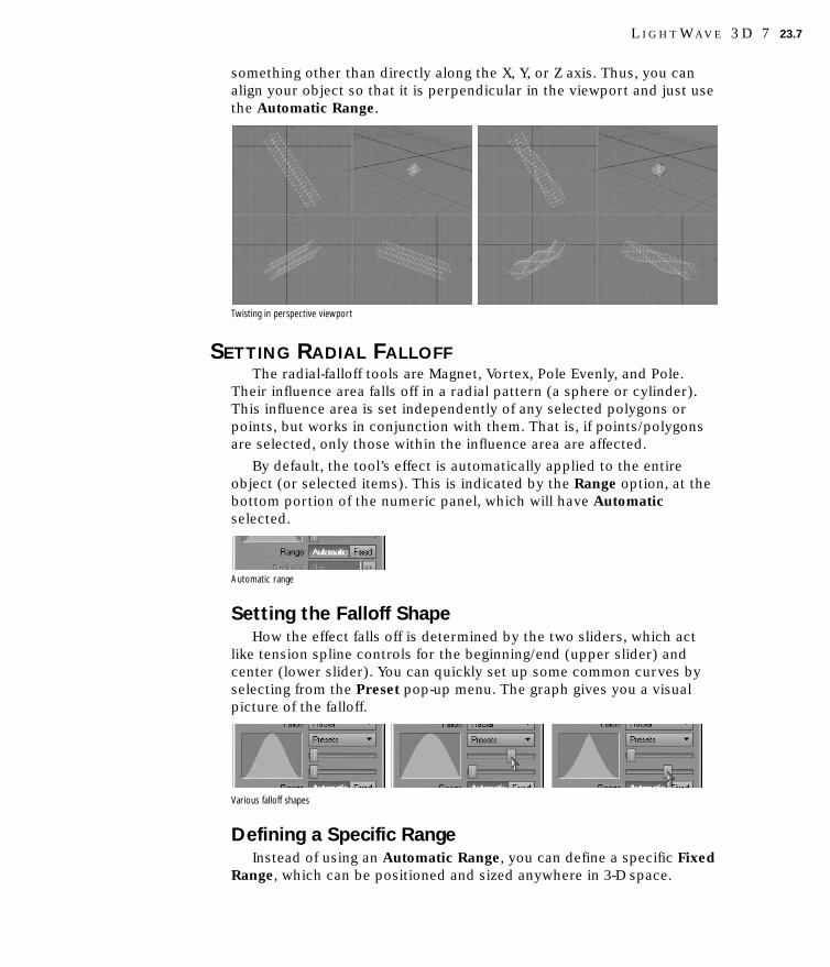
something other than directly along the X, Y, or Z axis. Thus, you canalign your object so that it is perpendicular in the viewport and just usethe Automatic Range.

Twisting in perspective viewport

SETTING RADIAL FALLOFFThe radial-falloff tools are Magnet, Vortex, Pole Evenly, and Pole.

Their influence area falls off in a radial pattern (a sphere or cylinder).This influence area is set independently of any selected polygons orpoints, but works in conjunction with them. That is, if points/polygonsare selected, only those within the influence area are affected.

By default, the tool’s effect is automatically applied to the entireobject (or selected items). This is indicated by the Range option, at thebottom portion of the numeric panel, which will have Automaticselected.

Automatic range

Setting the Falloff ShapeHow the effect falls off is determined by the two sliders, which act

like tension spline controls for the beginning/end (upper slider) andcenter (lower slider). You can quickly set up some common curves byselecting from the Preset pop-up menu. The graph gives you a visualpicture of the falloff.

Various falloff shapes

Defining a Specific RangeInstead of using an Automatic Range, you can define a specific Fixed

Range, which can be positioned and sized anywhere in 3-D space.

L I G H T W A V E 3 D 7 23.7

To set the influence area:1 Select the desired radial-falloff tool and drag out the influence area

tree with your RMB. (The Range option will be set to Fixed on thenumeric panel.) At this point, you have defined a cylindrical area thatextends infinitely along an axis perpendicular to the viewport. Use theCTRL key to constrain to a circle.

2 Resize the initial area as needed by dragging the outline edge handleswith your RMB or reposition by dragging the center handle.

3 To limit the depth of the area, drag out the outline in a differentviewport. The amount of influence is strongest at the center anddiminishes towards the edges. Polygons with all points outside of thearea will not be affected.


NOTECreating the radial-falloff influence area is similar to creating a Boxprimitive, particularly in a perspective viewport.

To reset the influence area:To reset the influence area, click your mouse pointer on an inactive

interface area. Note this will also switch you back to the AutomaticRange mode.

The Numeric PanelThe Radius X, Y, and Z values reflect the size and shape of the

influence area. If you have defined a cylindrical (i.e., two-dimensional)area, one axis will be 0. The Center X, Y, and Z values define the centerof the area of influence.

SYMMETRICAL EDITINGThe Symmetry mode (Symmetry button, located along bottom edge)

not only works on selection, but also on editing. Operations on thepositive side of the X axis also inversely affect the negative side of the Xaxis. When this mode is active, your object is theoretically split in half atX=0.

Generally, you should perform all of your edits on the positive side ofthe X axis when using Symmetry. Using the negative side may lead tounpredictable results.

If you get unpredictable results, make sure the negative-sidegeometry is exactly the mirror of the positive-side geometry with X=0 as

L I G H T W A V E 3 D 7 23.9

the center point. If the negative-side geometry is the slightest bit off, itwill not be affected. Generally speaking, this mode was meant to be usedwhere the geometry to the left and right of X=0 mirror each other.(However, all of the geometry does not need to be a mirror image, onlythe portion you want to work on symmetrically.)

Left: The ball is symmetrical. Right:The ball is not symmetrical

NOTEThe Fit Selected command (SHIFT + A) respects symmetry. If bothsides of an object are selected and Symmetry is active, then only one-half of the selection is used to compute the fit.

ACTION CENTER CONTROLThe rotate and stretch tools (i.e., Rotate, Size, Stretch, Twist, Taper 1,

Taper 2, Vortex, Pole 1, and Pole 2) can use different centers. This ActionCenter state is set on the Mode pop-up menu. Mouse means to use themouse position. Origin is XYZ 0, 0, 0. Selection uses the center of abounding box around what is currently selected. Pivot uses the firstlayer’s pivot point.

Modeler Modes menu


THE MOVE GROUPThis group of tools and functions are used to reposition geometry.

The Move ToolThe Move tool (Modify > Move: Move) is the basic tool used to

reposition geometry.

To move geometry:1 Select your points or polygons.

2 Choose Modify > Move: Move and drag your mouse in any view. Theselected geometry will follow your movement.

Left: Moving points. Right: Moving a polygon

3 Hold the CTRL key before you drag to constrain the movement alongone of the axes.

NOTETo directly set a point’s location, see Chapter 27, “Point Information.”

The Snap ToolThe Snap tool (Modify > Move: Snap) allows points to be dragged and

snapped to align with other points. When you drag a point with the Snaptool, the point is snapped to the grid or to one of the non-moving points,if any.

If you set Drag Set to One Point on the numeric panel, only the singlepoint will move. If you choose Connected Points, points that areconnected to the point being dragged will also move. If you choose All

L I G H T W A V E 3 D 7 23.11

Points, all points will move. As with other tools, you can use selection tolimit which points are affected. Snap makes it easy to manipulateunconnected parts without having to make explicit selections.

With View Alignment, points will be snapped to approximately alignwith the other points along an axis perpendicular to the viewport, butnot fully in three dimensions.

NOTEAlthough this tool works on individual points, selecting polygons andworking in the Polygon Edit mode will limit its effect to points thatshare a vertex with the selected polygons.

The Drag ToolTo freely drag points use the Drag tool.

To drag points:1 To limit the edit to certain points, select them first. The Drag tool will

not affect unselected points unless none are selected. Thus, if youhave points in-line with each other in a viewport and don’t want todrag all of them, select the target points first. (Note that all of theselected points do not move as you drag, only the ones under yourmouse pointer.)

2 Choose Modify > Move: Drag to access the Drag tool.

3 Position your mouse pointer directly over a point and drag.

The DragNet ToolDum Da Dum Dum. The story you are about to hear is true... The

DragNet tool (Modify > Move: DragNet) combines the Drag and Magnettools. While you might use it somewhat interchangeably with Magnet,they operate quite differently. Magnet’s radial-falloff influence area worksindependently from the actual use of the tool. With DragNet, the


spherical range is always centered around the initial point of dragging.Moreover, you must actually drag a point, although other points in theinfluence area will also move.

DragNet uses the same falloff controls as the other radial-falloff tools.However, there is no automatic range setting.

The influence area is defined by the Radius around the initial pointerposition. You can graphically set this by dragging out a circle with yourRMB.

To use the DragNet tool:Select Modify > Move: DragNet and drag a point. Other points in the

influence area will also move, though not as much.

The information display tells you the Offset value, that is, how faryou dragged the mouse. If you set the influence area interactively withthe RMB, the information display shows the Radius value.

L I G H T W A V E 3 D 7 23.13

The Offset X, Y, and Z values on the numeric panel reflect the amountof movement along those axes for the tool’s last operation. You can editthe values and then click the Apply button to apply them, which you cando multiple times.

The Magnet ToolThe Magnet tool (Modify > Move: Magnet) is a nifty tool for pushing

in or pulling out sections of objects. The effect is smoothly applied, so ittends to create soft-edged bulges or dips in a surface. You might use theMagnet tool to create an egg shape from a sphere. (Simply enclose theupper hemisphere in the influence range, center the area near the top ofthe sphere, and drag upward with the LMB.)

To use the Magnet tool:Select Modify > Move: Magnet and drag your LMB in a viewport. The

initial pointer location defines the center of the move, although this maynot be obvious if it is located outside of a defined range.

The information display tells you the Offset amount for the affectedaxes, that is, the distance you have moved your mouse.

The Offset X, Y, and Z values on the numeric panel will reflect theamount of movement along those axes for the tool’s last operation. Youcan edit the values and then click the Apply button to apply them, whichyou can do multiple times.


The Shear ToolNo, this doesn’t have anything to do with sheep. (Good guess

though.) Shearing is making an object slant to one side. A good exampleis italicized text. Think of Shear as Move with axial falloff. That is, thestrength of the moving influence is not equal across the object, butgradually falls off along a selected axis.

To use the Shear tool:Select Modify > Move: Shear and drag your LMB in a viewport in the

direction you want the slant.

The information display tells you how much Offset you applied alongtwo of the three axes, depending on the view you edit in. Hold the CTRL

key down while dragging to constrain the shear to your initial draggingaxis.

The Offset X, Y, and Z values on the numeric panel will reflect theamount of movement along those axes for the tool’s last operation.

L I G H T W A V E 3 D 7 23.15

The Rove ToolThe Rove tool (Modify > Move: Rove) allows you to move and rotate

with a single tool! To move an object, simply click and drag. Dragging onan axis constrains movement to that axis. Rotate the object about thecenter of the tool by clicking and dragging the rotation ring. The centerof rotation can be repositioned by dragging the center of the tool.

The Rove tool

Center DataThe Center Data command (Modify > Move: Center) centers the

contents of the foreground layer(s) around the Origin (i.e., 0, 0, 0).

Center1DThe Center1D command (Modify > Move: Center1D) is similar to

Center, except a requester will appear that lets you center along a singleaxis. The center of the object is placed at the 0 position for the selectedAxis.

Rest_On_GroundThe Rest_On_Ground command (Modify > Move: Rest_On_Ground)

will move selected polygons so that they rest on a defined ground plane,that is, where X, Y, or Z equals 0.

The Rest Axis is the axis perpendicular to the plane you want theobject to rest on. You may also Center the object on any of the axes. The


Sense option rests the object on the positive (+) side of the plane or thenegative (-) side. The default setting would be ideal for, say, centering avehicle around the Origin and placing it so it sits flat on the Y axis plane.

AlignerAligner will align geometry not only with axes, but also other

geometry. The Mode setting determines what type of alignment youwant.

Aligner in World mode

The World mode will align geometry in the foreground to the X, Y andZ axes. The c setting will center on the axis. The minus (-) or plus (+)setting will place the geometry on the negative or positive side of theaxis. Off disables that axis. So if you had a “floor” at Y = 0 and youwanted the object centered, but resting on this floor, set the Z and Xaxes to c and the Y axis to +.

In the F.G.->B.G. mode, the foreground is aligned to the background.This mode uses a bounding box around all of the geometry in thereference layer (the background). You can center or position on thenegative or positive side of the reference. The -+ setting will align theright edge of the geometry with the right edge of the reference layer. The+- setting will align the left edge of the geometry with the right edge ofthe reference layer. You may also scale the geometry to the referencelayer. Select the axis or axes to scale using the Scale Axis pop-up menu.

The B.G.->F.G. mode works just like F.G.->B.G., but uses theforeground as the reference for the background.

The Absolute mode works like the World mode except you cannumerically define where the center is. In other words, you can make itsomething other than 0, 0, 0.

L I G H T W A V E 3 D 7 23.17

THE ROTATE GROUPThis group of tools and functions are used to rotate geometry.

Rotating an entire object in Modeler is much the same as doing it inLayout, except you rotate around the perpendicular axis of the viewport.As such, you will often have to use various viewports to rotate an object.

The Rotate ToolSelect Modify > Rotate: Rotate and drag your LMB left for counter-

clockwise rotation or right for clockwise rotation. The center of theeffect is determined by the Action Center setting, discussed previously.Hold the CTRL key down as you drag to rotate in 15-degree increments.The information display (lower-left corner of the interface) will tell youthe angle of rotation, that is, the number of degrees you have rotated.

The Rotate Numeric PanelThe Angle defines the degree of rotation. The Axis setting defines the

axis of rotation. When you click in a viewport, the axis is an imaginaryline running perpendicular to the view you are editing in (i.e., comingstraight out towards you). For the Back view, it would be the Z axis; inthe Top view, it would be the Y axis; and in the Right view, it would bethe X axis. If arbitrary axes were used, no Axis will be selected.

The Center XYZ values define the center of rotation coordinates.


HINTIn any viewport, pressing the R key will rotate an object clockwise 90degrees around a perpendicular axis located at the current mousepointer location.

The Bend ToolThe Bend tool (Modify > Rotate: Bend) is a combination of Rotate

and Shear. It will move one side of an object and rotate it at the sametime, causing the entire object to bend.

To use the Bend tool:Select the tool and drag your LMB in the direction you want the bend

to occur. The initial pointer location defines the center of the rotation.

The information display tells you the Angle of bending, that is, thenumber of degrees you bent the object. Hold the CTRL key while draggingto constrain movement to increments of 15 degrees—this makes it mucheasier to bend along a single axis.

The Angle value on the numeric panel will reflect the degrees ofrotation.

The Twist ToolThe Twist tool (Modify > Rotate: Twist) is similar to Shear, although

the results are quite different. With Shear, the sides of the object aremoved one way or the other. With Twist, one end of the object is rotatedwhile the other remains stationary. Think of Twist as Rotate with axialfalloff. That is, the strength of the rotational influence is not equal acrossthe object, but gradually falls off along a selected axis.

L I G H T W A V E 3 D 7 23.19

To use the Twist tool:Select the tool and drag your LMB left for counterclockwise twisting

or right for clockwise. The center of the effect is determined by theAction Center setting, discussed previously.

The cow says “ouch!”

The information display tells you the Angle of twisting, that is, howmany degrees you twisted. Hold the CTRL key down while dragging totwist in increments of 15 degrees.

The Angle value on the numeric panel reflects the degrees ofrotation. The Axis buttons relate to the rotational axis. If you use anarbitrary axis (i.e., twist in a perspective viewport), no Axis buttons areselected. The Center X, Y, and Z values indicate the center point ofrotation, through which the axis runs.

The Vortex ToolThe Vortex tool (Modify > Rotate: Vortex) will smoothly rotate a

selected area of an object.

HINTYou might use Vortex to create a swirl on an ice cream cone, awhirlpool in an ocean, or a cosmic whorl of stars.


To use the Vortex tool:Select the tool and drag your LMB in a viewport. Dragging right will

rotate the influence area clockwise, while dragging left will rotatecounterclockwise. The center of the effect is determined by the ActionCenter setting, discussed previously.

The information display will tell you the amount of Angle of rotation.

The Angle value on the numeric panel reflects the degrees ofrotation. The Axis buttons relate to the rotational axis. If you use anarbitrary axis (i.e., rotated in a perspective viewport), no Axis buttonsare selected. The Center X, Y, and Z values indicate the center point ofrotation, through which the axis runs. You can edit the values and thenclick the Apply button to apply them, which you can do multiple times.

DangleDangle will rotate a layer or selection relative to a rotation center. The

Reference is what determines the axes used for rotation. Selection is abounding box around the selected geometry, World is the Origin, andB.G. Layer is a bounding box around the background layer geometry.

L I G H T W A V E 3 D 7 23.21

Dangle

If Influence is set to Affect Layer, the rotation is applied to all of thegeometry in the layer. With Affect Selection, only the selected geometryis rotated. Note that the rotation center can still be based on theSelection, even if you are using Affect Layer.

When the c setting is used for Axis, the rotation center is at thecenter of the Reference. Use the minus (-) or plus (+) options to movethe rotation center to the negative or positive side of the bounding area,along the axis—these obviously have no effect if World is used.

When the bounding area is computed, an angle for the top “polygon”is measured based on its normal. If you use Absolute mode, it willchange the rotation angle to be the exact amount entered. Relative willadd the rotation to the geometry.

Enter the desired rotational values in the XYZ fields. These relate tothe axis around which the rotation is performed.

To use the Distance function, select two points prior to runningDangle. The distance between those two points will be shown in theDistance field. Enter a new value and set Influence to Affect Selection.Click Ok. The two points will now be apart the entered distance.Essentially, the points are scaled, using the rotation center defined byDangle, until the points are at the defined distance. If you use AffectLayer, the entire layer will be scaled up proportionately. (If only onepoint is selected, the Origin is used as the other point.)


RotateAnyAxisThe RotateAnyAxis command (Modify > Rotate: RotateAnyAxis) lets

you rotate the contents of a layer around an arbitrary axis defined by atwo-point polygon in the background layer. The rotation is centered onthe axis point nearest to the Origin.

RotateHPBThe RotateHPB command (Modify > Rotate: RotateHPB) lets you

rotate the contents of a layer using heading, pitch, and bank values, likein Layout.

Rotate-About-NormalThe Rotate-About-Normal command (Modify > Rotate: Rotate-About-

Normal) will rotate selected polygons using the surface normal of thefirst selected polygon as the perpendicular axis of rotation.

Rotate-Arbitrary-AxisThe Rotate-Arbitrary-Axis command (Modify > Rotate: Rotate-

Arbitrary-Axis) will rotate selected polygons around an arbitrary axisdefined by a two-point polygon in the background layer.

Rotate-To-GroundThe Rotate-To-Ground command (Modify > Rotate: Rotate-To-

Ground) will rotate and move selected polygons to a defined groundplane based on the first polygon selected. The Rest Axis is the axisperpendicular to the plane you want the object to rest on. The Sense

L I G H T W A V E 3 D 7 23.23

option rests the object on the positive (+) side of the plane or thenegative (-) side.

Rotate-To-ObjectThe Rotate-To-Object command (Modify > Rotate: Rotate-To-Object)

will rotate relative to a polygon. The first selected polygon defines thetarget orientation. The second and any other selected polygons willrotate and align to the first selected polygon.

THE STRETCH GROUPThe Stretch group of tools is used to scale geometry. Many of the

tools are a brother-sister team, with one that scales the geometryequally on all axes and the other that lets you scale the objectindependently along each axis. These tools are similar to Layout’s toolswith the same names. However, you use the different viewports tochange the XYZ values.

The Size ToolSelect Modify > Stretch: Size and drag your LMB right to increase the

size and left to decrease it. The center of the effect is determined by theAction Center setting, discussed previously. The information display willtell you the scaling factor you have applied.


The Size Numeric PanelThe Size numeric panel has only two basic settings: the Center XYZ

values, defining the coordinates for the center of sizing; and the sizeFactor, which defines amount of sizing, as a percent.

The Stretch ToolThe Stretch tool (Modify > Stretch: Stretch) is similar to the Size tool,

except you can scale the object independently along each axis.

To stretch an object:Select the Stretch tool (Modify > Stretch: Stretch) and drag your

mouse right or left to increase or decrease the size along the horizontalaxis. Moving up or down will increase or decrease the size along thevertical axis. The center of the effect is determined by the Action Centersetting, discussed previously. The information display will tell you thescaling factor you have applied. Hold the CTRL key while dragging toconstrain movement along the initial dragging axis.

The Stretch Numeric PanelThe Axis setting defines the axis of scale. When you click in a

viewport, the axis is an imaginary line running perpendicular to the viewyou are editing in. The Horizontal Factor and the Vertical Factorrepresent the amount of scaling on those axes for the viewport. TheCenter XYZ values define the coordinates for the center of scaling.

L I G H T W A V E 3 D 7 23.25

Tapering ObjectsThe Taper Evenly tool (Modify > Stretch: Taper 1) will resize an

object at one end. You could use this tool to turn a box into a pyramid.Think of Taper Evenly as Size with axial falloff. That is, the strength ofthe sizing influence is not equal across the object, but gradually falls offalong a selected axis.

To use the Taper Evenly tool:Select Modify > Stretch: Taper 1 and drag your LMB left/right to

apply the scaling. The center of the effect is determined by the ActionCenter setting, discussed previously.

The information display tells you the Scale factor you applied.

The Factor value on the numeric panel reflects the amount of scaling.The Center X, Y, and Z values indicate the center point of scaling.


Taper Take 2The Taper tool (Modify > Stretch: Taper 2) is very similar to the

Taper Evenly tool. The difference is you can scale the affected endindependently on the two axes. Basically, Taper is to Taper Evenly, whatScale is to Size. Think of Taper as Stretch with axial falloff. That is, thestrength of the moving influence is not equal across the object, butgradually falls off along a selected axis.

To use the Taper tool:Select Modify > Stretch: Taper 2 and drag your LMB left/right to

apply the scaling horizontally. Drag your LMB down to apply it vertically.The center of the effect is determined by the Action Center setting,discussed previously.

The information display tells you the Scale factor you applied alongthe two affected axes. Hold the CTRL key down while dragging toconstrain the tapering to your initial dragging axis.

The Horizontal Factor and Vertical Factor values on the numericpanel reflect the amount of scaling in those directions relative to theviewport used. The Axis buttons relate to the axis along which the effectoccurs. If you use an arbitrary axis (i.e., taper in a perspective viewport),no Axis buttons are selected. The Center X, Y, and Z values indicate thecenter point of tapering, through which the axis runs.

L I G H T W A V E 3 D 7 23.27

The Pole Evenly ToolThe Pole Evenly tool (Modify > Stretch: Pole 1) scales an area of an

object along the vertical and horizontal axes.

To use the Pole Evenly tool:Select Modify > Stretch: Pole 1 and drag your LMB in a viewport. The

center of the effect is determined by the Action Center setting,discussed previously.

The information display tells you the Scale factor you applied.

Nutting wrong with this cow, eh?

The Factor value on the numeric panel reflects the amount of scaling.The Center X, Y, and Z values indicate the center point of scaling. Youcan edit the values and then click the Apply button to apply them, whichyou can do multiple times.

The Pole ToolThe Pole tool (Modify > Stretch: Pole 2) is identical to Pole Evenly,

except you can scale an area independently on the two axes—draggingyour LMB left/right to affect horizontally and up/down to affectvertically.

The information display tells you the Scale factor you applied alongthe two relevant axes.


The Horizontal Factor and Vertical Factor values on the numericpanel reflect the amount of scaling in those directions relative to theviewport used. The Axis buttons relate to the axis along which the effectoccurs. If you use an arbitrary axis (i.e., use in a perspective viewport),no Axis buttons are selected. The Center X, Y, and Z values indicate thecenter point of scaling, through which the axis runs. You can edit thevalues and then click the Apply button to apply them, which you can domultiple times.

Absolute SizeAbsolute Size allows you to scale geometry with great flexibility and

precision. When the Values setting is Independent, the object can bescaled independently on each axis. If Locked is used, the aspect of thegeometry is maintained—only change one axis value in this mode.

L I G H T W A V E 3 D 7 23.29

Absolute Size

The Reference setting determines a reference for the selected ActionCenter. Bounding Box uses a bounding box around all of the geometry.World uses the Origin. B.G. Layer uses a bounding box around geometryin the background. Absolute lets you numerically set the center position.

The c setting will scale using the center of the reference. The minus (-) or plus (+) setting will scale using the negative or positive side of thereference.

Smooth ScalingA variant of the Stretch tool is the Smooth Scale command (Modify >

Stretch: Sm Scale). This command will scale selected polygons, butattempt to smooth things out as it scales. No new geometry is added, sothe smoothing is done using existing points and polygons. The Offsetvalue, editable on the numeric panel, is the exact amount that the objectwill increase in size overall; however, due to the smoothing effect, not allparts will increase this much. Negative numbers are also allowed, whichreverse the effect.

HINTSmooth Scale is great for use on SubPatch objects. Use it on thestomach of a figure to give it a beer belly.


The Spline Guide ToolGenerally, the Spline Guide tool (Modify > Stretch: Spline Guide)

performs interactive deforming operations based on a guide curve.Clicking in the window creates the initial guide curve and center axis.Initially, the guide curve will be aligned along the longest distance of theselected geometry, extending from its minimum to maximum point. Thecenter axis is centered within the geometry.

Initially, the guide curve points have no effect on the geometry—likebones in their rest position. However, moving the points will vary thestrength of the effect. Moving the center axis will change the influence ofall the points on the curve.

What effect is applied is determined by the Operation setting on thenumeric panel.

Spline Guide numeric panel

The Scale operation scales the geometry in the plane perpendicularto the axis around the center axis. Moving the guide points closer to thecenter shrinks the geometry, moving them farther away expands it.

L I G H T W A V E 3 D 7 23.31

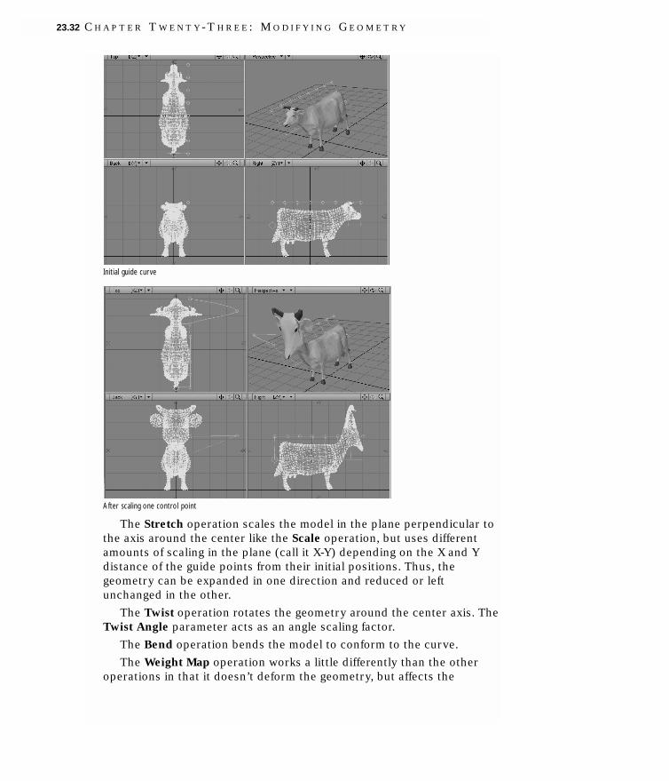
Initial guide curve

After scaling one control point

The Stretch operation scales the model in the plane perpendicular tothe axis around the center like the Scale operation, but uses differentamounts of scaling in the plane (call it X-Y) depending on the X and Ydistance of the guide points from their initial positions. Thus, thegeometry can be expanded in one direction and reduced or leftunchanged in the other.

The Twist operation rotates the geometry around the center axis. TheTwist Angle parameter acts as an angle scaling factor.

The Bend operation bends the model to conform to the curve.

The Weight Map operation works a little differently than the otheroperations in that it doesn’t deform the geometry, but affects the


selected weight map instead. Essentially, it sets the values based on thereshaped curve. Move them closer to the center axis for negativeweights, farther for positive.

Using Weight Map

If you activate Make Curve, a curve polygon will be created from theguide curve when you deselect the tool. Use this to save the guide curveshape. This curve can be placed in a background layer and loaded intothe guide curve by clicking Get Background Curve.

Click Keep Edit to accept the current changes without resetting thecurve. This is useful if you want a certain curve to be applied insubsequent operations.

Changing the Curve Points value will resample the curve into moresegments. Note that resampling the curve can change its shape,particularly if the number is incremented gradually, like with the mini-slider. If you want a more refined curve that accurately matches the oneyou have drawn, enter the new number directly into the field to avoidthe intermediate curves.

OTHER STRETCHING COMMANDS

CenterScaleThe CenterScale command (Construct > Utility: Additional >

CenterScale) will scale objects in the current layers about the object’s

L I G H T W A V E 3 D 7 23.33

implied center by a given Factor. The factor can be specified as a UserCommand argument, in which case, no requester will appear.

CenterStretchThe CenterStretch command (Construct > Utility: Additional >

CenterStretch) will stretch objects in the current layers along one of theaxes about the object’s implied center by a given Factor. The factor andaxis can be specified as a User Command argument (e.g., Y 0.3333), inwhich case no requester will appear.

THE DEFORM GROUP

The Jitter CommandThe Smooth command’s ugly sister is Jitter (Modify > Deform: Jitter).

This command will add a roughness to the polygons of an object byrandomly moving points within a certain radius of their current position.Jitter has several Type settings, each applying the effect in a differentmanner.

Uniform Uniform performs a uniform jitter on every point within arectangular region. A point may be shifted by as much as thevalue specified for the Radius parameter.

Gaussian Gaussian results in a slightly less ragged jitter than theUniform option, performing a normal distribution around thestarting point’s location in an ellipsoid of the given Radius. Apoint may be shifted by as much as the value specified forthe Radius parameter.

Normal Normal uses the local surface normal and randomly movespoints plus or minus within the specified Range along thatsurface normal.

Radial Radial randomly distributes points inward or outward alonga radial vector from a single point defined by the Centercoordinates. Range is the value used to set the range withinwhich a point may move from its current location.


Scaling Scaling is a variation of the Radial option. Points are jitteredoutward from a center point defined by the Centercoordinates. Factor is the value used to set the range, as apercentage, within which a point may move from its currentlocation.

A jitter value of 0 applies no jittering, meaning no change will occur.Values above or below 0 will affect the object.

The Smooth CommandThe Smooth command (Modify > Deform: Smooth) causes Modeler to

try to smooth any jagged surfaces. There are no correct values for thesesettings; however, even relatively low Strength values can overly distortan object. Iterations specifies how many times the smoothing algorithmshould be reapplied.

NOTESmooth is most effective when Iterations is set to a high value.

HINTFor more drastic smoothing, you might use Metaform (Construct >Subdivide: Subdivide) instead; however, this tool increases thenumber of points and polygons.

L I G H T W A V E 3 D 7 23.35

The Quantize CommandThe Quantize command (Modify > Deform: Quantize) will snap points

to specific coordinate spacing intervals (like a grid). This is very usefulfor snapping a non-planar polygon into a specific plane or flattening oneside of an organic or curved object.


cchhaapptteerr24Multiplying Geometry

Chapter 24:Multiplying Geometry

Modeler features some great tools for multiplying your geometry andautomatically creating additional points and polygons. There are tools toadd a bevel, extrude existing geometry, clone polygons, model usingbackground geometry, create mirror images, and more.

MAKE UVS OPTIONThe tools/commands that perform an extruding operation (Extrude,

Lathe, Rail Extrude, etc.) have Make UVs options. You can have the U orV value assigned to a range from 0 to 1. Note that a UV Texture must beselected or this option will be ghosted. (See Chapter 28 for moreinformation.)

THE EXTEND GROUPThis group of tools multiplies geometry by extending it in some

fashion, adding additional geometry along the way.

The Bevel ToolThe Bevel tool (Multiply > Extend: Bevel) is likely one of the most

commonly used modeling functions. Basically, it takes a polygon andextrudes it away from the original along the surface normal. It is similar

L I G H T W A V E 3 D 7 24.1

to using the Extrude tool, but there will be no polygon at the position ofthe original polygon. When applied to multiple polygons, each polygonreceives its own bevel—even on a double-sided polygon.

Dragging your pointer after activating the tool lets you graphicallyplace the bevel. Deactivating Bevel or selecting another tool makes thebevel. Click on an open area of the interface to cancel the bevel before itis made or use Undo.

Dragging up/down lets you interactively change the Shift amount, thedistance that the selected polygon will move along its surface normal.On the numeric panel, positive values make the bevel move in the samedirection as the normal. Negative values make it move the oppositedirection.

Dragging left/right lets you interactively change the Inset amount, thedistance that the edges of the polygon will move in the same plane asthe polygon. On the numeric panel, positive values move inward andnegative values move outward.

Drag at an angle to simultaneously change Shift and Inset. Hold theCTRL key to constrain to Shift or Inset, depending on which direction youdrag initially.

If you select polygon(s), the top polygon will remain selected so youcan perform bevel operations one after another. Click your RMB toaccept the current bevel and begin a new bevel operation. You can alsopress the B key twice to make and start a new bevel.

24.2 C H A P T E R T W E N T Y - F O U R : M U L T I P L Y I N G G E O M E T R Y

You can bevel multiple polygons simultaneously too!

Other Numeric OptionsThe +/- fields on the numeric panel let you set randomization for the

Inset and Shift values. The actual value applied will be varied by arandom number between plus or minus the +/- value. For example, ifInset was 20m and its +/- was 5m, then the actual Inset would bebetween 15 and 25 meters. Generally, you want to use this feature onlywhen beveling many polygons simultaneously.

HINTTo avoid negative random values, make sure the +/- value is always lessthan or equal to the related Inset or Shift value.

Inner is the default Edges setting and bevels the polygon inward andforward along the surface normal. Outer will bevel outward andbackward; however, the original polygon does not move and the newbeveled edges extend away from the surface normal. This optionreverses the mouse movement effects. In most cases, you use Inner.

By default, the surface name of the source polygon is used for thenew geometry. If you select New Surface, you can enter a surface name(even an existing one) in the input field. You can change this settinganytime before accepting the bevel.

L I G H T W A V E 3 D 7 24.3

NOTENote that the selected polygon retains its surface name; only the newedge polygons receive the defined name.

Beveling Tips• After performing a bevel, the selected polygon remains selected. To

accentuate the beveled edge when the surface uses the Smoothingsurface option, perform a quick cut and paste to separate theselected (top) polygon from the added sides. This action precludesLightWave from smoothing over the beveled edge. You may also wantto cut and paste the original polygon (before performing the bevel).Make sure you do not merge points after doing this!

Left: Polygons not separated. Right: Starting and top polygons separated

• If you use the same surface, which uses Smoothing, and the geometrygoes from straight to curved, you may want to separate the polygons(with a cut-and-paste) at the transition point to get a clean edge.

Left: Polygons not separated. Right: Starting (top) polygon separated

• If you want to create an enclosed solid object when beveling a 2Dpolygon, copy it to another layer first and choose Detail > Polygons:Flip. Go back to the original layer and perform the bevel normally.Then, paste the flipped polygon back into the original layer andchoose Construct > Reduce: Merge Polygons to merge points.


• Cut and paste a polygon (like one side of a box) away from its hostand bevel it a very small amount. Then, cut and paste the toppolygon as well. This makes a nice clean edge that catches specularglints.

• When you bevel polygons with sharp edges, you can often run intothe problem of points being too close at the corners—very commonwhen you bevel text characters. One solution is to deleteunnecessary points near the corners prior to beveling. Don’t be tooscared about deleting too many points; the change is usually so slightthat no one will notice, particularly if the text is animated.

NOTESometimes you also need to manually drag points on the new polygonaway from the corner.

L I G H T W A V E 3 D 7 24.5

• Another corner-fixing trick is to bevel out instead of in. This has thebenefit of not requiring you to mess with any points, but it affects thespacing between characters, if you are working with text. For this, usethe Outer setting for Edges in the Bevel numeric panel.

The Extrude ToolUse the Extrude tool (Multiply > Extend: Extrude) to give depth to a

two-dimensional shape. You can extrude any two-dimensional polygon orcurve. The distance and angle from the initial dragging point sets theextrusion length and direction. As you continue to drag your mouse, yousee the extrusion length and angle change accordingly.

The initial dragging point is not significant, only the distance anddirection matter. In fact, when you release the mouse button, the axiswill reposition itself starting at the object. You can further manipulatethe axis by dragging its end in any viewport.

When you are satisfied, simply click Multiply > Extend: Extrude again(or select another tool). To reset, click a non-active part of the interfaceor click Undo.

The numeric panel for Extrude defines the relative XYZ coordinatesfor the end of the axis in the Extent fields. You can change the number ofSides created on the panel, which can be useful for multi-segmenteditems like snakes, or objects you wish to bend or twist.


Extrude Tool numeric panel

The Lathe ToolThe Lathe tool (Multiply > Extend: Lathe) will sweep an object

around an axis. Essentially, Lathe creates a cylindrical object with aprofile of the original form. For example, if you lathe a circular-shapedpolygon, you create a donut. You can sweep any two-dimensional objector curve. The classic use of this tool is to create a vase or cup.

Dragging your mouse in a viewport determines the initial axis. Thelathe axis has a crosshair at its Center (the initial dragging point), whichis used to drag the entire axis around. To change the angle, drag eitherend of the axis. You can also drag out the axis, which gives you morecontrol over the effect, but the length of the axis does not in itselfinfluence the impact of the tool.

When you are satisfied, deselect the tool or select a different one toexecute the edit. To cancel, simply click in an open area on the interfaceor click Undo.

NOTEWith this tool, polygons may end up flipped the wrong way.To correctthem, simply hit the F key.

If you wish to change the number of sides in the lathed object (likethe number of slices in a pie), you can use the LEFT and RIGHT ARROWKEYS.If you’d prefer to lathe less than a full 360 degrees, you can drag thehandles as indicated in the following illustration. (Note: If the twohandles are overlapped, you can still drag to separate them.)

L I G H T W A V E 3 D 7 24.7

Lathe interactive handles

You can also open the Lathe tool’s numeric requester to numericallychange settings. The Start Angle and End Angle fields let you enter thedegree of lathing, Sides sets the number of sides, and Offset will shift theshape along the lathe axis. The Center values define the center ofrotation coordinates.

Lathe Tool numeric panel

HINTTo create a coiled spring: create a disc with, say, a one meter diameter.Select Lathe and place the axis about one meter to one side of thedisc.Then, open the numeric requester and set the End Angle to 720degrees (two full rotations), Sides to 48, and Offset to 2m.

The Rail Bevel ToolRail Bevel (Multiply > Extend: Rail Bevel) is a very fancy beveling

tool that works in a manner similar to the normal Bevel tool. Draggingyour mouse left/right adjusts the new bevel geometry's distance from theoriginal polygon. Dragging up/down adjusts the inset direction (towardsor away from the polygon’s center). The CTRL key constrains the changeto a given degree of freedom—just like the normal Bevel tool.

The difference between Rail Bevel and Bevel is that Rail Bevel uses aprofile from a background layer to generate several bevel operations in asingle step.


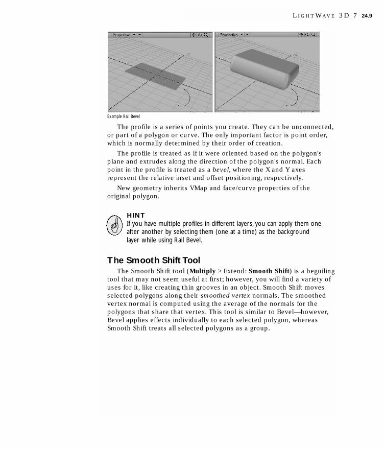
Example Rail Bevel

The profile is a series of points you create. They can be unconnected,or part of a polygon or curve. The only important factor is point order,which is normally determined by their order of creation.

The profile is treated as if it were oriented based on the polygon'splane and extrudes along the direction of the polygon's normal. Eachpoint in the profile is treated as a bevel, where the X and Y axesrepresent the relative inset and offset positioning, respectively.

New geometry inherits VMap and face/curve properties of theoriginal polygon.

HINTIf you have multiple profiles in different layers, you can apply them oneafter another by selecting them (one at a time) as the backgroundlayer while using Rail Bevel.

The Smooth Shift ToolThe Smooth Shift tool (Multiply > Extend: Smooth Shift) is a beguiling

tool that may not seem useful at first; however, you will find a variety ofuses for it, like creating thin grooves in an object. Smooth Shift movesselected polygons along their smoothed vertex normals. The smoothedvertex normal is computed using the average of the normals for thepolygons that share that vertex. This tool is similar to Bevel—however,Bevel applies effects individually to each selected polygon, whereasSmooth Shift treats all selected polygons as a group.

L I G H T W A V E 3 D 7 24.9

Left: Bevel. Right: Smooth Shift

Smooth Shift numeric panel

Polygons on a convex surface tend to expand since the normals attheir vertices point slightly apart, while polygons on a concave surfacetend to shrink. Polygons that are smoothed together stay together sincethey share normals at their shared vertices. Where polygons pull apart,either because their smoothed vertex normals diverge and exceed theMax Smoothing Angle or because some are selected and some are not,the gaps are filled with bands of new polygons.

The Offset is the distance of shifting along the vertex normal. Positivevalues make the shift occur in the same direction as the normal.Negative values make it shift in the opposite direction.

The smoothing method in Smooth Shift requires a cutoff angle. TheMax Smoothing Angle on the numeric panel determines whetherpolygons will be smoothed over. Any two polygons with adjoining edgesat angles greater than this value will be smoothed across.

Dragging your mouse horizontally will change the Offset amount onthe numeric panel.

The Scale setting, accessible from the numeric panel only, expands orshrinks the new geometry around the center of its bounding (box) area.

HINTTo achieve what amounts to a group-bevel,—where the selectedpolygons are treated as one instead of individually—use SmoothShift with an Offset of 0.Then, manually move the polygons (whichwill still be selected).


The Path Extrude CommandThe Path Extrude command (Multiply > Extend: Path Extrude) will

extrude a point, polygon, or object along a motion path. It is nearlyidentical to the Path Clone command, discussed later. The difference isthat Path Extrude forms a continuous skin for the object instead ofmaking individual copies of the object.

When you select the Path Extrude, a file requester asks for a motionfile. Then, a dialog will appear.

Path Extrude dialog

Enter the First and Last frames of the motion path you wish to use(the values default to the entire length of the path). Step indicates howmany segments to clone in terms of frames (a Step value of one willcreate one segment for each frame). So a motion path that takes 30frames with a Step of 1 will have 30 segments. The same motion pathwith a Step of 2 will have 15 segments.

Left: Object motion path in Layout. Right: Flat box extruded along same path

NOTEThe motion path for an item in Layout can be saved by selecting it andthen choosing File > Save > Save Motion File.

If you a UV Texture is currently selected, the Make UVs options areavailable. You can create the UV map perpendicular to the U or V axis.

L I G H T W A V E 3 D 7 24.11

The Rail Extrude CommandThe Rail Extrude command (Multiply > Extend: Rail Extrude) will

extrude a point, polygon, or object along a curved path (single railclone) or multiple paths (multiple rail clone). It is nearly identical to theRail Clone command, discussed later. The difference is that Rail Extrudeforms a continuous skin for the object instead of making individualcopies of the object.

The curve(s) must be in the background layer and the polygons to beextruded in the foreground layer. The orientation and position of theforeground polygons will affect the result. Generally, they should be atthe very beginning of the curve and oriented perpendicular to it—as ifthe curve was a thread you were threading through the polygons.

The direction that the curve faces (which end is considered thebeginning) will have bearing on both the shape and direction of thecloning. The direction affects the direction of the extruding. If you don’tget the results you expect, try flipping the curve’s starting point withDetail > Polygons: Flip. If you are using multiple curves, generally, theyshould run in the same direction.

If you a UV Texture is currently selected, the Make UVs options areavailable. You can create the UV map perpendicular to the U or V axis.

Single Curve

The Rail Extrude: Single dialog will appear when a single curve is inthe background.

Segments Segments is the number of segments in the resultingobject. Select Automatic to distribute a number ofsegments along the rail curve (based on the CurveDivisions setting on the General Options panel)according to the curve’s knot (point) spacing.

Select Uniform Lengths to distribute some number ofsegments (which you specify) evenly along the length ofthe entire curve. No matter what the knot spacing is, thesegments will remain evenly spaced.

Select Uniform Knots to distribute some number ofsegments (which you specify) evenly between the knots


that make up the curve. Whether the knots are closetogether or far apart, there will be the same number ofsegments between each.

Oriented Oriented determines the orientation of the polygontemplate as it follows the curved path. When active, itcauses all segments to angle themselves automatically sothat they are aligned with the rail curve as it turns. Wheninactive, it causes all segments to remain in the sameorientation as the template so that they face exactly thesame way.

A one-rail example

Multiple Curves

The Rail Extrude: Multiple dialog will appear when multiple curvesare in the background. In practice, one curve will act as the main cloningcurve and the other(s) act as shaping curves. The effect of the shapingcurves is determined by the distance from the main curve. However, youmay change the effect by moving the polygons closer or farther awayfrom any of the curves.

Segments Segments is the number of segments in the resultingobject. Select Automatic to distribute a number ofsegments along the rail curve, based on the CurveDivisions setting on the General Options panel. If youalso select Knot, segments are distributed with regard tothe curve’s knot (point) spacing. If you use Length, knotspacing is disregarded.

L I G H T W A V E 3 D 7 24.13

To specify the number of segments, choose Uniform andenter the number in the input field. If Length is alsoactive, the segments will remain evenly spaced no matterwhat the knot spacing is. If you use Knot instead, therewill be the same number of segments between each knot,no matter how close together or far apart they are.

Strength Strength determines how strongly the rails vie forcontrol of the point locations. You will not notice muchof a difference unless you have Scaling (below)deselected. The higher the Strength value, the closer theobject will hug the rails.

Oriented Oriented determines the orientation of the polygontemplate as it follows the curved path. When active, itcauses all segments to angle themselves automatically sothat they are aligned with the rail curve as it turns. Wheninactive, it causes all segments to remain in the sameorientation as the template so that they face exactly thesame way.

Scaling Scaling determines how segments along an axis aresized. If the rails in the background layer spread apartalong any axis or axes, then the segments willautomatically stretch along those axes as well. TurnScaling on to scale segments equally, rather than alongthose specific axes only.

For example, with Scaling off, if you Rail Extrude a polygon along theZ axis using two rails that spread further apart in the X axis, thesegment’s copies will be stretched on the X axis to maintain theirrelationship to the guide rails.

Left: Disc and two curves in background. Right: Result with Scaling off


Turning Scaling on causes this expansion to occur equally on both Xand Y axes.

Result with Scaling on

The Extender CommandThe Extender command (Multiply > Extend: Extender) clones

selected points and creates new geometry connecting the original pointsand the clones. Essentially, Extender is like using Smooth Shift with 0Offset, except with points instead of polygons.

Left: Extender executed on selected points. Right: Cloned points moved away from original positions

The SeaShellToolThe SeaShell tool (Multiply > Extend: SeaShellTool) lets you

interactively make seashell shapes. Essentially, this is like using theLathe with a scaling factor on an object.

L I G H T W A V E 3 D 7 24.15

SeaShell numeric panel

Open the numeric panel to set options. Axis is the perpendicular axisaround which the shell is twisted. # of Loops is the number of times thesource polygon is twisted fully. Sides per Loop is the number ofsegments to use per loop. Shift per Loop controls the vertical shifting ofthe loop. Scale per Loop is the scaling factor achieved after each loop.SeaShell also has automatic UV creation options. Like any tool, you mustdeselect it to make your object.

The Spikey ToolThe Spikey tool (Multiply > Extend: Spikey) subdivides the selected

polygons and moves the center point out in the direction of the surfacenormal giving a spiked appearance. Simply select the tool and drag yourmousepointer in a viewport.


The Spikey tool applied to a basic ball

The Create Skin CommandWith the Create Skin command (Multiply > Extend: Skin), you can

cover a series of polygons or curves with a polygon skin. The shapes donot need to have the same number of points in common. This is alsocalled lofting or loafing (as if covering the slices of a loaf of bread).

The polygons or curves must be selected (or created) in the orderthat you want them connected.

Create Skin works best when you use single-sided polygons for theframework. Double-sided polygons can result in strangely skinnedobjects.

If you skin using polygon curves, the curves will remain in theModeler workspace following the operation. However, they do notbecome part of the resulting skinned object.

Although Create Skin is similar to the Make Spline Patch command(Multiply > Combine: Patches > Make Spline Patch), which uses curves,the difference between the two commands is significant. The Make SplinePatch command tends to follow smooth contours, which maintains arounded surface. Create Skin tends to connect curves with straight-linesegments, which creates less smooth profiles.

L I G H T W A V E 3 D 7 24.17

The Morph Polygons CommandThe Morph Polygons command (Multiply > Extend: Morph) will

create a number of connected intermediate polygons between twoselected polygons or curves that have the same number of points. Theywill have an outer surface, as if you also used the Skin command onthem. Morph Polygons works best when you use it between single-sidedpolygons.

HINTTo get a twist effect, rotate the source or target polygon a little.

If you morph using curves, the curves are treated as straight-edgedpolygons, and will morph in a linear fashion. The curves also remain inthe Modeler workspace following the operation, although they will notbe part of the morphed object.

The Number of Segments field defines the number of morphed stepsyou desire between the two selected polygons.

NOTEAs with the morphing function in Layout, the Morph Polygonscommand is dependent on point order.As such, you should create thesource and target from the same polygon.You will probably need to flipsome polygons after using this command.

THE COMBINE GROUPThis group of tools multiplies geometry by using other geometry as

carving or set-up tools.

The Boolean CommandThe Boolean command (Multiply > Combine: Boolean) is similar in

some respects to the Solid Drill command, discussed later. However,Boolean operations treat objects as solids with volume, instead of hollow3D objects. They will merge, split, carve, and join objects in a variety of


ways. Like the drilling tools, you must have an object in the backgroundlayer. The major distinction of Boolean is that it treats the foregroundobject as a solid mass and thus creates inside surfaces along cut edges.

With Boolean, some portion of the foreground and backgroundobjects must physically overlap in 3D space.

Union Union joins the background layer with the foregroundlayer, taking the solid objects and combining them into asingle object. Interior faces are removed and no newpolygons or surfaces are created; therefore, all surfaceswill retain their original names.To work properly, bothobjects must be closed 3D solids.

Union mode before (left) and after (right)

From the rendering perspective, you could get a similarresult by just pasting both objects into one layer; however,Boolean results in the fewest polygons and smaller objectfiles, which will use fewer system resources and renderfaster. There may be times, however, that due to thecomplexity of objects, Boolean will not produce acceptableresults.

Intersect Intersect takes solid objects and leaves behind whateverportion was common between them. It leaves behind onlythose portions of the background layer and foregroundlayer that were overlapping. (This corresponds to theportion that the Union operation discards.) No newpolygons or surfaces are created; therefore all surfaces willretain their original names. To work properly, both objectsmust be closed 3D solids.

L I G H T W A V E 3 D 7 24.19

Intersect mode before (left) and after (right)

Subtract Subtract removes the background drilling template objectfrom the foreground object, leaving a copy of itselfembedded there. Essentially, it carves the backgroundlayer out of the foreground layer, leaving new insidesurfaces in its wake. New surfaces will take on the namesof surfaces that carved them. To work properly, bothobjects must be closed 3D solids.

Subtract mode before (left) and after (right)

The results of this operation will vary depending whetherthe polygons being drilled consist of single-sided ordouble-sided polygons (see subsequent discussion).

Add Add joins the background layer with the foreground layerso that the overlapping shapes are fully combined as one.You can use combinations of 2D and 3D objects. This isdifferent from simply saving two overlapping objects fromtwo different layers, since the polygons that physicallyoverlap are merged in a form of mutual drill operation. Nonew surfaces are created, although some polygons may besubdivided. Therefore all surfaces will retain their originalnames.


Add mode before (left) and after (right)

The result is similar to just cutting and pasting the tubeobject into the apple layer. The difference is that wheresurface polygons from the two objects intersect they aresliced by each other to form a common edge. All interiorpolygons and surface names are retained.

You can use more than two objects at a time, but it’s often better towork with a pair at a time. The math involved in Boolean operations iscomplex, and using multiple objects in a single operation is quite time-consuming.

To use the Boolean command:1 Place the target object in a layer.

2 Place the other object in another layer and put the object from step 1in the background.

3 Position the object in the foreground as desired. If you plan to use itto cut away parts of the target object, it must align accordingly in 3Dspace.

4 Swap foreground and background layers using the apostrophe key (‘)shortcut.

5 Click Multiply > Combine: Boolean.

6 Select the type of boolean Operation. Click OK.

Single vs. Double-sided PolygonsSingle-sided and double-sided polygons play a unique role in the

Boolean Subtract operation. Imagine that you are a knife blade, slicingthrough a 3D sphere made of single-sided polygons. Every time you cutthrough a polygon layer, you pass from the outside of the sphere to theinside. If you passed through only one polygon, you are now inside the3D sphere. Accordingly, a Boolean knife blade slicing through a one-sidedsphere would leave solid halves.

L I G H T W A V E 3 D 7 24.21

Normal boolean Subtract on two solid objects

Now say there are two spheres made of single-sided polygons, onesphere being smaller than the other, with the smaller one inside theother (normals facing in). You pass through the first polygon—from airto solid—then through a second polygon—from solid back to air. Youwould now be inside a hollow core inside the inner sphere. A Booleanknife slicing through this sphere would leave a hollow core.

Boolean Subtract on (single-sided interior) hollow ball

Now, if our two spheres were double-sided instead, Modeler wouldtreat each sphere as if it were constructed with paper-thin walls (double-sided polygons are just back-to-back polygons). Remember, normally thesphere would be treated as a solid ball. Upon encountering a double-sided polygon, Modeler will think that it has passed through twopolygons. In the paper-thin space between the front-facing and back-facing polygon, the Boolean knife blade sliced through air, then solid,then air again.


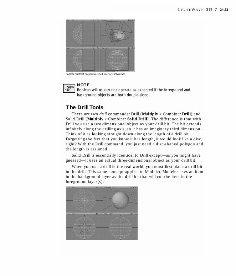
Boolean Subtract on (double-sided interior) hollow ball

NOTEBoolean will usually not operate as expected if the foreground andbackground objects are both double-sided.

The Drill ToolsThere are two drill commands: Drill (Multiply > Combine: Drill) and

Solid Drill (Multiply > Combine: Solid Drill). The difference is that withDrill you use a two-dimensional object as your drill bit. The bit extendsinfinitely along the drilling axis, so it has an imaginary third dimension.Think of it as looking straight down along the length of a drill bit.Forgetting the fact that you know it has length, it would look like a disc,right? With the Drill command, you just need a disc-shaped polygon andthe length is assumed.

Solid Drill is essentially identical to Drill except—as you might haveguessed—it uses an actual three-dimensional object as your drill bit.

When you use a drill in the real world, you must first place a drill bitin the drill. This same concept applies to Modeler. Modeler uses an itemin the background layer as the drill bit that will cut the item in theforeground layer(s).

L I G H T W A V E 3 D 7 24.23

NOTEIf your drill bit is an open curve, Modeler will treat it as a closed curvewith its endpoints joined.

Both drill tools have the same four options:

Core The Core operation will include all polygons that resideinside the 3D space of the drill bit, plus portions of thepolygons that straddle the borders.

Core mode before (left) and after (right)

Tunnel Tunnel is the opposite of Core. It creates a tunnel in yourobject. All polygons that reside outside the 3D space of thedrill bit will be included, plus the trimmed polygons thatstraddle the borders.

Tunnel mode before (left) and after (right)


Stencil The Stencil option stencils the drill bit’s shape onto anyintersecting polygons. It also names all of the polygons thatfall within the bit’s shape. You can either enter a surfacename in the field or select an existing name from the pop-upmenu.

Stencil mode before (left) and after (right)

This option is great for stenciling text or logos ontoobjects—an alternative to using surface color textures. Tohelp draw attention to a stenciled area, you might wish touse the Bevel tool (Multiply > Extend: Bevel) or Smooth Shifttool (Multiply > Extend: Smooth Shift) on the stencil.

Slice Slice is the same as Stencil, except it does not rename anysurfaces.

Slice mode before (left) and after (right)

To drill an object:1 Place the target object in a layer.

2 Place your bit object in another layer and put the target object in thebackground.

3 Position the bit object as desired. Use the viewport whoseperpendicular axis (i.e., the axis you can’t affect) is the one you wantto drill along. For example, if you wanted to drill along the Z axis,position the bit object in the Back type viewport.

L I G H T W A V E 3 D 7 24.25

4 Swap foreground and background layers using the apostrophe key (‘)shortcut.

5 Choose Multiply > Combine: Drill.

6 Select the drilling Axis and the type of drilling Operation. Click OK.

The Solid Drill ToolThe Solid Drill command (Multiply > Combine: Solid Drill) will work

just like the Drill command, but you have control over the effect alongthe drilling axis. There is no Axis option. It is unnecessary since you usea 3D object that has no implied third dimension.

NOTEThe objects in the foreground and background layers must physicallyoverlap for the tool to work properly.They cannot be just lined up onan axis.

NOTEBoth the drill bit and the item to be drilled must be closed solids.Ahemisphere with one open side, or a hollow tube, would not qualify,but a closed hemisphere or a tube with sealed ends would.

Faster and Better Drills and BooleansComplex Drill and Boolean operations require a lot of computing.

Selecting the affected polygons in the foreground layer before usingeither command will greatly speed things up. This lets Modelerconcentrate on only those polygons that need to be affected. Also, ifyour initial result is not satisfactory—particularly with complexobjects—try it again after nudging one of the objects on an axis a little.

Patches MenuThe commands in the Multiply > Combine: Patches menu are covered

in Chapter 29.


THE DUPLICATE GROUPThis group of tools multiplies geometry by replicating existing

geometry.

The Mirror ToolUse the Mirror tool (Multiply > Duplicate: Mirror) to create an exact

mirror image of an item. You can mirror the whole object, selectedpoints, or selected polygons. Many objects you create will besymmetrical in nature. So it often makes sense to build only half of anobject, create a mirror image, and join them together. Other times yourobject may include certain parts that are identical, and an automatedway to duplicate them is very helpful.

This interactive tool works using a mirroring fence. You drag out thefence with your mouse. This forms the main axis for the fence’s length.Once you release the mouse button you can reposition by simplyclicking somewhere off the fence—you are essentially repositioning theinitial drag point. You can rotate the fence using the rotation handles.The swing rotation handle swings the fence like a gate around one end ofthe fence. The axis rotation handle rotates the fence around the axisalong the length of the fence.

If Free Rotation is inactive on the numeric panel, the default setting,you will only be able to draw and rotate the fence across planes alignedwith an axis. If you hold the CTRL key down, you will be able to use 15-degree increments. If Free Rotation is active, you are free to draw androtate the fence at any angle.

Left: Initial drag. Right: Repositioning using perspective viewport

L I G H T W A V E 3 D 7 24.27

Left: Swinging the fence. Right: Rotating around the axis

When you are satisfied, simply click Multiply > Duplicate: Mirroragain (or select another tool). To reset, click a non-active part of theinterface or click Undo.

NOTEIf adjusting the axis rotation handle only resizes the fence, try adjustingthe handle in the perspective view.

The numeric panel defines the XYZ coordinates of the Center point(where the position handle is). The Axis, if any, is the axis perpendicularto the fence. If the Merge Points option is active, any overlapping pointsare merged automatically. Use this if you are mirroring two halves of anobject together.

Mirror numeric panel

Paste ToolThe Paste tool (Multiply > Duplicate: Paste) lets you interactively

paste whatever is in Modeler’s copy buffer (i.e., something youpreviously cut or copied). Once you click in a viewport, you can positionthe geometry by dragging your mouse. Like most tools, drop it or selectanother to make the geometry, or click your RMB to create the geometrywithout dropping the tool.

Using the numeric panel, you can even scale the size of the geometry.


NOTEThe Paste tool has no effect on the actual contents of the copy buffer.

The Array CommandThe Array command (Multiply > Duplicate: Array) duplicates the

selected item any number of times using specific increments of distance.You can create a grid out of this object, like a matrix. (Unfortunately, noone can be told what the matrix is.) The shape of the array can either beRectangular (box-shaped) or Radial (circular). Use the Merge Pointsoption to automatically merge points at the end of the operation.

Array Type: RectangularWhen Rectangular is selected, you will have the following settings

available:

Count Count is the number of repetitions of the original objectalong each of the axes.

Jitter Jitter adds randomization. A distance up to the valueentered is added or subtracted to what the positionwould have otherwise been.

Offset Automatic uses the object’s own dimensions as thespacing value. The Scale fields define a percentage of thedimensions to use. A value of 100 percent in the inputfields will place the objects side by side. Manual lets youenter specific spacing values for each axis.

L I G H T W A V E 3 D 7 24.29

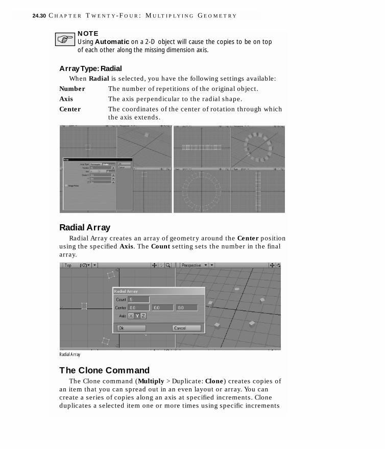
NOTEUsing Automatic on a 2-D object will cause the copies to be on topof each other along the missing dimension axis.

Array Type: RadialWhen Radial is selected, you have the following settings available:

Number The number of repetitions of the original object.

Axis The axis perpendicular to the radial shape.

Center The coordinates of the center of rotation through whichthe axis extends.

Radial ArrayRadial Array creates an array of geometry around the Center position

using the specified Axis. The Count setting sets the number in the finalarray.

Radial Array

The Clone CommandThe Clone command (Multiply > Duplicate: Clone) creates copies of

an item that you can spread out in an even layout or array. You cancreate a series of copies along an axis at specified increments. Cloneduplicates a selected item one or more times using specific increments


of distance, rotation, and scaling. You can create a spiral staircase out ofa single step, or a wood screw out of a triangular polygon outline, forexample.

Immediately after a Clone operation involving a template (i.e., 2D)polygon, you can use the lasso to encircle and select the entire group ofnewly cloned polygons. They are automatically selected in the orderthey were created. This means you can use the Create Skin command(Multiply > Extend: Skin) to place an outer surface around the newframework. After using Create Skin, the framework polygons are nolonger needed (since they are inside the skin and will not renderanyway). They are still selected, so you can delete them (except maybethe two ends), and leave only the skinned object remaining. Thistechnique is useful when you create objects like a wood screw, whereyou no longer need the internal (unseen) polygons after you completethe outer surface.

Left: Clones. Right:After skinning

Enter the number of copies of the selection to create in the Numberof Clones fields.

The Offset fields determine the incremental distance between oneclone and the next along the X, Y, and Z axes. The Scale fields set theamount of incremental scaling for each copy. The Rotation fields set theamount of incremental rotating.

L I G H T W A V E 3 D 7 24.31

NOTEThe effect is progressive, so the change is applied to each clone basedon the previous clone. So, for example, with scaling, the copies will getprogressively larger or smaller.

The Center fields define the coordinates to use as the center point,around which the operation takes place.

HINTIf you plan to clone with rotation, try to build your base object so thatthe rotation can happen around the Origin whenever possible.

HINTTo evenly space objects around an axis, take the number of totalobjects you want to end up with and divide it into 360. (You can evenenter the formula into the input field.) This gives you the incrementalrotation.Then set the Number of Clones to the total objects minusone.

The Path Clone CommandThe Path Clone command (Multiply > Duplicate: Path Clone) works

just like the Path Extrude command, discussed earlier. However, insteadof resulting in an object with a smooth skin, it creates skinless segmentclones along the motion path.

Left: Object motion path in Layout. Right: Flat box cloned along same path


The Rail Clone CommandThe Rail Clone command (Multiply > Duplicate: Rail Clone) works

just like the Rail Extrude command, discussed earlier. However, insteadof resulting in an object with a smooth skin, it creates skinless segmentclones along the background curve(s).

Left: Starting object in foreground and curve in background. Right: Result with Automatic mode

Left: Disc and two curves in background. Right: Result with Scaling on

The Symmetrize CommandThe Symmetrize command (Multiply > Duplicate: Symmetrize) clones

an object n times with a rotation each time so that the result displays n-fold symmetry about the selected Axis.

L I G H T W A V E 3 D 7 24.33

Symmetrize

Point-Clone-PlusThe Point-Clone-Plus command (Multiply > Duplicate: Point-Clone-

Plus+) will clone objects in the foreground to the locations of points inthe background. You can randomize the rotation, scale, and centeringindependently for every axis between two values. Random Size willrandomly change the overall scaling of objects. The XYZ Axis optionsspecify whether the objects should be centered on the points or flush onone side or another. To specify static values, enter the same number inthe Min and Max fields.


This command is great for cloning and placing, say, tree objects on alandscape or putting hair on a head.

L I G H T W A V E 3 D 7 24.35

cchhaapptteerr25Constructing Geometry

Chapter 25:Constructing Geometry

So far, we’ve covered modeling tools that create an object by adding,rearranging and duplicating points/polygons. In this chapter we willcover some basic point and polygon maintenance tools as well as sometime-saving ways to add and remove points and polygons. We’ll alsodiscuss some tools where you can use other objects and curves asmodeling tools.

BASIC POINT AND POLYGON MAINTENANCEThe basic steps to copy and paste points and polygons are essentially

the same. First, you select the points or polygons. Then you either clickthe Copy button (c) to copy the selection into the memory buffer,retaining the original, or click the Cut (X) button to delete the selection.You can also use the DEL key to run the Delete command; it is similar toCut, but does not copy the data to memory for future pasting.

Once something is in the memory buffer, you can click the Pastebutton (V) to paste the contents back into the layer. The memory bufferis not reset after pasting. Thus, you can paste the contents multipletimes. The buffer contents change only when they are replaced by asubsequent cut or copy.

NOTEGeometry cut (or copied) to the memory buffer loses its associationwith geometry it is cut away from, even when it is pasted back in.

NOTEFor interactive pasting, use the Paste tool (Multiply > Duplicate:Paste) discussed in Chapter 24.

L I G H T W A V E 3 D 7 25.1

THE REMOVE POLYGONS COMMANDFrequently, you want to use some of the points of an object (often

primitives) in creating your objects. A good example is using part of adisc’s points to model a rounded corner. The way to do it is to use theRemove Polygons command (Construct > Reduce: Rem Polygons).

To remove polygons but not points:1 Select the target polygons.

2 Choose Construct > Reduce: Rem Polygons or press the K key.

HINTAn easy way to remember this keyboard shortcut is to think of it as“killing” the polygons.

THE REMOVE POINTS COMMANDThe Remove Points command (Construct > Reduce: Rem Points)

disassociates the selected point(s) from the selected polygon, but doesnot delete the point. Non-selected polygons that used that point remainunchanged.

To remove a point from a polygon:1 Select the polygon(s) containing the point to be removed (Polygon

Selection mode).

2 Select the points to be removed (Point Selection mode).

25.2 C H A P T E R T W E N T Y - F I V E : C O N S T R U C T I N G G E O M E T R Y

3 Choose Construct > Reduce: Rem Points. To actually delete thepoints, use the Cut function.

THE MERGE POLYGONS COMMANDConstruct > Reduce: Merge Polygons joins two selected polygons

that share at least one common edge. A common edge is one where twoor more polygons share all of the points along that edge.

The Merge Polygons command also works on curves, if they share acommon terminating point. It doesn’t matter if you use the start or endof the curve. They will be merged into one continuous curve.

Common problems are edges that don’t share all points. Try mergingpoints first, to eliminate overlapping points. After using this command,check for non-planar polygons, which often result.

THE MERGE POINTS COMMANDUse the Merge Points command (Construct > Reduce: Merge Points)

to remove points that occupy the same or very nearly the same space.Remember, if all of the points along a polygon’s edge are shared,LightWave’s surface smoothing can smooth over the two polygons. Manycircumstances exist where you may create unnecessary duplicate points,but here is a list of some common ones:

• After you cut polygons to a separate layer and then paste them back.

• After you use the Mirror tool and drill operations, because thecomplex mathematics involved often generates extra points.

L I G H T W A V E 3 D 7 25.3

Left: Overlapping points cause visible seam. Right:After merging points there is no visible seam or panty line

Merge Points Automatic Range

Merge Points Fixed Range

If the Keep 1-Point Polygons option is disabled, polygons areautomatically deleted if they become single points (due to their verticesmerging together). The default is for these polygons to be retained.

The Merge Points command has two Range modes: Automatic andFixed. These basically determine the criteria for when points should beconsidered mergeable.

Automatic merges the points that share the same space. For objectsor portions of objects that you have cut from the main object with theintention of merging later (back into their original positions) useAutomatic.

Absolute merges any points within the specified Distance of oneanother. When merged, one point will move to the location of another—Merge will not average the distance between points to create a new pointmidway between them. As such, the related polygon may be stretched asnecessary.

HINTTo speed the operation, select the points you wish to merge beforeusing this command. (It’s OK if you select more than you need.)


NOTESee also the Weld command, in Chapter 26.

COLLAPSE POLYGONSThe Collapse Polygons command (Construct > Reduce: Collapse Pols)

replaces selected polygons with a single point at their average position.It is like moving all of the points for the selected polygons to their centerand then merging the points.

Left: Four polygons selected. Right:After using Collapse Polygons

THE UNIFY POLYGONS COMMANDThe Unify Polygons command (Construct > Reduce: Unify Polygons)

converts selected polygons sharing the same points (such as double-sided polygons) into a single polygon. It creates single-sided polygonswith regard to the direction of their surface normals. However, unusualobject shapes can occasionally fool its complex algorithms, resulting insingle-sided polygons facing the incorrect direction. If this happens, youmay need to use the Align Polygons or Flip Polygons commands tocorrect the resulting direction of the normals.

THE QEMLOSS2 FUNCTIONThe qemLOSS2 function (Construct > Reduce: qemLOSS2) uses a

surface simplification algorithm in an attempt to reduce the number ofpolygons in an object. The plug-in lets you rapidly produce good qualityapproximations of excessively detailed polygonal models. qemLOSS2 isan excellent way to create low resolution stand-in objects for scenelayout or for multi-resolution models. You can use the object

L I G H T W A V E 3 D 7 25.5

replacement capability in Layout to substitute a low resolution object inplace of an object with a high polygon count when it is far away from thecamera.

Left: standard 5,502-polygon cow. Right: slim 2,750-polygon version.

This plug-in uses routines adapted from Michael Garland's publicdomain QSlim Simplification Software. The algorithms used in thissoftware are described in the papers written by Michael Garland andPaul S. Heckbert, Surface Simplification Using Quadric Error Metrics,SIGGRAPH 97, and Simplifying Surfaces with Color and Texture usingQuadric Error Metrics, IEEE Visualization 98.

IntroductionMany 3D models contain a large number of polygons, especially

algorithmically created models (such as those created by implicitsurface construction techniques) and models created with 3D scannersand digitizers. Polygon reduction in these types of models is currently avery active research area in computer graphics. Obviously, rendering 3Dscenes is much faster when the models contain a minimum number ofpolygons. Also with the current trend towards sharing 3D worlds overthe Internet using VRML, level of detail models (LOD) are becomingabsolutely necessary for creating worlds in which the user can browseand interact in a reasonable manner.

This plug-in provides polygon reduction on objects within Modeler.Only one parameter, the reduction Goal, must be set by the user, theremaining default values should provide good reduction for manyobjects with a high polygon count. However, to get the best results, theuser must understand some of the basic concepts behind the algorithm.

TerminologyThe simplification algorithm is based on contractions of vertex pairs.

It supports two types of contractions: edge and non-edge contractions. Anedge contraction occurs when the vertex pair shares an edge. This is the


primary type of contraction that occurs during the reduction stage (infact, non-edge contractions are turned off by the default parameters).The following figure shows an example of an edge contraction wherevertex v1 and vertex v2 are joined to form a new vertex v3. Since v1 andv2 share an edge (highlighted below), one or more triangles will alwaysbe removed during this contraction. In this example, two triangles areeliminated from the mesh.

Edge Contraction

Non-edge contractions let the algorithm join unconnected areas of theobject together. The next figure shows an example of a non-edgecontraction (also called aggregation).

Non-edge Contractions

In fact, there are two non-edge contractions taking place: v1 and v2contract to form v5; v3 and v4 contract to form v6. Since by definitionthe vertices in the contraction pairs do not share an edge (there is noedge between v1 and v2, or the v3, v4 pair), there is no actual reductionin the polygon count of the object. However, since this feature joinspreviously unconnected areas of the object together, the potential existsfor future reductions. Many times this can also provide a better lowresolution approximation of an object that has many disconnectedregions.

As the algorithm proceeds through each iteration, an approximationof geometric error accumulates at each vertex of the object. If thisgeometric error is less than the user defined Maximum Error Tolerance,the vertex is marked as a viable candidate for another contraction. Oncethe geometric error for a vertex becomes greater than the maximumthreshold value, it will no longer be considered in any morecontractions. During each iteration, the vertex pair with the smallestcombined geometric error is chosen for the current contraction.

The algorithm proceeds until the simplified object is reduced to theuser's targeted Goal (number of polygons) or until all the vertex errorshave become greater than the Maximum Error Tolerance. These twoparameters control how much reduction will take place, the remainder ofthe parameters control various aspects of the vertex contractions.

L I G H T W A V E 3 D 7 25.7

Two types of vertices receive special consideration by this plug-in:surface border and boundary vertices. Parameters are provided for youto weight the geometric error for these two special types of vertices:

• A surface border vertex is a point that is shared by two or moresurfaces.

• An edge that exists in only one triangle is a boundary edge, anddetermines two endpoints that are called boundary vertices.

The Surface Border Weight and Boundary Preservation Weightparameters let you weigh the geometric error at these points. The higherthe weight, the less likely the vertex will be replaced. Clever use of theseparameters (along with some equally clever surfacing) can provide quitea bit of control over the contraction process. The Polygon AreaWeighting parameter, causes every vertex's geometric error to beweighted by the area of the polygons that contain the vertex. Once againcausing larger values (triangles with larger areas) to be less likely to beremoved.

To help preserve the shape of these shared borders, weighting of thesurface border vertices, using Surface Border Weight, has been addedto the algorithm to help restrict movement/replacement of thosevertices.

WARNINGAlways save your objects before you run qemLOSS2!

Using qemLOSS2Make sure you have an object in the current foreground layer(s) of

Modeler. You also need at least one empty layer, because the existingobject remains unchanged, and the reduced object is placed in the firstavailable empty layer. Choose Construct > Reduce: qemLOSS2 and youare presented with the following panel.


NOTEqemLOSS2 ignores any polygon selections and works only on theentire object in the foreground layer, including any hidden polygons.

Goal lets you set the final number of polygons you would like in thesimplified object. You may enter either a desired polygon count (aninteger such as 1000), or a percent based on the number of polygonsfound in the original object (a real number with a percent sign at theend, such as 65.2%). If you enter a percentage, it will simply calculate thepolygon goal by multiplying that percentage by the total polygon countin the original object. So 100% will mean no reduction takes place, and0% means the object will disappear completely.

The first major step qemLOSS2 takes is to triple your polygons, whichwill increase the polygon count, if your model contains non-triangularpolygons. A Goal of 100%, however, will reduce the number of polygonsback to the original number, but now they will all be triangles. If thatreduction doesn't preserve your model's shape well enough, don'thesitate to try percentages over 100%, those models will still be smallerthan the tripled original.

NOTEOther parameter settings may cause the algorithm to fail to reach thereduction goal.

Maximum Error Tolerance sets the geometric error threshold. Alarge value (such as the default 1,000,000) almost guarantees that youwill achieve the reduction goal in the previous parameter field. Smallervalues may preserve the shape of the original object better, however youmay not achieve the desired reduction goal entered above.

Surface Border Weight gives you some control over how often andfar surface border vertices are relocated during the reduction process. Alarge value restricts the relocation of points that lie along surfaceborders, thereby preserving the shape of the border fairly well. Smallervalues let the points move farther from their original location, possiblycausing the border to change its shape. A value of 0 will not constrainthe surface borders at all, and vertices along a border may not end upwhere you expect when the simplification is finished.

Boundary Preservation Weight allows you some control over howboundary vertices are relocated during the contraction process. A smallvalue lets the boundary points move farther than larger values. A valueof 0 will not constrain the boundary at all, and the object may not look atall like you expect when the simplification is finished.

If you end up with unexpected gaps between non-contiguous polygonsurfaces, you can try to preserve those boundaries by increasing theBoundary Preservation Weight. However, you might get better results

L I G H T W A V E 3 D 7 25.9

by merging the edge points together before running qemLOSS2. You canalways just cut and paste the polygons afterward, if the separation wasessential.

Pair Selection Tolerance determines whether non-edge contractionsare performed during the simplification process. If this value is 0, non-edge contractions are turned off, and only edge contractions will takeplace during the simplification. Any value greater than 0 will cause non-edge contractions to be possible during the reduction. If you enter anegative number, qemLOSS2 will automatically use 5% of the radius ofthe object's bounding sphere. This is the value you should use if youwant to start experimenting with this parameter.

Take care when changing this value to anything but 0! It is stronglyrecommended that you leave this at 0 for all complex models with lots ofpolygons. If you use this, first reduce the model to a fairly small polygoncount with it turned off (=0), then reduce the reduction again with acarefully chosen Pair Selection Tolerance, or better yet, just use anegative number. It is a very memory intensive operation.

Vertex Placement Policy is best left at Optimal. When a pair ofvertices is contracted, the algorithm must decide where to locate thenew vertex. The algorithm can use any one of the three final optionslisted in this selection of buttons. Optimal calculates the new placementbased on the location with the least amount of geometric error. Doesn'thurt to experiment with these options though.

Sometimes vertex pair contractions do not preserve the orientationof the faces in certain areas of the contraction, If Preserve Mesh Qualityis changed to Yes, the normal of each neighboring face is comparedbefore and after the contraction. If the normal flips, the contraction ispenalized greatly by making the geometric error for that contractionvery large (so that contraction will probably never take place). In mostcases, this will not be a problem, and the plug-in will work faster if thisparameter stays set to No. But it's not terribly slow, so it certainlydoesn't hurt to experiment with it.

If you change Polygon Area Weighting to Yes, the area of the trianglecontaining the vertex is used to weight the geometric error. This willcause larger triangles to increase the geometric errors of its vertices, soit is less likely to be chosen for simplification.

The qemLOSS2 function displays a progress monitor while it createsthe reduced object in the first available empty layer. Here is whathappens: first, the object in the foreground layer(s) is copied to the firstavailable empty layer, then all its polygons are converted to trianglesusing Modeler's Triple command. Next, all vertices and polygons areconverted into the necessary data structures needed for thesimplification routines, and the copied object is subsequently removed.Once the simplification routine finishes, the reduced polygon object isplaced in the previously empty layer.


NOTEFor additional information, check out http://amber.rc.arizona.edu/lw.

THE REDUCE-POINTS COMMANDThe Reduce-Points command (Construct > Reduce: Reduce-Points)

traverses polygon edges and removes any points (from the polygons)that form an angle with its adjacent points that is less than the Degreessetting. This plug-in is especially useful to reduce the number of pointsand polygons generated by extruding or beveling text objects. Simplyselect a Point Reduction Threshold Setting and the Degrees will be setautomatically. You can also enter your own Degrees setting. ActivateDelete Points to delete the removed points.

THE REDUCE-POLYGONS COMMANDThe Reduce-Polygons command (Construct > Reduce: Reduce-

Polygons) merges co-planar polygons with three or more vertices into asingle polygon and can optionally remove any stray points resulting fromthe polygon removal. Polygons are merged if the relative angle betweentwo polygons is less than the Polygon Reduction setting, they share anedge, and have the same surface name.

Colinear Point Removal deletes points that are still a vertex of a newpolygon. You may set the level of this removal computation. To delete allpoints that are no longer a vertex of a polygon, check the Delete Pointsbox.

L I G H T W A V E 3 D 7 25.11

ADDING POLYGON POINTSSometimes you will need to add a point to a polygon and then move

the point to change the shape of the polygon. You might also want toadd multiple points so you can manually subdivide a polygon intosmaller polys.

To add a point to a polygon:1 First, select the target polygon. If your selected edge is shared with

another polygon, select that one as well. If you do not, the edge willsplit and the polygons will no longer be joined.

2 Choose Construct > Subdivide: Add Points.

3 Click the black plus sign at your desired insertion point along theedge.

THE KNIFE TOOLThe Knife tool (Construct > Subdivide: Knife) lets you interactively

get results similar to the Drill function’s Slice option; however, it requiresno background object. You simply drag out a slicing line in anyviewport—nothing need be in a background layer. The line is infinitealong the axis perpendicular to the view you initially drag in.

The other viewports will let you see the line from a different angleand a small dotted line will be visible that shows you the direction of theslice. After you have released the mouse button, you can drag the T-handles at the ends of the line (in any viewport) to reposition them ordrag the center of the line to move the entire line. The tip of the dotted


line can also be dragged to change the direction in increments of 90degrees. This is an interactive tool so you will see the new geometryresults as you position the line.

Like most tools, drop it or select another to make the geometry, orclick your RMB to create the geometry without dropping the tool. Clickon an open area of the interface to cancel the operation before it is madeor use Undo.

The Knife tool’s numeric requester indicates the Start and End XYZcoordinates, defining the end points of the line. The Axis settings definea target point, relative to the base of the dotted direction line, that theline goes through.

THE SUBDIVIDE POLYGONS PANELThe Subdivide Polygons panel appears when you choose Construct >

Subdivide: Subdivide. This panel provides several commands that letyou automatically increase the detail of existing polygons. To use thispanel, you must select the target polygons first.

NOTEYou cannot use Subdivide Polygons on polygons with more than foursides.

Randomizing OptionsAll Subdivide options let you enter a Fractal factor that will randomly

jitter newly created points. The result is a subdivided object with itspoints randomly jittered. A factor of 0 will not jitter points and highervalues will jitter points more.

The jitter radius is a fraction of the edge length, times the Fractalfactor. A factor of 1 jitters the new points by at most 50 percent of thelength of the edge that they will subdivide. A factor of 0.1 is five percentjitter and a factor of 2 will move points 100 percent of the edge length.Points added to the center of four-point polygons are jittered acomparable amount, although the formula for them is more complicated.

L I G H T W A V E 3 D 7 25.13

Using Fractal

Faceted SubdivideThe Faceted option adds more segments to existing polygons, but

doesn’t change the overall shape. Let’s say you made a box, but justwanted one side to have multiple segments. In this case you could useFaceted.

Faceted Subdivide

NOTEFaceted Subdivide works on triangles, like after the Triple command isused.

Smooth SubdivideSmooth will subdivide objects that have curved, smoothed, or

rounded areas. Modeler assumes any two polygons are part of a smoothsurface and will extrapolate where subdivided detail should be placed tomaintain (even enhance) the curvature of the original form.

The value entered in the Max Smoothing Angle field is used todetermine whether adjoining polygons should be smoothed or not.Adjacent polygons whose normals form an angle above this value willnot be smoothly subdivided. The default is 89.5 degrees, so polygons atright angles or sharper will not be affected.


Smooth Subdivide

Smooth SubdivideMetaform is another method of subdividing. The object will be

smoothed dramatically, with the original object acting as kind of abounding box template for a slightly smaller, more rounded form.Metaform is very useful for creating smooth organic-looking objects outof simple geometric structures.

Smooth Subdivide

Metaform is an adaptive process, meaning that locations that containgreater detail (i.e., more points/polygons) will have more detail in thesmoothing process. It is easy to create rounded forms with Metaform.Moreover, if you use Metaform on part of an object by selectingpolygons, you can create specific areas of greater detail on an objectwithout subdividing the entire object again and again.

Adjoining polygons with surface normal angles greater than the MaxSmoothing Angle will not be subdivided in a smooth manner. Thedefault angle is 179 degrees, so only polygons that are nearly parallelwith each other are not affected.

Metaform is often used one or more times on a box to create arounded starting point for SubPatch cages. It is superior to using, say, aball primitive, since all polygons are quads.

L I G H T W A V E 3 D 7 25.15

NOTESmooth and Metaform can achieve similar results using the samemaximum smoothing angle; however, Smooth will tend to smoothoutward, and make a slightly larger object. Metaform, on the otherhand, smoothes inward, and make a more compact object.

THE BANDSAW COMMANDBzzzzzzzzzzzzzzzzzzzzz...super knife! BandSaw will slice through a

contiguous band of four-point polygons (or patches). To use theBandsaw, just select a polygon and activate the BandSaw tool (Construct> Subdivide: Bandsaw). (If you select more than one polygon, the firstselected polygon controls the operation.) This tool is tailored for use onSubPatch objects in areas where you need more control points.

Bandsaw

The operation continues all the way around until it hits itself or anon-four-point polygon. The Edge to select option determines thedirection. With a quad, there are only two ways and these are describedas Even or Odd. Select Auto for BandSaw to pick the direction for you.

Single polygon selected


Some results using Bandsaw

By default, there will be a single default slice right in the center. Thisis the positioning of the slice that will be made on the polygons. You canmove it by selecting the Edit mode and dragging it with your mouse. Youcan also add more slices in the Add mode or remove them in the Deletemode.

Uniform equalizes the spacing between slices. Mirror will mirror theselected slice across the center. Reverse inverts the order—handy if youplaced the slice(s) on the wrong side.

To actually perform the slice, you need to activate the Enable divideoption. However, you can also use BandSaw to just select the band ofpolygons by not activating this option.

THE SPLIT POLYGONS COMMANDChoosing Construct > Subdivide: Split will divide a polygon into two

smaller polygons using its existing points. If used on a curve, the curvewill be split into two distinct curves.

Select a polygon and switch to the Point edit mode. Select two pointsthat do not share any edges. Clicking Split will subdivide the polygonalong a line between those two points.

Splitting polygons

THE TRIPLE COMMANDThe Triple command (Construct > Subdivide: Triple) converts the

selected polygon(s) into triangular polygons. For example, a squarepolygon becomes two triangular polygons. Triangles cannot by definitionbecome non-planar; therefore, this tool is useful for objects you wish to

L I G H T W A V E 3 D 7 25.17

animate using bones, or objects that will have displacement maps.Tripling non-planar polygons makes them planar. Note that tripling doesnot change the general shape of the object/polygons. Also, once apolygon is a triangle, tripling it again has no effect.

Before (left) and after (right) tripling polygons

HINTTo select only non-planar polygons, use the Polygon Statistics panel(Modeler > Windows > Statistics).

NOTEAlso see the Fast-Triple-Fan and Fast-Triple-Traverse commandsdiscussed later.

THE JULIENNE COMMANDThe Julienne command (Construct > Subdivide: Julienne) slices an

object into sections that are regularly spaced along a given axis. Julienneis very useful for subdividing objects that will be bent or used with adisplacement map.


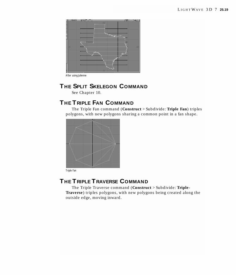
After using Julienne

THE SPLIT SKELEGON COMMANDSee Chapter 10.

THE TRIPLE FAN COMMANDThe Triple Fan command (Construct > Subdivide: Triple Fan) triples

polygons, with new polygons sharing a common point in a fan shape.

Triple Fan

THE TRIPLE TRAVERSE COMMANDThe Triple Traverse command (Construct > Subdivide: Triple-

Traverse) triples polygons, with new polygons being created along theoutside edge, moving inward.

L I G H T W A V E 3 D 7 25.19

Triple Traverse

SUBPATCHESSee Chapter 29.

THE FREEZE COMMANDThe Freeze command (Construct > Convert: Freeze) is used to

convert curves (see Chapter 22), SubPatch objects (see Chapter 29) andMeta-primitives (see Chapter 29) into polygons.

MAKE... COMMANDSThe Make... commands in the Construct > Convert: menu group are

used to create skelegons (see Chapter 10) and Meta-primitives (seeChapter 29) from normal geometry.

THE TOGGLE METAMESH COMMANDThis command toggles the display of Meta-primitives on/off. See

Chapter 29.

JUDGING DISTANCE AND ANGLESYou will often need to estimate distances and angles in the modeling

process. The grid size can yield reasonably accurate figures, but if thetwo points are not aligned somewhat vertically or horizontally,estimating can be more difficult.

Fortunately, Modeler provides what is best described as a virtual tapemeasure. With it, you can measure the distance between any two pointsin any view.

To use the Measure tool:Choose Construct > Utility: Measure > Measure Tool and then drag

between the two positions you want to measure between. Theinformation display in the bottom left corner will tell you the exactdistance. You can reposition either end by dragging it. To reset, click in anon-active part of the interface.


Measuring distance between horns

In a similar manner you can also measure angles.

To use the Angle Tool:1 Choose Construct > Utility: Measure > Angle Tool.

2 Place your pointer at the vertex of the angle you wish to measure anddrag the LMB out to form one side of the angle. A line will extendfrom the drag point.

3 Release the mouse button. You can reposition the end of the line bydragging it; however, you cannot move the starting position at thispoint.

4 Place your mouse pointer near the starting point (but not on top of it)and drag out the other side of the angle. The information display willnow tell you the angle between the two lines.

Measuring horn angle

5 Once you release the mouse button, you can reposition the vertex oreither end by dragging them. To reset, click in a non-active part of theinterface.

NOTEIf you place your mouse pointer on top of the starting point in step 4,the starting point will become the other end to the angle and you willdrag out the vertex.

Both of these tools can be used in any viewport to measure any anglein 3D space.

The BoundingBox CommandThe BoundingBox command (Construct > Utility: Measure >

BoundingBox) displays size and center-position information forforeground layers. Clicking OK will replace the layer(s) with acorresponding bounding box. Use this command to create stand-ins forcomplex objects, which can be replaced for the final rendered animation.

L I G H T W A V E 3 D 7 25.21

BoundingBox dialog

The PointCenter CommandThe PointCenter command (Construct > Utility: Measure >

PointCenter) will display a requester that gives you the XYZ coordinatesof the center of the object in the foreground.

PointCenter dialog

LSCRIPTTo learn how to create and edit LScripts, see the documentation

included on the CD. They are treated as plug-ins and can be installed inthe same manner plug-ins are. You can run them just like any other plug-in command.

ADDITIONALPlug-in and LScript commands that do not have a default menu

location will appear in the catchall Construct > Utility: Additional pop-up menu.


cchhaapptteerr26Detailing Geometry

Chapter 26:Detailing Geometry

The Detail menu contains a variety of commands. Many are coveredelsewhere in the manual.

THE PIVOT POINT TOOLGenerally, the pivot point is the positional focal point of the layer’s

geometry when animated in Layout. By default, it is located at the Origin.Use the Pivot Point tool (Detail > Layers: Pivot) to move the pivot point.(See Chapter 7 for more information.)

LAYER SETTINGSChoose Detail > Layers: Layer Settings to bring up a dialog to set the

current layer name and parent. (See Chapter 20 for more information.)

Layer Settings

FLATTEN LAYERSChoose Detail > Layers: Flatten Layers to flatten multiple foreground

layers into a single layer in one step.

CHANGE SURFACEChoose Detail > Polygons: Surface to bring up the Change Surface

dialog to set the surface name and basic attributes for the selectedpolygons. (See Chapter 31 for more information.)

L I G H T W A V E 3 D 7 26.1

Change Surface dialog

FLIP POLYGONSOften as you create polygons or use various tools with single-sided

polygons, their surface normals will point in the wrong direction.Modeler provides some tools to help you change their direction.

To flip polygons:Simply select the polygon(s) and choose Detail > Polygons: Flip. This

action reverses the direction of the surface normal for the selectedpolygons.

NOTEPolygons facing the wrong direction is a common problem and one youshould get in the habit of checking for regularly.

This command also reverses the direction of selected curves.

SPIN QUADSThe Spin Quads command (Detail > Polygons: Spin Quads) can be

applied to adjacent four-point polygons (i.e., quads) that share an edge.It merges the two polygons together and then splits them using adifferent set of opposing polygons. If you apply Spin Quads three times,you’ll be right back where you started.

26.2 C H A P T E R T W E N T Y - S I X : D E T A I L I N G G E O M E T R Y

Applying Spin Quads three times to a pair of polygons

So what good is this? Well, it can be quite handy fixing areas on aSubPatch object where a seam just doesn’t look right.

ALIGNING POLYGONSModeler has another command called Align Polygons (Detail >

Polygons: Align) that attempts to automatically make all polygons facethe correct direction. After using, you may still need to use the FlipPolygons command (Detail > Polygons: Flip) before you are done.

L I G H T W A V E 3 D 7 26.3

To align polygons:1 Select an area that includes the polygons needing to be flipped, as

well as a large number of polygons facing the correct direction.Selecting polygons that share points and edges helps.

2 Choose Detail > Polygons: Align. Verify that the polygons wereflipped as desired. By its very nature, this command sometimesrequires some trial and error.

MAKE 2 SIDEDSometimes you’ll actually want double-sided polygons, like when you

need to go inside a hollow object. Most of the time, you can get awaywith simply using the Double-sided surface attribute on the Basic tab ofthe Surface Editor. However, if you need to actually model the double-sided polygons, it is pretty simple. Just choose Detail > Polygons: Make-2 Sided.

It is also possible to make double-sided polygons manually using thefollowing procedure:

1 Select the target polygons (even if it is the entire object).

2 Copy (C) the selection.

3 Paste (v) the selection.

4 Choose Detail > Polygons: Flip to flip the (still) selected polygons.


5 Choose Construct > Reduce: Merge Points to merge points.

CHANGE SKETCH COLORWhen using the Sketch mode Rendering Style in a viewport (see

Chapter 27), you can change the polygon shading color by choosingDetail > Polygons: Sketch Color.

SET VALUEThe Set Value command (Detail > Points: Set Value) sets the X, Y, or Z

position values for the selected points or polygons. This is a great toolfor aligning all of the points along a strict axis. You may find a need forthis when you are trying to merge to halves of a mirrored object togetherand are having trouble merging all points along the mirroring axis.

Before using Set Value

After using Set Value

WELDING COMMANDSThe Weld command (Detail > Points: Weld) is similar to the Merge

Points command (see Chapter 25) except the selected points are weldedto the last point selected.

L I G H T W A V E 3 D 7 26.5

Welding one end of a cylinder to a single point

The Weld Points To Average command (Detail > Points: WeldAverage) is similar, but averages the distance between points beforewelding.

Unwelding PointsThe Unweld command (Detail > Points: Unweld) lets you create

multiple copies of the selected points so that none are shared by twopolygons at once—effectively reversing an executed Weld command.

CURVE COMMANDSCurves and their special editing tools are discussed in Chapter 22.

SKELEGON AND METABALL COMMANDSSkelegon commands are discussed in Chapter 10. Metaballs are

discussed in Chapter 29.


cchhaapptteerr27Display Menu

Chapter 27:Display Menu

The Display menu contains functions to help you in adjustingviewports, selecting geometry, and changing visibility options.

VIEWPORTS MENU GROUPThe following options help you change and configure your viewports.

ZoomingModeler provides many ways to zoom around your viewports. You’re

gonna zoom, zoom, zooma zoom. First, you can adjust viewportmagnification by pressing the period key (.) to zoom in or the commakey (,) to zoom out. (These are shortcuts for Display > Viewports: ZoomIn / Zoom Out.) Holding the SHIFT key while pressing either key (i.e., the> and < keys) will double the zoom amount.

Another way to adjust magnification is to use the Zoom tool (Display> Viewports: Zoom). You can drag out a rectangular box using the mouseand the view will automatically zoom in so the rectangular box fills theview window.

The Magnify tool (Display > Viewports: Magnify) provides yetanother way to interactively zoom in and out. This feature lets yousmoothly zoom in or out on your pointer position by dragging yourmouse left and right.

If you have the titlebars visible, you can drag the zoom drag buttonto zoom.

OpenGL Display ClippingIn some cases, if you zoom in too far, OpenGL will clip out points and

polygons—essentially causing them to disappear. Unfortunately, this is afeature of OpenGL. (Actually, anything that is not in the exact center ofthe viewport gets clipped. If you center your viewport on an item, itcontinues to be visible.)

L I G H T W A V E 3 D 7 27.1

PanningEach viewport is a window to a larger world. You can pan the

viewport beneath your mouse by using the ARROW keys—one grid squarefor each press. Holding the SHIFT key will move the view four gridsquares. Holding the ALT key will nudge by one-tenth of a grid square orthe (Fixed) Snap Value amount on the Units tab of the Display Optionspanel (Display > Viewports: View Options), if that option is active. ALT +SHIFT will nudge ten times this amount. (It may help you to think of thisas moving a window around as opposed to moving the object.)

You may also pan a viewport by holding the ALT key down anddragging a viewport. (This feature is also activated with the Pan tool(Display > Viewports: Pan).) If you have the titlebars visible, you candrag the move drag button to pan.

Automatic Pan and ZoomCertain commands will automatically fit objects into the viewport. To

fit the object in all viewports, use the A key, a shortcut for Display >Viewports: Fit All. You’ll often want to use this to center-up an objectwhen it is first loaded.

Before and after using Fit All

Press SHIFT + A (or choose Display > Viewports: Fit Selected) to fitonly the selected parts of an object into all viewports.

Before and after using Fit Selected

27.2 C H A P T E R T W E N T Y - S E V E N : D I S P L A Y M E N U

The Fit One View command (CTRL + A) will fit the object in theviewport under the mouse pointer into that viewport.

After using Fit One View. Mousepointer in Back viewport

Pressing the G key will center your view around the mouse pointer.This is a very quick way to maneuver around. Remember this shortcut!

NOTEOther viewports will also change to stay in sync with the window youare changing (unless they are Center/Zoom independent, discussedlater).

VIEW OPTIONSModeler’s interface is highly configurable, so you can set things up to

be most efficient for different users or different uses. You can change thearrangement of viewports as well as change the display characteristicsfor each viewport independently. Choose Display > Viewports: ViewOptions to bring up the Display Options panel.

Display Options Panel, Layout TabLayout options control the global arrangement of the viewports, the

number of viewports and some other global display settings. Use thePresets pop-up menu to quickly set common layout configurations(Quad is the default setting). Selecting a Preset will affect the Layoutsetting, as well as settings on the Viewports tab.

L I G H T W A V E 3 D 7 27.3

Display Options Presets

If you want to set up your own custom layout, make a selection fromthe Layout pop-up menu. The icon to the left of the description will giveyou an idea of how the viewports will be arranged. Later, you will seethat you have total control over what is in each viewport. In fact, eachLayout option will remember the Viewport settings as they were the lasttime that Layout option was used.

Texture ResolutionThe Texture Resolution setting determines the resolution to use for

displaying textures in viewports that have their Rendering Style set toTexture. Higher settings increase the detail of image textures displayedin viewports, but increase memory usage and display refreshing time.

Perspective AmountThe amount of perspective in the perspective view can be varied by

changing the Perspective Amount slider on the Layout tab. You can gofrom a very wide-angle to a flat nearly orthogonal view. The setting isglobal and affects all the perspective views the same way.

Adjusting Perspective Amount


Background ColorUse the Background Color selector to change the color that appears

in the background for viewports using a shaded display. (See Chapter 3for information on using color selectors.)

Show OptionsThe various Show visibility options let you independently set what

you want to see globally in your viewports.

Points Points appear as small dots.

Surfaces Surfaces are the polygon (or SubPatch) surfaces.

Cages A cage is the outline that connects all of the controlpoints when you edit a SubPatch object.

L I G H T W A V E 3 D 7 27.5

Point SelectionPoints appear highlighted when this option is active, ifyou select points.

Guides Guides are the dotted-lines that extend from the surface(patch vertex) to the control points on the cage (ifvisible) when you edit a SubPatch object.

Normals Normals are dotted lines that extend perpendicularlyfrom selected (planar) polygons.


Grid The grid is the background reference grid.

Polygon Selection Polygons appear highlighted when this option isactive, if you select polygons.

Normals are off here

Backdrop A Backdrop is an image loaded for viewports on theBackdrop tab.

NOTEThese visibility options can be overridden independently for eachviewport on the Viewports tab.

L I G H T W A V E 3 D 7 27.7

Display Options Panel,Viewports TabViewport options let you change how objects are displayed in each

viewport. To change the settings for a viewport, first select it using theViewport buttons. For a quad layout, the viewports are top-left (TL), top-right (TR), bottom-left (BL), and bottom-right (BR).

Use the Presets pop-up menu to quickly set the options on this tabfor the selected viewport region. The selections are listed by view types,but will affect all of the settings on this tab.

Presets pop-up menu

The View Type pop-up menu determines the editing axes you want touse for the selected region. For the orthogonal settings, the namesgenerally indicate the viewing perspective. Back (XY), for example, letsyou edit along the X and Y axes. This means you are looking along the Zaxis. Since it is called Back, that means your perspective is from the back(i.e., negative side) of the Z axis, looking toward the positive side. UVTexture is an entirely different animal (that is, not a cow). (See Chapter28 for information on UV Texture maps.)

View Type pop-up menu


Left to right:Top, Bottom, Back and Front

Left to right: Right, Left and Perspective

There are four Display (group) commands assigned by default tocertain keyboard shortcuts which affect the viewport beneath yourmousepointer. SHIFT+F1 toggles the view between Back and Front,SHIFT+F2 toggles between Top and Bottom, SHIFT+F3 toggles betweenRight and Left, and SHIFT+F4 toggles between Perspective and UV.

PerspectiveYou may edit in a Perspective viewport, just as you would in any

other, but you may also rotate your view perspective. This is Modeler’svirtual trackball, which enables you to rotate the object without affectingits orientation in the other three edit windows. It effectively providesyou with three axes of rotation. While holding down the ALT key, you canperform these actions:

• Rotate around the X axis (pitch) by dragging up or down directlyacross the circle.

• Rotate around the Y axis (heading) by dragging left or right directlyacross the circle.

• Rotate around the Z axis (bank) by dragging to the left or rightaround the perimeter of the circle.

If the titlebars are visible, you can drag the rotate drag button withyour LMB to rotate. If you use the RMB, the viewport will rotate aroundits perpendicular axis. Holding the CTRL key (or using your MMB) willcause rotations to snap to 15-degree increments.

HINTImagine you are manipulating an imaginary ball with your mouse whenyou manipulate the Preview window.

L I G H T W A V E 3 D 7 27.9

Rendering StyleThe Rendering Style pop-up menu determines the style of display

you want to use for the selected region.

Rendering Style menu

Wireframe Although the Wireframe is arguably the most limiteddisplay mode, it is the most commonly usedRendering Style because of its ease in viewing,selecting, and unselecting points and polygons.

Color Wireframe This is nearly the same as Wireframe, except thepolygon edges are drawn using their Sketch color(Detail > Polygons: Sketch Color).

Sketch Sketch shows an object in a combined wireframe andflat-shaded view. All polygon edges are drawn, butfaces are also visible. This mode does not accountfor surface settings, however. The polygon edges are


always drawn in white and faces are gray.Background layers are visible.

You can change the polygon shading color in thismode by choosing Detail > Polygons: Sketch Color.

Wireframe Shade Wireframe Shade is a smooth-shaded mode thatoverlays the wireframe lines.

Flat Shade In Flat Shade mode, the object is shown as a flat-shaded solid. This mode supports some surfacesettings, but not smoothing.

Smooth Shade Smooth Shade is a smooth-shaded mode thatsupports some surface settings, such as Color,Diffusion, Specularity, Glossiness, Smoothing, andDouble-sided.

Weight Shade Weight Shade provides visual feedback for editingweight maps (see Chapter 28).

L I G H T W A V E 3 D 7 27.11

Texture Texture is similar to Smooth Shade, but it alsoshows images mapped to surfaces.

Upright RotationThe Upright Rotation pop-up menu lets you rotate a viewport

clockwise by 0, 90, 180, and 270 degrees.

Titlebar ShortcutsYou can change the View Type and Rendering Style of a viewport

without going to the Display Options panel by using the pop-up menuson the titlebar. The left-most pop-up shows the current View Type,clicking it allows you to choose another. The pop-up menu just to itsright—it has only a down arrowhead—lets you choose anotherRendering Style.

View Type and Rendering Style pop-up menus

Note that if you have UV Texture selected as the View Type, theRendering Style pop-up menu will instead list all loaded images. Selectone to load it into the backdrop of that viewport.

List of loaded images on pop-up menu when using UV Texture view

Independent OptionsThe Independent options let you make certain viewport

characteristics independent from other viewports. Changes to theselected characteristic do not affect that characteristic in otherviewports and vice versa. For example, if a viewport uses IndependentZoom, zooming in it does not affect the zoom of other viewports. Youmust have your pointer over the viewport to affect an independent


viewport. Independent Rotation is only applicable to perspective views.Normally, it is enabled. If you have multiple perspective views with thisoption disabled, they will move in unison when you rotate a view.

Independent options

Independent VisibilityThe lower portion of the panel contains the independent visibility

options. You can individually select which visibility options areindependent. To use them, you must also activate the IndependentVisibility option. This option lets you quickly enable/disable this featurewithout losing the state of each setting.

Independent visibility options

Display Options Panel, Backdrop TabOn the Backdrop tab, you can add full-color backdrop images that act

as reference guides when you build objects. They let you model muchlike tracing a picture using tracing paper. To use backdrops, select theViewport and the desired image from the Image pop-up menu.

L I G H T W A V E 3 D 7 27.13

Display Options Panel, Backdrop Tab

Backdrops added to orthogonal viewports

NOTEIf you are using a UV Texture viewport, you can choose a backdropusing any loaded image from what is normally the Rendering Style pop-up menu on the viewport’s titlebar.

From the Presets pop-up menu, you can save the settings for theselected Viewport to a file by choosing Save Current Backdrop. You canload this file later using Load Backdrop for any selected Viewport. Youcan also save the settings for all viewports by choosing Save AllBackdrops. When this file is loaded later—using Load Backdrop—, theindividual viewport settings are restored.


Saving and loading backdrops

NOTEThe backdrop images for the current default layout for each viewconfiguration are cached as long as possible.Also, backdrops are notsaved in config files or view presets.

You can also adjust Brightness and Contrast. You can invert thecolors by activating the Invert option. If you want to blend pixels forcloseup work, activate the Pixel Blend option. Image Resolutiondetermines the accuracy of the displayed image.

Aspect and Video imagesThe two Center and Size input fields are horizontal (top field) and

vertical (lower field). Clicking Automatic Size will enter values that fitthe defined image into an implied bounding box that surrounds visiblegeometry.

Backdrop Center and Size fields

If you activate the Fixed Aspect Ratio option, you can enter a frameaspect ratio in the input field. Then, you need only specify a horizontalsize—the vertical size is computed automatically.

If your images originated from video, you need to account for thepixel aspect ratio, since video pixels are not square like computer pixels.For example, a D1 NTSC image is 720 x 486 pixels; however, the frameaspect ratio is not 1.48 (720/486) as you might expect. The width of a D1NTSC pixel is 90 percent of the width, that is, a pixel aspect ratio of .9. Assuch, the true frame aspect ratio is 1.333 (720/486*.9).

NOTEThe frame aspect ratio of a D1 PAL image is also 1.333(720/576*1.067).

L I G H T W A V E 3 D 7 27.15

If you do not account for this difference, your models may appearslightly stretched when ultimately viewed on videotape. A way to fix thisis to scale the object after the fact.

Display Options Panel, Interface Tab

Display Options Panel, Interface Tab

The Alert Level affects how error, warning and informationalmessages are displayed. (See also Chapter 6.)

The Toolbar Position setting determines if the main toolbar appearson the Left or Right side. Activate Hide Toolbar to make it hidden andmaximize your screen real estate. You can also choose Modeler >Interface > Hide Toolbar On/Off to toggle this setting.

The Viewport Titles option turns the titlebars, which appear aboveeach viewport, on or off.

Viewport titlebars

Use the Input Device buttons to select the type of input device youare using.

The Fine Detail Cursor option, when active, makes yourmousepointer use the main crosshair pointer at all times instead ofchanging when the various tools and selection functions are used.

The File Dialog and Color Picker pop-up menus let you use customLightWave dialogs for file loading/saving and picking colors. (SeeChapter 3 for more information.) Selecting Default will use your standardsystem dialogs. The custom dialogs provide many additional features notavailable with the standard system dialogs.


The Color Format setting determines the scale used where the colorselector appears. Integer uses values 000 to 255, Float uses .00 to 1.00and Percentage uses 0% to 100%.

Example color selection setting

The Simple Wireframe Edges option turns off polygon offsetting forthe sketch-like display modes. This may fix display problems on somevideocards. The Simple Wireframe Points setting uses OpenGL's ownpoints for wireframe points and selected points at a user-specified size.These points can draw much faster than the standard points.

Simple Wireframe Edges and Simple Wireframe Points options

Display Options Panel, Units Tab

Display Options Panel, Units Tab

The Unit System determines the units of measurement that are usedand displayed by the Modeler screen.

SI SI is the International System of Units (SI is the abbreviation ofthe French “Le Système International d’Unites.”) Unitmeasurements in Modeler will now use a base system of meters.Grid sizes and distances can be measured in megameters,kilometers, meters, millimeters, micrometers, and nanometers.

Metric The Metric System is the same as SI with the addition ofcentimeters.

English The English System uses miles, feet, and inches.

NOTEWe recommend you use the SI or Metric systems to model objects,since a system based on 10 is often much easier to use for purposessuch as applying textures and adjusting object movement.

L I G H T W A V E 3 D 7 27.17

If you input a value that uses a different unit of measurement thanthat the default, LightWave will convert it on the fly. For example, youmay be using meters, but typing in “5 ft” will convert to “1.524 m.”

Default UnitUse the Default Unit pop-up menu to set an assumed measure when

none is given for distance values.

NOTEIf you use a metric Unit System, you should set the Default Unit tometers.

For information on units of measurement, please see the Appendix.

Grid UnitsGrid Units affects the zoom step amount but has no effect on the

actual size of the object. You will likely find that 1 2.5 5 and 1 2 5 areyour most commonly used grid unit settings.

1 The grid resizes in values that begin with 1, as in 10m, 1m,100mm, 10mm, etc.

1 5 The grid resizes in values that begin with 1 or 5, as in 1m,500mm, 100mm, 50mm, 10mm, etc.

1 2.5 5 The grid resizes in values that begin with 1, 25, or 5, as in 1m,500mm, 250mm, 100mm, 50mm, etc.

1 2 5 The grid resizes in values that begin with 1, 2, or 5, as in 1m,500mm, 200mm, 100mm, 50mm, etc.

1 2 The grid resizes in values that begin with 1 or 2, as in 1m,200mm, 100mm, 20mm, 10mm, etc.

Grid SnapThe Grid Snap setting forces point creation and item movement to be

limited to a specific increment.

None None deactivates grid snap, so that items move freely and arenot constrained by any grid intersections.

Standard Standard sets the grid snap to one-tenth of the current gridsize.

Fine Fine makes the grid snap as small as possible for the currentzoom level. This will be typically two- to five-times smallerthan using Standard.

Fixed Fixed lets you specify the increment of movement in the SnapValue input field. The grid will resize itself to use the value youspecify. This also fixes the grid’s graticule on screen to bedisplayed at that increment.


Time FormatThe Time Format setting allows you to set the display format for time

values, like the Frame Slider Label option on Layout’s General Optionstab of the Preferences panel. If the Hub is active, Layout and Modelersettings will be kept in sync.

PRESETTING VIEWSAs you work with Modeler you will no doubt find that you use the

viewports in particular view configurations. Luckily, you can customizeModeler’s display to fit your work habits by assigning workspace viewsettings to the keys on your numeric keypad.

To assign views to keys:1 Turn on your NUMLOCK key.

2 Hold the CTRL key and press one of the numbers 1 through 9 on thenumeric keypad.

Whole Window options

Single Pane options

You can choose to save either the parameters for a Single Pane (theviewport beneath your mouse pointer when you activated the function)or the Whole Window (all viewports). The available options differdepending on whether you select Single Pane or Whole Window. Theoptions relate to the corresponding settings on the Display Optionspanel. (Note: Mapping Type (Single Pane mode) is called View Type onthe Display Options panel.)

Keys set using Single Pane will apply those changes to the viewportunder your mouse pointer. If your mouse is not over a viewport, allviewports are affected.

If you name your assignment and select Single Pane, the nameappears in the Presets pop-up menu on the Viewport tab of the DisplayOptions panel, discussed previously. If you select Whole Window, thename appears on the Presets pop-up menu on the Layout tab.

L I G H T W A V E 3 D 7 27.19

Full-screen Toggle FeatureBy default the NUMKEY 0 key toggles the viewport under your mouse

pointer between full screen and the current viewport settings.

SELECTION MENU GROUPThe following options help you with selection and other related tasks.

Point InformationSelect one or more points and choose Display > Selection: Info to

bring up the Point Info panel. From here you can get detailed informationon individual points and even edit the data on a point-by-point basis.

Point Info panel

Displayed is the number of polygons the points is associated with,and its XYZ position. If the point has any vertex maps, those are listed aswell. To help you locate the related points, point numbers will becomevisible in your viewports corresponding to entries in the list.

You can change any of the selected point(s) settings, including vertexmap data, using the settings at the bottom of the panel. For Vertex Color,you can simply set the new color and Alpha percentage. For Weightmaps, adjust the weighting percentage. For UV Textures, you must enterthe specific U and V values. For Morph maps, you must enter the amountof XYZ position offset.


To change what type of data is being edited for the selected entries,use the Edit Value pop-up menu. Alternatively, you can select the type ofdata with your mouse in the list.

You can have multiple selections, which will show “(mixed)” when thesettings differ for the selected points. Changing settings will affect allselected points.

The OK button will accept any changes and close the panel. ClickCancel to forget any changes (even though they are reflected in yourviewports) and close the panel. Deselect will unselect any pointsselected on the panel and remove them from the list. Edit All will selectall entries. (You can also select and unselect entries with your mouse.)Open All will uncollapse all of the entries and show their details. CloseAll does the opposite.

Point numbers visible for selected polygons

L I G H T W A V E 3 D 7 27.21

Polygon InformationSelect one or more polygons and choose Display > Selection: Info to

bring up the Polygon Info panel. From here you can get specificinformation about each selected polygon and even edit the data.

Polygon Information panel

Displayed for each polygon is the type of polygon (e.g., Face,Skelegon, SubPatch, Metaball, etc.), number of points, the flatnesspercentage (see Chapter 21, “Non-planar Polygons”), surface name, partname, and sketch color (see Chapter 26). To help you locate the relatedpolygon, polygon numbers will become visible in your viewportscorresponding to entries in the list.

You can change the surface name, part name and sketch color for theselected polygon(s) using the settings at the bottom of the panel. Youcan have multiple selections, which will show “(mixed)” when thesettings differ for the selected polygons. Changing settings will affect allselected polygons.

The OK button will accept any changes and close the panel. ClickCancel to forget any changes (even though they are reflected in yourviewports) and close the panel. Deselect will unselect any polygonsselected on the panel and remove them from the list. Edit All will selectall entries. (You can also select and unselect entries with your mouse.)Open All will uncollapse all of the entries and show their details. CloseAll does the opposite.


Polygon numbers visible for selected polygons

Expanding and Shrinking SelectionThe Select Connected command (Display > Selection: Sel Connect)

automatically selects all points or polygons that are connected to thecurrently highlighted points or polygons. This is a powerful tool and oneyou should add to your memory banks. An object that is surrounded byothers may not be easily selected using a volume, and may have severalsurface names (making name selection tedious).

NOTEPolygons that have overlapping points, but don’t share any of thosepoints, will not be affected. Use the Merge Points command(Construct > Reduce: Merge Points) to make the edge shared.

The Expand command (Display > Selection: Expand) is a single-stepversion of the Select Connected command. All points/polygons that are

L I G H T W A V E 3 D 7 27.23

adjacent to selected elements are themselves selected. The Contractcommand (Display > Selection: Contract) is similar, except that anyelements that are adjacent to unselected elements are deselected.

To reverse the state of selected and unselected points or polygons,simply choose Display > Selection: Sel Invert.

GROUPINGS

Polygon PartsParts are the polygon version of point selection sets. (One distinction,

however, is that a polygon can be assigned to only one part name, whilea point can be a member of multiple selection sets.) You can quicklyselect a user-defined set of polygons by name in much the same way youcan with surface names. This feature operates independently and inparallel with surface naming.

To name polygon parts:1 Select a group of polygons.

2 Click Display > Selection: Grouping > Change Part Name. Enter thedesired name in the Name field and click OK.

You can add to an existing part group by selecting the additionalpolygons and then selecting the group’s name from the pop-up menu.

Updating Old ObjectsBefore the parts feature existed, some users would use surface names

to help select and modify geometry, when they really needed only asingle surface name for rendering purposes. The Surfaces To Partscommand (Display > Selection: Grouping > Surfaces to Parts) can helpto convert such objects by automatically converting the surfaces ofselected polygons to part names. The selected polygons are renamedusing a defined Surface Name.

To select parts:1 In Polygon Selection mode, choose Modeler > Windows > Statistics

Open/Close to open the Polygon Statistics panel.


2 Click on the pop-up menu triangle on the last line in the panel. (If itisn’t visible, drag the bottom of the panel down.) Select the desiredpart name.

3 The selected part’s name will appear on the line. Click the plus sign(+) to select all of the polygons defined by the part.

Like surfaces, any one polygon can have only one part name.Therefore, if you create a new part that uses polygons from anexisting part, those polygons will become associated with the newpart only.

Point Selection SetsYou can save groups of points that can be reselected by a user-

defined name. Note that a point can be a member of multiple sets.

To create a point selection set:1 Select a group of points.

2 Click Display > Selection: Grouping > Point Selection Sets. Enter thedesired name in the Name field and click OK.

You can add to an existing set by selecting the additional points andthen selecting the set’s name from the pop-up menu.

L I G H T W A V E 3 D 7 27.25

To select points in a selection set:1 In Points Selection mode, open the Point Statistics panel (Modeler >

Windows > Statistics Open/Close).

2 Click on the pop-up menu triangle on the last line in the panel. (If itisn’t visible, drag the bottom of the panel down.) Select the desiredselection set.

3 The selected set’s name will appear on the line. Click the plus sign (+)to select all of the points in the set.

To remove points from a selection set:1 Select the points you wish to remove.

2 Click Display > Selection: Grouping > Point Selection Sets. Select theset from the pop-up menu.

3 Activate the Remove Points option and click OK.

You can delete the entire set reference by selecting it and thenclicking the Delete button. Note that neither deleting operation willphysically delete the points.

SELECTION BY VMAPSHere are some VMap commands that deal with selection.

Select by MapThe Select by Map command (Display > Selection: Maps > Select by

Map) selects or deselects points that have entries in the chosen VertexMap.

Select By Map

Select By Map InfluenceThis LScript will allow you to select points in a weight map based on

their weight values. To use, first select the target weight map on theVmap pop-up menu. If you want to select a specific value only, enableAbsolute. If you want to define a range, enable Range. You may alsoselect polygons associated with the selected points. This will include anypolygon that uses at least one selected point.


Select By Map Influence

Select Polygons from Selection SetThe Select Polygons from Selection Set command (Display >

Selection: Maps > Select Polygons from Selection Set) lets you selectpolygons based on VMap names.

Select Polygons from Selection Set

Use the command while in Polygon edit mode by simply selecting theVMap name in the pop-up menu and clicking OK. Any polygon thatincludes a point with that VMap is selected. If you select Exclusive, all ofthe polygon’s points must use the VMap to be selected.

Normally, the new selection replaces the current selection. To add thenew selection to your current selection, activate Keep CurrentSelection.

Per-Polygon UV Map Selection CommandsSee Chapter 28, “Per-Polygon UV Mapping” for information on the

Select by Polygon Map and Select UV Seam commands in the Display >Selection: Maps > Select by Map menu.

SKELEGON SELECTION COMMANDSTwo commands can help you select skelegons: Select Child Skelegon

(Display > Selection: Select Child), which selects the child of thecurrently selected skelegon, and Select Parent Skelegon (Display >Selection: Select Parent), which selects the parent of the currentlyselected skelegon.

RADIAL SELECTRadial selection will select the points that fall within a defined radius.

Origin is the XYZ center of the selection area. Points will be selected ifthey fall within the Inner radius and Outer radius.

L I G H T W A V E 3 D 7 27.27

Radial Select

VISIBILITY MENU GROUPIn some cases, you want to hide the polygons that you don’t want

edited. This makes it easier to work on parts of a complex object withoutsplitting it up between layers. The polygons are still there, but anyediting operations will not directly affect the hidden polygons.

To hide a polygon:Select some polygons (using any of the previously discussed

methods) and then click Display > Visibility: Hide Sel to hide selectedpolygons.

You can also hide the unselected polygons by clicking Display >Visibility: Hide Unsel. Clicking Display > Visibility: Invert will reverse thehidden states. To reveal hidden polygons, click Display > Visibility:Unhide.

NOTEAlthough you cannot directly affect hidden polygons, you can affectthem if you modify visible polygons that share points.

SWAP LAYER STATESChoose Display > Visibility: Swap Layers to swap the foreground and

background layers. This is a handy command to use with tools thatrequire background objects like Boolean and Drill.


cchhaapptteerr28Vertex Maps

Chapter 28: Vertex Maps

As you might expect, every point in an object has independentposition information. Points even have rotational information, althoughyou normally don’t rotate individual points. A vertex map (VMap) isadditional data that a user can add onto each point in an object. Anypoint in an object can have a unique entry (value) for a particular VMapor no entry at all. The VMap data is all stored in the object file.

Basically, VMaps are to points, what surfaces are to polygons. Likesurfaces, you name your VMaps, which allows you to access them toperform certain operations. Some VMaps types are designed for specialbuilt-in functions. For example, UV Maps hold texture placementinformation. Endomorphs hold offset information for point position.Weight maps are used more generally, like for bone influence; however,the SubPatch weight map is used specifically for control-point tension.

If a point has no entry for a particular VMap, the VMap is notassigned to that point—this map will have holes in it. Note that anassigned value of 0 is not the same as not having the VMap assigned tothat point. However, some functions that use VMaps consider these twostates to be equal—usually by necessity—essentially filling the holeswith zeros.

VMaps are normally created using the buttons in the lower-rightcorner of Modeler. Once the map is created, you can set or edit thevalues in the map. Many LightWave commands, however, also have theability to create VMaps.

NOTEVMaps are extra data and will increase your object’s file size.Thus,depending on the situation, you may be able to minimize the file size byjudiciously assigning VMaps to points.

Because you can use vertex maps (VMaps) throughout LightWave,you should have a solid understanding of how they work. Here are someimportant basic points:

L I G H T W A V E 3 D 7 28.1

• Weight maps have a general range of -100% to +100%.

• Use the Selection Info command (Display > Selection: Info) todetermine what VMaps and values are assigned to individual points.

• Internally, there is a single list of VMaps, which includes the mapsfrom all the objects that are loaded. However, editing a map in oneobject will not affect other objects (using the same VMap name)because the data in the map is attached to the geometry of thatobject. There is no cross-talk between objects, except in the case ofrenaming. If you rename a VMap, all VMaps (for loaded objects) withthe same name are renamed.

• Generally, the only VMaps listed in the main VMap pop-up menu arethose that contain actual data in the current object. Other VMaps arefiltered out. Not all VMap pop-up menus will do this filtering,however, particularly those on plug-ins.

New VMaps are an exception to the above standard. Initially, they willappear in pop-up menus even if they contain no data. However, if youdeselect a new VMap before using it, it will disappear from currentVMap listings. To possibly save you some typing time, Modeler stillplaces the name in the pop-up menu that appears beside the namingfield when you are creating a new VMap.

• There can be one selected VMap of each general category (weight, UVtexture, etc.), and they can be selected in different ways. The pop-upmenu in the bottom-right corner of Modeler shows the currentselection for the weight, UV texture, and morph categories, and canbe used to change them. The VMap List window, discussed later, alsoshows the selected map in each category. Note that all new mapsstart out selected.

VMAP LIST WINDOWYou can display a non-modal window listing all VMaps in the current

object, grouped by type, by choosing Modeler > Windows > Vertex MapsOpen/Close.

Right-clicking on a map will display a pop-up menu where you canselect various maintenance operations. This menu is also available forthe VMap selected in the list using the pop-up menu button (downarrowhead) in the upper-right corner.

28.2 C H A P T E R T W E N T Y - E I G H T : V E R T E X M A P S

List window pop-up menu

The pop-up menu also has options to show all vertex maps or to onlyshow those that are in use in the current object, the default.

VMap SelectionThere are two levels of selection. First, one main VMap, regardless of

type, can be selected by clicking on its name in the window (or selectingit in the pop-up menu in the lower-right corner of the Modelerinterface). Its name will become highlighted. This is used by variouscommands that work on any type of Vmap (e.g., Copy VMap and DeleteVMap).

Generally, one VMap from each type (e.g., Weight and Morph) may beselected by clicking in the Sel column. A checkmark appears for these.(Note that the main selected VMap is always the selected VMap for itstype.) This selection state is used by tools that only deal with certainVMaps, like the Airbrush tool.

Selecting VMaps

Changing the VMap selected in the pop-up menu on the (main)Modeler interface will change the main selected VMap and the VMapselected for its type. However, remember that not all VMap types (e.g.,color VMaps) are accessible from this pop-up menu.

For display purposes, you can select up to four weight maps. Theywill be visible in Weight Shade mode using different colors.

L I G H T W A V E 3 D 7 28.3

Multiple weight maps selected

GENERAL VMAP COMMANDSHere are some commands you can use to perform general

maintenance on VMaps. Remember, even the special purpose VMaps,like endomorphs, UV maps, and so on, are all just vertex maps.

Generally, the following commands operate on the currently selectedvertex map. This is the one highlighted in the Vertex Maps window,discussed previously. This may be different than the one showing in thelower-right corner of the Modeler interface!

Setting Map ValuesThe Set Vertex Map Value command (Map > General: Set Map Value)

sets the current VMap value to whatever you enter. To use thecommand, set the Vertex Map from the pop-up menu on the panel andenter the desired value for the (entire) map.

Different Value Types are available so that you can, if necessary,enter the appropriate value depending on the type of VMap you select.This is important for plug-ins because Modeler doesn’t know what typeof units you need.

The extra Value fields are for VMaps that require more than onevalue. For example, a morph target actually has three values per point.The point needs to know its X, Y, and Z delta to move the vertexappropriately. Other VMaps might need only one value and some mayneed up to four.


Copy, Delete, and Rename CommandsCopy Vertex Map (Map > General: Copy Map), Delete Vertex Map

(Map > General: Delete Map), and Rename Vertex Map (Map > General:Rename Map) are commands that will affect the currently selectedVMap.

Clearing Maps from PointsYou can clear the selected VMap from selected points using the Clear

Map from Vertices function (Map > General: Clear Map). If you don’tselect any points, it clears the map from all points. The map name willstill appear—as if you were creating a new map—, but if you do not editthe map, it will eventually disappear.

NOTENotwithstanding the Delete Map command, the Clear Map FromVertices command is still useful since you can clear a map from someof the points (using the map), without deleting the entire map.

CullMapThe CullMap function (Map > General: Cull Map) selects or deselects

points that have entries in the selected vertex map, if the magnitude ofthe map at that point is below the Threshold Magnitude. Activate ClearMap to remove these points from the VMap.

The magnitude in UV space is given by the square root of U squaredplus V squared. Since UVs are on a scale from 0 to 1, the greatestmagnitude possible would be the square root of 2, or 1.414. Thus, toselect or clear all points from the UV map that are in a certain region ofyour texture, you would use this function.

Normalizing ValuesYou can also normalize a vertex map with the Scale VMap Values

function (Map > General: Normalize Map). The selected VMap values arescaled to fit between the Minimum and Maximum range. This does notclip the values.

L I G H T W A V E 3 D 7 28.5

Normal BakerNormal Baker will store the (normalized) point normal for each vertex

as three numbers into a VMap called PNT_NORMALS. The values, startingwith the first, represent the X, Y and Z directions of the vertex's normal.

Details of single point after using Normal Baker

WEIGHT MAPSHere’s a question: how much does a point weigh? Well, you might say

nothing, but you might be wrong. Weights are arbitrary values associatedwith object points. These values can be used by built-in functions andplug-ins. Weights can control the falloff of modeling tools, change theaffect of bones, influence the control point bias in a SubPatch cage, andmuch more.

There are two types of weight maps: SubPatch and general purpose.The SubPatch Weight map lets you create SubPatch objects (see Chapter29) with much greater control and accuracy without adding complexityto the cage. General purpose weight maps are used for a variety offunctions, like bone weighting, modeling tool falloff, and so on.

To create a general weight map:1 Click the Weight map button in the lower-right portion of the

interface, which is marked with the letter W. (Alternatively, you canchoose Map > Weight & Color: New Weight Map and skip to step 3.)

2 In the pop-up menu to the right, select (new).


3 Enter a map name in the Name field. If you wish to set the initialweight value for all points, activate Initial Value and enter the desiredinitial value in the input field. Click OK.

Once you create a weight map, you can assign/modify point weightvalues. Understand that if you don’t use the initial value option, merelycreating the weight map does not assign any information to your points.

Instead of typing in a map name, you can use the pop-up menu buttonto the right of the Name field. This lists all maps used in the currentsession, even if no points use the map. Do not confuse it with the vertexmap selection pop-up in the lower-right corner of the interface. Thatpop-up selects the map you are editing. It will also list all of the VMapsthat have points with values.

To change a point weight:1 Select the Weight map W button and the previously defined weight

map name in the pop-up.

2 Change the viewport style to Weight Shade (use the pop-up menu onthe viewport titlebar.). You need to change it only for the viewportyou will be working in. It’s kind of neat to do this in a perspectiveviewport.

NOTEThe Weight Shade style gives you a visual indication of a map’sinfluence in the form of color shading.This can be very important,particularly when weights are not visibly influencing object geometry.

3 Activate the Weights tool (Map > Weight & Color: Weights).

4 Open the numeric panel (N).

5 Put your mouse pointer over the point you want to edit.

6 Drag right to increase the weight of the point and left to decrease it(weight can even be negative). You will receive feedback in the formof color in the viewport. Red indicates positive weight and blueindicates negative weight. You will also see the percentage of changein the numeric panel.

L I G H T W A V E 3 D 7 28.7

NOTEThe percentage of change is a relative change. If you release the mousebutton, the change is set. Dragging again applies another changestarting at 0%.

NOTEUsing the Weights tool with no points selected, will add the currentweight map to all points, not just the one being edited. Non-editedpoints are assigned a 0% value. If you do not want this to happen,select the points to be affected before using the Weight tool.

Weight Tool FalloffThe Weight tool defaults to Point as the Falloff type. However, on the

numeric panel, you can change this to any of the falloff settings (seeChapter 23).

The Airbrush ToolThe Airbrush tool (Map > Weight & Color: Airbrush) interactively

adjusts point weights, vertex colors, or morph maps to mimic the effectof an airbrush. Remember, however, that the airbrush is limited by theoptions allowed by the VMap for any one polygon’s vertices—you can’tpaint an S on a square polygon. You can achieve greater detail whenthere are more points.

The Airbrush has a pop-up menu, on the numeric panel, to choosethe map that it affects. Only those VMaps present in the current objectare listed. Selecting a weight map makes it the current map. Also,selecting a new weight map in the main interface (or VMap window) willchange the airbrush selection.

Left: to Right:Weight,Vertex Color, and Morph map settings

To use the Airbrush:1 Set up the same way as if you plan to use the Weights tool.

2 Select Map > Weight & Color: Airbrush. On the numeric panel, theRadius value sets a relative size for the falloff. You can interactivelyadjust this value with the RMB. The Strength value sets intensity ofthe tool. Small values (around 10%) will usually work best. Negativevalues will reduce the amount of weight, even below zero.


For weight maps, the Weight Value can be adjust higher or lowerfrom the default 100%.

For color vertex maps, you can adjust the Color. If you are using aRGBA map, you can set the Alpha amount.

For Morph maps, the airbrush basically paints a selected morph maponto the current morph map. The Vertex Map setting is the morphmap that acts as the “paint.” The Shape value adjusts the strength ofthe morphing.

Airbrushing a weight map

Hold the SHIFT key as you drag to subtract weight or the CTRL key toadjust toward 0. On a vertex color map with alpha, the CTRL modifier willreduce the alpha.

NOTEThe radius area must actually touch a point for this tool to have aneffect since it must add value to a point.Also, if you have pointsselected, only those will be affected.

Left: Before airbrushing the morph map. Right:The morph map used as the paint

L I G H T W A V E 3 D 7 28.9

Morph after airbrushing some areas

HINTThe Airbrush can act sluggish when used on a complex object.As analternative, try the Weights tool and use Point Radial as the Falloffon the numeric panel.You must be directly over a point to use thismethod, but you will get faster updates and you can decreaseweighting by dragging left. (For more information on Falloff, seeChapter 23.)

Using Weight Maps with Modeling ToolsInstead of using one of the standard Falloff settings (on the numeric

panel), many tools let you use a weight map to control their effect.Points with 100% weighting are affected normally, but 0% weightedpoints are not affected at all. Points with weighting in between areaffected proportionately. Negative weighting has inverse effects. Using aweight map gives you point-level control on how a tool is applied.

Using the Move tool with a Weight Map Falloff. Note the effect of positive and negative weighting.

Changing the weight of a point in a SubPatch weight map makes thecorner much sharper without adding more control points. (See Chapter29 for details.)


Effect of a SubPatch weight map

VERTEX COLOR MAPSA vertex color map is VMap type that lets you color the vertices (i.e.,

points) in your object mesh. The color for areas in between the verticesis averaged. (The Baker surface shader also uses vertex color maps.)You can see the effects of vertex color maps in Flat shade, Smoothshade, and Texture viewport modes. Vertex coloring is multiplied on topof the base surface color with its texture.

NOTEBasically, vertex color maps work like a (color surface) texture layerusing Multiply as the Blending Mode.The Vertex Coloringpercentage operates like layer opacity.

The reason the color is multiplied, instead of added, is thatmultiplying provides better illumination maps, which is the most usefulapplication of vertex color maps. The effect may surprise you in somesituations, however. For example, if you have a green surface (RGB0,255,0) and you apply a red vertex color map (RGB 255,0,0), the result isis black (RGB 0,0,0). Each color component is multiplied.

L I G H T W A V E 3 D 7 28.11

To Use Vertex Color Maps:1 Choose Map > Weight & Color: New Color Map. Enter a name in the

input field and choose the surface that will use this vertex color mapon the apply to surface menu. Generally, you should keep Use Alphachecked, but see the following discussion.

2 Open the Advanced tab of the Surface Editor and select the samesurface used above. You will see the map you just created alreadyselected on the Vertex Color Map pop-up menu. (The VertexColoring is a blending amount. You can leave it at 100%.) If in thefuture you need to change the color map or remove it from thesurface, you would do it here.


3 Choose Map > Weight & Color: Airbrush. On the numeric panel, pickyour map on the Weight or Color Map pop-up menu. Choose anappropriate Radius, Strength, Color, and Alpha. Start painting.

NOTEThe density of points greatly affects how much detail you can paint.

Vertex Color AlphaVertex color maps come in two flavors: RGB and RGBA. (The A stands

for alpha.) The Use Alpha option, when active, selects RGBA.

The RGB maps have only a red, green, and blue value at each vertex,or no color at all, if the point is not in the map. The color from an RGBmap is blended according to the Vertex Coloring percentage with thesurface. If that value is 100%, for example, then the color at a point is theRGB in the map, or the normal surface color if the vertex is unmapped.

NOTERemember, a vertex with a value of 0 is not the same as a vertex withno value in the VMap.

The RGBA map adds an alpha value for each vertex (to the RGBinformation), and the alpha is also used to blend in the vertex color. So,if the Vertex Coloring percentage is set to 100%, as above, it's stillpossible for individual vertices to blend their value with the normalsurface color. This allows for better feathering effects at the edges ofmaps.

The difference between RGB and RGBA is best illustrated with theAirbrush tool. If you have an empty RGB map and start painting, you seethat as you add vertices to the map, they first receive a black color. Thisresults from mapped and unmapped vertices sharing the same polygon.Then, as you paint more, the Airbrush color gradually fades in.

With an RGBA map, you see better feathering and none of the oddeffects along the edges of the map.

L I G H T W A V E 3 D 7 28.13

In general RGBA maps are better and more flexible than RGB maps.However the alpha value takes up space, and is unnecessary for mapsthat will be defined for all vertices and that can uniformly blend with (orreplace) the base color.

HINTWhen in doubt, activate the Use Alpha mode.

Vertex PaintVertex Paint is covered at the end of the chapter.

ColorMap Adjust ToolYou can use the ColorMap Adjust Tool (Map > Weight & Color:

ColorMap Adjust Tool) to interactively adjust an existing color map. Thetool appears as three vertical sliders in all viewports. You can repositionthe group of sliders by dragging the small circle handle in the lower-leftcorner. You will need to display the numeric panel to get at the controls.

Since this is a tool, you can reset your changes by clicking in a resetarea. Also, closing the tool, or selecting another, accepts your changes.

The first option lets you control the adjustment using red, green, andblue (RGB), or hue, saturation, and brightness (HSB). These settingsoperate independently. That is, when you switch between settings, thevalues are not converted to the other standard.

Select the source vertex color map on the Color Map pop-up menu.The changes will affect the Output Color Map, which may be different ifdesired. (Note that you can only see the color map in a viewport, if it isassigned to the visible surface.)

To invert the color map, click the Make Negative button. This willalso reset the sliders to 0.

You can change the color values by dragging the sliders or editing thevalue on the numeric panel.

The Use Alpha option makes the output map an RGBA vmap insteadof just RGB. Even if no adjustments are made, this can be used to copyan RGB map to an RGBA. The percentage setting is the amount of alphaused.


ColorMap Adjust Tool

UV to WeightThe UV to Weight command (Map > Weight & Color: UV to Weight)

converts the U or V values (0 to 1) from a UV Texture map to weight mapvalues (0% to 100%). This can be handy if you (really) want to use a UVas a gradient input parameter (which isn’t allowed).

The Shift Value setting will adjust the U or V value by the enteredamount. Then, Scale Value adds the entered U or V value. (Note: Valuesare not clipped and there is no constraining during the conversion.)

HINTIf you want to turn a typical 0-to-1 UV map into a (minus)-1-to-1weight map, set Scale Value to 200% and Shift Value to -1.

L I G H T W A V E 3 D 7 28.15

UV Map JitterUse UV Map Jitter to add some randomness to a UV map. Simply

select the UV map from the Vmap pop-up menu and enter the minimumand maximum amount of jitter. Remember that UV values normally gofrom 0 to 1, so small settings go a long way.

UV Map Jitter

Before (left) and after (right) jittering

Texture VMapThe TextureVMap function (Map > Weight & Color: Texture VMap)

can apply the luminosity values of a standard texture to a weight ormorph map, or the color values to a color map.

A morph map and vertex color map combined

Set the VMap Type to either Weight Map, Morph Target, or VertexColor (map). Entering a new VMap Name will create it, if it doesn’talready exist.

Click the Texture button to bring up the Texture editor. Create atexture as you would normally for, say, a bump map.


The values along the selected Axis are affected by the brightnessvalues of the texture. Leave the panel open as you experiment withdifferent textures—updates are in real-time. To freeze the texture youwant, simply close the panel.

The Offset value will move the 3D texture through the surface. TheScale value sets the overall size of the texture in a manner not muchdifferent than the XYZ Scale settings for a normal surface texture.

HINTYou can get an interesting effect by creating a weight map with thisplug-in and then using the weight map as the Falloff for a tool like Size.

HINTUse Texture VMap to quickly establish a starting point for vertex colormaps.This saves you from painting all of the points individually. See thediscussion on “Vertex Color Maps” later in this chapter.

Bone WeightsSee Chapter 10, “Bone Weight Help.”

Point Color CommandThe Point Color command (Map > Weight & Color: Point Color) lets

you set the vertex color for selected points. Enter an existing or newname for the vertex color map in the Name field. You can choosewhether to include an Alpha value with the Use Alpha option, as well asdefine what that value is.

The Color Mode determines how the color value is applied. Replacesimply overwrites the color value. The Add mode adds the value to theexisting color, if any. Note that the result can be greater than (RGB) 255.The Blend mode averages the defined and existing colors.

UV TEXTURE MAPSSometimes, standard image mapping tools (i.e., planar, cylindrical,

and spherical mapping) may be somewhat limiting where the surface isirregular in shape. These techniques usually work well only where you

L I G H T W A V E 3 D 7 28.17

can globally map the entire texture image using a linear interpolationalong two axes. The object geometry essentially has no influence on howthe texture is applied.

However, what if you could assign areas of a texture image to pointson the surface, essentially tacking it down at key points? Well, you canwith UV mapping in Modeler. Between the tacks, the image is stretchedsmoothly.

The U and V refer to texture map coordinates and are really not muchdifferent than the XYZ coordinates you are familiar with. In fact, UVmapping is the process of setting up a relationship between the twodimensions of an image, U and V, with the three dimensions of an objectsurface, XYZ.

UV map (with overlayed graph labels) for a sphere. Note selected polygons in both views.

Once this relationship is set up, changing any parameter (i.e., U, V, X,Y, or Z) will also relatively change the appearance of the texturemapping. With UV mapping, the object provides additional informationfor texture mapping, which can be different for any given point on thesurface. The texture is more or less stuck to points on the surface usinga relationship that you define.

UVs and Projection UVs have to come from somewhere. For existing polygonal models,

the choices are limited to setting the UV coordinates for each point inthe object manually, or applying some projection, which automaticallygenerates the 2D texture coordinates from the given 3D point positions.In LightWave, you can create UVs by using projections, which alsohappen to be the same as the standard projections for texture mapping(i.e., planar, cylindrical, and spherical).

Usually, the projection for the UV map is not perfect for the modeleverywhere. The projected UV map must be tweaked—eyes and nostrilsmoved over the right parts of a face, or texture features matched togeometry features.


NOTEKeep in mind that standard projection mapping is more accuratebecause it has some exact, continuous value over the entire surface.UV mapping, on the other hand, is technically accurate only at smallsample points.The surface for the large areas in between the samplepoints are interpolated.Adjusting the sample points so that theinterpolated areas look right is difficult and the reason why UVs aremore difficult to use.

For illustration purposes, let’s say you had your texture image printedon a piece of very flexible rubber and wanted to fit it on a toy car madeof wood. You could conform the rubber material to contours of the carby tacking it down with thumbtacks. That is more or less what UVmapping does. However, it is a little bit reversed: what you do is tack theUV points down onto the image.

L I G H T W A V E 3 D 7 28.19

To create a UV map:1 Load or create an object in Modeler.

2 For one of your viewports (not your perspective view though), go tothe titlebar and set the Type to UV Texture. Also, change yourperspective viewport’s Style setting to Texture, so you can see thetexture maps.

3 Select the T button (texture) at the bottom of the Modeler windowand select (new) from the pop-up menu next to it. (Alternatively, youcan choose Map > Texture: New UV Map. Both execute the Create UVTexture Map command) This lets you define your new UV texturemap and give it some initial settings.

4 Edit the Texture Name field if you want to use something other thanthe default.

5 Normally, you check the Initial Value option and define initial UVmapping coordinates. This is done similarly to the way you setnormal texture mapping.


Automatic will automatically size the texture or you can use theManual mode and define specific Center and Size parameters.

You may want Initial Value off if you will later create the UV mapautomatically, for example, using one of the primitive tools.

6 Click OK when done. The name should now be displayed on the pop-up button in the lower-right corner of the Modeler interface.

NOTEYou can set up multiple UV maps, each with its own independent set ofassigned points.Whichever map name appears on the button is theactive map.

7 Press the A key to autofit the object into the viewport.

8 Open the Surface editor and select one of the surfaces on your object.

L I G H T W A V E 3 D 7 28.21

9 Click the Color parameter’s Texture button to open the Texture editorand set Projection to UV. In the UVMap pop-up menu, select the UVTexture map you created earlier. Select (load image) from the Imagepop-up menu and load the image you wish to map.

NOTEYou can actually use a UV map on any surface texture.

10 You should see your image UV mapped on the object in yourPerspective viewport. Click Use Texture.

In the UV Texture viewport, you see the points and polygons of your3D object surface in a 2D mapping grid format.


11 Choose the image from the UV Texture viewport’s toolbar. (This isquicker than setting it as the backdrop on the Display Options panel.)This lets you see how the points and polygons line up with the imagein UV space.

12 To edit the UV mapping, use a modify tool (like Move) in the UVTexture viewport to move the points/polygons around and therebyredefine the relationship between the UV and the XYZ coordinates.Note that editing in this view has no effect on the geometry of theobject.

NOTEThere are two ways to match image to surface with UV mapping.Youcan either take an image and move the UVs on the image (displayed asbackground), or you can take a screenshot of your existing UVs, anduse it as a template image to paint textures on.

Depending on your object, interior points can end up in weird areas.Here is a simple illustration below on the left. Notice how the interiorpoints are outside of the points at the opening. On the right, the UV Mappoints for those interior points have been moved manually to alloweasier matchup with an image.

L I G H T W A V E 3 D 7 28.23

NOTEUV Points that are off the image will always wrap to the opposite side(as if the image was tiled).

Guess Viewport UV Image CommandIf the current UV map is part of the surface currently selected in the

Surface Editor, the Guess Viewport UV Image command (SHIFT+F9) willattempt to guess the backdrop image for a UV Texture viewport. If theviewport under the mouse is a UV viewport then only that one will bechanged, otherwise all UV viewports will be affected, if there are morethan one.

Atlas Map TypeYou can generate a texture atlas by selecting Atlas from the Map Type

pop-up menu. The selected polygons are spread out in UV texture spaceso that they do not overlap, and have a minimum of distortion. (Atlas is astandard name for this type of mapping and has obvious similarities tobooks with the same name.)

The Relative Gap Size value sets the spacing between groups. Thehigher this percentage is set, the larger the gaps between disjointedgroups. Additional spacing may help with interaction between adjacentareas in a UV map, but it will reduce the resolution of the image for eachpart. There is also a limit to how far apart they can get, since they allmust fit into a finite area.

You can also specify where the atlas has discontinuities betweenpolygons with different surfaces or parts.

Recognize this ol’ girl?


Atlas is great for quick UV mapping situations, particularly where youdon’t need precise texture details (e.g., hair, clothes, and so on). It’s alsogood for objects that have large flat planar surface areas that don't all lieat nice 90-degree angles. If you’ve got a totally symmetrical object, cut itin half and Atlas map it. Then, mirror the missing half back. This will giveyou a nice symmetrical UV map.

Texture Guide For more interactive adjustment of projection textures and UVs, or to

create UVs from an existing projection, the Texture Guide tool (Map >Texture: Texture Guide see Chapter 31), is indispensible. To use it, youshould have a textured object already loaded, and its texture layer openin the Surface Editor. When the Texture Guide tool is launched, it candetermine the texture parameters from the texture editor, and modifythese. If a UV map for the object is available, the Texture Guide can alsosample the projection into the UVs interactively.

The Make UVs CommandYou can also choose Map > Texture: Make UVs to assign values to an

existing UV map or new one. You might use this if you did not use theInitial Value option when you created the UV map. To create a new UVmap, just enter a unique name in the Texture Name field. To edit anexisting UV map, choose it from the pop-up menu.

To assign UV map information to only part of an object, select thedesired points/polygons before you execute the Make UVs command.You can even use a different Map Type for each selection.

The difference between the Make UVs and the Create UV Texture Mapcommands is subtle. The latter begins with a texture name that isguaranteed to be unique (i.e., unused) and optionally lets you set initialvalues. The Make UVs command, on the other hand, begins with thecurrent UV map name and always applies values.

L I G H T W A V E 3 D 7 28.25

Creating from Command PanelsMany command panels have VMap input fields (with a pop-up menu

to the right). Entering a non-existent map name will create that map. Theappropriate type of map (e.g., weight, UV, etc.) will be created, if thepanel does not let you specify the type.

Automatic UV MakingYou can also automatically create UVs when you create primitives by

activating the Make UVs option on the related numeric panel. You mustalready have pre-defined and selected a texture name. A default UV iscreated for the currently selected texture map based on the geometry ofthe object.

To use Make UVs:1 Create a UV texture map and open a texture viewport.

2 Make a primitive with Make UVs active on the numeric panel. Youshould see a grid in the UV view that is the default UV assignment forthe primitive shape.

With the sweep operations, like Extrude, Lathe, Path Extr, and so on,you can assign one of the values, U or V, to a range from 0 to 1 along thesegments of the sweep. For example, if you create a flat disc with MakeUVs active, you will see a line in the UV Texture viewport.


A disc and its default UV

The line represents the UV coordinates for the points around thedisc. They go from 0 to 1 on the U axis and are all at 0.5 on the V axis. Ifyou sweep this disc, say with a Lathe, then you can see different resultsin the UV Texture view depending on the Make UVs setting for the tool.

With None, you'll see the same line as before. This is the same set of24 points that make up the original ring.

If you set the value to U, then you’d see a line again, but this is all thepoints of the torus, not just the original ring. In this case the 0.5 V valueis duplicated and the U value ranges from 0 to 1 along the lathe. That'sthe wrong choice in this case, although it would be right if the originalline had been vertical (along V) instead of horizontal.

If you set the value to V, then you see the grid that you would expect,which is the proper UV parameterization of a torus. The values on U goaround the small radius, and the values on V go around the large radius.

L I G H T W A V E 3 D 7 28.27

The original U values from the ring are duplicated on all the slices andthe V value is set to 0 to 1 as we go along the lathe. The original 0.5 Vvalue is discarded.

Set UV ValueThe Set UV Value command (Map > Texture: Set UV) can be used to

set either the U or V value for the selected point(s). This is analogous tothe Set Value command, but works on the current UV map instead of thepoints’ XYZ values.

Transform UV Values CommandThe Transform UV Values command (Map > Texture: Transform UV)

allows numeric adjustments to the current UV map values by doing anoffset, scale, and/or rotation around an optional center. Coordinatevalues are specified as percentages in UV space.


Flip UVsThe Flip UVs command (Map > Texture: Flip UVs) reverses the UV

map along the U, V, or both axes. Note that you may not get acceptableresults if there are discontinuous UVs. You may want to unweld, flip, andthen re-weld.

Left: Before flipping. Right:After flipping

Spread UVsThe Spread UVs command (Map > Texture: Spread UVs) operates on

four-point polygons (a.k.a. quads). Basically, it sizes the polygons’ UVmap to the entered values.

Single quad selected

Result of using Spread UVs

L I G H T W A V E 3 D 7 28.29

Quantize UVsThe Quantize UVs command (Map > Texture: Quantize UVs) snaps

selected UV points to the specified U or V value (0 to 1).

Left: Before quantizing. Right:After quantizing

DISCONTINUOUS UVSVMaps now support discontinuous values across polygon boundaries,

which are useful for UV texture coordinates, gradient weights, and otherVMap-controlled surfacing parameters. Discontinuous UVs are nowautomatically used when appropriate with Modeler’s modeling tools.This means you should rarely encounter the dreaded seam problem,discussed below.

WARNINGDiscontinuous UVs are now created in the normal course of(Modeler) business, thus a firm understanding of them is imperative.

That Dreaded Seam ProblemPrior to LightWave 6.5, when you used any of the automatic UV

creation options on continuous geometry (like a sphere or cylinder), youwould often encounter weird seam polygons where most of the UVtexture would wrap backwards along a seam in the geometry. Thetexture on this polygon would be mapped from something like 0.93 to0.07 and the entire image would get squished backwards onto thispolygon—usually not the desired result.

NOTEThe following illustration was created using pre-6.5 Modeler.You willnot normally be confronted with this seam problem. However, this willgive you a better understanding of discontinuous UV Maps.


To illustrate, below is a seven-sided cylinder and UV map. Note wherethe selected polygon is on the cylinder and UV map.

Next, let’s skip a polygon and note its position on the UV map, below.

So far, we’ve seen that two non-contiguous polygons are on the rightand left edges of the UV map. Where do you think the UV points are forthe polygon in between? (See below for the answer.)

Did you guess correctly? Nearly the entire image—less a smallportion on the left and right—is mapped backward on this polygon.

The fundamental reason for this is that the nice continuous projectionis actually discontinuous at this seam. Ideally, the vertices for the circledUV points would be double-valued, using a 1.07 for this selected polygon,and a 0.07 for the one selected in the previous screenshot.

L I G H T W A V E 3 D 7 28.31

Below is an example (on a six-sided cylinder) where the effect of theseam polygon is readily visible.

Instead of the “1” being mapped onto the polygon, the polygon isgetting the “23456” part of the image mapped backward!

Enter Discontinuous UVsBelow is an example where the UV map was created with

discontinuous UVs.

Notice on the UV map, above, how there are no visible points for theleft edge of polygon 1. The reason is that the two points on the rightedge actually hold two sets of UV positioning data: one set for the rightside of polygon 6 and the other set for the left side of polygon 1.


If you use the Unweld command on the two right-edge points, thisseparates the edge between polygon 6 and polygon 1. Since polygon 1now has its own left edge, the points become accessible. See below.

Below, we have unwelded all four points of polygon 1 and thendragged the floating polygon in the UV Texture viewport to straddle the4 and 5. This demonstrates how a polygon with all points discontinuouscan be dragged anywhere without disturbing the UV mapping of otherpolygons.

NOTEThe discontinuous state of VMaps will survive a merge pointsoperation.

L I G H T W A V E 3 D 7 28.33

Below, the Make UVs Atlas mode was used on a simple box. Thisillustrates an extreme discontinuous UV situation. Here, each polygon isindependent with respect to UV mapping.

An extreme discontinuous UV situation

If you attempted to select and move polygon 3, the four points thatinclude the discontinuous UV data for polygon 3 also move—messing uppolygons 4, 5, and 6. Polygon 3 is unaffected by the move because youcannot change the discontinuous UV data unless you have access to thepoints (by unwelding).

Moving polygon 3 affects other polygons

Now, if we select polygon 3 and unweld it first, we are free to move itanywhere without affecting the other polygons.

After unwelding, moving polygon 3 has no effect on other polygons


It is not necessary, but let’s say we unselect all polygons and mergepoints. Then, when we reselect and move polygon 3, it again affects theother polygons.

After point merge, moving the polygon affects others

When Modeler creates UV maps, it creates discontinuous UVcoordinates, as appropriate, to prevent seams in wrap-around maps. Italso tries to do a better job at the poles, although polygons that straddlethe axis of a rotational mapping will still get distorted.

For example, the UV coordinates should fit the sphere much better,removing seams at the wraparound edge and adding seams at the poles.Images can be mapped this way with much less distortion than before.

Left: Previous version. Right: New version

Unweld CommandThe Unweld command (Detail > Points: Unweld) creates multiple

copies of the selected points so that none are shared by two polygons.Each polygon is given its own copy of the selected vertices, and VMapvalues for the polygon are made continuous over the new vertices. Thistool is the key to being able to edit discontinuous UVs.

L I G H T W A V E 3 D 7 28.35

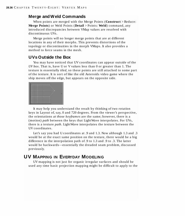
Merge and Weld CommandsWhen points are merged with the Merge Points (Construct > Reduce:

Merge Points) or Weld Points (Detail > Points: Weld) command, anyintroduced discrepancies between VMap values are resolved withdiscontinuous UVs.

Merge points will no longer merge points that are at differentlocations in any of their morphs. This prevents distortions of thetopology or discontinuities in the morph VMaps. It also provides amethod to force seams in the mesh.

UVs Outside the BoxYou may have noticed that UV coordinates can appear outside of the

UV box. That is, have U or V values less than 0 or greater than 1. Thetexture is essentially tiled, so these points are still attached to some partof the texture. It is sort of like the old Asteroids video game where theship moves off the edge, but appears on the opposite side.

It may help you understand the result by thinking of two rotationkeys in Layout of, say, 0 and 720 degrees. From the viewer’s perspective,the orientations at those keyframes are the same; however, there is a(motion) path between the keys that LightWave interpolates. For UVs,there is a texture path. LightWave interpolates the texture between theUV coordinates.

Let’s say you had U coordinates at .9 and 1.3. Now although 1.3 and .3would be at the exact same position on the texture, there would be a bigdifference in the interpolation path of .9 to 1.3 and .9 to .3. The latterwould be backwards—essentially the dreaded seam problem, discussedpreviously.

UV MAPPING IN EVERYDAY MODELINGUV mapping is not just for organic irregular surfaces and should be

used any time basic projection mapping might be difficult to apply to the


finished surfaces. Here is a simple segmented box with a wood image UVmap.

Big deal, eh? A simple cubic image map could do this. But what if youwanted to bend your piece of wood?

Wow! Notice how the grain follows the curvature of the bend. “A littlemore difficult,” you say. Perhaps it’s more difficult, but I guess you couldsomehow bend the image in a paint program to match the geometry.

L I G H T W A V E 3 D 7 28.37

What about adding a little twist?

We’ve finished cloning around with this illustration, but I think youcan see just how powerful UV mapping is, even for non-organic objects.The real secret is to plan ahead and create your UV maps early.

PER-POLYGON UV MAPPINGThe predecessor to discontinuous UVs is per-polygon UV mapping (orpolymap for short) introduced in LightWave 6.0b.

NOTEFor UV textures created using version 6.5 and after, generally, there isno need to use these per-polygon UV mapping tools.

Per-Polygon UV Mapping solved the same problems thatdiscontinuous UVs solve, but in a less elegant and more proprietarymanner. It basically overrode the normal continuous UV map used by atexture with new UV values.

Below is an example of using Lock UVs to Polygon:Here we will use Lock UVs to Poly (Map > Texture: Lock to Poly) on

the 6 polygon because we plan to move the right UV points to fix the 1polygon. If we didn’t do this, the 6 polygon’s UV map would get wreckedwhen we fixed the 1 polygon.


Next, we select the two right points on the UV map and move them tothe far left.

The 1 polygon is now fixed using normal UVs. The 6 polygoncontinues to look fine since we locked it in before moving the points.

To delete a per-polygon UV map:Select the polygon(s) and choose Map > Texture: Clear Poly Map.

Select UV SeamThe Select UV Seam command (Display > Selection: Maps > Select UV

Seam) automatically selects polygons where the UV values span morethan half the image—thus assuming that they are seam polygons,discussed previously. If you activate Patch with Poly Map, it willautomatically turn these into per-polygon UVs.

Below, only the seam polygons have been selected.

L I G H T W A V E 3 D 7 28.39

Next, you see the seam polygons after using the Patch with PolyMap.

Select UV Seam is limited, because it will not set UV values past 1.0or less than 0. Thus, it is possible that some important portion of yourimage will get missed (e.g., you really needed a 1.2 U or V value).

Editing PolymapsLightWave uses many of the modeling tools used for editing vertex

positions to also modify UV values. This works smoothly because theVMaps, like the mesh, are continuous. Moving a point moves it in all thepolygons that use it. With polymaps, however, any operation on a vertexalso must specify which polygon's view of that vertex is edited.(Polymaps are locked snapshots of some UV mapping of a polygon.)

You can select polygons using per-poly UVs by choosing the Select byPoly Map command (Display > Selection: Maps > Select by PolygonMap).

The tools for editing polymaps in the Adjust Polygon Map function(Map > Texture: Adjust Poly Map) include 2D transformations of the UVcoordinates, as well as adjusting the connection between texture pointsand the polygon's vertices. The power of these operations is limited incomparison to the tools for editing VMaps. Note that you need to selectthe polygon(s) first.

You can use this function on discontinuous UVs by entering the map’sname in the Vertex Map field. For polymaps, leave the field blank.


Left to right: 6 is per-poly mapped. Reverse Order. Shift Order. Rotation Angle 90 degrees. Scale V to 60%

A quick method for editing a highly discontinuous texture is to usethe Unweld command to duplicate all the points in your model, so thatno polygon shares a point with any other. After this is done, you canmove entire textured polygons anywhere over the texture image, withoutpulling the neighboring polygon's texture.

NOTEUnweld removes per-polygon UV mapping.Then, you can use thenormal Modeler tools, which support discontinuous UVs.

Leaving the model physically discontinuous like this is usuallyundesirable, but assuming the points haven't been moved, the Mergecommand will automatically fuse these points. Merging the points will, ofcourse, destroy their independent VMap values, so Lock UVs to Polygon(Map > Texture: Lock to Poly) should be used on the polygons prior tothe re-merge.

Unwelding all points is an extreme, but effective method. Unweldingselected points and locking the appropriate polygons individually is alsoquite feasible on low-polygon models, or where there are fewdiscontinuities.

Selected per-polygon UV maps can also be converted todiscontinuous UVs by choosing Map > Texture: Poly Map to UVs.

Using Separate Editing UV MapsAnother approach to editing is to copy the main UV map and edit the

copy. You fix just the problem polygons by locking them based on thecopy UV map. This approach assumes that most of the polygons, thenon-fixed ones, will be fine with the original UV map. You can makesubsequent changes to the per-polygon UV mapped polygons withoutaffecting other polygons.

HINTYou may want to use a different surface name on your problempolygons—while editing—that points to the UV map copy.After the p-map has been locked, you can apply the regular UV mapped surface to

L I G H T W A V E 3 D 7 28.41

it. (Remember, since there is only one per-polygon map per polygon, itdoesn’t matter which UV map is used in the surface texture.)

Quad Polygon MapsA convenient use of polymaps is to simply apply an entire image to a

polygon. This makes sense in the case of polygons, which like images,are four-sided (i.e., quadrangles or quads). These are particularly usefulin the case of a low-polygon model where the face of a model matchesthe textured parts, and every polygon edge is also a texture seam.

The New Quad Polygon Map command (Map > Texture: New QuadPolygon Map) generates polymaps like these easily. It will take selectedquads and assign their corners to the four corners of UV space. If youenter a name in the Vertex Map field, discontinuous UVs are created. (Ifthe name is already a UV map for the object, it will be altered. Otherwise,a UV map will be created.) If the field is blank, a poly map is createdinstead.

Since the choice of which UV corner goes to which quad corner isbasically arbitrary, the order and orientation of the image can beselected. It will likely take a little trial and error to get the results youwant.

The Polygon Normal UVs command (Map > Texture: Poly Norm UVs)projects the texture UVs along the polygon normals, mapping the imageflat on the normal. It is something like a per-polygon atlas mode or theNew Quad Polygon Map operation performed on non-quads. The resultson a cube would be the same as cubic image mapping.

ENDOMORPHSSometimes, deforming an object using bones does not provide the

accuracy you may need for a particular project. LightWave also lets youforce an object to change its shape using another object. This is calledmorphing. Morphing provides absolute control over the final shape,something displacement maps and bones usually cannot offer. You maywish to use morphing to move the muscles in an arm or face, to get aflower to bloom, or to transform a car into a plane. The different statesor poses are generally referred to as morph targets. You might think ofthem as different poses of the same object.


This object is in the LightWave6_5\[6] Projects\Character\EndomorphHead directory. It’s called StuHead_WithEndomorphs.lwo

You handle morphing through morph maps, which are special VMaps(yes, just like point weighting). Each morph target defines differentpositions for each associated base-object point. All of the morphinginformation is contained in a single object file, called an endomorph.

LightWave has two types of morph targets. Relative targets areaffected relatively for any changes to the base object. Absolute targetsare not affected by positional changes to the base object, althoughchanges to the number of points are always reflected.

L I G H T W A V E 3 D 7 28.43

NOTESee Chapter 9 for information on how to animate Endomorphs.

To set up a morph map:1 Create your base object in Modeler.

2 Click the M button in the lower-right corner to activate the morphmap mode. (base) should become selected in the selection pop-upmenu, which appears to the right of the WTM buttons.

3 Select (new) from the selection pop-up menu to the right. The CreateMorph Map dialog will appear. Enter a name using a group.poseformat, something like HEAD.SMILE or EYE.CLOSE and set the Type.

The pop-up menu on the Create Morph Map dialog lists existingtargets.

NOTEIf you change an existing target’s Type, it applies only to changes afterthat time.

Poses with the same group appear on the same tab of the controlinterface called Morph Mixer.


NOTEBelow is an example Morph Mixer panel shot (see Chapter 9,“Animating Endomorphs”).

4 Click OK to create the map. The new map will appear in the selectionpop-up menu.

5 Modify the new map in some way.

Now, if you use the selection pop-up menu and go between the (base)object and the morph map you created, you will see that the (base) isnot affected by the change to the morph map.

Left: (base) object. Right: morph map

L I G H T W A V E 3 D 7 28.45

However, if you used the metaform command (which adds geometry),for example, that change is reflected in the (base) object.

Left: (base) object. Right: morph map

WARNINGWe strongly suggest that you do modifications, like adding andsubtracting geometry, on the base object and use the morph mapsonly for posing (i.e., moving points). Otherwise, you can end up withincorrect point orders.

Below is an example using a more complex object with several morphmaps.

Inserting a Layer into a Morph MapYou can insert a background layer into a Morph Map using the Bkg to

Morph command (Map > Morph: Bkg to Morph). Simply place thegeometry you want to insert into the map in the background. Thenexecute the command. A dialog prompts you for a map name. Pointcount and order must still match, just as in any morph target.


HINTYou can use the Bkg to Morph command to insert an object savedwith Layout’s Save Transformed Object command (File > Save >Save Transformed Objects) that has been deformed in Layout.

Merging Morph MapsUse the Apply Morph command (Map > Morph: Apply Morph) to

merge a specified percent of a (relative) morph map into the base. Notethat all relative morph maps—including the one selected—are affectedby changes to the base.

Rotate Morph FunctionRotating the base of an EndoMorph with the normal Rotate tool often

does not add the proper amount of rotation to its morph targets. Youmay achieve better results with the Rotate Morph function (Modify >Rotate: Rotate Morph).

Here is an example:

Left: Base object. Right: Morph target

Left: Base rotated with the Rotate tool. Right: Morph target

L I G H T W A V E 3 D 7 28.47

Notice how the extended points rotate somewhat—basically, theyhave moved only the amount that those points moved in the base objectwith the rotation. Probably not what you expect nor want. Below is themorph using Rotate Morph instead, with the same settings used to rotatethe base.

Scale Morph FunctionScaling the base of an EndoMorph with a normal sizing tool may not

add the proper amount of scaling to its morph targets. You may getbetter results with the Scale Morph function (Modify > Stretch: ScaleMorph).

Here is an example:

Left: Base object. Right: Morph target


Left: Rotated base. Right: Morph target

Notice how the extended points scale somewhat—basically, they havemoved only the amount that those points moved in the based objectwith the scaling. Not what you expect nor want. Below is the morphusing Scale Morph instead, with the same settings used to scale thebase.

L I G H T W A V E 3 D 7 28.49

VERTEXPAINTVertexPaint (Map > Weight & Color: VertexPaint) is a plug-in for

painting vertex color maps and weight maps on bones. The displaywindow gives you a 3-D view of the object loaded into Modeler. You paintyour object in this view.

Main VertexPaint panel

NOTEReferences to bones really means skelegons, since (technically) bonescannot be used in Modeler directly.

The view controls operate just like Modeler’s, so dragging with ALT

key rotates, SHIFT + ALT pans and CTRL + ALT zooms. There are alsocorresponding drag buttons in the upper right corner.

Two types of projections are available for displaying the object in 3Dspace: Persp (perspective), the default and Ortho (orthogonal).Sometimes painting vertex colors is easier using the orthogonal mode.

When using the perspective mode, you can modify the zoom factorusing Fov setting. Higher values simulate a telephoto lens zoom andlower values simulate a wide angle lens.

You can quickly switch to certain preset views by choosing one fromthe pop-up menu (down arrow) just to the left of the projection modepop-up menu.


Preset views pop-up menu

Component and Blend DisplayLightWave uses the point's alpha information as a mixed value ratio

for blending point and surface colors. The formulas look like:

Color.Red = Vertex.Red * Vertex.Alpha + Surface.Red * (1.0 -Vertex.Alpha)

Color.Green = Vertex.Green * Vertex.Alpha + Surface.Green * (1.0 -Vertex.Alpha)

Color.Blue = Vertex.Blue * Vertex.Alpha + Surface.Blue * (1.0 -Vertex.Alpha)

When you set the rendering mode to Vertex Color or WireframeColor, pressing the B (blend) button will display both the point colorand alpha channel.

When you paint, you apply both color and alpha values whenVertexPaint is in blend mode only by pressing the B button. Otherwiseyou apply color or alpha values based on the mode set by the pop-upmenu just to the right of the Edit pop-up menu button. This is thecomponent mode (i.e., B button off).

When in component mode and state is set to RGB paint mode, only the point color is rendered

L I G H T W A V E 3 D 7 28.51

When in component mode and state is set to Alpha paint mode, brightness of alpha is rendered, with black as 100 percenttransparent and white as opaque.

When in blend mode and state is set to either RGB paint or Alpha paint mode, the point color and the surface color are mixedwhen rendered.

Rendering ModesYou can view the object in various rendering modes using the pop-up

menu just above the window on the left.

Render modes pop-up menu

Points The points that form the object are rendered.The color of the point is set to the point color.Lights are not used.


Wireframe The object is rendered as a wireframe. The pointcolor is set by the points of each line. When thecolor at the start of the line differs from the colorat the end, it is displayed as a gradation. Lightsare not used.

Frontface Only the polygons with surface normals that facethe camera are rendered as wireframe. Lights arenot used.

Vertex Color The object's polygon is rendered using the colorinformation from the current vertex color map.Lights are not used.

Wireframe Color The object is rendered using the colorinformation from the current vertex color mapwith an overlay of wireframe lines. Lights are notused.

Lighting Shade The object is rendered using the lights set in thelight mode. The color attributes for the polygonsurfaces are used but the vertex color map is notrendered.

Weight Value The weight value set for the current weight mapis displayed in red. Unaffected areas aredisplayed in gray. The closer the gradation is togray from the maximum red, the less influencethe bone has on those points. This is aconvenient mode to view your weight map whenyou have finished painting the map.

Weight Value render mode

L I G H T W A V E 3 D 7 28.53

Weight Ratio The ratio of influence on each point by eachbone is rendered using a color gradation. Whenno bone exerts influence over a point, it isrendered as gray. Before bone influence iscalculated, the colors red, blue, and green arerepeated in order. Each point color iscompensated on the basis of the percentage ofinfluence of the bone.

Weight Ratio render mode

PreferencesWhen you select Preferences from the File menu, you can customize

many settings.

VertexPaint preferences


Changing the RGB values for the BG Color will modify thebackground color of the 3-D view. When the Preference panel is movedor closed, the view will be updated to reflect a change. This setting issaved between sessions.

The second item modifies the RGB values of the Wire Color in the 3-Dview. This affects the following rendering styles: Wireframe Color,Weight Value, and Weight Ratio. When the Preference panel is moved orclosed, the view will be updated to reflect a change. This setting is savedbetween sessions.

The Window Size option will change the size of the VertexPaintwindow. You must exit and restart VertexPaint for the changes to takeeffect. If you choose a size larger than your desktop, parts of the screenwill not be visible.

Hide Unselected Bones specifies how unselected bones are displayed

Mirror Epsilon is the error quantity used when you paste boneweight values symmetrically on the X axis. (See “Copying and PastingWeight.”)

Undo Levels is the maximum number of undos in Color and Weightmode.

Default Keyboard/Mouse OperationsThe chart below summarizes keyboard/mouse operations.

Operation Command

LMB + ALT Rotate view

LMB + CTRL + ALT Zoom in/out of view

LMB + ALT + SHIFT Pan view

LMB Rotate view (using Rotate button)

LMB Zoom in/out of view (using Zoom button)

LMB Pan view (using Move button)

LMB Paint point color (Color mode)

RMB Set the size of the color paint brush (Colormode)

LMB + CTRL + SHIFT Select color from 3D view, like eyedropper (Colormode)

LMB Select color from color palette (Color mode)

LMB Paint bone weight (Weight mode)

LMB + CTRL Rotate bone

LMB + SHIFT Select bone

RMB Set the size of the weight paint brush (Weightmode)

LMB Move Lights (Light mode)

L I G H T W A V E 3 D 7 28.55

LMB + CTRL + SHIFT Select color from 3-D view (Light mode)

LMB Select color from color pallet (Light mode)

LMB Select polygon (Show mode)

RMB Deselect polygon (Show mode)

LMB CTRL-+ SHIFT Rectangle selection of polygon (Showmode)

RMB + CTRL + SHIFT Rectangular deselect of polygon (Show mode)

a Center object

A Center current bone

, Zoom out

. Zoom in

F Front view

T Top view

S Side view

F1 Points Render mode

F2 Wireframe Render mode

F3 Front Face Render mode

F4 Vertex Color Render mode

F5 Wireframe Color Render mode

F6 Lighting Shade Render mode

F7 Weight Value Render mode

F8 Weight Ratio Render mode

u Undo

up arrow Select next bone

down arrow Select previous bone

c Copy current bone weight

v Paste current bone weight

V X axial symmetrical paste of current bone weight

x Clear current bone weight

+ Scale up current bone weight

- Scale down current bone weight

r Reset current bone to rest position

R Reset all bones to rest position

Customizing Keyboard/Mouse OperationsYou can change keyboard/mouse operations, by selecting the

command with the Command pop-up menu and then the correspondingkeystrokes on the Operation pop-up menu.


If the keyboard/mouse operation is already being used by anothercommand, the operations for the two commands will be swapped. Closethe Preference panel to set the new Command+Operation combination.

Modifying ModesVertexPaint offers four operating modes. You change modes by

selecting the relevant tab on the left side of the interface. The contentsof the Edit menu will change to the commands for the current mode.

Color tab Vertex color map edit mode

Weight tab Bone weight edit mode

Light tab Light settings mode

Show tab Polygon show/hide setting mode

Setting the Morph MapIf you are using EndoMorphs in Modeler, this menu lets you change

the object deformation state to reflect the selected Morph map. If thereare no Morph maps in the object, the drop-down menu will be inactive.

Color Mode TabBefore you can begin painting points, you must first define at least

one vertex color map. If a color map is already applied to the object,VertexPaint sets the first color map as the current map.

NOTEIf there is no information in the vertex color map, it will not be loadedinto VertexPaint. If you want to define your vertex color maps inModeler, you must first add some values (color) to the map.

To create a new color map in VertexPaint, you must be in Color mode.Choose Edit > Create Vertex Color Map. A dialog box appears where youname your vertex color map (this name must be unique). Then click theOK button. If the name already exists a number is appended to the name.

To modify the name of the current vertex color map, choose Edit >Rename Vertex Color Map.

To delete a vertex color map, set the map you wish to delete as thecurrent map and choose Edit > Delete Vertex Color Map.

There are two types of vertex color maps: RGBA (color + alphachannel) and RGB (color only). The first includes alpha channelinformation, the other does not. VertexPaint defaults to RGBA, but youcan change the type using the pop-up menu. Modeler will not be updateduntil you close VertexPaint.

You can reset the point color of the selected map to the surface colorof the object by choosing Edit > Reset To Surface Colors.

L I G H T W A V E 3 D 7 28.57

Baking the ColorVertex paint can use the light information set in the Light mode tab to

bake (OpenGL) color information into the color map. Before baking thesurface to a color map, you can verify the results using the LightingShade rendering mode. To adjust the way the object is lit, use theoptions on the Light tab to change the strength and position of lightsused to calculate the light mode.

Select the color map for which you want to apply the bakedinformation, and choose Edit > Burn Shading Colors. Note that thewhole object must be within the 3-D view for this to work properly. Anyportion of a polygon outside the 3-D view will not receive point colorvalue and possible errors may occur.

Light calculations.This is viewable in the Lighting Shade rendering mode.

After choosing Burn Shading Colors, the baked point color will be rendered, as seen here in Wireframe Color rendering mode:

Point ColorWhen you use the brush, there are three Paint Modes available for

painting point color.

Color / Paint Paint a single point

Color / Index Paint a polygon point index unit

Color / Polygon Paint a single polygon unit


To start painting, select a color map from the Color Map pop-upmenu, then drag your LMB over the object in the 3-D view. You can useeither the color sliders or the palette to select the color you want forpainting.

The slider operates in two modes RGB and HSV. Each slider affectsthe numeric entry field to the right of its location. Values for all slidersare displayed in a range from 1 to 256, although floating point values areused internally by VertexPaint.

The palette gives the user a visual way to select the active color forpainting. Use the LMB within the palette to select a color. Use the sliderto select alpha colors.

You can also select the active color directly from the object in the 3Dview. This works similarly to an eye-dropper tool. To do this, hold theCTRL + SHIFT keys simultaneously and click on the color using the LMB.The color is displayed in the active color selection box.

Painting a Point When you select the paint mode Color / Point, painting will affect

points. The Brush Size and Front Face parameters affect the painting ofa point.

Color / Point mode

The brush size is represented by a disc, which is the color of theactive paint color, and sits below the mouse pointer when you press theLMB in the 3-D view. To adjust the brush size, use the Brush Size sliderand numeric entry field under the mode tab. You can also drag your RMBin the 3-D view to adjust interactively.

When you paint, all points receive paint whether they face you or not.The paint brush will pass through the object and paint points on theopposite side. If you activate the Front Face button (to the right of theBrush Size slider), only the front face will receive color.

Painting a Polygon Point IndexWhen you select Color / Index, you apply paint based on the polygon

point index. When you paint in this mode, only the point index of the

L I G H T W A V E 3 D 7 28.59

polygon surface receives paint. Brush Size and Front Face settings areignored. Which polygon point index receives color is based on thepolygon nearest to the cursor when paint is applied.

Color / Index mode

Painting a PolygonWhen you select Color / Polygon, you apply paint to a polygon. When

you paint in this mode, only the polygon surface receives paint from thebrush. Brush Size and Front Face settings are ignored. When paint isapplied, the polygon beneath the mouse pointer receives color.

Color / Polygon mode

Weight Mode TabWhen you select a bone (i.e., skelegons), it is highlighted in yellow. By

default, unselected bones are hidden. You can display all bones, activeand inactive, by deactivating Hide Unselected Bones in the Preferencespanel. Unselected bones are displayed as white.

VertexPaint offers three methods for selecting bones:

• In Weight mode, select the name of the bone from the Bone pop-upmenu.

• Use your arrow keys to cycle through the next and previous bone.

• Hold the SHIFT key on the keyboard and click with the LMB to selecta bone directly in the 3D view


Bones as they are displayed when Hide Unselected Bones is deactivated

In addition, you can rotate a bone more easily when it is centered inthe 3-D view. To center the currently selected bone, press the A key orselect Fit Bone from the pull-down menu (represented by a downwardtriangle).

Rotating BonesVertexPaint lets you test bone deformation on the object while you

work on weight maps. The selected bone is displayed with HPB rotationcontrols. The display rings affect rotation as follows: red - Heading (Yaxis), green - Pitch (X axis), blue - Bank (Z axis).

While holding the CTRL key, drag your LMB to rotate the bone. Torotate only one axis, drag right on top of an axis. The selected axis willbe indicated by a thick ring.

To reset a bone to its default state (Rest Position), make sure theWeight tab is selected. Then choose Reset the Bone from the Edit menu.To reset all bones, select Reset All Bones.

Renaming BonesTo rename a bone, choose Edit > Rename Bone in Weight mode.

Enter the new name for the bone in the dialog and press the OK button.When you exit VertexPaint, a dialog box will ask you to update Modeler.Press OK and the changes will take effect in Modeler.

L I G H T W A V E 3 D 7 28.61

Bone renaming dialog

Renaming Weight MapsTo rename a weight map, edit the name of the weight map directly in

the VMap field. When you exit VertexPaint, a dialog box will ask you toupdate Modeler. Press OK and the changes will take affect in Modeler.

Name field of weight map

Copying and Pasting WeightTo copy the weight values of the current bone to the VertexPaint

clipboard buffer, press the C key or choose Edit > Copy. To paste theweight values to the weight map of the selected bone, press the V key orchoose Edit > Paste.

You can also paste the weight values to another bone symmetricallyon the X axis . Select the bone you wish to paste the values to and pressSHIFT + V or choose Edit > Paste-X. When the weight map value is pasted,the point coordinate is searched for symmetrical positions along the Xaxis.

NOTEYou can set the computing error quantity when searching the axialsymmetrical point by setting its value in the Mirror Epsilon settingfound in the Preferences panel.

Clearing WeightTo clear all values from the weight map of the current bone, press the

X key or choose Edit > Clear.

Normalizing WeightWhen you use the paint feature in VertexPaint to calculate bone

weight for Modeler, the values can sometimes exceed the range of 0.0 to1.0. When you normalize the weight value (to a range of 0.0 to 1.0), thebone is easier to control. To normalize the weight values, choose Edit >Normalize.


A weight map that has not been Normalized

A weight map that has been Normalized

Trimming WeightSometimes independent bones can cause a divergence across the

object by deforming areas controlled by other bones. This occurs whenthe weight maps for the independent bones were created using thecalculated weight falloff function (see “Calculating Weight”), for example,when you arrange bones for the fingers of a hand. When falloff iscalculated, only distance to the bone is measured to set the point weightvalue.

Before applying Trim Branch. Because there is a weight influence from the bone of the ring finger on the middle and little finger,when the ring finger is bent the middle and little fingers are also deformed.

L I G H T W A V E 3 D 7 28.63

When you choose Edit > Trim Branch, it trims the bone weight valuesalong the route of the bone system for the selected weight map. It firstseeks the primary bone of each point (the point to which the bone isclosest). When a point is found that is not part of the selected bonesystem, it is selected and the weight value is cleared for that point inrelation to the current bone. The route of the bone system and itsdivergence from the parent is shown below.

System of the selected bone.The darker bones represent the system of the selected bone, whereas the lighter bones representthe bones of other systems.

When you perform this command on a bone divergence such as thejoint of a finger, sometimes the points in the joint will not deformsmoothly. We recommend that you execute the command first along onlycertain bones of the divergence. In addition, trimming may not work welldepending on the arrangement of the bones. If this is the case, use theERA and SUB functions of the weight brush to manually adjust the valueof the weights.

After applying Trim Branch.The weight values that affected the middle and little fingers are cleared of their value, so the ring fingercan now be deformed independently without affecting the other fingers.


Painting Weight ValuesTo paint weight values in Weight mode, select the Paint subtab.

Different input fields and operations are displayed for painting weightvalues. Choose an operation and enter your desired values, then dragyour LMB in the 3-D view over the points you wish to paint.

The Brush Size and Front Face parameters function the same aswhen you paint point color.

Operation lets you set the type of operation that occurs when youpaint weight values along the object's points.

The ADD operation adds the value set in the Value field to the weightmap along the object. Drag your LMB over the points where you wish tomodify the value. The change is applied once to each affected point. Tomodify the point value more than once, release the LMB and repeat theprocess.

The SUB operation subtracts the value set in the Value field to theweight map along the object. Drag your LMB over the points where youwish to modify the value. The change is applied once to each affectedpoint. To modify the point value more than once, release the LMB andrepeat the process.

This REP mode replaces the current weight value with the value setin the Value field.

The ERA mode erases the value of the weight for the affected pointsand sets them to 0.0.

The Color Scale value adjusts the display strength of the red colorgradation in the Weight Value rendering mode. Adjusting this value doesnot affect the influence exerted in the actual weight map.

Calculating WeightTo calculate the weight map using falloff in weight mode, select the

Calc subtab. The parameter fields used to calculate weight are displayed.These parameters work in basically the same way as BoneWeight inModeler.

L I G H T W A V E 3 D 7 28.65

Falloff sets the method for calculating the value of the weight map.With Linear, the points closest to the bone receive a value of 1.0, allothers are set to 0.0. With Distance, the point weight value is set to theinverse number of the distance from the bone, creating a gradation ofinfluence. With Distance ^ 2, the point weight value is set to the inversenumber of the distance to the second power from the bone, creating agradation of influence, and so on.

When Normalization is active, the value of the weight map iscalculated using a range from 0.0 to 1.0.

When Calculate Weights is clicked, the weight map is calculatedusing the above settings. Weight maps for all bones are created.

Scaling WeightSelect the Scale subtab in Weight mode to display the parameters for

scaling weight map values.

Scale sets the method for scaling weight values. With Whole, thescale is applied evenly along the weight map. With At Start Joint, thescale is applied from the base of the bone. With At End Joint, the scaleis applied from the tip of the bone.

Clicking the + button will increase the weight value based on thevalue in the field to the right. Pressing the + key will also perform thisfunction.

Clicking the - button will reduce the weight value based on the valuein the field to the right. Pressing the - key will also perform this function.


Increasing the weight map value using the At Start Joint scale modifier.

Increasing the weight map value using the At End Joint scale modifier.

Clamping WeightTo activate the clamp weight, selected the Clamp subtab. When

deformation for a single skin object is calculated, calculation speed isdirectly related to the number of matrixes that must be calculated forthe bone. Calculation speed can be improved by truncating the weightvalue for points that receive little influence from the bone. When dealingwith the deformation of single skin objects for real-time animation, thisbecomes an element of great importance for performance tuning.

N of Matrix sets the maximum number of matrixes, when calculatingthe deformation for each point. The weight value of each pointinfluenced by the current bone is set to the number of N of Matrix inorder of greatest influence. For example, in one mesh bone, 20 is

L I G H T W A V E 3 D 7 28.67

clamped with the N of Matrix setting of 5. You keep the weight value ofthe points influenced by the bone that are greater than 5, and the valueof points whose influence is below 5 are cut off and set to 0.0.

The Clamp button applies the clamp function based on settings.

Status of WeightSelect the Stat subtab to set values for displaying weight maps.

Threshold sets the value for the selection process. Any weight valueless than the value set in Threshold will be selected. The entry field tothe right allows you to set this value either by weight Value or as a Ratio(a percentage value based on the normalized weight value from 0.0 to1.0).

When the Select button is clicked, all points whose weight value isless than the value set in Threshold are selected and displayed asyellow. To deselect the points, press the Deselect button.

When Discard Selected is clicked, the selected points of the weightmap, displayed in yellow, are set to a weight value of 0.0 and deselected.

Lights Mode TabYou can set the number of lights and their positions/values, which are

used in the Lighting Shade rendering mode. In addition, the lightsettings here are used by the Burn Lighting Colors command (Edit pop-up in Color mode) for baking color information into the color map.

You can use eight lights with VertexPaint. This is the maximumnumber of active lights with OpenGl.

You can select lights from the Name pop-up menu or by clicking onthem in the 3-D view. Lights look like yellow null objects when selected.


When you turn on the Active check box for the light selected on theName pop-up menu, the light is set to its active state. When you uncheckthis box, the light becomes inactive and does not cast light in the scene.

You can drag the selected light in the 3-D view to reposition or enterXYZ coordinates in the numeric entry fields under the Name pop-upmenu.

The color of each light can be set independently. The color slider andpalette are used the same way as in Color mode.

NOTEVertexPaint lights operate independent of normal Layout lights.

Show Mode TabThe Show mode tab offers several ways to hide portions of the object

while you work. The following operations are available for selectingpolygons to hide.

Selecting PolygonsIn the 3-D view, drag your LMB over the polygons you wish to select.

If you use the RMB, the current polygons are deselected.

You can select polygons with a bounding box by holding the CTRL

while you drag your LMB in the 3-D view. When you release the LMB, anypolygons within the box are selected. If you drag with the RMB whileholding CTRL, any polygons within the rectangular box are deselected.

Bounding box selection

When you choose Select All or Hide All from the Edit menu, thewhole object is selected or deselected.

L I G H T W A V E 3 D 7 28.69

Show and HideThere are two selection modes on the Select pop-up menu: By

Polygon and By Surface. In By Polygon mode, the buttons work asfollows:

Show All polygons shown

Select All polygons are selected

Hide Selected polygons are hidden

Hide UnSel Unselected polygons are hidden

If By Surface is used, select the surface you want to work on from theSurface pop-up menu. In this mode, the buttons work as follows:

Show Polygons on the selected surface are displayed.

Select Polygons on the selected surface are selected.

Hide Polygons on the selected surface are hidden.

Hide UnSel Unselected polygons and unselected surfaces are hidden.

Frequently Asked QuestionsQ. Why is the mesh of the SubPatch not displayed?

VertexPaint does not support SubPatch objects. In Modeler, eitherpress the TAB key to reset the SubPatch to polygon mode, or use theFreeze command to convert the SubPatch to a polygon mesh.

Q. The vertex color map was created, but the point color is not rendering inModeler. Why?

Make sure you have the map selected on the Advanced tab of theSurface Editor under the Vertex Color Map.


cchhaapptteerr29Organic Modeling Tools

Chapter 29:Organic Modeling Tools

LightWave includes some powerful tools to help you create soft-edgedorganic objects. The SubPatch method is a parallel modeling mode thatworks with the same modeling tools and commands. Metamesh objectsare sort of like interactive hypervoxels. Spline patching is a technique ofcreating a basic shape out of linked curves and then smoothly patchingthe areas between the curves with a mesh of polygons.

SUBPATCHESStandard polygonal surfaces need many polygons to approximate a

smooth surface. Even so, a smooth surface made up of polygons willeventually reveal its inherent sharp-edged nature, if it’s examined closelyenough. Although you can create such polygon-heavy objects, it is oftendifficult to manipulate and manage them from the perspective ofmemory-consumption and editing.

A “SubPatch,” an abbreviation for subdivision patch, is a “bi-cubicpatch.” The idea behind SubPatching is to repeatedly refine the controlmesh until you achieve a smooth surface, called the “limit surface.” TheSubPatch modeling mode is not unlike a real-time implementation of theMetaform (Construct > Subdivide: Subdivide) command.

MetaForm performed three times in succession on the same object (no surface smoothing)

L I G H T W A V E 3 D 7 29.1

Same object with SubPatch activated.

CREATING A SUBPATCH OBJECTYour starting control mesh must begin with an object consisting of

three- and/or four-point polygons. A good place to start is to make asimple box and then use Metaform (Construct > Subdivide: Subdivide)once (or maybe twice depending on your needs). This starts you off witha nice cage made only of quads (four-point polygons).

Left: Simple box. Right: Processed once with Metaform

You activate SubPatch mode by pressing the TAB key or choosingConstruct > Convert: SubPatch. In most instances you want to affect theentire object, so no polygons are selected when you press the key. Ifpolygons are selected, only those will have the SubPatch mode turnedon. This can get confusing because the polygons become unselected. Ifyou press the TAB key again, the SubPatch state of all polygons isreversed. If you do this by accident, use Undo and make sure allpolygons are unselected before turning SubPatch on again. (You can alsouse the Polygon Statistics panel to select/re-select just the SubPatchsurfaces.)

29.2 C H A P T E R T W E N T Y - N I N E : O R G A N I C M O D E L I N G T O O L S

SubPatch mode enabled

To change the shape of the SubPatch object, you manipulate theshape of the polygonal cage (i.e., control mesh) using most of thestandard modeling tools, including Bevel, Smooth Shift, Metaform, andso on, or by just dragging points and polygons around. Don’t use toolsthat may create greater than four-point polygons, like Boolean.

Editing polygon cage affects SubPatch object

You can select the SubPatch vertices by clicking either on the true(polygon cage) vertex location or the location of the vertex whenmapped on the SubPatch surface.

When you use SubPatch, you often manipulate the polygons into whatwould normally be non-planar, degenerate, or cattiwompus polygons.Since the polygonal cage is merely a reference for the SubPatch object,this is perfectly acceptable.

HINTIf you end up editing a very complex cage, the display can becomeconfusing. In such a case, the cage is often close in shape to theSubPatch surface.Thus, you may be able to edit the normal polygonsand just flick the SubPatch mode on to check the results.

L I G H T W A V E 3 D 7 29.3

USING WEIGHT MAPSSubPatch objects can utilize a special type of weight map that affects

the bias of control points. You can thus create objects with much greatercontrol and accuracy without adding complexity to the cage.

To adjust a SubPatch weight map:1 Click the Weight map button in the lower-right portion of the

interface, which is marked with the letter W, and choose SubPatchWeight in the pop-up menu to the right. (Weight maps are discussedin Chapter 28.)

2 Use any of the weight-editing tools, like the Weights tool (Map >Weight & Color: Weights) to adjust point weights. You can increase ordecrease the bias of individual control points on the SubPatchsurface, which can sharpen (or unsharpen for negative values) thecurvature of the object.

ADDING MORE DETAILSAdding more polygons to a specific area is somewhat problematic.

Remember, your object must be composed only of quads (or triangles).Fortunately, there are a number of ways to easily add detail to aSubPatch cage.

If you are working with a single, selected polygon, the Bevel tool(Multiply > Extend: Bevel) is perfect because it will essentially add fournew quads along the edges of the original polygon. Moreover, if you keepthe Inset and Shift values at 0 (just click your RMB in a viewport), thebevel won’t change the surface shape—although it will affect theunderlying SubPatch form. (The beveled polygon sits in the samelocation so you can’t see the new sides.) The polygon is still selectedafter the beveling operation, so you can then fine-tune the shape withthe tools Stretch, Move, and so on.


Beveling out two polygons

The Smooth Shift tool (Multiply > Extend: Smooth Shift) workssimilarly, but keeps a group of selected polygons together. Just click yourRMB in a viewport to use an Offset of 0.

Smooth Shifting two polygons (left) and then moving them (right)

SPECIFIC DISPLAY OPTIONSThe display options for the Cage and Guides viewport specifically

affect how SubPatch objects are displayed. Some folks find the cagesclutter the screen too much and prefer to just grab the end of the guidesto move points on the control mesh (See Chapter 27).

Left: Cage on. Right: Cage off

L I G H T W A V E 3 D 7 29.5

NOTESee Chapter 9 for a discussion on using SubPatch object in Layout.

META-PRIMITIVE OBJECTSMeta-primitives are another cool modeling tool that comes in several

flavors: plain Metaballs, Metaedges and Metafaces. Meta-primitives aresimilar to HyperVoxels except they are polygon-based, and their surfaceand interaction is more apparent and viewable in Modeler. In fact, Meta-primitives are a good place to start before you set up with HyperVoxels,because of their real-time feedback. All Meta-primitives will interact witheach other, even though they are different types, but only if they are inthe same layer.

To draw a Metaball object:1 Activate the Draw Metaballs tool. (Create > Elements: Metaballs)

2 Click in a Modeler viewport. Use any Rendering Style other thanWireframe and you will see the metaball.

3 You can move the metaball by dragging its center handle. You canchange its size by dragging the sizing handle that looks like anorbiting circle. If you click anywhere else, another metaball will becreated.


4 If you move or increase a metaball so that its surface approaches thesurface of another, they will adhere to each other, like the stuff in alava lamp.

5 Drop the Draw Metaballs tool (i.e., reselect it or press the SPACEBAR).

Surface texture added

Metaedges and MetafacesMetaedges and Metafaces are essentially multi-point versions of plain

Metaballs. To draw Metaedges, you can choose Create > Elements:Metaedges. Your initial clicking point establishes the first point. Holdyou LMB down and drag out the second point. Other than there beingtwo points, this tool works just like the Draw Metaballs tool.

L I G H T W A V E 3 D 7 29.7

Metaedges

There is no draw Metafaces tool. They must be created from three- orfour-point polygons or curves. Just select the polygon/curve and chooseConstruct > Convert: Make Metafaces.

Metafaces


Metaedge, Metaface, and Metaball interacting together

Radius and Influence SettingsThe numeric panel has Radius and Influence settings. Radius is

simply the size of the Meta-primitive ball. Adjusting the Influencechanges the interaction between balls. Setting a negative Influence willinvert the primitive causing it to eat away neighboring Meta-primitivesinstead of blending. (See “Editing Meta-primitives” for example.)

Metaedge with different Influence settings

Converting to Metaballs and MetaedgesYou can also convert points into plain Metaballs using the Make

Metaballs command (Construct > Convert: Make Metaballs). Similarly,Metaedges can be created from two-point polygons or curves. Simplyselect the polygon/curve and choose Construct > Convert: MakeMetaedges.

L I G H T W A V E 3 D 7 29.9

Metaball AppearanceThe amount of detail for displaying Meta-primitives is handled by the

Metaball Resolution setting on Modeler’s General Options panel(Modeler > Options > General Options). The value represents thenumber of subdivisions (pixels per metaball on the screen). To get asmoother surface, increase the value. There is no limit.

For a discussion on rendering and Layout display, see Chapter 9,“Metaball Display and Render Levels.”

You can also toggle the Meta-primitive mesh on/off by choosingConstruct > Convert: Toggle Metamesh. You may want to do this if youhave a lot of Meta-primitives and your display refresh is too slow. This isnot just a display change and is similar to toggling off SubPatches. If yousave a Meta-primitive with the mesh off, you will not be able to see thesurface in Layout.

You can surface Meta-primitives as you would any object; however,you are allowed only one surface per layer.

Animating Meta-primitivesYou can animate Meta-primitives the same way you would animate

any object. Of course, you won’t take advantage of their coolness unlessyou animate point positions. For this, you can use features like morphtargets, bones, displacement maps, and so on. Note that only Meta-primitives in the same layer will interact with each other.

Editing Meta-primitivesActivate the Edit Metaballs tool (Detail > Other: Edit Metaballs) to

edit existing Meta-primitives. On the numeric panel, you can adjust theRadius and Influence.


Negative Influence eating-away neighboring Meta-primitive

Deactivate the tool by dropping it, reselecting it, or hitting theSPACEBAR when you are done.

PATCH LEVEL AND CONVERSION TO POLYGONSAlthough you can use a SubPatch model or Meta-primitives as is,

occasionally you may want to convert it into a normal polygon mesh.

To convert to a polygons mesh, use the Freeze command (Construct> Convert: Freeze). The amount of polygonal detail in the object is alsodetermined by the Patch Divisions setting on the General Options panel(Modeler > Options > General Options). (See Chapter 20 for moreinformation.)

Once frozen, the control mesh no longer exists. As such, you shouldsave the object before you perform a freeze just in case you later decideyou want to modify its shape.

NOTEThe Patch Divisions setting on the General Options panel alsoaffects the level of smoothing in the viewport displays.

L I G H T W A V E 3 D 7 29.11

NOTEThe Freeze command supports discontinuous UVs. It will also generateall the morph target objects, as if they had been frozen individually. Forgeometry that changes topology when morphed—like metaballs—thecurrently selected morph generates the frozen mesh and all othermorphs are discarded.

SPLINE PATCHINGModeler’s feature for spline patching lets you model with curves and

then smoothly spread a mesh of polygons over them.

To use spline patching:1 Make three or four curves that create one or more fully enclosed

areas. Note that the curves share end points.

2 In the Polygon Selection mode, select the curves that surround theenclosed area. Do this in a clockwise or counterclockwise fashion.Remember which curve you selected first! It’s okay if you also selectsome polygons in addition to the curves, they will be ignored in thepatching operation.

3 Choose Multiply > Combine: Patches > Make Spline Patch. The fieldsfor Perpendicular and Parallel refer to the number of polygons toput along the side that is perpendicular or parallel to the first curve


you selected. Knots and Length let you choose to space yourpolygons equally according to the overall length or relative to theknots or points on the splines.

4 Click OK. You should see a polygon mesh added to the area withinthe three curves you selected.

5 Repeat this for the other areas. If you patch an opposing side, selectthe curves in the same order and direction. (For this boat hull, theouter curve was selected first, then the other curves were selected inclockwise order.)

Sometimes a spline cage will be patched unexpectedly. There aresome fixes you can try. All of the selected curves should flow in thesame direction, based on their heads and tails. If they don’t, you can flipthem and try the patch again. (See Chapter 22 for more information oncurves.) You can also try selecting the curves in the opposite direction.

L I G H T W A V E 3 D 7 29.13

Sometimes the resulting surface normals face the wrong way. Justselect at least one polygon on that side. Choose Display > Selection: SelConnect to select all of the connected polygons in the patch. Then, pressthe F key to flip the polygons.

If there are not enough curves or they do not share points properly,an error message appears. If this happens, check the joining pointscarefully to make certain they are not merely overlapping. Choose eitherConstruct > Reduce: Merge Points or Detail > Points: Weld to correct.

AUTOPATCHERMKThe AutoPatcherMK command (Multiply > Combine: Patches >

AutoPatcherMK) automatically patches a spline cage. You can set thenumber of rows and columns of the patch between 0 and 20. To spacethe polygons according to the length of the curve, select the LengthSpacing checkbox. To insure success, never have more than four knotsin a curve.

WHY SPLINE PATCH?Often it is much faster and easier to create patch-type objects with

SubPatch, but there may be times that only spline patching will get thedesired results. For example, if you need to create a smooth area thatwill adhere to existing polygons, spline patches work better because youcan align the edge using exact points. Since SubPatch uses the points asa reference only, it is difficult—if not impossible—to align the resultingSubPatch object with existing geometry.


cchhaapptteerr30Image Editor

Chapter 30:Image Editor

The Image Editor handles functions related to images and video clips.You can load images and video clips from this panel to make themavailable for various functions where images are needed, like for surfacetextures. You can also adjust certain image characteristics, likebrightness and contrast, without actually affecting the original file. If youload an animation file (e.g., AVI) or image sequence, you can specify thebeginning and ending frames to use and set what happens before andafter the sequence begins and starts.

The Image Editor

L I G H T W A V E 3 D 7 30.1

QUICK ACCESS TO IMAGE EDITORPop-up menus for image-loading throughout LightWave include time-

saving functions that bypass the Image Editor. You can always editloaded images by clicking the related Edit Image button that appearsnear image-loading pop-up menus.

The Edit Image button on the Texture Editor

THE IMAGE EDITOR FILE LIST WINDOWThe controls on the various tabs to the right will affect the selected

image file. The image will appear in the preview window below. If theitem is a sequence/animation, you will display the first image.

You can collapse/uncollpase the list window by clicking the left-facingarrow button.

30.2 C H A P T E R T H I R T Y : I M A G E E D I T O R

Left: List window open. Right: List window closed

FILE-HANDLING OPTIONSYou can select the current image by either clicking on it in the list

window or by selecting it from the Image pop-up menu.

Click the Load button to load a new image file to add to the list. Usethe Replace button to replace the selected image in the list window. Todelete an image from the list, simply select it and press the DELETE key.

File-handling options

The Clone pop-up menu has two items. Instance creates a new entryfor the cloned clip and lets you apply independent settings on the Editingand Processing tabs. The duration (e.g., In/Out) is linked to the originalclip. Changes to the original image will affect any instances (made fromthat original). However, you can always make multiple instances andapply changes to only the instances, leaving the original untouched.

Duplicate creates a completely independent copy of the original thatyou can adjust in any way you want; however, it is available only forimage sequences.

L I G H T W A V E 3 D 7 30.3

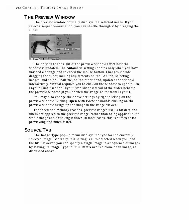
THE PREVIEW WINDOWThe preview window normally displays the selected image. If you

select a sequence/animation, you can shuttle through it by dragging theslider.

The options to the right of the preview window affect how thewindow is updated. The Automatic setting updates only when you havefinished a change and released the mouse button. Changes includedragging the slider, making adjustments on the Edit tab, selectingimages, and so on. Realtime, on the other hand, updates the windowinteractively. Manual requires you to click on the window to update. UseLayout Time uses the Layout time slider instead of the slider beneaththe preview window (if you opened the Image Editor from Layout).

You may also change the above settings by right-clicking on thepreview window. Clicking Open with IView or double-clicking on thepreview window brings up the image in the Image Viewer.

For speed and memory reasons, preview images use 24-bit data andfilters are applied to the preview image, rather than being applied to thewhole image and shrinking it down. In most cases, this is sufficient forpreviewing and much faster.

SOURCE TABThe Image Type pop-up menu displays the type for the currently

selected image. Generally, this setting is auto-detected when you loadthe file. However, you can specify a single image in a sequence of imagesby leaving its Image Type to Still. Reference is a clone of an image, asdiscussed above.


Loading a SequenceIf you wish to load a sequence of files, you can select any image in the

sequence—it doesn’t need to be the first. Initially, the sequence will betreated as a Still. However, you can just change the Image Type toSequence and LightWave automatically analyzes the overall sequence offiles and completes the related fields on the panel.

The Sequence tab

Each separate file must have the same name, followed by a number.The numeric sequence may be staggered, but the name must beconsistent. For example, this is a valid image sequence: FLY001.TGA,FLY002.TGA, FLY005.TGA, FLY007.TGA, FLY010.TGA.

By default, each number corresponds to a frame. If images are missingin a sequence, then the previous image is used until the next image in thesequence comes up. Thus, with the sequence SIENNA001, SIENNA002,SIENNA005, SIENNA006, ... SIENNA002 is used at frames 2 through 4.

Alpha ChannelBe careful using files with an embedded alpha channel. This can

cause unexpected results, like some or all of the image not appearing onsurfaces when rendered, due to the alpha channel masking—the alphachannel is not taken into account in OpenGL. If appropriate, set AlphaChannel to Disable to ensure any alpha channel information is ignored.

InterlaceIf the image is interlaced (e.g., digitized video), indicate whether the

fields are interlaced with even or odd lines first using the Interlace pop-up menu. Non-interlaced images should set this option to Off.

Sequence DigitsFor sequenced images, Sequence Digits sets the number of digits in

the sequence filenames. When you load an image sequence, LightWaveexamines the way that the files have been named in an attempt to

L I G H T W A V E 3 D 7 30.5

automatically detect the base filename and the numeric extension. Youcan change Sequence Digits, if LightWave has difficulty discerning thenumbering scheme used.

For example, assume you have a sequence of 60 images namedPARK001.TGA through PARK060.TGA. You select Load, and click onPARK045.TGA (since selecting any image from the sequence will work).When the Clip Type is changed to Sequence, LightWave determines thatthe base filename is PARK (its name in the list window will show PARK

(SEQUENCE) and that there are three Sequence Digits.

Frame RateFrame Rate controls the incrementing of an image sequence with

respect to the scene’s Frame Per Second setting on Layout’s GeneralOptions tab of the Preferences panel. So, if you set this to, say, 15 andyour scene Frame Per Second is 30, the image sequence will incrementevery two frames.

Image Sequence SettingsThe First Frame and Last Frame settings display which files (or

frames for an animation file) are treated as an image sequence inLightWave. This is computed when you load an animation file or switchthe Image Type pop-up menu to Sequence (after loading a single imagefrom the sequence).

First Frame defines which image file in your sequence is thebeginning. So, if your sequence is named IMGSEQ003...IMGSEQ100, your firstframe is 3. For animation files, your first frame is set to 0.

NOTEIf an image is missing in the sequence, the first preceding image thatexists is used.

Last Frame defines which image file ends your sequence. So, if yoursequence is named IMGSEQ003...IMGSEQ100, your last frame is 100.

Because of the infinite possibilities for sequence naming, LightWavemay not be able to correctly set the First Frame and Last Frame fields. Ifso, input the correct values.

NOTEYou should not use the First Frame and Last Frame settings to trim asequence. It may lead to unpredictable results. Use the In and Outsliders for trimming.

Use the In and Out sliders to trim the ends of the sequence oranimation.

Start Frame specifies the Layout frame when the sequence will begin.


The Post Behavior settings determine what happens to frames afterthe defined sequence. You can hold the start or last frame, or loop thesequence.

EDIT TABYou can independently adjust (and envelope) various image

parameters for the selected image on the Editing tab, if you want theimages altered before LightWave uses them.

The Edit tab

NOTEThese image operations do not affect the actual file on your harddrive.

PROCESSING TABAccess this tab to add image-processing filters. You may use any of

the non-post-processing filters described in Chapter 14. Image filtersadded here will not update the Preview window interactively unless theAnimate Filters option is activated.

The Processing tab

L I G H T W A V E 3 D 7 30.7

cchhaapptteerr31Surface Editor

Chapter 31:Surface Editor

With only a few exceptions, LightWave objects are composed of oneor more polygons. What each polygon looks like is defined by its surfaceattributes or usually just surface for short. Groups of polygons can sharethe same surface and the polygons need not be contiguous. Thepolygons can even be in different objects.

SURFACING OBJECTSLet’s take a simple cube. It has six sides and, therefore, at least six

polygons. Each side could have its own individual surface, all six sidescould use the same surface, or any combination in between.

The polygons that make up a surface are given a name, usually inModeler. The name can be changed, however, in the Surface Editor.

The surfacing information associated with the surface name is storedin the object file. When an object is later loaded, the surfaces used in itare also loaded, including any image files referenced in the surfaceattributes.

WARNINGSurface settings are saved as part of the associated object file(s), not inthe Scene file.To save surface settings, save the object.

L I G H T W A V E 3 D 7 31.1

To assign surface names to polygons:1 In Modeler, select the polygons.

HINTWhen you rename all of the polygons that already have a surfacename, use the Statistics panel (Modeler > Windows > StatisticsOpen/Close) to select them.Also, if you are naming all polygons, youdon’t need to select any.

2 Choose Detail > Polygons: Surface to open the Change Surface dialog.

Change Surface dialog

3 Enter the surface name for the selected polygons and click OK. Youcan also select an existing surface name from the pop-up menu.

You should strive to give your surfaces meaningful names. Forexample, say you had a car object. One surface might be called“chrome,” which you apply to the bumper, door handles, antenna,etc. “BlackRubber” might be another surface, which you apply to thetires, rubber gaskets, etc. You might use “RedMetal” for all of theexterior painted metal parts of the car.

4 To set some basic surface settings, activate Set Initial Color andadjust the available settings as desired. You can perform moreadvanced surface editing using the Surface Editor.

5 The Make Default option automatically updates the Surface option onModeler’s General Options panel (Modeler > Options > GeneralOptions). This controls the default surface name used when youcreate new geometry. (See Chapter 20 for more information.)

31.2 C H A P T E R T H I R T Y - O N E : S U R F A C E E D I T O R

THE SURFACE EDITOR PANELYou give your named surfaces their characteristics on the Surface

Editor panel; you can access this panel from both the Layout andModeler modules.

You can collapse/uncollapse the surface list by clicking the arrowbutton. When collapsed, a pop-up menu is added near the top fordisplaying and changing the current surface.

L I G H T W A V E 3 D 7 31.3

Surface list collapsed

Surface Edit ModesLightWave offers two edit modes when you work in the Surface

Editor: Object and Scene, which are discrete and global edit modes,respectively. These are selected using the Edit by pop-up menu. Whilesurfaces are always saved within the object file itself, there are timeswhen many objects share the same surface name. In Object mode, eachobject’s surfaces are protected from changes made on other objects withthe same name. When in Scene mode, all surfaces are flattened, so thatany item in the scene that uses the current surface name receives thesame changes to the surface attributes.

The Edit mode is saved from session to session and affects howLightWave handles objects loaded with identical surface names. If theScene edit mode is active, the last loaded object’s surfaces will control.

When working in Scene mode you will notice that the Surface Listshows only a raw list of surface names. While working in Object editmode, you will see a complete list of the loaded objects with theirsurfaces listed beneath the object names.


Left: Object mode. Right: Scene mode

Object Edit ModeThe default mode, Object, gives you many items in a scene with

discrete surface settings. For example, you may have two goblins,HOBGOBLIN and BOBGOBLIN loaded into a scene and each may have asurface called SKIN. In Object mode, LightWave internally holds an objectcomposite library for each item. So, while they both have a surfacecalled SKIN, LightWave sees them as HOBGOBLIN/SKIN and BOBGOBLIN/SKIN sothat you can make changes to either one without worry of interferingwith the other.

When you change from Object to Scene mode, the last-loaded itemdetermines the attributes for shared surface names.

Scene Edit ModeThe Scene mode is very handy if you want many objects to share a

surface. With this mode enabled you can quickly make changes to agroup of objects by changing their common surfaces. Internally,LightWave just drops the object composite library mentioned above, sothat surfaces are referenced by their raw surface name, without objectlisting.

For example, you may have a troop of soldiers that all share acommon uniform surface JUNGLE_CAMO_JACKET. Internally, LightWavesimply manages the surface name JUNGLE_CAMO_JACKET rather thanSOLDIER.01/JUNGLE_CAMO_JACKET, SOLDIER.02/JUNGLE_CAMO_JACKET, etc. If youwant to change the base color of all soldier jackets, you can work inScene mode and make a single change that propagates throughout allitems with a surface named JUNGLE_CAMO_JACKET.

L I G H T W A V E 3 D 7 31.5

Surface ListThe large text window on the left lists the surfaces available for edit.

The Filter by pop-up menu lets you filter elements shown in the surfacelist window. Objects shows all objects and their related surfaces. Nameshows all surface names. Texture shows all surfaces that use proceduraltextures. Shader shows all surfaces that use surface shaders. Previewlists all surfaces that are visible in the image currently in the renderbuffer (you need to render a frame first). This is determined on a pixel-by-pixel basis. (Note that the Preview setting is only available if theSurface Editor is accessed from Layout.)

Filter by works in conjunction with the Pattern input field, which is asimple include filter. Any item that includes any of the text you enter willappear in the list window. You don’t need to specify wildcards, likeasterisks; when you leave the input field blank, you include all surfacesin the Filter by category.

Select a surface to edit by clicking on its name in the list. If the objectname is listed, you can expand or collapse the displayed surfaces byclicking on the arrow to the left of the object name.

When you right-click over the surface list window, a pop-up menuappears. You can Copy the selected surface to a memory buffer. Then,select a different surface and Paste the contents of the buffer over thesettings of the selected surface.

Surface Name list pop-up menu

Mass Surface ChangesYou can select multiple surfaces in the Surface Name list and make

mass surface changes. Hold the SHIFT key to select a range of surfaces orhold the CTRL key to select/unselect surfaces independently.

Parameters with input fields that have different settings for theselected surfaces will show (mixed) in the field. If textures are different,the T button will appear in an intermediate state. Changing a surface


attribute changes it for all selected surfaces, including mixed states. Shift-clicking on the T or E button removes the texture or envelope for allselected surfaces.

Multiple surfaces selected

NOTECurrently, you cannot make mass changes to surface shaders.

Preset Shelf and VIPERIf you would like to use VIPER (Layout only) or the Preset Shelf, click

their respective buttons on the main toolbar. See Chapter 3 for moreinformation.

L I G H T W A V E 3 D 7 31.7

Preview WindowThe Preview window shows you surface samples for the active

surface. You can access several preview options by clicking the Optionsbutton.

Preview window options dialog

Sample Size is the diameter of the sampled area on the surface. Youget the most accurate preview if you set this option to the approximatesurface size to which you are applying the current attributes. PreviewType sets the shape of your sample surface.

You have several options for the preview Background. Checkerboardis nice for surfaces with some level of transparency. If you select Layout,it uses Layout’s backdrop settings. You can reduce jaggies in the previewby using the Antialiasing option.

If Use Scene Lights is active, the lights from your scene will be usedinstead of the default preview light. This option is applied as if thepreview object was at the Origin and also affects VIPER. Obviously, thisis only available if the Scene Editor is open from Layout.

The Refresh Rate setting determines how the preview is refreshedwhen you make changes to surface settings. If you set the rate toRealtime, the preview updates as you change interactive controls; forexample, if you adjusted a mini-slider. When it is set to Automatic, thepreview updates when you release the control. Manual requires you toclick on the preview window to update.

You can further tailor the preview to reflect only certain internalchannels (buffers) instead of the normal Rendered Output with theDisplay mode pop-up menu. This is very useful when you want todetermine the effects you get on a specific channel. For example, if youapply a diffuse texture, you may want to see the effects of your settingson the actual diffuse channel.

NOTEYou can quickly set options by using the pop-up menu that appearswhen you hold the RMB over the Preview window.


BASIC SURFACE PARAMETERSThe surface attributes on the Basic tab are fundamental for virtually

all objects. Each represents a certain characteristic of a surface’sappearance. You may never have thought about it before, but if you lookat the surface of objects around you, they differ by much more than theircolor. Are they shiny? Dull? Do they reflect other items in the room? Canyou see through the material? These characteristics help you determinewhat materials objects are made of.

LightWave attempts to divide the different surface characteristics intocontrollable parameters.

ColorColor is probably the most obvious surface parameter. It doesn’t take

much experience to know that if we want something to look like abanana, we need to make it yellow, right? However, since you are dealingwith a 24-bit color palette and, thus, over 16 million colors, there areprobably thousands of shades of yellow. Moreover, other settings, suchas Diffuse, can have a dramatic effect on the final rendered color.

LuminosityLuminosity refers to how much a surface appears to glow of its own

light. However, unless you use Radiosity (Lights > Global: Global Illum),luminosity does not have any actual light emitting properties—you needto add an actual light for that. A value of 0% is most common for thissetting, unless a special need arises such as the surface of a modeledlight bulb. This surface property is not the same as Glow on theAdvanced tab.

L I G H T W A V E 3 D 7 31.9

Left: Luminosity = 0%. Right: Luminosity = 100%

DiffuseDiffuse (sometimes called diffusion) is the amount of light scattered

by a surface. A high level scatters a lot of light, and therefore, thesurface appears bright. A low level absorbs most of the light, andtherefore, the surface appears dark and dull. Metal and dirt surfaces aregood candidates for a low Diffuse level. Common values are 40% to 80%.Surfaces must have some diffusion for shadows that cast on them to bevisible.

Left: Diffuse = 100%. Right: Diffuse = 60%

SpecularitySpecularity is a kind of reflection or highlight that occurs on the

surface of smooth or shiny objects. This highlight is really the reflectionof the light source. High Specular levels are commonly used on glassspheres, chrome bumpers, and so on. How the surface reflects thishighlight tells the observer if the surface is dull, smooth, shiny, hard, oreven metallic. Generally, the highlight assumes the color of the lightsource that causes it, but you may change this with the Color Highlightssettings (Advanced tab).

Left: Specularity = 25%. Right: Specularity = 100%


GlossinessWhen some level of Specularity exists, Glossiness determines how a

highlight spreads out. A low setting creates a large highlight, whereas ahigher setting creates a smaller highlight.

Left: Glossiness = 5%. Right: Glossiness = 50%

ReflectionReflection determines how much a surface shows a reflection of its

surroundings. A mirror is an example of a highly reflective surface.LightWave will ray trace reflections or you may use options that fakethem, which can substantially reduce rendering time. (See the discussionon the reflection options on the Environment tab, later in the chapter.)

Left: (Ray-traced) Reflection = 25%. Right: (Ray-traced) Reflection = 100%

TransparencyTransparency lets you make a surface see-through; it is the opposite

of opacity. Now, whenever light passes through a transparent object, thelight will bend. An example of this can be seen when you look through aglass of water or down through a clear pool of water. The amount of thislight bending is controlled by the Refraction Index.

Transparent diamond

L I G H T W A V E 3 D 7 31.11

Refraction Chart IndexMaterial Index

Vacuum 1.00000Air 1.0003Cinnamon Cat 1.136Carbon Dioxide, Liquid 1.200Ice 1.309Water 1.333Acetone 1.360Ethyl Alcohol 1.360Sugar Solution (30%) 1.380Alcohol 1.329Flourite 1.434Quartz, Fused 1.460Calspar2 1.486Sugar Solution (80%) 1.490Glass 1.500Glass, Zinc Crown 1.517Glass, Crown 1.520Sodium Chloride 1.530Sodium Chloride (Salt) 1 1.544Polystyrene 1.550Quartz 2 1.553Emerald 1.570Glass, Light Flint 1.575Lapis Lazuli 1.610Topaz 1.610Carbon Bisulfide 1.630Quartz 1 1.644Sodium Chloride (Salt) 2 1.644Glass, Heavy Flint 1.650Calspar1 1.660Glass, Dense Flint 1.660Methylene Iodide 1.740Ruby 1.770Sapphire 1.770Glass, Heaviest Flint 1.890Crystal 2.000Diamond 2.417Chromium Oxide 2.705Copper Oxide 2.705Amorphous Selenium 2.920Dougbrainium 3.039Iodine Crystal 3.340


NOTEAlso see the discussion on the refraction options on the Advanced tab,later in the chapter.

NOTETo control the amount of edge transparency, you must add a shader,discussed later.

TranslucencyTranslucency allows back lighting. The effect can be seen when

someone (or something) stands behind a curtain and you see asilhouette through the material. Other examples include seeing bones inyour hand with a flashlight in your palm, or bugs crawling on theunderside of leaves.

Translucent curtain

Translucency is similar to Transparency in that all lightingproperties, like color and luminosity, will show through. The obviousdifference is that translucency doesn’t add a see-through effect.

If you want to make a silhouette visible, something must cast ashadow on the back side. Note that you do not need rear-facing polygonsfor the back side, nor must you use a double-sided surface to catch theshadow.

Bump MapNearly all real world surfaces have some amount of texture or

bumpiness. Such bumps are apparent due to the way light falls across thesurface. A Bump map is applied to a surface to give the appearance of atexture. However, no real geometry is added and if you looked across thesurface from the side, the illusion could be ruined. Shadows and edges canalso reveal this lack of geometry in certain circumstances. The defaultsetting is 100%.

If you want your bumps to actually displace geometry, try the BumpDisplacement option (Object Properties) discussed in Chapter 9.

L I G H T W A V E 3 D 7 31.13

Left: Bump mapped ball. Right: Close-up reveals straight-edge polygons and no bumps

Surface SmoothingSmoothing causes objects to appear to have smoothly rounded

surfaces even though the object is composed of flat-faced polygons. Todo this, LightWave uses a technique known as phong shading. If the edgesof two smooth-shaded polygons share vertices (points), they appear asone continuous, curved surface. The shared edge between them is nolonger visible.

Left: No Smoothing. Right: Same surface with Smoothing

Smooth ThresholdBy default, LightWave will not smooth across two polygons if the

angle between them is 90 degrees or sharper, unless you adjust theSmooth Threshold. This value adjusts the range of the smoothingfunction; it defines the angle beyond which LightWave will not smoothover the seam between adjoining polygons. The angle is measured usingthe surface normals of the adjoining polygons. If this angle is less thanthe Smooth Threshold, the surfaces are rendered smoothly. The defaultof 89.5° assures that any surfaces at right angles (90°) or greater to eachother are not smoothed.

How angle is measured between two polygons


Sometimes, due to the way an object is modeled, you may getunexplained rendering errors on smoothed surfaces. Try increasing theSmoothing Threshold to correct for such errors. We recommend usingsmaller increases first, although for extreme displacement-mappedobjects, you may try fairly high values if rendering produces a mixture ofjagged and smoothed results.

NOTEAs with Bump, Smoothing does not actually change the surface’sgeometry.As such, the edges of a ball can still expose the straightpolygon nature of the object. If this becomes a problem, make theactual geometry smoother.You can use modeling tools like Metaform,for example.

Sharing PointsThe concept of sharing points is important in surface smoothing.

Unlike the real world, objects, and their points, can occupy the exactsame space. A simple cube has eight points and six sides. Any one pointis shared by three sides. However, you can create a seemingly identicalcube that doesn’t share any points or sides. Each side would be a totallyindependent polygon, thus there would be 24 points (six sides times fourpoints).

The obvious reason for using shared points and sides is that itcreates a more compact object. Remember, the simpler the object, thefaster it renders and the lower the amount of resources used (i.e., RAM).However, sometimes you will find that you want the polygons separated.

Using SeparationSurface smoothing can occur only where two polygons share all of

the points along an edge. However, sometimes this smoothing is notwhat you want. For example, if you were modeling something where youwanted a visible physical break, like a seam, you’d want to cut thepolygons away and then paste them right back in. You may also find thatwhen you have a flat surface that rounds over a corner, separating theflat polygons from the initial rounded polygons gives a more realisticlook.

If you examine objects around you, you should notice that they allhave seams. Very few objects in the real world are perfectly smooth withedges that align. Separating polygons can add subtle detail to objectsthat give them a real world look.

L I G H T W A V E 3 D 7 31.15

Left: surface smoothing. Right: separated polygons

NOTESeparating polygons will double the points along the previously sharededge since each polygon now has its own set of those points.

HINTUsing the shortcut keys, X and V, to cut and paste, is a quick way toseparate polygons.

This technique lets you control smoothing by using a single surfacename. Although you could create independent surfaces with identicalsettings—except one has smoothing on and the other does not—youmay prefer to have one with smoothing on and use this separationtechnique to create the seam.

Double Sided Sometimes you want to see both sides of a polygon, such as when

you want to go inside a model (and wall thickness is not a concern).Also, if you import objects from other 3D modeling programs, eitherdirectly or through a conversion utility, some polygons may end upfacing the wrong direction, which causes the object to renderimproperly. Click Double Sided to treat all polygons on the selectedsurface as two-sided.

As a consequence of using Double Sided, rendering time will increasesomewhat because LightWave must calculate more polygons. Note alsothat Double Sided is only a surface attribute. The object, when loadedinto Modeler, will show the true single-sided polygons. To create truedouble-sided polygons, see Chapter 26.

CommentYou can add a comment to the surface in the Comment field.

NUMERICAL SETTINGSAll of the numerical settings have mini-sliders. You can enter a

numerical value into the input field or use the slider. The range of theslider is based on realistic settings; however, the input field will accept


values beyond the maximum and minimum possible with the slider,including positive and negative values. Keep in mind, except for maybeLuminosity, values outside the normal range of 0 to 100 percent will beunrealistic.

Numerical input fields

ENVELOPES AND TEXTURESVery few things in the real world have constant surface properties.

Color patterns, discoloration, nicks, scratches, and such, can all subtlycontribute to an object’s appearance. The real world is anything butconsistent, but that is what makes things look real. The E and T buttonslet you use envelopes and textures, respectively, instead of a staticnumerical value. The proper use of these features often results in a muchmore realistic surface. The Texture Editor is discussed later in thechapter.

Envelope and Texture buttons

Envelopes let you vary a value over time. For example, instead ofLuminosity having the same value throughout your animation, it candiffer on each frame. However, in any particular frame, it will have thatvalue over the entire surface. To vary the value over the surface area,you must use a Texture, discussed next.

Envelopes use the Graph Editor, which is discussed in depth inChapter 8.

NOTEEnvelopes are not limited to surface values, so you will find envelope Ebuttons throughout LightWave.

TEXTURE EDITORWhile you can vary a parameter over time with an envelope, the

parameter is not dynamic over the surface: the value for a particularframe is the value for the entire surface. Textures, on the other hand,essentially let you vary the value dynamically over the surface (as wellas in time). A Color texture is probably the easiest illustration. Instead of

L I G H T W A V E 3 D 7 31.17

using the same color on a surface, you can map a picture (a color textureimage map) onto the surface that lets the color differ over the surfacearea.

The Texture Editor

You can use image maps for more than just color. On other surfaceparameters, the color element is ignored and just the brightness of eachpixel varies the value over the surface. For example, you can use animage map with Specularity to suggest scratches on a surface. Textureslet you divide a surface into thousands of smaller areas and apply adifferent level of the surface attribute to each individual area.

In addition to Image Map textures, you can also use ProceduralTextures and Gradients. Procedurals are more or less mathematicallycomputed images. Gradients act as a type of envelope, except that thevalue can change over a condition other than time. Select these optionsby using the Layer Type pop-up menu.


Texture LayersLightWave can layer surfaces infinitely; once you set the original

texture, you can add another layer by using the Add Layer pop-up menu.You can choose to add any of the layer types—the type can be changedlater if necessary.

The layer list window shows you all of the layers. The first columnindicates whether the layer is active (checked) or not (blank). You cantoggle the status by clicking in the column. The next column shows thelayer name, which indicates the type of layer. Next is the opacitypercentage, followed by the Blending mode (e.g., + for Additive).

You can choose which layer to work on by simply clicking on it in thewindow. To remove a layer, select it and then click Remove Layer.

Copy and PasteYou can copy the currently selected layer or all of the layers in the

Surface list to a memory buffer by using the Copy pop-up menu. For thePaste operations, Replace Current Layer will replace the selected layerwith the buffer contents, even if the buffer contains more than one layer.Replace all Layers will clear all existing layers and then add the buffercontents. Add to Layers simply appends the buffer contents to the endof the list.

NOTEThe buffer contents will remain until you quit LightWave.

Layer OrderTexture layers are always listed in order from top to bottom. New

layers are added on top of existing layers. Keep this in mind when youset up multiple layers. For example, if you want an image map withfractal noise across the entire surface including the image, you must mapthe image first and add the fractal noise afterwards. Of course, you canreorder layers by dragging them with your mouse.

L I G H T W A V E 3 D 7 31.19

NOTEThe base surface settings—those set on the Surface Editor’s Basictab—always sit beneath all layers.

Blending LayersTo set the opacity of a texture, use the Layer Opacity field. Reducing

the value from 100% makes the overall texture more and moretransparent. Setting it above 100% can force a texture layer to unnaturalvalues.

The Blending Mode determines how the layer is blended with otherlayers. With Normal, underlying layers will be totally covered (i.e.,replaced) by the texture, assuming Layer Opacity is 100%. The textureacts like an alpha matte; thinner areas of the texture allow the underlyinglayers to show through. If Layer Opacity is 50%, you get 50% of the layerand 50% of the underlying layers. Additive, adds the texture (times theLayer Opacity) to underlying layers.

NOTEIn versions prior to 7, “Normal” was called “Additive.” The currentAdditive mode is new for version 7.

To achieve an even blend between multiple texture layers, useNormal. Then divide the number of the layers into 100% and use theresulting value as your texture opacity value. For example, the first(bottom-most) layer would be set to 100% (100/1), the second layer willbe set to 50% (100/2), the third layer will be set to 33% (100/3) and thefourth layer will be set to 25% (100/4).

Subtractive subtracts the layer from the underlying layers.Difference is similar to Subtractive but takes the absolute value of thedifference. Multiply factors the layer by the underlying layers.Multiplying by darker colors will darken the image, while brighter colorswill brighten. Divide multiplies the underlying layers by inverse of thelayer. This generally has the opposite effect of Multiply.

The Alpha blending mode makes the layer an alpha channel on thepreceding layer. In other words, it cuts out parts of the preceding layerand makes those areas transparent. White in the alpha image createsopaque areas and black creates transparent areas. Shades in betweenwill do a little of both. If the image, procedural, or gradient has color, thealpha image is based on the brightness of the areas.

Each layer’s blending mode is indicated in the right-most column ofthe layer list.


Layer blend mode indicator

Top layer: alpha image. Middle: image being cut. Bottom: Smoky1 procedural

Left to right:The three layers from top-most to bottom-most, the Surface Preview window

L I G H T W A V E 3 D 7 31.21

Texture Displacement displaces (distorts) layers above it, similar ineffect to a bump map.

Texture Displacement

LAYER TYPE: IMAGE MAPPINGExcept with the Color surface attribute, when you use image maps

the brighter the data, the higher the setting, and the darker the data, thelower the setting. A totally white image is the same as a 100 attributevalue and a totally black picture is the same as a 0 attribute value. Assuch, if you use a standard RGB picture, you cannot get values higherthan 100 or less than 0, but it will usually contain a wide array ofbrightness values. However, if you use a high dynamic range image,discussed in Chapter 16, you can exceed this limit.

NOTETo see image maps in the Layout view, make sure the viewport is setto Textured Shaded Solid.You can change this on a viewport’s titlebar.

Image Map ProjectionSince images are usually rectangular and surfaces may or may not be,

you must tell LightWave how you want the image map projected onto thesurface. The common projection types settings are Planar, Cylindrical,Spherical, Cubic and Front.

NOTESee Chapter 28 for information on UV mapping.

Generally, you should pick the shape that best describes the surfaceshape. (Note that this is not necessarily the object’s overall shape sincethat may be made up of many surfaces.) For example, if you weremapping a label image on the sides of a soda can, you’d use Cylindrical.For a planet, you’d use Spherical. For a wall, Planar would do the trick.For a brick, Cubic might be best.

What about a die? Cubic? This may be a trick question. Since a diehas a different number of dots on each side, you’d use a different Planar(or UV) map on each one.


Planar ProjectionPlanar projection will project an image onto a surface as if you were

projecting the image through a slide projector onto a wall. Planar imagemaps are best used on flat, or nearly flat surfaces like the sides ofbuildings and the screens of video monitors.

For the X and Y axes, Planar images are projected from the positive-axis side of a surface towards the negative-axis side. This means that theimage appears correct when viewed from the positive side and itappears reversed if you view it from the negative side. For the Z axis,Planar images are projected from the negative side.

HINTIf you encounter this reversing effect and it isn’t what you want, youcan reverse an image back by making the Scale value negative for theaxis that needs to be reversed.

Cylindrical ProjectionCylindrical projection wraps an image around the selected axis like a

paper towel wrapped about a cardboard tube. By default, an image iswrapped so it covers the surface once, allowing the side edges of theimage to meet on the back of the surface. A soda can or tree trunk areboth good examples of surfaces that would use Cylindrical projection.

L I G H T W A V E 3 D 7 31.23

Cylindrical projection is always wrapped about a surface so the topof the image appears towards the positive-axis side of the Texture Axis.

Spherical ProjectionSpherical projection wraps an image around a surface as if you were

stretching a flat piece of rubber around a ball, but without having toworry about the edges all meeting. Planets, basketballs, and marblescould all use a Spherical projection.

Spherical projection does not use Scale parameters. Images arewrapped completely around the surface (using the wrap values,discussed later). Spherical projection is always oriented so the top ofthe image appears toward the positive-side of the Texture Axis.

Cubic ProjectionCubic projection is essentially the same as Planar, except that you

cannot select a Texture Axis. Cubic projects the image from all threeaxes at the same time. The image is projected like Planar, exceptsimultaneously along all three axes. Use Cubic where you wish to applythe same image to all sides of a rectangular shape, such as an image oftiling bricks wrapped about the sides of a building, or wallpaper on thewalls of a room.


Cubic Projection

Front ProjectionThe concept of Front projection is very simple and quite similar to a

chroma-key effect. However, instead of applying an image where a colorscreen is, it replaces the selected surface(s) with a selected image.

In most cases, the image you select for a front projection map is thesame image you use for the Background Image on Layout’s Compositingtab of the Effects panel (Scene > Effects: Compositing).

Scale, Position, and so on, are not relevant with Front projection. It isalways the size (and frame/pixel aspect) it would be if loaded as aBackground Image. As such, changing the Resolution or Pixel AspectRatio on the Camera Properties panel will also affect the Frontprojection.

L I G H T W A V E 3 D 7 31.25

Front projection is used primarily for comp (compositing) work whereyou combine LightWave objects with a live-action background image orsequence. A common example occurs when you want a LightWave objectto cast a shadow (believably) onto the image or behind a portion of thebackground image.

The image used in the surface and the background will pin-register thesurface to the background, letting you go in front or behind. Your objectthen appears to interact with the environment. You can cast shadows orcause reflections from a regular 3D object onto the surface that is frontprojection mapped.

Left: Original image. Right: Layout screenshot

The ground object is just a flat box with Front projection imagemapping that uses the same image as the background. Its job is merelyto catch the cow’s shadow. The cow is placed with her feet slightlybelow the level of the ground object, so it looks like she is standing indirt.

Front-projection mapped ground surface catches cow’s shadow


Here is an example of poking an object out from behind something.

Left: Original image. Right: Layout screenshot

The result. Notice the shadow on the window frame.

Another example is to use an image of trees as your backgroundimage and fly a UFO between them so the UFO appears to go in front ofsome trees and behind others. All you need to do is model some roughshapes that match the trees you wish to fly behind (they could even beflat planes).

Another good example for Front projection is to create a flat planeand align it to an image of an ocean or a lake. Front projecting the watersurface onto it lets you place an object beneath the water and push itthrough the surface. Submarines and sea creatures will appear to breakthe surface this way.

The hardest part of front projection is aligning the objects, matchinglighting, and getting the right camera angle. Using Background Image asthe Camera View Background on Layout’s Display Options tab of thePreferences panel (Display > Display Options) helps a lot. You also mustsearch for the right balance of Luminosity and Diffuse for the Frontprojection surface so that the object’s true shape is not revealed byshading.

L I G H T W A V E 3 D 7 31.27

NOTEDon’t use the Soft Filter (Camera Properties panel) with Frontprojection. It will soften only the image used on the object surfaces,not the background.

Fixed ProjectionFront projection surfaces will always look the same no matter where

you move the object or which way you rotate it. The image does notnormally stick to the surface. However, if you activate the FixedProjection option (previously Sticky Projection), it fixes (i.e., locks) theprojection from the camera’s perspective at the specified Time.

The default unit of measure for Time depends on the Frame SliderLabel setting on the General Options tab of the Preferences panel inLayout or the Time Format setting on the Display options panel, Unitstab in Modeler. You may specify the unit of measure by appending f forframes or s for seconds to the entered number (e.g., 22f for frame 22, 31sfor 31 seconds). You may also enter SMPTE timecode, like 00:00:01:16 forone second, frame 16. The entry is converted to the default unit ofmeasure.

Use Fixed Projection to create parallax with two-dimensional imagesby using a technique called camera mapping. (Use the ReferenceCamera setting to select the camera, if you have multiple cameras inyour scene.)

Essentially, you set the frame where the texture will be pin-registeredto the background (like normal front projection mapping). On all otherframes, the texture is stretched to compensate for more or less of thetexture being visible, which is caused by factors like the camera beingmoved.

For example, if you had a picture of some buildings, you could placethe LightWave camera in the same place as the original camera inrelation to some simple 3D buildings. Then, project the picture onto thebuildings and lock it at frame 0. You’ll also need a doctored backgroundimage/object—also using Fixed Projection—that reveals stuff behind thebuildings. If you move the camera forward, it will appear to fly into oraround the buildings.


Left: Front projection map for buildings and ground. Right: Front projection map for background.

HINTUse your paint program’s rubber stamp function to erase areas wherebackground Fixed Projection surfaces will be revealed.

Background image FP mapped to large plane. Foreground image FP mapped to other simple geometry

Left: Initial frame. Right: Last frame. Camera flies into image

L I G H T W A V E 3 D 7 31.29

NOTEObviously, there are great limitations in getting three-dimensional dataout of a two-dimensional picture. However, short slow-movingsequences can be pretty realistic.

Image PropertiesAfter you select one of the Projection settings, use the Image pop-up

menu to select or load an image/sequence. Clicking the Edit Imagebutton launches the Image Editor panel. Here you can adjust certainaspects of the image(s).

The available image settings on the Texture Editor panel varydepending on the Projection setting. Two settings always appear,however. Pixel Blending smoothes out the pixelization that can occurwhen a camera gets close to the mapped surface. Texture Antialiasingreduces artifacts in finely-detailed image maps and yields a softer look.Select it to help reduce or remove scintillation—those annoying lines offlashing pixels and moire patterns that are especially noticeable whenfine lines in a texture image converge in perspective (particularly ontelevision displays). Generally, choose Texture Antialiasing when apattern is somewhat distant in the scene, such as a recedingcheckerboard pattern, although it can help with other busy texturepatterns and images as well.

NOTEDo not confuse Texture Antialiasing with Antialiasing on theCamera Properties panel.The latter one works primarily on the edgesof objects.

The antialiasing Strength value determines the amount of antialiasing.The default setting of 1 should be used in most cases; however, the levelmay need to be raised or lowered slightly to better match the particularimage. This value can be set to higher levels to add blurring effects tothe image.


NOTETexture Antialiasing can cause the mapped image to appear blurry.

Planar, Cubic, and Cylindrical image map projection have tiling (i.e.,repeating) options, which you can set independently for the horizontaland vertical repeating directions.

Reset Reset is the no-repeat mode. The underlying surface will bevisible if the image is smaller than the surface area.

Repeat Repeat tiles the image until it fills the surface.

L I G H T W A V E 3 D 7 31.31

Mirror Mirror tiles the image, but flips the image horizontally orvertically.

Edge Edge extends the edges of the image to cover the surface.This setting works best when the outer edges are a solidcolor.

NOTEThe repeating options are relevant only if the Scale, Position, andRotation settings (at the bottom) are set such that the image will notfill the surface area.

Cylindrical and Spherical have wrapping options that set how manytimes the image appears horizontally Width Wrap Amount, andvertically, Height Wrap Amount (not applicable to Cylindrical). Thissets how many times you want the image wrapped for the given Scalevalues. Generally, you’ll want this set at 1.

NOTEWrap amounts can be negative, which will reverse the image as it iswrapped around in the opposite direction.


Texture PlacementOnce you set the image properties, you must now scale and position

the image. Textures are initially positioned referenced to the X, Y, or ZTexture Axis. For Planar projection, think of the axis as a nail used tohold a photograph to a wall. For Cylindrical, think of the axis as thecardboard center of a roll of paper towels. Spherical can be thought of inmuch the same way. You cannot select an axis for a Cubic map, however.

For example, a soda can would use a Y Texture Axis because it sitsvertically. The fuselage of an airplane, on the other hand, wouldprobably use the Z Texture Axis.

NOTEYou should generally model objects so that they face the positive Z axis.

If the Texture Axis is perpendicular to a surface (such as the sides ofa box using the same surface name as the projected side, the image willrun through the surface.

Surface Size, Position, and RotationScale defines the size of the surface to which the texture is applied.

Position defines the coordinates of the center of the texture on thesurface. Rotation defines how much the texture rotates around thecenter Position.

NOTEDifferent combinations of Texture Axis and Rotation can achievethe same results.

Generally, you want to match these settings with the actual surface.Automatic Sizing causes LightWave to calculate the Scale and Positionof a selected surface and input those values. It computes an imaginarybounding box around all areas using the current surface. This will fit animage map perfectly onto the surface. (Of course, it’s our definition ofperfect.)

L I G H T W A V E 3 D 7 31.33

HINTUse Automatic Sizing for starting values when using proceduraltextures.

If the Scale is smaller than the surface size, an image map will tileacross the surface (assuming you have one of the repeat options active).You might also see the tiling effect if the Position is not set to the actualsurface center.

Because LightWave’s textures are three-dimensional, there is no rulestating that the center of a texture must be located somewhere withinthe bounds of the surface. You can place the texture center outside ofthe surface and still get a texture to appear across the surface. Texturesextend in all directions throughout the virtual space in Layout, butappear only on the surfaces that are set to display them.

There are definitely times where you don’t want the texture sizedexactly to match the surface. Such is the case with procedural textures,which usually look better when the Scale is smaller than the surface sizebecause it adds more detail. Another example is when you use only partof an image that is texture mapped.

FalloffThe Falloff values specify the apparent falloff for every unit of

distance moving away from the texture center, defined by the Positionsettings. (The unit of distance is defined by the Default Unit setting onthe General Options tab of the Preferences panel.) When you animate thePosition with an envelope, the position at frame 0 is used as the centerfor falloff purposes.

The Type pop-up menu determines the shape of the falloff. (Inprevious versions, the falloff was always cubic.) Linear Falloff types (i.e.,LinearX, LinearY, and LinearZ) operate only in one direction. If you use100% LinearX, for example, the texture will fall off only in the positive Xdirection from the texture center. To fall off towards negative X, use -100%.

With Cubic, the falloff occurs on both the positive and negative sides.You can achieve a linear-type falloff, but in both directions, by usingCubic and setting the two axes you do not wish to fall off to 0%.


Using the Reference ObjectAlthough you can explicitly set the position, size, and rotation of a

texture, you can also assign a Reference Object—normally a Nullobject—and get similar results. The reference object makes all of thesesettings operate relative to itself. You can better control the textureanimation by animating the reference object. Moreover, you can usedifferent reference objects for different surface textures (e.g., surfacecolor, diffusion, specular, and so on).

NOTEAn object’s pivot point does not affect surfacing.

Freezing Reference Object/CameraIf you set a Reference Object (or Reference Camera used with Front

Projection mapping) and then select (none) from the related pop-upmenu, a dialog appears that asks, “Do you want to keep item’sparameters?”.

If you click Yes, you will store the reference item’s state at the currentframe in the object. (Don’t forget to save it.)

World CoordinatesNormally, textures are locked to a surface and travel with it, as the

object is moved, stretched, rotated, or deformed. Selecting WorldCoordinates will lock the texture to LightWave’s Origin instead of thoseof the surface. Moving the object now will result in the object travelingthrough the texture. All texture settings continue to be valid, but now arerelevant to the world coordinates.

World Coordinates can create the look of light beams movingthrough a fog. You create this effect by using transparent light beamswith a fractal noise texture for Color and/or Luminosity activated. As thelight beam is moved about, it will move through the fog created by thefractal noise. Using World Coordinates on a Transparency map withfalloff can make a spaceship cloak (turn invisible).

L I G H T W A V E 3 D 7 31.35

TEXTURE GUIDE TOOLModeler’s Texture Guide tool (Map > Texture: Texture Guide) can

interactively set position, rotation, and scale, as well as create a UV Map,for a surface texture. You can select the affected surface using theSurface pop-up menu.

You can move the texture by using the center drag handle. For Planarand Cubic mapping, to resize the texture, drag any of the circle handlesin the corners. To rotate Planar, spin the guide by dragging one of therotation handles—these are lines coming from the center. (Rotation issometimes difficult, so you may want to set this numerically.)

For Cylinder mapping, you can interactively adjust the mapping axissize. There are no interactive adjustments for Spherical mapping.

You can automatically create a UV map by selecting that option andentering a new UV map name or choosing an existing UV map from thepop-up menu.

The Camera mapping mode lets you create a UV map from theperspective of any point in 3D space, similar to pointing a camera inLayout. You can rotate the perpendicular axis by dragging the tip of thepyramid. The X handle moves the entire outline.


Use Texture Guide interactively while viewing in a Texture mode viewport.

Note that you can affect only the first layer, if you have multiplelayers in the texture. As such, you may need to drag a layer to thebottom of the list (in the Texture Editor), if you want to use TextureGuide on it.

NOTEOpenGL will show only the first layer if a texture has multiple layers.

NOTERemember this is a tool, so deactivate it by selecting it in the menuagain (or select another tool).

LAYER TYPE: PROCEDURAL TEXTUREAn alternative to using an image as a Texture is to use built-in

mathematical computations called Procedural Textures. These serve thesame purpose as image maps; however, since they are mathematicallycomputed they are applied seamlessly on a surface. Thus, you do notneed to worry about a projection method.

L I G H T W A V E 3 D 7 31.37

NOTEAll Procedural Textures are available for use on each surface attribute.

To add a procedural texture layer:Click on the Add Layer button and select Procedural from the pop-up

menu. You can also change an existing layer’s type by changing its LayerType to Procedural Textures.

NOTEGenerally, you cannot see procedural textures in a viewport. However,see Chapter 14 for a procedure to use the TextureFilter filter to makethis possible.

Texture Color and Texture ValueUnless you are adding a texture to surface Color, you must specify a

Texture Value, which is the value for the texture pattern at its mostintense points. This can even be a negative value.

If you are adding a texture to surface Color, you do not define a valuebut a Texture Color. The color chosen here will be the color of thetexture at its most intense points.

Unless the texture pattern fills all of the surface area, there will betransparent and semi-transparent areas, revealing underlying layers. Inareas where the texture is below 100%, the texture will blend withunderlying layers.

You can change the background color used in the thumbnail windowby right-clicking on it—a color selection dialog will appear. You can alsodrag the texture around with your LMB.

Texture ScaleGenerally, you want your scale to be a fraction of the surface size to

properly see the texture on the surface. Unless you know the exactdimension of your surface, it may be handy to click Automatic Sizingfirst and then modify the resulting Scale values.

HINTUse LightWave’s math feature and append, say, “/4” to the automatic-sizing values.This divides the value by four. For example, adding “/4” toa value of “24 m” would look like “24 m/4” (don’t enter quotes).Whenyou move to the next field the result is calculated automatically!


Procedural Texture SettingsThe following is a list of the Procedural Textures. Remember that

although they are described in essentially surface color terms, they canalso be used for Diffuse, Specularity, Transparency, and so on.

Brick

Brick produces an array of symmetrically spaced bricks. The TextureColor is the color of the mortar. Mortar Thickness determines the widthof the mortar. At 1.0, no brick is visible. Fuzzy Edge Width makes theouter dot edges soft and faded. Since procedural textures are three-dimensional, you may need to tweak size and position values if a surfacecuts through mortar and that is all you see on an edge.

Bump Array

Bump Array produces an array of symmetrically spaced circular dotsthat appear to have depth. You can use this texture to create a golf ballsurface.

Radius sets the radius of each bump used in the bump array pattern.Spacing sets the spacing between each bump.

Checkerboard

Checkerboard generates a tiled appearance on an object’s surface,like that of a checkerboard or chessboard. Your XYZ Scale values set thesize of each square in the pattern. For example, to see ten checkerboardsquares on the surface of an object, divide its length by ten. A 50-metercube would yield a Scale of 5 (for X, Y, and Z) to achieve ten squares.

L I G H T W A V E 3 D 7 31.39

Crumple

Crumple is a very detailed texture that gives the appearance of asurface that was crumpled under pressure. You can use it to simulatecrumpled paper, hammered metal, ice cubes, stucco, and evencauliflower.

Frequencies refers to the number of different scales of detail addedto the pattern. A value of 1 makes a surface appear partially crumpled sothat it has only a few large dents. A value of 5 makes a surface appearvery crumpled so that it has many smaller dents.

Small Power affects the appearance of the large and small featuresadded to a surface. The default values create the appearance of a surfacewith large and small dents. A higher Small Power (1.0 or above) causesthe smaller dents to be shaded with the same degree of intensity as thelarger dents so that the surface becomes busier and the larger dents losesome of their distinction. A lower Small Power (under .50) makes forless distinction between the large and small features.

Crust

Crust is one of the more complex textures. It produces raised circularsplotches on a surface. This is good for barnacles, warts, or mooncraters.

Coverage determines how much of the crusty pattern covers thesurface. A low value (0.0 to 0.5) makes many small islands of crustacross the surface, whereas if you use a high value (0.6 or higher) thecrust pattern begins to cover the surface color underneath.

The patterns that display Ledge Level are shaded so that the surfaceappears to have raised edges. Ledge Level shifts the position of theledge that defines the edges of the pattern further outward from thepattern itself, into the surface color. The values that make visiblechanges in these patterns are subtle, so change them in smallincrements until you understand their effects well (on the order of 0.1 ata time).


Ledge Width alters the apparent depth of the valleys formed by theridges in the pattern. The values that make visible changes in thesepatterns are subtle, so change them in small increments until youunderstand their effects well (on the order of 0.1 at a time). Ledge Widthwill affect the sharpness of the slope falling off of the discolorationpattern. The default values create a ridge just along the outside of thepattern discoloration. Higher values move the ridge further outwardfrom the pattern, lower values move it inward. Most useful values will fallbetween 0.3 and 1.0.

Dots

Dots produces an array of evenly spaced dots. The dots canoptionally have a soft edge. Dot Diameter determines the size of the dotsin the dot pattern. At 1.0 the edges of dots will touch. Fuzzy Edge Widthmakes the outer dot edges soft and faded

FBM

FBM is another fractal pattern that uses the same settings as FractalNoise.

FUN FACTSFractional Brownian motion (FBM) is named after botanist RobertBrown, who observed the random movement of pollen grains. Einsteinlater explained that the movement was due to surrounding moleculesmoving in random directions.

L I G H T W A V E 3 D 7 31.41

Fractal Noise

Fractal Noise produces a random fractal pattern. It is undoubtedlythe most commonly used texture, since it can quickly mask somewhatthe computerized look of 3D imagery. Use this as a bump map forterrains and brushed metal (use an exaggerated value along the graindirection). As a transparency map, Fractal Noise can generate realistic-looking clouds. As a surface color (or diffuse) map, it can give aweathered look to surfaces, such as grass or dirt ground. You’ll findnumerous possibilities for this texture. (Also see the Turbulencetexture.)

Frequencies affects the level of detail produced in the noise pattern.Increasing this level will increase the variation in the pattern. Valuesabove 6 are not useful (the level of detail is so small it may not benoticeable, and it will increase rendering time unnecessarily). Contrastadjusts the blending of the texture. The higher the level (above 1.0), thegreater the contrast, and the more pronounced the pattern. Values lowerthan 1.0 (between 0 and 1.0) produce a less stark, more softly blendedpattern. Small Power refers to the amount of intensity applied to bothlarge and small details. It changes the intensity of the smaller details. Ahigher Small Power (1.0 or above) causes the smaller dents to beshaded with the same degree of intensity as the larger dents so that thesurface becomes busier and the larger dents lose some of theirdistinction. A lower Small Power (under .50) makes for less distinctionbetween the large and small features.

Use very small XYZ Scale values in a bump map to add random pitsto surfaces.

Fractal Noise with small XYZ Scale values


NOTEThe Fractal Bumps option in previous versions of LightWave—onlyavailable for bump maps—was really Fractal Noise with Contrastand Small Power set to .5.

Grid

Grid generates a grid across an object’s surface. The grid is a three-dimensional grid. Therefore, lines project into all three dimensions.Often, you want a 2D grid superimposed on an object’s surface, likegraph paper. In such cases where you use the grid texture and seeunwanted portions of the grid showing up, try expanding the size of thegrid texture along that axis (this expands it off the surface of the object).For example, if you map a grid onto a one-meter ball, the texture scale ofthe Z axis can cause the appearance of ripples that break up the nicegraph paper look of the X and Y texture scale. Using a texture scale of0.25m, 0.25m, 1m will get the proper look.

The Line Thickness value determines the thickness of the lines in thegrid pattern.

HoneyComb

HoneyComb produces a hive of activity in the form of a honeycomb(won’t cha be my baby...). The Texture Color is the color of the lines.Line Thickness determines the width of the lines. Fuzzy Edge Widthmakes the outer dot edges soft and faded.

L I G H T W A V E 3 D 7 31.43

Marble

Marble produces fractal-like patterns that imitate marble veins. Thepattern is calculated in veins that wrap around a selected axis, much likerings wrap around the center of a tree.

Frequencies sets the level of detail produced in the pattern. Thehigher the value, the better-looking the pattern becomes, but the longerthe rendering time as well. (A value above 6 is not useful here, becausethe variance is microscopic in size and virtually invisible.) TheTurbulence value should be a fraction (often one-half) of the VeinSpacing value. It determines how close a vein may come to aneighboring vein. Vein Spacing sets the distance between veins in themarble pattern. Vein Sharpness sets the level of blending/contrast of thepattern. The lower the value, the more blending that will occur. Highervalues will produce very sharp, distinct veins.

HINTSelect a Vein Spacing and Texture Axis that you like first, then setFrequencies, Turbulence, and Scale afterward.

Ripples

Ripples and Ripples2 produce the appearance of fluid waves orripples to a surface. Use small ripples to simulate water, or large ripplesto put a wave in a flag.

Wave Sources determines the number of ripple sources. The higherthe value, the greater the number of areas rippling with waves. A value of1 will create a single ripple pattern, like that of a solitary water dropletfalling into a pond. Values higher than 16 are not recommended; theyrequire longer rendering time and may not add to the appearance of thetexture.

Wavelength controls the distance between the ripples. The lower thevalue, the closer the waves will appear to each other. Wave Speed setsthe speed of the ripples.


Looping Wave RipplesIn order to loop the movement of ripples throughout the course of

the animation, use this formula to determine the proper Wave Speed:Wavelength divided by the number of frames over which the patternshould loop equals the Wave Speed (i.e., Wavelength/# of frames to loop= Wave Speed).

Smoky1, 2, and 3

The Smoky textures use the same settings as Fractal Noise with theaddition of a Turbulence control, which lets you adjust the patterndisturbance.

Turbulence

Turbulence combines fractal noise layers, each at a different scale(or frequency). It produces an effect very similar to Fractal Noise, butwill normally yield more eye-pleasing results. It also gives better controlover the range of frequencies found in the noise, from smooth todetailed, grainy textures, due to the small scale noise that is added in.The settings are the same as those for Fractal Noise.

Underwater

Underwater produces the rippling pattern effect of refracted light,much like you see on the bottom of a swimming pool. You can also usethis texture to simulate nighttime sky effects such as the AuroraBorealis, changes in cloud patterns, or even electrical shocks.

L I G H T W A V E 3 D 7 31.45

NOTEYou can generate actual real world effects by using Layout’s Causticsfeature (Lights > Global: Global Illum), but rendering times will besignificantly greater.

Wave Sources determines the number of ripple sources. The higherthe value, the greater the number of areas rippling with waves. A value of1 would create one ripple. Values higher than 16 are not useful.Wavelength controls the distance between the ripples. The lower thevalue, the closer the waves will appear to each other. Wave Speed setsthe speed of the ripples. Band Sharpness sets the level ofblending/contrast of the pattern. The lower the value, the more blendingthat will occur. Higher values will produce very sharp, distinct bands.

Looping Wave RipplesIn order to loop the movement of ripples throughout the course of

the animation, use this formula to determine the proper Wave Speed:Wavelength divided by the number of frames over which the patternshould loop equals the Wave Speed (i.e., Wavelength/# of frames to loop= Wave Speed).

ValueThe Value procedural lets you create a layer of uniform value or

color. You can use this to composite layers with alpha channels.

Veins

Veins produces a series of raised areas separated by canals or veins.This is great for cracked mud, leaded glass, stone walls, leaves, and soon.

Coverage determines how much of the vein pattern covers thesurface. A low value (0.0 to 0.4) applies the vein color only to veinsthemselves, whereas a high value (0.5 or higher) causes the vein color tofill in between the veins, overtaking the surface color underneath.

The patterns that display Ledge Level are shaded so that the surfaceappears to have raised edges. Ledge Level shifts the position of the ledgethat defines the edges of the pattern further outward from the patternitself, into the surface color. The values that make visible changes inthese patterns are subtle, so change them in small increments until youunderstand their effects (on the order of 0.1 at a time).


Ledge Width alters the apparent depth of the valleys formed by theridges in the pattern. The values that make visible changes in thesepatterns are subtle, so change them in small increments until youunderstand their effects (on the order of 0.1 at a time). Ledge Widthaffects the depth of the veined ridges. Values just above the defaultsetting have the most visible effect. The default values create a ridge justalong the outside of the pattern. Higher values shift the ridge furtheroutward from the pattern, lower values move it inward. Most usefulvalues fall between 0.2 and 1.0.

Wood

Wood is similar to Marble, but produces a pattern imitating the ringsin a piece of wood.

Frequencies sets the level of detail produced in the pattern. Thehigher the value, the better-looking the pattern becomes, but the longerthe rendering time as well. (A value above 6 is not useful here, as thevariance is microscopic in size and virtually invisible.) The Turbulencevalue should be a fraction (often one-half) of the Ring Spacing value. Itdetermines how close a wood ring may come to a neighboring ring. RingSpacing sets the distance between rings in the pattern. Ring Sharpnesssets the level of blending/contrast of the pattern. The lower the value,the more blending that will occur. Higher values will produce very sharp,distinct rings.

HINTStart by selecting a Ring Spacing and Texture Axis that you likefirst, then set Frequencies, Turbulence, and Scale afterward.

Additional Procedural TexturesA number of additional procedural textures are available; these

textures are based on the noise and fractal routines presented in thetextbook Texturing and Modeling: A Procedural Approach by David Ebert,F. Kenton Musgrave, Darwyn Peachey, Ken Perlin, and Steve Worley(Morgan Kaufmann Publishers, 2nd Ed., July 1998, ISBN 0122287304).

Fractals are the most commonly used tool in computer graphics foradding visual complexity to 3D surfaces. Fractals create this complexityby repeating a common underlying noise pattern at various scale sizes,and accumulating those scaled patterns into a final surface texture.

L I G H T W A V E 3 D 7 31.47

The following parameters are common to most of the followingprocedural textures:

Increment controls the fractal dimension of the texture. When set tozero, the fractal function looks like white noise. As the value gets larger,the fractal will become smoother.

Lacunarity is the amount of change in the frequency of noise thatoccurs between each successive iteration of the fractal calculation. Asthis parameter increases, the average size of the gaps between thescaled patterns will also increase.

Octaves are the number of times the texture is scaled down to asmaller pattern, and added back again to the larger pattern. Largervalues add more small details to the final texture, but also increaserendering times.

Offset exists in all the multi-fractal procedurals (where the fractaldimension varies throughout the texture). When set to zero, the fractaldimension will change greatly throughout the texture. This causes theroughness of the texture to vary greatly across the surface of the texture.Larger values cause the roughness (or smoothness) to be moreconsistent across the entire surface of the texture.

Threshold specifies a threshold value that is used to determinewhether the texture should be displayed or not. If the procedural texturevalue is higher than threshold, that value modifies the surface. If theprocedural's texture value lower than threshold, that value does notalter the existing surface attribute at all.

Noise Type uses Perlin noise as the most common and fastest noisefunction available in these procedurals. The other options (Value,Gradient, Value-Gradient, Lattice Convolution and Sparse Convolution)are different implementations of noise written by Darwyn Peachey anddescribed in chapter 2 of Texturing and Modeling: A Procedural Approach,referenced above. While these implementations may provide betterquality noise, they are definitely slower than Perlin Noise.

Coriolis

Coriolis is a texture used to simulate the shearing effect of theatmospheric flow on earth caused by the earth spinning faster at theequator, and slower towards the north and south poles.


Coriolis Scale scales the value calculated by the coriolis texture. Itseffect is to vary the contrast between the clouds and the underlyingsurface. Smaller values create less contrast, and larger values display ahigh contrast between the clouds and surface.

Coriolis Twist is the amount of twist or rotation of the clouds fromthe poles to the equator.

Coriolis Offset is added to the value calculated by the coriolistexture. Larger values create more dense clouds and smaller valuesresult in fewer, thinner clouds.

Cyclone

Cyclone is a turbulence texture with a single vortex, used to simulatecyclones and hurricanes.

Cyclone Radius is the maximum radius of the cyclone. Outside of thisradius, the clouds will not appear twisted.

Cyclone Twist is the amount of twist or rotation of the clouds withinthe cyclone radius.

Cyclone Offset is added to the value calculated by the cyclonetexture. Larger values create more dense clouds and smaller valuesresult in fewer, thinner clouds.

Dented

Dented is a turbulent noise function that creates crumpled dentpatterns. Scale adjusts the magnitude of the texture output.

Power is the fractal dimension of the dent texture. A value of 1.0looks like crumpled paper. 3.0 makes smaller, isolated dents on thesurface.

Frequency is the frequency of the dents, affecting the detail of thepattern.

L I G H T W A V E 3 D 7 31.49

FBM Noise

FBM Noise is a typical homogeneous fractal noise function since thefractal dimension does not vary.

Hetero Terrain

Hetero Terrain is a multi-fractal texture that is smoother at lowerelevations and progressively gets rougher as the altitude increases.

Hybrid Multi-fractal

Hybrid Multi-fractal is another multi-fractal texture that smoothes thevalleys of the texture at all altitudes, not just at lower elevations.

Multi-fractal

A multi-fractal is a function whose fractal dimension varies dependingon the location of the point being shaded or displaced.This is similar toFBM, except that it uses multiplication in its inner loop computationrather than addition.


Puffy Clouds

Puffy Clouds is a thresholded FBM noise function that creates soft,puffy cloud patterns.

Ridged Multi-fractal

Ridged Multi-fractal is a hybrid multi-fractal texture that uses athreshold value to create ridges in the terrain.

Turbulent Noise

Turbulent Noise (formerly TurbNoise) is a modified FBM texture thatuses an absolute value function, adding a turbulent effect to the texture.

LAYER TYPE: GRADIENTWhile envelopes let you vary a setting based on time, a gradient lets

you vary a setting (color, luminosity, etc.) based on features like heightof surface bumps, or distance to another object. So, for example, with anenvelope, you can make the Diffuse level 20% at frame 23. With agradient, you can make the Diffuse level 20% if a surface is 3.23 metersfrom the Cow object or the slope angle of the surface is 26.2 degrees.

The Input Parameter determines what feature the setting varies over.Think of gradients as filters for the selected Input Parameter. Forexample, if the surface is bumpy, colors can be different based on theheight of the surface being colored if the Bump option is used. You caneven use the preceding texture layer.

Gradients use gradient ramps (the colored bar) to depict the valuechange. You define different values along the bar. LightWaveautomatically determines the in-between values. Essentially, the different

L I G H T W A V E 3 D 7 31.51

colors along the gradient correspond to texture color/values for therelated Input Parameter. The gradient is just a colorful (and clever) wayto create a graph.

Gradient and equivalent XY graph format

The Input Parameter defines what item will dynamically control theparameter.

Previous Layer Previous Layer uses the brightness data from theimmediately underlying layer.

Bump Bump uses the height of surface using the Layout’sDefault Unit on the General Options tab of thePreferences panel.

Slope Slope changes the parameter based on the angle (indegrees) of the surface relative to the ground (flat onY axis).

Incidence Angle Incidence Angle uses the angle (in degrees) of thesurface relative to the Camera.

Light Incidence Light Incidence is similar to Incidence Angle, but theangle is relative to the selected light. Use the Lightpop-up menu that appears.

Local Density (HyperVoxels only) Local Density uses the density ofthe HyperVoxel.


Distance to... The Distance to... settings change the parameterindependently based on the distance from thesurface to the selected camera or object. The X, Y,and Z distance settings measure the distance onlyalong the respective axis. If you select the distance toan object, an Object selection pop-up menu willappear.

Weight Map Weight Map uses the weight map selected on theWeight Map pop-up menu.

NOTEOther Input Parameter options may be available depending on whatfeature the gradient texture controls.

The Gradient BarOK, once you determine your Input Parameter, you need to set the

value of the new texture color/value. The Gradient Bar is where yougraphically set your key values. (A key is characterized by threenumbers: its value, parameter, and alpha.) As with envelopes, you cancreate, edit, and delete keys. The keys change the color of the gradientand ultimately the parameter values.

If the parameter is a color, the bar is in color and color transitionsappear from one key to the next. If the parameter relates to numericvalues, the bar appears in grayscale. The lowest set key value is blackand the highest is white.

The Start and End fields, at the top and bottom of the Gradient Bar,respectively, set the beginning and end of the visible area of the gradient.Whether or not these values are editable, depends on the InputParameter you selected; however, their default values should work formost situations. Also, you can set keys outside this range.

L I G H T W A V E 3 D 7 31.53

To add a key:1 Click on the Gradient bar and hold down your LMB. A key marker that

looks like an arrow will appear.

If you continue to hold the mouse button down, you can drag torefine the position of your key. The Parameter field will change asyou drag your mouse. Note that this value is not limited to wholenumbers.

NOTETo prevent accidentally adding a new key, you can drag the key usingthe arrowhead.

2 Release the mouse button to create the key.

To delete an existing key:

Click on the end of the arrow.

The Current KeyThe Value/Color, Alpha, and Parameter fields show the

corresponding settings for the current key. This is the key that ishighlighted in the Gradient Bar. Click on a key’s arrowhead to select it asthe current key. When the panel is active, you can also use your UP andDown Arrowkeys to select the preceding or next key as the current key.(Make sure that you do not also have an input field active.)

NOTEWhen you edit a surface Color, the value is a color selector.All othertypes of textures have a numeric input field for value.

The Parameter setting determines the current key’s numericalposition on the bar. Note that this setting can have decimals. TheValue/Color is the texture value or color for the current key.

The Alpha setting is the amount of opacity. Higher values are moreopaque: 100% is fully opaque and 0% is fully transparent. You can see abackground checkerboard when you use Alpha settings below 100%.


Changing Key ValuesYou can change the current key’s Color or Value, as the case may be,

by adjusting that setting. You see the gradient bar change as you adjustthe setting.

To prevent a key from being changed:Right-click on the arrowhead. It will invert, indicating the key is fixed

and cannot be altered.

Changing Key PositionsYou can move a key—but not past a neighboring key—by dragging

the key’s arrowhead with your mouse.

NOTEAlthough you can also drag the middle of the arrow, it’s notrecommended because you can accidentally add a new key.

You can also numerically move a key by entering a value (including adecimal if needed) into the Parameter field. Note that you still cannotmove the key past a neighboring key.

Smoothing Between KeysBy default, the values between a key and the preceding key (next one

above it on bar) are transitions in a Linear fashion. Setting theSmoothing pop-up menu to Spline will apply an ease-in/ease-outtransition to the preceding key. The Step setting will hold the precedingkey value until the next key.

Scale and ShiftYou can scale and shift the key positions by dragging up and down on

the Scale Keys and Shift Keys buttons. Similarly, you can scale and shiftthe key values by dragging on the Scale Values and Shift Values buttons.Invert Keys reverses the values of the keys. This will not affect theposition of keys on the bar, however.

L I G H T W A V E 3 D 7 31.55

SURFACE EDITOR:ADVANCED TABThe Alpha Channel option affects the contents of LightWave’s alpha

buffer. Thus the alpha image is saved when saving alpha images is activeon the Render Options panel (Rendering > Render Options). This optionis applied on a surface-by-surface basis; each surface can have adifferent setting.

Surface Opacity, the default, uses the opacity of a surface to createthe corresponding alpha area. Thus, if a surface has some level oftransparency, the alpha channel information will be somewhere between0 and 255. If you select Unaffected by Surface the surface has no effecton the alpha image. When you select Constant Value, the Alpha Valuefield can be set to a specific number from 0 to 255. Shadow Density usesthe density of shadows in creating the alpha image.

The Special Buffers function works in conjunction with certain imageor pixel filters and lets you make surface-by-surface adjustments.Essentially, the settings are arbitrary values associated with a surfaceand can be used any way the filter wants. For example, the Corona imagefilter can use special buffers for its Threshold Mask setting.

When you click the Special Buffers button, a dialog will appear withfour input fields. The values you enter depend on what the filter seeks.


NOTEUse values from 0 to 1 for older filters requiring 0 to 255 integervalues.

The Special Buffer 1 field relates to the first filter in the image orpixel filter list on the Processing tab of the Effects panel. Special Buffer2 relates to the second image filter, and so on. The Special Buffer 4 fieldworks on the fourth filter and all that follow it.

Adding a Glow Intensity amount will render a glow around theselected surface. The overall amount and intensity of the glow aredetermined by the settings entered for (glow) Intensity and Glow Radiuson the Processing tab of the Effects panel (Scene > Effects: ImageProcess). The glow will appear in the color of the surface, even if it istexture mapped.

NOTEEnable Glow must be active on the Effects panel in order forLightWave to calculate glows around surfaces.

Render Outlines renders the outline of a polygon rather than its face.All of the polygons belonging to the current surface will render with theiredges appearing in the surface color. If you apply an image or texturemap to the surface, the outlines will show portions of this mapping. Usethis option to surface open frameworks or the gaps around hatches. LineSize is outline line size in pixels. Lines are drawn with the currentsurface color.

The Vertex Color Map pop-up sets the vertex color map you wish touse. This feature colors the object vertices. (See Chapter 28 for details.)

Color Highlights causes a surface’s own color to show through aspecular highlight. Normally, a specular highlight shows in the color ofthe light striking the object. For example, a white light illuminating a redball leaves a white specular highlight on the surface of the ball. But withColor Highlights, the highlight appears red. A color highlight blends theobject’s surface color with the color of the light source, which causes amore metallic appearance. When a reflection map is used, reflectionmaps are also tinted by the surface color.

Color Filter is available when a surface has some degree oftransparency. It allows the surface color of an object to tint all of theobjects seen through it. A good example is a green wine bottle. Lightshining through the bottle tints all objects seen behind it with green.

With Additive Transparency, the color of an object is added to thecolors of the objects visible behind it. (Obviously, the surface must besomewhat transparent.) The surface therefore appears brighter in colorand intensity, as if it was overexposed. The brighter color will tend

L I G H T W A V E 3 D 7 31.57

ultimately toward white (255, 255, 255), because this is the brightest itcan reach. Use this control to enhance the glow of rocket flames, jetexhausts, and the like.

Diffuse Sharpness causes a more severe shadow cutoff zone onobjects rather than the gradual falloff of light. It enhances theappearance of contrast between the lit and unlit sides of the object.Diffuse Sharpness is usually used for very large-scale objects, likeplanets.

SURFACE EDITOR: ENVIRONMENT TABReflection Options determines what you want reflected onto the

surface. You can choose between different combinations of the backdrop(Background Image), actual ray tracing, and an image map. SphericalReflection Map causes the reflective surface to reflect the imageselected as the Reflection Map. This reflection is a spherical image thatis mapped onto the inside of an all-encompassing sphere that surroundsthe scene at an infinite distance.

Environment tab

Image Seam Angle determines where LightWave places the seam ofthe reflected image. The 3D universe is considered a mathematicalsphere, with all rendering occurring inside this sphere. LightWave usesthe Reflection Map image to wallpaper the inside surface. In this manner,the image can be reflected off the different surfaces on objects within thescene, no matter which angle they face.

Unless the image you choose is seamless (i.e., it has matched edges),a visible seam appears where its edges meet. You may or may not seethis seam in the reflection, depending on where you point the camera. Ifthe seam is visible, you can adjust where it falls by changing the Image


Seam Angle. This setting corresponds with heading in Layout—as if youwere standing at the center of the Layout grid (0, 0, 0), and lookingstraight ahead into the positive Z axis.

The Reflection Blurring value allows you to add soft ray-tracedreflections. The value controls the spread of the semi-random reflectionrays. This is a sensitive settings and small values go a long way.

With (left) and without (right) Reflection Blurring

Refraction Options have the same available settings but affect whatis refracted through the surface. Note that if you select SphericalRefraction Map, you will not see any objects through transparentsurfaces. If you select Ray Tracing + Spherical Map, you should seeother objects being refracted, with the spherical map behind them. Therays will bend and go off until they either hit an object or the map.

NOTEIf you use Ray Tracing options, you must activate the Ray TraceReflection and/or Ray Trace Refraction options on the Renderpanel (Rendering > Render Options).These will also take muchlonger to render.

NOTEObviously, your success in using either of these mapping optionsdepends on how closely the viewer can scrutinize the affected surface.

SURFACE EDITOR: SHADERS TABLightWave lets you use surface shaders to change surface attributes.

Here you can add, remove, and reorder shaders, as well as change theirsettings. To add the shader, select it from the Add Shader pop-up menu.To access its settings, double-click on the shader in the list. Dependingon the shader, the options, if any, will either appear in their own dialogor below the shader list.

L I G H T W A V E 3 D 7 31.59

Shaders tab with options showing for selected shader

NOTEIf a shader does not appear in the pop-up menu and you think itshould, you may need to add the plug-in. See Chapter 4 for informationon how to do this.

BRDFBRDF (Bidirectional Reflectance Distribution Function) is really a

multi-function shader. First, you can totally exclude specified lights fromaffecting the surface. You do this by unchecking the light in the list.

BRDF’s second function is to let you stack up to three specularhighlights with different settings. Multiple specular layers are importantfor surfaces like the car paint on a shiny red 1996 Mazda Miata namedSeiko, where the first layer of paint is the color red and has a less glossyspecular highlight and the top layer of paint is actually a sealer that isclear and high gloss (at least when it’s been washed recently). So youcan now have a low-gloss colored specular under a high-gloss whitespecular.

Real world surfaces like machined metals reflect light unevenly,yielding what is often called a brushed-metal look. This is calledanisotropic distortion, and it’s the shader’s third function. Compared to asmooth surface, these surfaces will have a softer and broader specularhighlight.


BRDF panel

On the left, you select which lights to affect. On the rest of the panelyou set up multiple specular highlights, and make the shape of thehighlight different by applying anisotropic distortion. The BRDF specularsettings work with the normal Specular surface attribute, so you musthave some Specular on the surface to see any change.

For anisotropic shading, you must know two directions lying in thesurface. The specular reflection will be stronger along one direction. Anexample is a surface that has long highlights along fine grooves andshort ones across them. With the Anisotropy and AnisotropicIIreflection types, you can set Alpha and Beta settings, which essentiallydetermine two different angles of disturbance. These effectively add tinygrooves to the surface that make the specular highlight imperfect—sortof like a micro bump.

With AnisotropicII, you can specify a UV map to define thesedirections. The Alpha parameter is essentially an angle for groovesharpness and blends the plain reflection with the anisotropicreflection—90 degrees is 0% anisotropic. Beta is the angle between thethe U direction and the maximum reflection, and so it rotates thegrooves in relation to the UVs.

L I G H T W A V E 3 D 7 31.61

BRDF using AnisotropicII

NOTEThe UV Direction map works only with AnisotropicII.

There are many models for anisotropy and two are featured in thisshader. Basically, these differ in the pitch and bank variance on a surfaceof the grooves.

Left: Normal high-gloss specular. Right: Normal low-gloss specular

Low- and High-gloss Regular specular using BRDF

Edge TransparencyThe Edge Transparency shader affects the degree of clarity and

definition for the polygon edges belonging to a transparent object.


Opaque creates an adjustable edge. Normal creates a solid edge.Transparent causes the edges of the object to blend into itssurroundings.

Left to right: Opaque, Normal and Transparent edges

Edge Threshold is available for Opaque or Transparent transparencysettings only. It determines the amount of blending between the surfacecolor and the transparent edge of the object surface. This transitionzone may be wide and softly blended over the face of the surface, or itmay be sharp and seen as a thinner line. Edge Threshold is normally setat 1.0. Use lower values for a sharper transition. Use higher values for asofter transition.

Edge Threshold = .5

NOTEWhen you fine-tune for glass-like objects, we recommend you useLimited Region (Camera Properties) to render a small portion ofthe image at full resolution.Test rendering at lower resolutions maycause jaggy edges that won’t be visible at your higher final resolution.

Fast FresnelIn the real world, the angle between the viewer and a surface affects

the amount of light that is reflected and refracted. For example, a lake isoften nearly clear close to the viewer and gets gradually more reflectivefarther way.

The FastFresnel shader works in combination with the basic surfaceparameters that you set and then modifies those settings based onviewing angles and the FastFresnel parameters.

L I G H T W A V E 3 D 7 31.63

FUN FACTSThe fresnel effect was discovered by French physicist Augustin JeanFresnel (pronounced “ fra nel”)

The glancing angle is measured from the surface normal, thus 0degrees is any surface normal that points directly at the camera and 90degrees refers to any normal that is perpendicular to the camera.

The regular surface value always occurs looking directly at thesurface. However, you can adjust the point when the value begins tomigrate towards the FastFresnel settings using the Minimum GlancingAngle. At a 90-degree angle, the attribute becomes equal to the value seton the FastFresnel panel. Essentially, the regular surface settings changeto the FastFresnel settings as the angle of incidence goes from theMinimum Glancing Angle to 90 degrees. (Although, the MinimumGlancing Angle can be 0 to 89 degrees, you’ll usually want this at ornear 0 to create a wide range for the effect.)


Semi-transparent reflective ball without FastFresnel

Default FastFresnel settings (regular Reflection=0 and Transparency=100)

Parameters that default to 100, like Reflectivity, naturally get strongeras you reach the higher glancing angles. Parameters that default to 0, likeTransparency, naturally get less intense as you reach the higherglancing angles.

HalftoneIn print, halftone screens are made up of dots that control how much

ink is deposited at a specific location. Varying their size and proximitiescreates the illusion of variations of continuous color.

L I G H T W A V E 3 D 7 31.65

The Spacing and Variation settings set the spacing of the pattern anda percentage that you can use to vary it (for randomness), respectively.You can choose different pattern shapes with the Spot Type pop-upmenu. The Screen Angle value lets you change the angle of the patternfrom the true horizontal.

If you specify a UV Map, the shader determines a direction in thesurface to align the lines or the crosshatching. HalftoneShader iscalculated like a cubic texture, if no UV Map is specified.

InterferenceThe Interference shader adds the sort of distortion seen on an oil

slick. This interference pattern is caused by the light reflecting betweentwo layers of various thickness. In the case of an oil slick, light reflectsbetween the water and the oil. This often appears rainbow-like, whereyou can see all spectral colors swirling about. This shader adds allspectral colors in a banding fashion and uses incidence angles to varywhich colors are visible.

Spectrum Scale determines how far through the color spectrum theshader will travel across the slope of the surface. This is dependent onthe Min and Max Angle Range settings. For example, the default settingsof Spectrum Scale=100%, Min=42, and Max=50 tell the shader to travelthrough the entire spectrum (100%) as the angle of incidence changesfrom 42 degrees to 50 degrees, or a delta of 8 degrees. The spectral rangecolors are red, orange, yellow, green, blue, indigo, and violet. If youchange only the Spectrum Scale to 50%, the surface travels only throughred, orange, yellow, and green, across the same angle.

Activating the Single Band option restricts the spectral change to asingle ring between the Min and Max angles. In effect, this keeps thetexture from repeating across the entire surface.

The Add Color Mode adds the color values of the interferencepattern to the original surface colors. If a pixel was originally shaded at100, 100, 100, and the interference color for that pixel was to be 0, 0, 100,the resulting pixel value will be 100, 100, 200. The Multiply optionmultiplies the original pixel values by a number between 0 and 1. If the


original pixel value was 255, it is multiplied by one. If it was 0, the newpixel value is multiplied by zero. Intermediate values are altered on asliding scale.

The Blend Color Mode blends the pattern with the original surfaceattributes using the percentage field. At 50%, the default, the interferencepattern is seen on top of the original surface with a strength of 50% of itsown color values.

RealFresnelThe RealFresnel shader is similar to FastFresnel, but based on real

physics and thus features few user-definable controls. It is essentially setup to create a transparent item by calculating falloff for the transparencyvalue with the Fresnel equation.

Specular Polarization and Reflective Polarization are the values forthose surface attributes that will be used when the camera isperpendicular to the surface.

RealFresnel shader

RealFresnel is more accurate than FastFresnel, but will probablyrequire more time and effort to find settings that will work for yourscene.

L I G H T W A V E 3 D 7 31.67

SuperCelShaderSuperCelShader alters the shading algorithm to make large bands of

solid color across a surface—like a cartoon—rather than a smoothgradient between light and dark areas. This shader should be used withSilhouette Edges, Unshared Edges, Sharp Creases, and Surface Borders(Object Properties panel, Edges tab). (See Chapter 9, “Polygon Edges.”)

Defining Color ZonesSuperCelShader has four possible color zones (1 through 4). An area’s

amount of diffuseness (i.e., brightness) determines how many zones thesurface is broken down to. The zones go from darker to lighter from 1 to4, respectively. Essentially the Min and Max settings define the colorzones.

Min and Max values should range from 0 to 100% and must getprogressively higher. For example, the Zone 3 Diffuse: Min must behigher than or equal to the Zone 2 Diffuse: Max. If the Min value is thesame as the lower zone’s Max, a hard edge is created between the zones.Separating the values will smooth the color transition.

The default settings for the panel disable Zone 1 by making the Zone1 Diffuse: Max value equal to zero. Note that the Zone 1’s diffuseminimum is always zero and Zone 4’s diffuse maximum is always 100%—there are no input fields for these.

Notice the 5% difference between the Zone 2 Diffuse: Max and theZone 3 Diffuse: Min values, creating a slight smoothing between thecolor transition.


BrightnessThe Brightness settings control how bright the corresponding zone

will be. These settings are totally independent; however, in most cases,you want them to get progressively higher. Values should range from 0(black) to 100% (brightest), although higher settings are possible.

Colored LightsActivating the Use Light Colors option will tint the surface with the

light color. Normally, the normal Surface Color attribute determines thesurface’s color.

Specular HighlightsIf Specular Highlights is not active, the specular highlights of the

surface appear normal (i.e., as without SuperCelShader). Activating thisoption results in cartoony-looking specular highlights.

The Min and Max specular settings define which part of the specularhighlight to show. A value of 0% equates to its darkest part and 100%equates to its brightest part—this range can often be hard to see in anormal specular highlight because they are naturally bright. Making the

L I G H T W A V E 3 D 7 31.69

Min and Max values the same creates a hard edge to the highlight, whileseparating the values creates a smoother transition. The higher the Minvalue, the smaller the specular highlight will be.

Left: Low Min setting equal to Max setting. Right: High Min setting equal to Max setting

Brightness controls how bright you want the overall highlight to be.Saturation determines how much of the surface color you want tosaturate the highlight.

In some cases, you want to soften the edges of cel-shaded surfaces toavoid the harshness that can sometimes occur. Activating the BumpedEdges option makes the edges soft and fuzzy. This has no direct effect onthe shading of the zones, other than near the edges where the surfacenormal is angled toward 90 degrees from the camera—like the edges ofthe ball in the preview window.

Limit basically defines the minimum angle—of the surface normalrelative to the camera—to be affected. 100% is a surface normal pointingat the camera and 0% is perpendicular to the camera. As Limit is settowards 100%, more edges are affected. Strength determines how muchto affect the edges. Values greater than 100% begin to eat away theedges.

Surface BakerThe Surface Baker surface shader allows the baking of lights,

shadows, textures, and so on. You can save this information to an imageto UV map back onto the object, or you can apply the informationdirectly to the object’s vertices. After you use Baker, you can seecomplex textures in real-time in your viewports!


If the surface has sharp creases or is not smooth, you may not wantto interpolate across polygon boundaries. Uncheck Continuous Map:this essentially turns off polygon smoothing and the map will changesharply at each vertex. You might, for example, keep this option off ifyou were baking a room and did not want to smooth between the walls.

Bake Entire Object is a time-saving option that lets you add Baker toa single surface and create its results for all of the object’s surfaces.

You can independently choose to bake in color, diffuse shading (e.g.,bumps and diffuse textures), illumination (all the lighting from the scene,including shadows, projection images, even radiosity and caustics), aswell as other shaders in the surface baking computation.

Baking the illumination takes the lighting environment intoconsideration for the diffuse reflection. If Bake Illumination is off, it's likethe surface is calculated in an environment without lights and 100%white ambient color. If it is the only option on, then you bake only thelight intensities that reach the surface and discard the surface settings.

NOTEWhen baking surface shaders, Baker can be anywhere in the shaderlist. It does not need to be at the top or bottom.

Baking TipsDue to the complexity of the computations, only polygon faces with

three or four vertices can be baked. Other faces are ignored. (Triplingyour polygons will ensure you meet this requirement.) Moreover, someportion of the surface you are baking must be visible to the camera at

L I G H T W A V E 3 D 7 31.71

the time of rendering. It is not necessary for the entire surface to bevisible, just some portion of it. (If the surface is not visible, the plug-indoes not get executed during the render.)

You cannot bake elements that depend on the relative position of thecamera and the lights, like incidence angle gradients, transparency,refractions, and reflections. These will not bake correctly. However, youmay use the incidence angle from a light as the Input Parameter forgradients (but not the incidence angle from the camera).

Image ModeWith the Image mode (Bake To pop-up menu), each polygon is

painted onto the final image based on its UV coordinates. Once Bakercreates the full image, you simply UV map it onto the surface, as youwould normally. With the proper UV map, the surface is seamless.

Left: UV map created for a sphere. Right: Image created with Baker

Left: Normal procedural texture. Right: UV mapped image

The UV-mapped version, above right, is slightly grainier and not assharp, but you can imagine how much rendering time this could save ifthe original surface had multiple layers of procedurals.

The key to pulling off this effect is starting with a good UV map. If themap cannot acceptably line up the UVs with the appropriate parts of theimage, you will get unacceptable results.

The Image Resolution (Image mode) sets the pixel width and heightof the image to be created.


Use the Image Base Name button to navigate to a directory to saveyour image files. Enter a base filename. A frame counter and formatextension will be added automatically. Because the frame counter will beincremented, you can save an image sequence of your surface.

If you choose an Image Type that supports alpha channel, thewireframe view of the mesh is saved to the alpha channel.

There are options at the bottom of the panel to toggle Antialiasingand Shading Noise Reduction algorithms on or off. If View Image ischecked, baked images will be displayed after rendering.

Object ModeWith the Object mode (Bake To pop-up menu), the surface is sampled

at each vertex and assigned to a vertex-shading VMap called a vertexcolor map. Essentially, color information is stored with the points andthus becomes part of the object. To use this map on the surface, go tothe Advanced tab and select it from the Vertex Color Map pop-up menu.Set the blending percentage in the Vertex Coloring field.

Vertex Color Map settings

The surface area between each vertex is interpolated, whichobviously means the result can be only an approximation of the originalsurface. A higher density of points (i.e., vertices) in the surface willincrease accuracy.

L I G H T W A V E 3 D 7 31.73

Segmented flat box

Left: Normal rendered surface. Right: vertex color map version

NOTESince the Object mode samples only at each vertex, it computes muchfaster than the Image mode.

NOTEBaking to a vertex color map saves RGBA data, using floating pointvalues for RGB, not limited to 1.The alpha value is 1.0. Baking to animage can also save RGBA data, using floating point values for RGB,not limited to 1. However, the alpha channel is saved only if the fileformat supports it and the wireframe is saved in the alpha channel.

To use Baker:1 If you plan to use the Image mode, you must first create a UV map in

Modeler.

2 In Layout, add the Baker surface shader to the target surface.

3 Select the surface attributes you want to bake in.

4 Select the Bake To mode.

5 Set the vertex color map name (VMap Name) or Image File Name,depending on mode used.

6 Close the panel.

7 Render a frame (F9).


8 Remove the Baker shader from the surface or deactivate it.

NOTEVertex color maps are discussed in Chapter 24.

Instant RadiosityYou can use Baker and radiosity to compute an accessibility map. An

accessibility map shows how accessible a point is on the surface, whichlets you create dirt, weathering, or radiosity lighting effects. Surfaces arenormally darker in grooves and creases, not only because less lightreaches these areas, but also because dirt has a tendency to accumulatethere.

To simulate this effect:1 Here is the groovy object in Layout before turning down the lights.

2 Set lights and ambient intensity to 0%. Enable radiosity. Set thebackdrop color to white. The object will turn black in the viewport.

3 Set the surface color to white with 100% Diffuse.

4 Add Baker to the surface and Bake to Object.

L I G H T W A V E 3 D 7 31.75

5 Render a frame. You’ll see something like the image that follows. Onlythe grooves get some shading due to radiosity.

6 Remove Baker and add the Vertex Color Map you just created. Setyour basic surface parameters as you would normally (e.g., changethe color, reduce Diffuse, and so on).

7 Notice how the object now has some nice shading in its grooves,compared to the image in step one. You’ve basically preprocessedradiosity, which can save a lot of time, particularly on static objects.Note that since you apply coloring only to the points, the mesh needsto be sufficiently detailed and have a good uniform distribution ofvertices.


ThinFilmSimilar in effect to Interference, the ThinFilm shader also changes the

color spectrum based on the surface’s angle to the camera. It can beused for effects like an oil film on water. Primary Wavelength is thecolor in the spectrum that the shader will use as its base color. You mayeither enter the wavelength value or simply click on a color in thespectrum. Angle Variation is the angle at which the colors will start toshift.

When Color Mixing is set to Add, it adds the color values of theinterference pattern to the original surface colors. If a pixel wasoriginally shaded at 100, 100, 100, and the interference color for thatpixel was to be 0, 0, 100, the resulting pixel value will be 100, 100, 200.The Multiply option multiplies the original pixel values by a numberbetween 0 and 1. If the original pixel value was 255, it is multiplied byone. If it was 0, the new pixel value is multiplied by zero. Intermediatevalues are altered on a sliding scale.

When Color Mixing is set to Blend, it blends the pattern with theoriginal surface attributes using the percentage field. At 50%, the default,the interference pattern is seen on top of the original surface with astrength of 50% of its own color values.

ZShaderZShader lets you vary the values of certain surface attributes over a

specified distance from the camera.

Define the distance from the camera range using the Min and Maxfields. Activate the attribute you want to vary by selecting its button.Enter the values for the minimum and maximum distances in the fieldsprovided. In-between values will be interpolated.

L I G H T W A V E 3 D 7 31.77

SURFACING IDEASBy no means should you restrict yourself to using, say, a procedural

texture for what its name implies. The unlimited combination of settings,layers, and different surface attributes yields an infinite number of visualpossibilities.

You are encouraged to load and render the various objects that comewith LightWave. Study their surfacing techniques. Change them if youwant. However, do not fall into the trap of thinking the surfaces areperfect. Many of them are far from it. Surfacing is an art form and 3Dartists each have their own opinions on the best approaches. You needto develop your own.

SURFACE MANAGEMENTYou can save surface attributes in a special surface file that you can

re-use later. (Your Surfaces subdirectory should contain a multitude ofpre-defined surface files.) Use the Load and Save buttons to do this. Usethe Rename button to rename the surface.

NOTEWhen you load a surface file, remember that the surface textureScale, Position, and so on are also loaded.Thus, if the object youapply the surface to is a different scale, you may need to tweak texturepositioning data.


cchhaapptteerr32Shadow and Light

Chapter 32: Shadow and Light

Along with objects and the camera, lights are a basic element in anyLightWave Scene. In Layout, a Scene must always have at least one light.In fact, LightWave will not allow you to remove the last light source. Ifyou really don’t need it, you can just turn it’s Light Intensity to zero ordeactivate the light on the Scene Editor (see Chapter 12).

LightWave has several types of lights, and you can give them differentnames, colors, and attributes. Along with lens flares, volumetric andshadow casting options, you can control light with a high degree ofprecision. All of these features are found within the Light Propertiespanel. LightWave also features radiosity and caustic light effects, whichcan add tremendous realism to your scenes.

NOT THE REAL WORLDRemember that LightWave lights do not act exactly like lights in the

real world. For instance, you cannot see a LightWave light source, onlyits illuminating effect in the scene. This is actually a handy featurebecause unlike on a movie set, you can place lights anywhere, includingin front of the camera!

You can also place lights inside of objects. For example, you may havea solid ball inside of a box and you may want the inside walls of the boxto be lit. Placing a point light inside of the ball will shine light through theball onto the inside of the box. Likewise, you could light the faces of a

L I G H T W A V E 3 D 7 32.1

string of dominoes by placing one light aimed at the face of the firstdomino in line. Of course, you may not want the light to go past the firstdomino or through the ball and so there are options that allow for thisrealistic behavior as well.

LightWave lights also differ from the real world because you can havenegative lights that take away color, as well as diffuse and specularshading.

DISPLAY SIZELights are displayed on the Layout screen in a size relative to the

Grid. If you increase or decrease the Grid Square Size on the DisplayOptions tab of the Preferences panel (Display > Display Options), alllights change size to match the grid. This does not affect the lightsource’s coverage or intensity at all, only its visual representation. Also,the true light source is actually located at a center point within thevisual representation of the light.

To add a light:Choose Items > Add > Lights and select the desired light type from

the submenu.

NOTEA dialog prompts you for a name when you add lights. Click OK toaccept the default.

To remove a light:Select the light and choose Items > Clear > Clear Selected Items or

Clear All Lights.

32.2 C H A P T E R T H I R T Y - T W O : S H A D O W A N D L I G H T

To adjust a light’s properties:Select the light and open its properties panel (P). If the panel is open,

you can choose different lights to adjust using the Current Light pop-upmenu.

EXCLUSIONSYou can exclude lights, radiosity and caustics from affecting certain

objects. (See Chapter 9 for more information.)

SAVING LIGHTSMake sure you turn the lights off after you exit a room... No wait.

That’s saving electricity. Choose File > Save > Save Current Light to savethe current light to a file. You save normal light settings as well as lensflare and volumetric light settings. You can add the light to a scene bychoosing File > Load > Load Items from Scene and selecting thepreviously saved light file—which is really just a scene file with only lightinformation.

L I G H T W A V E 3 D 7 32.3

LIGHT TYPESLightWave has several types of lights, each with their own

characteristics, features, and abilities. Once you add a light, you canchange its type by changing the Light Type on the Light Propertiespanel.

The Distant LightA Distant light is like the light from the sun. Surfaces receive an

infinite amount of parallel light rays traveling in the direction that theDistant light points. Distant lights are handy when you want equalillumination on objects in a scene.

Distance light

The location of a Distant light doesn’t matter—only its rotation isrelevant. Because of this, you may place one Distant light in a scenepointing straight down and all objects in your scene are lit as if fromabove—the light can be a million meters below the object or one meterabove. You will see the exact same results on the object. In most cases,you will need only one Distant light in a scene, although you can addmore. Generally, you will get much more realistic results using the othertypes of lights, if you need more.

NOTEBecause LightWave, by default, places one Distant light aimed from theupper left to the lower right in a scene, you can simply load any objectand immediately hit the Render (F9) button (without setting any keyframes) to see what the object looks like.

The Point LightA Point light sends light out from a central location equally in all

directions. Light bulbs, camp fires, and fireflies are good examples forPoint lights. In a way, a Point light is the opposite of a Distant light. Itdoesn’t matter how you rotate a Point light since it casts light in alldirections, but it does matter where it is located.


Point light

Intensity FalloffPoint lights, as well as Spotlights, can be set to fall off over a specified

distance. You activate the option on the Intensity Falloff pop-up menu.The falloff can be Linear or non-linear. The non-linear option InverseDistance reduces intensity as the light moves farther from its source.The Inverse Distance ^2 uses a higher level of reduction.

The Range/Nominal Distance values set the distance from the lightwhere the light’s intensity is zero.

In orthogonal views, the falloff area is visible as a circle around thelight. The light will fall off to zero exactly at the edge of the circle.

NOTEIf you do not use Intensity Falloff, the light will travel forever, unlessa shadow option is active.

The SpotlightSpotlights behave like their real world counterparts, sending light out

in a specified direction and size. Spotlights are probably the most usefultype of light available to the LightWave animator. Flashlights, carheadlights, and searchlights are all good examples of a Spotlight.

Spotlight

L I G H T W A V E 3 D 7 32.5

As you might have guessed, a Spotlight can project light onto objectsusing a cone of light. The size of the cone is determined by the SpotlightCone Angle and Spot Soft Edge Angle values.

The Spotlight Cone Angle determines the width of the cone of light. Itis equal to the angle from the edge of the Spotlight to an imaginary lineprojecting straight out from the middle of the light source. So a 30-degreeSpotlight Cone Angle actually defines a 60-degree arc of light.

The Spot Soft Edge Angle determines the width of the falloff zonefrom the illuminated cone to the Spotlight edge. It is equal to the anglefrom the Spotlight edge to the line projecting straight out from thespotlight. Within this area, the spotlight slowly fades away to no light,thereby creating a soft edge.

A Spot Soft Edge Angle of 0 degrees creates a Spotlight with a hardedge, while a setting less than or equal to the Spotlight Cone Anglecreates a soft-edged light.

Hard-edge spotlight


NOTESpotlights also have the same Intensity Falloff options as Point lights.See the preceding discussion.

Virtual ProjectorAnother cool feature of Spotlights lets you use the light to project an

image onto an object, much like a movie projector. You select the imageto project from the Projection Image pop-up menu.

Projected image

NOTEThe projected image will not conform to the circular shape of thecone angle.To do this, you could place a cookie-cutter object (e.g., a flatbox with a round hole) in front of the spotlight or use a paint packageto edit the image and fill the unwanted area with black.You may alsowant to use the BlurFilter to soften the edges.

Spotlight Viewport DisplayYou can manipulate how Spotlights display in Layout. First, when you

selected the Spot Cone Angle, it is represented by lines emanating fromthe light. If you interactively adjust the cone angle (Lights > Cone Angle)the shape of the lines will expand and contract.

If you use the Light View mode (on a viewport’s titlebar), you see acircle that represents the Spot Cone Angle. If you adjust the Spot ConeAngle in this view, the circle remains the same size. As such, it looks likeyou are zooming in/out.

If Fit Cone is not active for the spotlight and the Map Angle is equalto or smaller than the Spot Cone Angle, you will see a square outline.This represents the Map Angle.

L I G H T W A V E 3 D 7 32.7

Light view for spotlight

Linear and Area LightsIf you could turn a two-point polygon into a light, you’d have

something similar to a Linear light. Light is sent out equally in alldirections, except at the ends. This type of light is great to use in objectslike fluorescent lamps.

Linear light

Now, if you could turn a four-point double-sided polygon into a light,you’d have an Area light. Light is sent out equally in all directions,except along the edges. This type of light might be used for flat lightpanels.

Area light


Unlike the Distant, Point, and Spotlight lists, you can size these lights,just as you would an object. Another distinction is that ray-tracedshadows will have fuzzy geometrically-accurate edges.

The range of the Linear/Area Light Quality setting (for linear andarea lights) is adjustable from 1 to 5 (4 is default), which corresponds to1, 4, 9, 16, and 25 samples per area light. Lower settings reduce rendertimes, although soft shadow edges may appear grainier. A setting of 1 isfast, but noisy; you will need to use high antialiasing levels.

NOTEWhen you use these types of lights, you probably need to use aMedium or High Antialiasing setting (Camera Properties) tosmooth out the shadow. Keeping the light size as small as possible willalso help.

A comparison of quality settings and examples of their effect on image quality and rendering time

L I G H T W A V E 3 D 7 32.9

The Cow Light

LIGHT COLOR AND INTENSITYThe Light Color setting on the Light Properties panel modifies the

color for the current light.

Light Intensity lets you set the brightness for the current light. Youcan drag the mini-slider to set a value between 0% and 100%, or enter anumeric value manually. You can even enter values greater than 100%.This is sometimes necessary, particularly when using radiosity (GlobalIllumination panel).

NOTEThe default light is set at 100%; however, lights added subsequentlyhave a 50% Light Intensity setting.

The intensity of lights is additive, so if multiple lights hit a surface,their intensities are added together. As such, too high a Light Intensityvalue tends to wash out a scene, particularly when you have multiplelights. Eventually, the rendered image becomes solid white where thevalues of light sources exceed a certain brightness.

NOTEA surface hit with multiple lights that exceed a total of 100% is notnecessarily a bad thing, and usually occurs in most scenes. Elements likesurface Diffuse values, shadows, light falloff, and so on, will all tend todiminish the initial light intensities.

Light Intensity ToolYou can use the Light Intensity tool (Lights > Lgt Intensity) to adjust

the intensity of selected light(s) by dragging your mouse.


Negative LightsThe Light Intensity can also be set to a negative value. This takes

away Diffuse and Specular shading. Moreover, if you use a colored light,that is, something other than white, a negative light subtracts the lightcolor from the surfaces it affects.

The Envelope PleaseNumeric light properties can use envelopes to control their values

over time. A highlighted E button signifies that an envelope is in use.Clicking on the E button allows you to make changes to an envelope inthe Graph Editor. SHIFT + LMB on a highlighted E button removes theenvelope.

OTHER LIGHT ATTRIBUTESDeactivate Affect Diffuse to prevent a light from affecting the general

color or brightness of a scene. This is particularly useful when you addlights to a scene for creating specular highlights. Often you want a lightthat creates a nice specular spot on a surface, but you don’t want it toaffect the rest of the lighting.

Deactivate Affect Specular to prevent the light from creating specularhighlights; the light still affects the color and brightness of the scene,however. This is very nice for adding lights in a scene to approximatethe look of radiosity. Many times a scene needs a very high number oflights to give it the appropriate realism and warmth. However, addingtoo many lights can cause objects with a high specularity setting toreveal the light’s presence with multiple hot spots. By disablingspecularity for these lights you can overcome the problem. For similarreasons, there is a Affect Caustics option.

The Affect OpenGL option is for display purposes only. It will notaffect the effect a light has on a rendered image. With this option youcan prevent the light from affecting Layout’s display, which usesOpenGL. This is important since you can use a limited number of lightsto affect your OpenGL display (see the Display Options tab of thePreferences panel).

ME AND MY SHADOWIn LightWave, the light goes through objects unless the light is set to

generate shadows. So unless you use a light with Intensity Falloff, thelight will continue on forever.

L I G H T W A V E 3 D 7 32.11

NOTEIf you couldn’t tell, the preceding light type illustrations all had shadowsactive.

With shadows inactive

When a light generates shadows, it respects objects that block thebeam, which keeps the light from continuing on its merry way. A shadowis created when you have a lighted area next to an unlighted or partiallylighted area.

Say you have a scene containing a house with a fully-detailed interior.Without shadows, if you have a light emulating the sun, its light alwaysaffects the interior of the house, even if you position the light itselfoutside of the house. It’s funny to think about it, but a house is darkinside during the day only because of the shadows from the wall.

In order for an object to cast ray-traced shadows onto other objects,it must contain polygons that face the object receiving the shadow. Inother words, the surface normal of a polygon must face the surfacereceiving the shadow. This is rarely a problem with solid objects, but ifyou cast shadows of flat planes, and do not see a shadow, make sure touse the Double Sided surfaces attribute or build the object withpolygons facing both ways.

NOTEVolumetric lights pass directly through objects when there are noshadows.

Shadow TypeYou initially set lights to generate shadows via the Shadow Type

setting. By default, any light added to a scene has its Shadow Type setto Ray Trace. Ray tracing a light produces accurate shadows. Distant,Point, and Spotlights produce ray-traced shadows with hard edges.Linear and Area lights produce ray-traced shadows with soft edges.


NOTEWhen ray tracing shadows, Ray Trace Shadows option (RenderOptions panel) must also be active.

NOTESingle-point polygons (particles) and two-point (lines) polygons do notcast ray-traced shadows.They will, however, cast shadows with shadowmaps.

Shadow MappingAn alternative to ray-traced shadows is the Shadow Map option,

available only for Spotlights (for a limited time, if you call now...) Theseare not as accurate as their ray-traced cousins, but will render muchmore quickly and can have a soft edge. Shadow mapping is a derivativeof the same procedure used to calculate areas that are hidden from thecamera view by objects. Instead of the camera’s view, LightWavedetermines whether areas are hidden in the light’s view. If so, these areaswill be in shadow.

NOTEMake sure that Enable Shadow Maps is active on the GlobalIllumination panel (Lights > Global: Global Illum) or shadow mapswill not appear.

Transparent ObjectsOne of the biggest limitations of shadow maps is that they do not

respect transparent surfaces or dissolved objects. The shadow appearsas if the object is solid. For transparent shadows, you must use a ray-traced light source.

Left: Shadow Map. Right: Ray Trace shadows

Cache Shadow MapCache Shadow Map specifies that the shadow map for the light

should be calculated only once during each render session, no matter

L I G H T W A V E 3 D 7 32.13

how many motion blur passes or frames are rendered. This savesrendering time, but should be used only when the light and all objectsthat are illuminated by it are not moving.

Shadow Map SizeThe Shadow Map Size value determines the resolution of the shadow

map. This number represents one side of a square view, therefore thedefault of 512 generates a shadow map that is 512 by 512 pixels. Thehigher the setting the finer the detail of the shadow map. Too low asetting results in artifacts that manifest as pixelated shadows with jaggededges, or shadows that jump while animated.

Remember that the Shadow Map Size has a direct correlation tomemory requirements. The amount of required memory is equal to fourtimes the square of the Shadow Map Size value. Therefore a value of 512consumes one megabyte of memory (512 x 512 x 4 = 1,048,576 bytes = 1megabyte). A size of 1,024 consumes four megabytes of memory.

Shadow Map AreaWhen Use Cone Angle is active, the default, the area covered by the

shadow map is determined by the Spotlight Cone Angle. In other words,the entire area lit by the Spotlight is calculated in the shadow map.

Deactivating the Use Cone Angle option lets you enter anindependent Map Angle. Use this option when you want to illuminate alarge area by the Spotlight but do not have enough RAM to effectivelyshadow map the entire area, or when you need only a small areashadowed.

HINTThe best-looking shadow maps occur when you have the largestShadow Map Size you can afford and the smallest Map Anglepossible for the given Spotlight.

Smoothing Out an EdgeYou can set the edge sharpness or smoothness of shadows cast by a

shadow map by changing the Shadow Fuzziness value. Higher valuesgive a fuzzier edge while lower values yield a sharper edge. A value of 0results in no smoothing and you will see the square pixels of the shadowmap.


NOTEAlso see the discussion in Chapter 9, “Object Shadow Options.”

Lightening ShadowsAn easy technique to lighten a light’s shadow is to clone the light and

set the Shadow Type to Off for the clone. Then adjust the LightIntensity of both lights so that they add up to the value for the originalsingle light. The more intensity you give to the non-shadow light, thelighter the shadow.

LENS FLARESLightWave was the first professional 3D package to incorporate lens

flares into its arsenal. Simply put, a lens flare is an artifact that appearsin the lens elements of a camera when you aim it toward a source oflight. It is by all definitions a defect—a limitation of the camera lens.However, by imitating this defect, you can add the realism of using anactual camera to LightWave animations.

HINTWhile LightWave’s lens flares are easy to use and the effect is oftenvery appealing, remember that lens flares are an artifact that most filmand video directors try resolutely to avoid. Judicious use of lens flarescan enhance your work, but overuse can quickly detract from it.

You use lights to position lens flares since lights cause them. Lensflares are implemented as a light property. You can use any type of light;however, Linear and Area lights will generate only a single lens flare, asdo the others. The light retains all of its normal lighting functions, butwhen it appears within a frame, a lens flare is generated.

L I G H T W A V E 3 D 7 32.15

NOTEMake sure that Enable Lens Flares is active on the GlobalIllumination panel (Lights > Global: Global Illum) or LightWave willnot create lens flares.

Understand that lens flares are an additive effect, which means theyare added to a rendered image after LightWave calculates the scene’sappearance. Because of this, you can accidentally create too many flares,or flares so hot that they wash out other items in the scene. Of course,this may be a desired effect, such as when a large explosion takes place.

Since lens flares are an additive effect, they will not show up in analpha channel saved image. Moreover, since flares theoretically existonly in the lens of the camera, they will not show up in any reflections orrefractions in an object’s surfaces.

Lens Flare OptionsThe central glow of a lens flare light source is white, while the glow

around it is tinted by the light’s Light Color. Unlike real lens flares,LightWave gives you tremendous control over how your flares look.Additionally, since lens flares are used by LightWave animators for morethan camera lens artifacts, there are some options that help the flareslook more like real physical phenomenon, like fire, glowing, andexplosions.

To set up a lens flare:1 Open the Global Illumination panel (Lights > Global: Global Illum).

2 Make sure there is some percentage of Global Lens Flare Intensity.100% should work in most instances.

3 Activate Enable Lens Flares.

4 Select the light.

5 Click Lights > Lens Flare to turn the option on for the selected light.

6 Click Lights > Flare Options and set the options as desired.

NOTEYou can also access the Lens Flare state and Lens Flare Optionspanel from the Lights Properties panel.


Lens Flare Options panel

Lens Flare Viewport PreviewYou can see an approximation of your lens flare settings in any

viewport using the Camera view. You must activate the OpenGL LensFlare option on the Display Options tab of the Preferences panel(Display > Display Options). Note that this is just an approximation ofhow the actual lens flare will appear and the actual rendered effect willlikely be somewhat different.

Lens Flare visible in viewport

NOTENot all lens flare options can be seen in the preview, so you need todo test renders (F9).

L I G H T W A V E 3 D 7 32.17

Fade and Dissolve OptionsFlare Intensity sets the brightness of the lens flare. The default value

is a good starting point.

Select Fade Off Screen when you want a lens flare light source toreduce its flare intensity automatically as the light source enters or exitsat the edge of the screen. This simulates the properties of actual lensflares within a film camera. When this option is not active, the lens flarewill remain constant as it moves off screen.

Activate Fade In Fog when you want a lens flare to automaticallyreduce its flare intensity as it is affected by the minimum and maximumdistances set for fog on the Effects panel’s Volumetrics tab (Scene >Effects: Volumetrics). The further into the fog the lens flare is, the lessbright it will be. Once past the maximum fog distance, the lens flare iscompletely dissolved by the fog. If Fade in Fog is not selected, the lensflare will remain bright no matter how far away it is.

Select Fade Behind Objects when you want a lens flare to reduceintensity automatically as the light moves behind other objects in thescene. This simulates the properties of actual lens flares within a filmcamera. Flares even change color when passing behind stained glasswindows with the Fade Behind Objects option, which uses ray tracing todetermine when lights are obscured by objects. If you do not select thisoption, flares will appear through objects.

Left: Normal. Right: With Fade Behind Objects

Selecting Fade With Distance will automatically fade a lens flare as itsdistance from the camera increases. If you bring a flare closer to thecamera, it grows brighter.

The Nominal Distance field, active only when Fade With Distance isselected, is the distance from the camera where the flare is at its inputintensity. For instance, if your Flare Intensity is 100%, and your NominalDistance is 10 meters, moving the flare to a distance of 20 meters causesthe intensity to drop to 50% (at twice the distance it drops to one-halfthe brightness). Conversely, at half the distance, 5 meters, it climbs totwice the intensity, 200%.

Enter a Flare Dissolve value to adjust the transparency of the lensflare effect. This option is handy when you wish to see large streaks oflight coming from the lens flare but do not want a bright hot spot at thecenter of the flare. The higher the Flare Intensity, the larger the streaks(if selected), and the brighter the flare. Flare Dissolve values below 0%or above 100% are not useful, since the flare is either fully visible or fullyinvisible and cannot be more so.


Glow OptionsCentral Glow is a glow of light at the center of the light source flare.

This is the color of the light source. Red Outer Glow is a luminous, soft-edged red glow around the light source, available only when CentralGlow is active. You may want this option off for deep underseaenvironments, where the color red is not visible.

Glow Behind Objects simulates a glow that surrounds a light source.This effect is different from that of a true lens flare, and should not beconfused with that effect. A true lens flare is a phenomenon that occurswithin the camera lens and thus appears to be in front of all objects in ascene. When the light source that causes the flare is obscured by objectsbetween it and the camera lens, the flare fades or disappears dependingon whether the light is partially or completely obscured (an effect that ishandled by the Fade Behind Objects option).

Glow Behind Objects is designed to simulate glows physicallylocated at the light source rather than within the lens. These glows arecaused by the illumination of a medium surrounding the light (such asmurky water or foggy atmosphere) as opposed to true lens flares, whichare caused by diffraction and reflections among the glass elements insidea lens assembly. Unlike true lens flares, glows, at a distance, can bepartially visible even if the light source itself is obscured.

Left: Normal. Right: With Glow Behind Objects

Central RingCentral Ring is a small ring of light, like a halo, surrounding the light

source. The Ring Color option controls its color. The ring’s size is set bythe Ring Size value, which defaults to 22%.

HINTUse an enveloped Ring Size for shock waves or other similaranomalies.

Anamorphic DistortAnamorphic Distortion causes the lens flare to stretch horizontally.

This simulates the effect of the wider lens flares you see in motionpictures filmed in Panavision. The Distortion Factor acts as an aspect

L I G H T W A V E 3 D 7 32.19

ratio control. The height of a flare is determined by its intensity settingand proximity to the camera. The relative width of the flare isdetermined by the Distortion Factor.

The default value, 1.77, sets the flare’s width at 1.77 times the flare’sheight. A default value of 3 causes the flare’s width to be three timeswider than it is tall, and so forth. The higher the value, the moreelongated the flare. To distort the flare vertically, enter a value less than1. The lower the value, the taller the flare.

StreaksStar Filter is a pop-up that lets you choose the number of points on

the star-shaped streaks that emanate from the flare. The + n secondaryoptions add in-between minor streaks. You can rotate the streaks withRotation Angle. Positive values rotate the streaks clockwise as seenfrom the camera. Negative values rotate the streaks counterclockwise.

4 + 4 Point

Off Screen Streaks allow lens flares that move off the visible screenarea to continue to cast occasional streaks across the LightWave cameraand into the scene.

NOTEYou must activate Fade Off Screen to use Off Screen Streaks.

Anamorphic Streaks are elliptical horizontal blue streaks emanatingfrom the lens flare light source. This simulates the effect of similarstreaks seen in motion pictures filmed in Panavision.

The Random Streaks options adds dozens of tiny random streaks oflight emanating from the light source. The intensity of these streaks isgoverned by the Streak Intensity, which is a percentage of the brightness


of the lens flare. The higher the value, the brighter and larger thestreaks. The default value of 3.0% produces streaks that closely matchthose found in film.

Random streaks

Streak Density sets the number of random streaks. The number youenter is used as a rough approximation to determine the actual numberof streaks, but your results will be close to the value entered. Highervalues make for more streaks.

Streak Sharpness determines how defined the random streak edgesfall off and blend into the background. Low values blur the streakstogether, making for softer, wider streaks. Higher values create verydistinct streaks. The default value of 6.0 closely matches streak effectsfound in film.

NOTEA very low Streak Sharpness value (like .0001) will blur the streaksinto each other to create a glow-like effect.

Lens ReflectionsThe Lens Reflections option adds reflections of light in the LightWave

camera, as if it were shooting the scene through a standard camera lensassembly. This effect emulates the multiple lens elements that make up atypical lens. Such flares commonly occur whenever you aim a camera atan intense light source.

L I G H T W A V E 3 D 7 32.21

If either the light source or the camera is moving, then the reflectionswill move across the screen also. This can be a dramatic effect.

HINTTo get the most visibility out of Lens Reflections, place the lens flarelight near the side or corner of the camera’s view.

The Polygonal Element Shape will change the shape of thereflections. The sided settings simulate lenses with n-blade irises. Sincethere's just one iris per lens on a real camera, all polygonal reflections ina particular flare have the same shape. Settings are global for the scene,which means that different lights can't have different patterns.

Some available shapes

You can modify the default Element Type, Element Position, ElementSize, and Element Color for each of the sixteen reflection elements. Toedit an element, first select it using the Current Reflection Element pop-up menu. The elements are aligned in a straight line going through thecenter of the camera’s view through the light.

By default, the Elements 1 through 16 are aligned starting near thelight, then through the center and on to the opposite side. However, eachelement’s position could be anywhere, if you want it to be. An Element


Position of 0 is at the center of the screen, 1 at the light’s position and -1on the opposite side. You can use values beyond 1 or -1 to moveelements past those positions.

Left: Position = -1. Middle: Position = 0. Right: Position = 1

An Element Size of 100% vertically fits the element to the cameraresolution. It can be clipped or there can be space to the left and right,depending on the relative camera resolution Height setting.

Left: Size = 100% (Even Center Type). Middle: Size = 100% (Bright Center Type). Right: Size = 10% (Even Center Type)

NOTEA reflection using a Bright Center Element Type will not be the samesize as the Even Center.

The Element Type setting determines the shape and densitycharacteristics of the reflection.

Circle - Bright Center

Circle - Even Center

Circle - Dim Center

L I G H T W A V E 3 D 7 32.23

Circular Ring

Polygon - Bright Center

Polygon - Even Center

Polygon - Dim Center

Polygonal Ring

Rainbow Ring

NOTEIf you select a Polygon Element Type, you should also choose a shapeother than Circular as the Polygonal Element Shape.

NOTEThe viewport display will not show all lens reflection attributes.


VOLUMETRIC LIGHTSLights > Vol Lighting turns a selected light into a volumetric light. This

gives lights—or more accurately their beams—physical volume. Theseeffects are common in everyday life and can play a key role in creatingdramatic and realistic environments.

NOTEUse Lights > Global: Enable > Enable Volumetric Lights On/Offto enable or disable all volumetric lights in the scene.

NOTEAlso see the Volumetric Antialiasing option on the Volumetrics tabof the Effects panel, discussed in Chapter 15.

An outline of the volume for volumetric lights is displayed in Layout’sviewports.

NOTELinear and Area lights cannot be volumetric.

L I G H T W A V E 3 D 7 32.25

To display a selected light’s volumetric options, choose Lights > VolLight Opts.

Sprite Mode This mode will render the effect much faster.However, there are a few limitations, the biggestbeing that volumetric shadows will not be cast.Also, in some cases, the light textures will lookunnatural—this occurs mostly with spot lightswhen looking in the direction of the light. Notethat the Quality setting becomes unavailablewhen using this mode.

Quality Use the lowest Quality setting that achievesacceptable results. Obviously, higher settings willtake longer to render.

Effect Dissolve Effect Dissolve reduces the amount of the effect.

Fade in Fog Activate Fade in Fog for volumetric lights todissolve into fog, just like lens flares can.


Opacity Casts ShadowsThis option causes volumetric lights to cast ray-traced shadows based on the volumetric light’sOpacity setting. If Opacity is set to 0, no shadowwill result. (Since shadows are ray-traced, theilluminating light must have Shadow Type set toRay Trace and Ray Trace Shadows needs to beactive on the Render Options panel.)

Volumetric light casting ray-traced shadow

Radius Radius is the radius of the volumetric beam forDistant and Point lights.

Cone Base If the light is a Spot, The Cone Base setting(replaces the Radius setting) lets you adjustwhere the base of the cone begins.

Left: Cone Base adjusted higher than 0. Right: Rendered result.

Height Height is the length of the beam for Spotlightsand Distant lights.

Luminosity Luminosity is the strength of the effect. Valuescan be positive or negative. Negative values haveno physical sense, but you can use them tocreate interesting effects. A 0 value means thatno light is emitted from the medium, which canbe useful if you want dark smoke or dust effects.

Opacity Opacity is the effect’s surface opacity, that is,how non-transparent the effect is. A high valuewill cause an object inside and behind to blendinto the effect. Negative values are allowed that

L I G H T W A V E 3 D 7 32.27

can cause dense areas to get very bright. Youmay need to increase Luminosity to compensatefor increased Opacity settings.

Attenuation Attenuation determines how fast the effectdeclines in intensity as the light leaves theemitting point. The default value is 25%. LowAttenuation values will make dense areasbecome very bright and totally saturated. Highvalues will make dense areas darker and makethe volume boundaries brighter.

NOTESome level of effect attenuation always exists.

Red Shift The Red Shift setting works in conjunction withAttenuation, controlling the interior behavior oflight. When light scatters from one point, it musttravel inside the medium from the point ofemission to the viewer. During this travel, thelight attenuates depending on the length of thetravel and on the light's wavelength.

The sky is a good example of this: at sunset, lightfrom the sun gets red because the thickness ofthe atmosphere crossed at the horizon is morethan at the zenith. Red light is attenuated lessover long distances, thus the horizon is red whilethe sky is blue. The Red Shift parameter is usedfor this: 0 values means that Attenuation is notwavelength dependent, which means that lightwill be attenuated with no color changes.Positive values will make the color shift towardsthe red, while negative values will make a shifttowards the blue.

Density Density controls the global density of themedium. This essentially works like a multiplierfor Luminosity and Opacity.

Specify Medium Color Activate this option to set the color of themedium (i.e., the substance) through which thevolumetric light is transmitted.

Light TexturesTo add a texture to the volumetric effect using the Texture Editor,

click Edit Texture. The Enable Texture option must be active to applythe texture settings. Deactivating it will not affect any existing settings.


The Texture Only option means that the texture is not blending with thebase color, but replacing it totally. (See Chapter 31 for more informationon how to use the Texture Editor.)

NOTEThe axis of the light beam for unidirectional lights is the Z axis.

Here is an example of just two volumetric distant lights. The innerlight uses a Vein procedural texture and the outer light uses Ripples. Thesecret to this effect is to use one wave source and place the Ripples Zposition far away (i.e., negative Z) so that the ripple is relatively flat.

Learn to think outside the box with volumetric lights. Below, a singlevolumetric point light fills the screen with a cool cloud effect.

NOTEThe point light, above, was placed at the Origin with no rotation.TheCrumple texture was animated along the Z axis.A gradient using thePrevious Layer (the texture) as the Input Parameter was used toadd color highlights and drop out the lower parts of the texture usinglow Alpha values.The Volumetric light Luminosity was cranked up toaround 400%. Texture Only (Volumetric Options panel) was alsoactivated.

L I G H T W A V E 3 D 7 32.29

The VIPER Window and PresetsTo use the Preset Shelf or VIPER window, activate those options on

the main Layout interface.

NOTEYou can preview animated textures with VIPER. See Chapter 3 formore information.

Volumetric Shadows within LightsTo achieve volumetric shadows within lights, make sure you enable

shadow maps (Lights > Global: Enable > Enabled Shadow Maps On/Off),if you are using shadow map shadows. If you are using ray-tracedshadows, activate the Ray Trace Shadows option on the Render Optionspanel (Rendering > Render Options).

Note that it is much better to use shadow maps because they rendermuch faster and you can control the fuzziness of the shadows. If you findthe shadow “rays” are creating aliasing patterns, you can easily correctthis by increasing the Shadow Fuzziness value (Light Properties). This isa better solution than increasing the Volumetric light Quality setting,which increases render times.


GLOBAL ILLUMINATION PANELYou access the Global Illumination panel by choosing Lights > Global:

Global Illum. Here you can adjust some of the global lighting controls,including radiosity and caustics.

The Global Light Intensity value is an overriding volume control forall lights. 100% is the normal setting. However, you can ramp all of yourlights up or down, or even create an envelope. The Global Lens FlareIntensity is a similar control for lens flares.

You must activate Enable Lens Flares, Enable Volumetric Lights, andEnable Shadow Maps when you are using any of these features. (Youmay find it quick to toggle these settings from the Lights > Global:Enable menu.) These switches are quick ways to turn these options offglobally for test purposes, without losing any of your settings. However,note that they do not turn off the light sources themselves.

Ambient LightAmbient light does not come from any light source, and it produces

no shadows. It is a general, ever-present light source that gets into everynook and cranny; it provides a type of fill light for objects and shadows.The ambient light settings are on the Global Illumination panel (Lights >Global: Global Illum). Selecting Ambient Color lets you choose a colorfor the ambient light. Changing the Ambient Intensity value lets youdetermine the amount of ambient light in a scene.

LightWave’s ambient light does not exist in the real world because itdoes not come from any specific source or direction. Many animatorsuse lower intensity lights aimed in the opposite direction of the main

L I G H T W A V E 3 D 7 32.31

light source to simulate reflected bounce light as opposed to usingLightWave’s ambient light feature. Basically, these are ways to fakeradiosity—the bouncing of light off of surfaces. Although LightWave hasa radiosity option (discussed later), these faking techniques offer greatercontrol and faster rendering times.

HINTMost professionals considered the default Ambient Intensity of 25percent too high. Settings below 10 and sometimes as low as 0 arecommon. However, the default setting lets beginners see something intheir rendered images, even if they aim lights incorrectly.

Shading Noise ReductionThe Shading Noise Reduction option is designed to reduce the

graininess in the shading of diffuse surfaces from linear/area lights orusing radiosity with low Tolerance values. This option will add sometime to rendering, but will result in smoother shading. For radiosity, thealternative of using a higher Rays per Evaluation setting would addmuch more to rendering time.

RadiosityWithout using LightWave’s radiosity option, all surfaces are lit directly,

with lights or ambient light. Radiosity, the scattering (reflection) of lightoff of diffuse surfaces, causes surfaces to become (indirect) lightsources—like in the real world—generally resulting in much morerealistic images.

Image by DigiMania


Copyright ©1999 Stuart Aitken

Image by Bob Quinn

In LightWave, the scattered light includes surfaces that generate theirown light through use of the Luminosity surface attribute. The imagesthat result from a radiosity renderer are characterized by soft gradualshadows. Radiosity is typically used to render images of the interior ofrooms, due to the high amount of bounced light, and can achieveextremely photo-realistic results for scenes that comprise diffusereflecting surfaces.

There are no lights in this scene. Just luminous panels. Image by Mike Ash

LightWave can calculate secondary rays bouncing from surfaces orcoming from the atmosphere. This adds a very subtle, but photo-realisticeffect. When combined with the high dynamic range calculations, therenderings become astoundingly realistic.

Looking at the images below, we can see a room that is illuminatedfrom a distant light source (the sun). This image shows us a standard

L I G H T W A V E 3 D 7 32.33

ray-traced image with shadows. Notice how many details of the scenedisappear as they are obscured by the shadows in the room. This looksunnatural to the human eye, as a room in midday would never be thisdark.

The next image shows the scene with radiosity turned on.Immediately we can see an added level of realism as LightWavecalculates the secondary rays and the room is illuminated from bouncedlight. In this example, however, the light source is limited to 100%, whichis a natural choice because it is actually the limit in many applications.After all, what good is a bright light when the pixels can't really showbeyond 100%? (Brilliant question!)

LightWave has some special uses for pixels that are exceptionallybright. Take a look at the next image. This one uses a light set to 200%.Notice now that the floor is illuminated a little more brightly. Also noticethat the entire room gets a little brighter. Though the displayed pixels onthe floor can never go beyond 100% luminous, the bounced light fromthat pixel will carry the extra data, the high dynamic range data. Thisallows the bounced light to illuminate the room more strongly.


The final image uses a light set to 1000%. This time you can see thefloor light is still the same brightness but the secondary rays aredefinitely much stronger as they dramatically light up the room—just asit would look at mid day.

How Radiosity Is CalculatedLightWave approximates radiosity using “projection hemispheres.”

These basically “sit” on surfaces, each projecting out multiple radiosityrays at various angles using the theoretical normals of each polygon inthe hemisphere. This is called an “irradiance evaluation.”

An illustration of a projection hemisphere

If a radiosity ray strikes a surface that scatters light, some amount ofthat light illuminates the surface where the ray originated—colors aredetermined in the usual (non-radiosity) way, which can include theeffects of luminosity, mirror reflections, caustics, and so on. The light-scattering surfaces are essentially extra little light sources, used instead

L I G H T W A V E 3 D 7 32.35

of ambient lighting, that affect the diffuse shading of the current surface.Evaluated and non-evaluated areas are blended to compute the finaleffect.

NOTEIf you activate the Unseen by Rays option on the Rendering tab ofthe Object Properties panel, that object’s luminous surface is notconsidered a source of light for radiosity purposes.

Performing a full irradiance evaluation (tracing hundreds of rays)every time a point must be shaded is too time-consuming. Fortunately,unlike direct lighting, with its concentrated sources that can causesudden changes across a surface (e.g., shadow boundaries), the indirectlighting that radiosity is meant to handle tends to change gradually overa surface. LightWave can use the results of each previous evaluation andsmoothly interpolate between them. Only when no previous evaluationsare close enough to the point being shaded, is it necessary to fire a newset of rays.

What is close enough? Each time LightWave performs a full evaluation,it estimates the size of the area that can produce valid results. Thisdepends on factors like how far the rays traveled. If all rays went a greatdistance before hitting anything, then the indirect light must be fairlyconstant and the calculated irradiance should be good for a large area.But if several rays hit nearby objects, then the indirect light might bevarying more rapidly across the surface and the irradiance evaluationsshould be more closely spaced.

The Tolerance setting is a scale factor on these valid area estimates.With a large Tolerance, the renderer reuses previous irradiance valuesmore often rather than computing new ones, and rendering time isreduced at the expense of accuracy (i.e., in some areas, small localchanges in indirect lighting might be missed). With lower Tolerancevalues, full hemispherical evaluations are performed more frequently—azero value won't interpolate at all (always do a complete newevaluation). As such, Tolerance acts as a limit on the amount of errorallowed in the radiosity calculations, although there will always be someerrors due to using a finite number of rays.

Evaluation points tend to crowd closer together in corners and otherconfined areas, so to prevent the renderer from spending too much timein those areas, a minimum spacing distance (Minimum EvaluationSpacing) is enforced (unless Tolerance is zero). The maximum limit onthe valid ranges of the evaluation points is 100 times the minimumspacing.


The Radiosity Settings

Activate Enable Radiosity for LightWave to render this phenomenon.

In order of increasing complexity, the radiosity Type choices are:Backdrop Only, Monte Carlo, and Interpolated. Monte Carlo uses a zeroTolerance value. Interpolated allows you to set the Tolerance value.Backdrop Only evaluates only the rays that hit the backdrop. It is fasterthan Monte Carlo for environmental illumination, especially in sceneswith “expensive” textures or lighting. However, it does not account fordiffuse inter-reflection, luminous surfaces, and so on.

Cache Radiosity saves radiosity data for subsequent render passesand frames, which can significantly reduce rendering time. The resultscan be inaccurate if objects or lights are animated, but this option worksparticularly well with scenes like walk-throughs in which only thecamera moves.

You can increase or decrease the overall amount of radiosity byadjusting the Intensity setting from its default value of 100%.

Tolerance can be set from 0 to 1, but the default is .3. WhenTolerance is greater than zero, LightWave tries to save rendering time byinterpolating between stored values and doing a full-radiosity evaluationonly when needed. This works if the indirect lighting on a surface variessmoothly and gradually, which is normally the case.

The n by n Rays Per Evaluation selections (e.g., 8 x 24) represent thenumber of sides and segments of the projection hemisphere (yeah, likewhen you model a ball), which determine the number of radiosity rayssent out for evaluation. As you might expect, the higher the density, themore accurate, but the longer rendering will take.

NOTESee also the Shading Noise Reduction option on the GlobalIllumination panel, discussed earlier.

LightWave attempts to optimize the number of hemispheres in ascene. The Minimum Evaluation Spacing sets how close at a minimumthe hemispheres can be. The maximum is 100 times this number. Thelower the setting, the greater the radiosity accuracy, but the longer therender time. The default setting is 20mm.

L I G H T W A V E 3 D 7 32.37

Lighting ConsiderationsRadiosity must consider global illumination, which means accounting

for all lighting, whether direct or indirect. This includes indirect lightprovided by the backdrop, sometimes referred to as “skylighting.”

When the radiosity rays are fired, the color and brightness of theclosest element hit by each ray (other than direct light sources, whichare accounted for separately) are added into the global illumination forthat point. It doesn't matter if a ray hits another diffuse shaded polygon,a luminous polygon, or the backdrop—whatever is hit will be taken intoaccount.

Of course, if the backdrop is blocked by objects, it won't affectshading. For example, in a scene with an infinite ground plane object, thelower half of the backdrop gradient won't matter since no rays will everreach it. Similarly, when shading the floor of an enclosed room, only theareas of the backdrop seen through open doors, windows or skylightswill contribute.

Moreover, with gradient backdrops, orientation matters. If the sky isdark blue at the zenith, but bright at the horizon, then the sides of anoutdoor object may get more skylighting than the top. This is becauseradiosity rays are fired more densely near the direction of the surfacenormal than around the base of the sampling hemisphere for eachshaded point. Thus, light coming in perpendicularly is more importantthan light coming in at a glancing angle.

VolumetricRadiosity commandThe VolumetricRadiosity command can be used to control whether

volumetrics are taken into account by radiosity rays. This is enabled bydefault, but can be disabled to avoid potentially long rendering times.You will need to add this command to a menu or shortcut to access.

Radiosity and High Dynamic Range ImagesHigh dynamic range images (HDRI) contain color and brightness

information beyond what is possible in standard 24-bit image formats.One of the most obvious uses for them is with radiosity.

NOTESee the Appendix for more information on HDRI and the file formatsthat support it.

A neat trick is to enclose your scene in luminous polygons mappedwith HDRI. In this manner, you can actually light a scene without anyconventional lights! You can simulate environments by usingphotographs with HDRI data and illuminate 3D worlds.


Left: No lights. Lit by HDRI and radiosity. Right: Lit by single Area light and radiosity. Both images by Terrence Walker.

Lit by HDRI. Image by Jason Bickerstaff.

NOTESee the Appendix for more information on HDRI.

Ambient LightAmbient light, controlled by Ambient Intensity on the Global

Illumination panel (Lights > Global: Global Illum), is not directly addedto surface points that are shaded with radiosity—where radiosity raysoriginate. However, it is added to points that are shaded withoutradiosity—where radiosity rays hit a surface. If not for this, a newevaluation point would be spawned at the hit points and render timewould explode.

Ambient light will still brighten every surface, but only indirectly,after bouncing off other surfaces. Thus it can simulate light that wouldhave come from further radiosity bounces.

As a result, the same exact polygon can be lit in two different waysduring the rendering of the same image! This is because shading is atemporary thing that LightWave computes on the fly. Just because apolygon is shaded with ambient light when hit by a radiosity ray doesn'tpreclude it from being shaded without ambient light in the part of theframe where it's seen directly by the camera—polygons are forgetful(forgiving?) and don’t remember being hit by those rays.

L I G H T W A V E 3 D 7 32.39

For example, let's say we have a white floor polygon and a red ceilingpolygon, 25% ambient light and no direct lights or other objects. If yourender this without radiosity, ambient light will show the floor andceiling as dark gray and dark red polygons. However, with radiosityactive, the floor will appear red too.

The floor is red because it no longer gets direct ambient light.Instead, it is lit by radiosity rays that reach out and find the red ceiling—which is shaded with ambient light when hit by these rays—and that redindirect light illuminates the white surface, resulting in red. When theceiling is rendered, it too is now lit only by radiosity rays that are hittingthe white floor (which now gets ambient light as far as those rays areconcerned) and that white indirect light illuminates its red surface, so itends up red too.

Using Radiosity“Blotchiness” in areas lit by radiosity occurs when different

evaluations come up with different results. If the lighting environment iscomplex and there are not enough rays to properly sample it, then twoor more nearby evaluations can be different enough to causeblotchiness. This can occur, for example, when Tolerance is set too high.

Consider a scene lit only by a single luminous polygon. The smallerthat polygon is (as seen from the surface being shaded), the larger thenumber of rays necessary to ensure that at least one of them hits it. Ifonly one of two adjacent radiosity evaluations contains a ray that hitsthat polygon, then the other evaluation will result in a dark patch on thesurface. You can minimize this effect by increasing the evenness of theenvironment—that is, making the luminous polygon bigger or dimmer orusing more rays to increase the density of the sampling pattern.

The same principle applies to indirect lighting. A brightly lit area isvery much like a luminous polygon as far as radiosity is concerned. Forexample, when shading a ceiling, more rays are required if the adjacentwall has a few tight spotlights shining on it than if the wall is lit by abroad floodlight. Specular highlights or caustics can also act as tinyindirect light sources that can require a higher sampling density.

Without using radiosity, lighting is relatively simple. Basically, itamounts to a small range of light intensities and a linear mapping of theresulting surface brightnesses into image pixel values. Radiosity,however, is essentially a physically-based simulation, with all of thecomplications that go with it. In the real world, light intensities vary overa huge range, and so it is with radiosity.

Radiosity by its very nature tends to be dim. Ambient light will still bea factor and can help brighten the scene. You may want to processrendered images with a gamma correction filter for radiosity renderingsviewed on a computer monitor. This boosts pixel values in shadowyareas, and makes radiosity effects more noticeable.


CausticsGenerally, a caustic occurs in the real world when light reflects off a

curved surface or refracts through a transparent surface so that it isfocused on a small area. Light through a wine glass is a good example.With a more complex surface, the caustic can create a random patternlike those seen on the floor and sides of a swimming pool.

Activate Enable Caustics to render this effect in your scene. CacheCaustics saves caustics data for subsequent render passes and frames,which can significantly reduce rendering time. The results can beinaccurate if objects or lights are animated, but this option worksparticularly well with scenes like walk-throughs in which only thecamera moves.

Intensity is a scaling factor on the brightness of the caustics. If a lightshines on a disco ball, casting dots of light around a room, and you wantto halve the intensity of the light source without affecting the brightnessof the dots, you can just double the caustic Intensity to compensate.This parameter does not affect rendering time nor interact with theother two caustics settings.

L I G H T W A V E 3 D 7 32.41

Accuracy (1-10000) determines how many caustic rays are fired tocompute the caustics. The time needed for the initial rendering pass isdirectly proportional to the Accuracy setting, so you can reduce thesetting to speed up rendering. However, if you need to accurately rendersharp-edged or intricate caustic patterns, you may need to increase thevalue. You may also need to increase it if the reflecting or refractingobjects in the scene are small compared to their distances from the lightsource—they are a harder target for the rays to hit.

Softness (1 to 100) determines how many nearby caustic rays to takeinto account when rendering. It affects the speed of the polygonrendering pass (as opposed to the caustics preprocessing). The morerays are averaged together, the more blurry the effect. If the caustics aretoo noisy, this setting can be increased. Reducing it will produce sharpercaustics, which may require a higher Accuracy setting.

NOTEThe default values for Accuracy and Softness should be fine in mostcases.

If you do not want specific lights to contribute to the caustics effect,deactivate the Affect Caustics option on the Light Properties panel.

Radiosity and Caustic Caching ConsiderationsYou should not use the cache options for radiosity and caustics when

using distributed rendering on multiple machines. Each machine mayhave a different cache, which can cause flickering.

Unfortunately, not using caching will probably result in flickeringtoo—even when you render on just one machine. Generally, the moststable method is to render on a single machine with caching active. Thisassumes, however, that nothing changes during the scene that wouldaffect the lighting (otherwise caching should not be used). Flickeringmay be less severe if you increase Rays Per Evaluation for radiosity orAccuracy for caustics.


Appendix

Appendix

MACINTOSH INFORMATION

Right Mouse Button ActionTo apply a RMB action (i.e., drag or click), hold the COMMAND (APPLE)

key while you press the mouse button.

Memory AllocationTo change the amount of memory allocated to LightWave 3D, select

the icon and choose File > Get Info.

Command Line FilesOn the Macintosh platform, you can use a special text file to specify

executable options. (On the Windows platform, these are entered ascommand line parameters in a DOS window or shortcut icon). The filemust be named the same as the application followed by a space andthen the word CMDLINE.

For example, if the file LIGHTWAVE CMDLINE contained only the followingline, the Hub would be disabled and the config path would be redirectedto SOMEPLACEELSE.

-0 -CHD:SOMEPLACEELSE

The same holds for Modeler, the Hub and lwsn. An example of thecontents of a LWSN CMDLINE file might be:

-2 HD:apps:purple:programs:job1 HD:apps:purple:programs:ack1

YOUR DISPLAYDepending on your computer platform and display cards, you can run

LightWave in a number of different screen resolutions and color depths.However, the larger your resolution and the more colors you are using,the slower your LightWave interface will be. LightWave does require atleast a 16-bit display to function.

L I G H T W A V E 3 D 7 App.1

NOTEEven though you may be using a lower number of display colors, youcan still save 24-bit images when you render your final output.

FILENAMES AND EXTENSIONSAvoid using spaces in hard drive, directory, and file names for scene,

image, and object files: this can possibly cause problems later if you useLightWave’s distributed rendering feature.

LightWave uses several filename extensions for the different types offiles it uses. The following list gives you some examples of theseextensions:

.env Envelope data

.lwo LightWave object

.lws LightWave scene file

.mot Motion data

.p Plug-in

.srf Surface attribute file

Generally, LightWave will automatically add the appropriate extensionto filenames when saving files, if one is not provided. However, this isnot the case with most plug-ins.

Additionally, there are numerous standard filename extensions (.bmp,.iff, .tga, .wav, etc.) that LightWave uses, but are not specific to thisapplication.

FOREIGN OBJECT SUPPORTYou may load foreign object formats supported by LightWave directly

into Layout or Modeler. However, Modeler must be used to save anobject using a foreign object format. To do this in Modeler, choose File >Export and select one of the Export_ options.

Imported FormatsOBJ M, SA, UV

DXF M, SA

3DS M, SA, SSP, T, UV

FACT M, SA, SSP, T

App.2 A P P E N D I X

Exported FormatsLW5 (5.x LWO format) M, SSP, T

OBJ M, SA, UV

DXF M, SA, T, UV

3DS M, SSP, T, UVM = Geometry meshSA = Surface assignments (LW default properties)SSP = Standard surface properties (color, glossy, etc.)T = Texture maps (non-procedural)UV = UV texture information

NOTEBefore exporting to a foreign object format, save the object as aLightWave .LWO file first.

When appropriate, an options dialog may appear when you load orsave a foreign object format file. Some trial and error may be needed toget acceptable results.

3DS import option dialog

3DS import option dialog

NOTEGenerally, you should merge points after loading a 3DS object.


IMAGE AND ANIMATION TYPESYou can load and save various image and animation formats. What is

available to you depends on the platform you are using, as well as theplug-ins you have active. Please check the NewTek Web site(www.newtek.com) for additional plug-ins as they become available.

The Flexible Format, TIFF LogLuv, and Radiance image formatscontain high dynamic range data (discussed below). In addition, theystore the data with floating-point accuracy instead of using integers. Thisapproach results in much more accurate image data.

NOTEWhen a 32-bit format is selected for saved RGB images, the 8-bitAlpha image is stored along with the 24-bit RGB data. However, whenyou save alpha images directly, you save only the alpha image, even ifthe format is 32-bit.

NOTEThe filename extension for Radiance images is .HDR. If you have any ofthese images using the .PIC extension, you should rename them.

Images and MemoryMipmapping is a process where a series of images with progressively

lower resolutions are created from a base (full-resolution) image. Eachpre-processed image is a power of two smaller than the previous level.As textures move farther away from the camera, they obviously must bescaled down. However, because the mipmaps are pre-processed andloaded into memory, they can be used immediately for textures insteadof continually shrinking down the base image; this saves rendering time,but requires more memory.

Eight-bit grayscale and eight-bit index-color images remain in eight-bitform internally. For color images, their mipmaps, however, are 24-bitsince they must include colors in between color palette entries.Grayscale images remain at eight-bit for mipmaps. Floating-point imagesuse 96 bits per pixel and have 96-bit mipmaps.

Here are some examples dealing with a 512 x 512 image in variousformats, and how much memory is used for the base image and the firstcouple mipmaps:

512 x 512 eight-bit grayscale image:Base image 262,144 bytes (512 x 512 x 1)

First mipmap 65,536 bytes (256 x 256 x 1)

Second mipmap 16,384 bytes (128 x 128 x 1)

Total 344,064 bytes


512 x 512 eight-bit color-mapped image:Base image 262,144 bytes (512 x 512 x 1)



Total 507,904 bytes

512 x 512 24-bit image:Base image 786,432 bytes (512 x 512 x 3)



Total 1,032,192 bytes

512 x 512 floating-point imageBase image 3,145,728 bytes (512 x 512 x 12)



Total 4,128,768 bytes

High Dynamic Range Images (HDRI)In computer graphics, color is displayed as a triplet value: red, green

and blue. These values typically range from 0 to 255. Those 256 steps ofcolor represent eight bits and together all three channels make up a 24-bit image. This means the maximum amount of color or luminancevariation an image is allowed is merely 256 steps.

NOTESee the discussion on radiosity in Chapter 32 for additionalinformation on high dynamic range images.

In the real world, the human eye can perceive a much higher range ofbrightness and color values. Film can also react to a much wider range.Video cameras, however, are limited to a fixed range that fits closely tothe same 256-step limit.

When exposed to high dynamic range visuals, such as a sunset or adesert landscape, the lens of a camera will produce some level ofartifacting. Some of those artifacts can be seen as blooming areas ofbrightness, color bleed, luminance spill, lens streaking, and many othervisual cues that tell the viewer there is a very bright light source in thescene.

These very bright surfaces can also contribute to the overall lightingof a scene. For example, sunlight streaming into a room will bounce offthe floor and add a subtle illumination to the walls and ceiling that


would otherwise be left dark (i.e., radiosity). All of these effects can beseen in images captured by devices that do not support high dynamicranges.

Because computer graphics applications were designed to output todevices that would not understand pixel values above RGB 255, 255, 255,most applications do not provide for any value to exceed these limits.LightWave, however, calculates all internal data without limits and withIEEE floating-point accuracy. This means that when LightWave points alight at a surface, while the final rendered pixel may reach only RGB 255,255, 255 for pure white, internally that pixel may have reached ten timesthat amount. This may not seem significant at first glance—white iswhite after all—but, if we look at how LightWave utilizes that data, itbecomes very exciting.

Import/ExportLightWave can utilize high dynamic range detail, as it is generated

internally (e.g., in the case of a very bright light) or from data in imagefiles. This can be imagery generated from a series of photographs takenat various exposures and composited (see Recovering High DynamicRange Radiance Maps from Photographs by Paul E. Debevec and JitendraMalik at HTTP://WWW.CS.BERKELEY.EDU/~DEBEVEC/RESEARCH/HDR/) or datarendered in LightWave saved in one of the high dynamic range formats.

Once these images are imported into the system, they can be usedjust like any other image in LightWave 3D (e.g., as a texture, background,etc.). During the rendering process LightWave will respect the extra datain the image to assist in secondary lighting and other calculations.

Imagine using a high dynamic range image as an environment wrap(e.g., using the Image World environment plug-in. See Chapter 14.), whichalso illuminates the scene. With the appropriate imagery you canilluminate a scene without any lights and the results will match the lookand feel of the original photograph.

Image by Terrence Walker.

Once LightWave finishes rendering, you can export images with thesame high dynamic range data. This lets you bring that data back intoLightWave or into compositing applications that support such data.


Using this extra data in the compositing process is very important as itcan more accurately represent imagery as it would look if it wererecorded directly to film. For example, compositing applications coulduse the extra dynamic range data to calculate the amount of diffusebloom or color bleed from one pixel to the next.

Internal CompositingAnother area where high dynamic range imagery is supported is in

LightWave's own internal compositing through pixel and image filters.Any filter can be designed to take advantage of the high dynamic rangedata with floating-point accuracy. This way, high dynamic range data canbe leveraged in the post-process phase with included filters and by third-party additions.

PREVIEW COMPRESSION CODECThe NTCodec.dll adds LightWave's preview compression scheme into

the Windows AVI codec. You just need to install it if you want toplay/load compressed preview anims into other Windowsapplications/players. See the README.TXT file located in the NTCODEC

directory for installation instructions.

CONFIGURATION FILESThe various LightWave configuration files are stored in your PROFILES

directory under Windows NT or the DOCUMENTS AND SETTINGS directoryunder Windows 2000. Generally, you will not need to edit these filesdirectly. On the Macintosh, they are in the SYSTEM:PREFERENCES folder (withlong names).

Custom Configuration FilesLayout (LIGHTWAV.EXE), Modeler (MODELER.EXE) and the Hub (HUB.EXE) all

support a -c command line argument that allows you to save yourconfiguration files somewhere other than the system default (e.g.,C:\WINNT\PROFILES). To use, add a -c<path> parameter when you launchthe appropriate executable.

Example: MODELER.EXE -CD:\MONKEY

NOTEFor Windows systems, just create a shortcut.

The -c argument sets up entries that the Hub tracks. So, if you clickthe Modeler button on the Layout interface, for example, it will run withthe proper config file.

You must run Layout and Modeler with this argument at least once tostore the entry in the Hub. Moreover, you must continue to use this


argument when you run Layout or Modeler from an icon. If you don’t, theconfig path entry in the Hub will change to the default. This can happen,for example, if you run Layout or Modeler directly from their .EXE icons.

The path must be valid or the default will be used. Do not add atrailing backslash unless you are using the root directory. If your pathincludes spaces, enclose the entire argument in quotes, like “-CD:\WHY

DID I USE SPACES\CFGS.”

A -p<path> parameter can also be added to select a different plug-indatabase file (LWEXT3.CFG). The path can be either a directory or acomplete filename.

Layout Startup CommandIf the LW3.CFG configuration file contains a line beginning with

“StartupCommand,” Layout will try to execute the rest of the line as acommand after the main interface is first opened. The command canhave arguments and it can refer to a generic plug-in or script.

Customizing Layout Viewport NavigationThe mouse directions used for viewport navigation can be

customized by editing the WorldNavigation entry in the LW3.CFG

configuration file. It has four boolean values that correspond to panningvia icon and ALT key, and rotation via icon and ALT key. Zero values meanthat the viewpoint moves in the same direction as the mouse, and onesmean that the world appears to move with the mouse. For example, thedefault 6.0 is 0 1 0 1. The old 5.6 setting would be 1 1 0 0.

Customizing Camera PresetsThe camera resolution presets are stored in the LW3.CFG configuration

file using the keyword “ResolutionPreset.” Each preset includes a widthand height, pixel aspect ratio, mask settings (left, top, width, and height)and a name that will appear in the pop-up menu. They can be modified,deleted, or added to. If no presets are found in the file, the original list isrestored. See the configuration file for examples.

LIGHTWAVE LIMITS• unlimited points and polygons per object

• 1,023 points per polygon

• 4,096 bones per object

• 32,000 cameras per scene (see note)

• 32,000 objects per scene (see note)

• 32,000 lights per scene (see note)

• 65,536 object layers

• unlimited images

• unlimited surfaces


NOTEBecause of memory considerations, the available number of cameras,objects and lights per scene is set at 100, 1000, and 1000, respectively,in the LW3.CFG file.The values may be increased—within the limitsabove, but not decreased below 100; however, this will require morememory, so keep the new values as small as possible. Do not edit theCFG file while LightWave is running.

MEASUREMENT UNITSLightWave supports a large number of units of measurement. When

entering numeric values into input fields, you may specify the unit ofmeasurement using the following abbreviations:

Abbreviation Description

um Microns (one-millionth meter)

mm Millimeters (one-thousandth meter)

cm Centimeters (one-hundredth meter)

m Meters

km Kilometers (one thousand meters)

Mm Megameters (one million meters)

mil Mils (one-thousandth inch)

in or “ Inches (2.540 centimeters)

ft or ‘ Feet (.3048 meters)

kft Kilofeet (One-thousand feet)

mi Miles (5,280 feet)

nmi Nautical miles (1.151 miles or 1852 meters)

f frame

s seconds

HINTSince the meter is the default unit of measure for the SI or Metricunit systems, entering the meter equivalent is often easier than typingin the abbreviations. For example, enter .01 for centimeters, .001 formillimeters, 1000 for kilometers, and so on.

DO THE MATHBasic math functions are supported in numeric input fields. You can

input a string such as “12ft+14m” and get an answer of “17.6576m.”


Math Functions

Functionsabs(x) absolute valueacos(x) arccosine, return value in radiansacosh(x) inverse hyperbolic cosineasin(x) arcsine, return value in radiansasinh(x) inverse hyperbolic sineatan(x) arctangent, return value in radiansatan2(y,x) arctangent of y/x, return value in radiansatanh(x) inverse hyperbolic tangentbessi(m,x) Bessel function Im(x)bessj(m,x) Bessel function Jm(x)bessk(m,x) Bessel function Km(x)ceil(x) round upcos(x) cosine, x in radianscosh(x) hyperbolic cosinedbessi(m,x) derivative of Bessel function: Im’(x)dbessj(m,x) derivative of Bessel function: Jm’(x)dbessk(m,x) derivative of Bessel function: Km’(x)djroot(m,n) nth non-zero root of Jm’(x)exp(x) e (2.718..) raised to the power of xfact(n) factorial (n!)floor(x) round downjroot(m,n) nth non-zero root of Jm(x)ln(x) natural logarithm (base e)log(x) logarithm to the base 10noise(x,y,z) Perlin noiserand(n) Random value, seed nsgn(x) -1 if x<0, 0 if x=0, +1 if x>0sin(x) sine, x in radianssinh(x) hyperbolic sinesqrt(x) squareroottan(x) tangent, x in radianstanh(x) hyperbolic tangent

Constants_acres_per_sq_km 247.1_air_density 1.293_air_mol_mass .02897_atm_per_psi .06804_avagadro 6.0220e23_boltzmann 1.3807e-23_c 2.997925e8_cm_per_in 2.54_coulomb_const 8.98755e9_deg_per_rad 57.2958


_earth_esc_spd 1.12e4_earth_grav 9.80665_earth_mass 5.98e24_earth_radius 6.37e6_earth_to_moon 3.844e8_earth_to_sun 1.496e11_eps0 8.85419e-12_erg_per_joule 1e7_eulers_const .57721566490153286061_ft_per_m 3.280839895_g 6.672e-11_gas_const 8.314_gauss_per_tesla 1e4_gm_per_oz 28.34952313_golden_ratio 1.6180339887498948482_h 6.6262e-34_hbar 1.05459e-34_joule_per_btu 1054.35_joule_per_cal 4.184_joule_per_ftlb 1.356_joule_per_kwh 3.6e6_kg_per_slug 14.59_km_per_mi 1.609344_knots_per_mph .86897624_lbs_per_kg 2.204622622_lit_per_gal 3.785411784_me 9.1095e-31_mn 1.67495e-27_moon_grav 1.62_moon_mass 7.35e22_moon_period 2360448_moon_radius 1.738e6_mp 1.67265e-27_mu0 1.256637e-6_oz_per_gal 128_pasc_per_atm 101325_pasc_per_psi 6895_pasc_per_torr 133.32_pi 3.14159265358979323846_qe 1.60219e-19_solar_const 1350_speed_sound 331_sun_mass 1.99e30_sun_radius 6.96e8_watts_per_hp 745.712_zero_deg_cels 273.15


Otherifeq(a,b,t,f) if-equal, returns t if a equals b otherwise

returns fiflt(a,b,t,f) if-less-than, returns t if a is less than b

otherwise returns fifgt(a,b,t,f) if-greater-than, returns t if a is greater than b

otherwise returns fiflte(a,b,t,f) if-less-or-equal, returns t if a is less than or

equal to b otherwise returns fifgte(a,b,t,f) if-greater-or-equal, returns t if a is greater

than or equal to b otherwise returns f


“It is a poor craftsman that blames his tools.”


Index

0-9

3ds object format,App.24XStoryboard, 16.11

A

Absolute size, 23.29Action center control, 23.10Activating scene items, 12.3Adaptive sampling, 13.8Add points (to polygon), 25.12Additional menu, the, 25.22Additive changes in Layout, 7.11Additive transparency, 31.57Adjust polymap, 28.40Affect caustics, 32.11Affect diffuse, 32.11Affect specular, 32.11Affect OpenGL, 32.11Airbrush tool, 28.8Alert level, 6.21, 27.16Align polygons, 26.3Align to path, 11.41Aligner, 23.17Allow fractional current frame, 6.24Alpha channel, 30.5, 31.56Alpha images, 14.18Alpha, vertex color, 28.13Alternate aspect overlay, 6.41Ambient light, 32.31, 32.39Anaglyph stereo: compose, 14.23Anaglyph stereo: simulate, 14.23Angle tool, 25.21Animated dither, 14.21Animation formats,App.4Answer to all your problems,App.14Antialiasing, 13.7Apply morph command, 28.47Area light, 32.8-32.9

Array command, 24.29Atlas map type, 28.24Audio, 12.7AudioChannel, 8.59Auto key, see “Keyframing”Automatic frame advance, 16.2AutoPatcherMK, 29.14Axes, world and local, 6.4

BBackdrop, Layout

Color, 14.1, 6.40Gradient, 14.2Image, 6.40Preview animation, 6.41

Backdrop, Modeler, 27.13-27.16Background color, Modeler, 27.4Background image, Layout, 14.3Background plate, making a, 14.5Baking motion, 8.25Ball tool, 22.6BandSaw command, 25.16Batch render on one computer, 19.8Bend tool, 23.19

Deform:Bend, 9.29Bevel tool, 24.1-24.6Bezier spline, 8.42Bezier tool, 22.22Bias, 8.40Bkg to morph command, 28.46Bloom, 14.24Bones, 10.1-10.2, see also “Skelegons”

Adding, 10.3Activating, 10.4Bone weight shade, 6.10Bone-friendly objects, 10.2Drawing, 10.4Falloff type, 10.19From another object, 10.4Influence area, 10.18Joint compensation, 10.20Limited range, 10.20Muscle flexing, 10.21Rest Length, 10.18Rest position, 10.4Scaling strength, 10.14Selecting, 10.2Strength, 10.13Subdivision order, 9.13

L I G H T W A V E 3 D 7 Idx.1

Weight maps, using,10.14-10.17Weight normalization, 10.17

Boolean command, 24.18Better booleans, 24.26

Bounding box threshold, 6.35BoundingBox command, 25.21Box tool, 22.5BRDF shader, 31.60-31.62Brick texture, 31.39Bump array texture, 31.39Bump displacement, 9.27Bump map, 31.13

CCache caustics, 32.41, 32.42Cache radiosity, 32.37, 32.42Cache shadow map, 32.13Cage command, 22.32Camera, 13.1

Adaptive sampling, 13.8Antialiasing, 13.7Aperture height, 13.4Depth of field, 13.13-13.16Frame aspect ratio, 13.3Lens, 13.4Limited region, 13.6Mask, 9.2, 13.6Motion blur, 13.10Multiple, 13.2Pixel aspect ratio, 13.3Presets, customizing,App.8Resolution, 13.2Resolution multiplier, 13.2Segment memory, 13.7Soft filter, 13.9Stereoscopic rendering, 13.13Unseen by camera, 9.46Video fields, 13.12Viewport effects, 13.5

Camera view background, 6.40, 14.4Camera/light size, 6.12, 32.2Capsule tool, 22.8Cast shadow, 9.47Caustics, 32.41

Accuracy, 32.42Affect caustics, 32.11Cache caustics, 32.41, 32.42Intensity, 32.41Softness, 32.42

Cel shading, see “SuperCelShader”Center data, 23.16Center viewport, 6.7, 27.2Center1D, 23.16CenterScale, 23.33CenterStretch, 23.34Change surface, 26.1, 31.2Channel bin, 8.14Channel motion modifiers, 8.58-8.68, 17.29ChannelFollower, 8.59Checkerboard texture, 31.39Chroma depth, 14.25Clear map, 28.5Clear polymap, 28.39Clearing scene items, 7.6Clip mapping, 9.41-9.42Clone command, 24.30Cloning items, 7.6Collapse polygons, 25.5Color channels, 8.21Color chart,App.13Color filter, 31.57Color format, 27.17Color highlights, 31.57Color map adjust tool, 28.14Color picker, see “Color selection”Color saturation, 14.22Color selection, 3.14-3.15, 6.22, 27.16Color, surface 31.9ColrPikr, see “Color selection”Command history, 6.44Comment, surface, 31.16Comments plug-in, 6.25Compositing, 14.17

Alpha images, 14.18Foreground fader alpha, 14.19Foreground images, 14.17Foreground key, 14.20

Compression codec, preview,App.7Cone tool, 22.7Configuration files,App.7

Camera presets,App.8Custom configuration files,App.7Layout startup command,App.8Layout viewport navigation,App.8

Content Directory, 6.14-6.16, 6.22, 20.18Relative links, 6.14

Content Manager, 6.26Contextual menus, see “Pop-up menus, special”

Idx.2 I N D E X

Continuity, 8.40Contract selection, 27.24Controllers, heading, pitch and bank, 11.15, 11.40Coordinate system, 7.9Copy geometry, 25.1Copy map, 28.5Coriolis texture, 31.48Corona, 14.26Create skin command, 24.17Crumple texture, 31.40Crust texture, 31.40Cubic projection, 31.24CullMap, 28.5Current (Layout) item, 6.18Curve divisions, 20.19Curves, motion

Controls, 8.37Edit window, 8.16

Curve objects, 22.23Adding points to, 22.25Bezier tool, 22.22Control points, 22.25Converting into polygons, 22.27Creating from points, 22.24Deleting points from, 22.25Direction, curve, 22.25Divisions, 20.19Modeling tools, effect of, 22.27Sketching, 22.21Smoothing, 22.26Spline draw tool, 22.23

CurveConform, 9.27CurveConstraint, 11.25Custom objects, 9.2-9.10Cut geometry, 25.1Cycler (channel motion modifier), 8.59Cyclist (item motion modifier), 11.26Cyclone texture, 31.49Cylindrical projection, 31.23

DDangle, 23.21Data Overlay, 16.9Default polygon, 20.18Default surface, 31.2, 20.18Default unit, 6.25, 27.18Deform:Bend, 9.29Deform:Pole, 9.29Deform:Shear, 9.30

Deform:Taper, 9.30Deform:Twist, 9.31Deform:Vortex, 9.31Deforming, disabling, 9.41Delete map, 28.5Dented texture, 31.49Depth of field, 13.13-13.16Depth-of-field blur, 14.28Diffuse, 31.10

Affect diffuse, 32.11Diffuse sharpness, 31.58Digital confusion, 14.28-14.31Disc tool, 22.7Discontinuous UVs, 28.30

Merge points command, 28.36Outside the box, 28.36Seam problem, the, 28.30-28.35Unweld command, 28.35Weld command, 28.36

Displacement maps, 9.19-9.26DisplacementTexture, 9.32NormalDisplacement, 9.35Versus bump mapping, 9.26

Displacement plug-ins, 9.27-9.41DisplacementTexture, 9.32Display mode, 6.9Display options (Layout), 6.33-6.44Display options (Modeler), 27.3-27.19

Change sketch color, 26.5Layout presets, 27.3

Display, your,App.1Distance dissolve, 9.44Distant light, 32.4Distributed rendering, 19.1, see also“ScreamerNet”Dither intensity, 14.21Dongle, see “Hardware lock”Double sided, 26.4, 31.16Dots texture, 31.41Drag tool, 23.12DragNet tool, 23.12Draw metaballs, 29.6-29.8Draw metaedges, 29.7Drill tools, 24.23Dual-handled control points, 8.43Dxf object format,App.2Dynamic update, 6.35


EEdge transparency shader, 31.62Edge Z scale, 9.50Edit font list panel, 22.17Edit metaballs, 29.10Edit by modes, surface, 31.4Effector (custom object), 9.4Effector (displacement), 9.32Effector (item motion modifier), 11.28Enable lens flares, 32.16, 32.31Enable shadow maps, 32.13, 32.31Enable volumetric lights, 32.25, 32.31Encapsulated PostScript

Exporting from Modeler, 20.14Loading into Modeler, 20.13

EndoMorphs, 28.42-28.46, see also “Vertexmaps”

Airbrushing, 28.9Animating, 9.16-9.19Apply morph command, 28.47Bkg to morph command, 28.46Inserting layer into, 28.46Morph mixer, 9.17, 28.45Rotate morph function, 28.47Saving endomorph mix, 9.19Scale morph function, 28.48Subdivision order, 9.13Texture VMap, 28.16

Enter/tab keys, 3.14Envelopes, 31.17, see also “Graph editor”Environments, 14.7-14.16Equilateral function, 22.11Expand selection, 27.23Expression (displacement), 9.33Expression (item motion modifier), 11.29Expressions, 8.44-8.48Expressions (channel motion modifier) 8.60-8.66Extended RLA export, 14.31Extender command, 24.15Extrude tool, 24.6

FFaceted subdivide, 25.14Fact object format,App.2Fader alpha mode, 16.17Falloff, Modeler tool, 23.1

Linear, 23.2-23.7None, 23.2

Point, 23.2Point radial, 23.2Polygon, 23.2Radial, 23.2, 23.7-23.9Weight map, 23.3

Fast fresnel shader, 31.63-31.65Faster highlights, 6.39fBm texture, 31.41FBM noise texture, 31.50Field chart, show, 6.42Field rendering, 13.12File dialog, 6.22, 27.16Filenames and extensions,App.2Film expand, 16.11Fine detail cursor, 27.16Fit all, 27.2Fit one view, 27.3Fit selected, 27.2Fixed near clip distance, 6.34Fixed projection, 31.28-31.30Flatness limit, 20.18, 21.5Flatten layers, 26.1Flexing object on arbitrary axis, 23.6Flip polygons, 26.2

Changing skelegon direction, 10.11Flip UVs, 28.29Fog, normal,15.3, see also “GroundFog”

OpenGL, 6.42Show fog circles, 6.36Textured, 15.4Unaffected by fog, 9.46

Follower (item motion modifier), 11.29Foreground fader alpha, 14.19Foreground images, 14.17Foreground key, 14.20Foreign object support,App.2

3ds object format,App.2Dxf object format,App.2Fact object format,App.2Obj object format,App.2

Forward kinematics, 11.11Fractal noise texture, 31.42Fractional current frame, 6.24Frame aspect ratio, 13.3Frame rate, 30.6Frame rate meter, 9.5Frame slider, 8.2

Label, 6.23Show keys, 6.24

Idx.4 I N D E X

Frames per second, 6.23, 30.6Freeze command, 25.20, 29.11Front projection 31.25-31.28Full precision blur, 14.31Full precision gamma, 14.32Full-screen toggle, 27.20FX_Link (channel motion modifier), 17.29FX_Link (item motion modifier), 17.25FX_Linker, 17.26FX_Motion, 17.27

GGear function, 22.11Gemstone tool, 22.10General options, Layout, 6.21-6-25General options, Modeler, 20.17-20.20Generic plug-ins, 6.25-6.30Gimbal lock, 7.10Global illumination, 32.31, see also “Radiosity”and “Caustics”

Ambient light color and intensity, 32.31Enable lens flares, 32.31Enable shadow maps, 32.31Enable volumetric lights, 32.31Global lens flare intensity, 32.31Global light intensity, 32.31Shading noise reduction, 32.32

Global lens flare intensity, 32.31Global light intensity, 32.31Glossiness, 31.11Glow

Enable, 14.22Intensity, 14.22, 31.57Radius, 14.22

Go to specific frame, 8.2Goal-directed motion, see “Inverse Kinematics”Gradients, 31.51

Add key, 31.54Alpha, 31.54Bar, gradient 31.53Color, 31.54Delete key, 31.54HyperVoxel input parameters, 15.31Input parameter, 31.51Invert keys, 31.55Moving key, 31.55Parameter, 31.54Preventing changes, 31.55Scaling and shifting, 31.55

Smoothing between keys, 31.55Value, 31.54

Graph Editor, 8.10-8.58Channel bin, 8.14Channel bin pop-up menu, 8.34Color channels, 8.21Control points, 8.43Curve controls, 8.37Curve edit window pop-up menu, 8.36Curve editing, 8.16Edit mode, 8.17Exercises, 8.48-8.58Expressions, 8.44-8.48Incoming curves, 8.39Key pop-up menu, 8.36Keyboard shortcuts, 8.29Keys, operations on, 8.18-8.20Menus, 8.29Multiple values, 8.37Options, 8.33Pre- and post-behaviors, 8.38TCB adjustments, interactive, 8.41Toolbar, 8.23-8.34Zooming and panning, 8.22

Gravity, 11.31Grid, Layout, 6.12, 6.34

Auto-size adjustment, 6.13Effect on positioning, 6.13Relative camera/light sizes, 6.12, 32.2

Grid, ModelerUnits, 27.18Snap, 27.18

Grid texture, 31.43GroundFog, 15.5, see also “Fog, normal”Grouping points and polygons, 27.24-27.26

HHalftone, 14.22HalfToneShader, 31.65Handles, item, 6.37, 7.11Hardware lock, 1.2HDR exposure, 14.32Hetero terrain texture, 31.50Hiding panels, 20.12High dynamic range images (HDRI),App.5-App7

HDR exposure, 14.32Radiosity, 32.38

HoneyComb texture, 31.43HPB fields in Layout, 7.13


Hub, 3.1-3.3Hybrid multi-fractal texture, 31.50HyperVoxels, 15.7-15.33

Align to path, 15.21Baking, 15.25Basics, 15.10-15.13Blending, 15.15-15.17, 15.21Gradient input parameters, 15.31HyperTextures, 15.30Maintain volume, 15.21ParticleStorm color, 15.23Preview (VIPER), 15.17Rotating, 15.20Shading tab: sprite mode, 15.27Shading tab: surface mode, 15.24Shading tab: volume mode, 15.24Shadows and HyperVoxels, 9.48Show particles, 15.23Sprite clip frame offset, 15.29Sprites, 15.18,15.19Stretching, 15.21Transparent surfaces, 15.9Use Z-buffer, 15.18Volumetrics, 15.13-15.15

HyperVoxelsParticles, 9.33

IIK, see “Inverse kinematics”Image editor, 30.1-30.7

Alpha channel, 30.5Clone, 30.3Duplicate, 30.3File list window, 30.2First frame, 30.6Frame rate, 30.6Editing image, 30.7Image processing, see “Image filters”Image type, 30.4In slider, 30.6Instance, 30.3Interlace, 30.5Last frame, 30.6Loading images, 30.3Out slider, 30.6Post behavior, 30.7Preview window, 30.4Quick access to, 30.2Reference, 30.4Replace, 30.3

Sequence, 30.5Sequence digits, 30.5Start frame, 30.6Still, 30.4

Image filters, 14.23-14.50, see also “Image editor”Image formats,App.4Image mapping, 31.22

Automatic sizing, 31.33Cubic projection, 31.24Cylindrical projection, 31.23Edit image, 31.30Falloff, 31.34Fixed projection, 31.28-31.30Front projection 31.25-31.28Image menu, 31.30Pixel blending, 31.30Planar projection, 31.23Position, 31.33Projection, 31.22Reference object, 31.35Rotation, 31.33Scale, 31.33Spherical projection, 31.24Strength, 31.30Texture antialiasing, 31.30Texture axis, 31.33Texture guide tool, 31.36Tiling options, 31.31-31.32World coordinates, 31.35Wrapping options, 31.32

Image viewer, 3.3-3.7, 16.3Image world, 14.7ImageLister, 6.28Images and memory,App.4Independent viewport options, 27.12Inertia, 9.34Info, 27.20-27.23Input device, 6.22, 27.16Input parameter, gradient, 31.51Interference shader, 31.66Interlace, image, 30.5Inverse kinematics, 11.11-11.12

Enable IK, 11.12Full-time, 11.12Goal orientation, match, 11.18, 11.23Goal strength, 11.18Goals, 11.16Keep goal within reach, 11.17Mixing with forward kinematics, 11.14

Idx.6 I N D E X

Pointing the chain, 11.14Rotational limits, 11.40Setting up, 11.20-11.22Show IK chains, 6.37, 11.16Stiffness, 11.19, 11.23Unaffected by IK of descendants, 11.19, 11.23

Item (Layout), see “Scene items”Item motion modifiers, 11.25-11.40, 17.25Item motion options, 11.1Item properties, 9.1Item shape custom object, 9.5ItemPicker, 6.31

JJitter command, 23.34Joint morph, 9.34Joints and muscles, 10.20-10.21Jolt!, 11.32Julienne command, 25.18

KKeyboard shortcuts, 5.7

Assigning, 5.8Customizing, 5.7Finding assignments, 5.8Graph editor, 8.29Mapping sets, 5.9Middle mouse button, 5.9Panel-specific shortcuts, 5.7Unassigning, 5.8

Keyframing, 8.1-8.2, see also “Graph editor”Copying, 8.4Creating, 8.3Creating and modifying automatically, 6.22, 8.4Deleting, 8.5-8.8Scene Editor, 12.4

Knife tool, 25.12

LLathe Tool, 24.7Layer (Modeler)

Browser panel, 20.10Flatten, 26.1Layer settings, 26.1Loading, 20.12Navigation, 20.9Saving, 20.14Swap layer states, 27.28

Layout, 6.1Commands, 6.44Modeler access, 6.3Startup command,App.8Tools and commands, 7.6Viewport navigation, changing,App.8

Left mouse button item select, 6.23Lens flares, 32.15

Anamorphic distort, 32.19Central ring, 32.19Color, 32.16Enable lens flares, 32.16, 32.31Fade and dissolve options, 32.17-32-18Global intensity, 32.16, 32.31Glow options, 32.18Lens reflections, 32.21-32.24OpenGL, 6.43Seeing in viewports, 32.16Streaks, 32.20-32.21

Lens reflections, 32.21-32.24Level-of-detail mesh refinement, 9.6Level-of-detail object replacement, 9.11Light intensity tool, 32.10Lights, 32.1, see also “Shadows,” “Lens flares,”“Volumetric lights,” and “Global Illumination”

Adding, 32.2Affect caustics, 32.11Affect diffuse, 32.11Affect OpenGL, 32.11Affect specular, 32.11Area light, 32.8-32.9Clearing, 32.2Color, 32.10Display size, 32.2Distant light, 32.4Envelopes, 32.11Excluding, 9.48Intensity, 32.10Intensity falloff, 32.5Intensity, global, 32.31Intensity tool, 32.10Linear light, 32.8-32.9Negative lights, 32.11OpenGL maximum, 6.38Point light, 32.4Projecting image, 32.7Properties, 32.3Removing, 32.2Saving and loading, 32.3


Shading noise reduction, 32.32, 32.37Spotlight, 32.5-32.8Turning off, 12.3, 31.1Types, 32.4-32.10

LightWaveInstallation, 1.2Interface terms, 2.8Registering, 1.3Running the program, 1.4Virtual world, 6.3

Limit dynamic range, 14.21Limited region, 13.6Limits,App.8Line objects, 9.45

Size and scaling, 9.46Line size, 31.57Linear light, 32.8-32.9List windows, 3.15

Pop-up menu, 6.20Reorganizing, 3.16

Lock UVs to polygon, 28.38, 28.41Locking scene items, 12.4LScript, 3.13, 4.4, 6.45, 25.21LScript commander, 6.45Luminosity, 31.9LW_ColrPikr, 3.15

MMacintosh information,App.1Magnet Tool, 23.14Magnify viewport, 27.1Make 2-sided, 26.4Make metaballs, 29.9Make metaedges, 29.9Make metafaces, 29.8Make spline patch, 29.12Make triangle fan, 22.32Make triangle strip, 22.32Make UVs command, 28.25Make UVs option, 22.8, 24.1, 28.26Manual, about, 1.1Map angle, 32.14Marble texture, 31.44Mask, camera, 9.2, 13.6MasterChannel, 6.31Math functions,App.9-App.12Math in input fields, 3.13MD_Plug, 18.17MD_MetaPlug, 18.18

MD_MetaPlug_Morph, 18.18MD_Scan, 18.19Measure tool, 25.20Measurement unit system, 6.24Measurement units,App.9Memory considerations, 1.4, 13.6,App.4Menus, 5.1

Adding commands, 5.4Adding groups, 5.3Default menu locations, 5.5Deleting items, 5.6Divider line, in Modeler, 5.3Finding command assignments, 5.5Groups, 5.3Hierarchy, 5.2-5.3Menu sets, 5.6Menu tabs, arranging, 5.7Modeler, 20.5More buttons, the, 5.4Renaming items, 5.4Reorganizing, 5.5Top menu group, 5.3Window pop-up, 5.6

Merge points command, 25.3, 28.41Merge polygons command, 25.3Meta-primitive objects, 29.6

Animating, 29.10Display and render levels, 9.15Draw metaballs, 29.6-29.8Draw metaedges, 29.7Editing metaballs, 29.10Freeze command, 29.11Influence, 29.9Level of detail mesh refinement, 9.6Make metaballs, 29.9Make metaedges, 29.9Make metafaces, 29.8Metaball resolution, 20.19, 29.10Metamesh, toggle, 25.20, 29.10Patch division setting, 29.11Radius, 29.9

Metaball, see “Meta-primitive objects”Metaball resolution, 20.19, 29.10Metaedge, see “Meta-primitive objects”Metaface, see “Meta-primitive objects”Metaform, 25.15Metamesh, toggle, 25.20, 29.10Middle mouse button, 5.9Mipmapping,App.4

Idx.8 I N D E X

Mirror tool, 24.27Modeler

Interface, 20.3-20.5, 27.4, 27.16Layer

Browser panel, 20.10Navigation, 20.9

Layout communication, 20.9Menus, 20.5Multi-document environment, 20.8Panels, hiding, 20.12Preferences, 20.15Resetting tools, 20.6Viewports, 20.6

Modeling, 20.1-20.3, 22.1More buttons, the, 5.4Morph mixer, see “Endomorphs”Morph polygons command, 24.18Morph targets, 9.15, see also “Endomorphs”

Multiple target/single envelope, 9.16Subdivision order, 9.13

Motion baker, 11.31Motion blur, 13.10-13.12

Full precision blur, 14.31Vector blur, 14.36

Motion Designer, 18.1-18.26Collision detection, 18.24Collision settings, 18.10Helpful tips, 18.15MD_MetaPlug, 18.18MD_MetaPlug_Morph, 18.18MD_Plug, 18.17MD_Scan, 18.19Motion files, saving, 18.5Property panel: environment tab, 18.14Property panel: object tab, 18.3-18.5Property panel: surface tab, 18.5-18.10Tutorials, 18.20

Motion modifiers, see “Item motion modifiers”and “Channel motion modifiers”Motion paths

Editing directly, 8.5Saving and loading motion files, 8.8Showing, 6.35

Move keys, 8.27, 12.5Move tool, 23.11Moving an item, 7.6Multi-fractal texture, 31.50Multithreading, 16.9

NNavigating the scene, 8.2New color map, 28.12New UV map, 28.20New weight map, 28.6NoisyChannel, 8.67Non-planar polygons 21.4

Flatness limit, 20.18, 21.5Normal, 21.14NormalDisplacement, 9.35Normalize map, 28.5Null object, 7.3Numeric panel, 21.15, 22.4, 23.1

Actions menu, 22.4Make UVs option, 22.8

Numerical adjustments, 7.13

OObj object format,App.2Object dissolve, 9.43Object replacement, 9.11Objects (Layout)

Clearing, 7.6Dissolve, 9.43Exclusions, 9.48File links, 6.15File vs. scene file, 7.5Loading into Layout, 7.1Loading from Modeler, 7.3Properties, 9.1Renaming, 7.6Replacing, 7.6, 9.11Saving, 7.4Saving a copy, 7.4Saving endomorph, 9.19Saving transformed, 7.5Scaling objects, 7.10Squashing, 7.11

Objects (Modeler), 20.1-20.2Closing, 20.15Exporting, 20.14Loading into Modeler, 20.12Multi-layer, 20.8New object, 20.13Saving, 20.14

ObjectSequence, 9.12ObjList, 9.12One-point polygon, see “Single-point polygon”


OpenGL display clipping, 27.1OpenGL fog, 6.42OpenGL lens flares, 6.43OpenGL lights, maximum, 6.38OpenGL pixel blending, 6.38OpenGL reflections, 6.39OpenGL textures, 6.38OpenGL transparency, 6.39Origin, 6.4, 7.2Oscillator (channel motion modifier), 8.66Oscillator (item motion modifier), 11.37Overlay color, 6.38

PPanels and dialogs, 3.13

Hiding, 20.12Panning viewport, 27.2Parametric surface object function, 22.14Parenting, 11.1-11.3

Loading chain, 11.3Local axis rotation, 11.7Parent in place, 6.23, 11.8Schematic view, in, 6.11Unparenting, 11.7

Particle FX, 17.1-17.35Browser, 17.1Collision controller, 17.20-17.24Collision detection, 17.34Controller groups, 17.5Controller properties, 17.1Controllers, adding and deleting, 17.2Controllers, loading/saving, 17.5Emitter controller, 17.6-17.15Emitter, HV and polygon, 17.6FX_Link (channel motion modifier), 17.29FX_Link (item motion modifier), 17.25FX_Linker, 17.26FX_Motion, 17.27Getting started, 17.30Gravity controller, 17.19-17.20Object as emitter, 17.15Object for collisions, 17.24Options, 17.3Partigons, 17.1Saving particle motions, 17.13, 17.14Start button, 17.3Wind controller, 17.15-17.19

Particles, 9.45, 21.5Show HyperVoxel particles, 15.23

Size and scaling, 9.45Volumetrics, 15.3

ParticleStorm color, 15.23Partigons, 17.1Parts, 27.24

Surfaces to parts, 27.24Paste geometry, 25.1Paste tool, 24.28Patch division setting, 20.19, 29.11Path clone command, 24.32Path extrude command, 24.11Pen tool, 22.16Per-polygon UV mapping, 28.38

Adjust polymap, 28.40Clear polymap, 28.39Lock UVs to polygon, 28.38, 28.41Polygon map to UVs, 28.41Polygon normal UVs, 28.42Quad polygon maps, 28.42Select by polymap, 28.40Select UV seam, 28.39Unweld command, 28.41

Pivot point, 7.14-7.17Pivot point tool, 26.1Pixel aspect ratio, 13.3Pixel blending, 31.30Pixel blending, OpenGL, 6.38Pixel filters, 14.22-14.23Planar projection, 31.23Platonic solid command, 22.33Platonic solid tool, 22.9Play at exact rate, 6.24Playing the scene, 8.3Plot1D function, 22.14Plot2D function, 22.15Plug-in commands

Copying, 6.20Generic (Layout), 6.25-6.30Options panel, 6.20Pasting, 6.20Removing, 6.20Links, viewing, 6.44

Plug-in filesAdding, 4.1Configuration file, 4.4Deleting, 4.3Editing, 4.3File grouping method, 4.4Legacy, 4.4

Idx.10 I N D E X

Renaming, 4.3Scanning directory for, 4.2, 4.3

Point-clone-plus, 24.34Point color command, 28.17Point light, 32.4Point selection sets, 27.25Point tool, 22.28PointCenter command, 25.22Points

Copy and paste, 25.1Information, 27.20Merging, 25.3Point tool, 22.28Random points, 22.30Selection sets, 27.25Spray points tool, 22.29

Points and polygons, 20.2Pole 1 tool, 23.28

Deform:Pole, 9.29Pole 2 tool, 23.28

Deform:Pole, 9.29Polygon map to UVs, 28.41Polygon normal UVs, 28.42Polygons, 21.3

Adding points to, 25.12Aligning, 26.3Copy and paste, 25.1Creating from points, 22.30Default in Modeler, 20.18Double-sided, make, 26.4Edges, 9.49Flatness limit, 20.18, 21.5Flipping, 26.2Hiding, 27.28Information, 27.22Making, 22.29Merging, 25.3Non-planar, 21.4One (single)-point, see “Single-point polygons”Outlines, 9.49Parts, 27.24

Surfaces to parts, 27.24Removing, 25.2Removing points, 25.2Selecting, see “Selecting in Modeler”Sizing, 9.44Sketching, 22.20Surface normal, 21.14Triangles, 21.5

Two-point, 21.6Pop-up menus, special, 3.16Pre and post behaviors, 8.38Preferences, Modeler, 20.15Preset shelf, 3.11-3.12, 31.7, 32.30Preview animations, 8.8

In background, 6.41Primitives, 22.1

Arrow keys, 22.4Creating, 22.2-22.3Creating in perspective 22.3Right mouse button usage, 22.3

Primitives command, 22.34Procedural textures, 31.37-31.51

Add layer, 31.38Seeing in viewport, 14.35Texture color, 31.38Texture scale, 31.38Texture value, 31.38

Processing effects, 14.20Projecting images, 32.7Properties, item, 9.1Protractor, 9.7ProxyPick, 6.32Puffy clouds texture, 31.51

QqemLOSS2 function, 25.5-25.11Quad polygon maps, 28.42Quantize command, 23.36Quantize UVs, 28.30Quickshade rendering mode, 16.5QuickTime_Stereo, 16.11QuickTime VR_Object, 16.12-16.16

RRadial array command, 24.30Radiosity, 32.32-32.40

Ambient light, effect of, 32.39Cache radiosity, 32.37, 32.42High dynamic range images, 32.38Lighting considerations, 32.38Minimum evaluation spacing, 32.37Rays per evaluation, 32.37Shading noise reduction, 32.32, 32.37Tolerance, 32.36, 32.40VolumetricRadiosity command, 32.38

Rail bevel tool, 24.8


Rail clone command, 24.33Rail extrude command, 24.12Random points, 22.30Random pricks, 22.31Range finder, 9.7Ray recursion limit, 16.9Ray tracing

Optimization, 16.8Ray recursion limit, 16.9Reflection, 16.6Refraction, 16.7Shadows, 16.6, 32.12Unseen by rays, 9.46

RealFresnel shader, 31.67Realistic render mode, 16.5Receive shadow, 9.47Reduce-points command, 25.11Reduce-polygons command, 25.11Reference object, surface, 31.35Reflections, 31.11

OpenGL, 6.39Options, 31.58Reflection map, 31.58Soften reflections, 14.33

RefractionIndex chart, 31.12Options, 31.58Refraction map, 31.58

Remove points command, 25.2Remove polygons command, 25.2Rename map, 28.5Rename surface, 31.77Renaming scene items, 7.6Render buffer export, 14.34Render buffer view, 14.24Render outlines, 9.49, 31.57Rendering options, 16.1

4XStoryboard, 16.11Automatic frame advance, 16.2Current frame, render, 16.3Data Overlay, 16.9Fader alpha mode, 16.17Filename format, 16.16Film expand, 16.11Frame end beep, 16.2Frames, render, 16.1Multithreading, 16.9Quickshade, 16.5QuickTime_Stereo, 16.11

QuickTime VR_Object, 16.12-16.16Ray recursion limit, 16.9Ray trace optimization, 16.8Ray trace reflection, 16.6Ray trace refraction, 16.7Ray trace shadows, 16.6Ray trace transparency, 16.7Realistic, 16.5Render display, 16.3Rendering mode, 16.5Save alpha, 16.16Save animation, 16.10Save RGB, 16.16

32-bit formats, 16.16Scene, render, 16.3Selected objects, rendering, 16.4Serial port recording, 16.17Show rendering in progress, 13.9, 16.2, 16.9Storyboard, 16.11VIPER, enable, 16.3Wireframe, 16.5

Rendering style, display, 27.10-27.12Rendering without LightWave, 19.9Replacing scene items, 7.6Resetting position, rotation, and size, 7.18Resetting tools, 20.6Resolution, 13.2Resources, 1.4Rest_on_ground, 23.16Ridged multi-fractal texture, 31.51Ripples texture, 31.44Rotate-about-normal, 23.23Rotate-arbitrary-axis, 23.23Rotate morph function, 28.47Rotate-to-ground, 23.23Rotate-to-object, 23.24Rotate tool, 23.18RotateAnyAxis, 23.23RotateHPB, 23.23Rotating an item, 7.8Rotational limits, 11.40Rove tool, 23.16Ruler, 9.8

SSasquatch Lite, 9.51-9.57Saving

Alpha, 16.16Animation, 16.10

Idx.12 I N D E X

Automatic, 3.2Endomorph, 9.19Filename format, 16.16Image viewer, from, 3.4Objects, see “Objects”Save RGB, 16.16

32-bit formats, 16.16Scenes, see “Scenes”

Scale keys, 8.19, 8.27, 12.7Scale morph function, 28.48Scaling objects, 7.10Scene editor, 12.1-12.8

Activating scene items, 12.3Audio, 12.7Channels, 12.2Color, item, 12.2, 12.4Hierarchy, 12.5Locking, item, 12.4Scale keys, 12.7Selection, item, 12.6Shift keys, 12.7Visibility, item, 12.3, 12.6

Scene itemsActivating, 12.3Additive changes, 7.11Clearing, 7.6Cloning items, 7.6Color, 12.2, 12.4Handles, item, 7.11Locking, 12.4Moving, 7.6Multiple, 7.11Numerical adjustments, 7.13Pivot point, 7.14-7.17Protecting from changes, 7.13Renaming, 7.6Replacing, 7.6Resetting position, rotation, and size, 7.18Rotating, 7.8Visibility, 12.2, 12.5

Scene master plug-ins, 6.30-33Scenes

File vs. object file, 7.5Going to a specific frame, 8.2Loading and saving, 6.16Navigating, 8.2Playing, 8.3Recipe for, 6.17Relative links, 6.14

Saving a copy, 6.17Statistics, 6.17

Schematic view, 6.11-6.12, 6.43View tools, 6.28

ScreamerNetBatch render on one computer, 19.8Classic, 19.1Rendering without LightWave, 19.9ScreamerNet II, 19.2-19.8

SeaShellTool, 24.15Segment memory, 13.7Select by VMap, 27.26Select by polymap, 28.40Select children, 6.47Select connect, 27.23, 29.14Select from selection set, 27.27Select hierarchy, 6.47Select invert, 27.19Select UV seam, 28.39SelectGroup, 6.29Selecting in Layout, 6.18

By name, 6.20Children, selecting, 6.47Hierarchy, selecting, 6.47Multiple items, 6.19Unselecting, 6.20

Selecting in Modeler, 21.1, 21.6-21.12Adding to, 21.3, 21.8Contract selection, 27.24Expand selection, 27.23Invert selection, 27.24Lasso, 21.3, 21.8Lasso volume, 21.11Points, 21.1-21.3Polygons, 21.6-21.12Radial select, 27.27Select child skelegon, 27.27Select connect, 27.23, 29.14Select from selection set, 27.27Select invert, 27.19Select parent skelegon, 27.27Selecting VMaps, 28.2Selection by VMaps, 27.26Statistics panel, using, 21.12Symmetrical selection, 21.9Unselecting, 21.3, 21.8VMap influence, by, 27.26Volume selection, 21.10

Selection sets, 27.25


Self Shadow, 9.47Serial port recording, 16.17Serpent, 9.37Set UV value, 28.28Set value function, 26.5SetDrivenKey, 8.67Setting map values, 28.4Shading noise reduction, 32.32, 32.37Shadows, 32.11

Cache shadow map, 32.13Cast Shadow, 9.47Enable shadow maps, 32.13, 32.31HyperVoxels, 9.48Lightening, 32.15Map angle, 32.14Ray trace shadows, 32.12Receive Shadow, 9.47Self Shadow, 9.47Shadow fuzziness, 32.14Shadow map size, 32.14Shadow mapping, 32.13Shadow type, 32.12Transparent objects, from, 32.13Use cone angle, 32.14Volumetric lights, from, 32.27Volumetric lights, within, 32.30

Shear tool, 23.15Deform:Shear, 9.30

Shift keys, 12.7Shockwave3D, 6.47-6.52Shortcuts, see “Keyboard shortcuts”Show backdrop, 27.7, 27.13 Show cages, 27.5, 27.13Show current texture editor layer, 6.38Show field chart, 6.42Show fog circles, 6.36Show grid, 27.7, 27.13Show guides, 27.6, 27.13Show handles, 6.37, 7.9Show IK chains, 6.37Show keys in slider, 6.24Show motion paths, 6.35Show normals, 27.6, 27.13Show point selection, 27.6, 27.13 Show points, 27.5, 27.13Show polygon selection, 27.7, 27.13Show rendering in progress, 13.9, 16.2, 16.9Show safe areas, 6.41Show SubPatch cages, 6.36

Show surfaces, 27.5, 27.13Show target lines, 6.37ShowCurve, 9.8Shutdown, automatic, 3.2Single-point polygon, 21.5, 22.16, 22.30Size tool, 23.24Skelegons, 10.5

Auto weight maps, 10.18Bank rotation handle, 10.8Changing direction, 10.11Converting to bones, 10.12Drawing, 10.6Editing, 10.10Making, 10.9Select child skelegon, 27.27Select parent skelegon, 27.27Splitting, 10.11Tree panel, 10.11Weight maps, 10.7

Skelegons2Nulls, 6.29Sketch color, change, 26.5Sketch tool, 22.20Skytracer2, 14.8-14.16Smoky textures, 31.45Smooth command, 23.35Smooth scale, 23.30Smooth shift tool, 24.9Smooth subdivide, 25.14Smoothing, surface, 31.14Snap tool, 23.11SockMonkey

Custom object, 9.9Displacement plug-in, 9.38-9.41

Soft filter, 13.9Soften reflections, 14.33Solid drill tool, 24.26Special buffers, 31.56Specularity, 31.10

Affect specular, 32.11Speedometer, 9.10Spherical projection, 31.24Spikey tool, 24.16Spin quads, 26.2Spline draw tool, 22.23Spline guide, 23.31Spline patching, 29.12

AutoPatcherMK, 29.14Make spline patch, 29.12

Splines, see “Curve objects”

Idx.14 I N D E X

Split polygons command, 25.17Spotlight, 32.5-32.8Spray points tool, 22.29Spreadsheet scene manager, 6.62-6.70Spread UVs, 28.29Sprites, see “HyperVoxels”Squashing objects, 7.11Startup command, Layout,App.8Startup command, Modeler, 20.17Statistics panel, 21.12Stereoscopic rendering, 13.13

Anaglyph stereo: compose, 14.23Anaglyph stereo: simulate, 14.23

Stipple command, 22.31Storyboard, 16.11Stretch tool, 23.25Subdivide polygons, 25.13

Faceted, 25.14Fractal factor, 25.13Smooth, 25.14Metaform, 25.15, 29.1, 29.2

Subdivision order, 9.13SubPatches, 29.1-29.3

Adding details, 29.4Cage and guide display options, 27.5, 27.6, 29.5Display and render levels, 9.14Level of detail, 9.6Patch divisions, 20.19Show cages, 6.36Subdivision order, 9.13Using in Layout, 9.13Using weight maps on, 29.4

Sun Spot, 11.38Superquadric tool, 22.9SuperCelShader, 31.68-31.70Surface baker, 31.70-31.76Surface editor, see “Surfacing objects”Surface normal, see “Normal”Surface previews, see “VIPER”Surfaces to parts, 27.24Surfacing objects, 31.1, see also “Texture editor”

Additive transparency, 31.57Alpha channel, 31.56Assigning surfaces, 31.2Bump map, 31.13Change surface, 26.1, 31.2Color, 31.9Color filter, 31.57Color highlights, 31.57

Comment, 31.16Default surface, 20.10, 31.2Diffuse, 31.10Diffuse sharpness, 31.58Double sided, 31.16Edit by modes, 31.4Envelopes, 31.17Glossiness, 31.11Glow intensity, 31.57Line size, 31.57Luminosity, 31.9Mass surface changes, 31.6Naming surfaces, 31.2Numerical settings, 31.16Preset shelf, 31.7Preview window, 31.8Reference object, 31.35Reflection, 31.11, 31.58Refraction index, 31.12Refraction options, 31.58Rename surface, 31.77Render outlines, 31.57Shared points, effect of, 31.15Smoothing, 31.14Special buffers, 31.56Specularity, 31.10Shaders, surface, 31.59-31.77Surface editor panel, 31.3Surface files, loading and saving, 31.78Surface list, 31.6Surface smoothing, 31.14Texture button, 31.17, see also “Texture

editor”Translucency, 31.13Transparency, 31.11Using separation, 31.15Vertex color map, 31.57VIPER, 3.10, 31.7

Swap layer states, 27.28Symmetrize command, 24.33Symmetry mode, 21.9, 23.9

TTaper 1 tool, 23.26

Deform:Taper, 9.30Taper 2 tool, 23.27

Deform:Taper, 9.30Targeting, 11.8

Show lines, 6.37


TCB Spline, 8.39Teapot command, 22.34Technical support, 1.5Tension, 8.40Terms & concepts, 2.3-2.10Text tool, 22.17-22.20

Edit font list panel, 22.17Texture antialiasing, 31.30Texture editor, 31.17, see also “Image mapping,”“Procedural textures,” and “Gradients”

Blending layers, 31.20Copying and pasting layers, 31.19Layers, texture. 31.19Layer order, 31.19OpenGL textures, 6.38Show current layer, 6.38

Texture, see also “Image mapping” and“Procedural textures”

Axis, 31.33Color, 31.38Resolution, 27.4Value, 31.38

Texture environment, 14.16Texture guide tool, 28.25, 31.36Texture VMap, 28.16TextureChannel, 8.68TextureFilter, 14.35TextureMotion, 11.39ThinFilm shader, 31.77Time format, 27.19Titlebar shortcuts, 27.12Toolbar, Layout, 6.2, 6.22Toolbar, Modeler

Hide, 20.4, 27.16Position, 27.16

Toroid function, 22.13Transform UV values command, 28.28Translucency, 31.13Transparency, 31.11

OpenGL, 6.39Triangles, 21.4

Make triangle fan, 22.32Make triangle strip, 22.32

Triple-fan command, 25.19Triple-traverse command, 25.19Tripling polygons

Triple command, 25.17Triple-fan command, 25.19Triple-traverse command, 25.19

Turbulence texture, 31.45Turbulent noise texture, 31.51Twist tool, 23.19

Deform:Twist, 9.31Two-point polygons, 21.6Typographic conventions, 2.1-2.2

UUnaffected by fog, 9.46Underwater texture, 31.45Undo/redo

Layout, in, 8.10Modeler, in, 20.19-20.20

Unify polygons command, 25.5Unit system, 27.17Unit, default, 27.18Unparenting, 11.7Unseen by camera, 9.46Unseen by rays, 9.46Unweld, 26.6, 28.35, 28.41Upright rotation, 27.12User commands, 20.15-20.17UV Texture maps, 28.17-28.23, see also “Vertexmaps” and “Discontinuous UVs”

Atlas map type, 28.24Creating from command panels, 28.26Everyday modeling, using in, 28.36Flip UVs, 28.29Guess viewport image, 28.34Make UVs command, 28.25Make UVs option, 22.8, 24.1, 28.26New color map, 28.12New UV map, 28.20Outside UV box, 28.36Quantize UVs, 28.30Set UV value, 28.28Spread UVs, 28.29Texture guide , 28.25Titlebar shortcut, 27.12Transform UV values command, 28.28UV map jitter, 28.16UV to weight, 28.15

UV to weight, 28.15

VValue texture, 31.46VBFileRequester, see “Visual browser”Vector blur, 14.36

Idx.16 I N D E X

Veins texture, 31.46Vertex color maps, 28.11, see also “Vertex maps”and “VertexPaint”

Alpha, 28.13Color map adjust tool, 28.14New color map, 28.12Point color command, 28.17Surface editor, 31.57Texture VMap, 28.16UV to weight, 28.15

Vertex maps, 28.1-28.2, see also “Weight maps,”“Vertex color maps,” “UV Texture maps,”“Discontinuous UVs,” “Per-polygon UV mapping,”and “EndoMorphs”

Clear map, 28.5Copy map, 28.5CullMap, 28.5Delete map, 28.5List window, 28.2Normal baker, 28.6Normalizing values, 28.5Rename map, 28.5Selecting, 28.3Setting values, 28.4

VertexPaint, 28.50-28.70Video fields, 13.12Video legalize, 14.38Video safe areas, 6.41Video tap, 14.39View options, see “Display options (Modeler)”View type, 27.8Viewports, Layout, 6.5, see also “Schematic view”

Bone weight shade, 6.10Camera view, 13.5Centering, 6.7Changing point of view, 6.7Display mode, 6.9Layout, 6.34Resetting, 6.9

Viewports, Modeler, 20.6Assigning to keys, 27.19Backdrop, 27.13Center, 27.3Fit all, 27.2Fit one view, 27.3Fit selected, 27.2Independent options, 27.12Full-screen toggle, 27.20Magnify, 27.1

OpenGL display clipping, 27.1Panning, 27.2Perspective amount, 27.4Perspective, editing in, 27.9Preset layouts, 27.3Preset viewports, 27.8Presets, custom, 27.19Rendering style, 27.10-27.12Titlebar shortcuts, 20.4, 27.12Titles, 27.16View type, 27.8Zooming, 27.1

VIPER, 3.8-3.11Enabling, 16.3HyperVoxels, 15.11Surface editor, 31.7Volumetric lights, 32.30

Virtual darkroom, 14.39-14.42Visual browser, 3.7VMap, see “Vertex maps”Volume mode, see “Selecting in Modeler”Volumetric lights, 32.25

Enable volumetric lights, 32.25, 32.31Options, 32.26-32.28Preset shelf, 32.30Shadows, casting, 32.27Shadows within, 32.30Sprite mode, 32.26Textures, 32.28Volumetric antialiasing, 32.25VIPER, 32.30

VolumetricRadiosity command, 32.38Volumetrics, 15.1-15.2, see also “Fog, normal,”“GroundFog,” and “HyperVoxels”

Antialiasing, 15.4, 32.25Particles, 15.3

Vortex tool, 23.20Deform:Vortex, 9.31

VRML exporter, 6.53-6.61Custom object, 9.10

WWaterMark, 14.42WaveFilterImage, 14.42-14.50Wedge function, 22.12Weight maps, 28.6, see also “Vertex maps” and“VertexPaint”

Airbrush tool, 28.8Bones, using with, 10.14-10.17


Falloff, Modeler tool, 23.3New weight map, 28.6Skelegon Tree, 10.11Skelegons, using with, 10.7SubPatch objects, with, 29.4Texture VMap, 28.16Using with modeling tools, 28.10UV to weight, 28.15Weight shade, 28.7Weights tool, 28.7

Weight shade, 28.7Weights tool, 28.7Weld, 26.5, 28.36, 29.14Weld average, 26.6Wireframe edges, 27.17Wireframe points, 27.17Wireframe rendering mode, 16.5Wood texture, 31.47World and local axes, 6.4World coordinates, 31.35

XXCommand, 20.17XYZ fields in Layout, 7.13

YYes and no buttons, 3.14

ZZoom box tool, 8.22Zooming viewport, 27.1ZShader, 31.77

Idx.18 I N D E X

LightWave 3D 7 Manual

Documents

Transcript of LightWave 3D 7 Manual