Lifting non-finite axiomatizability results to extensions of process algebras

Acta Informatica manuscript No.(will be inserted by the editor)

Lifting Non-Finite Axiomatizability Results to Extensions of ProcessAlgebras

Luca Aceto · Wan Fokkink · Anna Ingolfsdottir ·MohammadReza Mousavi

the date of receipt and acceptance should be inserted later

Abstract This paper presents a general technique for obtaining new results pertaining to the non-finite

axiomatizability of behavioural (pre)congruences over process algebras from old ones. The proposed tech-

nique is based on a variation on the classic idea of reduction mappings. In this setting, such reductions

are translations between languages that preserve sound (in)equations and (in)equational provability over

the source language, and reflect families of (in)equations responsible for the non-finite axiomatizability of

the target language.

The proposed technique is applied to obtain a number of new non-finite axiomatizability theorems

in process algebra via reduction to Moller’s celebrated non-finite axiomatizability result for CCS. The

limitations of the reduction technique are also studied. In particular, it is shown that prebisimilarity is not

finitely based over CCS with the divergent process Ω, but that this result cannot be proved by a reduction

to the non-finite axiomatizability of CCS modulo bisimilarity. This negative result is the inspiration for

the development of a sharpened reduction method that is powerful enough to show that prebisimilarity is

not finitely based over CCS with the divergent process Ω.

1 Introduction

Process algebras, such as the Algebra of Communicating Processes (ACP) [12], the Calculus of Communi-

cating Systems (CCS) [31] and Communicating Sequential Processes (CSP) [26], are prototype languages

for the description of reactive systems. Since these languages may be used for describing specifications of

process behaviour as well as their implementations, an important ingredient in their theory is a notion

of equivalence or approximation between process descriptions. The equivalence between two terms in a

process algebra indicates that, although possibly syntactically different, these terms describe essentially

the same behaviour. Behavioural equivalences are therefore typically used in the theory of process algebras

as the formal yardstick by means of which one can establish the correctness of an implementation with

respect to a given specification.

The work of Aceto, Ingolfsdottir and Mousavi has been partially supported by the projects “The Equational Logicof Parallel Processes” (nr. 060013021), “A Unifying Framework for Operational Semantics” (nr. 070030041) and“New Developments in Operational Semantics” (nr. 080039021) of the Icelandic Research Fund.

L. AcetoSchool of Computer Science, Reykjavık University, Kringlan 1, IS-103, Reykjavık, Iceland

W. FokkinkDepartment of Computer Science, Vrije Universiteit Amsterdam, NL-1081HV, The Netherlands

A. IngolfsdottirSchool of Computer Science, Reykjavık University, Kringlan 1, IS-103, Reykjavık, Iceland

M.R. MousaviDepartment of Computer Science, Eindhoven University of Technology, NL-5600MB Eindhoven, The Netherlands

2

In the light of the algebraic nature of process algebras, a natural question is whether the chosen

notion of behavioural equivalence or approximation can be axiomatized by means of a finite, or at least

finitely describable, collection of equations. An equational axiomatization characterizes in a nutshell all the

valid equivalences that hold in the model of concurrent computation under study, and it is conceptually

very satisfactory, as well as aesthetically pleasing, to be able to describe in a purely syntactic fashion

all the sound semantic equivalences. Such a syntactic characterization allows one to compare notions of

equivalence that may have been defined in very different styles simply by looking at the equations that

those equivalences satisfy. Finally, an axiomatization of the relevant notion of equivalence may form the

basis for verification tools based on theorem-proving technology [14,21].

From the theoretical point of view, a fundamental question in the study of algebras of processes is

whether they afford a finite (in)equational axiomatization. The first negative results concerning finite

axiomatizability of process algebras go back to the Ph.D. thesis of Faron Moller [32], in which he showed

that strong bisimilarity is not finitely based over CCS and over ACP without the left-merge operator.

Since then, several other non-finite axiomatizability results have been obtained for a wide collection of

very basic process algebras—see, e.g., [5] for a survey of such results.

In general, results concerning (non-)finite axiomatizability are very vulnerable to small changes in, and

extensions of, the formalism under study. The addition of a single operator to a non-finitely axiomatizable

formalism may make it finitely axiomatizable (e.g., adding the left-merge operator to the synchronization-

free subset of CCS [13]). Conversely, the addition of a single operator may ruin the finite axiomatizability

of a calculus (e.g., adding parallel composition to the sequential subset of CCS [31,33]). Also, apparently

simple changes to the semantics of process calculi, e.g., adding aspects such as timing, may ruin the original

(non-)finite axiomatizability results and make their proofs obsolete (e.g., adding timing to synchronization-

free CCS with left merge makes it non-finitely axiomatizable, as shown in [9]). Furthermore, proofs of

non-finite axiomatizability results in the concurrency-theory literature are extremely delicate and error-

prone; they are often rather long, and involve several levels of structural induction and case distinction

on the structure of the terms appearing in the equations. Hence, we believe that it would be useful to

find some general techniques that can be used to prove non-finite axiomatizability results. Such a general

theory would allow one to relate non-finite axiomatizability theorems for different formalisms, and spare

researchers (some of) the delicate technical analysis needed to adapt the proofs of such results. Despite

some initial proposals, like the ones in [3,16–18], it is fair to say that such a general theory is missing to

date.

In this paper, we present a meta-theorem offering a general technique that can be used to prove

non-finite axiomatizability results, and present some of its applications within concurrency theory. In this

meta-theorem, we give sufficient criteria to obtain new non-finite axiomatizability results from known

ones. The proposed technique is based on a variation on the classic idea of reduction mappings, which

underlies the proofs of many classic undecidability results in computability theory and of lower bounds in

complexity theory—see, e.g., [40] for a textbook presentation.

The basic idea underlying the reduction-based method we propose in this study is as follows. Assume

that we have a language Lo that we know is not finitely axiomatizable modulo some (pre)congruence

-o. Typically, such a negative result is shown by exhibiting an infinite family E of sound (in)equations,

which no finite sound axiom system can prove. Intuitively, E encapsulates one of the reasons why the

(pre)congruence -o is hard to axiomatize finitely over Lo. Suppose now that we wish to prove that some

language Le is also not finitely axiomatizable modulo some (pre)congruence -e. According to the method

we propose in this paper, to do so it suffices only to give a mapping from Le to Lo (which we call a

reduction) that preserves sound (in)equations and (in)equational provability over the source language, and

reflects the family of (in)equations E responsible for the non-finite axiomatizability of the target language.

Intuitively, the existence of such a reduction witnesses the fact that the “bad” collection of (in)equations

E is also present, in some form, in the source language Le, and that if it could be proved from a finite

collection of sound (in)equations over the source language, then it could also be shown to hold by means

of a finite sound axiom system over the target language. Since, by our assumption, no finite sound axiom

system over Lo can prove E, the existence of the reduction allows us to conclude that Le is also not finitely

axiomatizable modulo -e.

We show the applicability of our reduction-based technique by obtaining several, to our knowledge

novel, non-finite axiomatizability results for timed and stochastic process algebras. Namely, we prove non-

3

finite axiomatizability results for the following process algebras modulo their corresponding notions of

(pre)congruence:

1. Discrete-time CCS modulo timed bisimilarity [41],

2. Temporal CCS modulo timed bisimilarity [35],

3. ATP modulo timed bisimilarity [38],

4. TACSUT modulo faster-than preorder [27],

5. TACSLT modulo MT-preorder [28],

6. TACS modulo urgent timed bisimilarity [29] and

7. IMC modulo strong Markovian bisimilarity [25].

All the aforementioned results are proved by using CCS modulo bisimilarity as the target language for

our reductions. We study the limitations of this specific proof technique by exhibiting an example of an

equational theory within the realm of classic process algebra, namely the theory of prebisimilarity for CCS

with the divergent process Ω [7,23,30], whose non-finite axiomatizability cannot be shown in that fashion.

An analysis of the reasons for the failure of our basic reduction-based method in this setting leads us to

propose a sharpening of our approach that can be applied to show that prebisimilarity is not finitely based

over CCS with the divergent process Ω.

Our meta-theorems are algebraic in nature and do not rely on any assumption on the specification

of the semantics of the languages to which they can be applied. We believe that the general results we

present in this study pave the way for several other meta-theorems, once further assumptions are made

regarding the underlying models. For example, we expect that, by committing to SOS rules in the style of

Plotkin [39] as means of defining the semantics of the formalism, one may invoke existing meta-theorems

from the theory of SOS (see, e.g., [10]) to provide sufficient syntactic conditions guaranteeing that the

premises of our algebraic meta-theorems hold. A promising future direction of research is to study whether

one can apply our meta-theorems in conservative and orthogonal language extensions (in the sense of [11,

20] and [37], respectively).

The paper is organized as follows. In Section 2, we review some preliminary definitions from universal

algebra. Section 3 presents our reduction-based technique for proving non-finite axiomatizability results.

In Section 4 we apply our approach to obtain seven new non-finite axiomatizability results. In Section 5, we

illustrate the limitations of our proof methodology by presenting a non-finite axiomatizability result that

cannot be proved using the strategy we employed to obtain the results in Section 4. This negative result

is the inspiration for the development in Section 5.3 of a sharpened reduction method that is powerful

enough to show that prebisimilarity is not finitely based over CCS with the divergent process Ω. Finally,

Section 6 concludes the paper and presents some directions for future and ongoing research.

2 Preliminaries

We begin by recalling some basic notions from universal algebra that will be used throughout the paper.

We refer the interested reader to, e.g., [24] for more information.

A signature Σ is a set of function symbols f, g, . . . with fixed arities. A function symbol of arity zero is

often called a constant (symbol). Given a signature Σ and a set of variables V , terms t, u, . . . ∈ T (Σ) are

constructed inductively (from function symbols and variables) while respecting the arities of the function

symbols. (In what follows, whenever we write a term f(t1, . . . , tn) we tacitly assume that the arity of f is

n.) Closed terms p, q, . . . ∈ C(Σ) are terms that do not contain variables. We write ≡ for syntactic equality

over terms.

A precongruence - over C(Σ) is a substitutive preorder over C(Σ)—that is, a preorder over C(Σ) that

is preserved by all the function symbols in Σ. A congruence ∼ over C(Σ) is a substitutive equivalence

relation. Each precongruence - over C(Σ) induces a congruence ∼ thus: p ∼ q iff p - q - p.

A (closed) substitution maps variables in V to (closed) terms. For every term t and substitution σ, the

term σ(t) is obtained by replacing every occurrence of a variable x in t by σ(x). Note that σ(t) is closed

if σ is a closed substitution. We write [t1/x1, . . . , tn/xn], where the xi (1 ≤ i ≤ n) are distinct variables,

for the substitution mapping each variable xi to ti, and acting like the identity function on all the other

variables.

4

Given a relation R over closed terms, for open terms t and u, we define t R u if σ(t) R σ(u) for each

closed substitution σ.

Consider a signature Σ. A set E of equations t = t′, where t, t′ ∈ T (Σ), is called an axiom system

(over T (Σ)). We write E ` t = t′ when t = t′ is derivable from E by the following set of inference rules.

(refl)E ` t = t

(trans)E ` t0 = t1 E ` t1 = t2

E ` t0 = t2

(cong)E ` t1 = t′1 . . . E ` tn = t′nE ` f(t1, . . . , tn) = f(t′1, . . . , t′n)

(E)E ` σ(t) = σ(t′)

t = t′ ∈ E

(Deduction rule (cong) is a rule schema with one instance for each function symbol f in the signature

Σ.) For axiom systems E and E′, we write E′ ` E when E′ ` t = u for each t = u ∈ E. Above, we

intentionally did not include the inference rule for symmetry, i.e.,

(symm)E ` t = t′

E ` t′ = t.

Excluding (symm) does not restrict the applicability of our results by any measure. Any set of equations

can be closed under symmetry by simply adding to it a symmetric copy of each equation, and this

transformation preserves finiteness. (In what follows, when dealing with axiom systems for congruences,

we tacitly assume that the axiom system is closed with respect to symmetry.) Furthermore, the omission of

the rule for symmetry allows us to deal with axiom systems for precongruences, which are not necessarily

symmetric relations. When working with precongruences, our axiom systems consist of inequations t ≤ t′

between terms.

Given a congruence ∼⊆ T (Σ)× T (Σ), an equation t = t′ is sound modulo ∼ when t ∼ t′. An axiom

system is sound modulo ∼ if each of its equations is sound modulo ∼. An axiom system E is complete

modulo ∼ if for each sound equation t = t′, it holds that E ` t = t′. A sound and complete axiom system

modulo ∼ is also called an axiomatization of ∼. An axiom system E is ground-complete modulo ∼ if for

each closed sound equation p = q, it holds that E ` p = q. A ground-complete axiomatization of ∼ is a

sound axiom system that is ground-complete modulo ∼. We say that ∼ is finitely based over T (Σ) if there

is a finite axiomatization for T (Σ) modulo ∼. Similar definitions apply to precongruences and inequational

axiom systems.

3 The Reduction Theorem

Our aim in this section will be to present a general result that will allow us to lift non-finite axiomatizability

results from one process algebra to another. Throughout this section, we fix two signatures Σo and Σe,

a common set of variables V and two precongruences -o and -e over T (Σo) and T (Σe), respectively.

Intuitively, the signature Σo stands for the collection of operations in an original process language for

which we already have a non-finite axiomatizability result modulo the precongruence -o. On the other

hand, the signature Σe stands for the collection of operations in an extended process language for which

we intend to prove a non-finite axiomatizability result modulo the precongruence -e. Since a congruence

is a symmetric precongruence, all the results we present in the remainder of this section apply equally well

when any of -o and -e is a congruence relation.

Consider a mapping b : T (Σe) → T (Σo). For an axiom system E over T (Σe), we define the axiom

system bE over T (Σo) to be bt ≤ bu | t ≤ u ∈ E.

Definition 1 A function b : T (Σe) → T (Σo) is a reduction from T (Σe) to T (Σo), when for all t, u ∈T (Σe),

1. t -e u ⇒ bt -o bu (that is, b preserves sound inequations), and

2. E ` t ≤ u ⇒ bE ` bt ≤ bu, for each axiom system E over T (Σe) (that is, b preserves provability).

5

Definition 2 Let E be an axiom system over T (Σo). A reduction b is E-reflecting, when for each t ≤ u ∈E, there exists an inequation t′ ≤ u′ over T (Σe) that is sound modulo -e such that bt′ ≡ t and bu′ ≡ u.

A reduction b is called ground E-reflecting if for each closed inequation p ≤ q ∈ E, there exists a closed

inequation p′ ≤ q′ on T (Σe) that is sound modulo -e such that bp′ ≡ p and bq′ ≡ q.

We are now ready to state the general tool that we shall use in this paper to lift non-finite axiomatizability

results from T (Σo) modulo -o to T (Σe) modulo -e.

Theorem 1 Assume that there is a set of inequations E over T (Σo) that is sound modulo -o and that

is not derivable from any finite sound axiom system over T (Σo). If there exists an E-reflecting reduction

from T (Σe) to T (Σo), then -e is not finitely based over T (Σe).

Proof Assume, towards a contradiction, that some finite axiom system F is sound and complete for T (Σe)

modulo -e. Let b be the E-reflecting reduction given by the proviso of the theorem, and let E′ be the

corresponding set of sound inequations (modulo -e) over T (Σe) such that cE′ = E. It follows from the

soundness of E′ and the completeness of F that F ` E′. So by item 2 of Definition 1, bF ` t ≡ bt′ ≤ bu′ ≡ u,

for each t ≤ u ∈ E. Furthermore, by item 1 of Definition 1 and the soundness of F with respect to -e,bF is sound modulo -o. Thus, there exists a finite sound axiom system for T (Σo) modulo -o, namely bF ,

from which E can be derived. This contradicts the hypothesis of the theorem. ut

Remark 1 Let E be a set of inequations over T (Σo) that is sound modulo -o and that is not derivable

from any finite sound axiom system over T (Σo). Suppose that b is an E-reflecting reduction from T (Σe)

to T (Σo). Let E′ be the collection of sound inequations over T (Σe) such that cE′ = E. The proof of

Theorem 1 yields that E′ is not derivable from any finite axiom system over T (Σe) that is sound modulo

-e. ut

The above theorem gives us a general technique to lift non-finite axiomatizability results from a language

T (Σo) modulo -o to a language T (Σe) modulo -e. Indeed, suppose that we know that a precongruence

-o is not finitely based over T (Σo). Typically, such a negative result is shown by exhibiting an infinite

collection E of sound inequations that cannot be proved from any finite sound axiom system over Σo.

(See, e.g., [2,4–6,9,15,19,32,34] and the references therein.) In the light of the above theorem, to show

that -e is not finitely based over T (Σe) it suffices only to exhibit an E-reflecting reduction from T (Σe)

to T (Σo).

As the examples we present in Section 4 will show, Theorem 1, albeit not technically complex, is widely

applicable. In all our applications of Theorem 1, the reduction from Σe to Σo is defined inductively on

the structure of terms. Since such “structural” reductions play an important role in the remainder of the

paper, we now proceed to define them precisely and to prove a very useful property such reductions afford.

Definition 3 A mapping b : T (Σe) → T (Σo) is structural if

1. it is the identity function over variables, i.e., bx ≡ x for each x ∈ V ,

2. it does not introduce new variables, i.e., vars( f(x1, . . . , xn)) ⊆ x1, . . . , xn, for each f ∈ Σe and

sequence of distinct x1, . . . , xn ∈ V , and

3. it is defined compositionally, i.e., f(t1, . . . , tn) ≡ f(x1, . . . , xn) [ bt1/x1, . . . , btn/xn], for each f ∈ Σe,

and sequences of distinct x1, . . . , xn ∈ V and of t1, . . . , tn ∈ T (Σe).

We note that f(y1, . . . , yn) ≡ f(x1, . . . , xn)[y1/x1, . . . , yn/xn], by conditions 1 and 3 in the definition

above. Moreover, it is easy to see that, whenever b is structural, vars(bt) ⊆ vars(t), for each t ∈ T (Σe).

Structural mappings afford the following crucial property, which describes their interplay with substi-

tutions and is akin to the classic “substitution lemma” from denotational semantics—see, e.g., [22]. In the

statement of the subsequent lemma, for each substitution σ over Σe we use bσ to denote the substitution

over Σo mapping each variable x to dσ(x).

Lemma 1 Let b : T (Σe) → T (Σo) be a structural mapping. Then dσ(t) ≡ bσ(bt), for each term t ∈ T (Σe)

and each substitution σ over Σe.

6

Proof By structural induction on t. Condition 1 in Definition 3 is used to handle the case t ≡ x for some

variable x. The case t ≡ f(t1, . . . , tn) for some f ∈ Σe and t1, . . . , tn ∈ T (Σe) is dealt with using induction

and conditions 2–3. ut

Remark 2 Note that the above lemma would fail if structural substitutions were not required to satisfy

condition 2 of Definition 3. To see this, consider, for instance, the term t ≡ f(x), and assume thatdf(x) ≡ x + y. Then, since b satisfies the third condition in Definition 3,

dσ(t) ≡ df(x)[ dσ(x)/x] ≡ (x + y)[ dσ(x)/x] ≡ bσ(x) + y .

On the other hand, bσ(bt) ≡ bσ(x + y) ≡ bσ(x) + bσ(y) .

If bσ(y) is different from y, then the terms bσ(x) + y and bσ(x) + bσ(y) are not equal. ut

The following theorem shows that, if the reduction is structural, one can dispense with proving item 2 of

Definition 1. Since each reduction we consider in this paper is structural, this result eases our applications

of Theorem 1 considerably.

Theorem 2 A structural mapping satisfies item 2 of Definition 1.

Proof By an induction on the depth of the proof of the statement E ` t = u. We distinguish cases based

on the last inference rule applied to derive t = u from E. The case for (refl) is trivial. The case for (trans)

follows from the induction hypothesis. The case for (cong) is handled using condition 3 in Definition 3.

Finally, the case for (E) follows easily from Lemma 1 using the definition of bE. ut

Ground completeness. If the collection of equations E mentioned in the statement of Theorem 1 is closed,

then one can prove impossibility of a finite ground-complete axiom system of -e over T (Σe), which is a

stronger result than Theorem 1.

Theorem 3 Assume that there is a set of closed equations E that is sound modulo -o, and that is not

derivable from any finite axiom system over T (Σo) that is sound modulo -o. If there exists a ground

E-reflecting reduction from Σe to Σo, then there exists no sound and ground-complete finite axiom system

for -e over T (Σe).

Proof The proof is analogous to the proof of Theorem 1. All appearances of “complete” need to be replaced

by “ground-complete”, all terms need to be replaced by closed terms, and “E-reflecting” is to be replaced

by “ground E-reflecting”. ut

For structural reductions whose source is a language over a signature that contains at least one constant,

in order to apply Theorem 3 it suffices to show that the reduction is E-reflecting by the following theorem.

Thus, if the collection of equations E is closed and the reduction is structural, one can readily obtain

impossibility of a finite ground-complete axiom system without any further work (by showing that the

premises of Theorem 1 hold).

Theorem 4 An E-reflecting structural reduction b is also ground E-reflecting, provided that the signature

Σe contains at least one constant symbol.

Proof We need to show that if p ≤ q ∈ E is sound modulo -o, then there exist closed terms p′, q′ ∈ C(Σe)

such that p′ -e q′, bp′ ≡ p and bq′ ≡ q. To this end, assume that p ≤ q ∈ E. The reduction b is E-reflecting

by the proviso of the theorem, and thus there exist two (possibly open) terms t, u ∈ T (Σe) such that

t -e u, bt ≡ p and bu ≡ q. Take an arbitrary closed substitution σ : V → C(Σe). (Such a substitution

exists because, by the proviso of the theorem, Σe contains at least one constant symbol.) It holds that

σ(t) -e σ(t). If we show that dσ(t) ≡ bt ≡ p and dσ(u) ≡ bu ≡ q, then the theorem follows.

To see that dσ(t) ≡ bt ≡ p, simply observe that, using Lemma 1 and the assumption that p is closed,

dσ(t) ≡ bσ(bt) ≡ bσ(p) ≡ p .

Since dσ(u) ≡ bu ≡ q also holds by a similar argument, the proof is complete. ut

7

Remark 3 The proviso that the signature Σe contains at least one constant symbol is necessary for the

previous theorem to hold. Consider, for instance, a signature Σe that only contains a function symbol f of

arity one. Let Σo consist only of the constant symbol c. As congruences ∼e and ∼o, consider the universal

relations over the sets of Σe- and Σo-terms, respectively. Let E be the axiom system consisting only of

the equation c = c.

Define the mapping b to be the identity function over variables and let df(t) = c for each term t over

the signature Σe. We have that:

1. b is E-reflecting and

2. b is structural. (This is because df(t) = c = df(x)[bt/x], for each variable x and term t.)

However, b is not ground E-reflecting because there are no closed terms over Σe. ut

The set of basic (in)equations that we shall use throughout the rest of this paper in our applications of

Theorem 1 is closed and, furthermore, all our reductions are structural; thus, all the impossibility results

we present in the subsequent section hold for ground-complete as well as complete axiom systems. In other

words, in all our future examples where Theorem 1 is applicable, Theorem 3 is applicable, as well.

4 Applications

In this section, we take a well-known non-finite axiomatizability result in the setting of process algebra

due to Moller [32,33], and use Theorem 1 to establish other, to the best of our knowledge novel, non-finite

axiomatizability results for several notions of behavioural (pre)congruences over other process algebras.

A brief comparison between the full proof of the original result in [32,33] and those based on Theorem 1

presented in the remainder of this section reveals that our proofs are substantially more concise and

simpler than direct proofs. This is despite the fact that the calculi and notions of (pre)congruence treated

henceforth are more sophisticated than the ones treated in [32,33].

4.1 Basic Theory

Consider the subset of CCS [31] with the following syntax.

P ::= 0 | a.P | P + P | P ||P

Note that here a.P stands for one unary operator (action-prefixing with one particular action a) and not,

as it is customary, for a collection of unary operators. Henceforth, we denote the signature of the above-

mentioned calculus by Σo since that fragment of CCS will be the target language in all the applications

of Theorem 1 to follow.

The operational semantics of the calculus above is given by the following SOS rules.

(a)a.x

a→o x(c0)

x0a→o y

x0 + x1a→o y

(c1)x1

a→o y

x0 + x1a→o y

(p0)x0

a→o y0

x0 ||x1a→o y0 ||x1

(p1)x1

a→o y1

x0 ||x1a→o x0 || y1

Note that, since there is only one action (and no co-action) in our signature, the standard SOS rule for

communication in CCS can be safely omitted.

Definition 4 A symmetric relation R ⊆ C(Σo) × C(Σo) is a strong bisimulation when for all (p, q) ∈ R

and p′ ∈ C(Σo), if pa→o p′ then there exists a q′ such that q

a→o q′ and (p′, q′) ∈ R. Two closed terms p

and q are strongly bisimilar (or just bisimilar), denoted by p↔o q, when there exists a strong bisimulation

R such that (p, q) ∈ R.

8

Moller showed in [32,33] that strong bisimilarity affords no finite ground-complete axiomatization over

the above calculus. His negative result was a corollary of a statement to the effect that the following set

of closed equations (which are sound modulo strong bisimilarity), denoted henceforth by M, cannot be

derived from any finite set of sound axioms over the signature Σo:

a1 ||(a1 + a2 + · · ·+ an) = a.(a1 + a2 + · · ·+ an) + a2 + a3 + · · ·+ an+1 | n ≥ 1 ,

where, for each i ≥ 1,ai = a. . . . .a.| z

i times

0 .

Theorem 5 (Moller [32,33]) There is no finite axiom system E over the signature Σo that is sound

modulo strong bisimilarity and proves all the equations in M.

In the remainder of this section, we use Theorems 1 and 5 to obtain other non-finite axiomatizability

results, with the aforementioned fragment of CCS as the target language for our reductions. In order to

make the paper self-contained, we present the syntax, operational semantics and a notion of behavioural

equivalence or preorder for each of the languages we consider in what follows. However, we refer the reader

to the original literature for motivation and examples.

4.2 Discrete-time CCS and Timed Bisimilarity

Timed CCS is a timed extension of CCS proposed by Wang Yi [41]. In [9], we proved some non-finite ax-

iomatizability results for Timed CCS modulo timed bisimilarity under the assumption that the underlying

time domain satisfy a density property, and left open whether those results carry over to the discrete-

time fragment of Timed CCS (referred to as DiTCCS in what follows). In this section, we instantiate our

reduction theorem to show that a finite sound and ground-complete axiom system for DiTCCS modulo

timed bisimilarity does not exist.

Let A be a set of actions that contains the action a and does not contain τ . Following Milner, we write

A for the set of complementary actions b | b ∈ A, and assume that α = α for each α ∈ A ∪A.

The syntax of DiTCCS is given below:

P ::= 0 | µ.P | ε(d).P | P + P | P ||P ,

where µ.P is a set of unary operators, one for each µ ∈ A ∪ A ∪ τ, and ε(d).P is a set of unary delay

operators, one for each d ∈ N = 1, 2, . . .. In this subsection, we refer to the signature of DiTCCS as Σe

since we use this language as our source language in applying Theorem 1.

Remark 4 In a discrete-time setting, it would be enough to consider the fragment of DiTCCS that only

contains the delay-prefixing operator ε(1). . Indeed, modulo any reasonable notion of equivalence for that

calculus, one can express an arbitrary delay prefixing ε(d).P , with d ∈ N, thus:

ε(d).P = ε(1). . . . .ε(1).| z d times

P .

The non-finite axiomatizability result we present below holds true also for the language that only contains

the delay-prefixing operator ε(1). . ut

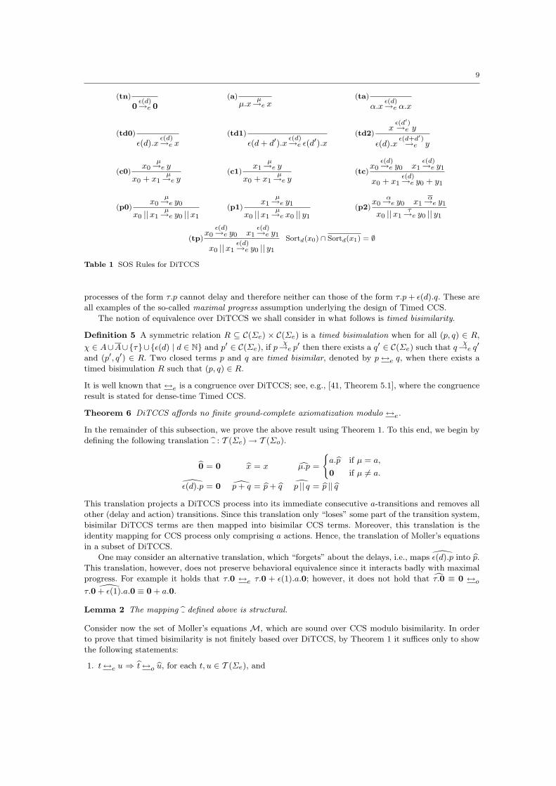
The operational semantics of DiTCCS is given by the set of SOS rules in Table 1, where α ∈ A ∪ A,

µ ∈ A ∪ A ∪ τ and d, d′ ∈ N. Those rules define transitions between closed DiTCCS terms. The side

condition in rule (tp) on Table 1 uses the timed sort Sortd(p), where p is a closed DiTCCS term and

d ∈ N, which is defined thus:

Sortd(p) = α ∈ A ∪A | p ε(d′)→e p′α→e for some p′ and d′ < d .

(The timed sort of a process can be defined structurally as in [41, Definition 4.1].) For example, the side

condition prevents the process ε(1).a.0 || a.0 from delaying for two time units. Note, furthermore, that

9

(tn)

0ε(d)→e 0

(a)µ.x

µ→e x(ta)

α.xε(d)→e α.x

(td0)

ε(d).xε(d)→e x

(td1)

ε(d + d′).xε(d)→e ε(d′).x

(td2)x

ε(d′)→e y

ε(d).xε(d+d′)→e y

(c0)x0

µ→e y

x0 + x1µ→e y

(c1)x1

µ→e y

x0 + x1µ→e y

(tc)x0

ε(d)→e y0 x1ε(d)→e y1

x0 + x1ε(d)→e y0 + y1

(p0)x0

µ→e y0

x0 ||x1µ→e y0 ||x1

(p1)x1

µ→e y1

x0 ||x1µ→e x0 || y1

(p2)x0

α→e y0 x1α→e y1

x0 ||x1τ→e y0 || y1

(tp)x0

ε(d)→e y0 x1ε(d)→e y1

x0 ||x1ε(d)→e y0 || y1

Sortd(x0) ∩ Sortd(x1) = ∅

Table 1 SOS Rules for DiTCCS

processes of the form τ.p cannot delay and therefore neither can those of the form τ.p + ε(d).q. These are

all examples of the so-called maximal progress assumption underlying the design of Timed CCS.

The notion of equivalence over DiTCCS we shall consider in what follows is timed bisimilarity.

Definition 5 A symmetric relation R ⊆ C(Σe) × C(Σe) is a timed bisimulation when for all (p, q) ∈ R,

χ ∈ A∪A∪τ∪ε(d) | d ∈ N and p′ ∈ C(Σe), if pχ→e p′ then there exists a q′ ∈ C(Σe) such that q

χ→e q′

and (p′, q′) ∈ R. Two closed terms p and q are timed bisimilar, denoted by p ↔e q, when there exists a

timed bisimulation R such that (p, q) ∈ R.

It is well known that ↔e is a congruence over DiTCCS; see, e.g., [41, Theorem 5.1], where the congruence

result is stated for dense-time Timed CCS.

Theorem 6 DiTCCS affords no finite ground-complete axiomatization modulo ↔e.

In the remainder of this subsection, we prove the above result using Theorem 1. To this end, we begin by

defining the following translation b : T (Σe) → T (Σo).

b0 = 0 bx = x cµ.p =

(a.bp if µ = a,

0 if µ 6= a.

ε(d).p = 0 p + q = bp + bq dp || q = bp || bqThis translation projects a DiTCCS process into its immediate consecutive a-transitions and removes all

other (delay and action) transitions. Since this translation only “loses” some part of the transition system,

bisimilar DiTCCS terms are then mapped into bisimilar CCS terms. Moreover, this translation is the

identity mapping for CCS process only comprising a actions. Hence, the translation of Moller’s equations

in a subset of DiTCCS.

One may consider an alternative translation, which “forgets” about the delays, i.e., maps ε(d).p into bp.

This translation, however, does not preserve behavioral equivalence since it interacts badly with maximal

progress. For example it holds that τ.0 ↔e τ.0 + ε(1).a.0; however, it does not hold that cτ.0 ≡ 0 ↔oτ.0 + ε(1).a.0 ≡ 0 + a.0.

Lemma 2 The mapping b defined above is structural.

Consider now the set of Moller’s equations M, which are sound over CCS modulo bisimilarity. In order

to prove that timed bisimilarity is not finitely based over DiTCCS, by Theorem 1 it suffices only to show

the following statements:

1. t↔e u ⇒ bt↔o bu, for each t, u ∈ T (Σe), and

10

2. b is M-reflecting.

For the proof of these two items, we make use of the following lemma.

Lemma 3

1. For all p ∈ C(Σe) and p′ ∈ C(Σo), if bp a→o p′ (i.e., with respect to the operational semantics of CCS),

then there exists some p′′ ∈ C(Σe) such that pa→e p′′ (i.e., with respect to the operational semantics of

DiTCCS), and cp′′ ≡ p′.2. For all p, p′ ∈ C(Σe), if p

a→e p′, then bp a→obp′.

Proof

1. We prove this item by structural induction on p.

– Assume that p ≡ 0. This case is trivial since bp does not afford an a-transition.

– Assume that p ≡ µ.p0. Then µ should be a, i.e., p must be of the form a.p0 (in order for bp to make

an a-transition) and thus, bp = a. bp0a→o bp0 = p′. The claim then follows since a.p0

a→e p0.

– Assume that p ≡ ε(d).p0. This case is trivial since then bp is not able to make an a-transition.

– Assume that p ≡ p0 +p1. Then bp ≡ bp0 + bp1. Suppose, without loss of generality, that the transitionbp0 + bp1a→o p′ is due to an application of rule (c0); thus, bp0

a→ p′. It then follows from the induction

hypothesis that p0a→e p′′ for some p′′ such that cp′′ ≡ p′. By applying deduction rule (c0), we

obtain p ≡ p0 + p1a→e p′′.

– The case p ≡ p0 || p1 is similar to the one above.

2. By an induction on the depth of the proof for pa→e p′. We distinguish the following cases based on the

last deduction rule applied to obtain pa→e p′. (We assume that a 6= τ .)

(a) In this case, p is of the form a.p0 and p′ ≡ p0 Thus, using the same deduction rule in the semantics

of CCS, we have bp ≡ a. bp0a→o bp0.

(c0) Then p ≡ p0 +p1 and p0a→e p′ by a shorter inference. It follows from the induction hypothesis thatbp0

a→obp′ and, using rule (c0) in the semantics of CCS, we infer that bp0 + bp1

a→obp′. Furthermore,

by the definition of b, we have that bp ≡ bp0 + bp1.

The cases for deduction rules (c1), (p0) and (p1) are similar to the case of (c0). ut

Next, we give the proofs of the above two statements.

1. Proof of t↔e u ⇒ bt↔o bu.

In order to prove this statement, it suffices to show that the relation

R = (σ(bt), σ(bu)) | t↔e u ∧ σ : V → C(Σo)

is a bisimulation. To this end, observe, first of all, that R is symmetric. Assume that σ(bt) R σ(bu) and

σ(bt) a→o p′0. By Lemmas 1 and 2, σ(bt) ≡ dσ(t). It follows from item 1 of Lemma 3 that σ(t)a→e p′′0 , for

some p′′0 such that cp′′0 ≡ p′0. Furthermore, as t and u are timed bisimilar, σ(u)a→e p′′1 , for some p′′1 such

that p′′0 ↔e p′′1 . From item 2 of Lemma 3 and Lemmas 1–2, we have that σ(bu) ≡ dσ(u)a→o

cp′′1 and, by

the definition of R, we may conclude that p′0 ≡ cp′′0 R cp′′1 , which was to be shown.

2. Proof of the fact that b is M-reflecting.

We show that all sound axioms (including those in M) are sound modulo ↔e. Since b is the identity

over CCS terms, the statement then follows immediately. To this end, we prove the following two

claims.

(a) For each p ∈ C(Σo) and positive integer d, pε(d)→e p′ iff p ≡ p′. We prove this claim by an induction

on the structure of p. The cases for 0 and a.p0 follow from deduction rules (tn) and (ta), respec-

tively. The cases for p0 + p1 and p0 || p1 follow from the induction hypothesis, and (tc) and (tp),

respectively. Note that in the case of (tp), it trivially holds that Sortd(p0)∩Sortd(p1) = ∅ because

the sorts of p0 and p1 can only contain action a (and no co-action).

11

(b) For each p, q ∈ C(Σo), if p↔o q then p↔e q.

We show that ↔o is a timed bisimulation. To this end, note, first of all, that the relation ↔o

is symmetric. Assume now that pa→e p′ and p↔o q. Using item 2 of Lemma 3 proved above, we

have that pa→o p′ (note that, since p is a CCS term, p′ will be a CCS term as well and hencebp′ ≡ p′). Since ↔o is a bisimulation, it follows that q

a→o q′ and hence qa→e q′ for some q′ such that

p′↔o q′, and we are done. That delay transitions of p may be matched by q follows trivially from

the previous item.

Since all the provisos of Theorem 1 are met, Theorem 6 follows.

4.3 Temporal CCS

In the paper [35], Moller and Tofts proposed another timed extension of Milner’s CCS, which they called

Temporal Calculus of Communicating Systems (referred to as TCCSMT in what follows to avoid any

confusion with Wang Yi’s Timed CCS), and studied its semantics theory modulo timed bisimilarity. Our

order of business in this section will be to use our reduction-based method to show that timed bisimilarity

affords no finite sound and ground-complete axiom system over TCCSMT.

For our purposes in this section, TCCSMT is the language generated by the following grammar:

P ::= 0 | µ.P | (d).P | δ.P | P + P | P ⊕ P | P ||P ,

where µ.P is a set of unary operators, one for each µ ∈ A∪A∪τ, and (d).P is a set of unary operators,

one for each positive integer d. The intuition underlying each of the operators in the signature of TCCSMT

is carefully described in [35, Pages 402–403]. For the sake of clarity, however, we find it useful to mention

that:

– process terms of the form 0 or α.p cannot delay, unlike in DiTCCS;

– (d).p behaves exactly like ε(d).p in DiTCCS;

– δ.p describes a process which behaves like p, but is willing to wait any amount of time before doing

so; and

– p ⊕ q is a “weak choice” between p and q. The choice between p and q is made upon performance

of an action from either of the two processes, or at the occurrence of a time delay which can only

be performed by one of the processes. By way of example, as a.p cannot delay, a process of the form

a.p⊕ (1).0 will be transformed into 0 after a delay of one time unit.

In order to define the operational semantics of the weak choice operator, the Plotkin-style rules for that

operator from [35] make use of the function maxdelay(), which associates a non-negative integer or ω

with each closed TCCSMT term. The function maxdelay() is defined by structural induction on terms as

follows:maxdelay(0) = maxdelay(µ.p) = 0 maxdelay(δ.p) = ω

maxdelay(p + q) = maxdelay(p || q) = min(maxdelay(p), maxdelay(q))

maxdelay(p⊕ q) = max(maxdelay(p), maxdelay(q)) .

The operational semantics of closed TCCSMT terms is given by means of two types of transitions, namely

actions transitionsµ→e with µ ∈ A ∪ A ∪ τ and delay transitions

ε(d)→e , with d ∈ N. The transition

relationsµ→e are defined as for DiTCCS; the action transitions of the new operators are briefly described

below.

– (d).p has no outgoing action transitions,

– p⊕ q has the same outgoing action transitions as p + q, and

– the action transitions of δ.p are exactly those of p—i.e., they are those provable using the rules

xµ→e y

δ.xµ→e y

(µ ∈ A ∪A ∪ τ) .

12

δ.xε(d)→e δ.x

(d).xε(d)→e x (d + d′).x

ε(d)→e (d′).x

xε(d′)→e y

(d).xε(d+d′)→e y

x0ε(d)→e y0 x1

ε(d)→e y1

x0 ⊕ x1ε(d)→e y0 ⊕ y1

x0ε(d)→e y0 maxdelay(x1) < d

x0 ⊕ x1ε(d)→e y0

x1ε(d)→e y1 maxdelay(x0) < d

x0 ⊕ x1ε(d)→e y1

x0ε(d)→e y0 x1

ε(d)→e y1

x0 + x1ε(d)→e y0 + y1

x0ε(d)→e y0 x1

ε(d)→e y1

x0 ||x1ε(d)→e y0 || y1

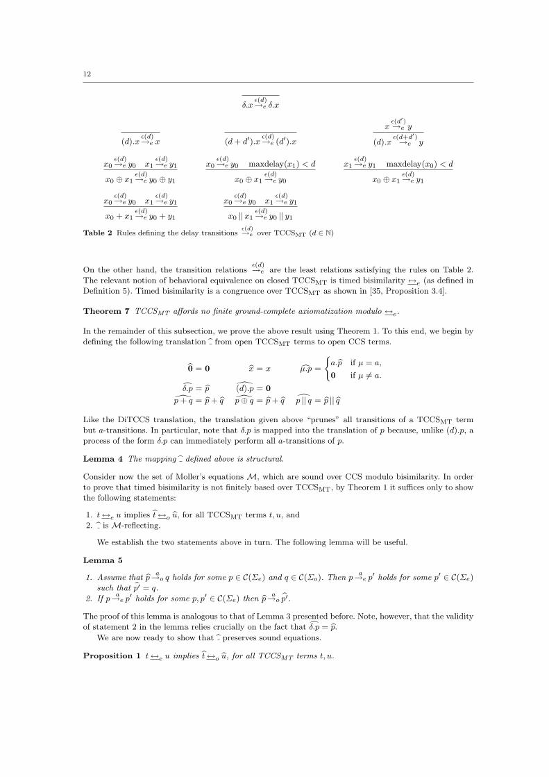
Table 2 Rules defining the delay transitionsε(d)→e over TCCSMT (d ∈ N)

On the other hand, the transition relationsε(d)→e are the least relations satisfying the rules on Table 2.

The relevant notion of behavioral equivalence on closed TCCSMT is timed bisimilarity ↔e (as defined in

Definition 5). Timed bisimilarity is a congruence over TCCSMT as shown in [35, Proposition 3.4].

Theorem 7 TCCSMT affords no finite ground-complete axiomatization modulo ↔e.

In the remainder of this subsection, we prove the above result using Theorem 1. To this end, we begin by

defining the following translation b from open TCCSMT terms to open CCS terms.

b0 = 0 bx = x cµ.p =

(a.bp if µ = a,

0 if µ 6= a.cδ.p = bp (d).p = 0

p + q = bp + bq p⊕ q = bp + bq dp || q = bp || bqLike the DiTCCS translation, the translation given above “prunes” all transitions of a TCCSMT term

but a-transitions. In particular, note that δ.p is mapped into the translation of p because, unlike (d).p, a

process of the form δ.p can immediately perform all a-transitions of p.


Consider now the set of Moller’s equations M, which are sound over CCS modulo bisimilarity. In order

to prove that timed bisimilarity is not finitely based over TCCSMT, by Theorem 1 it suffices only to show

the following statements:

1. t↔e u implies bt↔o bu, for all TCCSMT terms t, u, and


We establish the two statements above in turn. The following lemma will be useful.

Lemma 5

1. Assume that bp a→o q holds for some p ∈ C(Σe) and q ∈ C(Σo). Then pa→e p′ holds for some p′ ∈ C(Σe)

such that bp′ = q.

2. If pa→e p′ holds for some p, p′ ∈ C(Σe) then bp a→o

bp′.The proof of this lemma is analogous to that of Lemma 3 presented before. Note, however, that the validity

of statement 2 in the lemma relies crucially on the fact that cδ.p = bp.

We are now ready to show that b preserves sound equations.

Proposition 1 t↔e u implies bt↔o bu, for all TCCSMT terms t, u.

13

Proof It suffices to show that the relation

R = (bp, bq) | p↔e q, with p, q closed TCCSMT terms

is a strong bisimulation. Indeed, assuming that R is a strong bisimulation, we can show the proposition

as follows. As shown in Section 4.2, because b− is structural, once we prove that R is a bisimulation, it

holds that if t↔e u holds for some TCCSMT terms t, u, then bt↔o bu holds. So we are left to show that R

is indeed a strong bisimulation. This can be easily checked using Lemma 5. ut

To complete the proof of Theorem 7, we now show that b is M-reflecting. Since b is the identity function

over CCS terms, it suffices to prove the following result. (Note that, since CCS is a reduct of the language

TCCSMT, it makes sense to consider CCS terms modulo ↔e.)

Proposition 2 The relations ↔e and ↔o coincide over CCS terms.

Proof The relation ↔e is included in ↔o over the collection of CCS terms by Proposition 1. The converse

inclusion follows because ↔o is a timed bisimulation. This can be shown using Lemma 5 and observing

that pε(d)9 holds for each closed CCS term p and positive integer d. ut

Since all the provisos of Theorem 1 are met by our reduction, Theorem 7 follows.

4.4 ATP and Timed Bisimilarity

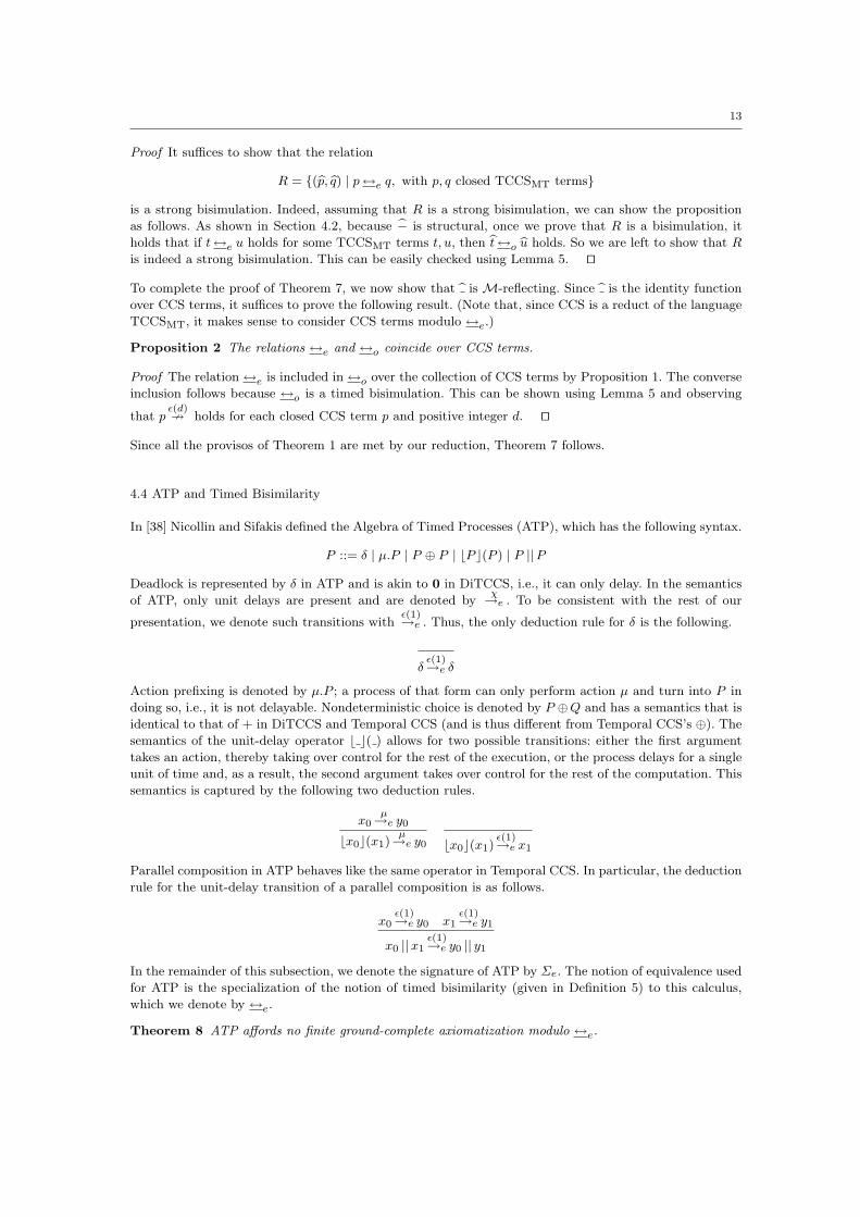
In [38] Nicollin and Sifakis defined the Algebra of Timed Processes (ATP), which has the following syntax.

P ::= δ | µ.P | P ⊕ P | bP c(P ) | P ||P

Deadlock is represented by δ in ATP and is akin to 0 in DiTCCS, i.e., it can only delay. In the semantics

of ATP, only unit delays are present and are denoted byχ→e . To be consistent with the rest of our

presentation, we denote such transitions withε(1)→e . Thus, the only deduction rule for δ is the following.

δε(1)→e δ

Action prefixing is denoted by µ.P ; a process of that form can only perform action µ and turn into P in

doing so, i.e., it is not delayable. Nondeterministic choice is denoted by P ⊕Q and has a semantics that is

identical to that of + in DiTCCS and Temporal CCS (and is thus different from Temporal CCS’s ⊕). The

semantics of the unit-delay operator b c( ) allows for two possible transitions: either the first argument

takes an action, thereby taking over control for the rest of the execution, or the process delays for a single

unit of time and, as a result, the second argument takes over control for the rest of the computation. This

semantics is captured by the following two deduction rules.

x0µ→e y0

bx0c(x1)µ→e y0 bx0c(x1)

ε(1)→e x1

Parallel composition in ATP behaves like the same operator in Temporal CCS. In particular, the deduction

rule for the unit-delay transition of a parallel composition is as follows.

x0ε(1)→e y0 x1

ε(1)→e y1

x0 ||x1ε(1)→e y0 || y1

In the remainder of this subsection, we denote the signature of ATP by Σe. The notion of equivalence used

for ATP is the specialization of the notion of timed bisimilarity (given in Definition 5) to this calculus,

which we denote by ↔e.

Theorem 8 ATP affords no finite ground-complete axiomatization modulo ↔e.

14

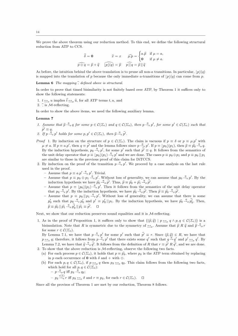
We prove the above theorem using our reduction method. To this end, we define the following structural

reduction from ATP to CCS.

bδ = 0 bx = x cµ.p =

(a.bp if µ = a,

0 if µ 6= a.

p⊕ q = bp + bq bpc(q) = bp dp || q = bp || bqAs before, the intuition behind the above translation is to prune all non-a transitions. In particular, bpc(q)is mapped into the translation of p because the only immediate a-transitions of bpc(q) can come from p.


In order to prove that timed bisimilarity is not finitely based over ATP, by Theorem 1 it suffices only to

show the following statements:

1. t↔e u implies bt↔o bu, for all ATP terms t, u, and


In order to show the above items, we need the following auxiliary lemma.

Lemma 7

1. Assume that bp a→o q for some p ∈ C(Σe) and q ∈ C(Σo), then pa→e p′, for some p′ ∈ C(Σe) such thatbp′ ≡ q.

2. If pa→e p′ holds for some p, p′ ∈ C(Σe), then bp a→e

bp′.Proof 1. By induction on the structure of p ∈ C(Σe). The claim is vacuous if p ≡ δ or p ≡ µ.p′ with

µ 6= a. If p ≡ a.p′, then q ≡ bp′ and the lemma follows since pa→e p′. If p ≡ bp0c(p1), then bp ≡ bp0

a→o q.

By the induction hypothesis, p0a→e p′, for some p′ such that bp′ ≡ q. It follows from the semantics of

the unit delay operator that p ≡ bp0c(p1)a→e p′ and we are done. The cases p ≡ p0⊕p1 and p ≡ p0 || p1

are similar to those in the previous proof of this claim for DiTCCS.

2. By induction on the proof of the transition pa→e p′. We proceed by a case analysis on the last rule

used in the proof.

– Assume that p ≡ a.p′a→e p′. Trivial.

– Assume that p ≡ p0 ⊕ p1a→e p′. Without loss of generality, we can assume that p0

a→e p′. By the

induction hypothesis we have bp0a→o

bp′. Thus, bp ≡ bp0 + bp1a→o

bp′.– Assume that p ≡ bp0c(p1)

a→e p′. Then it follows from the semantics of the unit delay operator

that p0a→e p′. By the induction hypothesis, we have bp0

a→obp′. Then bp ≡ bp0

a→obp′.

– Assume that p ≡ p0 || p1a→e p′, Without loss of generality, we can assume that there is some

p′0 such that p0a→e p′0 and p′ ≡ p′0 || p1. By the induction hypothesis, we have bp0

a→obp′0. Then,bp ≡ bp0 || bp1

a→obp′0 || bp1 ≡ bp′. ut

Next, we show that our reduction preserves sound equalities and it is M-reflecting.

1. As in the proof of Proposition 1, it suffices only to show that (bp, bq) | p ↔e q ∧ p, q ∈ C(Σe) is a

bisimulation. Note that R is symmetric due to the symmetry of ↔e. Assume that bp R bq and bp a→o r

for some r ∈ C(Σo).

By Lemma 7.1, we have that pa→e p′ for some p′ such that bp′ ≡ r. Since (bp, bq) ∈ R, we have that

p↔e q; therefore, it follows from pa→e p′ that there exists some q′ such that q

a→ q′ and p′ ↔e q′. By

Lemma 7.2, we have that bq a→obq′. It follows from the definition of R that r ≡ bp′ R bq′, and we are done.

2. To show that the above reduction is M-reflecting, observe the following two facts.

(a) For each process p ∈ C(Σo), it holds that p ≡ bpδ, where pδ is the ATP term obtained by replacing

in p each occurrence of 0 with δ and + with ⊕.

(b) For each p, q ∈ C(Σo), if p ↔o q then pδ ↔e qδ. This claim follows from the following two facts,

which hold for all p, q ∈ C(Σo):

– pa→o q iff pδ

a→e qδ;

– pδε(1)→e r iff pδ ↔e δ and r ≡ pδ, for each r ∈ C(Σe). ut

Since all the provisos of Theorem 1 are met by our reduction, Theorem 8 follows.

15

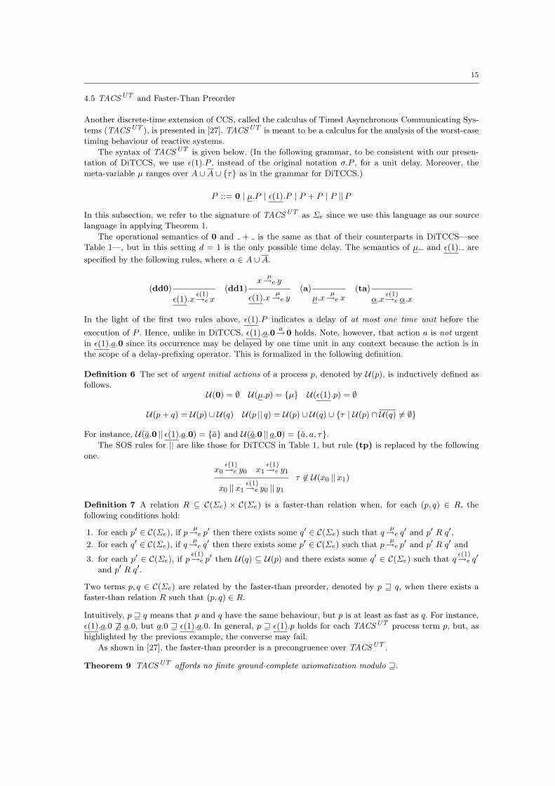
4.5 TACSUT and Faster-Than Preorder

Another discrete-time extension of CCS, called the calculus of Timed Asynchronous Communicating Sys-

tems (TACSUT ), is presented in [27]. TACSUT is meant to be a calculus for the analysis of the worst-case

timing behaviour of reactive systems.

The syntax of TACSUT is given below. (In the following grammar, to be consistent with our presen-

tation of DiTCCS, we use ε(1).P , instead of the original notation σ.P , for a unit delay. Moreover, the

meta-variable µ ranges over A ∪A ∪ τ as in the grammar for DiTCCS.)

P ::= 0 | µ.P | ε(1).P | P + P | P ||P

In this subsection, we refer to the signature of TACSUT as Σe since we use this language as our source

language in applying Theorem 1.

The operational semantics of 0 and + is the same as that of their counterparts in DiTCCS—see

Table 1—, but in this setting d = 1 is the only possible time delay. The semantics of µ. and ε(1). are

specified by the following rules, where α ∈ A ∪A.

(dd0)

ε(1).xε(1)→e x

(dd1)x

µ→e y

ε(1).xµ→e y

(a)µ.x

µ→e x(ta)

α.xε(1)→e α.x

In the light of the first two rules above, ε(1).P indicates a delay of at most one time unit before the

execution of P . Hence, unlike in DiTCCS, ε(1).a.0a→0 holds. Note, however, that action a is not urgent

in ε(1).a.0 since its occurrence may be delayed by one time unit in any context because the action is in

the scope of a delay-prefixing operator. This is formalized in the following definition.

Definition 6 The set of urgent initial actions of a process p, denoted by U(p), is inductively defined as

follows.U(0) = ∅ U(µ.p) = µ U(ε(1).p) = ∅

U(p + q) = U(p) ∪ U(q) U(p || q) = U(p) ∪ U(q) ∪ τ | U(p) ∩ U(q) 6= ∅

For instance, U(a.0 || ε(1).a.0) = a and U(a.0 || a.0) = a, a, τ.The SOS rules for || are like those for DiTCCS in Table 1, but rule (tp) is replaced by the following

one.

x0ε(1)→e y0 x1

ε(1)→e y1

x0 ||x1ε(1)→e y0 || y1

τ 6∈ U(x0 ||x1)

Definition 7 A relation R ⊆ C(Σe) × C(Σe) is a faster-than relation when, for each (p, q) ∈ R, the

following conditions hold:

1. for each p′ ∈ C(Σe), if pµ→e p′ then there exists some q′ ∈ C(Σe) such that q

µ→e q′ and p′ R q′,

2. for each q′ ∈ C(Σe), if qµ→e q′ then there exists some p′ ∈ C(Σe) such that p

µ→e p′ and p′ R q′ and

3. for each p′ ∈ C(Σe), if pε(1)→e p′ then U(q) ⊆ U(p) and there exists some q′ ∈ C(Σe) such that q

ε(1)→e q′

and p′ R q′.

Two terms p, q ∈ C(Σe) are related by the faster-than preorder, denoted by p w q, when there exists a

faster-than relation R such that (p, q) ∈ R.

Intuitively, p w q means that p and q have the same behaviour, but p is at least as fast as q. For instance,

ε(1).a.0 6w a.0, but a.0 w ε(1).a.0. In general, p w ε(1).p holds for each TACSUT process term p, but, as

highlighted by the previous example, the converse may fail.

As shown in [27], the faster-than preorder is a precongruence over TACSUT .

Theorem 9 TACSUT affords no finite ground-complete axiomatization modulo w.

16

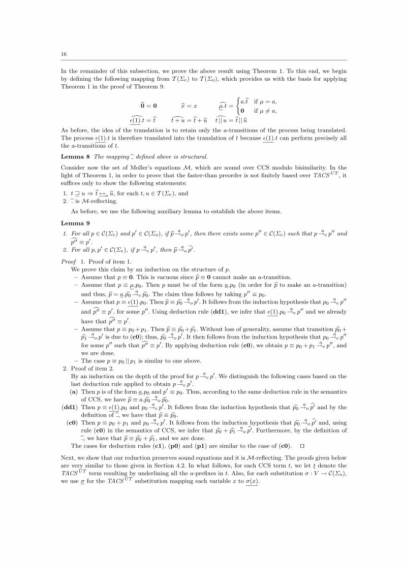
In the remainder of this subsection, we prove the above result using Theorem 1. To this end, we begin

by defining the following mapping from T (Σe) to T (Σo), which provides us with the basis for applying

Theorem 1 in the proof of Theorem 9.

b0 = 0 bx = x cµ.t =

(a.bt if µ = a,

0 if µ 6= a,

ε(1).t = bt t + u = bt + bu dt ||u = bt || buAs before, the idea of the translation is to retain only the a-transitions of the process being translated.

The process ε(1).t is therefore translated into the translation of t because ε(1).t can perform precisely all

the a-transitions of t.


Consider now the set of Moller’s equations M, which are sound over CCS modulo bisimilarity. In the

light of Theorem 1, in order to prove that the faster-than preorder is not finitely based over TACSUT , it

suffices only to show the following statements:

1. t w u ⇒ bt↔o bu, for each t, u ∈ T (Σe), and


As before, we use the following auxiliary lemma to establish the above items.

Lemma 9

1. For all p ∈ C(Σe) and p′ ∈ C(Σo), if bp a→o p′, then there exists some p′′ ∈ C(Σe) such that pa→e p′′ andcp′′ ≡ p′.

2. For all p, p′ ∈ C(Σe), if pa→e p′, then bp a→o

bp′.Proof 1. Proof of item 1.

We prove this claim by an induction on the structure of p.

– Assume that p ≡ 0. This is vacuous since bp ≡ 0 cannot make an a-transition.

– Assume that p ≡ µ.p0. Then p must be of the form a.p0 (in order for bp to make an a-transition)

and thus, bp = a. bp0a→e bp0. The claim thus follows by taking p′′ ≡ p0.

– Assume that p ≡ ε(1).p0. Then bp ≡ bp0a→o p′. It follows from the induction hypothesis that p0

a→e p′′

and cp′′ ≡ p′, for some p′′. Using deduction rule (dd1), we infer that ε(1).p0a→e p′′ and we already

have that cp′′ ≡ p′.– Assume that p ≡ p0 +p1. Then bp ≡ bp0 + bp1. Without loss of generality, assume that transition bp0 +bp1

a→o p′ is due to (c0); thus, bp0a→o p′. It then follows from the induction hypothesis that p0

a→e p′′

for some p′′ such that cp′′ ≡ p′. By applying deduction rule (c0), we obtain p ≡ p0 + p1a→e p′′, and

we are done.

– The case p ≡ p0 || p1 is similar to one above.

2. Proof of item 2.

By an induction on the depth of the proof for pa→e p′. We distinguish the following cases based on the

last deduction rule applied to obtain pa→e p′.

(a) Then p is of the form a.p0 and p′ ≡ p0. Thus, according to the same deduction rule in the semantics

of CCS, we have bp ≡ a. bp0a→o bp0.

(dd1) Then p ≡ ε(1).p0 and p0a→e p′. It follows from the induction hypothesis that bp0

a→obp′ and by the

definition of b, we have that bp ≡ bp0.

(c0) Then p ≡ p0 + p1 and p0a→e p′. It follows from the induction hypothesis that bp0

a→obp′ and, using

rule (c0) in the semantics of CCS, we infer that bp0 + bp1a→o

bp′. Furthermore, by the definition ofb, we have that bp ≡ bp0 + bp1, and we are done.

The cases for deduction rules (c1), (p0) and (p1) are similar to the case of (c0). ut

Next, we show that our reduction preserves sound equations and it is M-reflecting. The proofs given below

are very similar to those given in Section 4.2. In what follows, for each CCS term t, we let t denote the

TACSUT term resulting by underlining all the a-prefixes in t. Also, for each substitution σ : V → C(Σo),

we use σ for the TACSUT substitution mapping each variable x to σ(x).

17

1. Proof of t w u ⇒ bt↔o bu.

In order to prove this statement, it suffices to show that the symmetric closure of the relation

R = (σ(bt), σ(bu)) | t w u ∧ σ : V → C(Σo)

is a bisimulation. Assume now that σ(bt) R σ(bu) because t w u, and σ(bt) a→o p′0. Note that σ(bt) ≡ dσ(t)

by Lemmas 1 and 8. It follows from item 1 of Lemma 9 that σ(t)a→e p0, for some p0 such that bp0 ≡ p′0.

Furthermore, σ(u)a→e p1, for some p1 such that p0 w p1, since σ(t) w σ(u) because t w u. From item

2 of Lemma 9, Lemma 1 and Lemma 8, we have that dσ(u) ≡ σ(bu)a→o bp1 and, by the definition of R,

we may conclude that bp0 R bp1. A similar argument applies when σ(bt) R σ(bu) because u w t.

2. Proof of the fact that b is M-reflecting.

We show that all equations in M are sound modulo w once we underline all the occurrences of the

a-prefixing operator in CCS terms. (The statement then follows immediately since bt = t holds for each

CCS term t.) To this end, we prove the following two claims.

(a) For each p ∈ C(Σo), pε(1)→e p′ iff p ≡ p′. By an induction on the structure of p. The cases for 0

and a.p0 follow from deduction rules (tn) and (ta), respectively. The cases for p0 + p1 and p0 || p1

follow from (tc) and (tp) and the induction hypothesis, respectively. Note that p0 and p1 can only

afford a-transitions and hence deduction rule (tp) is always applicable.

(b) For each p, q ∈ C(Σo), p↔o q ⇒ p w q.

We show that the relation

R = (p, q) | p↔o q and p, q ∈ C(Σo)

satisfies the defining transfer properties for w (see Definition 7). To this end, assume that p R q

and pa→e r for some r. It is easy to see that p

a→o p′ for some p′ such that r = p′. It follows from

p↔o q that qa→o q′ for some q′ such that p′↔o q′. It is an immediate consequence of our embedding

that qa→e q′. Finally, r = p′ R q′ holds by the definition of R.

Furthermore, if pε(1)→e p′, it follows from the above item that p ≡ p′. Again using the above item,

we have that qε(1)→e q and, by assumption, p R q. It also follows immediately from p ↔o q that

U(p) = U(q), and we are done since the relation R is symmetric.


4.6 Other Timed Calculi, Equivalences and Preorders

There are many other timed extensions of CCS in the literature, and each of these languages comes

equipped with notions of behavioural equivalence and/or preorder. In this section, we introduce a couple

of the resulting process algebras studied in the research literature, and give the appropriate reductions to

prove their non-finite axiomatizability using Theorem 1. Since the proofs of the provisos of Theorem 1 are

almost identical to those in the previous two subsections, we dispense with them in this subsection.

TACSLT and the MT-preorder. In [28], Luttgen and Vogler introduced the language TACSLT , which is

syntactically the same as DiTCCS, but its only delay prefixing operator is ε(1). . Semantically, unlike

DiTCCS, TACSLT does not implement the so-called maximal progress and allows for time delays for

τ -prefixing, just like any other action prefixing. To obtain the SOS rules for TACSUT , one must take the

SOS rules of DiTCCS presented in Table 1, fix d = 1 in the rules for delay transitions, remove rules (td1)

and (td2), which do not apply when one only considers unit-delay transitions, and replace symbol α in

deduction rule (ta) by µ. This means that ε(1).P indicates a delay of at least one time unit before the

execution of P . Hence, like in DiTCCS and contrary to the situation in TACSUT , ε(1).aa9 . As argued by

Luttgen and Vogler, TACSLT is a calculus that is suitable for the study of lower bounds on the execution

speed of processes.

In this part of the paper, we refer to the signature of TACSLT as Σe since we use this language as

our source language in applying Theorem 1.

18

The notion of preorder that is considered over TACSLT in [28] is the MT-preorder due to Moller and

Tofts [36].

Definition 8 A relation R ⊆ C(Σe) × C(Σe) is an MT-relation, when for each (p, q) ∈ R, for each

p′ ∈ C(Σe), and action µ,

1. if pµ→e p′, then there exist a k ≥ 0 and q′, p′′ ∈ C(Σe) such that q

ε(1)→ek µ→e q′, p′

ε(1)→ekp′′ and p′′

A∼MT q′,

2. if pε(1)→e p′, then there exists a q′ ∈ C(Σe) such that q

ε(1)→e q′ and p′A∼MT q′,

3. if qµ→e q′, then there exists a p′ ∈ C(Σe) such that p

µ→e p′ and p′A∼MT q′, and

4. if qε(1)→e q′, then there exists a p′ ∈ C(Σe) such that p

ε(1)→e p′ and p′A∼MT q′.

Two terms p, q ∈ C(Σe) are related by the MT-preorder, denoted by pA∼MT q, when there exists an

MT-relation R such that (p, q) ∈ R.

As shown in [27, Theorem 2], the MT-preorder is a precongruence over TACSLT . Moreover,A∼MT coin-

cides with strong bisimilarity over CCS terms. It follows that the family of equations M is sound moduloA∼MT . These observations pave the way to the following result.

Theorem 10 TACSLT affords no finite ground-complete axiomatization moduloA∼MT .

The above result can, once more, be proved by instantiating Theorem 1. The function b from T (Σe) to

T (Σo) is identical to the same function for TACSUT , defined in Section 4.5, if one removes the underlinings

under the action and delay prefixes. It is not hard to show that b is an M-reflecting structural reduction,

from which Theorem 10 follows.

In proving that b is a reduction, the following lemma is used.

Lemma 10

1. For all p ∈ C(Σe) and r ∈ C(Σo), if bp a→o r, then there exist some k ≥ 0 and p′, p′′ ∈ C(Σe) such that

pε(1)→e

kp′a→e p′′ and cp′′ ≡ r.

2. For all p, p′, p′′ ∈ C(Σe) and k ≥ 0, if pε(1)→e

kp′a→ p′′, then bp a→o

cp′′.Remark 5 Since the operational semantics of TACSLT is very similar to that of DiTCCS, the attentive

reader might wonder why the reduction b we have defined for TACSLT handles terms of the form ε(1).t dif-

ferently from the reduction for DiTCCS, and why Lemma 10 takes a different form from the corresponding

ones for DiTCCS (Lemma 3) and TACSUT (Lemma 9). The reason is that a reduction b satisfying

ε(1).t = 0

would not preserve equations that are valid moduloA∼MT . By way of example, we have that

a.0A∼MT ε(1).a.0 .

However, a.0 is not bisimilar to 0, which would be the translation of ε(1).a.0 given by a reduction that

satisfies ε(1).t = 0.

The correspondence between the a-labelled transitions of bp and the transitions of p takes the form

stated in Lemma 10 because of the way the reduction is defined over terms of the form ε(1).t, and because,

unlike in TACSLT , the transitions from p in a term of the form ε(1).p can only be executed after at least

one time unit has passed. This means that, in order to mimic an a-labelled transition from bp, a process p

might have to embark first in a sequence of delays that “guard” the executed occurrence of action a in p.

ut

19

TACS and Urgent Timed Bisimulation. In [29], TACSUT and TACSLT were combined to obtain TACS .

In this calculus, the underlined prefixing operators, inherited from TACSUT , are used to model potentially

urgent actions and upper time bounds on action occurrences. The non-underlined prefixing operators,

inherited from TACSLT , are used to model lazy actions and lower time bounds on action occurrences.

In this part of the paper, we refer to the signature of TACS as Σe since we use this language as our

source language in applying Theorem 1.

The rules for the operational semantics of TACS are just a combination of those for TACSUT and

TACSLT . Finally, the set U(p) of urgent actions of a TACS process p is defined by structural induction

on processes in [29, Table 2, page 212]. The key clauses in such a definition are as follows:

U(µ.p) = µU(ε(1).p) = U(ε(1).p) = U(µ.p) = ∅ .

This is in agreement with the intuition that µ.p indicates the potential urgency of initial action µ, whereas

that action is lazy in any of the other prefixing contexts in TACS .

The notion of equivalence that is used for the full TACS calculus in [29] is urgent timed bisimilarity.

Definition 9 A symmetric relation R ⊆ C(Σe) × C(Σe) is an urgent timed bisimulation when for all

(p, q) ∈ R and p′ ∈ C(Σe),

1. for each µ ∈ A ∪A ∪ τ, if pµ→e p′ then there exists a q′ ∈ C(Σe) such that q

µ→e q′ and (p′, q′) ∈ R,

2. if pε(1)→e p′ then U(q) ⊆ U(p) and there exists a q′ ∈ C(Σe) such that q

ε(1)→e q′ and (p′, q′) ∈ R.

Urgent timed bisimilarity is the largest urgent timed bisimulation.

As shown in [29], urgent timed bisimilarity is a congruence over TACS . Moreover, urgent timed bisimilarity

coincides with strong bisimilarity over CCS terms. It follows that the family of equations M is sound

modulo urgent timed bisimilarity.

Theorem 11 TACS affords no finite ground-complete axiomatization modulo urgent timed bisimilarity.

The above result can, again, be proved by instantiating Theorem 1. The function b from T (Σe) to T (Σo)

is just a combination of the reductions for TACSUT and TACSLT , and is given below for the sake of

completeness. b0 = 0 bx = xca.t = ca.t = a.bt cµ.t = cµ.t = 0 for µ 6= a

ε(1).t = ε(1).t = bt t + u = bt + bu dt ||u = bt || buIt is not hard to show that b is an M-reflecting structural reduction, from which Theorem 10 follows. In

proving that b is a reduction, we use the extension of Lemma 10 to TACS .

4.7 Interactive Markov Chains and Markovian Bisimilarity

In [25], Hermanns presented the calculus of Interactive Markov Chains (IMC) to model and reason about

stochastic processes. The syntax of IMC (modulo minor notational changes) is given below:

P ::= 0 | µ.P | λ.P | P + P | P ||S

P ,

where µ ∈ A ∪ τ, λ ∈ R≥0 (we use R≥0 to denote the set of non-negative real numbers) and S ⊆ A.

Here 0 stands, as usual, for an inactive process. For each µ ∈ A ∪ τ, following Milner, µ.P represents

action prefixing. On the other hand, λ.P , with λ ∈ R≥0, is rate prefixing, meaning that before proceeding

with P there is a delay drawn from a negative exponentially-distributed random variable with rate λ.

Nondeterministic choice has its usual interpretation. IMC uses a CSP-like scheme for parallel composition,

i.e., in P ||S Q, the two processes run in parallel, but must synchronize on actions in S. Note that parallel

processes do not synchronize on the internal action τ and no internal action can be generated as the result

of a synchronization. In this subsection, we denote the signature of IMC by Σe.

20

The operational semantics of IMC is given by the following deduction rules, where β ranges over

A ∪ τ ∪ R≥0.

(β)β.x

β→e x(ic0)

x0β→e y

x0 + x1β→e y

(ic1)x1

β→e y

x0 + x1β→e y

(ip0)x0

β→e y0

x0 ||S x1β→e y0 ||S x1

β /∈ S (ip1)x1

β→e y1

x0 ||S x1β→e x0 ||S y1

β /∈ S (ip2)x0

β→e y0 x1β→e y1

x0 ||S x1β→e y0 ||S y1

β ∈ S

As discussed in, e.g., [25, Page 91], the above rules define a transition relationµ→e , for each action µ.

On the other hand, the rules should be read as defining a multi-relation when β ∈ R≥0. This ensures, for

instance, that two λ-labeled transitions are generated for any process of the form λ.p + λ.p, which should

be equivalent to 2λ.p. We refer the reader to [25] for a thorough discussion of this issue, which, however,

will be immaterial in the technical developments to follow.

For each closed term p and set of closed terms C, we define

γ(p, C) =X

λ | λ ∈ R≥0, pλ→e p′ and p′ ∈ C .

Note that

γ(λ.p + λ.p, p) = 2λ = γ(2λ.p, p) ,

sinceλ→e is a multi-relation.

A notion of behavioural equality for IMC is strong Markovian bisimilarity [25, Definition 5.2.1], which

is defined below for the sake of completeness.

Definition 10 An equivalence relation R ⊆ C(Σe)× C(Σe) is a strong Markovian bisimulation when for

all (p, q) ∈ R, p′ ∈ C(Σe), and µ ∈ A ∪ τ,

1. if pµ→e p′, then there exists a q′ ∈ C(Σe) such that q

µ→e q′ and (p′, q′) ∈ R, and

2. if pτ9e , then γ(p, C) = γ(q, C) for each equivalence class C ∈ C(Σe)/R.

Processes p, q ∈ C(Σe) are strongly Markovian bisimilar, denoted by p ↔e q, when there exists a strong

Markovian bisimulation R such that (p, q) ∈ R.

Note that, in the light of condition 2 in the above definition, delay rates are irrelevant for processes that

afford τ -labelled transitions. For instance, τ.p+λ.q↔e τ.p for all closed IMC terms p and q. This condition

in the definition strong Markovian bisimilarity implements a form of maximal progress.

As shown in [25], strong Markovian bisimilarity is a congruence over IMC. Moreover, in [25, Page 110]

Hermanns gave a complete axiomatization of strong Markovian bisimilarity over a language that includes

the fragment of IMC we consider here. That axiomatization, however, involves the use of an expansion-like

law—axiom (X) on Table 5.6 in [25]. It is therefore natural to ask oneself whether the use of an axiom

schema like (X) can be “simulated” by means of a finite collection of equations over the signature of IMC.

We now show that it cannot, as stated in the following theorem.

Theorem 12 Strong Markovian bisimilarity has no finite sound and ground-complete axiom system over

the language IMC.

The above theorem can be proved by applying Theorem 1. Since IMC uses CSP-style synchronization [26],

we have to slightly adapt our reduction. Namely, our reduction maps the τ actions of IMC to a visible a

action of CCS and removes all other actions.

In order to apply Theorem 1, we define the following translation from IMC terms, i.e., T (Σe), to CCS

terms (with a as the only action), i.e., T (Σo).

b0 = 0 bx = xcτ.p = a.bp cβ.p = 0 for β 6= τ, β ∈ A ∪ R≥0

p + q = bp + bq p ||S q = bp || bq

21


Consider now the set of Moller’s equations M, which are sound over CCS modulo bisimilarity. In the

light of Theorem 1, in order to prove that strong Markovian bisimilarity is not finitely based over IMC, it

suffices only to show the following statements:

1. t↔e u ⇒ bt↔o bu, for each t, u ∈ T (Σe), and


Once we prove the above claims, Theorem 12 follows as a corollary of Theorem 1. The proof of the former

claim is very similar to the proof of the same statement in the case of DiTCCS, and uses the following

lemma.

Lemma 12

1. Assume that bp a→o r holds for some p ∈ C(Σe) and r ∈ C(Σo). Then pτ→e p′ holds for some closed IMC

term p′ such that bp′ = r.

2. If pτ→e p′ for some p, p′ ∈ C(Σe), then bp a→o

bp′.Remark 6 Statement 2 in the above lemma would not hold if we translated a visible action a 6= τ in IMC

to action a in CCS, as we did in the previous subsections. For example, a.0 ||S a.0a→e 0 ||S 0 when a ∈ S.

However, a.0 || a.0a9o 0 ||0. Note, moreover, that a reduction such thatcλ.p = bp

would not preserve equations that are valid modulo strong Markovian bisimilarity since it would abstract

away from the role that maximal progress plays in the semantics of IMC. By way of example, consider

the valid equality

τ.τ.0 + λ.τ.0↔e τ.τ.0 .

This equation would be translated into the unsound equality

a.a.0 + a.0↔o a.a.0 .ut

In order to establish that b is M-reflecting, it suffices only to show that all axioms t = u in M are

sound modulo ↔e, once we replace all occurrences of || with ||∅ in CCS terms. Indeed, the statement then

follows by taking the IMC terms t∅ and u∅ that are obtained from t and u, respectively, by replacing each

occurrence of || with ||∅. Again, the proof is similar to that of similar claims in the previous sections, but

a few details are slightly different. We prove the following two statements, where, for each p ∈ C(Σo), p∅is the IMC term obtained from p by replacing each occurrence of || with ||∅.

1. For each p ∈ C(Σo) and non-negative real number λ, p∅λ9 . This means that γ(p∅, C) = 0 for each

C ∈ C(Σe)/↔e. (This claim is easily established by structural induction on p.)

2. For all p, q ∈ C(Σo), if p↔o q then p∅↔e q∅. (This follows because the relation

R = (p∅, q∅) | p↔o q and p, q ∈ C(Σo) ∪ (r, r) | r ∈ C(Σe)

is easily seen to be a strong Markovian bisimulation. Note that R is an equivalence relation over

C(Σe).)


5 Limitations and Extensions of Our Approach

As witnessed by the applications described in the previous section, our reduction-based method for proving

non-finite axiomatizability results, based on Theorem 1, is widely applicable. Moreover, in all the appli-

cations of Theorem 1 we presented in Section 4, we used CCS modulo bisimilarity as our target language

for an M-reflecting reduction. In this section, we give an example of an equational theory within the

realm of classic process algebra, whose non-finite axiomatizability cannot be shown in that fashion. An

analysis of the limitations of the basic reduction-based method we have employed so far will lead us to

the development of a sharpening of the results offered in Section 3.

22

5.1 CCSΩ and Prebisimilarity

Consider the following syntax for the language CCSΩ (a variant of the calculus presented in [7]).

P ::= 0 | Ω | a.P | P + P | P ||P

The operational semantics of CCSΩ is given by two ingredients:a→o transitions, which are defined by

the same deduction rules as in CCS (thus, Ω has no outgoing transitions), and a convergence predicate ↓,which is the least predicate over closed CCSΩ terms satisfying the rules given below.

0 ↓ a.p ↓

p ↓ q ↓

p + q ↓

p ↓ q ↓

p || q ↓

We write p ↑ if it does not hold that p ↓. So, for instance, a.Ω ↓, but Ω ↑ and a ||Ω ↑.The following notion of prebisimilarity is a relevant notion of behavioural preorder in the presence

of divergence as adopted in, e.g., [1,7,8,23,30]. We refer the interested reader to those papers and the

references therein for a wealth of results on the semantic theory of CCSΩ modulo prebisimilarity.

Definition 11 The relation@∼pre is the largest relation over the closed terms of CCSΩ satisfying the

following clauses, whenever p@∼pre q,

1. for each p′, if pa→o p′ then there exists a q′ such that q

a→o q′ and p′@∼pre q′;

2. if p ↓, then

(a) q ↓ and

(b) for each q′, if qa→o q′, then there exists a p′ such that p

a→o p′ and p′@∼pre q′.

The relation@∼pre is a preorder and a precongruence over closed CCSΩ terms.

Before we proceed with our results in this section, we introduce an auxiliary definition capturing the

concept of “convergence along all traces” of a process execution, which we call strong convergence.

Definition 12 The set of strongly convergent processes is the largest set of closed CCSΩ terms such that,

for each strongly convergent p, it holds that p ↓, and p′ is also strongly convergent whenever pa→o p′.

The following lemma will be useful in the technical developments in the rest of this section.

Lemma 13 The following statements hold.

1. For each CCSΩ term t, it holds that Ω@∼pre t.

2. For each two closed CCSΩ terms p and q, if p@∼pre q and p is strongly convergent, then q is also

strongly convergent.

3. Each closed CCSΩ term p is strongly convergent if and only if it is a CCS term—that is, if it does not

contain occurrences of Ω.

4. For each two CCS terms t and u, t@∼pre u if and only if t↔o u.

5.2 Non-finite Axiomatizability of@∼pre

Our order of business in this section will be to show that the inequational theory of CCSΩ modulo

prebisimilarity is not finitely axiomatizable. Moreover, we prove that CCSΩ modulo prebisimilarity affords

no finite sound and ground-complete axiom system. Afterwards, we prove that our meta-theorem comes

short of providing a proof for that result if we use CCS modulo bisimilarity as the target language of our

reduction.

Theorem 13 CCSΩ affords no finite sound and ground-complete axiom system modulo@∼pre .

23

Proof Assume, towards a contradiction, that E is a finite collection of sound axioms over CCSΩ modulo@∼pre , and that E is ground-complete. It follows from Lemma 13(4) that Moller’s set of equations M is

sound modulo@∼pre . Thus, we have that E ` M. Moreover, we may assume that each of the proofs of

equations in M from E only mentions closed terms.

Let E′ be the set of axioms contained in E that are used in the proofs of equations in M from E.

Claim Each axiom in E′ is an equation over the signature of CCS that is sound modulo ↔o.

Using this claim, a contradiction to Theorem 5 follows, since we have found a finite set of sound CCS

axioms, namely E′, which can prove all the equations in M.

To prove the above claim, observe that all the process terms involved in a proof of an equation in Mare strongly convergent (Lemma 13(2)). It follows that if t ≤ u is contained in E′, then Ω does not occur

in t and u (Lemma 13(3)). Therefore t and u are CCS terms, and the equation t = u is sound over CCS

modulo strong bisimilarity, since t ≤ u is sound over CCSΩ modulo@∼pre and CCS is a sub-language of

CCSΩ (Lemma 13(4)).

We may therefore conclude that CCSΩ affords no finite sound and ground-complete axiom system

modulo@∼pre . ut

It is natural to wonder whether the above result can be established, like all those we presented in Section 4,

by using CCS modulo bisimilarity as our target language for an M-reflecting reduction. The following

theorem shows that this is not possible.

Theorem 14 There is no M-reflecting reduction from CCSΩ modulo@∼pre to CCS modulo strong bisim-

ilarity.

Proof Consider a reduction b from CCSΩ modulo@∼pre to CCS modulo strong bisimilarity. This reduction

is a constant function modulo strong bisimilarity over CCSΩ terms. To see this, recall that, for each CCSΩ

term t, it holds that Ω@∼pre t (Lemma 13(1)). Since reductions preserve the validity of inequations (see

Definition 1), we have that bΩ is strongly bisimilar to bt, for each CCSΩ term t. This means that b is indeed

a constant function modulo strong bisimilarity, as claimed. A constant function modulo strong bisimilarity

is not M-reflecting since a1 ||(a1 + a2 + · · ·+ an) and a1 ||(a1 + a2 + · · ·+ am) are not strongly bisimilar

when n 6= m. ut

Remark 7 The attentive reader may have already observed that a stronger result than Theorem 14 does

in fact hold. Indeed, let E be a set of CCS equations that are sound modulo strong bisimilarity, and

contain two equations p1 = q1 and p2 = q2, where p1 and p2 are not strongly bisimilar. Then there is no

E-reflecting reduction from CCSΩ modulo@∼pre to CCS modulo strong bisimilarity. Indeed, as indicated

in the proof of Theorem 14, any reduction b from CCSΩ modulo@∼pre to CCS modulo strong bisimilarity

is a constant function modulo strong bisimilarity over CCSΩ terms. If b were E-reflecting, then

p1 = bt1 ↔obt2 = p2 ,

for some CCSΩ terms t1 and t2. This contradicts our assumption that p1 and p2 are not strongly bisimilar.

ut

5.3 Sharpening the Reduction Method

Our aim in this section will be to offer a sharpened version of the reduction-based method from Section 3

that will allow us to provide an alternative proof of Theorem 13. The sharpening of our method is inspired

by the realization that, as we observed in the previous section, the first requirement in Definition 1 is

too strong if we try to apply reductions to prove Theorem 13. Indeed, that requirement asks for the

preservation of each valid inequation over CCSΩ modulo prebisimilarity. This forces a reduction mapping

to be constant (modulo bisimilarity) and therefore notM-reflecting. If we examine the proof of Theorem 13

carefully, however, we can see that all closed proofs of equations in M that use inequations that are sound

24

modulo prebisimilarity can only employ (in)equations relating strongly convergent terms. This observation

suggests that, in order to prove that result using reductions, it would be useful to relax the first constraint

in Definition 1 so that it only requires that inequations satisfying certain properties be preserved. In the

specific setting of CCSΩ modulo prebisimilarity such inequations would be precisely those relating terms

that do not contain occurrences of Ω—that is, those relating CCS terms.

We now proceed to formalize these observations. Following the developments in Section 3, below we fix

two signatures Σo and Σe, a common set of variables V and two precongruences -o and -e over T (Σo)

and T (Σe), respectively. In addition, we assume that we have a unary predicate Pe over the collection of

Σe-inequations. The predicate Pe should satisfy the following closure property:

for each axiom system E over Σe and for each Σe-inequation t ≤ u such that Pe(t ≤ u), any

inequation that occurs in a proof of t ≤ u from E satisfies Pe as well. (In particular, only inequations

in E satisfying Pe can be used in such proofs.)

For example, consider the signature for CCSΩ as our Σe and prebisimilarity as -e. Then, in the light of

Lemma 13, the predicate Pe that is satisfied by an inequation t ≤ u if, and only if, both t and u do not

contain occurrences of Ω has the closure property stated above.

Definition 13 A function b : T (Σe) → T (Σo) is a Pe-reduction from T (Σe) to T (Σo), when for all

t, u ∈ T (Σe),

1. if t -e u and Pe(t ≤ u) then bt -o bu (that is, b preserves sound inequations satisfying the predicate

Pe), and

2. if E ` t ≤ u and Pe(t ≤ u) then bE ` bt ≤ bu, for each axiom system E over T (Σe) (that is, b preserves

provability of inequations satisfying the predicate Pe).

Definition 14 Let E be an axiom system over T (Σo). A Pe-reduction b is E-reflecting, when for each

t ≤ u ∈ E, there exists an inequation t′ ≤ u′ over T (Σe) that is sound modulo -e such that Pe(t′ ≤ u′),bt′ ≡ t and bu′ ≡ u. A Pe-reduction b is called ground E-reflecting if for each closed inequation p ≤ q ∈ E,

there exists a closed inequation p′ ≤ q′ on T (Σe) that is sound modulo -e such that Pe(p′ ≤ q′), bp′ ≡ p

and bq′ ≡ q.

The following result sharpens Theorems 1 and 3. (In the proof of the following theorem, for a set of

inequations E, we write Pe(E) to mean that each inequation in E satisfies Pe.)

Theorem 15 Assume that there is a set of inequations E over T (Σo) that is sound modulo -o and that is

not derivable from any finite sound axiom system over T (Σo). If there exists an E-reflecting Pe-reduction

from T (Σe) to T (Σo), then -e is not finitely based over T (Σe). Moreover, if E is a collection of closed

inequations and there exists a ground E-reflecting Pe-reduction from T (Σe) to T (Σo), then -e affords no

finite ground-complete axiomatization over T (Σe).

Proof We only prove the former statement since the proof of the latter follows similar lines.

Assume, towards a contradiction, that some finite axiom system F is sound and complete for T (Σe)

modulo -e. Let b be the E-reflecting Pe-reduction given by the proviso of the theorem, and let E′ be

the corresponding set of sound inequations (modulo -e) over T (Σe) such that cE′ = E and Pe(E′). It

follows from the soundness of E′ and the completeness of F that F ` E′. Let F ′ be the subset of F

used in proving the equations in E′. By the closure property of Pe, it holds that Pe(F′). By item 1 of

Definition 13 and the soundness of F ′ with respect to -e, the axiom system cF ′ is sound modulo -o. By

item 2 of Definition 13, cF ′ ` t ≤ u, for each t ≤ u ∈ E. Thus, there exists a finite sound axiom system

for T (Σo) modulo -o, namely cF ′, from which E can be derived. This contradicts the hypothesis of the

theorem. ut

Note that Theorem 15 subsumes Theorems 1 and 3, i.e., Theorems 1 and 3 are corollaries to Theorem 15,

by taking Pe to be true for each inequation on T (Σe).

The following theorem again shows that, if the reduction is structural, one can dispense with proving

item 2 of Definition 13. The result is shown as its sibling statement Theorem 2 using the closure property

of the predicate Pe when invoking the inductive hypothesis.

25

Theorem 16 A structural mapping satisfies item 2 of Definition 13.

We now argue how to obtain an alternative proof of Theorem 13 using Theorem 15. As already remarked,

the predicate Pe that is satisfied by an inequation t ≤ u over CCSΩ if, and only if, both t and u do not

contain occurrences of Ω has the closure property needed for applying Theorem 15. Consider the mapping

from CCSΩ to CCS that maps Ω to 0, is the identity over variables and is extended homomorphically to

the other terms. Such a mapping is structural, groundM-reflecting and, in the light of Lemma 13, preserves

inequations that are sound modulo prebisimilarity and satisfy Pe. We can therefore apply Theorem 15 to

derive that CCSΩ modulo prebisimilarity affords no finite ground-complete axiomatization.

6 Conclusions

In this paper, we have proposed a meta-theorem for proving non-finite axiomatizability results. This theo-

rem can be used to show such results when there exists a reduction from the calculus under consideration

to a calculus for which non-finite axiomatizability is known. If the reduction is defined structurally (in

the sense of Definition 3), then one only needs to prove that the reduction preserves sound (in)equalities

and that it reflects a set of “difficult” (in)equations that form the core of the non-finite axiomatizability

result over the target calculus. We have shown seven new non-finite axiomatizability results in process

algebra by applying our meta-theorem and reducing different calculi (modulo their respective notion of

equivalence or preorder) to a subset of CCS. We intend to apply our reduction technique to obtain several

other new non-finite axiomatizability results in process algebra.

The above-mentioned conditions on the reductions can be established following similar lines for the

different calculi and different notions of (pre)congruence studied in this paper. The resulting proofs are

substantially more concise and simpler than typical proofs of non-finite axiomatizability. We believe that

the proofs of the aforementioned two conditions can be further simplified if one commits to particular

models such as those given by Plotkin-style SOS rules. A promising future research direction is to study

whether one can apply our meta-theorem in conservative and orthogonal language extensions. Using

the SOS meta-theory, one can seek sufficient syntactic conditions on the reduction function that would

automatically provide us with the properties required by our meta-theorem.

Furthermore, in this paper, we pointed out a limitation of our original meta-theorem offered in Section 3

by presenting a non-finite axiomatizability result that cannot be proved using it. Studying the roots of such

a limitation led to the development of a sharpened version of our methods discussed in Section 5.3. The

application of our methods to more examples may lead to further improvements upon the meta-theorems

presented in this paper. We leave this interesting topic for further research.

Acknowledgments We thank the anonymous referees of IFIP TCS 2008 and Acta Informatica for their

careful reading of our paper and their comments, which led to improvements in both the technical results

and their presentation.

References

1. S. Abramsky. A domain equation for bisimulation. Information and Computation, 92(1):161–218, 1991.2. L. Aceto, T. Chen, W. Fokkink, and A. Ingolfsdottir. On the axiomatizability of priority. Proceedings of

Automata, Languages and Programming, 33rd International Colloquium, ICALP 2006, Venice, Italy, July 10-14, 2006, Part II, volume 4052 of LNCS, pages 480–491, Springer, 2006.

3. L. Aceto, W. Fokkink and A. Ingolfsdottir. Ready to preorder: Get your BCCSP axiomatization for free!Proceedings of CALCO’07, volume 4624 of LNCS, pages 338–367. Springer, 2007.

4. L. Aceto, W. Fokkink, A. Ingolfsdottir, and B. Luttik. CCS with Hennessy’s merge has no finite equationalaxiomatization. Theoretical Computer Science, 330(3):377–405, 2005.

5. L. Aceto, W. Fokkink, A. Ingolfsdottir, and B. Luttik. Finite equational bases in process algebra: Results andopen questions. In A. Middeldorp, V. van Oostrom, F. van Raamsdonk, and R. C. de Vrijer, editors, Processes,Terms and Cycles: Steps on the Road to Infinity, Essays Dedicated to Jan Willem Klop, on the Occasion ofHis 60th Birthday, volume 3838 of LNCS, pages 338–367. Springer, 2005.

6. L. Aceto, W. Fokkink, A. Ingolfsdottir, and S. Nain. Bisimilarity is not finitely based over BPA with interrupt.Theoretical Computer Science, 366(1–2):60–81, 2006.

7. L. Aceto and M. Hennessy. Termination, deadlock, and divergence. Journal of the ACM, 39(1):147–187, 1992.

26

8. L. Aceto, A. Ingolfsdottir. CPO models for compact GSOS languages. Information and Computation,129(1):107–141, 1996.

9. L. Aceto, A. Ingolfsdottir and M. R. Mousavi. Impossibility results for the equational theory of Timed CCS.Proceedings of CALCO’07, volume 4624 of LNCS, pages 80–95, Springer, 2007.

10. L. Aceto, W. Fokkink, and C. Verhoef. Structural operational semantics. In Handbook of Process Algebra,pages 197–292. North-Holland, 2001.

11. L. Aceto, W. Fokkink and C. Verhoef. Conservative extension in structural operational semantics. In G. Paun,G. Rozenberg and A. Salomaa, eds., Current Trends in Theoretical Computer Science - Entering the 21stCentury, pages 504–524, World Scientific, 2001.

12. J.C.M. Baeten and W. P. Weijland. Process Algebra. Cambridge University Press, 1990.13. J.A. Bergstra and J.W. Klop. Process algebra for synchronous communication. Information and Control,

60(1–3):109–137, 1984.14. S.C.C. Blom, W. Fokkink, J.F. Groote, I. van Langevelde, B. Lisser, and J.C. van de Pol. mCRL: A toolset

for analysing algebraic specifications. Proceedings of CAV’01, volume 2102 of LNCS, pages 250-254, Springer,2001.

15. S. L. Bloom and Z. Esik. Nonfinite axiomatizability of shuffle inequalities. Proceedings of TAPSOFT’95, volume915 of LNCS, pages 318–333. Springer, 1995.

16. T. Chen. Clocks, Dice and Processes. Ph.D. Thesis, Vrije Universiteit Amsterdam, 2009.17. T. Chen, W. Fokkink, and R. van Glabbeek. Ready to preorder: The case of weak process semantics. Information

Processing Letters, 109(2):104–111, 2009.18. D. de Frutos Escrig, C.G. Rodriguez and M. Palomino. Ready to preorder: An algebraic and general proof.

Journal of Logic and Algebraic Programming, to appear.19. Z. Esik and M. Bertol. Nonfinite axiomatizability of the equational theory of shuffle. Acta Informatica,

35(6):505–539, 1998.20. W. Fokkink and C. Verhoef. A conservative look at operational semantics with variable binding. Information

and Computation, 146(1):24-54, 1998.21. J. F. Groote, A. Mathijssen, M. Reniers, Y. Usenko, and M. van Weerdenburg. The formal specification language

mCRL2. In Proceedings of the Dagstuhl Seminar, 2007. Available from http://www.mcrl2.org.22. C. Gunter. Semantics of Programming Languages: Structures and Techniques. Foundations of Computing

Series. MIT Press, 1992.23. M. Hennessy. A term model for synchronous processes. Information and Control, 51(1):58–75, 1981.24. M. Hennessy. Algebraic Theory of Processes. Foundations of Computing Series. MIT Press, 1988.25. H. Hermanns. Interactive Markov Chains and the Quest for Quantified Quality. Volume 2428 of LNCS,

Springer, 2002.26. C.A.R. Hoare. Communicating Sequential Processes. Prentice Hall, 1985.27. G. Luttgen and W. Vogler. Bisimulation on speed: worst-case efficiency. Information and Computation, 191(2):

105–144, 2004.28. G. Luttgen and W. Vogler. Bisimulation on speed: Lower time bounds. Proceedings of FOSSACS’04, volume

2987 of LNCS, Springer, 2004.29. G. Luttgen and W. Vogler. Bisimulation on speed: A unified approach. Theoretical Computer Science, 360(1–

3):209-227, 2006.30. R. Milner. A modal characterisation of observable machine. Proceedings of CAAP’81, volume 112 of LNCS,

pages 25–34, Springer, 1981.31. R. Milner. Communication and Concurrency. Prentice Hall, 1989.32. F. Moller. Axioms for Concurrency. Ph.D. Thesis, University of Edinburgh, 1989.33. F. Moller. The nonexistence of finite axiomatisations for CCS congruences. In Proceedings, Fifth Annual IEEE

Symposium on Logic in Computer Science, pages 142–153. IEEE Computer Society, 1990.34. F. Moller. The importance of the left merge operator in process algebras. In Proceedings of ICALP’90, volume

443 of LNCS, pages 752–764. Springer, 1990.35. F. Moller and C.M.N. Tofts. A temporal calculus of communicating systems. In Proceedings of CONCUR’90,

volume 458 of LNCS, pages 401–415. Springer, 1990.36. F. Moller and C. Tofts. Relating processes with respect to speed. In Proceedings of CONCUR ’91, volume 527

of LNCS, pages 424–438. Springer, 1991.37. M.R. Mousavi and M.A. Reniers. Orthogonal extensions in structural operational semantics. Proceedings of

ICALP’05, volume 3580 of LNCS, pages 1214–1225, Springer, 2005.38. X. Nicollin, J. Sifakis. The algebra of timed processes, ATP: Theory and application. Information and Com-

putation, 114(1):131–178, 1994.39. G. D. Plotkin. A structural approach to operational semantics. Journal of Logic and Algebraic Programming,

60–61:17–139, 2004.40. M. Sipser. Introduction to the Theory of Computation. 2nd Ed., PWS Publishing, 2005.41. W. Yi. Real-time behaviour of asynchronous agents. In Proceedings of CONCUR’90, volume 458 of LNCS,

pages 502–520. Springer, 1990.

Lifting non-finite axiomatizability results to extensions of process algebras

Documents

Transcript of Lifting non-finite axiomatizability results to extensions of process algebras