Liberalized trade and domestic price stability. The case of rice and wheat in India

Journal of Development EconomicsŽ .Vol. 65 2001 417–441

www.elsevier.comrlocatereconbase

Liberalized trade and domestic price stability.The case of rice and wheat in India

P.V. Srinivasan, Shikha Jha)

( )Indira Gandhi Institute of DeÕelopment Research, General A.K. Vaidya Marg, Goregaon East ,Mumbai 400 065, India

Received 1 June 1998; accepted 1 December 2000

Abstract

This paper analyzes the effects of liberalizing foodgrain trade on domestic price stabilityusing a multi-market equilibrium model in which the direction of trade is determinedendogenously and world prices are sensitive to the amount traded by India. Simulationresults demonstrate that contrary to popular belief, freeing of trade by India leads to greaterdomestic price stability even though world prices are more volatile. Freeing of trade byIndia also leads to higher world price stability. Under liberalized trade, variable leviesrsub-sidies are more effective in stabilizing domestic prices compared to buffer stocks. It istherefore in India’s interest to argue for non-zero binding on import tariffs and exportsubsidies at the WTO negotiations. q 2001 Elsevier Science B.V. All rights reserved.

JEL classification: Q17; Q18Keywords: Trade liberalization; Foodgrain price stabilization; Rational expectations; Variable levies;Buffer stocks; WTO; GATT; Tariff bindings

1. Introduction

Instability in world market prices of foodgrains is much greater than domesticprice variability in India. There are therefore apprehensions to liberalizing food-grain trade as it could lead to increased domestic price variability and in turnincreased public costs of price stabilization. The issue of the impact of interna-tional price volatility on domestic price stability is difficult to resolve analytically.

) Corresponding author. Tel.: q91-22-8400919; fax: q91-22-8402752.Ž .E-mail address: [email protected] S. Jha .

0304-3878r01r$ - see front matter q2001 Elsevier Science B.V. All rights reserved.Ž .PII: S0304-3878 01 00143-2

( )P.V. SriniÕasan, S. JharJournal of DeÕelopment Economics 65 2001 417–441418

Ž . Ž .Greenaway et al. 1993 and Williams and Wright 1991, Chapter 9 demonstratethat even in stylized single commodity models it is difficult to get unambiguousresults. Outcomes depend on, among other things, the slopes of the excess demandand supply schedules, the relative size of production in the countries concernedand the correlation between production shocks. Such issues can be resolved at bestempirically through stochastic simulation exercises. For example, based on astochastic simulation model for a small open economy, Bigman and ReutlingerŽ .1979 suggest that international trade can provide domestic price stability at acost lower than that incurred in maintaining buffer stocks. The present studyexamines first the effect of liberalizing external trade in the two major foodgrains,rice and wheat, on their domestic price variability in the absence of any govern-ment intervention. It then considers the case where the government operates priceband stabilization schemes to stabilize domestic prices.

Under normal weather conditions, domestic output levels of rice and wheat inIndia are nearly sufficient to meet the domestic demand for these grains. Due toweather fluctuations, the country faces a situation of deficit in some years andsurplus in some others and thus it is neither a regular importer nor exporter. Thismeans that given the domestic demand for these grains and the export and importparity prices, trade will not take place quite often even without any restriction orcontrol on international trade. Thus, in the modeling framework used in ourstochastic simulation exercises, the direction of trade is determined endogenously.The model also incorporates private storage behavior with rational price expecta-tions as well as the effects that India’s exportsrimports can have on world rice

Ž .prices the ‘large country’ case . This latter feature is very important because ofthe small size of the world rice market and the amount traded by India can form aconsiderable proportion of total world trade so as to influence world prices. 1

The rest of the paper is organized as follows. Section 2 summarizes the Indianexperience with price stabilization and foreign trade in foodgrains. Section 3describes the model and the computational steps while Section 4 discusses theimpacts of free trade defined as liberalized external trade in the absence ofgovernment intervention. Section 5 analyzes the effects of trade liberalizationwhen government intervenes through price band stabilization policies. Section 6provides a summary of the findings and draws some conclusions.

2. Indian experience with food price stabilization and trade

The Indian government attaches a great importance to stabilizing grain pricesand income to farmers through price support policies as agricultural output varies

1 Indian exports of rice peaked at 5.6 million tonnes in 1995–1996 and again reached 4.9 milliontonnes in 1998–1999. This makes up a large fraction of total world trade in rice, which is of the orderof about 20 million tonnes.

( )P.V. SriniÕasan, S. JharJournal of DeÕelopment Economics 65 2001 417–441 419

largely with monsoons. In order to protect consumers’ interests, it attempts toprevent prices from reaching exorbitant levels through buffer stock operations andpublic distribution of fixed quotas of grains at subsidized prices. Given theseobjectives, grain storage forms an integral part of the government’s food policy.While part of the public stocks are meant for the operation of the subsidizeddistribution scheme and other welfare programs, the rest act as a buffer to counterfluctuations in production.

Ž .The Food Corporation of India FCI carries out the procurement, transport,storage and distribution operations on behalf of the government. High-pricesupport to farmers through procurement has led to a large grain stockholdingcausing a drain on the government’s resources. In late 1990s, the carrying cost of

Ž .buffer stocks grew at the rate of about 15% per annum Jha and Srinivasan, 2000 .But in spite of the high costs, there is a general preference for domestic bufferstocks over external trade to stabilize prices. This is due to the apprehension thatforeign markets can be unreliable sources of supply and demand and the higherprice variability in these markets may induce greater instability in domestic

2 Žprices. The coefficients of variation calculated as deviations from the trend for.the period 1964–1965 to 1994–1995 of domestic market prices of wheat and rice

are, respectively, 8.22% and 6.15%. The corresponding numbers for their borderprices are, respectively, 18.45% and 34.75%. The lower volatility of domesticprices could be partly due to price interventions by the government. Therefore, thecomparison is valid only if we consider the inherent volatility in domestic prices,which would prevail in the absence of government intervention. Domestic produc-tion of rice and wheat, for instance, is found to be much more unstable comparedto the instability in world production and in the absence of price interventiondomestic prices could possibly have been more unstable than world prices.3

However, using counterfactual simulations, we find that even in a situation wherethere is no government intervention and the economy is closed, domestic pricevariability is lower than world price variability. The coefficients of variation ofdomestic prices of rice and wheat are 16.7% and 13.9%, respectively, which arestill lower than the corresponding numbers for the border prices. This is becauseprice variability is determined not just by supply but also the demand factors.

Due to fears such as those expressed above, foreign trade in foodgrain has notbeen effectively used to reduce stabilization costs. Import of foodgrains wascanalized through the FCI. Exports were subject to quotas and were required to

2 Ž . Ž .See, among others, Dantwala 1993 and Nayyar and Sen 1994 . By simulating the effects of freeŽ .trade in rice in five Asian countries, Islam and Thomas 1996 show that free trade increases domestic

price variability to levels several times higher than historically observed.3 Ž .Ramesh 1998 shows that the instability indices of production of rice and wheat in India were,

respectively, 11.99% and 7.48% compared to the respective world figures of 2.52 and 5.03 for theperiod 1980–1993. The instability index is defined as the annual percent deviation from trend values.


fetch a specified minimum export price. Some of these restrictions have, however,been relaxed in recent years due to the mounting stocks of foodgrains with thegovernment and also due to market access requirement under the GATT agree-ment. In the light of the above discussion, we examine through simulationexercises the effects of liberalized international trade on domestic price variabilityin the scenarios of with and without government intervention.

3. The model

We use a dynamic stochastic simulation model with a multi-market equilibriumapproach where prices, consumption, production, trade and stocks of rice andwheat are all determined simultaneously.4 In contrast to a single-commoditymodel, a multi-commodity framework allows for substitution possibilities in bothconsumption and storage. An implication of the former possibility is that if theprice of one grain rises due to a shortage in the domestic economy, its importrequirements would be much less than if it was not possible to substitute the othergrain for it. With a joint storage capacity, for each grain there is a flexibility ofstoring more than would be the case if the capacities were individually specified.Thus, with the use of a multi-commodity set-up, it is possible to achieve a morerealistic picture of price stability. A description of various aspects of the model isprovided below.

3.1. Consumption

The aggregate demand equations for rice and wheat are calibrated using theŽ .elasticities estimated by Radhakrishna and Ravi 1994 . Demand for each grain

depends on its own price, price of the other grain and income, all relating to thecurrent period. We assume consumer incomes to be fixed over time. The ownprice elasticities of demand for rice and wheat are, respectively, y0.51 and y0.58and the cross-price elasticities are, respectively, 0.072 and 0.19.

3.2. Production

Aggregate supply response for each cereal is assumed to depend on ownexpected future market price with producers having rational price expectations.Price elasticity of supply at mean is 0.16 for rice and 0.09 for wheat.5 Forestimation purposes, these expectations are approximated by 1-year ahead fore-

4 Detailed steps involved in the computations can be obtained from the authors on request.5 Empirical estimations of this relationship included a time trend also. However, in the model

simulations, it is assumed that crop yields are stable with no technological change.


casts obtained from an ARIMA model fitted to the price series. In the computationof the model, however, domestic price expectations, which are common to bothproducers and private storage agents, are derived to be internally consistent based

Ž .on the procedure described in Williams and Wright 1991 .

3.3. PriÕate storage

Private storage agents are assumed to be risk neutral and have rational priceexpectations. Private storage satisfies the arbitrage equations obtained from ex-pected profit maximization.

y1p qkG 1qr E p , sp s0 1Ž . Ž . Ž .t t tq1 t

y1p qks 1qr E p , sp )0 2Ž . Ž . Ž .t t tq1 t

Žwhere, p is the current price, k the marginal cost of storage services assumedt. Ž .constant , E p the expected future price, r the interest rate and ‘sp’ thet tq1

amount of private storage.6 The optimal solution for storage is obtained using anumerical technique based on the recursive logic of stochastic dynamic program-ming. The expected future price appearing in the arbitrage equations for privatestorage is derived using the polynomial approximation procedure described in

Ž . 7Williams and Wright 1991, Chapter 3 .

3.4. GoÕernment behaÕior

The government provides price support to farmers and protects consumers fromunduly high prices by operating a price band stabilization policy. According to thispolicy, prices are maintained within a specified price band through either bufferstocks or variable leviesrsubsidies on trade. In the case of buffer stocks, there arestorage constraints. Limited capacity for physical storage of grain puts an upperbound on government stocks. In addition, the closing stocks cannot be negative.Thus, it may not be possible to keep prices within the price band whenever thesestorage constraints become binding. In the case of variable leviesrsubsidies, wehave two sets of simulations. In the first set, there are no constraints imposed onthe taxrsubsidy levels and hence prices are always maintained within the specifiedprice band.8 In the second one, in order to be consistent with GATT commitments,

6 In the simulation exercises, the marginal cost of storage, k is assumed to be Rs. 52 per quintal forboth rice and wheat and the interest rate r is taken to be 10%.

7 Ž .Miranda 1998 provides a comparison of different numerical methods used to solve the nonlinearrational expectations commodity market model.

8 There can however be some exceptions. For example, assume that a drought in the home countryoccurs at the same time when the rest of the world faces a drought situation and physical restrictionsare imposed on exports by countries in the rest of the world. Then, no matter how high the importsubsidy is, domestic prices may not be brought down. Such situations are ruled out in our simulations.


we impose the constraint for rice that import taxes and export subsidies cannot bepositive.9 In the case of wheat, however, India has set a tariff binding of 100% andtherefore in our simulations we set an upper bound of 100% for import tax. Forcomputational ease, we use the same bound for export subsidy on wheat. Althoughas per the Uruguay round agreement countries were required not to extend exportsubsidies to commodities, which were not subsidized in the base period Aexportsubsidies are allowed up to certain levels instead of being explicitly illegal as they

Ž .are for nonagricultural productsB Ingco, 1995 .

3.5. International trade

Private external trade in foodgrains is modeled under the large open economyassumption. That is, the import demand and export supply functions of the rest ofthe world are price elastic. Since the world rice market is thin and India is slowlyemerging as a major exporter, we need to consider the effect that Indian riceexports can have on world prices. In order to obtain this ‘large country’ effect, anelasticity of y0.14 is assumed for the short-run price responsiveness of world riceprice to increases in India’s trade. This elasticity is based on estimates from the

Ž .International Model for Policy Analysis of Commodities and Trade IMPACTŽ .developed at the International Food Policy Research Institute IFPRI . This gives

the percentage decrease in world rice price due to one million tonnes of additionalŽ .Indian exports as 4.7% as reported by Gardner and Rosegrant, 1996 . India’s

share in world wheat trade is very small and does not call for a large-economyassumption. However, in order to have uniformity in functional specification, weretain this assumption for wheat also, with a low elasticity of y0.001.10 In oursimulations, we assume the import and export elasticities to be the same. Weadjust the price received for Indian exports for the margins between the internalprice in India and the world price, which occur due to currency conversion,qualitative differences between the quoted world rice types, and transportation andother handling costs incurred in exporting rice onto the world market. These

Ž .margins for rice and wheat are taken from Pursell and Gupta 1996 . Given thetrade elasticities, commodities are shifted off or on the world market whenever themarginal revenue adjusted for transportation and transaction costs, falls short of orexceeds the current value of grain.

For a closed economy, equilibrium price is given by the inverse demandŽ .function depicted by the curve DD in Fig. 1 , which is a function of domestic

output of grain net of private and public storage. However, in a scenario where

9 In the recent negotiations under article XXVII of GATT, the Indian authorities have, however,succeeded in raising substantially the import tariff bound on rice.

10 This elasticity is based on the assumption that the elasticity of excess demand for wheat exportsŽ .with respect to price is unity Mitchell, 1996 . Since Indian wheat exports form around 0.1% of world

exports, this translates into an elasticity of y0.001 at the base year levels of exports.


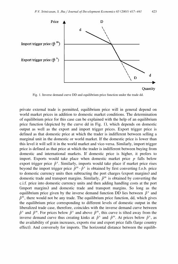
Fig. 1. Inverse demand curve DD and equilibrium price function under the trade dd.

private external trade is permitted, equilibrium price will in general depend onworld market prices in addition to domestic market conditions. The determinationof equilibrium price for this case can be explained with the help of an equilibrium

Ž .price function depicted by the curve dd in Fig. 1 , which depends on domesticoutput as well as the export and import trigger prices. Export trigger price isdefined as that domestic price at which the trader is indifferent between selling amarginal unit in the domestic or world market. If the domestic price is lower thanthis level it will sell it in the world market and vice-versa. Similarly, import triggerprice is defined as that price at which the trader is indifferent between buying fromdomestic and international markets. If domestic price is higher, it prefers toimport. Exports would take place when domestic market price p falls belowexport trigger price px. Similarly, imports would take place if market price risesˆbeyond the import trigger price pmPpx is obtained by first converting f.o.b. priceˆ ˆ

Ž .to domestic currency units then subtracting the port charges export margins anddomestic trade and transport margins. Similarly, pm is obtained by converting theˆc.i.f. price into domestic currency units and then adding handling costs at the portŽ .import margins and domestic trade and transport margins. So long as theequilibrium price given by the inverse demand function DD lies between px andˆpm, there would not be any trade. The equilibrium price function, dd, which givesˆthe equilibrium price corresponding to different levels of domestic output in theliberalized trade case, therefore, coincides with the inverse demand curve betweenpx and pm. For prices below px and above pm, this curve is tilted away from theˆ ˆ ˆ ˆinverse demand curve thus creating kinks at px and pm. At prices below px, asˆ ˆ ˆ

Žthe availability of grain increases, exports rise and export price falls large country.effect . And conversely for imports. The horizontal distance between the equilib-


rium price function and the inverse demand curve gives the amount importedŽ . m Ž x .exported when the equilibrium price is above p below p . The slopes of theˆ ˆequilibrium price function above pm and below px are calibrated using the importˆ ˆand export elasticities, respectively.

3.6. SolÕing for equilibrium

Equilibrium outcomes are computed for a sequence of 1000 periods withdifferent possible random realizations of domestic yields and border prices. Therealizations of these random variables are generated independently using a randomnumber generator.11 A discrete joint probability distribution is derived for devia-tions from trend values of domestic output of rice and wheat based on historicaldata. Similarly, another discrete joint probability distribution is derived for devia-tions from trend values of world prices of rice and wheat independent of the

12 Ž .earlier one. Prices in the rest-of-the-world ROW are assumed to be seriallyuncorrelated. Storage of grain by the rest of the world would, however, induceserial correlation in world prices. But, this effect is not taken into account in oursimulations. While it would be of interest to model storage behavior of the ROW,it is not attempted here since we do not have sufficient data to obtain demand andsupply relations for the ROW. Moreover, since the focus of this paper is on theeffect of liberalized trade on domestic price variability, importance is given tocapturing the interaction between domestic demands for the two grains than tomodeling storage behavior in the ROW.13

Equilibrium prices and quantities for each period are obtained by matchingŽcurrent availability with domestic consumption and storage demand public and

.private for each grain. Availability of grain in any period is defined as therealized production plus net imports in that period. Storage demand is the sum of

Žchanges in private and government stocks. Planned or expected output the supply.equation for any period is obtained as a function of the price expected for that

period. The realized production is obtained by adding to the expected output arandom deviation generated from the estimated probability distribution. Given the

11 Historical data shows a positive but low and statistically insignificant correlation between domesticoutput and world price fluctuations. From the data between 1964–1965 and 1994–1995, this correla-tion is found to be 0.267 for rice and 0.07 for wheat.

12 In the simulations, the import and export trigger prices are derived from the randomly generatedborder price. The equilibrium world market price, however, is determined endogenously since theinverse import demand and export supply functions in the model are responsive to changes in thequantity traded.

13 Ž .Makki et al. 1996 , e.g., incorporate in their model storage behavior of the US and EU, the twomajor exporters of wheat since their focus is on analyzing the impact of reduction in export subsidies.Another major difference between the two models is that Makki et al. in their model take the direction

Ž .of trade as given the US and EU export and the ROW imports whereas the determination of thedirection of trade is endogenous in our model.


availability of grains for the initial period, the demand and supply equations, theno-arbitrage conditions for private storage, the rules for government price stabi-lization program and the realizations of random world prices; the equilibriumprices, additions to stocks by private and government agencies, levels ofimportsrexports, etc., are all computed simultaneously, taking into account theirinterdependence. This exercise is repeated sequentially for 1000 periods. Themeans and variances of different variables including consumption, production,price, producer and consumer surplus, etc., are then derived to comment on thewelfare implications of different alternatives.

For each model scenario, there are two main steps involved in the simulationexercises.

Ž .1 Polynomial approximation: A reduced form relationship between expectedfuture price and current storage carryout is obtained using the polynomial approxi-mation procedure. The iterative procedure used for this purpose involves, solvingfor the entire model, for all possible states of nature for each round of iterations.According to this technique, the next period’s expected price is approximated by apolynomial in private storage, so that price expectations of storage agents areinternally consistent. In the scenarios where government storage is used tostabilize prices, expected price is approximated by a polynomial in two variables,private and public storage. Once such a polynomial is obtained, it is used in boththe output supply functions and the arbitrage equations to generate equilibriumprices and stocks.

Ž .2 Model simulations: Equilibrium values for each period are obtained sequen-tially. Starting with some initial values for expected price and carry-in of publicand private stocks and the realizations of shocks to domestic output and worldprices from a random number generator, all the endogenous variables of the modelare solved for simultaneously. The polynomial obtained in the first step is used insolving for private storage. The expected future price and private and public stockcarryout obtained from this solution replace the initial starting values for expectedprice and carry-in of public and private stocks, respectively, for the subsequent

Ž .period. This process is repeated for the desired number of periods simulations .

4. Implications of free trade

This section discusses the results for the scenario where there is no pricestabilizing intervention by the government. In this paper, the term ‘free trade’ isused to refer to the scenario where private traders are free to trade externally andthere is no government intervention of any kind. The term ‘liberalized trade’ isused to refer to the situation where private external trade is subject to pricestabilizing intervention by the government. The base year for the study is

Ž .1995–1996. Price variability is depicted by the coefficient of variation CV ofprices obtained from the 1000 period simulations. The combined variability of rice


and wheat prices is measured as a simple average of the CVs of their individualprices.

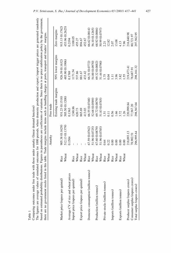
Historically, it is observed that domestic market clearing price is mostly belowthe export parity price for rice. In the case of wheat, domestic price is mostlybelow the import parity price and above the export parity price. In line with theseobservations, our simulations reveal that with liberalization of trade, the averagevolume of rice exports is greater than imports and domestic equilibrium price of

Ž .rice moves to a higher level Table 1 . The volume of wheat imports is greaterthan exports resulting in a lower domestic wheat price as compared to the case ofautarky. Exports take place more frequently than imports in the case of rice andvice versa in the case of wheat.

Due to freeing of trade, production of rice increases while there is not muchchange in that of wheat. Given the pattern of trade, domestic consumption of ricefalls marginally whereas that of wheat rises. With the possibility of exports,average private stocks of rice double and with liberalized imports of wheat

Ž .average private stocks reduce by half Table 1 . Producer surplus increases andconsumer surplus decreases, but there is a net increase in total surplus.

Since world prices are much more volatile than domestic prices, by linking thelatter to the former through liberalization of trade, there is a potential risk ofexposing domestic producers and consumers to greater price instability. In the caseof stable world prices, it is easy to see that price variability reduces due to freetrade. This follows from the shape of the equilibrium price curve in Fig. 1, whichsuggests that the price variations due to fluctuating domestic output get dampenedor remain unchanged due to free trade. The extent of reduction in price fluctua-tions depends on the level of exposure to trade, which is determined by thedistance between the export and import trigger prices, given the fluctuations indomestic output. For example, if the distance between export and import triggerprices is large enough such that equilibrium price is always between these twoprices, then there can be no effect on domestic price variability due to free trade.But as the trigger prices are brought closer, say through a reduction in exportrim-

Ž .port margins port charges, etc. , there would be a monotonic decrease in pricevariability. Thus, if world prices are stable, maximum reduction in price variabilitywill be achieved when all the relevant margins which drive a wedge betweendomestic and world prices are set to zero, that is, when both px and pm are equalˆ ˆto the border price. Note that in general, domestic and world market prices differ

Žfrom each other due to trade margins transportation to the port, port charges and.other handling charges . In addition to this, if government imposes any trade

taxrsubsidy, this would also contribute to the difference between domestic andworld prices.

In the case of unstable world prices, it is possible for price variability to eitherrise or fall with free trade. However, the simulation results show that even withunstable world prices, domestic price variability is lower under free trade com-

Ž .pared to autarky Table 1 .


Tab

le1

Ž.

Com

pari

ngou

tcom

esun

der

free

trad

ew

ithth

ose

unde

rau

tark

ylin

ear

dem

and

func

tion

The

figu

res

are

aver

age

valu

esof

sim

ulat

edou

tcom

esfo

r10

00pe

riod

s,w

here

dom

estic

prod

uctio

nan

dex

portr

impo

rttr

igge

rpr

ices

are

gene

rate

dra

ndom

lyba

sed

ones

timat

edpr

obab

ility

dist

ribu

tions

.Fig

ures

inpa

rent

hese

sar

eco

effi

cien

tsof

vari

atio

n.Si

nce

ther

eis

nopr

ice

stab

iliza

tion

polic

yby

the

gove

rnm

ent,

ther

ear

eno

gove

rnm

ent

stoc

kslis

ted

inth

ista

ble.

Tra

dem

argi

nsin

clud

eite

ms

such

asha

ndlin

gch

arge

sat

port

s,tr

ansp

ort

and

trad

ers’

mar

gins

.

Aut

arky

Free

trad

e

Exi

stin

gtr

ade

mar

gins

50%

low

erm

argi

nsZ

ero

mar

gins

Ž.

Ž.

Ž.

Ž.

Ž.

Mar

ketp

rice

rupe

espe

rqu

inta

lR

ice

905.

380.

1629

931.

230.

1518

926.

390.

1632

915.

130.

1762

Ž.

Ž.

Ž.

Ž.

Whe

at51

2.13

0.13

7950

5.50

0.12

0848

5.90

0.19

0645

3.96

0.26

25A

vera

geC

Vof

rice

and

whe

atpr

ices

0.15

040.

1363

0.17

690.

2194

Ž.

Impo

rtpr

ice

rupe

espe

rqu

inta

lR

ice

–12

48.8

611

71.5

411

00.0

5W

heat

–62

0.73

537.

8645

5.27

Ž.

Exp

ortp

rice

rupe

espe

rqu

inta

lR

ice

–86

5.69

881.

6789

4.67

Whe

at–

413.

0343

3.42

452.

67Ž

.Ž

.Ž

.Ž

.Ž

.D

omes

ticco

nsum

ptio

nm

illio

nto

nnes

Ric

e67

.59

0.07

6266

.55

0.07

4866

.51

0.07

7266

.62

0.08

14Ž

.Ž

.Ž

.Ž

.W

heat

51.9

60.

0725

52.6

80.

0589

54.0

00.

0970

56.1

00.

1265

Ž.

Ž.

Ž.

Ž.

Ž.

Prod

uctio

nm

illio

nto

nnes

Ric

e67

.60

0.08

7969

.72

0.08

7969

.32

0.08

8268

.92

0.08

86Ž

.Ž

.Ž

.Ž

.W

heat

51.9

60.

0785

51.8

30.

0785

51.4

40.

0790

50.9

90.

0797

Ž.

Priv

ate

stoc

ksm

illio

nto

nnes

Ric

e0.

641.

511.

752.

21W

heat

0.22

0.11

0.04

12.8

2Ž

.Im

port

sm

illio

nto

nnes

Ric

e0.

000.

561.

112.

07W

heat

0.00

1.66

3.96

13.0

8Ž

.E

xpor

tsm

illio

nto

nnes

Ric

e0.

003.

723.

824.

13W

heat

0.00

1.26

1.55

7.96

Ž.

Prod

ucer

surp

lus

rupe

escr

ores

218,

093.

1322

0,99

9.84

219,

473.

4121

6,84

0.98

Ž.

Con

sum

ersu

rplu

sru

pees

cror

es78

,902

.51

77,5

67.2

078

,687

.91

80,7

21.9

7Ž

.T

otal

surp

lus

rupe

escr

ores

296,

995.

6429

8,56

7.04

298,

161.

3229

7,56

2.95


4.1. SensitiÕity of the results to the specification of demand functions

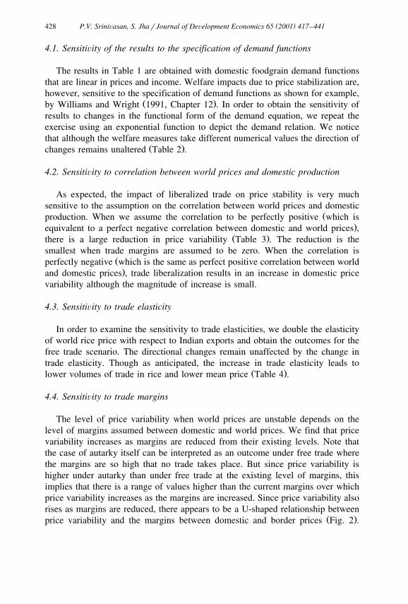
The results in Table 1 are obtained with domestic foodgrain demand functionsthat are linear in prices and income. Welfare impacts due to price stabilization are,however, sensitive to the specification of demand functions as shown for example,

Ž .by Williams and Wright 1991, Chapter 12 . In order to obtain the sensitivity ofresults to changes in the functional form of the demand equation, we repeat theexercise using an exponential function to depict the demand relation. We noticethat although the welfare measures take different numerical values the direction of

Ž .changes remains unaltered Table 2 .

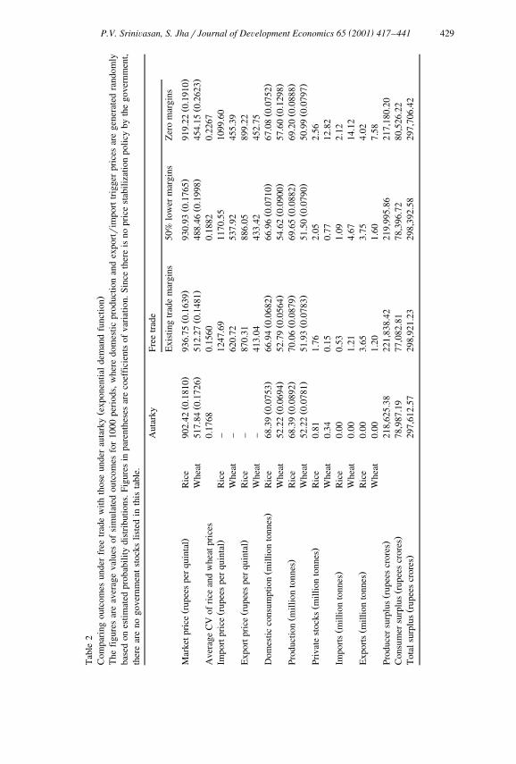
4.2. SensitiÕity to correlation between world prices and domestic production

As expected, the impact of liberalized trade on price stability is very muchsensitive to the assumption on the correlation between world prices and domestic

Žproduction. When we assume the correlation to be perfectly positive which is.equivalent to a perfect negative correlation between domestic and world prices ,

Ž .there is a large reduction in price variability Table 3 . The reduction is thesmallest when trade margins are assumed to be zero. When the correlation is

Žperfectly negative which is the same as perfect positive correlation between world.and domestic prices , trade liberalization results in an increase in domestic price

variability although the magnitude of increase is small.

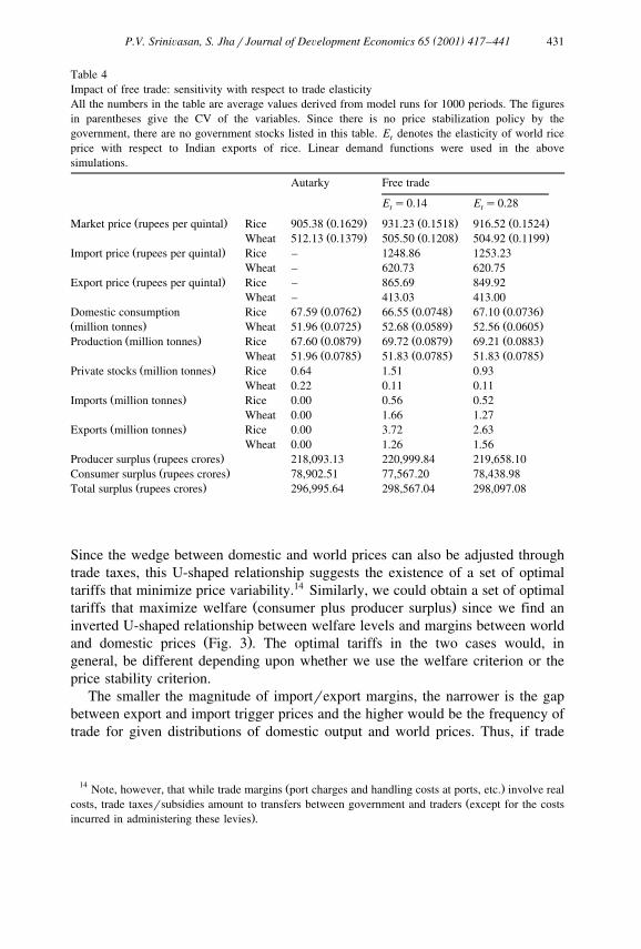
4.3. SensitiÕity to trade elasticity

In order to examine the sensitivity to trade elasticities, we double the elasticityof world rice price with respect to Indian exports and obtain the outcomes for thefree trade scenario. The directional changes remain unaffected by the change intrade elasticity. Though as anticipated, the increase in trade elasticity leads to

Ž .lower volumes of trade in rice and lower mean price Table 4 .

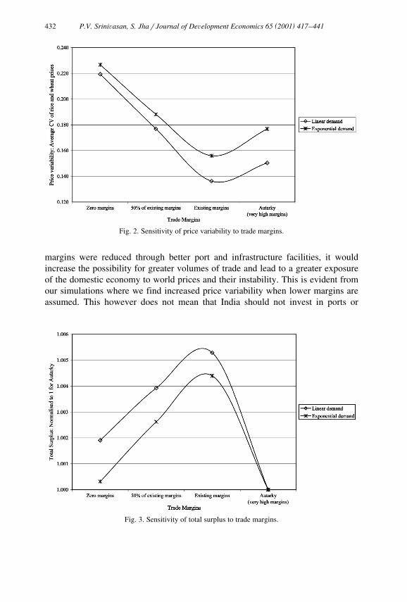
4.4. SensitiÕity to trade margins

The level of price variability when world prices are unstable depends on thelevel of margins assumed between domestic and world prices. We find that pricevariability increases as margins are reduced from their existing levels. Note thatthe case of autarky itself can be interpreted as an outcome under free trade wherethe margins are so high that no trade takes place. But since price variability ishigher under autarky than under free trade at the existing level of margins, thisimplies that there is a range of values higher than the current margins over whichprice variability increases as the margins are increased. Since price variability alsorises as margins are reduced, there appears to be a U-shaped relationship between

Ž .price variability and the margins between domestic and border prices Fig. 2 .


Tab

le2

Ž.

Com

pari

ngou

tcom

esun

der

free

trad

ew

ithth

ose

unde

rau

tark

yex

pone

ntia

lde

man

dfu

nctio

nT

hefi

gure

sar

eav

erag

eva

lues

ofsi

mul

ated

outc

omes

for

1000

peri

ods,

whe

redo

mes

ticpr

oduc

tion

and

expo

rtr

impo

rttr

igge

rpr

ices

are

gene

rate

dra

ndom

lyba

sed

ones

timat

edpr

obab

ility

dist

ribu

tions

.Fig

ures

inpa

rent

hese

sar

eco

effi

cien

tsof

vari

atio

n.Si

nce

ther

eis

nopr

ice

stab

iliza

tion

polic

yby

the

gove

rnm

ent,

ther

ear

eno

gove

rnm

ent

stoc

kslis

ted

inth

ista

ble.

Aut

arky

Free

trad

e

Exi

stin

gtr

ade

mar

gins

50%

low

erm

argi

nsZ

ero

mar

gins

Ž.

Ž.

Ž.

Ž.

Ž.

Mar

ketp

rice

rupe

espe

rqu

inta

lR

ice

902.

420.

1810

936.

750.

1639

930.

930.

1765

919.

220.

1910

Ž.

Ž.

Ž.

Ž.

Whe

at51

7.84

0.17

2651

2.27

0.14

8148

8.46

0.19

9845

4.15

0.26

23A

vera

geC

Vof

rice

and

whe

atpr

ices

0.17

680.

1560

0.18

820.

2267

Ž.

Impo

rtpr

ice

rupe

espe

rqu

inta

lR

ice

–12

47.6

911

70.5

510

99.6

0W

heat

–62

0.72

537.

9245

5.39

Ž.

Exp

ortp

rice

rupe

espe

rqu

inta

lR

ice

–87

0.31

886.

0589

9.22

Whe

at–

413.

0443

3.42

452.

75Ž

.Ž

.Ž

.Ž

.Ž

.D

omes

ticco

nsum

ptio

nm

illio

nto

nnes

Ric

e68

.39

0.07

5366

.94

0.06

8266

.96

0.07

1067

.08

0.07

52Ž

.Ž

.Ž

.Ž

.W

heat

52.2

20.

0694

52.7

90.

0564

54.6

20.

0900

57.6

00.

1298

Ž.

Ž.

Ž.

Ž.

Ž.

Prod

uctio

nm

illio

nto

nnes

Ric

e68

.39

0.08

9270

.06

0.08

7969

.65

0.08

8269

.20

0.08

88Ž

.Ž

.Ž

.Ž

.W

heat

52.2

20.

0781

51.9

30.

0783

51.5

00.

0790

50.9

90.

0797

Ž.

Priv

ate

stoc

ksm

illio

nto

nnes

Ric

e0.

811.

762.

052.

56W

heat

0.34

0.15

0.77

12.8

2Ž

.Im

port

sm

illio

nto

nnes

Ric

e0.

000.

531.

092.

12W

heat

0.00

1.21

4.67

14.1

2Ž

.E

xpor

tsm

illio

nto

nnes

Ric

e0.

003.

653.

754.

02W

heat

0.00

1.20

1.60

7.58

Ž.

Prod

ucer

surp

lus

rupe

escr

ores

218,

625.

3822

1,83

8.42

219,

995.

8621

7,18

0.20

Ž.

Con

sum

ersu

rplu

sru

pees

cror

es78

,987

.19

77,0

82.8

178

,396

.72

80,5

26.2

2Ž

.T

otal

surp

lus

rupe

escr

ores

297,

612.

5729

8,92

1.23

298,

392.

5829

7,70

6.42


Tab

le3

Impa

ctof

free

trad

eon

pric

est

abili

ty:

sens

itivi

tyto

corr

elat

ion

betw

een

dom

estic

outp

utan

dw

orld

pric

efl

uctu

atio

nsŽ

.T

henu

mbe

rsin

this

tabl

ear

eav

erag

eva

lues

deri

ved

from

mod

elru

nsfo

r10

00pe

riod

s.T

hefi

gure

sin

pare

nthe

ses

give

the

coef

fici

ento

fva

riat

ion

CV

ofth

eva

riab

les.

Aut

arky

Free

trad

e

Exi

stin

gtr

ade

mar

gins

50%

low

erm

argi

nsZ

ero

mar

gins

Per

fect

posi

tiÕe

corr

elat

ion

Ž.

Ž.

Ž.

Ž.

Ž.

Mar

ketp

rice

rupe

espe

rqu

inta

lR

ice

905.

380.

1629

946.

300.

0135

944.

140.

0226

939.

470.

0370

Ž.

Ž.

Ž.

Ž.

Whe

at51

2.13

0.13

7950

7.70

0.04

7949

9.21

0.10

7845

2.64

0.17

01A

vera

geC

Vof

rice

and

whe

atpr

ices

0.15

040.

0307

0.06

520.

1036

Per

fect

nega

tiÕe

corr

elat

ion

Ž.

Ž.

Ž.

Ž.

Ž.

Mar

ketp

rice

rupe

espe

rqu

inta

lR

ice

905.

380.

1629

945.

170.

1732

947.

920.

1721

940.

830.

1772

Ž.

Ž.

Ž.

Ž.

Whe

at51

2.13

0.13

7951

4.13

0.13

6550

7.54

0.15

5145

7.13

0.17

18A

vera

geC

Vof

rice

and

whe

atpr

ices

0.15

040.

1549

0.16

360.

1745


Table 4Impact of free trade: sensitivity with respect to trade elasticityAll the numbers in the table are average values derived from model runs for 1000 periods. The figuresin parentheses give the CV of the variables. Since there is no price stabilization policy by thegovernment, there are no government stocks listed in this table. E denotes the elasticity of world ricet

price with respect to Indian exports of rice. Linear demand functions were used in the abovesimulations.

Autarky Free trade

E s0.14 E s0.28t t

Ž . Ž . Ž . Ž .Market price rupees per quintal Rice 905.38 0.1629 931.23 0.1518 916.52 0.1524Ž . Ž . Ž .Wheat 512.13 0.1379 505.50 0.1208 504.92 0.1199

Ž .Import price rupees per quintal Rice – 1248.86 1253.23Wheat – 620.73 620.75

Ž .Export price rupees per quintal Rice – 865.69 849.92Wheat – 413.03 413.00

Ž . Ž . Ž .Domestic consumption Rice 67.59 0.0762 66.55 0.0748 67.10 0.0736Ž . Ž . Ž . Ž .million tonnes Wheat 51.96 0.0725 52.68 0.0589 52.56 0.0605

Ž . Ž . Ž . Ž .Production million tonnes Rice 67.60 0.0879 69.72 0.0879 69.21 0.0883Ž . Ž . Ž .Wheat 51.96 0.0785 51.83 0.0785 51.83 0.0785

Ž .Private stocks million tonnes Rice 0.64 1.51 0.93Wheat 0.22 0.11 0.11

Ž .Imports million tonnes Rice 0.00 0.56 0.52Wheat 0.00 1.66 1.27

Ž .Exports million tonnes Rice 0.00 3.72 2.63Wheat 0.00 1.26 1.56

Ž .Producer surplus rupees crores 218,093.13 220,999.84 219,658.10Ž .Consumer surplus rupees crores 78,902.51 77,567.20 78,438.98

Ž .Total surplus rupees crores 296,995.64 298,567.04 298,097.08

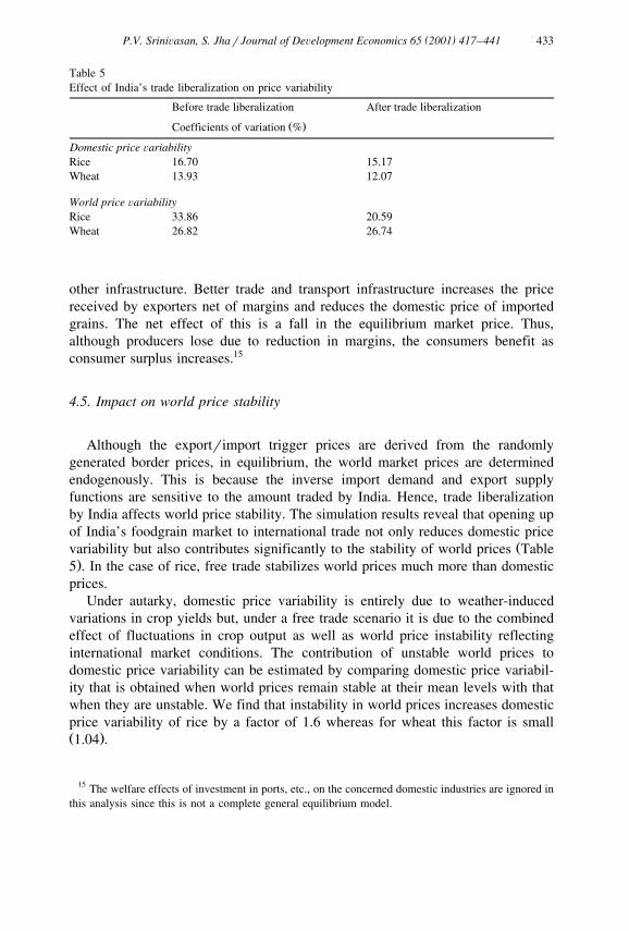
Since the wedge between domestic and world prices can also be adjusted throughtrade taxes, this U-shaped relationship suggests the existence of a set of optimaltariffs that minimize price variability.14 Similarly, we could obtain a set of optimal

Ž .tariffs that maximize welfare consumer plus producer surplus since we find aninverted U-shaped relationship between welfare levels and margins between world

Ž .and domestic prices Fig. 3 . The optimal tariffs in the two cases would, ingeneral, be different depending upon whether we use the welfare criterion or theprice stability criterion.

The smaller the magnitude of importrexport margins, the narrower is the gapbetween export and import trigger prices and the higher would be the frequency oftrade for given distributions of domestic output and world prices. Thus, if trade

14 Ž .Note, however, that while trade margins port charges and handling costs at ports, etc. involve realŽcosts, trade taxesrsubsidies amount to transfers between government and traders except for the costs

.incurred in administering these levies .


Fig. 2. Sensitivity of price variability to trade margins.

margins were reduced through better port and infrastructure facilities, it wouldincrease the possibility for greater volumes of trade and lead to a greater exposureof the domestic economy to world prices and their instability. This is evident fromour simulations where we find increased price variability when lower margins areassumed. This however does not mean that India should not invest in ports or

Fig. 3. Sensitivity of total surplus to trade margins.


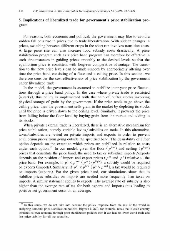
Table 5Effect of India’s trade liberalization on price variability

Before trade liberalization After trade liberalization

Ž .Coefficients of variation %

Domestic price ÕariabilityRice 16.70 15.17Wheat 13.93 12.07

World price ÕariabilityRice 33.86 20.59Wheat 26.82 26.74

other infrastructure. Better trade and transport infrastructure increases the pricereceived by exporters net of margins and reduces the domestic price of importedgrains. The net effect of this is a fall in the equilibrium market price. Thus,although producers lose due to reduction in margins, the consumers benefit asconsumer surplus increases.15

4.5. Impact on world price stability

Although the exportrimport trigger prices are derived from the randomlygenerated border prices, in equilibrium, the world market prices are determinedendogenously. This is because the inverse import demand and export supplyfunctions are sensitive to the amount traded by India. Hence, trade liberalizationby India affects world price stability. The simulation results reveal that opening upof India’s foodgrain market to international trade not only reduces domestic price

Žvariability but also contributes significantly to the stability of world prices Table.5 . In the case of rice, free trade stabilizes world prices much more than domestic

prices.Under autarky, domestic price variability is entirely due to weather-induced

variations in crop yields but, under a free trade scenario it is due to the combinedeffect of fluctuations in crop output as well as world price instability reflectinginternational market conditions. The contribution of unstable world prices todomestic price variability can be estimated by comparing domestic price variabil-ity that is obtained when world prices remain stable at their mean levels with thatwhen they are unstable. We find that instability in world prices increases domesticprice variability of rice by a factor of 1.6 whereas for wheat this factor is smallŽ .1.04 .

15 The welfare effects of investment in ports, etc., on the concerned domestic industries are ignored inthis analysis since this is not a complete general equilibrium model.


5. Implications of liberalized trade for government’s price stabilization pro-gram

For reasons, both economic and political, the government may like to avoid asudden fall or a rise in prices due to trade liberalization. With sudden changes inprices, switching between different crops in the short run involves transition costs.A large price rise can also increase food subsidy costs drastically. A pricestabilization program such as a price band program can therefore be effective insuch circumstances in guiding prices smoothly to the desired levels so that theequilibrium price is consistent with long-run comparative advantage. The transi-tion to the new price levels can be made smooth by appropriately altering overtime the price band consisting of a floor and a ceiling price. In this section, wetherefore consider the cost effectiveness of price stabilization by the governmentunder liberalized trade.

In the model, the government is assumed to stabilize inter-year price fluctua-tions through a price band policy. In the case where private trade is restrictedŽ .autarky , this policy is implemented with the help of buffer stocks involvingphysical storage of grain by the government. If the price tends to go above theceiling price, then the government sells grain in the market by depleting its stocksuntil the price is driven down to the ceiling level. Similarly, it prevents the pricefrom falling below the floor level by buying grain from the market and adding toits stocks.

When private external trade is liberalized, there is an alternative mechanism forprice stabilization, namely variable leviesrsubsidies on trade. In this alternative,taxesrsubsidies are levied on private imports and exports in order to preventequilibrium prices from going outside the specified band. The desirability of eitheroption depends on the extent to which prices are stabilized in relation to costs

16 Ž low . Ž high.under each option. In our model, given the floor p and ceiling pprices that constitute the price band, the need to tax or subsidize importsrexports

Ž m x .depends on the position of import and export prices p and p relative to thex low Ž m high.price band. For example, if p -p p )p , a subsidy would be required

Ž . m low Ž x high.on exports imports . Similarly, if p -p p )p , a tax would be requiredŽ .on imports exports . For the given price band, our simulations show that to

stabilize prices subsidies on imports are needed more frequently than taxes onimports. A similar statement applies to exports. The average rate of subsidy is alsohigher than the average rate of tax for both exports and imports thus leading topositive net government costs on an average.

16 In this study, we do not take into account the policy response from the rest of the world inŽ .analyzing domestic price stabilization policies. Bigman 1980 , for example, notes that if each country

insulates its own economy through price stabilization policies then it can lead to lower world trade andless price stability for all the countries.


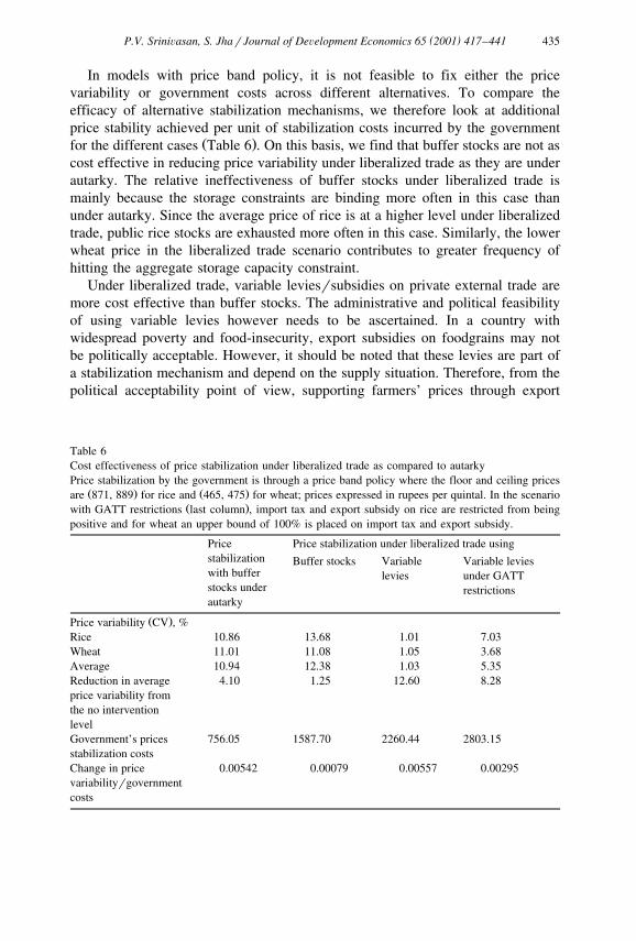
In models with price band policy, it is not feasible to fix either the pricevariability or government costs across different alternatives. To compare theefficacy of alternative stabilization mechanisms, we therefore look at additionalprice stability achieved per unit of stabilization costs incurred by the government

Ž .for the different cases Table 6 . On this basis, we find that buffer stocks are not ascost effective in reducing price variability under liberalized trade as they are underautarky. The relative ineffectiveness of buffer stocks under liberalized trade ismainly because the storage constraints are binding more often in this case thanunder autarky. Since the average price of rice is at a higher level under liberalizedtrade, public rice stocks are exhausted more often in this case. Similarly, the lowerwheat price in the liberalized trade scenario contributes to greater frequency ofhitting the aggregate storage capacity constraint.

Under liberalized trade, variable leviesrsubsidies on private external trade aremore cost effective than buffer stocks. The administrative and political feasibilityof using variable levies however needs to be ascertained. In a country withwidespread poverty and food-insecurity, export subsidies on foodgrains may notbe politically acceptable. However, it should be noted that these levies are part ofa stabilization mechanism and depend on the supply situation. Therefore, from thepolitical acceptability point of view, supporting farmers’ prices through export

Table 6Cost effectiveness of price stabilization under liberalized trade as compared to autarkyPrice stabilization by the government is through a price band policy where the floor and ceiling prices

Ž . Ž .are 871, 889 for rice and 465, 475 for wheat; prices expressed in rupees per quintal. In the scenarioŽ .with GATT restrictions last column , import tax and export subsidy on rice are restricted from being

positive and for wheat an upper bound of 100% is placed on import tax and export subsidy.

Price Price stabilization under liberalized trade usingstabilization Buffer stocks Variable Variable levieswith buffer levies under GATTstocks under restrictionsautarky

Ž .Price variability CV , %Rice 10.86 13.68 1.01 7.03Wheat 11.01 11.08 1.05 3.68Average 10.94 12.38 1.03 5.35Reduction in average 4.10 1.25 12.60 8.28price variability fromthe no interventionlevelGovernment’s prices 756.05 1587.70 2260.44 2803.15stabilization costsChange in price 0.00542 0.00079 0.00557 0.00295variabilityrgovernmentcosts


subsidies is not very different from the current situation where large public stocksof foodgrains co-exist with widespread poverty and hunger.

5.1. SensitiÕity of the results to cross-price elasticity of demand

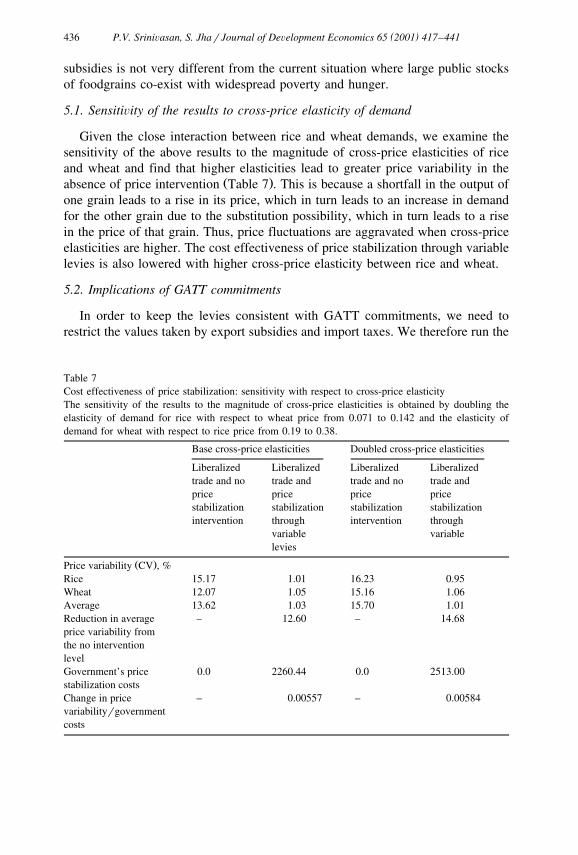
Given the close interaction between rice and wheat demands, we examine thesensitivity of the above results to the magnitude of cross-price elasticities of riceand wheat and find that higher elasticities lead to greater price variability in the

Ž .absence of price intervention Table 7 . This is because a shortfall in the output ofone grain leads to a rise in its price, which in turn leads to an increase in demandfor the other grain due to the substitution possibility, which in turn leads to a risein the price of that grain. Thus, price fluctuations are aggravated when cross-priceelasticities are higher. The cost effectiveness of price stabilization through variablelevies is also lowered with higher cross-price elasticity between rice and wheat.

5.2. Implications of GATT commitments

In order to keep the levies consistent with GATT commitments, we need torestrict the values taken by export subsidies and import taxes. We therefore run the

Table 7Cost effectiveness of price stabilization: sensitivity with respect to cross-price elasticityThe sensitivity of the results to the magnitude of cross-price elasticities is obtained by doubling theelasticity of demand for rice with respect to wheat price from 0.071 to 0.142 and the elasticity ofdemand for wheat with respect to rice price from 0.19 to 0.38.

Base cross-price elasticities Doubled cross-price elasticities

Liberalized Liberalized Liberalized Liberalizedtrade and no trade and trade and no trade andprice price price pricestabilization stabilization stabilization stabilizationintervention through intervention through

variable variablelevies

Ž .Price variability CV , %Rice 15.17 1.01 16.23 0.95Wheat 12.07 1.05 15.16 1.06Average 13.62 1.03 15.70 1.01Reduction in average – 12.60 – 14.68price variability fromthe no interventionlevelGovernment’s price 0.0 2260.44 0.0 2513.00stabilization costsChange in price – 0.00557 – 0.00584variabilityrgovernmentcosts


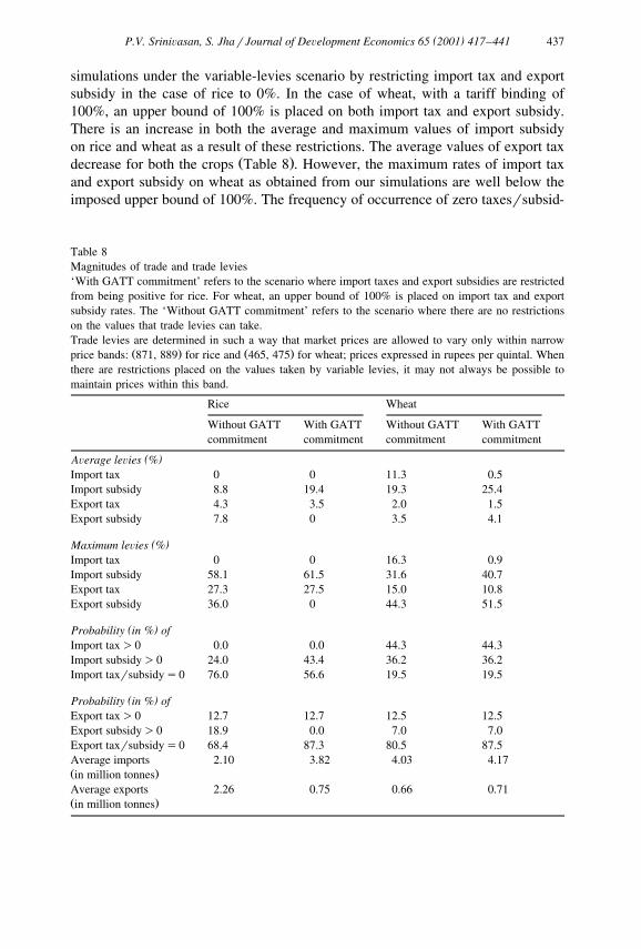
simulations under the variable-levies scenario by restricting import tax and exportsubsidy in the case of rice to 0%. In the case of wheat, with a tariff binding of100%, an upper bound of 100% is placed on both import tax and export subsidy.There is an increase in both the average and maximum values of import subsidyon rice and wheat as a result of these restrictions. The average values of export tax

Ž .decrease for both the crops Table 8 . However, the maximum rates of import taxand export subsidy on wheat as obtained from our simulations are well below theimposed upper bound of 100%. The frequency of occurrence of zero taxesrsubsid-

Table 8Magnitudes of trade and trade levies‘With GATT commitment’ refers to the scenario where import taxes and export subsidies are restrictedfrom being positive for rice. For wheat, an upper bound of 100% is placed on import tax and exportsubsidy rates. The ‘Without GATT commitment’ refers to the scenario where there are no restrictionson the values that trade levies can take.Trade levies are determined in such a way that market prices are allowed to vary only within narrow

Ž . Ž .price bands: 871, 889 for rice and 465, 475 for wheat; prices expressed in rupees per quintal. Whenthere are restrictions placed on the values taken by variable levies, it may not always be possible tomaintain prices within this band.

Rice Wheat

Without GATT With GATT Without GATT With GATTcommitment commitment commitment commitment

( )AÕerage leÕies %Import tax 0 0 11.3 0.5Import subsidy 8.8 19.4 19.3 25.4Export tax 4.3 3.5 2.0 1.5Export subsidy 7.8 0 3.5 4.1

( )Maximum leÕies %Import tax 0 0 16.3 0.9Import subsidy 58.1 61.5 31.6 40.7Export tax 27.3 27.5 15.0 10.8Export subsidy 36.0 0 44.3 51.5

( )Probability in % ofImport tax)0 0.0 0.0 44.3 44.3Import subsidy)0 24.0 43.4 36.2 36.2Import taxrsubsidys0 76.0 56.6 19.5 19.5

( )Probability in % ofExport tax)0 12.7 12.7 12.5 12.5Export subsidy)0 18.9 0.0 7.0 7.0Export taxrsubsidys0 68.4 87.3 80.5 87.5Average imports 2.10 3.82 4.03 4.17Ž .in million tonnesAverage exports 2.26 0.75 0.66 0.71Ž .in million tonnes


ies on imports and exports is reduced from 76% to 56.6% due to the restrictions.The high frequency of zero levies implies that prices do not tend to go outside thegiven price band in most of the years when trade takes place.

On the whole, price variability is increased as a result of the constraintsŽ .imposed by GATT agreements Table 6 . The cost-effectiveness of variable levies

in achieving price stability is thus reduced under these restrictions although theycontinue to be better than buffer stocks. As such, introduction of variable leviesreduces the average volume of exports and increases that of imports of both riceand wheat. This is revealed by a comparison of exportrimport volumes under

Ž .‘free trade’ Table 1, column 2 with those when variable levies are introduced forŽ . 17price stabilization purposes Table 8 . The restrictions placed on import taxes

and export subsidies due to GATT commitments, lead to a further increase in thevolume of imports and reduction in the volume of exports. This is especially thecase in rice since we restrict both import tariff and export subsidy to 0% ascompared to 100% in the case of wheat. Mean imports of rice increase by 82%and mean exports decrease by 67%. In the case of wheat, the changes in thevolume of trade are small.

Despite the restrictions imposed by GATT, one of the innovative features of theŽ .Uruguay Round UR agreement is a built-in negotiating agenda for agriculture,

among other sectors. Agricultural trade liberalization is an important element ofthe agenda for future negotiations and variable tariffs used for price stabilization isone type of trade barrier that might be constrained by changes in the WTO rules. Itis to be noted that even though industrial countries are required to cut expenditureon export subsidies by 36%, their high pre-UR subsidies that reached 90–95% forcertain commodities would mean that they continue to subsidize their exports to alarge extent. In contrast, binding the tariff at zero for India, particularly for rice,would have deleterious implications for Indian trade scenario as observed from theabove simulation results. This means that it would be favorable for India torenegotiate for a level playing field in terms of non-zero binding on exportsubsidies and import tariffs in order to fruitfully exercise the option of usingvariable levies for price stabilization. In fact, negotiations under Article XXVII ofGATT were successfully completed in December 1999 by the Indian authoritiesand the import tariff bound for rice has been raised substantially along with othercommodities like maize, millets, etc.

6. Concluding remarks

The main purpose of this paper was to analyze the impact of external tradeliberalization on food price stability. The model used for this purpose has several

17 The distinction between ‘free’ trade and ‘liberalized’ trade is as given in the beginning ofSection 4.


important features. The stochastic dynamic simulation approach takes into accountthe year to year fluctuations in domestic production and world prices in analyzingalternative policy scenarios. The multi-commodity framework captures the substi-tution possibilities in the consumption and storage of rice and wheat. Externaltrade is modeled in such a way that the direction of trade is determined endoge-nously.

The main findings of this paper can be summarized as follows.Ž .1 Freeing of external trade in foodgrains by India reduces domestic price

variability even though international prices are much more volatile than domesticprices. It also brings greater stability to world prices.

Ž .2 The welfare consequences of free trade are, however, sensitive to the levelsof margins between border and domestic prices. Although a reduction in themargin levels, say, through investment in port and other infrastructure facilities,leads to higher price instability in the economy it increases consumer surplus.

Ž .3 A U-shaped relationship is found between price variability and the marginsbetween domestic and border prices implying the existence of optimal levels forthese margins. These optimal levels could, for example, be achieved by adjustinglevies on trade.

Ž .4 The qualitative results are robust to changes in the price elasticity of riceexports and in the functional form of domestic demand functions.

Ž .5 Liberalization of trade allows the use of variable leviesrsubsidies on tradeto stabilize prices. These are found to be more effective compared to buffer stocksincluding in the case where restrictions are placed on levies due to GATTcommitments.

Ž .6 Price stabilization through variable levies reduces exports and increasesimports of both rice and wheat. With restrictions on these levies due to GATTcommitments, average volume of exports is further reduced and that of importsfurther increased especially so in the case of rice.

Ž .7 Simulation results reveal that the maximum values of trade taxrsubsidyrequired for the purpose of price stabilization are not very high. For example,import tariffs are well below the current bound of 100% for wheat.

These findings suggest that Indian policy makers can consider the use ofvariable levies for the purpose of food price stabilization in order to reduce costs.Considering the current scenario of mounting public foodgrain stocks and therising storage costs and losses, it is worth trying out this alternative. The generalfear that liberalizing trade can destabilize domestic prices is seen to be unfounded.The cost effectiveness of variable levies in stabilizing prices is, however, reduceddue to the constraints imposed by the commitments made to the World TradeOrganization in the form of bound tariff rates. There is a case for negotiating for

Ž .positive non-zero bound on export subsidies even though no subsidy wasŽ .extended to rice and wheat during the base period 1986–1988 . This would bring

in fairness to the requirement under GATT agreement that member countries limittheir export subsidies. The policy of allowing countries that earlier heavily


subsidized their exports to continue to subsidize, although at lower levels, whiletotally preventing those that did not earlier subsidize their exports from providingexport subsidy is perceived to be unfair. Moreover, in the GATT agreement importtariffs and export subsidies are not treated symmetrically with respect to thesafeguard provision. In the case of import duties, a special safeguard measureexists by which a country can charge additional duty, subject to some restrictions,whenever the quantity of import in any particular year exceeds a quantity triggerlevel or whenever the price of the imported product goes below a trigger price thatis announced by the member country. No such measure exists in the case of exportsubsidy. Removal of these shortcomings would ensure more effective use ofvariable levies for price stabilization.

Acknowledgements

We thank Deepak Ahluwalia, David Bigman, Benoıt Blarel, Bruce Gardner,ˆDina Umali-Deininger and two anonymous referees of this journal for the manyuseful comments and suggestions on previous versions of this paper. Earlierextended versions of this paper were presented at the World Bank, Washington,

Ž .DC and at the Indira Gandhi Institute of Development Research IGIDR , Mum-bai, India. We have benefited from the comments made by participants at theseseminars, particularly by Stephen Howes, Kirit Parikh and Roberto Zhaga. Theresponsibility for any remaining error, however, lies fully with us. We are gratefulto the World Bank for financing this study. However, the views expressed here areours and should not be attributed to the World Bank or IGIDR.

References

Bigman, D., 1980. Stabilization and welfare with trade, variable levies and internal price policies.European Review of Agricultural Economics 7, 185–202.

Bigman, D., Reutlinger, S., 1979. Food price and supply stabilization: National Buffer Stocks andTrade Policies. American Journal of Agricultural Economics 61, 657–667.

Dantwala, M.L., 1993. Agricultural policy: prices and public distribution system: a review. IndianŽ .Journal of Agricultural Economics 48 2 .

Gardner, B.L., Rosegrant, M.W., 1996. India’s Rice Exports and World Rice Prices, Department ofAgricultural and Resource Economics, University of Maryland, College Park, mimeo.

Greenaway, D., Morgan, C.W., Rayner, A.J., Reed, G.V., 1993. Trade liberalization and domestic priceinstability in an agricultural commodity market. Applied Economics 25, 199–205.

Ingco, M.D., 1995. Agricultural Trade Liberalization in the Uruguay Round: One Step Forward, OneStep Back? Policy Research Working Paper No. 1500, The World Bank, Washington DC.

Islam, N., Thomas, S., 1996. Foodgrain Price Stabilization in Developing Countries, Issues andExperiences in Asia. International Food Policy Research Institute, Food Policy Review Series No.3, Washington, DC.


Jha, S., Srinivasan, P.V., 2000. On improving the effectiveness of the public distribution system inachieving food security. Proceedings of the National Seminar on Food Security in India: TheEmerging Challenges in the Context of Economic Liberalization, Centre for Economic and SocialStudies Hyderabad, March 25–27, 2000, India.

Makki, S.S., Tweeten, L.G., Miranda, M.J., 1996. Wheat storage and trade in an efficient globalŽ .market. American Journal of Agricultural Economics 78 4 , 879–890.

Miranda, M.J., 1998. Numerical strategies for solving the nonlinear rational expectations commoditymarket model. Computational Economics 11, 71–87.

Mitchell, D., 1996. The small country assumption and the world grains market: The impact of Indiangrain exports. mimeo. Commodity Policy and Analysis Unit, International Economics Department,World Bank, January.

Nayyar, D., Sen, A., 1994. International Trade and Agricultural Sector in India. Economic and PoliticalWeekly, May 14, pp. 1187–1203, India.

Pursell, G., Gupta, A., 1996. Trade Policies and Incentives in Indian Agriculture, Background Statisticsand Protection and Incentive Indicators, 1965–95. World Bank. mimeo.

Radhakrishna, R., Ravi, C., 1994. Food Demand in India: Emerging Trends and Perspectives. mimeo.Ramesh, C., 1998. Removal of import restrictions and India’s agriculture: the challenge and strategy.

Ž .Economic and Political Weekly 33 15 , 850–854, India.Williams, J.C., Wright, B.D., 1991. Storage and Commodity Markets. Cambridge Univ. Press,

Cambridge.

Liberalized trade and domestic price stability. The case of rice and wheat in India

Documents

Transcript of Liberalized trade and domestic price stability. The case of rice and wheat in India