University of Denver University of Denver

Digital Commons @ DU Digital Commons @ DU

Electronic Theses and Dissertations Graduate Studies

1-1-2016

Leveraging Client Processing for Location Privacy in Mobile Local Leveraging Client Processing for Location Privacy in Mobile Local

Search Search

Wisam Mohamed Eltarjaman University of Denver

Follow this and additional works at: https://digitalcommons.du.edu/etd

Part of the Databases and Information Systems Commons, and the Information Security Commons

Recommended Citation Recommended Citation Eltarjaman, Wisam Mohamed, "Leveraging Client Processing for Location Privacy in Mobile Local Search" (2016). Electronic Theses and Dissertations. 1218. https://digitalcommons.du.edu/etd/1218

This Dissertation is brought to you for free and open access by the Graduate Studies at Digital Commons @ DU. It has been accepted for inclusion in Electronic Theses and Dissertations by an authorized administrator of Digital Commons @ DU. For more information, please contact jennifer.cox@du.edu,dig-commons@du.edu.

Leveraging Client Processing for Location Privacy in Mobile Local Search

A Dissertation

Presented to

the Faculty of the Daniel Felix Ritchie School of Engineering and Computer Science

University of Denver

In Partial Fulfillment

of the Requirements for the Degree

Doctor of Philosophy

by

Wisam M. Eltarjaman

November 2016

Advisor: Prof. Ramakrishna Thurimella

Co Advisor: Dr. Rinku Dewri

Author: Wisam M. EltarjamanTitle: Leveraging Client Processing for Location Privacy in Mobile Local SearchAdvisor: Prof. Ramakrishna ThurimellaCo Advisor: Dr. Rinku DewriDegree Date: November 2016

Abstract

Usage of mobile services is growing rapidly. Most Internet-based services targeted for

PC based browsers now have mobile counterparts. These mobile counterparts often are

enhanced when they use user’s location as one of the inputs. Even some PC-based services

such as point of interest Search, Mapping, Airline tickets, and software download mirrors

now use user’s location in order to enhance their services. Location-based services are

exactly these, that take the user’s location as an input and enhance the experience based

on that. With increased use of these services comes the increased risk to location privacy.

The location is considered an attribute that user’s hold as important to their privacy.

Compromise of one’s location, in other words, loss of location privacy can have several

detrimental e�ects on the user ranging from trivial annoyance to unreasonable persecution.

More and more companies in the Internet economy rely exclusively on the huge data

sets they collect about users. The more detailed and accurate the data a company has about

its users, the more valuable the company is considered. No wonder that these companies are

often the same companies that o�er these services for free. This gives them an opportunity

to collect more accurate location information. Research community in the location privacy

protection area had to reciprocate by modeling an adversary that could be the service

provider itself. To further drive this point, we show that a well-equipped service provider

can infer user’s location even if the location information is not directly available by using

other information he collects about the user.

There is no dearth of proposals of several protocols and algorithms that protect loca-

tion privacy. A lot of these earlier proposals require a trusted third party to play as an

intermediary between the service provider and the user. These protocols use anonymization

ii

and/or obfuscation techniques to protect user’s identity and/or location. This requirement

of trusted third parties comes with its own complications and risks and makes these pro-

posals impractical in real life scenarios. Thus it is preferable that protocols do not require

a trusted third party.

We look at existing proposals in the area of private information retrieval. We present

a brief survey of several proposals in the literature and implement two representative algo-

rithms. We run experiments using di�erent sizes of databases to ascertain their practicabil-

ity and performance features. We show that private information retrieval based protocols

still have long ways to go before they become practical enough for local search applications.

We propose location privacy preserving mechanisms that take advantage of the pro-

cessing power of modern mobile devices and provide configurable levels of location privacy.

We propose these techniques both in the single query scenario and multiple query scenario.

In single query scenario, the user issues a query to the server and obtains the answer. In

the multiple query scenario, the user keeps sending queries as she moves about in the area

of interest. We show that the multiple query scenario increases the accuracy of adver-

sary’s determination of user’s location, and hence improvements are needed to cope with

this situation. So, we propose an extension of the single query scenario that addresses this

riskier multiple query scenario, still maintaining the practicability and acceptable perfor-

mance when implemented on a modern mobile device. Later we propose a technique based

on di�erential privacy that is inspired by di�erential privacy in statistical databases. All

three mechanisms proposed by us are implemented in realistic hardware or simulators, run

against simulated but real life data and their characteristics ascertained to show that they

are practical and ready for adaptation.

This dissertation study the privacy issues for location-based services in mobile environ-

ment and proposes a set of new techniques that eliminate the need for a trusted third party

by implementing e�cient algorithms on modern mobile hardware.

iii

Acknowledgments

My whole gratitude goes first to Allah Almighty.

I thank my advisors Dr. Ramki Thurimella and Dr. Rinku Dewri, for their guidance,

patience and more importantly their wholehearted support. No dissertation can come to

fruition without the advisor’s guidance and mine is no di�erent. But mine would not

have happened without their support that was immensely needed and useful during these

eventful several years of my research. I want to thank my committee members Dr. Matthew

Rutherford and Dr. Nathan Sturtevant, whose constructive criticism made me think, and

greatly improved the final product. My thanks go to fellow student Prasad Annadata, who

did draft reviews and served as a sounding board for my ideas. My sincere thanks go to

Mr. Andre Roudik, who often bent over backward to cleverly fulfill always urgent and big

requests, always with a smile. He has become a true friend. Lastly, my thanks to Ms. Susan

Bolton, often working in the background and making sure things run smoothly and often

keep us in check, always available and took on whatever we threw at her.

The study years for me at the University of Denver, have been eventful, to say the least.

My family and I went through several events any of which would have easily broken my

resolve to keep going. This would not have happened without His blessings. The blessings

came in the form of my family that went through the roller coaster of the last few years

with me, supporting me wholeheartedly, believing in me and more importantly motivating

me to get this done. My deepest gratitude goes to my wife and kids.

iv

Contents

1 Introduction 11.1 Mobile Local Search . . . . . . . . . . . . . . . . . . . . . . . . . . . . . . . 31.2 Impacts of Location Privacy Breaches . . . . . . . . . . . . . . . . . . . . . 61.3 Location Privacy Attacks . . . . . . . . . . . . . . . . . . . . . . . . . . . . 8

1.3.1 Identity inference . . . . . . . . . . . . . . . . . . . . . . . . . . . . . 81.3.2 Predicting user’s location of interest . . . . . . . . . . . . . . . . . . 10

1.4 Contribution . . . . . . . . . . . . . . . . . . . . . . . . . . . . . . . . . . . 111.5 Dissertation Outline . . . . . . . . . . . . . . . . . . . . . . . . . . . . . . . 12

2 Location Privacy Mechanisms 142.1 Policy Based Protection . . . . . . . . . . . . . . . . . . . . . . . . . . . . . 14

2.1.1 Access control policy . . . . . . . . . . . . . . . . . . . . . . . . . . . 152.1.2 Privacy policy . . . . . . . . . . . . . . . . . . . . . . . . . . . . . . 16

2.2 Anonymization . . . . . . . . . . . . . . . . . . . . . . . . . . . . . . . . . . 172.2.1 k-anonymity . . . . . . . . . . . . . . . . . . . . . . . . . . . . . . . 182.2.2 Major problems with anonymization . . . . . . . . . . . . . . . . . . 22

2.3 Obfuscation . . . . . . . . . . . . . . . . . . . . . . . . . . . . . . . . . . . . 242.4 Spatio-temporal Cloaking . . . . . . . . . . . . . . . . . . . . . . . . . . . . 292.5 Cryptography Based Mechanisms . . . . . . . . . . . . . . . . . . . . . . . . 302.6 Di�erential Privacy . . . . . . . . . . . . . . . . . . . . . . . . . . . . . . . . 33

2.6.1 Intuition of di�erential privacy . . . . . . . . . . . . . . . . . . . . . 332.6.2 Di�erential privacy for location data . . . . . . . . . . . . . . . . . . 36

2.7 Motivation . . . . . . . . . . . . . . . . . . . . . . . . . . . . . . . . . . . . 372.8 Problem Statement . . . . . . . . . . . . . . . . . . . . . . . . . . . . . . . . 39

3 State of User’s Location Privacy 413.1 Collecting Driving Habits Data: Problem Definition . . . . . . . . . . . . . 423.2 Location Privacy Model . . . . . . . . . . . . . . . . . . . . . . . . . . . . . 443.3 Driving Habits Data . . . . . . . . . . . . . . . . . . . . . . . . . . . . . . . 45

3.3.1 Data collection . . . . . . . . . . . . . . . . . . . . . . . . . . . . . . 463.3.2 Pre-processing . . . . . . . . . . . . . . . . . . . . . . . . . . . . . . 46

3.4 Location Inference Method . . . . . . . . . . . . . . . . . . . . . . . . . . . 473.4.1 Area map as a graph . . . . . . . . . . . . . . . . . . . . . . . . . . . 483.4.2 Generating candidate paths . . . . . . . . . . . . . . . . . . . . . . . 493.4.3 Candidate ranking . . . . . . . . . . . . . . . . . . . . . . . . . . . . 51

v

3.5 Empirical Observations . . . . . . . . . . . . . . . . . . . . . . . . . . . . . 543.5.1 Illustrative example . . . . . . . . . . . . . . . . . . . . . . . . . . . 553.5.2 Ranking performance . . . . . . . . . . . . . . . . . . . . . . . . . . 56

3.6 Summary . . . . . . . . . . . . . . . . . . . . . . . . . . . . . . . . . . . . . 58

4 Architecture 594.1 Privacy in Local Search . . . . . . . . . . . . . . . . . . . . . . . . . . . . . 594.2 Non-private Architecture . . . . . . . . . . . . . . . . . . . . . . . . . . . . . 634.3 Request–Response Protocol . . . . . . . . . . . . . . . . . . . . . . . . . . . 64

4.3.1 First round-trip . . . . . . . . . . . . . . . . . . . . . . . . . . . . . . 654.3.2 Second round-trip . . . . . . . . . . . . . . . . . . . . . . . . . . . . 66

4.4 PIR Based Approach . . . . . . . . . . . . . . . . . . . . . . . . . . . . . . . 674.5 Statistical Based Approach . . . . . . . . . . . . . . . . . . . . . . . . . . . 684.6 Ranking the POIs . . . . . . . . . . . . . . . . . . . . . . . . . . . . . . . . 694.7 Threat Model . . . . . . . . . . . . . . . . . . . . . . . . . . . . . . . . . . . 704.8 Abstract Model for LPPM . . . . . . . . . . . . . . . . . . . . . . . . . . . . 72

4.8.1 Assessments . . . . . . . . . . . . . . . . . . . . . . . . . . . . . . . . 724.9 LPPM implementation . . . . . . . . . . . . . . . . . . . . . . . . . . . . . . 754.10 Summary . . . . . . . . . . . . . . . . . . . . . . . . . . . . . . . . . . . . . 77

5 Investigation of PIR As a Candidate Solution 795.1 Preliminaries . . . . . . . . . . . . . . . . . . . . . . . . . . . . . . . . . . . 80

5.1.1 Information theoretic PIR techniques . . . . . . . . . . . . . . . . . 815.1.2 Computational PIR techniques . . . . . . . . . . . . . . . . . . . . . 83

5.2 PIR Protocol Model . . . . . . . . . . . . . . . . . . . . . . . . . . . . . . . 845.2.1 Description of QRP . . . . . . . . . . . . . . . . . . . . . . . . . . . 855.2.2 Description of FHP . . . . . . . . . . . . . . . . . . . . . . . . . . . 88

5.3 Implementation Details . . . . . . . . . . . . . . . . . . . . . . . . . . . . . 905.4 Results and Analysis . . . . . . . . . . . . . . . . . . . . . . . . . . . . . . . 915.5 Summary . . . . . . . . . . . . . . . . . . . . . . . . . . . . . . . . . . . . . 94

6 Single Query Scenario 966.1 Proposed LPPM . . . . . . . . . . . . . . . . . . . . . . . . . . . . . . . . . 966.2 Interests Set Computation . . . . . . . . . . . . . . . . . . . . . . . . . . . . 986.3 kd-Tree Branch-and-bound Search . . . . . . . . . . . . . . . . . . . . . . . 100

6.3.1 Building augmented kd-tree . . . . . . . . . . . . . . . . . . . . . . . 1016.3.2 Find the top-k POIs . . . . . . . . . . . . . . . . . . . . . . . . . . . 102

6.4 Improving the Grid Search Time . . . . . . . . . . . . . . . . . . . . . . . . 1066.4.1 Skip top-k search for equivalent cells . . . . . . . . . . . . . . . . . 1066.4.2 Reducing the search space for non-border cells . . . . . . . . . . . . 107

6.5 Evaluation . . . . . . . . . . . . . . . . . . . . . . . . . . . . . . . . . . . . . 1076.5.1 Experimental setup . . . . . . . . . . . . . . . . . . . . . . . . . . . . 1076.5.2 Runtime performance . . . . . . . . . . . . . . . . . . . . . . . . . . 1086.5.3 Expected privacy and overhead . . . . . . . . . . . . . . . . . . . . . 110

6.6 Summary . . . . . . . . . . . . . . . . . . . . . . . . . . . . . . . . . . . . . 113

vi

7 Multiple Query Scenario 1147.1 Extended Attacker Model . . . . . . . . . . . . . . . . . . . . . . . . . . . . 1157.2 Algorithm for Multiple Query Scenario . . . . . . . . . . . . . . . . . . . . . 116

7.2.1 Selection area . . . . . . . . . . . . . . . . . . . . . . . . . . . . . . . 1167.2.2 Choosing a box . . . . . . . . . . . . . . . . . . . . . . . . . . . . . . 1187.2.3 Obfuscation . . . . . . . . . . . . . . . . . . . . . . . . . . . . . . . . 119

7.3 Specific Scenario . . . . . . . . . . . . . . . . . . . . . . . . . . . . . . . . . 1197.3.1 Uncertainty of the attacker . . . . . . . . . . . . . . . . . . . . . . . 121

7.4 General Scenario . . . . . . . . . . . . . . . . . . . . . . . . . . . . . . . . . 1227.4.1 Movement model . . . . . . . . . . . . . . . . . . . . . . . . . . . . . 1227.4.2 Computing Pr(I|c) . . . . . . . . . . . . . . . . . . . . . . . . . . . 126

7.5 Empirical Evaluation for General Scenario . . . . . . . . . . . . . . . . . . . 1277.5.1 Experimental setup . . . . . . . . . . . . . . . . . . . . . . . . . . . . 1277.5.2 Privacy . . . . . . . . . . . . . . . . . . . . . . . . . . . . . . . . . . 1297.5.3 Bandwidth impact . . . . . . . . . . . . . . . . . . . . . . . . . . . . 1317.5.4 Impact of box size . . . . . . . . . . . . . . . . . . . . . . . . . . . . 134

7.6 Summary . . . . . . . . . . . . . . . . . . . . . . . . . . . . . . . . . . . . . 135

8 Di�erential Privacy Based Solution 1378.1 Architecture . . . . . . . . . . . . . . . . . . . . . . . . . . . . . . . . . . . . 1388.2 Enforcing Indistinguishability . . . . . . . . . . . . . . . . . . . . . . . . . . 139

8.2.1 Geo-indistinguishability . . . . . . . . . . . . . . . . . . . . . . . . . 1408.2.2 Indistinguishability for top-K results . . . . . . . . . . . . . . . . . . 141

8.3 Applying 2-Roundtrip Querying Architecture . . . . . . . . . . . . . . . . . 1448.3.1 radz, radR and radI . . . . . . . . . . . . . . . . . . . . . . . . . . . 1458.3.2 Choosing a top-K set . . . . . . . . . . . . . . . . . . . . . . . . . . 1458.3.3 Characterization . . . . . . . . . . . . . . . . . . . . . . . . . . . . . 147

8.4 Retrieval Accuracy . . . . . . . . . . . . . . . . . . . . . . . . . . . . . . . . 1508.4.1 Base match distribution . . . . . . . . . . . . . . . . . . . . . . . . . 1508.4.2 Match probability . . . . . . . . . . . . . . . . . . . . . . . . . . . . 1518.4.3 Choosing ‘ . . . . . . . . . . . . . . . . . . . . . . . . . . . . . . . . 153

8.5 Parametric Evaluation . . . . . . . . . . . . . . . . . . . . . . . . . . . . . . 1548.6 An Android Implementation . . . . . . . . . . . . . . . . . . . . . . . . . . . 1578.7 Comparative Performance . . . . . . . . . . . . . . . . . . . . . . . . . . . . 1618.8 Adopting Multiple Queries . . . . . . . . . . . . . . . . . . . . . . . . . . . . 1638.9 Summary . . . . . . . . . . . . . . . . . . . . . . . . . . . . . . . . . . . . . 164

9 Conclusion 1659.1 Results and Discussion . . . . . . . . . . . . . . . . . . . . . . . . . . . . . . 1679.2 Further Directions . . . . . . . . . . . . . . . . . . . . . . . . . . . . . . . . 1689.3 Summary . . . . . . . . . . . . . . . . . . . . . . . . . . . . . . . . . . . . . 170

vii

List of Figures

1.1 Typical mobile local search architecture. . . . . . . . . . . . . . . . . . . . . 41.2 A TTP-based location privacy architecture. . . . . . . . . . . . . . . . . . . 5

2.1 Location data for Example 2.2.1 . . . . . . . . . . . . . . . . . . . . . . . . 192.2 Location generalization for clocked region in Example 2.2.1 . . . . . . . . . 202.3 Cloaked dataset with sensitive attribute . . . . . . . . . . . . . . . . . . . . 232.4 Outliers problem with k-anonymity . . . . . . . . . . . . . . . . . . . . . . . 232.5 Spatial obfuscation types: ¸u is the user’s location, the entire map repre-

sents imprecision obfuscation, ¸1

represents inaccuracy obfuscation, and ¸2

vagueness obfuscation. . . . . . . . . . . . . . . . . . . . . . . . . . . . . . . 252.6 Movement trajectory data . . . . . . . . . . . . . . . . . . . . . . . . . . . . 302.7 Sample of medical dataset. . . . . . . . . . . . . . . . . . . . . . . . . . . . 34

3.1 Disabling of shortest path constraint while exploring highway nodes. . . . . 493.2 Turns along an explored path. . . . . . . . . . . . . . . . . . . . . . . . . . . 513.3 Speed profile for a trip, along with that generated from the ideal and the

augmented models for a di�erent path. . . . . . . . . . . . . . . . . . . . . . 533.4 Sample candidate paths generated for a trip. Candidate path 118 is the actual

route taken during the trip. The bottom right plot shows the destinations ofall (196) candidate paths generated for this trip. A: start node; B: end node.Map data: Google (2013). . . . . . . . . . . . . . . . . . . . . . . . . . . . . 56

3.5 Speed profile during actual trip and that generated by augmented model forsample paths. . . . . . . . . . . . . . . . . . . . . . . . . . . . . . . . . . . . 57

4.1 Pizza locations returned by Google search in 5 Av / w 43 St, New York, NY,USA. . . . . . . . . . . . . . . . . . . . . . . . . . . . . . . . . . . . . . . . . 61

4.2 Client/Server communication steps in PIR based LPPM. . . . . . . . . . . . 674.3 Client/Server communication steps in heuristic based LPPM. . . . . . . . . 68

6.1 Building a 2d-tree example. . . . . . . . . . . . . . . . . . . . . . . . . . . . 1016.2 Example of kd-tree search . . . . . . . . . . . . . . . . . . . . . . . . . . . . 1056.3 Average run times (milliseconds) on actual device (for 40x40) . . . . . . . . 1106.4 Uniform-local (right) and gaussian (left) background knowledge. Darker cells

imply higher probability. . . . . . . . . . . . . . . . . . . . . . . . . . . . . 1116.5 Expected privacy and expected interest set size trade-o�. Data points in each

line correspond to Z = 80, 40, 20, 10, 8 and 5, from left to right. . . . . . . 112

viii

7.1 Location inference during multiple queries. . . . . . . . . . . . . . . . . . . 1157.2 Selection area for a (4 ◊ 4 size) box. . . . . . . . . . . . . . . . . . . . . . . 1177.3 Entropy of the obfuscated area with Gaussian background knowledge for the

attacker. . . . . . . . . . . . . . . . . . . . . . . . . . . . . . . . . . . . . . . 1237.4 Entropy of the obfuscated area with precise background knowledge for the

attacker. . . . . . . . . . . . . . . . . . . . . . . . . . . . . . . . . . . . . . . 1247.5 Prior and posterior distribution after queries along a path. Darker (red)

regions signify higher probability mass. . . . . . . . . . . . . . . . . . . . . . 1257.6 Nearness and areal privacy variation along a path. Search keyword = gas

station and b = 32 cells. . . . . . . . . . . . . . . . . . . . . . . . . . . . . . 1307.7 Nearness and areal privacy quartiles. b = 32 cells. . . . . . . . . . . . . . . 1307.8 Empirical CDF of distance between last cell in a path and the most probable

cell in the inferred distribution. b = 32 cells. . . . . . . . . . . . . . . . . . . 1327.9 Total number of POIs for which details are retrieved during queries along the

paths. b = 32 cells. . . . . . . . . . . . . . . . . . . . . . . . . . . . . . . . . 1337.10 Frequency distribution of interest set (POIs for which details are retrieved)

sizes. Total potential queries = 264,627. . . . . . . . . . . . . . . . . . . . . 1337.11 Nearness and areal privacy quartiles for di�erent box size b and search keywords.134

8.1 Variation in the top-10 cafe set in Los Angeles. Ranking performed with– = 0.8. . . . . . . . . . . . . . . . . . . . . . . . . . . . . . . . . . . . . . . 142

8.2 Zm(c0

) and Cm with Zm(c0

) µ Cm. . . . . . . . . . . . . . . . . . . . . . . . 1488.3 Desired minimum starting distance of a zone relative to a location. . . . . . 1498.4 Observed and fitted base match distribution (rad = 2 km, K = 10) for cafes

in Los Angeles, CA, USA. Inset figure shows probability of obtaining matchesin the set chosen by mechanism Mfgi. . . . . . . . . . . . . . . . . . . . . . 151

8.5 Observed match frequencies in three di�erent POI categories. Top-10 setscomputed with – = 0.8 and radI = 2 km. Mfgi samples using ‘ = 30. . . . 153

8.6 Computed ‘ using various base distributions and confidence levels v = 0.99, 0.95and 0.90. . . . . . . . . . . . . . . . . . . . . . . . . . . . . . . . . . . . . . 154

8.7 Impact of radz on retrieval accuracy. radI = radz. . . . . . . . . . . . . . . 1558.8 Impact of – on retrieval accuracy. . . . . . . . . . . . . . . . . . . . . . . . . 1568.9 Impact of privacy parameter (‘) on retrieval accuracy. . . . . . . . . . . . . 1578.10 Android application screenshot. . . . . . . . . . . . . . . . . . . . . . . . . . 1588.11 Position of POIs in the true top-K set when missed by the application. . . 1598.12 Retrieval accuracy. . . . . . . . . . . . . . . . . . . . . . . . . . . . . . . . . 1608.13 Overall performance of the 2-roundtrip application. . . . . . . . . . . . . . . 1608.14 Expected estimation error of adversary. . . . . . . . . . . . . . . . . . . . . 163

ix

Nomenclature

AI Interest Area

AR Retrieval Area

AZ Obfuscation Area

cPIR computational PIR

FHE Fully Homomorphic Encryption

GIS Geographic Information System

GPS Global Positioning System

itPIR information-theoretic PIR

LBS Location Based Service

LoP Level of Privacy

LPPM Location Privacy Preserving Mechanism

LSP Location Based Service Provider

P2P Peer-to-Peer

PIR Private Information Retrieval

POI Point Of Interest

QI Quasi Identifiers

QoS Quality of Service

TTP Trusted Third Party

x

Chapter 1

Introduction

Privacy or the right to be left alone in the realm of computer science can be understood

as a personal preference of how much of information an individual wants others to have

access to. In general, there is no direct quantitative measurement for privacy and it can

be di�erent from one person to another and varies based on many factors such as culture,

circumstance, financial gain, services being consumed or the entity trying to access the

information.

Recent evolution in mobile phones and communication technologies has lead to a sig-

nificant increase in the number of subscribers to mobile networks. It is estimated that there

will be 6.1 billion smartphone users across the world by 2020, which represents 70% of the

global population at that time [24]. Further, the development of mobile data technologies

allow many mobile users to access the Internet via their mobile devices and leads to very

attractive and useful applications. Examples of these applications include mobile enter-

tainment, locating nearby points of interest, updating friends and family of one’s location,

tourist guidance, language translation etc. Improvements both in the quantity and qual-

ity of publicly available data lead to significant improvements to the capabilities of these

mobile applications. For example, a user can not only search for nearby restaurants but

put additional criteria such as availability of specific food (e.g. gluten free) or having a

higher than threshold user review rating. While there are multiple categories of mobile

1

applications available, the category of applications that is most interesting to the privacy

research community falls under Location Based Services (LBS).

An LBS is a service provided to a mobile user, typically using a mobile application, that

has at least two entities involved, a server and a client. It works like any other client/server

architecture where the client initiates the transaction by placing a service request, and the

server responds to that request. What di�erentiates LBS from other mobile services is the

fact that the location of the user is one of the inputs to the service request. While some

service providers and devices support the concept of “push” services that allow the server

to push relevant service messages to the mobile phone, they can be considered a special case

of the client/server transaction, as one could consider the installation and registration of

the application with the service provider represents the initial service request by the client.

In LBSs the transactions between the user terminal and the service provider are usually

carried over mobile networks. For the service provider to provide a useful service to the user,

the location of the user needs to be known by the server. It can be obtained either by using

the Global Positioning System (GPS) which is supported today by most of the smartphones

and tablets. Other approaches such as WiFi/cell tower triangulation are possible. A set of

di�erent location sensing techniques has been explored by Hightower and Borriello in [84].

If the service provider was not able to manipulate all the location data that is required to

accomplish the service, then the service provider will obtain that data from the Geographic

Information System (GIS). A GIS database is a separate entity that is designed to store

and process geographic data.

LBSs are used in a wide variety of applications that includes locating an object such

as grocery store or locating people such as finding a friend on a social network. It may also

include some business applications such as advertising coupons or deals to clients, or billing

them for a service dynamically based on their current location. A new application of LBSs

is mobile location based gaming such as a Geocaching1 hunting game, where the player tries

to locate a hidden container in an interesting location based on the GPS coordinates.

1www.geocaching.com

2

Location-based services are very useful and so are consumed by many mobile users. One

of the query parameters, namely, the user’s current location, is of immense importance to

the privacy research community. The current or the past location of the user is considered

private information. Moreover, it is generally thought that the more accurate the location

of a user traced by an unauthorized entity, the bigger breach it is of user’s privacy. On the

other hand, the more accurate the user location supplied to the service provider, the more

useful response the service provider can give. A considerable amount of research, including

the current dissertation, deals with the fine balancing required between these two conflicting

aspects.

People consider their geographic location to be private information. They do not want

unauthorized entities to know where they are or where they have been. Breach of location

privacy could present several serious problems to the user. Moreover, precise location

information of consumers has proven to be a profitable asset in this day of personalized

marketing. This has caused several breaches, escalations of privileges and very service

provider leaning privacy policies such as longer retention intervals of user’s location data.

Because of the financial gains, there is added motivation on the part of service providers

to be able to obtain and use precise user location information. On the other hand, the

users, equipped with their smartphone, want and sometimes need, to consume location-

based services. So, techniques are needed to preserve the location privacy of the user even

when the attacker happens to be the service provider itself while allowing the user to still

consume location-based services without considerable degradation of quality.

1.1 Mobile Local Search

One area of interest for the privacy research community within the LBS space is mobile

local search. While in several LBSs like navigation systems, friend finders, social networking

apps etc., the mobile local search is arguably the most widely used system where the semi-

trusted service provider can gain considerable knowledge based on both the location and

query string used as part of the query. A typical search transaction starts with a user

3

Client

LSP

Query String + location

Sorted POI List

Figure 1.1: Typical mobile local search architecture.

looking for a certain object (often called Point Of Interest or POI). The user sends a query

to the service provider with a keyword that defines the type of required POIs in addition

to the location information that refers to her current geographical position. With proper

permissions, the location data can be directly obtained by the application from an on-board

positioning device. The LBS provider receives this query and the geographic position of

the user and returns a list of POIs that match the query, sorted based on some criteria.

If the service provider already maintains a database of the requested type of POIs, then

it can answer the query immediately; otherwise, the server must request this information

from GIS.

The most common architecture for mobile local search prevalent today is depicted in

Figure 1.1. It is a simple client/server architecture where the client is a mobile application

that directly communicates with the server. When it comes to location privacy of the user

in this architecture, it is totally based on the privacy policy as published by the Location

Based Service Provider (LSP). In other words, the LSP is trusted completely: the LSP will

only use the location information in accordance with published privacy policy. Of course,

there are many issues even if the LSP is trusted, as the privacy policies themselves can

be long and complicated that few users really understand them. A detailed discussion of

policy-based privacy mechanism is presented later in Chapter 2.

When the service provider is completely trusted, then the location privacy problem

with respect to mobile local search becomes a privacy policy research issue. Assuming

that mechanisms from information security research area are already implemented that

4

Clients

TTP

Query String + location

Sorted POI List

Query String + locationSorted POI List

Query String + location

Sorted POI List LSP

Anonymized Query

Answer

Figure 1.2: A TTP-based location privacy architecture.

encrypt the communications between the client and the server and prevent attackers from

eavesdropping, the problem becomes trivial. But, what would be the case if the LSP is

semi-trusted instead of completely trusted? The challenge is to come up with a solution

that provides the user all the advantages of mobile local search, without compromising her

location privacy even in the case of a semi-trusted LSP.

An often proposed solution in the literature for this problem is to find a Trusted Third

Party (TTP) that could act as a mediator between the user and the LSP. As shown in Figure

1.2, the TTP runs some anonymization algorithm that prevents the LSP from learning the

exact location information of the user. Instead of direct communication with the LSP, the

user now will send her query to the TTP which anonymizes this query (usually with other

queries from di�erent users) and sends it to the LSP, which searches its database and replies

back the found answer. The LSP can answer the anonymized query but should not learn any

information about the user who issued the query. Normally, this answer includes additional

mixed data, and it is the TTP’s job to split out this data and return the correct answer to

each user. Numerous problems come with this solution will be discussed in Section 2.3.

5

1.2 Impacts of Location Privacy Breaches

Violation of location privacy are considered serious in many privacy conscious societies.

Research shows several potential impacts of location privacy breach, especially on the user’s

front. Some of these impacts are listed and described below.

A feeling of being violated. One could imagine that a feeling of being violated is

the primary impact of a location privacy breach. But this impact happens only on the

user discovering that her location privacy is breached. This feeling is common among all

privacy breaches. A discovery of location privacy breach or even the perception by the

user of an LBS can have further secondary impacts such as loss of trust, reduced usage of

location-based services, implementation of privacy enhancing mechanisms, retaliation, and

legal actions.

Personal safety. With a lot of vulnerable persons such as activists, victims of various

social crimes, potential victims and children using Internet increasingly, their personal safety

could be in jeopardy if their location privacy is breached and their location is revealed to

powerful attackers. One could imagine that this risk increases if the fact about the location

breach is unknown to the user.

Escalation to further privacy breaches. A powerful attacker may have even worse

goals (e.g. personal physical attack, burglary, arrest etc.) and figuring out the location of

the victim could be the first step in such an attack. In other words, a breach of location

privacy can be escalated by a motivated attacker to facilitate further more serious attacks.

Unreasonable prosecution. With the Internet and mobile technologies being used in

various social causes by the activists, particularly in restrictive societies, a breach of location

privacy of these activists could lead to their identification (or worse could implicate an

innocent person) and could subject to greater scrutiny or even prosecution.

6

Uninvited marketing. Intrusive solicitations and uninvited marketing arguably is the

most prevalent impact of location privacy breaches. The intentional or unintentional rev-

elation of location leads to more targeted marketing by various entities. In most practical

scenarios, the marketing entities or marketing facilitators are themselves providers of LBSs

making this risk very prevalent.

Breach of privacy of others. This is particularly true in the case where the attackers

are antagonistic administrations whose intention is to identify and locate the entire group

of activists. A breach of location privacy of one victim could reveal the locations of close

associates, co-workers, and friends even if those third parties are non-users of LBS.

Loss of trust. When the users discover or perceive the breach of location privacy, even

unintentional (e.g. the service provider itself being victim of a hacking attack), it results

in loss of trust on service providers causing reduced utilization of useful services and in-

crease in overall costs, as the victims usually overcome this by implementing various privacy

preserving mechanisms.

Loss of revenue. Loss of trust in service providers generally results in reduced utilization

that could result in major losses in revenue to service providers. The mere perception of

loss of privacy by users, not a full knowledge of a breach, is enough to cause loss of trust and

loss of revenue. It results in service providers spending resources to portray a perception

of trust. One example is the amount of time and money spent by major LBS providers on

public relationship campaigns.

Changes in behavior. Privacy of a person includes behavioral aspects, especially sen-

sitive ones such as religious practices and political activities. The privacy breach of the

user’s location can be escalated to the breach of privacy of these aspects; the breach of pri-

vacy can lead to changes in behavior. The changes could range from towing the party line,

implementation of privacy preserving techniques, reduced use of LBSs or even disloyalty.

7

Societal impact. Breach of privacy and loss of trust indirectly a�ects the ability for

individuals to communicate and share sensitive information with each other without any

concerns of being monitored by other people or organizations. In the long run, this can

have major impacts on the society as a whole and could cause regressive societies.

Technical Impacts. Loss of trust for LBSs not only have financial costs. It also impacts

the e�ciency of the systems. For example, Parris and Henderson [131] run a simulation of

two real-world datasets and show that users’ privacy concerns can significantly downgrade

routing performance in the opportunistic networks. Their results show that message delivery

ratio can be reduced to zero. From the users’ perspective, implementation of additional

measures to preserve privacy often result in loss of Quality of Service (QoS), which results

from an increase in bandwidth costs and processing resources.

1.3 Location Privacy Attacks

LBSs are very useful and are being used by more and more mobile users today [28].

Along with their adoption and increased utilization comes increased risk to location privacy.

In the previous section, several possible impacts of location privacy breach are discussed that

ranged from benign risks such as intrusive marketing to serious ones such as unreasonable

prosecution or bodily harm. Privacy protection techniques can be appreciated and their

e�cacy can be judged better if one has an understanding of di�erent attack techniques that

a capable and smart attacker could use. In this section, the broad categories of location

privacy attacks in the literature are discussed. The corresponding preservation techniques

proposed will be discussed in Chapter 2.

1.3.1 Identity inference

Perhaps the most obvious location privacy protection technique is to replace the actual

identifier of the user with an alias identifier or pseudonym. Since certain locations such as

the o�ce or home can be strongly related to the user, an attacker could easily identify the

8

user by linking the pseudonym to these locations. This kind of attack was demonstrated

by Beresford and Stajano [15] and the results show that all users in the tested database

can be identified correctly. The algorithm is run in two steps: (1) given a pseudonym,

observe where that pseudonym spends most of the time and (2) given a location, see which

pseudonym spends more time than any other in that location.

In many situations where the attacker is a third party that can observe the communica-

tions happening between clients of LBS and the server, it is often possible for the attacker

to determine the location of the query origination and sometimes even the contents of the

query. In an identity inference attack, the attacker, who is assumed to have access to the

location the query originated from, tries to infer the identity of the user that originated the

query. The attacker who is also assumed to have access to publicly available databases and

some background information, like the work location of the victim, could try to combine

this information with observations of the communications between the user and LSP to

guess the identity of the user. Once a user is identified, more powerful attacks are possi-

ble as the attacker now can associate any observed pseudonym or a quasi-identifier such

as a phone ID or electronic serial number to the actual identity of the user during future

observations. Quasi-identifiers are attributes of a database record that are non-identifying

by themselves, but can be used to uniquely identify individuals when used in combination.

The attacker could exploit quasi-identifiers to escalate the attacks or to identify other users

of the system; for example, by simply ruling out already identified users. Re-identification

of the Massachusetts Governor, William Weld’s health records was done based on gender,

postal code and date of birth [73, 149]. Later research showed that individuals can be

identified using di�erent pseudo-identifiers such as web search history [13], social network

structure [119], movie rating content or even familial structures [74].

A more powerful attack is presented by Gruteser and Hoh in [76] that uses Reid’s

algorithm of multiple-tracking hypothesis [132]. They demonstrated their attack by tracking

three anonymous users over extended periods of time using sample GPS location data. The

sampled locations can be linked to the identity of each individual by building separate

9

path for each user. A simplified version of Reid’s algorithm is used to repeatedly generates

hypotheses for the new locations of the users and adjust this information with new location

samples. The results show that the algorithm may be confused between users temporarily,

especially if the paths are crossing, but eventually for a long run it can recover and correctly

sample the users. Krumm [97] runs an experiment over a sample of 172 volunteers. The

author shows that given GPS locations, the home for each user is identified with a median

error of about 60 meters. About 5% of users could be identified by name using free Web-

based services. While using a commercial reverse geocoder, the accuracy raises to 13%.

De Montjoye et al. [40] shows that 95% of individuals can be uniquely identified using just

four spatiotemporal points. This is done by analyzing data collected for fifteen months

from a half million mobile users. By analyzing more than 30 billion call records, Zang

and Bolot [166] tried to find the top N records of users. They set up an experiment that

determined the user’s location at di�erent granularity level such as sector, city, county,

whole state, etc. They concluded that 50% of users can be identified by using their top 3

locations determined by analyzing their call records to the granularity of a sector. Using

the same top 3 locations, 10% and up to 50% of users’ locations can be determined to the

city level and 1% and up to 5% to the county level.

1.3.2 Predicting user’s location of interest

To identify user’s places of interest, Marmasse and Schmandt [111] propose the “com-

Motion” software which uses GPS to determine the user’s location and track her movement.

This software links the movement traces to the important places for the user by gradually

learning the locations visited by her on a regular basis. The place is identified by circular

region around a point within which the GPS appears and disappears. A similar work by

Ashbrook and Starner [9] cluster the location data collected from GPS and use a Markov

model to learn useful information from this data, such as prediction of the next place the

user is going to visit and the presence of other people at the same location as the user.

10

Kang et al. [91] used a time-based clustering algorithm for coordinate traces of the user

to recognize the important places for her, while Hariharan and Toyama [79] consider both

time and location to build a hierarchy from the location data histories. The hierarchy is

represented as “stays” and “destinations”. The destination is a cluster of stays while the

stay is defined as the place where the user had spent some time. Instead of mapping GPS

location coordinates, “BeaconPrint” algorithm by Hightower et al. [85] identifies important

places for the user by collecting WiFi and GSM base stations visited frequently by the user.

Montoliu and Gatica-Perez [117] developed a smartphone application to obtain the

user’s location by integrating di�erent sensors of the phone. Similar to Hariharan and

Toyama [79], the authors use time and location-based clustering to identify significant places.

“CrowdSense@Place” algorithm by Chon et al. [30] monitors everyday user’s places by

opportunistically collecting images and audio clips from a smartphone. The collected image

and audio data is classified in the processing stage and linked to location marks obtained

by the GPS/WiFi sensors. Several approaches recently are proposed by researchers for

predicting the next destination of the user (e.g. [31, 39, 99, 138, 151]), making not just the

current location vulnerable to the attacks, but the future locations of the user as a target

for several attacks.

Sometimes quasi-identifiers can be used to infer the location data. Dewri et al. [14,

43] implemented an attack that shows how driving habits data such as speed and time

collected by auto-insurance companies to assess accident risk can be manipulated to infer

the destination of the trip. We discuss this attack in more detail later in Chapter 3 as an

example of how a semi-trusted service provider can use other data to predict the user’s

location.

1.4 Contribution

In this dissertation, we begin by arguing why the requirement of a TTP is not a prac-

tical solution and how it can be eliminated by taking advantage of the power of modern

smart devices. We propose a TTP free two-round trip generic architecture upon which

11

Location Privacy Preserving Mechanisms (LPPM) can be implemented. Proceeding from

that architecture we, therefore:

• present a kd-tree e�cient POI ranking process that considers both location and promi-

nence2 information of the POIs in contrast to existing LPPMs which use only the

location,

• explore the practicability of implementing cryptography-based methods, namely PIR

techniques, as an LPPM and show that none of the available techniques are practical

enough,

• present a novel LPPM for single queries that enable location and prominence based

ranking of POIs, and implement it entirely on a mobile device to demonstrate feasi-

bility,

• show how there is a higher risk of privacy loss in the multiple query scenario, and

propose an improved LPPM to handle this scenario,

• present and implement an alternative LPPM that uses di�erential privacy whose pri-

vacy guarantees can be mathematically ascertained.

The proposed LPPMs in this dissertation are implemented to show that they are all

practical to be run entirely on a mobile device without compromising too much of the QoS.

We analyze our results and, where appropriate, compare them with some representative

algorithms to show that our contribution makes significant improvements to location privacy

in the context of mobile local search with minimal communication and computation costs.

1.5 Dissertation Outline

This dissertation addresses the privacy issues encountered by the users of LBS during

POI searches. As explained above, location privacy is important and loss of privacy has

real consequences to the users. There is a lot of progress in terms of protecting privacy

2More discussion about POI ranking process and the prominence value in Section 4.1

12

against third parties. But during these days where richer user profiles are monetized, the

service providers themselves have an incentive to both track and store location data of the

users as accurately as possible. So there is a need for techniques that not only avoid third

parties but also protect user’s privacy against semi-trusted service providers. This disserta-

tion investigates existing techniques, studies their practicability after implementation and

proposes a few practical techniques.

In the next chapter, we survey the existing research in LBS privacy and present a view of

the progression of these techniques. In Chapter 3, we show that protecting location privacy

does not stop at protecting just the location coordinates. We show that a clever semi-trusted

provider can use quasi-identifiers to infer the location of the user pretty closely. In Chapter

4, we propose an architecture for third party free protocols. We present nomenclature that

will be used in rest of the dissertation as other techniques are explained. In Chapter 5,

we delve into Private Information Retrieval , a set of cryptography-based techniques and

investigate them as a potential solution for our third party free architecture. Chapters 6

through 8, present heuristics-based techniques. In chapter 6, we propose a third party free

technique that can be implemented on a smart mobile device that achieves user desired

privacy level in the single query scenario. We extend this technique in Chapter 7 to address

the same issue in the multiple query scenario where the user moves around while issuing

queries. In Chapter 8, we propose an improved technique based on di�erential privacy as a

measure for a guaranteed privacy level.

13

Chapter 2

Location Privacy Mechanisms

In this chapter, we present existing privacy protection mechanisms in the form of a

quick survey of existing literature. We can broadly categorize the privacy protection mech-

anisms that are in practice or proposed in the literature based on policy, anonymization,

obfuscation, cryptography or a combination of these. While policy-based techniques require

the user to trust the service provider, the other techniques o�er various degrees of privacy

even from the service provider. We discuss these issues in detail below.

2.1 Policy Based Protection

Policy-based privacy protection is arguably still the most prevalent in practice today.

It gains importance as the focus of privacy protection shifts from protection against a

third party eavesdropper to protection against a curious service provider itself. Currently,

most LBS consumers have no choice but to trust the service provider and assume that the

service provider adheres to the protections promised in the privacy policy. The policy-based

controls are deployed into two di�erent ways: a policy that regulates the access for various

entities to private data and a policy that details how private information will be used and

sets an expectation (promise) of privacy to the user.

14

2.1.1 Access control policy

Access control policy is a commonly practiced technique in organizations to ensure the

security of their information systems. Role-based access control is proposed by Sandhu et

al. [136, 137] as a large-scale access authorization model for database systems. Walking

in the same steps, di�erent research e�orts attempted to use access control policies in

order to protect the privacy of individuals. Agrawal et al. [2] proposed the concept of the

Hippocratic database system as an architecture to regulate the privacy of database records.

This architecture consists of two metadata tables. The first table consists of privacy policy

attributes. External recipients and retention period are described for each attribute in

the table. User authorizations are listed in the second table. Byun and Li [22] suggested a

“purpose” based model of access management to handle advanced data management systems

e.g. those based on XML. The purpose describes the reason(s) for accessing data that is

organized in hierarchical relationships. Basically, a user is allowed to access the data item

if the purpose of the request matches the intended purpose of that object.

On the other hand, Lalana and Hal [89] think that pure access restriction systems based

only on information access are outdated and inadequate for addressing the privacy issues

in recent technologies. As an example, the authors considered an access control policy

that guards sensitive information such as SSN for an individual from being published.

However, various researches showed that user identity can be recovered with a high degree

of accuracy from auxiliary information available in public databases including government

sources [61,118,120].

Access control policy, while plays a role in privacy preservation, cannot be the only

measure. This is because access control controls the access to private information, among

other things, to unauthorized entities but if the protection is needed from a service provider

itself, these measures fail completely. Similarly, if third parties are involved in enhancing

privacy, these third parties often need to have access to user’s private information and are

often given access. Any breach of security at the third parties will completely nullify if

access control policy is the only protection available. In other words, access control policy

15

is totally ine�ective, if the entity that is given access is not completely trusted. Hence there

is a need to look at other mechanisms that are more e�ective.

2.1.2 Privacy policy

Policy-based privacy preservation is arguably the most prevalent form of privacy pro-

tection mechanism today. Most LSPs and providers that collect location data publish an

extensive privacy policy that tries to spell out exactly what private information is collected

and how the data is used. These service providers collected and continue to collect huge

volumes of data about their users, causing the advent of “big data” which essentially means,

application of machine learning techniques to huge data sets of information about users to

predict future behavior. Because of this, these service providers are able to monetize the

private information of the users they have collected. So, most of these LSPs give away their

service for free or very cheap, but make it a condition that the users of the LBS agree to

the privacy policies that essentially give permission to them to collect and monetize private

information of their users including their location data.

In the privacy policy-based preservation mechanism, within the system, there are two

issues that are in play. One, the users trust the LSP to adhere to the policy they have

published, which includes in most cases, a restriction that the data needs to be anonymized

before being sold to third parties. Second, there is a trust placed on the LSPs by the users,

that the LSPs implement proven, strong enough security and access mechanisms in place

that prevents powerful attackers from forcibly obtaining the private information. Another

expectation from the LSPs by the users is to assume that the third parties that do get the

private information are properly scrutinized and adhere to privacy policies that are at least

as strong as that of the LSP. Thus, one can imagine that if a benign or malicious breach of

any of these di�erent expectations placed on the LSPs is broken, the privacy of the user is

completely breached.

There are however some external checks and balances that seem to push LSPs to strive

hard to preserve the trust placed in them. First, a loss of trust by the users in the LSP’s

16

ability or willingness to preserve private information means loss or decrease of the LBSs

provided by those LSPs. This means that they can collect less private data, which translates

to a loss of revenue. The other way, a check is placed on the system because of activist

and vigilant groups that scrutinize the privacy policies of major LSPs. Any change in the

privacy policy that gives additional advantages to the LSPs at the cost of privacy of the

users immediately becomes popular news and because of extensive usage of these services

by large populations, they are often discussed and protection mechanisms published and

implemented right away. LSPs on the other hand, often provide ways for their users to

configure some of their privacy settings including tracking and use of location data so that

they can set them to suit their comfort level. Any changes to this reconfigurability including

new/additional ways to configure privacy at nuanced levels are again well published as far

as popular LSPs are concerned. Essentially, user awareness of the privacy policy, being

educated about what private data is used and learning how to tune the data collection

and usage of their private information seems to be the major privacy protection measures

available to the user in the case of policy-based privacy.

2.2 Anonymization

An early attempt to maintain the privacy of location data proposed by Beresford and

Stajano [15]. They used pseudonyms during the communication transaction instead of the

true identifier of the user so that even if an attacker was able to capture the communication

between the user and LBS, the true identifier of the user is not directly revealed. But, long

term utilization of the same pseudonym for the same user can make her location vulnerable

to historical tracking attacks. To overcome this problem, the authors recommend that the

pseudonym should be changed periodically. Thus, the attacker’s opportunity for tracking

the user and accumulating enough movement history to infer her identity will be reduced.

The authors presented the concept of mix-zones to develop their method of updating the

pseudonym of the user. A mix-zone is defined as a spatial region where the location of the

user is not revealed to the applications. If the identities of the users are changed randomly

17

(mixed) when users entered the mix-zone, then the application cannot distinguish them

when they exit from that zone. An anonymity set is the group of users that are in the mix-

zone in a given time period. An obvious measurement for location privacy in this context is

the size of the anonymity set. The authors in that work assume the size of the anonymity

set as a preference parameter that can be selected by the user to maintain her minimum

level of privacy.

2.2.1 k-anonymity

Even when using a pseudonym instead of the actual identifier of the user, LBSs will

disclose the position of the user at a certain point of time. In fact, the correlation of these

two attributes reveals very sensitive information about the user. By collecting the location

information of the user over a long enough period of time, the attacker can eventually,

recover the true identity of the user. For example, a study by Golle and Partridge [74]

shows that location traces for a pseudonym can be linked to the home/work address of an

individual.

Alternatively, the user can hide her actual query in an anonymity set of dummy queries

with incorrect location tags [94]. Yiu et al. [164] propose a framework, called “SpaceTwist”,

based on k nearest neighbor queries. The process starts with a location di�erent from

the user’s actual location, then incrementally retrieve nearest neighbor locations until an

accurate query result is reported. Gruteser and Grunwald [75] borrowed the concept of

k-anonymity [134, 135] from privacy protection in the relational database and utilized it

for protecting the privacy of locations in a typical POI search application. According

to Samarati and Sweeney [135], k-anonymity in relational databases can be achieved by

partitioning the records of the intended table into a set of groups based on the values of

certain fields of that table, called quasi-identifiers (QI). Next, the exact values of the QI are

replaced by more generalized values, e.g., numeric fields can be generalized to a range of

values. A table satisfies k-anonymity if each group in that table includes at least k records.

A quasi-identifier is an attribute that an attacker may use to determine the individual

18

instead of the user identifier. It has been found that 87% of the population in the United

States could be identified based on their Zip code, gender, and date of birth [150]. Since

the QI can be accessed from publicly available data, most privacy protection architectures

consider these identifiers as a background knowledge of the attacker.

For location privacy, k-anonymity is satisfied if the location of the user that is inferred

from the sent query is indistinguishable from at least k ≠ 1 other users. The k users

form the anonymity set. k-anonymity ensures that an attacker, without other background

knowledge, cannot guess the real location of the user with probability greater than 1

k . For

a better understanding of this concept, we will use a simple example for illustration.

Example. Consider the location data for six users as shown in Figure 2.1a. Each record

in the table consists of the following fields.

• The user identifier (ID) which uniquely identifies each individual user.

• The exact two-dimensional location data of the user that is formed by x-coordinate

and y-coordinate fields.

user identifier x≠coordinate y≠coordinate1 7 42 2 23 5 64 7 25 4 36 8 5

(a) (b)

Figure 2.1: Location data for Example 2.2.1

Figure 2.1b shows the location for each user in a two-dimensional coordinate map. The

attacker is assumed to know the contents of the query issued by the user or can guess it

with a high level of confidence. In most realistic LBS scenarios, the location information of

a user can be used by the adversary as a QI to infer the identity of the user. The privacy

protection algorithm used in this example promises to preserve k-anonymity for each user

19

with k = 3 . In order to protect the location privacy, the algorithm will cloak the location

data of the user before sharing it with other entities.

Let us suppose that the user u1

is looking for the nearest night club from her location.

Instead of sending the exact location data of u1

along with the query, the anonymization

algorithm determines the nearest two users to u1

, group them together in one generalized

region and send the geolocation data of this region to the intended LSP. The generalization

operation, shown in Figure 2.2, which groups exact location points into a region is referred

to as spatial cloaking. This region is shown by the shaded square in Figure 2.1b.

user identifier x≠coordinate y≠coordinate1 7 ≠ 8 2 ≠ 54 7 ≠ 8 2 ≠ 56 7 ≠ 8 2 ≠ 5

Figure 2.2: Location generalization for clocked region in Example 2.2.1

When an attacker observes the query and the cloaked region that contains u1

, without

any other knowledge, the identity of u1

is protected since all users in the cloaked region are

indistinguishable from each other when looking at the query. From the attacker’s point of

view, the probability that the query was issued by u1

is 1

3

. Thus k-anonymity achieved its

goal and the privacy of user u1

is protected.

Gruteser and Grunwald [75] suggested a quad-trees to build the cloaked region; this

region could be any shape and it could be created by using any technique as long as it

contains k users. The cloaking is performed at a TTP site. Several research based on

the k-anonymity concept to satisfy location privacy used di�erent techniques to build the

cloaked region [80, 112, 115, 116]. Cloaking regions can be created with features such as

a limited number of still objects [12] or a threshold level of entropy is maintained in the

queries originating from that region [106]. Privacy level can be configured by using the

popularity of public regions [161]. However, Marconi et al. [109] show that this method

is futile if the attacker can track generated regions over time. An entropy-based dummy

location selection algorithm with the objective of making the selected locations spread as

far as possible is proposed by Niu et al. [122,123].

20

Instead of requiring a TTP, Chow et al. [34] propose a peer-to-peer (P2P) algorithm

to construct the cloaked region without involving a third party. They propose a P2P

network of users that achieve k-anonymity together by forming groups. Before sending a

request to the LSP, the mobile client creates a group of at least k ≠ 1 other users. Initially,

the requesting mobile client propagates a special message called, FORM_GROUP, with

hop sequence number of one. Any neighbor device that can detect this message will send

the acknowledgment to the originator device. If the originator receives k ≠ 1 responses

or more, then the k-anonymity requirement is satisfied and the client creates a cloaked

region (the area that includes these devices) and uses it as part of the request. If no

su�cient number of neighbors responded, the originator sends another request with hop

number incremented. This request is forwarded by any receiver to their neighbors after

decrementing the hop number. All the responses go back to the originator. This hierarchical

group expansion continues till at least k ≠ 1 responses are received. They also eliminate

one of the main disadvantages of k-anonymous algorithms, i.e., if k users are concentrated

in a small identifiable region such a restaurant, the precise location is revealed. They do

this by proposing a minimum area for the cloaked region. Shokri et al. [142] proposed a

collaborative peer-to-peer model where mobile devices keep their previous search results to

answer queries of their peers, thus no location data revealed to LSP. However, this approach

is impractical in the sense that it requires two interfaces on each mobile device, one that

communicates with the service provider and one that communicates with the peers. Another

aspect of this proposal that makes it impractical is its need for a critical number of users

that sign up for the system to have k ≠ 1 other users being available during query times.

In fact, this problem is common among most k-anonymity based approaches.

Based on the number of users logged on Wi-Fi access points, Ahamed et al [4] proposed

a probabilistic approach for building the k-anonymity set. The number of users located

in the region of an access point in a certain period of time is predicted from the historic

data of the logged on users. Each Wi-Fi access point represents a landmark on the map.

The spatial locality around the landmark is defined as the dominance space. The proposed

21

architecture requires an additional entity called Dominance Space Mapper (DSM) which

has a database for location information of all access points on the map. The DSM is the

operational component that can calculate the dominance space for each access point and

estimate the number of users under it at specific time periods. Both user and LSP must

subscribe with DSM to get an updated list of the access points and their dominance spaces.

2.2.2 Major problems with anonymization

As the attacker combines the observations with other background knowledge, k-anonymity

starts breaking down. However, other anonymization models try to overcome this problem.

The history of pseudonym user requests of a particular service could be used to link lo-

cation information of the individual and act as a quasi-identifier. The notion of historical

k-anonymity is introduced by Bettini et al. [16] to assess the risk of disclosure of sensitive

personal information based on location data.

Sensitive attributes Machanavajjhala et al. [108] observed that some attributes are

private to the individual and must be kept secret to protect the privacy, these attributes

are called sensitive attributes. Consider the same dataset from Figure 2.1 with one more

attribute “Age”. This attribute is sensitive to all users in the database. The association

between users and the age should be kept secret. For the cloaked region shown in Figure

2.1b, assume that the attacker can associate age attributes to the individuals in the dataset

shown in Figure 2.3. Although the exact locations of the users are anonymized, the attacker

can tell with high confidence that u1

has issued the query “night club”, because it is usually

people in that age group that are generally interested in night clubs. To avoid this problem,

Machanavajjhala et al. [108] proposed a new measure called l-diversity. A group of records

created by the anonymization algorithm satisfies l-diversity if it contains at least l well-

represented values for the sensitive attributes, i.e., the probability that an individual in this

group can be linked to a sensitive attribute value is at most 1

l . The group in Figure 2.3

satisfies 1-diversity for the query “night club”. Li et al. [105] argue that l-diversity does not

work in the cases of skewed distributions. If the attacker can classify the users into groups of

22

homogeneous sensitive attribute values, he could infer the value of the sensitive attribute. So

they proposed t-closeness to maintain same distribution of sensitive attributes for the entire

dataset. To improve the diversity of the anonymized dataset, a di�erent grouping strategy

that considers such sensitive values could be used. Inheriting from both k-anonymity and

l-diversity, Wong et al. [156] proposed (–, k)-anonymity to protect the location privacy.

To satisfy (–, k)-anonymity, a data table must satisfy k-anonymity and the frequency of

sensitive values for each group in the table must be –k. Multiple other suggestions are

available to prevent sensitive attributes association [45,69,133,140].

user identifier x≠coordinate y≠coordinate age1 7 ≠ 8 2 ≠ 5 274 7 ≠ 8 2 ≠ 5 776 7 ≠ 8 2 ≠ 5 81

Figure 2.3: Cloaked dataset with sensitive attribute

Outliers From pure LBS perspective, k-anonymity tends to fail when there are outliers

[90]. Consider Figure 2.4 . If the attacker knows the location of users u1

, u2

, u3

, u4

and

Figure 2.4: Outliers problem with k-anonymity

also that k = 3, then observes that a query comes from the region marked by the larger

rectangle, R1

, the attacker can figure out that the query must have come from u1

. This

is because, if the query came from anyone else, the smaller rectangle, R2

, will be observed

in the query. To solve this problem, Chow and Mokbel [33] defined a new property called,

k-sharing-region. This property requires that the cloaked region must be shared by at

least k-users, i.e., at least k-users included in that region only. In the example of Figure

2.4, if the privacy algorithm chooses the region R2

for the users u2

, u3

, and u4

then the

region R1

cannot be chosen for the users u1

, u2

, u4

and the algorithm must find another two

23

users sharing the same region with the user u1

. Kalnis et al. [90] discuss the importance

of the reciprocity property and show how the quad-tree based algorithms for k-anonymity

(discussed in Section 2.2.1) fail in the case of outliers. To maintain reciprocity, the cloaking

algorithm must return the same cloaking region for all the queries made by any user in that

region [70].

Cloak region size Even without assuming background knowledge for the attacker, k-

anonymity still may fail to protect the location information of the user in some skewed

distribution cases. For example, if k = 3 and all three users are using LBSs while sitting

in a small room. The narrow region returned by the algorithm is granular enough for the

attacker to locate the users. So, most of the location privacy algorithms guarantee that

the size of a cloaked region is greater than some threshold area in addition to k-anonymity

property.

Clearly, the above solutions add more restrictions on the privacy algorithm to determine

the cloaked region and hence increases the chance of not satisfying the query, which degrades

down the QoS. Finally, it has to be noted that, most of the problems common to k-anonymity

based approaches also apply to techniques based on the anonymity sets if they consider the

minimum size of the anonymity set as the main privacy parameter.

2.3 Obfuscation

Location obfuscation is a technique used in LBS to protect the location privacy of the

user by degrading the quality of information about her location in order to avoid revealing

the exact spatial location. Duckham and Kulik developed a formal model for spatial obfus-

cation and privacy [48]. They define obfuscation as: “introducing imperfection as the result

of the deliberate degradation of spatial information quality.” They refer to three types of

imperfection: inaccuracy, imprecision, and vagueness. Inaccuracy is a situation in which

the provided information is not true; imprecision occurs when the provided information is

not specific; vagueness is the lack of definite boundary. For example, the position of the

24

user shown in the map in Figure 2.5 can be obfuscated by giving an imprecise location data,

such as saying that the user is located in the campus of the University of Denver, or an

inaccurate position such as the intersection of Evans Ave and S University Blvd, or a vague

location such as near to Daniels College of Business.

Figure 2.5: Spatial obfuscation types: ¸u is the user’s location, the entire map representsimprecision obfuscation, ¸

1

represents inaccuracy obfuscation, and ¸2

vagueness obfuscation.

The straightforward approach for implementing this technique is by creating a closed

region around the client’s location and send it to the service provider instead of revealing

the exact location information in order to obtain a specific LBS [7,29,48,160]. The service

provider returns the candidate result based on the given region. Obviously, this approach

puts the onus on the client to determine and send a large enough region as part of the query

to the LBS and to process the large dataset containing information about the large region

25

coming back from the LBS as a response. With both processing power on mobile devices

at that time and communication bandwidth being precious, this straightforward approach

needs to be improved. This had led to several existing approaches that use TTP that does

the obfuscation on behalf of the users and processes the bigger datasets obtained as part

of the response from LBS for obfuscated region queries. In fact, these approaches impose a

change to the current working structure of the LBSs. Additionally, in practice, it is di�cult

in real life scenarios to obtain a trusted third party and even then, get enough critical mass

of users that trust the same TTP. Further, TTP has the major disadvantage of creating a

bottleneck for data transmission and also become a single point of failure both in terms of

utility and privacy. A breach of security on the TTP often results in total loss of privacy

of all users utilizing that TTP.

There were several attempts to eliminate the use of TTP. For example, Yiu et al. [165]

proposed the “SpaceTwist” algorithm to o�er location privacy for n nearest neighboring

POIs without requiring a TTP anonymizer. The client sends a fake location information

called anchor to the server. The SpaceTwist on the server returns POIs to the client in

ascending order based on their distances from the received anchor. The client iteratively

processes the received POIs based on the actual location of the user until the nearest n-

neighbor POIs are collected. For the same purpose of avoiding the TTP, Kim [95] proposed

a framework based on Voronoi diagrams [1, 11, 101] to obfuscate the location of the user.

Similar to Yiu et al. [165], the service of finding the best set of POIs for the user has

been reduced to the problem of finding the nearest neighbor object and ignore any other

possible user’s preferences for the POI. Another approach is the coordinate transformation

by Gutscher [78, 152] where the mobile client applies a geometric transformation function

over the user’s location and then sends it to the LSP. For example, in range query, after

receiving transformed coordinates of the query area, the LSP selects all POIs located in

that area and sends them to the mobile client. The client then applies inverse transforms

to the locations of the returned objects. The main disadvantages of this approach were

26

observed by Gutscher [78]: (1) additional processing complexity needed for transformation,

and (2) it provides a relatively “weak” protection.

Hashem et al. [82] adopted obfuscation approach in order to answer a query of group

nearest location of a meeting place. For example, consider a group of users who wants to

meet in a restaurant where the total travel distance is minimized for all group members.

The privacy of the user is protected by sending an obfuscated region to the LSP instead

of the exact position in such a way that the results returned by the LSP will include the

actual nearest neighbors of the user. The set of candidate answers is passed to each user

individually in a random order to modify it. The actual answer is broadcast after all users

modify the set of candidate answers. If the attacker already has a background knowledge

about the targeted map he may be able to reduce the size of the obfuscated area by using

this background knowledge.

Based on the geographic context of the map, Damiani et al. [37,38] proposed an obfus-

cation technique in which any POI on the map is abstracted as a feature of a specific type.

The privacy profile of the user describes the sensitivity level for each type. The cloaked

region covers both sensitive and non-sensitive areas. This is done in such a way that the

probability of associating the user to a sensitive feature is below a configured threshold.

Ardagna et al. [8] characterized the probabilistic requirements for a general model of geo-

graphic aware obfuscation mechanisms.

The literature discussed so far is based on giving imprecise information to the service

provider in order to obfuscate the location information of the user. An alternative type

of location information imperfection is when the user presents an inaccurate or a false

position to other parties in a communication system. Using a Bayesian network model An

et al. [5] shows how the user can choose the “right” false position, i.e., the position that

seems reasonable to the attacker. The natural extension of this work is when the user

needs to navigate a path from some source location to a destination. If the attacker can

successfully trace some of the requested paths by the user, then the attacker may have a

good chance of finding out the identity of the user and some of her activities based on the

27

collected source and destination locations (see Section 1.3.2 & Chapter 3). To solve this

problem, Krumm [98] proposes generating extra false trips that are indistinguishable from

the true one to confuse the attacker that is trying to trace. Towards the same purpose, Lee

et al. [103] suggested adding extra fake sources and destinations to path queries.

Most proposals that use obfuscation techniques, model an attacker and discuss various

ways the attacker can gain more knowledge even in the case of obfuscation. Duckham et

al. [50] model a geographic environment of road networks as a weighted graph where the user

can move between adjacent nodes along the edges. The weight of the edge represents the

distance along that edge. The authors presented in that work a formal model for di�erent

possible strategies for an attacker to enhance his knowledge about the user’s location given

an obfuscated location information over time.

Although they require some changes, most existing privacy preserving algorithms for

LBSs are designed based on the mobile telecommunications infrastructure, e.g., base sta-

tions or cell towers and mobile phones in large geographical areas. Consequently, these

algorithms cannot be applied to an ad-hoc environment such as mobile P2P networks,

where a user can only communicate with other peers through P2P multi-hop routing with-

out any support from servers. Several works [35, 81] proposed obfuscation algorithms for

mobile P2P networks.

QoS vs LoP trade o�. The main disadvantage of any obfuscation technique comes

from the clear trade-o� between QoS and Level of Privacy (LoP) that can be achieved by

the obfuscation. Most proposals that use an obfuscation technique provide a configurable

parameter or a tuning mechanism that achieves a balance between QoS and LoP based

on the intended situation. For example, Duckham and Kulik [48] propose a negotiation

algorithm between the user and the service provider to find a satisfactory balance of QoS

and LoP. They present di�erent negotiation strategies and simulate them [49]. They propose

that the obfuscation region can be imagined as a set of discrete location. The negotiation

process terminates if the proportion of the obfuscation set that is closest to each POI in the

query is greater than or equal to some threshold value selected by the user. This threshold

28

is a fraction ranges from 0.0 to 1.0, and it is called the confidence value. The confidence

value reflects the satisfactory QoS chosen by the user where 1.0 means perfect QoS. Cheng

et al. [29] also study this trade-o� in their proposed probabilistic model for range queries.

2.4 Spatio-temporal Cloaking

Many researchers in the mobile location privacy field tried to combine both k-anonymity

and obfuscation to benefit from the advantage of both approaches [64,75,167]. This involves

creating a cloaked region of minimum area Amin which satisfies the condition of k-anonymity

i.e., the clocked region is guaranteed to include k ≠ 1 users in addition to the user that

generated the query. Usually, the parameters k and Amin are considered as the privacy

requirements set by the user. The literature refers to this approach as spatial cloaking.

Obviously, the main disadvantage of spatial cloaking is the need for TTP anonymizers

inherited from the k-anonymity approach. Although spatial cloaking can protect the privacy

of the user at specific time snapshot, it is not guaranteed to maintain the required k and

Amin for a location trajectory of the user. An attacker may use the location trajectory

data as a QI to discover the actual identity of the user. Di�erent clustering and analysis

algorithms for location trajectory data was developed e.g., [102,153,159].

The location trajectory in this context is the path that a moving object follows through

a geographical area as a function of time. It can be represented by discrete timestamped

location points (xi, yi, ti) ordered in time. Consider a toy example of a dataset of trajectories

that captures the movements of people as shown in Figure 2.6. Each record in the dataset

has a unique pseudonym, ID, corresponding to a user. For instance an individual with

ID = 2 visited the locations (2, 1) , (5, 5) , (7, 6) at timestamps 1, 3, 4 respectively. Although

this data set does not contain any identifier such as name or a QI such as age, the attacker

may still be able to link the given spatiotemporal data points of a record to a certain user.

Let us assume the attacker knows that the individual of ID = 3 was at work at time 1 and

the work location is (2, 2), then the attacker can link this path to that person and learn

other locations visited by her. This shows that combining some background knowledge to

29

ID Trajectory1 (1, 3, 1) æ (2, 5, 3) æ (4, 3, 4) æ (5, 5, 7) æ (5, 7, 8)2 (2, 1, 1) æ (5, 5, 3) æ (7, 6, 4)3 (2, 2, 1) æ (3, 2, 5) æ (4, 2, 6) æ (7, 5, 7)

Figure 2.6: Movement trajectory data

a published spatial and temporal database creates threats to the privacy of the individuals

in that database.

Di�erent approaches for protecting spatiotemporal location privacy were developed.

Ghinita et al. [67] propose a spatiotemporal cloaking that prevents the attacker from tracing

exact locations based on prior knowledge about maximum user velocity. The attacker’s

background knowledge of the map represented by privacy sensitive locations is considered

in that approach to improve the privacy. Chow and Mokbel [33] propose that cloaked regions

need to be selected in such a way that the group of k-users selected for the cloaked region of

the first query must be included in all cloaked regions of the subsequent queries. One obvious

disadvantage of this approach is that the area of the cloaked region can become very large,

eventually, after processing a su�cient number of queries as the users move farther. The

cloaked region area can be reduced if the anonymizer was able to get movement directions

and velocities of the users in addition to their locations beforehand. An algorithm to cluster

queries based on the mobility patterns of the users proposed by Pan et al. [129]. The

algorithm tries to balance between the o�ered level of privacy and the incurred distortion

from the anonymization. Other alternative approaches are also proposed for protecting

spatiotemporal location information, such as mix-zone [126–128], path cloaking [87,88] and

dummy paths [104].

2.5 Cryptography Based Mechanisms

Privacy protection mechanisms discussed so far, except for the policy-based ones, su�er

from the following general disadvantages.

• QoS/Privacy level trade o�.

30

• The area of the obfuscation region can be reduced if the attacker has a background

knowledge about the map.

• Heavy dependence on the distribution of other mobile users over the geographic space.

• Requires a critical mass of users to sign up for the service so as to ensure the timely

formation of anonymity sets.

• Dropped/unanswered queries if the required privacy parameters cannot be met with

threshold time limits.

• Trusted third party requirement, which requires major changes to the current commu-

nication network topologies, represents a performance bottleneck and can be a single

point of attack or failure.

In contrast, the cryptographic approaches try to apply cryptographic techniques to the

query/answering mechanism to achieve location privacy. In this section, we review the

proposals in this area.

Khoshgozaran and Shahabi [92] give a method to process private queries for n nearest

neighbor objects by transforming all static and dynamic objects of the map to another space

using Hilbert curves. The proposed method preserves the privacy of the user in a relatively

e�cient manner in terms of computational cost compared to the classical encryption tech-

niques. The Hilbert curve is a type of space-filling curve that can preserve the closeness of

points in the transformation. For a query from the user, the privacy aware database returns

the set of points that are nearest to the queried point in the Hilbert curve space. Another

cloaking algorithm that uses Hilbert curve is proposed by Kalnis et al. [90] also preserves

the reciprocity property.

A combination of Private Information Retrieval (PIR) technique [32] and Hilbert curve

proposed by Ghinita et al. [68] to achieve location privacy. The database initially is pop-

ulated with approximate neighbors using Hilbert curve and the clients use PIR to retrieve

nearest neighbors without revealing the query. The biggest drawback of private query

methods is the requirement of a preprocessing step that encrypts the entire database at

31

the service provider. This is very impractical in typical LBS scenarios. Moreover, such

encryption and lack of visibility into the contents of the user’s query is a tough sell, where

the service provider has to blindly answer the queries. We compared the performance of

di�erent PIR methods and suggest some performance enhancing heuristics in our paper [57].

To overcome the di�culties that come along PIR implementation, Khoshgozaran et al. [93]

and Papadopoulos et al. [130] suggested a secure processor on the server side to ensure that

the content provider is oblivious of the retrieved answer of the query. Further discussion on

PIR techniques and their implementation challenges in Chapter 5.

To protect the location privacy in proximity service where the LSP alerts the user if

one of her friends is in her vicinity, Mascetti et al. [113] proposed two protocols called

C-Hide&Seek and C-Hide&Hash. The two protocols rely on the symmetric cryptography

concept. Because it uses symmetric key cryptography, it is assumed that users are sharing

the same secret key. Each user has to send an update of her location to the LSP periodically,

but since this update is encrypted it is guaranteed that the LSP cannot determine her

position. Regarding the privacy with respect to other users, i.e., friends, the user will

express her position by specifying a region of a geographical space with a spatial granularity

that satisfies her privacy preferences.

Marias et al. [110] proposed an approach based on the secret sharing scheme of Shamir

[139]. The main idea of Shamir’s scheme is to express the secret information by some random

polynomial of any degree n, f(x) = a0

+a1

x+ . . . +anxn. Let the secret information be the

number a0

, then compute the secret shares which are the evaluation of the polynomial at

n+1 points such as f(1), . . . f(n+1). Clearly, all the shares are required to reconstruct the

polynomial and then compute the secret information, a0

= f(0). The approach requires a

di�erent architecture where the location information needs to be partitioned into a number

of shares and distributed among a set of LSPs. The user that is interested to find the

location information of an object must access all the servers holding the shares of that

object’s location. The main disadvantage of this approach is the requirement of keeping

synchronized information among all the servers.

32

2.6 Di�erential Privacy

Anonymization and obfuscation mechanisms discussed previously are describing a method

for concealing the user’s data; but, do not give a measurement tool for the advertised pri-

vacy level. Although di�erent evaluation methods are proposed e.g., [7, 29], yet they lack

for a precise measurement of the amount of leaked information that could be useful for the

adversary [144]. Furthermore, anonymity and entropy-based metrics could produce inaccu-

rate assessments of the privacy levels o�ered by the algorithms [141]. Recently, the research

tends toward di�erential privacy as an alternative mechanism to protect the privacy of loca-

tion data. Di�erential privacy was first proposed by Dwork [52], and then later enhanced in

several works [25,65,107] to avoid many of the weaknesses and suit di�erent types of appli-

cations. Di�erent implementation techniques and application areas for di�erential privacy

have been studied [51,53,114,157].

The most important feature of this technique is the disciplined statistical analysis for

evaluating the protection level of privacy. On the other hand, the attacker’s background

information is one of the biggest challenges that faces any privacy protection mechanism

in general. Substantial background information for LSP are publicly available today with

su�ciently high reliability and detail, which makes this problem remarkable for a privacy

protection mechanism. Based on strong mathematical theory, di�erential privacy ensures

that the attacker cannot identify individuals from a protected dataset regardless of the

amount of background information that he has.

First, the main concept of di�erential privacy technique is introduced, then we will

explore di�erent methods suggested in the previous research to implement this technique

in the realm of location privacy preservation.

2.6.1 Intuition of di�erential privacy

In statistical databases, the communication with the database typically occurs through

aggregate queries. The main idea of di�erential privacy is that, instead of publishing the

original database, another copy is created in a way so that the statistical accuracy of the

33

Name Age HIVPeter 27 1John 50 0Mary 45 1Sally 32 0Luis 60 0

Helen 28 0Iris 33 1

Figure 2.7: Sample of medical dataset.

answer to the aggregate query against the released (modified) database is degraded to

guarantee non-disclosure of any information related to any specific record in the database.

Consequently, the attacker cannot determine whether or not a certain record from the

original database changed in the released database. For a deep discussion of the method

with related mathematical proofs, the reader is referred to Dwork and Roth [54]. We

present here a quick overview to give an intuition about the main concept. In Chapter 8,

we discuss di�erential privacy further and present our implementation for protecting privacy

in LBSs using this technique. We use the following trivial example to illustrate the idea of

compromising a statistical database. Assume a database table, T , shown in Figure 2.7 for

medical records, where the value 1 for the field HIV indicates that the corresponding person

has that disease and 0 is not. Assume the attacker knows that Mary’s age is 45, then he

can execute the query,

Q1

: select sum(HIV) from T where AGE = 45,

to find out if Mary has HIV or not. Similarly, even if the attacker does not know the exact

age, his knowledge about the victim could be enhanced by using this attack. For instance,

if the attacker knows that Peter is one of the patients in the database and he does a query

as follows

Q2

: select sum(HIV) from T,

34

he will get an answer 3. Based on that, his guess of Peter being HIV positive is 3

7

. If the

attacker knows that, Peter is between age 25 and 35, he can issue the following queries

Q3

: select count(ú) from T where AGE Ø 25 and AGE Æ 35,

Q4

: select sum(HIV) from T where AGE Ø 25 and AGE Æ 35.

The attacker will gather that there is a total of four records that match Q3

and the

query Q4

returns 2. So, the attacker can conclude that the chance of Peter being HIV

positive is now 1

2

, which is greater than his previous conclusion. One way to enhance the

privacy in this situation is to introduce a perturbation mechanism in the answer. When

the attacker who is expected to know the privacy enhancing techniques in place sees the

answer for query Q4

, he cannot be sure about his probability assignment of Peter being

HIV positive anymore. We formalize this concept as di�erential privacy as follows.

Consider a statistical database where, instead of returning the exact answer, it uses

some random perturbation mechanism that takes a dataset T as input and produces output

y œ Y . A mechanism, M : T æ Y , is applied to the answer before it is returned. The

mechanism M is called ‘≠di�erentially private if

Pr [M (T ) = y]Pr [M (T Õ) = yÕ] Æ exp(‘)’y, yÕ œ Y, (2.1)

where the datasets T and T Õ di�er in at most one record. It is obvious from Equation

2.1 that the smaller the value of ‘ the higher the privacy level. If both numerator and

denominator were 0, then by convention the ratio is assumed 1.

Let T Õ be a copy of T with Mary’s record removed. Assume now that the attacker can

access this new copy, T Õ, and he knows how the mechanism M works. The attacker sends

the query Q1

to the server and gets the answer as perturbed by the privacy mechanism,

y = M (Q1

) œ Y . Given y, T Õ, and M , the question now is the attacker able to determine

whether Mary is HIV positive or not? Since the returned value, y, is chosen at random from

the output set Y , the attacker may add Mary’s record to the dataset T Õ and execute Q1

35

for each possible value of HIV field, which is {0, 1} in this example. Let the answers be y0

and y1

for the inputs 0 and 1, respectively. From Equation 2.1, Pr[y0=y]

Pr[y1=y]

Æ e‘, which means

that the chance for the attacker to di�erentiate between the two possible values of HIV is

not greater than the threshold value, e‘. The concept can be generalized for any range of

the output set as long as the condition in Equation 2.1 is satisfied for each possible output

y œ Y . From this example, it is clear that di�erential privacy does not put any limitations

on the attacker’s power.

2.6.2 Di�erential privacy for location data

To the best of our knowledge, Machanavajjhala et al. [107] is the first work that formally

proposes di�erential privacy to protect location data. It suggests an enhanced version of the

di�erential privacy, called the probabilistic di�erential privacy, which is utilized to create

synthetic datasets from the US Census Bureau data for the purposes of statistical analysis

for mobility patterns of individuals. The basic idea was centered on building a statistical

model derived from the original data, and then use this model to replace some of the points

in the original data.

Applying di�erential privacy to protect spatial data is not easy due to the di�culties

that may arise from the sensitivity of these applications. Perturbing location data without

carefully calibrating the added noise, usually, yields to a meaningless result. Another prob-

lem faced by di�erential privacy technique in LBS is that di�erential privacy was designed

to deal with applications in which the published information is collected for many users.

While in the case of LBS, what is required is to protect the data for a single user. Instead

of directly applying di�erential privacy, Dewri [42] introduced the idea of creating a set of

k anonymous locations, and then a random location drawn from a Laplace distribution is

selected for the query. The advantage is that the probability of choosing any one of these

locations does not exceed certain threshold e‘. To protect the spatiotemporal data of a

moving object Assam and Seidl [10] require a TTP that uses a Kalman filter to generate

36

an optimized set of di�erentially private obfuscated nearby locations. The query’s location

is chosen from that set and sent to the LPS.

A new privacy metric, ‘≠geo-indistinguishability, is introduced by Andrés et al. [6].

The authors argue that a user normally will demand higher privacy in his near perimeter

while she is going to be less interested in privacy as this perimeter is increased. To achieve

this, they add planar Laplace noise to the location data of the user. As a result, the

amount of noise shall be higher in locations closer to the true location of the user and

progressively less as we move away from it. Many other approaches extend the concept of

‘≠geo-indistinguishability [18,26,121,158] to build location privacy protection mechanisms.

2.7 Motivation

Location privacy loss has been a recognized problem for several years and hence several

attempts have been made by the research community in coming up with algorithms that

preserve location privacy while not giving up the utility of LBSs. LPPMs come in various

flavors. Initially, these LPPMs were one-size-fits-all solutions that o�ered enhanced privacy

to all users of the system at an equal level. Soon, researchers realized that privacy needs are

di�erent for di�erent users, and even for the same user, privacy requirements are di�erent

in di�erent situations. The most recent LPPMs proposed in the literature provide their

users configurable levels of privacy that are balanced against QoS.

A common theme emerges when one looks at the survey of existing techniques. TTP-

based techniques su�er from several disadvantages. They are impractical as they require

fundamental changes to current architectures and revenue models. In real life, it is di�cult

to find a trusted third party that is cheap or free. Payment-based third parties can become

expensive. Also, most TTP-based techniques require a critical mass of customers for them to

achieve reasonable privacy levels. This requirement of TTP has a significant impact on QoS

as users often have to wait till k other users accumulate. Some algorithms even proposed

discarding the user’s query if it cannot be answered by the TTP within a specified threshold

time period [63]. Third parties become additional attack targets and in many cases a breach

37

of a TTP results in total loss of privacy for the customers. TTP-based techniques evolved

during a time when mobile devices had a very limited processing power and can only be

considered thin clients. So, third parties not only played a role in enhancing privacy, but also

in taking most of the client side processing burden. This creates a performance bottleneck

in the architecture at the third parties. A third party with performance problems will

impact all the clients connected to it. Although one might assume that these bottlenecks

can be avoided by using redundant third party servers, it will only exacerbate the other

problems such as cost of building trust, waiting for critical mass of clients on the failover

server, reconfiguration of clients etc., So there is a need for the research community to look

into third party free protocols, study them and propose new techniques.

Later developments in hardware have resulted in mobile devices that are powerful

enough to implement e�cient algorithms. Thus newly proposed privacy preserving tech-

niques that take advantage of the superior, although limited, power of current mobile de-

vices should be practical for current day user. The techniques need to work within the

framework of current service providers without requiring them to make huge architectural

changes. This will eliminate single points of failure and distribute the computing require-

ments more e�ciently. Moreover, they need to be practical in terms of the kind of data

expected from service providers. In recent years, LBS search often results in richly tagged

POIs that not only contain location information, but also other interesting information such

as ranking, customer reviews, business hours etc., Without other meta-data about POIs,

the POI search boils down to nearest neighbor search problem and there are several pro-

posals in the literature that address this problem. So, techniques proposed should do more

than just rank the result set only based on distance from the user.

Eliminating the requirement of trusted third party does not eliminate the threat to

user’s location privacy. Now, the techniques have to deal with a sophisticated attacker that

can be the service provider itself. Thus techniques are needed that enhance user’s location

privacy in the presence of a semi-trusted LSP.

38

2.8 Problem Statement

Lots of existing proposals in the LBS privacy area require trusted third parties that

have their own problems as explained earlier. These proposals assume a very limited mobile

devices hardware and don’t properly utilize the capabilities of modern mobile hardware.

Moreover, most of these techniques fail if the attacker is a semi-trusted service provider

itself. So our problem statement can be summed up as follows.

We need a set of LBS privacy preserving techniques with the following properties.

TTP needs to be avoided. As discussed earlier, a TTP introduces inherent problems

such as single point of failure in terms of availability, performance, security, and privacy.

Take advantage of the modern mobile hardware. Modern mobile hardware can be

compared with personal computers from a few years ago in terms of their performance

capabilities, programmability, and available resources. Any proposal should take advantage

of these advances.

Does not require extensive changes in existing architectures. Any proposal should

not require extensive changes in existing LBS architectures. Such proposals immediately

become impractical as they require huge expenditures from the service providers, where

customer privacy may not be the top most priority.

Provide for configurable LoP. Privacy requirements, even for the same user changes

based on the situation. The user may not care if she is placed accurately in a sports stadium,

but may care even if placed inaccurately when traveling across town by an attacker. So any

technique proposed should be able to take this into consideration and be configurable using

some parameters.

QoS cost. The privacy achieved often comes with a cost of degrading quality. Often

in the form of delay between request and response. So any technique proposed should be

39

practical enough that, the noticeable delay should still be in the acceptable range for the

given parameters.

Should address both single and multiple query scenarios. The proposed techniques

should, of course, preserve the privacy of the user when making a single query to the LBS.

Most users though use the LBS in a repeated fashion as they move around . As we show later

in Chapter 7, multiple query scenario poses its own risk to the privacy. So any technique

should consider both scenarios.

Measurable improvement in privacy. Any technique proposed should be implemented

using openly available standard libraries. Their practicability needs to be proven (or dis-

proven) based on the observations and measurements made on this implementation. More-

over, specific privacy measures need to be considered and shown that the implementation

has actually improved these privacy measures.

Realistic top-K ranking. The majority of proposed privacy preservation mechanisms

for location-based services in the existing research ranks the result set of POI based only on

distance. Since this approach boils down the problem of calculating the result set of POIs

to the nearest neighbor search, it has an advantage of less demanding computations. But,

real providers for location based services rank the result set of POIs based on the distance

and the prominence value of each POI on the set.

40

Chapter 3

State of User’s Location Privacy

In this chapter, we present the current state of location privacy in terms of LBSs by

presenting how powerful the service provider can be in determining accurate user locations

even with incomplete data. By showing this, we wish to drive the point on the need for

equipping the client with defensive privacy protection mechanisms that are practical and

do not rely on trusted third parties.

Location privacy is an important expectation by the users of LBS. Location privacy

can be lost when an attacker eavesdrops and monitors communication between the users

and the service provider. There are several techniques proposed and implemented in the

communications security space that address this problem. In this dissertation, we are mainly

concerned with loss of location privacy in spite of an assumption of secure communication

between the user and service provider. We are concerned with the case where the user has a

certain expectation of location privacy when using the LBS from the service provider. But

in these days, where, accurate information about the user including her location is treated

as an asset and can be easily monetized by service providers, many users pay attention to

what data is being collected about them and often interested in implementing LPPMs that

reduce the accuracy of location inference by the service provider to acceptable levels. In this

chapter, we present our work done in this regard, which shows that the user’s expectation if

not being tracked can be easily breached by a resourceful service provider without directly

41

collecting location data. The example we pick is the driving habits data, that is commonly

being collected by automobile insurance companies. Most of these programs do not directly

collect user’s location, but collect driving habits data, in exchange for which they o�er the

opt-in users a potential discount. We show that, by using few techniques, these companies

are capable of inferring user’s location with reasonable accuracy breaching the expectation of

the user of her location privacy. Using this, we argue that, similar to the modern techniques

being developed to enhance location privacy, the service providers have access to data and

techniques that enhance the accuracy of inference of user’s location. This builds a case for

the importance and urgency of location privacy preservation techniques presented in this

work.

3.1 Collecting Driving Habits Data: Problem Definition

To demonstrate such a situation, we use the case of pay-how-you-drive programs. Many

automobile insurance providers these days o�er programs where they collect driving habits

data from their customers in exchange for discounts in their premiums. Many auto-insurance

owners are probably familiar with the insurance discounts one can get by enrolling in

telematics-based pay-how-you-drive programs. Examples of such programs include Pro-

gressive’s Snapshot1 , AllState’s Drivewise2, Safeco’s Rewind3, Aviva’s Drive4, and many

others. These programs rely on the collection of driving habits data (time of driving, speed,

mileage, etc.) during a monitoring period, which is later analyzed to o�er a customized

discount to the policy holder [43].

These pay-how-you-drive programs o�er many advantages to both insurers and the

consumers. Insurers can o�er more accurate pricing to consumers based on their driving

habits. This increases a�ordability for safe drivers, and motivates others to adopt safer

1www.progressive.com/auto/snapshot2www.allstate.com/drive-wise.aspx3www.rewindprogram.com4www.aviva.co.uk/drive

42

driving habits. Given the incentive to drive less, these programs also help reduce road

accidents, tra�c congestion, and vehicle emissions. Telematics have also proven useful in

monitoring driver safety (e.g. the OnStar program), evaluating accident liability, preventing

vehicle theft, tracking fleet movement, and routing tra�c e�ciently. For the customer, the

advantage, particularly for a safer driver, is that their premium matches the risk profile

more closely and they are usually promised that their premiums will not increase due to

the participation in these programs.

While few programs disclose that their data collection devices track the driver, most

do not (or at least claim not to) track exact GPS locations, and imply an expectation of

privacy that the customer’s destinations are not tracked. Please note that all insurance

companies are required to collect their customers address, so they already know the source

of most user’s trips. So, privacy of the destination location is expected by most users of

these programs. Privacy policies clearly state what information is collected, the possibility

of sharing the data with third-parties, using it for fraud prevention and research, or to

comply with the law. Even if the service provider itself is trusted, the sharing of the data

with third parties for processing, fraud prevention, compliance etc., increases the risk to

location privacy from entities that are authorized to get the data.

Our goal is to show that, service providers or authorized third parties, are capable

of breaching user’s location privacy even if GPS location data is not directly part of the

collected data. A number of researchers have shown that privacy cannot be guaranteed

simply by avoiding sharing or avoiding the direct collection of private data. The possibility

of linking using quasi-identifiers, or other sophisticated methods, always remain (Section

1.3.1). Half of the individuals in the U.S. population can be uniquely determined if their

home and work locations are known at the level of a census block [74]. In GPS logs, people

can be identified based on the last destination of the day and the most populated cluster of

points [86, 97]. We treat driving habits data as quasi identifiers in our technique, but our

goal is to identify the destination of the trip instead of the identity of the user.

43

To achieve this, we develop a location inference attack that executes on real traces of

driving habits data, and attempts to identify the destinations of the trips during which the

data were collected. Our techniques extract potentially quasi-identifying information such

as tra�c stops, driving speed and turns from the data, and match them to publicly available

map information to determine potential destinations of a trip. In the rest of the chapter,

we describe the implementation of these techniques and demonstrate that a number of trips

can indeed be geographically matched to their destinations using simple driving features.

Our conclusions are based on a probabilistic ranking of the possible destinations of a trip.

Although not a foolproof method, this study shows that the destinations of certain trips

can be very easily identified, thereby raising concerns about current expectations of privacy

set by the data collection agencies. Of greater concern is the relatively unsophisticated

(often common sense) nature of the concepts underlying our inference algorithm. We can

only imagine, in the hands of a resourceful attacker with access to better databases, the

accuracy of the destination inference can be further improved.

3.2 Location Privacy Model

In this section we model the user’s location privacy in the context of driving habits

data. Location tracking enables inferences about an individual’s lifestyle and social circles,

most of which may be considered private. Although the decision to share one’s location is

a personal one, such decisions can only be made when the intent to collect location data is

fully disclosed. Therefore, location data collection and sharing practices should be explicitly

stated in the privacy policies of pertinent businesses. The di�culty arises when the location

information is inferable from other types of seemingly unrelated data, in which case, either

the possibility of inference is unknown to the business, or the location data is inferred and

used without consumer’s consent. We make the conservative assumption that if inferences

are possible, they will be made.

We study the threat of location data in Section 1.3. Location inference is a deduction

about the geographic location of an event from other known facts. We focus on the problem

44

in the context of driving habits data collected with the consent of the driver. The collected

data has no direct tracking of the user’s location. Therefore, user’s are led to have an expec-

tation that the data collection agency, or an adversary with access to the data, is unable to

track the driver using this data. Consequently, we assume that obtaining knowledge of the

destinations of travel is a clear violation of the location privacy expectations of the driver.

This also implies that if a destination can be reached via more than one route, an inference

of the correct destination is considered a violation even if the correct route is not inferred.

We also assume that the driver has typical driving habits, such as staying within reasonable

speed limits and taking best possible routes.

3.3 Driving Habits Data

In the pay-how-you-drive context, the intent of collecting driving habits data is to assess

the risk of the driver, not necessarily to determine where the user is driving to. So driv-

ing habits data includes features such as time of driving, speed, acceleration/deceleration

patterns, distance traveled, braking practices, and others. Unless the associated service

explicitly requires customer tracking, collection of location data is avoided for privacy con-

cerns. We explain a typical data collection exercise by using an auto-insurance discount

program as an example. Typical auto-insurance discount programs (propelled by driving

habits data) are opt-in programs where the driver has to enroll to be evaluated for a dis-

count in her insurance premium. Upon enrollment, the driver receives a data collection

device that can be plugged into the on-board diagnostic (OBD) port of the vehicle. The

device collects driving habits data over a period of several days to few months. Some devices

can periodically upload the data to a background server using consumer telecommunication

networks. The device is returned to the agency at the completion of the data collection

phase. Based on factors such as distances driven, time when driven, and absence of hard

brakes, the driver is issued a discount in the insurance premium for the current and future

terms.

45

3.3.1 Data collection

Often some insurance companies let the user view near real time plots of the driving

habits data collected on them. Unfortunately, the data underlying these plots is not avail-

able for download. With the ability to read most of the data from the vehicle’s on-board

computer, the collected raw data is expected to be precise and frequent. Therefore, we

used a commodity tracking device (LandAirSea GPS Tracking Key) to collect the raw data

pertinent to this study. This battery powered device logs detailed driving data such as ve-

hicle speed and GPS position, which can be later extracted into a computer through a USB

connection. Note that a device connected to the OBD port can easily obtain more than ten

samples per second; our tracking device operates at a much lower resolution of one sample

per second. Although the device collects the GPS location (useful for validation later), the

only data fields used in the inference process are: time stamp (t), driving speed (s), and

distance traveled (d). We introduce here the term “trip” to mean a subset of the collected

data, signifying a drive from one point of interest (e.g. home, o�ce, hospital, store, friend’s

home, etc.) to another. Each Èt, s, dÍ tuple of a trip is a data point of the trip.

We kept the devices in our vehicles for a period of 15 days in order to collect data from

regular home-o�ce trips, occasional shopping trips, and visits to infrequent places. We also

collected a few trips between random locations at varying distances. During these trips,

normal driving habits were maintained.

We use a total of 30 trips in this study. All trips are in the Denver, Colorado area, and

includes home to work and work to home drives, visits to the airport, the downtown area,

local grocery stores, school drop-o�s, social visits, and others. Length of trips range from 1

mile to 25 miles, and spanned interstates, state highways, city roads and residential areas.

3.3.2 Pre-processing

Pre-processing is the first step in our inference attack. The idea in this step is to clean

the data and remove anomalies that are a result of tra�c stops and occasional zero-speed

points we attribute to device errors. Our inference algorithms currently do not account for

46

slow or “stop-and-go” driving resulting from heavy tra�c; removal of data points collected

during such conditions help infer locations accurately in more number of trips.

Two steps are performed in this process. In the first step, we identify the data points

where the driving speed is zero (possible stop in tra�c). Thereafter, all data points between

two zero-speed data points (inclusive) are removed if the total distance traveled between

those two points is less than a threshold (0.5 mile used in this study). In the next step,

consecutively time-stamped zero-speed data points are removed if they do not span a time

interval of at least 3 seconds.

After the tra�c pre-processing, we note the unique distance values corresponding to the

remaining data points with a zero speed value. We refer to these distances as stop-points,

possible distances from the beginning of a trip where the driver had to halt due to tra�c

stops at signals or stop signs at intersections.

3.4 Location Inference Method

Our location inference method works under the hypothesis that the stop-points of a trip

can be used as a set of quasi-identifiers for the destination of the trip. Therefore, if the start-

location of the trip is known, we can search a map of the area for paths that begin at the

start-location, and have tra�c stops at distances given by the stop-points. The assumption

of a known start-location is not unrealistic, since the data collectors are typically aware of

the street address where the vehicle is parked overnight. Start-locations in subsequent trips

can be obtained from the destinations of previous trips. Unless the roadways in the area

are very regular, it is expected that a relatively smaller number of paths will satisfy the

constraint to match every stop-point. The end-points of these candidate paths are potential

destinations of the trip. We will employ a ranking process when multiple candidate paths

are identified. In the following, we give a step-by-step account of the inference process as

executed by us.

47

3.4.1 Area map as a graph

The first step in identifying candidate paths is to obtain a reliable map of the area.

We obtained the map data available from the crowd-sourced OpenStreetMap project. The

map data is collected for the greater Denver area, where our experiments took place. The

data comes in the form of XML formatted .osm files. These files are processed to generate

a graph with 323928 nodes, and 639395 directed edges representing motorways, trunks,

primary/secondary/tertiary/residential roads, and corresponding link roads. Nodes are

typically placed at intersections. Nodes are also placed between two intersections if the road

in between is curved. Therefore, the length of a road segment can be accurately computed

by aggregating the distances between successive nodes placed on the road segment. Each

node is labeled with its latitude and longitude coordinates. Each edge is labeled with the

geodesic distance between the two nodes of the edge. Distances are computed using the

Vincenty inverse formula for ellipsoids, available as part of the gdist function in the Imap

R package. Edges are also annotated with a road type extracted from the downloaded

XML files. This map data5 covers an area of more than 1500 sq. miles in Denver, Colorado

and its suburbs, spanning between latitudes 39.41015oN and 39.91424oN , and longitudes

105.3150oW and 104.3554oW .

Speed limit information was di�cult to obtain. Although it was available with some

commercial providers, we were not able to obtain that information. After experimenting

with some free data we obtained from Denver county, we figure out that precise speed data

for each road segment does not improve the accuracy much compared with when we assign

an estimated speed limit based on the road type. So we assigned speed limit values to the

edges of the graph based on the road type indicated in the OpenStreetMap xml data. For

example, for internal roads we assigned a 25 mph speed limit and 65 mph for the highways.

A capable adversary can obtain more accurate speed limit data from commercial sources.

5crisp.cs.du.edu/datasets

48

start node beforegetting on highway

start node changeswhen on highway

start node aftergetting off highway

highway

Figure 3.1: Disabling of shortest path constraint while exploring highway nodes.

3.4.2 Generating candidate paths

Candidate paths are generated by performing a standard depth-first search (DFS) of

the map graph. The DFS starts at a node corresponding to the start-location of a trip and

outputs all paths that satisfy the constraints discussed next.

Stop-point matching

During the DFS traversal, we keep track of the length of the path from the start node.

This constraint requires that, at any stage of the traversal, the current path must have

an intersection node (3-way or more) at all stop-points less than the current length of the

path. However, since tra�c stops often happen a few feet away from the signal (the exact

coordinates of the intersection), we allow for a slack while matching the path length to a

stop-point. The slack is set to 500 feet in this study. Stop-point matching is not performed

for the last stop-point, since the last stop-point appears due to the vehicle being parked,

rather than due to a tra�c stop.

Shortest path

The second constraint requires that, at any stage of the traversal, a path to a node

must always be the shortest one (within a slack of 0.1 miles) from the start node to that

49

node. The constraint is motivated by typical driving behavior where a shortest path is

preferred when traveling short distances inside the city. In such cases, shortest paths are

often fastest paths too. This is a reasonable assumption in lieu of tra�c conditions data

at the time of the trip. However, the assumption fails when traveling long distances, where

the driver is likely to take a faster (not necessarily shorter) route through the highway.

Nonetheless, we can make the assumption that the driver would take the shortest route up

to the highway, and then again from the point of exit on the highway to the destination. We

incorporate this assumption by changing the start node to be the currently explored node,

if the current node is part of a highway segment. As a result, the shortest path constraint

remains disabled as long as the exploration continues on the highway nodes; the constraint

is enabled when the exploration enters non-highway nodes, although the start node now is

the last highway node (point of exit) on the path (Figure 3.1).

Turn feasibility

The third constraint requires a path to always satisfy feasible speed limits at points of

right and left turns. At every point of the exploration, we compute the angle by which a

vehicle would have to turn when moving from the current node to the next node(Figure

3.2). An angle higher than 60o is considered a turn, in which case we consult the trip data

to ensure that the speed at that point of time was under 25 mph. We use the current length

of the path to extract the closest data point from the trip, and use the speed in that data

point as the current driving speed.

Length

The length constraint terminates the exploration along a particular path when the path

length exceeds the trip length. The path is then a candidate path if all stop-points (except

the last one) have been matched in the path. When multiple candidate paths to the same

end node are discovered, we retain the one with the least number of turns.

50

turnangle

next nodein exploration

previousnode in

path

currentnode

Figure 3.2: Turns along an explored path.

The nodes in our map graph correspond to points on roadways. However, the initial few

data points (and the last few as well) of a trip may correspond to driving on a parking lot or

a driveway. We used the GPS coordinates logged by the tracking device to manually discard

some of these initial data points such that the first data point of a trip always corresponds

to a node of the map graph. This processing is not required when more elaborate map

data is used to generate the graph; many online services (e.g. Google Maps) already use

commercial maps with data for parking areas, bikeways, and pedestrian paths.

3.4.3 Candidate ranking

The output of the DFS traversal above subject to the four constrains presented is a list

of candidate paths. The candidate paths in our experiments ranged from as few as 4 to

as many as 196. We process the candidates through a ranking procedure to arrive at the

top inferred destination of a trip. This is where the speed limits assigned by road types

come into picture again. The ranking procedure makes use of information on typical speed

limits along the candidate paths to find ones that best match the speed changes observed

in the trip data points. We begin by first creating an ideal speed model for each candidate,

then augment the model with driving behavior typically seen when making turns, and then

compute a probability for the observed trip data to have been generated from the model.

The candidates are ranked based on decreasing order of the probabilities. In other words,

51

we create a speed profile of a typical driver for each candidate path and compare it against

the actual speeds observed.

Ideal speed model

The ideal speed model of a path P is a representation of the speeds that an ideal

driver would follow when driving along the path under ideal conditions. An ideal driver is

considered to be one who drives at exactly the speed limit, and ideal conditions imply no

acceleration or decelerations in the driving speed. The model can be formally expressed as

a function M of distance d and a path P . The output of such a function is the legal speed

limit at distance d from the beginning of path P (assuming speed limit is same along both

directions of travel).

M(d, P ) = slimit (3.1)

In a discrete representation, the ideal speed model is an array of distance and speed pairs

at points where the speed limit changes along the path.

Augmenting the model

An ideal speed model can be improved by correcting the output speed in parts of the

path where the vehicle would be performing a turn. Even an ideal driver in ideal conditions

will decelerate to a reasonable speed to make a right or a left turn. A turn is assumed to

happen exactly at the node joining the two edges that make the turn. We assume that

all left turns happen at a speed of 15 mph and all right turns happen at 10 mph. The

augmented model, denoted by Maug, gradually reduces the output speed to the turning

speed over a distance that depends on the acceleration and deceleration capabilities of the

vehicle. Similarly, the model also incorporates the required acceleration behavior after the

turn is complete. For all vehicles in this study, we use a fixed deceleration rate of 25 feet/s2

(= 7.8m/s2 = 0.8g, g being the acceleration of gravity), and a fixed acceleration rate of

6.5 feet/s2(= 2m/s2).

52

distance (miles)

speed (

mph

)

0 1 2 3 4

010

2030

40

trip dataideal modelaugmented model

stop stop stop & right-turn stop stop

left-turn

left-turn begin

end

trip

Figure 3.3: Speed profile for a trip, along with that generated from the ideal and theaugmented models for a di�erent path.

The augmented model also incorporates the information that the vehicle must have

come to a complete halt at all stop-points. Similar to the turns, the output speed is

corrected around the vicinity of the stop-points as well. Figure 3.3 compares the speed

values from a trip, and the values generated from the ideal speed model and the augmented

model along a similar path to the same destination.

Probability of a candidate path

Given a trip T with n data points, Èti, di, siÍ; i = 1, ..., n, and a path P , we obtain the

speed values generated by the augmented model along path P at distances d1

, ..., dn. We

denote these values by sÕ1

, ..., sÕn. The probability we seek is

PrËT |Maug(di, P ) = s

Õi; i = 1, ..., n

È. (3.2)

We assume independence of speed values across time and distance, which gives us the

probability asnŸ

i=1

PrËÈti, di, siÍ|Maug(di, P ) = s

Õi

È. (3.3)

Therefore, for each time instant ti, we seek to compute the probability of observing

speed si when the speed should have been sÕi at distance di along the path. The probability

is computed from speed variation models based on standard Gaussian distributions. For

53

speed value sÕi, the distribution used is

f =

Y__]

__[

N (sÕi + s

Õi

10

,s

Õi

30

) , sÕi Ø 20mph

N (sÕi, 1) , otherwise

, (3.4)

where N (µ, ‡) signifies a Gaussian distribution with mean µ and standard deviation ‡. The

distribution implies that, for speed limits of 20 mph or more, the mean driving speed is 10%

higher, and 99.7% of the drivers drive between speeds of sÕi and s

Õi + s

Õi/20. For example,

in a road with speed limit 60 mph, most drivers are assumed to drive at speeds between

60-72 mph, with 66 mph being the mean. For lower speed limits, we assume that drivers

are more likely to stay close to the limit. The probability is then computed as

PrËÈti, di, siÍ|Maug(di, P ) = s

Õi

È=

si+‘ˆsi≠‘

f(x)dx, (3.5)

where ‘ is a negligible number (10≠5). To avoid issues of precision, we take the sum of the

logarithm of the probabilities instead of the product of the probabilities at di�erent time

instances. The ranking is not a�ected because of this transformation.

3.5 Empirical Observations

We applied the inference algorithm to the data from 30 trips. Inference correctness

depends on factors such as stop-points, abidance to the shortest path assumption, ability to

drive at speed limits, accuracy of the data collection device, and the correctness of the map

data. The algorithm was unable to generate any path leading to the actual destination in

12 out of the 30 trips. However, in 16 of the remaining 18 trips, the actual destination was

always in the top three destinations generated after the ranking. In fact, in 11 of the 30

trips, the actual destination of the user is also the destination indicated by the first ranked

path generated by our attack. Table 3.1 lists the trip length, number of candidate paths,

54

Table 3.1: Rank of actual trip destination from amongst the candidate paths.

trip length (miles) number of candidates rank of actual destination1.48 12 11.59 12 12.60 50 13.23 15 13.78 11 23.85 23 13.93 52 13.93 49 13.95 37 35.47 11 25.89 18 15.84 20 17.95 196 29.42 26 413.15 37 314.10 53 114.57 68 124.10 42 13

and rank of actual destination for the 18 trips with successful inference. We are unable to

find a correlation between the number of candidate paths and the ranking performance.

3.5.1 Illustrative example

Figure 3.4 shows five candidate paths identified for one of the trips. A total of 196

candidate paths were found for this trip. All candidate paths match the four stop-points of

the trip (7.95 miles in length). Candidate path 118 is also the actual route taken during the

trip. The last plot in the figure shows the end nodes (destinations) of all candidate paths.

Irrespective of the large number of candidate paths identified for this trip, most destination

nodes cluster around a small number of localities. This is worth noting, since only four

stop-points are involved over a distance of 7.95 miles in this trip; yet the ways to match

them to an actual map are quite limited!

Figure 3.5 compares the speed profiles of the actual trip and that generated by the

augmented model for a path. It is clear that the more similar the speed limits and turns

55

candidate #118 (actual trip) candidate #106 candidate #60

candidate #32 candidate #9 all destinations

stop-points

Figure 3.4: Sample candidate paths generated for a trip. Candidate path 118 is the actualroute taken during the trip. The bottom right plot shows the destinations of all (196)candidate paths generated for this trip. A: start node; B: end node. Map data: Google(2013).

along a path are to that of the actual route, the higher is the ranking. Candidate paths 9, 32

and 118 progressively cover more of the highway, thereby increasing the match probability.

3.5.2 Ranking performance

In spite of our attack operating with less accurate and detailed data (device limitations)

and with lesser environmental data (such as tra�c conditions for the day of the trip), the

ranking method is found to be robust in identifying the actual destination of a trip. If

the destination is the end point of a candidate path, the path is often found in the three

most likely paths that match the speed profile of the trip. Note that the ranking procedure

does a point-by-point probabilistic comparison of the speed values observed in the trip and

that along an entire path. Therefore, although we are not interested in the actual route

followed during a trip, the obtained paths often represent the exact driving route. An

56

distance (miles)

speed (

mph

)

speed during actual trip speed from augmented model along candidate path

0 2 4 6 80

2040

60 candidate #9rank 167

0 2 4 6 8

020

4060 candidate #32

rank 100

0 2 4 6 8

020

4060 candidate #118

rank 2

0 2 4 6 8

020

4060 candidate #119

rank 1

Figure 3.5: Speed profile during actual trip and that generated by augmented model forsample paths.

interesting observation is that, even if the top ranked destination is not the actual one,

they are usually very close (within 0.5 miles) to each other. Therefore, the locality of the

destination can be inferred almost always! The ranking method su�ers when speed limits

are not reasonably followed, either due to excessive speeding or slow movement in tra�c,

and another candidate path matches this noisy speed profile. Again, a capable adversary

with insurance risk information based on user demographics can come up with a more

realistic speeding model for the user e.g. based on age or make/model of the car, tra�c

density information of the locality etc. In addition, the attacker can easily get access to

commercially available information such as tra�c conditions on day of the trip, actual speed

limit information, road blockages, whether intersection has signal or a stop sign etc., which

can be utilized to improve the accuracy.

57

3.6 Summary

We developed an inference algorithm to demonstrate that inferring the destinations of

driving trips is possible with access to simple features such as driving speed and distance

traveled. The algorithm does fail in some cases. However, we believe that communicating

the existence of this threat to privacy is a priority over perfecting the algorithm. We

summarize our observations in this study in the following points.

• Although multiple candidate paths may satisfy the stop-points and turn feasibility

constraints, the number of neighborhoods where the paths end can still be limited.

• A robust ranking method can easily identify candidate paths that do not conform

with the speed profile of the trip, possibly leaving behind ones that end near the true

destination.

• The speed attribute in the collected data is a crucial component in the inference

process. It is worth exploring how the data collection process can be modified to

introduce noise in this attribute, of course, without a�ecting its intended use.

• Finally, it is possible to infer the destination (often the full route) of a trip from

driving habits data such as speed and distance traveled. It is crucial that agencies

that collect such data acknowledge this fact and inform their customers about it.

Through in this work, we showed that keeping the GPS location private is not su�cient,

especially if the attacker is someone that has authorized access to the data such as the service

provider itself or an authorized third party, thus highlighting the need for developing LPPMs

that protect against a curious service provider itself. For a reader interested in studying

this attack further with the intention of developing a method to prevent this specific attack,

we direct them to concentrate on the failed inferences in our experiments. In other words,

determine what features of the data made the inference fail and incorporate those features

into the OBD device.

58

Chapter 4

Architecture

In this chapter, we present the sequence of interactions between the user’s mobile device

and service provider, a high-level overview of the data exchanged and exactly what part

of the interaction needs protection in order to maintain a configured level of privacy when

the user consumes local search services. First, we briefly discuss the current typical setup.

The rest of the discussion elaborates on our proposed architecture. The changes we propose

while disruptive will not require any new physical asset installations such as towers and

are confined to software changes. The fact that physical changes to the topology are not

required makes our proposal practical. The overall flow of interactions between the mobile

device and the service provider in our proposal is common across all the protocols presented

in the rest of the dissertation. We also, maintain the practicality aspect when we propose

the data that is exchanged i.e. to allow for detailed meta-data of points of interest to be

exchanged, not just their geographic location.

4.1 Privacy in Local Search

Substantial development of technologies in mobile devices has led to the emergence of

many applications that take advantage of multiple capabilities of such devices. Most mobile

devices these days come with a positioning chip, so much so that it has become an integral

part of these devices. Taking advantage of the location information that is available via

59

this GPS chip has become a major focus of software companies in the mobile space. Among

the most popular applications is local search. Local search applications such as Google

Places1, Yelp2, AroundMe3, and others, appeared in the last decade to meet a wide range

of users’ demands. Providing useful local search based on user’s location has become a

major o�ering and is considered an important revenue stream for these service providers.

These applications are essentially web searches for points of interest, except that the query

the user enters is appended with her location tag. The service provider responds with a list

of POIs sorted based both on the distance and the prominence value, decided by the service

provider. In spite of the development of these applications and excellent utility they provide

to users, collecting location data raises various concerns about the privacy of individuals.

Indeed, we find a large portion of users demand to protect their location privacy, yet consider

local search applications to be an invaluable tool in their devices [19]. Unfortunately, the

current design of the local search applications fails to meet the privacy requirements of the

user who asks for pragmatic guarantees for non-disclosure of her location data. In today’s

real scenarios the service provider undertakes to abide by a privacy policy toward the user,

which often prevents the user from taking full advantage of the local search application,

or give up her expectations about maintaining her location data private (Section 2.1). We

start our discussion here by the following example.

Alice is located at Point A, 5 Av & w 43 St, New York, NY, USA, and wants to find

neighboring pizza locations. She uses a local search platform such as Google Places to

perform the search on her mobile device. Figure 4.1a shows the top ten locations retrieved

by Google based on their prominence and distance from the true location of Alice. However,

Alice is unwilling to reveal her true coordinates. Hence, she denies permission to access her

GPS coordinates and instead executes a search query for pizza from point B. Results of

this query are shown in Figure 4.1b. Note that, only 30% of POIs are common between the

two results. Therefore, results returned in this search are inaccurate. On the other hand

1www.google.com/search/about/features/022www.yelp.com/mobile3www.aroundmeapp.com/

60

(a) Locations for the query point, A (b) Locations for the query point, B

(c) Locations for the query point,C

Figure 4.1: Pizza locations returned by Google search in 5 Av / w 43 St, New York, NY,USA.

point B is 10 km away from Alice’s true location, A. From the standpoint of QoS, in this

case, Alice is unaware of the level of degradation in the result. Figure 4.1c shows the top

ten pizza locations from another pseudo location point, C, which is 5 km away from A. The

results now di�er from the query of the actual location only in one POI.

This example illustrates the existence of a trade-o� between QoS and the level of privacy

protection in location-based applications. Notice that Alice can ensure her location privacy

and at the same time, obtain an acceptable QoS level as the ratio of common POIs between

the two locations is 90% although the point C is five kilometers away from the true location.

A recent study on privacy for location-based search (2014) [46] determines that the form of

61

information exchanged between the user and the service provider plays an important role in

the QoS/privacy trade-o� in LBSs. Empirical results of that study show that it is unlikely

to obtain accurate results while maintaining privacy at the same time if a high density of

queried objects were in the search area. So, an LPPM should allow the user to aggressively

trade o� the QoS for a large enough area to achieve a su�ciently perturbed location. Shokri

et al. [143] considered the QoS/privacy trade-o� as one of the fundamental elements of any

LPPM. The authors model user–attacker objectives by using the framework of Stackelberg

Bayesian games. They developed an optimization algorithm to determine the best pseudo

location that minimizes the chance for the attacker to discover the user’s location while

maintaining the minimum distance between true and pseudo locations. Along the same line

Bordenabe et al. [18] develop a method that maximizes the QoS for a threshold degree of

geo-indistinguishability. Both of these works assume that the POI list from the server is

sorted only by distance. An arbitrary ranking function for local search results, instead, is

proposed by Dewri and Thurimella [46]. If one were to observe most popular POI search

providers these days, the list of POIs is not necessarily sorted only by the distance from

the location of the user. In fact, most popular providers, e.g. Google, use three main

factors for object determination in local search [124]. First factor is the relevance, which

involves the semantic matching of search keywords and object descriptions. Prominence

value is the second factor, which is expressed as the relative importance of the relevant

objects regardless of their location. The third factor is the distance from the query point.

The prominence of a POI is derived from multiple sub-factors such as reference counts, the

highest score of objects that refer to this object, the number of user reviews, and the extent

of services o�ered, among others. Interestingly, in the earlier example we can clearly see the

e�ect of the prominence value on the search results. The POI p2

is replaced by pÕ1

when the

query is issued from point C; p2

appears in the search results in Figure 4.1a although it is

farther than pÕÕ1

from A. The same scene is repeated in Figure 4.1b. For instance, it is very

clear that the POIs pÕ1

, pÕ2

, pÕ3

, pÕ4

are closer to A than the POIs p1

, p2

, p9

, p10

. However, we

see in Figure 4.1a that p1

, p2

, p9

, p10

show up in the search results instead of pÕ1

, pÕ2

, pÕ3

, pÕ4

.

62

4.2 Non-private Architecture

The interaction with the service provider starts with the user, using some mobile ap-

plication, typing in a query (e.g. pizza restaurant in Denver) and submitting it to the

application. The application uses the GPS chip that is commonly found on all modern

mobile devices to obtain the geographic location of the user. It adds this location tag to the

query that the user typed and sends the request to the service provider. Note that, the more

accurate the user’s location that is sent along with the query, the more useful (relevant) the

results the service provider returns. In the current LBS model, the service provider returns

not just one, but a sorted list of POIs (typically 10–20) to the requesting application on

the user’s mobile device. Points of interest data that service providers maintain nowadays

contain lot more data than just a name and geographic location. It contains metadata such

as detailed description of the business, business hours, user reviews etc. These additional

attributes are combined together into a single value called the prominence, which represents

the importance of the POI. The user is not just interested in the nearest POI, but a POI

that is optimum based on both distance from the current location and its prominence. So,

the sort order of the returned list is based not just on the distance, but also the prominence

value of the POIs. The user then picks one of these POIs for her purpose.

One has to note that the location privacy in this scenario is based entirely on the

privacy policy of the service provider. If the service provider is assumed to be semi-honest,

i.e. honest but curious, then the location privacy of the user is completely lost, as it is

exposed to the service provider directly. In this case, one of the LPPMs such as the ones

discussed in Chapter 2 needs to be implemented to enhance the location privacy. Our

objective in this chapter is to come up with a general architecture for a TTP free LPPM

that allows for the prominence value to be transmitted and be used.

63

4.3 Request–Response Protocol

We use a di�erent request-response architecture which is performed in two round-trips.

The first round-trip is to get a list of POIs with just their names, locations, and their

prominence values. In the second round-trip, the mobile application sends a set of POIs

that are of interest to obtain detailed information about the POIs that are chosen. That is,

initially, the user sends a query that includes the keyword(s) along with her location tag to

the service provider. Location tags help the server define a wide geographical area wherein

objects relevant to the search are identified. The location tag could be the name of a public

area, a postal code, a street address, or an exact latitude/longitude of the location. LSP

then responds by sending the set of matching POIs with respect to the user’s location. In

order to prevent unwarranted data collection and protect the privacy of the user, we adopt a

TTP less protocol where the client and server ends of the application perform intermediate

meta-data exchanges to calculate the final result set. The client end application uses the

meta-data to assess the results with respect to some geographic cloaking area or multiple

pseudo location points. Given this information and the user’s privacy preferences, the

client-end application can now retrieve, privately, the query’s answer.

One has to note that, in this model, during the first round-trip, the location information

is sent as coarse as possible so that the service provider cannot accurately determine the

location of the user. However, when a smaller set of POIs are included in the second round-

trip, whose detailed information is desired, the service provider can easily pinpoint user’s

location to a more granular level. So, preventing the service provider from learning a more

accurate location of the user when the second query is issued is the core goal of our proposal.

In this dissertation, we deal with two approaches to this problem.

1. Encrypting the query in such a way that the service provider cannot tell exactly what

POIs the user is looking for extra information on, but still be able to respond with

valid results.

64

2. We propose several approaches to anonymize the queried set of POIs in the second

round-trip.

In either approach, the first round-trip of getting a list of POIs over a large region

remains the same. The second round-trip is where LPPMs come into play. Although the

techniques used and the exact query di�ers in the approaches presented, the idea remains

common; the attacker should not be able to gain more than an acceptable level of knowledge

about the user’s location from the second round-trip.

4.3.1 First round-trip

The user starts the process by specifying the search keyword through the client applica-

tion interface. The client application determines a large geographical area that includes the

current position of the user. This can be done by randomly select a su�ciently large area

(say 500km2) around the user’s location, which could be obtained using the onboard GPS

unit. We will refer to this area as retrieval area, AR. An example of this query format will

be a query such as “cafe in Los Angeles, CA,” as is supported by the Radar Search method

of the Google Places API4. We require such a large AR to prevent inference attacks against

the user’s location during this step. The client sends the coordinates of the generated AR

along with the search keyword to the server. After it receives the query, the server compiles

it and determines the matching set of POIs. The location information and prominence

value of each obtained POI are sent to the client. We aim to reduce the communication

overhead by sending only the location and the prominence information instead of entire

features (e.g. object names, phone numbers, addresses, etc.) corresponding to each POI at

this point. It is assumed that the user does not care if the attacker places her in the large

area picked in this step. If the user requires better privacy than this, then the size of AR

can be increased. But beyond some point, the user is better o� using an o�ine approach

such as using downloaded maps or o�ine GPS locators.

4developers.google.com/places/web-service/search

65

4.3.2 Second round-trip

In the second round-trip, an LPPM considers the current user location and the list

of POIs and their prominence information obtained from the first round-trip to produce

a smaller list of POIs that are preferable based on their location and prominence. These

preferred POIs are then used in a query to the server to obtain detailed information about

them. The number of preferred POIs that the user wishes the algorithm to pick can be

configured, represented by a number K. Naturally one can argue that just by increasing

K, the user can increase her privacy, as more POIs generally seem to get distributed across

larger areas. But this method works only to an extent. Our assumption is that the attacker

knows the algorithm and most of the parameters used in the LPPM, and he can pre-calculate

the top-K POIs for each location on the map and keep the list ready. Now, his job, if he

is able to see the exact top-K POIs used in this step is to match them against his pre-

calculated list and determine the exact location of the user. If the LSP is semi-trusted,

more sophisticated algorithms are needed. This is because, a semi-trusted LSP can easily

determine the exact location of the user (or at least narrow it down to a very small area)

if it has the knowledge of the top-K POIs, as the LSPs have access to vast amounts of

geographical data at their disposal [56].

So, based on desired sensitivities, the user configures the application with an area large

enough that she does not care if the attacker locates her there. In the application, this

is usually specified by the user in the settings screen where she can pick a block, mall,

subdivision etc., indicating the large enough acceptable area. This coarseness specification

is internally translated into a number representing the side of a square area. Now, the goal

of the LPPM is to prevent the attacker from determining the location of the user in an area

smaller than the configured square. In order to do this, we present two sets of techniques.

One based on encryption and second based on heuristics. These approaches are presented

at a high level in the next two sections, with just enough detail to show the di�erences in

the contents of the second query produced in this step.

66

Client Server

Coordinates of large area + Search query

Location + Prominence for all matching POIs

Encrypted request for detailed features of top-K POIs

Encrypted response for detailed features of top-K POIs

1

2

34

First round-trip

Second round-trip

Figure 4.2: Client/Server communication steps in PIR based LPPM.

4.4 PIR Based Approach

The PIR method mentioned in Section 2.5 seems like a plausible candidate solution to

our problem. This method uses cryptographic techniques based on rigorous mathematical

assumptions that allow the user to privately download information from a database provider,

i.e., the content provider cannot tell which information had been accessed by the user.

Figure 4.2 shows the protocol steps.

In these techniques, the query for the top-K POIs is encrypted using some private key

and sent to the server. The server performs its computation on the encrypted query and

returns the answer to the client. Notice that, the private key is required to decrypt the

answer, so the server cannot decrypt the query nor the answer. Once it has the answer

from the server, the client can decrypt this answer using its private key and hence get the

required detailed information about the top-K POIs.

The PIR approach o�ers a high level of privacy protection and in fact, it solves this

problem both in the single query and multiple queries scenarios. A single query scenario

is where the user issues a single query and a subsequent query is issued after enough time

that the attacker assumes both queries to be independent. In a multiple query scenario the

user keeps issuing queries as she moves around. The multiple query scenario carries with it

higher risk and will be explained in detail in Chapter 7. Since the attacker cannot observe

the contents of a query at all (because of encryption), he cannot narrow down the user’s

location to an area smaller than the AR selected by the client application in the first step,

67

Request: detailed features for the interest set

Response: detailed features for the interest set

Client Server

Coordinates of large area + Search query

Location + Prominence for all matching POIs1

2

34

First round-trip

Second round-trip

Figure 4.3: Client/Server communication steps in heuristic based LPPM.

no matter how many subsequent queries are issued by the client. Therefore, the attacker

cannot learn any additional information about the user’s location.

4.5 Statistical Based Approach

As we will see in Chapter 5, PIR su�ers from a problem of very high demand for

computation and bandwidth resources, making this method impractical as a solution to

our problem. Thus, we propose a new architecture for LPPM based on statistical privacy

guarantees. Figure 4.3 summarizes the steps of the communication between the client and

the server for this new protocol. Steps 1 and 2 are identical to the previous one (Figure

4.2). For Step 3, we develop a method that will run on the client device to determine a

set of POIs in such a way that the semi-trusted LSP cannot easily estimate the precise

location of the user. The POI set that is generated by the local privacy algorithm must

include the top-K POIs, so as to not reduce the utility of the LBS to the user. This set of

POIs obtained by running the algorithm locally is called the interest set. The interest set

is a set of POIs that contains the top-K POIs with respect to the user’s current location

and few additional POIs to guarantee privacy preservation for the user. The client now

requests the detailed feature information about the interest set and the server will respond

by sending back the requested details. Requesting detailed information about specific POIs

68

is already widely supported by major service providers, e.g., the Google Places API5 has a

Place-Details call that provides detailed information including user reviews.

Compared to the conventional process, this protocol incurs slight additional commu-

nication and computation overhead. However, as demonstrated later, the overhead can be

maintained within levels that does not have a noticeable impact on user experience.

4.6 Ranking the POIs

The query in the second round-trip needs to be built in such a way that it contains all

the POIs that the user may be interested in. The first step in this process is to rank the

POIs obtained in the first round-trip based on their distance and prominence and pick the

top K POIs. Towards this goal, we model the broad geographical area (AR) selected in

Step 1 of the protocol by a square grid G of size Z ◊Z cells. The set of all cells is denoted by

C. A geographic location is then signified by a cell c œ C. A cell is defined as the smallest

amount of distance the user has to move to be recognized as existing in a di�erent location.

This means, as long as the user moves within the boundaries of a cell, she will be considered

as staying in the same location. A user located in the cell cu sends a search keyword to

the server for a specific type of POI. Suppose that P = {p1

, p2

..., pn} represents the set of

POIs within the broad area and corresponds to the search keyword sent by the user. Let

0 < Pi Æ 1 be the prominence value of the POI pi œ P and assume that pi is located in

a specific cell ci in the grid G. Let the user be currently located at the cell cu. The rank

of pi is computed as a weighted combination of its prominence value and the normalized

distance from ci, given as

rankÕ(pi, cu) = – ◊ distnorm(cu, ci) + (1 ≠ –)(1 ≠ Pi). (4.1)

The length of the diagonal of G is used as the normalization factor for the distance.

The parameter – is a weighting coe�cient such that 0 < – Æ 1. Thus, the ranks of objects

5developers.google.com/places/documentation/

69

are between 0 and 1, with lower ranks implying better choices. In most situations, values

of – and Pi are not revealed to the user. Hence, we redefine the ranking function as

rank(pi, cu) = distnorm(cu, ci) + “i, (4.2)

where “i = 1≠–– (1 ≠ Pi). Since – is a constant, both functions result in the same ranked

ordering of the objects.

Therefore, in the first round-trip, the server sends the tuples T = {Èidi, li, “iÍ |i = 1...n}

to the client, where li is the POI’s location6 and idi is a unique identifier for the POI. Using

T and the current location of the user, the privacy-preserving algorithm can sort the set P

based on the rank of its items and extract out the subset of top-K POIs.

The key di�erence between the PIR-based and the statistical-based LPPMs when it

comes to privacy is that PIR uses encryption and keeps the query secret from the attacker,

i.e. the attacker does not know the contents of the query in the second round-trip, whereas

in statistical/heuristic approaches, the attacker can observe the contents of the query in

the second round-trip, but still cannot determine the user’s location precisely. Hence, for

PIR, the privacy guarantee is straightforward. But with statistical-based LPPMs, such as

the ones presented in chapters 6,7, and 8, the privacy achieved needs to be quantified in

order to prove their e�cacy. Towards that goal, in the rest of the sections of this chapter,

we build the model and symbols needed as a background to discuss the statistical-based

approach.

4.7 Threat Model

The main privacy requirement for the client in the context of our problem is to not

disclose the location information of the user when the query is sent to the server. This

privacy requirement arises from the model of a semi-trusted service provider. In this model,

the trust on the service provider is defined in terms of two dimensions, (i) answering the

6Locations are typically provided as latitude/longitude pairs; we convert them to cell coordinates as perthe AR discretization setting.

70

client’s query and (ii) discovering private information about the client. A semi-trusted

service provider is trusted in the first dimension, which is the query answer, where it is

clear that the service provider is not interested in giving a malicious answer for any query.

On the other hand, the service provider can collect the user’s queries and infer some private

information about her from these queries. Similar to what is typically assumed in the

literature, the security protocol is publicly known. So everyone, including the attacker,

knows details of the LPPM algorithm utilized by the user. In addition, the attacker:

• has the ability to eavesdrop and observe the contents of the query and interest set;

• is also assumed to have some information (background knowledge) on the initial lo-

cation of the user, e.g., the attacker may know the user’s residential or work address;

• knows the map of the geographical area and has access to the POI database;

• knows (or can accurately guess) the user’s selection of privacy preference parameters;

• can pre-process a POI database to map the observed interest set to the corresponding

smallest geographic area;

The service provider or an eavesdropping adversary, defined above, will try to figure

out the location of the user from the exchanged messages between the client and the server

when they process the protocol steps shown in Figure 4.3. So, ultimately, his goal is to

determine the cell the user is in, based on the observed interest set.

At this point we will focus on the single query scenario and the enhancements to the

attacker model required in the case of multiple queries will be presented in Chapter 7. Let

the probability distribution � represent the adversary’s knowledge about the user’s location.

We denote the prior probability estimate of the attacker for the user being located in the

cell c by �0

(c). Since the adversary knows the details of the utilized LPPM, by observing

the interest set, he can update his probability distribution as follows:

�1

(c) = Pr (c|I) = Pr (I|c) �(c)Pr (I) ’c œ C,

71

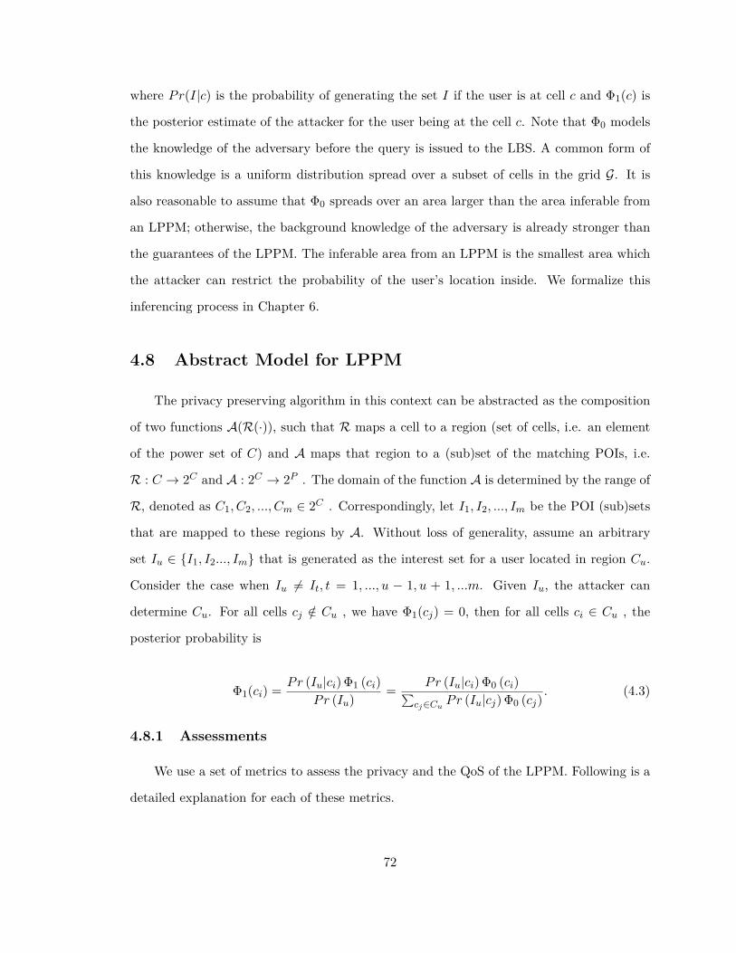
where Pr(I|c) is the probability of generating the set I if the user is at cell c and �1

(c) is

the posterior estimate of the attacker for the user being at the cell c. Note that �0

models

the knowledge of the adversary before the query is issued to the LBS. A common form of

this knowledge is a uniform distribution spread over a subset of cells in the grid G. It is

also reasonable to assume that �0

spreads over an area larger than the area inferable from

an LPPM; otherwise, the background knowledge of the adversary is already stronger than

the guarantees of the LPPM. The inferable area from an LPPM is the smallest area which

the attacker can restrict the probability of the user’s location inside. We formalize this

inferencing process in Chapter 6.

4.8 Abstract Model for LPPM

The privacy preserving algorithm in this context can be abstracted as the composition

of two functions A(R(·)), such that R maps a cell to a region (set of cells, i.e. an element

of the power set of C) and A maps that region to a (sub)set of the matching POIs, i.e.

R : C æ 2C and A : 2C æ 2P . The domain of the function A is determined by the range of

R, denoted as C1

, C2

, ..., Cm œ 2C . Correspondingly, let I1

, I2

, ..., Im be the POI (sub)sets

that are mapped to these regions by A. Without loss of generality, assume an arbitrary

set Iu œ {I1

, I2

..., Im} that is generated as the interest set for a user located in region Cu.

Consider the case when Iu ”= It, t = 1, ..., u ≠ 1, u + 1, ...m. Given Iu, the attacker can

determine Cu. For all cells cj /œ Cu , we have �1

(cj) = 0, then for all cells ci œ Cu , the

posterior probability is

�1

(ci) = Pr (Iu|ci) �1

(ci)Pr (Iu) = Pr (Iu|ci) �

0

(ci)qcjœCu

Pr (Iu|cj) �0

(cj) . (4.3)

4.8.1 Assessments

We use a set of metrics to assess the privacy and the QoS of the LPPM. Following is a

detailed explanation for each of these metrics.

72

Obfuscation

This technique has been applied to protect the location privacy in LBS in various other

research (Section 2.3). It is based on hiding the user’s location within a geographical area

of the site that contains the real location of the user, rather than accurately revealing the

exact location when requesting the service. So, the user can have access to the information

related to her location, while upholding the privacy. In order to achieve obfuscation, we

should have a “large” number of cells (including the cell of the user) in the region Cu with

positive probabilities. This number may be specified as part of the privacy policy of the

user. However, the user specified requirements cannot be achieved if the adversary has a

prior probability knowledge that allows him to narrow the user’s location down to a smaller

area. Hence, a precise statement (such as the �0

function) is necessary for the adversary’s

knowledge.

The adversary can sample one cell at a time (without replacement) based on the distri-

bution �. The expected number of cells that the adversary would sample before arriving at

the user’s actual location creates an obfuscation area for the user. We call this the expected

inexact privacy metric. It can be computed using the following closed form expression

expected_inexact(�, cu) =ÿ

c ”=cu

�(c)�(c) + �(cu) . (4.4)

Expected inexact privacy can be viewed as the smallest obfuscation area one can expect

if the attacker is successful in learning an approximate presence area using the sampling

method. The area can be obtained by multiplying the metric’s value with the area of one cell.

We will refer to this measure by the areal privacy metric. On the other hand, the expected

exact privacy reflects the probability of not arriving at the user’s location in one single

attempt. The expected estimation error of the adversary measures the average distance

between the true location of the user and the location estimated by the adversary [143].

When � is a uniform distribution over a subset C of cells, expected inexact privacy is equal

to |C|≠1

2

cells. For example, for a uniform distribution over an area of 32 ◊ 32 cells, the

73

expected inexact privacy is 511.5 cells. Say that the cell area is 0.01km2, then the areal

privacy of the user is 5.115km2.

Convergence

Based on the prior probability distribution of the attacker, the chances for the user being

in some cells may be higher than the chances of the other cells within the region Cu. In fact,

the disclosure of the interest set Iu, which is part of the execution of the protocol proposed in

the Section 4.3, gives the attacker some additional information about the current position

of the user. The attacker is now able to build a new posterior probability distribution

based on Iu and his prior probability distribution (Equation 4.3). However, if the posterior

probability distribution of the attacker for the region Cu is directly proportional to the

prior probability distribution, then this will ensure that the set Iu has no contribution to

improving the attacker’s knowledge about the new location of the user within the boundaries

of the region Cu. We refer to this as the convergence property of the algorithm. In Equation

4.3, convergence is achieved if Pr(Iu|ci), for any ci œ Cu , is a constant. Therefore, the

probability of producing the output Iu should be equal for all cells in the region Cu.

The convergence condition is hard to satisfy for the case of multiple queries. So in order

to measure the contribution of an LPPM in improving the attacker’s knowledge about the

new location of the user, we use a metric called nearness privacy. This metric is based on

the adversary’s best guess according to the distribution �. Given a probability distribution

� over the cells in the grid and the user’s current location cu, nearness privacy is computed

as

nearness(�, cu) = distance(maxc

�(c), cu). (4.5)

We use Euclidean distance in our evaluation. If multiple cells have the most probable

value, then we pick the cell closest to cu as the adversary’s guess. Note that when � is a

uniform distribution, nearness will be zero.

74

The quality of service

To achieve a high level of obfuscation, the region Cu must contain the largest possible

number of cells; in other words, a trivial solution is to always use the entire grid G in the

query of the second round-trip. But, this may degrade the QoS by increasing the expected

communication overhead (Steps 3 and 4 in Figure 4.3). Therefore, the privacy algorithm

must choose the smallest possible set of POIs that covers the area of the region Cu. Ideally,

the sets I1

, I2

..., In should each have only K elements.

4.9 LPPM implementation

It is di�cult to identify all the forms that can be taken by the privacy algorithm that

o�ers an acceptable level of obfuscation, convergence, and high QoS. Here we present the

formulation of the problem and give an outline for designing an LPPM model that preserves

the desired properties.

Let’s assume that C is partitioned into regions R1

, R2

, ..., Rq, such that the top-K POI

sets for each cell in a given region are the same. Let the sets P1

, P2

, ..., Pq represent the

top-K POIs for these q regions. The function R is responsible for the creating disjoint

groups C1

, C2

, ..., Cm of the q regions such that, Ci = Ri1t

...t

Rit . The interest set of a

given group of cells Ci is obtained by the function A, Ii = A(Ci) = Pi1t

...t

Pit . Ideally,

the m groups created using the R function should satisfy the following constraints.

1. For all groups Ci,---{c œ Ci|�(c) > 0}

--- Ø ”. The parameter ” indicates the obfuscation

level requested by the user. The trivial method to meet this requirement is to create

a single group of the union of all q regions. However, this solution may negatively

impact the quality of service of the application, which motivates us to include the

second constraint.

75

2. Suppose that the function f(C1

, C2

..., Cm) determines the e�ect of grouping the dif-

ferent regions on the quality of service. The function f may be defined as

f(C1

, C2

..., Cm) = maxi=1,2,··· ,m

--Ii

--, (4.6)

where Ii is the interest set corresponds to the group Ci. What is commanded here is

to minimize f . In our setting, it decreases the communication overhead.

Therefore, given a cell cu, a privacy algorithm using R and A returns the set Iu as the

interest set if cu œ Cu. Note that R is a many-to-one function, i.e. a cell can belong to

only one of the C1

, C2

, ..., Cm regions. The function A also is not necessarily a one-to-one

mapping but is many-to-one. The obfuscation and convergence requirements hold for this

algorithm. Assuming Iu is unique (A(Ci) = Iu ≈∆ i = u), for all cells ci œ Cu , we have

Pr(Iu|ci) = 1.

) ’ci œ Cu, �1

(ci) = Pr (Iu|ci) � (ci)Pr (Iu) = constant ◊ � (ci) . (4.7)

For all cells cj /œ Cu , we have �1

(cj) = 0. By virtue of the first constraint of our prob-

lem, we have Ci,---{c œ Ci|�(c) > 0}

--- Ø ”; therefore, at least ” cells (including the cell of

the user) in Cu have positive posterior probability (obfuscation). Also, the posterior prob-

abilities associated with this reduced set of cells is directly proportional to the background

knowledge (convergence). The observations trivially hold when Iu is not unique.

The function R is required to create m partitions from the regions R1

, R2

, ..., Rq, and

each partition Ci has at least ” cells with probability � > 0. Let the number of cells with

probability � > 0 for each region Ri is xi, where i = 1, 2, · · · q. So, we can represent the

set of regions {R1

, R2

, ..., Rq} by the set of integers X = {x1

, x2

, ..., xq}. The problem that

the function R should solve is: find {C1

, C2

, · · · Cm} partitions for the multi-set of positive

integers X such that the sum of the numbers of each partition Cj Ø ” ’j = 1, 2, · · · m. The

function R takes three input parameters; namely, the set X, the number of partitions m,

and minimum sum threshold parameter ”. By invoking R (X, ”, m) we should either get

76

the required partitions or a flag which tell us that no such partition is possible. We claim

that if there is a computationally e�cient algorithm to solve the problem of the function

R, then this algorithm can solve the number partitioning problem. Number partitioning

is an NP-complete problem [62]. The problem asks for deciding whether a given multiset

S of positive integers can be partitioned into two subsets such that the summation of the

numbers in both sets are equal. The algorithm that can solve number partitioning using R

is described as follows.

Given a set S of integers we compute the sum L of the numbers in S. If L is odd

then no partition exists for S, so we stop. If L is even we invoke R1S, L

2

, 22.

Then S has a partition if R succeeded; otherwise, S has no partition.

Verifying an instance solution of the problem R is trivial and we just show its NP

hardness; thus, the problem is NP-complete. We introduce in later chapters our heuristics

based techniques that achieve acceptable performance in terms of privacy achieved without

giving in too much of QoS.

4.10 Summary

In this chapter, we briefly describe the current prevalent communication architecture

and describe the changes we propose in order to implement a TTP free LPPM. The general

architecture we proposed, consisting of two communication round-trips, can be commonly

used across both PIR based techniques and heuristic-based techniques discussed in this

dissertation.

In the case of statistical-based techniques, we presented an abstract model that will be

used to quantify the privacy achieved and presented few metrics that can be used. One may

think of this abstract model as an outline to design a heuristic based LPPM. We show that

in heuristic based approaches, achieving privacy without compromising much of quality of

service boils down to creating an e�cient partition of grid regions to improve obfuscation

and convergence while not losing too much QoS. We also showed that a technique that

77

tries to achieve the optimum solution is NP-complete, and motivate the need for using

heuristic-based approaches that can e�ciently partition the cells of the grid G into regions

that satisfy both privacy and QoS requirements.

In the next chapter, we present the first TTP less protocol, using PIR, as it has got con-

siderable attention from the research community. Our goal there is to study and implement

two representative PIR schemes and assess their feasibility for real life applications.

78

Chapter 5

Investigation of PIR As a

Candidate Solution

PIR techniques allow users to query and retrieve records from a database without re-

vealing the query to the database. These techniques gather more importance as more and

more users rely on on-line services and at the same time demand better privacy. Compu-

tational PIR (cPIR) is a category of PIR that uses mathematical techniques to achieve its

goals. It requires the database to be pre-processed in some way at the service provider.

Once honestly followed, the PIR protocols ensure that it is computationally expensive for

the attacker, or the service provider itself, to decrypt the query, at the same time, be able

to respond with correct answers to it. The high level of privacy achieved using these tech-

niques comes at the cost of added computational and communication overhead. As new

mathematical techniques such as fully homomorphic encryption emerge, so does adoption

of them into cPIR. The e�ort has been trending towards making cPIR e�cient enough for a

practical implementation. There have been a few notable proposals in cPIR in recent years.

In Section 4.4 we characterize a protocol architecture (Figure 4.2) that adopts PIR to

preserve the location privacy of the user. We argue that, a PIR based protocol may represent

an ideal solution for our problem since the LSP will not be able to draw any additional

information about the user’s location through that protocol. In this chapter we present

79

a brief survey of PIR methods and then we pick the most promising of these proposals,

implement them, run them against typical database and block sizes, and compare their

performance. The last such comparative study was done in 2007 by Sion and Carbunar [147]

and there is a need to take into account recent advances, and check if the performance of the

latest proposals come close to practical adoption. Although each algorithm proposed has

its computational and communication complexity measures presented in terms of database

size, anyone that implements it will quickly realize that, because of the multiplier parameter

associated with each order term, the performance achieved “in reality” using standard

implementations on practical hardware and network technologies can be quite di�erent

from what one expects by just looking at the big O terms.

5.1 Preliminaries

In typical client/server scenarios, the user sends a query to the database, and the

database locates the relevant records and responds with the data i.e. the database server

has to know the query to be able to respond. In contrast, PIR is a protocol aimed to protect

the client’s privacy by allowing the user to still retrieve relevant information but without

revealing the query to the database. The need for such protocols to protect the privacy

of the clients arises from the model of semi-trusted service providers, where our problem

(location based search) exemplify this scenario.

A trivial protocol to solve this problem is for the server to send a copy of the entire

database to the client, who can then choose the required record(s) from this copy. It is obvi-

ous that this solution o�ers ultimate privacy to the client, since the server has no idea about

which record(s) the client is actually interested in. It is also obvious that this approach is

impractical as the transfer of the entire database has high communication cost. The problem

now is to determine some approach that guarantees almost the same privacy but with lesser

communication overhead. Chor et al. [32] introduced the term PIR to define this problem

and propose the information-theoretic PIR scheme (itPIR). This scheme actually provides

an absolute privacy guarantee (the same level as the trivial solution provides) for the client

80

with more reasonable communication cost. The main drawback of this scheme is that it

requires an identical copy of the database available with at least two non-colluding servers.

In fact Chor et al. [32] shows that nontrivial itPIR is not possible in the case of a single

database server. Another scheme to implement PIR is to use mathematical (cryptographic)

techniques known as computational PIR (cPIR). Here “computational” means to guarantee

that the server can compromise the privacy of the client only if it can solve a computation-

ally hard problem. The main advantage of this scheme is that it waives the requirement

of multiple servers. Unfortunately, the protocols that attempt to satisfy this approach, in

general, introduce high communication and computational overheads. We mentioned the

two major schemes of PIR viz., itPIR and cPIR. We discuss the details of various proposal

in each scheme below.

5.1.1 Information theoretic PIR techniques

In a simple itPIR scheme, the database is modeled as an n-bit string, x, replicated

among k servers where k Ø 2. In order to retrieve a certain bit xi from the database,

the client will send a uniform random bit string Sj of length n to each server such that

S1

ü · · · ü Sk = ei, where all the bits of ei are zero except for the bit at the ith position.

Each server responds by sending the result of bitwise XOR of x and Sj . The client then

XORs all the responses together to recover the bit xi. To reduce communication costs Chor

et al. [32] proposed embedding x in a d-dimensional cube, so the server can cover its string

Sj and all strings at Hamming distance 1 from it by d-bit long strings. For instance, by

embedding x in a 3-dimensional cube, two servers can emulate up to eight servers with a

total communication complexity O ( 3Ôn). Unfortunately, to emulate any larger number of

servers, it is required that the emulating server cover all possible codes with a Hamming

distance > 1, which adds more communication overhead.

Another set of proposals to reduce the number of servers use locally decodable codes

(LDC) [27,55,96,162]. LDCs are error-correcting codes in which a message x is encoded into

a codeword C (x) such that any bit of xi can be recovered e�ciently, with high probability, by

81

querying only k coordinates randomly in C (x). For PIR protocols based on this technique,

all the k servers are supposed to store the encoding of x. In order to retrieve the bit xi,

the client requests a uniform random coordinate (ideally one bit) in C (x) from each server.

Although the k coordinates requested by the client must be su�cient to recover the bit xi,

each server can see that the client is just interested in one uniformly selected coordinate in

C (x).

Although bit retrieval theoretically is extensible, retrieving a block (or a record) of

several bits from the database is a more realistic scenario. Here a linear algebraic query

model is used where the database is modeled as a matrix D of n blocks, b1

, · · · bn, each block

bi is m-bits long. By generalizing the simple itPIR scheme explained above, if k servers

have exactly the same replica of the database, the client can retrieve the block i privately

with total communication cost of k · (n + m). The first step is the same, where the client

generates k uniform bit strings of length n, such that S1

ü · · · ü Sk = ei, and sends one

bit string to each server. The server j now returns the vector vj = Sj ◊ D. The client

recovers the ith record by computing v1

ü · · · ü vk = ei ◊ D. This scheme is based on a

simple secret sharing mechanism. The secret is the index of the interested record, i, and

the secret shares are the bit strings S1

, · · · , Sk, since i can be determined only if we know

all of these bit strings. But this scheme will fail if one of the servers does not respond, or

even worse, replies with a false answer. This problem can be described in general as follows.

Given total number of servers ¸, only k of them answers the client’s query. From these k

servers, h servers reply honestly, and the rest could lie. The goal is to retrieve the client’s

query privately for up to t non-colluding servers. Goldberg [71] addressed this problem

and proposes a protocol based on Shamir’s secret sharing [139] to generate the query’s

secret shares and then recover the answer code words using the Guruswami-Sudan error

correcting algorithm [77]. Devet et al. [41] improve the computation speed of Goldberg’s

protocol, as well as the minimum bound for the number t of non-colluding servers. Devet

used dynamic programming to decide the answer recovery algorithm among Berlekamp-

Welch [155], Guruswami-Sudan [77] or brute force methods. Henry et al. [83] also built on

82

the Goldberg’s protocol to develop a method for retrieving multiple blocks simultaneously

from the database.

itPIR is reasonably fast (negligible computation cost) and can guarantee privacy if the

servers are trusted. But, the major problem with itPIR schemes is the vulnerability of

query exposure when the replicated servers collude. In the most simple case, colluding

servers can totally nullify query privacy. This requirement of multiple non-colluding servers

makes itPIR impractical in most real scenarios.

5.1.2 Computational PIR techniques

The first attempt to solve the PIR problem without the need for multiple non-colluding

database servers was made in 1997 by Kushilevitz and Ostrovsky [100]. The proposed solu-

tion is based on the assumption that the server cannot solve the quadratic-residuo problem

e�ciently (i.e., in polynomial time) [72]. In 2005 Gentry and Ramzan [66] constructed a

cPIR algorithm that is based on the „-hiding assumption, introduced by Cachin et al. [23].

The algorithm has a communication complexity of O (k + d), where k Ø log n is the se-

curity parameter and d is the length of the database block. This protocol achieves the

best performance in terms of reducing the communication cost compared to other known

cPIR protocols. However, it necessitates expensive computational operations, especially on

the server side, to generate the query response, which limits the practicality of the pro-

tocol [3, 130]. In fact, it turns out that the major deficiency in all cPIR protocols is the

high computational cost. In 2007, Sion and Carbunar [147] showed that the trivial PIR

protocol is more e�cient than any other PIR protocol proposed by that time, when im-

plemented on realistic hardware and communication networks. The authors have focused

only on the protocol of Kushilevitz and Ostrovsky [100] in their analysis for cPIR schemes

and completely rejected itPIR by assuming that the requirement of replicating a database

is an unsatisfiable condition in real scenarios. Aguilar-Melchor and Gaborit [3] proposed a

linear algebra based protocol that aims to achieve high computation throughput. A later

study by Olumofin and Goldberg [125] similar to the one done by Sion and Carbunar [147]

83

conclude that this protocol is an order of magnitude more e�cient than the trivial PIR.

Although, the query size for this protocol is large, the protocol has significantly reduced

the computational overhead compared to the previous protocols. Unfortunately, in 2012,

Jingguo Bi et al. [17] show a possible attack against the Aguilar-Melchor and Gaborit [3]

protocol by uncovering the secret linear relationship between the public keys and the secret

keys.

Xun Yi et al. [163] uses some variant of Dijk et al. [154] Fully Homomorphic Encryption

(FHE) to o�er a cPIR. For a database size of n-bits and consisting of m records each of

the same length, the total communication and computational overhead of the protocol are

O(“ log m + n“/m) and O(m“2 log m + n“/2), respectively, where “ is the cipher text size,

which is determined by specific security parameters. Changyu et al. [47] also proposed

a scheme based on fully homomorphic encryption in which they take advantage of the

inherent parallelism in the BGV algorithm [20] to reduce the communication complexity to

O(log log n). However, the authors describe the protocol for single bit retrieval and left the

more practical block retrieval protocol to be addressed in later work.

When one looks at the existing research, a clear pattern emerges. E�ciency achieved

on the communication overhead is balanced out by often increased computational com-

plexity. Even though newer proposals are clever and improve on both dimensions, further

improvements are needed for these to become really practical. In order to evaluate the

improvements achieved in cPIR performance over the years, we compare the first major

proposal [100] based on the quadratic residuosity assumption (QRP ) against the latest1

proposed protocol based on fully homomorphic encryption (FHE) [163].

5.2 PIR Protocol Model

In this section, we present just enough background of the protocols, QRP and FHP ,

to keep the discussion complete. Also, we present them with common symbols so readers

get a better feel for their performance when represented in those common terms. In our

1At the time of this writing

84

implementation for both QRP and FHP , we assume that the database consists of n blocks

(records) of equal length. Each block Bi is m-bit long. So the database is viewed as an

n ◊ m matrix, where each row in the matrix corresponds to one record in the database.

Before going into the details of the QRP and FHP protocols, it would be better to give an

overview of the general structure of cPIR schemes.

A cPIR protocol consists of three polynomial time algorithms; QueryGenerator,

ResponseGenerator and ResponseDecoder. First, the client uses the QueryGen-

erator algorithm to create an encrypted query and a private secret for a specific block of

index, j, and sends the query to the server. The server computes the response for the “en-

crypted” query on the database by using the Response-Generator algorithm, and then

sends this response back to the client. The client shall be able to retrieve the block j from

the received response using the Response-Decoder. In this chapter, we call execution

of all three algorithms, starting with query generation to response decoding on the client,

as a round-trip (this should not be confused with the previous definition for the round-trip

in Chapter 4). Two conditions must be satisfied by the cPIR scheme – correctness and

privacy. Correctness means that for any query generated for a block j by the QueryGen-

erator algorithm, the correct block must be recovered back from the response generated

by the ResponseGenerator algorithm by using the algorithm ResponseDecoder. The

privacy requirement stipulates that for any two queries for di�erent blocks i and j in the

database, the server cannot distinguish one from the other with a non negligible probability.

The communication overhead and computational cost of a cPIR scheme are measured in

terms of n and m (the size of the database) and the size of the overhead induced by the

privacy protocol.

5.2.1 Description of QRP

Since this protocol is based on the intractability of the quadratic residuosity problem,

we will introduce the problem briefly before we describe the protocol.

85

Given an integer N and an integer x œ ZúN , x is said to be a quadratic residue modulo

N if there exists an integer y œ ZúN such that x © y2 (mod N). Otherwise we say it is a

quadratic non-residue. We denote the set of quadratic residues modulo N by QRN and

the set of quadratic non-residues modulo N by N RN . The Jacobi symbol is defined over

the set ZN as the product of the Legendre symbols corresponding to the prime factors of

N , and it can be computed in polynomial time [36]. The Legendre symbol is defined in

Equation 5.1. If the modulus is a prime, p, then it is easy to decide whether an integer

x œ Zúp is quadratic residue or not by just computing the Jacobi symbol,

1xp

2. For composite

modulus, the Jacobi symbol cannot be directly used to decide the quadratic residuosity of

an integer x œ ZúN . Consider a composite modulus, N = p.q, where p and q are unknown

primes. We can still compute the Jacobi symbol!

xN

", but in this case

!xN

"=

1xp

2 1xq

2and

x œ QRN ≈∆1

xp

2=

1xq

2= 1. Half of the integers x œ Zú

N have Jacobi symbol equal to

≠1 where1

xp

2”=

1xq

2, and we know certainly that they are not quadratic residues modulo

N . But, the other half have Jacobi symbol equal to 1 where1

xp

2=

1xq

2. Notice that, if

1xp

2=

1xq

2= 1, then x œ QRN ; and, if

1xp

2=

1xq

2= ≠1, then x œ N RN .

3x

p

4=

Y_____]

_____[

0 if a © 0 (mod p);i.e., a /œ Zúp

1 if x œ QRp

≠1 if x œ N Rp

(5.1)

Therefore, if the Jacobi symbol is 1, Pr [x œ QRN ] = Pr [x œ N RN ] = 1

2

. A hard-set of

quadratic residuosity, Hk, is defined in Equation 5.2

Hk = {x|x œ ZúN , N = p.q

where p, q are k2

-bit primes and!

xN

"= 1

Ô (5.2)

The quadratic residuosity assumption states that for any integer x œ Hk, if the factor-

ization of N is unknown, there is no e�cient algorithm to decide whether x is a quadratic

residue modulo N or not. In addition to the hardness of deciding quadratic residuosity for

86

x œ Hk, the set Hk maintains a useful XOR property. That is, ’x, y œ Hk, the product x ·y

(mod N) is a QRN if both x and y are QRN or N RN ; otherwise the product is N RN .

Now that we have su�cient background, we describe the QRP PIR protocol. Steps

of QueryGenerator, ResponseGenerator and ResponseDecoder routines are de-

scribed in Algorithm 5.1. The round trip starts at the client side, when the QueryGen-

Algorithm 5.1 QRP algorithms.1: function QueryGenerator(⁄, n, j)2: p1, p2 Ωrand_prime, where |p1| = |p2| = k/23: N Ω p1 · p24: for i = 1 to n and i ”= j do5: Choose random qi œ Hk s.t. qi is QRN

6: end for7: Choose random qj œ Hk s.t. qj is N RN

8: return (p1, p2, [q1, · · · , qn])9: end function

10: function ResponseGenerator(N, [q1, · · · , qn] , DB)11: [z1, · · · , zm] Ω 112: for i = 1 to n do13: for t = 1 to m do14: if bi,t = 1 then15: zt Ω zt ◊ qi (mod N)16: end if17: end for18: end for19: return ([z1, · · · , zm])20: end function21: function ResponseDecoder([z1, · · · , zm] , p1, p2)22: for t = 1 to m do23: if zt is QRN then24: bj,t Ω 025: else26: bj,t Ω 127: end if28: end for29: return ([bj,1, · · · , bj,m])30: end function

erator routine is invoked to create the query vector [q1

· · · qn] for a database record j,

using the private key (p1

, p2

) and a public key N . The client then sends [q1

· · · qn] and N

to the server which computes the response [z1

· · · zm] and sends it back to the client. Using

the response received from the server, the client will recover the record Bj using the Re-

sponseDecoder routine, thus completing the round-trip. Notice that, deciding whether

87

an integer zt is QRN or not (line 17 in Algorithm 5.1) is a polynomial time operation

because the client knows the primes (p1

, p2

) which form the private key.

We will not present detailed proofs for the correctness and privacy of either algorithm

here. The interested reader may refer to the original references. However, the security

of QRP , intuitively, follows from the quadratic residuosity assumption. The correctness is

based on the XOR property of Hk. As it is obvious, if bj,t = 0 in the original database, then

zt is the accumulated product of QRN integers, which results in a QRN integer. On the

other hand, bj,t = 1, means the accumulated product of zt will include one N RN integer,

which results in a N RN integer.

5.2.2 Description of FHP

This protocol is based on a variant of the Fully Homomorphic Encryption (FHE) scheme

proposed by Dijk et al. [154]. In FHE, mathematical operations can be performed on

encrypted inputs to produce an encrypted version of the result. Thus, a semi-trusted

party can perform computations on encrypted inputs and produce correct results without

knowing the plain values of the inputs. In Dijk et al. [154] scheme the user chooses a security

parameter ⁄ and determines a parameter set fl = ⁄, ÷ = (⁄ + 3) Álog nË , “ = 5(⁄ + 3) Álog nË2

.

The secret key, sk, is a random odd integer of length ÷-bit. The public key is pk = sk · q0

,

where q0

is a random odd integer chosen from [1, 2“/sk). To encrypt M œ {0, 1}, the

user, who knows sk, chooses two random integers p œ1≠2⁄, 2⁄

2and q œ [1, 2“/sk). The

ciphertext, c = E (M, pk) © M + 2 · r + q · sk (mod pk). With the secret key sk, the user

decrypts a ciphertext as M = D (c, sk) © (c (mod sk)) (mod 2).

The protocol consists of the three algorithms given in Algorithm 5.2. In the Query-

Generator, the client calculates pk and sk based on the security parameter ⁄. In line

6, rs and qs are random integers chosen as specified by the FHE scheme described above.

Notice that, in line 6, –s œ {0, 1} is the plaintext and –s is its encryption. So the query

basically is nothing but an encryption of the index of the required block. For the Respon-

seGenerator algorithm, each block Bi is viewed as a bit vector [bi,1, · · · , bi,m]. Before it

88

Algorithm 5.2 FHP algorithms.1: function QueryGenerator(⁄, n, j)2: Generate pk and sk3: ¸ Ω Álog nË4: –1, · · · , –¸ Ωbinary_representation of j5: for s = 1 to ¸ do6: –s Ω E (–s, pk) = –s + 2 · rs + qs · sk (mod pk)7: end for8: return (sk, pk, [–1, · · · , –¸])9: end function

10: function ResponseGenerator(pk, [–1, · · · , –¸] , DB)11: ¸ Ω Álog nË12: for i = 1 to n do13: —i,1, · · · , —i,¸ Ωbinary_representation of i

14: Êi Ωr¸

s=1 –s + (—i,s ü 1) (mod pk)15: end for16: [z1, · · · , zm] Ω 017: for i = 1 to n do18: for t = 1 to m do19: if bi,t = 1 then20: zt Ω zt + Êi (mod pk)21: end if22: end for23: end for24: return ([z1, · · · , zm])25: end function26: function ResponseDecoder([z1, · · · , zm] , sk)27: for t = 1 to m do28: bj,t Ω (zt (mod sk)) (mod 2)29: end for30: return ([bj,1, · · · , bj,m])31: end function

can create the response, the algorithm must compute the encryption values corresponding

to each record Ê (lines 10–12 in Algorithm 5.2). This additional computation cost comes

as a penalty for the reduction that has been made in the communication cost. Hence, in

this protocol, the query size is logarithmically proportional to the number of records where

as it is linear in the case of QRP . Finally, recovery of queried record j at the client is

straightforward as shown in the ResponseDecoder routine.

89

5.3 Implementation Details

In implementing both QRP and FHP algorithms, we used open source, peer validated

libraries that implement the underlying arithmetic. A not too old, not too modern hardware

platform is chosen to represent a typically available hardware architecture. Also, normally

available Ethernet based LAN connections are used between the server and the client. Our

goal is to be realistic in terms of hardware and network platform selection. We implemented

both protocols using C++ on Ubuntu 14.04.3 LTS virtual server machine with 4 core Intelr

Xeonr CPU E5 ≠ 2695 v3 @ 2.30GHz with cache size of 35MB and Debian GNU/Linux 7

client machine –Intelr Xeonr E5405 @ 2.00GHz. We use the NTL (version 9.4.0) library

[145] to perform big integer modular operations. NTL is a high-performance free open

source C++ library that o�ers algorithms for processing arbitrary length integers.

Each of the algorithms was first validated for correctness, by making sure the retrieved

block of data on the client side exactly matches the corresponding block in the database.

The performance characteristics of each algorithm are verified independently. We used

similar techniques to test the performance as those used by the original authors of the

algorithms. This is so that we can compare our results with those published by the authors

and ensure that our implementation performs at least as good as those obtained by the

original authors.

After ensuring the correctness and satisfactory performance, the algorithms were nor-

malized by adjusting the parameters so that the privacy o�ered by each algorithm is similar,

i.e., if the semi trusted server were to break the privacy and figure out the index j that is

queried by the client, the amount of work needed should be similar for both algorithms.

For FHP protocol, the authors [163] propose ⁄ = 60. This gives “ = 2205 and a public

key length of 2205 bits, so all the integers exchanged between the client (queries) and the

server (responses) are going to be of length 2205 bits. In fact setting ⁄ = 60 gives us a

low security level t 260. We set ⁄ = 85, so we have a security level of 285. With ⁄ = 85,

the public key length is 3080 bit. For the quadratic residue protocol, we choose k = 500,

so the moduli N is 1000 bits long. The fastest known algorithm for integer factorization,

90

Table 5.1: Average Computation Time and Round-trip Time in minutes for QRP and FHPfor di�erent database sizes. Database Size is represented as number of records ◊ recordsize.

Database Size Computation RoundtripQRP FHP QRP FHP

10000 ◊ 10kB 2.041 1.361 2.111 1.36610000 ◊ 25kB 5.041 5.637 5.214 5.65110000 ◊ 50KB 10.353 11.308 10.698 11.33510000 ◊ 100kB 21.189 22.409 21.878 22.46520000 ◊ 10kB 4.068 3.070 4.137 3.07620000 ◊ 25kB 10.146 10.862 10.319 10.87720000 ◊ 50kB 21.239 22.721 21.583 22.75220000 ◊ 100kB 42.019 44.649 42.711 44.71130000 ◊ 10kB 6.034 4.553 6.103 4.55830000 ◊ 25kB 15.281 16.284 15.454 16.29930000 ◊ 50kB 31.349 33.126 31.701 33.15730000 ◊ 100kB 63.274 68.699 63.965 68.761

number field sieve [21], can factorize an integer of length 1000 bits (under some heuristic

assumptions) in a time ¥ 285. With these settings we compare the performance of both

protocols under the same level for privacy.

5.4 Results and Analysis

Table 5.1 shows experimental results for both protocols running on di�erent sized

databases. To generate the query, the QRP client creates n random integers of k bits

long, which gives a total computation complexity of k · n. FHP client encrypts log n bits

using DGHV a somewhat homomorphic encryption scheme, which require two multiplica-

tions and two additions for “ bits long integers. So the total computation complexity of the

query generation algorithm is 2 · “ · (“ + 1) · log n.

For response decoding, the QRP client will test the quadratic residuosity of each re-

ceived integer from the server. Given the factorization of N , the residuosity check requires

O1log3 N

2[146]. So the total computational complexity of the decoding algorithm is m ·k3.

For FHP , the response decoding algorithm is nothing but a long integer devision performed

91

iteratively over m integers; each of these integers is “ bits long, so the total cost of the al-

gorithm is m · “2 bit operations.

The QRP client query consists of n integers and the response generated by the server

is m integers. Since each of these integers is k bits, the total communication cost of the

protocol is k · (n + m) bits. On the other hand, the client using FHP sends log n integer

numbers for each query and receives m integers representing the response from the server,

where the length of each number is “ bits. In order to address the problem of large query size

for QRP , Kushilevitz and Ostrovsky [100] suggested a recursive technique to implement the

protocol. Unfortunately, this technique leads to exponential increment in both the response

size and the computational cost. Therefore we skip this technique in our implementation

and we choose to implement the QRP server using the classical producer/consumer pattern.

The server could start computing the elements of the response array as soon as the first

query element is received from the client, and then accumulatively update the response

array when new elements of the query array are available. Since the time for uploading the

query from client to server is negligible compared to the response computation time, this

implementation of the server would eliminate the impact of the large query size on the overall

roundtrip of the protocol. Clearly the query size of FHP is much smaller than the query size

of QRP . In Table 5.1 the di�erence between the roundtrip time and the server computation

time represents the total communication and the client computation costs. Notice that this

di�erence for QRP is ≥ 10 times larger than that for FHP . But as we will see shortly that

this gain in the query size of FHP comes at the cost of increased computation overhead at

the server side which can significantly impact the overall performance of the protocol.

The most expensive part for both protocols is the response generation that happens on

the server side. In the process of generating a response, both algorithms examine each single

bit in the database. If the bit is 1, the QRP server performs a modular multiplication for

two integers of k-bit, while the FHP server performs a modular addition for two integers of

“-bit. Even though “ = 3·k, NTL (on our server) performs modular addition of two 3000-bit

integers 10 times faster than a modular multiplication of two 1000-bit integers, which gives

92

a worthy advantage to FHP over QRP . But, since the query generated by the FHP client

represents the encryption of the address of the required record, the server now must compute

an encryption Ê corresponding to each record in the database. This step includes additional

n · log n modular multiplication and addition operations for integers of size “ bits at the

FHP server (lines 11, 12 in Algorithm 5.2). We solve this problem also by implementing the

producer/consumer pattern as we did in the QRP server. The response array elements are

computed accumulatively as the next encryption value Ê becomes ready. But, one should

notice that the computation cost of Ê is significantly higher than the communication cost

of sending k-bit numbers. Specifically, in our settings the communication cost of sending

1000 bits is 0.01 msec while the computation cost of Ê is 0.8 msec. The e�ect of this

additional computational cost of FHP increases with the number of records in the database,

which explains the performance degradation for FHP in our experimental results when the

number of the database records is increased (Table 5.1). Another observation is that the

FHP performance decreases as the size of the record increases. Notice that, the FHP

server needs to maintain two arrays, the size of each array is 3080 ◊ n bits, while the QRP

server will maintain one array of size 1000 ◊ n bits. This larger amount of memory (s 6

times) requirement by FHP causes a higher rate of cache misses; which in turn will increase

the computation time of the ResponseGenerator algorithm. We summarize the pros and

cons for both protocols in the following points.

• The QRP query size increases linearly with the number of records in the database,

n, while FHP o�ers a good solution to this problem since the query size increases

logarithmically with n.

• The FHP protocol demands larger bit size for the security parameter “ than the

security parameter k for the QRP protocol. This causes a negative e�ect on the

computation time and the response size for FHP .

• In general, the FHP performs better than the QRP for smaller databases while QRP

outruns FHP when the database is large.

93

• Unfortunately, neither protocol is e�cient enough to be practical. Both protocols

are much slower than a trivial protocol in which the server will transfer the entire

database to the client.

5.5 Summary

In this chapter we have implemented and evaluated both Quadratic-Residuosity based

and Fully-Homomorphic Encryption based cPIR protocols that represent earliest and latest

work in this area. We have used standard middle-of-the-ground hardware, software and

open source libraries to implement them. Our goal has been to study the performance

characteristics of each of these algorithms with a focus on testing if the latest improvements

in cPIR schemes give enough performance gains as to make them useful in practical appli-

cations. We have normalized the protocols to o�er similar acceptable privacy and run them

against various representative sizes of databases and records. We have compared the per-

formance statistics against that of the most trivial cPIR protocol. Our conclusion is that,

even though there are improvements in communication and computation costs, cPIR proto-

cols still require lot of work before they become e�cient enough for practical applications,

especially, TTP less protocol for LBS.

Moreover, when one observes the already prevalent LBS architecture, one can see that

PIR techniques (both cPIR and itPIR) cannot be practically implemented on the current

LBS architecture. Even if one were to ignore the client side processing and the commu-

nication costs, cPIR requires extensive processing overhead at the server side and itPIR

requires replication of the service provider databases. Service providers may not be inclined

to these changes that are counter intuitive to their revenue models in the LBS business.

The alternative, which is transferring the entire database to the client, is even more counter

productive for the service provider’s business model, not to mention the communication

and capacity costs imposed on the client and the entire system in general. Hence, having

considered and studied carefully, we rule out PIR as a feasible method for our purpose, the

TTP less LBS protocol. In the next few chapters, we propose our own protocols that use

94

statistical privacy techniques and apply heuristics to achieve that goal. While proposing

these techniques, our goal is not only to develop a proven technique in achieving guaran-

teed privacy levels, but also impose as minimal changes to existing prevalent architectures

as possible.

95

Chapter 6

Single Query Scenario

Continuing the discussion from Chapter 4, we present in this chapter implementation

details of an e�cient heuristic based LPPM. The goal is to implement optimizations and

heuristics with a focus on reducing processing times that makes it practical on mobile

devices. Even though mobile devices have come a long way in terms of processing power,

optimizations are required in order for the privacy protection methods to finish quickly

enough to preserve quality of service. Algorithms along with heuristics of the proposed

LPPM presented here are based on our work in [44]. Later, we present the implementation

details and assess the performance characteristics of the proposed LPPM.

First, we consider a simple scenario where the user issues a single query. In the next

chapter we enhance this architecture to be able to provide strong and e�cient privacy

guarantees when multiple queries are made by the user. However, the model and sym-

bols introduced in this chapter are maintained and extended throughout the rest of the

dissertation.

6.1 Proposed LPPM

High levels of privacy measures discussed in Section 4.8 serve as an objective that one

may try to achieve while designing a search algorithm for local search. However, the question

remains open whether the computational cost associated with implementing this solution

96

on a mobile device will be practical or not. Alternatively, instead of obtaining the optimal

regions C1

, C2

, ..., Cm, (Section 4.9) we have taken the engineering approach and divide the

set of cells C into predefined regions. These regions are created by overlaying the grid G

with a coarser grid of size Z ◊Z. All cells contained within a coarser cell then form a region.

We will refer to such a region also as a box. In this case, we have m =1

ZˆZ

22

(assume Z is a

multiple of Z) and each box Bi is simply a sub-grid of the grid G with size of b ◊ b, where

b = ZˆZ. Note that, in this formulation, the user configures her required level of obfuscation

by setting the value of the parameter b indicating that she does not care if the attacker

narrows her location to an area greater than or equal to a b cells by b cells (b ◊ b box). This

is often specified in real life approximations such as a mall, block and sub-division that is

usually translated by the application into the parameter b that represents their size. So,

pinpointing the user’s location to an area that is less than a b ◊ b box will be considered a

breach of her expected privacy.

If the box Bu happens to be the b◊b box where the user is located, then the interest set,

Iu, is the union of the most highly ranked K POIs (top-K POIs) for each cell in Bu. The

need is to compute a set of top-K POIs for each cell in a subset of cells Cu and return the

union of these sets. Here, the subset Cu is a set of cells that form a box Bu which contains

the user’s cell, cu. Clearly, the obfuscation requirement is satisfied for this algorithm, since

for each cell c œ Cu, �1

(c) > 0. Equation 4.3 for the probability that the user exists in a

cell ci œ Cu can be rewritten as follows

�1

(ci) = Pr (ci|Cu) = Pr (Cu|ci) �0

(ci)qcjœCu

Pr (Cu|cj) �0

(cj) . (6.1)

Since the grid G has been pre-partitioned into non-overlapping boxes of size b ◊ b, for any

box B, Pr (C|ci) = 1, ’ci œ C, where C is the subset of cells included in B. By substituting

into Equation 6.1, we have �1

(ci) = a constant ◊ �0

(ci); hence convergence holds as well.

Service loss minimization is also not performed explicitly; nonetheless, we expect the

union size of the top-K sets to be relatively low since neighboring cells are collected together

97

to form the regions. The interest set computation for the user is then performed in two

steps:

1. R: determine the box Bu where the cell of the user belongs.

2. A: obtain the union of the top-K POI sets of the cells in Bu.

Following the steps of the architecture presented in Section 4.5, the client determines

a large geographical area that includes the user’s location (AR), and sends the coordinates

of this area along with search keywords to the server. The server finds the list of matching

POIs within AR from its database, and sends back only the location and the prominence

information of the obtained POIs. The client locally ranks the received list of POIs and

determines the interest set Iu corresponding to the box Bu. The client then queries the

server for detailed information about the POIs in the set Iu. The server responds with

details of those POIs.

To determine the interest set, a brute force search is the trivial solution to compute

the union of the top-K POIs of the cells in a box. But it is computationally impractical to

implement on the client end, i.e., the mobile device. Hence, a faster algorithm to calculate

the interest set locally on the client end has been proposed.

6.2 Interests Set Computation

The top level procedure of our method is given in Algorithm 6.1. The algorithm starts

with the following pre-computations:

1. Partition the set Cu into two subset Cborder and Cinternal. The set Cborder is a set of

cells that occur at the border of the box Bu; Cinternal is the set of the remaining cells

of Bu.

2. Determine subset Pbox œ P , the set of POIs that occur inside, or on the border of the

box Bu.

98

Algorithm 6.1 Compute the top-K set of POIs for the user’s box.Input: Set P of all POIs; Set Cu of all cells in the box Bu; Prameter KOutput: Interest set I: the unioun of the top-K POIs for all cells ci œ Cu

1: function CreateTopK-List(P , Cu, K)2: Cborder Ω border cells of Bu Û subset of Cu

3: Cinternal Ω non-border cells of Bu Û complement of Cborder

4: Pbox Ω POIs included in the box Bu Û subset of P5: I Ω ?6: root Ω BuildTree(Data(P ), 1)7: for all ci œ Cborder do8: I Ω Ifi CellTopPOIs(root, ci, K)9: end for

10: Preduced Ω Pbox fi I11: root Ω BuildTree(Data(Preduced), 1)12: for all ci œ Cinternal do13: if I = Preduced then exit for14: I Ω Ifi CellTopPOIs(root, ci, K)15: end for16: return I17: end function

Stage-I

Build the interest set for the border cells cumulatively by iterating through the cells of

Cborder, computing the top-K POIs for each cell and add it to the interest set I. In order to

obtain the set of the top-K POI for a cell, we use a kd-tree based branch-and-bound search

algorithm. The details of constructing the tree and modifying this technique to satisfy our

problem requirements are going to be discussed later in this chapter. For this stage we build

the kd-tree using the full set of POIs, P . In the next stage we will use a reduced search

space (POIs set) to build the kd-tree with less number of nodes, which leads to a smaller

tree and so improves the search time. Moreover, at this stage we do the computation for

a smaller partition of Cu cells, namely the border cells, while the small tree is used for the

larger partition.

Stage-II

By the end of Stage-I we have the set I that represents the top-K POIs for the border

cells of the box Bu. We create a new reduced search set of POIs, Preduced, for this stage by

99

computing the union of the sets I and Pbox, where Pbox is the set of POIs that are located

within the box. Now a new kd-tree is built using the set Preduced. We use this kd-tree and

iterate through the cells of the set Cinternal to obtain the top-K POIs for each cell. Again

we cumulatively add the top-K POIs from each cell to the interest set, I. The algorithm

ends after either exhausting all the cells in set Cinternal or if I = Preduced, since we cannot

add any more POIs to I.

6.3 kd-Tree Branch-and-bound Search

A kd-tree data structure is chosen, because it is a data structure that gracefully adapts

the distribution of k-dimensional points and also can be used “e�ciently” for range searching

and range counting queries. We built the kd-tree using the search set of the POIs, and then

used it to determine the top-K POIs for a cell cref in the grid. The tree built here is a

slightly modified version of the standard 2d-tree data structure (in our application k = 2).

So the concept of a 2d-tree is briefly reviewed here before the implementation of the proposed

2d-tree is explained.

The main idea of a 2d-tree is that it recursively partitions the plane into two half planes.

Let’s take as an example a set of points that are distributed in the xy-plane as shown in

Figure 6.1a and build a 2d-tree based on these points. Consider any random permutation of

the points, say (c3

, c2

, c7

, c9

, c6

, c4

, c10

, c1

, c8

, c5

). Take the point c3

, which is the first point

that appears in the random list, and set this point as the root of the tree. The plane is

divided into two parts based on a vertical line through this point. In the tree, all points

that fall to the left of the point c3

, i.e., the points with smaller x-coordinate values must

be added to the left subtree of the node c3

. Similarly, every point with x-coordinate value

greater than the x-coordinate value of the point c3

must be in the right subtree of the node

c3

. At this point the x-axis is referred to as the cutting dimension of the node. Then we get

the next point c2

where we switch our partitioning of the plane according to the horizontal

line that passes through this point. At the node c2

in the tree the left subtree consists of

the set of points that are below the horizontal line (smaller y-coordinate values) and the

100

9c

7c8c

2c

5c3c

10c 6c

4c

1c

(a) Data points

9c

7c 2c

3c

10c

6c

4c

1c

8c

5c

(b) 2d-tree

Figure 6.1: Building a 2d-tree example.

right subtree will include only the points above the horizontal line (greater y-coordinate

values). In this step, the cutting dimension is the y-axis. Continuing the same process for

the rest of the points we end up with the tree shown in Figure 6.1b. The left subtree for

any node ci represents the set of all points in the plane with a cutting dimension coordinate

values less than the value of the point ci, and the right subtree will contain all the points

that have values greater than the value of the point ci. The resulting tree is nothing but a

binary search tree in which the key is alternated based on the cutting dimension (axis) of

the node.

6.3.1 Building augmented kd-tree

Clearly, keeping a binary search tree balanced will significantly reduce the search time.

In Algorithm 6.2, the kd-tree is built by using a composite array, data, for the set P of POIs

that is sorted based on both x and y coordinate values. To create the first node (root) of the

tree the median point from the data set is chosen based on the current cutting dimension.

Then, branches of the tree are built recursively by considering all points and placing them

on either side of the root node. This ensures a more balanced kd-tree compared to building

it iteratively using randomly ordered points. Additionally, in Algorithm 6.2, each node in

the tree is augmented with the minimum possible “ value of POIs included in the subtree

101

rooted at that node including the node itself (recall from Section 4.6 that “i = 1≠–– (1≠Pi)).

We denote this value by “min(.).

Algorithm 6.2 Build kd-tree.Input: Composite array data of all POIs sorted based on both x and y; Index of cutting

dimension cdOutput: The root of kd-tree for the given set of POIs

1: function BuildTree(data, cd) Û cd is the cutting dimension2: if size(data) = 1 then3: t Ω kdNode(data[cd, 1], cd)4: else5: median Ω size(data)/26: t Ω kdNode(data[cd, median], cd)7: if median > 1 then8: t.Left Ω BuildTree(LeftPoints(data[cd], median), ((cd + 1)%2) + 1)9: t.MinLeftGamma Ω Min(t.Left.Gamma, t.Left.MinChildGamma)

10: end if11: if median < size(data) then12: t.Right Ω BuildTree(RightPoints(data[cd], median), ((cd + 1)%2) + 1)13: t.MinRightGamma Ω Min(t.Right.Gamma, t.Right.MinChildGamma)14: end if15: end if16: return t17: end function

6.3.2 Find the top-k POIs

Algorithm 6.3 shows how to calculate the top-K POIs for a given query cell cref . Two

lists are maintained – (i) a list T representing the top-K nodes (POIs), ordered according

to the rank of the nodes with respect to cref , and (ii) a list L of nodes to be explored,

sorted by a lower bound value. The lower bound value for a node represents the minimum

possible rank achievable for the subtree rooted at that node.

To compute the lower bound value for a node we associate two distance estimates to

every node c, dx(c) and dy(c), representing the minimum possible distance we expect to

find in the subtree rooted at node c, along x- and y- dimensions, respectively. Equation 6.2

gives the lower bound of the rank values in the subtree at node c.

102

Algorithm 6.3 Compute the top-K set for reference cell.Input: Root node root of kd-tree; Reference cell cref ; Parameter KOutput: Ordered list of top-K POIs with respect to the cell cref

1: function CellTopPOIs(root, cref , K)2: T Ω empty list3: L Ω empty list4: L.Append(root)5: while L is not empty do6: ntest Ω L.Remove-And-Return-Head()7: i Ω 18: if T.size = K and @isuch thatntest.lbound Æ T [i].rank then exit while9: ntest.CalcRank(Cref )

10: T.PriorityInsert(ntest) Û rank based.11: if T.size > K then T .RemoveLast()12: If there exists ntest.left node then13: L.PriorityInsert(ntest.left) Û lbound based.14: If there exists ntest.rigth node then15: L.PriorityInsert(ntest.rigth) Û lbound based.16: end while17: return T18: end function

LB(c) =

Òdx(c)2 + dy(c)2

N+ “min(c), (6.2)

where N is normalization factor for distance (see Section 4.6). Both distance estimates

are initialized to zero for the root of the tree and then updated as we explore the tree. Let

cref be (xref , yref ) and we want to calculate the lower bound for the left and right child

nodes of the node ci = (xi, yi). Further, assume that x-axis is the cutting dimension at the

node ci.

• If xref < xi, then the minimum possible x-distance for the nodes in the “right”

subtree of ci with respect to cref is dx(right) = |xref ≠ xi|, because all nodes in the

right subtree of ci have x-coordinate values greater than xi. We cannot estimate the

minimum y-distance for the right subtree here because we split on x-dimension at

this node. However, we can still retain the estimate from the node ci itself, e�ectively

giving us dy(right) = dy(ci). For the left subtree we will retain the estimate for both

x and y distances from the node ci, i.e., dx(left) = dx(ci) and dy(left) = dy(ci).

103

• If xref Ø xi, then the minimum possible x-distance for the nodes in the “left” subtree

of ci with respect to cref is dx(left) = |xref ≠ xi|, because all nodes in the left subtree

of ci have x-coordinate values less than xi. As in the previous case, dy(left) = dy(ci),

dx(right) = dx(ci) and dy(right) = dy(ci).

The same line of reasoning can can be applied if the splitting dimension on node ci was

y-axis instead of x-axis.

During the search, we explore the nodes in L in their order of appearance, and terminate

when L becomes empty (line 5 in Algorithm 6.3), or it is determined that no node in the

subtree can potentially change the existing T list (line 8 in Algorithm 6.3). The latter case

can happen when the lower bound value of the first node in L is greater than the rank

value of the last node in T . Exploring a node involves the steps of checking if the node can

be inserted in the T list based on its rank (lines [9 ≠ 11] in Algorithm 6.3), computing the

lower bounds for the left and right children, and then inserting them in L (lines [12 ≠ 15]

in Algorithm 6.3).

Example. We present this example for further illustration of the process. In this example,

a grid size is assumed to be 320 ◊ 320 cells, giving us a normalization factor N = 1

320

Ô2

.

We consider a top-3 search query for the cell cref . In state–1, the first node c1

in L is the

root of the subtree shown in Figure 6.2. The minimum distance estimates for the root node

c1

are assumed as dx(c1

) = 15 and dy(c1

) = 5. The location and the “ values for cref and

for each node in our example subtree are listed below.Location (x, y) “ “min

cref (204, 115)

c1

(190, 72) 0.26

c2

(180, 125) 0.25

c3

0.47

c4

0.38

c5

0.35

104

Split on y-dimension

1cmin=0.25

1cmin=0.25

2cmin=0.25

5cmin=0.38

4cmin=0.35

3cmin=0.47

1c : 0.285 ac : 0.425Lbc : 0.294 cc : 0.401T

state-1

bc : 0.294 1c : 0.360 cc : 0.401bc : 0.294 1c : 0.360 cc : 0.401T2c : 0.283 ac : 0.425 3c : 0.508L 2c : 0.283 ac : 0.425 3c : 0.508

state-2

4c : 0.383 5c : 0.418 ac : 0.425 3c : 0.508Lbc : 0.294 1c : 0.360 cc : 0.401bc : 0.294 2c : 0.307 1c : 0.360T

state-3

Split on x-dimension

Split on x-dimension

Figure 6.2: Example of kd-tree search

Following Algorithm 6.3, if L is not empty we remove the first node, c1

, and check

whether is it possible to add this node to T . Since the rank of c1

isÔ

(204≠190)

2+(115≠72)

2

320

Ô2

+

0.26 = 0.360 it will be inserted into T , after the node cb, as shown in state–2. Then we

look for the left and right children of c1

. Since on c1

we split on x-dimension, all nodes

on the left subtree of c1

have x-coordinate values < 190. Since the x-coordinate of cref is

greater than the x-coordinate of c1

, the minimum x-distance for the left subtree of c1

is

dx(c2

) = |204 ≠ 190| = 14. The same argument is not possible for the minimum y-distance

of c2

, so we retain this value from the parent node, dy(c2

) = dy(c1

) = 5. Thus, the lower

bound for c2

is LB(c2

) =Ô

14

2+5

2

320

Ô2

+ 0.25 = 0.283. For the right child, c3

, we can only

retain the values from the parent, i.e., dx(c3

) = dx(c1

) = 15, dy(c3

) = dy(c1

) = 5. Thus,

the lower bound for c3

is 0.508. Now, nodes c2

and c3

are inserted into L based on their

lower bound as shown in state–2. In the next iteration, we remove the node c2

from L,

so the cutting dimension this time is the y-axis. Since y-coordinate of cref is less than

the y-coordinate of c2

, all nodes on the right subtree of c2

will have y-coordinate > 125,

giving dy(c5

) = |115 ≠ 125| = 10. With dx(c5

) = dx(c2

) = 14, the lower bound for c5

isÔ

14

2+10

2

320

Ô2

+ 0.38 = 0.418. For the left child, c4

, dx(c4

) = dx(c2

) = 14, dy(c4

) = dy(c2

) = 5

and the lower bound is 0.383. The rank of c2

is 0.307. The node c2

is inserted into T based

on its rank, and the nodes c4

and c5

are inserted into L based on their lower bound. The

status of both L and T at the end of this iteration is shown in state–3 in Figure 6.2. Once

105

we observe that the lower bound value for c4

(the first node in L) is greater then the rank

of the last node in T , we can terminate the search and return the list T .

6.4 Improving the Grid Search Time

Even though optimized using a kd-tree, any reduction we can do on the number of the

top-K POI calculations could further improve the performance of our algorithm.

6.4.1 Skip top-k search for equivalent cells

We observe that when top-K POIs are being determined for consecutive cells (e.g. a

row or column of cells), it may be possible to skip the top-K search for certain cells. So

whenever Algorithm 6.1 iterates through a set of cells, it will take them either by rows

or by columns and invokes the actual determination of top-K POIs for that cell (function

CellTopPOIs) only when it is necessary.

Assume that T is the vector of top-(K + 1) POIs obtained for a cell cs using the kd-

tree search. Let ct be a subsequent cell in the same row or column. Given the structure

of the ranking function, the rank of any POI with respect to cs can at best reduce by

distnorm(cs, ct) (the “ values are constant) when computed with respect to ct . Consider

the (K + 1)th top POI for cs , i.e. T [K + 1]. The rank of this POI, and any other POI

not in T , can at best be  = rank(T [K + 1], cs) ≠ distnorm(cs, ct) when computed with

respect to ct . Therefore, if we reorder T based on the ranks of the POIs with respect to

ct , and observe that the Kth POI rank is less than or equal to Â, then no other POI can

replace the first K POIs in the reordered T . In that case, the kd-tree search for ct can be

skipped, and the first K POIs in the reordered T are the top-K POIs for ct . Note that the

(K + 1)th POI is only known for cell cs, the last cell where a full search was performed.

Hence, Â should always be calculated using the last fully searched cell.

106

6.4.2 Reducing the search space for non-border cells

An improvement can also be achieved if the number of nodes in the kd-tree itself can be

reduced. A smaller set of POIs (Preduced) is used in Stage-II of Algorithm 6.1 to construct

a new kd-tree for this purpose. One can easily verify that in the plane R2, the top-K POIs

of a point inside any given box is either inside the box, or is the same as the top-K POIs of

some point on the boundary of the box. The same argument also applies to our discretized

grid, provided the discretization is fine enough that, for any real-valued query point between

two cells on a border of the region, the top-K set matches the top-K set of either one of the

neighboring cells. For example, if set T1

is the top-K set of cell (1, 1) and T2

is the top-K

set of cell (1, 2), then the top-K set of any point (1, y); 1 < y < 2 is either of T1

or T2

.

The physical distance between two cells in our empirical evaluation is 100 meters, which is

reasonably small to maintain the accuracy of this heuristic.

6.5 Evaluation

In this section, we discuss a set of experiments aimed to estimate the runtime perfor-

mance and the expected privacy overhead of the proposed architecture.

6.5.1 Experimental setup

We consider a 320 ◊ 320 grid over a 32 ◊ 32 km2 broad area (AR) centered at Los

Angeles, CA downtown (34.0522oN, 118.2428oW). This area is divided into a grid of cells

measuring 100m ◊ 100m. Default values of – = 0.8 and K = 10 are used, and all distance

computations are Euclidean. We use multiple search keywords to obtain di�erent POI

distributions, in terms of size and density. The business listings are obtained from the Sim-

pleGeo Places database. The SimpleGeo database does not include prominence values for

POIs; we assigned values to the POIs from {0.95, 0.90, ...,0.2, 0.25} using a Zipf distribution

with exponent 0.8. Lower prominence scores are more frequent under this distribution.

Experiments are performed on a 2.8 GHz quad-core Intel XeonTMsystem running Mac

OS XTM10.8.2 with 8GB memory. Run times of the algorithms to be executed on mobile

107

devices are obtained on an AndroidTMemulator running a virtual device with an ARM

Cortex-A8 processor (≥ 800 MHz) and 512MB memory. We also run the algorithms on a

virtual device using the Intel Atom system image (with 1GB memory). All implementations

are single-threaded.

6.5.2 Runtime performance

Table 6.1 lists the average time to compute the interest set across the di�erent regions

for a given coarse grid G consisting of Z ◊ Z regions. The number of cells in each region is

b◊b = ZˆZ

◊ ZˆZ. For example, a 10◊10 coarse grid results in 100 regions (sub-grids) of 32◊32

cells. The execution time for each region is taken as the average of 10 identical runs. Each

cell in the table shows the time for the two di�erent devices (ARM and Atom). Except for

when large regions (a 5◊5 coarse grid) are created for some high density POIs, the execution

time using the ARM processor is within one second; in fact, it is less than 500 milliseconds

for a majority of the cases. We get almost a five fold improvement in the computation

time by using the Atom processor, with most computations in the 20 to 100 ms range.

Although the Atom processors are currently more suitable for tablet computers, e�orts

have already been successful in porting them to smartphones. We also tested our algorithm

on a physical Samsung Galaxy Note smartphone with a dual-core 1.5GHz Snapdragon S3

processor. The observed run times for the 10 ◊ 10 coarse grid are a three fold improvement

over the emulated values on the ARM device. In addition to the overhead associated with

the interest set computation, our architecture also incurs a communication overhead. This

overhead appears in the first round-trip of the architecture (Figure 4.3), where the client

has to obtain the locations and “ values of the matching POIs inside the AR. However, the

overhead is negligible if—the latitude, longitude and “ values of a POI are encoded as 32-bit

numbers, and 1000 matching POIs exist inside the AR, then a total of 12KB of data needs

to be downloaded before computing the interest set. Assuming a 3G connection with 320

KB/s speed [148] , this download will incur an additional 37.5 ms to the process. Observe

the average times the algorithm took to run on a real android device in Figure 6.3 on a

108

Table 6.1: Average time (milliseconds) to compute interest set for di�erent sizes of thecoarse grid (Z ◊ Z). Top and bottom values correspond to the ARM processor and theAtom processor virtual devices respectively.

computation time (ms) given a coarse gridsearch query no. of POIs 80 ◊ 80 40 ◊ 40 20 ◊ 20 10 ◊ 10 8 ◊ 8 5 ◊ 5

bus station 3210.83 15.32 24.41 43.47 49.65 76.962.0 2.9 4.71 8.62 9.84 15.18

farmers market 5024.99 31.93 45.69 74.04 92.25 140.884.03 5.4 8.12 13.62 17.32 26.78

police 8435.12 46.72 71.25 128.58 179.54 396.825.82 7.93 12.41 22.93 31.9 70.38

starbucks co�ee 9233.73 43.51 63.26 117.24 156.18 478.985.5 7.21 10.79 20.57 27.49 84.84

grocery 9534.49 44.11 64.43 119.55 178.24 386.675.89 7.84 12.02 23.03 34.48 75.34

restaurant italian 12446.1 57.39 81.74 155.23 206.6 539.147.29 9.3 13.77 27.02 36.2 94.71

liquor store 12550.29 64.12 92.82 180.66 277.67 831.417.54 9.88 14.8 29.42 45.38 135.69

bookstore 12646.29 57.12 80.66 152.26 221.03 650.297.63 9.92 14.83 29.55 43.41 128.76

library 14158.54 72.38 102.61 194.44 275.47 783.868.67 11.02 16.19 31.38 44.88 128.72

night club 14961.27 72.56 96.27 172 266.14 644.268.84 10.9 15.35 29.59 46.25 115.82

clothing store 16972.09 86.95 120.06 235.17 320.04 920.3411.14 13.99 20.53 42.34 58.63 171.79

car rental 19691.37 107.25 142.95 252.14 352.26 889.8413.67 16.89 23.97 44.91 63.83 165.54

parking 281136.63 160.78 202.45 363.43 504.01 1248.9219.55 23.91 33.26 62.34 87.48 220.6

atm 297131.66 148.88 190.53 339.13 491.26 1382.0318.62 21.75 29.72 57.46 85.47 250.42

gas station 347153.38 169.56 210.34 383.49 565.08 1580.9623.12 26.32 34.82 69.25 105.49 308.41

pharmacy 369173.49 195.14 247.32 446.25 649.94 1846.0124.45 28.08 36.97 70.33 104.13 303.26

cafe 608305.48 328.5 385.3 613.32 805.09 2097.4244.18 49.64 61.73 107.47 146.33 407.17

bakery 834444.79 457.99 525.32 803.75 1078.03 2776.0461.7 66.73 80.89 137.3 193.21 539.39

109

40 ◊ 40 coarse grid. The average across all POIs we experimented with is around 100ms.

Figure 6.3: Average run times (milliseconds) on actual device (for 40x40)

So, even combined with communication overhead, most mobile users should see sub-second

response times.

6.5.3 Expected privacy and overhead

We consider three di�erent forms for the adversary’s prior probability distribution – (i)

no knowledge–uniform-global: equal probability throughout the 320 ◊ 320 cells, (ii) locality

knowledge–uniform-local: equal probability in a circle of 25 cells radius, zero everywhere

else, and (iii) precise knowledge–gaussian: normally distributed probabilities; mean cell at

the center and variance of 50 cells. Figure 6.4 depicts the uniform-local and the gaussian

knowledge distributions. We assume that the attacker’s background knowledge is always

correct, i.e. the user can never be at a cell where the attacker’s prior probability is zero.

Figure 6.5 shows the expected privacy achieved for di�erent coarse grid sizes. The data

points in each line correspond to Z = 80, 40, 20, 10, 8 and 5, from left to right. We choose

110

34.0522o N118.2428o W

5000 meters

Figure 6.4: Uniform-local (right) and gaussian (left) background knowledge. Darker cellsimply higher probability.

three di�erent keywords—starbucks co�ee (92 POIs), gas station (347 POIs) and bakery

(834 POIs)—to evaluate the quantities in the case of low, medium and high density POIs.

Based on empirical data, it is reasonable to say that the expected exact privacy for all

three POI densities is much above levels of concern, greater than 90% in this case. This

implies that it will be di�cult for the adversary to accurately make a random “guess” about

the user’s location using the posterior distribution, even if precise information (Gaussian

knowledge adversary) on the whereabouts of the user is available to the adversary.

The expected privacy under inexact localization depends primarily on the extent of

background knowledge. As expected, the uncertainty about the user’s location is signifi-

cantly less when the adversary has more precise knowledge. Larger values of Z help improve

the expected privacy to some extent. Note that, for lower values of Z (larger sub-grids),

the privacy level we observe (high or low) is primarily due to the prior knowledge of the

adversary. Larger sub-grids will encompass most of the locality where the adversary’s prior

knowledge is concentrated. Since the convergence requirement is enforced, the expected

privacy value from the posterior distribution will be the same as that from the prior distri-

bution.

The expected interest set size shows some variations across di�erent knowledge forms

and POI densities. In general, smaller values of Z results in more cells in a region; therefore,

more number of top-K sets are merged to create the interest set. The denser the POI, the

higher is the number of unique top-K sets. The set sizes are larger for the uniform-local

111

10 15 20 25 30

05

00

10

00

15

00

20

00

expected size of interest set

exp

ect

ed

pri

vacy

(in

exa

ct)

starbucks coffeegas stationbakery

uniform−global

10 20 30 40 50 60

02

00

40

06

00

80

0

expected size of interest set

exp

ect

ed

pri

vacy

(in

exa

ct)

uniform−local

10 20 30 40 50 60

01

00

20

03

00

40

0

expected size of interest set

exp

ect

ed

pri

vacy

(in

exa

ct)

gaussian

exp

ect

ed

pri

vacy

(exa

ct)

0.9

40

.96

0.9

81

.00

uniform−global uniform−local gaussian

Figure 6.5: Expected privacy and expected interest set size trade-o�. Data points in eachline correspond to Z = 80, 40, 20, 10, 8 and 5, from left to right.

and gaussian knowledge adversaries; since the user is highly likely to be located in central

downtown, the variations in the top-K POIs are also expected to be the most (due to the

higher concentration of POIs).

The solid data points in the first three plots signify the case of Z = 10 (output regions

of the R function are 32 ◊ 32 cells). Irrespective of the general trends, use of this value

results in expected privacy levels of at least 2 km2 (200 cells) and interest sets of around

30. An area of 2 km2 is equivalent to around 1000 homes with 22, 000 ft2 lots, which we

consider to be a significantly large area for a privacy conscious user. The expected interest

set size is larger than what is necessary, but may prove to be useful if the user does not find

an acceptable choice in the top-10 results. Retrieval of detailed feature data for 30 POIs

112

is also not expensive considering that most current applications already retrieve more than

that (Google Places allows retrieval of data on up to 60 POIs in a query).

6.6 Summary

In this chapter, we proposed our first algorithm that fits into the two-roundtrip archi-

tecture. We used the realistic ranking method that considers the prominence of the POIs in

addition to the distance from the query point. We brought together several techniques to

ensure that the LPPM is e�cient enough for a client side implementation. We implement

these algorithms on realistic simulators and actual mobile devices to ensure that the cost

of quality of service drop is minor.

113

Chapter 7

Multiple Query Scenario

Pursuing our model from the previous chapter, the user is located in box Bu which

consists of b ◊ b cells and the interest set Iu is the union of the top-K POIs of each cell

in Bu. As long as multiple queries by the user happen when the user is in the same box,

the attacker’s knowledge of the user’s location will not be enhanced. The coarseness of

the attacker’s estimation of user’s location remains b ◊ b cells. Consider the case where the

user moves form one box to another between two consecutive queries and the time interval

between these two queries is larger than the time needed by the user to reach the farthest

cell in AR from the current cell. In this case, the attacker is still not able to enhance his

knowledge about the user’s location. This is because, there is enough time for the user to

move to any cell in the grid G. The work in this chapter is based on our outcome in [58,60].

Now we consider the converse scenario, where the time interval between the two queries

is less than the time needed by the user to go from the current cell to the farthest possible

cell in grid G. In this case, the attacker may be able to narrow down the user’s location

to an area less than b ◊ b cells. This is illustrated in Figure 7.1. Let T be the time period

needed by the user to move by one cell, assumed to be constant. It shows two adjacent

boxes A and B, where b = 4. Assume that the time interval between two queries, t, is less

than or equal to the time required to move by one cell (0 < t Æ T ). Let us further assume

that the user was in one of the cells in box A that borders with box B. The user moves by

114

one cell into box B and then issues her second query. This clearly allows the attacker to

narrow down the user’s location to the boundary cells (shaded) of the box B because he sees

the first query’s interest set matches with box A and the second query’s interest set matches

with box B, and the user had only enough time to move by one cell. The attacker is able to

narrow down the user’s location to an area much smaller than b ◊ b, thus clearly breaching

the user’s privacy requirement. This shows that obfuscation is not guaranteed in the case of

multiple queries happening across boxes: this is the main problem this chapter addresses.

The techniques proposed for single query scenario need to be enhanced to preserve the

privacy of the user to the expected b ◊ b level in the case of multiple queries.

Figure 7.1: Location inference during multiple queries.

7.1 Extended Attacker Model

For the multiple query scenario, in addition to the capabilities mentioned in Section 4.7,

we assume that the attacker knows the unit time period, T , needed by the user to move by

one cell. If the attacker observes two consecutive queries, based on the time elapsed between

the two queries, the attacker can estimate the maximum number of cells, n, the user can

move between the two queries. For the multiple query scenario, we continue utilizing the

notations introduced so far, but we modify it by using a subscript to indicate the query

number, e.g. Bk represents the box selected for interest set generation during the kthquery

qk. By definition, Bk contains the user’s location at that time instance and Ck is the set

of cells in Bk. Correspondingly, Ik is the generated interest set, and �k represents the

115

attackers estimated probability distribution at the end of the kth query. The distribution

�1

is the attacker’s estimation after the first query is made, as given by Equation 4.3.

The attacker’s goal is to narrow down the user’s location to a specific cell. Short of

that, the attacker tries to determine the likelihood of existence of the user in a particular

cell, by calculating a probability distribution of the user’s existence in each cell. Within the

selected area, the attacker can pre-determine the possible b ◊ b sized boxes that could be

selected by the algorithm. He computes the interest set for each of these boxes. Once he

observes the interest set Ik, for any query, he looks up the boxes whose interest set match

Ik and determines the possible set of b ◊ b boxes the user could be in.

7.2 Algorithm for Multiple Query Scenario

The reason for privacy loss during multiple queries with time interval constraints is due

to the fixed pre-partitioning. Fixed pre-partitioning is suitable for the single query scenario

or the first query, but not for the subsequent queries in the multiple query scenario. In the

case of multiple queries, to prevent this privacy loss during a subsequent query, instead of

keeping the initial fixed partitioning, we first create a new area, hereafter called the selection

area, by expanding the box generated at the previous query to its neighboring cells. If n is

the number of T time periods elapsed between two subsequent queries, then a neighboring

cell is any cell that is no more than n rows or columns away from the current box. Formally,

n =Ï

tk≠tk≠1T

Ì, where tk≠1

and tk are the time of issuing queries k ≠ 1 and k, respectively.

Next, the box for the new query is determined by selecting a random box of size b ◊ b from

within the selection area that also includes the user’s cell.

7.2.1 Selection area

The selection area, Sk, represents all possible boxes the user could be in for query, qk,

given asSk =

Ób ◊ b boxes in ficœBk≠1 nbr(c, n)

Ô

nbr(c, n) = {cÕ|cÕ can be reached from c in n steps} .(7.1)

116

If the user does not hit the border of the grid G while moving n steps from any cell in

box Bk≠1

, then the selection area Sk for the query qk forms a square of size (b+2n)◊(b+2n).

If the border of G is reached before the n steps, Sk can be a rectangle. However, if Z is

large enough, the chance of having a rectangular Sk is slim. Figures 7.2a and 7.2b show Sk

where n = 1 and n = 2, respectively. The numbers inside each cell ci signify the number of

b ◊ b boxes inside the selection area that contain the cell, i.e., the number of possible b ◊ b

boxes from which the algorithm could choose for the next query if the user is located in ci.

We call this number the weight wi of a cell. For instance, in Figure 7.2b the algorithm can

(a) n = 1.

4 6 8 8 6 46 9 12 12 698 12 16 16 12 8

4 6 8 8 6 46 9 12 12 698 12 16 12 8

(b) n = 2.

Figure 7.2: Selection area for a (4 ◊ 4 size) box.

choose one out of sixteen possible boxes.

Let the cells of Sk be numbered c1

, c2

, c3

...c(b+2n)

2 starting at the top left corner, con-

tinuing row by row. As we advance by one cell to the right along the horizontal direction,

the number of possible boxes that could be created from the cell c2

increase by one as well.

If 2n Ø b, this increment continues until the cell cb is reached. This is illustrated in Figure

7.2b, where b = 4 and n = 2 . When 2n < b, the increment of the number of possible boxes

stops at the cell c2n+1

as shown in Figure 7.2a, where b = 4 and n = 1. The number of

possible boxes for the rest of the cells in the first row continue to be b until we reach the

cell occurring b cells before the top right corner if 2n Ø b. If 2n < b, then it will continue

to be 2n + 1 until we reach the cell that occurs 2n + 1 cells before the top right corner.

117

Thereafter, the number of possible boxes decrease till it becomes one again at the cell on

the top right corner. Coming to the second row, one can easily deduce that the first cell

on the second row has two possible boxes, one from the cell above and one at the current

cell. Similarly, the next cell can generate four possible boxes, two boxes created at the cell

above and two created at the current cell, and so on. The number of possible boxes for

rest of the cells can be determined following the same process. One has to note that the

same logic applies for a traversal along the vertical direction. A weights matrix with the

number of possible boxes for each cell can be formulated as follows. Create a row vector

x of the weights of the first row and a column vector y of the weights of the first column.

The multiplication y ◊ x gives the weights matrix for the entire Sk.

7.2.2 Choosing a box

Our algorithm makes the selection of the b ◊ b box (for interest set generation) based

on whether the issued query is the first one, or one of the subsequent ones. Algorithm 7.1

uses pseudo functions whose objectives are discussed next. For the first query, as described

Algorithm 7.1 Box selection for interest set generation.Global Initialization: Time of previous query tp = 0; Previous box Bp = nullInput: Current time t; Box size b; User cell cu

Output: Box B1: function BoxForCurrentQuery(t, b, cu)2: G Ω Z ◊ Z grid Û Initial grid.3: if first query then4: B Ω G.FixedBox(b, cu) Û (b ◊ b) box from pre-partitoned grid.5: else6: n Ω

Ït≠tp

T

Ì

7: S Ω G.GetSelectionAreaBoxes(Bp, n) Û (b ◊ b) boxes in selection area.8: B Ω RandomSampling(S, cu) Û Random box from S includes cu.9: end if

10: tp Ω t11: Bp Ω B12: return B13: end function

in Section 6.1, the grid G is pre-partitioned into fixed non-overlapping boxes of size b ◊ b.

The algorithm simply chooses the box that contains the user’s cell.

118

Let us assume that the algorithm is trying to generate the interest set for query qk and

n be the maximum number of cells the user could have moved after the previous query.

For the second query, and subsequent ones, the algorithm first calculates n based on query

timestamps and determines the selection area Sk. The box for the current query Bk is

selected by picking a b ◊ b box uniformly at random from Sk such that it contains the user.

The algorithm uses the same techniques presented in the previous chapter for the single

query scenario to e�ciently generate the interest set Ik.

Since the client can cache earlier results, it only requests details for POIs that are new

to this box, i.e. Iretrieve = Ik ≠ I, where I is the cache (set) of all POIs retrieved earlier and

Iretrieve is the set of POIs to be retrieved by the current query. This will continue till the

current user session ends. When the time interval is large enough for the user to reach the

farthest cell in G, the algorithm starts a new session with the fixed pre-partitioning step.

7.2.3 Obfuscation

Since the user cannot move any farther in the given number of time units (n), the

chance for the user being in a cell outside the selection area is zero. Refer to Figure 7.2 for

the cases where n = 1 and n = 2. Further, each cell in the selection area (any numbered

cell in the figure) has a chance (probability > 0) that the user could exist in that cell after

n time units. Algorithm 7.1 randomly selects a box from this selection area when issuing

query qk, and because there is non-zero probability of user being in any cell of the box

selected for the new query, obfuscation is preserved.

7.3 Specific Scenario

In this scenario, we assume that the selection area Sk is a square and the attacker can

infer the exact interest set Ik. Given Ik, the attacker is able to find all boxes of size b ◊ b

corresponding to the set Ik. But we assume here that, there is exactly one b ◊ b box (the

one that was actually used by the algorithm Bk) corresponding to Ik. Further, the user’s

movement model is assumed to be a simple random walk. So, the user located in any cell

119

ci œ Ck≠1

, can move n cells in any direction or she could stay in the same cell with equal

probabilities before issuing query qk. This gives us a square of side length n+b+n = 2n+b,

which represents the set of all possible cells, Ck, the user could move to in n time units

from current cell ci. In this case, for any cell cj œ Ck the transition probability Pr(ci æ cj)

is a constant value fl = 1

(b+2n)

2 ; for all other cells, it is zero.

Refer to Figure 7.2. It shows the selection area Sk that is created based on the box

Bk≠1

. By following the same logic used for counting the number of possible boxes from a

cell ci in Section 7.2.1, if the user moves n steps or less from the top left corner cell of the

selection area, we can reach only the top left corner cell of the box Bk≠1

. Considering the

next cell in the first row of Sk , we can reach the first two cells in the box Bk≠1

. This will

continue until the cell cb, if 2n Ø b, or the cell c2n+1

, if 2n < b. The process is symmetric if

started from the right side, vertically down from the top corner, or vertically up from the

bottom corner. Thus, the weight wi also represents the number of cells in Bk≠1

that the

user could be in and reach ci in at most n steps. Note that for cells within Bk, the weight

wi includes the possibility that the user decides to stay in the same cell, ci. By the time the

user performs query qk, the attacker combines his knowledge of the user’s movement model

and Bk to compute a new distribution for the user’s location as follows.

⁄k(ci) =ÿ

cjœC

(Pr(cj |Bk≠1

) ◊ Pr(ci æ cj)) , (7.2)

where ⁄k represents the probability distribution of the user’s location based on the move-

ment model. After observing the new interest set, and a subsequent determination of the

box Bk of the current query, the attacker can enhance his knowledge using Bayesian infer-

ence

�k(ci) = Pr(ci|Bk) = Pr(Bk|ci) ◊ ⁄k(ci)qcjœBk

(Pr(Bk|cj) ◊ ⁄k(cj)) . (7.3)

Let the previous probability distribution for the attacker �k≠1

be uniform, i.e., �k≠1

(ci) =1

b2 ’ci œ Bk≠1

. We have – (i) the number of non zero terms (or 1

b2 terms) in ⁄k(ci), given by

120

Equation 7.2, is wi and Pr(ci æ cj) = fl, ’cj œ Bk. Hence, ⁄k(ci) = fl.wib2 , (ii) the weight wi

of any cell ci in the selection area also represents the number of boxes that includes ci, and

selection is done uniformly at random, hence Pr(Bk|ci) = 1

wi. By substituting these values

of ⁄k(ci) and Pr(Bk|ci) into Equation 7.3, the probability distribution in the new box Bk is

�k(ci) =1

wi◊ fl.wi

b2q

cjœBk

11

wj◊ flwj

b2

2 = 1b2

. (7.4)

So we conclude that, the probability distribution for the current query �k is uniform if the

probability distribution for the previous query was uniform.

7.3.1 Uncertainty of the attacker

To measure the attacker’s uncertainty, we use entropy (Equation 7.5). Intuitively, a

higher entropy value reflects higher uncertainty for the attacker about the user’s exact

cell [141]. If the attacker’s expectation of the user’s existence in all cells, c œ Ck, is equal,

then the entropy is maximum and it is equal to 2 log b, where b is the side length of the box.

Throughout the following discussion, we will refer to a box that maintains this property as

a balanced box. A balanced box is a square area of size b ◊ b where the probabilities of the

user’s existence in any cell is the same

H (�k) = ≠ÿ

cœCk

�k(c) log �k(c). (7.5)

Without any other background knowledge, if the attacker narrows down the user to a

b ◊ b box, he assigns equal probability of 1

b2 to each cell in this box, which indicates highest

uncertainty for the attacker.

We have just shown that if the box used in the previous query is balanced, then the box

used for the current query will also be balanced. Even for the case where the previous query

uses a unbalanced box, in most cases, the entropy measure for the next query increases.

It eventually converges (not in an ever increasing sequence) to the maximum value (the

entropy of a balanced box). We show this phenomenon in action by using four movement

121

simulations: two along pre-defined paths (denoted by P1

and P2

) for 1000 queries, one along

a random path (denoted by P3

) for 5000 queries and a spiral path (denoted by P4

) originating

at the top-left corner of a 320 ◊ 320 cells map, and moving towards the center. The pre-

defined paths are generated such that the user is exposed to varying local distributions of

the POIs. The privacy parameter b is set to 32, which implies an obfuscation expectation

of roughly 10km2. We simulate two di�erent scenarios for the attacker’s initial knowledge

�0

.

Gaussian a two-dimensional Gaussian distribution centered at the user’s actual location.

Precise probabilities distributed between the user’s actual location and a few neighbor-

ing cells.

Figure 7.3 summarize the entropy values for the four movement simulations in the context

of the Gaussian initial knowledge. The quick convergence1 to a uniform posterior distribu-

tion (entropy saturation) is evident in all three simulations under our assumptions for this

scenario. It is also evident that once the entropy attains its highest value, changes do not

occur. Figure 7.4 depict similar observations for the case of a precise knowledge attacker.

7.4 General Scenario

In the above section, we assume an attacker having high inference capabilities that can

infer the exact interest set and relate that to a single box. But we model that attacker with

an assumption of a random walk in terms of user’s movement behavior. This is done to

introduce the concepts that we will discuss with a more realistic attacker in this section.

7.4.1 Movement model

After the first query, the user starts moving along a path and uses the LPPM to retrieve

POIs at time t > 1. We assume now that a summary of the user’s movement patterns is

1Entropy in Figure 7.3 looks like a flat line because only for the few first queries the attacker will getvalues less than the saturation value.

122

(a) Path P1. (b) Path P2.

(c) Path P3. (d) Path P4.

Figure 7.3: Entropy of the obfuscated area with Gaussian background knowledge for theattacker.

available to the adversary in the form of a transition matrix. A transition matrix T (Ai, Aj)

provides the probability of the user moving from one area Ai in G to another area Aj .

For example, the set of cells can be divided into non-overlapping areas of b ◊ b cells, and

the adversary’s knowledge of the user transitioning between these areas is encoded in the

transition matrix. A transition matrix can be extracted from available traces of a user’s

movement [141]. We consider the transition probability between individual cells to be

directly proportional to the transition probability between the areas to which they belong.

If ci and cj are two cells in areas Ai and Aj respectively, we compute the cell-wise transition

probability matrix as

Pr(ci æ cj) = Pr(Ai æ Aj)b2 ◊ b2

= T (Ai, Aj)b4

. (7.6)

This computation does assume that all cells in an area are habitable; it is easy to accom-

modate the case of some cells being inhabitable by modifying the proportionality constant

b4.

123

(a) path 1. (b) path 2.

(c) path 3. (d) path 4.

Figure 7.4: Entropy of the obfuscated area with precise background knowledge for theattacker.

Let tk≠1

denote the time step when the user last used the LPPM, and the current

time be tk = tk≠1

+ Tn. The LPPM outputs Ik at this time step. Before using this

new observation, the adversary refines his location distribution using the known movement

model of the user. Starting with the notation ⁄0

= �k≠1

, the adversary first obtains ⁄k by

iteratively applying the following expression

⁄k(c) =ÿ

cÕœC

!⁄k≠1

(cÕ) ◊ Pr(cÕ æ c)"

. (7.7)

This computation updates the adversary’s last known distribution with information based

only on the movement patterns of the user. This is same as the forward variable in a typical

forward-backward algorithm. In the absence of any output from the LPPM, �k = ⁄k. A

final update can be performed using the output Ik, similar to as in the first query

�k(c) = Pr(c|Ik) = Pr(Ik|c)⁄k(c)q

cÕœCPr(Ik|cÕ)⁄k(cÕ) . (7.8)

124

currentlocation

perturbedquery

location

points inpath

Prior distribution (before query)

Posterior distribution (after query using perturbed location)

beginning of path halfway through path towards end of path

maximumprobability

minimumprobability

Figure 7.5: Prior and posterior distribution after queries along a path. Darker (red) regionssignify higher probability mass.

Figure 7.5 shows snapshots of the inference process of the adversary at di�erent points

in time. The user in this case uses an LPPM to generate a perturbed location by adding

planar Laplace distributed noise, and makes queries using this location. The figure depicts

how the location of the perturbed query point (in addition to knowledge of the perturbation

mechanism and the user’s transition matrix) helps the adversary refine the prior distribution.

As seen in the beginning of the path, the refinement resulted in good approximation of the

user’s actual location. As the user moves, the distribution becomes more concentrated, and

refinements depend on where the perturbed point is generated.

Given all outputs generated by an LPPM along an entire path, the posterior distribution

at a time step can be better refined by using knowledge of what output was produced after

that point in time (by using a backward variable). We do not perform this refinement in

the computation of �k. As such, the accuracy of the adversary’s method in estimating

intermediate locations of the user (the path) is assumed to be not critical; it is the final

destination that we seek to keep private. The presented method aligns with the forward-

125

backward algorithm when executed at the last query point; no observations exist after the

last query to compute a backward variable.

7.4.2 Computing Pr(I|c)

Let Iretrieve denote the interest set observed by the adversary in the query qk. Recall

that the POIs of interest Ik may only partially be in this set, since some of them may be

available in the cache I of earlier queries. Consider the following two sets.

‹k(c) = {B|B œ Sk and c œ B}

÷k(c) = {B|B œ ‹k(c) and Iretrieve ™ BS(B) ™ I fi Iretrieve} (7.9)

‹k(c) denotes the set of b ◊ b boxes in the selection area Sk that contain cell c; ÷k(c)

are boxes in ‹k(c) such that all newly requested POIs (Iretrieve) are part of the POIs box

set BS for all boxes B œ ‹k, which itself is fully contained in the union of the cache and

the newly requested set. Pr(Iretrieve|c) is then equal to |÷k(c)||‹k(c)| .

Computation of ÷k(c) is straightforward for the adversary once ‹k(c) is known. However,

the adversary does not know Sk since it depends on the previous boxes, Bk≠n. Nonetheless,

the adversary can perform approximations, denoted by ‹k(c) and ÷k(c). As base cases, we

have ‹1

(c) = {B|c œ B} and ÷1

(c) = {B|c œ B and BS(B) = I1

}. To approximate ‹k(c),

the adversary can consider the union of all selection areas that can be generated from boxes

in ÷k≠1

(c).

‹k(c) = {B|BÕ œ ÷k≠1

(c) and B œ SÕ and c œ B}

÷k(c) = {B|B œ ‹k(c) and Iretrieve ™ BS(B) ™ I fi Iretrieve}, (7.10)

where SÕ is the selection area generated from the box BÕ. We use in |÷t(c)||‹t(c)| as an estimate

of Pr(Ik|c) in Equation 7.8.

126

7.5 Empirical Evaluation for General Scenario

In this section, we discuss the experiments performed to support the conclusions from

several aspects of the proposed algorithm. The first set of experiments compare both privacy

and performance of our LPPM against the geo-indistinguishability based LPPM introduced

by Andres et al. [6]. The second experiment is performed to show that requesting the details

of the additional POIs in incremental fashion will significantly reduce the bandwidth impact.

In the third experiment we measure the impact of the box size on the privacy of our LPPM.

Andrés et al. generate perturbed locations for location-based POI search. Geo-indistingui-

shability provides probabilistic limits on the inferential advantage that an adversary can

gain with knowledge of the perturbed location and the perturbation mechanism. Given a

user cell cu and a privacy parameter ‘, the mechanism adds random noise drawn from a

planar Laplace (extension of the Laplace distribution to two dimensions) distribution to the

user’s location and generates the perturbed location z. Doing so provides the guarantee

thatPr(z|c

1

)Pr(z|c

2

) Æ e‘d(c1,c2), (7.11)

where c1

and c2

are any two cells, and d is a distance function. To retrieve POI details, the

mechanism then issues a query using z and an AR around z. All POIs inside the AR are

retrieved from the service provider. Andrés et al. provide confidence bounds on the size

of the AR that also includes a specific area around the actual location of the user called

the interest area, denoted by AI . The user can then choose a POI from the retrieved set

depending on how far it is from her location.

7.5.1 Experimental setup

The same experimental setup described in Section 6.5.1 is used here. We further process

the grid to identify cells that are not habitable (potentially because of a natural or artificial

blockage). We perform this step by collecting the latitude and longitude of the center

127

of each cell, and then using the snapToRoads function in Google’s Maps Roads API2 to

determine the cells that have a road within 100 meters. This gives us a bitmap signifying

if a cell is habitable or not.

Paths and transition matrix

To generate paths along which queries will be made, we consider five regions surrounding

Los Angeles–El Segundo, Pasadena, Hollywood, Montebello and the Los Angeles downtown–

and use them as sources/destinations that the user mostly travels between. We randomly

choose a pair of cells from these five regions as source and destination locations of the user,

and then generate a path originating at the source cell and ending at the destination cell.

We generate a set of 100 paths using this method. A path is always generated such that it

contains habitable cells only.

We encode the 100 paths into multiple transition matrices for use in adversarial infer-

ence. Assuming region sizes of 16◊16 cells (2.56km2), 32◊32 cells (10.24km2), and 64◊64

cells (40.96km2), we create three transition matrices. Each transition matrix is obtained by

the dividing the 320◊320 grid into regions of the corresponding size, and then counting the

frequency of transitions happening between regions in the 100 paths. The three di�erent

region sizes are used in parametric evaluation of our method. For all other experiments,

the 32 ◊ 32 size is used as the default. A transition matrix is known to the adversary,

while the exact paths are unknown. Note that a transition matrix created in this manner

implies strong background knowledge since it captures all (and only those) paths on which

we will apply an LPPM. It also implies that the adversary’s background knowledge is al-

ways considered correct, i.e. the user can never be in a region (or cell) where the transition

probability is zero.

2developers.google.com/maps/documentation/roads/snap

128

POI retrieval and local cache

We consider that query results must be up-to-date at all points along a path; therefore,

the LPPM is invoked at every point along a path. However, we implement the LPPMs

with local caching functionality, i.e. results retrieved earlier will not be downloaded again.

The geo-indistinguishability approach, as described in the original work, cannot directly

make use of the local cache. We assume a modification where the server only returns

identifiers of POIs inside AR; details are then retrieved only for POIs not in the cache. The

geo-indistinguishability AR is also not guaranteed to contain the top-K POIs for the user.

For fair comparison, we always set the radius of the AR to the smallest value such that it

contains the user location, as well as all POIs in the top-K set of the user.

7.5.2 Privacy

When multiple queries are performed, the distribution of the POIs along the path has

a direct impact on the interest set requested by the user. As such, the nearness and areal

privacy metrics (Section 4.8.1) can fluctuate (both increase or decrease) over time. Figure

7.6 depicts the values of these two metrics for one of the paths, with “gas station” as the

search keyword, and box length b = 32 cells. Since our interest set retrieval mechanism (ISR)

issues requests only if the POIs are not in the cache, the number of queries are subsequently

lower than the geo-indistinguishability (GI) approach. The GI approach can also makes use

of a cache; however, it must issue a query at every time step to determine which POIs in

the cache correspond to the result set. When retrievals are made infrequently, the nearness

metric can be sustained comparatively higher. More queries enable better approximations

for the adversary. It is di�cult to make a similar observation on the areal metric from the

figure.

In order to understand the overall behavior in multiple paths, we look at the quartiles

of the two metrics across all the paths and three POIs with varying density. Figure 7.7

depicts this result. Similar to the observation stated above, nearness in the ISR approach is

maintained at a higher level than that in the GI approach. The maximum value of nearness

129

01

23

40

510

1520

0 50 100 150 200 250 300

nearn

ess

(km

)are

al (k

m2)

query number

ISR queryGI query

Figure 7.6: Nearness and areal privacy variation along a path. Search keyword = gas stationand b = 32 cells.

12

34

50

510

1520

25nearn

ess

(km

)are

al (k

m2)

GIISR

starbucks coffee gas station bakery

Figure 7.7: Nearness and areal privacy quartiles. b = 32 cells.

130

in the lower quartile (25%) of the ISR data is indeed higher than the upper quartile (75%)

of the GI data. The interquartile ranges show no overlap, demonstrating strong evidence

that the median nearness value in the two approaches are significantly di�erent.

For areal privacy, we observe that ISR has a higher median value in the three POI types;

although, there is no evidence of significant di�erences. We do observe that for medium and

high density POIs (“gas station” and “bakery” respectively), the ISR approach maintains

comparatively lower variance in the areal privacy than the GI approach. This is indicative

of a stable approach, irrespective of the path taken by the user during the queries. For

most parts (upper 75%), the metric is also higher (Ø 8km2) than the theoretical minimum

(5.1km2).

We can assess how much information a privacy mechanism has revealed by also focussing

strictly on the final destination of a path. Destinations of travel can be argued to be more

private than the exact path taken by the user to the destination. Therefore, it is important

to analyze what is the state of the adversary’s inference when the user has reached the end

of a path. Figure 7.8 shows the empirical cumulative distribution function (CDF) of the

distance between the last cell of a path and the cell with the highest probability in the

adversary’s final inferred distribution, i.e. the nearness value. The CDF is generated by

collating observations in all the 100 paths and the three POI keywords. Comparatively,

about 10% of the cases in the ISR approach has a final nearness value as low (¥ 1.8km) as

the GI approach; in general, the values are always better. The adversary’s inferred location

in the ISR approach is significantly distant (> 5km) in about 30% of the cases, and more

than 2km in 95% of the cases.

7.5.3 Bandwidth impact

The interest set retrieval mechanism aims to exploit the fact that top-K sets do not

frequently (and significantly) change for nearby query points. We exemplified this in Figure

7.6, which shows gaps between query points. Further, since the approach only retrieves

details on pertinent objects, i.e. objects that are part of a top-K set along the path, we

131

0 5 10 15 20

0.0

0.2

0.4

0.6

0.8

1.0

distance d (km)

em

pir

ical Pr(

dis

tan

ce

d)

GIISR

Figure 7.8: Empirical CDF of distance between last cell in a path and the most probablecell in the inferred distribution. b = 32 cells.

also expect that download bandwidth is preserved. Figure 7.9 shows the quartiles for the

total number of POIs for which details are retrieved by the ISR and GI approaches. The

figure also shows the maximum number of POIs inside the large geographical area for each

of the three keywords. It can be seen that the GI approach could potentially result in

the download of details for all the POIs as a result of using an AR. To contrast this, the

ISR approach downloads details on a median of 12%–30% of the POIs. Although the ISR

approach uses a union of various top-K sets to generate the box set, it does not result in

too many redundant downloads.

Figure 7.10 displays the frequency distribution of the cardinality of the interest set

across all queries (three search keywords and all paths). A total of 264,627 data points are

used to generate this distribution. Recall that the interest set is the set for which details

are retrieved from the server at a query point. It is empty if the required details are already

in the cache (retrieved earlier). We observe that in approximately 90% of the query points,

no communication was necessary with the server (empty interest set). This confirms our

statement that top-K sets seldom undergo changes between query points. Further, the

distribution is heavy tailed, with the frequency dropping significantly as size increases. In

132

gasstation

num

ber

of

PO

Is w

ith d

eta

ils r

etr

ieved

GIISR

starbuckscoffee bakery0

2040

6080

100

0100

200

300

400

0200

400

600

800

total POIs inside large area

Figure 7.9: Total number of POIs for which details are retrieved during queries along thepaths. b = 32 cells.

perc

enta

ge f

requency

0.0

0.2

0.4

0.6

0.8

1.0

0 4 8 13 20 26 34 51 58new object count in interest set

Figure 7.10: Frequency distribution of interest set (POIs for which details are retrieved)sizes. Total potential queries = 264,627.

133

other words, smaller interest sets are abundant. This is evident of the fact that whenever

top-K sets change between successive query points, the changes are often very small (one

or two POIs). The top-K set landscape in local search is recurrently plateaued and is slow

rising; to the best of our knowledge, this characteristic is rarely exploited by a privacy

mechanism.

7.5.4 Impact of box size

Figure 7.11 depicts the nearness and areal privacy for three di�erent choices of the

parameter b. Recall that smaller box sizes imply lower expectations of privacy. The trends

we observed in the case of 32 ◊ 32 box size is repeated for other box sizes too, albeit at

varying degrees. For example, using a smaller box size leads to lower privacy values, and

they increase as larger box sizes are used. A larger box size does imply a larger box set,

and can lead to the retrieval of more number of POI details.

02

46

810

020

4060

nearn

ess

(km

)are

al (k

m2)

starbucks coffee gas station bakery

16x16 box32x32 box64x64 box

Figure 7.11: Nearness and areal privacy quartiles for di�erent box size b and search key-words.

134

7.6 Summary

In the previous chapter and this chapter, we have presented two LPPMs that address

the single and multiple query scenarios respectively. As discussed in Chapter 4, both LPPMs

are proposed within a two round-trip communication architecture. The focus of both chap-

ters has been to propose algorithms that are TTP free, but are practical enough for a mobile

device. Much of the client-server programming interfaces necessary to implement the pro-

posed method are readily available today. The interfaces available in the Google Places API

can be adopted to implement the protocol. The Google Places API Radar Search Service3

allows an application developer to search and retrieve information for up to 200 places at

once, but with less detail than is typically returned in other forms of search. A request is

made using a HTTP URL, and can include the query keyword, a location, and a radius.

For the method proposed in this work, the location used may be a popular landmark, or

simply the center of a randomly generated large box that includes the user. The maximum

allowed radius is 50km. The result of the request is returned either as a JSON object or

an XML document, which includes the matching POIs’ geometry (latitude and longitude),

place_id (a unique identifier of the POI) and rating, among other metadata. Although the

developer can use the place rating as a prominence value, the exact value used by Google is

not yet contained in this result. Details of POIs in the interest set can be obtained using a

Place Details4 request. Such a request returns detailed information about a place identified

using a place_id. The returned JSON object or XML document includes data such as the

address of the POI, current events happening there, phone number, opening hours, photos,

price level of services o�ered, user reviews, the POI’s rating, and the website of the business,

among other things. The availability of programming interfaces such as these makes the

proposed privacy preserving POI search architecture feasible in the current market.

We show how both the LPPMs perform well in di�ering attacker’s background knowl-

edge situations. We have shown these LPPMs to be reasonable in terms of performance

3developers.google.com/places/web-service/search4developers.google.com/places/web-service/details

135

using simulation and proved their e�cacy using empirical data. We feel the need to extend

these concepts such that the privacy o�ered can be measured more using statistical tools. In

the next chapter we address this while maintaining the same communication architecture.

136

Chapter 8

Di�erential Privacy Based Solution

Our proposals in chapters 6 and 7 for location privacy centered around the cloaking

of the user’s location. However, this model failed to provide a formal guarantee on what

an adversary can learn by observing the communication between a location privacy pre-

serving mechanism (LPPM) and the application server. More recent proposals such as

geo-indistinguishability by Andres et al. [6] address this issue by bounding the degree to

which an adversary can distinguish between two locations. A persistent assumption in

these proposals (more than a decade worth of research) is that location-based queries (or

geo-queries) produce results that are dictated only by the distance of a result object from

the query location. However, clearly verifiable in any popular location-based application,

geo-query results are ranked based on multiple criteria, distance being just one of them

(Section 4.1).

Extending location privacy models to bridge this long present gap is therefore im-

portant, and forms the main goal for this chapter. We provide analytical results that

characterize the privacy and the quality of service assurances of our extended model. We

provide conclusive evidence to support our claims by applying the approach to a nearby POI

search in a real-world database. In addition, we develop a prototype Android application

to demonstrate how existing third party APIs can be utilized to execute the various steps

137

in the approach, and assess its e�ciency and accuracy on a mobile device. The work in this

chapter is based on our outcome in [59].

For most part in this chapter, the empirical evaluation is performed using the same

experimental settings described in Section 6.5.1. Parametric evaluation is shown on three

POI keywords, namely bookstore, gas station, and cafe. There are 155 bookstores, 347

gas stations and 608 cafes inside the evaluation area, thereby giving us three scenarios

corresponding to low, medium, and high occupancy POIs. As before (Section 6.5.1), we

assigned values to the POIs from {0.95, 0.90, ...,0.2, 0.25} using a Zipf distribution with

exponent 0.8. To further validate our claims, we implement an Android application that

can use the on-board GPS device, or a simulated GPS that can provide any desired latitude

and longitude to the application. Using this application, we perform experiments covering

five di�erent cities (Los Angeles, New York, Paris, Vienna and Beijing), and 15 di�erent

keywords chosen from the place types list in the Google Places API. More details on the

experiments are provided in their respective sections.

8.1 Architecture

A typical location privacy preserving mechanism (LPPM) for geo-queries may generate

an obfuscated location for a query and then retrieve a set of POIs contained within an area

centered at the obfuscated location. Execution of these steps is supported, for example,

in the nearbysearch and details endpoints in the Google Places API. The retrieved

set is then filtered for the user’s actual location and presented to the user. We refer to

this architecture as a 1-roundtrip architecture. LLPMs can di�er in terms of their privacy

guarantees depending on how the obfuscated location is generated. They also di�er in terms

of their communication overhead depending on the size of the area of retrieval. The local

filtering of results can be done strictly on the basis of distance (keep only POIs that are

within a certain distance of the user), or on a combination of distance and the prominence

value. Note that the former method has received the most attention in the privacy research

community, while the latter method is what is deployed in most non-private local search

138

applications. For example, a search for “cafe” in a popular platform such as Google does

not always return the nearest cafes, but the top cafes determined by the query location and

the prominence value. Therefore, a geo-query search is more accurately a top-K search.

Any LPPM designed along the lines of the above discussion can provide top-K results

by modifying the filtering mechanism. Therefore, we do not consider the filtering process

to be a significant downside of an LPPM. However, the architecture levies a high commu-

nication overhead owing to the retrieval of all POIs in a large area. The data pertaining to

a complete POI typically contains details such as name, address, contact numbers, ratings,

photos, and multiple reviews. Since most POIs will be filtered out, the bandwidth con-

sumed while retrieving all such details for the POIs inside the area of retrieval is wasted.

We therefore consider our 2-roundtrip querying architecture described in Chapter 4 which

significantly reduces this communication overhead and allows for the ranking of POIs based

on an arbitrary function based on location and prominence.

Recall that in the 2-roundtrip architecture, an LPPM retrieves minimal details about

the set of POIs within AR. It is su�cient to obtain the location and prominence of a POI in

this step. Search providers do provide results with such minimal information, for example,

a radarsearch query in the Google Places API returns the names and locations of POIs

within a specified distance of the given location. Prominence values are not yet included

in these results, but as shown in Section 4.6, they can be communicated without revealing

the underlying computation function. A filtering process is next applied on the POIs and

a relevant subset is determined. All details for this subset of POIs are then retrieved from

the provider and presented to the user.

8.2 Enforcing Indistinguishability

Consider an LPPM that generates some output set o of POIs and shares it with the

service provider as part of the querying process. This output in turn can be used by an

adversary to infer potential locations for the user. Under the assumption that the LPPM

under use is known to the adversary, along with knowledge of underlying parameters (except

139

the user’s location), this inference can be expressed in terms of an odds-ratio with respect

to any two locations c and cÕ , given as

Pr (c|o)Pr (cÕ|o) = Pr (o|c) � (c)

Pr (o|cÕ) � (cÕ) , (8.1)

where � represents the prior knowledge of the adversary, expressed as a probability dis-

tribution over the set of possible locations C. If an LPPM generates o independent of the

location, i.e. Pr(o|c)

Pr(o|cÕ)

= 1, we can say that Pr(c|o) Ã �(c) (convergence), implying that the

LPPM did not reveal any information of significance to the adversary. We can then say

that any two locations are indistinguishable based on the output of the LPPM. Since the

prior knowledge of the adversary can vary, and is outside the control of the LPPM, it is

often the output probabilities (Pr(c|o)) that are subjected to analysis. The objective is to

maintain a degree of indistinguishability between two locations, i.e. the odds-ratio should

remain as close as possible to the ratio of the prior probabilities.

8.2.1 Geo-indistinguishability

The principle of geo-indistinguishability provides a quantifiable degree to which the

odds-ratio can deviate from the ratio of the prior probabilities [6]. Consider a 1-roundtrip

LPPM that generates an obfuscated location cz from a discrete set of locations, and then

retrieves all POIs within a distance radR of cz.

Definition 8.1 (‘-geo-indistinguishability). An LPPM is ‘-geo-indistinguishable if, for any

output cz produced by the LPPM, and any two locations c, cÕ œ C ™ C with d(c, cÕ) Æ r, we

can havePr (cz|c)Pr (cz|cÕ) Æ e‘r,

where d is a distance function.1

For an intuitive understanding, assume that the LPPM is used to query for a user

located in Los Angeles downtown. Geo-indistinguishability then ensures that an adversary

1Division by zero in ab Æ c can be resolved by writing the expression as a Æ bc.

140

will be unable to distinguish with high certainty the user’s location from other locations in

the downtown area; although, the odds-ratio will enable the adversary distinguish between

a location in the downtown area versus a location in one of the suburbs (farther away from

the user’s location). The odds-ratio is always within a factor of exp {‘d(c, cÕ)} of the ratio

of prior probabilities. Therefore, the inferential advantage due to the use of the LPPM

decreases as the adversary attempts to narrow down the user’s location to smaller and

smaller areas. Andres et al. proposed this principle for LPPMs along with a mechanism

that achieves it. Their mechanism generates cz using a planar Laplace distribution centered

at the user’s location. They also discuss how radR can be determined such that it contains

all POIs within a distance radI from the user’s actual location.

8.2.2 Indistinguishability for top-K results

We first introduce the notion of a zone. A zone for a given location tells us what other

locations generate similar top-K results. We use topK(.) to denote a function that returns

the top-K POIs for a given location.

Definition 8.2 (Zone). For a given location c0

and 0 Æ m Æ K, a zone Zm is defined as

Zm(c0

) = {c|c œ C, |topK(c0

) fl topK(c)| = K ≠ m} .

Therefore, zone Zm contains all locations with exactly m mismatches in the top-K set,

relative to the given location c0

.

Figure 8.1 depicts an area of Los Angeles, overlaid with a set of zones. Assume that the

user is located in the central zone Z0

. For any pair of locations in Z0

, the top-10 cafe sets

are the same (zero mismatch). When expanding into zone Z1

, the top-10 set undergoes a

change in one of the POIs (one mismatch). Therefore, for any location c œ Z1

and cÕ œ Z0

,

we have |top10

(c) fl top10

(cÕ)| = 9. Similarly, the number of mismatch increases as we move

father out from Z0

.

An ‘-geo-indistinguishable LPPM introduces probabilistic uncertainty based on the

distance between two locations. As such, the adversary will gain some inferential advantage

141

Figure 8.1: Variation in the top-10 cafe set in Los Angeles. Ranking performed with – = 0.8.

when distinguishing between the point pairs (A, B) or (C, D) in Figure 8.1. With ‘ = ln 4

2000m ,

the prior probability ratio will at most change by a factor of 1.94531 for A and B (or D),

and by 3.24901 between A and C. However, from the standpoint of querying from zone

Z0

, locations A and B are equivalent since they produce the same result set; similarly C

and D are equivalent under the relation of mismatch count. This brings us to the question

of whether geo-indistinguishability can be extended to arbitrary functions (instead of only

distance) of locations, and if so, under what constraints. More specifically, in the context of

ranked geo-queries, we would like an LPPM that provides indistinguishability between two

locations based on the similarity of query output from the two locations. In this direction,

we extend ‘-geo-indistinguishability as follows.

Definition 8.3 ((f, ‘)-geo-indistinguishability). Let C be a set of locations and O be the

discrete set of outputs produced by an LPPM M . Given a function f such that f : C ◊C æ

[0, 1] and a privacy parameter ‘ Ø 0, the mechanism M is (f, ‘)-geo-indistinguishability if

142

’C ™ C and ’o œ O, we havePr (o|c)Pr (o|cÕ) Æ e‘”,

where f (c œ C, cÕ œ C) Æ ”.

In other words, for any subset of locations where pairwise relations (as measured by the

f function) are bounded by some ”, the degree of indistinguishability is also bounded by a

function of ”. The principle can also be extended to any subset of O if M has a continuous

range. Since the condition applies to any conceivable subset of locations, we can say that

if f(c, cÕ) = ” for any c, cÕ œ C ™ C, then

e≠‘” �(c)�(cÕ) Æ Pr (c|o)

Pr (cÕ|o) Æ e‘” �(c)�(cÕ) . (8.2)

For example, if f measures the fraction of mismatches, then all locations in Z0

(Figure

8.1) form a subset where ” = 0. This gives us perfect indistinguishability for locations in

Z0

, i.e. Pr(c|o) à �(c), ’c œ Z0

. The boundaries of the zones depicted in Figure 8.1 can

expand or shrink depending on the density of the POIs in the area and how ranking is

performed. If large central zones do exist for the user, it presents us with an opportunity

to provide strong privacy guarantees.

The next question is whether a (f, ‘)-geo-indistinguishable mechanism exists. Indeed,

the general di�erential privacy mechanism suggested by McSherry and Talwar holds the

evidence that a (f, ‘)-geo-indistinguishable mechanism is possible [114]. This mechanism is

driven by a quality function that can associate a real valued score to any (o œ O, c œ C)

pair, with higher scores being more desirable.

Theorem 8.1. Let s be a quality scoring function s : O ◊ C æ R+. Given c œ C and ‘ Ø 0,

the general mechanism Mg chooses output o with probability Pr(o|c) Ã exp)

‘2

s(o, c)*. The

general mechanism Mg is (f, ‘µ)-geo-indistinguishable, if ’C ™ C, we have

143

maxoÕœO;c,cÕœC

!s(oÕ, c) ≠ s(oÕ, cÕ)

"= µ”,

where ” = maxc,cÕœC f(c, cÕ) and µ is a constant.

Proof. For some output o œ O, and any c, cÕ œ C ™ C such that maxc,cÕœC f(c, cÕ) = ” and

maxoÕœO;c,cÕœC = (s(oÕ, c) ≠ s(oÕ, cÕ)) = µ”, we have

Pr (o|c)Pr (o|cÕ) = exp

5‘

2!s(o, c) ≠ s(o, cÕ)

"6 qoÕœO exp

#‘2

s(oÕ, cÕ)$

qoÕœO exp

#‘2

s(oÕ, c)$ Æ exp

5‘

2µ”6

exp5

‘

2µ”6

= e‘µ”.

The general mechanism requires that, in all subsets of locations, the sensitivity of the

quality function (maximum di�erence in scores) is always within a constant factor of the

maximum value of the f function in the subset. Therefore, as more and more locations are

considered, the sensitivity of the quality function must grow at a rate proportional to the

change e�ectuated in the maximum f value. The proportionality constant µ is important

here since it dictates the inferential advantage controlled by the mechanism. Next, we

instantiate this mechanism in the context of the 2-roundtrip querying architecture.

8.3 Applying 2-Roundtrip Querying Architecture

The application we consider for a 2-roundtrip querying architecture first retrieves lo-

cation and prominence data on a set of POIs, computes the top-K sets of a specific set

of locations, and then retrieves details on K POIs. More specifically, the application first

chooses a location cz uniformly at random from within a radius radz from the user’s lo-

cation cu. The area created by using this radius is the obfuscation area and denoted by

AZ . Then, the application, retrieves the location and prominence of all POIs matching the

search keyword that are within a distance radR of cz(POIs included inside AR). Thereafter,

the top-K set of every location (cell) within a radius of radI from cz is determined. One of

these sets is chosen using a (f, ‘)-geo-indistinguishable mechanism and details are retrieved

144

for POIs in the set. Before discussing the mechanism, we provide some insight into the

choice of the various radius values in the application.

8.3.1 radz, radR and radI

A typical nearbysearch using the Google Places API requires specification of a similar

radius. Consequently, AR must fully encompass AZ . This can be achieved by setting

radR Ø 2 · radz. A typical radarsearch using the Google Places API allows for this value

to be up to 50 km. Top-K sets are computed for every location (cell) in AI , and a choice is

made from within these sets. We want the top-K set of the user to be a part of this sampling;

since cz is always within a distance of radz from cu, inclusion of the user’s top-K set can

be guaranteed by setting radI Ø radz. We do not assume that the three radii values are

unknown to the adversary. Therefore, the choice of radI reveals a first level approximation

of the area of presence of the user. We choose radz to control this approximation, and

subsequently set radI = radz. Service providers can limit the number of POIs returned

from within the area of retrieval (radarsearch puts a limit of 200); therefore, we choose

radR to the minimum value necessary, i.e. 2·radz. This approach leaves us with making one

parametric choice, radz , with the other two decided as radR = 2 · radz and radI = radz.

8.3.2 Choosing a top-K set

We use the computation process discussed in Chapter 6 to determine the top-K sets

of all locations in AI . Let T = {t1

, t2

, · · · , tm} represent the collection of these top-K

POI sets corresponding to the cells c1

, c2

, · · · , cm œ AI , i.e. topK(ci) = ti. We consider the

following instantiation of the general mechanism Mg.

Definition 8.4 (Mechanism Mfgi ). Let the quality scoring function s : T ◊ AI æ R+ be

the fraction of matches between a set t œ T and the top-K set of location c œ AI , i.e.

s(t, c) = |t fl topK(c)|K

.

145

Given the user location cu, mechanism Mfgi outputs a set t œ T with probability Pr(t|cu) Ã

e‘2 s(t,cu).

Details are subsequently retrieved for the POIs included in the output produced by

Mfgi.

Theorem 8.2. Mechanism Mfgi is (f, ‘)-geo-indistinguishable for locations in when

f(c, cÕ) = 1 ≠ |topK(c) fl topK(cÕ)|K

.

Proof. The f function here is the fraction of mismatches in the top-K sets of two locations

c and cÕ. If maxc,cÕœC™C f(c, cÕ) = ”, i.e. f(c, cÕ) Æ ”, then |topK(c) fl topK(cÕ)| Ø K (1 ≠ ”).

Consider |topK(c) fl topK(cÕ)| = K (1 ≠ ”). Therefore, the two top-K sets di�er in K”

elements. The maximum di�erence in quality is provided by the set t which has the least

overlap with one of the sets, and the most overlap with the other while satisfying the

condition. If t overlaps in K” + b elements in one set, then at least b elements of t will also

appear in the other set. Therefore, the maximum di�erence in quality scores in this case

will be K”+bK ≠ b

K = ”.

For cases where |topK(c) fl topK(cÕ)| > K (1 ≠ ”), the sets will di�er in less than K”

elements; so the maximum di�erence in quality scores will be less than ”.

Combining both cases, when |topK(c) fl topK(cÕ)| Ø K (1 ≠ ”), the maximum di�erence

in quality scores will be ”.

maxoœO;c,cÕœC™C such that f(c,cÕ

)Æ”

!s (o, c) ≠ s

!o, cÕ""

= ”.

Here the constant µ = 1. Therefore, by Theorem 8.1, the mechanism is (f, ‘)-geo-

indistingui-shable.

(f, ‘)-geo-indistinguishability implies that, for all pairs of locations in AI whose top-K

sets have at most a fraction of ” mismatch, the probabilities of producing a certain output

from either location in the pair will di�er at most by a factor of e‘” and at least by a

146

factor of e≠‘” of each other. For location pairs where there are no mismatches (” = 0),

the probabilities will be equal. For location pairs with complete mismatch (” = 1), the

probability ratio is between e‘ and e≠‘. This captures the guarantee that any location c

(including the user location cu) will be indistinguishable in zone Z0

(defined corresponding

to topK(c)), and di�cult to distinguish from locations in nearby zones. The best case

happens when the entire AI is covered in a single zone, a possibility that can emerge when

POIs are sparse, and their ranking involves both distance and prominence.

8.3.3 Characterization

Mechanism Mfgi makes locations in zone Z0

indistinguishable from each other; however,

the degree of indistinguishability reduces with respect to locations in other zones. Therefore,

we seek to understand how indistinguishability degrades compared to a conventional ‘-geo-

indistinguishable mechanism. The degradation depends on the rate at which the zones

change, which for a characteristic set of locations, creates favorable conditions.

Theorem 8.3. Let o be the output of an ‘gi-geo-indistinguishable mechanism and o be

the output of an (f, ‘fgi)-geo-indistinguishable mechanism when the input (user) location is

c0

. Let Cm = {c|c œ C, d(c0

, c) Ø ‘fgim/‘giK} with d as the Euclidean distance function. If

Zm(c0

) ™ Cm for all m œ {0, 1, · · · , K}, then ’c œ C

Pr (c|o)Pr (c

0

|o) Æ Pr (c|o)Pr (c

0

|o) .

Proof. Figure 8.2 illustrates the relationship between Zm(c0

) and Cm. For all c œ Z ™

Zm(c0

) ™ Cm, we have f(c, c0

) = mK . Therefore,

maxcœZPr(o|c)

Pr(o|c0)

= e‘fgim/K

Æ e‘gid(c0,c), ’c œ Z [since c œ Cm]

Æ maxcœZPr(o|c)

Pr(o|c0)

.

147

Figure 8.2: Zm(c0

) and Cm with Zm(c0

) µ Cm.

Considering Z as singleton sets (Z = {c}), we obtain ’c œ Zm(c0

)

Pr (o|c)Pr (o|c

0

) Æ Pr (o|c)Pr (o|c

0

) .

Using the fact that C =Kfi

m=0

Zm(c0

), we have from Equation 8.1, ’c œ C

Pr (c|o)Pr (c

0

|o) Æ Pr (c|o)Pr (c

0

|o) .

The above theorem characterizes when a (f, ‘)-geo-indistinguishable mechanism is not

worse than a conventional geo-indistinguishable mechanism in terms of the discriminatory

advantage (the odds-ratio) introduced by the mechanisms. In conventional geo-indistingui-

shability, relative to any fixed location c0

, indistinguishability as measured by the out-

put probability ratio diminishes continuously with increasing distance from c0

; whereas

the changes generate a monotonic step function in Mfgi. Theorem 8.3 implies that the

step function ‘fgi

‘gif (c

0

, .) should preferably grow slower than the distance function d (c0

, .).

Therefore, any zone Zm should start at a distance of ‘fgim‘giK

or more from c0

. Figure 8.3

shows this minimum distance in three di�erent scenarios. Each scenario captures the case

148

min

imum

sta

rtin

g d

ista

nce

(km

)

01

23

45

Figure 8.3: Desired minimum starting distance of a zone relative to a location.

when the ‘ values are chosen such that a given level of confidence (v) is always present

in the service quality. The parameter ‘ in geo-indistinguishability is chosen so that the

area of retrieval contains the obfuscation area (radz = 1km) with confidence v [6]–the

three corresponding ‘gi values are ‘0.99

= 0.00664, ‘0.95

= 0.00474, and ‘0.90

= 0.00389.

Correspondingly, the parameter in (f, ‘)-geo-indistinguishability is obtained such that at

most 8 mismatches can happen with probability v–the three corresponding ‘fgi values are

‘0.99

= 32.67, ‘0.95

= 19.68, and ‘0.90

= 13.38. We discuss the methodology for this in

Section 8.4.3. At a confidence level of 95%, zones are required to have a span of at least

415.19 m, which changes to 492.02 m at 99%. When a zone is wider than this minimum

necessary size, it allows subsequent zones to be narrower by an equal amount. Since not all

locations in Z0

are always the required distance away from the closest border of Z0

, it is

clear that the inequality does not hold for all query locations c0

. Nonetheless, the inequality

may still hold farther out if subsequent zones are wider than necessary. On 1000 random

queries in Los Angeles with – = 0.8, we observed that the average radius of Z0

and Z1

(relative to the centroid of Z0

) is 908 m and 2.086 km respectively for a dense POI such

as cafe, while it is 1.212 km and 2.473 km for a sparse POI such as bookstore. In Section

8.7, we empirically compare the privacy guarantee under the expected distance estimation

149

error metric that captures the overall impact of the user possibly querying from central and

border locations in Zm.

8.4 Retrieval Accuracy

The retrieval accuracy in the 2-roundtrip architecture described above is determined

by the number of matches in the top-K set chosen by mechanism Mfgi and the top-K set

corresponding to the user location. This in turn is influenced by the density of relevant POIs

in the neighborhood of the user. For example, the top-10 restaurants relative to a residential

location may not be very di�erent, while that relative to a downtown location can change

within a short distance of the user location. Similarly, for a more focussed query such as

“mediterranean food,” the result set may stay the same over a significantly large area. This

makes it di�cult to analyze the retrieval accuracy without incorporating information from

physical POI distributions. Therefore, our approach includes some observations derived

from real world POI categories and their densities.

8.4.1 Base match distribution

A top-K ranking function emphasizes both distance and prominence of a POI. As

a result, the top-K set corresponding to a location does not undergo abrupt changes in

neighboring locations. It can therefore be expected that, irrespective of the use of any

privacy mechanism, the top-K set relative to the user’s location will have matches with

the top-K set of nearby locations. The base match distribution attempts to capture this

similarity as a probability mass function.

Definition 8.5 (Base match distribution). The base match distribution wrad,K is the

probability distribution corresponding to the discrete random variable Rrad,K : C ◊ C æ

{�, 0, 1, · · · , K} where

Rrad,K

Y__]

__[

� , if d(c, cÕ) > rad

|topK(c) fl topK(cÕ)| , otherwise

.

150

Figure 8.4: Observed and fitted base match distribution (rad = 2 km, K = 10) for cafesin Los Angeles, CA, USA. Inset figure shows probability of obtaining matches in the setchosen by mechanism Mfgi.

The base match distribution wrad,K(m) provides the probability that any two locations

within a distance rad of each other will have m matches in their top-K sets. For example,

Figure 8.4 shows a histogram of the number of matches (top-10 “cafe” sets) seen in a sample

of 106 location pairs in Los Angeles, with locations in a pair being at a distance of at most

20 cells (2 km) from each other. We obtain an estimate of the base match distribution w20,10

by fitting a beta-binomial distribution to this data. This estimate is useful in obtaining an

insight into the approximate scale of ‘ that needs to be chosen in Mfgi for the mechanism

to generate useful results. It is impractical to estimate a base match distribution for every

possible search keyword; therefore, we also validate the comparative e�ectiveness of using

a simple binomial distribution, or even a uniform distribution.

8.4.2 Match probability

When the base match distribution is skewed towards higher matches, a uniform sam-

pling from the di�erent top-K sets can itself lead to a majority of high matches. For example,

151

w20,10

implies a match of 8 or more in approximately 60% of the cases. Mechanism Mfgi

further scales these probabilities to make the drawing of high match sets significantly more

likely.

Proposition 8.1. Mechanism Mfgi produces an output t for the user cell cu such that

Pr (|t fl topK(cu)| Ø m) =qK

i=m wrad,K (i) exp)

‘2K i

*

qKj=0

wrad,K (j) exp)

‘2K j

* ,

where wrad,K is the base match distribution for the top-K search.

Proof. For any output choice t that has i matches with topK(cu), we have s(t, cu) = i/K.

Since the expected number of top-K sets with i matches in a radius of rad is wrad,K (i), we

have

Pr (|t fl topK(cu)| = i) =wrad,K (i) exp

)‘

2K i*

qKj=0

wrad,K (j) exp)

‘2K j

* .

Therefore,

Pr (|t fl topK(cu)| Ø m) =qK

i=m Pr (|t fl topK(cu)| = i)

=qK

i=mwrad,K(i) exp{ ‘

2K i}qK

j=0 wrad,K(j) exp{ ‘2K j} .

We can cluster the candidate top-K sets into equivalence classes based on the number

of matches they have with topK(cu). The base distribution then provides an estimate of

the percentage of sets with a given quality score. Mechanism Mfgi exponentially scales the

probability of choosing an output with higher quality score. The inset plot in Figure 8.4

shows the impact of this scaling when picking a top-10 cafe set in the example. The scaling

increased the probability of obtaining 8 or more matches to 98% with ‘ = 30. Figure 8.5

depicts the match frequencies in three di�erent POI categories, having low, medium and

high occupancy across the query area. Mechanism Mfgi is used here with radI = 2 km,

‘ = 30, and – = 0.8 for top-10 ranking. For each category, the data points are generated by

performing queries from 1000 randomly chosen locations within the experiment area, with

152

Figure 8.5: Observed match frequencies in three di�erent POI categories. Top-10 setscomputed with – = 0.8 and radI = 2 km. Mfgi samples using ‘ = 30.

100 executions of Mfgi at each location. The match probabilities computed from using a

fitted base distribution reasonably captures the observed match frequencies. As expected,

sparse POIs (bookstore in this case) induce a higher retrieval accuracy.

8.4.3 Choosing ‘

The choice of ‘ directly influences the output probabilities of the sets, and in turn

impacts the retrieval accuracy. We can ensure that Mfgi provides a minimum of m matches

with confidence v by solving for ‘ in the following equation derived from Proposition 8.1.

vm≠1ÿ

i=0

wrad,K (i) exp;

‘

2Ki<

≠ (1 ≠ v)Kÿ

i=m

wrad,K (i) exp;

‘

2Ki<

= 0 (8.3)

We use a Newton-Raphson iterative solver in R to solve for ‘. Figure 8.6 illustrates

the minimum ‘ value necessary to guarantee at least m matches (x-axis) in the chosen set

with a confidence of 90%, 95% and 99%. While the use of the base match distribution

is preferable in determining ‘, it is not necessarily practical. The figure also presents the

‘ values obtained by using two other distributions in lieu of the base match distribution–

153

Figure 8.6: Computed ‘ using various base distributions and confidence levels v = 0.99, 0.95and 0.90.

a uniform distribution signifying no knowledge of the base distribution, and a binomial

distribution with parameters n = 10 and p = 0.7962. The parameters of the binomial

distribution are chosen such that approximately 2

3

of the probability mass is concentrated

in values greater than 7. This choice is made after analyzing the empirical base distribution

of 15 di�erent POI categories, where the total probability mass in 8, 9 and 10 matches is

observed to be between 60-75%. The binomial distribution approximates the trends of the

three low, medium, and high occupancy POI categories better than the uniform distribution.

It overestimates ‘ when higher match counts are desired. Based on the binomial base

distribution, a value of ‘ = 32.67 gives us a 99% probability of obtaining 8 or more matches.

8.5 Parametric Evaluation

The performance of the proposed 2-roundtrip application is determined by a combina-

tion of three parameters, namely – : the weight given to distance in the ranking function,

radz : the obfuscation radius, and ‘ : the privacy parameter in Mfgi. We provide compar-

ative results of their impact on the retrieval accuracy for the three example POI categories.

The default values are radz = 2 km and ‘ = 30, with top-10 ranking performed using

– = 0.8.

154

number of matches (m)

perc

enta

ge f

requency

bookstore gas station cafe

Figure 8.7: Impact of radz on retrieval accuracy. radI = radz.

radz impact. Figure 8.7 depicts the percentage frequency when exactly m matches are

obtained between the actual top-K result set and that generated by Mfgi. The chances of

retrieving the exact set drops as the obfuscation area becomes larger, while that of retrieving

a set with one or two mismatches increases. The behavior is not surprising since larger radz

values, correspondingly a larger radI , imply that the potential set of outputs contains a

comparatively smaller fraction of samples with m = 10. As such, the base distribution has

a lower mass at that point. However, increasing radz also creates higher chances of covering

zones Z1

and Z2

. The number of potential sets in Z1

and Z2

are combinatorially higher

than in Z0

(single top-K set); increasing radz creates avenues for inclusion of more of these

sets. As long as radz is not set so large that other low match sets get included in majority,

we can expect to retain the high retrieval accuracy. At radz = 5 km, we still obtain 8 or

more matches with probability greater than 90%, higher in some POI categories.

– impact. Figure 8.8 depicts the impact of – on the retrieval accuracy. – = 0 signifies

ranking based only on prominence, and hence there is a single top-K set corresponding

to all locations. – = 1 signifies a K-nearest-neighbor ranking; this case presents the least

favorable condition for mechanism Mfgi. Between these two extreme conditions, di�erences

in the retrieval accuracy is mostly observed for m = 9 and m = 10. The di�erences are

155

Figure 8.8: Impact of – on retrieval accuracy.

less prominent in the sparsely distributed POI as changes in the top-K set are unlikely for

small changes in the user location. With half the weight on the distance value, we obtain a

significantly high probability of obtaining 9 or more matches.

‘ impact. Figure 8.9 depicts the impact of ‘ on the retrieval accuracy. Lower values of ‘

reduce the influence of the exponential weights on the base match distribution. At ‘ = 0,

the mechanism samples proportional to the base distribution. High matches can be made

more likely by increasing its value. Observe that the di�erences in match probability is

more prominent in cases such as m = 9 and m = 10. Even with a small value such as ‘ = 1,

we observe probabilities as high as 80% for 7 or 8 matches. We discussed in Section 8.4.3

how the parameter can be appropriately chosen when a given level of certainty is desired

in the number of matches.

156

Figure 8.9: Impact of privacy parameter (‘) on retrieval accuracy.

8.6 An Android Implementation

We implemented the 2-roundtrip POI search architecture in Android using the Google

Places API to perform the queries. The application allows the user to input a search keyword

and reads the device GPS (or a simulated GPS) to obtain the user location. It then retrieves

POI locations for the search category using a radarsearch query. A radarsearch query

returns locations and unique identifiers for POIs within a specific radius (radR) of the

query point. The obfuscation area (radz) is a configurable parameter which we set to 2

km in the following; correspondingly radR = 2radz = 4 km. 10-nearest-neighbor ranking

is performed (– = 1), partly because prominence data is not yet available using the Places

API, and partly because K-nearest-neighbor search produces the worst case behavior as

per the parametric evaluation. Details are then retrieved (using the details endpoint and

identifiers of the POIs) for 10 POIs decided by the (f, ‘)-geo-indistinguishable mechanism

Mfgi with ‘ = 30. The application is run on a Nexus 5X smartphone over a 4GLTE

connection. All networking tasks are performed using a thread-pool with 4 threads.

157

details retrieved

missed POI

user location

Figure 8.10: Android application screenshot.

We use a desktop application to perform 1000 radarsearch queries from random lo-

cations for each of the 15 chosen search keywords and in each of five chosen cities (Los

Angeles, New York, Paris, Vienna and Beijing), giving a total of 75000 queries. We also

run mechanism Mfgi to pick a set for details retrieval. This process allows us to compute

retrieval accuracy and analyze the ranks of missed POIs. For a subset of 100 queries (per

city per keyword), the Android application is executed on the smartphone and performance

results such as timing and bandwidth usage are gathered. We restrict the experiments on

the smartphone to a smaller subset since running all 75000 queries from the phone would

incur a large cumulative 4G bandwidth (¥ 7.6GB).

Figure 8.10 displays a screenshot of the application where a search for cafes is performed

at Hofburg Palace, Vienna, Austria. It shows the 10 POIs chosen by the mechanism, as

well as the user’s location and the POI that appears in the actual 10 nearest cafes, but

missed in the sampling process. The user’s location and missed POI are shown here for

demonstration only, and should not be communicated to a third party.

158

posi

tion o

f m

ism

atc

hed P

OIs

bus

stat

ion

rest

aura

nt

atm

clot

hing

sto

re

supe

rmar

ket

phar

mac

y

cafe

bake

ry

gas

stat

ion

book

stor

e

park

ing

polic

e

libra

ry

car r

enta

l

nigh

t clu

b

2

4

6

8

10

Figure 8.11: Position of POIs in the true top-K set when missed by the application.

Rank of missed POIs. Figure 8.11 shows whisker plots of the position (1 = highest

rank, to 10 = lowest rank) of POIs that appear in the actual top-10 set but are missed

by the application. Results from the five cities are summarized across di�erent categories.

The median position is approximately 8, with POIs in the top 6 positions being retrieved

at least 75% of the times. This highlights that changes appearing in the top-10 sets are

incremental and often starts in the lower ranked POIs.

Retrieval accuracy. Figure 8.12 summarizes the percentage number of times (empirical

probability) when at least a given number of matches are found. The key point we highlight

here is that the observations are very similar across the di�erent cities (8.12a) and across

di�erent keywords (8.12b). The observations are in accordance with the results seen in the

evaluation performed within the Los Angeles area alone.

Performance. Figure 8.13a shows the quartiles of the end-to-end time to execute one

complete query in the Android application. The end-to-end time consists of compute and

network time. Compute time includes the parsing of network data, computing top-K sets,

computing the probability mass function, sampling using the mechanism, and updating the

user interface with details of retrieved results. Network time includes connection time to

Google servers, issuing requests, and then bu�ering of responses. As a result of the fast

top-K computation algorithm, the compute time is under half a second in all cases. The

network communication takes the most time, contributing a median of 2.5 seconds. Note

159

number of matches (m)

em

pir

ica

l P

r(m

atc

he

s≥

m)

0 2 4 6 8 100.0

0.2

0.4

0.6

0.8

1.0

(a) Per keyword for all cities.

number of matches (m)

em

pir

ica

l P

r(m

atc

he

s≥

m)

0 2 4 6 8 10

0.0

0.2

0.4

0.6

0.8

1.0

(b) Per city for all keywords

Figure 8.12: Retrieval accuracy.

tim

e (

seco

nds)

compute network

0.5

1.0

1.5

2.0

2.5

3.0

3.5

total

(a) End to end time of one query in theAndroid application.

resu

lt si

ze (

KB

)

radar query detail query

020

40

60

80

100

(b) Size (KB) of JSON file retrieved ina radarsearch and POI detail query.radR = 4 km.

Figure 8.13: Overall performance of the 2-roundtrip application.

160

that the total time to execute a query in a typical search application (e.g. Google Maps

search for Android) averages around 2.5 seconds. Therefore, the overhead introduced in the

2-roundtrip application is negligible. Figure 8.13b shows the size of the responses (as JSON

files) received from performing a radarsearch and a POI detail query. A radarsearch

query returns an average size of 43.3 KB of data, a median of 26.1 KB, and sizes are

between 100 KB to 110 KB in 25% of the queries. Each query to retrieve details about one

POI returns an average of 6.3 KB, and a median of 5.4 KB. The 2-roundtrip application

performs one radarsearch query and retrieves details on K = 10 POIs, therefore incurring

a median cost of 78.8 KB and an average of 107 KB per query. A 1-roundtrip application

will have to retrieve details on all POIs inside the area of retrieval, which amounts to an

average size of 1.2 MB per query for 200 POIs found inside the area of retrieval.

8.7 Comparative Performance

For a given prior distribution � on locations, the expected estimation error of the ad-

versary measures the average distance between the true location of the user and the location

estimated by the adversary (4.8.1). Therefore, this computes the privacy level taking into

consideration the likelihood of the user being in locations favorable under Theorem 8.3,

as well as those that are not. If o is the output of a mechanism M , then the expected

estimation error is computed as

experrM =ÿ

c,cÕœC;oœO

�(c)Pr(o|c)Pr(cÕ|o)d(c, cÕ). (8.4)

For a geo-indistinguishable mechanism, O = C. Following the methodology of Andres

et al. [6], we compute the minimum required value of ‘ such that the obfuscation area,

radZ = 1 km, is contained within an area of retrieval radR = 2 · radz = 2 km with

confidence v = 0.90—‘0.90

= 0.00389.

161

For mechanism Mfgi, O = T and Pr(o|c) is computed as

Pr(o|c) =ÿ

czœCPr(cz|c)Pr(o|cz) (8.5)

since the output is generated by first selecting a location (cz) for retrieval and then choosing

an output from one of the top-K sets. Specifically, Pr(cz|c) = 0 if d(c, cz) > radz and is1

firad2z

otherwise (cz is uniformly chosen for POI location retrieval).

Similarly, Pr(o|cz) is zero if o is not the top-K set of some location within a distance

of radz (radI = radz) from cz. For the prior distribution, we consider a uniform distri-

bution inside an area with 1km radius centered at Los Angeles downtown (34.0522o N,

118.2428o W). We consider the ‘ parameter in Mfgi under two accuracy requirements: 8

or more matches with 95% confidence, and 9 or more matches with 90% confidence. We

compute the parameter by solving Equation 8.3 using the empirical base match distribution

corresponding to the search keyword and a Bin(10, 0.7962) distribution as the base match

distributions.

For a mechanism that results in uniform probabilities for the terms in Equation 8.4,

the expected error in the given scenario is 908 m. Such a mechanism only reveals the

area of retrieval, and that the user is most likely somewhere inside it. Figure 8.14 shows

the expected error for a top-10 search with the keyword “cafe.” The ‘-geo-indistinguishable

mechanism provides an expected error of 691 m; comparatively, the use of mechanism Mfgi

results in an expected error of 840 m when using the binomial base distribution (8 matches

at 95% confidence level). The di�erence between the two approaches also appears in the

resulting bandwidth usage. There is an average of 117 cafes inside an area of retrieval

of radius 2 km. Using the average response sizes reported in Section 8.6, a query using

a geo-indistinguishable mechanism would result in the usage of 737.1 KB, compared to

approximately 85 KB with the (f, ‘)-geo-indistinguishable mechanism.

162

expect

ed e

stim

ati

on e

rror

(km

)

0.0

0.2

0.4

0.6

0.8

1.0

geo-i

ndis

tingu

ishabili

ty

Mfg

i-

8 a

t 9

5%

- e

mpir

ical base

Mfg

i-

8 a

t 9

5%

- b

inom

ial base

Mfg

i-

9 a

t 9

0%

- e

mpir

ical base

Mfg

i-

9 a

t 9

0%

- b

inom

ial base

uniform output mechanism

Figure 8.14: Expected estimation error of adversary.

8.8 Adopting Multiple Queries

As with geo-indistinguishability, the privacy assurances in (f, ‘)-geo-indistinguishability

also degrade if used to protect multiple locations. For the scenario where n queries are made

in sequence, the e�ective ‘ value in both mechanisms is n‘ at the end of the queries. Clearly,

an inherent trade-o� can be achieved in the accuracy of query results and the corresponding

privacy guarantees. For example, if the value of the parameter is set to ‘ = ‘endn , the privacy

level begins at a higher level and degrades to that produced by setting the parameter to

‘ = ‘end in a single query scenario. If n is large, then ‘end æ 0. This however still provides

a bound on the accuracy level, as given by the base match distribution. Note that the

empirical privacy evaluation in Section 8.5 indicates that a reasonable level of privacy can

be expected with a value such as ‘ = 30. We also observe in the parametric evaluation

(Figure 8.9) that the accuracy levels of using ‘ = 1 and ‘ = 30 (or ‘ = 50) are not

significantly di�erent. Therefore, it is possible to start with a lower ‘ value, and increase

up to to an e�ective high ‘ value without inducing significant degradation in the utility.

163

8.9 Summary

In this chapter, we propose a di�erential privacy based LPPM. Similar to the other

LPPMs proposed in this dissertation, this one natively fits our two-roundtrip architecture

proposed in Chapter 4. In contrast to the LPPMs proposed in the earlier chapters, the

enhanced feature of this LPPM is the rigorous mathematical basis for the privacy guarantee

that is proved in this chapter. We introduced a new concept of (f, ‘)-geo-indistinguishability

in which the di�erential privacy is maintained for any arbitrary function f in contrast to

the classical ‘-geo-indistinguishability in which the di�erential privacy is maintained with

respect to the distance between two locations. Since ‘-geo-indistinguishability is the state of

art, we compare our results against a recent ‘-geo-indistinguishability LPPM [6] and show

that our method can perform better. Finally, we implemented our LPPM as an Android

application and tested it. Our method on average adds one second delay compared to the

standard GooglMaps application for Android (which does not provide any privacy to the

user) thus maintaining the main theme of this dissertation.

164

Chapter 9

Conclusion

In this chapter, we summarize the dissertation, enlist our contributions to the research

in mobile privacy protection, and finally present our thoughts on future direction for this

research e�ort.

Location based services are proving to be very useful to the mobile users as more and

more people depend on it. They are of course very attractive to the service providers, as

they provide immense opportunities for monetizing knowledge of location of the users. As

the utilization of these services increase, so does the concern for user’s privacy. There are

considerable e�orts from the research community to measure, analyze and mitigate this

threat. This work makes novel contributions and furthers the research in mobile location

privacy.

We started this e�ort by introducing the concept of location privacy in the context of

location searches. We then discuss in detail, how location is considered private by most

of the users and the possible problems that could emerge if this privacy is violated. Since

having accurate user location information is considered an asset, many service providers

give away their service for free, with the intention of monetizing the location data obtained.

These service providers have published privacy policies that the user needs to agree to as a

condition of utilizing the service. Without technical privacy protection mechanisms, often,

the service provider is trusted to adhere to the privacy policy. Here we introduced the

165

concept of a semi-trusted service provider who is curious to know the accurate location of

the user.

We then present a brief overview of the e�ort that already is put in by the computer

science research community into location privacy. While doing this, we show an evolution

of privacy preserving techniques over several years. Then, we discuss how most of the

current techniques fall short of wide adaptation of the requirement of third parties. The

introduction of trusted third parties introduce several risks both in terms of privacy and

availability. Although some existing LPPMs successfully avoid the TPP requirement, they

rank the top-K results of the query based only on the distance from the query point. We

discussed this issue in Chapter 4 and showed that real local search applications rank the

query results based on both the distance and the prominence value of the retrieved POIs.

We justify our approach of TTP less protocol by discussing all these problems in detail, and

then clearly stating the problem we address in this research.

We then presented an architecture for a communication protocol that can be used

in a TTP less fashion. As part of this, we presented definitions and notation for the

di�erent items that make discussions and analysis about our proposed techniques precise.

We proposed a two-round-trip architecture. In the first round, the client gets a list of points

of interest that pertain to a large region, thus not revealing her location accurately. She

then applies an LPPM to the result set to arrive at a narrowed down list of POIs whose

detailed information is requested in the second round trip. The LPPM or the encryption

applied ensures that the attacker cannot pin point the user’s location beyond an acceptable

coarse threshold area.

Before proposing our LPPM, we first took a serious look at existing techniques that

could be applied as a possible solution to the TTP less LPPM. We explored in detail a

mathematical technique called private information retrieval and gave it a serious consider-

ation. We not only discussed this technique in detail, but also implemented two algorithms

for this technique using standard hardware configurations and readily available open source

software libraries. The results we obtained show that they are still far away from practical-

166

ity to solve our problem. By showing that PIR is still not e�cient enough to be practical,

we motivate the need to come up with practical LPPMs.

Our solution is to come with LPPMs that eliminate the need for TTP by taking advan-

tage of the processing capabilities available in modern mobile devices. We proposed three

LPPMs, and implemented them on representative mobile devices to show that they perform

reasonably well, and analyzed them to show that privacy protection characteristics are up

to par. In the section below, we summaries the results obtained and discuss those results.

9.1 Results and Discussion

First LPPM we proposed deals with simple scenario where the user issues a single

local search and expect the attacker, who can be a semi-trusted service provider, to not

be able to place her in a large enough configurable area. Also, the search needs to work

with realistic ranking which considers prominence and other attributes of POIs, not just

the distance from her current location. We came up with privacy measurements that we use

to calculate achieved privacy and performance, and also to make valid comparisons against

other LPPMs. Another important result is that we demonstrated the feasibility of these

computations by running the algorithm on di�erent sets of real world POI distributions

and realistic mobile hardware. Our timing experiments show that the average computation

overhead is less than 0.5 seconds which is a reasonable delay in response felt by the user for

the privacy achieved.

Next we extend this simple LPPM to accommodate the case of multiple queries scenario,

where the user is expected to launch a sequence of queries in succession as she moves around.

This scenario adds more challenges to our LPPM since the user now will repeatedly retrieve

POI data from a service provider which makes the LPPM more vulnerable to inference

analysis under a Bayesian adversary model. We first model this scenario to show how in a

multiple query scenario, the single query algorithm fails to achieve the expected privacy. We

propose our algorithm along with heuristics to retrieve only needed additional POIs. We

show through empirical analysis that our improved LPPM leaks little or no advantageous

167

information to the attacker. The adversarial inferences are limited in a setting with real

world POI distributions.

The above approach can e�ciently operate in a mobile device, and has minimal impact

on the communication bandwidth; empirical comparison of an LPPM implemented under

our architecture against other techniques shows that our architecture needs less amount of

data exchange between the client and the server. However, this approach does not provide a

theoretical guarantee on the privacy level. So in the next step of development, we suggested

a di�erential privacy based LPPM to implement our proposed architecture in order to math-

ematically justify their privacy level guarantee. In contrast to ‘-geo-indistinguishability, we

introduced the (f, ‘)-geo-indistinguishability principle that a privacy mechanism can enforce

in order to limit the distinguishability between locations. In (f, ‘)-geo-indistinguishability,

locations that are evaluated as being similar under the f function enjoy the same level

of privacy under this principle. In the new LPPM, all locations whose top-K result sets

have the same number of mismatches relative to the top-K set of a query point become

equally indistinguishable. We theoretically characterized the conditions under which the

new mechanism provides stronger levels of privacy than a ‘-geo-indistinguishable mecha-

nism, and provided the framework necessary to tune the mechanism to guarantee a required

level of accuracy. The empirical evaluation that we performed drives us to the conclusion

that our LPPM can retain high similarity with the sought top-K set, irrespective of how

much contribution distance makes to the ranking, the density of the POIs in the search

area, or variations in the ‘ parameter. Of course we made sure that the mechanism can

execute on a mobile device without generating any noticeable delays or incurring excessive

bandwidth cost.

9.2 Further Directions

• We briefly discussed the multiple queries scenario for (f, ‘)-geo-indistinguishability in

Section 8.8. An in-depth exploration of this insight is left for future work.

168

• The quality scoring function s for the LPPM Mfgi introduced in the Definition 8.4

consider the number of matching POIs between the top-K set result from any location

c and the top-K set of the true location of the use, cu, as the quality of the result

set. In Section 8.6 we analyze the rank of missed POIs in the output set produced

by the mechanism Mfgi. Even though empirical demonstration shows that there is a

75% chance to retrieve POIs in the top 6 positions of the actual set (the set that will

result from cu), further research is needed in this direction. Another LPPM with a

di�erent scoring function that takes into account the rank of the top-K POIs can be

explored.

• Although there is a good amount of research that went into applying cryptographic

techniques for achieving location privacy, they all seem impractical in the real world

scenarios, some reasons being; (i) requirement of preprocessing/encryption of data

on the service provider, (ii) additional processing on the mobile devices, (iii) major

communication overhead, and (iv) lack of precision that comes inherently with trans-

formations such as Hilbert curves. In chapter 5, we took a closer look at one possible

cryptography protocol, namely PIR, and we saw that it can o�er a high level of pri-

vacy protection in both single query and multiple query scenarios. Unfortunately, the

current available techniques are not su�cient for the local search problem. Further re-

search and improvements in these techniques can significantly contribute in the design

of a LPPM.

• Throughout our discussion in this dissertation we consider the adversary who is in-

terested in finding the last destination of the user. Our privacy metrics focus on that

threat model and our proposed LPPMs try to protect the privacy from that perspec-

tive. Future research direction is recommended to consider a LPPM(s) under our

architecture that protects the user from an attacker that tries to draw traces for the

user and infer her movement behavior.

169

9.3 Summary

Our goal has been to make the privacy enhancing mechanisms useful and practical. We

saw a problem where there are several privacy enhancing algorithms, but most confined to

laboratories, as their implementation requires huge resources and changes. We noticed the

presence and requirement of third parties as the major obstacle to practical implementation.

We studied few existing proposals that are already TTP less. We found an opportunity there

where we could eliminate a TTP by taking advantage of the considerable power modern

mobile devices have. We proposed and implemented three di�erent algorithms that follow

the same messaging schema, but achieve configurable location privacy in three di�erent

scenarios. We took care to do our simulations using real life data feeds and real mobile

devices. To achieve the goal of making the algorithms practical on mobile devices, we

implemented several heuristics and ideas borrowed from di�erent fields to ensure that the

algorithms perform well enough, i.e., without causing noticeable delay in response times.

Some of our proposals have been accepted in peer reviewed platforms, vindicating that this

research advances the area of privacy in mobile local search.

170

References

[1] Pankaj K Agarwal, Mark De Berg, Jirí Matousek, and Otfried Schwarzkopf. Con-

structing levels in arrangements and higher order Voronoi diagrams. SIAM Journal

on Computing, 27(3):654–667, 1998.

[2] Rakesh Agrawal, Jerry Kiernan, Ramakrishnan Srikant, and Yirong Xu. Hippocratic

databases. In 28th International Conference on Very Large Data Bases, pages 143–

154. VLDB Endowment, 2002.

[3] Carlos Aguilar-Melchor and Philippe Gaborit. A lattice-based computationally-

e�cient private information retrieval protocol. Technical report, Cryptology ePrint

Archive, 2007.

[4] Sheikh I. Ahamed, Chowdhury S. Hasan, Md. M. Haque, and Md. O. Gani. Towards

TTP-free lightweight solution for location privacy using location-based anonymity

prediction. In 2011 ACM Symposium on Research in Applied Computation, pages

293–297. ACM, 2011.

[5] Xiangdong An, Dawn Jutla, and Nick Cercone. Reasoning about obfuscated private

information: Who have lied and how to lie. In 5th ACM Workshop on Privacy in

Electronic Society, pages 85–88. ACM, 2006.

[6] Miguel E Andrés, Nicolás E Bordenabe, Konstantinos Chatzikokolakis, and Catuscia

Palamidessi. Geo-indistinguishability: Di�erential privacy for location-based systems.

In 2013 ACM SIGSAC Conference on Computer & Communications Security, pages

901–914. ACM, 2013.

171

[7] Claudio Agostino Ardagna, Marco Cremonini, Ernesto Damiani, De Capitani

Di Vimercati, and Pierangela Samarati. Location privacy protection through

obfuscation-based techniques. In 21st Annual IFIP WG 11.3 Working Conference

on Data and Applications Security, pages 47–60. Springer, 2007.

[8] Claudio Agostino Ardagna, Marco Cremonini, and Gabriele Gianini. Landscape-aware

location-privacy protection in location-based services. Journal of System Architecture,

55(4):243–254, 2009.

[9] Daniel Ashbrook and Thad Starner. Using GPS to learn significant locations and

predict movement across multiple users. Personal Ubiquitous Computing, 7(5):275–

286, 2003.

[10] Roland Assam and Thomas Seidl. A model for context-aware location identity preser-

vation using di�erential privacy. In 12th IEEE International Conference on Trust, Se-

curity and Privacy in Computing and Communications, pages 346–353. IEEE, 2013.

[11] Franz Aurenhammer and Otfried Schwarzkopf. A simple on-line randomized incre-

mental algorithm for computing higher order Voronoi diagrams. International Journal

of Computational Geometry & Applications, 2(4):363–381, 1998.

[12] Bhuvan Bamba, Ling Liu, Peter Pesti, and Ting Wang. Supporting anonymous loca-

tion queries in mobile environments with privacygrid. In 17th International Confer-

ence on World Wide Web, pages 237–246. ACM, 2008.

[13] Michael Barbaro, Tom Zeller, and Saul Hansell. A face is exposed for AOL searcher

no. 4417749. New York Times, 9(2008), 2006.

[14] Jake Bellati, Andrew Brunner, Joseph Lewis, Prasad Annadata, Wisam Eltarjaman,

Rinku Dewri, and Ramakrishna Thurimella. Driving habits data: Location privacy

implications and solutions. In IEEE Security and Privacy. to appear.

[15] Alastair R. Beresford and Frank Stajano. Location privacy in pervasive computing.

IEEE Pervasive Computing, 2(1):46–55, 2003.

172

[16] Claudio Bettini, X Sean Wang, and Sushil Jajodia. Protecting privacy against

location-based personal identification. In 2nd VLDB Workshop on Secure Data Man-

agement, pages 185–199. Springer, 2005.

[17] Jingguo Bi, Mingjie Liu, and Xiaoyun Wang. Cryptanalysis of a homomorphic encryp-

tion scheme from ISIT 2008. In 2012 IEEE International Symposium on Information

Theory Proceedings, pages 2152–2156. IEEE, 2012.

[18] Nicolás E Bordenabe, Konstantinos Chatzikokolakis, and Catuscia Palamidessi. Op-

timal geo-indistinguishable mechanisms for location privacy. In 2014 ACM SIGSAC

Conference on Computer and Communications Security, pages 251–262. ACM, 2014.

[19] Jan Lauren Boyles, Aaron Smith, and Mary Madden. Privacy and data management

on mobile devices. Pew Internet & American Life Project, 4, 2012.

[20] Zvika Brakerski, Craig Gentry, and Vinod Vaikuntanathan. (Leveled) fully homomor-

phic encryption without bootstrapping. In 3rd Innovations in Theoretical Computer

Science Conference, pages 309–325. ACM, 2012.

[21] Joe P Buhler, Hendrik W Lenstra Jr, and Carl Pomerance. Factoring integers with

the number field sieve. In The Development of the Number Field Sieve, pages 50–94.

Springer, 1993.

[22] Ji-Won Byun and Ninghui Li. Purpose based access control for privacy protection in

relational database systems. The VLDB Journal, 17(4):603–619, 2008.

[23] Christian Cachin, Silvio Micali, and Markus Stadler. Computationally private infor-

mation retrieval with polylogarithmic communication. In 1999 International Con-

ference on the Theory and Applications of Cryptographic Techniques, pages 402–414.

Springer, 1999.

[24] Patrik Cerwall. Ericsson mobility report, June 2015. http://www.ericsson.com/

res/docs/2015/ericsson-mobility-report-june-2015.pdf.

173

[25] Konstantinos Chatzikokolakis, Miguel E Andrés, Nicolás Emilio Bordenabe, and

Catuscia Palamidessi. Broadening the scope of di�erential privacy using metrics. In

13th International Symposium on Privacy Enhancing Technologies Symposium, pages

82–102. Springer, 2013.

[26] Konstantinos Chatzikokolakis, Catuscia Palamidessi, and Marco Stronati. Location

privacy via geo-indistinguishability. ACM SIGLOG News, 2(3):46–69, 2015.

[27] YeowMeng Chee, Tao Feng, San Ling, Huaxiong Wang, and LiangFeng Zhang. Query-

e�cient locally decodable codes of subexponential length. Computational Complexity,

22(1):159–189, 2013.

[28] Ruizhi Chen and Robert Guinness. Geospatial computing in mobile devices. Artech

House, 2014.

[29] Reynold Cheng, Yu Zhang, Elisa Bertino, and Sunil Prabhakar. Preserving user

location privacy in mobile data management infrastructures. In 6th International

Workshop on Privacy Enhancing Technologies, pages 393–412. Springer, 2006.

[30] Yohan Chon, Nicholas D. Lane, Fan Li, Hojung Cha, and Feng Zhao. Automatically

characterizing places with opportunistic crowdsensing using smartphones. In 2012

ACM Conference on Ubiquitous Computing, pages 481–490. ACM, 2012.

[31] Yohan Chon, Hyojeong Shin, Elmurod Talipov, and Hojung Cha. Evaluating mobility

models for temporal prediction with high-granularity mobility data. In 2012 IEEE

International Conference on Pervasive Computing and Communications, pages 206–

212. IEEE, 2012.

[32] Benny Chor, Eyal Kushilevitz, Oded Goldreich, and Madhu Sudan. Private informa-

tion retrieval. Journal of the ACM, 45(6):965–981, 1998.

[33] Chi-Yin Chow and Mohamed F Mokbel. Enabling private continuous queries for

revealed user locations. In 10th International Conference on Advances in Spatial and

Temporal Databases, pages 258–273. Springer, 2007.

174

[34] Chi-Yin Chow, Mohamed F Mokbel, and Xuan Liu. A peer-to-peer spatial cloaking

algorithm for anonymous location-based service. In 14th Annual ACM International

Symposium on Advances in Geographic Information Systems, pages 171–178. ACM,

2006.

[35] Chi-Yin Chow, Mohamed F Mokbel, and Xuan Liu. Spatial cloaking for anony-

mous location-based services in mobile peer-to-peer environments. Geoinformatica,

15(2):351–380, 2011.

[36] Henri Cohen. A course in computational algebraic number theory. Springer Science

& Business Media, 2013.

[37] Maria Luisa Damiani, Elisa Bertino, and Claudio Silvestri. Protecting location privacy

against spatial inferences: The probe approach. In 2nd ACM SIGSPATIAL Interna-

tional Workshop on Security and Privacy in GIS and LBS, pages 32–41. ACM, 2009.

[38] Maria Luisa Damiani, Elisa Bertino, and Claudio Silvestri. The PROBE framework

for the personalized cloaking of private locations. Transactions on Data Privacy,

3(2):123–148, 2010.

[39] Manlio De Domenico, Antonio Lima, and Mirco Musolesi. Interdependence and pre-

dictability of human mobility and social interactions. Pervasive and Mobile Comput-

ing, 7(6):798–807, 2013.

[40] Yves-Alexandre de Montjoye, César A Hidalgo, Michel Verleysen, and Vincent D

Blondel. Unique in the crowd: The privacy bounds of human mobility. Scientific

Reports, 3(1376):1–5, 2013.

[41] Casey Devet, Ian Goldberg, and Nadia Heninger. Optimally robust private informa-

tion retrieval. In 21st USENIX Conference on Security Symposium, pages 269–283,

2012.

175

[42] Rinku Dewri. Local di�erential perturbations: Location privacy under approximate

knowledge attackers. IEEE Transactions on Mobile Computing, 12(12):2360–2372,

2013.

[43] Rinku Dewri, Prasad Annadata, Wisam Eltarjaman, and Ramakrishna Thurimella.

Inferring trip destinations from driving habits data. In 12th ACM Workshop on Pri-

vacy in the Electronic Society, pages 267–272. ACM, 2013.

[44] Rinku Dewri, Wisam Eltarjaman, Prasad Annadata, and Ramakrishna Thurimella.

Beyond the thin client model for location privacy. In 2013 International Conference

on Privacy and Security in Mobile Systems, pages 1–8. IEEE, 2013.

[45] Rinku Dewri, Indrakshi Ray, and David Whitley. Query m-invariance: Preventing

query disclosures in continuous location-based services. In 11th International Confer-

ence on Mobile Data Management, pages 95–104. IEEE, 2010.

[46] Rinku Dewri and Ramakrisha Thurimella. Exploiting service similarity for privacy

in location-based search queries. IEEE Transactions on Parallel and Distributed Sys-

tems, 25(2):374–383, 2014.

[47] Changyu Dong and Liqun Chen. A fast single server private information retrieval

protocol with low communication cost. In 19th European Symposium on Research in

Computer Security, pages 380–399. Springer, 2014.

[48] Matt Duckham and Lars Kulik. A formal model of obfuscation and negotiation for

location privacy. In 3td International Conference on Pervasive Computing, pages

152–170. Springer, 2005.

[49] Matt Duckham and Lars Kulik. Simulation of obfuscation and negotiation for location

privacy. In 2005 International Conference on Spatial Information Theory, pages 31–

48. Springer, 2005.

176

[50] Matt Duckham, Lars Kulik, and Athol Birtley. A spatiotemporal model of strategies

and counter strategies for location privacy protection. In 4th International Conference

on Geographic Information Science, pages 47–64. Springer, 2006.

[51] Cynthia Dwork. Di�erential privacy: A survey of results. In 5th International Con-

ference on Theory and Applications of Models of Computation, pages 1–19. Springer,

2008.

[52] Cynthia Dwork. Di�erential privacy. In Encyclopedia of Cryptography and Security,

pages 338–340. Springer, 2011.

[53] Cynthia Dwork and Jing Lei. Di�erential privacy and robust statistics. In 41st Annual

ACM Symposium on Theory of Computing, pages 371–380. ACM, 2009.

[54] Cynthia Dwork and Aaron Roth. The algorithmic foundations of di�erential privacy.

Foundations and Trends in Theoretical Computer Science, 9(3-4):211–407, 2014.

[55] Klim Efremenko. 3-queryy locally decodable codes of subexponential length. SIAM

Journal on Computing, 41(6):1694–1703, 2012.

[56] Electronic Privacy Information Center. Locational privacy, Mar 2016. https://epic.

org/privacy/location_privacy/.

[57] Wisam Eltarjaman and Prasad Annadata. Comparative study of private information

retrieval protocols. In 6th International Multi-Conference on Complexity, Informatics

and Cybernetics. IMCIC, 2016.

[58] Wisam Eltarjaman, Prasad Annadata, Rinku Dewri, and Ramakrishna Thurimella.

Leveraging smartphone advances for continuous location privacy. In 16th IEEE In-

ternational Conference on Mobile Data Management, pages 197–202. IEEE, 2015.

[59] Wisam Eltarjaman, Rinku Dewri, and Ramakrishna Thurimella. Indistinguishability

of ranked geo-query results. Under review.

177

[60] Wisam Eltarjaman, Rinku Dewri, and Ramakrishna Thurimella. Private retrieval of

POI details in top-Kqueries. Under review.

[61] Srivatsava Ranjit Ganta, Shiva Prasad Kasiviswanathan, and Adam Smith. Compo-

sition attacks and auxiliary information in data privacy. In 14th ACM International

Conference on Knowledge Discovery and Data Mining, pages 265–273. ACM, 2008.

[62] Michael R. Garey and David S. Johnson. Computers and intractability: a guide to

the theory of NP-completeness. W. H. Freeman & Co., 1990.

[63] B. Gedik and Ling Liu. Location privacy in mobile systems: A personalized

anonymization model. In 25th IEEE International Conference on Distributed Com-

puting Systems, pages 620–629. IEEE, 2005.

[64] Bu�ra Gedik and Ling Liu. Protecting location privacy with personalized k-

anonymity: Architecture and algorithms. IEEE Transactions on Mobile Computing,

7(1):1–18, 2008.

[65] Quan Geng and Pramod Viswanath. Optimal noise adding mechanisms for approxi-

mate di�erential privacy. IEEE Transactions on Information Theory, 62(2):952–969,

2013.

[66] Craig Gentry and Zulfikar Ramzan. Single-database private information retrieval

with constant communication rate. In 32nd International Colloquium on Automata,

Languages, and Programming, pages 803–815. Springer, 2005.

[67] Gabriel Ghinita, Maria Luisa Damiani, Claudio Silvestri, and Elisa Bertino. Prevent-

ing velocity-based linkage attacks in location-aware applications. In 17th ACM Inter-

national Conference on Advances in Geographic Information Systems, pages 246–255.

ACM, 2009.

[68] Gabriel Ghinita, Panos Kalnis, Ali Khoshgozaran, Cyrus Shahabi, and Kian-Lee Tan.

Private queries in location based services: Anonymizers are not necessary. In 2008

178

ACM SIGMOD International Conference on Management of Data, pages 121–132.

ACM, 2008.

[69] Gabriel Ghinita, Panos Kalnis, and Spiros Skiadopoulos. PRIVE: anonymous

location-based queries in distributed mobile systems. In 16th International Conference

on World Wide Web, pages 371–380. ACM, 2007.

[70] Gabriel Ghinita, Keliang Zhao, Dimitris Papadias, and Panos Kalnis. A reciprocal

framework for spatial k-anonymity. Information Systems, 35(3):299–314, 2010.

[71] Ian Goldberg. Improving the robustness of private information retrieval. In 2007

IEEE Symposium on Security and Privacy, pages 131–148. IEEE, 2007.

[72] Shafi Goldwasser, Silvio Micali, and Charles Racko�. The knowledge complexity of

interactive proof-systems. SIAM Journal on computing, 18(1):186–208, 1989.

[73] Philippe Golle. Revisiting the uniqueness of simple demographics in the us population.

In 5th ACM workshop on Privacy in electronic society, pages 77–80. ACM, 2006.

[74] Philippe Golle and Kurt Partridge. On the anonymity of home/work location pairs.

In 7th International Conference on Pervasive Computing, pages 390–397. Springer,

2009.

[75] Marco Gruteser and Dirk Grunwald. Anonymous usage of location-based services

through spatial and temporal cloaking. In 1st International Conference on Mobile

Systems, Applications and Services, pages 31–42. ACM, 2003.

[76] Marco Gruteser and Baik Hoh. On the anonymity of periodic location samples. In

2nd International Conference on Security in Pervasive Computing, pages 179–192.

Springer, 2005.

[77] Venkatesan Guruswami and Madhu Sudan. Improved decoding of reed-solomon and

algebraic-geometric codes. In 39th Annual Symposium on Foundations of Computer

Science, pages 28–37. IEEE, 1998.

179

[78] Andreas Gutscher. Coordinate transformation - a solution for the privacy problem of

location based services. In 20th IEEE International Parallel & Distributed Processing

Symposium, pages 7–13. IEEE, 2006.

[79] Ramaswamy Hariharan and Kentaro Toyama. Project lachesis: Parsing and modeling

location histories. In 3rd International Conference on Geographic Information Science,

pages 106–124. Springer, 2004.

[80] Tanzima Hashem and Lars Kulik. Safeguarding location privacy in wireless ad-hoc

networks. In 9th International Conference on Ubiquitous Computing, pages 372–390.

Springer, 2007.

[81] Tanzima Hashem and Lars Kulik. "don’t trust anyone": privacy protection for

location-based services. Pervasive Mobile Computing, 7(1):44–59, 2011.

[82] Tanzima Hashem, Lars Kulik, and Rui Zhang. Privacy preserving group nearest

neighbor queries. In 13th International Conference on Extending Database Technology,

pages 489–500. ACM, 2010.

[83] Ryan Henry, Yizhou Huang, and Ian Goldberg. One (block) size fits all: Pir and

spir with variable-length records via multi-block queries. In 20th Annual Network and

Distributed Systems Security Symposium, 2013.

[84] Je�rey Hightower and Gaetano Borriello. Location systems for ubiquitous computing.

Computer, 34(8):57–66, 2001.

[85] Je�rey Hightower, Sunny Consolvo, Anthony LaMarca, Ian Smith, and Je� Hughes.

Learning and recognizing the places we go. In 7th International Conference on Ubiq-

uitous Computing, pages 159–176. Springer, 2005.

[86] Baik Hoh, Marco Gruteser, Hui Xiong, and Ansaf Alrabady. Enhancing security and

privacy in tra�c-monitoring systems. IEEE Pervasive Computing, 5(4):38–46, 2006.

180

[87] Baik Hoh, Marco Gruteser, Hui Xiong, and Ansaf Alrabady. Preserving privacy

in GPS traces via uncertainty-aware path cloaking. In 14th ACM Conference on

Computer and Communications Security, pages 161–171. ACM, 2007.

[88] Baik Hoh, Marco Gruteser, Hui Xiong, and Ansaf Alrabady. Achieving guaranteed

anonymity in GPS traces via uncertainty-aware path cloaking. IEEE Transactions on

Mobile Computing, 9(8):1089–1107, 2010.

[89] Lalana Kagal and Hal Abelson. Access control is an inadequate framework for privacy

protection. In W3C Privacy Workshop, pages 1–6, 2010.

[90] Panos Kalnis, Gabriel Ghinita, Kyriakos Mouratidis, and Dimitris Papadias. Prevent-

ing location-based identity inference in anonymous spatial queries. IEEE Transactions

on Knowledge and Data Engineering, 19(12):1719–1733, 2007.

[91] Jong Hee Kang, William Welbourne, Benjamin Stewart, and Gaetano Borriello. Ex-

tracting places from traces of locations. ACM SIGMOBILE Mobile Computing and

Communications Review, 9(3):58–68, 2005.

[92] Ali Khoshgozaran and Cyrus Shahabi. Blind evaluation of nearest neighbor queries

using space transformation to preserve location privacy. In 10th International Con-

ference on Advances in Spatial and Temporal Databases, pages 239–257. Springer,

2007.

[93] Ali Khoshgozaran, Cyrus Shahabi, and Houtan Shirani-Mehr. Location privacy: going

beyond k-anonymity, cloaking and anonymizers. Knowledge and Information Systems,

26(3):435–465, 2011.

[94] Hidetoshi Kido, Yutaka Yanagisawa, and Tetsuji Satoh. An anonymous communi-

cation technique using dummies for location-based services. In 2005 International

Conference on Pervasive Services, pages 88–97. IEEE, 2005.

181

[95] Hyoungshick Kim. A spatial cloaking framework based on range search for nearest

neighbor search. In 4th International Workshop on Data Privacy Management, pages

93–105. Springer, 2010.

[96] Swastik Kopparty, Shubhangi Saraf, and Sergey Yekhanin. High-rate codes with

sublinear-time decoding. Journal of the ACM, 61(5):28:1–28:20, 2014.

[97] John Krumm. Inference attacks on location tracks. In 5th International Conference

on Pervasive Computing, pages 127–143. Springer, 2007.

[98] John Krumm. Realistic driving trips for location privacy. In 7th International Con-

ference on Pervasive Computing, pages 25–41. Springer, 2009.

[99] John Krumm and AJ Bernheim Brush. Learning time-based presence probabilities. In

9th International Conference on Pervasive Computing, pages 79–96. Springer, 2011.

[100] Eyal Kushilevitz and Rafail Ostrovsky. Replication is not needed: single database,

computationally-private information retrieval. In 38th Annual Symposium on Foun-

dations of Computer Science, pages 364–373. IEEE, 1997.

[101] Der-Tsai Lee. On k-nearest neighbor Voronoi diagrams in the plane. IEEE Transac-

tions on Computers, 31(6):478–487, 1982.

[102] Jae-Gil Lee, Jiawei Han, and Kyu-Young Whang. Trajectory clustering: A partition-

and-group framework. In 2007 ACM SIGMOD International Conference on Manage-

ment of Data, pages 593–604. ACM, 2007.

[103] Ken C.K. Lee, Wang-Chien Lee, Hong Va Leong, and Baihua Zheng. Navigational

path privacy protection. In 18th ACM Conference on Information and Knowledge

Management, pages 691–700. ACM, 2009.

[104] Po-Ruey Lei, Wen-Chih Peng, Ing-Jiunn Su, and Chien-Ping Chang. Dummy-based

schemes for protecting movement trajectories. Journal of Information Science and

Engineering, 28(2):335–350, 2012.

182

[105] Ninghui Li, Tiancheng Li, and Suresh Venkatasubramanian. t-closeness: privacy

beyond k-anonymity and l-diversity. In In 21st IEEE International Conference on

Data Engineering, pages 106–115. IEEE, 2007.

[106] Fuyu Liu, Kien A Hua, and Ying Cai. Query l-diversity in location-based services. In

10th International Conference on Mobile Data Management, pages 436–442. IEEE,

2009.

[107] Ashwin Machanavajjhala, Daniel Kifer, John Abowd, Johannes Gehrke, and Lars

Vilhuber. Privacy: theory meets practice on the map. In IEEE 24th International

Conference on Data Engineering, pages 277–286. IEEE, 2008.

[108] Ashwin Machanavajjhala, Daniel Kifer, Johannes Gehrke, and Muthuramakrishnan

Venkitasubramaniam. l-diversity: privacy beyond k-anonymity. ACM Transactions

on Knowledge Discovery from Data, 1(1):1–52, 2007.

[109] Luciana Marconi, Roberto Di Pietro, Bruno Crispo, and Mauro Conti. Time warp:

how time a�ects privacy in LBSs. In 12th International Conference on Information

and Communications Security, pages 325–339. Springer, 2010.

[110] Giannis F Marias, Constantinos Delakouridis, Leonidas Kazatzopoulos, and Panagi-

otis Georgiadis. Location privacy through secret sharing techniques. In 6th IEEE

International Symposium on a World of Wireless Mobile and Multimedia Networks,

pages 614–620. IEEE, 2005.

[111] Natalia Marmasse and Chris Schmandt. Location-aware information delivery with

commotion. In 2nd International Symposium on Handheld and Ubiquitous Computing,

pages 157–171. Springer, 2000.

[112] Sergio Mascetti and Claudio Bettini. A comparison of spatial generalization algo-

rithms for LBS privacy preservation. In 2007 International Conference on Mobile

Data Management, pages 258–262. IEEE, 2007.

183

[113] Sergio Mascetti, Dario Freni, Claudio Bettini, X.Sean Wang, and Sushil Jajodia.

Privacy in geo-social networks: proximity notification with untrusted service providers

and curious buddies. The International Journal on Very Large Data Bases, 20(4):541–

566, 2011.

[114] Frank McSherry and Kunal Talwar. Mechanism design via di�erential privacy. In

48th Annual IEEE Symposium on Foundations of Computer Science, pages 94–103.

IEEE, 2007.

[115] Mohamed F Mokbel, Chi-Yin Chow, and Walid G. Aref. The new casper: query

processing for location services without compromising privacy. In 32nd International

Conference on Very Large Data Bases, pages 763–774. VLDB Endowment, 2006.

[116] Mehrab Monjur and Sheikh I. Ahamed. Towards a landmark influence framework

to protect location privacy. In 2009 ACM Symposium on Applied Computing, pages

219–220. ACM, 2009.

[117] Raul Montoliu and Daniel Gatica-Perez. Discovering human places of interest from

multimodal mobile phone data. In 9th International Conference on Mobile and Ubiq-

uitous Multimedia, pages 12:1–12:10. ACM, 2010.

[118] Arvind Narayanan and Vitaly Shmatikov. Robust de-anonymization of large sparse

datasets. In 2008 IEEE Symposium on Security and Privacy, pages 111–125. IEEE,

2008.

[119] Arvind Narayanan and Vitaly Shmatikov. De-anonymizing social networks. In 30th

IEEE Symposium on Security and Privacy, pages 173–187. IEEE, 2009.

[120] Arvind Narayanan and Vitaly Shmatikov. Myths and fallacies of personally identifi-

able information. Communications of the ACM, 53(6):24–26, 2010.

[121] Hoa Ngo and Jong Kim. Location privacy via di�erential private perturbation of

cloaking area. In IEEE 28th Computer Security Foundations Symposium, pages 63–

74. IEEE, 2015.

184

[122] Ben Niu, Qinghua Li, Xiaoyan Zhu, Guohong Cao, and Hui Li. Achieving k-anonymity

in privacy-aware location-based services. In 2014 IEEE Conference on Computer

Communications (INFOCOM), pages 754–762. IEEE, 2014.

[123] Ben Niu, Qinghua Li, Xiaoyan Zhu, Guohong Cao, and Hui Li. Enhancing privacy

through caching in location-based services. In 2015 IEEE Conference on Computer

Communications (INFOCOM), pages 1017–1025. IEEE, 2015.

[124] Brian O’clair, Daniel Egnor, and Lawrence E Greenfield. Scoring local search results

based on location prominence, 2011. http://www.google.com/patents/US8046371.

[125] Femi Olumofin and Ian Goldberg. Revisiting the computational practicality of private

information retrieval. In 15th International Conference on Financial Cryptography

and Data Security, pages 158–172. Springer, 2011.

[126] Balaji Palanisamy and Ling Liu. MobiMix: protecting location privacy with mix-zones

over road networks. In IEEE 27th International Conference on Data Engineering,

pages 494–505. IEEE, 2011.

[127] Balaji Palanisamy and Ling Liu. E�ective mix-zone anonymization techniques for

mobile travelers. GeoInformatica, 18(1):135–164, 2014.

[128] Balaji Palanisamy, Ling Liu, Kisung Lee, Shicong Meng, Yuzhe Tang, and Yang Zhou.

Anonymizing continuous queries with delay-tolerant mix-zones over road networks.

Distributed and Parallel Databases, 32(1):91–118, 2014.

[129] Xiao Pan, Xiaofeng Meng, and Jianliang Xu. Distortion-based anonymity for contin-

uous queries in location-based mobile services. In 17th ACM SIGSPATIAL Interna-

tional Conference on Advances in Geographic Information Systems, pages 256–265.

ACM, 2009.

[130] Stavros Papadopoulos, Spiridon Bakiras, and Dimitris Papadias. Nearest neighbor

search with strong location privacy. VLDB Endowment, 3(1-2):619–629, 2010.

185

[131] Iain Parris and Tristan Henderson. The impact of location privacy on opportunistic

networks. In 2011 IEEE International Symposium on a World of Wireless, Mobile

and Multimedia Networks, pages 1–6. IEEE, 2011.

[132] Donald Reid. An algorithm for tracking multiple targets. IEEE Transactions on

Automatic Control, 24(6):843–854, 1979.

[133] Daniele Riboni, Linda Pareschi, Claudio Bettini, and Sushil Jajodia. Preserving

anonymity of recurrent location-based queries. In 2009 International Symposium on

Temporal Representation and Reasoning, pages 62–69. IEEE, 2009.

[134] Pierangela Samarati. Protecting respondents identities in microdata release. IEEE

Transactions on Knowledge and Data Engineering, 13(6):1010–1027, 2001.

[135] Pierangela Samarati and Latanya Sweeney. Protecting privacy when disclosing in-

formation: k-anonymity and its enforcement through generalization and suppression.

Technical report, SRI Computer Science Laboratory, 1998.

[136] Ravi Sandhu. Role hierarchies and constraints for lattice-based access controls. In

4th European Symposium on Research in Computer Security, pages 65–79. Springer,

1996.

[137] Ravi Sandhu, David Ferraiolo, and Richard Kuhn. The NIST model for role-based

access control: Towards a unified standard. In 5th ACM Workshop on Role-based

Access Control, pages 47–63. ACM, 2000.

[138] Salvatore Scellato, Mirco Musolesi, Cecilia Mascolo, Vito Latora, and Andrew T

Campbell. NextPlace: a spatio-temporal prediction framework for pervasive systems.

In 9th International Conference on Pervasive Computing, pages 152–169. Springer,

2011.

[139] Adi Shamir. How to share a secret. Communications of the ACM, 22(11):612–613,

1979.

186

[140] Heechang Shin, Jaideep Vaidya, and Vijayalakshmi Atluri. A profile anonymization

model for location-based services. Journal of Computer Security, 19(5):795–833, 2011.

[141] Reza Shokri, George Theodorakopoulos, Jean-Yves Le Boudec, and Jean-Pierre

Hubaux. Quantifying location privacy. In 2011 IEEE Symposium on Security and

Privacy, pages 247–262. IEEE, 2011.

[142] Reza Shokri, George Theodorakopoulos, Panos Papadimitratos, Ehsan Kazemi, and

Jean-Pierre Hubaux. Hiding in the mobile crowd: Locationprivacy through collab-

oration. IEEE Transactions on Dependable and Secure Computing, 11(3):266–279,

2014.

[143] Reza Shokri, George Theodorakopoulos, Carmela Troncoso, Jean-Pierre Hubaux, and

Jean-Yves Le Boudec. Protecting location privacy: optimal strategy against localiza-

tion attacks. In 2012 ACM Conference on Computer and Communications Security,

pages 617–627. ACM, 2012.

[144] Reza Shokri, Carmela Troncoso, Claudia Diaz, Julien Freudiger, and Jean-Pierre

Hubaux. Unraveling an old cloak: k-anonymity for location privacy. In 9th Annual

ACM Workshop on Privacy in the Electronic Society, pages 115–118. ACM, 2010.

[145] Victor Shoup. NTL - Version 9.4.0, a C++ library for number theory computation.

http://www.shoup.net/ntl/.

[146] Victor Shoup. A computational introduction to number theory and algebra. Cambridge

University Press, 2005.

[147] Radu Sion and Bogdan Carbunar. On the computational practicality of private in-

formation retrieval. In Network and Distributed Systems Security Symposium, 2007.

[148] Mark Sullivan. 3g and 4g wireless speed showdown: which networks are fastest?

PC World, 2012. www.pcworld.com/article/253808/3g_and_4g_wireless_speed_

showdown_which_networks_are_fastest_.html.

187

[149] Latanya Sweeney. Weaving technology and policy together to maintain confidentiality.

The Journal of Law, Medicine & Ethics, 25(2-3):98–110, 1997.

[150] Latanya Sweeney. K-anonymity: a model for protecting privacy. International Journal

of Uncertainty, Fuzziness and Knowledge-Based Systems, 10(5):557–570, 2002.

[151] Jameson L. Toole, Yves-Alexandre Montjoye, Marta C González, and Alex Sandy

Pentland. Modeling and understanding intrinsic characteristics of human mobility. In

Social Phenomena: From Data Analysis to Models, pages 15–35. Springer, 2015.

[152] Georg Treu, Axel Kupper, and Ruppel Peter. Anonymization in proactive location

based community services. In Adjunct Proceedings of 3rd International Conference

on Pervasive Computing, 2005.

[153] Praveen Kumar Tripathi, Madhuri Debnath, and Ramez Elmasri. Extracting dense

regions from hurricane trajectory data. In 2007 Workshop on Managing and Mining

Enriched Geo-Spatial Data, pages 5:1–5:6. ACM, 2007.

[154] Marten Van Dijk, Craig Gentry, Shai Halevi, and Vinod Vaikuntanathan. Fully ho-

momorphic encryption over the integers. In 29th Annual International Conference

on the Theory and Applications of Cryptographic Techniques, pages 24–43. Springer,

2010.

[155] Lloyd R Welch and Elwyn R Berlekamp. Error correction for algebraic block codes,

1986. US Patent 4,633,470.

[156] Raymond Chi-Wing Wong, Jiuyong Li, Ada Wai-Chee Fu, and Ke Wang. (–, k)-

anonymity: An enhanced k-anonymity model for privacy preserving data publishing.

In 12th ACM SIGKDD International Conference on Knowledge Discovery and Data

Mining, pages 754–759. ACM, 2006.

[157] Xiaokui Xiao, Guozhang Wang, and Johannes Gehrke. Di�erential privacy via wavelet

transforms. IEEE Transactions on Knowledge and Data Engineering, 23(8):1200–

1214, 2011.

188

[158] Yonghui Xiao and Li Xiong. Protecting locations with di�erential privacy under

temporal correlations. In 22nd ACM SIGSAC Conference on Computer and Commu-

nications Security, pages 1298–1309. ACM, 2015.

[159] Min Xie. EDS: a segment-based distance measure for sub-trajectory similarity search.

In 2014 ACM SIGMOD International Conference on Management of Data, pages

1609–1610. ACM, 2014.

[160] Jianliang Xu, Xueyan Tang, Haibo Hu, and Du Jing. Privacy-conscious location-

based queries in mobile environments. IEEE Transactions on Parallel and Distributed

Systems, 21(3):313–326, 2010.

[161] Toby Xu and Ying Cai. Feeling-based location privacy protection for location-based

services. In 16th ACM Conference on Computer and Communications Security, pages

348–357. ACM, 2009.

[162] Sergey Yekhanin. Locally decodable codes and private information retrieval schemes.

Springer Science & Business Media, 2010.

[163] Xun Yi, Mohammed Golam Kaosar, Russell Paulet, and Elisa Bertino. Single-

database private information retrieval from fully homomorphic encryption. IEEE

Transactions on Knowledge and Data Engineering, 25(15):1125–1134, 2013.

[164] Man Lung Yiu, Christian S Jensen, Xuegang Huang, and Hua Lu. Spacetwist: Man-

aging the trade-o�s among location privacy, query performance, and query accuracy

in mobile services. In IEEE 24th International Conference on Data Engineering, pages

366–375. IEEE, 2008.

[165] Man Lung Yiu, Christian S. Jensen, Jesper Møller, and Hua Lu. Design and analysis of

a ranking approach to private location-based services. ACM Transactions on Database

Systems, 36(2):10:1–10:42, 2011.

189

[166] Hui Zang and Jean Bolot. Anonymization of location data does not work: a large-scale

measurement study. In 17th Annual International Conference on Mobile Computing

and Networking, pages 145–156. ACM, 2011.

[167] Chengyang Zhang and Yan Huang. Cloaking locations for anonymous location based

services: a hybrid approach. GeoInformatica, 13(2):159–182, 2009.

190