Lecture Notes: Chet Nath Tiwari Department of Mathematics ...
634
Lecture Notes: Chet Nath Tiwari Department of Mathematics Tri-Chandra Multiple Campus Tribhuwan University, Nepal
-
Upload
khangminh22 -
Category
Documents
-
view
1 -
download
0
Transcript of Lecture Notes: Chet Nath Tiwari Department of Mathematics ...

Lecture Notes:
Chet Nath Tiwari
Department of Mathematics
Tri-Chandra Multiple Campus
Tribhuwan University, Nepal

ii

List of Figures
1.1 Direction field and equlibrium solution for (1.17) . . . . . . . . . . . 12
1.2 Direction field and equlibrium solution for (1.19) . . . . . . . . . . . 13
1.3 Direction field and equlibrium solution for (1.21) . . . . . . . . . . . 14
1.4 Graphs of (1.25), for different values of y0. . . . . . . . . . . . . . . . 16
1.5 Graph of (1.27), for different values of y0. . . . . . . . . . . . . . . . 17
1.6 Graphs of solutions (1.29), for different values of c. . . . . . . . . . . 19
1.7 Graph of (1.30) for different value of a . . . . . . . . . . . . . . . . . 20
1.8 Graph of (1.31) for different value of b . . . . . . . . . . . . . . . . . 21
1.9 Graph of (1.30) for different value of b . . . . . . . . . . . . . . . . . 22
2.1 f(y) versus y for dydx = f(y) = r
(1− y
K
)y . . . . . . . . . . . . . . . 72
2.2 Logistic growth dydx = r
(1− y
k
)y (a) The phase line (b) plot of y
versus t. . . . . . . . . . . . . . . . . . . . . . . . . . . . . . . . . . . 72
2.3 . . . . . . . . . . . . . . . . . . . . . . . . . . . . . . . . . . . . . . . 76
2.4 . . . . . . . . . . . . . . . . . . . . . . . . . . . . . . . . . . . . . . . 78
2.5 . . . . . . . . . . . . . . . . . . . . . . . . . . . . . . . . . . . . . . . 80
2.6 . . . . . . . . . . . . . . . . . . . . . . . . . . . . . . . . . . . . . . . 82
2.7 . . . . . . . . . . . . . . . . . . . . . . . . . . . . . . . . . . . . . . . 85
2.8 . . . . . . . . . . . . . . . . . . . . . . . . . . . . . . . . . . . . . . . 90
2.9 . . . . . . . . . . . . . . . . . . . . . . . . . . . . . . . . . . . . . . . 108
9.1 Triangular wave . . . . . . . . . . . . . . . . . . . . . . . . . . . . . . 510
9.2 Graph of Example 330 . . . . . . . . . . . . . . . . . . . . . . . . . . 513
9.3 Graph of the function . . . . . . . . . . . . . . . . . . . . . . . . . . 519
9.4 The graph of given function . . . . . . . . . . . . . . . . . . . . . . . 526
9.5 Even function . . . . . . . . . . . . . . . . . . . . . . . . . . . . . . . 535
9.6 Odd function . . . . . . . . . . . . . . . . . . . . . . . . . . . . . . . 536
9.7 Odd Periodic Extension . . . . . . . . . . . . . . . . . . . . . . . . . 544
9.8 Even Periodic Extension . . . . . . . . . . . . . . . . . . . . . . . . . 544
10.1 Dirichlet Problem for a rectangle . . . . . . . . . . . . . . . . . . . . 603
10.2 Dirichlet Problem for a rectangle . . . . . . . . . . . . . . . . . . . . 606
iii

iv LIST OF FIGURES

List of Tables
v

vi LIST OF TABLES

Contents
List of Figures iii
List of Tables v
1 Introduction of Differential Equations 1
1.1 Introduction . . . . . . . . . . . . . . . . . . . . . . . . . . . . . . . 1
1.2 Classification of Differential equations . . . . . . . . . . . . . . . . . 2
1.3 Order and Degree . . . . . . . . . . . . . . . . . . . . . . . . . . . . . 3
1.4 Linear and Nonlinear Equation . . . . . . . . . . . . . . . . . . . . . 3
1.5 Solution of Differential Equations . . . . . . . . . . . . . . . . . . . . 5
1.6 Direction Fields . . . . . . . . . . . . . . . . . . . . . . . . . . . . . . 10
1.7 Initial Value Problem . . . . . . . . . . . . . . . . . . . . . . . . . . 14
1.8 Construction of Mathematical Models . . . . . . . . . . . . . . . . . 22
2 First Order Linear and Nonlinear Differential Equations 27
2.1 Linear Equation; Method of Integrating Factors . . . . . . . . . . . . 27
2.1.1 Linear equation . . . . . . . . . . . . . . . . . . . . . . . . . . 27
2.1.2 Exact . . . . . . . . . . . . . . . . . . . . . . . . . . . . . . . 28
2.1.3 Integrating Factor of Linear Equation . . . . . . . . . . . . . 28
2.2 Separable Equations . . . . . . . . . . . . . . . . . . . . . . . . . . . 40
2.3 Modeling with First Order Equations . . . . . . . . . . . . . . . . . . 46
2.3.1 Mixture Problem . . . . . . . . . . . . . . . . . . . . . . . . . 46
2.3.2 Compound Interest . . . . . . . . . . . . . . . . . . . . . . . . 54
2.3.3 Newton’s Law of Cooling . . . . . . . . . . . . . . . . . . . . 58
2.4 Difference Between Linear and Nonlinear Equations . . . . . . . . . 60
2.4.1 Bernoulli Equation . . . . . . . . . . . . . . . . . . . . . . . . 66
2.5 Autonomous Equation and Population Dynamics . . . . . . . . . . . 69
2.5.1 Exponential Growth . . . . . . . . . . . . . . . . . . . . . . 69
2.5.2 Logistic Growth . . . . . . . . . . . . . . . . . . . . . . . . . 70
2.5.3 A Critical Threshold . . . . . . . . . . . . . . . . . . . . . . . 75
2.5.4 Logistic Growth with a Threshold . . . . . . . . . . . . . . . 78
2.6 Exact Equation and Integrating Factor . . . . . . . . . . . . . . . . . 91
vii

viii CONTENTS
2.6.1 Exact Equation . . . . . . . . . . . . . . . . . . . . . . . . . . 91
2.6.2 Integrating Factor . . . . . . . . . . . . . . . . . . . . . . . . 102
2.7 Numerical Aproximations: Euler’s Method . . . . . . . . . . . . . . . 108
2.8 First Order Difference Equation . . . . . . . . . . . . . . . . . . . . . 118
2.8.1 Linear difference equation . . . . . . . . . . . . . . . . . . . . 118
3 Second Order Linear Equations 123
3.1 Second Order Linear Equation . . . . . . . . . . . . . . . . . . . . . 123
3.1.1 Non Linear Equation . . . . . . . . . . . . . . . . . . . . . . . 124
3.1.2 Initial Value Problem . . . . . . . . . . . . . . . . . . . . . . 124
3.1.3 Homogeneous and Non-homogeneous . . . . . . . . . . . . . . 124
3.1.4 Homogeneous Equation with Constant Coefficients and its So-
lution . . . . . . . . . . . . . . . . . . . . . . . . . . . . . . . 124
3.2 Solution of Linear Homogeneous Equations; the Wronskian . . . . . 131
3.2.1 Derivative Operator and Differential Operators . . . . . . . . 132
3.2.2 The Wronskian . . . . . . . . . . . . . . . . . . . . . . . . . . 136
3.3 Complex Roots of the Characterstics Equation . . . . . . . . . . . . 149
3.3.1 Euler’s Form . . . . . . . . . . . . . . . . . . . . . . . . . . . 149
3.3.2 Solution of Differential Equation with Complex Roots . . . . 150
3.3.3 Euler’s Equation . . . . . . . . . . . . . . . . . . . . . . . . . 159
3.4 Repeated Roots; Reduction of Order . . . . . . . . . . . . . . . . . . 163
3.4.1 Repeated Roots . . . . . . . . . . . . . . . . . . . . . . . . . . 163
3.4.2 Reduction of order . . . . . . . . . . . . . . . . . . . . . . . . 170
3.5 Nonhomogeous Equatio; Method of Undetermined Coefficients . . . 176
3.5.1 Method of Undetermined Coefficients . . . . . . . . . . . . . 178
3.6 Variation of Parameters . . . . . . . . . . . . . . . . . . . . . . . . . 192
3.7 Mechanical and Electrical Vibration . . . . . . . . . . . . . . . . . . 202
3.7.1 Spring Problem: Undamped Free Vibrations . . . . . . . . . 205
3.7.2 Spring Problem: Free Vibration with Damping . . . . . . . . 213
3.7.3 Electric Vibration . . . . . . . . . . . . . . . . . . . . . . . . 219
3.8 Force Vibration . . . . . . . . . . . . . . . . . . . . . . . . . . . . . . 223
3.8.1 Forced Vibration with Damping . . . . . . . . . . . . . . . . 223
3.8.2 Forced Vibration with out Damping . . . . . . . . . . . . . . 233
4 Higher Order Linear Equations 239
4.1 Higher Order Linear Equation . . . . . . . . . . . . . . . . . . . . . 239
4.2 Solution of Linear Homogeneous equations; the Wronskian . . . . . . 240
4.2.1 Linear Dependence and Independence . . . . . . . . . . . . . 245
4.3 Homogeneous Equations with Constant Coefficients . . . . . . . . . . 247
4.4 Nonhomogeneous Equations; Method of Undetermined Coefficients 256
4.5 Variation of Parameters . . . . . . . . . . . . . . . . . . . . . . . . . 267

CONTENTS ix
5 System Of First Order Linear Equations 281
5.1 Introduction . . . . . . . . . . . . . . . . . . . . . . . . . . . . . . . . 281
5.2 Linear Independence and Linear Dependence . . . . . . . . . . . . . 291
5.3 Eigenvalues and Eigenvectors . . . . . . . . . . . . . . . . . . . . . . 298
5.4 Basic Theory of System of First Order Linear Equations . . . . . . . 309
6 Differential Equation of First Order but not of the First degree 317
6.1 Solvable for p . . . . . . . . . . . . . . . . . . . . . . . . . . . . . . . 317
6.2 Equation Solvable for y . . . . . . . . . . . . . . . . . . . . . . . . . 329
6.3 Equation Solvable for x . . . . . . . . . . . . . . . . . . . . . . . . . 332
6.4 Equation Homogeneous in x and y . . . . . . . . . . . . . . . . . . . 335
6.5 Clairaut’s Equation . . . . . . . . . . . . . . . . . . . . . . . . . . . . 336
6.5.1 Reducible to Clairaut’s Form . . . . . . . . . . . . . . . . . . 341
7 Partial Differential Equations of the first order 347
7.1 Definition and Examples . . . . . . . . . . . . . . . . . . . . . . . . . 347
7.1.1 Order of a Partial Differential Equation . . . . . . . . . . . . 348
7.1.2 Degree of a Partial Differential Equation . . . . . . . . . . . . 348
7.1.3 Linear and Non-linear Partial Differential Equations . . . . . 348
7.2 Origin Of First Order Partial Differential Equation . . . . . . . . . 348
7.2.1 By Elimination of Arbitrary Constants . . . . . . . . . . . . . 348
7.2.2 By the Elimination of Arbitrary Functions . . . . . . . . . . . 352
7.3 Cauchy’s Problem for First-Order Equations . . . . . . . . . . . . . . 357
7.4 Linear Equation of the First Order . . . . . . . . . . . . . . . . . . . 358
7.5 Lagrange’s Method for More than Two Variables . . . . . . . . . . . 369
7.6 Integral Surface Passing through a Given Curve . . . . . . . . . . . . 370
7.7 Geometrical Interpretation of Pp+Qq = R . . . . . . . . . . . . . . 378
7.8 Charpit’s Method . . . . . . . . . . . . . . . . . . . . . . . . . . . . . 385
7.8.1 Non-Linear Partial Differential Equation . . . . . . . . . . . . 385
7.8.2 Types of Solutions . . . . . . . . . . . . . . . . . . . . . . . . 385
7.8.3 General Method of Solution of a Non-linear Partial Differen-
tial Equation of Order One with Two Independent Variable
(Charpit’s method) . . . . . . . . . . . . . . . . . . . . . . . . 386
7.9 Special Types of Equations . . . . . . . . . . . . . . . . . . . . . . . 395
7.9.1 Type I: Equations That Tnly Involve p and q . . . . . . . . . 396
7.9.2 Type II: Equations not Involving the Independent Variables . 398
7.9.3 Type III: Separable Equation . . . . . . . . . . . . . . . . . . 402
7.9.4 Type IV: Clairaut’s Equation . . . . . . . . . . . . . . . . . 405
8 Partial Differential Equations of Second Order 409
8.1 The Origin of Second Order Partial Differential Equation . . . . . . 409
8.2 Linear Partial Differential Equation with Constant Coefficients . . . 415

x CONTENTS
8.2.1 Linear Homogeneous and Non-homogeneous Equation with
Constant Coefficients . . . . . . . . . . . . . . . . . . . . . . . 416
8.2.2 Linear Differential Operator . . . . . . . . . . . . . . . . . . . 417
8.2.3 Solution . . . . . . . . . . . . . . . . . . . . . . . . . . . . . 417
8.2.4 Method of Finding the Complementary Function of PDE with
Constant Coefficients. . . . . . . . . . . . . . . . . . . . . . . 419
8.2.5 Determination of Particular Integral (P.I.) . . . . . . . . . . . 422
8.3 Non-homogeneous . . . . . . . . . . . . . . . . . . . . . . . . . . . . 432
8.3.1 Reducible Partial Differential Equations . . . . . . . . . . . . 433
8.3.2 Irreducible Partial Differential Equation . . . . . . . . . . . . 436
8.4 Second Order Partial Differential Equation with Variable Coefficients 442
8.4.1 Canonical Forms (Method of Transformations) . . . . . . . . 442
8.5 General Method of Solving Rr + Ss+ Tt = V . . . . . . . . . . . . . 461
8.5.1 Monge’s Method for Rr + Ss+ Tt+ U(rt− s2) = V . . . . . 473
9 Partial Differential Equations and Fourier Series 479
9.1 Boundary Value Problem . . . . . . . . . . . . . . . . . . . . . . . . 479
9.1.1 Two Points Boundary Balue Problem . . . . . . . . . . . . . 479
9.1.2 Homogeneous and Non-homogeneous Boundary Value Probelms479
9.1.3 Eigenvalue Problems . . . . . . . . . . . . . . . . . . . . . . . 489
9.2 Fourier series . . . . . . . . . . . . . . . . . . . . . . . . . . . . . . . 500
9.2.1 Periodic Functions . . . . . . . . . . . . . . . . . . . . . . . . 500
9.2.2 Orthogonality of sine and cosine Functions . . . . . . . . . . 502
9.2.3 Trigonometric Series . . . . . . . . . . . . . . . . . . . . . . . 506
9.2.4 Fourier Series . . . . . . . . . . . . . . . . . . . . . . . . . . . 507
9.2.5 Determination of Fourier Coefficients . . . . . . . . . . . . . . 507
9.3 The Fourier Convergence Theorem . . . . . . . . . . . . . . . . . . . 523
9.4 Odd and Even Functions . . . . . . . . . . . . . . . . . . . . . . . . 535
9.4.1 Fourier sine series or Fourier series of odd functions . . . . . 540
9.4.2 Fourier cosine series or Fourier series of even functions . . . . 540
9.4.3 Even and Odd Extension . . . . . . . . . . . . . . . . . . . . 542
10 Separation of Variables 549
10.1 One Dimensional Heat Equation . . . . . . . . . . . . . . . . . . . . 549
10.1.1 Fourier ’s Law of Heat Conduction . . . . . . . . . . . . . . . 549
10.1.2 Derivation of One Diamensional heat Equation . . . . . . . . 549
10.1.3 Initial and boundary conditions . . . . . . . . . . . . . . . . . 551
10.1.4 Separation of Variables . . . . . . . . . . . . . . . . . . . . . 551
10.1.5 Solution of One Diamensional Heat Equation by Separation
of Variables . . . . . . . . . . . . . . . . . . . . . . . . . . . 554
10.2 Other Heat Conduction Problem . . . . . . . . . . . . . . . . . . . . 566
10.2.1 Non-homogeneous Boundary conditions, and its Solution . . 567

CONTENTS xi
10.2.2 Bar with Insulated Ends . . . . . . . . . . . . . . . . . . . . . 573
10.3 The Wave Equation: Vibrations of an Elastic String . . . . . . . . . 580
10.3.1 General Solution of One Dimensional Wave Equation . . . . . 582
10.3.2 Vibration of Elastic String with Non-zero Initial Displacement 583
10.3.3 Vibration of Elastic String with Non-zero Initial Velocity . . 594
10.4 Laplace Equation . . . . . . . . . . . . . . . . . . . . . . . . . . . . . 602
10.4.1 Dirichlet Problem for a Rectangule . . . . . . . . . . . . . . . 602
10.4.2 Laplace’s Equation in Polar form . . . . . . . . . . . . . . . . 608
10.4.3 Dirichlet Problem for a Circle . . . . . . . . . . . . . . . . . . 610
10.4.4 Laplace Equation with Numann Boundary Conditions . . . . 616
Bibliography 621

xii CONTENTS

Contents
xiii

Chapter 1
Introduction of Differential
Equations
In this chapter we will study definition and classification of differential equation ,
solution and some mathematical models.
1.1 Introduction
Many of the principles, or laws, underlying the behavior of the natural world are
statements or principle or relations involving rates at which the things happen.
When expressed in mathematical terms, the relations are equations and the rates
are derivatives. Equations containing derivatives are differential equations.
A differential equation that describes some physical process is called a mathematical
model of the process and many such models are discussed.
Example 1.
Suppose that an object is falling in the atmosphere near sea level. Formulate a
differential equation that describes the motion.
Solution: Let v represent the velocity of a falling object of mass m at any time t.
Then v is function of time and we will assume positive in downward direction. From
the Newton’s second law of motion, the net force F on this object is
F = ma (1.1)
where a is acceleration of the object and it is given by the relation
a =dv
dt
Thus from (1.1),
F = mdv
dt(1.2)
1

2 CHAPTER 1. INTRODUCTION OF DIFFERENTIAL EQUATIONS
Now we consider the forces that acts on the objects as it falls.
1. Gravity exerts a force equal to the weight of the object mg, where g is acceleration
due to gravity.
2.There is also a force due to air resistance or drag. This drag force is directly
proportinal to velocity. Thus, drag force is equal to γv, where γ is drage coefficient
and act upwward direction.
Hence net force
F = mg − γv
From (1.2),
mg − γv = mdv
dt
or, mdv
dt= mg − γv
which is a mathematical model of an object falling in the atmosphere near to the
sea level.
1.2 Classification of Differential equations
The classification of differntial equation is based on wheather the unknown functions
depends on a single independent variable or on the several variables.
(a) Ordinary Differential Equation: If the unkown function depend on one
independent variable, only ordinary derivatives appear in the differential equation,
and it is called an ordinary differential equation. For example
1. mdy
dt+ γv = mg
2. x2 d2y
dx2+ 2x
dy
dx+ y = tanx
3. x2 d2y
dx2+ 2x
(dy
dx
)3
+ y2 = tanx
(1.3)
(b) Partial Differential Equation If the unkown function depend on more than
one independent variables, then partial derivatives appear in the differential equa-
tion, and it is called a partial differential equation.
1.∂2z
∂x2+∂z
∂y= x+ y
2. x2 ∂z
∂x+∂z
∂y= z

1.3. ORDER AND DEGREE 3
1.3 Order and Degree
The order of a differential equation is the order of the higest derivative that appear
in the equation. Degree of a differential equation is the power of the highest ordered
derivative involved in the equation, which is free from the radical sign. For example
1.d3y
dt3+ et
d2
dt2+ y
dy
dt= t3
is third order differential equation with degree one.
2.d3y
dt3=√t+ 2y
or,
(d3y
dt2
)2
= t+ 2y
is third order differential equation with degree two.
1.4 Linear and Nonlinear Equation
The ordinary ordinary differential equation
F (t, y′, y′′, · · · , y(n)) = 0
is said to be linear if F is linear function of y, y′, y′′, · · · , y(n). The general linear
ordinary equation of order n is
a0(t)dny
dtn+ a1(t)
dn−1y
dtn−1+ · · ·+ an−1(t)
dy
dt+ an(t)y = g(t) (1.4)
where a0(t) 6= 0. Thus, a differential equation is called linear if
1. dependent variables and derivatives occur only in the first degree.
2. product of dependent variables do not occur.
3. product of derivatives do not occur.
4. the product of dependent variable and derivative do not occur.
Examples:
1.d2y
dt2+ sin t
dy
dt+ 2ty = t2 + 1
2. td3y
dt3+ t
dy
dt+ 2ty = t2 + 1
3,∂2z
∂2x+
∂2z
∂y∂x+∂z
∂y= z
A nonlinear equation is an equation which is not linear. Foer examplr
1. (x+ y)dy
dt+ y2 = t

4 CHAPTER 1. INTRODUCTION OF DIFFERENTIAL EQUATIONS
Example 2.
Determine the order of the given differential equations; also state whether the
equations is linear or not.
1. (1 + y2)d2y
dt2+ t
dy
dt+ y = et
2.dy
dt+ ty2 = 0
3.d3y
dt3+ t
dy
dt+ cos2 t y = t3
4. t2d2y
dt2+ t
dy
dt+ 3y = sin t
Solution: 1. The given differential equation
(1 + y2)d2y
dt2+ t
dy
dt+ y = et
This is second order and present of y2 the equation is nonlinear.
2. Here
dy
dt+ ty2 = 0
This is first order and present of y2 the equation is nonlinear.
3. Here
d3y
dt3+ t
dy
dt+ cos2 t y = t3 (1.5)
This is third order and linear equation.
4. Here
t2d2y
dt2+ t
dy
dt+ 3y = sin t
is linear equation of order three.
Example 3.
Determine the order of the given partial differential equations; also state whether
the equations is linear or not.
1. uxx + uyy + uzz = 0
2. uxx + uyy + uux + uuy + u = 0
3. ut + uux = 1 + uxx
Solution: 1. The given differential equation
uxx + uyy + uzz = 0

1.5. SOLUTION OF DIFFERENTIAL EQUATIONS 5
This is second order and linear equation.
2. Here
uxx + uyy + uux + uuy + u = 0
This is second order and present of uux, the equation is nonlinear.
3. Here
ut + uux = 1 + uxx
This is second order and present of uux, the equation is nonlinear.
1.5 Solution of Differential Equations
A solution of a differential equation is a function that satisfies the differential equa-
tion on some open interval. For example, the function y1 = sin t is a solution of the
differential equation
y′′ + y = 0 (1.6)
for all t. Since
y1 = sin t
y′1 = cos t
y′′1 = − sin t
∴ y′′1 + y1 = − sin t+ sin t = 0
Example 4.
Verify that each given function is a solution of the differential equation
1. ty′ − y = t2; y = 3t+ t2
2. y′′ + 2y′ − 3y = 0; y1(t) = e−3t, y2(t) = et
3. t2y′′ + 5ty′ + 4y = 0; t > 0, y1(t) = t−2, y2(t) = t−2 ln t
4. y′′ + y = sec t; 0 < t < π/2, y = cos t ln cos t+ t sin t
5. y′ − 2ty = 1; y = et2
∫ t
0e−s
2ds+ et
2
Solution:
1. Here the given equation is
ty′ − y = t2 (1.7)

6 CHAPTER 1. INTRODUCTION OF DIFFERENTIAL EQUATIONS
The given function is
y = 3t+ t2
Differentiating,
y′ = 3 + 2t
Substituting, the values of y and y′ in (1.7)
t(3 + 2t)− (3t+ t2) = t2
or, t2 = t2
Hence, y = 3t+ t2 is solution of (1.7).
2. Here the given equation is
y′′ + 2y′ − 3y = 0 (1.8)
The given function is
y = e−3t
Differentiating,
y′ = −3e−3t, y′′ = 9e−3t
Substituting, the values of y, y′ and y′′ in (1.8)
9e−3t − 6e−3t − 3e−3t = 0
or, 0 = 0
Hence, y = e−3t is solution of (1.8).
Again, another fuction is
y = et
Differentiating,
y′ = et, y′′ = et
Substituting, the values of y, y′ and y′′ in (1.8)
et + et − 3et = 0
or, 0 = 0
Hence, y = et is solution of (1.8).
3. Here the given equation is
t2y′′ + 5ty′ + 4y = 0; t > 0, (1.9)
1.5. SOLUTION OF DIFFERENTIAL EQUATIONS 7
The given function is
y = t−2
Differentiating,
y′ = −2t−3 = − 2
t3, y′′ = 6t−4 =
6
t4
Substituting, the values of y, y′ and y′′ in (1.9)
6t2 · 1
t4− 10t · 1
t3+ 4
1
t2= 0
or,10
t2− 10
t2= 0
or, 0 = 0
Hence, y = t−2 is solution of (1.9).
Again, another fuction is
y = t−2 ln t
Differentiating,
y′ = −2t−3 ln t+ t−2 1
t= −2 ln t
t3+
1
t3
y′′ = 6t−4 ln t− 2t−3 1
t− 3
t4
y” =6 ln t
t4− 5
t4
Substituting, the values of y, y′ and y′′ in (1.9)
t2(
6 ln t
t4− 5
t4
)+ 5t
(−2 ln t
t3+
1
t3
)+
4 ln t
t3= 0
or, 0 = 0
Hence, y = t−2 ln t is solution of (1.9).
4. Here the given equation is
y′′ + y = sec t; 0 < t < π/2, (1.10)
The given function is
y = cos t ln cos t+ t sin t
Differentiating,
y′ = − sin t ln cos t− cos tsin t
cos t+ t cos t+ sin t
or, y′ = − sin t ln cos t+ t cos t
y′′ = − cos t ln cos t+sin2 t
cos t− t sin t+ cos t

8 CHAPTER 1. INTRODUCTION OF DIFFERENTIAL EQUATIONS
Substituting, the values of y, y′ and y′′ in (1.10)
− cos t ln cos t+sin2 t
cos t− t sin t+ cos t+ cos t ln cos t+ t sin t = sec t
or,sin2 t
cos t+ cos t = sec t
or,sin2 t+ cos2 t
cos t= sec t
or,1
cos t= sec t
or, sec t = sec t
Hence, y = cos t ln cos t+ t cos t is solution of (1.10).
5. Here the given equation is
y′ − 2ty = 1 (1.11)
The given function is
y = et2
∫ t
0e−s
2ds+ et
2
Differentiating,
y′ = 2tet2
∫ t
0e−s
2ds+ et
2e−t
2+ 2tet
2
or, y′ = 2tet2
∫ t
0e−s
2ds+ 1 + 2tet
2
Substituting, the values of y, y′ and y′′ in (1.11)
2tet2
∫ t
0e−s
2ds+ 1 + 2tet
2 − 2t
(et
2
∫ t
0e−s
2ds+ et
2
)= 1
or, 1 = 1
Hence, y = et2 ∫ t
0 e−s2ds+ et
2is solution of (1.11).
Example 5.
Determine the value of r for which the given differential equation has the solution
of the form y = ert
1. y′ + 2y = 0
2. y′′ − y = 0
Solution: 1. Here the given equation is
y′ + 3y = 0 (1.12)

1.5. SOLUTION OF DIFFERENTIAL EQUATIONS 9
If y = ert is a solution of (1.12), then it must be satisfy the equation (1.12). There-
fore,
rert + 3ert = 0
or, ert(r + 3) = 0
or, r + 3 = 0
or, r = −3
2.. Here the given equation is
y′ − y = 0 (1.13)
If y = ert is a solution of (1.12), then it must be satisfy the equation
r2ert − ert = 0
or, ert(r2 − 1) = 0
or, (r − 1)(r + 1) = 0
or, r = −1, 1
Example 6.
Determine the value of r for which the differential equation
t2y′′ − 4ty′ + 4y = 0
has the solution of the form y = tr for t > 0.
Solution: Here the given differential equation is
t2y′′ − 4ty′ + 4y = 0 (1.14)
Let y = tr be solution of the equation (1.14), Then putting
y = tr, y′ = rtr−1, y′′ = r(r − 1)tr−2
in (1.14).
t2r(r − 1)tr−2 − 4trtr−1 + 4tr = 0
or, tr(r2 − 5r + 4) = 0
or, r2 − 5r + 4 = 0
or, r2 − 4r − r + 4 = 0
or, r(r − 4)− 1(r − 4) = 0
or, r = 4, r = 1
Example 7.

10 CHAPTER 1. INTRODUCTION OF DIFFERENTIAL EQUATIONS
Verify that y1 = cosx cosh y and u2 = ln(x2 + y2) are solutions of uxx + uyy = 0.
Solution: The given partial differential equation is
uxx + uyy = 0 (1.15)
Here u = cosx cosh y. Differentiating u partially with respect with respect to x and
y,
ux =∂u
∂x= − sinx coshy
uxx =∂2u
∂x2= − cosx coshy
uy =∂u
∂y= cosx sinh y
uxx =∂2u
∂x2= cosx coshy
Putting the value of uxx and uyy in (1.15), we get
− cosx coshy + cosx coshy = 0
or, 0 = 0
Thus u = cosx coshy is solution of (1.15).
Again, u = ln(x2 + y2). Differentiating u partially with respect with respect to x
and y
ux =∂u
∂x=
2x
x2 + y2
uxx =∂2u
∂x2=
2(x2 + y2)− 4x2
(x2 + y2)2=
2y2 − 2x2
(x2 + y2)2
uy =∂u
∂y=
2y
x2 + y2
uxx =∂2u
∂x2=
2(x2 + y2)− 4y2
(x2 + y2)2=
2x2 − 2y2
(x2 + y2)2
Putting the values of uxx and uyy in (1.15), we get
2y2 − 2x2
(x2 + y2)2+
2x2 − 2y2
(x2 + y2)2= 0
or, 0 = 0
Thus, u = ln(x2 + y2) is solution of (1.15).
1.6 Direction Fields
Direction field are valuable tools in the studying of differential equation of the form
dy
dt= f(t, y) (1.16)

1.6. DIRECTION FIELDS 11
where f(t, y) is rate function, which is function of two variables t and y.
To find the direction field.
1. The direction field of equation (1.16) can be constructed by evaluting f at each
point of grid.
2. At each point of the grid, a short line segment is drawn whose slope is the value
of f at that point. Thus each line segment is tangent to the graph of the solution
passing through that point.
A direction field drawn on a fairly fine grid gives a good picture of the overal be-
haviour of the solution of the differential equation. Usually a grid consisting of a
few hundred point is sufficient. The construction of a direction field is often a useful
first step in the investigation of differential equation.
Two observation are worth particular mention. First, in constructing a direction
field, we do not have to solve equation (1.16), but evaluate the given function f(t, v)
many times. Thus the direction field can be readily constructed even for equations
that may be quit difficult to solve. Second repeated evaluation of the given function
is a task for which a computer programmin (MatLab, Mathematica) is well suited,
and you should usually use a computer to draw a direction field.
Example 8.
Draw direction field for the differential equation y′ = 3 − 2y. Based on the
direction field, determined the behavior of y as t→∞. If the behavior depends on
the initial value of y at t = 0, describe the dependency.
Solution: The given differential equation is
dy
dt= 3− 2y
or,dy
dt= −2
(y − 3
2
)(1.17)
From (1.17), we getdy
dt= 0 at y =
3
2
Hence the equilibrium solution is y = 32 .
For
y >3
2, we get
dy
dt< 0
the slope of tangent is negative, inclination tangent is greater than π2 and y is
decreasing and indecreasing reason we give downward arrow.
For
y <3
2, we get
dy
dt> 0
, the slope of tangent is positive, inclination tangent is less than π2 and y is increasing
and we give arrow in upward direction.
The figure of direction field As we see that as t → ∞, direction field converges to

12 CHAPTER 1. INTRODUCTION OF DIFFERENTIAL EQUATIONS
Figure 1.1: Direction field and equlibrium solution for (1.17)
y = 32 . We obesrve that the converges is faster if y0 is near to the equilibrium solu-
tion y = 1.5.
Example 9.
Write down the differential equation of the form dydt = ay+b whose solution have
the following required behavior as t→∞.
1. all solutions approach y = 3.
2. All other solutions diverge from y = 13 .
Solution: 1. Here we wish to construct a differential equation
dy
dt= ay + b (1.18)
where all solutions approaches to y = 3.
But For the equlibrium solution
dy
dt= 0
or, ay + b = 0
or, y = − ba
Hence the equilibrium solution is
y = − ba.

1.6. DIRECTION FIELDS 13
For the equilibrium solution y = 3, one of the possibility is b = 3 and a = −1. Then
Equation (1.18) becomes
dy
dt= −y + 3 = −(y − 3) (1.19)
Clearly , the solution decreases for y > 3 and increases for y > 3. Hence direction
field of (1.19) is shown as figure.
Figure 1.2: Direction field and equlibrium solution for (1.19)
2. Again we wish to construct a differential equation
dy
dt= ay + b (1.20)
where all solutions diverges to from y = 13 . But the equlibrium solution is
y = − ba
For the equilibrium solution y = 13 , one of the possibility is b = −1 and a = 3. Then
Equation (1.18) becomes
dy
dt= 3y − 1 = 3
(y − 1
3
)(1.21)
Clearly , the solution increase for y > 13 and decrease for y < 1
3 . Hence the direction
field of (1.21) is shown as figure.

14 CHAPTER 1. INTRODUCTION OF DIFFERENTIAL EQUATIONS
Figure 1.3: Direction field and equlibrium solution for (1.21)
1.7 Initial Value Problem
Let us consider a first order differential equation
dy
dt= f(t, y) (1.22)
where y is a function of independent variables t.
Let the value of y(t) at initial point t0 be known.
y(t0) = y0 (1.23)
The differential equation (1.22) with the initial condition (1.23), is called initial value
problem. The solution of a initial value problem gives the integral curve through
(t0, y0) point in ty−plane.
Example 10.
Solve the initial value problem
dy
dy= −y + 10, y(0) = y0
and plot the solutions of several value of y0.

1.7. INITIAL VALUE PROBLEM 15
Solution: Here the given initial value problem.
dy
dt= −y + 10, y(0) = y0
or,dy
y − 10= −dt
Integrating
or, ln |y − 10| = −t+ C
or, |y − 10| = eCe−t
or, y − 10 = ±ece−t
or, y − 10 = ce−t
or, y = 10 + ce−t (1.24)
Using the initial conditions y(0) = y0, we get
y(0) = 10 + c
or, y0 = 10 + c
or, c = y0 − 10
From (1.24)
y = 10 + (y0 − 10)e−t (1.25)
This solution is plotted for the different value of y0 : -20,-10,0,10,20, 30. The solu-
tions are converging to the equilibrium solution y = 10.

16 CHAPTER 1. INTRODUCTION OF DIFFERENTIAL EQUATIONS
Figure 1.4: Graphs of (1.25), for different values of y0.
Example 11.
Solve the initial value problem
dy
dy= y − 3, y(0) = y0
and plot the solutions of several value of y0.
Solution: Here the given initial value problem.
dy
dt= y − 3, y(0) = y0
or,dy
y − 3= dt
Integrating
or, ln |y − 3| = t+ C
or, |y − 3| = eCet
or, y − 3 = ±ecet
or, y − 3 = cet
or, y = 3 + cet (1.26)

1.7. INITIAL VALUE PROBLEM 17
Using the initial conditions y(0) = y0, we get
y(0) = 3 + c
or, y0 = 3 + c
or, c = y0 − 3
From (1.26)
y = 3 + (y0 − 3)et (1.27)
This solution is plotted for the different value of y0. The solutions are diverging
away from the equilibrium solution y = 3.
Figure 1.5: Graph of (1.27), for different values of y0.
Example 12.
Consider the differential equation
dy
dt= −ay + b
where a and b are positive numbers.
1. Solve the differential equation.
2. Sketch the solution for several different initial condtions.

18 CHAPTER 1. INTRODUCTION OF DIFFERENTIAL EQUATIONS
3. Describe how the solutions change under each of the following conditions.
(a) a increases.
(b) b increases.
(c) Both a and b increase, but the ratio ba remains the same.
Solution: 1. Here the given initial value problem.
dy
dt= −ay + b, y(0) = y0
or,dy
ay − b= −dt
Integrating
or,1
aln |ay − b| = −t+
C
aor, ln |ay − b| = −at+ C
or, |ay − b| = eCe−at
or, ay − b = ±eCe−at
or, ay − b = ce−at
or, y =1
a(b+ ce−at) (1.28)
which is required solution.
2. Let
dy
dt= 0
or, − ay + b = 0
or, y =b
a
Thus, y = ba is equilibrium solution.
In particular we take a = 1 and b = 2. Then, the equilibrium solution is
y =b
a= 2
and the solution (1.28) becomes
y = 2 + ce−t (1.29)
The graph the solution (1.29) for different values of c : 3, 2, 1, 0,−1,−2 and −3.
These solution converge to the solution y = 2.

1.7. INITIAL VALUE PROBLEM 19
Figure 1.6: Graphs of solutions (1.29), for different values of c.
3. (i) Here we fix b = 2 and c = 3. The equation becomes
y =1
a
(2 + 3e−at
)(1.30)
We plot the solutions for different value of a. We plot the solutions for different
value of a
When a = 1, the equilibrium solution is
y =b
a= 2
and equation (1.30) become
y = 2 + 3e−t
When a = 2, the equilibrium solution is
y =b
a= 1
and equation (1.30) become
y =1
2
(2 + 3e−2t
)When a = 3, the equilibrium solution is
y =b
a=
2
3

20 CHAPTER 1. INTRODUCTION OF DIFFERENTIAL EQUATIONS
and equation (1.30) become
y =1
3
(2 + 3e−3t
)
When the value of a increased, the equilibrium is lowered and is approached must
faster (for lower value of t).
Figure 1.7: Graph of (1.30) for different value of a
3(ii) Let us fix a = 1 and c = 3. Then the solution becomes
1.7. INITIAL VALUE PROBLEM 21
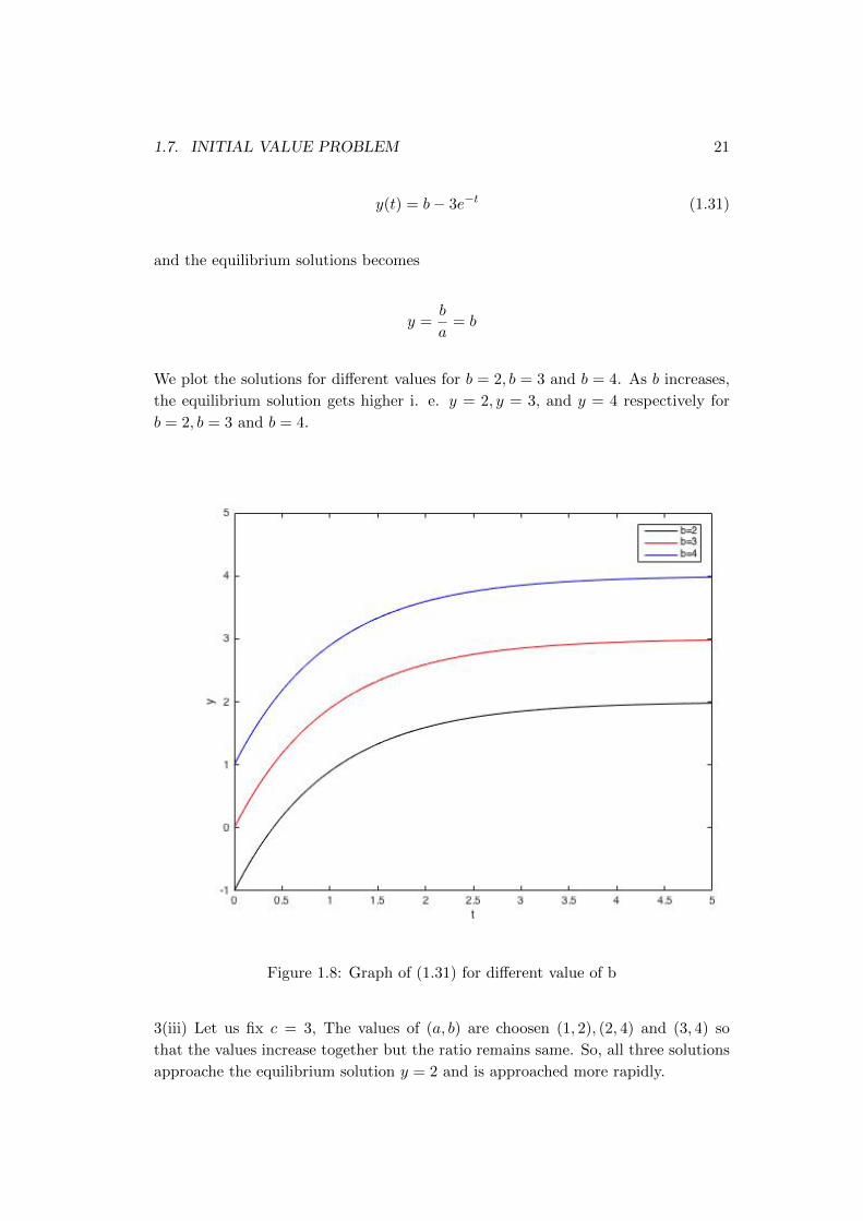
y(t) = b− 3e−t (1.31)
and the equilibrium solutions becomes
y =b
a= b
We plot the solutions for different values for b = 2, b = 3 and b = 4. As b increases,
the equilibrium solution gets higher i. e. y = 2, y = 3, and y = 4 respectively for
b = 2, b = 3 and b = 4.
Figure 1.8: Graph of (1.31) for different value of b
3(iii) Let us fix c = 3, The values of (a, b) are choosen (1, 2), (2, 4) and (3, 4) so
that the values increase together but the ratio remains same. So, all three solutions
approache the equilibrium solution y = 2 and is approached more rapidly.

22 CHAPTER 1. INTRODUCTION OF DIFFERENTIAL EQUATIONS
Figure 1.9: Graph of (1.30) for different value of b
1.8 Construction of Mathematical Models
In applying differential equation to any of the numerous field in which they are
useful, it is neccesary first to formulate the appropriate differential equation that
describes , or models, the problem being investigated. The following steps are useful
for the formulation of problem:
1. Identify the independent and dependent variables and assign letters to repre-
sent them. In many cases the independent variable is time.
2. Choose the units of measurement for each variable. In a sense the choice of
units is arbitrary, but some choices may be more convenient than others.
3. Articulate the basic principle that underlines or governs the problem you are
investigating. That may be physical law or it may be a more a speculative
assumption that may be based on your own experience or observations.
4. Express the principle or law in step 3 in terms of variable you choose in step
1. It may be require the introduction of physical constants or parameters and
determination of appropriate value of them.
5. Make sure that each term in your equation has the same units. If the unit
agree, then your equation at least is dimensionally consistent.
6. In the problem considered here, the result of step 4 is a single differential
equation which consitute the desired mathematical model. Keep in mind,
through, that in more complex problems the resulting mathematical model
1.8. CONSTRUCTION OF MATHEMATICAL MODELS 23
may be much complicated, perhaps involving a system of several differential
equations.
Example 13.
Newton’s law of cooling state that the temperature of an object changes at a rate
proportinal to the difference between the temperature of the object itself and the
temperature of its surrounding. Suppose that the ambient teperature is 75oF and
that the rate constant is 0.05min−1. Write a differential equation for the temperature
of the object at any time.
Solution: Let T be the temperature of the object at any time t and the surrounding
temerature be T0. By Newton’s law of cooling,
dT
dt= r(T − T0)
where r is proportionality constants. Again r = 0.05min−1 and T0 = 75oF , thus the
equation becomes
dT
dt= 0.05(T − 75)
Example 14.
A certain drug is being administered intravenously to a hospital patient. Fluid
containing 5mg/cm3 of the drug enters the patient’s bloodstream at a rate of
100cm3/h. The drug is absorbed by body tissue or otherwise leaves the bloodstream
at a rate proportional to the amount present, with a rate constant of 0.4(h)−1.
(a) Assuming that the drug is always uniformly distributed throughout the blood-
strem, write a differential equation for the amount of the drug that is present in the
bloodstrem at any time.
(b) How much of the drug is present in the bloodstream after a long time?
Solution: (a) Let q mg be amount of drug in the patient’s body at any time t in
hours. Then
rate of change in drug = rate of drug enter body− rate of drug leave or absorbed(1.32)
Since a fluid containing 5mg/cm3 of the drug enter the patient bloodstrem at a rate
of 100cm3/h , the rate at drug is enter into body 5× 100mg/h = 500mg/h.
Again the quantity of drug in body is q(t) leave or absorbed at constant rate 0.4(h)−1,
so the rate at which the drug leave or absorbed = q(t)× 0.4 = 0.4q(t)mg/h.
Hence from (1.32), we get
dq
dt= 500− 0.4q

24 CHAPTER 1. INTRODUCTION OF DIFFERENTIAL EQUATIONS
(b) After the long time i.e. steady state , we have
dq
dt= 0
or, 500− 0.4q = 0
or, q =500
0.4= 1250mg
Hence 1250 mg of the drug is present in the bloodstream after a long time.
Example 15.
Consider a population p of field mice that grows at a rate proportinal to the
current population, so that dpdt = rp.
(a) Find the rate constant r if the population doubles in 40 days.
(b) Find r if the population doubles in N days.
Solution: The given differential equation is
dp
dt= rp
or,dp
p= rdt
Integrating,
ln p = rt+ ln c
or, p = cert (1.33)
Initially let p(0) = p0, so from (1.33), we get
p0 = c
Putting the value of c in (1.33)
p(t) = p0ert (1.34)
(a) Let the population double in 40 days. Then take t = 40 and p(t) = 2p0, from
(1.34)
2p0 = p0e40r
or, ln 2 = 40r
or, r =1
40ln 2 per day (1.35)
(b) Let the population double at t = N days. Then from (1.33), we get
2p0 = p0erN
or, 2 = erN
or, ln 2 = rN
or, r =1
Nln 2

1.8. CONSTRUCTION OF MATHEMATICAL MODELS 25
Example 16.
A radioactive material, such as the isotope thorium-234, disintegrate at a rate
proportional to the amount currently present. If Q(t) is the amount present at time
t, then dQdt = −rQ, where r > 0 is the decay rate.
(a) If 100 mg of thorium-234 decays to 82.04 mg in 1 week, determine the decay rate
r.
(b) Find an expression for the amount of thorium-234 present at any time t.
(c) Find the required for the thorium-234 to decay to one -half its original amount.
Solution: The given differential equation is
dQ
dt= −rQ
or,dQ
Q= −rdt
Integrating,
lnQ = −rt+ ln c
or, Q = ce−rt (1.36)
Initially let Q(0) = Q0, so from (1.36), we get
Q0 = c
Putting the value of c in (1.36)
Q(t) = Q0e−rt (1.37)
(a) If Q0 = 100, t = 7 day and p(t) = 82.04mg, from (1.37)
82.04 = 100e−7r
or, e7r =100
82.04
or, 7r = ln
(100
82.04
)or, r =
1
7ln
(100
82.04
)= 0.028 per day. (1.38)
(b) The required expression for the amount at t days is
Q(t) = 100e−0.028t (1.39)
(b) Let the t = T days be half-life . Then from (1.39), we get
50 = 100e−0.028T
or,1
2= e−0.028T
or, ln1
2= −0.028T
or, T = 24.5 days

26 CHAPTER 1. INTRODUCTION OF DIFFERENTIAL EQUATIONS
Chapter 2
First Order Linear and
Nonlinear Differential Equations
IntroductionThis chapter deals with differential equations of first order
dy
dt= f(t, y) (2.1)
where f is a given function of two variables t and y. Any differential function
y = φ(t) that satisfies this equation for all t in some interval is called a solution. Our
object is to determine wheather such function exists and if so, to develop methods
for finding them. We also discuss some of important applications of first order
differential equation, introduce the idea ,of aprroximating a solution by numerical
computation.
2.1 Linear Equation; Method of Integrating Factors
2.1.1 Linear equation
If the differential equation
dy
dt= f(t, y) (2.2)
depends linearly on the dependent variable y, then the equation (2.2), is called a
first order linear equation. i.e.
dy
dx= −p(t)y + g(t)
Thus, the first order linear equation can be written as
dy
dt+ p(t)y = g(t) (2.3)
27

28CHAPTER 2. FIRST ORDER LINEAR ANDNONLINEARDIFFERENTIAL EQUATIONS
For exampledy
dt+ tan t y = sec t
If p and q are constants then the equation (2.3) is called the linear equation with
constant coefficients. i.e.
dy
dt+ ay = b
2.1.2 Exact
The general first order equation is
dy
dt= f(t, y) (2.4)
which can be written as
Mdy +Ndt = 0 (2.5)
where M and N are functions of t, y or constants. The differential equation (2.5) is
said to be exact if it takes the form
dG(t, y) = 0
Integrating, we get solution G(t, y) = c.
2.1.3 Integrating Factor of Linear Equation
Let us consider a linear equation
dy
dt+ p(t)y = g(t) (2.6)
where p and g are functions of t or constants. To determine appropriate integrating
factor, we multiply (2.6) by an yet undetermined function µ(t), so that
µ(t)dy
dt+ µ(t)p(t)y = µ(t)g(t) (2.7)
be exact. Then LHS of (2.7) is the derivative of the product µ(t)y if µ(t) satisfies
d
dt[µ(t)] = p(t)µ(t)
or,dµ(t)
µ(t)= p(t)dt
Integrating, by assuming µ(t) positive for all t,
ln[µ(t)] =
∫p(t)dt+ c

2.1. LINEAR EQUATION; METHOD OF INTEGRATING FACTORS 29
By choosing the arbitrary constant c to be zero, we obtained the simplest possible
function for µ
ln[µ(t)] =
∫p(t)dt
or, µ(t) = e∫p(t)dt
Note that µ(t) is positive for all t, as we assumed. Hence equation (2.7) can be
written as
d
dt[µ(t)y] = µ(t)g(t)
Integrating,
µ(t)y =
∫µ(t)g(t)dt+ k
where k is an arbitrary constant. However, in general this is not possible, so the
general solution of the equation (2.6)
y =1
µ(t)
[∫ t
t0µ(s)g(s)ds+ k
](2.8)
where t0 is some convenient lower limit of the integration.
Method of solving linear differential equation
Let us consider a linear equation
dy
dt+ p(t)y = g(t) (2.9)
where p and g are functions of t or constants.
Integrating factor
I.F. = e∫pdt
Multiplying the equation (2.9) by I.F., we get
e∫pdtdy
dt+ e
∫pdtp(t)y = g(t)e
∫pdt
or,d
dt
(e∫pdty
)= g(t)e
∫pdt
or, d(e∫pdty
)= g(t)e
∫pdtdt
Integrating,
e∫pdty =
∫ (g(t)e
∫pdtdt
)dt+ c
which gives the solution.
Example 17.

30CHAPTER 2. FIRST ORDER LINEAR ANDNONLINEARDIFFERENTIAL EQUATIONS
Solve the differential equation dydt = −ay + b.
Solution: The given differential equation is
dy
dt= −ay + b
or,dy
dt+ ay = b (2.10)
Integrating factor
I.F. = e∫pdt = e
∫adt = eat
Multiplying the equation (2.10), we get
eatdy
dt+ ayeat = beat
or,d
dt
(eaty
)= beat
or, d(eaty
)= beatdt
Integrating,
eaty = b
∫eatdt+ c
or, eaty =b
aeat + c
or, y =b
a+ ce−at
Example 18.
Solve the differential equation dydt − 2y = 4− t. Discuss the behavior of solution
as t→∞.
Solution: The given differential equation is
dy
dt− 2y = 4− t (2.11)
Integrating factor
I.F. = e∫pdt = e
∫−2dt = e−2t
Multiplying the equation (2.11), we get
e−2tdy
dt− 2ye−2t = 4e−2t − te−2t
or,d
dt
(e−2ty
)= 4e−2t − te−2t
or, d(e−2ty
)= 4e−2tdt− te−2tdt

2.1. LINEAR EQUATION; METHOD OF INTEGRATING FACTORS 31
Integrating,
e−2ty = 4
∫e−2tdt−
∫te−2tdt+ c
or, e−2ty =4
−2e−2t −
t
∫e−2t −
∫ (dt
dt
∫e−2tdt
)dt
+ c
or, e−2ty = −2e−2t −− t
2e−2t −
∫−1
2e−2tdt
dt+ c
or, e−2ty = −2e−2t +t
2e−2t +
1
4e−2t + c
or, e−2ty = −7
4e−2t +
1
2te−2t + c
or, y = −7
4+
1
2t+ ce2t
As t→∞, e2t →∞ for a positive value of c and y(t)→∞.
Example 19.
Find the general solution of the differential equation dydt + 3y = t+ e−2t. Discuss
the behavior of solutions as t→∞.
Solution: The given differential equation is
dy
dt+ 3y = t+ e−2t (2.12)
Integrating factor
I.F. = e∫pdt = e
∫3dt = e3t
Multiplying the equation (2.12), we get
e3tdy
dt+ 3ye3t = te3t + e3te−2t
or,d
dt
(e3ty
)= te3t + et
or, d(e3ty
)= te3t + et
Integrating,
e3ty =
∫te3tdt+
∫etdt+ c
or, e3ty = t
∫e3t −
∫ (dt
dt
∫e3tdt
)dt+ et + c
or, e3ty =1
3te3t −
∫1
3e3tdt+ et + c
or, e3ty =1
3te3t − 1
9e3t + et + c
or, y =t
3− 1
9+ e−2t + ce−3t

32CHAPTER 2. FIRST ORDER LINEAR ANDNONLINEARDIFFERENTIAL EQUATIONS
Since the exponential functions e−2t and e−3t decrease rapidly as compare to the
linear function t3 −
19 , so e−2t → 0 and e−3t → 0 as t → ∞. Thus, solution y is
asymptotic to t3 −
19 and y →∞ as t→∞.
Example 20.
Find the general solution of the differential equation dydt − 2y = t2e2t. Discuss
the behavior of solutions as t→∞.
Solution: The given differential equation is
dy
dt− 2y = t2e2t (2.13)
Integrating factor
I.F. = e∫pdt = e
∫−2dt = e−2t
Multiplying the equation (2.13), we get
e−2tdy
dt− 2ye−2t = t2e−2te2t
or,d
dt
(e−2ty
)= t2
or, d(e−2ty
)= t2dt
Integrating,
e−2ty =
∫t2dt+ c
or, e−2ty =t3
3+ c
or, y =1
3t3e2t + ce2t
AS y →∞ as t→∞ for all positive c.
Example 21.
Find the general solution of the differential equation tdydt + 2y = sin t, t > 0,
and use it to determine how solutions behave as t→∞.
Solution: The given differential equation is
tdy
dt+ 2y = sin t t > 0
or,dy
dt+
2
ty =
sin t
t(2.14)
Integrating factor
I.F. = e∫pdt = e
∫2tdt = e2 ln t = eln t2 = t2
2.1. LINEAR EQUATION; METHOD OF INTEGRATING FACTORS 33
Multiplying the equation (2.14), we get
t2dy
dt+ 2ty = t sin t
or,d
dt
(t2y)
= t sin t
or, d(t2y)
= t sin tdt
Integrating,
t2y =
∫t sin tdt+ c
or, t2y = t
∫sin tdt−
∫ (dt
dt
∫sin t dt
)+ c
or, t2y = −t cos t+
∫cos t dt+ c
or, t2y = −t cos t+ sin t+ c
or, y =c+ sin t− t cos t
t2
For behaviour of solution as t→∞
limt→∞
y = limt→∞
c+ sin t− t cos t
t2
= limt→∞
(c
t2+
sin t
t2− cos t
t
)= 0
Example 22.
Find the general solution of the differential equation (1 + t2)dydt + 4ty = 1(1+t2)2
,
and use it to determine how solutions behave as t→∞.
Solution: The given differential equation is
(1 + t2)dy
dt+ 4ty =
1
(1 + x2)2
or,dy
dt+
4t
1 + t2y =
1
(1 + t2)3(2.15)
Integrating factor
I.F. = e∫pdt = e
∫4t
1+t2dt
= e2∫
2t1+t2
dt= e2 ln(1+t2) = eln(1+t2)2 = (1 + t2)2
Multiplying the equation (2.15), we get
(1 + t2)2dy
dt+ 4t(1 + t2)y =
1
1 + t2
or,d
dt
((1 + t2)2y
)=
1
1 + t2
or, d((1 + t2)2y
)=
1
1 + t2dt

34CHAPTER 2. FIRST ORDER LINEAR ANDNONLINEARDIFFERENTIAL EQUATIONS
Integrating,
(1 + t2)2y =
∫1
1 + t2dt+ c
or, (1 + t2)2y = tan−1 t+ c
or, y =c+ tan−1 t
(1 + t2)2
For behaviour of solution as t→∞
limt→∞
y = limt→∞
c+ tan−1 t
(1 + t2)2= lim
t→∞
1
4t(1 + t2)2= 0
using the L-Hopital rule.
Example 23.
Solve the initial value problem tdydt + 2y = 4t2, y(1) = 2.
Solution: The given differential equation is
tdy
dt+ 2y = 4t2, y(1) = 2
or,dy
dt+
2
ty = 4t (2.16)
Integrating factor
I.F. = e∫pdt = e
∫2tdt = e2
∫1tdt = e2 ln t = eln t2 = t2
Multiplying the equation (2.16), we get
t2dy
dt+ 2ty = 4t3
or,d
dt
(t2y)
= 4t3
or, d(t2y)
= 4t3 dt
Integrating,
t2y = 4
∫t3dt+ c
or, t2y = t4 + c
or, y = t2 +c
t2(2.17)
which is general solution.
Using the initial condition y(1) = 2 in (2.17), we get
1 + c = 2
or, c = 1
From (2.17), the required solution is
y = t2 +1
t2

2.1. LINEAR EQUATION; METHOD OF INTEGRATING FACTORS 35
Example 24.
Solve the initial value problem 2dydt + ty = 2, y(0) = 1.
Solution: The given differential equation is
2dy
dt+ ty = 2, y(0) = 1
or,dy
dt+t
2y = 1 (2.18)
Integrating factor
I.F. = e∫pdt = e
∫t2dt = e
t2
4
Multiplying the equation (2.18), we get
et2
4dy
dt+t
2et2
4 y = et2
4
or,d
dt
(ye
t2
4
)= e
t2
4
or, d
(ye
t2
4
)= e
t2
4 dt
Integrating,
yet2
4 =
∫et2
4 dt+ c
or, yet2
4 =
∫et2
4 dt+ c
which gives the general solution.
The integral on the right sides can not be evaluated in term of the usual elementary
functions, so we leave the integral as unevaluate. However, by choosing the lower
limit of the integral as initial point t0 = 0. Thus the solution is
yet2
4 =
∫ t
0es2
4 ds+ c (2.19)
Using the initial conditions t = 0, y = 0, from (2.19), we get
e0 1 =
∫ 0
0es2
4 ds+ c
or, c = 1
From (2.19), we get
et2
4 y =
∫ t
0es2
4 ds+ 1
or, y = e−t2
4
∫ t
0es2
4 ds+ e−t2
4

36CHAPTER 2. FIRST ORDER LINEAR ANDNONLINEARDIFFERENTIAL EQUATIONS
Example 25.
Solve the initial value problem tdydt + 2y = t2 − t+ 1, y(1) = 12 .
Solution: The given differential equation is
tdy
dt+ 2y = t2 − t+ 1, y(1) =
1
2
or,dy
dt+
2
ty = t− 1 +
1
t(2.20)
Integrating factor
I.F. = e∫pdt = e
∫2tdt = e2 ln t = eln t2 = t2
Multiplying the equation (2.20), we get
t2dy
dt+ 2ty = t3 − t2 + t
or,d
dt
(t2y)
= t3 − t2 + t
or, d(t2y)
= (t3 − t2 + t) dt
Integrating,
t2y =
∫(t3 − t2 + t)dt+ c
or, t2y =t4
4− t3
3+t2
2+ c
or, y =t2
4− t
3+
1
2+c
t2(2.21)
Using the initial condition y(1) = 12 in (2.21), we get
or,1
4− 1
3+
1
2+ c =
1
2
or, c =1
12
From (2.21), the required solution is
y =t2
4− t
3+
1
2+
1
12
is solution of the initial value problem.
Example 26.
Solve the initial value problem dydt − 4y = e4t, y(0) = 4.
Solution: The given differential equation is
dy
dt− 4y = e4t, y(0) = 4
or,dy
dt− 4y = e4t (2.22)

2.1. LINEAR EQUATION; METHOD OF INTEGRATING FACTORS 37
Integrating factor
I.F. = e∫pdt = e
∫−4dt = e−4t
Multiplying the equation (2.22), we get
e−4tdy
dt− 4e−4ty = e−4te4t
or,d
dt
(e−4ty
)= 1
or, d(e−4ty
)= dt
Integrating,
e−4ty = t+ c
or, y = (t+ c)e4t (2.23)
which is general solution.
Using the initial condition y(0) = 2 in (2.23), we get
c = 2
From (2.23), the required solution is
y = (t+ 2)e4t
Example 27.
Solve the initial value problem t3 dydt + 4t2y = e−t, y(−1) = 0, t < 0.
Solution: The given differential equation is
t3dy
dt+ 4t2y = e−t, y(−1) = 0, t < 0
or,dy
dx+
4
t=e−t
t3(2.24)
Integrating factor
I.F. = e∫pdt = e
∫4tdt = e4 ln t = eln t4 = t4
Multiplying the equation (2.24), we get
t4dy
dt+ 4t3y = te−t
or,d
dt
(t4y)
= te−t
or, d(t4y)
= te−tdt

38CHAPTER 2. FIRST ORDER LINEAR ANDNONLINEARDIFFERENTIAL EQUATIONS
Integrating,
t4y =
∫te−tdt+ c
t4y = t
∫e−tdt−
∫ (dt
dt
∫e−tdt
)dt+ c
or, t4y = −te−t +
∫e−tdt+ c
or, t4y = −te−t − e−t + c (2.25)
which is general solution.
Using the initial condition y(−1) = 0 in (2.25), we get
(−1)4 · 0 = −(−1)e1 − e1 + c
or, c = 0
From (2.25), the required solution is
t4y = −te−t − e−t
or, y = −(t+ 1)e−t
t4
Example 28.
Solve the initial value problem tdydt + (t+ 1)y = t, y(ln 2) = 1, t > 0.
Solution: The given differential equation is
tdy
dt+ (t+ 1)y = t, y(ln 2) = 1, t > 0
or,dy
dx+
(1 +
1
t
)y = 1 (2.26)
Integrating factor
I.F. = e∫pdt = e
∫(1+ 1
t )dt = et+ln t = eteln t = tet
Multiplying the equation (2.26), we get
tetdy
dt+ tet
(1 +
1
t
)y = tet
or,d
dt
(tety
)= tet
or, d(tety
)= tetdt
Integrating,
tety =
∫tetdt+ c
tety = t
∫etdt−
∫ (dt
dt
∫etdt
)dt+ c
or, tety = tet −∫etdt+ c
or, tety = tet − et + c (2.27)

2.1. LINEAR EQUATION; METHOD OF INTEGRATING FACTORS 39
which is general solution.
Using the initial condition t = ln 2, y(ln 2) = 1 in (2.27), we get
ln 2 eln 2 · 1 = ln 2 eln 2 − eln 2 + c
or, 0 = −2 + c
or, c = 2
From (2.27), the required solution is
tety = tet − et + 2
or, y =tet
tet− et
tet+
2
tet
or, y = 1− 1
t+
2e−t
t
or, y =t− 1 + 2e−t
t
Example 29.
Consider the initial value problem
dy
dx− 3
2y = 3t+ 2et, y(0) = y0
Find the value of y0 that separates solutions that grow positively as t → ∞ from
those that grow negatively. How does the solution that corresponds to the critical
value of y0 behaves as t→∞.
Solution: The given differential equation is
dy
dt− 3
2y = 3t+ 2et, (2.28)
Integrating factor
I.F. = e∫pdt = e
∫− 3
2dt = e−
3t2
Multiplying the equation (2.28), we get
e−3t2dy
dt− 3
2e−
3t2 y = 3te−
3t2 + 2ete−
3t2
or, d(e−
3t2 y)
=(
3te−3t2 + 2e−
t2
)dt
Integrating,
e−3t2 y = 3
∫te−
3t2 dt+ 2
∫e−
t2dt
e−3t2 y = 3t
∫e−
3t2 dt− 3
∫ (dt
dt
∫e−
3t2 dt
)dt− 4e−
t2 + c
or, e−3t2 y = −2te−
3t2 + 2
∫e−
3t2 dt− 4e−
t2 + c
or, e−3t2 y = −2te−
3t2 − 4
3e−
3t2 − 4e−
t2 + c
or, y = −2t− 4
3− 4et + ce3t/2 (2.29)

40CHAPTER 2. FIRST ORDER LINEAR ANDNONLINEARDIFFERENTIAL EQUATIONS
which is general solution.
Using the initial condition t = 0, y(0) = y0 in (2.29), we get
y0 = −4
3− 4 + c
or, y0 = −16
3+ c
or, c = y0 +16
3
The critical value of y0 that separates solutions that grow positively as t→∞ from
those that grow negatively is when c = 0. i.e.
y0 = −16
3
For this critical value of y0 the solution is
y = −2t− 4
3− 4et
As −2t and −4et both diverge to−∞ as t→∞. Also, y → −∞ as t→∞.
2.2 Separable Equations
The general first order differential equation is
dy
dx= f(x, y) (2.30)
If f(x, y) has in the form f(x, y) = M(x)N(y) then the differntial equation is called
variable separeted form. The equation(2.30) becomes
dy
dx=M(x)
N(y)
or, N(y)dy = M(x)dx
Integrating, we get the solution∫N(y)dy =
∫M(x)dx+ c
Example 30.
Solve the given differential equations
(a) y′ =x2
1− y2, (b) y′ =
3x2 − 1
3 + 2y
(c) y′ =x2
y, (d) y′ =
x2
1 + y2
2.2. SEPARABLE EQUATIONS 41
(e) y′ = cos2 x cos2 y (f) y′ =x− e−x
y + ey
Solution: (a) The given differential equation is
dy
dx=
x2
1− y2
or, (1− y2)dy − x2dx = 0
Integrating,
y − y3
3− x3
3= c
(b) The given differential equation is
dy
dx=
3x2 − 1
3 + 2y
or, 3dy + 2ydy − 3x2dx+ dx = 0
Integrating,
3y + y2 − x3 + x = c
(c) The given differential equation is
dy
dx=x2
y
or, ydy − x2dx = 0
Integrating,
y2
2− x3
3= c
or, 3y2 − 2x3 = c
(d) The given differential equation is
dy
dx=
x2
1 + y2
or, dy + y2dy − x2dx = 0
Integrating,
y +y3
3− x3
3=c
3or, 3y + y3 − x3 = c

42CHAPTER 2. FIRST ORDER LINEAR ANDNONLINEARDIFFERENTIAL EQUATIONS
(e)The given differential equation is
dy
dx= cos2 x cos2 y
or, sec2 ydy − cos2 xdx = 0
or, sec2 ydy −(
1
2+
1
2cos 2x
)dx = 0
Integrating,
tan y − 1
2x− 1
4sin 2x = c
(d) The given differential equation is
dy
dx=x− e−x
y + ey
or, ydy + eydy − xdx+ e−xdx = 0
Integrating,
y2
2+ ey − x2
2− e−x = c
Example 31.
Solve the initial value problem
dy
dx=
4x− x3
4 + y3
Also determine the solution passing through (0, 1).
Solution: The given differential equation
dy
dx=
4x− x3
4 + y3
or, (4 + y3)dy = (4x− x3)dx
Integrating,
4y +y4
4= 2x2 − x4
4+c
4or, y4 + 16y + x4 − 8x2 = c (2.31)
where c is arbitrary constant. Using the initial conditions x = 0, y = 1 in (2.31), we
get
1 + 16 = c, c = 16
Putting the value of (2.31)
y4 + 16y + x4 − 8x2 = 16

2.2. SEPARABLE EQUATIONS 43
Example 32.
Solve the initial value problem
dy
dx=
3x2 + 4x+ 2
2(y − 1), y(0) = −1
and determine the interval in which the solution exists.
Solution: The given differential equation
dy
dx=
3x2 + 4x+ 2
2(y − 1)
or, 2(y − 1)dy = (3x2 + 4x+ 2)dx
Integrating,
y2 − 2y = x3 + 2x2 + 2x+ c (2.32)
where c is arbitrary constant. Using the initial conditions x = 0, y = −1 in (2.32)
1 + 2 = c, c = 3
Putting the value of (2.32)
y2 − 2y = x3 + 2x2 + 2x+ 3
or, y2 − 2y − (x3 + 2x2 + 2x+ 3) = 0
Solving for y
y =2±
√4 + 4(x3 + 2x2x+ 3)
2
or, y = 1±√x3 + 2x2 + 2x+ 4
Thus we get two solutions
y = 1 +√x3 + 2x2 + 2x+ 4 (2.33)
y = 1−√x3 + 2x2 + 2x+ 4 (2.34)
When x = 0, from (2.33), we get y = 1 +√
4 = 3, which is not solution. When
x = 0,from (2.34), we get y = 1−√
4 = −1 i.e. (2.34) satisfied the initial condition.
Thus the solution of the initial value problem is
y = 1−√x3 + 2x2 + 2x+ 4
or, y = 1−√x2(x+ 2) + 2(x+ 2)
or, y = 1−√
(x2 + 2)(x+ 2)
(2.35)
When x > −2 the fuction (x2+2)x−(−2) is positive and y = 1−√
(x2 + 2)(x+ 2)
is defined. Thus the initial value problem has solution in [−2,∞).

44CHAPTER 2. FIRST ORDER LINEAR ANDNONLINEARDIFFERENTIAL EQUATIONS
Example 33.
Solve the initial value problem
y′ = 2y2 + xy2, y(0) = 1
and determine where the solution attains its minimum value.
Solution: The given differential equation is
dy
dx= 2y2 + xy2
or,dy
dx= y2(x+ 2)
or,1
y2
dy
dx= x+ 2
or,1
y2dy = xdx+ 2dx
Integrating, ∫1
y2
dy
dx=
∫xdx+ 2
∫dx+ c
or, − 1
y=x2
2+ 2x+ c (2.36)
Using initial condition y(0) = 1, in (2.36) ,
−1 = c
Now, from the equation (2.36)
−1
y=x2
2+ 2x− 1
or, y =−2
x2 + 4x− 2(2.37)
is the required solution.
For a minimum value of y,
y′ = 0
or, y2(x+ 2) = 0
or, x = −2
Also,
y′ = y2(x+ 2)
Differentiating
y′′ = 2yy′(x+ 2) + y2 (2.38)
or, y′′ = 4y3(x+ 2)3 + y2 (2.39)

2.2. SEPARABLE EQUATIONS 45
When x = −2, y = −24−8−2 = 1
3 6= 0 and from (2.39), we get
y′′ = 4y2 · 0 + y2 = y2 > 0
Hence, the solution attains minimum value at x = −2.
Example 34.
Solve the initial value problem
y′ = 2(1 + x)(1 + y2), y(0) = 0
and determine where the solution attains its minimum value.
Solution: The given differential equation is
dy
dx= 2(1 + x)(1 + y2)
or,dy
dx= 2(1 + y2)(x+ 1)
or,1
1 + y2
dy
dx= 2(1 + x)
or,1
1 + y2dy = 2(1 + x)dx
Integrating, ∫1
1 + y2dy =
∫2xdx+ 2
∫dx+ c
or, tan−1 y = x2 + 2x+ c (2.40)
Using initial condition y(0) = 0, in (2.40) ,
0 = c
Now, from the equation (2.40)
tan−1 y = x2 + 2x
or, y = tan(x2 + 2x) (2.41)
is the required solution.
For a minimum value of y,
y′ = 0
or, (1 + y2)(x+ 1) = 0
or, x = −1

46CHAPTER 2. FIRST ORDER LINEAR ANDNONLINEARDIFFERENTIAL EQUATIONS
Also,
y′ = 2(1 + y2)(x+ 1)
Differentiating
y′′ = 4yy′(x+ 1) + 2(1 + y2)
or, y′′ = 8y(1 + y2)(x+ 1)2 + 2(1 + y2) (2.42)
When x = −1, y = tan(−1) 6= 0 and from (2.42), we get
y′′ = 0 + 2(1 + y2) > 0
Hence, the solution attains minimum value at x = −1.
2.3 Modeling with First Order Equations
Some examples that are applications of first order differential equations.
2.3.1 Mixture Problem
Example 35.
At time t = 0 a tank contains Q0 lb of salt dissolved in 100 gal of water. Assume
that water containing 14 lb of salt/gal is entering the tank at a rate of r gal/min and
that well-strirred mixture is draining from the tank at the same rate.
1. Set up the initial value problem that describes this flow process.
2. Find the amount of salt Q(t) in the tank at any time.
3. Find the limiting amount QL that is present after a very long time.
4. If r = 3 and Q0 = 2QL, find the time T after the salt level is within 2% of QL.
5. Find the flow rate that is required if the T is not to exceeds 45 min.
Solution: Here Q(t) is amount of salt at any time t.
1. The rate of change of salt in the tank dQdt , is equal to the rate at which salit
flowing in minus the rate at which it is flowing out.
dQ
dt= rate in− rate out (2.43)
Again, rate in = concentration × rate in= 14 × r = r
4 lb/min.
Since the rates of flow in and out are equal, the volume of water in the tank remains
constant at 100 gal and well-stirred, the concentration throughout the tank is same,
so concentration outQ(t)
100lb/gal
Therefore, the rate at which salt leaves the tank is
= concentration× rate out =rQ(t)
100lb/min

2.3. MODELING WITH FIRST ORDER EQUATIONS 47
Thus, the differential equation governing this process, from (2.43) is
dQ
dt=r
4− rQ(t)
100(2.44)
The initial condition is
Q(0) = Q0 (2.45)
2. Rewritting the equation (2.44),
dQ
dt+rQ(t)
100=r
4(2.46)
Thus, the integrating factor is
I.F. = e∫pdt = er/100
∫dt = ert/100
Multiplying the equation (2.46), we get
ert/100dQ
dt+
r
100ert/100y =
r
4tert/100
or, d(ert100Q
)=r
4ert/100dt
Intrgrating,
Qert/100 =r
4
∫ert/100dt+ c
or, Qert/100 =r
4
100
rert/100 + c
or, Qert/100 = 25ert/100 + c
or, Q(t) = 25 + ce−rt/100 (2.47)
Using the initial condition Q(0) = Q0, in (2.47), we get
Q0 = 25 + c =⇒ c = Q0 − 25
From (2.47)
Q(t) = 25 + (Q0 − 25)e−rt/100 (2.48)
which gives the concentration of salt at any time t.
3. As t→∞, Q(t)→ 25. Therefore, QL = 25.
4. Now suppose that r = 3 and Q0 = 2QL = 50, then equation (2.48) becomes
Q(t) = 25 + (50− 25)e−3t/100
or, Q(t) = 25 + 25e−0.03t (2.49)

48CHAPTER 2. FIRST ORDER LINEAR ANDNONLINEARDIFFERENTIAL EQUATIONS
Again Q(t) = 25 + 2%of 25 = 25.5. Thus from (2.49)
25.5 = 25 + 25e−0.003t
or, 0.5 = 25e−0.003t
or, e0.03t =25
0.5= 50
or, 0.03t = ln 50 taking log on both sides
or, t =ln 50
0.03= 130.4min.
5. To determine r so that t = 45 min. we return to the equation (2.48), take
Q(t) = 25.5, Q0 = 50, we get
25.5 = 25 + 25 e−45r100
or, 0.5 = 25 e−45r100
or, e45r100 = 50
or,45r
100= ln 50
or, r =100
45ln 50 = 8.89gal/min.
Example 36.
Consider a tank used in certain hydrodynamic experiments. After one experi-
ment, the tank contains 150L of a dye solution with a concentration of 1 g/L. To
prepare for the next experiment, the tank is to be rinsed with fresh water flowing
in at a rate of 2L/min, the well-stirred solution flowing out at the same rate. Find
the time that will elapse before the concentration of the dye in the tank reaches 1%
of its original value.
Solution: Initially Q(0) = Q0 = 1g/L × 150L = 150g. Let Q(t)g be the amout of
dye in the tank at any time t in min.
The fresh water has the concerntration 0%.
Rate in = Concentration× rate = 0× 2 = 0
At any time amout of dye is Q(t), in 150 L of water, so concentration of dye at any
timeQ(t)
150
Since the solution is flowing out at the same rate as it enter i.e. the solution is
flowing out at rate 2L/min.
Rate out = Concentration× rate =Q(t)
150× 2 =
Q(t)
75

2.3. MODELING WITH FIRST ORDER EQUATIONS 49
∴dQ
dt= rate in− rate out (2.50)
or,dQ
dt= 0− Q(t)
75
or,dQ
Q= − 1
75dt
or,
∫dQ
Q= − 1
75
∫dt+ c
or, lnQ = − t
75+ ln c
or, Q = ce−t75 (2.51)
Using the initial condition Q(0) = 150, we get
150 = c
Putting, value of c, in (2.51)we get
Q = 150 e−t75 (2.52)
Again, Q = 1% of 150=1.5, so from (2.52),
1.5 = 150 e−t75
or, et75 = 100
or,t
75= ln 100
or, t = 75 ln 100 = 345.4 min. (2.53)
Example 37.
A tank is initally contains 120L of pure water. A mixture containing a con-
centration γg/L, of salts enters the tank at a rate of 2L/min and the well-stirred
mixture leave out at the same rate. Find an expression in term of γ for the amount
of salt in the tank at any time t. Also find the limiting amount of salt in the tank
as t→∞.Solution: Initially Q(0) = Q0 = 0g/L× 120L = 0g. Let Q(t) be the amout of salt
in the tank at any time t in min.
.
Rate in = Concentration× rate = γ × 2 = 2γ
At any time amout of dye is Q(t), in 120 L of water, so concentration of salt at any
timeQ(t)
120Since the solution is flowing out at the same rate as it enter i.e. the solution is
flowing out at rate 2L/min.
Rate out = Concentration× rate =Q(t)
120× 2 =
Q(t)
60

50CHAPTER 2. FIRST ORDER LINEAR ANDNONLINEARDIFFERENTIAL EQUATIONS
dQ
dt= rate in− rate out
or,dQ
dt= 2γ − Q(t)
60
or,dQ
Q+Q(t)
60= 2γ (2.54)
Which is linear,
I.F. = e∫pdt = e
160
∫dt = e
t60
Multiplying (2.54) by I.F.
et60dQ
Q+Q(t)
60et60 = 2γe
t60 (2.55)
or,d
dt
(Qe
t60
)= 2γe
t60 (2.56)
or, d(Qe
t60
)= 2γe
t60dt (2.57)
Integrating,
Q et60 = 2γ
∫et60dt+ c
Q et60 = 120γe
t60 + c (2.58)
Using the initial condition Q(0) = 0, we get
c = −120γ
Putting, value of c, in (2.58)we get
Q et60 = 120γe
t60 − 120γ
Q(t) = 120γ − 120γe−t60
Q(t) = 120γ(
1− e−t60
)(2.59)
As t→∞, Q(t) = 120γ.
Example 38.
A tank originally contains 100 gal of water. Then the water containing 12 lb of
salt per gallon is poured into a rate of 2gal/min, and the mixture is allowed to leave
at the same rate. After 10 min the process is stopped, and fresh water is poured
into the tank at a rate of 2gal/min, with the mixture again leaving at the same rate.
Find the amount of salt in the tank at the end of additional 10 min.
Solution: For first 10 minutes
Initially, for fresh water concerntration is 0, Q(0) = Q0 = 0 lb/gal × 100gal = 0lb.
Let Q(t) lb be the amout of dye in the tank at any time t in min.
Rate in = Concentration× rate =1
2lb/gal× 2gal/min = 1 lb/min

2.3. MODELING WITH FIRST ORDER EQUATIONS 51
At any time amout of salt is Q(t) lb, in 100 gal of water, so concentration of dye at
any timeQ(t)
100
Since the solution is flowing out at the same rate as it enter i.e. the solution is
flowing out at rate 2L/min.
Rate out = Concentration× rate =Q(t)
100× 2 =
Q(t)
50
dQ
dt= rate in− rate out (2.60)
or,dQ
dt= 1− Q(t)
50
or,dQ
dt=
50−Q50
or,dQ
50−Q=
1
50dt
or,
∫dQ
50−Q=
1
50
∫dt+ c
or, − ln(50−Q) =t
50+ c (2.61)
Using the initial condition Q(0) = 0, we get
− ln 50 = c
Putting, value of c, in (2.61)we get
− ln(50−Q) =t
50− ln 50
or, ln 50− ln(50−Q) =t
50
or, ln50
50−Q=
t
50
or,50
50−Q= e
t50
or,50−Q
50= e−
t50
or, 50−Q = 50e−t50
or, Q = 50(
1− e−t50
)(2.62)
When t = 10 min.
Q = 50(
1− e−1050
)= 9.0635lb

52CHAPTER 2. FIRST ORDER LINEAR ANDNONLINEARDIFFERENTIAL EQUATIONS
For next additional 10 min.
Initially, concerntration is 0, Q(0) = Q0 = 9.0635 lb. Let Q(t) lb be the amout of
salt in the tank at any time t in min.
Rate in = Concentration× rate = 0 lb/gal× 2gal/min = 0 lb/min
At any time amout of salt is Q(t) lb, in 100 gal of water, so concentration of dye at
any timeQ(t)
100
Since the solution is flowing out at the same rate as it enter i.e. the solution is
flowing out at rate 2L/min.
Rate out = Concentration× rate =Q(t)
100× 2 =
Q(t)
50
dQ
dt= rate in− rate out (2.63)
or,dQ
dt= 0− Q(t)
50
or,dQ
Q= − dt
50
or, lnQ = − t
50+ ln c
or, Q = ce−t50 (2.64)
Using the initial condition Q(0) = 9.0635 lb, we get
9.0635 = c
Putting, value of c, in (2.64)we get
Q = 9.0635e−t50 (2.65)
After the 10 min additional time
Q = 9.0635e−1050 = 7.4205lb
Example 39.
A tank with capacity of 500 originally contains 200 gal of water with 100 lb of salt
in solution. Water containing 1lb of salt per gallon is entering at a rate of 3gal/min,
and the mixture is allowed to flow out of the tank at the rate of 2 gal/min. Find
the amount of salt in the tank at any time prior to the instant when the solution
begin to overflow. Find the concentration of salt in the tank when it is on the point
of overflow. Compare this concentration with the theoritical limiting concentration

2.3. MODELING WITH FIRST ORDER EQUATIONS 53
if the tank had infinite capacity.
Solution: Initially Q(0) = Q0 = 200lb. Let Q(t)g be the amout of dye in the tank
at any time t in min.
Rate in = Concentration× rate = 1lb/gal × 3gal/min = 3 lb/min.
Let us assume that the solution overflow after time t. Since the solution is collected
at the rate of 1gal/min. Hence, in t minutes the collected solution is 200 + t gallons.
Therefore the concentration isQ(t)
200 + t
Rate out = Concentration× rate =Q(t)
200 + t× 2 =
2Q(t)
200 + t
dQ
dt= rate in− rate out
or,dQ
dt= 3− Q(t)
200 + t
or,dQ
dt+
2Q(t)
200 + t= 3 (2.66)
Thus, the integrating factor is
I.F. = e∫pdt = e
∫2
200+tdt = e2 ln(200+2) = eln(200+t)2 = (200 + t)2
Multiplying the equation (2.66), we get
(200 + t)2dQ
dt+ 2(200 + t)y = 3(200 + t)2
or, d((200 + t)2Q
)= 3(200 + t)2dt
Intrgrating,
(200 + t)2Q = (200 + t)3 + c
or, Q = 200 + t+c
(200 + t)2(2.67)
Using the initial condition Q(0) = 100, in (2.67), we get
100 = 200 +c
40000
c = −4000000 = −4× 10⁶
From (2.67)
Q = 200 + t− 4× 10⁶
(200 + t)2

54CHAPTER 2. FIRST ORDER LINEAR ANDNONLINEARDIFFERENTIAL EQUATIONS
But the total collection 200 + t, if t is time of follow the
200 + t = 500
or, t = 300
‘So the required solution is
Q = 200 + t− 4× 10⁶
(200 + t)2if t < 300 (2.68)
At the point of overflow i.e. t = 300, the concerntation of salt
Q(300) = 200 + 300− 4× 10⁶
(200 + 300)2= 484lb
The concentration of the salt at that time
c(300) =Q(300)
volume=
484
500= 0.968 lb/gal
Also, the concerntration of salt any time t is
c(t) =Q(t)
volume at time t=
200 + t− 4×10⁶
(200+t)2
200 + t
If the tank had infinite capacity it takes infinite minutes to fill up the tank.Thus,
taking t→∞
limt→∞
c(t) = limt→∞
(1− 4× 10⁶
(200 + t)3
)= 1
2.3.2 Compound Interest
The value S(t) of the investment at any time t depends on the frequency with
which interest is compounded as well as on the interest rate. If we assume that
compounding takes place continuously, then we can set up a simple initial value
problem.
The rate of change of the value of the investment is dSdt , and this quantity is equal
to the rate at which interest accrues which is the interest rate r times the current
value of the investment S(t). Thus
dS
dt= rS (2.69)
Suppose that we also know the value of investment at some time particular time,
say
S(0) = S0 (2.70)

2.3. MODELING WITH FIRST ORDER EQUATIONS 55
From the equation (2.69),
dS
S= rdt
or, lnS = rt+ ln c
or, lnS − ln c = rt
or, lnS
c= rt
or,S
c= ert
or, S = cert (2.71)
Using the initial condition S(0) = S0 in 2.71, we get
S0 = c
From (2.71), we get
S = S0ert
Again, let us suppose that there may be deposites or with drawals in addition to
the accrual interest, dividents, or capital gain. If we assume that the deposite or
withdrawals take place at a constant rate k, then the equation (2.69) is replaced by
dS
dt= rS + k
or,dS
dt− rS = k (2.72)
where k is positive for deposits and negative for withdrawls. The equation (2.72) is
linear . Integrating factor
I.F. = e∫
(−r)dt = e−rt
Multiplying the equation (2.72) by I.F.
e−rtdS
dt− rS = ke−rt
or,d
dt
(Se−kt
)= ke−rt
Integrating,
or, Se−rt = −krke−rt + c
S = cert − k
r(2.73)
Let the initial investment be S0. Then we get
c = S0 +k
r

56CHAPTER 2. FIRST ORDER LINEAR ANDNONLINEARDIFFERENTIAL EQUATIONS
Thus, the solution of the IVP (3.4) is
S(t) = S0ert +
k
r
(ert − 1
)(2.74)
If there is no initial investment i.e. S0 = 0, the equation (2.74) becomes
S(t) =k
r
(ert − 1
)(2.75)
Example 40.
A young person with no initial capital invest k dollars per year at of return r.
Assume that investments are made continuously and that return is compounded
continuosly.
(a) Determine the sum S(t) accumulated at any time t.
(b) If r = 7.5%, determine k so that $1 milion will be available for retirement in 40
years.
(c) If k = $2000/year, determine the return rate r that must be obtained to have $1
million avialable in 40 years.
Solution: 1.Let S(t) be amount accumulate at any time t. Also $k/year be annual
deposite and r be the annual rate of return. Then
dS
dt= rS + k
or,dS
dt− rS = k (2.76)
where k is positive for deposits and negative for withdrawls. The equation (2.76) is
linear . Integrating factor
I.F. = e∫
(−r)dt = e−rt
Multiplying the equation (2.76) by I.F.
e−rtdS
dt− rS = ke−rt
or,d
dt
(Se−kt
)= ke−rt
Integrating,
or, Se−rt = −krke−rt + c
S = cert − k
r(2.77)
Since initial investment be S(0) = 0. Then from (2.77)
0 = c− k
r
or, c =k
r(2.78)

2.3. MODELING WITH FIRST ORDER EQUATIONS 57
S(t) =k
r
(ert − 1
)(2.79)
2. Here r = 7.5% = 0.075 S(t) = $1000000, t = 40 years and k =?. Then from
(2.79, we get
1000000 =k
0.075
(e0.075×40 − 1
)or, 100000× 0.075 = k(20.0855− 1)
or, k =1000000
19.0855= $49787
3.Here k−20000/year S(t) = $1000000, t = 40 years and r =?. Then from (2.79,
we get
1000000 =20000
r
(e40r − 1
)or, 100 = k(20.0855− 1)
Solving the graphic calculator or Matlab we get r = 0.0977 = 9.77%.
Example 41.
Suppose that a sum S0 is investeted at an annual rate of return r compounded
continuously.
1. Find the time T required for the original sum to double in value as a function of
r.
2. Determine T if r = 8%.
3. Find the return rate that must be achived if the initial investment is to double
in 8 years.
Solution: Let S(t) be the investment at any time t. Here a sum S0 is investeted
at an annual rate of return r% compounded continuously.
∴ S(0) = S0
The rate of change of invsetment dSdt is equal to the rate of interest times the current
value .
dS
dt= rS
dS
S= rdt
or, lnS = rt+ ln c
or, lnS − ln c = rt
or, lnS
c= rt
or,S
c= ert
or, S = cert (2.80)
58CHAPTER 2. FIRST ORDER LINEAR ANDNONLINEARDIFFERENTIAL EQUATIONS
Using the initial condition S(0) = S0 in (2.80), we get
S0 = c
From (2.71), we get
S = S0ert (2.81)
1. When t = T, S = 2S0, from (2.80), we get
2S0 = S0erT
or, 2 = erT
or, ln 2 = rT ln e
or, T =ln 2
r(2.82)
2. if r = 8% per annum = 0.08 then (2.82),
T =ln 2
r=
ln 2
0.08= 8.66 years
3. If T = 8 years and S = 2S0 then from (2.82)
2S0 = S0e8r
or, 2 = erT
or, ln 2 = 8r ln e
or, r =ln 2
8= 0.0866 = 8.66%
2.3.3 Newton’s Law of Cooling
Newton’s law of cooling state that the temperature of an object changes at a rate
proportional to the difference between its temperature and that of its surrounding.
Example 42.
Suppose that the temperature of a cup of coffee obeys Newton’s Law of cooling.
If the coffee has a temperature of 200oF when freshly poured and 1 min later has
cooled to 190oF in a room at 70oF , determine when the coffee reaches a temperature
of 150oF .
Solution: Let T oF be the temperature of coffee at any time t min. Then according
to Newton’s law of cooling, we have
dT
dt= k(T − Ts)
where Ts is the temperature of the surrounding and k is the constant of proportion-
ality. But Ts = 70oF and T (0) = 200oF . Hence initial value problem becomes
dT
dt= k(T − 70), T (0) = 200oF (2.83)

2.3. MODELING WITH FIRST ORDER EQUATIONS 59
From (2.83),
dT
T − 70= kdt
or, ln(T − 70) = kt+ ln c
or, ln(T − 70)− ln c = kt
or, lnT − 70
c= kt
or,T − 70
c= ekt
or, T (t) = 70 + cekt (2.84)
Using the initial condition T (0) = 200oF , we get
200 = 70 + c
or, c = 130
Putting the value of c = 130 in (2.84), we get
T (t) = 70 + 130 ekt (2.85)
When t = 1 min, T = 190oF , so from (2.85), we get
190 = 70 + 130ek
or, 120 = 130 ek
or, ek =120
130
or, k = ln12
13= −0.08
Substituting the value of (2.85), we get
T (t) = 70 + 130 e−0.08t (2.86)
which gives the temperature of coffee at time t. When T = 150, from (2.86)
150 = 70 + 130 e−0.08t
or, 80 = 130 e−0.08t
or, e0.08t =130
80
or, 0.08t = ln130
80
or, t =1
0.08ln
130
80= 6.07 min.

60CHAPTER 2. FIRST ORDER LINEAR ANDNONLINEARDIFFERENTIAL EQUATIONS
2.4 Difference Between Linear and Nonlinear Equations
We have discussed a number of initial value problems, each had a solution and
apparently only one solution. This raises the question of wheather this is true of all
initial value problems for first order equations. The following fundamental theorem
gives the sufficient condition for the existence and uniqueness of solution for an
initial value problem involving a linear differential equation of first order.
Theorem 1.
If the functions p(t) and g(t) are continuous on an open interval I = (α, β)
containing the point t = t0, then there exists a unique function y = φ(t) that
satisfies the differential equation
dy
dt+ p(t)y = g(t) (2.87)
for each t ∈ I and that also satisfies the initial condition
y(t0) = y0 (2.88)
where y0 is an arbitrary prescribed initial value.
Example 43.
Find an interval in which the solution of the given initial value problem is certain
to exist.
1. tdy
dt+ 2y = 4t2, y(1) = 2
2. (t− 3)dy
dt+ (ln t)y = 2t, y(1) = 2
3. t(t− 5)dy
dt+ y = 0, y(2) = 1
4.dy
dt+ (tan t)y = sin t, y(π) = 0
5. (4− t2)dy
dt+ 2ty = 3t2, y(−3) = 1
6. (ln t)dy
dt+ y = cot t, y(2) = 3
Solution: 1. The given initial value problem is
tdy
dt+ 2y = 4t2, y(1) = 2 (2.89)
Rewritting the equation in the standard form, we have
dy
dt+
2
ty = 4t

2.4. DIFFERENCE BETWEEN LINEAR AND NONLINEAR EQUATIONS 61
Comparing this equation with
dy
dt+ p(t) y = g(t)
p(t) =2
t, g(t) = 4t
Thus, g(t) = 4t is continuous for all t, while p(t) = 2t is not continuous at t = 0
and continuous only for t < 0 or t > 0. The interval t > 0 contains the initial
point t = 1; consequently, the initial value problem (2.89) has unique solution on
the interval 0 < t <∞.
2. The given initial value problem is
(t− 3)dy
dt+ ln t y = 2t, y(1) = 2 (2.90)
Rewritting the equation in the standard form, we have
dy
dt+
ln t
t− 3y =
2t
t− 3
Comparing this equation with
dy
dt+ p(t) y = g(t)
p(t) =ln t
t− 3, g(t) =
2t
t− 3
Thus, g(t) = 2tt−3 is continuous for all t except t = 3, while p(t) = ln t
t−3 is not
continuous at t = 3 and t ≤ 0; and is continuous only for 0 < t < 3 or t > 3. The
interval 0 < t < 3 contains the initial point t = 1; consequently, the initial value
problem (2.90) has unique solution on the interval 0 < t < 3.
3. The given initial value problem is
t(t− 5)dy
dt+ y = 0, y(1) = 2 (2.91)
Rewritting the equation in the standard form, we have
dy
dt+
1
t(t− 5)y = 0
Comparing this equation with
dy
dt+ p(t) y = g(t)
p(t) =1
t(t− 3), g(t) = 0
Thus, g(t) = 0 is continuous for all t, while p(t) = 1t(t−5) is not continuous at t = 0, 5
; and continuous for t < 0 or 0 < t < 5 or t > 5. The interval 0 < t < 5 contains the
62CHAPTER 2. FIRST ORDER LINEAR ANDNONLINEARDIFFERENTIAL EQUATIONS
initial point t = 1; consequently, the initial value problem (2.91) has unique solution
on the interval 0 < t < 5.
4. The given initial value problem is
dy
dt+ tan t y = sin t (2.92)
Comparing this equation with
dy
dt+ p(t) y = g(t)
p(t) = tan t, g(t) = sin t
Thus, g(t) = sin t is continuous for all t, while p(t) = tan t is not continuous at
t = (2n+1)π2 ; and continuous for
R−
(2n+ 1)π
2, n ∈ Z
The interval π
2 < t < 3π2 contains the initial point t = π; consequently, the initial
value problem (2.92) has unique solution on the interval π2 < t < 3π
2 .
5. The given initial value problem is
(4− t2)dy
dt+ 2ty = 3t2, y(−3) = 1 (2.93)
Rewritting the equation in the standard form, we have
dy
dt+
2t
4− t2y =
3t2
4− t2
Comparing this equation with
dy
dt+ p(t) y = g(t)
p(t) =2t
4− t2, g(t) =
3t2
4− t2
Thus, g(t) = 2t4−t2 and p(t) = 3t2
4−t2 are continuous for all t except t = ±2. The
interval t < −2 contains the initial point t = −3; consequently, the initial value
problem (2.93) has unique solution on the interval −∞ < t < −2.
6. The given initial value problem is
(ln t)dy
dt+ y = cot t, y(2) = 1 (2.94)
Rewritting the equation in the standard form, we have
dy
dt+
1
ln ty =
cot t
ln t

2.4. DIFFERENCE BETWEEN LINEAR AND NONLINEAR EQUATIONS 63
Comparing this equation with
dy
dt+ p(t) y = g(t)
p(t) =1
ln t, g(t) =
cot t
ln t
Thus, g(t) = 1ln t is continuous on 0 < t < ∞ except t = 1 and p(t) = cot t
ln t is
continuous for all t > 0, except t = nπ : n ∈ N and t = 1. The interval 1 < t < π
contains the initial point t = 2; consequently, the initial value problem (2.94) has
unique solution on the interval 1 < t < π.
Turning to the nonlinear differential equation, the existance and uniqueness theorem
is
Theorem 2.
Let the functions f and ∂f∂y be continuous in some rectangle α < t < β, γ < y < δ
containing the point (t0, y0). Then, in some interval t0 − h < t < t0 + h containing
in α < t < β, there is a unique solution y = φ(t) of the initial value problem
dy
dt= f(t, y), y(t0) = y0
Example 44.
State where in the ty−plane, the following equations have solutions
1.dy
dx= (1− t2 − y2)1/2
1.dy
dx=
t− y2t+ 5y
3.dy
dx=
ln |ty|1− t2 + y3
Solution: 1. The given differential equation is
dy
dt= (1− t2 − y2)1/2 (2.95)
Comparing (2.95) with dydt = f(t, y) we get
f(t, y) = (1− t2 − y2)1/2
Thus, f(t, y) is continuous if 1− t2 − y2 ≥ 0 i.e.
t2 + y2 ≤ 1 (2.96)
Also
∂f
∂y=
1
2(1− t2 − y2)−1/2(−2y) =
2y√1− t2 − y2

64CHAPTER 2. FIRST ORDER LINEAR ANDNONLINEARDIFFERENTIAL EQUATIONS
which is continuous if 1− t2 − y2 > 0, i.e.
t2 + y2 < 1 (2.97)
Hence from (2.96) and (2.97), f and ∂f∂t are continuous in t2 + y2 < 1. Hence, the
given equation has unique solution in interior of unit circle t2 + y2 < 1.
2. The given differential equation is
dy
dt=
t− y2t+ 5y
(2.98)
Comparing (2.98) with dydx = f(t, y) we get
f(t, y) =t− y
2t+ 5y
Thus, f(t, y) is continuous if 2t+ 3y 6= 0 i.e.
2t+ 3y > 0 or, 2t+ 3y < 0 (2.99)
Also
∂f
∂y=
(2t+ 5y)(−1)− 5(t− y)
(2t+ 5y)2=−7t+ 10y
(2t+ 5y)2
. Thus, ∂f∂y is continuous if 2t+ 3y 6= 0 i.e.
2t+ 3y > 0 or, 2t+ 3y < 0 (2.100)
Hence f and ∂f∂t are continuous in 2t + 3y > 0 or 2t + 3y < 0. Hence, the given
equation has unique solution in 2t+ 3y > 0 or 2t+ 3y < 0.
3. The given differential equation is
dy
dt=
ln |ty|1− t2 + y2
(2.101)
Comparing (2.98) with dydx = f(t, y) we get
f(t, y) =ln |ty|
1− t2 + y2
Thus, f(t, y) is continuous if 1− t2 + y2 6= 0 i.e.
1− t2 + y2 > 0 or, 1− t2 + y2 < 0 (2.102)
and t 6= 0, y 6= 0. Also
∂f
∂y=
(1− t2 + y2)(
1ty
)− 2y ln |ty|
(1− t2 + y2)2(2.103)
which is continuous if 1− t2 − y2 6= 0, and t 6= 0, y 6= 0 i.e. Hence from (2.102) and
(2.103), f and ∂f∂t are continuous in 1 − t2 − y2 6= 0, and t 6= 0, y 6= 0. Hence, the
given equation has unique solution in 1− t2 − y2 6= 0, and t 6= 0, y 6= 0.

2.4. DIFFERENCE BETWEEN LINEAR AND NONLINEAR EQUATIONS 65
Example 45.
Solve the initial value problem and determine how the interval in which the
solution exists depends on the initial value y0,dydt = −4t
y .
Solution: Here,
dy
dt= −4t
y, y(0) = y0
or, ydy = −4tdt
or,y2
2= −4t2
2+c
2or, y2 = c− 4t2 (2.104)
When t = 0, y(0) = y0, from (2.104), we get
y20 = c
Putting the value of c in (2.104)
y2 = y20 − 4t2
or, y = ±√y2
0 − 4t2, y0 6= 0 (2.105)
Thus, the value of y given by (2.105) is defined and continuous if and only if
y20 − 4t2 > 0
or, t2 <y2
0
4
or, |t| < |y0|2
So, the required interval is
0 < |t| < |y0|2
Example 46.
Solve the initial value problem and determine how the interval in which the
solution exists depends on the initial value y0,dydt = t2
y(1+t3).
Solution: Here,
dy
dt=
t2
y(1 + t3), y(0) = y0
or, ydy =t2
1 + t3dt
or, 3ydy =3t2
1 + t3dt
or,3y2
2= ln(t3 + 1) + c (2.106)

66CHAPTER 2. FIRST ORDER LINEAR ANDNONLINEARDIFFERENTIAL EQUATIONS
When t = 0, y(0) = y0, from (2.106), we get
3y20
2= c
Putting the value of c in (2.104)
3y2
2= ln(t3 + 1) +
3y20
2
or, y2 =2
3ln(t3 + 1) + y2
0,
or, y =
√2
3ln(t3 + 1) + y2
0, y0 6= 0 (2.107)
Thus, the value of y given by (2.105) is defined and continuous if and only if
2
3ln(t3 + 1) + y2
0 > 0
or,2
3ln(t3 + 1) > −y2
0
or, ln(t3 + 1) > −3
2y2
0
or, t3 + 1 > e−32y20
or, t > −1− e−32y201/3
or, −1− e−32y201/3 < t <∞
2.4.1 Bernoulli Equation
Sometimes it is possible to solve a nonlinear equation by making a change of the
dependent variable that convert it into a linear equation. The most important such
equation has the form
y′ + p(t)y = q(t)yn
and is called a Bernoulli equation.
Example 47.
1. Solve Bernoulli equation y′ + p(t)y = q(t)yn when n = 0; and n = 1.
2. Show that if n 6= 0, 1, then substitution v = y1−n reduces Bernoulli equation to
a linear equation.
Solution: We have Bernoulli’s equation
dy
dt+ p(t)y = q(t)yn (2.108)
1(a) When n = 0, then the equation (2.108) becomes
dy
dt+ p(t)y = q(t) (2.109)

2.4. DIFFERENCE BETWEEN LINEAR AND NONLINEAR EQUATIONS 67
which is linear.
Integrating factor
I.F. = e∫pdt
Multiplying the equation (2.109), we get
e∫pdtdy
dt+ pe
∫p(t)y = q(t)e
∫p(t)dt
or,d
dt
(e∫p(t)dty
)= q(t)e
∫p(t)dt
or, d(e∫p(t)dty
)= e
∫p(t)dt dt
Integrating,
e∫p(t)dty =
∫q(t)e
∫p(t)dtdt+ c
or, e∫p(t)dty =
∫q(t)e
∫p(t)dtdt+ c
which gives the general solution.
(b) When n = 1, then the equation (2.108) becomes
dy
dt+ p(t)y = q(t)y
or,1
y
dy
dt= q(t)− p(t)
or,1
ydy = (p(t)− q(t))dt
∴ ln y =
∫(p(t)− q(t))dt+ ln c
or, y(t) = ce∫
(p(t)−q(t))dt
2. Again, the Bernoulli equation is
dy
dt+ p(t)y = q(t)yn
or,1
yndy
dt+
1
yn−1p(t) = q(t) (2.110)
Let
z =1
yn−1= y−(n−1)
. Thendz
dt= −(n− 1)
yndy
dt
− 1
n− 1
dz
dt=
1
yndy
dt
68CHAPTER 2. FIRST ORDER LINEAR ANDNONLINEARDIFFERENTIAL EQUATIONS
From (2.110)
− 1
n− 1
dz
dt+ p(t)z = q(t)
or,dz
dt+ (1− n)z = (1− n)q(t)
Example 48.
Solve the Bernoulli’s equation y′ = ε y − σy3 and σ > 0. (This equation occurs
in the study of stability of fluid flow)
Solution: The Bernoulli equation is
dy
dt− ε y = −σy3
or,1
y3
dy
dt− ε 1
y2= −σ (2.111)
Let
z =1
y2
. Thendz
dt= − 2
y3
dy
dt
−1
2
dz
dt=
1
y3
dy
dt
From (2.110)
−1
2
dz
dt− εz = −σ
or,dz
dt+ 2εz = 2σ
which is linear.
Integrating factor
I.F. = e∫
2ε dt = e2εt
Multiplying the equation (2.109), we get
e2εtdz
dt+ 2ε e2εtz = 2σe2εt
or,d
dt
(e2εtz
)= 2σe2εt
or, d(e2εtz
)= 2σe2εt dt

2.5. AUTONOMOUS EQUATION AND POPULATION DYNAMICS 69
Integrating,
e2εtz = 2σ
∫e2εtdt+ c
or, e2εtz =2σ
2εe2εt + c
or, z =σ
ε+ ce−2εt
or,1
y2=
1
ε(σ + cεe−2εt)
or, y = ±√
ε
σ + cεe−2εt(2.112)
which gives the general solution.
2.5 Autonomous Equation and Population Dynamics
An important class of first order equation consists of those in which the independent
variable does not appear. Such equations are called autonomous and have the form
dy
dt= f(y) (2.113)
Such type of equations occurs in the contest of the growth or decay of population
of a species, economic and medicine.
2.5.1 Exponential Growth
The simplest hypothesis concerning the variation of population is that the rate of
change of y proportional to the current value of y, that is
dy
dt= ry (2.114)
where the constant of proportionality r is called the rate of growth or decline, de-
pending on whether it is positive or negative. Let r > 0. i.e. the population is
increasing. Let us consider the initial condition
y(0) = y0 (2.115)
From (2.114)
dy
y= rdt
or, ln y = rt+ ln c (integrating)
or, y = cert (2.116)

70CHAPTER 2. FIRST ORDER LINEAR ANDNONLINEARDIFFERENTIAL EQUATIONS
Using the initial condition y(0) = y0, we get
c = y0
From (2.116), we get
y = y0 ert (2.117)
Thus the mathematical model consisting of the initial value problem (2.114), (2.115),
with r > 0 predicts that the population will grow exponentially for all time. In
practice, this can not continue indefinitely, limitations on space, food supply or other
resourses will reduce the growth rate and bring an end to uninhibited exponetial
growth.
2.5.2 Logistic Growth
The growth rate depends on the current population y
dy
dt= ry (2.118)
Let us replace the constant r by a function h(y) and therefore the modified equation
dy
dt= h(y) y (2.119)
We want to choose h(y) such that
h(y) =
r > 0 when y is small
decrease as y grow large and
h(y) < 0 when y is sufficiently large
(2.120)
The simplest function that has these properties is
h(y) = r − ay
where a is also positive constant. Using this in the Eq. (2.119), we get
dy
dt= (r − ay)y (2.121)
Equation (2.121) is known as the Verhult equation or the Logistic equation. The
equation (2.121) can be written as
dy
dt= r
(1− a
ry)y
or,dy
dt= r
(1− y
K
)y where K =
r
a(2.122)
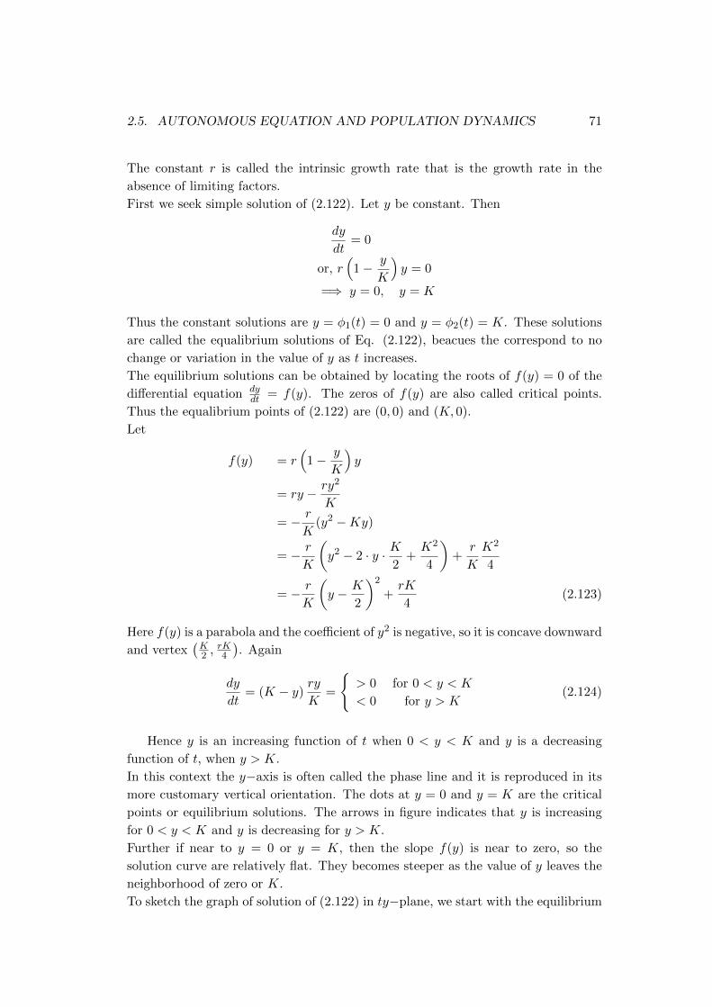
2.5. AUTONOMOUS EQUATION AND POPULATION DYNAMICS 71
The constant r is called the intrinsic growth rate that is the growth rate in the
absence of limiting factors.
First we seek simple solution of (2.122). Let y be constant. Then
dy
dt= 0
or, r(
1− y
K
)y = 0
=⇒ y = 0, y = K
Thus the constant solutions are y = φ1(t) = 0 and y = φ2(t) = K. These solutions
are called the equalibrium solutions of Eq. (2.122), beacues the correspond to no
change or variation in the value of y as t increases.
The equilibrium solutions can be obtained by locating the roots of f(y) = 0 of the
differential equation dydt = f(y). The zeros of f(y) are also called critical points.
Thus the equalibrium points of (2.122) are (0, 0) and (K, 0).
Let
f(y) = r(
1− y
K
)y
= ry − ry2
K
= − r
K(y2 −Ky)
= − r
K
(y2 − 2 · y · K
2+K2
4
)+
r
K
K2
4
= − r
K
(y − K
2
)2
+rK
4(2.123)
Here f(y) is a parabola and the coefficient of y2 is negative, so it is concave downward
and vertex(K2 ,
rK4
). Again
dy
dt= (K − y)
ry
K=
> 0 for 0 < y < K
< 0 for y > K(2.124)
Hence y is an increasing function of t when 0 < y < K and y is a decreasing
function of t, when y > K.
In this context the y−axis is often called the phase line and it is reproduced in its
more customary vertical orientation. The dots at y = 0 and y = K are the critical
points or equilibrium solutions. The arrows in figure indicates that y is increasing
for 0 < y < K and y is decreasing for y > K.
Further if near to y = 0 or y = K, then the slope f(y) is near to zero, so the
solution curve are relatively flat. They becomes steeper as the value of y leaves the
neighborhood of zero or K.
To sketch the graph of solution of (2.122) in ty−plane, we start with the equilibrium

72CHAPTER 2. FIRST ORDER LINEAR ANDNONLINEARDIFFERENTIAL EQUATIONS
Figure 2.1: f(y) versus y for dydx = f(y) = r
(1− y
K
)y
solutions y = 0 and y = K, then we draw other curves that are increasing when
0 < y < K, decreasing when y > K, and flatten out as y approaches either of the
values 0 or K. Thus the graph of solutions of equation (2.122) must have the general
shape is shown in Figure.
Figure 2.2: Logistic growth dydx = r
(1− y
k
)y (a) The phase line (b) plot of y versus
t.
Again, f(y) = ry−ay2 is a quadractic polynomial in y and ∂f∂y = r−2ay is linear.
Both f and ∂f∂y are continuous for all t ∈ R. Thus the equation (2.122) has only
one solution passes through a given point in ty−plane. So the curve does intersect
each other. Althogh other solutions may be asymptotic to the equilibrium solution

2.5. AUTONOMOUS EQUATION AND POPULATION DYNAMICS 73
as t→∞, they can not intersect at a finite time.
We can determine the concavity of the solution curves and locate the point of in-
flection.
We have
dy
dt= f(y)
or,d2y
dt2=
d
dt(f(y)) =
d
dy(f(y))
dy
dt= f ′(y)f(y)
=
> 0 if both f(y) and f ′(y) have the same sign
< 0 if both f(y) and f ′(y) have the opposite signs
=
Concave upward if both f(y) and f ′(y) have the same sign
Concave downward if both f(y) and f ′(y) have the opposite signs
Hence
f(y) =dy
dt= (K − y)
ry
K=
> 0 for 0 < y < K
< 0 for y > K(2.125)
f ′(y) = r − 2ry
K=rK − 2ry
K
=2r
K
(K
2− y)
=
> 0 for 0 < y < K
2
< 0 for y > K2
(2.126)
Interval f(y) from Eq.(2.125) f ′(y) from Eq.(2.126) y′′ = f(y)f ′(y) y is concave
0 < t < K2 +ve +ve +ve upwards
K2 < t < K +ve −ve −ve downwards
t > K −ve −ve +ve upwards
The line y = K2 ,separates the graph of the solution from concave upward to from
downward. So, the graphs are sigmoidal (S-shaped). Since K is the upper bound
that is approached, but not exceeded, by growing populations starting below this
value. Thus, it is natural to refer to K as saturated level. for the given species. The
last row of the table is not applicable.
Analytic soltion The logistic model is from (2.122)
dy
dt= r
(1− y
K
)y where K =
r
a
or,dy(
1− yK
)y
= rdt
or,
1
y+
1/k
1− yk
dy = rdt
(2.127)
Integrating,
ln |y| − ln∣∣∣1− y
k
∣∣∣ = rt+ ln c (2.128)

74CHAPTER 2. FIRST ORDER LINEAR ANDNONLINEARDIFFERENTIAL EQUATIONS
where the constant is determined from the initial conditions y(0) = y0, the initial
ppopulation of the species.
Case I: For 0 < y0 < K, 0 < y < K, both y and 1− Ky are positive. From (2.128),
we get
ln y − ln(
1− y
k
)= rt+ ln c
or, ln
(y
1− yk
)= rt+ ln c
or,y
1− yk
= cert (2.129)
Using the initial condition y(0) = y0, we get
y0
1− y0k
= c
From (2.129)
y
1− yk
=y0
1− y0k
ert
or,1− y
k
y=
1− y0k
y0e−rt
or,1
y− 1
K=
(1
y0− 1
K
)e−rt
or,1
y=
1
K+
(1
y0− 1
K
)e−rt
or,1
y=y0 + (K − y0)e−rt
ky0
or, y =ky0
y0 + (K − y0)e−rt(2.130)
which gives the solution of initial value problem for 0 < y0 < K.
For the long time
limt→∞
y = limt→∞
Ky0
y0 + (K − y0)e−rt=Ky0
y0= K
Thus, for each y0 > 0, the solution approaches the equilibrium solution y = K as
t → ∞. So, the constant solution y = K is an asymptotically stable solution of
the logistic model. As r increases, the solutions approach the equilibrium solution
y = K, more rapidly.
Case II: For y0 > K, y > K, y is positive and 1− Ky is negative. From (2.128), we
get
ln y − ln(yk− 1)
= rt+ ln c
or, ln
(yyk
− 1
)= rt+ ln c
or,y
yk − 1
= cert (2.131)

2.5. AUTONOMOUS EQUATION AND POPULATION DYNAMICS 75
Using the initial condition y(0) = y0, we get
y0y0k − 1
= c
From (2.129)
yyk − 1
=y0
y0k − 1
ert
or,yk − 1
y=
y0k − 1
y0e−rt
or,1− y
k
y=
1− y0k
y0e−rt
or,1
y− 1
K=
(1
y0− 1
K
)e−rt
or,1
y=
1
K+
(1
y0− 1
K
)e−rt
or,1
y=y0 + (K − y0)e−rt
ky0
or, y =ky0
y0 + (K − y0)e−rt
which gives the solution of initial value problem for 0 < y0 < K.
For the long time
limt→∞
y = limt→∞
Ky0
y0 + (K − y0)e−rt=Ky0
y0= K
Thus, for each y0 > 0, the solution approaches the equilibrium solution y = K as
t → ∞. So, the constant solution y = K is an asymptotically stable solution of
the logistic model. As r increases, the solutions approach the equilibrium solution
y = K, more rapidly.
2.5.3 A Critical Threshold
We consider the another logistic equation
dy
dt= −r
(1− y
T
)y (2.132)
where r and T are given positive constants, T is the critical amplitude. This equation
is differs from the logistic equation (2.122) only in the presence of the minus sign.
The graph of f(y) = −r(1− y
T
)y versus y is the downward parabola .
f(y) = 0
or, y = 0 = φ1, y = T = φ2(t)

76CHAPTER 2. FIRST ORDER LINEAR ANDNONLINEARDIFFERENTIAL EQUATIONS
as the critical points or the equilibrium soutions . Thus, (0, 0) and (0, T ) are critical
points of Eq. (2.132).
f(y) = −r(
1− y
T
)y
= −ry +ry2
T
=r
K(y2 − Ty)
=r
T
(y2 − 2 · y · T
2+T 2
4
)− r
T
T 2
4
=r
T
(y − T
2
)2
− rT
4(2.133)
Hefe f(y) is a parabola and the coefficient of y2 is positive, so it is concave upward
and vertex(T2 ,−
rT4
). Again
dy
dt= − (T − y)
ry
K=
< 0 for 0 < y < T
> 0 for y > T(2.134)
Figure 2.3:
Hence y is an decreasing function of t when 0 < y < T and y is a increasing
function of t, when t > T .
In this context the y−axis is often called the phase line and it is reproduced in its

2.5. AUTONOMOUS EQUATION AND POPULATION DYNAMICS 77
more customary vertical orientation. The dots at y = 0 and y = K are the critical
points or equilibrium solutions. The arrows in fig indicate that y is decreasing for
0 < y < T and y is increasing for t > T . Hence y = 0 is asymptotically stable and
y = K
We can determine the concavity of the solution curves and locate the point of in-
flection.
We have
dy
dt= f(y)
or,d2y
dt2=
d
dt(f(y)) =
d
dy(f(y))
dy
dt= f ′(y)f(y)
=
> 0 if both f(y) and f ′(y) have the same sign
< 0 if both f(y) and f ′(y) have the opposite signs
=
Concave upward if both f(y) and f ′(y) have the same sign
Concave downward if both f(y) and f ′(y) have the opposite signs
Hence
f(y) =dy
dt= − (T − y)
ry
T=
< 0 for 0 < y < T
> 0 for y > T(2.135)
f ′(y) = −r +2ry
T=
2ry − rTT
=2r
T
(y − T
2
)=
< 0 for 0 < y < T
2
> 0 for y > T2
(2.136)
Interval f(y) from Eq.(2.125) f ′(y) from Eq.(2.126) y′′ = f(y)f ′(y) y is concave
0 < t < T2 −ve −ve +ve upwards
T2 < t < T −ve +ve −ve downwards
t > T +ve +ve +ve upwards
The line y = T2 ,separates the graph of the solution from concave upward to from
downward.
Also y > T , the curve is increasing and concave upward. We conclude that as time
inceases, y either approaches to 0 or grows without bound, depending on wheather
the initail value y0 is less than or greater than T . Hence T is a thresthold level,
below which the population dies out.
However we get solution of (2.132) as replacing −r by r, and K by T in (2.130)
or, y =Ty0
y0 + (T − y0)ert(2.137)
If 0 < y0 < T ,as t → ∞, y → 0. This agrees with our qualitative geomeric
analysis.

78CHAPTER 2. FIRST ORDER LINEAR ANDNONLINEARDIFFERENTIAL EQUATIONS
Figure 2.4:
If y0 > T then let
y0 + (T − y0)ert′
= 0
or ert′
=y0
y0 − T> 1
or, rt′ = ln
(y0
y0 − T
)or, t′ =
1
rln
(y0
y0 − T
)> 0
If y0 > T then the denominator of the equation (2.137), is zero and the population
becomes unbounded in a finite value of t.
2.5.4 Logistic Growth with a Threshold
The threshold model
dy
dt= −r
(1− y
T
)y (2.138)
may need to modified so that unbounded growth does not occur when y is above
the threshold T . The simplest way to do this to introduce another factor that will
have the effect of making dydt negative when y is large. For this we consider
dy
dt= −r
(1− y
T
)(1− y
K
)y = f(y) (2.139)
where r > 0 and 0 < T < K.

2.5. AUTONOMOUS EQUATION AND POPULATION DYNAMICS 79
Example 49.
Sketch the graph of f(y) versus y, determine the critical points and classify each
one as asymptotically stable or unstable. Draw the phase line and draw graph of
several graphs of solution in the ty−plane for
dy
dt= ay + by2, a > 0, b > 0, −∞ < y0 <∞
Solution: The given differential equation is
dy
dt= ay + by2 = f(y), a > 0, b > 0, −∞ < y0 <∞ (2.140)
Let
dy
dt= 0
or ay + by2 = 0
or, y = 0, y = −ab
Hence critical points are y = 0 and y = − ba .
Interval dydt = f(y) = a(y − 0)y −
(−ab
) y is
−∞ < y < −ab
dydt = f(y) = a(y − 0)−vey −
(ab
)−ve = +ve increasing
−ab < y < 0 dy
dt = f(y) = a(y − 0)−vey −(ab
)+ve = −ve decreasing
y > 0 dydt = f(y) = a(y − 0)+vey −
(ab
)+ve = +ve increasing
We can determine the concavity of the solution curves and locate the point of in-
flection.
We have
dy
dt= f(y)
or,d2y
dt2=
d
dt(f(y)) =
d
dy(f(y))
dy
dt= f ′(y)f(y)
=
> 0 if both f(y) and f ′(y) have the same sign
< 0 if both f(y) and f ′(y) have the opposite signs
=
Concave upward if both f(y) and f ′(y) have the same sign
Concave downward if both f(y) and f ′(y) have the opposite signs
Hence
f(y) =dy
dt= ay(a+ by) =
> 0 for −∞ < y < −a
b
< 0 for − ab < y < 0
> 0 for y > 0
(2.141)
f ′(y) = a+ 2by = 2b[y −
(− a
2b
)]=
< 0 for y < − a
2b
> 0 for y > − a2b
(2.142)

80CHAPTER 2. FIRST ORDER LINEAR ANDNONLINEARDIFFERENTIAL EQUATIONS
Sign change points are −ab , −
a2b , 0
Interval f(y) from (2.141) f ′(y) from(2.142) y′′ = f(y)f ′(y) y is concave
−∞ < y < −ab +ve −ve −ve downward
−ab < y < − a
2b −ve −ve +ve upward
− a2b < y < 0 −ve +ve −ve downward
y > 0 +ve +ve +ve upward
Using all these, the graph of y(t) in ty−plane, the of f(y) versus y and phase diagram
is shown as figure.
Figure 2.5:
Example 50.
Sketch the graph of f(y) versus y, determine the critical points and classify each
one as asymptotically stable or unstable. Draw the phase line and draw graph of
several graphs of solution in the ty−plane for
dy
dt= y(y − 1)(y − 2), −∞ < y0 <∞
Solution: The given differential equation is
dy
dt= y(y − 1)(y − 2)quad−∞ < y0 <∞ (2.143)
Let
dy
dt= 0
or y(y − 1)(y − 2) = 0
or, y = 0, y = 1, y = 2

2.5. AUTONOMOUS EQUATION AND POPULATION DYNAMICS 81
Hence critical points are y = 0, y = 1 and y = 2.
Interval dydt = f(y) = (y − 0)(y − 1)(y − 2) y is
−∞ < y < 0 dydt = f(y) = (y − 0)−ve(y − 1)−ve(y − 2)−ve = −ve decreasing
0 < y < 1 dydt = f(y) = (y − 0)+ve(y − 1)−ve(y − 2)−ve = +ve increasing
1 < y < 2 dydt = f(y) = (y − 0)+ve(y − 1)+ve(y − 2)−ve = −ve decreasing
y > 2 dydt = f(y) = (y − 0)+ve(y − 1)+ve(y − 2)+ve = +ve increasing
We can determine the concavity of the solution curves and locate the point of in-
flection.
We have
dy
dt= f(y)
or,d2y
dt2=
d
dt(f(y)) =
d
dy(f(y))
dy
dt= f ′(y)f(y)
=
> 0 if both f(y) and f ′(y) have the same sign
< 0 if both f(y) and f ′(y) have the opposite signs
=
Concave upward if both f(y) and f ′(y) have the same sign
Concave downward if both f(y) and f ′(y) have the opposite signs
Hence
f(y) =dy
dt= (y − 0)(y − 1)(y − 2) =
< 0 for −∞ < y < 0
> 0 for 0 < y < 1
< 0 for 1 < y < 2
> 0 for y > 2
(2.144)
f(y) = y3 − 3y2 + 2y
f ′(y) = 3y2 − 6y + 2
= 3
(y2 − 2y +
2
3
)= 3
(y2 − 2y · 1 + 12 − 1 +
2
3
)= 3
(y − 1)2 − 1
3
= 3
y −
(1− 1√
3
)y −
(1 +
1√3
)
=
> 0 for −∞ < y < 1− 1√
3
< 0 for 1− 1√3< t < 1 + 1√
3
> 0 for t > 1 + 1√3
(2.145)

82CHAPTER 2. FIRST ORDER LINEAR ANDNONLINEARDIFFERENTIAL EQUATIONS
Sign change points are 0, 1− 1√3, 1, 1 + 1√
3, 2
Interval f(y) from (2.144) f ′(y) from(2.145) y′′ = f(y)f ′(y) y is concave
−∞ < y < 0 −ve +ve −ve downward
and decreasing
0 < y < 1− 1√3
+ve +ve +veupward
and increasing
1− 1√3< y < 1 +ve −ve −ve downward
and increasing
1 < y < 1 + 1√3
−ve −ve +veupward
and decreasing
1 + 1√3< y < 2 −ve +ve −ve downward
and decreasing
y > 2 +ve +ve +veupnward
and increasing
Using all these, the graph of y(t) in ty−plane, the of f(y) versus y and phase diagram
is shown as figure.figure y = 1 is stable but y = 0 and y = 2 are unstable.
Figure 2.6:
Example 51.

2.5. AUTONOMOUS EQUATION AND POPULATION DYNAMICS 83
Sketch the graph of f(y) versus y, determine the critical points and classify each
one as asymptotically stable or unstable. Draw the phase line and draw graph of
several graphs of solution in the ty−plane for
dy
dt= y2(y2 − 1), −∞ < y0 <∞
Solution: The given differential equation is
dy
dt= y2(y2 − 1), −∞ < y0 <∞ (2.146)
Let
dy
dt= 0
or y2(y2 − 1) = 0
or, y = 0, y = 1, y = −1
Hence critical points are y = −1, y = 0 and y = 1.
Interval dydt = f(y) = y2 [y − (−1)] (y − 1) y is
−∞ < y < −1 dydt = f(y) = y2
+ve [y − (−1)]−ve(y − 1)−ve = +ve increasing
−1 < y < 0 dydt = f(y) = y2
+ve [y − (−1)]+ve(y − 1)−ve = −ve decreasing
0 < y < 1 dydt = f(y) = y2
+ve [y − (−1)]+ve(y − 1)−ve = −ve decreasing
y > 1 dydt = f(y) = y2
+ve [y − (−1)]+ve(y − 1)+ve = +ve increasing
We can determine the concavity of the solution curves and locate the point of in-
flection.
We have
dy
dt= f(y)
or,d2y
dt2=
d
dt(f(y)) =
d
dy(f(y))
dy
dt= f ′(y)f(y)
=
> 0 if both f(y) and f ′(y) have the same sign
< 0 if both f(y) and f ′(y) have the opposite signs
=
Concave upward if both f(y) and f ′(y) have the same sign
Concave downward if both f(y) and f ′(y) have the opposite signs
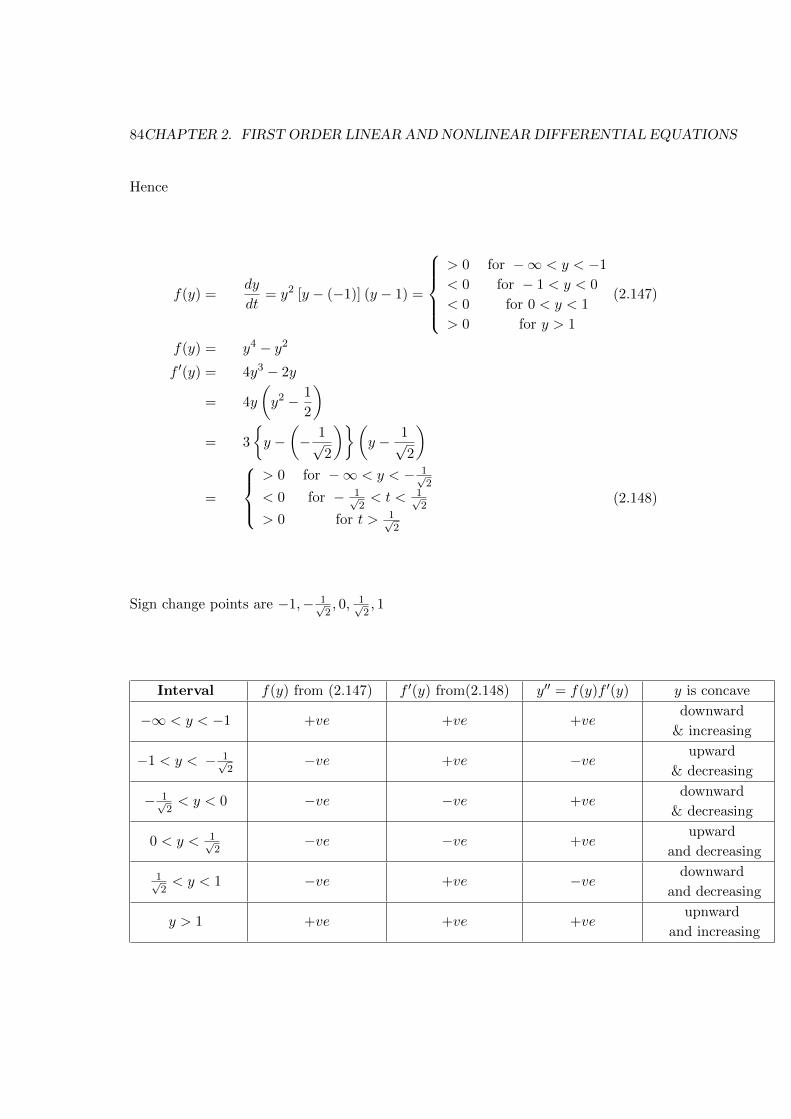
84CHAPTER 2. FIRST ORDER LINEAR ANDNONLINEARDIFFERENTIAL EQUATIONS
Hence
f(y) =dy
dt= y2 [y − (−1)] (y − 1) =
> 0 for −∞ < y < −1
< 0 for − 1 < y < 0
< 0 for 0 < y < 1
> 0 for y > 1
(2.147)
f(y) = y4 − y2
f ′(y) = 4y3 − 2y
= 4y
(y2 − 1
2
)= 3
y −
(− 1√
2
)(y − 1√
2
)
=
> 0 for −∞ < y < − 1√
2
< 0 for − 1√2< t < 1√
2
> 0 for t > 1√2
(2.148)
Sign change points are −1,− 1√2, 0, 1√
2, 1
Interval f(y) from (2.147) f ′(y) from(2.148) y′′ = f(y)f ′(y) y is concave
−∞ < y < −1 +ve +ve +vedownward
& increasing
−1 < y < − 1√2
−ve +ve −ve upward
& decreasing
− 1√2< y < 0 −ve −ve +ve
downward
& decreasing
0 < y < 1√2
−ve −ve +veupward
and decreasing
1√2< y < 1 −ve +ve −ve downward
and decreasing
y > 1 +ve +ve +veupnward
and increasing
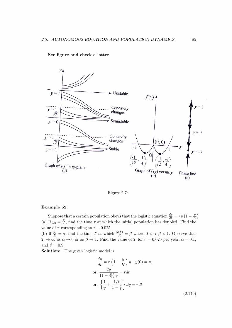
2.5. AUTONOMOUS EQUATION AND POPULATION DYNAMICS 85
See figure and check a latter
Figure 2.7:
Example 52.
Suppose that a certain population obeys that the logistic equation dydt = ry
(1− y
K
)(a) If y0 = K
4 , find the time τ at which the initial population has doubled. Find the
value of τ corresponding to r − 0.025.
(b) If y0K = α, find the time T at which y(T )
K = β where 0 < α, β < 1. Observe that
T →∞ as α→ 0 or as β → 1. Find the value of T for r = 0.025 per year, α = 0.1,
and β = 0.9.
Solution: The given logistic model is
dy
dt= r
(1− y
K
)y y(0) = y0
or,dy(
1− yK
)y
= rdt
or,
1
y+
1/k
1− yk
dy = rdt
(2.149)

86CHAPTER 2. FIRST ORDER LINEAR ANDNONLINEARDIFFERENTIAL EQUATIONS
Integrating,
ln |y| − ln∣∣∣1− y
k
∣∣∣ = rt+ ln c (2.150)
where the constant is determined from the initial conditions y(0) = y0, the initial
population of the species.
(a)For 0 < y0 = K4 < K, 0 < y < K, both y and 1 − K
y are positive. From (2.154),
we get
ln y − ln(
1− y
k
)= rt+ ln c
or, ln
(y
1− yk
)= rt+ ln c
or,y
1− yk
= cert (2.151)
Using the initial condition y(0) = y0, we get
y0
1− y0k
= c
From (2.151)
y
1− yk
=y0
1− y0k
ert
or,1− y
k
y=
1− y0k
y0e−rt
or,1
y− 1
K=
(1
y0− 1
K
)e−rt
or,1
y=
1
K+
(1
y0− 1
K
)e−rt
or,1
y=y0 + (K − y0)e−rt
Ky0
or, y =Ky0
y0 + (K − y0)e−rt
or,y
K=
y0
y0 + (K − y0)e−rt(2.152)

2.5. AUTONOMOUS EQUATION AND POPULATION DYNAMICS 87
If y0 = K4 , then we have to find the time τ when y = 2y0 = K
2 . From (2.152),
1
2=
K4
K4 + (K − K
4 )e−rτ
or,1
2=
14
14 + 3
4e−rτ
or,1
4+
3
4e−rτ =
1
2
or,3
4e−rτ =
1
4
or, e−rτ =1
3or, erτ = 3
or, rτ = ln 3
or, τ =1
rln 3 =
1
0.025ln 3 = 43.95 years
(b) Again, from (2.152)
y
K=
y0
y0 + (K − y0)e−rt
or,y
K=
y0K
y0K +
(1− y0
K
)e−rt
But y0K = α, t = T and β = y
K .
β =α
α+ (1− α)e−rT
or,α
β= α+ (1− α)e−rT
or,α
β− α = (1− α)e−rT
or,α(1− β)
β= (1− α)e−rT
or, erT =β(1− α)
α(1− β)
or, rT = ln
(β(1− α)
α(1− β)
)Hence, as α→ 0 or β → 1, then T →∞.
Also, taking α = 0.1, β = 0.9 and r = 0.025 per year.
T =1
0.025ln
(0.9× 0.9
0.1× 0.1
)= 175.78 years
Example 53.

88CHAPTER 2. FIRST ORDER LINEAR ANDNONLINEARDIFFERENTIAL EQUATIONS
The logistic model has been applied to the natural growth of the haibut popula-
tion in certain areas of the pacific Ocean. Let y, measure in kilograms, be the total
mass or biomass, of the halibut population at time t. The parameters in the logistic
equation are estimated to have the values r = 0.71/ year and K = 80.5 × 10⁶ kg.
If the initial biomass is y0 = 0.25K, find the biomass 2 years latter. Also find the
time τ for which y(τ) = 0.75K.
Solution: The given logistic model is
dy
dt= r
(1− y
K
)y y(0) = y0
or,dy(
1− yK
)y
= rdt
or,
1
y+
1/k
1− yk
dy = rdt
(2.153)
Integrating,
ln |y| − ln∣∣∣1− y
k
∣∣∣ = rt+ ln c (2.154)
where the constant is determined from the initial conditions y(0) = y0, the initial
population of the species.
(a)For 0 < y0 = K4 < K, 0 < y < K, both y and 1 − K
y are positive. From (2.154),
we get
ln y − ln(
1− y
k
)= rt+ ln c
or, ln
(y
1− yk
)= rt+ ln c
or,y
1− yk
= cert (2.155)
Using the initial condition y(0) = y0, we get
y0
1− y0k
= c

2.5. AUTONOMOUS EQUATION AND POPULATION DYNAMICS 89
From (2.151)
y
1− yk
=y0
1− y0k
ert
or,1− y
k
y=
1− y0k
y0e−rt
or,1
y− 1
K=
(1
y0− 1
K
)e−rt
or,1
y=
1
K+
(1
y0− 1
K
)e−rt
or,1
y=y0 + (K − y0)e−rt
Ky0
or, y =Ky0
y0 + (K − y0)e−rt
or,y(t)
K=
y0K
y0K + (1− y0
K )e−rt(2.156)
Using the given data y0K = 0.25, r = 0.71/year, t = 2 years and K = 80.5× 10⁶ kg.
y(2)
80.5× 106=
0.25
0.25 + 0.75e−1.42= 0.5797
or, y(2) = 0.5797× 80.5× 106 = 46.7× 10⁶kg
To find τ when y(τ) = 0.75K, solving (2.156)
y(y0 + (K − y0)e−rτ
)= Ky0
or, 0.75K(0.25K + (K − 0.25K)e−rτ
)= 0.25K2
or, 0.75K2(0.25 + 0.75e−0.71τ ) = 0.25K2
or, 0.75(0.25 + 0.75e−0.71τ ) = 0.25
or, 9 = e0.71τ
or, ln 9 = 0.71τ
or, τ =ln 9
0.71= 3.095 years (2.157)
Example 54.
A pound form as water collects in a conical depression of radius a and depth h.
Suppose that water flows in at a constant rate K and is lost through evaporation at
the rate proportional to the surface area.
(a) Show that the volume V (t) of water in the pond at time t satisfies the differential
equation
dV
dt= k − α
(3a
πh
)2/3
V 2/3
where α is the coefficient of evaporation.
(b) Find the equilibrium depth of water in the pound. Is the equilibrium asymtoti-
cally stable?

90CHAPTER 2. FIRST ORDER LINEAR ANDNONLINEARDIFFERENTIAL EQUATIONS
(c) Find a condition that must be satisfied if the pond is not to overflow?
Solution: Here we take a pound form as water collects in a conical depression of
radius a and depth h. Let V be volume, r be the radius of top and l be the depth
of water at any time t in the pound.
Figure 2.8:
Since the water is colecting at a constant rate k and the rate of decrease of
evaporation is porportinal to the upper surface area of the water . Thus the rate of
change of the volume of the water is given by
dV
dt= k − απr2 (2.158)
But
r
l=a
h=⇒ l =
rh
a
Again,
V =1
3πr2l =
1
3πr2 rh
a=
1
3aπr3
or, r3 =3V a
πh
or, r =
(3V a
πh
)1/3

2.6. EXACT EQUATION AND INTEGRATING FACTOR 91
Putting the value of r in (2.158)
dV
dt= k − απ
(3V a
πh
)2/3
(b) For equilibrium
dV
dt= 0
or, k − απr2 = 0
or, r2 =k
απ
or, r =
√k
απ
∴ l =rh
a=h
a
√k
απ
When the water depth increase, more area is exposed for evaporation which again
tends to decrease the water depth. When the water depth decrease, due to less
evaporation, the depth increase. Hence the equilibrium depth is asymptotically
stable.
(c) For the pond is not to overflow, we must have
l ≤ h
=⇒ h
a
√k
απ≤ h
=⇒ k2
απ≤ a2
=⇒ k
α≤ πa2
which is a required condition.
2.6 Exact Equation and Integrating Factor
For the first order equations there are a number of integration methods are applicable
to various problem. Here we consider a class of equations, which are exact.
2.6.1 Exact Equation
Let a differential equation
M(x, y) +N(x, y)dy
dx= 0 (2.159)
be given. Suppose that we can identify a function ψ(x, y) such that
∂ψ
∂x= M(x, y) and
∂ψ
∂y= N(x, y) (2.160)

92CHAPTER 2. FIRST ORDER LINEAR ANDNONLINEARDIFFERENTIAL EQUATIONS
and such that ψ(x, y) = c defines y = φ(x) implicitly as a differential function of x.
Then
M(x, y) +N(x, y)dy
dx=∂ψ
∂x+∂ψ
∂y
dy
dx=
d
dxψ(x, y)
From the differential equation (2.160), becomes
d
dxψ(x, y) = 0 (2.161)
Integrating,
ψ(x, y) = c (2.162)
whcin is solution of (2.159).
Thus, a first order differential equation
M(x, y) +N(x, y)dy
dx= 0
is said to be exact if there exist a function ψ(x, )y such that
d
dxψ(x, y) = M(x, y) +N(x, y)
dy
dxor, d(ψ(x, y)) = M(x, y)dx+N(x, y)dy
Let a differential equation is not exact. If it is possible to make exact by multi-
plying it an appropriate factor u(x, y), which is called an integrating factor for the
differential equation.
Theorem 3.
Let the functions
M,N,∂M
∂y, and
∂N
∂x
be continuous in the rectangular region R : α < x < β; γ < y < δ. Then
M(x, y) +N(x, y)dy
dx= 0
is an exact differential equation in R if and only if
∂M
∂y=∂N
∂x
That is , there exists a function ψ(x, y) satisfying such that
∂ψ
∂x= M(x, y),
∂ψ
∂y= N(x, y)
if and only if M and N satisfy the equation
M(x, y) +N(x, y)dy
dx= 0
Steps for solving the exact differentail equation of first order

2.6. EXACT EQUATION AND INTEGRATING FACTOR 93
1. Make the given equation in the form
M(x, y) +N(x, y)dy
dx= 0
2. if ∂M∂y = ∂N
∂x then it is exact. Otherwise, do not follow it.
3. Consider∂ψ
∂x= M(x, y),
∂ψ
∂y= N(x, y)
4. Integrate ∂ψ∂x = M(x, y) with respect to x, to get ψ.
ψ = φ+ h(y) (2.163)
Here h is an unknown function of y and which is constant of integration.
5. Differentiating, (2.163) partially with respect to y, we get
∂ψ
∂y= φy + h′(y)
6. Equate
∂ψ
∂y= N(x, y)
or, φy + h′(y) = N(x, y)
or, h′(y) = N(x, y)− φy
Integrating, we get h(y).
7. Putting the value of h(y) in (2.163), we get the required solution.
Example 55.
Solve the differential equation
y cosx+ 2xey + (sinx+ x2ey − 1)dy
dx= 0
Solution: Comparing the equation
y cosx+ 2xey + (sinx+ x2ey − 1)dy
dx= 0 (2.164)
with
M(x, y) +N(x, y)dy
dx= 0 (2.165)
we get
M = y cosx+ 2xey, N = sinx+ x2ey − 1

94CHAPTER 2. FIRST ORDER LINEAR ANDNONLINEARDIFFERENTIAL EQUATIONS
∴∂M
∂y= cosx+ 2xey,
∂N
∂x= cosx+ 2xey
∂M
∂y=∂N
∂x(2.166)
Hence, the given differential equation is exact. Thus, thier exists a function ψ(x, y)
such that
∂ψ
∂x= M(x, y),
∂ψ
∂y= N(x, y)
or,∂ψ
∂x= y cosx+ 2xey, (2.167)
∂ψ
∂y= sinx+ x2ey − 1 (2.168)
Integrating with respect to x, the equation (2.167), we get
ψ(x, y) =
∫∂ψ
∂xdx+ h(y)
= y
∫cosxdx+ 2ey
∫xdx+ h(y)
= y sinx+ x2ey + h(y) (2.169)
But from (2.168), we get
N(x, y) =∂ψ
∂y
or, sinx+ x2ey − 1 = sinx+ x2ey + h′(y)
=⇒ h′(y) = −1
=⇒ h(y) = −y + c
Hence, from (2.169), we get
ψ(x, y) = y sinx+ x2ey − y + c = 0
which is required solution.
Example 56.
Determine whether the equation
(2x+ 4y) + (2x− 2y)dy
dx= 0
is exact. If it is exact, find the solution.
Solution: Comparing the equation
(2x+ 4y) + (2x− 2y)dy
dx= 0 (2.170)

2.6. EXACT EQUATION AND INTEGRATING FACTOR 95
with
M(x, y) +N(x, y)dy
dx= 0
we get
M = 2x+ 4y, N = 2x− 2y
∴∂M
∂y= 4,
∂N
∂x= 2
∂M
∂y6= ∂N
∂x
Hence, the given differential equation is not exact.
Example 57.
Determine whether the equation
dy
dx= −ax− by
bx− ay
is exact. If it is exact, find the solution.
Solution: Comparing the equation
dy
dx= −ax− by
bx− ay
(ax− by) + (bx− ay)dy
dx= 0 (2.171)
with
M(x, y) +N(x, y)dy
dx= 0
we get
M = ax− by, N = bx− ay
∴∂M
∂y= −b, ∂N
∂x= b
∂M
∂y6= ∂N
∂x
Hence, the given differential equation is not exact.
Example 58.

96CHAPTER 2. FIRST ORDER LINEAR ANDNONLINEARDIFFERENTIAL EQUATIONS
Determine whether the equation
(2x+ 3) + (2y − 2)dy
dx= 0
is exact. If it is exact, find the solution.
Solution: Comparing the equation
(2x+ 3) + (2x− 2)dy
dx= 0 (2.172)
with
M(x, y) +N(x, y)dy
dx= 0
we get
M = 2x+ 3, N = 2x− 2
∴∂M
∂y= 0,
∂N
∂x= 0
∂M
∂y=∂N
∂x
Hence, the given differential equation is exact. Thus, there exists a function ψ(x, y)
such that
∂ψ
∂x= M(x, y),
∂ψ
∂y= N(x, y)
or,∂ψ
∂x= 2x+ 3, (2.173)
∂ψ
∂y= 2y − 2 (2.174)
Integrating with respect to x, the equation (2.173), we get
ψ(x, y) =
∫∂ψ
∂xdx+ h(y)
=
∫(2x+ 3)dx+ h(y)
= x2 + 3x+ h(y) (2.175)
But from (2.174), we get
N(x, y) =∂ψ
∂y
or, 2y − 2 = h′(y)
=⇒ h′(y) = 2y − 2
=⇒ h(y) = y2 − 2y + c
Hence, from (2.175), we get
ψ(x, y) = x2 + 3x+ y2 − 2y + c = 0
which is required solution.
2.6. EXACT EQUATION AND INTEGRATING FACTOR 97
Example 59.
Determine whether the equation
(2xy2 + 2y) + (2x2y + 2x)dy
dx= 0
is exact. If it is exact, find the solution.
Solution: Comparing the equation
(2xy2 + 2y) + (2x2y + 2x)dy
dx= 0 (2.176)
with
M(x, y) +N(x, y)dy
dx= 0
we get
M = 2xy2 + 2y, N = 2x2y + 2x
∴∂M
∂y= 4xy + 2,
∂N
∂x= 4xy + 2
∂M
∂y=∂N
∂x
Hence, the given differential equation is exact. Thus, thier exists a function ψ(x, y)
such that
∂ψ
∂x= M(x, y),
∂ψ
∂y= N(x, y)
or,∂ψ
∂x= 2xy2 + 2y, (2.177)
∂ψ
∂y= 2x2y + 2x (2.178)
Integrating with respect to x, the equation (2.177), we get
ψ(x, y) =
∫∂ψ
∂xdx+ h(y)
=
∫(2xy2 + 2y)dx+ h(y)
= x2y2 + 2xy + h(y) (2.179)
But from (2.178), we get
N(x, y) =∂ψ
∂y
or, 2x2y + 2x = 2x2y + 2x+ h′(y)
=⇒ h′(y) = 0
=⇒ h(y) = c

98CHAPTER 2. FIRST ORDER LINEAR ANDNONLINEARDIFFERENTIAL EQUATIONS
Hence, from (2.179), we get
ψ(x, y) = x2y2 + 2xy + c = 0
which is required solution.
Example 60.
Determine whether the equation
(x ln y + xy) + (y lnx+ xy)dy
dx= 0
is exact. If it is exact, find the solution.
Solution: Comparing the equation
(x ln y + xy) + (y lnx+ xy)dy
dx= 0 (2.180)
with
M(x, y) +N(x, y)dy
dx= 0
we get
M = x ln y + xy, N = y lnx+ xy
∴∂M
∂y=x
y+ x,
∂N
∂x=y
x+ y
∂M
∂y6= ∂N
∂x
Hence, the given differential equation is not exact.
Example 61.
Solve the initial value problem and determine at least aprroximately where the
solution is valid
(2x− y)dx+ (2y − x)dy = 0, y(1) = 3
Solution: Comparing the equation
(2x− y) + (2y − x)dy
dx= 0
with
M(x, y) +N(x, y)dy
dx= 0
we get
M = 2x− y, N = 2y − x

2.6. EXACT EQUATION AND INTEGRATING FACTOR 99
∴∂M
∂y= −1,
∂N
∂x= −1
∂M
∂y=∂N
∂x
Hence, the given differential equation is exact. Thus, thier exists a function ψ(x, y)
such that
∂ψ
∂x= M(x, y),
∂ψ
∂y= N(x, y)
or,∂ψ
∂x= 2x− y, (2.181)
∂ψ
∂y= 2y − x (2.182)
Integrating with respect to x, the equation (2.181), we get
ψ(x, y) =
∫∂ψ
∂xdx+ h(y)
=
∫(2x− y)dx+ h(y)
= x2 − xy + h(y) (2.183)
But from (2.182), we get
N(x, y) =∂ψ
∂y
or, 2y − x = −x+ h′(y)
=⇒ h′(y) = 2y
=⇒ h(y) = y2 + c‘
Hence, from (2.179), we get
ψ(x, y) = c
or, x2 − xy + y2 + c = 0 (2.184)
Using the initial condition y(1) = 3 i.e. x = 1, y = 3 in (2.184),
1− 3 + 9 + c = 0
or, c = −7

100CHAPTER 2. FIRST ORDER LINEAR ANDNONLINEARDIFFERENTIAL EQUATIONS
Putting the value of (2.184)
x2 − xy + y2 − 7 = 0
or, y2 − xy + x2 − 7 = 0
or, y =x±
√x2 − 4 · 1 · (x2 − 7)
2
or, y =x±√
28− 3x2
2
Either, y =x−√
28− 3x2
2(2.185)
or y =x+√
28− 3x2
2(2.186)
When x = 1, from (2.185), we get y = 1−52 = −2. Thus, (2.185) does not satisfied
the initial condition. Which is not solution of the the initial value problem. Again
when x = 1, from (2.186), we get y = 1+52 = 3. Thus, (2.186) satisfied the initial
condition. Which is solution of the the initial value problem. Thus solution is
y =x+√
28− 3x2
2(2.187)
The solution is valid when
28− 3x2 ≥ 0
or, x2 ≤ 28
3
or, |x|2 ≤ 28
3
or, |x| ≤√
28
3
or, −√
28
3≤ x ≤
√28
3
This interval contains the initial point x = 1. Hence the solution of the given
equation is valid in −√
283 ≤ x ≤
√283 .
Example 62.
Find the value of b for which the differential equation
(ye2xy + 4x3)dx+ bxe2xydy = 0
is exact and solve it using that value of b.
Solution: Comparing the equation
(ye2xy + 4x3) + bxe2xy dy
dx= 0
2.6. EXACT EQUATION AND INTEGRATING FACTOR 101
with
M(x, y) +N(x, y)dy
dx= 0
we get
M = ye2xy + 4x3, N = bxe2xy
∴∂M
∂y= e2xy + 2xye2xy,
∂N
∂x= bye2xy + 2bxye2xy
Since the equation is exact
∂M
∂y=∂N
∂x
or, e2xy + 2xye2xy = b(e2xy + 2xye2xy
)or, b = 1
Hence, the exact equation is
(ye2xy + 4x3) + xe2xy dy
dx= 0 (2.188)
. Thus, thier exists a function ψ(x, y) such that
∂ψ
∂x= M(x, y),
∂ψ
∂y= N(x, y)
or,∂ψ
∂x= ye2xy + 4x3, (2.189)
∂ψ
∂y= xe2xy (2.190)
Integrating with respect to x, the equation (2.189), we get
ψ(x, y) =
∫∂ψ
∂xdx+ h(y)
= y
∫e2xydx+ 4
∫x3dx+ h(y)
= y1
2ye2xy + x4 + h(y)
=1
2e2xy + x4 + h(y) (2.191)
But from (2.190), we get
N(x, y) =∂ψ
∂y
or, xe2xy =1
22xe2xy + h′(y)
=⇒ h′(y) = 0
=⇒ h(y) = c′
102CHAPTER 2. FIRST ORDER LINEAR ANDNONLINEARDIFFERENTIAL EQUATIONS
Hence, from (2.191), we get
ψ(x, y) = c′
or,1
2e2xy + x4 = −c′
or, e2xy + 2x4 = c
2.6.2 Integrating Factor
Let a differential equation is not exact. If it is possible to make exact by multi-
plying it an appropriate factor µ(x, y), which is called an integrating factor for the
differential equation. Let the differential equation
M(x, y) +N(x, y)dy
dx= 0
or, M(x, y)dx+N(x, y)dy = 0 (2.192)
is not exact. Let µ(x, y) such that
µ(x, y)M(x, y)dx+ µ(x, y)N(x, y)dy = 0 (2.193)
is exact. But the equation (2.193) is exact if and only if
(µM)y = (µN)x
or, µyM + µMy = µxN + µNx
or, Mµy −Nµx + (My −Nx)µ = 0 (2.194)
If a function µ satisfying equation (2.194) can be found then the equation (2.193)
will be exact. In general, finding out µ from the equations like (2.194) is not easy.
We consider some special cases as µ is function of x only or y only.
Let us consider µ = µ(x). Then
(µM)y = µMy and (µN)x = µNx +Ndµ
dx
From condition of exactness (µM)y = (µN)x implies
µMy = µNx +Ndµ
dx
or, Ndµ
dx= µMy − µNx
or,dµ
µ=My −Nx
Ndx (2.195)
which is a linear ordinary differential equation of first order with variables separated
ifMy−Nx
N is a function of x alone. Futher µ(x) can be found by solving (2.195),

2.6. EXACT EQUATION AND INTEGRATING FACTOR 103
which is both linear and separable.
Let us consider µ = µ(y). Then
(µM)y = µMy +Mdµ
dyand (µN)x = µNx
From condition of exactness (µM)y = (µN)x implies
µMy = µNx +Ndµ
dy
or, Mdµ
dy= µ(Nx −My)
or,dµ
µ=Nx −My
Mdy (2.196)
which is a linear ordinary differential equation of first oder with variables separated
ifNx−My
M is a function of y alone. Futher µ(y) can be found by solving (2.196),
which is both linear and separable.
Example 63.
Find an integrating factor for the equation
(3xy + y2) + (x2 + xy)dy
dx= 0
and then solve the equation.
Solution: Comparing the equation
(3xy + y2) + (x2 + xy)dy
dx= 0 (2.197)
with
M(x, y) +N(x, y)dy
dx= 0
we get
M = 3xy + y2, N = (x2 + xy)
or, My =∂M
∂y= 3x+ 2y, Nx =
∂N
∂x= 2x+ y
∴My −Nx
N=
3x+ 2y − (2x+ y)
x2 + xy=
x+ y
x(x+ y)=
1
x
which is function of x only. Let µ is integrating factor. Then
dµ
µ=My −Nx
Ndx
or,dµ
µ=
1
xdx
∴ lnµ = lnx
=⇒ µ = x
104CHAPTER 2. FIRST ORDER LINEAR ANDNONLINEARDIFFERENTIAL EQUATIONS
Multiplying the equation (2.197) by integrating factor, we get
(3x2y + xy2) + (x3 + x2y)dy
dx= 0 (2.198)
which is exact. Comparing the equation with
M1(x, y) +N1(x, y)dy
dx= 0
we get
M1 = 3x2y + xy2, N1 = x3 + x2y
Thererfore, we get a function ψ(x, y) such that
∂ψ
∂x= M1(x, y),
∂ψ
∂y= N1(x, y)
or,∂ψ
∂x= 3x2y + xy2, (2.199)
∂ψ
∂y= x3 + x2y (2.200)
Integrating with respect to x, the equation (2.199), we get
ψ(x, y) =
∫∂ψ
∂xdx+ h(y)
= 3y
∫x2dx+ y2
∫xdx+ h(y)
= x3y +1
2x2y2 + h(y) (2.201)
But from (2.182), we get
N1(x, y) =∂ψ
∂y
or, x3 + x2y = x3 + x2y + h′(y)
=⇒ h′(y) = 0
=⇒ h(y) = c‘
Hence, from (2.201), we get
ψ(x, y) = 0
or, x3y +1
2x2y2 + c = 0
Example 64.
Find an integrating factor for the equation
dx+
(x
y− sin y
)dy = 0
2.6. EXACT EQUATION AND INTEGRATING FACTOR 105
and then solve the equation.
Solution: Comparing the equation
1 +
(x
y− sin y
)dy
dx= 0 (2.202)
with
M(x, y) +N(x, y)dy
dx= 0
we get
M = 1, N =
(x
y− sin y
)or, My =
∂M
∂y= 0, Nx =
∂N
∂x=
1
y
∴My −Nx
N=
0− 1y(
xy − sin y
)which is not function of x only. Again
Nx −My
M=
1y − 0
1=
1
y
Let µ is integrating factor. Then
dµ
µ=Nx −My
Mdy
or,dµ
µ=
1
ydy
∴ lnµ = ln y
=⇒ µ = y
Multiplying the equation (2.197) by integrating factor, we get
y + (x− y sin y)dy
dx= 0 (2.203)
which is exact. Comparing the equation with
M1(x, y) +N1(x, y)dy
dx= 0
we get
M1 = y, N1 = x− y sin y
Thererfore, we get a function ψ(x, y) such that
∂ψ
∂x= M1(x, y),
∂ψ
∂y= N1(x, y)
or,∂ψ
∂x= y, (2.204)
∂ψ
∂y= x− y sin y (2.205)

106CHAPTER 2. FIRST ORDER LINEAR ANDNONLINEARDIFFERENTIAL EQUATIONS
Integrating with respect to x, the equation (2.204), we get
ψ(x, y) =
∫∂ψ
∂xdx+ h(y)
= y
∫dx+ h(y)
= xy + h(y) (2.206)
But from (2.205), we get
N1(x, y) =∂ψ
∂y
or, x− y sin y = x+ h′(y)
=⇒ h′(y) = −y sin y
=⇒ h(y) = −∫y sin ydy‘
= −y
∫sin ydy −
∫ (dy
dy
∫sin ydy
)dy
= −
−y cos y +
∫cos ydy
= y cos y − sin y
Hence, from (2.206), we get
ψ(x, y) = 0
or, xy + y cos y − sin y + c = 0
Example 65.
Find an integrating factor for the equation(4x3
y2+
3
y
)dx+
(3x
y2+ 4y
)dy = 0
and then solve the equation.
Solution: Comparing the equation(4x3
y2+
3
y
)+
(3x
y2+ 4y
)dy
dx= 0 (2.207)
with
M(x, y) +N(x, y)dy
dx= 0
we get
M =4x3
y2+
3
y, N =
3x
y2+ 4y
or, My =∂M
∂y= −8x3
y3− 3
y2, Nx =
∂N
∂x=
3
y2
(2.208)

2.6. EXACT EQUATION AND INTEGRATING FACTOR 107
Now,
Nx −My
M=
3y2
+ 8x3
y3+ 3
y2
4x3
y2+ 3
y
=2
y
Let µ is integrating factor. Then
dµ
µ=Nx −My
Mdy
or,dµ
µ=
2
ydy
∴ lnµ = 2 ln y = ln y2
=⇒ µ = y2
Multiplying the equation (2.207) by integrating factor, we get
(4x3 + 3y) + (3x+ 4y3)dy
dx= 0 (2.209)
which is exact. Comparing the equation with
M1(x, y) +N1(x, y)dy
dx= 0
we get
M1 = 4x3 + 3y, N1 = 3x+ 4y3
Thererfore, we get a function ψ(x, y) such that
∂ψ
∂x= M1(x, y),
∂ψ
∂y= N1(x, y)
or,∂ψ
∂x= 4x3 + 3y, (2.210)
∂ψ
∂y= 3x+ 4y3 (2.211)
Integrating with respect to x, the equation (2.210), we get
ψ(x, y) =
∫∂ψ
∂xdx+ h(y)
=
∫(4x3 + 3y)dx+ h(y)
= x4 + 3xy + h(y) (2.212)
But from (2.211), we get
N1(x, y) =∂ψ
∂y
or, 3x+ 4y3 = 3x+ h′(y)
=⇒ h′(y) = 4y3
=⇒ h(y) = 4
∫y3dy = y4 + c

108CHAPTER 2. FIRST ORDER LINEAR ANDNONLINEARDIFFERENTIAL EQUATIONS
Hence, from (2.212), we get
ψ(x, y) = 0
or, x4 + 3xy + y4 + c = 0
2.7 Numerical Aproximations: Euler’s Method
Let us consider a first order initial velue problem
dy
dt= f(t, y), y(t0) = y0 (2.213)
If f and ∂f∂y are contionuous, the the initial value problem (2.213) has unique solution
y = φ(t) in some in interval containing the initial points t = t0. In some case it
can not be solved analytically. Therefore, it is important to be able to aprroach the
problem in other ways. i.e. numerical approach. Now we will discuss about Euler’s
method or Tangent line method.
Let y = φ(t) be exact solution. We know that the solution of the equation (2.213)
Figure 2.9:
passes through the initial point (t0, y0) and from the differential equation, the slope
of the tangent is
m =
(dy
dt
)t0,y0
= f(t0, y0)
The equation of tangent is
y − y0 = f(t0, y0)(x− x0)
or, y = y0 + f(t0, y0)(x− x0) (2.214)

2.7. NUMERICAL APROXIMATIONS: EULER’S METHOD 109
The tangent line is good approximation to the actual solution curve on a short
interval so that the slope of the solution does not change. If t1 is close to t0, we
can approximate φ(t1) by the value y1 determined by substituting t = t1 into the
tangent line approximattion (2.214) at t = t0, thus
y1 = y0 + f(t0, y0)(t1 − t0)
Again, we construct the line through (t1, y1) with slope f(t1, y1)
y = y1 + f(t1, y1)(t− t1) (2.215)
To approximate the value of φ(t) at a nearby the point t2, we use the equation
(2.215)
y2 = y1 + f(t1, y1)(t2 − t1)
Continuing the same process, the general expression for the tangent line at (tn, yn)
is
y = yn + f(tn, yn)(t− tn) (2.216)
hence the approximate value yn+1 at tn+1 in terms of tn, tn+1 and yn is
yn+1 = yn + f(tn, yn)(tn+1 − tn), n = 0, 1, 2, 3 · · · (2.217)
Finally, we assume that there is uniform step size h between the points t0, t1, · · · , tnthen tn+1 − tn = h for all n = 1, 2, 3, · · · , so the Euler’s formula becomes
yn+1 = yn + hf(tn, yn), n = 0, 1, 2, 3 · · · (2.218)
Example 66.
Find approximate values of the solution of the given initial value probelm at
t = 0.2, 0.4, 0.6, 0.8 and 1 and compare the values obtained by exact solution.
y′ = 3− 2t− 1
2y, y(0) = 1
Solution: The given differential equation is
dy
dx+
1
2y = 3− 2t (2.219)
Integrating factor
I.F. = e∫pdt = e
∫1/2dt = e
t2
Multiplying the equation (2.219), we get
et/2dy
dx+ yet/2 = 3et/2 − 2tet/2
or,d
dt
(et/2y
)= 3et/2 − 2tet/2
or, d(et/2y
)= 3et/2dt− 2tet/2

110CHAPTER 2. FIRST ORDER LINEAR ANDNONLINEARDIFFERENTIAL EQUATIONS
Integrating,
et/2y = 3
∫et/2dt− 2
∫tet/2dt+ c
or, et/2y = 6et/2 − 2
t
∫et/2dt−
∫ (dt
dt
∫et/2dt
)dt
+ c
or, et/2y = 6et/2 − 4tet/2 + 4
∫et/2dt+ c
or, et/2y = 6et/2 − 4tet/2 + 8et/2 + c
or, et/2y = 14et/2 − 4tet/2 + c
or, y = 14− 4t+ ce−t/2
Using the initial condition t = 0, y = 1, we get
1 = 14 + c
or, c = −13
Thus exact solution is
y = 14− 4t− 13e−t/2 (2.220)
Exact valuet value of y = 14− 4t− 13e−t/2
0 y = 14− 4× 0− 13e−0 = 1
0.2 y = 14− 4× 0.2− e−0.1 = 1.43711
0.4 y = 14− 4× 0.4− e−0.2 = 1.75650
0.6 y = 14− 4× 0.6− e−0.3 = 1.96936
0.8 y = 14− 4× 0.8− e−0.4 = 2.08584
1 y = 14− 4× 1− e−0.5 = 2.11510
To find approximate solution by Euler’s method:
We have
f(t, y) = 3− 2t− y/2
For approximate solution at t1 = 0.2 :
When t0 = 0, y0 = 1,
f0 = f(t0, y0) = f(0, 1) = 3− 0− 1/2 = 2.5
The equation of tangent line near t = 0 is
y = y0 + f(t0, y0)(t− t0)
or, y = 1 + 2.5(t− 0)
or, y = 1 + 2.5t

2.7. NUMERICAL APROXIMATIONS: EULER’S METHOD 111
Taking t = t1 = 0.4, the approximate value of y1 of the solution is
y1 = 1 + 2.5× 0.2 = 1.5
For approximate solution at t = 0.2 :
f1 = f(t1, y1) = f(0.2, 1.5) = 3− 2× 0.2− 1.5/2 = 1.85
The equation of tangent line near t = 0.4 is
y = y1 + f(t1, y1)(t− t1)
or, y = 1.5 + 1.85(t− 0.4)
or, y = 1.13 + 1.85t
Taking t2 = 0.4, the approximate value of y2 of the solution is
y2 = 1.13 + 1.85× 0.4 = 1.87
For approximate solution at t3 = 0.6 :
f2 = f(t2, y2) = f(0.4, 1.87) = 3− 2× 0.4− 1.87/2 = 1.265
The equation of tangent line near t2 = 0.6 is
y = y2 + f(t2, y2)× (t− t2)
or, y = 1.87 + 1.265(t− 0.6)
or, y = 1.364 + 1.265t
Taking t = t3 = 0.6, the approximate value of y3 of the solution is
y3 = 1.364 + 1.265× 0.6 = 2.123
For approximate solution at t4 = 0.8 :
f3 = f(t3, y3) = f(0.6, 2.123) = 3− 2× 0.6− 2.123/2 = 0.7385
The equation of tangent line near t3 = 0.6 is
y = y3 + f(t3, y3)× (t− t3)
or, y = 2.123 + 0.7385(t− 0.6)
or, y = 1.6799 + 0.7385t
Taking t = t4 = 0.8, the approximate value of y4 of the solution is
y4 = 1.6799 + 0.7385× 0.8 = 2.77070

112CHAPTER 2. FIRST ORDER LINEAR ANDNONLINEARDIFFERENTIAL EQUATIONS
Again
f4 = f(t4, y4) = f(0.8, 2.77070) = 3− 2× 0.8− 2.77070/2 = 0.26467
The tangent line at 0.8 is
y = y4 + f(t4, y4)× (t− t4)
or, y = 2.77070 + 0.26467(t− 0.8)
or, y = 2.05898 + 0.26467t
Solution at t5 = 1
2.05898 + 0.26467× 1 = 2.32363
Comarision of exact and Euler’s method for the step size h = 0.1
t Exact Euler Approximation Tangent line
0 1 1 y = 1 + 2.5t
0.2 1.43711 1.5 y = 1.13 + 1.85t
0.4 1.7565 1.87 y = 1.364 + 1.265t
0.6 1.96936 2.123 y = 1.6799 + 0.7385t
0.8 2.08584 2.27070 y = 2.05898 + 0.26465t
1 2.11510 2.32363
Example 67.
Find approximate values of the solution of the given initial value probelm at
t = 0.1, 0.2, 0.3 and 0.4 and compare the values obtained by exact solution.
y′ = 3 + t− y, y(0) = 1
Solution: The given differential equation is
dy
dx+ y = 3 + t (2.221)
Integrating factor
I.F. = e∫pdt = e
∫dt = et
Multiplying the equation (2.221), we get
etdy
dx+ yet = 3et + tet
or,d
dt
(ety)
= 3et + tet
or, d(ety)
= 3etdt+ tet

2.7. NUMERICAL APROXIMATIONS: EULER’S METHOD 113
Integrating,
ety = 3
∫etdt+
∫tetdt+ c
or, ety = 3et + t
∫etdt−
∫ (dt
dt
∫etdt
)dt+ c
or, ety = 3et + tet −∫etdt+ c
or, ety = 3et + tet − et + c
or, ety = tet + 2et + c
or, y = t+ 2 + ce−t
Using the initial condition t = 0, y = 1, we get
1 = 0 + 2 + c
or, c = −1
Thus exact solution is
y = t+ 2− e−t (2.222)
Exact valuet value of y = t+ 2− e−t
0 y = 0 + 2− e−0 = 1
0.1 y = 0.1 + 2− e−0.1 = 1.1952
0.2 y = 0.2 + 2− e−0.2 = 1.3813
0.3 y = 0.3 + 2− e−0.3 = 1.5592
0.4 y = 0.4 + 2− e−0.4 = 1.7297
To find approximate solution by Euler’s method:
We have
f(t, y) = 3 + t− y
For approximate solution at t1 = 0.1 :
When t0 = 0, y0 = 1,
f0 = f(t0, y0) = f(0, 1) = 3 + 0− 1 = 2
The equation of tangent line near t = 0 is
y = y0 + f(t0, y0)(t− t0)
or, y = 1 + 2(t− 0)
or, y = 1 + 2t
Taking t = t1 = 0.1, the approximate value of y1 of the solution is
y1 = 1 + 2× 0.1 = 1.2

114CHAPTER 2. FIRST ORDER LINEAR ANDNONLINEARDIFFERENTIAL EQUATIONS
For approximate solution at t = 0.2 :
f1 = f(t1, y1) = f(0.1, 1.2) = 3 + 0.1− 1.2 = 1.9
The equation of tangent line near t = 0.1 is
y = y1 + f(t1, y1)(t− t1)
or, y = 1.2 + 1.9(t− 0.1)
or, y = 1.01 + 1.9t
Taking t2 = 0.2, the approximate value of y2 of the solution is
y2 = 1.01 + 1.9× 0.2 = 1.39
For approximate solution at t3 = 0.3 :
f2 = f(t2, y2) = f(0.2, 1.39) = 3 + 0.2− 1.39 = 1.81
The equation of tangent line near t2 = 0.2 is
y = y2 + f(t2, y2)× (t− t2)
or, y = 1.39 + 1.81(t− 0.2)
or, y = 1.028 + 1.81t
Taking t = t3 = 0.3, the approximate value of y3 of the solution is
y3 = 1.028 + 1.81× 0.3 = 1.571
For approximate solution at t4 = 0.4 :
f3 = f(t3, y3) = f(0.3, 1.571) = 3 + 0.3− 1.571 = 1.729
The equation of tangent line near t3 = 0.3 is
y = y3 + f(t3, y3)× (t− t3)
or, y = 1.571 + 1.729(t− 0.3)
or, y = 1.0523 + 1.729t
Taking t = t4 = 0.4, the approximate value of y4 of the solution is
y4 = 1.0523 + 1.729× 0.4 = 1.7439
Again
f4 = f(t4, y4) = f(0.4, 1.7439) = 3 + 0.4− 1.7439 = 1.6561

2.7. NUMERICAL APROXIMATIONS: EULER’S METHOD 115
The tangent line at 0.4 is
y = y4 + f(t4, y4)× (t− t4)
or, y = 1.7439 + 1.6561(t− 0.4)
or, y = 1.08146 + 1.6561t
Comarision of exact and Euler’s method for the step size h = 0.1
t Exact Euler Approximation Tangent line
0 1 1 y = 1 + 2t
0.1 1.1952 1.2 y = 1.01 + 1.9t
0.2 1.3813 1.39 y = 1.028 + 1.81t
0.3 1.5592 1.571 y = 1.0523 + 1.729t
0.4 1.7297 1.7439 y = 1.08146 + 1.6561t
Example 68.
Find approximate values of the solution of the given initial value probelm at
t = 0.1, 0.2, 0.3 and 0.4 and compare the values obtained by exact solution.
y′ = 2y − 1, y(0) = 1
Solution: The given differential equation is
dy
dx− 2y = −1 (2.223)
Integrating factor
I.F. = e∫−2dt = e
∫dt = e−2t
Multiplying the equation (2.223), we get
e−2t dy
dx− 2ye−2t = −e−2t
or,d
dt
(e−2ty
)= −e−2t
or, d(e−2ty
)= e−2tdt
Integrating,
e−2ty = −∫e−2tdt+ c
or, e−2ty =1
2e−2t + c
or, y =1
2+ ce2t
Using the initial condition t = 0, y = 1, we get
1 =1
2+ c

116CHAPTER 2. FIRST ORDER LINEAR ANDNONLINEARDIFFERENTIAL EQUATIONS
or, c =1
2
Thus exact solution is
y =1
2+
1
2e2t =
1
2(1 + e2t)
Exact valuet value of y = 1
2(1 + e2t)
0 y = 12(1 + e2×0) = 1
0.1 y = 12(1 + e2×0.1) = 1.1107
0.2 y = 12(1 + e2×0.2) = 1.2459
0.3 y = 12(1 + e2×0.3) = 1.4111
0.4 y = 12(1 + e2×0.4) = 1.6128
To find approximate solution by Euler’s method:
We have
f(t, y) = 2y − 1
For approximate solution at t1 = 0.1 :
When t0 = 0, y0 = 1,
f0 = f(t0, y0) = f(0, 1) = 2× 1− 1 = 1
The equation of tangent line near t = 0 is
y = y0 + f(t0, y0)(t− t0)
or, y = 1 + 1(t− 0)
or, y = 1 + t
Taking t = t1 = 0.1, the approximate value of y1 of the solution is
y1 = 1 + 0.1 = 1.1
For approximate solution at t = 0.2 :
f1 = f(t1, y1) = f(0.1, 1.1) = 2× 1.1− 1 = 1.2.
The equation of tangent line near t = 0.1 is
y = y1 + f(t1, y1)(t− t1)
or, y = 1.1 + 1.2(t− 0.1)
or, y = 0.98 + 1.2t
Taking t2 = 0.2, the approximate value of y2 of the solution is
y2 = 0.98 + 1.2× 0.2 = 1.22

2.7. NUMERICAL APROXIMATIONS: EULER’S METHOD 117
For approximate solution at t3 = 0.3 :
f2 = f(t2, y2) = f(0.2, 1.22) = 2× 1.22− 1 = 1.44
The equation of tangent line near t2 = 0.2 is
y = y2 + f(t2, y2)× (t− t2)
or, y = 1.22 + 1.44(t− 0.2)
or, y = 0.932 + 1.441t
Taking t = t3 = 0.3, the approximate value of y3 of the solution is
y3 = 0.932 + 1.44× 0.3 = 1.364
For approximate solution at t4 = 0.4 :
f3 = f(t3, y3) = f(0.3, 1.364) = 2× 1.364− 1 = 1.728
The equation of tangent line near t3 = 0.3 is
y = y3 + f(t3, y3)× (t− t3)
or, y = 1.364 + 1.728(t− 0.3)
or, y = 0.8456 + 1.728t
Taking t = t4 = 0.4, the approximate value of y4 of the solution is
y4 = 0.8456 + 1.728× 0.4 = 1.5368
Again
f4 = f(t4, y4) = f(0.4, 1.5368) = 2× 1.5368− 1 = 2.0736
The tangent line at 0.4 is
y = y4 + f(t4, y4)× (t− t4)
or, y = 1.5368 + 2.0736(t− 0.4)
or, y = 0.7074 + 2.0736t
Comarision of exact and Euler’s method for the step size h = 0.1
t Exact Euler Approximation Tangent line
0 1 1 y = 1 + t
0.1 1.1107 1.1 y = 0.98 + 1.2t
0.2 1.2459 1.22 y = 0.932 + 1.44t
0.3 1.4111 1.364 y = 0.8456 + 1.728t
0.4 1.6128 1.5368 y = 0.7074 + 2.0736t

118CHAPTER 2. FIRST ORDER LINEAR ANDNONLINEARDIFFERENTIAL EQUATIONS
2.8 First Order Difference Equation
A continuous model leading to a differential equation is resonable and atrractive for
many problems, there are some cases in which a discreate model may be more nat-
ural. Some times popultion growth may be described more accuretly by a discreate
than by a continuous model. This is true of the species whose generations do not
overlap and that propagate at regular intervals such as a particular times of the
year. Then the population yn+1 of the species in the year n+ 1 is some function of
n and the population yn in the preceding year.
yn+1 = f(n, yn), n = 1, 2, 3, · · · . (2.224)
The equation (2.224) is called a first order difference equation. It is called first
order because the value of yn+1 depends on the value of yn but not the values
yn−1, yn−2, · · ·The difference equation (2.224) is called linear if f is a linear function of yn; other-
wise, it is nonlinear.
A solution of the difference equation (2.224) is a sequence of numbers y1, y2, · · · that
satisfy the equation for each value of n. In addition to the difference equation itself
, there may also be an initial condition
y0 = α (2.225)
that prescribes the value of the first term of the sequence.
Let us assume that the function f in the equation (2.224) depends only on yn. Then
yn+1 = f(yn), n = 1, 2, · · · (2.226)
with a given initial condiition y0. Thus
y1 = f(y0)
y2 = f(y1) = f(f(y0)) = f2(y0)
y3 = f(y2) = f(f2(y0)) = f3(y0)
...
yn = fn(y0)
Solutions for which yn has the same value for all n is called equilibrium solutions.
If the equilibrium solution exist then we can get it by solving the equation
yn = f(yn) (2.227)
2.8.1 Linear difference equation
Let the population of a certain species in a given region in year n + 1, denoted by
yn+1 be given by
yn+1 = ρnyn, n = 0, 1, 2, 3 · · · (2.228)

2.8. FIRST ORDER DIFFERENCE EQUATION 119
where ρn is reproduction rate, which may differ from year to year. Then
y1 = ρ0y0
y2 = ρ1y1 = ρ1ρ0y0
y3 = ρ2y2 = ρ2ρ1ρ0y0
...
yn = ρn−1yn−1 = ρn−1ρn−2 · · · ρ0y0 n = 1, 2, · · · (2.229)
If the reproduction rate ρn is constant and has the same value ρ for each n then the
difference equation (2.228) becomes
yn+1 = ρyn, n = 0, 1, 2, 3 · · · (2.230)
and cosequetly,
yn = ρny0 (2.231)
Thus, yn is a geometric sequence with commom ratio ρ and
limn→∞
yn =
0 if |ρ| < 1
y0 if ρ = 1
does not exists otherwise
(2.232)
In otherwords, the equilibrium solution yn = 0 ia asymptotically stable for |ρ| < 1
and unstable if ρ > 1. Now we will modify the population model represented by
(2.228) to include the effect of of immigration or emigration. If bn is the net increase
in population in year n due to immigration, then the population in year n+ 1 is the
sum of those due to natural reproduction and those due to immigration. Thus
yn+1 = ρyn + bn n = 0, 1, 2, · · · (2.233)
where we assuming that the reproduction rate ρ is constant. We can solve the
equation (2.228)
y1 = ρy0 + b0
y2 = ρy1 + b1 = ρ(ρy0 + b0) + b1 = ρ2y0 + ρb0 + b1
y3 = ρy2 + b2 = ρ(ρ2y0 + ρb0 + b1) + b2 = ρ3y0 + ρ2b0 + ρb1 + b2...
yn = ρny0 + ρn−1b0 + ρn−2b1 + · · ·+ ρbn−2 + bn−1
yn = ρny0 +n−1∑j=0
ρn−1−jbj (2.234)
In the special case where bn = b 6= 0 for all n, the difference equation (2.233) becomes
yn+1 = ρyn + b (2.235)
120CHAPTER 2. FIRST ORDER LINEAR ANDNONLINEARDIFFERENTIAL EQUATIONS
and from (2.234)
yn = ρny0 + (1 + ρ+ ρ2 + · · ·+ ρn−1)b (2.236)
If ρ 6= 1, then (2.236) becomes
yn = ρny0 +1− ρn
1− ρb
or, yn = ρny0 +b
1− ρ− bρn
1− ρ
or, yn = ρn(y0 −
b
1− ρ
)+
b
1− ρ(2.237)
where the two terms on the right are effect ot the original population and immigra-
tion. For long time behavior, of yn, From the equation (2.237)
limn→∞
yn =
b
1−ρ if |ρ| < 1
does not exists if |ρ| > 1, ρ = −1(2.238)
So, for ρ 6= 1 the equilibrium solution is b1−ρ .
If ρ = 1, the from (2.236)
yn = y0 + nb
and yn becomes unbounded for n→∞.
Example 69.
Solve the difference equation yn+1 = −0.8yn interm of the initial value y0. De-
scribe the behavior of the solution as n→∞.
Solution: Here
yn+1 = −0.8yn
Taking, n = 0, 1, 2, · · ·
y1 = −0.8y0
or, y2 = −0.8y1 = (−1)2(0.8)2y0
or, y3 = −0.8y2 = (−1)3(0.8)3y0
...
or, yn = (−1)n(0.8)ny0
As n→∞, yn → 0.
Example 70.

2.8. FIRST ORDER DIFFERENCE EQUATION 121
Sove the difference equation yn+1 =√
n+3n+1 yn interm of the initial value y0.
Describe the behavior of the solution as n→∞.
Solution: Here
yn+1 =
√n+ 3
n+ 1yn
Taking, n = 0, 1, 2, · · ·
y1 =√
3 y0 =√
3y0 =√
1 + 2y0
or, y2 =√
2 y1 =√
2√
3y0 =√
6 y0 =√
1 + 2 + 3 y0
or, y3 =
√5
3y2 =
√5
3
√6 y0 =
√1 + 2 + 3 + 4 y0
...
or, yn =√
1 + 2 + 3 + · · ·+ n+ (n+ 1) y0
=
√n(n+ 1)
2+ (n+ 1) y0
=
√(n+ 1)(n+ 2)
2y0
(2.239)
As n→∞, yn →∞.
Example 71.
Sove the difference equation yn+1 = −0.5 yn + 6 interm of the initial value y0.
Describe the behavior of the solution as n→∞.
Solution: Here
yn+1 = −0.5 yn + 6
Taking, n = 0, 1, 2, · · ·
y1 = −0.5 y0 + 6
or, y2 = −0.5 y1 + 6 = −0.5(−0.5 y0 + 6) + 6 = (−0.5)2 y0 + 6× (−0.5) + 6
or, y3 = −0.5 y2 + 6 = −0.5((−0.5)2 y0 + 6× (−0.5) + 6) + 6
= (−0.5)3 y0 + 6[1 + (−0.5) + (−0.5)2]
...
or, yn = (−0.5)ny0 + 6[1 + (−0.5) + (−0.5)2 + · · ·+ (−0.5)n−1
]= (−0.5)ny0 +
6(1− (0.5)n)
1 + 0.5= (−0.5)ny0 + 4[1− (−0.5)n]
As n→∞, yn → 4 since (−0.5)n →∞

122CHAPTER 2. FIRST ORDER LINEAR ANDNONLINEARDIFFERENTIAL EQUATIONS
Example 72.
An investor deposites $1000 in an account paying interest at a rate of 7% com-
pounded monthly and also make additional deposits of $25 per month. Find the
balance in the account after 4 years.
Solution: Let yn be the balance at the end of nth months , then
yn+1 =(
1 +r
12
)yn + 25
yn+1 = ρyn + 25
where ρ = 1 + r12 = 1 + 7/100
12 = 1.006. Therefore,
y1 = ρ y0 + 25
y2 = ρ y1 + 25
or, y2 = ρ(ρy0 + 25) + 25 = ρ2y0 + 25ρ+ 25
y3 = ρy2 + 25
= ρ(ρ2y0 + 25ρ+ 25) + 25
= ρ3y0 + 25ρ2 + 25ρ+ 25
= ρ3y0 + 25(ρ2 + ρ+ 1)
...
yn = ρny0 + 25(1 + ρ+ ρ2 + · · ·+ ρn−1)
= ρny0 + 251− ρn
1− ρ
= ρny0 −25ρn
1− ρ+
25
1− ρ
= ρn(y0 −
25
1− ρ
)+
25
1− ρ(2.240)
In 4 years n = 4× 12 = 48 months, y0 = $1000 and ρ = 1.006, from (2.240)
y48 = (1.006)48
(1000− 25
1− 1.006
)+
25
1− 1.006
= 6871.67− 4166.67
= $2705
Chapter 3
Second Order Linear Equations
3.1 Second Order Linear Equation
A second order differential equation has form
d2y
dt2= f
(t, y,
dy
dt
)(3.1)
where f is some given function.
The equation (3.1) is said to be linear if the function f has form
f
(t, y,
dy
dt
)= g(t) = p(t)
dy
dt− q(t)y (3.2)
i.e. if f is linear function in y and dydt . In equation (3.2) g, p and q are specified
functions of the independent variable y but not dependent variable y. Now the
equation (3.1) becomes
d2y
dt2= g(t)− p(t)dy
dt
or,d2y
dt2+ p(t)
dy
dt+ q(t)y = g(t)
or, y′′ + p(t)y′ + q(t)y = g(t) (3.3)
where the primes denots differentiation with respect to t. Instead of equation3.3 we
often see the equation
P (t)y′′ +Q(t)y′ +R(t)y = G(t) (3.4)
where P (t) 6= 0.Dividing both sides by P (t) we get
y′′ +Q(t)
P (t)y′ +
R(t)
P (t)y =
R(t)
P (t)
123

124 CHAPTER 3. SECOND ORDER LINEAR EQUATIONS
y′′ + p(t)y′ + q(t)y = g(t)
where,
p(t) =Q(t)
P (t), q(t) =
R(t)
P (t), g(t) =
G(t)
P (t)
which is in the form 3.3.
3.1.1 Non Linear Equation
If the equation 3.1 is not the form of 3.3 and 3.4 is called non linear.
3.1.2 Initial Value Problem
An initail value problem of second order differential equation consists of a differential
equationd2y
dt2= f
(t, y,
dy
dt
)with a pair of initial conditions, like
y(t0) = y0, y′(to) = y0
3.1.3 Homogeneous and Non-homogeneous
A second order linear equation
y′′ + p(t)y′ + q(t)y = g(t)
is said to be homogeneous if g(t)=0 for all t and non-homogeneous if g(t) 6= 0 for
some value of t.
3.1.4 Homogeneous Equation with Constant Coefficients and its
Solution
A linear second order differential equations of the form
ay′′ + by′ + cy = 0 (3.5)
where a, b, c are constant is called homogeneous second order linear equation with
constant coefficients. Let y = ert be a solution of (3.5). Then
y′ = rert, y′′ = r2ert
Substituting the values of y, y′ and y′′ in (3.5) we get
(ar2 + br + c)ert = 0

3.1. SECOND ORDER LINEAR EQUATION 125
Since, ert 6= 0 for all t ∈ R
ar2 + br + c = 0 (3.6)
The equation (3.6) is called the auxiliary or characteristics equation for the differ-
ential equation (3.5). The roots of the (3.6) are
r1 =−b+
√b2 − 4ac
2a, r2 =
−b−√b2 − 4ac
2a
Now we will have the following cases
1. r1 and r2 real and distinct if b2 − 4ac > 0.
2. r1 and r2 and equal if b2 − 4ac = 0
3. r1 and r2 conjugate complex if b2 − 4ac < 0.
Case I Auxiliary equatio having real and different roots. Let r=r1, r2 be the two
real and unequal roots of the auxiliary equation. Then er1t and er2t are two solution
of (3.5). The general solution of (3.5) is
y = c1er1t + c2e
r2t
where c1 and c2 are two arbitary constants.
Case II Auxiliary equation having real and equal roots. Let r = r1, r2 be the two
real and equal roots of the auxiliary equation. Then the general equation of (3.5) is
y = (c1 + c2t)er1t
where c1 and c2 are constants.
Case III Auxiliary equation having imaginary and conjugate roots. Let r = α+ iβ
and r = α − iβ be roots of the auxiliary equation. Then the generall solution of
(3.5) is
y = eαt(c1 cosβt+ c2 sinβt)
where c1 and c2 are constants.
Example 73.
Find the general solution of
y′′ + 5y′ + 6y = 0
Solution: The given second degree equation is
y′′ + 5y′ + 6y = 0
126 CHAPTER 3. SECOND ORDER LINEAR EQUATIONS
Its auxiliary equation is
r2 + 5r + 6 = 0
or, (r + 2)(r + 3) = 0
or, r = −2,−3
Thus the general solution is
y = c1er1t + c2e
r2t = c1e−2t + c2e
−3t
Example 74.
Find the general solution of
6y′′ − y′ − y = 0
Solution: The given second degree equation is
6y′′ − y′ − y = 0
Its auxiliary equation is
6r2 − r − 1 = 0
or, (3r + 1)(2r − 1) = 0
or, r = −1
3,
1
2
Thus the general solution is
y = c1er1t + c2e
r2t = c1e− 1
3t + c2e
12t
Example 75.
Find the general solution of
y′′ − 16y = 0
Solution: The given second degree homogeneous equation is
y′′ − 16y = 0
Its auxiliary equation is
r2 − 16 = 0
or, (r + 4)(r − 4) = 0
or, r = −4, 4
Thus the general solution is
y = c1er1t + c2e
r2t = c1e−4t + c2e
4t

3.1. SECOND ORDER LINEAR EQUATION 127
Example 76.
Find the general solution of
y′′ − 9y′ + 9y = 0
Solution: The given second degree equation is
y′′ − 9y′ + 9y = 0
Its auxiliary equation is
r2 − 9r + 9 = 0
or, r =−b±
√b2 − 4ac
2a
or, r =−(−9)±
√(−9)2 − 4 · 1 · 92 · 1
=9± 3
√3
2
Thus the general solution is
y = c1er1t + c2e
r2t = c1e9+3√
32
t + c2e9−3√3
2t
Example 77.
Find the general solution of
y′′ + 5y′ + 6y = 0, y(0) = 2, y′(0) = 3
Solution: The given second degree equation is
y′′ + 5y′ + 6y = 0
Its auxiliary equation is
r2 + 5r + 6 = 0
or, (r + 2)(r + 3) = 0
or, r = −2,−3
Thus the general solution is
y(t) = c1er1t + c2e
r2t = c1e−2t + c2e
−3t (3.7)
Differentiating with respect to t
y′(t) = −2c1e−2t − 3c2e
−3t (3.8)
Also, using the initial conditions y(0) = 2, y′(0) = 3. Then from (3.7) and (3.8)
we get
y(0) = 2 =⇒ c1 + c2 = 2 (3.9)
y′(0) = 3 =⇒ −2c1 − 3c2 = 3 (3.10)

128 CHAPTER 3. SECOND ORDER LINEAR EQUATIONS
Solving the equations (3.9) and (3.10), we get
c1 = 9, c2 = −7
Putting these values in the equation (3.7), we obtained the solution
y = 9e−2t − 7e−3t
Example 78.
Find the general solution of
y′′ + 4y′ + 3y = 0, y(0) = 2, y′(0) = −1
Solution: The given second degree equation is
y′′ + 4y′ + 3y = 0
Its auxiliary equation is
r2 + 4r + 3 = 0
or, (r + 1)(r + 3) = 0
or, r = −1,−3
Thus the general solution is
y(t) = c1er1t + c2e
r2t = c1e−t + c2e
−3t (3.11)
Differentiating with respect to t
y(t) == −c1e−t − 3c2e
−3t (3.12)
Also, using the initial conditions y(0) = 2, y′(0) = −1. Then from (3.11) and
(3.12) we get
y(0) = 2 =⇒ c1 + c2 = 2 (3.13)
y′(0) = 3 =⇒ −2c1 − 3c2 = −1 (3.14)
Solving the equations (3.13) and (3.14), we get
c1 =5
2, c2 = −1
2
Putting these values in the equation (3.11), we obtained the solution
y =5
2e−t − 1
2e−3t
Example 79.

3.1. SECOND ORDER LINEAR EQUATION 129
Find the general solution of
4y′′ − 8y′ + 3y = 0, y(0) = 2, y′(0) = −1
2
Solution: The given second degree equation is
4y′′ − 8y′ + 3y = 0
Its auxiliary equation is
4r2 − 8r + 3 = 0
or, (3r − 2)(2r − 1) = 0
or, r =2
3,
1
2
Thus the general solution is
y(t) = c1er1t + c2e
r2t = c1e23t + c2e
12t (3.15)
Differentiating with respect to t
y(t) =2
3c1e
23t +
1
2c2e
12t (3.16)
Also, using the initial conditions y(0) = 2, y′(0) = −12 . Then from (3.15) and
(3.16) we get
y(0) = 2 =⇒ c1 + c2 = 2 (3.17)
y′(0) = −1
2=⇒ 3
2c1 +
1
2c2 = −1
2(3.18)
Solving the equations (3.17) and (3.18), we get
c1 = −1
2, c2 =
5
2
Putting these values in the equation (3.11), we obtained the solution
y = −1
2e
32t +
5
2et2
Example 80.
Find the general solution of
2y′′ − 3y′ + y = 0, y(0) = 2, y′(0) = −1
2
Then determine the maximum value of the solution and also find the point where
the solution is zero.
Solution: The given second degree equation is
2y′′ − 3y′ + y = 0
130 CHAPTER 3. SECOND ORDER LINEAR EQUATIONS
Its auxiliary equation is
2r2 − 3r + 1 = 0
or, (2r − 1)(r − 1) = 0
or, r =1
2, 1
Thus the general solution is
y(t) = c1er1t + c2e
r2t = c1et + c2e
12t (3.19)
Differentiating with respect to t
y(t) = c1et +
1
2c2e
12t (3.20)
Also, using the initial conditions y(0) = 2, y′(0) = 12 . Then from (3.19) and (3.20)
we get
y(0) = 2 =⇒ c1 + c2 = 2 (3.21)
y′(0) = 3 =⇒ c1 +1
2c2 =
1
2(3.22)
Solving the equations (3.21) and (3.22), we get
c1 = −1, c2 = 3
Putting these values in the equation (3.11), we obtained the solution
y = −et + 3et2
For stationary point:
Differentiating y with respect to t,
y′ = −et +3
2et2
y′′ = −et +3
4et2
For maxima and minima:
y′ = 0
or, − et +3
2et2 = 0
or, et =3
2et2
or, et2 =
3
2

3.2. SOLUTIONOF LINEAR HOMOGENEOUS EQUATIONS; THEWRONSKIAN131
Taking log on both sides
ln et2 = ln
3
2
or,t
2= ln
3
2
or, t = 2 ln3
2= ln
9
4
Putting the value of t = ln 94 in y′′, we get
y′′ = −eln 94 +
3
4eln 9
8t = −9
4+
9
8= −9
8< 0
Hence y has maximum value at x = ln 94 and the maximum value is
ymax = −eln 94 + 3e
12
ln 94 = −9
4+ 3eln 3
2 = −9
4+
9
2=
9
4
For zero solution:
Let
y = 0
or, − et + 3et2 = 0
or, et = 3et2
or, et2 = 3
or, ln et2 = ln 3
or,t
2= ln 3
or, t = 2 ln 3 = ln 9
Hence, the solution y is zero when t = ln 9.
3.2 Solution of Linear Homogeneous Equations; the Wron-
skian
In the previous section, we discuss about the process of solving the homogeneous
linear second order differential equation of the form
ay′′ + by′ + cy = 0
where a, b, c are constants.
In this section, we discuss the homogeneous equation of second order of the form
y′′ + p(t)y′ + q(t)y = 0 (3.23)
where p and q are continuous real valued functions on an open interval I = (α, β),
where α and β are finite or α =∞ or both are infinite.

132 CHAPTER 3. SECOND ORDER LINEAR EQUATIONS
3.2.1 Derivative Operator and Differential Operators
In differential calculus the derivative operator D defined as
D =d
dt
∴dy
dt= Dy
and it transform a differential function into another function. For example
D(tan t) =d
dttan t = sec2 t
The higher order derivatives can be expressed in terms of D as
d2y
dt2=
(d
dt
)2
y = D2y,d3y
dt3=
(d
dt
)3
y = D3y
dny
dtn=
(d
dt
)ny = Dny
Let φ be a twice differential function operator on open interval I, we define the
differential operator L by the equation
L[φ] = φ′′ + pφ′ + qφ (3.24)
Here L[φ] is a function on I. The value of L[φ] at a point t is
L[φ](t) = φ′′(t) + p(t)φ′(t) + q(t)φ(t) (3.25)
For example, if p(t)− t3, q(t) = (1 + t2) and φ(t) = sin 2t. Then
L[φ](t) = (sin 2t)′′ + t3(sin 2t)′ + (1 + t2) sin 2t
= −4 sin 2t+ 2t3 cos 2t+ (1 + t2) sin 2t
Again from (3.24)
L[φ] = φ′′ + pφ′ + qφ
= D2φ+ pDφ+ qφ
= (D2 + pD + q)φ
Hence we write
L = D2 + pD + q
Now in this section the seond order homogeneous equation can be written as
φ′′ + pφ′ + qφ = 0
or, L[φ] = 0
or, L[y] = y′′ + py′ + q = 0 where y = φ (3.26)

3.2. SOLUTIONOF LINEAR HOMOGENEOUS EQUATIONS; THEWRONSKIAN133
where equation (3.26), we consider initial conditions
y(t0) = y0, y′(t0) = y0 (3.27)
where t0 ia any point in the interval I, and y(t0) and y′(t0) are given real numbers.
Theorem 4. Existence and Uniquness Consider the initial value proble
y′′ + p(t)y′ + q(t)y = g(t) y(t0) = y0, y′(t0) = y′0 (3.28)
where p, q and φ(t) are continuous on an open interval I that contaiins the point t0.
Then there is exactly one solution y = φ(t) of this problem, and the solution exists
throughout the interval I
The theorems says
1. The initial value problem has a solution; that is a solution exists.
2. The initial value problem has only one solution; that is the solution is unique.
3. The solution φ is defined throughout the interval I where the coefficient are
continuous and is at least twice differentiable there.
Example 81. Find the longest interval in which the solution of the initial value
problem
(t2 − 2t)y′′ + ty′ − (t+ 3)y = 0, y(1) = 2, y′(1) = 1
Solution: The given initial value problem is
(t2 − 3t)y′′ + ty′ − (t+ 3)y = 0, y(1) = 2, y′(1) = 1
or, y′′ +t
t2 − 3ty′ − t+ 3
t2 − 3ty = 0
or, y′′ +1
t− 3y′ − t+ 3
t(−3)y = 0
Comparing this equation with
y′′ + p(t)y′ + q(t)y = g(t)
we get
p(t) = − 1
t− 3, q(t) = − t+ 3
t(t− 3), g(t) = 0
When t = 0, p(t) =∞ and when t = 0, 3 q(t) =∞. These the points of discontin-
uty are t = 0 and t = 3. Therefore, the longest open interval containing the initial
point t = 1, in which all the coefficients are continuous is 0 < t < 3. Thus (0, 3) is
the largest interval in which the solution of the initial value problem exists.
Example 82.

134 CHAPTER 3. SECOND ORDER LINEAR EQUATIONS
Find the longest interval in which the solution of the initial value problem
ty′′ + 3y = 0, y(2) = 1, y′(2) = 3
Solution: The given initial value problem is
ty′′ + 3y = 0, y(2) = 1, y′(2) = 3
or, y′′ +3
ty = 0
Comparing this equation with
y′′ + p(t)y′ + q(t)y = g(t)
we get
p(t) =3
t, q(t) = 0, g(t) = 0
When t = 0, p(t) = ∞. These the pointof discontinuty is t = 0. Therefore, the
longest open interval containing the initial point t = 2, in which all the coefficients
are continuous is 0 < t <∞. Thus (0,∞) is the longest interval in which the solution
of the initial value problem exists.
Example 83.
Find the longest interval in which the solution of the initial value problem
(t− 1)y′′ − 3ty′ + 4y = sin t, y(−2) = 2, y′(−2) = 1
Solution: The given initial value problem is
(t− 1)y′′ − 3ty′ + 4y = sin t, y(1) = 2, y′(1) = 1
or, y′′ − 3t
t− 1y′ +
4
t− 1y = sin t
Comparing this equation with
y′′ + p(t)y′ + q(t)y = g(t)
we get
p(t) = − 3t
t− 1, q(t) =
4
(t− 1), g(t) =
sin t
t− 1
When t = 1, p(t), q(t), g(t) = ∞. These the point of discontinuty is t = 1. There-
fore, the longest open interval containing the initial point t = −2, in which all the
coefficients are continuous is −∞ < t < 1. Thus (−∞, 1) is the largest interval in
which the solution of the initial value problem exists.
Example 84.

3.2. SOLUTIONOF LINEAR HOMOGENEOUS EQUATIONS; THEWRONSKIAN135
Find the longest interval in which the solution of the initial value problem
t(t− 4)y′′ + 3ty′ + 4y = 2, y(3) = 0, y′(3) = −1
Solution: The given initial value problem is
t(t− 1)y′′ + 3ty′ + 4y = 2, y(3) = 0, y′(3) = −1
or, y′′ +3
(t− 4)y′ +
4
t(t− 4)y =
2
t(t− 4)
Comparing this equation with
y′′ + p(t)y′ + q(t)y = g(t)
we get
p(t) =3
t− 4, q(t) =
4
t(t− 4), g(t) =
2
t(t− 4)
When t = 4, p(t), g(t) = ∞ and at t = 0, t = 4, q(t) = ∞.Thus the points of
discontinuty are t = 0, 3. Therefore, the longest open interval containing the initial
point t = 3, in which all the coefficients are continuous is 0 < t < 4. Thus (0, 4) is
the longest interval in which the solution of the initial value problem exists.
Example 85.
Find the longest interval in which the solution of the initial value problem
(t− 3)y′′ + ty′ + ln |t|y = 2, y(1) = 0, y′(1) = 1
Solution: The given initial value problem is
(t− 3)y′′ + ty′ + ln |t|y = 2, y(1) = 0, y′(1) = 1
or, y′′ +t
(t− 3)y′ +
ln |t|(t− 3)
y =2
(t− 3)
Comparing this equation with
y′′ + p(t)y′ + q(t)y = g(t)
we get
p(t) =t
t− 3, q(t) =
ln |t|(t− 3)
, g(t) =2
(t− 3)
When t = 3, p(t), g(t) = ∞ and at t = 0, t = 3, q(t) = ∞. Thus the points of
discontinuty are t = 0, 3. Therefore, the longest open interval containing the initial
point t = 1, in which all the coefficients are continuous is 0 < t < 3. Thus (0, 3) is
the longest interval in which the solution of the initial value problem exists.
Theorem 5. Principle of Superposition

136 CHAPTER 3. SECOND ORDER LINEAR EQUATIONS
If y1 and y2 are two solutions of the differential equation
L[y] = y′′ + p(t)y′ + q(t)y = 0
then the linear combination c1y1 + c2y2 is also a solution for any values of c1 and c2.
Proof: Since y1 and y2 are solutions of L[y] = y′′ + p(t)y′ + q(t)y = 0, so
L[y1] = y′′1 + p(t)y′1 + q(t)y1 = 0
L[y2] = y′′2 + p(t)y′2 + q(t)y2 = 0
Let c1 and c2 be any constants. Then
L[c1y1 + c2y2]
= (c1y1 + c2y2)′′ + p(t)(c1y1 + c2y2)′ + q(t)(c1y1 + c2y2)
= c1y′′1 + c2y
′′2 + p(t)(c1y
′1 + c2y
′2) + q(t)(c1y1 + c2y2)
= c1(y′′1 + p(t)y′1 + q(t)y1) + c2(y′′2 + p(t)y′2 + q(t)y2)
= c1l[y1] + c2L[y2]
= c1 · 0 + c2 · 0 = 0
This shows that c1y1 + c2y2 is a solution of L[y] = 0. Proved
Note Let y1, y2, · · · , yn be solutions of L[y] = 0. Then c1y1 + c2y2 + · · · + cnyn is
solution of L[y] = 0.
3.2.2 The Wronskian
Let us consider the initial value problem
L[y] = y′′ + p(t)y′ + q(t)y = 0 with initial condition y(t0) = y0, y′(t0) = y0(3.29)
Let y1(t) and y2(t) be two solutions of (3.29). Then we can costruct an infinitely
family of solutions by
y(t) = c1y1(t) + c2y2(t)3tw (3.30)
By the initial condition y(t0) = y0 gives from (3.30)
c1y1(t0) + c2y2(t0) = y0 (3.31)
and from the initial condition y′(t0) = y′0 gives from (3.30)
c1y′1(t0) + c2y
′(t0) = y′0 (3.32)
The determinant of the coefficient of c1 and c2 of the equations (3.31) and (3.32) is
W =
∣∣∣∣∣ y1(t0) y2(t0)
y′1(t0) y′2(t0)
∣∣∣∣∣ = y1(t0)y′2(t0)− y′1(t0)y2(t0)

3.2. SOLUTIONOF LINEAR HOMOGENEOUS EQUATIONS; THEWRONSKIAN137
When W 6= 0, the equations (3.31) and (3.32) have a unique solution (c1, c2). Solving
the equations by Cramer’s rule
c1 =
∣∣∣∣∣ y0 y2(t0)
y′0 y′2(t0)
∣∣∣∣∣∣∣∣∣∣ y1(t0) y2(t0)
y′1(t0) y′2(t0)
∣∣∣∣∣c2 =
∣∣∣∣∣ y1(t0) y0
y′1(t0) y′0
∣∣∣∣∣∣∣∣∣∣ y1(t0) y2(t0)
y′1(t0) y′2(t0)
∣∣∣∣∣With these values of c1 and c2 the expression (3.30) satisfies the initial conditions
y(t0) = y0 and y′(t0) = y0. The determinant
W =
∣∣∣∣∣ y1(t0) y2(t0)
y′1(t0) y′2(t0)
∣∣∣∣∣is called the Wronskian Determinat or Wronskian of the solutions y1 and y2.
Some time it is denoted by
W = W (y1, y2)(t0)
Theorem 6. Let y1 and y2 be two solutions of
L[y] = y′′ + p(t)y′ + q(t)y = 0 (3.33)
and that the initial condition
y(t0) = y0, y′(t0) = y′0 (3.34)
Then it is always possible to choose the constants c1, c2 so that
y = c1y1(t) + c2y2(t)
satisfies the differential equation (3.33) and the initial condition (3.34) if and only
if the Wronskian
W =
∣∣∣∣∣ y1(t0) y2(t0)
y′1(t0) y′2(t0)
∣∣∣∣∣ 6= 0
Example 86. Find the Wronskian of the solutions y1(t) = e−2t and y2 = e−3t of
the differential equation
y′′ + 5y′ + 6y = 0
Solution: The Wronskian of two solutions y1(t) = e−2t and y2 = e−3t is
W =
∣∣∣∣∣ y1(t0) y2(t0)
y′1(t0) y′2(t0)
∣∣∣∣∣=
∣∣∣∣∣ e−2t e−3t
−2e−2t −3e−3t
∣∣∣∣∣ = −3e−2te−3t + 2e−2te−3t = −e−3t 6= 0
for all value of t, thus the functions y1 and y2 can be used to construct solutions
of the given differential equation, together with initial conditions for any prescribed
value of t.

138 CHAPTER 3. SECOND ORDER LINEAR EQUATIONS
Example 87. Find the Wronskian of the given pair of functions
1. cos t, sin t 2. e−2t, te−2t, 3. x, xex, 4. et sin t, et cos t
Solution: 1. Let y1 = cos t and y2 = sin t. Then y′1 = − sin t and y′2 = cos t.
Therefore, the Wronskian of y1 and y2 is
W =
∣∣∣∣∣ y1 y2
y′1 y′2
∣∣∣∣∣=
∣∣∣∣∣ cos t sin t
− sin t cos t
∣∣∣∣∣ = cos2 t+ sin2 t = 1
2. Let y1 = e−2t and y2 = te−2t. Then y′1 = −2e−2t and y′2 = e−2t − 2te−2t.
Therefore, the Wronskian of y1 and y2 is
W =
∣∣∣∣∣ y1 y2
y′1 y′2
∣∣∣∣∣=
∣∣∣∣∣ e−2t te−2t
−2e−2t e−2t − 2te−2t
∣∣∣∣∣= e−2t
(e−2t − 2te−2t
)+ 2e−2tte−2t = e−4t
3. Let y1 = x and y2 = xex. Then y′1 = −1 and y′2 = xex + ex. Therefore, the
Wronskian of y1 and y2 is
W =
∣∣∣∣∣ y1 y2
y′1 y′2
∣∣∣∣∣=
∣∣∣∣∣ x xex
1 ex + xex
∣∣∣∣∣= xex + x2ex − xex = x2ex
4. Let y1 = et sin t and y2 = et cos t. Then y′1 = et sin t+ et cos t and y′2 = et cos t−et sin t. Therefore, the Wronskian of y1 and y2 is
W =
∣∣∣∣∣ y1 y2
y′1 y′2
∣∣∣∣∣=
∣∣∣∣∣ et sin t et cos t
et sin t+ et cos t et cos t− et sin t
∣∣∣∣∣= e2t
∣∣∣∣∣ sin t cos t
sin t+ cos t cos t− sin t
∣∣∣∣∣= e2t(sin t(cos t− sin t)− cos t(sin t+ cos t))
= −e2t(sin2 t+ cos2 t) = −e2t

3.2. SOLUTIONOF LINEAR HOMOGENEOUS EQUATIONS; THEWRONSKIAN139
Theorem 7.
Let y1 and y2 be two solutions of the differntial equation
L[y] = y′′ + p(t)y′ + q(t)y = 0
Then the family of solutions
y = c1y1 + c2y1
with arbitrary coefficients c1 and c2 includes every solution if and only if there is a
point t0 where the Wronskian of y1 and y2 is not zero.
Example 88. Suppose that y1 = eµt and y2 = eλt are two fundamental solutions of
the form
L[y] = y′′ + p(t)y′ + q(t)y = 0
Show that they form a fundamental solutions if λ 6= µ.
Solutions: We have y1 = eµt and y2 = eλt. Then y′1 = µeµt and y′2 = λeλt.
Therefore, the Wronskian of y1 and y2 is
W =
∣∣∣∣∣ y1 y2
y′1 y′2
∣∣∣∣∣=
∣∣∣∣∣ eµt eλt
µeµt λeλt
∣∣∣∣∣= eµteλt
∣∣∣∣∣ 1 1
µ λ
∣∣∣∣∣ = e(λ+µ)t(λ− µ) 6= 0
(3.35)
for all t when λ 6= µ. Hence y1 and y2 forms a fundamental solutions.
Example 89.
Show that y1(t) = t1/2 and y2 = t−1 form a fundamental set of solution of
2t2y′′ + 3ty′ − y = 0, t > 0
Solution: The given differential equation is
2t2y′′ + 3ty′ − y = 0, t > 0 (3.36)
Here y1(t) = t1/2. Then
y′1(t) =1
2t−1/2, y′′1(t) = −1
4t−3/2

140 CHAPTER 3. SECOND ORDER LINEAR EQUATIONS
From (3.36)
2t2(−1
4t−3/2
)+ 3t
(1
2t−1/2
)− t1/2 = 0
or, 0 = 0
Hence, y1 = t1/2 is a solution of (3.36).
Here y2(t) = t−1. Then
y′2(t) = −t−2, y′′2(t) = 2t−3
From (3.36)
2t2(2t−3
)+ 3t
(−t−2()
)− t−1 = 0
or, 0 = 0
Hence, y2 = t−1 is a solution of (3.36). The Wronskian of y1 and y2 is
W =
∣∣∣∣∣ y1 y2
y′1 y′2
∣∣∣∣∣=
∣∣∣∣∣ t1/2 t−1
12 t−1/2 −t−2
∣∣∣∣∣= t1/2(−t2)− 1
2t−1/2t−1 = −3
2t−3/2 6= 0, for t > 0
Thus, W (y1, y2) 6= 0 for t > 0. Hence y1, y2 form a fundamental set of solutions.
Example 90.
Show that y1(t) = t2 and y2 = t−1 form a fundamental set of solution of
t2y′′ − 2y = 0, t > 0
Then show that y = c1t+ c2t−1 is also solution of this equation for any c1 and c2.
Solution: The given differential equation is
t2y′′ − 2y = 0, t > 0 (3.37)
Here y1(t) = t2. Then
y′1(t) = 2t, y′′1(t) = 2
From (3.36)
t2 (2)− 2t2 = 0
or, 0 = 0
Hence, y1 = t2 is a solution of (3.37).
Here y2(t) = t−1. Then
y′2(t) = −t−2, y′′2(t) = 2t−3

3.2. SOLUTIONOF LINEAR HOMOGENEOUS EQUATIONS; THEWRONSKIAN141
From (3.36)
t2(2t−3
)− 2t−1 = 0
or, 0 = 0
Hence, y2 = t−1 is a solution of (3.37). The Wronskian of y1 and y2 is
W =
∣∣∣∣∣ y1 y2
y′1 y′2
∣∣∣∣∣=
∣∣∣∣∣ t2 t−1
2t −t−2
∣∣∣∣∣= t2(−t−2)− 2t(t−1) = −3 6= 0
Thus, W (y1, y2) 6= 0 for t > 0. Hence y1, y2 form a fundamental set of solutions.
Also y = c1y1 + c2y2 is solution for all t > 0.
Example 91. Verify that y1(t) = 1 and y2(t) = t12 are solutions of the differential
equation yy′′ + (y′)2 = 0 for t > 0. Then show that y = c1 + c2t12 is not general
solution of this equation. Explain.
Solution: The given differential equation is
yy′′ + (y′)2 = 0 for t > 0 (3.38)
Here y1(t) = 1. Then
y′1 = 0, y′′1 = 0
From (3.38)
0− 2 · 0 = 0
or, 0 = 0
Again, we have y2(t) = 12 t
12 . Then
y′2 =1
2t−1/2, y′′2 = −1
4t−3/2
From (3.38)
t1/2(−1
4t−3/2
)+
(1
2t1/2)2
= 0
or, 0 = 0
Thus, y2 = t1/2 is a solution of (3.38) If y = c1y1 + c2y2 = c1 + c2t1/2 and
y′ =1
2c2t−1/2, y′′ = −1
4c2t−3/2

142 CHAPTER 3. SECOND ORDER LINEAR EQUATIONS
substituted in the given equation, we get
yy′′ + (y′)2 =(c1 + c2t
1/2)(−1
4c2t−3/2
)+
(1
2c2t−1/2
)2
= −c1c2
4t−3/2 − c2
2
4t−1 +
c22
4t−1 = −c1c2
4t−3/2
which is zero only when c1 = 0 or c2 = 0. Thus the linear combination of two
solutions is not, in general, a solution. The Wronskian of y1 and y2 is
W =
∣∣∣∣∣ y1 y2
y′1 y′2
∣∣∣∣∣ =
∣∣∣∣∣ 1 t1/2
0 12 t−1/2
∣∣∣∣∣ =1
2t−1/2for t > 0.
Thus, W (y1, y2) 6= 0 for t > 0. This contradiction due to the fact the differential
equation is not linear.
Theorem 8.
Consider the differential equation
L[y] = y′′ + p(t)y′ + q(t)y = 0 (3.39)
whose coefficients p(t) and q(t) are continuous on some interval I. Choose some
point t0 ∈ I. Let y1 be solution of the equation (3.39) that also satisfies the initial
conditions
y1(t0) = 1, y′1(t0) = 0
and y2 be solution of the equation (3.39) that also satisfies the initial conditions
y2(t0) = 0, y′2(t0) = 1
Then y1 and y2 form a fundamental set solution of equation (3.39).
Proof: To show that they form a fundamental set of solution, we need to calcuate
their Wronskian at t0
W (y1, y2)(t0) =
∣∣∣∣∣ y1(t0) y2(t0)
y′1(t0) y′2(t0)
∣∣∣∣∣ =
∣∣∣∣∣ 1 0
0 1
∣∣∣∣∣ = 1 6= 0
That is W (y1, y2)(t0) 6= 0. Thus, their Wronskian is not zero at the point t0, the
functions y1 and y2 do form a fundamental solutions.
Example 92.
Le p(t) and q(t) be continuous and that the functions y1 and y2 are solutions of
the differential equation y′′ + p(t)y′ + q(t)y = 0 on an open interval I.
1. Prove that if y1 and y2 are zero at same point in I, they can not be a funda-
mental set of solution on that interval.

3.2. SOLUTIONOF LINEAR HOMOGENEOUS EQUATIONS; THEWRONSKIAN143
2. Prove that if y1 and y2 have maximum or minimum at the same point in I,
then they can not be a fundamental set solutions on that interval.
Solution: 1. Let y1 and y2 are solutions of the differential equation
y′′ + p(t)y′ + q(t)y = 0
on an open interval I, such that y1(t0) = 0 and y2(t0) = 0 where t0 ∈ I. Now the
Wronskian at t0
W (y1, y2)(t0) =
∣∣∣∣∣ y1(t0) y2(t0)
y′1(t0) y′2(t0)
∣∣∣∣∣ =
∣∣∣∣∣ 0 0
y′1(t0) y′2(t0)
∣∣∣∣∣ = 0
That is W (y1, y2)(t0) = 0. Thus, their Wronskian is zero at the point t0, the
functions y1 and y2 do not form a fundamental soution.
2. Let y1 and y2 are solutions of the differential equation
y′′ + p(t)y′ + q(t)y = 0
on an open interval I, such that y1 and y2 have maxima or minima at t0. Then
y′1(t0) = 0 and y′2(t0) = 0 where t0 ∈ I. Now the Wronskian at t0
W (y1, y2)(t0) =
∣∣∣∣∣ y1(t0) y2(t0)
y′1(t0) y′2(t0)
∣∣∣∣∣ =
∣∣∣∣∣ y1(t0) y2(t0)
0 0
∣∣∣∣∣ = 0
That is W (y1, y2)(t0) = 0. Thus, their Wronskian is zero at the point t0, the
functions y1 and y2 do not form a fundamental soution.
Example 93.
Find the fundamental set of solution specified by theorem 8 for the differential
equation
y′′ − y = 0
using the initial point t0 = 0.
Solution: The given differential equation is
y′′ − y = 0 initial point t0 = 0 (3.40)
The auxiliary equation of (3.40) is
r2 − 1 = 0
and roots are r = ±1. So the solutions of (3.40) are
y1(t) = et, y2(t) = e−t
The general solution is
y = c1et + c2e
−t

144 CHAPTER 3. SECOND ORDER LINEAR EQUATIONS
The Wronskian of the solutions is
W (y1, y2) =
∣∣∣∣∣ y1 y2
y′1 y′2
∣∣∣∣∣ =
∣∣∣∣∣ et e−t
et −e−t
∣∣∣∣∣= −ete−t − ete−t = −1− 1 = −2 6= 0
and hence the exponential form a fundamental set of solutions . Howevere,
y1(t0) = y1(0) = e0 = 1
y′1(t0) = y′1(0) = e0 = 1
y2(t0) = y2(0) = e0 = 1
y′2(t0) = y′2(0) = −e0 = −1
and hence they are not the fundamental solutions indicated by Theorem (8). We
need to find the solutions satisfying the initial coonditions
y3(t0) = 1, y′3(t0) = 0, y4(t0) = 0, y′4(t0) = 1
Since general solution of equation (3.40) is c1et + c2e
−t, so let
y3(t) = c1et + c2e
−t, and y4 = d1et + d2e
−t
∴ y′3(t) = c1et − c2e
−t, and y4 = d1et − d2e
−t
Since, y3(0) = 1, so
c1 + c2 = 1 (3.41)
and y′3(0) = 0, so
c1 − c2 = 0 (3.42)
Solving the equations (3.41) and (3.42), we get
c1 =1
2, c2 =
1
2
Thus,
y3(t) =1
2et +
1
2e−t = cosh t
Since, y4(0) = 0, so
d1 + d2 = 0 (3.43)
and y′4(0) = 1, so
d1 − d2 = 1 (3.44)
3.2. SOLUTIONOF LINEAR HOMOGENEOUS EQUATIONS; THEWRONSKIAN145
Solving the equations (3.43) and (3.44), we get
d1 =1
2, d2 = −1
2
Thus,
y4(t) =1
2et − 1
2e−t = sinh t
Also, y′3(t) = sinh t and y′4(t) = cosh t, therefore,
W (y3, y4)(t) =
∣∣∣∣∣ y1 y2
y′1 y′2
∣∣∣∣∣ =
∣∣∣∣∣ cosh t sinh t
sinh t cosh t
∣∣∣∣∣= cosh2 t− sinh2 t = 1 6= 0
Hence y3(t) and y4(t) forms a fundamental set of solution of the the differential
equation (3.40) and the general solution is
y = k1y3 + k2y4 = k1 cosh t+ k2 sinh t
where k1 and k2 are arbitrary constants.
Example 94.
Find the fundamental set of solution specified by theorem 8 for the differential
equation
y′′ + 4y′ + 3y = 0
using the initial point t0 = 1.
Solution: The given differential equation is
y′′ + 4y′ + 3y = 0 initial point t0 = 1 (3.45)
The auxiliary equation of (3.40) is
r2 + 4r + 3 = 0
and roots are r = −1, r = −3. So the solutions of (3.45) are
y1(t) = e−3t, y2(t) = e−t
The general solution is
y = c1e−3t + c2e
−t
The Wronskian of the solutions is
W (y1, y2) =
∣∣∣∣∣ y1 y2
y′1 y′2
∣∣∣∣∣ =
∣∣∣∣∣ e−3t e−t
−3e−3t −e−t
∣∣∣∣∣= −e−3te−t + 3e−3te−t = 2e−4t 6= 0 at t0 = 1 where t0 = 1

146 CHAPTER 3. SECOND ORDER LINEAR EQUATIONS
and hence the exponential functions form a fundamental set of solutions . Howevere,
y1(t0) = y1(1) = e−3 =1
e3
y′1(t0) = y′1(1) = −3e−3 = − 3
e3
y2(t0) = y2(1) = e−1 =1
e
y′2(t0) = y′2(0) = −e−1 = −1
e
and hence they are not the fundamental solutions indicated by Theorem (8). We
need to find the solutions satisfying the initial coonditions
y3(t0) = 1, y′3(t0) = 0, y4(t0) = 0, y′4(t0) = 1
Since general solution of equation (3.40) is c1e−3t + c2e
−t, so let
y3(t) = c1e−3t + c2e
−t, and y4 = d1e−3t + d2e
−t
∴ y′3(t) = −3c1e−3t − c2e
−t, and y4 = −3d1e−3t − d2e
−t
Since, y3(1) = 1, so
c1e−3 + c2e
−1 = 1
or, c1 + c2e2 = e3 (3.46)
and y′3(0) = 0, so
−3c1e−3 − c2e
−1 = 0
or, 3c1 + c2e2 = 0 (3.47)
Solving the equations (3.41) and (3.42), we get
c1 = −e3
2, c2 =
3e
2
Thus,
y3(t) = −e3
2e−3t +
3e
2e−t = −1
2e−3(t−1) +
3e
2e−t = −1
2e−3(t−1) +
3
2e−(t−1)
Since, y4(0) = 0, so
d1e−3 + d2e
−1 = 0
or, d1 + d2e2 = 0 (3.48)
and y′4(0) = 1, so
−3d1e−3 − d2e
−1 = 1
or, − 3d1 − d2e2 = e3 (3.49)

3.2. SOLUTIONOF LINEAR HOMOGENEOUS EQUATIONS; THEWRONSKIAN147
Solving the equations (3.48) and (3.49), we get
d1 = −e3
2, d2 =
e
2
Thus,
y4(t) = −e3
2e−3t +
e
2e−t = −1
2e−3(t−1) +
1
2e−(t−1)
Also, y′3(t) = 32e−3(t−1) − 3
2e−(t−1) and y′4(t) = 3
2e−3(t−1) − 1
2e−(t−1), therefore,
W (y3, y4)(t) =
∣∣∣∣∣ y3 y4
y′3 y′4
∣∣∣∣∣=
∣∣∣∣∣ −12e−3(t−1) + 3
2e−(t−1) −1
2e−3(t−1) + 1
2e−(t−1)
32e−3(t−1) − 3
2e−(t−1) 3
2e−3(t−1) − 1
2e−(t−1)
∣∣∣∣∣= −e−4(t−1) 6= 0
Hence y3(t) and y4(t) forms a fundamental set of solution of the the differential
equation (3.40) and the general solution is
y = k1y3 + k2y4 = k1
(−1
2e−3(t−1) +
3
2e−(t−1)
)+ k2
(−1
2e−3(t−1) +
1
2e−(t−1)
)where k1 and k2 are arbitrary constants.
The following theorem, gives a simple explicit formula for the Wronskial of any two
solutions of any homogeneous equation, even if the solutions themselves are not
known.
Theorem 9. Abel’s Theorem
If y1 and y2 are two solutions of the differential equation
L[y] = y′′ + p(t)y′ + q(t)y = 0 (3.50)
where p(t) and q(t) are continuous on an open interval I, then the Wronskian
W (y1, y2)(t) is given by
W (y1, y2)(t) = ce∫p(t)dt (3.51)
where c is a certain constant that depends on y1 and y2 but not on t. Further,
W (y1, y2)(t) either is zero foe all t in I or else is never zero in I (if c 6= 0).
Solution: The given differential equation is
L[y] = y′′ + p(t)y′ + q(t)y = 0 (3.52)
Let y1 and y2 be solutions of (3.52). Then
y′′1 + p(t)y′1 + q(t)y1 = 0 (3.53)
y′′1 + p(t)y′2 + q(t)y2 = 0 (3.54)

148 CHAPTER 3. SECOND ORDER LINEAR EQUATIONS
Multiplying the equation (3.53) by y2 and (3.54) by y1 and subtracting, we get
(y1y′′2 − y′′1y2) + p(t)(y1y
′2 − y′1y2) = 0 (3.55)
We have
W = W (y3, y4)(t) =
∣∣∣∣∣ y3 y4
y′3 y′4
∣∣∣∣∣ = y1y′2 − y′1y2
Differentiating both sides with respect to t,
dW
dt= y1y
′′2 + y′1y
′2 − y′′1y2 − y′1y′2 = y1y
′′2 − y′′1y2
Using these values in (3.55)
dW
dt+ p(t)W = 0
or,dW
W= −p(t)dt
Integrating, ∫dW
W= −
∫p(t)dt+ ln c
or, lnW = −∫p(t)dt+ ln c
or, W = e−∫p(t)dt+ln c
or, W = ce−∫p(t)dt
where c is a constant. The value of c depends on which pair of solution (3.52).
However the exponential function is never zero, W (t) is not zero unless c = 0, in
this case W (t) = 0 for all t.
Example 95.
Let y1(t) = t1/2 and y2(t) = t−1 be solutions of the equation 2t2y′′ + 3ty′ − y =
0, t > 0. Find the Wronskian W (y1, y2)(t) and also verify it by Abel’s formula
W (y1, y2) = ce−∫p(t)dt
Solution: The given differential equation is
2t2y′′ + 3ty′ − y = 0, t > 0 (3.56)
Given that y1(t) = t1/2 and y2(t) = t−1 are solution of (3.56). The Wronskian of y1
and y2 is
W =
∣∣∣∣∣ y3 y4
y′3 y′4
∣∣∣∣∣=
∣∣∣∣∣ t1/2 t−1
12 t−1/2 −t−2
∣∣∣∣∣= t1/2(−t2)− 1
2t−1/2t−1 = −3
2t−3/2 6= 0 for t > 0

3.3. COMPLEX ROOTS OF THE CHARACTERSTICS EQUATION 149
Thus, W (y1, y2) 6= 0 for t > 0. Hence y1, y2 form a fundamental set of solutions.
The equation (3.56) can be written as
y′′ +3
2ty′ − 1
2t2y = 0
Comparing it with y′′ + p(t)y′ + q(t)y = 0, we get
p(t) =3
2t
From Abel’s theorem
W (y1, y2)(t) = ce−∫p(t)dt
= ce−∫
32tdt
= ce−32
ln t
= celn t−3/2
= ct−3/2
Choose c = −32 , we get
W (y − 1, y2) = −3
2t−3/2
Hence, verified.
3.3 Complex Roots of the Characterstics Equation
3.3.1 Euler’s Form
We have Euler’s form of complex number
eiθ = cos θ + i sin θ
and
e−iθ = cos(−θ) + i sin(−θ) = cos θ − i sin θ
Example 96.
Use Euler’s Formula to write the given expression in the form of a+ ib.
1.e1+2i, 2. 21−i, 3.π−1+2i
Solution: 1.
e1+2i = e · e2i = e(cos 2 + i sin 2)
2. We have
x = elnx

150 CHAPTER 3. SECOND ORDER LINEAR EQUATIONS
Putting x = 2−i
2−i = eln(2−i) = e−i ln 2 = cos(ln 2)− i sin(ln 2)
Now,
21−i = 2 · 2−i = 2(cos ln 2− i sin ln 2)
3. We have
x = elnx
Putting x = 2−i
π2i = eln(π2i) = eπ ln 2 = cos(π ln 2) + i sin(π ln 2)
Now,
π−1+2i = π−1π2i =1
π(cos(π ln 2) + i sin(π ln 2))
3.3.2 Solution of Differential Equation with Complex Roots
Let us consider the second order homogeneous equation of constant coefficients
ay′′ + by′ + cy = 0 (3.57)
Let y = ert be a solution of (3.57). Then the auxiliary equation is
ar2 + br + c = 0 (3.58)
Solving (3.58), we get
r =−b±
√b2 − 4ac
2a
Let b2 − 4ac < 0. Then roots of (3.58)
r =−b± i
√4ac− b2
2a= α± iβ, where α = − b
2a, β =
√4ac− b2
2a(3.59)
where α and β are real numbers. Thus solutions of the equation (3.57) are
y1 = e(α+iβ)t, y2 = e(α−iβ)t
We have by Euler’s formula
eiθ = cos θ + i sin θ
e−iθ = cos θ − i sin θ
Hence
y1 = e(α+iβ)t = eαteiβt = eαt(cosβt+ i sinβt)
y2 = e(α−iβ)t = eαte−iβt = eαt(cosβt− i sinβt)

3.3. COMPLEX ROOTS OF THE CHARACTERSTICS EQUATION 151
and
y′1 = (α+ iβ)e(α+iβ)t, y′2 = (α− iβ)e(α−iβ)t
Now Wronskian is
W (y1, y2) =
∣∣∣∣∣ y1 y2
y′1 y′2
∣∣∣∣∣=
∣∣∣∣∣ e(α+iβ)t e(α−iβ)t
(α+ iβ)e(α+iβ)t (α− iβ)e(α−iβ)t
∣∣∣∣∣= e(α+iβ)te(α−iβ)t
∣∣∣∣∣ 1 1
(α+ iβ) (α− iβ)
∣∣∣∣∣= e2iβ[α− iβ − (α+ iβ)]
= −2iβe2αt 6= 0
hence y1 and y2 forms a fundamental set of solution of (3.57) and hence the general
solution is the linear combination
c1y1 + c2y2
where c1 and c2 are arbitrary constants. In particular
1
2(y1 + y2),
1
2(y1 − y2)
are solutions. Now1
2(y1 + y2) =
1
2
eαt(cosβt+ i sinβt) + eαt(cosβt− sinβt)
= eαt cosβt
1
2(y1 − y2) =
1
2
eαt(cosβt+ i sinβt)− eαt(cosβt− sinβt)
= eαt sinβt
which are real solutions. Let
u(t) = eαt cosβt, v(t) = eαt sinβt
Then
u′(t) = αeαt cosβt− βeαt sinβt = eαt(α cosβt− β sinβt)
v′(t) = αeαt sinβt+ βeαt cosβt = eαt(α cosβt+ β sinβt)
Now, the Wronskian of u and v is
W (u, v) =
∣∣∣∣∣ u v
u′ v′
∣∣∣∣∣=
∣∣∣∣∣ eαt cosβt eαt sinβt
eαt(α cosβt− β sinβt) eαt(α cosβt+ β sinβt)
∣∣∣∣∣= eαteαt
∣∣∣∣∣ cosβt sinβt
(α cosβt− β sinβt) (α sinβt+ β cosβt)
∣∣∣∣∣= e2αt(α cosβt sinβt+ β cos2 βt− α sinβt cosβt+ β sin2 βt)
= e2αtβ 6= 0 as β 6= 0

152 CHAPTER 3. SECOND ORDER LINEAR EQUATIONS
Thus, u(t) and v(t) form a fundamental set of solution and hence the general solution
is
y = c1u+ c2v = eαt(c1 cosβt+ c2 sinβt)
Example 97.
Find the general solution of the differential equation
y′′ + y′ + 9.25y = 0
by finding out the fundamental set of solution. Also, find the solution that satisfies
the initial conditions
y(0) = 2, y′(0) = 8
Solution: The given second order homogeneous equation of constant coefficients
y′′ + y′ + 9.25y = 0 (3.60)
The auxiliary equation is
r2 + r + 9.25 = 0
Solving (??), we get
r =−b±
√b2 − 4ac
2a
=−1±
√12 − 4 · 1 · 9.25
2 · 1
=−1±
√1− 37
2=−1± 6i
2= −1
2± 3i
Thus solutions of the equation (3.60) are
y1 = e(− 12
+3i)t = e−12te3it = e−
12t(cos 3t+ i sin 3t)
y2 = e(− 12−3i)t = e−
12te−3it = e−
12t(cos 3t− i sin 3t)
and
y′1 =
(−1
2+ 3i
)e(− 1
2+3i)t, y′2 =
(−1
2− 3i
)e(− 1
2−3i)t
Now Wronskian is
W (y1, y2) =
∣∣∣∣∣ y1 y2
y′1 y′2
∣∣∣∣∣=
∣∣∣∣∣ e(− 12
+3i)t e(− 12−3i)t(
−12 + 3i
)e(− 1
2−3i)t
(−1
2 + 3i)e(− 1
2−3i)t
∣∣∣∣∣= e(− 1
2+3i)te(− 1
2+3i)t
∣∣∣∣∣ 1 1
(−12 + 3i) (−1
2 − 3i)
∣∣∣∣∣= e−t[−1
2− 3i+
1
2− 3i]
= −6ie−t 6= 0

3.3. COMPLEX ROOTS OF THE CHARACTERSTICS EQUATION 153
hence y1 and y2 forms a fundamental set of solution of (3.60) and hence the general
solution is the linear combination
c1y1 + c2y2
where c1 and c2 are arbitrary constants. In particular
1
2(y1 + y2),
1
2(y1 − y2)
are solutions. Now
1
2(y1 + y2) =
1
2
e−
12t(cos 3t+ i sin 3t) + e−
12t(cos 3t− sin 3t)
= e−
12t cos 3t
1
2(y1 − y2) =
1
2
e−
12t(cos 3t+ i sin 3t)− e−
12t(cos 3t− sin 3t)
= e−
12t sin 3t
which are real solutions. Let
u(t) = e−12t cos 3t, v(t) = e−
12t sin 3t
Then
u′(t) = −1
2e−
12t cos 3t− 3e
12t sin 3t = −e−
12t
(1
2cos 3t+ 3 sin 3t
)
v′(t) = −1
2e−
12t sin 3t+ 3e−
12t cos 3t = e−
12t
(−1
2cos 3t+ 3 sin 3t
)Now, the Wronskian of u and v is
W (u, v) =
∣∣∣∣∣ u v
u′ v′
∣∣∣∣∣=
∣∣∣∣∣ e−12t cos 3t e−
12t sin 3t
−e−12t(
12 cos 3t+ 3 sin 3t
)e−
12t(−1
2 cos 3t+ 3 sin 3t) ∣∣∣∣∣
= e−12te−
12t
∣∣∣∣∣ cos 3t sin 3t
−12 cos 3t− 3 sin 3t −1
2 cos 3t+ 3 sin 3t
∣∣∣∣∣= e−t(−1
2cos 3t sin 3t+ 3 cos2 3t+
1
2sin 3t cos 3t+ 3 sin2 3t)
= 3e−t 6= 0
Thus, u(t) and v(t) form a fundamental set of solution and hence the general solution
is
y = c1u+ c2v = e−12t(c1 cos 3t+ c2 sin 3t)
where c1 and c2 are arbitrary constants. Using the initial condition
y(0) = 2
=⇒ 1[c1 cos 0 + c2 sin 0] = 2
=⇒ c1 = 2

154 CHAPTER 3. SECOND ORDER LINEAR EQUATIONS
Again,
y′(t) = −1
2e−
12t(c1 cos 3t+ c2 sin 3t) + 3e−
12t(c1 sin 3t+ c2 cos 3t)
Again y′(0) = 8 gives
8 = −1
2c− 1 + 3c2
or, 8 = −1 + 3c2
or, c2 = 3
Hence, the required solution of the given initial value problem is
y = e−t/2(2 cos 3t+ 3 sin 3t)
Example 98.
Find the general solution of the following equations
1. y′′ + 9y = 0
2. y′′ + 2y′ + 2y = 0
3. y′′ + 6y′ + 13y = 0
4. 9y′′ + 9y′ − 4y = 0
Solution: 1. The given differetial equation is
y′′ + 9y = 0 (3.61)
The charaterstics equation of (3.61) is
r2 + 9 = 0
Solving it we get r = 0± 3i. Thus, the general solution is
y = e0t(cos 3t+ c2 sin 3t) = c1 cos 3t+ c2 sin 3t
2. The given differetial equation is
y′′ + 2y′ + 2y = 0 (3.62)
The charaterstics equation of (3.61) is
r2 + 2r + 2 = 0
Solving it we get
r =−2±
√22 − 4 · 1 · 22 · 1
=−2±
√−4
2= −1± 2i

3.3. COMPLEX ROOTS OF THE CHARACTERSTICS EQUATION 155
Thus, the general solution is
y = e−t(cos 2t+ c2 sin 2t) = e−t(c1 cos 2t+ c2 sin 2t)
3. The given differetial equation is
y′′ + 6y′ + 13y = 0 (3.63)
The charaterstics equation of (3.63) is
r2 + 6r + 13 = 0
Solving it we get
r =−6±
√62 − 4 · 1 · 13
2 · 1=−6±
√−16
2= −3± 2i
Thus, the general solution is
y = e−3t(cos 2t+ c2 sin 2t) = e−3t(c1 cos 2t+ c2 sin 2t)
3. The given differetial equation is
9y′′ + 9y′ − 4y = 0 (3.64)
The charaterstics equation of (3.64) is
9r2 + 9r − 4 = 0
Solving it we get
r =−9±
√92 − 4 · 9 · (−4)
2 · 9=−9±
√225
18=−9± 15
18
∴ r =1
3, r = −4
3
Thus, the general solution is
y = c1et/3 + c2e
−4t/3
Example 99.
Find the solution of the initial value problem of the following differential equation
1. y′′ + 4y = 0, y(0) = 0, y′(0) = 1.
2. 16y′′ − 8y′ + 145y = 0 = 0, y(0) = −2, y′(0) = 1.
3. y′′ − 6y′ + 13y = 0, y(π/2) = 0, y′(pi/2) = 2.
4. y′′ + y′ + 1.25y = 0, y(0) = 4, y′(0) = 1.

156 CHAPTER 3. SECOND ORDER LINEAR EQUATIONS
Solution: 1. The given differential equation is
y′′ + 4y = 0 (3.65)
The characterstics equation of (3.65) is
r2 + 4 = 0
Solving it we get r = 0± 2i. Thus, the general solution is
y = e0t(c1 cos 2t+ c2 sin 2t) = c1 cos 2t+ c2 sin 2t (3.66)
where c1 and c2 are arbitrary constants, is general solution.
Using the initial condition y(0) = 0, we get
c1 = 0
Also,
y′ = −2c1 sin 2t+ 2c2 cos 2t
Using y′(0) = 0, we get
2c2 = 1
∴ c2 =1
2
Putting the values of c1 and c2 in (3.66), we get
y =1
2sin 2t
Solution: 2. The given differential equation is
16y′′ − 8y′ + 145y = 0, y(0) = −2, y′(0) = 1 (3.67)
The characterstics equation of (3.67) is
16r2 − 8r + 145 = 0
Solving,
r =8±
√(−8)2 − 4 · 16 · 145
2 · 16
=8± 96i
32=
1
4± 3i
Thus, the general solution is
y = e1/4t(c1 cos 3t+ c2 sin 3t) (3.68)

3.3. COMPLEX ROOTS OF THE CHARACTERSTICS EQUATION 157
where c1 and c2 are arbitrary constants, is general solution.
Using the initial condition y(0) = −2, we get
c1 = −2
Also,
y′ = et/4 (−3c1 sin 3t+ 3c2 cos 3t) +1
4et/4(c1 cos 3t+ c2 sin 2t)
Using y′(0) = 1, we get
3c2 +1
4c1 = 1
or, 3c2 −1
2= 1
or, c2 =1
2
Putting the values of c1 and c2 in (3.68), we get
y = et/4(−2 cos 3t+
1
2sin 3t
)Solution: 3. The given differential equation is
y′′ − 6y′ + 13y = 0, y(pi/2) = 0, y′(pi/2) = 2 (3.69)
The characterstics equation of (3.69) is
r2 − 6r + 13 = 0
Solving,
r =6±
√(−6)2 − 4 · 1 · 13
2 · 1=
6± 4i
2= 3± 2i
Thus, the general solution is
y = e3t(c1 cos 2t+ c2 sin 2t) (3.70)
where c1 and c2 are arbitrary constants, is general solution.
Using the initial condition y(π/2) = 0, we get
c1 = 0
Hence, from (3.70), we get
y = e3tc2 sin 2t (3.71)

158 CHAPTER 3. SECOND ORDER LINEAR EQUATIONS
Also,
y′ = 3c2e3t sin 2t+ 2c2e
3t cos 2t
Using y′(π/2) = 2, we get
3c2e3π/2 sinπ + 2c2e
3π/2 cosπ = 2
or, − 2c2e3π/2 = 2
or, c2 = −e−3π/2
Putting the values of c1 and c2 in (3.71), we get
y = −e3te−3π/2 sin 2t = −e3(t−π2 ) sin 2t
Solution: 4. The given differential equation is
y′′ + y′ + 1.25y = 0, y(0) = 4, y′(0) = 1 (3.72)
The characterstics equation of (3.69) is
r2 + r + 1.25 = 0
4r2 + 4r + 5 = 0
Solving,
r =−4±
√(4)2 − 4 · 4 · 52 · 4
=−4± 8i
2= −1
2± i
Thus, the general solution is
y = e−t2 (c1 cos t+ c2 sin t) (3.73)
where c1 and c2 are arbitrary constants, is general solution.
Using the initial condition y(0) = 4, we get
c1 = 4
Also,
y′ = −1
2e−
t2 (c1 cos t+ c2 sin t) + e−
t2 (−c1 sin t+ c2 cos t)
Using y′(0) = 1, we get
c2 −1
2c1 = 1
or, c2 − 2 = 1
or, c2 = 3
Putting the values of c1 and c2 in (3.71), we get
y = e−t/2(4 cos t+ 3 sin t)

3.3. COMPLEX ROOTS OF THE CHARACTERSTICS EQUATION 159
3.3.3 Euler’s Equation
An equation of the form
t2d2y
dt2+ αt
dy
dt+ βy = 0 (3.74)
where α and β are real constants, is called an Euler’s Equation. To solve the
equation (3.74). let us put
t = ez that is z = ln t
Thendz
dt=
1
t
Now,
dy
dt=dy
dz
dz
dt=
1
t
dy
dz
or, tdy
dt=dy
dz
Again,
d2y
dt2=
d
dt
(dy
dt
)=
d
dt
(1
t
dy
dz
)= − 1
t2dy
dt+
1
t
d
dt
(dy
dz
)= − 1
t2dy
dt+
1
t
d
dz
(dy
dz
)dz
dt
= − 1
t2dy
dt+
1
t2d2y
dz2
∴ t2d2y
dt2= −dy
dt+d2y
dt2
The equation (3.74) becomes
−dydt
+d2y
dz2+ α
dy
dz+ βy = 0
or,d2y
dz2+ (α− 1)
dy
dz+ βy = 0
The equation (3.75) has constant coefficents. If y1(z) and y2(z) form fundamental
set of solution of the equation (3.75), then y1(ln t) and y2(ln t) form fundamental set
of solution of the equation (3.74).
Example 100.

160 CHAPTER 3. SECOND ORDER LINEAR EQUATIONS
Find the general solution to the following Euler’s equations
1. t2y′′ + ty′ + y = 0.
2. t2y′′ + 4ty′ + 2y = 0.
3. t2y′′ − 4y′ − 6y = 0.
Solution: 1.The given equation is
t2d2y
dt2+ t
dy
dt+ y = 0 (3.75)
To solve the equation (3.75). let us put
t = ez that is z = ln t
Thendz
dt=
1
t
Now,
dy
dt=dy
dz
dz
dt=
1
t
dy
dz
or, tdy
dt=dy
dz
Again,
d2y
dt2=
d
dt
(dy
dt
)=
d
dt
(1
t
dy
dz
)= − 1
t2dy
dt+
1
t
d
dt
(dy
dz
)= − 1
t2dy
dt+
1
t
d
dz
(dy
dz
)dz
dt
= − 1
t2dy
dt+
1
t2d2y
dz2
∴ t2d2y
dt2= −dy
dt+d2y
dt2
The equation (3.74) becomes
−dydt
+d2y
dz2+dy
dz+ y = 0
or,d2y
dz2+ y = 0

3.3. COMPLEX ROOTS OF THE CHARACTERSTICS EQUATION 161
Its auxiliary equation is
r2 + 1 = 0
or, r = 0± i
The general solution is
y = e0z(c1 cos z + c2 sin z)
or, y = c1 cos(ln t) + c2 sin(ln t)
Solution: 2.The given equation is
t2d2y
dt2+ 4t
dy
dt+ 2y = 0 (3.76)
To solve the equation (3.76). let us put
t = ez that is z = ln t
Thendz
dt=
1
t
Now,
dy
dt=dy
dz
dz
dt=
1
t
dy
dz
or, tdy
dt=dy
dz
Again,
d2y
dt2=
d
dt
(dy
dt
)=
d
dt
(1
t
dy
dz
)= − 1
t2dy
dt+
1
t
d
dt
(dy
dz
)= − 1
t2dy
dt+
1
t
d
dz
(dy
dz
)dz
dt
= − 1
t2dy
dt+
1
t2d2y
dz2
∴ t2d2y
dt2= −dy
dt+d2y
dt2
The equation (3.74) becomes
−dydt
+d2y
dz2+ 4
dy
dz+ 2y = 0
or,d2y
dz2+ 3
dy
dz+ 2y = 0

162 CHAPTER 3. SECOND ORDER LINEAR EQUATIONS
Its auxiliary equation is
r2 + 3r + 2 = 0
or, r2 + 2r + r + 2 =
or, (r + 2)(r + 1) = 0
or, r = −1,−2
The general solution is
y = c1e−2z + c2e
−z
or, y = c1e−2 ln t + c2e
− ln t
or, y =c1
t2+c2
t
Solution: 3.The given equation is
t2d2y
dt2− 4t
dy
dt− 6y = 0 (3.77)
To solve the equation (3.77). let us put
t = ez that is z = ln t
Thendz
dt=
1
t
Now,
dy
dt=dy
dz
dz
dt=
1
t
dy
dz
or, tdy
dt=dy
dz
Again,
d2y
dt2=
d
dt
(dy
dt
)=
d
dt
(1
t
dy
dz
)= − 1
t2dy
dt+
1
t
d
dt
(dy
dz
)= − 1
t2dy
dt+
1
t
d
dz
(dy
dz
)dz
dt
= − 1
t2dy
dt+
1
t2d2y
dz2
∴ t2d2y
dt2= −dy
dt+d2y
dt2

3.4. REPEATED ROOTS; REDUCTION OF ORDER 163
The equation (3.77) becomes
−dydt
+d2y
dz2− 4
dy
dz− 6y = 0
or,d2y
dz2− 5
dy
dz− 6y = 0
Its auxiliary equation is
r2 − 5r − 6 = 0
or, r2 − 6r + r − 2 =
or, (r − 6)(r + 1) = 0
or, r = 6,−1
The general solution is
y = c1e6z + c2e
−z
or, y = c1e6 ln t + c2e
− ln t
or, y = c1t6 +
c2
t
3.4 Repeated Roots; Reduction of Order
3.4.1 Repeated Roots
Let us consider the second degree homogeneous differential equation of constant
coefficients
ay′′ + by′ + cy = 0 (3.78)
where a, b, c are constants. The characterstics equation of the given equation is
ar2 + brc = 0 (3.79)
Let b2 − 4ac = 0. Then the roots of (3.78) are given by
r =−b±
√b2 − 4ac
2a= − b
2a
hence r1 = r2 = − b2a . Therefore, y1 = e−
bt2a is one of the solution (3.78). To find
the general solution of (3.78), we need to find another independent solution.
Let
y = v(t)e−bt2a (3.80)

164 CHAPTER 3. SECOND ORDER LINEAR EQUATIONS
Differentiating,
y′ = v′(t)e−bt2a − b
2av(t)e−
bt2a (3.81)
y′′ = v′′(t)e−bt2a − b
2av′(t)e−
bt2a − b
2av′(t)e−
bt2a +
b2
4a2v(t)e−
bt2a
= v′′(t)e−bt2a − b
av′(t)e−
bt2a +
b2
4a2v(t)e−
bt2a (3.82)
Putting the values of y, y′ and y′′ in (3.78), we get
a
(v′′(t)e−
bt2a − b
av′(t)e−
bt2a +
b2
4a2v(t)e−
bt2a
)+ b
(v′(t)e−
bt2a − b
2av(t)e−
bt2a
)+cv(t)e−
bt2a = 0
or,
(av′′(t)− bv′(t) +
b2
4av(t) + bv′(t)− b2
2av(t) + cv(t)
)e−
bt2a = 0
or, av′′(t)− bv′(t) +b2
4av(t) + bv′(t)− b2
2av(t) + cv(t) = 0
or, av”(t)− b2
4a+ cv(t) = 0
or, av′′(t)− b2 − 4ac
2av(t) = 0
or,av”(t) = 0 as b2 − 4ac = 0
or, v′′(t) = 0
Integrating,
v′(t) = c1
or, v(t) = c1t+ c2
From (3.80),
y = (c1t+ c2)e−bt2a
= c1te− bt
2a + c2e− bt
2a
hence, y is linear combinations of two functios y1 = te−bt2a and y2 = e−
bt2a .
For Wronskian of y1 and y2
y′1 = e−bt2a − b
2ate−
bt2a , y′2 = − b
2ae−
bt2a

3.4. REPEATED ROOTS; REDUCTION OF ORDER 165
Now, the Wronskian of y1 and y2 is
W =
∣∣∣∣∣ y1 y2
y′1 y′2
∣∣∣∣∣=
∣∣∣∣∣ te−bt2a e−
bt2a
e−bt2a − b
2a te− bt
2a − b2ae− bt
2a
∣∣∣∣∣= e−
bt2a e−
bt2a
∣∣∣∣∣ t 1
1− bt2a − b
2a
∣∣∣∣∣= e−
bta
(− bt
2a− 1 +
bt
2a
)= −e−
bta 6= 0 for all t.
Hence y1 and y2 are fundamental set of solutions of (3.78) and the general solutions
is
y = (c1t+ c2)e−bt2a
Example 101.
Find the general solution of the following equations
1. 4y′′ + 12y′ + 9y = 0
2. 25y′′ − 20y′ + 4y = 0
3. 4y′′ − 4y′ − 3y = 0
4. y′′ − 2y′ + 10y = 0
Solution: 1. The given differential equation is
4y′′ + 12y′ + 9y = 0 (3.83)
The characterstic equation is
4r2 + 4r + 9 = 0
or, (2r)2 + 2 · 2r · 3 + 32 = 0
or, (2r + 3)2 = 0
or, 2r + 3 = 0
∴ r1 = r2 = −3
2
The general solution is
y = (c1 + c2t)er1t = (c1 + c2t)e
− 3t2
Solution: 2. The given differential equation is
25y′′ − 20y′ + 4y = 0 (3.84)

166 CHAPTER 3. SECOND ORDER LINEAR EQUATIONS
The characterstic equation is
25r2 − 20r + 4 = 0
or, (5r)2 − 2 · 5r · 2 + 22 = 0
or, (5r − 2)2 = 0
or, 5r − 2 = 0
∴ r1 = r2 = −2
5
The general solution is
y = (c1 + c2t)er1t = (c1 + c2t)e
2t5
Solution: 3. The given differential equation is
4y′′ − 4y′ + 3y = 0 (3.85)
The characterstic equation is
4r2 − 4r − 3 = 0
or, 4r2 − 6r + 2r − 3
or, 2r(2r − 3) + 1(2r − 3) = 0
or, (2r − 3)(2r + 1) = 0
∴ r1 =3
2r2 = −1
2
The general solution is
y = c1er1t + c2e
r2t = c1e3t2 + c1e
− t2
Solution: 4. The given differential equation is
y′′ − 2y′ + 10y = 0 (3.86)
The characterstic equation is
r2 − 2r + 10 = 0
(3.87)
or, r =−b±
√b2 − 4ac
2a
=2±√
4− 40
2= 1± 3i
The general solution is
y = eαt(c1 cosβt+ c2 sinβt) = et(c1 cos 3t+ c2 sin 3t)

3.4. REPEATED ROOTS; REDUCTION OF ORDER 167
Example 102.
Solve the following initial value problem
1. y′′ − y′ + 0.25y = 0, y(0) = 2, y′(0) = 13
2. y′′ − 6y′ + 9y = 0, y(0) = 0, y′(0) = 2
3. 9y′′ − 12y′ + 4y = 0, y(0) = 2, y′(0) = −1
Solution: 1. The given differential equation is
y′′ − y′ + 0.25y = 0, y(0) = 2, y′(0) =1
3
The characterstic equation is
r2 − r + 0.25 = 0
or, r2 − 2 · (0.5)r · 2 + (0.5)2 = 0
or, (r − 0.5)2 = 0
or, r − 0.5 = 0
∴ r1 = r2 =1
2
The general solution is
y = (c1 + c2t)er1t = (c1 + c2t)e
t2 (3.88)
From first initial condition
y(0) = 2 =⇒ c1 = 2
Again digfferentiating both sides with respect to t,
y′(t) = c2et2 +
1
2(c1 + c2t)e
t2
Using the second initial condition
y′(0) =1
3
=⇒ c2 +1
2c1 =
1
3
=⇒ c2 + 1 =1
3
=⇒ c2 = −2
3
Putting the value of c1 and c2 in (3.88), we get the solution of initial value problem
y =
(2− 2t
3
)et2

168 CHAPTER 3. SECOND ORDER LINEAR EQUATIONS
Solution: 2. The given differential equation is
y′′ − 6y′ + 9y = 0, y(0) = 0, y′(0) = 2
The characterstic equation is
r2 − 6r + 9 = 0
or, r2 − 2 · 3 · r + (3)2 = 0
or, (r − 3)2 = 0
or, r − 3 = 0
∴ r1 = r2 = 3
The general solution is
y = (c1 + c2t)er1t = (c1 + c2t)e
3t (3.89)
From first initial condition
y(0) = 0 =⇒ c1 = 0
Again digfferentiating both sides with respect to t,
y′(t) = c2e3t + 3(c1 + c2t)e
3t
Using the second initial condition
y′(0) = 2
=⇒ c2 + 3c1 = 2
=⇒ c2 = 2
Putting the value of c1 and c2 in (3.89), we get the solution of initial value problem
y = 2te3t
Solution: 3. The given differential equation is
9y′′ − 12y′ + 4y = 0, y(0) = 2, y′(0) = −1
The characterstic equation is
9r2 − 12r + 4 = 0
or, (3r)2 − 2 · ·(3r) · 2 + (2)2 = 0
or, (3r − 2)2 = 0
or, 3r − 2 = 0
∴ r1 = r2 =2
3

3.4. REPEATED ROOTS; REDUCTION OF ORDER 169
The general solution is
y = (c1 + c2t)er1t = (c1 + c2t)e
2t3 (3.90)
From first initial condition
y(0) = 2 =⇒ c1 = 2
Again digfferentiating both sides with respect to t,
y′(t) = c2e2t3 +
2
3(c1 + c2t)e
3t2
Using the second initial condition
y′(0) = −1
=⇒ c2 +2
3c1 = −1
=⇒ c2 +4
3= −1
=⇒ c2 = −7
3
Putting the value of c1 and c2 in (3.89), we get the solution of initial value problem
y =
(2− 7t
3
)e
2t3
Example 103.
Consider the initial value problem
y′′ − y′ + 0.25y = 0, y(0) = 2, y′(0) = b
Find the solution as a function of b and determine the critical value of b that separate
the grow positively from those that eventually grow negatively.
Solution: The given differential equation is
y′′ − y′ + 0.25y = 0, y(0) = 2, y′(0) = b
The characterstic equation is
r2 − r + 0.25 = 0
or, r2 − 2 · (0.5)r · 2 + (0.5)2 = 0
or, (r − 0.5)2 = 0
or, r − 0.5 = 0
∴ r1 = r2 =1
2
The general solution is
y = (c1 + c2t)er1t = (c1 + c2t)e
t2 (3.91)

170 CHAPTER 3. SECOND ORDER LINEAR EQUATIONS
From first initial condition
y(0) = 2 =⇒ c1 = 2
Again digfferentiating both sides with respect to t,
y′(t) = c2et2 +
1
2(c1 + c2t)e
t2
Using the second initial condition
y′(0) = b
=⇒ c2 +1
2c1 = b
=⇒ c2 + 1 = b
=⇒ c2 = b− 1
Putting the value of c1 and c2 in (3.91), we get the solution of initial value problem
y = (2 + (b− 1)t) et2
Since the second term dominates, the long term solution depends on the coefficient
b− 1. The critical value is b = 1.
3.4.2 Reduction of order
Let y1(t) be a solution not everywhere zero of
y′′ + p(t)y′ + q(t)y = 0 (3.92)
Then
y′′1 + p(t)y′1 + q(t)y1 = 0 (3.93)
To find the second solution, let
y(t) = v(t)y1(t) (3.94)
Then
y′ = v′(t)y1(t) + v(t)y′1(t)
y′′ = v′′(t)y1(t) + v′(t)y′1(t) + v′(t)y′1(t) + v(t)y′′1(t)
y′′ = v′′(t)y1(t) + 2v′(t)y′1(t) + v(t)y′′1(t)
Putting the values of y, y′, y′′ in (3.92),
v′′(t)y1(t) + 2v′(t)y′1(t) + v(t)y′′1(t) + p(t)(v′(t)y1(t) + v(t)y′1(t)) + q(t)v(t)y(y) = 0
or, v′′y1 + (2y1 + py1)v′ + (y′′1 + p(t)y′1 + q(t)y1) = 0
or, v′′y1 + (2y1 + py1)v′ = 0
which is a first order differential equation for the function the derivative of v i.e. in
v′ and can be solved either as first order linear equation or as a separable equation.
After finding v′, v can be obtained by integration. y is obtained from (3.94).

3.4. REPEATED ROOTS; REDUCTION OF ORDER 171
Example 104.
Use the method of reduction of order to find second solution of the given differ-
etial equation
1. t2y′′ + 2ty′ − 2y = 0, t > 0, y1(t) = t
2. t2y′′ + 3ty′ + y = 0, t > 0, y1(t) = t−1
3. t2y′′ − 4ty′ + 6y = 0, t > 0, y1(t) = t2
Solution: 1. The given differential equation is
t2y′′ + 2ty′ − 2y = 0, t > 0, (3.95)
Also one of solution is
y1(t) = t (3.96)
To obtain a second solution, we consider
y(t) = v(t)y1(t) = tv(t) (3.97)
Then
y′ = tv′(t) + v(t)
y′′ = v′′(t)t+ v′(t) + v′′(t)
y′′ = v′′(t)t+ 2v′(t)
Putting the values of y, y′, y′′ in (3.95),
t2(tv′′ + 2v′) + 2t(tv′ + v)− 2tv = 0
or, t3v′′ + 4t2v′ = 0
or,v′′
v′= −4
t
or,1
v′dv′
dt= −4
t
or,dv′
v′==
4
tdt
Integrating, we get ∫dv′
v′=
∫4
tdt
or, ln v′ = −4 ln t+ ln c1
or, ln v′ = ln t−4 + ln c1
or, ln v′ = ln(c1t−4)
or, v′ = c1t−4
or,dv
dt= c1t
−4
or, dv = c1
∫t−4dt

172 CHAPTER 3. SECOND ORDER LINEAR EQUATIONS
Integrating, ∫dv = c1
∫t−4dt+ c2
or, v = c1t−3
(−3)+ c2
or, v = c2 −c1
3t3
Substituting the value of v(t) in (3.97), we get
y = t(c2 −
c1
3t2
)= c2t−
c1
3t2
Hence, y is linear combination of two solutions
y1 = t, y2 =1
t2
Solution: 2. The given differential equation is
t2y′′ + 3ty′ + y = 0, t > 0, (3.98)
Also one of solution is
y1(t) =1
t(3.99)
To obtain a second solution, we consider
y(t) = v(t)y1(t) =v(t)
t= t−1v(t) (3.100)
Then
y′ = t−1v′(t)− t−2v(t)
y′′ = v′′(t)t−1 − t−2v′(t)− t−2v′(t) + 2vt−3
or, y′′ = t−1v′′ − 2v′t−2 + 2vt−3
Putting the values of y, y′, y′′ in (3.98),
t2(t−1v′′ − 2v′t−2 + 2vt−3) + 3t(t−1v′(t)− t−2v(t)) + t−1v = 0
or, tv′′ + v′ = 0
or,v′′
v′= −1
t
or,1
v′dv′
dt= −1
t
or,dv′
v′= −1
tdt

3.4. REPEATED ROOTS; REDUCTION OF ORDER 173
Integrating, we get ∫dv′
v′= −
∫1
tdt
or, ln v′ = − ln t+ ln c1
or, ln v′ = ln t−1 + ln c1
or, ln v′ = ln(c1t−1)
or, v′ = c1t−1
or,dv
dt= c1t
−1
or, dv = c1
∫t−1dt
Integrating, ∫dv = c1
∫1
tdt+ ln c1
or, v = c1 ln t+ c2
Substituting the value of v(t) in (3.97), we get
y =1
t(c1 ln t+ c2) = c1
ln t
t+
1
tc2
Hence y is linear combination of two solutions
y1(t) =1
t, y2 =
ln t
t
Solution: 3. The given differential equation is
t2y′′ − 4ty′ + 6y = 0, t > 0, (3.101)
Also one of solution is
y1(t) = t2 (3.102)
To obtain a second solution, we consider
y(t) = v(t)y1(t) = t2v(t) (3.103)
Then
y′ = t2v′ + 2tv
y′′ = t2v′′ + 2tv′ + 2tv + 2v′
or, y′′ = t2v′′ + 4tv + 2v′

174 CHAPTER 3. SECOND ORDER LINEAR EQUATIONS
Putting the values of y, y′, y′′ in (3.98),
t2(t2v′′ + 4tv + 2v′)− 4t(t2v′ + 2tv) + 6t2v = 0
or, t2v′′ = 0
or, v′′ = 0
Integrating, we get
v′ = c1
or,dv
dt= c1
or, dv = c1dt
or, v = c1t+ c2 (3.104)
Substituting the value of v(t) in (3.103), we get
y = t2 (c1t+ c2) = c1t3t+ c2t
2
Hence y is linear combination of two solutions
y1(t) = t3, y2 = t2
Example 105.
Given that y1(t) = t−1 is a solution of
2t2y” + 3ty′ − y = 0, t > 0
Find a fundamental solution.
Solution: 3. The given differential equation is
t2y′′ + 3ty′ − y = 0, t > 0, (3.105)
Also one of solution is
y1(t) = t−1 (3.106)
To obtain a second solution, we consider
y(t) = v(t)y1(t) = t−1v(t) (3.107)
Then
y′ = t−1v′ − t−2v
y′′ = t−1v′′ − t−2v′ − t−2v′ + 2t−3v
or, y′′ = t−1v′′ − 2t−2v′ + 2t−3v

3.4. REPEATED ROOTS; REDUCTION OF ORDER 175
Putting the values of y, y′, y′′ in (3.98),
2t2(t−1v′′ − 2t−2v′ + 2t−3v) + 3t(t−1v′ − t−2v)− t−1v = 0
or, 2tv′′ − v′ = 0
or,v′′
v′=
1
2t
Integrating, we get
ln v′ =1
2ln t+ ln c1
or, ln v′ = ln t1/2 + ln c1
or, ln v′ = ln(t1/2c1)
or, v′ = c1t1/2
or,dv
dt= c1t
1/2
or, dv = c1t1/2dt
or, v =2c1
3t3/2 + c2
Substituting the value of v(t) in (3.107), we get
y = t−1
(2c1
3t3/2 + c2
)=
2c1
3t1/2 +
c2
t
Hence y is linear combination of two solutions
, y1(t) =1
t, y2(t) = t1/2
Differentiating,
y′1(t) = − 1
t2, y′2(t) =
1
2t−1/2
W =
∣∣∣∣∣ y1 y2
y′1 y′2
∣∣∣∣∣=
∣∣∣∣∣ 1t t1/2
− 1t2
12 t−1/2
∣∣∣∣∣=
1
2t−3/2 + t−3/2 =
3
2t3/26= 0 for t > 0
Hence
y1 =1
t, y2 = t1/2
forms a fundamental set of a solution.

176 CHAPTER 3. SECOND ORDER LINEAR EQUATIONS
3.5 Nonhomogeous Equatio; Method of Undetermined
Coefficients
Let us consider the second order nonhomogeneous equation
L[y] = y′′ + p(t)y′ + q(t)y = g(t) (3.108)
where p, q and g are functions continuous on the open interval I. Then the equation
L[y] = y′′ + p(t)y′ + q(t)y = 0 (3.109)
in which g(t) = 0 ans p and q are same as in (3.108) is called homogeneous equation
corresponding to the equation (3.108).
The following two theorems describes the structure of the general solutions of non-
homogeous equation (3.108).
Theorem 10.
If Y1 and Y2 are two solutions of the nonhomogeous equation
L[y] = y′′ + p(t)y′ + q(t)y = g(t)
Then their different Y1 − Y2 is a solution of the corresponding homogeous equation
L[y] = y′′ + p(t)y′ + q(t)y = 0
If, in addition, y1 and y2 are a fundamental set of solution of the equation
L[y] = y′′ + p(t)y′ + q(t)y = 0
then
Y1(t)− Y2(t) = c1y1 + c2y2
where c1 and c2 are certain constants.
Proof: We have, Y1 and Y2 are two solutions of the nonhomogeous equation
L[y] = y′′ + p(t)y′ + q(t)y = g(t)
so
L[Y1] = Y ′′1 + p(t)Y ′1 + q(t)Y1 = g(t) (3.110)
L[Y2] = Y ′′2 + p(t)Y ′2 + q(t)Y2 = g(t) (3.111)
Subtracting the equation (3.111) from (3.111), we get
L[Y1]− L[Y2] = Y ′′1 − Y ′′2 + p(t)(Y ′1 − Y ′2) + q(t)(Y1 − Y2) = (g(t)− g(t))
or, L[Y1]− L[Y2] = (Y1 − Y2)′′ + p(t)(Y1 − Y2)′ + q(t)(Y1 − Y2) = 0 (3.112)

3.5. NONHOMOGEOUS EQUATIO; METHODOF UNDETERMINED COEFFICIENTS177
using the linearity of the derivative,
(Y1 − Y2)′′ = Y ′′1 − Y ′′2 , (Y1 − Y2)′ = Y ′1 − Y ′2
Thus, from (3.112) shows that Y1 − Y2 is a solution of
L[y] = y′′ + p(t)y′ + q(t)y = 0
Again y1 and y2 are fundamental solutions of L[y] = 0, so all solutions of L[y] = 0
can be expressed as linear combination of y1 and y2. Hence
Y1 − Y2 = c1y1 + c2y2
where c1 and c2 are constants.
Theorem 11.
The general solution of the nonhomogeous equation
L[y] = y′′ + p(t)y′ + q(t)y = g(t) (3.113)
can be written in the form
y = φ(t) = c1y1(t) + c2y2(t) + Y (t)
where y1 and y2 are a fundamental solutions of the correspondiing homogeneous
equation
L[y] = y′′ + p(t)y′ + q(t)y = 0
where c1 and c2 are arbitrary constants, and Y is some specific solution of the
nonhomogeneous equation (3.113).
Proof: Here y1, y2 are fundamental solutions of
L[y] = y′′ + p(t)y′ + q(t)y = 0
Therefore,
y′′1 + p(t)y′1 + q(t)y1 = 0 (3.114)
y′′2 + p(t)y′2 + q(t)y2 = 0 (3.115)
Multiplying (3.114) by c1 and (3.115) by c2 and adding,
c1y′′1 + c2y
′′2 + p(t)(c1y
′1 + c2y
′2) + q(t)(c1y1 + c2y2) = 0 (3.116)
Again Y (t) is a solution of
L[y] = y′′ + p(t)y′ + q(t)y = g(t)

178 CHAPTER 3. SECOND ORDER LINEAR EQUATIONS
so
Y ′′ + p(t)Y ′ + q(t)Y = g(t) (3.117)
Now, we show that
y = y = φ(t) = c1y1(t) + c2y2(t) + Y (t)
is solution of
L[y] = y′′ + p(t)y′ + q(t)y = g(t)
Now,
y′′ + p(t)y′ + q(t)y = (c1y1(t) + c2y2(t) + Y (t))′′ + p(t)(c1y1(t) + c2y2(t) + Y (t))′
+q(t)(c1y1(t) + c2y2(t) + Y (t))
= (c1y′′1(t) + c2y
′′2(t) + Y (t)′′) + p(t)(c1y
′1(t) + c2y
′2(t) + Y ′(t))
+q(t)(c1y1(t) + c2y2(t) + Y (t))
= c1y′′1 + c2y
′′2 + p(t)(c1y
′1 + c2y
′2) + q(t)(c1y1 + c2y2) +
+Y ′′ + p(t)Y ′ + q(t)Y
= 0 + Y ′′ + p(t)Y ′ + q(t)Y form (3.116).
= g(t) from (3.117) (3.118)
Thus, y = y = φ(t) = c1y1(t) + c2y2(t) + Y (t) is a solution of L[y] = g(t).
Note: The theorem states that to solve the nonhomogeous equation, we must have
1. Find the general solution c1y1+c2y2 of the corresponding homogeous equation.
This solution is called the coplemetrary solution and may be represented by
yc(t).
2. Find some singular solution Y (t) of the nonhomogeous equation. Obtain this
solution is called particular solution.
3. Add together the functions found in the two proceding steps.
3.5.1 Method of Undetermined Coefficients
We know that yc(t) is solution of homogeneous equation L[y] = 0. We will the
particular solution of
L[y] = y′′ + p(t)y′ + q(t)y = g(t)
in the following cases

3.5. NONHOMOGEOUS EQUATIO; METHODOF UNDETERMINED COEFFICIENTS179
When the right hand side is an exponential i.e. g(t) = eαt.
The second order differential equation becomes
L[y] = y′′ + p(t)y′ + q(t)y = eαt (3.119)
Let the specific solution of (3.119) be y = Aeat where A is a constant. Then
y′ = Aaeat, y′′ = Aa2eat
Therefore, the equation (3.119) becomes
Aa2eat + pAaeat + qeat = eat
or, (a2 + pa+ q)A = 1
When Aa2 + pa+ q 6= 0. Then
A =1
a2 + pa+ q
Thus, the required particular solution is
y =1
a2 + pa+ qeat
When a2 + pa+ q = 0 let y = Ateat be solution. Then
y′ = aAteat +Aeat, y′′ = a2Ateat +Aeat = a2Ateat + 2aAeat
Now the equation (3.119), becomes
Aa2teat + 2aAeat + p(aAteat +Aeat) + qAteat = eat
or, (a2 + pa+ q)At+ (2a+ p)Aeat = eat
or, (2a+ p)A = 1
or, A =1
2a+ p
Hence, the particular solution is
y =t
2a+ peat
Example 106.
Find a particular solution of
y′′ − 3y′ − 4y = 3e2t
Solution: The given differential equation
y′′ − 3y′ − 4y = 3e2t (3.120)

180 CHAPTER 3. SECOND ORDER LINEAR EQUATIONS
Let the specific solution of (3.120) be Y = Ae2t, where A is a constant. Then
Y ′ = 2Ae2t, Y ′′ = 4Ae2t
Therefore, the equation (3.120) becomes
Y ′′ − 3Y ′ − 4Y = 3e2t
or, 4Ae2t − 6Ae2t − 4Ae2t = 3e2t
or, − 6A = 3
or, A = −1
2
Hence the paricular solution is
Y (t) = −1
2e2t
Example 107.
Find a particular solution of
y′′ − 2y′ − 3y = 3e2t
Solution: The given differential equation
y′′ − 2y′ − 3y = 3e2t (3.121)
Let the specific solution of (3.121) be Y = Ae2t, where A is a constant. Then
Y ′ = 2Ae2t, Y ′′ = 4Ae2t
Therefore, the equation (3.120) becomes
Y ′′ − 2Y ′ − 3Y = 3e2t
or, 4Ae2t − 4Ae2t − 3Ae2t = 3e2t
or, − 3A = 3
or, A = −1
Hence the paricular solution is
Y (t) = −e2t
Example 108.
Find a particular solution of
y′′ − 3y′ − 4y = 2e−t
Solution: The given diffential equation
y′′ − 3y′ − 4y = 3e2t (3.122)

3.5. NONHOMOGEOUS EQUATIO; METHODOF UNDETERMINED COEFFICIENTS181
Note
L[a] = L[1] = (−1)2 − 3(−1)− 4 = 0
Let the specific solution of (3.122) be Y = Ate−t where A is a constant. Then
Y ′ = −Ate−t +Ae−t, Y ′′ = Ate−t −Ae−t −Ae−t = Ate−t − 2Ae−t
Therefore, the equation (3.122) becomes
Y ′′ − 2Y ′ − 3Y = 3e2t
or, Ate−t − 2Ae−t − 3(−Ate−t +Ae−t)− 4Ate−t = 2e−t
or, − 5Ae−t = 2e−t
or, A = −2
5
Hence the particular solution
Y (t) = −2
5te−t
When the R .H.S. g(t) = sin at
In this case the second order non-homogeous equation becomes
L[y] = y′′ + py′ + qy = sin at (3.123)
Let
Y = A sin at+B cos at
be a particular solution of (3.123). Then
Y ′ = aA cos at− aB sin at, Y ′′ = −a2A sin at− a2B cos at
Now the equation (3.123) becomes
−a2(A sin at+B cos at) + p a(A cos at−B sin at) + q(A sin at+B cos at) = sin at
or, (−Aa2 − pBa+ qA) sin at+ (−a2B + apA+ qB) cos at = sin at
Equating the coefficients of cos at and sin at, we get
−Aa2 − pBa+ qA = 1
or,A(−a2 + q)− apB − 1 = 0 (3.124)
and apA+ (−a2 + q)B + 0 = 0 (3.125)
Solving (3.124) and (3.125) by method of cross multiplication
A
0 + (−a2 + b)=
B
−ap− 0=
1
(−a2 + q)2 + a2p2
or,A
−a2 + b=
B
−ap=
1
a4 − 2a2q + q2 + a2p2
or, A =−a2 + b
a4 − 2a2q + q2 + a2p2, B =
ap
a4 − 2a2q + q2 + a2p2

182 CHAPTER 3. SECOND ORDER LINEAR EQUATIONS
Hence the particular solution is
Y (t) =−a2 + b
a4 − 2a2q + q2 + a2p2sin at− ap
a4 − 2a2q + q2 + a2p2cos at
Similar method for g(t) = cos at.
Note :
1. If g(t) = c1 sin at+ c2 sin at, where c1 and c2 are constants, then we must form
the particular solution of the form
Y (t) = A sin at+B cos at
where A and B are undetermined coefficients to be determined by the given
equation.
2. If ai is not root of the auxiliary equation r2 + pr + q = 0 then the particular
solution as
Y (t) = A cos at+B sin at
3. If ai is a root of the auxiliary equation r2+pr+q = 0, then we let the particular
solution as
Y (t) = t(A cos at+B sin at)
Example 109.
Find the particular solution of y′′ − 3y′ − 4y = 2 sin t
Solution: Let
L[y] = y′′ − 3y′ − 4y = 2 sin t (3.126)
Let
Y (t) = A sin t+B cos t
be a particular solution of (3.126). Then
Y ′(t) = A cos t−B sin t, Y ′′ = −A sin t−B cos t
Now the equations (3.126) becomes
−A sin t−B cos t− 3(A cos t−B sin t)− 4(A sin t+B cos t) = 2 sin t
or, (−2A+ 3B) sin t+ (−3A− 5B) cos t = 2 sin t+ 0 cos t
Equating coefficients of cos t and sin t, we get
−2A+ 3B = 1 (3.127)
−3A− 5B = 0 (3.128)
3.5. NONHOMOGEOUS EQUATIO; METHODOF UNDETERMINED COEFFICIENTS183
Solving the equations (3.127) and (3.128), we get
A = − 5
17, B =
3
17
Putting the values of A and B in Y (t), the particular solution is
Y (t) = − 5
17sin t+
3
17cos t
Example 110.
Find the particular solution of y′′ + 2y′ + 5y = 3 cos 2t
Solution: Let
L[y] = y′′ + 2y′ + 5y = 3 cos 2t (3.129)
Let
Y (t) = A sin 2t+B cos 2t
be a particular solution of (3.126). Then
Y ′(t) = 2A cos 2t− 2B sin 2t, Y ′′ = −4A sin 2t− 4B cos 2t
Now the equations (3.126) becomes
−4A sin 2t− 4B cos 2t− 3(2A cos 2t− 2B sin 2t)− 4(A sin 2t+B cos 2t) = 3 cos 2t
or, (A− 4B) sin 2t+ (4A−B) cos 2t = 0 sin 2t+ 3 cos 2t
Equating coefficients of cos t and sin t, we get
A− 4B = 0 (3.130)
4A−B = 3 (3.131)
Solving the equations (3.130) and (3.130), we get
A = −12
17, B = − 3
17
Putting the values of A and B in Y (t), the particular solution is
Y (t) = −12
17sin 2t− 3
17cos 2t
Example 111.
Find the solution of initial value problem of
y′′ + 4y = 2 sin 2t, y(0) = 2, y′(0) = −1
Solution: Let
L[y] = y′′ + 4y = 2 sin 2t, y(0) = 2, y′(0) = −1 (3.132)

184 CHAPTER 3. SECOND ORDER LINEAR EQUATIONS
The auxiliary equation is
r2 + 4 = 0
Solving, we get
r = ±2i
Thus, the complementry function is
yc = c1 cos 2t+ c2 sin 2t (3.133)
Since g(t) = 2 sin 2t and ia = 2i is a solution of r2 + 4 = 0 i.e. auxiliary equation,
so we let the particular solution as
Y (t) = t(A sin 2t+B cos 2t)
Then
Y ′(t) = t(2A cos 2t− 2B sin 2t) +A sin 2t+B cos 2t
Y ′′(t) = −t(4A sin 2t+ 4B cos 2t) + (2A cos 2t− 2B sin 2t) + 2A cos 2t− 2B sin 2t
= −4t(A sin 2t+B cos 2t) + 4A cos 2t− 4B sin 2t
Putting the values in the equation (3.132)
−4t(A sin 2t+B cos 2t) + 4A cos 2t− 4B sin 2t+ 4t(A sin 2t+B cos 2t) = 2 sin 2t
or, 4A cos 2t− 4B sin 2t2t = 3 sin 2t
Equating coefficients of cos t and sin t, we get
4A = 0, −4B = 2
or, A = 0, B = −1
2
Hence the particular solutionn is
Y (t) = −1
2t cos 2t
y(t) = yc(t) + Y (t)
= c1 cos 2t+ c2 sin 2t− 1
2t cos 2t (3.134)
Also,
y′(t) = −2c1 sin 2t+ 2c2 cos 2t− 1
2cos 2t+ t sin 2t (3.135)
Using the initial condition y(0) = 2 in (3.134), we get
c1 = 2

3.5. NONHOMOGEOUS EQUATIO; METHODOF UNDETERMINED COEFFICIENTS185
and the initial condition y′(0) = −1 in (3.135), we get
0 + 2c2 −1
2+ 0 = −1
or, c2 = −1
4
Putting the values of c1 and c2 in (3.134), the initial value problem is
y(t) = 2 cos 2t− 1
4sin 2t− 1
2t cos 2t
When R.H.S. is a polynomial function
Let
g(t) = a0tn + a1t
n−1 + a2tn−2 + · · ·+ an
In this caes, the nonhomogeneous equation becomes
ay′′ + by′ + cy = a0tn + a1t
n−1 + a2tn−2 + · · ·+ an (3.136)
To obtained the a particular solution we assume that
Y (t) = A0tn +A1t
n−1 +A2tn−2 + · · ·+An (3.137)
Differentiating, we get
Y ′(t) = nA0tn−1 + (n− 1)A1t
n−2 + (n− 2)A2tn−3 + · · ·+An−1
Y ′′(t) = n(n− 1)A0tn−2 + (n− 1)(n− 2)A1t
n−3 + (n− 2)(n− 3)A2tn−4 + · · ·+An−2
Then the equation (3.136) becomes
an(n− 1)A0t
n−2 + (n− 1)(n− 2)A1tn−3 + (n− 2)(n− 3)A2t
n−4 + · · ·+An−2
+bnA0t
n−1 + (n− 1)A1tn−2 + (n− 2)A2t
n−3 + · · ·+An−1
+cA0t
n +A1tn−1 +A2t
n−2 + · · ·+An
= a0tn + a1t
n−1 + a2tn−2 + · · ·+ an (3.138)
Equating the coefficients of like term, we get
cA0 = a0
cA1 + nbA0 = a1
cAn + bAn−1 + 2aAn−2 = an
Now we have the following cases
Case I: If c 6= 0, then from above we get
A0 =a0
c

186 CHAPTER 3. SECOND ORDER LINEAR EQUATIONS
and the remaining equations give the values of A1, A2, A3, · · · , An successively.
Case II: If c = 0 and b = 0 then the polynomial on the left (3.138) is of degree
n− 1 and we can not satsify. In this case, we choose
Y (t) = t(A0t
2 +A1tn−1 +A2t
n−2 + · · ·+An−1t+An)
Case III If c = 0 and b = 0 then the polynomial on the left (3.138) is of degree
n− 2 and we can not satisfy. In this case we choose
Y (t) = t2(A0t
2 +A1tn−1 +A2t
n−2 + · · ·+An−1t+An)
Example 112.
Find the solution of initial value problem of
y′′ + y′ − 2y = 2t, y(0) = 0, y′(0) = 1
Solution: Let
L[y] = y′′ + y′ − 2y = 2t, y(0) = 0, y′(0) = 1 (3.139)
The auxiliary equation is
r2 + r − 2 = 0
or, r2 + 2r − r − 2 = 0
or, r(r + 2)− 1(r + 2) = 0
or, (r − 1)(r + 2) = 0
or, r = 1, r = −2
Thus, the complementry function is
yc = c1et + c2e
−2t (3.140)
Since g(t) = 2t, so we let the particular solutions as
Y (t) = At+B
∴ Y ′ = A, Y ′′ = 0
Putting the values of Y ′′, Y ′ and Y in the given equation
0 +A− 2At−B = 2t
or, (A−B)− 2At = 2t
Equating the coefficients of like terms, we get
A−B = 0 (3.141)
2A = 2 (3.142)

3.5. NONHOMOGEOUS EQUATIO; METHODOF UNDETERMINED COEFFICIENTS187
Solving (3.141) and (3.142), we get
A = −1, B = −1
2
Hence particular solution is
Y (t) = −t− 1
2
Hence, the general solution is
y(t) = yc(t) + Y (t)
or, y(t) = c1et + c2e
−2t − t− 1
2(3.143)
Differentiating,
y(t) = c1et − 2c2e
−2t − 1 (3.144)
Using the initial condition y(0) = 0 in (3.143), we get
c1 + c2 =1
2or, 2c1 + 2c2 = 1 (3.145)
and using the initial condition y′(0) = 1 in (3.145), we get
c1 − 2c2 − 1 = 1
or, c1 − 2c2 = 2 (3.146)
Solving the equations (3.145) and (3.146), we get
c1 = 1, c2 = −1
2
Putting the values of c1 and c2, the solution of initial value problem is
y(t) = et − 1
2e−2t − t− 1
2
IV When the right side is of the form g(t) = eαtPn(t)
The second order nonhomogeous equation is
ay′′ + by′ + cy = eαtPn(t) (3.147)
Let Y (t) = eαtu(t) be a solution. Then
Y ′(t) = eαu′(t) + αeαtu(t) = eαt(αu(t) + u′(t))
Y ′′(t) = αeαt(αu(t) + u′(t)) + eαt(αu′(t) + u′′(t)) = eαt(u′′(t) + 2αu′(t) + α2u(t))
The equation (3.147)
aαeαt[u′′(t) + 2αu′(t) + α2u(t)
]+ beαt(αu(t) + u′(t)) + eαtαu(t) = eαtPn(t)
or, au′′(t) + (2aα+ b)u′(t) + (aα2 + bα+ c)u(t) = Pn(t)

188 CHAPTER 3. SECOND ORDER LINEAR EQUATIONS
If aα2 + bα+ c 6= 0 then, we consider
u(t) = A0tn +A1t
n−1 +A2tn−2 + · · ·+An
and hence the particular solution is
Y (t) = eαt(A0tn +A1t
n−1 +A2tn−2 + · · ·+An)
If aα2 + bα+ c = 0, 2aα+ b 6= 0 then, we consider
u(t) = t(A0tn +A1t
n−1 +A2tn−2 + · · ·+An)
and hence the particular solution is
Y (t) = teαt(A0tn +A1t
n−1 +A2tn−2 + · · ·+An)
If aα2 + bα+ c = 0, 2aα+ b = 0 then, we consider
u(t) = t2(A0tn +A1t
n−1 +A2tn−2 + · · ·+An)
and hence the particular solution is
Y (t) = t3eαt(A0tn +A1t
n−1 +A2tn−2 + · · ·+An)
V. When the right side g(t) is product of a trigonometric and exponential
function
Let g(t) = eαt cosβt. The second order nonhomogeous equation is
ay′′ + by′ + cy = eαt cosβt (3.148)
Let Y (t) = eαt(A cosβt+B sinβt) be a solution. Then
Y ′(t) = αeαt(A cosβt+B sinβt) + βeαt(−A sinβt+B cosβt)
= eαt [(αA+ βB) cosβt+ (αB − βA) sinβt]
Y ′′ = αeαt [(αA+ βB) cosβt+ (αB − βA) sinβt]
+eαt [−β(αA+ βB) sinβt+ β(αB − βA) cosβt]
= eαt[A(α2 − β2) + 2αβB cosβt+ B(α2 − β2)− 2αβA sinβt
]Putting the values of Y, Y ′, Y ” in (3.148), we get
aeαt[A(α2 − β2) + 2αβB cosβt+ B(α2 − β2)− 2αβA sinβt
]+beαt [(αA+ βB) cosβt+ (αB − βA) sinβt] + ceαt(A cosβt+B sinβt)
= eαt(cosβt+ 0 sinβt)
[(α2 − β2 + αa+ b)A+ (2αβ + aβ)B] cosβt+
[(α2 − β2 + αa+ b)B − (2αβ + aβ)A] sinβt cosβt+ 0 sinβt

3.5. NONHOMOGEOUS EQUATIO; METHODOF UNDETERMINED COEFFICIENTS189
Equating the coefficients of like terms, we get
(α2 − β2 + αa+ b)A+ (2αβ + aβ)B = 1
(α2 − β2 + αa+ b)B − (2αβ + aβ)A = 0
Solving the equations we get the values of A and B, and hence we get a particular
solution.
Example 113.
Find the particular solution of
y′′ − 3y′ − 4y = −8et cos 2t
Solution: The given differential equation is
y′′ − 3y′ − 4y = −8et cos 2t (3.149)
In this case, we assume that the prticular solution Y (t) as product of et and the
linear combination of sin 2t and cos 2t.
Y (t) = et(A cos 2t+B sin 2t)
Differentiating,
Y ′(t) = et(A cos 2t+B sin 2t) + et(−2A sin 2t+B cos 2t)
= et[(A+ 2B) cos 2t+ (−2A+B) sin 2t]
Y ′′(t) = et[(A+ 2B) cos 2t+ (−2A+B) sin 2t] + et[−2(A+ 2B) cos 2t+ 2(−2A+B) cos 2t]
= et[(−3A+ 4B) cos 2t+ (−4A− 3B) sin 2t]
Substituting the values of y, y′ and y′′ in the equation (3.149)
et[(−3A+ 4B) cos 2t+ (−4A− 3B) sin 2t]− 3et[(A+ 2B) cos 2t+ (−2A+B) sin 2t]
−4et(A cos 2t+B sin 2t) = −8et cos 2t
or, − (10A+ 2B) cos 2t+ (2A− 10B) sin 2t = −8 cos 2t+ 0 sin 2t
Equating the coefficient of like terms, we get
10A+ 2B = 8
2A− 10B = 0
Solving the equations we get the values of A and B,
A =10
13, B =
2
13

190 CHAPTER 3. SECOND ORDER LINEAR EQUATIONS
the particular solution as
Y (t) = et(
10
13sin 2t+
2
13sin 2t
)VI When g(t) = eαtPn cosβt or eαtPn cosβt
The second order nonhomogeous equation is
ay′′ + by′ + cy = eαtPn cosβt or ay′′ + by′ + cy = eαtPn sinβt
From Euler’s Formula
cosβt =eiβt + e−iβt
2, sinβt =
eiβt − e−iβt
2i
Now
g(t) = eαtPn(t) sinβt
= Pn(t)eαt+iβt − eαt−iβt
2i
In this case, we choose a particular solution as
Y (t) = eαt+iβt(C0tn + C1t
n−1 + Cn−1tn−2 + · · ·+ Cn)
+eαt−iβt(D0tn +D1t
n−1 +Dn−1tn−2 + · · ·+Dn)
= eαteiβt(C0tn + C1t
n−1 + Cn−1tn−2 + · · ·+ Cn)
+eαte−iβt(D0tn +D1t
n−1 +Dn−1tn−2 + · · ·+Dn)
= eαt(cosβt+ i sinβt)(C0tn + C1t
n−1 + Cn−1tn−2 + · · ·+ Cn)
+eαt(cosβt− i sinβt)(D0tn +D1t
n−1 +Dn−1tn−2 + · · ·+Dn)
= eαt(A0tn +A1t
n−1 +An−1tn−2 + · · ·+An) cosβt+
eαt(B0tn +B1t
n−1 +Bn−1tn−2 + · · ·+Bn) sinβt
Same result for g(t) = eαtPn(t) cosβt.
When g(t) = g1(t) + g2(t)
In this case the given differential equation becomes
ay′′ + by′ + cy = g1(t) + g2(t) (3.150)
Let Y1 and Y2 be two solutions of the equations
ay′′ + by′ + cy = g1(t)
ay′′ + by′ + cy = g2(t)
Then
aY ′′1 + bY ′1 + cY1 = g1(t) (3.151)
aY ′′2 + bY ′2 + cY2 = g1(t) (3.152)

3.5. NONHOMOGEOUS EQUATIO; METHODOF UNDETERMINED COEFFICIENTS191
Putting y = Y1 + Y2 in (3.150), we get
a(Y1 + Y2)′′ + b(Y1 + Y2)′ + c(Y1 + Y2) = g(t) + g2(t)
or,a(Y ′′1 + Y ′′2 ) + b(Y ′1 + Y ′2) + c(Y1 + Y2) = g(t) + g2(t)
or, aY ′′1 + bY ′1 + cY1 + aY ′′2 + bY ′2 + cY2 = g1(t) + g2(t)
or, g1 + g2 = g1 + g2
This shows that y = Y1 +Y2 is a solution of (3.150). Similar conclusion holds if g(t)
is the sum of any finite number of functions.
Example 114.
Find the solution of initial value problem of
y′′ + 4y = t2 + 3et, y(0) = 0, y′(0) = 2
Solution: Let
y′′ + 4y = t2 + 3et, y(0) = 0, y′(0) = 2 (3.153)
The auxiliary equation is
r2 + 4 = 0
Solving, we get r = ±2i Thus, the complementry function is
yc = c1 cos 2t+ c2 sin 2t (3.154)
Since g(t) = t2 + 3et, so we let the particular solutions as
Y (t) = At2 +Bt+ C +Det
∴ Y ′ = 2At+B +Det, Y ′′ = 2A+Det
Putting the values of Y ′′, Y ′ and Y in the given equation
2A+Det + 4(At2 +Bt+ C +Det) = t2 + 3et
or, 4At2 + 4Bt+ 5Det + (2A+ 4C) = t2 + 3et
(3.155)
Equating the coefficients of like terms, we get
4A = 1, 4B = 0, 5D = 3, 2A+ 4C = 0
or, A =1
4, B = 0, D =
3
5, C = −1
8
Hence particular solution is
Y (t) =1
4t2 − 1
8+
3
8et

192 CHAPTER 3. SECOND ORDER LINEAR EQUATIONS
Hence, the general solution is
y(t) = yc(t) + Y (t)
or, y(t) = c1 cos 2t+ c2 sin 2t+1
4t2 − 1
8+
3
8et (3.156)
Differentiating,
y′(t) = −2c1 sin 2t+ 2c2 cos 2t+1
2t+
3
8et (3.157)
Using the initial condition y(0) = 0 in (3.156), we get
c1 + 0 + 0− 1
8+
3
8= 0
or, c1 = −19
40(3.158)
and using the initial condition y′(0) = 2 in (3.157), we get
0 + 2c2 + 0 +3
5= 0
or, c2 =7
10
Putting the values of c1 and c2, the solution of initial value problem is
y(t) = −19
40cos 2t+
7
10sin 2t+
1
4t2 − 1
8+
3
5et
3.6 Variation of Parameters
Let us consider a differential equation
y′′ + p(t)y′ + q(t)y = q(t) (3.159)
where p(t) and q(t) are given continuous functions. Let
yc(t) = c1y1 + c2y2 (3.160)
is general solution of the homogeneous equation.
y′′ + p(t)y′ + q(t)y = 0 (3.161)
Let us replace c1 and c2 by the functions u1(t) and u2(t), in (3.161), we get
y(t) = u1(t)y1(t) + u2(t)y2(t) (3.162)
We try to determine u1(t) and u2(t), so that the expression (3.162) is a solution of
the nonhomogeous equation (3.159). Now differentiating (3.162) with respect to t,
y′ = u′1(t)y1(t) + u1(t)y′1(t) + u′2(t)y2(t) + u2(t)y′2(t)
= u1(t)y′1(t) + u2(t)y′2(t) + u′1(t)y1(t) + u′2(t)y2(t) (3.163)
3.6. VARIATION OF PARAMETERS 193
We choose u1 and u2 such that
u′1(t)y1(t) + u′2(t)y2(t) = 0 (3.164)
Now the equation (3.163), becomes
y′ = u1(t)y′1(t) + u2(t)y′2(t) (3.165)
Further, by differentiating again, we obtain
y′′ = u′1(t)y′1(t) + u1(t)y′′1(t) + u′2(t)y′2(t) + u2(t)y′′2(t) (3.166)
Putting values of y, y′, y” in (3.159) from
u′1(t)y′1(t) + u1(t)y′′1(t) + u′2(t)y′2(t) + u2(t)y′′2(t)
+p(t)(u1(t)y′1(t) + u2(t)y′2(t))
+q(t)(u1(t)y1(t) + u2(t)y2(t)) = g(t)
or, u1(t)(y′′1(t) + p(t)y′1(t) + q(t)y1(t))
+u2(t)(y′′2(t) + p(t)y′2(t) + q(t)y2(t))
u′1(t)y′1(t) + u′1(t)y′2(t) = g(t) (3.167)
Since y1 and y2 are solutions of (3.161), so
y′′1(t) + p(t)y′1(t) + q(t)y1(t) = 0
and
y′′2(t) + p(t)y′2(t) + q(t)y2(t) = 0
Using these results in (3.167), we get
u′1(t)y′1(t) + u′2(t)y′2(t) = g(t) (3.168)
Solving the equations (3.164) and (3.168) by Cramer’s rule,
u′1 =
∣∣∣∣∣ 0 y2(t)
g(t) y′2(t)
∣∣∣∣∣∣∣∣∣∣ y1(t) y2(t)
y′1(t) y′2(t)
∣∣∣∣∣, u′2 =
∣∣∣∣∣ y1(t) 0
y′1(t) g(t)
∣∣∣∣∣∣∣∣∣∣ y1(t) y2(t)
y′1(t) y′2(t)
∣∣∣∣∣or, u′1(t) =
−y2(t)g(t)
W (y1, y2)(t), or, u′2(t) =
y1(t)g(t)
W (y1, y2)(t),
where W (y1, y2) is the Wronskian of y1 and y2 which is non-zero. Integrating,
u1(t) =
∫−y2(t)g(t)
W (y1, y2)(t)dt, u2(t) =
∫y1(t)g(t)
W (y1, y2)(t)dt
After substiting the values of u1 and u2 in
y = u1(t)y1(t) + u2(t)y2(t)
we get the required general solution of the given differential equation.

194 CHAPTER 3. SECOND ORDER LINEAR EQUATIONS
Theorem 12.
If the function p(t), q(t) and g(t) continuous on an open open interval I, and if
the functions y1 and y2 are a fundamental set of solution of the homogeous equation
y′′ + p(t)y′ + q(t)y = 0
Then a particular solution of
y′′ + p(t)y′ + q(t)y = g(t)
is
Y (t) = −y1(t)
∫ t
0
y2(s)g(t)
W (y1, y2)(s)ds+ y2(t)
∫ t
0
y1(s)g(s)
W (y1, y2)(s)ds
where t0 is any conveniently chosen point in I0. Then general solution is
y = c1y1(t) + c2y2(t) + Y (t)
Example 115.
Find the general solution of y′′−y′−2y = 2e−t by using the method of variation
of parameter.
Solution: The given differential equation is
y′′ − y′ − 2y = 2e−t (3.169)
The auxiliary equation is
r2 − r − 2 = 0
or, r2 − 2r + r − 2 = 0
or, r(r − 2) + 1(r − 2) = 0
or,(r + 1)(r − 2) = 0
∴ r = −1, r = 2
Thus, the complemetry solution is
yc = c1e−t + c2e
2t (3.170)
Let y1 = e−t and y2(t) = e2t. Then
y′1 = −e−t y2 = 2e2t
Also
W =
∣∣∣∣∣ y1(t) y2(t)
y′1(t) y′2(t)
∣∣∣∣∣=
∣∣∣∣∣ e−t e2t
−e−t 2e2t
∣∣∣∣∣ = 2et + et = 3et 6= 0

3.6. VARIATION OF PARAMETERS 195
Hence y1 and y2 are fundamental solutions of the given diffential equation. Also,
g(t) = 2e−t
Nowy2(t)g(t)
W (y1, y2)=e2t 2e−t
3et=
2
3
andy1(t)g(t)
W (y1, y2)=e−t 2e−t
3et=
2
3e−3t
The particular solution is
Y (t) = −y1(t)
∫y2(t)g(t)
W (y1, y2)+ y2(t)
∫y1(t)g(t)
W (y1, y2)dt
= − e−t∫
2
3dt+ e2t
∫2
3e−3tdt
= −2
3te−t − 2
9e−t
Hence the general solution
y(t) = yc(t) + Y (t)
or, y(t) = c1e−t + c2e
2t − 2
3te−t − 2
9e−t
Example 116.
Find the general solution of y′′ + n2y = secnt by using the method of variation
of parameter.
Solution: The given differential equation is
y′′ + n2y = secnt (3.171)
The auxiliary equation is
r2 + n2 = 0
or, n = ±ni
Thus, the complemetry solution is
yc = c1cosnt+ c2 sinnt (3.172)
Let y1 = cosnt and y2(t) = sinnt. Then
y′1 = −n sinnt y′2 = n cosnt

196 CHAPTER 3. SECOND ORDER LINEAR EQUATIONS
Also
W =
∣∣∣∣∣ y1(t) y2(t)
y′1(t) y′2(t)
∣∣∣∣∣=
∣∣∣∣∣ cosnt sinnt
−n sinnt n cosnt
∣∣∣∣∣ = n(sin2 nt+ cos2 nt) = n 6= 0
Hence y1 and y2 are fundamental solutions of the given diffential equation. Also,
g(t) = secnt
Nowy2(t)g(t)
W (y1, y2)=
sinnt secnt
n=
tannt
n
andy1(t)g(t)
W (y1, y2)=
cosnt secnt
n=
1
n
The particular solution is
Y (t) = −y1(t)
∫y2(t)g(t)
W (y1, y2)+ y2(t)
∫y1(t)g(t)
W (y1, y2)dt
= − cosnt
∫tannt
ndt+ sinnt
∫1
ndt
= −cosnt ln(secnt)
n2+t
nsinnt
Hence the general solution
y(t) = yc(t) + Y (t)
or, y(t) = c1 cosnt+ c2 sinnt− cosnt ln(secnt)
n2+t
nsinnt
Example 117.
Find the general solution of y′′ + y = tan t by using the method of variation of
parameter.
Solution: The given differential equation is
y′′ + y = tan t (3.173)
The auxiliary equation is
r2 + 1 = 0
or, n = ±i
Thus, the complemetry solution is
yc = c1cost+ c2 sin t (3.174)

3.6. VARIATION OF PARAMETERS 197
Let y1 = cos t and y2(t) = sin t. Then
y′1 = − sin t y′2 = cos t
Also
W =
∣∣∣∣∣ y1(t) y2(t)
y′1(t) y′2(t)
∣∣∣∣∣=
∣∣∣∣∣ cos t sin t
− sin t cos t
∣∣∣∣∣ = (sin2 t+ cos2 t) = 1 6= 0
Hence y1 and y2 are fundamental solutions of the given diffential equation. Also,
g(t) = tan t
Nowy2(t)g(t)
W (y1, y2)=
sin t tan t
1= sin2 t sec t
andy1(t)g(t)
W (y1, y2)=
cos t tan t
n= sin t
The particular solution is
Y (t) = −y1(t)
∫y2(t)g(t)
W (y1, y2)+ y2(t)
∫y1(t)g(t)
W (y1, y2)dt
= − cos t
∫sin2 t sec tdt+ sin t
∫sin tdt
= − cos t
∫(1− cos2 t) sec t− sin t cos t
= − cos t
∫sec tdt+ cos t
∫cos tdt− sin t cos t
= − cos t ln(sec t+ tan t) + sin t cos t− sin t cos t
= − cos t ln(sec t+ tan t)
Hence the general solution
y(t) = yc(t) + Y (t)
or, y(t) = c1 cos t+ c2 sin t− cos t ln(sec t+ tan t)
Example 118.
Find the general solution of y′′ + 4y′ + 4y = t−2e−2t by using the method of
variation of parameter.
Solution: The given differential equation is
y′′ + 4y′ + 4y = t−2e−2t (3.175)
198 CHAPTER 3. SECOND ORDER LINEAR EQUATIONS
The auxiliary equation is
r2 + 4r + 4 = 0
or, (r + 2)2 = 0
or, n = −2
Thus, the complemetry solution is
yc = (c1 + c2t)e−2t (3.176)
Let y1 = e−2t and y2(t) = te−2t. Then
y′1 = −2e−2t, y′2 = e−2t − 2te−2t
Also
W =
∣∣∣∣∣ y1(t) y2(t)
y′1(t) y′2(t)
∣∣∣∣∣=
∣∣∣∣∣ e−2t te−2t
−2e−2t e−2t − 2te−2t
∣∣∣∣∣ = e−2t − 2te−4t + 2te−4t = e−4t 6= 0
Hence y1 and y2 are fundamental solutions of the given diffential equation. Also,
g(t) = t−2e−2t
Nowy2(t)g(t)
W (y1, y2)=te−2tt−2e−2t
e−4t=
1
t
andy1(t)g(t)
W (y1, y2)=e−2tt−2e−2t
e−4t= t
The particular solution is
Y (t) = −y1(t)
∫y2(t)g(t)
W (y1, y2)+ y2(t)
∫y1(t)g(t)
W (y1, y2)dt
= −e2t
∫1
tdt+ te−2t
∫t−2dt
= −e−2t ln t− te−2t 1
t= −e−2t ln t− e−2t
Hence the general solution
y(t) = yc(t) + Y (t)
or, y(t) = (c1 + c2t)e−2t − e−2t ln t− e−2t

3.6. VARIATION OF PARAMETERS 199
Example 119.
Find the general solution of 4y′′+ y = 2 sec t/2 by using the method of variation
of parameter.
Solution: The given differential equation is
4y′′ + y = 2 sec t/2 (3.177)
The auxiliary equation is
4r2 + 1 = 0
or, n = ±1
2i
Thus, the complemetry solution is
yc = c1cost/2 + c2 sin t/2 (3.178)
Let y1 = cos t/2 and y2(t) = sin t/2. Then
y′1 = −1
2sin t/2 y′2 =
1
2cos t/2
Also
W =
∣∣∣∣∣ y1(t) y2(t)
y′1(t) y′2(t)
∣∣∣∣∣=
∣∣∣∣∣ cos t/2 sin t/2
−12 sin t/2 1
2 cos t/2
∣∣∣∣∣ =1
2(sin2 t/2 + cos2 t/2) =
1
26= 0
Hence y1 and y2 are fundamental solutions of the given diffential equation. Also,
g(t) = tan t
Nowy2(t)g(t)
W (y1, y2)=
cos t/2 · 2 sec t/2
1/2= 4 tan t/2
andy1(t)g(t)
W (y1, y2)=
cos t/2 · 2 sec t/2
1/2= 2
The particular solution is
Y (t) = −y1(t)
∫y2(t)g(t)
W (y1, y2)+ y2(t)
∫y1(t)g(t)
W (y1, y2)dt
= − cos t/2
∫4 tan t/2dt+ sin t/2
∫2dt
= − cos t/2(− ln(cos t/2))
1/2+ 2t sin t/2
= 8 cos t/2 ln(cos t/2) + 2t sin t/2

200 CHAPTER 3. SECOND ORDER LINEAR EQUATIONS
Hence the general solution
y(t) = yc(t) + Y (t)
or, y(t) = c1 cos t/2 + c2 sin t/2 + 8 cos t/2 ln(cos t/2) + 2t sin t/2
Example 120.
Find the general solution of y′′ + 4y = 3 csc t by using the method of variation
of parameter.
Solution: The given differential equation is
y′′ + 4y = 3 csc t (3.179)
The auxiliary equation is
r2 + 4 = 0
or, n = ±2i
Thus, the complemetry solution is
yc = c1cos2t+ c2 sin 2t (3.180)
Let y1 = cos 2t and y2(t) = sin 2t. Then
y′1 = −2 sin 2t y′2 = 2 cos 2t
Also
W =
∣∣∣∣∣ y1(t) y2(t)
y′1(t) y′2(t)
∣∣∣∣∣=
∣∣∣∣∣ cos 2t sin 2t
−2 sin 2t 2 cos 2t
∣∣∣∣∣ = 2(sin2 2t+ cos2 2t) = 2 6= 0
Hence y1 and y2 are fundamental solutions of the given diffential equation. Also,
g(t) = tan t
Nowy2(t)g(t)
W (y1, y2)=
sin 2t · 3 csc t
2=
6 sin t cos t csc t
2= 3 cos t
andy1(t)g(t)
W (y1, y2)=
cos 2t3 csc t
2=
3
2(1− 2 sin2 t) csc t =
3
2(csc t− 2 sin t)
The particular solution is
Y (t) = −y1(t)
∫y2(t)g(t)
W (y1, y2)+ y2(t)
∫y1(t)g(t)
W (y1, y2)dt
= − cos 2t
∫3 cos tdt+ sin 2t
∫3
2(csc t− 2 sin t)dt
= −3 cos 2t sin t+3
2sin 2t ln | csc t− cot s|+ 3 sin 2t cos t

3.6. VARIATION OF PARAMETERS 201
Hence the general solution
y(t) = yc(t) + Y (t)
or, y(t) = c1cos2t+ c2 sin 2t− 3 cos 2t sin t+3
2sin 2t ln | csc t− cot s|+ 3 sin 2t cos t
Example 121.
Verify that y1 = t2, y2(t) = t−1 satisfy the corresponding homogeneous equa-
tion of the differential equation and find a particular solution of the non homogeneous
equation
t2y′′ − 2y = 3t2 − 1 t > 0
Solution: The given differential equation is
t2y′′ − 2y = 3t2 − 1 t > 0
or, y′′ − 2
t2y =
3t2 − 1
t2(3.181)
Comparing the equation (3.181), with
y′′ + p(t)y′ + q(t)y = g(t)
we get
g(t) =3t2 − 1
t2
The corresponding he homogeneous equation is
y′′ − 2
t2y = 0 (3.182)
We take, y1(t) = t2, we have
y′1 = 2t, y′′1 = 2
Now, from (3.182), we have
y′′1 −2
t2y1 = 0
or, 2− 2
t2t2 = 0
or, 0 = 0
This shows that y1 = t2 is a solution of (3.182).
Again, we take, y2(t) = t−1, we have
y′2 = −t−2, y′′2 = 2t−3

202 CHAPTER 3. SECOND ORDER LINEAR EQUATIONS
Now, from (3.182), we have
y′′1 −2
t2y1 = 0
or,2
t3− 2
t2t−1 = 0
or,2
t3− 2
t3= 0
or, 0 = 0
This shows that y2 = t−1 is a solution of (3.182).
Also,
W =
∣∣∣∣∣ y1(t) y2(t)
y′1(t) y′2(t)
∣∣∣∣∣=
∣∣∣∣∣ t2 t−1
2t −t−2
∣∣∣∣∣ = −1− 2 = −3 6= 0
Hence y1 and y2 form a fundamental set of solution of (3.181) Now,
y2(t)g(t)
W (y1, y2)=
1t
(2t2−1t2
)−3
=3t2 − 1
−3t3
y1(t)g(t)
W (y1, y2)=t2(
2t2−1t2
)−3
=3t2 − 1
−3
The particular solution is
Y (t) = −y1(t)
∫y2(t)g(t)
W (y1, y2)+ y2(t)
∫y1(t)g(t)
W (y1, y2)dt
= −t2∫ (
3t2 − 1
−3t2
)dt+
1
t
∫ (3t2 − 1
(−3)
)dt
=t2
3
∫ (3
t− t−3
)dt− 1
3t
∫(3t2 − 1)dt
=t2
3
(3 ln t+
1
2t2
)− 1
3t(t3 − t)
= t2 ln t+1
6− 1
3t2+
1
3
= t2 ln t− 1
3t2+
1
2
3.7 Mechanical and Electrical Vibration
Liear homogeous differential equations with constant coefficients have important
application in physics and enginearing. We will discuss two important areas of
application in the field of Mechanical and Electric ocillations. Let us consider a

3.7. MECHANICAL AND ELECTRICAL VIBRATION 203
mass m hanging on the end of a spring of original length l. The mass causes an
enolgation L of spring the downward direction. In this case there are two force L
of spring in the downward direction. In this case there are two forces acting to the
spring. They are
1. The gravitational force or weight of the mass, act on downward direction and
has the magnitude mg, where g is accelaration due to gravity.
2. A force Fs due to spring, which acts upward direction. From Hook’s Law, the
upward spring force is proportional to the enolgation L, of the spring
Fs = −kL (3.183)
where the constant of proportinality k is called the spring constant, and the
minus sign is due to the fact that the spring force act in upward direction.
Since the mass is in equilibrium, the two forces balance each other, i.e.
mg − kL = 0 (3.184)
Let an external force F (t) act be applied on the mass m and u(t) be displcement
of the mass from equilibrium position at time t. Then u(t) is related to the forces
acting on the mass. From Newton’s Law of motion
mu′′(t) = f(t) (3.185)
where u′′ is acceleration of the mass and f(t) is net force acting on the mass. Here
both u(t) and f(t) are functions of t. In determing f there are four forces that must
be considered:
1. The weight w = mg of mass always act downward.

204 CHAPTER 3. SECOND ORDER LINEAR EQUATIONS
2. Spring force
Fs = −k(L+ u)
where L + u is total elongation of the spring. If L + u > 0, the spring is
extended and spring force act upward. On the other hand L + u < 0, the
spring is compressed by the length |L+ u| and the spring acts downward.
3. The damping or resistive force Fd always acts in the direction opposite to that
motion of the mass. This force may arise from several sources: resistance
from to the air or other medium in which the mass moves, internal energy
dissipiation due to the extension or compression of the spring, friction between
the mass and the guides that constrains its motion. It is assume that the
resistive force is proportional to the speed∣∣∣∣dudt∣∣∣∣ = |u′(t)|
of the mass. This is usually reffered to as viscous damping. Then Fd is directed
upward and is given by
Fd(t) = −γu′(t) (3.186)
where γ is proportionality constant, which is positive, is known as the damping
constant.
4. An applied force F (t) is directed upward or downward as F (t) is negative or
positive. The force may vary with time t, but independent of displacement u
and velocity u′ of the mass. The motion is called free if F = 0 and is forced if
F 6= 0.
Hence the net act force is
f(t) = mg + Fs(t) + Fd(t) + F (t)
From Newton second law of motion, i.e. from Eq.(3.186), we have
mu′′(t) = mg + Fs(t) + Fd(t) + F (t)
or, mu′′(t) = mg − k[L+ u(t)]− γu′(t) + F (t)
or, mu′′(t) = mg − kL− ku(t)]− γu′(t) + F (t)
or, mu′′(t) = −ku(t)]− γu′(t) + F (t) as mg − kL = 0
or, mu′′(t) + γu′(t) + ku′(t) = F (t) (3.187)
where the coefficients m, γ and k are positive constants. It is ordinary differential
equation of second order. to complete formulation of the vibration problem required
two initial conditions, the initial position u0 and the initial velocity v0 of the mass
u(0) = u0, u′(0) = u0

3.7. MECHANICAL AND ELECTRICAL VIBRATION 205
Example 122.
A mass weight 4lb streches a spring 2 in. Suppose that the mass is displaced an
additional 6 in. in the positive direction and the realsed. The mass is in a medium
that exerts a viscous force of 6 lb when velocity of 3 ft/s. Under the assumption,
formulate the initial value problem that govern the motion of the mass.
Solution: Let us measure the displacement u in feet. Since nothing about the
statement of external force, we assume that F (t) = 0. To determine m, note that
m =w
g=
4lb
32lb/ft2=
1
8lbs2/ft
For damping force Fd = 6lb and velocity u′(t) = 3ft/s
γ =Fdu′(t)
=6 lb
32ft2/s2= 2lbs/ft
The spring constant k is found from the statement that the mass stretches the spring
by l = 2in = 212ft = 1
6ft.
k =w
l=
4lb
1/6ft= 24lb/ft
Therefore, the equation of motion
mu′′(t) + γu′(t) + ku′(t) = F (t)
becomes
1
8u′′ + 2u′ + 24u = 0 (3.188)
For u(0) and u′(0): We have, the mass is displaced an additional 6in. in positive
direction when the mass is released. Therefore,
u(0) = 6in. =6
12ft =
1
2ft
and
u′(0) = 0ft/s
The second intial condition is implies by realesed in the statement of problem, when
we interpret to mean that the mass is set in motion with no initial velocity.
3.7.1 Spring Problem: Undamped Free Vibrations
We discuss a particular case when there is no damping and external force. Then
γ = 0, F (t) = 0

206 CHAPTER 3. SECOND ORDER LINEAR EQUATIONS
The equation of motion
mu′′(t) + γu′(t) + ku′(t) = F (t)
becomes
mu′′ + ku = 0
or, u′′ +k
mu = 0
or, u′′ + w20u = 0 (3.189)
where w20 = k
m is a positive constant. The auxiliary equation of (3.189) is
r2 + w20 = 0
or, r = ±w0i
Thus, the general solution of (3.189) is
u(t) = A cosw0t+B sinw0t (3.190)
Let
A = R cos δ and B = R sin δ
Then
R =√A2 +B2, tan δ =
B
A
Thus, the general solution (3.190) becomes
u(t) = R cos δ cosw0t+R sin δ sinw0t = R cos(w0t− δ) (3.191)
The corresponding motion of (3.189) is harmonic oscillation. Since the trigonometric
function cos(w0t− δ) is periodic and has period
T =2π
w0=
2π√k/m
= 2π
√m
k
1. The circular frquency
w0 =
√k
m
measure in radian per unit time, is called the naural frquency of the vibration.
2. A maximum value of cos(w0t− δ) is 1, so the maximum displacement of mass
from equlibrium is R, which is called the amplitude of the motion.
3. The dimensionless parameter δ is called the phase or phase angle and measure
the displacement of the wave from its normal position δ = 0.
From (3.191), we have the following obervation

3.7. MECHANICAL AND ELECTRICAL VIBRATION 207
1. As there is no damping, the motion has a constant amplitude R, thereby
dissipating no energy.
2. For a given mass m and the spring constant k, the frequency of the motion is
w =
√k
m
is always constant.
3. The time period T of the oscillation increase with increasing mass m and
decrease with increase of spring constant k. It means that the spring vibrates
more rapidly for small mass and stiffer string.
Example 123.
Express the following in the form of u = R cos(w0t− δ).
1. u = − cos t+√
3 sin t
3. u = 3 cos 2t+ 4 sin 2t
Solution: 1. Here u = − cos t+√
3 sin t. Let
− cos t+√
3 sin t = R(cos δ cos t+ sin δ sin t) = R cos(t− δ) (3.192)
Thus R cos δ = 1 and R sin δ =√
3. Then sqiaring and adding, we get
R2(cos2 δ + sin2 δ) = 1 + 3 = 4
∴ R = 2
Also,
tan δ =B
A=
√3
−1
∴ δ = π − π
3=
2π
3
Thus from (3.192), we get
u(t) = 2 cos
(t− 2π
3
)1. Here u = − cos t+
√3 sin t. Let
− cos t+√
3 sin t = R(cos δ cos t+ sin δ sin t) = R cos(t− δ) (3.193)
Thus R cos δ = 1 and R sin δ =√
3. Then sqiaring and adding, we get
R2(cos2 δ + sin2 δ) = 1 + 3 = 4

208 CHAPTER 3. SECOND ORDER LINEAR EQUATIONS
∴ R = 2
Also,
tan δ =B
A=
√3
−1
∴ δ = π − π
3=
2π
3
Thus from (3.193), we get
u(t) = 2 cos
(t− 2π
3
)where w0 = 1.
2. Here u = − cos t+√
3 sin t. Let
3 cos 2t+ 4 sin 2t = R(cos δ cos 2t+ sin δ sin 2t) = R cos(2t− δ) (3.194)
Thus R cos δ = 3 and R sin δ = 4. Then sqiaring and adding, we get
R2(cos2 δ + sin2 δ) = 9 + 16 = 25
∴ R = 5
Also,
tan δ =B
A=
√4
3
∴ δ = tan−1
(4
3
)Thus from (3.194), we get
u(t) = 5 cos
(2t− tan−1
(4
3
))where w0 = 2.
Example 124.
A mass weighting 3lb stretches a spring 3in. if the mass is pushed upward,
contracting the spring 1in., and then set in motion with downward velocity of 2ft/s
and if there is no damping, find the expression for the position u of the mass at any
time t. Also determine the frequency, period, amplitude and phase of the motion.
Solution: Let us measure the displacement u in feet. Since nothing about the
statement of external force, we assume that F (t) = 0. To determine m, note that
m =w
g=
3lb
32ft2/s2=
3
32lbs2/ft
3.7. MECHANICAL AND ELECTRICAL VIBRATION 209
and
w20 =
k
m=
12
3/32= 128/s2
and the equation of motion
u′′(t) + w20u(t) = 0
becomes
u′′ + 128u = 0 (3.195)
For u(0) and u′(0):
We have, the mass is pushed in 1in. upward direction. Therefore,
u(0) = −1in = − 1
12ft, u′(0) = 2ft/s
The auxiliary equation of (3.195) is
r2 + 128 = 0
or, r = ±8√
2i
Thus, the general solution is
u(t) = A cos 8√
2t+B sin 8√
2t (3.196)
Using the initial condition
u(0) = − 1
12
=⇒ A cos 0 +B sin 0 = − 1
12
or, A = − 1
12
Again, differentiating (3.196), we get
u′(t) = −8√
2A sin 8√
2t+√
2B cos 8√
2t
But
u′(0) = 2
or, − 8√
2A sin 8√
2 0 + 8√
2B cos√
2 0 = 2
or, B =1
4√
2
Putting the values of A and B in (3.196), the displacement is given by
u(t) = − 1
12cos 8
√2t+
1
4√
2sin 8√
2t (3.197)
210 CHAPTER 3. SECOND ORDER LINEAR EQUATIONS
Now the natural frequency
w0 = 8√
2
The time period
T =2π
w0=
2π
8√
2=
π
4√
2s
The amplitude
A =√A2 +B2 =
√1
144+
1
32=
√11
288
The phase angle
tan δ =B
A= −
14√
2
− 112
= − 3√2
Since A < 0 and B > 0, so phase angle δ lies on the second quadrant
δ = π − tan−1
(3√2
)Example 125.
A mass of 100 g stretches a spring 5cm. If the mass is set in motion from
equilibrium position from equlibrium position when a downward velocity 10cm/s
and there is no damping, determine the position u of the mass at any time t. When
does the mass first return to its equlibrium position?
Solution: Let us measure the displacement u in cm. Since nothing about the
statement of external force, we assume that F (t) = 0 and mass m = 100g. Since
there is nothing about damping , so γ = 0. To determine m, note that
k =w
l=
100× 980
5= 19600g/s2
and
w20 =
k
m=
19600
100= 196
and the equation of motion
u′′(t) + w20u(t) = 0
becomes
u′′ + 196u = 0 (3.198)
For u(0) and u′(0):
We have, the mass is pushed in 1in. upward direction. Therefore,
u(0) = 0cm, u′(0) = 10cm/s
The auxiliary equation of (3.198) is
r2 + 196 = 0
or, r = ±14i
3.7. MECHANICAL AND ELECTRICAL VIBRATION 211
Thus, the general solution is
u(t) = A cos 14t+B sin 14t (3.199)
Using the initial condition
u(0) = 0
=⇒ A cos 0 +B sin 0 = 0
or, A = 0
Again, differentiating (3.198), we get
u′(t) = −14A sin 14t+ 14B cos 14t
But
u′(0) = 10
or, 14B = 10
or, B =5
7
Putting the values of A and B in (3.196), the displacement is given by
u(t) =5
7sin 14t (3.200)
For the equilibrium position,
u(t) = 0
or,5
7sin 14t
or, 14t = nπ
or, t =nπ
14
For the first equilibrium n = 1,
t =π
14s
Example 126.
Suppose that a mass of weighting 100lb stretches a spring 2 in. If the mass is
displaced an additional 2 in. and set in motion with an initial velocity of 1 ft/s.
Determine the position of the mass at any time t. Also, determine the period, ampli-
tude and phase angle of the motion. Solution: Let us measure the displacement
u in feet. Since nothing about the statement of external force, we assume that
F (t) = 0. To determine m, note that
m =w
g=
10lb
32ft2/s2=
10
32lb s2/ft2

212 CHAPTER 3. SECOND ORDER LINEAR EQUATIONS
Since there is no damping, so γ = 0. The spring constant k is found from the
statement that the mass stretches the spring by l = 2in. = 212ft = 1
6ft.
k =w
l=
10lb
1/6ft= 60lb/ft
Also
w20 =
k
m=
60
10/32= 192/s2
and the equation of motion
u′′(t) + w20u(t) = 0
becomes
u′′ + 192u = 0 (3.201)
For u(0) and u′(0):
We have, the mass is pushed in 1in. upward direction. Therefore,
u(0) = 2in =2
12ft =
1
6ft, u′(0) = −1ft/s
The auxiliary equation of (3.201) is
r2 + 192 = 0
or, r = ±8√
3i
Thus, the general solution is
u(t) = A cos 8√
3t+B sin 8√
3t (3.202)
Using the initial condition
u(0) =1
6
=⇒ A cos 0 +B sin 0 =1
6
or, A =1
6
Again, differentiating (3.196), we get
u′(t) = −8√
3A sin 8√
3t+ 8√
3B cos 8√
3t
But
u′(0) = −1
or, − 8√
3A sin 8√
3 0 + 8√
3B cos√
3 0 = −1
or, B = − 1
8√
3

3.7. MECHANICAL AND ELECTRICAL VIBRATION 213
Putting the values of A and B in (3.196), the displacement is given by
u(t) =1
6cos 8
√3t− 1
8√
3sin 8√
3t (3.203)
Now the natural frequency
w0 = 8√
3
The time period
T =2π
w0=
2π
8√
3=
π
4√
3s
The amplitude
A =√A2 +B2 =
√1
144+
1
32=
√19
756
The phase angle
tan δ =B
A= −− 1
8√
216
= −√
3
4
Since A > 0 and B < 0, so phase angle δ lies on the fourth quadrant
δ = − tan−1
(√3
4
)
3.7.2 Spring Problem: Free Vibration with Damping
If we include the effect of damping γ 6= 0, with no external force (F (t) = 0, the
differential equation of governing the motion of the mass becomes
mu′′ + γu′ + ku = 0 (3.204)
The characterstics equation is
mr2 + γr + k = 0
This equation has two roots. Let r1 and r2 be roots of the equation. Then
r1, r2 = −−γ ±√γ2 − 4km
2m(3.205)
Taking poisitive sign we get one root and negative sign we get another root. Now
we have the following cases
Case I If γ2 − 4km > 0 then the solution is in the form
u(t) = er1t + c2er2t (3.206)
where r1 and r2 are real and distinct. Since γ, k,m are positive,so
γ2 − 4km < γ2
or, ± γ2 − 4km < γ
or, − γ ± γ2 − 4km < 0
=⇒ r1, r2 =−γ ± γ2 − 4km
2m< 0

214 CHAPTER 3. SECOND ORDER LINEAR EQUATIONS
This implies that the both roots are negative. Now
limt→∞
er1t = 0, limt→∞
er2t = 0 as r1 < 0, r2 < 0
=⇒ limt→∞
u(t) = limt→∞
(c1er1t + c2e
r2t) = 0
Hence, the motion is non-oscillatory and dies out increasing time.
Case II If γ2 − 4km = 0, then solution is
u(t) = (A+Bt)e−γt2m
Again, u(t) → ∞ as t → ∞. hence the motion is non-oscillatory and die out with
increasing time.
Case III If γ2 − 4km < 0, then roots of the characterstics equation are
r1 =−γ + i
√(4km− γ2)
2m, r2 =
−γ − i√
(4km− γ2)
2m
or, r1 = − γ
2m+ iµ, r2 = − γ
2m− iµ, where µ =
√(4km− γ2)
2mIn this case, the solution of the given equation is
u(t) = e−γt2m (A cosµt+B sinµt) (3.207)
Let A = R cos δ and B = R sin δ. Then the equation (3.207) becomes
u(t) = e−γt2m (cos δ cosµt+ sin δ sinµt)
= e−γt2m cos(µt− δ)
Also,
−1 ≤ cos(µt− δ) ≤ 1
=⇒ −Re−γt2m ≤ Re−
γt2m cos(µt− δ) ≤ Re−
γt2m
=⇒ −Re−γt2m ≤ u(t) ≤ Re−
γt2m
Hence u(t) lies between −Re−γt2m and Re−
γt2m and the amplitude of the wave decrease
as t increase. Also due to factor cos(µt− δ) the distance u(t) = 0 for infinitely many
value of t. Thus, the motion is damped oscilliation. Although, the motion is not
periodic, the parameter µ determine the frequency with which the mass oscilliates
back and forth; cosequently µ is called the quasi frequency. The quantity
Td =2π
µ
is called the quasi period. If w0 is initial frequency of the undamped motion then
µ
w0=
√(4km−γ2)
2m√km
=
(1− γ2
4km
)1/2
= 1− γ2
8kmapproximately
µ
w0< 1 as
γ2
8km> 0 (3.208)

3.7. MECHANICAL AND ELECTRICAL VIBRATION 215
for small value of γ2
4km . Thus, the quasi-frequency is slightly less than the natural
frequency w0.
The relation between Td and T is given by
TdT
=
2πµ2πw0
=w0
µ
=
(w0
µ
)−1
=
(1− γ2
4km
)−1/2
= 1 +γ2
8kmappro. (3.209)
for small value of γ2
4km . Therefore, Td > T , this shows that a small damping increase
the quasi-period.
Example 127.
The motion of a certain spring mass system is generated by the differential
equation
u′′ + 0.125u′ + u = 0
where u is measure in feet and t is in second. If u(0) = 2 and u′(0) = 0, determine
the position of the mass at any time t. Find the quasi-frequency and quasi-period,
as well as the time at which the mass pass through the equilibrium position.
Solution: We have ,
u′′ + 0.125u′ + u = 0 (3.210)
with the initial conditions
u(0) = 2, u′(0) = 0
The characterstic equation of (3.210)
r2 + 0.125r + 1 = 0
or, r2 +1
8r + 1 = 0
or, r =−1
8
2±
√18 − 4
2
or, r = − 1
16±√
225
16
or, r = − 1
16± i√
255
16
216 CHAPTER 3. SECOND ORDER LINEAR EQUATIONS
Hence the general solution is
u(t) = e−t16
(A cos
√255t
16+B sin
√255t
16
)(3.211)
Applying the initial condition
u(0) = 0 =⇒ A = 2
Again differentiating u(t) with respest to t, we get
u′(t) = − 1
16e−
t16
(A cos
√255t
16+B sin
√255t
16
)
+e−t16
(−√
255
16A sin
√255t
16+
√255
16B cos
√255t
16
)Using
u′(0) = 0 =⇒√
255
16B − 1
16A = 0
Putting A = 2, we get
B =2√255
Putting the values of A and B in (3.211), we get
u(t) = e−t16
(2 cos
√255t
16+
2√255
sin
√255t
16
)(3.212)
If we take
2 = R cos δ,2√255
= R sin δ
Then
R =
√22 +
(2√255
)2
=32√255
(3.213)
and
tan δ =
2√255
2=
1√255
∴ δ = 0.0625
Thus from (3.211), we get
u(t) = e−t16R
(cos δ cos
√255t
16+ sin δ sin
√255t
16
)
= e−t16
32√255
cos
(√255t
16− δ
)

3.7. MECHANICAL AND ELECTRICAL VIBRATION 217
where δ = 0.0625. Which gives the displacement of mass as function of time.
The quassi-frquency
µ =
√255
16= 0.998
The quasi-period
Td =2π
µ= 6.295s
The mass return to equilibrum, when
u(t) = 0
or, cos
(√255t
16− δ
)= 0
=⇒√
255t
16− δ =
π
2
or, t =16√255
(π2
+ δ)
= 1.637s
Example 128.
A spring is stretched 20cm by a force 6N . A mass of 2kg is hung from the spring
and is attached to a viscous damper that exerts a force of 3N when the velocity of
the mass 5m/s. If the mass is pulled down 5cm below its equilibrium position and
given an initial velocity of 10cm/s, determine its position u at any time t. Find the
quassi-frequency µ and the ratio of µ to the natural frequency of the corresponding
undamped motion.
Solution: Here the spring constant
k =FsL
=6
0.2= 30N/m
Damping constant
γ =Fdu′
=3
5Ns/m
Since there is no external force, F (t) = 0. The equation of motion is
mu′′ + γu′ + ku = 0
or, 2u′′ +3
5u′ + 30u = 0
or, 10u′′ + 3u′ + 150u = 0 (3.214)
with the initial conditions
u(0) = 5cm = 0.05m, u′(0) = 10cm/s = 0.1m/s
The characterstic equation of (3.210)
10r2 + 3r + 150 = 0
or, r =−3±
√9− 6000
20
or, r = − 3
20±√
5991
20i
218 CHAPTER 3. SECOND ORDER LINEAR EQUATIONS
Hence the general solution is
u(t) = e−3t20
(A cos
√5991t
20+B sin
√5991t
20
)(3.215)
Applying the initial condition
u(0) = 0.05 =⇒ A = 0.05
Again differentiating u(t) with respest to t, we get
u′(t) = − 3
20e−
3t20
(A cos
√5991t
20+B sin
√5991t
20
)
+e−3t20
(−√
5991
20A sin
√5991t
20+
√5991
20B cos
√5991t
20
)
Using
u′(0) = 0.1 =⇒ −3
20A+
√5991
20B = 0.1
Putting A = 0.05, we get
B = 0.028
Putting the values of A and B in (3.211), we get
u(t) = e−3t16
(0.05 cos
√5991t
20+ 0.028 sin
√5991t
20
)(3.216)
If we take
0.05 = R cos δ, 0.028 = R sin δ
Then
R =√
(0.05)2 + (0.028)2 = 0.0571 (3.217)
and
tan δ =0.028
0.05∴ δ = 0.50709
Thus from (3.211), we get
u(t) = e−t16R
(cos δ cos
√255t
16+ sin δ sin
√255t
16
)
= 0.0571e−t16 cos
(√5991t
20− 0.50709
)

3.7. MECHANICAL AND ELECTRICAL VIBRATION 219
Which gives the displacement of mass as function of time.
The quassi-frquency
µ =
√5991
20= 3.87008
But the natural frequency
w0 =
√k
m=
√30
2= 3.8729
Therefore,µ
w0=
3.87008
3.8729= 0.9993
3.7.3 Electric Vibration
We shall considerflow of electric current in a simple RLC-circuit. Now we have the
following terms.
1. The curent I, measure in amperes (A), which is function of time t.
2. The resistance R, measure in ohms (Ω).
3. The capacitance C, measure in farads (F ).
4. The inductance L in henerys (H).
5. The impress voltage E in volts (V).
6. The total charge Q in coulombs (C) on the capacitor.

220 CHAPTER 3. SECOND ORDER LINEAR EQUATIONS
The resistance R, capacitance C, and inductance L, all are assumed to be positive
constants and voltage E is function of time and charge Q is function of time.
The relation between charge Q and current I is
I =dQ
dt
We have, from elementry law of electricity
1. The voltage drop across the resister is IR.
2. The voltage drop across the capacitor is QC .
3. The drop a cross the inductance is LdIdt .
From Krichhoff’s second law: In a closed circuit the impressed voltage is equal to
sum of voltage drop in the rest of the circuit. Hence
LdI
dt+RI +
1
CQ = E(t)
Substituting the values of I = dQdt , we get the second order differential equation
Ld2Q
dt2+R
dQ
dt+
1
CQ = E(t) (3.218)
for charge. We consider following initial conditions
Q(t0) = Q0, Q′(t0) = I(t0) = I0
Example 129.
A series circuit has a capacitor of 10−5F , a resistor of 3× 10²Ω, and the charge
an inductor of 0.2H. The initial charge is 10−6 and there is no initial current. Find
the charge Q on the capacitor at any time t.
Solution: Here
C = 10−5F, R = 3× 10²Ω, L = 0.2H
Since there is no external impressed voltage, so E(t) = 0.
Initial condition are
Q(0) = 10−6, Q′(0) = I0 = 0
Now the differential equation
Ld2Q
dt2+R
dQ
dt+
1
CQ = E(t)
becomes
0.2d2Q
dt2+ 300
dQ
dt+
1
10−5Q = 0
or,d2Q
dt2+ 1500
dQ
dt+ 5× 10⁵Q = 0 (3.219)

3.7. MECHANICAL AND ELECTRICAL VIBRATION 221
The auxiliary equation of (3.219) is
r2 + 1500r + 5× 105 = 0
or, r =−1500±
√225× 104 − 20× 105
2or, r = −750± 250
Thus, the general solution is
Q(t) = Ae−1000t +Be−500t (3.220)
Using initial condition
Q(0) = 10−6 =⇒ A+B = 10−6 (3.221)
Differentiating, (3.220) with respect to t,
Q′(t) = −1000Ae−1000t − 500Be−500t (3.222)
Again
Q′(0) = 0 =⇒ −100A− 500B = 0
or, B = −2A (3.223)
Solving (3.221) and (3.223), we get
A = −10−6, B = 2× 10⁻⁶
Putting the values of A and B in (3.220)
Q(t) = 10−6(e−1000t + e−500t
)Example 130.
A series circuit has a capacitor of 0.25 × 10⁻⁶Fand inductance 1H, the initial
charge is 10−6C and there is no initial current. Find the charge Q on the capacitor
at any time t.
Solution: Here
C = 0.25× 10⁻⁵F, R = 0Ω, L = 1H
Since there is no external impressed voltage, so E(t) = 0.
Initial condition are
Q(0) = 10−6, Q′(0) = I0 = 0
Now the differential equation
Ld2Q
dt2+R
dQ
dt+
1
CQ = E(t)
222 CHAPTER 3. SECOND ORDER LINEAR EQUATIONS
becomes
d2Q
dt2+ 4× 10⁶Q = (3.224)
The auxiliary equation of (3.224) is
r2 + 4× 106 = 0
or, r = ±2× 10³i
Thus, the general solution is
Q(t) = A cos 200t+B sin 200t (3.225)
Using initial condition
Q(0) = 10−6 =⇒ A = 10−6 (3.226)
Differentiating, (3.225) with respect to t,
Q′(t) = −200A sin 2000t+ 2000B cos 2000t (3.227)
Again
Q′(0) = 0 =⇒ 2000B = 0
or, B = 0 (3.228)
Q(t) = 10−6cos2000tC
Example 131.
If a series current has a capacitor of C = 1.6 × 10⁻⁶F and an inductance of
L = 0.4H, find the resistance so that the current is critically damped.
Solution: Here
C = 1.6× 10⁻⁶F, R = 0Ω, L = 0.4H
Since there is no external impressed voltage, so E(t) = 0.
Now the differential equation
Ld2Q
dt2+R
dQ
dt+
1
CQ = E(t)
becomes
0.4d2Q
dt2+R
dQ
dt+ 4× 10⁶Q = (3.229)
The auxiliary equation of (3.229) is
r2 +Rr + 1.6× 10−6 = 0
(3.230)
The circuit will be critically damped if the discriminat of the equation is zero i.e
b2 − 4ac = 0
or, R2 − 4× 0.4× 106
1.6= 0
or, R = 1000

3.8. FORCE VIBRATION 223
3.8 Force Vibration
3.8.1 Forced Vibration with Damping
We have the general equation of spring -mass system subject to an extenal force
F (t) is
mu′′(t) + γu′(t) + ku(t) = F (t) (3.231)
where m, γ and k are the mass, damping coefficient and spring constant.
Let the external force be given by
F (t) = F0 coswt
where F0 and w are positive constants, representing, the amplitude and frequency,
respectively of the force. Then the equation (3.231)
mu′′(t) + γu′(t) + ku(t) = F0 coswt (3.232)
Let
uc(t) = c1u1 + c2u2
be complementary function of (3.234) and
U(t) = A coswt+B sinwt
be a particular solution of (3.234), where A and B are to be determine. Then the
general solution is
uc(t) = c1u1 + c2u2 +A coswt+B sinwt (3.233)
The characterstics equation of (3.232) is
mr2 + γr + k = 0
This equation has two roots. Let r1 and r2 be roots of the equation. Then
r1, r2 = −−γ ±√γ2 − 4km
2m(3.234)
Taking poisitive sign we get one root and negative sign we get another root. Now
we have the following cases
Case I If γ2 − 4km > 0 then the complementary solution is in the form
uc(t) = er1t + c2er2t (3.235)
where r1 and r2 are real and distinct. Since γ, k,m are positive,so
γ2 − 4km < γ2
or, ± γ2 − 4km < γ
or, − γ ± γ2 − 4km < 0
=⇒ r1, r2 =−γ ± γ2 − 4km
2m< 0

224 CHAPTER 3. SECOND ORDER LINEAR EQUATIONS
This implies that the both roots are negative. Now
limt→∞
er1t = 0, limt→∞
er2t = 0 as r1 < 0, r2 < 0
=⇒ limt→∞
uc(t) = limt→∞
(c1er1t + c2e
r2t) = 0
Hence, the motion is non-oscillatory and dies out increasing time.
Case II If γ2 − 4km = 0, then solution is
uc(t) = (A+Bt)e−γt2m
Again, uc(t)→∞ as t→∞.
Case III If γ2 − 4km < 0, then roots of the characterstics equation are
r1 =−γ + i
√(4km− γ2)
2m, r2 =
−γ − i√
(4km− γ2)
2m
or, r1 = − γ
2m+ iµ, r2 = − γ
2m− iµ, where µ =
√(4km− γ2)
2m
In this case, the solution of the given equation is
uc(t) = e−γt2m (A cosµt+B sinµt) (3.236)
Let A = R cos δ and B = R sin δ. Then the equation (3.236) becomes
uc(t) = e−γt2m (cos δ cosµt+ sin δ sinµt)
= e−γt2m cos(µt− δ)
Also,
−1 ≤ cos(µt− δ) ≤ 1
=⇒ −Re−γt2m ≤ Re−
γt2m cos(µt− δ) ≤ Re−
γt2m
=⇒ −Re−γt2m ≤ uc(t) ≤ Re−
γt2m
Hence uc(t) lies between−Re−γt2m andRe−
γt2m and the amplitude of the wave decrease
as t increase. Thus uc(t) → 0 as t → ∞. Hence in all cases uc(t) is transient
solution. In many application it is of little importance and depending on γ, may
well undetactable after only a few seconds.
The particular solution
U(t) = A coswt+B sinwt
does not die out as t increase but persist indefinitely as the external force applied.
They represent a steady oscillation with the same frequency as th external force and
are called the steady state or forced response. Now
U(t) = A coswt+B sinwt

3.8. FORCE VIBRATION 225
Differentiating,
U ′(t) = −Aw sinwt+Bw coswt
U ′′(t) = −Aw2 coswt−Bw2 sinwt
But U(t) satisfy the equation (3.232), so
−mw2(A coswt+B sinwt) + γw(−Aw sinwt+Bw coswt) + k(A coswt+B sinwt) = F0 coswt
or, (kA−mw2A+ γwB − F0) coswt+ (−γwA− w2mB + kB) sinwt = F0 coswt
Equatinf the both sides, we get
(k −mw2)A+ γwB − F0 = 0 (3.237)
and − γwA+ (k − w2m)B − 0 · F0 = 0 (3.238)
Solving the equations (3.237) and (3.238), by method of cross-multiplication
A
k −mw2=
B
γw=
F0
(k −mw2)2 + γ2w2
or,A
k −mw2=
B
γw=
F0
(k −mw2)2 + γ2w2=F0
∆2=R
∆
(3.239)
where
∆ =√
(k −mw2)2 + γ2w2, R =F0
∆
Thus
A =R
∆(k −mw2), B =
R
∆γw (3.240)
If A = R sin δ and B = R sin δ, then from (3.240), we get
sin δ =γw
∆
cos δ =k −mw2
δ= m
km − w
2
∆=m(w2
0 − w2)
∆
where
w0 =
√k
m
is natural frequency of the spring mass system without damping and forcing force
is zero. Also,
∆ =√
(k −mw2)2 + γ2m2
=
√m2
(k
m− w2
)+ γ2m2
=√m2(w2
0 − w2) + γ2w2

226 CHAPTER 3. SECOND ORDER LINEAR EQUATIONS
Substituting the values of A and B in U(t)
U(t) = A coswt+B sinwt
= R coswt cos δ +R sinwt sin δ
= R cos(wt− δ)
Now we investigate how the amplitude R of the steady oscillation depends on the
frequency w of the external force. We have
R =F0
∆(3.241)
Now,
∆ =√m2(w2
0 − w2)2 + γ2w2
= mw20
√(1− w2
w20
)2
+γ2w2
m2w20w
20
= mk
m
√(1− w2
w20
)2
+γ2w2
m2 kmw
20
where w20 =
k
m
= k
√(1− w2
w20
)2
+γ2
km
w2
w20
(3.242)
= k
√(1− w2
w20
)2
+ Γw2
w20
where Γ =γ2
km
From (3.241)
R =F0
k
√(1− w2
w20
)2+ Γw2
w20
or,RF0k
=1√(
1− w2
w20
)2+ Γw2
w20
(3.243)
which gives the ratio of the amplitude R of forced response to F0k , the static dis-
placement of the spring produced by a force F0.
From (3.243), for low frequency excitation (w → 0), we have
RF0k
→ 1
=⇒ R→ F0
k
and for high frequency excitation w →∞,
RF0k
→ 0

3.8. FORCE VIBRATION 227
=⇒ R→ 0
For maximum value of R: We have
R =F0
∆
=F0√
m2(w20 − w2)2 + γ2w2
R will be maximum, when
g(w) = m2(w20 − w2)2 + γ2w2
is minimum. For minimum value of g(w), differentiating g(w) with respect to w,
g′(w) = −4m2w(w20 − w2) + 2γ2w
g′′(w) = (8m2w2 + 2γ2) > 0 (3.244)
For minimum value of g(w):
g′(w) = 0
or, − 4m2w(w20 − w2) + 2γ2w = 0
or, w2 = w20 −
γ2
2m2
At this value of w, R has maximum value, let this value be denoted by wmax. Then
w2max = w2
0 −γ2
2m2
= w20
(1− γ2
2m2w20
)= w2
0
(1− γ2
2mk
)w2max
w20
= 1− γ2
2mk(3.245)

228 CHAPTER 3. SECOND ORDER LINEAR EQUATIONS
Since γ2
2mk > 0, so wmax < w0. For small value of γ, wmax ' w0
The maximum value of R is
Rmax =F0
∆
=F0
k
√(1− w2
max
w20
)2+ γ2
kmw2max
w20
from (3.241) (3.246)
=F0
k
√(1−
(1− γ2
2mk
))2+ γ2
km
(1− γ2
2mk
) from (3.245)
=F0
k√
γ4
4m2k2+ γ2
km
(1− γ2
2mk
) from (3.245)
=F0
k√
γ2
km −γ2
4k2m2
=F0
k γ√km
√1− γ
4km
=F0
γ√
km
√1− γ2
4km
=F0
γw0
(1− γ2
4km
)−1/2
≡ F0
γw0
(1 +
γ2
8km
)for small value of γ.
Example 132.
A mass of 6kg stretches a spring 12cm. The mass 5kg is acted on by an external
force of 10 sin t/2N and moves in a medium that impart a viscous force 2N when
the speed of the mass is 4cm/s. If the mass is set in motion from its equilibrium
position with an initial velocity of 3cm/s.
1. Formulate the initial value problem describing the motion of the mass.
2. Find the solution of the initial value problem.
3. Identify the transient and steady state solution.
Solution: Here the spring constant
k =FsL
=6.8
0.12= 490N/m

3.8. FORCE VIBRATION 229
Damping constant
γ =Fdu′
=2
0.0= 50s/M
Extenal force F (t) = 10 sin t/2N and mass m = 5kg. The equation of motion is
mu′′ + γu′ + ku = F (t)
or, 5u′′ + 50u′ + 490u = 10 sin t/2
or, u′′ + 10u′ + 98u = 2 sin t/2 (3.247)
Since the motion is set from equilibrium from its equilibrium position with an initial
velocity 3cm/s, so
u(0) = 2, u′(0) = 3cm/s = 0.03m/s
The characterstic equation of (3.247)
r2 + 10r + 98 = 0
or, r =−10
2±√
102 − 4 · 1 · 98
2
or, r = −5±√
73i
Hence the complementrary solution is
u(t) = e−5t(c1 cos
√73t+ c2 sin
√73t)
(3.248)
Let U(t) = A cos t/2 +B sin t/2 be a particular solution of (3.247). Then differenti-
ating,
U ′(t) = −A2
cos t/2 +B
2sin t/2
U ′′(t) = −A4
cos t/2− B
4sin t/2
Putting the values of U(t), U ′(t) and U ′′(t) in (3.247)
A
4cos t/2− B
4sin t/2 + 10
(−A
2cos t/2 +
B
2sin t/2
)+
98 (A cos t/2 +B sin t/2) = 0 · cos t/2 + 2 sin t/2
or,
(−A
4+ 5B + 98A
)cos t/2 +
(−B
2− 5A+ 98B
)sin t/2 = 0 · cos t/2 + 2 sin t/2
Equating the coefficients of like term
−A2
+ 5B + 98A = 0
or, B = −391
20A (3.249)
and − B
4− 5A+ 98B = 2
or, − 20A+ 391B = 8 (3.250)

230 CHAPTER 3. SECOND ORDER LINEAR EQUATIONS
Solving Eq. (3.249) and Eq. (3.250), we get
A = − 160
153281, B =
3138
153281
Substituting the values of A and B in particular solution, we get
U(t) = − 160
153281cos t/2 +
3138
153281sin t/2
Hence, the general solution is
u(t) = C.F.+ P.I.
= e−5t(c1 cos
√73t+ c2 sin
√73t)− 160
153281cos t/2 +
3138
153281sin t/2(3.251)
Using the initial condition
u(0) = 0 =⇒ c1 −160
153281= 0
or, c1 =160
153281
Differentiating (3.251),
u′(t) = −5e−5t(c1 cos
√73t+ c2 sin
√73t)
+ e−5t(−√
73c1 sin√
73t+√
73c2 cos√
73t)
+160
2× 153281sin t/2 +
3138
2× 153281cos t/2
Using the initial conditions
u′(0) =2
100
or, − 5c1 +√
73c2 +3138
2× 153281=
3
100
or, c2 =383443
153281× 100√
73(3.252)
Putting the values of c1 and c2 in (3.251),
u(t) = e−5t
(160
153281cos√
73t+383443
153281× 100√
73sin√
73t
)− 160
153281cos t/2 +
3138
153281sin t/2 (3.253)
Hence the transient part is
e−5t
(160
153281cos√
73t+383443
153281× 100√
73sin√
73t
)and steady part is
− 160
153281cos t/2 +
3138
153281sin t/2

3.8. FORCE VIBRATION 231
Example 133.
A spring is stretched 6 in. by a mass that weight 8lb. The mass is attached to a
dashpot mechanism that has a damping of 0.25lb.s/ft and acted on by an external
force of 4 cos 2tlb. Determine the steady state response of the system.
Solution: Here the spring constant
k =FsL
=8
1/2= 16lb/ft
Damping constant
γ = 0.25 =1
4lbs2/ft
Extenal force F (t) = 2 sin 2tN and mass m = Wg = 8
32 = 14 lbs
2/ft. The equation of
motion is
mu′′ + γu′ + ku = F (t)
or,1
4u′′ +
1
4u′ + 16u = 4 cos 2t
or, u′′ + u′ + 64u = 16 cos 2t (3.254)
Let U(t) = A cos 2t+B sin 2t be a particular solution of (3.254). Then differentiating,
U ′(t) = −2A sin 2t+ 2B cos 2t
U ′′(t) = −4A cos 2t− 4B sin 2t
Putting the values of U(t), U ′(t) and U ′′(t) in (3.247)
(−4A cos 2t− 4B sin 2t)− 2A sin 2t+ 2B cos 2t+ 16(A cos 2t+B sin 2t) = 16 sin 2t
or, (2B + 60A) cos 2t+ (−2A+ 60B) sin 2t = 16 sin 2t+ 0 sin 2t
Equating the coefficients of like term
2B + 60A = 8
or, B + 30A = 4 (3.255)
and − 2A+ 60B = 0
or, A = 30B (3.256)
Solving Eq. (3.255) and Eq. (3.256), we get
A =240
901, B =
8
901
Substituting the values of A and B in particular solution, we get
U(t) =240
901cos 2t+
8
901sin 2t

232 CHAPTER 3. SECOND ORDER LINEAR EQUATIONS
Example 134.
A spring mass system has spring constants 3N/s. A mass of 2kg attached to
the string and the motion takes place in a viscous fluid that offers a resistance
numerically equal to the magnitude of the instaneous velocity. If the system is driven
by an external force of 3 cos 3t − 2 sin 3t N. Determine the steady state response of
this system. Express your answer in the form of R cos(wt− δ).Solution: Here the spring constant
k = 3N/s
Damping constant
γ = 1Ns/m
Extenal force F (t) = 3 cos 3t−2 sin 3tN and mass m = 2kg. The equation of motion
is
mu′′ + γu′ + ku = F (t)
or, 2u′′ + u′ + 3u = 3 cos 3t− 2 sin 3t (3.257)
Let U(t) = A cos 3t+B sin 3t be a particular solution of (3.257). Then differentiating,
U ′(t) = −3A sin 3t+ 3B cos 3t
U ′′(t) = −9A cos 3t− 9B sin 3t
Putting the values of U(t), U ′(t) and U ′′(t) in (3.257)
−2(9A cos 3t+ 9B sin 3t)− 3A sin 3t+ 3B cos 3t+ 3(A cos 3t+B sin 3t) = 3 cos 3t− 2 sin 3t
or, (−15A+ 3B) cos 3t+ (−15B − 3A) sin 3t = 3 cos 3t− 2 sin 3t
Equating the coefficients of like term
−15A+ 3B = 3
or, − 5A+B = 1 (3.258)
and 15B + 3A = 2 (3.259)
Solving Eq. (3.258) and Eq. (3.259), we get
A = −13
78= −1
6, B =
1
6
Substituting the values of A and B in particular solution, we get
U(t) = −1
6cos 3t+
1
6sin 3t
Let
R cos δ, R sin δ =1
6

3.8. FORCE VIBRATION 233
Then
R =
√1
36+
1
36=
√2
6
and
tan δ = −1 =⇒ δ =3π
4
Thus, U(t) becomes
U(t) =
√2
6
(cos 3t sin
3π
4+ cos 3t sin
3π
4
)=
√2
6cos
(3t− 3π
4
)
3.8.2 Forced Vibration with out Damping
Let us assume that the mass m be attached to a spring with spring constant k,
without damping γ = 0 and a forcing function be F0 coswt. Then the equation of
motion becomes
mu′′ + ku = F0 coswt
or, u′′ +k
mu =
F0
mcoswt
or, u′′ + w20u =
F0
mcoswt
where w20 = k
m is natural frequency. The solution of the equation on the forcing
frequency w is different from the w0 or is equal to the natural frequency w0 of
unforced frequency .
Case I Let w 6= w0. The auxiliary equation is
r2 + w20 = 0
or, r = ±i
The complementry function is
C.F. = c1 cosw0t+ c2 sinw0t
Let U(t) = A coswt+B sinwt be a paricular solution. Then
U ′(t) = −wA sinwt+ w0B coswt
U ′′(t) = −w2A coswt− w2B sinwt
Putting the values of ′(t), U ′(t) and U ′′(t) in (3.260)
−w2(A coswt+B sinwt) + w20(A coswt+B sinwt) =
F0
mcoswt
or, (w20 − w2)(A coswt+B sinwt) =
F0
mcoswt

234 CHAPTER 3. SECOND ORDER LINEAR EQUATIONS
Equating the coefficients of like term
A =F0
m(w20 − w2)
, B = 0
Putting the values of A and B in U(t)
U(t) =F0
m(w20 − w2)
coswt
The general solution is
u(t) = C.F.+ P.I.
or, u(t) = c1 cosw0t+ c2 sinw0t+F0
m(w20 − w2)
coswt (3.260)
The constants c1 and c2 are determined by the initial conditions. The resulting
motion is, in general, the sum of two periodic motions of different frequencies (w0
and w) and different amplitudes as well.
In particular case, let us assume that the mass initially at rest, so that the initial
conditions
u(0) = 0, u′(0) = 0
Now
u(0) = 0 =⇒ c1 +F0
m(w20 − w2)
= 0
c1 = − F0
m(w20 − w2)
Again differentiating both sides with respect to t,
u′(t) = −w0c1 sinw0t+ w0c2 cosw0t−wF0
m(w20 − w2)
sinwt
Using
u′(0) = 0 =⇒ c2 = 0
Putting the values of c1 and c2 in (3.260), we get
u(t) = − F0
m(w20 − w2)
cosw0t+ +F0
m(w20 − w2)
coswt
=F0
m(w20 − w2)
(coswt− cosw0t)
=
[2F0
m(w20 − w2)
sin(w0 − w)t
2
]sin
(w0 + w)t
2
(3.261)
If |w − w0| is small, then w0 + w is much greater than |w0 − w|. Consequeently,
sin (w+w0)t2 is rapidly oscilating function compare to sin (w−w0)t
2 . The motion is

3.8. FORCE VIBRATION 235
a rapid oscillation with the frequency w+w02 but with a slowly varying sinusoidal
amplitude.
R =2F0
m[w20 − w2]
∣∣∣∣sin (w + w0)t
2
∣∣∣∣Case II Let w = w0. As previous case the
C.F. = c1 cosw0t+ c2 sinw0t
Since the frequency of forcing function is same as the natural frequency of the system.
Let a particular solution is of the form
U(t) = t(A cosw0t+B sinw0t)
Then
U ′(t) = A cosw0t+B sinw0t+ w0t(−A sinw0t+B cosw0t)
U ′′(t) = −Aw0 sinw0t+Bw0 cosw0t+ w0(−A cosw0t+B sinw0t)
−w20t(A cosw0t+B sinw0t)
Putting the value of U(t), U ′(t) and U ′′(t) in (3.260)
−Aw0 sinw0t+Bw0 cosw0t+ w0(−A cosw0t+B sinw0t)
−w20t(A cosw0t+B sinw0t) + w2
0t(A cosw0t+B sinw0t)
=F0
mcosw0t
or, − 2w0A sinw0t+ 2w0B sinw0t =F0
mcosw0t
Therefore,
A = 0, B =F0
2mw0
Hence the particular solution is
U(t) =F0
2mw0sinw0t
The general solution is
u(t) = C.F.+ P.I.
or, u(t) = c1 cosw0t+ c2 sinw0t+F0
2mw0t sinw0t
Because of te present of the term t sinw0t, the solution u(t) will be unbounded as
t → ∞. In reality, the unbounded oscilliation do not occur. As soon as u becomes
large, the mathematical model is not valid.
Example 135.
236 CHAPTER 3. SECOND ORDER LINEAR EQUATIONS
Express the following expression as a product of two trigonometric functions of
the different frequencies (1). cos 9t− cos 7t (2). cosπt+ cos 2πt.
Solution (1).
cos 9t− cos 7t = −2 sin9t+ 7t
2sin
9t− 7t
2= −2 sin 8t sin t
Hence it is product of two sine functions with frequencies 8 and 1.
(2).
cosπt+ cos 2πt = 2 cosπt+ 2πt
2cos
π + 2πt
2= 2 cos
3πt
2cos
πt
2
Hence it is product of two cosine functions with frequencies 3π2 and π
2 .
Example 136.
A mass weight 4 lb stretches a spring 1.5 in. The mass is displaced 2 in. in
positive direction from its equlibrium position and released with no initial velocity.
Assume that there is no damping and is acted on by an external force of 2 cos 3t lb,
formulate the initial value problem describing the motion of the mass and solve it.
Solution: Let us measure the displacement u in feet. To determine m, note that
m =w
g=
4lb
32ft2/s2=
1
8lb s2/ft2
Since there is no damping, so γ = 0 and external fforce F (t) = 2 cos 2tlb The
spring constant k is found from the statement that mass stretches the spring by
l = 1.5in. = 212ft = 1
6ft by weight 4lb.
k =w
l=
4lb
1/8ft= 32lb/ft
The equation of motion
mu′′(t) + γu′ + ku = F (t)
becomes
1
8u′′ + 32u = 4 cos 3t
or, u′′ + 256u = 16 cos 3t (3.262)
For u(0) and u′(0):
We have, the mass is pushed in 1in. upward direction. Therefore,
u(0) = 2in =2
12ft =
1
6ft, u′(0) = 0
The auxiliary equation of (3.262) is
r2 + 256 = 0
or, r = ±16i
3.8. FORCE VIBRATION 237
Thus, the general solution is
u(t) = c1 cos 16t+ c2 sin 16t (3.263)
Let U(t) = A cos 3t+B sin 3t be a particular solution of (3.262) Then
U ′(t) = −3A sin 3t+ 3B cos 3t
U ′′(t) = −9A cos 3t− 9B sin 3t
Putting the values of U(t), U ′(t) and U ′′(t) in (3.262), we get
−9A cos 3t− 9B sin 3t+ 256(A cos 3t+B sin 3t) = 16 cos 3t
or, 247A cos 3t+ 247B sin 3t = 16 cos 3t
Equating the coefficients
A =16
247, B = 0
Hence the particular solution is
U(t) =16
247cos 3t
hence the general solution is
u(t) = C.F.+ P.I.
= c1 cos 16t+ c2 sin 16t+16
247cos 3t (3.264)
Using the initial condition
u(0) =1
6
=⇒ c1 +16
247=
1
6
or, c1 =151
1482
Again, differentiating (3.264), we get
u′(t) = −16c1 sin 16t+ 16c2 cos 16t− 48
247sin 3t
u′(0) = 0 =⇒ c2 = 0
Putting the values of c1 and c2 in (3.264), the displacement is given by
u(t) =151
1482cos 16t+
16
247cos 3t
which is required solution.

238 CHAPTER 3. SECOND ORDER LINEAR EQUATIONS

Chapter 4
Higher Order Linear Equations
4.1 Higher Order Linear Equation
The nth order ordinary linear differential equation has form
P0(t)dny
dtn+ P1(t)
dn−1y
dtn−1+ · · ·+ Pn−1(t)
dy
dt+ Pn(t)y = G(t) (4.1)
where P0(t), P1(t), P2(t), · · · , Pn(t) and G(t) are continuous real-valued functions on
an open interval I = (α, β) and P0(t) 6= 0 for all t ∈ I.
Dividing by P0(t)
L[y] =dny
dtn+ p1(t)
dn−1y
dtn−1+ · · ·+ pn−1(t)
dy
dt+ pn(t)y = g(t) (4.2)
The eqution (4.2), is consider with the following initial values
y(t0) = y0, y′(t0) = y′0, · · · , y(n−1)(t0) = y(n−1)0 (4.3)
where t0 ∈ I = (α, β) and y0, y′0, · · · , y
(n−1)0 are real numbers, is higher order IVPs.
Theorem 13. Existence and Uniqueness
Consider the initial value problem
dny
dtn+ p1(t)
dn−1y
dtn−1+ · · ·+ pn−1(t)
dy
dt+ pn(t)y = g(t)
with initial values: y(t0) = y0, y′(t0) = y′0, · · · , y(n−1)(t0) = y(n−1)0
where p1(t), p2(t), p3(t) · · · pn(t) and g(t) are continous on an open interval I that
contains the point t0. Then there is exactly one solution y = φ(t) of this problem,
and the solution exists throughout the interval I.
Example 137.
239

240 CHAPTER 4. HIGHER ORDER LINEAR EQUATIONS
Find the interval in which the solution of the following equation is certain to
exists
1. ty′′′ + (sin t)y′ + 3y = cos t
2. y′′′ + ty′′ + t2y′ + t3y = ln t
3. t(t− 1)y(4) + ety′′ + 4t2y = 0
Solution: 1. The given differential equation
ty′′′ + (sin t)y′ + 3y = cos t
or,y′′′ +sin t
ty′ +
3
ty =
cos t
t
Since the functions sin tt ,
33 ,
cos tt all are continuous for all real t excect t = 0, so
the solution of the given differential equation lies on the interval −∞ < t < 0 and
0 < t <∞.
Solution: 2. The given differential equation
y′′′ + ty′′ + t2y′ + t3y = ln t
Since the functions t, t2 all are continuous for all real t but ln t continuous all real
except x = 0, so the solution of the given differential equation lies on the interval
−∞ < t < 0 and 0 < t <∞. Solution: 3. The given differential equation
t(t− 1)y(4) + ety′′ + 4t2y = 0
or, y(4) +et
t(t− 1)y′′ +
4t2
t(t− 1)y =
cos t
t
Since the functions et
t(t−1) ,4t2
t(t−1) all are continuous for all real t except t = 0, t = 1,
so the solution of the given differential equation lies on the interval −∞ < t < 0, 0 <
t < 1 and 0 < t <∞.
4.2 Solution of Linear Homogeneous equations; the Wron-
skian
Let us consider the homogeneous linear nth order differential equation of the form
L[y] =dny
dtn+ p1(t)
dn−1y
dtn−1+ · · ·+ pn−1(t)
dy
dt+ pn(t)y = 0 (4.4)
where p1, p2, · · · , pn are continuous real valued functions on an open interval I =
(α, β) where α and β are finite or α = ∞ or β = ∞ or both are infinite. Let

4.2. SOLUTIONOF LINEAR HOMOGENEOUS EQUATIONS; THEWRONSKIAN241
y1, y2, · · · , yn be solutions of (4.4). Then
dny1
dtn+ p1(t)
dn−1y1
dtn−1+ · · ·+ pn−1(t)
dy1
dt+ pn(t)y1 = 0 (4.5)
dny2
dtn+ p1(t)
dn−1y2
dtn−1+ · · ·+ pn−1(t)
dy2
dt+ pn(t)y2 = 0 (4.6)
...dnyndtn
+ p1(t)dn−1yndtn−1
+ · · ·+ pn−1(t)dyndt
+ pn(t)yn = 0 (4.7)
Let us consider the linear combination
y = c1y1 + c2y2 + · · ·+ cnyn (4.8)
Putiing the value of y in L. H. S. of (4.4), we get
dn
dtn(c1y1 + c2y2 + · · ·+ cnyn) + p1(t)
dn−1
dtn−1(c1y1 + c2y2 + · · ·+ cnyn)
+ · · ·+ pn−1(t)d
dt(c1y1 + c2y2 + · · ·+ cnyn) + pn(t)(c1y1 + c2y2 + · · ·+ cnyn)
= c1
(dny1
dtn+ p1(t)
dn−1y1
dtn−1+ · · ·+ pn−1(t)
dy1
dt+ pn(t)y1
)+c2
(dny1
dtn+ p1(t)
dn−1y1
dtn−1+ · · ·+ pn−1(t)
dy1
dt+ pn(t)y1
)+ · · ·
+cn
(dnyndtn
+ p1(t)dn−1yndtn−1
+ · · ·+ pn−1(t)dyndt
+ pn(t)yn
)= c1 · 0 + c2 · 0 + · · ·+ cn · cn = 0 using (4.5), (4.6), · · · , (4.7)
Thus y = c1y1 + c2y2 + · · · + cnyn is solution of the Eq. (4.4). The values of
c1, c2, · · · , cn are determined by the initial conditions
y(t0) = y0, y′(t0) = y′0, · · · , y(n−1)(t0) = y(n−1)0 (4.9)
Using, the initial conditions (4.9) to (4.8), we get the following system of linear
equations
c1y1(t0) + c2y2(t0) + · · ·+ cnyn(t0) = y0
c1y′1(t0) + c2y
′2(t0) + · · ·+ cny
′n(t0) = y′0
... (4.10)
c1y(n−1)1 (t0) + c2y
(n−1)2 (t0) + · · ·+ cny
(n−1)n (t0) = y
(n−1)0
Equations (4.10) can be solved uniquely for the constants c1, c2 · · · , cn provided that
the determinant of the coefficients is not zero. If the determinant of the coefficients is
zero, then it is always possible to chhose values of y0, y′0, · · · , y
(n−1)0 so that equations
(4.10) do not have a solution. Hence a neccessary and sufficient condition for the

242 CHAPTER 4. HIGHER ORDER LINEAR EQUATIONS
existance of a solution of the equations (4.10) for arbitrary values of y0, y′0, · · · , y
(n−1)0
is that the Wronskian
W (y1, y2, · · · , yn)(t0) =
∣∣∣∣∣∣∣∣∣∣y1(t0) y2(t0) · · · yn(t0)
y′1(t0) y′2(t0) · · · y′n(t0)...
......
...
y(n−1)1 (t0) y
(n−1)2 (t0) · · · y
(n−1)n (t0)
∣∣∣∣∣∣∣∣∣∣6= 0 (4.11)
If W (y1, y2, · · · , yn)(t0) 6= 0, then the solution of the equations (4.10) givenby
c1 =1
W
∣∣∣∣∣∣∣∣∣∣y0(t0) y2(t0) · · · yn(t0)
y′0(t0) y′2(t0) · · · y′n(t0)...
......
...
y(n−1)0 (t0) y
(n−1)2 (t0) · · · y
(n−1)n (t0)
∣∣∣∣∣∣∣∣∣∣
c2 =1
W
∣∣∣∣∣∣∣∣∣∣y1(t0) y0(t0) · · · yn(t0)
y′1(t0) y′0(t0) · · · y′n(t0)...
......
...
y(n−1)1 (t0) y
(n−1)0 (t0) · · · y
(n−1)n (t0)
∣∣∣∣∣∣∣∣∣∣...
cn =1
W
∣∣∣∣∣∣∣∣∣∣y1(t0) y2(t0) · · · y0(t0)
y′1(t0) y′2(t0) · · · y′0(t0)...
......
...
y(n−1)1 (t0) y
(n−1)2 (t0) · · · y
(n−1)0 (t0)
∣∣∣∣∣∣∣∣∣∣Example 138.
Verify that the functions 1, cos(2t), sin(2t) are solutions of the differential equa-
tion y′′′ + 4y′ = 0 and determine their Wronskian.
Solution: The given differential equation is
y′′′ + 4y′ = 0 (4.12)
Let y1 = 1, y2 = cos 2t, y3 = sin 2t. Then substituting, y1 = 1 in (4.12)
0 + 4 · 0 = 0
or, 0 = 0
Hence y1 = 1 is a solution of (4.12).
Again, y2 = cos 2t, y′2 = −2 sin 2t, y′′2 = −4 cos 2t, y′′′2 = 8 sin 2t. Then substituting,
y1 = 1 in (4.12)
8 sin 2t− 8 sin 2t = 0
or, 0 = 0

4.2. SOLUTIONOF LINEAR HOMOGENEOUS EQUATIONS; THEWRONSKIAN243
Hence y2 = cos 2t is a solution of (4.12).
Again, y3 = sin 2t, y′3 = 2 cos 2t, y′′3 = −4 sin 2t, y′′′3 = −8 cos 2t. Then substitut-
ing in (4.12)
−8 cos 2t+ 8 cos 2t = 0
or, 0 = 0
Hence y1 = sin 2t is a solution of (4.12). Now the Wronskian of y1, y2, and y3, is
W (y1, y2, y3)(t) =
∣∣∣∣∣∣∣y1(t) y2(t) y3(t)
y′1(t) y′2(t) y′3(t)
y′′1(t) y′′2(t) y′′3(t)
∣∣∣∣∣∣∣=
∣∣∣∣∣∣∣1 cos 2t sin 2t
0 −2 sin 2t 2 cos 2t
0 −4 cos 2t −4 sin 2t
∣∣∣∣∣∣∣= 1
∣∣∣∣∣ −2 sin 2t 2 cos 2t
−4 cos 2t −4 sin 2t
∣∣∣∣∣= 8(sin2 2t+ cos2 2t) = 8 6= 0
Example 139.
Verify that the functions et, e−t, e−2t are solutions of the differential equation
y′′′ + 2y′′ − y′ − 2y = 0 and determine their Wronskian.
Solution: The given differential equation is
y′′′ + 2y′′ + y′ − 2y = 0 (4.13)
Let y1 = et, y2 = e−t, y3 = e−2t. Then substituting, y1 = et, y′1 = et, y′′1 = et in
(4.13)
et + 2et − et − 2et = 0
or, 0 = 0
Hence y1 = et is a solution of (4.13).
Again, y2 = e−t, y′2 = −e−t, y′′2 = e−t, y′′′2 = −e−t. Then substituting, in (4.13)
−e−t + 2e−t + e−t − 2e−t = 0
or, 0 = 0
Hence y2 = e−t is a solution of (4.13).
Again, y3 = e−2t, y′2 = −2e−2t, y′′2 = 4e−2t, y′′′2 = −8e−2t. Then substituting, in
(4.13)
−8e−2t + 8e−2t + 2e−2t − 2e−2t = 0
or, 0 = 0

244 CHAPTER 4. HIGHER ORDER LINEAR EQUATIONS
Hence y1 = e−2t is a solution of (4.13).
W (y1, y2, y3)(t) =
∣∣∣∣∣∣∣y1(t) y2(t) y3(t)
y′1(t) y′2(t) y′3(t)
y′′1(t) y′′2(t) y′′3(t)
∣∣∣∣∣∣∣=
∣∣∣∣∣∣∣et e−t e−2t
et −e−t −2e−2t
et e−t −4e−2t
∣∣∣∣∣∣∣= et e−t e−2t
∣∣∣∣∣∣∣1 1 1
1 −1 −2
1 1 −4
∣∣∣∣∣∣∣= e−2t
∣∣∣∣∣∣∣1 0 0
1 −2 −3
1 0 3
∣∣∣∣∣∣∣ = e−2t(−6) = −6e−2t
Example 140.
Verify that the functions x, x2, x−1 are solutions of the differential equation
x3y′′′ + x2y′′ − 2xy′ + 2y = 0 and determine their Wronskian.
Solution: The given differential equation is
x3y′′′ + x2y′′ − 2xy′ + 2y = 0 (4.14)
Let y1 = x, y2 = x2, y3 = x−1. Then substituting, y1 = x, y′1 = 1, y′′1 = 0, y′′′1 = 0
in (4.14)
x3 · 0 + x2 · 0− 2x+ 2x = 0
or, 0 = 0
Hence y1 = x is a solution of (4.14).
Again, y2 = x2, y′2 = 2x, y′′2 = 2, y′′′2 = 0. Then substituting, in (4.14)
x3 · 0 + 2x2 − 4x2 + 2x2 = 0 = 0
or, 0 = 0
Hence y2 = x2 is a solution of (4.14).
Again, y3 = x−1, y′3 = −x−2, y′′2 = 2x−3, y′′′2 = −6x−4. Then substituting, in
(4.14)
−6x3x−4 + 2x2x−3 + 2x x−2 + 2x−1 = 0
or, − 6
x+
6
x= 0
or, 0 = 0

4.2. SOLUTIONOF LINEAR HOMOGENEOUS EQUATIONS; THEWRONSKIAN245
Hence y1 = x−1 is a solution of (4.14).
W (y1, y2, · · · , yn)(x) =
∣∣∣∣∣∣∣y1(x) y2(x) y3(x)
y′1(x) y′2(x) y′3(x)
y′′1(x) y′′2(x) y′′3(x)
∣∣∣∣∣∣∣=
∣∣∣∣∣∣∣x x2 x−1
1 2x −x−2
0 2 2x−3
∣∣∣∣∣∣∣= x
∣∣∣∣∣ 2x −x−2
2 2x−3
∣∣∣∣∣− 1
∣∣∣∣∣ x2 −x−1
2 2x−3
∣∣∣∣∣= x
(4
x2+
2
x2
)− 2
x+
2
x
=6
x
4.2.1 Linear Dependence and Independence
The set of functions f1, f2, · · · , fn are said to be linearly dependent on the interval
I if there exists a set of constants k1, k2, · · · kn not all zero such that
k1f1 + k2f2 + · · ·+ knfn = 0 (4.15)
for all t ∈ I.
The set of functions f1, f2, · · · , fn are said to be linearly independent on the
interval I if
k1f1 + k2f2 + · · ·+ knfn = 0 =⇒ k1 = k2 = k3 = · · · kn = 0
for all t ∈ I.
Example 141.
Determine wheather the functions f1(t) = 1, f2(t) = t and f3(t) = t2 are linearly
independent or dependent on the interval I :∞ < t <∞.
Solution: From the linear combination
k1f(t) + f2(t) + k3f(t) = k1 + k2t+ k3t2
Let set this linear combination with zero
k1 + k2t+ k3t2 = 0 (4.16)

246 CHAPTER 4. HIGHER ORDER LINEAR EQUATIONS
The equation (4.16) is hold for all t. Thus we take t = 0, t = 1, and t = −1 in (4.16)
and obtained the following equations
k1 = 0
k1 + k2 + k3 = 0 (4.17)
k1 − k2 + k3 = 0
Solving the equations in (4.17), we get k1 = 0, k2 = 0, k3 = 0. Thus the given
functions are linearly independent on I.
Example 142.
Determine wheather the functions f1(t) = 1, f2(t) = 2 + t and f3(t) = 3− t2 are
linearly independent or dependent on the interval I : −∞ < t <∞.
Solution: From the linear combination
k1f(t) + f2(t) + k3f(t) = k1 + k2(2 + t) + k3(3− t2)
Let set this linear combination with zero
k1 + k2(2 + t) + k3(3− t2) = 0 (4.18)
The equation (4.18) is hold for all t. Thus we take t = 0, t = −2, and t = −1 in
(4.16) and obtained the following equations
k1 + 2k2 + 3k3 = 0
k1 − k3 = 0 (4.19)
k1 + 3k2 + 2k3 = 0
Solving the equations in (4.17), we get k1 = 1, k2 = −4, k3 = 5. Thus the given
functions are linearly dependent on every I.
Example 143.
Determine wheather the functions f1(t) = 2t−3, f2(t) = t2+1 and f3(t) = 2t2−3t
are linearly independent or dependent on the interval I : −∞ < t <∞.
Solution: From the linear combination
k1f(t) + f2(t) + k3f(t) = k1(2t− 3) + k2(t2 + 1) + k3(2t2 − 3t)
= (k2 − 3k1) + (2k1 − 3k3)t+ (k2 + 2k3)t2
Let set this linear combination with zero
(k2 − 3k1) + (2k1 − 3k3)t+ (k2 + 2k3)t2 = 0
or, (k2 − 3k1) + (2k1 − 3k3)t+ (k2 + 2k3)t2 = 0 + 0 · t+ 0 · t2

4.3. HOMOGENEOUS EQUATIONS WITH CONSTANT COEFFICIENTS 247
The equation (4.18) is hold for all t. Equating the coefficients of the like terms, we
get the following equations
k2 − 3k1 = 0
2k1 − 3k3 = 0 (4.20)
k2 + 2k3 = 0
Solving the equations in (4.17), we get k1 = 0, k2 = 0, k3 = 0. Thus the given
functions are linearly independent on every I.α
4.3 Homogeneous Equations with Constant Coefficients
Let us consider nth order linear homogeneous differential equation of constant coef-
ficients
L[y] = a0y(n) + a1y
(n−1) + · · ·+ an−1y′ + any = 0 (4.21)
where a0, a1, a2, · · · an are real numbers. Let y = ert a solution of (4.21). Then
y′ = rert, y′′ = r2ert, y′′ = r3ert, yn = rnert
From the equation (4.21), we get
ert(a0rn + a1r
n−1 + · · ·+ an−1r + an) = 0
Since ert 6= 0, so
Z(r) = a0rn + a1r
n−1 + · · ·+ an−1r + an = 0 (4.22)
The polynomial Z(r) is called characterstics polynomial and Z(r) = 0 is called
the characterstics equation of the differential equation. The equation (4.22) is a
polynomial equation of the degree n, has n roots r1, r2, · · · , rn, some of them are
equal. We can write the polynomial equation as
Z(r) = a0(r − r1)(r − r2)(r − r3) · · · (r − rn) (4.23)
We have the following cases
Case I : Real and unequal If the roots of the characterstics equation are real and
no two are equal, then we have n distinct solutions er1t, er2t, er3t, · · · , ernt of (4.21).
If these function are linearly independent i.e. Wronskian W 6= 0, then the general
solution of (4.21) is
y = c1er1t + c2e
r2t + · · ·+ cnernt (4.24)
Case II Complex roots If the characterstics equation has complex roots, they
must occur in conjugate pairs λ ± iµ since the coefficients a0, a1, · · · , an are real

248 CHAPTER 4. HIGHER ORDER LINEAR EQUATIONS
number. Provided that none of the roots is repeated, the general solution (4.24).
However as the second order, we can replace the complex-valued solutions e(λ+iµ)t
and e(λ−iµ)t by real-valued solutions
eλt cosµt and eλt sinµt (4.25)
obtained as the real and imaginary part of e(λ+iµ)t.
Case III: Repeated roots If the roots of the characterstics equation are not
distinct, then the solution of (4.21) is not in the form (4.24). Suppose the real root
m, be repeated in s times, where s ≤ n. Then
emt, temt, t2emt, · · · , ts−1emt
If a complex root λ + iµ is repeated s times, then the comple conjugate λ − iµ is
also repeated s times. Thus, 2s complex valued solutions can be replaced by real
solutions
eλt cosµt, teλt cosµt, t2eλt cosµt, · · · , ts−1eλt cosµt
eλt sinµt, teλt sinµt, t2eλt sinµt, · · · , ts−1eλt sinµt
Example 144.
Find the general solution of 2y′′′ − 4y′′ − 2y′ + 4y = 0.
Solution: The fiven differential equation
2y′′′ − 4y′′ − 2y′ + 4y = 0
Its characterstic equation is
2r3 − 4r2 − 2r + 4 = 0
or, 2r2(r − 2)− 2(r − 2) = 0
or, (r2 − 1)(r − 2) = 0
or, (r − 1)(r + 1)(r − 2) = 0
or, r = −1, 1, 2
Hence, required general solution is
y = c1e−t + c2e
t + c3e2t
Example 145.
Find the general solution of y(4) + y′′′− 7y′′− y′+ 6y = 0. Also find the solution
that satisfies the initial conditions
y(0) = 1, y′(0) = 0, y′′(0) = −2, y′′′(0) = −1

4.3. HOMOGENEOUS EQUATIONS WITH CONSTANT COEFFICIENTS 249
Solution: The given differential equation
y(4) + y′′′ − 7y′′ − y′ + 6y = 0
with initial conditions
y(0) = 1, y′(0) = 0, y′′(0) = −2, y′′′(0) = −1
Its characterstic equation is
r4 + r3 − 7r2 − r + 6 = 0
or, r4 + r3 − 7r2 − 7r + 6r + 6 = 0
or, r3(r + 1)− 7r(r + 1) + 6(r + 1) = 0
or, (r + 1)(r3 − 7r + 6) = 0
or, (r + 1)(r3 − r2 + r2 − r − 6r + 6) = 0
or, (r + 1)[r2(r − 1) + r(r − 1)− 6(r − 1)] = 0
or, (r + 1)(r − 1)(r2 + r − 6) = 0
or, (r + 1)(r − 1)(r2 + 3r − 2r − 6) = 0
or, (r + 1)(r − 1) [r(r + 3)− 2(r + 3)] = 0
or, (r + 1)(r − 1)(r − 2)(r + 3) = 0
or, r = −1, 1, 2, −3
Therefore the general solution is
y = c1e−t + c2e
t + c3e2t + c4e
−3t
Differentiating both sides with respect t
y′ = −c1e−t + c2e
t + 2c3e2t − 3c4e
−3t
y′′ = c1e−t + c2e
t + 4c3e2t + 9c4e
−3t
y′′′ = −c1e−t + c2e
t + 8c3e2t − 27c4e
−3t
Using the initial condition
y(0) = 1, y′(0) = 0, y′′(0) = −2, y′′′(0) = −1
we get
c1 + c2 + c3 + c4 = 1
c1 − c2 + 2c3 − 3c4 = 0 (4.26)
c1 + c2 + 4c3 + 9c4 = −2
c1 − c2 + 8c2 − 27c4 = −1

250 CHAPTER 4. HIGHER ORDER LINEAR EQUATIONS
By solving this system of algebraic equations, we find
c1 =11
8, c2 =
5
12, c3 = −2
3, c4 = −1
8
Therefore the solution of the initial value problem is
y =11
8et +
5
12e−t − 2
3e2t − 1
8e−3t
Example 146.
Find the general solution of 6y′′′ + 5y′′ + y′ = 0. Also find the solution that
satisfies the initial conditions
y(0) = −2, y′(0) = 2, y′′(0) = −1
Solution: The given differential equation
6y′′′ + 5y′′ + y′ = 0
with initial conditions
y(0) = 1, y′(0) = 0, y′′(0) = −2, y′′′(0) = −1
Its characterstic equation is
6r3 + 5r2 + r = 0
or, r(6r2 + 5r + 1) = 0
or, r(6r2 + 3r + 2r + 1) = 0
or, r(3r(2r+1) + 1(2r + 1)) = 0
or, r(2r + 1)(3r + 1) = 0
or, r = 0, −1
2,−1
3
Therefore the general solution is
y = c1e0 t + c2e
− 12t + c3e
− 13t = c1 + c2e
− 12t + c3e
− 13t
Differentiating both sides with respect t
y′ = −1
2c2e− 1
2t − 1
3c3e− 1
3t
y′′ =1
4c2e− 1
2t +
1
9c3e− 1
3t
Using the initial condition, we get
y(0) = 2 =⇒ c1 + c2 + c3 = −2
y′(0) = 2 =⇒ −1
2c2 −
1
3c3 = 2 =⇒ 3c2 + 2c2 = −12
y′′(0) = 0 =⇒ 1
4c2 +
1
9c3 = 0 =⇒ 9c2 + 4c3 = 0

4.3. HOMOGENEOUS EQUATIONS WITH CONSTANT COEFFICIENTS 251
By solving this system of algebraic equations, we find
c1 = 8, c2 = 8, c3 = −18
Therefore the solution of the initial value problem is
y = 8 + 8e−12t − 18e−
13t
Example 147.
Find the general solution of 2y(4)−y′′′−9y′′+4y′+4y = 0. Also find the solution
that satisfies the initial conditions
y(0) = −2, y′(0) = 0, y′′(0) = −2, y′′′(0) = 0
Solution: The given differential equation
2y(4) − y′′′ − 9y′′ + 4y′ + 4y = 0
with initial conditions
y(0) = −2, y′(0) = 0, y′′(0) = −2, y′′′(0) = 0
Its characterstic equation is
2r4 − r3 − 9r2 + 4r + 4 = 0
or, 2r4 − 2r3 + r3 − r2 − 8r2 + 8r − 4r + 4 = 0
or, 2r3(r − 1) + r2(r − 1)− 8r(r − 1)− 4(r − 1) = 0
or, (r − 1)(2r3 + r2 − 8r − 4) = 0
or, (r − 1)(r2(2r + 1)− 4(2r + 1)) = 0
or, (r − 1)(2r + 1)(r2 − 4) = 0
or, r = 1, −1
2, 2, −2
Therefore the general solution is
y = c1et + c2e
2t + c3e−2t + c4e
− 12t
Differentiating both sides with respect t
y′ = c1et + 2c2e
2t − 2c3e−2t − 1
2c4e− 1
2t
y′′ = c1et + 4c2e
2t + 4c3e−2t +
1
4c4e− 1
2t
y′′′ = c1et + 8c2e
2t − 8c3e−2t − 1
8c4e− 1
2t

252 CHAPTER 4. HIGHER ORDER LINEAR EQUATIONS
Using the initial condition, we get
y(0) = −2 =⇒ c1 + c2 + c3 + c4 = −2
y′(0) = 0 =⇒ c1 + 2c2 − 2c3 −1
2c4 = 0 (4.27)
y′′(0) = −2 =⇒ c1 + 4c2 + 4c3 +1
4c4 = −2
y′′′(0) = 0 =⇒ c1 + 8c2 − 8c3 −1
4c4 = 0
(4.28)
By solving this system of algebraic equations, we find
c1 = −2
3, c2 = − 1
10, c3 = −1
6, c4 =
16
15
Therefore the solution of the initial value problem is
y = −2
3e−t +
1
10e2t − 1
6e−2t +
16
18e−1/2t
Example 148.
Find the general solution of y(6) + y = 0.
Solution: The given differential equation
y(6) + y = 0
It’s characterstic equation is
r6 + 1 = 0
or, r6 = −1
or, r6 = cosπ + i sinπ Polar form
or, r6 = cos(π + 2kπ) + i sin(π + 2kπ) General Polar form
or, r = [cos(π + 2kπ) + i sin(π + 2kπ)]1/6 De-Moivre’s Theorem
or, r = cos
(π + 2kπ
6
)+ i sin
(π + 2kπ
6
)k = 0, 1, 2, 3, 4, 5
Thus, the solution are
r =
√3
2− i
2,
√3
2+i
2, i, −i, −
√3
2+i
2, −
√3
2− i
2
Hence, required general solution is
y = e√32t
(c1 cos
t
2+ c2 sin
t
2
)+ c3 cos t+ c4 sin t+ e
−√3
2t
(c1 cos
t
2+ c2 sin
t
2
)Example 149.

4.3. HOMOGENEOUS EQUATIONS WITH CONSTANT COEFFICIENTS 253
Find the general solution of y(4) + y = 0.
Solution: The given differential equation
y(6) + y = 0
It’s characterstic equation is
r4 + 1 = 0
or, r4 = −1
or, r4 = cosπ + i sinπ Polar form
or, r4 = cos(π + 2kπ) + i sin(π + 2kπ) General Polar form
or, r = [cos(π + 2kπ) + i sin(π + 2kπ)]1/4De-Moivre’s Theorem
or, r = cos
(π + 2kπ
4
)+ i sin
(π + 2k
4
)k = 0, 1, 2, 3
Thus, the solution are
r =1√2− i√
2, − 1√
2+
i√2, − 1√
2− i√
2, − 1√
2+
i√2
Hence, required general solution is
y = et√2
(c1 cos
t√2
+ c2 sint√2
)+ e− t√
2
(c1 cos
t√2
+ c2 sint√2
)Example 150.
Find the general solution of y(4) + 2y′′ + y = 0.
Solution: The given differential equation
y(6) + 2y′′ + y = 0
It’s characterstic equation is
r4 + 2r2 + 1 = 0
or, (r2 + 1)(r2 + 1) = 0
or, r = i, i,−i,−i
Hence, required general solution is
y = c1 cos t+ +c2 sin t+ c3t cos t+ c4t sin t
Example 151.
Find the general solution of y′′′ + 3y′′ − 4y = 0.
Solution: The given differential equation
y′′′ + 3y′′ − 4y = 0
254 CHAPTER 4. HIGHER ORDER LINEAR EQUATIONS
It’s characterstic equation is
r3 + 3r2 − 4 = 0
or, r3 − r2 + 4r2 − 4 = 0
or, r2(r − 1) + 4(r2 − 1) = 0
or, r2(r − 1) + 4(r − 1)(r + 1) = 0
or, (r − 1)(r2 + 4r + 4) = 0
or, (r − 1)(r + 2)2 = 0
∴ r = 1, −2, −2
Hence, required general solution is
y = c1et + c2e
−2t + c2t e−2t
Example 152.
Find the general solution of y(6) − y′′ = 0.
Solution: The given differential equation
y(6) − y′′ = 0
It’s characterstic equation is
r6 − r2 = 0
or, r2(r4 − 1) = 0
or, r2(r2 − 1)(r2 + 1) = 0
or, r = 0, 0, 1, −1, i, −i
Hence, required general solution is
y = (c1 + tc2)e0t + c3et + c4e
−t + c5 cos t+ c6 sin t
or, y = c1 + c2t+ c3et + c4e
−t + c5 cos t+ c6 sin t
Example 153.
Find the general solution of y(4) − 4y′′′ + 4y′′ = 0.
Solution: The given differential equation
y(4) − 4y′′′ + 4y′′ = 0
It’s characterstic equation is
r4 − 4r3 + 4r2 = 0
or, r2(r2 − 4r + 4) = 0
or, r2(r − 2)2 = 0
or, r = 0, 0, −2, −2

4.3. HOMOGENEOUS EQUATIONS WITH CONSTANT COEFFICIENTS 255
Hence, required general solution is
y = (c1 + c2t)e0t + (c3 + tc4)e−2t
or, y = c1 + c2t+ (c3 + tc4)e−2t
Example 154.
Find the general solution of y(4)− y = 0. Also find the solution that satisfies the
initial conditions
y(0) =7
2, y′(0) = −4, y′′(0) =
5
2, y′′′(0) = −2
Solution: The given differential equation
y(4) − y = 0
with the initial conditions
y(0) =7
2, y′(0) = −4, y′′(0) =
5
2, y′′′(0) = −2
It’s characterstic equation is
r4 − 1 = 0
or, (r2 − 1)(r2 + 1) = 0
or, r = 1, −1, i, −i
Hence, required general solution is
y = c1et + c2e
−t + c3 cos t+ c4 sin t (4.29)
Differentiating
y = c1et + c2e
−t + c3 cos t+ c4 sin t
or, y′ = c1et − c2e
−t − c3 sin t+ c4 cos t
or, y′′ = c1et + c2e
−t − c3 cos t− c4 sin t
or, y′′′ = c1et − c2e
−t + c3 sin t− c4 cos t
Using the initial conditions
y(0) =7
2=⇒ c1 + c2 + c3 =
7
2y′(0) = −4 =⇒ c1 − c2 − c4 = −4 (4.30)
y′′(0) =5
2=⇒ c1 + c2 − c3 =
5
2y′′′(0) = −2 =⇒ c1 − c2 − c4 = −2
Solving the equations (4.30) we get
c1 = 0, c2 = 3, c3 =1
2, c4 = −1
Thus, the solution of the given initial value problem from (4.29), we get
y = 3e−t +1
2cos t− sin t

256 CHAPTER 4. HIGHER ORDER LINEAR EQUATIONS
4.4 Nonhomogeneous Equations; Method of Undeter-
mined Coefficients
We consider the second order nonhomogeneous equation
L[y] = a0yn + a1y
n−1 + · · ·+ any = g(t) (4.31)
We know that the Yc(t) is solution of homogeneous equation L[y] = 0. Let Z(r) =
a0rn + a1r
n−1 + · · · + an = 0 be auxiliary equation of (4.31). We will find the
particular solution of
L[y] = g(t)
in the follwing cases
Case I: When the right hand side is an exponential i.e. g(t) = eat where α is a
constant, the particular solution must be of the form
(a) Y (t) = Aeat if α is not a root of auxiliary equation Z(r) = 0.
(b) Y (t) = Atseαt if α is a root of multiplicity s the auxiliary equation Z(r) = 0.
where A is undetermied coefficient.
Case II: When the right hand side is an exponential i.e. g(t) = b0tn+b1t
n−1+· · ·+bnwhere b0, b1, · · · , bn are constants, the particular solution must be of the form
(a) Y (t) = A0tn+A1t
n−1 + · · ·+An if 0 is not a root of auxiliary equation Z(r) = 0.
(b) Y (t) = ts(A0tn + A1t
n−1 + · · · + An) is a root of multiplicity sthe auxiliary
equation Z(r) = 0. where A0, A1, · · · , An are undetermied coefficients.
Case III: When the right hand side is an exponential i.e. g(t) = A1 cosβt+A2 sinβt
where A1, A2 are constants, the particular solution must be of the form
(a) Y (t) = B1 cosβt+B2 sinβt if iβ is not a root of auxiliary equation Z(r) = 0.
(b) Y (t) = ts(B1 cosβt + B2 sinβt) if iβ is a root of multiplicity s the auxiliary
equation Z(r) = 0. where B1, B1 are undetermied coefficients.
Case IV: When the right hand side is an exponential i.e. g(t) = eαt(A1 cosβt +
A2 sinβt) where A1, A2 are constants, the particular solution must be of the form
(a) Y (t) = eαt(B1 cosβt + B2 sinβt) if α ± iβ is not a root of auxiliary equation
Z(r) = 0.
(b) Y (t) = tseαt(B1 cosβt+B2 sinβt) if α±iβ is a root of multiplicity sthe auxiliary
equation Z(r) = 0. where B1, B1 are undetermied coefficients.
Case V: When the right hand side is an exponential i.e. g(t) = eαt(b0tn + b1t
n−1 +
· · · + bn) where b0, b1, · · · , bn are constants, the particular solution must be of the
form
(a) Y (t) = eαt(A0tn + A1t
n−1 + · · · + An) if α is not a root of auxiliary equation
Z(r) = 0.
(b) Y (t) = tseαt(A0tn+A1t
n−1+· · ·+An) if α is a root of multiplicity s the auxiliary
equation Z(r) = 0. where A0, A1, · · · , An are undetermied coefficients.
Case VI: When the right hand side is an exponential i.e. g(t) = (b0tn + b1t
n−1 +
· · ·+ bn)(d1 cosβ+d2 sinβt) where b0, b1, · · · , bn, d1, d2 are constants, the particular

4.4. NONHOMOGENEOUS EQUATIONS; METHODOF UNDETERMINED COEFFICIENTS257
solution must be of the form
(a) Y (t) = (A0tn + A1t
n−1 + · · ·+ An) cosβt+ (A0tn + A1t
n−1 + · · ·+ An) sinβt if
±iβ are not a root of auxiliary equation Z(r) = 0.
(b) Y (t) = ts
(A0tn +A1t
n−1 + · · ·+An) cosβt+ (A0tn +A1t
n−1 + · · ·+An) sinβt
if±iβ is a root of multiplicity sthe auxiliary equation Z(r) = 0. whereA0, A1, · · · , Anare undetermied coefficients.
Case VII: When the right hand side is an exponential i.e. g(t) = eαt(b0tn+b1t
n−1 +
· · ·+ bn)(d1 cosβ+d2 sinβt) where b0, b1, · · · , bn, d1, d2 are constants, the particular
solution must be of the form
(a) Y (t) = eαt(A0tn +A1t
n−1 + · · ·+An) cosβt+ (A0tn +A1t
n−1 + · · ·+An) sinβt
if α± iβ are not a root of auxiliary equation Z(r) = 0.
(b) Y (t) = ts
(A0tn +A1t
n−1 + · · ·+An) cosβt+ (A0tn +A1t
n−1 + · · ·+An) sinβt
if α ± iβ is a root of multiplicity s the auxiliary equation Z(r) = 0. where
A0, A1, · · · , An are undetermied coefficients.
Case VIII If g(t) = g1(t) + g1(t) + g1(t) + · · ·+ gn(t) then find the particular Yi(t)
solution for
L[y] = gi(t) i = 1, 2, · · · , n
Then the sum Y (t) = Y1 + Y2 + · · · + Yn is the particular solution of the given
equation.
Example 155.
Find a general solution of
y′′′ − 3y′′ + 3y′ − y = 4et
Solution: The given diffential equation
y′′′ − 3y′′ + 3y′ − y = 4et (4.32)
The characterstics solution is
r3 − 3r2 + 3r − 1 = 0
or, (r − 1)3 = 0
or, r = 1, 1 , 1
Thus the roots is repeated three times, hence the complemetry function is
yc(t) = c1et + c2te
t + c3t2et (4.33)
Since α = 1 is repeated root of the characterstic equation three times, so let the
specific solution (4.32) be Y = At3e2t where A is a constant. Then
Y ′ = A(t3et + 3t2et) = Aet(t3 + 3t2)
Y ′′ = A(t3et + 3t2et + 3t2et + 6tet) = Aet(t3 + 6t2 + 6t)
Y ′′′ = Aet(t3 + 6t2 + 6t) +Aet(3t2 + 12t+ 6) = Aet(t3 + 9t2 + 18t+ 6)

258 CHAPTER 4. HIGHER ORDER LINEAR EQUATIONS
Therefore, the equation (4.32) becomes
Aet(t3 + 9t2 + 18t+ 6)− 3Aet(t3 + 6t2 + 6t) + 3Aet(t3 + 3t2)−At3e2t = 4e2t
or, 6Aet = 4et
or, A =2
3
Hence the particular solution is
Y (t) =2
3t3et
Required general solution is
y = yc(t) + Y (t)
or, y = c1et + c2te
t + c3t2et +
2
3t3et
Example 156.
Find the general solution of y(4) + 2y′′ + y = 3 sin t− 5 cos t.
Solution: The given differential equation
y(4) + 2y′′ + y = 3 sin t− 5 cos t (4.34)
It’s characterstic equation is
r4 + 2r2 + 1 = 0
or, (r2 + 1)(r2 + 1) = 0
or, r = i, i,−i,−i
Hence, required general solution is
y = c1 cos t+ +c2 sin t+ c3t cos t+ c4t sin t
For particular solution, here g(t) = 3 sin t− 5 cos t, and β = 1. Also, ±iβ = ±i, are
solutions of the characterstic equation repeated two times, the particular solution
Y (t) = t2A cos t+Bt2 sin t. Differentiating both sides
Y ′ = 2At sin t+At2 cos t+ 2Bt cos t−Bt2 sin t
Y ′′ = 2A sin t+ 2At cos t+ 2At cos t−At2 sin t+ 2B cos t− 2B sin t− 2Bt sin t−Bt2 cos t
= 2A sin t+ 4At cos t−At2 sin t+ 2B cos t− 3Bt sin t−Bt2 cos t
Y ′′′ = 2A cos t+ 4A cos t− 4At sin t− 2At sin t−At2 cos t− 2B sin t− 3B sin t
−3Bt cos t− 2Bt cos t+Bt2 cos t
= 6A cos t− 6At sin t−At2 cos t− 5B sin t− 5Bt sin t+Bt2 sin t
y(4) = −6A sin t− 6A sin t+ 6At cos t− 2At cos t+At2 sin t− 5B cos t
−5B cos t+ 5Bt sin t+ 2Bt sin t+Bt2 cos t
= −12A sin t+ 4At cos t+At2 sin t− 10B cos t+ 5B sin t+ 7Bt sin t+ bt2 cos t

4.4. NONHOMOGENEOUS EQUATIONS; METHODOF UNDETERMINED COEFFICIENTS259
Putting the values in (4.34)
−12A sin t+ 4At cos t+At2 sin t− 10B cos t+ 5B sin t+ 7Bt sin t+ bt2 cos t+
2(2A sin t+ 4At cos t−At2 sin t+ 2B cos t− 3Bt sin t−Bt2 cos t) +
t2A cos t+Bt2 sin t = 3 sin t− 5 cos t
or,− 8A sin t− 8B cos t = 3 sin t− 5 sin t
Equating coefficients of sin t and cos t on both sides, we get
−8A = 3, −8B = −5
A = −3
8, B =
5
8
Thus the specific solution is
Y (t) = −3
8t2 sin t+
5
8t2 cos t
Hence, required general solution of given differential equation (4.34)
y = yc(t) + Y (t)
= c1 cos t+ +c2 sin t+ c3t cos t+ c4t sin t− 3
8t2 sin t+
5
8t2 cos t
Example 157.
Find the general solution of y(4) + y′′ = sin 2t.
Solution: The given differential equation
y(4) + y′′′ = sin 2t (4.35)
It’s characterstic equation is
r4 + r3 = 0
or, r3(r + 1) = 0
or, r = 0, 0, 0,−1
Hence, required general solution is
y = c1 + c2t+ c3t2 + c4e
−t
For particular solution, here g(t) = sin 2t, and β = 2. Also, ±iβ = ±2i, are
not solutions of the characterstic equation ,so let the particular solution Y (t) =
A cos 2t+B sin 2t. Differentiating both sides
Y ′ = −2A sin 2t+ 2B cos 2t
Y ′′ = −4A cos 2t− 4B sin 2t
Y ′′′ = 8A sin 2t− 8B cos 2t
Y (4) = 16A cos 2t+ 16B sin 2t

260 CHAPTER 4. HIGHER ORDER LINEAR EQUATIONS
Putting the values in (4.35)
16A cos 2t+ 16B sin 2t+ 8A sin 2t− 8B cos 2t = sin 2t
or,(16A− 8B) cos 2t+ (16B + 8A) sin 2t = 0 cos 2t+ sin 2t
Equating coefficients of sin t and cos t on both sides, we get
16A− 8B = 0, 16B + 8A = 1
A =1
40, B =
1
20
Thus the specific solution is
Y (t) =1
40cos 2t+
1
20sin 2t
Hence, required general solution of given differential equation (4.34) is
y = yc(t) + Y (t)
= c1 + c2t+ c3t2 + c4e
−t +1
40cos 2t+
1
20sin 2t
Example 158.
Find the general solution of
y′′′ + y′′ + y′ + y = 4t+ et
Solution: The given diffential equation
y′′′ + y′′ + y′ + y = 4t+ et (4.36)
The characterstics solution is
r3 + r2 + r + 1 = 0
or, r2(r + 1) + 1(r + 1) = 0
or,(r + 1)(r2 + 1) = 0
or, r = −1, i ,−i
Thus the complemetry function is
yc(t) = c1et + c2 cos t+ c3 sin t (4.37)
Since g(t) = e−t + 4t sum of the two functions, so the particular solution is sum of
particular solutions of following equations
y′′′ + y′′ + y′ + y = e−t (4.38)
y′′′ + y′′ + y′ + y = 4t (4.39)

4.4. NONHOMOGENEOUS EQUATIONS; METHODOF UNDETERMINED COEFFICIENTS261
For the particular solution of (4.38): Here α = −1 is solution of the characterstics
equation, so Y1(t) = A te−t particular solution but not Ae−t.
Y ′ = A(e−t − te−t) = A(1− t)e−t
Y ′′ = −Ae−t −A(1− t)e−t = A(t− 2)e−t
Y ′′′ = Ae−t −A(t− 2)e−t = A(3− t)e−t
Therefore, the equation (4.38) becomes
A(3− t)e−t +A(t− 2)e−t +A(1− t)e−t +A te−t = e−t
or, A(3− t+ t− 2 + 1− t+ t) = 1
or, 2A = 1
or, A =1
2
Hence the particular solution is
Y1(t) =1
2t e−t
Again, for the particular solution of (4.39), let Y2 = Bt+ C
Y ′ = B, , Y ′′ = 0, Y ′′′ = 0
(4.40)
Therefore, the equation (4.39) becomes
0 + 0 +B +Bt+ C = 4t
or, Bt+ (B + C) = 4t+ 0
∴ B = 4, B + C = 0
or, B = 4, C = −4
Hence the particular solution is
Y2(t) = 4t− 4
Hence the required particular solution is
Y (t) = Y1(t) + Y2(t) =1
2t e−t + 4t− 4
Required general solution is
y = yc(t) + Y (t)
or, y = c1et + c2 cos t+ c3 sin t+
1
2t e−t + 4t− 4
Example 159.

262 CHAPTER 4. HIGHER ORDER LINEAR EQUATIONS
Find a general solution of
y(4) − y = 3t+ sin t
Solution: The given diffential equation
y(4) − y = 3t+ sin t (4.41)
The characterstics solution is
r4 − 1 = 0
or, (r2 − 1)(r2 + 1) = 0
or, r = −1,−1, i ,−i
Thus the complemetry function is
yc(t) = c1e−t + c2e
t + c2 cos t+ c3 sin t (4.42)
Since g(t) = 3t+ sin t sum of the two functions, so the particular solution is sum of
particular solutions of following differential equations
y(4) − y = 3t (4.43)
y(4) − y = sin t (4.44)
Again, for the particular solution of (4.39), let Y2 = Bt+ C
Y ′ = B, , Y ′′ = 0, Y ′′′ = 0, y(4) = 0
(4.45)
Therefore, the equation (4.39) becomes
−(Bt+ C) = 3t
∴ B = −3, C = 0
Hence the particular solution is
Y2(t) = −3t
For the particular solution of (4.44), here ±iβ = ±i is solution of the characterstics
equation, so Y1(t) = t(A cos t+B sin t) solution but not A cos t+B sin t.
Y ′ = (A cos t+B sin t) + t(−A sin t+B cos t)
Y ′′ = (−A sin t+B cos t) + (−A sin t+B cos t) + t(−A cos t−B sin t)
= −2A sin t+ 2B cos t+ t(−A cos t−B sin t)
Y ′′′ = −2A cos t− 2B sin t−A cos t−B sin t+ t(A sin t−B cos t)
= −3A cos t− 3B sin t+ t(A sin t−B cos t)
y(4) = −3A sin t− 3B cos t+ (A sin t−B cos t) + t(A cos t+B sin t)
= −2A sin t− 4B cos t+ t(A cos t+B sin t)
(4.46)

4.4. NONHOMOGENEOUS EQUATIONS; METHODOF UNDETERMINED COEFFICIENTS263
Therefore, the equation (4.38) becomes
−2A sin t− 4B cos t+ t(A cos t+B sin t)
or, 2A = 1
or, A =1
2
Hence the particular solution is
Y1(t) =1
2t e−t
Hence the required particular solution is
Y (t) = Y1(t) + Y2(t) =1
2t e−t + 4t− 4
Required general solution is
y = yc(t) + Y (t)
or, y = c1et + c2 cos t+ c3 sin t+
1
2t e−t + 4t− 4
Example 160.
Find the general solution of
y′′′ − 4y′ = t+ 3 cos t+ e−2t
Solution: The given diffential equation
y′′′ − 4y′ = t+ 3 cos t+ e−2t (4.47)
The characterstics solution is
r3 − 4r = 0
or, r = 0, −2, 2
Thus the complemetry function is
yc(t) = c1 + c2e2t + c2e
−2t (4.48)
Since g(t) = t+ 3 cos t+ e−2t sum of the two functions, so the particular solution is
sum of particular solutions of following equations
y′′′ − 4y′ = t (4.49)
y′′′ − 4y′ = 3 cos t (4.50)
y′′′ − 4y′ = e−2t (4.51)

264 CHAPTER 4. HIGHER ORDER LINEAR EQUATIONS
Again, for the particular solution of (4.49), here t = 0 is a root so let particular
solution be Y1 = t(At+B) = At2 +Bt, not (At+B).
Y ′1 = 2At+B, , Y ′′1 = 2A, Y ′′′1 = 0
Therefore, the equation (4.49) becomes
0− 4(2At+B) = t
or, − 8At− 4B = t+ 0
or, − 8B = 1, −4B = 0
or, B = −1
8, B = 0
Hence the particular solution is
Y1(t) = −1
8t2
For the particular solution of (4.50), here ±iβ = ±i are not solutions of the charac-
terstics equation, so Y2(t) = (C cos t+D sin t) solution.
Y ′2 = −C sin t+D cos t
Y ′′2 = −C cos t−D sin t
Y ′′′2 = C sin t−D cos t
(4.52)
Therefore, the equation (4.50) becomes
C sin t−D cos t− 4(−C sin t+D cos t) = 3 cos t
or, − 5D cos t+ 5C sin t = 3 cos t+ 0 sin t
or, D = −3
5, C = 0
Hence the particular solution is
Y2(t) = −3
5sin t
Finally for the equation (4.51) here α = −2 is single root of the characterstic equa-
tion, so we assume that the particular solution as
Y3 = Ete−2t
Differentiating,
Y ′3 = E(e−2t − 2te−2t
)Y ′′3 = E
(−2e−2t − 2e−2t + 4te−2t
)= E
(−4e−2t + 4te−2t
)Y ′′′3 = E
(8e−2t + 4e−2t − 8te−2t
)= E
(12e−2t − 8te−2t
)(4.53)

4.4. NONHOMOGENEOUS EQUATIONS; METHODOF UNDETERMINED COEFFICIENTS265
Therefore, the equation (4.50) becomes
E(12e−2t − 8te−2t
)− 4E
(e−2t − 2te−2t
)= e−2t
or, 8E = 1
or, E =1
8
Y3 =1
8e−2t
Hence the required particular solution is
Y (t) = Y1(t) + Y2(t) = −1
8t2 − 3
5sin t+
1
8e−2t
Required general solution is
y = yc(t) + Y (t)
or, y = c1 + c2e2t + c2e
−2t − 1
8t2 − 3
5sin t+
1
8e−2t
Example 161.
Find the solution of the following initial value problem
y′′′ − 3y′′ + 2y′ = t+ et, y(0) = 1, y′(0) = −1
4, y′′(0) = −3
2
Solution: The given diffential equation
y′′′ − 3y′′ + 2y′ = t+ et (4.54)
with the initial value
y(0) = 1, y′(0) = −1
4, y′′(0) = −3
2
The characterstics solution is
r3 − 3r2 + 2r = 0
or,r(r − 1)(r − 2) = 0
or, r = 0, 1, 2
Thus the complemetry function is
yc(t) = c1 + c2et + c2e
2t (4.55)
Since g(t) = t + et sum of the two functions, so the particular solution is sum of
particular solutions of following equations
y′′′ − 3y′′ + 2y′ = t (4.56)
y′′′ − 3y′′ + 2y′ = et (4.57)

266 CHAPTER 4. HIGHER ORDER LINEAR EQUATIONS
Again, for the particular solution of (4.54), here t = 0 is a root so let particular
solution be Y1 = t(At+B) = At2 +Bt, not (At+B).
Y ′1 = 2At+B, , Y ′′1 = 2A, Y ′′′1 = 0
Therefore, the equation (4.49) becomes
0− 6A+ 2(2At+B) = t
or, 4At− 6A+ 2B = t+ 0
or, 4A = 1, −6A+ 2B = 0
or, A =1
4, B =
3
4
Hence the particular solution is
Y1(t) =1
4t2 +
3
4t
Finally for the equation (4.57) here α = 1 is single root of the characterstic equation,
so we assume that the particular solution as
Y3 = Ctet
Differentiating,
Y ′3 = C(et + tet
)Y ′′3 = C
(et + et + tet
)= E
(2et + tet
)Y ′′′3 = C
(2et + et + tet
)= E
(3et + tet
)(4.58)
Therefore, the equation (4.50) becomes
C(3et + tet
)− 3C
(2et + tet
)+ 2C(et + tet) = et
or, C = −1
Y3 = −tet
Hence the required particular solution is
Y (t) = Y1(t) + Y2(t) =1
4t2 +
3
4t− tet
Required general solution is
y = yc(t) + Y (t)
or, y = c1 + c2et + c2e
2t +1
4t2 +
3
4t− tet

4.5. VARIATION OF PARAMETERS 267
Differentiating, both sides with respect to t,
y′ = c2et + 2c3e
2t +1
2t+
3
4− et − tet
y′′ = c2et + 4c3e
2t +1
2− et − et − tet
Using initial conditions
y(0) = 1 =⇒ c1 + c2 + c3 = 1
y′(0) = −1
4=⇒ c2 + 2c3 +
3
4− 1 = −1
4(4.59)
y′′(0) = −3
2=⇒ c2 + 4c3 +
1
2− 2 = −3
2
Solving the equations (4.59), we get c1 = 1, c2 = c3 = 0. The solution of the initial
value problem is
y(t) = 1− 1
4t2 +
3
4t− tet
4.5 Variation of Parameters
Let us consider a differential equation
L[y] = a0yn + a1y
n−1 + · · ·+ any = g(t) (4.60)
Let
yc(t) = c1y1 + c2y2 + c3y3 + · · ·+ cnyn (4.61)
is general solution of the homogeneous equation
L[y] = a0yn + a1y
n−1 + · · ·+ any = (4.62)
Let us replace c1, c2, · · · , cn by the functions u1(t), u2(t), · · · , un(t), in (4.61) we get
Y (t) = u1y1 + u2y2 + u3y3 + · · ·+ unyn (4.63)
We try to determine u1(t), u2(t), · · · , un(t) so that the expression (4.63) is a solution
of the nonhomogeneuos equation (4.60). Now differentiating (4.63) with respect to
t
Y ′ = u1y′1 + u2y
′2 + u3y
′3 + · · ·+ uny
′n + u′1y1 + u′2y2 + u′3y3 + · · ·+ u′nyn (4.64)
We choose u1(t), u2(t), · · · , un(t) such that
u′1y1 + u′2y2 + u′3y3 + · · ·+ u′nyn = 0 (4.65)
. Now the equation (4.64) becomes
Y ′ = u1y′1 + u2y
′2 + u3y
′3 + · · ·+ uny
′n (4.66)
268 CHAPTER 4. HIGHER ORDER LINEAR EQUATIONS
Further, by differentiating (4.66) again, we obtain
Y ′′ = u1y′′1 + u2y
′′2 + u3y
′3 + · · ·+ uny
′′n + u′1y
′1 + u′2y
′2 + u′3y
′3 + · · ·+ u′ny
′n (4.67)
We choose u1(t), u2(t), · · · , un(t) such that
u′1y′1 + u′2y
′2 + u′3y
′3 + · · ·+ u′ny
′n = 0 (4.68)
Continuning this process in a similar mannar through n− 1 derivatives of Y gives
Y (m) = u1y(m)1 + u2y
(m)2 + u3y
(m)3 + · · ·+ uny
(m)n , m = 0, 1, 2, · · · , n− 1 (4.69)
and the following n− 1 conditions on the fuctions u1, u2, · · · , un
u′1y(m−1)1 + u′2y
(m−1)2 + u′3y
(m−1)3 + · · ·+ u′ny
(m−1)n = 0, m = 0, 1, 2, · · · , n− 1(4.70)
The nth derivative of Y is
Y (n) = u1y(n)1 + u2y
(n)2 + u3y
(n)3 + · · ·+ uny
(n)n + u′1y
(n)1 + u′2y
(n)2 + · · ·+ u′ny
(n)n (4.71)
Finally we impose the condition that Y must be a solution of (4.60). On substituting
for the derivatives of Y i.e. Y, Y ′, Y ′′ · · ·Y (n), collecting terms, and making use of
the fact taht L[yi] = 0, i = 1, 2, · · · , n, we obtain
u′1y(n−1)1 + u′2y
(n−1)2 + u′3y
(n−1)3 + · · ·+ u′ny
(n−1)n = g(t) (4.72)
Equation (4.72), coupled with the n−1 equations (4.70), gives n simultaneous linear
nonhomogeneous algebraic equations for u′1, u′2 · · · , u′n:
u′1y′1 + u′2y
′2 + u′3y
′3 + · · ·+ u′ny
′n = 0
u′1y′′1 + u′2y
′′2 + u′3y
′3 + · · ·+ u′ny
′′n = 0
u′1y′′′1 + u2y
′′′2 + u′3y
′′′3 + · · ·+ u′ny
′′′n = 0 (4.73)
...
u′1y(n−1)1 + u′2y
(n−1)2 + u′3y
(n−1)3 + · · ·+ u′ny
(n−1)n = g(t)
Above syetem is a linear algebraic system for the unknowns u′1, u′2 · · · , un. Solving
the equations by Cramer’s rule
u′m(t) =g(t)Wm(t)
W (t), m = 1, 2, 3 · · · ,m (4.74)
where
W (t) = W (y1, y2, · · · , yn)(t)
=
∣∣∣∣∣∣∣∣∣∣y1 y2 · · · yny′1 y′2 · · · y′n...
y(n−1)1 y
(n−2)2 · · · y
(n−1)n
∣∣∣∣∣∣∣∣∣∣

4.5. VARIATION OF PARAMETERS 269
Wm(t) is the determinat obtained from W (t) by replacing mth column by the column0
0...
1
(4.75)
From (4.74),
um(t) =
∫ t
0
g(t)Wm(t)
W (t)ds m = 1, 2, · · · , n for some t0 ∈ I.
Hence,
Y (t) = u1y1 + u2y2 + u3y3 + · · ·+ unyn
=n∑
m=1
ym
∫ t
0
g(t)Wm(t)
W (t)ds
Aslo, from Abel’s theorem
W (t) = W (y1, y2, · · · , yn)(t) = ce−∫p1(t)dt
Example 162.
Find the general solution of y′′′ − y′ = t by using the method of variation of
parameters.
Solution: The given differential equation is
y′′′ − y′ = t (4.76)
The auxiliary equation of (??) is
r3 − r = 0
or, r(r2 − 1) = 0
or, r = 0, 1 − 1
Thus, the complementrary solution is
yc = c1e0t + c1e
t + c2e−t = c1 + c2e
t + c2e−t
Let y1 = 1, y2 = et and y3 = e−t.Then
y′1 = 0, y′′1 = 0, y′2 = et, y′′2 = et, y′3 = −e−t, y′′3 = e−t,
Also
W (y1, y2, y3) =
∣∣∣∣∣∣∣y1(t) y2(t) y3(t)
y′1(t) y′2(t) y3(t)′
y′′1(t) y′′2(t) y′′3(t)
∣∣∣∣∣∣∣ =
∣∣∣∣∣∣∣1 et e−t
0 et −e−t
0 et e−t
∣∣∣∣∣∣∣

270 CHAPTER 4. HIGHER ORDER LINEAR EQUATIONS
= 1
∣∣∣∣∣ et −e−tet e−t
∣∣∣∣∣ = ete−t + ete−t = 2 6= 0
Hence y1, y2, y3 are fundamental solutions of the given differential equation. Also,
g(t) = t
W1(t) =
∣∣∣∣∣∣∣0 y2(t) y3
0 y′2(t) y′31 y′′2(t) y′′3
∣∣∣∣∣∣∣=
∣∣∣∣∣∣∣0 et e−t
0 et −e−t
1 et e−t
∣∣∣∣∣∣∣ = 1
∣∣∣∣∣ et e−t
et −e−t
∣∣∣∣∣= −ete−t − ete−t = −2
W2(t) =
∣∣∣∣∣∣∣y1 0 y3
y′1 0 y′3y′′1 1 y′′3
∣∣∣∣∣∣∣=
∣∣∣∣∣∣∣1 0 e−t
0 0 −e−t
0 1 e−t
∣∣∣∣∣∣∣ = 1
∣∣∣∣∣ 0 e−t
1 −e−t
∣∣∣∣∣ = e−t
W3(t) =
∣∣∣∣∣∣∣y1 y2 0
y′1 y′2 1
y′′1 y′′2 1
∣∣∣∣∣∣∣=
∣∣∣∣∣∣∣1 et 0
0 et 0
0 et 1
∣∣∣∣∣∣∣ = 1
∣∣∣∣∣ et 0
et 1
∣∣∣∣∣ = et

4.5. VARIATION OF PARAMETERS 271
u1(t) =
∫g(t)W1(t)
W (t)dt =
∫−2t
2dt = −1
2t2
u2(t) =
∫g(t)W2(t)
W (t)dt
=
∫te−t
2dt
=1
2
∫te−tdt
=1
2
t
∫e−tdt−
∫ (dt
dt
∫e−tdt
)dt
=
1
2
−te−t +
∫e−tdt
=
1
2
−te−t − e−t
= −1
2(t+ 1)e−t
u3(t) =
∫g(t)W3(t)
W (t)dt
=
∫te−t
2dt
=1
2
∫tetdt
=1
2
t
∫etdt−
∫ (dt
dt
∫etdt
)dt
=
1
2
tet −
∫etdt
=
1
2
te−t − et
=
1
2(t− 1)et
The particular solution
Y (t) = y1(t)u1(t) + y2u2(t) + y3(t)u3(t)
= −1
2t2 · 1− 1
2(t+ 1)e−tet +
1
2e−tet(t− 1)
=1
2t2 − 1
which is a particular solution of (4.76). Hence the general solution
y(t) = yc(t) + Y (t)
or, y(t) = c1 + c2et + c2e
−t +1
2t2 − 1 = c1 + c2e
t + c2e−t +
1
2t2
we may assume c1 − 1 as c1.
Example 163.
Find the general solution of y′′′ − y′ = t by using the method of variation of
parameters.

272 CHAPTER 4. HIGHER ORDER LINEAR EQUATIONS
Solution: The given differential equation is
y′′′ + y′ = sec t − π
2< t <
π
2(4.77)
The auxiliary equation of (4.77) is
r3 + r = 0
or, r(r2 + 1) = 0
or, r = 0, i − i
Thus, the complementrary solution is
yc = c1e0t + c2 cos t+ c2 sin t = c1 + c2 cos t+ c2 sin t
Let y1 = 1, y2 = cos t and y3 = sin t. Then
y′1 = 0, y′′1 = 0, y′2 = − sin t, y′′2 = −cost y′3 = cos t, y′′3 = − sin t,
Also
W (y1, y2, y3) =
∣∣∣∣∣∣∣y1(t) y2(t) y3(t)
y′1(t) y′2(t) y3(t)′
y′′1(t) y′′2(t) y′′3(t)
∣∣∣∣∣∣∣ =
∣∣∣∣∣∣∣1 cos t sin t
0 − sin t cos t
0 − cos t − sin t
∣∣∣∣∣∣∣= 1
∣∣∣∣∣ − sin t cos t
−cost − sin t
∣∣∣∣∣ = sin2 t+ cos2 t = 1 6= 0
Hence y1, y2, y3 are fundamental solutions of the given differential equation. Also,
g(t) = sec t
W1(t) =
∣∣∣∣∣∣∣0 y2(t) y3
0 y′2(t) y′31 y′′2(t) y′′3
∣∣∣∣∣∣∣=
∣∣∣∣∣∣∣0 cos t sin t
0 − sin t cos t
1 − cos t − sin t
∣∣∣∣∣∣∣ = 1
∣∣∣∣∣ cos t sin t
− sin t cos t
∣∣∣∣∣= cos2 t+ sin2 t = 1
W2(t) =
∣∣∣∣∣∣∣1 0 y3
y′1 0 y′3y′′1 1 y′′3
∣∣∣∣∣∣∣=
∣∣∣∣∣∣∣1 0 sin t
0 0 cos t
0 1 − sin t
∣∣∣∣∣∣∣ = 1
∣∣∣∣∣ 0 cos t
1 − sin t
∣∣∣∣∣ = − cos t
4.5. VARIATION OF PARAMETERS 273
W3(t) =
∣∣∣∣∣∣∣y1 y2 0
y′1 y′2 1
y′′1 y′′2 1
∣∣∣∣∣∣∣=
∣∣∣∣∣∣∣1 cos t 0
0 − sin t 0
0 − cos t 1
∣∣∣∣∣∣∣ = 1
∣∣∣∣∣ − sin t 0
− cos t 1
∣∣∣∣∣ = − sin t
u1(t) =
∫g(t)W1(t)
W (t)dt =
∫sec tdt = ln(sec t+ tan t)
u2(t) =
∫g(t)W2(t)
W (t)dt
=
∫sec t(− cos t)
1dt
= −∫dt = −t
u3(t) =
∫g(t)W3(t)
W (t)dt
=
∫sec t (− sin t)
1dt
= −∫t tan tdt
= ln(cos t)
The particular solution
Y (t) = y1(t)u1(t) + y2u2(t) + y3(t)u3(t)
= 1 · ln(sec t+ tan t)− t cos t+ sin t ln(cos t)
= ln(sec t+ tan t)− t cos t+ sin t ln(cos t)
which is a particular solution of (4.76). Hence the general solution
y(t) = yc(t) + Y (t)
or, y(t) = c1 + c2 cos t+ c2 sin t+ ln(sec t+ tan t)− t cos t+ sin t ln(cos t)
.
Example 164.
Find the general solution of y′′′ − 2y′′ − y′ + 2y = e4t by using the method of
variation of parameters.
Solution: The given differential equation is
y′′′ − 2y′′ − y′ + 2y = e4t (4.78)

274 CHAPTER 4. HIGHER ORDER LINEAR EQUATIONS
The auxiliary equation of (4.78) is
r3 − 2r2 − r + 2 = 0
or, r2(r − 2)− 1(r − 2) = 0
or, (r − 2)(r + 1)(r − 1) = 0
or, r = 2, 1 − 1
Thus, the complementrary solution is
yc = c1e−t + c2e
t + c2e2t
Let y1 = e−t, y2 = et and y3 = e2t. Then
y′1 = −e−t, y′′1 = e−t, y′2 = et, y′′2 = et y′3 = 2e2t, y′′3 = 4e2t,
Also
W (y1, y2, y3) =
∣∣∣∣∣∣∣y1(t) y2(t) y3(t)
y′1(t) y′2(t) y3(t)′
y′′1(t) y′′2(t) y′′3(t)
∣∣∣∣∣∣∣ =
∣∣∣∣∣∣∣e−t et e2t
−e−t et 2e2t
e−t et 4e2t
∣∣∣∣∣∣∣= e−tete2t
∣∣∣∣∣∣∣1 1 1
−1 1 2
1 1 4
∣∣∣∣∣∣∣= e2t
∣∣∣∣∣∣∣1 0 0
−1 2 3
1 0 3
∣∣∣∣∣∣∣ = 6e2t 6= 0
Hence y1, y2, y3 are fundamental solutions of the given differential equation. Also,
g(t) = sec t
W1(t) =
∣∣∣∣∣∣∣0 y2(t) y3
0 y′2(t) y′31 y′′2(t) y′′3
∣∣∣∣∣∣∣=
∣∣∣∣∣∣∣0 et e2t
0 et 2e2t
1 et 4e2t
∣∣∣∣∣∣∣ = 1
∣∣∣∣∣ et e2t
et 2e2t
∣∣∣∣∣= e3t
W2(t) =
∣∣∣∣∣∣∣1 0 y3
y′1 0 y′3y′′1 1 y′′3
∣∣∣∣∣∣∣=
∣∣∣∣∣∣∣e−t 0 e2t
−e−t 0 2e2t
e−t 1 4e2t
∣∣∣∣∣∣∣ = ete2t
∣∣∣∣∣∣∣1 0 1
−1 0 2
1 1 4
∣∣∣∣∣∣∣ = −3et

4.5. VARIATION OF PARAMETERS 275
W3(t) =
∣∣∣∣∣∣∣y1 y2 0
y′1 y′2 0
y′′1 y′′2 1
∣∣∣∣∣∣∣=
∣∣∣∣∣∣∣e−t et 0
−e−t et 0
e−t et 1
∣∣∣∣∣∣∣ =
∣∣∣∣∣ e−t et
−e−t et
∣∣∣∣∣ = 1 + 1 = 2
u1(t) =
∫g(t)W1(t)
W (t)dt =
∫e4te3t
6e2tdt =
1
6
∫e5tdt =
1
30e5t
u2(t) =
∫g(t)W2(t)
W (t)dt =
∫e4t(−3)et
6e2tdt
= −1
2
∫e3tdt = −1
6e3t
u3(t) =
∫g(t)W3(t)
W (t)dt
=
∫e4t 2
6e2tdt
=1
3
∫e2tdt
=1
6e2t
The particular solution
Y (t) = y1(t)u1(t) + y2u2(t) + y3(t)u3(t)
= e−t · 1
30e5t + et
(−1
6e3t
)+ e2t 1
6e2t
=1
30e4t − 1
4e4t +
1
6e4t =
1
30e4t
which is a particular solution of (4.76). Hence the general solution
y(t) = yc(t) + Y (t)
or, y(t) = c1e−t + c2e
t + c2e2t +
1
30e4t
.
Example 165.
Given that y1(t) = et, y2(t) = tet and y3 = e−t are solutions of the homoge-
neous equation corresponding to
y′′′ − y′′ − y′ + y = g(t)

276 CHAPTER 4. HIGHER ORDER LINEAR EQUATIONS
detemine a paricular solution in term of an integral.
Solution: The given differential equation is
y′′′ − y′′ − y′ + y = g(t) (4.79)
Here y1 = et, y2 = tet and y3 = e−t. Then
y′1 = et, y′′1 = et, y′2 = tet + et, y′′2 = tet + 2et y′3 = −e−t, y′′3 = e−t,
Also
W (y1, y2, y3) =
∣∣∣∣∣∣∣y1(t) y2(t) y3(t)
y′1(t) y′2(t) y3(t)′
y′′1(t) y′′2(t) y′′3(t)
∣∣∣∣∣∣∣ =
∣∣∣∣∣∣∣et tet e−t
et (t+ 1)et −e−t
et (t+ 2)et e−t
∣∣∣∣∣∣∣= etete−t
∣∣∣∣∣∣∣1 t 1
1 t+ 1 −1
1 t+ 2 1
∣∣∣∣∣∣∣= et
∣∣∣∣∣∣∣0 t 1
2 t+ 1 −1
0 t+ 2 1
∣∣∣∣∣∣∣ Operating C1 → C1 − C2
= −2et
∣∣∣∣∣ t 1
t+ 2 1
∣∣∣∣∣= 4et
Hence y1, y2, y3 are fundamental solutions of the given differential equation.
W1(t) =
∣∣∣∣∣∣∣0 y2(t) y3
0 y′2(t) y′31 y′′2(t) y′′3
∣∣∣∣∣∣∣=
∣∣∣∣∣∣∣0 tet e−t
0 (t+ 1)et −e−t
1 (t+ 2)et e−t
∣∣∣∣∣∣∣ = 1
∣∣∣∣∣ tet e−t
(t+ 1)et −e−t
∣∣∣∣∣= −2t− 1
W2(t) =
∣∣∣∣∣∣∣y1 0 y3
y′1 0 y′3y′′1 1 y′′3
∣∣∣∣∣∣∣=
∣∣∣∣∣∣∣et 0 e−t
et 0 −e−t
et 1 e−t
∣∣∣∣∣∣∣ = ete−t
∣∣∣∣∣∣∣1 0 1
1 0 −1
1 1 1
∣∣∣∣∣∣∣ = 2

4.5. VARIATION OF PARAMETERS 277
W3(t) =
∣∣∣∣∣∣∣y1 y2 0
y′1 y′2 0
y′′1 y′′2 1
∣∣∣∣∣∣∣=
∣∣∣∣∣∣∣et tet 0
et (t+ 1)et 0
et (t+ 2)et 1
∣∣∣∣∣∣∣ =
∣∣∣∣∣ et tet
et (t+ 1)et
∣∣∣∣∣ = e2t
u1(t) =
∫ t
0
g(t)W1(s)
W (s)ds =
∫ t
0
g(s)(−1− 2s)
4esds
u2(t) =
∫g(t)W2(t)
W (t)dt =
∫g(s)(2)
4esds
=1
2
∫ t
0g(s)e−sds
u3(t) =
∫ t
0
g(s)W3(s)
W (s)ds
=
∫ t
0
g(s)e2s
4esds
=1
4
∫ t
0g(s)esds
The particular solution
Y (t) = y1(t)u1(t) + y2u2(t) + y3(t)u3(t)
= et∫ s
0
g(s)(−1− 2s)
4esds+
1
2tet∫ t
0g(s)e−sds+
1
4e−t∫ t
0g(s)esds
Example 166.
Giventhat x, x2 and 1x are solutions of the homogeneous equation corresponding
to
x3y′′′ + x2y′′ − 2xy′ + 2y = 2x4, x > 0
determine a particular solution.
Solution: The given differential equation is
x3y′′′ + x2y′′ − 2xy′ + 2y = 2x4
y′′′ +1
xy′′ − 2
x2y′ +
2
x3y = 2x2 (4.80)
Here y1 = x , y2 = x2 and y3 = 1x . Then
y′1 = 1, y′′1 = 0, y′2 = 2x, y′′2 = 2, y′3 = − 1
x2, y′′3 =
2
x3,

278 CHAPTER 4. HIGHER ORDER LINEAR EQUATIONS
Also
W (y1, y2, y3) =
∣∣∣∣∣∣∣y1(t) y2(t) y3(t)
y′1(t) y′2(t) y3(t)′
y′′1(t) y′′2(t) y′′3(t)
∣∣∣∣∣∣∣=
∣∣∣∣∣∣∣x x2 1/x
1 2x − 1x2
0 2 2x3
∣∣∣∣∣∣∣= x
∣∣∣∣∣ 2x − 1x2
2 2x2
∣∣∣∣∣− 1
∣∣∣∣∣ x2 1/x
2 2/x2
∣∣∣∣∣= x
(4x
x3+
2
x2
)− 1
(2x2
x3− 2
x
)=
6
x
Hence y1, y2, y3 are fundamental solutions of the given differential equation.
W1(t) =
∣∣∣∣∣∣∣0 y2(t) y3
0 y′2(t) y′31 y′′2(t) y′′3
∣∣∣∣∣∣∣=
∣∣∣∣∣∣∣0 x2 1
x
0 2x − 1x2
1 2 2x3
∣∣∣∣∣∣∣ = 1
∣∣∣∣∣ x2 1x
2x − 1x2
∣∣∣∣∣= −1− 2 = −3
W2(t) =
∣∣∣∣∣∣∣y1 0 y3
y′1 0 y′3y′′1 1 y′′3
∣∣∣∣∣∣∣=
∣∣∣∣∣∣∣x 0 1
x
1 0 − 1x2
0 1 2x3
∣∣∣∣∣∣∣ = −
∣∣∣∣∣ x 1/x
1 −1/x2
∣∣∣∣∣ = 2/x
W3(t) =
∣∣∣∣∣∣∣y1 y2 0
y′1 y′2 0
y′′1 y′′2 1
∣∣∣∣∣∣∣=
∣∣∣∣∣∣∣x x2 0
1 2x 0
0 2 1
∣∣∣∣∣∣∣ =
∣∣∣∣∣ x x2
1 2x
∣∣∣∣∣ = 2x2 − x2 = x2
g(x) = 2x (4.81)

4.5. VARIATION OF PARAMETERS 279
u1(x) =
∫g(x)W1(x)
W (x)dx =
∫2x(−3)
6/xdx = −x
3
3
u2(x) =
∫g(x)W2(x)
W (x)dx =
∫2x · 2/x
6/xdx
=4
6
∫xdx =
x2
3
u3(x) =
∫g(x)W3(x)
W (x)dx
=
∫ t
0
2x · x2
6/xdx
=x5
15
The particular solution
Y (t) = y1(t)u1(t) + y2u2(t) + y3(t)u3(t)
= −x4
3+x4
3+x4
15=x4
15

280 CHAPTER 4. HIGHER ORDER LINEAR EQUATIONS

Chapter 5
System Of First Order Linear
Equations
5.1 Introduction
Systems of simultaneous ordinary differential equations arise naturally in prob-
lems involving several dependent variables, each of which is a function of the same
single independent variable.. We will denote the independent variable by t and
x1, x2, x3, · · · , xn dependent variables that are functions of t. Differentiation with
respect to t will be denoted by a prime.
Let us consider an arbitrary nth order equation
y(n) = F (t, y, y′, y′′, · · · , y(n−1)) (5.1)
This equation can be transformed into a system of n first order equations by intro-
ducing the variables x1, x2, · · · , xn defined by
x1 = y, x2 = y′, x3 = y′′, · · · , xn = y(n−1). (5.2)
Example 167.
Transform the following equations into a system of first orderequations
1. u′′ + 0.125u′ + u = 0 2. mu′′ + γu′ + ku = F (t)
3. u′′ + 2u′ + 2u = 0 4. t2u′′ + t2u′ + (t2 − 1)u = 0
5. u′′ + 0.5u′ + 2u = 3 sin t 6. u(4) − u = 0
Solution: 1. The given differential equation
u′′ + 0.125u′ + u = 0 (5.3)
Let x1 = u and x2 = u′. Then it follows that x′1 = u′ = x2 and u′′ = x′2. Then, by
substituting for u, u′ and u′′ in (5.3),
x′2 + 0.125x2 + x1 = 0
x′2 = −0.125x2 − x1
281

282 CHAPTER 5. SYSTEM OF FIRST ORDER LINEAR EQUATIONS
Thus, x1 and x2 satisfy the following system of two first order differential equations
x′1 = x2
x′2 = −x1 − 0.125x2
Solution 2. The given differential equation
mu′′ + γu′ + ku = 0 (5.4)
Let x1 = u and x2 = u′. Then it follows that x′1 = u′ = x2 and u′′ = x′2. Then, by
substituting for u, u′ and u′′ in (5.4),
mx′2 + γx2 + kx1 = F (t)
x′2 = − kmx1 −
γ
mx2 +
1
mF (t)
Thus, x1 and x2 satisfy the following system of two first order differential equations
x′1 = x2
x′2 = − kmx1 −
γ
mx2 +
1
mF (t)
Solution: 3. The given differential equation
u′′ + 2u′ + 2u = 0 (5.5)
Let x1 = u and x2 = u′. Then it follows that x′1 = u′ = x2 and u′′ = x′2. Then, by
substituting for u, u′ and u′′ in (5.5),
x′2 + 2x2 + 2x1 = 0
x′2 = −2x2 − 2x1
Thus, x1 and x2 satisfy the following system of two first order differential equations
x′1 = x2
x′2 = −2x1 − 2x2
Solution: 4. The given differential equation
t2u′′ + tu′ + (t2 − 1)u = 0 (5.6)
Let x1 = u and x2 = u′. Then it follows that x′1 = u′ = x2 and u′′ = x′2. Then, by
substituting for u, u′ and u′′ in (5.6),
t2x′2 + tx2 + (t2 − 1)x1 = 0
x′2 = − t2 − 1
t2x1 −
1
tx2

5.1. INTRODUCTION 283
Thus, x1 and x2 satisfy the following system of two first order differential equations
x′1 = x2
x′2 = − t2 − 1
t2x1 −
1
tx2
Solution: 5. The given differential equation
u′′ + 0.5u′ + 2u = 2 sin t (5.7)
Let x1 = u and x2 = u′. Then it follows that x′1 = u′ = x2 and u′′ = x′2. Then, by
substituting for u, u′ and u′′ in (5.7),
x′2 + 0.5x2 + 2x1 = 2 sin t
x′2 = −0.5x2 − 2x1 + 2 sin t
Thus, x1 and x2 satisfy the following system of two first order differential equations
x′1 = x2
x′2 = −2x1 − 0.5x2 + 2 sin t
Solution: 6. The given differential equation
u(4) − u = 0 (5.8)
Let x1 = u, x2 = u′, x3 = u′′ and x4 = u′′′. Then it follows that
x′1 = u′ = x+ 2
x′2 = u′′ = x3
x′3 = u′′′ = x4
From (5.8)
x′4 = u(4) = u = x1
Thus, x1 and x2 satisfy the following system of two first order differential equations
x′1 = x2
x′2 = x3
x′3 = x4
x′4 = x1
(5.9)
Example 168.
284 CHAPTER 5. SYSTEM OF FIRST ORDER LINEAR EQUATIONS
Transform the given initial value problem into an initial value problem for two
first order equation, u′′ + u′ + 4u = 2 sin 4t, u(0) = 1, u′(0) = 3.
Solution: . The given initial value problem is
u′′ + u′ + 4u = 2 sin t u(0) = 1, u′(0) = 3 (5.10)
Let x1 = u and x2 = u′. Then it follows that x′1 = u′ = x2 and u′′ = x′2. Then, by
substituting for u, u′ and u′′ in (5.10),
x′2 + x2 + 4x1 = 2 sin 4t
x′2 = −x2 − 4x1 + 2 sin 4t
Thus, x1 and x2 satisfy the following system of two first order differential equations
x′1 = x2
x′2 = −4x1 − x2 + 2 sin 4t
Also,
u(0) = 1 =⇒ x1(0) = 1
u′(0) = 3 =⇒ x2(0) = 3
Hence initial value problem of first order
x′1 = x2, x1(0) = 1
x′2 = −4x1 − x2 + 2 sin 4t x2(0) = 3
Generalization: Let us consider an arbitrary nth order equation
y(n) = F (t, y, y′, y′′, · · · , y(n−1)) (5.11)
This equation can be transformed into a system of n first order equations by intro-
ducing the variables x1, x2, · · · , xn defined by
x1 = y, x2 = y′, x3 = y′′, · · · , xn = y(n−1). (5.12)
It follows that
x′1 = x2
x′2 = x3
... (5.13)
x′n−1 = xn
From equation (5.13)
xn = F (t, x1, x2, · · · , xn) (5.14)
5.1. INTRODUCTION 285
From the equations (5.13) and (5.14) we get the following system
x′1 = Fn(t, x1, x2, · · · , xn)
x′2 = Fn(t, x1, x2, · · · , xn)
... (5.15)
x′n = Fn(t, x1, x2, · · · , xn)
and is a system of n first order equations.
A solution of the system (5.15) on the interval I = (α, β) is a set of n functions
x1 = φ1(t), x2 = φ2(t), · · · , xn = φn(t),
that are differentiable at all points in the interval I and that satisfy the system of
equations (5.15) at all points in this interval.
In addition to the differential equations, there may also given initial conditions of
the form
x1(t0) = x01, x2(t0) = x0
2 · · · , xn(t0) = x0n (5.16)
that t0 is a specified value of t in I, and x01, x
02, · · · , x0
2 are prescribed numbers. The
differential equations (5.15) with the initial conditions (5.16) form an initial value
problem.
The following conditions on F1, F2, · · · , Fn the initial value problem (5.15),(5.16)
has a unique solutions:
Theorem 14.
Let each functions F1, F2, · · · , Fn and the partial derivatives ∂F1∂x1
, · · · ∂F1∂xn
, · · · ∂Fn∂x1, · · · ∂Fn∂xn
becontinuous in a region R of tx1x2 · · ·xn−space defined by α < tβ, α1 < x1 <
β1, · · ·αn < tβn and the pont (t0, x01, x
02, · · · , x0
n) in R. Then there is an interval
|t− t0| < h in which there exists a unique solution x1 = φ1(t), · · ·xn = φn(t) of the
system of differential equations
x′1 = Fn(t, x1, x2, · · · , xn)
x′2 = Fn(t, x1, x2, · · · , xn)
...
x′n = Fn(t, x1, x2, · · · , xn)
that also satisifies the initial conditions
x1(t0) = x01, x2(t0) = x0
2 · · · , xn(t0) = x0n
Linear and Nonlinear system: If each the functions F1, F2, · · · , Fn in the
equation (5.15) is a linearfunction of dependent variables x1, x2, · · · , xn, then the

286 CHAPTER 5. SYSTEM OF FIRST ORDER LINEAR EQUATIONS
system of the equations is said to be linear, otherwise, it is non-linear. The most
general system of n first order linear equations has the form
x′1 = p11(t)x1 + · · ·+ p1n(t)xn + g1(t)
x′2 = p21(t)x1 + · · ·+ p2n(t)xn + g2(t)
... (5.17)
x′n = pn1(t)x1 + · · ·+ pnn(t)xn + gn(t)
If each of the functions g1(t), g2(t), · · · , gn(t) is zero for all t in the interval I, then
the system (5.17) is said to be homogeneous; otherwise, it is nonhomogeneous.
Theorem 15.
If p11(t), p12(t), · · · , p1n(t), · · · , pn1(t), · · · pn1(t) and g1(t), · · · , gn(t) are continu-
ous on an open interval I = (α, β) then there exists unique solution x1 = φ1(t), x2 =
φ2(t), · · · , xn = φn(t) of the system
x′1 = p11(t)x1 + · · ·+ p1n(t)xn + g1(t)
x′2 = p21(t)x1 + · · ·+ p2n(t)xn + g2(t)
... (5.18)
x′n = pn1(t)x1 + · · ·+ pnn(t)xn + gn(t)
with the initial conditions
x1(t0) = x01, x2(t0) = x0
2 · · · , xn(t0) = x0n (5.19)
Moreover, the solution exists throughout the interval I.
Example 169.
System of first order equations can be transformed into a single equation of
higher order. Consider the system
x′1 = −2x1 + x2, x′2 = x1 − 2x2
(a) Solve the first equation for x2 and substitute into the second equation, thereby
obtaining a second order equation for x1. Solve this equation for x1 and then deter-
mine x2
(b) Find the solution of the given system that also satisfies the initial conditions
x1(0) = 2 and x2(0) = 3. T.U. (2073)
Solution: The given system of equations is
x′1 = −2x1 + x2 (5.20)
x′2 = x1 − 2x2 (5.21)

5.1. INTRODUCTION 287
Solving for x1
Differentiating (5.20) , we get
x′′1 = −2x′1 + x′2
Putting the value of x′2, from (5.21)
x′′1 = −2x′1 + x1 − 2x2
(5.22)
Again, putting x2 = x′1 + 2x1 from (5.20)
x′′1 = −2x′1 + x1 − 2(x′1 + 2x1)
or, x′′1 + 4x′1 + 3x1 = 0 (5.23)
which is second order linear equations in x1 with constant coefficients. Its charac-
terstic equation is
r2 + 4r + 3 = 0
or,r2 + 3r + r + 3 = 0
or, r(r + 3) + 1(r + 3) = 0
or,(r + 1)(r + 3) = 0
∴ r = −1,−3.
Thus the solution of (5.23) is
x1(t) = c1e−t + c2e
−3t (5.24)
Aslo from (5.20),
x2 = 2x1 + x′1
or, x2 = 2(c1e−t + c2e
−3t)− c1e−t − 3c2e
−3t
or, x2 = c1e−t − c2e
−3t (5.25)
Using the initial conditions x1(0) = 2, in (5.24), we get
x1(0) = c1 + c2
or,c1 + c2 = 2 (5.26)
Using the initial conditions x2(0) = 3, in (5.25), we get
x2(0) = c1 − c2
or,c1 − c2 = 3 (5.27)

288 CHAPTER 5. SYSTEM OF FIRST ORDER LINEAR EQUATIONS
Solving the equations (5.26) and (5.27), we get
c1 =5
2, c2 = −1
2
Hence requaired solutions from (5.24) and (5.25)
x1(t) =5
2e−t − 1
2e−3t
x2(t) =5
2e−t +
1
2e−3t
Example 170.
Consider the system
x′1 = 2x2, x1(0) = 3
x′2 = −2x1, x2(0) = 4
(a) Transform the above system into a single equation of second order.
(b) Find the solution of the given system that satisfies the initial conditions
(c) Sketch the graph of the solution in the x1x2−plane.
Solution: The given system of equations is
x′1 = 2x2 (5.28)
x′2 = −2x1 (5.29)
Solving for x1
Differentiating (5.28) , we get
x′′1 = x′2
Putting the value of x′2, from (5.29)
x′′1 = −4x1
or,x′′1 + 4x1 = 0 (5.30)
which is second order linear equations in x1 with constant coefficients. Its charac-
terstic equation is
r2 + 4 = 0
or,r2 = −4
∴ r = ±2i.
Thus the solution of (5.30) is
x1(t) = c1 cos 2t+ c2 sin 2t (5.31)

5.1. INTRODUCTION 289
Aslo from (5.28),
x2 =1
2x′1
or, x2 =1
2(−2c1 sin 2t+ 2c2 cos 2t)
or, x2 = −c1 sin 2t+ c2 cos 2t (5.32)
Using the initial conditions x1(0) = 3, in (5.31), we get
x1(0) = c1 + 0
or,c1 = 3 (5.33)
Using the initial conditions x2(0) = 3, in (5.32), we get
x2(0) = 0 + c2
or,c2 = 4 (5.34)
Hence requaired solutions from (5.31) and (5.32) are
x1(t) = 3 cos 2t+ 4 sin 2t
x2(t) = −3 sin 2t+ 4 cos 2t
Squaring and adding,
x21 + x2
2 = (3 cos 2t+ 4 sin 2t)2 + (−3 sin 2t+ 4 cos 2t)2
or, x21 + x2
2 = 9 cos2 2t+ 24 cos 2t sin 2t+ 16 sin2 2t+ 9 sin2 2t− 24 cos 2t+ 16 cos2 2t
or, x21 + x2
2 = 9(cos2 2t+ sin2 2t) + 16(sin2 2t+ cos2 2t)
or, x21 + x2
2 = 16
Example 171.
Consider the system
x′1 = x1 − 2x2, x1(0) = −1
x′2 = 3x1 − 4x2, x2(0) = 2
(a) Transform the above system into a single equation of second order.
(b) Find the solution of the given system that satisfies the initial conditions
Solution: The given system of equations is
x′1 = x1 − 2x2 (5.35)
x′2 = 3x1 − 4x2 (5.36)
Solving for x1
Differentiating (5.35) , we get
x′′1 = x′1 − 2x′2

290 CHAPTER 5. SYSTEM OF FIRST ORDER LINEAR EQUATIONS
Putting the value of x′2, from (5.36)
x′′1 = x′1 − 2(3x1 − 4x2)
or, x′′1 = x′1 − 6x1 + 8x2
Again, putting x2 = 12(−x′1 + x1) from (5.35)
x′′1 = x′1 − 6x1 + 4(−x′1 + x1)
or, x′′1 + 3x′1 + 2x1 = 0 (5.37)
which is second order linear equations in x1 with constant coefficients. Its charac-
terstic equation is
r2 + 3r + 2 = 0
or, r2 + 2r + r + 2 = 0
or, r(r + 2) + 1(r + 2) = 0
or, (r + 1)(r + 2) = 0
∴ r = −1,−2.
Thus the solution of (5.37) is
x1(t) = c1e−t + c2e
−2t (5.38)
Aslo from (5.35),
x2 =1
2
(x1 − x′1
)or, x2 =
1
2
(c1e−t + c2e
−2t + c1e−t + 2c2e
−2t)
or, x2 = c1e−t +
3
2c2e−3t (5.39)
Using the initial conditions x1(0) = −1, in (5.38), we get
x1(0) = c1 + c2
or, c1 + c2 = −1 (5.40)
Using the initial conditions x2(0) = 2, in (5.39), we get
x2(0) = c1 +3
2c2
or,2c1 + 3c2 = 4 (5.41)
Solving the equations (5.40) and (5.41), we get
c1 = −7, c2 = 6
Hence requaired solutions from (5.24) and (5.25)
x1(t) = −7e−t + 6e−2t
x2(t) = −7e−t + 9e−2t

5.2. LINEAR INDEPENDENCE AND LINEAR DEPENDENCE 291
5.2 Linear Independence and Linear Dependence
A set of k vectors x(1),x(2), · · ·x(k) is said to be linearly dependent if there exists a
set of complex or real numbers c1, c2, · · · , ck, at least one of which is nonzero such
that
c1x(1) + c2x
(2) + · · ·+ x(n) = 0 (5.42)
On the other hand x(1),x(2), · · ·x(k) is said to be linearly independent if
c1x(1) + c2x
(2) + · · ·+ x(n) = 0 =⇒ c1 = 0, c2 = 0, · · · , cn = 0
Example 172.
Determine whether the vectors
x(1) =
1
2
−1
,x(2) =
2
1
3
,x(3) =
−4
1
−11
are linearly independent or dependent. If they are linearly dependent, find a linear
relation among them.
Solution: The given vectors are
x(1) =
1
2
−1
,x(2) =
2
1
3
,x(3) =
−4
1
−11
Consider
c1x(1) + c2x
(2) + x(3) = 0 (5.43)
or, c1
1
2
−1
+ c2
2
1
3
+ c3
−4
1
−11
=
0
0
0
or,
1 · c1 + 2 · c2 − 4 · c3
2 · c1 + 1 · c2 + 1 · c3
−1 · c1 + 3 · c2 − 11 · c3
=
0
0
0
or,
1 2 −4
2 1 1
−1 3 −11
c1
c2
c3
=
0
0
0
ı.e.Ax = b
where
A =
1 2 −4
2 1 1
−1 3 −11
, x =
c1
c2
c3
, b =
0
0
0

292 CHAPTER 5. SYSTEM OF FIRST ORDER LINEAR EQUATIONS
The augmented matrix is
[A : b] =
1 2 −4 : 0
2 1 1 : 0
−1 3 −11 : 0
∼
1 2 −4 : 0
0 −3 9 : 0
0 5 −15 : 0
, R2 → R2 − 2R1, R3 → R1 +R2
∼
1 2 −4 : 0
0 1 −3 : 0
0 0 0 : 0
, R2 → 2R2 + 3R1, R3 → 5R1 −R3
Thus obtained the equivalent system
c1 + 2c2 − 4c3 = 0
c2 − 3c3 = 0 (5.44)
From the second equation of (5.44), we get c2 = 3c3, and from the first we obtaine
c1 = 4c3 − 2c2 = −2c3. Thus we solved for c1 and c2 in term of c3, with the latter
remaining arbitrary. Hence the there are infinitly many solutions. Hence the system
is linearly dependent. Now from (5.43)
−2c3x(1) + 3c3x
(2) + c3x(3) = 0
or, 2x(1) − 3x(2) − x(3) = 0
Example 173.
Determine whether the vectors
x(1) =
2
1
0
,x(2) =
1
1
0
,x(3) =
−1
2
0
are linearly independent or dependent. If they are linearly dependent, find a linear
relation among them.
Solution: The given vectors are
x(1) =
2
1
0
,x(2) =
1
1
0
,x(3) =
−1
2
0
5.2. LINEAR INDEPENDENCE AND LINEAR DEPENDENCE 293
Consider
c1x(1) + c2x
(2) + x(3) = 0 (5.45)
or, c1
2
1
0
+ c2
1
1
0
+ c3
−1
2
0
=
0
0
0
or,
2 · c1 + 1 · c2 − 1 · c3
1 · c1 + 1 · c2 + 2 · c3
0 · c1 + 0 · c2 + 0 · c3
=
0
0
0
or,
2 1 −1
1 1 2
0 0 0
c1
c2
c3
=
0
0
0
ı.e.Ax = b
where
A =
2 1 −1
1 1 1
0 0 0
, x =
c1
c2
c3
, b =
0
0
0
The augmented matrix is
[A : b] =
2 1 −1 : 0
1 1 1 : 0
0 0 0 : 0
∼
1 1 2 : 0
2 1 −1 : 0
0 0 0 : 0
, Interchanging R1, R2
∼
1 1 2 : 0
0 −1 −5 : 0
0 0 0 : 0
, R2 → R2 − 2R1, R3 → 5R1 −R3
Thus obtained the equivalent system
c1 + c2 + 2c3 = 0
−c2 − 5c3 = 0 (5.46)
From the second equation of (5.44), we get c2 = −5c3, and from the first we obtaine
c1 = 5c3 − 2c2 = 3c3. Thus we solved for c1 and c2 in term of c3, with the latter
remaining arbitrary. Hence the there are infinitly many solutions. Hence the system
is linearly dependent. Now from (5.47)
3c3x(1) − 5c3x
(2) + c3x(3) = 0
or, 3x(1) − 5x(2) + x(3) = 0

294 CHAPTER 5. SYSTEM OF FIRST ORDER LINEAR EQUATIONS
Example 174.
Determine whether the vectors
x(1) =
1
2
−1,
0
,x(2) =
2
3
1
−1
,x(3) =
−1
0
2
2
x(3) =
3
−1
1
3
are linearly independent or dependent. If they are linearly dependent, find a linear
relation among them.
Solution: The given vectors are
x(1) =
1
2
−1,
0
,x(2) =
2
3
1
−1
,x(3) =
−1
0
2
2
x(3) =
3
−1
1
3
Consider
c1x(1) + c2x
(2) + x(3) = 0 (5.47)
or, c1
1
2
−1
0
+ c2
2
3
1
−1
+ c3
−1
0
2
2
+ c4
3
−1
1
3
=
0
0
0
or,
1 · c1 + 2 · c2 − 1 · c3 + 3 · c4
2 · c1 + 3 · c2 + 0 · c3 − 1 · c4
−1 · c1 + 1 · c2 + 2 · c3 + 1 · c4
0 · c1 − 1 · c2 + 2 · c3 + 3 · c4
=
0
0
0
0
or,
1 2 −1 3
2 3 0 −1
−1 1 2 1
0 −1 2 3
c1
c2
c3
c4
=
0
0
0
0
ı.e.Ax = b
where
A =
1 2 −1 3
2 3 0 −1
−1 1 2 1
0 −1 2 3
, x =
c1
c2
c3
c4
, b =
0
0
0
0

5.2. LINEAR INDEPENDENCE AND LINEAR DEPENDENCE 295
The augmented matrix is
[A : b] =
1 2 −1 3 : 0
2 3 0 −1 : 0
−1 1 2 1 : 0
0 −1 2 3 : 0
∼
1 2 −1 3 : 0
0 −1 2 −7 : 0
0 3 1 4 : 0
0 −1 2 3 : 0
, Interchanging R2 → R2 − 2R1, R3 → R1 +R3
∼
1 2 −1 3 : 0
0 −1 −5 −7 : 0
0 0 7 17 : 0
0 0 0 10 : 0
, R3 → 3R2 +R3, R4 → R4 −R2
Thus obtained the equivalent system
c1 + 2c2 − c3 + 3 c4 = 0
−c2 + 2c3 − 7 c4 = 0
7c3 − 17 c4 = 0
10c4 = 0 (5.48)
Solving these equations, we get c4 = 0, c3 = 0, c2 = 0, c1 = 0 is only solution. Hence
the given vectors are linearly independent.
Example 175.
Determine whether the vectors
x(1) =
(et
2e−t
),x(2) =
(e−t
e−t
),x(3) =
(3e−t
0
)
are linearly independent or dependent. If they are linearly dependent, find a linear
relation among them.
Solution: The given vectors are
x(1) =
(et
2e−t
),x(2) =
(e−t
e−t
),x(3) =
(3e−t
0
)

296 CHAPTER 5. SYSTEM OF FIRST ORDER LINEAR EQUATIONS
Consider
c1x(1) + c2x
(2) + x(3) = 0 (5.49)
or, c1
(et
2e−t
)+ c2
(3e−t
0
)+ c3
−4
1
−11
=
0
0
0
or,
e−t · c1 + e−t · c2 + 3e−t · c3
2e−t · c1 + e−t · c2 + 0 · c3
0 · c1 + 0 · c2 + 0 · c3
=
0
0
0
or,
e−t e−t 3e−t
2e−t e−t 0
0 0 0
c1
c2
c3
=
0
0
0
ı.e.Ax = b
where
A =
e−t e−t 3e−t
2e−t e−t 0
0 0 0
, x =
c1
c2
c3
, b =
0
0
0
The augmented matrix is
[A : b] =
e−t e−t 3e−t : 0
2e−t e−t 0 : 0
0 0 0 : 0
∼
1 1 3 : 0
2 1 0 : 0
0 0 0 : 0
, R1 → etR1, R2 → etR1
∼
1 1 2 : 0
0 −1 0 : 0
0 0 0 : 0
, R2 → R2 − 2R1
Thus obtained the equivalent system
c1 + 2c2 + 3c3 = 0
−c2 − 6c3 = 0 (5.50)
From the second equation of (5.44), we get c2 = 6c3, and from the first we obtaine
c1 = −4c3 − 3c3 = −7c3. Thus we solved for c1 and c2 in term of c3, with the latter
remaining arbitrary. Hence the there are infinitly many solutions. Hence the system
is linearly dependent. Now from (5.51)
−7c3x(1) + 6c3x
(2) + c3x(3) = 0
or, 7x(1) − 6x(2) − x(3) = 0

5.2. LINEAR INDEPENDENCE AND LINEAR DEPENDENCE 297
Example 176.
Determine whether the vectors
x(1) =
(2 sin t
sin t
),x(2) =
(sin t
2 sin t
)are linearly independent or dependent. If they are linearly dependent, find a linear
relation among them.
Solution: The given vectors are
x(1) =
(2 sin t
sin t
),x(2) =
(sin t
2 sin t
)Consider
c1x(1) + c2x
(2) = 0 (5.51)
or, c1
(2 sin t
sin t
)+ c2
(sin t
2 sin t
)=
(0
0
)
or,
(2 sin t · c1 + sin t · c2
sin t · c1 + 2 sin t · c2
)=
(0
0
)
or,
(2 sin t sin t
sin t 2 sin t
)(c1
c2
)=
0
0
0
ı.e.Ax = b
where
A =
(2 sin t sin t
sin t 2 sin t
), x =
(c1
c2
), b =
(0
0
)The augmented matrix is
[A : b] =
(2 sin t sin t : 0
sin t 2 sin t : 0
)
∼
(2 1 : 0
1 2 : 0
), R1 →
1
sin tR1, R2 →
1
sin tR2
∼
(1 2 : 0
2 1 : 0
), R1 ↔ R2
∼
(1 2 : 0
0 −3 : 0
), R2 → R2 − 2R1
Thus obtained the equivalent system
c1 + 2c2 = 0
−3c3 = 0 (5.52)

298 CHAPTER 5. SYSTEM OF FIRST ORDER LINEAR EQUATIONS
Solving these equations, we get c2 = 0, c1 = 0.Hence the given vectors are linearly
independent.
5.3 Eigenvalues and Eigenvectors
The equation
Ax = y (5.53)
is a linear transformation that maps a given vector x into a new vector y. Vector that
are transformed into multiples of themselves are important. To find such vectors,
we set y = λx, where λ is a scalar proportionality factor. Now the equation (5.53)
becomes
Ax = λx (5.54)
or, (A− λI)x = 0
where I is the identity matrix of order n. The equation (5.54) has nonzero solution
if and only if det(A− λI) = 0.
The eigen value of a square matrix A = (ajk) is a number λ such that the equation
(5ei1) has a solution x 6= 0. The x is called an eigenvector of A corresponding
eigenvalue λ.
The equation det(A − λI) = 0 is called characterstics equations. It polynomial
equation of degree n in λ. The roots of the charecterstics equation are eighenvalue of
the matrix A. Substituting the value of λ in the equation (5ei1), we get eigenvectors
of A corresponding to the eigenvalues.
Example 177.
Find the eigenvalue and eigenvectors of the matrix
A =
(3 −1
1 1
)Solution: The given matrix is
A =
(3 −1
1 1
)The characterstic matrix is
= A− λI
=
(3 −1
1 1
)− λ
(1 0
0 1
)
=
(3− λ −1
1 1− λ
)(5.55)

5.3. EIGENVALUES AND EIGENVECTORS 299
The charetersics equation is
|A− λI| = 0
or,
∣∣∣∣∣ 3− λ −1
1 1− λ
∣∣∣∣∣ = 0
or, (3− λ)(1− λ) + 1 = 0
or, 3− λ− 3λ+ λ2 + 1 = 0
or, λ2 − 4λ+ 4 = 0
or, (λ− 2)2 = 0
or, λ = 2
Eigen value of the matrix A is λ = 2.
Let
x =
(x1
x2
)be eigenvector of the matrix A corresponding to eigenvalue λ = 2. Then the marix
equation is
(A− λI)x = 0
or,
(3− λ −1
1 1− λ
)(x1
x2
)=
(0
0
)But λ = 2
or,
(3− 2 −1
1 1− 2
)(x1
x2
)=
(0
0
)
or,
(1 −1
1 −1
)(x1
x2
)=
(0
0
)
or,
(x1 − x2
x1 − x2
)=
(0
0
)Thus each row of this vector equation leads to the condition x1 = x2. Let x1 = x1 =
c 6= 0. Hence, eigenvectors corrosponding to eigenvalue λ = 2 are
x =
(x1
x2
)=
(c
c
)= c
(1
1
), c 6= 0
Example 178.
Find the eigenvalue and eigenvectors of the matrix
A =
(3 −1
4 −2
)

300 CHAPTER 5. SYSTEM OF FIRST ORDER LINEAR EQUATIONS
Solution: The given matrix is
A =
(3 −1
4 2
)The characterstic matrix is
= A− λI
=
(3 −1
4 2
)− λ
(1 0
0 1
)
=
(3− λ −1
4 −2− λ
)(5.56)
The charetersics equation is
|A− λI| = 0
or,
∣∣∣∣∣ 3− λ −1
4 −2− λ
∣∣∣∣∣ = 0
or, − (3− λ)(2 + λ) + 4 = 0
or, 6− 2λ+ 3λ− λ2 − 4 = 0
or, λ2 − λ− 2 = 0
or, λ2 − 2λ+ λ− 2
or, (λ− 2)(λ+ 1) = 0
or, λ = 2, −1
Eigen value of the matrix A are λ1 = 2 and λ2 = −1.
Let
x =
(x1
x2
)be eigenvector of the matrix A corresponding to eigenvalue λ = 2. Then the marix
equation is
(A− λI)x = 0
or,
(3− λ −1
4 −2− λ
)(x1
x2
)=
(0
0
)(5.57)
Taking λ = 2 in (5.57)
or,
(3− 2 −1
4 −2− 2
)(x1
x2
)=
(0
0
)
or,
(1 −1
4 −4
)(x1
x2
)=
(0
0
)
or,
(x1 − x2
4x1 − 4x2
)=
(0
0
)
5.3. EIGENVALUES AND EIGENVECTORS 301
Thus each row of this vector equation leads to the condition x1 = x2. Let x1 = x1 =
c 6= 0. Hence, eigenvectors corrosponding to eigenvalue λ = 2 are
x =
(x1
x2
)=
(c
c
)= c
(1
1
), c 6= 0
Taking λ = −1 in (5.57)
or,
(3 + 1 −1
4 −2 + 1
)(x1
x2
)=
(0
0
)
or,
(4 −1
4 −1
)(x1
x2
)=
(0
0
)
or,
(4x1 − x2
4x1 − 4x2
)=
(0
0
)
Thus each row of this vector equation leads to the condition 4x1 = x2. Let x1 =
c 6= 0. Then x2 = 4c Hence, eigenvectors corrosponding to eigenvalue λ = 2 are
x =
(x1
x2
)=
(c
4c
)= c
(1
4
), c 6= 0
Example 179.
Find the eigenvalue and eigenvectors of the matrix
A =
(3 −2
4 −1
)
Solution: The given matrix is
A =
(3 −2
4 −1
)
The characterstic matrix is
= A− λI
=
(3 −2
4 −1
)− λ
(1 0
0 1
)
=
(3− λ −2
4 −1− λ
)(5.58)

302 CHAPTER 5. SYSTEM OF FIRST ORDER LINEAR EQUATIONS
The charetersics equation is
|A− λI| = 0
or,
∣∣∣∣∣ 3− λ −2
4 −1− λ
∣∣∣∣∣ = 0
or, − (3− λ)(1 + λ) + 4× 2 = 0
or, − 3− 3λ− λ+ λ2 + 8 = 0
or, λ2 − 2λ+ 5 = 0
or, λ =−(−2)±
√(−2)2 − 4× 1× 5
2× 1
or, λ =2±√
4− 20
2=
2± 4i
2= 1± 2i
or, λ = 1 + 2i, 1− 2i
Eigenvalue of the matrix A are λ1 = 1 + 2i and λ2 = 1− 2i.
Let
x =
(x1
x2
)
be eigenvector of the matrix A corresponding to eigenvalue λ. Then the marix
equation is
(A− λI)x = 0
or,
(3− λ −2
4 −1− λ
)(x1
x2
)=
(0
0
)(5.59)

5.3. EIGENVALUES AND EIGENVECTORS 303
Taking λ = 1 + 2i in (5.59)
or,
(3− 1− 2i −2
4 −1− 1− 2i
)(x1
x2
)=
(0
0
)
or,
(2− 2i −1
4 −2− 2i
)(x1
x2
)=
(0
0
)
or,
((2− 2i)x1 − 2x2
4x1 − (2 + 2i)x2
)=
(0
0
)
or,
((1− i)x1 − x2
2x1 − (1 + i)x2
)=
(0
0
)
or,
((1− i)x1 − x2
2(1− i)x1 − (1 + i)(1− i)x2
)=
(0
0
)Multiplying second row by 1− i
or,
((1− i)x1 − x2
2(1− i)x1 − (12 − i2)x2
)=
(0
0
)
or,
((1− i)x1 − x2
2(1− i)x1 − 2x2
)=
(0
0
)
or,
((1− i)x1 − x2
(1− i)x1 − x2
)=
(0
0
)
Thus each row of this vector equation leads to the condition (1 − i)x1 = x2. Let
x1 = c 6= 0 Then x2 = (1 − i)c. Hence, eigenvectors corrosponding to eigenvalue
λ = 2 are
x =
(x1
x2
)=
(c
c(1− i)
)= c
(1
1− i
), c 6= 0

304 CHAPTER 5. SYSTEM OF FIRST ORDER LINEAR EQUATIONS
Taking λ = 1− 2i in (5.59)
or,
(3− 1 + 2i −2
4 −1− 1 + 2i
)(x1
x2
)=
(0
0
)
or,
(2 + 2i −2
4 −2 + 2i
)(x1
x2
)=
(0
0
)
or,
((2 + 2i)x1 − 2x2
4x1 + (−2 + 2i)x2
)=
(0
0
)
or,
((1 + i)x1 − x2
2x1 + (−1 + i)x2
)=
(0
0
)
or,
((1 + i)x1 − x2
2(1 + i)x1 − (1 + i)(1− i)x2
)=
(0
0
)Multiplying second row by 1− i
or,
((1 + i)x1 − x2
2(1 + i)x1 − (12 − i2)x2
)=
(0
0
)
or,
((1 + i)x1 − x2
2(1 + i)x1 − 2x2
)=
(0
0
)
or,
((1 + i)x1 − x2
(1 + i)x1 − x2
)=
(0
0
)
Thus each row of this vector equation leads to the condition (1 + i)x1 = x2. Let
x1 = c 6= 0 Then x2 = (1 + i)c. Hence, eigenvectors corrosponding to eigenvalue
λ = 1− 2i are
x =
(x1
x2
)=
(c
c(1 + i)
)= c
(1
1 + i
), c 6= 0
Example 180.
Find the eigenvalue and eigenvectors of the matrix
A =
119 −2
989
−29
29
109
89
109
59
Solution: The given matrix is
A =
119 −2
989
−29
29
109
89
109
59
=1
9
11 −2 8
−2 2 10
8 10 5

5.3. EIGENVALUES AND EIGENVECTORS 305
The characterstic matrix is
= A− λI
=1
9
11 −2 8
−2 2 10
8 10 5
− λ 1 0 0
0 1 0
0 0 1
=
1
9
11− 9λ −2 8
−2 2− 9λ 10
8 10 5− 9λ
The charetersics equation is
|A− λI| = 0
or,1
9
∣∣∣∣∣∣∣11− 9λ −2 8
−2 2− 9λ 10
8 10 5− 9λ
∣∣∣∣∣∣∣ = 0
or, (11− 9λ)
∣∣∣∣∣ 2− 9λ 10
10 5− 9λ
∣∣∣∣∣+ 2
∣∣∣∣∣ 2 10
8 5− 9λ
∣∣∣∣∣+ 8
∣∣∣∣∣ −2 2− 9λ
8 10λ
∣∣∣∣∣ = 0
or, (11− 9λ) [(2− 9λ)(5− 9λ)− 100] + 2(10− 18λ− 80) + 8(−20λ− 16 + 72λ) = 0
or, − 729(λ3 − 2λ2 − λ+ 2 = 0
or, λ2(λ− 2)− 1(λ− 2) = 0
or, (λ− 2)(λ2 − 1) = 0
or, (λ− 2)(λ− 1)(λ+ 1) = 0
or, λ = 2, 1, −1
Eigenvalue of the matrix A are λ1 = 2, λ2 = 1 and λ3 = −1.
Let
x =
x1
x2
x3
be eigenvector of the matrix A corresponding to eigenvalue λ. Then the marix
equation is
(A− λI)x = 0
or,1
9
11− 9λ −2 8
−2 2− 9λ 10
8 10 5− 9λ
x1
x2
x3
=
0
0
0
(5.60)
or,
11− 9λ −2 8
−2 2− 9λ 10
8 10 5− 9λ
x1
x2
x3
=
0
0
0
(5.61)

306 CHAPTER 5. SYSTEM OF FIRST ORDER LINEAR EQUATIONS
Taking λ = 1 in (5.59) 11− 9 −2 8
−2 2− 9 10
8 10 5− 9
x1
x2
x3
=
0
0
0
or,
2 −2 8
−2 −7 10
8 10 4
x1
x2
x3
=
0
0
0
Applying R2 → R2 +R1, R3 → R3 − 4R1
or,
2 −2 8
0 −9 18
0 18 −36
x1
x2
x3
=
0
0
0
or,
2 −2 8
0 −9 18
0 0 0
x1
x2
x3
=
0
0
0
Using R3 → R2 +R3
The correponding system is
2x1 − 2x2 + 8x3 = 0
−9x2 + 18x3 = 0
If we take x2 = c then from second equation x2 = 2c and from first 2x1 = 4c − 8c
or, x1 = −2c.
x =
x1
x2
x1
=
−2c
2c
c
= c
−2
2
1
, c 6= 0
Similarly eigenvectors can be computed for the eigenvalues λ = −1, 2.
Example 181.
Find the eigenvalue and eigenvectors of the matrix
A =
0 1 1
1 0 1
1 1 0
Solution: The given matrix is
A =
0 1 1
1 0 1
1 1 0

5.3. EIGENVALUES AND EIGENVECTORS 307
The characterstic matrix is
= A− λI
=
0 1 1
1 0 1
1 1 0
− λ 1 0 0
0 1 0
0 0 1
=
−λ 1 1
1 −λ 1
1 1 −λ
The charetersics equation is
|A− λI| = 0
or,
∣∣∣∣∣∣∣−λ 1 1
1 −λ 1
1 1 −λ
∣∣∣∣∣∣∣ = 0
or, − λ
∣∣∣∣∣ λ 1
1 −λ
∣∣∣∣∣− 1
∣∣∣∣∣ 1 1
1 −λ
∣∣∣∣∣+ 1
∣∣∣∣∣ 1 −λ1 1
∣∣∣∣∣ = 0
or, − λ(−λ2 − 1)− (−λ− 1) + 1(1 + λ) = 0
or, − (λ3 − 2λ2 − λ+ 2 = 0
or, − λ3 + 3λ+ 2 = 0
or, λ3 − 3λ− 2
or,λ3 − 2λ2 + 2λ2 − 4λ+ λ− 2 = 0
or, λ2(λ− 2) + 2λ(λ− 2) + 1(λ− 2) = 0
or, (λ− 2)(λ2 + 2λ+ 1) = 0
or, (λ− 2)(λ+ 1)2 = 0
or, λ = 2, −1, −1
Eigenvalue of the matrix A are λ1 = 2, λ2 = 1 and λ3 = −1.
Let
x =
x1
x2
x3
be eigenvector of the matrix A corresponding to eigenvalue λ. Then the marix
equation is
(A− λI)x = 0
or,
−λ 1 1
1 −λ 1
1 1 −λ
x1
x2
x3
=
0
0
0
(5.62)

308 CHAPTER 5. SYSTEM OF FIRST ORDER LINEAR EQUATIONS
Taking λ = 2 in (5.62) −2 1 1
1 −2 1
1 1 −2
x1
x2
x3
=
0
0
0
or,
1 −2 1
−2 1 1
1 1 −2
x1
x2
x3
=
0
0
0
Applying R↔ R2
Applying R2 → R2 + 2R1, R3 → R3 −R1
or,
1 −2 1
0 −3 3
0 3 −3
x1
x2
x3
=
0
0
0
or,
1 −2 1
0 −3 3
0 3 −3
x1
x2
x3
=
0
0
0
or,
1 −2 1
0 −3 3
0 0 0
x1
x2
x3
=
0
0
0
Using R3 → R2 +R3
The correponding system is
x1 − 2x2 + x3 = 0
−3x2 + 3x3 = 0
If we take x3 = c then from second equation x2 = c and from first x1 = 2c − c or,
x1 = c.
x(1) =
x1
x2
x1
=
c
c
c
= c
1
1
1
, c 6= 0
Taking λ = 1 in (5.62) 1 1 1
1 1 1
1 1 1
x1
x2
x3
=
0
0
0
The correponding system is a single equation
x1 + x2 + x3 = 0 (5.63)
Thus values for two of the quantities x1, x2, x3 can be choosen arbitrarily, and the
third is determined from the equation (5.63). For example, if x1 = c1, x2 = c2. In
vector notation
x =
x1
x2
x1
=
c1
c2
−c1 − c2
= c1
1
0
−1
+ c2
0
1
−1

5.4. BASIC THEORYOF SYSTEMOF FIRST ORDER LINEAR EQUATIONS309
Thus, by choosing c1 = 1 and c2 = 0 we obtaine the eigenvector
x(2) =
1
0
−1
Again, by choosing c1 = 0 and c2 = 1 we obtaine the eigenvector
x(3) =
0
1
−1
x(2) and x(3) are linealy independent vectors. Therefore, in this example, two linearly
independent eigenvector are associated with the double eigenvalue.
5.4 Basic Theory of System of First Order Linear Equa-
tions
Let us considera system of n first order linear differential equations
x′1 = p11(t)x1 + p12(t)x2 + · · ·+ p1n(t)xn + g1(t)
x′2 = p21(t)x1 + p22(t)x2 + · · ·+ p2n(t)xn + g2(t)
... (5.64)
x′n = pn1(t)x1 + pn2(t)x2 + · · ·+ pnn(t)xn + gn(t)
The system (??) can be written asx′1x′2...
x′n
=
p11(t) p12(t) · · · p1n(t)
p21(t) p22(t) · · · p2n(t)...
......
...
pn1(t) pn2(t) · · · pnn(t)
x1
x2
...
xn
+
g1(t)
g2(t)...
gn(t)
We can write the system as
x′ = P(t)x + g(t) (5.65)
where
x′ =
x1
x2
...
xn
, P (t) =
p11(t) p12(t) · · · p1n(t)
p21(t) p22(t) · · · p2n(t)...
......
...
pn1(t) pn2(t) · · · pnn(t)
x =
x1
x2
...
xn
, g(t) =
g1(t)
g2(t)...
gn(t)

310 CHAPTER 5. SYSTEM OF FIRST ORDER LINEAR EQUATIONS
P (t) is called the coefficient matrix. The matrices A(t) and g(t) are said to be contin-
ious on some interval I = (α, β) if each of the scalar functions p11, p12, · · · , p1n, g1(t), · · · , gn(t)
are continous on that interval.
A vector x = φ(t) is said to be a solution of (5.65) if its components satisfy the
system of equations (5.64).
If g(t) = 0, then the system
x′ = P(t)x (5.66)
is called homogeneous equation, obtained from (5.65). Once the homogeneous equa-
tion has been solved, there are several methods that can be used to solve the non-
homogeneous equation (5.65)
We first use the following notations for a specific solutions of (5.66)
x(1) =
x11(t)
x21(t)...
xn1(t)
, x(2)(t) =
x12(t)
x22(t)...
xn2(t)
, etc · · · (5.67)
We state following some theorems without proof.
Theorem 16.
If the vector functions x(1) and x(2) are solutions of the system
x′ = P(t)x
then the linear combination c1x(1) + c2x
(2) is also solution for for any constants c1
and c2.
Thus, the theorem state that if x(1),x(2), · · · ,x(n) are solutions of the equation
x′ = P(t)x
Then
x = c1x(1) + c2x
(2) + · · ·+ cnx(n)
is also a solution for any contansts c1, c2, · · · , cn.
Let x(1),x(2), · · · ,x(n) be solutions of the equation
x′ = P(t)x
Let us consider the matrix X(t) whose columns are the vectors x(1),x(2), · · · ,x(n)
X(t) =
x11(t) x12(t) · · · x1n(t)
x21(t) x22(t) · · · x2n(t)...
......
...
xn1(t) xn2(t) · · · xnn(t)
(5.68)

5.4. BASIC THEORYOF SYSTEMOF FIRST ORDER LINEAR EQUATIONS311
The columns of X(t) are linearly independent for a given value of t if and only if
det X 6= 0 for all value of t ∈ (α, β). This determinat is called the Wronskian of the
n solutions x(1),x(2), · · · ,x(n) and is denoted by W [x(1),x(2), · · · ,x(n)]. i.e.
W [x(1),x(2), · · · ,x(n)] = det X(t) =
∣∣∣∣∣∣∣∣∣∣x11(t) x12(t) · · · x1n(t)
x21(t) x22(t) · · · x2n(t)...
......
...
xn1(t) xn2(t) · · · xnn(t)
∣∣∣∣∣∣∣∣∣∣(5.69)
The solutions x(1),x(2), · · · ,x(n) are linearly independent if and only ifW [x(1),x(2), · · · ,x(n)] 6=0.
Example 182.
If x(1),x(2), · · · ,x(n) are linearly independent solutions of the homogeneous sys-
tem
x′ = P(t)x
for each points in the interval (α, β) then each solution x = φ(t) of the system can
be expressed as a linear combination of x(1),x(2), · · · ,x(n) i.e
φ(t) = c1x(1) + c2x
(2) + · · ·+ cnx(n)
in exactly one way.
Theorem 17.
If x(1),x(2), · · · ,x(n) are solutions of
x′ = P(t)x
on the interval (α, β), then in this interval W [x(1),x(2), · · · ,x(n)] either is identically
zeros or else never vanishes.
Trace of a square matrix: Let
P (t) =
p11(t) p12(t) · · · p1n(t)
p21(t) p22(t) · · · p2n(t)...
......
...
pn1(t) pn2(t) · · · pnn(t)
be a square matrix. Then trace of matrix P (t) is denoted by trP (t) and is
tr(P (t)) = p11(t) + p22(t) + p33(t) + · · ·+ pnn(t)

312 CHAPTER 5. SYSTEM OF FIRST ORDER LINEAR EQUATIONS
The Wronskian of x(1),x(2), · · · ,x(n) satisfies the following relation
dW
dt= tr(P (t))W
or,dW
W= tr(P (t))dt
or,
∫dW
W=
∫tr(P (t))dt
or, lnW =
∫tr(P (t))dt+ ln c
or, W = ce∫
tr(P (t))dt
or, W = ce∫
[p11(t)+p22(t)+p33(t)+···+pnn(t)]dt
where c is an arbitrary constant.
Example 183.
Show that the Wronskians of two fundamental set of of solutions of the system
x′ = P(t)x
where
P (t) =
p11(t) p12(t) · · · p1n(t)
p21(t) p22(t) · · · p2n(t)...
......
...
pn1(t) pn2(t) · · · pnn(t)
can differe at most by a multiplicative constant.
Solution: Let W1(t) and W2(t) be two fundamental sets of solutions of
x′ = P(t)x
where
P (t) =
p11(t) p12(t) · · · p1n(t)
p21(t) p22(t) · · · p2n(t)...
......
...
pn1(t) pn2(t) · · · pnn(t)
Then
W1(t) = c1e∫
[p11(t)+p22(t)+p33(t)+···+pnn(t)]dt (5.70)
W2(t) = c2e∫
[p11(t)+p22(t)+p33(t)+···+pnn(t)]dt (5.71)
Then dividing (5.70) by (5.71), we get
W1 =c1
c2W2
Hence W1(t) and W2(t) are differe by only in the multiplicative constants.

5.4. BASIC THEORYOF SYSTEMOF FIRST ORDER LINEAR EQUATIONS313
Theorem 18.
Let
e(1) =
1
0...
0
, e(2) =
0
1...
0
, · · · , e(n) =
0
0...
1
further let x(1),x(2), · · · ,x(n) are solutions of
x′ = P(t)x
that satisfy the initial conditions
x(1)(t0) = e(1),x(2)(t0) = e(2), · · · ,x(n)(t0) = e(n)
respectively, where t0 is any point in (α, β). Then x(1),x(2), · · · ,x(n) form a funda-
mental set of solution of the
x′ = P(t)x
Example 184.
Show that the general solution of x′ = P(t)x + g(t) is sum of particular solution
xp this equation and the general solution xc of the corresponding homogeneous
equation.
Solution: The given differential equation is
x′ = P(t)x + g(t) (5.72)
Let xg be general solution of (5.72). Then
dx(g)
dt= P(t)x(g) + g(t) (5.73)
For xc to be any solution of the homogeneous system
x′ = P(t)x
Then
dx(c)
dt= P(t)x(c) (5.74)
Also, x(p) is any particular solution of (5.72). Then
dx(p)
dt= P(t)x(p) + g(t) (5.75)

314 CHAPTER 5. SYSTEM OF FIRST ORDER LINEAR EQUATIONS
Now, we shall show that x(g) = x(c) + x(p) is a solution of (5.72). For this adding
(5.74) and (5.74), and using linearity of derivative and matrix multiplication
dx(c)
dt+dx(p)
dt= P(t)x(c) + P(t)x(p) + g(t)
or,d
dt(x(c) + x(p)) = P(t)
(x(c) + x(p)
)+ g(t)
Thus, x(g) = x(c) + x(p) is a solution of (5.72).
Example 185.
Consider the vectors
x(1)(t) =
(t
1
), x(2)(t) =
(t2
2t
)
(a) Compute the Wronskian of x(1) and x(2).
(b) In what interval are x(1) and x(2) linearly independent?
(c) What conclusion can be drawn about the coefficients in the system of homoge-
neous differential equations satisfied by x(1) and x(2)?
(d)Find the system of lequations and verify the conclusions of the part (c).
Solution: The given vectors are
x(1)(t) =
(t
1
), x(2)(t) =
(t2
2t
)
(a) The Wronkian is
W (x(1)(t),x(2)(t)) =∣∣∣ x(1) x(2)
∣∣∣ =
∣∣∣∣∣ t t2
1 2t
∣∣∣∣∣ = 2t2 − t2 = t2
(b) x(1) and x(2) are linearly independent at each point where W = t2 6= 0 for t 6= 0.
So the vectors are independent on every interval not containing t = 0.
(c) Since W (t) should either identically be zero or nowhere vanishes on any interval
α < t < β on which the matrix is continuous. Also, as W (t) = 0 for t = 0 and
W (t) 6= 0 for t 6= 0, there should be at least one coefficcient in the matrix P (t) of the
homogeous system x′ = P(t)x satisfied by x(1) and x(2). Which are discontinuous
at t = 0.
(d) Let
P (t) =
(a11 a12
a21 a22
)Let the system of differential equations be
x′ = P(t)x (5.76)

5.4. BASIC THEORYOF SYSTEMOF FIRST ORDER LINEAR EQUATIONS315
Taking x =
(t
1
), x′ =
(1
0
)and P (t) =
(a11 a12
a21 a22
)in (5.76),
(1
0
)=
(a11 a12
a21 a22
)(t
1
)a11t+ a12 = 1 (5.77)
a21t+ a22 = 0 (5.78)
Again, taking x =
(t2
2t
), x′ =
(2t
2
)and P (t) =
(a11 a12
a21 a22
)in (5.76),
(2t
2
)=
(a11 a12
a21 a22
)(t2
2t
)a11t
2 + 2a12t = t2 =⇒ a11t+ 2a12 = t (5.79)
a21t2 + a22t = 2t =⇒ a21t+ a22 = 2 (5.80)
Solving (5.77), (5.78), (5.79) and (5.80) we get a11 = 0, a12 = 1, a21 = − 2t2
and
a22 = 2t . So the corresponding system
x′ =
(0 1
− 2t2
2t
)x
Both the coefficients in the second row are discontinuous at t = 0. So, the conclusion
of (c) is verified.
Example 186.
Consider the vectors
x(1)(t) =
(t
1
), x(2)(t) =
(et
et
)
(a) Compute the Wronskian of x(1) and x(2).
(b) In what interval are x(1) and x(2) linearly independent?
(c) What conclusion can be drawn about the coefficients in the system of homoge-
neous differential equations satisfied by x(1) and x(2)?
(d)Find the system of lequations and verify the conclusions of the part (c).
Solution: The given vectors are
x(1)(t) =
(t
1
), x(2)(t) =
(et
et
)(a) The Wronkian is
W (x(1)(t),x(2)(t)) =∣∣∣ x(1) x(2)
∣∣∣ =
∣∣∣∣∣ t et
1 et
∣∣∣∣∣ = tet − et = et(t− 1)
316 CHAPTER 5. SYSTEM OF FIRST ORDER LINEAR EQUATIONS
(b) x(1) and x(2) are linearly independent at each point where W = et(t− 1) 6= 0 for
t 6= 1. So the vectors are independent on every interval not containing t = 1.
(c) Since W (t) should either identically be zero or nowhere vanishes on any interval
α < t < β on which the matrix is continuous. Also, as W (t) = 0 for t = 1 and
W (t) 6= 0 for t 6= 1, there should be at least one coefficcient in the matrix P (t) of the
homogeous system x′ = P(t)x satisfied by x(1) and x(2). Which are discontinuous
at t = 1.
(d) Let
P (t) =
(a11 a12
a21 a22
)Let the system of differential equations be
x′ = P(t)x (5.81)
Taking x =
(t
1
), x′ =
(1
0
)and P (t) =
(a11 a12
a21 a22
)in (5.81),
(1
0
)=
(a11 a12
a21 a22
)(t
1
)a11t+ a12 = 1 (5.82)
a21t+ a22 = 0 (5.83)
Again, taking x =
(et
et
), x′ =
(et
et
)and P (t) =
(a11 a12
a21 a22
)in (5.81),
(et
et
)=
(a11 a12
a21 a22
)(et
et
)a11e
t + a12et = et =⇒ a11 + a12 = 1 (5.84)
a21et + a22e
t = et =⇒ a21t+ a22 = 1 (5.85)
Solving (5.82), (5.83), (5.84) and (5.85) we get a11 = 0, a12 = 1, a21 = 11−t and
a22 = − t1−t . So the corresponding system
x′ =
(0 11
1−t −t
1−t
)x
Both the coefficients in the second row are discontinuous at t = 1. So, the conclusion
of (c) is verified.

Chapter 6
Differential Equation of First
Order but not of the First
degree
Introduction :
In this unit, we will consider the differential equations which are of first order but
are of degree higher than one.The most general form of a differential equation of
first order not of first degree is i.e. of n degree is(dy
dx
)n+ P1
(dy
dx
)n−1
+ P2
(dy
dx
)n−2
+ · · ·Pn−1
(dy
dx
)+ Pn = 0 (6.1)
where P1, P2, · · · , Pn−1, Pn are functions of x and y. Let p = dydx . Then the equation
(6.1) becomes
pn + P1pn−1 + P2p
n−2 + · · ·+ Pn−1p+ Pn = 0 (6.2)
This equation can be written as
f(x, y, p) = 0
The above equation can not be solved in general form. Here we discuss five special
types of such equations
1. Solvable for p
2. Solvable for y
3. Solvable for x
4. Homogeous in x and y.
5. Clairaut’s Equation.
6.1 Solvable for p
We have the first order differential equation higher order is
f(x, y, p) = 0 (6.3)
317

318CHAPTER 6. DIFFERENTIAL EQUATION OF FIRST ORDER BUT NOTOF THE FIRST DEGREE
Let the differential equation (6.3) can be solved for p and is of the equation can be
written as
[p− f1(x, y)][p− f2(x, y)] · · · [p− fn(x, y)] = 0 (6.4)
Equating each factor to zeros we get equations of the first order and the first degree.
Solving each equations we get solutions as
φ1(x, y, c1) = 0, φ2(x, y, c2) = 0, · · · , φn(x, y, cn) = 0
Without any loss of generality, we can write
c1 = c2 = · · · cn = c
Thus the solutions becomes
φ1(x, y, c) = 0, φ2(x, y, c) = 0, · · · , φn(x, y, c) = 0
Therefore, the solution of the equation (6.3) can be put in the form
φ1(x, y, c)φ2(x, y, c)φ3(x, y, c) · · ·φn(x, y, c) = 0
Example 187.
Solve (p− xy)(p− x2)(p− y2) = 0
Solution: The given equation is
(p− xy)(p− x2)(p− y2) = 0
Equating each factor with zero
p− xy = 0 (6.5)
or, p− x2 = 0 (6.6)
or, p− y2 = 0 (6.7)
From (6.5), we get
p− xy = 0
or, p = xy
or,dy
dx= xy
or,dy
y= xdx
or,
∫dy
y=
∫xdx
or, ln y =x2
2+ c
or, ln y − x2
2− c = 0 (6.8)
6.1. SOLVABLE FOR P 319
From (6.6), we get
p− x2 = 0
or, p = x2
or,dy
dx= x2
or, dy = x2dx
or,
∫dy =
∫x2dx
or, y =x3
3+ c
or, y − x3
3− c = 0 (6.9)
From (6.7), we get
p− y2 = 0
or, p = y2
or,dy
dx= y2
or,dy
y2= dx
or,
∫dy
y2=
∫dx
or, − 1
y= x+ c
or,1
y+ x+ c = 0 (6.10)
From (6.8), (6.9) and (6.10) the combined solution is(ln y − x2
2− c)(
y − x3
3− c)(
1
y+ x+ c
)= 0
Example 188.
Solve (p+ y + x)(xp+ y + x)(p+ 2x) = 0
Solution: The given equation is
(p+ y + x)(xp+ y + x)(p+ 2x) = 0
Equating each factor with zero
p+ y + x = 0 (6.11)
or, xp+ y + x = 0 (6.12)
or, p+ 2x = 0 (6.13)

320CHAPTER 6. DIFFERENTIAL EQUATION OF FIRST ORDER BUT NOTOF THE FIRST DEGREE
From (6.11), we get
p+ y + x = 0
or,dy
dx+ y = −x (6.14)
(6.15)
which is linear. I.F.= e∫dx = ex. Multiplying the equation (6.14) by I.F., we get
exdy
dx+ exy = −xex
or,d
dx(exy) = −xex
or, d(exy) = −xexdx
Integrating, ∫d(exy) = −
∫xexdx+ c
or, exy = −[x
∫exdx−
∫ (dx
dx
∫exdx
)dx
]+ c
or, exy = −[xex −
∫exddx
]+ c
or, exy = −xex + ex + c
or, exy + xex − ex − c = 0
or, x+ y − 1− ce−x = 0 (6.16)
From (6.12), we get
xp+ y + x = 0
or, xdy
dx+ y = −x
or,d
dx(xy) = −x
or,d(xy) = −xdx
Integrating,
xy = −x2
2+ c
or, x2 + 2xy − c = 0 (6.17)
From (6.13), we get
p+ 2x = 0
or,dy
dx+ 2x = 0
or, dy + 2xdx = 0
or,
∫dy + 2
∫xdx = c
or, y + x2 − c = 0 (6.18)

6.1. SOLVABLE FOR P 321
From (6.16), (6.17) and (6.18), the combined solution is(x+ y − 1− ce−x
) (x2 + 2xy − c
) (y + x2 − c
)= 0
Example 189.
Solve p2 − 7p+ 12 = 0
Solution: The given equation is
p2 − 7p+ 12 = 0
or, p2 − 3p− 4p− 12 = 0
or, p(p− 3)− 4(p− 3) = 0
or, (p− 3)(p− 4) = 0
Equating each factor with zero
p− 3 = 0 (6.19)
or, p− 4 = 0 (6.20)
From (6.19), we get
dy
dx− 3 = 0
or, dy − 3dx = 0
∴ y − 3x− c = 0 (6.21)
From (6.20), we get
dy
dx− 4 =
or, dy − 4dx = 0
∴ y − 4x− c = 0 (6.22)
Thus, the combined solution is
(y − 3x− c)(y − 4x− c) = 0
Example 190.
Solve p2 + 2py cotx = y2
Solution: The given equation is
p2 + 2py cotx− y2 = 0

322CHAPTER 6. DIFFERENTIAL EQUATION OF FIRST ORDER BUT NOTOF THE FIRST DEGREE
Solving for p
p =−2y cotx±
√4y2 cot2 +4y2
2
=−2y cotx± 2y cscx
2
= y
(−cosx
sinx± 1
sinx
)= y
(−cosx
sinx+
1
sinx
)or y
(−cosx
sinx− 1
sinx
)= y
(1− cosx
sinx
)or − y
(1 + cosx
sinx
)= y
(2 sin2 x/2
2 sinx/2 cosx/2
)or − y
(2 cos2 x/2
2 sinx/2 cosx/2
)dy
dx= y tan
x
2or − y cot
x
2
Thus, we get the following equations
dy
dx= y tan
x
2(6.23)
dy
dx= −y cot
x
2(6.24)
From the equation (6.23), we get
dy
y= tan
x
2dx
or,
∫dy
y=
∫tan
x
2dx
or, ln y = 2 ln secx
2+ lnB
or, ln y = ln(B sec2 x
2
)or, y = B sec2 x
2
or, y cos2 x
2= B
or, y(1 + cosx) = 2B = c
or, y(1 + cosx)− c = 0 (6.25)

6.1. SOLVABLE FOR P 323
From the equation (6.24), we get
dy
y= − cot
x
2dx
or,
∫dy
y= −
∫cot
x
2dx
or, ln y = −2 ln sinx
2+ lnA
or, ln y = − ln(
sin2 x
2
)+ lnA
or, y =A
sin2 x/2
or, y sin2 x
2= A
or, y(1− cosx) = 2A = c
or, y(1− cosx)− c = 0 (6.26)
From (6.25) and (6.26), the combined solution is
[y(1 + cosx)− c][(1− cosx)− c] = 0
Example 191.
Solve x2p2 + xyp− 6y2 = 0
Solution: The given equation is
x2p2 + xyp− 6y2 = 0
or, x2p2 + 3xyp− 2xyp− 6y2 = 0
or, xp(xp+ 3y)− 2y(xp+ 3y) = 0
or, (xp− 2y)(xp+ 3y) = 0
or, p =2y
x(6.27)
p = −3y
x(6.28)
From (6.27)
dy
dx=
2y
x
or,dy
y=
2dx
x
or,
∫dy
y= 2
∫dx
x+ lnc
or, ln y = 2 lnx+ ln c
or, ln y = ln(cx2)
or, y = cx2
or, y − cx2 = 0 (6.29)

324CHAPTER 6. DIFFERENTIAL EQUATION OF FIRST ORDER BUT NOTOF THE FIRST DEGREE
From (6.28)
dy
dx= −3y
x
or,dy
y= −3dx
x
or,
∫dy
y= −3
∫dx
x+ lnc
or, ln y = −3 lnx+ ln c
or, ln y = ln(cx−3)
or, y = cx−3
or, yx3 = c
or, yx3 − c = 0 (6.30)
From (6.29) and (6.30), the combined solution is
(y − cx2)(yx3 − c) = 0
Example 192.
Solve xy2(p2 + 2) = 2py3 + x3
Solution: The given differential equation is
xy2(p2 + 2)− 2py3 − x3
or, xy2p2 − x3 − 2py3 + 2xy2 = 0
or, x(y2p2 − x2)− 2y2(yp− x) = 0
or, x(yp+ x)(yp− x)− 2y2(yp− x) = 0
or,(yp− x)(xyp− x2 − 2y2) = 0
Thus
yp− x = 0 (6.31)
Or,
xyp− x2 − 2y2 = 0 (6.32)
From (6.31),
ydy
dx− x = 0
or, ydy − xdx = 0
or,y2
2− x2
2=c
2or, y2 − x2 − c = 0 (6.33)
6.1. SOLVABLE FOR P 325
Again, from (6.32)
xydy
dx= 2y2 − x2
or,dy
dx=
2y2 − x2
xy(6.34)
Which is homogeous equation. Let us put y = vx. Then
dy
dx= x
dv
dx+ v
Now from (6.34)
xdv
dx+ v =
2v2x2 − x2
xvx=
2v2 − 1
v
or, xdv
dx=
2v2 − 1
v− v =
v2 − 1
v
or,2v
v2 − 1dv = 2
dx
x
∴∫
2v
v2 − 1dv = 2
∫dx
x+ ln c
or, ln(v2 − 1) = 2 lnx+ ln c
or, ln(v2 − 1) = ln(cx2)
or, v2 − 1 = cx2
or,y2
x2− 1 = cx2
or, y2 − x2 − cx4 = 0 (6.35)
Combined the solutions (6.34) and (6.35)
(y2 − x2 − c)(y2 − x2 − cx4) = 0
Example 193.
Solve p3 + 2xp2 − y2p2 − 2xy2p = 0.
Solution: The given equation is
p3 + 2xp2 − y2p2 − 2xy2p = 0
or, p2(p− y2) + 2xp(p− y2) = 0
or, (p− y2)(p2 + 2xp) = 0
or, p(p− y2)(p+ 2x) = 0
Therefore,
p = 0 (6.36)

326CHAPTER 6. DIFFERENTIAL EQUATION OF FIRST ORDER BUT NOTOF THE FIRST DEGREE
or,
p+ 2x = 0 (6.37)
p− y2 = 0 (6.38)
From (6.36)
dy
dx= 0
or, dy = 0
or, y = c
or, (y − c) = 0 (6.39)
From (6.37), we get
p+ 2x = 0
or,dy
dx+ 2x = 0
or, dy + 2xdx = 0
or,
∫dy + 2
∫xdx = c
or, y + x2 − c = 0 (6.40)
From (6.38), we get
p− y2 = 0
or, p = y2
or,dy
dx= y2
or,dy
y2= dx
or,
∫dy
y2=
∫dx
or, − 1
y= x+ c
or,1
y+ x+ c = 0 (6.41)
Thus, from (6.39), (6.40) and (6.41) the combined solution is
(y − c)(y + x2 − c)(1
y+ x+ c) = 0
Example 194.

6.1. SOLVABLE FOR P 327
Slove x2p3 + y(1 + x2)p2 + y3p = 0.
Solution: The given differential equation is
x2p3 + y(1 + x2y)p2 + y3p = 0
or, p(x2p2 + y(1 + x2y)p+ y3) = 0
or, pp(x2p+ y) + y2(x2p+ y) = 0
or, p(p+ y2)(x2p+ y) = 0
Therefore,
p = 0 (6.42)
or,
p+ y2 = 0 (6.43)
x2p+ y = 0 (6.44)
From (6.42)
dy
dx= 0
or, dy = 0
or, y = c
or, (y − c) = 0 (6.45)
From (6.43), we get
p+ y2 = 0
or, p = −y2
or,dy
dx= −y2
or,dy
y2= −dx
or,
∫dy
y2= −
∫dx
or, − 1
y= −x+ c
or, x− 1
y− c = 0 (6.46)
From (6.44), we get
x2p+ y = 0
or, x2 dy
dx+ y = 0
or,dy
dx+
1
x2y = 0

328CHAPTER 6. DIFFERENTIAL EQUATION OF FIRST ORDER BUT NOTOF THE FIRST DEGREE
which is linear and multiplying by integrating factor
I.F. = e∫
1x2dx = e−
1x
e−1xdy
dx+ e−
1x
1
x2y = 0
or,d
dx
(ye−
1x
)= 0
or, ye−1x = c
or, ye−1x − c = 0
Thus, from (6.39), (6.40) and (6.41) the combined solution is
(y − c)(x− 1
y− c)
(ye−
1x − c
)= 0
Example 195.
Solve yp2 + (x− y)p− x = 0
Solution: The given differential equation is
yp2 + (x− y)p− x = 0
or, yp2 + xp− yp− x = 0
or, p(yp+ x)− 1(yp+ x) = 0
or, (p− 1)(yp+ x) = 0
Therefore,
p = 1 (6.47)
or,
yp+ x = 0 (6.48)
From (6.47), we get
dy
dx− 1 = 0
or, dy − dx = 0
∴ y − x− c = 0 (6.49)
From (6.48), we get
ydy
dx+ x = 0
or, ydy + xdx = 0
∴y2
2+x2
2=c
2or,(x2 + y2 − c) = 0 (6.50)
Required solution is , form (6.49) and (6.50)
(y − x− c)((x2 + y2 − c) = 0
6.2. EQUATION SOLVABLE FOR Y 329
6.2 Equation Solvable for y
If the differential equation g(x, y, p) = 0 is solvable for y, then
y = f(x, p) (6.51)
Differentiating with respect to x, gives
p =dy
dx= φ
(x, p,
dp
dx
)(6.52)
which is an equation in two variables x and p, and it will give rise to a solution of
the form
F (x, p, c) = 0 (6.53)
The elimination of p between equations (6.51) and (6.53) gives a relation between
x, y and c, which is required solution. When the elimination of p between these
equation is not easily done, the values of x and y in term of p can be found, and
these together will constitute the required solution.
Example 196.
Solve y + px = x4p2
Solution: The given differential equation is
y = −px+ x4p2 (6.54)
Differentiating with respect to x, gives
p =dy
dx= −p− xdp
dx+ 4x3p2 + 2x4p
dp
dx
or, 2p− 4x3p2 = −xdpdx
+ 2x4pdp
dx
or, 2p(1− 2x3p) = −x(1− 2x3p)dp
dx
or, 2p = −xdpdx
or,dp
p+ 2
dx
x= 0
Integrating,
ln p+ 2 lnx = ln c
or, ln(x2p) = ln c
or, x2p = c
or, p =c
x2(6.55)
Substituting the value of p from (6.55) to (6.54)
y = − cx
+ c2
or, xy + c = c2x

330CHAPTER 6. DIFFERENTIAL EQUATION OF FIRST ORDER BUT NOTOF THE FIRST DEGREE
Example 197.
Solve y = sin p− p cos p
Solution: The given differential equation is
y = sin p− p cos p (6.56)
Differentiating with respect to x, gives
p =dy
dx= cos p
dp
dx− cos p
dp
dx+ p sin p
dp
dx
or, p = p sin pdp
dxor, sin pdp = dx
Integrating,
− cos p+ c = x
or cos p = c− x (6.57)
From (6.56)
p cos p = sin p− y
or, p =sin p− y
cos p=
√1− cos2 p− y
cos p
or, p =
√1− (c− x)2 − y
c− x
or, p =
√1− c2 + 2cx− x2 − y
c− xPutting the value of p in (6.57)
c− x = cos
(√1− c2 + 2cx− x2 − y
c− x
)Example 198.
Solve y = yp2 + 2px
Solution: The given differential equation is
y = yp2 + 2px (6.58)
or, y =2px
1− p2(6.59)
Differentiating with respect to x, gives
dy
dx= p2 dy
dx+ 2yp
dp
dx+ 2p+ 2x
dp
dx
or, p = p3 + 2ypdp
dx+ 2p+ 2x
dp
dx
or, 0 = p3 + p+ 2ypdp
dx+ 2x
dp
dx

6.2. EQUATION SOLVABLE FOR Y 331
Putting the value of y from (6.59)
0 = p3 + p+ 2p2px
1− p2
dp
dx+ 2x
dp
dx
or, 0 = p3(1− p2) + p(1− p2) + 4p2xdp
dx+ 2x(1− p2)
dp
dx
or, 0 = p3 − p5 + p− p3 + (4p2x+ 2x− 2xp2)dp
dx
or, 0 = p(1− p4) + (2p2x+ 2x)dp
dx
or, 0 = p(1− p2)(1 + p2) + 2x(p2 + 1)dp
dx
or, 0 = p(1− p2) + 2xdp
dx
or,2dp
p(p− 1)(p+ 1)=dx
x(6.60)
Let
2
p(p− 1)(p+ 1)=A
p+
B
p− 1+
C
p+ 1(6.61)
or, 2 = (p− 1)(p+ 1)A+Bp(p+ 1) + Cp(p− 1) (6.62)
Putting p = 0 in (6.62) we get A = −2.
Putting p = 1 in (6.62) we get B = 1.
Putting p = −1 in (6.62) we get C = 1. Substituting the values of A,B and C in
(6.61)
2
p(p− 1)(p+ 1)= −2
p+
1
p− 1− 1
p+ 1(6.63)
Again, from (6.60)
−2dp
p+
dp
p− 1+
dp
p+ 1=dx
x
Integrating,
−2 ln p+ ln(p− 1) + ln(p+ 1) = lnx+ ln c
or, lnp2 − 1
p2= ln cx
or,p2 − 1
p2= cx
or, p2 − 1 = cxp2
or, p =1√
1− cx

332CHAPTER 6. DIFFERENTIAL EQUATION OF FIRST ORDER BUT NOTOF THE FIRST DEGREE
From (6.58)
y =y
1− cx+
2√1− cx
x
or, y − cxy = y + 2x√
1− cxor, cxy + +2x
√1− cx = 0
6.3 Equation Solvable for x
If the differential equation g(x, y, p) = 0 is solvable for y, then
x = f(y, p) (6.64)
Differentiating with respect to y, gives
1
p=dx
dy= φ
(y, p,
dp
dx
)(6.65)
which is an equation in two variables y and p, and it will give rise to a solution of
the form
F (y, p, c) = 0 (6.66)
The elimination of p between equations (6.64) and (6.66) gives a relation between
x, y and c, which is required solution. When the elimination of p between these
equation is not easily done, the values of x and y in term of p can be found, and
these together will constitute the required solution.
Example 199.
Solve y2 ln y = xyp+ p2
Solution: The given differential equation is
y2 ln y = xyp+ p2 (6.67)
or, x =1
py ln y − p
y(6.68)

6.3. EQUATION SOLVABLE FOR X 333
Differentiating with respect to y, gives
dx
dy=
d
dy
(1
py ln y
)− d
dy
(p
y
)or,
1
p=p ddy (y ln y)− y ln y dpdy
p2−y dpdy − py2
or,1
p=p(1 + ln y)− y ln y dpdy
p2−y dpdy − py2
or,1
p=py2(1 + ln y)− y3 ln y dpdy − y
2pdpdy + p3
p2y2
or, py2 = py2(1 + ln y)− y3 ln ydp
dy− p2y
dp
dy+ p3
or, py2 = py2 + py2 ln y − y3 ln ydp
dy− p2y
dp
dy+ p3
or, 0 = p3 + py2 ln y − y3 ln ydp
dy− p2y
dp
dy
or, 0 = p(p2 + y2 ln y)− y(y2 ln y + p2
) dpdy
or, 0 = (p2y2 ln y)
(p− y dp
dy
)or,0 = p− y dp
dy
or,dp
p=dy
y
(6.69)
Integrating,
ln p = lnx+ ln c
or, ln p = ln(cx)
or, p = cx (6.70)
Substituting the value of p from (6.70) to (6.68)
ln y = cx+ c2
Example 200.
Solve xp3 = a+ bp
Solution: The given differential equation is
xp3 = a+ bp (6.71)
or, x =a
p3+
b
p2= ap−3 + bp−2 (6.72)

334CHAPTER 6. DIFFERENTIAL EQUATION OF FIRST ORDER BUT NOTOF THE FIRST DEGREE
Differentiating with respect to y, gives
1
p= −3a
p4
dp
dy− 2b
p3
dp
dy
or, dy +3a
p3dp+
2b
p2dp = 0
Integrating,
y − 3a
2p2− 2b
p= c
y =3a
2p2+
2b
p+ c (6.73)
Hence eliminating, p from
x =a
p3+
b
p2
y =3a
2p2+
2b
p+ c
we get required solution.
Example 201.
Solve x = y + a ln p
Solution: The given differential equation is
x = y + a ln p (6.74)
Differentiating with respect to y, gives
1
p= 1 +
a
p
dp
dy
or,1− pp
=a
p
dp
dy
or, dy =a
1− pdp
Integrating,
y = c− a ln(1− p)
Also from (6.74)
x = c− a ln(1− p) + a ln p (6.75)
Hence eliminating, p from
x = c− a ln(1− p) + a ln p
y = c− a ln(1− p)
we get required solution.

6.4. EQUATION HOMOGENEOUS IN X AND Y 335
6.4 Equation Homogeneous in x and y
When the equation is homogeneous in x and y, it can be written as
F
(dy
dx,y
x
)= 0
Then it is possible to solve it for dydx and solve it for y
x and obtained
y = xφ(p) (6.76)
Differentiating, (6.76) with respect to x, we get
p = φ(p) + xφ′(p)dp
dx,
dx
x=
φ′(p)
p− φ(p),
which is variable separated form.
Example 202.
Solve x2p2 − 2xyp+ 2y2 − x2 = 0.
Solution: The given differential equation is
x2p2 − 2xyp+ (2y2 − x2) = 0
Solving for p
p =2xy ±
√4x2y2 − 4x2(2y2 − x2)
2x2
or, p =2xy ± 2x
√y2 − (2y2 − x2)
2x2
or, p =y ±
√x2 − y2
x
or,dy
dx=y
x±√
1−(yx
)2(6.77)
which is homogeous equaation. Let y = vx. Then
dy
dx= x
dv
dx+ v
Now the equation (6.77) becomes
xdv
dx+ v = v ±
√1− v2
or,dv√
1− v2= ±dx
x

336CHAPTER 6. DIFFERENTIAL EQUATION OF FIRST ORDER BUT NOTOF THE FIRST DEGREE
Integrating, we get ∫dv√
1− v2= ±
∫dx
x+ c
or, sin−1(v) = ± lnx+ ln c
Taking positive sign,
sin−1(v) = lnx+ ln c
or, sin−1 v = ln(cx)
or, v = sin ln cx
or, y = x sin ln cx
or, y − x sin ln cx = 0
Taking negative sign,
sin−1(v) = − lnx+ ln c
or, sin−1 v = ln(c/x)
or, v = sin ln c/x
or, y = x sin ln c/x
or, y − x sin ln c/x = 0
Hence the general solution is
(y − x sin ln cx)(y − x sin ln
c
x
)= 0
6.5 Clairaut’s Equation
A first order differential equation of the form
y = px+ f(p) (6.78)
where p = dydx is called Clairaunt’s equation.
To find the solution of (6.78), differentiating equation (6.78) with respect to x,
dy
dx= p+ x
dp
dx+ f ′(p)
dp
dx
or,p = p+ xdp
dx+ f ′(p)
dp
dx
or,0 = xdp
dx+ f ′(p)
dp
dx
or,(x+ f ′(p))dp
dx= 0
Thus,
dp
dx= 0 (6.79)

6.5. CLAIRAUT’S EQUATION 337
Or,
x+ f ′(p) = 0 (6.80)
From (6.79), integrating
p = c
Putting the value of p = c in (6.78), we get
y = px+ f(p) (6.81)
is the complete solution.
If we eliminate p from
y = px+ f(p)
and
x+ f ′(p) = 0
we get a solution, which ia does not contains any arbitrary constant . This solution
is called a singular solution.
Example 203.
Find the general solution of (y − px)(p− 1) = p.
Solution: The given equation is
(y − px)(p− 1) = p
or, y = px+p
p− 1(6.82)
Differentiating both sides with respect to x,
p = p+ xdp
dx+
(p− 1) dpdx − pdpdx
(p− 1)2
or,
(x− 1
(p− 1)2
)dp
dx= 0
Therefore,dp
dx= 0
Integrating,
p = c
Putting the value of p in (6.82), we get
(y − cx)(c− 1) = c
Example 204.

338CHAPTER 6. DIFFERENTIAL EQUATION OF FIRST ORDER BUT NOTOF THE FIRST DEGREE
Find the general solution of p = ln(px− y).
Solution: The given equation is
p = ln(px− y) (6.83)
or, ep = px− yor, y = px− ep
Differentiating both sides with respect to x,
p = p+ xdp
dx− ep dp
dx
or, (x− ep) dpdx
= 0
Therefore,dp
dx= 0
Integrating,
p = c
Putting the value of p in (6.82), we get
c = ln(cx− y)
Example 205.
Find the general solution of sin px cos y = cos px sin y + p.
Solution: The given equation is
sin px cos y = cos px sin y + p (6.84)
or, sin px cos y − cos px sin y = p
or, sin(px− y) = p
or, px− y = sin−1 p
or, y = px− sin−1 p
Differentiating both sides with respect to x,
p = p+ xdp
dx− 1√
1− p2
dp
dx
or,
(x− 1√
1− p2
)dp
dx= 0
Therefore,dp
dx= 0
Integrating,
p = c
Putting the value of p in (6.82), we get
sin cx cos y = cos cx sin y + c
6.5. CLAIRAUT’S EQUATION 339
Example 206.
Find the general and singular solution of y = px+ ap .
Solution: The given differential equation is
y = px+a
p(6.85)
Differentiating both sides with respect to x,
p = p+ xdp
dx− a
p2
dp
dx
or,
(x− a
p2
)dp
dx= 0
Thus,
dp
dx= 0 (6.86)
Or,
x− a
p2= 0 (6.87)
Therefore, from (6.86)dp
dx= 0
Integrating,
p = c
Putting the value of p in (6.85), we get
y = cx+a
c
which is general soution.
Again, from (6.87)
x− a
p2= 0
or, x =a
p2
or, p =
√a
x
Again, from (6.85)
y =
√a
xx+
a√ax
or, y =√ax+
√ax
or, y2 = 4ax
which is singular solution.
340CHAPTER 6. DIFFERENTIAL EQUATION OF FIRST ORDER BUT NOTOF THE FIRST DEGREE
Example 207.
Find the general and singular solution of y = px+√a2p2 + b2.
Solution: The given differential equation is
y = px+√a2p2 + b2 (6.88)
Differentiating both sides with respect to x,
p = p+ xdp
dx+
2a2p
2√
1− p2
dp
dx
or,
(x+
a2p√a2p2 + b2
)dp
dx= 0
Thus,
dp
dx= 0 (6.89)
Or,
x+a2p√
a2p2 + b2= 0 (6.90)
Therefore, from (6.89)dp
dx= 0
Integrating,
p = c
Putting the value of p in (6.88), we get
y = cx+√a2c2 + b2
which is general soution.
Again, from (6.90)
x+a2p√
a2p2 + b2= 0
or, x = − a2p√a2p2 + b2
(6.91)
or,x
a= − ap√
a2p2 + b2
Again, from (6.88)
y = − a2p2√a2p2 + b2
+√a2p2 + b2 =
b2√a2p2 + b2
y
b=
b√a2p2 + b2
(6.92)

6.5. CLAIRAUT’S EQUATION 341
Squaring and adding (6.92) and (6.92)
x2
a2+y2
b2=
a2p2
a2p2 + b2+
b2
a2p2 + b2
or,x2
a2+y2
b2= 1
which is singular solution.
6.5.1 Reducible to Clairaut’s Form
By using appropriate substitutions, some differential equations can be reduced to
Clairaunt’s form.
Example 208.
Reduce xyp2 − (x2 + y2 − 1)p+ xy = 0 to Clairaunt’s form and find its singular
solution.
Solution: The given differential equation is
xyp2 − (x2 + y2 − 1)p+ xy = 0 (6.93)
Let x2 = u and y2 = v. Then
du = 2xdx, dv = 2ydy
∴dv
du=y
x
dy
dx=
√v√up
or, p =
√u√v
dv
du(6.94)
Now, from (6.93)
√u√vu
v
(dv
du
)2
− (u+ v − 1)
√u√v
dv
du+√u√v = 0
or, u
(dv
du
)2
− (u+ v − 1)dv
du+ v = 0
or, uP 2 − (u+ v − 1)P + v = 0 where P =dv
duor, uP 2 − uP − vP + P + v = 0
or, v(1− P )− uP (1− P ) + P = 0
or, v(1− P ) = uP (1− P )− P
or, v = uP +P
P − 1(6.95)

342CHAPTER 6. DIFFERENTIAL EQUATION OF FIRST ORDER BUT NOTOF THE FIRST DEGREE
which is of Clairaut’s form. Differentiating it with respect to u
dv
du=
d
du(uP ) +
d
du
(P
P − 1
)or, P = P + u
dP
du+
(P − 1)dPdu − Pd(P−1)du
(P − 1)2
or, 0 = udP
du+
(1− P )dPdu − PdPdu
(P − 1)2
or, udP
du+
(P − 1− P(P − 1)2
)dP
du= 0
or, udP
du− 1
(P − 1)2
dP
du= 0
or,
(u− 1
(P − 1)2
)dP
du= 0
(6.96)
To get singular solution, we consider
u− 1
(P − 1)2= 0
or, P − 1 =1√u
or, P = 1 +1√u
(6.97)
Putting the value of P in (6.95)
v = u
(1 +
1√u
)+
(1 + 1√
u
)1 + 1√
u− 1
or, v = u+√u+√u+ 1
or, v = u+ 2√u+ 1
or, y2 = x2 + 2x+ 1
or, y2 = (x+ 1)2
which is required singular solution.
Example 209.
Solve (px− y)(py + x) = h2p.
Solution: The given differential equation is
(px− y)(py + x) = h2p = 0
or, xyp2 + (x2 − y2 − h2)p− xy = 0 (6.98)

6.5. CLAIRAUT’S EQUATION 343
Let x2 = u and y2 = v. Then
du = 2xdx, dv = 2ydy
∴dv
du=y
x
dy
dx=
√v√up
or, p =
√u√v
dv
du(6.99)
Now, from (6.93)
√u√vu
v
(dv
du
)2
+ (u− v − h2)
√u√v
dv
du−√u√v = 0
or, u
(dv
du
)2
+ (u− v − h2)dv
du− v = 0
or, uP 2 + (u− v − h2)P − v = 0 where P =dv
duor, uP 2 + uP − vP − h2P − v = 0
or, − v(1 + P ) + uP (1 + P )− h2P = 0
or, v(1 + P ) = uP (1 + P )− h2P
or, v = uP − h2P
P + 1(6.100)
which is of Clairaut’s form. Differentiating it with respect to u
dv
du=
d
du(uP )− h2 d
du
(P
P + 1
)or, P = P + u
dP
du− h2 (P + 1)dPdu − P
d(P+1)du
(P + 1)2
or, 0 = udP
du− h2 (P + 1)dPdu − P
dPdu
(P + 1)2
or, udP
du− h2
(P + 1− P(P + 1)2
)dP
du= 0
or, udP
du− h2
(P + 1)2
dP
du= 0
or,
(u− h2 1
(P + 1)2
)dP
du= 0
(6.101)
For general solution, we consider
dP
du= 0 =⇒ P = c
Hence, from (6.100)
v = cu− h2c
c+ 1
or, y2 = cx2 − h2c
c+ 1

344CHAPTER 6. DIFFERENTIAL EQUATION OF FIRST ORDER BUT NOTOF THE FIRST DEGREE
which is general solution. To get singular solution, we consider
u− h2 1
(P + 1)2= 0
or, P + 1 =h√u
or, P =h√u− 1
(6.102)
Putting the value of P in (6.100)
v = u
(h√u− 1
)− h2
(h√u− 1)
h√u− 1 + 1
or, v = h√u− u− h(h−
√u)
or, v = 2h√u− u− h2
or, y2 = 2hx− x2 − h2
which is required singular solution.
Example 210.
Solve y = 2px+ y2p3.
Solution: The given differential equation is
y = 2px+ y2p3
or, y2 = 2pxy + y3p3 = 0 (6.103)
Let y2 = v. Then differentiating both sides with respect to x
dv
dx= 2y
dy
dx= 2√vp
or, p =1
2√v
dv
dx=
1
2√vP where P =
dv
dx
Now from (6.103)
v = 2√vx
1
2√vP + v
√v
(1
2√vP
)3
or, v = Px+1
8P 3
which Clairaut’s form and the solution is
v = cx+1
8c3
or, y2 = cx+1
8c3

6.5. CLAIRAUT’S EQUATION 345
Example 211.
Solve y = 2px+ yp2.
Solution: The given differential equation is
y = 2px+ yp2
or, y2 = 2pxy + y2p2 = 0 (6.104)
Let y2 = v. Then differentiating both sides with respect to x
dv
dx= 2y
dy
dx= 2√vp
or, p =1
2√v
dv
dx=
1
2√vP where P =
dv
dx
Now from (6.103)
v = 2√vx
1
2√vP + v
(1
2√vP
)2
or, v = Px+1
4P 2
which Clairaut’s form and the solution is
v = cx+1
4c2
or, y2 = cx+1
4c2
Example 212.
Reduce axyp2 + (x2 − ay2 − b)p − xy = 0 to Clairaunt’s form and solve the
equation.
Solution: The given differential equation is
axyp2 + (x2 − ay2 − b)p− xy = 0 (6.105)
Let x2 = u and y2 = v. Then
du = 2xdx, dv = 2ydy
∴dv
du=y
x
dy
dx=
√v√up
or, p =
√u√v
dv
du(6.106)

346CHAPTER 6. DIFFERENTIAL EQUATION OF FIRST ORDER BUT NOTOF THE FIRST DEGREE
Now, from (6.93)
a√u√vu
v
(dv
du
)2
+ (u− av − b)√u√v
dv
du−√u√v = 0
or, au
(dv
du
)2
+ (u− av − b)dvdu− v = 0
or, auP 2 + (u− av − b)P − v = 0 where P =dv
duor, auP 2 + uP − avP − bP − v = 0
or, − v(aP + 1) + uP (aP + 1)− bP = 0
or, v(aP + 1) = uP (aP + 1)− bP
or, v = uP − bP
aP + 1(6.107)
which is of Clairaut’s form. The general solution is
v = uc− bc
ac+ 1
or, y2 = cx2 − bc
ac+ 1

Chapter 7
Partial Differential Equations of
the first order
7.1 Definition and Examples
Equations which contain one or more partial derivatives are called Partial differen-
tial equations.
Such equations arise in geometry, engineering and physics when the number of in-
dependent variables in the problem under consideration are two or more. Whenever
we consider case of two independent variables, x and y usually be taken as the inde-
pendent variables and z as the dependent variable. We adopt the following notations
through out the text.
p =∂z
∂x, q =
∂z
∂y, r =
∂2z
∂x2, s =
∂2z
∂x∂y, t =
∂2z
∂y2
Examples
1.∂z
∂x+∂z
∂y= xy2 + z
2. (∂z
∂x
)3
+∂2z
∂y2= xy
∂z
∂y
3.
∂3z
∂x3=
(1 +
∂z
∂y
)1/2
4.
z∂z
∂x+∂z
∂y= x2
347

348CHAPTER 7. PARTIAL DIFFERENTIAL EQUATIONS OF THE FIRST ORDER
7.1.1 Order of a Partial Differential Equation
The order of a partial differential equation is defined as the order of the highest
partial derivative occurring in the partial differential equation.
The examples 1 and 4 are first order, example 2 is second order and 3 is third order
partial differential equations.
7.1.2 Degree of a Partial Differential Equation
The degree of a partial differential equation is defined as the degree of the highest
order of partial derivative involved in the PDE after it has been made free from
radicals and fraction in partial derivatives and dependent variable.
For examples, the equation 1,2,3 have degree 1 and the equation 3 has degree 2.
The mathematical definition of degree of a PDE as stated above is unimpressive.
The concept of degree cannot be attributed to all PDE. For example, the PDE
sin p+ eq = 1
has no degree.
7.1.3 Linear and Non-linear Partial Differential Equations
A partial differential equation is said to be linear if the dependent variable and
its partial derivatives occurs in the first power only and are not multiplied. A
partial differential equation which is not linear is called non-linear partial differential
equation. Example 1 is linear and 2,3,4 are non-linear.
7.2 Origin Of First Order Partial Differential Equation
Partial differential equations can be derived in two ways:
1. By the elimination of the arbitrary constants from a relation between x, y and
z.
2. By the elimination of arbitrary functions of these variables.
7.2.1 By Elimination of Arbitrary Constants
Let z be a function of x and y such that
f(x, y.z, a, b) = 0 (7.1)
where a and b are arbitrary constants.
Differentiating (7.1) partially with respect to x and y, we get the relations
∂f
∂x+∂f
∂z
∂z
∂x= 0 i.e.,
∂f
∂x+∂f
∂zp = 0 (7.2)

7.2. ORIGIN OF FIRST ORDER PARTIAL DIFFERENTIAL EQUATION 349
and
∂f
∂y+∂f
∂z
∂z
∂y= 0 i.e.,
∂f
∂x+∂f
∂zq = 0 (7.3)
By help of the equations (7.1), (7.2) and (7.3) two constants a and b can be eliminated
and we obtained a relation of the form
φ(x, y, z, p, q) = 0 (7.4)
This shows that the system of surfaces (7.1) gives to a partial differential equation
of the first order given by (7.4)
In similar method it can be shown that if there are more arbitrary constants than
the number of independent variables, the above method of elimination will give rise
to a partial differential equations of higher order.
Eliminating the constants from above method we may have following cases:
1. Case I. When the number of arbitrary constants is less than the number of
independent variables, then the elimination of arbitrary constants usually give
rise to more than one PDE of order one.
2. Case II.When the number of arbitrary constants is equal to the number of
independent variables, then the elimination of arbitrary constants usually give
rise to one PDE of order one.
3. Case III. When the number of arbitrary constants is greater than the number
of independent variables, then the elimination of arbitrary constants usually
give rise to a PDE of order greater than one.
Example 213. Form a partial differential equation by elimination of the arbitrary
constant a from z = ax+ y
Note in this case there is only one arbitrary constant a and two independent vari-
ables x and y.
Solution: Given equation of the plane is
z = ax+ y (7.5)
Differentiating (7.5) partially w.r.t x and y
∂z
∂x= a (7.6)
and
∂z
∂y= 1 (7.7)
Eliminating a from (7.5) and (7.6) gives
z = x∂z
∂x+ y (7.8)
Since (7.7) does not contains arbitrary constant, so (7.7) is a PDE under consider-
ation. Thus we get two PDEs (7.7) and (7.8).
350CHAPTER 7. PARTIAL DIFFERENTIAL EQUATIONS OF THE FIRST ORDER
Example 214. The equation of all spheres of radius r having its center in XOY
plane is
(x− a)2 + (y − b)2 + z2 = r2
Form a partial differential equation by eliminating the constant a and b, assume r
as fixed.
Solution: Given equation of sphere is
(x− a)2 + (y − b)2 + z2 = r2 (7.9)
Differentiating both sides, (7.9) partially w.r.t x and y
2(x− a) + 2z∂z
∂x= 0
Or, x− a = −zp (7.10)
and
2(y − b) + 2z∂z
∂x= 0
Or, y − b = −zq (7.11)
Substituting the values from (7.10) and (7.11) in the given equation (7.9)
z2(p2 + q2 + 1) = r2
which is required PDE.
Example 215. Find the partial differential equation by the elimination of a and c
from
x2 + y2 + (z − c)2 = a2
Solution: The equation of sphere is
x2 + y2 + (z − c)2 = a2 (7.12)
Differentiating (7.12), partially w.r.t x and y
2x+ 2(z − c)∂z∂x
= 0
Or, z − c = −xp
(7.13)
and
2y + 2(z − c)∂z∂y
= 0
Or, z − c = −yq
(7.14)
From (7.13) and (7.14)−xp
=−yq
Or, xq − yp = 0
which is required PDE.

7.2. ORIGIN OF FIRST ORDER PARTIAL DIFFERENTIAL EQUATION 351
Example 216. Find the PDE of the set of all right circular cones whose axes
coincide with z-axis.
Solution: The set of all right circular cones whose axes coincide with z-axis, having
semi-vertical angle α and vertex (0, 0, c) is given by
x2 + y2 = (z − c)2 tan2 α (7.15)
where c and α both are arbitrary constants. Differentiating both sides of (7.15)
w.r.t. x and y we get
2x = 2(z − c)∂z∂x
tan2 α
Or, x = p(z − c) tan2 α (7.16)
and
2y = 2(z − c)∂z∂y
tan2 α
Or, y = q(z − c) tan2 α (7.17)
From (7.16) and (7.17)x
y=p
q
Or, xq − yp = 0
Example 217. Find the PDE by eliminating a and b from
z = (x+ a)(y + b)
Solution: The given equation is
z = (x+ a)(y + b) (7.18)
Differentiating both sides of (7.18) w.r.t x and y we get
∂z
∂x= (y + b)
Or, p = y + b (7.19)
and
∂z
∂y= x+ a
Or, q = x+ a (7.20)
From (7.19) and (7.20)
z = pq

352CHAPTER 7. PARTIAL DIFFERENTIAL EQUATIONS OF THE FIRST ORDER
Example 218. Find the PDE by eliminating a and b from
2z = (ax+ y)2 + b
Solution: The given equation is
2z = (ax+ y)2 + b (7.21)
Differentiating both sides of (7.18) w.r.t x and y we get
2∂z
∂x= 2a(ax+ y)
Or, p = a(ax+ y) (7.22)
and
2∂z
∂y= 2(ax+ y)
Or, q = ax+ y (7.23)
From (7.22) and (7.23)
p = aq
a =p
q(7.24)
Putting values of a in (7.23) we get desired PDE as
q =p
qx+ y
Or, q2 = px+ qy
7.2.2 By the Elimination of Arbitrary Functions
Let us suppose we have relation between x, y and z of type
f(u, v) = 0 (7.25)
where u and v are functions of x, y and z and f is arbitrary function of u and v.
Differentiating (7.25) partially with respect to each of the independent variables x
and y, regarding z as dependent variable
∂f
∂u
(∂u
∂x
∂x
∂x+∂u
∂y
∂y
∂x+∂u
∂z
∂z
∂x
)+∂f
∂v
(∂v
∂x
∂x
∂x+∂v
∂y
∂y
∂x+∂v
∂z
∂z
∂x
)= 0
As∂x
∂x= 1,
∂y
∂x= 0
∂z
∂x= p
∂z
∂y= q

7.2. ORIGIN OF FIRST ORDER PARTIAL DIFFERENTIAL EQUATION 353
we get∂f
∂u
(∂u
∂x+∂u
∂zp
)+∂f
∂v
(∂v
∂x+∂v
∂zp
)= 0
Or,∂f
∂u
(∂u
∂x+∂u
∂zp
)= −∂f
∂v
(∂v
∂x+∂v
∂zp
)(7.26)
and similarly
Or,∂f
∂u
(∂u
∂y+∂u
∂zq
)= −∂f
∂v
(∂v
∂y+∂v
∂zq
)(7.27)
Eliminating ∂f∂u and ∂f
∂v from (7.26) and (7.27) i.e. dividing
∂u∂x + ∂u
∂z p∂u∂y + ∂u
∂z q=
∂v∂x + ∂v
∂zp∂v∂y + ∂v
∂z q
Or,
(∂u
∂x+ p
∂u
∂z
)(∂v
∂y+ q
∂v
∂z
)=
(∂u
∂y+ q
∂u
∂z
)(∂v
∂x+ p
∂v
∂z
)(∂u
∂y
∂v
∂z− ∂v
∂y
∂u
∂z
)p+
(∂v
∂x
∂u
∂z− ∂u
∂x
∂v
∂z
)q =
∂u
∂x
∂v
∂y− ∂u
∂y
∂v
∂x
Pp+ qQ = R (7.28)
where
P =∂u
∂y
∂v
∂z− ∂v
∂y
∂u
∂z=∂(u, v)
∂(y, z),
Q =∂v
∂x
∂u
∂z− ∂u
∂x
∂v
∂z=∂(u, v)
∂(z, x)
and
R =∂u
∂x
∂v
∂y− ∂u
∂y
∂v
∂x=∂(u, v)
∂(x, y)
The equation (7.28) is a partial equation of the first order.
Example 219. Eliminate the arbitrary function from the function
z = xy + f(x2 + y2)
Solution: The given function is
z = xy + f(x2 + y2) (7.29)
Differentiating (7.29) partially with respect to x and y
p = y + 2xf ′(x2 + y2)
Or,p− y
2x= f ′(x2 + y2) (7.30)

354CHAPTER 7. PARTIAL DIFFERENTIAL EQUATIONS OF THE FIRST ORDER
and
q = x+ 2yf ′(x2 + y2)q − x
2y= f ′(x2 + y2) (7.31)
From (7.30) and (7.31)p− y
2x=q − x
2y
Or py − y2 = qx− x2
which is required PDE.
Example 220. Find a PDE,by eliminating the arbitrary function from the function
z = x+ y + f(xy)
Solution: The given function is
z = x+ y + f(xy) (7.32)
Differentiating (7.32) partially with respect to x and y
p = 1 + yf ′(xy)
Or,p− 1
y= f ′(xy) (7.33)
and
q = 1 + xf ′(xy)
Or,q − 1
x= f ′(xy) (7.34)
From (7.33) and (7.34)p− 1
y=q − 1
x
Or px− x = qy − y
which is required PDE.
Example 221. Find a PDE,by eliminating the arbitrary function from the function
z = f(xyz
)Solution: The given function is
z = f(xyz
)(7.35)

7.2. ORIGIN OF FIRST ORDER PARTIAL DIFFERENTIAL EQUATION 355
Differentiating (7.35) partially with respect to x and y
p = yf ′(xyz
) ∂
∂x
(xz
)Or, p = yf ′
(xyz
)(z · 1− x · pz2
)Or,
pz2
y(z − xp)= f ′
(xyz
)(7.36)
and
q = xf ′(xyz
) ∂
∂y
(yz
)Or, p = xf ′
(xyz
)(z · 1− y · qz2
)Or,
qz2
x(z − yq)= f ′
(xyz
)(7.37)
From (7.33) and (7.34)pz2
y(z − xp)=
qz2
x(z − yq)Or, xp(z − yq) = qy(z − xp)
Or, xpz − pqxy = qyz − pqxy
Or, px = qy
which is required PDE.
Example 222. Find a PDE,by eliminating the arbitrary function from the function
f(x2 + y2 + z2, z2 − 2xy
)= 0
Solution: The given function is
f(u, v) = 0
where
u = x2 + y2 + z2, v = z2 − 2xy
The required PDE is
∂(u, v)
∂(y, z)p+
∂(u, v)
∂(z, x)q =
∂(u, v)
∂(x, y)(7.38)
Now∂(u, v)
∂(y, z)=
∂u∂y
∂u∂z
∂v∂y
∂v∂z
=2y 2z
−2x 2z
356CHAPTER 7. PARTIAL DIFFERENTIAL EQUATIONS OF THE FIRST ORDER
= 4(y + x)z
∂(u, v)
∂(z, x)=
∂u∂z
∂u∂x
∂v∂z
∂v∂x
=2z 2x
2z −2y
= −4(y + x)z
∂(u, v)
∂(x, y)=
∂u∂x
∂u∂y
∂v∂x
∂v∂y
=2x 2y
−2y −2x
= −4(x2 − y2)
From equation (7.38), the required equation is
4(x+ y)zp− 4z(y + x)q = −4(x2 − y2)
z(p− q) + x− y = 0
Example 223. (T.U.2070) Eliminate f from
z = y2 + 2f
(1
x+ loge x
)Solution: Given function
z = y2 + 2f
(1
x+ loge y
)Differentiating both sides partially w.r.t x and y
p = − 2
x2f ′(
1
x+ loge y
)
Or, − x2p = 2f ′(
1
x+ loge y
)(7.39)
and
q = 2y +1
yf ′(
1
x+ loge y
)
Or, y(q − 2y) = f ′(
1
x+ loge y
)(7.40)
From (7.39) and (7.40)
−x2p = y(q − 2y)
Or, x2p+ yq = 2y2
which is desired PDE.

7.3. CAUCHY’S PROBLEM FOR FIRST-ORDER EQUATIONS 357
7.3 Cauchy’s Problem for First-Order Equations
All Partial differential equation do not have solution and if solution exist, it may
not be unique. In this section we discuss about the existence and uniqueness of first
order PDE
Theorem 19. Cauchy’s Problem for the First Order
If
(a) x0(µ), y0(µ) and z0(µ) are functions which, together with their first derivatives,
are continuous in the interval M defined by µ1 < µ < µ2;
(b) F (x, y, z, p, q) is a continuous function of x, y, z, p and q in a certain region U of
the xyzpq space, then we find the existence of a function φ(x, y) with the following
properties:
(1) φ(x, y) and its partial derivatives with respect to x and y are continuous functions
of x and y in a region R of the xy space.
(2) For all values of x and y lying in R, the point x, y, φ(x, y), φx(x, y), φy(x, y)lies in U and
F (x, y, φ(x, y), φx(x, y), φy(x, y)) = 0
(3) For all µ ∈M , the point x0(µ), y0(µ) ∈ R, and
φx0(µ), y0(µ) = z0(µ)
Geometrically, it tells us that there exists a surface z = f(x, y) that passes through
the curve Γ with the parametric equations
x = x0(µ), y = y0(µ) and z = z0(µ) (7.41)
and at every point of which the direction (p, q,−1) of normal is such that
F (x, y, z, p, q) = 0 (7.42)
Theorem 20.
If
(a) g(y) and all its derivatives are continuous for |y − y0| < δ i.e. immediate neigh-
borhood of y0
(b) z0 = g(y0), q0 = g′(y0) where x0 is given number and
(c) f(x, y, z, q) and all its partial derivatives are continuous in a region S given by
|x− x0| < δ, |y − y0| < δ, |q − q0| < δ
then there exists a unique function φ(x, y) such that:
(a) φ(x, y) and all its partial derivatives are continuous in a region R defined by
|x− x0| < δ1, |y − y0| < δ2

358CHAPTER 7. PARTIAL DIFFERENTIAL EQUATIONS OF THE FIRST ORDER
(b) For all (x, y) ∈ R, z = φ(x, y) is a solution of the equation
∂z
∂x= f
(x, y, z,
∂z
∂y
)(c) For all values of y in the interval |y − y0| < δ1, φ(x0, y) = g(y).
7.4 Linear Equation of the First Order
The partial differential equation of the type
Pp+Qq = R
where P, Q, R are functions of x, y, z, is called a linear partial equation of the first
order or Lagrange’s linear equation.
Theorem 21.
The general solution of the linear partial differential equation
Pp+Qq = R
is
F (u, v) = 0
where F is arbitrary function and u(x, y, z) = c1 and v(x, y, z) = c2 form solution of
the equationsdx
P=dy
Q=dz
R
Proof
We have Let u and v be two function of x, y, z connected by the relation
F (u, v) = 0 (7.43)
where F is arbitrary function. It is now to be shown that, on the elimination of the
arbitrary function F from (7.43), a partial differential equation will be formed and
moreover it will be linear. Regarding z as dependent variable and differentiating
partially with respect to x and y, we get
∂F
∂u
(∂u
∂x+∂u
∂z
∂z
∂x
)+∂F
∂v
(∂v
∂x+∂v
∂z
∂z
∂x
)= 0
Or,∂F
∂u
(∂u
∂x+ p
∂u
∂z
)+∂F
∂v
(∂v
∂x+ p
∂v
∂z
)= 0 (7.44)
7.4. LINEAR EQUATION OF THE FIRST ORDER 359
and
∂F
∂u
(∂u
∂y+∂u
∂z
∂z
∂y
)+∂F
∂v
(∂v
∂y+∂v
∂z
∂z
∂y
)= 0
Or,∂F
∂u
(∂u
∂y+ q
∂u
∂z
)+∂F
∂v
(∂v
∂y+ q
∂v
∂z
)= 0 (7.45)
Eliminating ∂F∂u ,
∂F∂v between (7.44) and (7.45) by determinant method, we get∣∣∣∣∣∣∣
∂u∂x + p∂u∂z
∂v∂x + p∂v∂z
∂u∂y + q ∂u∂z
∂v∂y + q ∂v∂z
∣∣∣∣∣∣∣ = 0
Or
(∂u
∂x+ p
∂u
∂z
)(∂v
∂y+ q
∂v
∂z
)−(∂u
∂y+ q
∂u
∂z
)(∂v
∂x+ p
∂v
∂z
)= 0
Or,
(∂u
∂y
∂v
∂z− ∂u
∂z
∂v
∂y
)p+
(∂u
∂z
∂v
∂x− ∂u
∂x
∂v
∂z
)q =
∂u
∂x
∂v
∂y− ∂u
∂y
∂v
∂x
Or,∂(u, v)
∂(y, z)p+
∂(u, v)
∂(z, x)q =
∂(u, v)
∂(x, y)(7.46)
which is in the form of
Pp+Qq = R
where P is the Jacobian
P =∂(u, v)
∂(y, z)=
∣∣∣∣∣∣∣∂u∂y
∂u∂z
∂v∂y
∂v∂z
∣∣∣∣∣∣∣and so on for Q and R.
Consider u(x, y, z) = c1 and v(x, y, z) = c2 where c1 and c2 are arbitrary constants.
Taking differentials, du = 0 and dv = 0 we get(∂u
∂x
)dx+
(∂u
∂y
)dy +
(∂u
∂z
)dz = 0 (7.47)(
∂v
∂x
)dx+
(∂v
∂y
)dy +
(∂v
∂z
)dz = 0 (7.48)
Solving (7.47) and (7.48), by method of cross multiplication for dx, dy and dz
dx∂u∂y
∂v∂z −
∂u∂z
∂v∂y
=dy
∂u∂z
∂v∂x −
∂u∂x
∂v∂z
=dz
∂u∂x
∂v∂y −
∂u∂y
∂v∂x
Using P,Q,R as Jacobian, we get
dx
P=dy
Q=dz
R(7.49)

360CHAPTER 7. PARTIAL DIFFERENTIAL EQUATIONS OF THE FIRST ORDER
Now (7.49) represent the differential equation whose solutions are u(x, y, z) = c1
and v(x, y, z) = c2. Having found u and v, we can say F (u, v) = 0 is the solution of
Pp+Qq = R. Note The differential equations
dx
P=dy
Q=dz
R
are called Lagrange’s auxiliary equations or subsidiary equations or characteristic
equation for
Pp+Qq = R
Steps for solving Pp+Qq = R
1. Put the given PDE in the standard form Pp+Qq = R
2. Write down Lagrange’s auxiliary equations
dx
P=dy
Q=dz
R
3. Solve these equations by well known method. Let u(x, y, z) = c1 and v(x, y, z) =
c2 are two independent solutions.
4. The general solution is then written one of the equivalent form
F (u, v) = 0, u = F (v) or v = F (u)
where F is an arbitrary function.
Solved examples
Rule for Solving dxP = dy
Q = dzR
Suppose that one the variables either cancels or absent from two fraction of the
auxiliary equation. Then an integral can be obtained by usual methods. The same
procedure can be repeated with the another set of two fractions of given auxiliary
equation.
Example 224. Find the general integral of the differential equation
y2z
xp+ zxq = y2
Solution: The given PDE is in the form
Pp+Qq = R

7.4. LINEAR EQUATION OF THE FIRST ORDER 361
The Lagrange’s auxiliary equations are
dx
P=dy
Q=dz
ROr,
dx
y2z/x=dy
zx=dz
y2
From first two fractionsxdx
y2z=dy
zx
Or, x2dx = y2dy
Integrating,
x3 − y3 = c1
Also from first and third fractions
xdx
y2z=dz
y2
Or, xdx = zdz
Integrating,
x2 − z2 = c2
Hence general integral is given by
F (x3 − y3, x2 − y2) = 0 Or x3 − y3 = F (x2 − y2)
Example 225. Find the general integral of the differential equation
y2p− xyq = x(z − 2y)
Solution: The Lagrange’s auxiliary equations are
dx
y2=
dy
−xy=
dz
x(z − 2y)
From first two ratios
xdx+ ydy = 0
Integrating,
x2 + y2 = c1
From second and third ratiosdy
−y=
dz
z − 2y
Or, ydz + zdy = 2y
Or, d(yz) = 2y
Integrating,
zy − y2 = c2

362CHAPTER 7. PARTIAL DIFFERENTIAL EQUATIONS OF THE FIRST ORDER
Therefore, the required solution is
F (x2 + y2, zy − y2) = 0
Rule II for solving dxP = dy
Q = dzR
To solve, such equations some time we choose multipliers P1, Q1, R1 so that P1dx+
Q1dy +R1dz is exact differential of P1P +Q1Q+R1R. Then
P1dx+Q1dy +R1dz
P1P +Q1Q+R1R
is combined with a suitable ratio of dxP = dy
Q = dzR . This combination will give a
solution.
Example 226. Find the general integral of the linear partial differential equation
px(x+ y) = qy(x+ y)− (x− y)(2x+ 2y + z))
Solution: The given PDE is
px(x+ y)− qy(x+ y) = −(x− y)(2x+ 2y + z))
The Lagrange’s auxiliary equations are
dx
x(x+ y)=
dy
−y(x+ y)=
dz
−(x− y)(2x+ 2y + z)(7.50)
From first two ratiosdx
x= −dy
y
Integrating,
loge x = − loge y + loge c1
Or, loge(xy) = loge c1
∴ xy = c1 (7.51)
Again the auxiliary eq (7.50) can be written as
dx+ dy
x(x+ y)− y(x+ y)= − dz
(x− y)(2x+ 2y + z)
Or,dx+ dy
(x− y)(x+ y)= − dz
(x− y)(2x+ 2y + z)
Or,dx+ dy
x+ y= − dz
2x+ 2y + z
Or,dx+ dy
x+ y=
−dz − dx− dy2x+ 2y + z − x− y

7.4. LINEAR EQUATION OF THE FIRST ORDER 363
Or,dx+ dy
x+ y+dx+ dy + dz
x+ y + z= 0
Integrating,
loge(x+ y) + loge(x+ y + z) = loge c2
Or, loge(x+ y)(x+ y + z) = loge c2
∴ (x+ y)(x+ y + z) = c2 (7.52)
Hence the required general solution from (7.51) and (7.52), is
(x+ y)(x+ y + z) = F (xy)
Example 227. Find the general solution of the differential equation
x2 ∂z
∂x+ y2 ∂z
∂y= (x+ y)z
Solution: The Lagrange’s auxiliary equations for the given equation are
dx
x2=dy
y2=
dz
(x+ y)z(7.53)
From first two ratiosdx
x2=dy
y2
Integrating,
1
x− 1
y= c1
x− y = C1xy (7.54)
Again from (7.53)
dx− dyx2 − y2
=dz
(x+ y)z
Or,dx− dyx− y
=dz
z
Integrating,
loge(x− y) = loge z + loge c2
Or, logex− yz
= loge c2
x− yz
= c2 (7.55)
From (7.54) and (7.55) we get
xy
z= c3 (7.56)
From (7.55) and (7.56), the general solution is
F
(xy
z,x− yz
)= 0

364CHAPTER 7. PARTIAL DIFFERENTIAL EQUATIONS OF THE FIRST ORDER
Example 228. Find the general solution of the linear partial differential equation
px(z − 2y2) = (z − qy)(z − y2 − 2x3)
Solution: Rewriting the given differential equation as
px(z − 2y2) + qy(z − y2 − 2x3) = z(z − y2 − 2x3)
The Lagrange’s auxiliary equations are
dx
x(z − 2y2)=
dy
y(z − y2 − 2x3)=
dz
z(z − y2 − 2x3)(7.57)
From last two ratiosdy
y=dz
z
Integrating,
loge y = loge z + loge c1
Or, logey
z= loge c1
y
x= c1 (7.58)
Choosing 0,−2y, 1 as multipliers, for each fraction of (7.57) and equating with first
ratiodx
x(z − 2y2)=
−2ydy + dz
−2y2(z − y2 − 2x3) + z(z − y2 − 2x3)
Or,dx
x(z − 2y2)=
dz − 2ydy
(z − 2y2)(z − y2 − 2x3)
Or,dx
x=
dz − 2ydy
z − y2 − 2x3
Let t = z − y2. Then dt = dz − 2ydy,and above equation becomes
dx
x=
dt
t− 2x3
Or,dt
dx=t− 2x3
x
Or,dt
dx− 1
xt = −2x2 (7.59)
which is ordinary linear differential equation whose I.F. is
I.F. = e−∫
1xdx = e− loge x = eloge x
−1=
1
x

7.4. LINEAR EQUATION OF THE FIRST ORDER 365
Multiplying equation (7.59) by I.F.
1
x
dt
dx− 1
x2t = −2x
Or,d
dx
(t
x
)= −2x
Or, d
(t
x
)= −2xdx
Integrating,t
x= −x2 + c2
Or,z − y2
x+ x2 = c2
Or,z − y2 + x3
x= c2 (7.60)
From (7.58) and (7.60), the general solution of the given equation is
F
(y
x,z − y2 + x3
x
)= 0
Example 229. Solve
p cos(x+ y) + q sin(x+ y) = z
Solution: The Lagrange’s auxiliary equations are
dx
cos(x+ y)=
dy
sin(x+ y)=dz
z
Or,dx+ dy
cos(x+ y) + sin(x+ y)=
dx− dycos(x+ y)− sin(x+ y)
=dz
z
Taking first two members
cos(x+ y)− sin(x+ y)
cos(x+ y) + sin(x+ y)(dx+ dy) = dx− dy
Integrating,
loge(cos(x+ y) + sin(x+ y)) = x− y + loge c1
cos(x+ y) + sin(x+ y) = c1ex−y
(cos(x+ y) + sin(x+ y))ey−x = c1 (7.61)
Again taking first and the third members, we get
dx+ dy
cos(x+ y) + sin(x+ y)=dz
z
366CHAPTER 7. PARTIAL DIFFERENTIAL EQUATIONS OF THE FIRST ORDER
Or,dx+ dy√
2(sin(x+ y) cos π4 + cos(x+ y) sin π
4
) =dz
z
Or,√
2dz
z= cosec
(x+ y +
π
4
)(dx+ dy)
Integrating√
2 loge z = loge tan1
2
(x+ y +
π
4
)+ loge c2
Or, z√
2 = c2 tan1
2
(x+ y +
π
4
)
c2 = z√
2 cot1
2
(x+ y +
π
4
)= z
√2 cot
(x2
+y
2+π
8
)(7.62)
Hence, from (7.61) and (7.62), the general solution of given equation is given by
(cos(x+ y) + sin(x+ y))ey−x = F(z√
2 cot(x
2+y
2+π
8
))Rule III for solving dx
P = dyQ = dz
R
The given Lagrange’s can be written as
dx
P=dy
Q=dz
R=P1dx+Q1dy +R1dz
P1P +Q1Q+R1R
This is true for any multipliers P1, Q1 and R1. But we choose the multipliers as
P1P +Q1Q+R1R = 0
Then we get an equation of the form
P1dx+Q1dy +R1dz = 0
Integrating, we can get an integral of the form u(x, y, z) = 0 . With help of another
set of suitable chosen of multipliers, or other method we may obtain another integral
v(x, y, z) = c2. Then required general solution is F (u, v) = 0.
Example 230. Find the general integral of the differential equation
z(xp− yq) = y2 − x2
Solution: The given PDE is
zxp− zyq = y2 − x2
The Lagrange’s auxiliary equation are
dx
zx=
dy
−zy=
dz
y2 − x2(7.63)

7.4. LINEAR EQUATION OF THE FIRST ORDER 367
From first two ratios,dx
zx=
dy
−zy
Or,dx
x+dy
y= 0
Integrating
loge x+ loge y = loge c1
Or, loge(xy) = loge c1
∴ xy = c1 (7.64)
Again choosing multiplier x, y, z to the fraction of (7.63) we get
dx
zx=
dy
−zy=
dz
y2 − x2=
xdx+ ydy + zdz
zx2 − zy2 + zy2 − zx2=xdx+ ydy + zdz
0
∴ xdx+ ydy + zdz = 0
Integrating,x2
2+y2
2+z2
2=c2
2
Or, x2 + y2 + z2 = c2 (7.65)
Here (7.64) and (7.65) are the integral of the auxiliary equations. The general
solution is
x2 + y2 + z2 = F (xy)
Or we may write the general solution as
F (x2 + y2 + z2, xy) = 0
Example 231. Find the general solution of the linear partial differential equation
(y + zx)p− (x+ yz)q = x2 − y2
Solution: The auxiliary equation are
dx
y + zx=
dy
−(x+ yz)=
dz
x2 − y2(7.66)
Taking x, y,−z as multipliers on (7.66),
dx
y + zx=
dy
−(x+ yz)=
dz
x2 − y2=
xdx+ ydy − zdzxy + zx2 − xy − y2z − zx2 + zy2
=xdx+ ydy − zdz
0
∴ xdx+ ydy − zdz = 0

368CHAPTER 7. PARTIAL DIFFERENTIAL EQUATIONS OF THE FIRST ORDER
Integrating,
x2 + y2 − z2 = c1 (7.67)
Again taking y, x, 1 as multiplier on (7.66)
dx
y + zx=
dy
−(x+ yz)=
dz
x2 − y2=
ydx+ xdy + dz
y2 + xyz − x2 − xyz + x2 − y2=ydx+ xdy + dz
0
∴ ydx+ xdy + dz = 0
d(xy) + dz = 0
Integrating,
xy + z = c2 (7.68)
From Eq. (7.67) and (7.68), the general solution is
F (x2 + y2 − z2, xy + z) = 0
Example 232. (TU 2059,072) Solve
(mz − ny)p+ (nx− lz)q = ly −mx
Solution The Lagrange’s auxiliary equations for the given equation is
dx
mx− ny=
dy
nx− lz=
dz
ly −mx(7.69)
Choosing x, y, z as multipliers, each fraction
dx
mz − ny=
dy
nx− lz=
dz
ly −mx=xdx+ ydy + zdz
0
∴ xdx+ ydy + zdz = 0
Integrating
x2 + y2 + z2 = c1 (7.70)
Again taking l,m, n as multipliers, each fraction
dx
mz − ny=
dy
nx− lz=
dz
ly −mx=ldx+mdy + ndz
0
∴ ldx+mdy + ndz = 0
Integrating
lx+my + nz = c2 (7.71)
Here (7.70) and (7.71) are the integrals of the auxiliary equations. The general
solution is
F (x2 + y2 + z2, lx+my + nz) = 0
where F is arbitrary function.
7.5. LAGRANGE’S METHOD FOR MORE THAN TWO VARIABLES 369
7.5 Lagrange’s Method for More than Two Variables
The Lagrange’s method for two variables can be extended to the case of n inde-
pendent variables. Let the n independent variables be x1, x2, · · · , xn. Let z be the
dependent variable and
pi =∂z
∂xi: i = 1, 2, · · · , n.
Lagrange’s theorem can be written as
Theorem 22.
If ui(x1, x2, · · · , xn, z) = ci, i = 1, 2, 3 · · · , n are n independent solution of the
equationsdx1
P1=dx2
P2= · · · = dxn
Pn=dz
R
then the relation φ(u1, u2, · · · , un) = 0, in which φ is arbitrary function, is a general
solution of the linear partial differential equation
P1∂z
∂x1+ P2
∂z
∂x2+ · · ·+ Pn
∂z
∂xn= R ///
Example 233. Solve
x∂u
∂x+ y
∂u
∂y+ z
∂u
∂z= xyz
Solution: The auxiliary equations of given PDE
dx
x=dy
y=dz
z=
du
xyz
Taking first and second members
dx
x=dy
y
Integrating,
loge x = loge y + loge c1
Or, logex
y= loge c1
Similarly, taking first and third members, we get
x
z= c2
Again,dx
x=dy
y=dz
z=
du
xyz=yzdx+ zxdy + xydz
xyz + xyz + xyz
∴du
xyz=yzdx+ zxdy + xydz
3xyz
Or, 3du = d(xyz)

370CHAPTER 7. PARTIAL DIFFERENTIAL EQUATIONS OF THE FIRST ORDER
Integrating,
3u = xyz + c3
Or, 3u− xyz = c3
Hence the general solution of given PDE is
φ
(x
y,x
z, 3u− xyz
)= 0
where φ is an arbitrary function.
Example 234. Find the general solution of the partial differential equation
(y − z)∂u∂x
+ (z − x)∂u
∂y+ (x− y)
∂u
∂z= 0
Solution: The auxiliary equation of the given PDE are
dx
y − z=
dy
z − x=
dz
x− y=du
0
The equations are equivalent to the three relations
du = 0
dx+ dy + dz = 0
xdx+ ydy + zdz = 0
Integrating above three equations, we get following integrals
u = c1
x+ y + z = c2
x2 + y2 + z2 = c3
Thus the general solution is
u = φ(x+ y + z, x2 + y2 + z2)
7.6 Integral Surface Passing through a Given Curve
We know that the general solution of the PDE Pp + Qq = R is φ(u, v) = 0 where
φ is arbitrary function. Now we will discuss two methods of using such a general
solution to get the integral surface which passes through given curve.
Method I
Let Pp+Qq = R be a linear equation of first oder and its auxiliary equations are
dx
P=dy
Q=dz
R

7.6. INTEGRAL SURFACE PASSING THROUGH A GIVEN CURVE 371
Let
u(x, y, z) = c1 and v(x, y, z) = c2 (7.72)
be two independent solutions of the auxiliary equations. Then we know that any
solution of the corresponding linear equation is of the form
F (u, v) = 0 (7.73)
which arising from a relation
F (c1, c2) = 0 (7.74)
We now determine the function F in special circumstances. Let it be the integral
surface pass through the parametric curve
x = x(t), y = y(t), z = z(t)
where t is a parameter. Then the particular solution (7.72) must be such that
u (x(t), y(t), z(t)) = c1 and v (x(t), y(t), z(t)) = c2
We eliminate single parameter t from this and we will get a relation containing c1
and c2. Finally we eliminate the constants c1 and c2 with help of (7.72) and we
obtained the required integral surface.
Method II Let
u(x, y, z) = c1 and v(x, y, z) = c2 (7.75)
be two independent solutions of auxiliary equations of the PDE
Pp+Qq = R.
Suppose we wish to find the integral surface passing through the curve which deter-
mined by the equations
f(x, y, z) = 0 and g(x, y, z) = c2 (7.76)
We eliminate x, y, z from four equations of (7.75) and (7.76) and obtain a relation
between c1 and c2. Finally putting c1 = u and c2 = v in that relation we get required
integral surface.
Example 235. Find the integral surface of the linear partial equation
x(y2 + z)p− y(x2 + z)q = (x2 − y2)z
containing the line x+ y = 0, z = 1.

372CHAPTER 7. PARTIAL DIFFERENTIAL EQUATIONS OF THE FIRST ORDER
Solution: The auxiliary equation of the given PDE are
dx
x(y2 + z)=
dy
−y(x2 + z)=
dz
(x2 − y2)z
Taking 1/x, 1/y, 1/z as multipliers
dx
x(y2 + z)=
dy
−y(x2 + z)=
dz
(x2 − y2)z=
1/xdx+ 1/ydy + 1/zdz
y2 + z − x2 − z + x2 − y2
∴dx
x+dy
y+dz
z= 0
Integrating,
loge x+ loge y + loge z = loge c1
Or, loge(xyz) = loge c1
∴ xyz = c1
Again taking x, y,−1 multipliers
dx
x(y2 + z)=
dy
−y(x2 + z)=
dz
(x2 − y2)z=
xdx+ ydy − dzx2y2 + x2z − x2y2 − y2z − x2z + y2z
∴ xdx+ ydy − dz = 0
Integrating,
x2 + y2 − 2z = c2
Hence solutions of auxiliary equations are
xyz = c2 and x2 + y2 − 2z = c2 (7.77)
The equation of straight line is
x+ y = 0, z = 1
From Method I
Parametric form of the straight line is
x = t, y = −t and z = 1
Putting values of x, y, z in equation (7.77), we get
−t2 = c1 2t2 − 2 = c2
Eliminating t from them, we find a relation
2c1 + c2 + 2 = 0

7.6. INTEGRAL SURFACE PASSING THROUGH A GIVEN CURVE 373
Substituting the values of c1 and c2
x2 + y2 + 2xyz − 2z + 2 = 0
which is desire integral surface.
From method II Using z = 1 in (7.77), we get
xy = c1, x2 + y2 − 2 = c2
=⇒ (x+ y)2 − 2xy = 2 + c2
Or, 02 − 2c1 = 2 + c2 as x+ y = 0
=⇒ c2 + 2c1 + 2 = 0
Putting values of c2 and c1 we get
x2 + y2 + 2xyz − 2z + 2 = 0
which is desire integral surface.
Example 236. Find the equation of the integral surface of the differential equation
2y(z − 3)p+ (2x− z)q = y(2x− 3)
which passes through the circle z = 0, x2 + y2 = 2x.
Solution: The auxiliary equation of the given PDE are
dx
2y(z − 3)=
dy
2x− z=
dz
y(2x− 3)(7.78)
Taking first and last fractions of (7.78),
(2x− 3)dx− 2(z − 3)dz = 0
Integrating
x2 − 3x− z2 + 6z = c1 (7.79)
Again choosing 1/2, y,−1 as multipliers, each fraction of (7.78)
dx
2y(z − 3)=
dy
2x− z=
dz
y(2x− 3)=
12dx+ ydy − dz
yz − 3y + 2xy − yz − 2xy + 3y
=⇒ 1
2dx+ ydy − dz = 0
Integrating
x+ y2 − 2z = c2 (7.80)

374CHAPTER 7. PARTIAL DIFFERENTIAL EQUATIONS OF THE FIRST ORDER
Again equation of circle is
z = 0, x2 + y2 = 2x
The parametric form of the circle is
x = t y = (2t− t2)1/2, z = 0
Substituting these value in (7.79) and (7.80), we have
c1 = t2 − 3t, c2 = 3t− t2
Eliminating t from these equations
c1 + c2 = 0
Putting values of c1 and c2 from (7.79) and (7.80),
x2 − 3x− z2 + 6z + x+ y2 − 2z = 0
Or, x2 + y2 − z2 − 2x+ 4z = 0
which is desired integral surface.
Example 237. Find the integral surface of PDE
(2xy − 1)p+ (z − 2x2)q = 2(x− yz)
which passes through the line x = 1, y = 0.
Solution: The Lagrange’s equations for the given equation are
dx
2xy − 1=
dy
z − 2x2=
dz
2(x− yz)
Taking z, 1, x as multipliers, each of fraction
dx
2xy − 1=
dy
z − x2=
dz
2(x− yz)=
zdx+ dy + xdz
2xyz − z + z − 2x2 + 2x2 − 2xyz
=⇒ zdx+ dy + xdz = 0
=⇒ d(xz) + dy = 0
Integrating
xz + y = c1 (7.81)
Again, taking x, y, 1/2 as multipliers, each fraction
dx
2xy − 1=
dy
z − 2x2=
dz
2(x− yz)=
xdx+ ydy + 12dz
2x2y − x+ yz − 2x2y + x− yz

7.6. INTEGRAL SURFACE PASSING THROUGH A GIVEN CURVE 375
=⇒ xdx+ ydy +1
2dz = 0
Integrating
x2 + y2 + z = c2 (7.82)
Also the solutions (7.81) and (7.82) passes through the line
x = 1 y = 0
Putting x = 1 and y = 0 in the equations (7.81) and (7.82) we get
z = c1 z + 1 = c2
Eliminating z from these two equations
c1 + 1 = c2
Putting values of c1 and c2 from (7.81) and (7.82) we get
xz + y + 1 = x2 + y2 + z
Or, x2 + y2 − xz − y + z = 1
which is desired integral surface.
Example 238. Find the integral surface of the equation
(x− y)y2p+ (y − x)x2q = (x2 + y2)z
passing through the curve xz = a3, y = 0
Solution: The Lagrange’s equations are
dx
(x− y)y2=
dy
(y − x)x2=
dz
(x2 + y2)z
From first two members, we get
x2dx+ y2dy = 0
Integrating
x3 + y3 = c1 (7.83)
Againdx− dy
y2(x− y) + x2(x− y)=
dz
(x2 + y2)z

376CHAPTER 7. PARTIAL DIFFERENTIAL EQUATIONS OF THE FIRST ORDER
Or,dz
z=dx− dyx− y
Integrating
loge z = loge(x− y) + loge c2
z
x− y= c2 (7.84)
Also the solutions (7.83) and (7.84) pass through the curve
xz = a3 y = 0
Putting y = 0 in the equations (7.83) and (7.84) we get
x3 = c1 and c2 =z
x
=⇒ x = c1/31 and z = c2 c
1/31
Putting values of x and y in xz = a3
c1/31 c2 c
1/31 = a3
Cubing
c21c
32 = a3
Again putting values of c1 and c2
(x3 + y3)2
(z
x− y
)3
= a3
(x3 + y3)2z3 = a2(x− y)3
which is required surface.
Example 239. Find the general integral of the equation
(x− y)p+ (y − x− z)q = z
and the particular solution through the circle z = 1, x2 + y2 = 1.
Solution: The Lagrange’s auxiliary equations corresponding to the given equa-
tion aredx
x− y=
dy
y − x− z=dz
z
Choosing 1, 1, 1 as multipliers,
dx
x− y=
dy
y − x− z=dz
z=dx+ dy + dz
0

7.6. INTEGRAL SURFACE PASSING THROUGH A GIVEN CURVE 377
=⇒ dx+ dy + dz = 0
Integrating
x+ y + z = c1 (7.85)
From last two members
dy
y − c1 − y=dz
zas x+ z = c1 − y
Or,2dy
2y − c1=
2dz
z
Integrating
loge(2y − c1) = 2 loge z + loge c2
Or, loge2y − c1
z2= loge c2
Or,2y − c1
z2= c2
Putting value of c1 from (7.85)
y − x− zz2
= c2 (7.86)
Hence the general integral equation is
F
(x+ y + z,
y − x− zz2
)= 0
Since the required curve is given by
z = 1, x2 + y2 = 1
so putting these values in (7.85) and (7.86), we get
x+ y = c1 − 1 y − x = c2 − 1
But we have
2(x2 + y2) = (x+ y)2 + (y − x)2
Or, 2 = (c1 − 1)2 + (c2 − 1)2
Or, 2 = c21 − 2c1 + 1 + c2
2 − 2c2 + 1
Or, c21 + c2
2 − 2c1 − 2c2 = 0
Putting values of c1 and c2 from (7.85) and (7.86), we get the general surface
z4(x+ y + z)2 + (y − x− z)2 − 2z4(x+ y + z) + 2z2(y − x− z) = 0

378CHAPTER 7. PARTIAL DIFFERENTIAL EQUATIONS OF THE FIRST ORDER
Example 240. Find the solution of xp+ yq = z representing a surface meeting the
parabola y2 = 4x, z = 1.TU 2056,2065
Solution: The auxiliary equations are
dx
x=dy
y=dz
z
From first and last membersdx
x=dz
z
Integrating,
logx = loge z + loge c1
x
z= c1 (7.87)
Similarly, taking the second and third members
y
z= c2 (7.88)
Since the required curve is given by
y2 = 4x, z = 1
so putting these values in (7.87) and (7.88), we get
x = c1 and y = c2
Putting values of c1 and c2 in y2 = 4x
c22 = 4c1
Again putting values of c1 and c2 from (7.87) and (7.88)
y2
z2= 4
x
z
Or, y2 = 4xz
7.7 Geometrical Interpretation of Pp+Qq = R
We have
P p+Q q + (−1)R = 0 (7.89)
We know that the direction ratios of the normal at a point on the surface f(x, y, z) =
0 are∂f
∂x,∂f
∂y,∂f
∂z

7.7. GEOMETRICAL INTERPRETATION OF PP +QQ = R 379
−∂f∂x/∂f
∂z,−∂f
∂y/∂f
∂z,−1
From the partial differential of implicit function
∂z
∂x= −∂f
∂x/∂f
∂zand
∂z
∂y= −∂f
∂y/∂f
∂z
Thus, the direction ratios of the normal at a point on the surface f(x, y, z) = 0 are
∂z
∂x,∂z
∂y,−1 Or, p, q, −1
Therefore, given equation (7.89) shows that the normal to the desired surface is
perpendicular to the line whose direction ratios are P,Q,R.
We also know that the simultaneous equations
dx
P=dy
q=dz
R
represent a family of curves such that the tangent at any point on those curves have
direction ratios P,Q,R. Therefore, these curves lie wholly on the surface. Thus, the
general solution of (7.89) is the surface φ(x, y) = 0, which passes through the curves
u = c1 and u = c2
Theorem 23. Show that the equation
Pdx+Qdy +Rdz = 0
(if it integrable) represents a family of surfaces orthogonal to the family represented
by
Pp+Qq = R.
Proof: We know that the direction ratios of the normal at a point (x, y, z) to
the surface represented by Pdx+Qdy +Rdz = 0 are P,Q,R.
Also the direction cosines of the normal at the point (x, y, z) to the surface Pp+Qq =
R are p, q,−1. But the equation Pp + Qq = R shows that the two normals are
perpendicular to each other.
Hence the two surfaces given by the differential equations
Pdx+Qdy +Rdz = 0 and Pp+Qq = R
are orthogonal to each other. Proved
Working rule:
Case I If given family has the differential equation
Pp+Qq = R
then the orthogonal surface is given by
Pdx+Qdy +Rdz = 0

380CHAPTER 7. PARTIAL DIFFERENTIAL EQUATIONS OF THE FIRST ORDER
Case II If the given family of surface is
f(x, y, z) = c
then is normal will have direction ratios are
∂f
∂x,∂f
∂y,∂f
∂z
Also if the desired orthogonal surface is
φ(x, y, z) = 0
then its normal will have direction ratios
∂φ
∂x,∂φ
∂y,∂φ
∂zi.e. p, q,−1
But these two surfaces φ(x, y, z) = 0 and f(x, y, z) = c are orthogonal, so
p∂f
∂x+ q
∂f
∂y− ∂f
∂z= 0
Or, p∂f
∂x+ q
∂f
∂y=∂f
∂z
This is the partial differential equation of orthogonal surface. Solving it, we can find
the desired surface.
Example 241. Find the surface which intersects the surface of the system
z(x+ y) = c(3z + 1)
orthogonally and which passes through the circle
x2 + y2 = 1 z = 1
Solution: The given surface is
f(x, y, z) =z(x+ y)
3z + 1
Differentiating f partially with respect to x, y and z
∂f
∂x=
z
3z + 1,
∂f
∂y=
z
3z + 1
and∂f
∂z= (x+ y)
(3z + 1) · 1− z · 3(3z + 1)2
=x+ y
(3z + 1)2
The differential equation of orthogonal surface is
p∂f
∂x+ q
∂f
∂y=∂f
∂z

7.7. GEOMETRICAL INTERPRETATION OF PP +QQ = R 381
z
3z + 1p+
z
3z + 1q =
x+ y
(3z + 1)2
Or, z(3z + 1)p+ z(3z + 1)q = (x+ y)
Its Lagrange’s auxiliary equations are
dx
z(3z + 1)=
dy
z(3z + 1)=
dz
x+ y(7.90)
From first two members of (7.90)
dx = dy
Integrating
x− y = c1 (7.91)
Using x, y,−z(3z + 1) as multipliers in (7.90)
dx
z(3z + 1)=
dy
z(3z + 1)=
dz
x+ y=
xdx+ ydy − z(3z + 1)dz
xz(3z + 1) + yz(3z + 1)− (x+ y)z(3z + 1)
=⇒ xdx+ ydy − z(3z + 1)dz = 0
Integratingx2
2+y2
2− 3z3
3− z2
2=c2
2
x2 + y2 − 2z3 − z2 = c2 (7.92)
From (7.91) and (7.92), the general surface orthogonal to given surface is
x2 + y2 − 2z3 − z2 = φ(x− y) (7.93)
Since the general surface contains the circle
x2 + y2 = 1, z = 1
so from (7.93)
−2 = φ(x− y)
Now from (7.93), required surface is
x2 + y2 − 2z3 − z2 + 2 = 0
Example 242. Find the surface which is orthogonal to the one parameter system
z = cxy(x2 + y2)
and which passes through the rectangular hyperbola x2 − y2 = a2, z = 0.
382CHAPTER 7. PARTIAL DIFFERENTIAL EQUATIONS OF THE FIRST ORDER
Solution: The given surface is
f(x, y, z) =z
xy(x2 + y2)= c
Differentiating f partially with respect to x, y and z
∂f
∂x= − z(3x2y + y3)
[xy(x2 + y2)]2= − z(3x2 + y2)
x2y(x2 + y2)2
∂f
∂y=−z(3y2 + x2)
xy2(x2 + y2)2
and∂f
∂z=
1
xy(x2 + y2)
The differential equation of orthogonal surface is
p∂f
∂x+ q
∂f
∂y=∂f
∂z
− z(3x2 + y2)
x2y(x2 + y2)2p+−z(3y2 + x2)
xy2(x2 + y2)2q =
1
xy(x2 + y2)
Or,3x2 + y2
xp+
x2 + 3y2
yq = − z
x2 + y2
Its Lagrange’s auxiliary equations are
xdx
3x2 + y2=
ydy
x2 + 3y2= − zdz
x2 + y2(7.94)
From first two members of (7.90) and equating with third
xdx+ ydy
4(x2 + y2)=−zdzx2 + y2
Or,xdx+ ydy = −4zdz
Integrating
x2 + y2 + 4z2 = c1 (7.95)
From first two members of (7.90) and equating with third
xdx− ydy2(x2 − y2)
=−zdzx2 + y2
2xdx− 2ydy
(x2 − y2)= − 4zdz
−4z2 + c1
Integrating
loge(x2 − y2) =
1
2loge(c1 − 4z2) +
1
2c2

7.7. GEOMETRICAL INTERPRETATION OF PP +QQ = R 383
Or,(x2 − y2)2
x2 + y2= c2 (7.96)
From (7.95) and (7.96), the general surface orthogonal to given surface is
x2 + y2 + 4z2 = φ
((x2 − y2)2
x2 + y2
)(7.97)
Since the general surface contains the circle
x2 − y2 = a2, z = 0
so from (7.97)
x2 + y2 = φ
(a4
x2 + y2
)(7.98)
Let
v =a4
x2 + y2
Then
x2 + y2 =a4
v
Now from (7.98)
φ(v) =a4
v
φ
((x2 − y2)2
x2 + y2
)=
a4
(x2−y2)2
x2+y2
=a4(x2 + y2)
(x2 − y2)2
Now (7.97) becomes
x2 + y2 + 4z2 =a4(x2 + y2)
(x2 − y2)2
Or, (x2 + y2 + 4z2)(x2 − y2) = a4(x2 + y2)
which is required surface.
Example 243. Find the equation of the system of surfaces which cut orthogonally
the cones of the
x2 + y2 + z2 = cxy
Solution: The given equation of system of surface is
f(x, y, z) =x2 + y2 + z2
xy=x
y+y
x+z2
xy= c
Differentiating f partially w.r.t x, y and z we get
∂f
∂x=
1
y− y
x2− z2
x2y
384CHAPTER 7. PARTIAL DIFFERENTIAL EQUATIONS OF THE FIRST ORDER
∂f
∂y= − x
y2+
1
x− z2
xy2
∂f
∂z=
2z
xy
The differential equation of orthogonal surface is
p∂f
∂x+ q
∂f
∂y=∂f
∂z
Or,
(1
y− y
x2− z2
x2y
)p+
(− x
y2+
1
x− z2
xy2
)q =
2z
xy
Or,x2 − y2 − z2
x2yp+
y2 − x2 − z2
xy2q =
2z
xy
Or,x2 − y2 − z2
xp+
y2 − x2 − z2
yq = 2z
The auxiliary equations are
xdx
x2 − y2 − z2=
ydy
y2 − x2 − z2=dz
2z(7.99)
Taking 1, 1, z as multipliers
xdx
x2 − y2 − z2=
ydy
y2 − x2 − z2=dz
2z=xdx+ ydy + zdz
0
=⇒ xdx+ ydy + zdz = 0
Integrating,
x2 + y2 + z2 = c1 (7.100)
Again from first and second and equating with third
xdx− ydyx2 − y2
=dz
z
Integrating,
loge(x2 − y2) = 2 loge z + loge c2
Or,x2 − y2
z2= c2 (7.101)
From (7.100) and (7.101) we get required surface
x2 + y2 + z2 = φ
(x2 − y2
z2
)

7.8. CHARPIT’S METHOD 385
7.8 Charpit’s Method
7.8.1 Non-Linear Partial Differential Equation
A differential equation containing p and q with higher power other than one and
product of p and q is called non-linear partial differential equation. For example
z2(p2 + q2 + 1) = 1
7.8.2 Types of Solutions
Solution
A solution of a differential equation is a relation between variables, which is free
from the derivatives, which satisfy the given differential equation.
Complete solution:
We have seen that the relation of type
φ(x, y, z, a, b) = 0 (7.102)
give rise to a partial differential equation of the first order of the form
f(x, y, z, p, q) = 0 (7.103)
on the elimination of the arbitrary constants a and b. Here x and y are independent
variables and z is dependent variable. The relation (7.102) is solution of (7.103). Any
such relation which contains as many arbitrary constants as there are independent
variables and is a solution of partial differential equation of the first order is called
a complete solution or a complete integral of that equation.
Particular solution:
A particular solution of a partial differential equation is obtained by giving particular
values to the arbitrary constants in the complete integral.
Singular solution:
The equation of envelope of the surfaces represented by the complete integral of a
given differential equation is called its singular solution.
If there is a differential equation
f(x, y, z, p, q) = 0
whose complete integral is
φ(x, y, z, a, b) = 0
then the equation is obtained by eliminating a and b from
φ = 0,∂φ
∂a= 0, and
∂φ
∂b= 0
is a singular solution of the PDE.
General solution:

386CHAPTER 7. PARTIAL DIFFERENTIAL EQUATIONS OF THE FIRST ORDER
Let φ(x, y, z, a, b) be a complete solution of f(x, y, z, p, q) = 0. Let the constant b be
a function of a i.e.
b = Ψ(a)
Then the solution becomes
φ(x, y, z, a,Ψ(a)) = 0 (7.104)
It is one parameter subfamily of the family (7.102). The equation of the envelope of
the family of surfaces represented by (7.104) is also a solution of the equation (7.103).
This solution is called the general solution of f(x, y, z, p, q) = 0 corresponding to the
complete integral φ(x, y, z, a, b) = 0
The general solution or equation of envelope of the surfaces represented by (7.104)
is obtained by eliminating a from
φ(x, y, z, a,Ψ(a)) = 0, and∂f
∂a= 0
7.8.3 General Method of Solution of a Non-linear Partial Differen-
tial Equation of Order One with Two Independent Variable
(Charpit’s method)
Let the given partial differential equation be
f(x, y, z, p, q) = 0 (7.105)
Since z is dependent variable of independent variables x and y, so
dz =∂z
∂xdx+
∂z
∂ydy = pdx+ qdy (7.106)
The fundamental idea in Charpit’s method is to introduce a second partial differen-
tial equation of first order
g(x, y, z, p, q, a) = 0 (7.107)
containing an arbitrary constant a such that
1. The equation (7.105) and (7.107) can be solved to find
p = p(x, y, z, a), q = q(x, y, z, a)
2. Substituting these values of p and q in (7.106), the equation
dz = p(x, y, z, a)dx+ q(x, y, z, a)dy (7.108)

7.8. CHARPIT’S METHOD 387
is integrable.
If such a relation (7.107) has been founded, the solution of equation (7.108)
φ(x, y.z, a, b) = 0 (7.109)
containing two arbitrary constants a and b will be a solution of the equation (7.105).
Also a complete solution of the equation (7.105).
Now the main problem is to derive a method of finding the relation (7.107) . Let us
assume that (7.107) is the relation which when taken along with (7.105) gives those
values of p and q which make (7.106) integrable. Differentiating (7.105) and (7.107)
with respect to x, we get
∂f
∂x+∂f
∂z
∂z
∂x+∂f
∂p
∂p
∂x+∂f
∂q
∂q
∂x= 0
Or,∂f
∂x+∂f
∂zp+
∂f
∂p
∂p
∂x+∂f
∂q
∂q
∂x= 0 (7.110)
and similarly
∂g
∂x+∂g
∂zp+
∂g
∂p
∂p
∂x+∂g
∂q
∂q
∂x= 0 (7.111)
Again, differentiating (7.105) and (7.107) with respect to y, we get
∂f
∂y+∂f
∂zq +
∂f
∂p
∂p
∂y+∂f
∂q
∂q
∂y= 0 (7.112)
and
∂g
∂y+∂g
∂zq +
∂g
∂p
∂p
∂y+∂g
∂q
∂q
∂y= 0 (7.113)
For elimination of ∂p∂x from (7.110) and (7.111) ,multiplying (7.110) by ∂g∂p and (7.111)
by ∂f∂p and subtracting we get(∂f
∂x
∂g
∂p− ∂f
∂p
∂g
∂x
)+ p
(∂f
∂z
∂g
∂p− ∂f
∂p
∂g
∂z
)+∂q
∂x
(∂f
∂q
∂g
∂p− ∂f
∂p
∂g
∂q
)= 0 (7.114)
and eliminating ∂q∂y from (7.112) and (7.113)(∂f
∂y
∂g
∂q− ∂f
∂q
∂g
∂y
)+ q
(∂f
∂z
∂g
∂q− ∂f
∂q
∂g
∂z
)+
∂p
∂y
(∂f
∂p
∂g
∂q− ∂f
∂q
∂g
∂p
)= 0 (7.115)
Since∂q
∂x=
∂2z
∂x∂y=∂p
∂y
388CHAPTER 7. PARTIAL DIFFERENTIAL EQUATIONS OF THE FIRST ORDER
Hence adding (7.114) and (7.115) and rearranging, we get(∂f
∂x+ p
∂f
∂z
)∂g
∂p+
(∂f
∂y+ q
∂f
∂z
)∂g
∂q+(
−p∂f∂p− q∂f
∂p− q∂f
∂q
)∂g
∂z+
(−∂f∂p
)∂g
∂x+
(−∂f∂q
)∂g
∂y= 0 (7.116)
This is a linear partial differential equation of the first oder with x, y, z, p, q as
independent variables and g as dependent variable Lagrange’s auxiliary equations
are
dp
fx + pfz=
dq
fy + qfz=
dz
−pfp − qfq=
dx
−fp=
dy
−fq(7.117)
This equations are known as Charpit’s auxiliary equations, where
fx =∂f
∂xand so on.
Any integral of eq. (7.117) satisfy eq. (7.116). If such an equation contains p or
q, it can be taken as the required second relation. It should be noted that not all
of Charpit’s auxiliary equation (7.117) need be used, but that p or q must in the
solution obtained. Of course, the simpler the integral involving p or q or both that
derived from (7.117), the easier will be subsequent labour in finding the solution of
the given equation. Substituting the values of p and q in
dz = pdx+ qdy
and integrating we get desired solution.
Example 244. Find complete integral of the equation
p2x+ q2y = z (TU2059, 2073)
Solution: The given differential equation is
f : p2x+ q2y − z = 0 (7.118)
dp
fx + pfz=
dq
fy + qfz=
dz
−pfp − qfq=
dx
−fp=dy
fq
Ordp
p2 − p=
dq
q2 − q=
dx
−2px=
dy
−2qy= · · ·
It follows that
p2dx+ 2pxdp
−2p3x− 2p2x+ 2p3x=
q2dy + 2qydq
−2q3y − 2q2y + 2q3x
Or,p2dx+ 2pxdp
p2x=q2dy + 2qydq
q2y

7.8. CHARPIT’S METHOD 389
Integrating,
loge p2x = loge q
2y + loge a
∴, p2x = aq2y (7.119)
Solving (7.118) and (7.119) for p and q we get
q =
z
(1 + a)y
1/2
and p =
az
(1 + a)x
1/2
Putting values of (p) and q in
dz = pdx+ qdy
we get
dz =
az
(1 + a)x
1/2
dx+
z
(1 + a)y
1/2
dy
√1 + a
dz√z
=√adx√x
+dy√y
Integrating, √(1 + a)z =
√ax+
√y + b
which is required complete integral of (7.118)
Example 245. Find complete integral of the equation
(p2 + q2)y = qz
Solution: The given differential equation is
f : (p2 + q2)y − qz = 0 (7.120)
dp
fx + pfz=
dq
fy + qfz=
dz
−pfp − qfq=
dx
−fp=dy
fq
Ordp
−pq=
dq
p2 + q2 − q2=
dx
−2py=
dy
−2qy + z= · · ·
From which it follows thatdp
−pq=dq
p2
Or, pdp+ qdq = 0
Integrating,
p2 + q2 = c
For simplicity set c = a2
∴ p2 + q2 = a2 (7.121)

390CHAPTER 7. PARTIAL DIFFERENTIAL EQUATIONS OF THE FIRST ORDER
Solving (7.120) and (7.121) for p and q we get
q =a2y
z, p =
a
z
√z2 − a2y2
Putting values of (p) and q in
dz = pdx+ qdy
we get
dz =a
z
√z2 − a2y2dx+
a2y
zdy
zdz − a2ydy = a√z2 − a2y2dx
zdz − a2ydy√z2 − a2y2
= adx
Integrating, √z2 − a2y2 = ax+ b
Or, z2 = a2y2 + (ax+ b)2
which is required complete integral of (7.120).
Example 246. Find a complete integral of
p = (qy + z)2.
Solution: The given differential equation is
f : p− (qy + z)2 = 0 (7.122)
dp
fx + pfz=
dq
fy + qfz=
dz
−pfp − qfq=
dx
−fp=dy
fq
Ordp
2p(qy + z)=
dq
4q(qy + z)=dx
−1=
dy
−2y(qy + z)= · · ·
From which it follows thatdp
p= −dy
y
Integrating,
py = a
Putting p = ay in (7.122)
(qy + z)2 =a
y
∴ q =1
y
√a
y− z
(7.123)

7.8. CHARPIT’S METHOD 391
Putting the value of p and q in
dz = pdx+ qdy
we get
ydz + zdy = adx+
√a
ydy
Or, d(zx) = adx+
√a
ydy
Integrating,
yz = ax+ 2√ay + b
which is required complete integral of (7.122).
Example 247. Find a complete integral of
z2 = pqxy
Solution: The given differential equation is
f : z2 − pqxy = 0 (7.124)
dp
fx + pfz=
dq
fy + qfz=
dz
−pfp − qfq=
dx
−fp=dy
fq
Or,dp
−pqy + 2pz=
dq
−pqx+ 2qz=
dx
qxy=
dy
pxy= · · ·
From which it follows that
xdp+ pdx
2pxz=ydq + qdy
2qyz
d(xp)
xp=d(yq)
yq
Integrating,
loge px = loge qy + loge a2
px = a2qy (7.125)
Solving (7.124) and (7.124) simultaneously for p and q, we get
q =z
ayand p =
az
x
∴ q =1
y
√a
y− z
(7.126)

392CHAPTER 7. PARTIAL DIFFERENTIAL EQUATIONS OF THE FIRST ORDER
Putting the value of p and q in
dz = pdx+ qdy
we get
dz =az
xdx+
z
aydy
Or,dz
z=a
xdx+
1
a
dy
y
Integrating,
loge z = a loge x+1
aloge y + loge b
z = bxay1/a
which is required complete integral of (7.124).
Example 248. Find a complete integral of
2(z + px+ qy) = yp2
Solution: The given differential equation is
f : 2(z + px+ qy)− yp2 = 0 (7.127)
dp
fx + pfz=
dq
fy + qfz=
dz
−pfp − qfq=
dx
−fp=dy
fq
Or,dp
2p+ 2p=
dq
2q − p2 + 2q=
dx
−2x+ 2py=
dy
pxy= · · ·
From which it follows thatdp
2p=dy
−yIntegrating,
loge p+ 2 loge y = loge a
py2 = a (7.128)
Solving (7.127) and (7.128) simultaneously for p and q, we get
p =a
y2and q = −z
y− ax
y3+
a3
2y4
Putting the value of p and q in
dz = pdx+ qdy
we get
dz =a
y2dx+
(−zy− ax
y3+
a3
2y4
)dy

7.8. CHARPIT’S METHOD 393
Or, ydz + zdy = a
(ydx− xdy
y2
)+
a2
2y3dy
Or, d(yz) = ad(yx
)+
a2
2y3dy
Integrating,
yz =ax
y2− a2
4y3+ b
z =ax
y3− a2
4y4+b
y
which is required complete integral of (7.124).
Example 249. Solve by General method
z = pq TU2061, 2066, 2067
Solution: The given differential equation is
f : z − pq = 0 (7.129)
The Charpit’s auxiliary equations
dp
fx + pfz=
dq
fy + qfz=
dz
−pfp − qfq=
dx
−fp=dy
fq
Or,dp
0 + p=
dq
0 + q= · · ·
From which it follows thatdp
p=dq
q
Integrating,
loge p = loge q + loge a
p = aq (7.130)
Solving (7.129) and (7.130) simultaneously for p and q, we get
q =
√z
aand q = a
√z
a=√az
Putting the value of p and q in
dz = pdx+ qdy
we get
dz =√azdx+
√z
ady
Or,

394CHAPTER 7. PARTIAL DIFFERENTIAL EQUATIONS OF THE FIRST ORDER
Or,√adz√z
= adx+ dy
Integrating,
2√az = ax+ y + b
which is required complete integral of (7.129).
Example 250. Solve by General method
q = px+ p2 TU2071
Solution: The given differential equation is
f : q − px− p2 = 0 (7.131)
dp
fx + pfz=
dq
fy + qfz=
dz
−pfp − qfq=
dx
−fp=
dy
−fq
Or,dp
−p=dq
0=
dx
x+ 2p=dy
−1· · ·
From which it follows thatdp
p=dy
1
Integrating,
loge p = y + loge a
logep
a= y
p = aey (7.132)
Solving (7.131) and (7.132) simultaneously for p and q, we get
p = aey and q = axey + a2e2y
Putting the value of p and q in
dz = pdx+ qdy
we get
dz = aeydx+ axeydy + a2e2ydy
Or, dz = ad(xey) + a2e2ydy
Integrating,
z = axey +a2
2e2y + b
which is required complete integral of (7.131).
7.9. SPECIAL TYPES OF EQUATIONS 395
Example 251. Solve by General method
(p+ q)(px+ qy)− 1 = 0 TU2069
Solution: The given differential equation is
f : (p+ q)(px+ qy)− 1 = 0 (7.133)
dp
fx + pfz=
dq
fy + qfz=
dz
−pfp − qfq=
dx
−fp=
dy
−fq
Or,dp
p2 + pq=
dq
pq + q2· · ·
From which it follows thatdp
p=dq
q
Integrating,
loge p = loge q + loge a
loge p = loge aq
p = aq (7.134)
Solving (7.133) and (7.134) simultaneously for p and q, we get
p = aq and q =1√
1 + a√ax+ y
Or, p =a√
1 + a√ax+ y
and q =1√
1 + a√ax+ y
Putting the value of p and q in
dz = pdx+ qdy
we get
dz =1√
1 + a
adx+ dy√ax+ y
Integrating,
z =2√
1 + a
√ax+ y + b
which is required complete integral of (7.133).
7.9 Special Types of Equations
In this section we shall consider some shorter methods for special types of first oder
partial differential equations.

396CHAPTER 7. PARTIAL DIFFERENTIAL EQUATIONS OF THE FIRST ORDER
7.9.1 Type I: Equations That Tnly Involve p and q
Let the partial differential equation containing p and q be
f(p, q) = 0 (7.135)
The Charpit’s auxiliary equations are
dx
−fp=
dy
−fq=
dz
−pfp − qfq=
dp
fx + pfz=
dq
fy + qfz
reduce todp
0=dq
0= · · ·
=⇒ dp = 0, dq = 0
Integrating,
p = a, and q = b
where a and b arbitrary constants. In (7.135), replacing p and q by a and b respec-
tively, we get
f(a, b) = 0
Solving this for b, we get
b = φ(a)
Putting these values in
dz = pdx+ qdy
we get
dz = adx+ φ(a)dy
Integrating,
z = ax+ φ(a)y + c (7.136)
which is a complete solution of (7.135). It contains two arbitrary constants a and
c.
Singular Integral: The singular integral, if it exists, is obtained by eliminating a
and c between the complete integral (7.136) and the equations formed by differenti-
ating (7.136) partially w.r.t. a and c i.e. between the equations
z = ax+ φ(a)y + c
0 = x+ φ′(a)y
and 0 = 1
Since 1 = 0 is inconsistent, therefore, in this case there is no singular solution.

7.9. SPECIAL TYPES OF EQUATIONS 397
Example 252. Solve
p2 + q2 = m2
where m is a constant.
Solution: The given differential equation is
p2 + q2 = m2 (7.137)
where m is a constant, is of the form f(p, q) = 0. Its solution is of the form
z = ax+ by + c
Therefore, putting p = a and q = b in (7.137) we get
a2 + b2 = m2
b =√m2 − a2
Putting the value of b in above solution, the general solution is
z = ax+√m2 − a2 y + c (7.138)
Singular Solution: Differentiating (7.138) partially with respect to a and c sepa-
rately, we get
0 = x− ax√m2 − a2
and 0 = 1
However 0 = 1 is not possible. Hence the equation (7.137) has no singular solution.
General integral Put c = φ(a) in complete solution (7.138). Then we get
z = ax+ y√m2 − a2 + φ(a) (7.139)
Differentiating (7.139) partially with respect to a
0 = x− ay√m2 − a2
+ φ′(a) (7.140)
Eliminating a from (7.139) and (7.140) , we get general solution of (7.137).
Example 253. Find complete integral of the equation
p+ q = pq
Solution: The given differential equation is
p+ q − pq = 0 (7.141)
is of the form f(p, q) = 0. Its solution is of the form
z = ax+ by + c
398CHAPTER 7. PARTIAL DIFFERENTIAL EQUATIONS OF THE FIRST ORDER
Therefore, putting p = a and q = b in (7.141) we get
a+ b− ab = 0
b =a
a− 1
Putting the value of b in above solution, the general solution is
z = ax+a
a− 1y + c
Example 254. Find complete integral of the equation
pq = 1
Solution: The given differential equation is
pq = 1 (7.142)
is of the form f(p, q) = 0. Its solution is of the form
z = ax+ by + c
Therefore, putting p = a and q = b in (7.142) we get
ab = 1
b =1
a
Putting the value of b in above solution, the general solution is
z = ax+1
ay + c
7.9.2 Type II: Equations not Involving the Independent Variables
If the partial differential equation does not contain the independent variables x and
y, then it is of the form
f(z, p, q) = 0 (7.143)
In this case, Charpit’s auxiliary equations reduces to
dx
−fp=
dy
−fq=
dz
−pfp − qfq=
dp
pfz=
dy
qfz
Form which it follows thatdp
p=dq
q
Integrating,
loge q = loge p+ loge a

7.9. SPECIAL TYPES OF EQUATIONS 399
∴ q = ap
where a is arbitrary constant Solving
q = ap and f(z, p, q) = 0
we obtained expression for p and q, and integrating
dz = pdx+ qdy
we get required solution.
Alternative method
From
dz = pdx+ qdy
we get
dz = p(dx+ ady) as q = ap
Or, dz = pdX, where X = x+ ay
∴ p =dz
dXand q = a
dz
dX
Putting these values of p and q in (7.143), we get
f
(z,dz
dX, adz
dX
)= 0
which is an ordinary differential equation of first oder and solving it a complete
integral can be obtained.
Example 255. Find a complete integral of
p2z2 + q2 = 1
Solution: The given partial differential equation is
f : p2z2 + q2 − 1 = 0 (7.144)
which is in the form f(z, p, q) = 0. Putting
p = aq
where a is arbitrary constant, in (7.144) we get
q =1√
1 + a2z2
and
p = a1√
1 + a2z2

400CHAPTER 7. PARTIAL DIFFERENTIAL EQUATIONS OF THE FIRST ORDER
Again putting values of p and q in dz = pdx+ qdy we get√(1 + (az)2)dz = adx+ dy
Integrating,
1
2aaz√
(1 + (az)2) +12
2alog(az +
√(1 + (az)2) = ax+ y + b
Or, z√
(1 + a2z2) + loge(az +√
(1 + a2z2) = 2a(ax+ y + b)
which is required general integral.
Example 256. Find a complete integral of
z = p2 − q2
Solution: The given partial differential equation is
f : z − (p2 − q2) = 0 (7.145)
which is in the form f(z, p, q) = 0. Putting
p = aq
where a is arbitrary constant, in (7.145) we get
q =
√z√
a2 − 1
and
p = a
√z√
a2 − 1
Again putting values of p and q in dz = pdx+ qdy we get√a2 − 1
dz√z
= adx+ dy
Integrating,
2√a2 − 1
√z = ax+ y + b
which is required general integral.
Example 257. Find a complete integral of
zpq = p+ q

7.9. SPECIAL TYPES OF EQUATIONS 401
Solution: The given partial differential equation is
f : zpq − p− q = 0 (7.146)
which is in the form f(z, p, q) = 0. Putting
p = aq
where a is arbitrary constant, in (7.146) we get
q =1 + a
az
and
p =1 + a
z
Again putting values of p and q in dz = pdx+ qdy we get
dz =(1 + a)(adx+ dy)
az
Or, zdz =(1 + a)(adx+ dy)
a
Integrating,z2
2=
(1 + a)
a(ax+ y) +
b
2
Or,z2 = 2(1 + a)(x+
y
a
)+ b
which is required general integral.
Example 258. Find a complete integral of
z2(p2 + q2 + 1) = c2 TU2057
Solution: The given partial differential equation is
f : z2(p2 + q2 + 1) = c2 (7.147)
which is in the form f(z, p, q) = 0. Let
u = x+ ay
where a is arbitrary constant. Now
p =dz
duand q = a
dz
du
Putting values of p and q in (7.147) we get
z2
((dz
du
)2
+ a2
(dz
du
)2
+ 1
)= c2

402CHAPTER 7. PARTIAL DIFFERENTIAL EQUATIONS OF THE FIRST ORDER
Or, z2
((dz
du
)2
+ a2
(dz
du
)2)
= c2 − z2
Or, zdz
du
√1 + a2 =
√a2 − z2
Or, − 1
2
√a2 + 1
(−2z)dz√c2 − z2
dz = du
Integrating,
−1
2
√a2 + 1 2
√a2 − z2 = u+ b as
∫f ′(x)√f(x)
dx = 2√f(x) + c
Or, −√
(a2 + 1)√a2 − z2 = (x+ ay + b)
Squaring
(a2 + 1)(a2 − z2) = (x+ ay + b)2
which is complete solution.
7.9.3 Type III: Separable Equation
We say that a first oder partial equation is separable if it can be written in the form
f(x, p) = g(y, q)
For such an equation Charpit’s equations becomes
dx
fp=
dy
−gq=
dp
−fx=
dq
−gq
from which it follows that
fxdx+ fpdp = 0 i.e.∂f
∂xdx+
∂f
∂pdp = 0
df = 0
=⇒ f(x, p) = a = constant
Thus given equation can be written as
f(x, p) = g(y, q) = a
Solving these equations for p and q , we determine
p = F1(x, a) and q = F2(y, a)
Putting the values of p and q in dz = pdx+ qdy we get
dz = F1(x, a)dx+ F2(y, a)dy

7.9. SPECIAL TYPES OF EQUATIONS 403
Integrating
z =
∫F1(x, a)dx+
∫F2(y, a)dy + b
where b is arbitrary constant. This is the complete solution, since it contains two
arbitrary constants.
Example 259. Find a complete integral of
p2 + q2 = x+ y
Solution: The given equation can be written as
p2 − x = y − q2 = a
∴ p =√x+ a and q =
√y − a
Putting values of p and q in
dz = pdx+ qdy
we get
dz =√x+ adx+
√y − ady
Integrating,
z =2
3(x+ a)3/2 +
2
3(y − a)3/2 + b
which is a complete integral of the given equation.
Example 260. Find a complete integral of
p2y(1 + x2) = qx2
Solution: The given equation can be written as
p2(1 + x2)
x2=q
y= a
∴ p =ax√
1 + x2and q = a2y
Putting values of p and q in
dz = pdx+ qdy
we get
dz =ax√
1 + x2dx+ a2ydy
dz =a
2
2x√1 + x2
dx+ a2ydy
Integrating,
z =a
22√
1 + x2 +a2y2
2+ b
Or, z = a√
1 + x2 +a2y2
2+ b
which is a complete integral of the given equation.

404CHAPTER 7. PARTIAL DIFFERENTIAL EQUATIONS OF THE FIRST ORDER
Example 261. Find a complete integral of
p2q(x2 + y2) = p2 + q
Solution: The given equation can be written as
x2 + y2 =1
q+
1
p2
Or, x2 − 1
p2=
1
q− y2 = a2
∴ p =1√
x2 − a2and q =
1√a2 + y2
Putting values of p and q in
dz = pdx+ qdy
we get
dz =1√
x2 − a2dx+
1√a2 + y2
dy
Integrating,
z = loge(x+√x2 − a2) + loge(y +
√a2 + y2) + b
which is a complete integral of the given equation.
Example 262. Solve the partial differential equation√p+√q = 2x. (TU 2060)
Solution: The given equation can be written as
√p− 2x = −√q = a
∴ p = (a+ 2x)2 and q = a2
Putting values of p and q in
dz = pdx+ qdy
we get
dz = (a+ 2x)2dx+ a2dy
Integrating,
z =(a+ 2x)3
6+ a2y + b (7.148)
which is a complete integral of the given equation.
Singular solution Differentiating (7.148) with respect to a and b, separately
0 =1
2(a+ 2x)2 + 2ay and 0 = 1

7.9. SPECIAL TYPES OF EQUATIONS 405
Since 0 = 1 is not possible, singular solution does not exist.
General solution: Take b = φ(a), where φ denotes an arbitrary function. Then
equation (7.148) becomes
z =(a+ 2x)3
6+ a2y + φ(a) (7.149)
Differentiating (7.149) partially with respect to a we get
0 =1
2(a+ 2x)2 + 2ay + φ′(a) (7.150)
Eliminating a from (7.149) and (7.150), we get required general solution.
7.9.4 Type IV: Clairaut’s Equation
A first oder partial differential equation of the form
z = px+ qy + f(p, q) (7.151)
where f is a function a function of p and q, is said to be of Clairaunt’s partial
differential equation.
The Charpit’s auxiliary equations take the form
dx
p+ fp=
dy
y + fq=dp
0=dq
0
From which it follows that
dp = 0 dq = 0
=⇒ p = a q = b
where a and b are arbitrary constants.
Substituting the values of p and q in (7.151), we get
z = ax+ by + f(a, b) (7.152)
This is the complete integral, since it contains two arbitrary constants.
To find the general solution, put b = φ(a) in (7.152), where φ is an arbitrary function.
Then
z = ax+ φ(a)y + f(a, φ(a)) (7.153)
Differentiating (3) partially with respect to a, we get
0 = x+ yφ′(a) + f ′(a, φ(a)) (7.154)
Eliminating a from (7.153) and (7.154), the general solution is obtained.
To find the singular integral, eliminate a and b from the three equations
z = ax+ by + f(a, b)
0 = x+∂f
∂a
0 = y +∂f
∂b

406CHAPTER 7. PARTIAL DIFFERENTIAL EQUATIONS OF THE FIRST ORDER
Example 263. Find a complete integral of the equation
(p+ q)(z − xp− yq) = 1
Solution: Writing the given equation in the form
z = xp+ yq +1
p+ q
Putting p = a and q = b
z = ax+ by +1
a+ b
which is a complete integral.
Example 264. Find a complete integral of the equation
pqz = p2(xq + p2) + q2(yp+ q2)
Solution: Writing the given equation in the form
z = xp+ yq +p4 + q4
pq
Putting p = a and q = b
z = ax+ by +a4 + b4
ab
which is a complete integral.
Example 265. Find the singular integral of
z = px+ qy + loge(pq)
Solution: The complete integral of the given equation is
z = ax+ by + loge(ab) (7.155)
Differentiating (7.155) partially with respect to a and b, we get
0 = x+1
aand 0 = y +
1
b
∴ a = −1
xand b = −1
y
Eliminating a and b between (7.155), we get
z = x
(−1
x
)+ y
(−1
y
)+ loge
(1
xy
)Or, z = −2− loge(xy)
which is required general solution.

7.9. SPECIAL TYPES OF EQUATIONS 407
Example 266. Solve
z = px+ qy + pq (TU 2064)
Solution: The given differential equation is in the Clairaut’s form. Therefore,
a complete solution is
z = ax+ by + ab (7.156)
where a and b are arbitrary constants.
Singular Integral: Differentiating (7.156) partially with respect to a and b sepa-
rately, we get
0 = x+ b and 0 = y + a
x = −b and y = −a
Putting values of a and b in (7.156) we get
z = −xy − xy + xy
Or, z = xy
which is required singular solution.
General Integral: Take b = φ(a), where φ is arbitrary function. Then (7.156)
becomes
z = ax+ φ(a)y + aφ(a) (7.157)
Differentiating (7.157) partially with respect to a, we get
0 = x+ φ′(a)y + φ(a) + aφ′(a) (7.158)
Eliminating a from (7.157) and (7.158), we get required general solution of given
PDE.
Example 267. Solve
z = px+ qy −√pq (TU 2064, 2060, 2065)
Solution: The given differential equation is in the Clairaut’s form. Therefore,
a complete solution is
z = ax+ by − 2√ab (7.159)
where a and b are arbitrary constants.
Singular Integral: Differentiating (7.159) partially with respect to a and b sepa-
rately, we get
0 = x− 2b
2√ab
and 0 = y − 2a
2√ab
408CHAPTER 7. PARTIAL DIFFERENTIAL EQUATIONS OF THE FIRST ORDER
Or, x =
√b
aand y =
√a
b
∴ xy = 1
is one singular solution. Which contains only x and y. For another singular solution
which contains x, y, z
Putting values of x and y in (7.159) we get
z = a
√b
a+ b
√a
b− 2√ab = 0
∴ (x− z) =
√b
aand y − z =
√b
a
Hence
(x− z)(y − z) = 1
is required singular solution.
General Integral: Take b = φ(a), where φ is arbitrary function. Then (7.159)
becomes
z = ax+ φ(a)y −√aφ(a) (7.160)
Differentiating (7.160) partially with respect to a, we get
0 = x+ φ′(a)y − 2φ(a) + aφ′(a)
2√aφ(a)
0 = x+ φ′(a)y − φ(a) + aφ′(a)√aφ(a)
(7.161)
Eliminating a from (7.160) and (7.161), we get required general solution of given
PDE.

Chapter 8
Partial Differential Equations of
Second Order
8.1 The Origin of Second Order Partial Differential Equa-
tion
Suppose that the function z is given by
z = f(u) + g(v) + w (8.1)
where f and g are arbitrary functions of u and v respectively and u, v and w are
functions of x and y. The writing
p =∂z
∂x, q =
∂z
∂y, r =
∂2z
∂x2, s =
∂2z
∂x∂y, t =
∂2z
∂y2(8.2)
Differentiating (8.1) partially with respect to x and y, we get
p = f ′(u)ux + g′(v) vx + wx
q = f ′(u) uy + f ′(v) vy + wy
Again, differentiating p and q
r = f ′′(u) u2x + g′′(v) v2
x + f ′(u) uxx + g′(v) vxx + wxx
s = f ′′(u) ux uy + g′′(v) vx vy + f ′(u) uxy + g′(v) vxy + wxy
t = f ′′(u) u2y + g′′(v) v2
y + f ′(u) uyy + g′(v) vyy + wyy
We now have five equations involving the four arbitrary quantities f ′, f ′′, g′, g′′. If
we eliminate these four quantities from the equations, we obtained the relation
p− wx ux vx 0 0
q − wy uy vy 0 0
r − wxx uxx vxx u2x v2
x
s− wxy uxy vxy uxuy vxvyt− wyy uyy vyy u2
y v2y
= 0 (8.3)
409

410CHAPTER 8. PARTIAL DIFFERENTIAL EQUATIONS OF SECONDORDER
which involves only the derivatives p, q, r, s, t and known functions of x and y. It is
second order partial differential equation.
The determinant of (8.3), when we expanded with respect to the first column gives
a partial differential equation of the form
Rr + Ss+ Tt+ Pp+Qq = W
where R,S, T, P,Q and R are known functions of x and y. So equation (8.1) can be
considered as a solution of the second order linear PDE (8.3).
Example 268. Find a differential equation from z = f(x + ay) + g(x − ay) by
eliminating the arbitrary functions f and g, where a is a constant.
Solution: The given function is
z = f(x+ ay) + g(x− ay) (8.4)
Differentiating (8.4) partially w.r.t. x and y
p =∂z
∂x= f ′(x+ ay) + g′(x− ay) (8.5)
q =∂z
∂y= af ′(x+ ay)− ag′(x− ay) (8.6)
Again, differentiating (8.5) partially with respect to x, we get
r =∂2z
∂x2= f ′′(x+ ay) + g′′(x− ay) (8.7)
and differentiating (8.6) partially with respect to y, we get
t =∂2z
∂y2= a2f ′(x+ ay) + a2g′(x− ay) (8.8)
From (8.7) and (8.8)
t = a2r
which is required PDE.
Example 269. Verify that the partial differential equation
∂2z
∂x2− ∂2z
∂y2=
2z
x2
is satisfied by
z =1
xφ(y − x) + φ′(y − x)
where φ is arbitrary function.

8.1. THE ORIGIN OF SECONDORDER PARTIAL DIFFERENTIAL EQUATION411
Solution: The given function is
z =1
xφ(y − x) + φ′(y − x) (8.9)
Differentiating (8.9) partially w.r.t. x
∂z
∂x= −
1
xφ′(y − x) +
1
x2φ(y − x)
− φ′′(y − x) (8.10)
Again, differentiating (8.10) partially with respect to x, we get
∂2z
∂x2= −
−1
xφ′′(y − x)− 1
x2φ′(y − x)− 1
x2φ′(y − x)− 2
x3φ(y − x)
+ φ′′′(y − x)
=1
xφ′′(y − x) +
2
x2φ′(y − x) +
2
x3φ(y − x) + φ′′′(y − x) (8.11)
Differentiating (8.9) partially with respect to y, we get
∂z
∂y=
1
xφ′(y − x) + φ′′(y − x)
∂2z
∂y2=
1
xφ′′(y − x) + φ′′′(y − x) (8.12)
Subtracting (8.12) and (8.11) we get
∂2z
∂x2− ∂2z
∂y2=
2
x2φ′(y − x) +
2
x3φ(y − x)
=2
x2
1
xφ(y − x) + φ′(y − x)
=
2z
x2
which is required PDE.
Example 270. If u = f(x + iy) + g(x − iy), where the functions f and g are
arbitrary, show that∂2u
∂x2+∂2u
∂y2= 0
Solution: The given function is
u = f(x+ iy) + g(x− iy) (8.13)
Differentiating (8.13) partially with respect to x and y
∂u
∂x= f ′(x+ iy) + g′(x− iy)
∂2u
∂x2= f ′′(x+ iy) + g′′(x− iy)
∂u
∂y= i f ′(x+ iy)− i g′(x− iy)
∂2u
∂y2= i2f ′′(x+ iy) + i2g′′(x− iy)
= −(f ′′(x+ iy) + g′′(x− iy)
)as i2 = −1

412CHAPTER 8. PARTIAL DIFFERENTIAL EQUATIONS OF SECONDORDER
∴∂2u
∂x2+∂2u
∂y2= f ′′(x+ iy) + g′′(x− iy)− (f ′′(x+ iy) + g′′(x− iy)) = 0
Example 271. Show that, if f and g are arbitrary functions, then
u = f(x− vt+ iαy) + g(x− vt− iαy)
is solution of∂2u
∂x2+∂2u
∂y2=
1
c2
∂2u
∂t2
provided that
α2 = 1− v2
c2
Solution: The given equation is
u = f(x− vt+ iαy) + g(x− vt− iαy) (8.14)
Differentiating partially with respect to x
∂u
∂x= f ′(x− vt+ iαy) + g′(x− vt− iαy)
∂2u
∂x2= f ′′(x− vt+ iαy) + g′′(x− vt− iαy)
Differentiating partially with respect to y
∂u
∂y= (iα)f ′(x− vt+ iαy) + (−iα)g′(x− vt− iαy)
∂2u
∂y2= (iα)2f ′′(x− vt+ iαy) + (−iα)2g′′(x− vt− iαy)
∂2u
∂y2= −α2f ′′(x− vt+ iαy)− α2g′′(x− vt− iαy)
Differentiating partially with respect to t
∂u
∂t= (−v)f ′(x− vt+ iαy) + (−v)g′(x− vt− iαy)
∂2u
∂t2= v2f ′′(x− vt+ iαy) + v2g′′(x− vt− iαy)
1
v2
∂2u
∂t2= f ′′(x− vt+ iαy) + g′′(x− vt− iαy) (8.15)
Now,
∂2u
∂x2+∂2u
∂y2= (1− α2)f ′′(x− vt+ iαy) + (1− α2)g′′(x− vt− iαy)
or,∂2u
∂x2+∂2u
∂y2= (1− α2)(f ′′(x− vt+ iαy) + g′′(x− vt− iαy))

8.1. THE ORIGIN OF SECONDORDER PARTIAL DIFFERENTIAL EQUATION413
Using the equaation (8.15)
∂2u
∂x2+∂2u
∂y2=
(1− α2)
v2
∂2u
∂t2(8.16)
But we have
α2 = 1− v2
c2
or,v2
c2= 1− α2
or,1
c2=
1− α2
v2
Now, from (8.16), we get
∂2u
∂x2+∂2u
∂y2=
1
c2
∂2u
∂t2(8.17)
Hence (8.14) is solution of (8.17).
Example 272. If
z = f(x2 − y) + g(x2 + y)
where f, g are arbitrary functions, prove that
∂2z
∂x2− 1
x
∂z
∂x= 4x2 ∂
2z
∂y2
Solution: Here
z = f(x2 − y) + g(x2 + y) (8.18)
Differentiating (8.18) partially with respect to x,
∂z
∂x= 2x f ′(x2 − y) + 2x g′(x2 + y) (8.19)
or,1
x
∂z
∂x= 2
(f ′(x2 − y) + g′(x2 + y)
)(8.20)
Again, differentiating (8.19) with respect to x
∂2z
∂x2= 2 f ′(x2 − y) + 2 g′(x2 + y) + 4x2 f ′′(x2 − y) + 4x2 g′′(x2 + y) (8.21)
Differentiating (8.18) with respect to y
∂z
∂y= −f ′(x2 − y) + g′(x2 + y)
∂2z
∂y2= f ′′(x2 − y) + g′′(x2 + y)
∴ 4x2 ∂2z
∂y2= 4x2f ′′(x2 − y) + 4x2g′′(x2 + y) (8.22)

414CHAPTER 8. PARTIAL DIFFERENTIAL EQUATIONS OF SECONDORDER
Now from (8.20) and (8.22)
∂2z
∂2x− 1
x
∂z
∂x= 2 f ′(x2 − y) + 2 g′(x2 + y) + 4x2 f ′′(x2 − y) + 4x2 g′′(x2 + y)
−2(f ′(x2 − y) + g′(x2 + y
)= 4x2f ′′(x2 − y) + 4x2g′′(x2 + y)
From (8.22)
∂2z
∂x2− 1
x
∂z
∂x= 4x2 ∂
2z
∂y2
Example 273. Verify that tha partial differential equation
2r + 5s+ 2t = 0
is satisfied by
z = f(2y − x) + g(y − 2x)
where f and g are arbitrary functions. TU 2066.
Solution: Here
p =∂z
∂x= −f ′(2y − x)− 2g′(y − 2x)
q =∂z
∂y= 2f ′(2y − x) + g′(y − 2x)
r =∂2z
∂x2= f ′′(2y − x) + 4g′′(y − 2x)
t =∂2z
∂y2= 4f ′′(2y − x) + g′′(y − 2x)
s =∂2z
∂x∂y= −2f ′′(2y − x)− 2g′′(y − 2x)
Now,
2r + 5s+ 2t = 2f ′′(2y − x) + 8g′′(y − 2x)− 10f ′′(2y − x)− 10g′′(y − 2x)
+8f ′′(2y − x) + 2g′′(y − 2x) = 0
Hence, the partial differential equation
2r + 5s+ 2t = 0
is satisfied by
z = f(2y − x) + g(y − 2x)
where f and g are arbitrary functions.

8.2. LINEAR PARTIAL DIFFERENTIAL EQUATIONWITH CONSTANT COEFFICIENTS 415
Example 274. Verify that tha partial differential equation
4r + 12s+ 9t = 0
is satisfied by
z = f(2y − 3x) + xg(2y − 3x)
where f and g are arbitrary functions. TU 2066.
Solution: Here
z = f(2y − 3x) + xg(2y − 3x)
Diferetiating partially with respect to x and y,
p =∂z
∂x= −3f ′(2y − 3x) + g(2y − 3x)− 3xg′(2y − 3x)
q =∂z
∂y= 2f ′(2y − 3x) + 2xg′(2y − 3x)
r =∂2z
∂x2= 9f ′′(2y − 3x)− 3g′(2y − 3x)− 3g′(2y − 3x) + 9xg′(2y − 3x)
t =∂2z
∂y2= 4f ′′(2y − 3x) + 4xg′′(2y − 3x)
s =∂2z
∂x∂y= −6f ′′(2y − 3x) + 2g′(2y − 3x)− 6xg′′(2y − 3x)
Now,
4r + 12s+ 9t = 36f ′′(2y − 3x)− 12g′(2y − 2x)− 12g′(2y − 2x) + 36xg′′(2y − 3x)
−72f ′′(2y − 3x) + 24g′(2y − 3x)− 72xg′′(2y − 3x) + 36f ′′(2y − 3x) +
36xg′′(2y − 3x) = 0
(8.23)
Hence, the partial differential equation
4r + 12s+ 9t = 0
is satisfied by
z = f(2y − 3x) + xg(2y − 3x)
where f and g are arbitrary functions.
8.2 Linear Partial Differential Equation with Constant
Coefficients
A partial differential equation is said to be linear if all the terms in the equations
involve the partial derivatives at most in first degree. A general linear partial dif-

416CHAPTER 8. PARTIAL DIFFERENTIAL EQUATIONS OF SECONDORDER
ferential equation will be of the form(A0
∂nz
∂xn+A1
∂nz
∂xn−1∂y+ · · ·+An
∂nz
∂yn
)+
+
(B0
∂n−1z
∂xn−1+B1
∂n−1z
∂xn−2∂y+ · · ·+Bn−1
∂n−1z
∂yn−1
)+ · · ·+(
M0∂z
∂x+M1
∂z
∂y
)+N0z = f(x, y) (8.24)
where A0, A1, · · · , An, B0, · · · ,M0,M1, N0 are all functions of x, y or constants.
If A0, A1, · · · , An, B0, · · · ,M0,M1, N0 are all constants then the equation (8.24) is
called linear partial differential equation of first order with constant coefficients.
For simplicity, we denote the operators,
D =∂
∂x, and D′ =
∂
∂y, and Dn =
∂n
∂x2, D′n =
∂n
∂y2
In this notations the equation (8.24) becomes
F (D,D′)z = f(x, y) (8.25)
where
F (D,D′) = (A0Dn+A1D
n−1D′+· · ·+AnD′n)+(B0Dn−1+B0D
n−2D′+· · ·+Bn−1Dn−1)
+ · · ·+ (M0D +M1D′) +N0
8.2.1 Linear Homogeneous and Non-homogeneous Equation with
Constant Coefficients
A partial diffeential equation of the form
A0∂nz
∂xn+A1
∂nz
∂xn−1∂y+ · · ·+An
∂nz
∂yn= f(x, y) (8.26)
where A0, A1, · · · , An all are constants and f(x, y) is function of independent vari-
ables x and y, is called as linear homogenous partial differential equation of nth order
with constant coefficients. i.e.
F (D,D′)z = f(x, y)
is homogenous if F (D,D′) is a homogeous function in D,D′ of degree n.
When all the derivatives in F (D,D′) are not of the same order, then it is called a
non-homogenous linear partial differential equation with constant coefficients.

8.2. LINEAR PARTIAL DIFFERENTIAL EQUATIONWITH CONSTANT COEFFICIENTS 417
8.2.2 Linear Differential Operator
We classify linear differential operator F (D,D′) into two type
1. Reducible A linear operator F (D,D′) is said to be reducible if it can be
written as the product of linear factor of the form D + aD′ + b where a and
b are constants. For example, the oprator F (D,D′) = D2 −D′2 is reducible,
since it can be written as
F (D,D′) = (D −D′)(D −D′)
2. Irreducible A linear operator F (D,D′) is said to be irreducible if it can not
be written as the product of linear factor of the form D+aD′+ b where a and
b are constants. For example, the oprator F (D,D′) = D2 +D′2 is irreducible,
since it can not be written as product of two linear factors.
8.2.3 Solution
As in case of ordinary differential equations, the complete solution of partial differ-
ential equation
F (D,D′)z = f(x, y)
consists of two parts
1. Complementary function: The complementry function of the partial dif-
ferential equation
F (D,D′)z = f(x, y)
is the general solution of
F (D,D′)z = 0
2. Particular Integral: Let the differential equation can be
F (D,D′)z = f(x, y)
Operating the oprator1
F (D,D′)
on both sides, we get
1
F (D,D′)F (D,D′)z =
1
F (D,D′)f(x, y)
or, z =1
F (D,D′)f(x, y)
as,1
F (D,D′)and F (D,D′) inverse of each of others.
418CHAPTER 8. PARTIAL DIFFERENTIAL EQUATIONS OF SECONDORDER
Thus the value of
z =1
F (D,D′)f(x, y)
is called particular integral.
Theorem 24. If u is the complementary function and z1 a particular integral inte-
gral of a linear partial differential equation, then u+ z1 is a general solution of the
equation.
Proof: The given differential equation be
F (D,D′)z = f(x, y) (8.27)
Since u is complementary function of (8.27), so it is general solution of F (D,D′)z =
0, so
F (D,D′)u = 0 (8.28)
and u contains as many arbitrary functions as in the order of (8.27). Also z1 is a
particular integral of (8.27) and it does not contains any arbitrary functions and
constants. Thus
F (D,D′)z1 = f(x, y) (8.29)
Adding, the equations (8.28) and (8.29)
F (D,D′)u+ F (D,D′)z1 = f(x, y)
F (D,D′)(u+ z1) = f(x, y)
This shows that u+ z1 is general solution of (8.27)
Theorem 25. If u1, u2, u3, · · · , un are solutions of homogeneous linear partial dif-
ferential equation F (D,D′)z = 0 then
n∑r=1
crur
where the cr are arbitrary constants, is a solution.
Proof: Here, u1, u2, u3 · · · , un are solutions of homogeneous linear partial differ-
ential equation
F (D,D′)z = 0 (8.30)
Then
F (D,D′)ur = 0 for all r = 1, 2, · · · , n (8.31)

8.2. LINEAR PARTIAL DIFFERENTIAL EQUATIONWITH CONSTANT COEFFICIENTS 419
Since, the differential operator F (D,D′) is linear, so
F (D,D′)(crur) = crF (D,D′)ur for any constant cr
and
F (D,D′)
n∑r=1
ur =
n∑r=1
F (D,D′)ur
Thus,
F (D,D′)
n∑r=1
crur =
n∑r=1
F (D,D′)crur = cr
n∑r=1
F (D,D′)ur = 0 using (8.31)
Hencen∑r=1
crur
is a solution of homogeneous linear partial differential equation.
8.2.4 Method of Finding the Complementary Function of PDE with
Constant Coefficients.
Let F (D,D′)z = f(x, y) be the given partial differential equation with constant
coefficients. The complementary function is solution of F (D,D′)z = 0.
Let
F (D,D′) = (D = m1D′)(D −m2D
′) · · · (D −mnD′)
where m1,m2,m3, · · · ,mn are constants. Consider
(D −mnD′)z = 0
or,∂z
∂x−mn
∂z
∂y= 0
or, p−mnq = 0
which is linear. The lagrange’s auxiliary equations are
dx
1=
dy
−mn=dz
0
From first two ratios
dy +mndx = 0
Integrating,
y +mnx = c1 (8.32)
and from last two ratios
dz = 0

420CHAPTER 8. PARTIAL DIFFERENTIAL EQUATIONS OF SECONDORDER
Integrating,
z = c2 (8.33)
From (8.32) and (8.33), we have
c2 = φn(c1)
or, z = φn(y +mnx)
is a solution of (D−mnD′)z = 0 and is of F (D,D′)z = 0. When m1,m2,m3, · · · ,mn
are all are distinct, we get n distinct solutions z = φr(y+mrx), where r = 1, 2, · · · , nof F (D,D′)z = 0 and from theorem (25),
z =
n∑r=1
φr(y +mrx)
is solution of F (D,D′)z = 0. Thus, the complementary function of F (D,D′)z =
f(x, y) is
z = φ1(y +m1x) + φ2(y +m2x) + φ3(y +m3x) + · · ·+ φn(y +mnx)
1. Let z = φ(y+mx) be a solution of the homogeneous partial differential equa-
tion
(Dn +A1Dn−1D′ +A2D
n−2D′ + · · ·+AnD′n)z = 0 (8.34)
Then
Dz =∂z
∂x= mφ′(y+mx), Drz = mrφ(r)(y+mx), Dnz = mnφ(n)(y+mx)
D′z =∂z
∂x= φ′(y +mx), D′rz = φ(r)(y +mx), D′nz = φ(n)(y +mx)
But r + s = n, so
DrD′sz = DrD′sφ(y+mx) = Drφ(s)(y+mx) = mrφ(r+s)(y+mx) = mrφ(n)(y+mx)
Putting z = φ(y +mx) in the equation (8.33) , we get
(mn +A1mn−1 +A2m
n−2 + · · ·+An)φ(n)(y +mx) = 0
=⇒ mn +A1mn−1 +A2m
n−2 + · · ·+An = 0
Thus, if y = φ(y +mx), where φ is arbitrary function, is soution of
(Dn +A1Dn−1D′) +A2D
n−2D′ + · · ·+AnD′n)z = 0
then m is a solution of
mn +A1mn−1 +A2m
n−2 + · · ·+An = 0 (8.35)
This equation (8.35), is called auxiliary equation of (8.34). Which is obtained
by putting D = m and D′ = 1 in F (D,D′) = 0.

8.2. LINEAR PARTIAL DIFFERENTIAL EQUATIONWITH CONSTANT COEFFICIENTS 421
2. 2 If the partial differential equation of second order, then
(D2 +A1DD′ +A2D
′2)z = 0
The auxiliary equation is
m2 +A1m+A2 = 0
which is quadratic in m and it has two solutions m1 and m2.
(a) If m1 and m2 are unequal, then
z = φ1(y +m1x) + φ2(y +m2x)
is required solution.
(b) If two roots equal say m, then the given equation can be written as
(D −mD′)(D −mD′)z = 0 (8.36)
Let u = (D −mD′)z. Then the equation (8.36) becomes
(D −mD′)u = 0
and the equation has solution
u = φ(y +mx)
Thus,
(D −mD′)z = φ1(y +mx)
or, p−mq = φ1(y +mx)
The lagrange’s auxiliary equations are
dx
1=
dy
−m=
dz
φ1(y +mx)
From, first two ratios
dy +mdx = 0
Integrating,
y +mx = c1 (8.37)
From first and last ratios,
dx
1=
dz
φ1(y +mx)
or, dx =dz
φ(c1)

422CHAPTER 8. PARTIAL DIFFERENTIAL EQUATIONS OF SECONDORDER
or, dz = φ1(c1)dx
Integrating,
z = xφ1(c1) + c2
or, c2 = z − xφ1(y +mx)
Required solution is
c2 = φ2(c1)
or, z − xφ1(y +mx) = φ2(y +mx)
or, z = xφ1(y +mx) + φ2(y +mx) (8.38)
which is required solution.
If a root m is repeated r times, then the general solution is
z = φ1(y +mx) + xφ2(y +mx) + x2φ3(y +mx) + · · ·+ xr−1φr(y +mx)
8.2.5 Determination of Particular Integral (P.I.)
We have, the particular integral of linear homogeneous partial differential equation
F (D,D′)z = f(x, y) is
P.I. =1
F (D,D′)f(x, y)
Now we have the following cases
Case I
1
F (D,D′)φ(ax+by) =
1
F (a, b)×nth integral of φ(t) where t = ax+by if F (a, b) 6= 0
Case II1
F (D,D′)eax+by =
1
F (a, b)eax+by if F (a, b) 6= 0
Case III1
F (D,D′)sin(ax+ by) and
1
F (D,D′)sin(ax+ by)
is obtained by putting D2 = −a2, DD′ = −ab and D′2 = −b2, provided the denom-
inator is not zero.
Case IV1
F (D,D′)
(eax+by V
)= eax+by 1
F (D + a,D + b)V
Case V1
F (D,D′)xmyn = (F (D,D′))−1xmyn
and expand the expression [F ‘(D,D′)] as Dn[1 + φ(D,D′)]
Notes
r =∂2z
∂x2= D2z, s =
∂2z
∂x∂y= DD′z, and t =
∂2z
∂y2= D′2z

8.2. LINEAR PARTIAL DIFFERENTIAL EQUATIONWITH CONSTANT COEFFICIENTS 423
Example 275. Solve the equation
∂4z
∂x4− ∂4z
∂y4=
∂4z
∂x2∂y2
Solution: We have
D =∂
∂x, D′ =
∂
∂y
The given PDE is
(D4 +D′4 − 2D2D′2)z = 0
Put D = m, D′ = 1, the auxiliary equation is
m4 − 2m2 + 1 = 0
or, (m− 1)2(m+ 1)2 = 0
∴ m = 1, 1 and m = −1,−1
Thus, the solution is
z = φ1(y + x) + xφ2(y + x) + φ3(y − x) + xφ3(y − x)
where φ1, φ2, φ3 and φ4 are arbitrary functions.
Example 276. Solve
r = a2t
Solution: The given PDE is
r = a2t
or,∂2x
∂x2= a2 ∂
2z
∂y2
or, (D2 − a2D′2)z = 0
The auxiliary equation is
m2 − a2 = 0
∴ m = a, m = −a
Therefore, the solution is
z = φ1(y + ax) + φ2(y − ax)
Example 277. Solve∂4z
∂x4− ∂4z
∂y4= 0

424CHAPTER 8. PARTIAL DIFFERENTIAL EQUATIONS OF SECONDORDER
Solution: The given partial diffeential is
(D4 −D′4)z = 0
The auxiliary equation is
m4 − 1 = 0
or, (m2 + 1)(m2 − 1) = 0
∴ m = ±i, m = ±1
Thus, the solution is
z = φ1(y + x) + φ2(y − x) + φ3(y + ix) + φ4(y − ix)
Note:1
Df =
∫fdx here we integrate taking y as a constant
1
D′f =
∫fdy here we integrate taking x as a constant
Example 278. Find the solution of the equation
∂2z
∂x2− ∂2z
∂y2= x− y
Solution: The given PDE is
(D2 −D′2)z = x− y
The auxiliary equation is
m2 − 1 = 0
Solving,
m = 1, −1
Thus, the complementary function is
C.F. = φ1(y + x) + φ2(y − x)
8.2. LINEAR PARTIAL DIFFERENTIAL EQUATIONWITH CONSTANT COEFFICIENTS 425
For particular integral, we have
P.I. =1
F (D,D′)(x− y)
=1
D2 −D′2(x− y)
=1
D2
(1− D′2
D2
)−1
(x− y)
=1
D2
(1 +
D′2
D2+D′4
D4+ · · ·
)(x− y)
as (1 + x)n = 1 + nx+n(n− 1)x2
2!+n(n− 1)(n− 2)x3
3!+ · · ·
=1
D2
((x− y) +
D′2
D2(x− y) +
D′4
D4(x− y) + · · ·
)=
1
D2((x− y) + 0)
as D′2(x− y) =∂2
∂y2(x− y) =
∂
∂y
(∂
∂y(x− y)
)=
∂
∂y(−1) = 0
D′4(x− y) = 0, and so on
=1
D
∫(x− y)dx
=1
D
(x2
2− xy
)=
1
2
∫x2 − y
∫xdx
=x3
6− x2y
2
Required solution is
z = C.F.+ P.I.
= φ1(y + x) + φ2(y − x) +x3
6− x2y
2
Example 279. Solve∂2z
∂x2− ∂2z
∂x∂y− 6
∂2z
∂y2= xy
Solution: The given partial differential equation is
(D2 −DD′ − 6D′2)z = xy
The auxiliary equation is
m2 −m− 6 = 0
or, (m− 3)(m+ 2) = 0
426CHAPTER 8. PARTIAL DIFFERENTIAL EQUATIONS OF SECONDORDER
∴,m = 3, m = −2
THus, the complementary function is
C.F. = φ1(y + 3x) + φ2(y − 2x)
and
P.I. =1
F (D,D′)f(x, y)
=1
D2 −DD′ − 6D′2xy
=1
D2
(1−
(D′
D+ 6
D′2
D2
))−1
xy
=1
D2
(1 +
D′
D+D′2
D2+ · · ·
)(xy)
=1
D2
(xy +
D′
D(xy) +
D′2
D2(xy) + · · ·
)=
1
D2
(xy +
1
Dx+ 0
)as D′(xy) =
∂
∂y(xy) = x
=1
D2
(xy +
∫xdx
)=
1
D2
(xy +
x2
2
)=
1
D
∫ (xy +
x2
2
)dx
=1
D
(x2y
2+x4
4
)=
y
2
∫x2dx+
1
4
∫x4dx
=x3y
6+x5
24
Required solution is
z = C.F.+ P.I.
or, z = φ1(y + 3x) + φ2(y − 2x) +x3y
6+x5
24
Example 280. Solve
r − 7s+ 12t = ex−y
Solution: The given partial differential equation is
(D2 − 7DD′ + 12D′2)z = ex−y
The auxiliary equation is
m2 − 7m+ 12 = 0

8.2. LINEAR PARTIAL DIFFERENTIAL EQUATIONWITH CONSTANT COEFFICIENTS 427
or, (m− 3)(m− 4) = 0
∴ m = 3, m = 4
The complementary function is
C.F. = φ1(y + 3x) + φ2(y + 4x)
Particular integral
P.I. =1
D2 − 7DD′ + 12D′2ex−y =
ex−y
12 − 7 · 1 · (−1) + 12 · (−1)2=ex−y
20
The complete solution is
z = C.F.+ P.I.
or,z = φ1(y + 3x) + φ2(y + 4x) +ex−y
20
Example 281. Solve
r + s− 2t = ex+y
Solution: The given partial differential equation is
(D2 +DD′ − 2D′2)z = ex+y
The auxiliary equation is
m2 +m− 2 = 0
or, (m+ 2)(m− 1) = 0
∴ m = −2, m = 1
The complementary function is
C.F. = φ1(y − 2x) + φ2(y + x)
Particular integral
P.I. =1
D2 +DD′ − 2D′2ex+y (8.39)
If we substitute D = 1 and D′ = 1, the denominator vanishes, so we multiply the
expression by x and differentiate denominator with respect to D
P.I. = x1
2D +D′ex+y = x
ex+y
2 · 1 + 1=x
3ex+y
The complete solution is
z = C.F.+ P.I.
or,z = φ1(y − 2x) + φ2(y + x) +xex+y
3

428CHAPTER 8. PARTIAL DIFFERENTIAL EQUATIONS OF SECONDORDER
Theorem 26. If the given partial differential equation is F (D,D′)z = φ(ax + by),
where F (D,D′) is homogeous function of D and D′ of degree n, then the particular
integral of the PDE is
1
F (D,D′)φ(n)(ax+ by) =
1
F (a, b)φ(ax+ by)
where F (a, b) 6= 0, φ(n) being the nth derivative of φ(ax+ by) with respect to ax+ by.
Note:
P.I. =1
F (a, b)× nthderivative of φ(ax+ by) with respect to ax+ by.
i.e. P.I. =1
F (a, b)× nthderivative of φ(t) with respect to t = ax+ by.
(8.40)
Example 282. Solve∂2z
∂x2+∂2z
∂y2= 24(x+ y)
Solution: The given partial differential equation is
(D2 +D′2)z = ex+y
The auxiliary equation is
m2 + 1 = 0
or, m2 = −1 = i2
∴ m = −i, m = i
The complementary function is
C.F. = φ1(y − ix) + φ2(y + ix)
Particular integral
P.I. =1
D2 +D′224(x+ y)
=24
12 + 12
∫ ∫(tdt)dt
= 12 · 1
2
∫t2dt
=12
6t3 = 2(x+ y)3
The complete solution is
z = C.F.+ P.I.
or, z = φ1(y − ix) + φ2(y + ix) + 2(x+ y)3
8.2. LINEAR PARTIAL DIFFERENTIAL EQUATIONWITH CONSTANT COEFFICIENTS 429
Example 283. Solve∂2z
∂x2+ 3
∂2z
∂x∂y+ 2
∂2z
∂y2= x+ y
Solution: The given partial differential equation is
(D2 + 3DD” + 2D′2)z = x+ y
The auxiliary equation is
m2 + 3m+ 2 = 0
or, (m+ 2)(m+ 1) = 0
∴ m = −2, m = −1
The complementary function is
C.F. = φ1(y − x) + φ2(y − 2x)
Particular integral
P.I. =1
D2 + 3DD′ + 2D′2(x+ y)
=1
12 + 3 · 1 · 1 + 2 · 12
∫ ∫(tdt)dt
=1
6· 1
2
∫t2dt
=1
36t3 =
(x+ y)3
36
The complete solution is
z = C.F.+ P.I.
or, z = φ1(y − 2x) + φ2(y − x) +(x+ y)3
36
Example 284. Solve
∂3z
∂x3− 2
∂3z
∂x2∂y− ∂3z
∂x∂y2+ 2
∂3z
∂y3= ex+y
Solution: The given partial differential equation can be written as
(D3 − 2D2D′ −DD′2 + 2D′3)z = ex+y
The auxiliary equation is
m3 − 2m2 −m+ 2 = 0
or, m2(m− 2)− 1(m− 2) = 0
or, (m− 2)(m− 1)(m+ 1) = 0
∴ m = 1, m = −1, m = 2

430CHAPTER 8. PARTIAL DIFFERENTIAL EQUATIONS OF SECONDORDER
The complementary function is
C.F. = φ1(y + x) + φ2(y + 2x) + φ3(y − x)
Particular integral
P.I. =1
D3 − 2D2D′ −DD′2 + 2D′3ex+y
= x1
3D2 − 4DD′ −D′2ex+y as F (1, 1) = 0
=1
3 · 12 − 4 · 1 · 1− 12
∫ ∫etdt dt
= −x2et = −xe
x+y
2
The complete solution is
z = C.F.+ P.I. = φ1(y + x) + φ2(y + 2x) + φ3(y − x)− xex+y
2
General Method for Particular Integral
Let us consider the equation
(D −mD′)z = f(x, y)
or,∂z
∂x−m∂z
∂y= f(x, y)
or, p−mq = f(x, y)
The Lagrange’s auxiliary equation are
dx
1=
dy
−m=
dz
f(x, y)
From first two ratios
dy = −mdx
Integrating,
y +mx = c
From first and third ratios
dz = f(x, y) = f(x, c−mx)dx Putting value of y
Integrating,
z =
∫f(x, c−mx)dx
After integration c−mx is repleaced by y, it does not contains any arbitrary constant.
Now
(D −mD′)z = f(x, y)
=⇒ 1
D −mD′f(x, y) = z

8.2. LINEAR PARTIAL DIFFERENTIAL EQUATIONWITH CONSTANT COEFFICIENTS 431
Putting values of z
1
D −mD′f(x, y) =
∫f(x, c−mx)dx
Which gives particular integral of (D −mD′)z = f(x, y).
Again, let the given partial differential equation be
F (D,D′)z = f(x, y)
Let F (D,D′) = (D −m1D′)(D −m2D
′)(D −m3D′) · (D −mnD
′). Then
P.I. =1
F (D,D′)f(x, y) =
1
D −m1D′1
D −m2D′1
D −m3D′1
D −mnD′f(x, y)
can be determined by the repeated application of the method given above.
Example 285. Solve
r + s− 6t = y cosx
Solution: The given partial differential equation can be written as
(D2 +DD′ − 6D′2)z = y cosx
The auxiliary equation is
m2 +m− 6 = 0
or, (m+ 3)(m− 2) = 0
∴ m = −3, m = 2
The complementary function is
C.F. = φ1(y − 3x) + φ2(y + 2x)

432CHAPTER 8. PARTIAL DIFFERENTIAL EQUATIONS OF SECONDORDER
Also, particular integral
P.I. =1
D2 +DD′ − 6D′2y cosx
=1
(D − 2D′)(D + 3D′)y cosx
=1
D − 2D′1
D + 3D′y cosx
=1
D − 2D′
∫(c+ 3x) cosxdx
=1
D − 2D′
(c+ 3x)
∫cosxdx−
∫ (d
dx(c+ 3x)
∫cosxdx
)dx
=
1
D − 2D′
(c+ 3x) sinx− 3
∫sinx dx
=
1
D − 2D′(c+ 3x) sinx+ 3 cosx
=1
D − 2D′y sinx+ 3 cosx
=
∫(k − 2x) sinx+ 3 cosxdx
=
∫(k − 2x) sinx dx+ 3
∫cosxdx
= (k − 2x)
∫sinxdx−
∫ (d
dx(k − 2x)
∫sinxdx
)dx+ 3 sinx
= −(k − 2x) cosx− 2
∫cosxdx+ 3 sinx
= −(k − 2x) cosx− 2 sinx+ 3 sinx
= −y cosx+ sinx
The complete solution is
z = C.F.+ P.I. = φ1(y − 3x) + φ2(y + 2x)− y cosx+ sinx
8.3 Non-homogeneous
The linear partial differential equation which is not homogeneous is known as non-
homogeneous linear partial differential equation. We classify the linear operator
F (D,D′) into two type
(i) Reducible: A linear operator F (D,D′) is said to be reducible, if it can be
written as the product of linear factors of the form D + aD′ + b where a and b are
constants. For example, the operator F (D,D′) = D2−D′2 is reducible, since it can
be written as
F (D,D′) = D2 −D′2 = (D −D′)(D +D′)

8.3. NON-HOMOGENEOUS 433
(i) Irreducible: A linear operator F (D,D′) is said to be irreducible if it can not
be written as the product of linear factors of the form D + aD′ + b where a and b
are constants. For example, the operator F (D,D′) = D2 +D′2 is irreducible, since
it can be written as product of linear factors.
8.3.1 Reducible Partial Differential Equations
We have following results
Theorem 27. If the operator F (D,D′) is reducible in linear form, then the order
in which the linear factors occurs is unimportant.
Theorem 28. If αrD + βrD′ + γr is factor of F (D,D′) and φr(ξ) is an arbitrary
function of single variable ξ; and if αr 6= 0, then
ur = e−γrxαr φr(βrx− αry)
is a solution of F (D,D′)z = 0.
Theorem 29. If βrD′+ γr is factor of F (D,D′) and φr(ξ) is an arbitrary function
of single variable ξ; and if βr 6= 0, then
ur = e−γrxαr φr(βrx)
is a solution of F (D,D′)z = 0.
Theorem 30. If (αrD+βrD′+γr)
n is factor of F (D,D′) and φr1(ξ), φr2(ξ), · · · , φr2(ξ)
are arbitrary functions of single variable ξ; and if αr 6= 0, then
ur = e−γrxαr
[φr1(βrx− αry) + xφr2(βrx− αry) + x2φr2(βrx− αry) + · · ·+ xn−1φrn(βrx− αry)
]is a solution of F (D,D′)z = 0.
Theorem 31. If (βrD′ + γr)
n is factor of F (D,D′) and φr1(ξ), φr2(ξ), · · · , φr2(ξ)
are arbitrary functions of single variable ξ; and if βr 6= 0, then
ur = e−γrxαr
[φr1(βrx) + xφr2(βrx) + x2φr2(βrx) + · · ·+ xn−1φrn(βrx)
]is a solution of F (D,D′)z = 0.
Example 286. Solve
r + s− 2t− p− 2q = 0
Solution: The given partial differential equation is
(D2 +DD′ − 2D′2 −D − 2D′)z = 0
or, [D2 + 2DD′ −DD′ − 2D′2 − 1(D + 2D′)]z = 0
or, [D(D + 2D′)−D′(D + 2D′)− 1(D + 2D′)]z = 0
or, [(−D +D′ + 1)(D + 2D′)]z = 0

434CHAPTER 8. PARTIAL DIFFERENTIAL EQUATIONS OF SECONDORDER
Hence, the given partial differential equation is reducible. The solution correspond-
ing to
(D + 2D′)z = 0
is
ur = e−γrxαr φr(βrx− αry)
or, u1 = e0φ1(2x− y) = φ1(2x− y)
and the solution corresponding to
(−D +D′ + 1)z = 0
is
ur = e−γrxαr φr(βrx− αry)
or, u2 = e−x−1 φ2((1)x− (−1)y) = exφ2(x+ y)
Required solution is
z = u1 + u2
z = φ1(2x− y) + exφ2(x+ y)
Example 287. Solve
r + 2s+ t+ 2p+ 2q + z = 0
Solution: The given partial differential equation is
(D2 + 2DD′ +D′2 + 2D + 2D′ + 1)z = 0
or, [(D +D′)2 + 2(D +D′) + 12]z = 0
or, (D +D′ + 1)2z = 0
The general solution is
z = e−γrxαr [φ1(β1x− α1y) + xφ2(β1x− α1y)]
or, z = e−x[φ1(y − x) + xφ2(y − x)]
Example 288. Solve:
(D2 −DD′ +D′ − 1)z = cos(x+ 2y) + ey
Solution: We have
D2 −DD′ +D′ − 1 = D2 − 1−DD′ +D′
= (D − 1)(D + 1)−D′(D − 1)
= (D − 1)(D −D′ + 1)

8.3. NON-HOMOGENEOUS 435
Thus, the given partial differential equation is reducible to linear
(D − 1)(D −D′ + 1)z = cos(x+ 2y) + ey
C.F. = e−γ1xα1 φ1(β1x− α1y) + e
−γ2xα2 φ2(β2x− α2y)
= exφ1(y) + e−xφ2(y + x)
Now, particular integral
P.I. =1
D2 −DD′ +D′ − 1[cos(x+ 2y) + ey] = P1 + P2
where,
P1 =1
D2 −DD′ +D′ − 1cos(x+ 2y)
=1
−12 − (−1 · 2) +D′ − 1cos(x+ 2y)
=1
D′cos(x+ 2y)
=
∫cos(x+ 2y)dy
=sin(x+ 2y)
2
P2 =1
D2 −DD′ +D′ − 1ey
=1
(D − 1)(D −D′ + 1)ey
= ey1
(D − 1)(D − 1 + 1)1
= −ey 1
D(1−D)1
= −ey 1
D(1−D)−1 · 1
= −ey 1
D(1 +D +D2 + · · · )1
= −ey 1
D1
= −ey∫dx
= −xey
Hence, the complete solution is
z = C.F. + P.I. = C.F. + P1 + P2
z = exφ1(y) + e−xφ2(y + x) +1
2sin(x+ 2y)− xey
Example 289.
(D2 −DD′ − 2D)z = sin(3x+ 4y)

436CHAPTER 8. PARTIAL DIFFERENTIAL EQUATIONS OF SECONDORDER
Solution: The given partial differential equation is
D(D −D′ − 2)z = sin(3x+ 4y)
or,C.F. = φ(y) + e2xφ2(y + x)
P.I. =1
D2 −DD′ − 2Dsin(3x+ 4y)
=1
−32 − (−3 · 4)− 4Dsin(3x+ 4y)
=1
3− 2Dsin(3x+ 4y)
=3 + 2D
9− 4D2sin(3x+ 4y)
=3 + 3D
9− 4(−9)sin(3x+ 4y)
=3 + 3D
45sin(3x+ 4y)
=1
45(3 sin(3x+ 4y) + 3D sin(3x+ 4y))
=1
45
(3 sin(3x+ 4y) + 3
∂
∂xsin(3x+ 4y)
)=
1
45(3 sin(3x+ 4y) + 9 cos(3x+ 4y))
=1
15(sin(3x+ 4y) + 3 cos(3x+ 4y))
8.3.2 Irreducible Partial Differential Equation
If the operator F (D,D′) is irreducible, it is not always possible to find a solution
which contains full arbitrary functions.
Example 290. Solve:∂2z
∂x2=
1
k
∂z
∂t
Solution: Let
D =∂
∂xand D′ =
∂
∂t
Then the given partial differential equation is
(kD2 −D′)z = 0 (8.41)
Here, kD2 −D′ is not reducible to linear factor in D and D′. Let
z = Aeax+by
be a trial solution of the given partial differential equation. Then
D2z = Aa2eax+by, D′z = Abeax+by
8.3. NON-HOMOGENEOUS 437
Now from (8.41), we get
kAa2eax+by = Abeax+by
=⇒ b = ka2
Thus,
z = Aeax+ka2y
and the most general solution is
z =∑i
Aieaix+ka2i y
Example 291. Solve
r − s+ 2q − z = x2y2
Solution: Let
D =∂
∂xand D′ =
∂
∂y
Then the given partial differential equation is
(D2 −DD′ + 2D − 1)z = x2y2 (8.42)
For C.F. let
z = Aeax+by (8.43)
be solution of
(D2 −DD′ + 2D − 1)z = 0 (8.44)
Then
D2z = Aa2eax+by, DD′z = Aabeax+by, D′z = Abeax+by
From (8.44)
(Aa2 −Aab+ 2Ab−A)eax+by = 0
or, A(a2 − ab+ 2b− 1) = 0
or, a2 − ab+ 2b− 1 = 0
or, b =1− a2
2− aThus, the required C.F. is
C.F. =∑
Aeax+by where b =1− a2
2− aFor particular integral
P.I. =1
D2 −DD′ + 2D′ − 1x2y2
= −[1− (D2 −DD′ + 2D′)
]−1x2y2
= −[1 + (D2 −DD′ + 2D′) + (D2 −DD′ + 2D′)2 + (D2 −DD′ + 2D′)3 + · · · ](x2y2
)

438CHAPTER 8. PARTIAL DIFFERENTIAL EQUATIONS OF SECONDORDER
Expanding each term and taking the term involving up toD2 andD′2 a asD3(x2y2) =
0 and D′3(x2y2) = 0 and other higher order derivatives terms are zeros.
P.I. = −[1 +D2 −DD′ + 2D′ +D2D′2 + 4D′2 + 4D2D′ − 4DD′2 + 12D2D′2 · · · ](x2y2
)= −(x2y2 + 2y2 − 4xy + 4x2y + 4 + 8x2 + 16y − 16x+ 48)
= −x2y2 − 2y2 + 4xy − 4x2y − 8x2 − 16y + 16x− 52
Therefore, the general solution of the given equation is
z = C.F. + P.I.
=∑
Aeax+by − x2y2 − 2y2 + 4xy − 4x2y − 8x2 − 16y + 16x− 52
where b =1− a2
2− a
Example 292. Solve
(D2 −D′)z = 2y − x2
Solution: The given partial differential equation is
(D2 −D′)z = 2y − x2
Since D2 −D′ can not be resolved into linear factors in D and D′, so for C.F. let
z = Aeax+by
be solution of
(D2 −D′)z = 0 (8.45)
Then
D2z = Aa2eax+by, D′z = Abeax+by
From equation (8.45)
(Aa2 −Ab)eax+by = 0
=⇒ b− a2 = 0 as Aeax+by 6= 0
=⇒ b = a2
The required C.F. is ∑Aeax+by where b = a2
i.e. C.F.=∑
Aeax+a2y

8.3. NON-HOMOGENEOUS 439
For particular integral
P.I. =1
D2 −D′(2y − x2)
= − 1
D′
(1− D2
D′
)−1
(2y − x2)
= − 1
D′
(1 +
D2
D′+D4
D′2+ · · ·
)(2y − x2)
=
(− 1
D′− D2
D′2− D4
D′3+ · · ·
)(2y − x2)
= − 1
D′(2y − x2)− D2
D′2(2y − x2) as
D4
D′3(2y − x2) = 0, · · ·
= −2
∫ydy + x2
∫dy +
1
D′2(2)
= −2y2
2+ x2y + 2
∫ (∫dy
)dy
= −y2 + x2y − 2y2
2= −y2 + x2y + y2 = x2y
Therefore, the general solution is
z = C.F.+ P.I. =∑
Aeax+a2y + x2y
Example 293. Solve
(D2 −D′)z = e2x+y
Solution: The given partial differential equation is
(D2 −D′)z = e2x+y
Since D2 −D′ can not be resolved into linear factors in D and D′, so for C.F. let
z = Aeax+by
be solution of
(D2 −D′)z = 0 (8.46)
Then
D2z = Aa2eax+by, D′z = Abeax+by
From equation (8.45)
(Aa2 −Ab)eax+by = 0
=⇒ b− a2 = 0 as Aeax+by 6= 0
=⇒ b = a2

440CHAPTER 8. PARTIAL DIFFERENTIAL EQUATIONS OF SECONDORDER
The required C.F. is ∑Aeax+by where b = a2
i.e. C.F.=∑
Aeax+a2y
For particular integral
P.I. =1
D2 −D′eax+by
=1
22 − 1e2x+y =
eax+by
3
Therefore, the general solution is
z = C.F.+ P.I. =∑
Aeax+a2y + x2y
Example 294. Solve
(D2 −D′)z = ex+y
Solution: The given partial differential equation is
(D2 −D′)z = ex+y
Since D2 −D′ can not be resolved into linear factors in D and D′, so for C.F. let
z = Aeax+by
be solution of
(D2 −D′)z = 0 (8.47)
Then
D2z = Aa2eax+by, D′z = Abeax+by
From equation (8.48)
(Aa2 −Ab)eax+by = 0
=⇒ b− a2 = 0 as Aeax+by 6= 0
=⇒ b = a2
The required C.F. is ∑Aeax+by where b = a2
i.e. C.F.=∑
Aeax+a2y

8.3. NON-HOMOGENEOUS 441
For particular integral
P.I. =1
D2 −D′eax+by
= ex+y 1
(D + 1)2 − (D′ + 1)1 since D2 −D′ = 12 − 1 = 0
= ex+y 1
D2 + 2D + 1−D′ − 1(1)
= ex+y 1
D2 + 2D −D′(1)
= −ex+y 1
D′
(1− D2 +D′
D
)−1
(1)
= −ex+y 1
D′
(1 +
D2 +D′
D′+
(D2 +D′)2
D′2· · ·)
(1)
= −ex+y 1
D′(1 + 0)
= −ex+y
∫dy
= −yex+y
Therefore, the general solution is
z = C.F.+ P.I. =∑
Aeax+a2y − yex+y
Example 295. Solve
(D2 −D′)z = A cos(lx+my)
Solution: The given partial differential equation is
(D2 −D′)z = A cos(lx+my)
Since D2 −D′ can not be resolved into linear factors in D and D′, so for C.F. let
z = Aeax+by
be solution of
(D2 −D′)z = 0 (8.48)
Then
D2z = Ba2eax+by, D′z = Bbeax+by
From equation (8.48)
(Ba2 −Bb)eax+by = 0
=⇒ b− a2 = 0 as Beax+by 6= 0
=⇒ b = a2
442CHAPTER 8. PARTIAL DIFFERENTIAL EQUATIONS OF SECONDORDER
The required C.F. is ∑Beax+by where b = a2
i.e. C.F.=∑
Beax+a2y
For particular integral
P.I. =1
D2 −D′A cos(lx+my)
= A1
D2 −D′cos(lx+my)
= A1
−l2 −D′cos(lx+my)
= −A 1
l2 +D′cos(lx+my)
= −A l2 −D′
l4 −D′2cos(lx+my)
= −A l2 −D′
l4 − (−m2)cos(lx+my)
= −A l2 −D′
l4 +m2cos(lx+my)
=−A
l4 +m2
(l2 cos(lx+my)−D′ cos(lx+my)
)= − A
l4 +m2
(l2 cos(lx+my) +m sin(lx+my)
)Therefore, the general solution is
z = C.F.+ P.I. =∑
Beax+a2y − A
l4 +m2
(l2 cos(lx+my) +m sin(lx+my)
)8.4 Second Order Partial Differential Equation with Vari-
able Coefficients
8.4.1 Canonical Forms (Method of Transformations)
We shall consider the equation of form
Rr + Ss+ Tt+ F (x, y, z, p, q) = 0 (8.49)
where R,S, T are functions of x and y possessing continuous partial derivatives of
higher order as necessary.
We shall show that any equation of the type (8.49) can be reduced to one of the
three Canonical forms by a suitable change of independent variables.
Suppose we change the independent variable from x, y to u, v, where
u = u(x, y), v = v(x, y)

8.4. SECONDORDER PARTIAL DIFFERENTIAL EQUATIONWITH VARIABLE COEFFICIENTS443
Then, we have
p =∂z
∂x=∂z
∂u
∂u
∂x+∂z
∂v
∂v
∂x=∂u
∂x
∂z
∂u+∂v
∂x
∂z
∂v
q =∂z
∂y=∂z
∂u
∂u
∂y+∂z
∂v
∂v
∂y=∂u
∂y
∂z
∂u+∂v
∂y
∂z
∂v
∴∂
∂x=∂u
∂x
∂
∂u+∂v
∂x
∂
∂v
and∂
∂y=∂u
∂y
∂
∂u+∂v
∂y
∂
∂v
Now
r =∂2z
∂x2=
∂
∂x
(∂z
∂x
)=
(∂u
∂x
∂
∂u+∂v
∂x
∂
∂v
)(∂z
∂u
∂u
∂x+∂z
∂v
∂v
∂x
)=
∂u
∂x
∂
∂u
(∂z
∂u
∂u
∂x+∂z
∂v
∂v
∂x
)+∂v
∂x
∂
∂v
(∂z
∂u
∂u
∂x+∂z
∂v
∂v
∂x
)=
∂u
∂x
[∂
∂u
(∂z
∂u
∂u
∂x
)+
∂
∂u
(∂z
∂v
∂v
∂x
)]+∂v
∂x
[∂
∂v
(∂z
∂u
∂u
∂x
)+
∂
∂v
(∂z
∂v
∂v
∂x
)]=
∂u
∂x
[∂2z
∂u2
∂u
∂x+
∂
∂u
(∂u
∂x
)∂z
∂u+
∂2z
∂u∂v
∂v
∂x+
∂
∂u
(∂v
∂x
)∂z
∂v
]+∂v
∂x
[∂2z
∂u∂v
∂u
∂x+
∂
∂v
(∂u
∂x
)∂z
∂u+∂2z
∂v2
∂v
∂x+
∂
∂v
(∂v
∂x
)∂z
∂v
]Since u and v are independent variables, so
∂
∂u
(∂v
∂x
)= 0,
∂
∂v
(∂u
∂x
)= 0,
∂2z
∂u∂v=
∂2z
∂v∂u
r =∂u
∂x
[∂2z
∂u2
∂u
∂x+
∂
∂u
(∂u
∂x
)∂z
∂u+
∂2z
∂u∂v
∂v
∂x
]+∂v
∂x
[∂2z
∂u∂v
∂u
∂x+∂2z
∂v2
∂v
∂x+
∂
∂v
(∂v
∂x
)∂z
∂v
]=
∂2z
∂u2
(∂u
∂x
)2
+ 2∂2z
∂u∂v
∂u
∂x
∂v
∂x+∂2z
∂v2
(∂v
∂x
)2
+
+∂u
∂x
∂
∂u
(∂u
∂x
)∂z
∂u+∂v
∂x
∂
∂v
(∂v
∂x
)∂z
∂v
As∂u
∂x
∂
∂u
(∂u
∂x
)=∂2u
∂x2,
∂v
∂x
∂
∂v
(∂v
∂x
)=∂2v
∂2x
Therefore r becomes
r =∂2z
∂u2
(∂u
∂x
)2
+ 2∂2z
∂u∂v
∂u
∂x
∂v
∂x+∂2z
∂v2
(∂v
∂x
)2
+∂2u
∂x2
∂z
∂u+∂2v
∂x2
∂z
∂v

444CHAPTER 8. PARTIAL DIFFERENTIAL EQUATIONS OF SECONDORDER
Similarly
t =∂2z
∂u2
(∂u
∂y
)2
+ 2∂2z
∂u∂v
∂u
∂y
∂v
∂y+∂2z
∂v2
(∂v
∂y
)2
+∂2u
∂y2
∂z
∂u+∂2v
∂y2
∂z
∂v
and
s =∂2z
∂x∂y=
∂
∂x
(∂z
∂y
)=
(∂u
∂x
∂
∂u+∂v
∂x
∂
∂v
)(∂u
∂y
∂z
∂u+∂v
∂y
∂z
∂v
)=
∂u
∂x
∂
∂u
(∂u
∂y
∂z
∂u+∂v
∂y
∂z
∂v
)+∂v
∂x
∂
∂v
(∂u
∂y
∂z
∂u+∂v
∂y
∂z
∂v
)=
∂2z
∂u2
∂u
∂x
∂u
∂y+
∂2u
∂y∂x
∂z
∂u+
∂2z
∂u∂v
∂u
∂x
∂v
∂y+
∂2u
∂x∂y
∂z
∂v+
∂2z
∂u∂v
∂u
∂y
∂v
∂x
+∂v
∂x
∂u
∂y
∂2z
∂v2
=∂2z
∂u2
∂u
∂x
∂u
∂y+
∂2u
∂y∂x
∂z
∂u+
∂2z
∂u∂v
(∂u
∂x
∂v
∂y+∂u
∂y
∂v
∂x
)+
∂2u
∂x∂y
∂z
∂v+
∂v
∂x
∂u
∂y
∂2z
∂v2
Putting the values of r, s and t in (8.49) we get
A∂2z
∂u2+ 2B
∂2z
∂u∂v+ C
∂2z
∂v2+ F
(u, v, z,
∂z
∂u,∂z
∂v
)= 0 (8.50)
where
A = R
(∂u
∂x
)2
+ S∂u
∂x
∂u
∂y+ T
(∂u
∂y
)2
(8.51)
B = R∂u
∂x
∂v
∂x+S
2
(∂u
∂x
∂v
∂y+∂u
∂y
∂v
∂x
)+ T
∂u
∂y
∂v
∂y(8.52)
C = R
(∂v
∂x
)2
+ S∂v
∂x
∂v
∂y+ T
(∂v
∂y
)2
(8.53)
and the F is transformed form of the function of f .
Now our aim is to determine u and v so that the equation (8.50) may reduce to
simpler form. The procedure is simple when the discriminant of the quadratic form
(8.51)
S2 − 4RT
is every where either positive, negative or zero.
Case I Let
S2 − 4RT > 0
In this case, two roots λ1, λ2 of the equation
Rλ2 + Sλ+ T = 0 (8.54)

8.4. SECONDORDER PARTIAL DIFFERENTIAL EQUATIONWITH VARIABLE COEFFICIENTS445
will be real and distinct. Let u, v be such that
∂u
∂x= λ1
∂u
∂y(8.55)
∂v
∂x= λ2
∂v
∂y(8.56)
Now,
A = R
(∂u
∂x
)2
+ S∂u
∂x
∂u
∂y+ T
(∂u
∂y
)2
(8.57)
= (Rλ21 + Sλ1 + T )
(∂u
∂y
)2
= 0 ·(∂u
∂y
)2
= 0
Since λ1 is roots of (8.54), so
Rλ21 + Sλ1 + T = 0
Hence A = 0. Similarly C = 0.
Note that the equation (8.55) is linear. The lagrange’s auxiliary equations are
dx
1=
dy
−λ1=du
0=⇒ du = 0
∴ u = c1 (8.58)
Also,
dx
1=
dy
−λ1
or, dy + λ1dx = 0
Integrating
y + λ1x = c2 (8.59)
From (8.58) and (8.59), the solution of the equation (8.55) is
u = f1(y + λ1x)
We may suppose
u = f1(x, y)
Similarly, the genral solution of (8.56) is
u = f2(x, y)

446CHAPTER 8. PARTIAL DIFFERENTIAL EQUATIONS OF SECONDORDER
Now
AC −B2 =
[R
(∂u
∂x
)2
+ S∂u
∂x
∂u
∂y+ T
(∂u
∂y
)2][
R
(∂v
∂x
)2
+ S∂v
∂x
∂v
∂y+ T
(∂v
∂y
)2]
−[R∂u
∂x
∂v
∂x+S
2
(∂u
∂x
∂v
∂y+∂u
∂y
∂v
∂x
)+ T
∂u
∂y
∂v
∂y
]2
= R2
(∂u
∂x
)2(∂v∂x
)2
+RS
(∂u
∂x
)2 ∂v
∂x
∂v
∂y+RT
(∂u
∂x
)2(∂v∂y
)2
+
RS
(∂v
∂x
)2 ∂u
∂x
∂u
∂y+ S2∂u
∂x
∂u
∂y
∂v
∂x
∂v
∂y+ ST
∂u
∂x
∂u
∂y
(∂v
∂y
)2
+
+RT
(∂u
∂y
)2(∂v∂x
)2
+ ST
(∂v
∂y
)2 ∂v
∂x
∂v
∂y+ T 2
(∂u
∂y
)2(∂v∂y
)2
−R2
(∂u
∂x
)2(∂v∂x
)2
− S2
4
(∂u
∂x
∂v
∂y+∂u
∂y
∂v
∂x
)2
− T 2
(∂u
∂y
)2(∂v∂y
)2
−RS∂u∂x
∂v
∂x
(∂u
∂x
∂v
∂y+∂u
∂y
∂v
∂x
)− ST ∂u
∂y
∂v
∂y
(∂u
∂x
∂v
∂y+∂u
∂y
∂v
∂x
)−2RT
∂u
∂x
∂v
∂x
∂u
∂y
∂v
∂y
= RT
[(∂u
∂x
)2(∂v∂y
)2
+
(∂u
∂y
)2(∂v∂x
)2
− 2∂u
∂x
∂v
∂x
∂u
∂y
∂v
∂y
]
−S2
4
(∂u
∂x
∂v
∂y+∂u
∂y
∂v
∂x
)2
+ S2∂u
∂x
∂u
∂y
∂v
∂x
∂v
∂y
=1
4(4RT − S2)
(∂u
∂x
∂v
∂y− ∂u
∂y
∂v
∂x
)2
(8.60)
As A = C = 0,so from (8.60)
−B2 =1
4(4RT − S2)
(∂u
∂x
∂v
∂y− ∂u
∂y
∂v
∂x
)2
or, B2 =1
4(S2 − 4RT )
(∂u
∂x
∂v
∂y− ∂u
∂y
∂v
∂x
)2
(8.61)
Since (S2− 4RT ) > 0, so from (8.61), B 6= 0. Dividing the equation (8.50) by B, as
setting A = 0 and B = 0, we get
∂2z
∂x∂y= φ
(u, v, z,
∂z
∂u,∂z
∂v
)(8.62)
which is reqiuired canonical form of (8.49).
Case II When S2 − 4RT = 0, in this case two roots of
Rλ2 + Sλ+ T = 0

8.4. SECONDORDER PARTIAL DIFFERENTIAL EQUATIONWITH VARIABLE COEFFICIENTS447
are real and equal i.e. λ1 = λ2. In this case, we choose u such that
∂u
∂x= λ
∂u
∂y
As in case I, its general solution can be taken as
u = f(x, y)
Further, we take v to be any function of x and y and independent of u.
Similar to case I, A = 0. Also from (8.61) B = 0 as S2 − 4RT = 0. On the other
hand, in this case C 6= 0, otherwise v would be a function of u.
Putting A = 0, B = 0 and dividing both sides of (8.50) by C, we get desired
cannonical form∂2z
∂y2= φ
(u, v, z,
∂z
∂u,∂z
∂v
)Case III When S2 − 4RT < 0, in this case the roots of
Rλ2 + Sλ+ T = 0
will be complex and conjugate of each other. Proceeding as in Case I, in this case
also, we will get the same cannonical form as in Case I. But u and v are complex
conjugates. Further to obtained a real canonical form, we use
u = α+ iβ, v = α− iβ
where α, β are real.
∴, α =u+ v
2, β =
i(v − u)
2
=⇒ ∂z
∂u=∂z
∂α
∂α
∂u+∂z
∂β
∂β
∂u=
1
2
(∂z
∂α− i ∂z
∂β
)and
∂z
∂v=∂z
∂α
∂α
∂v+∂z
∂β
∂β
∂v=
1
2
(∂z
∂α+ i
∂z
∂β
)We also note that
∂
∂u=
1
2
(∂
∂α− i ∂
∂β
)∴
∂2z
∂u∂v=
∂
∂u
(∂z
∂x
)=
1
4
(∂
∂α− i ∂
∂β
)(∂z
∂α+ i
∂z
∂β
)=
1
4
(∂2z
∂α2+∂2z
∂β2
)which is real quantity. Using this in (8.62) we get(
∂2z
∂α2+∂2z
∂β2
)= ψ
(α, β, z,
∂z
∂α,∂z
∂β
)

448CHAPTER 8. PARTIAL DIFFERENTIAL EQUATIONS OF SECONDORDER
Working Rules
Step I Compare the given equation with
Rr + Ss+ Tt+ f(x, y, z, p, q) = 0 (8.63)
and obtaine the values of
R,S, T, f
Step II Form the quadratic equation
Rλ2 + Sλ+ T = 0
and solve it, we will get two values λ1, λ2. Now we have the following cases
1. If λ1, λ2 are unequal, then form two ordinary differential equations
dy
dx+ λ1 = 0
dy
dx+ λ2 = 0
Solving the equations we get two solutions f(x, y) = c1 and g(x, y) = c2. Now
we use the following transformations
u = f(x, y), v = g(x, y)
2. 2 If λ1 = λ2 then we get a single ordinary differential equation
dy
dx+ λ1 = 0
Solving this equation, we will get a solution
f(x, y) = c1
and take u = f(x, y) .We choose the other any function of v = g(x, y) inde-
pendent of u. Thus, we have two transformations u, v .
Steps III Find the values of p, q interms of
∂z
∂u,∂z
∂v
and r, s, t interms of∂z
∂u,∂z
∂v,∂2z
∂u2,∂2z
∂v2,∂2z
∂u∂v
Step IV Putting the values of p, q, r, s, t in (8.63) , we get the required Canon-
ical form, in term of u, v and their derivatives.
Example 296. Reduce the equation
∂2z
∂x2= x2 ∂
2z
∂y2

8.4. SECONDORDER PARTIAL DIFFERENTIAL EQUATIONWITH VARIABLE COEFFICIENTS449
Solution: The given equation can be written as
r = x2t (8.64)
Comparing it to the stardard form
Rr + Ss+ Tt+ f(x, y, z, p, q) = 0
we get
R = 1, S = 0, T = −x2
Now the quadratic equation
Rλ2 + Sλ+ T = 0
becomes
λ2 − x2 = 0
λ = ±x
which are real and distinct. Let λ1 = x and λ2 = −x. Hence the equations
dy
dx+ λ1 = 0 and
dy
dx+ λ2 = 0
become
dy
dx+ x = 0 and
dy
dx− x = 0
or, dy + xdx = 0 and dy − xdx = 0
Integrating these two
y +1
2x2 = c1 and y − 1
2x2 = c2
where c1 and c2 are constants. Hence the relations transform x, y to u, v are
u = y +1
2x2 and v = y − 1
2x2
∂u
∂x= x,
∂u
∂y= 1,
∂v
∂x= −x, ∂v
∂y= 1
450CHAPTER 8. PARTIAL DIFFERENTIAL EQUATIONS OF SECONDORDER
p =∂z
∂x=
∂z
∂u
∂u
∂x+∂z
∂v
∂v
∂x
= x∂z
∂u− x∂z
∂v
= x
(∂z
∂u− ∂z
∂v
)q =
∂z
∂y=
∂z
∂u
∂u
∂y+∂z
∂v
∂v
∂y
=∂z
∂u+∂z
∂v
r =∂2z
∂x2=
∂
∂x
(∂z
∂x
)=
∂
∂x
(x
(∂z
∂u− ∂z
∂v
))=
(∂z
∂u− ∂z
∂v
)∂x
∂x+ x
∂
∂x
(∂z
∂u− ∂z
∂v
)=
∂z
∂u− ∂z
∂v+ x
[∂
∂u
(∂z
∂u− ∂z
∂v
)∂u
∂x+
∂
∂v
(∂z
∂u− ∂z
∂v
)∂v
∂x
]=
∂z
∂u− ∂z
∂v+ x2
[∂
∂u
(∂z
∂u− ∂z
∂v
)− ∂
∂v
(∂z
∂u− ∂z
∂v
)]=
∂z
∂u− ∂z
∂v+ x2
[∂2z
∂u2− 2
∂2z
∂u∂v+∂2z
∂v2
]Again,
∂z
∂y=
∂z
∂u
∂u
∂y+∂z
∂v
∂v
∂y=∂z
∂u+∂z
∂v
∴∂
∂y=
∂
∂u+
∂
∂v
t =∂2z
∂y2=
(∂
∂u+
∂
∂v
)(∂z
∂u+∂z
∂v
)=
∂2z
∂u2+ 2
∂2z
∂u∂v+∂2z
∂v2
Substituting the values in (8.64)
∂z
∂u− ∂z
∂v+ x2
[∂2z
∂u2− 2
∂2z
∂u∂v+∂2z
∂v2
]= x2
(∂2z
∂u2+ 2
∂2z
∂u∂v+∂2z
∂v2
)or,
∂2z
∂u∂v=
1
4x2
(∂z
∂u− ∂z
∂v
)But
u = y +1
2x2 and v = y − 1
2x2 =⇒ u− v = x2
∴∂2z
∂u∂v=
1
4(u− v)
(∂z
∂u− ∂z
∂v
)which is required canonical form of the given equation.

8.4. SECONDORDER PARTIAL DIFFERENTIAL EQUATIONWITH VARIABLE COEFFICIENTS451
Example 297. Reduce the equation
(n− 1)2 ∂2z
∂x2− y2n ∂
2z
∂y2= nyn−1 ∂z
∂y
to canonical form and find the general solution.
Solution: The given equation can be written as
(n− 1)2r − y2nt− nyn−1q = 0 (8.65)
Comparing it to the stardard form
Rr + Ss+ Tt+ f(x, y, z, p, q) = 0
we get
R = (n− 1)2, S = 0, T = −y2n
Now the quadratic equation
Rλ2 + Sλ+ T = 0
becomes
(n− 1)2λ2 − y2n = 0
λ = ± yn
n− 1
which are real and distinct. Let λ1 = yn
n−1 and λ2 = − yn
n−1 . Hence the equations
dy
dx+ λ1 = 0 and
dy
dx+ λ2 = 0
becomesdy
dx+
yn
n− 1= 0 and
dy
dx− yn
n− 1= 0
or, (n− 1)y−ndy + dx = 0 and dx− (n− 1)y−ndy = 0
Integrating these two
x+ y1−n = c1 and x− y1−n = c2
where c1 and c2 are constants. Hence for the relations transform x, y to u, v, we take
u = x− y1−n and v = x+ y1−n
∂u
∂x= 1,
∂u
∂y= (n− 1)y−n,
∂v
∂x= 1,
∂u
∂y= −(n− 1)y−n

452CHAPTER 8. PARTIAL DIFFERENTIAL EQUATIONS OF SECONDORDER
p =∂z
∂x=
∂z
∂u
∂u
∂x+∂z
∂v
∂v
∂x=∂z
∂u+∂z
∂v
∴∂
∂x=
∂
∂u+
∂
∂v
q =∂z
∂y=
∂z
∂u
∂u
∂y+∂z
∂v
∂v
∂y
= (n− 1)y−n(∂z
∂u− ∂z
∂v
)r =
∂2z
∂x2=
(∂
∂u+
∂
∂v
)(∂z
∂u+∂z
∂v
)=
∂2z
∂u2+ 2
∂2z
∂u∂v+∂2z
∂v2
t =∂2z
∂y2=
∂
∂y
((n− 1)y−n
(∂z
∂u− ∂z
∂v
))= −n(n− 1)y−n−1
(∂z
∂u− ∂z
∂v
)+ (n− 1)y−n
∂
∂y
(∂z
∂u− ∂z
∂v
)= −n(n− 1)y−n−1
(∂z
∂u− ∂z
∂v
)+(n− 1)y−n
[∂
∂u
(∂z
∂u− ∂z
∂v
)∂u
∂y+
∂
∂v
(∂z
∂u− ∂z
∂v
)∂v
∂y
]Using
∂u
∂y= (n− 1)y−n,
∂u
∂y= −(n− 1)y−n
t = −n(n− 1)y−n−1
(∂z
∂u− ∂z
∂v
)+ (n− 1)2y−2n
[∂
∂u
(∂z
∂u− ∂z
∂v
)+
∂
∂v
(∂z
∂u− ∂z
∂v
)]= −n(n− 1)y−n−1
(∂z
∂u− ∂z
∂v
)+ (n− 1)2y−2n
[∂2z
∂u2− ∂2z
∂u∂v+∂2z
∂v2
]Substituting the values of r, t and q in (8.65)
(n− 1)2
(∂2z
∂u2+ 2
∂2z
∂u∂v+∂2z
∂v2
)+
y2nn(n− 1)yn−1
(∂z
∂u− ∂z
∂v
)− y2n(n− 1)2y−2n
[∂2z
∂u2+ 2
∂2z
∂u∂v+∂2z
∂v2
]= ny2n−1(n− 1)y−n
(∂z
∂u− ∂z
∂v
)4∂2z
∂u∂v= 0
or,∂2z
∂u∂v= 0
which is required canonical form of the the given equation.
For solution, we have∂2z
∂v∂u= 0

8.4. SECONDORDER PARTIAL DIFFERENTIAL EQUATIONWITH VARIABLE COEFFICIENTS453
Integrating with respect to v∂z
∂u= φ(u)
where φ(u) is arbitrary function of u. Again integrating with respect to u
z =
∫φ(u)du+ ψ2(v)
or, z = ψ1(u) + ψ2(v)
Putting the value of u and v,
z = ψ1(x− y1−n) + ψ2(x+ y1−n)
which is the general solution.
Example 298. Reduce the equation
∂2z
∂x2+ 2
∂2z
∂x∂y+∂2z
∂y2= 0
to canonical form and hence solve it.
Solution: The given equation can be written as
r + 2s+ t = 0 (8.66)
Comparing it to the stardard form
Rr + Ss+ Tt+ f(x, y, z, p, q) = 0
we get
R = 1, S = 2, T = 1
Now the quadratic equation
Rλ2 + Sλ+ T = 0
becomes
λ2 + 2λ+ 1 = 0
or, (λ+ 1)2 = 0
∴ λ = −1,−1
which are real and equal. Hence the equation
dy
dx+ λ = 0
becomesdy
dx− 1 = 0

454CHAPTER 8. PARTIAL DIFFERENTIAL EQUATIONS OF SECONDORDER
or, dy − dx = 0
Integrating,
x− y = c
where c is arbitrary constant and this relation transform x, y to u,
u = x− y
In this case, we take v an arbitrary function of x and y, which is independent of u.
Let us take v = x+ y.
∂u
∂x= 1,
∂u
∂y= −1,
∂v
∂x= 1,
∂v
∂y= 1
p =∂z
∂x=∂z
∂u
∂u
∂x+∂z
∂v
∂v
∂x=∂z
∂u+∂z
∂v
∂
∂x=
∂
∂u+
∂
∂v
q =∂z
∂y=∂z
∂u
∂u
∂y+∂z
∂v
∂v
∂y= −∂z
∂u+∂z
∂v
∂
∂x= − ∂
∂u+
∂
∂v
r =∂
∂x
(∂z
∂x
)=
(∂
∂u+
∂
∂v
)(∂z
∂u+∂z
∂v
)=∂2z
∂u2+ 2
∂2z
∂u∂v+∂2z
∂v2
s =∂
∂x
(∂z
∂y
)=
(∂
∂u+
∂
∂v
)(−∂z∂u
+∂z
∂v
)= −∂
2z
∂u2+∂2z
∂v2
t =∂
∂y
(∂z
∂y
)=
(− ∂
∂u+
∂
∂v
)(−∂z∂u
+∂z
∂v
)=
∂2z
∂u2− 2
∂2z
∂u∂v+∂2z
∂v2
Putting the values of r, s and t in (8.66), we get
∂2z
∂u2+ 2
∂2z
∂u∂v+∂2z
∂v2− 2
∂2z
∂u2+ 2
∂2z
∂v2+∂2z
∂u2− 2
∂2z
∂u∂v+∂2z
∂v2= 0
or, 4∂2z
∂v2= 0
or,∂2z
∂v2= 0

8.4. SECONDORDER PARTIAL DIFFERENTIAL EQUATIONWITH VARIABLE COEFFICIENTS455
which is required canonical form of (8.66). Now to solve this equation, we have the
canonical form is∂2z
∂v2= 0
Integrating,∂z
∂v= φ(u)
Again, integrating
z = φ1(u)
∫dv + φ2(u)
or, z = v φ1(u) + φ2(u)
or, z = (x+ y)φ1(x− y) + φ2(x− y)
which is required general solution, where φ1, φ2 are arbitrary functions.
Example 299.
y2 ∂2z
∂x2− 2xy
∂2z
∂x∂y+ x2 ∂
2z
∂y2=y2
x
∂z
∂x+x2
y
∂z
∂y
Solution: The given PDE is
y2r − 2xys+ x2t− y2
xp+
x2
yq = 0 (8.67)
Comparing it with the standard form
Rr + Ss+ Tt+ f(x, y, z, p, q) = 0
we obtain
R = y2, S = −2xy, T = x2
Now the quadratic equation
Rλ2 + Sλ+ T = 0
becomes
y2λ2 − 2xyλ+ x2 = 0
or, (yλ− x)2 = 0
or, λ =x
y,x
y
which is real and equal. Hence the equation
dy
dx+ λ = 0
becomesdy
dx+x
y= 0

456CHAPTER 8. PARTIAL DIFFERENTIAL EQUATIONS OF SECONDORDER
or, ydy + xdx = 0
Integrating,
x2 + y2 = c
where c is arbitrary constant and this relation transform x, y to u,
u = x2 + y2
In this case, we take v an arbitrary function of x and y, which is independent of u.
Let us take v = x2 − y2.
∂u
∂x= 2x,
∂u
∂y= 2y,
∂v
∂x= 2x,
∂v
∂y= −2y
p =∂z
∂x=∂z
∂u
∂u
∂x+∂z
∂v
∂v
∂x= 2x
∂z
∂u+ 2x
∂z
∂v= 2x
(∂z
∂u+∂z
∂v
)
q =∂z
∂y=∂z
∂u
∂u
∂y+∂z
∂v
∂v
∂y= 2y
∂z
∂u− 2y
∂z
∂v= 2y
(∂z
∂u− ∂z
∂v
)
r =∂
∂x
(∂z
∂x
)=
∂
∂x
(2x
(∂z
∂u+∂z
∂v
))= 2
(∂z
∂u+∂z
∂v
)+ 2x
∂
∂x
(∂z
∂u+∂z
∂v
)= 2
(∂z
∂u+∂z
∂v
)+ 2x
[∂
∂u
(∂z
∂u+∂z
∂v
)∂u
∂x+
∂
∂v
(∂z
∂u+∂z
∂v
)∂v
∂x
]= 2
(∂z
∂u+∂z
∂v
)+ 4x2
[∂
∂u
(∂z
∂u+∂z
∂v
)+
∂
∂v
(∂z
∂u+∂z
∂v
)]as
∂u
∂x=∂v
∂x= 2x
= 2
(∂z
∂u+∂z
∂v
)+ 4x2
[∂2z
∂u2+ 2
∂2z
∂u∂v+∂2z
∂v2
]
s =∂
∂x
(∂z
∂y
)=
∂
∂x
(2y
(∂z
∂u− ∂z
∂v
))= 2y
∂
∂x
(∂z
∂u− ∂z
∂v
)= 2y
[∂
∂u
(∂z
∂u− ∂z
∂v
)∂u
∂y+
∂
∂v
(∂z
∂u− ∂z
∂v
)∂v
∂y
]= 4xy
[∂
∂u
(∂z
∂u− ∂z
∂v
)+
∂
∂v
(∂z
∂u− ∂z
∂v
)]as
∂u
∂x=∂v
∂x= 2x
= 4xy
[∂2z
∂u2− ∂2z
∂v2
]

8.4. SECONDORDER PARTIAL DIFFERENTIAL EQUATIONWITH VARIABLE COEFFICIENTS457
t =∂
∂y
(∂z
∂y
)=
∂
∂y
(2y
(∂z
∂u− ∂z
∂v
))= 2
(∂z
∂u− ∂z
∂v
)+ 2y
∂
∂y
(∂z
∂u− ∂z
∂v
)= 2
(∂z
∂u− ∂z
∂v
)+ 2y
[∂
∂u
(∂z
∂u− ∂z
∂v
)∂u
∂y+
∂
∂v
(∂z
∂u− ∂z
∂v
)∂v
∂y
]= 2
(∂z
∂u− ∂z
∂v
)+ 4y2
[∂
∂u
(∂z
∂u− ∂z
∂v
)− ∂
∂v
(∂z
∂u− ∂z
∂v
)]as
∂u
∂x= 2y,
∂v
∂y= −2y
= 2
(∂z
∂u− ∂z
∂v
)+ 4y2
[∂2z
∂u2− 2
∂2z
∂u∂v+∂2z
∂v2
]Substituting the values of r, s and t in (8.67)
y2
[2
(∂z
∂u+∂z
∂v
)+ 4x2
(∂2z
∂u2+ 2
∂2z
∂u∂v+∂2z
∂v2
)]− 8x2y2
(∂2z
∂u2− ∂2z
∂v2
)+
x2
[2
(∂z
∂u− ∂z
∂v
)+ 4y2
(∂2z
∂u2− 2
∂2z
∂u∂v+∂2z
∂v2
)]=y2
x2x
(∂z
∂u+∂z
∂v
)+
x2
y2y
(∂z
∂u− ∂z
∂v
)
or,∂2z
∂2v= 0
which is the required Canonical form of (8.67). Now to solve this equation, we have
the canonical form is∂2z
∂v2= 0
Integrating,∂z
∂v= φ(u)
Again, integrating
z = φ1(u)
∫dv + φ2(u)
or, z = v φ1(u) + φ2(u)
or, z = (x2 − y2)φ1(x2 + y2) + φ2(x2 + y2)
which is required general solution, where φ1, φ2 are arbitrary functions.
Example 300. Reduce the equation
∂2z
∂x2+ x2 ∂
2z
∂y2= 0
to canonical form.

458CHAPTER 8. PARTIAL DIFFERENTIAL EQUATIONS OF SECONDORDER
Solution: The given PDE is
r + x2t = 0 (8.68)
Comparing it with the standard form
Rr + Ss+ Tt+ f(x, y, z, p, q) = 0
we obtain
R = 1, S = 0, T = x2
Now the quadratic equation
Rλ2 + Sλ+ T = 0
becomes
λ2 + x2 = 0
or, λ2 = −x2
or, λ = ±ix
which is real and equal. Hence the equations
dy
dx+ λ1 = 0 and
dy
dx+ λ2 = 0
becomedy
dx+ ix = 0 and
dy
dx− ix = 0
or, dy + ixdx = 0 or dy − ixdx = 0
Integrating,
y +i
2x2 = c1, and y − i
2x2 = c2
where c1 and c2 are arbitrary constants and this relations transform x, y to u, v are
u = y +i
2x2, and v = y − i
2x2
Since u and v are complex conjugates of each other, let us take
u = α+ iβ, v = α− iβ
∴ α = y, β =x2
2
∂α
∂x= 0,
∂α
∂y= 1,
∂β
∂x= x,
∂β
∂y= 0
p =∂z
∂x=∂z
∂α
∂α
∂x+∂z
∂β
∂β
∂x= x
∂z
∂β

8.4. SECONDORDER PARTIAL DIFFERENTIAL EQUATIONWITH VARIABLE COEFFICIENTS459
q =∂z
∂y=∂z
∂α
∂α
∂y+∂z
∂β
∂β
∂y=∂z
∂α
r =∂
∂x
(∂z
∂x
)=
∂
∂x
(x∂z
∂β
)=
∂z
∂β+ x
∂
∂x
(∂z
∂β
)=
∂z
∂β+ x
[∂
∂α
(∂z
∂β
)∂α
∂x+
∂
∂β
(∂z
∂β
)∂β
∂x
]=
∂z
∂β+ x2 ∂
2z
∂β2as
∂β
∂x= 1,
∂α
∂x= 0
t =∂
∂y
(∂z
∂y
)=
∂
∂y
(∂z
∂α
)=
∂
∂α
(∂z
∂α
)∂α
∂y+
∂
∂β
(∂z
∂α
)∂β
∂y
=∂2z
∂α2as
∂α
∂y= 1,
∂β
∂y= 0
Substituting the values of r and t in (8.68)
∂z
∂β+ x2 ∂
2z
∂β2+ x2 ∂
2z
∂α2= 0
or,∂2z
∂β2+∂2z
∂α2= − 1
x2
∂z
∂β
or,∂2z
∂β2+∂2z
∂α2= − 1
2β
∂z
∂β
which is required canonical form of the given equation.
Example 301. Show that, by simple substitution, the equation
Rr + Pp = W
can be reduces to a linear partial differential equation of the first oder, and outline
a procedure for determining the solution of the ordinary equation. Illustrate the
method by finding the solutions of the equations
(a) xr + 2p = 2y
(b) s− q = ex=y
Solution: The given partial dirfferential equation is
Rr + Pp = W
or, R∂
∂x
(∂z
∂x
)+ P
∂z
∂x= W
or, R∂p
∂x+ Pp = W as p =
∂z
∂x
or,∂p
∂x+P
Rp =
W
R(8.69)

460CHAPTER 8. PARTIAL DIFFERENTIAL EQUATIONS OF SECONDORDER
which is linear in p, regarding y as a constant. Now
I.F. = e∫PRdx
Multiplying the equation (8.69) by I.F. and integrating with respect to x, taking y
as a constant, we get
p× e∫PRdx =
∫ (W
Re∫PRdx
)dx+ f1(y)
or,∂z
∂x=
1
e∫PR dx
∫ (W
Re∫PRdx
)dx+
f1(y)
e∫PRdx
Again, integrating
z =
∫ (1
e∫PRdx
∫W
Re∫PRdxdx
)dx+ f1(y)
∫1
e∫PRdxdx+ f2(y)
Solution of (a): The given partial differential equation is
xr + 2p = 2y
or,∂p
∂x+
2
xp =
2y
x(8.70)
Integrating factor
I.F. = e∫
2xdx = e2 loge x = eloge x
2= x2
Multiplying the equation (8.70) by I.F.
x2 ∂p
∂x+ 2xp = 2xy
or,∂
∂x(x2p) = 2xy
Integrating, with respect to x, taking y as a constant
x2p = 2y
∫xdx+ f1(y)
or, x2p = x2y + f1(y)
or, p = y +1
x2f1(y)
or,∂z
∂x= y +
1
x2f1(y)
Again, integrating,
z = y
∫dx+ f1(y)
∫x−2dx+ f2(y)
or, z = xy − f1(y)
x+ f2(y)

8.5. GENERAL METHOD OF SOLVING RR+ SS + TT = V 461
where f1 and f2 are arbitrary functions, which is required general solution.
Solution of (a): The given partial differential equation is
s− q = ex+y
or,∂q
∂x− q = ex+y (8.71)
Integrating factor
I.F. = e∫
(−1)dx = e−x
Multiplying the equation (8.71) by I.F.
e−x∂q
∂x− e−xq = ey
or,∂
∂x(qe−x) = ey
Integrating, with respect to x, taking y as a constant
qe−x = ey∫dx+ f1(y)
or, e−xq = xey + f1(y)
or, q = xex+y + exf1(y)
or,∂z
∂y= xex+y + exf1(y)
Again, integrating taking x as a constant
z = xex∫eydy + ex
∫f1(y)dy + g(x)
or, z = xex+y + exf(y) + g(x)
as
f(y) =
∫f1(y)dy
where f and g are arbitrary functions, which is required general solution.
8.5 General Method of Solving Rr + Ss+ Tt = V
Theorem 32. Solve the second order partial differential equation Rr+Ss+Tt = V ,
where R,S, T and V are functions of x, y, z, p, q by Monge’s method.
Solution: The given partial differential equation is
Rr + Ss+ Tt = V (8.72)

462CHAPTER 8. PARTIAL DIFFERENTIAL EQUATIONS OF SECONDORDER
where R,S, T and V are functions of x, y, z, p, q. We have
dp =∂p
∂xdx+
∂p
∂ydy = rdx+ sdy
∴ r =dp− sdy
dx
dq =∂q
∂xdx+
∂q
∂ydy = sdx+ tdy
∴ t =dq − sdx
dy
Substituting the values of r and t in (8.72)
Rdp− sdy
dx+ Ss+ T
dq − sdxdy
= V
or,(Rdpdy + Tdqdx− V dxdy)− s(R(dy)2 − Sdxdy + T (dx)2
)= 0 (8.73)
The equations obtained by equating the expression with in brackets to zero, are
called Monge’s subsidiary equations. Hence, the Monge’s subsidiary equations
are
R(dy)2 − Sdxdy + T (dx)2 = 0 (8.74)
Rdpdy + Tdqdx− V dxdy = 0 (8.75)
Obviously, if some relation between x, y, z, p, q satisfying these relations (8.74) and
(8.75) will autometically satisfy (8.73) and hence (8.72).
The equation (8.74) is quadratic and can be resolved into two equations of type
dy −m1dx = 0 (8.76)
dy −m2dx = 0 (8.77)
Now we have the following cases
Case I : When m1 and m2 are distinct. From (8.76) and (8.75), combining if
necessary with dz = pdx+ qdy, we find two integrals
u1 = a and v1 = b
Then
u1 = f1(v1) (8.78)
is an intermidiate integral of (8.72), where f1 is an arbitrary function.
Similarly, taking (8.77) and (8.75) we get another intermidiate integral of (8.72) as
u2 = f2(v2) (8.79)

8.5. GENERAL METHOD OF SOLVING RR+ SS + TT = V 463
where f2 is an arbitrary function.
Thus, we have two intermediate integrals (8.78) and (8.79), which on solving them
give values of p and q interm of x and y. Now substituting these in
dz = pdx+ qdy
and integrating, we get the complete integral of (8.72).
Case II When m1 = m2. In this case we get only one intermidiate integral which
is in the form
Pp+Qq = R
Solving this with help of Lagrange’s method, we get the required complete integral
of (8.72).
Example 302. Solve the equation
r = a2t [T.U.2057, 2059, 2061, 2062, 2063, 2067, 2071]
by Monge’s method.
Solution: The given partial differential equation is
r = a2t (8.80)
Comparing with
Rr + Ss+ Tt = V
we get
R = 1, S = 0, T = −a2, V = 0
The Monge’s subsidiary equations are
Rdpdy + Tdqdx− V dxdy = 0 i.e. dpdy − a2dqdx = 0 (8.81)
and R(dy)2 − Sdxdy + T (dx)2 = 0 i.e. (dy)2 − a2(dx)2 = 0 (8.82)
From equation (8.82)
(dy − adx)(dy + adx) = 0
Hence we consider following two sytem of equations
dpdy − a2dqdx = 0, dy − adx (8.83)
and dpdy − a2dqdx = 0, dy + adx (8.84)
We consider the system (8.83), Integrating
dy − adx = 0
we get
y − ax = c1 (8.85)

464CHAPTER 8. PARTIAL DIFFERENTIAL EQUATIONS OF SECONDORDER
Again, putting
dy = adx
in
dpdy − a2dqdx = 0
we get
dp adx− a2dq dx = 0
or,dp− adq = 0
Integrating,
p− aq = b1 (8.86)
From (8.85) and (8.86) we have
p− aq = f1(y − ax) (8.87)
Again, we consider the system (8.84), Integrating
dy + adx = 0
we get
y + ax = c1 (8.88)
Again, putting
dy = −adx
in
dpdy − a2dqdx = 0
we get
dp adx+ a2dq dx = 0
or,dp+ adq = 0
Integrating,
p+ aq = b1 (8.89)
From (8.88) and (8.89) we have
p+ aq = f2(y + ax) (8.90)
Solving (8.87) and (8.90), we get
p =1
2[f1(y − ax) + f2(y + ax)]
8.5. GENERAL METHOD OF SOLVING RR+ SS + TT = V 465
q =1
2a[f1(y − ax)− f2(y + ax)]
Putting the values of p and q in dz = pdx+ qdy, we get
dz =1
2[f1(y − ax) + f2(y + ax)]dx+
1
2a[f1(y − ax)− f2(y + ax)]dy
or,dz =1
2af2(y + ax)(dy + adx)− 1
2af1(y − ax)(dy − adx)
Integrating,
z =1
2aφ2(y + ax)− 1
2aφ2(y − ax)
z = ψ1(y + ax) + ψ2(y − ax)
which is complete solution.
Example 303. Solve the equation
r = t
by Monge’s method.
Solution: The given partial differential equation is
r = t (8.91)
Comparing with
Rr + Ss+ Tt = V
we get
R = 1, S = 0, T = −1, V = 0
The Monge’s subsidiary equations are
Rdpdy + Tdqdx− V dxdy = 0 i.e. dpdy − dqdx = 0 (8.92)
and R(dy)2 − Sdxdy + T (dx)2 = 0 i.e. (dy)2 − (dx)2 = 0 (8.93)
From equation (8.93)
(dy − dx)(dy + dx) = 0
Hence we consider following two sytem of equations
dpdy − dqdx = 0, dy − dx (8.94)
and dpdy − dqdx = 0, dy + dx (8.95)
We consider the system (8.94), Integrating
dy − dx = 0

466CHAPTER 8. PARTIAL DIFFERENTIAL EQUATIONS OF SECONDORDER
we get
y − x = c1 (8.96)
Again, putting
dy = dx
in
dpdy − dqdx = 0
we get
dp dx− dq dx = 0
or,dp− dq = 0
Integrating,
p− q = b1 (8.97)
From (8.96) and (8.97) we have
p− q = f1(y − x) (8.98)
Again, we consider the system (8.95), Integrating
dy + dx = 0
we get
y + x = c1 (8.99)
Again, putting
dy = −dx
in
dpdy − dqdx = 0
we get
dpdx+ dq dx = 0
or,dp+ dq = 0
Integrating,
p+ q = b1 (8.100)
From (8.100) and (8.99) we have
p+ q = f2(y + x) (8.101)

8.5. GENERAL METHOD OF SOLVING RR+ SS + TT = V 467
Solving (8.98) and (8.101), we get
p =1
2[f1(y − x) + f2(y + x)]
q =1
2[f1(y − x)− f2(y + x)]
Putting the values of p and q in dz = pdx+ qdy, we get
dz =1
2[f1(y − x) + f2(y + x)]dx+
1
2[f1(y − x)− f2(y + x)]
or,dz =1
2f2(y + x)(dy + dx)− 1
2f1(y − x)(dy − dx)
Integrating,
z =1
2φ2(y + x)− 1
2φ2(y − x)
z = ψ1(y + x) + ψ2(y − x)
which is complete solution.
Example 304. Solve the equation
q2r − 2pqs+ p2t = 0
by Monge’s method.
Solution: The given partial differential equation is
q2r − 2pqs+ p2t = 0 (8.102)
Comparing with
Rr + Ss+ Tt = V
we get
R = q2, S = −2pq, T = p2, V = 0
The Monge’s subsidiary equations are
Rdpdy + Tdqdx− V dxdy = 0 i.e. q2dpdy + p2dqdx = 0(8.103)
and R(dy)2 − Sdxdy + T (dx)2 = 0 i.e. q2(dy)2 + 2pqdx dy + p2(dx)2 = 0
i.e. (pdx+ qdy)2 = 0(8.104)
From the equation (8.104), we have
pdx+ qdy = 0
or, dz = 0

468CHAPTER 8. PARTIAL DIFFERENTIAL EQUATIONS OF SECONDORDER
Integrating,
z = a1 (8.105)
Again, putting qdy = −pdx in (8.103), we get
−pqdpdx+ p2dqdx = 0
or, pdq = qdp
or,dp
p=dq
q
Integrating,
loge p = loge q + loge b1
or, loge p = loge(qb1)
or, p = qb1
or,p
q= b1 (8.106)
From (8.105) and(8.106) we get an intermediate integral
p
q= f(z)
or, p− qf(z) = 0
where f is arbitrary function. This is first order linear partial differential equationof
the form Pp+Qq = R. The Lagrange’s auxiliary equations are
dx
1=
dy
−f(z)=dz
0
From first and last ratios, we get
dz = 0
Integrating,
z = a2 (8.107)
Again from first and second ratios
dx
1= − dy
f(a2)
or, f(a2)dx = −dy
Integrating,
f(a2)x+ y = b2
or, xf(z) + y = b2 (8.108)
From (8.107) and (8.108) we get the general solution
b2 = g(a2)
or, xf(z) + y = g(z)
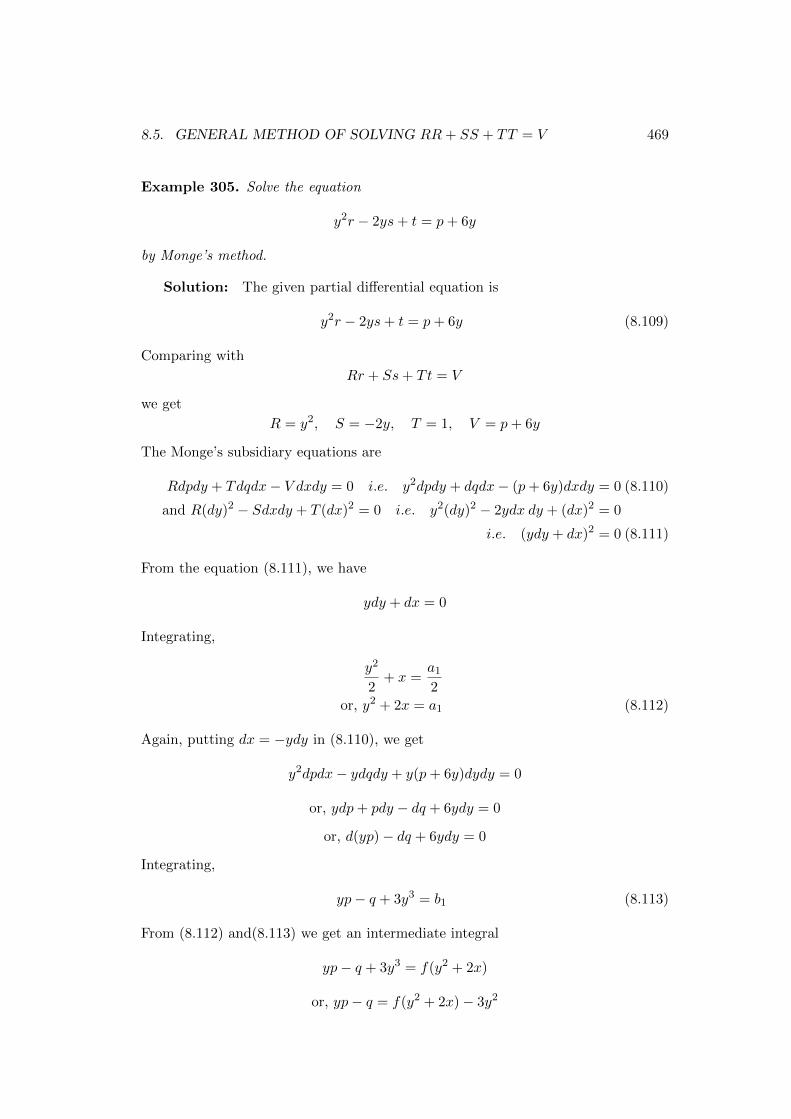
8.5. GENERAL METHOD OF SOLVING RR+ SS + TT = V 469
Example 305. Solve the equation
y2r − 2ys+ t = p+ 6y
by Monge’s method.
Solution: The given partial differential equation is
y2r − 2ys+ t = p+ 6y (8.109)
Comparing with
Rr + Ss+ Tt = V
we get
R = y2, S = −2y, T = 1, V = p+ 6y
The Monge’s subsidiary equations are
Rdpdy + Tdqdx− V dxdy = 0 i.e. y2dpdy + dqdx− (p+ 6y)dxdy = 0 (8.110)
and R(dy)2 − Sdxdy + T (dx)2 = 0 i.e. y2(dy)2 − 2ydx dy + (dx)2 = 0
i.e. (ydy + dx)2 = 0 (8.111)
From the equation (8.111), we have
ydy + dx = 0
Integrating,
y2
2+ x =
a1
2or, y2 + 2x = a1 (8.112)
Again, putting dx = −ydy in (8.110), we get
y2dpdx− ydqdy + y(p+ 6y)dydy = 0
or, ydp+ pdy − dq + 6ydy = 0
or, d(yp)− dq + 6ydy = 0
Integrating,
yp− q + 3y3 = b1 (8.113)
From (8.112) and(8.113) we get an intermediate integral
yp− q + 3y3 = f(y2 + 2x)
or, yp− q = f(y2 + 2x)− 3y2

470CHAPTER 8. PARTIAL DIFFERENTIAL EQUATIONS OF SECONDORDER
where f is arbitrary function. This is first order linear partial differential equationof
the form Pp+Qq = R. The Lagrange’s auxiliary equations are
dx
y=dy
−1=
dz
f(y2 + 2x)− 3y2
From first and second ratios, we get
ydy + dx = 0
Integrating,
y2
2+ x =
a2
2or, y2 + 2x = a2 (8.114)
Again from second and third ratios
or, [f(a2)− 3y2]dy + dz = 0
Integrating,
yf(a3)− y3 + z = b2
or, yf(y2 + 2x)− y3 + z = b2 (8.115)
From (8.114) and (8.115) we get the general solution
b2 = g(a2)
or, yf(y2 + 2x)− y3 + z = g(y2 + 2x)
Example 306. Solve the equation
z(qs− pt) = pq2 [T.U. 2068, 2070, 2074]
by Monge’s method.
Solution: The given partial differential equation is
z(qs− pt) = pq2 (8.116)
Comparing with
Rr + Ss+ Tt = V
we get
R = 0, S = zq, T = −zp, V = pq2
The Monge’s subsidiary equations are
Rdpdy + Tdqdx− V dxdy = 0 i.e. − zpdpdx− pq2dxdy = 0 (8.117)
and R(dy)2 − Sdxdy + T (dx)2 = 0 i.e. − zqdxdy − zp(dx)2 = 0 (8.118)

8.5. GENERAL METHOD OF SOLVING RR+ SS + TT = V 471
From the equation (8.117)
−pdx(zdq + q2dy) = 0
or, zdq + q2dy = 0 (8.119)
Again, from (8.118)
−zdx(qdy + pdx) = 0
or, pdx+ qdy = 0
or, dz = 0 as dz = pdx+ qdy
Integrating,
z = a1 (8.120)
Putting the value of z in (8.119)
a1dq + q2dy = 0
or,dq
q2+ dy = 0
Integrating,
−a1
q+ y = b1
−zq
+ y = b1 (8.121)
From the equations (8.120) and (8.121), we get the intermediate integral
−zq
+ y = F (z)
or,− z ∂y∂z
+ y = F (z)
or,∂y
∂z− y
z= −F (z)
z
or,∂y
∂z− y
z= G(z) (8.122)
where
G(z) = −F (z)
z
The equation (8.122) is linear partial differential equation in y and z. Its integrating
factor is
I.F. = e∫pdx = e−
∫dzz = e− loge z = eloge(z
−1) =1
z

472CHAPTER 8. PARTIAL DIFFERENTIAL EQUATIONS OF SECONDORDER
Multiplying the equation (8.122) by I.F.
1
z
∂y
∂z− y
z2=G(z)
z
or,∂
∂z
(yz
)=G(z)
z
Integrating,
y
z=
∫G(z)
zdz + f(x, y)
or, y = z[g(z) + f(x, y)]
where
g(z) =
∫G(z)
zdz
and which is the general solution.
Example 307. Solve the equation
pq = x(ps− qr)
by Monge’s method.
Solution: The given partial differential equation is
pq = x(ps− qr)or, − xqr + xps = pq (8.123)
Comparing with
Rr + Ss+ Tt = V
we get
R = −xq, S = xp, T = 0, V = pq
The Monge’s subsidiary equations are
Rdpdy + Tdqdx− V dxdy = 0 i.e. − xqdpdx− pqdxdy = 0 (8.124)
and R(dy)2 − Sdxdy + T (dx)2 = 0 i.e. − xq(dy)2 − xpdxdy = 0 (8.125)
From the equation (8.124)
qdy(xdp+ pdx) = 0
or,d(xp) = 0
Integrating,
xp = a1 (8.126)

8.5. GENERAL METHOD OF SOLVING RR+ SS + TT = V 473
Again, from (8.125)
xdy(qdy + pdx) = 0
or, pdx+ qdy = 0
or, dz = 0 as dz = pdx+ qdy
Integrating,
z = a1 (8.127)
From the equations (8.126) and (8.127), we get the intermediate integral
xp = f(z)
or, x∂z
∂y= F (z)
or,1
f(z)
∂z
∂x=
1
x
Integrating, ∫1
f(z)dz = loge x+ F (y)
or, G(z) = loge x+ F (y)
where
g(z) =
∫1
f(z)dz
and which is the general solution.
8.5.1 Monge’s Method for Rr + Ss+ Tt+ U(rt− s2) = V
Theorem 33. Solve the second order partial differential equation Rr + Ss + Tt +
U(rt = s2) = V , where R,S, T, U and V are functions of x, y, z, p, q by Monge’s
method.
Solution: The given partial differential equation is
Rr + Ss+ Tt+ U(rt− s2) = V (8.128)
where R,S, T, U and V are functions of x, y, z, p, q. We have
dp =∂p
∂xdx+
∂p
∂ydy = rdx+ sdy
∴ r =dp− sdy
dx
dq =∂q
∂xdx+
∂q
∂ydy = sdx+ tdy
∴ t =dq − sdx
dy

474CHAPTER 8. PARTIAL DIFFERENTIAL EQUATIONS OF SECONDORDER
Substituting the values of r and t in (8.128)
Rdp− sdy
dx+ Ss+ T
dq − sdxdy
+ U
(dp− sdy
dx
dq − sdxdy
− s2
)= V
or,(Rdpdy + Tdqdx+ Udpdq − V dxdy)
−s(R(dy)2 − Sdxdy + T (dx)2 + Udpdx+ Udqdy
)= 0 (8.129)
The equations obtained by equating the expression with in brackets to zero, are
called Monge’s subsidiary equations. Hence, the Monge’s subsidiary equations
are
M = Rdpdy + Tdqdx− V dxdy + Udpdq − V dxdy = 0 (8.130)
N = R(dy)2 − Sdxdy + T (dx)2 + Udpdx+ Udqdy = 0 (8.131)
The equation (8.131) can not be factorized on account of the term Udpdx+ Udqdy
present it, so let us try to factorize N + λM , where λ is some multiplier to be
determine latter. Now
N + λM =(R(dy)2 − Sdxdy + T (dx)2 + Udpdx+ Udqdy
)+λ(Rdpdy + Tdqdx+ Udpdq − V dxdy) = 0
= R(dy)2 + T (dx)2 − (S + λV )dxdy + Udpdx+ Udqdy +
+λRdpdy + λTdqdx+ λUdpdq (8.132)
Also let the factor of N + λM be
αdy + βdx+ γdp and α′dy + β′dx+ γ′dq
so that
N + λM = (αdy + βdx+ γdp)(α′dy + β′dx+ γ′dq) (8.133)
Equating the coefficients of (dy)2, (dy)2, dpdq in (8.132) and (8.133)
αα′ = R, ββ′ = T, γγ′ = λU
Now if we take
α′ = 1, β′ =1
k, γ′ =
λ
m
then
α = R β = kT, γ = mU
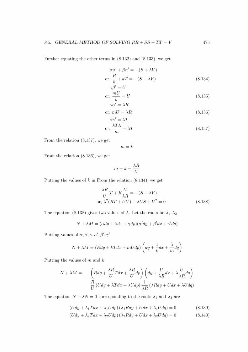
8.5. GENERAL METHOD OF SOLVING RR+ SS + TT = V 475
Further equating the other terms in (8.132) and (8.133), we get
αβ′ + βα′ = −(S + λV )
or,R
k+ kT = −(S + λV ) (8.134)
γβ′ = U
or,mU
k= U (8.135)
γα′ = λR
or, mU = λR (8.136)
βγ′ = λT
or,kTλ
m= λT (8.137)
From the relation (8.137), we get
m = k
From the relation (8.136), we get
m = k =λR
U
Putting the values of k in From the relation (8.134), we get
λR
UT +R
U
λR= −(S + λV )
or, λ2(RT + UV ) + λUS + U2 = 0 (8.138)
The equation (8.138) gives two values of λ. Let the roots be λ1, λ2
N + λM = (αdy + βdx+ γdp)(α′dy + β′dx+ γ′dq)
Putting values of α, β, γ, α′, β′, γ′
N + λM = (Rdy + kTdx+mUdp)
(dy +
1
kdx+
λ
mdq
)Putting the values of m and k
N + λM =
(Rdy +
λR
UTdx+
λR
Udp
)(dy +
U
λRdx+ λ
U
λRdq
)R
U(Udy + λTdx+ λUdp)
1
λR(λRdy + Udx+ λUdq)
The equation N + λN = 0 corresponding to the roots λ1 and λ2 are
(Udy + λ1Tdx+ λ1Udp) (λ1Rdy + Udx+ λ1Udq) = 0 (8.139)
(Udy + λ2Tdx+ λ2Udp) (λ2Rdy + Udx+ λ2Udq) = 0 (8.140)

476CHAPTER 8. PARTIAL DIFFERENTIAL EQUATIONS OF SECONDORDER
Now one of the factor of (8.139) is combined with one factor of (8.140) we get two
intermediate integrals. From these two intermediate integrals the values of p and q
can be determine then integrating
dz = pdx+ qdy
will give the solution of the given PDE.
Example 308. Solve the equation
r + 4s+ t+ (rt− s2) = 2
Solution : Comaparig the given equation with
Rr + Ss+ Tt+ U(rt = s2) = V
we get
R = 1, S = 4, T = 1, U = 1, V = 2
The equation
λ2(RT + UV ) + λUS + U2 = 0
becomes
3λ2 + 4λ+ 1 = 0
Solving this equation
λ1 = −1, λ2 = −1
3
Now the pair of equations becomes
Udy + λ1Rdy + λ2Udq = 0
Udx+ λ2Rdy + λ2Udq = 0
becomes
dy − dx− dp = 0 or dp+ dx− dy = 0
dx− 1
3dy − 1
3dq = 0 or dq + dy − 3dx = 0
Integrating,
P + x− y = c1, q + y − 3x = c2 (8.141)
Thus we get a intermidiate integral
p+ x− y = f(q + y − 3x) (8.142)
Again we consider the pair of equations becomes
Udx+ λ1Rdy + λ1Udq = 0

8.5. GENERAL METHOD OF SOLVING RR+ SS + TT = V 477
Udy + λ2Tdy + λ2Udq = 0
becomes
dx− dy − dq = 0 or dq + dx− dx = 0
dy − 1
3dx− 1
3dp = 0 or dq + dx− 3dy = 0
Integrating,
q + y − x = c3, p+ x− 3y = c4 (8.143)
Thus we get a intermidiate integral
p+ x− 3y = g(q + y − x) (8.144)
Let
q + y − 3x = α (8.145)
q + y − x = β (8.146)
we get
p+ x− y = f(α) (8.147)
p+ x− 3y = g(β) (8.148)
Solving (8.145) and (8.146) we get
x =1
2(β − α)
Solving (8.147) and (8.148) we get
y =1
2(f(α)− g(β))
=⇒ dx =1
2(dβ − dα) and dy =
1
2(f ′(α) dα− g′(β) dβ)
Also, from (8.147) and (8.146)
p = y − x+ f(α), q = x− y + β
dz = pdx+ qdy
= [y − x+ f(α)]dx+ [x− y + β]dy
= (ydx+ xdy)− xdx− ydy + f(α)dx+ βdy
= d(xy)− xdx− ydy + f(α)1
2(dβ − dα) + β
1
2(f ′(α) dα− g′(β) dβ)
= d(xy)− xdx− ydy +1
2[f(α)dβ + βf ′(α)dα]− 1
2f(α)dα− 1
2βg′(β)dβ
2dz = 2d(xy)− 2xdx− 2ydy + [f(α)dβ + βf ′(α)dα]− f(α)dα− βg′(β)dβ
2dz = 2d(xy)− 2xdx− 2ydy + d(βf(α))− f(α)dα− βg′(β)dβ

478CHAPTER 8. PARTIAL DIFFERENTIAL EQUATIONS OF SECONDORDER
Integrating,
2z = 2xy − x2 − y2 + βf(α)−∫f(α)dα−
∫βg′(β)dβ
Using the integration by part in the last term
2z = 2xy − x2 − y2 + βf(α)−∫f(α)dα−
(β
∫g′(β)dβ −
∫ [dβ
dβ
∫g′(β)dβ
]dβ
)
or, 2z = 2xy − x2 − y2 + βf(α)− βg(β)−∫f(α)dα+
∫g(β)dβ
or, 2z = 2xy − x2 − y2 + β[f(α)− g(β)]−∫f(α)dα+
∫g(β)dβ
Let ∫f(α)dα = φ(α) and
∫g(β)dβ = ψ(β)
Then
f(α) = φ′(α) and g(β) = ψ′(β)
∴ 2z = 2xy − x2 − y2β[φ′(α)− ψ′(β)]− φ(α) + ψ(β)
where
2x = β − α, 2y = φ′(α)− ψ′(β)
This is required solution in parametric form with α, β as parameters and φ, ψ being
arbitrary functions.

Chapter 9
Partial Differential Equations
and Fourier Series
9.1 Boundary Value Problem
9.1.1 Two Points Boundary Balue Problem
A boundary value problem is a differential equation together with a set of additional
constraints, at boundary. A differential equation and suitable boundary conditions
which specifies at two boundaries is forms a two-points boundary value problem.
Example 309.
A typical example is the differential equation
y′′ + p(x)y′ + q(x)y = g(x) (9.1)
with boundary conditions
y(α) = y0, y(β) = y1 (9.2)
A solution to a boundary value problem is a solution to the differential equation
which also satisfies the boundary conditions.
9.1.2 Homogeneous and Non-homogeneous Boundary Value Pro-
belms
Consider a two point boundary value problem
y′′ + p(x)y′ + q(x)y = g(x) (9.3)
with boundary conditions
y(α) = y0, y(β) = y1 (9.4)
479
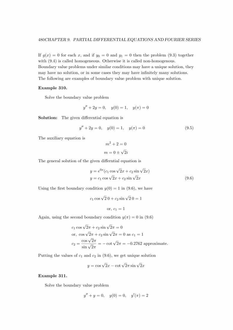
480CHAPTER 9. PARTIAL DIFFERENTIAL EQUATIONS AND FOURIER SERIES
If g(x) = 0 for each x, and if y0 = 0 and y1 = 0 then the problem (9.3) together
with (9.4) is called homogeneous. Otherwise it is called non-homogenous.
Boundary value problems under similar conditions may have a unique solution, they
may have no solution, or in some cases they may have infinitely many solutions.
The following are examples of boundary value problem with unique solution.
Example 310.
Solve the boundary value problem
y′′ + 2y = 0, y(0) = 1, y(π) = 0
Solution: The given differential equation is
y′′ + 2y = 0, y(0) = 1, y(π) = 0 (9.5)
The auxiliary equation is
m2 + 2 = 0
m = 0±√
2i
The general solution of the given differntial equation is
y = e0x(c1 cos√
2x+ c2 sin√
2x)
y = c1 cos√
2x+ c2 sin√
2x (9.6)
Using the first boundary condition y(0) = 1 in (9.6), we have
c1 cos√
2 0 + c2 sin√
2 0 = 1
or, c1 = 1
Again, using the second boundary condition y(π) = 0 in (9.6)
c1 cos√
2π + c2 sin√
2π = 0
or, cos√
2π + c2 sin√
2π = 0 as c1 = 1
c2 =cos√
2π
sin√
2π= − cot
√2π = −0.2762 approximate.
Putting the values of c1 and c2 in (9.6), we get unique solution
y = cos√
2x− cot√
2π sin√
2x
Example 311.
Solve the boundary value problem
y′′ + y = 0, y(0) = 0, y′(π) = 2

9.1. BOUNDARY VALUE PROBLEM 481
Solution: The given differential equation is
y′′ + y = 0, y(0) = 0, y′(π) = 2 (9.7)
The auxiliary equation is
m2 + 1 = 0
m = 0± i
The general solution of the given differntial equation is
y = e0x(c1 cosx+ c2 sinx)
y = c1 cosx+ c2 sinx (9.8)
Using the first boundary condition y(0) = 1 in (9.8), we have
c1 cos 0 + c2 sin 0 = 0
or, c1 = 0
Differentiating the equation (9.7) with respect to x
y′ = −c1 sinx+ c2 cosx
Again, using the second boundary condition y′(π) = 2 in (9.8)
−c1 cosπ + c2 sinπ = 2
or, c1 = −2
Putting the values of c1 and c2 in (9.8), we get unique solution
y = −2 cosx
Example 312.
Solve the boundary value problem
y′′ + 2y = 0, y′(0) = 1, y′(π) = 0
Solution: The given differential equation is
y′′ + 2y = 0, y′(0) = 1, y′(π) = 0 (9.9)
The auxiliary equation is
m2 + 2 = 0
m = 0±√
2i
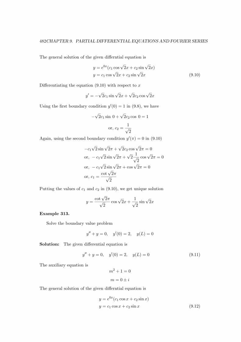
482CHAPTER 9. PARTIAL DIFFERENTIAL EQUATIONS AND FOURIER SERIES
The general solution of the given differntial equation is
y = e0x(c1 cos√
2x+ c2 sin√
2x)
y = c1 cos√
2x+ c2 sin√
2x (9.10)
Differentiating the equation (9.10) with respect to x
y′ = −√
2c1 sin√
2x+√
2c2 cos√
2x
Using the first boundary condition y′(0) = 1 in (9.8), we have
−√
2c1 sin 0 +√
2c2 cos 0 = 1
or, c2 =1√2
Again, using the second boundary condition y′(π) = 0 in (9.10)
−c1
√2 sin
√2π +
√2c2 cos
√2π = 0
or, − c1
√2 sin
√2π +
√2
1√2
cos√
2π = 0
or, − c1
√2 sin
√2π + cos
√2π = 0
or, c1 =cot√
2π√2
Putting the values of c1 and c2 in (9.10), we get unique solution
y =cot√
2π√2
cos√
2x+1√2
sin√
2x
Example 313.
Solve the boundary value problem
y′′ + y = 0, y′(0) = 2, y(L) = 0
Solution: The given differential equation is
y′′ + y = 0, y′(0) = 2, y(L) = 0 (9.11)
The auxiliary equation is
m2 + 1 = 0
m = 0± i
The general solution of the given differntial equation is
y = e0x(c1 cosx+ c2 sinx)
y = c1 cosx+ c2 sinx (9.12)

9.1. BOUNDARY VALUE PROBLEM 483
Differentiating the equation (9.12) with respect to x
y′ = −c1 sinx+ c2 cosx
Using the first boundary condition y′(0) = 2 in (9.12), we have
−c1 sin 0 + c2 cos 0 = 2
or, c2 = 2
Again, using the second boundary condition y(L) = 0 in (9.10)
c1 cosL+ c2 sinL = 0
or, c1 cosL+ 2 sinL = 0
or, c1 = −2 sinL
cosL= −2 tanL
Putting the values of c1 and c2 in (9.10), we get unique solution
y = −2 tanL cosx+ 2 sinx where cosL 6= 0
becaues if cosL = 0, then c1 is not defined and the equation has no solution.
Example 314.
Solve the boundary value problem
y′′ + 2y = x, y(0) = 0, y(π) = 0
Solution: The given differential equation is
y′′ + 2y = x, y(0) = 0, y(π) = 0
or, (D2 + 2)y = x y(0) = 0, y(π) = 0
The auxiliary equation is
m2 + 2 = 0
m = 0±√
2i
The general solution of the given differntial equation is
C.F. = e0x(c1 cos√
2x+ c2 sin√
2x)
y = c1 cos√
2x+ c2 sin√
2x
For particular integral:
P.I. =1
D2 + 2x
=1
2(1 + D2
2 )x
=1
2
(1 +
D2
2
)−1
x
=1
2
(1− D2
2+D4
4− · · ·
)x
=1
2x

484CHAPTER 9. PARTIAL DIFFERENTIAL EQUATIONS AND FOURIER SERIES
Rquired solution is
y = C.F.+ P.I.
y = c1 cos√
2x+ c2 sin√
2x+1
2x (9.13)
Using the first boundary condition y(0) = 0 in (9.13), we have
c1 cos 0 + c2 sin 0 +1
2· 0 = 0
or, c1 = 0
Again, using the second boundary condition y(π) = 0 in (9.13)
c1 cos√
2π + c2 sin√
2π +1
2π = 0
or, c2 sin√
2π +1
2π = 0
or, c2 = − π
2 sin√
2π
Putting the values of c1 and c2 in (9.13), we get unique solution
y = −π sin√
2x
2 sin√
2π+x
2
or, y =−π sin
√2x+ x sin
√2π
2 sin√
2π
Example 315.
Solve the boundary value problem
x2y′′ − 2xy′ + 2y = 0, y(1) = −1, y(2) = 1
Solution: The given differential equation is
x2y′′ − 2xy′ + 2y = 0, y(1) = −1, y(2) = 1
or, x2 d2y
dx2− 2x
dy
dx+ 2y = 0 y(1) = −1, y(2) = 1 (9.14)
Let us put x = ez i.e. z = loge x. Then
dz
dx=
1
x
Nowdy
dx=dy
dz
dz
dx=
1
x
dy
dz
xdy
dx=dy
dz

9.1. BOUNDARY VALUE PROBLEM 485
Again
d2y
dx2=
d
dx
(dy
dx
)or,d2y
dx2=
d
dx
(1
x
dy
dz
)or,d2y
dx2=
d
dx
(x−1
) dydz
+1
x
d
dx
(dy
dz
)or,d2y
dx2= − 1
x2
dy
dz+
1
x
d
dz
(dy
dz
)dz
dx
or,d2y
dx2= − 1
x2
dy
dz+
1
x2
d
dz
(dy
dz
)or, x2 d
2y
dx2= −dy
dz+d2y
dz2
Putting values of x dydx , and x2 d2ydx2
in (9.14), we get
d2y
dz2− dy
dz− 2
dy
dz+ 2y = 0
d2y
dz2− 3
dy
dz+ 2y = 0
The auxiliary equation is
m2 − 3m+ 2 = 0
m = 1, m = 2
The general solution of the given differntial equation is
y. = c1ez + c2e
2z
or, y = c1elog x + c2e
2 loge x
y = c1eloge x + c2e
loge x2
y = c1x+ c2x2 (9.15)
Using the first boundary condition y(1) = −1 in (9.15), we have
c1 + c2 = −1 (9.16)
Again, using the second boundary condition y(2) = 1 in (9.13)
2c1 + 4c2 = 1 (9.17)
Solving (9.16) and (9.17), we get
c1 = −5
2, c2 =
3
2

486CHAPTER 9. PARTIAL DIFFERENTIAL EQUATIONS AND FOURIER SERIES
Putting the values of c1 and c2 in (9.13), we get unique solution
y = −5
2x+
3
2x2
The following example illustrate that a nonhomogeneous boundary problem may
have no solution.
Example 316.
Solve the boundary value problem
y′′ + y = 0, y(0) = 1, y(π) = 3
Solution: The given differential equation is
y′′ + y = 0, y(0) = 1, y(pi) = 3 (9.18)
The auxiliary equation is
m2 + 1 = 0
m = 0± i
The general solution of the given differntial equation is
y = e0x(c1 cosx+ c2 sinx)
y = c1 cosx+ c2 sinx (9.19)
Using the first boundary condition y(0) = 1 in (9.19), we have
c1 cos 0 + c2 sin 0 = 1
or, c1 = 1
Again, using the second boundary condition y(π) = 3 in (9.19)
c1 cosπ + c2 sinπ = 3
or, c1 = −3
Thus, we get different value of c1 by the given two boundary conditions. Hence, the
given differentilal equation has no solution.
The following example shows that a boundary value problem may have trivial solu-
tion.
Example 317.

9.1. BOUNDARY VALUE PROBLEM 487
Solve the boundary value problem
y′′ + 2y = 0, y(0) = 0, y(π) = 0
Solution: The given differential equation is
y′′ + 2y = 0, y(0) = 0, y(π) = 0 (9.20)
The auxiliary equation is
m2 + 2 = 0
m = 0±√
2i
The general solution of the given differntial equation is
y = e0x(c1 cos√
2x+ c2 sin√
2x)
y = c1 cos√
2x+ c2 sin√
2x (9.21)
Using the first boundary condition y(0) = 0 in (9.21), we have
c1 cos 0 + c2 sin 0 = 0
or, c1 = 0
Again, using the second boundary condition y(π) = 0 in (9.10)
c1 cos√
2π + c2 sin√
2π = 0
or, c2 sin√
2π = 0
Since sin√
2π 6= 0, so c2 = 0.
Putting the values of c1 and c2 in (9.21), we get unique solution
y = 0
This solution y = 0 is trivial solution of the given boundary value problem.
The next exmples are of boundary value problem with infinitely many solutions.
Example 318.
Solve the boundary value problem
y′′ + y = 0, y(0) = 0, y(π) = 0
Solution: The given differential equation is
y′′ + y = 0, y(0) = 0, y(π) = 0 (9.22)
The auxiliary equation is
m2 + 1 = 0

488CHAPTER 9. PARTIAL DIFFERENTIAL EQUATIONS AND FOURIER SERIES
m = 0± i
The general solution of the given differntial equation is
y = e0x(c1 cosx+ c2 sinx)
y = c1 cosx+ c2 sinx (9.23)
Using the first boundary condition y(0) = 0 in (9.21), we have
c1 cos 0 + c2 sin 0 = 0
or, c1 = 0
Again, using the second boundary condition y(π) = 0 in (9.10)
c1 cosπ + c2 sinπ = 0
or, c2 sinπ = 0 as c1 = 0
Since sinπ = 0, the second boundary condition is also satisfied when c1 = 0, for all
values of c2. Thus, the solition of the system is
y = c2 sinx where c2 is arbitrary.
Hence, the given boundary value problem has infinitely many solutions.
Example 319.
Solve the boundary value problem
y′′ + 4y = cosx, y′(0) = 0, y′(π) = 0
Solution: The given differential equation is
y′′ + 4y = cosx, y′(0) = 0, y′(π) = 0
(D2 + 4)y = cosx, y′(0) = 0, y′(π) = 0 (9.24)
The auxiliary equation is
m2 + 4 = 0
m = 0± 2i
The completementrary function of
C.F. = e0x(c1 cos 2x+ c2 sin 2x)
C.F. = c1 cos 2x+ c2 sin 2x (9.25)
Particular integral is
P.I. =1
D2 + 4cosx
=1
−12 + 4cosx =
cosx
3

9.1. BOUNDARY VALUE PROBLEM 489
Hence, the general solution is
y = C.F.+ P.I.
or, y = c1 cos 2x+ c2 sin 2x+cosx
3(9.26)
Differentiating with respect to x
y′(x) = −2c1 sin 2x+ 2c2 cos 2x− sinx
3
Using the first boundary condition y′(0) = 0 we have
−2c1 sin 0 + 2c2 cos 0− 2
3sin 0 = 0
or, c2 = 0
Again, using the second boundary condition y′(π) = 0, we get
−2c1 sin 2π + c2 cos 2π − 2
3sin 2π = 0
or, c2 = 0
Both boundary conditions are also satisfied when for all values of c1. Thus, the
solution of the system is
y = c1 cos 2x+cosx
3where c2 is arbitrary.
Hence, the given boundary value problem has infinitely many solutions.
9.1.3 Eigenvalue Problems
Let A be a square matrix. Let us consider a matrix equation
Ax = λx (9.27)
The equation (9.27) has the solution x = 0 for every value of λ. But for certain values
of λ, there are non zero solutions, in this case the value of λ is called eigenvalues
and the nonzero solutions x are called eigen vectors. There is similar conditions for
the boundary value problems.
Consider the problem of differential equation
y′′ + λy = 0, y(0) = 0, y(π) = 0 (9.28)
The problem has only trivail solution y = 0, when λ = 1. We extend the terminolgy
associated with the equation (9.27), to the differential equation (9.28).
The values of λ for which nontrivial solutions of (9.28) occurs are called eigenvalues,
and the nontrivial solutions themselves are called eigenfunctions of the equation.
490CHAPTER 9. PARTIAL DIFFERENTIAL EQUATIONS AND FOURIER SERIES
Example 320. Find the eigenvalue and eigenfunction for the differential equation
y” + λy = 0, y(0) = 0, y(π) = 0
Solution: The given differential equation is
y” + λy = 0 y(0) = 0, y(π) = 0 (9.29)
The auxiliary equation of the given differentail equation is (9.29) is
m2 + λ = 0
or, m2 = −λ
Case I If λ = 0, then m2 = 0 which implies m = 0, 0. The general solution of
(9.29)
y = e0x(c1 + c2x)
y = c1 + c2x (9.30)
Using the boundary condition
y(0) = 0 =⇒ c1 = 0
and
y(π) = 0 =⇒ c1 + c2π = 0
c2π = 0
c2 = 0
Hence, the solution (9.30) becomes
y = 0
Which is trivial solution.
Case II If λ < 0 then −λ > 0.
m2 = −λm = ±
√−λ
The general solution of (9.29) is
y = c1e√−λx + c2e
−√−λx (9.31)
Using the boundary condition
y(0) = 0 =⇒ c1 + c2 = 0 (9.32)
9.1. BOUNDARY VALUE PROBLEM 491
and
y(π) = 0 =⇒ c1e√−λ π + c2e
−√−λ π = 0 (9.33)
Solving (9.32) and (9.33), we get
c1 = 0, c2 = 0
Putting the values of c1 and c2 in (9.31)
y = 0
which is trivial solution.
Case III If λ > 0, then −λ < 0
∴ m = 0± i√λ
The general solution of (9.29) is
y = e0x(c1 cos√λ x+ c2 sin
√λ x)
or, y = c1 cos√λ x+ c2 sin
√λ x (9.34)
Using the buondary conditions
y(0) = 0 =⇒ c1 cos 0 + c2 sin 0 = 0
c1 = 0
and
y(π) = 0 =⇒ c1 cos√λπ + c2 sin
√λπ = 0
or, c2 sin√λπ = 0 as c1 = 0
For c2 6= 0, we must have
sin√λx = 0
∴√λπ = nπ
or,√λ = n
or, λ = n2
Thus, λ1 = 12, λ2 = 22, λ3 = 32, · · · are eigenvalues of the given differential equation
and the corresponding non-trivial solutions are
y1(x) = sinx, y2(x) = sin 2x, y3(x) = sin 3x, y4(x) = sin 4x, · · · , yn = sinnx, · · ·
are eigenfunctions of the given differential equation.
492CHAPTER 9. PARTIAL DIFFERENTIAL EQUATIONS AND FOURIER SERIES
Example 321. Find the eigenvalues and eigenfunctions for the boundary value
problem
y” + λy = 0, y(0) = 0, y(L) = 0
Solution: The given differential equation is
y” + λy = 0 y(0) = 0, y(L) = 0 (9.35)
The auxiliary equation of the given differentail equation is (9.35) is
m2 + λ = 0
or, m2 = −λ
Case I If λ = 0, then m2 = 0 which implies m = 0, 0. The general solution of (9.35)
y = e0x(c1 + c2x)
y = c1 + c2x (9.36)
Using the boundary condition
y(0) = 0 =⇒ c1 = 0
and
y(π) = 0 =⇒ c1 + c2L = 0
c2L = 0
c2 = 0
Hence, the solution (9.35) becomes
y = 0
Which is trivial solution.
Case II If λ < 0 then −λ > 0.
m2 = −λm = ±
√−λ
The general solution of (9.35) is
y = c1e√−λx + c2e
−√−λx (9.37)
Using the boundary condition
y(0) = 0 =⇒ c1 + c2 = 0 (9.38)

9.1. BOUNDARY VALUE PROBLEM 493
and
y(L) = 0 =⇒ c1e√−λ L + c2e
−√−λ L = 0 (9.39)
Solving (9.38) and (9.39), we get
c1 = 0, c2 = 0
Putting the values of c1 and c2 in (9.37)
y = 0
which is trivial solution.
Case III If λ > 0, then −λ < 0
∴ m = 0± i√λ
Then the general solution of (9.29) is
y = e0x(c1 cos√λ x+ c2 sin
√λ x)
or, y = c1 cos√λ x+ c2 sin
√λ x (9.40)
Using the buondary condition
y(0) = 0 =⇒ c1 cos 0 + c2 sin 0 = 0
c1 = 0
and
y(L) = 0 =⇒ c1 cos√λL+ c2 sin
√λL = 0
or, c2 sin√λL = 0 as c1 = 0
For c2 6= 0, we must have
sin√λL = 0
∴√λL = nπ
or,√λ =
nπ
L
or, λ =n2π2
L2
Thus, λn = n2π2
L2 n = 1, 2, 3 · · · are eigenvalues of the given differential equation
and the corresponding non-trivial solutions are
yn(x) = sinnπ
Lx n = 1, 2, 3 · · ·
are eigenfunctions of the given differential equation.

494CHAPTER 9. PARTIAL DIFFERENTIAL EQUATIONS AND FOURIER SERIES
Example 322. Find the eigenvalues and eigenfunctions for the differential equation
y” + λy = 0, y(0) = 0, y′(π) = 0
Solution: The given differentialequation is
y” + λy = 0 y(0) = 0, y′(π) = 0 (9.41)
The auxiliary equation of the given differentail equation is (9.41) is
m2 + λ = 0
or, m2 = −λ
Case I If λ = 0, then m2 = 0 which implies m = 0, 0. The general solution of (9.41)
y = e0x(c1 + c2x)
y = c1 + c2x (9.42)
and y′ = c2
Using the boundary condition
y(0) = 0 =⇒ c1 = 0
and
y′(π) = 0 =⇒ c2 = 0
(9.43)
Hence, the solution (9.42) becomes
y = 0
Which is trivial solution.
Case II If λ < 0 then −λ > 0.
m2 = −λm = ±
√−λ
The general solution of (9.41) is
y = c1e√−λx + c2e
−√−λx (9.44)
y′ =√−λ(c1e
√−λx − c2e
−√−λx) (9.45)
Using the boundary condition
y(0) = 0 =⇒ c1 + c2 = 0 (9.46)

9.1. BOUNDARY VALUE PROBLEM 495
and
y′(π) = 0 =⇒ c1e√−λ π − c2e
−√−λ π = 0 (9.47)
Solving (9.46) and (9.47), we get
c1 = 0, c2 = 0
Putting the values of c1 and c2 in (9.44)
y = 0
which is trivial solution.
Case III If λ > 0, then −λ < 0
∴ m = 0± i√λ
Then the general solution of (9.29) is
y = e0x(c1 cos√λ x+ c2 sin
√λ x)
or, y = c1 cos√λ x+ c2 sin
√λ x (9.48)
or, y′ =√λ(−c1 sin
√λ x+ c2 cos
√λ x) (9.49)
Using the boundary conditions
y(0) = 0 =⇒ −c1 cos 0 + c2 sin 0 = 0
c1 = 0
and
y′(π) = 0 =⇒√λ(−c1 sin
√λπ + c2 cos
√λπ) = 0
or, c2 cos√λπ = 0 as c1 = 0
For c2 6= 0, we must have
cos√λπ = 0
∴√λπ =
(2n− 1)π
2
or,√λ = n− 1
2
or, λ =
(n− 1
2
)2
Thus, λn =(n− 1
2
)2n = 1, 2, 3 · · · are eigenvalues of the given boundary value
problem and the corresponding non-trivial solutions are
yn(x) = sin
(n− 1
2
)x n = 1, 2, 3 · · ·
are eigenfunctions of the given boundary value problem.

496CHAPTER 9. PARTIAL DIFFERENTIAL EQUATIONS AND FOURIER SERIES
Example 323. Find the eigenvalues and eigenfunctions for the differential equation
y” + λy = 0, y′(0) = 0, y(π) = 0.
Solution: The given differential equation is
y” + λy = 0 y′(0) = 0, y(π) = 0 (9.50)
The auxiliary equation of the given differentail equation is (9.50) is
m2 + λ = 0
or, m2 = −λ
Case I If λ = 0, then m2 = 0 which implies m = 0, 0. The general solution of (9.50)
y = e0x(c1 + c2x)
y = c1 + c2x (9.51)
and y′ = c2
Using the boundary condition
y′(0) = 0 =⇒ c2 = 0
and
y(π) = 0 =⇒ c1 + c2π = 0
=⇒ c1 = 0
Hence, the solution (9.50) becomes
y = 0
Which is trivial solution.
Case II If λ < 0 then −λ > 0.
m2 = −λm = ±
√−λ
The general solution of (9.50) is
y = c1e√−λx + c2e
−√−λx (9.52)
y′ =√−λ(c1e
√−λx − c2e
−√−λx)
Using the boundary condition
y′(0) = 0 =⇒ c1 − c2 = 0 (9.53)

9.1. BOUNDARY VALUE PROBLEM 497
and
y(π) = 0 =⇒ c1e√−λ π + c2e
−√−λ π = 0 (9.54)
Solving (9.53) and (9.54), we get
c1 = 0, c2 = 0
Putting the values of c1 and c2 in (9.52)
y = 0
which is trivial solution.
Case III If λ > 0, then −λ < 0
∴ m = 0± i√λ
Then the general solution of (9.50) is
y = e0x(c1 cos√λ x+ c2 sin
√λ x)
or, y = c1 cos√λ x+ c2 sin
√λ x (9.55)
or, y′ =√λ(−c1 sin
√λ x+ c2 cos
√λ x) (9.56)
Using the boundary condition
y′(0) = 0 =⇒ −c1 sin 0 + c2 cos 0 = 0
c2 = 0
and
y(π) = 0 =⇒ (c1 cos√λπ + c2 sin
√λπ) = 0
or, c1 cos√λπ = 0 as c2 = 0
For c1 6= 0, we must have
cos√λπ = 0
∴√λπ =
(2n− 1)π
2
or,√λ = n− 1
2
or, λ =
(n− 1
2
)2
Thus, λn =(n− 1
2
)2n = 1, 2, 3 · · · are eigenvalues of the given boundary value
problem and the corresponding non-trivial solutions are
yn(x) = cos
(n− 1
2
)x n = 1, 2, 3 · · ·
are eigenfunctions of the given boundary value problem.

498CHAPTER 9. PARTIAL DIFFERENTIAL EQUATIONS AND FOURIER SERIES
Example 324. Find the eigenvalues and eigenfunctions for the differential equation
y” + λy = 0, y′(0) = 0, y′(L) = 0
Solution: The given differential equation is
y” + λy = 0 y′(0) = 0, y′(π) = 0 (9.57)
The auxiliary equation of the given differentail equation is (9.57) is
m2 + λ = 0
or, m2 = −λ
Case I If λ = 0, then m2 = 0 which implies m = 0, 0 The general solution of (9.57)
y = e0x(c1 + c2x)
y = c1 + c2x (9.58)
and y′ = c2
Using the boundary condition
y′(0) = 0 =⇒ c2 = 0
and
y′(π) = 0 =⇒ c2 = 0
Hence, the solution (9.57) becomes
y = c1
Hence λ0 = 0 is eigenvalue with corresponding eigenfunction y0 = 1.
Case II If λ < 0 then −λ > 0.
m2 = −λm = ±
√−λ
The general solution of (9.57) is
y = c1e√−λx + c2e
−√−λx (9.59)
y′ =√−λ(c1e
√−λx − c2e
−√−λx)
Using the boundary conditions
y′(0) = 0 =⇒ c1 − c2 = 0 (9.60)
and
y′(L) = 0 =⇒ c1e√−λ L − c2e
−√−λ L = 0 (9.61)

9.1. BOUNDARY VALUE PROBLEM 499
Solving (9.60) and (9.61), we get
c1 = 0, c2 = 0
Putting the values of c1 and c2 in (9.59)
y = 0
which is trivial solution.
Case III If λ > 0, then −λ < 0
∴ m = 0± i√λ
Then the general solution of (9.29) is
y = e0x(c1 cos√λ x+ c2 sin
√λ x)
or, y = c1 cos√λ x+ c2 sin
√λ x (9.62)
or, y′ =√λ(−c1 sin
√λ x+ c2 cos
√λ x) (9.63)
Using the buondary condition
y′(0) = 0 =⇒ −c1 sin 0 + c2 cos 0 = 0
c2 = 0
and
y′(L) = 0 =⇒ (−c1 sin√λL+ c2 cos
√λL) = 0
or, c1 sin√λL = 0 as c2 = 0
For c1 6= 0, we must have
sin√λL = 0
∴√λL = nπ
or,√λ =
nπ
L
or, λ =n2π2
L2
Thus, λn = n2π2
L2 n = 1, 2, 3 · · · are eigenvalues of the given differential equation
and the corresponding non-trivial solutions are
yn(x) = cosn2π2
L2x n = 1, 2, 3 · · ·
are eigenfunctions of the given differential equation.
500CHAPTER 9. PARTIAL DIFFERENTIAL EQUATIONS AND FOURIER SERIES
9.2 Fourier series
9.2.1 Periodic Functions
A function f(x) is said to be periodic with period T > 0 if the domain of f contains
x+ T whenever it contains x, if
f(x+ T ) = f(x) (9.64)
for every value of x.
The graph of such periodic function is obatained by periodic repeatition of its graph
in any interval of length T .
From (9.64) it follow that, if n is any integer, then
f(x+ nT ) = f(x) for all x
Hence 2T, 3T, 4T, · · · are periods of f(x). The smallest value of T for which (9.64)
holds is called the fundamental period of f .
A constant function is a periodic function with an arbitrary period but no funda-
mental period.
Theorem 34. If f and g are any two functions with common period T , then
(i)fg
(ii) for any c1 and c2, c1f + c2g are periodic functions with period T .
Proof: Here f and g are periodic function with period T . Therefore,
f(x+ T ) = f(x), g(x+ T ) = g(x) for all x
(fg)(x+ T ) = f(x+ T )g(x+ T ) = f(x)g(x)
Hence fg is periodic function with period T .
(c1f + c2g)(x+ T ) = c1f(x+ T ) + c2g(x+ T ) = c1f(x) + c2g(x)
Thus, c1 f + c2 g is periodic function with period T .
Examples:
1. Each of the function sinx, cosx, secx, cscx is a periodic function with period
2π.
2. tanx, cotx are periodic function with period π.
3. sinnx, cosnx both are periodic functions with period 2πn .
Proof:
sinn
(x+
2π
n
)= sin (nx+ 2π) = sinnx for all x,
cosn
(x+
2π
n
)= cos (nx+ 2π) = cosnx for all x.

9.2. FOURIER SERIES 501
4. sin πxl , cos πxl are periodic functions with period 2l.
Proof:
sinπ
l(x+ 2l) = sin
(πxl
+ 2π)
= sinπx
l
cosπ
l(x+ 2l) = cos
(πxl
+ 2π)
= cosπx
l
5. The sum of a number of periodic functions is a periodic functions.
∞∑n=1
an cosnx,∞∑n=1
bn sinnx,∞∑n=1
(an cosnx+ bn sinnx)
all are periodic functions with period 2π.
Example 325. Determine whether the given function f(x) = sin πxL is periodic or
not. If periodic find fundamental period.
Solution: Here f(x) = sin πxL . Let T be the period of f(x). Then
f(x+ T ) = f(x)
or, sinπ(x+ T )
L= sin
πx
L
or, sin
(πx
L+πT
L
)= sin 7x
or, sinπx
Lcos
πT
L+ cos
πx
Lsin
πT
L= sin
πx
L+ 0 · cos
πx
L
Comparing coefficients
cosπT
L= 1, sin
πT
L= 0
or, cosπT
L= cos 2π, sin
πT
L= sin 2π least positive
∴πT
L= 2π
or, T =2L
T
Example 326. Determine whether the given function f(x) = sin 7x is periodic or
not. If periodic find fundamental period.
Solution: Here f(x) = sin 7x. Let T be the period of f(x). Then
f(x+ T ) = f(x)
or, sin 7(x+ T ) = sin 7x
or, sin(7x+ 7T ) = sin 7x
or, sin 7x cos 7T + cos 7x sin 7T = sin 7x+ 0 cos 7x

502CHAPTER 9. PARTIAL DIFFERENTIAL EQUATIONS AND FOURIER SERIES
Comparing coefficients
cos 7T = 1, sin 7T = 0
or, cos 7T = cos 2π, sin 7T = sin 2π least positive
∴ 7T = 2π
or, T =2π
7
9.2.2 Orthogonality of sine and cosine Functions
The inner product of two real valued functions u, v is denoted by (u, v) and is defined
on the interval a ≤ x ≤ b, is given by
(u, v) =
∫ b
au(x)v(x)dx
The function u and v are said to be mutually orthogonal on a ≤ x ≤ b if their inner
product is zero that is if
(u, v) = 0
or,
∫ b
au(x)v(x)dx = 0 (9.65)
Example 327. The function u(x) = x, v(x) = x4 are orthogonal on the interval
−1 ≤ x ≤ 1.
Solution: Here
(u, v) =
∫ 1
−1u(x)v(x)dx
=
∫ 1
−1xx4dx
=
∫ 1
−1x5dx
=
[x6
6
]1
−1
=1
6− 1
6= 0
A set of functions is said to be mutually orthogonal if each pair of functions in the
set are orthogonal. Let u1, u2, · · · be a set of real valued functions defined on
a ≤ x ≤ b are said to be orthogonal if
For m 6= n, (un, um) = 0
i.e.
∫ b
aunumdx = 0 (9.66)

9.2. FOURIER SERIES 503
Example 328. The functions
sinmπx
L, cos
mπx
L, m = 1, 2, 3 · · ·
form a mutually orthogonal set of functions on the interval −L ≤ x ≤ L. In fact,
they satisfy the following relations
∫ L
−Lsin
mπx
Lsin
nπx
Ldx =
0 m 6= n
L m = n(9.67)
∫ L
−Lcos
mπx
Lcos
nπx
Ldx =
0 m 6= n
L m = n(9.68)∫ L
−Lsin
mπx
Lcos
nπx
Ldx = 0 for all m,n (9.69)
Proof: To derive the Eq.(9.67), for m 6= n,
∫ L
−Lsin
mπx
Lsin
nπx
Ldx =
1
2
∫ L
−L2 sin
mπx
Lsin
nπx
Ldx
=1
2
∫ L
−L
[cos
(m− n)πx
L− cos
(m+ n)πx
L
]dx
=1
2
[sin (m−n)πx
L(m−n)π
L
−sin (m+n)πx
L(m+n)π
L
]L−L
=L
2π
[sin (m−n)πL
L
(m− n)−
sin (m+n)πLL
(m+ n)
]
− L
2π
[sin (m−n)π(−L)
L
m− n−
sin (m+n)π(−L)L
m+ n
]
=L
2π
[sin(m− n)π
(m− n)− sin(m+ n)π
(m+ n)
]− L
2π
[−sin(m− n)π
(m− n)+
sin(m+ n)π
(m+ n)
]= 0 as sin(m− n)π = 0, sin(m+ n)π = 0

504CHAPTER 9. PARTIAL DIFFERENTIAL EQUATIONS AND FOURIER SERIES
For m = n∫ L
−Lsin
mπx
Lsin
nπx
Ldx =
∫ L
−Lsin2 mπx
Ldx
=1
2
∫ L
−L2 sin2 mπx
Ldx
=1
2
∫ L
−L
[1− cos
2mπx
L
]dx
=1
2
[x−
sin 2mπxL
2mπL
]L−L
=1
2
[L−
sin 2mπLL
2mπL
−
(−L−
sin 2mπ(−L)L
2mπL
)]
=1
2
[2L− sin 2mπ
2mπL
+sin 2mπ
2mπL
]=
1
2[2L− 0− 0] = L
Hence
∫ L
−Lsin
mπx
Lsin
nπx
Ldx =
0 m 6= n
L m = n
To derive the Eq.(9.68), for m 6= n,
∫ L
−Lcos
mπx
Lcos
nπx
Ldx =
1
2
∫ L
−L2 cos
mπx
Lcos
nπx
Ldx
=1
2
∫ L
−L
[cos
(m− n)πx
L+ cos
(m+ n)πx
L
]dx
=1
2
[sin (m−n)πx
L(m−n)π
L
+sin (m+n)πx
L(m+n)π
L
]L−L
=L
2π
[sin (m−n)πL
L
(m− n)+
sin (m+n)πLL
(m+ n)
]
− L
2π
[sin (m−n)π(−L)
L
(m− n)+
sin (m+n)π(−L)L
(m+ n)
]
=L
2π
[sin(m− n)π
(m− n)+
sin(m+ n)π
(m+ n)
]− L
2π
[−sin(m− n)π
(m− n)− sin(m+ n)π
(m+ n)
]= 0 as sin(m− n)π = 0, sin(m+ n)π = 0

9.2. FOURIER SERIES 505
For m = n∫ L
−Lcos
mπx
Lcos
nπx
Ldx =
∫ L
−Lcos2 mπx
Ldx
=1
2
∫ L
−L2 cos2 mπx
Ldx
=1
2
∫ L
−L
[1 + cos
2mπx
L
]dx
=1
2
[x+
sin 2mπxL
2mπL
]L−L
=1
2
[L+
sin 2mπLL
2mπL
−
(−L+
sin 2mπ(−L)L
2mπL
)]
=1
2
[2L− sin 2mπ
2mπL
+sin 2mπ
2mπL
]=
1
2[2L− 0− 0] = L
Hence ∫ L
−Lcos
mπx
Lcos
nπx
Ldx =
0 m 6= n
L m = n
To derive the Eq.(9.69), let
f(x) = sinmπx
Lcos
nπx
L
Then
f(−x) = sinmπ(−x)
Lcos
nπ(−x)
L= − sin
mπx
Lcos
nπx
L= −f(x)
Thus, f(x) is odd functions∫ L
−Lf(x)dx = 0
or,
∫ L
−Lsin
mπx
Lcos
nπx
Ldx = 0 for all m,n
Note We have ∫ L
−Lsin
mπx
Lsin
nπx
Ldx =
0 m 6= n
L m = n(9.70)
∫ L
−Lcos
mπx
Lcos
nπx
Ldx =
0 m 6= n
L m = n(9.71)

506CHAPTER 9. PARTIAL DIFFERENTIAL EQUATIONS AND FOURIER SERIES
Since
f(x) = sinnπx
Lsin
mπx
Land f(x) = cos
nπx
Lcos
mπx
L
are even functions so∫ L
−Lsin
mπx
Lsin
nπx
Ldx = 2
∫ L
0sin
mπx
Lsin
nπx
Ldx
∫ L
−Lcos
mπx
Lcos
nπx
Ldx = 2
∫ L
0cos
mπx
Lcos
nπx
Ldx
Hence, the equations (9.70) and (9.71) becomes
∫ L
0sin
mπx
Lsin
nπx
Ldx =
0 m 6= nL2 m = n∫ L
0cos
mπx
Lcos
nπx
Ldx =
0 m 6= nL2 m = n
9.2.3 Trigonometric Series
A series of the form
a0
2+
∞∑n=1
(an cosnx+ bn sinnx)
is said to be a trigonometric series, where a0, an, bn are constants.
Note
1. When an = 0, the series will be pure sine series.
2. When bn = 0, the series will be pure cosine series.
3. Sum of sines of n angles in A.P.
sinα+ sin(α+ β) + sin(α+ 2β) + · · ·+ sin(α+ (n− 1)β)
=sinn.diff.
2
sin diff.2
sinfirst angle+last angle
2
=sin nβ
2
sin β2
sinα+ α+ (n− 1)β
2
=sin nβ
2
sin β2
sin
(α+
(n− 1)β
2
)
4. Sum of cosines of n angles in A.P.
9.2. FOURIER SERIES 507
cosα+ cos(α+ β) + cos(α+ 2β) + · · ·+ cos(α+ (n− 1)β)
=sinn.diff.
2
sin diff.2
cosfirst angle+last angle
2
=sin nβ
2
sin β2
cosα+ α+ (n− 1)β
2
=sin nβ
2
sin β2
cos
(α+
(n− 1)β
2
)
9.2.4 Fourier Series
If the trigonometric series
a0
2+
∞∑m=1
(am cos
mπx
L+ bm sin
mπx
L
)
converge to a function f(x), at each value of x then the trigonometric series is called
Fourier series of f . The constant terms a0, am, an are called Fourier coefficients.
9.2.5 Determination of Fourier Coefficients
Let us suppose the series of the form
a0
2+
∞∑m=1
(am cos
mπx
L+ bm sin
mπx
L
)
converges and let its sum be f(x) in −L ≤ x ≤ L. Then
f(x) =a0
2+
∞∑m=1
(am cos
mπx
L+ bm sin
mπx
L
)(9.72)

508CHAPTER 9. PARTIAL DIFFERENTIAL EQUATIONS AND FOURIER SERIES
The coefficients a0, am, bm can be related to f(x). Integrating, the Eq.(9.72) with
respect to x from −L to L.∫ L
−Lf(x)dx =
a0
2
∫ L
−Ldx+
∞∑m=1
(am
∫ L
−Lcos
mπx
Ldx+ bm
∫ L
−Lsin
mπx
Ldx
)
or,
∫ L
−Lf(x)dx =
a0
2[x]L−L +
∞∑m=1
(amL
mπ
[sin
mπx
L
]L−L
+bmL
mπ
[− cos
mπx
L
]L−L
)
or,
∫ L
−Lf(x)dx =
a0
22L+
∞∑m=1
(amL
mπ[sinmπ − sin(−mπ)] +
bmL
mπ[− cosmπ + cos(−mπ)]
)
or,
∫ L
−Lf(x)dx = La0 +
∞∑n=1
(amL
nπ[0 + 0] +
bmL
mπ[− cosmπ + cosmπ]
)or,
∫ L
−Lf(x)dx = La0
or, a0 =1
L
∫ L
−Lf(x)dx (9.73)
Multiplying, the Eq.(9.72)by cos nπxL , where n > 0 is fixed integer and integrating
with respect to x from −L to L.∫ L
−Lf(x) cos
nπx
Ldx =
a0
2
∫ L
−Lcos
nπx
Ldx+
∞∑m=1
(am
∫ L
−Lcos
mπx
Lcos
nπx
Ldx+
bm
∫ L
−Lsin
mπx
Lcos
nπx
Ldx
)(9.74)
From orthoganality relations we have
∫ L
−Lcos
mπx
Lcos
nπx
Ldx =
0 m 6= n
L m = n
∫ L
−Lsin
mπx
Lcos
nπx
Ldx = 0 for all m,n
and ∫ L
−Lcos
nπx
Ldx = 0
Using these results in Eq.(9.74) we get∫ L
−Lf(x) cos
mπx
Ldx = amL
or, am =1
L
∫ L
−Lf(x) cos
mπx
Ldx (9.75)

9.2. FOURIER SERIES 509
Again, multiplying, the Eq.(9.72)by sin nπxL , where n > 0 is fixed integer and inte-
grating with respect to x from −L to L.∫ L
−Lf(x) sin
nπx
Ldx =
a0
2
∫ L
−Lsin
nπx
Ldx+
∞∑m=1
(am
∫ L
−Lcos
mπx
Lsin
nπx
Ldx+
bm
∫ L
−Lsin
mπx
Lsin
nπx
Ldx
)(9.76)
From orthoganality relations we have∫ L
−Lsin
mπx
Lsin
nπx
Ldx =
0 m 6= n
L m = n∫ L
−Lcos
mπx
Lsin
nπx
Ldx = 0 for all m,n
and ∫ L
−Lsin
nπx
Ldx = 0
Using these results in Eq.(9.76) we get∫ L
−Lf(x) sin
mπx
Ldx = bmL
or, bm =1
L
∫ L
−Lf(x) sin
mπx
Ldx (9.77)
The equations (9.75) and (9.77) are know as the Euler-Fourier formulas for the
coefficients in a Fourier series.
Example 329. Suppose that there is a Fourier series converging to the function f
defined by
f(x) =
−x −2 ≤ x < 0
x 0 ≤ x < 2
f(x+ 4) = f(x)
Then, determine the coefficients in this Fourier series and hence, find the Fourier
series of the function.
Solution: Given function is
f(x) =
−x −2 ≤ x < 0
x 0 ≤ x < 2
f(x+ 4) = f(x)
This function represents a triangular wave and it has period 4.
∴ 2L = 4

510CHAPTER 9. PARTIAL DIFFERENTIAL EQUATIONS AND FOURIER SERIES
Figure 9.1: Triangular wave
or, L = 2
Let the Fourier series of the given function be
f(x) =a0
2+
∞∑m=1
(am cos
mπx
L+ bm sin
mπx
L
)or, f(x) =
a0
2+∞∑m=1
(am cos
mπx
2+ bm sin
mπx
2
)(9.78)
Then
a0 =1
L
∫ L
−Lf(x)dx
=1
2
∫ 2
−2f(x)dx
=1
2
∫ 0
−2f(x)dx+
1
2
∫ 2
0f(x)dx
=1
2
∫ 0
−2(−x)dx+
1
2
∫ 2
0xdx
= −1
2
[x2
2
]0
−2
+1
2
[x2
2
]2
0
= −1
2
(02
2− 22
2
)+
1
2
[22
2− 02
2
]= 2

9.2. FOURIER SERIES 511
am =1
L
∫ L
−Lf(x) cos
mπx
2dx
=1
2
∫ 2
−2f(x) cos
mπx
2dx
=1
2
∫ 0
−2f(x) cos
mπx
2dx+
1
2
∫ 2
0f(x) cos
mπx
2dx
=1
2
∫ 0
−2(−x) cos
mπx
2dx+
1
2
∫ 2
0x cos
mπx
2dx
=1
2
[−x∫
cosmπ
2dx
]0
−2
−∫ 0
−2
(d(−x)
dx
∫cos
mπx
2dx
)dx
+1
2
[x
∫cos
mπx
2dx
]2
0
−∫ 2
0
(dx
dx
∫cos
mπx
2dx
)dx
=1
2
[−x 2
πmsin
mπx
2
]0
−2
−∫ 0
−2(−1)
2
πmsin
mπx
2dx
+1
2
[x
2
πmsin
mπx
2
]2
0
−∫ 2
0
2
πmsin
mπx
2dx
=1
2(0− 0) +
1
πm
∫ 0
−2sin
mπx
2dx+
1
2(0− 0)− 1
πm
∫ 2
0sin
mπx
2dx
=2
m2π2
[− cos
mπx
2
]0
−2− 2
m2π2
[− cos
mπx
2
]2
0
=2
m2π2[−1 + cosmπ]− 2
m2π2[− cosmπ + 1]
=4
m2π2(cosmπ − 1), m = 1, 2, · · ·
=
− 8m2π2 m odd
0 even(9.79)
bm =1
L
∫ L
−Lf(x) sin
mπx
2dx
=1
2
∫ 2
−2f(x) sin
mπx
2dx
=1
2
∫ 0
−2f(x) sin
mπx
2dx+
1
2
∫ 2
0f(x) sin
mπx
2dx
=1
2
∫ 0
−2(−x) sin
mπx
2dx+
1
2
∫ 2
0x sin
mπx
2dx

512CHAPTER 9. PARTIAL DIFFERENTIAL EQUATIONS AND FOURIER SERIES
=1
2
[−x∫
sinmπ
2dx
]0
−2
−∫ 0
−2
(d(−x)
dx
∫sin
mπx
2dx
)dx
+1
2
[x
∫sin
mπx
2dx
]2
0
−∫ 2
0
(dx
dx
∫sin
mπx
2dx
)dx
=1
2
[x
2
πmcos
mπx
2
]0
−2
−∫ 0
−2(−1)
(−2)
πmcos
mπx
2dx
+1
2
[−x 2
πmcos
mπx
2
]2
0
−∫ 2
0
(−2)
πmcos
mπx
2dx
=1
2
(0 +
4
mπcosmπ
)− 1
πm
∫ 0
−2cos
mπx
2dx+
1
2
(− 4
mπcosmπ + 0
)+
1
πm
∫ 2
0cos
mπx
2dx
= − 1
πm
∫ 0
−2cos
mπx
2dx+
1
πm
∫ 2
0cos
mπx
2dx
= − 2
m2π2
[sin
mπx
2
]0
−2+
2
m2π2
[sin
mπx
2
]2
0
= − 2
m2π2[sin 0− sinmπ] +
2
m2π2[sinmπ − sin 0] = 0
Substituting the values of a0, am and bm in (10.17), we get
f(x) =2
2+∞∑m=1
(am cos
mπx
2+ 0 cos
mπx
2
)= 1 + a1 cos
πx
2+ a2 cos
2πx
2+ a3 cos
3πx
2+ a4 cos
4πx
2+ · · ·
= 1− 8
π2cos
πx
2− 8
32π2cos
3πx
2− 8
52π2cos
5πx
2− · · ·
= 1− 8
π2
(cos
πx
2+
1
32cos
3πx
2+
1
52cos
5πx
2+ · · ·
)= 1− 8
π2
∞∑m=1,3,5
1
m2cos
mπx
2
= 1− 8
π2
∞∑m=1
1
(2m− 1)2cos
(2m− 1)πx
2replacing m by (2m− 1)
which is required Fourier series.
Example 330. Let
f(x) =
0 −3 < x < −1
1 −1 < x < 1
0 1 < x < 3.
f(x+ 6) = f(x)
Sketch the graph, find the coefficients in the Fourier series and the series.

9.2. FOURIER SERIES 513
Solution: The given function is
f(x) =
0 −3 < x < −1
1 −1 < x < 1
0 1 < x < 3.
f(x+ 6) = f(x)
∴ 2L = 6
or, L = 3
The graph of the given function is
Figure 9.2: Graph of Example 330
Let the Fourier series of the given function be
f(x) =a0
2+∞∑m=1
(am cos
mπx
L+ bm sin
mπx
L
)or, f(x) =
a0
2+
∞∑m=1
(am cos
mπx
3+ bm sin
mπx
3
)(9.80)
Then
a0 =1
L
∫ L
−Lf(x)dx
=1
3
∫ 3
−3f(x)dx
=1
3
∫ −1
−3f(x)dx+
1
3
∫ 1
−1f(x)dx+
1
3
∫ 3
1f(x)dx
= 0 +1
3
∫ 1
−1dx+ 0
=1
3[x]1−1 =
1
3[1 + 1] =
2
3
514CHAPTER 9. PARTIAL DIFFERENTIAL EQUATIONS AND FOURIER SERIES
Aslo
am =1
L
∫ L
−Lf(x) cos
mπx
3dx
=1
3
∫ 3
−3f(x) cos
mπx
3dx
=1
3
∫ −1
−3f(x) cos
mπx
3dx+
1
3
∫ 1
−1f(x) cos
mπx
3dx+
1
3
∫ 3
1f(x) cos
mπx
3
= 0 +1
3
∫ 1
−1cos
mπx
3dx+ 0
=1
3
3
mπ
[sin
mπx
3
]1
−1
=1
mπ
[sin
mπ
3− sin
(−mπ)
3
]=
2
mπsin
mπ
3for m = 1, 2, 3, · · ·
Again,
bm =1
L
∫ L
−Lf(x) sin
mπx
3dx
=1
2
∫ 3
−3f(x) sin
mπx
3dx
=1
3
∫ −1
−3f(x) sin
mπx
3dx+
1
3
∫ 1
−1f(x) sin
mπx
3dx+
1
3
∫ 3
1f(x) sin
mπx
3
= 0 +1
3
∫ 1
−1sin
mπx
3dx+ 0
=1
3
∫ 1
−1sin
mπx
3dx = 0
As sin mπx3 is odd an function.
Putting the values of a0, an, and bn in (9.80)
f(x) =1
3+
∞∑m=1
2
mπsin
mπ
3cos
mπx
3
=1
3+
2
πsin
π
3cos
πx
3+
2
2πsin
2π
3cos
2πx
3+
2
3πsin
3π
3cos
3πx
3+ · · ·
=1
3+
√3
π
(cos
πx
3+
1
2cos
2πx
3− 1
4cos
4πx
3− 1
5cos
5πx
3+ · · ·
)As
sinπ
3= sin
2π
3=
√3
2, sinπ = 0, sin
4π
3= sin
5π
3= −√
3
2
Example 331. Find the Fourier series of
f(x) =
1 −L ≤ x < 0
0 0 ≤ x < L

9.2. FOURIER SERIES 515
f(x+ 2L) = f(x)
Solution: The given function is
f(x) =
1 −L ≤ x < 0
0 0 ≤ x < L
f(x+ 2L) = f(x)
Let the Fourier series of the given function be
f(x) =a0
2+∞∑m=1
(am cos
mπx
L+ bm sin
mπx
L
)(9.81)
Then
a0 =1
L
∫ L
−Lf(x)dx
=1
L
∫ 0
−Lf(x)dx+
1
L
∫ L
0f(x)dx
=1
L
∫ 0
−Ldx+ 0
=1
L[x]0−L =
1
L[0 + L] = 1
Aslo
am =1
L
∫ L
−Lf(x) cos
mπx
Ldx
=1
L
∫ 0
−Lf(x) cos
mπx
Ldx+
1
L
∫ L
0f(x) cos
mπx
Ldx
=1
L
∫ 0
−Lcos
mπx
Ldx+ 0
=1
L
L
mπ
[sin
mπx
L
]0
−L
=1
mπ
[sin 0− sin
(−mπL)
L
]=
1
mπ[sin 0 + sinmπ] = 0

516CHAPTER 9. PARTIAL DIFFERENTIAL EQUATIONS AND FOURIER SERIES
Again,
bm =1
L
∫ L
−Lf(x) sin
mπx
Ldx
=1
L
∫ 0
−Lf(x) sin
mπx
Ldx+
1
L
∫ L
0f(x) sin
mπx
Ldx
=1
L
∫ 0
−Lsin
mπx
Ldx+ 0
=1
L
L
mπ
[− cos
mπx
L
]0
−L
=1
mπ[−1 + cosmπ]
=
0 if n = even
− 2mπ if n = odd
Putting the values of a0, an and bn in (9.81)
f(x) =1
2+
∞∑m=odd
(− 2
mπ
)sin
mπx
L
=1
2− 2
π
∞∑n=1
sin (2n−1)πxL
(2n− 1)
as m is odd, so put m = (2n− 1).
Example 332. Find the Fourier series of
f(x) =
x+ L −L ≤ x < 0
L 0 ≤ x < L
f(x+ 2L) = f(x)
Solution: The given function is
f(x) =
x+ L −L ≤ x < 0
L 0 ≤ x < L
f(x+ 2L) = f(x)
Let the Fourier series of the given function be
f(x) =a0
2+
∞∑m=1
(am cos
mπx
L+ bm sin
mπx
L
)(9.82)

9.2. FOURIER SERIES 517
Then
a0 =1
L
∫ L
−Lf(x)dx
=1
L
∫ 0
−Lf(x)dx+
1
L
∫ L
0f(x)dx
=1
L
∫ 0
−L(x+ L)dx+
1
L
∫ L
0Ldx
=1
L
[x2
2+ Lx
]0
−L+L
L[x]L0
=1
L
[0− L2
2+ L2
]+ L
=L
2+ L =
3L
2
Aslo
am =1
L
∫ L
−Lf(x) cos
mπx
Ldx
=1
L
∫ 0
−Lf(x) cos
mπx
Ldx+
1
L
∫ L
0f(x) cos
mπx
Ldx
=1
L
∫ 0
−L(x+ L) cos
mπx
Ldx+
1
L
∫ L
0L cos
mπx
Ldx
=1
L
[(x+ L)
∫cos
mπx
L
]0
−L−∫ 0
−L
[d
dx(x+ L)
∫cos
mπx
Ldx
]dx
+L
mπ
[sin
mπx
L
]L0
=1
L
[(x+ L)
L
mπsin
mπx
L
]0
−L− L
mπ
∫ 0
−Lsin
mπx
L
+
L
mπ(sinmπ − sin 0)
=1
L
[0− 0]− L2
m2π2
[− cos
mπx
Ldx]0
−L
+ 0
=1
L
− L2
m2π2[−1 + cosmπ]
=
L
m2π2(1− cosmπ)
=
0 if m is even2Lm2π2 if m is odd

518CHAPTER 9. PARTIAL DIFFERENTIAL EQUATIONS AND FOURIER SERIES
Again,
bm =1
L
∫ L
−Lf(x) sin
mπx
Ldx
=1
L
∫ 0
−Lf(x) sin
mπx
Ldx+
1
L
∫ L
0f(x) sin
mπx
Ldx
=1
L
∫ 0
−L(x+ L) sin
mπx
Ldx+
1
L
∫ L
0L sin
mπx
Ldx
=1
L
[(x+ L)
∫sin
mπx
L
]0
−L−∫ 0
−L
[d
dx(x+ L)
∫sin
mπx
Ldx
]dx
+L
mπ
[− cos
mπx
L
]L0
=1
L
[−(x+ L)
L
mπcos
mπx
L
]0
−L+
L
mπ
∫ 0
−Lcos
mπx
L
+
L
mπ(− cosmπ + cos 0)
=1
L
[− L2
mπ+
(−L+ L)
mπcosmπ
]− L2
m2π2
[sin
mπx
L
]0
−L
+
L
mπ(1− cosmπ)
= − L
mπ− L
m2π2(sin 0− sin(−mπ)) +
L
mπ− L
mπcosmπ
= −L cosmπ
mπ=
(−1)m+1L
mπ
Putting the values of a0, an and bn in (10.89)
f(x) =3L
4+
∞∑m=1
(L
m2π2(1− cosmπ)cos
mπx
L− L cosmπ
mπsin
mπx
L
)
=3L
4+
∞∑m=odd
2L
m2π2cos
mπx
L+∞∑m=1
(−1)m+1L
mπsin
mπx
L
=3L
4+∞∑n=1
2L
(2n− 1)2π2cos
(2n− 1)πx
L+∞∑n=1
(−1)n+1L
nπsin
nπx
L
=3L
4+
∞∑n=1
(2L
(2n− 1)2π2cos
(2n− 1)πx
L+
(−1)n+1L
nπsin
nπx
L
)(9.83)
as m is odd, so put m = (2n− 1).
Example 333. Find the Fourier series of
f(x) =
x+ 1 −1 ≤ x < 0
1− x 0 ≤ x < 1
f(x+ 2) = f(x)

9.2. FOURIER SERIES 519
Solution: The given function is
f(x) =
x+ 1 −1 ≤ x < 0
1− x 0 ≤ x < 1
f(x+ 2) = f(x)
∴ 2L = 2 =⇒ L = 1
Let the Fourier series of the given function be
Figure 9.3: Graph of the function
f(x) =a0
2+∞∑m=1
(am cos
mπx
L+ bm sin
mπx
L
)or f(x) =
a0
2+∞∑m=1
(am cosmπx+ bm sinmπx) (9.84)
Then
a0 =1
L
∫ 1
−1f(x)dx
=
∫ 0
−1f(x)dx+
∫ 1
0f(x)dx
=
∫ 0
−1(x+ 1)dx+
∫ 1
0(1− x)dx
=
[x2
2+ x
]0
−1
+
[x− x2
2
]1
0
= 0− 1
2+ 1 + 1− 1
2− 0 = 1

520CHAPTER 9. PARTIAL DIFFERENTIAL EQUATIONS AND FOURIER SERIES
Aslo
am =1
L
∫ L
−Lf(x) cos
mπx
Ldx
=
∫ 1
−1f(x) cosmπxdx
=
∫ 0
−1f(x) cosmπxdx+
∫ 1
0f(x) cosmπxdx
=
∫ 0
−1(x+ 1) cosmπxdx+
∫ 1
0(1− x) cosmπxdx
=
[(x+ 1)
∫cosmxdx
]0
−1
−∫ 0
−1
d
dx(x+ 1)
∫cosmxdx
dx+
[(1− x)
∫cosmxdx
]0
−1
−∫ 1
0
d
dx(1− x)
∫cosmπxdx
dx
=
[(x+ 1)
sinmπx
mπ
]0
−1
− 1
mπ
∫ 0
−1sinmπxdx+
[(1− x)
sinmπx
mπ
]1
0
+1
mπ
∫ 1
0sinmπxdx
= 0− 0 +1
m2π2[cosmπx]0−1 + 0− 0− 1
m2π2[cosmπx]10
=1
m2π2(1− cosmπ)− 1
m2π2(cosmπ − 1)
=2
m2π2(1− cosmπ) =
0 if m is even4
m2π2 if m is odd

9.2. FOURIER SERIES 521
Again,
bm =1
L
∫ L
−Lf(x) sin
mπx
Ldx
=
∫ 1
−1f(x) sinmπxdx
=
∫ 0
−1f(x) sinmπxdx+
∫ 1
0f(x) sinmπxdx
=
∫ 0
−1(x+ 1) sinmπxdx+
∫ 1
0(1− x) sinmπxdx
=
[(x+ 1)
∫sinmxdx
]0
−1
−∫ 0
−1
d
dx(x+ 1)
∫sinmxdx
dx+
[(1− x)
∫sinmxdx
]0
−1
−∫ 1
0
d
dx(1− x)
∫sinmπxdx
dx
=[−(x+ 1)
cosmπx
mπ
]0
−1+
1
mπ
∫ 0
−1cosmπxdx+
[−(1− x)
cosmπx
mπ
]1
0
− 1
mπ
∫ 1
0cosmπxdx
= − 1
mπ+ 0 +
1
m2π2[sinmπx]0−1 + 0 +
1
mπ− 1
m2π2[sinmπx]10
= 0
Putting the values of a0, am and bm in (9.84) we get
f(x) =1
2+
∞∑m=odd
4
m2π2cosmπx
=1
2+
4
π2
∞∑n=1
cos(2n− 1)πx
(2n− 1)2
Example 334. Find the Fourier series of
f(x) =
0 −2 ≤ x < −1
2x −1 ≤ x < 1
0 1 ≤ x < 2
f(x+ 4) = f(x)
Solution: The given function is
f(x) =
0 −2 ≤ x < −1
2x −1 ≤ x < 1
0 1 ≤ x < 2
f(x+ 4) = f(x)

522CHAPTER 9. PARTIAL DIFFERENTIAL EQUATIONS AND FOURIER SERIES
∴ 2L = 4 =⇒ L = 2
Let the Fourier series of the given function be
f(x) =a0
2+∞∑m=1
(am cos
mπx
L+ bm sin
mπx
L
)or, f(x) =
a0
2+
∞∑m=1
(am cos
mπx
2+ bm sin
mπx
2
)(9.85)
Then
a0 =1
L
∫ L
−Lf(x)dx
=1
2
∫ 2
−2f(x)dx
=1
2
∫ −1
−2f(x)dx+
1
2
∫ 1
−1f(x)dx+
1
2
∫ 2
1f(x)dx
= 0 +1
2
∫ 1
−12xdx+ 0
= [x2]1−1 =1
2[1− 1] = 0
Aslo
am =1
L
∫ L
−Lf(x) cos
mπx
2dx
=1
2
∫ 2
−2f(x) cos
mπx
2dx
=1
2
∫ −1
−2f(x) cos
mπx
2dx+
1
2
∫ 1
−1f(x) cos
mπx
2dx+
1
2
∫ 2
1f(x) cos
mπx
2
= 0 +2
2
∫ 1
−1x cos
mπx
2dx+ 0 = 0
As
x cosmπx
2

9.3. THE FOURIER CONVERGENCE THEOREM 523
is an odd function. Again,
bm =1
L
∫ L
−Lf(x) sin
mπx
2dx
=1
2
∫ 2
−2f(x) sin
mπx
2dx
=1
2
∫ −1
−2f(x) sin
mπx
2dx+
1
2
∫ 1
−1f(x) sin
mπx
2dx+
1
2
∫ 2
1f(x) sin
mπx
2dx
= 0 +1
2
∫ 1
−12x sin
mπx
2dx+ 0
=2
2
∫ 1
−1x sin
mπx
2dx
=
[x
∫sin
mπx
2dx
]1
−1
−∫ 1
−1
(dx
dx
∫sin
mπx
2dx
)dx
=2
mπ
[−x cos
mπx
2
]1
−1+
2
mπ
∫ 1
−1cos
mπx
2dx
=2
mπ
[− cos
mπ
2− (−(−1)) cos
mπ(−1)
2
]+
4
m2π2
[sin
mπx
2
]1
−1
= − 4
mπcos
mπ
2+
4
m2π2
[sin
mπ
2− sin
mπ(−1)
2
]= − 4
mπcos
mπ
2+
8
m2π2sin
mπ
2
= − 4
mπcos
mπ
2+ 2
(2
mπ
)2
sinmπ
2
Putting the values of a0, an, and bn in (9.85)
f(x) =∞∑m=1
[− 4
mπcos
mπ
2+ 2
(2
mπ
)2
sinmπ
2
]sin
mπx
2
9.3 The Fourier Convergence Theorem
In previous section, we showed that if the Fourier series
a0
2+∞∑m=1
(am cos
mπx
L+ bm sin
mπx
L
)(9.86)
converges and thereby defines a function f , then f is periodic with period 2L, and
the coefficient am and bm are related to f(x) by Euler-Fourier formulas
am =1
L
∫ L
−Lf(x) cos
mπx
Ldx m = 0, 1, 2, 3 · · · (9.87)
bm =1
L
∫ L
−Lf(x) sin
mπx
Ldx m = 0, 1, 2, 3 · · · (9.88)

524CHAPTER 9. PARTIAL DIFFERENTIAL EQUATIONS AND FOURIER SERIES
If the given function f is periodic with periodic with period 2L and integrable on
the interval [−L,L], then we compute a set of coefficients am and bm from (9.87) and
(9.88), and formally construct a series of the form (9.86). The quaestion is whether
this series converges for each value of x and, if so, whether its sum is f(x). The
Fourier seies corresponding to a function f may not converge to f(x).
To guarantee convergence of a Fourier series to the function from which its coeffi-
cients were computed, it is essential to place additional conditions on the function.
Before stating convergece theorem for Fourier series, we define following terms.
Definition 1. Piecewise Continuous:
A function f is said to be piecewise continuous on an interval a ≤ x ≤ b if the
interval can be partitioned by a finite number of points a = x0 < x1 < x2 < · · · <xn = b so that
1. f is continuous on each open sub-interval xi−1 < x < xi for i = 1, 2, 3 · · · .2. f approaches a finite limit at the endpoints of each subinterval are approached
from within the sub interval.
Notation: The notation f(c+) is usud to denote the limit of f(x) as x→ c from
right i.e.
f(c+) = limx→c+
f(x)
and f(c+) is usud to denote the limit of f(x) as x→ c from left i.e.
f(c+) = limx→c−
f(x)
Definition 2. Piecewise Smooth:
A function f is said to be piecewise smooth on an interval a ≤ x ≤ b if f(x) and
f ′(x) both are piecewise continuous on [a, b].
Theorem 35. Suppose that f and f ′ are piecewise continuous on the interval −L ≤x ≤ L. Further, suppose that f is defined outside the interval −L ≤ x ≤ L so that
it is periodic with period 2L. Then f has a Fourier series
f(x) =a0
2+
∞∑m=1
(am cos
mπx
L+ bm sin
mπx
L
)whose coefficients are given by
am =1
L
∫ L
−Lf(x) cos
mπx
Ldx m = 0, 1, 2, 3 · · ·
bm =1
L
∫ L
−Lf(x) sin
mπx
Ldx m = 0, 1, 2, 3 · · ·

9.3. THE FOURIER CONVERGENCE THEOREM 525
The Fourier converges to f(x) at all points where f is continuous, and to
f(x+) + f(x−)
2
at all points where f is discontinuous.
Example 335. Parseval’s equation, let
f(x) =a0
2+∞∑m=1
(am cos
mπx
L+ bm sin
mπx
L
)Then show that
1
L
∫ L
−L[f(x)]2dx =
a20
2+
∞∑n=1
(a2n + b2n)
Proof: We have
f(x) =a0
2+
∞∑m=1
(am cos
mπx
L+ bm sin
mπx
L
)Multiplying both sides by f(x), we get
[f(x)]2 =a0
2f(x) +
∞∑m=1
(amf(x) cos
mπx
L+ bmf(x) sin
mπx
L
)Integrating, and dividing both sides by L
1
L
∫ l
−L[f(x)]2dx =
a0
2
1
L
∫ L
−Lf(x) +
∞∑m=1
(am
1
L
∫ L
−Lf(x) cos
mπx
Ldx+ bm
1
L
∫ L
−Lf(x) sin
mπx
Ldx
)
or,1
L
∫ L
−L[f(x)]2dx =
a0
2a0 +
∞∑n=1
(anan + bnbn)
or,1
L
∫ L
−L[f(x)]2dx =
a20
2+∞∑n=1
(a2n + b2n)
Example 336. Assume that the given function is periodically extended outside the
original interval. Find the Fourier series for the extended function. Sketch the graph
of the function to which the series converges for the period.
f(x) =
−1 −1 ≤ x < 0
1 0 ≤ x < 1
Solution: The given function is
f(x) =
−1 −1 ≤ x < 0
1 0 ≤ x < 1

526CHAPTER 9. PARTIAL DIFFERENTIAL EQUATIONS AND FOURIER SERIES
Figure 9.4: The graph of given function
The given function ia assume to be periodic with 2L = 2. It is discontinous at x = 0
as f(0−) = −1 and f(0+) = 1.
Let the Fourier series of the given function be
f(x) =a0
2+∞∑m=1
(am cos
mπx
L+ bm sin
mπx
L
)or, f(x) =
a0
2+
∞∑m=1
(am cosmπx+ bm sinmπx) (9.89)
a0 =1
L
∫ L
−Lf(x)dx
=
∫ 1
−1f(x)dx
=
∫ 0
−1f(x)dx+
∫ 1
0f(x)dx
=
∫ 0
−1(−1)dx+
∫ 1
01dx
= −[x]0−1 + [x]10
= −(0− (−1)) + 1− 0 = −1 + 1 = 0

9.3. THE FOURIER CONVERGENCE THEOREM 527
am =1
L
∫ L
−Lf(x) cos
mπx
Ldx
=
∫ 1
−1f(x) cosmπxdx
=
∫ 0
−1f(x) cosmπxdx+
∫ 1
0f(x) cosmπxdx
=
∫ 0
−1(−1) cosmπxdx+
∫ 1
0cosmπxdx
= −[
sinmπx
mπ
]0
−1
+
[sinmπx
mπ
]1
0
= − 1
mπ[sin 0− sinmπ] +
1
mπ[sinmπ − sin 0]
= 0
and
am =1
L
∫ L
−Lf(x) sin
mπx
Ldx
=
∫ 1
−1f(x) sinmπxdx
=
∫ 0
−1f(x) sinmπxdx+
∫ 1
0f(x) sinmπxdx
=
∫ 0
−1(−1) sinmπxdx+
∫ 1
0sinmπxdx
= −[−cosmπx
mπ
]0
−1+[−cosmπx
mπ
]1
0
=1
mπ[cos 0− cosmπ]− 1
mπ[cosmπ − cos 0]
=2(1− cosmπ)
mπ
=
0 if m is even4mπ if m is odd
Putting the values of a0, am and bm in (9.89), the Fourier series is
f(x) =4
π
∞∑m=odd
1
msinmπx
=4
π
∞∑n=1
sin(2n− 1)πx
2n− 1
The function is piecewise continous on each finite interval. The point of discontinu-
ties are at integer values of x. At the points, the series converges to
f(x+) + f(x−)
2= 0

528CHAPTER 9. PARTIAL DIFFERENTIAL EQUATIONS AND FOURIER SERIES
Example 337. Find the Fourier series of
f(x) =
L+ x −L ≤ x < 0
L− x 0 ≤ x < L
Solution: The given function is
f(x) =
L+ x −L ≤ x < 0
L− x 0 ≤ x < L
Let the Fourier series of the given function be
f(x) =a0
2+∞∑m=1
(am cos
mπx
L+ bm sin
mπx
L
)(9.90)
Then
a0 =1
L
∫ L
−Lf(x)dx
=1
L
∫ 0
−Lf(x)dx+
1
L
∫ L
0f(x)dx
=1
L
∫ 0
−L(L+ x)dx+
1
L
∫ L
0(L− x)dx
=1
L
[Lx+
x2
2
]0
−L+
1
L
[Lx− x2
2
]L0
=1
L
[L2 − L2
2
]+
1
L
[L2 − L2
2
]=
L
2+L
2= L

9.3. THE FOURIER CONVERGENCE THEOREM 529
am =1
L
∫ L
−Lf(x) cos
mπx
Ldx
=1
L
∫ 0
−Lf(x) cos
mπx
Ldx+
1
L
∫ L
0f(x) cos
mπx
Ldx
=1
L
∫ 0
−L(x+ L) cos
mπx
Ldx+
1
L
∫ L
0(L− x) cos
mπx
Ldx
=1
L
[(x+ L)
∫cos
mπx
Ldx
]0
−L−∫ 0
−L
[d
dx(x+ L)
∫cos
mπx
Ldx
]dx
+1
L
[(L− x)
∫cos
mπx
Ldx
]L0
−∫ L
0
[d
dx(L− x)
∫cos
mπx
Ldx
]dx
=1
L
[(x+ L)
L
mπsin
mπx
L
]0
−L− L
mπ
∫ 0
−Lsin
mπx
Ldx
+
+1
L
[(L− x)
L
mπsin
mπx
L
]L0
+L
mπ
∫ L
0sin
mπx
Ldx
=1
L
[0− 0]− L2
m2π2
[− cos
mπx
L
]0
−L
+
1
L
[0− 0] +
L2
m2π2
[− cos
mπx
L
]L0
=
1
L
− L2
m2π2[−1 + cosmπ]
+
1
L
L2
m2π2[− cosmπ + 1]
=
L
m2π2(1− cosmπ) +
L
m2π2(1− cosmπ)
=2L
m2π2(1− cosmπ)
=
0 if m is even4Lm2π2 if m is odd

530CHAPTER 9. PARTIAL DIFFERENTIAL EQUATIONS AND FOURIER SERIES
Again,
bm =1
L
∫ L
−Lf(x) sin
mπx
Ldx
=1
L
∫ 0
−Lf(x) sin
mπx
Ldx+
1
L
∫ L
0f(x) sin
mπx
Ldx
=1
L
∫ 0
−L(L+ x) sin
mπx
Ldx+
1
L
∫ L
0(L− x) sin
mπx
Ldx
=1
L
[(L+ x)
∫sin
mπx
Ldx
]0
−L−∫ 0
−L
[d
dx(L+ x)
∫sin
mπx
Ldx
]dx
+1
L
[(L− x)
∫sin
mπx
Ldx
]L0
−∫ L
0
[d
dx(L− x)
∫sin
mπx
Ldx
]dx
=1
L
[−(x+ L)
L
mπcos
mπx
L
]0
−L+
L
mπ
∫ 0
−Lcos
mπx
Ldx
+
1
L
[−(L− x)
L
mπcos
mπx
L
]L0
− L
mπ
∫ L
0cos
mπx
Ldx
=1
L
[− L2
mπ+
(−L+ L)
mπcosmπ
]− L2
m2π2
[sin
mπx
L
]0
−L
+
1
L
[0 +
L2
mπ
]+
L2
m2π2
[sin
mπx
L
]L0
= − L
mπ− L
m2π2(sin 0− sin(−mπ)) +
L
mπ+
L
mπ[sinmπ − sin 0]
= 0
Putting the values of a0, an and bn in (10.89)
f(x) =L
2+
∞∑m=odd
4L
m2π2cos
mπx
L
=L
2+
4L
π2
∞∑n=1
1
(2n− 1)2cos
(2n− 1)πx
L
as m is odd, so put m = (2n− 1).
The function f(x) is continuous. By the Fourier convergence theorem, the series
converges to the continuous function f(x).
Example 338. Let
f(x) =
0 −π ≤ x < −π
2
1 −π2 ≤ x <
π2
0 π2 ≤ x <
π2 .
Find the coefficients in the Fourier series and the series.

9.3. THE FOURIER CONVERGENCE THEOREM 531
Solution: The given function is
f(x) =
0 −π ≤ x < −π
2
1 −π2 ≤ x <
π2
0 π2 ≤ x <
π2 .
The given function is assumed to be periodic with 2L = 2π. Let its Fourier series
be
f(x) =a0
2+
∞∑m=1
(am cos
mπx
L+ bm sin
mπx
L
)or, f(x) =
a0
2+∞∑m=1
(am cos
mπx
π+ bm sin
mπx
π
)or,f(x) =
a0
2+
∞∑m=1
(am cosmx+ bm sinmx) (9.91)
Then
a0 =1
L
∫ L
−Lf(x)dx
=1
π
∫ π
−πf(x)dx
=1
π
∫ −π2
−πf(x)dx+
1
π
∫ π2
−π2
f(x)dx+1
π
∫ π
π2
f(x)dx
= 0 +1
π
∫ π2
−π2
dx+ 0
=1
π[x]
π2
−π2
=1
π
[π2
+π
2
]=
1
ππ = 1

532CHAPTER 9. PARTIAL DIFFERENTIAL EQUATIONS AND FOURIER SERIES
Also
am =1
L
∫ L
−Lf(x) cos
mπx
Ldx
=1
π
∫ π
−πf(x) cosmxdx
=1
π
∫ −π2
−πf(x) cosmxdx+
1
π
∫ π2
−π2
f(x) cosmxdx+1
π
∫ π
π2
f(x) cosmxdx
= 0 +1
π
∫ π2
−π2
cosmxdx+ 0
=1
π
1
m[sinmx]
π2
−π2
=1
mπ
[sin
mπ
2− sin
(−mπ
2
)]=
2
mπsin
mπ
2for m = 1, 2, 3, · · ·
=2
mπ
0 if m = 2n
(−1)n−1 if m = 2n− 1
=
0 if m = 2n i.e. m is even
2(−1)n−1
(2n−1)π if m = 2n− 1 i.e. m is odd
Again,
an =1
L
∫ L
−Lf(x) sin
mπx
Ldx
=1
π
∫ π
−πf(x) sinmxdx
=1
π
∫ −π2
−πf(x) sinmxdx+
1
π
∫ π2
−π2
f(x) sinmxdx+1
π
∫ π
π2
f(x) sinmxdx
= 0 +1
π
∫ π2
−π2
sinmxdx+ 0
=1
mπ[− cosmπ]
π2
−π2
=1
mπ
[− cosm
π
2+ cos
(−mπ
2
)]=
1
mπ
[− cos
mπ
2+ cos
mπ
2
]= 0
Putting the values of a0, an, and bn in (9.81)
f(x) =1
2+
2
π
∞∑n=1
(−1)n−1
(2n− 1)cos(2n− 1)x
The graph of the function to which the series converges is
The given function is piecewise discontinuous with discontinuities at odd multiple

9.3. THE FOURIER CONVERGENCE THEOREM 533
of π/2 i.e. at
xd =(2k − 1)π
2k = 1, 2, 3 · · ·
and at this point the series converges to
f(xd+) + f(xd−)
2=
1
2
Example 339. Find the general solution of the initial value problem
y′′ + ω2y = sinnt, y(0) = 0, y′(0) = 0
when n is a positive integer and ω2 6= n2. What happens if ω2 = n2?
Solution: The given equation is
y′′ + ω2y = sinnt (9.92)
The auxiliaray equation is
m2 + ω2 = 0
or,m = 0± ωi
Hence complemntary function is
C.F. = e0x(c1 cos(ωt) + c2 sin(ωt)) = c1 cos(ωt) + c2 sin(ωt)
Let
ω2 6= n2
Then particular integral
P.I. =1
D2 + ω2sinnt
=1
−n2 + ω2sinnt =
sinnt
ω2 − n2
Therefore the solution of (9.92) is
y = C.F.+ P.I
y(t) = c1 cos(ωt) + c2 sin(ωt) +sinnt
ω2 − n2(9.93)
Diffentiating with respect to t
y′(t) = c1ω cos(ωt)− c2ω sin(ωt) + ncosnt
ω2 − n2(9.94)
Using the initial condition y(0) = 0, we get from (9.93)
0 = c1

534CHAPTER 9. PARTIAL DIFFERENTIAL EQUATIONS AND FOURIER SERIES
and y′(0) = 0, we get from (9.94)
or, 0 = c1ω +n
ω2 − n2
c1 = − n
ω(ω2 − n2)
Putting values of c1 and c2 in (9.93), the solution is
y(t) = − n cosωt
ω(ω2 − n2)+
sinnt
ω2 − n2
or, y(t) =ω sinnt− n cosωt
ω(ω2 − n2)
Let ω2 = n2, the particulat integral is
P.I. =1
D2 + ω2sinnt
= t1
2Dsinnt
=t
2
∫sinntdt
= − t cosnt
2n
Therefore the solution of (9.92) is
y = C.F.+ P.I
y(t) = c1 cos(ωt) + c2 sin(ωt)− t cosnt
2n(9.95)
Diffentiating with respect to t
y′(t) = c1ω cos(ωt)− c2ω sin(ωt)− cosnt
2n+
sinnt
2(9.96)
Using the initial condition y(0) = 0, we get from (9.93)
0 = c1
and y′(0) = 0, we get from (9.96)
or, 0 = c2ω −1
2n
c2 =1
2nωBut ω = n, so
c2 =1
2n2
Putting values of c1 and c2 in (9.93), the solution is
y(t) =1
2n2sin(ωt)− t cosnt
2n=
sinωt− nt cosωt
2n2
Putting ω = n required solution is
y(t) =sinnt− nt cosnt
2n2

9.4. ODD AND EVEN FUNCTIONS 535
9.4 Odd and Even Functions
A function f(x) is said to be even function on the domain D if x ∈ D =⇒ −x ∈ Dand f(−x) = f(x) for all x ∈ D. The even function is symmetrical about y−axis.
Figure 9.5: Even function
Example 340. f(x) = cosx is an even function.
Solution: Here f(x) = cosx. Then
f(−x) = cos(−x) = cosx = f(x)
Therefore, f(x) is even function.
Example 341. f(x) = |x|5 is an even function.
Solution: Here f(x) = |x|5. Then
f(−x) = | − x|5 = |x|5 = f(x)
Hence f(x) is even function.
Following functions are even functions
(i) cosx (ii) secx (iii) x2
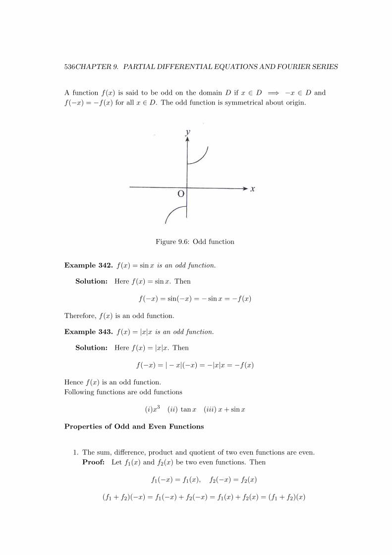
536CHAPTER 9. PARTIAL DIFFERENTIAL EQUATIONS AND FOURIER SERIES
A function f(x) is said to be odd on the domain D if x ∈ D =⇒ −x ∈ D and
f(−x) = −f(x) for all x ∈ D. The odd function is symmetrical about origin.
Figure 9.6: Odd function
Example 342. f(x) = sinx is an odd function.
Solution: Here f(x) = sinx. Then
f(−x) = sin(−x) = − sinx = −f(x)
Therefore, f(x) is an odd function.
Example 343. f(x) = |x|x is an odd function.
Solution: Here f(x) = |x|x. Then
f(−x) = | − x|(−x) = −|x|x = −f(x)
Hence f(x) is an odd function.
Following functions are odd functions
(i)x3 (ii) tanx (iii) x+ sinx
Properties of Odd and Even Functions
1. The sum, difference, product and quotient of two even functions are even.
Proof: Let f1(x) and f2(x) be two even functions. Then
f1(−x) = f1(x), f2(−x) = f2(x)
(f1 + f2)(−x) = f1(−x) + f2(−x) = f1(x) + f2(x) = (f1 + f2)(x)

9.4. ODD AND EVEN FUNCTIONS 537
This shows that f1 + f2 is an even function.
(f1 − f2)(−x) = f1(−x)− f2(−x) = f1(x)− f2(x) = (f1 − f2)(x)
This shows that f1 − f2 is an even function.
(f1f2)(−x) = f1(−x)f2(−x) = f1(x)f2(x) = (f1f2)(x)
This shows that f1f2 is an even function.(f1
f2
)(−x) =
f1(−x)
f2(−x)=f1(x)
f2(x)=
(f1
f2
)(x)
This shows that f1f2
is an even function.
2. The sum and difference of the two odd functions are odd, and the product and
quotient of two odd function is even.
Proof: Let f1(x) and f2(x) be two odd functions. Then
f1(−x) = −f1(x), f2(−x) = −f2(x)
(f1 + f2)(−x) = f1(−x) + f2(−x) = −f1(x)− f2(x) = −(f1 + f2)(x)
This shows that f1 + f2 is an odd function.
(f1 − f2)(−x) = f1(−x)− f2(−x) = −f1(x) + f2(x) = −(f1 − f2)(x)
This shows that f1 − f2 is an odd function.
(f1f2)(−x) = f1(−x)f2(−x) = (−f1(x))(−f2(x)) = f1(x)f2(x) = (f1f2)(x)
Thus, f1f2 is an even function.(f1
f2
)(−x) =
f1(−x)
f2(−x)=f1(x)
f2(x)=
(f1
f2
)(x)
Hence f1f2
is an even function.
3. The product and quotient of odd and even functions are odd.
Proof: Let f1(x) be an odd and f2(x) be an even function. Then
f1(−x) = −f1(x), f2(−x) = f2(x)
(f1f2)(−x) = f1(−x)f2(−x) = (−f1(x))(f2(x)) = −f1(x)f2(x) = −(f1f2)(x)
Thus, f1f2 is an odd function.(f1
f2
)(−x) =
f1(−x)
f2(−x)=−f1(x)
f2(x)= −
(f1
f2
)(x)
Hence, −f1f2
is an even function.
538CHAPTER 9. PARTIAL DIFFERENTIAL EQUATIONS AND FOURIER SERIES
4. If f is an even function, then∫ L
−Lf(x)dx = 2
∫ L
0f(x)dx
Proof: Here f(x) is an even function, so
f(−x) = f(x) for all x ∈ [−L,L] (9.97)
From properties of definite ingeral∫ b
af(x)dx =
∫ b
af(s)ds (9.98)∫ b
af(x)dx = −
∫ a
bf(x)dx (9.99)
and
∫ L
−Lf(x)dx =
∫ 0
−Lf(x)dx+
∫ L
0f(x)dx (9.100)
Letting x = −s and dx = −ds in the first term on the right side (9.100). When
x = 0 then s = 0 and when x = −L then s = L∫ L
−Lf(x)dx = −
∫ 0
Lf(−s)ds+
∫ L
0f(x)dx
or,
∫ L
−Lf(x)dx = −
∫ 0
Lf(s)ds+
∫ L
0f(x)dx using (9.97)
or,
∫ L
−Lf(x)dx = −
∫ 0
Lf(x)dx+
∫ L
0f(x)dx using (9.98)
or,
∫ L
−Lf(x)dx =
∫ L
0f(x)dx+
∫ L
0f(x)dx using (9.99)
or,
∫ L
−Lf(x)dx = 2
∫ L
0f(x)dx
5. If f is odd, then ∫ L
−Lf(x)dx = 0
Proof: Here f(x) is an odd function, so
f(−x) = −f(x) for all x ∈ [−L,L] (9.101)
From properties of definite ingeral∫ b
af(x)dx =
∫ b
af(s)ds (9.102)∫ b
af(x)dx = −
∫ a
bf(x)dx (9.103)

9.4. ODD AND EVEN FUNCTIONS 539
Let
I =
∫ L
−Lf(x)dx
Putting x = −s in I. Then dx = −ds, when x = −L, we get s = L and when
x = L, then s = −L.
I =
∫ L
−Lf(x)dx = −
∫ −LL
f(−s)ds
=
∫ −LL
f(s)ds using (9.101)
=
∫ −LL
f(x)dx using (9.102)
= −∫ L
−Lf(x)dx = −I using (9.103)
∴ 2I = 0
or, I = 0
or,
∫ L
−Lf(x)dx = 0
6. Prove that the derivatives of an even function is odd and the derivative of an
odd function is even.
Solution: Let f(x) be an even function Then
f(−x) = f(x)
Differentiating both sides with respect to x
−f ′(−x) = f ′(x)
or, f ′(−x) = −f ′(x)
This shows that f ′(x) is an odd function.
Let f(x) be an odd function. Then
f(−x) = −f(x)
Differentiating both sides with respect to x
−f ′(−x) = −f ′(x)
or, f ′(−x) = f ′(x)
Hence, f ′(x) is an even function.

540CHAPTER 9. PARTIAL DIFFERENTIAL EQUATIONS AND FOURIER SERIES
9.4.1 Fourier sine series or Fourier series of odd functions
Let f(x) be a function such that
1. f(x) is odd function.
2. f(x) and f ′(x) are piecewise continuous on −L ≤ x ≤ L.
3. periodic function with period 2L.
Let the Fourier series of f(x) be
f(x) =a0
2+∞∑m=1
(am cos
mπx
L+ bm sin
mπx
L
)(9.104)
Since f(x) is odd function so
a0 =1
L
∫ L
−Lf(x)dx = 0
We also know that cos mπxL is an even function. The the product of even and odd is
odd so f(x) cos mπxL is odd.
∴ bm =1
L
∫ L
−Lf(x) cos
mπx
Ldx = 0
Also, the product of two odds functions is even, so f(x) sin mπxL is even,. Hence
bm =1
L
∫ L
−Lf(x) cos
mπx
L=
2
L
∫ L
0f(x) cos
mπx
Ldx
Putting the values a0, am and bm in (9.104)
f(x) =∞∑m=1
bm sinmπx
L
Hence, the Fourier series for any odd function consists only of the odd trigonometric
function sin mπxL . This series is called Fourier sine series.
9.4.2 Fourier cosine series or Fourier series of even functions
Let f(x) be a function such that
1. f(x) is even.
2. f(x) and f ′(x) are piecewise continuous on −L ≤ x ≤ L.
3. periodic function with period 2L.

9.4. ODD AND EVEN FUNCTIONS 541
Let the Fourier series of f(x) be
f(x) =a0
2+
∞∑m=1
(am cos
mπx
L+ bm sin
mπx
L
)(9.105)
Since f(x) is an even function so
a0 =1
L
∫ L
−Lf(x)dx =
2
L
∫ L
0f(x)dx
We also know that cos mπxL is an even function.The the product of two even is even
so f(x) cos mπxL is even.
∴ bm =1
L
∫ L
−Lf(x) cos
mπx
Ldx =
2
L
∫ L
0f(x) cos
mπx
Ldx
Also, the product of even and odds functions is odd, so f(x) sin mπxL is odd,. Hence
bm =1
L
∫ L
−Lf(x) cos
mπx
L= 0
Putting the values a0, am and bm in (9.105)
f(x) =a0
2+∞∑m=1
am cosmπx
L
Hence, the Fourier series for any any function consists only of the trigonometric
function cos mπxL and constant term . This series is called Fourier cosine series.
Example 344. Let
f(x) = x, −L < x < L
and let f(−L) = f(L) = 0. Let f be defined elsewhere so that it is periodic of period
2L. The function defined in this manner is know as a sawtooth wave. Find the
Fourier series for this function.
Solution: Here
f(x) = x
is odd, so
am = 0, m = 0, 1, 2, · · ·

542CHAPTER 9. PARTIAL DIFFERENTIAL EQUATIONS AND FOURIER SERIES
and
bm =2
L
∫ L
0f(x) sin
mπx
Ldx
=2
L
∫ L
0x sin
mπx
Ldx
=2
L
[x
∫sin
mπx
Ldx
]L0
−∫ L
0
(dx
dx
∫sin
mπx
Ldx
)dx
=2
L
[− Lxmπ
cosmπx
L
]L0
+L
mπ
∫ L
0cos
mπx
Ldx
=2
L
− L2
mπcosmπ − 0 +
L2
m2π2
[sin
mπx
L
]L0
=
2
L
− L2
mπcosmπ − 0 +
L2
m2π2[sinmπ − sin 0]
=
−2L
mπcosmπ
=−2L
mπ(−1)m, m = 1, 2, 3 · · ·
=2L
mπ(−1)m+1
Therefore, the Fourier sine series of the given sawtooth wave function f is
f(x) =∞∑m=1
bm sinmπx
L
=
∞∑m=1
2L
mπ(−1)m+1 sin
mπx
L
=2L
m
∞∑m=1
(−1)m+1
msin
mπx
L
9.4.3 Even and Odd Extension
We can defined a function
fe(x) =
f(x) 0 ≤ x ≤ Lf(−x) −L < x < 0
and
fe(x+ 2L) = fe(x)
Then the function fe is thus even periodic extension of f . It Fourier series, which is
a cosine series represents f on [0, L]. i.e.
fe(x) =a0
2+∞∑n−1
an cosnπx
L

9.4. ODD AND EVEN FUNCTIONS 543
where
an =
∫ L
0f(x) cos
nπx
Ldx
Again, we can defined a function
f0(x) =
f(x) 0 < x < L
0 x = 0, L
−f(−x) −L < x < 0
and
fo(x+ 2L) = fo(x)
Then the function fo is thus odd periodic extension of f . It Fourier series, which is
a cosine series represents f on [0, L]. i.e.
fo(x) =∞∑n=1
bn sinnπx
L
where
bn =
∫ L
0f(x) sin
nπx
Ldx
Example 345. Find the even and odd periodic extension of
f(x) =
0 0 ≤ x < 1
1 1 ≤ x < 2
Solution: The given function is
f(x) =
0 0 ≤ x < 1
1 1 ≤ x < 2
For the periodic extension, we define
fe(x) =
f(x) 0 ≤ x ≤ 2
f(−x) −2 < x < 0
so fe(x) has even periodic extension of the period 4 whose graph is
f0(x) =
f(x) 0 < x < 2
0 x = 0, 2
−f(−x) −2 < x < 0

544CHAPTER 9. PARTIAL DIFFERENTIAL EQUATIONS AND FOURIER SERIES
Figure 9.7: Odd Periodic Extension
Figure 9.8: Even Periodic Extension
Then the function fo is thus odd periodic extension of f of the period 4 whose
graph is
Example 346. Find Fourirer seiries for the given function
f(x) = 1, 0 ≤ x ≤ π, cosine series, period 2π
Solution: Here L = π. For an even extension of the function, the sine coeffi-
cients are zero. The cosine coefficient are given by
a0 =2
L
∫ L
0f(x)dx
=2
π
∫ π
0dx =
2
π[x]π0 =
2
ππ = 2
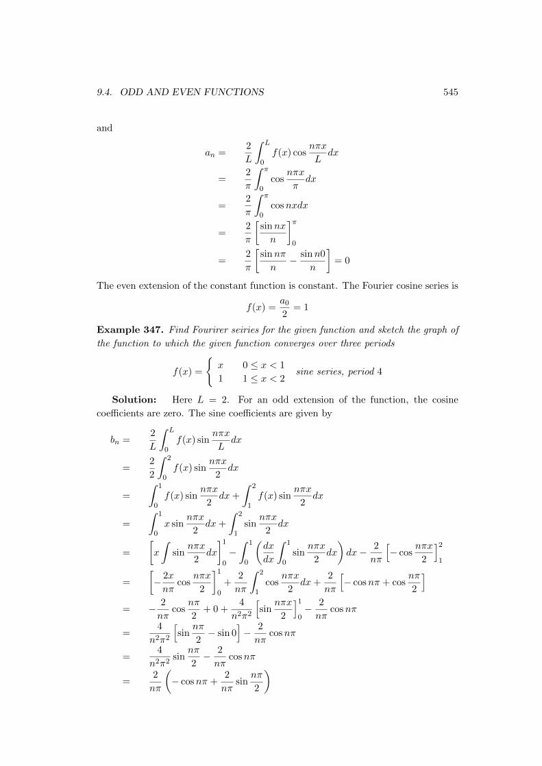
9.4. ODD AND EVEN FUNCTIONS 545
and
an =2
L
∫ L
0f(x) cos
nπx
Ldx
=2
π
∫ π
0cos
nπx
πdx
=2
π
∫ π
0cosnxdx
=2
π
[sinnx
n
]π0
=2
π
[sinnπ
n− sinn0
n
]= 0
The even extension of the constant function is constant. The Fourier cosine series is
f(x) =a0
2= 1
Example 347. Find Fourirer seiries for the given function and sketch the graph of
the function to which the given function converges over three periods
f(x) =
x 0 ≤ x < 1
1 1 ≤ x < 2sine series, period 4
Solution: Here L = 2. For an odd extension of the function, the cosine
coefficients are zero. The sine coefficients are given by
bn =2
L
∫ L
0f(x) sin
nπx
Ldx
=2
2
∫ 2
0f(x) sin
nπx
2dx
=
∫ 1
0f(x) sin
nπx
2dx+
∫ 2
1f(x) sin
nπx
2dx
=
∫ 1
0x sin
nπx
2dx+
∫ 2
1sin
nπx
2dx
=
[x
∫sin
nπx
2dx
]1
0
−∫ 1
0
(dx
dx
∫ 1
0sin
nπx
2dx
)dx− 2
nπ
[− cos
nπx
2
]2
1
=
[− 2x
nπcos
nπx
2
]1
0
+2
nπ
∫ 2
1cos
nπx
2dx+
2
nπ
[− cosnπ + cos
nπ
2
]= − 2
nπcos
nπ
2+ 0 +
4
n2π2
[sin
nπx
2
]1
0− 2
nπcosnπ
=4
n2π2
[sin
nπ
2− sin 0
]− 2
nπcosnπ
=4
n2π2sin
nπ
2− 2
nπcosnπ
=2
nπ
(− cosnπ +
2
nπsin
nπ
2
)

546CHAPTER 9. PARTIAL DIFFERENTIAL EQUATIONS AND FOURIER SERIES
Therefore, the Fourier sine series of the given function is
f(x) =∞∑n=1
bn sinnπx
2
=
∞∑n=1
[2
nπ
(− cosnπ +
2
nπsin
nπ
2
)]sin
nπx
2
Example 348. Find Fourirer seiries for the given function and sketch the graph of
the function to which the given function converges over three periods
f(x) =
x 0 ≤ x < π
0 π ≤ x < 2πcosine series, period 4π
Solution: Here L = 2π. For an even extension of the function, the sine
coefficients are zero.
bn = 0
The constant is
a0 =1
L
∫ L
0f(x)dx
=1
π
∫ π
0xdx
=1
π
[x2
2
]π0
=1
π
[π2
2− 02
2
]=π
2

9.4. ODD AND EVEN FUNCTIONS 547
The cosine coefficients are given by
an =2
L
∫ L
0f(x) cos
nπx
Ldx
=2
2π
∫ 2π
0f(x) cos
nπx
2πdx
=1
π
∫ π
0f(x) cos
nx
2dx+
∫ 2π
πf(x) cos
nx
2dx
=
1
π
∫ π
0x cos
nx
2dx+
∫ 2π
π0 cos
nx
2dx
=
1
π
[x
∫cos
nx
2dx
]π0
−∫ π
0
(dx
dx
∫cos
nx
2dx
)dx
=
1
π
[2x
nsin
nx
2
]π0
− 2
n
∫ 2
1sin
nx
2dx
=
1
π
2π
nsin
nπ
2+ 0 +
4
n2
[cos
nx
2
]π0
=
1
π
2π
nsin
nπ
2+
4
n2
[cos
nπ
2− cos 0
]=
1
π
2π
nsin
nπ
2+
4
n2
[cos
nπ
2− 1]
Therefore, the Fourier sine series of the given function is
f(x) =a0
2+
∞∑n=1
an cosnπx
L
=π
4+
1
π
∞∑n=1
2π
nsin
nπ
2+
4
n2
(cos
nπ
2− 1)
cosnx
2
Example 349. Find Fourirer seiries for the given function and sketch the graph of
the function to which the given function converges over three periods
f(x) =
1 0 < x < 1
0 1 < x < 2cosine series, period 4
Solution: Here L = 2. For an even extension of the function, the sine coeffi-
cients are zero.
bn = 0

548CHAPTER 9. PARTIAL DIFFERENTIAL EQUATIONS AND FOURIER SERIES
The constant is
a0 =1
L
∫ L
0f(x)dx
=1
2
∫ 2
0F (x)dx
=1
2
∫ 1
0f(x)dx+
∫ 2
1f(x)dx
=
1
2
∫ 1
0dx+
∫ 2
10dx
=
1
2[x]10 =
1
2
The cosine coefficients are given by
an =2
L
∫ L
0f(x) cos
nπx
Ldx
=2
2
∫ 2
0f(x) cos
nπx
2dx
=
∫ 1
0f(x) cos
nπx
2dx+
∫ 2
1f(x) cos
nπx
2dx
=
∫ 1
0cos
nπx
2dx+
∫ 2
10 cos
nπx
2dx
=2
nπ
[sin
nπx
2
]1
0
=2
nπ
[sin
nπ
2− sin 0
]=
2
nπ
0 if n = 2, 4, 6 · · ·1 if n = 1, 5, 9 · · ·−1 if n = 3, 7, 11, · · ·
=2
nπ
0 if n = 2, 4, 6 · · ·
(−1)n−1 if n = 1, 5, 9 · · ·(−1)n−1 if n = 3, 7, 11, · · ·
=2
nπ
0 if is n even
(−1)n−1 if is n odd
=2(−1)n−1
(2n− 1)π
Therefore, the Fourier sine series of the given function is
f(x) =a0
2+
∞∑n=odd
an cosnπx
L
=1
2+
2
π
∞∑n=1
(−1)n−1
(2n− 1)cos
(2n− 1)πx
2

Chapter 10
Separation of Variables
10.1 One Dimensional Heat Equation
10.1.1 Fourier ’s Law of Heat Conduction
Let us cosider a uniform rod insulated on the lateral surfaces so that heat flow on the
lateral surface only in the axial direction. Let us consider two parallel cross sections
of the same area A and different temperatures T1 and T2 respectively, are separated
by a small distance d, an amount of heat per unit time will pass from the warmer
section to the coolar one. The amount of heat flow per unit time is proportinal to
the area A, and to the temperature difference |T2 − T1| and inversely proportional
to the separation distance d.
Amount of heat flow per unit time =κA|T2 − T1|
d(10.1)
where the positive proportionality factor κ is called the termal conductivity and
depends on the materal of the rod. The relation (10.1) is called Fourier’s law of heat
conduction. Let the temperature depends on distance x and time t i.e.
T = u(x, t)
The the equation (10.1) become
Amount of heat flow per unit time =κA|u(x1, t)− u(x2, t)|
d
10.1.2 Derivation of One Diamensional heat Equation
1 Let us consider the element of rod lying between the cross section x and x + δx,
where x is arbitrary and δx is small. The instantaneous heat transfer H(x, t) from
1Student may leave the deduction
549

550 CHAPTER 10. SEPARATION OF VARIABLES
left to right across the section x is given by
H(x, t) = − limd→0
κAu(x+ d/2, t)− u(x− d/2, t)
d
= −κA ∂
∂xu(x, t) = −κAux(x, t) (10.2)
The minus sign appears in this equation because there will be a positive flow of the
heat from left to right only if the temperature is greater to the left of x than to the
right; in this case ∂u∂x is negative.
Similarly, the rate at which heat passes from left to right through the cross section
x+ δx is given by
H(x+ δx, t) = −κAux(x+ δx, t) (10.3)
The net rate at which the heat flows into the line segment of the bar between x and
x+ δx is thus given by
Q = H(x, t)−H(x+ δx) = κA [ux(x+ δx, t)− ux(x, t)]
The amount of heat entering this bar element in time δt
Qδt = κA [ux(x+ δx, t)− ux(x, t)] δt (10.4)
The average change in temperature δu in the interval δt, is proportional to the
amount of heat Qδt introduce and inversely proportinal to the mass δm of the
element. Thus
δu =Qδt
sδm=
Qδt
sρAδx(10.5)
where s is proportionality constant, is known as the specific heat of the metarial of
the bar, and ρ is its density.
The average temperature change δu in the bar element under consideration is the
actual temperature change at some intermediate point x+ θδx where 0, θ < 1.
δu = u(x+ θδx, t+ δt)− u(x+ θδx, t)
Now from (10.5)
u(x+ θδx, t+ δt)− u(x+ θδx, t) =Qδt
sρAδx
or, Qδt = [u(x+ θδx, t+ δt)− u(x+ θδx, t)] sρAδx (10.6)

10.1. ONE DIMENSIONAL HEAT EQUATION 551
From (10.4) and (10.6), we have
κA [ux(x+ δx, t)− ux(x, t)] δt = [u(x+ θδx, t+ δt)− u(x+ θδx, t)] sρAδx
Dividing both sides by δxδt
κ [ux(x+ δx, t)− ux(x, t)]
δx=
[u(x+ θδx, t+ δt)− u(x+ θδx, t)] sρ
δt
Letting δx→ 0 and δt→ 0
limδx→0
κ [ux(x+ δx, t)− ux(x, t)]
δx= lim
δt→0
[u(x+ θδx, t+ δt)− u(x+ θδx, t)] sρ
δt
or, κuxx = sρut
or,κ
sρuxx = ut
or, α2uxx = ut (10.7)
where α2 = κρs is called the termal diffusivity and it depends on the metarial.
10.1.3 Initial and boundary conditions
Let us assume that the initial temperature distribution in the rod is given by
u(x, 0) = f(x), 0 ≤ x ≤ L
and we consider the rod has fixed temperature 0 at the two ends of the rod at x = 0,
and x = L.
u(0, t) = 0, u(L, t) = 0 t > 0
Hence, a one diamensional heat equation with initial and boundary condition is
Partial differential equation: ut = α2uxx
Initial condition: u(x, 0) = f(x); 0 ≤ x ≤ LBoundary condition: u(0, t) = u(L, t) = 0, t > 0
10.1.4 Separation of Variables
Example 350. Find the ordinary differential equations to replace the partilal dif-
ferential equation
tuxx + xut = 0
by method of separation of variables. [B.Sc.2075]

552 CHAPTER 10. SEPARATION OF VARIABLES
Solution: The given partial differentialequation is
tuxx + xut = 0 (10.8)
Let u(x, t) = X(x)T (t) be the separation solution. Then
ut =∂u
∂t= XT ′ and uxx =
∂2u
∂x2= X ′′T
where primes refer to ordinary differentiation with respect to independent variables
x or t. Therefore, the equation (10.8) becomes
tX ′′ + xXT ′ = 0
or, tX ′′T = −xXT ′
or,X ′′
xX=−T ′
tT= λ say
which gives
X ′′ − λxX = 0, T ′ + λtT = 0
Example 351. Find the ordinary differential equations to replace the partilal dif-
ferential equation
xuxx + 2ut = 0
by method of separation of variables.
Solution: The given partial differential equation is
xuxx + 2ut = 0 (10.9)
Let u(x, t) = X(x)T (t) be the separation solution. Then
ut =∂u
∂t= XT ′ and uxx =
∂2u
∂t2= X ′′T
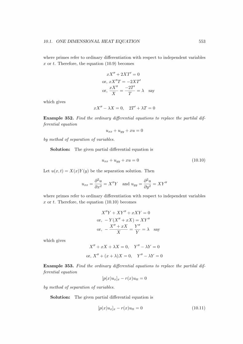
10.1. ONE DIMENSIONAL HEAT EQUATION 553
where primes refer to ordinary differentiation with respect to independent variables
x or t. Therefore, the equation (10.9) becomes
xX ′′ + 2XT ′ = 0
or, xX ′′T = −2XT ′
or,xX ′′
X=−2T ′
T= λ say
which gives
xX ′′ − λX = 0, 2T ′ + λT = 0
Example 352. Find the ordinary differential equations to replace the partilal dif-
ferential equation
uxx + uyy + xu = 0
by method of separation of variables.
Solution: The given partial differential equation is
uxx + uyy + xu = 0 (10.10)
Let u(x, t) = X(x)Y (y) be the separation solution. Then
uxx =∂2u
∂x2= X ′′Y and uyy =
∂2u
∂y2= XY ′′
where primes refer to ordinary differentiation with respect to independent variables
x or t. Therefore, the equation (10.10) becomes
X ′′Y +XY ′′ + xXY = 0
or, − Y (X ′′ + xX) = XY ′′
or, − X ′′ + xX
X=Y ′′
Y= λ say
which gives
X ′′ + xX + λX = 0, Y ′′ − λY = 0
or, X ′′ + (x+ λ)X = 0, Y ′′ − λY = 0
Example 353. Find the ordinary differential equations to replace the partilal dif-
ferential equation
[p(x)ux]x − r(x)utt = 0
by method of separation of variables.
Solution: The given partial differential equation is
[p(x)ux]x − r(x)utt = 0 (10.11)

554 CHAPTER 10. SEPARATION OF VARIABLES
Let u(x, t) = X(x)Y (y) be the separation solution. Then
ux = X ′T
or, p(x)ux = p(x)X ′T
or, [p(x)ux]x = Td
dx(p(x)X) = Tp′(x)X ′ + Tp(x)X ′′
and utt = XT ′′
where primes refer to ordinary differentiation with respect to independent variables
x or t. Therefore, the equation (10.11) becomes
Tp′(x)X ′ + Tp(x)X ′′ − r(x)XT ′′
or, Tp′(x)X ′ + Tp(x)X ′′ = r(x)XT ′′
or, T [p′(x)X ′ + p(x)X ′′] = r(x)XT ′′
or,p′(x)X ′ + p(x)X ′′
r(x)X=T ′′
T= −λ say
which gives
p′(x)X ′ + p(x)X ′′ + λr(x)X = 0, T ′′ + λT = 0
or, (p(x)X ′)′ + λr(x)X = 0, T ′′ + λT = 0
10.1.5 Solution of One Diamensional Heat Equation by Separation
of Variables
The one diamesional heat equation is
ut = α2uxx
or,∂u
∂t= α2∂
2u
∂x2(10.12)
where
α2 =κ
ρs
along with boundary conditions
u(0, t) = 0 and u(L, t) = 0, t > 0
and initial condition
u(x, 0) = f(x), 0 ≤ x ≤ L
Let u(x, t) = X(x)T (t) be a variable separation solution of the equation (10.12) with
the given boundary and initial conditions. Then
∂u
∂t= XT ′ and
∂2u
∂x2= X ′′T (10.13)

10.1. ONE DIMENSIONAL HEAT EQUATION 555
where primes refer to ordinary differentiation with respect to independent variables
x or t. Subsituting the values in (10.12) we get
XT ′ = α2X ′′T
or,X”
X=
1
α2
T ′
T= −λ (say) where λ > 0 (10.14)
Hence we obtain the following two ordinary differential equations
X ′′ + λX = 0 (10.15)
and T ′ + α2λT = 0 (10.16)
The auxiliary equation of (10.15) is
m2 + λ2 = 0
or, m2 = −λ2
or, m = ±i√λ
Hence, the general solution of (10.15) is
X(x) = c1 cos√λx+ c2 sin
√λx (10.17)
Using the boundary conditions
u(0, t) = 0, and u(L, t) = 0
or, X(0)T (t) = 0 and X(L)T (t) = 0
Since T (t) 6= 0, =⇒ X(0) = 0, X(L) = 0
Again, using X(0) = 0 in (10.17), we get
0 = c1 cos 0 + c2 sin 0
or, c1 = 0
and using X(L) = 0 in (10.17), we get
0 = c1 cos√λL+ c2 sin
√λL
or, c2 sin√λL = 0
For c2 6= 0, we must have
sin√λL = 0
=⇒√λL = nπ, n = 1, 2, 3, · · ·
or,√λ =
nπ
L, n = 1, 2, 3, · · ·
or, λ =n2π2
L2, n = 1, 2, 3, · · ·

556 CHAPTER 10. SEPARATION OF VARIABLES
Hence the equation (10.17) becomes
X = c2 sinnπx
L, n = 1, 2, 3, · · ·
Letting c2 = 1, the eigenfunction (non-zero solutions ) are
Xn(x) = sinnπx
L, n = 1, 2, 3, · · ·
associated with the eigenvalues
λn =n2π2
L2, n = 1, 2, 3 · · ·
Now turning to the equation (10.16), putting value of λ
T ′ + α2n2π2
L2T = 0
or,dT
dt= −α2n
2π2
L2T
or,dT
T= −α
2n2π2
L2dt
loge T = −α2n2π2
L2t integrating without arbitrary constant
or, T = e−α2n2π2
L2 t, n = 1, 2, 3, · · ·
or, Tn(t) = e−α2n2π2
L2 t, n = 1, 2, 3, · · ·
The value of T depends on n, so we suppose it as Tn. Therefore, the functions
u(x, t) = Xn(x)Tn(x)
= sinnπx
Le−
α2n2π2
L2 t, n = 1, 2, 3, · · ·
are solutions of the one diamensional heat equation under the given conditions. The
functions un are fundamental solutions of the given heat equation. It remains to
satisfy the initial condition
u(x, 0) = f(x), 0 ≤ x ≤ L
Now, we consider linear combination of all these solutions
u(x, t) =∞∑n=1
cn sinnπx
Le−
α2n2π2
L2 t (10.18)
Using the initial condition u(x, 0) = f(x), assuming the series convergent, we get
∞∑n=1
cn sinnπx
L= f(x)

10.1. ONE DIMENSIONAL HEAT EQUATION 557
which is a Fourier sine series of f(x) with period 2L, so that the series on the left
converge to the initial temperature f(x). Therefore,
cn =2
L
∫ L
0f(x) sin
nπx
Ldx
Hence, solution of the one dimensional heat equation is
u(x, t) =∞∑n=1
cn sinnπx
Le−
α2n2π2
L2 t
where
cn =2
L
∫ L
0f(x) sin
nπx
Ldx, n = 1, 2, 3, · · ·
Example 354. Find the solution of the heat conduction problem
100uxx = ut, 0 < x < 1, t > 0
u(0, t) = 0, u(1, t) = 0, t > 0
u(x, 0) = 2(sin 2πx− sin 5πx), 0 ≤ x ≤ 1
Solution: Let u(x, t) = X(x)T (t) be a variable separation solution of the given
equation with the given boundary and initial condition. Then
∂u
∂t= XT ′ and
∂2u
∂x2= X ′′T (10.19)
where primes refer to ordinary differentiation with respect to independent variables
x or t. Subsituting the values in the given heat equation, we get
100X ′′T = XT ′
or,X”
X=
1
100
T ′
T= −λ (say) where λ > 0 (10.20)
Hence we obtain the following two ordinary differential equations
X ′′ + λX = 0 (10.21)
and T ′ + 100λT = 0 (10.22)
The auxiliary equation of (10.21) is
m2 + λ2 = 0
or, m2 = −λ2
or, m = ±i√λ
Hence, the general solution of (10.21) is
X(x) = c1 cos√λx+ c2 sin
√λx (10.23)

558 CHAPTER 10. SEPARATION OF VARIABLES
Using the boundary conditions
u(0, t) = 0, and u(1, t) = 0
or, X(0)T (t) = 0 and X(1)T (t) = 0
Since T (t) 6= 0, =⇒ X(0) = 0, X(1) = 0
Again, using X(0) = 0 in (10.23), we get
0 = c1 cos 0 + c2 sin 0
or, c1 = 0
and using X(1) = 0 in (10.23), we get
0 = c1 cos√λ+ c2 sin
√λ
or, c2 sin√λ = 0
For c2 6= 0, we must have
sin√λ = 0
=⇒√λ = nπ, n = 1, 2, 3, · · ·
or,√λ = nπ, n = 1, 2, 3, · · ·
or, λ = n2π2, n = 1, 2, 3, · · ·
Hence the equation (10.23) becomes
X = c2 sinnπx, n = 1, 2, 3, · · ·
Letting c2 = 1, the eigenfunction (non-zero solutions ) are
Xn(x) = sinnπx, n = 1, 2, 3, · · ·
associated with the eigenvalues
λn = n2π2, n = 1, 2, 3 · · ·
Now turning to the equation (10.16), putting value of λ
T ′ + 100n2π2T = 0
or,dT
T= −100n2π2dt
or, loge T = −100n2π2t integrating without arbitrary constant
or, T = e−100n2π2t, n = 1, 2, 3, · · ·or, Tn(t) = e−100n2π2t, n = 1, 2, 3, · · ·
Therefore, the functions
u(x, t) = Xn(x)Tn(x)
= e−100n2π2t sinnπx, n = 1, 2, 3, · · ·

10.1. ONE DIMENSIONAL HEAT EQUATION 559
are solutions of the one diamensional heat equation under the given conditions. The
functions un are fundamental solutions of the given equation. It remains to satisfy
the initial condition
u(x, 0) = 2(sin 2πx− sin 5πx), 0 ≤ x ≤ 1
Now we consider linear combinations of all these solutions
u(x, t) =
∞∑n=1
cn sinnπx e−100n2π2t (10.24)
Using the initial conditions u(x, 0) = 2(sin 2πx− sin 5πx), assuming the series con-
vergent, we get
∞∑n=1
cn sinnπx = 2(sin 2πx− sin 5πx)
which is a Fourier sine series of with period 2L = 2 × 1 = 2, so that the series on
the left converge to the initial temperature 2(sin 2πx− sin 5πx). Therefore,
cn =2
L
∫ L
0f(x) sin
nπx
Ldx
=2
1
∫ 1
02(sin 2πx− sin 5πx) sinnπxdx
= 4
∫ 1
0sin 2πx sinnπxdx− 4
∫ 1
0sin 5πx sinnπxdx (10.25)
Using the orthogonality properties∫ 1
0sin 2πx sinnπxdx =
0 if n 6= 212 if n = 2
and ∫ 1
0sin 5πx sinnπxdx =
0 if n 6= 512 if n = 5
Hence from (10.25)
c2 = 4 · 1
2= 2, c5 = 0− 4 · 1
2= −2, cn = 0 for n 6= 2, 5.
Hence the solution (10.24) becomes
u(x, t) = 2e−400π2t sin 2πx− 2e−2500π2t sin 5πx
Example 355. Find the temperature u(x, t) at any time in a metrial rod 50cm long,
insulated on the sides, which initially has a uniform temperature of 200 throughout
and whose ends are maintained at 00C
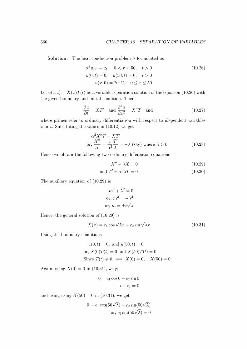
560 CHAPTER 10. SEPARATION OF VARIABLES
Solution: The heat conduction problem is formulated as
α2uxx = ut, 0 < x < 50, t > 0 (10.26)
u(0, t) = 0, u(50, t) = 0, t > 0
u(x, 0) = 200C, 0 ≤ x ≤ 50
Let u(x, t) = X(x)T (t) be a variable separation solution of the equation (10.26) with
the given boundary and initial condition. Then
∂u
∂t= XT ′ and
∂2u
∂x2= X ′′T and (10.27)
where primes refer to ordinary differentiation with respect to idependent variables
x or t. Subsituting the values in (10.12) we get
α2X ′′T = XT ′
or,X”
X=
1
α2
T ′
T= −λ (say) where λ > 0 (10.28)
Hence we obtain the following two ordinary differential equations
X ′′ + λX = 0 (10.29)
and T ′ + α2λT = 0 (10.30)
The auxiliary equation of (10.29) is
m2 + λ2 = 0
or, m2 = −λ2
or, m = ±i√λ
Hence, the general solution of (10.29) is
X(x) = c1 cos√λx+ c2 sin
√λx (10.31)
Using the boundary conditions
u(0, t) = 0, and u(50, t) = 0
or, X(0)T (t) = 0 and X(50)T (t) = 0
Since T (t) 6= 0, =⇒ X(0) = 0, X(50) = 0
Again, using X(0) = 0 in (10.31), we get
0 = c1 cos 0 + c2 sin 0
or, c1 = 0
and using using X(50) = 0 in (10.31), we get
0 = c1 cos(50√λ) + c2 sin(50
√λ)
or, c2 sin(50√λ) = 0

10.1. ONE DIMENSIONAL HEAT EQUATION 561
For c2 6= 0, we must have
sin 50√λ = 0
=⇒ 50√λ = nπ, n = 1, 2, 3, · · ·
or,√λ =
nπ
50, n = 1, 2, 3, · · ·
or, λ =n2π2
2500, n = 1, 2, 3, · · ·
Hence the equation (10.31) becomes
X = c2 sinnπx
50, n = 1, 2, 3, · · ·
Letting c2 = 1, the eigenfunction (non-zero solutions ) are
Xn(x) = sinnπx
50, n = 1, 2, 3, · · ·
associated with the eigenvalues
λn =n2π2
2500, n = 1, 2, 3 · · ·
Now turning to the equation (10.30), putting value of λ
T ′ +α2n2π2
2500T = 0
or,dT
T= −α
2n2π2
2500dt
or, loge T = −α2n2π2
2500t integrating without arbitrary constant
or, T = e−α2n2π2
2500t, n = 1, 2, 3, · · ·
or, Tn(t) = e−−α2n2π2
2500t, n = 1, 2, 3, · · ·
Therefore, the functions
un(x, t) = Xn(x)Tn(x)
= e−α2n2π2
2500t sin
nπx
50, n = 1, 2, 3, · · ·
are solutions of the one diamensional heat equation under the given conditions. The
functions un are fundamental solutions of the given equations. It remains to satisfy
the initial condition
u(x, 0) = 20 0 ≤ x ≤ 1
Now we consider linear combination of all these solutions
u(x, t) =
∞∑n=1
cn sinnπx
50e−−
α2n2π2
2500t (10.32)

562 CHAPTER 10. SEPARATION OF VARIABLES
Using the initial condition u(x, 0) = 20, assuming the series convergent, we get
∞∑n=1
cn sinnπx = 20
which is a Fourier sine series of with period 2L = 2 × 50 = 100, so that the series
on the left converge to the initial temperature 20. Therefore,
cn =2
L
∫ L
0f(x) sin
nπx
Ldx
=2
50
∫ 50
020 sin
nπx
50dx
=4
5
∫ 5
0sin
nπx
50dx
=4
5
50
nπ
[− cos
nπx
50
]50
0
=40
nπ(1− cosnπ)
=
80nπ , n odd
0, n even(10.33)
Hence the solution (10.32) becomes
u(x, t) =80
π
∑n=odd
1
nsin
nπx
50e−
α2n2π2
2500t
Example 356. Consider the conduction of hea in a rod 40cm in lenght whose ends
are maintained at 0oC for all t > 0 . Find an expression for the temperature u(x, t) in
the following cases if the initial temperature distribution in the rod is given function
. Suppose that α2 = 1.
1. u(x, 0) = 50, 0 < x < 40.
2. u(x, 0) = x, 0 < x < 40.
3.
u(x, 0) =
0, 0 ≤ x < 10
50 10 ≤ x ≤ 30
0 30 ≤ x ≤ 40
Solution: The heat conduction problem is formulated as, taking α2 = 1
uxx = ut, 0 < x < 40, t > 0 (10.34)
with initial conditions u(0, t) = 0, u(40, t) = 0, t > 0

10.1. ONE DIMENSIONAL HEAT EQUATION 563
Let u(x, t) = X(x)T (t) be a variable separation solution of the equation (10.34) with
the given boundary and initial condition. Then
∂u
∂t= XT ′ and
∂2u
∂x2= X ′′T and (10.35)
where primes refer to ordinary differentiation with respect to independent variables
x or t. Subsituting the values in (10.34) we get
X ′′T = XT ′
or,X”
X=T ′
T= −λ (say) where λ > 0 (10.36)
Hence we obtain the following two ordinary differential equations
X ′′ + λX = 0 (10.37)
and T ′ + λT = 0 (10.38)
The auxiliary equation of (10.37) is
m2 + λ2 = 0
or, m2 = −λ2
or, m = ±i√λ
Hence, the general solution of (10.37) is
X(x) = c1 cos√λx+ c2 sin
√λx (10.39)
Using the boundary conditions
u(0, t) = 0, and u(40, t) = 0
or, X(0)T (t) = 0 and X(40)T (t) = 0
Since T (t) 6= 0, =⇒ X(0) = 0, X(40) = 0
Again, using X(0) = 0 in (10.39), we get
0 = c1 cos 0 + c2 sin 0
or, c1 = 0
and using using X(40) = 0 in (10.39), we get
0 = c1 cos 40√λ+ c2 sin 40
√λ
or, c2 sin 40√λ = 0
For c2 6= 0, we must have
sin 40√λ = 0
=⇒ 40√λ = nπ, n = 1, 2, 3, · · ·
or,√λ =
nπ
40, n = 1, 2, 3, · · ·
or, λ =n2π2
1600, n = 1, 2, 3, · · ·

564 CHAPTER 10. SEPARATION OF VARIABLES
Hence the equation (10.39) becomes
X = c2 sinnπx
40, n = 1, 2, 3, · · ·
Letting c2 = 1, the eigenfunction (non-zero solutions ) are
Xn(x) = sinnπx
40, n = 1, 2, 3, · · ·
associated with the eigenvalues
λn =n2π2
1600, n = 1, 2, 3 · · ·
Now turning to the equation (10.38), putting value of λ
T ′ +n2π2
1600T = 0
or,dT
T= −n
2π2
1600dt
or, loge T = −n2π2
1600t integrating without arbitrary constant
or, T = e−n2π2
1600t, n = 1, 2, 3, · · ·
or, Tn(t) = e−−n2π2
1600t, n = 1, 2, 3, · · ·
Therefore, the functions
un(x, t) = Xn(x)Tn(x)
= e−n2π2
1600t sin
nπx
40, n = 1, 2, 3, · · ·
are solutions of the one diamensional heat equation under the given conditions. The
functions un are fundamental solutions of the given equation.
Now we consider linear combination of all these solutions
u(x, t) =
∞∑n=1
cn sinnπx
40e−
n2π2
1600t (10.40)
(1) Using the initial condition u(x, 0) = 50, assuming the series convergent, we get
∞∑n=1
cn sinnπx
40= 50

10.1. ONE DIMENSIONAL HEAT EQUATION 565
which is a Fourier sine series of with period 2L = 2× 40 = 80, so that the series on
the left converges to the initial temperature 50. Therefore
cn =2
L
∫ L
0f(x) sin
nπx
Ldx
=2
40
∫ 40
050 sin
nπx
40dx
=5
2
∫ 40
0sin
nπx
40dx
=5
2
40
nπ
[− cos
nπx
40
]40
0
=100
nπ(1− cosnπ)
Hence the solution (10.40) becomes
u(x, t) =100
π
∑n=1
1− cosnπ
nsin
nπx
40e−
n2π2
1600t
(2) Using the initial conditions u(x, 0) = x, 0 < x < 40, in (10.40) assuming the
series convergent, we get
∞∑n=1
cn sinnπx
40= x
which is a Fourier sine series of with period 2L = 2× 40 = 80, so that the series on
the left converge to the initial temperature u(x, 0) = x. Therefore,
cn =2
L
∫ L
0f(x) sin
nπx
Ldx
=2
40
∫ 40
0x sin
nπx
40dx
=1
20
[x
∫sin
nπx
40
]40
0
−∫ 40
0
(dx
dx
∫sin
nπx
40dx
)dx
=1
20
[−40x
nπcos
nπx
40
]40
0
+40
nπ
∫ 40
0cos
nπx
40dx
=1
20
[−1600
nπcos
40nπ
40+ 0
]+
1600
n2π2
[sin
nπx
40
]40
0
=
1
20
[−1600
nπcosnπ + 0
]+
1600
n2π2[sinnπ − 0]
= − 80
nπcosnπ = − 80
nπ(−1)n =
80
nπ(−1)n+1
Hence the solution (10.40) becomes
u(x, t) =80
π
∑n=1
(−1)n+1
nsin
nπx
40e−
n2π2
1600t

566 CHAPTER 10. SEPARATION OF VARIABLES
(3) Using the initial conditions ,
u(x, 0) =
0, 0 ≤ x < 10
50 10 ≤ x ≤ 30
0 30 ≤ x ≤ 40
assuming the series convergent, we get
∞∑n=1
cn sinnπx
40= u(x, 0)
which is a Fourier sine series of with period 2L = 2× 40 = 80, so that the series on
the left converge to the initial temperature f(x) = u(x, 0). Therefore,
cn =2
L
∫ L
0f(x) sin
nπx
Ldx
=2
40
∫ 40
0u(x, 0) sin
nπx
40dx
=1
20
∫ 10
0u(x, 0) sin
nπx
40dx+
1
20
∫ 20
10u(x, 0) sin
nπx
40dx+
1
20
∫ 40
20u(x, 0) sin
nπx
40dx
=1
20
∫ 10
00 sin
nπx
40dx+
1
20
∫ 30
1050 sin
nπx
40dx+
1
20
∫ 40
300 sin
nπx
40dx
= 0 +50
20
40
nπ
[− cos
nπx
40
]30
10+ 0
=100
nπ
(cos
nπ
4− cos
3nπ
4
)Hence the solution (10.40) becomes
u(x, t) =100
π
∑n=1
1
n
(cos
nπ
4− cos
3nπ
4
)e−
n2π2
1600t sin
nπx
40
10.2 Other Heat Conduction Problem
We considered the the problem consisting of the heat conduction equation
ut = α2uxx (10.41)
the boundary condition
u(0, t) = 0, u(L, t) = 0, t > 0 (10.42)
and the initial condition
u(x, 0) = f(x); 0 ≤ x ≤ L (10.43)

10.2. OTHER HEAT CONDUCTION PROBLEM 567
We found the solution
u(x, t) =∞∑n=1
cne−n2π2α2t
L2 sinnπx
L(10.44)
where the coefficients cn are the same as in the series
f(x) =
∞∑n=1
cn sinnπx
L(10.45)
The series is Fourier sine series for the function f , and its coefficients are given by
cn =2
L
∫ L
0f(x) sin
nπx
Ldx (10.46)
Therefore, the solution of the heat conduction problem (10.41), (10.42), (10.43) is
given by the equation (10.44) with the coefficients computed by the equation (10.46).
10.2.1 Non-homogeneous Boundary conditions, and its Solution
Suppose that one end of the bar is held at a constant temperature T1 i.e. u(0, t) = T1
and the other end at T2, i.e. u(L, t) = T2, t > 0. Then the heat problem becomes
ut = α2uxx (10.47)
the boundary condition
u(0, t) = T1, u(L, t) = T2, t > 0 (10.48)
and the initial condition
u(x, 0) = f(x); 0 ≤ x ≤ L (10.49)
This problem is slightly more difficult, because of the nono-homogeneous boundary
condition. We can solve it by reducing it to a problem having homogenous boundary
conditions, which can be solved.
Suppose that after long time as t → ∞ a steady temperature distribution v(x) is
reached, which is independent of the time t and initial conditions. Since v(x) satisfies
(10.47), we have
0 = α2v′′(x), 0 < x < L, as ut = 0 for steady state
v′′(x) = 0
Integrating,
v′(x) = c1
v(x) = c1x+ c2 (10.50)

568 CHAPTER 10. SEPARATION OF VARIABLES
Hence the steady state temperature distribution v(x) is a linear function of x. Fur-
ther v(x) must satisfy the boundary conditions
v(0) = T1, v(L) = T2
From (10.50), we get
c2 = T1, T2 = c1L+ c2
=⇒ c1 =T2 − T1
L
Putting the values of c1 and c2 in (10.50)
v(x) =T2 − T1
Lx+ T1 (10.51)
Now returning to the original problem, we will try to express u(x, t) as the sum of
the steady state distribution and another transient (time dependent) temperature
distribution w(x, t). Then
u(x, t) = v(x) + w(x, t) (10.52)
Now from (10.47)
(v + w)t = α2(v + w)xx
or, vt + wt = α2(vxx + wxx)
wt = α2wxx as vt = 0, vxx = 0 (10.53)
Aslo ,
w(0, t) = u(0, t)− v(0) = T1 − T1 = 0
w(L, t) = u(L, t)− v(L) = T2 − T2 = 0
w(x, 0) = u(x, 0)− v(x) = f(x)− v(x)
Hence the solution of the equation (10.53) is
w(x, t) =∞∑n=1
bne−n2π2α2
L2 t sinnπx
L(10.54)
where
bn =2
L
∫ L
0[f(x)− v(x)] sin
nπx
Ldx n = 1, 2, 3, · · · (10.55)
Hence from the (10.51),(10.54) and (10.55), the general solution of the heat conuc-
tion (10.47), with non-homogeneous boundary conditions (10.48), and the initial
condition (10.49) is
u(x, t) = v(x) + w(x, t)
= (T2 − T1)x
L+ T1 +
∞∑n=1
bne−n2π2α2t
L2 sinnπx
L

10.2. OTHER HEAT CONDUCTION PROBLEM 569
where
bn =2
L
∫ L
0
[f(x)− T2 − T1
Lx− T1
]sin
nπx
Ldx n = 1, 2, 3,
Example 357. Consider the heat conduction problem
ut = uxx, 0 < x < 30, t > 0
u(0, t) = 20, u(30, t) = 50, t > 0
u(x, 0) = 60− 2x; 0 < x < 30 (10.56)
Find the steady state temperature distribution and the boundary value problem that
determines the transient distribution.
Solution: The steady state temperature v(x) satisfies uxx = ut, so
v′′(x) = 0 (10.57)
and the boundary conditions
v(0) = 20 and v(30) = 50
Integrating, the equation (10.57)
v′(x) = c1, v(x) = c1x+ c2
Since,
v(0) = 20 =⇒ c2 = 20
Again, v(30) = 50, so
50 = 30c1 + 20
or, c1 = 1
Putting the values of c1 and c2 in v(x) we get
v(x) = x+ 20
which is steady state temperature distribution.
Consider u(x, t) as the sum of the steady state temperature distribution v(x) and
another transient temperature distribution w(x, t). Then
u(x, t) = v(x) + w(x, t)
The transient distribution w(x, t) satisfies the heat conduction equation
wxx = wt
with the homogeneous boundary conditions
w(0, t) = u(0, t)− v(0) = 20− 20 = 0
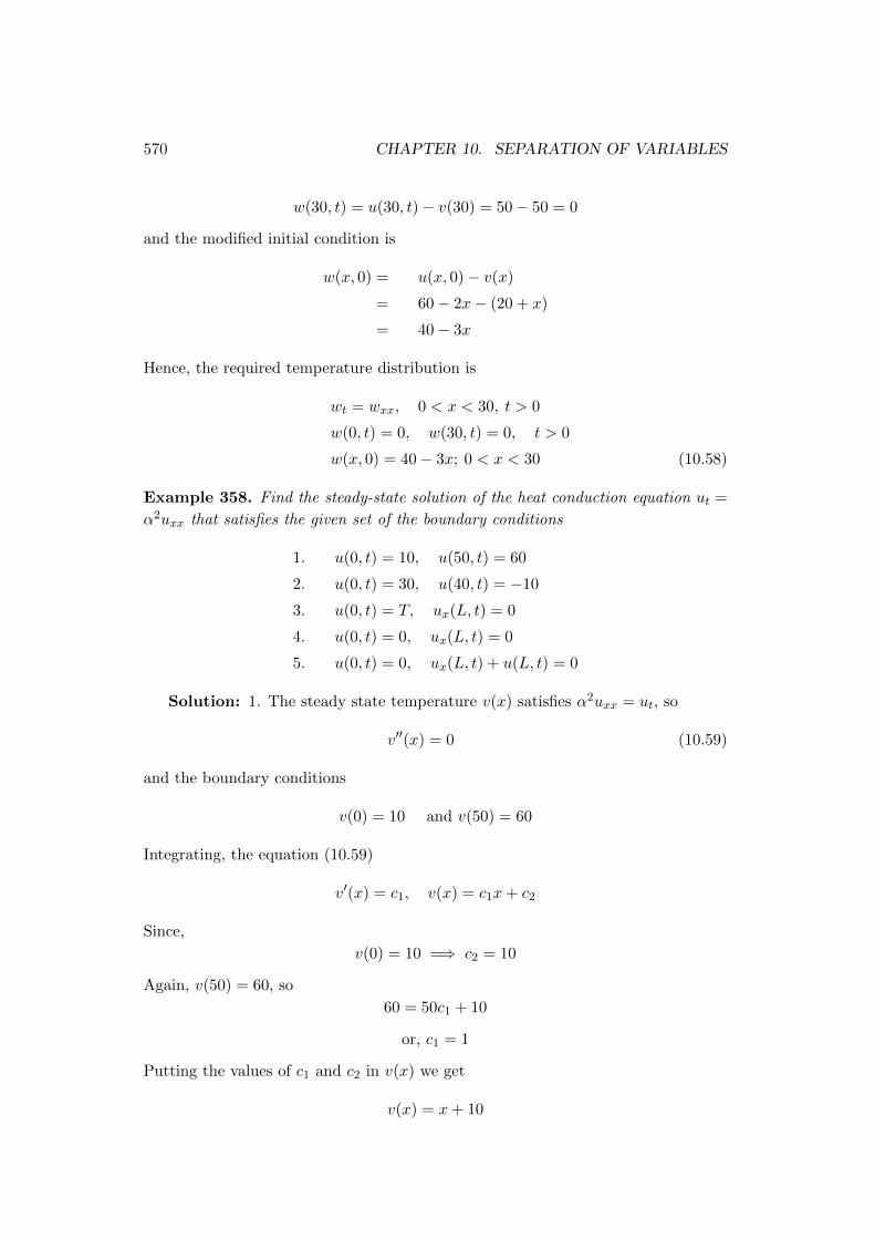
570 CHAPTER 10. SEPARATION OF VARIABLES
w(30, t) = u(30, t)− v(30) = 50− 50 = 0
and the modified initial condition is
w(x, 0) = u(x, 0)− v(x)
= 60− 2x− (20 + x)
= 40− 3x
Hence, the required temperature distribution is
wt = wxx, 0 < x < 30, t > 0
w(0, t) = 0, w(30, t) = 0, t > 0
w(x, 0) = 40− 3x; 0 < x < 30 (10.58)
Example 358. Find the steady-state solution of the heat conduction equation ut =
α2uxx that satisfies the given set of the boundary conditions
1. u(0, t) = 10, u(50, t) = 60
2. u(0, t) = 30, u(40, t) = −10
3. u(0, t) = T, ux(L, t) = 0
4. u(0, t) = 0, ux(L, t) = 0
5. u(0, t) = 0, ux(L, t) + u(L, t) = 0
Solution: 1. The steady state temperature v(x) satisfies α2uxx = ut, so
v′′(x) = 0 (10.59)
and the boundary conditions
v(0) = 10 and v(50) = 60
Integrating, the equation (10.59)
v′(x) = c1, v(x) = c1x+ c2
Since,
v(0) = 10 =⇒ c2 = 10
Again, v(50) = 60, so
60 = 50c1 + 10
or, c1 = 1
Putting the values of c1 and c2 in v(x) we get
v(x) = x+ 10

10.2. OTHER HEAT CONDUCTION PROBLEM 571
which is steady state temperature distribution.
Solution: 2. The steady state temperature v(x) satisfies α2uxx = ut, so
v′′(x) = 0 (10.60)
and the boundary conditions
v(0) = 30 and v(40) = −10
Integrating, the equation (10.60)
v′(x) = c1, v(x) = c1x+ c2
Since,
v(0) = 30 =⇒ c2 = 30
Again, v(40) = −10, so
−10 = 40c1 + 30
or, c1 = −1
Putting the values of c1 and c2 in v(x) we get
v(x) = −x+ 30
Solution: 3. The steady state temperature v(x) satisfies α2uxx = ut, so
v′′(x) = 0 (10.61)
and the boundary conditions
v(0) = T and v′(L) = 0
Integrating, the equation (10.61)
v′(x) = c1, v(x) = c1x+ c2
Since,
v(0) = T =⇒ c2 = T
Again, v′(L) = 0, so
c1 = 0
Putting the values of c1 and c2 in v(x) we get
v(x) = T
Solution: 4. The steady state temperature v(x) satisfies α2uxx = ut, so
v′′(x) = 0 (10.62)

572 CHAPTER 10. SEPARATION OF VARIABLES
and the boundary conditions
v(0) = 0 and v′(L) = 0
Integrating, the equation (10.61)
v′(x) = c1, v(x) = c1x+ c2
Since,
v(0) = 0 =⇒ c2 = 0
Again, v′(L) = 0, so
c1 = 0
Putting the values of c1 and c2 in v(x) we get
v(x) = 0
Solution: 5. The steady state temperature v(x) satisfies α2uxx = ut, so
v′′(x) = 0 (10.63)
and the boundary conditions
v(0) = T and v(L) + v′(L) = 0
Integrating, the equation (10.63)
v′(x) = c1, v(x) = c1x+ c2
Since,
v(0) = T =⇒ c2 = T
Again, v(L) + v′(L) = 0, so
c1L+ c2 + c1 = 0
or, c1(1 + L) + T = 0
or, c1 = − T
1 + L
Putting the values of c1 and c2 in v(x) we get
v(x) = − T
1 + Lx+ T =
T (1 + L− x)
1 + L

10.2. OTHER HEAT CONDUCTION PROBLEM 573
10.2.2 Bar with Insulated Ends
We consider a bar, with ends are insulated, so there is no passage of heat through
it. We know that, the rate of flow of heat across a cross section is proportional to
the rate of change of temperature in the x direction. Thus, in this case there is no
flow of heat. Hence the boundary conditions are
ux(0, t) = 0, ux(L, t) = 0, t > 0
The heat conduction problem becomes
ut = α2uxx (10.64)
the boundary conditions
ux(0, t) = 0, ux(L, t) = 0, t > 0 (10.65)
and the initial condition
u(x, 0) = f(x); 0 ≤ x ≤ L (10.66)
Let u(x, t) = X(x)T (t) be a variable separation solution of the equation (10.64) with
the given boundary and initial condition. Then
∂u
∂t= XT ′ and
∂2u
∂x2= X ′′T (10.67)
where primes refer to ordinary differentiation with respect to independent variables
x or t. Subsituting the values in (10.64) we get
XT ′ = α2X ′′T
or,X”
X=
1
α2
T ′
T= −λ (say) where λ > 0 (10.68)
Hence we obtain the following two ordinary differential equations
X ′′ + λX = 0 (10.69)
and T ′ + α2λT = 0 (10.70)
Using the boundary conditions
ux(0, t) = 0, and ux(L, t) = 0
or, X ′(0)T (t) = 0 and X ′(L)T (t) = 0
Since T (t) 6= 0, =⇒ X ′(0) = 0, X ′(L) = 0
The auxiliary equation of (10.69) is
m2 + λ = 0 (10.71)

574 CHAPTER 10. SEPARATION OF VARIABLES
Case I If λ < 0, then we may suppose λ = −µ2 where µ is real and positive. Then
by (10.71)
m2 = µ2
or, m = ±µ
Thus, the general solution of (10.69) is
X(x) = c1eµx + c2e
−µx
X ′(x) = µc1eµx − µc2e
−µx
Now X ′(0) = 0 =⇒ 0 = µc1 − µc2 (10.72)
or, c1 = c2
and X ′(L) = 0 =⇒ 0 = µc1eµL − µc2e
−µL (10.73)
Solving (10.72) and (10.73), we get
c1 = c2 = 0
Hence X(x) = 0, which is not acceptable and hence λ can not be negative.
Case II If λ > 0, then suppose that λ = µ2, where µ is real and positive. The
auxiliary equation of (10.71) is
m2 + µ2 = 0
or, m2 = −µ2
or, m = ±iµ
Hence, the general solution of (10.69) is
X(x) = c1 cosµx+ c2 sinµx (10.74)
X ′(x) = µ(−c1 sinµx+ c2 cosµx) (10.75)
Using X ′(0) = 0 in (10.75), we get
0 = −µ(c1 sin 0 + c2 cos 0)
or, c2 = 0
and using X ′(L) = 0 in (10.75), we get
0 = µ(−c1 sinµL+ c2 cosµL)
or, c1 sinµL = 0
For c1 6= 0, we must have
sinµL = 0
=⇒ µL = nπ, n = 1, 2, 3, · · ·or, µ =
nπ
L, n = 1, 2, 3, · · ·
or, λ = µ2 =n2π2
L2, n = 1, 2, 3, · · ·
10.2. OTHER HEAT CONDUCTION PROBLEM 575
Hence the equation (10.74) becomes
X = c1 cosnπx
L, n = 1, 2, 3, · · ·
Letting c2 = 1, the eigenfunction (non-zero solutions ) are
Xn(x) = cosnπx
L, n = 1, 2, 3, · · ·
associated with the eigenvalues
λn =n2π2
L2, n = 1, 2, 3 · · ·
Now turning to the equation (10.70), putting value of λ
T ′ + α2n2π2
L2T = 0
or,dT
T= −α
2n2π2
L2dt
loge T = −α2n2π2
L2t integrating without arbitrary constant
T = e−α2n2π2
L2 t, n = 1, 2, 3, · · ·
Tn(t) = e−α2n2π2
L2 t, n = 1, 2, 3, · · ·
Therefore, the functions
u0(x, t) = 1
un(x, t) = Xn(x)Tn(x)
= cosnπx
Le−
α2n2π2
L2 t, n = 1, 2, 3, · · ·
are solutions of the one diamensional heat equation under the given conditions. The
functions un are fundamental solutions of the given equation. It remains to satisfy
the initial condition
u(x, 0) = f(x), 0 ≤ x ≤ L
Now we consider linear combinations of all these solutions
u(x, t) =c0
2+∞∑n=1
cn cosnπx
Le−
α2n2π2
L2 t (10.76)
Using the initial conditions u(x, 0) = f(x), assuming the series convergent, we get
c0
2+
∞∑n=1
cn cosnπx
L= f(x)

576 CHAPTER 10. SEPARATION OF VARIABLES
which is a Fourier cosine series of f(x) with period 2L, so that the series on the left
converge to the initial temperature f(x). Therefore,
cn =2
L
∫ L
0f(x) cos
nπx
Ldx, n = 0, 1, 2, 3, · · ·
Hence, solution of the one dimensional heat equation is
u(x, t) =c0
2+
∞∑n=1
cn cosnπx
Le−
α2n2π2
L2 t
where
cn =2
L
∫ L
0f(x) cos
nπx
Ldx, n = 0, 1, 2, 3, · · ·
Example 359. Find the temperature u(x, t) of the heat equation α2uxx = ut in a
metal rod of length 25cm that is insulated on the ends as well as on the sides and
whose initial temperature distribution is u(x, 0) = x for 0 < x < 25.
Solution: Here the both ends of the rod of length 25cm are insulated, there is
no flow of heat through them.
ux(0, t) = 0, ux(25, t) = 0, t > 0
The heat conduction problem becomes
ut = α2uxx (10.77)
the boundary conditions
ux(0, t) = 0, ux(25, t) = 0, t > 0 (10.78)
and the initial conditions
u(x, 0) = x; 0 ≤ x ≤ 25 (10.79)
Let u(x, t) = X(x)T (t) be a variable separation solution of the equation (10.77) with
the given boundary and initial condition. Then
∂u
∂t= XT ′ and
∂2u
∂x2= X ′′T (10.80)
where primes refer to ordinary differentiation with respect to independent variables
x or t. Subsituting the values in (10.64) we get
XT ′ = α2X ′′T
or,X”
X=
1
α2
T ′
T= −λ (say) where λ > 0 (10.81)

10.2. OTHER HEAT CONDUCTION PROBLEM 577
Hence we obtain the following two ordinary differential equations
X ′′ + λX = 0 (10.82)
and T ′ + α2λT = 0 (10.83)
Using the boundary conditions
ux(0, t) = 0, and ux(25, t) = 0
or, X ′(0)T (t) = 0 and X ′(25)T (t) = 0
Since T (t) 6= 0, =⇒ X ′(0) = 0, X ′(25) = 0
The auxiliary equation of (10.82) is
m2 + λ = 0 (10.84)
Case I If λ < 0, then we may suppose λ = −µ2 where µ is real and positive. Then
by (10.84)
m2 = µ2
or, m = ±µ
Thus, the general solution of (10.82) is
X(x) = c1eµx + c2e
−µx
X ′(x) = µc1eµx − µc2e
−µx
Now X ′(0) = 0 =⇒ 0 = µc1 − µc2 (10.85)
or, c1 = c2
and X ′(25) = 0 =⇒ 0 = µc1eµ25 − µc2e
−µ25 (10.86)
Solving (10.72) and (10.73), we get
c1 = c2 = 0
Hence X(x) = 0, which is not acceptable and hence λ can not be negative.
Case II If λ > 0, then suppose that λ = µ2, where µ is real and positive. The
auxiliary equation of (10.71) is
m2 + µ2 = 0
or, m2 = −µ2
or, m = ±iµ
Hence, the general solution of (10.82) is
X(x) = c1 cosµx+ c2 sinµx (10.87)
X ′(x) = µ(−c1 sinµx+ c2 cosµx) (10.88)

578 CHAPTER 10. SEPARATION OF VARIABLES
Using X ′(0) = 0 in (10.88), we get
0 = −µ(c1 sin 0 + c2 cos 0)
or, c2 = 0
and using X ′(25) = 0 in (10.75), we get
0 = µ(−c1 sin 25µ+ c2 cos 25µ)
or, c1 sin 25µ = 0
For c1 6= 0, we must have
sin 25µ = 0
=⇒ 25µ = nπ, n = 1, 2, 3, · · ·or, µ =
nπ
25, n = 1, 2, 3, · · ·
or, λ = µ2 =n2π2
625, n = 1, 2, 3, · · ·
Hence the equation (10.87) becomes
X(x) = c1 cosnπx
25, n = 1, 2, 3, · · ·
Letting c2 = 1, the eigenfunction (non-zero solutions ) are
Xn(x) = cosnπx
25, n = 1, 2, 3, · · ·
associated with the eigenvalues
λn =n2π2
625, n = 1, 2, 3 · · ·
Now turning to the equation (10.83), putting value of λ
T ′ + α2n2π2
625T = 0
or,dT
T= −α
2n2π2
625dt
loge T = −α2n2π2
625t integrating without arbitrary constant
T = e−α2n2π2
625t, n = 1, 2, 3, · · ·
Tn(t) = e−α2n2π2
625t, n = 1, 2, 3, · · ·
Therefore, the functions
u0(x, t) = 1
un(x, t) = Xn(x)Tn(x)
= cosnπx
25e−
α2n2π2
625t, n = 1, 2, 3, · · ·

10.2. OTHER HEAT CONDUCTION PROBLEM 579
are solutions of the one diamensional heat equation under the given conditions. The
functions un are fundamental solutions of the given equations. It remains to satisfy
the initial condition
u(x, 0) = f(x), 0 ≤ x ≤ 25
Now we consider linear combinations of all these solutions
u(x, t) =c0
2+
∞∑n=1
cn cosnπx
25e−
α2n2π2
625t (10.89)
Using the initial conditions u(x, 0) = x, assuming the series convergent, we get
c0
2+∞∑n=1
cn cosnπx
25= x
which is a Fourier series of x with period 2L = 50, so that the series on the left
converge to the initial temperature x. Therefore,
cn =2
25
∫ 25
0x cos
nπx
Ldx, n = 0, 1, 2, 3, · · ·
For n = 0, c0 =2
25
∫ 25
0x · 1dx
=2
25
[x2
2
]25
0
=2
25
[625
2− 02
2
]= 25
For n 6= 0, cn =2
L
∫ L
0f(x) cos
nπx
Ldx
=2
25
∫ 25
0x cos
nπx
25dx
=2
25
[x
∫cos
nπx
25dx
]25
0
−∫ 25
0
(dx
dx
∫cos
nπx
25dx
)dx
=2
25
[25
nπx sin
nπx
25
]25
0
− 25
nπ
∫ 25
0sin
nπx
25dx
=2
25
−0 +
252
n2π2
[cos
nπx
25
]25
0
=
2
25
252
n2π2(cosnπ − 1)
=50
n2π2(cosnπ − 1)
=
− 100n2π2 for n is odd
0 for n is even
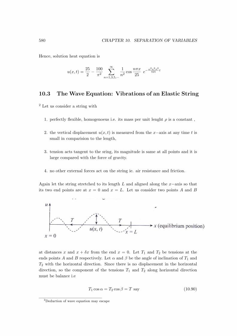
580 CHAPTER 10. SEPARATION OF VARIABLES
Hence, solution heat equation is
u(x, t) =25
2− 100
π2
∞∑n=1,3,5,···
1
n2cos
nπx
25e−
α2n2π2
625t
10.3 The Wave Equation: Vibrations of an Elastic String
2 Let us consider a string with
1. perfectly flexible, homogenoeus i.e. its mass per unit lenght ρ is a constant ,
2. the vertical displacement u(x, t) is measured from the x−axis at any time t is
small in comparision to the length,
3. tension acts tangent to the sring, its magnitude is same at all points and it is
large compared with the force of gravity.
4. no other external forces act on the string ie. air resistance and friction.
Again let the string stretched to its length L and aligned along the x−axis so that
its two end points are at x = 0 and x = L. Let us consider two points A and B
at distances x and x + δx from the end x = 0. Let T1 and T2 be tensions at the
ends points A and B respectively. Let α and β be the angle of inclination of T1 and
T2 with the horizontal direction. Since there is no displacement in the horizontal
direction, so the component of the tensions T1 and T2 along horizontal direction
must be balance i.e
T1 cosα = T2 cosβ = T say (10.90)
2Deduction of wave equation may escape

10.3. THE WAVE EQUATION: VIBRATIONS OF AN ELASTIC STRING 581
In vertical direction, we have, from Newton’s law of motion
T2 sinβ − T1 sinβ = ρ δx∂2u
∂t2
or,T
cosβsinβ − T
cosαsinα = ρδx
∂2u
∂t2from (10.90)
or,ρδx
T
∂2u
∂t2= tanβ − tanα
or,ρδx
T
∂2u
∂t2=∂u
∂x
∣∣∣∣x+δx
− ∂u
∂x
∣∣∣∣x
or,ρ
T
∂2u
∂t2=
∂u(x+δx)∂x − ∂u
∂x
δx
Letting δ → 0, we get
ρ
T
∂2u
∂t2=∂2u
∂t2
or, utt = a2uxx (10.91)
where
a2 =T
ρ
and a is a constant and its unit is length/time, i.e. of the velocity. It is known as
velocity propagation of the waves along the string. Equation (10.91) is known as
one diamensional wave equation.
For the complete description of the motion of the string, we specify the suitable
initial and boundary conditions for the displacement u(x, t).
The end point are assume to be fixed, and therefore the boundary conditions are
u(0, t) = 0, u(L, t) = 0 t ≥ 0 (10.92)
Sine the differential equation is of second order with respect to t, so we need two
initial conditions . These are (a) initial position of the string
u(x, 0) = f(x) 0 ≤ x ≤ L

582 CHAPTER 10. SEPARATION OF VARIABLES
(b) initial velocity of the string
ut(x, 0) = g(x) 0 ≤ x ≤ L
where f and g are given functions. In order to consistent results we have
f(0) = f(L) = 0 and g(0) = g(L) = 0 (10.93)
10.3.1 General Solution of One Dimensional Wave Equation
The vertical displacement u(x, t) must satisfy the wave equation
utt = a2uxx, 0 < x < L, t > 0 (10.94)
Let u(x, t) = X(x)T (t) be a variable separation solution of the equation (10.94) with
the given boundary and initial condition. Then
∂2u
∂t2= XT ′′ and
∂2u
∂x2= X ′′T (10.95)
where primes refer to ordinary differentiation with respect to independent variables
x or t. Subsituting the values in (10.94) we get
XT ′ = a2X ′′T
or,X”
X=
1
a2
T ′
T= −λ (10.96)
Hence we obtain the following two ordinary differential equations
X ′′ + λX = 0 (10.97)
and T ′′ + a2λT = 0 (10.98)
Now we have the flowing cases
Case I: When λ = 0, the equations (10.97) and (10.98)
X ′′ = 0, T ′′ = 0
Integrating,
X ′(x) = a1, T ′(t) = a2
and X(x) = a1x+ a3, T (t) = a2t+ a4
Case II : When λ < 0, let λ = −µ2. The roots of the charateristic equation of
(10.97) and (10.98) are
±µ and ± aµ
The solutions of (10.97) and (10.98) are
X(x) = b1eµx + c2e
−µx, and T (t) = b3eaµt + b4e
−aµt

10.3. THE WAVE EQUATION: VIBRATIONS OF AN ELASTIC STRING 583
Case III: When λ > 0, let λ = −µ2. The roots of the charateristic equation of
(10.97) and (10.98) are
±iµ and ± iaµ
The solutions of (10.97) and (10.98) are
X(x) = c1 cosµx+ c2 sinµx and T (t) = c3 cos aµt+ c4 sin aµt
Thus the various possible solutions are
u(x, t) = (a1x+ a3)(a2t+ a4)
u(x, t) =(b1e
µx + c2e−µx) (b3eaµt + b4e
−aµt)u(x, t) = (c1 cosµx+ c2 sinµx) (c3 cos aµt+ c4 sin aµt)
We have to choose that solution which consistent with the the physical nature of
the problem. The vibration u(x, t) must be periodic function of x and t. Thus, the
true solution is, which contains trigonometric functions i. e.
u(x, t) = (c1 cosµx+ c2 sinµx) (c3 cos aµt+ c4 sin aµt)
For this we chose λ > 0.
10.3.2 Vibration of Elastic String with Non-zero Initial Displace-
ment
Let us suppose that the string is distrubed from its equalibrium position and then
released at time t = 0 with initial velocity to vibrate freely. Then the vibration must
satisfy the wave equation
or, utt = a2uxx 0 < x < L, t > 0 (10.99)
the boundary conditions
u(0, t) = 0, u(L, t) = 0, t ≥ 0 (10.100)
and initial conditions
u(x, 0) = f(x), ut(x, 0) = 0, 0 ≤ x ≤ L (10.101)
where f is a given function describing the confugration of the string at t = 0.
Let u(x, t) = X(x)T (t) be a variable separation solution of the equation (10.99) with
the given boundary and initial conditions. Then
∂2u
∂t2= XT ′′ and
∂2u
∂x2= X ′′T (10.102)

584 CHAPTER 10. SEPARATION OF VARIABLES
where primes refer to ordinary differentiation with respect to independent variables
x or t. Subsituting the values in (10.99) we get
α2X ′′T = XT ′′
or,X”
X=
1
a2
T ′′
T= −λ (say) where λ > 0 (10.103)
Hence we obtain the following two ordinary differential equations
X ′′ + λX = 0 (10.104)
and T ′′ + a2λT = 0 (10.105)
The auxiliary equation of (10.104) is
m2 + λ2 = 0
or, m2 = −λ2
or, m = ±i√λ
Hence, the general solution of (10.104) is
X(x) = c1 cos√λx+ c2 sin
√λx (10.106)
Using the boundary conditions
u(0, t) = 0, and u(L, t) = 0
or, X(0)T (t) = 0 and X(L)T (t) = 0
Since T (t) 6= 0, =⇒ X(0) = 0, X(L) = 0
Again, using X(0) = 0 in (10.106), we get
0 = c1 cos 0 + c2 sin 0
or, c1 = 0
and using using X(L) = 0 in (10.106), we get
0 = c1 cos√λL+ c2 sin
√λL
or, c2 sin√λL = 0
For c2 6= 0, we must have
sin√λL = 0
=⇒√λL = nπ, n = 1, 2, 3, · · ·
or,√λ =
nπ
L, n = 1, 2, 3, · · ·
or, λ =n2π2
L2, n = 1, 2, 3, · · ·

10.3. THE WAVE EQUATION: VIBRATIONS OF AN ELASTIC STRING 585
Hence the equation (10.106) becomes
X = c2 sinnπx
L, n = 1, 2, 3, · · ·
Letting c2 = 1, the eigenfunction (non-zero solutions ) are
Xn(x) = sinnπx
L, n = 1, 2, 3, · · ·
associated with the eigenvalues
λn =n2π2
L2, n = 1, 2, 3 · · ·
The auxiliary equation of (10.105) is
m2 + a2λ = 0
m = ±a√λi = ±anπ
Li = ±nπa
Li
The general solution (10.105) is
T (t) = c1 cosnπat
L+ c2 sin
nπat
L(10.107)
T ′(t) = −nπaL
k1 sinnπat
L+nπa
Lk2 cos
nπat
L(10.108)
Also, we have
ut(x, 0) = 0 =⇒ X(x)T ′(0) = 0
=⇒ T ′(0) = 0
From (10.108), we get
T ′(0) = −nπaL
k1 sinnπa0
L+nπa
Lk2 cos
nπa0
L= 0
=⇒ k2 = 0
Thus, from (10.107), taking k1 = 1
T = cosnπat
L
Thus, the function
un(x, t) = sinnπx
Lcos
nπat
L(10.109)
consitute the fundamental solutions of (10.99) is along with the boundary conditions
and the initial condition ut(x, 0) = 0. It remains to satisfy the non-homogeous initial
condition
u(x, 0) = f(x), 0 ≤ x ≤ L

586 CHAPTER 10. SEPARATION OF VARIABLES
We assume u(x, t) has the form
u(x, t) =
∞∑n=1
bnun(x, t) =
∞∑n=1
bn sinnπx
Lcos
nπat
L, n = 1, 2, 3 · · · (10.110)
where
u(x, 0) =∞∑n=1
bn sinnπx
L(10.111)
This is the Fourier sine series of f(x) of period 2L and bn are given by
bn =2
L
∫ L
0f(x) sin
nπx
L, n = 1, 2, 3 · · · (10.112)
Example 360. Consider a vibrating string of length L = 50 that satisfy the wave
equation
4uxx = utt
Assume that the ends of the string are fixed and that the string is set in motion with
no initial velocity from the initial postion.
u(x, 0) = f(x) =
x10 , 0 ≤ x ≤ 10
30−x20 , 10 ≤ x ≤ 30
Find the displacement u(x, t) of the string and describe its motion through one period.
Solution: Here L = 30. The given wave equation is
or, utt = 4uxx 0 < x < 30, t > 0 (10.113)
the boundary conditions
u(0, t) = 0, u(30, t) = 0, t ≥ 0 (10.114)
and initial conditions
u(x, 0) = f(x) =
x10 , 0 ≤ x ≤ 10
30−x20 , 10 ≤ x ≤ 30
ut(x, 0) = 0, 0 ≤ x ≤ 30 (10.115)
Let u(x, t) = X(x)T (t) be a variable separation solution of the equation (10.113)
with the given boundary and initial conditions. Then
∂2u
∂t2= XT ′′ and
∂2u
∂x2= X ′′T (10.116)

10.3. THE WAVE EQUATION: VIBRATIONS OF AN ELASTIC STRING 587
where primes refer to ordinary differentiation with respect to independent variables
x or t. Subsituting the values in (10.113) we get
4X ′′T = XT ′′
or,X”
X=
1
4
T ′′
T= −λ (say) where λ > 0 (10.117)
Hence we obtain the following two ordinary differential equations
X ′′ + λX = 0 (10.118)
and T ′′ + 4λT = 0 (10.119)
The auxiliary equation of (10.118) is
m2 + λ2 = 0
or, m2 = −λ2
or, m = ±i√λ
Hence, the general solution of (10.118) is
X(x) = c1 cos√λx+ c2 sin
√λx (10.120)
Using the boundary conditions
u(0, t) = 0, and u(30, t) = 0
or, X(0)T (t) = 0 and X(30)T (t) = 0
Since T (t) 6= 0, =⇒ X(0) = 0, X(30) = 0
Again, using X(0) = 0 in (10.120), we get
0 = c1 cos 0 + c2 sin 0
or, c1 = 0
and using using X(30) = 0 in (10.120), we get
0 = c1 cos(30√λ) + c2 sin(30
√λ)
or, c2 sin(30√λ) = 0
For c2 6= 0, we must have
sin(30√λ) = 0
=⇒ 30√λ = nπ, n = 1, 2, 3, · · ·
or,√λ =
nπ
30, n = 1, 2, 3, · · ·
or, λ =n2π2
900, n = 1, 2, 3, · · ·

588 CHAPTER 10. SEPARATION OF VARIABLES
Hence the equation (10.120) becomes
X = c2 sinnπx
30, n = 1, 2, 3, · · ·
Letting c2 = 1, the eigenfunction (non-zero solutions ) are
Xn(x) = sinnπx
30, n = 1, 2, 3, · · ·
associated with the eigenvalues
λn =n2π2
900, n = 1, 2, 3 · · ·
The auxiliary equation of (10.119) is
m2 + 4λ = 0
m = ±2√λi = ±2
nπ
30i = ±2nπ
30i
The general solution (10.119) is
T (t) = k1 cos2nπt
30+ k2 sin
2nπt
30(10.121)
T ′(t) = −2nπ
30k1 sin
2nπt
30+
2nπ
30k2 cos
2nπt
30(10.122)
Also, we have
ut(x, 0) = 0 =⇒ X(x)T ′(0) = 0
=⇒ T ′(0) = 0
From (10.108), we get
T ′(0) = −2nπ
30k1 sin
2nπ0
30+
2nπ
30k2 cos
2nπ0
30= 0
=⇒ k2 = 0
Thus, from (10.121), taking k1 = 1
T = cos2nπt
30
Thus, the function
un(x, t) = sinnπx
30cos
2nπt
30(10.123)
consititute the fundamental solutions of (10.113) is along with the boundary condi-
tions and the initial condition ut(x, 0) = 0. It remains to satisfy the non-homogeous
initial condition
u(x, 0) = f(x) =
x10 , 0 ≤ x ≤ 10
30−x20 , 10 ≤ x ≤ 30

10.3. THE WAVE EQUATION: VIBRATIONS OF AN ELASTIC STRING 589
We assume u(x, t) has the form
u(x, t) =
∞∑n=1
bnun(x, t) =
∞∑n=1
bn sinnπx
30cos
2nπt
30, n = 1, 2, 3 · · · (10.124)
where
u(x, 0) =
∞∑n=1
bn sinnπx
30= f(x)
This is the Fourier sine series of f(x) of period 2L and bn are given by
bn =2
30
∫ L
0f(x) sin
nπx
30dx, n = 1, 2, 3 · · · (10.125)
=2
30
∫ 10
0f(x) sin
nπx
30dx+
2
30
∫ 30
10f(x) sin
nπx
30dx
=2
30
∫ 10
0
x
10sin
nπx
30dx+
2
30
∫ 30
10
30− x20
sinnπx
30dx
=2
300
[x
∫sin
nπx
30dx
]10
0
−∫ 10
0
[dx
dx
∫sin
nπx
30dx
]dx
+2
600
[(30− x)
∫sin
nπx
30dx
]30
10
−∫ 30
10
[d(30− x)
dx
∫sin
nπx
30dx
]dx
=2
300
[−30x
nπcos
nπx
30
]10
0
+30
nπ
∫ 10
0cos
nπx
30dx
+2
600
[−30(30− x)
nπcos
nπx
30
]30
10
− 30
nπ
∫ 30
10cos
nπx
30dx
=2
300
[−30× 10
nπcos
10nπ
30− 0
]+
900
n2π2
[sin
nπx
30
]10
0
+
2
600
[−0 +
600
nπcos
10nπ
30
]− 900
n2π2
[sin
nπx
30
]30
10
=
2
300
−300
nπcos
nπ
3+
900
n2π2
[sin
10nπ
30− 0
]+
2
600
600
nπcos
nπ
3− 900
n2π2
[sin
30nπ
30− sin
10nπ
30
]=
2
300
−300
nπcos
nπ
3+
900
n2π2
[sin
nπ
3− 0]
+2
600
600
nπcos
nπ
3− 900
n2π2
[sinnπ − sin
nπ
3
]= − 2
nπcos
nπ
3+
6
n2π2sin
nπ
3+
2
nπcos
nπ
3+
3
n2π2sin
nπ
3
=9
n2π2sin
nπ
3

590 CHAPTER 10. SEPARATION OF VARIABLES
Hence the rquired solution is
u(x, t) =
∞∑n=1
bnun(x, t) =
∞∑n=1
bn sinnπx
30cos
2nπt
30, n = 1, 2, 3 · · ·
where
bn =9
n2π2sin
nπ
3
u(x, t) gives the displacement of the string at any point x at any time t. The motion
is periodic in time with period 30, so it is suffices to analyze for 0 ≤ t ≤ 30.
Example 361. Consider an elastic string of length L whose ends are held fixed. The
string is set in motion with no initial velocity from an initial position u(x, 0) = f(x).
Let Find the displacement u(x, t) for the given initial position f(x).
(1) f(x) =
4xL 0 ≤ x ≤ L
4
1 L4 ≤ x <
3L4
4(L−x)L
3L4 ≤ x ≤ L
(2) f(x) =
1 L
2 − 1 < x < L2 + 1 (L > 2)
0 otherwise
Solution: The wave equation is
utt = a2uxx 0 < x < L, t > 0 (10.126)
the boundary conditions
u(0, t) = 0, u(L, t) = 0, t ≥ 0 (10.127)
and initial conditions
u(x, 0) = f(x) from 1 or 2
ut(x, 0) = 0, 0 ≤ x ≤ L (10.128)
Let u(x, t) = X(x)T (t) be a variable separation solution of the equation (10.126)
with the given boundary and initial condition. Then
∂2u
∂t2= XT ′′ and
∂2u
∂x2= X ′′T (10.129)
where primes refer to ordinary differentiation with respect to independent variables
x or t. Subsituting the values in (10.126) we get
a2X ′′T = XT ′′
or,X”
X=
T ′′
a2T= −λ (say) where λ > 0 (10.130)
10.3. THE WAVE EQUATION: VIBRATIONS OF AN ELASTIC STRING 591
Hence we obtain the following two ordinary differential equations
X ′′ + λX = 0 (10.131)
and T ′′ + a2λT = 0 (10.132)
The auxiliary equation of (10.131) is
m2 + λ2 = 0
or, m2 = −λ2
or, m = ±i√λ
Hence, the general solution of (10.131) is
X(x) = c1 cos√λx+ c2 sin
√λx (10.133)
Using the boundary conditions
u(0, t) = 0, and u(L, t) = 0
or, X(0)T (t) = 0 and X(L)T (t) = 0
Since T (t) 6= 0, =⇒ X(0) = 0, X(L) = 0
Again, using X(0) = 0 in (10.133), we get
0 = c1 cos 0 + c2 sin 0
or, c1 = 0
and using using X(L) = 0 in (10.133), we get
0 = c1 cos(L√λ) + c2 sin(L
√λ)
or, c2 sin(L√λ) = 0
For c2 6= 0, we must have
sin(L√λ) = 0
=⇒ L√λ = nπ, n = 1, 2, 3, · · ·
or,√λ =
nπ
L, n = 1, 2, 3, · · ·
or, λ =n2π2
L2, n = 1, 2, 3, · · ·
Hence the equation (10.133) becomes
X = c2 sinnπx
L, n = 1, 2, 3, · · ·
Letting c2 = 1, the eigenfunction (non-zero solutions ) are
Xn(x) = sinnπx
L, n = 1, 2, 3, · · ·

592 CHAPTER 10. SEPARATION OF VARIABLES
associated with the eigenvalues
λn =n2π2
L2, n = 1, 2, 3 · · ·
The auxiliary equation of (10.132) is
m2 + a2λ = 0
m = ±a√λi = ±nπa
Li = ±nπa
Li
The general solution (10.132) is
T (t) = k1 cosnπat
L+ k2 sin
nπat
L(10.134)
T ′(t) = −nπaL
k1 sinnπat
L+nπa
Lk2 cos
nπat
L(10.135)
Also, we have
ut(x, 0) = 0 =⇒ X(x)T ′(0) = 0
=⇒ T ′(0) = 0
From (10.135), we get
T ′(0) = −nπaL
k1 sinnπ0
L+nπa
Lk2 cos
nπ0
L= 0
=⇒ k2 = 0
Thus, from (10.134), taking k1 = 1
T = cosnπat
L
Thus, the function
un(x, t) = sinnπx
Lcos
nπat
L(10.136)
consitute the fundamental solutions of (10.126) is along with the boundary condi-
tions and the initial condition ut(x, 0) = 0. It remains to satisfy the non-homogeous
initial condition. We assume u(x, t) has the form
u(x, t) =∞∑n=1
bnun(x, t) =∞∑n=1
bn sinnπx
Lcos
nπat
L, n = 1, 2, 3 · · · (10.137)
where
u(x, 0) =∞∑n=1
bn sinnπx
L= f(x)
This is the Fourier sine series of f(x) of period 2L and bn are given by
bn =2
L
∫ L
0f(x) sin
nπx
Ldx, n = 1, 2, 3 · · · (10.138)
10.3. THE WAVE EQUATION: VIBRATIONS OF AN ELASTIC STRING 593
1. Let
f(x) =
4xL 0 ≤ x ≤ L
4
1 L4 < x < 3L
4
4(L−x)L
3L4 ≤ x ≤ L
From (10.138)
bn =2
L
∫ L/4
0f(x) sin
nπx
Ldx+
2
L
∫ 3L/4
L/4f(x) sin
nπx
Ldx+
2
L
∫ L
3L/4f(x) sin
nπx
Ldx
=2
L
∫ L/4
0
4x
Lsin
nπx
Ldx+
2
L
∫ 3L/4
L/4sin
nπx
Ldx+
2
L
∫ L
3L/4
4(L− x)
Lsin
nπx
Ldx
=8
L2
[x
∫sin
nπx
Ldx
]L/40
−∫ L/4
0
(dx
dx
∫sin
nπx
L
)dx
− 2
L
L
nπ
[cos
nπx
L
]3L/4
L/4
+8
L2
[(L− x)
∫sin
nπx
Ldx
]L3L/4
−∫ L
3L/4
[d(L− x)
dx
∫sin
nπx
Ldx
]dx
=8
L2
L
nπ
[−x cos
nπx
L
]L/40
+L
nπ
∫ L/4
0cos
nπx
Ldx
− 2
nπ
[cos
3nπ
4− cos
nπ
4
]
+8
L2
L
nπ
[−(L− x) cos
nπx
L
]L3L/4− L
nπ
∫ L
3L/4cos
nπx
Ldx
=8
L2
L
nπ
(−L
4cos
nπ
4+ 0
)+
L2
n2π2
[sin
nπx
L
]L/40
− 2
nπ
[cos
3nπ
4− cos
nπ
4
]+
8
L2
L
nπ
[0 +
L
4cos
3nπ
4
]− L2
n2π2
[sin
nπx
L
]L3L/4
= − 2
nπcos
nπ
4+
8
n2π2
[sin
nπ
4− 0]− 2
nπ
[cos
3nπ
4− cos
nπ
4
]+
2
nπcos
3nπ
4− 8
n2π2
[sinnπ − sin
3nπ
4
]=
8
n2π2
(sin
nπ
4+ sin
3nπ
4
)(10.139)
Hence from (10.137)
u(x, t) =8
π2
∞∑n=1
1
n2
(sin
nπ
4+ sin
3nπ
4
)sin
nπx
Lcos
nπat
L
which is required expression for the displacement.
2. Let
f(x) =
1 L
2 − 1 < x < L2 + 1 (L > 2)
0 otherwise

594 CHAPTER 10. SEPARATION OF VARIABLES
From (10.138)
bn =2
L
∫ L
0f(x) sin
nπx
Ldx
=2
L
∫ L/2−1
0f(x) sin
nπx
Ldx+
2
L
∫ L/2+1
L/2−1f(x) sin
nπx
Ldx+
2
L
∫ L
L/2+1f(x) sin
nπx
Ldx
=2
L
∫ L/2+1
L/2−1sin
nπx
Ldx
=2
L
L
nπ
[− cos
nπx
L
]L/2+1
L/2−1
=2
nπ
[− cos
(nπ2
+nπ
L
)+ cos
(nπ2− nπ
L
)]=
2
nπ
[cos(nπ
2− nπ
L
)− cos
(nπ2
+nπ
L
)]=
4
nπsin
nπ
2sin
nπ
L
Hence from (10.137)
u(x, t) =4
π
∞∑n=1
1
nsin
nπ
2sin
nπ
Lsin
nπx
Lcos
nπat
L
which is required expression for the displacement.
10.3.3 Vibration of Elastic String with Non-zero Initial Velocity
Let us suppose that the string is distrubed from its equalibrium position and then
released at time t = 0 with initial velocity g(x). Then the vibration must satisfy the
wave equation
or, utt = a2uxx 0 < x < L, t > 0 (10.140)
the boundary conditions
u(0, t) = 0, u(L, t) = 0, t ≥ 0 (10.141)
and initial conditions
u(x, 0) = 0, ut(x, 0) = g(x), 0 ≤ x ≤ L (10.142)
where g is initial velocity at the point x of the string.
Let u(x, t) = X(x)T (t) be a variable separation solution of the equation (10.140)
with the given boundary and initial condition. Then
∂2u
∂t2= XT ′′ and
∂2u
∂x2= X ′′T (10.143)

10.3. THE WAVE EQUATION: VIBRATIONS OF AN ELASTIC STRING 595
where primes refer to ordinary differentiation with respect to independent variables
x or t. Subsituting the values in (10.12) we get
α2X ′′T = XT ′′
or,X”
X=
1
a2
T ′′
T= −λ (say) where λ > 0 (10.144)
Hence we obtain the following two ordinary differential equations
X ′′ + λX = 0 (10.145)
and T ′′ + a2λT = 0 (10.146)
The auxiliary equation of (10.145) is
m2 + λ2 = 0
or, m2 = −λ2
or, m = ±i√λ
Hence, the general solution of (10.145) is
X(x) = c1 cos√λx+ c2 sin
√λx (10.147)
Using the boundary conditions
u(0, t) = 0, and u(L, t) = 0
or, X(0)T (t) = 0 and X(L)T (t) = 0
Since T (t) 6= 0, =⇒ X(0) = 0, X(L) = 0
Again, using X(0) = 0 in (10.147), we get
0 = c1 cos 0 + c2 sin 0
or, c1 = 0
and using using X(L) = 0 in (10.147), we get
0 = c1 cos√λL+ c2 sin
√λL
or, c2 sin√λL = 0
For c2 6= 0, we must have
sin√λL = 0
=⇒√λL = nπ, n = 1, 2, 3, · · ·
or,√λ =
nπ
L, n = 1, 2, 3, · · ·
or, λ =n2π2
L2, n = 1, 2, 3, · · ·

596 CHAPTER 10. SEPARATION OF VARIABLES
Hence the equation (10.147) becomes
X = c2 sinnπx
L, n = 1, 2, 3, · · ·
Letting c2 = 1, the eigenfunction (non-zero solutions ) are
Xn(x) = sinnπx
L, n = 1, 2, 3, · · ·
associated with the eigenvalues
λn =n2π2
L2, n = 1, 2, 3 · · ·
The auxiliary equation of (10.146) is
m2 + a2λ = 0
m = ±a√λi = ±anπ
Li = ±nπa
Li
The general solution (10.105) is
T (t) = k1 cosnπat
L+ k2 sin
nπat
L(10.148)
As u(x, 0) = 0 =⇒ X(x)T (0) = 0 =⇒ T (0) = 0
(10.149)
From (10.148), we get
T (0) = k1 cosnπa0
L+ k2 sin
nπa0
L
or, 0 = k1
=⇒ k1 = 0
Thus, from (10.148), taking k1 = 1
T = sinnπat
L
Thus, the function
un(x, t) = X(x)T (t) = sinnπx
Lcos
nπat
L(10.150)
consititute the fundamental solutions of (10.140) is along with the boundary condi-
tions and the initial condition u(x, 0) = 0. It remains to satisfy the non-homogeous
initial condition
ut(x, 0) = g(x), 0 ≤ x ≤ L
We assume u(x, t) has the form
u(x, t) =
∞∑n=1
bnun(x, t) =
∞∑n=1
bn sinnπx
Lsin
nπat
L(10.151)

10.3. THE WAVE EQUATION: VIBRATIONS OF AN ELASTIC STRING 597
Differentiating partially with respect to t, we get
ut(x, t) =∞∑n=1
bn∂
∂xun(x, t) =
L
nπa
∞∑n=1
bn sinnπx
Lcos
nπat
L, (10.152)
∴ ut(x, 0) = g(x)
or,∞∑n=1
L
nπabn sin
nπx
L= g(x)
Thus, the quantities nπaL bn are the coefficients in the Fourier sine series of the period
2L for g. Therefore,
nπa
Lbn =
2
L
∫ L
0g(x) sin
nπx
Ldx, n = 1, 2, 3 · · ·
or, bn =2
nπa
∫ L
0g(x) sin
nπx
Ldx, n = 1, 2, 3, · · ·
Hence, the required solution is
u(x, t) =∞∑n=1
bn sinnπx
Lsin
nπat
L
where
bn =2
nπa
∫ L
0g(x) sin
nπx
Ldx
Example 362. Consider an elastic string of length L, where both ends are held fixed.
The string is set in motion from its equilibrium position with an initial velocity
ut(x, 0) = g(x) =
2xL for 0 ≤ x ≤ L
2
2(L−x)L for L
2 < x ≤ L
Find the initial displacement u(x, t).
Solution: Here, the string is distrubed from its equalibrium position and then
released at time t = 0 with initial velocity g(x). Then the vibration must satisfy the
wave equation
or, utt = a2uxx 0 < x < L, t > 0 (10.153)
the boundary conditions
u(0, t) = 0, u(L, t) = 0, t ≥ 0 (10.154)
and initial conditions
u(x, 0) = 0, ut(x, 0) = g(x) =
2xL for 0 ≤ x ≤ L
2
2(L−x)L for L
2 < x ≤ L(10.155)

598 CHAPTER 10. SEPARATION OF VARIABLES
where g is initial velocity at the point x of the string.
Let u(x, t) = X(x)T (t) be a variable separation solution of the equation (10.153)
with the given boundary and initial condition. Then
∂2u
∂t2= XT ′′ and
∂2u
∂x2= X ′′T (10.156)
where primes refer to ordinary differentiation with respect to independent variables
x or t. Subsituting the values in (10.153) we get
α2X ′′T = XT ′′
or,X”
X=
1
a2
T ′′
T= −λ (say) where λ > 0 (10.157)
Hence we obtain the following two ordinary differential equations
X ′′ + λX = 0 (10.158)
and T ′′ + a2λT = 0 (10.159)
The auxiliary equation of (10.158) is
m2 + λ2 = 0
or, m2 = −λ2
or, m = ±i√λ
Hence, the general solution of (10.145) is
X(x) = c1 cos√λx+ c2 sin
√λx (10.160)
Using the boundary conditions
u(0, t) = 0, and u(L, t) = 0
or, X(0)T (t) = 0 and X(L)T (t) = 0
Since T (t) 6= 0, =⇒ X(0) = 0, X(L) = 0
Again, using X(0) = 0 in (10.160), we get
0 = c1 cos 0 + c2 sin 0
or, c1 = 0
and using X(L) = 0 in (10.147), we get
0 = c1 cos√λL+ c2 sin
√λL
or, c2 sin√λL = 0

10.3. THE WAVE EQUATION: VIBRATIONS OF AN ELASTIC STRING 599
For c2 6= 0, we must have
sin√λL = 0
=⇒√λL = nπ, n = 1, 2, 3, · · ·
or,√λ =
nπ
L, n = 1, 2, 3, · · ·
or, λ =n2π2
L2, n = 1, 2, 3, · · ·
Hence the equation (10.147) becomes
X = c2 sinnπx
L, n = 1, 2, 3, · · ·
Letting c2 = 1, the eigenfunction (non-zero solutions ) are
Xn(x) = sinnπx
L, n = 1, 2, 3, · · ·
associated with the eigenvalues
λn =n2π2
L2, n = 1, 2, 3 · · ·
The auxiliary equation of (10.159) is
m2 + a2λ = 0
m = ±a√λi = ±anπ
Li = ±nπa
Li
The general solution (10.159) is
T (t) = k1 cosnπat
L+ k2 sin
nπat
L(10.161)
As u(x, 0) = 0 =⇒ X(x)T (0) = 0 =⇒ T (0) = 0
(10.162)
From (10.161), we get
T (0) = k1 cosnπa0
L+ k2 sin
nπa0
L
or, 0 = k1
=⇒ k1 = 0
Thus, from (10.148), taking k1 = 1
T = sinnπat
L
Thus, the function
un(x, t) = X(x)T (t) = sinnπx
Lcos
nπat
L(10.163)
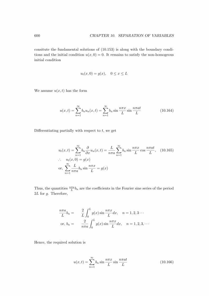
600 CHAPTER 10. SEPARATION OF VARIABLES
consitute the fundamental solutions of (10.153) is along with the boundary condi-
tions and the initial condition u(x, 0) = 0. It remains to satisfy the non-homogeous
initial condition
ut(x, 0) = g(x), 0 ≤ x ≤ L
We assume u(x, t) has the form
u(x, t) =∞∑n=1
bnun(x, t) =∞∑n=1
bn sinnπx
Lsin
nπat
L(10.164)
Differentiating partially with respect to t, we get
ut(x, t) =∞∑n=1
bn∂
∂xun(x, t) =
L
nπa
∞∑n=1
bn sinnπx
Lcos
nπat
L, (10.165)
∴ ut(x, 0) = g(x)
or,∞∑n=1
L
nπabn sin
nπx
L= g(x)
Thus, the quantities nπaL bn are the coefficients in the Fourier sine series of the period
2L for g. Therefore,
nπa
Lbn =
2
L
∫ L
0g(x) sin
nπx
Ldx, n = 1, 2, 3 · · ·
or, bn =2
nπa
∫ L
0g(x) sin
nπx
Ldx, n = 1, 2, 3, · · ·
Hence, the required solution is
u(x, t) =
∞∑n=1
bn sinnπx
Lsin
nπat
L(10.166)

10.3. THE WAVE EQUATION: VIBRATIONS OF AN ELASTIC STRING 601
where
bn =2
nπa
∫ L
0g(x) sin
nπx
Ldx
=2
nπa
∫ L/2
0g(x) sin
nπx
Ldx+
2
nπa
∫ L
L/2g(x) sin
nπx
Ldx
=2
nπa
∫ L/2
0
2x
Lsin
nπx
Ldx+
2
nπa
∫ L
L/2
2(L− x)
Lsin
nπx
Ldx
=4
nπaL
∫ L/2
0x sin
nπx
Ldx+
4
nπaL
∫ L
L/2(L− x) sin
nπx
Ldx
=4
nπaL
[x
∫sin
nπx
Ldx
]L/20
−∫ L/2
0
(dx
dx
∫sin
nπx
Ldx
)dx
+4
nπaL
[(L− x)
∫sin
nπx
Ldx
]LL/2
−∫ L
L/2
(d
dx(L− x)
∫sin
nπx
Ldx
)dx
=4
nπaL
[− L
nπx cos
nπx
L
]L/20
+
∫ L/2
0
L
nπcos
nπx
Ldx
+4
nπaL
[− L
nπ(L− x) cos
nπx
L
]LL/2
−∫ L
L/2
L
nπcos
nπx
Ldx
=4
nπaL
[− L2
2nπcos
nπ
2+ 0
]+
L2
n2π2
[sin
nπx
L
]L/20
+
4
nπaL
[0 +
L2
2nπcos
nπ
2
]− L2
n2π2
[sin
nπx
L
]LL/2
=
4L
n3π3a
[sin
nπ
2− 0]− 4L
n3π3a
[sinnπ − sin
nπ
2
]=
8L
n3π3asin
nπ
2
Hence the solution (10.166) becomes
u(x, t) =8L
π3a
∞∑n=1
1
n3sin
nπ
2sin
nπx
Lsin
nπat
L
Example 363. Dimensionless variables s = xL introduced to the wave equation
utt = a2uxx
Show that the wave equation becomes
a2uss = L2utt
Solution: The wave equation is
utt = a2uxx (10.167)
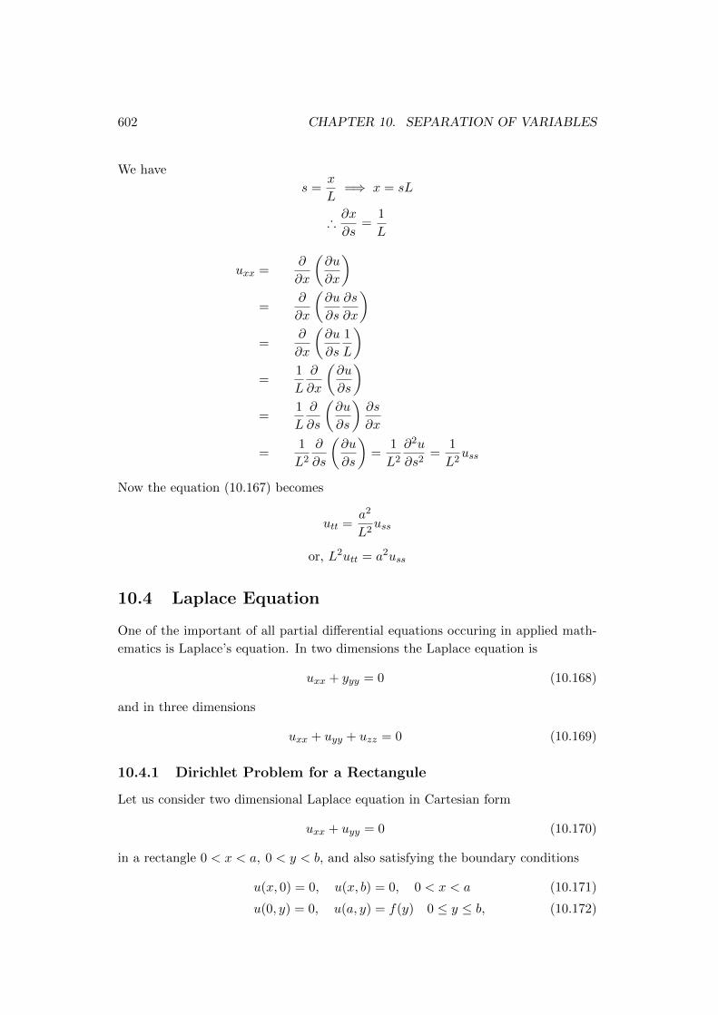
602 CHAPTER 10. SEPARATION OF VARIABLES
We have
s =x
L=⇒ x = sL
∴∂x
∂s=
1
L
uxx =∂
∂x
(∂u
∂x
)=
∂
∂x
(∂u
∂s
∂s
∂x
)=
∂
∂x
(∂u
∂s
1
L
)=
1
L
∂
∂x
(∂u
∂s
)=
1
L
∂
∂s
(∂u
∂s
)∂s
∂x
=1
L2
∂
∂s
(∂u
∂s
)=
1
L2
∂2u
∂s2=
1
L2uss
Now the equation (10.167) becomes
utt =a2
L2uss
or, L2utt = a2uss
10.4 Laplace Equation
One of the important of all partial differential equations occuring in applied math-
ematics is Laplace’s equation. In two dimensions the Laplace equation is
uxx + yyy = 0 (10.168)
and in three dimensions
uxx + uyy + uzz = 0 (10.169)
10.4.1 Dirichlet Problem for a Rectangule
Let us consider two dimensional Laplace equation in Cartesian form
uxx + uyy = 0 (10.170)
in a rectangle 0 < x < a, 0 < y < b, and also satisfying the boundary conditions
u(x, 0) = 0, u(x, b) = 0, 0 < x < a (10.171)
u(0, y) = 0, u(a, y) = f(y) 0 ≤ y ≤ b, (10.172)

10.4. LAPLACE EQUATION 603
Figure 10.1: Dirichlet Problem for a rectangle
where f is a given function on 0 ≤ y ≤ b. Let us suppose that
u(x, y) = X(x)Y (y) (10.173)
be solution of (10.170). Then
uxx = X ′′Y, uyy = XY ′′
and the equation (10.170) becomes
X ′′Y +XY ′′ = 0X ′′
X= −Y
′′
Y= λ
where λ is the separation constants. Thus we obtained two ordinary differential
equations
X ′′ − λX = 0 (10.174)
Y ′′ + λY = 0 (10.175)
Now using the boundary conditions
u(0, y) = 0 =⇒ X(0)Y (y) = 0 for all y
=⇒ X(0) = 0 (10.176)
u(x, 0) = 0 =⇒ X(x)Y (0) = 0 for all x
=⇒ Y (0) = 0 (10.177)
u(x, b) = 0 =⇒ X(x)Y (b) = 0 for all x
=⇒ Y (b) = 0 (10.178)

604 CHAPTER 10. SEPARATION OF VARIABLES
Now we find the solution of (10.175), the auxiliary equation is
r2 + λ = 0
or, r = i√λ
∴ Y (y) = c1 cos(√λy) + c2 sin(
√λy) (10.179)
Using the boundary conditions
Y (0) = 0 we get c1 = 0
and
Y (b) = 0 we get c2 sin√λb = 0
=⇒√λb = nπ
=⇒ λ =n2π2
b2
Y (y) is proportional to eighen function sin nπyb .
Putting the values of Y in (10.174), we obtained
X ′′ − nπ
nX = 0 (10.180)
The auxiliary equation of(10.175) is
r2 − n2π2
b2= 0
or, r =nπ
b
∴ X(x) = k1 coshnπx
b+ k2 sinh
nπx
b
Using the boundary condition X(0) = 0, we get
k1 cosh 0 + k2 sinh 0 = 0
or, k1 = 0 as cosh 0 = 1, sinh 0 = 0
Therefore,
X(x) = k2 sinhnπx
b
Thus, the solution X(x) is proportional to sinh nπxb . The Fundamental solution of
the given problem is
un(x, y) = sinhnπx
bsin
nπy
b
These functions satisfy the differenrial equation (10.170) and all the homogeneous
boundary conditions for each value of n.
To satisfy the remaining non-homogeous boundary conditions at x = a, we assuse
the solution u(x, y) in the form
u(x, y) =
∞∑n=1
cnun(x, y) =
∞∑n=1
cn sinhnπx
bsin
nπy
b(10.181)

10.4. LAPLACE EQUATION 605
The coefficient cn are determined by the boundary condition
u(a, y) = f(y)
or,
∞∑n=1
cn sinhnπa
bsin
nπy
b= f(y)
Therefore the quantities cn sinh nπab must be the coefficients in the Fourier sine series
of the period 2b for f and are given by
cn sinhnπa
b=
2
b
∫ b
0f(y) sinh
nπy
bdy
or, cn =2
b sinh nπab
∫ b
0f(y) sinh
nπy
bdy
Hence the fundamental solution is
u(x, y) =
∞∑n=1
cn sinhnπx
bsin
nπy
b
where
cn =2
b sinh nπab
∫ b
0f(y) sinh
nπy
bdy.
Example 364.
Find the solution of the Laplace equation
uxx + uyy = 0 (10.182)
in a rectangle 0 < x < a, 0 < y < b, and satisfying the boundary conditions
u(x, 0) = h(x), u(x, b) = 0, 0 ≤ x ≤ a (10.183)
u(0, y) = 0, u(a, y) = 0 0 < y < b, (10.184)
where h is a given function on 0 ≤ y ≤ b.Solution: Let us suppose that
u(x, y) = X(x)Y (y) (10.185)
be solution of (10.182). Then
uxx = X ′′Y, uyy = XY ′′
and the equation (10.170) becomes
X ′′Y +XY ′′ = 0X ′′
X= −Y
′′
Y= −λ

606 CHAPTER 10. SEPARATION OF VARIABLES
Figure 10.2: Dirichlet Problem for a rectangle
where λ is the separation constants. Thus we obtained two ordinary differential
equations
X ′′ + λX = 0 (10.186)
Y ′′ − λY = 0 (10.187)
Now using the boundary conditions
u(0, y) = 0 =⇒ X(0)Y (y) = 0 for all y
=⇒ X(0) = 0 (10.188)
u(x, b) = 0 =⇒ X(x)Y (b) = 0 for all x
=⇒ Y (b) = 0 (10.189)
u(a, y) = 0 =⇒ X(a)Y (y) = 0 for all y
=⇒ X(a) = 0 (10.190)
Now we find the solution of (10.186), the auxiliary equation is
r2 + λ = 0
or, r = i√λ
∴ X(y) = c1 cos(√λx) + c2 sin(
√λx) (10.191)
Using the boundary conditions
X(0) = 0 we get c1 = 0
and
X(a) = 0 we get c2 sin√λa = 0

10.4. LAPLACE EQUATION 607
=⇒√λa = nπ
=⇒ λ =n2π2
a2
X(x) is proportional to eighen function sin nπxa .
Putting the values of Y in (10.187), we obtained
Y ′′ − nπ
aY = 0 (10.192)
The auxiliary equation of(10.192) is
r2 − n2π2
b2= 0
or, r = ±nπa
∴ Y (y) = k1 coshnπy
a+ k2 sinh
nπy
a(10.193)
Using the boundary condition Y (b) = 0, we get
k1 coshnπb
a+ k2 sinh
nπa
b= 0
or,k2
k1= −
cosh nπba
sinh nπab
Thus from (10.193)
Y (y) = k1
(cosh
nπy
a+k2
k1sin
nπy
a
)
or, Y (y) = k1
(cosh
nπy
a−
cosh nπba
sinh nπba
sinnπy
a
)
or, Y (y) =k1
sinh nπba
(sinh
nπb
acosh
nπy
a− cosh
nπb
asinh
nπy
a
)or, Y (y) = dn sinh
nπ(b− y)
a
where
dn =k1
sinh nπba
Thus, the solution Y (x) is proportional to sinh nπ(b−y)a . The Fundamental solution
of the given problem is
un(x, y) = sinnπx
asinh
nπ(b− y)
a
These functions satisfy the differenrial equation (10.182) and all the homogeneous
boundary conditions for each value of n.

608 CHAPTER 10. SEPARATION OF VARIABLES
To satisfy the remaining non-homogeous boundary conditions at u(x, 0) = h(x), we
assuse the solution u(x, y) in the form
u(x, y) =∞∑n=1
cnun(x, y) =∞∑n=1
cn sinnπx
asinh
nπ(b− y)
a(10.194)
The coefficient cn are determined by the boundary condition
u(x, 0) = h(x)
or,
∞∑n=1
cn sinhnπx
asinh
nπb
a= h(x)
Therefore the quantities cn sinh nπba must be the coefficients in the Fourier sine series
of the period 2a for h and are given by
cn sinhnπb
a=
2
a
∫ a
0h(x) sin
nπx
adx
or, cn =2
a sinh nπba
∫ b
0h(x) sin
nπx
adx
Hence the fundamental solution is
u(x, y) =∞∑n=1
cn sinnπx
asinh
nπ(b− y)
a
where
cn =2
a sinh nπba
∫ b
0h(x) sin
nπx
adx.
10.4.2 Laplace’s Equation in Polar form
Example 365. From the Laplace equation of two dimension uxx+uyy = 0, obtained
the Laplace equation for polar form
urr +1
rur +
1
r2uθθ = 0
Solution: The two dimensional Laplace’s equation in Cartesian form is
uxx + uyy = 0
or,∂2u
∂x2+∂2u
∂y2= 0 (10.195)
Let
x = r cos θ, y = r sin θ
Then
∂x
∂r= cos θ,
∂x
∂θ= −r sin θ
∂y
∂r= sin θ,
∂x
∂θ= r cos θ

10.4. LAPLACE EQUATION 609
So,
∂u
∂r=
∂u
∂x
∂x
∂r+∂u
∂y
∂y
∂r
=∂u
∂xcos θ +
∂u
∂ysin θ
Also,
∂2u
∂r2=
∂
∂r
(∂u
∂xcos θ +
∂u
∂ysin θ
)= cos θ
∂
∂r
(∂u
∂x
)+ sin θ
∂
∂r
(∂u
∂y
)= cos θ
[∂
∂x
(∂u
∂x
)∂x
∂r+
∂
∂y
(∂u
∂x
)∂y
∂r
]+ sin θ
[∂
∂x
(∂u
∂y
)∂x
∂r+
∂
∂y
(∂u
∂y
)∂y
∂r
]= cos θ
[cos θ
∂2u
∂x2+ sin θ
∂2u
∂x∂y
]+ sin θ
[cos θ
∂2u
∂x∂y+ sin θ
∂2u
∂y2
]= cos2 θ
∂2u
∂x2+ 2 cos θ sin θ
∂2u
∂x∂y+ sin2 θ
∂2u
∂y2(10.196)
Again,
∂u
∂θ=
∂u
∂x
∂x
∂θ+∂u
∂y
∂y
∂θ
= −r sin θ∂u
∂x+ r cos θ
∂u
∂y

610 CHAPTER 10. SEPARATION OF VARIABLES
Now,
∂2u
∂θ2=
∂
∂θ
(∂u
∂θ
)=
∂
∂θ
(−r sin θ
∂u
∂x+ r cos θ
∂u
∂y
)= −r ∂
∂θ
(sin θ
∂u
∂x
)+ r
∂
∂θ
(cos θ
∂u
∂y
)= −r
[sin θ
∂
∂θ
(∂u
∂x
)+∂u
∂x
∂
∂θ(sin θ)
]+ r
[cos θ
∂
∂θ
(∂u
∂y
)+∂u
∂y
∂
∂θ(cos θ)
]= −r
[sin θ
∂
∂θ
(∂u
∂x
)+ cos θ
∂u
∂x
]+ r
[cos θ
∂
∂θ
(∂u
∂y
)− sin θ
∂u
∂y
]= −r
[sin θ
∂
∂x
(∂u
∂x
)∂x
∂θ+
∂
∂y
(∂u
∂x
)∂y
∂θ
+ cos θ
∂u
∂x
]+r
[cos θ
∂
∂x
(∂u
∂y
)∂x
∂θ+
∂
∂y
(∂u
∂y
)∂y
∂θ
− sin θ
∂u
∂y
]= −r
[sin θ
−r sin θ
∂2u
∂x2+ r cos θ
∂2u
∂x∂y
+ cos θ
∂u
∂x
]+r
[cos θ
−r sin θ
∂2u
∂x∂y+ r cos θ
∂2u
∂y2
− sin θ
∂u
∂y
]= −r
(cos θ
∂u
∂x+ sin θ
∂u
∂y
)+ r2
(sin2 θ
∂2u
∂x2− 2 sin θ cos θ
∂2u
∂x∂y+ cos2 θ
∂2u
∂y2
)= −r∂u
∂r+ r2
(sin2 θ
∂2u
∂x2− 2 sin θ cos θ
∂2u
∂x∂y+ cos2 θ
∂2u
∂y2
)∴
1
r2
∂2u
∂θ2= −1
r
∂u
∂r+
(sin2 θ
∂2u
∂x2− 2 sin θ cos θ
∂2u
∂x∂y+ cos2 θ
∂2u
∂y2
)(10.197)
Adding (10.196) and (10.197)
∂2u
∂r2+
1
r2
∂2u
∂θ2= −1
r
∂u
∂r+ (cos2 θ + sin2 θ)
∂2u
∂x2+ (sin2 θ + cos2 θ)
∂2u
∂y2
or,∂2u
∂r2+
1
r2
∂2u
∂θ2+
1
r
∂u
∂r=∂2u
∂x2+∂2u
∂y2
or,∂2u
∂r2+
1
r2
∂2u
∂θ2+
1
r
∂u
∂r= 0 from (10.195)
or, urr +1
rur +
1
r2uθθ = 0
10.4.3 Dirichlet Problem for a Circle
Consider the problem of solving Laplace’s equation in a circular region r < a subject
to the boundary conditions
u(a, θ) = f(θ) (10.198)

10.4. LAPLACE EQUATION 611
where f is a given function on 0 ≤ θ < 2π. In polar coordinates Laplace’s equation
has the form
urr +1
rur +
1
r2uθθ = 0
or, r2urr + rur + uθθ = 0 (10.199)
where x = r cos θ, y = r sin θ and r =√x2 + y2. We assume u(r, θ) is a single valued
function, periodic in θ with period 2π and bounded for r ≤ a.
Assume the following separation
u(r, θ) = R(r)Θ(θ) (10.200)
Then
ur = R′Θ, urr = R′′Θ, uθθ = RΘ′′
Using (10.200) in (10.199) we get
r2R′′Θ + rR′Θ +RΘ′′ = 0
or, r2R′′
R+ r
R′
R= −Θ′′
Θ= λ
where λ is a separation constant. This gives the following two ordinary differential
equations
r2R′′ + rR′ − λR = 0 (10.201)
and Θ′′ + λΘ = 0 (10.202)
Now we have the following cases
Case I If λ < 0, then let λ = −µ2 where µ > 0 . The equation (10.202) becomes
Θ′′ − µ2Θ = 0 (10.203)
The auxiliary equation of (10.203) is
m2 − µ2 = 0
or, m = ±µ
Thus solution of (10.203) is
Θ(θ) = c1eµθ + c1e
−µθ (10.204)
which is periodic if and only if c1 = c2 = 0 and we conclude that λ can to be
negative.
Case II If λ = 0 then the equation (10.202) becomes
Θ′′ = 0

612 CHAPTER 10. SEPARATION OF VARIABLES
Integrating,
Θ′ = c3
Θ′′ = c3θ + c4
For periodic we must have c4 = 0, so that Θ(θ) is constant and in particular, we can
take
Θ(θ) = 1, we assume c4 = 1
Again, for λ = 0, equation (10.201) becomes
r2R′′ + rR′ = 0
or, r2d2R
dr2+ r
dR
dr= 0
Let us put y = dRdr . Then the above equation becomes
r2dy
dr+ ry = 0
or, rdy
dr+ y = 0
or,d
dr(ry) = 0
Integrating,
ry = k1
or, rdR
dr= k1
or, dR =k1
rdr
Integrating
R = k1 loge r + k2
when r → 0, loge → −∞, so bounded value of u(r, θ), we must have c1 = 0. Hence R
must be constant i.e. R = k2 In particular we take k2 = 1 and u(r, θ) = R(r)Θ(θ) = 1
Case III: Finally let λ > 0. Then λ = µ2for some values of λ. Then the equations
(10.201) and (10.202) becomes
r2R′′ + rR′ − µ2R = 0 (10.205)
Θ′′ + µ2Θ = 0 (10.206)
The equation (10.205) is Euerian, has solution
R(r) = d1rµ + d2r
−µ (10.207)
At the same time the auxiliary equation of (10.206) is
m2 + µ2 = 0
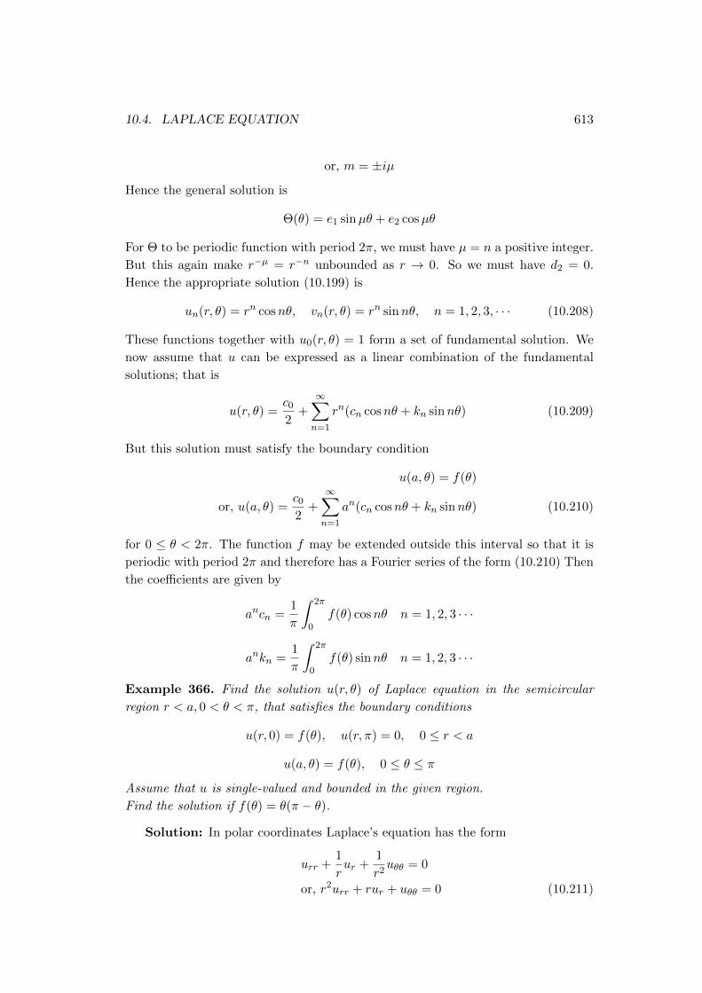
10.4. LAPLACE EQUATION 613
or, m = ±iµ
Hence the general solution is
Θ(θ) = e1 sinµθ + e2 cosµθ
For Θ to be periodic function with period 2π, we must have µ = n a positive integer.
But this again make r−µ = r−n unbounded as r → 0. So we must have d2 = 0.
Hence the appropriate solution (10.199) is
un(r, θ) = rn cosnθ, vn(r, θ) = rn sinnθ, n = 1, 2, 3, · · · (10.208)
These functions together with u0(r, θ) = 1 form a set of fundamental solution. We
now assume that u can be expressed as a linear combination of the fundamental
solutions; that is
u(r, θ) =c0
2+∞∑n=1
rn(cn cosnθ + kn sinnθ) (10.209)
But this solution must satisfy the boundary condition
u(a, θ) = f(θ)
or, u(a, θ) =c0
2+∞∑n=1
an(cn cosnθ + kn sinnθ) (10.210)
for 0 ≤ θ < 2π. The function f may be extended outside this interval so that it is
periodic with period 2π and therefore has a Fourier series of the form (10.210) Then
the coefficients are given by
ancn =1
π
∫ 2π
0f(θ) cosnθ n = 1, 2, 3 · · ·
ankn =1
π
∫ 2π
0f(θ) sinnθ n = 1, 2, 3 · · ·
Example 366. Find the solution u(r, θ) of Laplace equation in the semicircular
region r < a, 0 < θ < π, that satisfies the boundary conditions
u(r, 0) = f(θ), u(r, π) = 0, 0 ≤ r < a
u(a, θ) = f(θ), 0 ≤ θ ≤ π
Assume that u is single-valued and bounded in the given region.
Find the solution if f(θ) = θ(π − θ).
Solution: In polar coordinates Laplace’s equation has the form
urr +1
rur +
1
r2uθθ = 0
or, r2urr + rur + uθθ = 0 (10.211)

614 CHAPTER 10. SEPARATION OF VARIABLES
where x = r cos θ, y = r sin θ and r =√x2 + y2. We assume u(r, θ) is a single valued
function, periodic in θ with period 2π and bounded for r ≤ a.
Assume the following separation
u(r, θ) = R(r)Θ(θ) (10.212)
Then
ur = R′Θ, urr = R′′Θ, uθθ = RΘ′′
Using (10.212) in (10.211) we get
r2R′′Θ + rR′Θ +RΘ′′ = 0
or, r2R′′
R+ r
R′
R= −Θ′′
Θ= λ
where λ is a separation constant. This gives the following two ordinary differential
equations
r2R′′ + rR′ − λR = 0 (10.213)
and Θ′′ + λΘ = 0 (10.214)
The boundary conditions
u(r, 0) = 0, u(r, π) = 0, 0 ≤ r < a
=⇒ R(r)Θ(0) = 0, R(r)Θ(π) = 0 0 ≤ r < a
=⇒ Θ(0) = 0, Θ(π) = 0 0 ≤ r < a (10.215)
Let λ > 0. The equation (10.213) is Euerian, has solution
R(r) = d1r√λ + d2r
−√λ (10.216)
At the same time the auxiliary equation of (10.214) is
m2 + λ = 0
or, m = ±i√λ
Hence the general solution is
Θ(θ) = c1 sin√λθ + c2 cos
√λθ
Using the boundary condition
Θ(0) = 0 =⇒ c2 = 0
and Θ(π) = 0 =⇒ c1 sin√λπ + c2 cos
√λπ = 0
or, c1 sin√λπ = 0
For c1 6= 0, sin√λπ = 0
or,√λπ = nπ
or, λ = n2

10.4. LAPLACE EQUATION 615
Hence the eigenvalues are λn = n2 and corresponding eigen functions are Θn(θ) =
sinnθ.
Again the solution (10.216) becomes
R(r) = d1rn + d2r
−n
(10.217)
For boudedness at r = 0, we must have
limr→0
R(r) = limr→0
(d1r
n +d2
rn
)<∞
For this d2 = 0. Hence
R(r) = d1rn
Hence the fundamental solutions are
un(r, θ) = rn sinnθ
The most general solution is
u(r, θ) =∞∑n=1
cnun(r, θ) =
∞∑n=1
cnrn sinnθ
Using the condition
u(a, θ) = f(θ)
we get
∞∑n=1
cnrn sinnθ = f(θ)
which is a Fourier sine series of f(θ) with period 2π. So the coefficients are given by
cnan =
2
π
∫ π
0f(θ) sinnθdθ
cn =2
anπ
∫ π
0f(θ) sinnθdθ

616 CHAPTER 10. SEPARATION OF VARIABLES
Let f(θ) = θ(π − θ) = πθ − θ2. Then cn are given by
cn =2
anπ
∫ π
0f(θ) sinnθdθ
=2
anπ
∫ π
0(πθ − θ2) sinnθdθ
=2
anπ
[(πθ − θ2)
∫sinnθdθ
]π0
−∫ π
0
[d
dθ(πθ − θ2)
∫sinnθdθ
]dθ
=
2
anπ
[−(πθ − θ2)
cosnθ
n
]π0
+1
n
∫ π
0(π − 2θ) cosnθdθ
=
2
nanπ
0 +
[(π − 2θ)
∫cosnθdθ
]π0
−∫ π
0
[d
dθ(π − 2θ)
∫cosnθdθ
]dθ
=
2
nanπ
[(π − 2θ)
sinnθ
n
]π0
+2
n
∫ π
0sinnθdθ
=
2
n2anπ
−π sinnπ − π sin 0− 2
n[cosnθ]π0
= − 4
n3anπ(cosnπ − 1) =
4(1− cosnπ)
n3anπ
Thus the solution is
u(r, θ) =4
π
∞∑n=1
rn(1− cosnπ) sinnθ
ann3
10.4.4 Laplace Equation with Numann Boundary Conditions
Consider the problem of finding a solution u(x, y) of Laplace equation
uxx + uyy = 0 (10.218)
in a rectangle 0 < x < a, 0 < y < b, and satisfying the boundary conditions
ux(0, y) = 0, ux(a, y) = f(y), 0 < y < b (10.219)
uy(x, 0) = 0, uy(x, b) = 0 0 ≤ x ≤ a, (10.220)
This is example of a Neumann problem.
Show that Laplace equation and the homogeneous boundary condition determine
the fundamental set of solutions
u0(x, y) = c0, un(x, y) = cn coshnπx
bcos
nπy
b, n = 1, 2, 3, · · ·
Solution: Laplace equation is
uxx + uyy = 0 0 < x < a, 0 < y < b, (10.221)

10.4. LAPLACE EQUATION 617
and satisfying the boundary conditions
ux(0, y) = 0, ux(a, y) = f(y), 0 < y < b (10.222)
uy(x, 0) = 0, uy(x, b) = 0 0 ≤ x ≤ a, (10.223)
Let us suppose that
u(x, y) = X(x)Y (y) (10.224)
be solution of (10.221). Then
uxx = X ′′Y, uyy = XY ′′
and the equation (10.170) becomes
X ′′Y +XY ′′ = 0X ′′
X= −Y
′′
Y= λ
where λ > 0 is the separation constants. we neglect the λ ≤ 0 because the general
solutions obtained in this cases are not consitent with the physical nature of the
problem. Thus we obtained two ordinary differential equations
X ′′ − λX = 0 (10.225)
Y ′′ + λY = 0 (10.226)
Now using the boundary conditions
ux(0, y) = 0 =⇒ X ′(0)Y (y) = 0 for all y
=⇒ X ′(0) = 0 (10.227)
uy(x, 0) = 0 =⇒ X(x)Y ′(0) = 0 for all x
=⇒ Y ′(0) = 0 (10.228)
uy(x, b) = 0 =⇒ X(x)Y ′(b) = 0 for all y
=⇒ Y ′(b) = 0 (10.229)
Now we find the solution of (10.226), the auxiliary equation is
r2 + λ = 0
or, r = ±i√λ
(10.230)
The genral solution of (10.226) is
Y (y) = c1 cos(√
λy)
+ c2 sin(√
λy)
(10.231)

618 CHAPTER 10. SEPARATION OF VARIABLES
Differentiating with respect to y
Y ′(y) =√λ(−c1 sin
√λy + c2 cos
√λy)
(10.232)
Using the boundary conditions
Y ′(0) = 0 we get c2 = 0
and
Y ′(b) = 0 we get c1 sin√λb = 0
For c1 6= 0
sin√λb = 0
=⇒√λb = nπ
=⇒ λ =n2π2
b2
Y (y) is proportional to eighen function cos nπyb . Let it be YnPutting the values of λ in (10.225), we obtained
X ′′ − n2π2
b2X = 0 (10.233)
The auxiliary equation of(10.192) is
r2 − n2π2
b2= 0
or, r = ±nπb
(10.234)
Thus the genral solution is
X(x) = k1 coshnπx
b+ k2 sinh
nπx
b(10.235)
Differentiating both sides with respect to x, we get
X ′(x) =bk1
nπsinh
nπx
b+bk2
nπcosh
nπx
b(10.236)
Using the boundary condition X ′(0) = 0, we get
bk1
nπsinh 0 +
bk2
nπcosh 0 = 0
or, k2 = 0 as sinh 0 = 0, cosh0 = 0 (10.237)
Thus the solution (10.235) becomes
X(x) = k1 coshnπx
b

10.4. LAPLACE EQUATION 619
Letting k1 = 1, we have a solution depending on n so let it be Xn
Xn(x) = coshnπx
b, n = 0, 1, 2, · · ·
The fundamental solution of the Neumann problem is
un(x, y) = XnYn = coshnπx
bcos
nπy
b(10.238)
u0(x, y) = cosh 0 cos 0 = 1
The general solution is
u(x, y) =∞∑n=0
cnun(x, y)
or, u(x, y) =
∞∑n=0
cn coshnπx
bcos
nπy
b
or, u(x, y) = c0 cosh 0 cos 0 +
∞∑n=1
cn coshnπx
bcos
nπy
b
or, u(x, y) = c0 +∞∑n=1
cn coshnπx
bcos
nπy
b
Differentiating both sides partially with respect to x
ux(x, y) =∞∑n=1
nπcnb
sinhnπx
bcos
nπy
b
It remains to show that the solution satisfy ux(a, y) = f(y)
∞∑n=1
nπcnb
sinhnπa
bcos
nπy
b= f(y)
This is Fourier cosine series of f(y) with period 2b, and the constant are given by
nπcnb
sinhnπa
b=
∫ b
0f(y) cos
nπy
bdy
or, cn =2
nπ sinh nπab
∫ b
0f(y) cos
nπy
bdy
Thus the required solution is
u(x, y) = c0 +
∞∑n=1
cn coshnπx
bcos
nπy
b
where
cn =2
nπ sinh nπab
∫ b
0f(y) cos
nπy
bdy

620 CHAPTER 10. SEPARATION OF VARIABLES

Bibliography
621