Lecture 28th September 2016 Kai Olav Ellefsen - UiO

9/27/2016

1

INF3490 - Biologically inspired computingLecture 28th September 2016

Multi-Layer Neural NetworksKai Olav Ellefsen

Classification

Trained Classifier “DOG”

3

Perceptron

x1

x2

xn

...

w1

w2

wn

a=i=1n wi xi1 if a qy = 0 if a < q

y{

inputsweights

activation

outputq

Training a classifier (supervised learning)

Untrained Classifier “CAT”

9/27/2016

2

Training a classifier (supervised learning)

Untrained Classifier “CAT”

No, it was a dog.Adjust classifier parameters

6

Training a perceptron

x1

x2

xn

...

w1

w2

wn

a=i=1n wi xi1 if a qy = 0 if a < q

y{

inputsweights

activation

outputq

7

Decision Surface

x1

x2Decision linew1 x1 + w2 x2 = q1

1 1

00

00

01

8

A Quick Overview • Linear Models are easy to understand.• However, they are very simple.

– They can only identify flat decision boundaries(straight lines, planes, hyperplanes, ...).

• Majority of interesting data are not linearlyseparable. Then?

9/27/2016

3

9

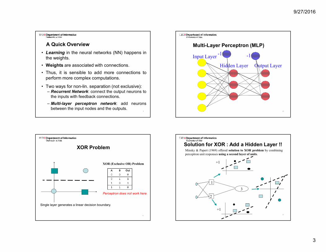
A Quick Overview• Learning in the neural networks (NN) happens in

the weights.• Weights are associated with connections.• Thus, it is sensible to add more connections to

perform more complex computations.• Two ways for non-lin. separation (not exclusive):

– Recurrent Network: connect the output neurons tothe inputs with feedback connections.

– Multi-layer perceptron network: add neuronsbetween the input nodes and the outputs.

Multi-Layer Perceptron (MLP)

10

Input LayerHidden Layer Output Layer

-1 -1

11

XOR Problem

XOR (Exclusive OR) Problem

Perceptron does not work here.

Single layer generates a linear decision boundary.12

Minsky & Papert (1969) offered solution to XOR problem by combiningperceptron unit responses using a second layer of units.

1

2

+1

+1

3

Solution for XOR : Add a Hidden Layer !!

9/27/2016

4

13

XOR Again

A B

DC

E-0.51 -1

-0.51 11 1-1

Inputs

Hidden Layer

Output

XOR Again

A B Cin Cout Din Dout Ein

0 0 -0.5 0 -1 0 -0.50 1 0.5 1 0 0 0.51 0 0.5 1 0 0 0.51 1 1.5 1 1 1 -0.5

A B

DC

E-0.51 -1

-0.51 11 1-1

MLP Decision Boundary – Nonlinear Problems, Solved!

15

In contrast to perceptrons, multilayer networks can learn notonly multiple decision boundaries, but the boundaries mayalso be nonlinear.

Input nodes Internal nodes Output nodes

X2

X1 16

Multilayer Network Structure• A neural network with one or more layers of nodes betweenthe input and the output nodes is called multilayer network.• The multilayer network structure, or architecture, or topology,consists of an input layer, one or more hidden layers, and oneoutput layer.• The input nodes pass values to the first hidden layer, its nodesto the second and so until producing outputs.

• A network with a layer of input units, a layer of hiddenunits and a layer of output units is a two-layer network.• A network with two layers of hidden units is a three-layer network, and so on.

9/27/2016

5

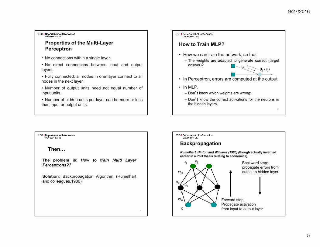
• No connections within a single layer.• No direct connections between input and outputlayers.• Fully connected; all nodes in one layer connect to allnodes in the next layer.• Number of output units need not equal number ofinput units.• Number of hidden units per layer can be more or lessthan input or output units.

Properties of the Multi-Layer Perceptron How to Train MLP?

• How we can train the network, so that– The weights are adapted to generate correct (target

answer)?

• In Perceptron, errors are computed at the output.• In MLP,

– Don’t know which weights are wrong:– Don’t know the correct activations for the neurons in

the hidden layers.18

x1 (tj - yj)

19

Then…The problem is: How to train Multi LayerPerceptrons??Solution: Backpropagation Algorithm (Rumelhartand colleagues,1986)

BackpropagationRumelhart, Hinton and Williams (1986) (though actually invented earlier in a PhD thesis relating to economics)

xk

xiwki

wjk

dj

dk

yj Backward step: propagate errors from output to hidden layer

Forward step: Propagate activation from input to output layer

9/27/2016

6

21

Training MLPsForward Pass

1. Put the input values in the input layer.2. Calculate the activations of the hidden nodes.3. Calculate the activations of the output nodes.

22

Training MLPsBackward Pass

1. Calculate the output errors2. Update last layer of weights.3. Propagate error backward, update hidden weights.4. Until first layer is reached.

23

Error Function• Single scalar function for entire network.• Parameterized by weights (objects of interest).• Multiple errors of different signs should not cancel out.• Sum-of-squares error:

24

• The backpropagation training algorithm usesthe gradient descent technique to minimizethe mean square difference between thedesired and actual outputs.• The network is trained initially selecting smallrandom weights and then presenting alltraining data incrementally.• Weights are adjusted after every trial untilthey converge and the error is reduced to anacceptable value.

Back Propagation Algorithm

9/27/2016

7

25

Gradient DescentE

w

26

Error Terms• Need to differentiate the error function• The full calculation is presented in the book.• Gives us the following error terms (deltas)

• For the outputs

• For the hidden nodes)(')( kkkk agty d

k

ikkii wug dd )('

27

Update Rules• This gives us the necessary update rules

• For the weights connected to the outputs:

• For the weights on the hidden nodes:

• The learning rate depends on the application. Values between 0.1 and 0.9 have been used in many applications.

jkjkjk zww dijijij xvv d

28

Y

BackPropagation Algorithm

XE

T

y1y2

y4

y3

e1e2

e4e3

x1x2x3x4x5

(X,T)

9/27/2016

8

Algorithm (sequential)1. Apply an input vector and calculate all activations, a and u2. Evaluate deltas for all output units:

3. Propagate deltas backwards to hidden layer deltas:

4. Update weights:

)(')( kkkk agty d

kikkii wug dd )('

jkjkjk zww dijijij xvv d

30

y1

y2

x1

x2

v11= -1v12= 0

v21= 0v22= 1v01= 1

v02= 1

w11= 1w12= -1

w21= 0w22= 1

Use identity activation function (ie g(a) = a) for simplicity of example

Example: Backpropagation

31

All biases set to 1. Will not draw them for clarity. Learning rate h = 0.1

y1

y2

x1

x2

v11= -1v12= 0

v21= 0v22= 1

w11= 1w12= -1

w21= 0w22= 1

Have input [0 1] with target [1 0].

x1= 0

x2= 1


32

Forward pass. Calculate 1st layer activations:

y1

y2

v11= -1v12= 0

v21= 0v22= 1

w11= 1w12= -1

w21= 0w22= 1

u2 = 2

u1 = 1

u1 = -1x0 + 0x1 +1 = 1u2 = 0x0 + 1x1 +1 = 2

x1= 0

x2= 1


9/27/2016

9

33

Calculate first layer outputs by passing activations through activation functions

y1

y2

x1

x2

v11= -1v12= 0

v21= 0v22= 1

w11= 1w12= -1

w21= 0w22= 1

z2 = 2

z1 = 1

z1 = g(u1) = 1z2 = g(u2) = 2


34

Calculate 2nd layer outputs (weighted sum through activationfunctions):

y1= 2

y2= 2

x1

x2

v11= -1v12= 0

v21= 0v22= 1

w11= 1w12= -1

w21= 0w22= 1

y1 = a1 = 1x1 + 0x2 +1 = 2y2 = a2 = -1x1 + 1x2 +1 = 2


z1 = 1

z2 = 2

35

Backward pass:

d1= 1

d2= 2

x1

x2

v11= -1v12= 0

v21= 0v22= 1

w11= 1w12= -1

w21= 0w22= 1

Target =[1, 0] so t1 = 1 and t2 = 0. So:d1 = (y1 - t1 )= 2 – 1 = 1d2 = (y2 - t2 )= 2 – 0 = 2


)(')( kkkk agty d

36

Calculate weight changes for 1st layer:d1 z1 =-1x1

x2

v11= -1v12= 0

v21= 0v22= 1

w11= 1w12= -1

w21= 0w22= 1

z2 = 2

z1 = 1

d1 z2 =-2d2 z1 =-2d2 z2 =-4


jkjkjk zww d

9/27/2016

10

37

Weight changes will be:

x1

x2

v11= -1v12= 0

v21= 0v22= 1

w11= 0.9w12= -1.2

w21= -0.2w22= 0.6


jkjkjk zww d38

Calculate hidden layer deltas:

D1 = 1

D2 = 2

x1

x2

v11= -1v12= 0

v21= 0v22= 1

D1 w11= 1D2 w12= -2D1 w21= 0D2 w22= 2


Dk

ikkii wug )('d

39

Deltas propagate back:

D1= 1

D2= 2

x1

x2

v11= -1v12= 0

v21= 0v22= 1

d1= -1

d2 = 2d1 = 1 - 2 = -1d2 = 0 + 2 = 2

Example: Backpropagation Dk

ikkii wug )('d

40

And are multiplied by inputs:

D1= -1

D2= -2

v11= -1v12= 0

v21= 0v22= 1

d1 x1 = 0

d2 x2 = -2x2= 1

x1= 0

d2 x1 = 0d1 x2 = 1


ijijij xvv d

9/27/2016

11

41

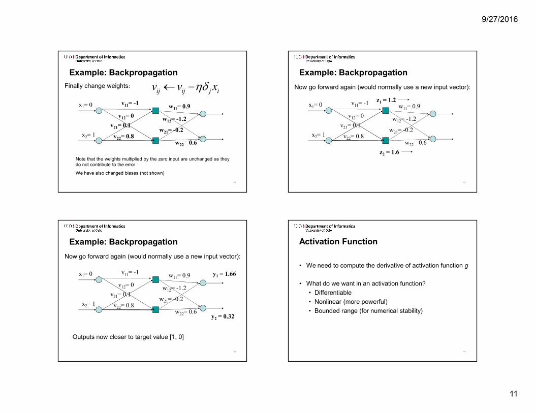
Finally change weights:v11= -1

v12= 0v21= 0.1v22= 0.8x2= 1

x1= 0 w11= 0.9w12= -1.2

w21= -0.2w22= 0.6

Note that the weights multiplied by the zero input are unchanged as theydo not contribute to the errorWe have also changed biases (not shown)

Example: Backpropagationijijij xvv d

42

Now go forward again (would normally use a new input vector):v11= -1

v12= 0v21= 0.1

v22= 0.8x2= 1

x1= 0 w11= 0.9w12= -1.2

w21= -0.2w22= 0.6

z2 = 1.6

z1 = 1.2


43

Now go forward again (would normally use a new input vector):v11= -1

v12= 0v21= 0.1v22= 0.8x2= 1

x1= 0 w11= 0.9w12= -1.2

w21= -0.2w22= 0.6 y2 = 0.32

y1 = 1.66

Outputs now closer to target value [1, 0]


44

Activation Function• We need to compute the derivative of activation function g• What do we want in an activation function?

• Differentiable• Nonlinear (more powerful)• Bounded range (for numerical stability)

9/27/2016

12

45

Hard Limit Function1.0

-1.0

x

y

Discontinuity where thevalue changes from 0 to 1.

46

A Quick Overview (Activation Functions)

a

y

a

y

a

y

a

y

threshold linear

piece-wise linear sigmoid

47

Sigmoidal Function - Common in MLPiaki

i eakag 11

)exp(11)(

• Where k is a positiveconstant.• The sigmoidal function givesa value in range of 0 to 1.• Alternatively can usetanh(ka) which is same shapebut in range –1 to 1.

48

Network Training• Training set shown repeatedly until stopping

criteria are met.• When should the weights be updated?

• After all inputs seen (batch)• After each input is seen (sequential)• Both ways, need many epochs - passes

through the whole dataset

9/27/2016

13

Batch TrainingInsert all training data

Calculate average errorCalculate deltas

Update weights

49

• One loop is called anepoch

• More accurate estimateof gradient

• Faster convergence tolocal optimum

Sequential TrainingInsert one training data

Calculate errorCalculate deltas

Update weights

50

• Simpler to program• Can avoid local optima

Compromise: MinibatchInsert one minibatch

Calculate average errorCalculate deltas

Update weights

51

• Split all data into Nminibatches

• Feed each minibatch tothe network

• Shuffle data and repat

• May lead to the benefitsof both batch-learningand sequential learning:– Rapid convergence– Avoiding local minima

52

Risk: Gradient descent takes us to local minimum

E

w

9/27/2016

14

How can we avoid the local minimum?• Initialize training many times with random

weights• Use momentum:

53

1DD tijijijij wzww

PRACTICAL ISSUES54

55

Amount of Training• How much training data is needed?

– Count the weights– Rule of thumb: use 10 times more data than the number of weights

56

How many hidden layers do we need?

Output of one sigmoid Addition of two sigmoids

9/27/2016

15

57

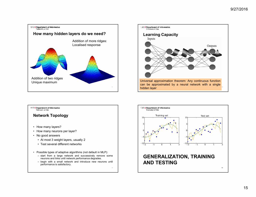
How many hidden layers do we need?

Addition of two ridgesUnique maximum

Addition of more ridges: Localised response

58

Learning Capacity

Universal approximation theorem: Any continuous functioncan be approximated by a neural network with a singlehidden layer

59

Network Topology• How many layers?• How many neurons per layer?• No good answers

• At most 3 weight layers, usually 2• Test several different networks

• Possible types of adaptive algorithms (not default in MLP):– start from a large network and successively remove someneurons and links until network performance degrades.– begin with a small network and introduce new neurons untilperformance is satisfactory.

GENERALIZATION, TRAINING AND TESTING

60

9/27/2016

16

61

Generalisation• Aim of neural network learning:

• Generalise from training examples to all possibleinputs.

• The objective of learning is to achieve goodgeneralization to new cases; we cannot train on allpossible data.

• Under-training is bad.• Over-training is also bad.

62

Generalisation - example

63

• Overfitting occurs when a model begins to learn the biasof the training data rather than learning to generalize.

• Overfitting generally occurs when a model is excessivelycomplex in relation to the amount of data available.

• A model which overfits the training data will generallyhave poor predictive performance, as it can exaggerateminor fluctuations in the data.

Overfitting

64

Overfitting

9/27/2016

17

65

• The training data contains information about the regularities inthe mapping from input to output.

• Training data also contains bias:– There is sampling bias. There will be accidental

regularities due to the finite size of the training set.– The target values may also be unreliable or noisy.

• When we fit the model, it cannot tell which regularities arerelevant and which are caused by sampling error.– So it fits both kinds of regularity.– If the model is very flexible it can model the sampling error

really well. This is not what we want.

Overfitting

66

The Problem of Overfitting• Approximation of the function y = f(x) :

2 neurons in hidden layer5 neurons in hidden layer40 neurons in hidden layer

x

y

67

The Solution: Cross-ValidationTo maximize generalization and avoid overfitting, split data

into three sets:• Training set: Train the model.• Validation set: Judge the model’s generalization ability

during training.• Test set: Judge the model’s generalization ability after

training.

68

Validation set• Data unseen by training algorithm – not used for

backpropagation.• Network is not trained on this data, so we can use it to

measure generalization ability.• Goal is to maximize generalization ability, so we should

minimize the error on this data set.

9/27/2016

18

69

Early StoppingError

TrainingNumber of epochs

Validation

Time to stop training

Testing set• Data unseen during training and validation.• Has no influence on when to stop training.• With early stopping, we’ve maximized the ability to generalize to the validation set;• To judge the final result, we should measure its ability to generalize to completely unseen data.

70

k-Fold Cross Validation• Validation and testing leaves less training data.• Solution: repeat over many different splits.

71

Source: Wikimedia Commons

Validation data

72

Leave-one-out Cross Validation

Lecture 28th September 2016 Kai Olav Ellefsen - UiO

Documents

Transcript of Lecture 28th September 2016 Kai Olav Ellefsen - UiO