Learning Product Characteristics and Consumer

Preferences from Search Data∗

Luis Armona

Stanford University

Greg Lewis

Microsoft Research

Georgios Zervas

Boston University

June 2, 2021

Abstract

A building block of many models in empirical industrial organization is a charac-

teristic space, where products are modeled as a bundle of characteristics over which

consumers have preferences. The ability of such models to predict counterfactual out-

comes depends on how well this characteristic space representation can capture sub-

stitution patterns. A limitation of existing methods is that product characteristics

must be observable. In this paper, we extend a machine learning approach (Bayesian

Personalized Ranking) that allows us to jointly learn latent product characteristics and

consumer preferences from search data. We then show how this can be combined with

existing demand estimation approaches to predict demand. Our application is to the

hotel market, where we combine two datasets: consumers’ web browsing histories, and

hotel prices and occupancy rates. Using an event study design, we show that close-

ness in latent characteristic space predicts competition: hotels that are close to new

entrants lose the most market share post-entry. We take a more structural approach to

the 2016 merger of Marriott and Starwood, demonstrating that by using latent char-

acteristics and consumer preferences learned from search data, we can substantially

improve post-merger predictions of demand relative to standard baselines.

JEL Codes: C13, C38, C51, C52, L1, L22, L81.

Keywords: E-Commerce; Search; Demand Estimation; Transfer Learning; Embeddings∗This research was started while Luis was an intern at Microsoft Research. We are grateful for comments

from Dean Eckles, Liran Einav, Matt Gentzkow, the participants at the Marketplace Innovation Workshop,

and our reviewers from the 22nd ACM Conference on Economics and Computation. We are also grateful to

Duane Vinson and STR for providing the hotel data for this paper.

1

1 Introduction

Demand estimation is a widely used tool in empirical industrial organization and beyond,

with applications to many industries, including transportation, healthcare and media.1 In

many of these industries, the number of products is large, and modeling demand over all the

products—as in the AIDS demand system (Deaton and Muellbauer 1980)—is impractical,

because it requires estimating a substitution matrix that is quadratic in the number of prod-

ucts. Building on the ideas of Lancaster and McFadden (Lancaster 1966, McFadden 1973),

a literature has emerged that assumes consumer preferences are over product characteristics

rather than products. When the number of characteristics is much smaller than the number

of products, this reduces data limitations. It also facilitates interpretation: products that

are close in characteristic space are competitors because they fight for the consumers who

value the characteristics they share.

There are two important practical problems with this approach. The first is that in some

markets—such as books (De los Santos and Wildenbeest 2017), movies (Einav 2007) and

cereal (Nevo 2001)—the observable characteristics, such as genre, length or mushiness, are

coarse. “Ben-Hur” and “The Lord of the Rings: The Return of the King” are both long

movies, but they may not be competing for the same viewers. As a result, demand systems

built from these observables cannot accurately capture substitution patterns. The second is

that it is notoriously difficult to estimate consumer preferences accurately from choice data

alone. As (Berry, Levinsohn, and Pakes 2004) and others have shown, the presence of second

choice data helps considerably in learning about the distribution of consumer tastes.

The main contribution of this paper is to propose a method that uses consumer search

data to address these practical difficulties. Our method builds off the observation that prior

to making a choice, consumers will evaluate many options that accord well with their pref-

erences i.e. that are close substitutes. Thus, products that are often searched together are

more likely to be close substitutes; and consumers that search the same sets of products

are likely to have similar preferences. Search data that reveals what products are consid-

ered together exists in many online markets (e.g., browsing data from a given e-commerce

platform.)

One limitation of search data is that it sometimes covers only a subset of the market.

For example, in our application to the hotel market, we use search data from Internet

1Some examples include (Berry, Levinsohn, and Pakes 1995, Berry and Jia 2010, Houde 2012,

Gowrisankaran, Nevo, and Town 2015, Ho and Lee 2017, Goolsbee and Petrin 2004, Crawford and

Yurukoglu 2012, Fan 2013).

1

Explorer (IE) users. The search patterns of IE users may not be reflective of the entire

market. Therefore, we combine this dataset with a choice dataset from STR, which has

high coverage of the entire hotel market. We show that product attributes and consumer

preferences learned from our auxiliary search dataset are useful in predicting choices, even in

an entirely different dataset. This may be useful in, for example, merger evaluation, where

the data typically seen on sales and prices of individual companies could be combined with

an outside source of consumer search data to better learn how closely the merging companies’

products compete, and improve the quality of post-merger predictions.

The main technical contribution of the paper is how we handle the search data. Follow-

ing Chade and Smith (2006), we write down a simple model of non-sequential search where

consumers see some subset of product characteristics (possibly unobserved to the econome-

trician), and click on options to learn more. Under some assumptions, the model implies that

the products a consumer chooses to click on are the ones which offer the highest expected

utility. This in turn implies a number of pairwise inequalities: if options A and B were

clicked, but C and D were not, the consumer expects more utility from A or B than C or D,

resulting in four inequalities. Compared to purchase data in discrete choice settings, where a

single product purchase decision is observed, this expands the number of consumer revealed-

choice inequalities seen by the researcher. We apply the Bayesian Personalized Ranking

method (Rendle, Freudenthaler, Gantner, and Schmidt-Thieme 2009) to these inequalities,

which allows us to learn latent characteristics for each product, and consumer preferences

for both latent and observable product characteristics.

These characteristics and preferences can be built into the canonical demand model

of BLP (Berry, Levinsohn, and Pakes 1995), by augmenting the demand model with the

additional latent product characteristics learned from the search data, and constraining the

distribution of random coefficients, which capture heterogeneity in consumer preferences over

product characteristics, to be a re-scaling of the preferences learned from the search data

(rather than the usual parametric restriction of multivariate normal preferences.)

We test our approach in a number of ways. Our first set of tests examines how much

we can learn from search data alone, ignoring all observable characteristics of hotels. We

fit the model to the search data to learn latent characteristics, and then predict held-out

observables from these latent features. This tests whether the latent characteristics encode

useful information. We find that we are able to predict observable characteristics well when

those characteristics are important determinants of consumer choice (e.g. hotel location),

and less well when they are not (e.g. the management company running each hotel).

2

We also check whether hotels that are clustered together in latent space are close com-

petitors. To do this, we estimate an event study design based on the entry of new hotels,

in which we try to predict which hotels will lose market share post-entry on the basis of

how close each hotel is to the new entrant, where the distance is either in latent, observable,

or geographic space. We find that the latent model predicts better than a model based on

standard observables (such as hotel class and amenities), but less well than one based purely

on geographic distance. We view this result as showing that the search data allows estima-

tion of latent characteristics that can predict substitution patterns, but if the observables

are rich—e.g. geography plus class and amenities—the value added from estimating latent

characteristics may be smaller. As noted earlier, there are markets (e.g. books, movies,

cereal) in which observable data are not rich.

The second set of tests concern merger analysis. We consider the 2016 merger of Marriott

International and Starwood Hotels & Resorts Worldwide, which created the world’s largest

hotel company. After showing that this merger has substantial price effects, we apply our

method to predicting out-of-sample post-merger market shares using only pre-merger data.

Here we run a horse-race between the canonical BLP model, which uses only observables

and choice data, and methods that use search data to add either latent characteristics,

latent consumer preferences or both. We find that adding search data yields substantial

improvements: while BLP fits better out-of-sample (in the sense of mean squared error)

than a standard logit by 39%, when we include both latent characteristics and consumer

preferences the corresponding improvement is 48% in our preferred specification. Notably,

models based on latent characteristics alone don’t perform well; all the improvements come

from combining both latent characteristics and preferences.

Our results suggest two ways in which the methods developed in the paper may be valu-

able in applications. First, in discovering latent characteristic representations of markets

with limited observables, which may facilitate discussions around market structure and the

nature of competition. Second, in improving demand estimation by allowing consumer pref-

erences to be learned (up to mean utility and scale parameters) “offline” from search data

where they are more plausibly identified.

1.1 Literature Review

Our paper relates to the literature on structural demand estimation, the literature on con-

sumer search, and the literature on incorporating machine learning methods in demand

estimation.

3

Structural Demand Estimation: This paper is most similar in spirit to a strand of the

marketing literature, beginning with Elrod and Keane (1995), that has concerned itself with

estimating the structure of markets via factor models using revealed choice (Elrod 1988, Elrod

and Keane 1995, Erdem and Keane 1996, Keane et al. 2013). These set of papers use repeated

observations of consumers in a panel structure to estimate latent characteristics of products,

identifying the market structure from consumers who switch from one product to another,

implying the products are close substitutes to each other. Our identification strategy follows

a similar procedure, instead relying on products that are searched together within a single

purchase decision to identify products as close substitutes.

Since Berry, Levinsohn, and Pakes (1995), structural demand estimation in economics has

often relied on modeling consumer preferences over a “characteristic space”, which is taken

as given, to determine how close products in a market are to each other (Berry, Levinsohn,

and Pakes 2004, Bajari and Benkard 2005, Petrin 2002, Gandhi and Houde 2016). Berry,

Levinsohn, and Pakes (2004) uses “second choice” data as supplemental micro-data that

aids the identification of substitution patterns across cars in the auto market. Our paper

uses search data, which is increasingly available to researchers, as a proxy to second choice

data, since search data in our framework measures multiple products an individual consumer

expects to yield high utility given their preferences.

There has been recent progress in the marketing literature on using search to identify

substitution patterns over the product characteristic space, with a focus on explicitly mod-

eling the choice set formation process. Kim, Albuquerque, and Bronnenberg (2010) and

Kim, Albuquerque, and Bronnenberg (2011) use aggregate search and sales data to estimate

the latent characteristics of products, and consumer preferences over these characteristics.

Amano, Rhodes, and Seiler (2019) uses the sparsity of choice sets in a market with many

products, to feasibly estimate consumer demand and substitution patterns in online set-

tings. Our paper similarly employs a search model to explain consumer preferences over

latent characteristics.

Our paper combines these literatures by using observed within-user variation in search be-

havior to identify substitution patterns, while embedding these substitution patterns within

a product space to be compatible with existing structural demand estimation methods based

on a characteristic space.

Search: We rely on search data to estimate our characteristic space, in addition to con-

sumer preferences. Our model of consumer search to motivate our estimation is built on

the literature using simultaneous search models (Chade and Smith 2006) to explain con-

4

sumer search patterns. In a series of papers, Honka and Chintagunta (2016) and Honka

(2014) estimate a simultaneous search model in the auto insurance market. De los Santos,

Hortacsu, and Wildenbeest (2012) tests various search models in an online context, and find

simultaneous search models are most consistent with observed search patterns. Ursu (2018)

estimates the effect of online rankings in demand for travel services using random variation

in rankings.

Machine Learning Methods In Economics: Our paper also relates to a new litera-

ture that seeks to employ machine learning methods to augment demand estimation (Bajari,

Nekipelov, Ryan, and Yang 2015). Most closely related to our own paper in this litera-

ture are those papers that attempt to directly estimate the characteristic space of products

using embeddings methods popularized in the machine learning literature for representing

a large number of products in a common domain (Salakhutdinov and Mnih 2008, Koren,

Bell, and Volinsky 2009, Johnson 2014, Rudolph, Ruiz, Mandt, and Blei 2016). A number

of recent papers use these methods to estimate latent characteristics, latent preferences, or

both in economic settings (Ruiz, Athey, and Blei 2017, Athey, Blei, Donnelly, Ruiz, and

Schmidt 2018, Sams 2019, Donnelly, Kanodia, and Morozov 2020). Our paper similarly

uses established machine learning methods, specifically the Bayesian Personalized Ranking

method of Rendle, Freudenthaler, Gantner, and Schmidt-Thieme (2009), to estimate the

latent characteristics and preferences over hotels from search data.

2 Model

2.1 Traditional Discrete Choice

A standard model for consumer demand in discrete choice settings, popularized by Berry,

Levinsohn, and Pakes (1995), and known as “BLP”, is the following mixed-logit utility

specification for consumer i purchasing good j in market t:

ui,j,t = −αipj,t + ~βoi · ~Xoj,t + ξj,t + εi,j,t (1)

[αi, ~βoi ] = [α, ~βo] + Σ~vi, vi ∼ N(~0, I), (2)

where pj,t denotes the price of good j in market t, Xoj,t is a K× 1 vector of observed product

characteristics, ξj,t are unobserved product characteristics, ~vi is a (K+1)×1 vector of random

unobserved heterogeneity across consumers, Σ is a (K + 1)× (K + 1) lower diagonal matrix

that captures the importance of the unobserved tastes, and εi,j,t denotes i.i.d. idiosyncratic

5

shocks distributed extreme-value type 1. Suppose there are Jt inside products to choose

from in each market, in addition to an outside option j = 0, whose utility is normalized to

zero. Consumers select the product that maximizes utility. Under this model, market shares

of each product can be written as follows:

sj,t =

∫exp(δj + ξj,t + αipj,t + βoiX

oj )

1 +∑

k∈Jt exp(δk + ξk,t + αipk,t + βoiXok)dG(vi) (3)

where G(vi) is the distribution of vi. The BLP model can capture substitution patterns

across products, using only aggregated market-level data, via the nonlinear parameters Σ.

Large values of Σ relating to a particular observable characteristic k imply that there are

many consumers are unwilling to substitute to products who do not share similar values in

Xoj,t,k.

2.2 An Alternative Model

The above model is fairly flexible in its ability to capture the substitution patterns charac-

terizing consumer demand in many markets. However, 3 cases stand out as situations where

the above model may be limiting in its ability to capture substitution patterns in demand.

First, the econometrician may lack access to data on characteristics ~Xoj,t which consumers

have preferences over. Given this scenario, the non-linear parameters Σ provide very little

bite in capturing substitution patterns, if the observed characteristics are not important

determinants of demand. Second, the characteristics over which consumers have preferences

may be high dimensional. This will make it infeasible to estimate substitution patterns over

these characteristics, unless the econometrician has access to market-level data over a propor-

tionally large number of markets. This situation applies to our empirical setting, the market

for hotels. Hotels are differentiated not only by the various amenities they may offer, but

also their location with respect to tourist destinations, which is difficult to summarize with

a low-dimensional collection of observable characteristics. Third, the parametric assumption

that unobserved heterogeneity across consumers is normally distributed may be constraining

and unable to capture heterogeneity in demand. The inclusion of a full covariance matrix

Σ that allows unobserved tastes for product characteristics to correlate with each other can

make the preference specification in Equation 2 very rich in capturing underlying consumer

demand. In practice, however, because these mixed logit models are typically estimated

based on market-level quantity and price data, it is often difficult to identify the correlation

structure in Σ, so Σ is typically assumed to be a diagonal matrix, which assumes unobserved

tastes for product characteristics are independent.

6

This paper seeks to address the above limitations of the BLP model by proposing an

alternative specification of the BLP demand model. Specifically, in this paper, we consider

the following alternative parametrization of consumer preferences:

ui,j,t = −αipj,t + ~βoi · ~Xoj,t + ~βγi ~γj + ξj,t + εi,j,t (4)

[αi, ~βoi ,~βγi ] = [α, βo, βγ] + vi, ~vi ∼ F (5)

where ~γj is a L × 1 time-invariant vector of unobserved, or latent, product characteristics,~βγi is a L × 1 vector of preferences over these unobserved attributes, and F ∈ ∆RL+K+1 is

a distribution of consumer preferences ~vi over prices pj,t, observable product characteristics

Xoj,t, and unobservable product characteristics γj.

The latent characteristics γj allow consumers in the same market to have a heterogeneous

match value with product j that is not constrained to depend on observable product charac-

teristics, outside of the i.i.d. idiosyncratic shock εi,j,t. These latent characteristics γj address

the first 2 limitations of the BLP model. For the first problem (no data on characteristics),

the unobservable attributes γj may be able to recover the unobserved characteristics. For

the second problem (too many attributes), we may be able to recover a low-dimensional

projection of characteristics through γj.

By being entirely unrestrictive on the distribution of vi, we may be able to recover

potential non-linearities in preference heterogeneity, along with correlations in preferences

along particular dimensions of the characteristics space. It may be the case that consumers

have heterogeneous clusters in preference structure that are not additive, as is implied by

the normal parametric specification typically assumed. For example, consumers may have

high preferences for hotels that are close to the city center only when they also have high

preferences for hotels near bars, but when the consumer is interested in visiting museums,

the correlation between preferences for nearby bars and the city center is eliminated.

With only market-level price and quantity data, the estimation of unobservable charac-

teristics γj and a non-parametric distribution of consumer heterogeneity F is largely hope-

less. Estimating even the correlation structure of preferences when F follows a parametric

normal distribution is challenging and often requires auxiliary microdata, for example the

second-choice data used in (Berry, Levinsohn, and Pakes 2004). Allowing F to be entirely

non-parametric would be even more challenging. A natural reason this is challenging in a

discrete choice setting is that consumers select at most one good for purchase when they ar-

rive to the market, which limits our ability to observe what the consumer would have chosen

in the absence of the purchased good. To estimate unobserved characteristics, along with

7

heterogeneous preferences over these characteristics, would require us to observe systemic

correlations in demand between hotels that are not similar on observable characteristics,

but still explainable by exogenous factors such as entries, exits, and mergers. Because the

discrete choice model means we at most observe a single decision by consumers, this is dif-

ficult to identify from the data. We would require, at the very least, data on preferences a

consumer has over other products besides those they purchase.

In order to address the estimation limitations of the more flexible demand model in

Equation 4, we make use of individual-level search data to supplement the traditional market-

level price and quantity data used to estimate discrete choice models. With the advent of

online commerce, search data is increasingly available to researchers interested in studying

consumer behavior. The primary advantage of search micro-data is it allows us to observe

substitution patterns within an individual consumer. In this way, we view our incorporation

of search data into demand estimation as an extension of the incorporation of “second choice”

data in (Berry, Levinsohn, and Pakes 2004) and micromoments used in (Petrin 2002). The

intuition is that learning all available information for each product in a market is costly,

particularly in an online setting when the number of products can be in the thousands.

Thus, consumers must form choice sets of a subset of all goods in the market before making

a purchase decision. Much like discrete choice demand models use a “revealed preference”

approach to infer purchased products yield high utility, we use the choice sets formed by

consumers as a revealed preference signal that consumers expect products they search to

yield high utility. The key difference is that we can observe multiple products entering a

consumer’s choice set, whereas purchase decisions in discrete choice settings are limited to

one good per person / purchase decision. The ability to observe multiple preferred products

during a single purchase decision allows us to better identify the parameters F and γj in

our model. For example, we may observe 2 hotels are systemically searched together that

do not share any observable characteristics, which would suggest they are similar along an

unobservable characteristic in ~γ.

One advantage of our approach is that we do not require purchase decisions to appear in

the search microdata in order to estimate demand. That is, we use the search data to esti-

mate F and γj “offline”, then, once these preferences/characteristics are estimated, we plug

these into a traditional BLP demand model, in place of the random (normally-distributed)

preferences and (in addition to) the observable characteristics Xo. This distinction is im-

portant because search data, while widely available, is typically from one specific platform.

If consumer preferences on that platform are representative of the broader population of

8

consumers in the entire market, our method will provide meaningful estimates of the unob-

served preferences ~βi and the distribution of unobserved characteristics γj. And even when

there is selection into use of that platform—i.e. the population is not fully representative—

co-occurrence in search may still help in estimating the demand model for the full market.

Then, using aggregate quantity and price data, we can still answer questions of interest that

affect an entire market, not just a single platform, such as the impact of a merger on welfare

or alternative policies set by a social planner.

2.3 A Model of Search

In this section, we formalize the intuition explaining how search data is a powerful tool

to help identify both consumer heterogeneity and unobserved characteristics. We do so

through a microfounded model of search in a discrete choice environment. We assume that

consumers engage in simultaneous search (Chade and Smith 2006), which has been shown

to be consistent with consumer search behavior in online settings (De los Santos, Hortacsu,

and Wildenbeest 2012).

Consumers arrive at the market with a prior on their match values with products. Before

they can purchase a good, they must choose a set of products to search, Ji (the consideration

set). They then learn the true match value ui,j for each of the searched products, and

purchase either the best of the searched goods (or the outside option of non-purchase).

That is, they solve the following optimization problem:

maxJi

E

[maxj∈Ji

Ui,j,t

]− |Ji|ci (6)

where |Ji| is the number of products they search, and ci is their (individual -specific) search

cost. The payoff function has two parts. The first is the expected utility of the best product

in their consideration set. This is strictly increasing in the number of products considered.

But consumers balance this incentive to search against the search costs, as captured in the

term |Ji|ci.In general this is a difficult optimization problem, but we will make some assumptions

that simplify the problem considerably. We assume that the only unobserved component of

utility at the time of search is the product-market shock, ξj,t. That is consumers know their

horizontal match value to the good but not the unobserved shock ξj,t that additively shifts

utility equally across all consumers. We assume consumers have a common and normal prior

over ξj,t:

ξj,t ∼ N(ξj + δppj,t, σ2ξ )

9

The prior mean of the unobserved product-time shock ξj,t has a product-specific, time invari-

ant component, ξj, but is also allowed to vary over time, depending on changes in the price

consumers observe pj,t before they search a product.2 Intuitively, if the consumer observes

a high price of a product relative to the past periods, they may infer that the product has

better unobserved quality this period, which leads the supplier to charge a higher price.

Now the prior expected utility offered by each product is given by:

E[ui,j,t] = (δp − αi)pj,t + ~βoi · ~Xoj,t + ~βγi · ~γj + ξj + εi,j,t (7)

Notice that the only unknown term in the utility function is the product-market shock ξj,t.

Because this is normally distributed with variance σ2ξ for all products, the prior distribution

of utilities for all options is identical up to a product-specific expected utility.

It follows from results in Chade and Smith (2006) that the optimal consideration set

has two properties: (i) if Ji products are searched, it is the top Ji products as ranked by

expected utility and (ii) the worst product included in Ji (i.e. the lowest in terms of expected

utility) must increase the expected consumption utility E[maxj∈Ji ui,j,t] by at least ci, while

including the next product would not. Since we are not interested in recovering search costs

in this paper, we focus only on the first implication of the model, to deduce the following

set of inequalities:

E[ui,j,t] ≥ E[ui,k,t], ∀j ∈ Ji, ∀k 6∈ Ji (8)

These inequalities are similar to those used in choice estimation : the product chosen has

higher utility than the alternatives. Equation 8 follows the same intuition, but because

choice sets can be larger than one item, search data serves as a means to “expand” the set

of revealed preference inequalities observed in the data. By observing a larger set of the

consumer’s rank-ordered preferences over products, the problem of identifying preferences as

well as unobservable characteristics becomes more feasible. We exploit this in our estimation

of consumer preferences and unobserved characteristics.

The model presented here for recovering latent characteristics is not without its limi-

tations. We discuss two of the most noteworthy ones below, and how a researcher might

address them:

2Our model allows for the prior to also depend on changes to observable characteristics Xoj,t. However, in

our setting, all observable product characteristics are time-invariant, so this dependence does not play a role

in our empirical setting. Future usage of the model may allow the prior to depend on changes to observable

characteristics, e.g. ξj,t ∼ N(ξj + δppj,t + δoXoj,t, σ

2ξ ), and would be internally consistent with our model.

10

Product Rankings. One of our leading assumptions is that although search costs may

vary across consumers, they are constant across products. This may be violated in practice

because of the important role that search rankings play on online platforms (Ursu 2018).

Higher ranked products are much more prominent, easier to find, and more often clicked.

One way to model this would be to allow for product-specific search costs ci,j,t that depend

on the rankings chosen by the platform at time t, so that high ranked products have low

search costs, and vice-versa. This is no longer a special case of Chade and Smith (2006),

since they assume that search costs do not vary across alternatives. As a result, we don’t

have a complete characterization of the optimal consideration sets. But we do know that

any product j ∈ Ji must be Pareto undominated by any product k 6∈ Ji, in the sense that it

must either offer higher expected utility or have a better search ranking (lower search cost).

Conversely, if a product j ∈ Ji has a worse search ranking than some product k 6∈ Ji, it must

offer higher expected utility. This allows us to generate a new set of inequalities:

E[ui,j,t] ≥ E[ui,k,t], ∀(j ∈ Ji, k 6∈ Ji : rj > rk) (9)

where rj is the search rank of product j, rk is the search rank of product k, and lower is

better (i.e. the top ranked product has rank 1). Unfortunately we do not observe search

rankings in our search data, and so we use the full set of inequalities in (8) rather than the

subset in (9), which may lead to some bias in estimation.

New Products. Because we estimate the latent characteristic vector ~γj based on consumer

search behavior, we are unable to use this model to characterize market outcomes if a new,

previously unavailable product became available. This is a well-known issue with embeddings

methods known as the “cold-start problem” (Schein, Popescul, Ungar, and Pennock 2002).

In Section 5.1, we show that, at least in this market, our estimated latent characteristics can

predict observable characteristics with reasonable accuracy. This suggests that if necessary,

researchers may be able to predict the latent characteristics of new products with success

using the set of observed characteristics, particularly if the researcher has access to high-

dimensional observable data, such as textual product descriptions.

3 Data

We draw on 3 datasets to estimate our model of discrete choice and conduct our empirical

analysis.

11

Hotel Demand and Price Data. Our first dataset, which we obtained from STR,

spans January 2001 to March 2019 and contains monthly financial performance data for

5,358 hotels in 5 western U.S. States (Arizona, California, Nevada, Oregon, and Washington).

Specifically, for each month-year, STR records an anonymized ID uniquely associated with

each hotel, the total number of rooms sold, and the total revenue received by the hotel from

room sales. From this, we can also infer, the average price per room sold, also known as the

average daily rate (ADR) in the hotel industry. We deflate the nominal ADR recorded each

month to real March 2019 U.S. dollars using the CPI for All Urban Consumers time series.

Participation in reporting financial performance data is voluntary on the part of hotels,

however coverage is quite high. Of the universe of hotels in these states, only 10% of hotels

reported no data for the entire sample, and we have data for 83% of all hotel-by-month-years,

our unit of observation.

Census of Hotel Characteristics. The second dataset we use from STR links anony-

mous hotel IDs to certain observable hotel characteristics. This dataset contains the market,

according to STR definitions, that each hotel competes in, the sub-market a hotel is located

(e.g. Hollywood/Beverly Hills within the Los Angeles market), an anonymized ID to link

to the transaction data, the total meeting space in square feet available in each hotel, the

month-year the hotel was first opened, the month-year the hotel closed (where applicable),

as well as categorical variables representing the size (total capacity in rooms) of each hotel,

the location type of each hotel (near airport, urban, suburban, near highway, near leisure

/ destination travel [resort area], or in a small metro / town), the operation structure of

the hotel (franchise, owned by chain, or an independently owned/branded hotel), and the

“class” or price segment the hotel belongs to, which is a categorization assigned to hotel

brands based on their typical ADR (higher class meaning more expensive hotels). This

dataset also includes anonymized IDs describing the affiliation brand of each hotel, the com-

pany owning the hotel, the management company managing day-to-day operations of the

hotel, and the parent company of hotel. For example, although we never observe the hotel,

affiliation, or company name in the data, a Ritz Carlton hotel in the dataset would contain a

numeric affiliation ID corresponding to all Ritz Carlton hotels in the dataset, and a numeric

parent company ID corresponding to Marriott International, Inc., the parent corporation

that owns the Ritz Carlton brand. The dataset also contains the zipcode associated with

each anonymized hotel ID, denoting the location of the hotel. We map this to the average

latitude-longitude within each zipcode, using a cross-walk originally based on 2013 U.S. cen-

12

sus data.3 We use latitude and longitude as a continuous measure of the spatial distribution

of hotels within a market, in order to capture the spatial component of product differenti-

ation in the hotel industry. Affiliation IDs are provided at the annual level, to account for

mergers and acquisitions, while all other characteristics are measured in 2019, and do not

change over time.

Internet Explorer Click-Stream Data. Finally, our third dataset consists of the

web browsing histories of a sample of 29,936 Internet Explorer (IE) users from June 1st,

2014 to May 31st, 2015 visiting the website expedia.com. We make use of a session ID

variable recorded by IE that captures the URLs visited by a single user during one continuous

“session” defined as continuous usage of their computer where the time between clicks is no

more than 30 minutes. The URLs in the click-stream data, contain the Expedia ID of each

hotel, the check-in date selected by the user, the price displayed to the user for each hotel that

appears on screen, as well as whether the user clicked on a particular hotel in expedia.com.

We classify a click on a hotel’s Expedia page that is displayed to a user on their web browser

as constituting a “search” of the hotel by a user. This allows us to group together hotels that

were jointly considered within each session. We use this search data to estimate consumer

heterogeneity and unobservable characteristics of hotels.

Tables 1 and 2 displays the summary statistics describing the observable characteristics

of the 4,128 hotels that appear in both datasets. For our search data, we remove consumers

who search more than 35 hotels during a single session, which are likely web-scrapers and

not actual consumers. We retain those visitors to the website who searched at least one of

the 4,218 hotels included in both datasets. Our final sample of searchers consists of 18,492

unique visitors who engage in 23,986 unique search sessions. Table 3 contains summary

statistics on the search sessions in the Expedia dataset.

4 Estimation

4.1 Search Model

Given an observed choice set of size |Ji|, the simultaneous search model of Section 2.3 implies

|Ji| ·(J−|Ji|) inequalities of the kind in equation 8 for each consumer i whose search patterns

3Source: https://gist.github.com/erichurst/7882666

13

Mean Std. Dev Minimum 25th Pctile Median 75th Pctile Maximum

Transaction Data

Monthly Price ($) 129.34 81.95 18.06 80.91 110.66 151.47 1,576.09

Monthly Hotel Occupancy 2,951.06 3,381.11 7 1,224 2,101 3,360 77,305

Continuous Variables

Latitude 37.50 4.77 31.39 33.81 36.13 38.65 48.95

Longitude -118.83 3.66 -124.19 -122.14 -119.02 -117.21 -108.95

Meeting Space (Sq. Ft.) 3,981.22 11,326.00 0 0 560 2,500 220,000

Year Hotel Opened 1984.22 27.24 1798 1977 1989 1999 2014

# of Hotels 4,218

# of Geographical Markets 21

# of Month-Years 87

Table 1: Summary Statistics: STR Hotel Dataset (Continuous Data)

Ownership Structure Size Category Price Segment Location Type

Value Mean Value Mean Value Mean Value Mean

Chain Management 0.16 Less Than 75 Rooms 0.32 Economy Class 0.24 Airport 0.08

Franchise 0.70 75 - 149 Rooms 0.43 Midscale Class 0.16 Interstate 0.07

Independent 0.13 150 - 299 Rooms 0.18 Upper Midscale Class 0.25 Resort 0.10

300 - 500 Rooms 0.05 Upscale Class 0.17 Small Metro/Town 0.16

Greater Than 500 Rooms 0.02 Upper Upscale Class 0.11 Suburban 0.45

Luxury Class 0.06 Urban 0.14

Table 2: Summary Statistics: STR Hotel Dataset (Categorical Variables)

Mean Std. Dev Minimum 25th Pctile Median 75th Pctile Maximum

Price of Hotels on Platform ($) 118.02 77.86 14.00 72.49 100.11 138.37 19,374.00

Price of Searched Hotels 207.88 253.92 16.95 99.99 145.00 221.88 19,374.00

# of Hotels Searched per Session 1.85 1.80 1 1 1 2 35

Pr(Hotel Stay Purchased) 0.05 0.21 0 0 0 0 1

# of Consumers 18,492

# of Search Sessions 23,986

Table 3: Summary Statistics: Expedia Search Dataset Hotel Dataset

14

we observe.4 Integrating over the logit shock εi,j,t, this implies:

Pr(E[ui,j,t] ≥ E[ui,k,t]) = σ(ηi(pj,t − pk,t) + ~βoi · ( ~Xo

j,t − ~Xok,t) + ~βγi · (~γj − ~γk) + (ξj − ξk)

)(10)

where σ denotes the sigmoid, or logit function, σ(x) = 11+exp(−x)

.

Recall that we make no distributional assumptions on the preferences ~βoi and ~βui . As a

result, we will treat them as individual-specific preference parameters to be learned, based on

the search data we observe on each individual. This will give us an empirical estimate of the

distribution of random coefficients F . We are equipped to do this in this setting due to the

large number of revealed preference inequalities observed for each consumer via their choice

sets. On average, each consumer has 10, 267 inequalities implied by their search patterns.

We note also that we cannot separately identify the δp and αi terms in the prior expected

utility expression (7) directly from search data. Said otherwise, we cannot separate the true

disutility a consumer experiences from paying higher prices, and the signal they receive about

unobserved quality ξj,t from a high price. We instead estimate the parameter ηi = δp − αifrom the search data, which combines both direct and indirect (signalling) price effects.

Thus the parameters of the search model consist of the individual consumer preferences,

ηi, βoi , β

γi , the unobserved characteristics of products, γj, and the consumer’s prior mean on

the demand shock, ξj. Let Si denote the set of search sessions a single consumer engages in

that we observe in the data, and Ji,s denote the choice set (clicked products) formed by con-

sumer i during search session s. Given an observed choice set Js,i for each consumer i in search

data, the likelihood we use to estimate the parameters of the model, Θ = {ηi, βoi , βγi , γj, ξj}

is as follows:

Pr(Θ|{Ji}) =∏i

∏s∈Si

∏j∈Ji,s

∏k 6∈Ji,s

Pr(E[ui,j,t] ≥ E[ui,k,t]|Θ) (11)

This is identical to the likelihood formed in Rendle, Freudenthaler, Gantner, and Schmidt-

Thieme (2009) for the Bayesian Personalized Ranking model, a machine learning model used

for large-scale embedding problems. This allows us to rely on similar tools to those in the

machine learning literature to obtain estimates in our high-dimensional parameter space.

4This number of inequalities is large in magnitude, particularly compared to those from a purchase

decision, which only reveals that the chosen product is preferred to J − 1 other available products when we

abstract from choice set formation. In particular, the increased number of revealed preference inequalities

revealed from search data relative to purchase data is (|Ji| − 1)× (J − |Ji| − 1). When J is large and |Ji| is

even moderately sized, this can result in significantly more data on consumer preferences.

15

We make use of all the inequalities available for each consumer. In our application, this

will mean learning from the fact that a consumer searching for a hotel in San Diego does not

click on any hotels in New York City. While this decision not to restrict the comparisons

— for example, to hotels within a market — may seem odd, it is exactly these comparisons

that allows the model to learn that hotels in San Diego should be far from hotels in New

York City in the latent space.

Identification. The demand estimation exercise amounts to simultaneously learning con-

sumer preferences ({ηi, βoi , βγi }) and latent product characteristics (γj, ξj). The intuition for

why these parameters are identified is as follows. Pairs of products that are often searched

together must have similar locations in product space, otherwise they wouldn’t both be

utility maximizing for a consumer with prefernces βγi . Similarly, consumers who all search

some product j must have similar preferences. And higher order relationships provide more

information: if a pair of consumers both search a particular pair of products, this is even

more evidence that both consumers and products are close in their respective spaces.

This is not to say that the model is identified in a formal sense. The likelihood acts to

maximize the “score” of consumers and products that are matched, ~βγi · (~γj). Written in

matrix form, this is the product BΓ, where B is I ×K for I the number of consumers, and

Γ is K×J . But we could construct equivalent scores from (B×U)× (U−1X) for any K×Kinvertible matrix U . So to get formal identification one would have to first constrain either

consumer preferences or latent product characteristics in some way. Moreover the maximum

likelihood estimator we use here may run into an incidental parameter problem unless we

do asymptotics where both the number of consumers and products tend to infinity, so that

there are an infinite number of inequalities to point identify locations on both sides of the

market. Analysis of these econometric issues is outside the scope of the paper. Our interest

is in whether the parameters we obtain from the search data are useful for the subsequent

demand analysis on aggregate data we describe below.

Specifications. To test how well this approach works, we want to consider specifications

in which we have only observable characteristics (and learn consumer preferences), those

where we only have latent product characteristics and preferences, and those where we have

both observables and unobservables:

1. Observed Characteristics: K = 13, L = 0. There are no unobservable characteris-

tics ~γj, but we use the search data to recover the distribution of consumer preferences

16

G(βi) over observable characteristics. This specification evaluates the usefulness of our

embedding algorithm solely for recovering consumer preferences.

2. Unobservable Characteristics: K = 0, L = 10. We assume that we do not have

access to observable characteristics of hotels from the STR dataset and evaluate the

ability for search data to non-parametrically recover a characteristic space that cap-

tures consumer preferences over differentiated hotels. We choose L = 10 so that the

dimensionality of unobserved characteristics is comparable to that of the observed

characteristic space in the STR dataset. Note that in this specification we still allow

consumers to have preferences over price because this is observed directly in the search

microdata.

3. Observed and Unobserved Characteristics: K = 13, L = 5. We allow consumers

to have unobserved heterogeneity over both observed and unobserved characteristics.

We choose L = 5 because improvements in the out-of-sample likelihood significantly

decreased after allowing for 5 latent factors.

Computational Details. For each of these specifications, we estimate the parameters

of the model using the keras machine learning package in python.5 This expedites the

time it takes to optimize the model’s parameters dramatically due to (1) automatic gra-

dient computation and (2) the ability to use GPUs for optimization. We maximize the

log-likelihood of the model using batch optimization6, using the ADAM stochastic gradient

optimizer (Kingma and Ba 2014).

In order to avoid overfitting the model parameters to the search data, we hold out 10%

of the sample of EIU inequalities (expressed in Equation 8) implied by the search data to

determine the optimal number of training iterations. This 10% sample (validation set) is

stratified by search session, so 10% of all inequalities implied from a single search session

are not included during training. After each iteration through the 90% training set of

inequalities, we evaluate the likelihood of the model on the held-out validation set, and

iterate until we do not improve the likelihood of the held-out validation set. We then re-run

the model on the full set of inequalities using the number of training iterations that maximize

the likelihood of the validation set.

5We use the Tensorflow platform as a backend.6We use a batch size of 10,000 inequalities per gradient evaluation

17

4.2 Demand Model

After estimating the parameters of the search model, we plug in our estimated search pref-

erences / characteristics into a mixed logit, discrete choice demand model. We deviate from

the search model above in assuming that consumers observe all choices in a geographical

market g, as is typically assumed in discrete choice models based on aggregate market-level

data. Though this is inconsistent with the model in Section 2, in which consumers form

consideration sets, we view this exercise as highlighting the ability of our search method to

plug into a standard model used by economists across the field.7

We define a market t as a geographical market × year.8 We estimate a demand specifi-

cation of the following form:

ui,j,t = δj + αipj,t + βiXj + ξj,t + εi,j,t

[αi, βi] = [α, β] + Σvi, vi ∼ G(i)

where δj is a product fixed effect, the product characteristics are denoted Xj ∈ RK+L,

the distribution of heterogeneous preferences is G, and Σ is a (K + L + 1) × (K + L + 1)

diagonal matrix that weights the relative importance of heterogeneity in preferences along

each characteristic of the firm. Both Xj and G vary across specifications as described below.

We include a hotel fixed effect, δj, so that differences in predictions between each model

do not reflect “level” differences in predicting demand from characteristics, but instead load

solely on the differences in substitution patterns (as measured by Σ) that each model is able

to estimate.

Notice that because hotel characteristics do not vary observably over time, we absorb

the term βXj into the fixed effect δj, so that β is not separately identified. We calibrate

the mean price parameter, setting α = −0.018. This is the preferred estimate in Lewis and

Zervas (2016) in their demand analysis on the same data, and implies an average demand

elasticity of approximately -2.3, which seems reasonable. We choose to make this calibration

because we are unable to find good supply-shifters for price. Lewis and Zervas (2016) are

able to circumvent this problem because they estimate a full model of the supply side that

accounts for capacity constraints; we do not want to do this in the present paper.

7The estimates from the search model could instead be plugged into a different demand model.8We set market size according to a heuristic similar to that of Lewis and Zervas (2016): for each geo-

graphical market g, we take the month-year with the largest total number of rooms sold by all hotels in that

market, and set market size Mg to 1.5 times this quantity, multiplied by 12 to account for the fact that we

estimate demand at the annual level. Thus the size of each geographical market is constant over time.

18

This leaves the hotel fixed effects δj and the parameter Σ to be estimated. Σ captures the

relative importance of preference heterogeneity for each characteristic in Xj. This hetero-

geneity, along with the choice of characteristic space itself (i.e. including only observable or

both observable and latent characteristics), will determine the substitution patterns relevant

to merger analysis.

Specifications. We consider 2 specifications of Xj, each corresponding to 2 of our 3 search

models:9

1. Observables from STR. Xj = Xoj

2. Observables from STR, plus 5 unobservable characteristics learned from search data,

conditional on observables. Xj = [Xoj , γj]

We assume that vi, the unobserved preferences, take 1 of 2 forms:

1. vi ∼ N(0, I). This follows the standard mixed logit assumption of (Berry, Levinsohn,

and Pakes 1995).

2. vi ∼ F where F is the empirical distribution of estimated search preferences for all

consumers in our search data. Preferences are demeaned to have mean zero for each

characteristic. That is, given the estimated parameters ηi, βoi , β

γi of the search model,

we define the distribution of unobserved preferences to be

vi =

ηi − ηβoi − βo

βγi − βγ

where x denotes the average across consumers in the search data of the preference

parameter xi. Because we are unable to identify the level of price preferences from the

search model, due to the role price plays in shifting consumer expectations over the

demand shock, we demean consumer search preferences to have mean zero. With our

calibrated price parameter, this ensures our demand model predicts the correct level

of average price sensitivity across consumers, while preserving the heterogeneity and

correlation structure in consumer preferences we estimate from the search data.

9In practice, we found that the Unobservable Characteristics model with search preferences learned zero

random coefficients, suggesting that this model overfit to the search data in a way that was non-informative

as to purchase decisions.

19

Estimation Details. We approximate the integral in Equation 3 implied by the demand

model by taking B samples from the distribution of vi in each market:

sj,t =1

B

∑i∼G(i)

exp(δj + ξj,t + αipj,t + βiXj)

1 +∑

k∈Jt exp(δk + ξk,t + αipk,t + βiXk)

For normally distributed heterogeneous preferences vi, we take a Halton draw of B =

20, 000 multivariate normal random variables. For search preferences, we use the empirical

distribution of the estimated preference parameters ηi, βoi , β

γi from the search model. Both

sets of preferences are held constant across all markets in the data. We constrain the diagonal

elements of Σ to be non-negative when we estimate our demand model.

To estimate the model, we use the pyblp package (Conlon and Gortmaker 2019). The

parameters we need to estimate include the fixed effects δj, and the non-linear parameters,

Σ. For each guess of Σ, we estimate δj,t = αpj,t + δj + ξj,t via a contraction mapping.

The fixed effects δj are then partialled out by demeaning the output of the contraction

mapping at the hotel level at each optimization step. We optimize Σ using two-step GMM,

based on the moments E[ξj,t|Zj,t] = 0, for a set of instruments Zj,t. In the second step, we

use the first step estimates to construct an approximate form of the optimal instruments,

Zoptj,t = 1

σ2ξE[∇θξj,t|ξj,t = 0, Zj,t], where σ2

ξ is the first-stage estimate of the variance of ξ, as

recommended by (Conlon and Gortmaker 2019).

We use the quadratic differentiation instruments proposed by (Gandhi and Houde 2016)

as our vector of first-step instruments.10 For each characteristic c in Xj, we construct

instruments Zj,t,c =∑

k∈t,k 6=fj,t(Xj,c − Xk,c)2, where fj,t denotes the set of hotels with

the same affiliation as j in market t. We then use these to form empirical moments

gc(Σ) = 1N

∑j,t ξj,t(Σ) × Zj,t,c, where ξ is implicitly a function of Σ due to the contrac-

tion mapping. Stacking these empirical moments into a vector ~g, we solve the following

GMM objective function, given a weighting matrix W = maxΣ ~g(Σ)TW~g(Σ). We solve

this optimization problem first using a weighting matrix equal to (Z′Z)−1, where Z is the

N × 2(K + L) matrix of instruments used. We then obtain an estimate of the optimal

weighting matrix for the optimal instruments constructed from the first step, (Zopt′Zopt)−1

and solve the objective once again to obtain our final estimates for each model.

10We only include the rival differentiation instruments in our estimation. Due to our hotel fixed effects,

variation in our differentiation instruments comes solely from entry/exit in markets from competing brands

during our sample.

20

5 Results

We evaluate our method in three ways. First, we characterize the information content

of search embeddings, by evaluating the efficacy of embeddings trained in the Unobserv-

able Characteristics model to predict observable characteristics of hotels not included in

estimation. Second, we evaluate the ability of the embeddings learned in the Unobserved

Characteristics model to capture substitution patterns in a reduced-form setting. We do

so by estimating a hotel entry event study, to examine the heterogeneous effect on demand

of incumbent hotels being “close in unobserved characteristics” to a new entrant hotel. In

Section 5.3, we plug in the preferences and unobservable characteristics learned from the

search data into a workhorse discrete choice model in industrial organization, in order to

evaluate their ability to better predict substitution patterns after a major merger occurred

in the hotel industry.

5.1 Information Content of Unobserved Characteristics

In this section, we evaluate whether search data alone can recover product differentiation,

by validating that the search model trained with no observable characteristics accurately

captures observable characteristics we know influence demand in the market for hotels. The

thought exercise is that, if we were unable to observe any characteristics of products, but

knew products were not homogeneous, could we learn characteristics from search data that

captured the product heterogeneity consumers care about?

We measure the information content of embeddings in predicting observable characteris-

tics by estimating a neural network that takes as inputs latent characteristics γj and attempts

to predict an observable characteristics Xoj,c. We split the sample of STR hotels randomly

into an 80%-20% training and test sample, and then use 20% of the training sample as a

validation sample to optimize hyperparameters of the neural network. We use a 10-layer

deep neural network to estimate the characteristic Xoj,c, using RELU activation functions for

intermediate layers, and optimize over (a) the number of nodes per layer, (b) the regular-

ization applied during training (c) the number of training iterations.11 Then, after tuning

the hyperparameters, to provide the best in-sample fit to the training data, we predict the

held-out 20% test sample of hotels, and evaluate the predictability of characteristic Xoj,c using

11Hyperparameters chosen for each characteristic are reported in Appendix Table A1

21

Latent Characteristics Observable Characteristics

In-Sample Out-of-Sample In-Sample Out-of-Sample

Price 46.15 34.08 49.26 32.86

Latitude-Longitude 32.36 28.68 0.37 -8.76

Independent Hotel 11.74 3.54 40.51 34.52

Near Airport 35.15 9.67 4.86 3.66

Hotel Size Category 30.82 31.45 68.18 67.64

Table 4: Predictability (R-Squared) of Observable Characteristics from Latent and Other

Observable Characteristics

the R2 metric:

R2c =

∑Ntestj=1 (Xo

j,c − f(γj))2∑Ntest

j=1 (Xoj,c − Xo

test,c)2

(12)

Which measures how much of the variation of characteristic Xoj,c in the test-sample is ex-

plained by the neural net f optimized over the training sample.

We pick as our target variables the average price of hotels pj in our STR transaction sam-

ple, the latitude-longitude location of each hotel, whether a hotel is independent, whether

a hotel is located near an airport, and the size category of each hotel. Table 4 reports the

R-squared metric for each characteristic from the neural net. We also use as a benchmark a

neural network trained only on obsevable characteristics.12. We find that latent character-

istics provide a better out-of-sample fit for predicting average price, geographical location,

and whether the hotel is near an airport. The largest gains by far for prediction from la-

tent vs observable characteristics come in predicting geographical location: nearly 30% of

the variation in latitude-longitude in held-out sample is explained by latent characteristics,

while the observable characteristics actually do worse than simply predicting the mean of

test sample hotels’ latitude/longitude (represented by the negative R-squared). For all char-

acteristics, we find that the latent characteristics can explain at least some of the variation in

characteristics of out-of-sample hotels. For price and hotel size, we find that latent charac-

teristics can explain as sizeable(over 30%) fraction of the variation in the held-out data. The

results suggest that our learned latent preferences do not recover only idiosyncratic search

patterns, but also correlate with characteristics we know consumers have preferences over

12For each neural net, we leave out the target observable characteristic when predicting with observable

characteristics

22

when making a decision for purchasing products in our empirical setting.

In Appendix A, we provide supplementary evidence for this exercise, by visualizing the

clusters that emerge in the hotel latent characteristic space, examining the correlation struc-

ture of latent consumer preferences, as well as implementing a classifier that shows hotels

with similar latent characteristics share observables such as brand. The Appendix results are

consistent with the evidence provided here: latent parameters recovered from search data

are meaningful in explaining product differentiation in the hotel market.

5.2 Entry Event Study

We evaluate the ability of our learned unobserved characteristics to capture substitution

patterns in a reduced-form setting. Fundamental to the concept of substitution patterns

is that consumers are more likely to substitute away from a particular product when there

are competing products available that are “close” in the characteristic space over which

consumers have preferences. Therefore, we expect when a new product enters the market,

the incumbent suppliers that stand to lose the most are products whose characteristics are

close to those of the entrant. We hypothesize that the learned characteristics we recover

from our search model capture parts of the characteristic space consumers have preferences

over yet the econometrician does not observe. To test this formally, we estimate an event

study that captures the heterogeneous effect of entry depending on whether an incumbent

hotel is “close” in characteristic space to the entrant.

We perform this exercise as follows: first, we identify all hotel entries that occurred be-

tween January 2002 and March 2018 based on the listed open date in the STR characteristics

dataset. Let te denote the entry month of entrant e. We then take all hotels in the same

geographical market for whom we have complete transaction data ±12 months around this

entry to produced a balanced panel. Given a characteristic space X , for each incumbent

hotel j included in the panel, we compute its distance in characteristic space to the entering

hotel e as follows:

dX (j, e) = ||Xj −Xe||2, Xj, Xe ∈ X (13)

where || · ||2 is the L2 norm. let HX ,e denote the empirical distribution of distances for all

hotels included in the panel for entrant e. We then classify a hotel as “close” in characteristic

space if its distance d is below the 10th percentile in distance among all hotels included in

23

the panel for entrant e.

1{j close in dX} =

1 if H−1X ,e(dX (j, e)) ≤ 0.1

0 else(14)

We perform this calculation for all entries in the STR dataset, stack the entry panels for

each entrant e, and estimate the following stacked event study specification:

log(qj,t,e) = αj,e + δt,e +11∑

s=−13

βs1{j close in dX} × 1{t− te = s}+ εi,t (15)

where αj,e denotes hotel-entry panel pair fixed effects, δt,e captures the effect of the entry in

period t on all hotels in the market, and βs measures the differential effect the hotel entry

on hotels close in characteristic space in month s relative to the entry date te. We expect

βs < 0 for s ≥ 0, implying that close hotels are more negatively effected in terms of sales

after the new hotel enters.

We consider 3 characteristic spaces for this event study:

1. Geographical Distance: This measures the distance between hotels, determined by

the euclidean distance in their latititude and longitude. Naturally, because preferences

for hotels are in part spatially correlated, we expect incumbent hotels physically near

an entrant to be more negatively effected.

2. Distance in Observable Characteristics: This measures the distance in all observ-

able characteristics provided by STR, in addition to their physical distance. Because

the units of the observable characteristics vary, we construct the observable character-

istics distance metric using the Mahalanobis distance. This is identical to the euclidean

distance implied by the L2 norm using the following transformed variable:

Xj = LXoj , where LL′ = Σ and Σ = Cov(Xo

j , Xoj ) (16)

Thus, we compute the covariance matrix of observable characteristics, perform a Cholesky

decomposition of this matrix to recover L then multiply the characteristics by L to

recover the standardized observable characteristics.

3. Distance in Unobservable Characteristics: Using the characteristics learned from

the Unobservable Characteristics model of L = 10, K = 0 described in Section 4, we

compute the euclidean distance in unobservable characteristics, so that Xj = γj. No

24

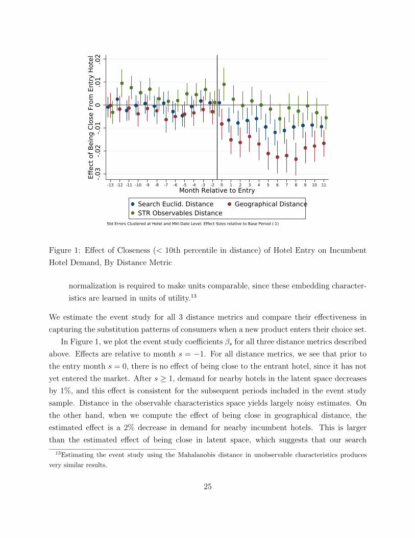
-.03

-.02

-.01

0.0

1.0

2Ef

fect

of B

eing

Clo

se F

rom

Ent

ry H

otel

-13 -12 -11 -10 -9 -8 -7 -6 -5 -4 -3 -2 0 1 2 3 4 5 6 7 8 9 10 11Month Relative to Entry

Search Euclid. Distance Geographical DistanceSTR Observables Distance

Std Errors Clustered at Hotel and Mkt-Date Level; Effect Sizes relative to Base Period (-1)

Figure 1: Effect of Closeness (< 10th percentile in distance) of Hotel Entry on Incumbent

Hotel Demand, By Distance Metric

normalization is required to make units comparable, since these embedding character-

istics are learned in units of utility.13

We estimate the event study for all 3 distance metrics and compare their effectiveness in

capturing the substitution patterns of consumers when a new product enters their choice set.

In Figure 1, we plot the event study coefficients βs for all three distance metrics described

above. Effects are relative to month s = −1. For all distance metrics, we see that prior to

the entry month s = 0, there is no effect of being close to the entrant hotel, since it has not

yet entered the market. After s ≥ 1, demand for nearby hotels in the latent space decreases

by 1%, and this effect is consistent for the subsequent periods included in the event study

sample. Distance in the observable characteristics space yields largely noisy estimates. On

the other hand, when we compute the effect of being close in geographical distance, the

estimated effect is a 2% decrease in demand for nearby incumbent hotels. This is larger

than the estimated effect of being close in latent space, which suggests that our search

13Estimating the event study using the Mahalanobis distance in unobservable characteristics produces

very similar results.

25

characteristics are unable to capture measures of product differentiation as relevant as one

of the primary ways hotels differentiate from one another, their physical location. This may

due to differential factors contributing to how consumers decide to search for hotels versus

actual purchases. Nonetheless, our estimated effects relying purely on learned characteristics

from search data are statistically significant and of reasonable economic magnitude, which

suggests that data on only search behavior is able to capture meaningful factors in how

product differentiation affect purchase decisions of consumers.

5.3 Demand Model

We estimate a modified version of a canonical discrete choice demand model , the mixed logit

with endogenous prices, or BLP (Berry, Levinsohn, and Pakes 1995) model, that uses the

unobserved heterogeneity and unobserved characteristics learned from the search data. We

then evaluate the fit of these demand models in predicting demand after a major merger in the

hotel industry that induced large price changes. In November 2015, Marriott International

announced it would be acquiring the competing Starwood Hotels company, creating the

largest hotel chain in the world (Dogru, Erdogan, and Kizildag 2018). In Appendix B, we

provide direct evidence that prices decreased by a large proportion (5%) in markets with

a high concentration of Marriott-Starwood hotels post-merger. We use these large price

changes to test whether our estimated demand model specifications can accurately predict

demand in an out-of-sample period which experienced large price changes, causing demand

substitution across products.

To perform this test, we estimate the demand system described in Section 4.2 on the

pre-merger hotel transaction data data (2012 to 2015), and evaluate the model’s ability to

predict demand changes for hotels post-merger announcement (2016 to 2018), which is held

out when we optimize the GMM objective function of BLP. While we are able to estimate

ξ in the pre-merger data to match market shares/demand exactly, this is unavailable in the

post-merger data. We evaluate the prediction of the model assuming ξj,t = 0; This is to be

consistent with the moments E[ξj,t|Zj,t] = 0.

Thus, predicted demand in the post-merger period(s) takes the following form:

qj,t(Σ, G(i)) = Mg

( 1

B

∑i∼G(i)

exp(δj + αipj,t + βiXj)

1 +∑

k∈Jt exp(δk + αipk,t + βiXk)

)(17)

Our loss function for evaluating demand prediction is the mean-squared error of log demand

26

in the post-merger dataset:

MSE(Σ, G) =1

Npost-merger

∑j,t

(log(qj,t)− log(qj,t))2 (18)

Table 5 displays the MSE of each demand model’s predictions, both pre and post-merger,

when we set the demand shock ξj,t to zero. The first row shows the predictive performance

of a simple logit model of demand with no unobserved heterogeneity in preferences. We

benchmark the performance of each model relative to the baseline logit model by computing

the relative decrease in MSE for model m from the logit model:

% Decrease from Logitm =MSEm −MSElogit

MSElogit

the second row shows the improvement in performance from a standard BLP model with

normally distributed heterogeneity over observable characteristics. BLP is able to improve

upon the logit in predicting both pre and post merger demand, improving the prediction er-

ror by 39% out-of-sample. Each other model that includes either latent preferences or latent

characteristics (or both) also generates improvements over the logit model. Our preferred

specification, which includes both observable and K = 5 unobservable characteristics, in ad-

dition to latent preferences, leads to a substantial improvement improvement of 48.48% over

the logit model in the out-of-sample fit. Specifications that include only latent preferences,

or only add latent characteristics, perform comparably to the standard BLP model. This

suggests that using latent preferences, latent characteristics, and observable characteristics

are import to capture substitution patterns in demand. Across our specifications, the in and

out of sample performance are comparable, suggesting we do not overfit in our estimation.

Our usage of transfer learning, by estimating a high dimensional latent characteristic and

preference space in a first stage with our large search dataset, allows us to estimate a small

number of parameters in demand estimation, which prevents overfitting.

In Appendix Table A2, we also compare predictions according to the Mean Absolute

Error (MAE) error metric. We obtain qualitatively similar results under this metric. Under

this metric, all models including latent characteristics and/or preferences outperform the

standard BLP model, suggesting the lower improvements in MSE may be driven by outlier

observations. In particular, larger gains come from including latent preferences in the de-

mand model. Taken together, the MAE and MSE results suggest that adding either latent

preferences or latent characteristics lead to comparable performance to the canonical BLP

model, but adding both leads to substantial gains in predictive performance. In Appendix

27

Pre-Merger (Training Data) Post-Merger (Test Data)

MSE % Decrease from Logit MSE % Decrease from Logit

Preferences Characteristics

None Observables 0.058 - 0.201 -

Normal Observables 0.046 -20.48% 0.123 -39.02%

Normal Observables & Latent 0.048 -17.06% 0.131 -35.02%

Search Observables 0.046 -21.33% 0.135 -32.88%

Search Observables & Latent 0.041 -28.76% 0.104 -48.48%

Table 5: Prediction Errors of Structural Demand Model

Preferences Normal Search

Characteristics Observables Observables & Latent

Price 0.0141 0.2154

Latitude 0.0000 0.0001

Longitude 0.0000 0.0007

Price Segment 0.0000 0.0735

Independent Hotel 0.0155 0.0000

Location = Airport 0.0001 0.0000

Location = Interstate 2.7485 0.0000

Location = Resort 0.0000 0.3347

Location = Small Metro/Town 0.0000 0.0233

Location = Suburban 0.0002 0.0000

Location = Urban 0.0000 0.0000

Log(Meeting Space+1) 0.0000 0.0455

Hotel Size Category 0.0000 0.0289

γj,1 (Latent and Observables) 0.0302

γj,2 (Latent and Observables) 0.0162

γj,3 (Latent and Observables) 0.2627

γj,4 (Latent and Observables) 0.0000

γj,5 (Latent and Observables) 0.0000

Table 6: Estimated Consumer Heterogeneity Demand Parameters

28

Table A3, we present results in terms of the total variation explained by each discrete choice

model (R-squared), which is inversely proportional to the mean-squared error.

To better understand the performance differences across the various models, Table 6 dis-

plays the estimates from the traditional BLP model with normal unobserved heterogeneity,

and our preferred specification- inclusion of observables and latent preferences/characteristics.

In Appendix Table A4, we report the full parameters from each of the 4 models considered.

Each row displays the estimated coefficient on individual-level heterogeneity along a certain

hotel characteristic. In the standard BLP model, price, whether a hotel is independently

owned, and the interstate location dummy capture most of the unobserved heterogeneity in

consumer preferences. In our preferred specification utilizing search data, we see positive

coefficients on 3 of the 5 the latent characteristics, suggesting that some of the latent char-

acteristics allow the model to capture substitution patterns that are not easily encoded in

observable characteristics. A consistent pattern across both models including latent pref-

erences is the large coefficient on consumer price heterogeneity. This may be because the

search-based model allows for multimodality in the distribution of random price coefficients,

which is ruled out by imposing the normal parametric structure.

6 Conclusion

We have presented an approach for using search data to augment demand estimation, in a

setting in which search is observed in one dataset, and choice is observed in another. The

key identification strategy in our methodology is that because there are multiple choices

made during the search process, latent preferences and product characteristics can be simul-

taneously estimated. As we have shown through an event study, the latent characteristics

are able to predict the relative losers on the supply side from a new entrant to a market,

suggesting they are meaningful and informative to market structure. In our analysis of the

Starwood-Marriott merger, it appears that the main value added lies in the estimation of

consumer preferences, since this allows us to model choice with a flexible distribution rather

than making strong parametric restrictions of random heterogeneity, and trying to identify

the model off a single choice alone.

Many questions are left open in this work. One is how best to use the data when

both search and choice are observed on the same platform, and the goal is counterfactual

prediction of events on that platform. A more streamlined model integrating search and

purchase preferences may more appropriately model demand in this case. A second is how

29

the platform’s own choices of product display and prominence (i.e. search rankings) should

be incorporated into the analysis. This may require a more complex model of search behavior

than that presented here. Last, a natural application that is left unexplored in the current

paper is to a market where observable characteristics are poor predictors of choice, such as

the market for books, so that latent characteristics recovered from search data could better

illuminate which products are in close competition.

References

Amano, T., A. Rhodes, and S. Seiler (2019): “Large-scale demand estimation with

search data,” .

Athey, S., D. Blei, R. Donnelly, F. Ruiz, and T. Schmidt (2018): “Estimating Het-

erogeneous Consumer Preferences for Restaurants and Travel Time Using Mobile Location

Data,” arXiv preprint arXiv:1801.07826.

Bajari, P., and C. L. Benkard (2005): “Demand estimation with heterogeneous con-

sumers and unobserved product characteristics: A hedonic approach,” Journal of political

economy, 113(6), 1239–1276.

Bajari, P., D. Nekipelov, S. P. Ryan, and M. Yang (2015): “Machine learning

methods for demand estimation,” American Economic Review, 105(5), 481–85.

Berry, S., and P. Jia (2010): “Tracing the Woes: An Empirical Analysis of the Airline

Industry,” American Economic Journal: Microeconomics, 2(3), 1–43.

Berry, S., J. Levinsohn, and A. Pakes (1995): “Automobile prices in market equilib-

rium,” Econometrica: Journal of the Econometric Society, pp. 841–890.

(2004): “Differentiated products demand systems from a combination of micro and

macro data: The new car market,” Journal of political Economy, 112(1), 68–105.

Chade, H., and L. Smith (2006): “Simultaneous search,” Econometrica, 74(5), 1293–1307.

Conlon, C., and J. Gortmaker (2019): “Best practices for differentiated products de-

mand estimation with pyblp,” Unpublished Manuscript.

Crawford, G. S., and A. Yurukoglu (2012): “The Welfare Effects of Bundling in

Multichannel Television Markets,” American Economic Review, 102(2), 643–85.

30

De los Santos, B., A. Hortacsu, and M. R. Wildenbeest (2012): “Testing models

of consumer search using data on web browsing and purchasing behavior,” American

Economic Review, 102(6), 2955–80.

De los Santos, B., and M. Wildenbeest (2017): “E-book pricing and vertical re-

straints.,” Quantitative Marketing and Economics, 15, 85–122.

Deaton, A., and J. Muellbauer (1980): “An Almost Ideal Demand System,” The

American Economic Review, 70(3), 312–326.

Dogru, T., A. Erdogan, and M. Kizildag (2018): “Marriott Starwood merger: what

did we learn from a financial standpoint?,” Journal of Hospitality and Tourism Insights.

Donnelly, R., A. Kanodia, and I. Morozov (2020): “A Unified Framework for Per-

sonalizing Product Rankings,” Available at SSRN 3649342.

Einav, L. (2007): “Seasonality in the U.S. motion picture industry,” The RAND Journal

of Economics, 38(1), 127–145.

Elrod, T. (1988): “Choice map: Inferring a product-market map from panel data,” Mar-

keting Science, 7(1), 21–40.

Elrod, T., and M. P. Keane (1995): “A factor-analytic probit model for representing

the market structure in panel data,” Journal of Marketing Research, 32(1), 1–16.

Erdem, T., and M. P. Keane (1996): “Decision-making under uncertainty: Capturing

dynamic brand choice processes in turbulent consumer goods markets,” Marketing science,

15(1), 1–20.

Fan, Y. (2013): “Ownership Consolidation and Product Characteristics: A Study of the

US Daily Newspaper Market,” American Economic Review, 103(5), 1598–1628.

Gandhi, A., and J.-F. Houde (2016): “Measuring substitution patterns in differentiated

products industries,” University of Wisconsin-Madison and Wharton School.

Goolsbee, A., and A. Petrin (2004): “The Consumer Gains from Direct Broadcast

Satellites and the Competition with Cable TV,” Econometrica, 72(2), 351–381.

Gowrisankaran, G., A. Nevo, and R. Town (2015): “Mergers When Prices Are

Negotiated: Evidence from the Hospital Industry,” American Economic Review, 105(1),

172–203.

31

Ho, K., and R. S. Lee (2017): “Insurer Competition in Health Care Markets,” Economet-

rica, 85(2), 379–417.

Honka, E. (2014): “Quantifying search and switching costs in the US auto insurance

industry,” The RAND Journal of Economics, 45(4), 847–884.

Honka, E., and P. Chintagunta (2016): “Simultaneous or sequential? search strategies

in the us auto insurance industry,” Marketing Science, 36(1), 21–42.

Houde, J.-F. (2012): “Spatial Differentiation and Vertical Mergers in Retail Markets for

Gasoline,” American Economic Review, 102(5), 2147–82.

Johnson, C. C. (2014): “Logistic matrix factorization for implicit feedback data,” Advances

in Neural Information Processing Systems, 27.

Keane, M. P., et al. (2013): Panel data discrete choice models of consumer demand.

Nuffield College.

Kim, J. B., P. Albuquerque, and B. J. Bronnenberg (2010): “Online demand under

limited consumer search,” Marketing science, 29(6), 1001–1023.

(2011): “Mapping online consumer search,” Journal of Marketing Research, 48(1),

13–27.

Kingma, D. P., and J. Ba (2014): “Adam: A method for stochastic optimization,” arXiv

preprint arXiv:1412.6980.

Koren, Y., R. Bell, and C. Volinsky (2009): “Matrix factorization techniques for

recommender systems,” Computer, (8), 30–37.

Lancaster, K. J. (1966): “A New Approach to Consumer Theory,” Journal of Political

Economy, 74(2), 132–157.

Lewis, G., and G. Zervas (2016): “The welfare impact of consumer reviews: A case study

of the hotel industry,” Unpublished manuscript.

Maaten, L. v. d., and G. Hinton (2008): “Visualizing data using t-SNE,” Journal of

machine learning research, 9(Nov), 2579–2605.

McFadden, D. (1973): “Conditional logit analysis of qualitative choice behavior,” Frontiers

in Econometrics, pp. 105–142.

32

Nevo, A. (2001): “Measuring Market Power in the Ready-to-Eat Cereal Industry,” Econo-

metrica, 69(2), 307–342.

Petrin, A. (2002): “Quantifying the benefits of new products: The case of the minivan,”

Journal of political Economy, 110(4), 705–729.

Rendle, S., C. Freudenthaler, Z. Gantner, and L. Schmidt-Thieme (2009):

“BPR: Bayesian personalized ranking from implicit feedback,” in Proceedings of the

twenty-fifth conference on uncertainty in artificial intelligence, pp. 452–461. AUAI Press.

Rudolph, M., F. Ruiz, S. Mandt, and D. Blei (2016): “Exponential family embed-

dings,” in Advances in Neural Information Processing Systems, pp. 478–486.

Ruiz, F. J., S. Athey, and D. M. Blei (2017): “SHOPPER: A Probabilistic Model of

Consumer Choice with Substitutes and Complements,” arXiv preprint arXiv:1711.03560.

Salakhutdinov, R., and A. Mnih (2008): “Bayesian probabilistic matrix factorization

using Markov chain Monte Carlo,” in Proceedings of the 25th international conference on

Machine learning, pp. 880–887. ACM.

Sams, J. A. (2019): “Learning or Herding? Understanding Social Interactions and the

Distribution of Success on a Social Music Sharing Platform,” Ph.D. thesis, Stanford Uni-

versity.

Schein, A. I., A. Popescul, L. H. Ungar, and D. M. Pennock (2002): “Methods and

metrics for cold-start recommendations,” in Proceedings of the 25th annual international

ACM SIGIR conference on Research and development in information retrieval, pp. 253–

260.

Ursu, R. M. (2018): “The power of rankings: Quantifying the effect of rankings on online

consumer search and purchase decisions,” Marketing Science, 37(4), 530–552.

33

Latent Characteristics Observable Characteristics

# Iterations Nodes/Layer Regularization # Iterations Nodes/Layer Regularization

Price 115 30 0.0001 397 40 0.2154

Latitude-Longitude 9127 10 0.0001 3488 40 0.0046

Independent Hotel 81 50 0.0000 723 40 0.0001

Near Airport 236 30 0.0046 348 20 0.0001

Hotel Size Category 180 20 0.0000 1084 40 0.0046

Table A1: Hyperparameters Chosen for Predicting Observable Characteristics

Pre-Merger (Training Data) Post-Merger (Test Data)

MAE % Decrease from Logit MAE % Decrease from Logit

Preferences Characteristics

None Observables 0.137 - 0.302 -

Normal Observables 0.116 -15.39% 0.226 -25.14%

Normal Observables & Latent 0.117 -15.01% 0.223 -26.34%

Search Observables 0.107 -22.38% 0.194 -35.86%

Search Observables & Latent 0.103 -24.99% 0.188 -37.90%

Table A2: Prediction Errors of Structural Demand Model (Mean Absolute Error)

Pre-Merger (Training Data) Post-Merger (Test Data)

R-Squared Increase From Logit R-Squared Increase From Logit

Preferences Characteristics

None Observables 0.917 - 0.686 -

Normal Observables 0.934 0.017 0.809 0.122

Normal Observables & Latent 0.931 0.014 0.796 0.110

Search Observables 0.935 0.018 0.789 0.103

Search Observables & Latent 0.941 0.024 0.838 0.152

Table A3: Fit of Structural Demand Model (R-Squared)

34

Preferences Normal Normal Search Search

Characteristics Observables Observables & Latent Observables Observables & Latent

Price 0.0141 0.0190 0.4073 0.2154

Latitude 0.0000 0.0000 0.0000 0.0001

Longitude 0.0000 0.0000 0.0005 0.0007

Price Segment 0.0000 0.0003 0.1140 0.0735

Independent Hotel 0.0155 0.0355 0.6479 0.0000

Location = Airport 0.0001 0.0000 0.0000 0.0000

Location = Interstate 2.7485 2.0458 0.0000 0.0000

Location = Resort 0.0000 0.0000 0.2801 0.3347

Location = Small Metro/Town 0.0000 0.0000 0.0000 0.0233

Location = Suburban 0.0002 0.0001 0.0000 0.0000

Location = Urban 0.0000 0.0146 0.0000 0.0000

Log(Meeting Space+1) 0.0000 0.0000 0.0511 0.0455

Hotel Size Category 0.0000 0.0000 0.0450 0.0289

γj,1 (Latent and Observables) 0.0000 0.0302

γj,2 (Latent and Observables) 0.0010 0.0162

γj,3 (Latent and Observables) 0.0008 0.2627

γj,4 (Latent and Observables) 0.0007 0.0000

γj,5 (Latent and Observables) 0.0000 0.0000

Table A4: Demand Parameters for All Model Estimates

35

A Understanding the Characteristics and Preference

Space: Supplementary Evidence

In this section, we provide supplementary evidence to Section 5.1 that our recovered latent

preferences and product characteristics from search data yield a sensible characterization of

the market for hotels.

First, we visually assess whether characteristics γj obtained from search data capture

the spatial distribution of hotels. We do so by projecting the 10-dimensional unobserved

characteristics obtained from the search model estimation to a two-dimensional space, using

the TSNE method (Maaten and Hinton 2008)14, to see if clusters formed on the 2-d space

correspond to STR’s geographical market definitions.

Figure A1 plots in the left panel the geographical locations of hotels in our STR dataset,

along with the 2-D projection of their locations in their latent characteristic space learned

from the search data in the right panel. Hotels are colored according to the geographical

market they reside in according to STR. We see clear hotel clusters formed in the latent char-

acteristic space that correspond to the geographical markets defined by STR. This suggests

that much of what is learned in the latent characteristic space is simply spatial differenta-

tion. However, there are some key differences in the cluster structure of hotels in the latent

characteristic space, suggesting physical geographical distance alone is an inadequate way

to measure competition between hotels and markets. For example, hotels in Los Angeles

(light grey) appear fairly close to a cluster of hotels in San Francisco/San Mateo (light blue),

as opposed to those hotels in the nearer region of Orange County (dark grey). This sug-

gests that consumers view San Francisco and Los Angeles as closer substitutes in terms of

destinations than Orange County and Los Angeles, which is intuitive since Orange County

is traditionally more of a resort-oriented tourist destination centered around its beaches,

whereas San Francisco and Los Angeles share urban amenities.

In Figure A2, we zoom in an a single large market, the Los Angeles market, and see if

the latent characteristics capture geographical differentiation beyond geographical dispersion

across markets in the Western United States. Here, hotels are colored according to their

STR sub-market (equivalent to a neighborhood within a market). Though clusters are less

clear than in the case of Figure A1, some patterns do exist. Hotels near the Los Angeles

International Airport are tightly clustered around each other, and there is lesser but still

14Our perplexity hyper-parameter is set to the square root of the number of hotels in each TSNE embedding

estimation routine

36

visible cluster of hotels in Northern Los Angeles.

We can also assess visually whether the recovered consumer search embeddings βi provide

plausible estimates of heterogeneity in demand for hotels. In Figure A3, we project the 18,492

unique preference vectors estimated from the unobservable characteristics only model into

a 2-dimensional space, split the sample of consumers into quartiles based on the average

price of hotels they searched, and produce density plots of consumer embeddings by price

quartile. We see some clear clusters emerge from the density plots, in particular among those

consumers who search very low-priced hotels. We can also assess whether our estimated

preferences are sensible by examining the correlation within-consumer of their preferences

over various characteristics of hotels. In Figures A4-A6, we plot the correlation matrix of

preferences over characteristics for each of the 3 estimated models. In Figure A4, where we

estimate preference heterogeneity only over observable characteristics, we find that latitude

and longitude preferences are strongly correlated, in addition to preferences for hotels that are

near highways or in small metropolitan areas. The former correlation represents a preference

for the overall spatial location of hotels (not just east-west or north-south), while the latter

is equally intuitive as both of those hotel location types are in predominantly rural locations.

Similarly, consumers with high preferences for hotels in resort location are less likely to have

preferences for hotels in urban and suburban locations, since travel to these locations differ

substantially in the amenities offered.

Second, we use an off-the-shelf method for classifying products, a top-k classifier, to see

if hotels that are close in the latent attribute space also share observable characteristics.

Specifically, given a candidate hotel j, we examine the characteristics of hotels that are the

top-10 closest in euclidean distance to j in the unobservable characteristic space:

d(j, k) = ||γj − γk||2 =

√√√√ L∑l=1

(γj,l − γk,l)2

where ~γj is the 10-d vector of latent characteristics learned in the unobservables only model.

We do this for all hotels k within the same STR-defined geographical market as j. We then

see what share of hotels classified as close according to the top-10 classifier share the same

brand, management company, ownership company, Parent company, and how close they are

in miles to the candidate hotel j. We perform this exercise for all hotels in our dataset, then

average across the classifiers for all J hotels in our dataset to see if, on average, the hotels

close in unobserved characteristics share observable attributes more often than those that

are classified as far away in the latent characteristic space.

37

Table A5 plots the result of the top-10 classifier for our targeted characteristics. Ob-

servations differ across target variables because not all hotels have a management, owner,

parent company, or brand (e.g. independent hotels have no parent company). We also use

as a comparison the results from a top-10 classifier based on the observable characteristics

of hotels, to benchmark our results.15 We find that in general, hotels closer in latent char-

acteristic are more likely to share supply-side characteristics such as brand/chain affiliation.

At the same time, the classifier based on observable characteristics performs better for all

characteristics, except distance. To an extent, this is not surprising since some character-

istics (such as class/price segment) are defined at the brand level, and many hotel chains

implement uniform characteristics across their locations.

15We use the Mahalanobis distance on observable characteristics to standardize the scale of each charac-

teristic. Because latitude and longitude is included in our input observable characteristics, we exclude it

when classifying for the distance metric.

38

125.0 122.5 120.0 117.5 115.0 112.5 110.0

32.5

35.0

37.5

40.0

42.5

45.0

47.5

GeographyMarket

Phoenix, AZPortland, ORArizona AreaCalifornia South/CentralSacramento, CAOregon AreaCalifornia NorthOakland, CACalifornia North CentralRiverside/San Bernardino, CASan Diego, CACalifornia Central CoastSeattle, WATucson, AZAnaheim/Santa Ana, CALos Angeles/Long Beach, CALas Vegas, NVWashington StateSan Francisco/San Mateo, CANevada (Exc Las Vegas)San Jose/Santa Cruz, CA

50 0 50

60

40

20

0

20

40

60

Latent Space (2D Projection)

Figure A1: Two-Dimensional Representation of Learned Latent Space by Market

Baseline Top-10 Classifier Based on Characteristics # Observations

All Hotels In Market Latent Observations

Pr(Same Brand) 0.029 0.038 0.093 3438

Pr(Same Mgmt Company) 0.027 0.051 0.098 1690

Pr(Same Owner) 0.037 0.066 0.117 1202

Pr(Same Parent Company) 0.133 0.165 0.251 3438

Distance (Miles) 51.413 32.197 37.261 4218

Table A5: Predictive Performance of Top-10 Classifier based on Distance in Latent and

Observable Characteristic Space

39

118.8 118.6 118.4 118.2 118.0 117.8

33.8

34.0

34.2

34.4

34.6

GeographyTract

Los Angeles North, CALos Angeles East, CALos Angeles Southeast, CASouth Bay, CAHollywood/Beverly Hills, CALong Beach, CALos Angeles CBD, CASanta Monica/Marina Del Rey, CPasadena/Glendale/Burbank, CALos Angeles Airport, CA

40 20 0 20 4040

20

0

20

40

Latent Space (2D Projection)

Figure A2: Two-Dimensional Representation of Los Angeles Learned Latent Space by Neigh-

borhood

60 40 20 0 20 40 60

50

25

0

25

50

Averaged Searched Price is $0-$101

60 40 20 0 20 40 60

Averaged Searched Price is $101-$147

60 40 20 0 20 40 60Averaged Searched Price is $147-$229

50

25

0

25

50

60 40 20 0 20 40 60Averaged Searched Price is $229+

0.00000

0.00003

0.00006

0.00009

0.00012

0.00015

0.00018

0.00021

0.00024

0.00027

Dens

ity

Figure A3: Heatmap of Two-Dimensional Representation of User Embeddings, by Quartiles

of Searched Prices

40

Size C

atego

ry

Log(M

eetin

g Spa

ce+1)

Indep

ende

nt Hote

l

Latitu

de

Longit

ude

Price

Segm

ent

Subu

rban L

ocatio

n

Small

Metro/T

own L

ocatio

n

Urban L

ocatio

n

Resort L

ocatio

n

Airport

Locat

ion

Inters

tate L

ocatio

nPri

cePrice

Interstate LocationAirport LocationResort LocationUrban Location

Small Metro/Town LocationSuburban Location

Price SegmentLongitude

LatitudeIndependent Hotel

Log(Meeting Space+1)Size Category 1.00

0.020.02

-0.02

-0.02

-0.04

-0.04

-0.04

-0.04

0.00

0.00

-0.03

-0.03

-0.22

-0.22

0.05

0.05

0.01

0.01

0.04

0.04

-0.08

-0.08

-0.01

-0.011.00

0.120.12

0.05

0.05

0.08

0.08

0.26

0.26

-0.09

-0.09

0.08

0.08

-0.01

-0.01

-0.06

-0.06

0.10

0.10

0.08

0.08

-0.01

-0.01

1.00

-0.06-0.06

0.05

0.05

0.03

0.03

-0.10

-0.10

0.02

0.02

0.04

0.04

0.12

0.12

0.07

0.07

0.03

0.03

-0.02

-0.02

1.00

-0.11-0.11

-0.01

-0.01

-0.29

-0.29

0.04

0.04

0.05

0.05

0.07

0.07

0.08

0.08

0.08

0.08

-0.03

-0.03

1.00

-0.06-0.06

-0.21

-0.21

0.02

0.02

-0.05

-0.05

0.09

0.09

0.12

0.12

0.02

0.02

0.04

0.04

1.00

-0.25-0.25

-0.03

-0.03

0.25

0.25

0.02

0.02

0.07

0.07

0.02

0.02

0.01

0.01

1.00-0.02-0.02

-0.04

-0.04

-0.03

-0.03

-0.13

-0.13

0.01

0.01

-0.03

-0.03

1.00

-0.11-0.11

-0.06

-0.06

0.02

0.02

0.13

0.13

0.00

0.00

1.00

0.230.23

0.04

0.04

0.05

0.05

-0.03

-0.03

1.00

0.060.06

0.05

0.05

0.02

0.02

1.00

0.020.02

0.13

0.13

1.00

-0.10-0.10

1.00

0.2

0.1

0.0

0.1

0.2

Pref

eren

ce C

orre

latio

n

Figure A4: Correlation Matrix of User Search Preferences: Observable Characteristics Model

Laten

t Dim

. 1

Laten

t Dim

. 2

Laten

t Dim

. 3

Laten

t Dim

. 4

Laten

t Dim

. 5

Laten

t Dim

. 6

Laten

t Dim

. 7

Laten

t Dim

. 8

Laten

t Dim

. 9

Laten

t Dim

. 10

Price

PriceLatent Dim. 10

Latent Dim. 9Latent Dim. 8Latent Dim. 7Latent Dim. 6Latent Dim. 5Latent Dim. 4Latent Dim. 3Latent Dim. 2Latent Dim. 1 1.00

0.160.16

-0.08

-0.08

0.18

0.18

0.05

0.05

-0.02

-0.02

-0.07

-0.07

-0.06

-0.06

-0.02

-0.02

0.12

0.12

0.14

0.141.00

-0.02-0.02

-0.03

-0.03

0.03

0.03

-0.01

-0.01

0.07

0.07

0.03

0.03

-0.04

-0.04

0.03

0.03

-0.07

-0.07

1.00

-0.02-0.02

-0.08

-0.08

0.00

0.00

0.00

0.00

0.03

0.03

0.06

0.06

-0.01

-0.01

-0.02

-0.02

1.00

0.050.05

-0.02

-0.02

-0.00

-0.00

-0.07

-0.07

-0.05

-0.05

0.05

0.05

0.05

0.05

1.00

-0.04-0.04

-0.02

-0.02

-0.05

-0.05

-0.03

-0.03

0.06

0.06

0.03

0.03

1.000.060.06

0.03

0.03

-0.02

-0.02

-0.07

-0.07

-0.01

-0.01

1.00

0.060.06

-0.04

-0.04

0.02

0.02

-0.07

-0.07

1.00

-0.03-0.03

-0.01

-0.01

-0.03

-0.03

1.00

-0.01-0.01

0.01

0.01

1.00

-0.00-0.00

1.00 0.15

0.10

0.05

0.00

0.05

0.10

0.15

Pref

eren

ce C

orre

latio

n

Figure A5: Correlation Matrix of User Search Preferences: Unobservable Characteristics

Model

41

Laten

t Dim

. 1

Laten

t Dim

. 2

Laten

t Dim

. 3

Laten

t Dim

. 4

Laten

t Dim

. 5

Size C

atego

ry

Log(M

eetin

g Spa

ce+1)

Indep

ende

nt Hote

l

Latitu

de

Longit

ude

Price

Segm

ent

Subu

rban L

ocatio

n

Small

Metro/T

own L

ocatio

n

Urban L

ocatio

n

Resort L

ocatio

n

Airport

Locat

ion

Inters

tate L

ocatio

nPri

cePrice

Interstate LocationAirport LocationResort LocationUrban Location

Small Metro/Town LocationSuburban Location

Price SegmentLongitude

LatitudeIndependent Hotel

Log(Meeting Space+1)Size CategoryLatent Dim. 5Latent Dim. 4Latent Dim. 3Latent Dim. 2Latent Dim. 1 1.00

0.020.02

-0.01

-0.01

-0.02

-0.02

-0.04

-0.04

0.01

0.01

-0.03

-0.03

-0.20

-0.20

0.05

0.05

-0.01

-0.01

0.02

0.02

-0.09

-0.09

0.01

0.01

-0.12

-0.12

0.10

0.10

-0.09

-0.09

0.11

0.11

0.07

0.071.00

0.040.04

-0.00

-0.00

0.03

0.03

0.24

0.24

-0.05

-0.05

0.02

0.02

0.02

0.02

0.03

0.03

0.06

0.06

0.02

0.02

-0.05

-0.05

0.01

0.01

0.03

0.03

0.02

0.02

0.00

0.00

-0.01

-0.01

1.00

-0.14-0.14

-0.10

-0.10

-0.00

-0.00

-0.07

-0.07

-0.02

-0.02

0.05

0.05

0.09

0.09

0.02

0.02

-0.00

-0.00

-0.01

-0.01

0.01

0.01

0.00

0.00

0.00

0.00

-0.00

-0.00

-0.01

-0.01

1.00

-0.21-0.21

-0.04

-0.04

-0.24

-0.24

0.07

0.07

0.06

0.06

0.09

0.09

0.06

0.06

0.05

0.05

-0.03

-0.03

0.02

0.02

-0.02

-0.02

0.00

0.00

0.05

0.05

-0.02

-0.02

1.00

-0.12-0.12

-0.20

-0.20

0.03

0.03

-0.04

-0.04

0.08

0.08

0.03

0.03

0.01

0.01

-0.01

-0.01

0.03

0.03

-0.06

-0.06

-0.00

-0.00

-0.04

-0.04

0.03

0.03

1.00

-0.16-0.16

-0.02

-0.02

0.13

0.13

0.06

0.06

0.06

0.06

-0.02

-0.02

-0.05

-0.05

-0.01

-0.01

-0.02

-0.02

-0.00

-0.00

0.00

0.00

-0.05

-0.05

1.00

-0.08-0.08

0.08

0.08

0.03

0.03

-0.06

-0.06

0.01

0.01

-0.02

-0.02

-0.05

-0.05

0.10

0.10

0.01

0.01

-0.05

-0.05

-0.02

-0.02

1.00

-0.11-0.11

-0.03

-0.03

0.02

0.02

0.11

0.11

0.03

0.03

0.08

0.08

-0.07

-0.07

0.08

0.08

-0.01

-0.01

0.02

0.02

1.000.14

0.140.00

0.00

0.02

0.02

-0.06

-0.06

-0.07

-0.07

0.06

0.06

0.04

0.04

0.03

0.03

-0.01

-0.01

1.000.04

0.04-0.00

-0.00

-0.03

-0.03

-0.01

-0.01

-0.06

-0.06

0.00

0.00

-0.00

-0.00

-0.04

-0.04

1.00

-0.00-0.00

0.05

0.05

0.01

0.01

-0.02

-0.02

-0.00

-0.00

0.00

0.00

-0.01

-0.01

1.00

-0.08-0.08

0.06

0.06

-0.02

-0.02

0.06

0.06

-0.01

-0.01

-0.02

-0.02

1.00

-0.00-0.00

0.00

0.00

-0.02

-0.02

0.01

0.01

0.01

0.01

1.00

-0.01-0.01

-0.01

-0.01

-0.05

-0.05

0.01

0.01

1.00

-0.08-0.08

0.03

0.03

-0.03

-0.03

1.00

-0.03-0.03

0.06

0.06

1.00

0.020.02

1.00

0.2

0.1

0.0

0.1

0.2

Pref

eren

ce C

orre

latio

n

Figure A6: Correlation Matrix of User Search Preferences: Observable & Unobservable

Characteristics Model

42

B Merger Impact on Hotel Conduct

In order to evaluate how effective our proposed demand model is in capturing actual substi-

tution patterns, we exploit a large merger that occurred during our sample period in the hotel

industry that induces plausibly exogenous price changes. On November 16, 2015, Marriott

International Inc announced that it would be acquiring the Starwood Hotels company. The

merger was completed on September 23, 2016 (Dogru, Erdogan, and Kizildag 2018). After

the merger completed, Marriott International became the largest hotel chain in the world.

After this transaction occurred, prices in markets with high concentration of Starwood /

Marriott hotels changed noticeably. Recall that the brand affiliations of each hotel in our

STR dataset is an anonymized ID, so we cannot observe which hotels in our transaction data

were Marriott or Starwood affiliates before the merger. Through further coordination with

STR, we were able to obtain counts of each hotel brand within each geographical market and

class segment, as of December 2015. We use this data to construct an “exposure index” to

the merger, Prj(Starwood or Marriott|Marketj, Classj), and measure the effect of exposure

to the merger on post-merger prices. The rationale behind this exposure index is that if

Marriott/Starwood hotels changed conduct in price-setting after a merger, then hotels be-

longing to the same geographical market/ class segment as Marriott/Starwood hotels will

also respond and change their price-setting behavior. The exposure index then captures both

“direct effects” of Marriott-Starwood hotels changing their price behavior due to backend

changes in costs and increased market power, as well as “indirect effects” of competing hotels

responding to the new price-setting behavior of Marriott/Starwood hotels.

We estimate the effect of exposure to the merger via the following event study specifica-

tion:

log(pj,t) = αj,month(t) +δt+

2019Q1∑q=2013Q1

βqPrj(Starwood or Marriott|Marketj, Classj)+εj,t (A1)

where αj,month(t) denotes hotel×month-of-year fixed effects , to capture time-invariant differ-

ences in hotel prices as well as seasonalities in pricing structure, δt is a geographical market

× month × year fixed effect, to capture common demand shocks occurring in each market-

month-year, and βs is the effect of the exposure index in quarter q on hotel j. We aggregate

the event-study specifications to the quarterly-level due to power concerns given the large

number of fixed effects. The control group in this event study are hotels in the same market

as Marriott-Starwood hotels but a different class segment. Because consumers have differen-

tial demand, hotels belonging to a different class are not as exposed to the changed pricing

43

behavior of Marriott-Starwood hotels after the merger.

Figure A7 plots the estimated event study. The dashed red line represents the time of the

merger announcement, while the solid red line represents the date the merger was completed.

The blue dots represent the estimated coefficients of the above specification, while the orange

dots replace the market-month-year fixed effects with market-month-year-location type (e.g.

urban vs suburban hotels in Los Angeles in May 2018) fixed effects.

In general, there do not appear to be strong pre-trends before the merger announcement.

We see large price decreases following the completion of the merger, which is consistent

with discussions surrounding the merger of cost reductions via centralization of sales and

customer service operations between the acquiring and target firms (Dogru, Erdogan, and

Kizildag 2018).

We use this event study as plausible evidence that the Marriott-Starwood merger led to

exogenous price changes by hotels in markets with high exposure to Marriott and Starwood

hotels, independent of demand fluctuations. Therefore, measuring the ability of our demand

models to accurately predict demand post-merger may serve as a test to whether a demand

model augmented with search data may perform “better” in predicting substitution patterns

after exogenous price changes.

44

Announcement Acquisition

-10

-5

0

5

ITT

% P

rice

Chan

ge

2013

Q1

2013

Q2

2013

Q3

2013

Q4

2014

Q1

2014

Q2

2014

Q3

2014

Q4

2015

Q1

2015

Q2

2015

Q3

2015

Q4

2016

Q1

2016

Q2

2016

Q3

2016

Q4

2017

Q1

2017

Q2

2017

Q3

2017

Q4

2018

Q1

2018

Q2

2018

Q3

2018

Q4

2019

Q1

Quarter-YearMarket Market-Location

Figure A7: Effect of Marriott-Starwood Merger on Prices in Regions with High Marriott-

Starwood Presence

45