LEARNING AND COMMUNICATION

IN SENDER-RECEIVER GAMES: AN ECONOMETRIC INVESTIGATION

Andreas Blume

Department of Economics University of Pittsburgh

Douglas V. DeJong

Tippie College of Business University of Iowa

George R. Neumann

Tippie College of Business University of Iowa

N.E. Savin*

Tippie College of Business University of Iowa

Iowa City, IA 52242 USA

Phone: 319-335-0855 Fax: 319-335-1956

gene-savin@uiowa.edu

August 1, 2001

* Corresponding author

ACKNOWLEDGEMENTS: The authors thank the referees and editor for their help. We also appreciate participants’ comments and suggestions at Aarhus University, National University of Ireland-Maynoth, Tilburg University, University of Wisconsin-Madison, Economic Science Association International Meeting (Manneheim University), Economic Science Association Annual Meeting and the 2000 World Econometrics Meetings. The authors thank the NSF for its support. General field: econometrics, game theory and experiments

JEL Classification Numbers: C72, C91, C92

SUMMARY

This paper compares stimulus response (SR) and belief-based learning (BBL) using data

from experiments with sender-receiver games. The environment, extensive form games

played in a population setting, is novel in the empirical literature on learning in games.

Both the SR and BBL models fit the data reasonably well in games where the preferences

of senders and receivers are perfectly aligned and where the population history of the

senders is known. The test results accept SR and reject BBL in games without population

history and in all but one of the games where senders and receivers have different

preferences over equilibria. Estimation is challenging since the likelihood function is not

globally concave and the data become uninformative about learning once equilibrium is

achieved.

1. INTRODUCTION

We study learning in simple games of communication between a privately informed

sender and a receiver when the sender’s message does not directly affect payoffs.

Sender–receiver games, introduced by Green and Stokey (1980) and Crawford and Sobel

(1982), provide the simplest stylized environment in which communication is essential in

order to establish a link between the receiver’s action and the sender’s private

information.

Sender-receiver games play a prominent role in theory and applied work in

accounting, economics, and political science. In accounting, Newman and Sansing (1993)

analyze voluntary disclosures made by management to its firm’s shareholders. In

economics, Stein (1989) examines communication between the Federal Reserve Board

and market traders. In political science, Austen-Smith (1990) considers the scope for

information transmission in debate among legislators with diverse preferences.

Sender-receiver games are played between an informed sender and an uninformed

receiver. The sender is privately informed about his type, �. The sender sends a message

m to the receiver, who responds with an action a. Payoffs to both players depend on the

sender’s private information � and the receiver’s action a. A strategy for the sender maps

types into messages m; for the receiver, a strategy maps messages m into actions a. A

strategy pair is a Nash equilibrium if the strategies are mutual best replies. An equilibrium

is called separating if each sender type is identified through his message. In a pooling

equilibrium, the equilibrium action does not depend on the sender’s type. Such an

equilibrium exists in every sender-receiver game.

�

1

Table 1a presents the payoffs for a simple game, Game 1, as a function of the

sender’s type �i and of the receiver’s action aj. If, for example, the sender’s type is �1,

then the receiver’s optimal action is a2. An example of a separating equilibrium in Game

1 is one where the sender sends m1 if he is type �1 and m2 otherwise, and where the

receiver takes action a2 after message m1 and a1 otherwise. An example of a pooling

equilibrium is one in which the sender, regardless of type, sends m1 and the receiver

always takes action a1. Game 1 is an example of a common interest game. Common

interest games have a unique, efficient payoff pair, whereas in divergent interest games

there is conflict over equilibria between senders and receivers.

In games like Game 1, where interests are closely aligned, informative equilibria are

plausible. However, conventional refinements like strategic stability (Kohlberg and

Mertens, 1986) do not rule out uninformative equilibria in sender-receiver games. Thus,

while we would expect separation in Game 1, the completely mixed equilibrium where

the sender randomizes uniformly over all messages, independent of type, and the receiver

randomizes uniformly over both actions independent of the message is also strategically

stable. In response, the literature has either resorted to a class of refinements that appeal

to the prior existence of a commonly understood language (Rabin, 1990, Matthews,

Okuno-Fujiwara and Postlewaite, 1991, and Farrell, 1993) or studied some evolutionary

or myopic learning dynamic (Blume, Kim and Sobel, 1993, Warneryd, 1993, and Blume

and Dieckmann, 1999). In the latter case, one can think of Nash equilibria as steady states

of the learning dynamic and thus, select equilibria according to the stability properties of

the steady states. We investigate an environment that is designed to make myopic

learning plausible.

2

In this paper, we restrict attention to an environment with repeated interactions among

a large population of individuals. There are at least two motivations for this restriction.

One is the view that communication evolves in a social context such as market exchange,

and is not just a one-shot interaction or confined to isolated exchange. The other is that

there are plausible equilibrium selection arguments for this environment. These include

the learning theories of Canning (1992) and Noldeke and Samuelson (1992) and the

evolutionary arguments of Blume et al. (1993), Warneryd (1993) and Blume and

Dieckmann (1999).

Blume, DeJong, Kim and Sprinkle (1998) have run experiments with Game 1 for 20

rounds where the design ensures that the messages are a priori meaningless.

Communication is essential in Game 1 because it is the only way to link the receiver’s

action to the sender’s private information, the sender’s type. In this environment, learning

is also essential for players to attach meanings to messages. Note that the optimal action

for the receiver is given the sender’s type is � and a given � . In the data produced

by the experiments, the receiver takes the optimal action given the sender’s type

approximately 50% of the time in the first round, as would be expected with meaningless

messages. This percentage gradually increases with more play; by round 20, the receiver

takes the optimal action 100% of the time. Thus, the data show that learning does indeed

take place and is gradual.

2a 1 1 2

The question addressed in the present paper is the form the learning takes in Blume et

al. (1998). There is a wide range of learning models to investigate, from naïve behavioral

models to sophisticated learning models like Kalai and Lehrer (1993). The typical result

for a sophisticated learning model is that under some restrictions on the prior beliefs of

3

the players, the players’ behavior will eventually converge to equilibrium behavior. Since

the folk theorem tells us that in repeated games (loosely speaking) “everything is an

equilibrium,” the implications of sophisticated learning models are often too weak to

provide a useful explanation of the empirical data. Specifically, equilibrium theories or

rational learning theories are consistent with an abundance of possible behaviors in the

Blume et al. (1998) experiments. However, these theories do not come close to

predicting the robust regularities in the data.

By contrast, a simple ad hoc stimulus response model (SR) provides a surprisingly

good explanation for many data sets. In the SR model, the probability that a player

chooses a particular action depends on the player’s past success with that action. Such

behavior requires only minimal cognitive abilities on the part of players, which is an

appealing feature for those who want to show that high-rationality predictions can be

derived from a low-rationality model. A closely related property is that SR learning

requires only minimal information. All that players need to know are the payoffs from

their own past actions; they need not know that they are playing a game, they need not

know their opponents’ payoff or their past play.

We find the SR model’s austere treatment of players’ information attractive because it

suggests a simple test of the validity of the model: Check whether the performance of the

SR model varies with the information condition in the data. Finally, we believe that once

we abandon the guiding principle of assuming agents are rational, simplicity can itself be

a virtue. At this juncture, there is more to be learned from exhibiting the merits and faults

of simple models than from using complex models, nested models or Bayesian estimation

to equivocate about varying degrees of rationality, heterogeneity of learning rules,

4

differences in information use, etc. These characteristics, its extensive use in the

literature, its minimal rationality assumption as well as its sharp assumption on the use of

information make the SR model a natural benchmark for our investigation.

On the other hand, it seems quite likely that individuals would try to exercise

more cognitive ability and hence try to use other available information. In belief-based

learning (BBL) models, players use more information than their own historical payoffs.

This information may include their own opponents’ play, the play of all possible

opponents and the play of all players. Models of this kind embody a higher level of

rationality; e.g. fictitious play can be interpreted as optimizing behavior given beliefs that

are derived from Bayesian updating under the assumption of stationary play of the other

players.

These two broad classes of learning models, namely, SR and BBL, are the

principal contenders in the literature on learning in experimental economics. For

example, see Boylan and El-Gamal (1993), Mookherjee and Sopher (1994, 1997),

Cheung and Friedman (1997), Cooper and Feltovich (1996), Cox, Shachat and Walker

(1995), Crawford (1995), Roth and Erev (1995), Erev and (1997), Erev and Rapoport

(1998). Both the SR and the BBL model are nested in the hybrid model of Camerer and

Ho (1999) and Camerer and Andersen (1999).

Using the Blume et al. (1998) data, we compare the SR model of Roth and Irev

(1995) and a simple BBL model in the spirit of fictitious play (Robinson, 1951) or one of

its stochastic variants (Fudenberg and Kreps, 1993).1 The Blume et al. (1998) data are

generated in experiments where an extensive form game is played repeatedly among a

population of players who are randomly matched before each period of play and receive

5

information about each other’s actions, not strategies. This population-game environment

is novel and particularly appropriate for a comparison of myopic learning rules. Since

players in the experiment observe only each other’s actions, the principal difference

between the two learning rules is in the roles they assign to own experience versus

population experience. Hence, the presence or absence of population history in the

experiments plays a crucial role.

Our empirical findings are as follows:

1. History matters. In the setting of common interest games, when information on

population history is available, both the SR and BBL models tend to fit the data

reasonably well. In the absence of history information, however, SR fits the data

substantially better than BBL. We find this reassuring since it is compatible with the view

that players use history information in forming their expectations, provided it is available.

2. Incentive structure matters. The values of the parameters for the SR model are different

for common interest and divergence interest games and similarly for the BBL model.

Furthermore, the comparison between SR and BBL also depends on the incentive

structure.

3. Equilibrium matters. For divergent interest games, the results are sensitive to the

equilibrium selected. Both SR and BBL fit the data reasonably well in the case of

convergence to a separating equilibrium, but neither performs well for experiments where

convergence is to a pooling equilibrium. The fit of BBL in the case of convergence to a

pooling equilibrium is especially poor.

4. Number of rounds matters. The number of rounds included in the analysis can

spuriously affect how well the models fit. Information about learning can be obtained

6

only as long as learning is taking place; after equilibrium is achieved, there is no further

learning. As a practical matter, however, the rounds included after the attainment of

equilibrium matter since they improve the fit of the model, although they provide no extra

information on learning. In other words, these additional rounds spuriously bias upwards

the fit of the model. Fortunately, this bias does not affect the comparison of the SR and

BBL models in the case of the Blume et al. (1998) data.

For the majority of the experiments, the data favors the SR model. However, this

does not imply that SR is the winner due to the first three factors cited above.

2. GAMES AND EXPERIMENTAL DESIGN

Our data are generated from repeated play of sender-receiver games among randomly

matched players. Players are drawn from two populations, six senders and six receivers.

Each period all players are matched, each sender with one receiver, and all pairings are

equally likely. The games played by each pair in each period are between an informed

sender and an uninformed receiver. The sender is privately informed about his type, ���or

�2, and types are equally likely.2 The sender sends a message, * or #, to the receiver, who

responds with an action, a1, a2 or a3. Payoffs depend on the sender's private information,

his type, and the receiver's action, and not on the sender’s message. The payoffs used in

the different treatments are given in Table 1b below, with the first entry in each cell

denoting the sender’s payoff and the second entry the receiver’s payoff. For example, in

Game 2, if the sender's type is �1 and the receiver takes action a2, the payoffs to the

sender and receiver are 700,700, respectively.

7

A strategy for the sender maps types into messages; for the receiver, a strategy maps

messages to actions. A strategy pair is a Nash equilibrium if the strategies are mutual

best replies. More formally let � be a finite set of types and �( ) the prior distribution of

types. The sender’s set of pure strategies is the set of mappings, s: �M, from the type

set to the finite set of messages, M. The receiver’s set of pure strategies is the set of

mappings, r����A, from M to the finite set of actions A. Given type ��� , message m�

M, and action a �A, the sender’s payoff is v

�

�

S(�, a) and the receiver’s payoff is vR(�, a).

Messages do not directly affect payoffs. For any finite set X, let �(X) denote the set of

probability distributions over X. The payoff from a mixed action ����(A) is vi(�,� )

( , ) ( ), , .ia Av a a i S R� �

�

� ��

We denote mixed behavior strategies for the sender and the receiver by ��and �,

respectively. Let �(m,�) denote the probability of type � sending message m and let

�(a,m) stand for the probability that the receiver will choose action a in response to

message m. The pair (�, �) is a Nash equilibrium if � and � are mutual best replies:

and '

'

( , ) 0, max ( , ) ( , ')

( , ) 0, max ( , ') ( , ) ( ).

sm M a A

Ra A

if m then m solves v a a m

if a m then a solves v a m�

� � � �

� � � � � �

��

���

�

�

�

�

The equilibrium is called separating if each sender type is identified through his

message. In a pooling equilibrium, the equilibrium action does not depend on the

sender's type; such equilibria exist for all sender-receiver games. In Game 2, an example

of a separating equilibrium is one where the sender sends * if he is �1 and # otherwise and

the receiver takes action a2 after message * and a1 otherwise. An example of a pooling

8

equilibrium is one in which the sender, regardless of type, sends * and the receiver always

takes action a3.

A replication of a game is played with a cohort of twelve players, six senders and six

receivers. Players are randomly designated as either a sender or receiver at the start of the

replication and keep their designation throughout. In each period of a game, senders and

receivers are paired using a random matching procedure. Sender types are independently

and identically drawn in each period for each sender.

In each period, players then play a two-stage game. Prior to the first stage, a sender is

informed about its type. In the first stage, a sender sends a message to its paired receiver.

In the second stage, a receiver takes an action after receiving a message from its paired

sender. Each sender and receiver pair then learns the sender type, message sent, action

taken and payoff received. All players next receive information about all sender types and

all messages sent by the respective sender types. This information is displayed for the

current and all previous periods of a session (to be described later) within a replication.

To ensure that messages have no a priori meaning, each player is endowed with his

own representation of the message space, i.e. both the form that messages take and the

order in which they are represented on the screen is individualized. The message space M

= {*, # } is observed by all players, and, for each player, either appears in the order (#,*)

or (*, #). Unique to each player, these messages are then mapped into an underlying,

unobservable message space, M = {A, B}.3 Consider one sender with an underlying

unobservable message mapping (A,B) and order of presentation (left, right) of (*,#) (#,*),

respectively, and two receivers with mappings and orderings of (#,*) (*,#), (*,#) (*,#),

respectively. If the sender sends the message that is ordered on the left side of the screen,

9

#, this translates into the underlying unobservable message space as B. If the message

was sent to the first receiver, the first receiver would observe the message * and its order

of appearance would be on the left side of the screen. When the aggregate history of

messages is shown to all players at the end of the period, the above message is displayed

to the second receiver (or another sender with the same mapping and ordering) under the

message # and its order of appearance would be on the right side of the screen. Similar

examples can be constructed for other pairings and messages. The mappings are designed

such that they destroy all conceivable focal points that players might use for a priori

coordination, Blume et al. (1998). The player representations and orderings are stable

over the replication. Thus, the experimental design focuses on the cohort's ability to

develop a language as a function of the game being played and the population history

provided.

Note that in this setting we observe the players’ action choices, not their strategies.

Also, the players themselves receive information about actions, not strategies. They do

not observe which message (action) would have been sent (taken) by a sender (receiver)

had the sender's type (message received) been different. This is important for how we

formulate our learning rules; e.g. the hypothetical updating (see Camerer and Ho,1997) of

unused actions that occurs in BBL does not and cannot rely on knowing opponents’

strategies but instead uses information about the population distribution of play.

We consider five experimental treatments, each with three replications. Each

replication is divided into two sessions, Session I, which is common to all treatments and

Session II, which varies across treatments. We concentrate on Session II data. The

treatments examined here differ in terms of the players’ incentives and the information

10

that is available after each period of play. For one treatment, the only information

available to a player is the history of play in her own past matches. Two questions are

examined for this case. The first is whether learning takes place. If learning does take

place, the second question is whether the SR model captures learning. In all the other

treatments, there is information available to the players in addition to the history of play

in their own past matches. For both senders and receivers, this information is the history

of play of the population of senders. Three questions are examined for these treatments.

The first again is whether learning takes place. If learning does take place, the second

question is whether learning is different from that in the previous treatment, and the third

is whether the BBL model better describes learning than the SR model.

The data from the experiments in Blume et al. (1998) consists of three replications

for each game. Replications for Game 1 and 2 were played for 20 periods and Game 3

and 4 for 40 periods. In the analysis of the experimental data only the first 20 periods are

used for G3 and G4. There were two different treatments conducted with Game 1, one

with and one without population history. The treatments are summarized in Table 2. 4

We observed separating outcomes for Game 1, Game 2 and the first two replications of

Game 3; we observed pooling outcomes for the third replication of Game 3 and all

replications of Game 4.

In this paper we focus on the analysis of sender behavior. This has two advantages.

First, the senders’ decision problems are comparable across treatments because in all

treatments there are two sender types and senders have two messages available. Second,

for senders there is a sensible, a priori, way of determining initial probabilities of sending

11

either message given the type because the experimental design enforces symmetry among

messages. We should also note that in our environment, sender- and receiver-data are not

readily comparable because all players in the experiment only ever observe the history of

sender play. Thus, senders face an interesting prediction problem if they are forming

beliefs about receiver play, as postulated by belief-based models. They cannot predict

future behavior of receivers from population information about past behavior of receivers

since no such information is available; instead, they have to predict future receiver

behavior from past sender data.

3. ESTIMATION OF THE SR MODEL

In this section we report the results of estimation for the SR model of behavior using

sender data. The SR and BBL models both use propensities to determine choice

probabilities. In our extensive form game setting, we have to make a choice of whether

we want to think of players as updating propensities of actions or of strategies. Both

choices constrain the way in which the updating at one information set affects the

updating at other information sets. If actions are updated, then there are no links across

the information sets. If strategies are updated, then choice probabilities change

continually at every information set. We chose updating of actions, which amounts to

treating each player-information set pair as a separate player. We use the index i to refer

to such a pair (�, �), where � denotes one of the six senders, � a type realization for that

sender, and the pair i is called a player.

12

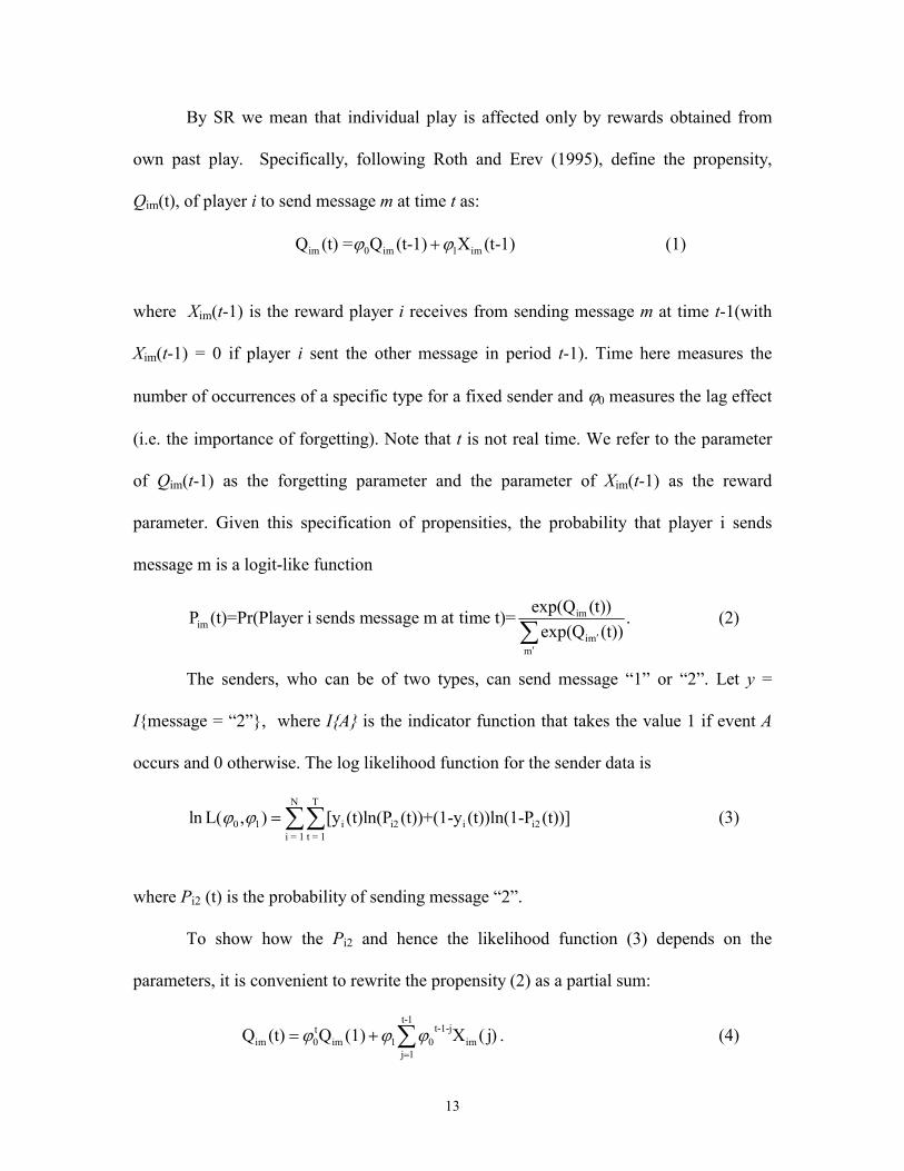
By SR we mean that individual play is affected only by rewards obtained from

own past play. Specifically, following Roth and Erev (1995), define the propensity,

Qim(t), of player i to send message m at time t as:

Q (1) im 0 im 1 im(t) = Q (t-1) X (t-1)� ��

where Xim(t-1) is the reward player i receives from sending message m at time t-1(with

Xim(t-1) = 0 if player i sent the other message in period t-1). Time here measures the

number of occurrences of a specific type for a fixed sender and 0 measures the lag effect

(i.e. the importance of forgetting). Note that t is not real time. We refer to the parameter

of Qim(t-1) as the forgetting parameter and the parameter of Xim(t-1) as the reward

parameter. Given this specification of propensities, the probability that player i sends

message m is a logit-like function

imim

imm

exp(Q (t))P (t)=Pr(Player i sends message m at time t)= .exp(Q (t))

�

�

� (2)

The senders, who can be of two types, can send message “1” or “2”. Let y =

I{message = “2”}, where I{A} is the indicator function that takes the value 1 if event A

occurs and 0 otherwise. The log likelihood function for the sender data is

(3) N T

0 1 i i2 i i2i = 1 t = 1

ln L( , ) [y (t)ln(P (t))+(1-y (t))ln(1-P (t))]� � ���

where Pi2 (t) is the probability of sending message “2”.

To show how the Pi2 and hence the likelihood function (3) depends on the

parameters, it is convenient to rewrite the propensity (2) as a partial sum:

. (4) t-1

t-1-jtim 0 im 1 0 im

j 1Q (t) Q (1) X ( j)� � �

�

� � �

13

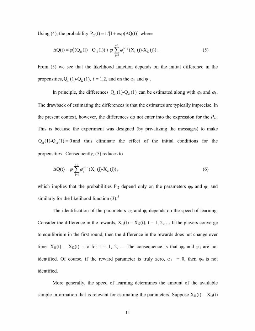
Using (4), the probability where i2P (t) 1/[1 exp( Q(t)]� � �

0

t-1t t-1-j0 i1 i2 1 i1 i2

j=1Q(t) (Q (1) Q (1)) (X (j)-X (j))� � �� � � � � . (5)

From (5) we see that the likelihood function depends on the initial difference in the

propensities, i = 1,2, and on the �i1 i2Q (1)-Q (1), 0 and �1.

In principle, the differences can be estimated along with i1 i2Q (1)-Q (1) 0 and 1.

The drawback of estimating the differences is that the estimates are typically imprecise. In

the present context, however, the differences do not enter into the expression for the Pi2.

This is because the experiment was designed (by privatizing the messages) to make

and thus eliminate the effect of the initial conditions for the

propensities. Consequently, (5) reduces to

i1 i2Q (1)-Q (1) = 0

0

t-1t-1-j

1 i1 ij=1

Q(t) (X (j)-X (j))� �� � � 2 , (6)

which implies that the probabilities Pi2 depend only on the parameters �0 and �1 and

similarly for the likelihood function (3).5

The identification of the parameters �0 and �1 depends on the speed of learning.

Consider the difference in the rewards, Xi1(t) – Xi2(t), t = 1, 2,…. If the players converge

to equilibrium in the first round, then the difference in the rewards does not change over

time: Xi1(t) – Xi2(t) = c for t = 1, 2,…. The consequence is that �0 and �1 are not

identified. Of course, if the reward parameter is truly zero, �1 = 0, then �0 is not

identified.

More generally, the speed of learning determines the amount of the available

sample information that is relevant for estimating the parameters. Suppose Xi1(t) – Xi2(t)

14

= c for t > T*. Then, increasing T beyond T* will not increase the precision of the

estimate. Rapid learning means that T* is small, and, hence, there is, relatively speaking,

little information available to estimate the parameters. On the other hand, increasing T

beyond T* will appear to improve the fit of the model to the data. We refer to this effect

as convergence bias. Convergence bias is discussed in more detail in section 8.

The likelihood function was maximized separately for each of the 15 replications

using observations from period 1 to 20. The results of doing so are shown in Table 3.

Columns 2 and 3 of the table contain the maximum likelihood (ML) estimates of �0 and

�1 and columns 4 and 5 contain the log likelihood value at the optimum, and McFadden's

(1974) psuedo-R2 statistic. The psuedo-R2 statistic is defined as 1- ln(L U)/ln(L R) where

LU is the maximized value of the likelihood, and LR is the value of the likelihood function

when �1= 0 and �1 = 0, LR = L(0, 0). From (2) the value of the lnL(0,0) = NTln(1/2) =

-(6�20)ln(2) = -83.17. This is because �1= 0 and �1 = 0 imply that Qim(t) = 0 for all t, and

hence that the probability of message “2” is Pi2(t) = 0.5.

The feature that stands out in Table 3 is the fit of the SR model. When the

parameters are chosen optimally, the SR model fits the experimental data well for the

common interest games with history, judging by the psuedo-R2 values reported in column

5. In general, the SR model tends to fit Game 1 with history better than Game 1 without

history. A puzzle is why history should matter for SR. The SR model performs well for

the divergent interest games when there is convergence to a separating equilibrium, which

occurs in G3R1 and G3R2. For G4R3 the relatively good performance is explained by the

fact that even though a separating equilibrium is not attained, one sender type, �2, is

15

almost fully identified. It should be noted that the ML estimates maximize the log

likelihood, not the psuedo-R2.

Figure 1 shows the probability of sending message 2 for each agent type by period

for the 15 replications. The smooth line marked with triangles shows the predicted

fraction of type 1 agents playing message “2” each period while the smooth line marked

with circles shows the model's predicted fraction of type 2 agents playing message “2”.

The fraction of type 1 agents actually playing message “2” is shown by the upper red

jagged line while the fraction of type 2 agents actually playing message 2 is shown by the

lower green jagged line. Thus, in the game shown in the top left-hand graph in the figure -

G1R1 - 50% of type 1 agents play message “2” in round 1, as do 50% of type 2 agents.

By period 7, 100% of type 1 agents play message 2, and 100% of type 2 agents play

message 1. A similar pattern appears in replications 2 of Game 1 and in all three

replications of Game 2. The players converge to equilibrium less rapidly in replication 3

of Game 1 and in the divergent interest games. A complete discussion of the empirical

patterns in these experiments is given in Blume et al. (1998). Figure 1 demonstrates that

in many experiments SR fits the data of Blume et al. (1998) reasonably well.

4. ESTIMATION OF THE BBL MODEL

An alternative literature (e.g., Van Huyck, Battalio, and Rankin, 1996, Cheung

and Friedman, 1997) argues that variants of fictitious play –BBL�are better

characterizations of play in experiments. BBL is expected to dominate SR because BBL

uses more information, namely in our setting the past behavior of other participants.

16

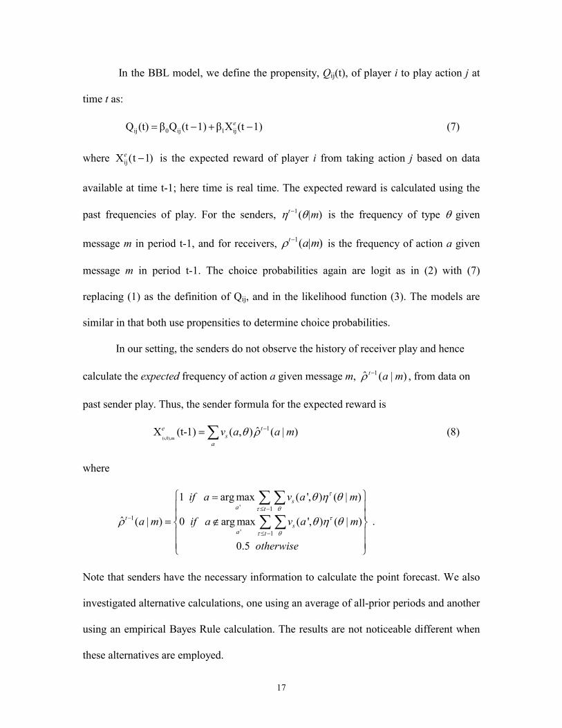
In the BBL model, we define the propensity, Qij(t), of player i to play action j at

time t as:

ij 0 ij 1 ijQ (t) β Q (t 1) β X (t 1)e� � � � (7)

where is the expected reward of player i from taking action j based on data

available at time t-1; here time is real time. The expected reward is calculated using the

past frequencies of play. For the senders, � � is the frequency of type � given

message m in period t-1, and for receivers, � is the frequency of action a given

message m in period t-1. The choice probabilities again are logit as in (2) with (7)

replacing (1) as the definition of Q

ijX (t 1)e�

t m�1( | )

t a m�1( | )

ij, and in the likelihood function (3). The models are

similar in that both use propensities to determine choice probabilities.

In our setting, the senders do not observe the history of receiver play and hence

calculate the expected frequency of action a given message m, , from data on

past sender play. Thus, the sender formula for the expected reward is

)|(ˆ 1 mat��

X ( (8) (ι,θ),m

1ˆt-1) ( , ) ( |e ts

a

v a a m� � �

�� )

)

� �

where

. ' 1

1

' 1

1 arg max ( ', ) ( |

ˆ ( | ) 0 arg max ( ', ) ( | )

0.5

sa t

ts

a t

if a v a m

a m if a v a m

otherwise

�

� �

�

� �

� � �

� �

� �

�

� �

� ��� �� �

� �� �� �� ��

��

��

Note that senders have the necessary information to calculate the point forecast. We also

investigated alternative calculations, one using an average of all-prior periods and another

using an empirical Bayes Rule calculation. The results are not noticeable different when

these alternatives are employed.

17

Table 4 contains the estimates for each of the 15 replications. Columns 2 and 3 of

the table contain the ML estimates of �0 and �1, and columns 4 and 5 contain the log

likelihood value at the optimum, and the psuedo-R2 statistic evaluated at the ML

estimates.

Two features stand out in the table. First, in the case of the common interest

games, the BBL model performs as expected in the sense that it tends to fit better when

history information is available. The comparison of psuedo-R2’s is suggestive: BBL fits

about as well as SR, sometimes better and sometimes worse, in common interest games

with population history information while SR wins without that information. SR tends to

fit better than BBL in divergent interest games. The fit of the BBL model is illustrated in

Figure 2, which shows the relation of predicted response and actual response by period. In

Figure 2 what stands out is the poor performance of BBL in Game 1 without history and

in Game 4.

Second, 0, the forgetting coefficient in the BBL model, is negative in two

replications of Game 1 without history, G1NHR1 and G1NHR2, and in two replications

of Game 4, G4R1 and G4R2. In every one of these four cases, the fit of the BBL model is

very poor, which suggests that the BBL model is not the correct model.

For these four cases, we also note that the null hypothesis that coefficient of the

expected reward is equal to zero, 1 = 0, is overwhelmingly accepted by the conventional

likelihood ratio test. In the conventional test, the asymptotic critical value is based on the

chi-square distribution with one degree of freedom. For each of the four likelihood ratio

tests, the P-value based on the chi-square (1) distribution is at least 0.30. Note that the

null hypothesis 1 = 0 is also accepted by the conventional likelihood ratio test for G3R3

18

as well as G4R3.

The test for 1 = 0 (i.e., there is no learning) is interesting because when 1 = 0 is

true, the forgetting parameter 0 is not identified. Thus, it is not so surprising that a

negative estimate of 0 occurs. Although the above test results for 1 = 0 appear to

support the conclusion that no learning is taking place, these test results must be treated

with caution. Even if the BBL model is correct, which is very doubtful, the conventional

test may produce misleading results due to the fact that nuisance parameter 0 is not

identified when the null 1 = 0 is true.

As in the case of the SR model, the lack of identification is due to the fact that

Qi1(t) = Qi2(t) for all t when 1 = 0, which implies that Pi2(t) = 0.5 for all t. Hansen

(1996), Andrews (1997), Stinchcombe and White (1998) and others have investigated the

general case of hypothesis testing when the nuisance parameter is not identified under the

null. Their results show that the relevant asymptotic distribution theory is nonstandard:

the asymptotic distribution of the test statistic, instead of being chi-square, may depend

on the value of the nuisance parameter.

Finally, the likelihood functions for the SR and BBL models are not globally

concave. One obvious example of this problem is given in Table 15 of Salmon

(forthcoming,2001). He reports that up to 69% of the maximum likelihood estimates of

the Camerer and Ho specification failed to converge using simulated data generated

according to the true data generation process.6 As a consequence, standard maximization

routines are not guaranteed to locate a global optimum. See Appendix A for a full

discussion of this problem, the proof of its pervasiveness and our procedures for

overcoming the global concavity concern.

19

5. POOLING

In the above analysis, we have treated each replication of a particular game as

independent, and obtained separate estimates of the parameters from each. Since the

underlying learning rule is assumed to be the same in each replication it may make sense

to pool the observations across each replication, and potentially across the different

games. If such aggregation were warranted, it would admit more precise inference.

Whether one can pool the replications of a particular experimental game involving

learning is of independent interest. One obvious circumstance where pooling would be

inappropriate is one where the participants followed different learning rules. In this case

combining the replications of a game will pool learning processes that are fundamentally

different, i.e., have different values of � �i or, i , i = 0,1.

Alternatively, even where the learning process is the same, the evolution of play

may be quite different because of the incentives that the participants face. For example,

in the games that we study, Games 1 and 2 have an equilibrium that both senders and

receivers strictly prefer. Note that in Game 2 there is also a pooling equilibrium where

action a3 is taken regardless of the message sent. In Games 3 and 4, by way of contrast,

the interests of the senders and receivers are not perfectly aligned, with receivers

preferring the separating over the pooling equilibrium relatively more in Game 3 than

Game 4. The possibility of different equilibrium selection in these games leads to the

possibility that the outcomes are situation specific and that the data from the replications

cannot be simply pooled.

To examine whether the replication data can be pooled we fit the SR model to the

20

three replications of each treatment or experimental game. Then the standard chi-squared

test based on minus 2 times the difference of the log likelihoods is used to compare the

constrained and unconstrained values of the likelihood function. There are three

replications for each game, so there are 2 � 3 = 6 parameters estimated in the

unconstrained case and 2 in the constrained case, resulting in chi-square tests with 4

degrees of freedom. The results are displayed in Table 5. In both Games 1 and 2 with

history, the data suggest that a common learning rule is followed. Indeed, the marginal

significance level of the test statistics is at least 35% across the tests, suggesting that it is

not even a close call. In contrast, the data for Games 3 and 4 are not compatible with a

common learning model. In each case the chi-square test rejects the hypothesis of a

learning rule with common parameter values, and, again, the rejection is not a close call.

Of course, other combinations could be tested for pooling. The message delivered by the

above results is that even pooling across the replications of the same treatment or

experimental game is not always possible, and, hence, the focus of the subsequent

statistical analysis is on individual replications.

6. COMPARING SR AND BBL MODELS

The results in Tables 3 and 4 show that SR and BBL tend to fit about equally well

for the common interest games with history on the basis of the psuedo-R2 values, and that

BBL fits better in the common interest games with history than without history. Further,

SR tends to fit better for the divergent interest games. While this is suggestive, it is

difficult to make probabilistic comparisons between the SR and BBL models because the

models are non-nested (Davidson and MacKinnon, 1984, 1993). By a non-nested model

21

we mean that the model being tested, the null hypothesis, is not a special case of the

alternative model to which it is compared. In our setting, the two models can be

artificially nested, however, with the consequence that they can be compared using

standard testing procedures. This fact has been exploited by Camerer and Ho (1999), who

recognized that SR and BBL models are nested in a general class of models that use

propensities to determine choice probabilities.

In this section, the approach of Camerer and Ho (1999) is adapted to our

experimental data. The updating equation is modified to include both own and expected

payoffs:

(9) ij 0 ij 1 ij 2 ijQ (t) Q (t-1) X (t-1) X (t-1)e� � �� � �

where is the expected payoff from making choice j at time t-1 and XijX (t-1)eij(t-1) is the

actual payoff from making choice j at time t-1; here time is real time. We refer to the

model with the updating equation (9) as the hybrid model since it is a combination of the

SR and BBL models.7

The likelihood function for the sender data was maximized separately for each of

the 15 replications using observations from period 2 onwards. The results of

maximization are shown in Table 6. Columns 2, 3 and 4 of the table contain the

estimates of ������ and ����and columns 5 and 6 contains the log likelihood value at its

optimum and the value of psuedo-R2. Since the psuedo-R2 is a monotonic function of the

log likelihood, it is no surprise that the fit of the hybrid model is at least as good as the fit

of either the SR or BBL model. Note that the ML estimation algorithm failed to converge

for G2R2 and G2R3, a problem that is due to a singular Hessian.

22

In Table 7, columns 2 and 3 report the Wald t statistics for testing the hypotheses

H0: �� = 0 and H0: �� = 0. Each null hypothesis is evaluated using a symmetric test at the

nominal 5% level, and, hence, by the Bonferroni inequality, the probability of

simultaneously rejecting both hypotheses is approximately 0.10. The results of this pair

of tests are summarized in columns 4, 5, 6 and 7. Rejection of H0: �� = 0 is interpreted as

acceptance of BBL and rejection of H0: �� = 0 as acceptance of SR.

From an inspection of these columns, we see that in 10 out of the 13 replications

SR is accepted and BBL is rejected. This is consistent with a ranking of the models based

on the psuedo-R2’s reported in Table 3 and 4. As is intuitively plausible, this result occurs

mainly in Game 1 without history and the Games 3 and 4, the divergent interest games.

Both SR and BBL are rejected in 2 out of 13 replications (H0: �� = 0 is accepted and H0:

�� = 0 is accepted); this occurs in Games 1 and 3, G1R2 and G3R1. In Game 1 with

history, the results are mixed. BBL was accepted and SR rejected (H0: �� = 0 is rejected

and H0: �� = 0 is accepted) in G1R1 while the reverse is true in G1R3. Both are rejected

in G1R2. The conclusions drawn from this testing exercise are similar to those produced

by comparing the psuedo-R2’s in Tables 3 and 4.

The tests were also conducted at the nominal 2.5% level, that is, using a critical

value of 2.27. In this case, the probability of simultaneously rejecting both hypotheses is

approximately 0.05 using the Bonferroni inequality. The tests results were unchanged by

increasing the critical value to 2.27.

There are two potential problems with artificial nesting using the hybrid model.

The first is that if H0: �� = 0 and H0: �� = 0 is true, then �0 is not identified. The argument

is similar to that previously discussed in connection with the BBL model. In this

23

situation, the usual asymptotic distribution theory does not apply: The asymptotic

distributions of the t statistics for testing H0: �� = 0 and H0: �� = 0 are not, in general,

standard normal when the nulls are true. Recall the previous finding that the null

hypotheses H0: �� = 0 and H0: �� = 0 are simultaneously accepted in two cases when the

absolute critical value is 2.00 and in three cases when the absolute critical value is 2.27.

In light of the identification problem, this finding must be treated with caution.

Second, the explanatory variables may be highly collinear. Our results appear to

be influenced by multicollinearity between the expected reward and the actual

reward X

ijX (t-1)e

ij(t-1). The source of the multicollinearity is due to learning. If play converges to

a pure strategy equilibrium, then the actual and expected reward variables take on

identical values. Thus, after convergence to equilibrium there is exact collinearity

between the two information variables. Multicollinearity tends to be more of a problem in

the common interest games; in particular, the rapid convergence to equilibrium appears to

explain the singular Hessian in G2R2 and G2R3. The degree of multicollinearity depends

on the number of observations included in the data after convergence has been achieved.

This matter is discussed in more detail in the convergence bias section.

7. RECEIVER DATA

In this section, we report our findings for receivers by focusing on the SR model

for Game 1 with and without history. Game 1 is a common interest game in which the

number of choices for both senders and receivers is two. Our experimental design draws

senders and receivers from two distinct populations. Given its information and updating

assumptions, the SR model predicts no difference in the behavior between senders and

24

receivers for Game 1 in both games with and without history.8 Strictly speaking, the SR

model predicts no difference in the behavior of senders and receivers across all games.

However, since we already know that sender behavior differs across games, we focus on

sender and receiver behavior in Game 1 where the SR prediction has its best chance for

success.

Table 8 contains the results of testing the hypothesis that senders and receivers

respond the same in Game 1. The test is constructed in the usual way: The unrestricted

likelihood function is maximized separately for sender data and separately for receiver

data, estimating a total of four coefficients. The restricted likelihood function is then

maximized on both sets of data. Column (3) of the table indicates that when population

history is available, the hypothesis that the coefficients are the same for each side is

overwhelmingly rejected by the data. But, when history is not available, the SR model

becomes a priori more likely, and tests of the equality of coefficients are not rejected

using a strict P-value of .01 or less (two out of three replications using a strict P-value of

.05 or less).

8. CONVERGENCE BIAS

It is common practice to include all observations from a particular replication or

treatment in any statistical estimation or testing exercise based on that replication or

treatment. Yet information about learning can only come from observations where

learning occurs. As noted earlier, once behavior has converged, which implies that Xi1(t)

- Xi2(t) = c for t > T*, additional observations provide no further information about

learning. Including such observations will make the model appear to “fit” better, while at

25

the same time reducing the contrast between models, making it difficult to distinguish the

models empirically. The data shown in Figures 1 and 2 indicate that convergence

typically occurs within 5 to 7 periods, while observations for all 20 periods are included

in the estimation.

To illustrate the possible bias that this might cause, we calculated the average log

likelihood (the maximized log likelihood divided by number of observations used) by

progressively removing observations from the later periods, that is, by removing

observations that include convergence. Figure 3 illustrates this bias for the replication

G1R1. Under the hypothesis of no convergence bias we would expect the average log

likelihood to be invariant to the number of periods included both for the SR and BBL

models. Hence, under the hypothesis, the curves in Figure 3 would have zero slope. In

fact, the two curves have positive slope, which is characteristic of convergence bias.

However, the difference between the curves is approximately constant in these data,

which suggests that convergence bias makes both models appear to fit the data better, but

does not otherwise bias the comparison of SR and BBL.

To measure the amount of bias requires taking a position on when convergence

has occurred, a classification that is better made on individual data. We define the

convergence operator Tp(yit) by

T y if y y yp it it it it p( ) ...� � � ��

1 1 ,�

(10)

� 0 else

In other words a player's (pure) strategy is said to have converged if the same action is

taken p times in a row.9 To eliminate convergence bias, one simply excludes

26

observations where Tp = 1. We used this procedure with p = 3 and p = 4 to assess the

extent of this bias. We found that at least for these data, the extent of the bias was small.

9. SUMMARY AND FUTURE AGENDA

In this paper, we focused on two principal learning models in the literature, SR

and BBL, using propensities to capture players’ predisposition to take certain actions.

These two models share much in common with the experience-weighted attraction

(EWA) or hybrid model since the EWA model also allows us to capture and compare SR,

BBL and EWA via propensities. We focus on a sender-receiver game; specifically, an

extensive form game is played repeatedly among players who are randomly matched

before each period of play. This population-game environment is particularly appropriate

for a comparison of myopic learning rules, if we believe that it lessens the role of

repeated game strategies. Sender-receiver games with costless and a priori meaningless

messages have the advantage that, no matter how we specify the incentives, coordination

requires communication and communication requires learning.

One consequence of studying learning in extensive form games here is that the

principal difference between the two learning models is in the roles they assign to own

experience versus population experience. This is because players in the experiment

observe only each others’ actions, not strategies. Another consequence is that there are

different natural specifications even for a learning model as simple as SR. We chose the

cognitively least demanding model, namely one in which experience at one information

set does not transfer to other information sets. Our results show that both the SR and BBL

models fit the data reasonably well in common interest games with history. On the other

27

hand, the test results accept SR and reject BBL in the games with no history and in all but

one of the divergent interest games.

It should be emphasized that we are quite agnostic about the “winning” learning

model and for that matter which one of the alternative models wins. While SR seems to

work “best,” there are clearly problems with the model. For common interest Game 1

with history and Game 2, the parameter values are stable across the replications of a given

game. However, the information condition between Game 1 with and without history

should not matter for SR, yet it obviously does. Moreover, the parameter values are not

stable across the replications of the other games nor are the parameters stable across the

different games, themselves.10 This suggests that the SR model (and for that matter the

BBL model) fails to capture the strategic aspects of the different games and the respective

learning involved.

One of the reasons economists are interested in learning is their concern about

mechanism design and the dynamics of institutions and their robustness. This includes a

concern about how learning fits into issues of common knowledge and strategy.

Alternative models should allow the theorist to recognize and modify theory to explain

the outcomes observed. This means that we should be able to econometrically distinguish

among the alternatives. For example, is the model a mixture of SR and BBL, i.e., EWA,

or is it heterogeneity in a parameter within a given learning model? However, care must

be taken not to introduce complexity for complexity sake; e.g., is it SR or SR with

heterogeneity, is it BBL or is it BBL with heterogeneity, or is it EWA versus EWA with

heterogeneity, and so on? Nevertheless, one of our findings, the inability to distinguish

28

between the SR and BBL models in common interest games with history, illustrates the

problems with discriminating among proposed learning models.

The critical issue is how to learn more about learning from experiments. The

characteristics of the various learning models and their econometric properties are not

well understood. The starting point for our agenda for the future is based on the fact that

learning models in games completely specify the data generating process. As a

consequence, the models can be simulated. Simulation provides a way of investigating

the economic and econometric properties of the models.

From a statistical point of view, our present treatment of testing with experimental

data has been classical and entirely conventional.11 We have assumed that standard

asymptotic theory is a reliable guide for inference. However, first-order asymptotic theory

often gives a poor approximation to the distributions of test statistics with the samples of

the sizes encountered in applications. For example, the nominal levels of tests based on

asymptotic critical values can be very different from the true values. Simulation studies

can be conducted to investigate the finite-sample performance of the tests based on

asymptotic critical values. The power of the tests can be explored once the probability of

making a Type I error is under control. The consideration of power leads to issues of

optimal design. Simulation can be used to help us design our experiments so that we learn

more about learning.

29

APPENDIX A

The likelihood functions for the SR and BBL models are not globally concave. As a

consequence, standard maximization routines are not guaranteed to locate a global

optimum. In fact, we frequently found that quasi-Newton methods alone would get stuck

at local optima, or wander aimlessly in flat sections of the function. Figure 4 shows the

typical shape of the likelihood function for SR models in games of common interest, in

this case G1R1, while Figure 5 shows the shape of the likelihood function for the BBL

model in the case of G1R1.

Note that although the likelihood functions are shaped quite differently, both

exhibit large flat spots and multiple local optima. The SR likelihood function also

characteristically has a long ridge, as the contour plots in Figure 4 illustrate.

To obtain the ML estimates, we initially used a grid search on the parameter

space, evaluating the function 2,500 times. This grid search always included the point

(0,0) so that the no-learning model was always considered. The maximum maximorum

of these points was used to pick the starting values for the first derivative method. We

used Broydon-Fletcher-Goldfarb-Shanno, BFGS, with golden section search to obtain an

optimum.12 Graphical inspection of the likelihood surface was used to assess whether a

global optimum had been reached. The motivation for using BFGS is to avoid the use of

second derivatives in calculating the ML estimates. Since the standard errors are

calculated by evaluating the Hessian at the BFGS estimates, there is no guarantee that the

standard errors are positive except at the optimum.

We now give a proof for the SR model that the likelihood function (3) is not

globally concave. The proof is similar for the BBL model and the hybrid model

30

introduced in Section 6. Now it is convenient to change the notation in (6) and let

. Then the contribution of player i to the log

likelihood function (3) in period t is

0

t-1t-1-j

it 1 i1 i2j=1

g ( ) (X (j)-X (j))� � �� �

it i i2 it i i2 it( ) y (t) ln[P (g ( ))] (1 y (t)) ln[1 P (g ( )].� �� � � �� � (11)

The gradient of (11) is

it i i2 it i2 it it

i2 it i2 it it

y (t)-P (g ) P (g ) g ,P (g )[1-P (g )] g� �

� �� �� � �

� � �

� �

� � (12)

and the Hessian is

2 2it it it it

i2 i2 i i2g g gP (1-P ) [y (t)-P ] .

� � � � � �

� � �� � �

� �� � � � � �

� �

� (13)

The contribution to the gradient has the form common to binary response models,

which suggests that nonlinear least squares could be used to find the ML estimates. The

Hessian elements are non-standard, however. The first matrix on the right-hand side of

(13) is negative semidefinite by construction since 1 > Pi2 > 0 and it itg g� �

� �

�� � is the outer-

product of the gradient. The second matrix may be of either sign, and the curvature of

the function g matters. In the standard logistic model, g = X� , so that 2

itg� �

�

�� �0,� and the

global concavity of the log likelihood function is guaranteed. In our case,

2itg ,

0a bb� �

� ��� ��� � �

� (14)

where

31

, t 1

t-3-j1 0

j 1(t-1-j)(t-2-j) ( j)a X� �

�

�

� �� i2

. t 1

t-2-j0 i2

1(t-1-j) X (j)

jb �

�

�

� ��

Thus, the log likelihood function (3) may have multiple local maxima.

32

REFERENCES

Andrews, D.K.K. (1997),“A conditional kolomogorov test,” Econometrica, 65, 1097-1128.

Austen-Smith, D. (1990), “Information transmission in debate,” American Journal of

Political Science, 34, 124-152. Blume, A., D.V. DeJong, Y.G. Kim and G.B. Sprinkle (1998), “Experimental evidence

on the evolution of the meaning of messages in sender-receiver games,” American Economic Review, 88, 1323-1340.

Blume, A. and T. Dieckmann (1999), “Learning to communicate in cheap-talk games,”

working paper, University of Iowa and National University of Ireland-Maynooth. Blume, A., Y.G. Kim, and J. Sobel (1993), “Evolutionary stability in games of

communication,” Games and Economic Behavior, 5, 547-75. Boylan, R.T. and M.A. El-Gamal (1993), "Fictitious play: A statistical study of multiple

economic experiments," Games and Economic Behavior, 5, 205-222. Broyden, C.G. (1970), “The convergence of a class of double-rank minimization

algorithms,” Journal of the Institute of Mathematics and Applications, 6, 76-90. Canning, D. (1992), “Learning language conventions in common interest signaling

games,” working paper, Columbia University. Camerer, C. and C.M. Andersen (1999), “Experience-weighted attraction learning in

sender-receiver signaling games,” social science working paper 1058, California Institute of Technology.

Camerer, C. and T.H. Ho (1999), “Experience-weighted attraction learning in

games: A unifying approach”, Econometrica, 67, 827-874. Cheung, Y.W. and D. Friedman (1997), “Individual learning in normal form games:

Some laboratory results,” Games and Economic Behavior, 19, 46-79. Cooper, D.J. and N. Feltovich (1996), “Reinforcement-based learning vs. bayesian

learning: A comparison,” working paper, University of Pittsburgh. Cox, J.C., J. Shachat, and M. Walker (1995), “An experiment to evaluate bayesian

learning of nash equilibrium,” working paper, University of Arizona. Crawford, V. P. (1995), “Adaptive dynamics in coordination games,” Econometrica, 63,

103-143.

33

Crawford, V.P. and J. Sobel (1982), “Strategic information transmission,” Econometrica,

50, 1431-1452. Davidson, R. and J.G. MacKinnon (1984), “Convenient specification tests for logit and

probit models,” Journal of Econometrics, 25, 241-62. Davidson, R. and J.G. MacKinnon (1993), Estimation and Inference in Econometrics,

Oxford, University of Oxford Press. El-Gamal, M.A., R.D. McKelvey and T.R. Palfrey (1993), “A bayesian sequential

experimental study of learning in games,” Journal of American Statistical Association, 88, 428-435.

El-Gamal, M.A. and T.R. Palfrey (1995), “Vertigo: Comparing structural models of

imperfect behavior in experimental games,” Games and Economic Behavior, 8, 322-348.

El-Gamal, M.A. and T.R. Palfrey (1996), “Economical experiments: Bayesian efficient

experimental design,” International Journal of Game Theory, 25, 495-517. Erev, I. and A. Rapoport (1998), “Coordination, “magic,” and reinforcement learning in a

market entry game.” Games and Economic Behavior, 23, 146-175. Erev, I. and A.E. Roth (1997), “Modeling how people play games: Reinforcement

learning in experimental games with unique, mixed strategy equilibria,” working paper, University of Pittsburgh.

Farrell, J. (1993), “Meaning and credibility in cheap-talk games,” Games and Economic

Behavior, 5, 514-531. Feltovich, N. (2000), “Reinforcement-based learning models in experimental asymmetric-

information games,” Econometrica, 68, 605-641. Fletcher, R. (1970), “A new approach to variable metric algorithms,” Computer Journal,

13, 317-322. Fudenberg, D. and D.M. Kreps (1993), “Learning mixed equilibria,” Games and

Economic Behavior, 5, 320-67. Goldfarb, D. (1970), “A family of variable metric updates derived by variational means,”

Mathematics of Computing, 24, 23-26. Green, J. and N. Stockey (1980), “A two-person game of information transmission,”

Harvard Institute of Economic Research Discussion Paper No. 751.

34

Hansen, B. (1996), “Inference when a nuisance parameter is not identified under the null

hypothesis,” Econometrica, 64, 413-430. Kalai, E. and E. Lehrer (1993), “Rational learning leads to nash equilibrium,”

Econometrica, 61, 1019-1045. Kohlberg, E. and J.M. Mertens (1986), “On the strategic stability of equilibrium,”

Econometrica, 54, 1003-1037. Matthews, S.A., M. Okuno-Fujiswara and A. Postlewaite (1991), “Refining cheap-talk

equilibria,” Journal of Economic Theory, 55, 247-274. McFadden, D. (1974), "Conditional logit analysis of qualitative choice behavior," in Paul

Zarembka, ed., Frontiers in Econometrics, New York, Academic Press. Mookherjee, D. and B. Sopher (1994), "Learning behavior in an experimental matching

pennies game," Games and Economic Behavior, 7, 62-91. Mookherjee, D. and B. Sopher (1997), "Learning and decision costs in experimental

constant sum games. Games and Economic Behavior, 19, 97-132. Newman, P. and R. Sansing (1993), “Disclosure policies with multiple users,” Journal of

Accounting Research, 31, 91-112. Noldeke, G. and L. Samuelson (1992), “The evolutionary foundations of backward and

forward induction,” working paper, University of Wisconsin. Rabin, M. (1990), “Communication between rational agents,” Journal of Economic

Theory, 51, 144-170. Robinson, J. (1951), “An iterative method of solving a game,” Annals of Mathematics,

54, 296-301. Roth, A.E. and I. Erev (1995), “Learning in extensive form games: Experimental data and

simple dynamic models in the intermediate term,” Games and Economic Behavior, 8, 164-212.

Salmon, T. (2001), “An evaluation of econometric models of adaptive learning,”

Econometrica, forthcoming. Shanno, D.F. (1970), “Conditioning of quasi-newton methods of function minimization,”

Mathematics of Computing, 24, 647-656.

35

Stein, J. (1989), “Cheap talk and the fed: A theory of imprecise policy announcements,” American Economic Review, 79, 32-42.

Stinchcombe, M.B. and H. White (1998), “Consistent specification testing with nuisance

parameters present only under the alternative,” Econometric Theory, 14, 295-325. Van Huyck, J.B., R.C. Battalio and F.W. Rankin (1997), “On the origin of convention:

Evidence from coordination games,” Economic Journal, 107, 576-596. Warneryd, K. (1993), “Cheap talk, coordination, and evolutionary stability,” Games and

Economic Behavior, 5, 532-46.

36

Table 1a. Payoffs of Game 1

Actions Types Game 1

a1 a2

�1 0,0 700,700 �2 700,700 0,0

Table 1b. Payoffs of Games in Experiments

Panel (a)

Actions Types Game 1 Game 2

a1 a2 a1 a2 a3

�1 0,0 700,700 0,0 700,700 400,400 �2 700,700 0,0 700,700 0,0 400,400

Panel (b)

Actions Types Game 3 Game 4

a1 a2 a3 a1 a2 a3

�1 0,0 200,700 400,400 0,0 200,500 400,400 �2 200,700 0,0 400,400 200,500 0,0 400,400

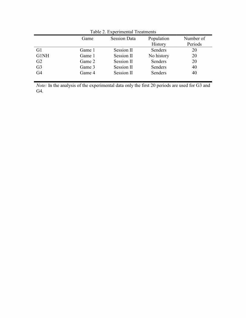
Table 2. Experimental Treatments Game Session Data Population

History Number of

Periods G1 Game 1 Session II Senders 20 G1NH Game 1 Session II No history 20 G2 Game 2 Session II Senders 20 G3 Game 3 Session II Senders 40 G4 Game 4 Session II Senders 40 Note: In the analysis of the experimental data only the first 20 periods are used for G3 and G4.

Table 3. Maximum Likelihood Estimates of SR Model Model �0 �1 LnL Psuedo-R2

G1R1

0.9456 (0.1538)

1.7403 (0.5652)

-47.80 .4253

G1R2

0.9172 (0.0181

1.5872 (0.1708)

-34.40 .5864

G1R3

0.4736 (0.1267)

3.5681 (0.8870)

-46.93 .4358

G1NHR1

0.1851 (0.1190)

5.5810 (1.4533)

-57.30 .3112

G1NHR2

0.8273 (0.1004)

1.4381 (0.4030)

-63.59 .2355

G1NHR3

0.7205 (0.0763)

3.1341 (0.7084)

-45.65 .4511

G2R1

0.5426 (0.1535)

4.7313 (1.4677)

-20.60 .7523

G2R2

0.7280 (0.2150)

3.5060 (1.0627)

-19.71 .7631

G2R3

0.5124) (0.1518)

4.9880 (1.4986)

-20.50 .7536

G3R1

0.9851 (0.3504)

2.8820 (1.0404)

-28.95 .6519

G3R2

0.9491 (0.0947)

1.2066 (0.3802)

-54.95 .3394

G3R3

0.8281 (0.1750)

1.0235 (0.4477)

-61.03 .2663

G4R1

1.6190 (0.2193)

-0.2497 (0.0408)

-72.38 .1299

G4R2

1.4765 (0.4789)

-.1514 (0.8147)

-72.18 .1322

G4R3

0.6861 (0.1056)

2.7581 (0.7122)

-34.43 .5860

Notes: The sample size is NT = 6 (20) = 120. The standard errors are given in parentheses beneath the coefficient estimates.

Table 4. Maximum Likelihood Estimates of BBL Model Model �0 �1 LnL Psuedo-R2

G1R1

1.7284 (0.5678)

0.4638 (0.3163)

-36.41 .5622

G1R2

0.8849 (0.1213)

1.8064 (0.5685)

-33.74 .5944

G1R3

1.2281 (0.0976)

0.8545 (0.3665)

-62.39 .2499

G1NHR1

-0.9465 (0.3421)

-0.3521 (0.3924)

-82.64 .0065

G1NHR2

-0.8265 (0.5927)

-0.2220 (0.3790)

-83.04 .0017

G1NHR3

1.0711 (0.1475)

0.3866 (0.2022)

-67.83 .1833

G2R1

0.9873 (0.1532)

1.9969 (0.6476)

-25.84 .6894

G2R2

2.2454 (0.126)

3.7093 (8.951)

-15.81 .8099

G2R3

1.0200 (0.1551)

1.7909 (0.6039)

-30.97 .6277

G3R1

0.9814 (0.2108)

9.8583 (3.4109)

-28.79 .6539

G3R2

1.7229 (0.6331)

0.0666 (0.1855)

-77.79 .0648

G3R3

0.0000 (1.5019)

0.0000 (0.7414)

-83.17 .0000

G4R1

-1.4393 (0.5116)

0.0732 (0.2082)

-82.73 .0053

G4R2

-0.6046 (1.9623)

-0.4218 (1.2747)

-83.17 .0007

G4R3

1.0663 (0.1647)

0.4338 (0.3367)

-83.04 .0017

Notes: See Table 3.

Table 5. Tests of pooling for SR model

Game �2(4) Pr(�2>x)

Game 1a 4.412 0.353 Game 2 0.288 0.991 Game 3 28.487 0.001 Game 4 22.857 0.001 a Game 1 with history

Table 6. Maximum Likelihood Estimates of Hybrid Model Model ��� ��� ��� lnL Psuedo-R2

G1R1

0.8130 (0.3266)

1.1212 (0.3810)

1.6447 (1.2291)

-36.05 .5666

G1R2

0.7561 (0.1836)

1.2515 (0.6917)

0.9965 (0.6125)

-31.94 .6159

G1R3

0.3642 (0.1495)

1.1935 (0.7053)

3.8228 (1.0649)

-42.40 .4903

G1NHR1

0.2115 (0.1303)

-0.3655 (0.4755)

5.1816 (1.4836)

-51.23 .3841

G1NHR2

0.8273 (0.1394)

-0.0000 (0.1709)

1.4381 (0.4961)

-63.59 .2355

G1NHR3

0.6872 (0.1147)

0.3774 (0.2841)

2.7282 (0.6555)

-44.64 .4633

G2R1

0.4476 (0.1859)

1.7137 (0.9218)

4.0113 (1.4409)

-17.73 .7869

G2R2a

137.9155 309.4403 1.9873 -12.34 .8516

G2R3a

0.5430 2.1311 4.3204 -17.38 .7910

G3R1

4.6007 (7.2234)

10.2102 (5.7366)

0.6294 (1.1680)

-25.61 .6922

G3R2

0.9001 (0.1243)

-0.7904 (0.8868)

1.2961 (0.3973)

-54.47 .3451

G3R3

0.8281 (0.1771)

0.0000 (0.8868)

1.0235 (0.3894)

-61.03 .2663

G4R1

0.6502 (0.1547)

0.6751 (0.7011)

1.0102 (0.3152)

-69.30 .1669

G4R2

0.5190 (0.1449)

-0.4692 (1.2318)

1.4801 (0.3458)

-66.44 .2012

G4R3

0.6614 (0.1055)

-0.2407 (0.8962)

2.6258 (0.6044)

-33.37 .5988

Notes: See Table 3. a ML failed to converge; Hessian singular at maximum.

Table 7. 0.05 Symmetric Wald t Tests of Hybrid Model Model t statistic

����������

t statistic ����������

�

A �����������

A ����������

R �����������

A ���������� A �����������

R ���������� R �����������

R ����������

G1R1

2.94 1.34 0 1 0 0

G1R2

1.81 1.63 1 0 0 0

G1R3

1.69 3.59 0 0 1 0

G1NHR1

0.77 3.49 0 0 1 0

G1NHR2

0.00 2.90 0 0 1 0

G1NHR3

1.33 4.16 0 0 1 0

G2R1

1.86 2.78 0 0 1 0

G2R2

G2R3

G3R1

1.78 0.54 1 0 0 0

G3R2

0.89 3.26 0 0 1 0

G3R3

0.00 2.63 0 0 1 0

G4R1

0.96 3.21 0 0 1 0

G4R2

0.38 4.28 0 0 1 0

G4R3

0.27 4.34 0 0 1 0

Total 2 1 10 0 Notes: A denotes acceptance of H0 using a nominal 0.05 symmetric asymptotic test and R the rejection of H0 using this test. The critical values are 2.0, and the nominal probability of simultaneously accepting both hypotheses when they are true is asymptotically at least 0.90 when both hypotheses are true.

Table 8.

Chi-Square Test of Equality of Coefficients for Senders and Receivers in Game 1 with and without History

Experiment -2*(LogLR-LogLU) P-value

G1R1 12.956 .0015 G1R2 23.054 .0000 G1R3 28.089 .0000 G1R1-NH 8.970 .0113 G1R2-NH 3.897 .1429 G1R3-NH 5.755 .0563

G1R1

1 5 10 15

.1

.3

.5

.7

.9

G1R2

1 5 10 15

.1

.3

.5

.7

.9

G1R3

1 5 10 15

.1

.3

.5

.7

.9

G1NHR1

1 5 10 15.1

.3

.5

.7

.9

G1NHR2

1 5 10 15

.1

.3

.5

.7

.9

G1NHR3

1 5 10 15

.1

.3

.5

.7

.9

G2R1

1 5 10 15

.1

.3

.5

.7

.9

G2R2

1 5 10 15

.1

.3

.5

.7

.9

G2R3

1 5 10 15

.1

.3

.5

.7

.9

G3R1

1 5 10 15

.1

.3

.5

.7

.9

G3R2

1 5 10 15

.1

.3

.5

.7

.9

G3R3

1 5 10 15

.1

.3

.5

.7

.9

G4R1

1 5 10 15

.1

.3

.5

.7

.9

G4R2

1 5 10 15

.1

.3

.5

.7

.9 G4R3

1 5 10 15

.1

.3

.5

.7

.9

Figure 1. Plots of the actual (jagged line) and the predicted fraction (smooth line) of players sending message 2 by type ( = type 1, 0 = type 2) assuming the SR model is true

G1R1

1 5 10 15

.1

.3

.5

.7

.9

G1R2

1 5 10 15

.1

.3

.5

.7

.9

G1R3

1 5 10 15

.1

.3

.5

.7

.9

G1NHR1

1 5 10 15.1

.3

.5

.7

.9

G1NHR2

1 5 10 15

.1

.3

.5

.7

.9

G1NHR3

1 5 10 15

.1

.3

.5

.7

.9

G2R1

1 5 10 15

.1

.3

.5

.7

.9

G2R2

1 5 10 15

.1

.3

.5

.7

.9

G2R3

1 5 10 15

.1

.3

.5

.7

.9

G3R1

1 5 10 15

.1

.3

.5

.7

.9

G3R2

1 5 10 15

.1

.3

.5

.7

.9

G3R3

1 5 10 15

.1

.3

.5

.7

.9

G4R1

1 5 10 15

.1

.3

.5

.7

.9

G4R2

1 5 10 15

.1

.3

.5

.7

.9 G4R3

1 5 10 15

.1

.3

.5

.7

.9

Figure 2. Plots of the actual (jagged line) and the predicted fraction (smooth line) of players sending message 2 by type ( = type 1, 0 = type 2) assuming the BBL model is true

-0.70

-0.65

-0.60

-0.55

-0.50

-0.45

-0.40

-0.35

-0.30

11 12 13 14 15 16 17 18 19 20

Periods

Figure 3. Convergence bias in G1R1: SR, BBL.

Figure 4. Log likelihood function for SR model using G1R1 data

Figure 5. Log likelihood function for BBL model using G1R1 data

ENDNOTES 1 Nick Feltovich (2000) performs a calibration exercise among a stimulus response

model, a belief based model and Nash equilibrium predictions applied to asymmetric

information games. However, estimation is not part of the paper’s design. 2 We emphasize that our usage of the term type refers to a single instance of play of a

sender-receiver game, not to the repeated game. 3 Technically, in our cohort of size 12 and with two messages, the mapping and orderings

are as follows for the senders detailed by player number, underlying unobservable

message mapping (A,B) and order of presentation on screen (left, right): 2 (*,#) (#,*), 4

(#,*) (*,#), 6 (*,#) (#,*), 8 (#,*) (#,*), 10 (*,#) (*,#), 12 (#,*) (#,*). For receivers, 1 (*,#)

(#,*), 3 (#,*) (*,#), 5 (*,#) (#,*), 7 (#,*) (#,*), 9 (*,#) (*,#), 11 (#,*) (#,*). 4 All replications had a common session, which preceded the games described above. In

particular, each cohort participated in 20 periods of a game with payoffs as in Game 1 and

a message space of M = {A, B}. The common session provides players with experience

about experimental procedures and ensures that players understand the structure of the

game, message space and population history. 5 We tested the null hypothesis that Qi1(1) –Qi2(1) = 0, i = 1,2; this null was accepted for

13 out of the 15 experiments. 6 This overstates the success of Salmon’s efforts to maximize the likelihood function as

no special efforts were made to assure that the “converged” value function was not just a

local maximum. 7 The coefficients in the hybrid model can be normalized so that the coefficients on the

information variables are � and (1- �), respectively, which makes the hybrid model look

similar to the model employed by Camerer and Ho (1999). 8 We do not consider the BBL model. While senders and receivers have the same

information available to them in games with history (i.e., the history of sender play), they

face entirely different inference problems. Consequently, we expect the BBL model to

differ across senders and receivers. Finally, we already know from our previous analysis

that the BBL model performs poorly for Game 1 without history.

1

9 Defining convergence for mixed strategies is conceptually the same as the pure strategy

case; empirically identifying convergence is more difficult. 10 For the BBL model, assessing the stability of the parameters is problematic because the

parameters depend on expectations. The process used to form the expectations depends

on the information at a particular point in time, which varies naturally across replications

and games. 11 For a Bayesian perspective to part of the problem detailed below, see, for example, El-

Gamal, McKelvey and Palfrey (1993), El-Gamal and Palfrey (1995) and El-Gamal and

Palfrey (1996). 12 The BFGS method is a quasi-Newton method that approximates the Hessian while

requiring that the estimate be positive definite (for minimization problems). The updating

rule is described in the papers by Broyden (1970), Fletcher (1970), Goldfard (1970) and

Shanno (1970).