Learning Active Fusion of Multiple Experts' Decisions: An Attention-Based Approach
34
LETTER Communicated by Nicol ´ as Garc´ ıa-Pedrajas Learning Active Fusion of Multiple Experts’ Decisions: An Attention-Based Approach Maryam S. Mirian [email protected] Control and Intelligent Processing Center of Excellence, Department of Electrical and Computer Eng., University of Tehran, Tehran, Iran Majid Nili Ahmadabadi [email protected] Babak N. Araabi [email protected] Control and Intelligent Processing Center of Excellence, University of Tehran, Tehran, Iran, and School of Cognitive Sciences, Institute for Research in Fundamental Sciences, Tehran, Iran Roland R. Siegwart [email protected] ASL, ETHZ, Switzerland, Autonomous Systems Lab, Institute of Robotics and Intelligent Systems, ETH Zurich, 8092 Zurich, Switzerland In this letter, we propose a learning system, active decision fusion learn- ing (ADFL), for active fusion of decisions. Each decision maker, referred to as a local decision maker, provides its suggestion in the form of a prob- ability distribution over all possible decisions. The goal of the system is to learn the active sequential selection of the local decision makers in order to consult with and thus learn the final decision based on the con- sultations. These two learning tasks are formulated as learning a single sequential decision-making problem in the form of a Markov decision process (MDP), and a continuous reinforcement learning method is em- ployed to solve it. The states of this MDP are decisions of the attended local decision makers, and the actions are either attending to a local decision maker or declaring final decisions. The learning system is pun- ished for each consultation and wrong final decision and rewarded for correct final decisions. This results in minimizing the consultation and decision-making costs through learning a sequential consultation policy where the most informative local decision makers are consulted and the least informative, misleading, and redundant ones are left unattended. An important property of this policy is that it acts locally. This means that the system handles any nonuniformity in the local decision maker’s Neural Computation 23, 558–591 (2011) C 2011 Massachusetts Institute of Technology
-
Upload
independent -
Category
Documents
-
view
4 -
download
0
Transcript of Learning Active Fusion of Multiple Experts' Decisions: An Attention-Based Approach
LETTER Communicated by Nicolas Garcıa-Pedrajas
Learning Active Fusion of Multiple Experts’ Decisions:An Attention-Based Approach
Maryam S. [email protected] and Intelligent Processing Center of Excellence, Department of Electrical andComputer Eng., University of Tehran, Tehran, Iran
Majid Nili [email protected] N. [email protected] and Intelligent Processing Center of Excellence, University of Tehran, Tehran,Iran, and School of Cognitive Sciences, Institute for Research in FundamentalSciences, Tehran, Iran
Roland R. [email protected], ETHZ, Switzerland, Autonomous Systems Lab, Institute of Robotics andIntelligent Systems, ETH Zurich, 8092 Zurich, Switzerland
In this letter, we propose a learning system, active decision fusion learn-ing (ADFL), for active fusion of decisions. Each decision maker, referredto as a local decision maker, provides its suggestion in the form of a prob-ability distribution over all possible decisions. The goal of the systemis to learn the active sequential selection of the local decision makers inorder to consult with and thus learn the final decision based on the con-sultations. These two learning tasks are formulated as learning a singlesequential decision-making problem in the form of a Markov decisionprocess (MDP), and a continuous reinforcement learning method is em-ployed to solve it. The states of this MDP are decisions of the attendedlocal decision makers, and the actions are either attending to a localdecision maker or declaring final decisions. The learning system is pun-ished for each consultation and wrong final decision and rewarded forcorrect final decisions. This results in minimizing the consultation anddecision-making costs through learning a sequential consultation policywhere the most informative local decision makers are consulted and theleast informative, misleading, and redundant ones are left unattended.An important property of this policy is that it acts locally. This meansthat the system handles any nonuniformity in the local decision maker’s
Neural Computation 23, 558–591 (2011) C© 2011 Massachusetts Institute of Technology
Learning Active Fusion of Multiple Experts’ Decisions 559
expertise over the state space. This property has been exploited in thedesign of local experts. ADFL is tested on a set of classification tasks,where it outperforms two well-known classification methods, Adaboostand bagging, as well as three benchmark fusion algorithms: OWA, Bordacount, and majority voting. In addition, the effect of local experts designstrategy on the performance of ADFL is studied, and some guidelines forthe design of local experts are provided. Moreover, evaluating ADFL insome special cases proves that it is able to derive the maximum benefitfrom the informative local decision makers and to minimize attending toredundant ones.
1 Introduction
Decision fusion—asking a set of experts’ response to a query and makingdecisions accordingly—has been a hot research topic. Decision fusion isa challenging problem, as each expert’s knowledge and expertise are ingeneral incomplete and nonuniform over the problem domain. Not onlyis each expert’s suggestion imperfect over the problem domain, it alsocan be misleading in response to a number of queries—those that are notposed in an expert’s area of expertise. To reflect these facts, we refer to anexpert or a decision maker as a local decision expert (LDE). Consultationwith LDEs is not cost free. By “cost,” we mean whatever resources shouldbe allocated for getting the LDEs’ suggestions. For example, in a medicaldiagnostic problem, consultation with another physician may require someadditional medical tests as different physicians may look at a single problemfrom different perspectives. This will at least cost the patient money andtime, disregarding the test’s side effects, which are important in most cases.Therefore, in this letter, we propose a learning system attentive decisionfusion learning (ADFL), that learns both whom to consult with and thefinal decision based on the consultations.
In the proposed method, it is assumed that suggestions, which we alsorefer to as outputs or decisions, of each LDE is a probability distribution overall of the possible final decisions. This natural assumption is not restrictive,because it necessitates homogeneity in neither the structure nor the inputsof the experts. Therefore, LDEs can have different structures and inputs.
The decision fusion problem is cast in an episodic sequential decision-making framework, and the costs of consultation and decision making aremodeled in the form of a reward function. Then a continuous reinforcementlearning (RL) method is employed to learn the optimal solution of the prob-lem. The learning results in a single policy for sequential consultation withLDEs and making the final decision accordingly. The policy is employedto select either the next LDE to be consulted or a final decision to be madebased on the consultations already made in the current episode.
One of the major properties of learned policy is being nonuniform overthe problem domain. It means that ADFL acts locally, not globally as in

560 M. Mirian et al.
common fusion methods, through learning to attend to the most infor-mative LDEs indirectly for each portion of the problem domain. Anotherimportant attribute of ADFL is to learn the best final decision based onthe consulted LDEs’ suggestions. These two properties resolve the chal-lenges of decision fusion: knowledge incompleteness and nonuniformityof the LDEs’ expertise over the problem domain and the cost reduction ofconsultation and decision making.
The rest of this letter is organized as follows. First, the related studies arereviewed. Then the problem is defined formally. In section 3, the proposedapproach is explained, followed by an explanation on how this approach isapplied to classification tasks. The case studies on the selected UCI data setsare mentioned and the results reported and analyzed. In section 6, the effectof LDEs’ properties on the performance of ADFL is studied, and someguidelines for the design of LDEs are provided. Moreover, some majorproperties of ADFL are verified through testing its performance in somespecial cases. The conclusions and the next steps of this work are discussedin the last section.
2 Related Studies
There are two classes of related studies and methods to the focus of thisresearch. The first covers the studies associated with active and adaptiveselection of inputs by a decision maker—sensors and features—to cut thecosts of information processing and improve decision quality. These studiesmainly offer top-down attention control methods, or what some researchersin the robotics domain refer to as active perception. The second categorycontains research on fusion of inputs. In this research, the inputs are sug-gestions of LDEs, and therefore we review the research on combining thedecisions of multiple decision makers.
Most of the existing attention control mechanisms are hand-designedbased on heuristics or biologically inspired algorithms. However, it ispreferable for attention control and decision-making policy to be learnedtogether at the same time since the optimal attention strategy is a functionof the decision-making policy and vice versa. Nevertheless, there are verylimited learning approaches to concurrent learning of attention and deci-sion policy (for example, Paletta & Pinz, 2000; Borji, Ahmadabadi, Araabi,& Hamidi, 2010; Paletta, Fritz, & Seifert, 2005; Minut & Mahadevan, 2001).Attention strategy in these studies is learned in the sensory space. In themethod introduced by Mirian, Firouzi, Ahmadabadi, and Araabi (2009),ADFL also works in the decision space, and the attention strategy is beinglearned in this alternative space. In fact, we adopt the idea of augmentedaction from Shariatpanahi and Nili Ahmadabadi (2008) to formulate theproblems of attention and decision learning as a single decision-makingproblem in the decision space.
Learning Active Fusion of Multiple Experts’ Decisions 561
The main idea behind active and budgeted learning techniques(Danziger, Zeng, Wang, Brachmann, & Lathrop, 2007; Lizotte, Madani, &Greiner, 2003) is to choose the most informative data from a set of trainingsamples to reduce the cost of learning and decision making. ADFL also triesto reduce the costs, but it does so through attentive sequential selection ofconsultations in the recall mode.
A variety of strategies for decision making are based on combining thedecisions of multiple decision makers. Ensemble-based methods such asmixture of experts (Jordan & Jacobs, 1994), stacked generalization (Wolpert,1992), Adaboost (Schapire, 2003), and Bagging (Polikar, 2007) are examples.In addition, there are plenty of standard decision fusion methods: classifierfusion (Zhu, 2003; Woods, Kegelmeyer, & Bowyer, 1997; Verikas, Lipnickas,Malmqvist, Bacauskiene, & Gelzinis, 1999), majority voting (Polikar, 2006),Borda count (Polikar, 2006) and OWA (Filev & Yager, 1998). Nevertheless,the main superiority of ADFL over these methods is its unsupervised learn-ing of the attentive sequential selection of decision makers to consult withand formation of locally optimal decision policies over the decision space.This superiority is experimentally verified in this letter.
3 Proposed Approach
The idea proposed here is to learn how to sequentially fuse the individualdecision makers’ decision to minimize a specific cost function. In otherwords, the learner agent learns to sequentially select those more helpfulLDEs in every state, combine their opinions, and learn to reach a finaldecision. Here, the cost function is a combination of the reward that thelearner gets in return for its final decision minus the costs of asking LDEsabout their decisions. We have named this the attentive decision fusionlearning (ADFL) agent.
3.1 Problem Statement. We assume that the ADFL agent has access to lLDEs: e1, e2, e3, . . . , el .1 Each ei looks at a segment of the entire input featurespace (F i ), an n-dimensional space represented by F (F i ⊆ F ). Here, F i s areoverlapping subsets of the F space and F = ⋃l
i=1 F i . Moreover, all LDEshave the same set of decisions expressed by D = {d1, d2, . . . , dc}, where cis the total number of possible decisions. The decision (output) of the ithLDE when given f i ∈ F i as input (by looking at point f ∈ F ) is its degreeof support for all possible decisions:
ei ( f i ) = �Pr (dei = d1| f i )Pr (dei = d2| f i )Pr (dei = d3| f i ) . . .
Pr (dei = dc | f i )�. (3.1)
1All vectors are in bold characters. Sets are denoted by capital letters.
562 M. Mirian et al.
This can be simplified as
[Pr (dk | f i )], k = 1, 2, 3, . . . , c.
Note that the ADFL agent cannot decide based on the features and shouldmake its decision based on consultation with LDEs. In other words, theADFL agent is an attentive decision fuser. Therefore, the state (s), action(a), and decision policy (π ) of the ADFL agent for every observation—or,equivalently, query— f ∈ F are defined as
⎧⎪⎪⎨⎪⎪⎩
s = [s1s2 . . . sl ], si ={
ei ( f i ), i ∈ selected experts so far01×c otherwise
a ∈ A, A = T ∪ Dπ = Pr (a |s),
(3.2)
where T = {t1, t2, . . . , tl} and ti is consultation with the ith LDE. The stateof ADFL is composed of the decisions of consulted LDEs. This definitionis similar to the description of decision profile in Kuncheva, Bezdek, andDuin (2001).
As Figure 1 and equation 3.2 show, an ADFL agent at each state decidesbetween two sets of possible actions: consult another LDE (Consultationactions ∈ T) or declare a final decision (Decision actions ∈ D). In Figure 1,consultation with an LDE is modeled by closing a switch. The ADFL agentupdates its state (s) after every consultation. Sequential consultation withLDEs continues until the ADFL agent decides to stop consulting and makesa final decision. The ADFL agent’s goal is to find an optimal policy (π∗)under which a specific utility function is maximized:
π∗ = argmaxπ
Qπ (s, a ) ∀s. (3.3)
The utility function Q (called Q-value as well) and the optimization method,which is done over every state, vary according to the information about theproblem at hand. However, the utility function, in its general form, is theexpected reinforcement that the ADFL agent receives for its decision in states. In other words, by maximizing its expected reward, the ADFL agent learnsto reach a reasonable trade-off between the quality of its final decision andthe cost of consulting with LDEs. This is achieved by considering predefinedcosts for consulting each LDE, as well as the benefits of making a reasonablefinal decision. Learning the optimal policy is modeled in the next section.
3.2 Attentive Decision Fusion Learning: Formulation. Since in gen-eral we do not know the best policy (the optimal sequence of consulta-tions) and the exact area of expertise of the experts, we opt for learningthe value of decisions and finding the optimal policy (π∗) at each state

Learning Active Fusion of Multiple Experts’ Decisions 563
e1ele2
Decision making
Feature Space (F)
f1 f2 fl
ei
fi
Update si using ei(fi)
ei(fi)
Tta i∈=
Dda j ∈=
AD
FL
agent
Figure 1: A cycle of decision making and state updating in ADFL.
(see equations 3.2 and 3.3). Thus, we have defined a flexible mechanismto set rewards and punishments for each decision. Reinforcement learning(RL) (Sutton & Barto, 1999) was chosen as the optimization method sinceit is one of the natural candidates for learning efficient sequential decisionmaking. As we will show, the state of the ADFL problem—or of the ADFLagent—is continuous while the actions are discrete. This continuous space iscalled the decision space because it is composed of the LDEs’ decisions (seethe definition of state (s) in equation 3.2). There are different variants of RLmethods for handling the continuous state: fuzzy Q-learning (Berenji, 1996),variants of the tile coding method (Whiteson, Taylor, & Stone, 2007), andthe Bayesian Q-learning approach (Firouzi, Ahmadabadi, & Araabi, 2008).Among the possible variants, we have used Bayesian Q-learning approach(Firouzi et al., 2008; Firouzi et al., 2009) because of its uncertainty handling

564 M. Mirian et al.
Table 1: Key Elements of Assumed MDP to Formulate ADFL.
State (S) sinit = 0l×c = the initial state of ADFL agent before consultingany LDE (Null).
s = [s1s2 . . . sl ], si ={
ei ( f i ), i ∈ selected experts so far01×c otherwise
ei ( f i ) = [Pr (dei = d1| f i )Pr (dei = d2| f i )Pr (dei = d3| f i ) . . .
Pr (dei = dc | f i )]l = the number of LDEsc = |D| = the size of the decision actions
Actions (A) A = T ∪ DTransition function if a = ti ∈ T ⇒ si ← ei ( f i )
(Tran)if a = d j ∈ D ⇒ s ← Terminal state
Reward function (r) r = High positive, if a = Correct Decision ∈ Dr = High negative, if a = Wrong Decision ∈ Dr = (Small negative) × (Number of already consulted experts),
if a ∈ T
and flexibility in generating state prototypes. Nevertheless, our approach istheoretically general and independent of the employed learning core. Here,we first cast the ADFL problem in an episodic Markov decision process(MDP) form and then use the RL method to solve it.
The corresponding MDP is defined by a 4-tuple (S, A, Tran, r) in whichS is the ADFL agent’s set of states and A is the set of its actions, Tran isthe state transition function, and r is the reward received. More details aregiven in Table 1.
As shown in Table 1, the state and action sets of the ADFL problem areexactly those of ADFL agent (see equation 3.2). The initial state is Null,which means that no consultation has been made. The transition functioneither concatenates the opinion of an LDE to the state (when the ADFLagent consults with that LDE) or transfers the state to the terminal stateif a final decision is made. Since the ADFL agent attempts to maximizeits expected reward, the rewards and punishments are defined such thatthe expected reward maximization results in making a correct final deci-sion with the fewest possible consultations. It is done by setting a largereward or punishment for correct or wrong final decisions. In addition, thepunishment for consultation—or, equivalently, the cost of consultation—islinearly increased with the number of already consulted LDEs. The slope ofthis is set to be small in order not to penalize the ADFL agent too much forconsultations, which forces it to make premature final decisions. Because asthe number of consultations can be easily extracted from the state, it doesnot violate the Markov property of the ADFL problem.
Similar to ordinary Q-learning (Watkins & Dayan, 1992), in ADFL thevalue of each state-action under policy π∗(Qπ∗
(s, a )) is learned while fol-lowing a Q-value-based soft policy, like Boltzman or ∈-greedy (Sutton &Barto, 1999). Since π∗ is a greedy policy, the soft policy is shifted gradually

Learning Active Fusion of Multiple Experts’ Decisions 565
Current State = Sinit
Reinforcement (+R/-R)
Decision Making:Consultation/Decision?
Update the Value of State-Action
A training Sample:
F
End of one cycle of training
Whom to consult?
Update si
Update the Value of State-Action
Reinforcement (-r)
Update s = Terminal
Tta i ∈=
Tta i ∈=Dda j ∈=
Environment (LDEs & Critic)
Environment (LDEs & Critic)
ei(fi)
Figure 2: A learning cycle of the ADFL agent.
toward the greedy one as learning the Q-values proceeds. Ultimately theQ-values are learned or converged in some learning cycles.
Each learning cycle starts with posing the ADFL agent a query. It isdone by giving the agent a training sample (see Figure 2). Actually, thequery is to ask the ADFL agent’s opinion about a stimulus—a point in thefeature space ( f ∈ F ). Since the agent cannot decide based on the featuresand should consult LDEs, it initializes its state to Null and decides who toconsult first.2 This decision is made according to a softmax policy on thepossible consultation actions in the Null state: a = softmax(Q(Null, t) ∀t ∈T). After the consultation, the ADFL receives a punishment associated withthe consultation and updates its state (see Table 1) along with its Q-valueusing the employed learning rule—Bayesian Q-learning here.
After the first consultation, the agent decides between two possible op-tions using a softmax policy: either consulting an LDE or making a finaldecision: a = softmax(Q(s, b)∀b ∈ T ∪ D) based on the acquired informa-tion. If it decides to perform another consultation, it gets a punishment
2Each action (either consultation action or final action) has a Q-value, and this valueshows how much that action is beneficial for the agent. The probability of selecting eachaction is proportional to its Q-value, that is, the probability of selecting more beneficialactions is higher.
566 M. Mirian et al.
again and updates its state as well as its corresponding Q-value. This pro-cess is repeated for every consultation. In case the ADFL agent makes a finaldecision, it receives the corresponding reward or punishment in return andupdates its corresponding Q-value after setting its next state to the terminalstate (see Figure 2 and Table 1). The learning cycle ends here.
The learning cycle is repeated over the training samples multiple timesuntil a stop criterion is met. The stop criterion is met when the error onthe evaluation samples is increased for a reasonable number of successivelearning cycles. Thereafter, the ADFL agent is tested on the test data. Thetest cycle is the same as the learning cycle except no knowledge updatingis involved.
4 Application in Classification Tasks
Up to this point, ADFL has been introduced in the most general form. Inthis section, we explain the realization of the proposed approach on a well-known type of decision-making task. A classification task is considereddue to a set of reasons: various appropriate tasks for active decision fusionlearning (like medical diagnosis) are kinds of classification; LDEs here canbe simply replaced by local classifiers; and we can benchmark our approachin comparison with well-established classification methods in addition towell-known decision fusion approaches.
In order to evaluate ADFL, we need a test system composed of a set ofreadily existing LDEs on a benchmark problem. Because such a test systemdoes not exist, we have selected some medical diagnoses data sets and a fewothers from the UCI data sets (Blake & Merz, 1998) and manually designedLDEs on them. The key design issue of LDEs is their locality attribute,which is aimed at generating diversity in LDEs’ areas of expertise. This canbe achieved through making LDEs different in their input feature space oroutput decision space, or both. In this research, we have chosen generatingdiversity in the input space.3
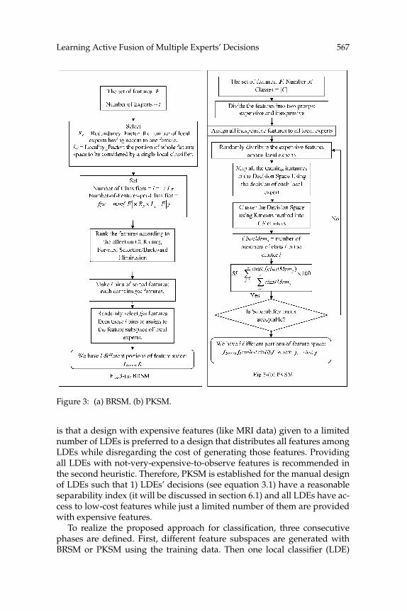
There is a wide spectrum of different strategies (Ebrahimpour, Kabir,Esteky, & Yousefi, 2008) on localization of the input space: from fully ran-dom to fully hand-designed partitioning of the space. In this letter, wehave selected a less random method balanced random subspace making(BRSM), and pre-knowledge subspace making (PKSM), which acts basedon both preknowledge (prior knowledge available about the features) andheuristics, which we discussed later.
BRSM is illustrated in Figure 3a. In BRSM, by binning the features and se-lecting from the bins, we find feature-diverse but performance-wise nearlysimilar LDEs. PKSM (see Figure 3b), is based on two heuristics. The first one
3Utilizing the output space facilitates the development of hierarchical decision making;thus, it can be helpful in problems with a high-dimensional decision space.
Learning Active Fusion of Multiple Experts’ Decisions 567
Figure 3: (a) BRSM. (b) PKSM.
is that a design with expensive features (like MRI data) given to a limitednumber of LDEs is preferred to a design that distributes all features amongLDEs while disregarding the cost of generating those features. Providingall LDEs with not-very-expensive-to-observe features is recommended inthe second heuristic. Therefore, PKSM is established for the manual designof LDEs such that 1) LDEs’ decisions (see equation 3.1) have a reasonableseparability index (it will be discussed in section 6.1) and all LDEs have ac-cess to low-cost features while just a limited number of them are providedwith expensive features.
To realize the proposed approach for classification, three consecutivephases are defined. First, different feature subspaces are generated withBRSM or PKSM using the training data. Then one local classifier (LDE)

568 M. Mirian et al.
Table 2: The Selected Data Sets.
Number of Number of Number ofData Sets Features Output Classes Instances
Heart (statlog) 13 2 270Hepatitis 19 2 155Liver Disorder (bupa) 6 2 345Pima Indian Diabetes 8 2 768Ionosphere 34 2 351Sonar 60 2 208Glass 9 6 214Vehicle 18 4 846Waveform 40 3 500Satimage 36 6 6435Dermatology 34 6 366
is assigned to each subspace and trained. The classification method forLDEs (such as k-NN, naive Bayes, support vector machines (SVM), andMLP artificial neural networks) is chosen considering the properties ofdata set (see Kotsiantis, Zaharakis, & Pintelas, 2006). Here, we have optedfor three general methods—k-NN, naive Bayes, and SVM—and comparedthe results. In the last phase, the ADFL agent learns (through employedBayesian Q-learning) to maximize the expected reward through sequentialselection of the most appropriate LDEs for consultation and declaring theclassification decision.
5 Case Studies: Evaluating the Approach on the Selected UCI Data Sets
We have benchmarked the performance of an implementation of ourmethod over 11 sample data sets from UCI machine learning repository(see Table 2) against several well-known approaches that have some simi-larities to our approach from different aspects.
Approaches selected for benchmarking are (1) a holistic k-NN in thefeature space; (2) Bagging (Polikar, 2007), (3) Adaboost (Schapire, 2003); (4)a holistic k-NN in the decision space;4 and (5) fusion-based methods inthree decision levels: only labels (majority voting), rank of the labels (Bordacount), and continuous outputs like a posteriori probabilities OWA withgradient descent learning of the optimal weights; Filev & Yager, 1998). Thefirst three methods work in the feature space, while the rest, along withADFL, work in the decision space.
The results of Bagging with k-NN base learners and those of Adaboostwith k-NN and SVM base learners are adopted from Garcia-Pedrajas (2009)
4This method works based on the pool of original training instances that are rep-resented in the decision space of designed local experts plus their corresponding classlabels.
Learning Active Fusion of Multiple Experts’ Decisions 569
and Garcia-Pedrajas and Ortiz-Boyer (2009); the rest of methods are our ex-periments. In Garcia-Pedrajas (2009) and Garcia-Pedrajas and Ortiz-Boyer(2009), 50% of each data set is used for training and the rest for the test.We followed the same data partitioning policy. Nevertheless, for ADFL, thesituation is harder since 8% of the training data is used for validation tofind the appropriate learning stop point.
Each experiment is performed over five replicates of randomly generatedtraining and test data, and the results are averaged. The reported resultsare the average correct classification rates (CCR) on the test data alongwith the statistical variances. For ADFL, CCR, and statistical variances onthe training data, along with the consultation ratio on the test, data arereported as well. Consultation ratio is defined as
Consultation ratio = Number of consulted LDEsTotal number of LDEs
. (5.1)
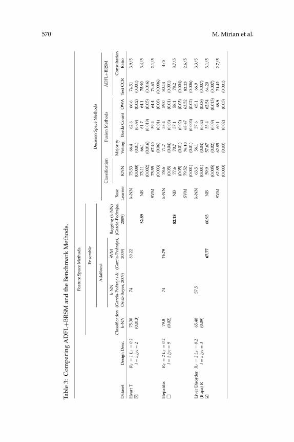
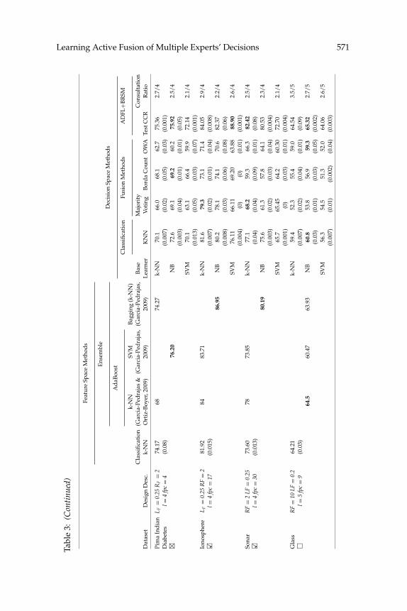
To have a fair comparison with the ensemble-based methods reportedin Garcia-Pedrajas (2009) and Garcia-Pedrajas and Ortiz-Boyer (2009), wehave also used SVM classifiers with gaussian kernels for LDEs. SVM learn-ing algorithm in multiclass problems is performed using functions from theLIBSVM library (Chih-Jen Lin, n.d.). The same parameters for SVM are alsoused: C (bound on the Lagrangian multipliers) is 10 and lambda (condition-ing parameter for the QP method) is 0.1. To employ Bayesian Q-learning,some initial parameter settings are made: the learning rate is decreased from0.4 to 0.1 in an exponential manner. The discount factor is 1 (because the lastaction of every episode has the highest importance) and the temperatureused for softmax action selection is exponentially changed from 0.8 to 0.01(in order to gradually move toward full greedy mode). The cost of consulta-tion is −1, the reward of correct decision making is +10, and the punishmentassociated with wrong decision making is −10. Table 3 shows the resultsof ADFL+BRSM (ADFL with BRSM-based LDEs) in addition to those ofthe benchmark methods. For every data set, the best result gained in eachclass of methods (ensemble-based and decision-space methods) is shown inboldface type. The same is done for the best result of ADFL over the threetypes of LDEs; k-NN, NB, and SVM. The name of a data set is marked with�× �� when the best result of ADFL is significantly lower (higher) than that ofits strongest competitor. An empty box is used when there is no significantdifference between ADFL’s best and the strongest benchmark method’sperformances. Table 3 demonstrates that ADFL+BRSM defeated all of itsfusion-based competitors in all of the data sets but not the ensemble-basedmethods. This issue is analyzed in section 6.1. Nevertheless, as the consulta-tion ratio indicates, the ADFL agent after training genuinely consults withmore knowledgeable LDEs in every state and LDEs that are recognized asunhelpful are left unattended. In this, ADFL is superior to the other meth-ods, which need to consider the decisions of all LDEs together or use a single
570 M. Mirian et al.
Tabl
e3:
Com
pari
ngA
DFL
+BR
SMan
dth
eB
ench
mar
kM
etho
ds.
Feat
ure
Spac
eM
etho
ds
Ens
embl
eD
ecis
ion
Spac
eM
etho
ds
Ad
aBoo
stC
lass
ifica
tion
Fusi
onM
etho
ds
AD
FL+B
RSM
k-N
NSV
MB
aggi
ng(k
-NN
)C
lass
ifica
tion
(Gar
cia-
Ped
raja
s&
(Gar
cia-
Ped
raja
s,(G
arci
a-Pe
dra
jas,
Bas
eM
ajor
ity
Con
sult
atio
nD
atas
etD
esig
nD
esc.
k-N
NO
rtiz
-Boy
er,2
009)
2009
)20
09)
Lea
rner
KN
NV
otin
gB
ord
aC
ount
OW
ATe
stC
CR
Rat
io
Hea
rtT
RF
=1
LF
=0.
275
.30
7480
.22
k-N
N75
.53
66.4
62.6
66.6
74.5
13.
9/5
�l=
5fp
c=
2(0
.013
)(0
.008
)(0
.01)
(0.0
9)(0
.02)
(0.0
01)
82.8
9N
B73
.11
66.1
61.7
64.1
75.9
03.
4/5
(0.0
02)
(0.0
16)
(0.0
19)
(0.0
5)(0
.016
)SV
M75
.55
67.4
059
.464
.474
.63
2.1/
5(0
.003
)(0
.06)
(0.0
1)(0
.08)
(0.0
006)
Hep
atit
isR
F=
2L
F=
0.2
79.8
7476
.79
k-N
N78
.671
.758
.459
.080
.14
4/5
�l=
5fp
c=
9(0
.02)
(0.0
5)(0
.04)
(0.0
3)(0
.01)
(0.0
01)
82.1
8N
B77
.670
.757
.158
.178
.23.
7/5
(0.0
5)(0
.01)
(0.0
2)(0
.03)
(0.0
04)
SVM
79.5
276
.10
68.4
763
.52
82.2
32.
6/5
(0.0
01)
(0.0
1)(0
.003
)(0
.02)
(0.0
06)
Liv
erD
isor
der
RF
=2
LF
=0.
265
.40
57.5
k-N
N63
.556
.157
.665
.166
.93.
3/5
(Bup
a)R
l=5
fpc=
3(0
.09)
(0.0
01)
(0.0
4)(0
.02)
(0.0
8)(0
.007
)��
67.7
760
.93
NB
59.9
57.6
755
.462
.54
64.2
03.
1/5
(0.0
05)
(0.0
2)(0
.09)
(0.0
15)
(0.0
07)
SVM
62.8
562
.85
60.1
68.9
71.4
22.
7/5
(0.0
03)
(0.0
3)(0
.02)
(0.0
3)(0
.001
)
Learning Active Fusion of Multiple Experts’ Decisions 571
Tabl
e3:
(Con
tinu
ed)
Feat
ure
Spac
eM
etho
ds
Ens
embl
eD
ecis
ion
Spac
eM
etho
ds
Ad
aBoo
stC
lass
ifica
tion
Fusi
onM
etho
ds
AD
FL+B
RSM
k-N
NSV
MB
aggi
ng(k
-NN
)C
lass
ifica
tion
(Gar
cia-
Ped
raja
s&
(Gar
cia-
Ped
raja
s,(G
arci
a-Pe
dra
jas,
Bas
eM
ajor
ity
Con
sult
atio
nD
atas
etD
esig
nD
esc.
k-N
NO
rtiz
-Boy
er,2
009)
2009
)20
09)
Lea
rner
KN
NV
otin
gB
ord
aC
ount
OW
ATe
stC
CR
Rat
io
Pim
aIn
dia
nL
F=
0.25
RF
=2
74.1
768
74.2
7k-
NN
70.1
66.0
68.1
62.7
75.3
62.
7/4
Dia
bete
sl=
4fp
c=
4(0
.08)
(0.0
07)
(0.0
2)(0
.05)
(0.0
3)(0
.001
)�
76.2
0N
B72
.669
.169
.260
.275
.92
2.5/
4(0
.003
)(0
.04)
(0.0
1)(0
.01)
(0.0
5)SV
M70
.163
.166
.459
.972
.14
2.1/
4(0
.013
)(0
.05)
(0.0
3)(0
.07)
(0.0
01)
Iono
sphe
reL
F=
0.25
RF
=2
81.9
284
83.7
1k-
NN
81.6
79.3
73.1
71.4
84.0
52.
9/4
��l=
4fp
c=
17(0
.015
)(0
.007
)(0
.02)
(0.0
1)(0
.04)
(0.0
08)
86.9
5N
B80
.278
.174
.170
.682
.37
2.2/
4(0
.008
)(0
.03)
(0.0
6)(0
.08)
(0.0
6)SV
M76
.11
66.1
169
.20
63.8
888
.90
2.6/
4(0
.004
)(0
)(0
)(0
.01)
(0.0
01)
Sona
rR
F=
2LF
=0.
2573
.60
7873
.85
k-N
N77
.168
.259
.366
.382
.42
2.5/
4��
l=4
fpc=
30(0
.013
)(0
.04)
(0.0
4)(0
.09)
(0.0
1)(0
.08)
80.1
9N
B75
.661
.357
.864
.180
.53
2.3/
4(0
.003
)(0
.02)
(0.0
3)(0
.04)
(0.0
04)
SVM
65.7
65.4
564
.260
.30
72.7
02.
1/4
(0.0
01)
(0)
(0.0
3)(0
.01)
(0.0
04)
Gla
ssR
F=
10LF
=0.
264
.21
k-N
N59
.452
.355
.459
.064
.54
3.5/
5�
l=5
fpc=
9(0
.03)
(0.0
07)
(0.0
2)(0
.04)
(0.0
1)(0
.09)
64.5
60.4
763
.93
NB
60.8
53.8
56.9
59.3
65.3
22.
7/5
(0.0
3)(0
.01)
(0.0
3)(0
.05)
(0.0
02)
SVM
56.3
54.5
51.3
52.0
64.0
62.
6/5
(0.0
07)
(0.0
1)(0
.002
)(0
.04)
(0.0
03)

572 M. Mirian et al.
Tabl
e3:
(Con
tinu
ed)
Feat
ure
Spac
eM
etho
ds
Ens
embl
eD
ecis
ion
Spac
eM
etho
ds
Ad
aBoo
stC
lass
ifica
tion
Fusi
onM
etho
ds
AD
FL+B
RSM
k-N
NSV
MB
aggi
ng(k
-NN
)C
lass
ifica
tion
(Gar
cia-
Ped
raja
s&
(Gar
cia-
Ped
raja
s,(G
arci
a-Pe
dra
jas,
Bas
eM
ajor
ity
Con
sult
atio
nD
atas
etD
esig
nD
esc.
k-N
NO
rtiz
-Boy
er,2
009)
2009
)20
09)
Lea
rner
KN
NV
otin
gB
ord
aC
ount
OW
ATe
stC
CR
Rat
io
Veh
icle
RF
=2
LF=
0.2
68.4
467
.5k-
NN
67.8
61.4
062
.24
62.1
075
.20
3.6/
5�
l=5
fpc=
9(0
.02)
(0.0
01)
(0.0
1)(0
.02)
(0.0
03)
(0.0
07)
77.1
968
.68
NB
64.5
359
.30
60.1
260
.50
73.8
13/
5(0
.005
)(0
.003
)(0
.01)
(0.0
4)(0
.000
2)SV
M61
.62
55.5
859
.65
59.2
565
.11
2.3/
4(0
.000
2)(0
.01)
(0.0
05)
(0.0
1)(0
.006
)W
avef
orm
RF
=2
LF=
0.2
81.4
668
83.6
1k-
NN
78.3
773
.52
54.9
069
.60
76.4
73.
1/5
�l=
5fp
c=
10(0
.05)
(0.0
007)
(0)
(0.0
07)
(0.0
17)
(0.0
01)
85.8
3N
B80
.40
75.0
050
.98
77.4
582
.84
3.1/
5(0
.000
4)(0
.004
)(0
)(0
.07)
(0.0
03)
SVM
74.0
770
.98
71.5
164
.70
78.9
22.
6/5
(0.0
05)
(0.0
01)
(0.0
01)
(0.0
64)
(0.0
004)
Sati
mag
eR
F=
2LF
=0.
285
.55
87.5
86.2
9k-
NN
91.0
470
.50
71.3
571
.42
93.2
32.
7/5
��l=
5fp
c=
18(0
.07)
(0.0
02)
(0.0
04)
(0.0
5)(0
.01)
(0.0
01)
89.8
2N
B90
.30
68.3
070
.56
69.3
090
.34
2.6/
5(0
.009
)(0
.002
)(0
.01)
(0.0
07)
(0.0
4)SV
M78
.82
68.5
070
.10
71.4
86.6
72.
1/5
(0.0
3)(0
.03)
(0.0
04)
(0.0
03)
(0.0
05)
Der
mat
olog
yR
F=
2LF
=0.
2591
.03
9295
.41
k-N
N89
.587
.587
.586
.25
90.0
02.
1/4
�l=
4fp
c=
13(0
.009
)(0
.05)
(0)
(0)
(0.0
03)
(0.0
012)
97.0
5N
B95
.00
82.5
85.0
81.2
597
.55
2.1/
4(0
.001
)(0
.001
)(0
.01)
(0.0
1)(0
.001
3)SV
M90
.10
85.8
290
.890
.091
.25
2/4
(0.0
012)
(0.0
01)
(0.0
3)(0
.01)
(0.0
003)
Learning Active Fusion of Multiple Experts’ Decisions 573
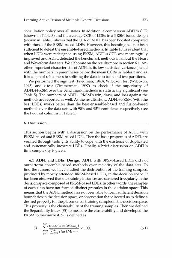
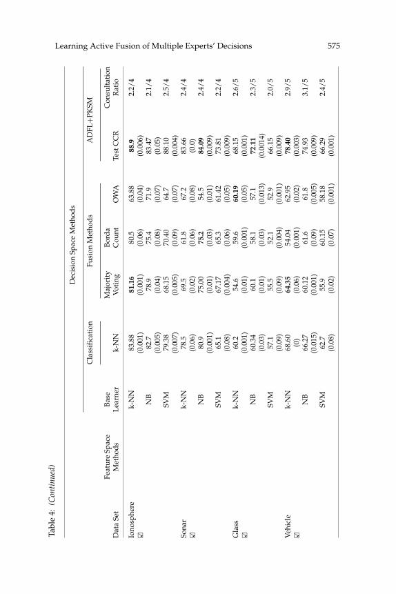
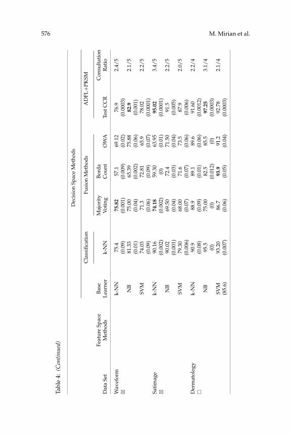
consultation policy over all states. In addition, a comparison ADFL’s CCR(shown in Table 3) and the average CCR of LDEs in a BRSM-based design(shown in Table 6) shows that the CCR of ADFL has been boosted comparedwith those of the BRSM-based LDEs. However, this boosting has not beensufficient to defeat the ensemble-based methods. In Table 4 it is evident thatwhen LDEs were redesigned using PKSM, ADFL’s CCR was meaningfullyimproved and ADFL defeated the benchmark methods in all but the Heartand Waveform data sets. We elaborate on the results more in section 6.1. An-other important characteristic of ADFL is its low statistical variance (statedwith the numbers in parentheses below the mean CCRs in Tables 3 and 4).It is a sign of robustness to splitting the data into train and test partitions.
We performed the sign test (Friedman, 1940), Wilcoxon test (Wilcoxon,1945) and t-test (Zimmerman, 1997) to check if the superiority ofADFL+PKSM over the benchmark methods is statistically significant (seeTable 5). The numbers of ADFL+PKSM’s win, draw, and loss against themethods are reported as well. As the results show, ADFL+PKSM (with thebest LDEs) works better than the best ensemble-based and fusion-basedmethods over the data sets with 90% and 95% confidence respectively (seethe two last columns in Table 5).
6 Discussion
This section begins with a discussion on the performance of ADFL withPKSM-based and BRSM-based LDEs. Then the basic properties of ADFL areverified through testing its ability to cope with the existence of duplicatedand systematically incorrect LDEs. Finally, a brief discussion on ADFL’stime complexity is given.
6.1 ADFL and LDEs’ Design. ADFL with BRSM-based LDEs did notoutperform ensemble-based methods over majority of the data sets. Tofind the reason, we have studied the distribution of the training samples,produced by mostly attended BRSM-based LDEs, in the decision space. Ithas been observed that the training instances are scattered irregularly in thedecision space composed of BRSM-based LDEs. In other words, the samplesof each class have not formed distinct granules in the decision space. Thismeans that the ADFL method has not been able to form sufficient decisionboundaries in the decision space, or observation that directed us to define adesired property for the placement of training samples in the decision space.This property is the clusterability of the training samples. Then we definedthe Separability Index (SI) to measure the clusterability and developed thePKSM to maximize it. SI is defined as
SI =C N∑j=1
maxi (clustMemi j )∑Ci=1 clustMemi j
× 100, (6.1)

574 M. Mirian et al.Ta
ble
4:C
ompa
ring
AD
FL+P
KSM
and
the
Ben
chm
ark
Met
hod
s.
Dec
isio
nSp
ace
Met
hod
s
Cla
ssifi
cati
onFu
sion
Met
hod
sA
DFL
+PK
SM
Feat
ure
Spac
eB
ase
Maj
orit
yB
ord
aC
onsu
ltat
ion
Dat
aSe
tM
etho
ds
Lea
rner
k-N
NV
otin
gC
ount
OW
ATe
stC
CR
Rat
io
Hea
rtR
efer
tok-
NN
71.1
066
.161
.163
.177
.93.
4/5
�Ta
ble
3.(0
.01)
(0.0
3)(0
.03)
(0.0
1)(0
.002
)N
B79
.772
.476
.569
.181
.92
3.5/
5(0
.04)
(0.0
6)(0
.05)
(0.0
7)(0
.008
)SV
M70
.15
66.1
058
.163
.576
.12
2.3/
5(0
.09)
(0.0
5)(0
.05)
(0.0
07)
(0.0
01)
Hep
atit
isk-
NN
77.3
71.3
57.1
61.0
81.3
53.
4/5
��(0
.01)
(0.0
2)(0
.02)
(0.0
3)(0
.007
)N
B77
.172
.158
.363
.379
.53.
1/5
(0.0
2)(0
.06)
(0.0
2)(0
.07)
(0.0
03)
SVM
80.0
71.3
66.6
67.1
86.2
03.
4/5
(0.0
2)(0
.05)
(0.0
2)(0
.02)
(0.0
03)
Liv
erD
isor
der
k-N
N60
.261
.159
.461
.071
.34
3.9/
5(B
upa)
(0.0
4)(0
.03)
(0.0
2)(0
.2)
(0.0
02)
��N
B60
.159
.16
55.9
63.6
65.3
2.2/
5(0
.004
)(0
.01)
(0.0
1)(0
.03)
(0.0
01)
SVM
63.1
565
.564
.669
.072
.62
2.7/
5(0
.09)
(0.0
13)
(0.0
9)(0
.001
)(0
.001
)Pi
ma
Ind
ian
k-N
N71
.15
69.1
568
.762
.976
.10
2.9/
4D
iabe
tes
(0.0
9)(0
.001
)(0
.09)
(0.0
01)
(0.0
1)�
NB
72.3
75.3
76.6
66.3
76.3
41.
9/4
(0.0
7)(0
.03)
(0.0
6)(0
.03)
(0.0
01)
SVM
70.5
63.9
65.2
61.1
73.2
52.
0/4
(0.0
1)(0
.001
)(0
.04)
(0.0
6)(0
.001
)
Learning Active Fusion of Multiple Experts’ Decisions 575Ta
ble
4:(C
onti
nued
)
Dec
isio
nSp
ace
Met
hod
s
Cla
ssifi
cati
onFu
sion
Met
hod
sA
DFL
+PK
SM
Feat
ure
Spac
eB
ase
Maj
orit
yB
ord
aC
onsu
ltat
ion
Dat
aSe
tM
etho
ds
Lea
rner
k-N
NV
otin
gC
ount
OW
ATe
stC
CR
Rat
io
Iono
sphe
rek-
NN
83.8
881
.16
80.5
63.8
888
.92.
2/4
��(0
.001
)(0
.001
)(0
.06)
(0.0
4)(0
.006
)N
B82
.778
.975
.471
.983
.47
2.1/
4(0
.005
)(0
.04)
(0.0
8)(0
.07)
(0.0
5)SV
M79
.38
68.1
570
.40
64.7
88.1
02.
5/4
(0.0
07)
(0.0
05)
(0.0
9)(0
.07)
(0.0
04)
Sona
rk-
NN
78.5
69.5
61.8
67.2
83.6
62.
4/4
��(0
.06)
(0.0
2)(0
.06)
(0.0
8)(0
.0)
NB
80.9
75.0
075
.254
.584
.09
2.4/
4(0
.001
)(0
.01)
(0.0
3)(0
.01)
(0.0
09)
SVM
65.1
67.1
765
.361
.42
73.8
12.
2/4
(0.0
8)(0
.004
)(0
.06)
(0.0
5)(0
.009
)G
lass
k-N
N60
.254
.659
.660
.19
68.1
52.
6/5
��(0
.001
)(0
.01)
(0.0
01)
(0.0
5)(0
.001
)N
B60
.34
60.1
58.1
57.1
72.1
12.
3/5
(0.0
3)(0
.01)
(0.0
3)(0
.013
)(0
.001
4)SV
M57
.155
.552
.152
.966
.15
2.0/
5(0
.09)
(0.0
9)(0
.004
)(0
.001
)(0
.009
)V
ehic
lek-
NN
68.6
064
.35
54.0
462
.95
78.4
02.
9/5
��(0
)(0
.06)
(0.0
01)
(0.0
2)(0
.003
)N
B66
.27
60.1
261
.661
.874
.93
3.1/
5(0
.015
)(0
.001
)(0
.09)
(0.0
05)
(0.0
09)
SVM
62.7
55.9
60.1
558
.18
66.2
92.
4/5
(0.0
8)(0
.02)
(0.0
7)(0
.001
)(0
.001
)
576 M. Mirian et al.
Tabl
e4:
(Con
tinu
ed)
Dec
isio
nSp
ace
Met
hod
s
Cla
ssifi
cati
onFu
sion
Met
hod
sA
DFL
+PK
SM
Feat
ure
Spac
eB
ase
Maj
orit
yB
ord
aC
onsu
ltat
ion
Dat
aSe
tM
etho
ds
Lea
rner
k-N
NV
otin
gC
ount
OW
ATe
stC
CR
Rat
io
Wav
efor
mk-
NN
75.4
75.8
257
.169
.12
76.9
2.4/
5�
(0.0
9)(0
.001
)(0
.009
)(0
.02)
(0.0
003)
NB
81.3
375
.00
65.3
975
.88
82.9
2.1/
5(0
.01)
(0.0
4)(0
.002
)(0
.06)
(0.0
01)
SVM
74.0
371
.372
.81
65.9
78.0
22.
2/5
(0.0
9)(0
.06)
(0.0
9)(0
.07)
(0.0
001)
Sati
mag
ek-
NN
90.1
674
.18
59.3
063
.95
95.0
23.
4/5
�(0
.002
)(0
.002
)(0
)(0
.01)
(0.0
001)
NB
90.0
269
.50
72.4
71.5
091
.52.
2/5
(0.0
01)
(0.0
4)(0
.03)
(0.0
4)(0
.005
)SV
M79
.30
68.0
071
.673
.587
.92.
0/5
(0.0
06)
(0.0
7)(0
.07)
(0.0
6)(0
.006
)D
erm
atol
ogy
k-N
N90
.988
.989
.189
.691
.60
2.2/
4�
(0.0
8)(0
.09)
(0.0
1)(0
.06)
(0.0
012)
NB
95.5
75.0
082
.585
.597
.25
3.1/
4(0
)(0
)(0
.012
)(0
)(0
.000
3)SV
M93
.20
86.7
93.9
91.2
92.7
82.
1/4
(85.
6)(0
.007
)(0
.06)
(0.0
5)(0
.04)
(0.0
003)

Learning Active Fusion of Multiple Experts’ Decisions 577
Table 5: Sign (ps), Wilcoxon (pw), and t-Test(pt) Results of ADFL+PKSM (withBest Base learners) versus Benchmark Methods.
Bagging Adaboost Adaboost Ensemble Fusion+k-NN +SVM +k-NN (Bests) (Best)
Win/draw/loss 9/0/2 8/2/1 11/0/0 7/2/2 10/0/1PKSM+ADFL ps = 0.0654 ps = 0.0117 ps = 0.0009 ps = 0.0654 ps = 0.0117
(Best) pw = 0.0048 pw = 0.0097 pw = 0.0009 pw = 0.0322 pw = 0.0019pt = 0.0068 pt = 0.0123 pt = 0 pt = 0.0406 pt = 0.0009
where clustMemi j is the number of members of class i in the cluster j andCN is the number of clusters.
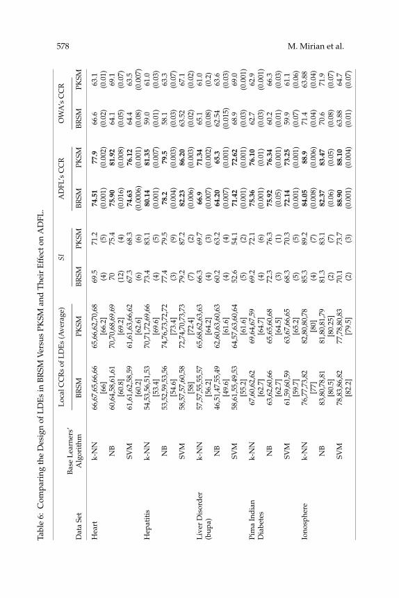
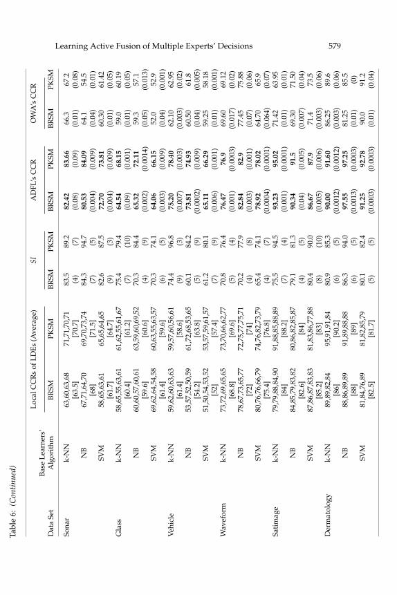
In Table 6, BRSM and PKSM methods are compared in terms of theLDEs’ CCR and the separability index, in addition to the CCR of the ADFL.The statistical variance of the separability index is reported in parentheses.More details about the PKSM method, including LDEs’ feature sets (F i , i =1, 2, . . . , c), are given in Table 7.
As can be inferred from Table 6, switching from BRSM to PKSM-basedLDEs improves the performance of fusion-based methods as well exceptin the Hepatitis and Waveform data sets. However, their improvement isnot sufficient to surpass the ensemble-based methods, where as ADFL candefeat them. Another observation is that ADFL surpasses OWA, a learningfusion method.
Table 6 shows an increase in both LDEs’ average CCR and SI results inimproved ADFL performance in all but in two cases: Waveform and Der-matology, with SVM and NB LDEs respectively, where the reductions areless than 1%. An increase in the average CCR of LDEs results in higher SI inmost cases, while the inverse is not always true. It means that improvementin SI does not necessarily require considerable enhancement of LDEs’ CCR.In fact, in some cases, an increase in SI by switching from BRSM to PKSMhas resulted in higher CCR for ADFL, while the average and maximumCCRs of LDEs are reduced. The cases are the Vehicle, Glass, Dermatology,and Ionosphere data sets with k-NN, SVM, SVM, and NB LDEs, respec-tively. To investigate the problem further, we generated 50 sets of LDEs forthe Liver and Hepatitis data sets, respectively, using the BRSM method. Wefound that the correlation of SI and the average CCR of LDEs is a small,negative value. All in all, it can be inferred that SI is a proper preevaluationmechanism to find out whether the designed LDEs are potentially suitablefor the ADFL algorithm even if their CCRs are not high. Note that the de-sign of LDEs with a high CCR is difficult in practice; increasing SI is muchsimpler.
Heart and Waveform are the only data sets where replacing BRSM-based LDEs with PKSM-based ones did not help ADFL to defeat ensemble-based benchmarks. Nevertheless, it assisted ADFL in improving its best
578 M. Mirian et al.Ta
ble
6:C
ompa
ring
the
Des
ign
ofL
DE
sin
BR
SMV
ersu
sPK
SMan
dT
heir
Eff
ecto
nA
DFL
.
Loc
alC
CR
sof
LD
Es
(Ave
rage
)SI
AD
FL’s
CC
RO
WA
’sC
CR
Bas
eL
earn
ers’
Dat
aSe
tA
lgor
ithm
BR
SMPK
SMB
RSM
PKSM
BR
SMPK
SMB
RSM
PKSM
Hea
rtk-
NN
66,6
7,65
,66,
6665
,66,
62,7
0,68
69.5
71.2
74.5
177
.966
.663
.1[6
6][6
6.2]
(4)
(5)
(0.0
01)
(0.0
02)
(0.0
2)(0
.01)
NB
60,6
4,58
,61,
6170
,70,
68,6
9,69
7075
.475
.90
81.9
264
.169
.1[6
0.8]
[69.
2](1
2)(4
)(0
.016
)(0
.008
)(0
.05)
(0.0
7)SV
M61
,61,
62,5
8,59
61,6
1,63
,66,
6267
.368
.374
.63
76.1
264
.463
.5[6
0.2]
[62.
6](6
)(6
)(0
.000
6)(0
.001
)(0
.08)
(0.0
07)
Hep
atit
isk-
NN
54,5
3,56
,51,
5370
,71,
72,6
9,66
73.4
83.1
80.1
481
.35
59.0
61.0
[53.
4][6
9.6]
(4)
(5)
(0.0
01)
(0.0
07)
(0.0
1)(0
.03)
NB
53,5
2,59
,53,
5674
,76,
73,7
2,72
77.4
79.5
78.2
79.5
58.1
63.3
[54.
6][7
3.4]
(3)
(9)
(0.0
04)
(0.0
03)
(0.0
3)(0
.07)
SVM
58,5
7,57
,60,
5872
,74,
70,7
3,73
79.2
87.2
82.2
386
.20
63.5
267
.1[5
8][7
2.4]
(7)
(2)
(0.0
06)
(0.0
03)
(0.0
2)(0
.02)
Liv
erD
isor
der
k-N
N57
,57,
55,5
5,57
65,6
8,62
,63,
6366
.369
.766
.971
.34
65.1
61.0
(bup
a)[5
6.2]
[64.
2](4
)(3
)(0
.007
)(0
.002
)(0
.08)
(0.2
)N
B46
,51,
47,5
5,49
62,6
0,63
,60,
6360
.263
.264
.20
65.3
62.5
463
.6[4
9.6]
[61.
6](4
)(4
)(0
.007
)(0
.001
)(0
.015
)(0
.03)
SVM
58,6
1,55
,49,
5364
,57,
63,6
0,64
52.6
54.1
71.4
272
.62
68.9
69.0
[55.
2][6
1.6]
(5)
(2)
(0.0
01)
(0.0
01)
(0.0
3)(0
.001
)Pi
ma
Ind
ian
k-N
N67
,60,
62,6
269
,64,
67,5
969
.272
.175
.36
76.1
062
.762
.9D
iabe
tes
[62.
7][6
4.7]
(4)
(6)
(0.0
01)
(0.0
1)(0
.03)
(0.0
01)
NB
63,6
2,60
,66
65,6
5,60
,68
72.3
76.3
75.9
276
.34
60.2
66.3
[62.
7][6
4.5]
(3)
(1)
(0.0
5)(0
.001
)(0
.01)
(0.0
3)SV
M61
,59,
60,5
963
,67,
66,6
568
.370
.372
.14
73.2
559
.961
.1[5
9.7]
[65.
2](5
)(5
)(0
.001
)(0
.001
)(0
.07)
(0.0
6)Io
nosp
here
k-N
N76
,77,
73,8
282
,80,
80,7
885
.389
.284
.05
88.9
71.4
63.8
8[7
7][8
0](4
)(7
)(0
.008
)(0
.006
)(0
.04)
(0.0
4)N
B83
,80,
78,8
181
,80,
81,7
981
.383
.182
.37
83.4
770
.671
.9[8
0.5]
[80.
25]
(2)
(7)
(0.0
6)(0
.05)
(0.0
8)(0
.07)
SVM
78,8
3,86
,82
77,7
8,80
,83
70.1
73.7
88.9
088
.10
63.8
864
.7[8
2.2]
[79.
5](2
)(3
)(0
.001
)(0
.004
)(0
.01)
(0.0
7)
Learning Active Fusion of Multiple Experts’ Decisions 579
Tabl
e6:
(Con
tinu
ed)
Loc
alC
CR
sof
LD
Es
(Ave
rage
)SI
AD
FL’s
CC
RO
WA
’sC
CR
Bas
eL
earn
ers’
Dat
aSe
tA
lgor
ithm
BR
SMPK
SMB
RSM
PKSM
BR
SMPK
SMB
RSM
PKSM
Sona
rk-
NN
63,6
0,63
,68
71,7
1,70
,71
83.5
89.2
82.4
283
.66
66.3
67.2
[63.
5][7
0.7]
(4)
(7)
(0.0
8)(0
.09)
(0.0
1)(0
.08)
NB
67,7
1,64
,70
69,7
0,73
,74
84.3
94.7
80.5
384
.09
64.1
54.5
[68]
[71.
5](7
)(5
)(0
.004
)(0
.009
)(0
.04)
(0.0
1)SV
M58
,65,
63,6
165
,65,
64,6
582
.687
.572
.70
73.8
160
.30
61.4
2[6
1.7]
[64.
7](9
)(3
)(0
.004
)(0
.009
)(0
.01)
(0.0
5)G
lass
k-N
N58
,65,
55,6
3,61
61,6
2,55
,61,
6775
.479
.464
.54
68.1
559
.060
.19
[60.
4][6
1.2]
(7)
(10)
(0.0
9)(0
.001
)(0
.01)
(0.0
5)N
B60
,60,
57,6
0,61
63,5
9,60
,69,
5270
.384
.465
.32
72.1
159
.357
.1[5
9.6]
[60.
6](4
)(9
)(0
.002
)(0
.001
4)(0
.05)
(0.0
13)
SVM
69,6
2,64
,54,
5860
,63,
55,6
3,57
70.3
74.1
64.0
666
.15
52.0
52.9
[61.
4][5
9.6]
(6)
(5)
(0.0
03)
(0.0
09)
(0.0
4)(0
.001
)V
ehic
lek-
NN
59,6
2,60
,63,
6359
,57,
60,5
6,61
74.4
96.8
75.2
078
.40
62.1
062
.95
[61.
4][5
8.6]
(9)
(3)
(0.0
07)
(0.0
03)
(0.0
03)
(0.0
2)N
B53
,57,
52,5
0,59
61,7
2,68
,53,
6560
.184
.273
.81
74.9
360
.50
61.8
[54.
2][6
3.8]
(5)
(9)
(0.0
002)
(0.0
09)
(0.0
4)(0
.005
)SV
M51
,50,
54,5
3,52
53,5
7,59
,61,
5761
.280
.165
.11
66.2
959
.25
58.1
8[5
2][5
7.4]
(7)
(9)
(0.0
06)
(0.0
01)
(0.0
1)(0
.001
)W
avef
orm
k-N
N73
,72,
69,6
5,65
73,7
0,66
,62,
7770
.876
.476
.47
76.9
69.6
069
.12
[68.
8][6
9.6]
(5)
(4)
(0.0
01)
(0.0
003)
(0.0
17)
(0.0
2)N
B78
,67,
73,6
5,77
72,7
5,77
,75,
7170
.277
.982
.84
82.9
77.4
575
.88
[72]
[74]
(4)
(8)
(0.0
03)
(0.0
01)
(0.0
7)(0
.06)
SVM
80,7
6,76
,66,
7974
,76,
82,7
3,79
65.4
74.1
78.9
278
.02
64.7
065
.9[7
5.4]
[76.
8](4
)(7
)(0
.000
4)(0
.000
1)(0
.064
)(0
.07)
Sati
mag
ek-
NN
79,7
9,88
,84,
9091
,88,
85,8
8,89
75.5
94.5
93.2
395
.02
71.4
263
.95
[84]
[88.
2](7
)(4
)(0
.001
)(0
.000
1)(0
.01)
(0.0
1)N
B84
,85,
79,8
3,82
80,8
6,82
,85,
8779
.181
.390
.34
91.5
69.3
071
.50
[82.
6][8
4](4
)(5
)(0
.04)
(0.0
05)
(0.0
07)
(0.0
4)SV
M87
,86,
87,8
3,83
81,8
3,86
,77,
8880
.490
.086
.67
87.9
71.4
73.5
[85.
2][8
3](8
)(1
0)(0
.005
)(0
.006
)(0
.003
)(0
.06)
Der
mat
olog
yk-
NN
89,8
9,82
,84
95,9
1,91
,84
80.9
85.3
90.0
091
.60
86.2
589
.6[8
6][9
0.2]
(6)
(5)
(0.0
012)
(0.0
012)
(0.0
03)
(0.0
6)N
B88
,86,
89,8
991
,89,
88,8
886
.394
.097
.55
97.2
581
.25
85.5
[88]
[89]
(6)
(5)
(0.0
013)
(0.0
003)
(0.0
1)(0
)SV
M81
,84,
76,8
981
,82,
85,7
980
.182
.491
.25
92.7
890
.091
.2[8
2.5]
[81.
7](5
)(5
)(0
.000
3)(0
.000
3)(0
.01)
(0.0
4)

580 M. Mirian et al.
Table 7: Feature Splits for the Best SI and the Corresponding Base LearnerAlgorithm.
Best SI by BaseData Set PKSM (var) Learner Feature Sets of LDEs
Heart 75.4 (4) NB F 1 = [1, 2, 3]F 2 = [1, 2, 3, 5]F 3 = [1, 2, 4, 6, 3, 8]F 4 = [1, 2, 6, 7, 5, 3]F 5 = [1, 2, 12, 7, 6, 13]
Hepatitis 87.2 (2) SVM F 1 = [1, 2, 4, 5, 6, 7, 10, 11, 12, 13, 19]F 2 = [1, 2, 3, 4, 5, 6, 7, 10, 11, 12, 13, 8, 9]F 3 = [1, 2, 14, 15, 16, 17, 18]F 4 = [1, 2, 4, 5, 6, 7, 10, 11, 12, 13,
14, 15, 17, 18]F 5 = [1, 2, 5, 18, 19]
Liver Disorder 69.7 (3) k-NN F 1 = [6, 2, 5](bupa) F 2 = [6, 1, 5]
F 3 = [6, 2, 3]F 4 = [6, 2, 3, 4]F 5 = [6, 3, 4, 5]
Pima Indian 76.3 (1) NB F 1 = [1, 3, 4, 6, 7, 8]Diabetes F 2 = [1, 2, 3, 5, 7, 8]
F 3 = [1, 3, 4, 5, 6, 8]F 4 = [1, 2, 5, 6, 7, 8]
Ionosphere 89.2 (7) k-NN F 1 = [6,15,8,3,14,17,12,1,11,2,9,5,13, 30]F 2 = [7,6,11,21,8,10,13, 14,28, 18, 20]F 3 = [25,16,12,13,20,9,15,19,34, 18,23,10,17]F 4 = [18,19,26,25,23,32,31,20,28,29,27]
Sonar 94.7 (5) NB F 1 = [17,26,10,11, 19,2, 39,14,7, 6,4,15,34, 5,22,1,3, 25,32, 30,12]
F 2 = [8,11,9, 50,18, 49,44, 26,22,17,19,51,39,15,30, 10, 12, 25]
F 3 = [21, 16, 50, 22, 19, 56, 55, 46, 38, 52,15,18, 60,51, 59, 44, 58, 25, 17,47]
F 4 = [57,54,23,60,59,37,48, 46, 36,50,35,52,51,21, 49,44,45,53,33
Glass 84.4 (9) NB F 1 = [9, 2, 6]F 2 = [5,2, 3, 4]F 3 = [2, 3, 9, 8]F 4 = [6, 2, 4]F 5 = [2, 3, 6, 7, 4]
Vehicle 96.8 (3) k-NN F 1 = [9,11, 15, 4, 16, 7, 12, 18, 6, 2]F 2 = [17, 18, 5, 12, 11, 10, 8, 9, 4, 13, 3]F 3 = [6, 8, 14, 9, 12, 13, 7, 5, 18, 2, 4]F 4 = [2, 7, 15,12, 17, 4, 1, 3, 8, 14, 10, 18, 6, 9]F 5 = [12,17, 10, 7, 1, 3,13, 8, 2, 9, 4,11, 18, 16]
Waveform 77.9 (8) NB F 1 = [14, 2, 22, 13, 6, 17, 5, 24, 26, 25,18,36, 8,15, 34, 7, 1,28,16, 35, 30, 19, 3, 32, 27]
F 2 = [8,17,25,32,33,24,16,10,3,35, 28,31, 7,19, 11, 2, 22, 9, 13, 12, 1, 34 15, 36]
F 3 = [15, 28,17, 7, 29, 3, 36, 6,26,24,10,18,12,35,13, 4, 25,33,16,34, 2, 11]

Learning Active Fusion of Multiple Experts’ Decisions 581
Table 7: (Continued)
F 4 = [22,13,7,10,30,6,32,31,21,29,24, 35,9, 5, 1,11,14,36,8,3]
F 5 = [28,25,20, 2, 8,15, 23,3,10, 4,30,7,21,17,18, 22, 34, 33,13, 29,14,24, 32,12]
Satimage 94.5 (4) k-NN F 1 = [28,9,19,30,1,20,26,29, 8,13,32,15,31,5, 14, 6,3, 4,27, 2,12,23,17, 18, 16]
F 2 = [17, 18,31,28, 3,13, 1,21, 2,35,26,34,14,5,30,23,11,25,16, 8,10]
F 3 = [12,9,4,24,3,16,22,13, 6, 14, 5,28,35,18,29,32,21,11,36,31, 7]
F 4 = [18,2,17,11, 36, 8, 13, 22, 7,34, 9,32,30,5,25,20,1,33,31,4,26]
F 5 = [22,18,12, 4, 10,6,26,35, 33,27, 24, 32,14,25,31, 3,21,5, 9,16,34,19, 17,30]
Dermatology 94.0 (5) NB F 1 = [23, 7,11,1,34,5,10,21,17, 2, 3]F 2 = [30,15,11,9,26,24,10,5,18,7,3]F 3 = [32,20,13,30,11,23,31,19,4,24,14,18]F 4 = [4,27,33, 6, 13, 26, 28,32,24, 25,14]
performance over LDEs from 75.9 to 81.92 in Heart and kept its performancein Waveform unchanged.
It is clear that SI is maximized in two abnormal circumstances: where allLDEs are perfect (CR = 100), or they are totally and systematically wrong(CCR = 0). We study the second situation in the next section by adding onesystematically wrong decision maker to our set of LDEs. It is obvious thatthis decision maker reduces the average CCR of LDEs.
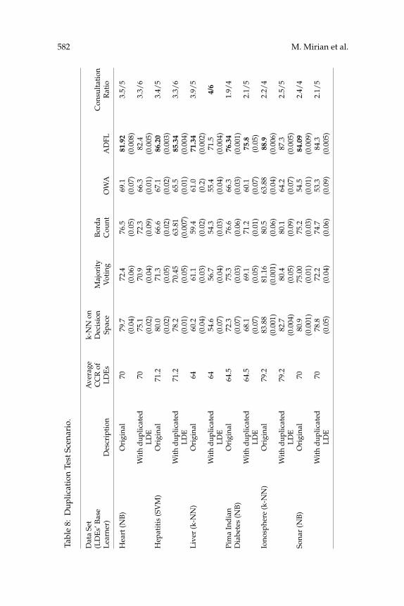
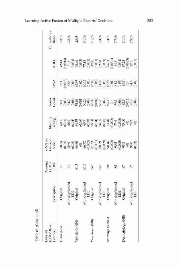
6.2 Duplicated and Systematically Wrong LDEs. An important prop-erty of ADFL, which is not usually a concern in classification and ensemble-based methods but is highly desired in information fusion systems, is itsrobustness to some sorts of problematic design of LDEs. To verify this prop-erty, we tested ADFL’s robustness against adding some duplicated andsystematically wrong LDEs to the set of existing LDEs. Such LDEs causedifficulty for common decision fusion methods. However, our experimentsrevealed that ADFL can automatically detect and manage consultation withduplicated LDEs and makes the best use of systematically incorrect ones aswell.
6.2.1 Duplicated Decision Makers. For each data set, the design with thebest performance is selected (from Table 4). Then one of the PKSM-basedLDEs is duplicated at a time, and ADFL is executed again. The results areaveraged over the LDEs (see Table 8). Each duplicated LDE adds c − 1 di-mensions to the decision space, which are actually redundant. The resultsshow that the fusion methods and k-NN in the decision space experience
582 M. Mirian et al.
Tabl
e8:
Dup
licat
ion
Test
Scen
ario
.
Dat
aSe
tA
vera
gek-
NN
on(L
DE
s’B
ase
CC
Rof
Dec
isio
nM
ajor
ity
Bor
da
Con
sult
atio
nL
earn
er)
Des
crip
tion
LD
Es
Spac
eV
otin
gC
ount
OW
AA
DFL
Rat
io
Hea
rt(N
B)
Ori
gina
l70
79.7
72.4
76.5
69.1
81.9
23.
5/5
(0.0
4)(0
.06)
(0.0
5)(0
.07)
(0.0
08)
Wit
hd
uplic
ated
7075
.170
.972
.366
.382
.43.
3/6
LD
E(0
.02)
(0.0
4)(0
.09)
(0.0
1)(0
.005
)H
epat
itis
(SV
M)
Ori
gina
l71
.280
.071
.366
.667
.186
.20
3.4/
5(0
.02)
(0.0
5)(0
.02)
(0.0
2)(0
.003
)W
ith
dup
licat
ed71
.278
.270
.45
63.8
165
.585
.34
3.3/
6L
DE
(0.0
1)(0
.05)
(0.0
07)
(0.0
1)(0
.004
)L
iver
(k-N
N)
Ori
gina
l64
60.2
61.1
59.4
61.0
71.3
43.
9/5
(0.0
4)(0
.03)
(0.0
2)(0
.2)
(0.0
02)
Wit
hd
uplic
ated
6454
.656
.754
.355
.471
.54/
6L
DE
(0.0
7)(0
.04)
(0.0
3)(0
.04)
(0.0
04)
Pim
aIn
dia
nO
rigi
nal
64.5
72.3
75.3
76.6
66.3
76.3
41.
9/4
Dia
bete
s(N
B)
(0.0
7)(0
.03)
(0.0
6)(0
.03)
(0.0
01)
Wit
hd
uplic
ated
64.5
68.1
69.1
71.2
60.1
75.8
2.1/
5L
DE
(0.0
7)(0
.05)
(0.0
1)(0
.07)
(0.0
5)Io
nosp
here
(k-N
N)
Ori
gina
l79
.283
.88
81.1
680
.563
.88
88.9
2.2/
4(0
.001
)(0
.001
)(0
.06)
(0.0
4)(0
.006
)W
ith
dup
licat
ed79
.282
.780
.480
.164
.287
.32.
5/5
LD
E(0
.004
)(0
.05)
(0.0
9)(0
.07)
(0.0
05)
Sona
r(N
B)
Ori
gina
l70
80.9
75.0
075
.254
.584
.09
2.4/
4(0
.001
)(0
.01)
(0.0
3)(0
.01)
(0.0
09)
Wit
hd
uplic
ated
7078
.872
.274
.753
.384
.32.
1/5
LD
E(0
.05)
(0.0
4)(0
.06)
(0.0
9)(0
.005
)
Learning Active Fusion of Multiple Experts’ Decisions 583
Tabl
e8:
(Con
tinu
ed)
Dat
aSe
tA
vera
gek-
NN
on(L
DE
s’B
ase
CC
Rof
Dec
isio
nM
ajor
ity
Bor
da
Con
sult
atio
nL
earn
er)
Des
crip
tion
LD
Es
Spac
eV
otin
gC
ount
OW
AA
DFL
Rat
io
Gla
ss(N
B)
Ori
gina
l61
60.3
460
.158
.157
.172
.11
2.3/
5(0
.03)
(0.0
1)(0
.03)
(0.0
13)
(0.0
014)
Wit
hd
uplic
ated
6159
.956
.954
.752
.871
.82.
5/6
LD
E(0
.05)
(0.0
4)(0
.08)
(0.0
9)(0
.004
)V
ehic
le(k
-NN
)O
rigi
nal
61.5
68.6
064
.35
54.0
462
.95
78.4
02.
9/5
(0)
(0.0
6)(0
.001
)(0
.02)
(0.0
03)
Wit
hd
uplic
ated
61.5
66.7
260
.750
.20
60.1
377
.91
3.1/
6L
DE
(0.0
05)
(0.0
3)(0
.04)
(0.0
5)(0
.001
)W
avef
orm
(NB
)O
rigi
nal
74.5
81.3
375
.00
65.3
975
.88
82.9
2.1/
5(0
.001
)(0
.04)
(0.0
02)
(0.0
6)(0
.001
)W
ith
dup
licat
ed74
.580
.59
76.0
565
.45
71.9
282
.50
2.4/
6L
DE
(0.0
09)
(0.0
8)(0
.07)
(0.0
3)(0
.009
)Sa
tim
age
(k-N
N)
Ori
gina
l88
90.1
674
.18
59.3
063
.95
95.0
23.
4/5
(0.0
02)
(0.0
02)
(0)
(0.0
1)(0
.000
1)W
ith
dup
licat
ed88
90.5
73.9
59.1
64.2
94.6
3.7/
6L
DE
(0.0
05)
(0.0
08)
(0.0
6)(0
.05)
(0.0
04)
Der
mat
olog
y(N
B)
Ori
gina
l87
95.5
75.0
082
.585
.597
.25
3.1/
4(0
)(0
)(0
.012
)(0
)(0
.000
3)W
ith
dup
licat
ed87
95.0
73.2
81.3
84.8
97.6
2.9/
5L
DE
(0.0
3)(0
)(0
.04)
(0.0
4)(0
.007
)
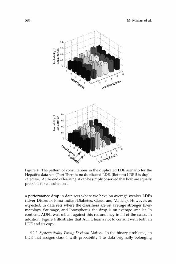
584 M. Mirian et al.
Figure 4: The pattern of consultations in the duplicated LDE scenario for theHepatitis data set. (Top) There is no duplicated LDE. (Bottom) LDE 5 is dupli-cated as 6. At the end of learning, it can be simply observed that both are equallyprobable for consultations.
a performance drop in data sets where we have on average weaker LDEs(Liver Disorder, Pima Indian Diabetes, Glass, and Vehicle). However, asexpected, in data sets where the classifiers are on average stronger (Der-matology, Satimage, and Ionosphere), the drop is on average smaller. Incontrast, ADFL was robust against this redundancy in all of the cases. Inaddition, Figure 4 illustrates that ADFL learns not to consult with both anLDE and its copy.
6.2.2 Systematically Wrong Decision Makers. In the binary problems, anLDE that assigns class 1 with probability 1 to data originally belonging
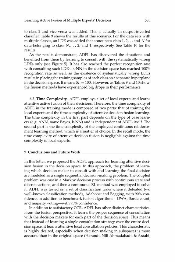
Learning Active Fusion of Multiple Experts’ Decisions 585
to class 2 and vice versa was added. This is actually an output-invertedclassifier. Table 9 shows the results of this scenario. For the data sets withmultiple classes, an LDE was added that announces class 1, 2,. . . and N fordata belonging to class N,. . . , 2, and 1, respectively. See Table 10 for theresults.
As the results demonstrate, ADFL has discovered the situations andbenefited from them by learning to consult with the systematically wrongLDEs only (see Figure 5). It has also reached the perfect recognition ratewith consulting such LDEs. k-NN in the decision space has reached 100%recognition rate as well, as the existence of systematically wrong LDEsresults in placing the training samples of each class on a separate hyperplanein the decision space. It means SI = 100. However, as Tables 9 and 10 show,the fusion methods have experienced big drops in their performance.
6.3 Time Complexity. ADFL employs a set of local experts and learnsattentive active fusion of their decisions. Therefore, the time complexity ofADFL in the training mode is composed of two parts: that of training thelocal experts and the time complexity of attentive decision fusion learning.The time complexity in the first part depends on the type of base learn-ers (e.g. ANN, naıve Bayes, k-NN) and is independent of ADFL itself. Thesecond part is the time complexity of the employed continuous reinforce-ment learning method, which is a matter of choice. In the recall mode, thetime complexity of attentive decision fusion is negligible against the timecomplexity of local experts.
7 Conclusions and Future Work
In this letter, we proposed the ADFL approach for learning attentive deci-sion fusion in the decision space. In this approach, the problem of learn-ing which decision maker to consult with and learning the final decisionare modeled as a single sequential decision-making problem. The coupledproblem was cast in a Markov decision process with continuous state anddiscrete actions, and then a continuous RL method was employed to solveit. ADFL was tested on a set of classification tasks where it defeated twowell-known classification methods, Adaboost and Bagging, with 90% con-fidence, in addition to benchmark fusion algorithms—OWA, Borda count,and majority voting—with 95% confidence.
In addition to satisfactory CCR, ADFL has other distinct characteristics.From the fusion perspective, it learns the proper sequence of consultationwith the decision makers for each part of the decision space. This meansthat instead of learning a single consultation strategy over the entire deci-sion space, it learns attentive local consultation policies. This characteristicis highly desired, especially when decision making in subspaces is moreaccurate than in the original space (Harandi, Nili Ahmadabadi, & Araabi,

586 M. Mirian et al.
Tabl
e9:
Out
put-
Inve
rted
Test
byU
sing
PKSM
-Bas
edL
DE
sin
the
Bin
ary
Dat
aSe
ts.
Dat
aSe
tD
escr
ipti
onA
vera
gek-
NN
(LD
Es’
Bas
e(A
vera
geC
CR
CC
Rof
onD
ecis
ion
Maj
orit
yB
ord
aC
onsu
ltat
ion
lear
ner)
ofL
DE
s)L
DE
saSp
ace
Vot
ing
Cou
ntO
WA
AD
FLR
atio
Hea
rt(N
B)
Ori
gina
l70
79.7
72.4
76.5
69.1
81.9
23.
5/5
(0.0
4)(0
.06)
(0.0
5)(0
.07)
(0.0
08)
Wit
hou
tput
-58
.310
064
.370
.261
.310
01.
3/6
inve
rted
LD
E(0
)(0
.08)
(0.0
1)(0
.08)
(0)
Hep
atit
is(S
VM
)O
rigi
nal
71.2
80.0
71.3
66.6
67.1
86.2
03.
4/5
(0.0
2)(0
.05)
(0.0
2)(0
.02)
(0.0
03)
Wit
hou
tput
-59
.310
059
.454
.360
.910
01.
6/6
inve
rted
LD
E(0
)(0
.05)
(0.0
4)(0
.04)
(0)
Liv
erD
isor
der
Ori
gina
l64
60.2
61.1
59.4
61.0
71.3
43.
9/5
(k-N
N)
(0.0
4)(0
.03)
(0.0
2)(0
.2)
(0.0
02)
Wit
hou
tput
-53
.310
052
.950
.155
.410
01.
2/6
inve
rted
LD
E(0
)(0
.05)
(0.0
3)(0
.09)
(0)
Pim
aIn
dia
nO
rigi
nal
64.5
72.3
75.3
76.6
66.3
76.3
41.
9/4
Dia
bete
s(N
B)
(0.0
7)(0
.03)
(0.0
6)(0
.03)
(0.0
01)
Wit
hou
tput
-51
.610
068
.970
.25
59.5
100
1.1/
5in
vert
edL
DE
(0)
(0.0
8)(0
.04)
(0.0
1)(0
)Io
nosp
here
Ori
gina
l79
.283
.88
81.1
680
.563
.88
88.9
2.2/
4(k
-NN
)(0
.001
)(0
.001
)(0
.06)
(0.0
4)(0
.006
)W
ith
outp
ut-
63.3
100
73.5
69.3
53.8
100
1.2/
5in
vert
edL
DE
(0)
(0.0
4)(0
.04)
(0.0
5)(0
)So
nar
(NB
)O
rigi
nal
7080
.975
.00
75.2
54.5
84.0
92.
4/4
(0.0
01)
(0.0
1)(0
.03)
(0.0
1)(0
.009
)W
ith
outp
ut-
5610
063
.969
.150
.110
01.
3/5
inve
rted
LD
E(0
)(0
.04)
(0.0
9)(0
.04)
(0)
a By
add
ing
asy
stem
atic
ally
inco
rrec
tcla
ssifi
erw
ith
anac
tual
CC
Rof
zero
,the
aver
age
loca
lCC
Ris
clea
rly
red
uced
.
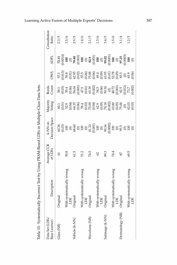
Learning Active Fusion of Multiple Experts’ Decisions 587
Tabl
e10
:Sy
stem
atic
ally
Inco
rrec
tTes
tby
Usi
ngPK
SM-B
ased
LD
Es
inM
ulti
ple-
Cla
ssD
ata
Sets
.
Dat
aSe
t(L
DE
s’A
vera
geC
CR
k-N
Non
Maj
orit
yB
ord
aC
onsu
ltat
ion
Bas
eL
earn
er)
Des
crip
tion
ofL
DE
sD
ecis
ion
Spac
eV
otin
gC
ount
OW
AA
DFL
Rat
io
Gla
ss(N
B)
Ori
gina
l61
60.3
460
.158
.157
.172
.11
2.3/
5(0
.03)
(0.0
1)(0
.03)
(0.0
13)
(0.0
014)
Wit
hsy
stem
atic
ally
wro
ng50
.810
052
.950
.450
.810
01.
5/6
LD
E(0
)(0
.04)
(0.0
6)(0
.01)
(0)
Veh
icle
(k-N
N)
Ori
gina
l61
.568
.60
64.3
554
.04
62.9
578
.40
2.9/
5(0
)(0
.06)
(0.0
01)
(0.0
2)(0
.003
)W
ith
syst
emat
ical
lyw
rong
51.2
100
58.4
47.9
55.5
100
1.4/
6L
DE
(0)
(0.0
3)(0
.01)
(0.0
6)(0
)W
avef
orm
(NB
)O
rigi
nal
74.5
81.3
375
.00
65.3
975
.88
82.9
2.1/
5(0
.001
)(0
.04)
(0.0
02)
(0.0
6)(0
.001
)W
ith
syst
emat
ical
lyw
rong
6210
062
.954
.569
.410
01.
3/6
LD
E(0
)(0
.05)
(0.0
6)(0
.09)
(0)
Sati
mag
e(k
-NN
)O
rigi
nal
89.3
90.1
674
.18
59.3
063
.95
95.0
23.
4/5
(0.0
002)
(0.0
02)
(0)
(0.0
1)(0
.000
1)W
ith
syst
emat
ical
lyw
rong
74.4
100
63.8
048
.72
52.7
810
01.
5/6
LD
E(0
)(0
.05)
(0.0
01)
(0.0
5)(0
)D
erm
atol
ogy
(NB
)O
rigi
nal
8795
.575
.00
82.5
85.5
97.2
53.
1/4
(0)
(0)
(0.0
12)
(0)
(0.0
003)
Wit
hsy
stem
atic
ally
wro
ng69
.510
062
.03
73.7
65.9
100
1.2/
5L
DE
(0)
(0.0
3)(0
.002
)(0
.06)
(0)
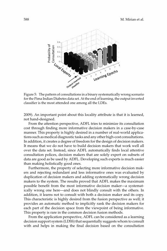
588 M. Mirian et al.
Figure 5: The pattern of consultations in a binary systematically wrong scenariofor the Pima Indian Diabetes data set. At the end of learning, the output invertedclassifier is the most attended one among all the LDEs.
2009). An important point about this locality attribute is that it is learned,not hand-designed.
From the attention perspective, ADFL tries to minimize its consultationcost through finding more informative decision makers in a case-by-casemanner. This property is highly desired in a number of real-world applica-tions such as medical diagnostic tasks and any other high-cost consultations.In addition, it creates a degree of freedom for the design of decision makers.It means that we do not have to build decision makers that work well allover the data set. Instead, since ADFL automatically finds local attentiveconsultation polices, decision makers that are solely expert on subsets ofdata are good as be used by ADFL. Developing such experts is much easierthan making holistically good ones.
Furthermore, the property of selecting more informative decision mak-ers and rejecting redundant and less informative ones was evaluated byduplication of decision makers and adding systematically wrong decisionmakers to the system. The results proved that ADFL makes the maximumpossible benefit from the most informative decision maker—a systemat-ically wrong one here—and does not blindly consult with the others. Inaddition, it learns not to consult with both a decision maker and its copy.This characteristic is highly desired from the fusion perspective as well; itprovides an automatic method to implicitly rank the decision makers foreach part of the decision space from the viewpoint of being informative.This property is rare in the common decision fusion methods.
From the application perspective, ADFL can be considered as a learningdecision support system (LDSS) that sequentially suggests whom to consultwith and helps in making the final decision based on the consultation
Learning Active Fusion of Multiple Experts’ Decisions 589
results. Such LDSSs are helpful in domains like medical diagnostic ande-consultant systems. We examined the first application in this letter.
ADFL can be used to construct classification systems as well. For theclassification tasks, the LDEs are usually not given and should be manuallydesigned, as done by BRSM and PKSM. Our current research is focusedon defining the desired properties of the local classifiers from an ADFLperspective and proposing efficient and automatic LDE design methodsaccordingly.
In this letter, we introduced k-NN on the decision space as well. Theresults showed that k-NN is a promising method for decision making in thedecision space provided that a granular distribution of data can be formedin that space. This formation can be acquired by the proper design of LDEs.Nevertheless, k-NN is a hard classifier—it considers only a fixed numberof neighbors—while ADFL generates soft decision boundaries through anattentive method. These characteristics justify higher performance of ADFLover k-NN in the decision space.
Acknowledgments
This research is supported by the University of Tehran and has also beenrealized in close collaboration with the BACS project supported by ECcontract number FP6-IST-02’140, Action line: Cognitive Systems. We thankG. N. Pedrajas for sharing his data and valuable information.
References
Berenji, H. R. (1996). Fuzzy Q-learning for generalization of reinforcement learning.In Proceedings of the Fifth IEEE International Conference on Fuzzy Systems, 1996.Piscataway, NJ: IEEE.
Blake, C. L., & Merz, C. J. (1998). UCI repository of machine learning databases, 1998.Irvine: University of California at Irvine.
Borji, A., Ahmadabadi, M. N., Araabi, B. N., & Hamidi, M. (2010). Online learningof task-driven object-based visual attention control. Image and Vision Computing,28, 1130–1145.
Chih-Jen Lin, C. C. (N.d.). LIBSVM. LIBSVM: Library for support vector machines.Available online at http://www.csie.ntu.edu.tw/∼cjlin/libsvm/.
Danziger, S. A., Zeng, J., Wang, Y., Brachmann, R. K., & Lathrop, R. H. (2007).Choosing where to look next in a mutation sequence space. Bioinformatics, 23(13),i104–i114.
Ebrahimpour, R., Kabir, E., Esteky, H., & Yousefi, M. R. (2008). View-independentface recognition with mixture of experts. Neurocomputing, 71(4–6), 1103–1107.
Filev, D., & Yager, R. R. (1998). On the issue of obtaining OWA operator weights.Fuzzy Sets and Systems, 94(2), 157–169.

590 M. Mirian et al.
Firouzi, H., Ahmadabadi, M. N., & Araabi, B. N. (2008). A probabilisticreinforcement-based approach to conceptualization. International Journal of In-telligent Technology, 3, 48–55.
Firouzi, H., Nili Ahmadabadi, M., N. Araabi, B., Amizadeh, S., Mirian, M. S., &Roland Siegwart. (2009). Interactive learning in continuous multimodal space: ABayesian approach to action based soft partitioning. Manuscript submitted forpublication.
Friedman, M. (1940). A comparison of alternative tests of significance for the problemof m rankings. Annals of Mathematical Statistics, 11(1), 86–92.
Garcia-Pedrajas, N. (2009). Constructing ensembles of classifiers by means ofweighted instance selection. IEEE Transactions on Neural Networks, 20(2), 258–277.
Garcia-Pedrajas, N., & Ortiz-Boyer, D. (2009). Boosting K-nearest neighbor classifierby means of input space projection. Expert Systems with Applications, 36(7), 10570–10582.
Harandi, M. T., Nili Ahmadabadi, M., & Araabi, B. N. (2009). Optimal local basis:A reinforcement learning approach for face recognition. International Journal ofComputer Vision, 81(2), 191–204.
Jordan, M. I., & Jacobs, R. A. (1994). Hierarchical mixtures of experts and the EMalgorithm. Neural Computation, 6(2), 181–214.
Kotsiantis, S. B., Zaharakis, I., & Pintelas, P. (2006). Supervised machine learning: Areview of classification techniques. Artificial Intelligence Review, 26(3), 159–190.
Kuncheva, L. I., Bezdek, J. C., & Duin, R. P. (2001). Decision templates for multipleclassifier fusion: An experimental comparison. Pattern Recognition, 34(2), 299–314.
Lizotte, D. J., Madani, O., & Greiner, R. (2003). Budgeted learning of na ve-bayes clas-sifiers. In Proceedings of the 19th Conference in Uncertainty. San Francisco: MorganKaufmann.
Minut, S., & Mahadevan, S. (2001). A reinforcement learning model of selectivevisual attention. In Proceedings of the Fifth International Conference on AutonomousAgents. Norwood, MA: Kluwer.
Mirian, M. S., Firouzi, H., Ahmadabadi, M. N., & Araabi, B. N. (2009). Concurrentlearning of task and attention control in the decision space. In Proceedings ofIEEE/ASME Advanced Intelligent Mechatronics (pp. 1353–1358). Piscataway, NJ:IEEE.
Paletta, L., Fritz, G., & Seifert, C. (2005). Q-learning of sequential attention for visualobject recognition from informative local descriptors. In Proceedings of the 22ndInternational Conference on Machine Learning. New York: ACM.
Paletta, L., & Pinz, A. (2000). Active object recognition by view integration andreinforcement learning. Robotics and Autonomous Systems, 31(1), 71–86.
Polikar, R. (2006). Ensemble based systems in decision making. IEEE Circuits andSystems Magazine, 6(3), 21–45.
Polikar, R. (2007). Bootstrap-inspired techniques in computational intelligence. IEEESignal Processing Magazine, 24(4), 59–72.
Schapire, R. E. (2003). The boosting approach to machine learning: An overview.Lecture Notes in Statistics. (pp. 149–172). New York: Springer-Verlag.
Shariatpanahi, F., & Nili Ahmadabadi, M. N. (2008). Biologically inspired frame-work for learning and abstract representation of attention control. In L. Paletta,
Learning Active Fusion of Multiple Experts’ Decisions 591
J. K. Tsotsos, & E. Rome (Eds.), Attention in Cognitive Systems. Theories and Systemsfrom an Interdisciplinary Viewpoint (pp. 324–324). New York: Springer.
Sutton, R. S., & Barto, A. G. (1999). Reinforcement learning. Journal of CognitiveNeuroscience, 11(1), 126–134.
Verikas, A., Lipnickas, A., Malmqvist, K., Bacauskiene, M., & Gelzinis, A. (1999).Soft combination of neural classifiers: A comparative study. Pattern RecognitionLetters, 20(4), 429–444.
Watkins, C. J., & Dayan, P. (1992). Q-learning. Machine Learning, 8(3), 279–292.Whiteson, S., Taylor, M. E., & Stone, P. (2007). Adaptive tile coding for value function
approximation (Tech. Rep. AI-TR-07-339). Austin: University of Texas.Wilcoxon, F. (1945). Individual comparisons by ranking methods. Biometrics Bulletin,
1(6), 80–83.Wolpert, D. H. (1992). Stacked generalization. Neural Networks, 5(2), 241–259.Woods, K., Kegelmeyer, W. P., & Bowyer, K. (1997). Combination of multiple clas-
sifiers using local accuracy estimates. IEEE Transactions on Pattern Analysis andMachine Intelligence, 19(4), 405–410.
Zhu, Y. (2003). Multisensor decision and estimation fusion. New York: Springer.Zimmerman, D. W. (1997). A note on interpretation of the paired-samples t test.
Journal of Educational and Behavioral Statistics, 22(3), 349–360.
Received January 18, 2010; accepted August 2, 2010.