U.U.D.M. Project Report 2022:6

Degree project E in mathematics Supervisor: Silvelyn Zwanzig Examiner: Julian Külshammer February 2022

Department of MathematicsUppsala University

Lattice Basis Reduction Using LLL Algorithm with Application to Algorithmic Lattice Problems

Juraj Polách

Lattice Basis Reduction Using LLL Algorithm

with Application to Algorithmic Lattice Problems

Juraj Polach

February 25, 2022

1

Abstract

The LLL algorithm is recognized as one of the most important achieve-ments of twentieth century with applications across many fields in math-ematics. Yet, the subject is explained only on an advanced level in thecurrent literature. We systematically present background and key con-cepts needed to understand the underlying problematic and afterwardsgive detailed proofs of all ideas needed to understand the algorithm. Thepaper focuses on application to lattice problems and proving results pre-sented in the original paper of A. K. Lenstra et al. published in 1982.

2

Contents

1 Introduction 4

2 Complexity Analysis of Lattice Problems 52.1 Complexity of Promise CVP . . . . . . . . . . . . . . . . . . . . . 72.2 Complexity of Promise SVP . . . . . . . . . . . . . . . . . . . . . 8

3 Lattices and Lattice Reduction 9

4 LLL Reduced Basis 144.1 LLL Algorithm . . . . . . . . . . . . . . . . . . . . . . . . . . . . 194.2 Solving CVP Using the LLL Algorithm . . . . . . . . . . . . . . 284.3 Run-time Analysis of LLL Algorithm . . . . . . . . . . . . . . . . 29

5 Conclusion 32

References 33

3

1 Introduction

Shortest vector problem and closest vector problem, or so called lattice prob-lems, are optimization problems in computer science related to additive groupscalled lattices.

Definition 1.1. A lattice L, is defined as the set of linear combinations oflinearly independent vectors v1, . . . , vn ∈ Rm (m ≥ n) with coefficients in Z,

L = {a1v1 + a2v2 + · · ·+ anvn : a1, a2, . . . , an ∈ Z} (1)

A very natural and intuitive example of a lattice is a simple grid. However,it turns out that extending the structure to n dimensions as by the definitionabove gives lattices rich combinatorial structure that makes it a powerful tool toaddress various problems within mathematics. These include integer program-ming, cryptography, factoring of polynomials over integers [8].

The most fundamental problems related to lattices: shortest vector problemand closest vector problem, are very difficult to solve. We start by outliningboth of these:

Problem 1.1 (Shortest Vector Problem (SVP)). Find a (there can be multiple)shortest non-zero vector v in a given lattice L. The distance can be defined inany norm, but we will focus on the Euclidean norm i.e. ‖v‖.

Problem 1.2 (Closest Vector Problem (CVP)). Given a vector x ∈ Rm suchthat x /∈ L, find a (again there can be multiple) vector v ∈ L that is closest tox. The distance can again be measured by any norm, but we focus on Euclideannorm i.e. we try to minimize ‖v − x‖.

We visualize SVP, CVP and concept of lattices in 2 dimensions in Figure 11 where the lattice points are indicated by a dot (notice that the lattice is notthe entire collection Z2 represented by the grid). In Figure 1, solutions to SVPare vectors t and s. Solutions of CVP given vector v are both w and u.

It turns out that one of the most efficient ways to find at least an approxi-mate solution to SVP and CVP is to manipulate basis vectors of the lattice inquestion in a specific way. This manipulation is referred to as a basis reduction.LLL algorithm developed by A. K. Lenstra et al. in 1982 [7] is the fundamentalmethod still used to perform the basis reduction, even it was developed around40 years ago. Despite its universal usefulness, the current literature is primarilyfor scholars that are already experts in the field. This paper presents the nec-essary background to the problematic as well as detailed proofs of all conceptsneeded to understand the LLL algorithm itself.

We show that using the LLL algorithm, one is able to find a vector that isno more than (2/

√3)n times longer than a shortest vector of a given lattice and

present a method using which one can find a vector at most 2(2/√

3)n timesfurther away than a vector closest to a target vector outside the lattice. The n

1Figures in this paper are made with GeoGebra

4

Figure 1: Visualisation of SVP and CVP

represents dimension of the given lattice. In contrast to the current literature,we present the LLL algorithm using 2 distinct subroutines while explaining howeach relates to the SVP. Each subroutine impacts the basis vectors and their socalled Gram-Schmidt orthogonalized counterparts in a different way. The mainresult of this paper is a detailed proof of how the subroutine of swapping basisvectors impacts the Gram-Schmidt orthogonalized vectors and the coefficientsused to construct them. For the sake of completeness, we also provide a proofof why the LLL algorithm terminates and a proof of its polynomial run-time.

Section 2 formalizes the notion of how difficult it is to solve SVP and CVPusing complexity theory. Section 3 introduces approximate versions of SVP andCVP and the concept of basis reduction used to solve these. The LLL algorithmused to find an LLL reduced basis is presented and analyzed in Section 4. Weconclude by explaining main ways the LLL algorithm can and has been improvedin Section 5.

2 Complexity Analysis of Lattice Problems

In order to understand the computational complexity of the SVP and CVP,we need to extend the definition of general optimization problem to a so calledpromise problem. This is a generalization of a decision problem where either”Yes” or ”No” is an outcome for every input to a problem where there canbe input instances for which neither ”Yes” or ”No” is the output. For theseinputs we are allowed to output anything. Throughout this paper, we denotethe shortest vector in a lattice L as λ(L). In other words:

λ(L) = arg min{‖x‖ : x ∈ L, x 6= 0}

Furthermore, when we write basis vectors of the lattice L as columns of amatrix, say B, we can also discuss a lattice generated by the matrix B. In such

5

case, we can write:

L(B) = {Bx : x ∈ Zn}

which is equivalent to the definition from equation (1).

Problem 2.1 (Promise SVP). We refer to instances as pairs (B, d) with B ∈Zm×n as basis of L and d ∈ R positive number. We then distinguish ”Yes” or”No” cases as:

1. (B, d) is a ”Yes” instance if λ(L) ≤ d

2. (B, d) is a ”No” instance if λ(L) > d

Problem 2.2 (Promise CVP). We refer to instances as triples (B, x, d) withB ∈ Zm×n as basis of L and d ∈ R positive number and a vector x ∈ Rm suchthat x /∈ L. We then distinguish ”Yes” or ”No” cases as:

1. (B, x, d) is a ”Yes” instance if ‖x− z‖ ≤ d for some z ∈ L

2. (B, x, d) is a ”No” instance if ‖x− z‖ > d for all z ∈ L

During this paper, we do not address any algorithmic challenges with imple-menting algorithms to solve the problems above, but analyze their complexityfrom a purely mathematical point of view. As such, we are interested in whetherthese problems can be solved efficiently or not. From the point of view of com-plexity theory we distinguish between many complexity classes, but in this paperwe shall focus primarily on the classes P and NP. The full formal definition ofthese classes is beyond this paper as well, but we shall outline key concepts inorder to provide intuition for the reader.

We describe complexity of a given problem in terms of a model of compu-tation. A natural reference point are Turing machines. For purposes of thispaper, we define 4 types of Turing machine using definitions presented by D. S.Johnson [5]:

1. Deterministic Turing Machines (DTMs) These machines read inputfrom one tape, have a finite size ’work tape’ in order to perform operationsand an output tape. They eventually halt and the output (solution) canbe read from the output tape. In this case, we are primarily interestedin time measured in number of steps before the machine halts and spacemeasured in how much of the ’work tape’ was visited at some point duringthe computation.

2. Non-Deterministic Turing Machines (NDTMs) These machines nowhave several choices where they should read the next command. This mayresult in different outcomes given one input. NDTMs can yield only 2 pos-sible answers: ”Yes” and ”No”. Thus, they can be only used for decisionand promise problems.

6

3. Random Turing Machines (RTMs) These are NDTMs such that foreach possible input there are either no accepting computations or at leasthalf of all computations are accepting (output is ”Yes” after the machinehalts).

4. Oracle Turing Machine (OTM) This is a DTM, NDTM or RTM whichis always associated with a given problem Y and the core idea is that theOTMs can solve this problem Y without any cost. It can also be viewedas invoking a subroutine for solving Y . Invoking this subroutine countsthen as one step. We do note that the space is generally considered.

We can now describe complexity classes P, NP and R in terms of the Turingmachines defined above. Class P can be seen as the class of problems that can besolved efficiently i.e. using a DTM in polynomial time in relation to the lengthof the input tape (more formally, string). Class NP is generally seen as the classof problems that are difficult to solve efficiently. In terms of Turing machines,we say that this is the set of decision problems solvable in polynomial-boundedtime with a NDTM. It can also be useful to think of the class NP as a set ofproblems for which the solution can be checked by a DTM in polynomial timein relation to the input length. Finally, we introduce the class R (sometimesdenoted also RP), which can be thought of as problems that can be solvedefficiently, but with randomness involved. These algorithms are always correcton the ”No” instances and ’usually’ correct on ”Yes” instances [8]. We remarkthat P ⊆ R ⊆ NP.

In order to determine membership of a given problem to a complexity class,we need to simply show a method for solving the problem that meets require-ments given by the class definition. As an example, by finding an algorithmthat can run on a DTM in polynomial time we can conclude that the problembelongs to complexity class P. Many times, this approach turns out to be ratherimpractical and so we use a method called ’reduction’. For this purpose weuse OTMs. As the name suggests, the key idea is to reduce a problem intoanother problem from a known class using a subroutine (Oracle). For example,if we have a DTM running in polynomial time solving problem X under theassumption that we have a DTM Oracle solving subroutine problem Y , we canconclude that X belongs to to class P if we are able to show that Y belongs toP (i.e. composition of polynomials is also a polynomial).

2.1 Complexity of Promise CVP

It was shown already in 1981 by P. van Emde Boas [13] that the promise CVPbelongs to complexity class NP. The core idea of the paper was to show thatpromise CVP can be reduced to another problem already known to be of NPcomplexity: The subset sum problem outlined below.

Problem 2.3 (Subset Sum Problem). Given a1, a2, . . . , an, s ∈ Z, find coeffi-cients yi ∈ {0, 1} for i = 1, 2, . . . , n such that

∑i yiai = s. The corresponding

promise problem is formulated by defining instances:

7

1. (a1, a2, . . . , an, s) is a ”Yes” instance if there exist coefficients yi ∈ {0, 1}for i = 1, 2, . . . , n such that

∑i yiai = s

2. (a1, a2, . . . , an, s) is a ”No” instance if there do not exist coefficients yi ∈{0, 1} for i = 1, 2, . . . , n such that

∑i yiai = s

This problem is proven to be NP-hard. For reference see Garey and Johnson[3]. In order to outline the reduction itself, we refer to [9], where D. Micciancioand S. Goldwasser associate a = [a1, a2, . . . , an] to lattice basis vectors bi andthe target sum s to the target vector t as follows:

bi = [ai, 0, . . . , 0︸ ︷︷ ︸i−1

, 2, 0, . . . , 0︸ ︷︷ ︸i−1

]T

t = [s, 1, . . . , 1︸ ︷︷ ︸n

]T

This way, the equivalent promise CVP problem instance in Lp-norm is givenby the triplet (B, t, p

√n) where the lattice defining matrix B is given as:

B =

[a

2In

]where In is the identity matrix in n-th dimension and a is written as row

vector. The reduction can be easily seen when looking at the difference By− t:

By − t =

∑i yiai − s2y1 − 1

...2yn − 1

If there exists y ∈ {0, 1}n such that

∑i yiai = s, the first entry is 0, re-

maining entries are ±1 and the distance ‖Bx − t‖ in Lp-norm is at most p√n.

Conversely, assuming the promise CVP instance (B, t, p√n) is a ”Yes” instance

with vector z ∈ Zn such that

‖Bz − t‖pp = |n∑i=1

ziai − s|p +

n∑i=1

|2zi − 1|p ≤ n (2)

we see that the only way the inequality in equation (2) holds is if∑ni=1 ziai =

s as 2zi − 1 = ±1 for all i.

2.2 Complexity of Promise SVP

In the previous section, we have demonstrated that promise CVP and in turnCVP itself is NP-hard. Despite obvious similarities between CVP and SVP,NP-hardness of the SVP problem remained an open problem for another 17years after 1981 when P. van Emde Boas published the conjecture in his paper.

8

Breakthrough has been achieved for so called randomized reductions by M. Ajtaiin 1998 [1]. The proof itself is well beyond the scope of this paper, thus in thissection we shall only focus on what kind of reduction was used during the proofand its implications.

The first concept important to understand is ’Reverse Unfaithful Random’reduction, in short RUR-reduction. We will use the definition as per D. S.Johnson [5] where properties that must be satisfied are:

1. Outputs must be ’faithful’ for ”No” instances in a sense that if the answeris ”No” in the promise SVP, corresponding outputs in the reduced problemare also ”No” instances.

2. Outputs must be ’abundant’ for ”Yes” instances in a sense that if theanswer is ”Yes” in the promise SVP then at least 1/p(x) correspondingoutputs in the reduced problem are ”Yes” instances (p(x) is a fixed poly-nomial depending on the length of input).

By repeating the probabilistic algorithm we can see that the probability thatwe would get a ”No” instance in the reduced problem given that the correspond-ing solution to the promise SVP is a ”Yes” instance is decreasing. Hardnessunder RUR-reductions gives evidence of intractability of SVP in a probabilisticsense. More concretely, it shows that the SVP is not in R unless R = NP [8].The key result of [1] is that M. Ajtai shown that there is this probabilistic Turingmachine which in polynomial time reduces any problem in NP to the SVP.

3 Lattices and Lattice Reduction

The previous two sections show that both SVP and CVP problems are verydifficult to solve exactly. The natural next step is to look for an approximatesolution. The approximation is given in relation to the dimension of Lattice:

Problem 3.1 (Approximate SVP). For a given lattice L of dimension n finda non-zero vector v that is no more than ψ(n) times longer than the shortestvector λ(L). We can define the distance in any norm, but we will focus on theEuclidean norm i.e. ‖v‖ ≤ ψ(n)‖λ(L)‖.

Problem 3.2 (Approximate CVP). Given a vector x ∈ Rm such that x /∈ L,find a vector v ∈ L that is closest to x up to factor of ψ(n). The distancecan again be measured by any norm, but we focus on Euclidean norm i.e. ifd is the distance to the closest vector in the lattice we try to find v such that‖v − x‖ ≤ ψ(n)d.

There are multiple ways one can approach the approximate problems above.As a basis for L is any set of independent vectors that generates L (and anytwo such sets have the same number of elements) [4], one of the most popularapproaches is lattice reduction. The notion of reduced basis v1, v2, . . . , vn ∈ Rmfor lattice L can be defined as follows:

9

Definition 3.1 (Reduced Basis). We call a basis v1, v2, . . . , vn ∈ Rm for alattice L reduced if it satisfies

|µij | ≤1

2for 1 ≤ j < i ≤ n (3)

and||vi|| ≤ ||vi+1|| for 1 < i ≤ n− 1 (4)

where µij is the Gram-Schmidt coefficient defined in (6).

Definition 3.2 (Gram-Schmidt Orthogonalization). Gram-Schmidt orthogo-nalization process gives mutually orthogonal vectors v∗i ∈ Rm with 1 ≤ i ≤ nand numbers µij ∈ R with 1 ≤ j < i ≤ n defined inductively as

v∗i = vi −i−1∑j=1

µijv∗j (5)

µij =vi · v∗j‖v∗j ‖2

(6)

where v1, v2, . . . , vn ∈ Rm is the basis of lattice L.

We can also write vectors v∗1 , v∗2 , . . . , v

∗n as columns of a matrix, say BGS .

Define also the matrix UGS ∈ Rn×n where the (i, j)th entry is µij defined for1 ≤ j < i ≤ n in equation (6). For i = j we set the entries to 1 and for i < j weset entries to 0. UGS is upper triangular with diagonal entries equal to 1 andso det(UGS) = 1. Matrices B and BGS can be also expressed as BGS = BUGS .Note, that these orthogonalized vectors are not necessarily a basis for the latticeL, but span(B) = span(BGS). Thus, even though the orthogonalization andbasis reduction are closely related, we need to keep clear distinction betweenthem.

Expanding on the notion of reduced basis, the first condition set by equation(3) essentially says that it should be ’as orthogonal as possible’. This can beseen on Figure 2 where the vector v∗2 is orthogonal to v1 and v′2 is a reducedvector that is not orthogonal to v1, but is as orthogonal as possible with µ21 ≤ 1

2 .The second condition set by equation (4) essentially says that vectors shouldbe ordered from shortest to longest. The solution to approximate SVP givena reduced basis is by construction v1, the shortest vector in the reduced basis.How good the approximation is, is determined by how ’well’ we are able toreduce the basis and on a particular reduction algorithm. We are able to alsosolve the CVP using a reduced basis and reduction algorithms, but here thegoodness of approximation doesn’t only depend on how ’well’ we are able toreduce the basis, but also on what we do afterwards. During this paper, we willpresent two methods:

1. Using Babai’s Closest Vertex Algorithm as outlined by Hoffstein et al. [4]to provide basic intuition.

10

Figure 2: Difference between basis reduction and orthogonalization

2. Using the celebrated LLL algorithm proposed by A. K. Lenstra et al. in1982 [7].

We will describe both of these methods assuming the lattice is of full rank.In other words, when span(B) = Rn which is the case when m = n for basisvectors such that v1, v2, . . . , vn ∈ Rm. Both methods can also be used in themore general case where m > n, but then we need to project w to the closestpoint in span(B) and look for closest vector to that point instead.

Algorithm 1 Babai’s Closest Vertex Algorithm

Let L be a lattice with basis vectors v1, v2, . . . , vn ∈ Rn. We denote the matrixB as the matrix with columns as the basis vectors of the lattice. Furthermore,let w ∈ span(B) = Rn be an arbitrary vector. The algorithm executes in 3steps:

1. Express w in terms of the basis vectors i.e. write w = Bt for t ∈ Rn.

2. Calculate a ∈ Rn as ai = dtic for i = 1, 2, . . . , n.

3. Return vector v = Ba

where the operator dxc returns the integer closest to x ∈ R.

We begin with Babai’s closest vertex algorithm given as Algorithm 1 anddemonstrate its underlying idea in the Figure 3. In the figure, we are trying toexpress the vector v in terms of the two basis vectors: v1 and v2. As indicatedby the parallel line p to v1, the way to express the target vector v using thebasis vectors is to take close to 2v2 and a bit less than 1

2v1 resulting in the

vector−−→OF . It is clear that the algorithm only performs well in case we have

a relatively ’good’ basis in terms of both the orthogonality as well as length of

11

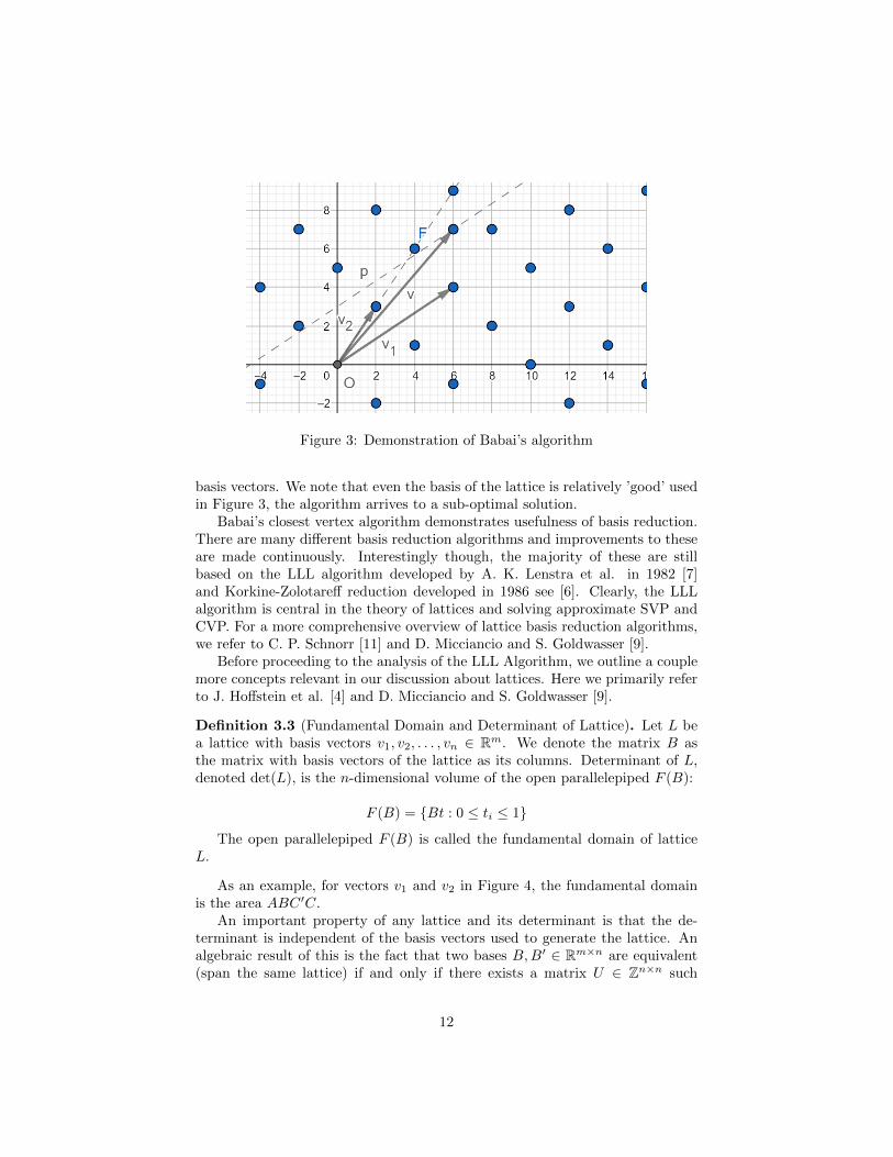
Figure 3: Demonstration of Babai’s algorithm

basis vectors. We note that even the basis of the lattice is relatively ’good’ usedin Figure 3, the algorithm arrives to a sub-optimal solution.

Babai’s closest vertex algorithm demonstrates usefulness of basis reduction.There are many different basis reduction algorithms and improvements to theseare made continuously. Interestingly though, the majority of these are stillbased on the LLL algorithm developed by A. K. Lenstra et al. in 1982 [7]and Korkine-Zolotareff reduction developed in 1986 see [6]. Clearly, the LLLalgorithm is central in the theory of lattices and solving approximate SVP andCVP. For a more comprehensive overview of lattice basis reduction algorithms,we refer to C. P. Schnorr [11] and D. Micciancio and S. Goldwasser [9].

Before proceeding to the analysis of the LLL Algorithm, we outline a couplemore concepts relevant in our discussion about lattices. Here we primarily referto J. Hoffstein et al. [4] and D. Micciancio and S. Goldwasser [9].

Definition 3.3 (Fundamental Domain and Determinant of Lattice). Let L bea lattice with basis vectors v1, v2, . . . , vn ∈ Rm. We denote the matrix B asthe matrix with basis vectors of the lattice as its columns. Determinant of L,denoted det(L), is the n-dimensional volume of the open parallelepiped F (B):

F (B) = {Bt : 0 ≤ ti ≤ 1}

The open parallelepiped F (B) is called the fundamental domain of latticeL.

As an example, for vectors v1 and v2 in Figure 4, the fundamental domainis the area ABC ′C.

An important property of any lattice and its determinant is that the de-terminant is independent of the basis vectors used to generate the lattice. Analgebraic result of this is the fact that two bases B,B′ ∈ Rm×n are equivalent(span the same lattice) if and only if there exists a matrix U ∈ Zn×n such

12

Figure 4: Fundamental domain

that B′ = BU and det(U) = ±1. In other words, we can express each basisby starting from the other one and sequentially (not simultaneously) adding orsubtracting respective basis vectors to and from each other. For example, wecan consider Figure 4 where we could instead of the basis vectors v1 and v2take basis vectors v1 and v′2 := v2 + v1. The fundamental domain of these twovectors (ABC ′′C ′) has the same area as the original two vectors as the heightv∗2 of the parallelepiped does not change. The determinant of the lattice L isalso equal to the square root of the determinant of the so-called Gram matrixBTB, which is an n× n matrix with its (i, j)th entry given as inner product ofvi and vj . The name relates to the orthogonality (or in other words projection)coefficient defined in (6). We can now utilize the matrices UGS and BGS definedduring the Gram-Schmidt orthogonalization process and summarize the aboveusing the following equation

det(L) =√

det(BTB) (7)

=√

det((BGSU−1GS)T (BGSU

−1GS)) (8)

=√

det((U−1GS)T )det(BTGSBGS)det(U−1GS) (9)

=

√√√√1 ·n∏i=1

||v∗i ||2 · 1 =

n∏i=1

||v∗i || (10)

where the vectors v∗i are Gram-Schmidt orthogonalized vectors defined inequation (5) and det(BTGSBGS) =

∏ni=1 ||v∗i ||2 follows from the fact that the v∗i

are mutually orthogonal. We can visualize the intuition behind the above againin Figure 4 as the area (2-dimensional volume) of the fundamental domain canalso be calculated as ‖v∗2‖ × ‖v1‖ = ‖v∗2‖ × ‖v∗1‖ as ‖v1‖ = ‖v∗1‖ by definition.

13

We now relate back to basis vectors v1, v2, . . . , vn with Hadamard’s inequality.

Lemma 3.1 (Hadamard’s Inequality). Let L be a lattice, take any basis v1, v2,. . . , vn ∈ Rm for L. Then

det(L) ≤ ‖v1‖‖v2‖ · · · ‖vn‖The closer a basis v1, v2, . . . , vn is to being orthogonal, the closer Hadamard’s

inequality comes to being an equality. Thus, one way to look at reducing a basisis to try to bring this inequality as close as possible to equality. With these termsdefined, we are ready to formalize concept of an LLL reduced basis in the nextsection.

4 LLL Reduced Basis

We now have the intuition behind how a reduced basis helps to solve the SVPand CVP. When working with the LLL reduced basis and LLL Algorithm, wechange the original idea of increasing length of basis vectors defined in (4), andinstead start working with Gram-Schmidt orthogonalized vectors v∗1 , v

∗2 , . . . , v

∗n.

Definition 4.1 (LLL Reduced Basis). As in A. K. Lenstra et al. [7], we definean LLL reduced basis v1, v2, . . . , vn ∈ Rm for a lattice L as a basis that satisfies

(Size Condition) |µij | ≤1

2for 1 ≤ j < i ≤ n

(Lovasz Condition) ||v∗i + µii−1v∗i−1||2 ≥

3

4||v∗i−1||2 for 1 < i ≤ n

where µij is a Gram-Schmidt coefficient defined in equation (6) and v∗1 , v∗2 ,

. . . , v∗n ∈ Rm are Gram-Schmidt orthogonalized vectors defined in (5).

We at this point remark that the constant 34 in (Lovasz Condition) can be

replaced by any real number δ ∈ ( 14 , 1), but in this paper we shall focus on

calculations with 34 . We will see later on in equation (31) that the idea behind

the left hand side of (Lovasz Condition) is to look at the length of the Gram-Schmidt orthogonalized vector of the basis vector vi if it would switch positionwith vi−1. The parameter δ thus represents a potential imperfection as lengthsof Gram-Schmidt orthogonalized vectors v∗i can decrease as i increases. Theidea is that if they would, they would do so slowly. It remains an open problemto see if the LLL algorithm terminates for δ = 1, which would get rid of thisimperfection. We can also compare the notion of an LLL reduced basis and basisreduced by Definition 3.1. It turns out that even these are closely related, onedoes not necessarily imply the other. To demonstrate this, we use the followingtwo examples. First, let v1, v2, v3 be defined as

[v1 v2 v3

]=

1 0 00 2 20 0 ε

14

where 0 < ε < 2√δ. Clearly v1, v2, v3 constitute a basis that is reduced by

Definition 3.1, but ||v∗3 + µ32v∗2 ||2 = ε2 ≤ 4δ = δ||v∗2 ||2. Next, let v′1, v

′2, v′3 be

defined as

[v′1 v′2 v′3

]=

1 0 00 2 00 0 2δ + ε′

where 0 < ε′ < 2(1 − δ). Clearly v′1, v

′2, v′3 constitute a basis that is LLL

reduced, but ‖v′2‖ > ‖v′3‖.We will now outline a couple of useful properties of any LLL reduced basis

as introduced by A. K. Lenstra et al. [7] in order to make the connection toapproximate SVP.

Lemma 4.1. Let a basis v1, v2, . . . , vn ∈ Rm for a lattice L be LLL reduced andlet v∗1 , v

∗2 , . . . , v

∗n be defined by the Gram-Schmidt orthogonalization process of

this basis. We then have

||vj ||2 ≤ 2i−1||v∗i ||2 for 1 ≤ j ≤ i ≤ n, (11)

det(L) ≤n∏i=1

||vi|| ≤ 2n(n−1)/4det(L) (12)

and

||v1|| ≤ 2(n−1)/4det(L)1/n (13)

Inequality (11), in Lemma 4.1 gives us a relation between the orthogonalizedvectors v∗i and the basis vectors vi. In particular, we can see that the length ofbasis vectors is bounded by the length of the orthogonalized vectors, howeverthe bound is exponentially weaker as we proceed through index i. This is easilyseen in Figure 5 where even though ‖v∗2‖ ≤ ‖v2‖ (which is always the case) wesee that

√2‖v∗2‖ ≥ ‖v2‖.

Inequality (12) tells us more about what is the worst case scenario whenit comes to ’orthogonality’ of an LLL reduced basis. Recall from Hadamard’sInequality (Lemma 3.1) that the closer the inequality is to equality, the moreorthogonal we can expect basis vectors to be.

Most importantly though, we are able to define a boundary for the lengthof the first (shortest) vector, v1, in an LLL reduced basis using inequality (13).Note, that the determinant of a lattice det(L) is independent of basis we choose.Thus, this boundary can be seen as a general property of any LLL reduced basis.We also note that this does not give us any relation just yet to the length of theshortest vector λ(L) in the lattice L.

If we work with the more general case of using δ instead of the constant 34 ,

powers of 2 in inequalities of Lemma 4.1 need to be replaced with powers of4/(4δ − 1) [7]. We leave the proof of the general case and instead proceed withthe proof in case δ = 3

4 .

15

Figure 5: Boundary on size of vectors

Proof of Lemma 4.1 We first begin by proving the inequality (11), byusing the definition of an LLL reduced basis. We can multiply out the square inleft hand side of (Lovasz Condition) as v∗i · v∗i−1 = 0 to arrive into a simplifiedversion:

||v∗i + µii−1v∗i−1||2 = ||v∗i ||2 + 2µii−1v

∗i · v∗i−1 + µ2

ii−1||v∗i−1||2

= ||v∗i ||2 + µ2ii−1||v∗i−1||2

implying

||v∗i ||2 ≥ (3

4− µ2

ii−1)||v∗i−1||2

where by (Size Condition) we have µ2ii−1 ≤ 1/4 and so ( 3

4 −µ2ii−1) ≥ 1

2 . Nowwe can deduce by induction ||v∗j ||2 ≤ 2i−j ||v∗i ||2 for 1 ≤ j ≤ i ≤ n. Next, usingthe definition of Gram-Schmidt orthogonalized vector v∗i in equation (5) andthe fact that v∗i · v∗j = 0 for i 6= j we get:

||vi||2 = ||v∗i +

i−1∑j=1

µijv∗j ||2 = ||v∗i ||2 +

i−1∑j=1

µ2ij ||v∗j ||2

≤ ||v∗i ||2 +

i−1∑j=1

1

42i−j ||v∗i ||2 = ||v∗i ||2(1 +

1

4

i−1∑j=1

2i−j)

= ||v∗i ||2(1 +1

4(2i − 2)) = ||v∗i ||2

1

2(2i−1 + 1)

≤ 2i−1||v∗i ||2

16

Inequality (11) now follows directly as we have shown earlier ||v∗j ||2 ≤2i−j ||v∗i ||2 for 1 ≤ j ≤ i ≤ n.

Proceeding further to (12), we can see that the first inequality is Hadamard’sInequality. The second inequality follows by taking the square root of (11) andusing the result of equation (10) which says that the determinant of L can becalculated as det(L) =

∏ni=1 ||v∗i ||.

Inequality (13) follows if we take the square root of (11) and we multiplyover 0 < i ≤ n with j = 1. In other words,

||v1||n ≤n∏i=1

2(i−1)/2||v∗i ||

= 2n(n−1)/4n∏i=1

||v∗i ||

= 2n(n−1)/4det(L)

Finally, taking the n-th root of both sides completes the proof.Lemma 4.1 laid the groundwork for us to now be able to finally give the

’goodness of approximation’ result for approximate SVP. In particular, we arelooking for a function ψ(n) such that v1 is at most ψ(n) times longer than theshortest vector λ(L) of the lattice L i.e. ‖v‖ ≤ ψ(n)‖λ(L)‖.

Lemma 4.2. Let basis v1, v2, . . . , vn ∈ Rm for lattice L be LLL reduced. Then

||v1||2 ≤ 2n−1||x||2 (14)

for every x ∈ L where x 6= 0.

Essentially, Lemma 4.2 is saying that the length of v1, the first vector of anLLL reduced basis, is at most 2(n−1)/2 times the length of any vector x ∈ L,including a shortest vector. Again, we can replace the constant 3

4 in (Lovasz

Condition) with δ to get the more general result ||v1|| ≤ (4/(4δ−1))(n−1)/2λ(L).It is also customary to work with δ = 1/4 + (3/4)n/(n−1) to keep δ < 1 ensuringpolynomial running time of the LLL algorithm. This way, we obtain the moresimplified version ||v1|| ≤ (2/

√3)nλ(L). This results in the approximation func-

tion ψ(n) = (2/√

3)n. Even though ψ is exponential in the rank of the lattice,this result is still an achievement as the approximation function is independentof the input size and the LLL algorithm allowed for the first time to solve SVPexactly in fixed dimension [9].

Proof of Lemma 4.2 Let v∗1 , v∗2 , . . . , v

∗n be defined by the Gram-Schmidt

orthogonalization process of v1, v2, . . . , vn. Using the definition of a lattice wecan write

x =

n∑i=1

rivi =

n∑i=1

r∗i v∗i

17

for some ri ∈ Z, r∗i ∈ R with i = 1, 2, . . . , n. Let k be the smallest integersuch that ri = 0 for all i > k. Then we have

x =

k∑i=1

rivi =

k∑i=1

r∗i v∗i

with |rk| ≥ 1. In other words, we express x using only the first k vectors ofthe basis. As this basis is LLL reduced, these are with high likelihood also kshortest vectors of the basis. Furthermore, as vj · v∗i = v∗j · v∗i = 0 for j < i andv∗j · v∗i = 0 for j > i, we can see that

x · v∗k =

k∑i=1

rivi · v∗k =

k−1∑i=1

rivi · v∗k + rkvk · v∗k = rkvk · v∗k

=

k∑i=1

r∗i v∗i · v∗k =

k−1∑i=1

r∗i v∗i · v∗k + r∗kv

∗k · v∗k = r∗kv

∗k · v∗k

In brief, x · v∗k = rkvk · v∗k = rkv∗k · v∗k = r∗kv

∗k · v∗k. As r∗k = rk ≥ 1 we have

||x||2 = ||k∑i=1

r∗i v∗i ||2 =

k∑i=1

(r∗i )2||v∗i ||2 (15)

≥ (r∗k)2||v∗k||2 ≥ ||v∗k||2 (16)

and by inequality (11) we have

||v1||2 ≤ 2k−1||v∗k||2 ≤ 2n−1||v∗k||2 ≤ 2n−1||x||2 (17)

As a remark, the result of the more general case when using δ instead of 34

can be seen by replacing the powers of 2 in equation (17) with 4/(4δ − 1).We finalize this section by extending the concept of the shortest vector in a

lattice to the concept of successive minima.

Definition 4.2 (Successive Minima). The ith minimum λi(L) of a lattice L isthe radius of the smallest sphere centered around the origin containing i linearlyindependent vectors x1, x2, . . . , xi ∈ L i.e. for Euclidean norm we have

λi(L) = max{||x1||, ||x2||, . . . , ||xi||}

For example, λ1(L) is the length of a shortest vector in lattice L. The nextlemma gives a relation between lengths of vectors in an LLL reduced basis andsuccessive minima of the corresponding lattice.

Lemma 4.3. Let a basis v1, v2, . . . , vn ∈ Rm for a lattice L be LLL reduced.Furthermore, let x1, x2, . . . , xl ∈ L be linearly independent. Then

18

||vi||2 ≤ 2n−1max{||x1||2, ||x2||2, . . . , ||xl||2}

for i = 1, 2, . . . , l.

In other words, Lemma 4.3 says that ||vi|| ≤ 2(n−1)/2λl(L) for the first lvectors in an LLL reduced basis (we will see that for the more general casewhen using δ we get ||vi|| ≤ (4/(4δ− 1))(n−1)/2λl(L) for the first l vectors in anLLL reduced basis). When we refer to the first l basis vectors, we are in highlikelihood referring to l shortest vectors in the basis.

Proof of Lemma 4.3 The trick lies in careful renumbering of xi and usingthe linear independence between xi. As in the previous lemma, we have xj =∑ni=1 rijvi for some rij ∈ Z with i = 1, 2, . . . , n and j = 1, 2, . . . , l. For fixed

j let k(j) be smallest integer such that rij = 0 for all i > k(j). Consider nowinequalities (15) and (16). Rewriting yields:

||xj ||2 = ||k(j)∑i=1

r∗ijv∗i ||2 =

k(j)∑i=1

(r∗ij)2||v∗i ||2

≥ (r∗k(j)j)2||v∗k(j)||

2 ≥ ||v∗k(j)||2.

We thus have ||v∗k(j)||2 ≤ ||xj ||2 for j = 1, 2, . . . , l.

Renumber xj such that k(1) ≤ k(2) ≤ · · · ≤ k(l). The claim is that j ≤ k(j)for all j = 1, 2, . . . , l. We show this by contradiction. Assume that there existsj such that j > k(j), 1 ≤ j ≤ l. We would then have x1, x2, . . . , xj that can allbe expressed by the linear combinations of x1, x2, . . . , xk(j)−1 this is less than jand as such in contradiction with x1, x2, . . . , xl ∈ L being linearly independent.From this and (11) we have

||vj ||2 ≤ 2k(j)−1||v∗k(j)||2 ≤ 2k(j)−1||xj ||2 ≤ 2n−1||xj ||2

for j = 1, 2, . . . , l completing the proof.

4.1 LLL Algorithm

We follow the original outline of the LLL algorithm presented by A. K. Lenstraet al. in [7] as closely as possible in order to be able to give more detailedproofs of claims presented in their paper. We first outline the algorithm ona high level to introduce its operations as well as intuition behind how eachstep gets us closer to a solution of approximate SVP. In order to analyze thealgorithm, we give properties of basis vectors during and after termination ofthe algorithm as lemmas. These lemmas are eventually all proven later on inthe paper. At the end of this section, we will extend the algorithm to find asolution of approximate CVP.

19

Figure 6: Visualization of the LLL algorithm in relation to the SVP

Algorithm 2 LLL Algorithm

We are given an arbitrary basis v1, v2, . . . , vn ∈ Rm for a lattice L and theLLL algorithm outputs a new basis that is LLL reduced. During the algorithmwe keep track of a current subscript k, k = 2, . . . , n, n + 1. The algorithm isinitialized by computing Gram-Schmidt orthogonalized vectors v∗1 , v

∗2 , . . . , v

∗n,

their lengths, respective µij for 1 ≤ j < i ≤ n and setting k = 2. Afterinitialization, we proceed with step 1: size reduction.

1. Size reduction

(a) If k = n + 1 terminate the algorithm and output the current set ofvectors v1, v2, . . . , vn.

(b) For l = k − 1, k − 2, . . . 1 set vk := vk − dµklcvl while updatingrespective µij ’s accordingly.

(c) Check if ||v∗k + µk,k−1v∗k−1||2 ≥ 3

4 ||v∗k−1||2 (Lovasz Condition) holds

If yes, set k := k + 1 and perform size reduction step from

start.

If no, perform swap step.

2. Swap

(a) Set( vkvk−1

):=( vk−1

vk

)and update respective µij ’s and v∗i ’s

(b) If k > 2 set k := k−1 and then perform size reduction step, otherwisejust perform the size reduction step directly.

Observe, that throughout the algorithm the vectors v1, v2, . . . , vn continu-ously change, but always in a way that in their entirety they remain a basisof L. We also note that the above outline of the LLL algorithm can be fur-ther optimized to achieve better computational performance. Computational

20

optimization of the algorithm is beyond the scope of this paper.We visualize how each step in the LLL algorithm gets closer to a solution

of SVP using Figure 6. If we consider the size reduction step on basis vectorsv1 and v2 with k = 2, we can see that the vector v2 would be size reduced tov′2 = v2 − 4v1. At this point, we can proceed to the check (in point 1.(c)) thatwill say that v∗2 is too long for v′2 to be the second vector in the basis and thenew basis will be given by (

v1v2

):=

(v′2v1

)during the swap step of the algorithm. After performing the size reduction

step one more time in order to finalize the algorithm, we can see that the newv1 (= v′2) is indeed a shortest vector in the lattice L.

Before continuing the analysis, we want to check whether the output vectors(in point 1.(a)) indeed form an LLL reduced basis and whether the algorithmactually terminates. We need to show that the LLL algorithm terminates sincethe value of the sub-script k may, but also may not be increased during the sizereduction step and it is decreased during the swap step. This is formalized inLemma 4.4 and Lemma 4.5.

Lemma 4.4. Output vectors v1, v2, . . . , vn of the LLL algorithm form an LLLreduced basis of the lattice L i.e. satisfy:

(Size Condition) |µij | ≤1

2for 1 ≤ j < i ≤ n

(Lovasz Condition) ||v∗i + µii−1v∗i−1||2 ≥

3

4||v∗i−1||2 for 1 < i ≤ n

where µij is the Gram-Schmidt coefficient defined in equation (6) andv∗1 , v

∗2 , . . . , v

∗n ∈ Rm are Gram-Schmidt orthogonalized vectors defined in (5).

Lemma 4.5. The LLL algorithm terminates.

We give a proof of Lemma 4.4 directly, but will need to wait with a proofof Lemma 4.5 until we have defined how each step of the algorithm impacts thevalues of orthogonalized vectors v∗i and the respective Gram-Schmidt coefficientsµij .

Proof of Lemma 4.4 Once the algorithm terminates, we have by con-struction of the swap step (Lovasz Condition) satisfied for all i = 1, 2, . . . , n.Furthermore, the size reduction step ensures that (Size Condition) |µij | ≤ 1

2 issatisfied for 1 ≤ j < i ≤ n. To show this, we compute the updated values of µkjafter size reducing (’orthogonalizing’) vk. Let l = k − 1 and rl = dµklc. Fromthe definition of the Gram-Schmidt orthogonalization process, equation (6), wehave coefficients µkj given as

µkj =vk · v∗j‖v∗j ‖2

for 1 ≤ j < k ≤ n.

21

From the definition of Gram-Schmidt orthogonalized vectors v∗j , equation(5), we see that v∗j is unaffected by updating vk for j = 1, 2, . . . , k − 1 and soµij remains unchanged for i = 1, 2, . . . , k − 1 and j = 1, 2, . . . , k − 2 (and alsowe see that (Lovasz Condition) still remains satisfied for i = 1, 2, . . . , n−1 afterperforming the last size reduction step). Updating vk := vk − rlvl implies

µkj =(vk − rlvl) · v∗j‖v∗j ‖2

=vk · v∗j‖v∗j ‖2

− rlvl · v∗j‖v∗j ‖2

= µkj − rlµlj (18)

for j = 1, 2, . . . , l − 1 and

µkl =(vk − rlvl) · v∗l‖v∗l ‖2

=vk · v∗l‖v∗l ‖2

− rlvl · v∗l‖v∗l ‖2

= µkl − rl. (19)

Clearly (19) implies that now µk,k−1 ≤ 12 . We proceed by setting l = k − 2

and rl = dµklc from which (19) implies µk,k−2 ≤ 12 . We can inductively see that

also µkj ≤ 12 for j = 1, 2, . . . k − 1. As the algorithm terminates once we reach

k = n + 1 we see that |µij | ≤ 12 is satisfied for 1 ≤ j < i ≤ n completing the

proof.Note, that if we would replace n+1 in point 1.(a) of the LLL algorithm with

l (1 ≤ l ≤ n), the output vectors v1, v2, . . . , vl−1 will constitute an LLL reducedbasis for a sub-lattice of lattice L. We now formalize how the updated values ofthe basis vectors v1, v2, . . . , vn, the orthogonalized vectors v∗1 , v

∗2 , . . . , v

∗n and the

coefficients µij are calculated through Lemma 4.6 and Lemma 4.7. It is fromLemma 4.7 we can see the intuition behind the (Lovasz Condition) and how thenew ‖v∗k−1‖2 (= ‖c∗k−1‖2) becomes less than 3

4 of its original value.

Lemma 4.6 (Size reduction iteration). The new values of µkj are given asµkj − rµrj for j = 1, 2, . . . , l − 1 and as µkj − r for j = l during each iterationin the step 1.(b). All other µij and v∗i are invariant during this part of thealgorithm.

Lemma 4.7 (Swap). For a given k, 1 < k ≤ n define

c∗i = v∗i for i = 1, 2, . . . , k − 2, k + 1, k + 2, . . . , n (20)

c∗k−1 = v∗k + µk,k−1v∗k−1 (21)

νk,k−1 = µk,k−1‖v∗k−1‖2

‖c∗k−1‖2=vk · v∗k−1‖c∗k−1‖2

(22)

c∗k = v∗k−1 − νk,k−1c∗k−1 (23)

(νk−1,jνkj

)=

(µkjµk−1,j

)for j = 1, 2, . . . k − 2 (24)

22

(νi,k−1νik

)=

(µik‖v∗k‖2/‖c∗k−1‖2 + µk,k−1νk,k−1

µi,k−1 − µikµk,k−1

)for i = k+1, k+2, . . . n (25)

νij = µij for 1 ≤ j < i ≤ n, {i, j} ∩ {k, k − 1}. (26)

The new values of µij and v∗i after the swap step are given as

v∗i := c∗i for i = 1, 2, . . . , n (27)

µij := νij for 1 ≤ j < i ≤ n. (28)

Proof of Lemma 4.6 Let rl = dµklc. During the proof of Lemma 4.4 wehave seen that the vectors v∗j are unaffected by updating vk for j = 1, 2, . . . , k−1and l = k − 1, k − 2, . . . 1 and so µij remains unchanged for i = 1, 2, . . . , k − 1and j = 1, 2, . . . , k − 2.

From equations (18) and (19) we see that the updated value of µkj is givenby µkj := µkj − rlµlj for j = 1, 2, . . . , l − 1 and µkl := µkl − rl.

We proceed by showing that also v∗k is unaffected. Plugging in vk − rlvl forvk, µkj−rlµlj for µkj with j = 1, 2, . . . , l−1 and µkj−rl for µkl in the definitionof Gram-Schmidt orthogonalized vector, equation (5), yields

v∗knew= vk − rlvl − (

l−1∑j=1

(µkj − rlµlj)v∗j + (µkj − rl)v∗l +

k−1∑j=l+1

µkjv∗j )

= vk − rlvl − (

l−1∑j=1

(−rlµlj)v∗j + (−rl)v∗l +

k−1∑j=1

µkjv∗j )

= vk −k−1∑j=1

µkjv∗j − rlvl + rl(

l−1∑j=1

µljv∗j + v∗l )

= vk −k−1∑j=1

µkjv∗j − rlvl + rlvl = v∗k.

We see that vk+1 remains unchanged, which enables us to verify that µk+1,j

remains unchanged for j = 1, 2, . . . , k which in turn enables us to see that vk+2 isunchanged. Inductively following these steps until vk+1 and µn,n−1 we concludethe proof.

Proof of Lemma 4.7 Clearly, c∗i = v∗i for 1 ≤ i ≤ k − 2 as well as fork + 1 ≤ i ≤ n. For 1 ≤ i ≤ k − 2 this follows from the fact that none of ck,ck−1, c∗k, c∗k−1 is used during the Gram-Schmidt orthogonalization process. Fork + 1 ≤ i ≤ n this follows from the fact that it geometrically does not make adifference with respect to which vector (ck or ck−1) one orthogonalizes first. Inother words, ck and ck−1 construct the same plane as vk and vk−1 (regardless

23

Figure 7: Orthogonalization with respect to plane generated by v1 and v2

what vector is used first during the construction). This is visualized on Figure7.

For c∗k−1, equation (21), we have

c∗k−1 = ck−1 −k−2∑j=1

νk−1,jc∗j = ck−1 −

k−2∑j=1

ck−1 · c∗j‖c∗j‖2

c∗j (29)

= vk −k−2∑j=1

vk · v∗j‖v∗j ‖2

v∗j (30)

= vk −k−1∑j=1

vk · v∗j‖v∗j ‖2

v∗j +vk · v∗k−1‖v∗k−1‖2

v∗k−1 = v∗k + µk,k−1v∗k−1. (31)

For c∗k, equation (23), we have

c∗k = ck −k−1∑j=1

νkjc∗j = ck −

k−2∑j=1

ck · c∗j‖c∗j‖2

c∗j −ck · c∗k−1‖c∗k−1‖2

c∗k−1

= vk−1 −k−2∑j=1

vk−1 · v∗j‖v∗j ‖2

v∗j −ck · c∗k−1‖c∗k−1‖2

c∗k−1

= v∗k−1 − νk,k−1c∗k−1

completing the proof for equations (20), (21), (23) and (27).Moving on to µ’s and ν’s we first observe that νij = µij for 1 ≤ j < i ≤ n

such that {i, j} ∩ {k, k − 1} as calculations of those don’t involve either c∗k orc∗k−1. Due to that the updated value of vk is simply vk−1 (and vice versa) wesee that νk−1,j = µkj and νkj = µk−1,j for j = 1, 2, . . . , k − 2. This completesthe proof of equations (24), (26) and their part of equation (28).

Matters become slightly more complicated for νk,k−1 as

24

νk,k−1 =ck · c∗k−1‖c∗k−1‖2

=vk−1 · (v∗k + µk,k−1v

∗k−1)

‖c∗k−1‖2(32)

= µk,k−1vk−1 · v∗k−1‖c∗k−1‖2

(33)

= µk,k−1‖v∗k−1‖2

‖c∗k−1‖2=vk · v∗k−1‖c∗k−1‖2

. (34)

where the step between (32) and (33) follows from the fact that vk−1 ·v∗k = 0and step between (33) and (34) from v∗i being mutually orthogonal implying

vk · v∗k = (v∗k +k−1∑j=1

µkjv∗j ) · v∗k = ‖v∗k‖2.

This completes the proof of equation (22) and its part of equation (28).We proceed by computing ν∗ik and ν∗i,k−1 for i > k

νi,k−1 =ci · c∗k−1‖c∗k−1‖2

=vi · (v∗k + µk,k−1v

∗k−1)

‖c∗k−1‖2(35)

=vi · v∗k‖c∗k−1‖2

+ µk,k−1vi · v∗k−1‖c∗k−1‖2

(36)

=(vi · v∗k)‖v∗k‖2

‖v∗k‖2‖c∗k−1‖2+ µk,k−1νk,k−1 (37)

= µik‖v∗k‖2

‖c∗k−1‖2+ µk,k−1νk,k−1 (38)

where the step between (36) and (37) follows from (34). For νik we start byobserving vi = ci for i > k. Using the definition of v∗i from the Gram-Schmidtorthogonalization process, we can write

v∗i +i−1∑j=1

µijv∗j = vi = ci = c∗i +

i−1∑j=1

νijc∗j . (39)

We have earlier shown v∗i = c∗i and νij = µij for 1 ≤ j < i ≤ n such that{i, j} ∩ {k, k − 1}. Substituting this into equation (39) yields

µikv∗k + µi,k−1v

∗k−1 = νikc

∗k + νi,k−1c

∗k−1. (40)

Next, we want to express v∗k and v∗k−1 in terms of c∗k and c∗k−1 due to c∗k nextto νik on the right hand side of (40). We can express v∗k−1 by rearranging termsin equation (23) to obtain

v∗k−1 = c∗k + νk,k−1c∗k−1. (41)

25

Plugging in from (41) to (21) we get

v∗k = c∗k−1 − µk,k−1(c∗k + νk,k−1c∗k−1) (42)

= (1− µk,k−1νk,k−1)c∗k−1 − µk,k−1c∗k (43)

= (‖c∗k−1‖2

‖c∗k−1‖2− µk,k−1

vk · v∗k−1‖c∗k−1‖2

)c∗k−1 − µk,k−1c∗k (44)

=‖c∗k−1‖2 − (vk · v∗k−1)2/‖v∗k−1‖2

‖c∗k−1‖2c∗k−1 − µk,k−1c∗k (45)

=‖v∗k‖2

‖c∗k−1‖2c∗k−1 − µk,k−1c∗k (46)

where the step between (43) and (44) follows from expressing νk,k−1 fromequation (34), the step between (44) and (45) from simply expressing µk,k−1using its definition and the final step follows from expressing ‖c∗k−1‖2 using (31)as

‖c∗k−1‖2 = ‖v∗k‖2 + µ2k,k−1‖v∗k−1‖2 = ‖v∗k‖2 +

(vk · v∗k−1)2

‖v∗k−1‖2. (47)

Using the newly obtained expressions for v∗k, v∗k−1 and νi,k−1 from equations(41), (46) and (38) in equation (40) yields

µik(‖v∗k‖2

‖c∗k−1‖2c∗k−1 − µk,k−1c∗k) + µi,k−1(c∗k + νk,k−1c

∗k−1) =

= νikc∗k + (µik

‖v∗k‖2

‖c∗k−1‖2+ µk,k−1νk,k−1)c∗k−1.

Subtracting µik‖v∗k‖

2

‖c∗k−1‖2c∗k−1 from both sides and rearranging terms yields

νikc∗k = µi,k−1(c∗k + νk,k−1c

∗k−1)− µikµk,k−1c∗k − µk,k−1νk,k−1c∗k−1 (48)

= (µi,k−1 − µk,k−1)νk,k−1c∗k−1 + (µi,k−1 − µikµk,k−1)c∗k. (49)

Multiplying both sides by c∗k sets the first term in (49) to zero as c∗kand c∗k−1are orthogonal and then dividing both sides by ‖c∗k‖2 yields

νik = µi,k−1 − µikµk,k−1completing the proof of equations (25) and (28) and in turn concluding the

proof of the entire lemma.

Proof of Lemma 4.5 Define values dl for l = 1, 2, . . . , n and D.

26

dl =

l∏i=1

‖v∗i ‖2

D =

n∏l=1

dl. (50)

Further, define c∗i for i = 1, 2, . . . , n and νij for 1 ≤ j < i ≤ n as in Lemma4.7. We show next that the swap step decreases the value of D by factor of lessthan 3

4 . In order to do so, we compute ‖c∗k‖2.

‖c∗k‖2 = ‖v∗k−1 − νk,k−1c∗k−1‖2 (51)

= ‖v∗k−1‖2 + ‖νk,k−1c∗k−1‖2 − 2νk,k−1v∗k−1c

∗k−1 (52)

= ‖v∗k−1‖2 + (vk · v∗k−1‖c∗k−1‖2

)2‖c∗k−1‖2 − 2vk · v∗k−1‖c∗k−1‖2

v∗k−1c∗k−1 (53)

= ‖v∗k−1‖2 +(vk · v∗k−1)2

‖c∗k−1‖2− 2

vk · v∗k−1‖c∗k−1‖2

v∗k−1(v∗k + µk,k−1v∗k−1) (54)

= ‖v∗k−1‖2 +(vk · v∗k−1)2

‖c∗k−1‖2− 2

vk · v∗k−1‖c∗k−1‖2

v∗k−1(vk −k−2∑j=1

µkjv∗j ) (55)

= ‖v∗k−1‖2 +(vk · v∗k−1)2

‖c∗k−1‖2− 2

vk · v∗k−1‖c∗k−1‖2

v∗k−1vk (56)

= ‖v∗k−1‖2 −(vk · v∗k−1)2

‖c∗k−1‖2=‖v∗k−1‖2‖c∗k−1‖2 − (vk · v∗k−1)2

‖c∗k−1‖2(57)

= ‖v∗k‖2 · ‖v∗k−1‖2/‖c∗k−1‖2 (58)

where the step between (57) and (58) follows from expressing ‖c∗k−1‖2 using(47). The Equation (58) implies

‖c∗k‖2‖c∗k−1‖2 =‖v∗k‖2 · ‖v∗k−1‖2

‖c∗k−1‖2‖c∗k−1‖2 = ‖v∗k‖2 · ‖v∗k−1‖2.

Thus, we can see that the only dl that is impacted by the swap step is dk−1.More concretely, we see that

dk−1new= ‖c∗k−1‖2

k−2∏i=1

‖c∗i ‖2 = ‖c∗k−1‖2k−2∏i=1

‖v∗i ‖2 (59)

≤ 3

4‖v∗k−1‖2

k−2∏i=1

‖v∗i ‖2 =3

4dk−1old (60)

where the step between (59) and (60) follows from (31) in Lemma 4.7 and(Lovasz Condition) implying ‖c∗k−1‖2 ≤ 3

4‖v∗k−1‖2. Consequently, Dnew ≤

27

34Dold and if we are now able to show that D has a lower bound larger than 0,we know that the swap step can be performed only finite amount of times. Ifwe denote the amount of times the swap step is performed by K, we know thatthe size reduction step is performed 2K + n − 1 times and then the algorithmterminates.

We now show that D has a lower bound larger than 0. From equation (10)we see that dl is a square of the determinant of the sub-lattice Ll with basisvectors v1, v2, . . . , vl. Equation (13) in Lemma 4.1 gives us the upper bound forthe first vector in an LLL reduced basis as

||v1|| ≤ 2(n−1)/4det(L)1/n.

Vectors v1, v2, . . . , vl do not need to constitute an LLL reduced basis for thesub-lattice Ll. Regardless, any vector in the sub-lattice Ll must be at least aslong as the shortest vector λ(Ll) of sub-lattice Ll. Thus, we have

λ(Ll) ≤ 2(n−1)/4det(Ll)1/n. (61)

Expressing det(Ll) from equation (61) we get√dl = det(Ll) ≥

λ(Ll)n

2n(n−1)/4> 0.

We conclude that each dl and thus also D has a lower bound larger than 0depending only on the lattice L, K is finite and the algorithm terminates after2K + n− 1 times performing the size reduction step.

4.2 Solving CVP Using the LLL Algorithm

We have now proven necessary properties of the LLL algorithm as well as out-lined key ideas that we can apply to solve approximate CVP. In particular, wehave seen that the LLL algorithm is able to return a solution to the Approxi-mate SVP within a factor of ψ(n) = (2/

√3)n when using δ = 1/4+(3/4)n/(n−1).

Using the LLL Algorithm (also called the nearest plane algorithm) we are ableto find a solution to approximate CVP within a factor of ψ(n) = 2(2/

√3)n

when using δ = 1/4 + (3/4)n/(n−1) [9]. The nearest plane algorithm is outlinedas Algorithm 3.

28

Algorithm 3 The Nearest Plane Algorithm

Given an LLL reduced basis v1, v2, . . . , vn ∈ Rm for lattice L and a target vectorx, an approximate closest vector v ∈ L to x can be found using the followingsteps:

1. Project x orthogonally to span(B) and call the resulting point xB

2. For l = n, n− 1, . . . 1 set xB := xB − d(xB · vl)/‖vl‖2cvl.

3. Output x− xB

where lattice basis vectors constitute columns of matrix B.

In other words, we are running the size reduction step of the LLL algorithmas if the target vector x is a new vector in the basis of the lattice L and insteadof the Gram-Schmidt orthogonalized vectors we are using lattice basis vectors.We visualize the steps during which the algorithm arrives to the vector that wein turn shall subtract from the target vector x to find solution to ApproximateCVP in Figure 8. We start with the target vector x and size reduction step of itwith respect to v2 of the LLL reduced basis to arrive to vector x′ := x− 3v2. Inthe second step we are size reducing with respect to v1. As (x′ ·v1)/‖v1‖2 = 1/2we arrive to x′′ := x′ − v1, but we can also stick with x′. The solution toApproximate CVP is then given by vector x − x′′ (or x − x′ resulting in thesecond vector that is as close to x as the first one). Note however, that pointsO1, R1 and T1 do not belong to the lattice.

4.3 Run-time Analysis of LLL Algorithm

The next natural question is whether we can in any meaningful way estimatethe number of times size reduction or swap steps are made. We give the upperbound as the next lemma.

Lemma 4.8. An upper bound on number of times the swap step is performed,denoted by K, is given by

K = O(n2 logB)

Proof of Lemma 4.8 Define the initial value of D from (50) as Dstart andthe value of D once the LLL Algorithm terminates Dend. Clearly,

Dend ≤ (3

4)KDstart

log3/4Dend ≥ K + log3/4Dstart

log(4/3)K ≤ logDstart − logDend

K ≤ log(Dstart/Dend)

log(4/3)

29

Figure 8: Visualization of the nearest plane algorithm

30

where flipping of inequalities follows from the fact that log3/4(x) < 0 forx > 1 and log(3/4) < 0. If we now take Dend as a constant, we can see

K = O(logDstart).

One useful estimation of Dstart is to use the length of the (not yet LLLreduced) basis vectors v1, v2, . . . , vn for lattice L ⊂ Rn given in the beginningof the LLL Algorithm. Define B = maxi=1,2,...,n ‖vi‖2. We can now observe

Dstart =

n∏l=1

dl =

n∏l=1

l∏i=1

‖v∗i ‖2 (62)

≤n∏l=1

l∏i=1

‖vi‖2 ≤n∏l=1

l∏i=1

B (63)

=

n∏l=1

Bl = Bn(n+1)/2 (64)

where the step between (62) and (63) follows from ‖vi‖2 ≥ ‖v∗i ‖2 which wecan see by expressing ‖vi‖2 in terms of ‖v∗i ‖2 using (5) and observing that the

term∑k−1j=1 µ

2kj‖v∗j ‖2 in (67) is a sum of squares

‖vi‖2 = ‖v∗k +

k−1∑j=1

µkjv∗j ‖2 (65)

= ‖v∗k‖2 + ‖k−1∑j=1

µkjv∗j ‖2 (66)

= ‖v∗k‖2 +

k−1∑j=1

µ2kj‖v∗j ‖2 (67)

Each of the above steps follows from v∗i · v∗j = 0 for i 6= j. We can nowconclude that

K = O(n2 logB).

From the relation of K to the initial value of D (Dstart), we can directly seethat one of the ways to decrease its upper bound is to decrease Dstart. Thisrelates to the structure of basis vectors at the initiation of LLL algorithm.

31

5 Conclusion

In order to make the LLL algorithm more approachable, we have taken thedirection of basis reduction instead of factoring of polynomials presented in theoriginal work of A. K. Lenstra et al. in [7]. In addition to presenting the subjectin an intuitive way, contribution of this paper are also detailed proofs of howeach step in the LLL algorithm impacts respective basis vectors outlined inLemma 4.7. It is in fact the proof of Lemma 4.7 that gives the most intuitionbehind the algorithm, yet it was neglected in the current literature.

Further research and improvements to the LLL algorithm can be seen fromtwo different perspectives:

1. Improving the theoretical worst case reduction result (measured for ex-ample by the approximation function ψ(n) in the Approximate SVP andCVP problems)

2. Improving the computational efficiency of lattice reduction algorithms

Some of the best known algorithms improving the theoretical worst casereduction result for approximate SVP in polynomial time are block-wise algo-rithms that solve SVP exactly in low dimension (by splitting the basis intoblocks), however the approximation factor of all of these algorithms remainsexponential as in the LLL algorithm [10]. Another notable improvement to ap-proximation factor is due to the probabilistic solution of Ajtai et. al. in 2001 [2]achieving ψ(n) = 2O(n ln lnn/ lnn), however the output of the algorithm is onlyguaranteed to be short with high probability.

When improving the computational efficiency, we are either concerned withhow well the algorithm is implemented or decreasing the upper bound K forhow many times the swap step is performed defined in Lemma 4.8. One of theimprovements in this direction was reduction in segments presented by C. P.Schnorr in [12] where the efficiency in terms of bit operations was improvedfrom O(n7+ε) of the original LLL algorithm to O(n3 log n) for ε > 0.

32

References

[1] M. Ajtai. The shortest vector problem in L2 is NP-hard for randomized re-ductions,. STOC ’98: Proceedings of the thirtieth annual ACM symposiumon Theory of computing, Pages 10–19, 1998.

[2] M. Ajtai, R. Kumar, and D. Sivakumar. A sieve algorithm for the shortestlattice vector problem. Proceedings on 33rd Annual ACM Symposium onTheory of Computing, STOC 2001, pages 266-275, 2001.

[3] M. R. Garey and D. S. Johnson. Computers and intractability: a Guide tothe theory of NP-completeness. W. H. Freeman, 1979.

[4] J. Hoffstein, J. Pipher, and J. H. Silverman. An introduction to mathemat-ical cryptography. Springer, second edition, 2008.

[5] D. S. Johnson. A catalog of complexity classes. In Handbook of Theoreti-cal Computer Science, vol. A (Algorithms and Complexity), pages 67–161.Elsevier Science Publishers, Amsterdam, 1990.

[6] J. C. Lagarias, H. W. Lenstra, Jr., and C. P. Schnorr. Korkine-Zolotareffbases and successive minima of a lattice and its reciprocal lattice. Tech Re-port MSRI 07718-86, Mathematical Sciences Research Institute, Berkeley.,1986.

[7] A. K. Lenstra, H. W. Lenstra, Jr., and L. Lovasz. Factoring polynomialswith rational coefficients. Mathematische Annalen, 1982.

[8] D. Micciancio. The shortest vector in a lattice is hard to approximateto within some constant. Society for Industrial and Applied Mathematics,2001.

[9] D. Micciancio and S. Goldwasser. Complexity of lattice problems, a cryp-tographic perspective. Kluwer Academic Publishers, 2002.

[10] P. Q. Nguyen and B. Vallee. The LLL algorithm, survey and applications.Springer, 2009.

[11] C. P. Schnorr. A hierarchy of polynomial time lattice basis reduction algo-rithms. Theoret. Comput. Sci. 53 201-224, 1987.

[12] C. P. Schnorr. Fast LLL-type lattice reduction. Information and Compu-tation, 2006.

[13] P. van Emde Boas. Another NP-complete partition problem and the com-plexity of computing short vectors in a lattice. Tech. Report 81-04, Math-ematische Instituut, Universiry of Amsterdam, 1981.

33