Large-scale distribution modelling and the utility of detailed ground data

Large-scale distribution modelling and the utilityof detailed ground data

Fred G. R. Watson,1* Rodger B. Grayson,1 Robert A Vertessy2

and Thomas A. McMahon11Cooperative Research Centre for Catchment Hydrology, Department of Civil and Environmental Engineering,

University of Melbourne, Parkville, Victoria 3052, Australia2Cooperative Research Centre for Catchment Hydrology, CSIRO Land and Water, GPO Box 1666, Canberra, ACT 2601, Australia

Abstract:A large-scale distribution function model was used to investigate the e�ect of di�ering parameter mappingschemes on the quality of hydrological predictions.Precipitation was mapped over a large forested catchment area (163 km2) using both one-dimensional linear

and three-dimensional non-linear interpolation schemes. Lumped stream ¯ow predictions were found to beparticularly sensitive to the di�erent precipitation maps, with the three-dimensional map predicting 12% highermean annual precipitation, resulting in 36% higher modelled stream ¯ow over a three-year period. However,spatial predictions of stream ¯ow appeared worse when derived from the three-dimensional map, which is

considered the better of the two precipitation maps. This implies uncertainty in either the model's response toprecipitation or the precipitation mapping process (the 12% precipitation di�erence was strongly determined bya single, short term gauge). Leaf area index (LAI) was mapped using both remote sensing and species based

methods. The two LAI maps had similar lumped mean values but exhibited signi®cant spatial di�erences. Theresulting lumped predictions of stream ¯ow did not vary. This suggests a linear response of water balance to LAIin the non-water-limited conditions of the study area, and de-emphasizes the importance of quantifying relative

spatial variations in LAI. Topographic maps were created for a small experimental subcatchment (15 ha) usingboth air photographic interpretation and ground survey. The two maps di�ered markedly and lead to signi®-cantly di�erent spatial predictions of runo� generation, but nearly identical predicted hydrographs. Thus,

at scales of small basins, accurate topographic mapping is suggested to be of little importance in distributionfunction modelling because models are unable to make use of complex spatial data.Predictions of water yield can be very sensitive (in the case of precipitation) or insensitive (in the case of small-

scale topography) to changes in spatial parameterization. In either case, increased complexity in spatial

parameterization does not necessarily result in better, or more certain prediction of hydrological response.# 1998 John Wiley & Sons, Ltd.

KEY WORDS forest hydrology; distribution function modelling; parameterization; uncertainty; precipitation;leaf area index (LAI); topography; digital elevation models (DEM); Macaque

INTRODUCTION

The realism of large-scale spatial models (LSSMs)

Our physical understanding of catchment hydrological processes is founded on observations at scalesof 0.1 to 100 metres. Large-scale spatial models (LSSMs) deal with catchments much larger than this scale

CCC 0885±6087/98/060873±16$17�50 Received 5 May 1997# 1998 John Wiley & Sons, Ltd. Revised 11 September 1997

Accepted 21 November 1997

Hydrological ProcessesHydrol. Process. 12, 873±888 (1998)

*Correspondence to: Fred G. R. Watson, Cooperative Research Centre for Catchment Hydrology, Department of Civil andEnvironmental Engineering, University of Melbourne, Parkville, Victoria 3052, Australia.

and must broach the gap in scales by dividing catchments into many smaller spatial units, each of whichrepresents an area within which physical processes are simulated. The characterization of a given spatial unitis made through a number of input parameters which must be mapped across the catchment so that eachspatial unit may be modelled correctly. We view this as a two-goal system. The ®rst goal is the representationof detailed processes within an elementary spatial unit. The second goal is the division of the catchment intoappropriate elementary spatial units, and the mapping of the parameters that distinguish and control theindividual behaviour of those units throughout the catchment. The achievement of a realistic simulationdepends on both goals being attained. It is questionable whether any LSSM modelling project to date hassimultaneously attained both goals. This paper investigates the second goal. Speci®cally, the e�ects ofdi�ering parameter mapping strategies on model behaviour are tested. The degree to which the ensuingresults in¯uence the uncertainty in model realism is discussed.

Outline of research

The wider aims of our work are to investigate the e�ects of land cover change and water yield in the watersupply catchments of the city of Melbourne in south-east Australia (Figure 1). Ultimately, we aim to predictlong-term (c. 100 years) changes in water yield associated with possible future changes in land cover; and tounderstand the physical processes governing water balance and its change (see Watson et al., 1997).

The speci®c aims of this paper are: to investigate how di�erences in parameter mapping strategies a�ectspatial and lumped predictions of water yield made by spatial models, in this case, Macaque; and to observewhether added spatial complexity in parameterization improves model predictions and/or decreases theiruncertainty. The conclusions we draw are applicable to most LSSMs.

The water balance of the catchments in question is hypothesized to depend on (amongst other things)precipitation, forest leaf area index (LAI) and topography. Precipitation and LAI vary markedly in bothspace and time throughout the catchments and topography varies markedly in space. A spatial modelprovides a framework within which we may organize our enquiry and understanding of the interactionsbetween these factors as they vary in space and time. A spatial model also allows the simulation of futureland cover conditions.

Thus, the spatial mapping of three parameters is investigated

. precipitation,

. leaf area index (LAI), and

. topography.

Initially, maps of these parameters are produced using commonly available methods. The model isparameterized and calibrated using these maps to the point where it operates in an apparently realisticmanner. Then, each parameter in turn is mapped by some alternative means based on a di�erent type ofspatial information, and the model is run using this map. Di�erences in model operation are assessed bycomparing spatial and temporal stream ¯ow predictions.

In the remainder of this paper, we brie¯y describe the model, and then introduce the study area and theinitial application of Macaque to the study area. In the later sections, di�erent parameter mapping strategiesare investigated in turn with respect to their e�ect on simulated water yield before a discussion of all theresults is presented.

MODEL DESCRIPTION

Macaque is a large-scale, long-term, physically based water balance model which predicts the water yield offorested catchments subject to land cover change. It operates at a daily time-step and is designed to simulatewater balance during periods of over 100 years for catchments over 100 km2 disaggregated into over1000 elementary spatial units (ESUs). In this special issue on GIS applications in hydrology, space does not

# 1998 John Wiley & Sons, Ltd. HYDROLOGICAL PROCESSES, VOL. 12, 873±888 (1998)

874 F. G. R. WATSON ET AL.

permit a full description of this new model. Our focus is on the use of spatial data in spatial models ratherthan on the model itself. A summary description of Macaque is, however, presented, highlighting the keydi�erences from parent models. The reader is referred to Watson (1997) for further details.

Macaque is a distribution function model (DFM), operating in a similar way to RHESSys (Band et al.,1993) and TOPMODEL (Beven et al., 1994). Catchments are ®rst divided into a number of hillslopes. Then,a topographic wetness index is calculated for all parts of each hillslope and areas of similar wetness index aregrouped together as the ESUs of the model. Lateral ¯ow between ESUs is implemented implicitly using ageneralized distribution function whereby, at each time-step, total hillslope saturated zone water isre-distributed amongst the ESUs in proportion to their wetness index and the mean wetness index of thehillslope.

Figure 1. Digital elevation model and location of the study area 55 km north-east of Melbourne, Australia. The ®ve large outlined areasare water supply catchments and the smaller outlined areas are experimental catchments


HYDROLOGICAL APPLICATIONS OF G15 5: DISTRIBUTED MODELLING 875

A key di�erence betweenMacaque and other DFMs is that Macaque is what we term a limitedDFM. Thisinvolves the limiting of lateral re-distribution of water according to a lateral redistribution factor. This can bethought of as a quanti®cation of subsurface lateral hydraulic conductivity. The lateral redistribution factorallows local variations in water table level to develop according to local recharge and evapotranspirationconditions. An example of the utility of this feature is as follows. The study area described below exhibitsdeep soils and deep water tables which only approach the surface near streams. Throughout most of thearea, the water table depth is relatively static, but near the streams, proximity to surface processes causes thewater table to rise and fall with individual storms. Surface saturated areas respond to the same dynamic.Conventional DFMs (such as TOPMODEL) force all water table variations to be homogeneous, to occur inunison throughout the hillslope. The limited DFM approach slows down the lateral redistribution of waterand allows local water table variations to develop, permitting realistic simulation of near-stream water tableand surface saturated area dynamics. The approach, whilst conceptual in nature, has been validated(dynamically) using daily water table data from a transect of piezometers. A related di�erence betweenMacaque and other DFMs is that base¯ow is calculated independently for each ESU according to its areaand the degree to which it is saturated. This forces an explicit representation of base¯ow generation fromdynamic saturated areas.

Within each ESU, the model implements a three-layer (canopy, understorey and soil) Penman±Monteithrepresentation of evapotranspiration, with detailed representation of such factors as energy balance, leafconductance, interception storage, radiation propagation, humidity gradients and soil water extraction.Much of the vertical structure is based on that embodied within Topog (Vertessy et al., 1993, 1995b; Hattonet al., 1995), COUPLES (Silberstein and Sivapalan, 1995) and RHESSys (Band et al., 1993).

From the software engineering perspective, the spatial data structure and algorithms of Macaque arevery highly re®ned. Features include: recursive, generic code for simulating di�erent levels of spatialdisaggregation (catchments, hillslopes, ESUs, etc.); hierarchical parameter inheritance between these levels;the ability to specify the value of any parameter at any spatial level at run time; and automatic spatio-temporal accounting and output of any model variable (including all inputs, outputs, stores, parameters andintermediate working variables). The code is completely original.

The model uses a large number of parameters, most of which are held constant in space and time.Generally, the climatic and topographic parameters are easily quanti®ed whilst vegetation and soil para-meters vary from being relatively insensitive and easily measured (e.g. albedo, porosity) to being quitesensitive and di�cult to ®x (e.g. hydraulic conductivity of the soil, aerodynamic resistance of the canopy towater vapour transfer). A number of key parameters are varied in space and time (e.g. LAI) and are the focusof this paper. Time-series inputs are limited to daily precipitation and maximum and minimum temperatureat a base station.

THE STUDY AREA

The study area comprises ®ve water supply catchments, collectively referred to as the Maroondah catch-ments (163 km2) (Figure 1). These form part of the total catchment area (1040 km2) supplying the city ofMelbourne, Australia (pop. 3.25 million). The largest of the Maroondah catchments contains a storagereservoir (1.9 km2, 22 Gl). Hydrographs from the three largest catchments (145 km2) are summed as one forthis study, the two smallest catchments being unreliably gauged. At a daily level, di�erences in timing of ¯owfrom these catchments are unimportant.

The area is a long-term hydro-ecological research site featuring 18 small gauged experimental catchmentswithin and around the water supply catchments (Figure 1). Research has focused on quantifying andpredicting the long-term e�ects on water yield of land cover change resulting from wild®re or logging (seeLangford, 1976; Kuczera, 1987; Vertessy et al., 1994a).

The area exhibits steep, deeply incised terrain with laterally con®ned stream lines and relief of over1000 m. Mean annual precipitation (MAP) varies markedly from around 1100 mm at lower elevations to



over 2800 mm on the highest mountain top. Most of the precipitation falls as rain. In mid-winter, snow iscommon above 1000 m but rarely accumulates to more than 30 cm deep. The catchments are almost entirelyforested and are dominated by pure stands of tall wet-sclerophyll ash-type forest, including 59% mountainash (Eucalyptus regnans) and 7% other ash-type species. Dry-sclerophyll `mixed species' eucalypt forest(22%) and cool temperate rainforest (5%) are the remaining major forest types. Only the ash forest has beenstudied in detail.

The area is characterized by very deep, permeable soils leading to deep, static water tables away fromstreams and shallow, dynamic and hydrologically signi®cant water table response near streams. Shallow soilsoccur on certain ridge tops and north-facing slopes.

Stream ¯ow originates from and responds to longitudinally extensive saturated areas that enlargesigni®cantly during wet periods (Duncan and Langford, 1977; Finlayson and Wong, 1982). A high andrelatively constant proportion of base¯ow to total ¯ow is maintained throughout the year. Mean annualruno� for the subject catchments is 743 mm (53-year record).

SPATIAL DISAGGREGATION OF THE STUDY AREA

The GRASS GIS, augmented by an array of purpose-written, GRASS-compliant GIS software, was usedthroughout.

A 25-metre digital elevation model (DEM) was interpolated from 20-metre digital contour data usingspline interpolation (Mitasova and Ho®erka, 1993) (Figure 1). From this, the upslope area per unit contourlength for each cell was calculated using a multiple ¯ow direction algorithm similar to that of Quinn et al.(1995). This formed the basis for the division of the catchment into hillslopes using the algorithm ofLammers and Band (1990). The hillslope size was chosen such that real hillslopes were delineated (asubjective judgement in this case). A total of 131 hillslopes resulted, with a mean area of 123 ha (1.23 km2), amedian of 89 ha, and a range of 0.75±491 ha.

The hillslopes were further disaggregated according to a wetness index. Technically, the form of thewetness index is constrained only by the requirement that it is static. However, it is desirable to choose anindex that, when input to the distribution function, leads to accurate predictions of water table depth along ahillslope catena. The index so chosen was the topographic wetness index used with TOPMODEL, ln(a/tan b)(where a is upslope area per unit contour length, and b is the terrain slope).

Each hillslope was divided into ESUs de®ned by sub-ranges of the wetness index, i.e. areas of similarwetness index were lumped together to form single ESUs. This resulted in 1848 ESUs in the entire study area(ranging from 0.6±168 ha, with a mean area of 8.7 ha and a median of 3.5 ha) and hence an average of14 ESUs per hillslope.

INITIAL PARAMETERIZATION AND CALIBRATION

BecauseMacaque is a physically basedmodel, the values of input parameters and internal variablesmust agreewith the physical quantities that they represent. Macaque uses a large number of parameters and internalvariables (the exact number depends upon what is considered to be `the model' and what is considered to beexternal to the model). Most parameter values were derived from physical measurements (e.g. maximum leafconductance). Others, particularly those applying to subsurface systems (e.g. hydraulic gradient within thesaturated zone), were derived from calibration against various observations of internal variables as well asobserved hydrographs. We have not used any optimization functions or automatic calibration procedures,but rather looked simultaneously at a range of variables whilst applying manual calibrations. Qualitatively,the criteria used to determine that the model was operating in a realistic manner are summarized as follows(quantitative results are given by Watson, 1997):

. predicted and observed hydrographs matched approximately at daily, weekly, monthly and yearly scales;

. all stream areas marked on a topographical map produced runo�;



. the runo� producing areas expanded in winter;

. the upslope and midslope areas of hillslopes did not produce runo� except in the highest rainfall areas;

. upslope water tables remained 10 metres or deeper below the soil surface (as observed using seismicsurvey);

. near-stream water tables remained within a few metres of the soil surface and varied by about one metreannually (as observed using piezometers);

. canopy and understorey transpiration remained near observed ranges (observed using heat-pulse probes);

. canopy conductance remained near observed ranges (observed data from Connor et al., 1977);

. interception of precipitation matched observed totals and temporal patterns (observed data available fromnumerous studies); and

. predicted climatic variables, such as Vapour pressure de®cit (VPD), and net radiation remained withinlocally observed ranges and displayed expected spatial patterns throughout the study area (numerousobserved data available).

INITIAL MODEL APPLICATION

Results derived using a reference parameter set are given initially. With reference to the parameter mappingtechniques described below, this parameter set used three-dimensional precipitation interpolation, species-based LAI mapping and air photograph interpreted topography. The results may be compared with resultsderived using the alternative parameter sets presented in the following sections. A three-year simulationperiod was used spanning the years 1982 to 1984. This covers a wide range of catchment conditions. The1982±1983 summer was extremely dry, the 1984 winter was wetter than most winters. Whilst the modeloperates with a daily time step, weekly hydrographs are presented for clarity. Figure 2a shows predicted andobserved hydrographs and Figure 3a maps the associated runo� source areas.

The predicted hydrograph follows the seasonal variation apparent in the observed hydrograph, perhapsunderestimating the variability between the dry 1982 and wet 1984 winters. Predicted base¯ow recession isquicker than is observed. Peaks resulting from storm ¯ow match the observed peaks in character but tend tobe overestimated in winter. This is likely to be associated with the assumption of constant hydraulic gradientwithin the water table near where it is ex®ltrating as base¯ow. Observations using piezometers show that thehydraulic gradient increases as the water table mounds during wet periods. Macaque, whilst able to predictmounding in the water table, does not as yet relate this to increases in hydraulic gradient. Thus, in order forbase¯ow to increase in wet periods, the saturated area must increase beyond realistic levels. This, in turn,leads to excessive storm ¯ow, as shown in Figure 2a.

Predicted stream ¯ow source areas (Figure 3a) are generally as expected. All mapped watercourses arerepresented as source areas, as are broad areas observed in the ®eld as `soaks'. The high precipitation areas inthe south-east generate more stream ¯ow from a greater proportion of each hillslope than other areas.A general failing of the model, however, is that stream ¯ow is predicted to originate from a number ofhillslopes known to be permanently unsaturated, such as the upper slopes of the south-west tip of thesouthern catchment. This is most likely related to the problem of excessive saturated areas noted above.

In the following sections, the model is run using alternative precipitation, LAI and topographic mappingschemes respectively, and the e�ects on the simulated hydrological response are examined.

PRECIPITATION MAPPING

Precipitation records are available from 73 past and present gauging sites within 15 km of the centre of thestudy area as shown in Figure 4, including eight gauges installed for the present study. This represents a



highly detailed data set ideal for the investigation of precipitation estimation techniques and their e�ects onhydrological model operation. Two such techniques are investigated here.

Precipitation distribution in mountainous regions is often estimated using a one-dimensional linearprecipitation/elevation correlation. Given the common observation that precipitation increases with

Figure 2. Predicted and observed weekly hydrographs aggregated from the three largest water supply catchments for the period 1982±1984. (a) Using the reference parameter set; (b) using one-dimensional linear instead of three-dimensional spline interpolation of

precipitation; and (c) using total LAI estimated from TM satellite imagery instead of forest type



elevation, this technique captures the basic pattern of precipitation distribution within a region. It is limited,however, where non-linear relationships are observed between precipitation and elevation (e.g. whereprecipitation approaches a limit above a certain elevation), or where horizontal spatial in¯uences existindependently of vertical in¯uences (e.g. proximity to the coast).

Figure 5a showsMAP estimated from one-dimensional linear regression of MMPI versus elevation at eachof the 73 gauge sites. By de®nition, precipitation distribution exactly matches the DEM (Figure 1). The meanvalue for the three largest catchments is 1610 mm.

An alternative means of estimating precipitation distribution is to use some form of non-linear inter-polation, and to use three spatial dimensions as independent variables. This allows more degrees of freedomin matching observed data and, providing a robust method is used, will more accurately reproduce observedspatial patterns. The cost of this accuracy and freedom is that data from a larger number of gauges is requiredin order that non-linearities and horizontal spatial patterns may be observed to begin with. A large amountof data are available for the Maroondah region. However, the investigations carried out here will also be ofbene®t in less intensely gauged regions by providing knowledge of precipitation patterns, which may be usedto develop accurate, parsimonious estimation methods, and by quantifying the e�ect on model operation ofchoosing di�erent interpolation schemes.

The ANUSPLIN package developed by Hutchinson (1995) was used to perform three-dimensional splineinterpolation of MMPI values from the 73 gauge sites using elevation, easting and northing as independentvariables. This resulted in the map of MAP shown in Figure 5b. The mean value for the three largestcatchments is 1807 mm, 12% higher than if the one-dimensional linear technique were used. Note that thistechnique cannot be implemented with the two-dimensional spline interpolation routines available in manyGIS (including GRASS) which use easting and northing as independent variables.

Figure 4. The 73 precipitation gauge sites within 15 km of the centre of the study area



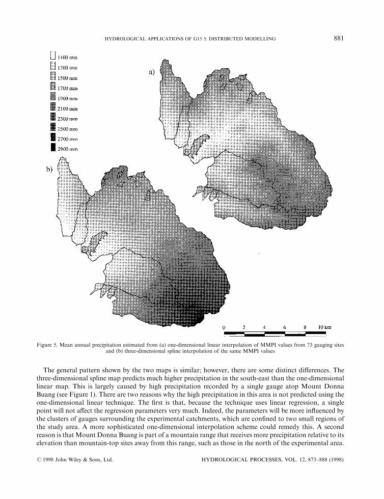
The general pattern shown by the two maps is similar; however, there are some distinct di�erences. Thethree-dimensional spline map predicts much higher precipitation in the south-east than the one-dimensionallinear map. This is largely caused by high precipitation recorded by a single gauge atop Mount DonnaBuang (see Figure 1). There are two reasons why the high precipitation in this area is not predicted using theone-dimensional linear technique. The ®rst is that, because the technique uses linear regression, a singlepoint will not a�ect the regression parameters very much. Indeed, the parameters will be more in¯uenced bythe clusters of gauges surrounding the experimental catchments, which are con®ned to two small regions ofthe study area. A more sophisticated one-dimensional interpolation scheme could remedy this. A secondreason is that Mount Donna Buang is part of a mountain range that receives more precipitation relative to itselevation than mountain-top sites away from this range, such as those in the north of the experimental area.

Figure 5. Mean annual precipitation estimated from (a) one-dimensional linear interpolation of MMPI values from 73 gauging sitesand (b) three-dimensional spline interpolation of the same MMPI values



Proximity to the mountain range represents a horizontal as well as a vertical in¯uence on precipitation whichcan not be represented by any one-dimensional interpolation.

Using the otherwise unchanged reference parameter set, Macaque was run using each of the two MMPImaps. The hydrographs produced using three-dimensional spline interpolated MMPI and one-dimensionallinear MMPI are shown in Figure 2a and 2b, respectively. The corresponding pair of maps of predictedstream ¯ow source areas are shown in Figure 3a and 3b. The hydrograph for the one-dimensional linear mapis lower and less peaky than that for the three-dimensional spline map. Mean daily ¯ow is 27% lower usingthe one-dimensional linear map (or 36% higher, vice versa). In the south-east of the study area, there is asigni®cant reduction in the proportion of hillslopes that generate stream ¯ow under the one-dimensionallinear map. These observations all relate to the lower precipitation predicted for the south east by the one-dimensional linear technique. The peakiness and excessive saturation of hillslopes predicted under the three-dimensional spline map were cited earlier as problems with the initial simulation so these observationsfavour the use of the more simple technique.

There is some uncertainty as to whether the more sophisticated mapping has resulted in improved pre-diction of stream ¯ow because predictions made under the simpler one-dimensional linear techniqueexhibited more desirable features than those made using the `improved', three-dimensional spline technique.The investigation has highlighted the sensitivity of precipitation mapping. It is important to note that thedensity of gauges available for this exercise was much greater than is usual. Nevertheless, the choice ofanalysis method greatly in¯uenced the simulated response. Future measurements will need to constrain theprediction of other elements of the water balance to the point where more can be said about the truedistribution of precipitation.

LEAF AREA INDEX MAPPING

LAI has been measured in the study area both as a result of destructive measurement, where trees arefelled and their leaves are measured, and by ground-based remote sensing using a light sensor or `LICOR'(e.g. Vertessy et al., 1994b, 1995a). Additionally, canopy species and age have been mapped in detail by theVictorian Department of Natural Resources and Environment. These data have been used to produce twomaps of total LAI (canopy plus understorey).

For the standard map, typical total LAI values were assigned to distinct forest types mapped on the basisof canopy species, as shown in Figure 6a. Spatial variability is dominated by the distribution of the threemajor forest types: mixed species (low LAI), ash (medium LAI) and rainforest (high LAI). The mean valuefor the three largest catchments is 3.78.

An alternative total LAI map was produced by combining LICOR measurements, destructive measure-ments and typical LAI values for areas of extreme LAI (both high and low) with satellite indices. FourLandsat TM images were obtained for this purpose. Each image was resampled to be geocoded in theAustralian Map Grid (AMG) with 25-metre pixels, then systematically translated in a range of directions toalign the image to the DEM by maximizing the correlation with DEM-derived theoretical shading imagesproduced using the Minnaert (1941) method. The images exhibited strong topographical shading which wascorrected separately for each of the seven bands in each image according to Colby (1991). Results from thefour images were then averaged to produce a temporal `mean' image comprised of seven bands. Maps ofvarious satellite indices were computed from the mean image, including a normalized di�erence vegetationindex (NDVI, see Barrett and Curtis, 1992) map (Band 47Band 3/Band 4 � Band 3) and an index using thesame bands based on shade corrected imagery (corrected Band 4/Band 3).

These indices were plotted against LICOR observations of LAI in order to ®nd a relationship predictingLAI from the satellite imagery. This was only partially successful because the range of measured LAI valueswas small. The corrected Band 4/corrected Band 3 image clearly distinguishes between areas of very low LAI(such as recently cleared areas) and areas of high LAI (such as 10-year old ash forest), so indices weresampled from these areas and added to the plot with typical LAI values for these forest types. A linear ®t was



constructed from these data and applied to the corrected Band 4/corrected Band 3 image to give a mappredicting total LAI, as shown in Figure 6b. The mean value for the three largest catchments is 3.77, which isvery close to the average obtained from the species-based map (3.78).

The model requires that total LAI be split into canopy and understorey components. For the ash forest,canopy LAI was estimated from forest age using an equation constructed by Watson and Vertessy (1996)from destructive measurements. Constant canopy LAI values were assigned to other forest types.Understorey LAI was then calculated as the di�erence between total and canopy values.

The average LAIs predicted by the species-based and satellite-based maps di�er by less than one per cent.Spatially, however, the two maps di�er signi®cantly. The species-based map shows large areas of uniformtotal LAI, broken only near the major boundary between ash-type and other forests (the latter occurring

Figure 6. Total LAI, (a) Estimated by assigning generally accepted values to each forest type; and (b) estimated from TMsatellite imagery



near the reservoir), and along the bands of rainforest bordering streams in high precipitation areas. Thesatellite-based map exhibits signi®cantly more spatial variability. For example, a large area of low LAI isshown in the south-east corner, coinciding with a large area of old growth ash forest. There is also variabilitythat appears to be aspect related, whereby numerous opposing north/south hillslopes have di�erent LAIs.This may be real, or it may be some residual topographic shading e�ect resulting from inadequate shadingcorrection, or it may be a combination of both. Insu�cient data are available at this stage to clarify this, sothere is uncertainty in both maps. The point here is that LAI is a vital parameter in any physical model offorest hydrology and the two maps represent equally viable, yet quite di�erent alternatives for mapping thisparameter.

Using the otherwise unchanged reference parameter set, Macaque was run using each of the two total LAImaps. The hydrographs produced using the species-based LAI map and the satellite-based LAI map areshown in Figure 2a and 2c, respectively. The corresponding pair of maps of predicted stream ¯ow sourceareas are shown in Figure 3a and 3c. There is almost no di�erence in the shape of the two hydrographs, andno di�erence in the mean daily stream ¯ow. This is because the mean LAI was virtually the same for the two.Spatial variations in LAI do not a�ect mean stream ¯ow for the study area. This suggests that evapo-transpiration as predicted by Macaque is linearly proportional to LAI and probably not limited by spatiallyvariable in¯uences such as soil moisture stress. Whilst this observation satis®es our perceptual model of ashforest behaviour, it may not be appropriate for drier, water-limited forests. There are small di�erences in themaps of stream ¯ow source areas, with the satellite based map reducing excessive hillslope saturation in drierareas. This indicates that the satellite-based map may be a better predictor of LAI, but further testing againstobserved data is needed before this assessment can be con®rmed.

TOPOGRAPHY MAPPING

Topographical data are available from two sources. The ®rst is digital contour data provided by theVictorian Division of Survey of Mapping and derived from air photographic interpretation (API). This isavailable for the entire catchment area in su�cient detail to construct a 25-metre gridded digital elevationmodel (DEM). The second source is a detailed ground survey of the Ettercon 3 experimental catchment(15 ha) (Figure 1) conducted as part of the current study, from which detailed DEMs have been produced.Watson et al. (1996) have shown that the API data describe a smoother terrain than reality, which is betterexpressed by the ground-based data. The API data are, however, the only data available for the entire studyarea and must be used as such.

The two DEMs were used to construct two separate maps of the ln(a/tanb) wetness index, which werediscretized into ESUs to provide two alternative topographic parameterization and spatial disaggregationschemes for Ettercon 3. Figure 7 shows the disaggregation into ESUs of the wetness index. The smoothrepresentation of topography by the API DEM is re¯ected in Figure 7a which shows only a limited con-vergence of high wetness areas along the stream. Figure 7b, on the other hand, shows a concentrated gullywith high wetness re¯ecting the incised topography more accurately represented by the ground surveyedDEM. This also more accurately re¯ects the shape of the ground surveyed saturated zone (during a relativelydry period) which is overlaid on both maps.

Macaque was run on each representation of Ettercon 3 with the otherwise unchanged reference parameterset. The resulting hydrographs are shown in Figure 8, and the predicted stream ¯ow source areas are shownin Figure 9. The two predicted hydrographs are almost identical and are reasonably accurate in both shapeand mean value. Neither hydrograph predicts the e�ects of the drought in the summer of 1982±1983 verywell, and both hydrographs are too variable during the high ¯ow period at the end of 1984. The fact that sucha marked di�erence in the two DEMs used to produce these hydrographs does not induce a di�erence in thehydrographs is perhaps surprising. The maps of runo� source area, however, are quite di�erent. Fieldobservations indicate that Figure 9a is an unrealistic simulation of the runo� producing area. The smoothingof terrain apparent in the API-derived map clearly spreads out the saturated area too much. Despite this



Figure 8. Predicted and observed weekly hydrographs for the Ettercon 3 experimental catchment for the period 1982±1984; (a) Usingthe API DEM; and (b) using the ground surveyed DEM

Figure 7. ESUs calculated from the a/tanb wetness index for the Ettercon 3 experimental catchment calculated from (a) the API DEM;and (b) the ground surveyed DEM. Both maps are overlaid with ground surveyed stream lines and saturated area boundaries (during a

relatively dry period)



spreading of the saturated area, it is clear from the hydrograph response that the e�ective evapotranspirationis una�ected by this spatial smoothing. It appears that whilst the maps of wetness index di�er, the statisticalrepresentation of topography that the two DEMs e�ect within the distribution function is almost the samefrom a hydrological point of view. This indicates that there would be little bene®t from obtaining moredetailed topographic data over the whole catchment because the structure of the distribution function modelis unable to exploit the greater detail.

DISCUSSION

In applying LSSMs, the user is faced with a myriad of questions regarding the way in which spatialinformation is to be used. In the case of data such as precipitation, point information must be interpolatedwhilst variables such as LAI must be derived from surrogate measures such as forest type or electromagneticre¯ectance. The way in which the modeller chooses to use the information has important implications formodel response. There is always great uncertainty regarding the true nature of spatially variable inputs and itis not always the case that apparently more sophisticated analytical approaches yield more certain results.

The three-dimensional interpolation of precipitation was strongly in¯uenced by data from a particulargauge so it was impossible to say whether the resulting rainfall distribution was a more realistic representa-tion or simply an artefact of an unrepresentative gauge.

Similar uncertainty existed in the estimation of LAI, a parameter to which models of forested areas arehighly sensitive. Fortunately, the mean LAI estimates by the two methods were similar so overall runo� wassimilar, but there were large spatial di�erences in LAI representation. The spatial variability of the satellite-derived data gave a more realistic looking spatial runo� response but there are no direct data to con®rm thisobservation. Ultimately, the user must simply accept that by choosing a particular method of representation,a certain spatial variability of response is `locked in'.

It must also be accepted that di�erent model structures can be limited in the extent to which they canexploit more detailed information. In the example given above, more detailed topographic data of a smallsubcatchment gave a clearly more realistic estimate of runo� producing area yet, even at this small scale, theimpact on the hydrograph was not detectable. This was because the representation of processes (especiallyevapotranspiration) within the model structure makes little distinction between saturated and almostsaturated soil. There would be no point in trying to obtain such detailed topographic data for the entire area.

Figure 9. Mean daily stream ¯ow source areas for the Ettercon 3 experimental catchment in 1984 using (a) the API DEM and (b) theground surveyed DEM



Model users must consider carefully whether the model they are using is able to exploit more detailedinformation.

Ultimately, the choice of spatial detail depends on the user's ability to assess whether the simulatedresponse is a better representation of reality. This can be both a quantitative and a qualitative assessment andshould consider not only whether the speci®c variable of interest is better represented but also whether thesimulated response of interest is a�ected. If the former is true but the latter is not, there may still be no valuein greater spatial detail since the model structure is unable to use the higher level of information.

ACKNOWLEDGEMENTS

We thank: Richard Silberstein, Larry Band, Scott Mackay, Richard Lammers, Richard Fernandes,Rob Lamb and Keith Beven for ideas and advice on modelling; Richard Campbell, Sharon O'Sullivan,Sharon Davis, Campbell Pfei�er, Judi Buckmaster and Andrew Western (all from Melbourne or MonashUniversities, Melbourne, Australia) for providing unpublished data on water tables, soil hydraulic conduct-ivity, transpiration, LAI and radiation; Petina Pert and Jill Smith of the Victorian Department of NaturalResources and Environment for supplying digital forest type data; and two reviewers for their helpfulcomments.

REFERENCES

Band, L. E., Patterson, P., Nemani, R., and Running, S. 1993. `Forest ecosystem processes at the watershed scale: incorporatinghillslope hydrology'. Agric. For. Meteorol., 63, 93±126.

Barrett, E. C. and Curtis, L. F. 1992. Introduction to Environmental Remote Sensing, (3rd edn). Chapman & Hall, London. 426 pp.Beven, K. J., Lamb, R., Quinn, P., Romanowicz, R., and Freer, J. 1994. `TOPMODEL', in Singh, V.P. (ed.), Computer Models of

Watershed Hydrology. Water Resources Publications, Highlands Ranch, Colorado. pp. 627±668.Colby, J. D. 1991. `Topographic normalisation in rugged terrain', Photogramm. Engng Remote Sens., 57, 531±537.Connor, D. J., Legge, N. J., and Turner, N. C. 1977. `Water relations of Mountain Ash (Eucalyptus regnans F. Muell.) forests', Aust. J.

Plant Physiol., 4, 753±762.Duncan, H. P. and Langford, K. J. 1977. `Stream ¯ow characteristics', in Langford, K. J. and O'Shaughnessy, P. J. (eds), First Progress

Report Ð North Maroondah, Rep. No.MMBW-W-0005. Water Supply Catchment Hydrology Research, Melbourne andMetropolitan Board of Works. pp. 215±229.

Finlayson, B. L. and Wong, N. R. 1982. `Storm runo� and water quality in an undisturbed forested catchment in Victoria', Aust. For.Res., 12, 303±315.

Hatton, T., Dyce, P., Zhang, L., and Dawes, W. 1995. `WAVES Ð an ecohydrological model of the surface energy and water balance:sensitivity analysis'. Tech. Memo. 95.2. CSIRO, Institute of Natural Resources and Environment, Division of Water Resources,Canberra.

Hutchinson, M. F. 1995. Ìnterpolating mean rainfall using thin plate splines'. Int. J. Geograph. Inform. Syst., 9, 385±403.Kuczera, G. A. 1987. `Prediction of water yield reductions following a bush®re in ash-mixed species eucalypt forest', J. Hydrol., 94,

215±236.Lammers, R. B. and Band, L. E. 1990. Àutomating object representation of drainage basins', Comp. Geosci., 16, 787±810.Langford, K. J. 1976. `Change in yield of water following a bush®re in a forest of Eucalyptus regnans', J. Hydrol., 29, 87±114.Minnaert, M. 1941. `The reciprocity principle in lunar photometry'. The Astrophys. J., 93, 403±410.Mitasova, H. and Ho®erka, L. 1993. Ìnterpolation by regularized spline with tension: II. Application to terrain modeling and surface

geometry analysis'. Math. Geol., 25, 657±669.Quinn, P. F., Beven, K. J., and Lamb, R. 1995. `The ln (a/tan b) index: how to calculate it and how to use it within the TOPMODEL

framework', Hydrol. Process., 9, 161±182.Silberstein, R. P. and Sivapalan, M. 1995. Èstimation of terrestrial water and energy balances over heterogeneous catchments',

Hydrol. Process., 9, 613±630.Vertessy, R. A., Hatton, T. J., O'Shaughnessy, P. J., Jayasuriya, M. D. A. 1993. `Predicting water yield from a mountain ash forest

catchment using a terrain analysis based catchment model'. J. Hydrol., 150, 665±700.Vertessy, R. A., Benyon, R., and Haydon, S. 1994a. `Melbourne's forest catchments: E�ect of age on water yield', Water, J. Aust. Wat.

Wastewat. Ass., 21, 17±20.Vertessy, R. A., Benyon, R. G., O'Sullivan, S. K., and Gribben, P. R. 1994b. `Leaf area and tree water use in a 15 year old mountain ash

forest, Central Highlands, Victoria', Report No. 94/3. Cooperative Research Centre for Catchment Hydrology, Monash University,Clayton, Victoria, Australia. 31 pp.

Vertessy, R. A., Benyon, R. G., O'Sullivan, S. K., and Gribben, P. R. 1995a. `Relationships between stem diameter, sapwood area, leafarea and transpiration in a young mountain ash forest', Tree Physiol., 15, 559±567.

Vertessy, R. A., Hatton, T. J., Benyon, R. J., and Dawes, W. R. 1995b. `Long term growth and water balance predictions for amountain ash (Eucalyptus regnans) forest catchment subject to clearfelling and regeneration', Tree Physiol., 16, 221±232.



Watson, F. G. R. 1997. `Physically based prediction of water yield from large forested catchments: integrated hydro-ecologicalmodelling of the Maroondah Catchments, Victoria', PhD Thesis. Department of Civil and Environmental Engineering, MelbourneUniversity, Melbourne.

Watson, F. G. R. and Vertessy, R. A. 1996. `Estimating leaf area index from stem diameter measurements in Mountain Ash forest',Report 96/7. Cooperative Research Centre for Catchment Hydrology, Monash University, Clayton, Victoria, Australia. 102 pp.

Watson, F. G. R., Vertessy, R. A., and Band, L. E. 1996. `Distributed parameterization of a large scale water balance model for anAustralian forested region', HydroGIS 96: Application of Geographic Information Systems in Hydrology and Water ResourcesManagement, Proceedings of the Vienna Conference, April, 1996, IAHS Publ., 235, 157±166.

Watson, F. G. R., Vertessy, R. A., and Grayson, R. B. 1997. `Large scale, long term, physically based prediction of water yield inforested catchments', pages 397±402 of proceedings, International Congress on Modelling and Simulation (MODSIM '97), Hobart,Tasmania, 8±11 December, 1997.



Figure 3. Mean daily stream ¯ow source areas for 1984. (a) Using the reference parameter set; (b) with MAP estimated usingone-dimensional linear instead of three-dimensional spline interpolation; and (c) with total LAI estimated from TM imagery instead of

forest type


Large-scale distribution modelling and the utility of detailed ground data

Documents

Transcript of Large-scale distribution modelling and the utility of detailed ground data