Labour Supply Effects of Conditional Transfers: Analyzing the Dominican Republic's Solidarity...

LABOUR SUPPLY EFFECTS OF CONDITIONAL TRANSFERS: ANALYZING THE DOMINICAN REPUBLIC’S SOLIDARITY PROGRAM

Gustavo Canavire Bacarreza

Harold Vásquez-Ruiz

No. 13‐08

2013

Labour Supply Effects of Conditional Transfers:Analyzing the Dominican Republic’s Solidarity

Program∗

Gustavo Canavire-Bacarreza†and Harold Vasquez-Ruiz‡

April 12, 2013

Abstract

This paper studies the impact of the conditional cash transfer programSolidaridad on changes in the labor market of the Dominican Republicbased on statistical data from the Evaluation of the Social Security Sur-vey 2010. The estimation methodology is based on matching techniques,which can discern the impact on both benenefit-receiving and non-benefit-receiving households. The results show a negative but very small impactof the different components of the program on labor market indicators,especially for the components related to children. However, the estimatesshow some heterogeneity in the effects on the most vulnerable sectors ofthe population.

Key terms: Social Programs, Solidaridad, Labor Market, ConditionalCash Transfers

JEL Classiffcation : H31, J08, J58

∗Funding for this study comes from the Inter-American Development Bank (IDB) underthe program CONOCER+. The opinions expressed here do not represent the views of thisinstitution nor the institutions where the authors are affi liated. We would like to thankto Fernando Rios, Martin Posada and Rafael Rivas for their research assistance. Also, wealso thank Fernando Rios, Antonio Morillo and Ramon Espinel for helpful comments andsuggestions.†EAFIT University, Medellin, Colombia and IZA, Germany‡Central Bank of the Dominican Republic and Technological Institute of Santo Domingo.

1

1 Introduction

The policy of redistribution of resources through conditional cash transfers (CCT) has

become one of the most important tools used by governments to reduce levels of poverty

and improve citizens’ quality of life. Currently, these programs have been implemented in a

variety of countries that range from the poorest and developing (e.g., Bolivia, Bangladesh,

Nigeria, etc.) to more developed countries (e.g., Japan and USA).1

Cash transfers are based on the contribution of cash to households that meet a number

of previously stipulated objectives for investment in the human capital of the recipients’

children to achieve health and education goals. The establishment of these goals not only

assumes that households do not have enough resources to invest the ”optimum” level

in human capital based on social and political parameters but also assumes that these

households may underestimate returns on investment in education. In the case of the

Dominican Republic, for example, Jensen (2010) estimates that the perception of eighth

graders on the return on investment in education is approximately one quarter of the rate

of return derived from an income survey.2

One of the main issues to be discussed when CCT programs are implemented is their

potential impact on the labor supply of adults. From a theoretical point of view, the

impact of these programs can be diverse. For example, if we consider leisure as a normal

good, the effect of transfer programs can be negative in terms of employment because an

increase in the income of individuals via cash transfers could increase the consumption of

leisure and reduce the labor supply. Additionally, workers may choose to reduce their labor

supply to qualify for benefits, or individuals may demonstrate less availability for work.

However, for those groups who are outside the labor market and for whom consumption

of leisure relative to labor is high, the impact could result in greater efforts in the job

search. Because individual preferences are crucial in this process, conclusions about the

1In the case of Japan, the aid programs for secondary education stand out. In the United States, thecash transfer programs of New York City and Washington D.C. have been remarkable.

2Another way that parents may underestimate the return on the education of their children is whenthey discount the future with a higher weighted rate than they should.

impact of CCT on labor supply can only be determined empirically (Rosen, 2009).

Our investigation uses statistical information from the Dominican Republic’s Eval-

uation of Social Security Survey 2010 to study the impact of the Solidaridad program

on household behavior as measured through changes in labor force participation, income

and informality. For this purpose, quasi-experimental methods are used as pared esti-

mates (matching) that may help identify impacts on benefit-receiving households and

non-beneficiaries. The contributions of this study will be useful not only for public policy

in the Dominican Republic for defining the effect on labor markets (positive or negative)

of the Solidaridad program, but it will also add new material to the existing literature in

terms of the evaluation of the impact of such programs on informality.

From an empirical perspective, the issue has been addressed extensively in developed

and medium-developed countries, and conclusions on the effects of CCT programs depend

on the characteristics of each program and the incentives that participants receive. For

example, Saez (2002) finds that cash transfer programs in the United States reduce the

intensity of work of employees but increase the level of labor force participation of the

unemployed. Similarly, Keane and Moffitt (1998) demonstrate that individuals who si-

multaneously participate in multiple transfer programs do not reduce their labor supply.

However, these results differ from studies on the effects of unconditional transfer pro-

grams, where there is a significant reduction in the labor force participation of enrollees

(Moffitt, 2002; Tabor, 2002).

In the case of Latin America, a number of studies have examined the effect of con-

ditional transfers on labor market, poverty, health, education and food indicators. In

general, there are significant positive relationship between participation in transfer pro-

grams, the increase in labor supply and improved incomes (Fizbein and Schady, 2009;

L. Alzua and Ripani, 2009). For example, CCT recipient households did not reduce in

any way the labor supply in the case of Ecuador and Mexico. However, there is a sig-

nificant reduction in the child labor supply, especially in Brazil, Ecuador, Mexico and

Nicaragua (Cecchini and Madariaga, 2011). Moreover, it is estimated that the Red de

Proteccion Social program in Nicaragua has caused a decrease in poverty levels between

five and nine points in the count rates and poverty gap. In Honduras, there is only a

slight increase in consumption for households that receive conditional transfers compared

to similar households that do not receive them, which is an expected result given the

small size of the transfers.3

Some studies link the decisions of individuals to choose a type of employment (e.g.,

formal or informal) to the availability of additional income and/or funding from other

sources. For example, in a recent report published by the World Bank (2005), the in-

crease in micro-enterprise is attributed to the growth of remittances and the tourism

sector. Dependence on external sources for these resources combined with the unfavor-

able international economic environment of recent years makes the informal-sector workers

a very vulnerable segment of the Dominican population.4

Other studies focus on how economic growth and business cycles affect the employment

level (OIT, 1975; Garcıa and Valdivia, 1985). In general, these studies indicate that

although the Dominican economy has been characterized by strong GDP growth compared

to other countries in the region, this growth has not manifested in a significant decrease

in the unemployment level. However, the low response of unemployment to changes

in the business cycle may be explained by the size and divergence of the definition of

unemployment as well as by problems in its measurement (Gregory, 1997; Marquez, 1998).

In general, studies devoted to the analysis of the Dominican labor market have been

characterized by a lack of technical rigor because they are based on descriptions of statis-

tical information from sources that are sometimes not comparable. In turn, the lack of a

systematic construction of economic indicators related to the labor market has led most

3In terms of health and education, CCTs have significantly increased school enrollment and atten-dance in both Latin American middle-income countries such as Chile (7.5%), Colombia (2.1%) and Mexico(1.9%), and lower income countries such as Honduras (3.3%), Nicaragua (6.6%) and Ecuador (10.3%).However, despite the fact that CCT programs have a significantly positive impact on school attendancelevels, these programs do not seem to influence school performance test results or learning levels. Fur-thermore, the effect of the programs on the use of preventive health services is not very clear (Fizbeinand Schady, 2009).

4For an analysis of the importance of micro-enterprises in the creation of jobs in the DominicanRepublic and the role that women have played in this sector, see Cabal (1993).

studies to focus on the analysis of surveys; the Labor Force Survey of the Central Bank

is one of the most consulted sources (Sanchez-Fung, 2000).

Recently, with the financial aid of international organizations, the establishment of new

assistance and training programs has allowed a more rigorous analysis of the Dominican

labor market. For example, Card et al. (2011) analyze the impact on employment gener-

ation of the Juventud y Empleo Program (2001-2006), which provides training and skills

development for young people age 18 to 29. Using a random sample of applicants to the

program, the authors find little evidence that participation in training programs affects

the employment status (employed or unemployed) of individuals participating in the pro-

gram, although they do encounter evidence of a slight increase in participants’ levels of

income (10). 5

Finally, conditional transfer programs have experienced a major peak in Latin America

since the mid-1990s, from only 3 countries in 1997 to 18 countries in 2010 (see Table 8

in the Appendix). The impact of these programs has been quantified. These programs

have not only achieved significant impacts in reducing poverty and on social inequality

indicators but are also considered instruments that are founded on beliefs in extensive

social protection and universal notions of rights (Cecchini and Martınez, 2011). Therefore,

the importance of these programs for the target population lies in the fact that they can

still be used as tools for social policy in the region. It is to this aspect that this study

aims to make a contribution.

2 Estimation Methodology

The methodology proposed to conduct the research is the impact evaluation method-

ology based on the propensity score matching technique developed by Rosenbaum and

Rubin (1983). The analysis focuses on the full sample to determine the program’s impact

on the behavior of beneficiary households, measured by labor force participation, wages

5The Juventud y Empleo Program was developed and implemented by the Dominican governmentwith financial assistance from the Inter-American Development Bank (IDB).

and informality through the propensity score matching technique and the estimation of

differences in average effect on treatment of the treated (ATT), described below.

2.1 Propensity Score Matching an Differences of the ATT

To evaluate the program’s impact on the labor market, it is necessary to consider two

aspects: (i) the impossibility of knowing what would have been the participants’ behavior

(or result, called Y ) if they had not participated in the program - what is called the coun-

terfactual state, and (ii) the possibility that participant and non-participant households

differ systematically, i.e., there are intrinsic characteristics of each household group.

The first of these issues is important because, if in addition to information on the

results of households that participate in the program it was also known what the results

would be if they did not participate, it would only be necessary to calculate the difference

between the result “with participation” (Y 1) and the result “with no participation” (Y 0).

The second issue refers to the distribution of households participating, which is not purely

random. If the results obtained by the participating households are only compared with

non-participants, the differences might mistakenly be attributed to the results of partici-

pation, when in fact the differences are due to observable characteristics inherent to each

group (socioeconomic status, for example).

The propensity score matching methodology allows us to manage both issues by pair-

ing the receiving and not-receiving households that have similar observable characteris-

tics. According to this methodology, “participation” can be treated as a “treatment” in

which some households participate and others do not. Participating households make the

“treatment group” and not-participating households constitute the “control group”. The

important issue is that the households in both groups have similar, observable character-

istics. Thus, we can estimate the average effect of treatment on the treated (ATT) by

finding the average of the difference between the results from households in the ”treat-

ment group” and the results from households in the ”control group”, which represents the

counterfactual state. Formally:

Let Pi be an indicator of participation, which takes the value of 1 if the household

participates and 0 otherwise, and let Y 1i be the result (household behavior) conditioned

by its participation (Pi = 1) and Y 0i be the result conditioned by its non-participation

(Pi = 0).

Then, the average effect of treatment on the treated is given by:

ATT = E(Y 1i − Y 0

i |Pi = 1) = E[Y 1i |Pi = 1]− E[Y 0

i |Pi = 1] (1)

Equation 1 shows the difference between the current situations of households that

participated compared with what their situation would have been if they had not partic-

ipated. The first term, E[Y 1i |Pi = 1], is fully observable because it represents the results

given household participation. The second term, E[Y 0i |Pi = 1] presents a problem because

when the household participates (Pi = 1), Y 1i is the variable that can be observed. Fur-

thermore, with the information provided by non-participating households, E[Y 0i |Pi = 0]

can be obtained, so the equation ATT cannot be solved with data observed in the same

household.

The solution proposed through the matching methodology is based on the assump-

tion that, given a set of observable characteristics X, the potential outcomes (when not

participating) are independent of the state of participation (conditional independence as-

sumption, CIA): Y 0i ⊥Pi|X. Therefore, after controlling for observable differences, the

average potential outcome is the same for P = 1 and P = 0, that is, E[Y 0i |P = 1, X] =

E[Y 0i |P = 0, X]. This enables the use of a control group. 6

Instead of matching based on X, Rosenbaum and Rubin (1983) suggest using the

household propensity to participate to reduce the dimensionality of the problem. This

propensity, which can be influenced by a large number of factors, is reduced to a scalar

p(X) called ”propensity score, PS”. In formal terms, the PS is defined as the conditional

probability of participating given a group of individual characteristics (X = xi) for each

6Authors quote no. 3 in text.

household:

p(x)≡Pr(Pi = 1|X = xi) (2)

After calculating the PS using a probabilistic model, various methods can be used to

estimate the average effect of treatment on the treated, including:

• Nearest Neighbor Matching: This method carries out the matching by looking

in each of the treated units for a unit in the control group whose PS is closest. That

is, the j untreated unit is chosen to be the control group (C(pi)) of the i treated

unit to minimize the difference between PS:

C(i) = minj[|Pi − Pj|] (3)

• Radius Matching: This method uses all control units within a predefined radius

of the PS, which is an advantage because it allows a larger number of control units

in case there is not an appropriate match. The equation indicates that the treated

unit i is matched to the control unit j such that:

δ > |pi − pj| = mink∈{D=0}|pi − pk| (4)

where δ > 0 is a specified radius. 7.

• Kernel Matching: This methodology matches the benefit-receiving households

with a weighted average of the control households that are closest, with weights

that are inversely proportional to the distance between the propensity scores of the

treated and the control groups. The weighted average is calculated as follows:

Wij = Kij

p∑j=1

Kij (5)

where:

Kij =K[(P (Xi)− P (Xj))/aN0]∑pj=1K[(P (Xi)− P (Xj))/aN0]

7For more details, see ?.

where aN0 is a band or smoothing parameter and K(·) is the kernel function of the

difference between the PS of the participants and of the control group. 8.

To quantify the impact of participation in the program on labor market outcomes, we

use the estimate of the difference of the ATT , which can be used to compare the situations

of participating and not-participating households.

Let t be the period after the receipt of remittances and t′ be the period before remit-

tances; the estimation of the difference of the ATT is given by:

E(Y 1it − Y 0

it |Pi = 1, X)− E(Y 0it − Y 0

it |Pi = 0, X) (6)

This indicator compares the results of the treatment group and the control group

(first difference) before and after treatment (second difference), eliminating unobservable

constant effects over time.

3 Data and Information from the Survey

In 2004, the Dominican Republic implemented the Solidaridad program to raise the human

capital (health and education) of families living in poverty. This program provides cash

assistance, subject to compliance by the participants with certain requirements, and aims

to address problems related to poor levels of education, malnutrition and infant mortality,

among others. Participants in this program are subject to strict monitoring control to

ensure that they continue to meet the requirements that give them access to benefits.

The Solidaridad program consists of two main components: (i) a health component and

(ii) an education component.

The health component aims to address issues of family health problems, malnutrition

and infant mortality, among others, through food and nutritional education and interven-

tions focused on children from poor families. In the program, households must follow a

series of specific protocols (e.g., vaccination plans for children, periodic checks for pregnant

8Idem

women, etc.) to obtain the transfer called ”Comer es Primero”. This transfer grants the

household RD$700 pesos ($18 U.S. dollars) per month to heads of households in extreme

and moderate poverty; the money must be used exclusively for the purchase of food.

The education component, or School Attendance Incentive (ILAE), consists of an in-

kind transfer to beneficiary households with children between the ages of six and sixteen

who are enrolled in basic education between first and eighth grade. Such transfers can

only be used to purchase school supplies, books, uniforms and medicine. The amount

transferred depends on the number of eligible children in the home and is set according

to the following scale:

• Households with one or two elegible children = RD$300.00

• Households with three elegible children = RD$450.00

• Households with four or more elegible children = RD$600.00

In 2010, the Inter-American Development Bank, in alliance with the Office of Social

Policy Coordination (GASO) and the Central Bank of the Dominican Republic, made

available to the public the new Evaluation of Social Security survey (EEPS), which cov-

ered 2,796 households, of which 52% were beneficiaries of charitable programs. This

instrument collects the socioeconomic characteristics of the interviewed households and a

significant number of other indicators for evaluation of the impact of social programs on

the Dominican labor market.

3.1 Labor Market and Income Cycle

The evolution of the labor market indicators and in particular the levels of employment

and real income closely reflect the behavior of the Dominican economic cycle. For example,

in 2000, approximately 486,000 workers (13.9% of the labor force) were unemployed. By

October 2004, after the financial crisis, the number of unemployed individuals exceeded

796,000, a figure that took the unemployment rate to the highest level of the decade

(19.7%). By 2011, after a period of significant economic recovery, the unemployment rate

stood at 14.6%.

As could be predicted, income figures underwent the reverse behavior in comparison to

the unemployment rate: when labor supply is high (many unemployed workers), income

falls. In the 2000-2004 period, the real hourly income of workers was reduced by almost

40% (especially in the crisis years 2003-2004). Real incomes recovered in subsequent

years. However, in 2010, real incomes were still approximately 20% below their levels at

the beginning of the decade.

As for the distribution of the Dominican labor force among the productive sectors,

we can say that it has changed significantly over the past five decades. The agricultural

sector has lost importance in job creation by reducing the percentage of individuals in the

employed labor force from 73% in 1960 to less than 35% by the end of the 1980s. Since

1990, the Dominican economy has acquired a model of employment generation oriented

to a service economy (e.g., tourism, trade and public administration).

One of the main characteristics of the Dominican labor market is its concentration

in the informal sector. In the last decade, the share of informal workers has fluctuated

approximately 54%, significantly increasing to 56.6% by the end of 2011. However, the

large number of workers in this sector only indicates ”the existence of a large proportion

of small productive units” (Guzman, 2011) because, contrary to popular opinion, the

definition of informality does not necessarily relate to aspects of precariousness or illegality.

In the case of the Dominican Republic, the National Workforce Survey defines informal

workers as those employees working in businesses with less than five employees as well

as unpaid workers, the self-employed, domestic service workers and bosses belonging to

non-industrial economic sectors. 9

9These bosses are in the following occupational groups: farming, operators and drivers, artisans andlaborers, merchants, salesmen and unskilled workers.

4 Estimates and Results

One of the main problems with conditional transfer programs is their potential to affect

the labor market through labor supply disincentives. For example, a conditional cash

transfer program can affect a household’s budget constraints, allowing the substitution

of leisure for work while still consuming the same basket of goods. Consequently, the

benefits received from transfers can potentially generate incentives to reduce labor market

participation and affect wages. Additionally, potential program enrollees could adjust

their participation in the workforce and become inactive in their job searches.

Given the characteristics of the survey and to fully exploit its information, we choose

the individual as the unit of analysis. To isolate the effect of the Solidaridad program

on the Dominican Republic’s labor market, households with at least one member par-

ticipating in the program are assigned to the treatment group. This strategy allows us

to identify the direct effects of the program on households and on individuals; the logic

behind this estimate is that the behavior of individuals is a function of the household’s

behavior.

Although the survey does not allow the identification of a baseline period, its design

does allow the generation of a control group. In fact, the survey takes a representative

selection of beneficiary households identified as the intervention group and matches it

with a set of households with similar conditions that for administrative reasons have

not been incorporated into the program. While this strategy can correct the potential

contamination of the control group, we additionally compile a set of structural variables

(covariates) that simultaneously affect the implementation of the program (treatment)

and are variables that affect labor market indicators (outcomes), as the literature has

proven. These structural variables seek to correct biases that may exist. In the absence

of a baseline, it is plausible that the selected variables are relatively stable over time and

are not directly affected by the program. These variables are used in the analysis to

control the observable differences among individuals who are affected by the Solidaridad

program and those who are not, thus isolating the impact of transfers. Control variables

are placed into three groups that capture demographic, human capital and household

characteristics. For demographic controls, we include gender (dummy = 1 if female),

age and age squared. For human capital variables, we include years of education (and

its square) and a dummy to indicate whether the participant can read and/or write.

We also determine the interaction between age and education. Finally, for household

characteristics, we include whether the individual is the head of the household, whether

he/she is married, the household size (number of people), the number of adults of working

age (age 18-64) and the number of seniors (age 65 or more). We also include as controls

the number of infants in the household (age 0-5) and the number of school age children

(age 6-16). Because the presence of children affects women’s decisions to work or look

for work, the interaction between ”number of infants” and the woman dummy variable is

included.

Outcome variables for the labor market are evaluated by taking into account three

main components. First, the probability of finding a job is defined as a dummy variable

that takes the value of 1 if the person is working and 0 if unemployed. This variable

measures the effect of the programs on the possibility that participants are working.

Because the programs do not directly affect the creation of new jobs, the impact of this

variable is expected to be minimal. Because the definition of wage employment includes

the self-employed, it is possible that many of the observed effects are generated through

this channel. The second outcome variable is the probability of entering the labor market

from inactivity, which is defined using a dummy with value 1 if the individual is employed

or unemployed, and 0 if the individual is inactive. This variable is intended to directly

capture the effects of the program.

Although there are different methods of propensity score matching to choose from,

our specification is based on the method with the best balance for our control variables.

Therefore, we use the nearest-neighbor methodology (in terms of the distribution of the

control variables) because it provides the best balance and is more likely to satisfy the

CIA. This estimate allows replacement (which generally reduces bias but could increase

the variance (Imbens and Wooldridge, 2009; Dehejia and Wahba, 2002)) during the stop.

Additionally, we estimate robust standard errors following Abadie and Imbens (2006).

Our specification seeks to find individuals unaffected by the program who are observably

similar to individuals affected by it, isolating only the remaining variation between the

treatments related to the program. This method allows the use of an ATT estimator

that is as unbiased as possible. An important feature of our matching estimator is its

transparency because it allows the identification of average labor market outcomes through

different programs.

4.1 Main Results

Table 1 presents the descriptive statistics from the sample; these statistics are close to

those that represent the official Dominican Republic statistics. While the Solidaridad

program components do not cover the entire universe of potential beneficiaries, programs

such as CEP and Bono Gas reach more than half of the population. Within the sample,

we observe parameters that complement those in the Dominican Republic and are similar

to those in the Latin American region. About half of the sample is female (49%), which

follows the official statistics. The level of literacy of the sample reaches 82%, the average

age is 33 years, the average household size is 4-5 members and approximately 13% of the

sample experience extreme poverty. While the extreme poverty indicator is higher than

expected, the result is justified by the sample and the program objectives.

Following Imbens and Abadie (2006) and Canavire-Bacarreza and Hanauer (2012), the

main criterion for the choice of the best estimator is the balance between the control group

and the treatment group. Table 2 presents the results of balance between the groups for

the preferred estimator (Kernel matching). The differences between the treatment group

and the control group in the structural variables are not significant.

Table 3 presents the main results of the matching. In general, the results show het-

erogeneous effects on the labor market of the various Solidaridad program components.

Table 1: Descriptive Statistics

Observ. Media Desv. Est. Min Max

CEP 9963 0.5217 0.4996 0.00 1.00ILAES 9963 0.1933 0.3949 0.00 1.00Bono Gas 9963 0.7142 0.4518 0.00 1.00Female 9963 0.4915 0.5000 0.00 1.00Literate 9963 0.8287 0.3768 0.00 1.00Age 9963 33.6590 21.7703 6.00 99.00Age2 9963 16.0683 18.6547 0.36 98.01Schooling 9963 5.6918 4.1551 0.00 19.00Schooling2 9963 49.6590 55.2134 0.00 361.00Schooling X Age 9963 170.4910 158.4612 0.00 1216.00Head of Household 9963 0.2764 0.4473 0.00 1.00Hosehold Size 9963 4.8498 1.9455 1.00 10.00# Adults 18-65 9963 2.4828 1.3160 0.00 8.00# Adults 65+ 9963 0.3861 0.6577 0.00 4.00Married 9963 0.3581 0.4795 0.00 1.00# Children 0-5 9963 0.4162 0.6969 0.00 4.00# Children 6-15 9963 1.2916 1.2071 0.00 4.00Female x # Child 0-5 9963 0.2222 0.5551 0.00 4.00Extreme Poverty 9963 0.1607 0.3673 0.00 1.00

Note. Data obtained by the authors from the survey.

In general, the implementation of the program has slightly negative effects (although re-

duced) on the labor market, which suggests that although there is an income effect of the

program, it tends to be small in terms of the labor market.

The programs focused on children, such as Comer es Primero and the school attendance

incentive program, have negative (although small) effects on earnings and participation

in the labor force. Given the size of the Solidaridad program effects on labor market

outcomes, it is possible to argue that the program has not had a significant impact in

terms of reduction in the labor supply. These results are in line with those found in

other studies (Ribas and Soares, 2011; Borraz and Gonzales, 2009; Rodriguez and Freije,

2011). However, our results differ significantly in that we find a small, positive effect of

labor force participation from the program. This fact leads us to carefully analyze the

heterogeneous effects that the program may have.

The results of the program components that are targeted directly to households, such

as Bono Gas, show the same trend as the programs aimed at children. The results

show positive (but not significant) effects on income, and negative and small effects on

participation in the labor market and individuals’ desire to work (job search).

4.2 Robustness and Heterogeneity of the Effects

Next, we check the robustness of our main estimator. First, we evaluate the sensitivity

of the estimator to unobserved heterogeneity between households that received treatment

and those that did not receive treatment by applying Rosenbaum bands. The aim of

this strategy is to identify how much the selected groups should differ (treatment and

control) to cancel the results in terms of the labor market. Second, we evaluate the

robustness of our estimators to changes in the control group by using placebo groups that

seek to imitate the treatment group. Additionally, one of the main questions to assess the

impact of conditional cash transfer policies on the labor market lies in the heterogeneity

of the effects across different groups (although this question goes beyond the scope of this

document, it can provide insight into the different effects that may exist). We review the

effects through different cohorts of age, sex and geographic area.

4.2.1 Internal Robustness of the Matching Specification

In any observational study, the ability to remove the bias associated with nonrandom se-

lection is limited by the understanding of the underlying selection process (Meyer, 1995).

The selection process should be analyzed from factors that can be observed and obtained.

If the selection and results processes are systematically determined only through observ-

able characteristics (that are controlled), then the treatment effect obtained through a

matching estimate that provides the right balance will be unbiased and consistent. How-

ever, if there are unobservable characteristics that are uncorrelated with observable char-

acteristics that can be controlled but also contribute to the selection and results, then the

estimates may be biased. The survey provides sufficient structural factors that control

the unobserved heterogeneity bias. However, we evaluate the sensitivity of our estimators

to unobserved heterogeneity or bias using Rosenbaum bands (Rosenbaum, 2002).

Sensitivity analysis of Rosenbaum bands measures the level of unobserved heterogene-

ity necessary to undermine the results of the matching process. If a large (small) amount

of heterogeneity is necessary to weaken the significance of the results, then the results

are relatively robust (sensitive). Table 9 in the Appendix indicates that the level of un-

observed heterogeneity (not considered) that would nullify the results is 10%. In other

words, the results are robust regarding potential unobserved heterogeneity.

4.2.2 External robustness of the matching specification through placebo anal-ysis

In our main specification, as well as in the heterogeneity analysis, we show that the Sol-

idaridad program generally has a negative effect (although small) on the labor market.

However, it may be that this result is a consequence of our inability to select a control

group that reflects the treatment group closely enough. To evaluate this potential prob-

lem, we apply a placebo analysis. The objective of this analysis is to evaluate whether our

set of variables (covariates) behaves appropriately to the construction of a counterfactual

for households that are similar (in mean) but do not receive treatment. In other words,

the placebo analysis evaluates whether the differences are due to other factors outside

the program. If the program was the only remaining source of variation across the treat-

ments, then we should not observe a significant difference between the placebo group and

the other controls. In this sense, the placebo is evaluated with two different strategies.

First, we generate two different control groups that are contrasted with the treatment

group. Second, we select a placebo group (within the control group) that is similar to the

originally treated group and we run the same specification, assigning the placebo group as

treated, in a procedure similar to the main analysis. This group is similar to the treated

group with the exception that the Solidaridad program did not affect the placebo group.

Consequently, if the variables capture the labor market trajectories correctly, we should

not observe significant differences between the groups. The results in Table 10 of the

Appendix show the different placebo strategies and demonstrate that there is no placebo

effect in the estimates. In other words, our set of variables seems to predict the trajectory

of labor market results relatively well.

4.2.3 Heterogeneity of the results

While the results found in the main estimation show small but negative effects of the

Solidaridad program on the labor market, there is a possibility that these effects are

different for different groups. It is therefore necessary to analyze the heterogeneity, and

although such an analysis goes beyond the objective of this document, it can identify

some parameters for program evaluation.

Observing Tables 4 through 7, it is confirmed that the effects are slightly higher for

the ILAE in relation to the other two programs. The positive employment effect is greater

for the most vulnerable groups (young and old) in relation to the rest of the adults (Table

4). Additionally, the effects on wages are higher in these groups, demonstrating the

vulnerability of these sectors. The overall results are in line with those found in the main

estimation, emphasizing a slightly negative effect on the probability of the program for

the older working group. When examining the results by gender, Table 5 shows that the

programs have a greater impact on women, particularly in relation to Bono Gas. This

result is expected because other studies have shown a greater income effect in developing

countries. When evaluating the effect by geographical area, we observe that the ILAE

tends to have a negative effect in terms of the probability of being employed in urban

areas, but not the other two components of the Solidaridad program (Table 7). In general,

the effects on participation in the labor market and on wages are higher in rural areas,

which is in line with the previous literature.

5 Conclusions

In 2004, the Dominican Republic implemented the Solidaridad program to increase the

human capital (health and education) of families living in poverty. The program has two

main components, health and education, and it attempts to reduce the problems related

to poor education, malnutrition and infant mortality through the provision of incentives

for the affected population through the sub-programs Comer es Primero, ILAE, and Bono

Gas. The objective of this study is the evaluation of the impact of the Solidaridad program

on the decisions of enrolled individuals to participate in the workforce.

The estimation methodology is based on matching estimates, which enables us to

discern the impact on beneficiary households and non-beneficiaries. The robustness of

the estimates is reviewed through three different methodologies: (i) Rosenbaum bands

sensitivity analysis, (ii) placebo strategies and (iii) analysis of the heterogeneity of the

results. In the first case, the results are robust to potential unobserved heterogeneity.

Furthermore, the different placebo strategies show that there is no placebo effect in the

estimations, meaning that our set of variables seems to predict the trajectory of labor

market outcomes. Finally, the estimates show some heterogeneity in their effects in that

those sectors of the population who are most vulnerable, such as children and young

adults, are most affected.

In general, the implementation of the program has negative effects of a small magnitude

on the labor market. This result means that while it is true that individuals reduce their

labor supply due to the income effect of the program, the impact is small relative to

the Dominican labor market. More specifically, we observe that the programs Comer

es Primero and the school attendance incentive program (ILAE) have negative effects

on income and participation in the labor force. However, given the magnitude of the

effect, combined with the size and coverage of the Solidaridad program, we think that the

program has not had a significant impact in terms of reduction of the labor supply in the

market. Additionally, the results of the program components that are targeted directly to

households, such as Bono Gas, show the same trend as the programs aimed at children:

positive (but not significant) on labor income and negative and small on participation in

the labor market and individuals’ desire to work (job search).

Finally, the estimates show great heterogeneity in the results. Specifically, the effects

of the Solidaridad program are slightly higher in the ILAE component in relation to

the other two programs. Additionally, the positive effect on employment is higher for

groups of young and older adults compared to the other adult groups, and the negative

effect on wages is higher in these groups, illustrating the vulnerability of these sectors.

The reduction in labor supply is more significant for women relative to men and among

individuals living in rural areas compared with urban areas.

Tab

le2:

Bal

ance

Res

ult

s(n

orm

aliz

edbia

s)fo

rK

ernel

Mat

chin

g

CE

PIL

AE

Bon

oG

asW

orks1

Wag

e2D

esir

eto

Wor

k3

Wor

ks

Wag

eD

esir

eto

Wor

kW

orks

Wag

eD

esir

eto

Wor

k

Fem

ale

7.57

6.5

1.2

8.9

5.73

0.86

0.89

0.78

0.16

Lit

erat

e3.

353.

50.

853.

585.

540.

20.

091.

80.

94A

ge7.

274.

120.

7711

.25

10.1

30.

491.

290.

140.

42A

ge2

7.13

3.76

0.54

11.3

18.

820.

670.

271.

040.

58Sch

ool

ing

1.09

0.26

0.81

7.08

7.19

0.59

3.18

1.46

1.62

Sch

ool

ing2

2.12

0.9

0.75

6.4

6.45

1.03

2.5

0.19

1.36

Sch

ool

ing

XA

ge3.

223.

460.

672.

621.

220.

493.

062.

342.

2H

ead

ofH

ouse

hol

d4.

833.

990.

847.

879.

612.

076.

296.

392.

95H

ouse

hol

dSiz

e1.

393.

61.

4911

.27

4.7

4.41

0.98

0.33

0.05

#A

dult

s18

-65

2.57

3.7

1.55

9.49

3.25

3.25

4.65

1.2

1.69

#Sen

iors

65+

3.27

2.84

2.3

0.14

2.38

0.12

0.04

1.03

3.17

Mar

ried

2.63

2.11

0.09

2.77

0.32

2.51

3.62

3.57

0.5

#C

hildre

n0-

51.

180.

070.

280.

091.

890.

572.

332.

261.

91#

Childre

n6-

151.

461.

790.

754.

760.

62.

144.

343.

280.

45F

emal

ex

#C

hild

0-5

6.43

1.44

0.5

2.86

4.35

0.48

1.38

0.05

0.84

Extr

eme

Pov

erty

0.43

0.34

0.1

8.33

4.43

4.54

2.34

1.62

0.73

Note.

Th

ese

tab

les

pre

sent

the

valu

eof

the

stat

isti

cof

the

norm

ali

zed

bia

s.T

he

gen

eral

rule

isth

at

ifth

eva

lue

of

the

stati

stic

isle

ssth

an

20,

the

diff

eren

ceof

valu

esb

etw

een

the

contr

olgr

oup

an

dth

etr

eatm

ent

isn

ot

sign

ifica

nt.

Th

ees

tim

ate

dp

op

ula

tion

incl

ud

es15-6

5ye

ars

old

.T

he

contr

olgr

oup

was

sele

cted

usi

ng

the

corr

esp

ond

ing

vari

able

sin

the

data

base

of

the

surv

ey.

To

evalu

ate

all

pro

gra

ms

(last

tab

le),

fam

ilie

sw

ho

hav

eb

enefi

ted

from

any

ofth

eth

ree

pro

gram

s(C

EP

,IL

AE

San

dB

ON

OG

AS

)are

defi

ned

as

trea

tmen

t.1T

he

Wor

kva

riab

leis

ad

um

my

vari

able

that

take

sth

eva

lue

of

1if

the

ind

ivid

ual

work

san

d0

ifu

nem

plo

yed

.2T

he

wage

ism

easu

red

as

the

nat

ura

llo

gari

thm

ofth

em

onth

lyla

bor

wag

e.3T

he

des

ire

tow

ork

ism

easu

red

as

ava

riab

leth

at

ass

um

es1

ifth

esu

bje

ctw

ork

sor

islo

okin

gfo

rw

ork

(un

emp

loye

d)

and

0if

the

sub

ject

isn

otw

ork

ing

nor

lookin

gfo

rw

ork

(not

inth

ela

bor

forc

e).

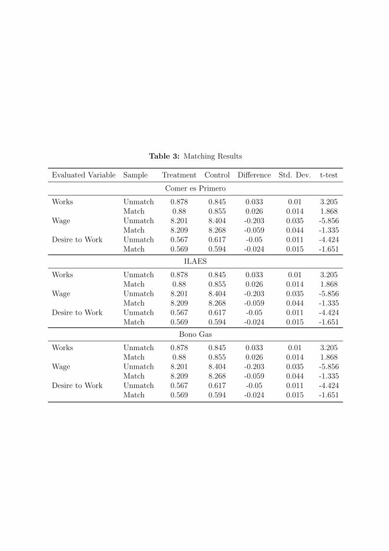
Table 3: Matching Results

Evaluated Variable Sample Treatment Control Difference Std. Dev. t-test

Comer es Primero

Works Unmatch 0.878 0.845 0.033 0.01 3.205Match 0.88 0.855 0.026 0.014 1.868

Wage Unmatch 8.201 8.404 -0.203 0.035 -5.856Match 8.209 8.268 -0.059 0.044 -1.335

Desire to Work Unmatch 0.567 0.617 -0.05 0.011 -4.424Match 0.569 0.594 -0.024 0.015 -1.651

ILAES




Bono Gas




Table

4:

Mat

chin

gR

esult

sby

Pro

gram

and

Age

Gro

up

Eva

luat

edV

aria

ble

Sam

ple

Com

eres

Pri

mer

oIL

AE

Bon

oG

asD

iffer

ence

Std

.D

ev.

t-te

stD

iffer

ence

Std

.D

ev.

t-te

stD

iffer

ence

Std

.D

ev.

t-te

st

You

ng

adult

s:15

-24

year

sol

d

Wor

ks

Unm

atch

0.05

90.

031.

982

0.08

20.

042.

035

0.02

10.

032

0.63

7M

atch

0.01

20.

041

0.28

50.

068

0.05

51.

231

0.04

70.

042

1.13

4W

age

Unm

atch

-0.1

440.

085

-1.6

89-0

.163

0.11

6-1

.409

-0.1

030.

093

-1.1

03M

atch

-0.1

090.

122

-0.8

95-0

.015

0.15

2-0

.099

-0.0

420.

12-0

.352

Wan

tsto

Wor

kU

nm

atch

-0.0

650.

022

-2.9

18-0

.103

0.02

8-3

.706

-0.0

680.

025

-2.7

19M

atch

-0.0

660.

028

-2.3

54-0

.051

0.03

4-1

.509

-0.0

520.

029

-1.7

78

Adult

s:25

-64

year

sol

d

Wor

ks

Unm

atch

0.02

50.

011

2.30

90.

016

0.01

51.

088

0.01

40.

012

1.19

2M

atch

0.01

70.

014

1.22

50.

010.

017

0.60

30.

022

0.01

41.

613

Wag

eU

nm

atch

-0.1

440.

038

-3.7

8-0

.049

0.05

1-0

.966

0.02

30.

042

0.55

5M

atch

-0.0

920.

048

-1.9

130.

036

0.06

40.

557

0.03

20.

048

0.66

8W

ants

toW

ork

Unm

atch

-0.0

460.

013

-3.4

24-0

.028

0.01

8-1

.562

-0.0

30.

015

-1.9

97M

atch

-0.0

210.

017

-1.2

07-0

.008

0.02

1-0

.4-0

.018

0.01

6-1

.116

Sen

iors

:65

+ye

ars

old

Wor

ks

Unm

atch

-0.0

030.

034

-0.0

840.

054

0.04

21.

289

-0.0

130.

037

-0.3

43M

atch

0.00

90.

053

0.16

60.

023

0.05

90.

387

-0.0

30.

059

-0.5

1W

age

Unm

atch

-0.2

470.

106

-2.3

41-0

.019

0.14

1-0

.133

-0.1

090.

118

-0.9

31M

atch

-0.3

120.

148

-2.1

04-0

.152

0.19

7-0

.769

-0.2

170.

153

-1.4

16W

ants

toW

ork

Unm

atch

0.05

30.

031.

793

0.06

40.

041.

572

0.00

10.

034

0.01

9M

atch

0.01

60.

039

0.41

30.

018

0.05

40.

327

-0.0

40.

041

-0.9

71

Table

5:

Mat

chin

gR

esult

sby

Pro

gram

and

Gen

der

Eva

luat

edV

aria

ble

Sam

ple

CE

PIL

AE

Bon

oG

asD

iffer

ence

Std

.D

ev.

t-te

stD

iffer

ence

Std

.D

ev.

t-te

stD

iffer

ence

Std

.D

ev.

t-te

st

Men

Wor

ks

Unm

atch

0.02

70.

011

2.46

40.

020.

015

1.38

9-0

.003

0.01

2-0

.228

Mat

ch0.

017

0.01

51.

174

0.01

20.

017

0.70

80.

008

0.01

40.

547

Wag

eU

nm

atch

-0.1

680.

042

-3.9

45-0

.019

0.05

6-0

.339

-0.0

30.

047

-0.6

4M

atch

-0.0

770.

054

-1.4

22-0

.007

0.07

3-0

.092

0.00

60.

054

0.11

2W

ants

toW

ork

Unm

atch

-0.0

090.

011

-0.7

970.

028

0.01

51.

874

-0.0

150.

012

-1.2

44M

atch

00.

014

0.01

90.

008

0.01

70.

464

00.

014

-0.0

32

Wom

en

Wor

ks

Unm

atch

-0.0

030.

022

-0.1

420.

001

0.03

0.02

10.

031

0.02

41.

32M

atch

0.04

70.

028

1.69

50.

018

0.03

90.

454

0.01

60.

030.

541

Wag

eU

nm

atch

-0.2

640.

064

-4.1

29-0

.147

0.08

8-1

.677

0.03

50.

069

0.50

9M

atch

-0.0

980.

082

-1.2

0.00

70.

114

0.06

0.12

50.

085

1.47

8W

ants

toW

ork

Unm

atch

-0.1

120.

021

-5.4

14-0

.066

0.02

7-2

.431

-0.0

550.

023

-2.4

2M

atch

-0.0

630.

026

-2.4

44-0

.08

0.03

4-2

.347

-0.0

370.

027

-1.3

77

Table

6:

Mat

chin

gR

esult

sby

Lev

elof

Inco

me

Eva

luat

edV

aria

ble

Sam

ple

Com

eres

Pri

mer

oIL

AE

Bon

oG

asD

iffer

ence

Std

.D

ev.

t-te

stD

iffer

ence

Std

.D

ev.

t-te

stD

iffer

ence

Std

.D

ev.

t-te

st

Low

Inco

me

Wor

ks

Unm

atch

0.09

10.

031

2.96

90.

102

0.03

72.

777

0.06

0.03

41.

773

Mat

ch0.

093

0.04

62.

028

0.06

50.

051

1.27

60.

061

0.04

61.

324

Wag

eU

nm

atch

-0.0

640.

069

-0.9

270.

087

0.08

21.

067

-0.0

350.

076

-0.4

57M

atch

0.02

80.

106

0.26

7-0

.132

0.11

9-1

.107

-0.0

350.

097

-0.3

6W

ants

toW

ork

Unm

atch

-0.0

190.

028

-0.6

870.

029

0.03

40.

867

-0.0

280.

031

-0.8

86M

atch

0.01

60.

037

0.43

50.

021

0.04

40.

482

-0.0

080.

039

-0.1

92

Mid

dle

Inco

me

Wor

ks

Unm

atch

0.03

70.

016

2.27

80.

007

0.02

20.

30.

027

0.01

81.

552

Mat

ch0.

030.

022

1.37

7-0

.021

0.02

8-0

.76

0.01

90.

022

0.86

8W

age

Unm

atch

0.00

30.

048

0.06

80.

054

0.06

30.

845

0.09

70.

052

1.86

8M

atch

0.05

30.

063

0.83

3-0

.023

0.08

2-0

.283

0.11

0.06

31.

756

Wan

tsto

Wor

kU

nm

atch

-0.0

50.

022

-2.2

61-0

.01

0.02

9-0

.358

-0.0

430.

024

-1.7

97M

atch

-0.0

420.

028

-1.4

76-0

.039

0.03

7-1

.06

-0.0

360.

028

-1.3

09

Hig

hIn

com

e

Wor

ks

Unm

atch

0.00

60.

013

0.42

30

0.02

-0.0

14-0

.021

0.01

5-1

.432

Mat

ch0.

020.

017

1.22

70.

007

0.02

40.

276

-0.0

180.

016

-1.1

22W

age

Unm

atch

-0.0

560.

058

-0.9

660.

167

0.08

61.

945

0.00

40.

063

0.06

9M

atch

-0.0

820.

076

-1.0

760.

113

0.10

61.

067

-0.0

680.

077

-0.8

83W

ants

toW

ork

Unm

atch

-0.0

160.

02-0

.79

-0.0

50.

029

-1.7

14-0

.011

0.02

2-0

.487

Mat

ch0.

006

0.02

50.

227

-0.0

50.

037

-1.3

450.

001

0.02

60.

04

Table

7:

Mat

chin

gR

esult

sby

Loca

tion

Eva

luat

edV

aria

ble

Sam

ple

CE

PIL

AE

Bon

oG

asD

iffer

ence

Std

.D

ev.

t-te

stD

iffer

ence

Std

.D

ev.

t-te

stD

iffer

ence

Std

.D

ev.

t-te

st

Urb

anA

rea

Wor

ks

Unm

atch

0.02

10.

018

1.14

9-0

.017

0.02

6-0

.635

0.01

50.

016

0.92

8M

atch

0.03

20.

032

1.00

1-0

.001

0.04

7-0

.025

0.05

40.

027

2.03

9W

age

Unm

atch

-0.1

390.

059

-2.3

72-0

.123

0.08

4-1

.463

0.04

30.

054

0.79

5M

atch

-0.0

50.

103

-0.4

860.

034

0.16

0.21

40.

139

0.09

1.53

9W

ants

toW

ork

Unm

atch

-0.0

250.

021

-1.1

97-0

.013

0.03

-0.4

29-0

.018

0.01

9-0

.93

Mat

ch-0

.023

0.03

3-0

.686

-0.0

480.

053

-0.9

06-0

.012

0.02

9-0

.41

Rura

lA

rea[U+FFFD]

Wor

ks

Unm

atch

0.01

10.

017

0.62

90.

023

0.01

71.

329

0.00

70.

018

0.36

9M

atch

0.01

30.

029

0.43

40.

040.

039

1.02

6-0

.015

0.03

-0.4

92W

age

Unm

atch

0.05

50.

065

0.84

30.

059

0.06

60.

901

0.09

10.

067

1.35

9M

atch

-0.0

50.

117

-0.4

24-0

.106

0.14

6-0

.728

0.04

70.

122

0.38

1W

ants

toW

ork

Unm

atch

-0.0

20.

024

-0.8

43-0

.018

0.02

3-0

.769

-0.0

190.

024

-0.7

78M

atch

-0.0

40.

036

-1.1

28-0

.076

0.04

1-1

.857

-0.0

60.

036

-1.6

34

References

Cabal, M. (1993). Evolucion de las Microempresas y Pequenas Empresas en la Republica

Dominicana, 1992-1993. Fondo Micro, 1 edition.

Cecchini, S. and Madariaga, A. (2011). Programas de Transferencias Condicionadas.

Balance de la Experiencia Reciente en America Latina y el Caribe. Naciones Unidas,

Santiago de Chile.

Cecchini, S. and Martınez, R. (2011). Proteccion Social Inclusiva en America Latina:

una mirada integral, un enfoque de derechos. Libros de la CEPAL, No. 111. Naciones

Unidas, Santiago de Chile.

Fizbein, A. and Schady, N. (2009). Conditional cash transfers : reducing present and

future poverty. Library of Congress Cataloging-in-Publication Data.

Garcıa, N. and Valdivia, M. (1985). Crisis externa, ajuste interno y mercado de trabajo:

Republica dominicana, 1980-83. Monografıa 49, Organizacion Internacional del Trabajo

(OIT), Santiago de Chile.

Gregory, P. (1997). Empleo y desempleo en la republica dominicana. Banco Central de

la Republica Dominicana.

Guzman, R. M. (2011). Composicion Economica Dominicana. El estrato de ingresos

medios en el umbral del siglo XXI. Editora Corripio, 1 edition.

Jensen, R. (2010). The (perceived) returns to education and the demand for schooling.

The Quarterly Journal of Economics, 125(2):515–548.

Keane, M. and Moffitt, R. (1998). A structural model of multiple welfare program par-

ticipation and labor supply. International Economic Review, 39(3):553–589.

L. Alzua, G. C. and Ripani, L. (2009). Labor supply responses to cash transfer programs.

experimental and non-experimental evidence from latin america. Paper presented a the

AFREA-Nonie-3ie Conference, Perspectives on Impact Evaluation. Cairo.

Moffitt, R. (2002). Welfare programs and labor supply. In Auerbach, A. J. and Feldstein,

M., editors, Handbook of Public Economics, volume 4, chapter 34, pages 2393–2430.

Elsevier, 1 edition.

Marquez, G. (1998). El desempleo en america latina y el caribe a mediados de los anos

90. Banco Interamericano de Desarrollo (BID), Documento de Trabajo, No. 377.

OIT (1975). Generacion de empleo productivo y crecimiento economico: el caso de la

republica dominicana. Technical report, Oficina Internacional del Trabajo.

Rosen, H. (2009). Public Finance. McGraw-Hill/Irwin, 9th edition.

Rosenbaum, P. R. and Rubin, D. B. (1983). The central role of the propensity score in

observational studies for causal effects. Biometrika, 70:41–55.

Saez, E. (2002). Optimal income transfer programs: Intensive versus extensive labor

supply responses. The Quarterly Journal of Economics, 117(3):1039–1073.

Sanchez-Fung, J. R. (2000). Empleo y mercados de trabajo en la republica dominicana:

una revision de la literatura. Revista de la CEPAL, 71:163–175.

Tabor, S. (2002). Assisting the poor with cash: Design and implementation of social

transfer programs. Social Protection Discussion Paper No. 0223.

Table 8: Conditional Cash Transfer Programs in Latin America and the Caribbean

Country Programs Operating Country Programs Operating(Year Started) (Year Started)

Argentina Asignacion Universal por Hijopara proteccion social (2009);Programa Ciudadania Portena(2005)

Bolivia Bono Juancito Pinto (2006);Bono Madre Nino-Nina (2009)

Brasil Bolsa Familia (2003) Chile Chile Solidario

Colombia Familias en Accion (2001);Red Juntos (2007); SubsidiosAsistencia Escolar (2005)

Costa Rica Avancemos (2006)

Ecuador Bono de Desarrollo Humano(2003)

El Salvador Comunidades Solidarias Ru-rales (2005)

Guatemala Mi Familia Progresa (2008) Honduras Programa de Asignacion Fa-miliar (1990); Bono 10.000Educacion, Salud y Nutricion(2010)

Jamaica Programa de Avance Salud yEducacion (2002)

Mexico Oportunidades (1997)

Panama Red de Oportunidades (2006) Paraguay Tekopora (2005); Abrazo(2005)

Peru Juntos (2005) DominicanRepublic

Solidaridad (2005)

Trinidad yTobago

Programa de TransferenciasMonetarias Condicionadas(2006)

Uruguay Asignaciones Familiares(2008)

Source: Cecchini, S. and Aldo Madariaga (2011), Table 1.1, pg. 11.

Table

9:

Ros

enbau

mR

esult

s

Eva

luat

edV

aria

ble

Sam

ple

Com

eres

Pri

mer

oIL

AE

Bon

oG

asD

iffer

ence

Std

.D

ev.

t-te

stD

iffer

ence

Std

.D

ev.

t-te

stD

iffer

ence

Std

.D

ev.

t-te

st

Ban

d=

0.1

Wor

ks

Unm

atch

0.02

50.

011

2.30

90.

016

0.01

51.

088

0.01

40.

012

1.19

2M

atch

0.01

90.

014

1.35

60.

018

0.01

61.

130.

007

0.01

30.

594

Wag

eU

nm

atch

-0.1

440.

038

-3.7

8-0

.049

0.05

1-0

.966

0.02

30.

042

0.55

5M

atch

-0.0

490.

047

-1.0

380.

019

0.05

70.

330.

011

0.04

30.

253

Wan

tsto

Wor

kU

nm

atch

-0.0

460.

013

-3.4

24-0

.028

0.01

8-1

.562

-0.0

30.

015

-1.9

97M

atch

-0.0

250.

017

-1.5

06-0

.002

0.02

-0.0

94-0

.023

0.01

5-1

.544

Ban

d=

0.01

Wor

ks

Unm

atch

0.02

50.

011

2.30

90.

016

0.01

51.

088

0.01

40.

012

1.19

2M

atch

0.01

60.

015

1.09

20.

024

0.01

61.

438

0.01

0.01

40.

731

Wag

eU

nm

atch

-0.1

440.

038

-3.7

8-0

.049

0.05

1-0

.966

0.02

30.

042

0.55

5M

atch

-0.0

620.

05-1

.248

0.05

20.

060.

864

0.04

20.

046

0.92

7W

ants

toW

ork

Unm

atch

-0.0

460.

013

-3.4

24-0

.028

0.01

8-1

.562

-0.0

30.

015

-1.9

97M

atch

-0.0

260.

017

-1.5

040.

010.

021

0.48

4-0

.007

0.01

6-0

.432

Ban

d=

0.00

1

Wor

ks

Unm

atch

0.02

50.

011

2.30

90.

016

0.01

51.

088

0.01

40.

012

1.19

2M

atch

0.01

70.

014

1.22

50.

010.

017

0.60

30.

022

0.01

41.

613

Wag

eU

nm

atch

-0.1

440.

038

-3.7

8-0

.049

0.05

1-0

.966

0.02

30.

042

0.55

5M

atch

-0.0

920.

048

-1.9

130.

036

0.06

40.

557

0.03

20.

048

0.66

8W

ants

toW

ork

Unm

atch

-0.0

460.

013

-3.4

24-0

.028

0.01

8-1

.562

-0.0

30.

015

-1.9

97M

atch

-0.0

210.

017

-1.2

07-0

.008

0.02

1-0

.4-0

.018

0.01

6-1

.116

Ban

d=

0.00

01

Wor

ks

Unm

atch

0.02

50.

011

2.30

90.

016

0.01

51.

088

0.01

40.

012

1.19

2M

atch

0.01

20.

018

0.68

7-0

.021

0.02

3-0

.932

0.01

10.

017

0.63

2W

age

Unm

atch

-0.1

440.

038

-3.7

8-0

.049

0.05

1-0

.966

0.02

30.

042

0.55

5M

atch

-0.1

50.

063

-2.3

82-0

.014

0.08

5-0

.16

0.02

10.

058

0.36

5W

ants

toW

ork

Unm

atch

-0.0

460.

013

-3.4

24-0

.028

0.01

8-1

.562

-0.0

30.

015

-1.9

97M

atch

-0.0

390.

02-1

.897

-0.0

350.

028

-1.2

66-0

.017

0.02

-0.8

74

Table

10:

Pla

ceb

oM

atch

ing

Tes

tR

esult

s

Eva

luat

edV

aria

ble

Sam

ple

Com

eres

Pri

mer

oIL

AE

Bon

oG

asD

iffer

ence

Std

.D

ev.

t-te

stD

iffer

ence

Std

.D

ev.

t-te

stD

iffer

ence

Std

.D

ev.

t-te

st

Tre

atm

ent

vs.

Con

trol

1

Wor

ks

Unm

atch

0.02

90.

013

2.20

40.

016

0.01

61.

016

0.01

60.

015

1.06

5M

atch

0.03

10.

018

1.66

80.

008

0.02

10.

411

0.01

70.

018

0.98

Wag

eU

nm

atch

-0.1

320.

046

-2.8

7-0

.052

0.05

5-0

.949

0.03

40.

053

0.64

8M

atch

0.00

80.

061

0.13

10.

048

0.07

30.

659

0.03

0.06

0.50

4W

ants

toW

ork

Unm

atch

-0.0

440.

016

-2.6

52-0

.019

0.01

9-0

.957

-0.0

290.

019

-1.5

17M

atch

-0.0

360.

022

-1.6

470.

015

0.02

50.

585

-0.0

050.

021

-0.2

35

Tre

atm

ent

vs.

Con

trol

2

Wor

ks

Unm

atch

0.02

10.

013

1.63

30.

016

0.01

61.

015

0.01

20.

016

0.76

6M

atch

0.02

50.

018

1.39

30.

016

0.02

0.80

30.

017

0.01

80.

934

Wag

eU

nm

atch

-0.1

570.

047

-3.3

35-0

.047

0.05

6-0

.834

0.01

10.

056

0.19

2M

atch

-0.1

160.

064

-1.8

-0.0

290.

074

-0.3

95-0

.016

0.06

4-0

.254

Wan

tsto

Wor

kU

nm

atch

-0.0

490.

017

-2.8

87-0

.037

0.01

9-1

.939

-0.0

30.

02-1

.526

Mat

ch-0

.037

0.02

2-1

.675

-0.0

40.

024

-1.6

27-0

.02

0.02

2-0

.913

Con

trol

1vs.

Con

trol

2

Wor

ks

Unm

atch

0.00

70.

016

0.45

8-0

.008

0.01

3-0

.639

0.00

30.

018

0.18

Mat

ch0.

008

0.01

70.

487

-0.0

110.

014

-0.7

85-0

.004

0.02

2-0

.161

Wag

eU

nm

atch

0.02

60.

054

0.47

40.

108

0.04

62.

376

0.11

20.

062

1.81

Mat

ch0.

007

0.05

90.

119

0.06

80.

051.

361

0.07

30.

073

1.00

4W

ants

toW

ork

Unm

atch

0.00

50.

019

0.25

40.

030.

016

1.81

90.

005

0.02

10.

256

Mat

ch0

0.02

0.01

30.

022

0.01

71.

281

0.01

70.

025

0.66

Variables Works WageDesire to Work

Works WageDesire to Work


Female 5.52 7.44 1.34 7.49 5.71 0.63 7.48 6.56 1.23Literate 0.04 2.34 2.54 3.61 3.53 1.13 3.74 3.69 1.01Age 7.78 5.97 0.03 6.69 3.34 0.07 7.77 4.15 1.00Age^2 7.03 5.05 1.09 6.47 2.93 0.16 7.67 3.86 0.85Schooling 0.98 1.89 0.69 0.60 0.04 1.52 1.17 0.42 0.80Schooling^2 1.84 3.52 1.22 1.72 1.23 1.42 2.29 0.74 0.65Schooling X Age 4.65 3.42 0.90 3.36 2.71 1.09 3.55 3.61 0.86Head of Household 8.35 4.78 0.63 4.95 4.58 0.07 5.14 4.24 0.89Household Size 3.15 3.43 2.49 1.55 3.29 1.76 0.85 3.69 1.64# Adults 18‐65 6.36 3.85 0.53 2.99 3.33 1.73 2.37 3.61 1.66# Seniors 65+ 4.78 1.67 2.18 2.92 2.12 2.33 2.78 2.24 1.99Married 4.84 2.23 0.12 2.13 1.93 0.33 2.72 2.58 0.09# Children 0‐5 1.12 1.31 2.14 2.32 0.14 0.38 1.30 0.04 0.07# Children 6‐15 2.03 0.95 1.80 2.41 1.98 0.75 2.19 2.02 0.55Female x # Child 0‐5 8.32 2.04 0.86 7.66 1.12 0.55 6.52 1.14 0.29Extreme Poverty 0.12 0.67 0.78 0.33 0.30 0.36 0.43 0.34 0.12

Table A‐1: Normalized bias (standardized) ‐ Comer es Primero Program

1‐1 matching K near matching Radius Matching

NOTE: These tables present the value of the standardized bias statistic after the matching. The general rule is that if the value of the statistic is less than 20, the difference between the values of the control group and the treatment group is not significant.NOTE 2: Different methodologies for the entire population were used for these tables (15‐98 years old). NOTE 3: The control group was selected using the corresponding variables in the database of the survey. To evaluate all programs (last table), families who have benefited from any of the three programs are defined as treatment (CEP, and Bonogas ILAES).NOTE 4: The Work variable is a dummy that takes the value of 1 if the individual works and 0 if unemployed. The wage is measured as the natural logarithm of monthly labor wage, the desire to work is measured as a variable that assumes 1 if the subject works or is looking for work (unemployed) and 0 if the individual is not working nor looking for work (not in the workforce). For the rest of the analysis Kernel matching is used as selected methodology.

Variables Works Wage Desire to Work

Works Wage Desire to Work

Works Wage Desire to Work


Table A‐1: Normalized bias (standardized) ‐ Comer es Primero Program (Cont.)

Kernel Matching Local linear regression Mahalanobis






Table A‐2: Normalized bias (standardized) ‐ ILAE Program







Table A‐2: Normalized bias (standardized) ‐ ILAE Program (Cont.)


Mahalanobis Kernel Matching Local linear regression





Table A‐3: Normalized bias (standardized) ‐ Bono Gas Program







Table A‐3: Normalized bias (standardized) ‐ Bono Gas Program (Cont.)

NOTE: These tables present the value of the standardized bias statistic after the matching. The general rule is that if the value of the statistic is less than 20, the difference between the values of the control group and the treatment group is not significant.NOTE 2: Different methodologies for the entire population were used for these tables (15‐98 years old). NOTE 3: The control group was selected using the corresponding variables in the database of the survey. To evaluate all programs (last table), families who have benefited from any of the three programs are defined as treatment (CEP, and Bonogas ILAES).NOTE 4: The Work variable is a dummy that takes the value of 1 if the individual works and 0 if unemployed. The wage is measured as the natural logarithm of monthly labor wage, the desire to work is measured as a variable that assumes 1 if the subject works or is looking for work (unemployed) and 0 if the individual is not working nor looking for work (not in the workforce) For the rest of the analysis Kernel matching is used as selected methodology

Kernel Matching Local linear regression Mahalanobis





Table A‐4: Normalized bias (standardized) ‐ All Programs






Female 0.89 0.78 0.16 1.15 3.14 0.21 1.54 0.26 0.44Literate 0.09 1.80 0.94 1.49 3.60 0.58 0.09 0.25 0.25Age 1.29 0.14 0.42 0.08 4.62 0.40 2.55 1.68 1.63Age^2 0.27 1.04 0.58 1.35 5.67 0.24 3.08 2.20 2.13Schooling 3.18 1.46 1.62 4.45 2.96 1.82 1.79 1.39 1.43Schooling^2 2.50 0.19 1.36 3.07 3.17 0.34 0.27 0.66 0.17Schooling X Age 3.06 2.34 2.20 4.82 0.22 2.89 0.60 0.11 0.17Head of Household 6.29 6.39 2.95 5.50 8.14 4.72 2.12 2.83 0.92Household Size 0.98 0.33 0.05 4.65 1.37 0.64 20.92 18.83 16.82# Adults 18‐65 4.65 1.20 1.69 8.43 0.84 2.13 10.17 9.77 9.02# Seniors 65+ 0.04 1.03 3.17 0.78 2.28 1.06 10.41 8.95 7.73Married 3.62 3.57 0.50 0.23 1.30 0.70 1.02 0.88 0.30# Children 0‐5 2.33 2.26 1.91 0.88 1.82 0.74 3.97 4.89 4.70# Children 6‐15 4.34 3.28 0.45 3.42 3.79 1.88 13.00 10.89 7.99Female x # Child 0‐5 1.38 0.05 0.84 1.08 0.56 0.69 2.20 2.96 3.14Extreme Poverty 2.34 1.62 0.73 3.61 2.25 0.56 7.31 7.23 5.69NOTE: These tables present the value of the standardized bias statistic after the matching. The general rule is that if the value of the statistic is less than 20, the difference between the values of the control group and the treatment group is not significant.NOTE 2: Different methodologies for the entire population were used for these tables (15‐98 years old). NOTE 3: The control group was selected using the corresponding variables in the database of the survey. To evaluate all programs (last table), families who have benefited from any of the three programs are defined as treatment (CEP, and Bonogas ILAES).NOTE 4: The Work variable is a dummy that takes the value of 1 if the individual works and 0 if unemployed. The wage is measured as the natural logarithm of monthly labor wage, the desire to work is measured as a variable that assumes 1 if the subject works or is looking for work (unemployed) and 0 if the individual is not working nor looking for work (not in the workforce). For the rest of the analysis Kernel matching is used as selected methodology.

Table A‐4: Normalized bias (standardized) ‐ All Programs (Cont.)

Mahalanobis Kernel Matching Local linear regression

MethodologyEvaluated Variable

Sample Treatment Control Difference Std. Dev. t‐test


Wage Unmatch 8.201 8.404 ‐0.203 0.035 ‐5.856Match 8.209 8.265 ‐0.056 0.052 ‐1.074

Desire to Work Unmatch 0.567 0.617 ‐0.050 0.011 ‐4.424Match 0.569 0.575 ‐0.005 0.017 ‐0.299










Works Unmatch 0.878 0.845 0.033 0.010 3.205Match 0.878 . . . .

Wage Unmatch 8.201 8.404 ‐0.203 0.035 ‐5.856Match 8.199 . . . .

Desire to Work Unmatch 0.567 0.617 ‐0.050 0.011 ‐4.424Match 0.567 0.576 ‐0.009 . .




Table B‐1: Matching Results ‐ Comer es Primero Program

Mahalanobis

1‐1 matching

K near

Radius Matching

Kernel matching

Local linear regression





















Table B‐2: Matching Program Results ‐ ILAES Program

1‐1 matching

K near

Radius Matching

Kernel matching


Mahalanobis





















Table B‐3: Matching Results ‐ Bono Gas Program

1‐1 matching

K near

Radius Matching

Kernel matching


Mahalanobis





















Table B‐4: Matching Results ‐ All Programs

Mahalanobis

1‐1 matching

K near

Radius Matching

Kernel matching


Variables Works WageDesire to

workWorks Wage

Desire to

workWorks Wage

Desire to

work



workWorks Wage

Desire to

workWorks Wage

Desire to

work


Table C‐1: Results by Age Group ‐ Comer es Primero Program

Table C‐2: Results by Age Group ‐ ILAE Program

NOTE: These exercises are performed using Kernel Matching. The values presented correspond to the standardized bias. For the younger group the variable related to being head of household is not used. Instead, the variable gender of the household head is used.

Young adults:15‐24 Adults: 25‐64 Seniors: 65+




workWorks Wage

Desire to

workWorks Wage

Desire to

work



workWorks Wage

Desire to

workWorks Wage

Desire to

work

Female 10.643 1.840 3.559 0.055 0.358 0.872 5.879 5.177 11.479Literate 8.980 1.277 4.526 6.399 4.430 2.122 16.197 5.959 5.248Age 0.486 1.821 0.747 1.722 3.081 0.695 15.421 17.784 6.621Age^2 0.112 2.896 0.662 2.279 3.718 0.667 14.876 17.530 6.782Schooling 13.535 11.739 1.284 0.403 0.203 2.269 2.167 7.164 1.781Schooling^2 12.862 13.532 0.369 0.585 0.336 2.570 2.735 3.295 0.767Schooling X Age 12.634 10.422 1.588 0.299 0.344 2.244 1.897 6.813 0.987Head of Household 10.474 20.310 1.023 5.114 5.786 3.400 13.945 8.119 6.858Household Size 5.655 2.108 5.570 0.319 1.935 1.463 6.558 5.570 1.522# Adults 18‐65 3.742 8.957 2.719 0.566 1.751 2.720 3.302 1.157 2.297# Seniors 65+ 5.384 21.015 2.083 1.406 2.259 0.102 26.562 2.238 3.674Married 7.500 5.144 0.840 4.112 0.958 1.673 6.786 2.250 5.493# Children 0‐5 10.321 10.944 1.110 2.416 1.942 0.959 1.392 8.964 0.023# Children 6‐15 2.815 6.341 2.842 3.436 3.968 1.037 3.927 6.890 0.147Female x # Child 0‐5 16.171 10.232 1.936 3.183 0.096 0.447 24.163 8.924 3.536Extreme Poverty 0.332 6.411 1.269 0.432 0.164 2.006 7.623 1.447 0.194NOTE: These exercises are performed using Kernel Matching. The values presented correspond to the standardized bias. For the younger group the variable related to being head of household is not used. Instead, the variable gender of the household head is used.

Table C‐3: Results by Age Group ‐ Bono Gas Program



Table C‐4: Results by Age Group ‐ All Programs



workWorks Wage

Desire to

work

Literate 1.714 1.643 0.374 3.073 8.035 6.093Age 1.518 1.555 0.390 3.782 0.098 3.386Age^2 0.969 1.968 0.195 3.158 0.554 3.333Schooling 0.287 1.013 1.027 1.743 3.953 4.196Schooling^2 2.046 0.810 1.140 3.505 1.521 3.896Schooling X Age 0.318 0.371 0.140 5.449 2.529 3.539Head of Household 2.292 0.434 0.974 0.800 1.127 0.457Household Size 2.565 0.354 2.254 0.323 7.684 0.039# Adults 18‐65 1.606 3.348 1.156 1.826 8.986 2.211# Seniors 65+ 2.451 3.145 6.447 1.229 3.321 4.229Married 2.007 3.552 4.226 4.979 7.535 2.019# Children 0‐5 2.817 3.056 3.103 2.669 5.915 0.700# Children 6‐15 5.096 3.158 5.135 1.345 2.443 0.170Extreme Poverty 0.985 1.039 0.894 0.290 0.620 0.945


workWorks Wage

Desire to

work




Table C‐5: Results by Gender ‐ Comer es Primero Program

Male Female

Table C‐6: Results by Gender ‐ ILAE Program

FemaleMale


workWorks Wage

Desire to

work



workWorks Wage

Desire to

work




Table C‐8: Results by Gender ‐ All Programs

Table C‐7: Results by Gender ‐ Bono Gas Program

Male Female

Male Female


workWorks Wage

Desire to

workWorks Wage

Desire to

work



workWorks Wage

Desire to

workWorks Wage

Desire to

work


Table C‐9: Results by Level of Income ‐ Comer es Primero Program

Table C‐10: Results by Level of Income ‐ ILAE Program

NOTE: income groups were calculated by dividing households into three equal groups according to household percapita income.

Low Income Middel Income High Income


High IncomeLow Income Middel Income


workWorks Wage

Desire to

workWorks Wage

Desire to

work



workWorks Wage

Desire to

workWorks Wage

Desire to

work

Female 5.611 0.826 0.829 4.026 4.156 0.301 3.377 5.918 3.446Literate 1.318 1.731 5.299 4.701 3.100 0.189 5.990 0.533 1.429Age 14.139 15.084 7.811 3.103 2.515 0.225 1.216 1.989 1.960Age^2 14.792 14.665 8.495 2.077 2.204 0.235 0.700 2.101 1.059Schooling 7.677 2.534 0.938 8.552 5.884 5.574 5.064 1.028 1.455Schooling^2 6.299 5.304 0.353 7.455 5.545 6.360 4.212 1.640 1.124Schooling X Age 5.736 2.158 3.522 7.477 6.326 5.058 3.589 0.002 4.734Head of Household 8.938 11.082 10.095 6.470 6.655 1.179 1.676 1.379 0.451Household Size 7.250 13.823 6.795 1.231 6.042 3.250 5.488 4.066 1.712# Adults 18‐65 3.829 7.686 0.102 0.354 10.811 2.642 4.798 4.338 2.595# Seniors 65+ 11.655 14.116 4.246 8.055 12.230 3.279 2.217 2.259 1.621Married 6.901 4.363 3.520 6.064 6.799 1.202 0.617 2.733 1.768# Children 0‐5 2.104 3.004 5.082 0.164 0.522 2.491 3.582 3.675 2.969# Children 6‐15 16.447 18.518 8.392 0.433 2.109 0.831 5.381 3.265 0.230Female x # Child 0‐5 2.502 5.271 5.487 1.455 5.049 1.124 4.522 4.832 2.391Extreme Poverty 7.442 0.113 3.782 0.484 0.488 0.258 4.032 0.611 4.619NOTE: income groups were calculated by dividing households into three equal groups according to household percapita income.

Table C‐11: Results by Level of Income ‐ Bono Gas Program


High Income

Table C‐12: Results by Level of Income ‐ All Programs Program Low Income Middel Income

Low Income Middel Income High Income


workWorks Wage

Desire to

workWorks Wage

Desire to

workWorks Wage

Desire to

Work

Female 6.122 7.696 1.903 4.572 5.902 0.266 3.230 5.911 0.286 3.561 3.202 4.578Literate 0.139 3.052 4.256 9.446 7.308 4.221 6.002 4.169 3.211 5.503 2.667 4.350Age 2.586 3.203 1.309 2.352 3.510 0.992 1.412 2.975 0.662 0.116 0.183 1.648Age^2 1.694 2.965 1.201 1.275 3.099 0.712 0.939 3.038 0.684 0.032 0.498 1.422Schooling 5.903 6.402 5.497 1.841 1.008 1.734 1.577 0.867 1.527 1.281 0.392 2.770Schooling^2 5.047 5.022 3.950 0.251 0.357 0.565 1.051 0.457 0.953 1.183 0.347 2.342Schooling X Age 4.663 5.562 5.903 3.221 1.848 1.497 1.715 0.780 1.202 1.871 0.197 2.654Head of Household 1.800 1.126 3.301 3.121 4.070 0.815 2.426 1.883 2.621 10.470 3.328 1.078Household Size 8.773 7.914 4.381 7.660 7.085 3.552 1.655 5.605 2.826 4.543 1.925 1.330# Adults 18‐65 7.778 7.399 4.609 7.203 6.625 4.893 1.658 4.417 4.074 6.410 1.473 4.351# Seniors 65+ 4.860 4.756 6.416 3.248 2.890 3.922 2.992 1.771 0.845 5.352 2.233 0.025Married 1.321 1.057 0.893 1.035 0.949 0.567 1.321 0.627 0.351 0.403 2.878 1.467# Children 0‐5 1.163 0.491 1.199 1.892 0.199 0.844 2.965 1.476 2.488 9.767 3.074 6.856# Children 6‐15 3.375 2.777 1.108 3.661 3.758 1.690 2.811 4.369 0.213 6.543 6.835 5.047Female x # Child 0‐5 3.829 1.006 0.626 3.634 1.521 0.329 4.593 0.592 1.505 8.700 1.447 1.997Extreme Poverty 0.803 0.850 0.876 0.425 0.058 0.007 0.031 0.217 0.343 0.000 0.000 0.000


workWorks Wage

Desire to

workWorks Wage

Desire to

workWorks Wage

Desire to

Work


Table C‐13: Matching Kernel Results with 4 Bands ‐ Comer es Primero Program

Table C‐14: Matching Kernel Results with 4 Bands ‐ ILAE Program

Band=0.0001

NOTE: To test the sensitivity, kernel matching was performed on 4 different bands.


Band=0.001Band=0.1 Band=0.01

Band=0.1 Band=0.01 Band=0.001 Band=0.0001


workWorks Wage

Desire to

workWorks Wage

Desire to

workWorks Wage

Desire to

Work



workWorks Wage

Desire to

workWorks Wage

Desire to

workWorks Wage

Desire to

Work


Table C‐15: Matching Kernel Results with 4 Bands ‐ Bono Gas Program

Table C‐16: Matching Kernel Results with 4 Bands ‐ ALL Programs

Band=0.001 Band=0.0001



Band=0.1 Band=0.01 Band=0.001 Band=0.0001

Band=0.1 Band=0.01


workWorks Wage

Desire to

workWorks Wage

Desire to

work



workWorks Wage

Desire to

workWorks Wage

Desire to

work


Table C‐17: Comparative Results of Treatments and Controls ‐ Comer es Primero Program

Table C‐18: Comparative Results of Treatments and Controls ‐ ILAE Program

Note: To test the sensitivity, a Placebo test was conducted as follows: the control sample is divided into two random groups. An estimation is then performed as indicated in the table header.

RND1 RND2 RND3

Treatment vs control2


Treatment vs control1 Control1 vs Control 2


workWorks Wage

Desire to

workWorks Wage

Desire to

work



workWorks Wage

Desire to

workWorks Wage

Desire to

work

Female 0.200 0.297 0.016 2.336 2.382 2.197 8.216 6.864 2.966Literate 2.064 5.340 5.144 3.088 1.220 0.361 2.051 2.812 0.470Age 5.292 9.158 4.023 5.001 8.677 0.895 3.086 4.848 0.701Age^2 5.530 9.147 3.847 4.236 8.134 0.953 3.209 4.812 0.785Schooling 3.420 3.296 3.925 5.460 3.802 3.010 2.244 1.829 1.168Schooling^2 2.917 0.375 3.406 5.942 4.058 3.291 4.256 5.447 2.466Schooling X Age 4.530 6.799 5.635 3.720 0.941 4.008 0.588 1.811 1.209Head of Household 0.511 0.388 0.348 8.075 9.397 0.870 0.959 2.728 0.434Household Size 2.714 0.720 2.013 0.499 1.829 1.032 2.267 1.837 4.483# Adults 18‐65 0.530 5.651 1.551 2.250 0.139 0.135 7.761 11.973 3.681# Seniors 65+ 4.558 7.195 1.400 1.987 0.053 0.928 4.252 6.683 1.577Married 3.253 0.894 0.622 0.703 1.049 1.547 4.625 1.450 1.412# Children 0‐5 2.331 1.526 0.626 0.836 1.866 1.218 0.199 4.157 6.028# Children 6‐15 1.141 0.510 0.308 2.725 3.792 0.525 3.214 9.264 0.695Female x # Child 0‐5 5.879 1.818 0.761 0.094 0.662 2.508 1.474 5.138 7.320Extreme Poverty 3.054 2.058 3.872 0.247 0.345 0.323 4.575 2.361 0.568Note: To test the sensitivity, a Placebo test was conducted as follows: the control sample is divided into two random groups. An estimation is then performed as indicated in the table header.

Table C‐19: Comparative Results of Treatments and Controls ‐ Bono Gas Program


RND2 RND3

RND1 RND2 RND3

Table C‐20: Comparative Results of Treatments and Controls ‐ All ProgramsRND1


workWorks Wage

Desire to

work

Female 7.453 1.105 1.253 0.561 4.907 1.500Literate 5.018 7.456 5.793 5.599 11.581 1.693Age 6.066 2.553 2.424 7.621 9.582 2.922Age^2 4.073 1.730 1.961 6.919 9.065 2.380Schooling 2.833 2.505 7.262 5.255 8.064 1.225Schooling^2 4.355 4.181 8.891 7.833 7.700 0.422Schooling X Age 8.577 6.620 8.633 2.965 5.875 2.342Head of Household 6.563 4.236 6.569 0.851 2.279 4.993Household Size 4.742 2.981 1.364 19.943 18.244 7.606# Adults 18‐65 7.111 8.460 0.693 12.956 9.289 0.515# Seniors 65+ 4.784 2.282 4.996 2.098 4.409 1.516Married 6.355 7.749 1.159 9.883 3.781 4.547# Children 0‐5 6.494 6.579 0.422 17.438 19.106 12.983# Children 6‐15 10.596 1.324 3.090 13.969 16.413 5.894Female x # Child 0‐5 0.104 2.491 2.401 10.048 12.817 9.049Extreme Poverty 0.000 0.000 0.000 2.945 2.085 2.069


workWorks Wage

Desire to

work


Table C‐21: Comparative Results by Location ‐ Comer es Primero Program

Table C‐22: Comparative Results by Location ‐ ILAE Program

Urban Area Rural Area


Note: To test the sensitivity, a Placebo test was conducted as follows: the sample is divided randomly into two control groups. An estimation is then performed as indicated in the table header.



workWorks Wage

Desire to

work



workWorks Wage

Desire to

work




Rural Area

Table C‐23: Comparative Results by Location ‐ Bono Gas Program

Table C‐24: Comparative Results by Location ‐ All Programs


Urban Area

Labour Supply Effects of Conditional Transfers: Analyzing the Dominican Republic's Solidarity...

Documents

Transcript of Labour Supply Effects of Conditional Transfers: Analyzing the Dominican Republic's Solidarity...