What we pay in the shadow:Labor tax evasion, minimum wage hike

and employment

Nicolas Gavoille∗ Anna Zasova †

This version: 22/04/2021

Abstract

The interactions between minimum wage policy and tax evasion remainlargely unknown. We study firm-level employment effects of a large and bitingminimum wage increase in Latvia conditional on labor tax compliance. TheLatvian labor market is characterized by the prevalence of envelope wages, i.e.,unreported cash-in-hand complements to the official wage. We apply machinelearning to classify firms between compliant and tax-evading using a uniquecombination of administrative and survey data. We then show that firms en-gaged in labor tax evasion are insensitive to the minimum wage shock. Ourresults suggest that these firms use wage underreporting as an adjustment mar-gin, converting (part of) the envelope into legal wage. Increasing minimumwage contributes to tax rule enforcement, but this comes at the cost of negativeemployment consequences for compliant firms.

Keywords: Minimum wage, employment, tax evasionJEL: J08, H26, E26

∗Stockholm School of Economics in Riga, Strelnieku iela 4a, Riga LV-1010 - Latvia. E-mail :nicolas.gavoille@sseriga.edu†Baltic International Centre for Economic Policy Studies, Strelnieku iela 4a, Riga LV-1010 -

Latvia. E-mail : anna@biceps.org

1

1 Introduction

How do firms respond to minimum wage shocks? The vast literature studying the

employment effect of minimum wage hikes remains largely inconclusive. Within

this literature, the few papers examining firm-level employment response describe

relatively small employment effects (Machin et al., 2003; Mayneris et al., 2018; Ha-

rasztosi and Lindner, 2019). A possible explanation is that firms may use margins

other than employment to absorb the shock, such as price pass-through (Harasztosi

and Lindner, 2019; Renkin et al., 2020; Allegretto and Reich, 2018), profits (Draca

et al., 2011; Harasztosi and Lindner, 2019; Bell and Machin, 2018; Drucker et al.,

2019) but also compliance (Clemens and Strain, 2020).

This papers studies firm-level employment effects of a minimum wage hike con-

ditional on labor tax evasion. We focus on a sequence of two minimum wage hikes

in Latvia in 2014 and 2015, representing altogether a 26% increase of the nominal

minimum wage and affecting about 20% of the workforce. We exploit a unique com-

bination of administrative and survey data structured around a matched employer-

employee dataset covering the whole population of employees at a monthly frequency

throughout the 2011-2017 period.

The interactions between minimum wage policy and labor tax evasion remain

largely unknown. We study a diffuse type of labor tax evasion: envelope wage, i.e., an

unreported cash-in-hand complement to the official wage. Income underreporting is a

widespread phenomenon documented in a large set of countries (e.g., Gorodnichenko

et al., 2009 in Russia, Putnins and Sauka, 2015 in the Baltic States, Tonin, 2011 in

Hungary, Pelek and Uysal, 2018 in Turkey, Perry et al., 2007 in Argentina but also

Hurst et al., 2014 for self-employed in the US). In this setup, minimum wage policy

can become a fiscal policy tool: a minimum wage hike pushes firms to convert part

of the envelope into official wage to comply with the new level, so that they remain

under the tax authorities’ radar. From an employment perspective, unreported wage

may hence act as a buffer to absorb minimum wage shocks (Tonin, 2011). At the same

time, not all firms are tax-evaders, and some firms genuinely pay their employees at

the minimum wage. The aim of this paper is to investigate whether compliant and

tax-evading firms do exhibit a different reaction in terms of employment following a

minimum wage hike.

2

Envelope wage is a major issue in the Latvian labor market. More than one in

ten employees in Latvia admitted to have received envelope wage (Eurobarometer,

2014). Putnins and Sauka (2015) estimate that 34% of total wages in Latvia are

paid in envelope. Jascisens and Zasova (2021) provide evidence of a sharp increase

in pregnant women’s wage during the time period taken into account to calculate

parental benefits, which they interpret as a shift from envelope to official wage.

To illustrate the prevalence of this issue, figure 1 displays the wage distribution

in January 2013. The dashed line at EUR 285 represents the minimum wage in

place in 2013 (gross). As the magnitude of the spike is linked to the prevalence

of underreporting (Tonin, 2013), this depicts a clear picture of the importance of

the issue. This figure also highlights how hard is the minimum wage hike biting.

Increasing from 285 to 320 euro in 2014 and then to 360 in 2015, more than 20% of

the workforce is affected.

Figure 1: Wage distribution in Latvia (January 2013)

0.000

0.002

0.004

0.006

0 500 1000 1500Gross wage (Eur)

Den

sity

Note: the dashed line indicate the minimum wage in 2013 (gross).

Our empirical analysis is composed of three main steps. First, we propose a

methodology to classify firms between compliant and tax-evading ones using machine

3

learning. We focus on firms with at least six employees to ensure that all firms operate

in a similar tax environment.1 Second, we implement a series of checks to ensure the

validity of our classification. Third, equipped with a binary indicator for tax evasion,

we estimate firm-level relationship between the fraction of affected workers prior to

the minimum wage hike and the percentage change in employment in the aftermath

of the reform, conditional on labor tax compliance.

Detecting firms involved in envelope wage payments is not a trivial task. The

literature on wage underreporting is mostly interested in estimating the thickness of

the envelope at the employee level rather than identifying tax-evading firms. When

it does so, it is usually at the aggregate level, with the use of survey data (see for

instance Putnins and Sauka, 2015). We use supervised machine learning techniques

to construct a firm-level classification of Latvian firms. It relies on three key ingredi-

ents: i) a classification algorithm; ii) firm-level information to use as predictors and

iii) a sample of firms for which we know the ”true” type to train the algorithm.

For the algorithm, we apply gradient boosting decision trees (Friedman, 2001;

Chen and Guestrin, 2016). Gradient boosting is an ensemble technique widely used

for its predictive performance and its ability to capture nonlinearities. The general

idea is to add new models to the ensemble sequentially. At each iteration, a new weak,

base-learner tree is trained with respect to the error of the whole ensemble learned

so far.2 Regarding predictors, we follow a vast literature in accounting and computer

science focusing on fraud detection and use information from firms’ balance sheets

(Beneish, 1999; Cecchini et al., 2010; West and Bhattacharya, 2016). This literature

usually aims at spotting public firms that have been convicted of fraud. As any

financial manipulation, income underreporting is likely to generate artefacts in the

balance sheet.

The main difficulty stems in the obtention of a sample of firms for which we know

whether they are tax-evading or compliant. As tax evasion is not directly observable,

we construct a sample based on (strong) assumptions. We consider that firms owned

1Firms employing five or less workers and with turnover below a defined threshold are eligiblefor a special micro enterprise tax scheme. Micro enterprise tax is levied on firms’ turnover anddoes not directly depend on employees’ wages. Hence micro enterprises have different reportingincentives and are therefore excluded from our analysis.

2See Athey and Imbens (2019) for a brief introduction to the method for economists.

4

by a Nordic company are compliant. DeBacker et al. (2015) provide strong evidence

that tax morale culture is imported in foreign-owned firms. Denmark, Finland,

Norway and Sweden are considered as benchmarks for legal compliance and regularly

top rankings such as the Corruption Perception Index. For the subsample of labor

tax-evading firms, we use firms that are paying a ”suspiciously low wage” to their

employees. In practice, we link the matched employer-employee dataset to several

waves of the Labor Force Survey (LFS). This allows us to estimate a wage equation for

a subsample of employees, regressing the administrative wage with a large amount of

individual characteristics. We are then able to track in which firms employees at the

bottom of the residuals distribution work (typically, employees predicted to receive

a fairly high wage but actually paid at the minimum wage), and consider these firms

as tax-evaders.

Applying the model to the whole population of firms, we estimate that 37% of

the companies in our sample, covering 24% of the employees, are labor tax-evaders

over the 2011-2013 period. This classification is broadly consistent with aggregate

and survey estimates. In particular, smaller firms are more likely to underreport

and construction is one of the most affected sectors, as documented by Putnins and

Sauka (2015).

The classification is admittedly based on strong assumptions. In the second

stage of the analysis, we perform three main checks to validate the relevance of our

classification. First, comparing the stated wage in LFS to the administrative wage, we

observe that employees of firms classified as tax-evading declare on average a higher

wage in the survey. This is not the case for employees of compliant firms. Second,

thanks to the matched employer-employee data, we can track individuals across firms.

The administrative wage of an individual switching from a tax-evading to a compliant

firm on average greatly improves, whereas it decreases for an individual switching

from a compliant to a tax-evading firm. Third, we implement a consumption-based

underreporting analysis a la Pissarides and Weber (1989). The main idea of this

approach is to compare food expenditures of a group of households suspected of

income underreporting to a reference group considered to be tax-compliant. Provided

that there is no incentives to misreport food consumption, a systematic difference in

propensity to food consumption between the two groups can be interpreted as wage

underreporting. We match our firm classification to the respondents of the Household

5

Budget Survey (HBS). Using households where the head is a public sector employee

(who presumably cannot engage in wage underreporting) as the reference group,

we do not find any sign of underreporting for household lead by an employee of a

compliant firm. We however estimate that households lead by an individual working

in a tax-evading firm underreport about 35% of their total income.

In a third stage, we study the impact of the minimum wage hike on firm-level

employment. Following Machin et al. (2003) and Harasztosi and Lindner (2019), we

estimate the relationship between the share of workers affected by the hike and the

percentage change in employment between a post-reform period t and a pre-reform

reference period. The interaction between the bite of the minimum wage increase

and the tax-evasion indicator allows to investigate whether tax-evading firms have

a different reaction than compliant firms. We find that tax-evading firms remained

largely unaffected by the hike, the level of exposure to the minimum wage hike not

being significantly related to changes in employment. At the same time, we find that

a year after the reform compliant firms employing only minimum wage workers had

a 12% lower employment growth than compliant firms with no workers affected by

the policy. This negative employment effect is driven by both the extensive (firm

closure) and the intensive margins (hiring/firing decisions). These results hold for

alternative measures of firm-level treatment intensity.

The difference in firm-reaction persists over time: three years after the minimum

wage hike, employment in tax evading firms remains insensitive to their initial level

of exposure to the minimum wage shock whereas employment growth in exposed

compliant firms incurs a large decrease. At the same time, the average income

increases for exposed firms irrespective of their type, as do the average income tax

and social security contributions per employee collected. The minimum wage was de

facto implemented, supporting the envelope wage conversion mechanism.

A trade-off emerges for policy-makers in a context of widespread labor tax eva-

sion: increasing the minimum wage has a positive effect on tax rules enforcement,

contributing to provide employees with social protections. This however comes at

the cost of negatively affecting tax compliant firms exposed to this hike.

This paper contributes to the vast literature on employment effects of the min-

6

imum wage in several ways. First, many papers rely on relatively small minimum

wage shocks. To identify the effect of a minimum wage hike, both the magnitude of

the raise and the intensity of the bite must be considered. In the Latvian case, the

minimum wage episode in consideration is sizeable (26% nominal increase between

2013 and 2015), uniform across sectors, and impacts a large fraction of the workforce.

This allows us to study firm reactions without having to focus on a specific sector

that can lead to sample selection issues (Manning, 2021).

Second, the standard specification relates the employment rate (computed from

survey data) in a state/region s at time t to the minimum wage, exploiting min-

imum wage heterogeneity across states. Cross-state policy variation can however

be correlated with shocks that also affect employment outcomes, and determining a

valid control group is not a trivial task (Allegretto et al., 2011; Dube et al., 2010).

The identification strategy we adopt in this paper exploits heterogeneity in firms’

exposure to the minimum wage hike, as in Machin et al. (2003), Draca et al. (2011)

and Harasztosi and Lindner (2019). This relies on the assumption that firms hav-

ing no employees impacted by the reform provide a valid counterfactual for affected

firms. We show that the employment change in the pre-hike period is not related

to the share of affected workers, reinforcing the validity of this assumption. A ma-

jor advantage of this approach is that all firms operate in the same institutional

framework.

Third, Meer and West (2016) suggest that the near-zero effect is the consequence

of a focus on direct employment levels rather than on the employment dynamics

over time. Our focus on percentage change in employment across firms addresses this

concern. The monthly frequency of our data moreover allows to precisely observe firm

reactions timing in the short and medium run.3 In particular, we do not observe any

change in employment growth in the immediate aftermath of the announcement of the

reform4. Rather, the employment effect of the policy becomes visible starting with

the second quarter of 2014 and remains significant throughout our sample (ending

in December 2017).

3To our knowledge, the only other paper on minimum wage using monhtly frequency data isGeorgiadis and Manning (2020).

4The January 1, 2014 minimum wage hike was approved in May 2013.

7

Fourth, the literature on minimum wage mostly focused on the US and other

advanced countries such as the UK (Machin et al., 2003) and Germany (Dustmann

et al., 2020), but a growing body of papers investigates the effect in less developed

countries5. The range of employment effect across countries is very wide. The meta-

analysis of Neumark and Corella (2021) aims at explaining this heterogeneity by

considering a few key economic and institutional factors such as the sector consid-

ered, the bindingness of minimum wages and the level of enforcement. This paper

provides evidence of a mechanism that can help to explain part of this heterogene-

ity. For instance, the very small employment elasticity documented by Harasztosi

and Lindner (2019) in Hungary could be partially explained by the absorption of

the shock by firms via the envelope margin. The effect estimated using all firms is

indeed a weighted average of the reaction of compliant and tax-evading firms. As

such, by exploring this type of labor tax-evasion we describe a different type of firms’

adjustment margin.

Fifth, another strand of the literature studies compliance to minimum wage

policy, observing that a higher minimum wage is associated with a higher non-

compliance, measured by the prevalence of subminimum wage payments (e.g., Ashen-

felter and Smith, 1979; Goraus-Tanska and Lewandowski, 2016; Clemens and Strain,

2020. Some papers suggest that the government may have incentives in ”turning a

blind eye”, i.e., not to enforce minimum wage legislation (Basu et al., 2010; Garnero

and Lucifora, 2020). In this paper, we document the flip side of the same coin: how

minimum wage can improve tax enforcement.

This paper also contributes to the literature on tax evasion and tax non-compliance.

There is no straightforward way to measure such an invisible phenomenon as tax eva-

sion. A few empirical strategies have been proposed to estimate tax evasion at the

micro-level. First, several papers exploit programs of random audits by fiscal author-

ities (see e.g. Slemrod, 2007 and Kleven et al., 2011). That type of audits programs

are however rare and expensive to produce. Instead, many papers use an exoge-

nous shift in the threat of audit (Pomeranz, 2015, Bergolo et al., 2017, Almunia and

5Several papers study the impact of minimum wage on the informal sector (see for instanceLemos, 2009, Bosch and Manacorda, 2010 and Meghir et al., 2015). In this literature, individualshave to choose whether to work in the formal or the informal sector. The type of informality thatwe study in this paper is different, as informality here is located at the intensive margin of formality.

8

Lopez-Rodriguez, 2018, Naritomi, 2019 among others). Another approach is to rely

on discrepancies between different datasources to study tax evasion. For instance,

Desai and Dharmapala (2009) measure corporate tax avoidance by inferring the dif-

ference between income reported to capital markets and tax authorities, Fisman and

Wei (2004) study discrepancies between Hong Kong’s reported exports to China and

China’s reported imports from Hong Kong, Artavanis et al. (2016) exploit the differ-

ence between a bank’s assessment of individual’s income and the reported income.

Kumler et al. (2020) compares the difference between the income reported to the

Mexican social security agency and the answer provided in a household survey. We

use a similar approach as a validation check for our classification.

To estimate the evolution of tax evasion following the adoption of a flat tax in

Russia, Gorodnichenko et al. (2009) propose a methodology based on the discrepancy

between reported household income and reported expenditures. The latter approach

also relates to the expenditure-based method of Pissarides and Weber (1989). This

method allows to estimate the average thickness of the envelope at pre-defined group

level, for instance by comparing public sector employees to self-employees (see e.g.,

Feldman and Slemrod, 2007; Hurst et al., 2014; Kukk et al., 2020 for applications).

This methodology hence does not allow to sort a general population between com-

pliant and evading observations, as we do in this paper. We use this approach as

another validation check.

Finally, a few papers study the link between minimum wage and tax evasion. The

closest to our paper is Tonin (2011), who develops a theoretical model describing

the interaction between minimum wage legislation and tax evasion by employed

labor. The model predicts that the introduction of the minimum wage in a context

of widespread income underreporting will result in an increase of compliance and

generate a spike at the minimum wage in the income distribution. Tonin (2013)

further studies the relationship between this spike and tax compliance. Exploiting

an exogenous change in audit threat in Hungary, Bıro et al. (2020) provides further

evidence that a significant share of minimum wage earners have much higher total

income than reported. They describe a fiscal trade-off: minimum wage enlarges the

tax base, as a fraction of firms and workers report a larger share of their income. But

on the other hand some workers might go totally informal. Our paper describes an

additional, different trade-off for policy-makers: increasing minimum wage increases

9

enforcement, but at the expense of a slower employment growth of tax-compliant

firms.

The paper proceeds as follows. Section 2 describes the institutional framework of

the Latvian labor market and the data. In Section 3 we introduce our methodology to

classify firms between compliant and tax-evading ones, and provide several validation

checks. Section 4 provides estimates of the impact of the minimum wage hike. Section

5 concludes.

2 Institutional context and data

2.1 Institutional context

The Latvian labor market is characterized by a low share of part-time jobs, especially

among women (11.9% of employed women and 6.4% of employed men in Latvia,

compared to 31.9% and 9.7% for the EU average in 2019) as well as a high share of

permanent contracts (93.4%). Trade unions are weak and the coverage of collective

bargaining in low, as in many countries in Eastern Europe (Magda, 2017). The

relatively strict employment protection legislation is weakly enforced (Eamets and

Masso, 2005; Zasova, 2011; OECD, 2013).

The minimum wage covers all employees and all industries. The minimum wage

is set by a special government decree after consultations with social partners. There

is no obligation for the government to revise the minimum wage regularly. In the

last decade, the ratio of the minimum wage to the median wage of full-time work-

ers in Latvia was 0.47-0.52 (the average ratio in the OECD countries that have a

statutory minimum wage was 0.50-0.54). The minimum wage between January 2011

and December 2013 was 200 Lats (approximately 285 euro)6. In June 2013, the

proposal to raise minimum wage to 320 euro on January 1, 2014 was approved by

the government, supported by the social partners and the finance ministry. In 2014,

the Finance Ministry proposed a further minimum wage hike to 330 euro, but the

initiative was not approved. Following the general election in November, the renewed

governing coalition approved a minimum wage raise to 360 euro in December 2014, to

6Latvia formally became part of the Eurozone on January 1, 2014. The Latvian currency waspegged to the Euro since 2005.

10

come into effect the following month. The minimum wage thus increased to 360 euro

on January 1, 2015. The two consecutive hikes represent a global nominal increase

of 26%, and impacts more than 20% of jobs. The minimum wage then remained

stable (with a yearly update to adjust for inflation, which was very low over the last

decade) till January 1, 2018, when it increased to 430 euro.

One of the explicit motivation for the Finance Ministry to support this series of

hikes was to reduce the size of the shadow economy by limiting underreporting be-

havior. As formalized by Tonin (2011), setting a minimum wage imposes a constraint

on the decision to underreport, full-time contracts officially paid below the minimum

wage being easily detected by fiscal authorities. Labor tax evasion through envelope

wage is a major issue in Latvia, which is considered to be the biggest tax fraud issue

(Bank, 2017; OECD, 2019). Putnins and Sauka (2015) and Jascisens and Zasova

(2021) provide further evidence supporting this claim. At the same time, (Hazans,

2011) observes that the share of employed workers without any contract is smaller

than in the majority of other European countries.

Regarding taxation, the personal income tax was imposed at a flat-rate (24% in

2013 and 2014, then 23%) before the introduction of different tax brackets in 2018.

To introduce some progressivity, income below a certain threshold is exempt from

personal income tax. This non-taxable threshold increased from 50 euro per month

in 2009 to 100 euro in 2016, but always remained far below the minimum wage. The

total cost of labor also encompasses a flat-rate social security contribution shared

between the employer and the employee (the employer and the employee respectively

pay 23.59% and 10.5% of gross earnings). The social security contributions are paid

from the first euro of wage, imposing a high tax wedge even for low wages. Income tax

and social security contributions are remitted by employers and wages are reported

to tax authorities by employers.

Three main changes in the policy environment taking place over the period in con-

sideration (2011-2017) could potentially interact with our empirical analysis. First,

Latvia joined the Eurozone on January 1, 2014. As mentioned above, the Lats was

in a fixed peg with the Euro since 2005. This formal change is hence unlikely to have

exerted a large impact on the conduct of firms’ business. Second, the 2014 Russian

crisis have had a significant impact on exporting Baltic firms, as evidenced by Las-

11

tauskas et al. (2021). Russia, Latvia’s third trading partner at that time, imposed

a trade ban on imports of a variety of food and agricultural products from the EU

in August 2014. This trade shock may have had an employment effect simultane-

ously to the 2015 minimum wage hike. We address this possible issue in two ways:

i) agriculture and farming companies are not included in the analysis, as detailed

below; ii) our analysis relies on monthly employment data. We do not detect any

visible drop nor kink in employment dynamics in the aftermaths of the ban. Third,

Latvia’s accession to OECD in 2016 implied the transposition of OECD anti-money

laundering and anti-tax evasion packages into the Latvian legal framework. These

packages however mostly concerns the transparency of international bank operations

and anti-bribery policies, not labor tax evasion per se.

2.2 Data

The analysis relies on a combination of administrative and survey data. Figure 2

maps the link between the six main datasources. The core part is a (anonymized)

matched employer-employee dataset at the monthly frequency. It provides the gross

wage and social security payment for all employees, as well as gender and date of

birth. We have access to the 2010-2019 period, but we focus on January 2011 -

December 2017 (as the minimum wage changed both in January 2011 and January

2018). This dataset is collected by the Latvian State Revenue Service. It covers

the whole population of firms (with the exception of some micro-entreprises and

some subsectors such as banking), and contains on average roughly 800,000 unique

employees per month after removing individuals with a null wage. It allows us to

measure the number of employees working in a firm at each given month as well as

the firm-level average wage. We compute the intensity of the minimum wage bite at

the firm level using using this information, as described in section 4.

Thanks to the firm ID, we can link this data to various firm-level information.

First, we link it with a set of general firm characteristics such as sector, date of

creation, juridical status and the likes. Second, we add yearly firm financial state-

ments, as reported to tax authorities. We use this balance sheets to detect firms

involved in labor tax evasion, as will be explained in the next section. Third, we also

connect our dataset to custom data. This dataset contains information on firm-level

export activities on a monthly basis, and provides information on export value and

12

Figure 2: Data map

Note: Dashed lines indicate link for a subsample of the population.

destination country. We use the export share (export/turnover) as a control in the

employment analysis provided in section 4.

On the other side, employee ID allows us to combine this administrative dataset

with two national surveys. First, we are able to connect our dataset to several waves

of the Labor Force Survey (LFS). This allows us to obtain very detailed individual

characteristics for a subset of employees such as education, experience, and the likes.

Second, we are also able to link our main dataset to the Household Budget Survey

(HBS). This survey provides information on household composition, consumption

and living conditions. However, the Latvian Central Statistical Bureau (CSB) started

to gather household members’ individual IDs only since the 2020 round of HBS

(covering the year 2019). We will nevertheless use this information as a validation

check for firm classification, as will be explained in the next section.

Our analysis focuses on four sectors: manufacturing, wholesale and retail, con-

struction, and transport. We exclude state-owned firms. Similar to Harasztosi and

Lindner (2019), we keep all the firms that operate in January 2013 (that we use as

a reference period) and that already existed in January 2011, three years before the

2014 minimum wage hike. We observe these firms till December 2017, the month

13

preceding the next significant minimum wage increase. We keep all the firms clos-

ing between the reference and the end of the sample, inputing 0 for the number of

employees. We obtain a final sample of 5,524 firms, representing 247,000 employees

(about 30% of the total workforce).

3 Detecting tax-evading firms

This sections begins with a detailed description of the methodology that we use to

classify firms between compliant and tax-evading ones. This classification relies on

a set of admittedly strong assumptions, we then proceed with a series of validation

checks.

3.1 Description of the approach

The central question this paper aims to answer is whether labor tax-evading firms

absorb minimum wage shocks differently than tax-compliant firms. Addressing this

question requires to disentangle compliant from non-compliant firms as a preliminary

step. Tax evasion being by nature largely unobservable, we would like to predict firm

type for all the observations in our sample. Machine learning tools can be of great

relevance when the goal is predictive accuracy (Varian, 2014)7. Implementing a

(supervised) classification task requires three key ingredients: 1) a set of variables

to be used as predictors; 2) a subsample of firms for which we know the ”true” type

and 3) an algorithm learning to classify firms.

The general procedure is the following. First, the subsample for which we know

the outcome is randomly split in two parts: the training sample (80% of observations)

and the test sample (20%). The algorithm is trained on the training sample using

10-fold cross-validation: the training sample is randomly divided in 10 equal sized

folds, the model is estimated using 9 of these folds and predicts the classification

of the firms contained in the 10th fold. This procedure is repeated until each of

the folds has been used as the validation fold. The model performance is evaluated

using the average out-of-sample performance. Using 10-fold cross-validation helps

7See Mullainathan and Spiess, 2017 and Athey and Imbens, 2019 and for a general comparisonof the goals and methods between the machine learning literature and ”traditional” econometrics.

14

to avoid overfitting and to obtain good out-of-sample performance. We tune model

parameters to obtain the best possible performance, using AUC as performance

metrics. The best model is then run on the firms contained in the test sample,

which has never been ”seen” by the algorithm at this stage to assess out-of-sample

performance. Finally, if performing well, the model can be used to classify the whole

universe of firms in the dataset.

We apply gradient boosting decision trees (Friedman, 2001).8 The general prin-

ciple of gradient boosting is to start with a naive prediction and then sequentially

update it by a series of additional model fitting the error of the previous model. Each

additional model partially correcting the error of its predecessor, this approach can

allow to obtain excellent predictive performance (Hastie et al., 2009). A disadvan-

tage of this method is that its blackbox nature makes it uninformative about the

relationship between the outcomes and the predictors.

More specifically, consider that yi denotes the realized outcome for observation

i and f(xi) denotes the the prediction based on the vector of predictors x. The

objective is to minimize a chosen loss function L(y, f(xi)) with respect to f(xi)

using gradient descent. The first step is to formulate an initial naive prediction,

usually the sample average outcome. The second step is to compute the negative

gradient −g(xi) = −∂L(y, F (xi))

∂F (xi). 9 The third step is to fit a regression tree h to

the negative gradient. The fourth step is to partially update the initial prediction

depending on the learning rate ρ, so that f ≡ f + ρh. Step 2 to 4 are then repeated

until a predetermined number of iterations is reached. This general framework allows

for a high flexibility, in particular regarding the loss function that is only required

to be differentiable. For binary classification tasks, a Log Loss function is generally

used. To prevent overfitting, a regularization term is introduced in the objective

function to penalize model complexity.

Regarding the set of predictors, a large accounting and computer science litera-

ture on fraud detection has shown that good prediction performance can be obtained

8We use Extreme Gradient Boosting (Chen and Guestrin, 2016) via its R implementation XG-Boost. Alternatively, we also implemented random forest and a standard logit model. Gradientboosting surpassed these alternative both in terms of AUC and prediction accuracy.

9As an illustration, note that in the case of a squared loss function like in OLS, the negativegradient is simply the vector of residuals.

15

using variables from firms’ annual financial reports (Cecchini et al., 2010; Hajek and

Henriques, 2017; Huang et al., 2014). This approach relies on accounting papers

establishing systematic relationships between the probability of manipulation and

financial statement items (Beneish, 1999). Labor tax evasion is a type of financial

manipulations, and is likely to result in specific balance sheet patterns such as under-

statement of revenue, assets, costs or liabilities. Economic theory does not provide

a formal model as to what these patterns can be. We hence follow a purely data-

driven approach and use a battery of financial statement items and financial ratios

that have been used in the literature. The complete list of features is provided in

Appendix A.

Obtaining a sample of firms for which we know whether they are compliant or

tax-evader is not trivial. In the absence of a clearcut measure, we need to rely on

assumptions to build this subsample. To determine a subset of tax compliant firms,

we consider that firms owned by a Nordic company (Denmark, Finland, Norway and

Sweden) are tax compliant. This assumption is motivated by several observations.

First, Braguinsky et al. (2014) and Braguinsky and Mityakov (2015) document a

greater transparency of wage reporting in foreign-owned firms operating in Russia.

Gavoille and Zasova (2021) obtain similar results in Latvia: employees of foreign-

owned firms are less likely to receive envelope wage. Second, DeBacker et al. (2015)

document a strong correlation between foreign-controlled owner’s cultural norms and

illicit corporate activities, in particular regarding tax compliance. Liu (2016) further

show that CEO’s cultural background is linked to corporate misconduct. At the

same time, Fisman and Miguel (2007) show that the misconduct of United Nations

officials in Manhattan is correlated with the corruption and legal enforcement norms

in the country of origin. Nordic countries regularly tops international ranking in

terms of tax compliance and control of corruption such as the Corruption Percep-

tions Index. Nordic-controlled firms account for approximately 30% of foreign-owned

firms in Latvia, and operate in various sectors. The four more represented sectors

are manufacturing, wholesale and retail, construction and transport, the same four

sectors we focus on. These firms are quite heterogeneous, be it as a matter of number

of employees, turnover or profit (see descriptive statistics in appendix A).

For the subset of tax-evading firms, we use firms that are paying a suspiciously

low wage to their employees. We estimate a wage equation regressing (the log of)

16

administrative wage on individual employee characteristics in order to spot wage

anomalies. We are then able to track firms for whom these individuals work, and

consider these firms as tax-evading. In practice, we link the matched employer-

employee dataset to the Labor Force Survey over the 2011-2013 period (before the

minimum wage hike takes place). LFS provides a great wealth of individual char-

acteristics absent from the employer-employee data such as occupation, experience,

level and field of education, etc. This allows us to estimate a wage equation for a

subsamples of employees, regressing the administrative wage on a large amount of

individual characteristics. Pooling these three years, excluding self-employed, em-

ployees of public firms and keeping only the four sectors of interest, we estimate

this wage equation using roughly 3000 employees. The R2 is equal to 0.28, which

is similar to other papers estimating this type of wage regression (see appendix A

for more details). We consider that employees in the bottom 10% of the residual

distribution are suspiciously low paid, and consider the firm employing them as tax-

evading. This is of course a strong assumption. In support of this assumption, we

know that a large share of the employees bunching at the minimum wage (see figure

1) do receive envelope wage, as evidenced by Tonin (2011). Many anomalies that we

detect are indeed individuals paid at the minimum wage whereas our wage model

predicts a much higher income. Second, a simpler version of this approach is used

by the Latvian State Revenue Service as an input in their decision to audit a firm10.

From aggregate data, we however know that among firms audited following suspicion

of underreported earnings, irregularities are detected in 90% of the cases. Hence this

approach may be crude, but rather effective.

To sum up, we train the gradient boosting algorithm using a sample of firms

composed of i) Nordic-owned firms, and ii) firms employing workers much below the

predicted wage. For both subgroups, we pool observations over the 2011-2013 period.

Descriptive statistics and details about the implementation of gradient boosting are

provided in appendix A.

Table 1 shows the performance of the tuned algorithm on the test set, indicating

a good out-of-sample performance. Note that the model is quite conservative and

classify very few compliant firms as tax-evading. The AUC is remarkably high, a

10Unfortunately, for legal reasons we do not have access to audit data. The outcome of the auditprocess could be used to create a sample of tax-evading firms.

17

Table 1: Out-of-sample per-formance

Actual0 1

Prediction 0 111 141 2 18

Accuracy 0.890AUC 0.932Kappa 0.629

Note: Prediction = 0 and Prediction =

1 respectively indicate a firm classified as

tax-compliant and a firm classified as tax-

evading.

coefficient of 0.9 denoting a very good performance. The accuracy is also quite good,

even though the base rate (the accuracy we would obtain by naively classifying all

the observations as compliant) is itself already quite high due to class imbalance.11.

The next step is to classify all the firms in our analysis. To be on the safe side

and remain as conservative as possible, in our definition of tax-evading firms we

label a firm as an evader if it is classified as an evader for the three years 2011-2012-

2013 in a row. The results of this classification are provided in table 2. Overall,

37% of the 5,524 firms in our dataset are considered to be tax-evading. The fact

that these firms cover 24% of the employees indicates that evasion mostly occur in

small firms, which is consistent with the literature (Putnins and Sauka, 2015). The

proportion drastically changes across sectors. The relative prevalence of tax evasion

across sectors is also in line with the literature, the construction sector often being

reported as particularly affected by envelope wage whereas manufacturing is known

to be one of the least impacted (Putnins and Sauka, 2015). This suggests that the

classification procedure provides reasonable results.

11Note also that we select the best model based on AUC since it is not affected by class imbalance.

18

Table 2: Classification results

Overall Construction Trade Manufacturing Transportation% firms 0.37 0.446 0.356 0.221 0.612% employees 0.237 0.268 0.266 0.108 0.375

3.2 Validation of the classification

The firm classification between compliant and labor tax-evading ones relies on strong

assumptions. In this subsection, we implement three checks to demonstrate the

relevance of this method.

First, we exploit the fact that LFS provides a self-reported measure of income. We

know in which firm an LFS respondent works, and we know her administrative wage.

We can hence compare the difference between the survey income and the official

income for employees of compliant firms to the the discrepancy for employees of tax-

evading firms. For the classification to make sense, we should observe on average

a larger positive discrepancy between the survey income and the official income for

employees of evading firms than for employees of compliant firms. In the Mexican

context, Kumler et al. (2020) implement a similar discrepancy approach, comparing

survey to administrative income to estimate wage underreporting. Their objective is

to investigate how the discrepancy depends on firm size. In our case, we simply want

to know whether the discrepancy is larger for employees of firms classified as tax-

evading than for employees of firms classified as tax-compliant. Geographically closer

to us, Paulus (2015) examines underreporting in Estonia using a similar comparison,

but focuses on underreporting heterogeneity across the income distribution.

In LFS, income is right censored at 1500 Lats (approximately 2000 Euro). We

thus exclude individuals with an administrative income larger than 1500 Lats. We

also exclude individuals with zero earnings, and focus on individuals reporting to

work full-time. Table 3 reports descriptive statistics (in euro) for the discrepancy

conditional on the type of the employer (using only pre-minimum wage hike observa-

tions). The median and the mean difference for employees of evading firms amounts

to respectively 10% and 20% of the minimum wage. On the other hand, the mean

and median difference is of much smaller magnitude (and negative) for employees of

19

Table 3: Difference administrative/reported wage

Statistic N Mean St. Dev. Pctl(25) Median Pctl(75)

Compliant firms 1, 750 −29.522 238.942 −103.981 −11.090 69.949Tax evading firms 528 66.607 178.963 −22.774 34.240 119.093

compliant firms.12 This confirms that employees of tax-evading firms are more prone

to income underreporting than employees of compliant firms.

Second, we can track individuals across firms thanks to the matched employer-

employee structure of the dataset. Intuitively, when considering to change employ-

ment an individual should compare her true wage to the true alternative wage. If

the firm classification is meaningful, we should expect to see on average a large

wage increase when an individual switches from a tax-evading firm to a compliant

one. Conversely, we should not observe much difference in wage when an employee

switches from a compliant firm to a tax-evading one, the wage increase likely being

paid in envelope. To check whether this is the case, we take all workers who changed

job over the 2011-2013 period for which we have a classification for both the original

and destination employer. We compute the average wage over the last three months

in the firm of origin (excluding the very last month, which may be truncated or

subject to departing bonus), and the average wage over the first three months in the

new firm (excluding the very first month for similar reasons). We then compute the

difference Ypost− Ypre for the four different types of transition (evading to compliant,

compliant to evading, evading to evading and compliant to compliant). The results

are provided in table 4. Employees switching from a compliant to an evading firm

see on average a decrease in their reported wage. On the other hand, individuals

switching from an evading to a compliant firm benefit on average of a large wage

increase. For employment change within the same type of employer, the average

wage change is modest and bounded by these two cases. The ordering of the four

transitions is exactly the same when comparing median changes.

Third, to validate the classification we implement an expenditure method a la

Pissarides and Weber (1989), who estimate underreporting of self-employed vis-a-vis

12In Estonia, Paulus (2015) reports a negative difference between survey income and administra-tive income for employees working in sectors where income underreporting is constrained.

20

Table 4: Change in wage

Statistic N Mean Pctl(25) Median Pctl(75)

∆ w from E to C 10, 763 85.127 −27.268 50.525 177.255∆ w from C to E 10, 474 −26.226 −102.786 0.000 85.669∆ w from E to E 5, 013 24.680 −41.947 11.227 90.000∆ w from C to C 36, 564 32.545 −71.065 29.022 163.305

regular ”clean” employees in the UK using household budget survey. The Engel

curve provides a relationship between food expenditure and income. Provided that

there is no incentives to misreport food expenditures, any systematic difference in

propensity to food consumption between the two groups can be interpreted as wage

underreporting.13 This methodology has been applied in a variety of contexts (see for

instance Hurst et al. (2014) in the US, Kukk and Staehr (2014) in Estonia, Engstrom

and Hagen (2017) in Sweden, Nygard et al. (2019) in Norway).

We implement a similar approach, comparing the propensity to food consumption

of households where the ”main breadwinner” is an employee of a compliant firm to

the propensity of households where she is an employee of a tax-evading firm. We use

households for which the household head is a public sector employee as a benchmark

(as in Paulus (2015). For this purpose, we link a wave of Household Budget Survey

(HBS) to our main data. This European-wide survey is implemented every year in

Latvia by the Central Statistical Bureau. However, the individual identifier of a

household member is collected only since the 2020 wave of the survey (covering year

2019). Hence, we cannot merge HBS with the rest of the data for the previous years.

To overcome this problem, we use the 2018-2019 firms’ balance sheet to obtain a firm

classification for the 2019 period. If the algorithm performs well in 2013, it should still

be of relevance to classify firms in 2019. Equipped with this 2019 firm classification,

we are able to classify households in three groups depending on its head: public

sector, compliant firms, tax-evading firms. In addition, we consider self-employed as

well, to compare the results with the rest of the literature. Appendix B provides

a full description of the model and of the sample construction. We estimate the

13See appendix B for a detailed presentation of the methodology.

21

Table 5: Misreporting regression

Dependent variable:

ln(consumption)

(1) (2)

β (consumption propensity) 0.407∗∗∗ 0.393∗∗∗

(0.074) (0.074)γ (compliant firms) −0.079 −0.039

(0.054) (0.059)γ (tax-evading firms) 0.185∗∗ 0.178∗∗

(0.077) (0.086)γ (self-employed) 0.300∗∗∗ 0.323∗∗∗

(0.105) (0.112)

Controls No YesObservations 431 431

Note: *** p<0.01, ** p<0.05, * p<0.1. Robust standard errors in parentheses. The

first column does not include controls (see the list in appendix B) whereas the second

column does.

following equation:

ln ci = α + βln yreportedi + γDi +X ′iφ+ ξi, (1)

where ci is the food consumption of household i and yreported is the total household

income reported in HBS. D is a set of three dummies respectively denoting household

head being employed by a compliant firm, a tax-evading firm or being self-employed.

Xi is a set of controls (age, number of children, etc.). The reported income is

endogenous by construction in the model. This equation is thus estimated via 2SLS,

instrumenting reported income by education and region (as for instance in Hurst

et al. (2014) and Kukk and Staehr (2014)). To stick to this literature, we restrict

the sample to households composed of two adults, with children or not.

We report the main results in table 5. We do not observe any difference in

propensity to food consumption between employees of the public sector and em-

ployees of compliant firms. However, the underreporting coefficient for employees

of tax-evading firms is significant. The share of underreported income amounts to

35%.14 Note that the underreporting coefficient for employees of tax-evading firm is

14See the details of the calculus in appendix B.

22

below the coefficient for self-employed, which is similar to what Kukk et al. (2020)

find for Latvia.15 This provides evidence of a reasonable classification.

4 The impact of the minimum wage hike

4.1 Empirical strategy

Equipped with a firm classification for tax-compliance, we now turn to the estimation

of the minimum wage hike effects. The identification strategy closely follows Machin

et al. (2003), Draca et al. (2011) and Harasztosi and Lindner (2019). It exploits the

heterogeneity in the intensity of the minimum wage impact: firms employing many

minimum wage workers are more affected by the reform than firms employing just

a few. It allows to implement a difference-in-differences analysis, using the intensity

of the impact as a continuous treatment. The regression model can be written as

follows:yit − yi,refyi,ref

= αt + βtFAi + δtDi + λtFAi ×Di + γtXit + εit (2)

The left-hand side of the equation is the percentage change in employment in firm

i between period t and January 2013, the reference period. This choice of a reference

period is driven by the fact that it precedes discussions related to an increase of

the minimum wage. As explained in section 2, we focus on firms with at least 6

employees. Firms that shut down are preserved in the sample, hence experiencing

a 100% decline in employment compared to the reference period. The estimated

employment effect measures both the intensive and extensive margins.

Di is the binary variable indicating whether firm i is tax-evader. FA denotes

the intensity of the minimum wage shock for firm i. We measure firm exposure in

two complementary alternative ways that are standard in the literature. First, FA,

the fraction of affected, is computed as the share of (full-time) workers receiving in

January 2013 a wage below the next minimum wage.16 Second, GAP is a measure

indicating the percentage increase of the total wage needed for a firm to comply with

15We obtain a larger estimate because our benchmark group is restricted to public employeeswhereas they use all employees.

16The data source does not indicate whether an employee us full-time or part-time. Appendix Cdescribes the methodology used to disentangle them.

23

the next minimum wage level:

GAPi =

∑jmax(wminji − wji, 0)∑

j wji.

Each of these two measures is computed in two ways. The minimum wage in-

creased by 12% on January 2014, then by 12.5% on January 2015. To study the

short-run employment effect of the 2014 hike, we compute FA2014 and GAP2014 de-

pending on the 2014 minimum wage level. This will allow us to observe employment

dynamics over the course of 2013 and 2014, independently from the second minimum

wage hike. For medium-run analysis, we compute FA2015 and GAP2015 based on the

2015 minimum wage level.17

The set of controls X contains firm age, legal status, NACE sector, average

export share, average share of labor, average profit as well as the square of the

latter three variables, measured between 2011 and 2013. Descriptive statistics are

provided in table 6. Appendix C display the distribution of FA for compliant and

tax-evading firms, as well as a binscatter plot describing the relationship between

FA and the percentage change in employment in a nonparametric way. All the

regressions are estimated using the logarithm of average turnover over the 2011-2013

period as weights, similar to Harasztosi and Lindner (2019).18

This empirical strategy essentially consists in a repeated cross-section analysis.

The regression is run for each period t. For compliant firms, βt provides the cu-

mulative change in employment between t and January 2013 relative to untreated

compliant firms. For tax-evading firms, the equivalent is provided by βt + δt + λt.

4.2 Results

We begin with a simple regression of the percentage change in employment on FA

and the set of controls for the subsample of compliant firms and the subsample of

tax-evading firms separately. Figure 3a displays the short-run estimates of β for the

subsample of tax-compliant firms. Period 0 indicates January 2013. The minimum

17Several papers similarly focus on a multi-stage increase of minimum wage, studying the sequenceof hikes as a whole event (e.g., Harasztosi and Lindner, 2019).

18Some papers use weights, some others do not (e.g., Machin et al., 2003; Draca et al., 2011). Allthe results presented below are qualitatively insensitive to this choice.

24

Table 6: Firm descriptive statistics

All Compliant Tax evadersN=5,524 N=3,312 N=2,212

Mean Median Mean Median Mean Median

# employees 44.634 17 57.215 22 25.797 13Average wage 477.289 332.346 578.036 422.769 326.442 277.085FA2014 0.275 0.1 0.212 0.02 0.371 0.2FA2015 0.390 0.2 0.307 0.1 0.515 0.6GAP2014 0.023 0.036 0.017 0.001 0.032 0.011GAP2015 0.062 0.015 0.047 0.01 0.085 0.054Firm age 14.421 15 14.140 15 14.842 16Profitability (profit/revenue) 0.021 0.018 0.019 0.017 0.023 0.021Export share (export/revenue) 0.118 0 0.166 0.000 0.047 0Labor share (labor cost/revenue) 0.136 0.102 0.135 0.103 0.138 0.101

Note: Firm descriptive statistics in January 2013. FA2014 and GAP2014 indicates the bite of the 2014 minimum wage

hike, FA2015 and GAP2015 the bite of the 2015 minimum wage increase.

wage hike is announced in period 5 (May 2013) and is implemented in period 12

(January 2014). A significant decrease in employment growth starting in April 2014

emerges. Employment in a compliant firm with 100% of its employees affected by

the minimum wage hike decreases by 12% compared to a similar firm not affected by

the hike. This is quite sizeable over such a short period of time. Note that nothing

happens in the direct aftermath of the announcement. It also takes a quarter after

the implementation to observe a significant effect. Figure 3b reports the results of

the same exercise but with the subsample of tax-evading firms. The results are in

stark contrast to the previous graph: the coefficient associated with FA is never

significant. In other words, the share of affected workers is irrelevant to explain the

change in employment in evading firms. Besides significance, the point estimates are

also of a much smaller magnitude than in the case of compliant firms. These results

are consistent with the hypothesis that labor tax evasion can be used as a shock

absorber.

An identifying assumption is that in the absence of a change in minimum wage,

employment in affected firms would have evolved in the same way as in non-affected

firms. To verify whether this assumption is credible, figure 3 also reports the esti-

mates for β when we compare employment in January 2013 to employment in past

periods. For instance, the point estimate at period -12 indicates the percentage

25

change in employment between January 2012 and January 2013. The share of af-

fected workers is not a determinant of the change in employment in the pre-minimum

wage reform, in accordance to the parallel trend assumption.

Figure 3: Employment effect - short run

−0.2

−0.1

0.0

−20 −10 0 10 20Period

FA E

stim

ate

(a) Compliant firms

−0.2

−0.1

0.0

−20 −10 0 10 20Period

FA E

stim

ate

(b) Tax evading firms

Does this difference between compliant and tax-evading firms persist over time?

We reproduce this exercise using firm exposure to the overall minimum wage hikes

to investigate the medium run effect. The results are displayed in figure 4. In

December 2017, three years after the January 2015 minimum wage hike, there is

still no discernable employment effect for tax-evading firms, indicating that they

absorbed the shock differently than than compliant firms. Compliant firms affected

by the minimum wage hike keep decreasing in size even in the medium-run.

26

Figure 4: Employment effect - medium run

(a) Compliant firms (b) Tax evading firms

We now turn to the estimation of equation 2 on the full sample of firms. We

first study the short run effect, focusing on the 2014 minimum wage hike alone, then

consider both hikes together. Columns 1 and 2 of table 7 report the regression results

using the percentage change in employment between January 2013 and December

2014 with and without the set of controls, using FA as the treatment variable. It

confirms that for a given share of affected workers, the employment response has

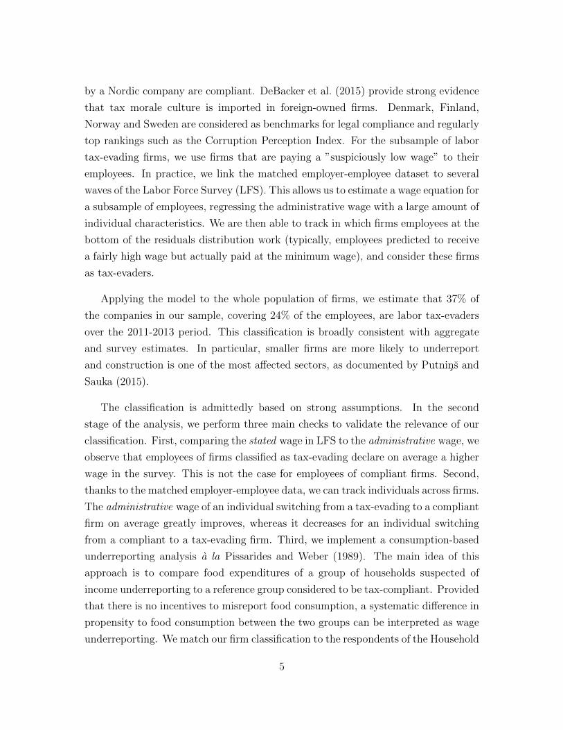
been much more salient for compliant firms than for tax-evading ones. Figure 5

plots the predicted change in employment between December 2014 and January 2013

conditional on the variables involved in this interaction.19 The change in employment

is very similar for compliant and tax-evading firms not affected by the policy change.

For firms with 100% of their employees affected, the point estimate is three times

smaller for evading firms than for compliant ones (-12.8% vs -4.6%). The same

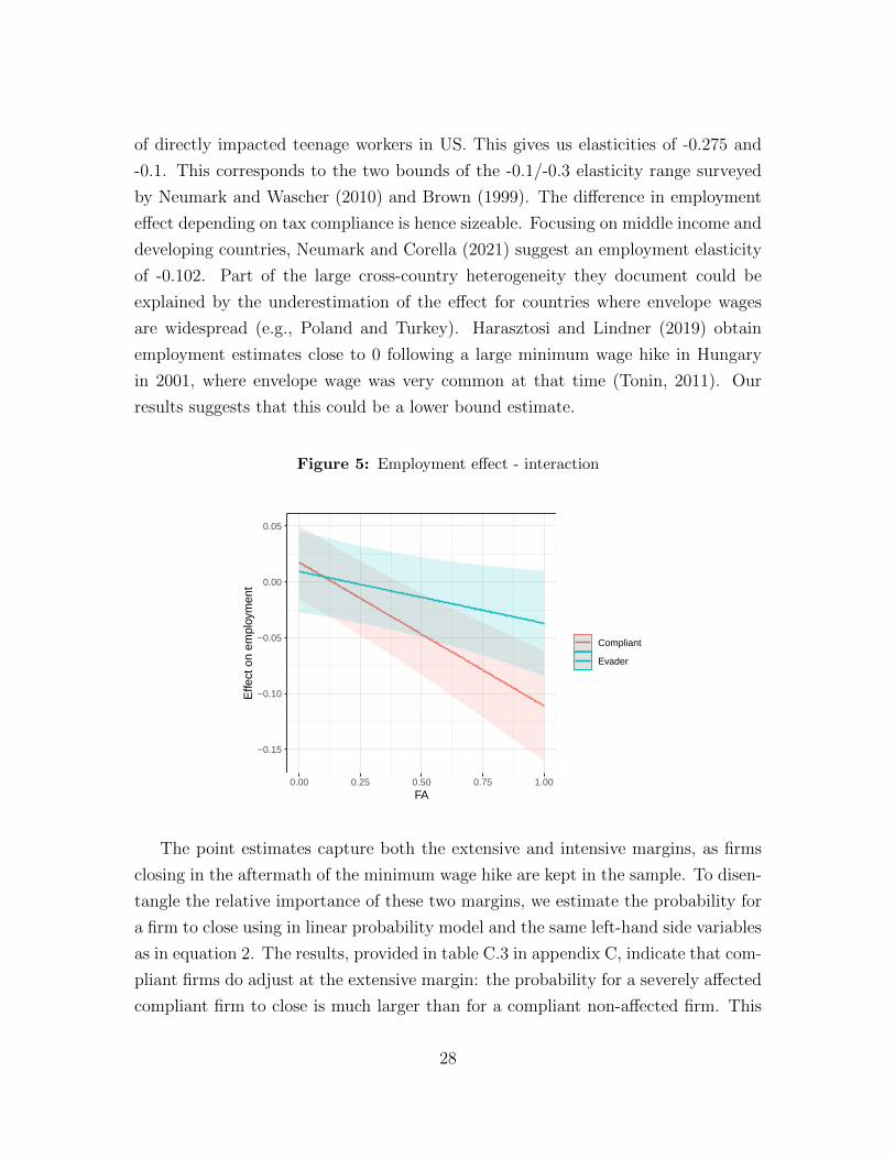
conclusion is reached when using GAP instead of FA, as displayed in columns 3 and

4.

The short run estimates imply an employment elasticity with respect to minimum

wage for the directly affected workers amounting to -1.1 for compliant firms and -

0.4 for evading firms. These elasticities are calculated using the whole population of

employees, and not only categories of employees particularly affected by the minimum

wage hike, such as teenage workers in the US literature. To be comparable with

the latter, we hence need to multiply our elasticities by 0.25, which is the share

19The graphical representation of the interaction using GAP is provided in appendix C.

27

of directly impacted teenage workers in US. This gives us elasticities of -0.275 and

-0.1. This corresponds to the two bounds of the -0.1/-0.3 elasticity range surveyed

by Neumark and Wascher (2010) and Brown (1999). The difference in employment

effect depending on tax compliance is hence sizeable. Focusing on middle income and

developing countries, Neumark and Corella (2021) suggest an employment elasticity

of -0.102. Part of the large cross-country heterogeneity they document could be

explained by the underestimation of the effect for countries where envelope wages

are widespread (e.g., Poland and Turkey). Harasztosi and Lindner (2019) obtain

employment estimates close to 0 following a large minimum wage hike in Hungary

in 2001, where envelope wage was very common at that time (Tonin, 2011). Our

results suggests that this could be a lower bound estimate.

Figure 5: Employment effect - interaction

−0.15

−0.10

−0.05

0.00

0.05

0.00 0.25 0.50 0.75 1.00FA

Effe

ct o

n em

ploy

men

t

Compliant

Evader

The point estimates capture both the extensive and intensive margins, as firms

closing in the aftermath of the minimum wage hike are kept in the sample. To disen-

tangle the relative importance of these two margins, we estimate the probability for

a firm to close using in linear probability model and the same left-hand side variables

as in equation 2. The results, provided in table C.3 in appendix C, indicate that com-

pliant firms do adjust at the extensive margin: the probability for a severely affected

compliant firm to close is much larger than for a compliant non-affected firm. This

28

Table 7: Short-run employment regressions

Dependent variable:

% change Jan 13 - Dec 14 % change Jan 13 - Jul 12

(1) (2) (3) (4) (5) (6)

Evasion −0.009 −0.008 −0.007 −0.004 0.006 0.006(0.013) (0.009) (0.012) (0.012) (0.009) (0.009)

FA −0.163∗∗∗ −0.128∗∗∗ 0.006(0.021) (0.012) (0.015)

FA× Evasion 0.082∗∗∗ 0.082∗∗∗ −0.003(0.029) (0.018) (0.021)

GAP −0.977∗∗∗ −0.727∗∗∗ −0.010(0.149) (0.150) (0.099)

GAP× Evasion 0.487∗∗∗ 0.452∗∗ 0.003(0.188) (0.186) (0.137)

Controls No Yes No Yes Yes Yes

Observations 5,524 5,524 5,524 5,524 5,524 5,524R2 0.013 0.048 0.010 0.046 0.067 0.067

Note: *** p<0.01, ** p<0.05, * p<0.1. Robust standard errors in parentheses. The set of controls include firm age, legal status,

NACE code, labor share and its square, profitability and its square, export share and its square .

contrasts with tax-evading firms, for which the probability to close remains about

the same irrespective of the intensity of the shock. Second, we estimate equation

2 keeping only firms surviving throughout the 2011-2017 period (hence excluding

all the firms that shut down after the hike). The results, displayed in table C.2 in

appendix C, show that compliant firms do also adjust employment at the intensive

margin.

29

Figure 6: Firm closure - interaction

0.025

0.050

0.075

0.00 0.25 0.50 0.75 1.00FA

P(c

lose

d)

Compliant

Evader

We document a clear difference in employment (no) response between compliant

and tax-evading ones in the short-run. We now investigate the medium run effect,

considering the two consecutive minimum wage hikes altogether. Table 8 provides

the results when comparing the percentage change in employment between January

2013 and December 2015, 2016 and 2017 (the last month of our sample). The

measure of treatment intensity is FA2015, the share of full-time employees paid below

the 2015 minimum wage in January 2013. The employment change for affected

compliant firms plummeted, whereas even in the medium run tax-evading firms did

not experience a significant staff reduction. Between January 2013 and December

2017, the employment elasticity with respect to minimum wage is equal to -1.2 for

compliant firms and -0.6 for tax evading ones, hence remaining largely different. The

results using GAP2015 are similar, and displayed in table 8.

The absence of employment reaction for tax-evading firms could also be explained

by a non-compliance with the new minimum wage, as documented for instance by

Basu et al. (2010). For instance, this could take the form of full-time employees artifi-

cially switching to part-time. To investigate this alternative channel, we estimate the

effect of minimum wage hike on average gross wage. Wage being only observable for

surviving firms, we restrict the sample accordingly. We examine changes in average

gross wage between January 2013 and four periods: June 2012 (one year before the

30

Table 8: Medium-run employment regressions

Dependent variable:

% change Jan 13 -Jan 12 Dec 15 Dec 16 Dec 17 Jan 12 Dec 15 Dec 16 Dec 17

(1) (2) (3) (4) (5) (6) (7) (8)

Evasion −0.005 −0.048∗∗∗ −0.070∗∗∗ −0.124∗∗∗−0.011 −0.034∗∗ −0.049∗∗∗ −0.099∗∗∗

(0.010) (0.018) (0.021) (0.025) (0.009) (0.016) (0.018) (0.022)FA2015 0.019 −0.197∗∗∗ −0.260∗∗∗ −0.316∗∗∗

(0.013) (0.023) (0.026) (0.028)FA2015× Evasion−0.027 0.164∗∗∗ 0.208∗∗∗ 0.275∗∗∗

(0.017) (0.031) (0.036) (0.039)GAP2015 0.038 −0.936∗∗∗ −1.225∗∗∗ −1.524∗∗∗

(0.061) (0.109) (0.122) (0.132)GAP2015× Evasion −0.063 0.759∗∗∗ 0.920∗∗∗ 1.276∗∗∗

(0.079) (0.141) (0.160) (0.177)

Observations 5,524 5,524 5,524 5,524 5,524 5,524 5,524 5,524R2 0.018 0.062 0.085 0.079 0.018 0.061 0.083 0.077

Note: *** p<0.01, ** p<0.05, * p<0.1. Robust standard errors in parentheses. FA2015 and GAP2015 measure the intensity

of the 2014 and 2015 minimum wage hikes altogether with respect to firm-level employment in January 2013. All regressions

include the following controls: firm age, legal status, NACE code, labor share and its square, profitability and its square, export

share and its square.

announcement of the hike, placebo check), June 2013 (announcement of the hike),

January 2014 (first month after the first hike) and January 2015 (first month after

the second hike).

The first panel of table 9 displays the results, alternatively using FA2015 and

GAP2015. We do not observe any difference in employment growth in the pre-hike

period. Average wage does not change in the direct aftermath of the minimum wage

announcement. However, average wages sharply increase directly after the imple-

mentation of the new minimum wage levels, both in 2014 and in 2015. The change

in average between January 2013 and January 2014 conditional on minimum wage

bite and tax evasion is plotted in figure 7a. The average wage increases in a parallel

way in the two groups, suggesting that tax evading firms did not avoid the increase in

labor cost differently than compliant firms. The conclusion is similar when focusing

on the 2015 hike. To further study this point, we proceed to the same analysis using

firm-level average income tax and average social contribution. The results are dis-

played respectively in panel 2 and panel 3 of table 9. Both exhibit a sharp increase

following the minimum wage hike. Firm reaction was similar irrespective of their

31

type, as shown in figure 7. Increasing minimum wage hence did have a negative em-

ployment effect, but did indeed increase income tax revenue and social contribution.

This rules out the explanation that tax-evading firms reduce their use of labor at the

intensive margin differently than compliant firms. From a policy point of view, these

results show that the objective of raising low-wage workers social cover effectively

targeted workers likely to receive envelope wage.

Figure 7: Effect on other measures

0.10

0.15

0.20

0.00 0.25 0.50 0.75 1.00FA

Effe

ct o

n w

age

Compliant

Evader

(a) Effect on wage

0.0

0.1

0.2

0.3

0.4

0.00 0.25 0.50 0.75 1.00FA

Effe

ct o

n ta

x

Compliant

Evader

(b) Effect on income tax

0.05

0.10

0.15

0.00 0.25 0.50 0.75 1.00FA

Effe

ct o

n so

cial

con

trib

utio

ns

Compliant

Evader

(c) Effect on social contribution

5 Conclusion

This paper provides a firm-level analysis of a minimum wage hike in a context of

prevalent labor tax evasion. We provide two main contributions to the literature.

First, we propose a novel methodology to classify firms between compliant and labor

tax avoiders using machine learning. This methodology relies on strong assumptions,

but several validity checks confirm the relevance of the approach. This classification

method can be used in other countries where envelope wage is a widespread phe-

nomenon provided that two necessary (but not sufficient) conditions are met: i) to

have access to firms’ balance sheet for the population of firms and employee-level

information for a subsample of workers; ii) to have a context where a subsample of

firms can be considered as compliant. The trends towards a more widespread access

to administrative data will make condition i) easier to satisfy in the coming years. An

alternative path could be to use audit data to construct a sample of compliant and

non-compliant firms. Audits are however rarely random, and this non-randomness

would imply that some types of evading firms are not captured. Our approach is

32

Table 9: Wage regressions

Dependent variable:

% change Jan 13 - Jun 12 Jun 13 Jan 14 Jan 15 Jun 12 Jun 13 Jan 14 Jan 15

(1) (2) (3) (4) (5) (6) (7) (8)

WageEvasion 0.007 0.015 0.020∗ 0.061∗∗∗ 0.014∗ 0.024∗∗ 0.063 0.005

(0.009) (0.009) (0.011) (0.019) (0.009) (0.011) (0.044) (0.008)FA2015 −0.001 −0.020 0.077∗∗∗ 0.158∗∗∗

(0.010) (0.013) (0.017) (0.024)FA2015× Evasion −0.011 −0.018 −0.011 −0.050

(0.015) (0.018) (0.022) (0.032)GAP2015 0.033 −0.169 0.767∗∗∗ 0.768∗∗∗

(0.100) (0.151) (0.180) (0.284)GAP2015× Evasion −0.076 −0.203 −0.192 −0.275

(0.140) (0.182) (0.217) (0.378)

Income taxEvasion 0.077∗∗ 0.061∗ 0.179∗∗∗ 0.071∗∗ 0.065∗∗ 0.154∗∗∗ 0.035

(0.028) (0.036) (0.032) (0.056) (0.031) (0.028) (0.044) (0.024)FA2015 0.027 0.028 0.118∗∗ 0.312∗∗∗

(0.042) (0.047) (0.048) (0.054)FA2015× Evasion −0.022 −0.068 −0.027 −0.149∗

(0.050) (0.058) (0.059) (0.083)GAP2015 0.454 0.439 1.412∗∗∗ 1.531∗∗∗

(0.368) (0.458) (0.455) (0.284)GAP2015× Evasion −0.144 −0.673 −0.503 −0.531

(0.452) (0.538) (0.558) (0.378)

Social contributionEvasion 0.008 0.015 0.020∗ 0.072∗∗∗ 0.014∗ 0.023∗∗ 0.074∗ 0.005

(0.009) (0.009) (0.011) (0.017) (0.009) (0.010) (0.044) (0.008)FA2015 −0.001 −0.020 0.076∗∗∗ 0.168∗∗∗

(0.010) (0.013) (0.016) (0.018)FA2015× Evasion −0.011 −0.019 −0.012 −0.054∗

(0.015) (0.018) (0.021) (0.028)GAP2015 0.032 −0.173 0.749∗∗∗ 0.777∗∗∗

(0.100) (0.150) (0.175) (0.284)GAP2015× Evasion −0.074 −0.205 −0.193 −0.280

(0.140) (0.182) (0.211) (0.378)

Observations 5,391 5,391 5,391 5,391 5,391 5,391 5,391 5,391

Note: *** p<0.01, ** p<0.05, * p<0.1. Robust standard errors in parentheses. FA2015 and GAP2015 measure the intensity of the

2014 and 2015 minimum wage hikes altogether with respect to firm-level employment in January 2013. All regressions include the fol-

lowing controls: firm age, legal status, NACE code, labor share and its square, profitability and its square, export share and its square.

not immune to this critic either, as what we capture is likely to emphasize labor

tax evasion at the bottom of the wage distribution. Note also that our classification

33

does not aim to serve as evasion detection device, but rather as a proxy for labor tax

evasion.

Equipped with this classification tool, we study conditional employment effect of

a large minimum wage hike. Compared to the existing literature, the magnitude and

the bite of this episode are both in the upper bound. We find that employment in

firms paying envelope wage is much less sensitive than in compliant firms. This is

consistent with the model proposed by Tonin (2011), and envelope wages can help

firms to absorb minimum wage shocks. Raising minimum wage hence contribute to

the enforcement of the tax policy and help to increase social protection coverage of

workers, in addition to increasing the average wage. Policy makers however do face a

trade-off, as a minimum wage hike can however have a negative effect on compliant

firms employing minimum wage workers. We only document short and medium run

partial equilibrium effects. One of the negative effects of labor tax evasion is a

competition distortion. If raising minimum wage increases compliance, on the long

run all compliant firms will benefit from a reduction in these distortions. Similarly,

our results are obtained focusing on firms that existed before the reform and we do not

address the question of firm entry. Also, we do not study the reallocation effect of the

minimum wage hike. Dustmann et al. (2020) provide evidence of such reallocation

effects studying the introduction of a minimum wage in Germany. Finally, even

if increasing minimum wage leads to an increase of workers’ social protection and

average reported wage, Tonin (2011) provides evidence that affected workers can

actually see a decrease in their total disposable income because of a larger tax base.

In future work, all these additional effects should be integrated in a unified framework

to estimate meaningful welfare consequences of a minimum wage hike.

34

A Classification details

This appendix provides additional details on the classification procedure. As for the

main part of the analysis, we restrict the sample to firms with at least 6 employees

over the 2011-2013 period operating in the manufacturing, trade/retail, construction

or transport sector. We begin with a description of the construction of the sample

for training and testing the classification algorithm. This sample is composed of two

parts. First, as a subsample of tax-compliant firms, we use the set of firms owned by

a Nordic company (Denmark, Finland, Norway, Sweden) over the 2011-2013 period.

Data on foreign ownership is provided by the Latvian Central Statistical Bureau

(CSB). In 2013, foreign-owned firms account for 13.3% of the firms in the sample

and Nordic-owned companies for 3.5%.

Second, to obtain a set of tax-evading firms we proceed as follows. We merge

the matched employer-employee data in the pre-reform period (2011-2013) to the

three LFS waves over the same period. Restricting the sample to the same sectors

as above and to full-time employees, we are left with roughly 3,000 individuals. We

then estimate a standard wage equation as follows, where the dependent variable is

the natural logarithm of the administrative wage (i.e., the wage reported to the tax

authorities). The set of regressors is composed of:

• Age, age2, experience and experience2 (all expressed in years),

• Dummy variables representing gender and whether the individual lives in a

urban or rural area,

• A series of categorical variables indicating the attained level education, the field

of education, the type of occupation, the sector, the region in Latvia where the

work is located, and the year where the interview has taken place.

The R2 is equal to 0.26, which is very close to other papers estimating a similar

wage equations (e.g., 0.27 in Harmon and Walker, 1995). We keep observations in

the bottom 10% of the residual distribution. From these 300 observations, more

than half earns no more than 110% of the minimum wage. We then retrieve in

which firms the individuals ”suspiciously low paid” individuals work and classify

them as tax-evaders. Each firm with at least one employee in the bottom of the

error distribution is classified as such. Anecdotally, we find only one Nordic-owned

35

firm that is having an employee in the bottom of the residual distribution. After

discarding this observation, we are left with 730 firm observations. This sample size

is of similar order as in the rest of the literature on financial fraud detection (see

e.g., Ravisankar et al., 2011 for a survey). Some descriptive statistics are provided

in table A.1. The four sectors are fairly represented across the two subsamples.

Table A.1: Sample statistics

N Pctl(25) Median Pctl(75)

Tax evading firms

# employees 126 23 47 119Turnover 126 744, 666.5 1, 868, 954 5, 794, 959.0Profit 126 48, 021.5 210, 469.5 648, 033.5Manufacturing 42Trade 37Transportation 33Construction 14

Compliant firms

# employees 569 15 35 76Turnover 569 1, 178, 442 3, 070, 452 7, 754, 268Profit 569 233, 658 586, 216 1, 433, 347Manufacturing 261Trade 237Transportation 52Construction 19

We use information from firms’ balance sheet as predictors. We use a combination

of ratio and direct balance sheet items that have previously been used for the study of

firm-level fraud detection (Beneish, 1999; Kotsiantis et al., 2006; Kirkos et al., 2007;

Cecchini et al., 2010; Ravisankar et al., 2011; West and Bhattacharya, 2016; Hajek

and Henriques, 2017). The complete list encompasses the following variables: asset,

fixed asset, net sales, gross profit, selling cost, other operating income, administrative

cost, net margin, operating margin, return on equity, return on asset, total asset to

revenue, cash to revenue, non-cash working capital to revenue, fixed asset to total

asset, growth in revenue, selling and administrative cost to revenue, non-cash working

capital, book debt to total asset, liquidity (cash to asset), growth of cash flow, tax

aggressiveness (corporate tax on asset). As suggested by Hastie et al. (2009), we do

36

not screen predictors based on their univariate correlation with the target variable

prior to cross-validation.

We divide the sample randomly in two parts: 80% of the observations are assigned

to the training group, the remaining 20% to the testing group. We apply gradient

boosting via the R package XGBoost though the Tidymodel interface. We set the

number of trees contained in the ensemble to 1000, and tune the model using four

hyperparameters: the maximum depth of the tree, the minimum number of data

points in a node that is required for the node to be split further, the learning rate,

and the reduction in the loss function required to split further. For finding the best

model (with respect to AUC), we use 10-fold cross-validation. We check the out-of-

sample performance on the training set, and then classify the whole universe of firms

contained in the main sample.

B The expenditure-based method

This appendix provides a description of the expenditure-based method originally

proposed by Pissarides and Weber (1989). This approach allows to estimate the

extent of underreporting for a group of households using reported income and ex-

penditures data. It relies on two main assumptions: i) food expenditures (or any

other item) is accurately reported for all groups; ii) income reporting is accurate

for at least one group in the population. Pissarides and Weber (1989) consider two

population groups: employees and self-employed, respectively denoted k = W and

k = S. Employees are assumed to correctly report wage. Food expenditures and

true permanent income are related by the Engel curve:

ln ci = α + βln yPi +X ′iφ+ εi (B.1)

where ci denotes food expenditure in household i, yPi is the permanent income,

Xi is a set of household characteristics (number of children, etc.) and εi is an error

term. Consumption is based on permanent income, but surveys usually enquire about

current income. Denoting pi the fraction of true current income to true permanent

income, we can write:

ln yi = ln pi + ln yPi . (B.2)

37

where pi is assumed to follow a log-normal distribution so that ln pi = µp + ui,

where µp is the sample mean of ln pi and ui is a disturbance with E[ui] = 0 and

σ2u = V ar(ui).

Self-employed respondents have incentives not to correctly report their income in

the survey (e.g., worries that survey answers are shared with tax authorities). The

relationship between the reported current income yi and the true current income y∗i

is

ln yi = ln κi + ln y∗i . (B.3)

κi is the underreporting factor, which is assumed to be log-normal so that ln κi =

µκ + vi with E[vi] = 0 and σ2v = V ar(vi). All employee households are assumed to

have κ = 1: they do not underreport their income. This implies that σ2v|W = 0 for

employees whereas σ2v|S > 0 for self-employed.

Combining equations B.2 and B.3, the true permanent income can be written as:

ln yPi = ln y∗i + ln κi − ln pi = ln y∗i + (µκ + vi)− (µp + u+ i) (B.4)

Inserting equation B.4 in equation B.1, the Engel curve is expressed as:

ln ci = α + βln y∗i + β(µκ − µp) +X ′iφ+ β(vi − ui) + εi (B.5)

This equation corresponds to empirical specification described in equation 1 in

section 3.2, where β(vi − ui) is substituted with γDi, so that γ = β(µκ +1

2(σ2

u|S −σ2u|W )), and the three error terms are encompassed in ξi. The coefficient γ captures

the systematic food expenditure shift of self-employed with respect to employees.

The mean underreporting factor κ can hence be computed as follows:

κ = exp

(γ

β+

1

2(σ2

v|S + σ2u|W − σ2

u|S)

)(B.6)

The variance terms usually being unknown, Pissarides and Weber (1989) show

that we can obtain lower and upper bound estimates for κ such that:

κ =

[exp

(γ

β− 1

2(σ2

ξ|S − σ2ξ|W )

), exp

(γ

β+

1

2(σ2

ξ|S − σ2ξ|W )

)](B.7)

38

Table B.1: HBS - descriptive statistics

Statistic N Mean St. Dev. Min Max

Ln food consumption 431 7.943 0.452 6.470 9.287Ln income 431 9.161 0.763 4.981 11.579Public sector 431 0.520 0.500 0 1Compliant firms 431 0.318 0.466 0 1Tax-evading firms 431 0.118 0.323 0 1Self-Employed 431 0.044 0.206 0 1

Note: Public sector, compliant firms, tax-evading firms and self-employed indicate the type of em-

ployment of the household head.

In the framework of this paper, we consider four groups of households: where the

head works in public sector, in a compliant firm, in a tax-evading firm or whether

the head is self-employed. Public sector is the base group, where envelope wages

presumably do not exist. This assumption is consistant with the Latvian context,

where several waves of public sector reforms have been implemented in the 2000’s.

Public sector employees are also used as the reference group in a study in Estonia

Paulus (2015). Note also that the underreporting estimates are relative. In other

words, it estimates the additional underreporting of a group of household compared

to another one. It provides an absolute measure only if the reference group does

indeed correctly report their income.

Turning to the estimation of equation 1, note that the reported income is en-

dogenous by construction. To overcome this issue, we instrument current income by

education of the household head (three levels) and region, since the average wage

differs across regions Latvia. The underlying assumption is that these variables do

not affect food expenditure other than through wage. As for the set of controls

included in both stages, it contains the number of children, the number of working

adults, head’s age and gender, and a dummy indicating whether the household rents

its dwelling. As is standard in the literature, we keep only households composed of

two adults and children (if any). Descriptive statistics are displayed in table B.1.

Assuming that the variance term is equal in the two groups, as for instance in

Hurst et al. (2014), then the underreporting estimate simplifies to κ = exp

(γ

β

).

From the regression results displayed in table 5, we can hence compute that for em-

39

ployees of tax-evading firms, κ = exp

(0.185

0.497

)≈ 1.57. The share of underreported

income is henceκ− 1

κ≈ 0.35, as reported in section 3.2.

40

C Minimum wage effect - Additional results

This section provides additional details regarding the estimation of the minimum

wage effect. First, as mentioned in section 4, the two measures FA and GAP are

computed using firm-level full-time employees. The motivation for this choice is that

before 2014 the number of hours was not mandatory to report. In addition, the

reported number of hours takes only into account effective hours. Employees taking

holidays will exhibit lower working hours this month than usual. This prevents us to

compute hourly wage, and compute the magnitude of the bite using all employees.

To disentangle part-time from full-time employees, we start by computing the

mode of working hours distribution for each month. This provides us with the

legal number of hours for a full-time equivalent job for each month. This number

changes every month depending on the number of working days. We then consider

an employee in a given firm as full-time for a given month if: i) the reported number

of hours is equal to or greater than 90% of the monthly mode or if ii) the number of

hours is missing but the wage is greater than 90% of the monthly minimum wage.

These assumptions are likely to overestimate the number of full-time employees. To

compute FA and GAP , in order to mitigate this effect we restrict full-time employees

as workers satisfying one of these conditions at least half of the months spent in a

given firm within a year. For instance, an employee working 6 months in a given

firm in 2012 earning 4 months more than the minimum wage but two months less

than the minimum wage will be considered as a full-time employee. The support for

FA conditional on firm type is displayed in figure C.1. For both types of firm, the

support ranges from 0 to 1.

41

Figure C.1: Distribution of FA

0

5

10

0.00 0.25 0.50 0.75 1.00FA

dens

ity

(a) Compliant firms

0.0

2.5

5.0

7.5

0.00 0.25 0.50 0.75 1.00FA

dens

ity

(b) Tax evading firms

Figure C.2 displays the unconditional relationship between FA and the percent-

age change in employment between January 2013 and December 2014, for compliant

and tax-evading firms separately. The number of bins is computed using the data-

driven approach of Cattaneo et al. (2019). Note the large difference in percentage

change in employment when comparing compliant and evading firms largely affected

by the minimum wage hike.

Figure C.2: Binscatter plot

42

Figure C.3 reproduces figure 5 using GAP instead of FA. It displays the inter-

action of GAP and the tax-evasion dummy from column (4) of table 7.

Figure C.3: Employment effect - interaction

−0.4

−0.3

−0.2

−0.1

0.0

0.0 0.1 0.2 0.3 0.4GAP

Effe

ct o

n em

ploy

men

t

Compliant

Evader

Table C.1 displays the results obtained when FA and GAP are not based on the

information in January 2013, but rather on the average number of employees over

2012. The results are in line with those displayed in table 7 in section 4.

Table C.2 is similar to table 7 in section 4 except that the models are run using

only firms that survived throughout the the whole period covered in the sample. The

results thus provide information on the employment effect at the intensive margin.

Together with table C.3, the results indicate that firms use both the intensive and

the extensive employment margins.

Table C.3 shows the effect of the interaction between minimum wage hike and

tax evasion on firm closure. The dependent variable takes the value 1 if the firm has

closed by the given period. Figure 6 in section 4 represents the interaction in column

(1).

43

Table C.1: Employment effect - average FA and GAP

Dependent variable:

% change Jan 13 - Dec 14 % change Jan 13 - Jul 12

(1) (2) (3) (4) (5) (6)

Evasion −0.020 −0.017∗ −0.019 −0.016 0.008 0.004(0.013) (0.009) (0.012) (0.012) (0.010) (0.009)

FAmean −0.127∗∗∗ −0.108∗∗∗ −0.007(0.021) (0.011) (0.013)

FAmean× Evasion 0.088∗∗∗ 0.085∗∗∗ −0.001(0.028) (0.016) (0.019)

GAPmean −1.278∗∗∗ −1.063∗∗∗ −0.115(0.199) (0.201) (0.126)

GAPmean× Evasion 0.940∗∗∗ 0.903∗∗∗ 0.106(0.261) (0.258) (0.177)

Controls No Yes No Yes Yes Yes

Observations 5,524 5,524 5,524 5,524 5,524 5,524R2 0.008 0.046 0.009 0.047 0.067 0.068

Note: *** p<0.01, ** p<0.05, * p<0.1 Robust standard errors in parentheses. The set of controls includes the following con-

trols: firm age, legal status, NACE code, labor share and its square, profitability and its square, export share and its square.

44

Table C.2: Employment effect - intensive margin

Dependent variable:

% change Jan 13 - Dec 14 % change Jan 13 - Jul 12

(1) (2) (3) (4) (5) (6)

Evasion −0.026∗∗ −0.023∗∗ −0.026∗∗ −0.023∗∗ 0.009 0.009(0.012) (0.009) (0.011) (0.012) (0.009) (0.008)

FA −0.102∗∗∗ −0.080∗∗∗ −0.001(0.018) (0.012) (0.014)

FA× Evasion 0.051∗∗ 0.052∗∗∗ −0.006(0.025) (0.017) (0.019)

GAP −1.025∗∗∗ −0.773∗∗∗ −0.008(0.184) (0.179) (0.138)

GAP× Evasion 0.573∗∗ 0.574∗∗ −0.092(0.246) (0.239) (0.188)

Controls No Yes No Yes Yes Yes

Observations 5,391 5,391 5,391 5,391 5,391 5,391R2 0.007 0.041 0.007 0.041 0.070 0.070

Note: *** p<0.01, ** p<0.05, * p<0.1 Robust standard errors in parentheses. The set of controls includes the following

controls: firm age, legal status, NACE code, labor share and its square, profitability and its square, export share and its

square.

45

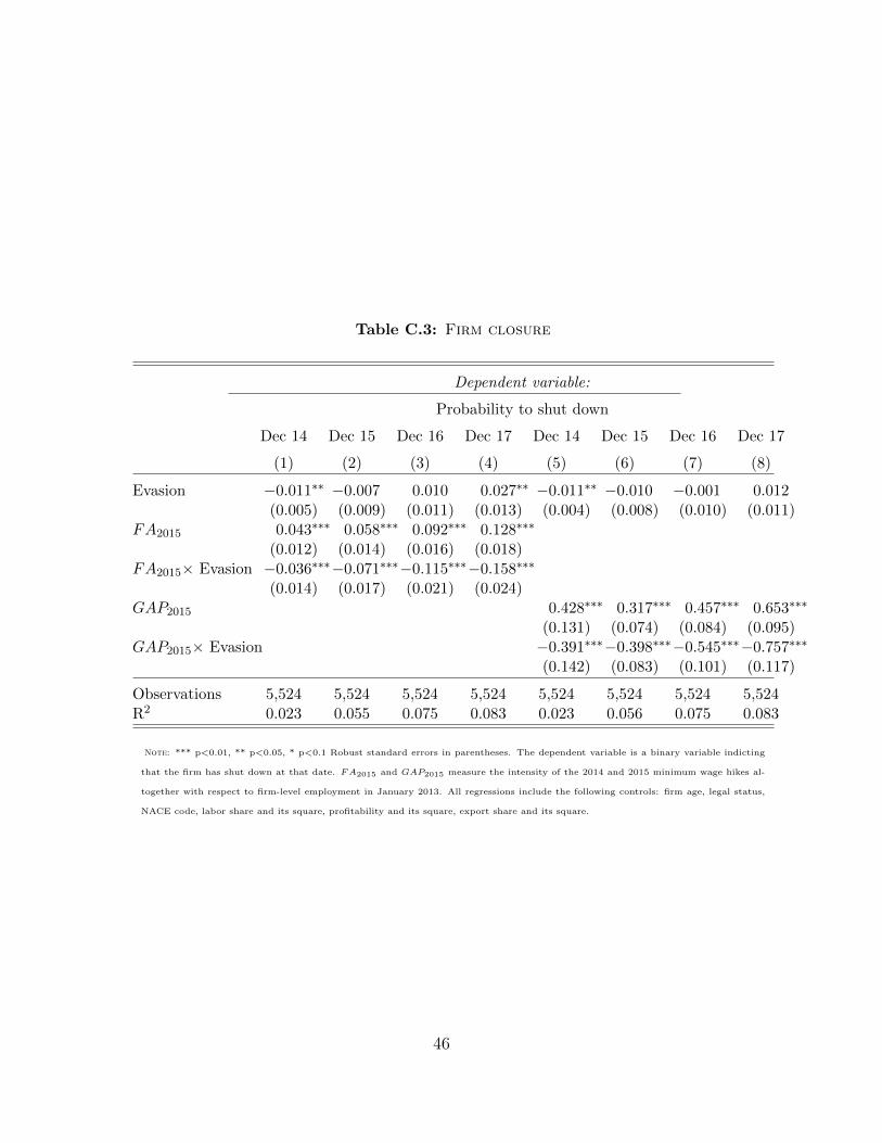
Table C.3: Firm closure

Dependent variable:

Probability to shut down

Dec 14 Dec 15 Dec 16 Dec 17 Dec 14 Dec 15 Dec 16 Dec 17

(1) (2) (3) (4) (5) (6) (7) (8)

Evasion −0.011∗∗ −0.007 0.010 0.027∗∗ −0.011∗∗ −0.010 −0.001 0.012(0.005) (0.009) (0.011) (0.013) (0.004) (0.008) (0.010) (0.011)

FA2015 0.043∗∗∗ 0.058∗∗∗ 0.092∗∗∗ 0.128∗∗∗

(0.012) (0.014) (0.016) (0.018)FA2015× Evasion −0.036∗∗∗−0.071∗∗∗−0.115∗∗∗−0.158∗∗∗

(0.014) (0.017) (0.021) (0.024)GAP2015 0.428∗∗∗ 0.317∗∗∗ 0.457∗∗∗ 0.653∗∗∗

(0.131) (0.074) (0.084) (0.095)GAP2015× Evasion −0.391∗∗∗−0.398∗∗∗−0.545∗∗∗−0.757∗∗∗

(0.142) (0.083) (0.101) (0.117)

Observations 5,524 5,524 5,524 5,524 5,524 5,524 5,524 5,524R2 0.023 0.055 0.075 0.083 0.023 0.056 0.075 0.083

Note: *** p<0.01, ** p<0.05, * p<0.1 Robust standard errors in parentheses. The dependent variable is a binary variable indicting

that the firm has shut down at that date. FA2015 and GAP2015 measure the intensity of the 2014 and 2015 minimum wage hikes al-

together with respect to firm-level employment in January 2013. All regressions include the following controls: firm age, legal status,

NACE code, labor share and its square, profitability and its square, export share and its square.

46

References

Allegretto, S., Reich, M., 2018. Are local minimum wages absorbed by price in-

creases? estimates from internet-based restaurant menus. ILR Review 71, 35–63.

Allegretto, S.A., Dube, A., Reich, M., 2011. Do minimum wages really reduce teen

employment? accounting for heterogeneity and selectivity in state panel data.

Industrial Relations: A Journal of Economy and Society 50, 205–240.

Almunia, M., Lopez-Rodriguez, D., 2018. Under the radar: The effects of monitoring

firms on tax compliance. American Economic Journal: Economic Policy 10, 1–38.

Artavanis, N., Morse, A., Tsoutsoura, M., 2016. Measuring income tax evasion using

bank credit: Evidence from greece. The Quarterly Journal of Economics 131,

739–798.

Ashenfelter, O., Smith, R.S., 1979. Compliance with the minimum wage law. Journal

of Political Economy 87, 333–350.

Athey, S., Imbens, G.W., 2019. Machine learning methods that economists should

know about. Annual Review of Economics 11, 685–725.

Bank, W., 2017. Latvia tax review.

Basu, A.K., Chau, N.H., Kanbur, R., 2010. Turning a blind eye: Costly enforcement,

credible commitment and minimum wage laws. The Economic Journal 120, 244–

269.

Bell, B., Machin, S., 2018. Minimum wages and firm value. Journal of Labor Eco-

nomics 36, 159–195.

Beneish, M.D., 1999. The detection of earnings manipulation. Financial Analysts

Journal 55, 24–36.

Bergolo, M.L., Ceni, R., Cruces, G., Giaccobasso, M., Perez-Truglia, R., 2017. Tax

audits as scarecrows: Evidence from a large-scale field experiment. Technical

Report. National Bureau of Economic Research.

47

Bıro, A., Prinz, D., Sandor, L., et al., 2020. Tax Evasion and the Minimum Wage.

Technical Report. Institute of Economics, Centre for Economic and Regional Stud-

ies.

Bosch, M., Manacorda, M., 2010. Minimum wages and earnings inequality in urban

mexico. American Economic Journal: Applied Economics 2, 128–49.

Braguinsky, S., Mityakov, S., 2015. Foreign corporations and the culture of trans-

parency: Evidence from russian administrative data. Journal of Financial Eco-

nomics 117, 139–164.

Braguinsky, S., Mityakov, S., Liscovich, A., 2014. Direct estimation of hidden earn-

ings: Evidence from russian administrative data. The Journal of Law and Eco-

nomics 57, 281–319.

Brown, C., 1999. Minimum wages, employment, and the distribution of income.

Handbook of labor economics 3, 2101–2163.

Cattaneo, M.D., Crump, R.K., Farrell, M.H., Feng, Y., 2019. On binscatter. arXiv

preprint arXiv:1902.09608 .

Cecchini, M., Aytug, H., Koehler, G.J., Pathak, P., 2010. Detecting management

fraud in public companies. Management Science 56, 1146–1160.

Chen, T., Guestrin, C., 2016. Xgboost: A scalable tree boosting system. Proceedings

of the 22nd acm sigkdd international conference on knowledge discovery and data

mining , 785–794.

Clemens, J., Strain, M.R., 2020. Understanding “Wage Theft”: Evasion and Avoid-

ance Responses to Minimum Wage Increases. Technical Report. National Bureau

of Economic Research.

DeBacker, J., Heim, B.T., Tran, A., 2015. Importing corruption culture from over-

seas: Evidence from corporate tax evasion in the united states. Journal of Financial

Economics 117, 122–138.

Desai, M.A., Dharmapala, D., 2009. Corporate tax avoidance and firm value. The

review of Economics and Statistics 91, 537–546.

48

Draca, M., Machin, S., Van Reenen, J., 2011. Minimum wages and firm profitability.

American economic journal: applied economics 3, 129–51.

Drucker, L., Mazirov, K., Neumark, D., 2019. Who pays for and who benefits from

minimum wage increases? Evidence from Israeli tax data on business owners and

workers. Technical Report. National Bureau of Economic Research.

Dube, A., Lester, T.W., Reich, M., 2010. Minimum wage effects across state borders:

Estimates using contiguous counties. The Review of Economics and Statistics 92,

945–964.

Dustmann, C., Lindner, A., Schonberg, U., Umkehrer, M., Vom Berge, P., 2020.

Reallocation effects of the minimum wage. Centre for Research and Analysis of

Migration Discussion Paper 7, 20.

Eamets, R., Masso, J., 2005. The paradox of the baltic states: Labour market

flexibility but protected workers? European Journal of Industrial Relations 11,

71–90.

Engstrom, P., Hagen, J., 2017. Income underreporting among the self-employed: a

permanent income approach. European Economic Review 92, 92–109.

Eurobarometer, S., 2014. Undeclared work in the European Union. Technical Report.

European Commission.

Feldman, N.E., Slemrod, J., 2007. Estimating tax noncompliance with evidence from

unaudited tax returns. The Economic Journal 117, 327–352.

Fisman, R., Miguel, E., 2007. Corruption, norms, and legal enforcement: Evidence

from diplomatic parking tickets. Journal of Political Economy 115, 1020–1048.

Fisman, R., Wei, S.J., 2004. Tax rates and tax evasion: evidence from “missing

imports” in china. Journal of Political Economy 112, 471–496.

Friedman, J.H., 2001. Greedy function approximation: a gradient boosting machine.

Annals of Statistics , 1189–1232.

Garnero, A., Lucifora, C., 2020. Turning a blind eye? Compliance to minimum

wages and employment. Technical Report. Working Paper.

49

Gavoille, N., Zasova, A., 2021. Foreign ownership and labor tax evasion: Evidence

from Latvia. Technical Report. BICEPS Working Paper.

Georgiadis, A., Manning, A., 2020. The impact of the uk minimum wage: Evidence

from high-frequency firm-level data. Available at SSRN 3560897 .

Goraus-Tanska, K., Lewandowski, P., 2016. Minimum wage violation in central and

eastern europe (iza discussion papers, no. 10098). Bonn: Institute for the Study

of Labor (IZA) .

Gorodnichenko, Y., Martinez-Vazquez, J., Sabirianova Peter, K., 2009. Myth and

reality of flat tax reform: Micro estimates of tax evasion response and welfare

effects in russia. Journal of Political economy 117, 504–554.

Hajek, P., Henriques, R., 2017. Mining corporate annual reports for intelligent detec-

tion of financial statement fraud–a comparative study of machine learning meth-

ods. Knowledge-Based Systems 128, 139–152.

Harasztosi, P., Lindner, A., 2019. Who pays for the minimum wage? American

Economic Review 109, 2693–2727.

Harmon, C., Walker, I., 1995. Estimates of the economic return to schooling for the

united kingdom. The American Economic Review 85, 1278–1286.

Hastie, T., Tibshirani, R., Friedman, J., 2009. The elements of statistical learning:

data mining, inference, and prediction. Springer Science & Business Media.

Hazans, M., 2011. Informal workers across europe: Evidence from 30 european

countries. World Bank Policy Research Working Paper .

Huang, S.Y., Tsaih, R.H., Yu, F., 2014. Topological pattern discovery and feature

extraction for fraudulent financial reporting. Expert systems with applications 41,

4360–4372.

Hurst, E., Li, G., Pugsley, B., 2014. Are household surveys like tax forms? evi-

dence from income underreporting of the self-employed. Review of economics and

statistics 96, 19–33.

50

Jascisens, V., Zasova, A., 2021. Million dollar baby: Should parental benefits depend

on wages when the payroll tax evasion is present? BICEPS Working Paper series

.

Kirkos, E., Spathis, C., Manolopoulos, Y., 2007. Data mining techniques for the

detection of fraudulent financial statements. Expert systems with applications 32,

995–1003.

Kleven, H.J., Knudsen, M.B., Kreiner, C.T., Pedersen, S., Saez, E., 2011. Unwilling

or unable to cheat? evidence from a tax audit experiment in denmark. Economet-

rica 79, 651–692.

Kotsiantis, S., Koumanakos, E., Tzelepis, D., Tampakas, V., 2006. Forecasting

fraudulent financial statements using data mining. International journal of com-

putational intelligence 3, 104–110.

Kukk, M., Paulus, A., Staehr, K., 2020. Cheating in europe: underreporting of

self-employment income in comparative perspective. International Tax and Public

Finance 27, 363–390.

Kukk, M., Staehr, K., 2014. Income underreporting by households with business

income: evidence from estonia. Post-Communist Economies 26, 257–276.

Kumler, T., Verhoogen, E., Frıas, J., 2020. Enlisting employees in improving payroll

tax compliance: Evidence from mexico. Review of Economics and Statistics 102,

881–896.

Lastauskas, P., Prosukute, A., Zaldokas, A., 2021. How do firms adjust when trade

stops? Unpublished manuscript .

Lemos, S., 2009. Minimum wage effects in a developing country. Labour Economics

16, 224–237.

Liu, X., 2016. Corruption culture and corporate misconduct. Journal of Financial

Economics 122, 307–327.

Machin, S., Manning, A., Rahman, L., 2003. Where the minimum wage bites hard:

Introduction of minimum wages to a low wage sector. Journal of the European

Economic Association 1, 154–180.

51

Magda, I., 2017. Do trade unions in central and eastern europe make a difference?

IZA World of Labor .

Manning, A., 2021. The elusive employment effect of the minimum wage. Journal

of Economic Perspectives 35, 3–26.

Mayneris, F., Poncet, S., Zhang, T., 2018. Improving or disappearing: Firm-level

adjustments to minimum wages in china. Journal of Development Economics 135,

20–42.

Meer, J., West, J., 2016. Effects of the minimum wage on employment dynamics.

Journal of Human Resources 51, 500–522.

Meghir, C., Narita, R., Robin, J.M., 2015. Wages and informality in developing

countries. American Economic Review 105, 1509–46.

Mullainathan, S., Spiess, J., 2017. Machine learning: an applied econometric ap-

proach. Journal of Economic Perspectives 31, 87–106.

Naritomi, J., 2019. Consumers as tax auditors. American Economic Review 109,

3031–72.

Neumark, D., Corella, L.F.M., 2021. Do minimum wages reduce employment in

developing countries? a survey and exploration of conflicting evidence. World

Development 137, 105165.

Neumark, D., Wascher, W., 2010. Minimum Wages. MIT Press, Cambridge, MA.

Nygard, O.E., Slemrod, J., Thoresen, T.O., 2019. Distributional implications of joint

tax evasion. The Economic Journal 129, 1894–1923.

OECD, 2013. Protecting jobs, enhancing flexibility: a new look at employment

protection legislation.

OECD, 2019. Oecd economic surveys: Latvia.

Paulus, A., 2015. Tax evasion and measurement error: An econometric analysis

of survey data linked with tax records. Technical Report. ISER Working Paper

Series.

52

Pelek, S., Uysal, G., 2018. Envelope wages, underreporting and tax evasion: The

case of turkey, 17th Louis-Andre-Gerard-Varet International Conference in Public

Economics, June.

Perry, G.E., Arias, O., Fajnzylber, P., Maloney, W.F., Mason, A., Saavedra-

Chanduvi, J., 2007. Informality: Exit and exclusion. The World Bank.

Pissarides, C.A., Weber, G., 1989. An expenditure-based estimate of britain’s black

economy. Journal of Public Economics 39, 17–32.

Pomeranz, D., 2015. No taxation without information: Deterrence and self-

enforcement in the value added tax. American Economic Review 105, 2539–69.

Putnins, T.J., Sauka, A., 2015. Measuring the shadow economy using company

managers. Journal of Comparative Economics 43, 471–490.

Ravisankar, P., Ravi, V., Rao, G.R., Bose, I., 2011. Detection of financial statement

fraud and feature selection using data mining techniques. Decision support systems

50, 491–500.

Renkin, T., Montialoux, C., Siegenthaler, M., 2020. The pass-through of minimum

wages into us retail prices: evidence from supermarket scanner data. Review of

Economics and Statistics , 1–99.

Slemrod, J., 2007. Cheating ourselves: The economics of tax evasion. Journal of

Economic perspectives 21, 25–48.

Tonin, M., 2011. Minimum wage and tax evasion: Theory and evidence. Journal of

Public Economics 95, 1635–1651.

Tonin, M., 2013. Underreporting of earnings and the minimum wage spike. IZA

Journal of European Labor Studies 2, 1–18.

Varian, H.R., 2014. Big data: New tricks for econometrics. Journal of Economic

Perspectives 28, 3–28.

West, J., Bhattacharya, M., 2016. Intelligent financial fraud detection: a compre-

hensive review. Computers & security 57, 47–66.

53

Zasova, A., 2011. Labour market institutions: an obstacle or support to latvian

labour market recovery? Baltic Journal of Economics 11, 5–23.

54