WP 2015: 15

Labor-intensive jobs for women and development Intrahousehold welfare effects and its transmission channels

Tigabu D. Getahun and Espen Villanger

Chr. Michelsen Institute (CMI) is an independent, non-profit research institution and a major international centre in policy-oriented and applied development research. Focus is on development and human rights issues and on international conditions that affect such issues. The geographical focus is Sub-Saharan Africa, Southern and Central Asia, the Middle East and Latin America.

CMI combines applied and theoretical research. CMI research intends to assist policy formulation, improve the basis for decision-making and promote public debate on international development issues.

1    

Labor-intensive jobs for women and development:

Intrahousehold welfare effects and its transmission channels

Tigabu D. Getahun and Espen Villanger

December 2015

Abstract

We examine the welfare impacts of women getting low-skilled jobs and find large positive effects, both at the household and the individual level. However, the women workers, their husbands and their oldest daughters reduced their leisure, but women to a much larger extent than the others. The leisure of the oldest son did not change. Investigating the transmission mechanisms suggests that the impacts did not only go through income and substitution effects, but also through a bargaining effect. Getting the job likely improved the bargaining position of the wife through several mechanisms, which in turn added to the positive impact on her welfare.

 

 

 

Keywords: salaried employment, wage labor, gender, bargaining, consumption, poverty, hunger

 

   

2    

 

1. Introduction

Growth in labor-intensive industries, especially those that employ the poor, is believed to be major route

out of poverty for developing countries, particularly those in Sub-Saharan Africa (Loayza and Raddatz

2010, Rodrik 2015). However, very little is known about the welfare impacts of such jobs at the micro

level where the first-order effects of such transitions may be identified (Blattman and Dercon 2015).

Moreover, there is surprisingly little solid evidence about the transmission mechanisms through which the

job may change the intrahousehold welfare allocations, including the links between women employment,

bargaining power and individual outcomes. In this paper, we study the impacts on intrahousehold welfare

of women transitioning from traditional activities into formal salaried low-skilled employment and assess

the income, substitution and bargaining effects.

A sector's poverty-reducing capacity may be related to the degree to which it employs unskilled labor,

since the poor can provide their labor as a production input (Loayza and Raddatz 2010). Such

employment may provide a direct link between economic growth and poverty reduction and hence,

policymakers have used many resources to attract such investments through financing special economic

zones, regulatory frameworks and direct subsidies (World Bank 2013). In addition, much of the low-

skilled industries employ mostly women, and increased earnings of women is believed to be particularly

important for investments in their children’s nutrition, health and education that in turn would enhance the

long-run poverty reducing effects (Duflo 2012). Jobs are also believed to be important for gender equality

by improving the position of women and their bargaining power and hence creates an additional interest

from policymakers (Duflo 2012).

In theory, the equilibrium wage is determined by the marginal product of the worker, factor prices are

equalized across sectors and the utility of the worker of getting the job would be equal to her

counterfactual outcome. Hence, in low-skilled industries where there are no minimum wages or labor

unions, monitoring is costless and there is abundance of labor, one would predict that the welfare effect of

getting such a job would not be substantial. This is indeed what Blattman and Dercon (2015) find in

manufacturing industries.

However, higher wages and worker utility can be maintained in imperfect markets, but also between

equilibria that in our setting typically is modelled as a structural transformation where manufacturing

3    

growth attracts labor from traditional rural agriculture by offering higher wages.1 We find large positive

household welfare effects from women getting low-skilled jobs in the rose farm sector in rural Ethiopia.

The effects are strong along all indicators used; consumption, income, various poverty measures, food

security and hunger indicators.

We identify effects by comparing women who got a job in the cut flower industry with similar women

who also applied for jobs, but for various reasons never started working. This accounts for self-selection

into job search. Moreover, the hiring of workers in the sector is claimed to be random by all involved

parties; farms recruit those who show up for work at the farm gate. Our inspection of the hiring process

and qualitative work suggests the same; farm management use no energy on screening the thousands of

applicants (e.g. no formal interview processes or assessment of candidates other than visual inspection),

no education or experience is required. In addition, the work-task are very simple and unproductive labor

can easily be laid off in a probation period. Moreover, there are insignificant differences between hired

and non-hired at women at the time they applied along most of the relevant indicators. Instrumenting

yields the same result qualitatively; selection bias seems not to matter much to the results.

Most likely, our results differ from those of Blattman and Dercon (2015) due to the counterfactual of

getting a job. In the poor rural areas we study, the alternatives to formal employment for women are less

attractive. They typically involve domestic work without pay (household chores), to run microbusinesses

with very low returns, or to contribute in traditional household agriculture. We find that having a job at

the rose farms is highly appreciated and that turnover rates are relatively low. On the other hand, in the

better functional labor markets in urban and semi-urban areas studied by Blattman and Dercon, they find

that many workers’ alternatives are to get another formal/semi-formal job or to engage in businesses with

higher returns. Many of their outside alternatives are more attractive in these areas, and as many as 77%

of the workers in the study companies had quit within a year.

Effects at the overall household level, or at the worker level, may disguise important intrahousehold

differences in welfare allocations. We find large differences in changes of leisure demand that conforms

to what is typically labelled as women “double” or “triple” working when she takings care of most of the

                                                                                                                         1 The most famous early model of such a structural transformation was formulated by Arthur Lewis (Lewis 1954). However, the key element of maintaining higher wages during transitions from one steady state to another can be found in a much wider specter of models relevant for the Ethiopian setting with large expansion in rose farming in a short time horizon. Moreover, such differentials can be maintained when union bargaining results in higher wages (Card 1996) or when there is labor poaching or efficiency wages (Katz et al. 1989, Shapiro and Stiglitz 1984, Akerlof and Yellen 1986) and in labor markets where learning is important (see the literature on learning and matching, for example Papageorgiou 2014).

4    

traditional household responsibilities in addition to a full time job. Women who got the job reduced their

leisure by more than two hours a day, which led to retrenchment of time for sleep. Husbands and older

daughters also reduced their leisure, but much less dramatically, while there were no changes for the sons’

leisure.

According to Ashraf (2009), intrahousehold bargaining may be crucial in order to understand the welfare

distributions within the household. Following the reasoning of cooperative household models, an

improvement in women´s bargaining power changes the resource allocation more in favor of the women’s

priorities (Von-Braun 1989, Sen 1990, Thomas, 1990, 1994; Engle 1993; Hoddinott and Haddad, 1995;

Duflo, 2003).  Therefore, if women securing formal, permanent employment also improves their

bargaining position within the household, one may expect that the allocations of welfare within the

household is skewed towards the women (Duflo 2012). We indeed find that bargaining power increases

among the hired women, and that this changes the resource allocation in a way that causes an additional

improvement in female welfare.

Our study relates to a small literature that identify and quantify causal effects of industrial employment on

intra household decisions. Jensen (2012) and Heath and Mobarak (2014) finds that improvements in labor

market opportunities for women leads to reduced fertility, postponed marriage and that women take more

education. Blattman and Dercon (2015), perhaps the study closest to ours, find that being offered a job in

various industries in Ethiopia does not lead to any different impacts for the workers in terms of  average

hours worked, income, and wages as compared to a control group that was not offered a job.

Most empirical welfare analysis still focuses on total household impacts rather than the intrahousehold

distributional effects (Ashraf 2009). Our work relates to the intrahousehold bargaining literature, which

suggests that the allocations within the household is the most important determinant of aggregate

inequality in poor countries (Hadded and Kanbur 1990 and Dercon and Krishnan 2000). We show that

failing to account for the intrahousehold allocations may lead to misleading conclusions about the impacts

of employment, and also to a lack of understanding the transmission mechanisms behind the outcomes.

Husbands are usually the household heads with more decision making power over the allocation of

household goods than the wife (see for example Lim et al. 2007). Some husbands may even confiscate the

wife’s income to spend it on his own consumption (Anderson and Baland 2002) or spend more on himself

when that is not revealed to his spouse (Ashraf 2009). In addition, other family members, such as older

children, may be affected by the relative bargaining power between the spouses. When the women gets a

job, it has been found that older children step in to take care of younger siblings and contribute to

5    

household chores (World Bank, 2012). It may matter a lot to outcomes whether gender inequalities are

reinforced by pulling the oldest girl out of school for such purposes, or if the tasks are more equally

distributed in the household.

In addition, there is also a descriptive literature discussing correlates between individual and household

characteristics and job opportunities. (Henderson 1997, Combes 2000, Blien et al. 2006, Sonobe et al.

2013). Although no causal impact can be detected from such studies, there are varying suggestions about

the degree to which these jobs bring about improvements in the workers lives – ranging from labels of

distress sale of labor while others described it as an important means to empower unskilled poor rural

women (Ilahi 2000, Doss 2011). Moreover, using Spanish data, Carrasco and Zamora (2010) suggests

that when women got salaried employment, it led to an increase in consumption of most household

commodities. Likewise, using survey data from poor urban women in India, Salway, Rahman and Jesmin

(2003) found significant and multifaceted improvements in livelihood from female employment. Our

findings on impacts on poverty are similar to the suggestions of previous studies such as Martin and

Robert (1984) and Stier and Lewin (2002). This also links to the food security literature. Our results

suggest that the job significantly improved their food security, which is similar to the findings of

Chiappori (1988), Von Braun (1989), Thomas (1994), Hoddinott and Haddad (1995) and Duflo (2003).

2. Context

The flower industry in Ethiopia emerged in the late 1990s and started to export in early 2000s. In 2002,

only three flower farms were exporting but other investors quickly realized the potential.2 Today around

100 commercial flower farms are in operation and more than 85,000 direct low-skilled jobs has been

created in the sector. In addition, this has created a large number of indirect jobs for the neighboring rural

communities, mostly for unskilled women who are believed to lack income opportunities (EHPEA 2013).

Moreover, the whole horticulture sector has grown tremendously during the last decade, based on the

same type of production offering the same type of low-skilled jobs and EHPEA claims it employs

180.000 workers.3

                                                                                                                         2 The government initiated a policy package in 2003 that marked start of the tremendous growth. The GoE allocated large areas of land (1000 ha) for flower productions and provided electricity, telecommunication services and long-term credit at affordable interest rate to both foreign and domestic investors (Gebreyesus and Lizuka 2012). 3 Schaefer and Abebe (2015) questions the EHPEA’s figures. In a comparison from 2011/12, they find that survey based estimates is around half of what is claimed by EHPEA (2013).

6    

This type of production is highly labor intensive and international competition in the product market is

fierce (Hortiwise 2012). Hence, the availability of cheap labor was likely an important condition for the

expansion. Widespread poverty and abundance of unskilled labor ensures the availability of workers at

internationally competitive wages in the commercial horticulture areas. In rural Oromia almost every third

household was below the national poverty line of approximately USD 0.5 per day in 2010/11 (MoFED

2012). Nevertheless, the daily wage for an unskilled rose farm worker was less than one USD, which was

comparable to the daily support that the food-insecure individuals would get in public works projects to

prevent hunger.

The low levels of skills and education are reflected in the illiteracy rates; for women in Oromia it was

62% while it was only 32% for men (CSA and ICF International, 2012). The gender disparities in

education underline the disadvantaged situation for women in the area: Almost half of the women in

Oromia do not have any education compared to 26% of the men. Similarly, only 37% of the women have

some primary education while around half of the men are in that category. The weak position of the

women gives an indication of the unequal power balance between the workers and the farm management,

which is exacerbated by the absence of functioning trade unions. Although the national trade union has

organized most of the commercial farms, there are few opportunities for the workers to raise issues of

concern. The management has actively discouraged unions both through termination of employment and

promotions to redirect their focus and it is usually not clear for the women workers what is the purpose of

the unions and what they do (Aman 2011, Villanger, Getahun and Solomon 2015).

The country also suffers from large gender inequalities, despite several recent positive policy reforms

(Mabsout and Staveren 2010). Very few Ethiopian women make household decisions by themselves.

Only half of the women participate with their husbands in all of three decisions on issues like her own

health care, household purchases and her own visits to her family or relatives, and almost three times

more men than women owns assets such as a house or have use rights over land (CSA and ICF

International, 2012). Even when the women do own or have rights to assets, these assets are usually

controlled by men (Lim et al. 2007). Also suggestive of large intrahousehold power imbalances, domestic

violence is common and accepted by both men and women. In parts of Ethiopia, 71 % of ever-partnered

women have been physically assaulted by a male partner (Garcia-Moreno et al. 2005) and 76 % of all

women in rural Ethiopia agrees that it is justified for a husband to beat his wife for some specific reason

(CSA and ICF International, 2012).

7    

The “land grabbing” debate is also part of this context as the rose farm expansions require large areas to

reach a profitable scale of cultivation (see for example Hall 2011). Since all land in Ethiopia is owned by

the state, it has been relatively straightforward for the government to reallocate large land areas from local

populations to commercial farms. However, most of the local population makes a living from agriculture.

With diminishing plot sizes due to population growth, with few and poor alternative income generating

opportunities, and with a continuous food deficit, a lot of critique has been raised against using productive

land to flower cultivation.

The rose farm industry also has a hazardous working environment. The production could cause water, air

and soil pollution because of its intensive and unregulated chemical usage and poor waste disposal

management (Organic Consumers Association 2006). Several women workers and their husbands did

complain about the potential negative health impacts of exposure to chemicals (Villanger, Getahun and

Solomon 2015). Moreover, the flower sector is characterized by its intensive use of water, which is said to

have negatively impacts on the adjacent farmers who rely on the ground water for their crop cultivation

and cattle breeding (Fatuma 2008 and Getu 2009).

3. Theoretical Model

We mainly use consumption as the welfare indicator since it captures the means by which households can

achieve welfare (Deaton 1997, Strengmann-Kuhn 2000, Wagle 2007). To model consumption demand,

we use a modified version of the Browning and Chiappori (1988) cooperative collective household model

that highlights intrahousehold conflicts and gender based power disparities (Browning, Chiappori and

Weiss 2011). Although Pareto efficiency of intrahousehold allocation does not always hold, as shown by

Udry (1996), we see no compelling argument that the bargaining over consumption in our setting would

yield inefficient solutions.

Assume that the husband and the wife are the only decision makers in the household and that the spouses

care about their own and their partner’s consumption and leisure. Accordingly, the preferences of each

spouse is represented by a direct utility function4 that allows altruism and externality, where the husbands

utility, 𝑈𝑈", and the wife’s utility,  𝑈𝑈$, are given by

                                                                                                                         4 The utility functions are assumed to be strictly concave and twice differentiable in all of their arguments.

8    

𝑈𝑈" 𝑄𝑄, 𝐶𝐶, 𝑞𝑞", 𝑞𝑞$, 𝑐𝑐", 𝑐𝑐$, 𝑙𝑙", 𝑙𝑙$ and 𝑈𝑈$ 𝑄𝑄, 𝐶𝐶, 𝑞𝑞", 𝑞𝑞$, 𝑐𝑐", 𝑐𝑐$, 𝑙𝑙", 𝑙𝑙$ (1)

where superscripts “h” and “w” refer to husband and wife, Q and q denotes the respective vectors of

purchased public and private goods, 𝑙𝑙 denotes leisure demand. Let C and c denote the vectors of home

produced public and private goods, respectively. The private goods are divided between the couples in

such a way that the husband receives 𝑞𝑞" and the wife receives 𝑞𝑞$so that 𝑞𝑞 = 𝑞𝑞ℎ + 𝑞𝑞$.

The decision choice problem of the Pareto efficient household is then algebraically represented by the

following maximization program (see also Browning, Chiappori and Weiss 2011):

max0,12,13,42,43,52,53,6

(1 − 𝜇𝜇)𝑈𝑈" 𝑄𝑄, 𝐶𝐶, 𝑞𝑞", 𝑞𝑞$, 𝑐𝑐", 𝑐𝑐$, 𝑙𝑙", 𝑙𝑙$      + 𝜇𝜇𝑈𝑈$ 𝑄𝑄, 𝐶𝐶, 𝑞𝑞", 𝑞𝑞$, 𝑐𝑐", 𝑐𝑐$, 𝑙𝑙", 𝑙𝑙$      

(2a)

Subject to

𝑃𝑃´𝑄𝑄 + 𝑝𝑝` 𝑞𝑞" + 𝑞𝑞$ ≤ 𝑊𝑊$𝐿𝐿C$ +𝑌𝑌E$ (2b)

   𝑙𝑙$ + 𝐿𝐿C$ + 𝐿𝐿F

$ = 1     & 𝑙𝑙" + 𝐿𝐿C" + 𝐿𝐿F

" = 1     (2c)

C(𝐶𝐶G ,𝑐𝑐G"  , 𝑐𝑐G$) = C(𝐿𝐿F" , 𝐿𝐿F

$) (2d)

Where 𝜇𝜇 = 𝜇𝜇 𝑃𝑃, 𝑝𝑝,𝑊𝑊",𝑊𝑊$  , 𝑌𝑌E4, 𝑧𝑧   and 𝑊𝑊",𝑊𝑊$, 𝑙𝑙", 𝑙𝑙$, 𝐿𝐿C," 𝐿𝐿C,

$  and  𝑌𝑌E4 denotes the hourly wage rate

of the husband, the hourly wage rate of the wife, leisure hour of the husband, leisure hour of the woman,

outside home working hour of the husband, outside home working hour of the wife and the overall non-

labor income of the household respectively. P and p denote the vectors of prices of the purchased public

and private goods, respectively. The Pareto weight µ represents the relative bargaining power of the women

and depends on the vector of prices, income and distributional factors.5 In the present context, differences

in the spouses’ age, education and wage after controlling the total effect of age, education and income are

used as a proxy for distributional factors.

In compliance with the data set and the purpose of the study, we also assume that the husband always works

at the market for a predetermined quantity of time while the woman choose whether to work or not at the

market. Hence, labor supply for the husband is upward sloping and exogenous to the model. Under this

assumption and normalizing the price, the female labor supply and the household consumption demand

function can be derived as the unique solution of the household utility optimization problem (2a-2d).

                                                                                                                         5  Bourguignon,  Browning  and  Chiappori  (1994)  defined  the  distributional  factors  as  a  set  of  variables  that  have  an  impact  on  the  decision  process  but  affects  neither  preferences  nor  budget  constraints.  

9    

𝐷𝐷L=D (𝑊𝑊$  , 𝑌𝑌E$,𝜇𝜇 𝑌𝑌E4,𝑊𝑊",𝑊𝑊$, 𝑧𝑧 ) (3a)

𝐿𝐿C$ =𝐿𝐿C

$ (𝑊𝑊$  , 𝑌𝑌E$,𝜇𝜇 𝑌𝑌E4,𝑊𝑊",𝑊𝑊$, 𝑧𝑧 ) (3b)

Where  𝐿𝐿C$  𝜖𝜖 0, 1 𝑌𝑌E$ =𝑌𝑌E4 + 𝑊𝑊"𝐿𝐿C

" and 𝐷𝐷L= (𝑄𝑄G,  𝑞𝑞G"; 𝑞𝑞G

$)′, j=1, 2, 3…, n indicates the list of consumption items.

Hence, the female labor force participation and consumption demand are jointly determined. The derived

household demand function (3a), unlike the standard Marshalian demand function, depends not only on the

total household budget but also on the relative bargaining power of the women. An increase in the woman´s

earnings will impact consumption and leisure demand (flip side of labor supply) of the women and the

household not only through the standard income and substitution effects but also through the distinguished

bargaining effect.6

4. Empirical specification

The bargaining model provides the basis for the reduced form empirical specifications. The log linear

transformation of the derived collective consumption demand function yields:

𝑙𝑙𝑙𝑙𝐷𝐷𝐷𝐷 =  𝛽𝛽T  +𝛽𝛽U𝑙𝑙𝑙𝑙(𝑊𝑊$ + 𝑊𝑊V) + 𝛽𝛽W𝑙𝑙𝑙𝑙𝑌𝑌E4 + 𝜃𝜃𝑙𝑙𝑙𝑙𝜇𝜇 𝑌𝑌E4,𝑊𝑊",𝑊𝑊$, 𝑧𝑧 (4)

where 𝜃𝜃  is a vector of parameters that captures the effect of the various bargaining variables. The leisure

demand function can be derived following the same procedure. A suitable functional form that simplifies

the complicated relationship between woman´s bargaining power and the identity of the household income

sources and other distributional factors are modelled following Fafchamps and Quisumbing (2006).

𝜇𝜇 𝑌𝑌E4,𝑊𝑊",𝑊𝑊$, 𝑧𝑧 =0.5𝑒𝑒 \$]\" ^_`  (a3]a32)^_`  (bcd3]bcd2)^e (5)

                                                                                                                         6 The income and substitution effect constitutes the price effect as given by the Slutsky equation.

10    

Where W$ − W" is spouses earned income gap,   YE4$ − YE4"   is the spouses unearned income gap

and Z$ − Z" denotes other distributional factors such as women´s attitude towards gender equitable

norms, self-confidence, education and age differences between the husband and wife. Substituting

equation (5) in to (4) yields:

𝑙𝑙𝑙𝑙𝐷𝐷𝐷𝐷 =  𝛽𝛽T  +𝛽𝛽U𝑙𝑙𝑙𝑙(𝑊𝑊$ + 𝑊𝑊V) + 𝛽𝛽W𝑙𝑙𝑙𝑙𝑌𝑌E4 + 𝜃𝜃( 𝑍𝑍ℎ − 𝑍𝑍𝑍𝑍 + ln  (𝑊𝑊V − 𝑊𝑊$)  + ln  (𝑌𝑌E4 − 𝑌𝑌E4 ) (6)

The consumption demand function is derived under the Pareto efficiency assumption. In case this

assumption does not hold in practice, we include controls for such behavioral effects. Moreover, we also

control for household and village specific variables. Consequently, by augmenting model (6) with the

vector of sociodemographic factors, the regression function is

𝑙𝑙𝑙𝑙𝐷𝐷𝐷𝐷 =  𝛽𝛽T  +𝛽𝛽U𝑙𝑙𝑙𝑙(𝑊𝑊$ + 𝑊𝑊V) + 𝛽𝛽W𝑙𝑙𝑙𝑙𝑌𝑌E4 + 𝜃𝜃( 𝑍𝑍ℎ − 𝑍𝑍𝑍𝑍 + ln  (𝑊𝑊V − 𝑊𝑊$)  + ln  (𝑌𝑌E4 − 𝑌𝑌E4))

+ 𝜋𝜋mn𝐻𝐻m +ε (7)

where ε is the error term and Hq denotes the vector of socio-cultural factors, demographics, household

and individual specific characteristics.7 To estimate the consumption welfare effect of the job, compared

with the controls, we add a job dummy.

However, in the case of selection effects at the hiring stage, then we need to drop some of the

consumption correlates that directly impacts the probability of being selected for the job. The omission of

such “bad controls” might in turn cause omitted variable bias, which we attempt to handle through

instrument variables. More importantly, the regression estimate of the coefficient of the job dummy in the

single equation model might be biased and inconsistent due to selection effects. Typically, the farms

might hire only high ability types that are more productive, and this is unobservable. Such challenges to

causal inference may be solved by instrumental variables, but requires good instruments that create an

exogenous link from the job participation to household demand.

To this end, we casted the manager’s decision to hire or not in terms of the underlying latent regression

𝐹𝐹∗ = 𝑋𝑋𝑋𝑋 + 𝑆𝑆𝑆𝑆 + 𝜈𝜈 (8)

                                                                                                                         7 Household composition, the structure of the household, age and education level (literacy) of the husband and wife, marital status, ethnicity, religion, migration status, birth place (region dummy), attitude towards male dominance and family background of the woman respondent (parent’s asset ownership and education).

11    

where 𝐹𝐹∗ denotes the expected net benefit of the farm from choosing the worker, X denotes all

characteristics that directly impact consumption welfare, 𝑋𝑋𝑋𝑋 + 𝑆𝑆𝑆𝑆   denotes the index function,  𝑆𝑆  

denotes the vector of the additional exclusive variables that directly impacts the workers likelihood of

being selected by the farm manager but impacts consumption welfare only through its impact on the

hiring process. Examples of such variables includes (i) women information source regarding job

availability at the flower-farm and (ii) distance from women´s home to the flower farm ; ψ and ω denotes

the associated vector of parameter to be estimated; and ν is the error term.

The employer latent benefit from hiring the women, 𝐹𝐹∗, is unobservable, we only observe whether the

women is selected for the job or not. That is,

𝐹𝐹 = 1  𝑖𝑖𝑖𝑖  𝐹𝐹∗ > 0  𝑎𝑎𝑙𝑙𝑎𝑎  𝐹𝐹 = 0  𝑖𝑖𝑖𝑖  𝐹𝐹∗ ≤ 0     (9)

The consumption demand function can then be rewritten in the following general form for the women

applicant (or their household) who were hired by the farm

𝑌𝑌U = 𝛼𝛼U + 𝑋𝑋𝑖𝑖𝛽𝛽U + 𝜀𝜀U (10)

where 𝑌𝑌U denotes household welfare indicators, in the present case consumption demand for the flower

job participant,  𝑋𝑋  denotes the vector of all conditioning variables consistent with model (equation 4) and

𝛽𝛽U  denotes the vector of parameters to be estimated for the flower participation regime. Similarly, the

consumption demand function can be rewritten in the following general form for the women applicants

(or their household) who were not hired by the farm

𝑌𝑌T = 𝑋𝑋𝛽𝛽T + 𝜀𝜀T (11)

where  𝑌𝑌T denotes household welfare indicators and 𝛽𝛽T  denotes the vector of parameters to be estimated

for the control regime and 𝜀𝜀T is the associated disturbance term. The consumption welfare function for

any household can then be defined in the following general functional form:

Y= 1 − 𝐹𝐹 ∗ 𝑌𝑌T + 𝐹𝐹 ∗ 𝑌𝑌U (12)

12    

So, for those who got a job, 𝑌𝑌U is observed, but not  𝑌𝑌T, while the opposite is true for those who did not get

a job (observes 𝑌𝑌T but not  𝑌𝑌U). The endogenous switching model is then defined and can be estimated by

the special maximum likelihood estimator.

5. Data and descriptive statistics

We use a household survey purposively designed for assessing the intrahousehold welfare effects of the

commercial farm jobs with data from a random sample of 664 households with women workers and a

control group of 182 households where a women had sought, but not got, such a job. Initially, we applied

a three stage sampling method. First, we selected two of the flower areas with the highest number of

flower farms, and second, 25 farms were randomly selected from a list of all such farms in those areas.8

At the third stage, women workers were randomly selected from the list of those living with a husband or

partner, and 664 were then interviewed in 2013.

We asked the respondents to name two of their friends who were seeking a job together with them at that

time, but for whatever reason did not end up with a job.9 The respondents were further probed to

nominate only friends who were comparable with themselves in terms of age, birthplace, education and

initial economic and occupational status. This resulted in 455 nominated women and we randomly

selected 182 of them to serve as the control group.

Nevertheless, this type of comparison groups may not control for any selection bias at the hiring stage, for

example if the control women were rejected a job because the farm management discovered that they

were low-productivity types. However, our qualitative work suggested that the hiring of women workers

was perceived to be random by all involved parties. In the survey, 93 percent of those who got a job stated

that the hiring was random. Nevertheless, we address possible selection biases through a careful

econometric approach elaborated below.

The survey instrument comprises household demographics, expenditure, income, asset, social

participation and attitude, decision-making, domestic responsibilities, time use and food insecurity and

                                                                                                                         8 One are is in Adaa, which is located in Debre Zeit (East of Addis Ababa), the other is in Walmera, which is located in Holeta (West of Addis Ababa). We selected 13 farms from Walmera and 12 farms from Adaa. 9 To maximize comparability, we excluded women who never applied to work at flower farm from the sampling frame of the control group. The inclusion of such women could lead to self-section bias if more productive women seek jobs and less productive do not. Hence, the observed outcome of women who never applied for a job position would not be a good counterfactual for the working women.    

13    

hunger perception modules.10 The food insecurity and hunger module was adopted from the USDA food

security core-module questionnaire but customized to fit the local context.11

In order to supplement the analysis and inquire deeper into the mechanisms through which the welfare

changes had been transmitted, we randomly selected half of the sample and invited them and their

husbands to focus group discussions. A semi-structured open-ended questionnaire set the frame for the

discussions and we coded and summarized the responses from the open-ended questions (see Villanger,

Getahun and Solomon 2015 for details).

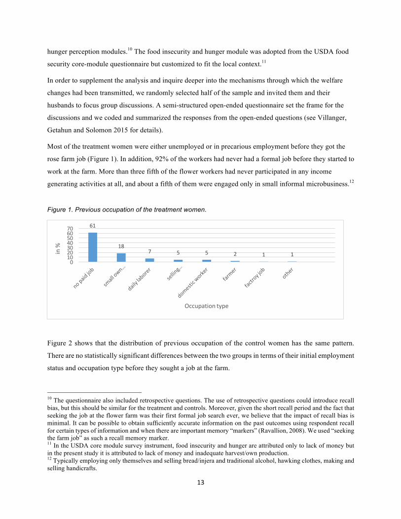
Most of the treatment women were either unemployed or in precarious employment before they got the

rose farm job (Figure 1). In addition, 92% of the workers had never had a formal job before they started to

work at the farm. More than three fifth of the flower workers had never participated in any income

generating activities at all, and about a fifth of them were engaged only in small informal microbusiness.12

 

Figure  1.  Previous  occupation  of  the  treatment  women.  

 

 

Figure 2 shows that the distribution of previous occupation of the control women has the same pattern.

There are no statistically significant differences between the two groups in terms of their initial employment

status and occupation type before they sought a job at the farm.

                                                                                                                         10 The questionnaire also included retrospective questions. The use of retrospective questions could introduce recall bias, but this should be similar for the treatment and controls. Moreover, given the short recall period and the fact that seeking the job at the flower farm was their first formal job search ever, we believe that the impact of recall bias is minimal. It can be possible to obtain sufficiently accurate information on the past outcomes using respondent recall for certain types of information and when there are important memory “markers” (Ravallion, 2008). We used “seeking the farm job” as such a recall memory marker. 11 In the USDA core module survey instrument, food insecurity and hunger are attributed only to lack of money but in the present study it is attributed to lack of money and inadequate harvest/own production. 12 Typically employing only themselves and selling bread/injera and traditional alcohol, hawking clothes, making and selling handicrafts.  

61

187 5 5 2 1 1

010203040506070

in  %

Occupation  type

14    

Figure  2.  Previous  occupation  of  the  control  women.  

  Moreover, the two groups were also almost identical along most of the measured socio-demographic

indicators (Table 1). The average age of the treatment and control women were not significantly different.

The percentages of literate, and completed third grade and six grade, were also not significantly different

across the two groups.13 Large majorities of both groups were married and they belonged to the same

religious group. More than two-thirds of both groups were born in rural area, and the overwhelming

majority of the respondents live in a nuclear family structure. The sex and age composition of their

household were also comparable.

 

Table  1.  Socio-­demographic  characteristics  of  the  women    

Characteristics   Control   Treatment   Difference  

Can  read  and  write     53.3   50.3   -­‐3.0  Years  of  schooling  completed   3.15   3.48   0.32  Completed    3rd  grade   45.05   48.49   3.44  Completed  6th  grade   29.12   31.78   2.66    Age   27.83   26.25   -­‐1.58  Knows  who  is  the    current  PM   49.45   56.92   7.47  Husband  can  read  and  write   65.56   74.58   9.02*  Husbands’  age   34.94   33.12   -­‐1.82  Married   86.81   90.77   3.96  Lives  in  an  extended  family  structure   13.19   13.25   0.06  Orthodox  Christian   81.32   84.64   3.32  Percentage  of  Oromo   86.26   75.15   -­‐11.11*  Years  of  living  in  current  place   16.16   15.91   -­‐0.24  Born  in  Oromia   86.81   82.98   -­‐3.83  

                                                                                                                         13  Together  with  the  employment  trajectories,  the  age  and  education  profiles  suggests  that  the  two  groups  also  have  a  similar  working  experience  before  seeking  employment.  

60

16 10 5 5 2 1 20

10203040506070

no  paid  job                  small  own  buisness

daily  laborer domestic  worker

Selling  charcoal  and  fuel  

wood

farmer factroy  job other

in  %

Occupation  type

15    

Born  in  Amhara   9.14   8.13   -­‐1.02  Born  in  an  urban  area   30.22   28.96   -­‐1.26  Born  in  Walmera  district   33.52   36.30   2.78  Born  in  Adaa   46.70   40.06   -­‐6.64  Household  size     3.76   3.29   -­‐0.46*  Adult  Equivalence  Household  size   2.11   1.91   -­‐0.21*  Has  children   73.62   76.34   2.72  Number  of  children  below  5  years   0.63   0.54   -­‐0.08  Number  of  young  age  member  (6-­‐14  years)   0.67   0.65   -­‐0.02  Number  of  working  age  member  (15-­‐64  years)   1.03   1.08   -­‐0.05  Had  inside  information  about  farm  job   16.67   72.96   56.29***  Travel  time  by  foot  from  home  to  farm  (minutes)   97.8   77.34   -­‐20.46***  Parents  own  agricultural  land     76.1   84.63   8.53***  Parents  own  cattle  (number)     4.35   4.67   0.32  Parents  own  pack-­‐animals  (number)   1.18   1.17   -­‐0.01  Father’s  average  years  of  schooling   1.01   1.65   0.64*  

Note: *  p  <  0.05,  **  p  <  0.01,  ***  p  <  0.001,  two  sided  t-­‐test  

 

However, the two groups were significantly different in terms of their connection to workers at the flower

farm. Almost three fourths of the treatments, but less than one fifth of the controls, had heard about the

vacancies from someone working inside the farm. Moreover, the controls reside significantly farther from

the farm and live in slightly larger households.14 In addition, fewer controls have literate husbands and

parents who own land, and their fathers also have a few months less education. However, there were no

differences in terms of livestock ownership, which is a key indicator of wealth in these societies.

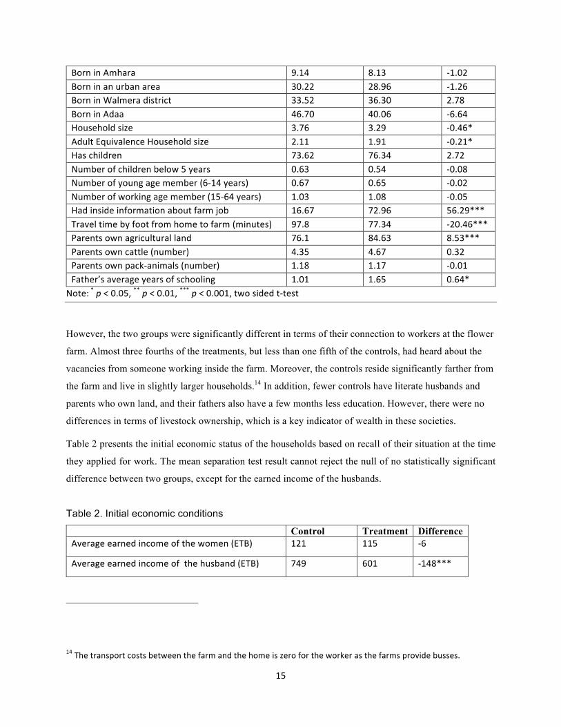
Table 2 presents the initial economic status of the households based on recall of their situation at the time

they applied for work. The mean separation test result cannot reject the null of no statistically significant

difference between two groups, except for the earned income of the husbands.

Table  2.  Initial  economic  conditions  

Control Treatment Difference Average  earned  income  of  the  women  (ETB)   121   115   -­‐6  

Average  earned  income  of    the  husband  (ETB)   749   601   -­‐148***  

                                                                                                                           

 14  The  transport  costs  between  the  farm  and  the  home  is  zero  for  the  worker  as  the  farms  provide  busses.  

16    

Average  per  adult  equivalent  income  (ETB)   432   458   26  

Average  per  adult  equivalence  food  consumption   318   303   -­‐15  

Average  per  adult  equivalence  consumption  (ETB)   445   433   -­‐12  

Poverty  rate,  income-­‐based   31.9   34.0   2.1  

Poverty  rate,  consumption-­‐based   36.3   35.9   0.4  

Food  insecurity  and  hunger  scale  (USDA)   4.48   4.33   -­‐0.15  

Number  of  times  adults  eat  per  day   2.57   2.62   0.05  

Number  of  times  children  eat  per  day   2.81   2.93   0.12  

Days  per  year  the  household  face  food  deficit   24   22   2  

Average  women's  share  of  household  income  (%)   13.2   15.8   2.6  

The    average  share  of  food  expenditure   66.6   65.2   -­‐1.4   Note: * p < 0.05, ** p < 0.01, *** p < 0.001, where 1 USD =11.8 ETB.

The similarities of the observables between the groups suggests that they are likely to be comparable also

in terms of their initial unobservable characteristics, contributing to identification (Wooldridge 2009).

6. Estimation Strategy and Results

In our model, household consumption, leisure demand and selection into the job are jointly determined.

Although the control group design accounts for self-selection of women deciding to search for a job, we

cannot rule out that there is selection at the hiring stage. Hence, we use a switching regression model with

a special maximum likelihood estimator developed by Lokshin and Sajaya (2004) and evaluate the mean

causal relationships between getting a job and standard treatment parameters by sorting respondents into

job and no-job regimes. Moreover, to account for the pre-job socioeconomic differences between the two

groups and to separate the impact of the job from time invariant confounders, we use the two-way fixed

effect model. To disentangle the agglomeration effect from time varying unobservable confounders, we

also used the difference-in-difference model combined with instrumental variable estimation techniques.

We show that the results are robust to econometric technique and test for job-effects in panel probit

models, poison models and binomial regression models.

17    

6.1 Impacts on consumption

 

Total household consumption15 and selection bias

The simple comparison of the average difference in per adult equivalent household consumption between

the treatment and control groups before and after getting the job suggested an estimated impact of 31 %

(138 Birr) increase of per adult equivalent household consumption. Controlling for correlates gives almost

the same estimate, a 30 % (134 Birr), and this would then be the preferred estimate if there was no

selection at the hiring stage.

Our endogenous switching regression model specification is a variant of the classical Heckman selection

model and can be estimated manually either by running Heckman two-step procedures twice or by the

ordinary maximum likelihood estimation. However, both of these estimation methods are inefficient and

require potentially cumbersome adjustments to derive consistent standard errors (Lokshin and Sajaya

2004). We therefore adopted a more efficient special maximum likelihood estimation procedure,

developed by Lokshin and Sajaya (2004) for such purposes, to estimate the selection and the consumption

welfare functions of the two groups of households. This estimation strategy addresses the selection bias

and generates consistent standard errors since it implements the Full Information Maximum Likelihood

Method (FILM) to simultaneously fit binary and continuous parts of the endogenous switching regression

model. The estimator assumes that the error terms in the switching, and consumption welfare equations

for both job and no-job regimes (  𝜈𝜈𝑖𝑖, 𝜀𝜀UÑ, 𝜀𝜀TÑ) have a tri-variate normal distribution with mean zero and

covariance matrix

𝛺𝛺 =𝜎𝜎á

W 𝜎𝜎Uá 𝜎𝜎Tá𝜎𝜎Uá 𝜎𝜎àâ

W .𝜎𝜎Tá . 𝜎𝜎àä

W

where 𝜎𝜎áW is a variance of the error term in the selection equation, and 𝜎𝜎àâ

W and 𝜎𝜎àãW are variances of the error

terms  𝜎𝜎Uá = 𝑐𝑐𝑐𝑐𝑐𝑐(𝜀𝜀U, 𝜈𝜈) and 𝜎𝜎Wá = 𝑐𝑐|𝑐𝑐𝑐𝑐(𝜀𝜀W, 𝜈𝜈)16.

                                                                                                                         15 Consumption based welfare measures are favored in poor countries because (i) consumption is a key argument in household utility functions (ii) consumption decisions are more related with other household decision outcomes such as nutrition and health (Deaton 1997, Atkinson 1991,Meyer 2003), (iii) Consumption is less erratic (than income) as it captures household’s access to credit and saving at times when their income is very low, and (iv) consumption data are more accurate than income. Reports of household income is likely to be understated compared to consumption expenditure reports. Expenditure on clothes and footwear can be considered as private (assignable) expenditures while the other expenditures may have benefited all household members and may hence be considered as public (household) expenditure. Moreover, an individual’s leisure is another assignable good important for welfare. 16 The covariance between 𝜎𝜎Uá and 𝜎𝜎Wá is not defined, as Y1i and Y0i are never observed simultaneously.                                                        

18    

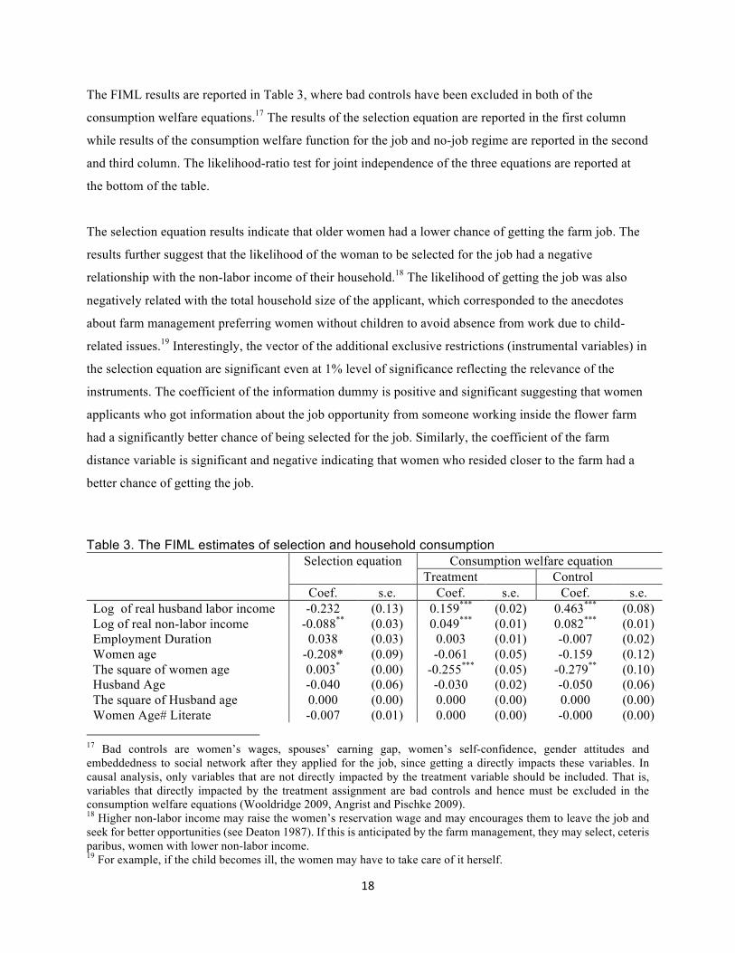
The FIML results are reported in Table 3, where bad controls have been excluded in both of the

consumption welfare equations.17 The results of the selection equation are reported in the first column

while results of the consumption welfare function for the job and no-job regime are reported in the second

and third column. The likelihood-ratio test for joint independence of the three equations are reported at

the bottom of the table.

The selection equation results indicate that older women had a lower chance of getting the farm job. The

results further suggest that the likelihood of the woman to be selected for the job had a negative

relationship with the non-labor income of their household.18 The likelihood of getting the job was also

negatively related with the total household size of the applicant, which corresponded to the anecdotes

about farm management preferring women without children to avoid absence from work due to child-

related issues.19 Interestingly, the vector of the additional exclusive restrictions (instrumental variables) in

the selection equation are significant even at 1% level of significance reflecting the relevance of the

instruments. The coefficient of the information dummy is positive and significant suggesting that women

applicants who got information about the job opportunity from someone working inside the flower farm

had a significantly better chance of being selected for the job. Similarly, the coefficient of the farm

distance variable is significant and negative indicating that women who resided closer to the farm had a

better chance of getting the job.

 

 Table  3.  The  FIML  estimates  of  selection  and  household  consumption     Selection equation Consumption welfare equation

Treatment Control Coef. s.e. Coef. s.e. Coef. s.e.

Log of real husband labor income -0.232 (0.13) 0.159*** (0.02) 0.463*** (0.08) Log of real non-labor income -0.088** (0.03) 0.049*** (0.01) 0.082*** (0.01) Employment Duration 0.038 (0.03) 0.003 (0.01) -0.007 (0.02) Women age -0.208* (0.09) -0.061 (0.05) -0.159 (0.12) The square of women age 0.003* (0.00) -0.255*** (0.05) -0.279** (0.10) Husband Age -0.040 (0.06) -0.030 (0.02) -0.050 (0.06) The square of Husband age 0.000 (0.00) 0.000 (0.00) 0.000 (0.00) Women Age# Literate -0.007 (0.01) 0.000 (0.00) -0.000 (0.00)

                                                                                                                         17 Bad controls are women’s wages, spouses’ earning gap, women’s self-confidence, gender attitudes and embeddedness to social network after they applied for the job, since getting a directly impacts these variables. In causal analysis, only variables that are not directly impacted by the treatment variable should be included. That is, variables that directly impacted by the treatment assignment are bad controls and hence must be excluded in the consumption welfare equations (Wooldridge 2009, Angrist and Pischke 2009). 18 Higher non-labor income may raise the women’s reservation wage and may encourages them to leave the job and seek for better opportunities (see Deaton 1987). If this is anticipated by the farm management, they may select, ceteris paribus, women with lower non-labor income. 19 For example, if the child becomes ill, the women may have to take care of it herself.  

19    

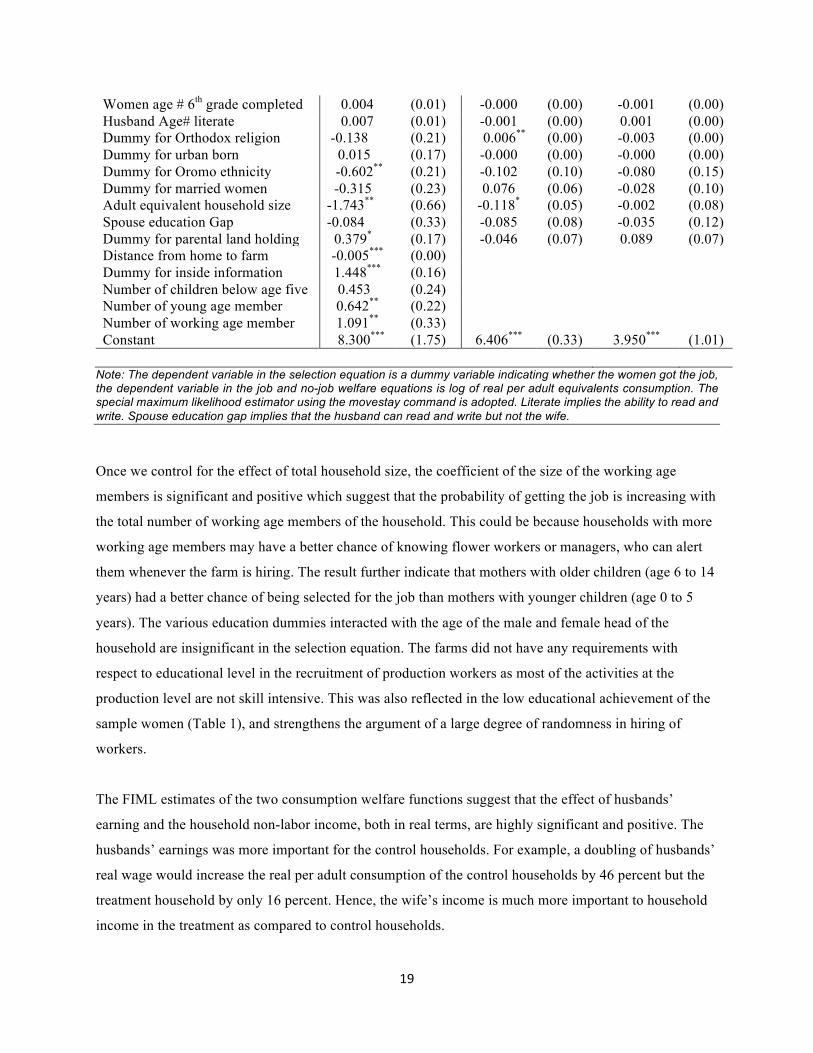
Women age # 6th grade completed 0.004 (0.01) -0.000 (0.00) -0.001 (0.00) Husband Age# literate 0.007 (0.01) -0.001 (0.00) 0.001 (0.00) Dummy for Orthodox religion -0.138 (0.21) 0.006** (0.00) -0.003 (0.00) Dummy for urban born 0.015 (0.17) -0.000 (0.00) -0.000 (0.00) Dummy for Oromo ethnicity -0.602** (0.21) -0.102 (0.10) -0.080 (0.15) Dummy for married women -0.315 (0.23) 0.076 (0.06) -0.028 (0.10) Adult equivalent household size -1.743** (0.66) -0.118* (0.05) -0.002 (0.08) Spouse education Gap -0.084 (0.33) -0.085 (0.08) -0.035 (0.12) Dummy for parental land holding 0.379* (0.17) -0.046 (0.07) 0.089 (0.07) Distance from home to farm -0.005*** (0.00) Dummy for inside information 1.448*** (0.16) Number of children below age five 0.453 (0.24) Number of young age member 0.642** (0.22) Number of working age member 1.091** (0.33) Constant 8.300*** (1.75) 6.406*** (0.33) 3.950*** (1.01)

Note:  The  dependent  variable  in  the  selection  equation  is  a  dummy  variable  indicating  whether  the  women  got  the  job,  the  dependent  variable  in  the  job  and  no-­job  welfare  equations  is  log  of  real  per  adult  equivalents  consumption.  The  special  maximum  likelihood  estimator  using  the  movestay  command  is  adopted.  Literate  implies  the  ability  to  read  and  write.  Spouse  education  gap  implies  that  the  husband  can  read  and  write  but  not  the  wife.

 

Once we control for the effect of total household size, the coefficient of the size of the working age

members is significant and positive which suggest that the probability of getting the job is increasing with

the total number of working age members of the household. This could be because households with more

working age members may have a better chance of knowing flower workers or managers, who can alert

them whenever the farm is hiring. The result further indicate that mothers with older children (age 6 to 14

years) had a better chance of being selected for the job than mothers with younger children (age 0 to 5

years). The various education dummies interacted with the age of the male and female head of the

household are insignificant in the selection equation. The farms did not have any requirements with

respect to educational level in the recruitment of production workers as most of the activities at the

production level are not skill intensive. This was also reflected in the low educational achievement of the

sample women (Table 1), and strengthens the argument of a large degree of randomness in hiring of

workers.

The FIML estimates of the two consumption welfare functions suggest that the effect of husbands’

earning and the household non-labor income, both in real terms, are highly significant and positive. The

husbands’ earnings was more important for the control households. For example, a doubling of husbands’

real wage would increase the real per adult consumption of the control households by 46 percent but the

treatment household by only 16 percent. Hence, the wife’s income is much more important to household

income in the treatment as compared to control households.

20    

 

Based on the FIML estimates of the parameters of the selection and the two consumption functions, we

computed the average causal impact of flower job participation through the evaluation of the standard

treatment parameters. As indicated in the strand of treatment evaluation literatures such Heckman (2004)

and Wooldridge (2009), average treatment effect (ATE) and average treatment effect on the treated group

(ATET) is statistically defined as:

ATE=E  (𝑌𝑌U − 𝑌𝑌T|X)    =    E  (𝑌𝑌U|X)  -­‐  E  (𝑌𝑌T|X)  =    𝑋𝑋𝛽𝛽U − 𝑋𝑋𝛽𝛽T                                                                                                                              (5.1)  

ATET==E(𝑌𝑌U − 𝑌𝑌T|X,F=1)=𝑋𝑋𝛽𝛽U − 𝑋𝑋𝛽𝛽T+E(𝜀𝜀UÑ-­‐  𝜀𝜀UT/  𝜈𝜈𝑖𝑖 ≥  −(𝑋𝑋𝑋𝑋 + 𝑆𝑆𝑆𝑆))                                                                          (5.2)                                    

where    E  (𝑌𝑌U|X,F=1)=  𝑋𝑋𝛽𝛽U + 𝜎𝜎Uá𝐼𝐼𝐼𝐼𝐼𝐼    and            E  (𝑌𝑌T|X,F=0)=  𝑋𝑋𝛽𝛽T − 𝜎𝜎Tá𝑁𝑁𝑆𝑆𝐻𝐻𝐼𝐼                                              (5.3)                                                    

and IMR and NSHR stands for inverse mills ratio and non-selection hazard rate20.

Table 4 presents the computed expected actual and counterfactual outcomes and the associated Average

Treatment Effect (ATE) and Average Treatment Effect on Treated (ATET)21 and suggests that getting the

job increased the real per adult equivalent consumption of the working women´s household by 25% (ETB

172) before controlling for initial conditions.

Table  4.  The  Computed  ATE  and  ATET  values  based  on  the  consumption  function  estimates  

n Average real per adult equivalent consumption

S.e. 95% confidence interval

E(Y1i/Xi) 672 650 6.705 637 663 E(Y0i/Xi) 672 504 8.328 487 520 ATE 672 146 4.507 137 155 E(Y1i/Xi, F=1) 524 663 8.077 647 679 E(Y0i/xi, F=1) 524 490 9.299 472 509 ATET 524 172 5.106 162 182

To account for potential initial socioeconomic differences between the treatment and control group as

well as to tidy up the employment impact from time invariant heterogeneities, we use two way fixed

effect (FE) model. Table 5 shows the results together with the DID model with covariates. The two

estimates are qualitatively comparable and suggest that getting the job increased the real per adult

                                                                                                                         20 The OLS estimation of the two consumption welfare functions yields inconsistent and biased estimate due to the omission of 𝐼𝐼𝐼𝐼𝐼𝐼 &  𝑁𝑁𝑆𝑆𝐻𝐻𝐼𝐼, which both are a function of X. 21 The conditional and unconditional expected actual and counterfactual real per adult equivalent consumptions of the two groups of the household are computed by executing the “mspredict” command after executing the “movestay” special command, the syntax of both commands are installed in Stata by Lokshin and Sajaya (2004).  

21    

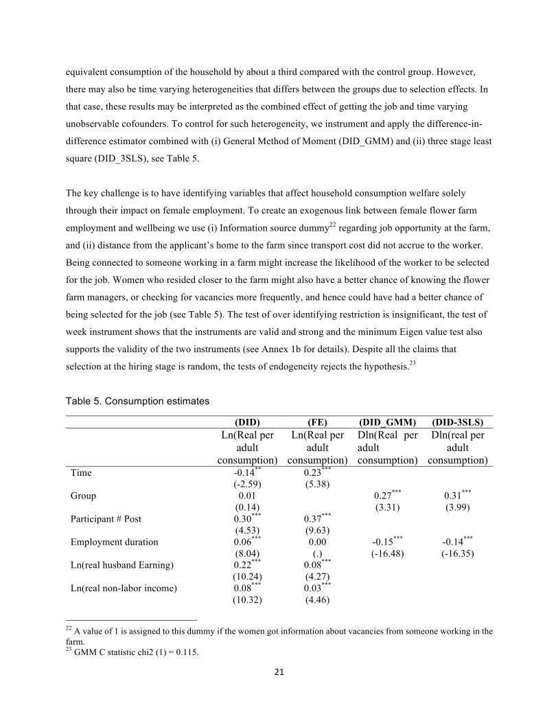
equivalent consumption of the household by about a third compared with the control group. However,

there may also be time varying heterogeneities that differs between the groups due to selection effects. In

that case, these results may be interpreted as the combined effect of getting the job and time varying

unobservable cofounders. To control for such heterogeneity, we instrument and apply the difference-in-

difference estimator combined with (i) General Method of Moment (DID_GMM) and (ii) three stage least

square (DID_3SLS), see Table 5.

The key challenge is to have identifying variables that affect household consumption welfare solely

through their impact on female employment. To create an exogenous link between female flower farm

employment and wellbeing we use (i) Information source dummy22 regarding job opportunity at the farm,

and (ii) distance from the applicant’s home to the farm since transport cost did not accrue to the worker.

Being connected to someone working in a farm might increase the likelihood of the worker to be selected

for the job. Women who resided closer to the farm might also have a better chance of knowing the flower

farm managers, or checking for vacancies more frequently, and hence could have had a better chance of

being selected for the job (see Table 5). The test of over identifying restriction is insignificant, the test of

week instrument shows that the instruments are valid and strong and the minimum Eigen value test also

supports the validity of the two instruments (see Annex 1b for details). Despite all the claims that

selection at the hiring stage is random, the tests of endogeneity rejects the hypothesis.23

 

Table  5.  Consumption  estimates  

(DID) (FE) (DID_GMM) (DID-3SLS) Ln(Real per

adult consumption)

Ln(Real per adult

consumption)

Dln(Real per adult consumption)

Dln(real per adult

consumption) Time -0.14** 0.23*** (-2.59) (5.38) Group 0.01 0.27*** 0.31*** (0.14) (3.31) (3.99) Participant # Post 0.30*** 0.37*** (4.53) (9.63) Employment duration 0.06*** 0.00 -0.15*** -0.14*** (8.04) (.) (-16.48) (-16.35) Ln(real husband Earning) 0.22*** 0.08*** (10.24) (4.27) Ln(real non-labor income) 0.08*** 0.03*** (10.32) (4.46)

                                                                                                                         22 A value of 1 is assigned to this dummy if the women got information about vacancies from someone working in the farm. 23 GMM C statistic chi2 (1) = 0.115.  

22    

Adult equivalent household size -0.25*** -0.39*** -0.09* -0.09* (-6.98) (-6.07) (-2.32) (-2.25) Women age -0.02 -0.11*** -0.01 -0.01 (-1.36) (-7.50) (-0.49) (-0.71) The square of women age 0.00 -0.00** -0.00 0.00 (0.76) (-2.97) (-0.22) (0.09) Husband age 0.00 0.00 0.03 0.03* (0.42) (.) (1.90) (2.11) The square of husband age -0.00 0.00 -0.00 -0.00 (-0.01) (1.75) (-0.92) (-0.90) Women age # Literate -0.00 -0.01 0.00 0.01* (-0.50) (-1.40) (1.54) (2.13) Women age #3rd grade completed -0.00 0.00 -0.00 (-0.16) (0.06) (-1.68) Woman age # 6th grade completed 0.01** 0.00 0.00 0.00 (3.25) (0.34) (0.32) (0.88) Husband age # Literate -0.00 0.01 -0.00 -0.00 (-0.83) (1.59) (-0.81) (-0.89) Spouse Education Gap -0.12 0.00 0.10 0.12 Dummy for married women -0.02 -0.16* -0.15** -0.13 (-0.50) (-2.20) (-2.64) (-1.90) Dummy for Urban born women -0.09* 0.00 -0.01 -0.03 (-2.39) (.) (-0.21) (-0.63) Dummy for Orthodox religion 0.02 0.00 -0.00 0.00 (0.47) (.) (-0.01) (0.04) Dummy for Oromo ethnic group -0.03 0.00 -0.05 -0.05 (-0.72) (.) (-0.99) (-1.04) Dummy for parental land holding -0.02(-0.56) N 1247 1409 512 512

 

The IV estimation produce similar results. The impact of getting a job increased the real per adult

equivalent consumption by 27 % (DID_GMM) and 31% (DID-3SLS) compared with the control group.24

In sum, all estimation techniques arrive at the same conclusion; the impact of getting a job in the flower

farms had large positive impacts on household consumption, and the increase is in the range between 25

% and 33 %. Moreover, there seems not to be strong effects of selection at the hiring stage on the

consumption impacts estimates.

 

Poverty

We define the poverty line based on the cost of 2,200 kcal per day per adult food consumption, with an

allowance for essential non-food expenditure.25 To calculate the poverty indices, the real per adult

                                                                                                                         24 In the DID-3SLS model, consumption growth, job participation and the two earning functions were simultaneously determined. The full estimation results of the DID-3SLS model are reported in annex 1a. 25 This is the minimum energy requirement for a person to lead a “normal” physical life under Ethiopian conditions.    

23    

equivalent consumption are first computed by deflating the nominal values of per adult equivalent

consumption by the spatial price indices (disaggregated at regional level relative to national average

prices) and temporal price indices (relative to 2005/6 constant prices). Second, the 2005/6 poverty line is

computed at 2010/11 prices.26 We then computed the incidence and depth of poverty following the

standard Foster, Greer and Thorbecke (1984) approach:-

𝑃𝑃ñ =1𝑁𝑁

𝑍𝑍 − 𝑦𝑦Ñ

𝑍𝑍

ñ1

U

Where Z is poverty line, 𝑦𝑦Ñ is real per adult equivalence consumption expenditure sorted in ascending

order, N is the total number of households and q is the number of poor household and 𝑃𝑃ñ is Foster, Greer

and Thorbecke class of poverty indices and α is the inequality aversion parameter (α≥0), which reflects

the policymaker’s degree of aversion to inequality among the poor. For α=0, we have the poverty

incidence, while for f α=1 we have the poverty depth index reflecting how far, on average, individuals

fall below the poverty line. Table 6 suggests that getting the job causes large reductions in household

poverty.

Table  6.  The  impact  on  poverty  

Poverty Incidence Food Poverty Depth of Poverty Coef. se Coef. se Coef. se Time 0.28* (2.07) -0.35* (-2.55) 0.09 (0.47) Group -0.06 (-0.48) 0.03 (0.22) 0.21 (1.04) Job -0.61*** (-4.02) -0.81*** (-4.98) -0.37+ (-1.62) Log of husband earning -0.42*** (-9.35) -0.26*** (-6.97) -0.13** (-2.62) Log of Non-labor income -0.16*** (-8.39) -0.11*** (-5.34) -0.05 (-1.72) Adult Equivalent household size 0.62*** (6.91) 0.48*** (4.52) 0.19 (1.46) Household head age -0.03 (-1.19) -0.01 (-0.36) 0.02 (0.48) Square of head Age 0.00 (0.77) 0.00 (0.87) 0.00 (0.02) Spouse age gap -0.01 (-0.23) -0.03 (-0.75) -0.03 (-0.58) Square of spouse age gap 0.00 (0.31) 0.00 (0.66) 0.00 (0.26) Woman age # Literate 0.00 (0.27) 0.01 (1.47) 0.00 (0.52) Woman age #3rd grade complete 0.00 (0.10) -0.00 (-0.42) -0.00 (-0.56) Woman age #6th grade complete -0.01** (-2.64) -0.00 (-0.64) -0.00 (-0.53) Husband age # Literate 0.00 (0.93) 0.00 (0.13) -0.00 (-0.15) Spouse Education gap 0.18 (1.02) 0.35 (1.64) 0.06 (0.21) Married women dummy -0.15 (-0.97) -0.35 (-1.51) 0.01 (0.05) Urban born dummy 0.11 (1.24) -0.01 (-0.08) 0.08 (0.55) Orthodox religion dummy -0.28* (-2.51) -0.44*** (-3.47) -0.19 (-1.17) Oromo ethnicity dummy 0.05 (0.50) 0.12 (0.86) 0.07 (0.39) N 1427 1427 551

Note: Marginal effects; t statistics in parentheses; (d) for discrete change of dummy variable from 0 to 1; +p<0.1,                                                                                                                          26 The food and absolute poverty lines for 2010/11 are determined by the Ethiopian national poverty lines of ETB 1985 and ETB 3781, respectively (MOFED 2012).

24    

* p < 0.05, ** p < 0.01, *** p < 0.001 ; ,# refers interaction, the consumption dimension of poverty is used. Spouse education gap implies husband can read and write but not the wife The coefficient of the impact variable, (Job, the interaction of the group identifying and post flower job

time dummy) is significant and negative for all the poverty measures. The coefficient of the time dummy

is positive and significant in the poverty incidence function reflecting the counterfactual outcome of

increasing poverty incidence.27 This suggests that getting the job protected many households from falling

in to poverty. Interestingly, the coefficient of the group identifying dummy is insignificant in all of the

three poverty functions suggesting no significance difference between the two groups of women before

they applied for the job. This strengthens the causal interpretation.

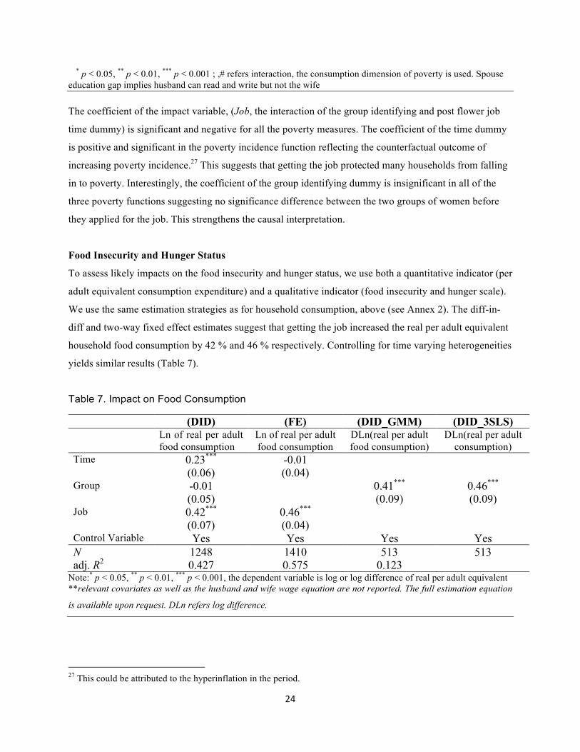
Food Insecurity and Hunger Status

To assess likely impacts on the food insecurity and hunger status, we use both a quantitative indicator (per

adult equivalent consumption expenditure) and a qualitative indicator (food insecurity and hunger scale).

We use the same estimation strategies as for household consumption, above (see Annex 2). The diff-in-

diff and two-way fixed effect estimates suggest that getting the job increased the real per adult equivalent

household food consumption by 42 % and 46 % respectively. Controlling for time varying heterogeneities

yields similar results (Table 7).

Table  7.  Impact  on  Food  Consumption  

(DID) (FE) (DID_GMM) (DID_3SLS) Ln of real per adult

food consumption Ln of real per adult food consumption

DLn(real per adult food consumption)

DLn(real per adult consumption)

Time 0.23*** -0.01 (0.06) (0.04) Group -0.01 0.41*** 0.46*** (0.05) (0.09) (0.09) Job 0.42*** 0.46*** (0.07) (0.04) Control Variable Yes Yes Yes Yes N 1248 1410 513 513 adj. R2 0.427 0.575 0.123

Note:* p < 0.05, ** p < 0.01, *** p < 0.001, the dependent variable is log or log difference of real per adult equivalent **relevant covariates as well as the husband and wife wage equation are not reported. The full estimation equation

is available upon request. DLn refers log difference.

                                                                                                                         27 This could be attributed to the hyperinflation in the period.

25    

The consumption measures may not provide the full picture about food security and hunger status of the

household (USDA, 2000). We therefore complement this with a qualitative composite food insecurity and

hunger index is analysis. The index captures the varied degree of the severity of food insecurity and huger

and is expressed by numerical values ranging from 0 to 10, where “0” denotes the condition of fully

secure, i.e. a household that has not experienced any of the conditions of food insecurity and “10”

represents the most severe condition, i.e. a household that has experienced all of the conditions of the

food insecurity and hunger (see USDA, 2000). Table 8 shows that the all impact estimates are similar and

suggesting that getting a job helped to reduce the severity of food insecurity and hunger.

Table  8.  Impact  on  Food  Insecurity  and  Hunger  scale-­Continuous     (DID) (FE) (DID_GMM) (DID_3SLS) FSH FSH D(FSF) D(FSH) Time 0.24 0.25 (0.24) (0.21) Group -0.10 -1.91*** -1.75*** (0.20) (0.43) (0.41) Participant #post -1.43*** -1.28*** (0.26) (0.20) Control variable Yes Yes Yes Yes N 1265 1427 530 530

Note: * p < 0.05, ** p < 0.01, *** p < 0.00,  In the DID and FE models the dependent variable is in levels while in the DID_GMM and DID_3SLS models the dependent variable is in first difference of the Food Insecurity and Hunger (FSH) scale. Relevant covariates as well as the husband´s and wife´s wage equation is not reported. The full estimation equation is available upon request’s stands for the continuous food insecurity and hunger scale, and D (FSH) implies the first difference of FSH.  

Intrahousehold distribution of welfare

In Ethiopia the single most exclusively assignable and recordable expenditure are expenditures on

clothing and footwear. The average annual expenditure on children, men´s and women´s clothing and

shoes for the two groups of households, a year preceding the survey period, are reported in Table 9. The

mean comparison test reported in the last column indicates a statistically significant mean difference in

terms of such expenditures between the women who got the job and those who did not, as well as between

the household members of the two groups. Table 9 also shows that getting a job benefited both spouses in

terms of assignable goods. Similarly, expenditure on children’s assignable private goods is also higher in

households where the women got the job than in the control households.

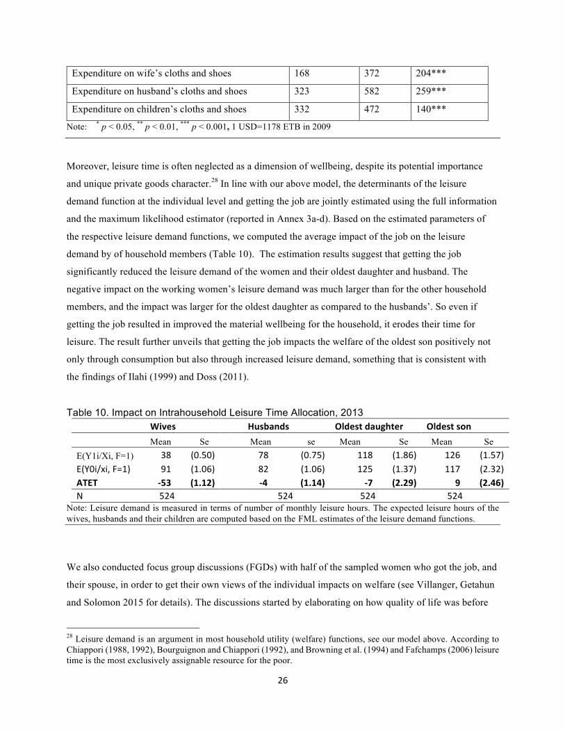
Table  9.  Annual  expenditure  on  clothing,  cloth,  tailoring  and  footwear  (Birr),  2013   Control Treatment Mean difference

26    

Expenditure on wife’s cloths and shoes 168 372 204***

Expenditure on husband’s cloths and shoes 323 582 259***

Expenditure on children’s cloths and shoes 332 472 140***

Note: * p < 0.05, ** p < 0.01, *** p < 0.001, 1 USD=1178 ETB in 2009

 Moreover, leisure time is often neglected as a dimension of wellbeing, despite its potential importance

and unique private goods character.28 In line with our above model, the determinants of the leisure

demand function at the individual level and getting the job are jointly estimated using the full information

and the maximum likelihood estimator (reported in Annex 3a-d). Based on the estimated parameters of

the respective leisure demand functions, we computed the average impact of the job on the leisure

demand by of household members (Table 10). The estimation results suggest that getting the job

significantly reduced the leisure demand of the women and their oldest daughter and husband. The

negative impact on the working women’s leisure demand was much larger than for the other household

members, and the impact was larger for the oldest daughter as compared to the husbands’. So even if

getting the job resulted in improved the material wellbeing for the household, it erodes their time for

leisure. The result further unveils that getting the job impacts the welfare of the oldest son positively not

only through consumption but also through increased leisure demand, something that is consistent with

the findings of Ilahi (1999) and Doss (2011).

 

Table  10.  Impact  on  Intrahousehold  Leisure  Time  Allocation,  2013   Wives        Husbands   Oldest  daughter   Oldest  son   Mean Se Mean se Mean Se Mean Se E(Y1i/Xi, F=1) 38   (0.50)       78   (0.75)   118   (1.86)   126   (1.57)  E(Y0i/xi,  F=1)   91   (1.06)       82   (1.06)   125   (1.37)   117   (2.32)  ATET   -­‐53   (1.12)       -­‐4   (1.14)   -­‐7   (2.29)   9   (2.46)  N          524                                  524                        524                    524  

Note: Leisure demand is measured in terms of number of monthly leisure hours. The expected leisure hours of the wives, husbands and their children are computed based on the FML estimates of the leisure demand functions.

We also conducted focus group discussions (FGDs) with half of the sampled women who got the job, and

their spouse, in order to get their own views of the individual impacts on welfare (see Villanger, Getahun

and Solomon 2015 for details). The discussions started by elaborating on how quality of life was before

                                                                                                                         28 Leisure demand is an argument in most household utility (welfare) functions, see our model above. According to Chiappori (1988, 1992), Bourguignon and Chiappori (1992), and Browning et al. (1994) and Fafchamps (2006) leisure time is the most exclusively assignable resource for the poor.

27    

the women got the job in terms of material and economic wellbeing and how they spent their time.

Subsequently, they were directed towards how their lives had changed as a result of woman getting the

job. The responses confirm the results of the econometric analysis (Figure 3).

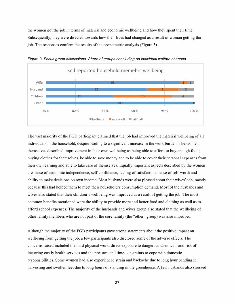
Figure  3.  Focus  group  discussions.  Share  of  groups  concluding  on  individual  welfare  changes.  

  The vast majority of the FGD participant claimed that the job had improved the material wellbeing of all

individuals in the household, despite leading to a significant increase in the work burden. The women

themselves described improvement in their own wellbeing as being able to afford to buy enough food;

buying clothes for themselves, be able to save money and to be able to cover their personal expenses from

their own earning and able to take care of themselves. Equally important aspects described by the women

are sense of economic independence, self-confidence, feeling of satisfaction, sense of self-worth and

ability to make decisions on own income. Most husbands were also pleased about their wives’ job, mostly

because this had helped them to meet their household’s consumption demand. Most of the husbands and

wives also stated that their children’s wellbeing was improved as a result of getting the job. The most

common benefits mentioned were the ability to provide more and better food and clothing as well as to

afford school expenses. The majority of the husbands and wives group also stated that the wellbeing of

other family members who are not part of the core family (the “other” group) was also improved.

Although the majority of the FGD participants gave strong statements about the positive impact on

wellbeing from getting the job, a few participants also disclosed some of the adverse effects. The

concerns raised included the hard physical work, direct exposure to dangerous chemicals and risk of

incurring costly health services and the pressure and time-constraints to cope with domestic

responsibilities. Some women had also experienced strain and backache due to long hour bending in

harvesting and swollen feet due to long hours of standing in the greenhouse. A few husbands also stressed

100

86

92

98

0

10

5

1

0

4

3

1

75  % 80  % 85  % 90  % 95  % 100  %

Other

Children

Husband

Wife

Self  reported  household  memebrs  wellbeing  

better  off worse  off half  half

28    

the intangible costs of their wives employment at the flower farm, in addition to the negative issues

mentioned above. A small but significant minority of husbands concluded that the impact of their wives’

job had been negative to their own wellbeing for the same reasons as given above. Some of these labeled

the flower farm employment as a distress sale of labor.

6.2 Transmission Mechanisms: Drivers of Welfare Changes

According to our theoretical model, the job could impact the consumption welfare of the women and

individual household members through its income, substitution and bargaining effects. Here we test the

relevance of each of these channels.

Income effects

First we assess the first order effect of the job on income.29 Table 11 reports the mean values of the

various sources of household income, both before and after the treatment and control women sought the

jobs. The diff-in-diff estimates suggest that the job had positive impacts on the earnings of the women,

while it negatively impacted household income from other sources. Getting the job increased the wage

income of the treatment women by more than 266 percent (ETB 322) on average, compared with the

change for control women. Nevertheless, the effect on remittances was negative; the job caused a

decrease in received remittances by 214 percent (ETB 45) compared with the control household.

Similarly, income from the sale of agricultural produce decreased by 76 percent (ETB 108) likely because

the job crowds out women’s time to spend on farming activities. The treatment women were away from

home for more than nine hours a day and six to seven days a week, so income from home based non-farm

business also decreased significantly.30 The net income effect of women´s industrial employment is

positive and large.

Table  11.  Impacts  on  income,  by  income  source  

Monthly income

(in Birr)

Before After

Diff-in- diff Control Treatment Control Treatment

Agriculture 142 152 192 94 -108***

Non-farm own business 159 134 156 70 -61*

                                                                                                                         29 Women wage, spouses earning gap, women self-confidence, gender equitable attitude and embeddedness to social network were excluded in the impact estimation models because getting the job impacted consumption and leisure demand by directly affecting these variables. 30  These  businesses  typically  involved  making  and  selling  bread,  injera,  and  drinks,  and  handicrafts  and  pottery.  

29    

Flower job 15 69 52 699 593***

Other hired work 579 409 781 583 28

Remittances 21 28 51 13 -45***

Women’s earnings 121 115 296 612 322**

Real household income 479 430 304 363 108*** Note * p < 0.05, ** p < 0.01, *** p < 0.001

When estimating the income effect of female flower job employment by two way fixed effect/DID

estimator using heteroskedasticity-robust estimator of the VCE of the least square estimator, we see that

the results do not change a lot (Table 12). The coefficient of the impact variable (the interaction of the

time and group identifying dummy) is highly significant and positive in the women´s earning and total

household income function. The magnitudes suggests that getting the job increases the average real wage

of the women by almost 200 percent and their households’ average real income by 50 percent over the

four years period. Again, the coefficients of the impact dummy in the non-labor income (remittance)

function is negative but only marginally significant. The coefficient of the group dummy in the women´s

earning function is insignificant indicating that the two groups were earning similar income before

applying for the job.31

Table  12.  DID  estimation:  effect  of  job  on  wage  and  non-­wage  income  

Log of women real

wage

Log of real non-labor income

Log of real household

income

Time 1.13*** -0.41 -0.32*** (0.24) (0.26) (0.07) Group -0.06 -0.23 -0.35*** (0.20) (0.22) (0.06) Job #Post 1.86*** -0.40 0.51*** (0.25) (0.29) (0.07) Impact duration 0.03 0.08** 0.07***

(0.02) (0.03) (0.01) Woman age 0.12***

(0.03) The square of woman age -0.00***

(0.00)                                                                                                                          31 The coefficient of experience (age) in both of the earning functions are statistically significant and positive. The impact of education in the wife´s and husband´s earning function is positive as expected but not statistically  significant at 0.05 level, probably because in rural settings the returns to education through unskilled employment are not substantial.  

30    

Woman years of schooling -0.05 (0.04)

Women complete 3rd grade 0.15 (0.21) Women complete 6th grade 0.13

(0.22) Women read and write 0.01

(0.16)

N 1688 1513 1675 Note: t statistics in parentheses,* p < 0.05, ** p < 0.01, *** p < 0.001. Time is a dummy taking a value of 1 for post flower job participation period; Group is a dummy taking 1 for flower job participating women

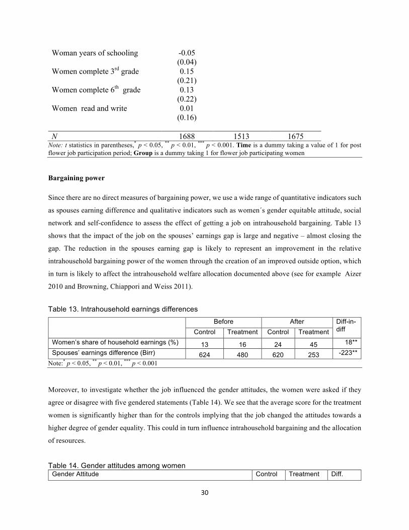
Bargaining power  Since there are no direct measures of bargaining power, we use a wide range of quantitative indicators such

as spouses earning difference and qualitative indicators such as women´s gender equitable attitude, social

network and self-confidence to assess the effect of getting a job on intrahousehold bargaining. Table 13

shows that the impact of the job on the spouses’ earnings gap is large and negative – almost closing the

gap. The reduction in the spouses earning gap is likely to represent an improvement in the relative

intrahousehold bargaining power of the women through the creation of an improved outside option, which

in turn is likely to affect the intrahousehold welfare allocation documented above (see for example Aizer

2010 and Browning, Chiappori and Weiss 2011).

 Table  13.  Intrahousehold  earnings  differences     Before   After   Diff-­in-­  

diff  Control   Treatment   Control   Treatment  Women’s  share  of  household  earnings  (%)   13   16   24   45   18**  Spouses’  earnings  difference  (Birr)   624   480   620   253   -­223**  

Note:* p < 0.05, ** p < 0.01, *** p < 0.001

Moreover, to investigate whether the job influenced the gender attitudes, the women were asked if they

agree or disagree with five gendered statements (Table 14). We see that the average score for the treatment

women is significantly higher than for the controls implying that the job changed the attitudes towards a

higher degree of gender equality. This could in turn influence intrahousehold bargaining and the allocation

of resources.  

Table  14.  Gender  attitudes  among  women      Gender  Attitude   Control     Treatment   Diff.  

31    

Women  should  subject  to  traditional  law/  should  not  treat  like  a  men   74   98   24***  A  husband  has  the  right  to  beat  his  wife  if  she  misbehave   57   92   35***  The  important  decisions  of  the  family  should  be  made  by  the  men  of  the  family  only  

66   91   25***  

A  wife   should   tolerate  being  beaten  by  her  husband   to   keep   the  family  together  

57   75   18**  

It  is  better  to  send  a  son  to  school  than  it  is  to  send  a  daughter   61   96   35  Average  Gender  Equitable    Score     3.1   4.5   1.4***  

Note:* p < 0.05, ** p < 0.01, *** p < 0.001, In all the five statements “agree” implies gender inequitable attitude.

We also looked into how the job influenced the self-confidence of the women. Table 15 shows that the job

made the women more independent and increased their self-reported self-confidence. Again, this may

influence the allocations.

 Table  15.  Self-­confidence:  Percentage  of  women  who  agree  with  the  following  statement       Control     Treatment   Differenc

 If  I  wanted  to  leave  my  husband,  I  could  support  my  family  on  

 my  own  

30  

 

51   21***  

I  can  achieve  whatever  I  set  my  mind  to  in  life  if  I  just  work  hard  

enough  

55   93   38***  

   Finally, the women were asked to indicate whether they are a member of (i) women´s prayers group (ii)

social insurance group (Idir), (iii) savings group (Equib) and (iv) workers group. Table 16 shows that the

average social network score of treatment women is significantly higher than the controls again

suggesting a positive impact of network formation from getting the job.32

Table  16.  Percentage  of  member  women  and  average  social  capital  score  

  Women’s   Prayer      

group  (%)  

Idir  (%)   Equib  (%)   Workers’  

union  (%)  

Average  

membership  Score  

Participant   18   61   53   23   1.55  Comparison   36   71   19   4   1.31  Mean  difference     -­18***   -­10**   34***   19***   0.24***  

Note:* p < 0.05, ** p < 0.01, *** p < 0.001. Idir is an association established among neighbors to raise funds to cover funeral expenses and other social costs within these groups and their families.  Equib is a rotating credit and saving scheme. The two are the most important informal social institutions in Ethiopia.

                                                                                                                         32 A value of 1 is assigned for the affirmative response and zero otherwise. A composite membership score is computed by adding the affirmative responses of the four questions. The score ranges from zero to four where four reflecting the highest level of network on the scale.

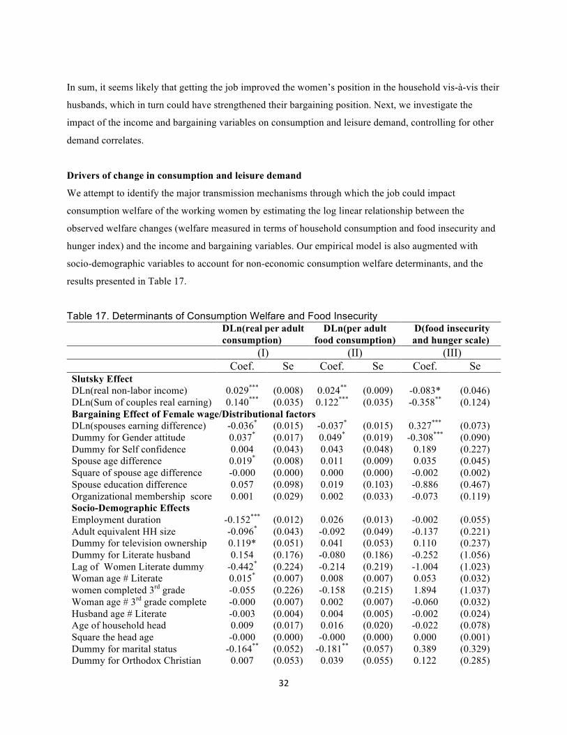
32    

 In sum, it seems likely that getting the job improved the women’s position in the household vis-à-vis their

husbands, which in turn could have strengthened their bargaining position. Next, we investigate the

impact of the income and bargaining variables on consumption and leisure demand, controlling for other

demand correlates.

Drivers of change in consumption and leisure demand

We attempt to identify the major transmission mechanisms through which the job could impact

consumption welfare of the working women by estimating the log linear relationship between the

observed welfare changes (welfare measured in terms of household consumption and food insecurity and

hunger index) and the income and bargaining variables. Our empirical model is also augmented with

socio-demographic variables to account for non-economic consumption welfare determinants, and the

results presented in Table 17.

Table  17.  Determinants  of  Consumption  Welfare  and  Food  Insecurity       DLn(real per adult

consumption) DLn(per adult

food consumption) D(food insecurity and hunger scale)

(I) (II) (III) Coef. Se Coef. Se Coef. Se Slutsky Effect DLn(real non-labor income) 0.029*** (0.008) 0.024** (0.009) -0.083* (0.046) DLn(Sum of couples real earning) 0.140*** (0.035) 0.122*** (0.035) -0.358** (0.124) Bargaining Effect of Female wage/Distributional factors DLn(spouses earning difference) -0.036* (0.015) -0.037* (0.015) 0.327*** (0.073) Dummy for Gender attitude 0.037* (0.017) 0.049* (0.019) -0.308*** (0.090) Dummy for Self confidence 0.004 (0.043) 0.043 (0.048) 0.189 (0.227) Spouse age difference 0.019* (0.008) 0.011 (0.009) 0.035 (0.045) Square of spouse age difference -0.000 (0.000) 0.000 (0.000) -0.002 (0.002) Spouse education difference 0.057 (0.098) 0.019 (0.103) -0.886 (0.467) Organizational membership score 0.001 (0.029) 0.002 (0.033) -0.073 (0.119) Socio-Demographic Effects Employment duration -0.152*** (0.012) 0.026 (0.013) -0.002 (0.055) Adult equivalent HH size -0.096* (0.043) -0.092 (0.049) -0.137 (0.221) Dummy for television ownership 0.119* (0.051) 0.041 (0.053) 0.110 (0.237) Dummy for Literate husband 0.154 (0.176) -0.080 (0.186) -0.252 (1.056) Lag of Women Literate dummy -0.442* (0.224) -0.214 (0.219) -1.004 (1.023) Woman age # Literate 0.015* (0.007) 0.008 (0.007) 0.053 (0.032) women completed 3rd grade -0.055 (0.226) -0.158 (0.215) 1.894 (1.037) Woman age # 3rd grade complete -0.000 (0.007) 0.002 (0.007) -0.060 (0.032) Husband age # Literate -0.003 (0.004) 0.004 (0.005) -0.002 (0.024) Age of household head 0.009 (0.017) 0.016 (0.020) -0.022 (0.078) Square the head age -0.000 (0.000) -0.000 (0.000) 0.000 (0.001) Dummy for marital status -0.164** (0.052) -0.181** (0.057) 0.389 (0.329) Dummy for Orthodox Christian 0.007 (0.053) 0.039 (0.055) 0.122 (0.285)

33    

Dummy for urban born women -0.020 (0.048) 0.029 (0.057) -0.000 (0.237) Dummy for Oromo ethnic -0.096 (0.055) -0.077 (0.066) -0.025 (0.240) Dummy for livestock ownership 0.045 (0.058) 0.118 (0.074) 0.331 (0.264) Intergenerational factors Dummy for parental land holding 0.055 (0.054) 0.034 (0.055) -0.208 (0.265) family highest years of schooling 0.008 (0.006) 0.009 (0.006) -0.043 (0.028) Dummy for parents owning cattle 0.005 (0.007) 0.010 (0.007) -0.038 (0.031) Parents owns pack animal 0.006 (0.017) -0.002 (0.018) -0.026 (0.073) Constant 0.348 (0.325) -0.066 (0.364) 1.927 (1.838) N 409 409 421 F(29 ,379)$, (Prob > F) 21.7

(0.000) 4.2

(0.000) 3.9

(0.000)

R-squared 0.5375 Note: * p < 0.05, ** p < 0.01, *** p < 0.001, $ the upper degree of freedom for the F-statistic associated with the last model is 391. D refers first difference & DLn refers first log difference. The Self-confidence dummy indicates whether the women is confident enough to help her family without seeking help from her husband. A heteroskedasticity-robust estimator of the VCE of the ordinary least square estimator is used. The overall F-statistic has a p-value of 0.000 in all of the three welfare functions indicating that the

regressors are jointly significant. The results suggest that the increase in woman’s earnings from getting

the job positively impacted the consumption demand and food security and hunger status of her

household not only by easing the budget constraint of their household (sum of the couple’s real earnings)

but also by improving the intrahousehold bargaining power of the women (reducing the couples earning

difference). The estimated elasticity of household consumption demand with respect to women’s wage

income indicate that a 100 % increment in the women´s salary would increase their household

consumption welfare by 14% through its Slutsky effect and by 4 % through its distinguished bargaining

effect.33 This finding is fully consistent with the prediction of our theoretical model and several other

studies.34

Getting the job improved not only the earned income of the women but also their social skills, self-

confidence and attitude towards positive gender equitable norms. Table 17 suggests that the improvement

in such distributional factors positively impacted the consumption welfare of the women´s household by

influencing the intrahousehold bargaining process; but without directly influencing the individual

preference of the couples or their joint budget set. For example, the coefficient of the gender dummy is

statistically significant and positive in the two consumption welfare functions and negative in the food

                                                                                                                         33 The vast majority of the women were not engaged in income generating activities before the emergence of the flower cluster 34 Thomas’s (1990, 1997) and Carrasco and Zamora (2010) also found that an increase in women´s earning due to employment causes an increase in consumption of most household commodities through its influence on the household budget constraint and on the intrahousehold bargaining process.

34    

insecurity and hunger function reflecting the additional channel through which the job positively

impacted household welfare.35 36

To further explore the transmission mechanism, a sample of treatment women who had reported increases

in wellbeing were also asked in the survey to indicate the major causes of the improvements. They were

specifically asked to choose from the long list of potential drivers, including improvements in harvest,

earning from the flower cluster and increment in other sources of income. Consistent with the quantitative

finding, the vast majority of the women attributed the observed improvements in wellbeing to the fact that

they got the job (see Annex 4).

We ran a poison regression model to investigate the transmission mechanisms through which the job

impacted leisure demand.37 Since the poison regression model is intrinsically heteroskedastic, we

employed a robust estimate of VCE for poison maximum likelihood estimates. The estimated marginal

effects and the VCE robust standard errors are reported in Table 18.

Table  18.  Determinants  of  leisure  demand  

Wife Husband Daughter MEs se MEs Se MEs se Log of real non labor income -0.004 (0.01) -0.011 (0.02) 0.043* (0.02) Log of real woman´s earning -0.032** (0.01) 0.002 (0.02) -0.114*** (0.03) Log of real Husbands income -0.083 (0.07) -0.294** (0.11) -0.112 (0.16) Log of real spouses income gap 0.055* (0.03) 0.065* (0.03) 0.024 (0.06) Dummy for positive gender attitude -0.088*** (0.02) -0.021 (0.03) 0.058* (0.04) Dummy for Women confidence 0.064 (0.04) 0.118* (0.06) 0.280*** (0.08) Membership/network score -0.038 (0.02) -0.073* (0.03) -0.011 (0.05) Spouses age gap 0.014 (0.01) 0.004 (0.01) 0.022 (0.02) The square of age gap -0.000 (0.00) -0.001 (0.00) 0.001 (0.00) Spouses education gap 0.060 (0.09) 0.155 (0.12) 0.065 (0.18) Employment duration in years 0.008 (0.01) 0.027 (0.01) 0.036* (0.02) Adult equivalent household size -0.018 (0.04) 0.061 (0.07) -0.105 (0.11) Dummy for Literate husband 0.571** (0.21) 0.183 (0.27) 0.855* (0.35) Dummy for Literate Woman 0.346 (0.20) 0.396 (0.31) -0.024 (0.45) Woman age # Literate -0.011 (0.01) -0.015 (0.01) -0.003 (0.01)

                                                                                                                         35 The control variables have the expected signs but most of them are insignificant. 36 McElroy (1990) also found similar result. Using household data sets from Bangladesh, Indonesia, Ethiopia, and South Africa, Quisumbing and Maluccio (2000) also found a positive association between women´s bargaining power and household consumption welfare. In the contrary, Fafchamps, Kebede and Quisumbing (2006) using data from poor rural Ethiopia found a week association between women´s bargaining power and intrahousehold welfare. 37 A linear regression estimate may not provide the best fit over the values of the leisure demand determinants since leisure time is a count variable (Wooldridge 2009).  

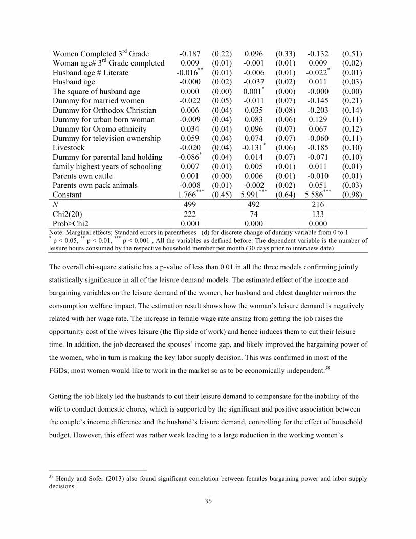
35    

Women Completed 3rd Grade -0.187 (0.22) 0.096 (0.33) -0.132 (0.51) Woman age# 3rd Grade completed 0.009 (0.01) -0.001 (0.01) 0.009 (0.02) Husband age # Literate -0.016** (0.01) -0.006 (0.01) -0.022* (0.01) Husband age -0.000 (0.02) -0.037 (0.02) 0.011 (0.03) The square of husband age 0.000 (0.00) 0.001* (0.00) -0.000 (0.00) Dummy for married women -0.022 (0.05) -0.011 (0.07) -0.145 (0.21) Dummy for Orthodox Christian 0.006 (0.04) 0.035 (0.08) -0.203 (0.14) Dummy for urban born woman -0.009 (0.04) 0.083 (0.06) 0.129 (0.11) Dummy for Oromo ethnicity 0.034 (0.04) 0.096 (0.07) 0.067 (0.12) Dummy for television ownership 0.059 (0.04) 0.074 (0.07) -0.060 (0.11) Livestock -0.020 (0.04) -0.131* (0.06) -0.185 (0.10) Dummy for parental land holding -0.086* (0.04) 0.014 (0.07) -0.071 (0.10) family highest years of schooling 0.007 (0.01) 0.005 (0.01) 0.011 (0.01) Parents own cattle 0.001 (0.00) 0.006 (0.01) -0.010 (0.01) Parents own pack animals -0.008 (0.01) -0.002 (0.02) 0.051 (0.03) Constant 1.766*** (0.45) 5.991*** (0.64) 5.586*** (0.98) N 499 492 216 Chi2(20) 222 74 133 Prob>Chi2 0.000 0.000 0.000

Note: Marginal effects; Standard errors in parentheses (d) for discrete change of dummy variable from 0 to 1 * p < 0.05, ** p < 0.01, *** p < 0.001 , All the variables as defined before. The dependent variable is the number of leisure hours consumed by the respective household member per month (30 days prior to interview date) The overall chi-square statistic has a p-value of less than 0.01 in all the three models confirming jointly

statistically significance in all of the leisure demand models. The estimated effect of the income and

bargaining variables on the leisure demand of the women, her husband and eldest daughter mirrors the

consumption welfare impact. The estimation result shows how the woman’s leisure demand is negatively

related with her wage rate. The increase in female wage rate arising from getting the job raises the

opportunity cost of the wives leisure (the flip side of work) and hence induces them to cut their leisure

time. In addition, the job decreased the spouses’ income gap, and likely improved the bargaining power of

the women, who in turn is making the key labor supply decision. This was confirmed in most of the

FGDs; most women would like to work in the market so as to be economically independent.38

Getting the job likely led the husbands to cut their leisure demand to compensate for the inability of the

wife to conduct domestic chores, which is supported by the significant and positive association between

the couple’s income difference and the husband’s leisure demand, controlling for the effect of household

budget. However, this effect was rather weak leading to a large reduction in the working women’s

                                                                                                                         38 Hendy and Sofer (2013) also found significant correlation between females bargaining power and labor supply decisions.

36    

leisure.39 Getting the job negatively impacted the leisure demand of the women not only through the

standard Marshallian price effect but also through the distinguished bargaining effect leading the woman

to disproportionally reduce leisure compared to the other household members.40

As it can be inferred from the daughters’ leisure demand function, mothers wage was positively

associated with the daughters’ leisure time probably because daughters had to step in for their mother’s

forgone housework. Similarly, the husbands’ leisure time was significantly and positively associated with

the earning difference between the husband and his wife; and hence negatively related with the wives

wage - implying that husbands were pulled into housework after their wives got the job. Interestingly, the

job impacted the leisure time of the husband primarily through its influence on the relative bargaining

power of the women and not through the usual Slutsky effect: In the husbands’ leisure demand function,

the coefficient of wives wage is insignificant while the coefficient of the spouses earning gap variable is

significant. 41 The results also indicate that daughters’ leisure time is positively associated with their

mothers’ gender equitable attitudes and confidence probably because mothers with strong self-confidence

and positive gender attitudes might influence the level of help that the male member of the household

provide with household chores (similarly to Doss 2011).42

7. Conclusion and suggestion for future research

Within the span of about a decade, the flower industry in Ethiopia has created job opportunities for a large

number of poor rural women with little education and few other income-generating opportunities. Our

research design and survey data from treatment and control groups of women who were balanced on

observables at the time they applied for the job is likely to control for the standard selection bias that

                                                                                                                         39 In the rural Ethiopia, performing domestic activities such as cleaning, washing, collecting fuel wood, fetching water and cooking are very important for a woman to be seen as a “good” or “proper” housewife. 40 Using Spanish data, Carrasco and Zamora (2010) found similar result. 41 To put it differently, controlling for the Slutsky effect, the husbands’ leisure was positively correlated with the relative bargaining power of the husband. The larger the earning difference between the husband and the wife, the higher the bargaining power of the husband since he would have a more favorable outside option (the threat point, which could be divorce). Husbands in a more favorable position were less likely to take over the women’s’ traditional responsibilities in the house.  42 The other control variables had shown the expected sign. The oldest daughters’ leisure time was positively related with the non-wage income of the household. The husbands’ leisure time was negatively associated with the husbands’ wage (price of leisure). Because the substitution effect of the price increase was much higher than the wealth effect for individuals who earned a wage rate lower than their targeted wage rate. The husbands’ leisure time had also positively associated with the husband’s literacy skill and had negatively associated with his household wealth status (livestock ownership).

37    

prevents credible analysis of impacts of salaried employment. We find that getting a job in the flower

farms has had a large positive impact on the material wellbeing of the working women and the individual

household members. Getting a job led to large increases in household consumption, reduced poverty and

improved food security. It also improved the bargaining power of the working women, but had a negative

impact on time for leisure, especially for the women. Moreover, we also document that the consumption

benefits were relatively equally distributed between husbands’ and wives private consumption goods, and

the children benefited considerably as well.

We show that it is important to account for endogeneity of the household’s allocation of labor and

income. Husbands helping with domestic work to cover for the wife may imply less work at the

household’s agricultural plot. Together with reduced agricultural labor input from the wife, we indeed

find that that getting the job reduces household income from agriculture. Moreover, the remittances

received by the household decreases as an effect of the job, something that may be explained by the high

visibility in family networks of women getting such a job.

Our investigation of the transmission mechanisms suggests that getting the job effected the consumption

welfare not only through the income and substitution effects, but also through a bargaining effect. In

addition, we find that the job improved the consumption welfare and leisure demand of their household

by influencing the various distributional factors such as spouses earning gap, gender attitude, improved

outside options, self-confidence and social network. The qualitative findings support the quantitative

findings, but unveil additional intangible benefits and costs of female in employment in the rose farm

sector.

We also note that the emergence of female labor market in the flower industry is likely to have multiplier

effects and impact the local communities including the sample respondents through various channels

other than the direct labor market channel. In particular, the large increase in consumption likely enhance

demand for locally produced goods and services. However, we have only documented the partial

equilibrium effects leaving the general equilibrium effects for future research.

38    

RReeffeerreenncceess    

 

Aizer, A. 2010. The gender wage gap and domestic violence. American Economic Review, 100(4), 1847-

59.

Akerlof, GA. and JL. Yellen. 1986. Efficiency wage models of the labor market. Cambridge University

Press.

Aman, H. 2011. Workers’ conditions and industrial relations in the Ethiopia horticulture sectors.

NFFPFATU Study Report. Addis Ababa: NFFPFATU.

Anderson, S. and JM. Baland. 2002. The Economics of Roscas and Intrahousehold Resource Allocation,

Quarterly Journal of Economics, 117(3), 963–95.

Angrist JD. and JS. Pischke. 2009. Mostly Harmless Econometrics: An Empiricist's Companion. New

Jersey: Princeton University Press.

Ashraf, N. 2009. Spousal Control and Intrahousehold Decision Making: An Experimental Study in the

Philippines. American Economic Review, 99(4), 1245–77.

Atkinson, A.B. 1991. Measuring Poverty and Differences in Family Composition, Economica, 59, 1–16.

Blattman, C. and S. Dercon. 2015. Industrial jobs in an early-industrializing society: Experimental

evidence from Ethiopia. Mimeo, Columbia University.

Blien, U., J. Suedekum, and K. Wolf. 2006. Local Employment Growth in West Germany: A Dynamic

Panel Approach, Labour Economics 13 (4), 445-458.

Bourguignon, F. and PA. Chiappori. 1994. The collective approach to household behavior. In R.

Blundell, I. Preston and I. Walker (eds.). The Measurement of Household Welfare. Cambridge:

Cambridge University Press.

Browning, M. and PA. Chiappori. 1998. Efficient intrahousehold allocations: a general characterization

and empirical tests, Econometrica, 66, 1241-1278.

Browning, M., PA. Chiappori and A. Lewbel. 2006. Estimating consumption economies of scale, adult

equivalence scales, and household bargaining power, Boston College Working Paper, WP588,

Department of Economics, Boston College.

Browning, M., PA. Chiappori and Y. Weiss. 2011. Family economics. Available at:

http://www.tau.ac.il/~weiss/fam_econ/BCW_Book_index_07_09_2011_MB.pdf

Card, D. 1996. The effect of unions on the structure of wages: A longitudinal analysis. Econometrica,

64(4), 957-979.

Carrasco, R. and B. Zamora. 2010. Estimating the Effect of Female Labor Participation on Household

Consumption. Mimeo, Department of Economics, Universidad Carlos III de Madrid.

Chiappori, PA. 1988. Rational Household Labor Supply, Econometrica 56(1), 63-90.

39    

Combes, P. 2000. Economic Structure and Local Growth: France, 1984-1993, Journal of Urban

Economics 47, 329-355.

CSA. 2013. National Statistics 2012. Available at:

http://www.csa.gov.et/index.php/component/content/article/14-survey-reports/123-

latestnationalstatistics-abstract

CSA and ICF International. 2012. Ethiopia Demographic and Health Survey 2011. Addis Ababa and

Calverton, Maryland: Central Statistical Agency and ICF International.

Deaton, A. 1987.The allocation of goods within the household: adults, children, and gender. LSMS

Working Paper number 39. Washington DC.: The World Bank.

Deaton, A. 1997. The analysis of household surveys. A micro econometric approach to development

policy. Baltimore: John Hopkins University Press.

Dercon, S., and P. Krishnan. 2000. Vulnerability, seasonality and poverty in Ethiopia. Journal of

Development Studies, 36(6), 25 – 53

Doss, CR. 1999. Intrahousehold Resource Allocation in Ghana: The Impact of the Distribution of Asset

Ownership within the Household. In Food Security, Diversification and Resource Management:

Refocusing the Role of Agriculture?. G.H. Peters and J. von Braun (eds.). 309–316. Aldershot, UK:

Dartmouth Publishing.

Doss, C. R. 2006. The Effects of Intrahousehold Property Ownership on Expenditure Patterns in Ghana,

Journal of African Economies, 15(1), 149-180.

Doss, C. R. 2011. Intrahousehold bargaining and resource allocation in developing countries. Background

paper for the World Development Report 2012. Washington DC.: The World Bank.

Dufo, E. 2003. Grandmothers and Granddaughters: Old Age Pension and Intra- Household Allocation in

South Africa, World Bank Economic Review, 17(1), 1-25.

Duflo, E. 2012. Women empowerment and economic development, Journal of Economic Literature

50(4), 1051-1079

EHPEA. 2013. Ethiopian Horticulture Producer Exporters Association: Sector Information. Addis Ababa:

Ethiopia Horticulture Development Agency. Available at

http://www.ehpea.org/GeneralInfo.aspx#medialink

Fafchamps, M. and Quisumbing, AR. 2002. Control and ownership of assets within rural Ethiopian

households, Journal of Development Studies, 38, 47–82.

Fafchamps, M., B. Kebede, and AR. Quisumbing. 2006. Intrahousehold welfare. Economics Series

Working Papers, GPRG-WPS-044, University of Oxford, Department of Economics.

Fafchamps, M., B. Kebede, and AR. Quisumbing. 2009. Intrahousehold Welfare in Rural Ethiopia,

Oxford Bulletin of Economics and Statistics, 71(4), 567–599.

40    

Fatuma A. 2008. Social and Environmental Implication of Floriculture. A stakeholder perception analysis

at Holeta Area, Wolmera District, Oromia Region. Addis Ababa University. School of Graduate

Studies. Environmental Science Program.

Foster, J., J., Greer and E. Thorbecke 1984. A class of decomposable poverty measures. Econometrica,

52, 761–776.

Garcia-Moreno, C., H. AFM. Jansen, M. Ellsberg, L. Heise, and C. Watts. 2006. Prevalence of intimate

partner violence: findings from the WHO multi-country study on women's health and domestic

violence, The Lancet, 368, 1260-69.

Gebreyesus, M. and M. Iizuka. 2012. Discovery of the flower industry in Ethiopia: experimentation and

coordination, Journal of Globalization and Development, 2, 1-27.

Getu, M. 2009. Ethiopian Floriculture and its Impact on the Environment: Regulation, Supervision, and

Compliance. Mizan Law Review, 3(2), 240-270.

Haddad, L. and R. Kanbur. 1990. How serious is the neglect of intra household inequality? The Economic

Journal, 100, 866-881.

Haddad, L., J. Hoddinott, and H. Alderman. 1997. Intrahousehold Resource Allocation in Developing

Countries: Methods, Models, and Policy. Baltimore: Johns Hopkins University Press for the

International Food Policy Research Institute.

Haddad, L., J. Sullivian and E. Kennedy. 1991. Identification and Evaluation of alternative indicators

food and nutrition security. Washington D.C.: IFPRI.

Hagenaars, A., K. de Vos and M.A. Zaidi. 1994. Poverty Statistics in the Late 1980s: Research Based on

Micro-data, Office for Official Publications of the European Communities. Luxembourg.

Hall, R. 2011. Land grabbing in Southern Africa: the many faces of the investor rush. Review of African

Political Economy, 38(128), 193-214.

Heath, Rachel and A. M. Mobarak. 2014. Manufacturing Growth and the Lives of Bangladeshi Women,

NBER Working Paper No. 20383.

Heckman, J. 1990. Varieties of Selection Bias, American Economic Review, 80, 313–318.

Heckman, J., H. Ichimura, and P. Todd. 1998. Matching as an Econometric Evaluation Estimator, Review

of Economic Studies, 65, 261–294.

Henderson, V. 1997. Externalities and Industrial Development. Journal of Urban Economics 42, 449-470.

Hendy, R. and C. Sofer. 2013. Within Resource Allocation in Egyptian Couples: Do Distribution Factors

Matter? Mimeo.

Hoddinott, J. and L. Haddad. 1995. Does Female Income Share Influence Household Expenditures?

Evidence from Côte d’Ivoire, Oxford Bulletin of Economics and Statistics, 57(1), 77-96.

Hortiwise. 2012. A Study on the Kenyan-Dutch Horticultural Supply Chain. Available at

41    

http://www.kenyaflowercouncil.org/pdf/Study%20on%20the%20KenyanDutch%20Horticultural%20Sup

ply%20Chain%20(3).pdf

Ilahi, N. 1999. The Intrahousehold Allocation of Time and Tasks: What Have We Learnt from the

Empirical Literature? Policy Research Report on Gender and Development. DEC Working Paper

Series No. 13. Washington DC.: The World Bank.

Katz, LF., LH. Summers, RE. Hall, CL. Schultze and RH. Topel. 1989. Industry rents: Evidence and

implications. Brookings Papers on Economic Activity, 1989, 209-290.

Jensen, R. 2012. Do labor market opportunities affect young women’s work and family decisions?

Experimental evidence from India, Quarterly Journal of Economics, 127, 753-792.

Lokshin, M. Zurab Sajaia. Z. 2004. Maximum likelihood estimation of endogenous switching regression

models, The Stata Journal 4 (3).

Lim, S., Winter-Nelson, A., and M. Arends-Kuenning. 2007. Household bargaining power and

agricultural supply response: Evidence from Ethiopian coffee growers. World Development, 35 (7),

1204–1220.

Loayza, N.V. and C. Raddatz. 2010. The composition of growth matters for poverty alleviation. Journal

of Development Economics, 93 (1), 137-151.

Mabsout, R. and I.v. Stavern. 2010. Disentangling Bargaining Power from Individual and Household

Level to Institutions: Evidence on Women’s Position in Ethiopia. World Development, 38(5), 783-

96.

Martin, J. and Roberts, C. 1984. Women and employment. A life time perspective.  Department of

Employment and Office of Population Censuses and Surveys, HMSO. London: HMSO.

McElroy, MB. 1990. The empirical content of Nash-bargained household behavior, Journal of Human

Resources, 25, 559-583.

Meyer, BD. and JX. Sullivan. 2003. Measuring the Well-Being of the Poor Using Income and

Consumption, Journal of Human Resources, 38, 1180-1220.

MOFED (Ministry of Finance and Economic Development) 2012. Ethiopia’s Progress towards

Eradicating Poverty: An Interim Report on Poverty Analysis Study (2012/13). Addis Ababa: The

Federal Democratic Republic of Ethiopia.

Papageorgiou, T. 2014. Learning your comparative advantages. The Review of Economic Studies,  81(3),

1263-1295.

Quisumbing, A., and J. Maluccio. 2002. Intrahousehold allocation and gender relations: new empirical

evidence from four developing countries. IFPRI discussion paper no.84. IFPRI: Washington DC.

42    

Quisumbing, A., and J. Maluccio. 2003. Resources at Marriage and Intrahousehold Allocation: Evidence

from Bangladesh, Ethiopia, Indonesia, and South Africa, Oxford Bulletin of Economics and

Statistics, 65(3), 283-327.

Rodrik, D. 2015. Premature deindustrialization. NBER Working Paper No. 20935. The National Bureau

of Economic Research, USA.

Salway, S., S. Rahman and S. Jesmin. 2003. A Profile of women’s work participation among the urban

poor of Dhaka. World Development, 31 (5), 881-901.

Shapiro, C. and J. Stiglitz. 1984. Equilibrium Unemployment as a Worker Discipline Device,

American Economic Review, 74 (3), 433-444.

Schaefer, F. and G. Abebe, 2015. The case for industrial policy and its application in the Ethiopian cut

flower sector. EDRI Working Paper 12. Addis Ababa: Ethiopia Development Research Institute.

Sen, A. 1989. Cooperation, inequality and the family, Population and Development Review, 15, 61-76.

Sen, A. 1990. Gender and cooperative conflicts. In Persistence of inequalities: Women and world

development, ed. Irene Tinker. New York: Oxford University Press.

Sonobe, T., Y. Higuchi, K. Otsuka. 2013. Productivity Growth and Job Creation in the Development

Process of Industrial Clusters. Background paper for the World Development Report 2013.

Washington DC.: The World Bank.

Stier, H. and A. Lewin. 2002. Does women employment reduce poverty? Evidence from Israel. Work,

Employment and Society, 16(2), 211-230.

Strengmann-Kuhn, W. 2000. Theoretical Definition and Empirical Measurement of Welfare and Poverty:

A Microeconomic Approach.  Paper Prepared for the 26th General Conference of The International

Association for Research in Income and Wealth, Cracow, Poland, 27 August to 2 September 2000.

Thomas, D. 1990. Intrahousehold Resource Allocation: An Inferential Approach. Journal of Human

Resources, 25(4), 635-64.

Thomas, D. 1994. Like Father, Like Son or Like Mother, Like Daughter: Parental Education and Child

Health, Journal of Human Resources, 29(4), 950-989.

Udry, C. 1996. Gender, Agricultural Production, and the Theory of the Household. Journal of Political

Economy, 104(5), 1010-1046.

USDA (United State Department of Agriculture). 2000. Guide to measuring household food insecurity:

Office of Analysis, Nutrition and Evaluation. USDA: Alexandria, VA. Available at:

http://www.fns.usda.gov/sites/default/files/FSGuide.pdf

Villanger, E., T. Getahun and D. Solomon. 2015. The horticulture industry expansion in Ethiopia:

Transformation of livelihoods and intrahousehold gender relations in poor rural areas. Revise and

resubmit to Journal of Development Studies.

43    

Von Braun, J., D. Peutz and P. Webb. 1988. Irrigation technology and commercialization of rice in the

Gambia: Effects on nutrition and income. International food policy report 75. IFPRI: Washington

DC.

Wagle, U. R. 2007. Poverty in Kathmandu: What do Subjective and Objective Economic Welfare

Concepts Suggest?, Journal of Economic Inequality, 5, 73-95.

Wooldridge, J. 2009. Introductory Econometrics: A Modern Approach, 4e. Mason, OH: South-Western

CENGAGE Learning.

World Bank 2011. World Development Report 2012: Gender Equality and Development. Washington

D.C: World Bank.

World Bank. 2015. Ethiopia poverty assessment 2014. Washington DC: World Bank.

     

44    

AAnnnneexxeess    

Annex 1a: The Selection and the wage equations of the DID_3SLS Estimate of Consumption

_cons 1.354087 .608094 2.23 0.026 .1622444 2.545929

AGEHUSsqr .0003416 .000346 0.99 0.324 -.0003366 .0010198

AGEHUS -.0578337 .02974 -1.94 0.052 -.1161229 .0004556

litracyH .0433373 .1165486 0.37 0.710 -.1850937 .2717683

D_lrhearn

_cons -.2980621 1.144016 -0.26 0.794 -2.540293 1.944169

WOMAGEsqr -.0009036 .0009426 -0.96 0.338 -.0027512 .0009439

WOMAGE .1041865 .0669631 1.56 0.120 -.0270589 .2354318

Educ6 -.1513726 .2815596 -0.54 0.591 -.7032193 .4004741

Educ3 -.2764737 .3260644 -0.85 0.396 -.9155483 .3626008

litracyW .0344072 .3012079 0.11 0.909 -.5559495 .6247638

L_lrwearn

_cons .67165 .3308267 2.03 0.042 .0232415 1.320058

L1. .0560837 .0492477 1.14 0.255 -.04044 .1526073

parentland

Orthodox -.0200478 .0495147 -0.40 0.686 -.1170948 .0769993

II_3Urbrth .0069145 .0405214 0.17 0.865 -.072506 .086335

mrtstatus -.0360325 .0695316 -0.52 0.604 -.1723119 .100247

EducH_W .0732476 .0446924 1.64 0.101 -.0143478 .1608431

v_4yrschoolwf -.0019046 .0065381 -0.29 0.771 -.014719 .0109097

AgeH_Wsqr .0001553 .0002541 0.61 0.541 -.0003427 .0006534

AgeH_W -.0001881 .0059826 -0.03 0.975 -.0119137 .0115375

WOMAGEsqr .0001742 .000213 0.82 0.413 -.0002432 .0005917

WOMAGE -.0074957 .0156876 -0.48 0.633 -.0382428 .0232514

workingage .0309774 .0246236 1.26 0.208 -.017284 .0792388

young .0617596 .0232693 2.65 0.008 .0161526 .1073667

chdbelow5 -.0513872 .0311067 -1.65 0.099 -.1123553 .0095809

L1. -.0053837 .0076531 -0.70 0.482 -.0203836 .0096161

lrynl

L1. -.2876116 .0864693 -3.33 0.001 -.4570883 -.118135

lrearnH_W

L1. .320363 .101672 3.15 0.002 .1210895 .5196365

lrhearn

L1. -.2901525 .0584978 -4.96 0.000 -.4048061 -.1754989

lrwearn

w2info .4106216 .0383149 10.72 0.000 .3355257 .4857175

ii_9farmdist -.000638 .0003164 -2.02 0.044 -.0012581 -.0000178

group

45    

Annex 1 b: Minimum Eigen Value Test

Annex 2: The FIML Estimates of log of per Adult Food Consumption Equations

Participant equation Nonparticipant equation Ln(husband earning) 0.113*** (0.02) 0.376*** (0.09) Ln(non-labor income) 0.044*** (0.01) 0.074*** (0.02) Employment duration -0.014 (0.01) -0.000 (0.02) Adult equivalent household size -0.220*** (0.05) -0.241* (0.12) Woman age -0.023 (0.02) -0.037 (0.07) The square of woman age 0.000 (0.00) 0.000 (0.00) Age husband 0.009 (0.02) 0.021 (0.03) The square of husband age -0.000 (0.00) 0.000 (0.00) The square of spouse age gap 0.000 (0.00) -0.000 (0.00) Woman age # Literate -0.002 (0.00) 0.000 (0.00) Woman age#6th grade completed 0.004 (0.00) 0.003 (0.00) Husband age # Literate 0.000 (0.00) -0.005 (0.00) Spouse Education gap -0.183 (0.10) 0.098 (0.18) Dummy for Orthodox religion 0.053 (0.06) -0.060 (0.11) Dummy for Urban born -0.099 (0.05) -0.050 (0.09) Dummy for Oromo ethnicity 0.042 (0.06) -0.096 (0.14) Dummy for Married woman -0.043 (0.08) -0.125 (0.14) Dummy for parental land holding -0.036 (0.07) -0.060 (0.10) Constant 6.046*** (0.34) 3.927** (1.34)

Note: Standard errors in parenthesis, * p < 0.05, ** p < 0.01, *** p < 0.001; dependent variable is log of per adult

equivalent food consumption. Spouse education gap implies husband can read and write but not the wife

LIML Size of nominal 5% Wald test 8.68 5.33 4.42 3.92

2SLS Size of nominal 5% Wald test 19.93 11.59 8.75 7.25

10% 15% 20% 25%

2SLS relative bias (not available)

5% 10% 20% 30%

Ho: Instruments are weak # of excluded instruments: 2

Critical Values # of endogenous regressors: 1

Minimum eigenvalue statistic = 88.5613

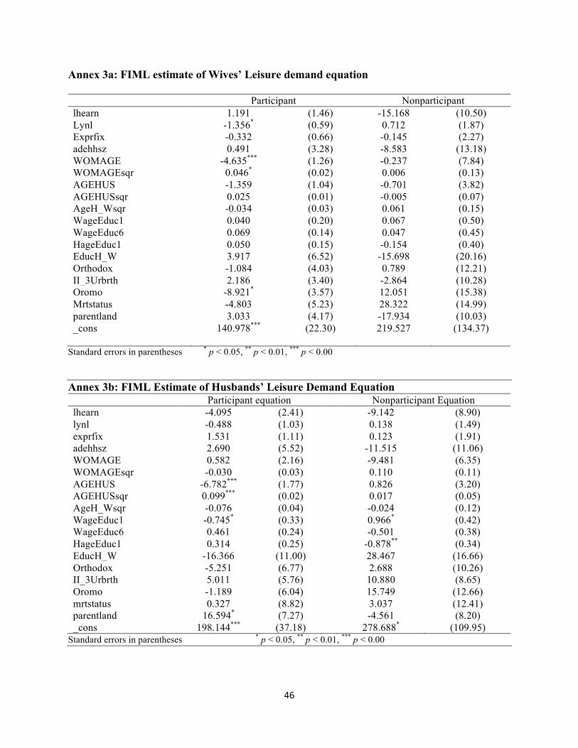
46    

Annex 3a: FIML estimate of Wives’ Leisure demand equation Participant Nonparticipant lhearn 1.191 (1.46) -15.168 (10.50) Lynl -1.356* (0.59) 0.712 (1.87) Exprfix -0.332 (0.66) -0.145 (2.27) adehhsz 0.491 (3.28) -8.583 (13.18) WOMAGE -4.635*** (1.26) -0.237 (7.84) WOMAGEsqr 0.046* (0.02) 0.006 (0.13) AGEHUS -1.359 (1.04) -0.701 (3.82) AGEHUSsqr 0.025 (0.01) -0.005 (0.07) AgeH_Wsqr -0.034 (0.03) 0.061 (0.15) WageEduc1 0.040 (0.20) 0.067 (0.50) WageEduc6 0.069 (0.14) 0.047 (0.45) HageEduc1 0.050 (0.15) -0.154 (0.40) EducH_W 3.917 (6.52) -15.698 (20.16) Orthodox -1.084 (4.03) 0.789 (12.21) II_3Urbrth 2.186 (3.40) -2.864 (10.28) Oromo -8.921* (3.57) 12.051 (15.38) Mrtstatus -4.803 (5.23) 28.322 (14.99) parentland 3.033 (4.17) -17.934 (10.03) _cons 140.978*** (22.30)

219.527 (134.37)

Standard errors in parentheses * p < 0.05, ** p < 0.01, *** p < 0.00 Annex 3b: FIML Estimate of Husbands’ Leisure Demand Equation Participant equation Nonparticipant Equation lhearn -4.095 (2.41) -9.142 (8.90) lynl -0.488 (1.03) 0.138 (1.49) exprfix 1.531 (1.11) 0.123 (1.91) adehhsz 2.690 (5.52) -11.515 (11.06) WOMAGE 0.582 (2.16) -9.481 (6.35) WOMAGEsqr -0.030 (0.03) 0.110 (0.11) AGEHUS -6.782*** (1.77) 0.826 (3.20) AGEHUSsqr 0.099*** (0.02) 0.017 (0.05) AgeH_Wsqr -0.076 (0.04) -0.024 (0.12) WageEduc1 -0.745* (0.33) 0.966* (0.42) WageEduc6 0.461 (0.24) -0.501 (0.38) HageEduc1 0.314 (0.25) -0.878** (0.34) EducH_W -16.366 (11.00) 28.467 (16.66) Orthodox -5.251 (6.77) 2.688 (10.26) II_3Urbrth 5.011 (5.76) 10.880 (8.65) Oromo -1.189 (6.04) 15.749 (12.66) mrtstatus 0.327 (8.82) 3.037 (12.41) parentland 16.594* (7.27) -4.561 (8.20) _cons 198.144*** (37.18) 278.688* (109.95)

Standard errors in parentheses * p < 0.05, ** p < 0.01, *** p < 0.00

47    

Annex 3c: FIML Estimate of Daughters` Leisure Demand Equation Participant Equation Non-participant Equation lhearn -2.997 (5.75) -7.283 (11.35) lynl 1.445 (2.03) 2.570 (1.83) exprfix 3.130 (2.22) 5.207* (2.33) adehhsz -1.786 (10.90) -15.843 (12.92) WOMAGE -18.394*** (4.86) -9.702 (10.45) WOMAGEsqr 0.213** (0.07) 0.120 (0.16) AGEHUS -2.882 (3.74) 0.618 (4.15) AGEHUSsqr 0.021 (0.05) 0.018 (0.07) AgeH_Wsqr 0.047 (0.07) -0.144 (0.15) WageEduc1 -0.053 (0.62) -0.886 (0.46) WageEduc6 0.785 (0.50) -0.139 (0.46) HageEduc1 -0.053 (0.48) 0.634 (0.37) EducH_W 6.634 (21.51) -38.443 (20.11) Orthodox -18.584 (15.72) 57.379*** (13.45) II_3Urbrth 10.424 (12.03) 4.028 (11.29) Oromo 5.249 (14.84) 25.488 (19.13) mrtstatus -11.545 (21.88) 4.996 (21.93) parentland -8.515 (16.60) -4.287 (10.80) _cons 560.808*** (96.81) 254.074 (152.36)

Standard errors in parentheses * p < 0.05, ** p < 0.01, *** p < 0.001 Annex 3d: FIML Estimate of Sons` Leisure Demand Equation Participant equation Non-participant Equation lhearn 1.532 (4.60) -36.814** (13.61) lynl 0.174 (2.03) 1.030 (2.29) exprfix 5.953** (2.21) 3.566 (3.08) adehhsz -18.690 (11.56) -10.066 (14.81) WOMAGE -3.349 (5.28) 14.894 (10.18) WOMAGEsqr 0.018 (0.07) -0.271 (0.16) AGEHUS -5.089 (4.64) -7.959 (4.70) AGEHUSsqr 0.058 (0.06) 0.131 (0.07) AgeH_Wsqr -0.034 (0.11) -0.273 (0.16) WageEduc1 0.580 (0.65) 0.000 (0.61) WageEduc6 -0.004 (0.50) 0.855 (0.58) HageEduc1 -0.611 (0.51) -0.648 (0.49) EducH_W 10.646 (22.94) -11.957 (25.58) Orthodox 26.684 (15.68) -5.621 (19.46) II_3Urbrth 31.781* (12.56) 1.354 (13.45) Oromo -5.020 (13.74) 3.122 (19.71) mrtstatus -4.112 (25.70) 23.797 (30.38) parentland 21.775 (15.96) -34.625* (13.66) _cons 277.348** (95.50) 322.034 (165.35)

Standard errors in parentheses * p < 0.05, ** p < 0.01, *** p < 0.001

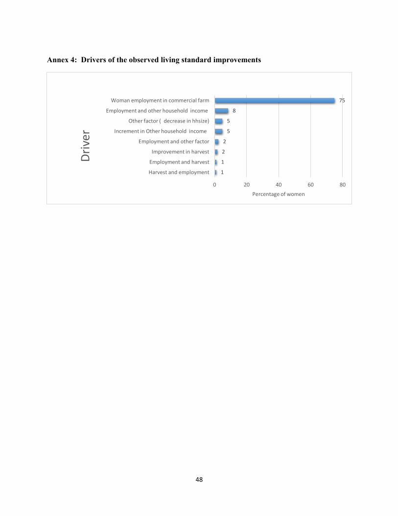
48    

Annex 4: Drivers of the observed living standard improvements

 

1

1

2

2

5

5

8

75

0 20 40 60 80

Harvest  and  employment

Employment  and  harvest

Improvement  in  harvest

Employment  and  other  factor

Increment  in  Other  household    income    

Other  factor  (    decrease  in  hhsize)

Employment  and  other  household    income  

Woman  employment  in  commercial  farm

Percentage  of  women

Driver

CMI WORKING PAPERSThis series can be ordered from:

CMI (Chr. Michelsen Institute)Phone: +47 47 93 80 00 Fax: +47 47 93 80 01E-mail: cmi@cmi.no

P.O.Box 6033 Bedriftssenteret,N-5892 Bergen, NorwayVisiting address: Jekteviksbakken 31, Bergen

Web: www.cmi.no

Printed version: ISSN 0804-3639Electronic version: ISSN 1890-5048Printed version: ISBN 978-82-8062-570-0Electronic version: ISBN 978-82-8062-571-7

This paper is also available at:www.cmi.no/publications

INDEXING TERMSSalaried employmentWage labor GenderBargaining ConsumptionPoverty Hunger

We examine the welfare impacts of women getting low-skilled jobs and find large positive effects, both at the household and the individual level. However, the women workers, their husbands and their oldest daughters reduced their leisure, but women to a much larger extent than the others. The leisure of the oldest son did not change. Investigating the transmission mechanisms suggests that the impacts did not only go through income and substitution effects, but also through a bargaining effect. Getting the job likely improved the bargaining position of the wife through several mechanisms, which in turn added to the positive impact on her welfare.