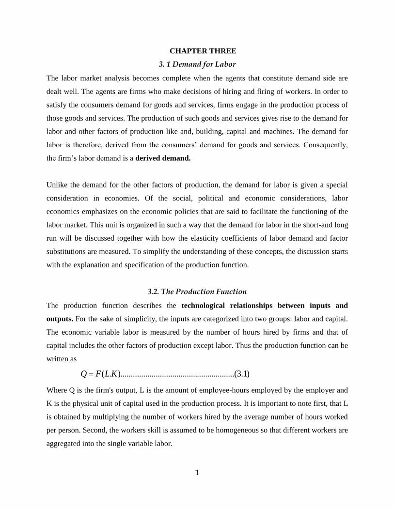
1

CHAPTER THREE

3. 1 Demand for Labor

The labor market analysis becomes complete when the agents that constitute demand side are

dealt well. The agents are firms who make decisions of hiring and firing of workers. In order to

satisfy the consumers demand for goods and services, firms engage in the production process of

those goods and services. The production of such goods and services gives rise to the demand for

labor and other factors of production like and, building, capital and machines. The demand for

labor is therefore, derived from the consumers’ demand for goods and services. Consequently,

the firm’s labor demand is a derived demand.

Unlike the demand for the other factors of production, the demand for labor is given a special

consideration in economies. Of the social, political and economic considerations, labor

economics emphasizes on the economic policies that are said to facilitate the functioning of the

labor market. This unit is organized in such a way that the demand for labor in the short-and long

run will be discussed together with how the elasticity coefficients of labor demand and factor

substitutions are measured. To simplify the understanding of these concepts, the discussion starts

with the explanation and specification of the production function.

3.2. The Production Function

The production function describes the technological relationships between inputs and

outputs. For the sake of simplicity, the inputs are categorized into two groups: labor and capital.

The economic variable labor is measured by the number of hours hired by firms and that of

capital includes the other factors of production except labor. Thus the production function can be

written as

( . ).......................................................(3.1)Q F L K

Where Q is the firm's output, L is the amount of employee-hours employed by the employer and

K is the physical unit of capital used in the production process. It is important to note first, that L

is obtained by multiplying the number of workers hired by the average number of hours worked

per person. Second, the workers skill is assumed to be homogeneous so that different workers are

aggregated into the single variable labor.

2

a) Marginal and Average Products

From the production function of which specification is given by equation (3.1) we can produce

two important concepts: Marginal Products and Average Products. As the inputs are categorized

into two groups, we can identify two marginal products the marginal product of labor and the

marginal product of capital. Formally the marginal product of labor (MP) is simply defined as

the change in physical output (∆Q) produced by hiring an additional unit of labor (∆L) holding

capital constant

( ).......................................................(3.2)L

QMP K

L

Similarly, the marginal product of capital LMP is defined as the change in output resulting from

a one-unit change in the capital stock K , holding labor constant

( ).......................................................(3.3)k

QMP L

k

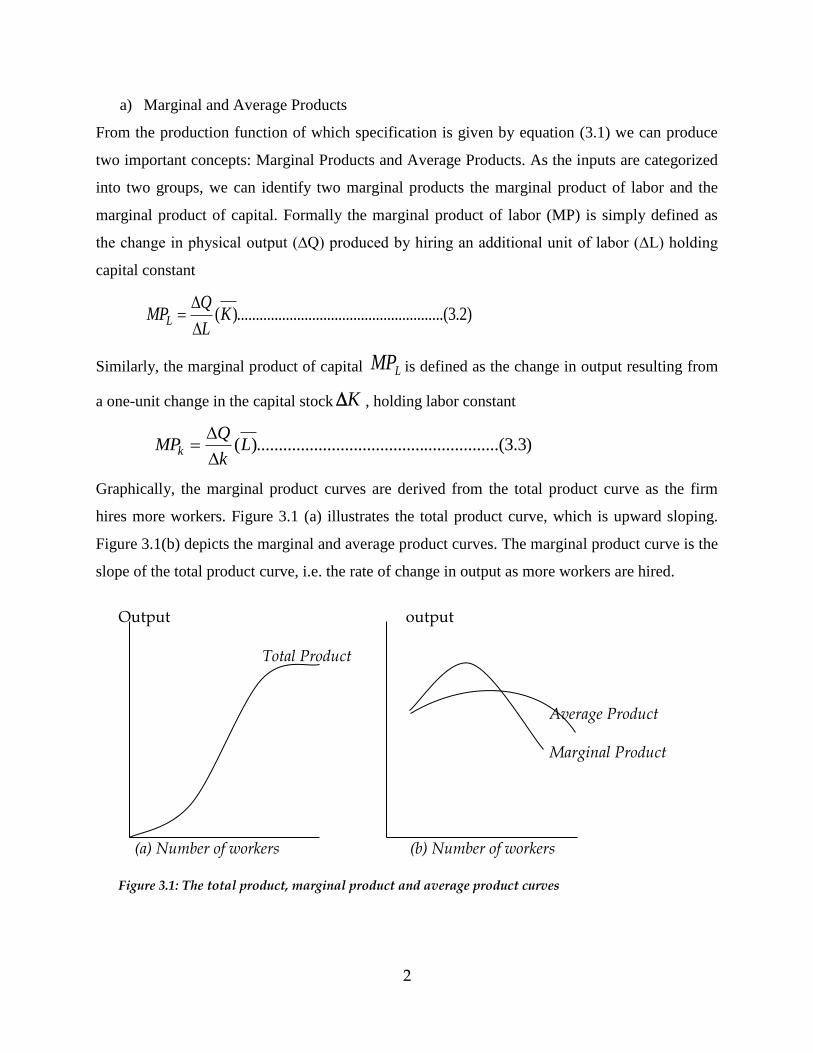
Graphically, the marginal product curves are derived from the total product curve as the firm

hires more workers. Figure 3.1 (a) illustrates the total product curve, which is upward sloping.

Figure 3.1(b) depicts the marginal and average product curves. The marginal product curve is the

slope of the total product curve, i.e. the rate of change in output as more workers are hired.

Output output Total Product

Average Product

Marginal Product (a) Number of workers (b) Number of workers Figure 3.1: The total product, marginal product and average product curves

3

It rises initially but eventually starts to decrease as more workers are hired. Since the marginal

product of labor is measured by holding capital constant the increment on output as more

workers employed must be subject to the law of diminishing returns.

The average product of labor )( LAP is defined as amount of output produced per person.

)4.3.....(........................................L

QAPL

From figure 4.1(b) we can establish the following relationship: the MPL curve lies above the MPL

curve when the latter is rising, and the APL curve lies below the APL curve when the latter is

falling. It implies that the MPL curve intersects the APL curve at the point where APL curve

peaks.

b) Marginal Revenue Product

Usually firms make production decisions by considering what is prevailing in the output market

rather than the availability of factors of production. Employment depends on the revenue

generated by producing and selling extra output in the market. The more important concept

associated with the production decision of firms is that of the marginal Revenue Product or the

value of marginal Product. It is defined as the money value generated from hiving an additional

worker.

)5.3...(........................................MRxMPMRP LL

Where VMPL is the value of marginal product of labor and MR is the marginal revenue. The

marginal revenue that is generated by an extra output sold depends on the bind of market in

which the product is sold. If the market is a perfectly competitive, then the marginal revenue is

identical to the product price (P) and equation (3.5) can written as

)6.3...(........................................PxMPVMP LL

Likewise, the value of average product of labor is given by the product of the average product

and product price

4

3.3. The Short-run demand for labor

3.3.1 The perfectly competitive seller

The short-run demand for labor analysis focuses on the firms behavior towards the labor demand

over a short period of time during which the capital stock is hold constant. As a result of this, the

law of diminishing marginal returns is regarded as the critical assumption that lies behind the

derivation of the labor demand curve in the short run. For exposition purpose, the firm works

under the perfectly competitive output market and hires labor from a competitive labor market so

that both the product price and the market wage rate the firm faces will be constant. Consider the

following example, and suppose that the product price is Birr 2 and the market wage rate is Birr

22. For the various level of labor employed the marginal product and the value of marginal

product is given as follows:

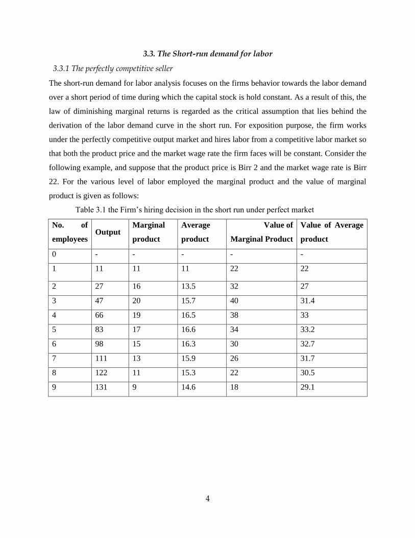
Table 3.1 the Firm’s hiring decision in the short run under perfect market

No. of

employees Output

Marginal

product

Average

product

Value of

Marginal Product

Value of Average

product

0 - - - - -

1 11 11 11 22 22

2 27 16 13.5 32 27

3 47 20 15.7 40 31.4

4 66 19 16.5 38 33

5 83 17 16.6 34 33.2

6 98 15 16.3 30 32.7

7 111 13 15.9 26 31.7

8 122 11 15.3 22 30.5

9 131 9 14.6 18 29.1

5

Birr

38 w/

22 w

A B LVAP

LVMP

1 4 8

Number of workers

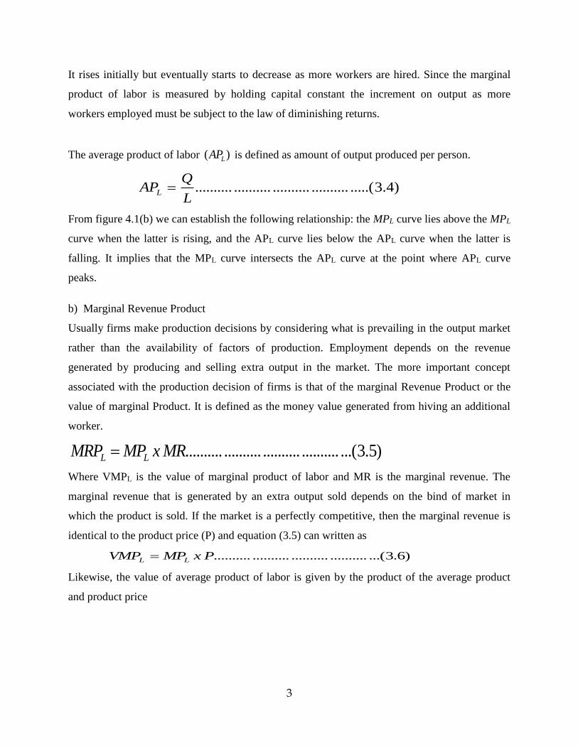
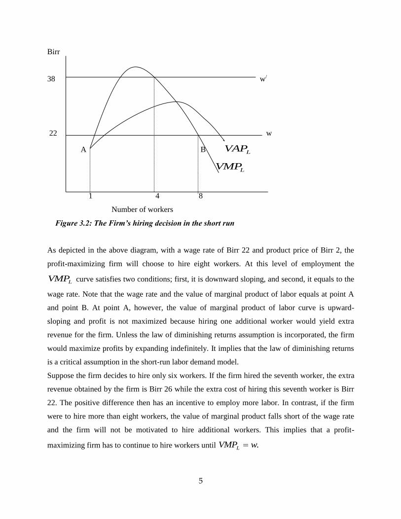
Figure 3.2: The Firm’s hiring decision in the short run

As depicted in the above diagram, with a wage rate of Birr 22 and product price of Birr 2, the

profit-maximizing firm will choose to hire eight workers. At this level of employment the

LVMP curve satisfies two conditions; first, it is downward sloping, and second, it equals to the

wage rate. Note that the wage rate and the value of marginal product of labor equals at point A

and point B. At point A, however, the value of marginal product of labor curve is upward-

sloping and profit is not maximized because hiring one additional worker would yield extra

revenue for the firm. Unless the law of diminishing returns assumption is incorporated, the firm

would maximize profits by expanding indefinitely. It implies that the law of diminishing returns

is a critical assumption in the short-run labor demand model.

Suppose the firm decides to hire only six workers. If the firm hired the seventh worker, the extra

revenue obtained by the firm is Birr 26 while the extra cost of hiring this seventh worker is Birr

22. The positive difference then has an incentive to employ more labor. In contrast, if the firm

were to hire more than eight workers, the value of marginal product falls short of the wage rate

and the firm will not be motivated to hire additional workers. This implies that a profit-

maximizing firm has to continue to hire workers until .wVMPL

6

It is important to note that only the level of employment that the firm can adjusts so that

.wVMPL In other words, the firm, being a competitive, do not have any influence on the

wage and cannot set the wage to the value of marginal product of labor. If, for instance, the

market wage rate is raised to a value of Birr 38, the firm should adjust its level of employment

only to four workers, at which .wVMPL If the firm hired the fourth worker, however, the

LVAP (Birr 33) would be lower than wage rate (Birr 38), and the firm would incur a loss and

leave the market. This implies that the hiring decision for the alternative given wage rates will

take place only if the LVMP curve is downward sloping and lies below the intersection point

with the LVAP .

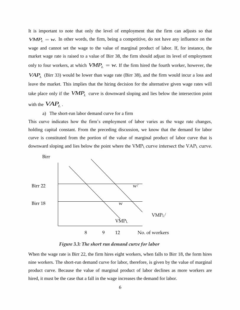
a) The short-run labor demand curve for a firm

This curve indicates how the firm’s employment of labor varies as the wage rate changes,

holding capital constant. From the preceding discussion, we know that the demand for labor

curve is constituted from the portion of the value of marginal product of labor curve that is

downward sloping and lies below the point where the VMPL curve intersect the VAPL curve.

When the wage rate is Birr 22, the firm hires eight workers, when falls to Birr 18, the form hires

nine workers. The short-run demand curve for labor, therefore, is given by the value of marginal

product curve. Because the value of marginal product of labor declines as more workers are

hired, it must be the case that a fall in the wage increases the demand for labor.

Birr Birr 22 w/

Birr 18 w VMPL/

VMPL 8 9 12 No. of workers

Figure 3.3: The short run demand curve for labor

7

The demand for labor curve is also affected by the change in output price. The short run labor

demand curve shifts upward for the given wage rate if the price of output increases. In fig. 4.3

for the given wage of Birr 22, suppose that the output price increases, which shifts the LVMP

outward to /LVMP . Then the firm’s demand for labor will increase from 8 to 12 workers.

Therefore, there is a positive relationship between short-run labor demand and product price. In

addition to the output price, productive efficiency of workers, which improve the marginal

product of labor employed, also affects the demand for labor curves my shifting it upward.

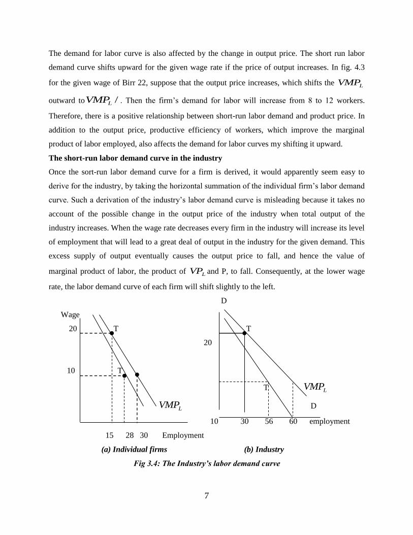
The short-run labor demand curve in the industry

Once the sort-run labor demand curve for a firm is derived, it would apparently seem easy to

derive for the industry, by taking the horizontal summation of the individual firm’s labor demand

curve. Such a derivation of the industry’s labor demand curve is misleading because it takes no

account of the possible change in the output price of the industry when total output of the

industry increases. When the wage rate decreases every firm in the industry will increase its level

of employment that will lead to a great deal of output in the industry for the given demand. This

excess supply of output eventually causes the output price to fall, and hence the value of

marginal product of labor, the product of LVP and P, to fall. Consequently, at the lower wage

rate, the labor demand curve of each firm will shift slightly to the left.

D

Wage

20 T T

20

10 T

T LVMP

LVMP D

10 30 56 60 employment

15 28 30 Employment

(a) Individual firms (b) Industry

Fig 3.4: The Industry’s labor demand curve

8

Each firm in the industry initially hires 15 workers when the wage rate is Birr 20. Then the total

employment in the industry will be 30 if there are only two firms in the industry. But if the wage

falls to Birr 10, each firm tends to hire 30 workers. The resulting total employment in the

industry would have been 60 had the labor demand in the industry been the horizontal

summation of the two firms’ demand for labor. And the demand for labor curve in the industry

would have been given by the curve DD in Fig 3.4(b).

Following the fall in wage from Birr 20 to Birr 10, however, firms in the industry will expand

output thereby reducing the price of output and the value of marginal product. Consequently, the

total employment in the industry will be 56 instead of 60, as the labor demand curve for the

industry becomes steeper. The ‘true’ industry labor demand curve is given by TT.

b) The Marginal Approach

The hiring decisions of firms could be alternatively reached by employing the marginal

productivity conditions. According to this alternative method the profit-maximization level of

employment is identified by equating the marginal cost with the marginal revenue-the additional

cost of producing an additional unit of output must be equal to the extra revenue obtained from

selling that output.

Formula derivation

i. Short run production function takes the form Q=f (L)

ii. The MPL is accordingly dQ/dL =f '(L). The profit function is given by ∏ =TR-TC.

iii. If the producer operates in perfectly competitive product and labor markets, then the market

price of the output, Px and the wage rate w, are given.

Therefore TR=P*Q and TC= WL. Implies that ∏ = P*Q- WL.

iv. ∏ is a max when d∏/dL= 0. (Necessary condition )

Therefore d∏/dL= Pf' (L)-W=0 = MRPL=W

v. The sufficient condition is

d2∏/d2L = Pf''(L)<0

3.2 .2 The imperfectly competitive seller

Most firms do not sell their product in purely competitive market. Rather they sell under

imperfectly competitive conditions. Because of product uniqueness of differentiation, the

imperfectly completive seller’s product demand curve is dawn ward sloping, rather than

9

perfectly elastic, and this means that the firm must lower its price to sell the output contributed

by each successive workers. Hence, the labor demand curve (MRP) for purely competitive seller

falls for a single reason: MPL diminishes while product price is constant. But the MRP of the

imperfectly competitive seller declines for two reasons: MPL falls and product price declines as

output increases. As in the case of perfectly competitive seller, application of the MRP= W rule

to the MRP curve will yield the conclusion that the MRP curve is firm’s labor demand curve.

However, all else being equal, the imperfect seller’s labor demand curve is steeper and less

elastic than that of purely competitive seller.

It is not surprising that the firm which possesses monopoly power is less responsive to wage rate

change than is the purely competitive seller. The tendency for the imperfectly competitive seller

to add few workers as the wage rate declines is merely the labor market reflection of the firm’s

tendency to restrict output in the product market. Other things being equal, the seller possessing

monopoly power will find it profitable to produce less output than would a purely competitive

seller. In producing this seller output, it will employ fewer workers.

3.4 The Demand for labor in the Long Run

The short-run labor demand discussion assumes that the time period is so short that the level of

capital stock remains fixed. In this section we will see what happens to the demand for labor if

the time period is long enough that the level of capital changes- the plant size can expand or

contract. Therefore, the long run profit-maximization condition requires making decisions about

the number workers to be employed and the amount of plant and equipment to invest in. The

explanation of this section starts by emphasizing the basic microeconomic concepts of cost

minimization.

Concepts of Cost Minimization

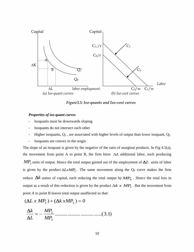
Iso-quants and iso-cost underlie the cost minimization concept. An iso-quant is the

possible combinations of capital and labor that produce the same level of Output.

10

Properties of iso-quant curves

- Isoquants must be downwards sloping

- Isoquants do not intersect each other

- Higher isoquants, Q1 , are associated with higher levels of output than lower isoquant, Q2.

- Isoquants are convex to the origin

The slope of an isoquant is given by the negative of the ratio of marginal products. In Fig 4.5(a),

the movement from point A to point B, the firm hires L additional labor, each producing

LMP units of output. Hence the total output gained out of the employment of L units of labor

is given by the product .LLxMP The same movement along the Q0 curve makes the firm

reduce k unites of capital, each reducing the total output byKMP . Hence the total loss in

output as a result of this reduction is given by the product kMPxk . But the movement from

point A to point B leaves total output unaffected so that:

0)()( Lk MPxkMPxL

)1.3......(..............................k

L

MP

MP

L

k

Capital Capital C1//r C1 C0/r A

K B Q1 C0

Q0

Labor

L labor employment. C0/w C1/w (a) Iso-quant curves (b) Iso-cost curves

Figure3.5: Iso-quants and Iso-cost curves

Figure3.5: Isoquants and Isocost curves

11

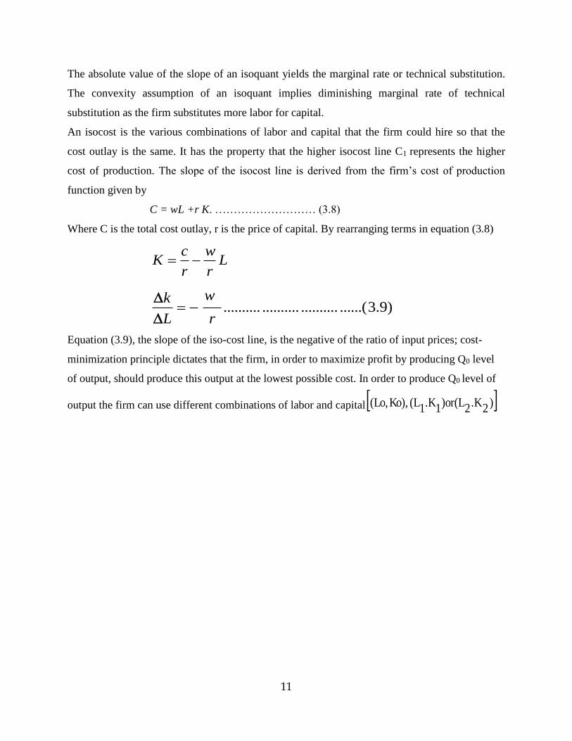
The absolute value of the slope of an isoquant yields the marginal rate or technical substitution.

The convexity assumption of an isoquant implies diminishing marginal rate of technical

substitution as the firm substitutes more labor for capital.

An isocost is the various combinations of labor and capital that the firm could hire so that the

cost outlay is the same. It has the property that the higher isocost line C1 represents the higher

cost of production. The slope of the isocost line is derived from the firm’s cost of production

function given by

C = wL +r K. ……………………… (3.8)

Where C is the total cost outlay, r is the price of capital. By rearranging terms in equation (3.8)

Lr

w

r

cK

)9.3......(..............................r

w

L

k

Equation (3.9), the slope of the iso-cost line, is the negative of the ratio of input prices; cost-

minimization principle dictates that the firm, in order to maximize profit by producing Q0 level

of output, should produce this output at the lowest possible cost. In order to produce Q0 level of

output the firm can use different combinations of labor and capital )2.K2)or(L1.K1(LKo),(Lo,.

12

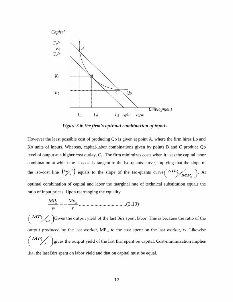
However the least possible cost of producing Qo is given at point A, where the firm hires Lo and

Ko units of inputs. Whereas, capital-labor combinations given by points B and C produce Qo

level of output at a higher cost outlay, C1. The firm minimizes costs when it uses the capital labor

combination at which the iso-cost is tangent to the Iso-quants curve, implying that the slope of

the iso-cost line r

w equals to the slope of the Iso-quants curve

k

L

MPMP . At

optimal combination of capital and labor the marginal rate of technical substitution equals the

ratio of input prices. Upon rearranging the equality

....................................(3.10)kL MpMP

w r

w

MPL Gives the output yield of the last Birr spent labor. This is because the ratio of the

output produced by the last worker, MPL, to the cost spent on the last worker, w. Likewise

r

MPk gives the output yield of the last Birr spent on capital. Cost-minimization implies

that the last Birr spent on labor yield and that on capital must be equal.

Capital C1/r K1 B C0/r K0 A K2 C Q0 Employment L1 L0 L2 c0/w c1/w

Figure 3.6: the firm’s optimal combination of inputs

13

In addition to cost-minimization, we need to consider the profit maximizing behavior of the firm

since the two concepts are different. Cost minimization constrains the firm to concentrate on the

given level of output, Qo, rather than considering the other options for profit-maximization.

Profit-maximization condition, however, enables the form to choose the optimal level of output,

by comparing the marginal cost and marginal revenue for different possible set of outputs.

Therefore the long –run profit-maximization condition requires that labor and capital are hired

until: LVMPW and )11.3.....(........................................kVMPr

Note that profit maximization implies cost minimization.

kL MPxPrandMPxPW

LMP

wP And

kMP

rP

)12.3........(....................r

w

MP

MP

MP

r

MP

w

K

L

kL

Equation (3.12) is the condition for cost- minimization. However, cost-minimization need not

imply profit-maximization.

The Long-run Demand Curve for Labor

The long-run Labor demand curve graphs the relationship between the long-run demand for

labor and wage rate. To see what the labor demand curve looks like where the wage rate change

let us consider that

The firm is initially producing Qo units of output

The corresponding input prices are W0 and r0

Qo satisfies both profit-maximizing and cost minimizing conditions

The optimal cost outlay associated with Qo level of output is given by Co

Suppose the market wage falls from Wo to W1. The slope of the isocost line becomes small and

the isocost line becomes flatter than before. Unless the firm’s total outlay, Co remains the same,

the new isocost line doesn’t rotate around the original intercept, Co/r. However, the firm’s cost

outlay need not be the same before and after the change in wage. Instead of originating from the

initial intercept, the new isocost line may start from an intercept, which is located over the

previous one. Another important result that follows from the wage cut is the fall in the marginal

14

cost of producing the firm’s output. An additional unit of output can be produced when labor

becomes cheap. The upward sloping marginal cost curve will shift rightward following this wage

cut. At the given output price, which is equal to the marginal revenue for competitive firm, the

profit-maximizing level of output, occurs at a higher level of output. After the wage cut the

Marginal cost

Shifts from MCo to MC1 and the new MC curve equates with the output with the output price at

Q level of output so that profit is maximized after the fall. Then the firm decides to produce Q1

level of output.

Figure 3-7(b) illustrates that the new iso-quant curve, Q1 corresponds with the profit maximizing

level of output, of the various mix of labor and capital used to produce Q1 level of output, the

cost-minimizing (optimal) one is given by point B, where the new isoquant curve, Q1, is tangent

to the new isocost line, C1. The new optimal mix is located to the right of the original mix,

implying that the firm’s demand for labor will always increase as the wage falls. However, the

fall in wage does not necessarily increase the use of capital. We can thus conclude that the long-

run demand curve for labor is also a downward sloping curve (see figure 3-8 below).

Birr K MC0 C1/r MC1 C0/r B A P Q1 Q0 Q L Q0 Q1 L0 L1 c0/w0 c1/w1

(a) Firm’s output decision (b) Firm’s hiring decision

Fig. 3.7 the Impact of wage reduction on output and employment of a profit-maximizing firm

15

Substitution and Scale Effects

The movement from point A to point B happens as a result of wage cut. It is possible to

decompose such a move into substitution and scale effects. In particular, the wage cut reduces

the price of labor relative to that capital. The decline in the wage encourages the firm to readjust

its input mix so that it is more labor intensive. In addition the wage cut reduces the marginal cost

of production and encourages the firm to expand. On the whole, the demand for labor becomes

high as the firm expands and takes advantage of the fall in the wage rate.

Initially the firm is producing Qo level of output and faces Wo wage rate, where it demands Lo

units of labor. As the wage falls to W1, the marginal cost declines and the firm expands its

production to a level of Q2 units, there by employing L1 units of labor. If we decompose the

move in to two stages, firstly the firm takes advantage of the wage cut by expanding production.

Since labor and capital are normal inputs, using the same analogy of normal goods the demand

for both labor and capital increases following the expansion of production. It is worth noting that

the newly introduced isocost line is parallel to and has the same slope as the original isocost line

so that the new tangency point C shows the expansion in output as both capital and labor

increases proportionately. The move from point A to point C is defined as the scale effect. The

scale effect thus increases both labor and capital.

Wage (Birr) Capital C1/r D C W0 B A Q1

W1 Q0

DLR labor employment L0 L1 L0 L2 L1 c0/w0 c1/w1 Fig. 3.8: the LR demand for labor Fig. 3.9: Substitution and scale effect

16

Secondly, the wage cut makes labor cheaper than before. This leads to the rearrangement of

input combination towards the labor- intensive techniques of production. The analysis of such an

effect, substitution effect, is undertaken by holding output fixed. So the movement along the new

isoquant curve, the move from point C to point B, reflects the substitution of labor for capital.

Unlike the scale effect, the substitution effect increases the firm’s demand for labor but reduces

the firm’s demand for capital. Whether the firm demands more capital as wage falls depends on

which effect outweighs. If the scale effect, which increases the demand for both inputs, exceeds

the substitution effect, the wage cut will make firms hire more capital. Otherwise, the firm would

use less capital as the wage falls.

3.5 Elasticity of Labor Demand

The responsiveness of labor demand for a change in the wage rates measures the elasticity of

labor demand. It is possible to measure both the short-run and long run elasticity.

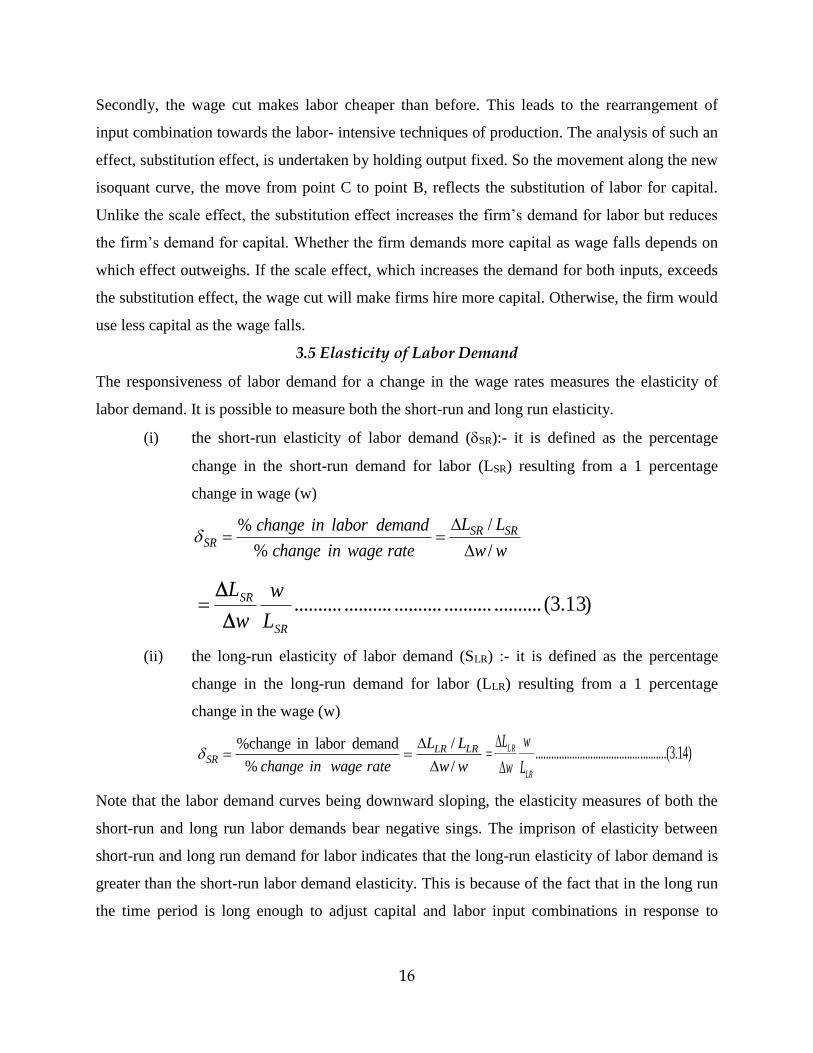
(i) the short-run elasticity of labor demand (SR):- it is defined as the percentage

change in the short-run demand for labor (LSR) resulting from a 1 percentage

change in wage (w)

/%

% /

SR SRSR

L Lchange in labor demand

change in wage rate w w

)13.3(..................................................SR

SR

L

w

w

L

(ii) the long-run elasticity of labor demand (SLR) :- it is defined as the percentage

change in the long-run demand for labor (LLR) resulting from a 1 percentage

change in the wage (w)

/%change in labor demand

% /

LR LRSR

L L

change in wage rate w w

..................................................(3.14)LR

LR

L w

w L

Note that the labor demand curves being downward sloping, the elasticity measures of both the

short-run and long run labor demands bear negative sings. The imprison of elasticity between

short-run and long run demand for labor indicates that the long-run elasticity of labor demand is

greater than the short-run labor demand elasticity. This is because of the fact that in the long run

the time period is long enough to adjust capital and labor input combinations in response to

17

changes in the wage rate. But in the short run the time period is too short to adjust its size

optimally.

3.6 The Elasticity of Factor substitution

The elasticity of substitution is a summary measure of the shape of the isoquant and thereby, of

the ease of substitution between labor and capital. The elasticity of substitution between labor

and capital (holding output constant) is given by

Elasticity of substitution = Percentage change in the ratio of capital to labor

Percentage change in the slope of the isoquant

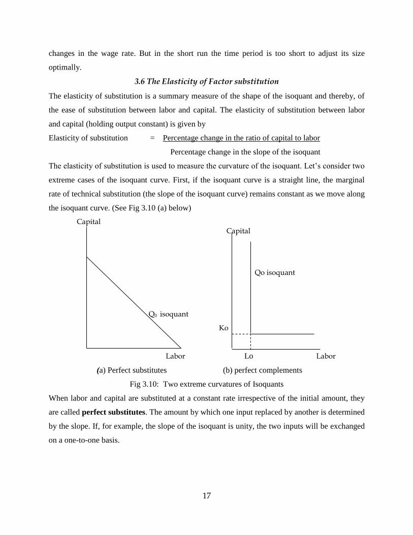
The elasticity of substitution is used to measure the curvature of the isoquant. Let’s consider two

extreme cases of the isoquant curve. First, if the isoquant curve is a straight line, the marginal

rate of technical substitution (the slope of the isoquant curve) remains constant as we move along

the isoquant curve. (See Fig 3.10 (a) below)

Capital Capital

Qo isoquant

Q0 isoquant

Ko

Labor Lo Labor

(a) Perfect substitutes (b) perfect complements

Fig 3.10: Two extreme curvatures of Isoquants

When labor and capital are substituted at a constant rate irrespective of the initial amount, they

are called perfect substitutes. The amount by which one input replaced by another is determined

by the slope. If, for example, the slope of the isoquant is unity, the two inputs will be exchanged

on a one-to-one basis.

18

The other extreme case appears to happen when the two inputs are perfectly complementary, i.e.

the isoquant curve is a right-angled one (see Fig 3.10) (b) above). We can either add more

workers by holding capital at some constant value, Ko or add more capital by holding labor

constant at a value of Lo; hours, in each case output remains the same. Thus a cost- minimizing

firm has only one optimal combination of labor and capital-Ko units of capital and Lo units of

labor.

Following this definition of extreme isoquant curvatures, we can measure the elasticity of

substitution between the two inputs. When the isoquant curve is a straight line, the firm

minimizes by producing at either of the extreme points depending on the cheaper alternative. If

the input price changes, the firm will shift to the other extreme position. As a result of this the

elasticity of substitution is infinite

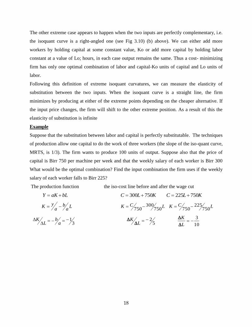
Example

Suppose that the substitution between labor and capital is perfectly substitutable. The techniques

of production allow one capital to do the work of three workers (the slope of the iso-quant curve,

MRTS, is 1/3). The firm wants to produce 100 units of output. Suppose also that the price of

capital is Birr 750 per machine per week and that the weekly salary of each worker is Birr 300

What would be the optimal combination? Find the input combination the firm uses if the weekly

salary of each worker falls to Birr 225?

The production function the iso-cost line before and after the wage cut

bLaKY KLC 750300 KLC 750225

La

ba

yK LCK

750300

750 LCK

750225

750

3

1

a

bL

K 5

2L

K

10

3

L

K

19

K K

17503

KC

b

y K1

3

1(

L

KQo

3

1

L

KQo

5

2

L

KCo

K0=0

Lo=0 300

C

2251

c

b

yL

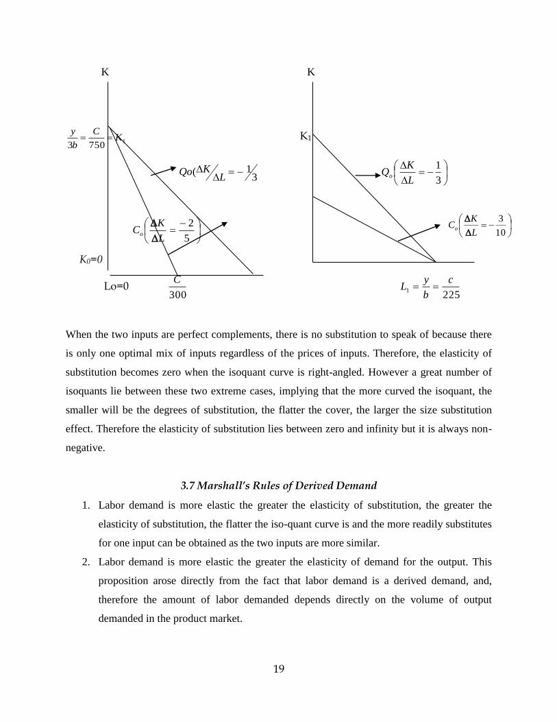
When the two inputs are perfect complements, there is no substitution to speak of because there

is only one optimal mix of inputs regardless of the prices of inputs. Therefore, the elasticity of

substitution becomes zero when the isoquant curve is right-angled. However a great number of

isoquants lie between these two extreme cases, implying that the more curved the isoquant, the

smaller will be the degrees of substitution, the flatter the cover, the larger the size substitution

effect. Therefore the elasticity of substitution lies between zero and infinity but it is always non-

negative.

3.7 Marshall’s Rules of Derived Demand

1. Labor demand is more elastic the greater the elasticity of substitution, the greater the

elasticity of substitution, the flatter the iso-quant curve is and the more readily substitutes

for one input can be obtained as the two inputs are more similar.

2. Labor demand is more elastic the greater the elasticity of demand for the output. This

proposition arose directly from the fact that labor demand is a derived demand, and,

therefore the amount of labor demanded depends directly on the volume of output

demanded in the product market.

10

3

L

KCo

20

3. Labor demand is more elastic the greater labor’s share in total costs. If labor is an

important input in the production process, the share of labor from total cost will be large.

A small rise in the wage rate leads to a large rise in the marginal cost of production and,

hence, a large rise in the output price. Consumers will respond by cutting back their

demand for the high price product that results in a substantial fall in employment.

4. The demand for labor is more elastic the greater the supply elasticity of other factors of

production, such as capital. If the two inputs are substitutes then a rise in the wage rate

will produce a substitution towards capital. If the supply curve of capital is inelastic, the

movement away from labor to capital will be reduced. But if the supply of capital is

elastic, firms are induced to substitute more capital for labor.