Knowledge Extraction and Consolidation from ... - CEUR-WS

Knowledge Extraction and Consolidation fromSocial Media (KECSM 2012)

Preface

In this new information age, where information, thoughts and opinions are sharedso prolifically through online social networks, tools that can make sense of thecontent of these networks are paramount. In order to make best use of this in-formation, we need to be able to distinguish what is important and interesting,and how this relates to what is already known. Social web analysis is all aboutthe users who are actively engaged and generate content. This content is dy-namic, rapidly changing to reflect the societal and sentimental fluctuations ofthe authors as well as the ever-changing use of language. While tools are avail-able for information extraction from more formal text such as news reports,social media affords particular challenges to knowledge acquisition, such as mul-tilinguality not only across but within documents, varying quality of the textitself (e.g. poor grammar, spelling, capitalisation, use of colloquialisms etc), andgreater heterogeneity of data. The analysis of non-textual multimedia informa-tion such as images and video offers its own set of challenges, not least becauseof its sheer volume and diversity. The structuring of this information requiresthe normalization of this variability by e.g. the adoption of canonical forms forthe representation of entities, and a certain amount of linguistic categorizationof their alternative forms.

Due to the reasons described above, data and knowledge extracted fromsocial media often suffers from varying, non-optimal quality, noise, inaccuracies,redundancies as well as inconsistencies. In addition, it usually lacks sufficientdescriptiveness, usually consisting of labelled and, at most, classified entities,which leads to ambiguities.

This calls for a range of specific strategies and techniques to consolidate, en-rich, disambiguate and interlink extracted data. This in particular benefits fromtaking advantage of existing knowledge, such as Linked Open Data, to compen-sate for and remedy degraded information. A range of techniques are exploitedin this area, for instance, the use of linguistic and similarity-based clusteringtechniques or the exploitation of reference datasets. Both domain-specific andcross-domain datasets such as DBpedia or Freebase can be used to enrich, in-terlink and disambiguate data. However, case- and content-specific evaluationsof quality and performance of such approaches are missing, hindering the widerdeployment. This is of particular concern, since data consolidation techniquesinvolve a range of partially disparate scientific topics (e.g. graph analysis, data

II

mining and interlinking, clustering, machine learning), but need to be appliedas part of coherent workflows to deliver satisfactory results.

The KECSM 2012 workshop aims to gather innovative approaches for knowl-edge extraction and consolidation from unstructured social media, in particu-lar from degraded user-generated content (text, images, video) such as tweets,blog posts, forums and user-generated visual media. KECSM has gathered novelworks from the fields of data analysis and knowledge extraction, and data en-richment, interlinking and consolidation. Equally, consideration has been givento the application perspective, such as the innovative use of extracted knowledgeto navigate, explore or visualise previously unstructured and disparate Web con-tent.

KECSM 2012 had a number of high-quality submissions. From these, the 8best papers were chosen for the two paper sessions of the programme. To initiatethe workshop, a keynote on perspectives of social media mining from an industryviewpoint was given by Seth Grimes.

We sincerely thank the many people who helped make KECSM 2012 sucha success: the Program Committee, the paper contributors, and all the partici-pants present at the workshop. In addition, we would like to add a special note ofappreciation for our keynote speaker, Seth Grimes, and the ARCOMEM project(http://www.arcomem.eu) for funding the best paper prize.

Diana MaynardStefan DietzeWim PetersJonathon Hare

Organisation

Organising Committee

Diana Maynard, University of Sheffield, United KingdomStefan Dietze, L3S Research Centre, Leibniz University Hannover, GermanyWim Peters, University of Sheffield, United KingdomJonathon Hare, University of Southampton, United Kingdom

Program Committee

Harith Alani, The Open University, United KingdomSoren Auer, University of Leipzig, GermanyUldis Bojar, University of Latvia, LatviaJohn Breslin, NUIG, IrelandMathieu D’Aquin, The Open University, United KingdomAnita de Waard, Elsevier, The NetherlandsAdam Funk, University of Sheffield, United KingdomDaniela Giordano, University of Catania, ItalyAlejandro Jaimes, Yahoo! Research Barcelona, SpainPaul Lewis, University of Southampton, United KingdomVeronique Malaise, Elsevier, The NetherlandsPavel Mihaylov, Ontotext, BulgariaWolfgang Nejdl, L3S Research Centre, Leibniz University Hannover, GermanyThomas Risse, L3S Research Centre, Leibniz University Hannover, GermanyMatthew Rowe, The Open University, United KingdomMilan Stankovic, Hypios & Universit Paris-Sorbonne, FranceThomas Steiner, Google Germany, GermanyNina Tahmasebi, L3S Research Centre, Leibniz University Hannover, GermanyRaphael Troncy, Eurecom, FranceClaudia Wagner, Joanneum Research, Austria

Keynote Speaker

Seth Grimes, Alta Plana Corporation, USA

Sponsors

The best paper award was kindly sponsored by the European project AR-COMEM (http://arcomem.eu).

Table of Contents

A Platform for Supporting Data Analytics on Twitter . . . . . . . . . . . . . . . . . 1Yannis Stavrakas and Vassilis Plachouras

SEKI@home, or Crowdsourcing an Open Knowledge Graph . . . . . . . . . . . . 7Thomas Steiner and Stefan Mirea

Cluster-based Instance Consolidation For Subsequent Matching . . . . . . . . . 13Jennifer Sleeman and Tim Finin

Semantically Tagging Images of Landmarks . . . . . . . . . . . . . . . . . . . . . . . . . . 19Heather Packer, Jonathon Hare, Sina Samangooei, and Paul Lewis

Ageing Factor . . . . . . . . . . . . . . . . . . . . . . . . . . . . . . . . . . . . . . . . . . . . . . . . . . . . 34Victoria Uren and Aba-Sah Dadzie

Lifting user generated comments to SIOC . . . . . . . . . . . . . . . . . . . . . . . . . . . . 48Julien Subercaze and Christophe Gravier

Comparing Metamap to MGrep . . . . . . . . . . . . . . . . . . . . . . . . . . . . . . . . . . . . . 63Samuel Alan Stewart, Maia Elizabeth von Maltzahn, and Syed SibteRaza Abidi

Exploring the Similarity between Social Knowledge Sources and Twitter . 78Andrea Varga, Amparo E. Cano, and Fabio Ciravegna

A Platform for Supporting Data Analytics on Twitter:

Challenges and Objectives1

Yannis Stavrakas Vassilis Plachouras

IMIS / RC “ATHENA”

Athens, Greece

{yannis, vplachouras}@imis.athena-innovation.gr

Abstract. An increasing number of innovative applications use data from

online social networks. In many cases data analysis tasks, like opinion mining

processes, are applied on platforms such as Twitter, in order to discover what

people think about various issues. In our view, selecting the proper data set is

paramount for the analysis tasks to produce credible results. This direction,

however, has not yet received a lot of attention. In this paper we propose and

discuss in detail a platform for supporting processes such as opinion mining on

Twitter data, with emphasis on the selection of the proper data set. The key

point of our approach is the representation of term associations, user associa-

tions, and related attributes in a single model that also takes into account their

evolution through time. This model enables flexible queries that combine com-

plex conditions on time, terms, users, and their associations.

Keywords: Social networks, temporal evolution, query operators.

1 Introduction

The rapid growth of online social networks (OSNs), such as Facebook or Twitter,

with millions of users interacting and generating content continuously, has led to an

increasing number of innovative applications, which rely on processing data from

OSNs. One example is opinion mining from OSN data in order to identify the opinion

of a group of users about a topic. The selection of a sample of data to process for a

specific application and topic is a crucial issue in order to obtain meaningful results.

For example, the use of a very small sample of data may introduce biases in the out-

put and lead to incorrect inferences or misleading conclusions. The acquisition of data

from OSNs is typically performed through APIs, which support searching for key-

words or specific user accounts and relationships between users. As a result, it is not

straightforward to select data without having an extensive knowledge of related key-

words, influential users and user communities of interest, the discovery of which is a

manual and time-consuming process. Selecting the proper set of OSN data is im-

portant not only for opinion mining, but for data analytics in general.

1 This work is partly funded by the European Commission under ARCOMEM (ICT 270239).

In this paper, we propose a platform that makes it possible to manage data analysis

campaigns and select relevant data from OSNs, such as Twitter, based not only on

simple keyword search, but also on relationships between keywords and users, as well

as their temporal evolution. Although the platform can be used for any OSN having

relationships among users and user posts, we focus our description here on Twitter.

The pivotal point of the platform is the model and query language that allow the ex-

pression of complex conditions to be satisfied by the collected data. The platform

models both the user network and the generated messages in OSNs and it is designed

to support the processing of large volumes of data using a declarative description of

the steps to be performed. To motivate our approach, in what follows we use opinion

mining as a concrete case of data analysis, however the proposed platform can equally

support other analysis tasks. The platform has been inspired by work in the research

project ARCOMEM2, which employs online social networks to guide archivists in

selecting material for preservation.

2 Related Work

There has been a growing body of work using OSN data for various applications.

Cheong and Ray [5] provide a review of recent works using Twitter. However, there

are only few works that explore the development of models and query languages for

describing the processing of OSN data. Smith and Barash [4] have surveyed visualiza-

tion tools for social network data and stress the need for a language similar to SQL

but adapted to social networks. San Martín and Gutierrez [3] describe a data model

and query language for social networks based on RDF and SPARQL, but they do not

directly support different granularities of time. Mustafa et al. [2] use Datalog to model

OSNs and to apply data cleaning and extraction techniques using a declarative lan-

guage. Doytsher et al. [1] introduced a model and a query language that allow to que-

ry with different granularities for frequency, time and locations, connecting the social

network of users with a spatial network to identify places visited frequently by users.

However, they do not consider any text artifacts generated by users (e.g. comments

posted on blogs, reviews, tweets, etc.).

The platform we propose is different from the existing works in that we incorpo-

rate in our modeling the messages generated by users of OSNs and temporally evolv-

ing relationships between terms, in addition to relationships between users. Moreover,

we aim to facilitate the exploration of the context of data and enable users to detect

associations between keywords, users, or communities of users.

3 Approach and Objectives

We envisage a platform able to adapt to a wide spectrum of thematically disparate

opinion mining campaigns (or data analysis tasks in general), and provide all the in-

2 http://www.arcomem.eu/

2 Yannis Stavrakas and Vassilis Plachouras

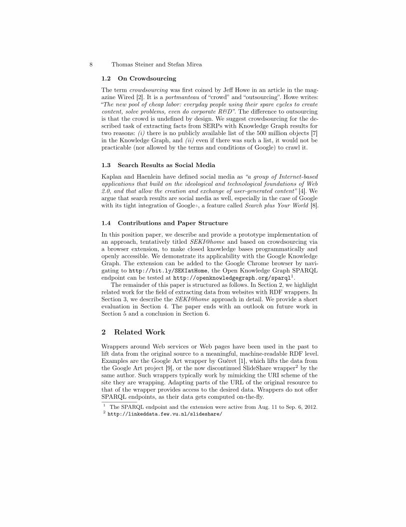
frastructure and services necessary for easily collecting and managing the data. This

platform is depicted in Fig. 1, and comprises three layers.

Integrated querying

Community

data

TwitterUser and tweet

metadata

Campaign

RepositoryCommunity

crawler

Tweet

crawler

Campaign manager

Campaign

configuration

CA

MP

AIG

N C

RA

WL

ING

INT

EG

RA

TE

D

MO

DE

LIN

G

Sentiment

analysis

OPINION MINING

DA

TA

AN

AL

YS

IS

Diversification

Tweets

Graph

Database

Temporal modeling

Community modeling

Entity recognition Term association

Opinion

dynamics

View on term, temporal, metadata, and

community criteria

Target

definition

Fig. 1: Platform architecture

The first layer is the Campaign Crawling layer. The objective of this layer is to al-

low for the definition and management of campaigns, and to collect all the relevant

“raw” data. A campaign is defined by a set of filters and a timespan. For each cam-

paign, the platform monitors the Twitter stream for the duration specified by the cam-

paign’s timespan, and incrementally stores in the Campaign Repository all the data

that match the campaign filters. Stored data fall into three categories: tweets, metada-

ta, and community data. Community data describe the relationships among Twitter

users, while metadata may refer either to tweets (timestamp, location, device, lan-

guage, etc.) or to users (place, total activity, account creation date, etc.). Selecting the

correct tweets for a campaign is of paramount importance; therefore, for converging

to the proper filters the process of campaign configuration follows an iterative ap-

proach: a preliminary analysis on an initial small number of tweets gives an overview

of the expected results, indicates the most frequent terms, and highlights the most

influential users, in order to verify that the campaign is configured correctly. If this is

not the case, an adjustment step takes place by modifying the terms that tweets are

expected to contain, the user accounts deemed most relevant to the topic of the cam-

paign, or by removing tweets from user accounts that have been identified to be ro-

A Platform for Supporting Data Analytics on Twitter 3

bots. Those modifications are based on suggestions made by the platform according to

the preliminary analysis of tweets.

The second layer is the Integrated Modeling layer. The objective of this layer is to

support a complex and flexible querying mechanism on the campaign data, allowing

the definition of campaign views. The significance of campaign views will become

apparent in a motivating example that will follow. A prerequisite for querying is the

modeling of the campaign “raw” data. The model should encompass three dimen-

sions. First, represent associations between interesting terms contained in tweets.

Such terms can be hashtags, or the output of an entity recognition process. Associa-

tions between terms can be partly (but not solely) based on co-occurrence of the terms

in tweets. Second, represent associations between users of varying influence forming

communities that discuss distinct topics. Finally, it should capture the evolution

across time of the aforementioned associations, term attributes, and user attributes.

This temporal, often overlooked, dimension is of paramount importance in our ap-

proach since it enables the expression of time-aware conditions in queries. The result-

ing model integrates all three dimensions above in a unified way as a graph. A suita-

ble query language is then used to select the tweets that satisfy conditions involving

content, user, and temporal constraints.

The third layer is the Data Analysis layer. The query language is used to define a

“target” view on the campaign data. This “target” view corresponds to a set of tweets

that hopefully contain the answer to an opinion-mining question. This set is then fed

into a series of analysis processes, like diversification for ensuring the correct repre-

sentation of important attribute values, and sentiment analysis for determining the

attitude of users towards the question. Opinion dynamics is important for recognizing

trends across time.

Motivating example. A marketing specialist wants to learn what people say in Twit-

ter about Coca-Cola: (a) in cases when Pepsi-Cola is also mentioned, and (b) during

the Olympic Games. The first step is to define a campaign. He launches a preliminary

search with the keywords coca cola. An initial analysis of the first results reveals

other frequent terms and hashtags, and after reviewing them he decides to include the

following in the campaign definition: #cc, #cola and coke. Moreover, the platform

suggests groups of users whose tweets contain most often the relevant keywords. He

decides to include some of them in the campaign definition. Having set the campaign

filters, he sets the campaign timespan, and launches the campaign. The crawler down-

loads data periodically, which are incrementally stored in the Campaign Repository

and modeled in the Graph Database. The next important step for our marketing spe-

cialist is to define suitable “targets” that correspond to his initial questions. He does

that by using the query language of the platform for creating views on the campaign

data. An intuitive description of the queries for the two cases follows.

The first query returns the tweets that will hopefully reveal what people say about

Coca-Cola in cases when Pepsi is also mentioned, using the following steps: 1) find

the terms that are highly associated with Pepsi Cola, 2) return the tweets in which

Coca- and Pepsi-related terms are highly associated.

The second query return the tweets that will hopefully reveal what people say

about Coca-Cola during the Olympics in the following steps: 1) find the terms that are


highly associated with Olympic Games, 2) find the time periods during which those

terms are most often encountered, 3) find the groups of people that most often use

those terms during the specific time periods, 4) return the tweets of those people,

during the specified time periods, which mention the Coca-Cola search terms.

The final step is to conduct opinion-mining analysis on the two sets of tweets re-

turned by the queries. In our approach the emphasis is on selecting the most suitable

set of tweets, according to the question we want to answer. In our view, selecting the

proper set is paramount for opinion mining processes to produce credible results.

4 Technical and Research Challenges

There are several technical and research challenges that need to be addressed in the

implementation of the proposed platform, with respect to the acquisition of data, as

well as the modeling and querying of data.

Scalable Crawling. In the case that the platform handles multiple campaigns in paral-

lel, there is a need to optimize the access to the OSN APIs, through which data is

made available. Typically, APIs have restrictions in the number of requests performed

in a given time span. The implementation of the platform should aim to minimize the

number of API requests while fetching data for many campaigns in parallel. Hence,

an optimal crawling strategy is required to identify and exploit overlaps between

campaigns and to merge the corresponding API requests.

Temporal Modeling. A second challenge is the modeling of large-scale graphs,

where both nodes and edges have temporally evolving properties. Our approach is to

treat such graphs as directed multigraphs, with multiple timestamped edges between

two vertexes [6]. Given that the scale of the graphs can be very large both in terms of

the number of vertexes and edges, but also along the temporal dimension, it is neces-

sary to investigate efficient encoding and indexing for vertexes and edges, as well as

their attributes. We have collected a set of tweets over a period of 20 days using Twit-

ter’s streaming API. In this set of tweets, we have counted a total of 2,406,250 distinct

hashtags and 3,257,760 distinct pairs of co-occurring hashtags. If we aggregate co-

occurring pairs of hashtags per hour, then we count a total of 5,670,528 distinct pairs

of co-occurring hashtags. Note that the sample of tweets we have collected is only a

small fraction of the total number of tweets posted on Twitter. If we can access a larg-

er sample of tweets and consider not only hashtags but also plain terms, then the cor-

responding graphs will be substantially larger.

Advanced Querying. A third challenge is the definition of querying operators that

can be efficiently applied on temporally evolving graphs. Algorithms such as Pag-

eRank, which compute the importance of nodes in a graph, would have to be comput-

ed for each snapshot of the temporally evolving graph. While there are approaches

that can efficiently apply such algorithms on very large graphs [7], they do not con-

sider the temporal aspect of the graphs that is present in our setting. Overall, the im-

plementation of querying operators should exploit any redundancy or repetition in the

temporally evolving graphs to speed-up the calculations.

A Platform for Supporting Data Analytics on Twitter 5

Data Analysis. The proposed platform allows users to define a body of tweets based

on complex conditions (“target definition” in Fig. 1), in addition to the manual selec-

tion of keywords or hashtags. Since the quality of any analysis process is affected by

the input data, a challenge that arises is the estimation of the bias of the results with

respect to the input data.

5 Conclusions and Future Work

In this paper we have proposed and described in detail a platform for supporting data

analytics tasks, such as opinion mining campaigns, on online social networks. The

main focus of our approach is not on a specific analysis task per se, but rather on the

proper selection of the data that constitute the input of the task. In our view, selecting

the proper data set is paramount for the analytics task to produce credible results. For

this reason we have directed our work as follows: (a) we are currently implementing a

campaign manager for crawling Twitter based on highly configurable and adaptive

campaign definitions, and (b) we have defined a preliminary model and query opera-

tors [6] for selecting tweets that satisfy complex conditions on the terms they contain,

their associations, and their evolution and temporal characteristics. Our next steps

include the specification and implementation of a query language that encompasses

the query operators mentioned above, and the integration of the implemented compo-

nents into the platform we described in this paper.

References

1. Y. Doytsher, B. Galon, and Y. Kanza. Querying geo-social data by bridging spatial net-

works and social networks. 2nd ACM SIGSPATIAL International Workshop on Location

Based Social Networks, LBSN '10, pages 39-46, New York, NY, USA, 2010.

2. W. E. Moustafa, G. Namata, A. Deshpande, and L. Getoor. Declarative analysis of noisy

information networks. 2011 IEEE 27th International Conference on Data Engineering

Workshops, ICDEW '11, pages 106-111, Washington, DC, USA, 2011.

3. M. San Martin and C. Gutierrez. Representing, querying and transforming social networks

with rdf/sparql. 6th European Semantic Web Conference on The Semantic Web: Research

and Applications, ESWC 2009 Heraklion, pages 293-307.

4. M. A. Smith and V. Barash. Social sql: Tools for exploring social databases. IEEE Data

Eng. Bull., 31(2):50-57, 2008.

5. M. Cheong and S. Ray. A Literature Review of Recent Microblogging Developments.

Technical Report TR-2011-263, Clayton School of Information Technology, Monash Uni-

versity, 2011.

6. V. Plachouras and Y. Stavrakas. Querying Term Associations and their Temporal Evolu-

tion in Social Data. 1st Intl VLDB Workshop on Online Social Systems (WOSS 2012), Is-

tanbul, August 2012.

7. U. Kang, D.H. Chau, C. Faloutsos: Mining large graphs: Algorithms, inference, and dis-

coveries. ICDE 2011: 243-254.


SEKI@home, or Crowdsourcingan Open Knowledge Graph

Thomas Steiner1? and Stefan Mirea2

1 Universitat Politècnica de Catalunya – Department LSI, Barcelona, [email protected]

2 Computer Science, Jacobs University Bremen, [email protected]

Abstract. In May 2012, the Web search engine Google has introducedthe so-called Knowledge Graph, a graph that understands real-world en-tities and their relationships to one another. It currently contains morethan 500 million objects, as well as more than 3.5 billion facts about andrelationships between these different objects. Soon after its announce-ment, people started to ask for a programmatic method to access the datain the Knowledge Graph, however, as of today, Google does not provideone. With SEKI@home, which stands for Search for Embedded KnowledgeItems, we propose a browser extension-based approach to crowdsourcethe task of populating a data store to build an Open Knowledge Graph.As people with the extension installed search on Google.com, the ex-tension sends extracted anonymous Knowledge Graph facts from SearchEngine Results Pages (SERPs) to a centralized, publicly accessible triplestore, and thus over time creates a SPARQL-queryable Open KnowledgeGraph. We have implemented and made available a prototype browserextension tailored to the Google Knowledge Graph, however, note thatthe concept of SEKI@home is generalizable for other knowledge bases.

1 Introduction

1.1 The Google Knowledge Graph

With the introduction of the Knowledge Graph, the search engine Google hasmade a significant paradigm shift towards “things, not strings” [7], as a post onthe official Google blog states. Entities covered by the Knowledge Graph includelandmarks, celebrities, cities, sports teams, buildings, movies, celestial objects,works of art, and more. The Knowledge Graph enhances Google search in threemain ways: by disambiguation of search queries, by search log-based summariza-tion of key facts, and by explorative search suggestions. This triggered demandfor a method to access the facts stored in the Knowledge Graph programmati-cally [6]. At time of writing, however, no such programmatic method is available.

? Full disclosure: T. Steiner is also a Google employee, S. Mirea a Google intern.

1.2 On Crowdsourcing

The term crowdsourcing was first coined by Jeff Howe in an article in the mag-azine Wired [2]. It is a portmanteau of “crowd” and “outsourcing”. Howe writes:“The new pool of cheap labor: everyday people using their spare cycles to createcontent, solve problems, even do corporate R&D”. The difference to outsourcingis that the crowd is undefined by design. We suggest crowdsourcing for the de-scribed task of extracting facts from SERPs with Knowledge Graph results fortwo reasons: (i) there is no publicly available list of the 500 million objects [7]in the Knowledge Graph, and (ii) even if there was such a list, it would not bepracticable (nor allowed by the terms and conditions of Google) to crawl it.

1.3 Search Results as Social Media

Kaplan and Haenlein have defined social media as “a group of Internet-basedapplications that build on the ideological and technological foundations of Web2.0, and that allow the creation and exchange of user-generated content” [4]. Weargue that search results are social media as well, especially in the case of Googlewith its tight integration of Google+, a feature called Search plus Your World [8].

1.4 Contributions and Paper Structure

In this position paper, we describe and provide a prototype implementation ofan approach, tentatively titled SEKI@home and based on crowdsourcing viaa browser extension, to make closed knowledge bases programmatically andopenly accessible. We demonstrate its applicability with the Google KnowledgeGraph. The extension can be added to the Google Chrome browser by navi-gating to http://bit.ly/SEKIatHome, the Open Knowledge Graph SPARQLendpoint can be tested at http://openknowledgegraph.org/sparql1.

The remainder of this paper is structured as follows. In Section 2, we highlightrelated work for the field of extracting data from websites with RDF wrappers. InSection 3, we describe the SEKI@home approach in detail. We provide a shortevaluation in Section 4. The paper ends with an outlook on future work inSection 5 and a conclusion in Section 6.

2 Related Work

Wrappers around Web services or Web pages have been used in the past tolift data from the original source to a meaningful, machine-readable RDF level.Examples are the Google Art wrapper by Guéret [1], which lifts the data fromthe Google Art project [9], or the now discontinued SlideShare wrapper2 by thesame author. Such wrappers typically work by mimicking the URI scheme of thesite they are wrapping. Adapting parts of the URL of the original resource tothat of the wrapper provides access to the desired data. Wrappers do not offerSPARQL endpoints, as their data gets computed on-the-fly.1 The SPARQL endpoint and the extension were active from Aug. 11 to Sep. 6, 2012.2 http://linkeddata.few.vu.nl/slideshare/

8 Thomas Steiner and Stefan Mirea

With SEKI@home, we offer a related, however, still different in the detail,approach to lift and make machine-readably accessible closed knowledge baseslike the Knowledge Graph. The entirety of the knowledge base being unknown,via crowdsourcing we can distribute the heavy burden of crawling the wholeKnowledge Graph on many shoulders. Finally, by storing the extracted factscentrally in a triple store, our approach allows for openly accessing the data viathe standard SPARQL protocol.

3 Methodology

3.1 Browser Extensions

We have implemented our prototype browser extension for the Google Chromebrowser. Chrome extensions are small software programs that users can installto enrich their browsing experience. Via so-called content scripts, extensions caninject and modify the contents of Web pages. We have implemented an extensionthat gets activated when a user uses Google to search the Web.

3.2 Web Scraping

Web scraping is a technique to extract data from Web pages. We use CSS se-lectors [3] to retrieve page content from SERPs that have an associated real-world entity in the Knowledge Graph. An exemplary query selector is .kno-desc(all elements with class name “kno-desc”), which via the JavaScript commanddocument.querySelector returns the description of a Knowledge Graph entity.

3.3 Lifting the Extracted Knowledge Graph Data

Albeit the claim of the Knowledge Graph is “things, not strings” [7], what getsdisplayed to search engine users are strings, as can be seen in a screenshot avail-able at http://twitpic.com/ahqqls/full. In order to make this data mean-ingful again, we need to lift it. We use JSON-LD [10], a JSON representationformat for expressing directed graphs; mixing both Linked Data and non-LinkedData in a single document. JSON-LD allows for adding meaning by simply in-cluding or referencing a so-called (data) context. The syntax is designed to notdisturb already deployed systems running on JSON, but to provide a smoothupgrade path from JSON to JSON-LD.

We have modeled the plaintext Knowledge Graph terms (or predicates) like“Born”, “Full name”, “Height”, “Spouse”, etc. in an informal Knowledge Graphontology under the namespace okg (for Open Knowledge Graph) with spacesconverted to underscores. This ontology has already been partially mapped tocommon Linked Data vocabularies. One example is okg:Description, whichdirectly maps to dbpprop:shortDescription from DBpedia. Similar to the un-known list of objects in the Knowledge Graph (see Subsection 1.2), there is noknown list of Knowledge Graph terms, which makes a complete mapping impos-sible. We have collected roughly 380 Knowledge Graph terms at time of writing,however, mapping them to other Linked Data vocabularies will be a perma-nent work in progress. As an example, Listing 1 shows the lifted, meaningfulJSON-LD as returned by the extension.

SEKI@home, or Crowdsourcing an Open Knowledge Graph 9

{"@id": "http :// openknowledgegraph.org/data/H4sIAAAAA [...]" ,"@context ": {

"Name": "http :// xmlns.com/foaf /0.1/ name","Topic_Of ": {

"@id": "http :// xmlns.com/foaf /0.1/ isPrimaryTopicOf","type": "@id"

},"Derived_From ": {

"@id": "http ://www.w3.org/ns/prov#wasDerivedFrom","type": "@id"

},"Fact": "http :// openknowledegraph.org/ontology/Fact","Query": "http :// openknowledegraph.org/ontology/Query","Full_name ": "http :// xmlns.com/foaf /0.1/ givenName","Height ": "http :// dbpedia.org/ontology/height","Spouse ": "http :// dbpedia.org/ontology/spouse"

},"Derived_From ": "http ://www.google.com/insidesearch/ -

features/search/knowledge.html","Topic_Of ": "http ://en.wikipedia.org/wiki/Chuck_Norris","Name": "Chuck Norris","Fact": ["Chuck Norris can cut thru a knife w/ butter ."],"Full_name ": [" Carlos Ray Norris"],"Height ": ["5' 10\""] ,"Spouse ": [

{"@id": "http :// openknowledgegraph.org/data/H4sIA [...]" ,"Query": "gena o'kelley","Name": "Gena O'Kelley"

},{

"@id": "http :// openknowledgegraph.org/data/H4sIA [...]" ,"Query": "dianne holechek","Name": "Dianne Holechek"

}]

}

Listing 1. Subset of the meaningful JSON-LD from the Chuck Norris KnowledgeGraph data. The mapping of the Knowledge Graph terms can be seen in the @context.

3.4 Maintaining Provenance Data

The facts extracted via the SEKI@home approach are derived from existingthird-party knowledge bases, like the Knowledge Graph. A derivation is a trans-formation of an entity into another, a construction of an entity into another,or an update of an entity, resulting in a new one. In consequence, it is consid-ered good form to acknowledge the original source, i.e., the Knowledge Graph,which we have done via the property prov:wasDerivedFrom from the PROVOntology [5] for each entity.


4 Evaluation

4.1 Ease of Use

At time of writing, we have evaluated the SEKI@home approach for the cri-terium ease of use with a number of 15 users with medium to advanced computerand programming skills who had installed a pre-release version of the browserextension and who simply browsed the Google Knowledge Graph by follow-ing links, starting from the URL https://www.google.com/search?q=chuck+norris, which triggers Knowledge Graph results. One of our design goals whenwe imagined SEKI@home was to make it as unobtrusive as possible. We askedthe extension users to install the extension and tell us if they noticed any dif-ference at all when using Google. None of them noticed any difference, whileactually in the background the extension was sending back extracted KnowledgeGraph facts to the RDF triple store at full pace.

4.2 Data Statistics

On average, the number of 31 triples gets added to the triple store per SERPwith Knowledge Graph result. Knowledge Graph results vary in their level of de-tail. We have calculated an average number of about 5 Knowledge Graph terms(or predicates) per SERP with Knowledge Graph result. While some Knowl-edge Graph values (or objects) are plaintext strings like the value “Carlos RayNorris” for okg:Full_name, others are references to other Knowledge Graphentities, like a value for okg:Movies_and_TV_shows. The relation of referencevalues to plaintext values is about 1.5, which means the Knowledge Graph iswell interconnected.

4.3 Quantitative Evaluation

In its short lifetime from August 11 to September 6, 2012, the extension usershave collected exactly 2,850,510 RDF triples. In that period, all in all 39 usershad the extension installed in production.

5 Future Work

A concrete next step for the current application of our approach to the Knowl-edge Graph is to provide a more comprehensive mapping of Knowledge Graphterms to other Linked Data vocabularies, a task whose difficulty was outlined inSubsection 3.3. At time of writing, we have applied the SEKI@home approachto a concrete knowledge base, namely the Knowledge Graph. In the future, wewant to apply SEKI@home to similar closed knowledge bases. Videos from videoportals like YouTube or Vimeo can be semantically enriched, as we have shownin [11] for the case of YouTube. We plan to apply SEKI@home to semantic videoenrichment by splitting the computational heavy annotation task, and store theextracted facts centrally in a triple store to allow for open SPARQL access.In [12], we have proposed the creation of a comments archive of things peoplesaid about real-world entities on social networks like Twitter, Facebook, andGoogle+, which we plan to realize via SEKI@home.

SEKI@home, or Crowdsourcing an Open Knowledge Graph 11

6 Conclusion

In this paper, we have shown a generalizable approach to first open up closedknowledge bases by means of crowdsourcing, and then make the extracted factsuniversally and openly accessible. As an example knowledge base, we have usedthe Google Knowledge Graph. The extracted facts can be accessed via the stan-dard SPARQL protocol from the Google-independent Open Knowledge Graphwebsite (http://openknowledgegraph.org/sparql). Just like knowledge basesevolve over time, the Knowledge Graph in concrete, the facts extracted via theSEKI@home approach as well mirror those changes eventually. Granted thatprovenance of the extracted data is handled appropriately, we hope to have con-tributed a useful socially enabled chain link to the Linked Data world.

Acknowledgments

T. Steiner is partially supported by the EC under Grant No. 248296 FP7 (I-SEARCH).

References1. C. Guéret. “GoogleArt — Semantic Data Wrapper (Technical Up-

date)”, SemanticWeb.com, Mar. 2011. http://semanticweb.com/googleart-semantic-data-wrapper-technical-update_b18726.

2. J. Howe. The Rise of Crowdsourcing. Wired, 14(6), June 2006. http://www.wired.com/wired/archive/14.06/crowds.html.

3. L. Hunt and A. van Kesteren. Selectors API Level 1. Candidate Recommendation,W3C, June 2012. http://www.w3.org/TR/selectors-api/.

4. A. M. Kaplan and M. Haenlein. Users of the world, unite! The challenges andopportunities of Social Media. Business Horizons, 53(1):59–68, Jan. 2010.

5. T. Lebo, S. Sahoo, D. McGuinness, K. Belhajjame, J. Cheney, D. Corsar, D. Garijo,S. Soiland-Reyes, S. Zednik, and J. Zhao. PROV-O: The PROV Ontology. WorkingDraft, W3C, July 2012. http://www.w3.org/TR/prov-o/.

6. Questioner on Quora.com. “Is there a Google Knowledge Graph API (or anotherthird party API) to get semantic topic suggestions for a text query?”, May 2012.http://bit.ly/Is-there-a-Google-Knowledge-Graph-API.

7. A. Singhal. “Introducing the Knowledge Graph: things, not strings”,Google Blog, May 2012. http://googleblog.blogspot.com/2012/05/introducing-knowledge-graph-things-not.html.

8. A. Singhal. “Search, plus Your World”, Google Blog, Jan. 2012. http://googleblog.blogspot.com/2012/01/search-plus-your-world.html.

9. A. Sood. “Explore museums and great works of art in the Google ArtProject”, Google Blog, Feb. 2011. http://googleblog.blogspot.com/2011/02/explore-museums-and-great-works-of-art.html.

10. M. Sporny, D. Longley, G. Kellogg, M. Lanthaler, and M. Birbeck. JSON-LDSyntax 1.0, A Context-based JSON Serialization for Linking Data. Working Draft,W3C, July 2012. http://www.w3.org/TR/json-ld-syntax/.

11. T. Steiner. SemWebVid – Making Video a First Class Semantic Web Citizenand a First Class Web Bourgeois. In Proceedings of the ISWC 2010 Posters &Demonstrations Track, Nov. 2010.

12. T. Steiner, R. Verborgh, R. Troncy, J. Gabarro, and R. V. de Walle. AddingRealtime Coverage to the Google Knowledge Graph. In Proceedings of the ISWC2012 Posters & Demonstrations Track. (accepted for publication).


Cluster-based Instance Consolidation ForSubsequent Matching

Jennifer Sleeman and Tim FininDepartment of Computer Science and Electrical Engineering

University of Maryland Baltimore CountyBaltimore. MD 21250 USA jsleem1,f [email protected]

September 7, 2012

Abstract

Instance consolidation is a way to merge instances that are thought to be thesame or closely related that can be used to support coreference resolution andentity linking. For Semantic Web data, consolidating instances can be as simpleas relating instances using owl:sameAs, as is the case in linked data, or merginginstances that could then be used to populate or enrich a knowledge model. Inmany applications, systems process data incrementally over time and as new datais processed, the state of the knowledge model changes. Previous consolidationscould prove to be incorrect. Consequently, a more abstract representation is neededto support instance consolidation. We describe our current research to performconsolidation that includes temporal support, support to resolve conf icts and anabstract representation of an instance that is the aggregate of a cluster of matchedinstances. We believe that this model will prove f exible enough to handle sparseinstance data and can improve the accuracy of the knowledge model over time.

1 IntroductionThough consolidation has been researched in other domains, such as the databasedomain, it is less explored in the Semantic Web domain. In relation to corefer-ence resolution (also known as instance matching and entity resolution), once twoinstances or entities are designated as the same or coreferent, they are tagged insome way (using owl:sameAs) or consolidated into a single entity using variousapproaches. What has received less attention is how to merge instances with con-f icted information and how to adapt consolidations over time. In this paper we de-scribe our ongoing work that supports instance consolidation by grouping matchedinstances into clusters of abstract representations. We develop our consolidationalgorithm to work with incremental online coreference resolution by providing away to improve the instance data that will be used in subsequent matching. Forexample, in the case of sparse instances, a consolidated representation of featureswould be more likely to match newly discovered instances. As more instances areadded to the cluster, the representation will become more enriched and more likely

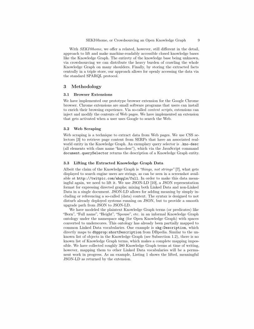
Figure 1: Conf icts During A Merge

to match a wider number of instances in subsequent matches. When performingsubsequent instance matching that includes both clusters and individual instances,the consolidated representation of clustered data, supported by our merging algo-rithm, can be used.

Figure 1 depicts an example of a consolidation when conf icts may occur. Inthis example, when we have a pair of attributes that are the same but their valuesdiffer, to consolidate we must determine whether both values are maintained, noneof the values are maintained or one of the values is maintained. For the purposes ofusing the consolidated instance for future matching, the merging of instance datais incredibly important as it affects the performance of future matching. This isparticularly true when working with data sets that are sparse.

The temporal support is an important aspect to this problem since over time anentity’s features may change. In Figure 2, the attribute population changes overtime. This example highlights two complexities that are a natural effect of time.An instance can be thought of as a snapshot in time, therefore an instance capturedat time t − 1 may not be as relevant as an instance captured at time t. This affectshow instances should be consolidated and is a good example of when a technique isrequired to resolve conf icts. Also, this implies that in certain cases, given enoughtime, two instances may no longer be coreferent, supporting the argument thattemporal issues play a signif cant role in consolidation and subsequent processing.

2 BackgroundSemantic Web data, which includes semantically tagged data represented using aResource Description Framework (RDF) [1, 2] triples (subject, predicate, object)format, is often used as a way to commonly represent data. Data which conformsto an ontology, data exported from social networking sites, and linked data foundon the Linked Open Data Cloud are often represented as triples. Attempting tomatch instances or entities among this type of data can be a challenge which isfurther complicated by noise and data spareness.

14 Jennifer Sleeman and Tim Finin

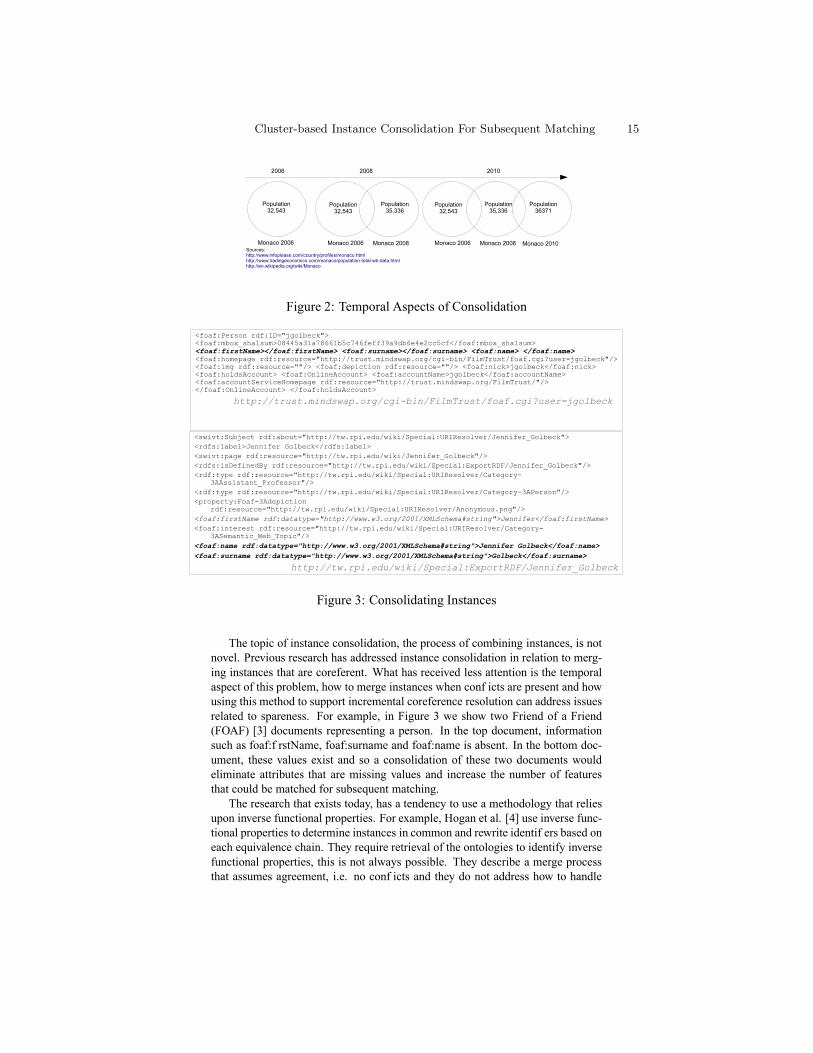
Figure 2: Temporal Aspects of Consolidation

Figure 3: Consolidating Instances

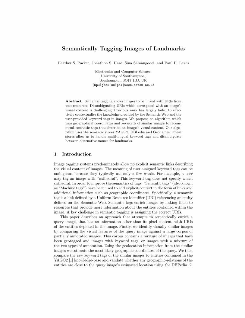
The topic of instance consolidation, the process of combining instances, is notnovel. Previous research has addressed instance consolidation in relation to merg-ing instances that are coreferent. What has received less attention is the temporalaspect of this problem, how to merge instances when conf icts are present and howusing this method to support incremental coreference resolution can address issuesrelated to spareness. For example, in Figure 3 we show two Friend of a Friend(FOAF) [3] documents representing a person. In the top document, informationsuch as foaf:f rstName, foaf:surname and foaf:name is absent. In the bottom doc-ument, these values exist and so a consolidation of these two documents wouldeliminate attributes that are missing values and increase the number of featuresthat could be matched for subsequent matching.

The research that exists today, has a tendency to use a methodology that reliesupon inverse functional properties. For example, Hogan et al. [4] use inverse func-tional properties to determine instances in common and rewrite identif ers based oneach equivalence chain. They require retrieval of the ontologies to identify inversefunctional properties, this is not always possible. They describe a merge processthat assumes agreement, i.e. no conf icts and they do not address how to handle

Cluster-based Instance Consolidation For Subsequent Matching 15

Source Avg Number of Attributes Number of Instancesvox 5.65 4492journal 9.71 1259ebiquity 19.78 217

Table 1: Average Number of Attributes

data that does not use inverse functional properties. Shi et al. [5] describe instanceconsolidation as ’smushing’ and performs ’smushing’ by taking advantage of theinverse functional property. They work at the attribute level and calculate attributelevel similarity measures. A property def ned as inverse functional implies thatthe inverse of the property is functional; that it uniquely identif es the subject [2].Again this work relies upon inverse functional properties and tends not to addresshow to resolve conf icts. Yatskevich et al. [6] address consolidation of graphs.They merge graphs if the instances belong to the same class, and if their stringsimilarity is higher than a threshold. They describe special cases for particulartypes. This merge process does not address conf icts and there is no indicationwhether they could reverse a consolidated graph. In our previous work [7, 8] thatexplored our approach using simple merging heuristics and coreferent clusteringof FOAF instances, particularly when working with sparse input, consolidation didpositively affect subsequent coreferent pairing.

In our person data set, specif cally using the FOAF ontology, we found a siz-able percentage of the instances contained very few attributes. In Table 1, we showthe number of instances originating from 3 different sources. Source ’vox’ had thehighest number of instances and also the lowest number of attributes per instance.We have found this is prevalent among social networking sites and sites that sup-port exports of user prof le data using the FOAF ontology. This is not specif c toFOAF instances and can present a problem for coreference resolution algorithms.

3 An ApproachWe def ne an instance as an abstract representation that can be either a cluster ofcoreferent instances, or a single entity instance. A formal def nition follows.Definition 1. Given a set of instances I and a set of clusters C, an abstract in-stance A ∈ (I ∪ C).

Definition 2. Given a pair of instances in and im, if the pair are coreferentor coref (in, im), then a cluster Cnm is formed such that the cluster Cnm ={in, im}.

Figure 4 depicts an example of a cluster that is formed with coreferent in-stances. Data relates to Monaco from three different sources (http://dbpedia.org/,http://www4.wiwiss.fu-berlin.de/, http://data.nytimes.com/) where each source rep-resents a perspective of Monaco. Given a system that processes unstructured textthat includes a reference to the instance Monaco, our work seeks to prove that weare more likely to recognize Monaco as an entity with the combined informationtaking the most relevant of features, rather than using a single instance. We willalso show how over time as attributes pertaining to these instances changes, themodel can ref ect these changes.


Figure 4: Instance Cluster

A consolidated representation is required in order to use the clustered data insubsequent matching. This consolidation can be as simple as a union between thesets of attributes of instances. However, as seen in Figure 1, this approach doesnot address situations where attributes are in conf ict. Even in this simple example,conf icts are present that should be resolved. Our initial work includes the mergingof instances and resolution of conf icts by using a basic set of rules and temporalinformation.

When evaluating two instances, for each attribute that is shared, if the valuesare equal, we retain one instance of the attribute. If two instances share the sameattribute but their values differ, we try to resolve the conf ict. If the two instancescontain attributes that are not shared we include their unshared attributes. In re-solving the conf ict, we f rst try to determine if the two values are synonymous.If they are synonymous, we keep both values for the particular attribute. If not,then we will use additional analysis such as temporal information. As the same in-stance is processed over time given a particular URI, we track the changes amongattributes for that instance. Given that attributes have changed for a particular in-stance we give the more recent values of the attributes a higher signif cance than aless recent values. We can then use this information to assist with resolving con-f icts. When conf icts can not be resolved we keep both values for the unresolvedattribute. We anticipate this approach will advance as we progress in our research.

Our cluster links are symbolic in nature. In order to support changes to the clus-ter over time, each instance in a cluster is linked and weighted to other instancesin the cluster. How the weight is def ned is based on the coreference resolution al-gorithm. In our work, we are using a clustering algorithm to cluster instances that

Cluster-based Instance Consolidation For Subsequent Matching 17

are thought to be coreferent. The output of our calculation that supports our clus-tering method will also be used as an assessment of how closely the two instancesare related for consolidation. Given the set of attributes for each instance in thecluster, we associate a score with each set of matched attributes. This score can bebased on a distance function or based on a more complex representation. The goalof this step is to weight common features among pairs of coreferent instances inthe cluster. Across all features in the cluster we wish to pick the most signif cantfeatures to be used for subsequent matching. We are currently exploring featurereduction mechanisms to perform this step. This structure gives us the ability tocompare coreferent relationships among instances over time, to remove coreferentrelationships given changes over time, or to add and modify existing relationshipsgiven new instances that are added to the cluster.

4 ConclusionWe have presented a need for a more adaptive-based consolidation approach. Acluster-based consolidation provides a powerful model for instance matching al-gorithms. It is meant to adapt to change over time, is f exible and could potentiallyimprove subsequent matching. Given the complexities of systems today, adapta-tion is a necessity. The challenge is developing a consolidation approach that isf exible enough to support the complexities of systems today, without incurring alarge performance penalty.

References[1] Beckett, D.: Rdf/xml syntax specif cation. http://www.w3.org/TR/REC-rdf-

syntax/ (2004)[2] Brickley, D., Guha, R.: Resource description framework (rdf) schema specif -

cation 1.0. http://www.w3.org/TR/rdf-schema/ (2004)[3] Brickley, D., Miller, L.: Foaf vocabulary specif cation .98 (August 2010)

http://xmlns.com/foaf/spec/.[4] Hogan, A., Harth, A., Decker, S.: Performing object consolidation on the

semantic web data graph. In: Proc. I3: Identity, Identif ers, Identif cation.Workshop at 16th Int. World Wide Web Conf. (February 2007)

[5] Shi, L., Berrueta, D., Fernandez, S., Polo, L., Fernandez, S.: Smushing rdfinstances: are alice and bob the same open source developer? In: Proc. 3rd Ex-pert Finder workshop on Personal Identif cation and Collaborations: Knowl-edgeMediation and Extraction, 7th Int. SemanticWeb Conf. (November 2008)

[6] Yatskevich, M., Welty, C., Murdock, J.: Coreference resolution on rdf graphsgenerated from information extraction: f rst results. In: the ISWC 06 Work-shop on Web Content Mining with Human Language Technologies. (2006)

[7] Sleeman, J., Finin, T.: A machine learning approach to linking foaf instances.In: Spring Symposium on Linked Data Meets AI, AAAI (January 2010)

[8] Sleeman, J., Finin, T.: Computing foaf co-reference relations with rules andmachine learning. In: The Third International Workshop on Social Data onthe Web, ISWC (November 2010)


Semantically Tagging Images of Landmarks

Heather S. Packer, Jonathon S. Hare, Sina Samangooei, and Paul H. Lewis

Electronics and Computer Science,University of Southampton,

Southampton SO17 1BJ, UK{hp3|jsh2|ss|phl}@ecs.soton.ac.uk

Abstract. Semantic tagging allows images to be linked with URIs fromweb resources. Disambiguating URIs which correspond with an image’svisual content is challenging. Previous work has largely failed to effec-tively contextualise the knowledge provided by the Semantic Web and theuser-provided keyword tags in images. We propose an algorithm whichuses geographical coordinates and keywords of similar images to recom-mend semantic tags that describe an image’s visual content. Our algo-rithm uses the semantic stores YAGO2, DBPedia and Geonames. Thesestores allow us to handle multi-lingual keyword tags and disambiguatebetween alternative names for landmarks.

1 Introduction

Image tagging systems predominately allow no explicit semantic links describingthe visual content of images. The meaning of user assigned keyword tags can beambiguous because they typically use only a few words. For example, a usermay tag an image with “cathedral”. This keyword tag does not specify whichcathedral. In order to improve the semantics of tags, “Semantic tags” (also knownas “Machine tags”) have been used to add explicit context in the form of links andadditional information such as geographic coordinates. Specifically, a semantictag is a link defined by a Uniform Resource Identifier (URI) referencing an entitydefined on the Semantic Web. Semantic tags enrich images by linking them toresources that provide more information about the entities contained within theimage. A key challenge in semantic tagging is assigning the correct URIs.

This paper describes an approach that attempts to semantically enrich aquery image, that has no information other than its pixel content, with URIsof the entities depicted in the image. Firstly, we identify visually similar imagesby comparing the visual features of the query image against a large corpus ofpartially annotated images. This corpus contains a mixture of images that havebeen geotagged and images with keyword tags, or images with a mixture ofthe two types of annotation. Using the geolocation information from the similarimages we estimate the most likely geographic coordinates of the query. We thencompare the raw keyword tags of the similar images to entities contained in theYAGO2 [1] knowledge-base and validate whether any geographic-relations of theentities are close to the query image’s estimated location using the DBPedia [2]

and Geonames [3] knowledge-bases. Finally, we use these selected entities toconstruct a list of URIs which are relevant to the content of the query image1.

The broader motivation of this work is to bridge the gap between unstruc-tured data attainable in real time, such as a GPS-location or image of a land-mark, and, rich, detailed and structured information about that landmark, there-fore facilitate more informed search and retrieval. For example, users can engagein semantic searching; targeting a particular church, architect, period in historyor architectural style. This kind of structured search can also support eventdetection [4] or lifelogging [5] by helping collate documents which refer to aparticular entity more accurately.

This work provides two contributions beyond state-of the-art. Specifically,we verify semantic tags using distance according to the height of the entitiesidentified in an image, and we also recommend URIs using a multi-language tagindex derived from multiple semantic web knowledge sources. The multi-lingualindex allows us to make recommendations from keywords in foreign languagesby identifying alternative names to utilise in our approach.

The structure of the paper is as follows: firstly, we discuss related work ontagging systems. Secondly we present details of our tagging approach. Finally, wediscuss the use of our system with some examples and provide our conclusions.

2 Related Work

Automatic image annotation is widely studied, but techniques that integratemultiple contexts using semantic web resources are relatively rare. The followingreview looks at works that recommend tags using both geographical coordinatesand visual image similarity. SpiritTagger [6] recommends keywords that reflectthe spirit of a location. It finds visually similar images using colour, texture, edgeand SIFT features [7], and clusters tags based within a geographical radius. Theseselected tags are ranked based on frequency and then importance. This enablestheir algorithm to recommend tags that are specific to a geographic region. Thefocus of our work is to recommend semantic tags (URIs) that describe a placeof interest, not tags relating to a larger area.

Moxley et al. [8] use a corpus of images and their tags, and organise them intosets of places, events and visual components. These are clustered based on theco-occurrence of words and the distance between named geographical entities.If an image matches, the wikipedia title is used as a recommendation for thename of the landmark in the image. This approach uses limited informationfrom wikipedia to identify and recommend tags. In our approach, we aim tovalidate semantic tags using additional information from semantic data sources.

Similar to Moxley et al. [6], Kennedy and Naaman [9]’s approach also con-siders the importance of tags relevant to a specific area or event. Their approachgenerates a representative image set for landmarks using image tags and geo-graphic coordinates. Their technique identifies tags that occur frequently within

1 A demonstration of our approach can be found here: http://gtb.imageterrier.org

20 Heather Packer, Jonathon Hare, Sina Samangooei and Paul Lewis

one geographic area, but infrequently elsewhere, in order to identify tags thatare uniquely local. They also filter tags that only occur during specific timeranges; this enables them to identify events such as the “New York Marathon”and determine whether this is relevant to a query image by analysing the dateit was taken. Their focus was not concerned with recommending semantic tags.

There are a number of datasets that contain flickr images and related URIs.For instance, the Ookaboo dataset was manually created by 170,000 contribu-tors who submitted images and classify them against a topic from wikipedia 2.In contrast, our approach recommends URIs automatically for an untagged im-age, by using tags from images that share visual features. The flickrtm wrapperAPI allows users to search with a URI of an entity on Wikipedia and search forimages that depict that entity. In particular, you can search for images within auser-specified distance of the geographical location of the searched entity (if theentity has a geographical location). This is the opposite problem to us, our queryis an image depicting a landmark where the landmark is unknown, whereas theirquery is an entity on Wikipedia. The work by [10] identify entities using naturallanguage processing by stemming words to find their root or base by removingany inflections, using Wordnet. They then identify any relationships betweenthese entities using the hypernym, holonym, meronym, and toponym relation-ships described in Wordnet to create the triples describing the entities describedin flickr tags. Our approach supports [10]’s, by generating the URI describingentities depicted in an image when it has no tags, so that their approach couldgenerate triples.

A number of other approaches simply use location and visual features toannotate images (e.g. [11]). There has also been work to recommend tags, basedon existing annotations (e.g. [12]), and recommending semantic entities, basedon existing tags (e.g. [13]).

3 Approach

Our semantic tag recommendation approach has five steps. Firstly, we search alarge index of visual features extracted from partially annotated images with thefeatures extracted from a query image in order to find images similar to the query.The index contains images that have either geographic tags or keyword tags (ora mixture of the two). From the set of similar images with geographic locationswe calculate a robust average of the latitude and longitude which estimates thegeographic location of the query. Secondly, we use the keyword tags associatedwith the similar images to identify entities close to the estimated coordinatesfrom YAGO2. Thirdly, we classify the types of entities that are possible rec-ommendations using the type hierarchies of YAGO2, DBPedia and Geonames.In the fourth step, we restrict our recommendations based on their height anddistance. In the final step, we expand our set of URIs with those from the closestcity in order to try and identify additional relevant semantic entities.

2 Ookaboo: http://ookaboo.com/o/pictures/

Semantically Tagging Images of Landmarks 21

Fig. 1. The query image of Trento Cathedral, and the resulting images that matched,based on an index of SIFT features.

The approach has been developed using an index of images crawled fromFlickr representing the Trentino region in Italy. More details of the dataset canbe found in Section 4. In the remainder of this section, we walk through each ofthe five steps in detail.

3.1 Visual Image Similarity

Firstly, we compare the visual content of an untagged query with the visual con-tent of each image in a dataset of tagged images. This is achieved by comparingvia a BoVW (Bag of Visual Words) [14] representation of both query image anddataset images, extracted using the OpenIMAJ Toolkit3 [15]. For efficient re-trieval, the BoVW of the dataset images is held in a compressed inverted index,constructed using ImageTerrier4 [16]. Once constructed, the index can be usedto retrieve dataset images which are most visually similar to a query image;the tags and geographic locations of the closest dataset images are passed on tothe next steps of our process. Specifically, the retrieval engine is tuned to onlyretrieve images that match with a very high confidence and thus only match thespecific landmark/object in the query image; the aim is not to classify imagesinto landmark classes, but rather to identify a specific instance.

The BoVW image representations are constructed by extracting difference-of-Gaussian SIFT features [17] from an of image and quantising them to a discretevocabulary. A vocabulary of 1 million features was learnt using approximate K-Means clustering [18] with SIFT features from the MIRFlickr25000 dataset [19].Once the content of each image is represented as a set of visual terms, we con-struct an inverted index which encodes each term in an image. The invertedindex is augmented with the orientation information of the SIFT feature corre-sponding to each term; this extra geometric information allows us to improve

3 OpenIMAJ Toolkit: http://openimaj.org4 ImageTerrier: http://imageterrier.org


retrieval precision using an orientation consistency check [20] at query time. Forevery query image, the SIFT features are extracted and quantised. The set ofvisual terms form a query against the inverted index which is evaluated usingthe Inverse-Document-Frequency weighted L1 distance metric [21]. Using thisstrategy we select the top ten images in the dataset. These images provide uswith potential keyword tags and geographic coordinates.

An iterative approach is used to robustly estimate the geographic locationof the query from the set of geotagged result images. The technique needs to berobust as there is a high probability of outliers. Starting with all the matchinggeotagged images, a geographic centroid is found and the image which is geo-graphically furthest from the centre is removed. The centroid is then updatedwith the remaining images. This process continues iteratively until the distancebetween the current centroid and furthest point from the centroid is less thana predefined threshold. Through initial tests on our dataset, we found that thethreshold of 0.8 returned between 70% and 100% of images that were visuallysimilar. An example of the visual similarity search and geographic localisationfor a query image of Trento Cathedral is illustrated in Figure 1.

3.2 Keyword-Entity Matching

The second step aims to find URIs representing entities in the query imageby attempting to match keyword tags to the names of entities. This can beproblematic because it is common for keyword tags to contain more than oneword without white space. Therefore, when searching for an entity in YAGO2that matches a tag representing more than one word it will yield no matches.For example, the keyword tag ‘trentocathedral’ will not match the YAGO2 en-tity ‘Trento Cathedral’. In order to enable us to search for flattened tags, weperformed a pre-processing step to create additional triples relating flattenedtags to entities within YAGO2. We also flattened the entities relating to an en-tity through the “isCalled” property because it contains alternate terms usedto refer to an instance (including foreign language names). For example, theYAGO2 entity for “Trento Cathedral” can also be called “Cattedrale di SanVigilio” and “Katedralo de Santka Vigilio”. Thus, we also use the flattened en-tity names “cattedraledisanvigilio” and “katedralodesantkavigilio” to represent“Trento Cathedral”. These additional triples and YAGO2 are used to look upall the tags using exact string matching. If there are matching entities then wecheck that they are in the same city (using the geographical coordinates fromYAGO2 and the estimated coordinates from step one). In our Trento example,we retrieve the URIs shown in Table 1 from the image’s tags.

3.3 Cross-Source Category Matches

The aim of the third step is to determine whether the entities identified in step2 and the keyword tags of the similar images are of a specific type. We organisedthese types into general categories, including town/city, region, country, date,weather, season, mountain, building, activity, transport and unknown. This list


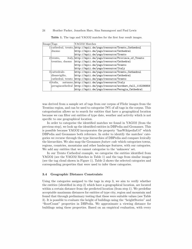
Table 1. The tags and YAGO2 matches for the first four result images.

Image Tags YAGO2 Matches

1 cathedral, trento,duomo

http://mpii.de/yago/resource/Trento_Cathedral

http://mpii.de/yago/resource/Cathedral

http://mpii.de/yago/resource/Trento

2 trento, italy,trentino, duomo

http://mpii.de/yago/resource/Province_of_Trento



http://mpii.de/yago/resource/Italy

3 cattedrale-disanvigilio,cathedral, trento

http://mpii.de/yago/resource/Trento_Cathedral



4 italia, autunno,perugiacathedral

http://mpii.de/yago/resource/Italy

http://mpii.de/yago/resource/wordnet_fall_115236859

http://mpii.de/yago/resource/Perugia_Cathedral

was derived from a sample set of tags from our corpus of Flickr images from theTrentino region, and can be used to categorise 78% of all tags in the corpus. Thiscategorisation allows us to search for entities that have a geographical locationbecause we can filter out entities of type date, weather and activity which is notspecific to one geographical location.

In order to categorise the identified matches we found in YAGO2 (from theprevious step), we look up the identified entities in DBPedia and Geonames. Thisis possible because YAGO2 incorporates the property “hasWikipediaUrl” whichDBPedia and Geonames both reference. In order to identify the matches’ cate-gories we recurse through the type hierarchies of DBPedia and compare lexicallythe hierarchies. We also map the Geonames feature code which categorises towns,regions, countries, mountains and other landscape features, with our categories.We add any entities that we cannot categorise to the ‘unknown’ set.

In our Trento Cathedral example, we categorise the entities identified fromYAGO2 (see the YAGO2 Matches in Table 1) and the tags from similar images(see the tag cloud shown in Figure 1). Table 2 shows the selected categories andcorresponding properties that were used to infer these categories.

3.4 Geographic Distance Constraints

Using the categories assigned to the tags in step 3, we aim to verify whetherthe entities (identified in step 2) which have a geographical location, are locatedwithin a certain distance from the predicted location (from step 1). We predefineacceptable maximum distances for entities of type city, region and mountain andfound that through preliminary testing that these were suitable values (see Table3). It is possible to evaluate the height of buildings using the “heightStories” and“floorCount” properties in DBPedia. We approximate a viewing distance forbuildings using these properties. Based on an empirical evaluation, with every


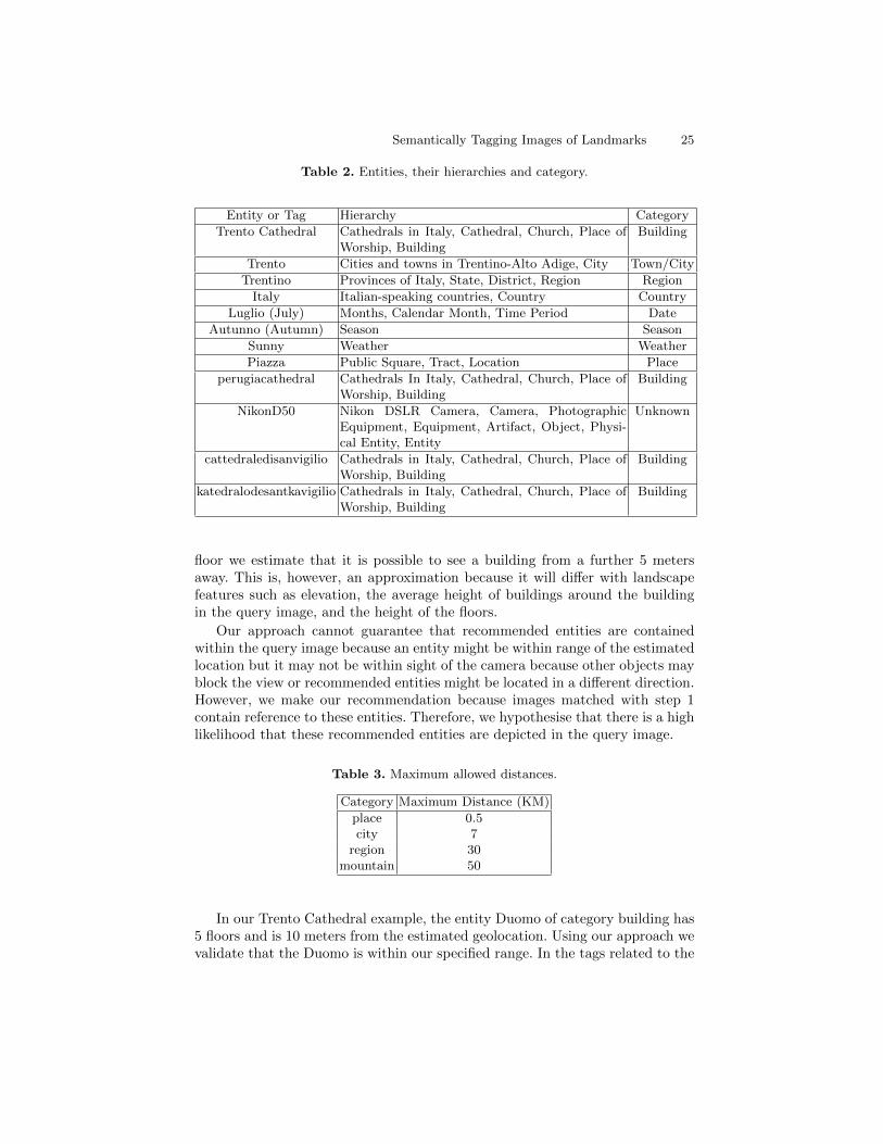
Table 2. Entities, their hierarchies and category.

Entity or Tag Hierarchy Category

Trento Cathedral Cathedrals in Italy, Cathedral, Church, Place ofWorship, Building

Building

Trento Cities and towns in Trentino-Alto Adige, City Town/City

Trentino Provinces of Italy, State, District, Region Region

Italy Italian-speaking countries, Country Country

Luglio (July) Months, Calendar Month, Time Period Date

Autunno (Autumn) Season Season

Sunny Weather Weather

Piazza Public Square, Tract, Location Place

perugiacathedral Cathedrals In Italy, Cathedral, Church, Place ofWorship, Building

Building

NikonD50 Nikon DSLR Camera, Camera, PhotographicEquipment, Equipment, Artifact, Object, Physi-cal Entity, Entity

Unknown

cattedraledisanvigilio Cathedrals in Italy, Cathedral, Church, Place ofWorship, Building

Building

katedralodesantkavigilio Cathedrals in Italy, Cathedral, Church, Place ofWorship, Building

Building

floor we estimate that it is possible to see a building from a further 5 metersaway. This is, however, an approximation because it will differ with landscapefeatures such as elevation, the average height of buildings around the buildingin the query image, and the height of the floors.

Our approach cannot guarantee that recommended entities are containedwithin the query image because an entity might be within range of the estimatedlocation but it may not be within sight of the camera because other objects mayblock the view or recommended entities might be located in a different direction.However, we make our recommendation because images matched with step 1contain reference to these entities. Therefore, we hypothesise that there is a highlikelihood that these recommended entities are depicted in the query image.

Table 3. Maximum allowed distances.

Category Maximum Distance (KM)

place 0.5city 7

region 30mountain 50

In our Trento Cathedral example, the entity Duomo of category building has5 floors and is 10 meters from the estimated geolocation. Using our approach wevalidate that the Duomo is within our specified range. In the tags related to the


similar images, we identify that the building “Perugia Cathedral” has 6 floorsand is 343.5 kilometers away from the estimated location. Therefore, we do notrecommend URI of this building because its is not within range.

3.5 Recommendation Expansion

In the final step of our approach, we aim to derive further matches by expand-ing our search terms. Specifically, we expand all non place entities (excludingentities of the type city, town, region and country) with the the closest placename, using the pattern [place name][non place entity]. This allows us todisambiguate entities that are common to many places, such as town halls,police stations and libraries. We then check whether the matches are locatedclose to the estimated coordinates. In our Trento Cathedral example, the tagpiazza is expanded to “Trento piazza” which is linked to by YAGO2 by the“isCalled” property to the entity “Trento-Piazza del Duomo”. We then validatethat the “Trento-Piazza del Duomo” is categorised with place and is within thegeographic distance range of 0.5km from the estimated geographical location.In Table 4 we detail the extended tags which we attempt to match to YAGO2.Table 5 details the recommended URIs for our example.

Table 4. Extended Tags and URIs.

Extended tag URI[place][non place entity]

Trento Cathedral http://www.mpii.de/yago/resource/Trento_Cathedral

Trento Piazza http://www.mpii.de/yago/resource/Trento_Piazza

Table 5. Recommended Entities and URIs.

Recommended Entity URI

Province of Trento http://en.wikipedia.org/wiki/Province_of_Trento

Trento http://en.wikipedia.org/wiki/Trento

Italy http://en.wikipedia.org/wiki/Italy

Trento Cathedral http://www.mpii.de/yago/resource/Trento_Cathedral

Trento Piazza http://www.mpii.de/yago/resource/Trento_Piazza

4 Examples and Discussion

In this section, we discuss the recommended URIs for four example query im-ages. The dataset of partially annotated images used as the basis to testing theapproach was crawled from Flickr. We first downloaded approximately 150,000geo-tagged images that were within the bounds of the province of Trentino, anarea of 2,397 square miles in the north of Italy. This set was then enriched withan additional 400,000 images with keyword tags relating to the Trentino region.


In total our image set consists of 472,565 images because of the intersectionof these images sets5. We randomly sampled 3,250 images from this set andmanually identified the theme of the image (see Table 6).

Table 6. Sample of topics from 3,250 images

Theme Percentage (%)

People 31.2Landscape 26.2

Houses 16.5Animals 12.5Churches 5.8

Other 5.6Transport 1.6

Trento Cathedral 0.6Buonconsiglio Castle 0

We considered using standard image sets such as the European Cities 50K[22]dataset and MIRFlickr[19]. However, we wanted to include images from thesurrounding area because often they are the most similar visually, areas typicallyhave a particular style due to tradition and age of the area. The European citiesset contains images from different cities and does not include whole regions.Similarly we chose not to use the MIRFlickr image set as it was not suitablebecause our approach requires both tags to identify landmarks and geotags todisambiguate between landmarks, and 88.948% of the images in MIRFlickr didnot contain geotags. Whereas our image set contains over double the number ofgeotagged images at 23% compared to 11%. To the best of our knowledge therewere no suitable datasets which contained a complete area of geotagged images,or that contained a ground truth of URIs associated with each image.

4.1 Example 1

The first query image depicts Trento Cathedral, the Neptune Fountain and aplaza, and the visual feature search returned the images that depict the cathedral(see Figure 2). The seventh similar image is a photograph of Trento Cathedraland that image is not geographically close to the landmark’s actual location.While estimating the geographical location of the image, the seventh image’sgeotags are removed by the threshold described in Section 3.1, and thereforedoes not effect the recommended URIs. Our approach correctly identifies thatthe query image contains Trento Cathedral and recommends the URIs for theItalian and English wikipedia URIs for the cathedral because the tag cloudcontains ‘trentocathedral’, ‘trento’ and ‘cathedral’. It also recommends URIsrelating to the region, such as town, region, and country, and URIs relating

5 Our image set can be downloaded here: http://degas.ecs.soton.ac.uk/~hp07r/fullcollection.csv


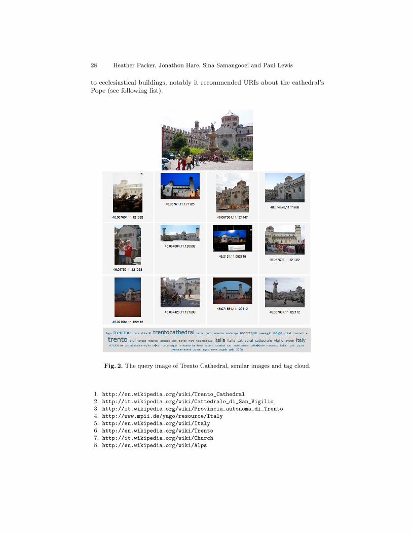
to ecclesiastical buildings, notably it recommended URIs about the cathedral’sPope (see following list).

Fig. 2. The query image of Trento Cathedral, similar images and tag cloud.

1. http://en.wikipedia.org/wiki/Trento_Cathedral

2. http://it.wikipedia.org/wiki/Cattedrale_di_San_Vigilio

3. http://it.wikipedia.org/wiki/Provincia_autonoma_di_Trento

4. http://www.mpii.de/yago/resource/Italy

5. http://en.wikipedia.org/wiki/Italy

6. http://en.wikipedia.org/wiki/Trento

7. http://it.wikipedia.org/wiki/Church

8. http://en.wikipedia.org/wiki/Alps


9. http://en.wikipedia.org/wiki/Cathedral

10. http://it.wikipedia.org/wiki/Trento

11. http://it.wikipedia.org/wiki/Cattedrale

12. http://it.wikipedia.org/wiki/The_Church

13. http://en.wikipedia.org/wiki/Province_of_Trento

14. http://en.wikipedia.org/wiki/Church

15. http://www.mpii.de/yago/resource/Province_of_Trento

16. http://en.wikipedia.org/wiki/Pope_Vigilius

17. http://it.wikipedia.org/wiki/Papa_Vigilio

18. http://it.wikipedia.org/wiki/Cathedral

19. http://en.wikipedia.org/wiki/Trentino

20. http://www.mpii.de/yago/resource/Trento

21. http://en.wikipedia.org/wiki/Mountain

22. http://en.wikipedia.org/wiki/Alto

4.2 Example 2

The second query image depicts Trento Cathedral, and the visual feature searchcorrectly matched seven images of the cathedral (see Figure 3). From the tagcloud we can see that one or more of the similar images has been incorrectlytagged with ‘Buonconsiglio’ and ‘Castle’. These tags refer to Buonconsiglio Cas-tle which is approximately 700 meters from Trento Cathedral. In step four of ourapproach, we disambiguate between places of interest when there is a distancegreater then 0.5km. However, in this case, our approach was unable to disam-biguate between the two places of interest because all the geotagged images werewithin 0.5km of Trento Cathedral (as defined on Geonames) and contained tagsrelating to both the cathedral and castle. If the image tagged with ‘Buoncon-siglio’ was geographically located at the castle, then our approach would haveonly recommended URIs relating to the cathedral. Our approach recommendedthe URIs in example 1 and those in the following list, and recommended URIsthat relate to both Buonconsiglio Castle and Trento Cathedral.

1. http://it.wikipedia.org/wiki/Castello_del_Buonconsiglio

2. http://en.wikipedia.org/wiki/Castello_del_Buonconsiglio

3. http://it.wikipedia.org/wiki/Castello

4. http://www.mpii.de/yago/resource/Trento_Cathedral

4.3 Example 3

The third query image also depicts Trento Cathedral (see Figure 4). The visualfeature search matched three images but only one of the images depicted TrentoCathedral. Non of these images were tagged, therefore our approach could notfind or expand any tags to look up entities in YAGO2, DBPedia or Geonames.



4.4 Example 4

The fourth query image depicts Buonconsiglio Castle. The visual feature searchreturned over 20 images. Figure 5 shows the first eight images which are themost similar to the query image. The first eight images all depict the castle.The visual feature search also returned images of Trento Cathedral, hence thetag cloud contains tags about the cathedral: cathedral, catedral, cathdrale, cat-tedrale, and vigilio. Unlike our second example, our approach was able to dis-ambiguate between the castle and cathedral because the similar images werecorrectly geotagged within 0.5km from the photographed landmark. Our ap-proach expanded the tag Buonconsiglio with castle (see Section 3.5), because itdetermined that castle was a type of building, and thus was able to identify thewikipedia URI http://en.wikipedia.org/wiki/Buonconsiglio_Castle. Thefollowing list contains our approach’s recommended URIs.

1. http://en.wikipedia.org/wiki/Buonconsiglio_Castle

2. http://it.wikipedia.org/wiki/Castello_del_Buonconsiglio

3. http://en.wikipedia.org/wiki/Castello_del_Buonconsiglio

4. http://it.wikipedia.org/wiki/Provincia_autonoma_di_Trento

5. http://en.wikipedia.org/wiki/Trento



6. http://www.mpii.de/yago/resource/Italy

7. http://en.wikipedia.org/wiki/Italy

8. http://it.wikipedia.org/wiki/Castello

9. http://it.wikipedia.org/wiki/Trento

10. http://www.mpii.de/yago/resource/Trento

11. http://en.wikipedia.org/wiki/Trentino

12. http://en.wikipedia.org/wiki/Province_of_Trento

13. http://www.mpii.de/yago/resource/Province_of_Trento

Our approach can be hindered by the quality of information in the semanticknowledge stores — the set of tags and the coordinates. The examples discussedin this section show that without approximately correct coordinates or tags, ouralgorithm will not be able to identify and recommend accurate semantic tags.Nor will our approach be able to validate the coordinates of places of interest,if the knowledge base does not contain them.

5 Conclusion

In this paper, we present an algorithm to recommend URIs that represent thevisual content of an image and focus on identifying places of interest using ge-ographical information from YAGO2, DBPedia, and Geonames. In order to usethese knowledge sources, we use large-scale image matching techniques to findsimilar images that are then used to estimate geo-coordinates and potential tags.

The four examples show that the quality our results highly depends on thequality of the image matching techniques and the reference corpus. Our approach


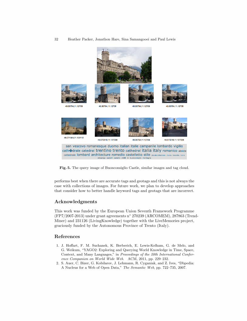
Fig. 5. The query image of Buonconsiglio Castle, similar images and tag cloud.

performs best when there are accurate tags and geotags and this is not always thecase with collections of images. For future work, we plan to develop approachesthat consider how to better handle keyword tags and geotags that are incorrect.

Acknowledgments

This work was funded by the European Union Seventh Framework Programme(FP7/2007-2013) under grant agreements n◦ 270239 (ARCOMEM), 287863 (Trend-Miner) and 231126 (LivingKnowledge) together with the LiveMemories project,graciously funded by the Autonomous Province of Trento (Italy).

References

1. J. Hoffart, F. M. Suchanek, K. Berberich, E. Lewis-Kelham, G. de Melo, andG. Weikum, “YAGO2: Exploring and Querying World Knowledge in Time, Space,Context, and Many Languages,” in Proceedings of the 20th International Confer-ence Companion on World Wide Web. ACM, 2011, pp. 229–232.

2. S. Auer, C. Bizer, G. Kobilarov, J. Lehmann, R. Cyganiak, and Z. Ives, “Dbpedia:A Nucleus for a Web of Open Data,” The Semantic Web, pp. 722–735, 2007.


3. B. Vatant and M. Wick, “Geonames Ontology,” GeoNames, Accessed, vol. 6, 2009.4. H. Packer, S. Samangooei, J. Hare, N. Gibbins, and P. Lewis, “Event Detection

using Twitter and Structured Semantic Query Expansion,” in CIKM2012 - TheFirst International Workshop on Multimodal Crowd Sensing, 2012.

5. H. Packer, A. Smith, and P. Lewis, “MemoryBook: Generating Narrative fromLifelogs,” in Hypertext2012 - The Second International Workshop on Narrativeand Hypertext Systems, 2012.

6. E. Moxley, J. Kleban, and B. Manjunath, “Spirittagger: a Geo-Aware Tag Sugges-tion Tool Mined from Flickr,” in Proceeding of the 1st ACM international Confer-ence on Multimedia Information Retrieval, 2008, pp. 24–30.

7. D. G. Lowe, “Object Recognition from Local Scale-Invariant Features,” IEEE In-ternational Conference on Computer Vision, vol. 2, p. 1150, 1999.

8. E. Moxley, J. Kleban, J. Xu, and B. Manjunath, “Not all Tags are Created Equal:Learning Flickr Tag Semantics for Global Annotation,” in IEEE InternationalConference on Multimedia and Expo., 2009, pp. 1452–1455.

9. L. Kennedy and M. Naaman, “Generating Diverse and Representative ImageSearch Results for Landmarks,” in Proceeding of the 17th International Confer-ence on World Wide Web, 2008, pp. 297–306.

10. M. Maala, A. Delteil, and A. Azough, “A conversion process from flickr tags to rdfdescriptions,” in BIS 2007 Workshops, 2008, p. 53.

11. H. Kawakubo and K. Yanai, “GeoVisualRank: a Ranking Method of GeotaggedImages Considering Visual Similarity and Geo-Location Proximity,” in Proceedingsof the 20th International Conference Companion on World Wide Web, 2011.

12. B. Sigurbjornsson and R. van Zwol, “Flickr Tag Recommendation Based on Col-lective Knowledge,” in Proceeding of the 17th International Conference on WorldWide Web, 2008, pp. 327–336.

13. J. Tang, S. Yan, R. Hong, G.-J. Qi, and T.-S. Chua, “Inferring Semantic Conceptsfrom Community-Contributed Images and Noisy Tags,” in Proceedings of the 17thACM International Conference on Multimedia, 2009, pp. 223–232.

14. J. Sivic and A. Zisserman, “Video Google: A Text Retrieval Approach to ObjectMatching in Videos,” in ICCV, October 2003, pp. 1470–1477.

15. J. S. Hare, S. Samangooei, and D. P. Dupplaw, “OpenIMAJ and ImageTerrier:Java libraries and tools for scalable multimedia analysis and indexing of images,”in Proceedings of ACM Multimedia 2011, ser. MM ’11. ACM, 2011, pp. 691–694.

16. J. Hare, S. Samangooei, D. Dupplaw, and P. Lewis, “Imageterrier: An extensibleplatform for scalable high-performance image retrieval.” in The ACM InternationalConference on Multimedia Retrieval (ICMR 2012), 2012.

17. D. Lowe, “Distinctive image features from scale-invariant keypoints,” IJCV, vol. 60,no. 2, pp. 91–110, January 2004.

18. J. Philbin, O. Chum, M. Isard, J. Sivic, and A. Zisserman, “Object Retrieval withLarge Vocabularies and Fast Spatial Matching,” in CVPR, 2007.

19. M. J. Huiskes and M. S. Lew, “The MIR flickr retrieval evaluation,” in Proceedingof the 1st ACM international conference on Multimedia information retrieval, 2008.

20. H. Jegou, M. Douze, and C. Schmid, “Hamming Embedding and Weak GeometricConsistency for Large Scale Image Search,” in Proceedings of the 10th EuropeanConference on Computer Vision, 2008, pp. 304–317.

21. D. Nister and H. Stewenius, “Scalable recognition with a vocabulary tree,” inCVPR, 2006, pp. 2161–2168.

22. Y. Avrithis, G. Tolias, and Y. Kalantidis, “Feature map hashing: Sub-linear in-dexing of appearance and global geometry,” in in Proceedings of ACM Multimedia,Firenze, Italy, October 2010.


Ageing Factor: a Potential Altmetric for Observing Events and Attention Spans in Microblogs

Victoria Uren1 and Aba-Sah Dadzie2 1Aston Business School, Aston University, The Aston Triangle, Birmingham, UK

2Department of Computer Science, 211 Portobello, The University of Sheffield, Sheffield, UK

We present an initial examination of the (alt)metric ageing factor to study posts in Twitter. Ageing factor was used to characterize a sample of tweets, which contained a variety of astronomical terms. It was found that ageing factor can detect topics that both cause people to retweet faster than baseline values, and topics that hold people’s attention for longer than baseline values.

1 Introduction

Our long-term goal is to study public communication about science: understanding what the public thinks about scientific research is important for many reasons, from developing science policy, through making the case for technological developments and determining the impact of research, to simply being able to characterize the vi-brant public discourse which marks a healthy society, in which science plays as im-portant a part as politics, popular culture or the arts. The new media of the social web, which are open to all, offer a fresh insight into public opinion to supplement the sur-veys, and so forth, used in Public Understanding of Science (PUS) research [20].

Because of the scale of data available (Twitter claims there are 340M tweets per day1), quantitative metrics are needed to aggregate the contributions of many individ-uals. Informetrics research has developed and used quantitative measures to study scholarly communication in traditional media for decades. Informetric methods have been shown to transfer to communication on the web [1] and latterly social media / Web 2.0 [2], in which field they are coming to be known as altmetrics. Altmetrics adapt tried and tested informetric methods to the analysis of scientific communication in social media. Used along with natural language methods, such as clustering and summarization, we believe they have much to offer analysts. Our aim, in the experi-ments reported in this paper, was to study a metric called ageing factor as a means to characterize whether people’s interest in discussion of scientific topics on Twitter is sustained or transient.

1 http://blog.twitter.com/2012/03/twitter-turns-six.html

1.1 Science in Social Media

While reservations about the use of social media in formal work still exist [3], many scientific communities have embraced social media as a mode of communica-tion [4]. In one survey [5], Twitter was one of the highest ranked services for seman-tic web researchers, but other communities favour different services, e.g., of informet-rics researchers only 16% had Twitter accounts while 70% used LinkedIn [2]. Ponte & Simon [4] similarly found, in a survey of researchers from different fields, that nearly 18% used micro-blogging services such as Twitter, while 40% used science-based blogs and social networks. The ways in which scientific communities use social media vary. In computer science, delegates tweet or blog running commentary on conferences, opening up the proceedings to delegates in other rooms as well as col-leagues who cannot attend [5] [6]. Whereas in biology, Mandavilli reports examples of intensive public critique of contentious articles [7].

However, scientists play only one part in the bigger picture of science communica-tion - science organizations, journalists (both science and public-interest media), lob-byists and the general public also have important contributions to make. The current ethos of science communication, as discussed by Nisbet & Scheufele [8] and many others, advocates engaging the public in dialogue. Social media support open access to discussion, and for science organizations, Web 2.0 has become an essential part of their public relations operation. As one white paper boldly states “the people formerly known as the audience are now at the center of media” [9]. This is echoed by Eysen-bach [10], who describes the “traces” left by both scientists and the lay public as they interact with information on the web. Individual scientists are increasingly aware of the public engagement agenda: Ponte and Simon [4] report scholars’ desire to make greater use of Web 2.0 methods for peer review and communication of research. Letierce [5] has shown that although researchers’ main motivation for using Twitter is to communicate with members of their own community (89%), some are also trying to reach general audiences (45.9%). Consequently, we argue that it is necessary to expand the scope of analysis of science communication in social media beyond the boundaries of scientists’ communication with each other to encompass wider public communication about science.

Compared to the numerous works on politics and marketing, relatively few studies exist about the public’s (as opposed to researchers’) scientific communication in mi-croblogs. Hubmann-Haidvogel et al. [11] present a visualization tool using climate change posts as a use case, and Chew and Eysenbach [12], report the timeliness of social media for highlighting trends in the development of pandemics. In our own experience [13], the lack of research may be because scientific topics typically have few posts compared to current affairs, popular culture etc., so that simple trend spot-ting methods can be ineffective. Furthermore, there is a high level of noise, with many “scientific” search terms being used in non-scientific contexts [13]. Chew and Eysen-bach [12], and Weller and Puschmann [14] also recognise the negative influence of noise in Twitter data. Chew and Eysenbach remark that “spam and popular news articles that contained key phrases can influence search results and create peaks in activity that may not be reflective of the concept”[12]. Both suggest the use of ad-

Ageing Factor 35

vanced natural language processing to support the identification of tweets containing scientific information and to filter out non-relevant or spurious use of domain-specific terms.

Weller et al. [15] have identified three classes of scientific microposts for their study of communication in scientific conferences: posts (tweets on Twitter) with links to scientific content, posts published by a scientist, and posts with a science related hashtag. To these we add posts that contain scientific terms used within a scientific context, as a more general definition of the sorts of posts we need to identify in order to analyse general public communication about science.

1.2 Ageing Factor

Our earlier work [13] which looked at changes in the usage of a sample of scien-tific terms over time, determined that the basic trend spotting approach, which looks for peaks of tweets occurring for a term on a timeline, is not effective for scientific data because the level of tweeting about science is very low compared to the level of tweets on popular culture. Furthermore, scientific terms are frequently used in non-scientific contexts. The combination of these two factors means that it is difficult to reliably identify peaks of discussion about science topics, because they are small and obscured by noise (irrelevant tweets using the same words). In order to study public communication about science in public media, we need an altmetric which is sensitive even on moderate sized samples of data, because big trend peaks, such as those seen in pandemics, will be relatively rare. We are interested in studying microblogging, for which time is a critical parameter, therefore, a metric which looks at temporal effects is needed.

The metric we test in the experiments presented here, called aging factor, is based on a well-established informetric measure. We follow the convention in which, by analogy, retweets are treated as citations (tweetations) by researchers working on altmetrics. For example, Eysenbach calculated a range of metrics for retweets of an-nouncements by the Journal of Medical Internet Research about the publication of new papers [10]. He uses these to determine whether initial interest indicated by re-tweets can be correlated with later citation rates. The metrics Eysenbach used include tweet half-life defined as “the point in time after publication by which half of all tweetations of that article within the first n days occur”.

Half-life is similar to the ageing factor metric used in this paper with a number of important differences, which we consider make ageing factor more suitable for the kind of data we are studying. Half-life takes what is called the diachronous view, i.e. the metric observes a fixed set of documents, such as one year’s articles in a given journal or one year’s tweets from a particular organization). It is therefore useful for organizations which want to judge the impact of their own tweets and are monitoring the occurrence of their Twitter name in retweets on an on-going basis. This is neces-sary in order to harvest every tweetation of a particular tweet in the first n days. By contrast, we want to take a snapshot of general discussion on scientific topics in a given time period. This is what is termed the synchronous view and requires a metric which does not rely on the originating tweet being present in the sample. For this we

36 Victoria Uren and Aba-Sah Dadzie

adapted Avremescu’s ageing factor measure as presented in [16], changing the counts of citations to retweets and changing time windows measured in years to windows measured in hours to suit the fast pace of communication on Twitter. Aging factor, AF, is defined below, where i is the cut-off time in hours, k is the number of retweets originating at least i hours ago and l is the number of retweets originating less than i hours ago.

AF = kk + l

i

We examined two values of i, i=1 giving the one hour ageing factor (1hAF), and i=24 giving the 24 hour ageing factor (24hAF). A convenient feature of 1hAF is that it is simply the ratio of retweets in a sample that originated more than one hour after the original createdAt time over the total number of retweets in the sample; this makes it easy to understand. The 24hAF is the 24th root of the similar ratio for a 24 hour cut-off. In either case, AF values are produced in the range 0-1 with higher values indicat-ing more retweets originating after the cut-off.

2 Experiments

In the context of communication on Twitter, low values of AF would suggest a flurry of activity typical of a trending topic, such as might happen following the post-ing of tweets about an exciting topic. This might be a special event - in our experi-ments we looked at retweeting about meteor showers. This fits with the findings in [10] that even for the most interesting or highly cited articles, twitter citations quickly fall off soon after announcement of publication. On the other hand, we interpret high values of AF as an indication that people have shown sustained interest in a topic and continue to read and retweet posts for a long (in terms of Twitter) time after they ap-pear. We argue that, for science, being able to show the public has a long attention span for ongoing developments in a field is as important as showing you can get a reaction to a hot news item. Based on these interpretations of what ageing factor could tell us, we made two assumptions about how to interpret ageing factor.

Assumption 1: ageing factors for topics which concern special events will be lower than suitable baselines.

Assumption 2: ageing factors which are higher than suitable baselines are associat-ed with topics in which interest is sustained over time.

The question of what constitutes a “suitable” baseline therefore arises. Unfortu-nately no benchmark corpus of Twitter presently exists (plans for a corpus to be held at the United States Library of Congress are believed to be underway at the time of writing). In this experiment, we have taken a pragmatic approach. We know there is a high level of noise in the samples (see table 1) - the majority of posts for selected terms are not about science. Therefore, we take the superset of tweets as a sample of general usage of that term on Twitter at that time, and use ageing factors for these sets as our baselines.

Ageing Factor 37

We chose the topic of astronomy for the experiment, because it has an enthusiastic following of amateur stargazers who own their own telescopes and are interested in observing events in the night sky for themselves. This led us to believe that it would be possible to harvest posts from Twitter, which discussed astronomical events and might provide evidence about the validity of assumption 1. We collected data on two nights when meteor showers were expected. Our data collection harvested tweets containing a broad range of astronomical terms in order to compare ageing factors for meteor showers with those for other astronomical topics.

2.1 Experiment 1 – Geminid Meteor Shower

As in our previous experiment [13], the UNESCO Thesaurus2 was used as a source of scientific terminology. The starting point was the terms under the subheading “As-tronomical Systems”. We used 32 of 33 terms for the initial filtering, a mix of single words and two word phrases (see Table 1). The 33rd term, Time, produced an unac-ceptably high level of noise and was therefore removed from the set after an initial test run of the harvesting program. Using the public Twitter stream, two data sets were collected: a training set, comprising 8980 tweets collected between Dec 14th 2011 at 22:36 GMT and Dec 14th 2011 at 23:18 GMT, and a test set, comprising 81891 tweets collected between Dec 14th 2011 at 23:18 GMT and Dec 15th 2011 at 03:30. Dec 13-14th 2011 were the nights on which the annual Geminid meteor show-er was expected to take place.

Table 1. Occurrence of retweets (RT) containing UNESCO terms in the training data, and the number of retweets judged to have scientific content (Sci) (where RT > 98).

UNESCO Term RT Sci UNESCO Term RT Sci Celestial bodies 0 Solar activity 0 Cosmic matter 0 Solar disturbances 0 Interstellar matter 0 Sunspots 0 Galaxies 1 Stars 174 7 Stellar systems 0 Quasars 0 Interstellar space 0 Universe 99 5 Black holes 2 Cosmos 5 Meteorites 0 Astronomy 14 Comets 9 Astrophysics 0 Meteors 13 Gravitation 1 Solar system 1 Celestial mechanics 0 Planets 28 Cosmology 0 Earth 213 8 Cosmogeny 0 Satellites 1 Space 166 27 Moon 241 9 Outer space 3 Sun 565 6 Space sciences 0

2 http://www2.ulcc.ac.uk/unesco/thesaurus.htm


For the AF calculations we needed to pick terms with reasonable levels of retweets.

Our previous experiment [13] with a range of scientific terms, lead us to predict that many of the tweets that used UNESCO terms would not have scientific content. This proved to be true for the astronomical terms (see Table 1). Of the UNESCO terms identified in retweets in significant numbers, most are words used in daily life, which do not necessarily have an astronomical meaning: Sun, Moon, Stars etc. are used in a multitude of colloquial ways. The proportion of retweets judged to be scientific, from the six terms categorised, was 0.043. This is substantially lower than levels reported elsewhere: e.g., Mejova and Srinivasan [17] report 0.389 tweets judged to be topical, for a collection of tweets with the categories movies, music albums, smart phones, computer games, and restaurants and note that this is low compared to 0.60 for their sample of blogs. They identify “the need for more precise retrieval strategies for Twitter”. We suggest this is even more important for scientific communication.

We considered terms with 99 or more retweets in the test data to be worth consid-ering in the experiment. These were classified by reading the tweets and making a judgement about whether or not they had scientific content. For example, “when I was little I thought the sun and moon followed me around everywhere!” was judged not scientific, whereas “If the Sun exploded we wouldn’t know for 8m 20s. Light & gravi-ty take that long to reach us. Then we’d vaporize” was judged scientific. Some re-tweets needed more research, for example, “RT @VirtualAstro: Make sure You watch a Night with the stars with your illustrious leader on Sunday night :)” was judged scientific after establishing the @VirtualAstro describes himself as “The Basil Fawlty of Astronomy, Science, Nature and more.”; he fits the profile of an amateur stargazer. As can be seen from Table 1, this classification exercise made clear the low level of scientific retweets.

Having identified UNESCO terms for which we could harvest reasonable levels of scientific retweets (albeit along with significant amounts of noise), we selected two baselines: the UNESCO thesaurus term Space, and a compound term we labelled Astro, which bundled together the UNESCO terms Earth, Moon, Sun, Stars, Universe and Space. In their raw condition, these both contain high levels of non-scientific usage of terms. Therefore, each can be considered as a sample of general use of those terms on Twitter at the sampled point in time. Subsets of the baseline, selected to filter out noise and represent scientific usage of the terms then had to be extracted.

Identifying Scientific Retweets. Ideally, we would use a natural language processing method to identify scientific

use of the terms. However, these experiments have the objective of testing whether AF is an appropriate metric for studying scientific communication. Therefore, we took a simple approach to identifying scientific retweets using SQL queries to reduce the noise in samples by adding narrower terms. We accept that this approach, based on human interpretation of the language of the domain, has limitations for practical implementation on the large scale and will need to be replaced in future work with advanced NLP methods as advocated by [12].

Ageing Factor 39

Table 3 shows both 1hAF and 24hAF for the searches. The 24hAF values for this

dataset were all in the range 0.8-0.95 (zero values were assigned when all retweets collected were within the 24 hour window), whereas 1hAF ranged from 0.25-0.65. In general, 24hAF tracks 1hAF. The culture of Twitter places high value on currency, and 24h is a long time for many Twitter users. 24hAF appears to be an insensitive metric and we used 1hAf only for the remainder of the experiments.

1hAF for the training data searches are often based on small samples of retweets, such that just two or three retweets can make a big difference to the 1hAF. For exam-ple, the 1hAf value for Space and gear of 0.73 in the training data is based on 11 re-tweets, and consequently the 0.4 difference compared to 1hAF in the test data (0.33) is unlikely to be significant. Therefore, the following observations look only at test data, and use Batch, Space and Astro test values as baselines. In this first experiment, we made a naïve interpretation of the results, simply looking for values of 1hAF that appeared high or low, then trying to explain them in terms of the content of retweets.

Table 3. Number of retweets, 1hAF and 24hAF values for experiment 1. Baselines for Space Astro and the whole batch are 0.34, 0.37 and 0.37 respectively

Search Label Training Data Test Data RT 1hAF 24hAF RT 1hAF 24hAF

Batch 1526 0.31 0.88 15583 0.37 0.91 Space 166 0.43 0.90 2594 0.34 0.90 Space AND sci 18 0.44 0.89 396 0.33 0.85 Space AND gear 11 0.73 0.90 375 0.33 0.83 Space AND amb 25 0.48 0.87 487 0.37 0.87 Space AND bodies 7 0.57 0 42 0.45 0.88 Space AND bodies+ 7 0.57 0 315 0.26 0.82 Astro 1425 0.31 0.88 14634 0.37 0.91 Astro AND events 25 0.44 0.93 597 0.26 0.86 Astro AND @ 14 0.43 0.90 23 0.65 0 Astro AND tech 16 0.25 0 122 0.58 0.90 Astro NOT meteor 29 0.55 0.91 511 0.36 0.88 Meteor 27 0.15 0 364 0.22 0.84

For the Space set, two searches have 1hAF values that look different to the base-

lines: 1hAF for Space AND bodies is increased (0.45 compared to 0.34 in the Space baseline and 0.37 for the batch), 1hAF for Space AND bodies+ is decreased (0.26 compared to the same baselines). For the Astro set of queries, all queries except Astro NOT Meteor show differences when compared to the baseline Astro. Searches with increased 1hAF are: Astro AND @ (0.65 compared to 0.37 for the Astro baseline, but with only 23 retweets in the sample we should be cautious about its significance), and Astro AND tech (0.58). Astro AND events shows decreased 1hAF (0.26). The search Meteor was run to isolate tweets concerning the Geminid meteor shower. As can be clearly seen, it has a low value of 1hAF (0.22 compared to 0.37 for the batch).

Ageing Factor 41

Assumption 1 would associate low 1hAF with an event of some kind. The text of the retweets was examined and we found a high level of retweets of “NASA launch new rover to Mars” tweet in both Space AND bodies+ (which contains the term Mars) and Astro AND events (which contains the term launch). It seems the high level of retweeting of this post brings the 1hAF down for these two subsets. These initial results were sufficiently encouraging to make us want to study 1hAF in more detail with a larger dataset.

2.2 Experiment 2: Quadrantid Meteor Shower

A larger sample of the public Twitter stream was then collected. This was filtered using the same 32 UNESCO astronomy terms and covers the full 24 hours of the 3rd of January 2012. This was the night on which the annual Quadrantid meteor shower was expected and our aim was to see if 1hAF values were low for this event, as per assumption 1, and whether the time of day matters (it must be dark to see meteors).

Initially we filtered out subsets using the searches we had developed using the training data for the first experiment (see Table 2). The day was divided into four periods 0:00-5:59 GMT (labelled 6), 6:00-11:59 GMT (12), 12:00-17:59 GMT (18) and 18:00-23:59 (24). Figure 1 shows the 1hAF values for these searches.

The first observation is that although the batch baseline 1hAF is steady in the range 0.32-0.37 through the day, the other two baselines each have one quarter of the day when they are high or low (24 for Space and 12 for Astro).

Fig. 1. 1hAF for 4*6 hour periods over the course of 3rd Jan. 2012

As in the previous experiment, the 1hAF values for Astro are more variable than those for Space. For example, both the Astro AND Events 1hAF and the Meteor 1hAF (both of which contain the term shooting star) are relatively low compared to the Astro baselines, especially for period 12 (2nd quarter of the day). It would be easy, but incorrect, to infer that 1hAF had identified a flurry of retweets about the meteor shower. Examination of the text of posts in the second quarter show that of 275 total retweets 18 contain the term quadrantid while 213 contain the term wish.


There are various original tweets, but “@iQuoteFresh: #IfYouWereMine I’d stop wishing on 11:11’s, birthday candles, dandelions and shooting stars...Because I’d have my wish ...” is a typical example. Noise from non-scientific posts clearly re-mains an important issue, a fact underlined by examination of the high 1hAF values observed for four of the Space searches. These turned out to be due largely to retweets of variants of humorous posts on the lines of “Oh really? You need space? You might as well join NASA.”, for which the original tweets were more than one hour old.

The searches were based on the sample of training data collected about two weeks earlier around the Geminid meteor shower. It seems that even in this short time, the ways terms were being used had changed. We therefore took further steps to remove noise from our samples. Three astronomical events that took place around the 3rd of Jan. 2012 were used as background knowledge to add narrower terms to three of the original searches. The events were the Quadrantid meteor shower on the night of 3-4 Jan., the second of the twin Grail spacecraft moving into orbit around the Moon on the 2nd of Jan., and the proximity of the Moon and the planet Jupiter in the night sky on the 2nd of Jan. Searches excluding the event related terms were also conducted (see Table 4) as non-overlapping sets in order to assess the significance of results.

Table 4. Terms used in modified searches, refer to table 2 for details of original searches

Search label Terms Space AND grail Space AND gear AND (grail|lunar|moon) Space NOT grail Space AND gear AND NOT (grail|lunar|moon) Space AND jupiter Space AND bodies+ AND (jupiter AND moon) Space NOT jupiter Space AND bodies+ AND NOT (jupiter AND moon) Astro AND quad Astro AND (quadrantid|meteor shower) Astro NOT quad Astro AND NOT (quadrantid|meteor shower)

Naïve interpretation of the results in Figure 2 (left) now seems promising. There is

a low 1hAF for the Space and Grail search in the third quarter of the day (@18, 0.23), which contains retweets of posts about Grail tweeted by NASA and SETI in the first half of the (USA) working day. 1hAF for Space AND jupiter is generally high, and particularly in the third quarter (@18, 0.83), with retweets typically of links to pic-tures taken the previous night. Finally, the 1hAF values for Astro and quad are in the range 0.11-0.22, some of the lowest we saw, compared to between 0.32 and 0.39 for Astro AND NOT quad. These retweets are of messages from several sources remind-ing people to get up before dawn in order to see the meteors.

However, the differences in sample size between the searches about events and the exclusion searches we are using for comparison could be extreme: the largest (Astro NOT quad @24) contains 26327 retweets, the smallest (Space and jupiter @18) which generates 1hAF of 0.83 contains just 6 retweets. We therefore require a method of determining whether the 1hAF values we are seeing are significant or are merely the effect of small samples. To gain insight into the significance of results we used a funnel plot (see Figure 2 right). Funnel plots are employed in meta-analyses to detect publication bias and other biases [18]. The rationale is that small samples are ex-

Ageing Factor 43

pected to show higher variance. Therefore, if the measured values (in this case 1hAF) are plotted on the x axis and sample size on the y axis, then if all the data points come from the same population a triangular spread of points around the mean would be expected. Asymmetry in the plot suggests the data points may not all come from the same population. Figure 2 (right) presents a funnel plot for the events searches, ex-cluding the points for Astro NOT quad, which have retweets in the thousands (plot-ting these would force us to use a log scale for the y axis making the funnel plot much harder to interpret).

Fig. 2. Left: Ageing Factor at one hour, 1hAF, for searches modified to detect specific astro-nomical events, measured for 4*6 hour periods over the course of 3rd Jan. 2012. Right: Funnel plot of 1hAF vs number of retweets for the same data (excluding Astro NOT quad).

Based on the funnel plot, two of the Astro AND quad points still look interesting (@time 1hAF RT: @18 0.15 182, @24 0.22 330). Therefore, we can infer that re-tweeting activity around the Quadrantid meteor shower was significant in the hours of darkness for the UK and USA, where the largest concentrations of English speaking Twitter users in the northern hemisphere would be expected to be. Other data points which previously looked interesting, such as (@18 0.23 57) for Space and grail, on the funnel plot look like normal fluctuation within the expected variance of the popu-lation. This suggests that, at least on the 3rd of Jan 2012, the progress of Grail was not exciting the public to a significant degree.

A third data point also deserves investigation, that for Space NOT grail (@6 0.71 274). Examination showed that 216 of the retweets in this set contained the phrase “join NASA”, from retweets of the humorous posts we identified earlier. We infer that people had a long attention span for that particular joke.

3 Discussion and Future Directions

Our objective in carrying out the two exploratory experiments described here was not to rate jokes, but to test ageing factor as an altmetric for analysing scientific communication in social media, and specifically to test whether it can give any in-sights for the smaller datasets typical of scientific content. For ageing factor calculat-


ed with a window of one hour (1hAF), several of our naïve observations fitted both assumption 1 (ageing factors for topics which concern special or exciting events will be lower than suitable baselines) and assumption 2 (ageing factors which are higher than suitable baselines are associated with topics in which interest is sustained over time). However, when a funnel plot was used to identify data points which lay outside the area of expected variance, only three data points appear significant: two with low 1hAF for retweets about the Quadrantid meteor shower, and one with high 1hAF for a (non-scientific) humorous post. We conclude that further investigation of 1hAF would be worthwhile, but that interpretation of the metric without reference to sample size must be avoided.

In these exploratory experiments, topics were identified using SQL searches. It would be intriguing to compare topics with low and high AF to the statistical linguis-tics approach used by Hu et al. [19] to classify tweets into episodic and steady catego-ries. Hu defines episodic tweets as “tweets that respond specifically to the content in the segments of the events” and steady tweets as those “that respond generally about the events”. Our intuitions about how ageing factor works suggest that episodic tweets would be more likely to show low 1hAF and steady tweets more likely to show high 1hAF.

24hAF gave similar values for all the searches in experiment 1. Therefore, we did not use 24hAF in experiment 2. As in [10], when analysing twitter data, especially about a specific event or topic, there is an upper limit beyond which relevant tweets tail off. In our experiments this was 24 hours, in [10], which examined scientific pub-lications, with a significantly longer lifetime, this started at 7 days, and up to 10, for publications released within a three month window. Future studies will look at a wid-er range of time windows to see if they give more sensitive results than the 24h win-dow and will apply the funnel plot technique to check significance. For example, a six hour window (6hAF) might be interesting to observe for studies like experiment 2 which divide the day into quarters.

The overall aim of this work is to contribute to the nascent development of meth-ods and metrics that will support analysis of public online scientific communications. It is clear that the big issue in achieving this is the level of noise in samples coupled with low actual levels of scientific communication in social media. These combine to make it difficult to get big enough samples to get statistically significant results. As an additional problem, the usage of terms on Twitter clearly varies considerably even over a few weeks: our experiments used data collected only a few weeks apart, but the searches developed in experiment 1 proved useless in experiment 2. This may make it difficult to devise standard filters for on-going monitoring of scientific communica-tion. Noise was addressed in this study by writing SQL queries to produce disambigu-ated subsets. However, in the future we will need to identify, and possibly develop, more subtle, NLP-based techniques for classifying tweets on science related topics. These techniques will need to adjust dynamically to pick up new topics as they arise.

As for future work, although our interest in ageing factor was stimulated by the small sample sizes we found for typical scientific topics, we are investigating the application of the technique to larger datasets and longer sequences of events. Fur-thermore, we have not explored the differences between types of participants. For

Ageing Factor 45

example, is there a difference between ageing factors observed for private individu-als’ tweets vs professional scientists’ vs organizations’? Techniques for distinguishing these groups will be particularly important in achieving our overall goal of analysing public opinion about science.

4 Acknowledgements

A-S Dadzie is currently funded by the UK MRC project Time to Change (129941). Thanks to Mike Thelwall and the Statistical Cybermetrics Research Group for en-couragement with pursuing the informetrics approach, and to Gary Simpson at Aston University for advice on the statistical issues.

5 References

1. M. Thelwall, “Webometrics,” in Annual Review of Information Science and Technology, 2005, pp. 81-135.

2. J. Bar-Ilan, S. Haustein, I. Peters, J. Priem, H. Shema, and J. Terliesner, “Beyond citations: Scholars’ visibility on the social Web,” 2012.

3. J. Priem, H. A. Piwowar, and B. M. Hemminger, “Altmetrics in the wild: Using social me-dia to explore scholarly impact,” arXiv12034745v1 csDL 20 Mar 2012, vol. 1203.4745, pp. 1-23, 2012.

4. D. Ponte and J. Simon, “Scholarly Communication 2.0: Exploring Researchers’ Opinions on Web 2.0 for Scientific Knowledge Creation, Evaluation and Dissemination,” Serials Review, vol. 37, no. 3, pp. 149-156, 2011.

5. J. Letierce, A. Passant, J. Breslin, and S. Decker, “Understanding how Twitter is used to widely spread Scientific Messages,” in In Proceedings of the WebSci10 Extending the Frontiers of Society OnLine, 2010.

6. K. Weller, E. Dröge, and C. Puschmann, “Citation Analysis in Twitter. Approaches for Defining and Measuring Information Flows within Tweets during Scientific Conferences,” in MSM2011 · 1st Workshop on Making Sense of Microposts, 2011, no. May, pp. 1-12.

7. A. Mandavilli, “Trial by Twitter,” Nature, vol. 469, pp. 286-287, 2011. 8. D. A. Nisbet, Matthew C., Scheufele, “What’s new for science communication? Promising

directions and lingering distractions,” American Journal of Botany, vol. 10, pp. 1767-1778, 2009.

9. J. Clark and P. Aufderheide, “Public Media 2.0: Dynamic, Engaged Publics,” Center for Social Media, 2009.

10. G. Eysenbach, “Can tweets predict citations? Metrics of social impact based on Twitter and correlation with traditional metrics of scientific impact,” Journal of Medical Internet Research, vol. 13, no. 4, p. e123, 2011.

11. A. Hubmann-Haidvogel, A. M. P. Brasoveanu, A. Scharl, M. Sabou, and S. Gindl, “Visu-alizing Contextual and Dynamic Features of Micropost Streams,” in Proceedings of the WWW’12 Workshop on “Making Sense of Microposts” , , April 16, 2012. CEUR Work-shop Proceedings V838, 2012.

12. C. Chew and G. Eysenbach, “Pandemics in the Age of Twitter: Content Analysis of Tweets during the 2009 H1N1 Outbreak,” PLoS ONE, vol. 5, no. 11, p. 13, 2010.


13. V. Uren and A.-S. Dadzie, “Relative Trends in Scientific Terms on Twitter,” in alt-metrics11: Tracking scholarly interest on the Web, Workshop at ACM WebSci’11, 2011.

14. K. Weller and C. Puschmann, “Twitter for Scientific Communication: How Can Cita-tions/References be Identified and Measured?” in Proceedings of the ACM WebSci11, 2011, pp. 1-4.

15. K. Weller, E. Dröge, and C. Puschmann, “Citation Analysis in Twitter: Approaches for Defining and Measuring Information Flows within Tweets during Scientific Conferences,” in Proceedings of the WWW’12 Workshop on “Making Sense of Microposts” , , April 16, 2012. CEUR Workshop Proceedings V838, 2012.

16. L. Egghe and R. Rousseau, Introduction to Informetrics. Elsevier, 1990. 17. Y. Mejova and P. Srinivasan, “Crossing Media Streams with Sentiment: Domain Adapta-

tion in Blogs, Reviews and Twitter,” in Sixth International AAAI Conference on Weblogs and Social Media, 2012, pp. 234-241.

18. M. E. Egger, G. Davey Smith, M. Schneider, and C. Minder, “Bias in meta-analysis de-tected by a simple, graphical test,” British Medical Journal, 1997.

19. Y. Hu, A. John, D. e D. Seligmann, and F. Wang, “What Were the Tweets About? Topical Associations between Public Events and Twitter Feeds,” in Sixth International AAAI Con-ference on Weblogs and Social Media, 2012, pp. 154-161.

20. J. D. Miller, "Public Understanding of, and Attitudes toward, Scientific Research: What We Know and What We Need to Know", in Public Understanding of Science, v. 13, 2004, pp. 273-294.

Ageing Factor 47

Lifting user generated comments to SIOC

Julien Subercaze and Christophe Gravier

LT2C, Telecom Saint-Etienne, Universite Jean Monnet10 rue Trefilerie, F-4200 France

{julien.subercaze,christophe.gravier}

@univ-st-etienne.fr

http://portail.univ-st-etienne.fr

Abstract. HTML boilerplate code is used on webpages as presentationdirectives for a browser to display data to a human end user. For ma-chines, our community has made tremenduous efforts to provide queryingendpoints using agreed-upon schemas, protocols, and principles since theavent of the Semantic Web. These data lifting efforts have been some ofthe primary materials for bootstrapping the Web of data. Data liftingusually involves an original data structure from which the semantic ar-chitect has to produce a mapper to RDF vocabularies. Less efforts aremade in order to lift data produced by a Web mining process, due tothe difficulty to provide an efficient and scalable solution. Nonetheless,the Web of documents is mainly composed of natural language twistedin HTML boilerplate code, and few data schemas can be mapped intoRDF. In this paper, we present CommentsLifter, a system that is ableto lift SIOC data from user-generated comments in Web 2.0.

Keywords: Data extraction, Frequent subtree mining, users comments

1 Introduction

The SIOC ontology [5] has been defined to represent user social interaction onthe web. It aims at interconnecting online communities. Nowadays SIOC dataare mostly produced by exporters 1. These exporters are plugins to existingframeworks such as blog platforms (Wordpress, DotClear , . . .), content man-agement systems (Drupal) and bulletin boards. Unfortunately, these exportersare not yet default installation plugins for these frameworks, except for Drupal 7.Therefore few administrators enable them and as a consequence the SIOC dataproduction remains rare2. There exists also numerous closed source platformsthat supports online communities. Among them are the online newspapers thatallow commenting on articles, Q&A systems. This subset of the user generatedcontent on the web will never be unlocked using exporters.

In this paper we present CommentsLifter, a web-mining approach that aimsat extracting users’ comments directly from HTML pages, in order to circumvent

1 http://sioc-project.org/exporters2 http://www.w3.org/wiki/SIOC/EnabledSites

the exporter issue. The comments are identified in webpages by mining frequentinduced subtrees from the DOM , and using heuristics allow to discriminate thedifferent field of the comment (username, date, . . .). This approach does notrequire any a priori knowledge of the webpage. We empirically evaluated ourapproach and obtained very good results.

The paper is structured as follows. The next section presents related workson both structuring data into semantic web formats and web mining approaches.Section 3 presents a formalisation of the problem and recalls some theoretical treemining results. Section 4 details the different steps of CommentsLifter, followedby experimental results. Finally, section 6 concludes.

2 Related works

Converting existing format of data into RDF is a cornerstone in the success of thesemantic web. The W3C maintains a list of available RDFizers on its website3. Input data can be either structured or unstructured. In the former case, ifthe semantics of the data can be extracted, then the conversion can take placewithout human intervention [14], otherwise the user needs to manually specifiythe semantics of the data. Sesame contains an API called SAIL (Storage AndInference Layer) that can be used to wrap existing data format into RDF. TheBIO2RDF project [3] uses this API to build bioinformatics knowledge systems.Van Assem presented a method for converting Thesauri to RDF/OWL [2] thathas been successfully applied for biological databases [3]. In order to convert amailing list archive into a RDF format, the authors of [11] developed SWAML,a python script that reads a collection of messages in a mailbox and generates aRDF description based on the SIOC ontology. Since the input data are alreadystructured (i.e. emails follow the RFC 4155) the conversion is straightforward.On the other side, there exist several approaches that aims at automatically orsemi-automatically adressing the case where user intervention is usually required.Text-To-Onto [19] is a framework to learn an ontology from text using textmining techniques as well as its successor Text2Onto [9]. However none of thesepapers provide a sound evaluation of the quality of learnt ontologies. This is dueto the very nature of ontology modeling in which no ground truth can be assessed,as there exists as many models as one could imagine for describing the samething. In [4], Berendt details relationships between web mining and semantic webmining. The different cases (ontology learning, mapping, mining the semanticweb, . . .) are detailed. From this categorization, the purpose of our research fallsinto the category of instance mining, which focuses on populating instances forexisting semantics. For this purpose, learning techniques have been proposed forweb scale extraction with a few semantic concepts [10] and presented promisingresults at the time of publication. Textrunner [22] also learns to perform web-scale information extraction, presenting good precision but a very low recall.Concerning non learning techniques, automatic modelling of user profiles has

3 http://www.w3.org/wiki/ConverterToRdf

Lifting user generated comments to SIOC 49

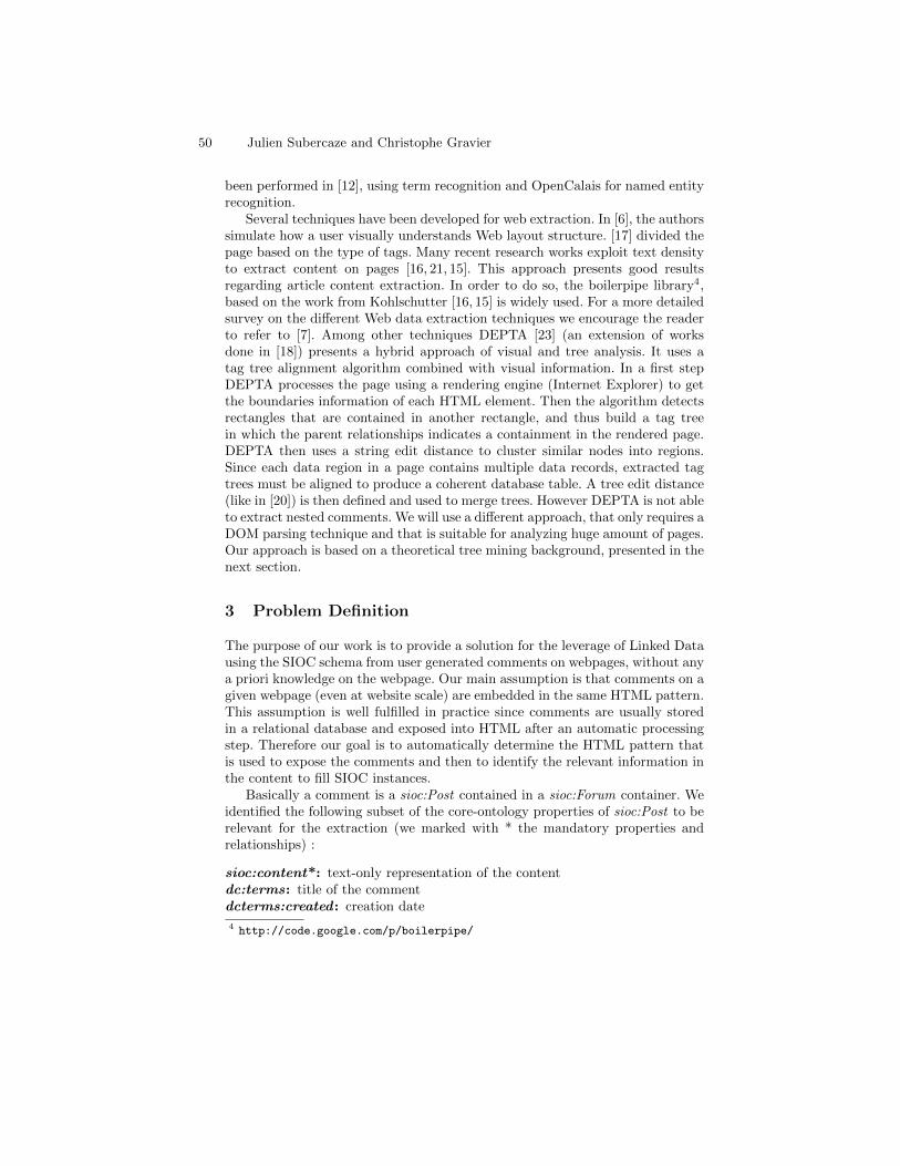
been performed in [12], using term recognition and OpenCalais for named entityrecognition.

Several techniques have been developed for web extraction. In [6], the authorssimulate how a user visually understands Web layout structure. [17] divided thepage based on the type of tags. Many recent research works exploit text densityto extract content on pages [16, 21, 15]. This approach presents good resultsregarding article content extraction. In order to do so, the boilerpipe library4,based on the work from Kohlschutter [16, 15] is widely used. For a more detailedsurvey on the different Web data extraction techniques we encourage the readerto refer to [7]. Among other techniques DEPTA [23] (an extension of worksdone in [18]) presents a hybrid approach of visual and tree analysis. It uses atag tree alignment algorithm combined with visual information. In a first stepDEPTA processes the page using a rendering engine (Internet Explorer) to getthe boundaries information of each HTML element. Then the algorithm detectsrectangles that are contained in another rectangle, and thus build a tag treein which the parent relationships indicates a containment in the rendered page.DEPTA then uses a string edit distance to cluster similar nodes into regions.Since each data region in a page contains multiple data records, extracted tagtrees must be aligned to produce a coherent database table. A tree edit distance(like in [20]) is then defined and used to merge trees. However DEPTA is not ableto extract nested comments. We will use a different approach, that only requires aDOM parsing technique and that is suitable for analyzing huge amount of pages.Our approach is based on a theoretical tree mining background, presented in thenext section.

3 Problem Definition

The purpose of our work is to provide a solution for the leverage of Linked Datausing the SIOC schema from user generated comments on webpages, without anya priori knowledge on the webpage. Our main assumption is that comments on agiven webpage (even at website scale) are embedded in the same HTML pattern.This assumption is well fulfilled in practice since comments are usually storedin a relational database and exposed into HTML after an automatic processingstep. Therefore our goal is to automatically determine the HTML pattern thatis used to expose the comments and then to identify the relevant information inthe content to fill SIOC instances.

Basically a comment is a sioc:Post contained in a sioc:Forum container. Weidentified the following subset of the core-ontology properties of sioc:Post to berelevant for the extraction (we marked with * the mandatory properties andrelationships) :

sioc:content*: text-only representation of the contentdc:terms: title of the commentdcterms:created : creation date

4 http://code.google.com/p/boilerpipe/

50 Julien Subercaze and Christophe Gravier

and relationships :

sioc:has creator*: points to a sioc:UserAccount which is the resourcesioc:has container*: indicates a sioc:Container objectsioc:reply to: links to a sioc:Post itemsioc:has reply : links to sioc:Post items

The sioc:Container pointed by sioc:has container can be from different typesin our case. We consider extraction from user reviews (sioct:ReviewArea), postson forum (sioc:Forum), comments from blogs (sioct:Weblog), Q&A answers(sioct:) or generally for newspaper discussion (sioc:Thread). However, distin-guishing these differents subclasses of sioc:Container would require classifica-tion from the webpages we intend to perform extraction on. This is out of thescope of our paper, we will therefore uniformally consider the container as aninstance of sioc:Container. Similarly there exists subclasses of a sioc:Post foreach container. As for the container, our algorithm will output sioc:Post items.

To summarize, our problem is the following : in order to generate SIOCdata from raw HTML, we must identify the different items (sioc:Post) and theirconversational relationships (sioc:reply to and sioc:has reply). For each item wemust identify the user (sioc:UserAccount), the content of the post (sioc:content)and when possible the date and the title.

3.1 Frequent Subtree Mining

In the case of product listing extraction, the goal is to extract frequent subtreesthat are identical in the page. For this purpose, a bottom-up subtree miningobjective is sufficient. For selecting a feature among mined items, for exampletitle and price, a filter on the leaf nodes can be applied. In the case of commentsextraction, the patterns can be nested. Assuming that the pattern we are lookingfor is [a[p; br; p; div]], if we encounter a reply to a comment, i.e. nested instancesin the pattern, the tag tree for the comment and its answer could be as follows :[a[p; br; p; div; [a[p; br; p; div]]]]. In the case of a single comment we will encounterour pattern [a[p; br; p; div]]. We observe that nodes can be skipped horizontallyalong with their descendants.

In frequent subtree mining, three types of subtrees are distinguished : bottom-up, induced and embedded. Figure 1 depicts these different subtrees. For moredetails on frequent subtree mining, we refer the reader to [8].

We observed empirically that instances are nested in the way we describedpreviously : the direct parenting relation is preserved. Consequently inducedsubtree is a sufficient type of subtree for our purpose. Embedded subtree min-ing could also be used, however since the algorithms complexity grow with thecomplexity of the pattern to mine, induced subtree mining is definitely moreappropriate. The main advantage of subtree mining over existing works is thatit provides a mine once extract many approach. In order to mine large web-sites, one would need to mine the pattern from only one webpage from each siteand could later extract data by simple pattern matching on other pages, thus


B

DE

F

(b)

A

B

DE

F

C

(a)

B

D F

(c)

A

DF

C

(d)

Fig. 1. Different types of subtree from tree (a) : bottom-up subtree (b) ; inducedsubtree (c) ; embedded subtree (d)

saving large amount of computational resources and time. In the next section,we present CommentsLifter, our approach to comments’ extraction based onfrequent subtree mining.

4 CommentsLifter

We now start the description of CommentsLifter. This section presents the dif-ferent steps of our algorithm. The underlying idea of CommentsLifter is to usesimple observations on Web page structures to reduce the candidate set gen-eration. This allows us to minimize the error rate while selecting the winningpattern, and to contribute to the runtime performance optimization objective.To extract comments from a Web page, CommentsLifter uses seven steps: Docu-ment preprocessing, Frequent subtrees extraction, Clustering, Merging, Patternexpansion, Winner selection, Field extraction, Data extraction. In the next sub-sections we detail the process followed in each step of our algorithm.

4.1 Preprocessing

Recommendations issued by the W3C aim at specifying the languages of theWorld Wide Web, with various versions of HTML and CSS. While pages follow-ing these recommendations produce clean DOM trees, they represent only 4.13% of the Web pages5. The remaining pages are made up of wrongly formattedHTML code that is often referred to as ”tag soup”6. Due to the large portionthat these pages represent, Web browser engines are able to handle malformedHTML tags, improperly nested elements, and other common mistakes. In ouralgorithm, the first step is to convert any input HTML document (malformedor not) and to output a well-formed document as a DOM tree. For this purpose,any dedicated library (Jsoup7, Jtidy8) or browser engine can be used.

5 http://arstechnica.com/Web/news/2008/10/opera-study-only-4-13-of-the-Web-is-standards-compliant.ars

6 http://en.wikipedia.org/wiki/Tag_soup7 http://jsoup.org/8 http://jtidy.sourceforge.net/


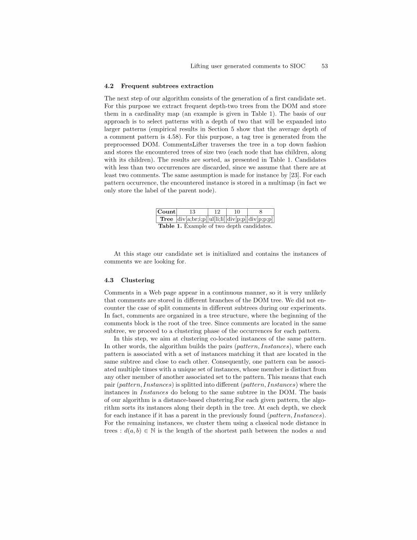
4.2 Frequent subtrees extraction

The next step of our algorithm consists of the generation of a first candidate set.For this purpose we extract frequent depth-two trees from the DOM and storethem in a cardinality map (an example is given in Table 1). The basis of ourapproach is to select patterns with a depth of two that will be expanded intolarger patterns (empirical results in Section 5 show that the average depth ofa comment pattern is 4.58). For this purpose, a tag tree is generated from thepreprocessed DOM. CommentsLifter traverses the tree in a top down fashionand stores the encountered trees of size two (each node that has children, alongwith its children). The results are sorted, as presented in Table 1. Candidateswith less than two occurrences are discarded, since we assume that there are atleast two comments. The same assumption is made for instance by [23]. For eachpattern occurrence, the encountered instance is stored in a multimap (in fact weonly store the label of the parent node).

Count 13 12 10 8

Tree div[a;br;i;p] ul[li;li] div[p;p] div[p;p;p]Table 1. Example of two depth candidates.

At this stage our candidate set is initialized and contains the instances ofcomments we are looking for.

4.3 Clustering

Comments in a Web page appear in a continuous manner, so it is very unlikelythat comments are stored in different branches of the DOM tree. We did not en-counter the case of split comments in different subtrees during our experiments.In fact, comments are organized in a tree structure, where the beginning of thecomments block is the root of the tree. Since comments are located in the samesubtree, we proceed to a clustering phase of the occurrences for each pattern.

In this step, we aim at clustering co-located instances of the same pattern.In other words, the algorithm builds the pairs (pattern, Instances), where eachpattern is associated with a set of instances matching it that are located in thesame subtree and close to each other. Consequently, one pattern can be associ-ated multiple times with a unique set of instances, whose member is distinct fromany other member of another associated set to the pattern. This means that eachpair (pattern, Instances) is splitted into different (pattern, Instances) where theinstances in Instances do belong to the same subtree in the DOM. The basisof our algorithm is a distance-based clustering.For each given pattern, the algo-rithm sorts its instances along their depth in the tree. At each depth, we checkfor each instance if it has a parent in the previously found (pattern, Instances).For the remaining instances, we cluster them using a classical node distance intrees : d(a, b) ∈ N is the length of the shortest path between the nodes a and


b. After building the set of (pattern, Instances), we remove elements where thecardinality of instances is equal to one.

For example, running our algorithm on the tree provided by Figure 2 with thepattern ul[li; li] would produce two pairs (pattern, Instances) that are depictedwith dotted and dashed boxes in the same figure.

div

lllllllllRRRRRRRRR

a

yyyyyyEEEEEE . . . div

ul

yyyyyyEEEEEE ul

yyyyyyEEEEEE ul

yyyyyyEEEEEE

li li li li li li

_ _ _ _ _ _ _��

��_ _ _ _ _ _ _

Fig. 2. Example output for section 4.3 with the pattern ul[li; li]

At the end of this step, CommentsLifter holds the set of pairs (pattern, Instances)that matches a pattern to a set of co-located instances in the DOM tree. In thenext step, we try to identify mergeable patterns from this data structure.

4.4 Merging

HTML patterns that contain comments often have a depth greater than two(see Section 5 for more details). Consequently our candidate set may at this stepcontain pairs of (pattern, Instances) that belong to the same global pattern,that we did not discover yet because the pattern expansion process will occurlater. Instead of discovering the same pattern from different candidates, we aimat merging these candidates beforehand for optimization.

For this purpose we perform a pairwise comparison between the sets of in-stances. We process a merge between sets of instance when every element of aset S1 is topped by an element from the other set of instances. An element istopped by another if the latter is a parent of the former. If a set of instancesis topped by another set, we discard this set and restart the process until nofurther updates to the candidate set are performed.

Algorithm 1 presents this merging process. After this step, the candidate setis again drastically pruned since we eliminated all potentially duplicate patternsfor the expansion phase. This process, together with the previous clusteringprocess, are the key phases of our algorithm since they discard both duplicateand irrelevant candidates.


Algorithm 1: MergePatterns : Merge similar pattern

Data: A collection of couple (Pattern,Instances) Input where all patterns aredifferent,

minDepth the mininum depth of the instances in the DOM treeResult: A collection Candidates of (pattern,Instances) where similar couples

have been mergedrecursion← false;Candidates← ∅;for i : 0 . . . Input.size do

for j : i . . . Input.size do//Depth of the highest common element ;commonDepth← depth(HighestCommon(Input[i].Instances,;Input[j].Instances));//Save useless computation ;if commonDepth < minDepth then

continue ;endSmall← setWithLessInstances(Input[i], Input[j]);Large← setWithMoreInstances(Input[i], Input[j]);if ∀k ∈ Small.Instances, ∃l ∈ Large.Instances, isParentOf(l, k) thenCandidates← Input \ Small;//Restart the merging process;MergePatterns(Candidates);//Cut the current call;break;;else Candidates← Candidates ∪ Large ∪ Small

end

endreturn Candidates;


4.5 Pattern expansion

Since the candidate set contains simple patterns (i.e. of depth two), we processa pattern expansion to discover the fully matching patterns. Patterns may beexpanded in both directions, towards the top and the bottom of the tree.

For each candidate (pattern, Instances), we distinguish two cases. In thefirst case every instance is at the same depth in the tree, this is the case ofproduct listing extraction that we call the flat case. This is the case of bottom-up subtree mining (see Figure 1). The second case also called the nested case isthe one where instances belong to the same subtree but at different depths, thisis the case of induced subtrees in Figure 1 . Top expansion is straightforward,we check if the type of the parent node (i.e. HTML markup tags) for everyinstance is the same, in this case we expand the pattern with the new parentnode and update the instances consequently. This process is executed until allthe instances do not share the same tag as parent node or if the same node (insense of label in the tree, not HTML markup tag) is the parent of all instances.This process is the same for both nested and flat cases.

div

jjjjjjjjjjj

UUUUUUUUUUU

div

~~~~~@@@@@

��

div

~~~~~@@@@@

UUUUUUUUUUU

ul

��////

--

a ul

��//// a div

li li p li li p . . .

_ _ _ _ _ _ _ _ _ _��

��_ _ _ _ _ _ _ _ _ _

_ _ _ _ _ _ _ _��

��_ _ _ _ _ _ _ _

Fig. 3. Pattern expansion process, top expansion until the same node (top div node) isshared by both instances, then bottom expansion for induced subtree (the most rightdiv is skipped)

Once a pattern is expanded in the top direction, the bottom expansion takesplace. This bottom expansion in the flat case, similar to the top expansion issimple since top-down subtrees are easy to extract. One just needs to traverse theinstances trees in a top-down lefmost direction, looking for nodes that are sharedby all instances. Once a node is not present in every instance the algorithm usesbacktracking to select the next sibling, and then continues its process.

However the nested case is not trivial since we look for embedded subtrees.Standard algorithms such as AMIOT [13] and FREQT [1] are dedicated to thistask, but as we mentioned in section 3.1 they performed poorly on the full Webpage, either the running was excessively long (some minutes) or the program


ended with an exception. To make efficient use of these algorithms, we takeadvantage of the specificities of comments extraction. Apart from the aforemen-tioned issues, the biggest problem we encountered using AMIOT or FREQT wasthat we were unable to adaptatively select the support (in fact, a percentage)for a Web page. However in our pattern expansion case, we know how muchinstances are present for each couple (pattern, Instances). Thus, we performeda modification in the algorithms (see Implementation in section 5.1 for furtherdetails) to discard candidate patterns not on a minimum support base, but on astrict occurrence equality base. Finally, instead of using the complete Web pageas the data tree, we construct a tree by adding all the instances in a tree. Moreprecisely since the instances are stored using only their top nodes (the whole in-stance is retrieved by applying the pattern to this node in the data tree), we buildthe data tree by adding the subtrees under the instances’ top nodes as childrenof the root node. Therefore, our data tree contains on ly the relevant instances.Consequently the set of candidate patterns is drastically reduced, comparedwith the use of the whole DOM page. To drive AMIOT in the right direction,the candidate pattern set is initialized with the current depth-two pattern, thusavoiding useless candidate generation for the first stage. Figure 3 depicts thisexpansion process. In this figure we present the instances as they appear in theDOM tree. Our starting pattern is ul[li; li], and its instances are representedwithin the dotted boxes. Both instances have a div node with a different labelas parent, consequently the pattern is expanded to the top : div[ul[li; li]]. Next,both instances again have a div node as parent but in this case this is the samenode. The top expansion process finishes. For the bottom expansion, we considerthis subtree as the data tree. AMIOT (resp. FREQT) performs a left to rightexpansion that adds the node a to the pattern: div[ul[li; li]; a]. The rightmost divnode is discarded since it does not belong with the left instance (the occurrenceis one whereas the algorithm expects two). Then AMIOT adds the node p to thepattern that becomes div[ul[li; li]; a[p]]. The figure does not show the part underthe right most div, in this part we could find for example another instance ofdiv[ul[li; li]; a[p]], resulting in a nested comment.

4.6 Winner selection

Recurring structures competing with the comments pattern in the candidate setare usually menu elements, links to other articles. In [15, 16], Kohlschutter de-veloped a densitometric approach based on simple text features that presentsexcellent results (F1−Score : 95 %) for news article boilerplate removal. Usergenerated comments also differentiate from menu elements on their text fea-tures. Comments are from different text lengths, the link density is low sincecomments are not part of a link in comparison to menu items. We developedsimple heuristics, based on our observations, to discard irrelevant candidatesand to rank the remaining candidates.

Our experimentation showed that instances with a link density greater than0.5 (Kohlschutter found 0.33 for news article) are always boilerplate. Short com-ments in very complex HTML boilerplate patterns can produce instances with a


quite high link density. We empirically observed that links are on the usernameor on its avatar and link to a profile page. Consequently we discard candidateswhere the average link density is above 0.5.

For the remaining candidates their score is given by the following formula:

Score(p, I) = lgt(I)×

√√√√ 1

n− 1

n∑

j=1

lgt(I)− lgt(Ij)2

(1)

The above formula computes the average text length times its standard de-viation. This heuristic promotes candidates where the instances have longertext length with variable length. Finally we did not use heuristics based ona lower bound of words (as in [15, 16]). Once again comments extraction differsfrom traditional boilerplate removal since some comments are sometimes justone word (e.g. lol, +1, first) or they may be longer than the article they arecommenting on. Therefore the standard deviation is very useful for eliminatingmenu items where the text length is often very close among their instances. The(pattern, Instances) couple with the highest score is promoted as the winner.At this step, the algorithm output the tree of instances, i.e. we have the struc-ture of the conversation, but we need to further structure the conversation byidentifying the different fields in the pattern.

4.7 Structuring the content

Once the HTML pattern containing comments has been selected, the next stepof our algorithm consists of extracting the related SIOC fields as we describedin section 3. Two fields are always present in a comment : the username andthe content of the comment. From our observations on various websites (onlinepress, Q&A, blogs, reviews), two other fields appear often. Firstly the date whenthe comment has been posted occurs in 97.95 % of the cases (See Table 2). Com-ments less often have a title, but the percentage we measured (24.48 %) remainshigh enough to be of interest. We voluntarily skipped the extraction of rare fields(vote on comments, account creation date) because of their few occurrences andthe fact that they complicate the whole field’s identification process. From ourobservations, we noticed that content and title are always contained in their ownHTML markup tags, i.e. it is very unlikely to see the title and the content inthe same div. However we noticed that username and date often occur betweenthe same markup tag, for example we often encountered comments fields suchas <div>John, May 25, 2012 at 5:00 p.m</div>. Therefore we apply the fol-lowing procedures : first, identifying the date field within the pattern. We storethe location of the date in the pattern and remove dates in every instances. Forinstance, the previous example will become<div>John</div>. At this point weare sure that the fields we are looking for will be in distinct nodes of the pattern.


Date parsing Date parsing library such as JodaTime9 and JChronic10 performwell on extracting date from messy data. These libraries takes a String as inputand return a Date object. However they do not offer the feature of returning theoriginal text without the substring containing the date. Therefore we developedour library, using features and heuristics from both of the above mentionedlibraries, that offers the date string removal feature.

Fields selection Our heuristic is based again on simple observations. We knowthat every comment contains at least a username and a content, with date andtitle being optional. For each leaf of our pattern, we compute the following mea-sures over its instances : percentage of date found, average text length, standarddeviation of text length, text entropy and average word count, standard devia-tion on word count. Using these values, we build two candidate sets, the first onefor the date, and the other one for title, content and username. We distinguishthese fields using the fact that title, content and username are unstructured text,however dates have a particular structure (containing year, days, . . .).

A node in the pattern is a candidate for the date field if its percentage ofdate found is over 0.7 (to take into account the fact that date extraction isnot perfect), has more than two words and has a coefficient of variation onthe word count that is inferior to 0.2. This latter condition requires that thenumber of words is very close from one instance to another. We did not set thevalue to zero to avoid discarding fields where the date has a variable length, forexample one hour ago and yesterday. From these candidates, we pick the fieldwith the highest entropy in order to discard constant fields that may have beenrecognized as a date. However if the set is empty, then no dates are specified forthe comments, in practice this happens very rarely.

The second candidate set should contain only nodes that instances own tex-tual data. For this purpose we discard the nodes in the pattern where the vari-ation of text entropy is equal to zero (constant text in every instance). Since weknow that the node containing the content must be present within this set, weaim at identifying this field in the first place. Luckily the content is very simpleto identify since it contains the most words, has a very variable length and wordcount. In the practice, selecting the node having the highest word count averageis sufficient. Once the content has been removed from this candidate set, we firstcheck its size. If the size is equal to one, the remaining candidate matches theusername. In the case where two candidates are present, we have to distinguishbetween username and title. Usernames are very short names, usually one or twowords, and are then in average shorter than the title. If two fields are present,the shorter is identified as being the username and the longest is then the title.

9 http://joda-time.sourceforge.net/10 https://github.com/samtingleff/jchronic


PagesGroundTruth

TruePositive

FalsePositive

Global 100 2323 2121 153Flat 77 1837 1674 125

Nested 23 486 447 26

Precision Recall F1

Global 93,3 % 91,3 % 92,3 %Flat 93.1 % 91.1 % 92.1 %

Nested 94.5 % 91.97 % 93.22 %

Table 2. Evaluation : steps one to six

Content Username Date Title

Occurrence (%) 100 100 97.59 24.48

Correct extraction (%) 100 87.75 83.67 81.63

Table 3. Evaluation, step seven : field identification

5 Mining experiments

This section presents the evaluation protocol of CommentsLifter as well as ourexperiment’s results. We first detail the experimental setup, which is a bit parti-culiar for comments extraction due to the large use of AJAX. Finally we presentglobal and detailed results for both flat and nested cases.

5.1 Setup

Many Web pages handle comments using AJAX, consequently downloading rawHTML along manual ground truth construction is not sufficient for building thedataset. To circumvent this issue we developed two components:

Firefox Extension We implemented a Firefox extension that sends the currentDOM (after browser-side Javascript processing) to a Web server.

Web Server The server receives the DOM from the browser through a POSTrequest on a servlet, then runs CommentsLifter and presents an evaluationform along with the extracted comments. The user is asked to evaluate thepertinence of the extraction. We distinguish three cases for the result. Weused Jena11 to generate the SIOC output.

5.2 Evaluation

The results obtained from our evaluation are given in Table 2 and Table 3.Table 2 presents extraction results of the pattern mining part (steps 1 to 6 of

11 http://jena.apache.org/


the algorithm) whereas Table 3 presents the field identification results (step 7).The first six steps of the algorithm present very good results, with a global F1

score over 92%. Concerning field identification we first present the occurrence ofthe different fields over our dataset. Username and content are always present,while the date is not far from being present in every comment. However titlesare to be found in one quarter of the comments. The evaluation accords to theheuristics we describe in section 4.7. Content extraction is a straightforward tasksince it is easy to ”measure” differences with other fields, our algorithm performsperfectly at this task. Date parsing is no easy task, however our algorithm stillperforms well with an identification rate of 83.67 %. However we note that whilethe rest of the process is language agnostic, date parsing libraries are designedto work with western languages (English, German, french, spanish, . . .) but mayfail with other languages, especially with non latin alphabet.

6 Conclusions and future work

In this paper, we presented CommentsLifter, an algorithm that extracts users’comments and outputs SIOC data. Our algorithm combines mining inducedsubtrees from the DOM with simple yet robust heuristics to select the patterncontaining the comment as well as identifying several fields within the pattern.The empirical evaluation presents very good results, for both extraction andfield identification. We successfully extracted comments from various types ofWeb sites, without a priori knowledge, such as online newspapers, forum, userreviews, blogs and we were able to reconstruct the conversations.

Further research will focus on refining the category of the extracted container,in order to determine whether the discussion takes into a forum, Q&A, blog orreview area.

References

1. Tatsuya Asai, Kenji Abe, Shinji Kawasoe, Hiroshi Sakamoto, and Setsuo Arikawa.Efficient substructure discovery from large semi-structured data. pages 158–174,2002.

2. Mark Van Assem, Maarten R. Menken, Guus Schreiber, Jan Wielemaker, andBob Wielinga. A method for converting thesauri to rdf/owl. In Proc. of the 3rdIntl Semantic Web Conf. (ISWC04), number 3298 in Lecture Notes in ComputerScience, pages 17–31. Springer-Verlag, 2004.

3. F. Belleau, M.A. Nolin, N. Tourigny, P. Rigault, and J. Morissette. Bio2rdf: to-wards a mashup to build bioinformatics knowledge systems. Journal of biomedicalinformatics, 41(5):706–716, 2008.

4. Bettina Berendt, Andreas Hotho, and Gerd Stumme. Towards semantic web min-ing. In Intl Semantic Web Conf. (ISWC02), pages 264–278. Springer, 2002.

5. J. Breslin, A. Harth, U. Bojars, and S. Decker. Towards semantically-interlinkedonline communities. The Semantic Web: Research and Applications, pages 71–83,2005.


6. D. Cai, S. Yu, J.R. Wen, and W.Y. Ma. Extracting content structure for web pagesbased on visual representation. In Proc. of the 5th Asia-Pacific conference on Webtechnologies and applications, pages 406–417. Springer-Verlag, 2003.

7. C.H. Chang, M. Kayed, R. Girgis, and K.F. Shaalan. A survey of web informationextraction systems. Knowledge and Data Engineering, IEEE Transactions on,18(10):1411–1428, 2006.

8. Y. Chi, R.R. Muntz, S. Nijssen, and J.N. Kok. Frequent subtree mining-anoverview. Fundamenta Informaticae, 66(1-2):161, 2005.

9. P. Cimiano and J. Volker. Text2onto. Natural Language Processing and Informa-tion Systems, pages 257–271, 2005.

10. M. Craven, D. DiPasquo, D. Freitag, A. McCallum, T. Mitchell, K. Nigam, andS. Slattery. Learning to construct knowledge bases from the world wide web.Artificial Intelligence, 118(1):69–113, 2000.

11. S. Fernandez, D. Berrueta, and J.E. Labra. Mailing lists meet the semantic web.In Proc. of the Workshop on Social Aspects of the Web, Poznan, Poland, 2007.

12. A. Gentile, V. Lanfranchi, S. Mazumdar, and F. Ciravegna. Extracting semanticuser networks from informal communication exchanges. The Semantic Web–ISWC2011, pages 209–224, 2011.

13. S. Hido and H. Kawano. Amiot: induced ordered tree mining in tree-structureddatabases. In Data Mining, Fifth IEEE International Conference on, 2005.

14. D. Huynh, S. Mazzocchi, and D. Karger. Piggy bank: Experience the semantic webinside your web browser. The Semantic Web–ISWC 2005, pages 413–430, 2005.

15. C. Kohlschutter, P. Fankhauser, and W. Nejdl. Boilerplate detection using shallowtext features. In Proceedings of the third ACM international conference on Websearch and data mining, pages 441–450. ACM, 2010.

16. C. Kohlschutter and W. Nejdl. A densitometric approach to web page segmen-tation. In Proceeding of the 17th ACM conference on Information and knowledgemanagement, pages 1173–1182. ACM, 2008.

17. S.H. Lin and J.M. Ho. Discovering informative content blocks from web documents.In Proceedings of the eighth ACM SIGKDD international conference on Knowledgediscovery and data mining, pages 588–593. ACM, 2002.

18. B. Liu, R. Grossman, and Y. Zhai. Mining data records in web pages. In Proceedingsof the ninth ACM SIGKDD international conference on Knowledge discovery anddata mining, pages 601–606. ACM, 2003.

19. A. Maedche and S. Staab. Ontology learning for the semantic web. IntelligentSystems, IEEE, 16(2):72–79, 2001.

20. D.D.C. Reis, P.B. Golgher, A.S. Silva, and AF Laender. Automatic web news ex-traction using tree edit distance. In Proceedings of the 13th international conferenceon World Wide Web, pages 502–511. ACM, 2004.

21. F. Sun, D. Song, and L. Liao. Dom based content extraction via text density.In Proceedings of the 34th international ACM SIGIR conference on Research anddevelopment in Information, pages 245–254. ACM, 2011.

22. A. Yates, M. Cafarella, M. Banko, O. Etzioni, M. Broadhead, and S. Soderland.Textrunner: open information extraction on the web. In Proceedings of HumanLanguage Technologies, pages 25–26. ACL, 2007.

23. Y. Zhai and B. Liu. Web data extraction based on partial tree alignment. InProceedings of the 14th international conference on World Wide Web, pages 76–85. ACM, 2005.


Comparing Metamap to MGrep as a Tool for MappingFree Text to Formal Medical Lexicons

Samuel Alan Stewart*1, Maia Elizabeth von Maltzahn2, Syed Sibte Raza Abidi1

1NICHE Research Group, Dalhousie University, 6050 University Ave., Halifax, NS, Canada.http://www.cs.dal.ca/ ˜niche.

2Department of Internal Medicine, University of Saskatchewan, 103 Hospital Drive, Saskatoon,SK, Canada

*Contact Author: [email protected]

Abstract. Metamap and Mgrep are natural language processing tools for map-ping medical free text to formal medical lexicons, but an indepth comparisonof the programs and their application to social media data has never been pur-sued. This project is interested in comparing the programs, in order to determinewhich program is most appropriate for mapping web 2.0 communication data.The archives of the Pediatric Pain Mailing List (PPML) were mapped with bothprograms, and each term returned was checked for correctness. The analysis re-sulted in Mgrep having a significantly higher precision (76.1% to 58.8%, differ-ence of 18%, p-value < 0.0001) while Metamap returned more terms: 2381 to1350. When considering only perfect or multiple matches, Mgrep still had bet-ter precision (81.2% to 71.3%, difference 10%, p-value < 0.0001). UltimatelyMgrep’s precision may make it the better choice for many applications, but whenthere is more value in number of correct terms returned over accuracy of thoseterms, Metamap’s larger set and superior scoring function may make it the toolof choice.

Keywords: Natural Language Processing; Semantic Mapping; MeSH; UMLS;Knowledge Management; Knowledge Translation

1 Introduction

Web 2.0 tools provide a valuable service to the healthcare community. Through onlinediscussion forums, mailing lists, blogs, etc., clinicians can find mediums through whichthey can communicate their problems and share their experiences, developing relation-ships and creating a virtual community of practice (Wenger, 2004). Notwithstandingthe evidence-based nature of modern healthcare, these online tools provide avenues forsharing experiential and tacit knowledge (Abidi, 2006) with colleagues in a way thatspans the temporal and geographical boundaries that often prevent face-to-face com-munication.

The archives of these online conversations contain vast amounts of tacit and experi-ential knowledge. Extracting this knowledge and making it available to the communitycan improve the overall knowledge base, but how best to process this unstructured freetext has proven a challenge.

Natural language processing approaches have been pursued in the past, includ-ing the semantic mapping of the unstructured text from the online tools to keywordsfrom structured medical lexicons, such as UMLS (UMLS, 2012) and MeSH (MeSH,2010). Of all the approaches to this mapping, the two most successful have been theMetamap program (Aronson, 2001) developed at the NLM, and Mgrep, the mappingtool of choice for the Open Biomedical Annotator (Jonquet et al., 2009).

These two programs take different approaches to the mapping process, and as suchresult in different sets of keywords when mapping the same source text. Previous re-search (Shah et al., 2009) has investigated comparing the two programs with respect tomapping the metadata associated with free, online databases, but this comparison didnot explore the successes and failures of each program in any great detail, and the natureof metadata is very different from the archives of social media tools.

This paper is interested in comparing the results of using Metamap and Mgrep tomap the archives of an unstructured medical mailing list to the MeSH medical lexicon.We first want to investigate general precision, to determine which program is moreaccurate with its mapping. We also want to delve deeper into the precision of the twoprograms, to determine if there is a relationship between mapping score and correctness,and we want to look at the overlap between the terms returned from the two programs.

The paper will proceed as follows: the background section will summarize the med-ical lexicon system, and the MeSH system in particular. It will explore some previ-ous semantic mapping techniques, along with in depth explanations of how Metamapand Mgrep work. The methods section will outline the data preparation, the mappingprocess, and the analysis plan. The results section will summarize the analysis of themappings by the two programs, and finally the discussion and conclusion sections willattempt to synthesize the analysis into a useful comparison of the two programs.

2 Background

In an evidence-based medical world, it is vital that knowledge be available to cliniciansat the point of care. Unfortunately, the lack of organization, proper indexing, aginginformation sources and poor distribution have been shown to negatively affect a clini-cian’s access to pertinent information (Covell et al., 1985; Timpka et al., 1989; Osheroffet al., 1991). The use of formal medical lexicons is a key step in improving clinicianaccess to medical knowledge by providing a unified indexing of the existing medicalknowledge.

The Unified Medical Language System (UMLS) is developed by the National Li-brary of Medicine (NLM) to facilitate the computerization of medical knowledge, withthe ultimate goal of allowing computer-systems to “understand” the meaning of biomed-ical and health text (UMLS, 2012). To this end they have created a number of tools, oneof which is the “Metathesaurus”, a formal lexicon that is the aggregate of over 150different medical lexicons. The Metathesaurus includes a semantic network, assigningeach term in the UMLS to one of the 135 generalized semantic types, which in turn have54 relations between them. For a full listing of the UMLS Semantic Types, visit http://www.nlm.nih.gov/research/umls/META3_current_semantic_types.html.

64 Authors Suppressed Due to Excessive Length

The Medical Subject Headings (MeSH) lexicon is one of the subsets of the UMLS(MeSH, 2010). MeSH is the NLM’s own controlled vocabulary, and is used to index theMEDLINE database. There are 26,142 terms in the 2011 edition of MeSH, arranged ina hierarchical fashion descending from 16 independent root nodes.

The UMLS and MeSH provide a valuable indexing resource to the medical pro-fession, but clinicians need to be able to leverage these semantic languages in orderto make full use of the formal indexing. Leroy and Chen (Leroy and Chen, 2001) de-veloped a system that processes general medical queries and returns a set of medicalkeywords from the UMLS. Cimino et al (Cimino et al., 1993) designed a system thatmaps clinician queries to a set of generic queries based on UMLS keywords. Both ofthese systems take questions and map them to formal terms from a medical lexicon,which, though a first step, is different from mapping unstructured free text to a medicallexicon.

2.1 Semantic Mapping Techniques

The process of mapping free text to formal medical lexicons (and specifically to theUMLS) has long been an objective of the medical research community. The value ofhaving formal representation of ideas combined with the challenge of performing thetask manually has made research into automated approaches very valuable. This prob-lem is often linked to MEDLINE, which is manually indexed by MeSH terms (MeSH,2010), and thus provides an objective reason to connect text to UMLS terms. Mi-croMeSH (Lowe, 1987) was one of the first attempts to do this, by providing a simplesystem to expand search queries to MEDLINE and provide a tool where users couldbrowse the MeSH tree around the terms they searched.

CHARTLINE (Miller et al., 1992) processed free text of medical records and con-nected them to relevant terms in the MeSH lexicon via a direct mapping. This processwas improved by SAPHIRE (Hersh and Greenes, 1990), which explored the idea ofprocessing free text and cleaning it by mapping terms to their synonyms. This was avaluable addition to the literature, as it normalized the process of mapping women towoman. This process was taken up by Nadkarni et al (Nadkarni et al., 2001) who usedthis synonym mapping along with a part of speech tagger to better identify the struc-ture of the conversations and attempt to identify specific words and phrases in the text.PhraseX (Srinivasan et al., 2002) also used this kind of synonym parser to analyze themapping of MEDLINE abstracts to the UMLS metathesaurus, in order to evaluate thecontents of UMLS itself. Other, similar approaches include KnowledgeMap (Dennyet al., 2003) and IndexFinder (Zou et al., 2003).

The current, gold standard is Metamap, though another product, called Mgrep (Shahet al., 2009) provides a very similar service. The creators of the Open Biomedical An-notator (OBA) (Jonquet et al., 2009) designed a system that leverages the results of anysemantic mapping service (Metamap or Mgrep) and the ontology relations within thelexicon to produce a more complete semantic mapping. The OBA authors decided tomake Mgrep their default mapping service, due largely to its vastly quicker processingtimes, but their approach would work with Metamap as well.

Comparing Metamap to MGrep 65

2.2 Metamap

Metamap uses a special natural language parser called SPECIALIST (Aronson, 2001)to find all the nouns and noun-phrases in a discussion thread, and maps them to one ormore UMLS terms. Each mapped UMLS term is assigned a score that is a measure ofhow strongly the actual term mapped to the UMLS vocabulary. The score is a weightedaverage of four metrics measuring the strength of the matching, with an overall rangein [0,1000], with higher scores indicating a better match. The formal equation for cal-culating the scores is:

1000× (Centrality+Variation+2×Coverage+2×Cohesiveness)6

(1)

– Centrality: An indicator of whether the matched (source) term is the head of thephrase

– Variation: A measure of the distance between the matched term and the root word.For example, if the source word is eye and the match is to the term ocular, thedistance is 2, as ocular is a synonym for eye

– Coverage and Cohesiveness: Measures of how well the source term and the UMLSterm match each other: if the source and UMLS terms are both “pain” then thematch is perfect, but if the source term ocular matches to the UMLS term OcularVision then the coverage and cohesiveness are less than perfect.

Metamap’s precision and recall in previous projects have varied depending on theformat of the text being processed, from values as high as 0.897 and 0.930 respectively(Kahn and Rubin, 2009) to values as low as 0.56 and 0.72 (Chapman et al., 2004). Thedifference between the precision and recall values show that Metamap does a good jobat returning pertinent MeSH terms, but also returns impertinent terms as well, i.e., its re-sults are somewhat noisy. Projects that reported low recall and precision with Metamapacknowledged that many of the problems come from the inherently ambiguous natureof the text being processed: in processing medical residents’ voice recordings, it wasnoted that Metamap failed to recognize abbreviations, acronyms or complex phrasesthat omitted key terms (Chase et al., 2009).

For our purposes, the Metamap scoring system provides a baseline measure of howwell the mapped UMLS term represents the original term in the PPML discussionthread. Table 1 contains some sample mappings to the MeSH lexicon and their scores.

Despite the inconsistencies in the terms returned by Metamap, it provides a valuabletool for mapping unstructured messages and conversations to a structured medical lex-icon. The Knowledge Linkage project (Stewart and Abidi, 2012) uses these mappingsto try and provide explicit knowledge links to the experiential knowledge being sharedwithin the community.

2.3 Open Biomedical Annotator and MGrep

The Open Biomedical Annotator (Jonquet et al., 2009) was developed to automate theprocess of providing keywords to datasets that are available on the web. Their processwas to take the metadata from the datasets, pass them through a semantic mapping


engine (either Metamap or Mgrep) and then post-process their output using ontologicalrelationships.

The authors of the Open Biomedical Annotator performed an experiment to com-pare MetaMap to Mgrep (Shah et al., 2009) in terms of accuracy and speed. They foundthat Mgrep performed slightly better in terms of precision and was much faster (1/5th ofa second compared to 8 minutes). The authors concluded that, because they were look-ing for real-time implementation, Mgrep was was a better option for them, and thus TheOpen Biomedical Annotator was implemented using Mgrep.

The details of how Mgrep works are not completely clear, and publications on ithave been limited to conference posters (Dai et al., 2008). The authors of the OpenBiomedical Annotator claim that it “implements a novel radix-tree-based data structurethat enables fast and efficient matching of text against a set of dictionary terms” (Jon-quet et al., 2009). The scoring algorithm as well is not completely explained, though itperforms a similar expansion scoring to Metamap, where partial matches and derivedmatches receive lower scores that perfect matches. Mgrep is not distributed itself, butis accessed via the OBA: performing a mapping with the OBA without using the on-tological expansions results in a strictly Mgrep-based mapping. Table 1 contains somesample mappings from Mgrep.

The report stated that when music therapy is used, the babies required less pain medica-tion. Does anyone know of any published reports of empirical research demonstratingthe effect?

Metamap Terms Mgrep TermsSource MeSH Term Score Source MeSH Term Scoremusic therapy Music Therapy 1000 Music Music 10

therapy therapy 10the babies Infant 966less pain medi-cation

Pain 660 Pain Pain 10

less pain medi-cation

PharmaceuticalPreparations

827

of any pub-lished reports

Publishing 694 Report Report 16

Research Research 10of empiricalresearch

Empirical Re-search

1000 Empirical Re-search

Empirical Re-search

10

Table 1: Sample message and its associated MeSH mappings from both Metamap andMgrep

2.4 Conclusion

It is clear that Metamap and Mgrep are the two most popular options for mappingmedical free text to structured medical lexicons. Minimal research has been done in


terms of comparisons, but more is needed, particularly within the mapping of socialmedia data. Using MeSH as a target lexicon has the benefit of having many comparableprojects, and the follow-up connection to MEDLINE and other sources that are indexedby MeSH is an additional reason to use it as a target lexicon.

3 Methods

The data for this project is the archives of the Pediatric Pain Mailing List (PPML)from January 2006 - December 2008. The data were originally extracted and processedfor the Knowledge Linkages project (Stewart and Abidi, 2012) and the parsing andcleaning details are contained therein. For our purposes the content of the messageswere extracted and cleaned to try and remove non-medical information (user signaturesand reply-text being the major targets). An attempt was made to remove non-pertinentmessages (such as conference announcements and job advertisements) as those typesof messages do not contain the embedded medical knowledge that we are interestedin. Once the data was cleaned and prepared it was mapped with both Metamap andthe Open Biomedical Annotator (OBA), producing a set of terms and scores for eachmessage from each program.

3.1 Mapping

In a paper by Abidi (Abidi et al., 2005) they outlined semantic filters they applied whenusing Metamap in mapping the content of clinical practice guidelines to formal medicalterms. Of the 135 semantic types in the UMLS certain types, such as Amphibian or Pro-fessional Society, were not deemed pertinent to the subject, and were filtered out. 108of the semantic types were used, while 27 were filtered out. The semantic types filteredout were: Amphibian, Animal, Bird, Class, Family Group, Fish, Functional Concept,Geographic Area, Group, Idea or Concept, Intellectual Product, Language, Mammal,Occupation or Disciple, Organization, Physical Object, Plant, Population Group, Pro-fessional Society, Professional or Organizational Group, Qualitative Concept, Quanti-tative Concept, Regulation or Law, Reptile, Research Device, Self-help or Relief Orga-nization, Spatial Concept, Temporal Concept and Vertebrate.

The mapping was done usingMetamap09. Though newer versions of Metamap havebeen made available the decision was made to use the same mappings that were done inthe original project (Stewart and Abidi, 2012). Changes between versions of Metamapare minimal, so a change to the new version of the program is not expected to drasticallyaffect the results.

ForMgrep, the mapping was done using the OBAREST services, available at http://bioportal.bioontology.org/annotator. The OBA has the same semantic typefilters as Metamap, and the same filtering set was used. None of the OBA expansionoptions were used, resulting in the OBA returning a strictly Mgrep-mapped set.

In order to make the scores comparable between the programs, the Metamap scoreswere divided by 100, putting them on the same [0, 10] range as the Mgrep scores. Foreach program, the terms within a specific message were aggregated. This means that,though the range for an individual mapping score is [0,10], the scores can in reality go


from [0,∞], as there could be multiple mappings of the same term in a message. For themappings reviewed, the maximum score returned was 128.26 for Metamap and 190 forMgrep.

Once the mappings were created they needed to be checked. The messages andtheir mappings were reviewed by a medical expert. For each message the content of themessage was first evaluated to determine if it was medically oriented, completing thefiltering process that was somewhat handled in the data cleaning process. After that eachMeSH term mapped to the message was reviewed and determined to be relevant to theconversation or not. The process was continued until 200 medically relevant messageshad been found, with 127 messages being deemed not medically relevant.

3.2 Analysis

The analysis will begin with a simple investigation of the precision of both programs.Since both programs report scores for each mapping, an investigation of the relationshipbetween score and correctness will also be investigated, to determine both the value ofthe scores being returned, and whether the scores could be used to improve the mappingprocess. We also want to compare the mappings between Mgrep and Metamap to studythe overlap. The natural partner when studying precision is recall, but while precision,the proportion of returned terms that are correct, is relatively simple to calculate, recall,the number of correct terms that were found, is not nearly as simple to find, as thisrequires the correct terms for each of the messages to be pre-specified, which was nota feasible task for this project. Relative recall (Clarke and Willett, 1997) is often usedto compare search strategies in which there is no annotated database to calculate recallfrom, but relative recall tends to favour system that return more results, and Metamapreturned many more terms, and thus must have a higher relative recall. We will insteadlook at the overlap between the two programs and its relationship to precision.

4 Analysis

Table 2 presents some summary statistics for both Mgrep and Metamap. As we can seein the table, Mgrep had significantly higher precision, with a p-value < 0.0001.

Program # terms # correct Precision difference p-valueMetamap 2381 1384 58.12%

Mgrep 1350 1027 76.07% 17.95% [14.9%,21.0%] < 0.0001Table 2: Summary of the mapping process for both programs. The p-value is calculatedusing a 2-sample z-test with a continuity correction.

4.1 Scores and Correctness

Though Mgrep has a higher general precision than Metamap, the relationship betweenscore and correctness reveals that Metamap’s precision may be better than it appears.


Figure 1 presents boxplots for both programs, comparing the scores for both programsbetween incorrect and correct mappings.

Metamap

Correct

Sco

re

05

1015

2025

No Yes

Mgrep

CorrectS

core

05

1015

2025

No Yes

Fig. 1: Boxplots for comparing scores to correctness for both programs. Note that theplots are truncated to the [0,25] range for clarity.

For both programs it appears that there is a significant relationship between scoreand correctness, though the difference is more pronounced for the Metamap scores, asthat program returns a wider range of scores. Infact, for individual terms Mgrep doesnot seem to return scores other than 8 or 10, with higher scores resulting from multiplemappings within the same message. Table 3 presents the comparison of correctnessto score, and finds that, for both programs the correct terms have significantly higherscores.

n mean Quantiles [5%,25%,50%,75%,95%] Mean diff. p-valueMetamap Correct 1384 12.40 [6.38, 8.27, 10.00, 11.63, 28.27]

Incorrect 997 9.82 [5.94, 7.89, 9.16, 10.00, 19.01] 2.57 < 0.0001Mgrep Correct 1027 13.68 [8, 8, 10, 10, 30]

Incorrect 323 10.13 [8, 8, 8, 10, 17.8] 3.55 < 0.0001Table 3: Comparing scores to correctness for both programs. The p-values are calculatedusing a Wilcoxon Rank-Sum test to account for the extreme skewness of the data.

The relationship between scores and correctness can be investigated further by look-ing at 10% quantiles of the data. Tables 4 and 5 report the correctness stratified by 10%quantiles of the scores. The quantiles of the Metamap scores are much more spreadout, which is to be expected as their scoring algorithm is more complex, resulting in a


wider range of values. What is interesting, looking at the table, is that there seems tobe a significant jump in precision for both programs for terms that score 10 points orhigher. Table 6 looks at the relationship between correctness and score dichotomized toabove/below 10 points.

Quantile [5.22,6.6) [6.6,7.55) [7.55,8.61) [8.61,8.75) [8.75,9.28) [9.28,10) [10,18.6) [18.6,128)Correct 129 77 135 94 109 149 247 57

Incorrect 94 175 104 143 56 56 554 201n 223 252 239 237 165 205 801 258

Precision 0.42 0.69 0.44 0.60 0.34 0.27 0.69 0.78Table 4: Correctness by 10% quantiles of scores for Metamap. Note that quantiles thatwere the same were collapsed together, thus the quantile [10, 18.6) has 801 observationsin it, which represents 3 quantiles of data.

Quantiles [8,10) [10,16) [16,20) [20,190)Correct 162 126 19 16

Incorrect 328 445 69 184n 490 571 88 200

Precision 0.67 0.78 0.78 0.92Table 5: Correctness by 10% quantiles of scores for Mgrep. Because of the lack ofrange of Mgrep scores many of the quantiles were similar, and were thus collapsed into4 groups from 10.

Metamap’s precision has jumped from 58% to 71%, while Mgrep’s has jumpedfrom 76% to 81%. Though Mgrep’s precision amongst only those terms that score≥ 10is still significantly higher (10% difference, 95% CI: [6.1%, 13.9%], p-value< 0.0001),Metamap improved it’s precision by 13%, whereas Mgrep only improved by 5%. It isclear that there is a significant relationship between score and correctness.


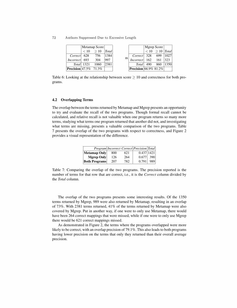
Metamap Score< 10 ≥ 10 Total

Correct 628 756 1384Incorrect 693 304 997

Total 1321 1060 2381Precision 47.5% 71.3%

m

Mgrep Score< 10 ≥ 10 Total

Correct 328 699 1027Incorrect 162 161 323

Total 490 860 1350Precision 66.9% 81.2%

Table 6: Looking at the relationship between score ≥ 10 and correctness for both pro-grams.

4.2 Overlapping Terms

The overlap between the terms returned byMetamap andMgrep presents an opportunityto try and evaluate the recall of the two programs. Though formal recall cannot becalculated, and relative recall is not valuable when one program returns so many moreterms, studying what terms one program returned that another did not, and investigatingwhat terms are missing, presents a valuable comparison of the two programs. Table7 presents the overlap of the two programs with respect to correctness, and Figure 2provides a visual representation of the difference.

Program Incorrect Correct Precision TotalMetamap Only 800 621 0.437 1421

Mgrep Only 126 264 0.677 390Both Programs 207 782 0.791 989

Table 7: Comparing the overlap of the two programs. The precision reported is thenumber of terms for that row that are correct, i.e., it is the Correct column divided bythe Total column.

The overlap of the two programs presents some interesting results. Of the 1350terms returned by Mgrep, 989 were also returned by Metamap, resulting in an overlapof 73%. With 2381 terms returned, 41% of the terms returned by Metamap were alsocovered by Mgrep. Put in another way, if one were to only use Metamap, there wouldhave been 264 correct mappings that were missed, while if one were to only use Mgrepthere would be 621 correct mappings missed.

As demonstrated in Figure 2, the terms where the programs overlapped were morelikely to be correct, with an overlap precision of 79.1%. This also leads to both programshaving lower precision on the terms that only they returned than their overall averageprecision.


�

Program

Pre

cisi

on

0.0

0.2

0.4

0.6

0.8

1.0

Metamap Only Mgrep Only Both

Overall Metamap PrecisionOverall Mgrep Precision

Fig. 2: Comparing the overlap of the two programs to their precision.

5 Discussion

Based strictly on precision, Mgrep outperforms Metamap. A difference of nearly 18%confirms the findings of (Shah et al., 2009) in their original investigation of the twoprograms. There is much more depth to the comparison, however, which reveals thepotential utility of Metamap in certain situations.

Though both programs provide mapping scores, Metamap’s seem more useful, pro-viding both a wider range of scores and a larger difference in precision between the lowand high scoring terms. One of the challenges of this comparison is a lack of detailson how the Mgrep scoring algorithm works, but, though the authors claim a range of[0,10], in reality only 8’s and 10’s were returned (with higher scores all being aggregatesof those two numbers).

Of particular interest is the poor performance of terms returned by Metamap thathave scores just below perfect: Looking back at Table 4, the fifth decile, [8.75, 9.28), hasa precision of only 34%. Looking into the mappings in this quantile, we see mappingsthat are based on variations in the root word, along with words that are based on aless than perfect coverage. The mappings in this group are inaccurate because they aretaking a source term like “replacing” and mapping it to the MeSH term “Replantation”,


which is rarely going to be the correct mapping. In an attempt to dig deeper into thepotential variations on source terms, Metamap seems to be hurting its overall precision.

When mappings are restricted to only perfect matches (or less than perfect matchesthat occur multiple times), the precision of both programs increases, but the increaseis more dramatic for Metamap (see Table 6). Previous studies that have investigatedMetamap could improve their results by putting more effort into leveraging theMetamapscores.

This does not mean that terms that score less than perfect should necessarily bedropped, however, as there is a more to the evaluation of the two programs than pre-cision. Looking back at table 6, removing all mappings with scores < 10 would drop693 correct Metamap mappings and 162 correct Mgrep mappings. If the objective ofthe mapping process is strictly about precision then this may be a logical step, but if theobjective is to try and find suggested terms to provide to the users, then there is littleharm in providing incorrect suggestions, especially if it leads to more pertinent termsbeing provided as well. Looking at the overlap of the two programs, though Mgrep hada higher precision, it missed 621 terms that Metamap provided, terms which may havebeen beneficial to the user. Likewise, there are 264 terms missed by Metamap that werereturned by Mgrep, which could also have been helpful.

If the objective of the mapping process is strictly to be as precise as possible, thenusing Mgrep and restricting the mapping solely to terms that score 10 points will resultin the most accurate mapping. If you are developing a suggestion engine, however, or ifyour system can leverage the mappings scores, as our Knowledge Linkage program did(Stewart and Abidi, 2012), then perhaps the larger set returned by Metamap, combinedwith the superior scoring function, may be more useful to your project.

Though it was not studied formally in this project, we did find that Mgrep was vastlyfaster than Metamap, even when used over the internet through their REST services.This confirms the findings of (Shah et al., 2009), and if you are trying to develop areal-time system then Metamap may be too slow for your application.

6 Conclusion

There is an obvious need for indexing engines that can process free text and match themto formal medical lexicons. Though this project focused on MeSH, there are obviousexpansions to any component of the UMLS, and mappings to ICD and SNOMED canprovide valuable resources to those working in health information technology.

The mapping of social media archives to MeSH is a challenging objective. A preci-sion of 58% by Metamap is at the low end of the range of precisions reported by otherpapers that studied program (Chapman et al., 2004; Chase et al., 2009), and the chal-lenges of mapping abbreviations, acronyms and complex phrases from medical chartscontinue to be a problem for the mapping of social media data. This does not mean thatthe mapping process cannot be used, but when leveraging the terms provided by theseprograms the potential for incorrect mappings must be taken into account.

This project had some shortcomings. A double review of the mappings rather thana single review would have provided more confidence in the “correctness” of the map-pings. The Metamap program used was the 2009 edition, as those were the mappings


that were produced for the Knowledge Linkage project (Stewart and Abidi, 2012), andthere have been multiple releases since then. Re-running the analysis with the new pro-gram would probably not change the precision of Metamap significantly, but it wouldcertainly change some of the mappings. We believe that the general structure of theanalysis would remain the same, however a comparison of the old and new versionsshould be investigated. More details of how Mgrep works need to be made available,especially with respect to the scoring algorithm. As well, the aggregation of multiplemappings needs to be broken down, which could be used to expand the results in section4.1. Correct/Incorrect may not be the best way to classify mappings: providing the term“Pain” in a discussion of needle stick injuries is not incorrect, but it is not as useful asthe MeSH term “Needle Stick”. Re-evaluating each mapping on a 5-point Likert Scalemay provide more valuable insights.

Developing a way to measure some form of recall would improve the analysis:studying the crossover between the two programs is helpful, but being able to identifyand study what was missed is a valuable component of the comparison of the two pro-grams. Each message could be reviewed, and the potential MeSH terms that are notpresent could be recorded, providing some insight into terms that were not mapped.This analysis will be done in future work.

Moving forward, the programs are best measured not by evaluating their correctnessin terms returned, but by their utility embedded in other programs. Re-implementing theKnowledge Linkage project with Mgrep and re-running the analysis from that project(Stewart and Abidi, 2012) would be a stronger way to measure whether Mgrep is moreor less useful in mapping free text to medical lexicons. A larger review set would alsoallow a more indepth analysis of the correctness as a function of position in the MeSHtree, both in terms of source root and depth from the top.


Bibliography

Abidi, S. (2006). Healthcare Knowledge Sharing: Purpose, Practices, and Prospects,chapter 6, pages 65–86.

Abidi, S., Kershaw, M., and Milios, E. (2005). Augmenting gem-encoded clinical prac-tice guidelines with relevant best evidence autonomously retrieved from medline.Health Informatics Journal, 11(2):95–110.

Aronson, A. R. (2001). Effective mapping of biomedical text to the umls metathesaurus:The metamap program. Proceedings of the AMIA Symposium.

Chapman, W. W., Fiszman, M., Dowling, J. N., Chapman, B. E., and Rindflesch, T. C.(2004). Identifying respiratory findings in emergency department reports for bio-surveillance using metamap. MEDINFO.

Chase, H. S., Kaufman, D. R., Johnson, S. B., and Mendonca, E. A. (2009). Voice cap-ture of medical residents’ clinical information needs during an inpatient rotation.Journal of the American Medical Informatics Association, 16:387–394.

Cimino, J., Aguirre, A., Johnson, S., and Peng, P. (1993). Generic queries for meet-ing clinical information needs. Bulletin of the Medical Library Association,81(2):195–206.

Clarke, S. J. and Willett, P. (1997). Estimating the recall performance of web searchengines. In Aslib Proceedings.

Covell, D., Uman, G., and Manning, P. (1985). Information needs in the office practice:are they being met? Annals of Internal Medicine, 103(4):596–599.

Dai, M., Shah, N., Xuan, W., Musen, M., Watson, S., Athey, B., and Meng, F. (2008).An efficient solution for mapping free text to ontology terms. AMIA Summit onTranslational Bioinformatics,.

Denny, J. C., Smithers, J. D., Miller, R. A., and Spickard, A. (2003). understandingmedical school curriculum content using knowledgemap. JAMIA, 10:351–362.

Hersh, H. and Greenes, R. (1990). Saphire - an information retrieval system featur-ing concept matching, automatic indexing, probabilistic retrieval, and hierarchicalrelationships. Comput Biomed Res, 23:410–425.

Jonquet, C., Shah, N. H., and Musen, M. A. (2009). The open biomedical annotator.Summit of Translational Bioinformatics, pages 56–60.

Kahn, C. E. J. and Rubin, D. L. (2009). Automated semantic indexing of figure captionsto improve radiology image retrieval. Journal of the American Medical InformaticsAssociation, 16:280–286.

Leroy, G. and Chen, H. (2001). Meeting medical terminology needs–the ontology-enhanced medical concept mapper. IEEE Transactions on Information Technologyin Biomedicine, 5(4):261–270.

Lowe, H. (1987). Micromesh: a microcomputer system for searching and exploringthe national library medicines medical subject headings (mesh) vocabulary. ProcAnnu Symp Comput Appl Med Care, pages 717–20.

MeSH (2010). Medical subject headings. http://www.nlm.nih.gov/mesh/.Miller, R. A., Gieszczykiewicz, F. M., Vries, J. K., and Cooper, G. F. (1992). Chart-

line: Providing bibliographic references relevant to patient charts using the umls


metathesaurus knowledge sources. Proc Annual Symposium of Comput Appl MedCare, pages 86–90.

Nadkarni, P., Chen, R., and Brandt, C. (2001). Umls concept indexing for productiondatabases: a feasibility study. JAMIA, 8:80–91.

Osheroff, J., Forsythe, D., Buchanan, B., Bankowitz, R., Blumenfeld, B., and Miller, R.(1991). Physicians’ information needs: analysis of questions posed during clinicalteaching. Annals of Internal Medicine, 114(7):576–581.

Shah, N. H., Bhatia, N., Jonquet, C., Rubin, D., Chiang, A. P., andMusen, M. A. (2009).Comparison of concept recognizers for building the open biomedical annotator.BMC Bioinformatics, 10 (suppl 9):S14.

Srinivasan, S., Rindflesch, T. C., Hole, W. T., Aronson, A. R., and Mork, J. G. (2002).Finding umls metathesaurus concepts in medline. Proc AMIA Symp, pages 727–731.

Stewart, S. A. and Abidi, S. S. R. (2012). An infobutton for web 2.0 clinical discussions:The knowledge linkage framework. IEEE Transactions on Information Technologyin Biomedicine, 16(1):129–135.

Timpka, T., Ekstrom, M., and Bjurulf, P. (1989). Information needs and informationseeking behavior in primary health care. Scandanavian Journal of Primary HealthCare, 7(2):105–109.

UMLS (2012). Unified medical language system fact sheet. Web.http://www.nlm.nih.gov/pubs/factsheets/umls.html.

Wenger, E. (2004). Knowledge management as a doughnut: Shaping your knowledgestrategy through communities of practice. Ivey Business Journal, pages 1–8.

Zou, Q., Chu, W. W., Morioka, C., Leazer, G. H., and Kangarloo, H. (2003). In-dexfinder: A method of extracting key concepts from clinical texts for indexing.AMIA Annu Symp Proc, pages 763–767.


Exploring the Similarity between Social KnowledgeSources and Twitter for Cross-domain Topic

Classification

Andrea Varga, Amparo Elizabeth Cano and Fabio Ciravegna1

OAK Group,Dept. of Computer Science,The University of Sheffield,

United [email protected]

Abstract. The rapid rate of information propagation on social streams has provento be an up-to-date channel of communication, which can reveal events happen-ing in the world. However, identifying the topicality of a short messages (e.g.tweets) distributed on these streams poses new challenges in the development ofaccurate classification algorithms. In order to alleviate this problem we study forthe first time a transfer learning setting aiming to make use of two frequently up-dated social knowledge source (KS) (DBpedia and Freebase) for detecting topicsin tweets. In this paper we investigate the similarity (and dissimilarity) betweenthese KS and Twitter at the lexical and conceptual(entity) level. We also evaluatethe contribution of these types of features and propose various statistical mea-sures for determining the topics which are highly similar or different in KS andtweets. Our findings can be of potential use to machine learning or domain adap-tation algorithms aiming to use named entities for topic classification of tweets.These results can also be valuable in the identification of representative sets of an-notated articles from the KS, which can help in building accurate topic classifiersfor tweets.

Keywords: social knowledge sources, transfer learning, named entities, data anal-ysis

1 Introduction

Micropost platforms such as Twitter serve as a real-time channel of information re-garding events happening around the world. Compared to traditional news sources, mi-croposts communicate more rapidly up-to-date information on a large number of topics.Identifying these topics in real-time could aid in different scenarios including i.e., emer-gency response, and terrorist attacks.

However, microposts mining poses several challenges since some of the character-istics of a tweet include: i) the use of non-standard English; ii) the restricted size of apost (limited to 140 characters); iii) the frequent misspellings and use of jargon; andiv) the frequent use of abbreviations.

The dynamic changes in both vocabulary and style pose additional challenges forsupervised classification algorithms, since the collection of annotated data becomesparticularly difficult. However, frequently updated social knowledge sources(KS), suchas DBpedia and Freebase, present an abundant source of structured data which couldpotentially aid in streamed topic detection. Similar to Twitter, these sources exhibitthe following characteristics: i) they are constantly edited by web users; ii) they aresocial and built on a collaborative manner; iii) they cover a large number of topics; andiv) they provide plentiful amount of annotated data.

In this work we present for the first time a comparative study which analyses thesimilarity between Twitter and two frequently updated KS including DBPedia and Free-base. This comparative study includes the analysis of various cross-domain(CD) topicclassifiers built on these KSs considering different lexical and conceptual features de-rived from named entities. Our intuition for the conceptual features is that the mentionof certain entity types could be a good indicator for a specific topic. For e.g. a tweet con-taining the entity “Obama” is more likely to be a trigger for the topics “Politics” and“War&Conflict” than for the topic “Entertainment”. Similarly, “Lady Gaga” is morelikely to appear in tweet messages about the topics “Entertainment” or “Music”, thanabout the topic “Sports”.

In addition, we propose different statistical measures for quantifying the similarityand differences between these KS and tweet messages. The main research questions weinvestigate are the following: i) Do KSs reflect the lexical changes in Twitter?; ii) Whichfeatures make the KSs look more similar to Twitter?; iii) How similar or dissimilar areKS to Twitter; and iv) Which similarity measure does better quantify the lexical changesbetween KS and Twitter?

The main contributions of this paper are as follows: i) we present a methodologyfor building CD topic classifiers for tweets making use of KSs; and ii) we present acomparative analysis exploring the similarity between KSs and Twitter at the level ofwords and named entities for CD topic classification;

In the remaining of the paper we briefly describe the DBpedia and Freebase KS, wethen present the state-of-the-art approaches in topic classification of Tweets, then wedescribe the main methodology and present the results obtained.

2 Social Knowledge Sources: an overview of DBpedia andFreebase

In this section we briefly review the main features of the DBpedia and Freebase KSs,highlighting the differences and similarities between them.

DBpedia1 is a structured knowledge base derived from Wikipedia2, the largest col-laboratively maintained encyclopaedia. The latest released, DBpedia 3.7, classifies 1.83million resources into 740,000 Wikipedia categories and 18,100,000 YAGO2 categories.For a given Wikipedia article DBpedia provides the following information [4]: i) the ti-tle of the Wikipedia article; ii) the abstract of the article corresponding to the first few

1 http://dbpedia.org2 http://wikipedia.org

Exploring the Similarity between Social Knowledge Sources and Twitter 79

paragraphs containing up to 500 words; iii) the Wikipedia categories (topics) assignedto the article; iv) various links such as the external links pointing to external Web re-sources, redirects pointing to other articles about synonymous terms, pagelinks describ-ing all the links in the article, inter-language links pointing to the translations of thearticle into multiple languages; v) disambiguation pages explaining different meaningof homonyms about a given term; vi) images depicting the resources from the article;vii) homepage or website information for an entity such as organisation or company;and viii) geo-coordinates of a particular resource of the article.

Similarly, Freebase3 is a huge online knowledge base which users can edit in a sim-ilar manner as Wikipedia. The latest version of Freebase 4 comprises of 85 domains,more than 20 million entities and more than 10 thousand relations across a large num-ber of these domains. In contrast to DBpedia however, in Freebase the source of articlesinclude Wikipedia as well as other sources such as MusicBrainz, WordNet, OurAir-ports, etc 5. The classification of articles in Freebase is also slightly different; for agiven Freebase article: i) a domain denote the topic of the article; ii) a type define a par-ticular kind of entity such as person or location (for e.g. “Lady Gaga” is a Person); andiii) properties describe an entity (for e.g. “Lady Gaga” has a “place of birth”). Anothernotable difference between the two knowledge source is the level of deepness in thehierarchy for a particular category or topic.

3 Related Work

DBpedia and Freebase KSs have been important knowledge sources in many classifi-cation tasks such as topic detection and semantic linking of Twitter messages. Theseapproaches mostly employ traditional machine learning algorithms building a classifieron Twitter dataset and deriving useful features from KSs.

To date, to the best of our knowledge, no analysis has been done in exploiting theseKSs for cross-domain (CD) topic classification of tweets and also in measuring thesimilarity between these KSs and Twitter. In the following section we thus provide asummary of the related work using these KSs for Twitter on topic detection and seman-tic linking.

Related Work on using DBpedia for Topic Classification of Tweets Ferragina et al.[7] propose the TAGME system, which enriches a short text with Wikipedia links bypruning n-grams unrelated to the input text. Milne et al. [11] propose an automaticcross-reference of Wikipedia documents and Wikipedia links by means of machinelearning classifiers. This method has been shown to not perform well when applied totweets [10]. Munoz et al [1] also address the problem of assigning labels to microposts,in order to identify what a micropost is about. In their approach they assign DBpediaresources to post by means of a lexicon-based similarity relatedness metric.

Meij et al [10], also assign resources to microposts. In their approach they makeuse of Wikipedia as a knowledge source, and consider a Wikipedia article as a concept,

3 http://www.freebase.com/4 http://download.freebase.com/datadumps/2012-07-19/5 http://wiki.freebase.com/wiki/Data_sources

80 Andrea Varga, Amparo E. Cano and Fabio Ciravegna

their task then is to assign relevant Wikipedia article links to a tweet. They proposea machine learning approach which makes use of Wikipedia n-gram and Wikipedialink-based features. Our approach differs from theirs in two main points: 1) rather thanconsidering a Wikipedia article or DBPedia resource link as a concept, we consider awhole DBpedia category as a concept; 2) our study analyses the use of DBpedia as anannotated source dataset, which can be used to increase the performance of machinelearning classifiers for assigning a topic label to a tweet.

Mendes et al. [12] propose the Topical Social Sensor, which is a system that allowsusers to subscribe to hashtags and DBpedia concepts in order to receive updates regard-ing these topics. They link a tweet with the DBpedia concepts derived from the entitiescontained in it. This system is designed for detecting a hype on a topic defined a priori.In our work rather than relating a tweet with the DBpedia concepts derived from namedentities, we propose the use of DBpedia articles to model a category, and perform anuse this articles as source dataset for training a topic classifier to assign a topic label toa tweet.

Related Work on using Freebase for Topic Classification of Tweets Kasiviswanathanet al[9] propose a detection-clustering based approach for streamed topic detection theymake use of entities and their types gathered from Freebase. In this paper, rather thanproposing a new approach for topic detection we compare the performance of two clas-sifiers; one based on DBpedia and the other on Freebase for detecting topics of tweets.

4 Methodology

This section describes three different steps required for the analysis presented in this pa-per. The first step, described in Section 4.1, consists on the compilation of datasets fromKSs; the second step, described in Section 4.2, consists on the use of these datasets forthe development of CD topic classifiers; and the third step consists on the introductionof similarity metrics that can characterise distributional changes between datasets.

4.1 Collecting Data from KS

In this section we refer to our datasets, which will be further described in Section 5. TheTwitter dataset consists of a collection of tweets, which were annotated with 17 differenttopics using the OpenCalais services. In order to compile a set of articles relevant toeach of these 17 topics, from both DBpedia and Freebase KSs, we performed two steps.In the case of DBpedia, for a given topic, we SPARQL6 queried for all resources whosecategories and subcategories are similar to the topic. For the returned resources weonly kept the first 500 characters from the resources’ abstracts. In the case of Freebase,we downloaded the articles using the Freebase Text Service API7. Given a topic, wecollected all the articles whose domain matched the topic 8. In addition, for some of the

6 http://www.w3.org/TR/rdf-sparql-query/7 http://wiki.freebase.com/wiki/Text_Service8 The collection of domains are enumerated at http://www.freebase.com/schema


topics (e.g. Disaster or War), which were not defined as domains in Freebase, we lookedat all the articles containing these topics in their title. While this service also allows todownload the full content of an article, similarly to DBpedia, we only considered thefirst paragraph up to 500 characters.

The following Subsection 4.2, describes how the DBpedia and Freebase datasets areused to built three different CD classifiers for detecting topics in tweets.

4.2 Building Cross-Domain(CD) Topic Classifier of Tweets

We formally describe each dataset D as a tuple (X,F, P (X)) composed of a set ofinstances X , a set of features F and a marginal probability distribution P (X). Eachinstance x ∈ X is represented by a vector of features x = (f1, .., fm), fi ∈ F . Thepossible topics y = {catY1

, . . . , catYd} for an instance x can take values from Y ∈

{cat1, . . . , catk}. The goal of the classification then is to learn a model h : X → Yfrom a set of annotated training data L = {(x1, y1), . . . , (xn, yn)|xi ∈ X, yi ∈ Y },that induces a non-injective map between X and Y such that multiple class labels canbe assigned to the same instance - e.g. h(x1) = {cat1, cat2}.

A CD scenario consists of a source dataset DS = (FS , XS , P (XS)) –on which theclassifier is built– and a test dataset DT = (FT , XT , P (XT )) –on which the classi-fier is evaluated–. As illustrated in Figure 1, in this paper we consider three cases forthe source dataset. The first two cases aim to investigate the usefulness of DBpediaand Freebase KSs independently, and the third case combines the contribution of bothKSs. Thus, the CD scenarios studied in the paper are described as follows: ScenarioI (Sc.DB) consisting of sole DBpedia articles; Scenario II (Sc.FB) consisting of soleFreebase articles; and Scenario III (Sc.DB-FB) consisting of a joint set of DBpediaand Freebase articles. The test dataset in each case is the Twitter dataset.

Retrieve articles

Concept enrichment

Build Cross-domain Classifier Annotate Tweets

Sc. FB Sc. DB-FBSc. DB

Retrieve tweets

Concept enrichment

Fig. 1. The Sc.DB, Sc.FB and Sc.DB-FB CD scenarios using concept enrichment.

We used as baseline classifier an SVM classifier with linear kernel, which has beenfound to perform best for transfer learning [6]. We also took the commonly used one-


vs-all approach to decompose our multi-label problem into multiple independent binaryclassification problems.

Feature Extraction The performance of the machine learning algorithm rely on thefeature representation employed. We propose two different feature sets for the examplesin both train and test datasets:

– a bag-of-word(BoW) representation: This representation captures our natural intu-ition to utilise what we know about a particular topic, so that the features whichare most indicative of a topic can be detected and the appropriate label(s) assigned.This feature consists of a collection of words weighted by TF-IDF (term frequency-inverse document frequency) in order to capture the relative importance of eachword.

– a bag-of-entities(BoE) feature representation. The second set of features makes useof named entities. These entities were extracted by querying OpenCalais API9 forentity extraction on each instance belonging to the Dbpedia, Freebase and Twitterdatasets as presented in Figure 1. We then used the dereferenceable URI and con-cepts returned by the API as features for the classifier. Our intuition is that entitiescan be characteristic of a topic, serving as trigger words for this topic; reducing inthis way the lexical differences between the source and target datasets.

4.3 Measuring Distributional Changes Between KS and Twitter

In addition to building the CD classifiers, we investigated various measures for quanti-fying the similarity between KSs and Twitter. When building a machine learning clas-sifier, it is expected that the closer the train dataset to the test dataset the better theperformance of the classifier [13]. Therefore, these similarity metrics can be potentiallyuseful in predicting the adequacy of the data collected from a KS in detecting topics intweets.

To measure the similarity between the distributions of the presented datasets, let −→drepresent a vector consisting of all the features occurring on a dataset. Then,−→ds denotessuch a vector for the train dataset and−→dt for the test dataset. In light with the feature setemployed, the −→ds and −→dt contain the TF-IDF weight for either the BoW or BoE featuresets. Then the proposed statistical measures are:

– the chi-squared (χ2) test: The χ2 test measures the independence between the fea-ture sets (FS and FT ) and the train and test datasets. Given the −→ds and −→dt vectors ,the χ2 test can be computed as

χ2 =∑ (O − E)2

E

, where O is the observed value for a feature, while E is the expected value calcu-lated on the basis of the joint corpus.

9 www.opencalais.com/


– the Kullback-Leibler symmetric distance (KL): Originally introduced in [3], thesymmetric KL divergence metric measures how different the −→ds and −→dt vectors areon the joint set of features FS ∪ FT :

KL(−→ds||−→dt) =

∑

f∈FS∪FT

(−→ds(f)−−→dt(f)) log

−→ds(f)−→dt(f)

– cosine similarity measure: The cosine similarity represents the angle that separatesthe train and test vectors −→ds and −→dt :

cosine(−→ds,−→dt) =

∑FS∪FT

k=1 (−→ds(fSk

)×−→ds(fTk))

∑FS∪FT

k=1 (−→ds(fSk

))2 ×∑FS∪FT

k=1 (−→dt(fTk

))2

We also note that some of these proposed functions measure actual similarity (cosine),while others measure distance KL, χ2.

5 Dataset and Data Pre-Processing

The Twitter dataset consists of tweets posted between October 2010 and January 2011,and was originally collected by [2],10 comprising more than 2 million Tweets postedby more than 1619 users. We further annotated this data set with topics returned by theOpenCalais service, which label each tweet with one or more topics (from a collectionof 17 topics). For our analysis we randomly selected one thousand tweets for each topic,excluding re-tweets, resulting in a collection of 12,412 Tweets. Some of these categoriesare presented in Table 1. Similarly from DBpedia and Freebase we randomly selectedone thousand articles for each topic, comprising of 9,465 articles from DBpedia and16,915 articles from Freebase.

88.6%

8.6%

1.8%0.9%

Dbpedia multilabel frequency

1 8 2 3+4+5+6+7+9

99.9% 0.1%

Freebase multilabel frequency

1 2

71%

22.3%

5.6%

1%0.1%

Twitter multilabel frequency

1 2 3 4 6+5

88.6%

8.6%

1.8%0.9%

Dbpedia multilabel frequency

1 8 2 3+4+5+6+7+9

99.9% 0.1%

Freebase multilabel frequency

1 2

71%

22.3%

5.6%

1%0.1%

Twitter multilabel frequency

1 2 3 4 6+5

Fig. 2. The multi-label distribution in DBpedia, Freebase and Twitter datasets. The numbers inthe legend indicate the number of topics assigned to an example, varying from 1 to 9 topics.

10 Available at http://wis.ewi.tudelft.nl/umap2011/


In line with previous approaches ([2]), for the datasets we removed all the stopwordsand we converted all words into lower case; after which a Lovins stemmer was applied.In addition, in order to reduce the vocabulary differences between the KS datasetsand Twitter, all hashtags, mentions and URL links, which are particular to the Twit-ter dataset, were removed. The feature space was also reduced to the top-1000 wordsweighted by TF-IDF for each category.

Figure 2 shows the distribution of the examples belonging to multiple topics in eachdataset. The Twitter dataset contain some tweets annotated with up to six categories,with the majority of them being annotated with only one topic. In the case of the Free-base dataset, due to the nearly flat hierarchical structure of the domains, the majorityof the articles belong to a single category. In the case of the DBpedia dataset the ma-jority of the articles belong to a single category, and less than 1% of the articles areannotated with 3,4,5,6,7 or 9 topics. The size of the vocabulary for each category and

Topic name Example tweetsBusiness&Finance(BusFi) visa cyber attack transactions affected account data safe

company nbcDisaster&Accident(DisAcc) happening accident people dying could phone ambulance

wakakkaka xdEducation(Edu) read book even final pass pages period readEnvironment(Env) good complain cause part energized midterms happeningEntertainment&Culture(EntCult) google adwords commercial greeeat enjoyed watching

greeeeeat dayHealth&Medical&Pharma(Health) unprocessed fat eat lose fat real butter coconut oil eggs olive

oil avocados raw nutsPolitics(Pol) quoting military source sk media reports deployed rocket

launchers decoys realSports(Sports) ravens good position games left browns bengals playoffsTechnology&Internet(TechIT) iphone cute ringtone download ringtone; lets enjoy wik-

ileaks tomorrow publish direct message everWar&Conflict(War) nkorea prepared nuclear weapons holy war south official

tells state media usaTable 1. Example tweets for some of the evaluated topics after preprocessing (removing thestopwords, hastags, mentions and URLs).

dataset is presented in Figure 3. This distribution presents a variation in the vocabularysize between the different datasets. Namely, in the DBpedia dataset each category isfeatured by a large number of words. This is expected, as the DBpedia articles are typ-ically longer than the Freebase articles. The richest topics in DBpedia being Religion,EntCult, TechIT . In contrast, in the Freebase dataset the topics are being described byless words. The richest topics in Freebase are Sports, TechIT , HumInt. While for theTwitter dataset these topics are Env, DisAcc, BusFi.

When looking at the frequency of the entities in Figure 4, we can observe similartrends. The DBpedia articles contain the most number of entities for each topic, onaverage 22.24± 1.44 entities. From the full collection 69(0.72%) of the articles do nothave any entity. In the case of Freebase, the average number of entities per article is


!"

#!!!"

$!!!"

%!!!"

&!!!"

'!!!!"

'#!!!"

'$!!!"

'%!!!"

()*+,"

-,*.//"

01)"

0234)53"

026"

78953:"

7;*<=8/"

7)>?23"

@9A;B"

@9C"

D;5"

=85,E,;2"

F;/?**)8"

F<;B3*"

G8/:?G"

H893:8B"

H9B"

IJ%'" I%&!"IIJ$" IIJI"

I&%!"I$K!" I$L$" I#%J" I'!!"

IJ#I" I$!I" I#&#" I#JK"IJL'" II%I" IIK!" I'$#"

&K%&"LI$#"

K$'#"

'!#'#"

LJJ$"LI!K" LI$#" L$##" LI$#" LI$#"

LK'&"

''L$I"

LI$#"

&'&I"

L&KJ"

&&J&"LI$#"

I&!I"

#'&L"

IK!K"

##J$"'&#J"

$%&$"

JK%#"

%JK'"

'J%&"

$JJ'"

%$'#"J&&&"

'&LK"

%&$#" %K#&"

#$#K"#KJ!"

'!K#'"

'!!L#"

L##'"

'''!!"

'!!I'"

''L%L"'#$#J"

'I!$L"

L&#I"

''J#I"

'IIIJ"

'J!I'"

'!!#L"

'#J!K"

'I&'L"

LLII"'!$IJ"

GMG"

F/N-("

F/N+("

F/N-(O+("

Fig. 3. The size of vocabulary in the source (Sc.DB, Sc.FB, Sc.DB-FB) and target (TGT) datasetsafter pre-processing.

!"

#!!!"

$!!!!"

$#!!!"

%!!!!"

%#!!!"

&!!!!"

&#!!!"

'!!!!"

'#!!!"

()*+,"

-,*.//"

01)"

0234)53"

026"

78953:"

7;*<=8/"

7)>?23"

@9A;B"

@9C"

D;5"

=85,E,;2"

F;/?**)8"

F<;B3*"

G8/:?G"

H893:8B"

H9B"

$II%" $JKK" $J!#" $J!#" $JK&" $'K$" $%J&" $#I$" $'#&" $ILI" %&$%"$$%!" $#$%" %$$L" $KJ&" %%JL"

$%!L"

%$$#L"%%&K&" %%!IL"

%&'#!"%%%J'"

%!LI%"

%%&K&" %%#K%" %%&K&" %%&K&"%!JII"

$KIK'"

%%&K&"

%'KK$"%&L'$"

%%%&I" %%&K&"

L'!$"

%&$L"

KL%%"

$I$&" %&J#"

#K#J"

IJ#$"

$'L&L"

%'%'"

KIK%"

$I%&!"

$%!#&"

%''$"

$J'K&"

$'$#&"

%J%I"

KIKK"

%K!K#"

%'#%'"

%I$J&"

%#%&L"%'&'#"

%#I!J"

&$LJ%"

&LL'$"

%'#KK"

%IIJK"

&I%JK"

%I&$!"

%'#IL"

'%&KI"

&K&!!"

%'J&&"

%III%"

GMG"

F/N-("

F/N+("

F/N-(O+("

Fig. 4. The number of entities in the source (Sc. DB, Sc. FB, Sc. DB-FB) and target (TGT)datasets after pre-processing.

8.14± 5.78. The percentage of articles without any entity is 19.96%(3,377 examples).Lastly, the Twitter dataset contains the smallest number of entities, on average 1.73 ±0.35 entities per articles. The number of articles mentioning no entity is 5,137 (41%).

The heatmap in Figure 5 demonstrates how the entity types’ frequencies differacross different datasets. The darker the color, the higher the frequency of an entityin a dataset. According to this figure, Organization and Position have a relatively highfrequency across all datasets. Other entities appearing frequently on these datasets arePerson, Country and Natural Feature. Entity types such as MedicalCondition, or Sport-sEvent appear to be more representative of particular topics such as Health and Sports.When checking the clustering by topic in Figure 5, we can notice that the Health andEdu topics present a similar entity distribution in DBpedia and Freebase; the War topic


Labo

r (Sc

.FB)

War

(TG

T)W

ar (S

c.FB

)So

cIss

ue (S

c.FB

)W

eath

er (S

c.FB

)Te

chIT

(Sc.

DB)

Hum

Int (

Sc.D

B)W

eath

er (S

c.DB

)So

cIss

ue (S

c.DB

)La

w (S

c.DB

)La

bor (

Sc.D

B)Di

sAcc

(Sc.

DB)

Hosp

Recr

(Sc.

DB)

EntC

ult (

Sc.F

B)Te

chIT

(Sc.

FB)

Hum

Int (

TGT)

EntC

ult (

TGT)

EntC

ult (

Sc.D

B)Te

chIT

(TG

T)Bu

sFi (

Sc.F

B)He

alth

(Sc.

FB)

Heal

th (S

c.DB

)Bu

sFi (

Sc.D

B)En

v (S

c.DB

)La

w (S

c.FB

)En

v (S

c.FB

)Di

sAcc

(Sc.

FB)

Hosp

Recr

(Sc.

FB)

Wea

ther

(TG

T)Di

sAcc

(TG

T)En

v (T

GT)

Edu

(Sc.

DB)

Edu

(Sc.

FB)

Spor

ts (S

c.DB

)W

ar (S

c.DB

)Hu

mIn

t (Sc

.FB)

Pol (

Sc.F

B)Sp

orts

(Sc.

FB)

Relig

ion

(Sc.

FB)

Spor

ts (T

GT)

Relig

ion

(TG

T)Po

l (TG

T)Po

l (Sc

.DB)

Relig

ion

(Sc.

DB)

Heal

th (T

GT)

Hosp

Recr

(TG

T)Bu

sFi (

TGT)

Labo

r (TG

T)So

cIss

ue (T

GT)

Edu

(TG

T)La

w (T

GT)

NaturalFeature

Country

Person

Position

Organization

Technology

MedicalCondition

SportsEvent

Region

Continent

Company

IndustryTerm

City

Facility

ProvinceOrState

Fig. 5. The distribution of the top 15 entity types the in the source (Sc. DB, Sc. FB) and target(TGT) datasets.

has a similar entity distribution in Twitter and Freebase; while the Pol category presentsa similar entity distribution in Twitter and DBpedia.

Based on the above figures on lexical richness and entity frequency, thus, we can no-tice that the Freebase dataset exhibits more similarity to Twitter than Dbpedia datasets.In order to get a better insight into this similarity, we will compare these datasets ac-cording to the proposed measures in the coming section.

6 Experiments

In this section we perform a series of experiments to investigate which KS exhibitsmore similarity to Twitter. In the first set of experiments we compare the performance ofthe SVM classifiers derived for the proposed cross-domain (CD) scenarios (Subsection4.2), with the SVM classifier built on Twitter data only. These classifiers were trainedusing the different BoW and BoE features(Section 6.1) in each scenario. Thereforein this first set of experiments we address the questions of which KS reflects betterthe lexical variation in Twitter? and what feature makes the KSs look more similar toTwitter?.

The second set of experiments, consists on computing the correlation between theproposed statistical measures (Section 6.2) and the accuracy of the CD classifiers. Inthis correlation analysis we investigate which statistical measure presents the highestcorrelations with the accuracy of a CD classifier? providing the most reliable estimatefor the quality of KSs in topic classification of tweets.


6.1 Comparison of the Different Feature Sets in Cross-Domain Scenarios

The SVM classifiers derived from the CD scenarios –Sc.DB, Sc.FB and Sc.DB-FB–were evaluated based on their performance when trained using BoW and BoE features.The TGT SVM classifier –based on Twitter data only– was built on 80% of the Twitterdata, and evaluated on 20% of the twitter data over five independent runs.

Figure 6 shows the results obtained using BoW and BoE features for the differ-ent CD scenarios. Based on the average performance in F1 measure, we can observe,that among the three CD scenarios, the best average performance was obtained by theSc.DB-FB SVM classifier using BoW features, which is followed by the Sc.FB andSc.DB SVM classifiers also using BoW features.

Using both feature sets, we found that for the Sc.DB-FB scenario the topics whichpresented a performance closer to the one obtained by the TGT classifier were theWeather and Edu. For the Sc.FB scenario these topics were the Edu, Weather, Labor.Finally for the Sc.DB scenario these topics were the Edu, Health. The topics for whichthe performance was higher using BoE features were the BusFi, Env, Pol, SocIssue,Sports. For Labor the performance was the same for both features .

Sc.D

B(Bo

E)

Sc.D

B(Bo

W)

Sc.F

B(Bo

E)

SC.F

B(Bo

W)

Sc.D

B−FB

(BoE

)

SC.D

B−FB

(BoW

)

TGT(

BoW

)

TGT(

BoE)

Edu

Sports

War

Labor

Weather

HumInt

Env

TechIT

DisAcc

SocIssue

HospRecr

Law

Pol

Health

Religion

EntCult

BusFi

37.40 37.80 42.50 47.20 42.50 45.70 71.90 71.30

10.30 11.70 26.50 26.20 26.20 26.00 60.10 59.20

9.30 10.90 23.90 23.60 24.60 25.70 67.60 72.70

1.40 1.30 31.90 31.90 30.10 29.90 79.90 79.40

3.10 7.00 39.80 39.90 36.70 36.00 81.20 81.50

1.10 1.40 2.00 1.60 1.50 2.20 33.60 34.20

15.20 14.20 2.20 2.20 8.90 8.40 46.60 48.30

1.60 2.40 18.40 18.60 12.40 9.90 57.40 58.00

8.30 9.70 14.50 14.50 21.00 21.10 57.50 59.20

1.30 2.00 8.80 9.00 9.70 9.10 44.20 44.00

1.40 2.30 17.20 19.50 11.30 13.90 41.60 42.60

0.90 2.70 16.80 17.80 14.80 13.30 46.80 46.40

22.20 21.00 27.80 26.80 24.20 26.80 45.10 44.90

28.60 30.30 25.60 24.70 26.90 25.40 51.70 51.80

23.40 25.10 14.40 14.70 21.00 20.40 58.40 58.50

15.30 15.10 15.50 16.20 19.50 20.20 42.20 43.10

21.40 21.20 11.50 15.30 18.60 19.10 47.50 46.50

Fig. 6. The performance in F1 measure of the Sc.DB, Sc.FB, Sc.DB-FB and TGT classifiersusing BoW and BoE features for each topic over five independent runs. The training set of TGTclassifier consists of 80% of the Twitter dataset (9,928 tweets). The Sc.DB, Sc.FB and Sc.DB-FBclassifier were trained only on social knowledge sources data.

A slightly different trend can be observe for the TGT classifier, where the bestaverage F1 measure was achieved using BoE features. There were 10 topics for which


BoE features were useful: DisAcc, EntCult , Env, Health, HospRec, HumInt, Religion,TechIT , War and Weather.

Overall, our results indicate that Sc.FB KS is more similar to Twitter than Sc.DB.Furthermore, combining the contribution of the Sc.DB and Sc.FB is beneficial for de-tecting topics in Tweets, since the Sc.DB-FB scenario achieves the best overall results.With regard to the features, we found that in 11 out of 17 cases the results obtainedusing BoW features were better, and in 5 out of 17 cases the BoE features were foundmore effective.

We also compared the performance of the Twitter classifier against the three CDclassifiers over the full learning curve, by gradually increasing the number of tweetsused to train the classifier. Our analysis revealed that in the majority of the cases theCD classifiers worked relatively well. That is, a sufficient amount of annotated tweetswere needed to significantly outperform the three CD classifiers over the full learningcurve. The number of annotations needed for each topic is summarised in Table 2. Fore.g. for more than 9 out of 17 topics the necessary amount of annotated tweets need toexceed 900. However, in a real-world scenario annotating tweets is an expensive task.

BusFi DisAcc Edu EntCult Env Health HospRec HumInt Labor993♣ 993♣ 993♣ 993♣ 993♣ 1, 986♣ 1, 986♠ 160♠ 320♠

Law Pol Religion SocIssue Sports TechIT Weather War640♠ 993♣ 320♠ 320♠ 993♠ 640♣ 320♠ 640♣

Table 2. Number of annotated tweets required for the Twitter classifier to beat the Sc.DB, Sc.FBand Sc.DB-FB CD classifiers. Significance levels: p-value < ♣0.01♠0.05

6.2 Comparison of Statistical Measures in Topic Classification of Tweets

In this second set of experiments we aimed to investigate our research question of howsimilar or dissimilar are social knowledge sources to Twitter posts; and which similaritymeasure does better reflect the lexical changes between KSs and Twitter posts?. We thusperformed a comparison between the proposed KL divergence, cosine similarity andχ2 test by measuring the correlation of these values with the performance of a CDclassifier using Sc.DB, Sc.FB and Sc.DB-FB scenarios.

Each CD classifier was evaluated on 20% of the Twitter data, and the performancewas averaged over five independent runs. The obtained F1 measures for the CD classi-fiers were then compared with the values obtained for the different statistical measures,and the Pearson correlation was computed.

Figure 7 show the correlations obtained using KL, cosine and χ2 values. A pos-itive correlation indicates that the performance of the CD classifiers increases as thedivergence decreases (the distribution are more similar); while a negative correlationindicates that the performance increases as the divergence increases (the distributionsare less similar). As we can notice, for the KL scores, there are 24 cases in which thecorrelation scores are higher than 70% in absolute terms. In the case of Cosine simi-larity these cases sum up to 25. While in the case of χ2 values for a total of 32 caseswere the correlation values higher than 70%.


KL−Sc.DB(BoW)

KL−Sc.FB(BoW)

KL−Sc.DB−FB(BoW)

KL−TGT(BoW)

KL−Sc.DB(BoE)

KL−Sc.FB(BoE)

KL−Sc.DB−FB(BoE)

KL−TGT(BoE)

Cosine−Sc.DB(BoW)

Cosine−Sc.FB(BoW)

Cosine−Sc.DB−FB(BoW)

Cosine−TGT(BoW)

Cosine−Sc.DB(BoE)

Cosine−Sc.FB(BoE)

Cosine−Sc.DB−FB(BoE)

Cosine−TGT(BoE)

Chi−Sc.DB(BoW)

Chi−Sc.FB(BoW)

Chi−Sc.DB−FB(BoW)

Chi−TGT(BoW)

Chi−Sc.DB(BoE)

Chi−Sc.FB(BoE)

Chi−Sc.DB−FB(BoE)

Chi−TGT(BoE)

BusFi

DisAcc Edu

EntCult Env

Health

HospR

ecr

HumIn

t

Labo

rLa

w Pol

Religio

n

SocIss

ue

Sports

Tech

ITW

ar

Wea

ther

−1.0

−0.5

0.0

0.5

1.0

Fig. 7. The Pearson correlation between the performance in F1 of the Sc.DB, Sc.FB, Sc.DB-FBCD classifiers and the KL, Cosine and χ2 measures

Based on these results, we found the χ2 to provide the best correlation scores for theusefulness of the KSs data. The second best score was for the cosine similarity, whichwas followed by the KL measure.

Figure 8 shows the pairwise similarity obtained for the source and target datasetsaccording to (χ2)−1 similarity measure.11 As expected the closest datasets to the testTwitter dataset is the training set for the Twitter classifier (ChiSc.TGT). The secondclosest dataset according to χ2 is the Sc.Fb dataset. The Sc.DB and Sc.DB-FB are thenthe less similar datasets to the test dataset.

7 Conclusions and Future Work

In this paper we presented a first attempt towards understanding the usefulness of DB-pedia and Freebase KSs in CD topic classification of tweets. We presented an analysis11 As χ2 measure distance rather than similarity we inverted its value to present the similarity

between topics better.


Chi−Sc.DB(BoE)

Chi−Sc.DB(BoW)

Chi−Sc.DB−FB(BoE)

Chi−Sc.DB−FB(BoW)

Chi−Sc.FB(BoE)

Chi−Sc.FB(BoW)

Chi−Sc.TGT(BoW)

Chi−TGT(BoE)

BusFi

DisAcc Edu

EntCult Env

Health

HospR

ecr

HumIn

t

Labo

rLa

w Pol

Religio

n

SocIss

ue

Sports

Tech

ITW

ar

Wea

ther

2.21

5.78

1.80

6.93

2.25

5.24

1.79

6.67

2.16

8.12

1.88

6.60

2.17

8.02

1.88

6.47

2.75

5.84

2.18

7.37

2.67

5.30

2.07

7.34

2.05

9.45

1.82

7.38

2.04

9.00

1.80

7.07

2.08

9.09

1.87

6.40

2.10

8.97

1.88

6.28

2.12

4.51

1.61

7.01

2.18

4.50

1.64

6.90

2.18

3.89

1.61

7.13

2.19

3.81

1.61

7.06

2.16

3.38

1.53

7.47

2.17

3.21

1.51

7.23

2.18

10.46

1.95

7.69

2.19

10.37

1.94

7.58

2.17

4.65

1.70

7.06

2.18

4.52

1.68

6.75

2.08

3.46

1.50

7.05

2.12

3.18

1.48

6.82

1.75

3.84

1.36

7.57

1.84

3.79

1.41

7.52

2.17

9.55

1.92

7.28

2.18

9.58

1.92

7.18

2.48

3.31

1.64

6.90

2.41

3.05

1.57

6.57

2.08

3.40

1.48

7.39

2.08

3.21

1.45

7.13

2.30

8.17

1.99

7.04

2.26

8.03

1.94

6.82

2.19

6.20

1.80

7.78

2.20

6.27

1.81

7.75

2

4

6

8

10

Fig. 8. The values of (χ2)−1 ∗ 10−5 for each Sc.DB, Sc.FB, Sc.DB-FB, TGT scenarios. Highvalues indicate that the topics are more similar between the source and target dataset.

between these data sources focusing on various lexical features (BoW) and entity fea-tures(BoE).

For a total of 17 topics we compiled a gold standard for each individual KS, andfor the joint set of these sources. From the resulted datasets we then built three CDclassifiers which we evaluated against a Twitter classifier using the different features.

Our analysis revealed that from the two KSs, Freebase topics seem to be much closerto the Twitter topics than the DBpedia topics due to the much restricted vocabulary usedin Freebase. Furthermore, we found that the two KSs contain complementary informa-tion, i.e.; the joint dataset was found more useful than the individual KS datasets. Withregard to the feature sets, we found that for the three CD classifiers on average theresults obtained using BoW were better than those obtained with BoE in 5 out of 17cases.

When comparing the results of these CD classifiers to the Twitter classifier we foundthat for some of the topics the Twitter classifier required a large number of annotationsto outperform these classifiers, indicating that in the absent of any annotated tweets,applying these CD classifiers is still beneficial. Previous research on transfer learn-ing has also shown, that outperforming the target (Twitter) classifier is extremely diffi-cult for many tasks including sentiment classification ([5, 13]). A promising alternative


found in the literature was to combine the annotated examples in the source and targetdatasets([6]). Our future work aims to follow this direction, focusing on building trans-fer learning algorithms which can effectively combine the contribution of the two KSs;and also exploring other features derived from the named entities.

Finally, we also looked at various statistical measures for predicting the usefulnessof the data gathered from these KSs. These experiments revealed the χ2 test as be-ing the best measure for quantifying the distributional differences among between KSsand Twitter. Our future work in this direction will focus in investigating more accuratemeasures for quantifying this difference for e.g. by taking into account the special vo-cabulary (abbreviations, misspellings, shortening) used in Twitter, and normalise this tostandard English terms ([8]).

References

1. Identifying topics in social media posts using dbpedia. In O. e. a. Munoz-Garcia, editor, InProceedings of the NEM Summit (27-29 September 2011), pages 81–86, 2011.

2. F. Abel, Q. Gao, G.-J. Houben, and K. Tao. Analyzing user modeling on twitter for person-alized news recommendations. In Proceedings of the 19th international conference on Usermodeling, adaption, and personalization, UMAP’11, pages 1–12, Berlin, Heidelberg, 2011.Springer-Verlag.

3. B. Bigi. Using kullback-leibler distance for text categorization. In Advances in InformationRetrieval, Lecture Notes in Computer Science Volume 2633, 2003.

4. C. Bizer, J. Lehmann, G. Kobilarov, S. Auer, C. Becker, R. Cyganiak, and S. Hellmann.Dbpedia - a crystallization point for the web of data. J. Web Sem., 7(3):154–165, 2009.

5. J. Blitzer, M. Dredze, and F. Pereira. Biographies, bollywood, boom-boxes and blenders: Do-main adaptation for sentiment classification. In Association for Computational Linguistics,Prague, Czech Republic, 2007.

6. H. Daume III. Frustratingly easy domain adaptation. In Proceedings of the 45th AnnualMeeting of the Association of Computational Linguistics.

7. P. Ferragina and U. Scaiella. Tagme: on-the-y annotation of short text fragments (bywikipedia entities). In Proc of the CIKM’10, 2010.

8. B. Han and T. Baldwin. Lexical normalisation of short text messages: makn sens a #twitter.In Proceedings of the 49th Annual Meeting of the Association for Computational Linguistics:Human Language Technologies - Volume 1, HLT ’11, pages 368–378, Stroudsburg, PA, USA,2011. Association for Computational Linguistics.

9. S. P. Kasiviswanathan, P. Melville, A. Banerjee, and V. Sindhwani. Emerging topic detectionusing dictionary learning. In Proceedings of the 20th ACM international conference onInformation and knowledge management, CIKM ’11, pages 745–754, New York, NY, USA,2011. ACM.

10. E. Meij, W. Weerkamp, and M. de Rijke. Adding semantics to microblog posts. In Pro-ceedings of the fifth ACM international conference on Web search and data mining, WSDM’12.

11. D. Milne and I. H. Witten., editors. Learning to link with Wikipedia. 2008.12. P. K. P. N. Mendes, A. Passant and A. P. Sheth. Linked open social signals. In In WI-IAT 10,

2010.13. S. J. Pan and Q. Yang. A survey on transfer learning. IEEE Transactions on Knowledge and

Data Engineering, 22(10):1345–1359, October 2010.


Knowledge Extraction and Consolidation from ... - CEUR-WS

Documents

Transcript of Knowledge Extraction and Consolidation from ... - CEUR-WS