1

Knowing the unknown across regions:

spatial tax evasion in Italy

Paolo Di Caroa and Giuseppe Nicotrab

This version: April 2014

Abstract

Using a novel and original dataset on tax audits this paper estimates the distribution and

the determinants of personal income tax evasion across Italian regions over the period

2007-2011. Endogeneity issues and spatial patterns are considered in the analysis, providing

an accurate image of why and where people do not pay taxes. Regional elasticities are

calculated with the aim of quantifying the actual responses of personal income to tax rate

variations when tax evasion is present. Three main insights derive from our study. Personal

income tax evasion in Italy depends on both regional structural factors like the labour

market and personal behavioural aspects such as human and social capital. Cross-border

sheltering activities matter. A specific comparison between two alternative spatial

econometric approaches is also discussed and presented. Some critical aspects and policy

suggestions are conclusively advanced.

Keywords: tax evasion, tax audits, spatial effects, regional heterogeneity.

JEL classification: H26, H71, C31, C33.

a Department of Economics and Business - University of Catania, Corso Italia, n.55 - 95129 – Catania, Italy.tel.: +39-095-7537738, e-mail pdicaro@unict.it(CORRESPONDING AUTHOR)b Guardia di Finanza (GdF) and Department of Economics and Business - University of Catania, Catania,Italy. e-mail giunicotra@unict.itA previous version of this paper circulated with the title ‘Knowing the unknown across regions: newevidences on Italy’. We are particularly grateful to Peter Burridge for his precious support. We wish to thankRay Chetty, Tiziana Cuccia, Bernard Fingleton, Paolo Graziano, Marco Maffezzoli, Isidoro Mazza, BelmiroJorge Oliveira, Roberto Patuelli, Dina D. Pomeranz, Francesco Porcelli, Alessandro Santoro, AlbertoZanardi, the participants at the XXV SIEP Annual Conference (Pavia), at the 6th J.Paelinck Seminar (Madrid),and many discussants at Bocconi University, Harvard Kennedy School and University of Pisa. We would liketo thank Mauro Favetta (Guardia di Finanza) and Filippo Cavazza (AVIS) for providing us data availability.The usual disclaimer applies.

1

1. Introduction

Understanding the size and the effects of tax evasion is not a trouble-free task given

that, by nature, taxes which are not paid are difficult to be detected and taxpayers non-

compliance decisions depend on several elusive behaviours. Irregular workforce, tax

sheltering and informal activities are tangible expressions of the overall shadow economy,

by representing the nebulous side of a particular economic context. It is not a case, then, if

many scholars and policymakers in almost every country of the world have been involved

in this challenging area of study.

While theoretical contributions have been focused on the broad set of motivations

on the basis of tax evasion, empirical analyses have deeply been devoted to the various

measurement issues and methodological aspects linked to the shadow economy lato sensu.

International comparisons on the size and the evolution of shadow activities represent the

bulk of the empirical research in this area. In recent years, however, the distribution of tax

evasion across regions of the same country has attracted a growing attention in the

academic debate in order to explain the spatial characteristics of the shadow economy (Alm

and Yunus 2009; Torgler et al. 2009; Gentry and Kahn 2009).

The main aim of this paper is to provide further evidences on both the geography

and the determinants of tax evasion within a country. Using an original dataset on tax

audits provided by the Italian finance police (Guardia di Finanza, thereafter GdF), next

sections will investigate tax compliance behaviour across the twenty Italian regions over the

period 2007-2011. In particular, the relations between tax evasion, the role of the State and

place-specific factors of non-compliance will be analysed by considering spatial interactions

among neighbouring areas.

At least three reasons can motivate the relevance of studying tax evasion at infra

national level by applying a spatial perspective. Firstly, regions within the same nation share

a more similar institutional and administrative environment than different countries,

providing a more reliable research environment. Secondly, not considering the magnitude

of spatial variation in tax evasion can be misleading and only partially informative,

especially in the presence of significant regional diversity about economic fundamentals.

Thirdly, by providing a more detailed knowledge of what is unknown at territorial level the

design of place-based tax policies can be suggested for hampering taxpayers non-

compliance in a more effective way.

2

The rest of the paper is organized as follows. Section II contains a brief overview of

the literature. Section III describes the data, illustrates some preliminary statistics and

defines the determinants of tax evasion which will be investigated. The spatial analysis is

developed in section IV. Section V summarizes and concludes.

2. Related Literature

A large and active literature speculating on this area of research reflects both the

importance of tax evasion for other economic variables and the different shortcomings

related to the definition and measurement of shadow activities. We limit our attention to

those aspects directly connected to our work, recognizing that a comprehensive survey of

the contributions developed in the last decades represents a task outside the boundaries of

this paper (for more detailed reviews of literature, see Slemrod and Yitzhaki 2002; Slemrod

2007; Alm 2012).

Since the seminal contribution of Allingham and Sandmo (1972), the theory of tax

evasion has been built upon the idea that people decide to not pay taxes motivated by

different reasons such as the chance of getting caught, the degree of risk aversion, the level

of enforcement operated by tax authorities and other individual and social factors.

Taxpayers can comply or not on the basis of intrinsic motivations, the level of education,

their social heterogeneity and complementary psychological attitudes. Individuals can evade

income, value added or capital taxes by undertaking a wide range of actions such as

overstating deductions, failing to file appropriate tax returns or underreporting their real

activities. Noncompliance directly affects public finances and the provision of public

services, undermining the overall stability of the public sector.

From an empirical point of view, two main methods can be distinguished according

to their sources of information, namely direct and indirect. The former relies upon survey

and audit data provided by tax administrations, which collect information on tax reports

and actual tax returns. Although this approach can be biased by the way of selecting

audited taxpayers and it is able to capture only detected evasion, it seems to offer a reliable

information about noncompliance (Andreoni et al. 1998). The indirect approach is

characterized by the identification of some proxies used for approximating the ‘real’

amount of tax evasion and the overall shadow side present at a given time in a particular

economy. Most of the indirect analyses have been based upon the estimation of shadow

activities through different specifications of money demand equations (Schneider and

3

Enste 2000), traces of true income such as electricity consumes or expenditure-based

relations.

Early cross-section analyses and modern panel data estimations have confirmed

some stylized facts about the determinants of tax evasion. The individual opportunity to

evade seems to increase with the unemployment rate and the presence of self-employed in

the labour force (Dubin et al. 1987), the average tax rate, the degree of urbanization and the

intensity of regulation (Torgler et al. 2009). On the contrary, the probability of detection,

the intensity of tax audits and the magnitude of punishing noncompliance appear to have a

negative impact on tax evasion (Dubin 2007). Additional deterrent effects have been

associated to the quality of institutions (Alm et al. 2011). Contrasting evidences,

furthermore, emerge looking at the degree of education of taxpayers, differences in income

and price indexes (Cebula and Feige 2012).

Most of the results valid at international level have been confirmed for the Italian

case. Using an indirect measure of evasion based on survey data collected by the Bank of

Italy, Cannari and D’Alessio (2007) pointed out the negative influence on personal income

evasion exerted by criminality, unemployment, social capital and institutional quality. Di

Porto (2011) conducted an empirical investigation to shed light on the enforcement activity

operated by a branch of the Italian tax administration for counteracting labour irregularities

in a particular region. More recently, Galbiati and Zanella (2012) have developed and

estimated a model of social interactions in tax noncompliance activities, relying upon about

80,000 individual tax audits on self-employed collected by the Italian finance police for the

fiscal year 1987 at tax jurisdictional level and aggregated across regions. These authors

identify a structural model of tax evasion where the perceived individual probability of

being audited is negatively related to the extent of tax evasion in the jurisdiction. Their

main finding is the presence of a sort of neighbourhood effects among taxpayers within the

same tax jurisdiction.

Few works have been focused on the geographical distribution of tax evasion across

Italian regions. Brosio et al. (2002) have presented some statistical tests for assessing the

correlation between tax evasion, regional GDP and local tax pressure in a public-good

framework. As a result, these authors claim a North-South divide in tax evasion for the

Italian case1. Using survey-based micro data for the year 2000, Fiorio and Zanardi (2007)

1 It is interesting to note that one of the main implication of the model developed by Brosio et al. (2002), namely that taxrates set on a local basis will result lower for poorer regions and higher for richer ones contrast with what is effectively

4

confirm the presence of regional variation and a possible North-South pattern in tax

evasion as well as the influence of other factors such as age, education and occupation.

To our knowledge, three previous studies have explicitly investigated the spatial

dimension of tax evasion. Gentry and Kahn (2009) have used zip-code level data on

reported income for the US in a cross-section framework for finding out some borders’

relationships. These authors underline, among other factors, the influence of geographic

proximity on tax sheltering behaviours among American taxpayers. Herwartz et al. (2010)

have integrated a MIMIC approach with spatial effects in order to estimate the size of the

shadow economy for the 238 EU regions (NUTS 2 classification level) and compare their

estimates with those elaborated at national level by other authors using different MIMIC

specifications.

The contribution of Alm and Yunus (2009) is probably the closest to our work.

These authors have developed a model of individual income tax compliance with dynamics

and interdependencies for the US using state-level data for the period 1979-1997. They

compare different estimations obtained by adopting various specifications: Panel-IV model,

a model of Spatial Panel Dependence with Spatial Error Correction, a dynamic panel

model using the Arellano and Bover-GMM estimator and a Spatial Dynamic Panel model.

The most intriguing result provided by Alm and Yunus (2009) is the opportunity to

disentangle the diverse effects (direct, indirect and spatial) of tax evasion across the US.

3. The determinants of tax evasion

3.1 Data description and preliminary statistics

Our empirical analysis is based upon a new and original dataset on tax audits at

regional level (n = 20) elaborated by the authors from novel data provided by the GdF for

the years 2007-2011. GdF is the operative body of the Italian tax administration and, in

particular, of the Italian Ministry of Finance. Its main tasks are the detection of tax evasion

lato sensu, the curb of illegal activities, the control of irregular workforce and many other

complementary services. Every year GdF’s tax auditors are involved in thousands of

inspections (verifiche) and controls (controlli) in order to capture the magnitude of unreported

income and the degree of tax avoidance with respect to both direct (e.g. on personal

income) and indirect (e.g. value added) taxes.

observable in the reality (see next section). Curiously, for most of the Italian regions the opposite is true: poorer regionslevy an higher local tax burden than richer ones, probably due to the worse local public finances of poorer regions.

5

Two potential shortcomings are related to this dataset. On the one hand, the absence

of precise selection criteria for undertaking tax audits makes not feasible the sampling

weight procedure suggested by Pfefferman (1993). On the other hand, tax audits can be a

not random representation of the population of taxpayers, given that tax cheaters can be

expected to be over-sampled. Two supporting arguments, however, suggest that our

sample is not so different than a random representation of the population. Firstly, it is

worth pointing out that GdF’s audits are organized on the basis of national Action Plans

which explicitly relate tax deterrence activities to objective criteria such as the number of

taxpayers, the average economic dimension of taxpayers and territorial aggregates like GDP

or income. Secondly, we have performed different Kolmogorov – Smirnov tests for

assessing the equality of the distribution of tax audits and the distribution of other variables

(GDP, income, number of taxpayers) across regions. In all the cases we are not able to

reject the hypothesis that the distribution of tax audits is statistically different than that of

the other variables2.

Insert about here:Table 1. – Tax audit activities Italian regions.

Tax audits operated by GdF allows us to obtain direct and helpful results for

analysing the dimension and the evolution of tax evasion in Italy, by favouring the

identification of the annual amount of unreported income for personal income taxes and

the total VAT which is not paid by contributors. Also, additional variables such as the

number of inspections and controls and the total number of tax officials are available. In

this paper, we focus on personal income or direct tax evasion (i.e. the Italian IRPEF),

leaving the study of VAT’s evasion to a companion paper, also because taxes like VAT

have a common tax rate valid for all the country, while direct tax rates partly differ across

regions (i.e. the Italian addizionale regionale)3.

The latter aspect is particularly relevant in countries like Italy, where in 2011, the

range of the region-specific additional tax rate varied quite significantly with the bottom

2 Using similar data on tax audits collected by GdF for the fiscal year 1987, Galbiati and Zanella (2012) have also foundthe quasi random nature of this informative source. The resulting p-values of the three Kolmogorov-Smirnov tests are thefollowing: 0.314 (taxaudits vs GDP); 0.452 (taxaudits vs income); 0.452 (taxaudits vs n. of taxpayers). All test results havebeen corrected for the small sample bias.3 It is worth pointing out that unreported income obtained by tax audits operated at a given time t is (mostly) referred totaxable activities and tax evasion of the previous time period, given that tax declarations are registered with one periodlag. For example, unreported income detected by tax auditors at the end of 2010 is related to noncompliance activities forthe previous year (2009), when it has effectively been generated the total income under control. For this reason, all ourvariables capturing evasion take into account this time-lag.

6

level (about 1.23%) registered in regions like Trentino A.A. and Valle d’Aosta and the top

rate (about 2.03%) set by regions like Campania and Calabria.

We construct three different variables in order to capture tax evasion. EVAS_1,

calculated as the relation between the unreported taxable income detected by tax auditors

for region i at time t divided by the reported regional taxable income for the same period;

EVAS_2, obtained as the unreported taxable income detected by tax auditors for region i

at time t divided by regional GDP. These two measures are quite common in the existing

literature. We also use another variable, namely EVAS_3, obtained as an adjusted measure

of tax evasion derived from a weighted unreported income derived from tax audits as in

Ardizzi et al. (2013)4. The definition, the source and summary statistics of all the variables

used in this paper are reported in the Appendix.

In order to understand the relation between enforcement activities and tax evasion,

we use the measure TAXAUDIT defined as the number of tax audits operated in region i

at time t divided by the total number of taxpayers in the same region for the same period.

The meaning of this variable is twofold. On the one side, it allows the consideration of the

role of the State for counteracting tax evasion at regional level weighted by the number of

taxpayers. On the other side, it is able to represent the probability of noncompliance

detection in a more accurate way, given that for the Italian case there are no available

information about the precise number of tax auditors acting at territorial level.

We are also interested in analysing the relation between the regional tax rate and the

amount of tax evasion detected in each region. To this end, we use the total tax rate

(TAXRATE), calculated as the sum of the regional tax rate plus the region-specific added

tax rate. The estimation strategy will also consider the following control variables: the

regional activity or labour force participation rate (ACTIVITY); the average years of

educational attainment of the population in a given region (HUMCAP) measured as in

Barro and Lee (2012); the number of blood donations on the population above 18 years-

old as a proxy for social capital (SOCCAP); the degree of regional urbanization (URBAN).

A more detailed discussion of the relation between each explanatory variable and tax

evasion is presented in section 4 together with the presentation of the empirical results.

4 To be more precise, EVAS_3 has been calculated as the relation between ‘adjusted evasion’ divided by ‘adjustedincome’, where adjusted evasion is the unreported income of region i detected at time t divided by its sample mean andadjusted income is the GDP of region i at time t-1 divided by its sample mean. As noted by Ardizzi et al. (2013), thisstandardization can favor the comparison of diverse areas characterized by different level of economic development.

7

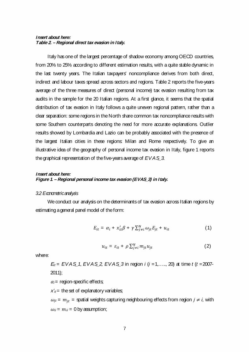
Insert about here:Table 2. – Regional direct tax evasion in Italy.

Italy has one of the largest percentage of shadow economy among OECD countries,

from 20% to 25% according to different estimation results, with a quite stable dynamic in

the last twenty years. The Italian taxpayers’ noncompliance derives from both direct,

indirect and labour taxes spread across sectors and regions. Table 2 reports the five-years

average of the three measures of direct (personal income) tax evasion resulting from tax

audits in the sample for the 20 Italian regions. At a first glance, it seems that the spatial

distribution of tax evasion in Italy follows a quite uneven regional pattern, rather than a

clear separation: some regions in the North share common tax noncompliance results with

some Southern counterparts denoting the need for more accurate explanations. Outlier

results showed by Lombardia and Lazio can be probably associated with the presence of

the largest Italian cities in these regions: Milan and Rome respectively. To give an

illustrative idea of the geography of personal income tax evasion in Italy, figure 1 reports

the graphical representation of the five-years average of EVAS_3.

Insert about here:Figure 1. – Regional personal income tax evasion (EVAS_3) in Italy.

3.2 Econometric analysis

We conduct our analysis on the determinants of tax evasion across Italian regions by

estimating a general panel model of the form:

= + + ∑ + (1)

= + ∑ (2)

where:

Eit= EVAS_1, EVAS_2, EVAS_3 in region i (i =1,….., 20) at time t (t =2007-

2011);

αi = region-specific effects;

x’it = the set of explanatory variables;

ωjt= = spatial weights capturing neighbouring effects from region j≠i, with

ωii= ii = 0 by assumption;

8

β,γ and = parameters to be estimated;

the error component which is initially assumed to be (0, ).

The panel model above is quite common in the empirical literature, apart from the

spatial components recently introduced by Alm and Yunus (2009). In this sub-section, we

ignore for a moment the possibility of spatial effects (ωji = = 0), which will be

subsequently addressed in section 4.2. The model without spatial terms cannot be correctly

estimated adopting traditional panel methods, given that TAXAUDIT is frequently found

to be an endogenous regressor. This endogeneity bias has been confirmed by several

contributions due to the fact that, as pointed out by Breusch (2005), ‘[tax audits] are usually

targeted toward suspected offenders and hence are biased estimators of aggregate

behaviour’. Given that we cannot exclude the possibility that tax audits in our sample are

exogenous, this issue needs to be carefully investigated.

The endogeneity of TAXAUDIT has been tested following two strategies. The

canonical Hausman two-stage procedure has been applied to our panel, by estimating a

first-stage equation where TAXAUDIT was the dependent variable and all the (exogenous)

variables of the general model plus the instrument TAXOFFICIAL have been used as

independent variables. In the second-stage, the residuals from the first-stage estimation

have been used as additional regressor in the general model describing tax evasion5. In

addition, the endogeneity issue has also been verified after the panel-IV estimation by

testing the null hypothesis that TAXAUDIT can be exogenous against the alternative (i.e.

presence of endogeneity).

The instrument TAXOFFICIAL has been constructed as the number of GdF’s tax

officials (auditors and not) in region i at time t divided by the total number of taxpayers in

the same region. In doing this, we have assumed that the overall number of GdF’s officials

at regional level is mostly related to tax evasion through its influence on TAXAUDIT. For

the Italian case, this assumption can be motivated by the fact that the distribution of

finance police officials does not depend on the amount of regional tax evasion (Bordignon

and Zanardi 1997), but it is based on national homogenous criteria such as the population

density of each region. Also note that some Italian regions show an extra-amount of

5 First-stage estimation results are the following: (dependent variable: TAXAUDIT), TAXOFFICIAL 0.02674***

[0.01010], R2 0.48. Second-stage estimation results are: (dependent variable: EVAS_1), first-stage residuals 652.58**

[278.89], R2 0.35; (dependent variable: EVAS_2), first-stage residuals 386.15*** [138.19], R2 0.25; (dependent variable:EVAS_3), first-stage residuals 156.31** [82.23], R2 0.25. Standard errors are in parentheses [].* implies significance at 10%,** implies significance at 5%, *** implies significance at 1%. Additional test results are available upon request.

9

finance police workforce when compared to the Italian average, which is independent from

some national and regional well-defined criteria. Probably, this misalignment is caused by

the usage of GdF’s public employment for different purposes (i.e. unemployment-

reducing) in some areas, like it has been documented for other public sectors.

3.3 Estimation results

Table 3 reports estimation results obtained by applying the panel Instrumental

Variable approach with fixed effects for the dependent variables: EVAS_1, EVAS_2,

EVAS_3. Results in column (1) derive from all the observations in the sample, while those

in column (2) have been obtained by excluding the biggest Italian region (Lombardia) in

terms of population, economic activities and number of total taxpayers. Fixed effects

results have been preferred given that regional differences can be plausibly related to unit-

specific aspects. This has been confirmed by rejecting the presence of random effects, after

adopting the testing procedure based on the artificial regression approach discussed in

Arellano (1993) and Wooldridge (2002).

Insert about here:Table 3. – Panel IV Fixed Effects estimates.

Table 3 also contains the Kleibergen-Paap rk LM-statistic for under-identification,

which is an LM test conducted under the null hypothesis that the equation is under-

identified. The validity of the instrument TAXOFFICIAL has been tested by means of the

difference-in-Sargan or C-statistic distributed as a chi-square with degrees of freedom equal

to the number of instruments. As reported in table 3, we are fairly confident on the

reliability of our instrument. In addition, the F-statistic of the first-stage IV estimation (>

10) has been reported for supporting the instrument adopted in the spirit of Staiger and

Stock (1997).

Three main results are worth commenting at this stage. Personal income tax evasion

across Italian regions is negatively related to the deterrence effect of enforcement activities

pursued by GdF. In line with the existing literature, the higher the probability of being

caught evading, the lower the incentives to evade taxes. High tax rates, national plus

region-specific, can activate individual incentives towards tax noncompliance. Therefore,

when a particular region decides to increase in its autonomous tax rate perhaps in order to

reduce some problems related to its public finances, it shall take into account the possible

10

counterbalancing effect of this decision, namely a rise in tax evasion and a reduction in its

total revenues.

As for control variables, the most significant one is the activity rate, which is

inversely related to personal income tax evasion. This relation can be interpreted as the

presence of higher incentives of tax noncompliance in those areas where economic

conditions and labour markets are weaker. Put differently, people can rationally decide to

not pay taxes if they are involved in informal activities or they operate in uncompetitive

environments. The effect of HUMCAP on tax evasion needs to be cautiously interpreted,

given that this connection requires more theoretical investigation and most of the existing

empirical literature has showed contrasting evidence (Goerke 2012). Either a high level of

human capital can increase tax morale attitudes contributing to reduce tax evasion or better

educated people, which probably earn a higher income in the future facing a greater tax

rate, show preferences for tax avoidance. All in all, Italian regions seem to show a negative

relation between human capital and evasion.

Despite the low statistical significance showed by the variable SOCCAP, it is

interesting to note the different effect (i.e. different sign of the coefficient) derived from

the two samples considered. Social capital has a positive sign when all the Italian regions

are considered (1), while it becomes negative when Lombardia is excluded (2). A positive

coefficient can explain the relation between the amount of tax noncompliance activities

detected in a particular region to the presence of strong social relations spread at regional

level; alternatively, a negative coefficient can reflect the possible virtuous connection

between civic attitudes and citizenship’s commitment. Unfortunately, we do not have

individual data which can help to understand this point. The negative coefficient associated

to the degree of urbanization is probably due to the lower detection of evasion in cities,

where both the population density and the higher anonymity of relations can reduce the

effective amount of evasion detected.

4. Spatial tax evasion

4.1 Regional elasticities

A first question about the spatial features of tax evasion in Italy is the possibility of

comparing the elasticities of evasion and actual income on a regional level. As recently

pointed out by Ray Chetty (2009), a marginal increase in the tax rate can have different

consequences in the presence of evasion: apart from the traditional labour supply effects, a

11

positive variation of the tax rate can lead to a higher level of tax evasion, which in turn

implies a reduction of public revenues. Chetty’s contribution, furthermore, has formally

showed that, under risk neutrality assumptions, tax revenue effects caused by variations in

the tax rates shall take into account the possibility of increasing the audit-generated tax

revenues, after that evasion has shifted up. From a policy perspective, the quantification of

regional elasticities in the presence of tax evasion can throw some light on the true

responses of income after a marginal tax increase/decrease. The effect of tax evasion

becomes important when efficiency aspects are considered: the region-specific Laffer curve

needs to be modified in the presence of tax evasion.

Insert about here:Table 4. – Regional elasticities tax evasion.

Table 4 reports regional elasticities for two measures of tax evasion, namely

EVAS_1 and EVAS_26. The marginal variation of the tax evasion has been calculated

only with respect to a marginal increase in the region-specific tax rate, which can be

considered as a flat tax, in order to overcome endogeneity issues linked to the graduated

personal income total (national plus regional) tax rate. In Italy, the region-specific tax rate

has been on average 1.22% over the time-period here considered and it has showed

variations across regions.

The marginal impact of a rise in the region-specific tax rate leads to a regional

average response of about 0.77% in terms of evasion. Regional policymakers shall be aware

about the size of this relation: for instance, if the regional government in Veneto aims to

raise the addizionale regionale of 1%, this may lead to an increase in personal income tax

evasion (EVAS_1) in the same region of about 0.64%. The same decision in Liguria will

imply a shift up of personal income tax evasion of about 0.90%. As a consequence, we

have different implications for regional and national public finances.

Unfortunately, we do not have enough disaggregate information on income

categories of individual taxpayers in each region, which is a crucial starting point for

undertaking an accurate analysis of the elasticity of taxable income in the presence of tax

evasion (Clotfelter 1983; Saez et al. 2012). In table 5, however, we provide a rough

description of the income effects of tax evasion, by comparing personal income elasticities

with and without tax evasion.

6 The estimated equations on which table 4 is based are available from the authors upon request.

12

Insert about here:Table 5. – Regional elasticities reported and actual income.

Our main aim is to infer the true effect of region-specific tax rates on real labour

supply in the spirit of the recent formula for estimating income elasticity discussed in

Chetty (2009), where the real response of personal income to a one unit positive variation

of the tax rate can be defined as the weighted average of the taxable (reported) income and

the total (actual) earned income elasticities. In our case, the marginal response of reported

income and actual income (i.e. the sum of reported and unreported income) to a marginal

positive increase in the region-specific tax rate has been calculated. In doing this, it is

possible to capture the overall effect of a rise in the marginal tax rate in terms of personal

income, by considering both the labour supply effects without evasion (column 1) and the

combination of labour supply effects and sheltering behaviours in the presence of evasion

(column 2).

For the Italian case, significant variations within and across regions can be observed.

In most of the Italian regions, personal income elasticity is higher when evasion is

introduced than in the absence of it. This can probably be due to the different optimizing

behaviours pursued by taxpayers in the presence of tax evasion: they combine labour

supply decisions with sheltering strategies. Regional differences in the real personal income

response to a one unit variation of the region-specific tax rate can be associated to different

reactions of actual income at a regional level. However, for the reasons previously

mentioned this results shall be taken cum grano salis and they shall be read as the first

attempt to quantify the real response of personal income to tax evasion at disaggregate

level for the Italian case.

4.2 Spatial econometric analysis

Alm and Yunus (2009) have recently proposed and estimated a spatial extension of

the model discussed in section 3.2 in order to study the possible presence of

neighbourhood effects in tax noncompliance decisions. These authors have pointed out the

importance of introducing spatial interactions across geographical units for a better

understanding of the determinants behind taxpayers’ behaviours regarding evasion. This

implies modelling tax evasion in region i as a function of both region-specific determinants

and spatial components, namely = ( , , ), where is personal income tax

13

evasion detected in the j’s-neighbour of region iand denotes the determinants of tax

evasion in the same neighbour.

Spatial effects can occur for different reasons. If the probability of detection is higher

in region ithan in its neighbour(s), tax evasion in the same region will be probably lower

than in surrounding areas: the region-specific deterrence effect is at work. Individuals can

decide to migrate from region i to the closest regions, where the probability of detection is

lower, for having more opportunities to evade taxes. This migration of the tax base will

reinforce the different level of evasion across regions: less taxpayers in region i implies

higher probability of detection in this area, while more taxpayers in region j’s will reduce

the region-specific probability of detection. As a consequence, we can expect a negative

relation between the dynamic of personal income tax evasion in one region and that of its

neighbours.

A similar argument can be related to geographical differences in the region-specific

tax rate (Karkalakos and Kotsogiannis, 2007). In the presence of significant tax rate

differentials across areas of the same country, taxpayers can move from one region having

a higher tax rate to another one where the tax rate is lower. In addition, the region with less

taxpayers can be forced to continuously rise the region-specific tax rate for

counterbalancing the negative revenue effect of the migration. This mechanism can sustain

a vicious circle of high tax rates and high evasion activities. Spatial effects can also derive

from the labour market channel.

As for two regions with different industrial structures and labour market

characteristics, it is quite realistic to assume that a common national shock will have

asymmetric consequences in these areas. If a generic region i is mostly based on heavy

industries such as steel production, while region j has small and medium enterprises

concentrated in the mechanical sector, an increase in the oil prices at national level will

probably affect more region i than region j. Initially, we can assume that region j has a

higher activity rate and lower tax evasion, while the opposite holds for region i. After the

aggregate shock, the starting differences in terms of tax evasion can be influenced by the

migration of workers: presumably, people move from the region most affected by the

shock to the less affected one. The resulting levels of activity rate and tax evasion depend

on the overall consequences of the shock for each regional labour market.

14

Although migration effects of taxpayers are not so widespread in Italy as in the US, it

does not seem so unrealistic to assume that a sufficient subset of mobile marginal taxpayers

exist. Moreover, as pointed out by Besley et al. (1997), some behavioural aspects influencing

tax noncompliance attitudes like human, social and civic capital can show spatially

correlated components across regions. All the above motivations suggest that tax evasion

can have spatial elements across units within the same country7.

To this end, we start to rewrite the general model in (1)and (2)in a more compact

form:

= + + + +

= + + (3)

= + (4)

= 1, … , ,

where is the 1 vector of cross sectional observations on the dependent variable

(EVAS) of regions at time , is a 1 vector capturing unobserved heterogeneity,

is an non-stochastic spatial weight matrix, is an matrix of exogenous

regressor, is an matrix of endogenous regressor. Or, = [ , , ] and

= [ , , ]′; is the 1 composite error term with = in the absence of spatial

dependence in the error term.

Spatial effects can derive from the spatial dependence term (γ), the spatial error

component ( ) or both. Thus, we want to know if the level of tax evasion in a particular

region is influenced by tax noncompliance activities detected in neighbouring regions,

configuring a sort of cross-border tax sheltering behaviour. Or, whether and how our

results can be modified in the presence of spatial-dependent factors in the unobserved

variables (i.e. the error component ).

Before estimating the spatial model above, a preliminary step is the selection of the

spatial weight matrix W(nxn), withωji (j≠i) denoting an individual element of it. Our

W represents the inverse of the geographical distance between centroids (i.e. regional

capital) of the k-nearest neighbours (k = 10, 15, 20). All the results discussed in this sub-

7 At this point, it is worth mentioning that we are not interested in explicitly developing a theoretical model of spatial taxevasion, which is a task outside the boundaries of the present paper. Indeed, our main aim is to find empirical resultswhich can be helpful starting points for subsequently investigating tax evasion from a theoretical perspective.

15

section have been obtained by setting the value k = 20, which allows the consideration of

spatial interactions among all Italian regions, though decreasing with distance. Instead of

assuming a priori spatial effects across Italian regions regarding tax evasion, we conduct the

usual explanatory spatial data analysis (ESDA) to our dataset, which suggests the presence

of stronger spatial effects when considering the variables EVAS_1 and EVAS_3. Test

results are reported in the Appendix.

The model in (3)and (4)is a traditional Cliff-Ord spatial autoregressive model with

autoregressive disturbances and additional endogenous regressors. Efficient and consistent

estimates can be conducted by applying the generalized method of moments (GMM) and

instrumental variable (IV) approach in the spirit of Keleijan and Prucha (1998). More

specifically, given the presence of heteroscedasticity in the error term , we have estimated

a three-step GMM-IV spatial HAC model as in Keleijan and Prucha (2010). The estimation

strategy proceeds as follows.

In the first step, the parameter in (3) is estimated by performing a 2SLS with

instrument matrix = [ , , , ] with the set of instruments used in the sub

section 3.2 for dealing with the endogeneity of TAXAUDIT. In the second step, it is

obtained a GMM estimator for the parameter based upon the 2SLS residuals from the

previous step and robust conditional moments. In the third step, the model in (3) is re-

estimated by applying a 2SLS procedure to the following Cochrane-Orcutt transformation:

= ( − ) + ( − )

= ( − ) (5)

4.3 Spatial estimation results

Table 6 reports estimation results obtained by applying the spatial three-step GMM-

IV approach after pooling our dataset. Estimates and tests have been obtained using a

spatial weight matrix with value k = 20 and applying a spectral standardization in order to

avoid misspecification issues arising from different normalization techniques (Kelejian and

Prucha, 2010). The determinants of tax evasion previously modelled such as the total tax

rate and the activity rate still appear to be significant across Italian regions. Tax avoidance

heterogeneity seems to be negatively driven by the spatial dependence factor ( ), and

16

positively by the spatial error component ( ). The latter, however, is not statistically

significant. More importantly, the application of the spatial three-step GMM-IV approach

needs to be further clarified, due to the fact that the coefficient of the spatial error

component lies outside the canonical invertibility region (-1,1).

Insert about here:Table 6. – Spatial three-step GMM-IV estimates.

As for the last point, we can note that the value of the spatial error component in

table 6 is 2.53 and 2.96 for the variables EVAS_1 and EVAS_3, respectively. At a first

glance, this does not seem a relevant problem given that, as yet noted by Kelejian and

Prucha (2010), in the presence of heteroscedasticity the parameter space of the spatial

coefficient shall be bounded, though not necessarily in the interval (-1,1). Moreover, from a

practical point of view the application of a scalar normalization can contribute to solve this

issue.

In some situations, however, when the spatial parameter lies outside the feasible

set the estimation procedure can be affected by singularity issues and the GMM-IV

estimator shall be cautiously interpreted (Burridge and Fingleton, 2010; Burridge, 2011).

This aspect can become particularly relevant in the presence of a quite small sample as in

our case. As a consequence, we have chosen to follow an alternative estimation route for

the SARAR (1,1) model in (3)and (4),which is based upon a Gaussian quasi maximum

likelihood (QML) procedure.

As recently pointed out by Bivand (2012), which has estimated and compared several

spatial models by applying the QML approach, even if the approximation of the true Data

Generating Process is unknown, QML estimators derived under the normal hypothesis

maintain their statistical properties. Assuming that the spatial weight matrix W is now

obtained by a row-standardization of the inverse of the geographical distance between

regional centroids, when it exists the log-likelihood of the SARAR (1,1) may be written as

follows:

lnℒ =−2 ln(2 )−

12 + [ − ] [ − ]

+ ln| | + ln| | (6)

17

where = − and = − , with and are required to be non-singular.

From (6)the score vector can be derived, which sets equal to zero is able to provide the

(quasi) maximum likelihood estimator of the parameters ′, , and (for a more

detailed discussion, see Burridge 2012).

Insert about here:Table 7. – Spatial QML estimates.

Table 7 reports estimation results obtained by applying the quasi maximum

likelihood specification to our panel. Two main comments are worth noting. Firstly, most

of the signs showed by the explanatory variables are in line with our previous findings,

confirming the validity of the different causes of tax evasion in Italy. Secondly, and

interestingly, the spatial error component ( ) is not only significant, but it now lies inside

the invertibility region (-1,1). Therefore, we are more confident with the latter spatial

estimates obtained by applying QML.

Spatial estimation results shall be carefully interpreted, given the lack of a sounded

theoretical framework, nonetheless it is interesting to observe how spatial dependence (i.e.

the explicit link between detected tax evasion across regions) shows a negative relation:

perhaps, this is the result of cross-border sheltering activities asymmetrically influenced by

the region-specific probability of detection as discussed above. Conversely, the spatial error

component (i.e. the unexplained spatial link between neighbourhoods) is positive: some

explanatory variables not considered here can act in the same direction across regions.

5. Conclusion

In 2012 the total amount of direct taxes in Italy counted for more than 50% of the

overall national revenues. If taxes are not systematically paid public finances suffer and

public services shrink. The relation between tax rates, tax evasion and public revenues is

particularly relevant for determining the real consequences of tax collection activities,

especially when a given fiscal system is at the peak of its Laffer curve. This paper

contributes to throw some light on personal income tax evasion in Italy.

Our work has been built upon a novel and previously unreleased dataset collected by

the Italian finance police, giving a certain image of what means real detected tax evasion. It

has been showed that the distribution of tax noncompliance behaviours is not just a post hoc

ergo propter hoc argument for consolidating the rooted North-South Italian divide, but it

18

depends on both structural aspects like labour markets characteristics and behavioural

factors as human and social capital.

From a spatial perspective, this contribution has favoured the knowledge of the

unknown at regional level in two complementary directions. Looking at regional elasticities,

it has been possible to quantify the asymmetric effects of tax rate variations in terms of

both actual income and tax evasion. As a result, the region-specific link between tax

evasion and public revenues can be approximated. Spatial estimation results have

confirmed the possible presence of cross-border sheltering activities, which represents a

crucial starting point in order to undertake more efficient deterrence policies in a place-

tailored view. Finally, the research questions here addressed and those left for future

contributions, such as the study of value-added tax evasion and labour irregularities based

on our dataset or the development of a robust spatial theory of tax evasion, are willing to

provide new and more robust insights for the public debate on tax evasion in Italy.

19

References

Alm J. (2012), Measuring, explaining, and controlling tax evasion: lessons from theory, experiments,and field studies, International Tax Public Finance, 19(1):54-77.

Alm J., J. Clark and K. Leibel (2011), Socio-economic Diversity, Social Capital, and Tax FilingCompliance in the United States, Department of Economics and Finance Working Papers inEconomics, University of Canterbury.

Alm J. and M. Yunus (2009), Spatiality and Persistence in U.S. Individual Income Tax Compliance,National Tax Journal, vol. LXII(1):101-124.

Ardizzi G., C. Petraglia, M. Piacenza and G. Turati (2013), Measuring the underground economywith the currency demand approach: a reinterpretation of the methodology, with anapplication to Italy, Review of Income and Wealth.

Besley T., I. Preston and M. Ridge (1997), Fiscal anarchy in the UK: modelling poll taxnoncompliance, Journal of Public Economics, 64:137-152.

Bivand R. (2012), After 'Raising the Bar': Applied Maximum Likelihood Estimation of Families ofModels in Spatial Econometrics, Estadìstica Española, 54(177):71-88.

Bordignon M. and A. Zanardi (1997), Tax evasion in Italy, Giornale degli Economisti e Annali diEconomia, 56(3-4):169-210.

Brosio G., A. Cassone and R. Ricciuti (2002), Tax evasion across Italy: rational noncompliance orinadequate civic concern?, Public Choice, 112:259-273.

Burridge P. and B. Fingleton (2010), Bootstrap inference in spatial econometrics: the J-Test, SpatialEconomic Analysis, 5(1):93-119.

Burridge P. (2011), A research agenda on general-to-specific spatial model search, InvestigacionesRegionales, 21:71-90.

Burridge P. (2012), Improving the J Test in the SARAR Model by Likelihood-based Estimation,Spatial Economic Analysis, 7(1):75-107.

Caballé J. and J. Panadés (2007), Tax rate, tax evasion and economic growth in a multi-periodeconomy, Revista de Economìa Pùblica, 183(4):67-80.

Cannari L. and G. D’Alessio (2007), The opinion of Italians on tax evasion, Bank of Italy EconomicResearch Papers, no. 618, Bank of Italy.

Cebula R.J. and E.L. Feige (2012), America’s unreported economy: measuring the size, growth anddeterminants of income tax evasion in the U.S., Crime Low Social Change, 57:265-285.

Chetty, R. (2009), Is the taxable income elasticity sufficient to calculate deadweight loss? Theimplications of evasion and avoidance, American Economic Journal: Economic Policy, 39(1):75-102.

Di Porto E. (2011), Undeclared Work, Employer Tax Compliance, and Audits, Public Finance Review,39(1):75-102.

Drukker D.M., P. and I. Prucha (2012), On two-step estimation of a spatial autoregressive modelwith autoregressive disturbances and endogenous regressors, Econometric Reviews, (1), onlineversion.

Dubin J.A. (2007), Criminal Investigation, Enforcement Activities and Taxpayer Noncompliance,Public Finance Review, 35(4):500-529.

Fiorio C.V. and A. Zanardi (2007), ‘‘It’s a lut but let it stay’’, How tax evasion is perceived acrossItaly, UNIMI – Research Papers in Economics, Business, and Statistics, University of Milan.

Galbiati R. and G. Zanella (2012), The tax evasion social multiplier: evidence from Italy, Journal ofPublic Economics, 96(5-6):485-494.

Gentry W.M. and M.E. Kahn (2009), Understanding spatial variation in tax sheltering: The role ofdemographics, ideology, and taxes, International Regional Science Review, 32(3):400-423.

Goerke L. (2012), Human capital formation and tax evasion, Bulletin of Economic Research, 65(1):91-105.

Herwartz H., F. Schneider and E. Tafenau (2010), One share fits all? Regional variations in theextent of shadow economy in Europe, Institute of Statistics and Econometrics, Christian-Albrechts-University of Kiel, working paper.

Karkalakos S. and C. Kotsogiannis (2007), A spatial analysis of provincial income tax responses:evidence from Canada, Canadian Journal of Economics, 40(30):782-811.

20

Kelejian H.H. and I.R. Prucha (2007), HAC Estimation in a Spatial Framework, Journal ofEconometrics, 140:131-154.

Kelejian H.H. and I.R. Prucha (2010), Specification and estimation of spatial autoregressive modelswith autoregressive and heteroskedastic disturbances, Journal of Econometrics, 157:53-67.

Saez E., J. Slemrod and S.H. Giertz (2012), The elasticity of taxable income with respect tomarginal tax rate: a critical review; Journal of Economic Literature, 50(1):3-50.

Schneider F. and D.H. Enste (2000), Shadow Economies: Size, Causes and Consequences, Journal ofEconomic Literature, 38(1):77-114.

Slemrod J. (2007), Cheating Ourselves: The Economics of Tax Evasion, The Journal of EconomicPerspectives, vol. 21(1):25-48.

Slemrod J. and S. Yitzhaki (2002), Tax Avoidance, Evasion and Administration, in A.J. Auerbachand M. Feldstein (eds), Handbook of Public Economics, vol. 3, chap. 22, Elsevier Science B.V.

Slemrod J. and C. Weber (2012), Evidence of the Invisible: Toward a Credibility Revolution in theEmpirical Analysis of Tax Evasion and the Informal Economy, International Tax PublicFinance, 19(1):25-53.

Torgler B., F. Schneider and C.A. Schaltegger (2009), Local autonomy, tax morale, and the shadoweconomy, Public Choice, 144(1-2):293-321.

21

Tables and Figures

TablesTable 1. – Tax audit activities Italian regions.

Region tot. num.of taxpayer

tot. num.of tax audits

reportedincome

(000 Euro)

unreportedincome(Euro)

Valle d'Aosta 100227 465 1955369 14443731

Piemonte 3281517 8082 63326529 1848386967

Liguria 1232483 3775 23829628 450688386

Lombardia 7123685 14313 153872712 16065775480

Trentino A.A. 817104 4692 15578347 542023070

Friuli V.G. 960583 3771 18055216 634502760

Veneto 3589677 8220 67209813 3538985060

Emilia Romagna 3386427 6694 66457795 2786529494

Toscana 2755502 8796 51206617 2755919996

Umbria 647901 2152 11206530 301162455

Marche 1160080 4030 19554775 688369157

Lazio 3820302 14108 78240910 6583346345

Abruzzo 937855 2040 14430170 448720219

Molise 226355 948 3174967 147636109

Campania 3168718 9081 48490535 2130295017

Puglia 2585087 10656 37091418 1367354273

Basilicata 391396 999 5451509 112948316

Calabria 1244968 4480 16522763 569751691

Sicilia 2979951 8098 43852611 1275986834

Sardegna 1083975 3473 17060042 374667940Note: calculations based on the five-years average (2007-2011) of observed variables.

Table 2. – Regional direct tax evasion in Italy, 2007-2011.Region EVAS_1 EVAS_2 EVAS_3

Valle d'Aosta 0.0074 0.0032 0.1317Piemonte 0.0291 0.0149 0.5717Liguria 0.0189 0.0102 0.3878

Lombardia 0.1041 0.0494 1.7042Trentino A.A. 0.0351 0.0161 0.6574

Friuli V.G. 0.0350 0.0177 0.6129Veneto 0.0526 0.0243 0.9284

Emilia Romagna 0.0418 0.0201 0.7393Toscana 0.0536 0.0264 0.9223Umbria 0.0268 0.0139 0.5068Marche 0.0351 0.0167 0.6089Lazio 0.0840 0.0391 1.4711

Abruzzo 0.0311 0.0154 0.5889Molise 0.0466 0.0224 0.9393

Campania 0.0438 0.0212 0.8021Puglia 0.0368 0.0192 0.8377

Basilicata 0.0206 0.0169 0.3792

22

Region EVAS_1 EVAS_2 EVAS_3Calabria 0.0344 0.0534 0.6336Sicilia 0.0290 0.0148 0.5605

Sardegna 0.0219 0.0112 0.4382Note: EVAS_1, EVAS_2 and EVAS_3 have been calculated as the five-years average(2007-2011) for each region. EVAS_1 describes unreported income/reportedincome, EVAS_2 stands for unreported income/GDP and EVAS_3 is an adjustedmeasure of evasion as explained in the main text.

Table 3. – Panel IV Fixed Effects estimates.Dependent Variable: EVAS_1 EVAS_2 EVAS_3

Variables (1) (2) (1) (2) (1) (2)

TAXAUDIT -11.1351**

(4.3325)-7.4052**

(3.5379)-8.6539***

(3.0015)-6.8274**

(2.7721)-146.56**

(65.6226)-74.2167*

(38.2212)

TAXRATE 1.2231***

(0.4073)0.8723**

(0.3555)0.5740***

(0.2035)0.4023**

(0.0195)14.1296***

(4.5790)6.6690**

(3.1970)

ACTIVITY -0.0016***

(0.0006)-0.0011**

(0.0005)-0.0011***

(0.0003)-0.0008***

(0.0003)-0.0171**

(0.0077)-0.0295*

(0.0080)

HUMCAP -0.0061*

(0.0032)-0.0033*

(0.0017)-0.0014(0.0021)

-0.0028(0.0020)

-0.0484(0.0580)

-0.0121(0.0477)

SOCCAP 0.0500(0.1079)

-0.0873(0.0822)

0.0429(0.0686)

-0.0242(0.0570)

0.7704(1.5923)

-2.9677*

(1.7167)

URBAN -0.0062(0.0226)

-0.0112(0.0197)

-0.0250*

(0.0133)-0.0275**

(0.0122)-0.0026(0.0040)

-0.2384(0.3702)

Observations 100 95 100 95 100 95Centered R2 0.23 0.11 0.06 0.08 0.16 0.08Un-centered R2 0.78 0.81 0.76 0.74 0.78 0.74

Kleibergen-Paap rk LM statistic ( ( )) 12.04[0.000]

11.67[0.000]

12.04[0.000]

11.67[0.000]

12.04[0.000]

11.67[0.000]

Endogeneity Test of TAXAUDIT ( ( )) 8.71[0.003] 8.62 [0.003] 9.91

[0.001]9.02

[0.002]4.15

[0.041] 2.91 [0.080]

F statistic first-stage (F(k,n-g)) 42.56[0.000] 37.01 [0.000] 42.56

[0.000] 37.01 [0.000] 42.56 [0.000] 37.01 [0.000]

Note: Estimates obtained by applying 2SLS estimator with fixed effects, efficient for arbitrary heteroscedasticity, statisticsrobust to heteroskedasticity. Standard errors are in parentheses ().* implies significance at 10%, ** implies significance at5%, *** implies significance at 1%. Figures in brackets are p-values. Centered R2 is obtained including a constant, Un-centered R2 is obtained excluding a constant. F statistic first-stage is referred to the first-stage IV estimationheteroscedasticity-robust: k indicates the number of instruments, n-g the difference between the total number ofobservations and the regressors.

Table 4. – Regional elasticities tax evasion.Region EVAS_1 EVAS_2

Valle d'Aosta 1.063 1.237Piemonte 0.822 0.977

Liguria 0.896 1.036Lombardia 0.537 0.705

Trentino A.A. 0.723 0.889Friuli V.G. 0.746 0.893

Veneto 0.644 0.820

23

Region EVAS_1 EVAS_2Emilia Romagna 0.744 0.915

Toscana 0.647 0.799Umbria 0.810 0.957Marche 0.747 0.911Lazio 0.591 0.773

Abruzzo 0.820 0.985Molise 0.754 0.928

Campania 0.754 0.921Puglia 0.731 0.874

Basilicata 0.845 0.631Calabria 0.809 0.979Sicilia 0.836 0.995

Sardegna 0.837 0.980Note: Elasticities are defined in terms of expected value of the dependent variable. All results arestatistically significant at the 95% level.

Table 5. – Regional elasticities reported and actual income.Region Reported Income

(1)Actual Income

(2)Real response

(3)

Valle d'Aosta 0.104 0.108 0.106

Piemonte 0.073 0.087 0.080

Liguria 0.026a 0.134a 0.080a

Lombardia 0.083a 0.057a 0.070a

Trentino A.A. 0.150a 0.155a 0.152a

Friuli V.G. 0.042 0.113 0.077

Veneto 0.028a 0.029a 0.028a

Emilia Romagna 0.083 0.127 0.105

Toscana 0.082 0.136 0.109

Umbria 0.086 0.098 0.092

Marche 0.091 0.112 0.101

Lazio 0.170 0.202 0.186

Abruzzo 0.188 0.189 0.188

Molise 0.035a 0.048a 0.041a

Campania 0.056 0.079 0.067

Puglia 0.064a 0.057a 0.060a

Basilicata 0.035a 0.047a 0.041a

Calabria 0.076 0.091 0.083

Sicilia 0.106 0.121 0.113

Sardegna 0.090 0.070 0.080

Note: reported income is the income declared by individuals; actual income is the sum of reportedincome and unreported income (income detected by tax auditors). Real response is the weightedaverage of reported and actual income. Elasticities have been calculated with respect to a marginalvariation of the region-specific tax rate (i.e. addzionale regionale). All results are statisticallysignificant at 90% level. a denotes results not statistically significant.

24

Table 6. – Spatial three-step GMM-IV estimates.Dependent variable: EVAS_1 EVAS_3

Variables

TAXAUDIT -3.2629*

(1.7325)-28.4689*

(16.7685)

TAXRATE 1.1883***

(0.4313)18.5358***

(6.8330)

ACTIVITY -0.0023**

(0.0010)-0.0392**

(0.0162)

HUMCAP -0.0076**

(0.0032)-0.1088**

(0.0525)

SOCCAP 0.0468(0.1718)

0.1147(0.7047)

URBAN 0.0101(0.0505)

0.2401(0.8163)

spatial dependence ( ) -0.9197***

(0.2900)-0.9462***

(0.2384)

spatial error ( ) 2.5305(2.1061)

2.9694(1.9333)

Note: Estimates efficient for arbitrary heteroskedasticity, statistics robust toheteroskedasticity. Standard errors are in parentheses ().*implies significance at 10%,**implies significance at 5%, ***implies significance at 1%.

Table 7. – Spatial QML estimates.Dependent variable: EVAS_1 EVAS_3

Variables

TAXAUDIT -3.0002*

(1.7473)-22.8145*

(10.0485)

TAXRATE 0.8242***

(0.2001)9.2692**

(4.5882)

ACTIVITY -0.0007*

(0.0003)-0.0111*

(0.0078)

HUMCAP -0.0201(0.0566)

-0.0868(0.1069)

SOCCAP 0.0170(0.0865)

0.9465(1.6033)

URBAN 0.0255(0.0150)

0.3862(0.2726)

spatial dependence ( ) -0.0941***

(0.0477)-0.7512***

(0.2569)

spatial error ( ) 0.4170*

(0.2441)0.3835*

(0.1765)Log Likelihood 253.71 -33.080R2 – between 0.51 0.47R2 – overall 0.37 0.33

Note: Estimates obtained by applying QML estimator. Standard errors are in parentheses().*implies significance at 10%, **implies significance at 5%, ***implies significance at 1%.

25

Figure 1. Regional personal income tax evasion (EVAS_3) in Italy.

Note: Tax evasion has been calculated as the five-years average (2007-2011) ofEVAS_3 at regional level. The three categories illustrated for EVAS_3 standrespectively for: low (£ 0.5), medium (0.5 – 1.0) and high (> 1.0).