BUCLD 39 Proceedings To be published in 2015 by Cascadilla Press Rights forms signed by all authors

Cognitive Limitations Impose Advantageous Constraints on Word Segmentation*

Kasia Hitczenko and Gaja Jarosz

Word segmentation is one of the first tasks infants must learn when acquiring language: they must learn to identify word boundaries in order to segment incoming speech into individual words. This task is nontrivial because, unlike what we perceive, there are no pauses or other language-independent cues to the location of word boundaries cross-linguistically. Despite this difficulty, infants show the capacity to segment by the time they are 8 months old (Saffran, Aslin, & Newport, 1996). Many researchers have proposed computational models to try to explain how infants might accomplish this task.

Computational models of word segmentation fall into two broad categories: a) constrained models that incorporate cognitive limitations in memory or processing to model how learning occurs procedurally (e.g. Brent, 1999; Venkataraman, 2001; Pearl, Goldwater & Steyvers, 2010), and b) ideal learner models that aim to formalize the underlying inference problem involved in the task (e.g. Goldwater, Griffiths, & Johnson, 2009). The constrained models generally involve search heuristics that impose memory or processing limitations on the learner in order to constrain it in cognitively realistic ways. In contrast, the ideal learner models seek to derive all predictions from the underlying probability model that is used to characterize the learning process abstractly, without interference from other constraints. Intuitively, we might expect constrained models to show worse performance than ideal learner models, simply because they have restrictions imposed on them that limit the amount of information they can process, both in terms of the total amount of information they can process and the window of information they can process at one time. However, limited memory and processing have been argued to be beneficial in accomplishing certain tasks (Newport, 1990; Pearl et al., 2010). As a clear example, the less-is-more hypothesis posits that children are better at learning aspects of language due to their greater cognitive limitations as compared to adults (Newport, 1990). Another instance of this pattern can be seen in word segmentation models. Venkataraman (2001) proposed an incremental, constrained segmentation model that exhibited relatively good segmentation performance while Goldwater et al. (2009) showed that an ideal learner model with precisely the same underlying probability model exhibited                                                                                                                * Kasia Hitczenko, University of Maryland, khit@umd.edu; and Gaja Jarosz, Yale University, gaja.jarosz@yale.edu.

massive undersegmentation. Goldwater et al. showed that the search heuristics of constrained models allow them to find relatively accurate segmentations although the probability models they rely on actually favor poor outcomes with substantial undersegmentation. They criticize the constrained model approach for making constraints on learning “implicit and difficult to examine” (p. 26).

In this paper, we examine the implicit learning constraints imposed by cognitive limitations on memory and processing. We ask how incremental processing can lead to such dramatic improvements in segmentation performance. To answer this question, we analyze the properties of the incremental, constrained learner proposed by Venkataraman (2001) and a batch, ideal learner version of Venkataraman’s learner that relies on the same probability model. We identify the crucial properties of this probability model responsible for undersegmentation. We then show that variants of the batch model with memory limitations imposed on them mimic incremental processing and segment as well as the constrained, incremental model. In sum, we show that cognitive limitations exert pressures during learning that shape learning outcomes, and we argue that these pressures are important to examine and understand when designing computational models of language acquisition. 1. Probability Model

In this section, we introduce the segmentation model proposed by Venkataraman (2001) whose behavior, with and without cognitive limitations, we will subsequently examine. The model assumes that individual words are independent and calculates the probability of any given segmentation by multiplying together the probabilities of all of the words that constitute it. Likewise, the likelihood of the entire corpus is found by multiplying the probabilities of all the utterances in it. The model defines the best segmentation as the one that maximizes the likelihood, as shown in (1). In this equation, s refers to a posited segmentation consisting of words w1,…,wn. (1) 𝑠 = 𝑎𝑟𝑔𝑚𝑎𝑥!𝑃 𝑠 = 𝑎𝑟𝑔𝑚𝑎𝑥! 𝑃 𝑤!!

!!! The model defines the probability of a given word, 𝑤!, differently depending on whether 𝑤! is present in the lexicon or not, as shown in (2). If the word, 𝑤! , is a known word (e.g. its count, c(wi), is greater than 0), then its probability depends on its relative frequency in the corpus. If the word 𝑤! is an unknown word, then its probability depends on the product of three components. The first is the base probability of an unknown word, which is the same for any unseen word and depends directly on the parameter λ that determines how many counts are allocated to unknown words. The second term in the equation corresponds to the probability of generating the phonemes that make up the unknown word. We follow the version of Venkataraman’s model that assumes a uniform probability distribution over all phonemes, in order to simplify the analysis. The model assumes phonemes are generated independently and that all phonemes,

including the special end-of-word symbol, #, are equally likely, generated with probability 1 𝑝 . The probability of a string of l phonemes is simply 1 𝑝 multiplied l times for each phoneme and one additional time for the end-of-word symbol. The consequence of this is that words of equal length will have equal probabilities, whereas longer unknown words will always be less probable than shorter unknown words, regardless of the phonemes that constitute it. The final term is simply a normalizing term to ensure that the total probability of all strings sums to 1 and, like the first factor, is the same for all unknown words.

(2) 𝑃 𝑤! =

! !!!!!

                                                           𝑖𝑓  𝑐 𝑤! > 0

!!!!

!!

!!! !

!!!!                      𝑜𝑡ℎ𝑒𝑟𝑤𝑖𝑠𝑒  

Overall, this model favors segmentations utilizing few, frequent words. Frequent words are more likely, and fewer words means fewer terms are multiplied together, resulting in a higher probability, all else being equal. After describing the data and evaluation measures, we examine how the relative balance of these preferences plays out when the lexicon must be learned from an unsegmented corpus. We show that whether segmenting new words is favored or not depends on the kinds of assumptions that are made about the learner’s cognitive abilities. 2. Evaluation 2.1. Corpus

The models were evaluated on the Bernstein-Ratner child-directed English corpus (1987). This corpus, which is available from the CHILDES database, consists of spontaneous speech to nine children between the ages of 13 to 23 months. It includes 9,790 utterances containing a total of 33,399 words that consist of 50 different phonemes. Infants are known to segment by 8 months of age, so a corpus of speech directed to younger infants would be preferable. However, this corpus has come to be the standard corpus used in research on word segmentation, so we make use of the same corpus for ease of comparison. Here, we make use of the phonemic transcriptions created by Brent (1999).

Following previous work, we assume that the input data provided to the models is an unsegmented version of the corpus, where all word boundaries have been removed with the exception of word boundaries corresponding to utterance boundaries. The utterance boundaries have been left intact, as these indicate long pauses in the speech stream. The task of the models is to discover the words and the segmentations that restore the word boundaries in the corpus. 2.2 Scoring

We measure performance using precision, recall, and F-score (Equations 3-5), each calculated over word boundaries, word tokens, and word types. These

measures are calculated by comparing the model’s segmentation output to the true segmentation of the corpus. (3)

(4)

(5)    

Precision determines how many of the model’s hypothesized boundaries, word tokens, or word types were correct. Recall determines how many of the true boundaries, word tokens, or word types the model found. F-score is the harmonic mean of these two measures, which means it can only be high when both precision and recall are high. All of these values range from 0 to 100, with 100 indicating the best possible performance. Boundary metrics measure how well the model finds the boundaries, word token metrics measure how well the model finds word tokens, which requires positing two correct boundaries, and, finally, word type metrics measure the quality of the lexicon hypothesized by the model. Although these three groupings tend to correlate, we present all nine metrics because each will prove to be invaluable in elucidating the models’ performance. For a more detailed discussion of these evaluation metrics, see Brent (1999) and Goldwater et al. (2009). In the next section, we replicate previous findings regarding the performance of a constrained and an ideal learner model that make use of the probability model defined previously. 3. Simulation 1: Batch versus Incremental Models 3. 1. Batch Model

We first analyze a batch learner without cognitive limitations that relies on the probability model described in Venkataraman (2001) and in section 1. This model is based on the Expectation-Maximization algorithm. Before the model performs any segmentation, it iterates through the entire corpus and calculates the probability of all of the strings separated by word boundaries, according to Equation 2, treating these as potential words. Initially, this will consist of all of the utterances in the corpus. In this way, the model constructs a rudimentary lexicon before segmenting. The lexicon is rudimentary because although the model has access to the whole corpus before performing segmentation, it is only provided with an unsegmented version of the data. While the model has access to the location of utterance boundaries, it does not have access to the location of individual word boundaries and, consequently, does not know how many words are in any given utterance. In order to succeed, the model must further segment the initial lexical entries into smaller, more productive units (words).

Precision= true positivestrue positives + false positives

Recall = true positivestrue positives + false negatives

F-score= 2*Precision*RecallPrecision + Recall

After estimating its initial lexicon and determining the number of distinct phonemes in the data, the model then considers each utterance one-by-one, identifying the most likely segmentation for that utterance given the current lexicon, according to Equation 1. This segmentation can be determined efficiently using dynamic programming. The model segments the entire corpus using the same lexicon, without updating any information. Consequently, an utterance segmented in one way will be segmented identically throughout the whole corpus. After the model has segmented every utterance, it consults the resulting segmentation of the corpus to re-estimate its parameters. This involves counting the number of occurrences of each word in the new segmentation and entering this information into the updated lexicon. The algorithm continues iterating between segmenting the corpus (an approximate expectation step) and re-estimating the parameters (the maximization step) until the results converge on a given segmentation of the corpus, at which point that segmentation is used as the output of the model. Each iteration has the potential to posit new word boundaries (and new words), which then enter the lexicon and potentially aid in segmenting out further words in the next iteration. 3. 2. Incremental Model

The algorithm proposed by Venkataraman (2001) makes use of an incremental search that better approximates the processing limitations of human learners, who only have the ability to process the data they have already observed. Venkataraman’s online algorithm processes each utterance one at a time and makes only a single pass through the corpus. For each utterance, the algorithm finds the most likely segmentation based on its current parameters, as defined by Equation 1, and then updates its lexicon after processing that utterance. Thus, unlike the batch search model, the online model updates all frequency counts and information based on its segmentation of each utterance and before considering the next one. Note that this estimation procedure provides a minimal contrast with the batch estimation procedure we defined in the previous section. Both algorithms alternate between finding the most likely segmentation and re-estimating parameters based on that segmentation. In the batch case, this procedure is calculated over the whole corpus, while in the incremental algorithm, it is calculated over individual utterances. 3.3. Results

The results are summarized in Table 1. For both the batch and incremental models, we tested a range of values between 5 and 4828 (the number of utterances occurring exactly once in the corpus) for λ. The results were nearly identical across λ values. For consistency, we focus our presentation on the results for λ=1000 across the models. For the batch model, the boundary F-score and word F-score converged to 0.03% and 9.55%, respectively. Due to the high number of utterances that are actually just one word, the model achieves

misleadingly high word token F-score rates. By simply not hypothesizing any word boundaries, the model accurately hypothesizes almost 10% of the words. Examining the boundary recall and precision statistics, which reach values of 0.01% and 100%, respectively, makes it clear that the model has posited only a few boundaries that are all correct, but fails to predict the vast majority of word boundaries. The model posits new boundaries only in the three utterances: “Yeah yeah”, “Okay there,” and “There, look.” Overall, the model exhibits massive undersegmentation of the corpus, as Goldwater et al. (2009) observed.

Model λ BP BR BF WP WR WF Batch 1000 100 0.01 0.03 21.07 6.18 9.55 Incremental 1000 75.8 81.8 76.7 64.4 68.0 66.2

Table 1: Comparison of results from the batch and incremental models.  

The incremental segmentation model proposed by Venkataraman (2001) exhibits significantly improved performance over batch estimation. We found that the incremental algorithm achieves a word token F-score of 66.2%, with a precision of 64.4% and a recall of 68%, replicating the results originally reported by Venkataraman. Because recall is higher than precision, the model is no longer resulting in such massive undersegmentation.

In sum, we replicated previous findings that the incremental version of this probability model performs significantly better than the batch version. In the next section, we show that the probability model proposed by Venkataraman is biased towards hypothesizing very few boundaries, and we identify two factors that help overcome this bias in the incremental case. 3.4. Analysis

In this section, we begin by addressing the question of why segmenting words is nearly impossible using the batch estimation algorithm. To address this question, we consider a hypothetical case where the model must determine how to segment the utterance [ðəkæt] – ‘the cat’ where /ð/, /ə/, /k/, /æ/, /t/ are all individual sounds, the word ‘ðə’ was seen frequently in the training corpus, but ‘kæt’ and all other subparts of the utterance were never seen as words. Because the batch learner estimated its initial lexicon from all utterances in the data, the utterance ‘ðəkæt’ has been seen at least once. Since the model must posit new words to succeed, the model should ideally segment out the known word (‘ðə’) and leave the remaining material as a novel word. That is, ideally, we want the model to segment ‘ðəkæt’ as ‘ðə#kæt,’ where ‘#’ represents a word boundary, under the assumption that ‘ðə’ was seen much more frequently than ‘ðəkæt.’

The model’s decision about how to segment this utterance rests solely upon which of ‘ðəkæt’ or ‘ðə#kæt’ is more probable. If ‘ðəkæt’ is more probable, the model will not posit any boundaries and its output segmentation, will consist of one known word. If ‘ðə#kæt’ is more probable, then the model will segment the

utterance into two words and the final segmentation will consist of one known word ‘ðə’ and one unknown word ‘kæt’. All other segmentations are less probable because they consist of two or more unknown words and no known words. Following equation (2), the probability of each of the two segmentations under consideration is calculated as follows by the batch model:

(6) 𝑃 ðəkæt = !(ðə!æ#)

!!!

(7) 𝑃 ðə#kæt = !(ðə)!!!

× !!!!

× !!!× !!!!!

For the Brent corpus, when unsegmented utterances are used to estimate the

initial parameters, n = 9830 and p = 50. For the model to posit an additional word, as in (7), the frequency of ‘ðə’ as compared to ‘ðəkæt’ would need to overpower the additional terms in the denominator of (7). Specifically, the frequency of ‘ðə’ would need to overpower (n + λ), which is a constant penalty for having an additional word, and it would need to overpower p4, which is the cost of positing a new word with three phonemes. This is almost never the case. The model only segments an utterance into multiple words if the resulting words are both very short and frequent, so few word boundaries are ever posited.

In general, there are two undersegmentation factors at work in the batch model. The first factor is that segmenting additional words incurs a fixed penalty whose strength depends on n. The second factor is that segmenting novel words incurs a penalty depending on the length of the new word while keeping the utterance unsegmented incurs no length penalty even though the utterance necessarily involves a longer word. This is because the utterance as a whole is treated as a seen word by the batch estimation procedure. With batch processing, positing novel words is extremely costly due to these two factors.

The sole difference between the batch and incremental models described is the type of search procedure they rely on. Merely switching from a batch search to an incremental search improves the model’s performance substantially and no longer results in undersegmentation. To consider the question of why online processing exerts additional pressure to segment as compared to the batch search, we consider the segmentations of ‘ðəkæt’ in the incremental model: (8) 𝑃 ðəkæt = !

!!!× !!!× !!!!!

(9) 𝑃 ðə#kæt = !(ðə)!!!

× !!!!

× !!!× !!!!!

There are two immediate consequences of switching to incremental

processing of the input data. First, when the model initially encounters the utterance ‘ðəkæt,’ it is unknown and the segmentation ‘ðəkæt’ is therefore assigned probability according to the equation for unknown words, as shown in (8). Second, the incremental model learns words one utterance at a time, and so n begins at 0 and gradually increases as more utterances are processed. As a

result, the cost of positing novel words is reduced, and the comparison between the two segmentations ‘ðəkæt’ (8) and ‘ðə#kæt’ (9) changes substantially in favor of ‘ðə#kæt’ as compared to the batch model. The probability of unsegmented ‘ðəkæt’ now includes a strong penalty for the length-six string, p6, since the entire string is treated as a novel word. Additionally, the penalty for positing an additional word in ‘ðə#kæt’ (n + λ) is substantially lower since n is almost always lower. This reverses both factors previously identified as favoring lack of segmentation in the batch model. In fact, for this corpus, as long as ‘ðə’ is seen frequently enough, the model will always choose to segment it as a word. Once the model chooses to segment out new words, segmentations with these words will be favored in subsequent utterances.

In sum, the fact that batch search leads to minimal segmentation can be explained by two factors: the fact that each utterance the model must segment is considered a known word and the fact that positing additional words incurs a heavy penalty that depends on the number of word tokens in the entire corpus. The incremental search imposes additional pressure to segment, by altering these factors. Although we have only considered one specific example here, the incremental model shows the same pattern of behavior throughout, showing a much stronger tendency to segment. 4. Simulation 2: Memory Limitations

To demonstrate that these factors are indeed responsible for the incremental model’s improved segmentation, we define and analyze additional models that impose memory constraints on the batch model. These memory restrictions are designed to affect the two factors in the same way as in the incremental model. 4. 1. The Models 4. 1. 1. Batch Subtract-k Model

The subtract-k variant of the model is identical to the batch search model, except that the counts of words in the lexicon are systematically ‘forgotten’. Specifically, while the batch search model estimates the probability of a word, wi, by finding its relative frequency in the entire corpus, the subtract-k version of the model subtracts a small fixed amount k from the count of every word. If a certain word in the lexicon occurs fewer than k times, then its count becomes zero. The consequence of this is that infrequently seen words are considered unknown if their frequency is less than or equal to k. 4.1.2. Batch Forget-p Model

In the forget-p batch model, counts of words in the lexicon are probabilistically ‘forgotten’. Specifically, after the batch search model has iterated through the corpus to re-estimate the various word probabilities, it

probabilistically forgets each word token’s count with a probability of p. For each word count, the word token will be forgotten and the word’s count will decrease by one with chance p. Once again, word types for which all of the word tokens are forgotten become unknown. 4.1.3. Incremental Forget-p Model

We also consider a forget-p variant of the incremental model to confirm that memory restrictions are not harmful to the incremental model. This model is identical to the incremental search model, except that when the model segments an utterance, words tokens in that utterance are probabilistically ‘forgotten’ with probability p and their counts are never updated. 4.1.4. Effects on the Undersegmentation Factors

These memory restrictions affect the undersegmentation factors we previously identified, much like incremental processing. The first relevant factor was that the batch model had an elevated lexicon size, relative to the incremental model. Forgetting counts, either by subtracting absolute counts or by forgetting them probabilistically, causes the total lexicon size to decrease substantially. For example, if we set k to 1, then the size of the resulting lexicon is nearly halved. Likewise, if we set p to 0.2, then we would expect many low frequency word types to be probabilistically forgotten altogether, decreasing the lexicon size. The second relevant factor is that in the batch model, the utterances that are being segmented are necessarily considered known, while this is often not the case for the incremental model. The batch memory-restricted models generally forget infrequent words. Because whole utterances are infrequently repeated, many of them are forgotten, which means that it is no longer the case that an utterance is reliably known when segmented. 4.2. Results

The results of these simulations are shown in Table 2,together with results from Simulation 1. The batch subtract-k and forget-p models outperform the batch model with perfect memory and show similar performance to that of the incremental model with perfect memory, which all achieve a boundary F-score in the mid-seventies. We also find that imposing additional memory restrictions on the incremental model does not result in a drop in performance; instead, we see quantitatively similar patterns of results.

p/k BP BR BF WP WR WF LP LR LF

Inc.

75.8 81.8 76.7 64.4 68.0 66.2 43.5 38.9 41.1 Batch

100 0.01 0.03 21.1 6.20 9.60 5.80 25.9 9.50

Sub-k 1 88.5 56.8 69.5 63.5 47.1 54.0 39.4 56.1 46.3 (bat.) 2 87.8 64.3 74.2 65.5 53.1 58.6 49.7 53.5 51.6

3 87.5 67.6 76.3 66.6 55.9 60.8 53.8 55.9 54.8

4 85.7 70.8 77.5 67.2 59.0 62.8 53.8 54.7 54.3

5 84.2 73.0 78.2 67.8 61.4 64.4 53.1 52.7 52.9

For-p .1 89.6 33.9 49.2 53.0 29.7 38.1 19.2 50.9 27.9 (bat.) .2 89.5 48.4 62.8 59.0 39.8 47.6 30.1 54.3 38.7

.3 88.5 55.8 68.4 61.1 45.2 51.9 39.8 54.4 46.0

.4 88.1 60.8 72.0 63.2 49.4 55.4 44.8 52.2 48.2

.5 87.1 63.0 73.1 63.1 50.8 56.3 50.5 51.4 50.9

.6 87.4 65.2 74.7 65.5 53.7 59.0 51.8 51.3 51.6

.7 88.2 63.7 74.0 64.0 51.4 57.0 50.6 51.2 50.9

For-p .1 77.0 81.2 79.0 65.5 68.0 66.7 43.3 42.4 42.8 (inc.) .2 77.7 80.5 79.1 65.8 67.5 66.6 42.9 45.0 43.9

.3 78.1 79.7 78.9 66.0 67.0 66.5 41.3 46.8 43.9

.4 79.1 78.5 78.7 66.8 66.4 66.6 39.4 49.0 43.7

.5 79.6 76.4 77.9 66.7 64.9 65.8 36.4 50.5 42.2

Table 2: Table of full results (highest LF scores in each group are shaded) 4.3. Discussion

In Section 3, we considered the previously demonstrated finding that a constrained word segmentation model outperforms an ideal learner model that makes use of the same underlying probability model. In particular, we analyzed the properties of the probability model that biased the batch model towards undersegmentation and considered what properties of incremental processing alleviated this pressure to allow the constrained model to exhibit relatively good performance. We found that there were two factors involved: both having observed too many word tokens and having false evidence that whole utterances were words caused the batch, ideal learner model to rarely hypothesize novel words. We considered variants of the previous models that had additional memory limitations imposed on them and showed that the memory constraints mimicked the incremental model. Specifically, memory limitations affected the undersegmentation factors in the same way as the incremental model. Indeed, with these factors altered, both batch models performed at the level of the incremental model, substantially outperforming the batch model with perfect memory. Therefore, our results suggest that including processing and memory restrictions leads to improved segmentation results. This improvement arises

because both kinds of cognitive limitations limit the total size of the lexicon and minimize the chance that utterances will be treated as known lexical entries.

4.4. Differences between Cognitive Limitations

Although the memory-restricted batch models and the incremental model show similar performance, there are two important qualitative differences in their behavior. First, while both models have almost identical boundary F-scores, they achieve this performance through different means. The memory-restricted batch models have higher precision than recall when it comes to boundaries, while the incremental model shows the opposite pattern. The relative difference between these two measures corresponds to how many boundaries the model is hypothesizing relative to how many boundaries actually exist. The incremental model is actually oversegmenting somewhat, while the memory-restricted batch models are not. Figure 2 illustrates this with example segmentations on which the two types of models differ in their predictions.

English Transcription

Incremental Segmentation

Batch Forget-p Segmentation

See if you can do it s i I f yu k&n du It si If yuk&nduIt Has to stay inside h&z tu st e In s 9d h&z tu st e In s9d

Lift it up l I f t It Ap lift It Ap Did you go to the pool

yesterday? dId yu go tu D6 p u l

yEs t Rd e dId yu go tu D6

pulyEstRde She’s sitting down Si z s It IN dQn Si z sIt IN dQn

Figure 2: Sample outputs of the incremental model with perfect memory and the batch forget-p model.

As can be seen in Figure 2, the incremental model is hypothesizing far too many boundaries, even proposing words with a single consonant in them. The batch memory-restricted models do not suffer from this same problem.

Second, while the incremental model shows a higher word token F-score, the memory-restricted batch models show a higher word type F-score, an indication of the quality of the lexicon it has hypothesized. We also see a difference in the models’ performance on word types of different frequencies. If we break down the words in the corpus into frequency bins, based on their relative occurrence in the corpus and measure the models’ performance on each bin, it turns out that the incremental model does well at finding extremely high-frequency words (such as ‘the’), but performs worse on low frequency words. In contrast, the memory-restricted batch models show more balanced performance across the various word-frequency bins. This can be seen in Figure 3.

Therefore, although the batch memory-restricted models reach levels comparable to those of the incremental model, there are some clear qualitative differences between the two types of cognitive limitations.

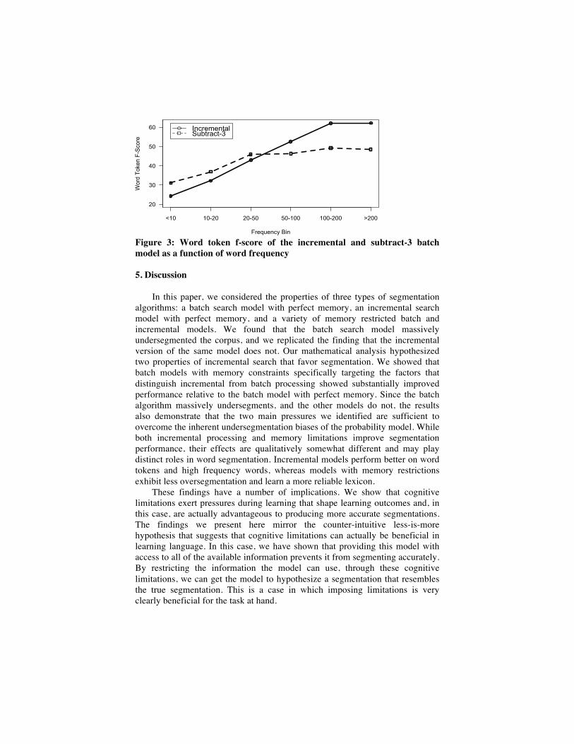
Figure 3: Word token f-score of the incremental and subtract-3 batch model as a function of word frequency 5. Discussion

In this paper, we considered the properties of three types of segmentation algorithms: a batch search model with perfect memory, an incremental search model with perfect memory, and a variety of memory restricted batch and incremental models. We found that the batch search model massively undersegmented the corpus, and we replicated the finding that the incremental version of the same model does not. Our mathematical analysis hypothesized two properties of incremental search that favor segmentation. We showed that batch models with memory constraints specifically targeting the factors that distinguish incremental from batch processing showed substantially improved performance relative to the batch model with perfect memory. Since the batch algorithm massively undersegments, and the other models do not, the results also demonstrate that the two main pressures we identified are sufficient to overcome the inherent undersegmentation biases of the probability model. While both incremental processing and memory limitations improve segmentation performance, their effects are qualitatively somewhat different and may play distinct roles in word segmentation.  Incremental models perform better on word tokens and high frequency words, whereas models with memory restrictions exhibit less oversegmentation and learn a more reliable lexicon.

These findings have a number of implications. We show that cognitive limitations exert pressures during learning that shape learning outcomes and, in this case, are actually advantageous to producing more accurate segmentations. The findings we present here mirror the counter-intuitive less-is-more hypothesis that suggests that cognitive limitations can actually be beneficial in learning language. In this case, we have shown that providing this model with access to all of the available information prevents it from segmenting accurately. By restricting the information the model can use, through these cognitive limitations, we can get the model to hypothesize a segmentation that resembles the true segmentation. This is a case in which imposing limitations is very clearly beneficial for the task at hand.

<10 10-20 20-50 50-100 100-200 >200

20

30

40

50

60

Frequency Bin

Wor

d To

ken

F-S

core

IncrementalSubtract-3

Although our analyses are just an initial exploration of the role of cognitive limitations in segmentation, we have shown that the implicit learning constraints imposed by search heuristics can be examined and understood. In this particular case, we were able to analyze the difference between the batch and incremental models to explain what factors allowed the incremental model to overcome the inherent bias of the probability model to leave utterances unsegmented. Such analyses help us understand how various cognitive limitations interact with and alter the learning task at hand.

This work, combined with previous findings, also raises questions about the conclusions that can be confidently drawn from an ideal learner perspective that ignores these cognitive limitations. Pearl et al. (2010) showed that conclusions drawn about ideal learners do not necessarily transfer to constrained learners. They showed that while the ideal learner defined by Goldwater et al. (2009) benefitted from modeling word-to-word dependencies, some models with cognitive limitations using the same probability model did not. Our work supports their conclusion that cognitive limitations themselves may play a critical role in language learning, but also shows that it is possible to understand what makes them critical. Further work is needed to understand more fully what learning constraints are imposed by the cognitive limitations themselves, and caution is warranted when drawing conclusions based on ideal learners since, as we have shown, cognitive constraints may fundamentally alter the nature of the learning task. Because we are ultimately trying to model infants, who are constrained learners, understanding the biases of constrained learners, in addition to those of ideal learners, will shed light on the nature of language learning and the various factors that influence this complex process. References Bernstein-Ratner, N. (1987). The phonology of parent-child speech. In K. Nelson & A.

van Kleeck (eds), Children’s language, Volume 6, 159-174. Hillsdale, NJ: Erlbaum. Brent, M. R. (1999). An efficient, probabilistically sound algorithm for segmentation and

word discovery. Machine Learning 34, 71-105. Brent, M. R., & Cartwright, T. A. (1996). Distributional regularity and phonotactic

constraints are useful for segmentation. Cognition 61(1), 93-125. Newport, E. L. (1990). Maturational constraints on language learning. Cognitive science,

14(1), 11-28. Goldwater, S., Griffiths, T. & Johnson, M. (2009). A Bayesian framework for word

segmentation: Exploring the effects of context. Cognition 112(1), 21-54. Pearl, L., Goldwater, S. and Steyvers, M. (2010). Online learning mechanisms for

Bayesian models of word segmentation. Research on Language and Computation 8(2-3), 107-132.

Saffran, J., Aslin, R., & Newport, E. (1996). Statistical learning in 8-month-old infants. Science, 274, 1926-1928.

Venkataraman, A. (2001). A statistical model for word discovery in transcribed speech. Computational Linguistics 27(3), 351-372.