1

Kaleckian Models of Growth and Distribution Revisited: Evaluating their relevance through simulation

Thomas DALLERY∗

University of Lille 1 Summary The past two decades have seen a sharp renewal of interest in the Kaleckian models of growth and distribution. These models have been put to so much use that it made us wonder if this trend was based on their ability to generate macroeconomic equilibrium variables located within a reasonable range of some conceivable economic reality. While the Kaleckians spend much time debating how much their models are wage-led vs. profit-led, our work lies upstream of these questions, for we are investigating the Kaleckian models’ existence properties. We conducted a series of simulations based on a basic, three-equation model: an investment function, a savings function and an equation for the firms’ objectives. By estimating the parameters composing these different functions without recourse to econometrics but by means of an economic diagnostic, and by specifying an assumed range of value for the equilibrium variable, we tested these models’ ability to produce plausible results. We also tested the models’ stability property. Although stability is often put forth as a pre-requisite in the study of such models, in the Kaleckian literature the question of how plausible is the stability is rarely raised. Our results suggest that there is a need to reconsider these models, their investment functions and, more particularly, certain of the parameters appearing in these functions. By comparing the relative performance of the models in terms of stability and plausibility, we are able to establish an interesting property: the most plausible models are unstable.

∗ CLERSE - University of Lille 1 email: thomas.dallery@ed.univ-lille1.fr

2

I - Introduction This paper is concerned with some recent, proliferating developments in connection with Kaleckian growth models. Over the last 20 years, numerous post-Keynesians have gone back to these models with renewed enthusiasm. This increased interest does not seem to be restricted to just the post-Keynesian school but figures into a more widespread movement towards rediscovering models of long-term growth within the field of economics.

It appears to us that the Kaleckians pay insufficient attention to the existence and stability conditions of their models, preferring especially to investigate the dynamics of growth – to see whether it is wage-led or profit-led. We leave to others the task of studying the various downstream properties of these models and concern ourselves only with the upstream plausibility of existence conditions. Our goal here is not to propose a new version of what some call the neo-Kaleckian models of growth, but rather to make a critical assessment of their relevance. By critical assessment, we do not mean making an evaluation of the causality illustrated by these models; we mean comparing, on the one hand, the values obtained through simulation for the long-term macroeconomic variables used in these models with, on the other, the values to be expected a priori for these same macroeconomic variables in a conceivable real economy. This is one way to align these models with their predictions and thus check their relevance. The relevance we are evaluating is not an empirical relevance, in the econometric sense; rather, we are talking about relevance a priori or ex ante which sets the models against the yardstick of a range of values that one can accept without departing from historical reality. We are running a check meant to find out if Kaleckian modeling is capable of describing economic reality -- not necessarily reality as it is but reality as it may be imagined, within a plausible range of values. We conduct plausibility checks that consist of determining to what extent the macroeconomic variables coming out of these models lie within these acceptable ranges of value. The profusion of publications in the field of Kaleckian macroeconomics can be partly explained by the malleability of this form of modeling, allowing the quick and easy inclusion of various topics. We ask in this paper whether Kaleckian modeling can also be justified by its qualities of relevance. To do so, we have studied different forms of the more widely used Kaleckian models. We also propose some variants of our own, dealing more particularly with the financialization of the economy. Beyond simple evaluation in terms of plausibility, we also analyze the question of these models’ stability. At issue is an old debate which it seems possible to push forward somewhat, given the results obtained here. To summarize our work, we question the plausibility of the Kaleckian models and also question the plausibility of the stability conditions they posit. These are the two investigations that lead to reconsider the attractiveness of models which on the one hand, strive to describe a conceivable capitalist economy and on the other, fail to observe the stability condition they set up as a prerequisite for any macroeconomic analysis.

The paper consists of five parts. Part One will focus on these Kaleckian growth models and highlight the principles upon which they work. Part Two will detail the methodology adopted for assessing the relevance of these models. Part Three will lay out the results of this inquiry with respect to plausibility. It seems that Kaleckian models of growth are somewhat lacking in this regard. Few of them manage to generate a satisfactory number of variants that might describe a plausible reality. In Part Four we will re-examine the stability question. In particular, we can state that the best-performing models in terms of plausibility are unstable.

3

Their persistent instability raises some questions, to which we will attempt to supply some answers. Finally, the last part will serve as our conclusion. II – Post-Keynesian models of growth and distribution The earliest post-Keynesian growth models were worked out for the purpose of extending Keynes’ General Theory1 to the long term. What Keynes pointed out for the short term needed to be confirmed for the long term. Though Keynes felt a certain disdain for the relatively long view of things2, it still remains true that a study of the long term in a Keynesian framework was necessary, in order to put up a complete alternative to traditional orthodoxy, which was always so quick to resort to the long term to combat Keynesian ideas. Before getting into our simulation, it might be appropriate to give an example of the models we will be testing later. So we shall examine in detail the architecture common to all Kaleckian models of growth and distribution. For that, we will rely on the presentations by Lavoie and Blecker in particular.3 The equilibrium is built in two steps. In the first step one has to bring out the effective demand constraint by equalizing savings and investment. It is specifically a matter of providing the profit rate experienced by firms; that is, the profit rate resulting from effective demand. In the second step, in order to obtain equilibrium, one equalizes the firms’ pricing behavior equation (objective) with the expression of the endogenous variable resulting from reports on the current period (or effective demand constraint), so that what is reported about firms matches up with their objective. In a less verbal fashion and by using functions currently in use4 we present below an adaptation of this reasoning for a concrete example of Kaleckian modeling:

(1) gs = s.r (2) rco = π.u / v

(3) gi = γ0 + γu.u + γr.r

where gs denotes the savings behavior of firms, s the propensity to save from profits5, r the rate of profit, rco the corporate objectives in terms of profit rate, π the profit share in value added, v the capital technical coefficient, u the capacity utilization rate, gi the growth rate of capital stock, γ0 an “autonomous” component of investment, γu the accelerator coefficient and γr the sensitivity of investment to the rate of profit.

We now discover the three pillars of the Kaleckian models: a savings function, an investment function and a firms’ objectives function6. We present here the three pillars while some

1 Cf. Keynes (1936). 2 No need to dwell here on the famous Keynesian utterance: “In the long run, we are all dead.” 3 Cf. Lavoie (1992: pp. 282-371, 2004) and Blecker (2002). 4 Cf. Rowthorn (1981), Lavoie (1995), Blecker (1989) and (2002), Missaglia (2007) among others. 5 Assuming that there is no savings from wages; 6 The firms’ objectives equation derives from a firms’ pricing behavior. Here it comes down to price-setting by the mark-up method. See below for a more detailed review of firms’ objectives equation.

4

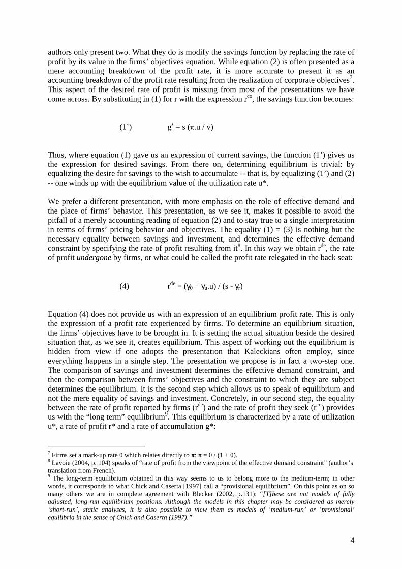
authors only present two. What they do is modify the savings function by replacing the rate of profit by its value in the firms’ objectives equation. While equation (2) is often presented as a mere accounting breakdown of the profit rate, it is more accurate to present it as an accounting breakdown of the profit rate resulting from the realization of corporate objectives7. This aspect of the desired rate of profit is missing from most of the presentations we have come across. By substituting in (1) for r with the expression rco, the savings function becomes: (1’) gs = s (π.u / v) Thus, where equation (1) gave us an expression of current savings, the function (1’) gives us the expression for desired savings. From there on, determining equilibrium is trivial: by equalizing the desire for savings to the wish to accumulate -- that is, by equalizing (1’) and (2) -- one winds up with the equilibrium value of the utilization rate u*. We prefer a different presentation, with more emphasis on the role of effective demand and the place of firms’ behavior. This presentation, as we see it, makes it possible to avoid the pitfall of a merely accounting reading of equation (2) and to stay true to a single interpretation in terms of firms’ pricing behavior and objectives. The equality (1) = (3) is nothing but the necessary equality between savings and investment, and determines the effective demand constraint by specifying the rate of profit resulting from it8. In this way we obtain rde, the rate of profit undergone by firms, or what could be called the profit rate relegated in the back seat: (4) rde = (γ0 + γu.u) / (s - γr) Equation (4) does not provide us with an expression of an equilibrium profit rate. This is only the expression of a profit rate experienced by firms. To determine an equilibrium situation, the firms’ objectives have to be brought in. It is setting the actual situation beside the desired situation that, as we see it, creates equilibrium. This aspect of working out the equilibrium is hidden from view if one adopts the presentation that Kaleckians often employ, since everything happens in a single step. The presentation we propose is in fact a two-step one. The comparison of savings and investment determines the effective demand constraint, and then the comparison between firms’ objectives and the constraint to which they are subject determines the equilibrium. It is the second step which allows us to speak of equilibrium and not the mere equality of savings and investment. Concretely, in our second step, the equality between the rate of profit reported by firms (rde) and the rate of profit they seek (rco) provides us with the “long term” equilibrium9. This equilibrium is characterized by a rate of utilization u*, a rate of profit r* and a rate of accumulation g*: 7 Firms set a mark-up rate θ which relates directly to π: π = θ / (1 + θ). 8 Lavoie (2004, p. 104) speaks of “rate of profit from the viewpoint of the effective demand constraint” (author’s translation from French). 9 The long-term equilibrium obtained in this way seems to us to belong more to the medium-term; in other words, it corresponds to what Chick and Caserta [1997] call a “provisional equilibrium”. On this point as on so many others we are in complete agreement with Blecker (2002, p.131): “[T]hese are not models of fully adjusted, long-run equilibrium positions. Although the models in this chapter may be considered as merely ‘short-run’, static analyses, it is also possible to view them as models of ‘medium-run’ or ‘provisional’ equilibria in the sense of Chick and Caserta (1997).”

5

(5) u* = γ0 / [(s - γr)(π/v) - γu] (6) r* = π.u* / v = γ0 / [(s - γr) - γu(v/π)] (7) g* = s.r* = s.γ0 / [(s - γr) - γu(v/π)]

At this point, Kaleckians state the equilibrium’s existence conditions. Quite obviously the equilibrium variables need to be positive, and so the numerator and denominator have to have the same sign. This is generally the only plausibility condition to be found in the literature. The stability conditions of these models, on the other hand, are mentioned almost routinely, even if they are never discussed in terms of their plausibility. Stability will be guaranteed if the reaction of savings to a variation in an endogenous variable is greater than the reaction of investment to a change in this same variable. The presentation that we have just made for a variant of the Kaleckian models of growth and distribution makes it easier to conceive the attraction this form of modeling might hold. Indeed, the structure of the model is relatively simple. You only have to specify one more or less Kaldorian savings function, one method for price setting and, lastly, one investment function that shows a good deal of flexibility. Such modeling therefore makes it possible to incorporate a whole series of different issues and to do so extremely quickly: a single change to the investment function will highlight this or that desired condition. The interpretations such models permit can be readily illustrated from the equilibrium variables. Depending on whether you are interested, for example, in the consequences of interest rate movements (Hein [2006]) or the importance of different socio-economic classes for growth and distribution (Lavoie [2006]), it will be possible to change the elements in the basic Kaleckian model without calling its structure into question. III – Simulation methodology In Part Three we shall present the procedure by which we compared the post-Keynesian models of growth with conceivable economic data. Our investigation consisted of determining to what extent the post-Keynesian macroeconomic models provide plausible or relevant results in light of common expectations. Our task was to check whether or not the conclusions of these models conform to some degree of realism. We conducted simulations by multiplying the numerical applications on the basis of what one might call a properly weighted economic diagnostic. As economists we felt free to attribute definite values to certain parameters appearing in the models tested. Depending on what these parameters represent, we are able to determine their value or give an interval10 within which their value can be reasonably ascribed. The parameters of each model were calibrated in this manner. Following such calibration, we calculated the values of the endogenous variables at equilibrium. Our endogenous variables here will always be the same: the rate of utilization of productive capacity (u*), the rate of profit (r*) and the rate of accumulation (g*). If one is an economist, a minimum of situational sense and familiarity with ranges of value will enable one to locate each of these variables in a certain plausibility interval11. For an economy to be conceivable it must have values for these variables that will lie within these plausibility 10 This interval might be called, for lack of a better term, the judgment interval. We are not talking about a confidence interval in the statistical sense (no statistical process was used) but one arrived at from expert economic judgment. 11 Here we mean a plausibility interval to denote the range of plausible values for our equilibrium variables.

6

intervals. We have adopted a definition of plausibility for u* such that, to be called plausible, a variant of the model should wind up with a utilization rate at equilibrium of between 60% and 120%. The values observed in our economies generally show a utilization rate in the neighborhood of 85-90%. We tolerated significant departure from this value in order to accept divergences attributable to the modeling and the “coarseness” of value ranges. Likewise, we posit that a plausible rate of profit lies between 5% and 30%12 and that a plausible rate of accumulation13 runs between 5% and 20%. We do not re-present each time the structure of the Kaleckian model under study. It suffices to refer back to what was said in the previous section. In the rest of this article we use the Kaleckian structure by testing eight different investment functions as well as two different price equations. But we always keep the same savings function. This means we will be testing 16 different models. Each time we determine the effective demand constraint represented by the realized profit (rde) equation, which we get by equating the different gi and the expression of gs. Then we reconcile these realized profit equations with the two possible equations that include firms’ objectives in terms of profit rate (rco). If the rate of profit seen in the market is equal to the rate of profit accepted by firms, we are definitely in a situation of voluntary, “stable”14 behavior, one which embodies medium-term equilibrium as we have defined it. The equilibrium values of variables are determined one after another: first, one obtains the value of the long-term utilization rate (u*), then that of the profit rate (r*) and then, finally, that of the accumulation rate (g*): (8) gi = gs ⇒ rde

(9) rde = rco ⇒ u* (10) rco(u*) ⇒ r* (11) gs(r*) ⇒ g*

It is at this point that the plausibility of the model becomes of interest. However, for our study’s purposes, we opted to evaluate only the plausibility of the utilization rate, considering that if u* is plausible, then r* and g* will be also, for parameter values falling in our judgment interval. Plausibility as we evaluate it is measured by whether or not a model’s equilibrium rate of utilization is included in our plausibility interval. Thus a model will be said to be plausible if its equilibrium rate of utilization lies between 60% and 120%. We tested eight investment functions, once with a mark-up pricing model and again with a target-return pricing model. In total we will have 16 different models tested for their plausibility; i.e., for their ability to generate a rate of utilization in a relevant interval. With each of these models we set up judgment intervals for all the parameters; that is, the confidence values between which we might reasonably think, as economists, each parameter will lie. For each parameter, we then divided the judgment interval into ten equal parts, so that

12 Hein and Krämer (1997, p. 20) report the rate of profit in France averaged 15.1% between 1984 and 1983 and 13.9% in Germany between 1983 and 1993. Aglietta (2006, p. 9) puts the rate of profit in France at 9.9% in 1982 as against 14.8% in 1997, and at 10.2% and 15% in Germany for the same years. 13 The rate of accumulation is not identical here to the rate of growth, as it involves the gross rate of accumulation, which therefore includes the replacement of obsolete capital in addition to increases to the capital stock. It is the ratio of gross investment to capital stock (I/K), which historically runs about 10%. 14 The stability spoken of here is behavioral stability and not the stability of the model. Behavior is said to be stable to the extent that it has no reason to change, all else being equal.

7

we measured eleven values for that parameter. Then, for all possible combinations of parameter values, we tested the plausibility of the utilization rate obtained by solving the model for each of these variants.15

The two expressions of the profit rate equation seen from the supply side are different, depending on whether firms are assumed to set their prices with the mark-up or the target-return pricing method. We have already mentioned with equation (2) the expression of the behavior of the mark-up firms:

(2) rco = π.u / v Here firms are supposed to determine their prices by setting up a mark-up on their costs. This is a strong, long-term decision. Then, they produce as much as market could absorb at these prices. Firms target a mark-up rate θ, to which corresponds for the theorician a profit share in value added. The above equation means that firms are willing to accept a profit rate rco, provided this share of profits and their ability to sell their products for given technical conditions. The parameters π and v have to be evaluated by a judgment interval. With respect to the profit share in value added (π), one can rather safely put that in the neighborhood of 30%. History shows that the distribution of value added between profits and wages experienced a pronounced change during the 1980s. Whereas this share of profits had previously been affected by an “overly” generous distribution to wage earners during the Golden Age of capitalism16, the advent of financialized capitalism profoundly changed the distribution of wealth. Numerous studies17 show that the share of profits in value added went from about 25% for the years before financialization, to something more like 35% during recent years18. For purposes of our simulations we used an average value of 30%19. For the judgment interval of the technical coefficient of capital v, the values will run from 1.8 to 2.2. This parameter appears to hover around 220 rather than 4 as Keynes thought in his era without the accounting and statistical tools available today. The target-return pricing method implies a firms’ behavior equation different from the one we have just seen. The mark-up is determined by firms, so that the normal utilization of capacity provides them a target rate of return: (12) rco = u.rs / us

15 A variant is therefore a version of the model representing a possible combination of values for each parameter. Each variant gives rise to equilibrium values for u*, r* and g*. 16 This expression stands for the 30-year post-WWII boom. See Marglin and Schor (1990) for a description. 17 Cf. for example Askénazy (2003) or Artus and Cohen (1997). 18 According to Plihon (2004, p. 53), in the European Union 15, the share of wages in the value added went from 74.6% on average over the 1971-1980 period to 68.4% in 2001-2002. It goes without saying that this decline in the share of wages is the accounting reflection of the increase in the share of profits. 19 Along with the 25% and 35% values, assuming an economy is or is not financialized. 20 The capital coefficient is relatively hard to estimate. It is assumed that it is about 2, a figure that can be arrived at by proceeding to an accounting breakdown of the capital coefficient. v ≡ K / Y = (K / I) x (I / Y). Now, (I/K) and (I/Y) are better understood: the first ratio is about 0.1 as previously mentioned and the second about 0.2. All in all it does seem that v is around 2.

8

where rs and us represent, respectively, the standard profit rate and standard utilization rate.

We propose a value for the target utilization rate of around 85%. This constant under-utilization of production capacity is perfectly explainable from a post-Keynesian perspective. One might argue, for example, that firms, even for the long-term, are faced with uncertainty. The standard rate of profit is intimately connected to assumptions about financialization. Absent a financialized environment, it seems the standard rate of profit can be put at about 10%. The target rate of profit that managers set for themselves when relatively free from shareholder interference does not exceed this reasonable rate that has been historically observed. Financialized capitalism is characterized by greater profitability requirements and by a higher target rate of profit. Here we shall use a value of 20%, taking into account this greater pressure from shareholders for profitability21. After this description of the two firms’ pricing behavior functions, we now have to study the different investment functions used and state for each one the judgment intervals for the parameters related to them. Financialization, through the increasing interference of shareholders in corporate governance, enhances the rs variable in our investment functions. This, in our eyes, makes it ideally possible to factor in changes brought on by greater shareholder involvement in the broad decision-making processes of our economy. In addition to constructing these investment functions, we have adopted basic forms of post-Keynesian growth models22. The first of them can be found in Lavoie (2004)23, but also in the pages of Marxist authors like Duménil and Lévy (1999), and it gives rise to the model hereinafter called Model A:

(13) gi = γ0 + γu(u - us)

where gi is the rate of growth of the capital stock, γ0 represents the underlying rate of investment growth, and γu is the parameter for the speed of adjustment by firms to a difference between their effective utilization rate and their target rate.

If firms are at their target rate of production capacity utilization (u = us), they will only increase capacity strictly to the extent of an anticipated increase in demand for their product, to which increase must be added replenishments of outworn and outmoded capital stock, etc. From combining these two components of underlying investment growth, one can deduce that the judgment interval for parameter γ0 will center around 10%24 and that its limits will be 6% and 14%. To grasp what value γu has, one need to examine the meaning of this parameter. It refers to the annual adjustment of production capacity when a gap arises between the effective and target

21 This increase in pressure from shareholders can be seen in the upward trend in the return on equity ratio (ROE), which measures the financial profitability of firms and indirectly it serves to measure the required global profitability. Plihon (2002, p. 88): “From the beginning of the 1950s until the first oil shock, ROE was somewhere between 10% and 12%; [...] during the 90s it grew [...] reaching 15% to 20% on average.” (author’s translation from French). 22 Most of these investment functions appear in Lavoie (1996, p. 118). 23 A presentation which itself came from an earlier formulation by Amadeo (1986). 24 The underlying investment growth can be approached by the historical growth of investment and the (I/K) ratio already mentioned; this then gives an average of 10% for γ0.

9

utilization rates. Firms hemmed in by uncertainty on all sides react gradually and only re-adjust in small measure to capacity underage and overage. To venture that firms fill in about 20% to 50% of their shortfalls per year seems a realistic assumption. The work we have just done concerning Model A, we also did it for each of the models studied. In particular, we did it for the Model B already discussed in Part One. This model can be specifically found in Lavoie (2002), who presents a very conventional form of the investment function. The initial assumption is relatively intuitive: investment varies directly with the utilization rate (representing the forces of demand) and the profit rate25:

(3) gi = γ0 + γu.u + γr.r In light of these considerations, it is easier to set the judgment intervals for these parameters. The γ0 represents an “autonomous” component of investment. It refers to investment outlays independent of the utilization rate or the profitability of investment projects. It will go up and down at the whim of entrepreneurs, but one can reasonably put it over the long term at an average of between 3% and 7%. And γu will lie between 0 and 2%26. So we grant an accelerator effect of just zero. And γr will see a range of values fluctuating between 0.2 and 0.6. This means that 1 percent more in the rate of profit will entail an increase in investment of from 0.2% to 0.6%. Following the publication of Bhaduri and Marglin’s article (1990), a controversy arose as to the choice of factors to be included in investment functions. Bhaduri and Marglin stated that it is not the rate of profit (r), but the share of profits in value added (π) which must be included in investment functions27. Thereafter many post-Keynesians28 performed the substitution sought by Bhaduri and Marglin (Model C): (14) gi = γ0 + γu.u + γπ.π For the plausibility intervals chosen for these parameters, as well as for those in the subsequent models, the reader is referred to Tables 1 and 2, as the reasoning behind them was already laid out for Models A and B. In addition to these more recent models, we also tested more traditional investment functions, descending directly from those used by Robinson and Kalecki themselves in their growth model. But here we have brought their investment function into the structure of post-Keynesian growth models. To present the Robinson version (Model D), we make use of this investment function:

25 It being understood that the profit rate is an incentive to invest, from the simple fact that profit is a source of financing of future investments and that the profit rate can be seen as an approximation of the return on these same future projects. 26 For his simulations, Van Treeck (2007b) uses a γu value of 1.5% and a γr value of 0.4. 27 We will not go into the opportunity that such a change represents. For a critical presentation, see Lavoie (1995, p. 797 & ff.) 28 In particular Van Treeck (2007a) and also Hein and Krämer (1997).

10

(15) gi = γ0 + γr.r

To stick as closely as possible to the Robinson tradition, it needs to be said that the rate of profit in equation (15) is in fact the anticipated rate of profit. But for the theoretical context that interests us, it is possible to state that this anticipated rate of profit is strongly correlated with the current rate of profit, because of repeated periods over the long term. Entrepreneurs, in the fog of daily business and their uncertain environment, tend to take past rates of profit as an approximation of future rates of profit. Accordingly, to present the Kaleckian29 version (model E), we will use:

(16) gi = γ0 + γu.u In order to study the impact of financialization within the post-Keynesian models of growth and distribution30, we created several investment functions which try to factor in the recessive effects on accumulation of heavier shareholder demands in terms of profit rate. So we will briefly present these three investment functions largely based on the versions detailed before. Model F1 develops the first form of the “financialized” investment function:

(17) gi = γ0 + γu.u + γr(r – rs) where γ0 represents an “autonomous” component of investment, γu the accelerator effect and γr takes account of an investment profitability effect affected by the comparison between the effective profit rate (r) and the standard profit rate required on account of financialization (rs).

This investment function tries both to take into account a traditional Keynesian effect of the utilization rate on investment dynamics and also to introduce financialization, by means of the variable rs. The meaning of this function is that there is such a thing as a profitability effect on investment but only above some standard of profitability, which acts as a “hurdle rate” on any investment project. In other words, we are formalizing the selectivity of investment projects. The second form of these investment functions (Model F2) is a slight modification of the function used in Model A:

(18a) gi = γ0 + γu(u - us) – τ.rs where τ directly introduces the depressive effect of a profitability standard (rs) on accumulation.

If the previous notation of the investment function has the merit of stressing the legacy of Lavoie or Amadeo, it does falsify the interpretation of various parameters. It would indeed be more accurate to rewrite it in the following form:

29 Lavoie (1996, p. 118) prefers to see this investment function as a Steindlian one rather than a Kaleckian one. 30 Hein and Van Treeck (2007), Van Treeck (2007a) and (2007b) or Skott and Ryoo (2007) also incorporate financialization into Kaleckian models.

11

(18b) gi = (γ0 – τ.rs) + γu(u - us) This shows more clearly that it is in fact all the terms in the first parenthesis which describe the animal spirits of entrepreneurs. These animal spirits are constrained by the shareholders’ demands of profitability. In our simulation we opted for a calibration “connecting” γ0 and τrs

in order to emphasize that at issue is one behavior described by several parameters and that therefore it is the function (γ0 – τ.rs) that needs to be given a judgment interval. We slightly changed the values for γ0

31and took values for τ of between 0.1 and 0.5. Thus, by combining these judgment intervals with the rs values, we wind up with results that boast good empirical performance, staying close to various accumulation rates. If rs is zero (no standard profitability requirements), then the gross rate of accumulation will be close to 20%, with optimistic animal spirits. If rs is equal to 20%, then you have a gross rate of accumulation of around 6%, with pessimistic animal spirits. On the one side you have the Chinese boom; on the other, soft growth with even the possibility of net disaccumulation. The third function used (Model F3) combines in a single function two functions already seen:

(19) gi = (γ0 – τ.rs) + γu.u

So this function is similar to the one before but introduces an accelerator effect on the utilization rate that does not depend on the normal utilization rate. The judgment interval for γu is therefore the same one it had in Model B. We have just presented all the specifications used in each of the three fundamental equations of the Kaleckian model (gi, gs and rco), as well as the estimation-related significance of each parameter making up these different equations. Now we are ready to examine our simulations and their results in detail. IV – Models lacking in plausibility Our investigation now bears on the comparison between what we obtain as equilibrium values for these models and what we know to be the plausible equilibrium values for these variables. If the simulated values of the equilibrium variables are in the range of what we know to be plausible values, all is well, and the post-Keynesian models of growth come out stronger from this evaluation. But if on the contrary, the simulated values of the equilibrium variables do not fall within the limits of plausibility, we then have a vexing problem on our hands. Indeed, if we start off with plausible values for the parameters used in the different variants of the models tested and do not obtain plausible equilibrium values, then either we have stated poorly the plausibility of the value of our parameters at the outset, or we misjudged the plausibility of the equilibrium values of the variables, or we are forced to accept that the construction of post-Keynesian models is flawed. Before having to decide this thorny question, it is necessary to look at the results obtained by the simulations performed.

31 We used values of 0.08 to 0.2, as opposed to 0.06 to 0.14 previously for model A.

12

The whole of the results is summarized in a few tables. Table 1 records the plausibility scores for all the models when firms set their prices based on the mark-up method. Table 2 is the equivalent of Table 1 for when firms set their prices based on the target return pricing method. These two tables deal with the models’ plausibility in a non-financialized economy, in the sense that the rate of profit required is “only” 10% (or the profit share in value added is only 25%)32. Financialization is introduced by a meaningful increase in these two parameters: an economy shall be considered as financialized if its required rate of profit reaches 20% or if the profit share in value added reaches 35%. Using a required rate of profit calls for what others before us have called a standard of financial profitability33. Financialization is then seen from the viewpoint of bigger shareholder appetites, manifestly shifting firms’ orientation with respect to their investment and profit distribution policies34. Using the share of profit in value added as an indicator of financialization aims instead at bringing out redistributive aspects observable over history: the underlying growth of this indicator that has gone along with the emergence of financial markets and a new institutional environment. We remind the reader that the criterion of plausibility adopted to gauge the performance of the different models is that the equilibrium utilization rate must be included between 60% and 120%. These are extremely broad limits; and the broader the evaluation criterion, the less tolerant we must be with the scores of the different models. As all the models tested do not refer to the same equations, they do not all have the same number of parameters. The number of variants tested is thus different from one model to the next, depending on the number of parameters that needed to be evaluated within the judgment intervals. Additionally, we did not take judgment intervals for each of the parameters, since some of them have a relatively certain value35.

Table 1: Plausibility results for the mark-up pricing models

gi Fixed variables

Evaluated variables

Number of variants u* Plausibility

%

Model A γ0 + γu(u - us)

s = 0.5 us = 0.85 v = 2 π1 = 0.25 π2 = 0.35

γ0 = [0.06 ; 0.14] γu = [0.2 ; 0.5]

112 = 121 (γ0 - γu.us) / [(s.π/v) - γu]

76.03% (π1 = 0.25)

86.78%

(π2 = 0.35)

Model B γ0 + γu.u + γr.r

s = 0.5 v = 2 π1 = 0.25 π2 = 0.35

γ0 = [0.03 ; 0.07] γu = [0 ; 0.02] γr = [0.2 ; 0.6]

113 = 1,331 γ0 / [(s - γr)(π/v) - γu]

2.03% (π1 = 0.25)

9.62%

(π2 = 0.35)

32 Financialization is introduced by the required rate of profit (rs) or by the profit share of value-added (π), depending which variable is present in the model under consideration. We prefer to use rs as the signifier for financialization; but when it is absent from the model, as in most of the mark-up models, we use a measure of π. 33 Cf. Boyer (2000), Plihon (2002), Aglietta and Rebérioux (2004). 34 Going from a policy of “retain and invest” to one of “downsize and distribute”. Cf. Lazonick and O’Sullivan (2000). 35 This is so for the propensity to save profits (0.5) or the normal utilization rate (85%). Bowles et Boyer (1995, p. 154) estimate a value of 0.5 for the difference between the propensity to save profits and the propensity to save wages, which here is zero.

13

Model C γ0 + γu.u + γπ.π

s = 0.5 v = 2 π1 = 0.25 π2 = 0.35

γ0 = [0.03 ; 0.07] γu = [0 ; 0.02] γπ = [0 ; 0.2]

113 = 1,331 (γ0 + γπ.π)/ (s.π/v - γu)

29% (π1 = 0.25)

52.9%

(π2 = 0.35)

Model D γ0 + γr.r

s = 0.5 v = 2 π1 = 0.25 π2 = 0.35

γ0 = [0.04 ; 0.08] γr = [0.2 ; 0.6]

112 = 121 γ0 / [(s - γr)(π/v)]

1.65% (π1 = 0.25)

9.91%

(π2 = 0.35)

Model E γ0 + γu.u

s = 0.5 v = 2 π1 = 0.25 π2 = 0.35

γ0 = [0.06 ; 0.1] γu = [0 ; 0.02]

112 = 121 γ0 / (s.π/v - γu)

14.05% (π1 = 0.25)

79.34%

(π2 = 0.35)

Model F1 γ0 + γu.u + γr(r - rs)

s = 0.5 π = 0.3 v = 2 rs1 = 0.1 rs2 = 0.2

γ0 = [0.06 ; 0.1] γr = [0 ; 0.2] γu = [0 ; 0.02]

113 = 1,331 (γ0 - γr.rs) / [(s - γr)(π/v) - γu]

28.02% (rs1 = 0.1)

48.16%

(rs2 = 0.2)

Model F2 (γ0 - τ.rs) + γu(u - us)

s = 0.5 π = 0.3 v = 2 us = 0.85 rs1 = 0.1 rs2 = 0.2

γ0 = [0.08 ; 0.2] τ = [0.1 ; 0.5] γu = [0.2 ; 0.5]

112 = 121 (γ0 - τ.rs - γu.us) / [(s.π/v) - γu]

71.9% (rs1 = 0.1)

98.3%

(rs2 = 0.2)

Model F3 (γ0 - τ.rs) + γu.u

s = 0.5 π = 0.3 v = 2 rs1 = 0.1 rs2 = 0.2

γ0 = [0.08 ; 0.2] τ = [0.1 ; 0.5] γu = [0 ; 0.02]

112 = 121 (γ0 - τ.rs) / [(s.π/v) - γu]

13.22% (rs1 = 0.1)

45.45%

(rs2 = 0.2)

Table 2: Plausibility results for target-return pricing models

gi Fixed variables

Evaluated variables

Number of variants u* Plausibility

%

Model A γ0 + γu(u - us)

s = 0.5 us = 0.85 rs1 = 0.1 rs2 = 0.2

γ0 = [0.06 ; 0.14] γu = [0.2 ; 0.5]

112 = 121 (γ0 - γu.us) / [(s.rs/us) - γu]

72.73% (rs1 = 0.1)

92.56%

(rs2 = 0.2)

Model B γ0 + γu.u + γr.r

s = 0.5 us = 0.85 rs1 = 0.1 rs2 = 0.2

γ0 = [0.03 ; 0.07] γu = [0 ; 0.02] γr = [0.2 ;0.6]

113 = 1,331 γ0 / [(s - γr)(rs/us) - γu]

1.42% (rs1 = 0.1)

20.51%

(rs2 = 0.2)

Model C γ0 + γu.u + γπ.π

s = 0.5 us = 0.85 π = 0.3 rs1 = 0.1 rs2 = 0.2

γ0 = [0.03 ; 0.07] γu = [0 ;0.02] γπ = [0 ; 0.2]

113 = 1,331 (γ0 + γπ.π)/ (s.rs/us - γu)

19.83% (rs1 = 0.1)

61.46%

(rs2 = 0.2)

14

Model D γ0 + γr.r

s = 0.5 us = 0.85 rs1 = 0.1 rs2 = 0.2

γ0 = [0.04 ; 0.08] γr = [0.2 ; 0.6]

112= 121 γ0 / [(s - γr)(rs/us)]

0.83% (rs1 = 0.1)

23.14%

(rs2 = 0.2)

Model E γ0 + γu.u

s = 0.5 us = 0.85 rs1 = 0.1 rs2 = 0.2

γ0 = [0.06 ; 0.1] γu = [0 ; 0.02]

112 = 121 γ0 / (s.rs/us - γu)

8.26% (rs1 = 0.1)

85.12%

(rs2 = 0.2)

Model F1 γ0 + γu.u + γr(r - rs)

s = 0.5 us = 0.85 rs1 = 0.1 rs2 = 0.2

γ0 = [0.06 ; 0.1] γr = [0 ; 0.2] γu = [0 ; 0.02]

113 = 1,331 (γ0 - γr.rs) / [(s - γr)(rs/us) - γu]

4.36% (rs1 = 0.1)

71.52%

(rs2 = 0.2)

Model F2 (γ0 - τ.rs) + γu(u - us)

s = 0.5 us = 0.85 rs1 = 0.1 rs2 = 0.2

γ0 = [0.08 ; 0.2] τ = [0.1 ; 0.5] γu = [0.2 ; 0.5]

112= 121 (γ0 - τ.rs - γu.us) / [(s.rs/us) - γu]

62.81% (rs1 = 0.1)

96.69%

(rs2 = 0.2)

Model F3 (γ0 - τ.rs) + γu.u

s = 0.5 us = 0.85 rs1 = 0.1 rs2 = 0.2

γ0 = [0.08 ; 0.2] τ = [0.1 ; 0.5] γu = [0 ; 0.02]

112= 121 (γ0 - τ.rs) / [(s.rs/us) - γu]

0.82% (rs1 = 0.1)

85.12%

(rs2 = 0.2)

What conclusions can be drawn from these results in terms of plausibility? For a start, it is noteworthy that performance was very unequal from one model to another and also very unequal depending whether the frame of reference was to a so-called financialized economy or not. As far as non-financialized economies are concerned, the performances were by and large mediocre. Granted, Models A and F2 did get scores over 60%; but all the others scored a plausibility of less than 30% and did so whatever the price-setting method. It seems hard to defend being satisfied with such a low level of a priori relevance, when less than one numerical application in three conformed to a range of values that might describe some conceivable reality. The Kaleckian models do not succeed in portraying any reality possible for a non-financialized economy. It is a serious failure of relevance whenever one presumes to give new depth to history and move economic features around in time. As financialization is but an extremely recent phase of capitalism, the Kaleckian models ought to be capable of reflecting non-financialized economies. Furthermore, once financialization is incorporated, it becomes apparent that plausibility increases spectacularly for every model. When a large difference appears between the plausibility percentages of rs1 and rs2 (or π1 and π2), this proves that the models in question are not robust, in the sense that they are too sensitive to parametric variances. Target-return model F3 makes a very telling example in this respect: while merely 0.82% of its variants are plausible in a non-financialized economy, plausibility climbs to 85.12% when financialization is included! If certain models present very satisfactory plausibility percentages, most of them are sorely lacking, since with mark-up models B, C, D, F1 and F3 and target-return models B, C and D, less than two-thirds of their variants are plausible, including those in a financialized economy. Should we conclude from this that Kaleckian models are relatively well-suited to describe financialized economies, whereas they are profoundly incapable on the whole of describing economies whose operation is not governed by finance? Instead of that, it seems to us the necessary conclusion is that Kaleckian models are only capable of describing conceivable economies for very specific parameter

15

values. In that sense, we have also experienced the fragility of plausible results by making marginal changes to the values of certain parameters. If you slightly move the limits of the judgment interval of γ0, the assessment of the models’ plausibility starts to change36. Beyond the observation about the sensitivity of plausibility tests to the marginal variance of parameters, this suggests that where the parameter γ0 is concerned, the theory of growth stemming from these models is in part tautological: growth comes from growth. In other words, the dependence on the part of this parameter leads one to reconsider the power of these growth models to explain growth. By giving γ0 the leading role in determining equilibrium, these models give us a theory of growth that is quasi-exogenous, since growth is explained by something otherwise unexplained -- except in terms of Keynesian animal spirits or the underlying investment growth or perhaps what is called the “autonomous” component of the investment function. These models are insufficiently explanatory, but it is the fate of Keynesian models to be subject to the erratic nature of investment. The outcome we find here as to the difficulty of formalizing the investment decision is something the Keynesians know all about37. V – A mischievous stability We have just seen that plausibility is not commonplace in Kaleckian models. We have also seen that it was volatile and dependent on the value of a particular parameter. Nevertheless, for those who would cling to the good behavior shown by models A and F2 in terms of plausibility, we propose doing further analysis of Kaleckian models by studying their stability and especially that of these two particular models. To begin with, it seemed to us that the Kaleckian models were developed in order to get rid of Harrod-type instability. This objective, while not explicitly mentioned by the models’ authors, nonetheless remains in our eyes the chief motivation for using this modeling. To be convinced of this all you have to do is look at how urgently the stability condition is put forth in the publications concerned. After attending to the plausibility of the different versions of post-Keynesian models of growth, we now proceed to an examination of their stability. By going in this order, we reverse the chronology followed by post-Keynesian authors. Indeed, as we noted already at the start of this section, post-Keynesian authors clearly put much emphasis on stability. Often it is a preliminary condition for studying their model. We prefer adopting a different order of priorities and not eliminating the possibility of instability in these models. If Kaleckian models are seldom illuminated with numerical applications so as to compare them with a conceivable reality and evaluate their plausibility, there are also very few of them that get tested for the implications of their stability conditions. The principle for one model’s stability condition is the same for all of them: the investment function has to react less strongly to a

36 By taking γ0 from an interval of [0.06 ; 0.14] to an interval of [0.08 ; 0.2] plausibility goes from 76.03% to 38.01% for mark-up model A. 37 Heye (1995, p. 197): “Few economics enterprises are at once as important and as poorly understood as the process of capital investment.” Heye was seeking to explain investment from the state of business confidence, where the animal spirits show themselves. Stockhammer (2004, p. 33) reminds us that certain Keynesians like Shackle and Vickers take it for granted that investment is quite simply unpredictable and that it is impossible to describe its behavior in any “determinable” equation.

16

change in an endogenous variable than does the savings function38. Put another way, the derivative of gi with respect to u* must be less than the derivative of gs with respect to u*, which can be graphically illustrated by the curve for gs crossing below the curve for gi. If the formalized condition of stability is automatically present, verifying that condition numerically is automatically neglected. Now, it turns out that when you apply the parameter values to this condition, the stability condition vanishes, or at least it is no longer so certain. Examination of the most plausible models (A and F2) shows that they are unstable. And conversely, the least plausible models are stable. The results are summarized in Tables 3 and 4. Keep in mind the general definition of the stability condition for each pricing method. In a mark-up method, it is possible to write gs as a function of the utilization rate using equation (1’):

(1’) gs = s.π.u / v The derivative of gs with respect to u flows immediately from equation (1’). Symmetrically, it is possible to write gs as a function of the utilization rate for the models where pricing is set by the target return pricing method. All you have to do is combine equations (1) and (12), and here again, the derivative of gs with respect to u plainly suggests itself. (12’) gs = s.u.rs / us Furthermore, the derivatives of the different investment functions with respect to this same utilization rate all39 arrive at the same parameter γu, even though the latter does not have the same meaning in all models, depending on whether you are dealing with an investment function where γu represents the accelerator effect40, or a parameter for firms’ speed of adjustment to difference between their effective and target utilization rates41. It will not take on the same value, which will quite obviously have significant implications as to the models’ stability property. We have already observed that the models with a “speed adjustment” γu were more plausible than models with an “accelerator effect” γu. But from a stability viewpoint the opposite is true. Indeed, if firms experience an effective utilization rate lower than their target rate (u* < us), they try to slow down their capacity investments so as not to generate too much productive overcapacity. In this way they expect to get back to their target utilization rate, with increases to capacity proceeding at a slower pace than increases in demand. Firms recover their target rate thanks to a demand trend higher than their budgeted production capacity increases. Though this reasoning holds at the micro-economic level, dealing with the macro-economic level is far more puzzling. In fact, by reducing their investment expenditures, firms depress overall demand for their product and thereby also reduce their utilization rate. Whereas firms were aiming at bringing u* close to u, by reducing their investments, the reduction of these investments has a greater effect upon u* and impedes a return to us: the economy goes into a depression. Conversely, if the effective rate is greater

38 Cf. Lavoie (2004, p. 104). 39 With the notable exception of model D, where you need to reason from the endogenous variable r* and not u*. The stability condition is therefore s > γr. 40 At issue are models B, C, E, F1 and F3. 41 At issue are models A and F2.

17

than the target rate, firms will have a tendency to increase their capital expenditures in order to re-establish equality between the effective and the target rate; but by increasing their investment, they feed demand and increase the disequilibrium in the over-utilization of capacity: the economy then experiences an economic boom. Again we have the Harrod instability. Table 3: Stability results for the mark-up models

gi Fixed variables

Evaluated variables

Plausibility %

δgs / δu* = sπ / v

δgi / δu* = γu

Stability (sπ / v >

γu)

Model A γ0 + γu(u - us)

s = 0.5 us = 0.85 v = 2 π1 = 0.25 π2 = 0.35

γ0 = [0.06 ; 0.14] γu = [0.2 ; 0.5]

76.03% (π1 = 0.25)

86.78%

(π2 = 0.35)

0.0625 (π1 = 0.25)

0.0875

(π2 = 0.35)

[0.2 ; 0.5] No

Model B γ0 + γu.u + γr.r

s = 0.5 v = 2 π1 = 0.25 π2 = 0.35

γ0 = [0.03 ; 0.07] γu = [0 ; 0.02] γr = [0.2 ;0.6]

2.03% (π1 = 0.25)

9.62%

(π2 = 0.35)

0.0625 (π1 = 0.25)

0.0875

(π2 = 0.35)

[0 ; 0.02] Yes

Model C γ0 + γu.u + γπ.π

s = 0.5 v = 2 π1 = 0.25 π2 = 0.35

γ0 = [0.03 ; 0.07] γu = [0 ;0.02] γπ = [0 ; 0.2]

29% (π1 = 0.25)

52.9%

(π2 = 0.35)

0.0625 (π1 = 0.25)

0.0875

(π2 = 0.35)

[0 ; 0.02] Yes

Model D γ0 + γr.r

s = 0.5 v = 2 π1 = 0.25 π2 = 0.35

γ0 = [0.04 ; 0.08] γr = [0.2 ; 0.6]

1.65% (π1 = 0.25)

9.91%

(π2 = 0.35)

0.5 [0.2 ; 0.6] Yes/No

Model E γ0 + γu.u

s = 0.5 v = 2 π1 = 0.25 π2 = 0.35

γ0 = [0.06 ; 0.1] γu = [0 ; 0.02]

14.05% (π1 = 0.25)

79.34%

(π2 = 0.35)

0.0625 (π1 = 0.25)

0.0875

(π2 = 0.35)

[0 ; 0.02] Yes

Model F1 γ0 + γu.u + γr(r - rs)

s = 0.5 π = 0.3 v = 2 rs1 = 0.1 rs2 = 0.2

γ0 = [0.06 ; 0.1] γr = [0 ; 0.2] γu = [0 ; 0.02]

28.02% (rs1 = 0.1)

48.16%

(rs2 = 0.2)

0.075 [0 ; 0.02] Yes

Model F2 (γ0 - τ.rs) + γu(u - us)

s = 0.5 π = 0.3 v = 2 us = 0.85 rs1 = 0.1 rs2 = 0.2

γ0 = [0.08 ; 0.2] τ = [0.1 ; 0.5] γu = [0.2 ; 0.5]

71.9% (rs1 = 0.1)

98.3%

(rs2 = 0.2)

0.075 [0.2 ; 0.5] No

Model F3 (γ0 - τ.rs) + γu.u

s = 0.5 π = 0.3 v = 2 rs1 = 0.1 rs2 = 0.2

γ0 = [0.08 ; 0.2] τ = [0.1 ; 0.5] γu = [0 ; 0.02]

13.22% (rs1 = 0.1)

45.45%

(rs2 = 0.2)

0.075 [0 ; 0.02] Yes

18

Table 4: Stability results for target-return pricing models

gi Fixed variables

Evaluated variables

Plausibility %

δgs / δu* = srs / us

δgi / δu* = γu

Stability (srs / us >

γu)

Model A γ0 + γu(u - us)

s = 0.5 us = 0.85 rs1 = 0.1 rs2 = 0.2

γ0 = [0.06 ; 0.14] γu = [0.2 ; 0.5]

72.73% (rs1 = 0.1)

92.56%

(rs2 = 0.2)

0.059 (rs1 = 0.1)

0.118

(rs2 = 0.2)

[0.2 ; 0.5] No

Model B γ0 + γu.u + γr.r

s = 0.5 us = 0.85 rs1 = 0.1 rs2 = 0.2

γ0 = [0.03 ; 0.07] γu = [0 ; 0.02] γr = [0.2 ; 0.6]

1.42% (rs1 = 0.1)

20.51%

(rs2 = 0.2)

0.059 (rs1 = 0.1)

0.118

(rs2 = 0.2)

[0 ; 0.02] Yes

Model C γ0 + γu.u + γπ.π

s = 0.5 us = 0.85 π = 0.3 rs1 = 0.1 rs2 = 0.2

γ0 = [0.03 ; 0.07] γu = [0 ; 0.02] γπ = [0 ; 0.2]

19.83% (rs1 = 0.1)

61.46%

(rs2 = 0.2)

0.059 (rs1 = 0.1)

0.118

(rs2 = 0.2)

[0 ; 0.02] Yes

Model D γ0 + γr.r

s = 0.5 us = 0.85 rs1 = 0.1 rs2 = 0.2

γ0 = [0.04 ; 0.08] γr = [0.2 ; 0.6]

0.83% (rs1 = 0.1)

23.14%

(rs2 = 0.2)

0.5 [0.2 ; 0.6] Yes/No

Model E γ0 + γu.u

s = 0.5 us = 0.85 rs1 = 0.1 rs2 = 0.2

γ0 = [0.06 ; 0.1] γu = [0 ; 0.02]

8.26% (rs1 = 0.1)

85.12%

(rs2 = 0.2)

0.059 (rs1 = 0.1)

0.118

(rs2 = 0.2)

[0 ; 0.02] Yes

Model F1 γ0 + γu.u + γr(r - rs)

s = 0.5 us = 0.85 rs1 = 0.1 rs2 = 0.2

γ0 = [0.06 ; 0.1] γr = [0 ; 0.2] γu = [0 ; 0.02]

4.36% (rs1 = 0.1)

71.52%

(rs2 = 0.2)

0.059 (rs1 = 0.1)

0.118

(rs2 = 0.2)

[0 ; 0.02] Yes

Model F2 (γ0 - τ.rs) + γu(u - us)

s = 0.5 us = 0.85 rs1 = 0.1 rs2 = 0.2

γ0 = [0.08 ; 0.2] τ = [0.1 ; 0.5] γu = [0.2 ; 0.5]

62.81% (rs1 = 0.1)

96.69%

(rs2 = 0.2)

0.059 (rs1 = 0.1)

0.118

(rs2 = 0.2)

[0.2 ; 0.5] No

Model F3 (γ0 - τ.rs) + γu.u

s = 0.5 us = 0.85 rs1 = 0.1 rs2 = 0.2

γ0 = [0.08 ; 0.2] τ = [0.1 ; 0.5] γu = [0 ; 0.02]

0.82% (rs1 = 0.1)

85.12%

(rs2 = 0.2)

0.059 (rs1 = 0.1)

0.118

(rs2 = 0.2)

[0 ; 0.02] Yes

From these tables it appears that models A and F2, which offer the most plausibility, are associated with an instability that is both unavoidable and undesirable. There we have a certain irony bestowed by the history of economic thought, for it was in fact the attempt to eradicate Harrod instability which prompted the development of these new, post-Keynesian models of growth. But it looks like there is no way around that instability. Or else we can just sacrifice plausibility and go ahead modeling what is no longer conceivable reality but quite frankly pure and simple fiction. We propose, instead, a re-evaluation of instability, which

19

ought no longer to be considered as a fatal flaw in a model but, rather, a likely outcome for any attempt at modeling. It is true that this tendency towards instability is not easily observable in reality, but that may be attributed to the existence of regulatory institutions which cushion structural jolts; and the non-existence of instability should not be too hastily inferred from its lack of visibility. More than the elimination of instability as a presumed motive for the development of the literature on new growth models, the insistence with which the stability condition is mentioned for every model does show a special attachment to stability. To find stability in these growth models it is necessary to give up on plausibility. Among the models tested it is necessary in one way or another to choose between stability and plausibility: if you want a stable model, you cease describing conceivable reality; and conversely, if you wish to describe conceivable reality, then you have to accept the instability of the model. VI - Conclusion After presenting the post-Keynesian models of growth and distribution, we did simulations to find out to what extent these models illuminated the actual functioning of capitalist economies as we can imagine them. We think we have shown these models suffer from certain failings. First we demonstrated a general lack of plausibility in the models. We do not deny their presentational, pedagogical value nor the malleability that makes them especially useful for incorporating a whole series of variables. However, we do expect more ex ante relevance from models that are basic to our theoretical representation of the macro-economy. Then we tried to highlight what does seem like a paradox at the heart of the history of these models. Finding instability in models constructed to forefend that very instability was a curious twist. What is called for now is to draw the right conclusions from the twin finding of defective plausibility and persistent instability. But that is not the purpose of this paper, which has sought only to bring to light these two challenges that need to be overcome. Bibliography : AGLIETTA M. (2006): “The future of capitalism”, pp. 9-36, in CORIAT B., PETIT P. and SCHMEDER G. (2006): The Hardship of Nations. Exploring the Paths of modern Capitalism, Edward Elgar, Cheltenham, coll. New Horizons in institutional and evolutionary Economics, 347 p. AGLIETTA M. and REBERIOUX A. (2004): Dérives du Capitalisme financier, Éditions Albin Michel, 394 p. AMADEO E.J. (1986): “Notes on capacity utilisation, distribution and accumulation”, Contributions to Political Economy, vol. 5, pp. 83-94. ARTUS P. and COHEN D. (1997): Partage de la Valeur Ajoutée, Rapport du CAE No.2, La Documentation Française. ASKENAZY P. (2003): “Partage de la valeur ajoutée et rentabilité du capital en France et aux Etats-Unis: une réévaluation”, Économie et Statistique, No.363-364-365, pp. 167-189.

20

BHADURI A. and MARGLIN S. (1990): “Unemployment and the real wage: the economic basis for contesting political ideologies”, Cambridge Journal of Economics, vol. 14, No.4, pp. 375-393. BLECKER R.A. (1989): “International competition, income distribution and economic growth”, Cambridge Journal of Economics, vol. 13, No.3, pp. 395-412. BLECKER R.A. (2002): “Distribution, demand and growth in neo-Kaleckian macro-models”, pp. 129-152, in SETTERFIELD M. (2002): The Economics of Demand-Led Growth, Edward Elgar, 306 p. BOWLES S. and BOYER R. (1995): “Wages, aggregate demand, and employment in an open economy: an empirical investigation”, pp. 143-171, in EPSTEIN G.A. and GINTIS H.M. (1995) Macroeconomic Policy after the conservative Era. Studies in Investment, Saving and Finance, Cambridge University Press, 471 p. BOYER R. (2000): “Is a finance-led growth regime a viable alternative to Fordism? A preliminary analysis”, Economy and Society, vol. 29, No.1, pp. 111-145. CHICK V. and CASERTA M. (1997): “Provisional equilibrium and macroeconomic theory”, pp. 223-237, in ARESTIS P., PALMA G. and SAWYER M. (1997): Markets, Unemployment and Economic Policy. Essays in Honour of Geoff Harcourt, Volume 2, Routledge, London and New York, 553 p. DUMENIL G. and LEVY D. (1999): “Being Keynesian in the short term and classical in the long term: the traverse to classical long-term equilibrium”, The Manchester School of Economic and Social Studies, vol. 67, No.6, pp. 684-716. HEIN E. (2006): “Interest, debt and capital accumulation – a Kaleckian approach”, International Review of Applied Economics, vol. 20, No.3, pp. 337-352. HEIN E. and KRAMER H. (1997): “Income shares and capital formation: patterns of recent developments”, Journal of Income Distribution, vol. 7, No.1, pp 5-28. HEIN E. and VAN TREECK T. (2007): “‘Financialisation’ in Kaleckian / Post-Kaleckian models of distribution and growth”, IMK Working Paper, No.7/2007, 33 p. HEYE C. (1995): “Expectations and investment: an econometric defense of animal spirits”, pp. 197-223, in EPSTEIN G.A. and GINTIS H.M. (1995) Macroeconomic Policy after the conservative Era. Studies in Investment, Saving and Finance, Cambridge University Press, 471 p. KEYNES J.M. (1936): Théorie générale de l’Emploi, de l’Intérêt et de la Monnaie, Éditions Payot et Rivages, Paris, (1969 – French translation), 387 p. LAVOIE M. (1992): Foundations of Post Keynesian Analysis, Edward Elgar, Aldershot, 464 p. LAVOIE M. (1995): “The Kaleckian model of growth and distribution and its neo-Ricardian and neo-Marxian critiques”, Cambridge Journal of Economics, vol. 19, No.6, pp. 789-818. LAVOIE M. (1996): “Traverse, hysteresis, and normal rates of capacity utilization in Kaleckian models of growth and distribution”, Review of Radical Political Economics, vol. 28, No.4, pp. 113-147. LAVOIE M. (2002): “The Kaleckian growth model with target return pricing and conflict inflation”, pp. 172-188, in SETTERFIELD M. (2002): The Economics of Demand-Led Growth, Edward Elgar, 306 p. LAVOIE M. (2004): L’Economie Postkeynésienne, Éditions La Découverte, coll. Repères, 128 p. LAVOIE M. (2006): “Cadrisme within a Kaleckian model of growth and distribution”, Communication at the University of Vermont, Burlington, Post-Keynesian Economics, Income Distribution and Distributive Justice, 23-24 September. LAZONICK W. and O’SULLIVAN M. (2000): “Maximizing shareholder value: a new ideology for corporate governance”, Economy and Society, vol. 29, No.1, pp. 13-35.

21

MARGLIN S.A. and SCHOR J.B. (1990): The Golden Age of Capitalism. Reinterpreting the Postwar Experience, Oxford University Press, Clarendon, 324 p MISSAGLIA M. (2007): “Demand policies for long run growth: being Keynesian both in the short and in the long run?”, Metroeconomica, vol. 58, No.1, pp. 74-94. PLIHON D. (2002): Rentabilité et Risque dans le nouveau Régime de croissance, Report by the Commissariat Général au Plan (General Commission on Planning), La Documentation Française, Paris, 210 p. PLIHON D. (2004): Le Nouveau Capitalisme, Editions La Découverte, coll. Repères, 2nd publication, Paris, 123 p. ROWTHORN R. (1981): “Demand, real wages and economic growth”, Thames Papers in Political Economy, Autumn, pp. 1-39. SKOTT P. and RYOO S. (2007): “Macroeconomic implications of financialization”, University of Massachusetts Amherst Working Paper, No.2007-08, 31 p. STOCKHAMMER E. (2004): The Rise of Unemployment in Europe: a Keynesian Approach, Edward Elgar, Cheltenham, 232 p. VAN TREECK T. (2007a): “Reconsidering the investment-profit nexus in finance-led economies: an ARDL-based approach”, IMK Working Paper, No.1/2007, 1/2007, 32 p. VAN TREECK T. (2007b): “A synthetic, stock-flow consistent macroeconomic model of Financialisation”, IMK Working Paper, No.6/2007, 28 p.