Ka-Band Satcom System for Airbus A320 Family
112
Design and Certification of an Aircraft Major Modification: Ka-Band Satcom System for Airbus A320 Family Bernardo Manuel Machado Duarte Thesis to obtain the Master of Science Degree in Aerospace Engineering Prof. Afzal Suleman Supervisors: Eng. Diogo Coutinho de Lucena Alvim Moreira Examination Committee Chairperson: Prof. Fernando José Parracho Lau Supervisor: Prof. Afzal Suleman Member of the Committee: Prof. Frederico José Prata Rente Reis Afonso November 2019
-
Upload
khangminh22 -
Category
Documents
-
view
0 -
download
0
Transcript of Ka-Band Satcom System for Airbus A320 Family
Design and Certification of an Aircraft Major Modification:Ka-Band Satcom System for Airbus A320 Family
Bernardo Manuel Machado Duarte
Thesis to obtain the Master of Science Degree in
Aerospace Engineering
Prof. Afzal SulemanSupervisors:Eng. Diogo Coutinho de Lucena Alvim Moreira
Examination Committee
Chairperson: Prof. Fernando José Parracho LauSupervisor: Prof. Afzal Suleman
Member of the Committee: Prof. Frederico José Prata Rente Reis Afonso
November 2019

ii

To my aunt Fatima, who always desired so much this my achievement as much as I did.
iii

iv

Acknowledgments
I would like to start off by expressing my gratitude to Professor Afzal Suleman. All the availability
provided in the correct moments to give the required guidance was indispensable. Furthermore, thank
you for allowing me work on a subject of my interest.
Secondly, I would like to thank Diogo Alvim, my supervisor in Jet Aviation, for all the support provided
in this dissertation during my traineeship. It was invaluable all the guidance and availability shared with
me. In addition, I would also like to declare how thankful I am for the support shown outside of the
dissertation. Thank you for all the concern shown about my well being during all this stage.
Thirdly, I would like to express my gratitude to Jet Aviation for receiving me in this journey and
providing all the resources required to perform this dissertation. Furthermore, thank you for all the
training, knowledge shared with me and the confidence shown in my daily work in the beginning of my
professional career. In addition, thank you to all the amazing colleagues that I met there and who played
an important role in my success on this thesis.
In fourth place, I would like to thank my friend Maria Jose Garcia for all the support given in my arrival
in Switzerland and all the good moments afforded while I was working in this dissertation. This made
me feel as if I was at home.
In fifth place, I would like to thank all my friends who shared this journey with me and who were an
important factor for this achievement. A special thanks to Joana Melo, an amazing person who I was
lucky to meet in the last years of university, for all the time spent together and the constant concerning
shown with my well being.
Finally, I would like to thank all my family for always pushing me up and believing in my capabilities.
Thank you to my grandparents Helena, Rosa and Fernando for the unconditional love and support.
Thank you to my sister Joana for the shared brotherhood independently of the distance which separate
us. Thank you to my uncle Pedro for the constant presence in my life and all the key advices to face the
life challenges and be successful. Thank you to my aunt Fatima for being my second mother, always
raising me and giving me the discipline to be a good person. Lastly, thank you to my mother Olinda for
the patience and for always putting me first whenever I needed it. Thank you for the unconditional love
independent of the life circumstances. Thank you to these last to very important persons on my life for
giving me everything I needed.
v

vi

Resumo
Com o aumento do numero de avioes no ceu nas ultimas decadas, um novo produto de mercado
emergiu, as modificacoes de aeronaves. Com o apoio da Jet Aviation, uma empresa especialista no
ramo, este trabalho percorre todas as etapas necessarias para se pedir um Supplement Type Certifi-
cate (STC) para realizar a instalacao de um sistema ka-band satcom, classificado como modificacao
grande, na estrutura primaria da aeronave, respeitando os regulamentos da EASA e da FAA. As prin-
cipais etapas abordadas sao o desenvolvimento do design, os requisitos de certificacao, as analises, a
instalacao, os testes experimentais e a documentacao necessaria. As provisoes estruturais deste sis-
tema sao desenvolvidas internamente e baseiam-se no standard industrial ARINC. Os ganhos do uso
deste standard no design sao abordados. O corpo desta tese e o desenvolvimento de uma optimizacao
parametrica das provisoes estruturais em termos de reducao de peso e tempo de vida de fadiga. Para
a realizacao do mesmo, tres modificacoes estruturais em tres componentes diferentes do design ini-
cial sao definidas e sao criados sete novos designs atraves de combinacoes dessas tres modificacoes.
As sete hipoteses sao sujeitas a uma analise estatica realizada por meio de uma combinacao entre
simulacao de elementos finitos e metodos analıticos, para verificar a sua integridade estrutural. Adi-
cionalmente, uma analise de fadiga e conduzida sobre os componentes crıticos para estimar o novo
tempo de vida de fadiga dos designs. Como resultado, e determinado o design otimo de entre os sete
em estudo.
Palavras-chave: Modificacoes de aeronaves, Sistema ka-band satcom, Certificacao, Pro-
jecto mecanico, Analise estatica, Analise fadiga
vii

viii
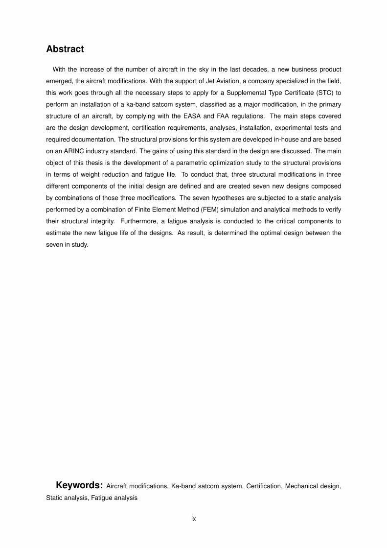
Abstract
With the increase of the number of aircraft in the sky in the last decades, a new business product
emerged, the aircraft modifications. With the support of Jet Aviation, a company specialized in the field,
this work goes through all the necessary steps to apply for a Supplemental Type Certificate (STC) to
perform an installation of a ka-band satcom system, classified as a major modification, in the primary
structure of an aircraft, by complying with the EASA and FAA regulations. The main steps covered
are the design development, certification requirements, analyses, installation, experimental tests and
required documentation. The structural provisions for this system are developed in-house and are based
on an ARINC industry standard. The gains of using this standard in the design are discussed. The main
object of this thesis is the development of a parametric optimization study to the structural provisions
in terms of weight reduction and fatigue life. To conduct that, three structural modifications in three
different components of the initial design are defined and are created seven new designs composed
by combinations of those three modifications. The seven hypotheses are subjected to a static analysis
performed by a combination of Finite Element Method (FEM) simulation and analytical methods to verify
their structural integrity. Furthermore, a fatigue analysis is conducted to the critical components to
estimate the new fatigue life of the designs. As result, is determined the optimal design between the
seven in study.
Keywords: Aircraft modifications, Ka-band satcom system, Certification, Mechanical design,
Static analysis, Fatigue analysis
ix

x

Contents
Acknowledgments . . . . . . . . . . . . . . . . . . . . . . . . . . . . . . . . . . . . . . . . . . . v
Resumo . . . . . . . . . . . . . . . . . . . . . . . . . . . . . . . . . . . . . . . . . . . . . . . . . vii
Abstract . . . . . . . . . . . . . . . . . . . . . . . . . . . . . . . . . . . . . . . . . . . . . . . . . ix
List of Tables . . . . . . . . . . . . . . . . . . . . . . . . . . . . . . . . . . . . . . . . . . . . . . xv
List of Figures . . . . . . . . . . . . . . . . . . . . . . . . . . . . . . . . . . . . . . . . . . . . . xvii
Nomenclature . . . . . . . . . . . . . . . . . . . . . . . . . . . . . . . . . . . . . . . . . . . . . . xxi
Glossary . . . . . . . . . . . . . . . . . . . . . . . . . . . . . . . . . . . . . . . . . . . . . . . . xxv
1 Introduction 1
1.1 Present State of Aeronautic Industry . . . . . . . . . . . . . . . . . . . . . . . . . . . . . . 1
1.2 Aircraft Modifications . . . . . . . . . . . . . . . . . . . . . . . . . . . . . . . . . . . . . . . 1
1.3 The Civil Aviation Authorities . . . . . . . . . . . . . . . . . . . . . . . . . . . . . . . . . . 2
1.4 Jet Aviation AG . . . . . . . . . . . . . . . . . . . . . . . . . . . . . . . . . . . . . . . . . . 3
1.5 Ka-Band Satcom System . . . . . . . . . . . . . . . . . . . . . . . . . . . . . . . . . . . . 4
1.5.1 Generic Concept . . . . . . . . . . . . . . . . . . . . . . . . . . . . . . . . . . . . . 4
1.5.2 Composition . . . . . . . . . . . . . . . . . . . . . . . . . . . . . . . . . . . . . . . 4
1.5.3 Certification - Supplemental Type Certificate . . . . . . . . . . . . . . . . . . . . . 5
1.6 Project Presentation . . . . . . . . . . . . . . . . . . . . . . . . . . . . . . . . . . . . . . . 5
1.7 Objectives . . . . . . . . . . . . . . . . . . . . . . . . . . . . . . . . . . . . . . . . . . . . . 6
1.8 Thesis Outline . . . . . . . . . . . . . . . . . . . . . . . . . . . . . . . . . . . . . . . . . . 6
2 ARINC 791 Standard 9
2.1 ARINC Standards . . . . . . . . . . . . . . . . . . . . . . . . . . . . . . . . . . . . . . . . 9
2.2 ARINC Characteristic 791 . . . . . . . . . . . . . . . . . . . . . . . . . . . . . . . . . . . . 10
2.2.1 KU/KA-Satcom System Description . . . . . . . . . . . . . . . . . . . . . . . . . . 10
2.2.2 Mechanical Interface: Antenna-Aircraft . . . . . . . . . . . . . . . . . . . . . . . . . 14
2.3 Advantages of using ARINC Standard . . . . . . . . . . . . . . . . . . . . . . . . . . . . . 16
3 Ka-band System Structural Base Design 18
3.1 Design’s Certification Requirements . . . . . . . . . . . . . . . . . . . . . . . . . . . . . . 18
3.2 Antenna Installation Position . . . . . . . . . . . . . . . . . . . . . . . . . . . . . . . . . . 21
3.3 Aircraft’s Airframe Environment 3D modelling . . . . . . . . . . . . . . . . . . . . . . . . . 23
xi
3.4 External Supplied Components - Radome, Adapter Plate and Fairing . . . . . . . . . . . . 29
3.5 Jet Aviation’s Structural Provisions Design . . . . . . . . . . . . . . . . . . . . . . . . . . . 31
4 Parametric Optimization 35
4.1 Hypotheses . . . . . . . . . . . . . . . . . . . . . . . . . . . . . . . . . . . . . . . . . . . . 35
4.2 Load Cases . . . . . . . . . . . . . . . . . . . . . . . . . . . . . . . . . . . . . . . . . . . . 37
4.3 Methodologies . . . . . . . . . . . . . . . . . . . . . . . . . . . . . . . . . . . . . . . . . . 39
4.3.1 Static Structural Analysis . . . . . . . . . . . . . . . . . . . . . . . . . . . . . . . . 40
4.3.2 Fatigue Analysis . . . . . . . . . . . . . . . . . . . . . . . . . . . . . . . . . . . . . 49
5 Results 53
5.1 Weight . . . . . . . . . . . . . . . . . . . . . . . . . . . . . . . . . . . . . . . . . . . . . . . 53
5.2 Static . . . . . . . . . . . . . . . . . . . . . . . . . . . . . . . . . . . . . . . . . . . . . . . 54
5.3 Fatigue . . . . . . . . . . . . . . . . . . . . . . . . . . . . . . . . . . . . . . . . . . . . . . 63
5.4 Optimal hypothesis . . . . . . . . . . . . . . . . . . . . . . . . . . . . . . . . . . . . . . . . 66
6 Design Initial Release 68
6.1 Installation’s Deviations . . . . . . . . . . . . . . . . . . . . . . . . . . . . . . . . . . . . . 68
6.2 Experimental Tests . . . . . . . . . . . . . . . . . . . . . . . . . . . . . . . . . . . . . . . . 70
6.3 Certification Documents . . . . . . . . . . . . . . . . . . . . . . . . . . . . . . . . . . . . . 70
6.3.1 Master Data List - MDL . . . . . . . . . . . . . . . . . . . . . . . . . . . . . . . . . 71
6.3.2 Certification Compliance Sheet - CCS . . . . . . . . . . . . . . . . . . . . . . . . . 71
6.3.3 Drawing List Mechanical - DLM . . . . . . . . . . . . . . . . . . . . . . . . . . . . . 72
6.3.4 Drawing List Electrical and Electrical Item List - DLE and EIL . . . . . . . . . . . . 72
6.3.5 Engineering Order - ENO . . . . . . . . . . . . . . . . . . . . . . . . . . . . . . . . 72
6.3.6 Weight and Balance Statement - WBS . . . . . . . . . . . . . . . . . . . . . . . . . 72
6.3.7 Structural Substantiation Report and Damage Tolerance Analysis - SSR and DTA 73
6.3.8 Analysis Report - ANA . . . . . . . . . . . . . . . . . . . . . . . . . . . . . . . . . . 73
6.3.9 Subcontractor Document Process Slip - DPS . . . . . . . . . . . . . . . . . . . . . 74
6.3.10 Flight Test Plan / Report - FTP/R . . . . . . . . . . . . . . . . . . . . . . . . . . . . 74
6.3.11 Instructions for Continued Airworthiness - ICA . . . . . . . . . . . . . . . . . . . . 74
7 Conclusions 75
7.1 Achievements . . . . . . . . . . . . . . . . . . . . . . . . . . . . . . . . . . . . . . . . . . . 75
7.2 Future Work . . . . . . . . . . . . . . . . . . . . . . . . . . . . . . . . . . . . . . . . . . . . 76
Bibliography 77
A Additional data 79
A.1 Geometrical dimensions of the modified fittings . . . . . . . . . . . . . . . . . . . . . . . . 79
A.2 Geometrical dimensions of the modified intercostals . . . . . . . . . . . . . . . . . . . . . 80
A.3 Shear-Bearing Efficiency Factor - Kbr . . . . . . . . . . . . . . . . . . . . . . . . . . . . . 80
xii

A.4 Lug Efficiency Factor for Tension - Kt . . . . . . . . . . . . . . . . . . . . . . . . . . . . . 81
A.5 Yield Factor - C . . . . . . . . . . . . . . . . . . . . . . . . . . . . . . . . . . . . . . . . . . 81
A.6 Efficiency Factor for Transverse Load - ktru and ktry . . . . . . . . . . . . . . . . . . . . . 82
A.7 Bearing Stress Concentration Factor - Ktb . . . . . . . . . . . . . . . . . . . . . . . . . . . 82
A.8 Stress Concentration Factor - Ktg . . . . . . . . . . . . . . . . . . . . . . . . . . . . . . . 83
A.9 Bearing Distribution Factor - θ . . . . . . . . . . . . . . . . . . . . . . . . . . . . . . . . . . 83
A.10 Stress-life (S-N) curves of aluminium 7050-T7451 plate . . . . . . . . . . . . . . . . . . . 84
A.11 Safety margins results for the critical mounting gusset in fitting 7 . . . . . . . . . . . . . . 85
A.12 Safety margins results for the critical frame . . . . . . . . . . . . . . . . . . . . . . . . . . 85
A.13 Safety margins results for the critical fastener - Mounting Gusset & Intercostal in fitting 7 -
NAS6203 . . . . . . . . . . . . . . . . . . . . . . . . . . . . . . . . . . . . . . . . . . . . . 85
xiii

xiv
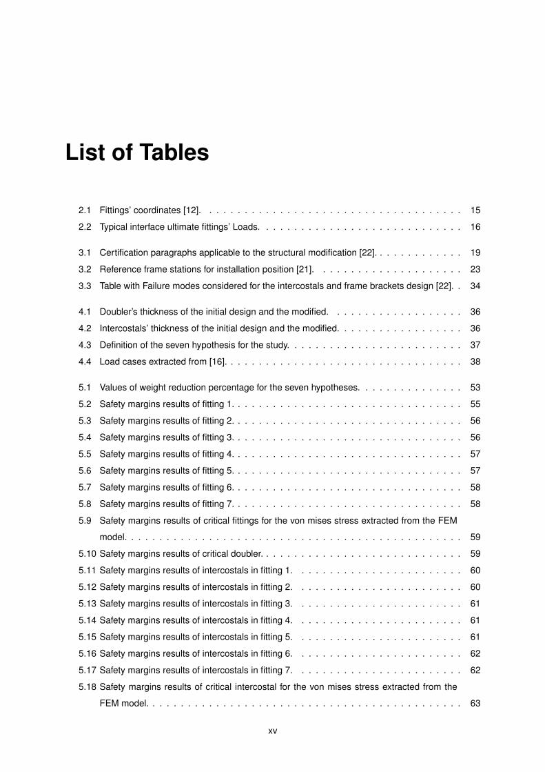
List of Tables
2.1 Fittings’ coordinates [12]. . . . . . . . . . . . . . . . . . . . . . . . . . . . . . . . . . . . . 15
2.2 Typical interface ultimate fittings’ Loads. . . . . . . . . . . . . . . . . . . . . . . . . . . . . 16
3.1 Certification paragraphs applicable to the structural modification [22]. . . . . . . . . . . . . 19
3.2 Reference frame stations for installation position [21]. . . . . . . . . . . . . . . . . . . . . 23
3.3 Table with Failure modes considered for the intercostals and frame brackets design [22]. . 34
4.1 Doubler’s thickness of the initial design and the modified. . . . . . . . . . . . . . . . . . . 36
4.2 Intercostals’ thickness of the initial design and the modified. . . . . . . . . . . . . . . . . . 36
4.3 Definition of the seven hypothesis for the study. . . . . . . . . . . . . . . . . . . . . . . . . 37
4.4 Load cases extracted from [16]. . . . . . . . . . . . . . . . . . . . . . . . . . . . . . . . . . 38
5.1 Values of weight reduction percentage for the seven hypotheses. . . . . . . . . . . . . . . 53
5.2 Safety margins results of fitting 1. . . . . . . . . . . . . . . . . . . . . . . . . . . . . . . . . 55
5.3 Safety margins results of fitting 2. . . . . . . . . . . . . . . . . . . . . . . . . . . . . . . . . 56
5.4 Safety margins results of fitting 3. . . . . . . . . . . . . . . . . . . . . . . . . . . . . . . . . 56
5.5 Safety margins results of fitting 4. . . . . . . . . . . . . . . . . . . . . . . . . . . . . . . . . 57
5.6 Safety margins results of fitting 5. . . . . . . . . . . . . . . . . . . . . . . . . . . . . . . . . 57
5.7 Safety margins results of fitting 6. . . . . . . . . . . . . . . . . . . . . . . . . . . . . . . . . 58
5.8 Safety margins results of fitting 7. . . . . . . . . . . . . . . . . . . . . . . . . . . . . . . . . 58
5.9 Safety margins results of critical fittings for the von mises stress extracted from the FEM
model. . . . . . . . . . . . . . . . . . . . . . . . . . . . . . . . . . . . . . . . . . . . . . . . 59
5.10 Safety margins results of critical doubler. . . . . . . . . . . . . . . . . . . . . . . . . . . . . 59
5.11 Safety margins results of intercostals in fitting 1. . . . . . . . . . . . . . . . . . . . . . . . 60
5.12 Safety margins results of intercostals in fitting 2. . . . . . . . . . . . . . . . . . . . . . . . 60
5.13 Safety margins results of intercostals in fitting 3. . . . . . . . . . . . . . . . . . . . . . . . 61
5.14 Safety margins results of intercostals in fitting 4. . . . . . . . . . . . . . . . . . . . . . . . 61
5.15 Safety margins results of intercostals in fitting 5. . . . . . . . . . . . . . . . . . . . . . . . 61
5.16 Safety margins results of intercostals in fitting 6. . . . . . . . . . . . . . . . . . . . . . . . 62
5.17 Safety margins results of intercostals in fitting 7. . . . . . . . . . . . . . . . . . . . . . . . 62
5.18 Safety margins results of critical intercostal for the von mises stress extracted from the
FEM model. . . . . . . . . . . . . . . . . . . . . . . . . . . . . . . . . . . . . . . . . . . . . 63
xv

5.19 Number of cycles of fatigue life. . . . . . . . . . . . . . . . . . . . . . . . . . . . . . . . . . 64
5.20 Number of cycles of fatigue life for doubler 2 for the initial design and seven hypothesis. . 65
5.21 Critical number of cycles of fatigue life which drives each hypothesis. . . . . . . . . . . . . 65
A.1 Safety margins results of the critical mounting gusset in fitting 7. . . . . . . . . . . . . . . 85
A.2 Safety margins results of the critical frame. . . . . . . . . . . . . . . . . . . . . . . . . . . 85
A.3 Safety margins results of the critical fastener - NAS6203. . . . . . . . . . . . . . . . . . . 85
xvi
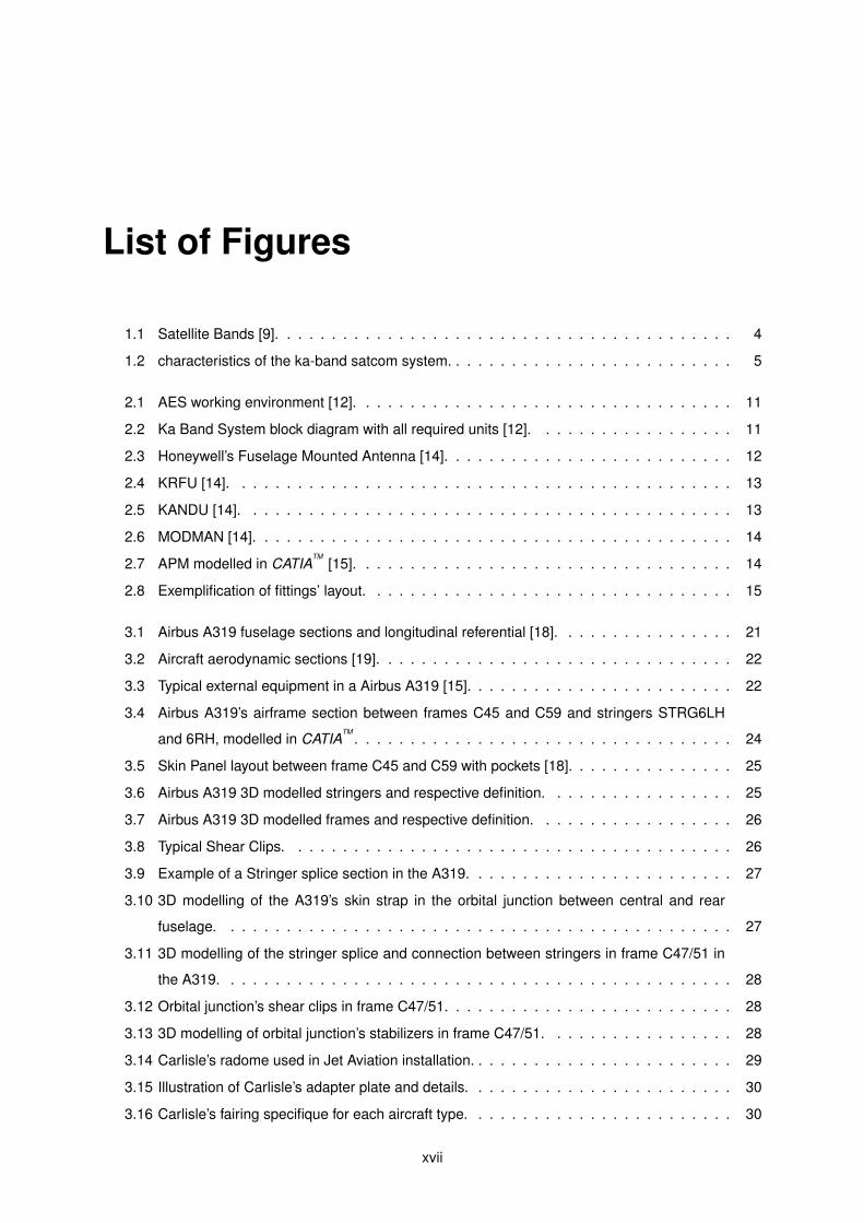
List of Figures
1.1 Satellite Bands [9]. . . . . . . . . . . . . . . . . . . . . . . . . . . . . . . . . . . . . . . . . 4
1.2 characteristics of the ka-band satcom system. . . . . . . . . . . . . . . . . . . . . . . . . . 5
2.1 AES working environment [12]. . . . . . . . . . . . . . . . . . . . . . . . . . . . . . . . . . 11
2.2 Ka Band System block diagram with all required units [12]. . . . . . . . . . . . . . . . . . 11
2.3 Honeywell’s Fuselage Mounted Antenna [14]. . . . . . . . . . . . . . . . . . . . . . . . . . 12
2.4 KRFU [14]. . . . . . . . . . . . . . . . . . . . . . . . . . . . . . . . . . . . . . . . . . . . . 13
2.5 KANDU [14]. . . . . . . . . . . . . . . . . . . . . . . . . . . . . . . . . . . . . . . . . . . . 13
2.6 MODMAN [14]. . . . . . . . . . . . . . . . . . . . . . . . . . . . . . . . . . . . . . . . . . . 14
2.7 APM modelled in CATIATM
[15]. . . . . . . . . . . . . . . . . . . . . . . . . . . . . . . . . . 14
2.8 Exemplification of fittings’ layout. . . . . . . . . . . . . . . . . . . . . . . . . . . . . . . . . 15
3.1 Airbus A319 fuselage sections and longitudinal referential [18]. . . . . . . . . . . . . . . . 21
3.2 Aircraft aerodynamic sections [19]. . . . . . . . . . . . . . . . . . . . . . . . . . . . . . . . 22
3.3 Typical external equipment in a Airbus A319 [15]. . . . . . . . . . . . . . . . . . . . . . . . 22
3.4 Airbus A319’s airframe section between frames C45 and C59 and stringers STRG6LH
and 6RH, modelled in CATIATM
. . . . . . . . . . . . . . . . . . . . . . . . . . . . . . . . . . 24
3.5 Skin Panel layout between frame C45 and C59 with pockets [18]. . . . . . . . . . . . . . . 25
3.6 Airbus A319 3D modelled stringers and respective definition. . . . . . . . . . . . . . . . . 25
3.7 Airbus A319 3D modelled frames and respective definition. . . . . . . . . . . . . . . . . . 26
3.8 Typical Shear Clips. . . . . . . . . . . . . . . . . . . . . . . . . . . . . . . . . . . . . . . . 26
3.9 Example of a Stringer splice section in the A319. . . . . . . . . . . . . . . . . . . . . . . . 27
3.10 3D modelling of the A319’s skin strap in the orbital junction between central and rear
fuselage. . . . . . . . . . . . . . . . . . . . . . . . . . . . . . . . . . . . . . . . . . . . . . 27
3.11 3D modelling of the stringer splice and connection between stringers in frame C47/51 in
the A319. . . . . . . . . . . . . . . . . . . . . . . . . . . . . . . . . . . . . . . . . . . . . . 28
3.12 Orbital junction’s shear clips in frame C47/51. . . . . . . . . . . . . . . . . . . . . . . . . . 28
3.13 3D modelling of orbital junction’s stabilizers in frame C47/51. . . . . . . . . . . . . . . . . 28
3.14 Carlisle’s radome used in Jet Aviation installation. . . . . . . . . . . . . . . . . . . . . . . . 29
3.15 Illustration of Carlisle’s adapter plate and details. . . . . . . . . . . . . . . . . . . . . . . . 30
3.16 Carlisle’s fairing specifique for each aircraft type. . . . . . . . . . . . . . . . . . . . . . . . 30
xvii
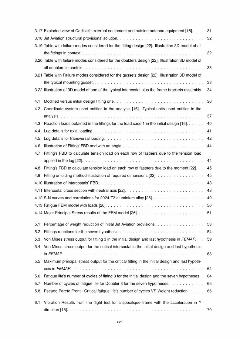
3.17 Exploded view of Carlisle’s external equipment and outside antenna equipment [15]. . . . 31
3.18 Jet Aviation structural provisions’ solution. . . . . . . . . . . . . . . . . . . . . . . . . . . . 32
3.19 Table with failure modes considered for the fitting design [22]. Illustration 3D model of all
the fittings in context. . . . . . . . . . . . . . . . . . . . . . . . . . . . . . . . . . . . . . . . 32
3.20 Table with failure modes considered for the doublers design [22]. Illustration 3D model of
all doublers in context. . . . . . . . . . . . . . . . . . . . . . . . . . . . . . . . . . . . . . . 33
3.21 Table with Failure modes considered for the gussets design [22]. Illustration 3D model of
the typical mounting gusset. . . . . . . . . . . . . . . . . . . . . . . . . . . . . . . . . . . . 33
3.22 Illustration of 3D model of one of the typical intercostal plus the frame brackets assembly. 34
4.1 Modified versus initial design fitting one. . . . . . . . . . . . . . . . . . . . . . . . . . . . . 36
4.2 Coordinate system used entities in the analysis [16]. Typical units used entities in the
analysis. . . . . . . . . . . . . . . . . . . . . . . . . . . . . . . . . . . . . . . . . . . . . . . 37
4.3 Reaction loads obtained in the fittings for the load case 1 in the initial design [16]. . . . . . 40
4.4 Lug details for axial loading. . . . . . . . . . . . . . . . . . . . . . . . . . . . . . . . . . . . 41
4.5 Lug details for transversal loading. . . . . . . . . . . . . . . . . . . . . . . . . . . . . . . . 42
4.6 Illustration of Fitting’ FBD and with an angle. . . . . . . . . . . . . . . . . . . . . . . . . . . 44
4.7 Fitting’s FBD to calculate tension load on each row of fastners due to the tension load
applied in the lug [22]. . . . . . . . . . . . . . . . . . . . . . . . . . . . . . . . . . . . . . . 44
4.8 Fitting’s FBD to calculate tension load on each row of fastners due to the moment [22]. . . 45
4.9 Fitting unfolding method illustration of required dimensions [22]. . . . . . . . . . . . . . . . 45
4.10 Illustration of intercostals’ FBD. . . . . . . . . . . . . . . . . . . . . . . . . . . . . . . . . . 48
4.11 Intercostal cross section with neutral axis [22]. . . . . . . . . . . . . . . . . . . . . . . . . 48
4.12 S-N curves and correlations for 2024-T3 aluminium alloy [25]. . . . . . . . . . . . . . . . . 49
4.13 Fatigue FEM model with loads [26]. . . . . . . . . . . . . . . . . . . . . . . . . . . . . . . . 50
4.14 Major Principal Stress results of the FEM model [26]. . . . . . . . . . . . . . . . . . . . . . 51
5.1 Percentage of weight reduction of initial Jet Aviation provisions. . . . . . . . . . . . . . . . 53
5.2 Fittings reactions for the seven hypothesis . . . . . . . . . . . . . . . . . . . . . . . . . . . 54
5.3 Von Mises stress output for fitting 3 in the initial design and last hypothesis in FEMAP. . . 59
5.4 Von Mises stress output for the critical intercostal in the initial design and last hypothesis
in FEMAP. . . . . . . . . . . . . . . . . . . . . . . . . . . . . . . . . . . . . . . . . . . . . 63
5.5 Maximum principal stress output for the critical fitting in the initial design and last hypoth-
esis in FEMAP. . . . . . . . . . . . . . . . . . . . . . . . . . . . . . . . . . . . . . . . . . . 64
5.6 Fatigue life’s number of cycles of fitting 3 for the initial design and the seven hypotheses. . 64
5.7 Number of cycles of fatigue life for Doubler 3 for the seven hypotheses. . . . . . . . . . . 65
5.8 Pseudo Pareto Front - Critical fatigue life’s number of cycles VS Weight reduction. . . . . 66
6.1 Vibration Results from the flight test for a specifique frame with the acceleration in Y
direction [15]. . . . . . . . . . . . . . . . . . . . . . . . . . . . . . . . . . . . . . . . . . . . 70
xviii
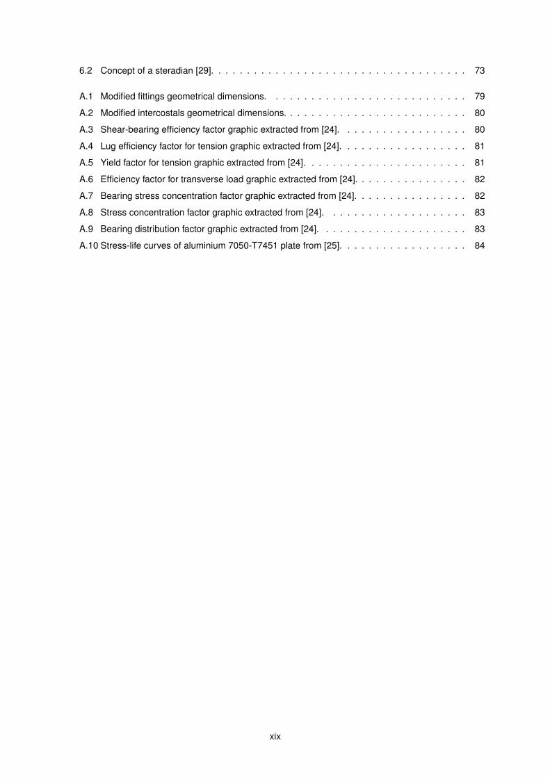
6.2 Concept of a steradian [29]. . . . . . . . . . . . . . . . . . . . . . . . . . . . . . . . . . . . 73
A.1 Modified fittings geometrical dimensions. . . . . . . . . . . . . . . . . . . . . . . . . . . . 79
A.2 Modified intercostals geometrical dimensions. . . . . . . . . . . . . . . . . . . . . . . . . . 80
A.3 Shear-bearing efficiency factor graphic extracted from [24]. . . . . . . . . . . . . . . . . . 80
A.4 Lug efficiency factor for tension graphic extracted from [24]. . . . . . . . . . . . . . . . . . 81
A.5 Yield factor for tension graphic extracted from [24]. . . . . . . . . . . . . . . . . . . . . . . 81
A.6 Efficiency factor for transverse load graphic extracted from [24]. . . . . . . . . . . . . . . . 82
A.7 Bearing stress concentration factor graphic extracted from [24]. . . . . . . . . . . . . . . . 82
A.8 Stress concentration factor graphic extracted from [24]. . . . . . . . . . . . . . . . . . . . 83
A.9 Bearing distribution factor graphic extracted from [24]. . . . . . . . . . . . . . . . . . . . . 83
A.10 Stress-life curves of aluminium 7050-T7451 plate from [25]. . . . . . . . . . . . . . . . . . 84
xix

xx
Nomenclature
Abbreviations
AEEC Airlines Electronic Engineering Committee
AMC Avionics Maintenance Conference
AMM Aircraft Maintenance Manual
APM Airplane Personality Module
ARINC Aeronautical Radio Incorporated
CFR Code Federal Regulations
CG Centre of Gravity
DOA Design Organization Approval
EASA European Aviation Safety Agency
FAA Federal Aviation Administration
FMA Fuselage Mounted Antenna
FSEMC Flight Simulator Engineering and Maintenance Committee
GAG Ground-Air-Ground
GA General Aviation
ICAO International Civil Aviation Organization
ICA Instruction for Continued Airworthiness
IPC Illustrated Part Catalogue
KANDU Ku/Ka-band Aircraft Networking Data Unit
KRFU Ku/Ka-band Radio Frequency Unit
MODMAN Modem and Manager
OEM Original Equipment Manufacturer
xxi

SAE-ITC Society of Automotive Engineers-Industry Technologies Consortia
SF Severity Factor
SRM Structural Repair Manual
STC Supplemental Type Certificate
Greek symbols
α Fastener hole condition factor.
β Hole filling factor.
θ Bearing distribution factor.
Roman symbols
A Area.
C Yield factor.
D Diameter.
E Young’s Modulus.
F Ultimate or yield stress.
f Applied stress.
g Gravity Acceleration.
I Moment of inertia.
K Fatigue quality index.
Kt Stress concentration factor.
kt Tensile efficiency factor.
kbr Shear bearing efficiency factor.
Ktb Bearing stress concentration factor.
Ktg Stress concentration factor parametrize.
Kth Local stress concentration factor.
ktru Tensile efficiency factor for transversal loads under ultimate condition.
ktry Tensile efficiency factor for transversal loads under yield condition.
L Length.
M Moment.
xxii

MS Safety Margin.
Nf Fatigue life number of cycles.
P Force.
R Reaction forces.
S Shear loads.
T Tensile loads.
t Thickness.
xxiii

xxiv

Glossary
CFD Computational Fluid Dynamics is a branch of
fluid mechanics that uses numerical methods
and algorithms to solve problems that involve
fluid flows.
CSM Computational Structural Mechanics is a
branch of structure mechanics that uses nu-
merical methods and algorithms to perform the
analysis of structures and its components.
xxv

xxvi
Chapter 1
Introduction
1.1 Present State of Aeronautic Industry
Since the beginning of air transportation’s history, this type of transport had a huge and important
impact in people’s lives and also in the world economy. Now-a-days, this tendency continues to be
observable, the number of transported passengers increases every year [1]. This continuous demand
for a quick transport for long distances in a relatively short time, made the aeronautic industry develop
in a large scale. This huge development was only possible with the great advances of major techno-
logical innovations, such as the introduction of jet aircraft for commercial use in the 1950s [2]. In the
modern days, the major on going innovation is the introduction of composite materials in more than
50% of aircraft’s structure. Aircraft Original Equipment Manufacturers (OEMs) as Boeing and Airbus
already achieved this high percentage with the Boeing 787 and Airbus A350 XWB [3]. In parallel, the
fast technological evolution and trends changes created new opportunities of business products in the
industry, more specifically in the sector of aircraft alterations/changes. The nomenclature alteration or
change rely on the regulation authority which the modification must be subjected. Alteration is used for
Federal Aviation Administration (FAA) and change for European Aviation Safety Agency (EASA). These
two regulations authorities are presented in more detail in section 1.3.
1.2 Aircraft Modifications
The definition of aircraft modification comes in two forms: Alterations/Changes and Repairs. The first
form refers to the modifications where it is added new equipments or features to the aircraft. The second
form refers to modifications where it is re-established the original strength and integrity of the damaged
areas in the aircraft. In addition, these two forms can be classified in major and minor modifications.
The definition of these two classifications has suffered several changes since the beginning of industry.
These definitions’ update were introduced in order to give a better clarity and guidance to the companies
which provide these types of services. Now-a-days, the updated definition for these concepts is given
by two documents, Federal Aviation Regulation (FAR) PART 1 and 43. These two documents, produced
1
by FAA, illustrate and distinguish major from minor alterations and repairs. As the main focus of this
thesis falls upon changes/alterations, the official definition for major and minor changes/alterations are
presented.
FAR PART 1 states that a major alteration is ”an alteration not listed in the aircraft, aircraft engine, or
propeller specifications-
1. That might appreciably affect weight, balance, structural strength, performance, powerplant oper-
ation, flight characteristics, or other qualities affecting airworthiness; or
2. That is not done according to accepted practices or cannot be done by elementary operations.”
On the other hand, a minor alteration is simply defined as ”an alteration other than a major alteration.”
[4]
Any of these modifications need to be certified by a competent authority, unless the company which is
performing the modification is certified by an airworthiness authority showing that it is capable to auto-
certify their own modifications. However, one of the options to certify a modification passes through the
creation of a supplemental type certificate (STC). This option to certify a modification is very expensive,
consequently it is only used when there is an interest in performing the same modification in several air-
craft. A STC is a document where the new features added to the initial aircraft are described. To apply
for an STC several different documents must be prepared. These will prove that there is compliance
with several certain requirements. These documents start with the CAF - Classification Assessment
Form, where the modification is introduced and also defined as a major or minor alteration, or repair.
And it goes until the instructions for continued airworthiness, known as Instructions for Continued Air-
worthiness (ICAs). An important document which proves that after the accomplished modification, the
aircraft continues to meet its appropriate airworthiness, noise, and emissions standards and states the
alterations in maintenance program and inspection intervals [5, 6].
1.3 The Civil Aviation Authorities
Since the aviation early times and subsequent rapid growth, every country found necessary the cre-
ation of autonomous institutions and national authorities to guarantee flight safety. This was the birth of
civil aviation authorities. These also known as airworthiness authorities which have the following main
tasks [5]:
• To prescribe airworthiness requirements and procedures;
• To inform the interested parties regarding the above-mentioned prescriptions;
• To control aeronautical material, design, manufacturing organizations, and aircraft operators;
• To certify aeronautical material and organizations;
2

On April 4th 1947, the International Civil Aviation Organization (ICAO) was established with main goals
of developing the principles and techniques of international air navigation and achieve a standardized
operation for a safe and efficient air service. This standardization was achieved with the elaboration of
18 annexes named as International Standards and Recommended Practises [5].
Presently, there are two main independent entities which groups several civil aviation authorities of
different countries. In the European space, there is the European Aviation Safety Agency (EASA) which
succeeded the Joint Aviation Authorities (JAA) and represents all Union European state members [5]. In
the United States, there is the Federal Aviation Authority (FAA) which represents all their states. These
two authorities play an important role in several areas such as rulemaking or inspections, training, and
standardization programs [5]. For the scope of this thesis, the most relevant function of these two
authorities is the certification and approval of STCs.
1.4 Jet Aviation AG
Jet Aviation AG is a recognized leader company in the business aviation industry. It was established
in 1967 by providing maintenance services in Basel, Switzerland, where presently is its headquarters.
Now-a-days Jet Aviation offers a variety of aircraft-support services, ranging from maintenance, comple-
tions and refurbishments to aircraft management and charter services [7]. As a recognized jet aircraft
repair station, Jet Aviation holds several authorizations and approvals from EASA, FAA and other sev-
enteen different national aviation authorities.
The companies’ engineering hub is based in Basel and provides custom solutions while meeting cus-
tomer’s specifications and ensuring technical feasibility and certification requirements. The engineering
teams are divided in two sections, the completions side and maintenance. These teams work close to
sales, interior design, production and installation teams since the initial conceptual design to the delivery.
Completions side has the main focus of providing the integration, customization and upgrade of equip-
ments and in-flight entertainment in several Airbus and Boeing aircraft types. While the maintenance
side, provides engineering and certification services to custom modifications for any aircraft of large
category [7]. Regarding, the engineering part, the maintenance side provides cabin layouts changes,
installation and upgrade of navigation and communication systems, repairs and most important for the
scope of this work, the development, installation and upgrade of satcom systems. These modifications
are only possible because Jet Aviation has several Design Organization Approvals (DOAs) from EASA,
FAA and other civil aviation authorities [7].
Inside the satcom systems there is the ka-band satcom system which is the main target for this
thesis.
3

1.5 Ka-Band Satcom System
1.5.1 Generic Concept
Now-a-days, the state of the art in aircraft communication via satellite is ka-band satcom antenna
which provides to the aircraft, data transmission and reception in high frequencies between 26.5–40
gigahertz (GHz). The ka-band stands for ”K-above” because it is the upper part of the original NATO
K band as shown in figure 1.1. The ka-band antenna predecessor was the ku-band antenna. The
bandwidth of the ku is around 2GHz for uplink and 1.3GHz for downlink with actual contiguous bandwidth
allocation of less than 0.5GHz per satellite. In comparison, the ka-band satcom has a bandwidth of
3.5GHz for both uplink and downlink [8]. Having a wider bandwidth, consequently greater resiliency to
interference is achieved. Presently, as it is required more and more wide bandwidth signals, the ka-band
antenna offers additional frequencies to communicate [9]. In parallel also, there is an increase of data
transfer due to the higher frequencies. Other reason why the ka-band is attractive as a satcom solution
is that requires smaller terminals which allows the ka-band satcom be made available for new markets
such as mobile platforms [8].
Figure 1.1: Satellite Bands [9].
This system in combination with the on-board technologies, allows the aircraft’s passengers to have
access to a broadband connectivity in a wide area of the globe and so they can connect to the social
media and communicate online with high speed internet velocity, as if they were at home [9]. Another
advantage is that it can provides faster updated information to the pilots regarding weather conditions or
other required information, however this system is not the critical one to obtain that information neither to
replace the one which is critical. Figure 1.2 presents the environment which provides the communication
between the aircraft and ground stations, and the coverage map of the ka band satcom provided by
Honeywell JetWave.
1.5.2 Composition
The ka-band satcom system can be divided in two distinct parts. The first refers to systems required
for the correct functionality of the antenna. All the fundamental systems are described in chapter 2. In
Jet Aviation all of these systems are bought from a supplier.
4

(a) Scheme of ka-band satcom antenna environment function-ality
(b) Coverage map of the system installed by Jet Aviation [10]
Figure 1.2: characteristics of the ka-band satcom system.
The second part is the structural part which is the mechanical interface between the antenna and
aircraft, where its ultimate goal is to withstand all the structural loads during a flight. These part is
composed by several components which are described in detail in chapter 3. Most of this structure is
fully developed in-house by Jet Aviation and this is the part that will be studied in order to be optimized
in terms of weight and durability, without forgetting the certificability.
1.5.3 Certification - Supplemental Type Certificate
With the installation of ka-band satcom system, the aircraft’s structural strength will be affected due to
the local introduction of additional flight loads, because new structural components are being added to
the primary structure. In addition, there will be changes in the aircraft’s airworthiness limitations. New
intervals and means of inspection must be defined. Finally, this modification will increment the aircraft’s
drag, but with a reduced impact in aircraft performance. Taking into account the points mentioned
before, this modification is classified as a major change [11]. Since Jet Aviation doesn’t have rights to
auto-certify major changes, and intend to perform this modification several times in many aircraft of the
same type, the profitable way to certify it is to apply for a STC in an airworthiness authority.
1.6 Project Presentation
During my traineeship, my main role was to contribute for the ka band antenna projects, where our
team developed the structural provisions and systems installation for a few different aircraft types. I had
a pleasure to help on these developments in airplanes as Boeing 747 variant -300 and -400 and some
variants of Boeing 737 Family.
With the interest of a customer to install the ka-band satcom system in his aircraft, an Airbus A319,
a new project rose up, the development of ka-band satcom system STC for Airbus A320 aircraft family.
Therefore, the first aircraft types included in this STC are the A319 and A320 CEO (Current Engine
Option) and NEO (New Engine Option).
5
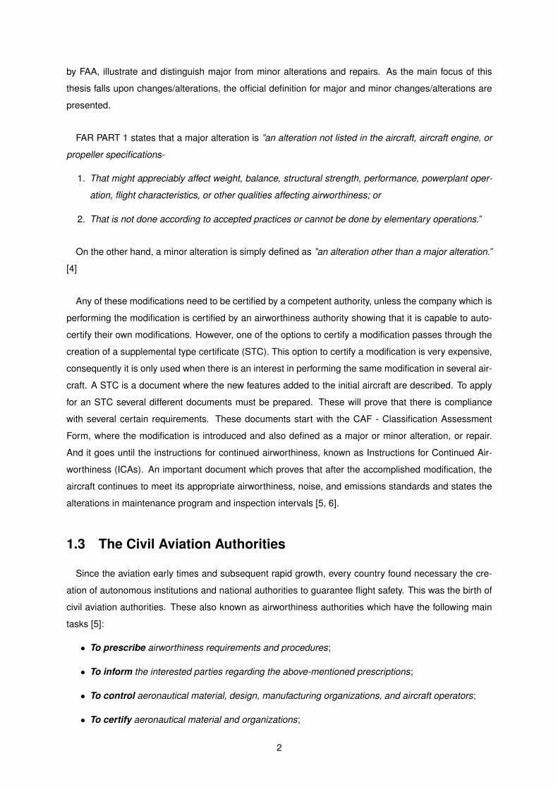
1.7 Objectives
The main objectives to be achieved within the scope of this thesis are:
• Illustrate all the steps to certify a major modification in the primary structure of an aircraft. Going
through the highlight of all the certification requirements that the modification must show compli-
ance until the required documentation for STC approval;
• Show how a standard can be helpful for the industry development;
• Find several hypothesis for the optimal structural solution for the design, by modifying three struc-
tural components of the initial design;
• Using Computational Structural Mechanics (CSM) to perform static structural and fatigue analysis
to study the several candidate hypothesis;
• Selection of the candidate hypothesis as optimal solution taking into account several different re-
quirements;
• Show how the flight tests helps in the certification.
• Highlight the main conclusions and possible future works;
1.8 Thesis Outline
A brief description of the contents of the following chapters are now presented:
Chapter 2
An introduction to the Aeronautical Radio Incorporated (ARINC) Standards, the involved organiza-
tions in the process and their goals are presented. Detail description of the target standard, ARINC
Characteristic 791, where is presented its definition, the required equipments and mechanical-interface
requirements. Finally, the advantages of using this standard as a background in the design is also
presented.
Chapter 3
A detailed description of the ka-band satcom structural base design for an Airbus A320 family, a Jet
Aviation Solution, is presented. Starting with identification of the certification requirements, followed by
the 3D modulation of the aircraft’s airframe and complementary environment, and the selection of the
optimum antenna installation location. Finally, geometry definition of new structural components which
compose the developed structural provisions are presented.
6

Chapter 4
A parametric optimization is developed, where seven possible hypothesis of design are defined and
presented. Furthermore, the methodologies used for the static and fatigue analysis are described.
Chapter 5
Results of the different analyses for the several hypothesis are presented. Followed by the selec-
tion of the optimal hypothesis taking in consideration several different requirements. In addition, the
experimental results of the flight test for the vibration and buffeting tests are presented.
Chapter 6
Installation process aside of Reverse Engineering is illustrated. Additionally, the required documenta-
tion, which reflects the aircraft after modification state for requiring the STC, is presented.
Chapter 7
Conclusions are drawn and future work is proposed.
7

8
Chapter 2
ARINC 791 Standard
2.1 ARINC Standards
ARINC Industry Activities is one of the industry programs of Society of Automotive Engineers-Industry
Technologies Consortia (SAE-ITC) which creates aviation industry committees and participates in re-
lated industry activities by providing technical leadership and guidance in order to benefit aviation [12].
Safety, efficiency, regularity and cost-effectiveness in aircraft operations are the aviation industry goals
promoted by these activities.
In addition, ARINC Industries activities provides secretary services for the international aviation or-
ganizations such as Airlines Electronic Engineering Committee (AEEC), Avionics Maintenance Con-
ference (AMC) and Flight Simulator Engineering and Maintenance Committee (FSEMC). While these
entities develop technical standards for airborne electronic equipment, aircraft maintenance equipment
and practices, and flight simulator equipment used in commercial, military and business aviation [12].
These standards are known as ARINC Standards and are published by SAE-ITC.
The ARINC Standards are divided in three classes and are defined as [12]:
1. ARINC Characteristics - ”Define the form, fit, function, and interfaces of avionics and other air-
line electronic equipment. ARINC Characteristics indicate to prospective manufacturers of airline
electronic equipment the considered and coordinated opinion of the airline technical community
concerning the requisites of new equipment including standardized physical and electrical charac-
teristics to foster interchangeability and competition.”
2. ARINC Specifications - ”Are principally used to define either the physical packaging or mounting
of avionics equipment, data communication standards, or a high-level computer language.”
3. ARINC Reports - ”Provide guidelines or general information found by the airlines to be good prac-
tices, often related to avionics maintenance and support.”
9
The focus of this work goes for the ARINC Characteristics which is the class that provides all the guide
lines used in the studied design.
2.2 ARINC Characteristic 791
ARINC Characteristic 791 also entitled as ”MARK I AVIATION KU-BAND AND KA-BAND SATELLITE
COMMUNICATION SYSTEM” is divided in two parts, where each part is defined in an individual docu-
ment.
The first part named as ”PHYSICAL INSTALLATION AND AIRCRAFT INTERFACES” presents an
overview of ku-band satcom and ka-band satcom systems. This defines the system provisions, attach-
ments, cooling and inter-system wiring. Part 1 is the relevant part for this work because it gives the
staring point for the design by defining the interface between the antenna and aircraft.
On the other hand, the part 2 entitled as ”ELECTRICAL INTERFACES AND FUNCTIONAL EQUIP-
MENT DESCRIPTION”, as the name refer, it presents the interface definition of the satcom systems.
To allow a simple aircraft integration, all signals crossing into or out of the communication system are
documented in this part.
2.2.1 KU/KA-Satcom System Description
For a complete understanding of this characteristic, its definition and a block diagram of the units
required for a correct functionality will be presented. In addition, each main unit will be briefly described.
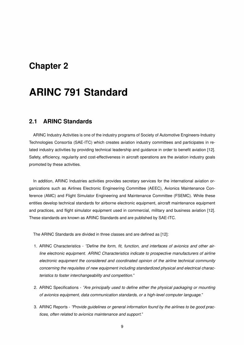
ARINC 791 characteristic defines an airborne Very Small Aperture Terminal (VSAT), also known as an
Aircraft Earth Station (AES), which uses commercial Ku or Ka-band satellite transponders [12]. Figure
2.1 illustrates the communication links between the AES and the Ground Earth Station (GES), passing
through the satellite.
The main function of the satcom systems is to provide aeronautical services by transmitting, receiving
and processing signals via satellite [13]. These services can be classified as safety and regularity com-
munications or non-safety related communications. The first classification covers the communications of
Air Traffic Services (ATS) and aircraft operators, known as Airline Operational Communications (AOC)
which impact the air transport safety and efficiency [13]. The non-safety related communications covers
private and public correspondence, such as Airline Administrative Communications (AAC) and Airline
Passenger Communications (APC) [13]. These services include several applications, such as, Internet
access, cellular telephony, email, and broadcast video and audio.
10
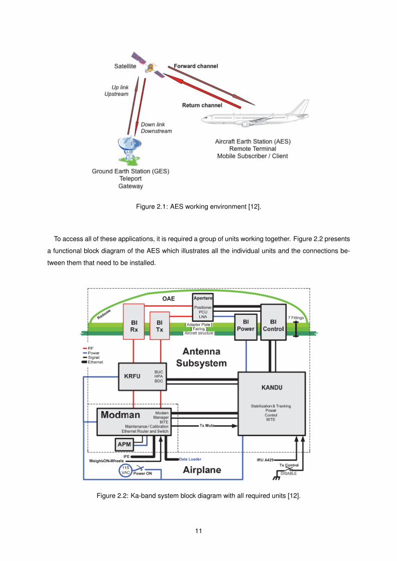
Figure 2.1: AES working environment [12].
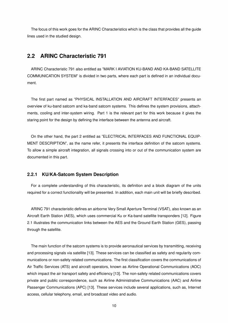
To access all of these applications, it is required a group of units working together. Figure 2.2 presents
a functional block diagram of the AES which illustrates all the individual units and the connections be-
tween them that need to be installed.
Figure 2.2: Ka-band system block diagram with all required units [12].
11
Jet Aviation not only designs the structural provisions for the satcom antenna, but also designs the
installation of all the required main units. The units under Jet Aviation systems’ installation design are
the antenna aperture, which is part of the Outside Antenna Equipment (OAE), the Ka/Ku-band Radio
Frequency Unit (KRFU) and Ka/Ku-band Aircraft Networking Data Unit (KANDU), which are part of the
inside antenna equipment, and finally the Modem and Manager (MODMAN) and Aircraft Personality
Module (APM), which are not part of the antenna subsystem [12]. Only the first three mentioned units
compose the antenna subsystem. These units are bought from Honeywell and will be described in the
next paragraphs.
• Antenna Aperture (AA)
The AA is a structure able to radiate with high gain and allows to receive and transmit ku-band
or ka-band radio frequency signals [12]. There are two types of antennas depending on the type
of solution which is required. The first type is used for small business jets where the antenna
is installed in the tail, this is known as Tail Mounted Antenna. The second type is the Fuselage
Mounted Antenna (FMA), as the name says, this antenna is installed in the fuselage and it is
commonly used for air transportation aviation. In the A320 project, this is the type of antenna
which will be installed since these are large aircraft. Figure 2.3 presents the antenna to be used in
the project.
Figure 2.3: Honeywell’s Fuselage Mounted Antenna [14].
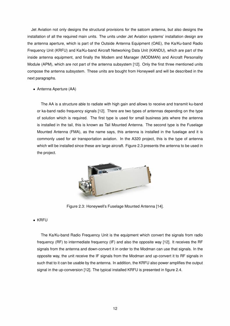
• KRFU
The Ka/Ku-band Radio Frequency Unit is the equipment which convert the signals from radio
frequency (RF) to intermediate frequency (IF) and also the opposite way [12]. It receives the RF
signals from the antenna and down-convert it in order to the Modman can use that signals. In the
opposite way, the unit receive the IF signals from the Modman and up-convert it to RF signals in
such that to it can be usable by the antenna. In addition, the KRFU also power amplifies the output
signal in the up-conversion [12]. The typical installed KRFU is presented in figure 2.4.
12

Figure 2.4: KRFU [14].
• KANDU
The Ka/Ku-band Aircraft Networking Data Unit is an equipment responsible for several func-
tions. The first, is controlling and monitoring the antenna subsystem while providing the power to
accomplish that. Secondly, the unit controls and manages the KRFU. Thirdly, it has the capabil-
ity of enabling or disabling the transmission. Finally, this provides the ethernet interface between
the KRFU, AA and Modman [12]. Figure 2.5 shows the Honeywell’s KANDU used in the system
installation.
Figure 2.5: KANDU [14].
• MODMAN
The Modman is a unit composed by two sub-units: the modem and manager, where each has
its own functions.
The Modem has several roles. The first is to impose the baseband data from the aircraft into a
RF carrier in order to can be transmitted by the antenna subsystem. In this case, the modem is
working as a modulator. In the inverse way, the modem works as a demodulator, it receives the IF
signals and convert them to baseband data [12]. In addition, this sub-unit also provides real-time
information to the antenna subsystem, such as signal strength [12].
13
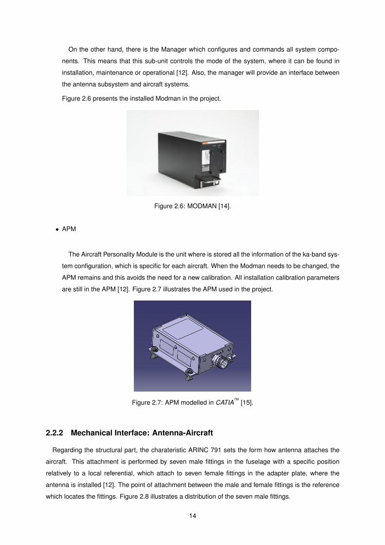
On the other hand, there is the Manager which configures and commands all system compo-
nents. This means that this sub-unit controls the mode of the system, where it can be found in
installation, maintenance or operational [12]. Also, the manager will provide an interface between
the antenna subsystem and aircraft systems.
Figure 2.6 presents the installed Modman in the project.
Figure 2.6: MODMAN [14].
• APM
The Aircraft Personality Module is the unit where is stored all the information of the ka-band sys-
tem configuration, which is specific for each aircraft. When the Modman needs to be changed, the
APM remains and this avoids the need for a new calibration. All installation calibration parameters
are still in the APM [12]. Figure 2.7 illustrates the APM used in the project.
Figure 2.7: APM modelled in CATIATM
[15].
2.2.2 Mechanical Interface: Antenna-Aircraft
Regarding the structural part, the charateristic ARINC 791 sets the form how antenna attaches the
aircraft. This attachment is performed by seven male fittings in the fuselage with a specific position
relatively to a local referential, which attach to seven female fittings in the adapter plate, where the
antenna is installed [12]. The point of attachment between the male and female fittings is the reference
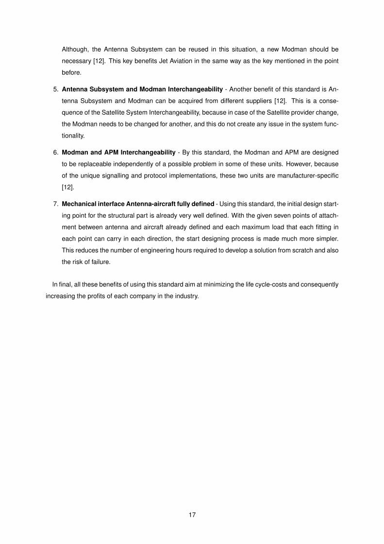
which locates the fittings. Figure 2.8 illustrates a distribution of the seven male fittings.
14
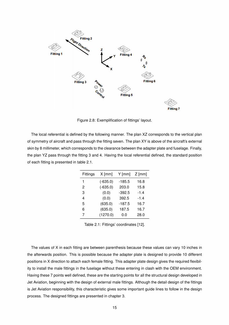
Figure 2.8: Exemplification of fittings’ layout.
The local referential is defined by the following manner. The plan XZ corresponds to the vertical plan
of symmetry of aircraft and pass through the fitting seven. The plan XY is above of the aircraft’s external
skin by 8 millimeter, which corresponds to the clearance between the adapter plate and fuselage. Finally,
the plan YZ pass through the fitting 3 and 4. Having the local referential defined, the standard position
of each fitting is presented in table 2.1.
Fittings X [mm] Y [mm] Z [mm]
1 (-635.0) -185.5 16.82 (-635.0) 203.0 15.83 (0.0) -392.5 -1.44 (0.0) 392.5 -1.45 (635.0) -187.5 16.76 (635.0) 187.5 16.77 (1270.0) 0.0 28.0
Table 2.1: Fittings’ coordinates [12].
The values of X in each fitting are between parenthesis because these values can vary 10 inches in
the afterwards position. This is possible because the adapter plate is designed to provide 10 different
positions in X direction to attach each female fitting. This adapter plate design gives the required flexibil-
ity to install the male fittings in the fuselage without these entering in clash with the OEM environment.
Having these 7 points well defined, these are the starting points for all the structural design developed in
Jet Aviation, beginning with the design of external male fittings. Although the detail design of the fittings
is Jet Aviation responsibility, this characteristic gives some important guide lines to follow in the design
process. The designed fittings are presented in chapter 3.
15

Additionally, it is presented the typical interface ultimate loads that each fittings have to be able to
carry without considering the bird strike loads. Table 2.2 presents these values.
Fitting No.Fx [N] Fy [N] Fz [N]
Forward AftSide
(Symmetrical)Down Up
1 - - 1100 400 40002 - - - 400 40003 1000 2300 - 2000 45004 1000 2300 - 2000 45005 - - 1100 1000 40006 - - - 1000 40007 - - - 800 8000
Table 2.2: Typical interface ultimate fittings’ Loads.
According to this standard, table 2.2 shows that each fitting must be designed only to withstand loads
in specific directions. This is possible by playing with the constraints in each couple of fittings by the use
of mechanisms to allow slipping in a specific axis. Furthermore, these does not experience any moment
in any direction due to the installed bearing in the fittings’ lug, which allow free rotation of the attachment
point between male and female fitting.
2.3 Advantages of using ARINC Standard
By using this standard as background for the design brings several advantages and positive aspects
to the final solution. These benefits are presented below.
1. Aircraft Type and Manufacturer Interchangeability - This standard is valid for all types of aircraft
and independent of the manufacturer [12]. Thus, the designed solution can be adapted to any
airframe, which means that there is a considerable time reduction in the conceptual design phase,
since it is only necessary to adapt the solution to the new environment.
2. Equipment Manufacturer Interchangeability - The equipments required in the installation are
not exclusive, different manufacturers’ equipments can fit in the standardized provisions [12]. This
key reduces the probability of Jet Aviation being stuck because of the lack of equipment in its
supplier’s stock and can not deliver their projects in the customers’ expectation time.
3. Frequency Band Interchangeability - The same structural solution is feasible for ka-band or ku-
band equipment [12]. This brings increased value in terms of reliability and flexibility to the final
product provided by Jet Aviation in a way that if one day the customers want to change to other
frequency band, they only need to replace the equipment.
4. Satellite System Interchangeability - This standard also provides flexibility regarding the satellite
provider. With the same antenna subsystem, it is possible to use different satellite systems [12].
16
Although, the Antenna Subsystem can be reused in this situation, a new Modman should be
necessary [12]. This key benefits Jet Aviation in the same way as the key mentioned in the point
before.
5. Antenna Subsystem and Modman Interchangeability - Another benefit of this standard is An-
tenna Subsystem and Modman can be acquired from different suppliers [12]. This is a conse-
quence of the Satellite System Interchangeability, because in case of the Satellite provider change,
the Modman needs to be changed for another, and this do not create any issue in the system func-
tionality.
6. Modman and APM Interchangeability - By this standard, the Modman and APM are designed
to be replaceable independently of a possible problem in some of these units. However, because
of the unique signalling and protocol implementations, these two units are manufacturer-specific
[12].
7. Mechanical interface Antenna-aircraft fully defined - Using this standard, the initial design start-
ing point for the structural part is already very well defined. With the given seven points of attach-
ment between antenna and aircraft already defined and each maximum load that each fitting in
each point can carry in each direction, the start designing process is made much more simpler.
This reduces the number of engineering hours required to develop a solution from scratch and also
the risk of failure.
In final, all these benefits of using this standard aim at minimizing the life cycle-costs and consequently
increasing the profits of each company in the industry.
17

Chapter 3
Ka-band System Structural Base
Design
3.1 Design’s Certification Requirements
Every aircraft has a document as an identification card, which includes all information concerning the
aircraft. All aircraft are only allowed to fly when they have this document. Information as general de-
scription of the aircraft, including its type and model, performance class and manufacturer, furthermore,
technical characteristics and operational limitations, operating and services instructions, and operational
suitability data are found there. This document is denominated as Type Certificate Data Sheet (TCDS).
Additionally, it provides essential information regarding the aircraft’s certification basis. This information
is required in the new modifications, in order to give a base line of the requirements that are needed to
show compliance.
In particular for the project, scope of this thesis, the certification basis for design change which Jet
Aviation elected to comply is the EASA certification specification 25 (CS25 - large aircraft) amendment
22. In addition, compliance with the FAA certification requirements in FAR 25 amendment 1 through
145 must be also ensured. For situations where is impracticable to comply with the last certification
specification, the certification basis of the TCDS - EASA IM.A.064 or FAA A28NM for the highest aircraft
standards will be used [11].
The certification specification is a document composed by several paragraphs, where each paragraph
gives the detailed requirement which needs to be complied. For each specific modification several
paragraphs are applied and are these which constrains the design. For the modification in study in this
work, specific for the designed structural provisions the paragraphs presented in table 3.1 are applied.
18

Paragraph Title Regulation AmendmentSubpart C - Structure
25.301 Loads CS-25 2225.303 Factor of Safety CS-25 2225.305 Strength and Deformation CS-25 2225.307 Proof of Structure CS-25 2225.321 Flight Loads - General CS-25 2225.365 Pressurized Compartment Loads CS-25 2225.561 Emergency Landing Conditions - General CS-25 22
Subpart D - Design and Construction25.613 Material Strength Properties and Design Values CS-25 2225.625 Fitting Factors CS-25 22
Table 3.1: Certification paragraphs applicable to the structural modification [16].
Some extracts from EASA CS-25 Amendment 22 are presented [17]:
• CS 25.301 - Loads
”(a) Strength requirements are specified in terms of limit loads (the maximum loads to be ex-
pected in service) and ultimate loads (limit loads multiplied by prescribed factors of safety). Unless
otherwise provided, prescribed loads are limit loads.”
• CS 25.303 - Factor of Safety
”Unless otherwise specified, a factor of safety of 1·5 must be applied to the prescribed limit load
which are considered external loads on the structure. When loading condition is prescribed in
terms of ultimate loads, a factor of safety need not be applied unless otherwise specified.”
• CS 25.305 - Strength and Deformation
”(a) The structure must be able to support limit loads without detrimental permanent deforma-
tion. At any load up to limit loads, the deformation may no interfere with safe operation.”
”(e) The aeroplane must be designed to withstand any vibration and buffeting that might occur
in any likely operating condition up to VD/MD, including stall and probable inadvertent excursions
beyond the boundaries of the buffet onset envelope. This must be shown by analysis, flight tests,
or other tests found necessary by the Agency.”
• CS 25.307 - Proof of Structure
”(a) Compliance with the strength and deformation requirements of this Subpart must be shown
for each critical loading condition. Structural analysis may be used only if the structure conforms to
that for which experience has shown this method to be reliable. In other cases, substantiating tests
19

must be made to load levels that are sufficient to verify structural behaviour up to loads specified
in CS 25.305.”
• CS 25.321 - Flight Loads (General)
”(a) Flight load factors represent the ratio of the aerodynamic force component (acting normal
to the assumed longitudinal axis of the aeroplane) to the weight of the aeroplane. A positive load
factor is one in which the aerodynamic force acts upward with respect to the aeroplane.”
”(d) The significant forces acting on the aeroplane must be placed in equilibrium in a ratio-
nal or conservative manner. The linear inertia forces must be considered in equilibrium with the
thrust and all aerodynamic loads, while the angular (pitching) inertia forces must be considered in
equilibrium with thrust and all aerodynamic moments, including moments due to loads on compo-
nents such as tail surfaces and nacelles. Critical thrust values in the range from zero to maximum
continuous thrust must be considered”
• CS 25.365 - Pressurized Compartment Loads
”(a) The aeroplane structure must be strong enough to withstand the flight loads combined with
pressure differential loads from zero up to the maximum relief valve setting.”
• CS 25.561 - Emergency Landing Conditions (General)
”(a) The aeroplane, although it may be damaged in emergency landing conditions on land or
water, must be designed as prescribed in this paragraph to protect each occupant under those
conditions.”
• CS 25.613 - Material Strength Properties and Design Values
”(a) Material strength properties must be based on enough tests of material meeting approved
specifications to establish design values on a statistical basis.”
• CS 25.625 - Fitting Factors
”(a) For each fitting whose strength is not proven by limit and ultimate load tests in which actual
stress conditions are simulated in the fitting and surrounding structures, a fitting factor of at least
1·15 must be applied to each part of – (1) The fitting; (2) The means of attachment; and (3) The
bearing on the joined members.”
20
3.2 Antenna Installation Position
Once there is an understanding about the certification requirements to have a feasible solution, the
next step before starting with the detail design of the structural components, is to decide where the
system will be installed. There are several possible positions, but in restricted area. This area refers
to the top of the fuselage in the upper crown area in order to allow the antenna to emit to the sky.
The optimum position in this area is aligned with the aircraft vertical plane of symmetry, because it is
the only direction where there is a reduced anti-symmetric flow perturbation. The references for the
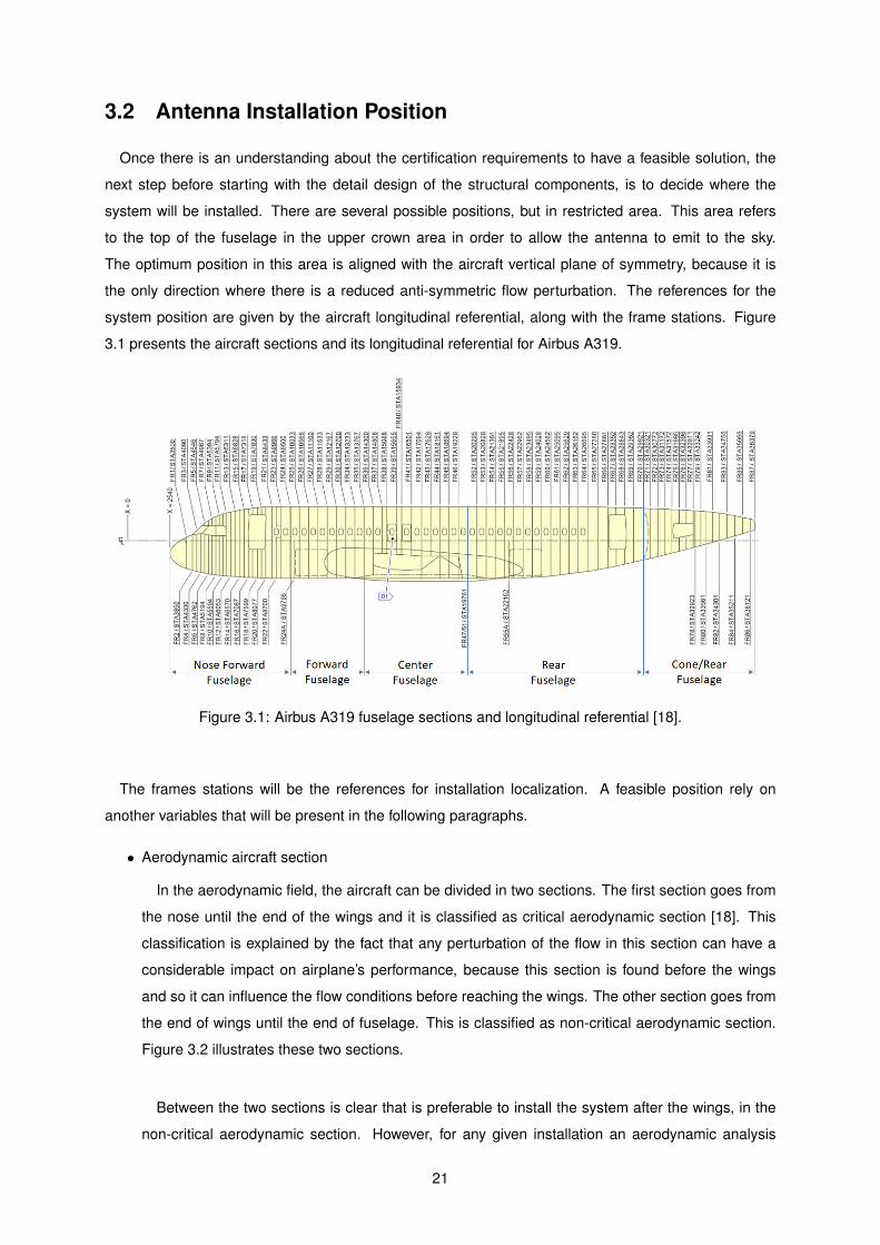
system position are given by the aircraft longitudinal referential, along with the frame stations. Figure
3.1 presents the aircraft sections and its longitudinal referential for Airbus A319.
Figure 3.1: Airbus A319 fuselage sections and longitudinal referential [18].
The frames stations will be the references for installation localization. A feasible position rely on
another variables that will be present in the following paragraphs.
• Aerodynamic aircraft section
In the aerodynamic field, the aircraft can be divided in two sections. The first section goes from
the nose until the end of the wings and it is classified as critical aerodynamic section [18]. This
classification is explained by the fact that any perturbation of the flow in this section can have a
considerable impact on airplane’s performance, because this section is found before the wings
and so it can influence the flow conditions before reaching the wings. The other section goes from
the end of wings until the end of fuselage. This is classified as non-critical aerodynamic section.
Figure 3.2 illustrates these two sections.
Between the two sections is clear that is preferable to install the system after the wings, in the
non-critical aerodynamic section. However, for any given installation an aerodynamic analysis
21
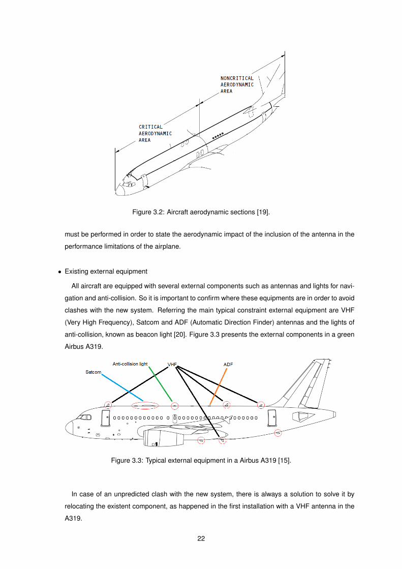
Figure 3.2: Aircraft aerodynamic sections [19].
must be performed in order to state the aerodynamic impact of the inclusion of the antenna in the
performance limitations of the airplane.
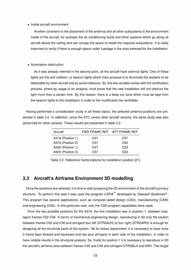
• Existing external equipment
All aircraft are equipped with several external components such as antennas and lights for navi-
gation and anti-collision. So it is important to confirm where these equipments are in order to avoid
clashes with the new system. Referring the main typical constraint external equipment are VHF
(Very High Frequency), Satcom and ADF (Automatic Direction Finder) antennas and the lights of
anti-collision, known as beacon light [20]. Figure 3.3 presents the external components in a green
Airbus A319.
Figure 3.3: Typical external equipment in a Airbus A319 [15].
In case of an unpredicted clash with the new system, there is always a solution to solve it by
relocating the existent component, as happened in the first installation with a VHF antenna in the
A319.
22
• Inside aircraft environment
Another constraint to the placement of the antenna and all other subsystems is the environment
inside of the aircraft, for example the air conditioning ducts and other systems which go along all
aircraft above the ceiling and can occupy the space to install the required subsystems. It is really
important to verify if there is enough space under fuselage in the area selected for the installation.
• Illumination obstruction
As it was already referred in the second point, all the aircraft have external lights. One of these
lights are the anti-collision, or beacon lights which main purpose is to illuminate the airplane to be
detectable by other aircraft and so avoid collisions. So, the last variable comes with the certification
process, where by usage of an analysis, must prove that the new installation will not obstruct the
light more than a certain limit. By this reason, there is a keep out zone which must be kept from
the beacon lights to the installation in order to the modification be certifiable.
Having performed a consideration study in all these topics, the selected antenna positions are pre-
sented in table 3.2. In addiction, since the STC covers other aircraft variants, the same study was also
performed for other variants. These results are presented in table 3.2.
Aircraft FWD FRAME REF AFT FRAME REF
A319 (Position 1) C47 C57A319 (Position 2) C57 C63A320 (Position 1) C47 C53A320 (Position 2) C57 C63
Table 3.2: Reference frame stations for installation position [21].
3.3 Aircraft’s Airframe Environment 3D modelling
Once the positions are selected, it is time to start preparing the 3D environment of the aircraft’s primary
structure. To perform this task it was used the program CATIATM
developed by Dassault Systemes R©.
This program has several applications, such as computer-aided design (CAD), manufacturing (CAM)
and engineering (CAE). In this particular task, only the CAD program capabilities were used.
From the two possible positions for the A319, the first installation was in position 1, between fuse-
lage’s frames C52-C56. In terms of mechanical engineering design, reproducing in 3D only the section
between frames C52 and C56 and stringers four left (STRG4LH) to four right (STRG4RH) is enough for
designing all the structural parts of the system. Yet for stress department, it is necessary to have more
3 frame bays forward and backward and two plus stringers in each side of the installation, in order to
have reliable results in the structural analysis. So, finally for position 1 it is necessary to reproduce in 3D
the aircraft’s airframe area between frames C45 and C59 and stringers STRG6LH and 6RH. This target
23

area is composed by two different aircraft’s sections. From frame C45 to C47/51 is the central fuselage
and from C47/51 to C59 is the rear fusleage. Figure 3.4 shows the complete A319’s airframe 3D model
of the referred target area.
Figure 3.4: Airbus A319’s airframe section between frames C45 and C59 and stringers STRG6LH and6RH, modelled in CATIA
TM.
This task was performed with the Airbus support which shared all the manuals concerning the target
aircraft models, such as Structural Repair Manuals (SRM), Illustrated Part Catalogues (IPC) and Aircraft
Maintenance Manuals (AMM). Additionally, all installation, assembly and part drawings were also pro-
vided. All these materials were obtained at the Airbus’s online portal named Airbus World. With these
complete information, it was possible to design in detail each part of the working airplane’s section.
Before presenting and describing each airframe’s structural component, it is important to highlight
one fact in the target environment section. In frame C47/51, there is an orbital junction, this means
this area is the junction between the two aircraft’s sections mentioned before. This area is specially
reinforced with some specific structural components in order to give additional strength to the structure.
These specific structural components will be also presented in the following paragraphs.
Firstly, the structural components from the central and rear fuselage will be presented and secondly,
the orbital junction components. Regarding the two fuselage sections, the main structural components
are the skin, stringers, frames and shear clips. Punctually, there may be a stringer splice section. A
detailed description of each component is presented below.
• Skin
The skin is a sheet metal part which covers all aircraft and gives torsional rigidity to the structure.
With the technological evolution, modern aircraft tend to be more optimized in terms of reducing
weight in order to achieve better performances. This optimization starts at the part level, where
each part is designed to have the minimum possible weight. An example of this, is the skin of
24

Airbus A319 which does not have an uniform thickness in the panel, it has several pockets with
different thicknesses. Figure 3.5 illustrates this example, the skin panel layout with pockets detail
and respective thicknesses for Airbus A319.
Figure 3.5: Skin Panel layout between frame C45 and C59 with pockets [18].
• Stringers
The stringers are a sheet metal component which goes along all the section and withstand the
tension and compression loads due to the longitudinal fuselage bending. In the A319, modelled
stringers have a J cross section with 0.063 inches (1.6mm) of thickness. The fuselage has a total
of 44 stringers all around. The modelled stringer and respective cross section is illustrated in figure
3.6.
(a) Ten modelled stringers in context (b) Typical stringer’s cross section
Figure 3.6: Airbus A319 3D modelled stringers and respective definition.
25
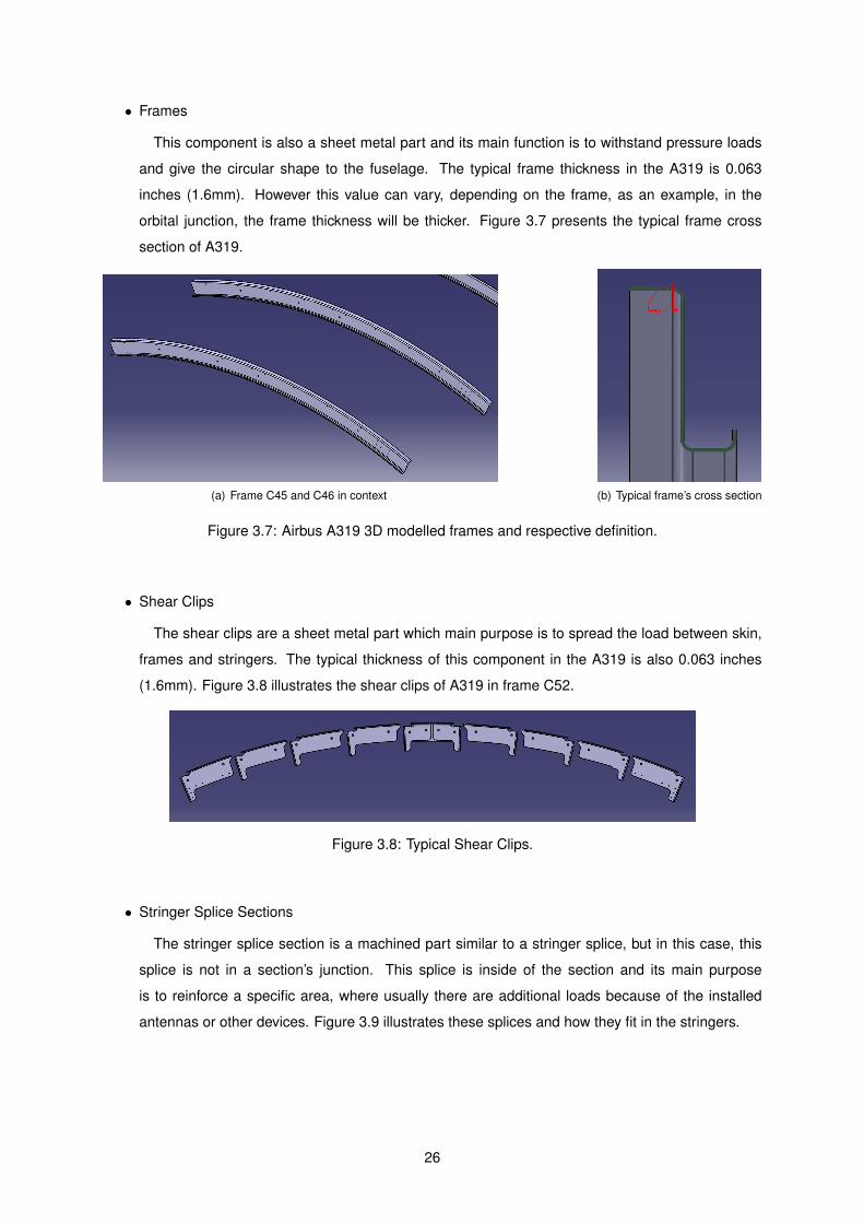
• Frames
This component is also a sheet metal part and its main function is to withstand pressure loads
and give the circular shape to the fuselage. The typical frame thickness in the A319 is 0.063
inches (1.6mm). However this value can vary, depending on the frame, as an example, in the
orbital junction, the frame thickness will be thicker. Figure 3.7 presents the typical frame cross
section of A319.
(a) Frame C45 and C46 in context (b) Typical frame’s cross section
Figure 3.7: Airbus A319 3D modelled frames and respective definition.
• Shear Clips
The shear clips are a sheet metal part which main purpose is to spread the load between skin,
frames and stringers. The typical thickness of this component in the A319 is also 0.063 inches
(1.6mm). Figure 3.8 illustrates the shear clips of A319 in frame C52.
Figure 3.8: Typical Shear Clips.
• Stringer Splice Sections
The stringer splice section is a machined part similar to a stringer splice, but in this case, this
splice is not in a section’s junction. This splice is inside of the section and its main purpose
is to reinforce a specific area, where usually there are additional loads because of the installed
antennas or other devices. Figure 3.9 illustrates these splices and how they fit in the stringers.
26
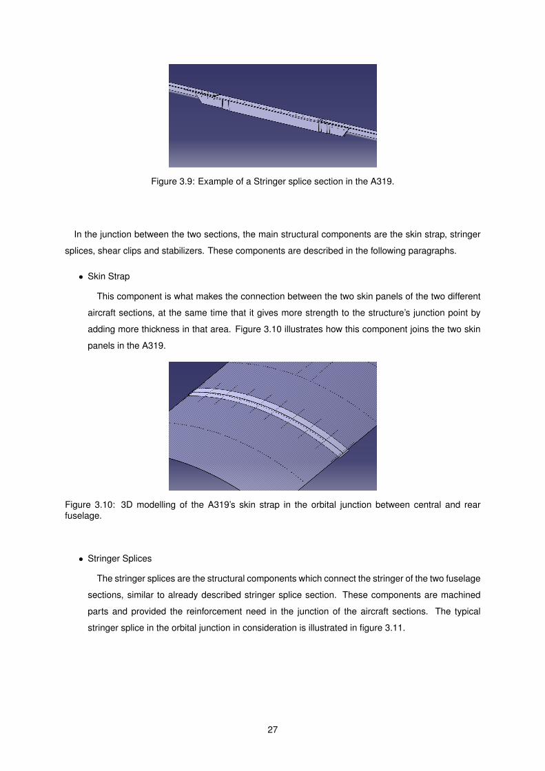
Figure 3.9: Example of a Stringer splice section in the A319.
In the junction between the two sections, the main structural components are the skin strap, stringer
splices, shear clips and stabilizers. These components are described in the following paragraphs.
• Skin Strap
This component is what makes the connection between the two skin panels of the two different
aircraft sections, at the same time that it gives more strength to the structure’s junction point by
adding more thickness in that area. Figure 3.10 illustrates how this component joins the two skin
panels in the A319.
Figure 3.10: 3D modelling of the A319’s skin strap in the orbital junction between central and rearfuselage.
• Stringer Splices
The stringer splices are the structural components which connect the stringer of the two fuselage
sections, similar to already described stringer splice section. These components are machined
parts and provided the reinforcement need in the junction of the aircraft sections. The typical
stringer splice in the orbital junction in consideration is illustrated in figure 3.11.
27
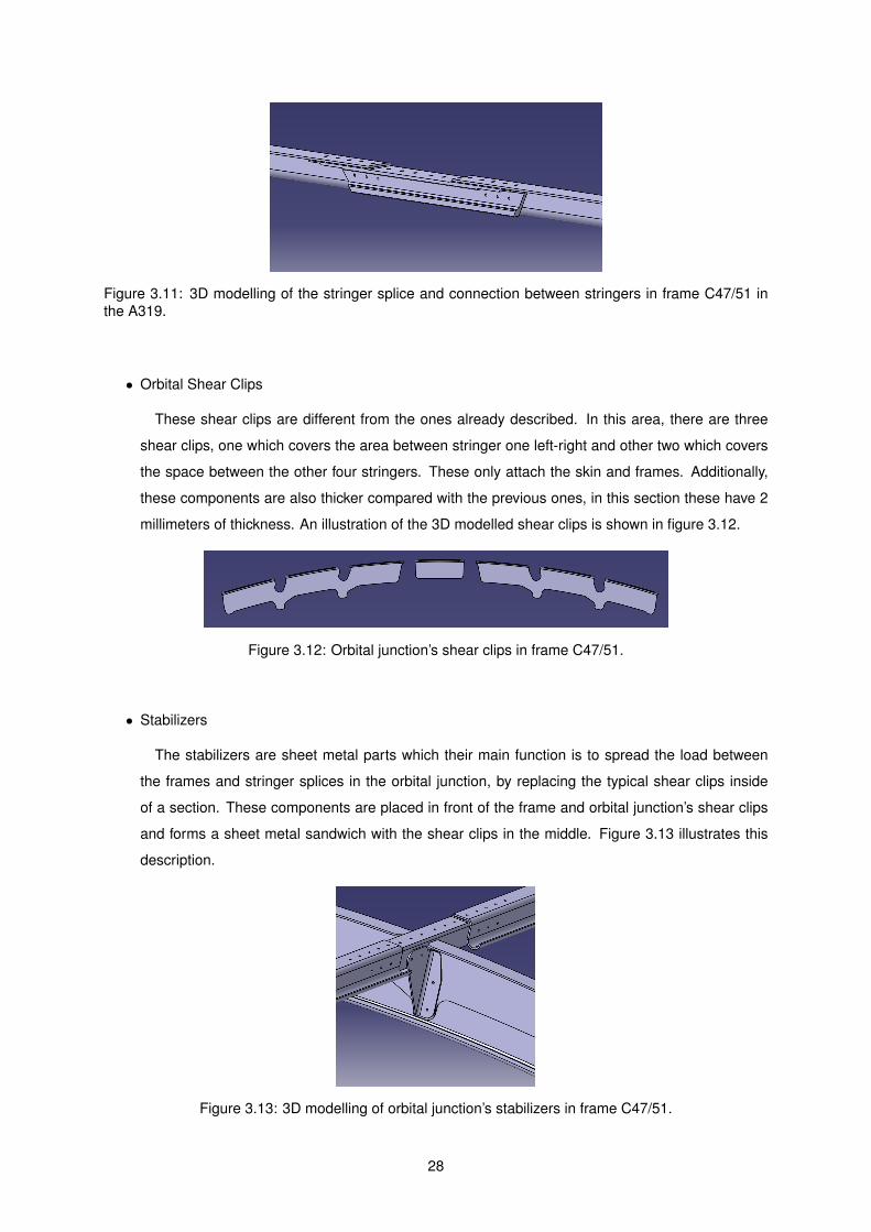
Figure 3.11: 3D modelling of the stringer splice and connection between stringers in frame C47/51 inthe A319.
• Orbital Shear Clips
These shear clips are different from the ones already described. In this area, there are three
shear clips, one which covers the area between stringer one left-right and other two which covers
the space between the other four stringers. These only attach the skin and frames. Additionally,
these components are also thicker compared with the previous ones, in this section these have 2
millimeters of thickness. An illustration of the 3D modelled shear clips is shown in figure 3.12.
Figure 3.12: Orbital junction’s shear clips in frame C47/51.
• Stabilizers
The stabilizers are sheet metal parts which their main function is to spread the load between
the frames and stringer splices in the orbital junction, by replacing the typical shear clips inside
of a section. These components are placed in front of the frame and orbital junction’s shear clips
and forms a sheet metal sandwich with the shear clips in the middle. Figure 3.13 illustrates this
description.
Figure 3.13: 3D modelling of orbital junction’s stabilizers in frame C47/51.
28
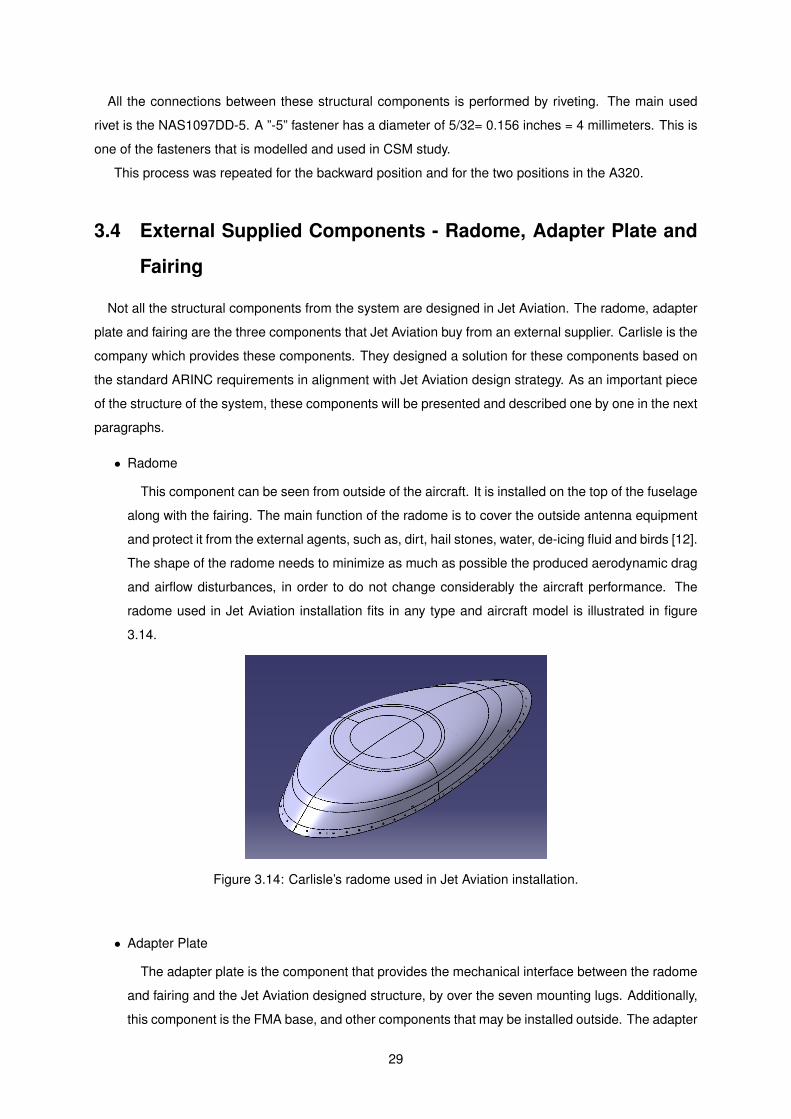
All the connections between these structural components is performed by riveting. The main used
rivet is the NAS1097DD-5. A ”-5” fastener has a diameter of 5/32= 0.156 inches = 4 millimeters. This is
one of the fasteners that is modelled and used in CSM study.
This process was repeated for the backward position and for the two positions in the A320.
3.4 External Supplied Components - Radome, Adapter Plate and
Fairing
Not all the structural components from the system are designed in Jet Aviation. The radome, adapter
plate and fairing are the three components that Jet Aviation buy from an external supplier. Carlisle is the
company which provides these components. They designed a solution for these components based on
the standard ARINC requirements in alignment with Jet Aviation design strategy. As an important piece
of the structure of the system, these components will be presented and described one by one in the next
paragraphs.
• Radome
This component can be seen from outside of the aircraft. It is installed on the top of the fuselage
along with the fairing. The main function of the radome is to cover the outside antenna equipment
and protect it from the external agents, such as, dirt, hail stones, water, de-icing fluid and birds [12].
The shape of the radome needs to minimize as much as possible the produced aerodynamic drag
and airflow disturbances, in order to do not change considerably the aircraft performance. The
radome used in Jet Aviation installation fits in any type and aircraft model is illustrated in figure
3.14.
Figure 3.14: Carlisle’s radome used in Jet Aviation installation.
• Adapter Plate
The adapter plate is the component that provides the mechanical interface between the radome
and fairing and the Jet Aviation designed structure, by over the seven mounting lugs. Additionally,
this component is the FMA base, and other components that may be installed outside. The adapter
29
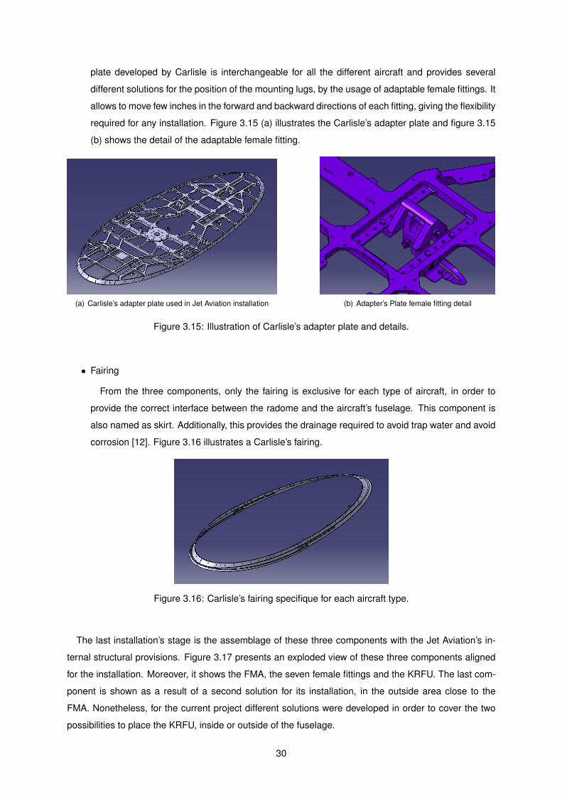
plate developed by Carlisle is interchangeable for all the different aircraft and provides several
different solutions for the position of the mounting lugs, by the usage of adaptable female fittings. It
allows to move few inches in the forward and backward directions of each fitting, giving the flexibility
required for any installation. Figure 3.15 (a) illustrates the Carlisle’s adapter plate and figure 3.15
(b) shows the detail of the adaptable female fitting.
(a) Carlisle’s adapter plate used in Jet Aviation installation (b) Adapter’s Plate female fitting detail
Figure 3.15: Illustration of Carlisle’s adapter plate and details.
• Fairing
From the three components, only the fairing is exclusive for each type of aircraft, in order to
provide the correct interface between the radome and the aircraft’s fuselage. This component is
also named as skirt. Additionally, this provides the drainage required to avoid trap water and avoid
corrosion [12]. Figure 3.16 illustrates a Carlisle’s fairing.
Figure 3.16: Carlisle’s fairing specifique for each aircraft type.
The last installation’s stage is the assemblage of these three components with the Jet Aviation’s in-
ternal structural provisions. Figure 3.17 presents an exploded view of these three components aligned
for the installation. Moreover, it shows the FMA, the seven female fittings and the KRFU. The last com-
ponent is shown as a result of a second solution for its installation, in the outside area close to the
FMA. Nonetheless, for the current project different solutions were developed in order to cover the two
possibilities to place the KRFU, inside or outside of the fuselage.
30

Figure 3.17: Exploded view of Carlisle’s external equipment and outside antenna equipment [15].
3.5 Jet Aviation’s Structural Provisions Design
Summarizing all the phases that have already been addressed. Firstly, it was presented the strategic
background which was used as baseline for Jet Aviation ka-band satcom system solution - the Industry
standard ARINC 791. Secondly, the certification requirements which the designed structural provisions
must comply with were presented. Thirdly, the optimum placement of the system and active constraints
were explored followed by the presentation of the structural components which composed the primary
structure of the target aircraft - Airbus A319. Finally, the external structural components which make
part the system but are not designed in Jet Aviation were also introduced. Now, it is only missing, the
structural provisions developed by Jet Aviation, which are the most relevant content for these thesis,
where a parametric optimization to the design will be performed.
The Jet Aviation’s base design is composed by seven external male fittings, a general idea was
already introduced in section 2.2.2 in the ARINC characteristic. Additionally, seven external doublers,
mounting gussets, intercostals and frame brackets compose the complete set of the Jet Aviation’s struc-
tural provisions. The external aircraft fittings are used to secure an adapter plate that support the an-
tenna mounting plate and radome. Each fitting is attached to the aircraft external fuselage surface
through a doubler. A mounting gusset is installed inside the fuselage along with each external fitting,
supported by internal intercostals within the fuselage supported by the fuselage frames. The connection
between these components is done by several different fasteners.
For each of these components will be explored the design process and the constraints which play
an important role in the design of these components, starting from the most external component, the
fittings and ends in the frame bracket. All of these components are sized and analysed under several
failures modes that are identified and checked for structural integrity. Figure 3.18 illustrates the complete
assembly of Jet Aviation’s design and the numbering for each groups of components for identification
purposes.
31
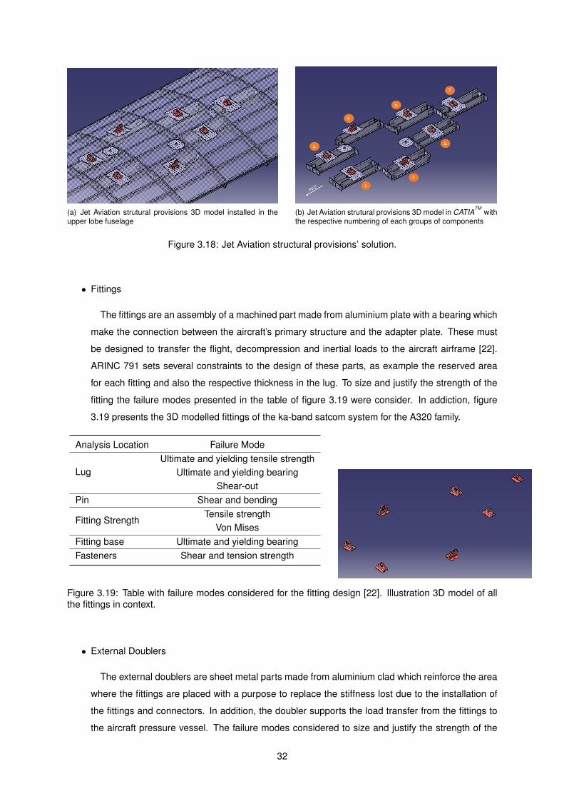
(a) Jet Aviation strutural provisions 3D model installed in theupper lobe fuselage
(b) Jet Aviation strutural provisions 3D model in CATIATM
withthe respective numbering of each groups of components
Figure 3.18: Jet Aviation structural provisions’ solution.
• Fittings
The fittings are an assembly of a machined part made from aluminium plate with a bearing which
make the connection between the aircraft’s primary structure and the adapter plate. These must
be designed to transfer the flight, decompression and inertial loads to the aircraft airframe [22].
ARINC 791 sets several constraints to the design of these parts, as example the reserved area
for each fitting and also the respective thickness in the lug. To size and justify the strength of the
fitting the failure modes presented in the table of figure 3.19 were consider. In addiction, figure
3.19 presents the 3D modelled fittings of the ka-band satcom system for the A320 family.
Analysis Location Failure Mode
LugUltimate and yielding tensile strength
Ultimate and yielding bearingShear-out
Pin Shear and bending
Fitting StrengthTensile strength
Von MisesFitting base Ultimate and yielding bearingFasteners Shear and tension strength
Figure 3.19: Table with failure modes considered for the fitting design [22]. Illustration 3D model of allthe fittings in context.
• External Doublers
The external doublers are sheet metal parts made from aluminium clad which reinforce the area
where the fittings are placed with a purpose to replace the stiffness lost due to the installation of
the fittings and connectors. In addition, the doubler supports the load transfer from the fittings to
the aircraft pressure vessel. The failure modes considered to size and justify the strength of the
32
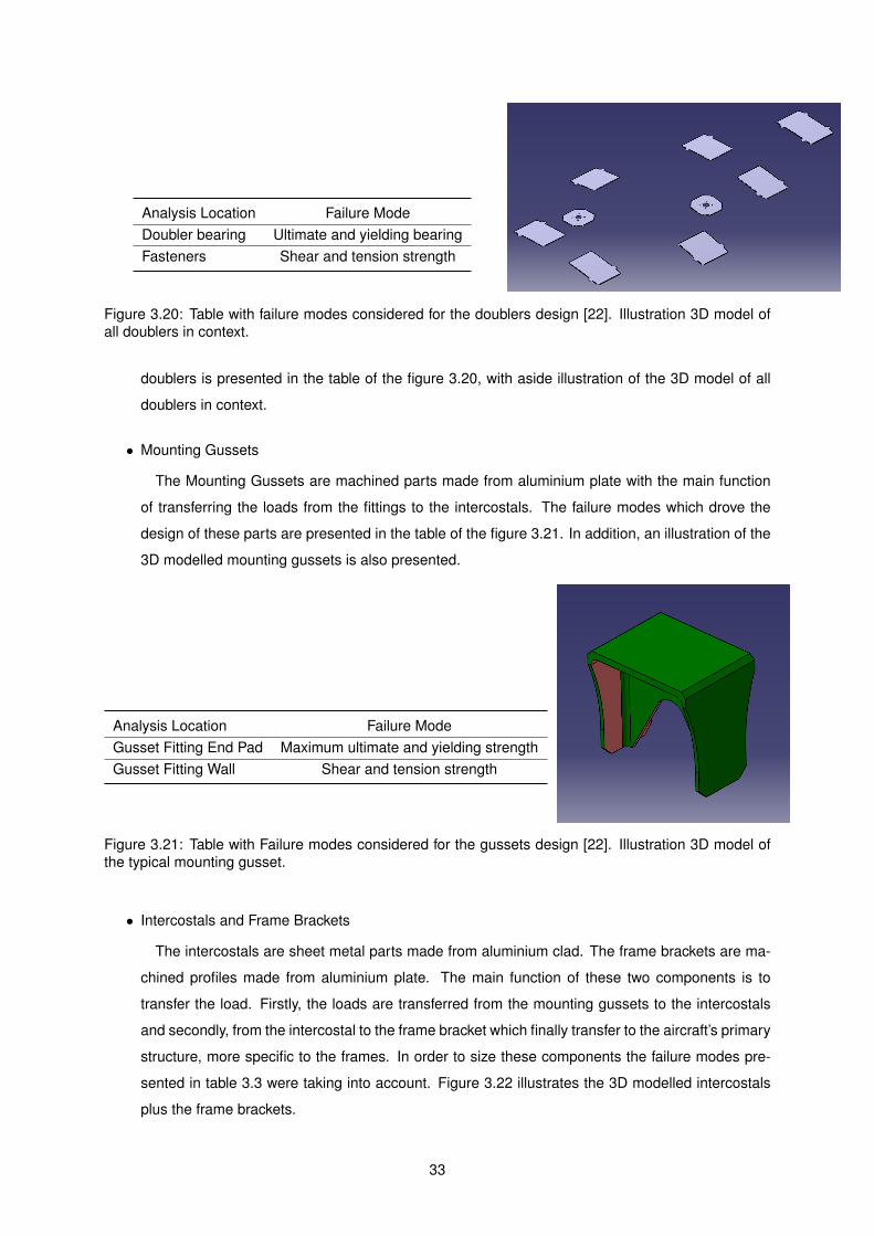
Analysis Location Failure ModeDoubler bearing Ultimate and yielding bearingFasteners Shear and tension strength
Figure 3.20: Table with failure modes considered for the doublers design [22]. Illustration 3D model ofall doublers in context.
doublers is presented in the table of the figure 3.20, with aside illustration of the 3D model of all
doublers in context.
• Mounting Gussets
The Mounting Gussets are machined parts made from aluminium plate with the main function
of transferring the loads from the fittings to the intercostals. The failure modes which drove the
design of these parts are presented in the table of the figure 3.21. In addition, an illustration of the
3D modelled mounting gussets is also presented.
Analysis Location Failure ModeGusset Fitting End Pad Maximum ultimate and yielding strengthGusset Fitting Wall Shear and tension strength
Figure 3.21: Table with Failure modes considered for the gussets design [22]. Illustration 3D model ofthe typical mounting gusset.
• Intercostals and Frame Brackets
The intercostals are sheet metal parts made from aluminium clad. The frame brackets are ma-
chined profiles made from aluminium plate. The main function of these two components is to
transfer the load. Firstly, the loads are transferred from the mounting gussets to the intercostals
and secondly, from the intercostal to the frame bracket which finally transfer to the aircraft’s primary
structure, more specific to the frames. In order to size these components the failure modes pre-
sented in table 3.3 were taking into account. Figure 3.22 illustrates the 3D modelled intercostals
plus the frame brackets.
33
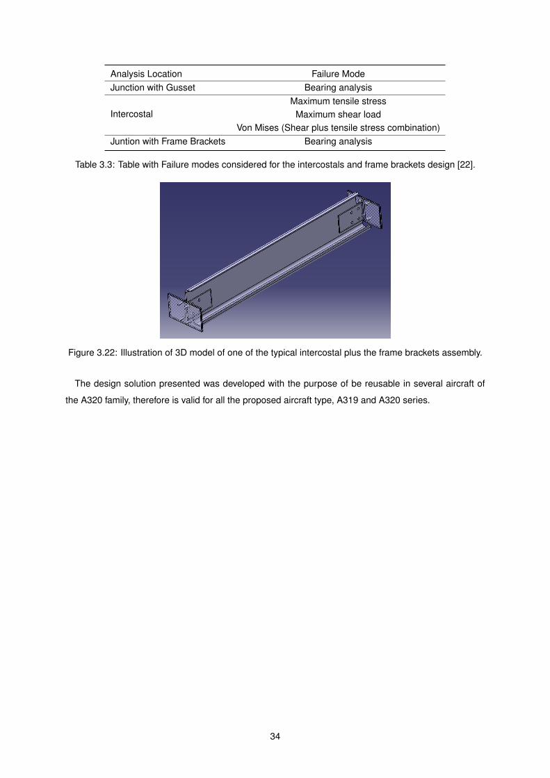
Analysis Location Failure ModeJunction with Gusset Bearing analysis
IntercostalMaximum tensile stress
Maximum shear loadVon Mises (Shear plus tensile stress combination)
Juntion with Frame Brackets Bearing analysis
Table 3.3: Table with Failure modes considered for the intercostals and frame brackets design [22].
Figure 3.22: Illustration of 3D model of one of the typical intercostal plus the frame brackets assembly.
The design solution presented was developed with the purpose of be reusable in several aircraft of
the A320 family, therefore is valid for all the proposed aircraft type, A319 and A320 series.
34
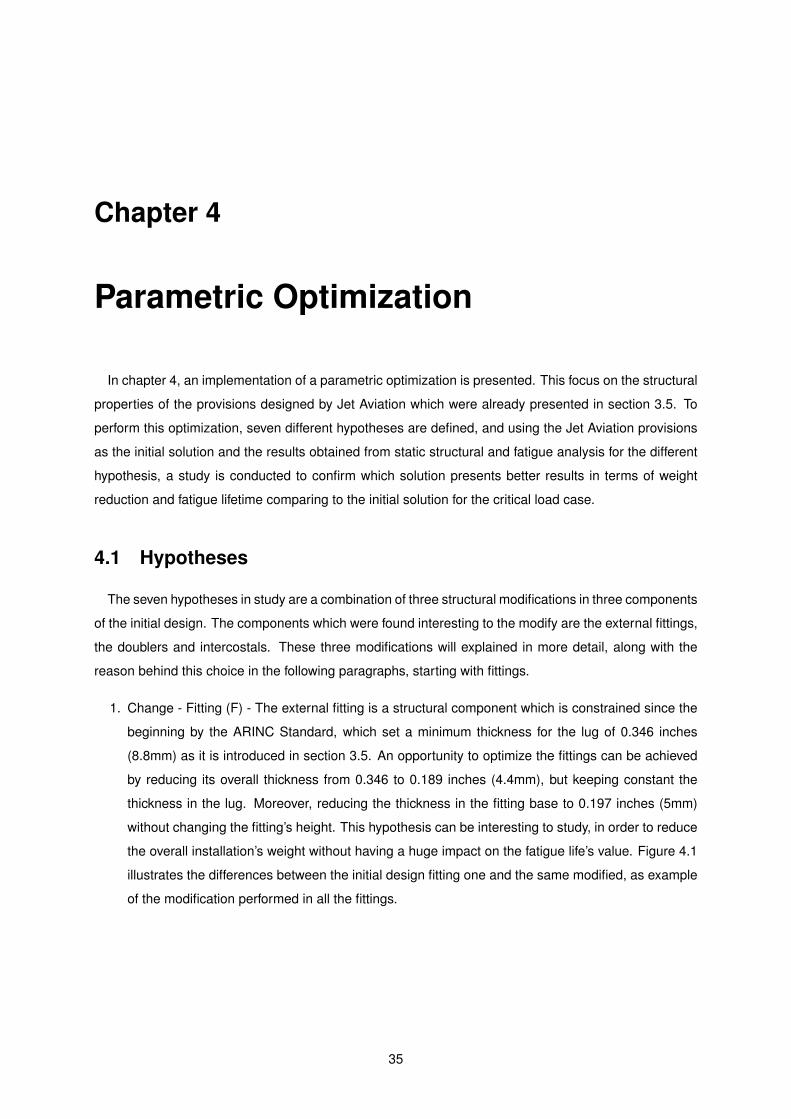
Chapter 4
Parametric Optimization
In chapter 4, an implementation of a parametric optimization is presented. This focus on the structural
properties of the provisions designed by Jet Aviation which were already presented in section 3.5. To
perform this optimization, seven different hypotheses are defined, and using the Jet Aviation provisions
as the initial solution and the results obtained from static structural and fatigue analysis for the different
hypothesis, a study is conducted to confirm which solution presents better results in terms of weight
reduction and fatigue lifetime comparing to the initial solution for the critical load case.
4.1 Hypotheses
The seven hypotheses in study are a combination of three structural modifications in three components
of the initial design. The components which were found interesting to the modify are the external fittings,
the doublers and intercostals. These three modifications will explained in more detail, along with the
reason behind this choice in the following paragraphs, starting with fittings.
1. Change - Fitting (F) - The external fitting is a structural component which is constrained since the
beginning by the ARINC Standard, which set a minimum thickness for the lug of 0.346 inches
(8.8mm) as it is introduced in section 3.5. An opportunity to optimize the fittings can be achieved
by reducing its overall thickness from 0.346 to 0.189 inches (4.4mm), but keeping constant the
thickness in the lug. Moreover, reducing the thickness in the fitting base to 0.197 inches (5mm)
without changing the fitting’s height. This hypothesis can be interesting to study, in order to reduce
the overall installation’s weight without having a huge impact on the fatigue life’s value. Figure 4.1
illustrates the differences between the initial design fitting one and the same modified, as example
of the modification performed in all the fittings.
35

(a) Initial design fitting 1 (b) Modified fitting 1
Figure 4.1: Modified versus initial design fitting one.
2. Change - Doublers (D) - In Jet Aviation, the doublers are designed following a ”repair” logic given
by the SRM, which states that the external doubler must be 0.008 inches (0.2 mm) thicker than the
skin in touch [18]. In contrast to this methodology, it will be used the ”new design” logic where it
will be studied and justified the case where the doubler’s thickness will be set to the same of the
skin. Table 4.1 presents the initial design value and the modified one for the doublers’ thickness.
Doubler Thickness [in]Initial doublers 0.071Modified doublers 0.063
Table 4.1: Doubler’s thickness of the initial design and the modified.
3. Change - Intercostal (I) - Before starting the A320 family project, it was developed the solution for
the Boeing Business Jet 737 family. In that solution the intercostals have a thickness of 0.08 inches
(2mm) whereas in the current project the intercostals have a thickness of 0.1 inches (2.54mm). It
is intend to study the usage of intercostals with the same thickness of the versions used on Boeing
737 solution. Table 4.2 summarize the information in consideration for this study.
Intercostal Thickness [in]Initial Design 0.1Case Study (B737 Family Solution) 0.08
Table 4.2: Intercostals’ thickness of the initial design and the modified.
From now on, the three changes are denominated as F,D and I referring the modifications on the
Fittings, Doublers and Intercostals to be more clear the different hypotheses in study. Table 4.3 presents
the complete set of hypotheses proposed for the study.
36
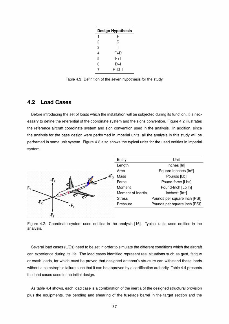
Design Hypothesis1 F2 D3 I4 F+D5 F+I6 D+I7 F+D+I
Table 4.3: Definition of the seven hypothesis for the study.
4.2 Load Cases
Before introducing the set of loads which the installation will be subjected during its function, it is nec-
essary to define the referential of the coordinate system and the signs convention. Figure 4.2 illustrates
the reference aircraft coordinate system and sign convention used in the analysis. In addition, since
the analysis for the base design were performed in imperial units, all the analysis in this study will be
performed in same unit system. Figure 4.2 also shows the typical units for the used entities in imperial
system.
Entity UnitLength Inches [In]Area Square Innches [In2]Mass Pounds [Lb]Force Pound-force [Lbs]Moment Pound-Inch [Lb.In]Moment of Inertia Inches4 [In4]Stress Pounds per square inch [PSI]Pressure Pounds per square inch [PSI]
Figure 4.2: Coordinate system used entities in the analysis [16]. Typical units used entities in theanalysis.
Several load cases (L/Cs) need to be set in order to simulate the different conditions which the aircraft
can experience during its life. The load cases identified represent real situations such as gust, fatigue
or crash loads, for which must be proved that designed antenna’s structure can withstand these loads
without a catastrophic failure such that it can be approved by a certification authority. Table 4.4 presents
the load cases used in the initial design.
As table 4.4 shows, each load case is a combination of the inertia of the designed structural provision
plus the equipments, the bending and shearing of the fuselage barrel in the target section and the
37
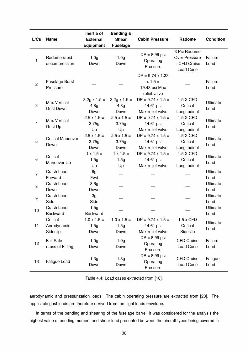
L/Cs NameInertia ofExternal
Equipment
Bending &Shear
FuselageCabin Pressure Radome Condition
1Radome rapiddecompression
1.0gDown
1.0gDown
DP = 8.99 psiOperatingPressure
3 Psi RadomeOver Pressure+ CFD Cruise
Load Case
FailureLoad
2Fuselage BurstPressure
— —
DP = 9.74 x 1.33x 1.5 =
19.43 psi Maxrelief valve
—FailureLoad
3Max VerticalGust Down
3.2g x 1.5 =4.8g
Down
3.2g x 1.5 =4.8g
Down
DP = 9.74 x 1.5 =14.61 psi
Max relief valve
1.5 X CFDCritical
Longitudinal
UltimateLoad
4Max VerticalGust Up
2.5 x 1.5 =3.75g
Up
2.5 x 1.5 =3.75g
Up
DP = 9.74 x 1.5 =14.61 psi
Max relief valve
1.5 X CFDCritical
Longitudinal
UltimateLoad
5Critical ManeuverDown
2.5 x 1.5 =3.75gDown
2.5 x 1.5 =3.75gDown
DP = 9.74 x 1.5 =14.61 psi
Max relief valve
1.5 X CFDCritical
Longitudinal
UltimateLoad
6CriticalManeuver Up
1 x 1.5 =1.5gUp
1 x 1.5 =1.5gUp
DP = 9.74 x 1.5 =14.61 psi
Max relief valve
1.5 X CFDCritical
Longitudinal
UltimateLoad
7Crash LoadForward
9gFwd
— — —UltimateLoad
8Crash LoadDown
8.6gDown
— — —UltimateLoad
9Crash LoadSide
3gSide
— — —UltimateLoad
10Crash LoadBackward
1.5gBackward
— — —UltimateLoad
11CriticalAerodynamicSideslip
1.0 x 1.5 =1.5g
Down
1.0 x 1.5 =1.5g
Down
DP = 9.74 x 1.5 =14.61 psi
Max relief valve
1.5 x CFDCriticalSideslip
UltimateLoad
12Fail Safe(Loss of Fitting)
1.0gDown
1.0gDown
DP = 8.99 psiOperatingPressure
CFD CruiseLoad Case
FailureLoad
13 Fatigue Load1.3g
Down1.3g
Down
DP = 8.99 psiOperatingPressure
CFD CruiseLoad Case
FatigueLoad
Table 4.4: Load cases extracted from [16].
aerodynamic and pressurization loads. The cabin operating pressure are extracted from [23]. The
applicable gust loads are therefore derived from the flight loads envelope.
In terms of the bending and shearing of the fuselage barrel, it was considered for the analysis the
highest value of bending moment and shear load presented between the aircraft types being covered in
38
the several installation positions, in order to analyse the critical condition and so the other possibilities
are covered by this analysis. Therefore, all the different installations are substantiated by the same
analysis.
• Load case 1 simulates an ultimate decompression condition, with a very conservative value of
pressure for the maximum differential pressure between the radome and the external environment.
This failure load is combined with the operating load conditions of the aircraft: 1g inertia and
fuselage loads, aerodynamic cruise loads, normal cabin operating pressure. The aerodynamic
loads are extracted from the Computational Fluid Dynamics (CFD) analyses performed by the
stress department.
• Load case 2 simulates the cabin burst pressure condition. This failure load case is needed to show
compliance with two extra paragraphs: 25.365(d) and 25.303. The paragraph 25.365 defines the
pressurized structure limit load as 1.33 times the maximum relief valve setting. This must be
multiplied by 1.5 as by paragraph 25.303 to obtain the corresponding ultimate load condition.
• Load cases 3 through 6 represent the critical manoeuvrer and gust conditions. The gust loads
factors are extracted from [23] - Airbus flight loads envelopes.
• There are more three crash load cases, but these are not consider because they are already
covered by Load Cases 8, 9 and 10. These cover the crash Load cases 6g down, 3g side and 1.5g
backward.
• Load cases 7 to 10 are crash load cases.
For this parametric optimization the first four load cases are the critical ones, however, it is only
used the load case number 1, radome rapid decompression load, which can be assumed as a good
approximation of the most critical load case. In addiction, for the fatigue analysis the load case 13, the
fatigue load, is used.
4.3 Methodologies
To conduct the parametric optimization, two types of analyses were performed. Firstly, a static struc-
tural analysis to verify the new safety margins of the modified parts and confirm the reliability of the over-
all installation after the modification. The second, a fatigue analysis which aims at calculating the new
fatigue life for the seven different hypotheses. For the two analyses the engineering software FEMAP
developed by Siemens PLM Software was used to build the finite element model, execute the simula-
tions and present the post-processing results. This model was built by the stress department with the
support of mechanical side which prepare all the geometries for the model, where I actively contribute.
The complete description of this model is presented in [16]. All the steps executed in the two analyses
are presented in the following paragraphs.
39
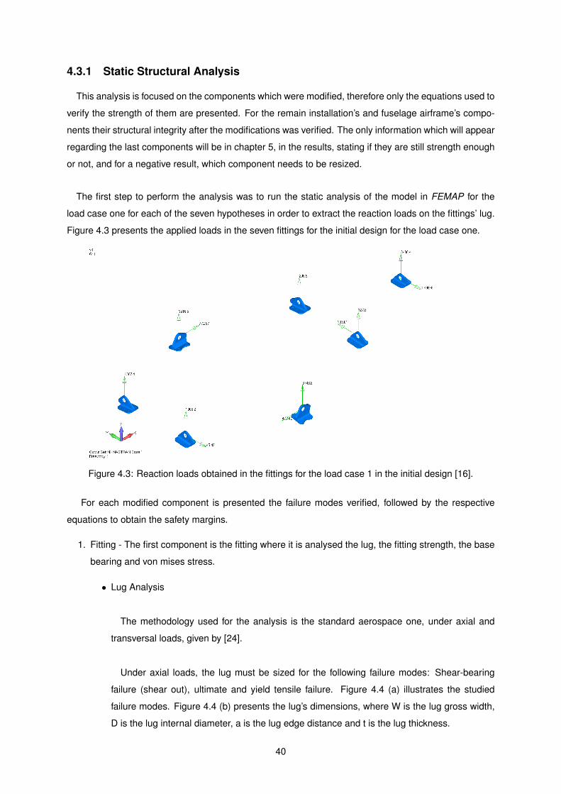
4.3.1 Static Structural Analysis
This analysis is focused on the components which were modified, therefore only the equations used to
verify the strength of them are presented. For the remain installation’s and fuselage airframe’s compo-
nents their structural integrity after the modifications was verified. The only information which will appear
regarding the last components will be in chapter 5, in the results, stating if they are still strength enough
or not, and for a negative result, which component needs to be resized.
The first step to perform the analysis was to run the static analysis of the model in FEMAP for the
load case one for each of the seven hypotheses in order to extract the reaction loads on the fittings’ lug.
Figure 4.3 presents the applied loads in the seven fittings for the initial design for the load case one.
Figure 4.3: Reaction loads obtained in the fittings for the load case 1 in the initial design [16].
For each modified component is presented the failure modes verified, followed by the respective
equations to obtain the safety margins.
1. Fitting - The first component is the fitting where it is analysed the lug, the fitting strength, the base
bearing and von mises stress.
• Lug Analysis
The methodology used for the analysis is the standard aerospace one, under axial and
transversal loads, given by [24].
Under axial loads, the lug must be sized for the following failure modes: Shear-bearing
failure (shear out), ultimate and yield tensile failure. Figure 4.4 (a) illustrates the studied
failure modes. Figure 4.4 (b) presents the lug’s dimensions, where W is the lug gross width,
D is the lug internal diameter, a is the lug edge distance and t is the lug thickness.
40
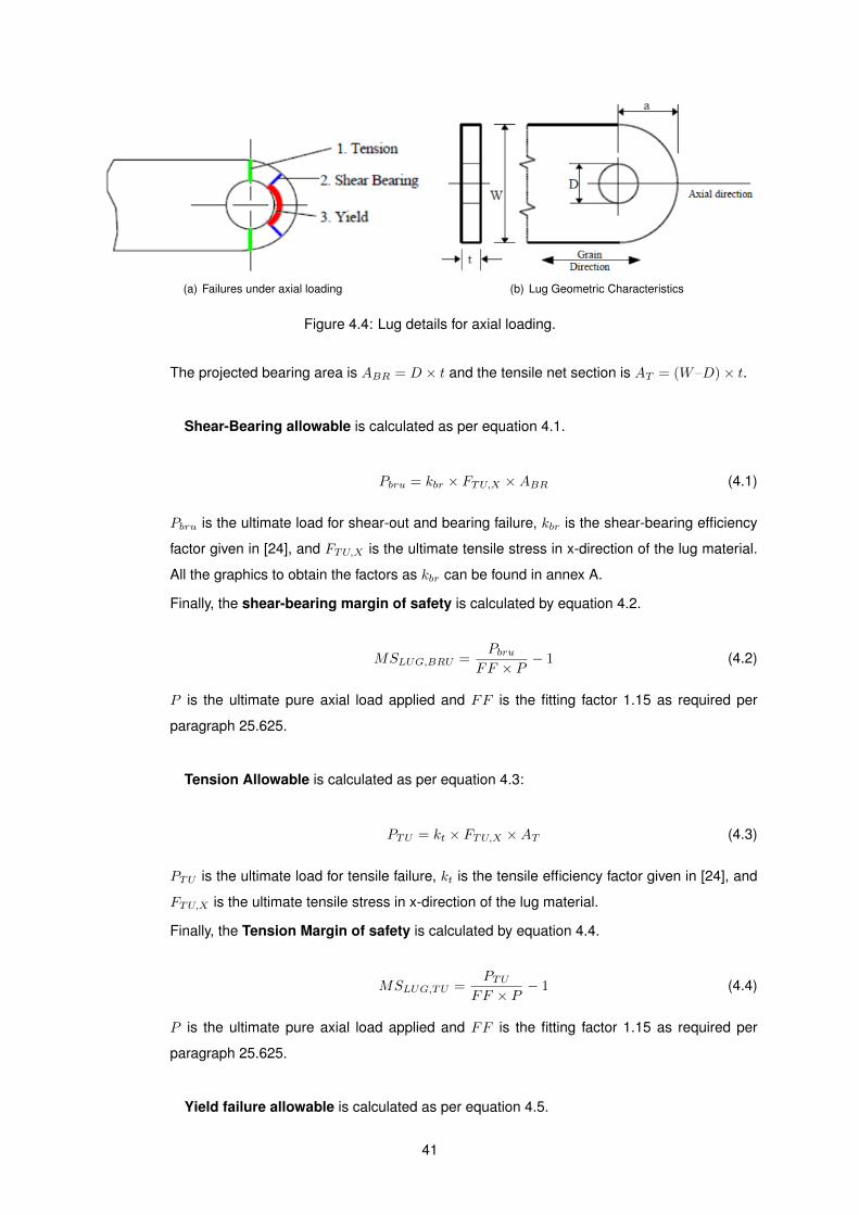
(a) Failures under axial loading (b) Lug Geometric Characteristics
Figure 4.4: Lug details for axial loading.
The projected bearing area is ABR = D × t and the tensile net section is AT = (W–D) × t.
Shear-Bearing allowable is calculated as per equation 4.1.
Pbru = kbr × FTU,X ×ABR (4.1)
Pbru is the ultimate load for shear-out and bearing failure, kbr is the shear-bearing efficiency
factor given in [24], and FTU,X is the ultimate tensile stress in x-direction of the lug material.
All the graphics to obtain the factors as kbr can be found in annex A.
Finally, the shear-bearing margin of safety is calculated by equation 4.2.
MSLUG,BRU =Pbru
FF × P− 1 (4.2)
P is the ultimate pure axial load applied and FF is the fitting factor 1.15 as required per
paragraph 25.625.
Tension Allowable is calculated as per equation 4.3:
PTU = kt × FTU,X ×AT (4.3)
PTU is the ultimate load for tensile failure, kt is the tensile efficiency factor given in [24], and
FTU,X is the ultimate tensile stress in x-direction of the lug material.
Finally, the Tension Margin of safety is calculated by equation 4.4.
MSLUG,TU =PTU
FF × P− 1 (4.4)
P is the ultimate pure axial load applied and FF is the fitting factor 1.15 as required per
paragraph 25.625.
Yield failure allowable is calculated as per equation 4.5.
41

PTY,X = C × (FTY,X
FTU,X) × PU,MIN (4.5)
PTY,X is the yield load, C is the yield factor given in [24], FTY,X is the ultimate tensile stress
in x-direction of the lug material and PU,MIN is the minimum between PTU and PBRU .
Finally, the Yield Margin of safety is calculated by equation 4.6.
MSLUG,Y =PTY,X
FF × PY− 1 (4.6)
PY is the limit pure axial load applied and FF is the fitting factor 1.15 as required per para-
graph 25.625.
Under transversal loads, the lug must be sized again for the same failure modes as in axial
loading: Ultimate and yield tensile and shear-bearing failure. Figure 4.5 (a) illustrates the
studied failure modes.
(a) Failures under transversal loading (b) Lug Geometric Characteristics
Figure 4.5: Lug details for transversal loading.
Figure 4.5 (b) presents the lug’s dimensions, where A1 and A4 are A1 = A4 = t2 × (W − D√
2),
A2 is A2 = t2 × (W − D), A3 is the least area on any radial section around the hole A3 =
t2 × (2 × a−D).
The average area is AAVG = 63
A1+ 1
A2+ 1
A3+ 1
A4
and the projected bearing area is ABR = D× t.
Tension Allowable is calculated as per equation 4.7.
PTRU = ktru × FTU,Y ×ABR (4.7)
PTRU is the ultimate load for tensile failure under transversal loads, ktru is the tensile effi-
ciency factor for transversal loads given in [24], and FTU,Y is the ultimate tensile stress in
transverse direction of the lug material.
Finally, the Tension Margin of safety is calculated by equation 4.8.
42
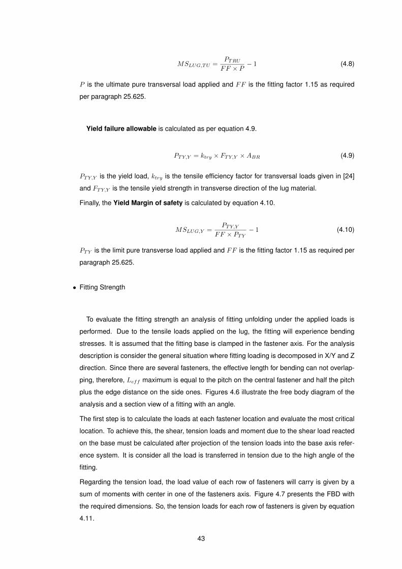
MSLUG,TU =PTRU
FF × P− 1 (4.8)
P is the ultimate pure transversal load applied and FF is the fitting factor 1.15 as required
per paragraph 25.625.
Yield failure allowable is calculated as per equation 4.9.
PTY,Y = ktry × FTY,Y ×ABR (4.9)
PTY,Y is the yield load, ktry is the tensile efficiency factor for transversal loads given in [24]
and FTY,Y is the tensile yield strength in transverse direction of the lug material.
Finally, the Yield Margin of safety is calculated by equation 4.10.
MSLUG,Y =PTY,Y
FF × PTY− 1 (4.10)
PTY is the limit pure transverse load applied and FF is the fitting factor 1.15 as required per
paragraph 25.625.
• Fitting Strength
To evaluate the fitting strength an analysis of fitting unfolding under the applied loads is
performed. Due to the tensile loads applied on the lug, the fitting will experience bending
stresses. It is assumed that the fitting base is clamped in the fastener axis. For the analysis
description is consider the general situation where fitting loading is decomposed in X/Y and Z
direction. Since there are several fasteners, the effective length for bending can not overlap-
ping, therefore, Leff maximum is equal to the pitch on the central fastener and half the pitch
plus the edge distance on the side ones. Figures 4.6 illustrate the free body diagram of the
analysis and a section view of a fitting with an angle.
The first step is to calculate the loads at each fastener location and evaluate the most critical
location. To achieve this, the shear, tension loads and moment due to the shear load reacted
on the base must be calculated after projection of the tension loads into the base axis refer-
ence system. It is consider all the load is transferred in tension due to the high angle of the
fitting.
Regarding the tension load, the load value of each row of fasteners will carry is given by a
sum of moments with center in one of the fasteners axis. Figure 4.7 presents the FBD with
the required dimensions. So, the tension loads for each row of fasteners is given by equation
4.11.
43
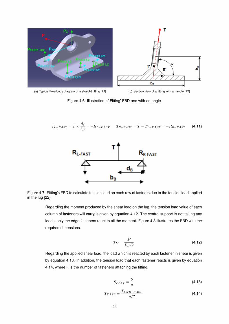
(a) Typical Free body diagram of a straight fitting [22] (b) Section view of a fitting with an angle [22]
Figure 4.6: Illustration of Fitting’ FBD and with an angle.
TL−FAST = T × dbbB
= −RL−FAST TR−FAST = T − TL−FAST = −RR−FAST (4.11)
Figure 4.7: Fitting’s FBD to calculate tension load on each row of fastners due to the tension load appliedin the lug [22].
Regarding the moment produced by the shear load on the lug, the tension load value of each
column of fasteners will carry is given by equation 4.12. The central support is not taking any
loads, only the edge fasteners react to all the moment. Figure 4.8 illustrates the FBD with the
required dimensions.
TM =M
LB/2(4.12)
Regarding the applied shear load, the load which is reacted by each fastener in shear is given
by equation 4.13. In addition, the tension load that each fastener reacts is given by equation
4.14, where n is the number of fasteners attaching the fitting.
SFAST =S
n(4.13)
TFAST =TLorR−FAST
n/2(4.14)
44
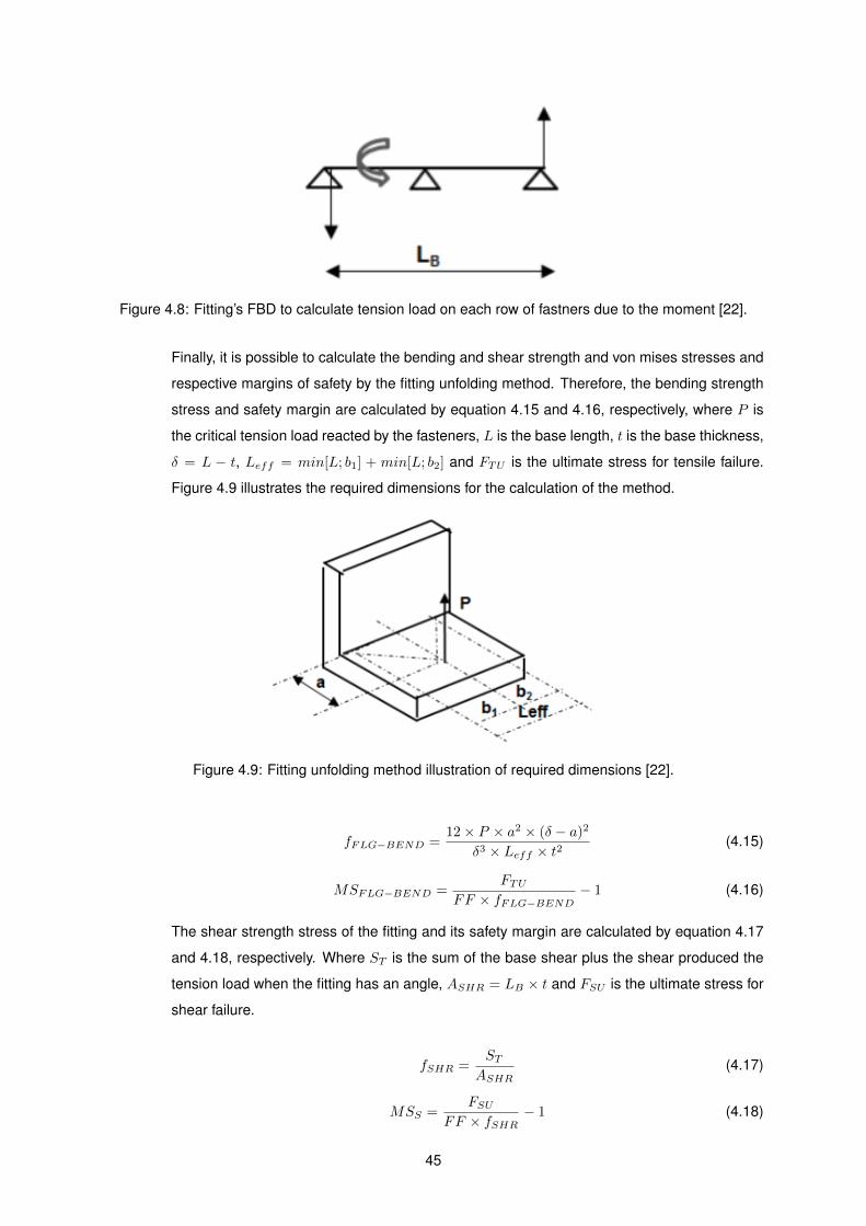
Figure 4.8: Fitting’s FBD to calculate tension load on each row of fastners due to the moment [22].
Finally, it is possible to calculate the bending and shear strength and von mises stresses and
respective margins of safety by the fitting unfolding method. Therefore, the bending strength
stress and safety margin are calculated by equation 4.15 and 4.16, respectively, where P is
the critical tension load reacted by the fasteners, L is the base length, t is the base thickness,
δ = L − t, Leff = min[L; b1] + min[L; b2] and FTU is the ultimate stress for tensile failure.
Figure 4.9 illustrates the required dimensions for the calculation of the method.
Figure 4.9: Fitting unfolding method illustration of required dimensions [22].
fFLG−BEND =12 × P × a2 × (δ − a)2
δ3 × Leff × t2(4.15)
MSFLG−BEND =FTU
FF × fFLG−BEND− 1 (4.16)
The shear strength stress of the fitting and its safety margin are calculated by equation 4.17
and 4.18, respectively. Where ST is the sum of the base shear plus the shear produced the
tension load when the fitting has an angle, ASHR = LB × t and FSU is the ultimate stress for
shear failure.
fSHR =ST
ASHR(4.17)
MSS =FSU
FF × fSHR− 1 (4.18)
45
The von mises stress is a combination of the bending plus the shear stresses. This is calcu-
lated by equation 4.19 and the respective safety margin by equation 4.20.
fVM =
√fFLG−BEND
2 + 3 × fSHR2 (4.19)
MSVM =FTU
FF × fVM− 1 (4.20)
• Fitting Base Bearing
Once the shear load applied to the fasteners is calculated, it is possible to determinate the
margin of safety under bearing for the fitting base for the ultimate and yield cases by equations
4.21 and 4.22, respectively, where, MSBRU and MSBRY are the ultimate and yield bearing
Margin of Safety, respectively, DFAST is the diameter of the fastener hole, t is the thickness
of the fitting base, FF is the fitting factor: 1.15 as per paragraph 25.625 and finally SFAST,U
and SFAST,L are the ultimate and limit applied shear load at each fastener, respectively.
MSBRU =FBRU ×DFAST × t
FF × SFAST,U− 1 (4.21)
MSBRY =FBRY ×DFAST × t
FF × SFAST,L− 1 (4.22)
• Von Mises Stress
Additionally, it was computed the critical von mises stress for the seven fittings to verify their
strength after the optimization pockets and check if there is no stess concentration in the area
around the lug. To perform this, it is used the post processing of the analysis run in FEMAP
to find the critical element with the highest von mises stress. The allowable of the material
in LT direction is extracted from the literature [25] and the safety margin can be calculated by
equation 4.23.
MSVM =FVM
FF × fVM− 1 (4.23)
2. External Doublers - Secondly, the doublers are analysed in bearing and von mises stress.
• Bearing
To verify the doubler’s strength in bearing, firstly, it is used the post processing of the anal-
ysis run in FEMAP to find the critical element with the highest shear load. Secondly, it is
calculated by equation 4.24 the bearing allowable of the doubler counting with a 20% abat-
ment for the wet fasteners. Where SBRU is the ultimate bearing strength stress, t is the
doubler thickness and D is the diameter of the critical hole in the doubler.
46

PBRU = SBRU × t×D × 0.8 (4.24)
Finally, the safety margin can be calculated by equation 4.25, where S is the shear load in the
critical element in the doubler.
MSBRU =PBRU
FF × S− 1 (4.25)
• Von Mises Stress
To verify the doubler’s strength in terms of von mises, it is used again the post processing of
the analysis run in FEMAP to find the critical element with the highest von mises stress. The
allowable of the material in LT direction is extracted from the literature and the safety margin
can be calculated by equation 4.26.
MSVM =FVM
FF × fVM− 1 (4.26)
3. Intercostals - Thirdly, the intercostals are analysed under the following failures modes: Bearing
analysis of the gusset intercostal junction and l-bracket junction; maximum tensile and compressive
stress on the outer and inner flange; maximum shear load in the intercostal’s web; and von mises
stress.
• Bearing Analysis
The analysis’ procedure performed in the gusset intercostal and intercostal l-bracket junctions
for the bearing is the same already presented for the fitting base.
• Maximum tensile and compressive stress on the outer and inner flange
The intercostal can me modelled as beam simply supported in the edges where is working
under the shear load transferred through the attachments in the gusset wall, the bending
moment in Y direction of aircraft axis due to this load and the extra bending moment due to
the eccentricity of the same load. The intercostal is supported by the frames through two
l-brackets attachments in the edges. The reactions in these attachments are calculated with
a sum of moments expressed in equation 4.27. With the reactions computed, it was possible
to evaluate the associated and eccentricity bending moments with equations 4.28 and 4.29,
respectively.
RA =P × L1
LRB =
P × (L− L1)
L(4.27)
My = RA × (L− L1) = RB × L1 (4.28)
47
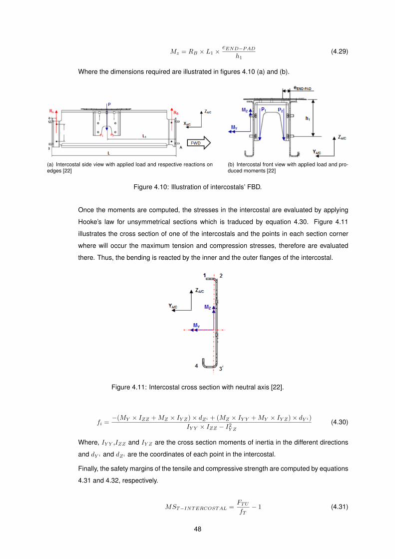
Mz = RB × L1 ×eEND−PAD
h1(4.29)
Where the dimensions required are illustrated in figures 4.10 (a) and (b).
(a) Intercostal side view with applied load and respective reactions onedges [22]
(b) Intercostal front view with applied load and pro-duced moments [22]
Figure 4.10: Illustration of intercostals’ FBD.
Once the moments are computed, the stresses in the intercostal are evaluated by applying
Hooke’s law for unsymmetrical sections which is traduced by equation 4.30. Figure 4.11
illustrates the cross section of one of the intercostals and the points in each section corner
where will occur the maximum tension and compression stresses, therefore are evaluated
there. Thus, the bending is reacted by the inner and the outer flanges of the intercostal.
Figure 4.11: Intercostal cross section with neutral axis [22].
fi =−(MY × IZZ +MZ × IY Z) × dZi + (MZ × IY Y +MY × IY Z) × dY i)
IY Y × IZZ − I2Y Z
(4.30)
Where, IY Y ,IZZ and IY Z are the cross section moments of inertia in the different directions
and dY i and dZi are the coordinates of each point in the intercostal.
Finally, the safety margins of the tensile and compressive strength are computed by equations
4.31 and 4.32, respectively.
MST−INTERCOSTAL =FTU
fT− 1 (4.31)
48

MSC−INTERCOSTAL =FCY
fC− 1 (4.32)
Where, FTU , FCY are the ultimate stresses of the material for the respective modes, tensile
and compressive.
• Maximum shear load in the intercostal’s web
To verify the intercostal’s web shear strength it is calculated the maximum shear load ap-
plied on it by equation 4.33 and, finally the safety margin by equation 4.34.
SMAX =3
2× S (4.33)
MSS =FSU
SMAX− 1 (4.34)
• Von mises stress
The analysis’ procedure for the von mises stress in the intercostal is the same one already
used for the fittings and doublers.
4.3.2 Fatigue Analysis
The fatigue analysis is performed in order to justify that the fatigue life is not a limiting factor for the
threshold inspection. Due to the highest load condition, the doublers are the critical components which
must be subjected to the study. In addiction, also the fatigue life of the modified fittings is studied in order
to compare with fatigue life of the initial fittings. The analysis is based on the material Wohler curves or
stress-life curves (S-N), which relates the maximum stress with the fatigue life, in cycles. The definition
of one cycle is presented in the following section. Figure 4.12 presents the S-N curves for the doublers
material, the 2024-T3 aluminium alloy.
Figure 4.12: S-N curves and correlations for 2024-T3 aluminium alloy [25].
49
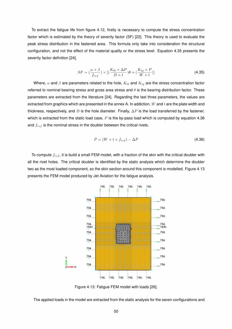
To extract the fatigue life from figure 4.12, firstly is necessary to compute the stress concentration
factor which is estimated by the theory of severity factor (SF) [22]. This theory is used to evaluate the
peak stress distribution in the fastened area. This formula only take into consideration the structural
configuration, and not the effect of the material quality or the stress level. Equation 4.35 presents the
severity factor definition [24].
SF = (α× β
fref) × [(
Ktb × ∆P
D × t)θ + (
Ktg × P
W × t)] (4.35)
Where, α and β are parameters related to the hole, Ktb and Ktg are the stress concentration factor
referred to nominal bearing stress and gross area stress and θ is the bearing distribution factor. These
parameters are extracted from the literature [24]. Regarding the last three parameters, the values are
extracted from graphics which are presented in the annex A. In addiction, W and t are the plate width and
thickness, respectively, and D is the hole diameter. Finally, ∆P is the load transferred by the fastener,
which is extracted from the static load case, P is the by-pass load which is computed by equation 4.36
and fref is the nominal stress in the doubler between the critical rivets.
P = (W × t× fref ) − ∆P (4.36)
To compute fref , it is build a small FEM model, with a fraction of the skin with the critical doubler with
all the rivet holes. The critical doubler is identified by the static analysis which determine the doubler
two as the most loaded component, so the skin section around this component is modelled. Figure 4.13
presents the FEM model produced by Jet Aviation for the fatigue analysis.
Figure 4.13: Fatigue FEM model with loads [26].
The applied loads in the model are extracted from the static analysis for the seven configurations and
50
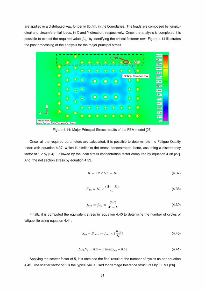
are applied in a distributed way, lbf per in [lbf/in], in the boundaries. The loads are composed by longitu-
dinal and circumferential loads, in X and Y direction, respectively. Once, the analysis is completed it is
possible to extract the required value fref by identifying the critical fastener row. Figure 4.14 illustrates
the post processing of the analysis for the major principal stress.
Figure 4.14: Major Principal Stress results of the FEM model [26].
Once, all the required parameters are calculated, it is possible to determinate the Fatigue Quality
Index with equation 4.37, which is similar to the stress concentration factor, assuming a discrepancy
factor of 1.2 by [24]. Followed by the local stress concentration factor computed by equation 4.38 [27].
And, the net section stress by equation 4.39.
K = 1.2 × SF = Kt (4.37)
Ktn = Kt ×(W −D)
W(4.38)
fnet = fref × (W )
W −D(4.39)
Finally, it is computed the equivalent stress by equation 4.40 to determine the number of cycles of
fatigue life using equation 4.41.
Seq = Smax = fnet × (Ktn
Kt) (4.40)
LogNf = 8.3 − 3.3log(Seq − 8.5) (4.41)
Applying the scatter factor of 5, it is obtained the final result of the number of cycles as per equation
4.42. The scatter factor of 5 is the typical value used for damage tolerance structures by OEMs [26].
51
N∗f = Nf/5 (4.42)
For the fittings case, it is extracted from the FEM model the maximum and nominal stresses and the
stress concentration factor Kt is calculated . Once the Kt is computed, is used the already described
methodology to find out the number of cycles of fatigue life, N∗f of the modified fittings.
Spectrum assumption
For this analysis is assumed that one cycle is equivalent to one flight. By the reason that, a conser-
vative once-per-flight constant amplitude Ground-Air-Ground (GAG) loading cycle has been considered
instead of a more complex flight-by-flight loading spectrum, based on [28].
To perform this analysis, the required geometry dimensions of the fittings and intercostals are ex-
tracted from the 3D model and summarized in figures A.1 and A.2 which are included in the appendix A
of this document.
52
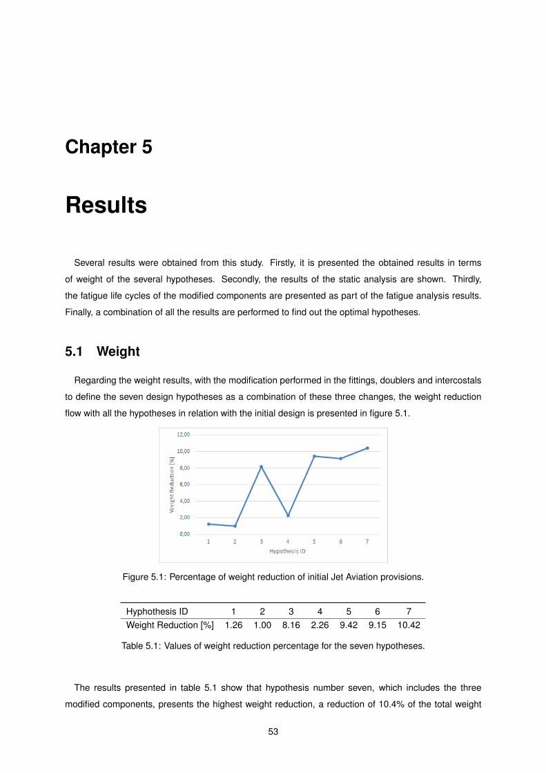
Chapter 5
Results
Several results were obtained from this study. Firstly, it is presented the obtained results in terms
of weight of the several hypotheses. Secondly, the results of the static analysis are shown. Thirdly,
the fatigue life cycles of the modified components are presented as part of the fatigue analysis results.
Finally, a combination of all the results are performed to find out the optimal hypotheses.
5.1 Weight
Regarding the weight results, with the modification performed in the fittings, doublers and intercostals
to define the seven design hypotheses as a combination of these three changes, the weight reduction
flow with all the hypotheses in relation with the initial design is presented in figure 5.1.
Figure 5.1: Percentage of weight reduction of initial Jet Aviation provisions.
Hyphothesis ID 1 2 3 4 5 6 7Weight Reduction [%] 1.26 1.00 8.16 2.26 9.42 9.15 10.42
Table 5.1: Values of weight reduction percentage for the seven hypotheses.
The results presented in table 5.1 show that hypothesis number seven, which includes the three
modified components, presents the highest weight reduction, a reduction of 10.4% of the total weight
53

of the initial design. In addition, it also shows that the modified component with the larger impact on
the weight reduction is the intercostals, due to the large number of times that this component is used
and also, due to its considerable initial weight compared to the other two modified parts. Following the
same logic, accounting only with two modified components, the hypothesis with the greater result is the
hypothesis number five, which combines the modified intercostals with the modified fittings, which are
the second component with more impact in the weight reduction.
To sum up, the hypothesis number seven is the lightest design from all the hypotheses. The static
analysis results will confirm if the structural configuration of this hypothesis maintains the structural
integrity by continuing to have positive safety margins in all the design components.
5.2 Static
The goal of the static analysis is to obtain results which confirm that each of the studied hypotheses
maintain the structural integrity. This was performed in two steps, already described in section 4.3.1.
From the first step, graphics in figure 5.2 present the extracted values of the reactions of all the fittings
in the respective directions for all the hypothesis.
((a)) Fittings reactions in X direction ((b)) Fittings reactions in Y direction
((c)) Fittings reactions in Z direction
Figure 5.2: Fittings reactions for the seven hypothesis
Remembering what was stated in section 2.2.2, the fittings are designed only to sustain loads in
specific directions. Figure 5.2 confirms that, for instance, loads in direction X and Y are only carried
54
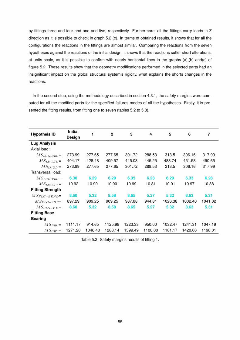
by fittings three and four and one and five, respectively. Furthermore, all the fittings carry loads in Z
direction as it is possible to check in graph 5.2 (c). In terms of obtained results, it shows that for all the
configurations the reactions in the fittings are almost similar. Comparing the reactions from the seven
hypotheses against the reactions of the initial design, it shows that the reactions suffer short alterations,
at units scale, as it is possible to confirm with nearly horizontal lines in the graphs (a),(b) and(c) of
figure 5.2. These results show that the geometry modifications performed in the selected parts had an
insignificant impact on the global structural system’s rigidity, what explains the shorts changes in the
reactions.
In the second step, using the methodology described in section 4.3.1, the safety margins were com-
puted for all the modified parts for the specified failures modes of all the hypotheses. Firstly, it is pre-
sented the fitting results, from fitting one to seven (tables 5.2 to 5.8).
Hypotheis IDInitial
Design1 2 3 4 5 6 7
Lug AnalysisAxial load:MSLUG,BRU= 273.99 277.65 277.65 301.72 288.53 313.5 306.16 317.99MSLUG,TU= 404.17 428.48 409.57 445.03 445.25 483.74 451.58 490.65MSLUG,Y = 273.99 277.65 277.65 301.72 288.53 313.5 306.16 317.99
Transversal load:MSLUG,TRU= 6.30 6.29 6.29 6.35 6.23 6.29 6.33 6.28MSLUG,TY = 10.92 10.90 10.90 10.99 10.81 10.91 10.97 10.88
Fitting StrengthMSFLG−BEND= 8.60 5.32 8.58 8.65 5.27 5.32 8.63 5.31MSFLG−SHR= 897.29 909.25 909.25 987.88 944.81 1026.38 1002.40 1041.02MSFLG−VM= 8.60 5.32 8.58 8.65 5.27 5.32 8.63 5.31
Fitting BaseBearing
MSBRU= 1111.17 914.65 1125.98 1223.33 950.00 1032.47 1241.31 1047.19MSBRY = 1271.20 1046.40 1288.14 1399.49 1100.00 1181.17 1420.06 1198.01
Table 5.2: Safety margins results of fitting 1.
55
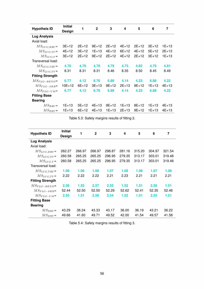
Hypotheis IDInitial
Design1 2 3 4 5 6 7
Lug AnalysisAxial load:MSLUG,BRU= 3E+12 2E+12 9E+12 2E+12 4E+12 2E+12 3E+12 1E+13MSLUG,TU= 4E+12 3E+12 1E+13 4E+12 6E+12 4E+12 5E+12 2E+13MSLUG,Y = 3E+12 2E+12 9E+12 2E+12 4E+12 2E+12 3E+12 1E+13
Transversal load:MSLUG,TRU= 4.70 4.70 4.70 4.79 4.73 4.82 4.79 4.81MSLUG,TY = 8.31 8.31 8.31 8.46 8.35 8.50 8.45 8.49
Fitting StrengthMSFLG−BEND= 6.77 4.12 6.76 6.89 4.14 4.23 6.88 4.22MSFLG−SHR= 10E+12 6E+12 3E+13 9E+12 2E+13 9E+12 1E+13 4E+13MSFLG−VM= 6.77 4.12 6.76 6.89 4.14 4.23 6.88 4.22
Fitting BaseBearing
MSBRU= 1E+13 5E+12 4E+13 9E+12 1E+13 8E+12 1E+13 4E+13MSBRY = 1E+13 6E+12 4E+13 1E+13 2E+13 9E+12 1E+13 4E+13
Table 5.3: Safety margins results of fitting 2.
Hypotheis IDInitial
Design1 2 3 4 5 6 7
Lug AnalysisAxial load:MSLUG,BRU= 262.27 266.97 266.97 298.87 281.16 315.20 304.97 321.54MSLUG,TU= 260.58 265.25 265.25 296.95 279.35 313.17 303.01 319.48MSLUG,Y = 260.58 265.25 265.25 296.95 279.35 313.17 303.01 319.48
Transversal load:MSLUG,TRU= 1.08 1.08 1.08 1.07 1.08 1.08 1.07 1.08MSLUG,TY = 2.22 2.22 2.22 2.21 2.23 2.21 2.21 2.21
Fitting StrengthMSFLG−BEND= 2.56 1.52 2.57 2.55 1.52 1.51 2.56 1.51MSFLG−SHR= 52.44 52.50 52.50 52.29 52.62 52.41 52.35 52.46MSFLG−VM= 2.55 1.51 2.56 2.54 1.52 1.51 2.55 1.51
Fitting BaseBearing
MSBRU= 43.29 36.24 43.33 43.17 36.00 36.19 43.21 36.22MSBRY = 49.66 41.60 49.71 49.52 42.00 41.54 49.57 41.58
Table 5.4: Safety margins results of fitting 3.
56
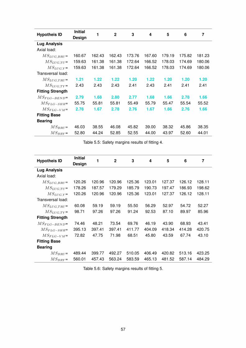
Hypotheis IDInitial
Design1 2 3 4 5 6 7
Lug AnalysisAxial load:MSLUG,BRU= 160.67 162.43 162.43 173.76 167.60 179.19 175.82 181.23MSLUG,TU= 159.63 161.38 161.38 172.64 166.52 178.03 174.69 180.06MSLUG,Y = 159.63 161.38 161.38 172.64 166.52 178.03 174.69 180.06
Transversal load:MSLUG,TRU= 1.21 1.22 1.22 1.20 1.22 1.20 1.20 1.20MSLUG,TY = 2.43 2.43 2.43 2.41 2.43 2.41 2.41 2.41
Fitting StrengthMSFLG−BEND= 2.79 1.68 2.80 2.77 1.68 1.66 2.78 1.66MSFLG−SHR= 55.75 55.81 55.81 55.49 55.79 55.47 55.54 55.52MSFLG−VM= 2.78 1.67 2.78 2.76 1.67 1.66 2.76 1.66
Fitting BaseBearing
MSBRU= 46.03 38.55 46.08 45.82 39.00 38.32 45.86 38.35MSBRY = 52.80 44.24 52.85 52.55 44.00 43.97 52.60 44.01
Table 5.5: Safety margins results of fitting 4.
Hypotheis IDInitial
Design1 2 3 4 5 6 7
Lug AnalysisAxial load:MSLUG,BRU= 120.26 120.96 120.96 125.36 123.01 127.37 126.12 128.11MSLUG,TU= 178.26 187.57 179.29 185.79 190.73 197.47 186.93 198.62MSLUG,Y = 120.26 120.96 120.96 125.36 123.01 127.37 126.12 128.11
Transversal load:MSLUG,TRU= 60.08 59.19 59.19 55.50 56.29 52.97 54.72 52.27MSLUG,TY = 98.71 97.26 97.26 91.24 92.53 87.10 89.97 85.96
Fitting StrengthMSFLG−BEND= 74.46 48.21 73.54 69.76 46.19 43.90 68.93 43.41MSFLG−SHR= 395.13 397.41 397.41 411.77 404.09 418.34 414.28 420.75MSFLG−VM= 72.82 47.75 71.98 68.51 45.80 43.59 67.74 43.10
Fitting BaseBearing
MSBRU= 489.44 399.77 492.27 510.05 406.49 420.82 513.16 423.25MSBRY = 560.01 457.43 563.24 583.59 465.13 481.52 587.14 484.29
Table 5.6: Safety margins results of fitting 5.
57

Hypotheis IDInitial
Design1 2 3 4 5 6 7
Lug AnalysisAxial load:MSLUG,BRU= 1E+13 7E+12 1E+09 1E+09 1E+13 1E+09 9E+12 1E+09MSLUG,TU= 2E+13 1E+13 1E+05 1E+05 2E+13 1E+05 1E+13 1E+05MSLUG,Y = 1E+13 7E+12 1E+05 1E+05 1E+13 1E+05 9E+12 1E+05
Transversal load:MSLUG,TRU= 36.73 36.40 36.40 34.81 36.39 34.80 34.51 34.51MSLUG,TY = 60.59 60.06 60.06 57.46 60.04 57.45 56.97 56.96
Fitting StrengthMSFLG−BEND= 51.96 33.66 51.51 49.27 33.65 32.18 48.85 31.90MSFLG−SHR= 4E+13 2E+13 3E+18 3E+18 3E+13 3E+18 3E+13 3E+18MSFLG−VM= 51.96 33.66 51.51 49.27 33.65 32.18 48.85 31.90
Fitting BaseBearing
MSBRU= 4E+13 2E+13 4E+18 4E+18 3E+13 3E+18 4E+13 3E+18MSBRY = 5E+13 2E+13 5E+18 4E+18 4E+13 4E+18 4E+13 3E+18
Table 5.7: Safety margins results of fitting 6.
Hypotheis IDInitial
Design1 2 3 4 5 6 7
Lug AnalysisAxial load:MSLUG,BRU= 3E+13 1E+12 1E+09 2E+12 1E+12 3E+12 2E+12 5E+13MSLUG,TU= 3E+13 1E+12 1E+05 2E+12 1E+12 2E+12 2E+12 4E+13MSLUG,Y = 3E+13 1E+12 1E+05 2E+12 1E+12 2E+12 2E+12 4E+13
Transversal load:MSLUG,TRU= 1.24 1.24 1.24 1.25 1.24 1.26 1.26 1.26MSLUG,TY = 2.46 2.46 2.46 2.49 2.47 2.49 2.49 2.49
Fitting StrengthMSFLG−BEND= 6.58 3.63 6.58 6.64 3.63 3.66 6.64 3.66MSFLG−SHR= 1E+14 6E+12 3E+17 8E+12 5E+12 1E+13 8E+12 2E+14MSFLG−VM= 6.58 3.63 6.58 6.64 3.63 3.66 6.64 3.66
Fitting BaseBearing
MSBRU= 6E+04 5E+04 6E+04 6E+04 5E+04 5E+04 6E+04 5E+04MSBRY = 7E+04 6E+04 7E+04 7E+04 6E+04 6E+04 7E+04 6E+04
Table 5.8: Safety margins results of fitting 7.
From observing the results in the tables above, firstly, it is noticeable that all the fittings are able to
withstand the applied loads for all the hypotheses. Secondly, it is possible to confirm the safety margin
reduction in some of the failures modes. One example is the fitting strength due to the bending, which
the safety margin goes from 2.56 in the initial design to 1.51 in the last hypothesis on fitting three, thus
this is the critical value obtained and the fitting three is the critical fitting, however, it is still in a safe zone.
58

The critical values for all the fittings are highlighted in blue and bold. Lastly, looking at all the values of
the seven hypotheses, the accentuated safety margin reduction always occur for the hypotheses where
the fittings are modified.
Regarding the von mises stress in all the fittings, from FEMAP it was possible to find out the most
stress fitting - fitting 3. Figure 5.3 presents the outputs for the initial design and hypothesis seven , from
which were extracted the maximum values of von mises stress to calculate the safety margins, where
the maximum values are in red. Table 5.9 presents the final results of the safety margins.
(a) Initial design (b) Hypothesis 7
Figure 5.3: Von Mises stress output for fitting 3 in the initial design and last hypothesis in FEMAP.
Hypotheis IDInitial
Design1 2 3 4 5 6 7
Von Mises StressMSFitting3= 0.97 0.11 0.97 0.99 0.12 0.11 0.99 0.12MSFitting7= 0.60 0.27 0.60 0.62 0.28 0.27 0.62 0.27
Table 5.9: Safety margins results of critical fittings for the von mises stress extracted from the FEMmodel.
Analysing the results, it confirms what was stated before, the fitting 3 is the most critical one inside
of the safe zone. In addiction, it is confirmed that the pockets in the web of the fittings does not create
critical peak of stress in the steps areas. This peak is still on the bending radius area, which does
happens in the initial fitting for the initial design.
Regarding the doublers, the analysis performed showed that the doubler three is the most critical.
Table 5.10 presents the safety margins results for that doubler.
Hypotheis IDInitial
Design1 2 3 4 5 6 7
BearingMSBRU= 2.69 2.68 2.42 2.67 2.42 2.67 2.42 2.42
Von Mises StressMS= 0.04 0.05 0.04 0.04 0.02 0.05 0.01 0.02
Table 5.10: Safety margins results of critical doubler - Doubler 3.
59
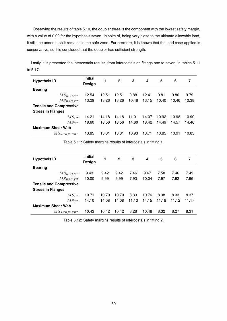
Observing the results of table 5.10, the doubler three is the component with the lowest safety margin,
with a value of 0.02 for the hypothesis seven. In spite of, being very close to the ultimate allowable load,
it stills be under it, so it remains in the safe zone. Furthermore, it is known that the load case applied is
conservative, so it is concluded that the doubler has sufficient strength.
Lastly, it is presented the intercostals results, from intercostals on fittings one to seven, in tables 5.11
to 5.17.
Hypotheis IDInitial
Design1 2 3 4 5 6 7
BearingMSBRG,U= 12.54 12.51 12.51 9.88 12.41 9.81 9.86 9.79MSBRG,Y = 13.29 13.26 13.26 10.48 13.15 10.40 10.46 10.38
Tensile and CompressiveStress in Flanges
MST = 14.21 14.18 14.18 11.01 14.07 10.92 10.98 10.90MSC= 18.60 18.56 18.56 14.60 18.42 14.49 14.57 14.46
Maximum Shear WebMSSHR,WEB= 13.85 13.81 13.81 10.93 13.71 10.85 10.91 10.83
Table 5.11: Safety margins results of intercostals in fitting 1.
Hypotheis IDInitial
Design1 2 3 4 5 6 7
BearingMSBRG,U= 9.43 9.42 9.42 7.46 9.47 7.50 7.46 7.49MSBRG,Y = 10.00 9.99 9.99 7.93 10.04 7.97 7.92 7.96
Tensile and CompressiveStress in Flanges
MST = 10.71 10.70 10.70 8.33 10.76 8.38 8.33 8.37MSC= 14.10 14.08 14.08 11.13 14.15 11.18 11.12 11.17
Maximum Shear WebMSSHR,WEB= 10.43 10.42 10.42 8.28 10.48 8.32 8.27 8.31
Table 5.12: Safety margins results of intercostals in fitting 2.
60
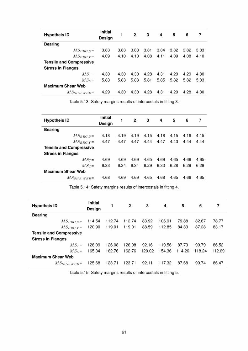
Hypotheis IDInitial
Design1 2 3 4 5 6 7
BearingMSBRG,U= 3.83 3.83 3.83 3.81 3.84 3.82 3.82 3.83MSBRG,Y = 4.09 4.10 4.10 4.08 4.11 4.09 4.08 4.10
Tensile and CompressiveStress in Flanges
MST = 4.30 4.30 4.30 4.28 4.31 4.29 4.29 4.30MSC= 5.83 5.83 5.83 5.81 5.85 5.82 5.82 5.83
Maximum Shear WebMSSHR,WEB= 4.29 4.30 4.30 4.28 4.31 4.29 4.28 4.30
Table 5.13: Safety margins results of intercostals in fitting 3.
Hypotheis IDInitial
Design1 2 3 4 5 6 7
BearingMSBRG,U= 4.18 4.19 4.19 4.15 4.18 4.15 4.16 4.15MSBRG,Y = 4.47 4.47 4.47 4.44 4.47 4.43 4.44 4.44
Tensile and CompressiveStress in Flanges
MST = 4.69 4.69 4.69 4.65 4.69 4.65 4.66 4.65MSC= 6.33 6.34 6.34 6.29 6.33 6.28 6.29 6.29
Maximum Shear WebMSSHR,WEB= 4.68 4.69 4.69 4.65 4.68 4.65 4.66 4.65
Table 5.14: Safety margins results of intercostals in fitting 4.
Hypotheis IDInitial
Design1 2 3 4 5 6 7
BearingMSBRG,U= 114.54 112.74 112.74 83.92 106.91 79.88 82.67 78.77MSBRG,Y = 120.90 119.01 119.01 88.59 112.85 84.33 87.28 83.17
Tensile and CompressiveStress in Flanges
MST = 128.09 126.08 126.08 92.16 119.56 87.73 90.79 86.52MSC= 165.34 162.76 162.76 120.02 154.36 114.26 118.24 112.69
Maximum Shear WebMSSHR,WEB= 125.68 123.71 123.71 92.11 117.32 87.68 90.74 86.47
Table 5.15: Safety margins results of intercostals in fitting 5.
61

Hypotheis IDInitial
Design1 2 3 4 5 6 7
BearingMSBRG,U= 66.78 66.20 66.20 50.42 66.18 50.41 49.99 49.98MSBRG,Y = 70.51 69.90 69.90 53.25 69.88 53.24 52.80 52.79
Tensile and CompressiveStress in Flanges
MST = 74.73 74.08 74.08 55.41 74.06 55.40 54.94 54.93MSC= 96.59 95.75 95.75 72.28 95.73 72.27 71.67 71.66
Maximum Shear WebMSSHR,WEB= 73.32 72.68 72.68 55.38 72.66 55.37 54.91 54.90
Table 5.16: Safety margins results of intercostals in fitting 6.
Hypotheis IDInitial
Design1 2 3 4 5 6 7
BearingMSBRG,U= 3.45 3.45 3.45 2.58 3.46 2.59 2.58 2.59MSBRG,Y = 3.70 3.70 3.70 2.78 3.70 2.78 2.78 2.79
Tensile and CompressiveStress in Flanges
MST = 4.20 4.20 4.20 3.11 4.20 3.11 3.11 3.11MSC= 5.70 5.70 5.70 4.34 5.70 4.34 4.34 4.34
Maximum Shear WebMSSHR,WEB= 3.88 3.88 3.88 2.93 3.89 2.93 2.93 2.93
Table 5.17: Safety margins results of intercostals in fitting 7.
Observing the results in the tables above, firstly, it shows that all the intercostals are able to withstand
the applied loads for all the hypothesis. Secondly, it is possible to confirm the safety margin reduction
in some of the failures modes in the successive hypotheses. The intercostals in fitting seven presented
the lowest safety margins, however the analytical method used does not account for the cut-out in
intercostals in fitting three and four. So, to verify which are the critical intercostals it is necessary to
verify in the FEM results with the von mises stress for instance. It can be expected that due to the
cut-out on intercostals of fitting three and four, there will be a peak of stress on the fillets of the cut-out of
these intercostals, so these probably will have the lowest safety margin. This will be verified in the next
paragraphs.
Similarly to the fittings, the von mises stress in all the intercostals were extracted from FEMAP and
it was possible to find out the most stress intercostal - the cut-outed intercostal in fitting 3. Figure 5.4
presents the outputs for the initial design and hypothesis seven, from which were extracted the maximum
values of von mises stresses to calculate the safety margins, where the maximum values are in red.
Table 5.18 presents the final results of the safety margins.
62
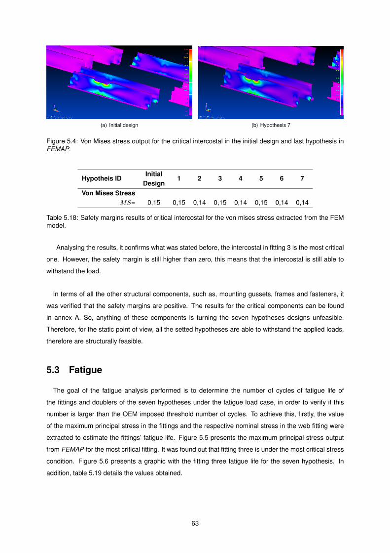
(a) Initial design (b) Hypothesis 7
Figure 5.4: Von Mises stress output for the critical intercostal in the initial design and last hypothesis inFEMAP.
Hypotheis IDInitial
Design1 2 3 4 5 6 7
Von Mises StressMS= 0,15 0,15 0,14 0,15 0,14 0,15 0,14 0,14
Table 5.18: Safety margins results of critical intercostal for the von mises stress extracted from the FEMmodel.
Analysing the results, it confirms what was stated before, the intercostal in fitting 3 is the most critical
one. However, the safety margin is still higher than zero, this means that the intercostal is still able to
withstand the load.
In terms of all the other structural components, such as, mounting gussets, frames and fasteners, it
was verified that the safety margins are positive. The results for the critical components can be found
in annex A. So, anything of these components is turning the seven hypotheses designs unfeasible.
Therefore, for the static point of view, all the setted hypotheses are able to withstand the applied loads,
therefore are structurally feasible.
5.3 Fatigue
The goal of the fatigue analysis performed is to determine the number of cycles of fatigue life of
the fittings and doublers of the seven hypotheses under the fatigue load case, in order to verify if this
number is larger than the OEM imposed threshold number of cycles. To achieve this, firstly, the value
of the maximum principal stress in the fittings and the respective nominal stress in the web fitting were
extracted to estimate the fittings’ fatigue life. Figure 5.5 presents the maximum principal stress output
from FEMAP for the most critical fitting. It was found out that fitting three is under the most critical stress
condition. Figure 5.6 presents a graphic with the fitting three fatigue life for the seven hypothesis. In
addition, table 5.19 details the values obtained.
63
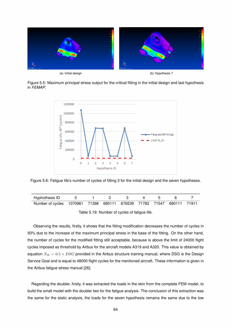
(a) Initial design (b) Hypothesis 7
Figure 5.5: Maximum principal stress output for the critical fitting in the initial design and last hypothesisin FEMAP.
Figure 5.6: Fatigue life’s number of cycles of fitting 3 for the initial design and the seven hypotheses.
Hyphothesis ID 0 1 2 3 4 5 6 7Number of cycles 1070961 71398 680111 676539 71782 71547 680111 71911
Table 5.19: Number of cycles of fatigue life.
Observing the results, firstly, it shows that the fitting modification decreases the number of cycles in
93% due to the increase of the maximum principal stress in the base of the fitting. On the other hand,
the number of cycles for the modified fitting still acceptable, because is above the limit of 24000 flight
cycles imposed as threshold by Airbus for the aircraft models A319 and A320. This value is obtained by
equation Nth = 0.5 ×DSG provided in the Airbus structure training manual, where DSG is the Design
Service Goal and is equal to 48000 flight cycles for the mentioned aircraft. These information is given in
the Airbus fatigue stress manual [26].
Regarding the doubler, firstly, it was extracted the loads in the skin from the complete FEM model, to
build the small model with the doubler two for the fatigue analysis. The conclusion of this extraction was
the same for the static analysis, the loads for the seven hypothesis remains the same due to the low
64

change in the inertia of the installation. Thus, it was used the initial design loads in the model for all the
hypotheses. The results obtained are presented in figure 5.7 and table 5.20.
Figure 5.7: Number of cycles of fatigue life for Doubler 3 for the seven hypotheses.
Hyphothesis ID 0 1 2 3 4 5 6 7Number of cycles 178740 167345 150107 160490 150597 161091 145079 145563
Table 5.20: Number of cycles of fatigue life for doubler 2 for the initial design and seven hypothesis.
The results shows a reduction in the number of cycles for all the hypothesis, having the maximum
reduction in the hypothesis where the doubler with a reduced thickness is employed. In addition, it also
shows the impact of changing the intercostals and the fittings in terms of doubler’s fatigue life, with a
reduction of 10% and 6% of number of cycles, respectively. In spite of that reduction, all the hypotheses
have the number of cycles above the threshold imposed again by Airbus of 24000 flight cycles.
Cross checking the obtained results for the fittings and doublers, it shows that with the fitting modifi-
cation, this component became the critical one in terms of fatigue life, due to the huge reduction of the
number of cycles. Therefore, the fatigue life of hypothesis 1, 4, 5 and 7 is driven by the fittings and not
the doublers as in the initial design. The other hypotheses continue to be driven by the doubler and does
not introduce a huge reduction in the number of cycles. Table 5.21 summarize the critical values of the
number of cycles for all hypotheses.
Hypotheis IDInitial
Design1 2 3 4 5 6 7
Number of cycles 178740 71398 150107 160490 71782 71547 145079 71911Critical Component Doubler Fitting Doubler Doubler Fitting Fitting Doubler Fitting
Table 5.21: Critical number of cycles of fatigue life which drives each hypothesis.
65
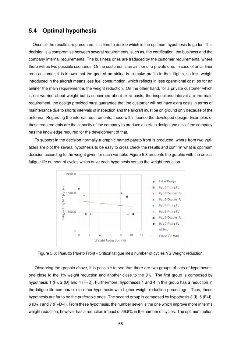
5.4 Optimal hypothesis
Once all the results are presented, it is time to decide which is the optimum hypothesis to go for. This
decision is a compromise between several requirements, such as, the certification, the business and the
company internal requirements. The business ones are traduced by the customer requirements, where
there will be two possible scenarios. Or the customer is an airliner or a private one. In case of an airliner
as a customer, it is known that the goal of an airline is to make profits in their flights, so less weight
introduced in the aircraft means less fuel consumption, which reflects in less operational cost, so for an
airliner the main requirement is the weight reduction. On the other hand, for a private customer which
is not worried about weight but is concerned about extra costs, the inspections interval are the main
requirement, the design provided must guarantee that the customer will not have extra costs in terms of
maintenance due to shorts intervals of inspection and the aircraft must be on ground only because of the
antenna. Regarding the internal requirements, these will influence the developed design. Examples of
these requirements are the capacity of the company to produce a certain design and also if the company
has the knowledge required for the development of that.
To support in the decision normally a graphic named pareto front is produced, where from two vari-
ables are plot the several hypothesis to be easy to cross check the results and confirm what is optimum
decision according to the weight given for each variable. Figure 5.8 presents the graphic with the critical
fatigue life number of cycles which drive each hypothesis versus the weight reduction.
Figure 5.8: Pseudo Pareto Front - Critical fatigue life’s number of cycles VS Weight reduction.
Observing the graphic above, it is possible to see that there are two groups of sets of hypotheses,
one close to the 1% weight reduction and another close to the 9%. The first group is composed by
hypothesis 1 (F), 2 (D) and 4 (F+D). Furthermore, hypotheses 1 and 4 in this group has a reduction in
the fatigue life comparable to other hypothesis with higher weight reduction percentage. Thus, these
hypothesis are far to be the preferable ones. The second group is composed by hypothesis 3 (I), 5 (F+I),
6 (D+I) and 7 (F+D+I). From these hypothesis, the number seven is the one which improve more in terms
weight reduction, however has a reduction impact of 59.8% in the number of cycles. The optimum option
66

can be hypothesis 6 which has 9.2% of weight reduction and the impact in the reduction of number of
cycles is lower compared with the hypothesis seven, 18.8% for this hypothesis .
Regarding the last requirement, the certification, all these design hypotheses are not certifiable yet
because it is necessary to prove that the hypotheses can withstand all the other mentioned load cases
in section 4.2 and for this study it was only considered the load case one which is good representation of
the critical load cases but is not enough. In addiction, a damage tolerance analysis must be performed
in order to find the inspection intervals, performing only a fatigue analysis is not enough again for certi-
fication. In spite of that, this initial study gives good indications which improvements can be done in the
initial design in order to achieve higher quality values.
67

Chapter 6
Design Initial Release
Reaching to the final stage, once the structural analyses are completed, the solution design is con-
verted in 2D drawings. These are composed by the installation drawing and the drawings of each part
which compose the structural installation solution. When all the drawings are completed and released
by the engineering, this moment is known as the Initial Release. This means that the installation’s tech-
nicians and production department can start their functions. However, before the technicians can start
the installation, the part’s drawings go for the production department to manufacture the parts. Once all
parts are produced, the installation can start and the engineering work in field as well, by giving sup-
port to the technicians to solve some unexpected deviations which were not accounted for in the design
because of the differences between a green and real aircraft, in order to not to stop the installation. In
the meanwhile, the engineering work also continues in the office by producing and finalizing the certifi-
cation documents which prove that all the requirements are complied and also will allow the aircraft to
perform a flight test to conduct some experimental tests. These three topics, installation’s deviations,
experimental tests and certification documents are developed in section 6.1, 6.2 and 6.3, respectively.
6.1 Installation’s Deviations
In any kind of project where is necessary to install a new feature in the existing environment, it is
normal that unexpected deviations will occur, because of the complexity of the environment is hard and
costly to have a complete and detailed 3D model of it. Additionally, the information about the environment
sometimes is not available which makes the process even more complex.
In order to solve the deviations, there are three actions that can be performed. The first is proceed with
revision of the drawing and update the drawing with the deviations. The second is to create a deviation
sheet. And the last is to perform a concession. These three options will be explored in the following
paragraphs.
68
• Drawing Revision
Every time a drawing is produced this starts in revision A. In a scenario where there is a deviation
and this drawing is impacted, one of the solution is to revise the drawing, going to the revision
B. To perform this, the engineer works closely with the technicians and there is a process of
reverse engineering, where from the installation are taken the new impacted data and the drawing
is updated with the new information, so there is a reversal of the usual process. Furthermore, this
method is used when the drawings will be reused more times, so in order not to prepare a deviation
sheet every time that an aircraft is being modified with those drawings. In terms of time, this type
of solution can take a considerable time to perform.
• Deviation Sheet
Every project has its own deadlines and the time is money for the company. So can happen in
the middle of the rush, to accomplish the deadline, appears an deviation, and it is necessary to
quickly act in order to do not stop the work flow. The solution used in this kind of situations, and
the most commonly used is to create a deviation sheet which can be performed faster than revise
the drawing. A deviation sheet is composed in three sections. In the first is presented the issue
and the solution to solve it, in the second is illustrated which part of the drawing is modified, by
showing how was and how is now the drawing. In the last section is presented the modifications
in the drawing’s Bill Of Materials (BOM). The BOM is a product structure, where all the parts
and assemblies are described, along with their properties (e.g.: quantities, material, dimensions),
needed to manufacture the final product.
• Concession
The last type solution happens when there is a deviation but this is not reported to engineering
during the installation process, this is actually included in a document prepared by the technicians
department to be approved after by the engineering before the aircraft leaves the company. Only
small deviations where engineering does not need to be called can be solved by a concession.
The number of deviations can give a measure on how the design can be flexible within the limits in
order to absorb the deviations. A lot of strategies can be used in order to give more flexibility to the
design. One for example, when there are fasteners placed in a part, these parts can be designed a
few larger in order to give more freedom to the technician place it respecting the design rules. With
this, there are more possibilities to install the fasteners, so there is less probability to the installation get
stack because of the impossibility of installing the fasteners. The general good practise to reduce the
number of deviations, starts by identifying which parts can be more susceptible to suffer a deviation and
anticipate it by changing these parts to new ones which are more robust.
Having a flexible design, the probability of the installation get stuck and requirement of the engineer-
ing action is lower, this means that the installation process goes faster and without problems. In terms
69
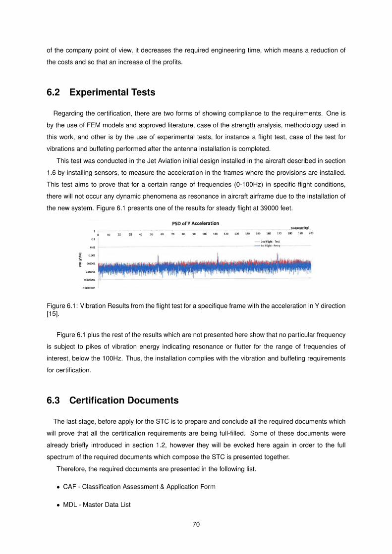
of the company point of view, it decreases the required engineering time, which means a reduction of
the costs and so that an increase of the profits.
6.2 Experimental Tests
Regarding the certification, there are two forms of showing compliance to the requirements. One is
by the use of FEM models and approved literature, case of the strength analysis, methodology used in
this work, and other is by the use of experimental tests, for instance a flight test, case of the test for
vibrations and buffeting performed after the antenna installation is completed.
This test was conducted in the Jet Aviation initial design installed in the aircraft described in section
1.6 by installing sensors, to measure the acceleration in the frames where the provisions are installed.
This test aims to prove that for a certain range of frequencies (0-100Hz) in specific flight conditions,
there will not occur any dynamic phenomena as resonance in aircraft airframe due to the installation of
the new system. Figure 6.1 presents one of the results for steady flight at 39000 feet.
Figure 6.1: Vibration Results from the flight test for a specifique frame with the acceleration in Y direction[15].
Figure 6.1 plus the rest of the results which are not presented here show that no particular frequency
is subject to pikes of vibration energy indicating resonance or flutter for the range of frequencies of
interest, below the 100Hz. Thus, the installation complies with the vibration and buffeting requirements
for certification.
6.3 Certification Documents
The last stage, before apply for the STC is to prepare and conclude all the required documents which
will prove that all the certification requirements are being full-filled. Some of these documents were
already briefly introduced in section 1.2, however they will be evoked here again in order to the full
spectrum of the required documents which compose the STC is presented together.
Therefore, the required documents are presented in the following list.
• CAF - Classification Assessment & Application Form
• MDL - Master Data List
70
• CCS - Certification Compliance Sheet
• DLM - Drawing List Mechanical
• DLE - Drawing List Electrical
• EIL - Electrical Item List
• ENO - Engineering Order
• WBS - Weight and Balance Statement
• SSR - Structural Substantiation Report
• DTA - Damage Tolerance Analysis
• ANA - Analysis Report
• DPS - subcontractor Document Process Slip
• FTP/R - Flight Test Plan / Report
• ICA - Instructions for Continued Airworthiness
These documents cover several areas, then as a result, each specific department is responsible for
certain documents. For example, the DLMs and WBSs are only responsibility of mechanical department.
The DLEs and EILs are prepared by the electrical department and the SSRs and DTAs are prepared
by the stress department. Some documents have the contribution of two different departments, which
are the case of ENO, ANA, CCS and ICA. All these documents will be presented and described in more
detailed in the next paragraphs, with the exception of the CAF which was already completely presented
in section 1.6.
6.3.1 Master Data List - MDL
The MDL is the master document where is presented all the documentation produced for the STC.
Basically, it shows the tree’s structure of the documentation and its organization in order to give a clear
view of all required files and help to ensure that no documents are forgotten.
6.3.2 Certification Compliance Sheet - CCS
The CCS is the document which summarize all information related to certification concerning a specific
aircraft’s modification. Therefore, it presents the applicable certification paragraphs which must been
shown compliance and the respective documents which prove that certification requirements are been
full-filled.
71
6.3.3 Drawing List Mechanical - DLM
The DLM is the document where all the mechanical drawings required for the modification must ap-
pear. Essentially, it is a sub master document which groups all the produced drawings in order to be
called by other documents and justify certain certification requirements. There are the situations when
the drawing does not include the bill of materials inside, this needs to be added as a second document.
Therefore, in these situations, two documents must be added to the DLM, the drawing and respective
BOM. Additionally, in the DLM, revision and release date of the drawings and BOMs must also appear,
otherwise, these will not be validated.
6.3.4 Drawing List Electrical and Electrical Item List - DLE and EIL
Similar to the mechanical side, electrical has to prepare a document where all the electrical drawings
produced are integrated. The content of these drawings is the definition of the connections between
the different components and the respective wire types and routings. This document is denominated as
Drawing List Electrical. On top of that, an Electrical Item List also must be prepared. The EIL includes
all the electrical equipment which will be installed in the modification, for instance, the ka-band systems,
kandu, krfu and others, all of them are mentioned in this document.
6.3.5 Engineering Order - ENO
The ENO is the document which states the actions that must be performed in order to the modification
be completed. As it was referred before, this document is prepared by two different departments, me-
chanical and electrical. As a result, the document is divided in several parts, some from the mechanical
side’s responsibility, for instance, the section of new parts to manufacture, removals and re-works. On
the other hand, the sections from electrical side’s responsibility, as example, the indication of the tests
that must be performed, in order to see if the installed electrical equipment is functional. To sum up, this
document is a work order which describes all the steps to complete the modification and in the end must
be signed by the in-charged person on the technical side and be returned to the engineering.
6.3.6 Weight and Balance Statement - WBS
When there is a modification in an aircraft, its weight can suffer alteration, the weight can increase or
decrease. In these two possible situations, a document denominated as weight and balance statement
must be prepared in order to present all the added or removed weights, the respective balance arms
and produced moments. The WBS is an extremely important document for two reasons. Firstly, it
presents the new state of the aircraft in terms of weights which will impact the centre of gravity of the
aircraft and therefore, the pilots before departure need to take into account this new state of the aircraft
in order to know where is the CG and have that in mind for the aircraft’s stability and fuel consumption
optimization. Secondly, is related to the additional produced bending moments, which need to be added
to the aircraft’s original bending moment, in order to be possible to perform reliable analyses with the
72
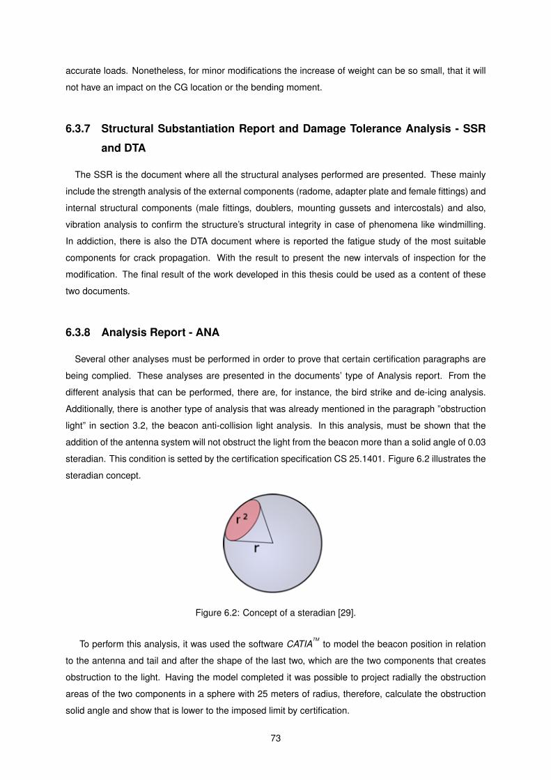
accurate loads. Nonetheless, for minor modifications the increase of weight can be so small, that it will
not have an impact on the CG location or the bending moment.
6.3.7 Structural Substantiation Report and Damage Tolerance Analysis - SSR
and DTA
The SSR is the document where all the structural analyses performed are presented. These mainly
include the strength analysis of the external components (radome, adapter plate and female fittings) and
internal structural components (male fittings, doublers, mounting gussets and intercostals) and also,
vibration analysis to confirm the structure’s structural integrity in case of phenomena like windmilling.
In addiction, there is also the DTA document where is reported the fatigue study of the most suitable
components for crack propagation. With the result to present the new intervals of inspection for the
modification. The final result of the work developed in this thesis could be used as a content of these
two documents.
6.3.8 Analysis Report - ANA
Several other analyses must be performed in order to prove that certain certification paragraphs are
being complied. These analyses are presented in the documents’ type of Analysis report. From the
different analysis that can be performed, there are, for instance, the bird strike and de-icing analysis.
Additionally, there is another type of analysis that was already mentioned in the paragraph ”obstruction
light” in section 3.2, the beacon anti-collision light analysis. In this analysis, must be shown that the
addition of the antenna system will not obstruct the light from the beacon more than a solid angle of 0.03
steradian. This condition is setted by the certification specification CS 25.1401. Figure 6.2 illustrates the
steradian concept.
Figure 6.2: Concept of a steradian [29].
To perform this analysis, it was used the software CATIATM
to model the beacon position in relation
to the antenna and tail and after the shape of the last two, which are the two components that creates
obstruction to the light. Having the model completed it was possible to project radially the obstruction
areas of the two components in a sphere with 25 meters of radius, therefore, calculate the obstruction
solid angle and show that is lower to the imposed limit by certification.
73
6.3.9 Subcontractor Document Process Slip - DPS
Since there are structural components for the installation which come from an external supplier, all
the drawings concerning this components are also provided by the supplier. Thus, these drawings have
to be included in the documentation for the STC. To accomplish that, there are the DPS which are a
document where all the provided drawings are listed.
6.3.10 Flight Test Plan / Report - FTP/R
After each system installation, the aircraft must do a flight test in order to collect some flight data
concerning stress subjects. With the final goal to validate the theoretical results with experimental ones
from the flight. Consequently, it must be prepared a FTP document stating all the conditions for the
flight test and procedures. Finally, a FTR is prepared with all the post processing data from the flight
and furthermore, it is presented the conclusion of the comparison between theoretical and experimental
results.
6.3.11 Instructions for Continued Airworthiness - ICA
As it was already introduced in section 1.2, the ICA is the document which presents all the applicable
changes in terms of maintenance instructions with the installation of the new system, as well as, the new
intervals of inspection for each new part and existing touched environment. In addition, it also presents
the new airworthiness limitations for all the new structural provisions along with the specific inspection
method. Finally, in the ICA are also identified the new fatigue critical structures.
Once all the documents are prepared and released, the modification can be closed and the process
for the STC application can go forward to the competent regulatory body to approve the modification
applicable for elected aircraft types. To sum up, in one shot, it was developed four different installations
to sell in the future for customers with A319 or A320 series aircraft.
Now, it is possible to proceed with the final chapter, to establish the conclusions of the developed
work.
74

Chapter 7
Conclusions
7.1 Achievements
Several achievements have been fulfilled in this work, starting with the demonstration of the benefits
for the industry by using a standard as the ARINC 791 for the ka-band antenna, which is the base of the
design developed by Jet Aviation.
Secondly, the illustration of all the steps to certify a major modification as the installation of the ka-
band system was accomplished, by going through the selection of the antenna location, the certification
requirements, the mechanical design development, the installation and respective deviations, the flight
test and the documentation required for the Supplemental Type Certificate (STC) application.
Thirdly, the major achievement in this work was the results obtained from the static and fatigue
analysis for the seven set hypotheses in the parametric optimization. The results proved that all designs
are strong enough to withstand the selected critical load case, rapid decompression of the radome.
All the structural components presented a safety margin higher than zero. In terms of fatigue, the
alterations introduced in the fittings, doubler and intercostals led to a reduction of the fatigue life for all the
hypotheses, although without any negative impact on the Airbus threshold. As final result, hypotheses
number six - design with modified doublers and intercostals - was considered the optimal due to the high
percentage of weight reduction and low reduction of the fatigue life number of cycles. To sum up, this
initial parametric optimization was useful to find an optimal design which can be an option in the future.
However, further analyses must be conducted to verify the structural integrity for other load cases and
to determine the threshold and intervals of inspection in order to be a certified design.
Lastly, the important role played by the experimental flight test in the certification of the initial design
of Jet Aviation was shown. The obtained results during the flight test covering the vibration and buffeting
requirement proved that any peaks of vibration energy indicating resonance or flutter occurs within the
required range of frequencies. With these results plus the numerical ones was achieved a certified solu-
tion, where an EASA Supplemental Type Certificate was issued with the number 10071445, named as
”KA Band Satcom System” applicable for the Airbus A319 and A320 series aircraft on the rear fuselage.
75

7.2 Future Work
As a future work, there are two identified opportunities.
The first one is to continue the scope of the present work, where the static analysis for the remaining
loads cases could be performed in order to prove that all the seven hypotheses are strong enough under
all the load cases. In addiction, the damage tolerance analysis could also be conducted in order to find
the intervals of inspections required for certification. With these two topics covered, the results could
show if all the hypotheses are certifiable designs or not.
The second option is to take the initial design developed at Jet Aviation and update it for the new
standard ARINC 792, where there were 7 fittings interfacing the antenna and the aircraft airframe, there
would be only six fittings, the most backward, the number seven having been removed. An initial study
could be performed to verify if the updated design is still feasible in terms of stress and certificability. In
case of a negative result, what changes could be performed in the design in order to make it feasible.
76
Bibliography
[1] Presentation of 2017 air transport statistical results. Technical report, ICAO, 2017.
[2] P. Belobaba, A. Odoni, and C. Barnhart. The Global Airline Industry. Wiley, 1st edition, 2009.
ISBN:978-0-470-74077-4.
[3] V. Giurgiutiu. Structural Health Monitoring of Aerospace Composites. Academic Press, 2016.
ISBN:978-0-12-409605-9.
[4] Title 14 of the Code of Federal Regulations — Aeronautics and Space, Chapter 1. Federal Aviation
Administration, Department of Transportation.
[5] F. D. Florio. Airworthiness: An Introduction to Aircraft Certification. Elsevier, 2nd edition, 2011.
ISBN:978-0-08-096802-5.
[6] M. ffilligan. ORDER 8110.54A - Instructions for Continued Airworthiness Responsibilities, Require-
ments, and Contents. U.S. Department of Transportation, Federal Aviation Administration, October
2010.
[7] Global Network & Capabilities Guide. Jet Aviation, Aeschengraben 6, 4051 Basel, Switzerland,
April 2019.
[8] S. C. L. et all. Ka band satellite communications design analysis and optimisation. DSTA Horizons,
pages 70–79, 2015.
[9] P. Miller. Ka-band – the future of satellite communication? TELE-satellite & Broadband, September
2007. Technology Background.
[10] H. I. Inc. Gx ka-band broadband connectivity, 3 2018.
[11] A320 family ka band satcom system installation. Classification Assessment & Application Form
JBSL-M-01326CAF-01, Jet Aviation AG, July 2019.
[12] AEEC. Mark 1 aviation ku-band and ka-band satellite communication system: Part 1 - physical
installation and aircraft interfaces. SAE-ITC, August 2014. ARINC Industry Activities - Characteristic
791-2.
77
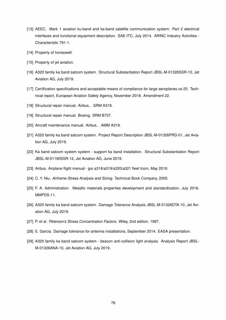
[13] AEEC. Mark 1 aviation ku-band and ka-band satellite communication system: Part 2 electrical
interfaces and functional equipment description. SAE-ITC, July 2014. ARINC Industry Activities -
Characteristic 791-1.
[14] Property of honeywell.
[15] Property of jet aviation.
[16] A320 family ka band satcom system. Structural Substantiation Report JBSL-M-01326SSR-10, Jet
Aviation AG, July 2019.
[17] Certification specifications and acceptable means of compliance for large aeroplanes cs-25. Tech-
nical report, European Aviation Safety Agency, November 2018. Amendment 22.
[18] Structural repair manual. Airbus, . SRM A319.
[19] Structural repair manual. Boeing. SRM B737.
[20] Aircraft maintenance manual. Airbus, . AMM A319.
[21] A320 family ka band satcom system. Project Report Description JBSL-M-01326PRD-01, Jet Avia-
tion AG, July 2019.
[22] Ka band satcom system system - support ka band installation. Structural Substantiation Report
JBSL-M-01190SSR-12, Jet Aviation AG, June 2019.
[23] Airbus. Airplane flight manual - jpo a318/a319/a320/a321 fleet fcom, May 2019.
[24] C. Y. Niu. Airframe Stress Analysis and Sizing. Technical Book Company, 2005.
[25] F. A. Administration. Metallic materials properties development and standardization, July 2016.
MMPDS-11.
[26] A320 family ka band satcom system. Damage Tolerance Analysis JBSL-M-01326DTA-10, Jet Avi-
ation AG, July 2019.
[27] P. et al. Peterson’s Stress Concentration Factors. Wiley, 2nd edition, 1997.
[28] E. Garcia. Damage tolerance for antenna installations, September 2014. EASA presentation.
[29] A320 family ka band satcom system - beacon anti-collision light analysis. Analysis Report JBSL-
M-01326ANA-10, Jet Aviation AG, July 2019.
78
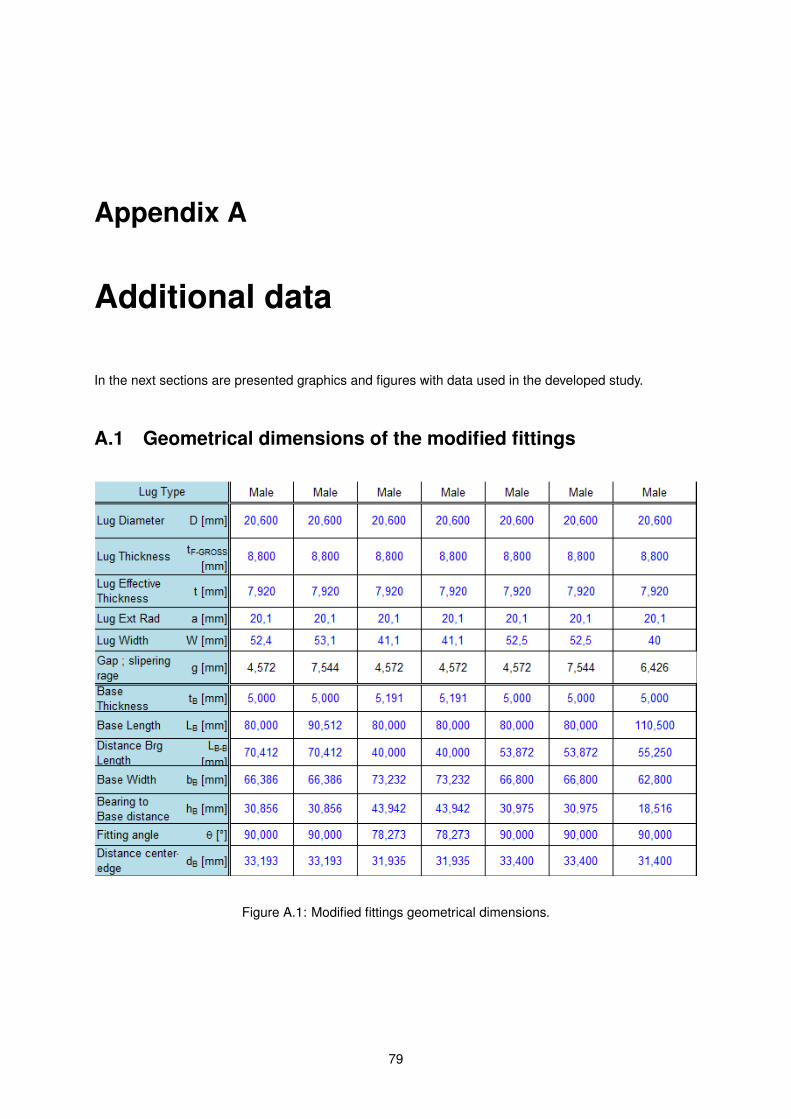
Appendix A
Additional data
In the next sections are presented graphics and figures with data used in the developed study.
A.1 Geometrical dimensions of the modified fittings
Figure A.1: Modified fittings geometrical dimensions.
79
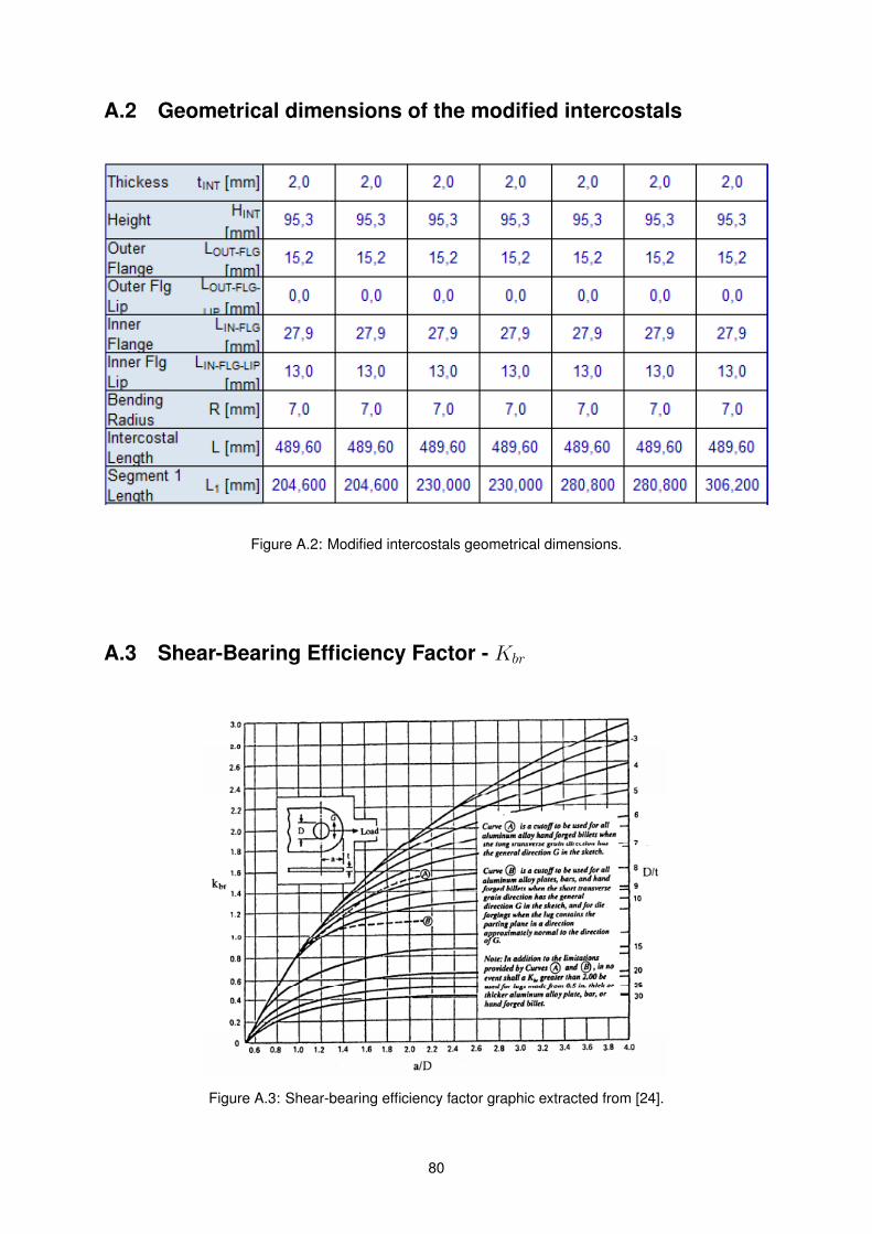
A.2 Geometrical dimensions of the modified intercostals
Figure A.2: Modified intercostals geometrical dimensions.
A.3 Shear-Bearing Efficiency Factor - Kbr
Figure A.3: Shear-bearing efficiency factor graphic extracted from [24].
80
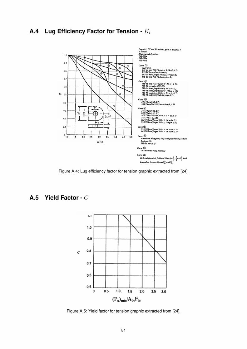
A.4 Lug Efficiency Factor for Tension - Kt
Figure A.4: Lug efficiency factor for tension graphic extracted from [24].
A.5 Yield Factor - C
Figure A.5: Yield factor for tension graphic extracted from [24].
81
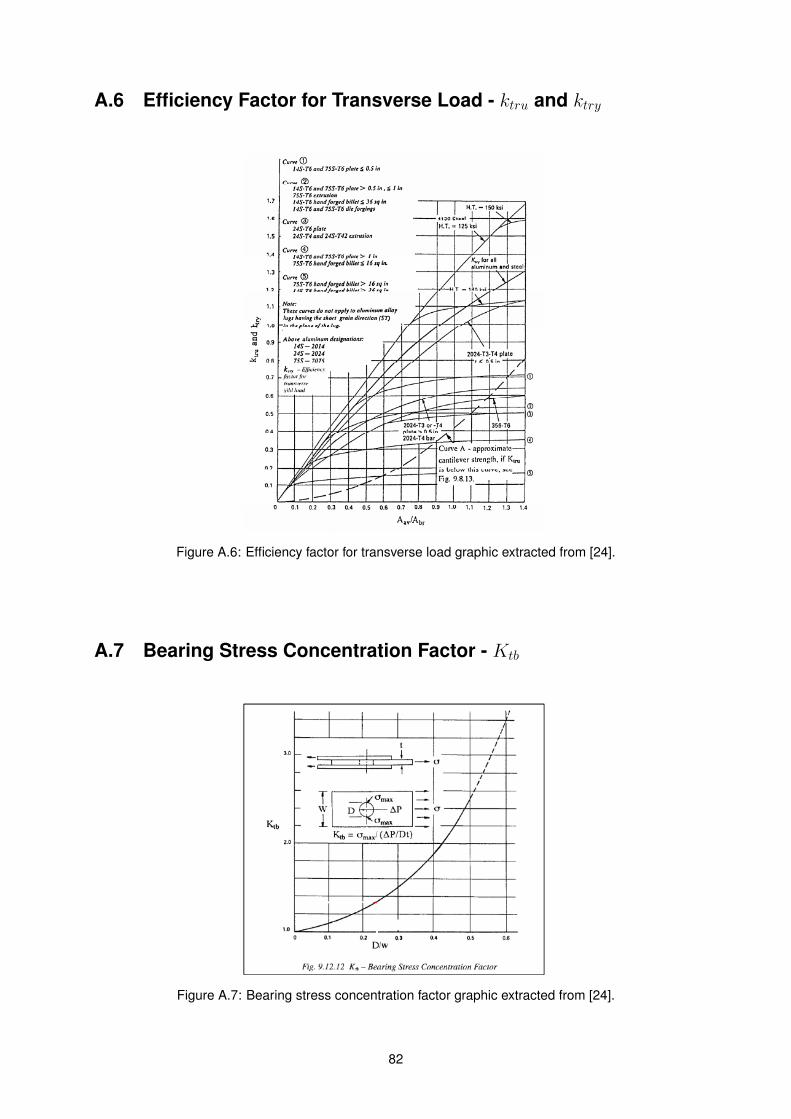
A.6 Efficiency Factor for Transverse Load - ktru and ktry
Figure A.6: Efficiency factor for transverse load graphic extracted from [24].
A.7 Bearing Stress Concentration Factor - Ktb
Figure A.7: Bearing stress concentration factor graphic extracted from [24].
82

A.8 Stress Concentration Factor - Ktg
Figure A.8: Stress concentration factor graphic extracted from [24].
A.9 Bearing Distribution Factor - θ
Figure A.9: Bearing distribution factor graphic extracted from [24].
83
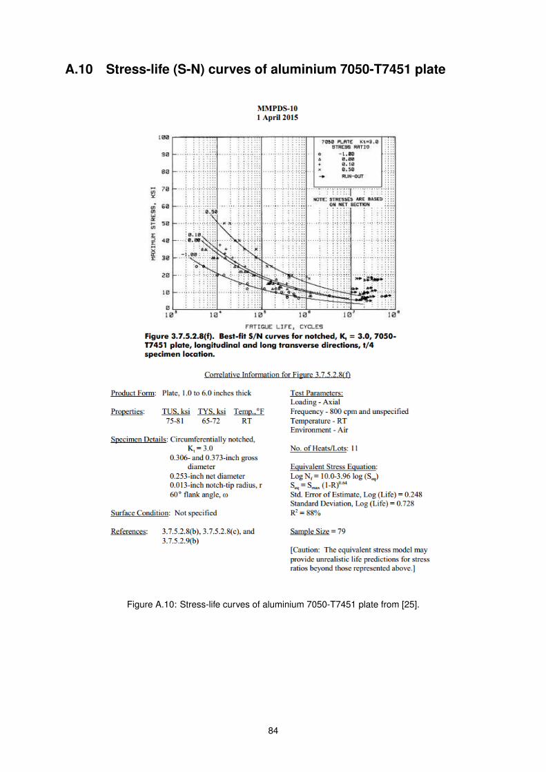
A.10 Stress-life (S-N) curves of aluminium 7050-T7451 plate
Figure A.10: Stress-life curves of aluminium 7050-T7451 plate from [25].
84
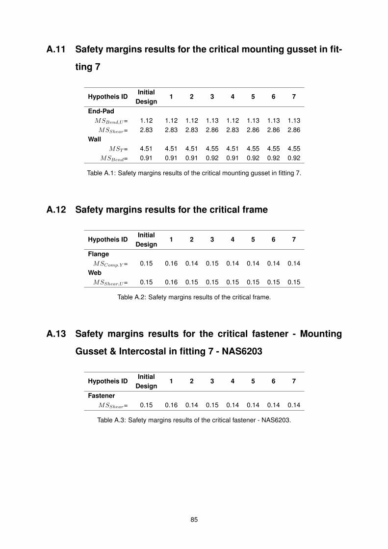
A.11 Safety margins results for the critical mounting gusset in fit-
ting 7
Hypotheis IDInitial
Design1 2 3 4 5 6 7
End-PadMSBend,U= 1.12 1.12 1.12 1.13 1.12 1.13 1.13 1.13MSShear= 2.83 2.83 2.83 2.86 2.83 2.86 2.86 2.86
WallMST = 4.51 4.51 4.51 4.55 4.51 4.55 4.55 4.55
MSBend= 0.91 0.91 0.91 0.92 0.91 0.92 0.92 0.92
Table A.1: Safety margins results of the critical mounting gusset in fitting 7.
A.12 Safety margins results for the critical frame
Hypotheis IDInitial
Design1 2 3 4 5 6 7
FlangeMSComp.Y = 0.15 0.16 0.14 0.15 0.14 0.14 0.14 0.14
WebMSShear,U= 0.15 0.16 0.15 0.15 0.15 0.15 0.15 0.15
Table A.2: Safety margins results of the critical frame.
A.13 Safety margins results for the critical fastener - Mounting
Gusset & Intercostal in fitting 7 - NAS6203
Hypotheis IDInitial
Design1 2 3 4 5 6 7
FastenerMSShear= 0.15 0.16 0.14 0.15 0.14 0.14 0.14 0.14
Table A.3: Safety margins results of the critical fastener - NAS6203.
85

86