July-2016-Newsletter-Deutsche-Bank-on-behalf-of ...

The 7th Annual GVS was held on March 16th in New York City. Joined by the other event sponsors,

including banks and exchanges, ten volatility and tail hedge managers hosted a crowd of 350

attendees including senior investment representatives from the largest global pensions, sovereign

wealth funds, endowments, foundations, and insurance companies.

2016 MANAGER PARTICIPANTS

Argentière Capital

BlueMountain Capital

Capstone Investment Advisors

Capula Investment Management

Ionic Capital Management

Man AHL

Parallax Volatility Advisors

PIMCO

Pine River Capital Management

True Partner Capital

2016 KEYNOTE AND GUEST SPEAKERS

The 2016 keynote speakers were Barney Frank and Marcus Luttrell. Barney Frank served as a US

Congressman for over 30 years and most recently as the Chairman of the House Financial Services

Committee from 2007 through 2011. He was a key author of the Dodd-Frank Wall Street Reform and

Consumer Protection Act. Marcus Luttrell is a decorated Navy Seal and best-selling author of Lone

Survivor. You can access their biographies and more information about the event on the website:

www.globalvolatilitysummit.com.

Dear Investor,

The Global Volatility Summit (“GVS”) brings together volatility and tail hedge managers, institutional

investors, thought-provoking speakers, and other industry experts to discuss the volatility markets

and the roles volatility strategies can play in institutional investment portfolios. The GVS aims to keep

investors updated on the volatility markets throughout the year, and educated on innovations within

the space.

Deutsche Bank has provided the latest piece in the GVS newsletter series on behalf of BlueMountain

Capital. Part II of the newsletter is enclosed. Please refer to the GVS website for Part I.

Cheers,

Global Volatility Summit

Questions? Please contact [email protected]

Website: www.globalvolatilitysummit.com

http://www.globalvolatilitysummit.com/

16 May 2016

Signal Processing

Deutsche Bank Securities Inc. Page 35

Grassroots crowding measures

In this section, we examine more direct measures of crowding based on

investor holding and interest (i.e., buying power). These are metrics that we

would expect to be more reliable measures of crowding because they use

information that is directly related to how investor share positions.

Holdings based measures

On face value, using the holdings data reported directly by money managers

(via 13F and other regulatory filings) seems to be the most obvious way to

measure crowdedness. If most managers hold deep value stocks then we

might infer that value strategies are crowded. Unfortunately, the problem with

ownership data is the lag between when a fund actually holds a position and

when it has to report that position (roughly two months later).This means that

any information gleaned from ownership data will be somewhat backwards

looking. Nonetheless, it is worth investigating.

We use the Thomson Reuters ownership database as our source for fund

holdings.10 The Thomson Reuter’s institutional dataset collects holding data

from global institutions, mutual funds, and individual investors. Short and cash

positions are not disclosed in the Thomson Reuters database. Data is available

on a quarterly basis since 13F disclosures are typically filed quarterly by

intuitions. Using this data, we compute the percentage of ownership for each

stock on each quarter end, using the most recently reported regulatory filings.

The percentage of ownership is essentially shares held by a class of

institutions divided by total shares outstanding. We term this as ownership

intensity factor.

7. Ownership intensity

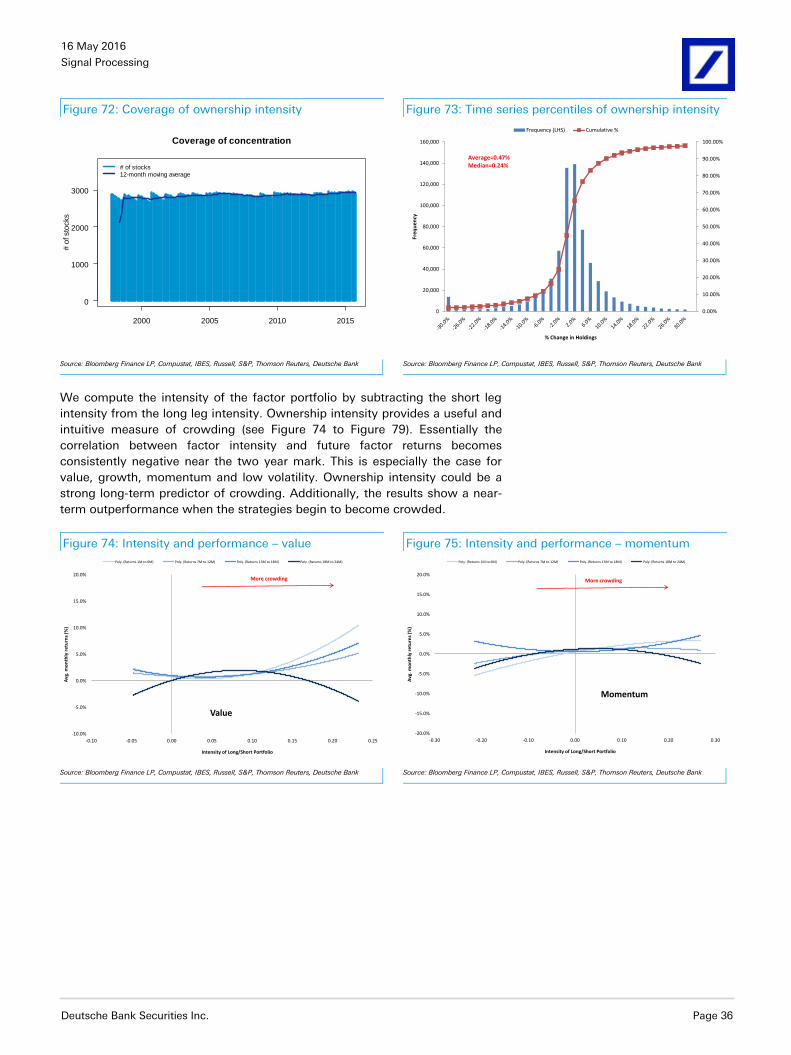
We test whether ownership intensity is indicative of crowding. Figure 72

shows the times series coverage of the ownership intensity factor within the

Russell 3000 universe. The coverage is fairly strong. Undoubtedly, every stock

should have an owner and our dataset has an expansive breadth of owners.

We also analyze the distribution of the change in intensity (see Figure 73).

Interestingly, the figure shows that the average change in ownership for

companies is approximately 0.5%. The mean and median are both positive

which suggests that on average, owners increase their positions in companies.

It may also reflect the onset of institutional money into equities and out of

other asset classes.

10 We have published multiple research papers using this database, see Jussa et al [2014], Wang et al

[2014], and Wang et al [2106].

We use the Thomson Reuters

ownership database as our

source for fund holdings.

Note that 13F disclosures are

typically filed quarterly by

intuitions

16 May 2016

Signal Processing

Deutsche Bank Securities Inc. 6

Figure 72: Coverage of ownership intensity Figure 73: Time series percentiles of ownership intensity

2000 2005 2010 2015

0

1000

2000

3000

Coverage of concentration

# o

f sto

cks

# of stocks12-month moving average

0.00%

10.00%

20.00%

30.00%

40.00%

50.00%

60.00%

70.00%

80.00%

90.00%

100.00%

0

20,000

40,000

60,000

80,000

100,000

120,000

140,000

160,000

Fre

qu

en

cy

% Change in Holdings

Frequency (LHS) Cumulative %

Average=0.47%Median=0.24%

Source: Bloomberg Finance LP, Compustat, IBES, Russell, S&P, Thomson Reuters, Deutsche Bank


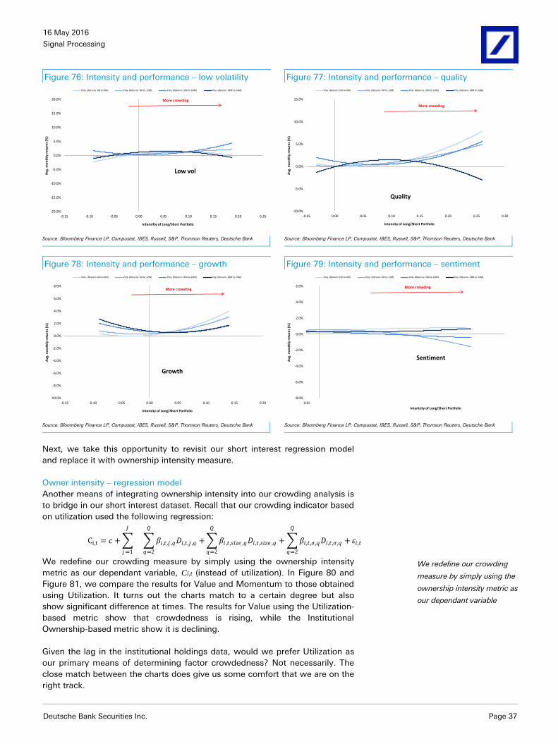
We compute the intensity of the factor portfolio by subtracting the short leg

intensity from the long leg intensity. Ownership intensity provides a useful and

intuitive measure of crowding (see Figure 74 to Figure 79). Essentially the

correlation between factor intensity and future factor returns becomes

consistently negative near the two year mark. This is especially the case for

value, growth, momentum and low volatility. Ownership intensity could be a

strong long-term predictor of crowding. Additionally, the results show a near-

term outperformance when the strategies begin to become crowded.

Figure 74: Intensity and performance – value Figure 75: Intensity and performance – momentum

-10.0%

-5.0%

0.0%

5.0%

10.0%

15.0%

20.0%

-0.10 -0.05 0.00 0.05 0.10 0.15 0.20 0.25

Avg

. mo

nth

ly r

etu

rns

(%)

Intensity of Long/Short Portfolio

Value

Poly. (Returns 1M to 6M) Poly. (Returns 7M to 12M) Poly. (Returns 13M to 18M) Poly. (Returns 18M to 24M)

More crowding

-20.0%

-15.0%

-10.0%

-5.0%

0.0%

5.0%

10.0%

15.0%

20.0%

-0.30 -0.20 -0.10 0.00 0.10 0.20 0.30

Avg

. mo

nth

ly r

etu

rns

(%)


Momentum


More crowding



16 May 2016

Signal Processing


Figure 76: Intensity and performance – low volatility Figure 77: Intensity and performance – quality

-20.0%

-15.0%

-10.0%

-5.0%

0.0%

5.0%

10.0%

15.0%

20.0%

-0.15 -0.10 -0.05 0.00 0.05 0.10 0.15 0.20 0.25

Avg

. mo

nth

ly r

etu

rns

(%)

Intensifty of Long/Short Portfolio

Low vol


More crowding

-10.0%

-5.0%

0.0%

5.0%

10.0%

15.0%

-0.05 0.00 0.05 0.10 0.15 0.20 0.25 0.30

Avg

. mo

nth

ly r

etu

rns

(%)


Quality


More crowding



Figure 78: Intensity and performance – growth Figure 79: Intensity and performance – sentiment

-10.0%

-8.0%

-6.0%

-4.0%

-2.0%

0.0%

2.0%

4.0%

6.0%

8.0%

-0.15 -0.10 -0.05 0.00 0.05 0.10 0.15 0.20

Avg

. mo

nth

ly r

etu

rns

(%)


Growth


More crowding

-8.0%

-6.0%

-4.0%

-2.0%

0.0%

2.0%

4.0%

6.0%

-0.01

Avg

. mo

nth

ly r

etu

rns

(%)

Intenisity of Long/Short Portfolio

Sentiment


More crowding



Next, we take this opportunity to revisit our short interest regression model

and replace it with ownership intensity measure.

Owner intensity – regression model

Another means of integrating ownership intensity into our crowding analysis is

to bridge in our short interest dataset. Recall that our crowding indicator based

on utilization used the following regression:

We redefine our crowding measure by simply using the ownership intensity

metric as our dependant variable, Ci,t (instead of utilization). In Figure 80 and

Figure 81, we compare the results for Value and Momentum to those obtained

using Utilization. It turns out the charts match to a certain degree but also

show significant difference at times. The results for Value using the Utilization-

based metric show that crowdedness is rising, while the Institutional

Ownership-based metric show it is declining.

Given the lag in the institutional holdings data, would we prefer Utilization as

our primary means of determining factor crowdedness? Not necessarily. The

close match between the charts does give us some comfort that we are on the

right track.

We redefine our crowding

measure by simply using the

ownership intensity metric as

our dependant variable

Ci,t = 𝑐 +

𝐽

𝑗=1

𝛽𝑖,𝑡 ,𝑗 ,𝑞𝐷𝑖,𝑡 ,𝑗 ,𝑞 +

𝑄

𝑞=2

𝛽𝑖 ,𝑡,𝑠𝑖𝑧𝑒 ,𝑞𝐷𝑖,𝑡 ,𝑠𝑖𝑧𝑒 ,𝑞 + 𝛽𝑖,𝑡 ,𝜎 ,𝑞𝐷𝑖,𝑡 ,𝜎 ,𝑞 +

𝑄

𝑞=2

𝑄

𝑞=2

𝜀𝑖 ,𝑡

16 May 2016

Signal Processing


Figure 80: Incremental Utilization versus incremental

Institutional Ownership for Q10 value stocks

Figure 81: Incremental Utilization versus incremental

Institutional Ownership for Q10 Momentum stocks

-10.0%

-5.0%

0.0%

5.0%

10.0%

15.0%

20.0%

25.0%

30.0%

35.0%-15.0

-10.0

-5.0

0.0

5.0

10.0

15.0

20.0

25.0

Q1

0 v

s Q

1 In

st. O

wn

ers

hip

(in

vert

ed

)

Q1

0 v

s Q

1 U

tiliz

atio

n (

%)

Momentum (short interest) Momemtum (concentration)

More Crowded

Less Crowded

-4.0%

-2.0%

0.0%

2.0%

4.0%

6.0%

8.0%

10.0%

12.0%

14.0%-5.0

0.0

5.0

10.0

15.0

20.0

Q1

0 v

s Q

1 In

st. O

wn

ers

hip

(in

vert

ed

)

Q1

0 v

s Q

1 U

tiliz

atio

n (

%)

Earnings yield (short interest) Earnings yield (concentration)

More Crowded

Less Crowded



Next, we analyze another potential crowding measure based on institutional

ownership.

8. Buying power

In Sias [2002], herding is measured using the holdings dataset consisted of

observing buying patterns of investors or owners. An owner is defined as a

buyer if the ownership of the stock increases. More specifically, if the position

held by the owner increases as a fraction of the shares outstanding, then the

owner is a buyer. For example, if an owner held 0.01% shares of IBM and the

following quarter it held 0.02% shares of IBM, then it would be classified as a

buyer.11 For each stock s at each quarter end q the herding or buying power

measure is simply:

Since the data is measured quarterly, owners that buy and sell the same

number of shares within the same quarter will not be counted as a trade. By

aggregating the buying power at a sector, market, and strategy level, we can

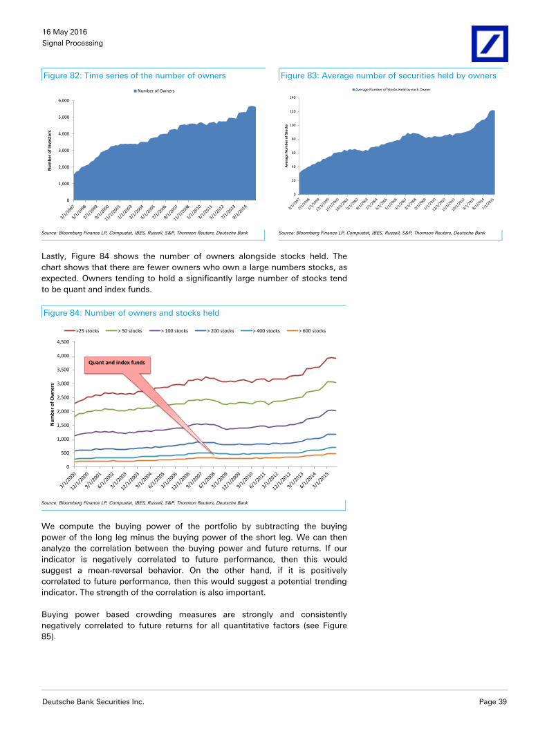
test whether this measure is indicative of crowding. To get a better sense of

the dataset, Figure 82 plots the number of owners over time. The current

number of owners exceeds 5,000 investors. Figure 83 shows the average

number of stocks held by owners. Investors on average hold approximately 75

stocks.

11 Note that 0.01% and 0.02% represent shares held over shares outstanding for that particular institution

at quarter end.

Sias’ approach to measure

herding using the holdings

dataset was by observing

buying patterns of investors

buying_powers,q =# of Owners Buyings,q

# of Owners Buyings,q + # of Owners Sellings,q

16 May 2016

Signal Processing


Figure 82: Time series of the number of owners Figure 83: Average number of securities held by owners

0

1,000

2,000

3,000

4,000

5,000

6,000

Nu

mb

er

of

Inve

sto

rs

Number of Owners

0

20

40

60

80

100

120

140

Ave

rage

Nu

mb

er

of

Sto

cks

Average Number of Stocks Held by each Owner



Lastly, Figure 84 shows the number of owners alongside stocks held. The

chart shows that there are fewer owners who own a large numbers stocks, as

expected. Owners tending to hold a significantly large number of stocks tend

to be quant and index funds.

Figure 84: Number of owners and stocks held

0

500

1,000

1,500

2,000

2,500

3,000

3,500

4,000

4,500

Nu

mb

er

of

Ow

ne

rs

>25 stocks > 50 stocks > 100 stocks > 200 stocks > 400 stocks > 600 stocks

Quant and index funds


We compute the buying power of the portfolio by subtracting the buying

power of the long leg minus the buying power of the short leg. We can then

analyze the correlation between the buying power and future returns. If our

indicator is negatively correlated to future performance, then this would

suggest a mean-reversal behavior. On the other hand, if it is positively

correlated to future performance, then this would suggest a potential trending

indicator. The strength of the correlation is also important.

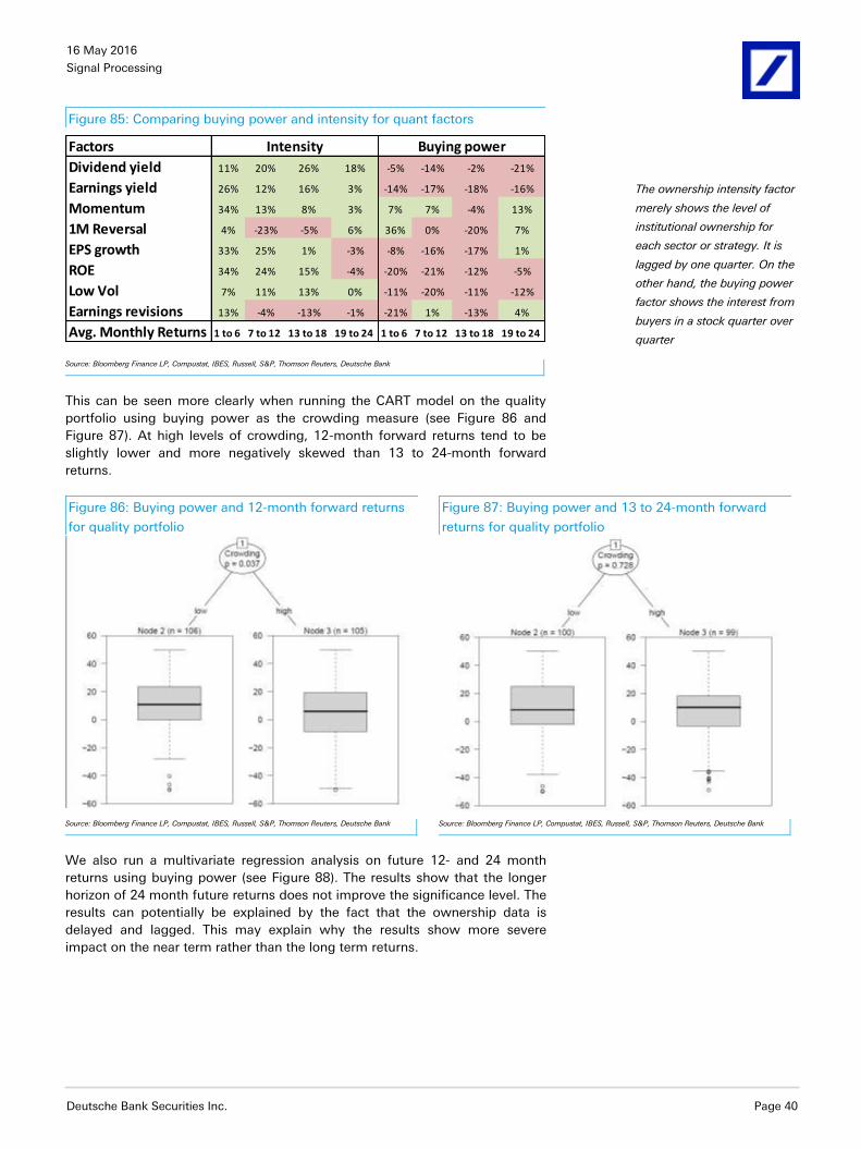
Buying power based crowding measures are strongly and consistently

negatively correlated to future returns for all quantitative factors (see Figure

85).

16 May 2016

Signal Processing


Figure 85: Comparing buying power and intensity for quant factors

Factors

Dividend yield 11% 20% 26% 18% -5% -14% -2% -21%

Earnings yield 26% 12% 16% 3% -14% -17% -18% -16%

Momentum 34% 13% 8% 3% 7% 7% -4% 13%

1M Reversal 4% -23% -5% 6% 36% 0% -20% 7%

EPS growth 33% 25% 1% -3% -8% -16% -17% 1%

ROE 34% 24% 15% -4% -20% -21% -12% -5%

Low Vol 7% 11% 13% 0% -11% -20% -11% -12%

Earnings revisions 13% -4% -13% -1% -21% 1% -13% 4%

Avg. Monthly Returns 1 to 6 7 to 12 13 to 18 19 to 24 1 to 6 7 to 12 13 to 18 19 to 24

Intensity Buying power


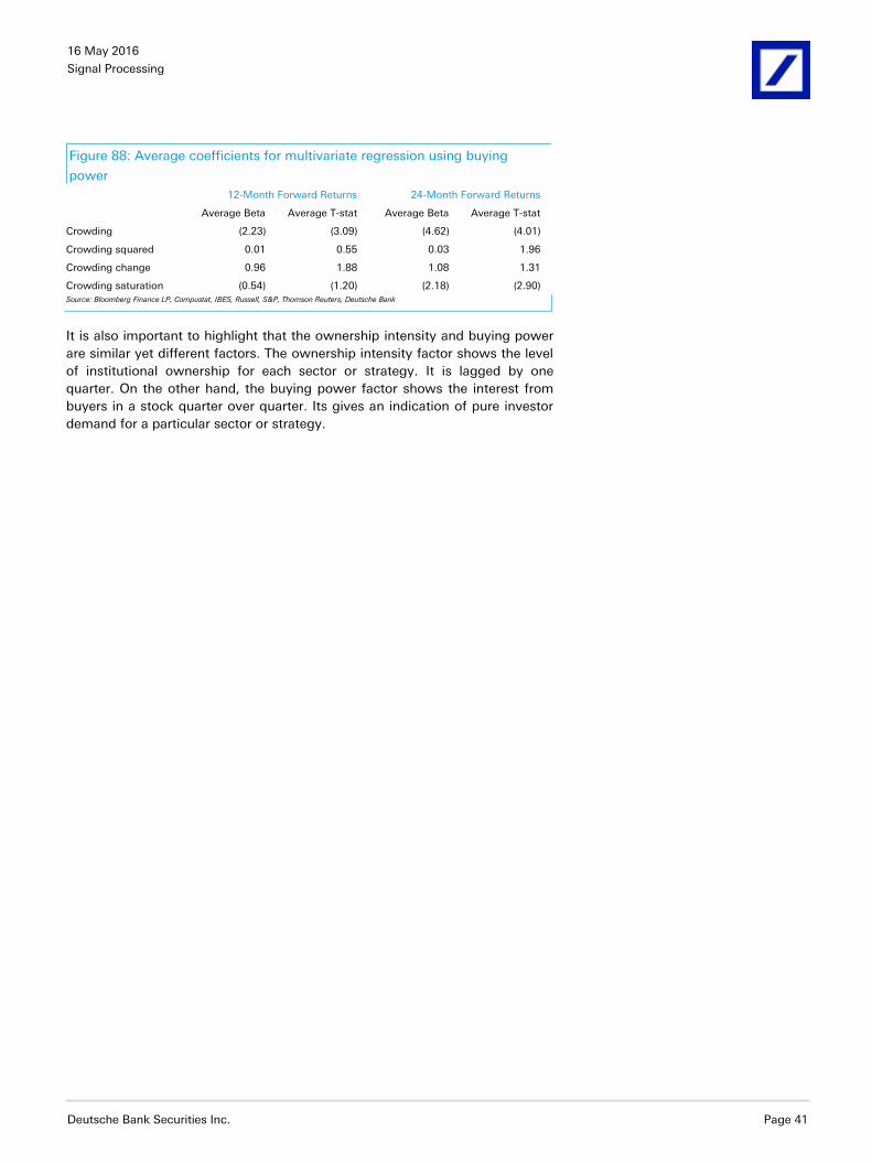
This can be seen more clearly when running the CART model on the quality

portfolio using buying power as the crowding measure (see Figure 86 and

Figure 87). At high levels of crowding, 12-month forward returns tend to be

slightly lower and more negatively skewed than 13 to 24-month forward

returns.

Figure 86: Buying power and 12-month forward returns

for quality portfolio

Figure 87: Buying power and 13 to 24-month forward

returns for quality portfolio



We also run a multivariate regression analysis on future 12- and 24 month

returns using buying power (see Figure 88). The results show that the longer

horizon of 24 month future returns does not improve the significance level. The

results can potentially be explained by the fact that the ownership data is

delayed and lagged. This may explain why the results show more severe

impact on the near term rather than the long term returns.

The ownership intensity factor

merely shows the level of

institutional ownership for

each sector or strategy. It is

lagged by one quarter. On the

other hand, the buying power

factor shows the interest from

buyers in a stock quarter over

quarter

16 May 2016

Signal Processing


Figure 88: Average coefficients for multivariate regression using buying

power

12-Month Forward Returns 24-Month Forward Returns

Average Beta Average T-stat Average Beta Average T-stat

Crowding (2.23) (3.09) (4.62) (4.01)

Crowding squared 0.01 0.55 0.03 1.96

Crowding change 0.96 1.88 1.08 1.31

Crowding saturation (0.54) (1.20) (2.18) (2.90)


It is also important to highlight that the ownership intensity and buying power

are similar yet different factors. The ownership intensity factor shows the level

of institutional ownership for each sector or strategy. It is lagged by one

quarter. On the other hand, the buying power factor shows the interest from

buyers in a stock quarter over quarter. Its gives an indication of pure investor

demand for a particular sector or strategy.

16 May 2016

Signal Processing


The ultimate crowding measures

In this section, we examine two portfolio level of crowding measures: the

concentration and diversification ratios. We have studied them as crowding

measures in Luo, et al [2014] and Wang, et al [2016].

9. Concentration ratio

In classic economics, the concentration ratio is a measure of the output

produced by each firm in an industry. CR4 measure the market share of the

four largest firms in an industry. Similarly, CR8 measures the market share of

the eight largest firms in an industry. The concentration ratio is a measure of

market control within an industry. It essentially measures the degree to which

an industry is oligopolistic (i.e., dominated by a few companies).

The traditional measure of competitiveness and concentration is the Herfindahl

index:

A similar measure of company domination can be calculated at the portfolio

level. The measure is called the concentration ratio or CR12.

It is a measure of portfolio concentration that takes the volatility of the stocks

into account. A higher CR is indicative of more concentrated positioning. For

example, take the hedge fund aggregate portfolio (HFA) based on institutional

ownership data. This simply aggregates the positions of most hedge funds. It

shows which companies most hedge funds are heavily invested in. If the HFA

portfolio has significant positions in a few highly volatile companies, then the

CR would show that this portfolio is fairly “concentrated”.

In general, if a portfolio has heavy positioning in volatile names, then the CR

would reflect that this portfolio is concentrated. In effect, the CR measures not

only the concentration of weights, but also the concentration of risks as assets

are weighted proportionally by their volatilities. 13

The concentration ratio and portfolio crowding

The CR ratio is typically used to measure crowdedness in aggregate portfolios.

For example, the CR can be used to measure the crowdedness of the HFA

portfolio described earlier. However, quants typically invest in a larger number

of securities than typical hedge funds. To test whether quantitative strategies

are crowded, we construct the quantitative representative portfolio or QRP.

12 As shown in Choueifaty and Coignard [2008] and Luo, et al [2014]

13 See Choueifaty and Coignard [2008] for more details.

In general, if a portfolio has

heavy positioning in volatile

names, the CR would reflect

that this portfolio is

concentrated

𝐻𝑒𝑟𝑓𝑖𝑛𝑑𝑎ℎ𝑙_𝐼𝑛𝑑𝑒𝑥 = market_sharesn2

𝐶𝑅 = 𝑤𝑖

2𝜎𝑖2𝑁

𝑖=1

𝑤𝑖𝜎𝑖𝑁𝑖=1

2

16 May 2016

Signal Processing


To do this we simply build a portfolio based on standard factors that quants

typically use, such as value, growth, momentum, sentiment, low volatility, and

quality. We sector neutralize each factor because quants typically avoid

making sector calls. Combining all these factors together forms our multifactor,

long only portfolio. We take the top 300 best stocks based on this multifactor

model and market cap weight them within the portfolio. We select a fixed

number of stocks (i.e., 300) because the CR ratio is fairly sensitive to the

number of securities. All else being equal, a larger breadth of securities will

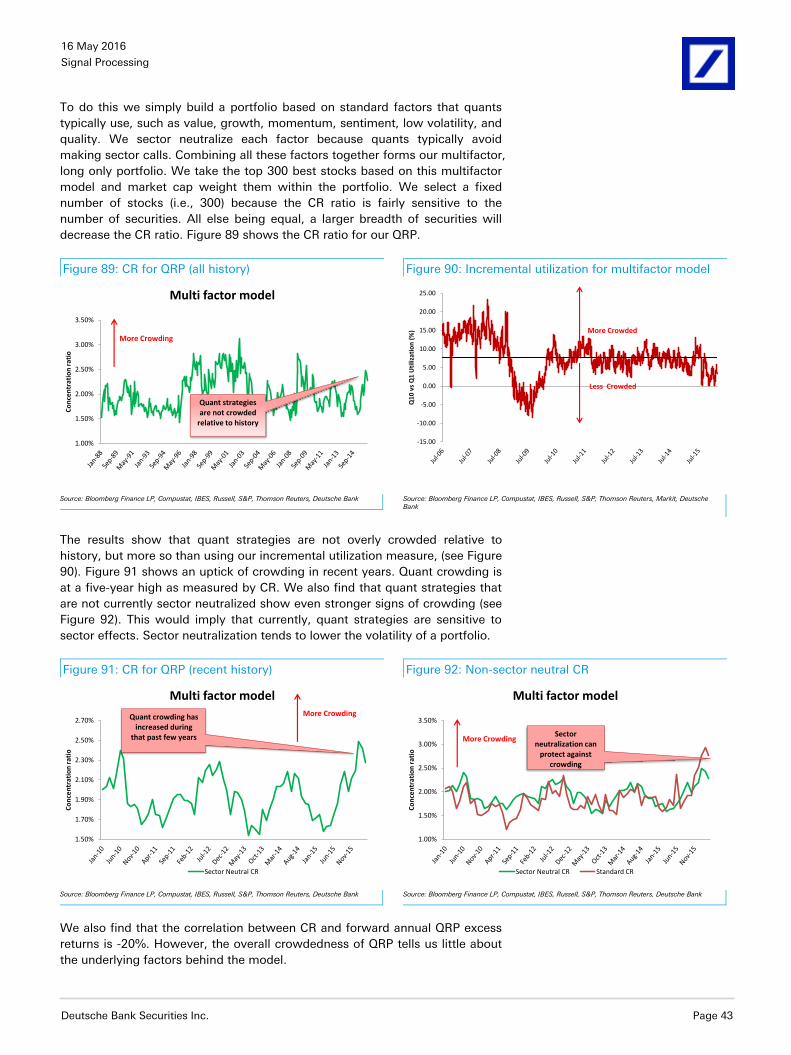
decrease the CR ratio. Figure 89 shows the CR ratio for our QRP.

Figure 89: CR for QRP (all history) Figure 90: Incremental utilization for multifactor model

1.00%

1.50%

2.00%

2.50%

3.00%

3.50%

Co

nce

ntr

atio

n r

atio

Multi factor model

More Crowding

Quant strategiesare not crowded

relative to history

-15.00

-10.00

-5.00

0.00

5.00

10.00

15.00

20.00

25.00

Q1

0 v

s Q

1 U

tiliz

atio

n (

%) More Crowded

Less Crowded


Source: Bloomberg Finance LP, Compustat, IBES, Russell, S&P, Thomson Reuters, Markit, Deutsche Bank

The results show that quant strategies are not overly crowded relative to

history, but more so than using our incremental utilization measure, (see Figure

90). Figure 91 shows an uptick of crowding in recent years. Quant crowding is

at a five-year high as measured by CR. We also find that quant strategies that

are not currently sector neutralized show even stronger signs of crowding (see

Figure 92). This would imply that currently, quant strategies are sensitive to

sector effects. Sector neutralization tends to lower the volatility of a portfolio.

Figure 91: CR for QRP (recent history) Figure 92: Non-sector neutral CR

1.50%

1.70%

1.90%

2.10%

2.30%

2.50%

2.70%

Co

nce

ntr

atio

n r

atio

Multi factor model

Sector Neutral CR

More CrowdingQuant crowding has increased during

that past few years

1.00%

1.50%

2.00%

2.50%

3.00%

3.50%

Co

nce

ntr

atio

n r

atio

Multi factor model

Sector Neutral CR Standard CR

More CrowdingSector

neutralization can protect against

crowding



We also find that the correlation between CR and forward annual QRP excess

returns is -20%. However, the overall crowdedness of QRP tells us little about

the underlying factors behind the model.

16 May 2016

Signal Processing


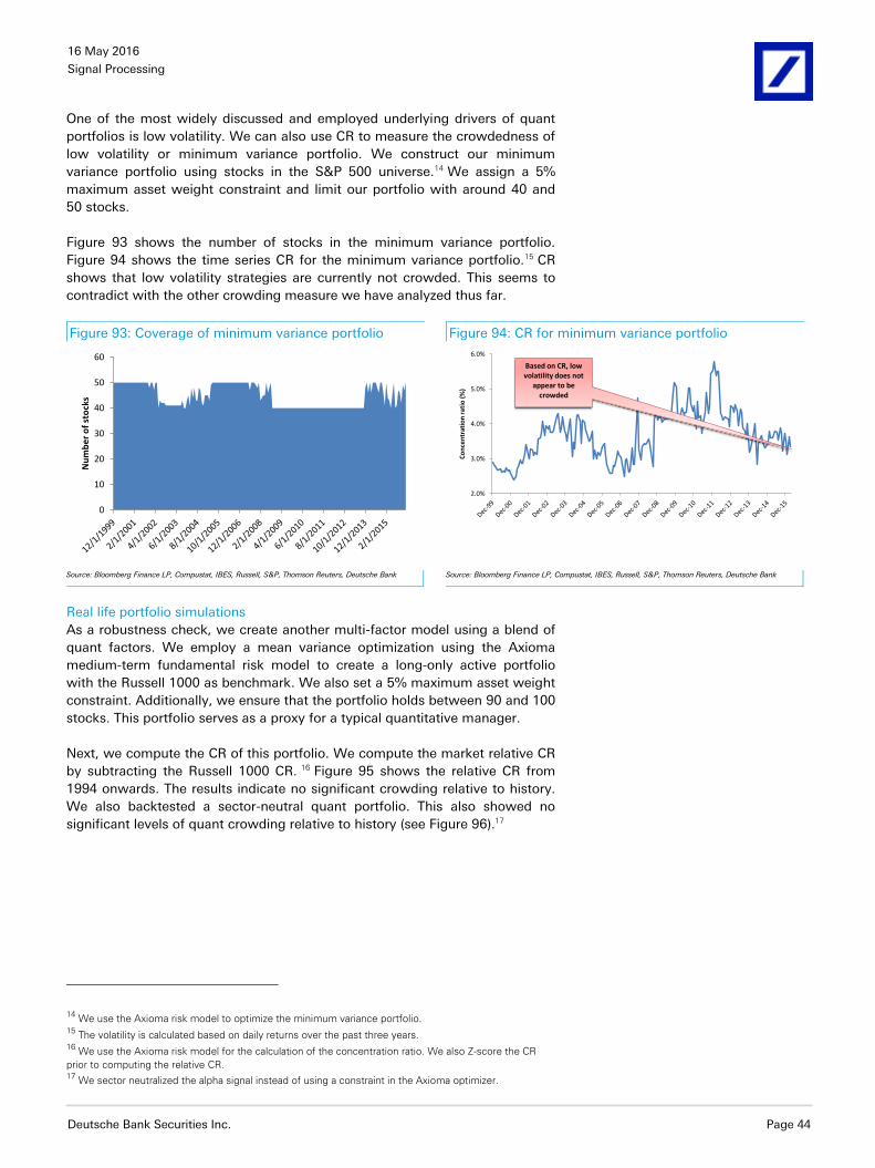
One of the most widely discussed and employed underlying drivers of quant

portfolios is low volatility. We can also use CR to measure the crowdedness of

low volatility or minimum variance portfolio. We construct our minimum

variance portfolio using stocks in the S&P 500 universe.14 We assign a 5%

maximum asset weight constraint and limit our portfolio with around 40 and

50 stocks.

Figure 93 shows the number of stocks in the minimum variance portfolio.

Figure 94 shows the time series CR for the minimum variance portfolio.15 CR

shows that low volatility strategies are currently not crowded. This seems to

contradict with the other crowding measure we have analyzed thus far.

Figure 93: Coverage of minimum variance portfolio Figure 94: CR for minimum variance portfolio

0

10

20

30

40

50

60

Nu

mb

er

of

sto

cks

2.0%

3.0%

4.0%

5.0%

6.0%

Co

nce

ntr

atio

n r

atio

(%

)

Based on CR, low volatility does not

appear to be crowded



Real life portfolio simulations

As a robustness check, we create another multi-factor model using a blend of

quant factors. We employ a mean variance optimization using the Axioma

medium-term fundamental risk model to create a long-only active portfolio

with the Russell 1000 as benchmark. We also set a 5% maximum asset weight

constraint. Additionally, we ensure that the portfolio holds between 90 and 100

stocks. This portfolio serves as a proxy for a typical quantitative manager.

Next, we compute the CR of this portfolio. We compute the market relative CR

by subtracting the Russell 1000 CR. 16 Figure 95 shows the relative CR from

1994 onwards. The results indicate no significant crowding relative to history.

We also backtested a sector-neutral quant portfolio. This also showed no

significant levels of quant crowding relative to history (see Figure 96).17

14 We use the Axioma risk model to optimize the minimum variance portfolio.

15 The volatility is calculated based on daily returns over the past three years.

16 We use the Axioma risk model for the calculation of the concentration ratio. We also Z-score the CR

prior to computing the relative CR. 17

We sector neutralized the alpha signal instead of using a constraint in the Axioma optimizer.

16 May 2016

Signal Processing


Figure 95: CR for optimized portfolio – Russell 1000 Figure 96: CR for optimized portfolio – sector neutral –

Russell 1000

-7.0

-6.0

-5.0

-4.0

-3.0

-2.0

-1.0

0.0

1.0

2.0

3.0

4.0

Co

nce

ntr

atio

n r

atio

(%

)

Mean variance (relative)

More Crowding

-7.0

-6.0

-5.0

-4.0

-3.0

-2.0

-1.0

0.0

1.0

2.0

3.0

4.0

Co

nce

ntr

atio

n r

atio

(%

)


More Crowding



We also find that the correlation between relative CR (as well as sector-neutral

relative CR) and forward annual excess returns is -40% and - 39% respectively.

This would suggest that relative CR is a reasonable measure of crowding.

However, the CR does not consider the correlation among stocks in the

portfolio. We address this next by introducing the diversification ratio.

10. Diversification ratio

The diversification ratio (DR) is similar to CR, but it takes into account the

correlation among the stocks in the portfolio (see Luo, Wang, Cahan, et al

[2013]). It is defined as the weighted average volatility divided by the total

portfolio volatility (which accounts for correlation). 18

In general, if a portfolio has heavy positioning in volatile names that are highly

correlated, the DR would reflect that this portfolio is concentrated. Reverting

back to our HFA example, if the HFA portfolio has significant positions in a few

highly volatile companies, then the DR would show that this portfolio is

undiversified or concentrated. If those names are also highly correlated, then

the DR would show significant concentration. The DR can also be written as a

function of CR. Therefore, the higher the pairwise correlation, the lower the DR.

18 See Choueifaty and Coignard [2008] for more details.

The diversification ratio (DR)

is similar to CR, but it takes

into account the correlation of

the stocks in the portfolio

𝐷𝑅 = 𝑤𝑖𝜎𝑖

𝑁𝑖=1

𝜎p

DR =1

ρaverage 1 − CR + CR

𝜎p = wi2σi

2

N

i=1

+ wiwjσiσjρij

N

i≠ji

16 May 2016

Signal Processing


The diversification ratio and factor crowding

We test how well DR can measure factor crowdedness using a similar

methodology outlined for CR. 19 We construct long only factor portfolio

reflective of the strategies that quants and other investors typically invest in.

These portfolios are: value, growth, momentum, sentiment, quality, reversal,

and low volatility. To construct these portfolios, we take the top 50 names

ranked by each factor. The universe is the Russell 3000. Note that the

portfolios are not sector neutralized.

Furthermore, we market cap weight as well as conviction weight (i.e., factor-

score weight). We also apply a 5% maximum weight constraint. Figure 97 and

Figure 98 show the time series DR for the momentum and low volatility

portfolio, respectively. We have inverted the y-axis, therefore a higher reading

is indicative of less diversification, more concentration, and hence more

crowding. We immediately notice that the DR has a trending component. On

average, it has increased over time.

This likely reflects the fact that more systematic and passive strategies have

entered the marketplace post the 1990s. And investors are chasing similar

strategies causing an increase in correlation. Based on DR, quality and low

volatility are showing signs of crowdedness, relative to their own history.

Figure 97: DR for quality cap-weighted portfolio Figure 98: DR for low volatility cap-weighted portfolio

1.00

1.50

2.00

2.50

3.00

3.50

4.00

Div

ers

ific

atio

n r

atio

Quality

More Crowding

1.00

1.50

2.00

2.50

3.00

3.50

4.00

Div

ers

ific

atio

n r

atio

Low Vol

More Crowding



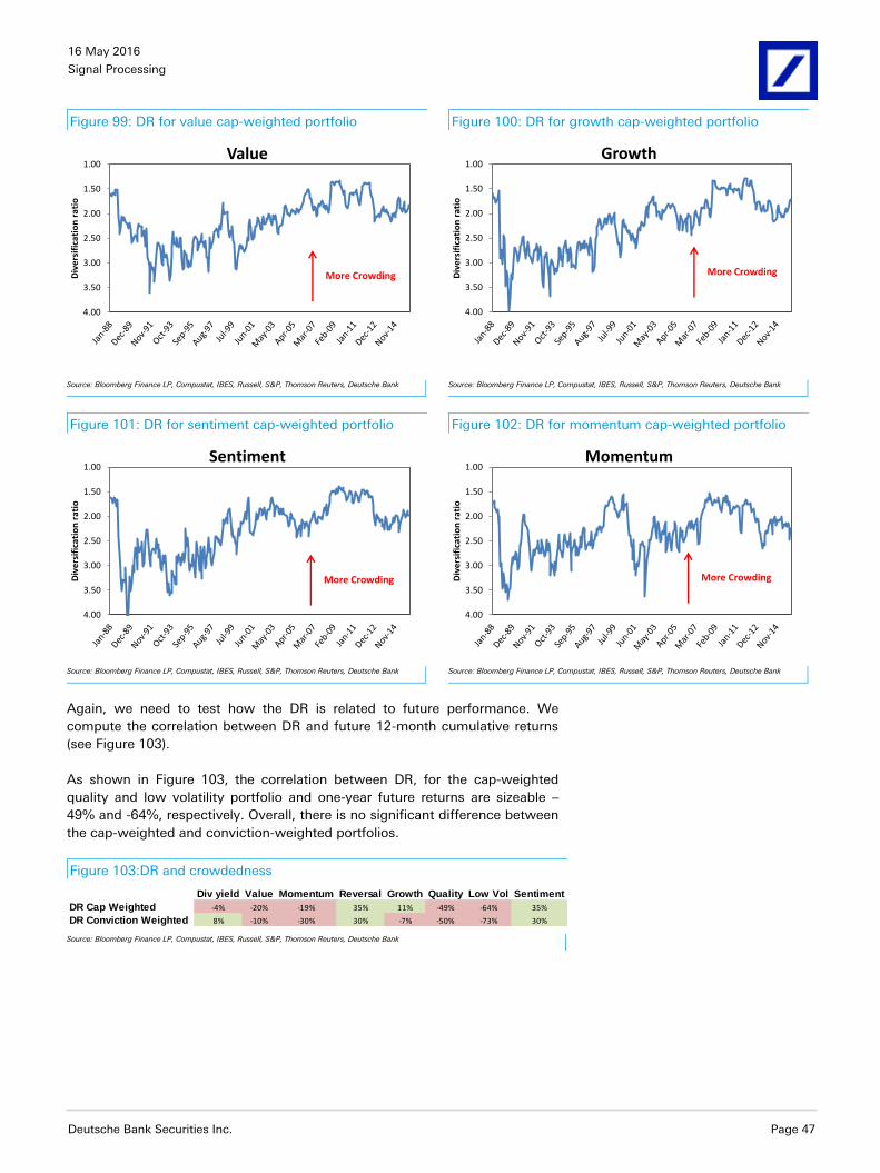
We also analyze the time series DR for the other factor portfolios (see Figure

99 to Figure 102). Again the DR ratio is showing an increasing trend overtime.

19 The calculation of DR requires the covariance matrix. We compute the sample covariance matrix for the

DR calculation using one year of daily returns.

Based on DR, quality and low

volatility are showing signs of

crowdedness, relative to their

own history

16 May 2016

Signal Processing


Figure 99: DR for value cap-weighted portfolio Figure 100: DR for growth cap-weighted portfolio

1.00

1.50

2.00

2.50

3.00

3.50

4.00

Div

ers

ific

atio

n r

atio

Value

More Crowding

1.00

1.50

2.00

2.50

3.00

3.50

4.00

Div

ers

ific

atio

n r

atio

Growth

More Crowding



Figure 101: DR for sentiment cap-weighted portfolio Figure 102: DR for momentum cap-weighted portfolio

1.00

1.50

2.00

2.50

3.00

3.50

4.00

Div

ers

ific

atio

n r

atio

Sentiment

More Crowding

1.00

1.50

2.00

2.50

3.00

3.50

4.00

Div

ers

ific

atio

n r

atio

Momentum

More Crowding



Again, we need to test how the DR is related to future performance. We

compute the correlation between DR and future 12-month cumulative returns

(see Figure 103).

As shown in Figure 103, the correlation between DR, for the cap-weighted

quality and low volatility portfolio and one-year future returns are sizeable –

49% and -64%, respectively. Overall, there is no significant difference between

the cap-weighted and conviction-weighted portfolios.

Figure 103:DR and crowdedness

Div yield Value Momentum Reversal Growth Quality Low Vol Sentiment

DR Cap Weighted -4% -20% -19% 35% 11% -49% -64% 35%

DR Conviction Weighted 8% -10% -30% 30% -7% -50% -73% 30% Source: Bloomberg Finance LP, Compustat, IBES, Russell, S&P, Thomson Reuters, Deutsche Bank

16 May 2016

Signal Processing


Robustness checks for the diversification ratio

Sector effects

Factor portfolios can take on significant sector exposure. Therefore the strong

results behind the DR crowding metric may be driven by sector effect. As such,

we sector adjust our factor portfolio and repeat our analysis.20 Figure 104 and

Figure 105 compare the time series DR and sector adjusted DR for the quality

and low volatility portfolios. We see no significant difference between the

original DR and sector adjusted DR.

Figure 104: Sector adjusted DR for quality cap-weighted

portfolio

Figure 105: Sector adjusted DR for low volatility cap-

weighted portfolio

1.00

1.50

2.00

2.50

3.00

3.50

4.00

Div

ers

ific

atio

n R

atio

DR: Quality Sector Netural DR: Quality

More Crowding

1.00

1.50

2.00

2.50

3.00

3.50

4.00

Div

ers

ific

atio

n R

atio

DR: Low Vol Sector Neutral DR: Low Vol

More Crowding



In terms of the influence of sectors, using adjusted DR as a crowding measure,

we see no significant differences when compared to the original DR measure

(see Figure 106). 21 This implies that the strong performance of DR as a

crowding measure is not driven primarily by sectors.

Figure 106:DR sector adjusted and crowdedness


DR Cap Weighted -4% -20% -19% 35% 11% -49% -64% 35%

DR Cap Weighted (sector neutral) -12% 1% -14% 24% 5% -39% -66% 33%


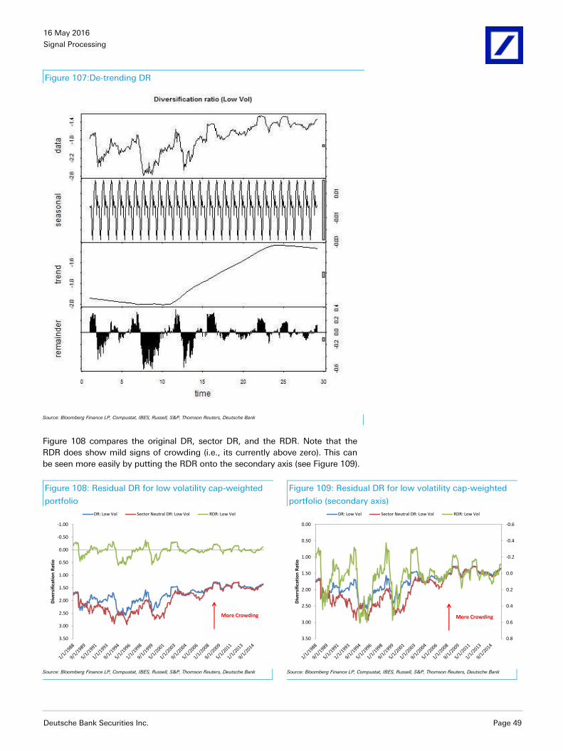
Trend effects

Next, we perform one more robustness check. We recall that the DR had a

significant trend component while returns normally do not. In this last section,

we de-trend our DR measure to test if it still holds up as an adequate crowding

measure. Figure 107 shows the original DR ratio, the seasonal component, the

trend component, and the residual DR (RDR).22 The seasonal component is

fairly small. However, the trend component is significant. The RDR is what

really interests us.

20 We sector adjust our factor portfolios by z-score the factors cross-sectionally across the GICS level 1

sectors rather than cross-sectionally across the entire Russell 3000 universe. 21

The correlation is computed from the year 2000 onwards. 22

We use the STL package in R to de-trend the DR ratio.

16 May 2016

Signal Processing


Figure 107:De-trending DR


Figure 108 compares the original DR, sector DR, and the RDR. Note that the

RDR does show mild signs of crowding (i.e., its currently above zero). This can

be seen more easily by putting the RDR onto the secondary axis (see Figure 109).

Figure 108: Residual DR for low volatility cap-weighted

portfolio

Figure 109: Residual DR for low volatility cap-weighted

portfolio (secondary axis)

-1.00

-0.50

0.00

0.50

1.00

1.50

2.00

2.50

3.00

3.50

Div

ers

ific

atio

n R

atio

DR: Low Vol Sector Neutral DR: Low Vol RDR: Low Vol

More Crowding

-0.6

-0.4

-0.2

0.0

0.2

0.4

0.6

0.8

0.00

0.50

1.00

1.50

2.00

2.50

3.00

3.50

Div

ers

ific

atio

n R

atio

DR: Low Vol Sector Neutral DR: Low Vol RDR: Low Vol

More Crowding



16 May 2016

Signal Processing


In terms of the strength of RDR as a crowding measure, we see no significant

differences compared to the original and sector adjusted DR’s (see Figure 110).

Again, our results reiterate that DR is a robust and effective measure of

investor crowding, especially for low volatility.

Figure 110: DR remainder and crowdedness


DR Cap Weighted -4% -20% -19% 35% 11% -49% -64% 35%

DR Cap Weighted (sector neutral) -12% 1% -14% 24% 5% -39% -66% 33%

DR Cap Weighted (residual) 11% 5% -15% 33% 21% -22% -51% 34% Source: Bloomberg Finance LP, Compustat, IBES, Russell, S&P, Thomson Reuters, Deutsche Bank

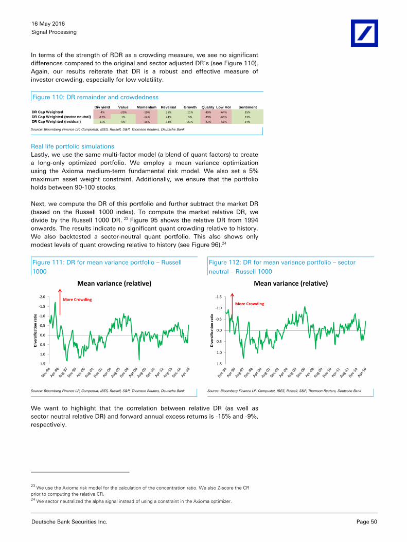
Real life portfolio simulations

Lastly, we use the same multi-factor model (a blend of quant factors) to create

a long-only optimized portfolio. We employ a mean variance optimization

using the Axioma medium-term fundamental risk model. We also set a 5%

maximum asset weight constraint. Additionally, we ensure that the portfolio

holds between 90-100 stocks.

Next, we compute the DR of this portfolio and further subtract the market DR

(based on the Russell 1000 index). To compute the market relative DR, we

divide by the Russell 1000 DR. 23 Figure 95 shows the relative DR from 1994

onwards. The results indicate no significant quant crowding relative to history.

We also backtested a sector-neutral quant portfolio. This also shows only

modest levels of quant crowding relative to history (see Figure 96).24

Figure 111: DR for mean variance portfolio – Russell

1000

Figure 112: DR for mean variance portfolio – sector

neutral – Russell 1000

-2.0

-1.5

-1.0

-0.5

0.0

0.5

1.0

1.5

Div

ers

ific

atio

n r

atio


More Crowding

-1.5

-1.0

-0.5

0.0

0.5

1.0

1.5

Div

ers

ific

atio

n r

atio


More Crowding



We want to highlight that the correlation between relative DR (as well as

sector neutral relative DR) and forward annual excess returns is -15% and -9%,

respectively.

23 We use the Axioma risk model for the calculation of the concentration ratio. We also Z-score the CR

prior to computing the relative CR. 24

We sector neutralized the alpha signal instead of using a constraint in the Axioma optimizer.

16 May 2016

Signal Processing


What about funds flow?

Lastly, we examine the practicality of using funds flow data as a measure of

crowding. The results suggest that funds flow is an interesting dataset; but, it

is more effective as a conditional variable to gauge the initial stages of

crowding. Funds flow is useful at assessing inflection points in the market.

Irrespective, we highlight the funds flow dataset in this research and welcome

the opportunity to do further research on it.

A brief introduction of funds flow

Fund flows track net new end-investor money flowing into or out of mutual

funds and ETFs. Our data set (from data providers EPFR Global and ICI) tracks

funds with total assets under management of almost $22 trillion globally

covering products across a wide range of asset classes, regions, countries,

sectors, styles and sizes. Fund flows provide an important measure of investor

demand and when combined with supply indicators explain movements in

prices well. For example, simple measures of US equity demand based on fund

flows and supply (issuance and buybacks) when combined have a 75%

correlation with quarterly S&P 500 price changes over the last 20 years. To get

a better sense of the dataset, we briefly analyze some recent themes based on

the funds flow dataset.

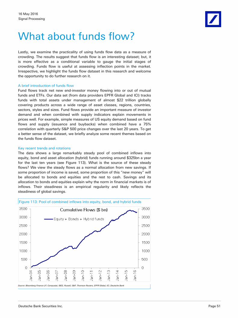
Key recent trends and rotations

The data shows a large remarkably steady pool of combined inflows into

equity, bond and asset allocation (hybrid) funds running around $325bn a year

for the last ten years (see Figure 113). What is the source of these steady

flows? We view the steady flows as a normal allocation from new savings. If

some proportion of income is saved, some proportion of this “new money” will

be allocated to bonds and equities and the rest to cash. Savings and its

allocation to bonds and equities explain why the norm in financial markets is of

inflows. Their steadiness is an empirical regularity and likely reflects the

steadiness of global savings.

Figure 113: Pool of combined inflows into equity, bond, and hybrid funds

Source: Bloomberg Finance LP, Compustat, IBES, Russell, S&P, Thomson Reuters, EPFR Global, ICI, Deutsche Bank

16 May 2016

Signal Processing


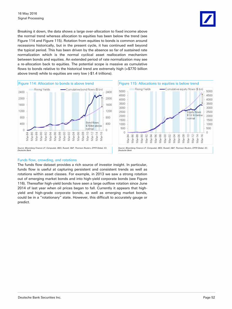
Breaking it down, the data shows a large over-allocation to fixed income above

the normal trend whereas allocation to equities has been below the trend (see

Figure 114 and Figure 115). Rotation from equities to bonds is common around

recessions historically, but in the present cycle, it has continued well beyond

the typical period. This has been driven by the absence so far of sustained rate

normalization which is the normal cyclical asset reallocation mechanism

between bonds and equities. An extended period of rate normalization may see

a re-allocation back to equities. The potential scope is massive as cumulative

flows to bonds relative to the historical trend are extremely high (+$770 billion

above trend) while to equities are very low (-$1.4 trillions).

Figure 114: Allocation to bonds is above trend Figure 115: Allocations to equities is below trend



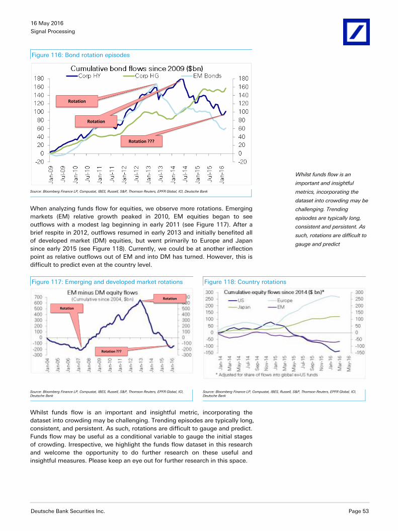
Funds flow, crowding, and rotations

The funds flow dataset provides a rich source of investor insight. In particular,

funds flow is useful at capturing persistent and consistent trends as well as

rotations within asset classes. For example, in 2013 we saw a strong rotation

out of emerging market bonds and into high-yield corporate bonds (see Figure

116). Thereafter high-yield bonds have seen a large outflow rotation since June

2014 of last year when oil prices began to fall. Currently it appears that high-

yield and high-grade corporate bonds, as well as emerging market bonds,

could be in a “rotationary” state. However, this difficult to accurately gauge or

predict.

16 May 2016

Signal Processing


Figure 116: Bond rotation episodes

Rotation

Rotation

Rotation ???


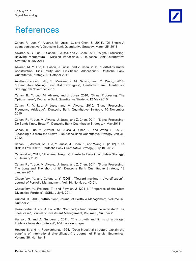
When analyzing funds flow for equities, we observe more rotations. Emerging

markets (EM) relative growth peaked in 2010, EM equities began to see

outflows with a modest lag beginning in early 2011 (see Figure 117). After a

brief respite in 2012, outflows resumed in early 2013 and initially benefited all

of developed market (DM) equities, but went primarily to Europe and Japan

since early 2015 (see Figure 118). Currently, we could be at another inflection

point as relative outflows out of EM and into DM has turned. However, this is

difficult to predict even at the country level.

Figure 117: Emerging and developed market rotations Figure 118: Country rotations

Rotation ???

Rotation

Rotation



Whilst funds flow is an important and insightful metric, incorporating the

dataset into crowding may be challenging. Trending episodes are typically long,

consistent, and persistent. As such, rotations are difficult to gauge and predict.

Funds flow may be useful as a conditional variable to gauge the initial stages

of crowding. Irrespective, we highlight the funds flow dataset in this research

and welcome the opportunity to do further research on these useful and

insightful measures. Please keep an eye out for further research in this space.

Whilst funds flow is an

important and insightful

metrics, incorporating the

dataset into crowding may be

challenging. Trending

episodes are typically long,

consistent and persistent. As

such, rotations are difficult to

gauge and predict

16 May 2016

Signal Processing


References

Cahan, R., Luo, Y., Alvarez, M., Jussa, J., and Chen, Z. [2011], “Oil Shock: A

quant perspective”, Deutsche Bank Quantitative Strategy, March 25, 2011

Alvarez, A., Y. Luo, R. Cahan, J. Jussa, and Z. Chen, 2011, “Signal Processing:

Reviving Momentum – Mission Impossible?”, Deutsche Bank Quantitative

Strategy, 6 July 2011

Alvarez, M, Y. Luo, R. Cahan, J. Jussa, and Z. Chen, 2011, “Portfolios Under

Construction: Risk Parity and Risk-based Allocations”, Deutsche Bank

Quantitative Strategy, 13 October 2011

Avettand-Fenoel, J.-R., S. Mesomeris, M. Salvini, and Y. Wang, 2011,

“Quantitative Musing: Low Risk Strategies”, Deutsche Bank Quantitative

Strategy, 16 November 2011

Cahan, R., Y. Luo, M. Alvarez, and J. Jussa, 2010, “Signal Processing: The

Options Issue”, Deutsche Bank Quantitative Strategy, 12 May 2010

Cahan, R., Y. Luo, J. Jussa, and M. Alvarez, 2010, “Signal Processing:

Frequency Arbitrage”, Deutsche Bank Quantitative Strategy, 10 November

2010

Cahan, R., Y. Luo, M. Alvarez, J. Jussa, and Z. Chen, 2011, “Signal Processing:

Do Bonds Know Better?”, Deutsche Bank Quantitative Strategy, 4 May 2011

Cahan, R., Luo, Y., Alvarez, M., Jussa, J., Chen, Z., and Wang, S. [2012].

“Standing out from the Crowd”, Deutsche Bank Quantitative Strategy, Jan 31,

2012.

Cahan, R., Alvarez, M., Luo, Y., Jussa, J., Chen, Z., and Wang, S. [2012]. “The

Risk in Low Risk?”, Deutsche Bank Quantitative Strategy, July 19, 2012.

Cahan et al., 2011, “Academic Insights”, Deutsche Bank Quantitative Strategy,

20 January 2011

Cahan, R., Y. Luo, M. Alvarez, J. Jussa, and Z. Chen, 2011, “Signal Processing:

The Long and The short of it”, Deutsche Bank Quantitative Strategy, 18

January 2011

Choueifaty, Y., and Coignard, Y. [2008]. “Toward maximum diversification”,

Journal of Portfolio Management, Vol. 34, No. 4, pp. 40-51.

Choueifaty, Y., Froidure, T., and Reynier, J. [2011]. “Properties of the Most

Diversified Portfolio”, SSRN, July 6, 2011.

Grinold, R., 2006, “Attribution”, Journal of Portfolio Management, Volume 32,

Number 2

Hasanhodzic, J. and A. Lo, 2007, “Can hedge fund returns be replicated? The

linear case”, Journal of Investment Management, Volume 5, Number 2

Hanson, S. and A. Sunderam, 2011, “The growth and limits of arbitrage:

Evidence from short interest”, NYU working paper

Heston, S. and K. Rouwenhorst, 1994, “Does industrial structure explain the

benefits of international diversification?”, Journal of Financial Economics,

Volume 36, Number 1

16 May 2016

Signal Processing


Hogan, S., R. Jarrow, M. Teo, and M. Warachka, 2004, “Testing market

efficiency using statistical arbitrage and applications to momentum and value

strategies”, Journal of Financial Economics, Volume 73, 525-565

Khandani, A. and A. Lo, 2008, “What happened to the quants in August 2007”

Evidence from factors and transaction data”, SSRN working paper,

Luo, Y., Cahan, R., Jussa, J., and M. Alvarez, 2010, “QCD Model: DB Quant

Handbook”, Deutsche Bank Quantitative Strategy, 22 July 2010

Luo, Y., R. Cahan, J. Jussa, and M. Alvarez, 2010, “Signal Processing: Style

Rotation”, Deutsche Bank Quantitative Strategy, 7 September 2010

Luo, Y., R. Cahan, M. Alvarez, J. Jussa, and Z. Chen, 2011, “Portfolios Under

Construction: Tail Risk in Optimal Signal Weighting”, Deutsche Bank

Quantitative Strategy, 7 June 2011

Luo, Y., Wang, S., Cahan, R., Jussa, J., Chen, Z., and Alvarez, M.[2012]. “DB

Handbook of Portfolio Construction: Part1”, Deutsche Bank Quantitative

Strategy, July 19, 2012.

Nelsen, R., 1999, “An introduction to copulas”, Springer-Verlag, New York

Pojarliev, M. and R. Levich, 2011, “Detecting crowded trades in currency

markets”, Financial Analysts Journal, Volume 67, Number 1

Ruenzi, S. and F. Weigert, 2012, “Extreme dependence structures and the

cross-section of expected stock returns”, SSRN working paper

Wang, S., Luo, Y., Alvarez, M., Jussa, J., and Wang, A. [2014]. “Global

Dividend Investing”, Deutsche Bank Quantitative Strategy, May 5, 2014.

Wang, S., Luo, Y., Alvarez, M., [2016]. “The Drug Business”, Deutsche Bank

Quantitative Strategy, March 28, 2016.

Jussa, J., Alvarez, M., and Wang, S. [2014]. “Smart Holdings”, Deutsche Bank

Quantitative Strategy, February 14, 2014.

Research Insight, MSCI [2015], “Lost in the Crowd?”, June 2015.

Sias, Richard W., Institutional Herding (February 24, 2002). Available at SSRN:

http://ssrn.com/abstract=307440 or http://dx.doi.org/10.2139/ssrn.307440

Frankel, Jeffrey A., A Test of Portfolio Crowding-Out and Related Issues in

Finance (September 1983). NBER Working Paper No. w1205. Available at

SSRN: http://ssrn.com/abstract=305582

Aas, Kjersti., [2004], “Modeling the dependence structure of financial assets: A

survey of four copulas”, December 2004

Rohal, G., Jussa, J., and Luo, Y. [2016]. “What does market breadth tell us

about 2016?”, Deutsche Bank Quantitative Strategy, January 5, 2016.

http://dx.doi.org/10.2139/ssrn.307440

http://ssrn.com/abstract=305582

16 May 2016

Signal Processing


Appendix 1

Important Disclosures

Additional information available upon request

*Prices are current as of the end of the previous trading session unless otherwise indicated and are sourced from local exchanges via Reuters, Bloomberg and other vendors . Other information is sourced from Deutsche Bank, subject companies, and other sources. For disclosures pertaining to recommendations or estimates made on securities other than the primary subject of this research, please see the most recently published company report or visit our global disclosure look-up page on our website at http://gm.db.com/ger/disclosure/DisclosureDirectory.eqsr

Analyst Certification

The views expressed in this report accurately reflect the personal views of the undersigned lead analyst(s). In addition, the undersigned lead analyst(s) has not and will not receive any compensation for providing a specific recommendation or view in this report. Javed Jussa/Gaurav Rohal/Sheng Wang/George Zhao/Yin Luo/Miguel-A Alvarez/Allen Wang/David Elledge/Binky Chadha/Parag Thatte/Rajat Dua

Hypothetical Disclaimer

Backtested, hypothetical or simulated performance results have inherent limitations. Unlike an actual performance record

based on trading actual client portfolios, simulated results are achieved by means of the retroactive application of a

backtested model itself designed with the benefit of hindsight. Taking into account historical events the backtesting of

performance also differs from actual account performance because an actual investment strategy may be adjusted any time,

for any reason, including a response to material, economic or market factors. The backtested performance includes

hypothetical results that do not reflect the reinvestment of dividends and other earnings or the deduction of advisory fees,

brokerage or other commissions, and any other expenses that a client would have paid or actually paid. No representation is

made that any trading strategy or account will or is likely to achieve profits or losses similar to those shown. Alternative

modeling techniques or assumptions might produce significantly different results and prove to be more appropriate. Past

hypothetical backtest results are neither an indicator nor guarantee of future returns. Actual results will vary, perhaps

materially, from the analysis.

Regulatory Disclosures

1.Important Additional Conflict Disclosures

Aside from within this report, important conflict disclosures can also be found at https://gm.db.com/equities under the

"Disclosures Lookup" and "Legal" tabs. Investors are strongly encouraged to review this information before investing.

2.Short-Term Trade Ideas

Deutsche Bank equity research analysts sometimes have shorter-term trade ideas (known as SOLAR ideas) that are

consistent or inconsistent with Deutsche Bank's existing longer term ratings. These trade ideas can be found at the SOLAR

link at http://gm.db.com.

http://gm.db.com/ger/disclosure/DisclosureDirectory.eqsr

https://gm.db.com/equities

http://gm.db.com/

16 May 2016

Signal Processing


Additional Information

The information and opinions in this report were prepared by Deutsche Bank AG or one of its affiliates (collectively "Deutsche

Bank"). Though the information herein is believed to be reliable and has been obtained from public sources believed to be

reliable, Deutsche Bank makes no representation as to its accuracy or completeness.

If you use the services of Deutsche Bank in connection with a purchase or sale of a security that is discussed in this report, or

is included or discussed in another communication (oral or written) from a Deutsche Bank analyst, Deutsche Bank may act as

principal for its own account or as agent for another person.

Deutsche Bank may consider this report in deciding to trade as principal. It may also engage in transactions, for its own

account or with customers, in a manner inconsistent with the views taken in this research report. Others within Deutsche

Bank, including strategists, sales staff and other analysts, may take views that are inconsistent with those taken in this

research report. Deutsche Bank issues a variety of research products, including fundamental analysis, equity-linked analysis,

quantitative analysis and trade ideas. Recommendations contained in one type of communication may differ from

recommendations contained in others, whether as a result of differing time horizons, methodologies or otherwise. Deutsche

Bank and/or its affiliates may also be holding debt securities of the issuers it writes on.

Analysts are paid in part based on the profitability of Deutsche Bank AG and its affiliates, which includes investment banking

revenues.

Opinions, estimates and projections constitute the current judgment of the author as of the date of this report. They do not

necessarily reflect the opinions of Deutsche Bank and are subject to change without notice. Deutsche Bank has no obligation

to update, modify or amend this report or to otherwise notify a recipient thereof if any opinion, forecast or estimate contained

herein changes or subsequently becomes inaccurate. This report is provided for informational purposes only. It is not an offer

or a solicitation of an offer to buy or sell any financial instruments or to participate in any particular trading strategy. Target

prices are inherently imprecise and a product of the analyst’s judgment. The financial instruments discussed in this report may

not be suitable for all investors and investors must make their own informed investment decisions. Prices and availability of

financial instruments are subject to change without notice and investment transactions can lead to losses as a result of price

fluctuations and other factors. If a financial instrument is denominated in a currency other than an investor's currency, a

change in exchange rates may adversely affect the investment. Past performance is not necessarily indicative of future results.

Unless otherwise indicated, prices are current as of the end of the previous trading session, and are sourced from local

exchanges via Reuters, Bloomberg and other vendors. Data is sourced from Deutsche Bank, subject companies, and in some

cases, other parties.

Macroeconomic fluctuations often account for most of the risks associated with exposures to instruments that promise to pay

fixed or variable interest rates. For an investor who is long fixed rate instruments (thus receiving these cash flows), increases

in interest rates naturally lift the discount factors applied to the expected cash flows and thus cause a loss. The longer the

maturity of a certain cash flow and the higher the move in the discount factor, the higher will be the loss. Upside surprises in

inflation, fiscal funding needs, and FX depreciation rates are among the most common adverse macroeconomic shocks to

receivers. But counterparty exposure, issuer creditworthiness, client segmentation, regulation (including changes in assets

holding limits for different types of investors), changes in tax policies, currency convertibility (which may constrain currency

conversion, repatriation of profits and/or the liquidation of positions), and settlement issues related to local clearing houses are

also important risk factors to be considered. The sensitivity of fixed income instruments to macroeconomic shocks may be

mitigated by indexing the contracted cash flows to inflation, to FX depreciation, or to specified interest rates – these are

common in emerging markets. It is important to note that the index fixings may -- by construction -- lag or mis-measure the

actual move in the underlying variables they are intended to track. The choice of the proper fixing (or metric) is particularly

important in swaps markets, where floating coupon rates (i.e., coupons indexed to a typically short-dated interest rate

reference index) are exchanged for fixed coupons. It is also important to acknowledge that funding in a currency that differs

from the currency in which coupons are denominated carries FX risk. Naturally, options on swaps (swaptions) also bear the

risks typical to options in addition to the risks related to rates movements.

Derivative transactions involve numerous risks including, among others, market, counterparty default and illiquidity risk. The

16 May 2016

Signal Processing


appropriateness or otherwise of these products for use by investors is dependent on the investors' own circumstances

including their tax position, their regulatory environment and the nature of their other assets and liabilities, and as such,

investors should take expert legal and financial advice before entering into any transaction similar to or inspired by the

contents of this publication. The risk of loss in futures trading and options, foreign or domestic, can be substantial. As a result

of the high degree of leverage obtainable in futures and options trading, losses may be incurred that are greater than the

amount of funds initially deposited. Trading in options involves risk and is not suitable for all investors. Prior to buying or

selling an option investors must review the "Characteristics and Risks of Standardized Options”, at

http://www.optionsclearing.com/about/publications/character-risks.jsp. If you are unable to access the website please contact

your Deutsche Bank representative for a copy of this important document.

Participants in foreign exchange transactions may incur risks arising from several factors, including the following: ( i)

exchange rates can be volatile and are subject to large fluctuations; ( ii) the value of currencies may be affected by numerous

market factors, including world and national economic, political and regulatory events, events in equity and debt markets and

changes in interest rates; and (iii) currencies may be subject to devaluation or government imposed exchange controls which

could affect the value of the currency. Investors in securities such as ADRs, whose values are affected by the currency of an

underlying security, effectively assume currency risk.

Unless governing law provides otherwise, all transactions should be executed through the Deutsche Bank entity in the

investor's home jurisdiction.

United States: Approved and/or distributed by Deutsche Bank Securities Incorporated, a member of FINRA, NFA and SIPC.

Analysts employed by non-US affiliates may not be associated persons of Deutsche Bank Securities Incorporated and

therefore not subject to FINRA regulations concerning communications with subject companies, public appearances and

securities held by analysts.

Germany: Approved and/or distributed by Deutsche Bank AG, a joint stock corporation with limited liability incorporated in the

Federal Republic of Germany with its principal office in Frankfurt am Main. Deutsche Bank AG is authorized under German

Banking Law and is subject to supervision by the European Central Bank and by BaFin, Germany’s Federal Financial

Supervisory Authority.

United Kingdom: Approved and/or distributed by Deutsche Bank AG acting through its London Branch at Winchester House,

1 Great Winchester Street, London EC2N 2DB. Deutsche Bank AG in the United Kingdom is authorised by the Prudential

Regulation Authority and is subject to limited regulation by the Prudential Regulation Authority and Financial Conduct

Authority. Details about the extent of our authorisation and regulation are available on request.

Hong Kong: Distributed by Deutsche Bank AG, Hong Kong Branch.

India: Prepared by Deutsche Equities India Pvt Ltd, which is registered by the Securities and Exchange Board of India (SEBI) as

a stock broker. Research Analyst SEBI Registration Number is INH000001741. DEIPL may have received administrative

warnings from the SEBI for breaches of Indian regulations.

Japan: Approved and/or distributed by Deutsche Securities Inc.(DSI). Registration number - Registered as a financial

instruments dealer by the Head of the Kanto Local Finance Bureau (Kinsho) No. 117. Member of associations: JSDA, Type II

Financial Instruments Firms Association and The Financial Futures Association of Japan. Commissions and risks involved in

stock transactions - for stock transactions, we charge stock commissions and consumption tax by multiplying the transaction

amount by the commission rate agreed with each customer. Stock transactions can lead to losses as a result of share price

fluctuations and other factors. Transactions in foreign stocks can lead to additional losses stemming from foreign exchange

fluctuations. We may also charge commissions and fees for certain categories of investment advice, products and services.

Recommended investment strategies, products and services carry the risk of losses to principal and other losses as a result of

changes in market and/or economic trends, and/or fluctuations in market value. Before deciding on the purchase of financial

products and/or services, customers should carefully read the relevant disclosures, prospectuses and other documentation.

"Moody's", "Standard & Poor's", and "Fitch" mentioned in this report are not registered credit rating agencies in Japan unless

Japan or "Nippon" is specifically designated in the name of the entity. Reports on Japanese listed companies not written by

analysts of DSI are written by Deutsche Bank Group's analysts with the coverage companies specified by DSI. Some of the

foreign securities stated on this report are not disclosed according to the Financial Instruments and Exchange Law of Japan.

http://www.optionsclearing.com/about/publications/character-risks.jsp

16 May 2016

Signal Processing


Korea: Distributed by Deutsche Securities Korea Co.

South Africa: Deutsche Bank AG Johannesburg is incorporated in the Federal Republic of Germany (Branch Register Number

in South Africa: 1998/003298/10).

Singapore: by Deutsche Bank AG, Singapore Branch or Deutsche Securities Asia Limited, Singapore Branch (One Raffles

Quay #18-00 South Tower Singapore 048583, +65 6423 8001), which may be contacted in respect of any matters arising

from, or in connection with, this report. Where this report is issued or promulgated in Singapore to a person who is not an

accredited investor, expert investor or institutional investor (as defined in the applicable Singapore laws and regulations), they

accept legal responsibility to such person for its contents.

Taiwan: Information on securities/investments that trade in Taiwan is for your reference only. Readers should independently

evaluate investment risks and are solely responsible for their investment decisions. Deutsche Bank research may not be

distributed to the Taiwan public media or quoted or used by the Taiwan public media without written consent. Information on

securities/instruments that do not trade in Taiwan is for informational purposes only and is not to be construed as a

recommendation to trade in such securities/instruments. Deutsche Securities Asia Limited, Taipei Branch may not execute

transactions for clients in these securities/instruments.

Qatar: Deutsche Bank AG in the Qatar Financial Centre (registered no. 00032) is regulated by the Qatar Financial Centre

Regulatory Authority. Deutsche Bank AG - QFC Branch may only undertake the financial services activities that fall within the

scope of its existing QFCRA license. Principal place of business in the QFC: Qatar Financial Centre, Tower, West Bay, Level 5,

PO Box 14928, Doha, Qatar. This information has been distributed by Deutsche Bank AG. Related financial products or

services are only available to Business Customers, as defined by the Qatar Financial Centre Regulatory Authority.

Russia: This information, interpretation and opinions submitted herein are not in the context of, and do not constitute, any

appraisal or evaluation activity requiring a license in the Russian Federation.

Kingdom of Saudi Arabia: Deutsche Securities Saudi Arabia LLC Company, (registered no. 07073-37) is regulated by the

Capital Market Authority. Deutsche Securities Saudi Arabia may only undertake the financial services activities that fall within

the scope of its existing CMA license. Principal place of business in Saudi Arabia: King Fahad Road, Al Olaya District, P.O. Box

301809, Faisaliah Tower - 17th Floor, 11372 Riyadh, Saudi Arabia.

United Arab Emirates: Deutsche Bank AG in the Dubai International Financial Centre (registered no. 00045) is regulated by the

Dubai Financial Services Authority. Deutsche Bank AG - DIFC Branch may only undertake the financial services activities that

fall within the scope of its existing DFSA license. Principal place of business in the DIFC: Dubai International Financial Centre,

The Gate Village, Building 5, PO Box 504902, Dubai, U.A.E. This information has been distributed by Deutsche Bank AG.

Related financial products or services are only available to Professional Clients, as defined by the Dubai Financial Services

Authority.

Australia: Retail clients should obtain a copy of a Product Disclosure Statement (PDS) relating to any financial product referred

to in this report and consider the PDS before making any decision about whether to acquire the product. Please refer to

Australian specific research disclosures and related information at https://australia.db.com/australia/content/research-

information.html

Australia and New Zealand: This research, and any access to it, is intended only for "wholesale clients" within the meaning of

the Australian Corporations Act and New Zealand Financial Advisors Act respectively.

Additional information relative to securities, other financial products or issuers discussed in this report is available upon

request. This report may not be reproduced, distributed or published without Deutsche Bank's prior written consent.

Copyright © 2016 Deutsche Bank AG

https://australia.db.com/australia/content/research-information.html

https://australia.db.com/australia/content/research-information.html

GRCM2016PROD035530

David Folkerts-Landau Chief Economist and Global Head of Research

Raj Hindocha Global Chief Operating Officer

Research

Marcel Cassard Global Head

FICC Research & Global Macro Economics

Steve Pollard Global Head

Equity Research

Michael Spencer Regional Head

Asia Pacific Research

Ralf Hoffmann Regional Head

Deutsche Bank Research, Germany

Andreas Neubauer Regional Head

Equity Research, Germany

International Locations

Deutsche Bank AG

Deutsche Bank Place

Level 16

Corner of Hunter & Phillip Streets

Sydney, NSW 2000

Australia

Tel: (61) 2 8258 1234

Deutsche Bank AG

Große Gallusstraße 10-14

60272 Frankfurt am Main

Germany

Tel: (49) 69 910 00

Deutsche Bank AG

Filiale Hongkong

International Commerce Centre,

1 Austin Road West,Kowloon,

Hong Kong

Tel: (852) 2203 8888

Deutsche Securities Inc.

2-11-1 Nagatacho

Sanno Park Tower

Chiyoda-ku, Tokyo 100-6171

Japan

Tel: (81) 3 5156 6770

Deutsche Bank AG London

1 Great Winchester Street

London EC2N 2EQ

United Kingdom

Tel: (44) 20 7545 8000

Deutsche Bank Securities Inc.

60 Wall Street

New York, NY 10005

United States of America

Tel: (1) 212 250 2500

July-2016-Newsletter-Deutsche-Bank-on-behalf-of ...

Documents

Transcript of July-2016-Newsletter-Deutsche-Bank-on-behalf-of ...