JOURNAL OF FORENSIC ECONOMICS Discounting Damage Awards Using the Zero Coupon Treasury Curve:...

JOURNAL OF

FORENSIC ECONOMICS

Discounting Damage Awards Using the Zero Coupon Treasury Curve: Satisfying Legal and Economic Theory While

Matching Future Cash Flow Projections

Joseph Irving Rosenberg*

Journal of Forensic Economics 21(2), 2010, pp. 173-194 http://www.JournalofForensicEconomics.com/doi/pdf/10.5085/jfe.21.2.173 © 2010 by the National Association of Forensic Economics

173

Discounting Damage Awards Using the Zero Coupon Treasury

Curve: Satisfying Legal and Economic Theory While Matching Future Cash Flow Projections

Joseph Irving Rosenberg*

Abstract

How to calculate damage awards has long been the subject of academic dispute. Much focus has been on what is the appropriate discount rate to con-vert future lost earnings into a lump sum amount. Conflicting or ambiguous legal guidance by the courts has lead to wide disparities in discount rate me-thodology. This paper presents a fresh, alternative approach to valuing lost earnings in damage awards using current market data from the zero coupon Treasury bond curve. Unlike many other approaches this approach satisfies legal requirements while offering several theoretical and practical benefits: (a) default free discounting; (b) market-based prices and yields; (c) a fully objective way to recompute awards if market conditions change materially in the course of litigation; (d) satisfaction of the "parity in risk" principal which requires consistent treatment of uncertainty in cash flows and discount rate, which is violated by using an arbitrary average of three-month T-bill rates if inflation is embedded in lost earnings; and (e) a theoretically investible stream of cash flows that can be maturity matched against projected lost earnings. DOI: 10.5085/jfe.21.2.173

I. Introduction

How to calculate an appropriate damage award by discounting future eco-nomic losses has been the subject of many conflicting journal articles and aca-demic disputes over the years. Much of the discussion has focused on what is the appropriate level of discount rate used to reduce a series of future cash flows into a lump sum number. However, the concept of discounting future cash flows goes far beyond deriving lump sum damage awards; it applies in all of finance and economics as a way to express the time value of money. To ad-dress this issue, it is important to understand the relationship of a discount rate to present value. In cases where the initial investment value or security price is known (i.e., present value), the discount rate is solved for and represents the internal rate of return (IRR) or yield to maturity (YTM). In other cases, where the initial investment value or security price is unknown (e.g., when valuing a bond, project, or a damage award), the discount rate is assumed and present value is calculated. For either purpose, the discount rate *Principal, Joseph I. Rosenberg, CFA, LLC (Financial Planning and Investment Advisory Service).

174 JOURNAL OF FORENSIC ECONOMICS

need not be a constant for each period, a topic that is discussed further in this paper (see Section III).

Conflicting or ambiguous legal guidance among the states and the Su-preme Court in its Pfeifer decision (see Section II) has lead to a wide disparity of discount rate values and the underlying interest rate maturity assumptions employed throughout the forensic economics community. This has been dem-onstrated via responses to questions in a number of surveys over the last 20 years. In a recently published survey, about 18% of respondents used short term bond interest rates, whereas over 80% used bond rates either of interme-diate term, long term, a mix of terms, or some other method (Brookshire, Lu-thy and Slesnick, 2006). The lack of any clear preferences among forensic econ-omists indicates the range of discretion that courts allow, diversity of jurisdic-tional requirements, and, most probably, the absence of a convincing single approach to addressing this question.

There is also the question of “parity in risk” argued for by Margulis (1992), Biederman and Basemann (1996), Henderson and Seward (1998), and Brush (2003), while discussed more broadly in Breeden (2003). Simply stated, the proponents of the “parity in risk” principal argue that the correct discount rate to apply in computing a lump sum award should be risk-adjusted to counter-balance the forecast uncertainties from estimating future losses. In other words, only future economic losses that are certain should be discounted with a risk-free discount rate. For instance, mitigating default risk is mandated by the Pfeifer decision. Risk parity for default may appear straightforward to achieve by incorporating default risk both in future earnings losses via work-life expectancy and in discounting. However, an academic dispute by Bell and Taub (1999) v. Ireland (1997) showed that agreement on how to eliminate de-fault risk in a way that is consistent with forecasted lost earnings is elusive.

Equally unclear is whether mitigating inflation risk either should be achieved (given that Pfeifer does not require it), or even could be achieved with-out investing lump sum award proceeds entirely in instruments such as Trea-sury Inflation Protected Securities (TIPS) or three-month T-bills. To those who believe the “parity in risk” principal is sound finance, the current practice of many forensic economists of including inflationary adjustments in forecasting future lost earnings while discounting at some multi-year average of three-month T-bills represents a clear violation of that principal.

The purpose of this paper is to propose an alternative discount rate ap-proach to most of the popular ones in usage. It might be called the Zero Coupon U.S. Treasury Curve Discount method. Rather than have a single, somewhat arbitrary discount rate for discounting all future cash flows, it is proposed in-stead to use a time series of default-free payments based on a ladder of zero coupon T-Bonds, using independent, widely accepted market prices for these instruments, such as those reported daily in the Wall Street Journal. This ap-proach uses observed secondary market prices for a series of zero coupon (ZC) U.S. Treasury bonds that corresponds with the time period of projected eco-nomic loss. The sum of each period’s ZC bond price multiplied by each period’s projected earnings loss would equal the appropriate lump sum amount to be awarded. Since prices are directly translatable into yield, a corresponding se-

Rosenberg 175

ries of discount rates also becomes observable, and by solving for the IRR asso-ciated with each period’s projected cash flow, an implied single discount rate also can be derived.

The benefits obtained by using this approach include: Default free discounting, consistent with Pfeifer; Prices and corresponding interest rates are completely objective, widely

accepted, and reflect prevailing market conditions; If market conditions change materially during the course of litigation,

there is a fully objective way to recompute the lump sum amount via updating the ZC bond prices using the exact same method;

“Parity in risk” is largely achieved. Since Pfeifer does not require that awards be free of inflation risk, and ZC bond values are also not free of inflation risk, parity of inflation risk is achieved by allowing inflation risk in both lost earnings projections and in discounting such projec-tions.1

Parity in default risk is more problematic to achieve, but it will

be argued that this approach addresses most of the concerns involving parity in default risk from the Ireland v. Bell and Taub dispute (See Section II).

A ladder of ZC bonds can be matched in maturity against projected lost earnings. This provides a theoretically investible, steady stream of pe-riodic (e.g., quarterly or annual) cash flows that could replace lost earnings, with only minimal interpolation for certain out-year observa-tions. Although it may be unlikely that a plaintiff would actually choose to invest his/her award in such a dedicated portfolio, the capa-bility of doing so renders this approach more theoretically correct and internally consistent than alternatives such as selecting a discount rate based arbitrarily on, say, a 20- or 30-year average of three-month T-bills.

A full exposition of this approach is provided in Section III, following a discus-sion of the legal issues centered on Pfeifer and how it has been interpreted.

II. Legal and Economic Issues Related To Discount Rate

In 1983, the U.S. Supreme Court gave its most explicit ruling ever on the topic of discounting and projecting lost earnings, which carries added weight since the opinion was unanimous (Jones & Laughlin Steel Corp. v. Pfeifer, 1983). This opinion was most explicit on the subjects of default risk and taxes,

1Moreover, this approach allows for the explicit, time-dependent inclusion of inflationary expecta-tions in both lost earnings projections and in discounting. This is achieved by deriving future lost wages based on using a real wage growth rate adjusted by the most widely recognized inflationary expectations over time, i.e., by netting the yields on regular coupon-bearing Treasuries and TIPS of equivalent maturities. Since inflationary expectations are seldom constant, especially as at present when it is almost non-existent but expected to rise over time, it is all the more important to recog-nize the time dependency and variability of inflationary expectations, which can be done with this approach consistently in the numerator and denominator of each discounted cash flow.


whereas it was less so on the subject of inflation. Regarding default risk and taxes, the court said:

Once it is assumed that the injured worker would definitely have worked for a specific term of years, he is entitled to a risk-free stream of future income to replace his lost wages; therefore, the discount rate should not reflect the market's premium for investors who are willing to accept some risk of default. Moreover, since under Norfolk & West-ern R. Co. v. Liepelt, 444 U. S. 490 (1980), the lost stream of income should be estimated in after-tax terms, the discount rate should also represent the after-tax rate of return to the injured worker.(Pfeifer, p. 537).

Clearly the Court intended to protect worker’s lost income from “risk of de-

fault” and taxes in Federal cases. Since the focus of this paper involves finan-cial/economic issues and theory affecting the discount rate in damage award cases, the separable issue of whether and how to incorporate income taxes in such cases is only discussed here at a high level, rather than being incorpo-rated directly in the numerical examples presented later. First, as Ireland (2004) points out, tax liabilities against lost earnings are not taken into ac-count in most states, being a consideration in only a handful of states plus Federal cases. Second, taking taxes into consideration requires both reducing the initial damage award to be expressed as after-tax lost income and an off-setting if not equal increase to make the plaintiff whole for having to pay taxes on future income earned after investing the award’s proceeds. Recognizing the need for consistency in income tax treatment, a U.S Appeals Court ruled that either both offsetting tax effects must be incorporated in the award calculation or else neither one should be incorporated (Trevino v. United States, 1986, p. 41). Given the above, and the desire to stay focused on discount rate methodol-ogy issues, the two offsetting income tax effects are not incorporated in this paper’s examples.

Returning to the Pfeiffer decision, while the Court was quite explicit in re-quiring the use of an after-tax rate of return, its direction on including infla-tion was less clear, mainly requiring consistency. It said that if inflation is in-corporated in the lost earnings estimate, then the discount rate should reflect expected inflation, i.e., it should be a market rate of interest. On the other hand, if inflation is not recognized in the earnings projection, then a below-market rate should be used for discounting, i.e., a real discount rate which only excludes inflation should be used if only real growth and no inflation are incor-porated in the earnings estimate. The Court went on to be fairly specific in what range of real interest rate net of inflation would be an appropriate below-market discount rate: “…we do not believe a trial court adopting such an ap-proach in a suit under § 5(b) should be reversed if it adopts a rate between 1% and 3% and explains its choice.” (Pfeifer, pp. 549-550)

Against this legal backdrop, and with much disagreement remaining in the academic community on discount rate-related issues, it is useful to group the areas of economic dispute into four related but separable issues: (a) “Parity in

Rosenberg 177

risk” principal; (b) default risk; (c) inflation risk; and (d) dedicated portfolio v. short-term rollover approach. A. “Parity in Risk” Principal

This principal was explained most clearly in 1992 by Margulis:

Parity in risk refers to consistency between the certainty of future lost earnings or profits and the choice of discount rate. It would be incon-sistent to discount an expected, but uncertain, stream of future losses by a rate of return earned on investments that are certain, or risk free. (p. 36)

He adds “…the preferred procedure for calculating damages is to discount ac-tual future losses to the date of valuation by a risk-free rate of return.” (p. 38) Noting that future losses are unknown when damages are awarded, he further adds: “To discount expected but uncertain, future sums of money by a risk free rate of return lacks parity in risk.” (p. 38)

Margulis describes the language in Pfeifer as “contradictory.” First he quotes Justice Stevens that “The lost stream (of income’s) length cannot be known with certainty….The probability that he would still be working at a given date cannot be known with certainty…” Then, he quotes Stevens again saying “Once it is assumed that the injured worker would definitely have worked for a specific term of years, he is entitled to a risk-free stream of future income to protect his lost wages.‟ (Pfeifer, p. 533 & 537, cited by Margulis, p. 36)

A year later, Albrecht (1993) used algebra in an attempt to refute “parity in risk” as described by Margulis’ claiming the latter’s “contention is not correct.” (Albrecht, p. 271) However, the dominant response of forensic economists on “parity in risk” has been expressly in support of Margulis (Biedermann and Basemann, 1996; Henderson and Seward, 1998; Brush, 2003). Other econo-mists, writing before Margulis, also took positions that can be construed as supporting the “parity in risk” principal in concept if not in name, including Jennings and Philips (1989, p. 123) and Levhari and Weiss (1974, p. 950).2

While “parity in risk” is a principal that most economists who have dis-cussed the issue appear to support, there is far less agreement on how to apply it to the specific risks raised in damage awards and informed by Pfeifer. B. Default Risk.

Citing Pfeifer, Ireland noted somewhat optimistically in 1997:

There is general agreement among forensic economists that default risk should be virtually eliminated from the discount rate used in per-

2Jennings and Philips (1989) argued that actual future labor income will deviate from expected future labor income and thus labor is not a risk-free asset: “To the extent that such deviations may occur, this would call for the stream of expected labor earnings to be discounted at a higher, risk adjusted rate.” (p. 123) Levari and Weiss are quoted supporting the position that human capital is probably more risky than physical capital.


sonal injury and wrongful death damage calculations….Given that damage calculations normally include reductions for probabilities that the individual will not survive, be a labor force participant or be un-employed, it would be inappropriate to use a discount rate with pre-miums to cover the possibility of nonpayment of the debt securities. To do so would double count the risks that the worker would not have earned projected incomes. (p. 93)

Bell and Taub counter Ireland’s treatment of default risk in a 1999 article

by asserting:

…that the risks of not earning projected income in the future and the risk of default on the bonds are not necessarily the same.” Although they concede that the two risks are “…superficially equivalent in that they are all downside risks which can only lead to a reduction of the fu-ture cash flows, (it is) not necessarily true that the size of the proba-bilities or states of nature in which they occur are the same (and thus they) should be treated as separate issues.” They add that future prod-uctivity growth also affects earnings growth but no downward adjust-ment is typically made for this in earnings projections, unlike for non-survival or non-participation in the labor force. Finally, they make the point cited by Breeden, above, and others, “the well known proposition in finance that only certainty equivalents are discounted with risk free interest rates. (pp. 153-154).

It seems clear that both Ireland and Bell and Taub (B&T) have valid

points. As explained in his own reply to B&T, Ireland says that “If you account for all of the risks by probability discounts to the earnings stream itself, you should not also account for them by using a discount rate containing premiums to compensate for those risks.” (Ireland, 1999, p. 158) B&T’s position is that risk of default and risk of not earning future income are not equivalent. How-ever, while B&T argue that these two risks should be treated as separate is-sues, they do not suggest any practical way to do so. Ireland’s position appears both logical and practical, as when he refers to default risk as “roughly the analog for risks that the worker would not obtain expected future wage bene-fits because of death, illness or unemployment.” (Ireland, 1997, p. 93) Another response might be that even though there is no straightforward way to directly equate default risk on bonds with workforce participation and survival risk on future income, the two downside risks at least offset each other in the same direction through separate numerator and denominator effects, each of which amounts to a reasonable discounting effect. One might add that while “parity in risk” treatment implies theoretical consistency, it doesn’t really address how to incorporate dissimilar downside risks in deriving an award, since there is no obvious, precise way to account for worklife expectancy in a discount rate based on financial instrument returns.

B&T also provide two other critiques of Ireland involving default risk. One is that future productivity growth is excluded as a factor in labor force partici-pation and survival and cannot be recognized by reducing projected earnings. They add that no adjustment is typically made to recognize the uncertainty of

Rosenberg 179

future productivity growth, and suggest that this is the basis for employing a non-risk free discount rate (B&T, 1999, p.154). Ireland counters that case law requires that such risks be accounted for in the earnings stream, not in the dis-count rate (Ireland, 1999, p. 158). It should be added that this is exactly the approach taken in this paper, using the Zero Coupon U.S. Treasury Curve Dis-count Method (ZC T-bond discount method, for short), as explained in detail in Section III. Since most economists would argue that the primary source of real wage growth is productivity gains, it is straightforward to add a “real wage growth” component (separate from an inflationary component) to future earn-ings projections, as there is no meaningful way to reflect productivity growth in a discount rate based on financial instruments.

B&T’s final critique is that only certainty equivalents should be discounted with risk free interest rates. Since Ireland himself limited his response by saying that B&T did not understand his distinction between default risk and inflation risk, and since inflation risk is addressed separately in the next sec-tion, it is only worth adding that the ZC T-bond discount approach presented in this paper includes inflation risk and thus does not employ a totally risk free interest rate. C. Inflation Risk

Inflation risk is usually viewed as the difference between expected inflation and actual inflation. The mitigation of this risk is achieved in many labor con-tracts via cost-of-living allowances or COLAs. Although Pfeifer was clear in re-quiring the exclusion of default risk in damage awards, as noted above, it only required consistency pertaining to the treatment of inflation risk. One way to achieve consistency is to offset projected inflation in lost wages (whether or not in COLAs) by a discount rate that reflects the same projected rate of inflation.

Several economists argue that Pfeifer requires exclusion of inflation risk as well as default risk (Yandell, 1991; Romans and Floss, 1992; Albrecht and Wood, 1998). However, Ireland, 1997, Brush, 1993, and others convincingly reject this interpretation since only the exclusion of default risk is explicitly required by the Pfeifer decision. For fixed income investors, inflation risk is a key factor in the term premium that usually results in longer maturity bonds exhibiting higher yields than comparable ones with shorter maturities, and Brush (1993) uses this maturity distinction in his analysis. He goes further in suggesting that award bias results from the exclusion of inflation risk such as by discounting lost earnings at short term T-bill rates: “If use of a risk-adjusted discount rate is considered appropriate, then discounting with Treasury bills will result in overcompensation of the plaintiff.” (p. 271) Brush estimated a wide degree of overcompensation based on length of future loss period, the his-torical period used, and selection of alternative non-risk free instruments, ranging from a low of 10% for shorter, 10-year loss periods, to almost double the compensation or 97% higher using corporate bonds and the period 1982-2001 (Brush, p. 271). Without quantifying its magnitude, Margolis also pointed out the danger of overcompensation resulting from violating the “parity in risk”


by failing to remove elements of uncertainty in the projection of future losses (Margulis, p. 33).

The issue of discounting at a risk free rate in which neither inflation nor default risk is incurred requires consideration of an important related ques-tion: Should either Treasury Inflation Protected Securities (TIPS) or short-term T-bill rates be used for discounting damage awards, and if so, under what circumstances?

The JFE April 1989 issue was devoted entirely to the question of “Selecting a Discount Rate.” Several economists said they used short term T-bill rate ei-ther for short term valuations or as one of many rate indices. Ray suggested that because over 70% of cases settle before trial, he advocates use of “a twenty-year average for ninety-day treasury bills (as)… more appropriate in many cases.” (Ray, p. 95) Others have also advocated a preference for short term risk free rates specifically to negate inflation risk, based on the idea that an average of such short rates smooths out fluctuations (Romans and Floss, p. 265) or based simply on an individual’s desire to minimize inflation risk (Houldsworth and McKinnon, p. 209).

By discounting awards to exclude inflation as permitted but not required by Pfeifer, using three-month T-bill rates as the discount rate results in the present value of awards as likely to be higher than by using almost any other type of financial instrument.

Ireland has long made the case for using TIPS as preferable to T-bills for discounting future earnings streams if the economist wishes to eliminate infla-tion risk. The issue for him is:

…whether there should be a reduction in the value of the discount rate to eliminate a risk premium for a risk that may produce either more or less purchasing power than forecast. Economists who do not feel that damage awards need to be free of an inflation risk would not necessar-ily use a discount rate based on inflation-adjusted bonds, regardless of (various) problems with the fit of the bonds… However, such econo-mists might still want to use the rates on TIPS bonds to determine the appropriate real rate of interest and the current expected rate of infla-tion. (1997, p. 95)

There is a lengthy back and forth between Bell and Taub and Ireland as to whether the two-sided risk of inflation (positive and negative variance) means that an increase in variance must result in a change in the present value cal-culation. (B&T, p. 155; Ireland, 1999, p. 158). Rather than sorting out the rela-tive merits in this fairly arcane dispute, the position held in this paper is that damage awards do not need to be free of inflation risk because Pfeifer was ex-plicit in only requiring awards to be free of default risk. If Pfeifer did require inflation free discounting, this might have forced more explicit thinking of how to resolve the “parity in risk” problem (i.e., zeroing out both inflation and de-fault risk would make the discount rate truly risk free and thus force the issue of making projected earnings losses a “certainty equivalent”). Ignoring the “parity in risk” problem for the moment, if Pfeifer did require inflation free dis-counting, the TIPS yield curve would be a far preferable source for excluding

Rosenberg 181

both inflation and default risk than would the three-month T-bill, the other leading contender for eliminating inflation risk via discounting.3

Use of TIPS for discounting to negate inflation risk would certainly compli-cate the analytics of compensating for earnings loss. This is due to the fact that coupon interest is only a portion of TIPS return; this creates a timing mis-match between taxes due on accreted value and actual cash flow (a timing problem even more pronounced with ZC T-bonds). However, T-bills are also highly unsuitable as a discount rate for backing out inflation accurately, due largely to their extremely high near-term volatility and the impact of arbitra-rily selecting a given time period for averaging. For example, the arbitrary time period selection of a 10-, 20- or 30-year average of T-bill yield yields (through September 2009) would result in discount rates of 2.82%, 3.87% and 5.55%, respectively. Clearly, all three cannot be said to all offset inflation with any accuracy. In addition, using observable T-bill yields at any one point in time, such as virtually any time from late 2008 through late 2009, would have resulted in near zero discounting of future lost earnings.

D. Dedicated Portfolio v. Short Term Rollover Approach

A dichotomy that economists have often used in describing alternative dis-

count rate approaches is to lump them into either “dedicated portfolios” or “short term rollover.” Three-month T-bills are the quintessential short term rollover instrument offered as a totally risk-free discount rate. The frequency that an investor can roll over any lump sum to adjust to changing rates is what negates inflation risk, and is the main argument used by short term rollover proponents (Harris, 1995, p.131; Houldsworth and McKinnon, 1994, p. 209). However, the only way that inflation risk can truly be avoided, ex post an award, would be to invest that award in an inflation-protected asset. Although this could be done with TIPS or T-bills, neither would likely be used exclu-sively for investing the actual award.

Dedicated portfolios also have been in use for damage cases for some time. As far back as 1977, this method has been favored by some, among other rea-sons, because (a) its results are more easily understood by jurors, who can be shown a specific investment plan that will produce the desired income stream, and (b) it doesn’t require an estimate of future average interest rates, precisely because it relies on known yields at the time of valuation (Hickman, 1997, p. 132).

As Brush puts it, “It is often argued that there should be no connection be-tween the determination of an appropriate discount rate and an appropriate investment allocation of a damage award.” (Brush, p. 265, citing Ireland, 1998,

3Ireland makes the cogent point that the three-month T-bill has a significant negative liquidity premium. This is evinced by the wide difference between the two instruments in their real rates of return, TIPS being over 1% higher in 1998, when he wrote his paper, and over 1.5% higher at the TIPS auction in July 2009. T-bills are only used as temporary stores of value, as when portfolio managers are willing to accept lower than market rate interest in exchange for their liquidity ad-vantage. As Ireland (1997) states, “…there is no basis in either legal requirements or in economic theory for arguing that the loss replacement fund should have the liquidity advantages available in Three Month Treasury Bills.” (pp. 10-11)


p. 269; and Romans and Floss, 1992, p. 266). Brush goes on to argue instead, that an appropriate discount rate should reflect the degree of risk associated with the future earnings stream that is to be discounted, i.e., “parity in risk.” By this logic, unless there is zero inflation risk in future earnings, there should not be zero inflation risk in discounting.

To summarize, it is recognized that whether the instrument is ZC T-bonds, three-month T-bills, or any other combination used for discounting damage awards, there need be no connection between the discount rate and the in-strument(s) in which the award is actually invested. Therefore, there is no rea-son why an effective discount rate based on a dedicated portfolio approach shouldn’t be used in award valuation, even if the award is not being so in-vested, as long as the dedicated portfolio and the future earnings stream have comparable risks, i.e., risk parity. The same cannot be said of an award based on 90-day T-bill rate, which lacks risk parity with any lost earnings stream that includes future inflation. It will be argued in the next section that the ZC T-bond discount method accomplishes parity in risk in the form of a dedicated portfolio that need not be actually invested, and that is objectively derived, theoretically correct and internally consistent. This approach offers a straightforward way to provide default risk free (but not inflation risk free) cash flows that match the future earnings stream in timing and amounts based on the same inflation assumptions, and avoids having to choose an average dis-count rate based on an arbitrary selection of past time periods.

III. Explanation and Example of Zero Coupon Treasury Bond Approach

The ZC-T-bond approach, if followed fully, requires the observed yield

curves of three types of Treasury bonds: Zero Coupon Treasuries, Coupon Bearing Treasuries, and Treasury Inflation Protected Securities, or TIPS. Daily yield and price data from dealer quotes are available for outstanding se-curities for all three Treasury bonds types via the on-line Wall Street Journal (WSJ). As an alternative data source, a series of daily interpolated yield curves have been constructed by a research division within the Federal Reserve Board, and are available online, with the first data sets and creation methodol-ogies explained in two papers (Gurkaynak, et al., 2006 and Gurkaynak, et al., 2008).4

Appendix I compares these two data sources, and explains that the

difference in results obtained when used in the same hypothetical damage award are extremely small (averaging less than 1 basis point in yield differ-ence) over all future years in common,

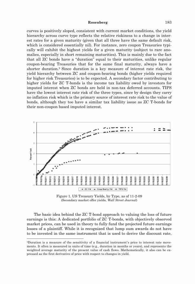
Figure 1 shows the three Treasury yield curves used to illustrate this me-thod based on the November 2, 2009 closing yields obtained from the next business day’s WSJ. As may be seen, while each of the three Treasury yield

4The first paper produced a smoothed off-the-run daily Treasury yield curve expressed in par yields, zero coupon yields and various forward rates. The second paper is a sequel to the first, and produced the same yield curve statistics for Treasury Inflation Protected Securities or TIPS. Both papers reference how researchers can access both data sets online, with the links provided in Ap-pendix I.

Rosenberg 183

curves is positively sloped, consistent with current market conditions, the yield hierarchy across curve type reflects the relative riskiness to a change in inter-est rates for a given maturity (given that all three have the same default risk, which is considered essentially nil). For instance, zero coupon Treasuries typi-cally will exhibit the highest yields for a given maturity (subject to rare ano-malies, especially in short remaining maturities). This is mainly due to the fact that all ZC bonds have a “duration” equal to their maturities, unlike regular coupon-bearing Treasuries that for the same final maturity, always have a shorter duration.5

Since duration is a key measure of interest rate risk, the

yield hierarchy between ZC and coupon-bearing bonds (higher yields required for higher risk Treasuries) is to be expected. A secondary factor contributing to higher yields for ZC T-bonds is the income tax liability owed by investors for imputed interest when ZC bonds are held in non-tax deferred accounts. TIPS have the lowest interest rate risk of the three types, since by design they carry no inflation risk which is the primary source of interest rate risk to the value of bonds, although they too have a similar tax liability issue as ZC T-bonds for their non-coupon based imputed interest.

Figure 1. US Treasury Yields, by Type, as of 11-2-09 (Secondary market offer yields, Wall Street Journal)

The basic idea behind the ZC T-bond approach to valuing the loss of future earnings is this: A dedicated portfolio of ZC T-bonds, with objectively observed market prices, can be used in theory to fully fund the projected future earnings losses of a plaintiff. While it is recognized that lump sum awards do not have to be invested in the same instrument that is used to derive the discount rate, 5Duration is a measure of the sensitivity of a financial instrument’s price to interest rate move-ments. It often is measured in units of time (e.g., duration in months or years), and represents the weighted average maturity of the present value of cash flows. Mathematically, it also can be ex-pressed as the first derivative of price with respect to changes in yield.


using observed prices for ZC bonds allows for basic consistency and “parity in risk” between earnings loss estimates and discounting:

Having no default risk on the ZC T-bonds effectively if not perfectly

corresponds with the one-way downside risk that Ireland explained (above) in terms of earnings and survival uncertainty built into wor-klife expectancy tables;

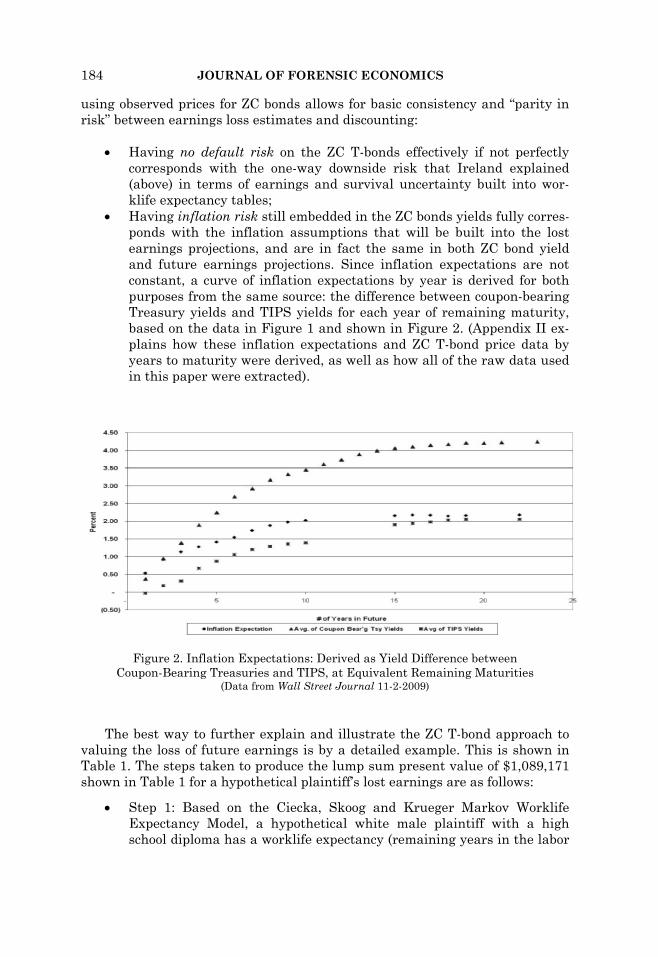
Having inflation risk still embedded in the ZC bonds yields fully corres-ponds with the inflation assumptions that will be built into the lost earnings projections, and are in fact the same in both ZC bond yield and future earnings projections. Since inflation expectations are not constant, a curve of inflation expectations by year is derived for both purposes from the same source: the difference between coupon-bearing Treasury yields and TIPS yields for each year of remaining maturity, based on the data in Figure 1 and shown in Figure 2. (Appendix II ex-plains how these inflation expectations and ZC T-bond price data by years to maturity were derived, as well as how all of the raw data used in this paper were extracted).

Figure 2. Inflation Expectations: Derived as Yield Difference between Coupon-Bearing Treasuries and TIPS, at Equivalent Remaining Maturities

(Data from Wall Street Journal 11-2-2009)

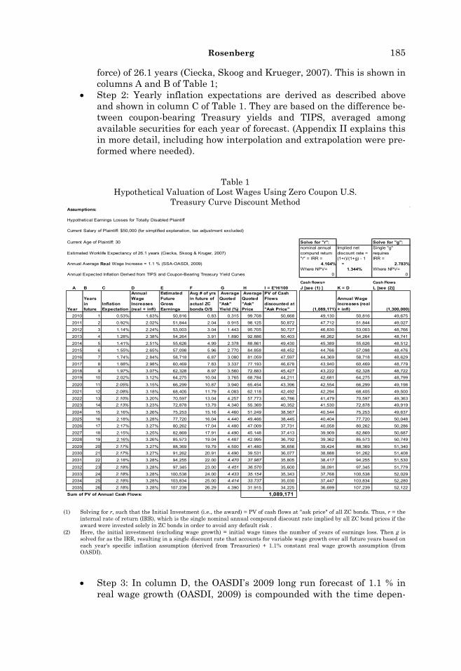
The best way to further explain and illustrate the ZC T-bond approach to valuing the loss of future earnings is by a detailed example. This is shown in Table 1. The steps taken to produce the lump sum present value of $1,089,171 shown in Table 1 for a hypothetical plaintiff’s lost earnings are as follows:

Step 1: Based on the Ciecka, Skoog and Krueger Markov Worklife Expectancy Model, a hypothetical white male plaintiff with a high school diploma has a worklife expectancy (remaining years in the labor

Rosenberg 185

force) of 26.1 years (Ciecka, Skoog and Krueger, 2007). This is shown in columns A and B of Table 1;

Step 2: Yearly inflation expectations are derived as described above and shown in column C of Table 1. They are based on the difference be-tween coupon-bearing Treasury yields and TIPS, averaged among available securities for each year of forecast. (Appendix II explains this in more detail, including how interpolation and extrapolation were pre-formed where needed).

Table 1 Hypothetical Valuation of Lost Wages Using Zero Coupon U.S.

Treasury Curve Discount Method Assumptions:

Hypothetical Earnings Losses for Totally Disabled Plaintiff

Current Salary of Plaintiff: $50,000 (for simplified explanation, tax adjustment excluded)

Current Age of Plaintiff: 30 Solve for "r": Solve for "g":nominal annual Single "g"

Estimated Worklife Expectancy of 26.1 years (Ciecka, Skoog & Kruger, 2007) compund return requires "r" = IRR = IRR =

Annual Average Real Wage Increase = 1.1 % (SSA-OASDI, 2009) 4.164% 2.783%Where NPV= 1.344% Where NPV=

Annual Expected Inflation Derived from TIPS and Coupon-Bearing Treasury Yield Curves 0 0

Cash flows= Cash Flows

A B C D E F G H I = E*H/100 J [see (1) ] K = D L [see (2)]

Year

Years in future

Inflation Expectation

Annual Wage Increases (real + infl)

Estimated Future Gross Earnings

Avg # of yrs in future of actual ZC bonds O/S

Average Quoted "Ask" Yield (%)

Average Quoted "Ask" Price

PV of Cash Flows discounted at "Ask Price" (1,089,171)

Annual Wage Increases (real + infl) (1,300,000)

2010 1 0.53% 1.63% 50,816 0.83 0.315 99.708 50,668 49,130 50,816 49,675

2011 2 0.92% 2.02% 51,844 2.04 0.915 98.125 50,872 47,712 51,844 49,027

2012 3 1.14% 2.24% 53,003 3.04 1.443 95.705 50,727 46,830 53,003 48,766

2013 4 1.28% 2.38% 54,264 3.91 1.890 92.886 50,403 46,262 54,264 48,741

2014 5 1.41% 2.51% 55,626 4.99 2.378 88.861 49,430 45,389 55,626 48,512

2015 6 1.55% 2.65% 57,098 5.96 2.770 84.858 48,452 44,766 57,098 48,476

2016 7 1.74% 2.84% 58,718 6.87 3.080 81.059 47,597 44,369 58,718 48,629

2017 8 1.88% 2.98% 60,469 7.83 3.337 77.193 46,678 43,940 60,469 48,779

2018 9 1.97% 3.07% 62,328 8.97 3.560 72.883 45,427 43,222 62,328 48,722

2019 10 2.02% 3.12% 64,275 10.04 3.765 68.784 44,211 42,681 64,275 48,799

2020 11 2.05% 3.15% 66,299 10.87 3.940 65.454 43,396 42,554 66,299 49,198

2021 12 2.08% 3.18% 68,405 11.79 4.083 62.118 42,492 42,294 68,405 49,500

2022 13 2.10% 3.20% 70,597 13.04 4.257 57.773 40,786 41,479 70,597 49,363

2023 14 2.13% 3.23% 72,878 13.79 4.340 55.369 40,352 41,530 72,878 49,919

2024 15 2.16% 3.26% 75,253 15.16 4.460 51.249 38,567 40,544 75,253 49,637

2025 16 2.18% 3.28% 77,720 16.04 4.440 49.466 38,445 40,404 77,720 50,048

2026 17 2.17% 3.27% 80,262 17.04 4.480 47.009 37,731 40,058 80,262 50,286

2027 18 2.15% 3.25% 82,869 17.91 4.490 45.148 37,413 39,909 82,869 50,687

2028 19 2.16% 3.26% 85,573 19.04 4.487 42.995 36,792 39,362 85,573 50,749

2029 20 2.17% 3.27% 88,369 19.79 4.500 41.480 36,656 39,424 88,369 51,340

2030 21 2.17% 3.27% 91,262 20.91 4.490 39.531 36,077 38,888 91,262 51,408

2031 22 2.18% 3.28% 94,255 22.00 4.470 37.987 35,805 38,417 94,255 51,530

2032 23 2.18% 3.28% 97,345 23.00 4.451 36.570 35,600 38,091 97,345 51,779

2033 24 2.18% 3.28% 100,538 24.00 4.433 35.154 35,343 37,768 100,538 52,029

2034 25 2.18% 3.28% 103,834 25.00 4.414 33.737 35,030 37,447 103,834 52,280

2035 26 2.18% 3.28% 107,239 26.29 4.390 31.915 34,225 36,699 107,239 52,122

Sum of PV of Annual Cash Flows: 1,089,171

Implied net discount rate =(1+r)/(1+g) - 1 =

(1) Solving for r, such that the Initial Investment (i.e., the award) = PV of cash flows at "ask price" of all ZC bonds. Thus, r = the internal rate of return (IRR), which is the single nominal annual compound discount rate implied by all ZC bond prices if the award were invested solely in ZC bonds in order to avoid any default risk .

(2) Here, the initial investment (excluding wage growth) = initial wage times the number of years of earnings loss. Then g is solved for as the IRR, resulting in a single discount rate that accounts for variable wage growth over all future years based on each year's specific inflation assumption (derived from Treasuries) + 1.1% constant real wage growth assumption (from OASDI).

Step 3: In column D, the OASDI’s 2009 long run forecast of 1.1 % in real wage growth (OASDI, 2009) is compounded with the time depen-


dent inflation forecast from column C and used to generate future gross earnings forecasts for each year in column E.

Step 4: Using the WSJ’s actual outstanding ZC bond prices, average maturities were calculated for bonds maturing in each whole year of the forecast. For each future year, the corresponding averages of bond “ask” yields and prices (i.e., those available to investors, unlike the “bid” yields and prices) were also calculated. The results are shown in columns F, G, and H.

Step 5: The Present Value of future cash flows is obtained by summing up the discounted value of each year’s estimated future earnings by the corresponding “ask” price for that year, i.e.,

(Pricei /100)(Estimated Future Gross Earningsi)

where i is each corresponding future year.6 In other words, in order to buy $100 of ZC T-bonds due on average

in forecast year 1, a lump sum investment of $99.708 is required. The same procedure is done for each forecast year, so for example, in order to buy $100 of ZC T-bonds due in year 26, a lump sum of 31.915 is re-quired. Applying this series of average ZC T-bond prices to each year’s forecasted lost earnings over the estimated 26 years of worklife gives a PV total of $1,089,171, shown in column I.

This captures the full procedure for deriving a lump sum PV of lost earnings. This method is consistent with the well-established practice in finance that “…a bond can be viewed as a package of zero coupon se-curities (each coupon being a unique bond, with one principal payment at the end), in which case a unique discount rate should be used to de-termine the present value of each cash flow.” (Fabozzi, 1996, p.26) This concept of having a separate discount rate for each cash flow is in fact

6While i represents each corresponding future year for earnings, for ZC bond prices and corresponding maturities, each i is the average remaining maturity for outstanding ZC bonds clos-est to each year in the future, such that the average maturity corresponds with the average price of those same bonds that mature each future year. For example, there are six ZC bonds that mature from 5/15/2010 to 2/15/2011, all of which are closer to one year of remaining maturity than to two years. The average maturity of these six “year one” bonds (i = 1) is .83 year after 11/9/2009, which is time zero, when the bond prices were observed. Those six bonds with an average maturity of .83 year have a corresponding average price of 99.708. Similarly, there are two ZC bonds that have remaining maturities closer to two years after time zero 11/9/2009 (i.e., 8/15/2011 and 2/15/2012). The average maturity and average price of these “year two” bonds (i = 2) are 2.04 years and 98.125, respectively. These values are shown in Table 1 (column F) as the average number of years in the future of the actual ZC bonds that will mature each year in the future and the corres-ponding average price of those bonds (column H). These average prices of bonds maturing each year are then applied to each year’s gross future earnings to obtain present values (column I). The same procedure is done to obtain bond average maturities and average prices for years 3 through year 26. Note for four of the out years, years 22 -25, no ZC bonds were maturing, so interpolation of prices was required from the year 21 and 26 average maturities (20.91 years and 26.29) and aver-age prices (4.49 and 4.39). It is understood that there is a very slight imprecision in employing non-integer yearly periods for discounting each future year’s lost earnings, but the effect on the annu-alized return and hence, present value of the award, is negligible. This was confirmed by compar-ing these results with those from a series of derived ZC bond yields and implied prices based on a series of exact yearly remaining maturity intervals obtained from another procedure developed at the Federal Reserve. See Appendix I for details. It should be added that a similar type of impreci-sion results from any damage award based on future annual earnings estimates and annual dis-counting, given that most people are paid at least monthly.

Rosenberg 187

the basis for most bond pricing models. However, it doesn’t directly an-swer what some people will want to know: What is the single net dis-count rate implied by this procedure with multiple effective discount rates? To answer that question, two more steps are required.

Step 6: Based on a lump sum investment of $1,089,171 at time zero, solve for the single discount rate, i.e., the internal rate of return (IRR), that equates the PV of lost earnings to that investment. Each year Price Estimated Gross Earnings is discounted at the IRR until the net present value or NPV = 0:

1

NPV Investment ( Price )(Estimated Gross Earnings ) / 1 IRR 0n

i

i ii

where i, as explained in footnote 6, is the average maturity in years closest to each integer future year of the actual ZC T-bonds outstand-ing, e.g., .83 years in year 1, 2.04 years in year 2, 3.04 in year 3, etc., and with the price being the average price corresponding with each fu-ture year’s maturating ZC T-bonds. This procedure solves for the single discount rate equivalent embedded in the series of ZC T-bond prices of r 4.164%, shown at the top of column J.

Step 7: Finally, a single earnings growth rate, g, is needed to calculate the implied net discount rate, which is (1 ) / (1 ) 1.r g The g is simi-larly derived as an IRR, only this time it is calculated by equating the present value of the estimated future gross earnings to the total earn-ings without any growth, i.e., (26 years) (50,000) in lost earnings today is $1,300,000

1

NPV Investment Estimated Gross Earnings / 1 IRR 0n

i

ii

This IRR formula is similar to the one above, except that the estimated yearly gross earnings are not discounted by ZC T-bond prices. That is because since we are only trying to see what is the single earnings growth rate implied by the average real wage growth (constant at 1.1%/yr) plus the expected inflation rate that varies each year. The re-sult is g = 2.783%, shown at the top of column L (column K repeats D). Taken together, the implied net discount rate is (1 ) / (1 ) 1 .0134r g or 1.34%.

It is asserted that the ZC T-bond method presented here is preferable in terms of sound finance theory to many of the alternative discount methods em-ployed, mainly because it is internally consistent in terms of inclusion of both default risk and inflation risk, it does not violate the “parity in risk” principal, nor does it rely on an arbitrarily selected historical period for averaging of short term T-bill rates that causes wide variations in present value results.

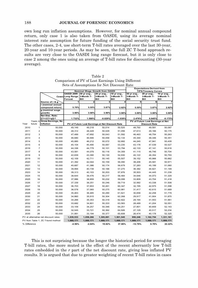
Table 2 compares the results from using this method with results calcu-lated using the same underlying assumptions of Table 1 but based on selected alternative net discount methods. Seven alternative cases are shown in Table 2. The first four cases use nominal wage growth from OASDI, which includes its


own long run inflation assumptions. However, for nominal annual compound return, only case 1 is also taken from OASDI, using its average nominal interest rate assumption for future funding of the social security trust fund. The other cases, 2-4, use short-term T-bill rates averaged over the last 30-year, 20-year and 10-year periods. As may be seen, the full ZC T-bond approach re-sults are very close to the OASDI long range forecast, but it is only close to case 2 among the ones using an average of T-bill rates for discounting (30-year average).

Table 2 Comparison of PV of Lost Earnings Using Different

Sets of Assumptions for Net Discount Rate

CasesOASDI 2009 Long Range Forcast

30 yr avg., 3-Month T-Bill






Source of r & g 1 2 3 4 5 6 7r (nominal annual compound return) 5.70% 5.55% 3.87% 2.82% 5.55% 3.87% 2.82%g (nominal wage growth) 3.90% 3.90% 3.90% 3.90% 3.00% 3.00% 3.00%Net Disc. Rate: [(1+r)/(1+g)]-1 1.732% 1.588% -0.029% -1.039% 2.476% 0.845% -0.175%

YearYears in future

Gross Earnings, No Inflation

2010 1 50,000 49,149 49,218 50,014 50,525 48,792 49,581 50,087

2011 2 50,000 48,312 48,449 50,029 51,056 47,613 49,166 50,175

2012 3 50,000 47,489 47,692 50,043 51,592 46,463 48,754 50,263

2013 4 50,000 46,680 46,946 50,058 52,134 45,340 48,346 50,351

2014 5 50,000 45,885 46,212 50,072 52,682 44,245 47,941 50,439

2015 6 50,000 45,104 45,490 50,087 53,235 43,176 47,539 50,527

2016 7 50,000 44,336 44,779 50,101 53,794 42,133 47,141 50,616

2017 8 50,000 43,581 44,079 50,116 54,359 41,115 46,746 50,704

2018 9 50,000 42,839 43,390 50,130 54,930 40,122 46,354 50,793

2019 10 50,000 42,109 42,711 50,145 55,507 39,152 45,966 50,882

2020 11 50,000 41,392 42,044 50,159 56,090 38,206 45,581 50,971

2021 12 50,000 40,687 41,386 50,174 56,679 37,283 45,199 51,060

2022 13 50,000 39,994 40,739 50,188 57,275 36,382 44,821 51,149

2023 14 50,000 39,313 40,103 50,203 57,876 35,503 44,445 51,239

2024 15 50,000 38,644 39,476 50,217 58,484 34,646 44,073 51,329

2025 16 50,000 37,986 38,859 50,232 59,099 33,809 43,704 51,418

2026 17 50,000 37,339 38,251 50,246 59,719 32,992 43,338 51,508

2027 18 50,000 36,703 37,653 50,261 60,347 32,195 42,975 51,598

2028 19 50,000 36,078 37,065 50,275 60,981 31,417 42,615 51,689

2029 20 50,000 35,463 36,485 50,290 61,621 30,658 42,258 51,779

2030 21 50,000 34,860 35,915 50,304 62,268 29,917 41,904 51,870

2031 22 50,000 34,266 35,353 50,319 62,922 29,194 41,553 51,961

2032 23 50,000 33,682 34,801 50,333 63,583 28,489 41,204 52,051

2033 24 50,000 33,109 34,257 50,348 64,251 27,801 40,859 52,143

2034 25 50,000 32,545 33,721 50,362 64,926 27,129 40,517 52,234

2035 26 50,000 31,991 33,194 50,377 65,608 26,474 40,178 52,325

PV at alternative net discount rates: 1,039,533 1,058,266 1,305,081 1,501,545 950,246 1,162,754 1,331,161

PV from Table 1, ZC T-bond method 1,089,171 1,089,171 1,089,171 1,089,171 1,089,171 1,089,171 1,089,171

% Difference -4.56% -2.84% 19.82% 37.86% -12.76% 6.76% 22.22%

Expectations Derived from TIPS/Treasury CurvesNominal Wage Growth from OASDI

PV of Future Lost Earnings at Net Discount RatePV of Future Lost Earnings at Net

Discount Rate

This is not surprising because the longer the historical period for averaging T-bill rates, the more muted is the effect of the recent aberrantly low T-bill rates embedded in the r part of the net discount rate, giving less inflated PV results. It is argued that due to greater weighting of recent T-bill rates in cases

Rosenberg 189

3 and 4, the PV results are increasingly distorted relative to those resulting from the full ZC T-bond approach of Table 1 (almost 20% and 40% higher re-spectively). Similarly, cases 3 and 4 result in much higher PVs relative to the OASDI assumptions embedded in case 1. The thing that the ZC T-bond method and the OASDI methods both have in common is that neither one unduly weights today’s extremely low inflation over time. The ZC method does incor-porate extremely low inflation expectations but, appropriately, only for the near forecast years, consistent with investor expectations embedded in the various Treasury yield curves. The same cannot be said for cases 3 and 4, which overweight the impact of today’s immediate inflation expectations in the shorter period (20- and 10-year) historical averages of T-bill rates.

Cases 5-7 are designed to be closest to the ZC T-bond method on earnings growth and inflation while showing how the arbitrary choice of different T-bill rates for discounting give widely varying award results. Cases 5-7 use the same 30-yr, 20-yr and 10-yr averages of T-bill rates for r respectively, as did cases 2-4. For “g,” which is a nominal annual growth measure, cases 5-7 all use the same 1.1% real wage growth from OASDI used in the ZC T-bond example, and the same average inflation expectation embedded in the Treasury yield curves used in the ZC T-bond example, i.e., 1.88%. Combining the OASDI real wage growth of 1.1% and the average inflation rate of 1.88%, together they give an implied nominal annual wage growth of 3.00% (= (1+.011) (1+.0188)-1). Thus, cases 5-7 are as close in comparison with the ZC T-bond discount method as possible, given that the r portion of the net discount rate must remain dif-ferent. As may be seen, case 5-7 results are more symmetric and generally closer to those of the ZC T-bond method. However, having a PV range that va-ries by 40% depending on whether one selects a 10-yr T-bill average or a 30-yr T-bill average underscores the arbitrariness of results based on the particular period selected for historical T-bill yields.

IV. Conclusion

The Zero Coupon Treasury bond discount approach to valuing lost future

earnings offers a theoretically sound and internally consistent alternative to many existing approaches, especially ones based on discounting future earn-ings at a rather arbitrarily-selected historical period of three-month T-bill yields. Using three-month T-bill yields as a discount rate effectively eliminates both default risk and inflation risk, resulting in a truly risk-free rate that is appropriate only for discounting cash flows that are a “certainty equivalent.” Unless both default and inflation risks also are removed from a projected lost future earnings stream, the “parity in risk” principal of finance is violated. Al-though Treasury bonds being free of default risk is not a perfect analogy to adjusting future earnings losses for worklife expectancy, both reflect the down-side risks of curtailing future cash flows. As Ireland argued in 1997 (and cited above), bond default risk is “roughly the analog for risks that the worker would not obtain expected future wage benefits because of death, illness or unem-ployment.” Considering these as satisfactorily offsetting is the only practical way to achieve default risk parity in valuing lost earnings. And the uncertainty of future wage increases due to productivity gains is best addressed separately


and directly, via incorporating a factor to represent real wage growth which in the long run can only spring from productivity gains.

Achieving parity of inflation risk is another matter. Unless one removes in-flation risk from both the discount rate and from future lost earnings by void-ing COLAs and related assumptions embedded in earnings projections, then the parity principal is violated. Only if future earnings can be presented some-how as a certainty equivalent cash flow stream can one really justify reducing this to a lump sum by using a fully risk free discount rate, which means ne-gating both inflation and default risk. On this score, while the ZC T-bond dis-count approach eliminates default risk, it explicitly allows for inflation risk, which is objectively derived from the Treasury bond market, and applied con-sistently as a time-dependent variable in both the discount rate and in pro-jected future lost earnings. Finally, by offering a market based approach that can be readily updated based on a well documented procedure, in the event that initial results based on it change materially by the time of a later court ruling, the ZC T-bond discount method is also robust, in addition to being ob-jective, internally consistent, and sound in finance theory.

References Albrecht, Gary R., “Compensatory Damages and the Appropriate Discount Rate, A

Comment,” Journal of Forensic Economics, 1993, 6(3), 271 –272. ___________, and John Wood, “Risk and Damage Awards: Short-Term Bonds vs. Long-

Term Bonds,” Journal of Legal Economics, 1998, 7(1), 48-59. Bell, Edward and Allan Taub, “Some Issues Concerning Risk Adjustments in Damage

Calculations,” Litigation Economics Digest, Fall 1999, 4(2), 153-155. Biedermann, Daniel K. and Robert C. Basemann, “Risk Free vs. Risk-Adjusted Discount

Rates: A Comment,” Journal of Forensic Economics, 1996, 9(1), 45-47 Brookshire, Michael L., Michael R. Luthy and Frank L. Slesnick, “2006 Survey of

Forensic Economists: Their Methods, Estimates, and Perspectives,” Journal of Foren-sic Economics, 2006, 19(1), 29-59.

Breeden, Charles H., “The „Income-Variance‟ Risk Factor and Jones & Laughlin v. Pfei-fer Guidelines for the Calculation of Present Value,” Journal of Forensic Economics, 2003, 15 (1), 19-29.

Brush, Brian C., “Risk, Discounting, and the Present Value of Future Earnings, Journal of Forensic Economics, 2003, 16(3), 263-274

Ciecka, James E, Gary R. Skoog and Kurt V. Krueger, “New Tabulations of the Markov Worklife Expectancy Model,” presented at the 19th Annual Meeting of the Academy of Economic and Financial Experts, March 29, 2007, Las Vegas, Nevada.

Fabozzi, Frank J., Bond Markets, Analysis and Strategies, Upper Saddle River, NJ: Prentice Hall, Third Edition, 1996.

Gurkaynak, Refet S., Brian Sack, and Jonathan H. Wright, “The U.S. Treasury Yield Curve: 1961 to the Present,” Finance and Economics Discussion Series, Divisions of Research and Statistics and Monetary Affairs Federal Reserve Board, Washington, DC, 2006-28.

___________, “The TIPS Yield Curve and Inflation Compensation,” Finance and Eco-nomics Discussion Series, Divisions of Research and Statistics and Monetary Affairs Federal Reserve Board, Washington, DC, 2008-05.

Harris, William G., “Do Tax-Exempt Discount Rates Eliminate Tax-Induced Errors,” Journal of Forensic Economics, 1995, 8(2), 131-138.

Rosenberg 191

Henderson, James W., and J. Allen Seward, “Risk Aversion and Overcompensation from the Risk Free Discount Rate,” Journal of Legal Economics, 1998, 8(2), 25-32.

Hickman, E. P., “Selecting Income Growth and Discount Rates in Wrongful Death and Injury Cases,” Journal of Risk and Insurance, 1997, 44(1), 129-132.

Houldsworth, Mark A. and Tom D. McKinnon, “Dedicated Portfolios And The Present Value Of Lost Earnings: A Comment,” Journal of Forensic Economics, 1994, 7(2), 209-210.

Ireland, Thomas, “The Pfeifer Decision, Risk and Damage Awards: An Extended Re-sponse to Albrecht and Wood,” Journal of Legal Economics, 1997a, 7(3), 23-34.

___________, “Forensic Implications of Inflation-Adjusted Bonds,” Litigation Economics Digest, 2(2), 1997b, 92-102

___________, “Why Inflation-Indexed Securities Are Not Poorly Suited For Discounting A Future Earnings Stream,” Journal of Forensic Economics, 1998, 11(3), 269-270.

___________, “Response to Bell and Taub: „Some Issues Concerning Risk Adjustments in Damage Calculations,” Litigation Economics Digest, 1999, 4(2), 157-158.

___________, “The Role of a Forensic Economist in a Damage Assessment for Personal Injuries,” The Earnings Analyst, 2004, 6, 15-46.

Jennings, William P., and G. Michael Phillips, “Risk as a Discount Rate Determinant in Wrongful Death and Injury Cases,” The Journal of Risk and Insurance, 1989, 56(1), 122-127.

Levhari, David, and Yoran Weiss, “The Effect of Risk on the Investment in Human Capital,” American Economic Review, 1974, 64(6), 950-963.

Margulis, Marc S., “Compensatory Damages and the Appropriate Discount Rate,” Jour-nal of Forensic Economics, 1992, 6(1), 33-41

Ray, Clarence G., “A Case Against the use of the Wall Street Journal Method of Select-ing a Discount Rate,” Journal of Forensic Economics, 1989, 2(2), 94-95.

Romans, Thomas J., and Frederick G. Floss, “Four Guidelines for Selecting a Discount Rate,” Journal of Forensic Economics, 1992, 5(3), 265-266.

Yandell, Dirk, “The Value of Lost Future Earnings: Methodology, the Discount Rate and Economic Theory,” Journal of Legal Economics, 1991, 1(3), 54-67.

2009 OASDI Trustees Report, officially called "The 2009 Annual Report of the Board of Trustees of the Federal Old-Age and Survivors Insurance and Federal Disability Insurance Trust Funds," 2009.

Cases Jones & Laughlin Steel Corp. v. Pfeifer, 462 U.S. 523 (1983) Trevino v. United States, 804 F2d 1512 (9th Cir. 1986)

Appendix I Comparison of Treasury Data Sources Available Online from the

Wall Street Journal and the Divisions of Research and Statistics and Monetary Affairs of the Federal Reserve Board (hereafter referred to as Fed R&S and MA Divisions)

All required data for use in the ZC-T-bond approach to valuing damage awards can

be obtained by either of the above two sources. The Wall Street Journal (WSJ) publishes dealer-provided price and ask-yield quotes for actual securities that are tradable at 3 pm each day the market is open. The second source of such data is the Fed R&S and MA Divisions. Like the WSJ, it produces a number of valuable daily yields and related measures that also are based on a large set of observable Treasury coupon-bearing se-curities (including TIPS) as described in two separate articles. (Although published by


the Fed, these data are labeled “not an official Federal Reserve statistical release”). Where this data series stands out is that off-the-run Treasuries (rather than on-the-run) are used precisely to minimize security-specific liquidity and demand issues exhi-bited in dealer quotes, such as those in the WSJ that its authors believe would detract from pure yield-curve related insights. The combined dataset explained in both Fed R&S and MA Divisions articles is particularly useful to researchers who need internally consistent data series for studies involving macroeconomic concepts such as term pre-mia and inflation compensation over time.

By using dealer quotes for actually tradable T-bonds, especially for ZC T-bonds, the WSJ data capture technical price and yield effects in terms of security-specific demand and liquidity issues. This has some added value if ones wishes to derive a damage award based on a dedicated portfolio valuation method. It is argued here that this is useful for award valuation purposes even if the plaintiff isn’t expected to actually invest only in such zero-coupon securities, just as proponents of using an arbitrary multi-year average of 90-day T-bill rates wouldn’t expect a plaintiff to actually invest only in 90-day T-bills, continuously rolling over the unused award proceeds into more such T-bills. The Fed R&S and MA Division, in contrast, derive data in the form of continuously compounded zero coupon yields from the smoothed par yield curve generated from off-the-run coupon bearing T-bonds. It does this by effectively “view(ing) coupon-bearing bonds as baskets of zero-coupon securities, one for each coupon payment and the prin-cipal payment.” (Gurkaynak, 2006, p. 11)

In the second Fed R&S and MA paper published in 2008, a series of breakeven in-flation rates is derived as the difference between nominal coupon-bearing Treasuries and TIPS. These breakeven rates are defined as “…the inflation rates which, if realized, would leave an investor indifferent between holding a TIPS and a nominal Treasury security.” (Gurkaynak, 2008, p. 9) While an extensive review of both Fed R&S and MA papers is beyond the scope of this paper, it is worth noting that this breakeven rate se-ries is described as representing inflation compensation, which includes not only infla-tion expectations but also an inflation risk premium (a plus) and a TIPS liquidity pre-mium (a minus). While recognizing this conflation of factors, the authors conclude that inflation compensation as they measure it “… is nonetheless a very useful indicator of investors‟ inflation concerns. Moreover, it is the only inflation indicator which is availa-ble over a high frequency, which makes it quite useful in a range of applications. (Gur-kaynak, 2008, p. 20) Academics may debate how much of “true” inflation expectations are embedded in the yield curve difference between coupon-bearing Treasuries and TIPS, however derived; but given some unavoidable subjectivity in separating these factors, and the inherent liquidity difference between the two instruments, it remains unclear whether a more objective, universally accepted, and meaningful way of deriving future inflation expectations can be found.

Although both data sources should be considered appropriate for use with the ZC T-bond method proposed in this paper, the WSJ data were selected due to the fact that they represent real tradable securities with published ask-prices and may be viewed as closer to what a dedicated portfolio would provide. Despite the methodological differ-ences between the two sources and varying differences by year of observation, the re-sults from both data sources observed on November 2, 2009 differed by a net amount of < 1 basis point when averaged over all future years in the example. Thus, the choice of source would have had only a negligible effect on the present value of the hypothetical award.

For interested readers, the two Fed R&S and MA Divisions data are available via the links below:

http://www.federalreserve.gov/pubs/feds/2006/ http://www.federalreserve.gov/pubs/feds/2008/

Extraction of WSJ data and required derivations are discussed next in Appendix II.

Rosenberg 193

Appendix II Data Extraction and Derivation of ZC T-Bond Prices and Inflation

Expectations by Year to Maturity

Since daily data are available with a one-business day lag, information from the Wall Street Journal on November 3, 2009 were extracted to obtain the desired Novem-ber 2 closing Treasury prices and yield data. These data may be extracted by anyone with a subscription to the online WSJ at www.wsj.com. Once at the home page, follow these links: /Markets/Market Data/Bonds, Rates and Credit Markets. Holding the cur-sor over “Bonds, Rates and Credit Markets,” a pop-up screen appears labeled “Quotes and Trading Statistics.” In the lower left side of that screen, the last three selections produce the prior day’s closing prices and yields by maturity date for the three types of Treasuries used in this paper:

Treasury Inflation-Protected Securities (TIPS) Treasury Quotes Treasury Strips

Note that the Treasury Quotes link displays data separately for Treasury Notes

and Bonds at the top and for Treasury Bills at the bottom. For this paper, only Treasury Notes and Bonds were used since, as coupon bearing instruments, their yields were more appropriate to use with TIPS in order to produce the inflation expectations by ma-turity data series. The Treasury Strips link displays data separately for, Treasury Bond and Note Stripped Principal, which are combined and used in this paper interchangea-bly since they both are zero coupon Treasuries that only pay principal at maturity. A third section with stripped coupon interest is ignored.

After copying to a spreadsheet the day’s raw prices, yields and maturity dates for all ZC T-bonds and notes (hereafter referred to collectively as “bonds”) listed in the WSJ, each bond’s ask price and a calculated number of fractional years of remaining maturity were grouped and averaged by nearest future year to maturity. (Similar to coupon-bearing Treasuries, in a rare number of cases, more than one ZC T-bond ma-tures on the same date, in which case an average price and yield for that maturity date was first obtained). Interpolation was then used to derive missing prices and yields for ZC T-bonds for years 22-25, using the fractional number of years to maturity of the ob-servations for years 21 and 26. It should be noted that the WSJ published yields are in bond-equivalent (i.e., semi-annual yield * 2), and will differ slightly from any calcula-tion based on annual yields, as in this paper.

To derive inflation expectations, raw data from the WSJ on yields for ordinary cou-pon-bearing Treasuries (notes and bonds) as well as for TIPS were similarly extracted from the WSJ and sorted by maturity date, Where the coupon-bearing Treasury secu-rity and a TIPS security of the same maturity date were both available, the latter is subtracted from the former to obtain a presumed inflation expectation for that future period. (In a rare number of cases, more than one Treasury security matures on the same date, in which case an average yield for that maturity date was obtained). If there was no corresponding coupon-bearing Treasury for the same maturity date as a TIPS, then interpolation based on the fractional number of years in the future was performed in order to obtain an estimate of the coupon-bearing Treasury yield for the maturity date needed to match the TIPS. The results were then aggregated by years to maturity (rounded to an integer). Finally, for those years where no TIPS yields were available and were needed for an earnings forecast year, interpolation and extrapolation were performed. For example, TIPS were missing for future years 11-14, and thus were in-terpolated from the year 10 observation of 2.02% and the year 15 observation of 2.16%. Similarly, for years 23-26, the last four future valuation years where no existing TIPS


would be outstanding, the derived expected inflation rate for year 22 (the final TIPS observation) was extrapolated as a constant, a seemingly reasonable assumption, given the flatness of derived future inflation rates from the last two yearly observations (e.g., 2.16% in year 19, and 2.18% in year 22). Finally, it should be noted that extrapolation would have been required regardless of data source, since the last year of derived brea-keven inflation compensation rates from the Fed R&S and MA Divisions was year 20.

JOURNAL OF FORENSIC ECONOMICS Discounting Damage Awards Using the Zero Coupon Treasury Curve:...

Documents

Transcript of JOURNAL OF FORENSIC ECONOMICS Discounting Damage Awards Using the Zero Coupon Treasury Curve:...