Journal of Economics, Finance and Accounting – (JEFA), ISSN
150
-
Upload
khangminh22 -
Category
Documents
-
view
2 -
download
0
Transcript of Journal of Economics, Finance and Accounting – (JEFA), ISSN


__________________________________________________________________________________ i
ABOUT THE JOURNAL Journal of Economics, Finance and Accounting (JEFA) is a scientific, academic, peer-reviewed,
quarterly and open-access online journal. The journal publishes four issues a year. The issuing
months are March, June, September and December. The publication languages of the Journal are
English and Turkish. JEFA aims to provide a research source for all practitioners, policy makers,
professionals and researchers working in the area of economics, finance, accounting and auditing.
The editor in chief of JEFA invites all manuscripts that cover theoretical and/or applied researches on
topics related to the interest areas of the Journal.
Editor-in-Chief
Prof. Suat Teker
Guest Editor for This Issue Prof. Sefer Sener
JEFA is currently indexed by
EconLit, EBSCO-Host, Ulrich’s Directiroy, ProQuest, Open J-Gate,
International Scientific Indexing (ISI), Directory of Research Journals Indexing (DRJI), International
Society for Research Activity(ISRA), InfoBaseIndex, Scientific Indexing Services (SIS), TUBITAK-
DergiPark, International Institute of Organized Research (I2OR)
Journal of Economics, Finance and Accounting – (JEFA), ISSN: 2148-6697, http://www.pressacademia.org/journals/jefa
Year: 2017 Volume: 4 Issue: 2
CALL FOR PAPERS
The next issue of JEFA will be publshed in September, 2017.
JEFA welcomes manuscripts via e-mail.
E-mail: [email protected]
Web: www.pressacademia.org/journals/jefa

__________________________________________________________________________________ ii
EDITORIAL BOARD Sudi Apak, Beykent University
Thomas Coe, Quinnipiac University Cumhur Ekinci, Istanbul Technical University
Laure Elder, Saint Mary's College, Notre Dame Metin Ercan, Bosphorus University
Ihsan Ersan, Istanbul University Umit Erol, Bahcesehir University Saygin Eyupgiller, Isik University
Abrar Fitwi, Saint Mary's College, Notre Dame Rihab Gıidara, University of Sfax
Kabir Hassan, University of New Orleans Halil Kiymaz, Rollins University
Coskun Kucukozmen, Economics University of Izmir Mervyn Lewis, University of South Australi
Bento Lobo, University of Tennessee Ahmed Ali Mohammed, Qatar University
Mehmet Sukru Tekbas, Turkish-German University Oktay Tas, Istanbul Technical University
Lina Hani Ward, Applied Science University of Jordan Hadeel Yaseen, Private Applied Science University
REFEREES FOR THIS ISSUE Ali Akdemir, Arel University
Volkan Alptekin, Celal Bayar University David Anderson, Eastern Michigan University
Bunyamin Bacak, Canakkale Onsekiz Mart University Tayfur Bayat, Inonu University
Unal Caglar, Istanbul University Thomas Coe, Quinnipiac University
Cumhur Ekinci, Istanbul Technical University Isin Erol, Ozyegin University
Jan Fidrmuck, Brunel University Volkan Hacioglu, Istanbul University
Lalita Hongratanawong, University of Thai Chambers of Commerce Andrew Kakabadse, University of Reading
Nada Kakabadse, University of Reading Mehmet Marangoz, Mugla Sitki Kocman University
Ghassan Omet, Jordan University Volkan Ongel, Beykent University
Muharrem Ozdemir, Istanbul Gelisim University Edwin Portugal, State University of New York
Mesut Savrul, Canakkale Onsekiz Mart University Sefer Sener, Istanbul University
Stefan Schepers, EU High Level Group for Innovation Ibrahim halil Sugozu, Sirnak University
Donal Staub, Isik University Selva Staub, Bandirma Onyedi Eylul University
Oktay Tas, Istanbul Technical University Tahanarerk Thanakijsombat, Mehidol University
Kadir Tuna, Istanbul University Cigdem Borke Tunali, Istanbul University
Julius Waller, EU High Level Group for Innovation Mustafa Yurttadur, Istanbul Gelisim University
Journal of Economics, Finance and Accounting – (JEFA), ISSN: 2148-6697, http://www.pressacademia.org/journals/jefa
Year: 2017 Volume: 4 Issue: 2

__________________________________________________________________________________ iii
CONTENT
Title and Author/s Page
1. Time reward of value investing: evidence from the Southeast Asia stock markets Yosuke Kakinuma……………………………………………………………………………………………………………………………………………. 70-86 DOI: 10.17261/Pressacademia.2017.436 JEFA-V.4-ISS.2-2017(1)-p.70-86
2. Asymmetric relationship between financial performance of Turkish banking sector and macroeconomic performance
Türk bankacılık sektörünün finansal performansı ve makroekonomik performans arasındaki asimetrik ilişki
Gulbahar Ucler, Dogan Uysal……………………………………………………………………………………………………………………………. 87-97 DOI: 10.17261/Pressacademia.2017.437 JEFA-V.4-ISS.2-2017(2)-p.87-97
3. Credit scoring by using generalized models: an implementation on Turkey’s SMSs Aysegul Iscanoglu Cekic, Kasirga Yildirak……………………………………………………………………………………………………..….. 98-105 DOI: 10.17261/Pressacademia.2017.438 JEFA-V.4-ISS.2-2017(3)-p.98-105
4. Empirical analysis of savings and investments relation in Turkey: cointegration test with structural breaks approach Izzet Tasar………………………………………………………………………………………………………………………………………………………… 106-111 DOI: 10.17261/Pressacademia.2017.439 JEFA-V.4-ISS.2-2017(4)-p.106-111
5. The study of the impact of e-commerce activities on firm value and the relationship between e-marketing and firm value Mustafa Yurttadur, Cansu Turker……………………………………………………………………………………………………………………. 112-120 DOI: 10.17261/Pressacademia.2017.440 JEFA-V.4-ISS.2-2017(5)-p.112-120
6. Efficiency of ICT development indicators in OECD countries Halil Tunali, Tugba Guz, Gulden Sengun………………………………………………………………………………………………………… 121-128 DOI: 10.17261/Pressacademia.2017.441 JEFA-V.4-ISS.2-2017(6)-p.121-128
7. Competitiveness analysis of the Turkish chemical industry: a comparison with the selected European Union countries Elife Akis…………………………………………………………………………………………………………………………………………………………… 129-137 DOI: 10.17261/Pressacademia.2017.442 JEFA-V.4-ISS.2-2017(7)-p.129-137
8. Influencing the practice of human resource accounting: skills and strategies
Krishna Priya Rolla……………………………………………………………………………………………………………………………………………. 138-144 DOI: 10.17261/Pressacademia.2017.443 JEFA-V.4-ISS.2-2017(8)-p.138-144
9. An investigation of self-service technology (SST) of participation banking in Turkey Waleed Mango, Busra Muceldili, Oya Erdil……………………………………………………………………………………………………… 145-153 DOI: 10.17261/Pressacademia.2017.444 JEFA-V.4-ISS.2-2017(9)-p.145-153
Journal of Economics, Finance and Accounting – (JEFA), ISSN: 2148-6697, http://www.pressacademia.org/journals/jefa
Year: 2017 Volume: 4 Issue: 2

__________________________________________________________________________________ iv
CONTENT
Title and Author/s Page
10. Regional determinants of the small and medium size manufacturing firm entry in a developing country: evidence from Turkey Mustafa Ozer…………………………………………………………………………………………………………………………………………………… 154-163 DOI: 10.17261/Pressacademia.2017.445 JEFA-V.4-ISS.2-2017(10)-p.154-163
11. Measuring the technology achievement index: comparison and ranking of countries Ahmet Incekara, Tugba Guz, Gulden Sengun……………………………………………………………………………………………………. 164-174 DOI: 10.17261/Pressacademia.2017.446 JEFA-V.4-ISS.2-2017(11)-p.164-174
12. A new approach on occupational health and safety: financial state support for employer O. Hakan Cavus……………………………………………………………………………………………………………………………………………….. 175-183 DOI: 10.17261/Pressacademia.2017.447 JEFA-V.4-ISS.2-2017(12)-p.175-183
13. Digital agriculture practices in the context of agriculture 4.0 Burak Ozdogan, Anil Gacar, Huseyin Aktas……………………………………………………………………………………………………… 184-191 DOI: 10.17261/Pressacademia.2017.448 JEFA-V.4-ISS.2-2017(13)-p.184-191
14. Selection among innovative project proposals using a hesitant fuzzy multiple criteria decision making method Basar Oztaysi, Sezi Cevik Onar, Cengiz Kahraman…………………………………………………………………………………………….. 192-200 DOI: 10.17261/Pressacademia.2017.449 JEFA-V.4-ISS.2-2017(14)-p.192-200
15. Invention and innovation in economic change Sefer Sener, Volkan Hacioglu, Ali Akdemir............................................................................................................. 201-206 DOI: 10.17261/Pressacademia.2017.450 JEFA-V.4-ISS.2-2017(15)-p.201-206
16. Information and technology intensıve sectors Yuksel Bayraktar,Ayfer Ozyilmaz, Metin Toprak…………………………………………………………………………………………….. 207-214 DOI: 10.17261/Pressacademia.2017.451 JEFA-V.4-ISS.2-2017(16)-p.207-214
Journal of Economics, Finance and Accounting – (JEFA), ISSN: 2148-6697, http://www.pressacademia.org/journals/jefa
Year: 2017 Volume: 4 Issue: 2

Journal of Economics, Finance and Accounting – JEFA (2017), Vol.4(2), p. 70-86 Kakinuma
_________________________________________________________________________________________________
DOI: 10.17261/Pressacademia.2017.436 70
TIME REWARD OF VALUE INVESTING: EVIDENCE FROM THE SOUTHEAST ASIA STOCK MARKETS
DOI: 10.17261/Pressacademia.2017.436 JEFA-V.4-ISS.2-2017(1)-p.70-86
Yosuke Kakinuma
1
1National Institute of Development Administration (NIDA), Bangkapi, Bangkok 10240, Thailand. [email protected].
To cite this document Kakinuma, Y. (2017). Time reward of value investing: evidence from the Southeast Asia stock markets. Journal of Economics, Finance and Accounting (JEFA), V.4, Iss.2, p.70-86. Permanent link to this document: http://doi.org/10.17261/Pressacademia.2017.436 Copyright: Published by PressAcademia and limited licenced re-use rights only.
ABSTRACT Purpose- This study tests the effectiveness of value investing and its relation to the length of investment horizon in Malaysia, Singapore,
and Thailand stock markets as well as the ASEAN market as a whole. Two simple financial ratios, namely, Price-to-Earning (PE) ratio and
Price-to-Book (PE) ratio, are employed to see if they represent value premium in a long-term investment.
Methodology- A simulation methodology that randomly selects an investment date is applied which effectively eliminates market timing
bias. Portfolios sorted by PE and PB ratios are formed on a randomly chosen date and held for different periods of time. Additionally, Fama-
Mcbeth (1973) regression checks a robustness of value premium of PE and PB ratios.
Findings- Portfolios constructed with low PE and PB ratio generate higher returns and form efficient portfolios with better risk-return
trade-off. In a long-term investment, PE and PB are indicators of value premium. Also, the ASEAN Link provides an excellent opportunity for
international diversification.
Conclusion- Value investors are rewarded for holding portfolios with low PE and PB stocks for a long period of time. Furthermore, investors
should construct portfolios with stocks from different markets to fully take advantage of international diversification, which significantly
reduces investment risk.
Keywords: Value investing, long-term investment, international diversification, financial simulation, emerging markets.
JEL Codes: G11, G15, G17
1. INTRODUCTION
Finding undervalued stocks is a basic principle of value investing. Benjamin Graham (1949), who is often referred as “the father of value investing,” stresses an importance to secure “margin of safety,” or in other words, the difference between a firm’s intrinsic value and the market price. Previous researches suggest that, among other financial ratios, Price-to-Earning (PE) ratio (Basu, 1977) and Price-to-Book (PB) ratio (Fama & French, 1992) are the key indicators of undervalued stocks. Today, the both ratios are popular and widely-available ratios for general investors.
Besides the margin of safety, another important aspect of value investing is a long-term investment horizon. Securing the margin of safety does not guarantee an instant profit but value investors are rewarded for holding stocks for a long term. Stock market is extremely volatile in the short-run, but in the long-run, market price should get closer to a firm’s intrinsic value.
In 2012, the ASEAN countries declared to establish the AEAN Exchange, a collaboration of securities exchanges of the ASEAN member countries, namely Singapore, Malaysia, Thailand, Vietnam, Philippines, and Indonesia (www.aseanexchanges.org). Its aim is to integrate the each countries’ exchanges into one capital market. The ASEAN Link is the platform for the single exchange market. As of April 2016, investors are able to trade securities on the Singapore
Journal of Economics, Finance and Accounting – (JEFA), ISSN: 2148-6697, http://www.pressacademia.org/journals/jefa
Year: 2017 Volume: 4 Issue: 2

Journal of Economics, Finance and Accounting – JEFA (2017), Vol.4(2), p. 70-86 Kakinuma
_________________________________________________________________________________________________
DOI: 10.17261/Pressacademia.2017.436 71
Exchanges, the Bursa Malaysia, and the Stock Exchange of Thailand, via the ASEAN Link. This means that an investor who has an account in the ASEAN Link is able to trade shares of Singapore, Malaysia, and Thailand, which together represents 70% of market capitalization of the ASEAN Exchange, in a single account. More member countries are expected to join this link in the near future, which creates a huge capital market in the Southeast Asia.
The ASEAN Link provides an excellent opportunity for the investors in the region to access to international diversification. On the contrary to Markowitz’s efficient market portfolio theory (1952) which proposes that risk-return optimization is realized through diversification, Gaudecker (2015) points out that general households tend to underdivesify, and the loss from the underdiversification can be significant over life time.
Table 1 shows the Pearson correlation coefficients of daily returns of the FTSE Bursa Malaysia EMAS index (FBMEMAS), the FTSE ST All SHARE index (FSTAS), and the SET index (SET) for the period from January 2000 to December 2015. The FBMEMAS represents the top 98% of stocks listed on the Bursa Malaysia by market capitalization. The FSTAS represents 98% of Singapore market capitalization. The SET is comprised of all the stocks listed on the Stock Exchange of Thailand.
Table 1: Correlation Matrix of Daily Market Index Returns
FBMEMAS (Malaysia)
FTAS (Singapore)
SET (Thailand)
FBMEMAS 1.0000 FTAS 0.5101*** 1.0000 SET 0.3813*** 0.4893*** 1.0000 *** denotes significance at 0.1%
Although the three countries are geographically close and economic ties are strong, the behavior of the each market is a different story. The correlation of daily returns between the Malaysia market and the Singapore market is only 0.51 although the two countries share the border and are the largest trade partners to the each other. The correlation of daily idex returns is even lower at 0.38 between the Malaysia market and the Thailand market. Thus, the relatively low correlation of the stock returns in the three markets provides the chance to form a better diversified portfolio.
In this study, I test a simple stock screening strategy by PE and PB ratios with a simulation method which portfolios are constructed on randomly selected dates. Returns are calculated for different holding periods to see if value investors are rewarded for longer time investment horizon. Additionally, the returns of the portfolios are compared to those of market benchmark indices. The advantage of international diversification through the ASEAN Link is also examined.
2. LITERATURE REVIEW
Graham (1949) pioneered in the field of value investing, and many followed his path to pursue value premium using financial ratios. Basu (1977) was the first to find out that stocks with low PE ratios yield a higher return. The low PE stocks even generated higher risk-adjusted return backed by higher Jensen’s alpha and Shape ratio. Chan, Hamao, and Lakonishok (1991) argue that Book to Market ratio (B/M) and Cash Flow Yield (CFY) are the two significant variables that explain excess return in the Japanese market. “Size-effect” is that smaller firms in term of market capitalization outperform bigger firms (Banz, 1981). Fama and French (1992) revealed a stunning outcome that challenges the capital asset pricing model. The Fama-French 3-factor model with market return, size-effect, and B/M remains as one of the most powerful asset pricing model today. Novy-Marx (2013) argues that gross profitabiliy, gross profit-to-assets, is as powerful measure of value premum as B/M. Fama and French (2015) incorporate profitability and investment factors in the 3-factor model and propose a new 5-factor model. Several studies state that value stocks respond diffrenly to the underlying economic condtions (Black and McMillan, 2004, 2005: Amman and Verhofen, 2006; Gulen, Xing, and Zhang, 2011; Sarwar, Mateus, and Todorovic, 2017). Value stocks are counter-cyclcial (Chen, Petkova and Zhang, 2008), meaning that value stocks perform much better during economic recessions than during expansions. Value investing is effective not only in the US market but in the international market as well (Bauman, Conover, and Miller, 1998; Sarewiwattahan, 2013).
International diversification is effective in reducing portfolio risk and increasing expected return. Solnik (1974) showed that significant reduction in risk can be achieved with portfolio diversification in foreign stocks as well as domestic common securities in the total of eight countries in the US and Europe. Lessard (1976) presented that, at the same level of risk, the world portfolio which is consisted of value-weighted 16 major national indices in the world generates a higher return than a single national index.
3. DATA AND METHODOLOGY
I obtained the following information on the Bursa Malaysia, the Singapore Exchange, and the Stock Exchange of Thailand from Thomson Reuters’ Datastream: 1) daily stock prices listed on the each market, 2) daily PE ratio of the stocks, 3) daily

Journal of Economics, Finance and Accounting – JEFA (2017), Vol.4(2), p. 70-86 Kakinuma
_________________________________________________________________________________________________
DOI: 10.17261/Pressacademia.2017.436 72
PB ratio of the stocks, and 4) daily index prices of the each market benchmearks. The testing period is 16 years starting from January 3, 2000 to December 31, 2015. During the 16 years of the test period, there were 4,174 trading days for the each stock market.
The total number of stocks available for this research is 655 in the Malaysia market, which are the constituents of FTSE Bursa Malaysia EMAS index (Datastream code-LKLSEMAS). For the Singapore market, I obtained the total of 806 stocks which represent all stocks listed on the Singapore Exchange (Datastream code-FSINQ). The total number of stocks in the Thai market is 554, which are the constituents of the SET index (Datastream code-LBNGKSET). Table 2 shows descriptive statistics of PB and PE ratios in the three markets. In the all three markets, there are some extreme samples, such as a stock with PE ratio as high as 390 in Thailand. Thus, there is a gap between the mean and the medium. Surprisingly, correlation between PB and PE are very small although statistical significance is strong. This suggests that a stock with low PB can have a high PE and vice versa.
Table 2: Descriptive Statistics of PB and PE Ratios in the Malaysia, Singapore and Thailand Markets
Mean Median SD Min Max Observation
Correlation PB and PE
Malaysia
PB 1.24 0.84 2.30 -49.77 82.43 2,733,970 0.056***
PE 17.40 11.30 25.06 0.00 199.30 2,733,970
Singapore
PB 1.59 0.98 4.52 -89.50 102.50 3,364,244 0.018***
PE 16.92 10.80 22.90 0.00 390.68 3,364,244
Thailand
PB 1.66 1.11 2.90 -70.10 99.80 2,312,396 0.162***
PE 17.40 11.00 24.58 0.00 299.90 2,312,396
*** denote Pearson correlation significance at 0.1%
A simulation technique on random date portfolio formation is employed for this study, which Rousseau and Rensburg (2004) used for a test in the South African market. The random date selection avoids a market timing bias (Muller, 1999).
First, on a randomly selected date, stocks are ranked according to PE ratio, PB ratio, and the both combined, in ascending order. Then stocks are divided into 5 groups by the ranking. Group 1 contains the first 20% of the lowest PE or PB stocks, which are value stocks. Group 5 gets the top 20% of the highest PE or PB stocks, which are growth stocks. The 6
th group is
formed by Negative PE and negative PB stocks. Stocks that PE or PB ratios are unavailable on the randomly selected data are excluded. Property funds, REIT, and investment trusts are eliminated from this portfolio formation process. Next, from the each group, 30 stocks are randomly selected and six equally-weighted portfolios are constructed. Thus, each portfolios are consisted of 30 stocks. For the PE and PB combined portfolios, the sum of the each ratio’s rank is used for the ranking. If either ratio is unavailable on a given day, the stock is eliminated from this combined-rank portfolio formation. This process is repeated 500 times. For the ASEAN market, portfolios are constructed from all the stocks in Malaysia, Singapore, and Thailand.
Monthly returns are obtained for the each portfolios. Then annualized returns and standard deviations are calculated for the five different holding periods of 6-month, 1 year, 1.5 year, 2 years, and 2.5 years. This process is repeated for the Thai, Malaysia, Singapore, and the ASEAN markets.
The portfolio returns are compared to the each market’s benchmark indices, namely the FTSE Bursa Malaysia EMAS index (FBMEMAS) for Malaysia, the FTSE ST All SHARE index (FSTAS) for Singapore, and the SET index (SET) for Thailand.
In order to check robustness of the effects of PE and PB ratios on stock returns in a long term investment, which I define as 18 months, the following equation is tested with Fama-Macbeth (1973) regression.
𝐴𝑛𝑛𝑢𝑎𝑙𝑖𝑧𝑒𝑑 𝑅𝑖𝑡+𝑘 =∝ + 𝛽1𝐵𝑡𝑀𝑖𝑡 + 𝛽2 𝐸𝑌𝑖𝑡 + 𝜀𝑡 𝑘 = (18 𝑚𝑜𝑛𝑡ℎ𝑠)
where 𝑅𝑖𝑡+𝑘 is an annualized return of stock i for a holding period k from date t . k takes 18 months (1.5 year), thus 𝑅𝑖𝑡+𝑘 is an annualized return of stock i for a holding periods of 1.5 year. 𝐵𝑡𝑀𝑖𝑡 is book-to-market ratio of stock i on date t, 𝐸𝑌𝑖𝑡 is earning yield of stock i at month t . Note that book-to-market ratio is a reciprocal of PB and earning yield is a reciprocal of PE. Value stocks generally have low PB and low PE. In other words, value stocks have high book-to-market and high earning

Journal of Economics, Finance and Accounting – JEFA (2017), Vol.4(2), p. 70-86 Kakinuma
_________________________________________________________________________________________________
DOI: 10.17261/Pressacademia.2017.436 73
yield. This conversion is made for a purpose of easier understanding of coefficients of 𝛽1 and 𝛽2 in the regression equation. I estimate the 𝛽1 and 𝛽2within the each year from 2000 to 2013 as well as across all the years.
4. FINDINGS AND DISCUSSIONS
4.1 The Malaysia Market
Table 3 reports the result of the Malaysia market. The returns shown in the table are average annualized returns for the different holding periods which start from randomly selected 500 trading dates. Standard deviations are also annualized figures. T-values are for the difference in the average return between the portfolios and the market (FBMEMAS). As the holding period gets longer, values stocks with low PE and low PB which are assigned to Group 1 first then Group 2 start outperforming growth stocks with high PE and high PB in Group 5. The difference in the average return between the value portfolios and the market gets statistical significance once the holding period reaches 18 months. The two portfolios, Group 1 and 2, consisted of the lowest PE stocks selected on randomly selected dates generate higher returns than the market at 5% or lower significance level for the holding period of 18 months or longer. Value portfolio with the lowest PB gets a statistically significant higher return when the holding period hits 24 months. For the value stocks selected by both PE and PB, the picture is similar to the raking by PE only. Group 1 and Group 2 portfolio outperform the market with the statistical significance after 18 months. The market generates relatively satisfactory average returns ranging from approximately 5% to 12% depending on a holding period, yet value stocks manage to outperform the market after held for 18 months or longer.
Figure 1 and 2 graphically illustrate the portfolio and the market returns for the holding period of 6-month and 18-mont respectively. None of the returns show a statistical significance in the 6-montht period. Figure 2 indicates that within the portfolio selection criteria, which are PE, PB, and the both PE and PB, value stocks clearly outperform growth stocks.
Figure 3 plots value portfolio (Group 1) and growth portfolio (Group 5) in risk-return pane. Values stocks, mostly PE only and the both PE and PB, with holding periods longer than 18 months form efficient portfolios which are circled with normal line in the pane. They generate higher returns at certain levels of risks with standard deviations ranging from approximately 10% to 20%. At the almost same level of risks, growth stocks generate inferior returns, which are circled with dashed line. Most PB value stocks produce higher return with higher risk while PB growth stocks generate lower return with lower risk.
Table 3: Average Returns and Standard Deviation of the Portfolios and the Market in Malaysia
Portfolio Group 1 2 3 4 5 Negative Market
Rank by PE 6-month Return -0.0144 0.1566 -0.0383 0.0342 -0.0380 -0.0039 0.0702
t-value -0.6572 0.8143 -0.9712 -0.3615 -1.1278 -0.2890 -
SD 0.1510 0.0973 0.0756 0.0655 0.0924 0.1848 0.1085
12-month Return 0.2573 0.2962 0.1908 0.1753 0.1763 0.2730 0.1179
t-value 1.0367 1.4163 0.7894 0.7083 0.6018 0.6272 -
SD 0.2243 0.1979 0.1486 0.1142 0.1597 0.3171 0.1254
18-month Return 0.3291* 0.3640** 0.1810 0.1552 0.1944 0.1674 0.0910
t-value 2.3035 2.8006 1.2789 1.0715 1.3408 0.4561 -
SD 0.1901 0.1686 0.1250 0.0981 0.1341 0.2624 0.1045
24-month Return 0.2528* 0.2729** 0.1239 0.1066 0.1223 0.1362 0.0522
t-value 2.4566 2.8199 1.3122 1.0650 1.1827 0.6555 -
SD 0.1772 0.1605 0.1212 0.0994 0.1246 0.2334 0.0976
30-month Return 0.2022* 0.1952* 0.0847 0.0799 0.0933 0.1068 0.0511
t-value 2.0460 2.0341 0.7035 0.6272 0.8192 0.5371 -
SD 0.1768 0.1630 0.1183 0.1033 0.1204 0.2144 0.1000
Rank by PB 6-month Return 0.0516 -0.1157 0.0326 0.0446 -0.0682 0.1774 0.0702
t-value -0.1940 -0.0349 -0.1863 -0.2224 -1.4132 0.3090 -

Journal of Economics, Finance and Accounting – JEFA (2017), Vol.4(2), p. 70-86 Kakinuma
_________________________________________________________________________________________________
DOI: 10.17261/Pressacademia.2017.436 74
SD 0.0470 0.0889 0.1438 0.0569 0.1164 0.1843 0.1085
12-month Return 0.3697 0.2547 0.2524 0.1539 0.1521 0.2489 0.1179
t-value 1.0688 0.9187 0.7593 0.4656 0.3962 0.7273 -
SD 0.3209 0.2240 0.2408 0.1149 0.1515 0.1462 0.1254
18-month Return 0.3811 0.2790 0.2217 0.1247 0.0756 0.1289 0.0910
t-value 1.6937 1.6121 1.1076 0.6085 -0.2386 0.3014 -
SD 0.2714 0.2017 0.1962 0.0952 0.1274 0.1321 0.1045
24-month Return 0.2981* 0.2065 0.1912 0.0904 0.0251 0.0890 0.0522
t-value 1.8491 1.6435 1.5329 0.8727 -0.5118 0.3867 -
SD 0.2481 0.1904 0.1729 0.0891 0.1152 0.1165 0.0976
30-month Return 0.2375 0.1508 0.1660 0.0557 0.0174 0.0684 0.0511
t-value 1.6675 1.2279 1.5408 0.1192 -0.7673 0.2189 -
SD 0.2373 0.1895 0.1612 0.0888 0.1110 0.1064 0.1000
Rank by PE & PB 6-month Return 0.1518 0.1218 -0.0286 0.0073 0.0618 0.0791 0.0702
t-value 0.6116 0.7994 -0.9661 -0.6570 -0.0565 0.0278
SD 0.0917 0.1100 0.0907 0.0791 0.1205 0.1610 0.1085
12-month Return 0.3044 0.3163* 0.1066 0.1908 0.0847 0.3238 0.1179
t-value 1.3540 2.4333 -0.1468 0.7153 -0.3720 1.0053
SD 0.2140 0.1628 0.1586 0.1798 0.1254 0.2128 0.1254
18-month Return 0.3391* 0.3099*** 0.1318 0.1453 0.0757 0.1781 0.0910
t-value 2.5583 3.7285 0.5717 0.7008 -0.2571 0.5967
SD 0.1776 0.1343 0.1427 0.1546 0.1032 0.1883 0.1045
24-month Return 0.2615** 0.2600*** 0.0974 0.1390 0.0484 0.1042 0.0522
t-value 2.5648 4.0237 0.7394 1.1565 -0.0835 0.4668
SD 0.1722 0.1303 0.1375 0.1528 0.0935 0.1677 0.0976
30-month Return 0.2293** 0.2022** 0.0820 0.0859 0.0448 0.0762 0.0511
t-value 2.5272 3.1380 0.5684 0.5372 -0.1589 0.2781
SD 0.1648 0.1360 0.1429 0.1486 0.0906 0.1530 0.1000
*,**, *** denote significance at 5%, 1%, and 0.1% respectively
Figure 1: 6-Month Returns of the Malaysia Market
-0,15
-0,1
-0,05
0
0,05
0,1
0,15
0,2
1 2 3 4 5
N_
PE 1 2 3 4 5
N_
PB 1 2 3 4 5
N_
PE
PB
PE PB PE & PB Market
Aver
age
Ret
urn
Malaysia 6-month Returns

Journal of Economics, Finance and Accounting – JEFA (2017), Vol.4(2), p. 70-86 Kakinuma
_________________________________________________________________________________________________
DOI: 10.17261/Pressacademia.2017.436 75
Figure 2: 18-Month Returns of the Malaysia Market
Table 4 reports the result of Fama-Macbeth (1974) regression. The mean coefficients of BtM and EY across the all years are both positively significant, suggesting that value stocks produce higher returns in a long term investment. Overall, the regression result supports the simulation outcome of Table 3.
When looking at the result of the individual years, BtM shows more consistency and it is positive with statistical significance in 9 out of 14 years, whereas EY is positively significant in only 7 years. In 2008, 2012 and2013, EY is negatively significant, which means value stocks with high earning yield led to lower returns in the particular three years.
Figure 3: Risk-Return Plot for Value Portfolios and Growth Portfolios of the Malaysia Market
Table 4: Regression Results for the Malaysia Market
The table represents the result of Fama-Macbeth (1973) regression. The dependent variable is annualized 1.5-year stock returns. The independent variables are BtM, book-to-market ratio, and EY, earning yield, which are reciprocal of PB and PE respectively.
𝐴𝑛𝑛𝑢𝑎𝑙𝑖𝑧𝑒𝑑 𝑅𝑖𝑡+𝑘 =∝ + 𝛽1𝐵𝑡𝑀𝑖𝑡 + 𝛽2 𝐸𝑌𝑖𝑡 + 𝜀𝑡 𝑘 = (18 𝑚𝑜𝑛𝑡ℎ𝑠)
00,10,20,30,40,5
1 2 3 4 5
N_
PE 1 2 3 4 5
N_
PB 1 2 3 4 5
N_
PE
PB
PE PB PE & PB Market
Aver
age
Ret
urn
Malaysia 18-month Returns
[SERIES NAME], 06
[SERIES NAME], 12
[SERIES NAME], 18
[SERIES NAME], 24
[SERIES NAME], 30
[SERIES NAME], 06
[SERIES NAME], 12
[SERIES NAME], 18
[SERIES NAME], 24 [SERIES NAME], 30
[SERIES NAME], 06
[SERIES NAME], 12 [SERIES NAME], 18
[SERIES NAME], 24
[SERIES NAME], 30
[SERIES NAME], 06
[SERIES NAME], 12
[SERIES NAME], 18
[SERIES NAME], 24
[SERIES NAME], 30
[SERIES NAME], 06
[SERIES NAME], 12 [SERIES NAME], 18
[SERIES NAME], 24
[SERIES NAME], 30
[SERIES NAME], 06
[SERIES NAME], 12
[SERIES NAME], 18 [SERIES NAME], 30
[SERIES NAME], 24
-0,1
-0,05
0
0,05
0,1
0,15
0,2
0,25
0,3
0,35
0,4
0,45
-0,1 -0,05 0 0,05 0,1 0,15 0,2 0,25 0,3 0,35
Ret
urn
Standard Deviation
⬛ : Low PE/PB portfolio (Group1) ▲: High PE/PB portfolio (Group 5)

Journal of Economics, Finance and Accounting – JEFA (2017), Vol.4(2), p. 70-86 Kakinuma
_________________________________________________________________________________________________
DOI: 10.17261/Pressacademia.2017.436 76
Year Constant BtM EY
2000 -0.2865*** -0.0118 0.3792**
2001 0.0201 0.0176*** 0.0305
2002 0.4650* -0.1255*** 0.2272***
2003 0.073*** 0.0084 0.1115**
2004 -0.1660*** 0.0109* 0.0827***
2005 -0.0833*** 0.03596*** 0.0435***
2006 0.1009*** 0.0582*** 0.1268***
2007 -0.1573*** 0.03225*** -0.0248
2008 -0.1318*** 0.0041 -0.0673***
2009 0.1600*** 0.0151* 0.0219*
2010 0.0475** 0.0215*** -0.0158
2011 -0.0112* 0.0087*** 0.001
2012 0.0454*** 0.02458*** -0.02928***
2013 0.0627*** 0.0532*** -0.0108**
Mean -0.191 0.0185*** 0.0590***
*,**, *** denote significance at 5%, 1%, and 0.1% respectively
4.2 The Singapore Market
The simulation result for the Singapore market is reported in Table 5. While value portfolios with low PE and/or PB outperform the market index regardless the length of holding periods, none of the portfolios gets statistically significant returns. This suggests that the higher returns of value stocks come from higher standard deviations of the portfolios. In other words, the higher return than the market is due to taking higher risk. The statistical insignificance implies the higher degree of efficiency of the Singapore market. On the randomly selected dates in this study, the Singapore market did not do well with the average returns falling in the range from -3% to 4%, yet the standard deviation was lower than the portfolios which outperformed the market.
Figure 4 and Figure 5 show the 6-month and 18-month returns of the all the portfolios and the market. The difference in the returns between the value stocks and growth stocks becomes more prominent as the holding period gets longer. Hence, value investors are likely to be rewarded for holding stocks for a longer period of time. Some growth stocks that form Group 4 and Group 5 portfolios and negative PE and/or PB portfolios posted negative returns. This connotes that value investing can be a defensive strategy against downside risk.
Table 5: Average Returns and Standard Deviation of the Portfolios and the Market in Singapore
Portfolio Group 1 2 3 4 5 Negative Market
Rank by PE 6-month Return 0.1735 0.1622 0.0093 0.0497 -0.0545 -0.2474 -0.0069
t-value 0.7861 1.8440 0.3673 0.6967 -0.4204 -0.8792 -
SD 0.1479 0.0796 0.1047 0.1153 0.0591 0.2372 0.1249
12-month Return 0.2543 0.1860 0.0459 0.1027 0.0666 0.1668 0.0379
t-value 0.7410 2.3689* 0.1831 0.9963 0.3319 0.3566 -
SD 0.2736 0.0683 0.0900 0.0842 0.0640 0.3567 0.1037
18-month Return 0.1264 0.1081 -0.0411 -0.0158 0.0352 0.0319 0.0076
t-value 0.7410 1.5749 -1.1061 -0.4055 0.4093 0.1004 -
SD 0.2442 0.0897 0.0959 0.0888 0.0679 0.3033 0.0989
24-month Return 0.1422 0.0950 -0.0136 -0.0096 0.0428 0.0417 0.0232
t-value 0.7900 1.2803 -1.0385 -0.6713 0.3287 0.0922 -

Journal of Economics, Finance and Accounting – JEFA (2017), Vol.4(2), p. 70-86 Kakinuma
_________________________________________________________________________________________________
DOI: 10.17261/Pressacademia.2017.436 77
SD 0.2187 0.0873 0.0981 0.0911 0.0612 0.2946 0.0981
30-month Return 0.2517 0.0183 -0.0602 -0.0631 -0.0137 -0.0323 -0.0318
t-value 1.3031 0.9605 -0.8467 -0.7455 0.3526 -0.0033 -
SD 0.3533 0.1364 0.1141 0.1102 0.0862 0.2940 0.1227
Rank by PB 6-month Return 0.1172 0.4032 0.0117 -0.0557 0.0345 0.0962 -0.0069
t-value 1.1303 1.6464 0.1496 -0.8656 0.1029 0.4275 -
SD 0.1006 0.2512 0.1415 0.1179 0.2987 0.1194 0.1249
12-month Return 0.3589 0.2342 0.0882 0.0267 0.0569 0.0060 0.0379
t-value 0.9075 1.3217 0.5515 -0.1969 0.0803 -0.2389 -
SD 0.3456 0.1820 0.1295 0.1079 0.2279 0.0951 0.1037
18-month Return 0.1674 0.1803 -0.0251 -0.0702 -0.0784 -0.0020 0.0076
t-value 0.6620 1.3732 -0.4618 -1.5264 -0.5032 -0.0975 -
SD 0.2979 0.1739 0.1270 0.1030 0.2266 0.0989 0.0989
24-month Return 0.1451 0.1439 -0.0262 -0.0142 -0.0698 0.0204 0.0232
t-value 0.6112 1.1686 -0.8275 -0.7156 -0.6125 -0.0293 -
SD 0.2912 0.1607 0.1269 0.1091 0.2435 0.1037 0.0981
30-month Return 0.0938 0.0752 -0.0443 -0.0845 -0.1245 -0.0166 -0.0318
t-value 0.7505 1.1618 -0.2020 -1.1619 -0.7392 0.1830 -
SD 0.2898 0.1841 0.1624 0.1276 0.2436 0.1079 0.1227
Rank by PE & PB 6-month Return 0.1868 0.0873 0.2311 -0.0735 0.0716 -0.0502 -0.0069
t-value 1.1597 0.8336 0.8506 -0.4084 0.3310 -0.1128 -
SD 0.0742 0.0789 0.2567 0.1435 0.1797 0.1610 0.1249
12-month Return 0.1125 0.1139 0.2023 0.0938 0.0162 0.0639 0.0379
t-value 0.6586 1.0122 0.9469 0.4434 -0.1428 0.0991 -
SD 0.0757 0.0886 0.1890 0.1419 0.1355 0.2128 0.1037
18-month Return 0.0933 0.0346 0.0425 0.0276 -0.1859 -0.0040 0.0076
t-value 0.9613 0.4651 0.2797 0.2276 -1.5199 -0.0593 -
SD 0.0945 0.0857 0.1736 0.1272 0.1668 0.1883 0.0989
24-month Return 0.0928 0.0345 0.0620 0.0210 -0.1058 0.0657 0.0232
t-value 0.9930 0.2106 0.4005 -0.0302 -1.1028 0.2356 -
SD 0.0940 0.0843 0.1604 0.1177 0.1819 0.1677 0.0981
30-month Return 0.0232 -0.0089 -0.0585 -0.0228 -0.1302 0.0332 -0.0318
t-value 0.8111 0.5051 -0.3140 0.1371 -0.9250 0.4344 -
SD 0.1068 0.1119 0.1727 0.1297 0.2151 0.1530 0.1227
* denotes significance at 5%

Journal of Economics, Finance and Accounting – JEFA (2017), Vol.4(2), p. 70-86 Kakinuma
_________________________________________________________________________________________________
DOI: 10.17261/Pressacademia.2017.436 78
Figure 4: 6-Month Returns of the Singapore Market
Figure 5: 18-Month Returns of the Singapore Market
Figure 6 plots value portfolio (Group1) and growth portfolios (Group 5) in risk-return pane. Most value portfolios circled with a normal line locate above growth portfolios circled with a dashed line. This means that with the same level of risk (standard deviation), value portfolios produce higher returns than growth stocks. İn other workds, value stocks form portfolios with higher risk-adjusted returns.
Figure 6: Risk-Return Plot for Value Portfolios and Growth Portfolios of the Singapore Market
-0,4
-0,2
0
0,2
0,4
0,61 2 3 4 5
N_
PE 1 2 3 4 5
N_
PB 1 2 3 4 5
N_
PE
PB
PE PB PE & PB Market
Aver
age
Ret
urn
Singapore 6-month Return
-0,3
-0,2
-0,1
0
0,1
0,2
1 2 3 4 5
N_
PE 1 2 3 4 5
N_
PB 1 2 3 4 5
N_
PE
PB
PE PB PE & PB Market
Aver
age
Ret
urn
Singapore 18-month Return
[SERIES NAME], 06
[SERIES NAME], 12
[SERIES NAME], 18 [SERIES NAME], 24
[SERIES NAME], 30
[SERIES NAME], 06
[SERIES NAME], 12
[SERIES NAME], 18 [SERIES NAME], 24 [SERIES NAME], 30
[SERIES NAME], 06
[SERIES NAME], 12
[SERIES NAME], 18
[SERIES NAME], 24
[SERIES NAME], 30
[SERIES NAME], 06
[SERIES NAME], 12
[SERIES NAME], 18 [SERIES NAME], 24
[SERIES NAME], 30
[SERIES NAME], 06
[SERIES NAME], 12
[SERIES NAME], 18 [SERIES NAME], 24
[SERIES NAME], 30
[SERIES NAME], 06 [SERIES NAME], 12
[SERIES NAME], 18
[SERIES NAME], 24
[SERIES NAME], 30
-0,2
-0,1
0
0,1
0,2
0,3
0,4
0 0,05 0,1 0,15 0,2 0,25 0,3 0,35 0,4
Ret
urn
Standard Deviation

Journal of Economics, Finance and Accounting – JEFA (2017), Vol.4(2), p. 70-86 Kakinuma
_________________________________________________________________________________________________
DOI: 10.17261/Pressacademia.2017.436 79
Table 6 reports Fama-Macbeth (1973) regression results. BtM gets positively significant mean coefficient while EY gets negative mean without significance. This indicates that BtM is more reliable value factor in the Singapore market. BtM is positive with significance in 10 out of 14 years. The regression result shows that EY does not possess value premium, which confirms the results of simulation study in Table 5. The more efficient and developed market characteristics in Singapore may be a cause of the insignificance of EY.
Table 6: Regression Results for the Singapore Market
The table represents the result of Fama-Macbeth (1973) regression. The dependent variable is annualized 1.5-year stock returns. The independent variables are BtM, book-to-market ratio, and EY, earning yield, which are reciprocal of PB and PE respectively.
𝐴𝑛𝑛𝑢𝑎𝑙𝑖𝑧𝑒𝑑 𝑅𝑖𝑡+𝑘 =∝ + 𝛽1𝐵𝑡𝑀𝑖𝑡 + 𝛽2 𝐸𝑌𝑖𝑡 + 𝜀𝑡 𝑘 = (18 𝑚𝑜𝑛𝑡ℎ𝑠)
Year Constant BtM EY
2000 -0.3658*** 0.1468*** 0.2052
2001 -0.1781*** 0.0754*** 0.007
2002 -0.438 0.1173*** -0.0035
2003 0.0271 0.0825*** -0.0996
2004 -0.1271*** 0.1174*** -0.2606***
2005 0.0487* 0.0673*** -0.3307***
2006 0.1386*** 0.0920*** -0.0344
2007 -0.270*** 0.050* 0.0026
2008 -0.2606 -0.0187 0.0695***
2009 0.1620*** 0.0381*** 0.0155
2010 -0.0809** 0.0214*** -0.073**
2011 -01549*** 0.0099 0.2200
2012 0.0711*** -0.0079*** 0.1730***
2013 0.040* -0.0124** 0.0738**
Mean -0.0729*** 0.0534*** -0.0137
*,**, *** denote significance at 5%, 1%, and 0.1% respectively
4.3.The Thailand Market
Table 7 reports the average returns and standard deviations of the portfolios for the Thai market. The mixed result shows that both value portfolios and growth portfolios generate higher returns than the market with statistical significance. When sorted by PE, the Group 1 portfolio with the lowest PE ratio significantly outperform the market when held for 12 months or longer. Sorting by PB produces the same result, which is the Group 1 portfolios excel with significance for a long term investment. This is different from the two other markets. With the ranking by both PE and PB, the value portfolio are generally superior to the market in terms of the average return. Nevertheless, their outperformance is statistically not significant except for the Group 2 portfolio with 18-month holding period. Figure 6 and Figure 7 exhibits average returns for all the portfolios for 6-month and 18-month investment horizon. The returns of value stocks as well as growth stocks exceed the market return for the both periods.
Table 7: Average Returns and Standard Deviation of the Portfolios and the Market in Thailand
Portfolio Group 1 2 3 4 5 Negative Market
Rank by PE 6-month Return 0.2906 0.1641 0.0864 0.1674 0.2503 0.0520 0.1309
t-value 1.1298 0.1763 -0.2563 0.1969 0.4382 -0.2056 -

Journal of Economics, Finance and Accounting – JEFA (2017), Vol.4(2), p. 70-86 Kakinuma
_________________________________________________________________________________________________
DOI: 10.17261/Pressacademia.2017.436 80
SD 0.2525 0.1959 0.1819 0.2423 0.3656 0.3740 0.2378
12-month Return 0.6050* 0.2337 0.2847 0.3657 0.6641* 0.6746 0.3096
t-value 2.4510 -0.4800 -0.2122 0.4414 2.1252 0.8772 -
SD 0.2232 0.1486 0.1718 0.1921 0.3511 0.4106 0.2339
18-month Return 0.3808** 0.1761 0.2653 0.2340 0.4139* 0.4396 0.1340
t-value 2.8624 0.3177 1.1075 1.0472 2.4497 1.0612 -
SD 0.2150 0.1262 0.1447 0.1751 0.3142 0.3721 0.2287
24-month Return 0.3641* 0.2401 0.2648 0.2555 0.3781 0.4267 0.2242
t-value 1.7475 0.1483 0.3767 0.3381 1.4946 0.9153 -
SD 0.2064 0.1251 0.1420 0.1574 0.2852 0.3300 0.2264
30-month Return 0.4998* 0.2901 0.4342 0.3319 0.5077* 0.8826 0.3555
t-value 1.8382 -0.6660 0.6734 -0.2843 1.7571 1.6580 -
SD 0.2114 0.1308 0.2087 0.1586 0.2688 0.5410 0.2176
Rank by PB 6-month Return 0.2906 0.1133 0.1488 0.1384 0.1240 -0.1530 0.1309
t-value 0.4607 -0.0886 0.0922 0.0383 -0.0453 -1.1146 -
SD 0.3789 0.2125 0.2679 0.2754 0.3078 0.2371 0.2378
12-month Return 0.7356* 0.4642 0.3808 0.5193 0.3827 0.8374 0.3096
t-value 2.0321 0.9183 0.5894 1.7707 0.7603 1.1519 -
SD 0.3172 0.2197 0.2182 0.2564 0.2677 0.4593 0.2339
18-month Return 0.5443** 0.3220 0.2738 0.3090* 0.1555 0.5697 0.1340
t-value 2.8946 1.5632 1.2151 1.9950 0.3112 1.3736 -
SD 0.2912 0.1972 0.1914 0.2378 0.2510 0.3956 0.2287
24-month Return 0.4967* 0.3398 0.2657 0.3259 0.2557 0.4953 0.2242
t-value 2.0908 1.1437 0.3795 1.3330 0.5213 1.0934 -
SD 0.2621 0.1922 0.1768 0.2185 0.2318 0.3474 0.2264
30-month Return 0.6283* 0.4440 0.3757 0.4886 0.4386* 0.8216 0.3555
t-value 2.3239 1.0166 0.1954 1.6419 1.0795 2.0753 -
SD 0.2626 0.1868 0.1920 0.2293 0.2472 0.3827 0.2176
Rank by PE & PB 6-month Return 0.1454 0.1246 0.3678 0.1929 0.1121 -0.0103 0.1309
t-value 0.0827 -0.0353 1.5273 0.4176 -0.0419 -0.6012 -
SD 0.2445 0.1719 0.2181 0.2556 0.4038 0.3215 0.2378
12-month Return 0.4147 0.4419 0.4688 0.3868 0.6263 0.4277 0.3096
t-value 0.6728 1.1919 1.5371 0.9980 1.1419 0.6829 -
SD 0.2172 0.1910 0.2189 0.2309 0.3232 0.2960 0.2339
18-month Return 0.2894 0.3575* 0.3288* 0.1950 0.3471 0.2138 0.1340
t-value 1.3715 2.3517 2.1142 1.0077 1.1193 0.6473 -
SD 0.1942 0.1682 0.1929 0.2291 0.3085 0.2652 0.2287
24-month Return 0.2853 0.3500 0.3297 0.2455 0.3760 0.2471 0.2242
t-value 0.6007 1.3460 1.2316 0.3781 0.9490 0.2178 -
SD 0.1825 0.1570 0.1765 0.2176 0.2810 0.2344 0.2264

Journal of Economics, Finance and Accounting – JEFA (2017), Vol.4(2), p. 70-86 Kakinuma
_________________________________________________________________________________________________
DOI: 10.17261/Pressacademia.2017.436 81
30-month Return 0.3797 0.4420 0.4269 0.3396 0.7854* 0.4387 0.3555
t-value 0.2637 0.9828 0.8248 -0.3050 1.9794 0.7798 -
SD 0.1844 0.1647 0.1853 0.2039 0.4170 0.2553 0.2176
* and ** denote significance at 5% and 1% respectively
Figure 6: 6-Month Returns of the Thailand Market
Figure 7: 18-Month Returns of the Thailand Market
Figure 8 presents risk-return plots of value and growth portfolios in the Thai market. Portfolios circled in dashed line, which are growth portfolios and value portfolios with a short term holding period of 6 months, are less efficient investment because of lower returns given a certain risk. On the other hand, portfolios circled in a normal line, value portfolios with holding period of 12 months or more, generate higher returns with the same degree of risk. Those are clearly more efficient investments.
Table 8 shows the result of Fama-Mcbeth (1973) regression for the Thai market. Similar to the other two markets, the mean coefficient of BtM is positive and significant. BtM demonstrates consistency across the each years, with the positively significant coefficients in 12 years out of 14 years. The mean coefficient of EY is also positive with significance. Looking at the individual years, EY is significantly positive in 8 years out of 14 years. The regression result partly verifies the simulation result of Table 7. However, in the Thai market, both value and growth stocks produce high returns in the simulation, which is not captured in the regression.
-0,2
-0,1
0
0,1
0,2
0,3
0,4
1 2 3 4 5
N_
PE 1 2 3 4 5
N_
PB 1 2 3 4 5
N_
PE
PB
PE PB PE & PB Market
Aver
age
Ret
urn
Thailand 6-month Return
00,10,20,30,40,50,6
1 2 3 4 5
N_
PE 1 2 3 4 5
N_
PB 1 2 3 4 5
N_
PE
PB
PE PB PE & PB Market
Aver
age
Ret
urn
Thailand 18-month

Journal of Economics, Finance and Accounting – JEFA (2017), Vol.4(2), p. 70-86 Kakinuma
_________________________________________________________________________________________________
DOI: 10.17261/Pressacademia.2017.436 82
Figure 8: Average Returns and Standard Deviation of the Portfolios and the Market in Thailand
Table 8: Regression Results for the Thailand Market
The table represents the result of Fama-Macbeth (1973) regression. The dependent variable is annualized 1.5-year stock returns. The independent variables are BtM, book-to-market ratio, and EY, earning yield, which are reciprocal of PB and PE respectively.
𝐴𝑛𝑛𝑢𝑎𝑙𝑖𝑧𝑒𝑑 𝑅𝑖𝑡+𝑘 =∝ + 𝛽1𝐵𝑡𝑀𝑖𝑡 + 𝛽2 𝐸𝑌𝑖𝑡 + 𝜀𝑡 𝑘 = (18 𝑚𝑜𝑛𝑡ℎ𝑠)
Year Constant BtM EY
2000 0.043 0.0355** 0.2597**
2001 0.2200*** 0.0070** 0.0607***
2002 0.1621*** 0.0652*** 0.1956***
2003 0.026 0.0789*** 0.2162*
2004 -0.1633*** 0.0658*** 0.044
2005 -0.0505** 0.0289*** 0.0633***
2006 0.0064 -0.0039 0.075***
2007 -0.1351*** -0.0012 0.0258
2008 -0.1984*** 0.0264*** 0.0035
2009 0.1604*** 0.0732*** 0.0361*
2010 0.1319*** 0.0376*** -0.0026
2011 0.0400** 0.0338*** 0.2205***
2012 0.1997*** 0.0566*** -0.1905***
2013 -0.073*** 0.1336*** 0.0714
Mean 0.0244* 0.0495*** 0.0699***
*,**, *** denote significance at 5%, 1%, and 0.1% respectively
[SERIES NAME], 06
[SERIES NAME], 12
[SERIES NAME], 18
[SERIES NAME], 24
[SERIES NAME], 30
[SERIES NAME], 06
[SERIES NAME], 12
[SERIES NAME], 18 [SERIES NAME], 24
[SERIES NAME], 30
[SERIES NAME], 06
[SERIES NAME], 12
[SERIES NAME], 18
[SERIES NAME], 24
[SERIES NAME], 30
[SERIES NAME], 06
[SERIES NAME], 12
[SERIES NAME], 18
[SERIES NAME], 24
[SERIES NAME], 30
[SERIES NAME], 06
[SERIES NAME], 12
[SERIES NAME], 18
[SERIES NAME], 24
[SERIES NAME], 30
[SERIES NAME], 06
[SERIES NAME], 12
[SERIES NAME], 18
[SERIES NAME], 24
[SERIES NAME], 30
0
0,1
0,2
0,3
0,4
0,5
0,6
0,7
0,8
0,9
0,15 0,2 0,25 0,3 0,35 0,4 0,45
Ret
urn
Standard Deviation

Journal of Economics, Finance and Accounting – JEFA (2017), Vol.4(2), p. 70-86 Kakinuma
_________________________________________________________________________________________________
DOI: 10.17261/Pressacademia.2017.436 83
4.4. The ASEAN Market
The simulation results for the ASEAN market where portfolios are constructed with all the stocks in the three markets is reported in Table 9. The PE-ranked Group 1 portfolios attain the highest returns for all the holding periods. For PB-ranked portfolios, it is 12 months or longer when the Group 1 portfolios outperform all the other groups. With the ranking by both PE and PB, the Group 1 portfolios beat Group 5 portfolios for all the holding periods, but it does not provide the highest returns among the groups. Figure 9 and Figure 10 exhibit the average returns for the all portfolios for the holding length of 6-month and 18-month. The outperformance of value portfolios become salient as the investment horizon gets longer from 6 months to 18 months.
Table 9: Average Returns and Standard Deviation of the Portfolios in the ASEAN market
Portfolio Group 1 2 3 4 5 Negative
Rank by PE
6-month Return 0.7536 0.3432 0.5939 0.3746 0.4340 0.6097
SD 0.1184 0.0348 0.1422 0.0929 0.1286 0.1994
12-month Return 0.3113 0.2455 0.2933 0.1852 0.1598 0.2140
SD 0.1857 0.0992 0.1543 0.1249 0.1679 0.2372
18-month Return 0.2327 0.2311 0.2285 0.1807 0.1562 0.1059
SD 0.1619 0.0906 0.1362 0.1126 0.1470 0.2048
24-month Return 0.1654 0.2013 0.2024 0.1783 0.1813 0.1657
SD 0.1616 0.0866 0.1222 0.1045 0.1345 0.1883
30-month Return 0.1234 0.1619 0.1634 0.1265 0.1533 0.1399
SD 0.1671 0.1051 0.1284 0.1178 0.1480 0.1845
Rank by PB 6-month Return 0.4395 0.2925 0.3867 0.3699 0.5161 0.0927
SD 0.1705 0.1206 0.0979 0.1315 0.1624 0.1086
12-month Return 0.3339 0.2378 0.1596 0.1200 0.1101 0.0109
SD 0.1654 0.1147 0.1264 0.1495 0.2184 0.1190
18-month Return 0.2950 0.1989 0.1338 0.0853 0.0975 -0.0086
SD 0.1745 0.1027 0.1155 0.1385 0.1813 0.1067
24-month Return 0.1955 0.1381 0.1432 0.0828 0.0649 0.0547
SD 0.1725 0.1041 0.1017 0.1277 0.1685 0.1301
30-month Return 0.1662 0.1250 0.1032 0.1008 0.0333 0.0377
SD 0.1817 0.0989 0.1102 0.1506 0.1658 0.1197
Rank by PE & PB 6-month Return 0.3263 0.2553 0.3405 0.8342 0.2032 0.4814
SD 0.1243 0.0738 0.1579 0.0753 0.0960 0.2635
12-month Return 0.1800 0.1804 0.1510 0.3998 -0.0399 0.0888
SD 0.1234 0.1116 0.1385 0.1936 0.1604 0.2343
18-month Return 0.1604 0.1768 0.1514 0.2473 -0.0317 0.1733
SD 0.1136 0.0990 0.1394 0.1775 0.1379 0.2303
24-month Return 0.1363 0.1704 0.0764 0.1976 -0.0340 0.1512
SD 0.1209 0.0898 0.1352 0.1590 0.1269 0.2066
30-month Return 0.0878 0.1457 0.0365 0.1993 -0.0502 0.1306
SD 0.1334 0.1058 0.1423 0.1532 0.1409 0.1909

Journal of Economics, Finance and Accounting – JEFA (2017), Vol.4(2), p. 70-86 Kakinuma
_________________________________________________________________________________________________
DOI: 10.17261/Pressacademia.2017.436 84
Figure 9: 6-Month Returns of the ASEAN Market
Figure 10: 18-Month Returns of the ASEAN Market
Figure 11 plots the Group1 value portfolios and Group 5 growth portfolios in risk-return pane. The advantage of international diversification is clearly seen. The standard deviation of the majority of the portfolios in the ASEAN market as a whole is well below the 20% mark. On the other hand, when the portfolios are formed within the single market, many portfolios’ standard deviations easily surpass 20% as indicated in Figure 3, Figure 6, and Figure 8. The portfolios in the normal circle line in Figure 11, which are mostly consisted of value stocks, form efficient portfolios. The less efficient portfolios are within the dashed line circle are mainly constituted by growth stocks, which yield less return at the same degree of risk.
0
0,2
0,4
0,6
0,8
1
1 2 3 4 5
N_
PE 1 2 3 4 5
N_
PB 1 2 3 4 5
N_
PE
PB
PE PB PE & PB
Aver
age
Ret
urn
(%
)
ASEAN 6-month Return
-0,1
0
0,1
0,2
0,3
0,4
1 2 3 4 5
N_
PE 1 2 3 4 5
N_
PB 1 2 3 4 5
N_
PE
PB
PE PB PE & PB
Aver
age
Ret
urn
(%
)
ASEAN 18-month Return

Journal of Economics, Finance and Accounting – JEFA (2017), Vol.4(2), p. 70-86 Kakinuma
_________________________________________________________________________________________________
DOI: 10.17261/Pressacademia.2017.436 85
Figure 11: Average Returns and Standard Deviation of the Portfolios in the ASEAN Market
5. CONCLUSION
This research aimed to test value investing in the three markets in the Southeast Asia using simulation study methodology. On the randomly selected dates, stocks are ranked according to PE and PB ratios, simple but popular indicators of value premium, then portfolios are built by the rank. In addition, returns are obtained for different investment lengths to see whether value investors are rewarded for holding stocks for a longer period of time. Advantage of international diversification through the ASEAN Link is also examined.
The results indicate that long-term value investing is an effective investment strategy in the ASEAN markets although the outcome is not the same for the each market. In the Malaysia market, all the portfolios sorted by PE, PB, and both PE and PB post superior performance with statistical significance for the investment horizon with 18 months or longer. In Singapore, value portfolios manage to outperform the growth portfolios but lack statistical significance. The gap in return between value and growth portfolios becomes wider as the holding period gets longer. In the Thai market, both value and growth portfolios interestingly beat the market. The value portfolios attain the statistically significant higher return when the stocks are held for 12 months or longer. The robustness of simulation results is checked by Fama-Mcbeth (1973) regression, which satisfactorily supports the outperformance of values stocks in a long term investment. The portfolios constructed from all the stocks in the three markets all have low standard deviations but not necessarily lower returns, an evident benefit from international diversification. This is a key contribution of this study which should encourage the investors in the region to hold more stocks from other markets besides their home country. Another important finding is that value stocks form more efficient portfolios, which risk-return trade-off is in a more favorable state. On the contrary, it is the growth stocks that constitute inefficient portfolios where taking extra risk is not rewarded with higher return.
Only PE and PB are employed for screening stocks in this research, but future research can be done using variables other than these two, such as market cap, dividend yield or ROE for example. At the time of the writing, only Malaysia, Singapore, and Thailand are integrated in the ASEAN Link, but other markets in the Southeast Asia such as Vietnam and Indonesia, are expected to join the system in the future, and they may add more values in terms of diversification.
[SERIES NAME], 06
[SERIES NAME], 12
[SERIES NAME], 18
[SERIES NAME], 24
[SERIES NAME], 30
[SERIES NAME], 06
[SERIES NAME], 12 [SERIES NAME], 18 [SERIES NAME], 24
[SERIES NAME], 30
[SERIES NAME], 06
[SERIES NAME], 12 [SERIES NAME], 18
[SERIES NAME], 24
[SERIES NAME], 30
[SERIES NAME], 06
[SERIES NAME], 12
[SERIES NAME], 18
[SERIES NAME], 24
[SERIES NAME], 30
[SERIES NAME], 06
[SERIES NAME], 12
[SERIES NAME], 18
[SERIES NAME], 24
[SERIES NAME], 30
[SERIES NAME], 06
[SERIES NAME], 12 [SERIES NAME], 18
[SERIES NAME], 24
[SERIES NAME], 30
-0,2
0
0,2
0,4
0,6
0,8
1
0,075 0,1 0,125 0,15 0,175 0,2 0,225
Ret
urn
Standard Deviation

Journal of Economics, Finance and Accounting – JEFA (2017), Vol.4(2), p. 70-86 Kakinuma
_________________________________________________________________________________________________
DOI: 10.17261/Pressacademia.2017.436 86
REFERENCES
Ammann, M. & Verhofen, M. (2006). The Effect of Market Regimes on Style Allocation, Financial Market and Portfolio Management, vol. 20, no. 3, pp. 309–337. Banz, R. (1981). The relationship between returns and market value of common stocks. Journal of Financial Economics, vol. 9, no. 1, pp. 3-18.
Basu, S. (1977). Investment Performance of Common Stocks in Relation to Their Price-Earnings Ratios: A Test of the Efficient Market Hypothesis. Journal of Finance, vol. 32, no. 3, pp. 663-682.
Black,A. & McMillan, D. (2004). Non-linear Predictability of Value and Growth Stocks and Economic Activity, Journal of Business Finance & Accounting, vol. 31, no. 3-4, pp. 439-472. Black,A. & McMillan, D. (2005). Value and Growth Stocks and Cyclical Asymmetries, Journal of Asset Management, vol. 6, no. 2, pp. 104-116. Bauman, W.S., Conover, C.M., & Miller, R.E. (1998). Growth versus Value and Large-Cap versus Small-Cap Stocks in International Markets. Financial Analysis Journal, vol. 54, no. 2, pp. 75-89.
Chan, L., Hamao,Y., & Lakonishok, J. (1991). Fundamentals and Stock Returns in Japan. Journal of Finance, vol. 46, no. 5, pp. 1739-1764.
Chen, L. & Petkova, R. & Zhang, L. (2008). The Expected Value Premium, Journal of Financial Economics, vol. 87, no.2, pp. 269-280. Fama, E.F., & French, K.R. (1992). The Cross-Section of Expected Stok Returns. Journal of Finance, vol. 47, no. 2, pp. 427-465.
Fama, E.F., & French, K.R. (2015). A Five-Factor Asset Pricing Model. Journal of Financial Economics, vol. 116, no. 1, pp. 1-22.
Fama, E. and MacBeth, D. (1973). Risk, Return, and Equilibrium: Empirical Tests. Journal of Political Economy, vol. 81, no. 3, pp. 607-636.
Gaudecker, H. (2015). How Does Household Portfolio Diversification Vary with Financial Sophistication and Financial Advice? Journal of Finance, vol. 70, no. 2, pp. 489-507.
Graham, B. (1949). Intelligent Investor. New York: HarperCollins.
Gulen, H. & Xing, Y. & Zhang, L. (2011). Value Versus Growth: Time-Varying Expected Stock Returns, Financial Management, vol. 40, no.2, pp. 381-407. Lessard, R. (1976). World, Country, and Industry Relationships in Equity Returns-Imprecations for Risk Reduction Through International Diversification. Financial Analysis Journal, vol. 32, no. 1, pp. 32-38.
Markowitz,H. (1952). Portfolio Selection. Journal of Finance, vol. 7, no. 1, pp. 77-79.
Muller, C. (1999). Investor Overreaction on the Johannesburg Stock Exchange. Investment Analysts Journal, vol. 49, no. 28, pp. 5-17.
Novy-Marx, R. (2013). The Other Side of of Value: The Gross Profitability Premium. Journal of Financial Economics, vol.108, no.1, pp. 1-28.
Rousseau, R. & Rensburg, P. (2004). Time and the Payoff to Value Investing. Journal of Asset Management, vol. 4, no. 5, pp. 318-325.
Sareewiwatthana, P. (2013).Common Financial Ratios and Value Investing in Thailand. Journal of Finance and Investment Analysis, vol. 2, no. 3, pp. 3-18.
Sarwar, G. & Mateus, C. & Tadorovic, N. (2017). A Tale of Two States: Asymmetries in the UK Small, Value, and Momentum Premiums, Applied Economics, vol.49, no.5, pp 456-476
Slonik, B. H. (1974) Why Not Diversify Internationally Rather Than Domestically? Financial Analysis Journal, vol. 30, no. 4, pp. 48-54.
Journal of Economics, Finance and Accounting – JEFA (2017), Vol.4(2), p.87-97 Ucler, Uysal
_________________________________________________________________________________________________
DOI: 10.17261/Pressacademia.2017.437 87
ASYMMETRIC RELATIONSHIP BETWEEN FINANCIAL PERFORMANCE OF TURKISH BANKING SECTOR AND MACROECONOMIC PERFORMANCE
DOI: 10.17261/Pressacademia.2017.437
JEFA-V.4-ISS.2-2017(2)-p.87-97
Gulbahar Ucler1, Dogan Uysal
2
1Ahi Evran University, Department of Economics, Kırsehir, Turkey. [email protected]. 2
Celal Bayar University, Department of Economics, Manisa, Turkey. [email protected].
To cite this document Ucler, G., U.Dogan (2017). Asymmetric relationship between financial performance of Turkish banking sector and macroeconomic performance. Journal of Economics, Finance and Accounting (JEFA), V.4, Iss.2., p.87-97. Permemant link to this document: http://doi.org/10.17261/Pressacademia.2017.437 Copyright: Published by PressAcademia and limited licenced re-use rights only.
ABSTRACT Purpose- This paper aims to examine the existence of asymmetric relationship between the financial performance (in terms of equity
profitability) of Turkish banking system and macroeconomic performance of Turkish economy. The macroeconomic performance variable
used in the research model is a weighted combination (scoring) of five different macroeconomic variables (per capita GDP, economic
growth rate, inflation rate, budget balance and current account).
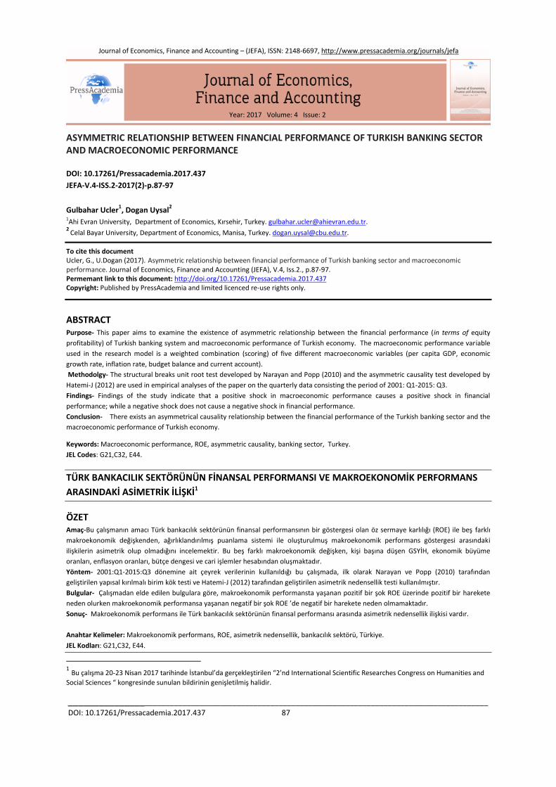
Methodolgy- The structural breaks unit root test developed by Narayan and Popp (2010) and the asymmetric causality test developed by
Hatemi-J (2012) are used in empirical analyses of the paper on the quarterly data consisting the period of 2001: Q1-2015: Q3.
Findings- Findings of the study indicate that a positive shock in macroeconomic performance causes a positive shock in financial
performance; while a negative shock does not cause a negative shock in financial performance.
Conclusion- There exists an asymmetrical causality relationship between the financial performance of the Turkish banking sector and the
macroeconomic performance of Turkish economy.
Keywords: Macroeconomic performance, ROE, asymmetric causality, banking sector, Turkey.
JEL Codes: G21,C32, E44.
TÜRK BANKACILIK SEKTÖRÜNÜN FİNANSAL PERFORMANSI VE MAKROEKONOMİK PERFORMANS
ARASINDAKİ ASİMETRİK İLİŞKİ1
ÖZET Amaç-Bu çalışmanın amacı Türk bankacılık sektörünün finansal performansının bir göstergesi olan öz sermaye karlılığı (ROE) ile beş farklı
makroekonomik değişkenden, ağırlıklandırılmış puanlama sistemi ile oluşturulmuş makroekonomik performans göstergesi arasındaki
ilişkilerin asimetrik olup olmadığını incelemektir. Bu beş farklı makroekonomik değişken, kişi başına düşen GSYİH, ekonomik büyüme
oranları, enflasyon oranları, bütçe dengesi ve cari işlemler hesabından oluşmaktadır.
Yöntem- 2001:Q1-2015:Q3 dönemine ait çeyrek verilerinin kullanıldığı bu çalışmada, ilk olarak Narayan ve Popp (2010) tarafından
geliştirilen yapısal kırılmalı birim kök testi ve Hatemi-J (2012) tarafından geliştirilen asimetrik nedensellik testi kullanılmıştır.
Bulgular- Çalışmadan elde edilen bulgulara göre, makroekonomik performansta yaşanan pozitif bir şok ROE üzerinde pozitif bir harekete
neden olurken makroekonomik performansa yaşanan negatif bir şok ROE ’de negatif bir harekete neden olmamaktadır.
Sonuç- Makroekonomik performans ile Türk bankacılık sektörünün finansal performansı arasında asimetrik nedensellik ilişkisi vardır.
Anahtar Kelimeler: Makroekonomik performans, ROE, asimetrik nedensellik, bankacılık sektörü, Türkiye.
JEL Kodları: G21,C32, E44.
1 Bu çalışma 20-23 Nisan 2017 tarihinde İstanbul’da gerçekleştirilen “2’nd International Scientific Researches Congress on Humanities and
Social Sciences “ kongresinde sunulan bildirinin genişletilmiş halidir.
Journal of Economics, Finance and Accounting – (JEFA), ISSN: 2148-6697, http://www.pressacademia.org/journals/jefa
Year: 2017 Volume: 4 Issue: 2

Journal of Economics, Finance and Accounting – JEFA (2017), Vol.4(2), p.87-97 Ucler, Uysal
_________________________________________________________________________________________________
DOI: 10.17261/Pressacademia.2017.437 88
1. GİRİŞ
Bankacılık sektörü, bir ülkede ekonomik ve finansal sektörlerin gelişmesinde önemli bir role sahiptir. 1980’li yıllardan beri, finansal liberalizasyon dalgası ve finansal küreselleşmenin bir sonucu olarak bankacılık faaliyetlerinin hızla gelişmesi nedeniyle hem yurtiçi hem de yurt dışı bankacılık faaliyetlerinde önemli değişiklikler meydana gelmiştir. Gelişmiş ülkeler 1990’lı yılların sonlarına doğru bankacılık sektöründe liberalleşme sürecini tamamlamıştır ve sonrasında ekonomik kalkınmadaki rolünü ve etkinliğini artırmak üzere gelişmekte olan ülkelerin finansal piyasalarında yer almaya başlamışlardır. Gelişmekte olan ülkeler için, finansal piyasaların az gelişmişliği göz önüne alındığında bankacılık sektöründeki gelişmeler finansal kaynakların dağılımı üzerinde önemli etkiye sahip olabilir. Çünkü sektör, özel yatırım finansmanının en önemli kaynağıdır (Barth, vd. 2006,5-6). Ekonomik büyüme ve tüketim eğilimindeki artış oranları hem hane halkını hem de işletmeleri daha fazla borçlanmaya teşvik etmektedir. Bu durum bankaların kredi verme ve mevduat toplama fonksiyonlarını geliştirmiştir. Bankacılık sektörünün ekonomi içerisindeki büyüklüğü arttıkça, makroekonomik istikrar ve ekonomik performans açısından da bankacılık sektörünün önemi artmaktadır.
Bankacılık sektöründe karlılığı artırmak ve piyasa paylarını genişletebilmek için karlılığını etkileyen faktörlerin belirlemesi gerekmektedir. Uzun vadede hayatta kalabilmek için bir bankanın, karlılığın belirleyicilerinin ne olduğunu bilmesi ve böylece güçlü belirleyicileri yöneterek karlılığını artıracak girişimlerde bulunması önemlidir. (Podder, 2012; 22-24). Bankacılık sektörünün karlılığını etkileyen faktörleri bankaya özgü faktörler (içsel) ve makroekonomik faktörler (dışsal) olarak sınıflandırabiliriz. İçsel faktörler bankanın karlılığını etkileyen bankaya özgü bireysel faktörlerdir (sermaye, verimlilik artışı, kredi riski, faaliyet giderleri yönetimi). Bu faktörler temel olarak banka yönetiminin kontrolünde olan belirleyicilerdir. Dış faktörler ise bankaların karlılığını etkileyen ancak bankaların kontrolünün dışında gerçekleşen ülke çapındaki etkenlerdir. (bütçe açığı, büyüme hızı, enflasyon oranı, reel faiz oranı, işsizlik oranları, sanayi üretim endeksi). Tunay ve Silpagar (2006), bankaların performansı artırabilmek ve sektörde kalabilmek için içsel değişkenleri etkin bir şekilde yönetmeleri gerekliliğinin yanında, makroekonomik istikrarın, genel finansal yapının ve rekabet koşullarının da bankacılık sektörünün etkinlik ve performansının temel koşulu olduğunu vurgulamaktadırlar. Ampirik literatürde seçilen model kalıpları çoğunlukla hem sektöre özgü faktörlerin hem de makroekonomik faktörlerin karlılık üzerindeki etkisini test etmeye yöneliktir.
Bu çalışmanın amacı, makroekonomik değişkenler ile Türkiye’de bankacılık sektörünün karlılığı arasındaki ilişkinin yönünü incelemektir. Bu konuda Türkiye ve diğer ülkeler için yapılan çalışmalarda farklı makroekonomik göstergeler ayrı ayrı modele dahil edilmiş ve her bir makroekonomik değişkenin sektörün karlılığı üzerindeki etkisi ortaya konulmaya çalışılmıştır. Bu çalışmada literatürdeki çalışmalardan farklı olarak, kişi başına düşen GSYİH, ekonomik büyüme oranları, enflasyon oranları, bütçe dengesi ve cari işlemler hesabından oluşan beş makroekonomik göstergeden oluşturulmuş makroekonomik performans endeksi ile sektörel karlılık ilişkisi incelenmiştir. Bu sayede spesifik olarak bir makroekonomik göstergenin karlılığa etkisini değil makroekonomik performansın, sektörün karlılığı ile ilişkisi incelenmiştir. Çalışmada konuyla ilgili kısa bir bilgilendirmenin yapıldığı giriş bölümünün ardından ikinci bölümde makroekonomik faktörler ve finansal performans arasındaki ilişkiye dair teorik çerçeveye yer verilmiştir. Konuyla ilgili ampirik ve teorik literatürün verildiği üçüncü bölümün ardından dördüncü bölümde model ve veri setine ilişkin bilgiler verilmiştir. Metodoloji ve ampirik bulguların yer aldığı beşinci bölümü takiben sonuç bölümü ile çalışma tamamlanacaktır.
2.MAKROEKONOMİK FAKTÖRLER VE FİNANSAL PERFORMANS
Enflasyon, gayri safi yurtiçi hasıla, döviz kuru, kamu açıkları ve faiz oranları gibi değişkenler hükümet, işletmeler ve tüketiciler tarafından yakından takip edilen ekonomik göstergelerdir. Ekonomide yaşanacak olası dalgalanmaların bankacılık sektörünün karar alma mekanizmaları üzerinde baskı yaratma etkisi nedeniyle makroekonomik göstergeler bankacılık sistemi için oldukça önemli göstergelerdir. Çünkü ekonomik koşullar ve piyasa ortamı bankaların varlık ve yükümlülük durumunu etkileyecektir. Bu nedenle bankacılık sektörünün finansal performansı üzerinde olumsuz etki yaratabilecek makroekonomik değişkenlerin belirlenmesi önemlidir.
Literatürde bankacılık sektörünün karlılığı ile en çok ilişkilendirilen makroekonomik gösterge GSYİH ve ekonomik büyüme oranlarıdır. Büyüme oranları ekonominin gelişmesini yansıtır ve gelişme dönemlerinde banka kredi arz ve talebinin de etkilenmesi beklenir. Sufian ve Habibullah (2010) GSYİH’ nın kredilerin arz ve talebi ile ilgili birçok faktörü etkilediğini savunmaktadırlar. Olumlu ekonomik koşullar, bankacılık hizmetlerinin arz ve talebini olumlu yönde etkileyecektir. Şayet ekonomi istikrarlı bir şekilde büyüyorsa, iyi yönetilen bankalar kredilerden ve menkul kıymet satışından kazanç sağlayacaktır. Güçlü ekonomik koşullar aynı zamanda finansal hizmetler için yüksek talep demektir ki bu durumda bankaların nakit akışlarını, karlarını ve faiz dışı kazançlarını artırır (Illo, 2011; 11-13). Öte yandan özellikle mevduat bankaları, fonların kaynak ve kullanımına bağlı olarak, ekonomik büyüme ve istikrara katkıda bulunabilmektedir. Bankaların fon kaynaklarındaki genişleme, büyümeyi kolaylaştırırken; bankaların kar amaçlı işlemlerinin ekonomik dalgalanmaları şiddetlendirmeyecek boyutta gerçekleşmesi istikrarın korunmasına yardımcı olabilmektedir (Parasız, 1997; 123-124). Dolayısıyla GSYİH ile bankacılık sektörünün finansal performansı arasında pozitif bir ilişki vardır. Kosmidou (2006) ve Hassan ve Bashir (2003), GSYİH büyümesinin bankacılık sektörünün karlılığını pozitif yönde etkilediğini savunmaktadırlar. Jiang, Law

Journal of Economics, Finance and Accounting – JEFA (2017), Vol.4(2), p.87-97 Ucler, Uysal
_________________________________________________________________________________________________
DOI: 10.17261/Pressacademia.2017.437 89
ve Sze (2003), Hong Kong bankacılık sektöründe faaliyet gösteren 14 bankaya ilişkin yaptığı çalışmada GSYİH’ da gerçekleşen büyüme oranı ile banka karlılığı arasında pozitif yönlü bir ilişki olduğuna dair bulgular elde etmişlerdir.
Temel makroekonomik göstergelerden birisi olan enflasyon oranları aynı zamanda bankacılık sektörünün finansal performansının en önemli belirleyicilerinden biridir. Demirgüç-Kunt ve Huizinga (1999), gelişmekte olan ülkelerdeki bankaların enflasyonist ortamlarda, daha az kazanç sağlama eğiliminde olduğunu savunmaktadırlar. Bu ülkelerde enflasyonist dönemlerde banka maliyetleri banka gelirlerinden daha hızlı artmaktadır. Benzer şekilde, Abreu ve Mendes (2002) enflasyonun yüksek maliyet içermesinden dolayı bankaya ek maliyet yüklediğini ve bu nedenle bankacılık sektörünün karlılığını negatif yönde etkilediğini söylemektedir. Abreu ve Mendes (2002)’nin aksine Bashir (2003) öngörülen enflasyonun sektörün karlılığına olumlu katkı sağlarken beklenmedik enflasyonun karlılığı olumsuz yönde etkilediğini savunmaktadır. Bashir (2003)’e göre beklenen enflasyon oranları, bankalara faiz oranlarını ayarlama fırsatı sağladığı için bankalar maliyetlerden daha hızlı artan gelir elde ederek yüksek kazanç sağlarlar. Öte yandan beklenmeyen enflasyon, maliyet artışı ve gelir artışı oranlarını tersine çevirecek ve sektörün karlılığını negatif yönde etkileyecektir. Bourke (1989)’a göre ise daha yüksek enflasyon oranları daha yüksek kredi faiz oranlarına yol açmakta ve karlılığı pozitif yönde etkilemektedir.
Diğer bir makroekonomik gösterge olan bütçe açıkları, bankacılık sektörünün finansal performansı üzerinde de etkilidir. Kamu açıklarının sürekli artması bu açıkları finanse edebilmek için bankacılık sektöründen borçlanmayı gerekli kılar. Bu durumda kamunun açıklarını finanse edebilmek amacıyla bankacılık sektöründen yüksek faizlerle borçlanma eğiliminin artması bankaların karlılık oranlarını artırmaktadır. Kaya (2002), bankacılık sektörünün karlılık göstergeleri ile enflasyon, bütçe açığı, gayri safi milli hasıla ve reel faiz oranları gibi makro değişkenler arasındaki ilişkiyi incelediği çalışmasında, bütçe açıkları ile bankacılık sektörünün karlılığı arasında pozitif yönlü bir ilişki tespit etmiştir.
Makroekonomik istikrarın sağlanması, istikrarlı bir bankacılık sektörü için oldukça önemlidir. Yiğit(2005) makroekonomik istikrar ortamının, bankaların amaç fonksiyonlarının maksimize ederek yeni stratejiler geliştirdiğini ve karlılıklarını artırdıklarını savunmuştur. Dolayısıyla ekonomik istikrarın sağlanması, istihdam oranlarının artırılması, enflasyon oranlarının düşürülmesi, bütçe açıklarının azaltılması ve yüksek büyüme performansının yakalanması bankacılık sektörünün karlılığını artırabilmek için önemli makroekonomik gelişmelerdir.
3.LİTERATÜR İNCELEMESİ
Bankacılık sektörünün performansını analiz eden ulusal ve uluslararası çok sayıda çalışma bulunmaktadır. Bu çalışmaların bazıları (Demirgüç-Kunt ve Huizinga; 1999, Bashir ;2000, Saunders ve Schumacher; 2000, Abreu ve Mendes; 2000) tek bir ülkenin bankacılık sisteminin performansını incelerken diğerleri ise panel veri setleri kullanarak çok sayıda ülkenin bankacılık sisteminin performansını incelemektedir. (Neely ve Wheelock ;1997, Barajas, Steiner ve Salazar ;1999, Naceur; 2003).
Ho ve Saunders (1981)’ in faiz oranı riski ve net faiz marjı arasındaki ilişkiyi inceldikleri çalışma bu konuda yapılmış ilk çalışmalar arasındadır. Ho ve Sanders (1981)’e göre Brezilya’da banka faiz marjlarının en önemli belirleyicisi makroekonomik değişkenleridir. Benzer şekilde Neely ve Wheelock (1997), ABD’nin 1980-1985 dönemine ilişkin verilerini kullanarak bankacılık sektörünün performansını inceledikleri çalışmalarında, banka karlılığı ile kişi başına düşen milli gelir arasında pozitif yönde bir ilişkinin varlığına yönelik bulgular elde etmişlerdir. Öte yandan Naceur ve Goaied (2001) Tunus’ta faaliyet gösteren bankaların 1980-1995 dönemi için karlılığının belirleyicilerini inceledikleri çalışmalarında, aktiflerine kıyasla daha yüksek oranda yatırım hesabına sahip olan bankaların karlılıklarını artırdığını ancak enflasyon ve büyüme oranları gibi makroekonomik değişkenlerin bankaların karlılık oranları üzerinde etkili olmadığı sonucuna ulaşmışlardır.
Bashir (2000), 1994-2001 dönemi verilerini kullanarak 60’dan fazla İslam ülkesine ait verileri kullanarak bu ülkelerde bankacılık sektörünün karlılığının belirleyicilerini incelemişlerdir. Yazar sektörün karlılığını etkileyen mikro değişkenlerin yanında makro belirleyicileri de modele dahil etmiştir. Çalışmada, milli gelirdeki artışların karlılığı etkileyen en önemli makroekonomik gösterge olduğu vurgulanmıştır.
Demirgüç-Kunt ve Huizingha (1999), Türkiye’nin de dahil olduğu 80 ülkeye ait 1988-95 dönemi verilerini kullanarak bankaların karlılığını etkileyen belirleyicilerini incelemişlerdir. Bu çalışmada, makroekonomik koşullar, vergi ve mevduat sigortası, kurumsal ve yasal göstergeler bankaların karlılığını etkileyen belirleyiciler olarak kullanılmıştır. Çalışmadan elde edilen bulgulara göre, hukuk ve yolsuzluk endeksi gibi kurumsal kalite göstergelerinin gelişmekte olan ülkelerde faiz marjı ve banka karlılığı üzerinde gelişmiş ülkelere kıyasla daha etkilidir. Demirgüç-Kunt ve Huizingha (1999),reel faiz oranı, enflasyon ve kişi başına düşen milli gelir arasında pozitif yönde ve anlamlı bir ilişki bulmuştur. Enflasyon ve kişi başına düşen milli gelir artışı, bankaların net faiz marjını artırmaktadır.
Abreu ve Mendes (2002), Avrupa ülkelerinde bankacılık sektörünün karlılığının belirleyicilerini inceledikleri çalışmalarında, işsizlik oranlarının banka karlılığını etkileyen en önemli makroekonomik değişken olduğunu ayrıca enflasyon oranları ile banka karlılığı arasında pozitif yönlü bir ilişki bulunduğunu belirlemişlerdir. Jiang vd. (2003), Hong Kong’daki 14 bankaya ilişkin 1992-2002 dönemi verilerini kullanarak vergi öncesi karın aktiflere oranının belirleyicilerini incelemişlerdir. Çalışmada faiz dışı giderlerin toplam aktiflere oranı, faiz dışı gelirlerin toplam gelirler içindeki payı gibi mikro değişkenlerin yanında,

Journal of Economics, Finance and Accounting – JEFA (2017), Vol.4(2), p.87-97 Ucler, Uysal
_________________________________________________________________________________________________
DOI: 10.17261/Pressacademia.2017.437 90
enflasyon, reel faiz oranı ve büyüme oranları gibi makroekonomik değişkenlerde kullanılmıştır. Çalışmanın ampirik bulgularına göre enflasyon, reel faiz oranı ve büyüme oranı ile karlılık arasında pozitif ve anlamlı bir ilişki vardır.
Kosmidou vd. (2005), bankaların karlılığını belirleyen içsel ve dışsal faktörleri 15 Avrupa Birliği ülkesinde faaliyet gösteren yerli ve yabancı bankalar için incelemişlerdir. Kosmidou vd (2005), dışsal faktörler olarak büyüme hızı, enflasyon oranı ve piyasa kapitalizasyon oranını kullanmıştır. Çalışmadan elde edilen bulgular makroekonomik faktörlerin bankacılık sektörünün karlılığını etkilediği yönündedir. Athanasoglou, Delis ve Straikouras (2006), Arnavutluk, Bosna-Hersek, Bulgaristan, Hırvatistan, Romanya, Makedonya ve Sırbistan-Karadağ’da bankacılık sektörünün karlılığını inceledikleri çalışmalarında, karlılığın belirleyicileri olarak bankalara ve sektöre özgü değişkenlerin yanında enflasyon ve kişi başına düşen milli gelir gibi makro göstergelere de yer vermişlerdir. Çalışmanın bulgularına göre, enflasyon arttıkça bankaların gelirleri, giderlerinden daha fazla artmaktadır. Dolayısıyla enflasyon artışının sektörün karlılığını olumlu yönde etkilemektedir.
Athanasoglou, Brissimis ve Delis (2008) Yunanistan’da bankacılık sektörünün karlılığını etkileyen unsurları belirlemeye yönelik yaptıkları çalışmalarında, hem bankaya hem de sektöre özgü unsurların yanında makroekonomik değişkenleri de modele dahil etmişlerdir. 1985-2001 dönemi verilerinin kullanıldığı çalışmanın bulgularına göre, makroekonomik değişkenlerden enflasyon ve sanayi üretim endeksinin sektörün karlılığı olumlu yönde etkilemektedir. Benzer şekilde Guru, Staunton ve Balashanmugam’ ın (2002) Malezya’da faaliyet gösteren bankalara ilişkin 1986-1995 dönemi verilerini kullanarak banka karlılığının belirleyicilerini incelemişlerdir. Çalışmada sektörün karlılığının belirleyicileri olarak kullanılan makroekonomik değişkenlerden, faiz oranlarının banka performansını negatif yönde enflasyonun ise pozitif yönde etkilediğine yönelik bulgular elde edilmiştir.
Türkiye’de bankacılık sektörünün performansını açıklamaya yönelik çalışmalar hem sektöre özgü hem de makroekonomik değişkenleri birlikte incelemektedir. Türker Kaya (2002) , Türkiye’de faaliyet gösteren 44 özel ve kamu bankasına ait 1997-2000 dönemi verilerini kullanarak mikro ve makro belirleyicilerin bankacılık sektörünün karlılığı üzerindeki etkisini incelemiştir. Sektörün karlılık göstergesi olarak net faiz marjı, aktife göre getiri ve öz kaynağa göre getiri oranlarının kullanıldığı çalışmada, makro değişkenler olarak enflasyon oranları, bütçe açığı, yıllık büyüme oranı ve reel faiz oranı kullanılmıştır. Çalışmada kullanılan üç farklı karlılık göstergesinin hepsinde enflasyon ve bütçe açığı, sektörün karlılığını etkileyen makro etkenler olarak bulunmuştur.
Tunay ve Silpagar (2006) Türk bankacılık sektöründe karlılığa dayalı performans analizi yaptıkları çalışmalarında performansın belirleyicileri olarak, hem bankaların etkin bir şekilde kontrol edebildikleri içsel değişkenleri, hem genel ekonomik koşulların oluşturduğu makroekonomik değişkenleri hem de finansal sistemin özelliklerini yansıtan finansal yapı değişkenlerini kullanmışlardır. Çalışmadan elde edilen bulgulara göre, mikro ve sektörel değişkenlerin yanında makroekonomik değişkenler de Türkiye’de bankacılık sektörünün karlılığını etkilemektedir. Ancak bankaya özgü içsel faktörler ve finansal yapı göstergelerinin etkileri bankanın ölçek veya sermaye yapısına göre değişiklik gösterirken, enflasyon ve milli gelir gibi makroekonomik değişkenler her model için önemli bir belirleyici olarak gösterilmektedir. Dağıdır (2010), Türkiye’de 2003:02-2008:08 dönemi verilerini kullanarak makro değişkenlerin banka karlılığını nasıl etkilediğini incelediği çalışmasında sektörün karlılık göstergesi olarak faiz marjı değişkeni kullanılırken makro ekonomik göstergeler olarak üretici fiyat endeksi, ekonomik büyümeyi temsilen GSYİH ve sanayi üretim endeksi değişkenlerini kullanmıştır. Dağıdır (2010), enflasyonun faiz oranlarını yükselterek yüksek maliyete yol açtığını ve faiz marjını negatif yönde etkilediğini söylemektedir. Benzer şekilde sanayi üretim endeksi ile faiz marjı arasında negatif yönlü ve anlamlı bir ilişki tespit edilirken ekonomik büyümeyi temsilen kullanılan GSYİH değişkeni ile faiz marjı arasında anlamlı bir ilişki bulunamamıştır. Sanayi üretiminin artması, istihdam oranlarını artırıp ekonomik canlılığı artıracak ve faiz marjını düşürecektir.
Gündoğdu ve Aksu (2011), 1994-2008 dönemi için Türkiye’de makroekonomik değişkenlerin, mevduat bankacılığının karlılığı üzerine etkilerini inceledikleri çalışmalarında makroekonomik göstergeler olarak reel faiz, fiyatlar genel düzeyi, bütçe açığı ve sanayi üretim endeksi değişkenlerini kullanmışlardır. Çalışmadan elde edilen bulgulara göre, reel faiz oranları kısa dönemde aktif karlılığı ve sermaye karlılığını pozitif yönde etkilemektedir. Dolayısıyla pozitif reel faiz politikaları kısa dönemde bankacılık sektörünün karlılığına olumlu yönde katkı yapmaktadır. Fiyatlar genel düzeyi aktif karlılık ve sermaye karlılığı üzerinde negatif yönde bir etkiye sahipken, konsolide bütçe açığı ve sanayi üretim endeksi her iki karlılık rasyosu üzerinde de pozitif yönde ve istatistiksel olarak anlamlı bir etkiye sahiptir. Taşkın (2011), Türkiye’de ticari bankaların performansını etkileyen faktörleri incelediği çalışmasında, 1995-2009 döneminde faaliyet gösteren ticari bankaların performansını etkileyen içsel ve dışsal faktörleri belirlemeyi amaçlamıştır. Bu amaçla yapılan çalışmada sektörün performans ölçütleri olarak aktif karlılığı, öz kaynak karlılığı ve net faiz marjı göstergeleri kullanılırken dışsal belirleyiciler olarak kişi başına düşen gsmh, sanayi üretim endeksi, faiz oranı ve enflasyon oranı kullanılmıştır. Çalışmanın sonucuna göre, Türk bankacılık sektörünün performansı daha çok içsel değişkenlerden etkilenmektedir. Analizden elde edilen bulgular makroekonomik faktörlerin sektörün karlılığı üzerinde anlamlı bir etkisinin olmadığı yönündedir. Samırkaş, Evci ve Ergün (2014), Türkiye’de faaliyet gösteren mevduat bankalarının karlılığını etkileyen faktörleri belirlemeye yönelik yaptıkları çalışmalarında, hem bankaya özgü faktörleri hem de makroekonomik faktörleri modele dahil etmişlerdir. Makroekonomik faktörler olarak GSYİH, mevduat faiz oranları ve tüketici fiyat endeksi alınmıştır. Çalışmadan elde edilen bulgulara göre,

Journal of Economics, Finance and Accounting – JEFA (2017), Vol.4(2), p.87-97 Ucler, Uysal
_________________________________________________________________________________________________
DOI: 10.17261/Pressacademia.2017.437 91
bankaya ve sektöre özgü içsel faktörler Türk bankacılık sistemindeki bankaların karlılığını etkilerken makroekonomik faktörlerin sektörün karlılığı üzerinde anlamlı bir etkisi yoktur.
4. MODEL, DEĞİŞKENLER ve VERİ SETİ
Bu çalışmada bankacılık sektörünün karlılığı ve makroekonomik performans arasındaki ilişkinin araştırılmasında aşağıdaki model tahmin edilmektedir:
𝑅𝑂𝐸𝑡 = 0 + 1𝑀𝐸𝑃𝑡 + 𝑢𝑡 (1)
Yukarıdaki eşitlikte ROE bankacılık sektörünün karlılığını, MEP ise makroekonomik performansı temsil etmektedir. Zaman serisi teknikleri kullanılarak tahmin edilen bu çalışma 2001:Q1-2015:Q3 dönemi verilerini kapsamaktadır.
2 Sektörün
karlılığını temsil eden bağımlı değişken ROE, BDDK veri dağıtım sisteminden, makroekonomik performans göstergesi ise ICRG (International Country Risk Guide) data setlerinden elde edilmiştir.
Ampirik çalışmalar incelendiğinde, kârlılık değişkeni olarak genellikle aktif kârlılığı (Return On Assets-ROA) (Bkz. Amato ve Wilder, 1985; Roquebert vd.,1996; Glancey, 1998; Mauri ve Michael, 1998; Fitzsimmons vd., 2005; Davidsson vd., 2009; Delmar vd., 2013; Li ve Wang, 2014) ya da özsermaye kârlılığı (Return On Equity-ROE) (Bkz. Ebaid, 2009; Ferati ve Ejupi, 2012; Velnampy ve Niresh, 2012; Bokhari ve Khan, 2013) değişkenlerinin kullanıldığı görülmektedir. Aktif kârlılığı, özellikle imalat sektörleri açısından ele alındığında gerek sermaye yoğunluğu, gerekse de varlıkların etkin kullanılması noktasında hızlı ve sağlıklı bir değerlendirme ölçütü olarak ön plana çıkmaktadır. Ayrıca, söz konusu ölçüt, ölçek ekonomisinin toplam kârlılık üzerinde yaratabileceği farklılaşmalarından kaynaklanan dezavantajları da yok etmektedir. Ancak, özellikle (finansal) hizmet sektörünü konu alan ampirik çalışmalarda kârlılık ölçütü olarak aktif kârlılığından çok, öz sermaye kârlılığının dikkate alındığı görülmektedir (Demirgüneş ve Üçler, 2015). Bu nedenle, çalışmada bankacılık sektörünün ele alınmasına bağlı olarak, kârlılık ölçütü olarak öz sermaye kârlılığının (ROE) kullanılmasının daha sağlıklı olacağı düşünülmektedir.
Makroekonomik göstergeler ve bankacılık sektörünün karlılığı arasındaki ilişkinin incelendiği çalışmalarda, enflasyon, ekonomik büyüme ve bütçe açığı gibi makro ekonomik değişkenler modele ayrı ayrı dahil edilmişlerdir. Bu çalışmada makroekonomik değişkenlerden oluşturulan bir endeks makroekonomik performans göstergesi olarak kullanılmaktadır. ICRG data setinden elde edilen bu endeks, mevcut ekonominin güçlü yönlerinin zayıf yönlerinden daha fazla olması durumunda güçlü makroekonomik performansı tam tersi durumda ise düşük ekonomik performansı simgelemektedir. Bu güçlü ve zayıf yönler, ekonomik performans bileşenleri olarak adlandırılan ve önceden belirlenmiş faktör gruplarına risk puanları atanarak belirlenir. Her bileşene atanan minimum puan sıfır iken maksimum puan, bileşene genel ekonomik performans değerlendirilmesinde verilen sabit ağırlığa bağlıdır. Endeksin hesaplanmasında kullanılan temel bileşenler, kişi başına düşen milli gelir, ekonomik büyüme oranı, enflasyon oranı, bütçe dengesinin GSYİH’ ya oranı, cari işlemler hesabının GSYİH’ ya oranıdır.
Aşağıdaki tabloda makroekonomik performans endeksini oluşturmada kullanılan bileşenler ve bu bileşenlerin endeks hesaplamasındaki ağırlıkları verilmektedir.
2 Türk bankacılık sektörü Şubat 2001 krizinde toplam aktif büyüklüğünün yaklaşık olarak ¼’ünü kaybetmiş ve aktif büyüklüğü 2000 yılında 166 milyar dolar iken, 2001 yılı sonunda 115 milyar dolara kadar gerilemiştir. Bankalar, faiz maliyetlerini kontrol edemediklerinden, faiz dışı giderlerini azaltma eğilimine girmişler ve buna bağlı olarak da şube ve personel sayılarını azaltmaya başlamışlardır. Bu eğilimle birlikte, BDDK’nın fon kapsamındaki bankaları satma planının işlerlik kazanmaması ve TMSF kapsamındaki bankaları kendi aralarında birleştirme ve tasfiye etme politikası izlemesi nedeniyle, bankacılık sektöründe 2000 yılında 3.587 çalışan, 2001 yılında ise 32.906 çalışan işini kaybetmiştir. 2000 yılı ile kıyaslandığında, 2002 yılı Temmuz ayında 1.758 banka şubesinin de kapatıldığı görülmektedir. Ayrıca, 2001 krizi sonrası dönemde yaşanan en önemli gelişmelerden biri, banka sayısında görülen azalmadır. Buna göre, 2001 yılında toplam banka sayısı 61 iken, bu sayı 2004 yılında 48'e düşmüştür. Görüldüğü üzere, 2001 yılından sonra oldukça köklü değişikliklerin görüldüğü bankacılık sektöründe, özellikle bu yıldan sonraki verilerin kullanılması yapılan ampirik analizlerden elde edilmesi beklenen sonuçların daha sağlıklı yorumlanabilmesi imkan sağlayacaktır.

Journal of Economics, Finance and Accounting – JEFA (2017), Vol.4(2), p.87-97 Ucler, Uysal
_________________________________________________________________________________________________
DOI: 10.17261/Pressacademia.2017.437 92
Tablo 1: Makroekonomik Performans Endeksinin Hesaplanmasında Kullanılan Göstergeler
Makroekonomik Gösterge Göstergenin Tanımı Puanlandırma Aralığı
Kişi Başına Düşen GSYİH ICRG kapsamındaki tüm ülkelerin toplam GSYİH' sının bir yüzdesi olarak puanlandırılmaktadır
min. puan: 0 max. puan: 5
Ekonomik Büyüme 1990 fiyatları ile yıllık GSYİH' daki değişim min. puan: 0 max. puan: 10
Yıllık enflasyon oranları TÜFE’ deki yıllık % değişim min. puan: 0 max. puan: 10
Bütçe Dengesi (%GSYİH) Belirli bir yıla ait ulusal para birimi cinsinden merkezi yönetim bütçesinin GSYİH' ya oranı
min. puan: 0 max puan: 10
Cari İşlemler Hesabı (% GSYİH) Cari İşlemler dengesinin GSYİH' ya oranı min. puan: 0 max. puan: 15
Not: Puanlandırmada her bileşen için farklı puan aralıkları kullanılmıştır. Puanlandırmada kullanılan aralık değerleri için ICRG Methodology Guide bakınız.
Tablo 1’de verilen bileşenler kullanılarak oluşturulan makroekonomik performans endeksi, 0.0 % - 24.5 % aralığında ise çok düşük makroekonomik performansı, 25.0 % - 29.9 % aralığında ise düşük makroekonomik performansı, 30.0 % - 34.9 % ortalama düzeyde makroekonomik performansı, 35.0 % 39.9 % aralığında yüksek makroekonomik performansı ve 40.0 % ve üzeri değerler ise çok yüksek makroekonomik performansı temsil etmektedir.
Şekil 1: Makroekonomik Performans Endeksi
22
24
26
28
30
32
34
36
94 96 98 00 02 04 06 08 10 12 14
Şubat 2000/Kas ım 2001
Krizi
Küresel Finansal Kriz
Şekil 1’de beş farklı bileşenden oluşturulan makroekonomik performans endeksi görülmektedir. Endeks incelendiğinde Türkiye ekonomisinin makroekonomik yapısını net bir şekilde yansıttığı görülmektedir. Özellikle Kasım 2000 ve Şubat 2001 krizlerinin, 2008 küresel finansal krizinin makroekonomik performans üzerindeki etkisi belirgin bir şekilde görülmektedir.
5. METODOLOJİ ve AMPİRİK BULGULAR
5.1. Durağanlık Analizi
Zaman serileri ile yapılan çalışmalarda durağanlık analizi için genellikle Dickey ve Fuller (1981) tarafından geliştirilen Dickey-Fuller (ADF) ve Phillips ve Perron (1988) tarafından geliştirilen PP birim kök testleri kullanılmaktadır. Ancak bu testler serilerdeki olası yapısal kırılmaları göz ardı etmektedir. Narayan ve Popp (2010) ADF tipi çift yapısal kırılmayı dikkate yeni bir birim kök testi geliştirmişlerdir. Narayan ve Popp (2010) birim kök testinde, sabitte iki yapısal kırılmaya izin veren (M1) ve hem sabitte hem de trendde iki yapısal kırılmaya izin veren (M2) olmak üzere iki farklı model geliştirmişlerdir. Testin regresyon denklemi aşağıdaki şekildedir:
ytM1 = ρyt-1+ α1+ β*t + θ1D(TB
' )1,t
+ θ2D(TB' )
2,t+ δ1DU
1,t-1' + δ2DU
2,t-1' + ∑ βj∆yt-j + et
kj=1 (2)
ytM2 = ρyt-1+ α* + β*t + Ω1D(TB
' )1,t
+ Ω2D(TB' )
2,t + δ1
*DU1,t-1' + δ2
*DU2,t-1' + γ1
*DT1,t-1' + γ2
*DT2,t-1' ∑ βj∆yt-j + et
kj=1 (3)

Journal of Economics, Finance and Accounting – JEFA (2017), Vol.4(2), p.87-97 Ucler, Uysal
_________________________________________________________________________________________________
DOI: 10.17261/Pressacademia.2017.437 93
Modelde yer alan , TB,i' , i=1,2 kırılma tarihleridir. θi ve γi parametreleri sırasıyla sabit ve trend kırılmalarının büyüklüğünü
ifade etmektedir. Burada kırılma tarihleri ardışık bir prosedür kullanılarak belirlenmektedir.3 Ho: ρ = 1 şeklindeki ve seride
birim kök olduğunu gösteren boş hipotez, H1: ρ < 1 şeklindeki alternatif hipotez ile test edilir. ρ ‘nin denklem 2 ve 3’te verilen t istatistikleri kullanılır. Kritik değerler Monte Carlo simülasyonu ile tespit edilir. Hesaplanan test istatistiği kritik değerlerden büyükse boş hipotez reddedilir.
Tablo 2: Narayan ve Popp (2010) Birim Kök Testi Sonuçları
Değişken Test İstatistikleri Kırılma Tarihleri
M1 M2 M1 M2
MEP -5.091** -4.406 2009:Q2, 2011:Q3 2008:Q4, 2009:Q2
ROE -4.649** -4.123 2006:Q2, 2006:Q4 2006:Q2, 2007:Q1
P -9.155* -8.529* 2008:Q4, 2009:Q2 2008:Q3, 2009:Q2
R -6.148* -7.123* 2006:Q1, 2006;Q3 2006:Q1, 2006:Q3
Kritik Değerler
1% -5.26 -5.94
5% -4.51 -5.18
10% -4.14 -4.79
Not: Kritik değerler Narayan ve Popp (2010)’dan elde edilmiştir. *, ** ve ***, sırasıyla %1, %5 ve %10 düzeylerinde anlamlılığı göstermektedir.
Değişkenlerin durağanlık düzeyleri hakkında bilgi sahibi olabilmek için serilerde iki yapısal kırılmaya izin veren Narayan ve Popp (2010) birim kök testi kullanılmıştır. Birim kök testinden elde edilen bulgular Tablo 2’de rapor edilmektedir. Tablo 2’de verilen birim kök testi sonuçlarına göre, modelde kullanılan her iki seri de M1 testinde durağan iken M2’de durağan değildir. Ancak serilerin fark değerleri ile yapılan birim kök testi sonuçlarına göre hem MEP hem de ROE serisinin ilk farkında durağan olduğu görülmektedir. Birim kök testinden elde edilen kırılma tarihleri incelendiğinde ağırlıklı olarak Türkiye’nin küresel krizden etkilendiği dönemler olduğu görülmektedir.
5.2. Nedensellik Testi
Geleneksel Granger (1969) nedensellik testinden bu yana literatürde birçok nedensellik testi geliştirilmiştir. (Toda, Yamamoto, 1995; Hacker-Hatemi-J, 2006). Ancak bu testlerde pozitif ve negatif şokların aynı etkiye sahip olacağı varsayılmaktadır. Hatemi-J (2012), bu şokların farklı etkilere sahip olabileceğini belirtmiş ve buradan hareketle asimetrik nedensellik ilişkisine izin veren yeni bir nedensellik testi geliştirmiştir (Bulut, 2016).
t = 1,2,…N iken 𝑦1𝑡 ve 𝑦2𝑡 rassal yürüyüşe sahip iki eşbütünleşik değişken ise;
𝑦1𝑡 = 𝑦1𝑡−1 + 1𝑡 = 𝑦1,0 + ∑ 1𝑖𝑡𝑖=0 𝑣𝑒 (4)
𝑦2𝑡 = 𝑦2𝑡−1 + 2𝑡 = 𝑦2,0 + ∑ 2𝑖 𝑡𝑖=0 (5)
Denklemde 𝑦1,0 ve 𝑦2,0 başlangıç değerlerini, 1𝑖 ve 2𝑖 hata terimlerini temsil etmektedir. Modelde pozitif ve negatif şoklar
ise aşağıdaki şekilde ifade edilmektedir:
1𝑖+ = 1𝑖
+ + 1𝑖− ve 2𝑖
+ = 2𝑖+ + 2𝑖
−
Buradan hareketle modele pozitif ve negatif şoklar dahil edilerek denklem yeniden yazıldığında;
𝑦1𝑡 = 𝑦1𝑡−1 + 1𝑡 = 𝑦1,0 + ∑ 1𝑖+𝑡
𝑖=1 + ∑ 1𝑖−𝑡
𝑖=1 (6)
𝑦2𝑡 = 𝑦2𝑡−1 + 2𝑡 = 𝑦2,0 + ∑ 2𝑖+ + ∑ 2𝑖
−𝑡𝑖=1
𝑡𝑖=1 (7)
Her değişken için pozitif ve negatif şoklar birikimli formda tanımlandığında ise denklem aşağıdaki şekilde tanımlanabilir:
𝑦1𝑖+ = ∑ 1𝑖
+𝑡𝑖=1 , 𝑦1𝑖
− = ∑ 1𝑖−𝑡
𝑖=1 , 𝑦2𝑖+ , ∑ 2𝑖
+𝑡𝑖=1 , 𝑦2𝑖
− = ∑ 2𝑖−𝑡
𝑖=1 (8)
Hatemi-J (2012), 𝑦𝑡+ = (𝑦1𝑡
+ , 𝑦2𝑡+ ) varsayımından hareketle bu bileşenler arasındaki nedensellik ilişkisini vektör otoregresif
modeli (VAR) kullanarak incelemektedir:
3 Söz konusu prosedürün detayları için Narayan ve Popp (2010)’a bakınız.
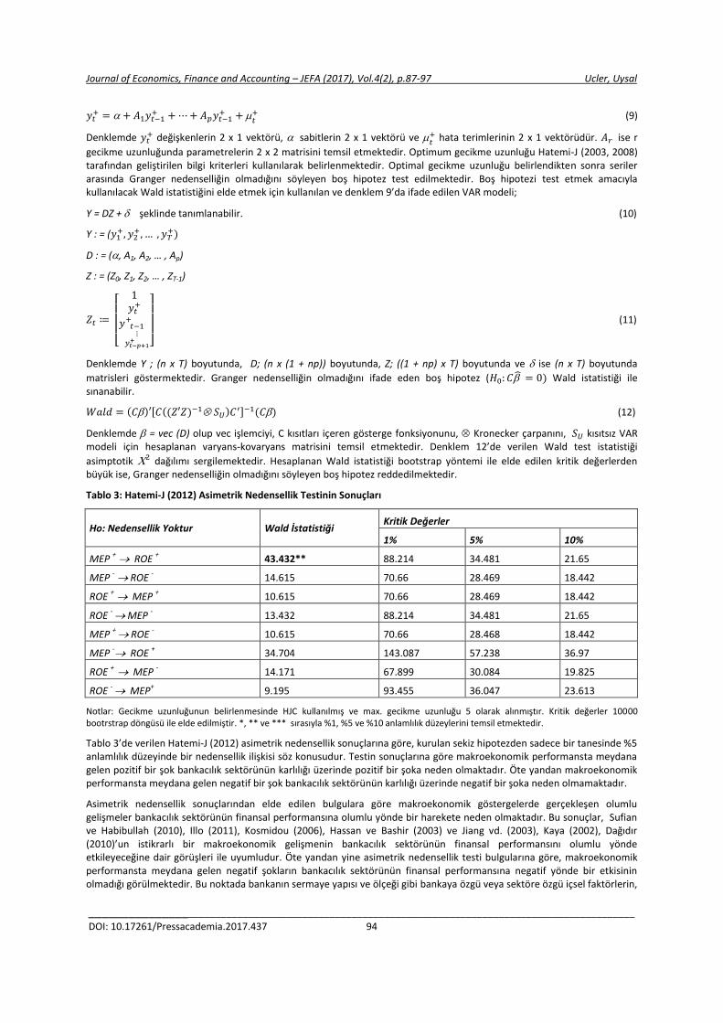
Journal of Economics, Finance and Accounting – JEFA (2017), Vol.4(2), p.87-97 Ucler, Uysal
_________________________________________________________________________________________________
DOI: 10.17261/Pressacademia.2017.437 94
𝑦𝑡+ = + 𝐴1𝑦𝑡−1
+ + ⋯+ 𝐴𝑝𝑦𝑡−1+ +
𝑡+ (9)
Denklemde 𝑦𝑡+ değişkenlerin 2 x 1 vektörü, sabitlerin 2 x 1 vektörü ve
𝑡+ hata terimlerinin 2 x 1 vektörüdür. 𝐴𝑟 ise r
gecikme uzunluğunda parametrelerin 2 x 2 matrisini temsil etmektedir. Optimum gecikme uzunluğu Hatemi-J (2003, 2008) tarafından geliştirilen bilgi kriterleri kullanılarak belirlenmektedir. Optimal gecikme uzunluğu belirlendikten sonra seriler arasında Granger nedenselliğin olmadığını söyleyen boş hipotez test edilmektedir. Boş hipotezi test etmek amacıyla kullanılacak Wald istatistiğini elde etmek için kullanılan ve denklem 9’da ifade edilen VAR modeli;
Y = DZ + şeklinde tanımlanabilir. (10)
Y : = (𝑦1+, 𝑦2
+, … , 𝑦𝑇+)
D : = (, A1, A2, … , Ap)
Z : = (Z0, Z1, Z2, … , ZT-1)
𝑍𝑡 ≔
[
1𝑦𝑡
+
𝑦 𝑡−1⋮
𝑦𝑡−𝑝+1+
+
]
(11)
Denklemde Y ; (n x T) boyutunda, D; (n x (1 + np)) boyutunda, Z; ((1 + np) x T) boyutunda ve ise (n x T) boyutunda
matrisleri göstermektedir. Granger nedenselliğin olmadığını ifade eden boş hipotez (𝐻0: 𝐶 = 0) Wald istatistiği ile sınanabilir.
𝑊𝑎𝑙𝑑 = (𝐶)′[𝐶((𝑍′𝑍)−1 𝑆𝑈)𝐶′]−1(𝐶) (12)
Denklemde = vec (D) olup vec işlemciyi, C kısıtları içeren gösterge fonksiyonunu, Kronecker çarpanını, 𝑆𝑈 kısıtsız VAR modeli için hesaplanan varyans-kovaryans matrisini temsil etmektedir. Denklem 12’de verilen Wald test istatistiği
asimptotik 2 dağılımı sergilemektedir. Hesaplanan Wald istatistiği bootstrap yöntemi ile elde edilen kritik değerlerden büyük ise, Granger nedenselliğin olmadığını söyleyen boş hipotez reddedilmektedir.
Tablo 3: Hatemi-J (2012) Asimetrik Nedensellik Testinin Sonuçları
Ho: Nedensellik Yoktur Wald İstatistiği Kritik Değerler
1% 5% 10%
MEP + ROE
+ 43.432** 88.214 34.481 21.65
MEP - ROE
- 14.615 70.66 28.469 18.442
ROE + MEP
+ 10.615 70.66 28.469 18.442
ROE - MEP
- 13.432 88.214 34.481 21.65
MEP + ROE
- 10.615 70.66 28.468 18.442
MEP - ROE
+ 34.704 143.087 57.238 36.97
ROE + MEP
- 14.171 67.899 30.084 19.825
ROE - MEP
+ 9.195 93.455 36.047 23.613
Notlar: Gecikme uzunluğunun belirlenmesinde HJC kullanılmış ve max. gecikme uzunluğu 5 olarak alınmıştır. Kritik değerler 10000 bootrstrap döngüsü ile elde edilmiştir. *, ** ve *** sırasıyla %1, %5 ve %10 anlamlılık düzeylerini temsil etmektedir.
Tablo 3’de verilen Hatemi-J (2012) asimetrik nedensellik sonuçlarına göre, kurulan sekiz hipotezden sadece bir tanesinde %5 anlamlılık düzeyinde bir nedensellik ilişkisi söz konusudur. Testin sonuçlarına göre makroekonomik performansta meydana gelen pozitif bir şok bankacılık sektörünün karlılığı üzerinde pozitif bir şoka neden olmaktadır. Öte yandan makroekonomik performansta meydana gelen negatif bir şok bankacılık sektörünün karlılığı üzerinde negatif bir şoka neden olmamaktadır.
Asimetrik nedensellik sonuçlarından elde edilen bulgulara göre makroekonomik göstergelerde gerçekleşen olumlu gelişmeler bankacılık sektörünün finansal performansına olumlu yönde bir harekete neden olmaktadır. Bu sonuçlar, Sufian ve Habibullah (2010), Illo (2011), Kosmidou (2006), Hassan ve Bashir (2003) ve Jiang vd. (2003), Kaya (2002), Dağıdır (2010)’un istikrarlı bir makroekonomik gelişmenin bankacılık sektörünün finansal performansını olumlu yönde etkileyeceğine dair görüşleri ile uyumludur. Öte yandan yine asimetrik nedensellik testi bulgularına göre, makroekonomik performansta meydana gelen negatif şokların bankacılık sektörünün finansal performansına negatif yönde bir etkisinin olmadığı görülmektedir. Bu noktada bankanın sermaye yapısı ve ölçeği gibi bankaya özgü veya sektöre özgü içsel faktörlerin,

Journal of Economics, Finance and Accounting – JEFA (2017), Vol.4(2), p.87-97 Ucler, Uysal
_________________________________________________________________________________________________
DOI: 10.17261/Pressacademia.2017.437 95
dışsal faktörlere nazaran bankaların finansal performansının üzerinde daha yüksek bir etkiye neden olduğu söylenebilir. Taşkın (2011) Türk bankacılık sektörünün finansal performansının belirleyicileri üzerine yaptığı çalışmasında içsel faktörlerin sektörün karlılığı açısından dışsal faktörlerden daha etkili olduğunu savunmaktadır.
6. SONUÇ
Finans sistemi içerisinde en önemli rolü üstlenen bankacılık sektörü, ekonomik büyümeyi sağlayan önemli sektörlerden biridir. İstikrarlı ve sürekli ekonomik büyüme bankacılık sektörü için ne kadar önemli ise bankacılık sisteminin finansal performansı ve istikrarı da ekonomik büyüme açısından aynı derecede önemlidir. Bankacılık sektörünün finansal performansı, bankanın ölçeği, sermaye yapısı, aktif kalitesi, rekabet seviyesi ve konsantrasyon gibi bankaya ve sektöre özgü faktörlerin yanında, büyüme oranı, enflasyon oranı, bütçe açığı, faiz oranı gibi makro ekonomiye özgü faktörlerden de etkilenmektedir. Türkiye’de bankacılık sektöründe karlılığın belirleyicilerini inceleyen literatür genellikle hem bankaya ve sektöre özgü değişkenleri hem de makro ekonomik değişkenleri birlikte ele almaktadır. Türk bankacılık sektörü için yapılan bu çalışmalar incelendiğinde farklı sonuçlar elde edildiği görülmektedir. Ancak bu çalışmalarda ağırlıklı olarak makroekonomik değişkenlerin sektörün karlılığı üzerinde etkili olduğu yönünde bulgular elde edilmiştir. Benzer şekilde bu çalışmaların çoğunda makroekonomik değişkenler olarak GSYİH, enflasyon, faiz oranı ve bütçe açığı göstergeleri kullanılmıştır. Bu çalışmada literatürdeki diğer çalışmalardan farklı olarak, makroekonomik değişkenlerin tamamını temsilen beş farklı makroekonomik göstergeden ağırlıklandırılmış puanlama sistemi ile elde edilmiş makroekonomik performans endeksi kullanılmıştır.
Ülkenin sahip olduğu makroekonomik performans endeksi ile bankacılık sektörünün karlılığı arasındaki asimetrik ilişkinin incelenmesi amacıyla yapılan bu çalışmada, Türk bankacılık sisteminin karlılığını temsilen öz sermaye karlılığı (ROE) ve makroekonomik performans endeksi kullanılmıştır. 2001:Q1-2015:Q3 dönemi verilerinin kullanıldığı çalışmada öncelikle serilerin durağanlığı iki yapısal kırılmaya izin veren Narayan ve Popp (2010) birim kök testi ile incelenmiş ve serilerin birinci farkında durağan olduğu görülmüştür. Birim kök testi sonrasında seriler arasında asimetrik ilişkilerin incelenmesi amacıyla Hatemi-J (2012) nedensellik testi yapılmıştır. Testten elde edilen bulgulara göre makroekonomik performansta gerçekleşen pozitif bir şok bankacılık sektörünün karlılığı üzerinde pozitif yönde bir harekete neden olmaktadır. Makroekonomik performansın yüksek olduğu dönemlerde bankalar için maliyetsiz kaynak olarak değerlendirilen vadesiz mevduatların miktarı artmaktadır. Yine yüksek makroekonomik performans dönemlerinde genellikle bankaların giderlerini faiz dışı kazançlardan finanse etme şansı yükselir. Bu sayede bankaların finansal performansı olumlu yönde etkilenir. Öte yandan makroekonomik performansta yaşanacak negatif şoklar, sektörün karlılığı üzerinde benzer yönde bir harekete neden olmamaktadır. Ekonominin kırılgan olduğu dönemlerde, bankalar toplam aktifleri içerisinde öz kaynak payını artırarak borçlanma maliyetlerini düşürebilirler. Bu durumda dışsal şoklar bankanın finansal performansı üzerinde negatif bir etki oluşturmaz. Benzer şekilde sektör, makroekonomik performansın düştüğü dönemlerde hizmet ve komisyon ücretlerini yükselterek faiz dışı gelirlerini artırabilmektedir.
KAYNAKÇA
Abreau, M. ve Mendes, M. 2002, “Commercial Bank Interest Margins and Profitability: Evidence from EU Countries” University of Porto Working Paper Series, 122.
Amato, L.H. ve Wilder, R.P. 1985, “The Effects of Firm Size on Profit Rate in U.S. Manufacturing”, Southern Economics Journal, 52, 181-190.
Athanasoglou, P.P., Brissimis, S. N. ve Delis, M.D. 2008, “Bank-Specific, Industry-Specific and Macroeconomic Determinants of Bank Profitability” Journal of International Financial Markets, Institutions & Money, 18: 121-136.
Athanasoglou, P., Delis, D. ve Staikouras, K. 2006, “Determinants of Bank Profitability in the South Eastern European Region”, Bank of Greece Working Paper, 47.
Barajas, A., Steiner, R. ve Salazar, N. 1999, “Interest Spreads in Banking in Colombia 1974-96”, IMF Çalısma Tebligi, 46, 196-224.
Barth, J. R., Tong L., Triphon P. ve Glenn Y. 2006, Capital Access Index 2006: Best Markets for Business Finance, Milken Institute.
Bashir, A. H. M. 2000, “Assessing the Performance of Islamic Banks: Some Evidence from the Middle East”, Islamic Economic Studies, 11(1).
Bashir. A. 2003, Determinants of Profitability in Islamic Banks: Some Evidence from the Middle East, Islamic Economic Studies, 11, 31-57.
Bokhari, H.W. ve. Khan, M.A. 2013, “The Impact of Capital Structure on Firm’s Performance: A Case of Non-Financial Sector of Pakistan”, European Journal of Business and Management, 5, 111-137.
Bourke, P. 1989, Concentration and Other Determinants of Bank Profitability in Europe, North America and Australia. Journal of Banking and Finance, 13, 65-79.
Dağıdır, C. 2010, “Türk Bankacılık Sektöründe Karlılık ve Makro Ekonomik Değişkenlerle İlişkisi”, Ekonomi Bilimleri Dergisi, 2(1), 25-33.

Journal of Economics, Finance and Accounting – JEFA (2017), Vol.4(2), p.87-97 Ucler, Uysal
_________________________________________________________________________________________________
DOI: 10.17261/Pressacademia.2017.437 96
Demirgüç-Kunt, A. ve Huizinga, H. P. 1999, “Determinants of Commercial Bank Interest Margins and Profitability: Some International Evidence”, World Bank Economic Review, 13, (March), 379-408.
Demirgüneş, K. ve Üçler, G. 2015, “Inter-Relationship Between Profitability, Growth and Size: Case of Turkey”, Journal of Business, Economics and Finance, 4(4), 659-678.
Ebaid, I.E. 2009, “The Impact of Capital Structure Choice on Firm Performance: Empirical Evidence from Egypt”, Journal of Risk Finance, 10, 477-487.
Ferati, R. ve Ejupi, E. 2012, “Capital Structure and Profitability: The Macedonian Case”, European Scientific Journal, 8, 51-58.
Fitzsimmons, J.R., Steffens, P.R. ve Douglas, E.J. 2005, Growth and Profitability in Small and Medium Sized Australian Firms, AGSE Entrepreneurship Exchange, Melbourne, February.
Glancey, K. 1998, “Determinants of Profitability in Small Entrepreneurial Firms”, International Journal of Entrepreneurial Behavior and Research, 4, 14-15.
Granger, Clive W.J. 1969, “Investigating Causal Relations by Econometric Models and Cross-spectral Methods”, Econometrica, 37, 424-438.
Gündoğdu, F. ve Aksu, H. 2011, “Mevduat Bankacılığında Karlılık ve Makroekonomik Değişkenler İlişkisi: Türkiye Üzerine Bir Uygulama”, Atatürk Üniversitesi İ.İ.B.F. Dergisi, 10. Ekonometri ve İstatistik Sempozyumu Özel Sayısı, 243-270.
Guru, B., Staunton, J. ve Shanmugam, B. 2000, Determinants of Commercial Bank Profitability in Malaysia, Asian Academy of Management Journal, V, 2, 1-22.
Hacker, R. S. ve Hatemi-J, A. 2006, “Tests for Causality between Integrated Variables Using Asymptotic and Bootstrap Distributions: Theory and Application”, Applied Economics, 38, 1489-1500.
Hatemi-J, A. 2012, “Asymetric Causality Tests with an Application”, Empirical Economics, 43, 447-456.
Hassan, M.K. ve Bashir A-H.M. 2003, "Determinants of Islamic Banking Profitability", Paper Presented at the Economic Research Forum (ERF) 10th Annual Conference, Marrakesh, Morocco, 16-18 December.
Ho, T. S. Y. ve Saunders, A. 1981, “The Determinants of Bank Interest Margins: Theory and Empirical Evidence”, Journal of Financial and Quantitative Analysis, 16, 581-600.
Illo, A.D. 2011, “The Effect of Macroeconomic Factors on Financial Performance of Commercial Banks in Kenya”, A Research Project in Department of Finance and Accounting School of Business, University of Nairobi.
Jiang, G., Tang, N., Law, E., ve Sze, A. 2003, "Determinants of Bank Profitability in Hong Kong," Hong Kong Monetary Authority Research Memorandum, September.
Kaya, Y.T. 2002, “Türk Bankacılık Sektöründe Karlılığın Belirleyicileri 1997-2000”, Bankacılık Düzenleme ve Denetleme Kurumu, MSPD Çalışma Raporları:2002/1.
Kosmidou, K., Tanna, S. ve Pasiouras, F. 2005,“Determinants of Profitability of Domestic UK Commercial Banks: Panel Evidence From the Period 1995-2002”, Applied Research Working Paper Series, Coventry University Business School. http://repec.org/mmfc05/paper45.pdf.
Mauri, A. ve Michael, M. 1998, “Firm and Industry Effects within Strategic Management: An Empirical Examination”, Strategic Management Journal, 19, 211-219.
Narayan, P. K. ve Popp, S. 2010, “A New Unit Root Test with Two Structural Breaks in Level and Slope at Unknown Time”, Journal of Applied Statistics, 37, 1425-1438.
Naceur, B. S. ve Goaied, M. 2001, “The Determinants of the Tunisian Deposit Banks’ Performance” Applied Financial Economics, 11: 317-319.
Neely, M. ve Wheelock, D. 1997, “Why Does Bank Performance Vary Across States?” Federal Reserve Bank of St. Louis Review. 79: 27-40.
Roquebert, J., Phillips, R ve Westfall, P. 1996, “Markets vs. Management: What “Drives” Profitability?”, Strategic Management Journal, 17, 653-664.
Parasız, İ. 1997, Para Banka ve Finansal Piyasalar, Ezgi Kitabevi Yayınları, 6. Baskı, Bursa.
Phillips, P.C.B. ve Perron, P. 1988, “Testing for a Unit Root in Time Series Regression”, Biometrika, 75, 335-346.
Podder, B. 2012, Determinants of Profitability of Private Commercial Banks in Bangladesh: An Empirical Study, A Thesis for a Professional Master in Banking and Finance, Asian Institute of Technology, Thailand
Sarıkamış, M.C., Evci, S. ve Ergün, B. 2014, “Türk Bankacılık Sektöründe Karlılığın Belirleyicileri”, Kafkas Üniversitesi İktisadi ve İdari Bilimler Fakültesi Dergisi, 5(8), 117-134.
Saunders, A. ve Schumacher, L. 2000, The Determinants of Bank Interest Margins: An International Study, Journal of International Money and Finance, 19,813-832.

Journal of Economics, Finance and Accounting – JEFA (2017), Vol.4(2), p.87-97 Ucler, Uysal
_________________________________________________________________________________________________
DOI: 10.17261/Pressacademia.2017.437 97
Sufian, F., Habibullah. M.S. 2009. “Bank Specific and Macroeconomic Determinants of Bank Profitability: Empirical Evidence from the China Banking Sector”, Frontiers of Economics in China,
4 (2), 274-291.
Taşkın, D. 2011, “Türkiye’de Ticari Bankaların Performansını Etkileyen Faktörler”, Ege Akademik Bakış, 11(2), 289-298.
Toda, H.Y. ve Yamamoto, T. 1995, Statistical Inference in Vector Autoregressions with Possibly Integrated Processes”, Journal of Econometrics, 66, 225-250.
Tunay, K.B. ve Silpagar, A.M. 2006, “Türk Ticari Bankacılık Sektöründe Karlılığa Dayalı Performans Analizi-II”, Türkiye Bankalar Birliği Araştırma Serisi, Sayı:2006-02.
Velnampy, T. ve Niresh, J.A. 2012, “The Relationship between Capital Structure and Profitability”, Global Journal of Management and Business Research, 12, 67-73.
Yiğit, P.A. 2005, “Düşen Enflasyon Ortamında Bankacılık ve Türk Bankacılık Sektörü, TC Merkez Bankası Uzmanlık Yeterlilik Tezi, Ankara.

Journal of Economics, Finance and Accounting – JEFA (2017), Vol.4(2), p.98-105 Cekic, Yildirak
_____________________________________________________________________________________________________ DOI: 10.17261/Pressacademia.2017.438 98
CREDIT SCORING BY USING GENERALIZED MODELS: AN IMPLEMENTATION ON TURKEY’S SMEs
DOI: 10.17261/Pressacademia.2017.438
JEFA- V.4-ISS.2-2017(3)-p.98-105
Aysegul Iscanoglu Cekic, Kasirga Yildirak
Trakya University, Faculty of Economics & Administrative Sciences, 22030 Edirne, Turkey. [email protected]
Author 2. Hacettepe University, Faculty of Science, 06800, Beytepe, Ankara, Turkey. [email protected]
To cite this document Cekic, A.I and K. Yildirak. (2017). Credit scoring by using generalized models: an implementation on Turkey’s SMEs. Journal of Economics, Finance and Accounting (JEFA), V.4, Iss.2, p.98-105. Permemant link to this document: http://doi.org/10.17261/Pressacademia.2017.438 Copyright: Published by PressAcademia and limited licenced re-use rights only.
ABSTRACT Purpose - In this study, we make an empirical research and a comparison study on econometric models used with logistic link functions.
We compare the predictive powers of models in credit granting process.
Methodology - We collected data belonging to 87 medium sized companies. 21 of these companies are defaulted. The data set includes 15
continuous financial ratios for estimation of the models. We implement three models which are Logistic Regression, Generalized Partially
Linear Models(GPLM) and Generalized Additive Models(GAM). For each model the best fitted model is selected according to AIC criteria.
Findings- GPLM have pointed out that the equity turnover ratio has a significant nonparametric effect. On the other hand GAM pointed
out that (total liability)/(total assets) and Increase in Sales have significant nonparametric effects. Comparison of the models have
implemented according to their accuracy ratios, Type I and Type II errors. Results show that generalized additive model with logistic link
outperforms both Logistic Regression and generalized partially linear model in terms of three performance measures.
Conclusion- After 1980s as a result of the financial crises the default events become a main issue of the credit agencies. For this reason, a
credit agency’ objective is to determine whether a credit application should be granted or refused. Here, the problem is to learn default
some time before the default event occurs. The empirical studies in this area have indicated that commonly used classification methods are
good to detect signals of defaults. Especially the models which allow logistic link function are good choices for modeling default risk. In this
study we mainly focused on the generalized linear models and its semi- and non-parametric extensions with logistic link function. We
compare their performances in a credit granting procedure. We use a real data belonging to Turkish SMEs. Our results show that the GAM
outperforms the other two models and it will be a good choice for credit granting procedure.
Keywords: Credit scoring, logistic regression, GPLM, GAM.
JEL Codes: C14, C38, C52
1. INTRODUCTION
In a credit granting procedure, the first step is to decide which credit applications should be accepted or rejected. The credit agency takes this decision by following an internal credit scoring procedures which is in fact based on the measured default risk of the applicant. If these procedures work properly then the risk of losing for a credit agency will not be a problem. Therefore, the main problem of a credit agency should be the selection of the best method to detect risky application before accepting the application.
The empirical studies in this area has indicated that commonly used classification methods are good canditates to detect signals of defaults especially the logistic link function is a good choice to estimate default risk. In this study, we make an
Journal of Economics, Finance and Accounting – (JEFA), ISSN: 2148-6697, http://www.pressacademia.org/journals/jefa
Year: 2017 Volume: 4 Issue: 2

Journal of Economics, Finance and Accounting – JEFA (2017), Vol.4(2), p.98-105 Cekic, Yildirak
_____________________________________________________________________________________________________ DOI: 10.17261/Pressacademia.2017.438 99
empirical research on logistic type models. We will mainly focus on statistical methodologies with logistic link function. These are classic logistic regression, generalized partially linear models ( semi-parametric models) and generalized additive models. Our aim is two fold. One is to decide which model is performed best and second is to decide which variables are important in explaining the default risk of Turkish SME’s. This study is important because credit scoring applications are very limited in Turkey.
The organization of the study is as follows. In Section 2 we give an overview of the literature. Section 3 gives a brief overview of the generalized models with logistic link function used in credit scoring. In Section 4 we follow a comparison study on logistic type models including logistic regression, generalized partial linear models, and generalized additive models with an implementation on credit data of Turkish SMEs. We also give performance results for the methods. Finally, in Section 5, we give a conclusion.
2. LITERATURE REVIEW
The correct classification of defaultable applicant has been an attractive issue for the researchers since the 1930’s. The studies in this area have considered various methodologies and variables. The first studies have been based only on simple ratio analysis. In these studies financial ratios of the defaulted companies have been compared that of the non-default companies. This methodology gives only an intuition to the credit agencies. In other words, this methodology does not have predictive power. These studies can be listed as follows: Ramser and Foster(1931), Fitzpatrick (1931), Smith and Winekor (1935), Merwin (1942).
The turning point of credit scoring is the first use of discriminant analysis. This is a turning point because the classification power of the model can be calculated. The discriminant analysis has been firstly applied by Beaver (1966). This study was followed by Altman (1968). In this study the Altman’s famous z-score was introduced including 5 variables which are (MV of equity) / (book value of debt), (net sales / total assets), (operating income) / (total assets), (retained earnings) / (total assets), (working capital) / (total assets). The results of this study showed that 94% classification accuracy in detecting defaulted and and 97% classification accuracy in detecting non-default companies and 95% overall classification accuracy (Altman (1968)). The other studies in this area can be listed as follow: Deakin (1972), Awh and Waters (1974), Sinkey (1975), Altman and Lorris (1976), Altman, Haldeman and Narayan (1977), Dambolena and Khory (1980) and, Pantalone and Platt (1987).
The main drawback of discriminant analysis is the strong assumptions on variables. Because of this the prediction performance is not very promising. Moreover, relative performances of the variables cannot be calculated.
In 1970’s the regression methodologies applied to credit scoring procedures. The linear regression was firstly applied regression analysis in credit scoring and was implemented by Orgler (1970). Then, Fitzpatrick(1976) applied a multivariate regression analysis. However, the linear regression has an important drawback because it assumes normality and could predict the default probabilities out of the interval [0, 1]. In order to overcome this major drawback Olhson (1980) implemented a logistic regression analysis. He used data belonging to the period of 1970-76 and calculated the type one and type two types of errors in different cut points. Then, Pantalone and Platt (1987) compared the logistic regression with the discriminant analysis. The results showed that logistic regression has 98% classification accuracy in detecting defaulted and 92% accuracy in detecting non-default companies. The implementation of logistic regression in credit scoring is important because it has no normality assumptions on variables, allows predictions and interpretation of coefficients and the estimated default risk is on the interval [0, 1]. The studies in which the logistic regression is implemented are as follows: Tam and Kiang (1992), Laitinen and Kankaanpaa (1999), Shi and Jin (2004), Miyamoto (2014).
The innovations in computer technologies make the use of modern optimization techniques and complex methodologies in credit scoring possible. Therefore, after 1990s numerous studies can be found in this area. These are extended from neural networks to fuzzy based methods including combination of methodologies like fuzzy logistic, neural network logistic, etc. Some can be listed as follows: Odom and Sharda (1990) , Cadden, Coats and Fant (1991), Tam and Kiang (1992), Coats and Fant (1993), Kiviluoto (1993), Laitinen, Sere and Wesel (1996), Laitinen and Kankaanpaa (1999), Muller and Kanz (1999), McKee and Greenstein (2000), Xiao and Fei (2006), Galindo and Tamayo (2006), Yang, Zhu and Cheng (2013), Huo, Chen and Chen (2017).
3. METHODOLOGY
In the study Xi ∈ R represents a financial ratio of the applicant, e.g., X1 may be the current assets/current liabilities ratio and so on. We identify each applicant by a tuple of p random variables by the vector X = (X1, X2, . . . , Xp). Moreover, we define the realization of the indicator variables for a particular applicant is x = (x1, x2, . . . , xp) ∈ X ∈ Rn.
In the problem the response variable takes only two values: 0 and 1. We represent defaulted companies (D) by Y=1 and non-defaulted companies (ND) by Y=0.

Journal of Economics, Finance and Accounting – JEFA (2017), Vol.4(2), p.98-105 Cekic, Yildirak
_____________________________________________________________________________________________________ DOI: 10.17261/Pressacademia.2017.438 100
3.1. Logistic Regression
Logistic regression is a form of generalized linear model. It is designed to model problems where the dependent variable is binary or dichotomous and the explanatory variables are of any type. The model aims to estimate the expected value of the dependent variable under the known explanatory variables, i.e., E(Y|x) (Hosmer D.W., and Lemeshow (2000))
Let us use the notation p(xi) = E(Y|xi) being the probability of default for the ith
firm. Then the logistic regression is defined as follows
p(x𝑖) = G(x𝑖 , w) = e
w0+𝑤1𝑥𝑖1+𝑤2𝑥𝑖2+⋯++𝑤𝑝𝑥𝑖𝑝
1 + ew0+𝑤1𝑥𝑖1+𝑤2𝑥𝑖2+⋯++𝑤𝑝𝑥𝑖𝑝
=e𝒙𝒊 𝒘
1 + e𝒙𝒊 𝒘, (1)
with the corresponding logit transformation given as follows
ln (p(x𝑖)
1−p(x𝑖)) = w0 + 𝑤1𝑥𝑖1 + 𝑤2𝑥𝑖2 + ⋯ + +𝑤𝑝𝑥𝑖𝑝 + 𝜀𝑖 = 𝒙𝒊 𝒘 + 𝜀𝑖 (2)
3.2. Generalized Partial Linear Models
Partial linear models are composed of two parts, a linear and non-parametric part. With a known link function G(•), a generalized partial linear model (GPLM) is represented by
𝐸(𝑌 |𝑈, 𝑇) = 𝐺(𝑈𝑇 𝛽 + 𝑚(𝑇)), (3)
where β = (β1, β2, ..., βk), U is n × k matrix including categorical variables, T is n × (p − k) matrix of numerical variables in X and m(•) is a smooth function.
The model with logistic link function is defined as follows:
ln (p(x𝑖)
1−p(x𝑖)) = 𝑈𝑇 𝛽 + 𝑚(𝑇), (4)
In this study we use the methodology stated in Muller (2000).
3.3. Generalized Additive Models
Generalized additive models (GAMs) are developed by Hastie and Tibshirani (1987). GAM is a more general version of generalized models. Therefore, it allows not only the estimation of parametric models but also the semi and non-parametric models.
The generalized additive models are defined as follows:
𝐺(𝐸(𝑌 |𝑋)) = 𝛽0 + ∑ 𝑓𝑖(𝒙𝒊)𝑝𝑖=1 , (5)
where fi are unknown smooth functions, G is the link function.
In this paper we apply the generalized additive logistic model. Generalized additive logistic model is defined as follows:
ln (p(x𝑖)
1−p(x𝑖)) = 𝛽0 + ∑ 𝑓𝑖(𝒙𝒊)
𝑝𝑖=1 , (6)
In estimation we follow the procedure described in Hastie (1991):
4. APPLICATION
In this study, we make an empirical research on logistic type models. We collected data from A Turkish bank, a set of annual reports, news and internet. We are able to gather a sample of 87 medium sized companies’ information. 21 of these companies are defaulted at some time in their history. We collect the information belonging to these defaulted companies from their last financial statements before the default event had occurred. Moreover, for the non-defaulted companies we collect information from their available last balance sheets. The data set includes 15 continuous explanatory variables which are listed as follows:
I. Liquidity Ratios:
• X1 : current ratio,
• X2 : liquidity ratio,
• X3 : cash ratio.

Journal of Economics, Finance and Accounting – JEFA (2017), Vol.4(2), p.98-105 Cekic, Yildirak
_____________________________________________________________________________________________________ DOI: 10.17261/Pressacademia.2017.438 101
II. Activity Ratios:
• X4 : receivables turnover ratio,
• X5 : inventory turnover ratio,
• X6 : equity turnover ratio,
• X7 : equity/(total liability),
• X8 : (total liability)/(total assets).
III. Profitability Ratios:
• X9 : gross merchandise margin,
• X10 : equity profitability ratio,
• X11 : active profitability ratio,
• X12 : net profit margin. IV. Growth Ratios:
• X13 : increase in sales,
• X14 : equity growth rate,
• X15 : active growth rate.
Table 1 summarizes the basic statistics of the corresponding 15 variables for defaulted and non-defaulted companies, separately. Accordingly, we see that nearly all the ratios show differences between defaulters and non- defaulters. The mean values show that before the default the liquidity, activity and profitability of the companies are decreasing and the ratios significantly differ from those for non-defaulters. However, defaulted companies show a growth before default. We also observe that the distribution of the ratios for non-defaulters are more skewed and leptokurtic than that of defaulters.
Table 2 illustrates the correlations between the quantitative variables. Accordingly, we see strong correlations between some variables which are listed as follows:
• current ratio, liquidity ratio and cash ratio,
• equity profitability ratio, active profitability ratio and (total liability)/(total assets),
• net profit margin and equity growth rate,
Therefore, in the estimation we exclude the variables X2, X3, X8, X10 and X12 from the list of quantitative variables.
Table 1: The Descriptive Statistics of the Quantitative Variables for Defaulted and Non-Defaulted Companies
Default Non-Default
Variables Mean Std.
Dev.
Min Max Skewness Kurtosis Mean Std.
Dev.
Min Max Skewness Kurtosis
X1 0.93 0.41 0.19 1.98 0.36 1.04 1.92 1.74 0.22 14.37 5.88 41.39
X2 0.35 0.25 0.00 0.78 0.60 -0.62 1.16 1.15 0.09 8.96 4.97 32.30
X3 0.06 0.08 0.00 0.29 1.73 3.08 0.40 0.85 0.01 6.40 5.78 39.82
X4 0.07 0.12 0.00 0.52 3.29 12.46 0.10 0.14 0.01 0.98 4.61 25.82
X5 0.08 0.16 0.00 0.74 4.16 18.21 0.13 0.43 0.01 3.51 7.79 62.27
X6 0.16 0.32 -0.11 1.37 3.07 11.02 0.04 0.06 -0.21 0.29 0.82 11.38
X7 0.30 0.54 -0.28 2.04 1.94 4.72 0.20 0.63 -0.09 3.67 4.23 18.93
X8 1.07 0.85 0.33 4.54 3.71 15.63 0.55 0.21 0.04 1.12 -0.02 -0.22
X9 1.58 2.52 -2.84 6.80 0.81 -0.16 0.16 0.36 0.00 2.60 5.30 32.82
X10 0.02 0.67 -1.96 1.08 -1.39 2.96 0.18 0.34 -1.56 0.75 -2.49 11.38
X11 -0.18 0.86 -3.89 0.25 -4.41 19.85 0.10 0.12 -0.18 0.41 0.60 0.61
X12 -0.63 1.82 -6.01 0.27 -2.82 6.90 0.15 0.51 -0.25 4.00 6.91 51.77
X13 1.82 3.45 -0.87 14.82 2.94 10.36 1.19 1.49 -0.42 12.41 6.73 50.75
X14 -1.11 7.06 -20.01 14.65 -1.06 3.07 0.97 1.21 -5.51 5.48 -1.20 15.24
X15 2.35 4.70 -0.06 22.31 4.19 18.46 0.97 0.51 0.17 3.08 1.37 4.03

Journal of Economics, Finance and Accounting – JEFA (2017), Vol.4(2), p.98-105 Cekic, Yildirak
_____________________________________________________________________________________________________ DOI: 10.17261/Pressacademia.2017.438 102
Table 2: The Correlations between Quantitative Variables
4.1. Credit Scoring Application Results
In this section we apply three versions of generalized models mentioned in Section3. We firstly apply the logistic regression. In the analysis the parameters of the logistic regression are obtained by using maximum likelihood estimation and the best model is selected by using a backward selection method. The coefficients of reduced model are summarized in Table 3. According to Wald-statistics of the reduced model intercept and the variables X1, X14 and X15 are all statistically significant at 0.05. On the other hand X4 is statistically significant at 0.10 and it is included in the reduced model. Therefore we accept the reduced model as final model.
Table 3: Coefficients of Logistic Regression
Estimate Std. Error Wald p.value
(Intercept) 4.1323 1.9434 2.126 0.03348 *
X1 -5.4169 1.645 -3.293 <0.01 **
X4 -5.8674 3.2167 -1.824 0.068145
X14 -0.3973 0.1682 -2.362 0.018198 *
X15 1.2024 0.5367 2.24 0.025077 *
Logit transform of our model is written as follows:
ln (p(x𝑖)
1 − p(x𝑖)) = 4.1323 − 5.4169 X1 − 5.8674 X4 − 0.3973 𝑋14 + 1.2024 𝑋15
For model diagnostics we firstly apply Hosmer-Lemeshow goodness of fit test. The test statistic is 5.8546 and corresponding p.value is 0.6635 which indicates a good fit. Secondly, we calculate McFadden Pseudo R2 as 0.5802. According to Louviere et. all. (2000) if the value of the McFadden Pseudo R2 is between 0.2 and 0.4 then the model fits good. Our value is above this level but it is not too much above therefore we can say that our model fits very well.
Secondly, we implement the generalized partially linear models with logistic link function. We try 63 different models including nonparametric individual and interaction effects of insignificant variables in reduced parametric logistic model. In estimation we use ‘uniform’ kernel and ‘backfitting’ algorithm. Among the models the best fitted generalized partially linear model is selected according to AIC values. The model with AIC value 49.084 is as follows:
ln (p(x𝑖)
1−p(x𝑖)) = m(X6) − 4.8978X1 − 6.0855X4 − 0.1602 𝑋14 + 1.5362 𝑋15
The summary of the statistics of coefficients is listed in Table 4. Accordingly the parametric effect of the variable X4 and X14 are not significant however as in the logistic regression we left this model as a final partially linear model with logistic link function.
X 1 X 2 X 3 X 4 X 5 X 6 X 7 X 8 X 9 X 10 X 11 X 12 X 13 X 14 X 15
X 1 1.000 - - - - - - - - - - - - - -
X 2 0.957 1.000 - - - - - - - - - - - - -
X 3 0.868 0.870 1.000 - - - - - - - - - - - -
X 4 -0.139 -0.142 0.000 1.000 - - - - - - - - - - -
X 5 -0.001 0.044 0.037 0.191 1.000 - - - - - - - - - -
X 6 -0.134 -0.131 -0.107 -0.015 -0.017 1.000 - - - - - - - - -
X 7 -0.005 -0.023 0.046 -0.114 -0.045 -0.087 1.000 - - - - - - - -
X 8 -0.348 -0.321 -0.231 -0.159 -0.085 0.191 -0.003 1.000 - - - - - - -
X 9 -0.157 -0.131 -0.108 0.007 0.025 0.259 0.026 0.081 1.000 - - - - - -
X 10 0.162 0.191 0.139 0.066 0.128 0.002 -0.041 -0.536 0.073 1.000 - - - - -
X 11 0.208 0.217 0.142 0.065 0.093 -0.027 -0.063 -0.872 0.018 0.581 1.000 - - - -
X 12 0.420 0.467 0.432 0.047 0.044 0.015 -0.163 -0.125 -0.028 0.146 0.178 1.000 - - -
X 13 -0.170 -0.141 -0.083 0.077 0.028 -0.093 -0.150 0.207 -0.163 0.097 -0.179 0.098 1.000 - -
X 14 0.076 0.065 0.053 0.126 0.035 -0.430 0.024 -0.163 0.015 0.221 0.094 0.560 0.143 1.000 -
X 15 -0.024 -0.119 -0.033 -0.033 -0.029 0.036 0.261 -0.051 0.060 0.027 0.010 0.057 0.040 -0.011 1.000

Journal of Economics, Finance and Accounting – JEFA (2017), Vol.4(2), p.98-105 Cekic, Yildirak
_____________________________________________________________________________________________________ DOI: 10.17261/Pressacademia.2017.438 103
Table 4: Coefficients of Partially Linear Models with Logistic Link
Variables Coeff. Std. Errors t p-value
m(X6) − − − −
X1 -4.8978 1.8623 -2.6299 0.0043**
X4 -6.0855 4.3250 -1.4071 0.0797
X14 -0.1602 0.1886 -0.8494 0.1978
X15 1.5362 0.7125 2.1561 0.0155*
We also check the goodness of fit of the model we refer to Muller’s study again (Muller (2000)). In the paper in order to test the effect of generalized partially linear model the following hypothesis is stated
H0: G (XT β + β0)
Ha: G(UT β + m(T)).
Then we use test statistic which is derived by Muller (2000). The test statistic is as follows:
𝑅𝜇 = 2 ∑ 𝐿(��𝑖 , ��𝑖)
𝑛
𝑖=1
− 𝐿(��𝑖 , ��𝑖),
where ��𝑖 represents the GPLM fit and ��𝑖 represents a `biased’ parametric estimate instead of parametric one. The result shows that test value is 29.672 and the corresponding alpha is < 0.01. Therefore, we can conclude that the model is correctly fitted.
Finally, we apply the generalized additive models with logistic link. We implement 63 different models including the individual effects of the insignificant variables in parametric logistic regression model. The best model is selected according to AIC values. The best model with AIC value 40.009 is as given in Table 5. X5 and X7 become significant when it is estimated nonparametrically.
Table 5: Coefficients of Generalized Additive Models with Logistic Link
Estimate Std. Error F Stat p.value
(Intercept) 23.7996 - -
X1 -42.4559 0.1942 45.720 <0.01**
X4 -20.2379 0.1132 26.634 <0.01**
X14 -2.6369 3.4386 809.379 < 0.01**
X15 9.9362 4.0534 954.082 <0.01**
Estimate Std. Error Chi Sq. p.value
s(X7) 35.2975 6.1379 4.0479 0.2563**
s(X13) 0.2685 0.2228 3.2987 0.3478**
Logit transform of the model is as follows:
ln (p(x𝑖)
1 − p(x𝑖)) = 23.7996 + 35.2975 s(𝑋7) + 0.2685 s(𝑋13) − 42.4559X1 − 20.2379 X4 − 2.6369 𝑋14 + 9.9362 𝑋15.
4.2. Comparison of Model Performances
In credit scoring classification power of the methods is an important issue. In this part of the paper we implement a comparison analysis. For this purpose we calculate Type I, Type II errors and accuracy ratios for Turkish SME’s data. The results are given in Table 6. Table 6: Type I, Type II Errors and Accuracy Ratio of Generalized Models with Logistic Link
Type II Type I Accuracy Ratio
Logistic Regression 0.3334 0.2121 0.8736
GPLM(Logit Link) 0.1905 0.0152 0.9425
GAM(Logit Link) 0.0476 0 0.9885

Journal of Economics, Finance and Accounting – JEFA (2017), Vol.4(2), p.98-105 Cekic, Yildirak
_____________________________________________________________________________________________________ DOI: 10.17261/Pressacademia.2017.438 104
Accordingly the accuracy ratio of generalized partially linear model and generalized additive model are higher than that of Logistic Regression. Both models perform comparably well in terms of accuracy ratio. However, in terms of Type II errors generalized additive model with logistic link function provides better results. Both logistic regression and generalized partially linear model show considerably high Type II errors and this is particularly undesirable feature in credit scoring.
5. CONCLUSION
In this paper, we have implemented a comparison analysis of generalized models and their application to credit scoring of Turkish SMEs data. In order to improve the reliability of the comparison the parametric part of the models has been remained unchanged for all models. The GPLM and GAM models have pointed out that different variables have significant nonparametric effects. In other words, GPLM uses the equity turnover ratio for nonparametric part on the other hand GAM shows significant nonparametric effect of (total liability)/(total assets) and Increase in Sales. Comparison of the models have implemented according to their accuracy ratios, Type I and Type II errors. Results show that generalized additive model with logistic link outperforms both Logistic Regression and generalized partially linear model in terms of three performance measures. Therefore, GAM model can be used to take decisions on credit granting process.
REFERENCES
Altman, E. (1968). Financial Ratios, Discriminant analysis and the prediction of corporate bankruptcy, The Journal of Finance, 589-609.
Altman, E.I., and Loris, B. (1976). A financial early warning system for over- the counter broker-dealers, The Journal of Finance, 31,4 1201-1217.
Altman, E., Haldeman, R. and Narayanan, P. (1977). ZETA Analysis: A New Model to Identify Bankruptcy Risk of Corporations, Journal of Banking and Finance, 29-54.
Awh, R. Y., & Waters, D. A. (1974). Discriminant analysis of economic, demographic, and attitudinal characteristics of bank charge card holders: A case study, The Journal of Finance, 29(3). 973-980.
Back B., Laitinen T., Sere K. and van Wezel M. (1996). Choosing bankruptcy predictors using discriminant analysis, logit analysis, and genetic algorithms, Turku Centre for Computer Science Technical Report 40
Beaver, W. (1966). Financial ratios as predictors of failure, Journal of Accounting Research, Empirical Research in Accounting: Selected Studies, 1966, supplement to vol.5, 71-111.
Coats, K.P. and Fant, L.F. (1991). A neural network approach to forecasting financial distress, The Journal of Business Forecasting, Vol. 10(4). 9-12.
Coats P. and Fant L. (1993). Recognizing financial distress patterns using a neural network toll, Financial Management, 22, 142-155.
Dambolena, I.G., and Khoury, S.J. (1980). Ratio stability and corporate failure, The Journal of Finance, 1017-1026.
Deakin,E.B. (1972). Discriminant analysis of predictors of business failure, Journal of Accounting Research, 10-1, 167-179.
Fitzpatrick, P. J. (1931). Symptoms of Industrial Failures as Revealed by an Analysis of the Financial Statements of the Failed Companies, Washington, D. C; Catholic University of America.
Fitzpatrick, D. B. (1976). An analysis of bank credit card profit, Journal of Bank Research, 7, 199- 205.
Hastie, T. J. (1991). Generalized additive models. Chapter 7 of Statistical Models in S eds. J. M. Chambers and T. J. Hastie, Wadsworth & Brooks/Cole.
Hastie, T. J. and Tibshirani, R. (1987). Generalized additive models: some applications, Journal of the American Statistical Association, Vol. 82, No. 398 pp. 371-386.
Hosmer D.W., and Lemeshow Jr.S. (2000). Applied Logistic Regression, New York, Wiley.
Huo, Y., Chen, H., and Chen J. (2017). Research on Personal Credit Assessment Based on Neural Network-Logistic Regression Combination Model, Open Journal of Business and Management, 5, 244-252.
Galindo, J. and Tamayo, P. (2006) Evaluation of Neural Networks and Data Mining Methods on a Credit Assessment Task for Class Imbalance Problem, Nonlinear Analysis: Real World Applications, 7, 720-747.
Laitinen, T. and Kankaanpaa, M. (1999). Comparative analysis of failure prediction methods: the finnish case, The European Accounting Review 8:1, 67-92.
Louviere, J. J., Hensher, D. A. and Swait, J. (2000). Stated choice methods: analysis and application. Cambridge University Press.

Journal of Economics, Finance and Accounting – JEFA (2017), Vol.4(2), p.98-105 Cekic, Yildirak
_____________________________________________________________________________________________________ DOI: 10.17261/Pressacademia.2017.438 105
McKee , T.E. and Greensten M. (2000). Predicting bankruptcy using recursive partitioning and a realistically proportioned data set. Journal of Forecasting, 19: pp. 219-230.
Mears, P. K., Discussion of financial ratios as predictors of failures, Jour- nal of Accounting Research, Emprical Research in Accounting: Selected Studies 4 (1966) 119-122.
Merwin, C. L. (1942). Financing Small Corporations: In Five Manufacturing Industries, 1926-36, National Bureau of Economic Research.
Miyamoto, M. (2014). Credit Risk Assessment for a Small Bank by Using a Multinomial Logistic Regression Model, International Journal of Finance & Accounting, 3, 327-334.
Muller, M. (2000). Semiparametric extensions to generalized linear models, Humboldt Universitat zu Berlin. Working Paper.
Muller M. and Ronz B. (1999). Credit scoring using semiparametric methods, Humboldt Universitaet Berlin in its series Sonderforschungsbereich 373 with number 1999-93.
Odom, M.D., and Sharda, R. (1990). A Neural network model for bankruptcy prediction, Neural Networks, IJCNN International Joint Conference on 17-21, 2, 163-168.
Orgler, Y.E. (1970). Credit scoring model for commercial loans, Journal of Money, Credit and Bank, 2: 435-445.
Pantalone, C. and Platt, M. (1987). Predicting commercial bank failure since deregulation, Federal Reserve Bank of Boston New England Economic Review, (July/ August):37-47.
Ramser, J. & Foster, L., A (1931). Demonstration of Ratio Analysis, Bulletin 40, Bureau of Business Research, University of Illinois, Urbana.IL.
Shi, Q. and Jin, Y. (2004). A Comparative Study on The Application of Various Personal Credit Scoring Models in China Statistical Research, 21, 43-47.
Smith, R. and Winakor, A. (1935). Changes in Financial Structure of Unsuccessful Industrial Corporations. Bureau of Business Research, Bulletin No. 51. Urbana:University of Illinois Press,
Sinkey, J.F. (1975). A Multivariate analysis of the characteristics of problem banks, The Journal of Finance, 30: 21-36.
Xiao, W. and Fei, Q. (2006). A Study of Personal Credit Scoring Models on Support Vector Machine with Optimal Choice of Kernel Function Parameters, Systems Engineering Theory & Practice, 26, 73-79.
Yang, S., Zhu, Q. and Cheng, C. (2013). The Building of the Combined Model for Personal Credit Rating: A Study Based on the Decision Tree-Neural Network, Financial Forum, 27, 57-61.

Journal of Economics, Finance and Accounting – JEFA (2017), Vol.4(2), p.98-105 Tasar
_____________________________________________________________________________________________________ DOI: 10.17261/Pressacademia.2017.439 106
EMPIRICAL ANALYSIS OF SAVINGS AND INVESTMENTS RELATION IN TURKEY: COINTEGRATION TEST WITH STRUCTURAL BREAKS APPROACH DOI: 10.17261/Pressacademia.2017.439
JEFA- V.4-ISS.2-2017(4)-p.106-111
Izzet Tasar
Firat University, Faculty of Economics and Administrative Sciences, Department of Economics, Elazig, Turkey. [email protected]
To cite this document Tasar, I,. (2017). Empirical analysis of savings and investments relation in Turkey: cointegration test with structural breaks approach. Journal of Economics, Finance and Accounting (JEFA), V.4, Iss.2, p.106-111. Permemant link to this document: http://doi.org/10.17261/Pressacademia.2017.439 Copyright: Published by PressAcademia and limited licenced re-use rights only.
ABSTRACT Purpose- The main aims of the economic growth policies implemented by governments are to reach high and sustainable economic growth rates. In this regard, to define the relation between economic growth and national savings is quite impotant. Savings are very important in terms of economic growth that makes it an important issue in order to achieve economy policy targets. Methodology- In this study, the relation between savings rates and investment rates will be investigated in the context of Feldstein – Horioka (1980) puzzle for the Turkish economy for the period from 1980 to 2015. Findings- Empirical findings show that variables have unit roots. Results obtained from Bai – Perron (2003) co-integration test which taking structural breaks into considiration show that there is a structural break in 1999 and the time span is taken into two sub-period. According to test results, the investigated relation between investments and savings is weak in the first period (1980 – 1998), while it is stronger in the second period starts from 1999 till 2015. Conclusion- Investment rates are above the savings rates in the entire analysis period. This situation reveals as one of the main reason of current account deficit in Turkish economy.
Keywords: Savings, investments, structural breaks, co-integration, economic growth.
JEL Codes: E21, E22, F43,
1.INTRODUCTION
According to many economic schools, investments are the main source of economic growth. Many governments struggle with the economic situations in order to reach high rates of investment. In the theory, the investments in growth models linked with savings. When the national savings are inefficient, governments mostly increase the interest rates in order to find foreign capital to finance the investments in the local economy. That makes it very crucial the domestic savings and the foreign savings ratio in the economy. Turkish economy, especially after 1989 integrated the international markets via regulations that encourages liberalization. With the liberalization in the capital flows, the investments started to be financed by foreign sources. That rises few questions that, and this analysis will focus on answers to that questions; For investments in Turkish economy what is the rate of foreign capital? After the liberalization in the capital markets, does Turkey attract enough foreign capital? Do investments and domestic savings influence each other within the framework of structural breaks?
The rest of the paper is organized as follows. The next section is devoted to summarize the existing literature investigating the Feldstein-Horioka (1980) puzzle. The second section, econometric methodology and the data are introduced. In the section three, empirical results are presented. Empirical findings are summarized and concluded in the last section.
Journal of Economics, Finance and Accounting – (JEFA), ISSN: 2148-6697, http://www.pressacademia.org/journals/jefa
Year: 2017 Volume: 4 Issue: 2

Journal of Economics, Finance and Accounting – JEFA (2017), Vol.4(2), p.98-105 Tasar
_____________________________________________________________________________________________________ DOI: 10.17261/Pressacademia.2017.439 107
2. THEORETICAL BACKGROUND AND LITERATURE REVIEW
Liteature has lots of examples that tries to define the relation between savings and investments. It is accepted that the milestone of all that arguments is the Feldstein-Horioka (1980) puzzle. Feldstein and Horioka (1980) investigated the investment saving relation in 16 different countries for the period from 1960 to 1974. Their model is;
0 1
I S
Y Y
(1)
1 coefficient presents the foreign caiptal movement ratio. Feldstein and Horioka (1980) assume the coefficient as one,
( 1 1 ) in the close economies due to the fact that there is no capital movement. Their second assumption is, that
coefficient will decrease in the growth economies. The results of their analysis are a paradox. The 16 developed countries that they used in their analysis has a ratio between 0.85-0.95, and that is quite high compared to the expectations. According to Feldstein and Horioka (1980) even in the developed countries, the investments are financed via domestic savings. Feldstein and Horioka (1980) paradox empirically questioned many times, some of them hired times series analysis,
some others preferred panel data analysis. Most of those studies aim to explain 1 coefficient in the model due to the fact
that it is a sign of the capital movement ratio. Feldstein (1983), Penati and Dooley (1984), Obsfeld (1995) Bayoumi (1990) and Wong (1990) supports Feldstein and Horioka (1980) paradox in the developed countries. Another finding is, the developing countries has smaller ratios. Ho (2002) employed FMOLS and DOLS method and applied his model on OECD countries for the period 1961-1997. FMOLS test results found out he coefficient as 0.84 and in DOLS method the result was 0.47, Blanchard and Giavazzi (2002) 1975-2001 again for OECD countries but in a different period tested the paradox via OLS method. The results were 0.58 for OECD countries and 0.41 for EU countries. Giannone and Lenza (2004) also tested the paradox for OECD countries and found out very low ratio for the coefficient. For the period 1970-1999 for 24 OECD
countries the FAPR method offered 0.23-0.53 for 1 . Kollias et al. (2008) for the period starting from1962 to 2002
examined EU countries via ARDL method, the result was 0.148. Ketenci (2010) for OECD countries, within the period 1970-2008 hired OLS and the result was 0.211, for EU15; 0.081, for NAFTA; 0.344 and for G7; 0.728, Ayaydın and Baltacı (2012) investigated BRICS by hiring GMM method for the period 1990-2011 and the coefficient was 0.796. Lastly, Erataş et al. (2013) for 1980-2012 period for G7 with CCE method found the coefficient 0.41.
Feldstein-Horioka (1980) puzzle is also implemented in Turkish economy in order to see if it is valid or not. Erden (2005) examined the period from 1963 to 1980 and separates the period into two. First period that the capital movements were limited is the period 1963-2002 and the second period of 1981-2002 when the capital movements were not limited investigated separately. As a result of the study, in the first period when the capital movements were limited, the savings-investment relationship was strong, whereas in the second period when the capital movements were not limited, the savings-investment relationship was weakened. Bolatoğlu (2005) analyzed for the 1970-2005 and stated that the relationship between savings and investments is weak because the financial and commercial openness of the Turkish economy is not in the same level compared to developed countries. Altıntaş and Taban (2011) suggested the conclusion that the relationship between savings and investments is weak due to the lack of integration of the Turkish economy with the international markets in their analysis for the period 1974-2007. Esen et al. (2012) for the 1975-2009 period, offers the validity of Feldstein-Horioka (1980) puzzle. Another important find out of the study is, the increase in the short-term capital movements results the savings and investments relation to be weaker.
3. EMPIRICAL ANALYSIS
In this study, the validity of the Feldstein-Horioka (1980) hypothesis was examined in the Turkish economy for the period 1980-2015. For this purpose, the ratio of saving and investment to gross domestic product are hired as variables. In the scope of the analysis, first the correlations between variables are defined and descriptive statistics are given. Unit root test, developed by Dickey-Fuller (1981), was conducted to examine whether variables are exposed to economic shocks or not. Traditional co-integration tests do not reveal situations where structural breaks exists, traditional tests considers the whole period. The co-integration test developed by Bai-Perron (2003) considers the structural breaks so it will reveal both structural break dates and the co-integration relations for each period.

Journal of Economics, Finance and Accounting – JEFA (2017), Vol.4(2), p.98-105 Tasar
_____________________________________________________________________________________________________ DOI: 10.17261/Pressacademia.2017.439 108
Graph 1 : Saving Ratio Graph 2 : Investment Ratio
Source: TCMB
If Graph 1 is examined, investment rates increased until 1999. From 1999 onwards, there has been a gradual decrease trend and the lowest investment rate was experienced in 2009 with the effect of 2008 global crisis. Saving rate, which is an important result of low income level, is below the world average in Turkey for the selected period. Investment rates show an independent structure from savings rate. The effects of January 24
th, that was a revolution in terms of liberalization
showed the affects lately because the investment rates tend to fall in the period 1981-1985. The investment ratios, which entered into an increasing tendency in the period of 1986-1993, entered into a decreasing trend with the effect of the April 5 crisis and reached the bottom with the November 2000-February 2001 finance and banking crisis in Turkey. The investment ratios had rising trend again in 2002-2008 and cut sharply after 2008 global crisis. It can be argued that there is an independent relationship between domestic savings and investments in the Turkish economy when the inter-relationship between savings and investments is taken into consideration under the assumption of closed economy.
Table 1: Correlation among Variables
INV SAV
INV 1 0.152
SAV 0.152 1
The correlation between variables is positive and can be accepted low at about 0.152. The main reason for the low correlation between investment and savings rate is the fact that the share of the public sector is quite high in total investment in the Turkish economy. Another explanation is, small investments are financed by domestic savings and large investments by foreign savings in Turkish economy.
Table 2: Descriptive Statistics of the Variables
Mean Maximum Minimum Standart Deviation
Skewness Kurtosis Jarque-Bera
INV 3.056 3.278 2.703 0.130 -0.853 3.873 5.525
(0.063)*
SAV 2.838 3.267 2.433 0.207 -0.015 2.208 0.941
(0.624)
Note: The values within the parenthesis present the probability ratio. ***.** and * stands for %1. %5 and %10 significance levels respectively.

Journal of Economics, Finance and Accounting – JEFA (2017), Vol.4(2), p.98-105 Tasar
_____________________________________________________________________________________________________ DOI: 10.17261/Pressacademia.2017.439 109
The standard deviation value, which is indicative of volatility, is higher for saving rates. Also, the skewness coefficient1 that
indicates the asymmetry in the probability distribution is considered, both variables are skewed to the left. According to the kurtosis coefficient
2 indicating the tail distribution of the distribution curve, it is seen that the saving rate is flat and the
investment rates are steep. According to the test statistic of the Jarque-Bera test, which has a normal distribution in the null hypothesis, the null hypothesis is accepted at the 5% significance level and the alternative hypothesis is rejected. According to this, the investment rate is not normally distributed at the level of 10% for the variable. The savings rate variable shows a normal distribution.
Table 3: ADF(1981) Unit Root Test Results
Leve
l
Variables ADF
Firs
t D
iffe
ren
ce
Variables ADF
Constant
INV -2.973 (1)
[0.047]** INV
-13.277 (0)
[0.00]***
SAV -1.856 (2)
[0.347] SAV
-2.949 (4)
[0.051]*
Constant and Trend
INV -3.006 (1)
[0.145] INV
-10.169 (0)
[0.00]***
SAV -2.331 (1)
[0.406] SAV
-4.027 (4)
[0.018]**
Note: ***.** and * presents %1. %5 and %10 significance levels respectively. The values within parenthesis presents optimal lag lengths
according to Schwarz information criteria. The values within brackets presents probability ratios. ADF test: Mac Kinnon (1996) critical values are as follows; For constant model 1 %. 5 % and 10 % significance levels 3.485. -2.885. -2.579 and for constant + trend model 1 %. 5 % and10 % significance level probability values are -3.483. -2.884. -2.579 respectively.
For the series to be stationary, the predicted τ (tau) statistic value of the series should be bigger than the absolute value of
MacKinnon (1996) ( h t ). According to Dickey-Fuller (1981) test results, Investment variable does not have unit root
at the 5% level of significance in the constant model. Saving rate on the other hand has the unit root in the model both models. However, when the first differences of both variables are taken, they are stationary.
Table 4: Co-Integration Test Results
Hypothesis F statistics %5 Critical Value Break Date
H0: No Break
H1: One Break 12.372 24.745 1999
H0: One Break
H1: Two Breaks 3.349 6.699 -
Note: ***.** and * values presents %1. %5 and %10 significance levels respectively. Trim value is considered 0.15 and max break number is considered 5. For the %5 significance level, the critical values are from Bai-Perron (2003).
1 For Skewness
0 skewed left0 symmetric30 skwewd rigth
S
2 For Kurtosis
3 flat3 normal43 steep
K

Journal of Economics, Finance and Accounting – JEFA (2017), Vol.4(2), p.98-105 Tasar
_____________________________________________________________________________________________________ DOI: 10.17261/Pressacademia.2017.439 110
It is necessary to find the number of co-integration and how many breaks exists. If the calculated F-statistic is greater than 5% of the critical value, the null hypothesis is rejected and the alternative hypothesis is accepted. Accordingly, the second null hypothesis is accepted that assumes a break in the second level. The date of the break is 1999. The preparation of the 7th Five Year Development Plan in 1996 and the entry into the Customs Union could be considered in the Turkish economy as a reason of the break date of the year 1999. As a result of the Customs Union agreement, the total expenditures in the Turkish economy have increased due to the fact that the European Union countries and customs tariffs and taxes are zero. With the significant developments in politics, the risk perception for the developing countries changed with the 1998 Russian economic crisis in the Asian countries in 1998, affected the Turkish economy.
Table 5: Co-integration Relations Considering the Break Dates
Variables Coefficient t statistic (Probability Value)
1980-1998 Period
SAV 0.103 11.325 (0.00)***
C 2.821 10.687 (0.00)***
1999-2015 Period
SAV 0.691 -2.980 (0.00)***
C 4.917 7.585 (0.00)***
Note: ***.** and * presents %1. %5 and %10 significance levels respectively.
The analysis period covers from 1980 to 2015. There is a significant break in 1999, so two periods will be considered. Coefficients and constants are statistically significant at the 1% significance level. In first period that is from 1980 to 1998, the increase in the saving rates by 1%, the investments increases by 0.103%. In the second period, 1999-2015, if savings increase 1%, investments increased by 0.691%. If the coefficients considered, the share of the public sector in the total investment is high, and the rate of influence of the domestic savings is lower in the period of 1980-1998. There is no significant relationship between domestic savings and investments in the Turkish economy, in the period that Turkey was almost a closed economy based on the amendment of the law on the protection of the value of Turkish currency in the 1980-1998 period, in particular by the Decree No. 32 of 1989, and which later became integrated with the international markets. Feldstein-Horioka (1980) puzzle does not hold in this period. A significant part of the financing of investments is also covered by domestic savings in the period 1999-2015, when the commercial and financial openness ratio is increasing by integrating to the international markets and close to the open economy assumption. In the study of Feldstein-Horioka (1980), the coefficient was between 0.85-0.95 for 16 developed country economies, and for Turkey it was about 0.7 in the second period. For the period 1999-2015, it is concluded that Feldstein-Horioka (1980) puzzle is valid for Turkish economy.
4.CONCLUSION
Savings are the main source when financing investments; this is an important rule in terms of economics theory and practice. When developed and developing countries examine the growth patterns, the most important determinants of investments are savings, it does not matter if they are going to be borrowed in equity or in the way of borrowing. In this study, the savings-investment relationship in the Turkish economy in 1980-2015 period was examined in the context of Feldstein-Horioka (1980) puzzle. During this period, it was determined that structural breakage occurred in 1999 and there are two periods. In the first period, from 1980 to 1998, the puzzle was not valid and in the second period; 1999-2015 the puzzle was valid. The use of public sector resources in the financing of investments in the 1980-1998 period has increased public sector borrowing requirement and created a crowding-out effect. In the period of 1999-2015, despite the inadequacy of internal savings, the domestic economy and the external demand were high and the Turkish economy recorded significant growth ratios. Saving rates tend to decrease in the vast majority of the 35-year period covered by the analysis. However, investment rates are above the savings rates in the entire analysis period. This situation reveals as one of the main reason of current account deficit in Turkish economy.

Journal of Economics, Finance and Accounting – JEFA (2017), Vol.4(2), p.98-105 Tasar
_____________________________________________________________________________________________________ DOI: 10.17261/Pressacademia.2017.439 111
REFERENCES
Altıntaş, H. ve Taban, S. 2011, “Twin Deficit Problem and Feldstein-Horioka Hypothesis in Turkey: ARDL Approach and Investigation of Causality” International Research Journal of Finance and Economics, 74: 30-45.
Ayaydın ve Baltacı, 2012,” Finansal Açıklık, Sermaye Hareketliliği, Tasarruf ve Yatırım İlişkisi: BRICS Ülkeleri Örneği”, Gazi Üniversitesi İktisadi ve İdari Bilimler Fakültesi Dergisi, 14/2, ss. 51-74.
Bai, J., & Perron, P. 2003. “Computation and analysis of multiple structural change models.” Journal of applied econometrics, 18(1), 1-22.
Bayoumi, 1990, “Saving-investment correlations: immobile capital, government policy, or endogenous behavior?” Staff Papers-International Monetary Fund, 360-387
Blanchard ve Giavazzi, 2002. "Current account deficit in the Euro area: The end of the Feldstein-Horioka Puzzle?", Brookings Papers on Economic Activity, 2, ss. 147-186.
Bolatoğlu, N. 2005, “Türkiye’de Yurt içi Yatırım ve Yurt içi Tasarruf Oranları Arasındaki İlişki” Ekonomik Yaklaşım, 16(56):19-32.
Dickey, David and Wayne Fuller. 1979, “Distribution Of The Estimators For Autoregressive Time Series With A Unit Root”, Journal of The American Statistical Association, 74, ss:427- 431.
Dickey, David and Wayne Fuller. 1981, “Likelihood Ratio Statistics For Autoregressive Time Series With A Unit Root” Econometrica, 49, ss:1057-72.
Dooley, Frankel & Mathieson, 1987, “International capital mobility: What do saving-investment correlations tell us?” Staff Papers-International Monetary Fund, 503-530
Erataş vd., 2013, “Feldstein-Horioka Bilmecesinin Gelişmiş Ülke Ekonomileri Açısından Değerlendirilmesi: Panel Veri Analizi”, Çankırı Karatekin Üniversitesi İktisadi ve İdari Bilimler Fakültesi Dergisi, 3(2), ss.18-
Erden, L. 2005, “Structural Adjustment and Domestic Private Saving and Investment Interaction in Turkey: A Cointegration Analysis” Yönetim ve Ekonomi, 12(1):95-103.
Esen, E., Yıldırım, S. ve Kostakoğlu, F. 2012, “Feldstein-Horioka Hipotezinin Türkiye Ekonomisi için Sınanması: ARDL Modeli Uygulaması” Eskişehir Osmangazi Üniversitesi İktisadi ve İdari Bilimler Fakültesi Dergisi, 7(1):251-267.
Feldstein ve Horioka, 1980, "Domestic saving and international capital flow", The Economic Journal, 90, p.15
Feldstein, 1983, “Domestic Saving and International Capital Movements in The Long Run and The Short Run”, European Economic Review, Vol.21, No: 1-2, pp.129-151.
Giannone ve Lenza, 2004. "The Feldsteın-Horıoka Fact”, Workıng Paper Series, No 873
Ho, 2002, “The Feldstein–Horioka puzzle revisited”, Journal of International Money and Finance, 21, pp:555–564.
Ketenci, 2010, “The Feldstein Horioka Puzzle by Groups of OECD Members: the Panel Approach”, MPRA Papers, http://mpra.ub.uni-muenchen.de/25848/, ss. 1-25
Kollias vd., 2008, “The Feldstein–Horioka puzzle across EU members:Evidence from the ARDL bounds approach and panel data”, International Review of Economics and Finance, 17, pp:380–387
MacKinnon, James. 1996. Numerical Distribution Functions For Unit Root and Cointegration Tests, Journal of Applied Econometrics, 11, ss:601–618.
Obstfeld, 1995, International capital mobility in the ‘90s. In P. B. Kenen (Ed.), Understanding Interdependence: The Macroeconomics of the Open Economy (pp. 201−261). Princeton: Princeton University Press
Penati & Dooley, 1984, “Current Account Imbalances and Capital Formation in Industrial Countries”,. Staff Papers-International Monetary Fund, 1-24
Wong, 1990, “What do saving-investment relationships tell us about capital mobility?” Journal of International Money and Finance, 9(1), 60-74 (Di Iorio & Fachin, 2007

Journal of Economics, Finance and Accounting – JEFA (2017), Vol.4(2),p-112-120 Yurttadur, Turker
_________________________________________________________________________________________________
DOI: 10.17261/Pressacademia.2017. 112
THE STUDY OF THE IMPACT OF E-COMMERCE ACTIVITIES ON FIRM VALUE AND THE RELATIONSHIP
BETWEEN E-MARKETING AND FIRM VALUE
DOI: 10.17261/Pressacademia.2017…
JEFA- V.-ISS.2-2017(1)-p.112-120
Mustafa Yurttadur1, Cansu Turker
2
1Istanbul Gelisim University, Faculty of Economics, Administrative and Social Sciences, Istanbul, Turkey. [email protected] 2Istanbul Gelisim University, Faculty of Economics, Administrative and Social Sciences, Istanbul, Turkey. [email protected]
To cite this document Yurttadur, M. and Turker, C., (2017). The study of the impact of e-commerce activities on firm value and the relationship between e-marketing and firm value. Journal of Economics, Finance and Accounting (JEFA), V.4, Iss.2, p.112-120 Permemant link to this document: http://doi.org/10.17261/Pressacademia.2017. Copyright: Published by PressAcademia and limited licenced re-use rights only.
ABSTRACT Purpose- This study aims to explain the importance of the internet activities for companies’ marketing strategies to add some value to the
company. - E-marketing activites, which add value to a firm, should be taken into consideration during decision making process. Therefore,
calculating the return on e-marketing activities investments is useful for both finance and marketing specialists.
Methodology- - In this study, the effects of e-commerce activities on firm value regarding tangible and intangible assets are examined.
Financial statements are analyzed for determining tangible assets. E-marketing activities are taken into consideration as intangible assets
and whether these activities affect firm value or not are analyzed. Accordingly, in this study, the firm value before and after launching e-
marketing activities as well as the change among the factors which add value to a firm are analyzed in detail.
Findings- - The relationship between firm value and the predetermined data of e-marketing activities is analyzed. The study first dwells on
the factors which affect firm value and shareholder value, and then on whether there is any difference between the factors before and
after launching e-marketing activities. Findings show that businesses have increased their firm value after they started e-commerce.
Conclusion- As a conclusion, after the introduction of e-commerce operations, it became clear that firm value of the companies increased
but starting e-commerce activities in early years doesn’t bring the competitive advantage to the early adapters of e-commerce.
Keywords: Firm value, e-marketing, e-commerce, social media, financial performance.
JEL Codes: G14, G32, M21, M31
1. INTRODUCTION
With the development of technology and internet, almost all the information can be obtained, information can be provided and communication with others are within the bounds of possibility. These possibilities and innovations bring new opportunities to the businesses. When the Internet is considered as a part of everyone's life, the retail industry has begun to follow these developments closely. By adopting these innovations and developing them for their own sector, firms are looking for solutions for making people’s life easier. In the light of these developments, businesses are working to improve and differentiate the values that they present to the consumers. Usage of the internet in the retail sector; effective communication with business partners, introduction of company products, inventory control. Besides of these areas, internet is also used for online commerce also known as e-commerce by the firms. E-commerce is a powerful alternative for traditional commerce. E-commerce brings many cost cuttings and opportunities to the firms, but it also brings some expenses and investment requirements to the firms. Development of the technology in this direction differentiate promotion activities from traditional marketing mix. The differentiations between traditional promotion and the new one lead us to e-marketing activities which are very important factors in e-commerce.
Journal of Economics, Finance and Accounting – (JEFA), ISSN: 2148-6697, http://www.pressacademia.org/journals/jefa
Year: 2017 Volume: 4 Issue: 2

Journal of Economics, Finance and Accounting – JEFA (2017), Vol.4(2),p-112-120 Yurttadur, Turker
_________________________________________________________________________________________________
DOI: 10.17261/Pressacademia.2017. 113
The change in technology and consumer’s purchasing habits encourage businesses to be more conscious of the investments they make on online channels. Companies must measure the return of its investments on online platforms and make decisions accordingly. These measurement methods are designed to maximize the interests of both the consumer and the firm. In this study, whether the retail enterprises in Turkey, which started performing e-commerce operations, made any difference in their firm value is analyzed. Moreover, the relation of the determined e-marketing data set with the firm value is examined. The starting point of this research is to associate companies' innovative marketing investments with company value within changing technological environment. Because of these relationships are getting more important for both marketing and financial specialists, further research has been conducted. The research of Özmen and Villi reveals the importance of social media and financial performance (Özmen & Villi, 2014).
This study aims to bring a perspective of the importance of measure return on e-marketing investments. This study can be important for two reasons. The first one is online platforms and online marketing applications are a new subject in the literature and the second is that this study can give ideas about e-marketing investments to businesses within the constantly changing structure of technology. Starting e-commerce activities enables firms to gain an operational and strategic advantage. It is important to have an innovative and predictive management approach, considering its contribution to market value of the firms and gaining competitive advantage in growing and developing online market. Revealing this relationship is also important for academic field (Subramani & Walden, 2001). Findings about the relationship between e-commerce activities and firm value in the research which was conducted by Submarini and Walden, contributes to the solution of our research problem.
This paper begin with explaining e-marketing activities, e-commerce and its development, then continues with analyzing nine retail companies firm value and its relationship with the e-commerce and e-marketing activities.
2. LITERATURE REVIEW
2.1. E-Commerce
There are various definitions in the literature for e-commerce which can be expressed as an alternative to traditional trade. The reason why it is not possible to depend on a single definition can be explained by technological developments which are constantly changing. In the literature; e-commerce is defined as an exchange process using the digital technology in the internet environment (Schniederjans et al., 2014). According to the definition of the Ministry of Economy, electronic trading is a three-step process of transactions in the internet environment, which can be accessed by technological means, including advertising and market research, ordering and payment and delivery (ekonomi.gov.tr, retrieved from: 14.03.2017). Another definition of e-commerce is defined by World Trade Organization (WTO) is production, marketing mix, sales and delivery of products and services electronically (wto.org, retrieved from: 14.03.2017). Taking all these definitions into consideration, electronic commerce can be defined as the possibility of purchasing products and services through web sites presented by internet-based business models.
2.2. Development of E-Commerce
Development of the web enables exchanging information easier and spreading the information faster. While developments are ongoing, such as the exchange of information and banking transactions, businesses realize that selling products and services over the web can be cheaper and faster. The widespread use of the e-commerce both on behalf of consumers and on behalf of businesses' purchases and sales is rapidly growing with technological developments (Kalakota & Whinston, 1997).
The concept of electronic commerce was first debated in Turkey in 1997. In the Supreme Council of Science and Technology, it has been decided to start working on the development and dissemination of electronic commerce in Turkey (ekonomi.gov.tr, retrieved from: 14.03.2017). Electronic commerce is a form of trade made by telephone, fax, television, electronic payment and money transfer systems, electronic data interchange (EDI) and Internet tools (Sarısakal, 2002). Today, as technology develops and the internet has an important place in people’s lives, e-commerce applications have been moved to internet platforms. Retailers who have started e-commerce activities are able to win new opportunities, new sales and new customers in global markets (Enginkaya, 2006). E-commerce present many advantages to consumers as much as the firms do. Consumers are offered a limited number and variety of products in stores where the diversity and stocks are wider in the internet environment. Consumers are offered the opportunity of making purchases wherever they want without having to physically go to the store (Galant et al., 2002).
2.3. The Role of E-Marketing in E-Commerce
The term of e-marketing is emerged with the changing concepts of marketing activities that develop in the online environment. With the development of e-commerce, distribution channels, communication activities, prices and methods of reaching products and services have been moved to a different dimension. In the light of these developments, marketing

Journal of Economics, Finance and Accounting – JEFA (2017), Vol.4(2),p-112-120 Yurttadur, Turker
_________________________________________________________________________________________________
DOI: 10.17261/Pressacademia.2017. 114
activities gain importance in online platforms. E-marketing is the concept that brings consumers and businesses together through technology, especially internet. E-marketing includes interactive technologies, customer relationship management, sales, research, analysis and planning (Brodie et al, 2007). The great advantage of e-marketing in terms of businesses is bringing the opportunity of making products and services easily accessible for the target customers that cannot reach these products and services due to some temporary reasons or location. E-marketing has led to the passing of favorable practices both from the point of view of the business and of the consumers by increasing access rates and reducing costs (Sheth & Sharma, 2005).
E-marketing activities can vary according to the methods used, communication factors, applications, brands, products and services. The common mistake is the reduction of e-marketing by two variables as building a website and internet advertising. It should be kept in mind that many factors, such as marketing activities, integrated marketing communication, customer communication management, carrying brand image on online platforms are also included in the scope of e-marketing (Krishnamurthy, 2006).
2.4. The Importance of E-Commerce Activities in Terms of Firm Value
Companies run their operations in order to reach general goals of all enterprises have such as increasing firm value and making profit as well as to reach their own specific purposes. Each of these goals has different significance levels at different times. Firm value is one of the top priorities for all businesses. Determination of the value of the firm is important in terms of the financial institutions, investors and firm partners related to the company (Birgili & Düzer, 2010). Factors that generate firm value are defined as any variable that affects business value. These elements are also tools that show the growth potential of the business (Külter & Demirgüneş, 2006). A study was conducted on the effects of innovations on firms' financial performance and firm value in 2004 (Pauwels et al., 2004). In the literature, it is seen that the opinions are dominant that the innovative companies are more likely to increase their firm values. Starting e-commerce operations provide strategic and operational advantages for the companies. For this reason, it can be said that positive approach of potential investors to these activities, indicating future value of firms (Subramani & Walden, 2001). Potential of increasing firm value brings new investment areas to the firms. These investments include online marketing expenditures that e-commerce activities cause. Where e-commerce and e-marketing investments are made, businesses are liable to their partners, what is the business' e-commerce investment to bring to the partners. For this reason, it is important to understand what these activities mean for the company, both in terms of sector and academic aspect. Variables in the measurement of these activities may vary according to the sector, the firm and the valuation method. In Zhu and Kraemer's study, e-commerce activities that affect firm value are considered as infrastructures and e-commerce capacity (Zhu & Kreamer, 2002). The measurement of the effectiveness of innovations applied by companies is important to be interpreted according to the way they contribute to firm value.
3. DATA AND METHODOLOGY
Main purpose of this study is to reveal the relationship between e-marketing activities and firm values of retail enterprises which operates e-commerce in Turkey. The return on investments of e-commerce and e-marketing activities and their effects on firm value are examined in detail. This research aims to reveal a perspective in financial dimension of firms. In the scope of the research, the relationship between the online performance of the companies and the financial performance of the firms can be defined and changes of the firm value before and after the e-commerce investments are calculated.
In the research, financial tables of 9 retail companies which were published on the Public Disclosure Platform (www.kap.gov.tr) and firms’ official websites are provided. To compare the difference of firm value, first financial statements are regarded in 2016 and before they have started e-commerce operations. Company equity items, debts and cash assets items were taken into account from the financial statements.
The formula used for this purpose is as follows:
FIRM VALUE = DEBTS + OWNER’S EQUITY - CASH
With this formula, value of nine firms are calculated to determine the difference of firm value before and after e-commerce activities start. To examine the effects of e-marketing activities on firm value, predetermined indicators that make up the research data set, from the related social networks Facebook, Twitter and Instagram, the rankings of the sites in Turkey, the average daily visitor and daily page views are provided from www.alexa.com. Alexa.com makes websites’ traffic information and rankings accessible. Alexa's traffic estimates are based on data from its global traffic panel. For the data set prepared to measure e-marketing activities, Hoffman and Fodor's "Relevant Metrics For Social Media Applications Organized By Key Social Media Objectives" scale was utilized. The scale is divided into brand awareness, brand loyalty and word of mouth dimensions and includes measurement formats used in online applications.
Number of social media followers, rankings of firm’s website, average daily visitors and daily page views are taken as the e-marketing activities indicators. These indicators lead this study to the findings and interpretations of the firms.

Journal of Economics, Finance and Accounting – JEFA (2017), Vol.4(2),p-112-120 Yurttadur, Turker
_________________________________________________________________________________________________
DOI: 10.17261/Pressacademia.2017. 115
4. FINDINGS AND DISCUSSIONS
In this study, a comparison was made between the company values of the previous year and of the year in which companies started e-marketing and the company values of the year 2016 in order to determine the degree of change in the value.
Table 1: Carrefoursa, Predetermined Marketing Data Set and Firm Value Change
As shown in Table 1, the biggest number of followers of Carrefoursa among social media platforms are on Facebook. It was understood that the firm value increased by about 84% after firm has started e-commerce activities. Thus, e-marketing has reached the point where it affects company value at a very high level.
Table 2: Migros, Predetermined Marketing Data Set and Firm Value Change
As shown in Table 2 , for Migros, most of the followers are on Facebook. The value of the firm after starting e-commerce operations (according to financial statements of the first 9 months of 2016) increased approximately by %284. Therefore, e-marketing has reached the point where it affects the company's value positively. When a comparison is made between Migros and Carrefoursa, considering that they are running businesses in the same sector, it is understood that Migros' e-marketing application is reflected more efficiently as a result of the proportionally larger growth of the firm value compared to Carrefoursa.

Journal of Economics, Finance and Accounting – JEFA (2017), Vol.4(2),p-112-120 Yurttadur, Turker
_________________________________________________________________________________________________
DOI: 10.17261/Pressacademia.2017. 116
Table 3: Bimeks, Predetermined Marketing Data Set and Firm Value Change
As shown in Table 3, for Bimeks, it is seen that the most of the followers are on Twitter. It is calculated that the firm value after e-marketing (financial data of the first 9 months of 2016) increased by 510%. This figure shows that the company value is increased about 5 times higher. Therefore, e-marketing has reached the point where it affects the company's value positively.
Table 4: Teknosa, Predetermined Marketing Data Set and Firm Value Change
As seen in Table 4, the most of the internet followers of Teknosa are Facebook users. It has been calculated that the value of the As shown in Table 1positively. When a comparison is made between Teknosa and Bimeks, considering they are operating in the same sector, it has been understood that Bimeks's corporate value has grown more proportionally than Teknosa, resulting in e-marketing implementation being reflected more efficiently in the sector.

Journal of Economics, Finance and Accounting – JEFA (2017), Vol.4(2),p-112-120 Yurttadur, Turker
_________________________________________________________________________________________________
DOI: 10.17261/Pressacademia.2017. 117
Table 5: Desa, Predetermined Marketing Data Set and Firm Value Change
As shown in Table 5, Desa has the largest number of internet followers on Facebook, and that the company value after e-commerce activities has begun to increase by about 11% (compared to the first 6 months of 2016). Therefore, e-marketing has reached the point where it affects the company's value positively.
Table 6: Derimod, Predetermined Marketing Data Set and Firm Value Change
As seen in Table 6, Derimod has the largest number of followers on Instagram, and the firm value after the start of e-commerce operations is increased by 1400%, by about 14 times (according to the financial statements of 2015). Therefore, e-marketing affects company's value positively. When a comparison between Derimod and Desa is made, considering they are running businesses at the same sector, it is understood that Derimod's firm value grew more proportionally compared to Desa, reflecting the effectiveness of e-marketing in the sector more efficiently.

Journal of Economics, Finance and Accounting – JEFA (2017), Vol.4(2),p-112-120 Yurttadur, Turker
_________________________________________________________________________________________________
DOI: 10.17261/Pressacademia.2017. 118
Table 7: Boyner, Predetermined Marketing Data Set and Firm Value Change
As seen in Table 7, Boyner has the largest number of internet followers on Facebook and about 11% (before the first 6 months of 2016) of pre-e-marketing and post-company values. Therefore, e-marketing has reached the point where it affects the company's value positively.
Table 8: Dagi, Predetermined Marketing Data Set and Firm Value Change
As shown in Table 8, Dagi has the largest number of internet followers on Facebook and firm value has increased by 38% after it started e-commerce activities. Therefore, e-marketing has reached the point where it affects the company's value positively.

Journal of Economics, Finance and Accounting – JEFA (2017), Vol.4(2),p-112-120 Yurttadur, Turker
_________________________________________________________________________________________________
DOI: 10.17261/Pressacademia.2017. 119
Table 9: Pasabahce, Predetermined Marketing Data Set and Firm Value Change
As shown in Table 9, Pasabahce has the largest number of followers on Instagram, and it is calculated that after e-commerce activities started the firm value has increased by 238%, by about 2.38 times. Therefore, e-marketing has reached the point where it affects the company's value positively.
5. CONCLUSION
In this research, the relationship between companies' e-commerce activities and the firm value are examined with the effect of predetermined e-marketing data. To achieve this, the secondary data of the companies have been meticulously gathered and the results from these data have been evaluated and the following results have been achieved. Evaluation was made based on the number of followers in e-marketing data. The number of followers is mostly clustered on Facebook and Instagram. In addition to this, Alexa ranking of the web pages of the companies in terms of the number of visitors per day and the number of daily pageview are very important. These findings can present a point of view for the researchers about the sales of the companies on the internet that can be affected by the information these data provide. Because it has a great importance for if sales figures are affected by the followers as well as the page display on the internet. The results of this study show that these e-marketing data has a significant role in sales figures. It has come to the conclusion that businesses have increased significantly in firm value after they started e-commerce. It has been calculated that some businesses have gone up to 3 times, 5 times, or even 14 times of their worth. It also shows that number of followers of companies has not significant importance in increasing the firm value. Thus, the company’s firm value which has 2,547,700 followers increased by 13% while the company with 137,333 followers grew by 14% after e-commerce activities started. In another example, the firm value of the company with 122,916 followers increased by 11% while the company value of the company with 27,700 followers grew by 510%. Besides these, e-marketing has strengthened the financial structure of the companies and caused them to become a more competitive in terms of capital structure.
The importance of e-marketing is appreciated day by day by the firms in every retail industry. In the global environment, technological developments lead the companies to increase e-marketing investments to gain competitive advantage.
The findings show that the companies that started e-commerce operations earlier do not have any superiority over the companies that started e-commerce operations later. Firm value of the companies are quite different from each other, even though the companies in the same sector have close e-commerce operations’ starting dates. So, it can be said that starting dates are not very important when it comes to growth of the companies. Alexa rankings, number of daily visitors, and number of pages viewed per day were also found to be ineffective in increasing firm value.
As a result, after the introduction of e-commerce operations, it became clear that firm value of the companies increased but this growth has not been affected significantly by Facebook followers, Twitter followers, Instagram followers, Alexa rankings, number of daily visitors and number of pages viewed per day.
This study is limited to revealing the effects of e-marketing data on firm values in Turkey-based companies. In this context, interpretations are made on the data belongs to 9 companies due to time and cost constraints. For this reason, it would not

Journal of Economics, Finance and Accounting – JEFA (2017), Vol.4(2),p-112-120 Yurttadur, Turker
_________________________________________________________________________________________________
DOI: 10.17261/Pressacademia.2017. 120
be right to generalize this study to all companies in Turkey or in the world. In addition to this, this study has sectoral limitations because it covers several sectors in the retail industry. For the further research, studies can be conducted by using different e-marketing data set and can be analyzed using more companies with different sectors.
REFERENCES
Birgili, E., Düzer, M. (2010).Finansal Analizde Kullanılan Oranlar ve Firma Değeri İlişkisi: IMKB’de Bir Uygulama, Muhasebe ve Finansman Dergisi, 46, 74-83
Brodie, R. J., Winklhofer, H., Coviello, N. E., Johnston, W. J. (2007) Is Marketing Coming of Age? An Examination of the Penetration of E-Marketing and Firm Performance, Journal of Interactive Marketing, 21 (1), 2-21
Enginkaya, E. (2006) Elektronik Perakendecilik ve Elektronik Alışveriş, Ege Akademik Bakış Dergisi, 6 (1), 10-16
Galant, V., Jakubczyc, J., Paprzycki, M. (2002). Infrastructure for E-commerce, Proceedings of the 10th Conference Extracting Knowledge from Databases, Wrocław University of Economics Press, 32-47
Hoffman D.L., Fodor M. (2010). Can You Measure the ROI of Your Social Media Marketing, MIT Sloan Management, 52 (1), 41-49
Kalakota, Ravi, Whinston, Andrew B. (1997). Electronic commerce a manager’s guide, Addison-Wesley
Krishnamurthy, S. (2006). Introducing E-Markplan: A Practical Methodology to Plan E-Marketing Activities, Business Horizons, 49 (1), 51-50
Külter, B., Demirgüneş, K. (2006) Değer Temelli Pazarlama (Finansal Boyut ve Müşteri Boyutu), İktisat ve İdari Bilimler Dergisi, 20 (2), 327-341
Özmen, H. İ., Villi, B. (2014). Sosyal Medya ve Finansal Performans: Borsa İstanbul’da İşlem Gören İşletmeler Üzerinde Bir Araştırma, AİBÜ Sosyal Bilimler Enstitüsü Dergisi, 14 (1), 269-293
Pauwels, K., Silve-Risso, J., Srinivasan, S., Hanssens, D. M. (2004). New Products, Sales Promotions and Firm Value: The Case of the Automobile Industry, Journal of Marketing, 68 (4), 142-156
Sarısakal, N. (2002) Veri Tabanlarının E-Ticaret Uygulamalarında Kullanılması-MNS Sigorta Şirketi Otomasyonu, İstanbul Üniversitesi Mühendislik Fakültesi Elektrik-Elektronik Dergisi, 1 (1), 41-48
Schniederjans, M. J., Cao, Q., Triche, H. H. (2014) E-commerce operation management, World Scientific Publication, 2nd Edition
Sheth, J. N., Sharma, A. (2005). International E-Marketing Opportunities and Issues, International Marketing Review, 22 (6), 611-622

Journal of Economics, Finance and Accounting – JEFA (2017), Vol.4(2), p-121-128 Tunali, Gun, Sengun
_________________________________________________________________________________________________
DOI: 10.17261/Pressacademia.2017.441 121
EFFICIENCY OF ICT DEVELOPMENT INDICATORS IN OECD COUNTRIES
DOI: 10.17261/Pressacademia.2017.441
JEFA-V.4-ISS.2-2017(6)-p.121-128
Halil Tunali1, Tugba Guz
2, Gulden Sengun
3
1 Istanbul University, Istanbul, Turkey. [email protected] 2 Istanbul University, Istanbul, Turkey. [email protected] 3 Istanbul University, Istanbul, Turkey. [email protected]
To cite this document Tunali, H., T. Guz, and G. Sengun. (2017). Efficiency of ICT development indicators in OECD countries. Journal of Economics, Finance and Accounting (JEFA), V.4, Iss.2, p.121-128. Permemant link to this document: http://doi.org/10.17261/Pressacademia.2017.441 Copyright: Published by PressAcademia and limited licenced re-use rights only.
ABSTRACT Purpose- Information and communication technologies have a strong influence on sustainable economic growth and global competition. The countries that adapt to the speed of these technologies and have skills, infrastructure and accessibility to use these technologies will benefit from the strong influence of ICT. Various analyses, measurements, and comparisons are made to measure this effect. Methodology- Information and Communication Technologies (ICT) Development Index prepared annually by the International Telecommunication Union (ITU) is a composite index calculated from eleven indicators to monitor developments in the field of ICT and make the comparison between countries. Findings- In this study, the efficiency of the indicators in the ICT Development Index (IDI) in OECD countries was examined by data
envelopment analysis.
Conclusion- By evaluating the relative effectiveness of the countries, the efficiency scores and reference values were determined for 2015.
Keywords: Data envelopment analysis, ICT development index (IDI), innovation, OECD countries, technology.
JEL Codes: O31, O33, 034
1. INTRODUCTION
Countries investing in human capital, producing information and converting the information they produce into technology provide significant advantages in becoming a global leader and achieving sustainable competition. Therefore, innovations towards information and technology, which have become an important power and competitive element, constitute driving force of economic growth and development. The efficient use of these technologies gives the countries advantages such as productivity increase, qualified employment and sustainable economic growth. It is necessary for countries to achieve positive growth performance in order to gain competitive power in the international arena and take a high part in the world rankings and to make this performance sustainable.
The countries that adapt to the speed of these technologies and have skills, infrastructure and accessibility to use these technologies will benefit from the strong influence of Information and Communication Technologies (ICT). Various analyses, measurements, comparisons, and indices created are being made to measure this effect.
Journal of Economics, Finance and Accounting – (JEFA), ISSN: 2148-6697, http://www.pressacademia.org/journals/jefa
Year: 2017 Volume: 4 Issue: 2

Journal of Economics, Finance and Accounting – JEFA (2017), Vol.4(2), p-121-128 Tunali, Gun, Sengun
_________________________________________________________________________________________________
DOI: 10.17261/Pressacademia.2017.441 122
ICT Diffusion Index reported by United Nations Conference on Trade and Development (UNCTAD), the Network Readiness Index developed by the World Economic Forum (WEF), and ICT Development Index (IDI) developed by the International Telecommunication Union (ITU) are included in the indices that measure the different aspect of the ICT.
Information and Communication Technologies (ICT) Development Index (IDI) provides a holistic picture of ICT development in countries. IDI is a composite index calculated from 11 indicators to monitor developments in the field of ICT and compares the level of ICT advancement in countries across the world. The index is grouped by the three sub-indices as ICT access, ICT use, and ICT skills. While ICT use index and skills index consist of three indicators, ICT access index includes five indicators.
The main purpose of the IDI is to measure the level and evolution over time of ICT developments within countries and their experience relative to other countries as well as evaluate advance in ICT development in developed and developing countries. It also indicates the potential of the ICT development and which countries can use them to increase growth and development in the context of existing abilities and skills. (Measuring the Information Society Report, 2016) The index is generated by using the Principal Component Analysis and each sub-indices in the IDI is weighted based on the Principal Component Analysis (PCA) results. (Measuring the Information Society Report, 2016)
In the study, the effectiveness of the ICT Development Index (IDI) indicators in OECD countries was examined by CCR output-oriented data envelopment analysis. With the help of the CCR output model, the total relative effectiveness of the countries was calculated to determine the relative effective and ineffective countries, and the relative effective countries that formed the country's efficiency scores and reference values for the year of 2015 were identified.
2. LITERATURE REVIEW
Factors such as innovation development capacity, knowledge production, technology development have become essential conditions for countries' growth activities, economic development and sustainable competition in the global arena. Thus, it has become important to create a suitable ICT infrastructure for the production, dissemination, and use and increase the efficiency of ICT that has become a strategic force for the countries.
Many methods have been used to measure countries' ICT developments, efficiency, and productivity. Data envelopment analysis is one of the analyses used to measure the relative effectiveness of ICT.
Bollou (2006) investigated the impact of ICT investments in the ICT sectors in six West African countries by using the DEA and some new analysis during the period of 1995 and 2002. Bollou examined the efficiency of ICT investments in ICT technical efficiency with regard to the expansion of ICT infrastructure and also investigated the efficiency of investments on GDP growth, and revenue growth. Furthermore, he indicated that how the countries could manage their ICT investments more efficient. As a result, his study shows that while some countries efficiently utilize their investments in ICT to achieve the significant return in infrastructure expansion, some do not.
Emrouznejad et al. (2010) developed an alternative approach to measure information and communication technology (ICT) of 183 economies by using Data Envelopment Analysis (DEA). The data used in the study were obtained from the International Telecommunications Union (ITU). They created a DEA Opportunity Index (DEA-OI) and compared it with the ICT Opportunity Index (ICT-OI) developed by the ITU. A high correlation was found between the two indices as a result of the comparison. Furthermore, 183 economies were grouped into four categories as low, medium, upper, and high for comparison with ICT-OI. As a result, both indices showed comparable and consistent measurement results.
Bankole et al. (2011) analyzed the efficiency of ICT utilization of four regions (SADC, ECOWAS, North Africa and East Africa) including 28 countries in Africa by using the Data Envelopment Analysis (DEA). The purpose of their study was to determine which regions are effective in the ICT utilization and the factors that affect the ICT utilization. As a result, their study shows that the ICT utilization in Africa was changed across the regions and the ICT utilization was determined by the level of infrastructure accessibility and the cost of ICT services. DEA result also indicates that the best managed of the group is North Africa region. This is followed by the ECOWAS, SADC, and East Africa regions.
Fatulescu (2013) compared two statistical methods, Data Envelopment Analysis (DEA) and Stochastic Frontier Analysis (SFA), to measure the impact of ICT utilization. Two hypotheses put forward in his study. The

Journal of Economics, Finance and Accounting – JEFA (2017), Vol.4(2), p-121-128 Tunali, Gun, Sengun
_________________________________________________________________________________________________
DOI: 10.17261/Pressacademia.2017.441 123
hypotheses of the study are that there is a real linkage between the scores obtained by DEA and SFA methods. It is assumed that the level of ICT use is higher for more developed countries and is driven by several key factors selected as input variables in this study. The results demonstrate that both hypotheses are valid because of the obtained efficacy scores are statistically correlated with different methods and the input variables are significant in the SFA model.
3. DATA AND METHODOLOGY
Data Envelopment Analysis (DEA) was first used in 1978 by Charnes, Cooper and Rhodes to measure the activities of state schools in the USA. Later on, the development of computer package programs has facilitated the solution of the models and has become widely used in the evaluation of the activities of hospitals, banks, the manufacturing sector, and comparison of resource utilization activities of countries and regions. (Ozden, 2008)
DEA is generally admitted as one of the best methods use for evaluating the efficiency of a set of decision-making units (DMU)s. The DEA model that input or output oriented is a nonparametric linear programming, based on empirically observed data. Thus, it allows multiple inputs and outputs to be examined together. Output-oriented DEA model is channeled towards maximizing the outputs acquired by the DMUs while keeping the inputs constant, the input-oriented models focus on minimizing the inputs used for processing the given amount of outputs. (Charnes, A. et al., 1978)
DEA is a method that enables to obtain a single activity value by analyzing multiple inputs and outputs together. DEA creates an empirical efficient boundary by using observed data. By using a large amount of output with a large number of inputs a boundary value accounts for the best unit. The relative effectiveness of each DMU is measured based on the distance to the boundary value of the best unit such as a country. The DEA calculates an efficiency score for each DMU in the range [0, 1]. In summary, the DMU farthest from the limit value is the unit with the lowest efficiency score. However, the DEA efficacy threshold can be used as a guide for ineffective units to improve their input and output in order to achieve the best unit efficiency value. (Cooper et. al. 2011).
The efficiency score is formulated as follows if the DEA which is a multi-factor productivity measurement model for measuring the relative effectiveness of similar decision-making units, is more than one input and output. (Cooper, W.,etal., 2000)
There are two commonly used DAE models in the literature. These models are the CCR model based on the fixed return-to-scale assumption developed by Charnes, Cooper and Rhodes (1978); BCC model based on the variable return-to-scale assumption developed by Banker, Charnes and Cooper(1984). (Charnes et al, 1994)
The CCR model measures the total effectiveness composed of the combination of technical efficiency and scale effectiveness. In determining the relative activities of DMUs using the CCR model, it is necessary to have both technical efficiency and scale efficiency so that the analyzed DMUs can be effectively accepted. The CCR model is addressed as "Input-Oriented CCR" and "Output-Oriented CCR". (Cooper et. al. 2011).
Efficiency ˭
u1y1 + u2y2 + ... + unyn
v1x1 + v2x2 + ... + vmxm
Un ˭ n. weight of output Yn ˭ n. amount of output
Vm ˭ m. weight of input Xm ˭ m. amount of input

Journal of Economics, Finance and Accounting – JEFA (2017), Vol.4(2), p-121-128 Tunali, Gun, Sengun
_________________________________________________________________________________________________
DOI: 10.17261/Pressacademia.2017.441 124
The output-oriented CCR model aims to maximize the output value without requiring more of the input values possessed. The DP model and the Envelope Model with regard to the output-oriented CCR model are given below. (Cooper et. al. 2011).
ø; The expansion coefficient, βj, determines how much the radial output of the DMU can be increased; For output-oriented models j. It shows the density value of DMU. The expansion coefficient, βj, determines how much the radial output of the DMU can be increased; For output-oriented models j. It shows the density value of DMU. (o. the value of the reference set of the DMU)
4. FINDINGS AND DISCUSSIONS
The data used in the study consist of data of 35 OECD countries belonging to the year of 2015. The data are derived from International Telecommunication Union (ITU) and the World Bank.
In the study, the effectiveness of the ICT Development Index (IDI) indicators in OECD countries was examined by CCR output-oriented data envelopment analysis. With the help of the CCR output model, the total relative effectiveness of the countries was calculated to determine the relative effective and ineffective countries, and the relative effective countries that formed the country's efficiency scores and reference values for the year 2015 were identified.
Data Envelopment Analysis (DEA), which is designed with CCR output model in the study, consists of nine inputs and three output variables, and the variables used as input and output are listed in Table 1 below.
Tablo 1: List of Variables Used in DEA Analysis
Input Variables Output Variables
Mobile-Cellular Telephone Subscriptions Per 100 Inhabitants (x1)
GDP Per Capita Growth (annual %)
International Internet Bandwidth per Internet User (x2) High Technology Export (% of manufactured export)
Percentage of Households with a Computer (x3) Patents granted to residents 2015 (number)
Percentage of Individuals Using the Internet (x4)
Fixed-Broadband Internet Subscriptions per 100 Inhabitants (x5)
Active Mobile-Broadband Subscriptions per 100 Inhabitants (x6)
Mean Years of Schooling (x7)
Secondary Gross Enrolment Ratio (x8)
Territary Gross Enrolment Ratio (x9)

Journal of Economics, Finance and Accounting – JEFA (2017), Vol.4(2), p-121-128 Tunali, Gun, Sengun
_________________________________________________________________________________________________
DOI: 10.17261/Pressacademia.2017.441 125
The results obtained from CCR output oriented Data Envelopment Analysis generated from the data for the year of 2015 are given in Table 2.
Table 2: Output Oriented CCR Model
CCR MODEL
Output Oriented
No DMU Efficiency Score Rank Reference set
1 Australia 0,536297503 26 15/19/22
2 Austria 0,609682051 21 10/15/19/22
3 Belgium 0,550814288 24 10/13/15
4 Canada 0,683587553 18 10
5 Chile 0,347218094 32 15/16/22
6 Czech Republic 0,676869457 19 10/15/16/22
7 Denmark 0,541360496 25 10/15/
8 Estonia 0,594799243 22 15/19/22/28
9 Finland 0,370073074 30 10/15/
10 France 1 1
11 Germany 1 1
12 Greece 0,671394901 20 10/13/
13 Hungary 1 1
14 Iceland 0,804479887 13 10/15/
15 Ireland 1 1
16 Israel 1 1
17 Italy 0,407298684 28 10/15/22/35
18 Japan 1 1
19 Korea 1 1
20 Latvia 0,709224241 17 10/15/16/22
21 Luxembourg 0,783618094 15 15/22/32
22 Mexico 1 1
23 Netherlands 0,794210516 14 10/13/15
24 New Zealand 0,361748857 31 15/19/22
25 Norway 0,742514604 16 10/15/19/32
26 Poland 0,558226496 23 10/15/16/22
27 Portugal 0,273136969 34 10/13/15
28 Slowak Republic 1 1
29 Slovenia 0,372677187 29 10/13/15
30 Spain 0,32274801 33 10/15/19
31 Sweden 0,527092384 27
32 Switzerland 1 1
33 Turkey 0,269123575 35 15/18/28
34 United Kingdom 0,83046303 12 10/15/22

Journal of Economics, Finance and Accounting – JEFA (2017), Vol.4(2), p-121-128 Tunali, Gun, Sengun
_________________________________________________________________________________________________
DOI: 10.17261/Pressacademia.2017.441 126
35 United States 1 1
In the analysis of the CCR model which is calculated of the countries efficiency values and reference groups, concluded that 11 countries from the 35 OECD countries were relatively effective and 24 countries were not. As shown in Table 2, while the country which has the lowest efficiency score among the ineffective countries is Turkey with a 0,269 value, the country which has the highest efficiency score is the United Kingdom with a 0.830 value.
While France, Ireland, and Mexico comprise the reference group of United Kingdom which ranked 12th in relative total effectiveness ranking; The reference group of Turkey which is the last in the ranking of relative effectiveness is Ireland, Japan, and the Slovak Republic.
Ireland has been shown as a reference for 21 times when the reference clusters of ineffective countries were examined. Following the Ireland, France 17, Mexico 11, Korea 6, Hungary 5, Israel 4, Slovakia 2, Switzerland 2, United States 1, Japan 1 time has been shown as a reference by ineffective decision-making units.
As the explanations for the potential improvement rates of the 35 OECD countries covered in the CCR-O analysis will be quite lengthy, the potential improvement values of the variables that cause only Turkey's and the United Kingdom output-oriented (CCR-O) total relative ineffectiveness are explained in this study. When we examine the potential improvement rates in the input values for Turkey in this context, Turkey needs to achieve a potential improvement in the following variables to become a relative effective country like the Ireland, Japan, and Slovakia that are in the reference set of Turkey: mobile-cellular telephone subscription per 100 inhabitants 49.85% , percentage of households with a computer 33.58%, percentage of individuals using the internet 32.48% active mobile-broadband subscriptions per 100 inhabitants 14,36%, mean years of schooling 31,99%, secondary gross enrollment ratio 53,22%, territory gross enrollment ratio 60,39%.
When we investigate the potential improvement rates in the input values for the United Kingdom, the United Kingdom needs to achieve a potential improvement in the following variables to become a relative effective country like the France, Ireland, and Mexico that are included in the reference set of the United Kingdom: mobile-cellular telephone subscription per 100 inhabitants 15,75%, international internet bandwidth per internet user 71,34%, percentage of households with a computer 15,20%, percentage of individuals using the internet 10,67%, fixed-broadband internet subscriptions per 100 inhabitants 9,41%, active mobile-broadband subscriptions per 100 inhabitants 16,71%, secondary gross enrolment ratio 10,21%.
The other countries potential improvement values are shown in Table 3.
Tablo 3: Potential Improvement Values
x1 x2 x3 x4 x5 x6 x7 x8 x9
Australia -13,01% 0,00% -5,44% 0,00% 0,00% -17,30% -6,55% -14,59% -17,90%
Austria -40,76% 0,00% -18,85% -14,32% 0,00% 0,00% -6,90% 0,00% -33,87%
Belgium -14,19% -52,96% -7,08% -7,82% 0,00% 0,00% -4,96% -35,62% -19,24%
Canada -6,80% -27,70% -27,82% -27,85% -14,22% 0,00% -33,91% -19,17% -29,72%
Chile -26,02% -68,11% -14,80% -0,43% 0,00% 0,00% -2,62% -4,39% -54,46%
Czech Republic -19,47% -19,43% -11,60% -9,76% 0,00% 0,00% -13,65% 0,00% -17,44%
Denmark -11,95% -54,78% -2,50% -4,40% 0,00% -25,98% 0,00% -3,52% -13,02%
Estonia -15,03% 0,00% -10,11% -3,02% -10,85% -26,66% 0,00% 0,00% -12,46%
Finland -33,10% -40,98% -18,97% -21,30% 0,00% -49,58% 0,00% -28,16% -35,87%
France 0,00% 0,00% 0,00% 0,00% 0,00% 0,00% 0,00% 0,00% 0,00%
Germany 0,00% 0,00% 0,00% 0,00% 0,00% 0,00% 0,00% 0,00% 0,00%
Greece -42,08% -21,93% -25,48% -20,85% -17,59% 0,00% -31,44% -35,46% -64,66%
Hungary 0,00% 0,00% 0,00% 0,00% 0,00% 0,00% 0,00% 0,00% 0,00%
Iceland -16,93% -83,09% -23,50% -21,03% -1,09% -23,79% 0,00% -7,13% -28,12%
Ireland 0,00% 0,00% 0,00% 0,00% 0,00% 0,00% 0,00% 0,00% 0,00%
Israel 0,00% 0,00% 0,00% 0,00% 0,00% 0,00% 0,00% 0,00% 0,00%
Italy -35,39% 0,00% -10,99% -1,87% 0,00% -11,81% 0,00% -13,60% -12,39%
Japan 0,00% 0,00% 0,00% 0,00% 0,00% 0,00% 0,00% 0,00% 0,00%
Journal of Economics, Finance and Accounting – JEFA (2017), Vol.4(2), p-121-128 Tunali, Gun, Sengun
_________________________________________________________________________________________________
DOI: 10.17261/Pressacademia.2017.441 127
Korea 0,00% 0,00% 0,00% 0,00% 0,00% 0,00% 0,00% 0,00% 0,00%
Latvia -11,52% -25,49% -4,77% -4,14% 0,00% 0,00% 0,00% -2,12% -17,23%
Luxembourg -70,59% -99,40% -71,38% -69,10% -73,87% -63,22% -61,31% -57,62% 0,00%
Mexico 0,00% 0,00% 0,00% 0,00% 0,00% 0,00% 0,00% 0,00% 0,00%
Netherlands -10,87% -50,70% -13,42% -8,36% -4,98% 0,00% 0,00% -12,07% -17,68%
New Zealand -8,60% 0,00% -2,22% -4,36% 0,00% -13,04% -2,51% 0,00% -0,50%
Norway 0,00% -47,89% -13,92% -9,19% 0,00% -1,18% -5,67% 0,00% 0,00%
Poland -40,65% -9,02% -25,91% -19,19% 0,00% 0,00% -26,52% -27,95% -33,44%
Portugal -25,17% -63,64% -14,79% -12,59% -17,73% 0,00% 0,00% -27,18% -26,91%
Slowak Republic 0,00% 0,00% 0,00% 0,00% 0,00% 0,00% 0,00% 0,00% 0,00%
Slovenia -11,34% -47,11% -10,21% -5,74% 0,00% 0,00% -13,83% -9,58% -35,83%
Spain -19,12% 0,00% -11,14% -12,43% 0,00% -8,97% 0,00% -27,00% -30,55%
Sweden -14,15% -70,91% -6,41% -3,37% 0,00% -32,95% -0,45% -5,09% 0,00%
Switzerland 0,00% 0,00% 0,00% 0,00% 0,00% 0,00% 0,00% 0,00% 0,00%
Turkey -49,85% 0,00% -33,58% -32,48% 0,00% -14,36% -31,99% -53,22% -60,39%
United Kingdom -15,75% -71,34% -15,20% -10,67% -9,41% -16,71% 0,00% -10,21% 0,00%
United States 0,00% 0,00% 0,00% 0,00% 0,00% 0,00% 0,00% 0,00% 0,00%
5. CONCLUSION
In this study, the effectiveness of the indicators in the ICT Development Index (IDI) of 35 OECD countries using the data of 2015 was examined by the CCR output-oriented DEA model. In the study, the total relative efficiencies of countries were calculated using nine inputs and three output variables, and effective and ineffective countries were identified. As a result of the calculations made with the CCR model, 11 countries were found to be relatively effective and 24 countries were found to be relatively ineffective. Relative effective countries consisting of 11 countries are France, Germany, Hungary, Ireland, Israel, Japan, Korea, Mexico, Slowak Republic, Switzerland, and United States.
This study predicts that which variables should be improved, which inputs should be reduced and which countries should be taken as a reference by 24 ineffective countries in order to be able to become a relatively effective country.
In this context, Turkey needs to achieve a potential improvement in the following variables to become a relative effective country: Mobile-Cellular Telephone Subscription per 100 inhabitants 49,85%; in Percentage of Households with a computer 33,58%; in Percentage of individuals using the internet 32,48%; in Active mobile-broadband subscriptions per 100 inhabitants 14,36%; in Mean years of schooling 31,99%; in Secondary gross enrollment ratio 53,22%; in Territory gross enrollment ratio 60,39%. Furthermore, according to analyses results of Turkey it is not necessary to make potential improvements in International Internet Bandwidth per Internet User and Fixed-Broadband Internet Subscriptions per 100 Inhabitants variables.

Journal of Economics, Finance and Accounting – JEFA (2017), Vol.4(2), p-121-128 Tunali, Gun, Sengun
_________________________________________________________________________________________________
DOI: 10.17261/Pressacademia.2017.441 128
REFERENCES
Bankole, F.O., Muata, K., -Bryson, O., Brown, I. 2011, “ICT Infrastructure Utilization in Africa: Data Envelopment Analysis Based Exploration”, Proceedings of SIG GlobDev AMCIS Workshop, Detroit, USA August 4, pp. 1-19
Bollou, F. 2006, “ICT Infrastructure Expansion in Sun-Sharan Africa: An Analysis of Six West African Countries from 1995 to 2002”, EJISDC 26, no. 5, pp. 1-16
Charnes, A., Cooper, W., Lewin, A.Y., Seiford, L. M., 1994, “Data Envelopment Analysis: Theory, Methodology and Application”, Kluwer Academic Publisher, Boston, USA.
Charnes, A., Cooper, W. Rhodes, E., 1978, “Measuring The Efficiency of Decision Making Units”, European Journal of Operational Research, 2(6),
Cooper, W., Seiford, I., and Tone, K., 2000, “Data Envelopment Analysis; A Comprehensive Text with Models, References and DEA-Solver Software”, Boston Kluwer Academic.
Cooper, W., Seiford, L.M., ZHU, J., 2011, “Handbook on Data Envelopment Analysis History, Models and Interpretations”, International Series in Operations Research & Management Science, Vol. 164, pp. 1-39.
Emrouznejad, A., Cabanda E., Gholami r., 2010, “An Alternatif Measure of the ICT-Opportunity Index”, Elsevier, Information & Management 47, pp. 246-254
Fatulescu, P., 2013, “A DEA-SFA Comparison of the Impact of ICT’s Utilization”, 1st Annual International Interdisciplinary Conference, AIIC 2013, 24-26 April, Azores, Portugal, pp. 736-744
International Telecommunication Union (ITU), 2016, “Measuring the Information Society Report”
Ozden, H.U., 2008, “Veri Zarflama Analizi (VZA) İle Turkiye’deki Vakıf Universitelerinin Etkinliginin Olculmesi”, Istanbul University Journal of the School of Business Administration, Vol: 37, No:2, pp. 167-185

Journal of Economics, Finance and Accounting – JEFA (2017), Vol.4(2), p-129-137 Akis
_________________________________________________________________________________________________
DOI: 10.17261/Pressacademia.2017. 442 129
COMPETITIVENESS ANALYSIS OF THE TURKISH CHEMICAL INDUSTRY: A COMPARISON WITH THE SELECTED EUROPEAN UNION COUNTRIES
DOI: 10.17261/Pressacademia.2017.442
JEFA- V.4-ISS.2-2017(7)-p.129-137
Elife Akis1
1Istanbul University, Istanbul, Turkey. [email protected]
To cite this document Akis, E., (2017). Competitiveness analysis of the Turkish chemical industry: a comparison with the selected European Union countries. Journal of Economics, Finance and Accounting (JEFA), V.4, Iss.2, p.129-137. Permemant link to this document: http://doi.org/10.17261/Pressacademia.2017.442 Copyright: Published by PressAcademia and limited licenced re-use rights only.
ABSTRACT Purpose- The aim of this study is to analyze the international competitiveness of the chemical industry of five EU member countries (Croatia, Hungary, Latvia, Lithuania, and Poland) and Turkey, which fall into 19 economies that are in the transition stage from 2nd level (efficiency- driven) to 3rd level (Innovation-driven) as stated in the Global Competitiveness Report classifying the countries according to their development levels. Methodology- The analysis was held according to STIC Rev.4 using the 2007-2015 actual export figures of the chemicals and related products by calculating the Revealed Comparative Advantage – RCA indices explained by Balassa. Findings- The results of the analysis show that Croatia, Hungary and Lithuania generally have rather high competitive advantage while Turkey, Poland and Latvia generally are lack of competitiveness. Turkey, Poland and Latvia have to develop their own technologies in producing high–tech, high value added goods in order to improve their chemical industries to a structure with competitiveness. Conclusion- Chemical industry, as the raw material and intermediate goods supplier of many sectors, has a very important role both in overall production and in foreign trade. The industrial development of a country increases its requirement of chemical products. In global perspective countries aiming to improve their international competitiveness have to strengthen their chemical industry.
Keywords: Competitiveness, revealed comparative advantage, chemical industry, Turkish chemical industry, selected EU countries chemical industry. JEL Codes: E00, F10
1. INTRODUCTION
Nowadays, limitless increase of impacts of globalization puts pressure on the firms, industries and the countries to strive to be competitive in order to survive in the new economy. The power of competitiveness means the purpose of deciding for the countries, regions and enterprises, how to manage their abilities in order to create long term growth, employment generation and enhance welfare. Countries when competing with each other, both countries develop; therefore power of competitiveness creates neither winner nor looser, instead leads development of all parties (Doğan, 2015:63). The economic growth achieved with the advantage of competition, increases the employment and production, in return providing economic development and social welfare enhance (Dereli, 2015: 1366). The international competitiveness of a country depends on the power of competitiveness of the firm on micro basis, and power of competitiveness of the industry and the country on macro basis.
Chemicals which are one of the important components of modern life because of their contribution to the life standards, play a crucial role in the areas from food to clean water supply, clothing and household, health and transportation, semi-conductive circuits and technology (Ertek, 2014: 11). The industrial development of a country increases its requirement of chemical products. Chemical industry is contributing to the areas that are directly related with chemistry as well as to other sectors activities with its newly supplied products and newly development technologies. Shortly the countries with less developed chemical industries have a little chance to develop.
Journal of Economics, Finance and Accounting – (JEFA), ISSN: 2148-6697, http://www.pressacademia.org/journals/jefa
Year: 2017 Volume: 4 Issue: 2

Journal of Economics, Finance and Accounting – JEFA (2017), Vol.4(2), p-129-137 Akis
_________________________________________________________________________________________________
DOI: 10.17261/Pressacademia.2017. 442 130
In light of these information, our study focused on chemical sector, because of its high value added products contribution and technological improvements provided to the sectors such as energy, agriculture, transportation, food, construction, electronics, textile, and environmental protection in several countries.
In The Global Competitiveness Report, the classification made according to the development rates of the countries, Turkey and five EU member countries ( Croatia, Hungary, Latvia, Lithuania, and Poland) standing among 19 economies that are in the transition stage from 2nd level (efficiency- driven) to 3rd level (Innovation-driven) is selected. At this development stage, for the 19 economies in transition period from stage 2 to stage 3, gross national income per capita is between US$ 9.000-17.000. Besides; institutions, infra structure, macroeconomic environment, basic requirements involving health and primary education, sub index weight between 20-40%; also involving higher education and training, goods and labour market effectiveness, financial market development, technological preparation, and market size, productive increasing sub index weight 50% ; and operational development, and innovation and sophisticated factors sub index weight 10-30% is considered. (WEF, 2016: 38).
Foreign trade indicators are one of the main factors showing the competitiveness of country. Therefore, the main objective of this study is; to determine the competitiveness power of Turkey and the selected countries, by using their chemical industry foreign trade data, actualized between 2007-2015, and calculating their RCA indices for their chemical industries.
2. DEFINITION AND OUTPUTS OF CHEMICAL INDUSTRY
Chemical Industry is the total procedures and institutions producing chemical products and their derivatives. (Britannica, 2017). In general, chemical industry can be defined as the industry that uses the chemistry science for the production of chemical products. Sector, realizes the production of more than 70.000 different products, processing the several different raw materials such as petroleum, natural gas, and the mines and minerals (Duru, 2014: 5). Outputs of chemical industry can be listed in three main groups (Ertek, 2014: 11):
Basic Chemicals, includes derivatives of petrochemical goods and basic inorganic products. The basic chemicals produced in large amounts, with relatively low value added, are widely used either in chemical or other industrial productions. Basic chemicals produced using continuous production techniques and sold mainly according to their chemical component types can be easily exchanged among several producers producing same products. The demand for the basic chemicals are usually is parallel to economic growth.
Performance Chemicals, are the compounds formulated with sensitive chemicals specially produced in low amounts and with relatively higher value added, providing contribution to product performance in several different sectors. On the contrary to basic chemicals these compounds are produced with batch technology, and these chemicals are evaluated not to according to their content but according to their functions, and used in end user sectors such as, electronics, textile, paint, agriculture, petroleum areas, also for some different sectors specially used as an additive for the finished products to provide specialties such as stickiness, anti-corrosion, no flammability.
Consumption Chemicals involves the products produced directly for the end user, such as soaps, detergents, shampoos, perfumes and cosmetics.
Chemical sector is mainly using the one third of its production, as input again in chemistry industry. Apart from its own consumption area of chemical substances, consumption chemicals are mostly used in segment including the cosmetics and cleaning sectors by 30%, secondly service sector by 17%. Main metals, machinery and electronics 9%, agriculture 7%, textile 6%, construction 5-6%, automotive 5%.
3. TURKISH CHEMICAL INDUSTRY
Chemical Industry which can be considered as production started only during Republic Period. Although, before the period of republic, soap, rose oil and gunpowder was produced, these products never reached an amount to be considered as industry (DPT, 2001: 3). The historical development of chemical sector in our country, can be studied under three headings within the frame work of economic policies; the period industrial plan period until the beginning of planned development period (1934-1962), from the beginning of the planned development period until the liberalization of economy (1963-1979) and the liberal economy period targeting export oriented growth open to foreign markets (after 1980).
In the first years of Republic due to insufficient capital accumulation, private sector was not able to invest to chemical industry sector. Therefore the first investments in the sector were implemented by the government to meet the semi-products requirement. With this purpose between within the framework of 1st Industrial Plan implemented between 1934-1938, the production of some important chemicals started. During above mentioned period, the studies developing in the World, regarding petroleum refining also started in our country. Governmental investments, was aiming the establishment of chemical industry, while providing the required raw materials for other sectors. Private sector investments were not

Journal of Economics, Finance and Accounting – JEFA (2017), Vol.4(2), p-129-137 Akis
_________________________________________________________________________________________________
DOI: 10.17261/Pressacademia.2017. 442 131
equally in large scales but instead mostly towards the production of consumption chemicals (T.C. Kalkınma Bakanlığı, 2015: 2-3).
Between the years 1963-1979 during Planned Development model with import substitute approach, governmental investments in chemical industry increased and production of several chemical industry raw materials realized. The rubber and plastic products sector which mainly obtain their inputs from chemical industry, was restructured, petrochemical investments for providing raw material to the sector was left far behind to meet the requirements of the rapidly growing sector. As a result of insufficient raw material supply of plastics and rubber sector, import of these raw materials continued to increase. In those years, in addition to refinery investments that provide important amount of input to chemical sector, other investments such as Petlas using petroleum products have also been finalized. Also refinery integration to Petkim; was realized during so called period which currently is the only integrated petrochemical facility of the country. Despite the completion of above mentioned investments, the construction of the planned organic and inorganic facilities could not be realized (DPT, 1979: 533-534).
In 1980, after starting to follow outward oriented economic policies in the country, and in 1984, right after the publication of Customs Law, price reductions in customs tariffs related to chemical products was observed. After the decisions made and policies applied, the capacity and the production amount of Turkish chemical industry rapidly increased and in connection with this development, exports rapidly increased (T.C. Kalkınma Bakanlığı, 2015: 3). In the development plans prepared after 1980; improving private sector’s role in the industrialization, to increase the share of private sector investments among total investments, to support technology transferee and development to enhance private sectors’ competitiveness power (DPT, 1989: 3) to take the necessary measures to reduce the input costs (DPT, 1995: 65) and to support R&D investments in information intensive sectors, was emphasized(DPT, 2000: 221).
Turkish chemical industry is composed of the facilities which produce various chemical raw materials and consumption goods such as mainly petrochemicals, soap, detergent, fertilizers, medicine, paint-varnish, synthetic fibers, and soda. The firms operating in the sector, varies in terms of scale and capital resources. The firms operating in the sector are mostly of small and medium size but large scale firms and multinational companies are also running their operations. Chemical industry is dependent on imports. 70% of the raw materials are imported, while only 30% is domestically supplied. The main input of plastics production is supplied from petrochemical sector at 90%. Petrochemical industry is a large scale and capital and technology intensive sector. Plastics and rubber sector is more than 90% import dependent (T.C. Ekonomi Bakanlığı, 2015: 4).
Turkey Chemical Substances and Products have foreseen an export share of 0.79% for 2023. To achieve this level, three basic areas to be focused on were determined: positioning the countries, technological development, adjustment of infrastructure and legislation. Within this scope, to use the enhanced image of Turkey is a leverage, to attract foreign capital, to increase the R&D infrastructure investments for technological transformation, to improve of bureaucratic legislation and incentive mechanisms, to realize reforming trade agreements and to provide support to diversified finance models were underlined emphasizing their importance (Uluengin, 2012: 46).
4. CHEMICAL INDUSTRY OF SELECTED EUROPEAN UNION COUNTRIES
Croatia’s chemical sector has a long past / tradition. The country is the land of two science people awarded by Nobel Prize in chemistry. This past indicates the accepted comparative superiority of chemical industry, with its well-educated, experienced high quality labour. The main productions of Croatian chemical sector are medicine, fertilizer, rubber and plastics, detergent, paint and varnish. Most of the firms operating in chemical sector in this country, especially the small and medium size enterprises are producing for local market. These firms are restructuring in line with the European Union’s production process. Their production processes are modernized and production costs decreased. Chemical products in this country are one of the industries that exports. However, the production is dependent on imports of the raw material. Sector adversely effected from global crisis. In 2009 both imports and exports declined. Exports share decreased by 37.75 comparing to previous year, while imports decreased by 26, 4% (Štibuhar, Picard and Kovačev, 2014: 5, 8).
In Hungary although a modernization was achieved in recent years, chemical industry history started before the World War 1st. In those years due to the lack of coal and raw materials were the main factors hindering sectoral development. After 1920, in spite of the difficulties in repairing economy, and great depression, sector realized important development. In 1929, the sector’s weight was 7% in 1938 increased to above 9%. During World War 2nd. the sector suffered once more. During this period the one third of Hungarian chemical industry was ruined. After the 2nd World War, especially after 1960, sector developed rapidly. Even an important portion of the current production capacity was achieved in those years. After 1970, the productivity of the sector improved significantly. In 10 years, with average 8, 8 % annual growth was realized in Hungary by the driving power of Petro chemical Industry. Between the years 1970-1989 Chemical Factories was established in the country. Sector today preserves its importance in Hungarian economy. Despite the fact that sector suffered from the

Journal of Economics, Finance and Accounting – JEFA (2017), Vol.4(2), p-129-137 Akis
_________________________________________________________________________________________________
DOI: 10.17261/Pressacademia.2017. 442 132
severe crisis in 2009 its performance is still above the Hungarian industries and also the European Chemical industry (MAVES’Z 25, 2015: 6, 7, 12).
In Latvia chemical sector is improving. Sector is above the country’s average sectoral productivity and in application of new technologies. It is one of the most powerful industries in the country. Sectoral sub branch productions are simple chemicals, paints, fertilizers, medicines, biotechnical products. Sector is considered to be export original as its share in countries exports a significant amount. However, most of its exports are to EU countries (UK Trade & Investment, 2010: 1-4).
Chemical sector of Letonia, is a strong industrial sub branch, producing a wide range of products from petrochemicals to paint and household chemicals. Letonia had a strong position in chemical sector during Soviet Union period. The 25% of total medicine requirement of Soviet Union used to be produced in Letonia. In the country, chemical and pharmaceutical sectors are in the 4th rank by 7.6%, in 2014, within the total manufacturing industry, and in the 5th rank by 6.7% from employment point of view. As of 2014, 490 firms are operating in the sector. Again according to the statistical data from 2014, chemicals and pharmaceutics exports are 39% and 30% respectively, being the leading sector in the total exports. The followers are plastics and rubber with 24% and 7% share in exports, respectively. The foremost export markets of Letonia are Lithuania, Estonia, and Commonwealth of Independent States (CIS) but mainly Russia, Germany, Sweden, Denmark and Poland LIAA, 2017: 1).
Chemical sector in Poland, has a past history. Petroleum was first used in Poland in a massive scale. Currently, the leading sectors in chemical industry are petrochemicals, plastics and artificial fertilizers. Pharmaceutics and cosmetics it is the care relatively in smaller scales. As of 2013, the number of firm operating in the sector is 11.000. Chemical Industry is in the second rank in the total industry after the food sector. Sector created 247.000 employments in 2012. Labour productivity is increasing. When compared with EU Countries, has the highest labour productivity after Lithuania. Recently, tendencies regarding to increase productivity and profitability, to increase effective use of energy due to satisfy limiting environmental standards and to conform environmental requirements gained importance. (Polish Information and Foreign Investment Agency, 2013: 4,6).
5. METHODOLOGY
One of the important factors that determine the competitiveness of a country is its “Foreign Trade Indicators”. Countries’ foreign trade is based on their comparative advantages. The changes in the comparative advantages in time can be explained by Foreign Trade Figures. It is difficult to measure the competitiveness of countries at international arena since the pre-trade relative prices are not known. For this reason, Revealed Comparative Advantage (RCA) Index, which is based on real Foreign Trade Figures, is used to exhibit the international competitiveness. (Yalçınkaya, 2014: 49).
RCA index, having a leading role in this context is the most widely used approach in measuring competitiveness among other approaches. Relative export performances of countries on pre-determined commodities are tried to be determined by this approach. RCA index was first originated by Liesner in 1958, then improved by Balassa. RCA approach assumes that the actual value of comparative advantage can only be driven from the post-trade figures. The goal in here, is the determination of whether the country has comparative advantage or not, rather than to identify the underlying sources of comparative advantage (Baltacı vd., 2012: 8).
RCA index, as improved by Balassa (1965) may be expressed as follows:
RCA = (Xij / Xit) / (Xnj / Xnt) = (Xij / Xnj ) / (Xit / Xnt) Here X indicate exports, i a country, j a good (or a sector), t goods (or sectors) and n a group of countries (or countries in the world). In accordance with these variables, RCA is measured by the proportion of the share exports a specific product or industry in the total exports of a certain country to the share of the same product or industry in the total trade of a group of countries or the world. If the calculated index value is greater than (RCA >1), it is assumed that the country has a comparative advantage in the measured area. If the calculated index value is less than (RCA< 1), it is considered that the subject country lacks competitiveness in production of that commodity. (Fertö and Hubbard, 2002: 5; Yue and Ping, 2002: 278; Utkulu and Seymen, 2004: 8-9).
6. DATA and EMPRICAL FINDINGS
Data related to Turkey’s and the selected European Countries’ chemical industries, are acquired from the UN COMTRADE database, which was prepared by United Nations, in the scope of SITC (Standard International Trade Classification) Rev.4. Table 1 exhibits the parts and sections of Chemical Industry Commodities.

Journal of Economics, Finance and Accounting – JEFA (2017), Vol.4(2), p-129-137 Akis
_________________________________________________________________________________________________
DOI: 10.17261/Pressacademia.2017. 442 133
Table 1: Chemical Industry Commodities According to SITC Rev.4 Classification
SITC Rev.4
5 Chemicals and related products, n.e.s.
51 Organic chemicals
52 Inorganic chemicals
53 Dyeing, tanning and colouring materials
54 Medicinal and pharmaceutical products
55 Essential oils and resinoids and perfume materials, toilet, polishing and Cleansing preparations
56 Fertilizers (other than those of group 272)
57 Plastics in primary forms
58 Plastics in non-primary forms
59 Chemical materials and products, n.e.s.
Source: UN COMTRADE Database, http://comtrade.un.org/data/, 03.03. 2017
Table 2: RCA Index for the Croation Chemical Industry (2007-2015)
SITC Rev.4 2007 2008 2009 2010 2011 2012 2013 2014 2015
5 1,00 1,03 0,87 1,06 1,10 1,08 1,08 1,02 1,09
51 0,16 0,12 0,12 0,13 0,12 0,16 0,16 0,17 0,23
52 0,49 0,39 0,25 0,12 0,11 0,14 0,34 0,50 0,25
53 0,97 1,14 0,97 1,00 1,09 1,01 1,05 0,98 0,96
54 0,93 0,90 0,93 1,24 1,46 1,66 1,57 1,41 1,54
55 1,01 1,29 1,14 1,22 1,45 1,64 2,07 1,94 1,62
56 9,31 5,51 5,24 6,85 7,73 8,48 8,09 7,02 6,55
57 1,73 1,78 1,38 1,66 1,07 0,30 0,31 0,29 0,29
58 0,91 1,07 0,98 0,98 0,98 1,10 1,35 1,51 1,57
59 0,40 0,38 0,35 0,40 0,39 0,28 0,33 0,41 0,51
* The table was calculated based on UN, Commodity Trade Statistics Database (COMTRADE).
Table 2 exhibits the RCA index values for Croatian chemical industry calculated for the period of 2007 – 2015. These values indicate the competitiveness of Croatia on essential oils and resinoids and perfume materials, toilet, polishing and cleansing preparations (55) and Fertilizers (56) both before and after the global economic crisis, without any interruption. Particularly in the section (56) Fertilizers, it is observed that Croatia has rather higher competitiveness in comparison to other designated countries. In 2015, Croatia has competitive advantage in Chemical Industry in general and in four subsections.

Journal of Economics, Finance and Accounting – JEFA (2017), Vol.4(2), p-129-137 Akis
_________________________________________________________________________________________________
DOI: 10.17261/Pressacademia.2017. 442 134
Table 3: RCA Index for the Hungarian Chemical Industry (2007-2015)
SITC Rev.4
2007 2008 2009 2010 2011 2012 2013 2014 2015
5 0,78 0,80 0,77 0,82 0,91 1,00 1,05 1,03 1,02
51 0,46 0,49 0,47 0,59 0,58 0,71 0,76 0,73 0,70
52 0,68 0,60 0,63 0,70 0,75 0,88 0,93 0,83 0,67
53 0,33 0,34 0,30 0,27 0,25 0,26 0,31 0,32 0,30
54 0,99 1,18 1,11 1,24 1,57 1,71 1,70 1,55 1,57
55 0,78 0,77 0,76 0,74 0,76 0,89 1,17 1,35 1,25
56 0,63 0,43 0,47 0,50 0,57 0,51 0,44 0,63 0,39
57 1,29 1,20 0,98 1,04 1,08 1,09 1,14 1,12 1,08
58 0,82 0,86 0,78 0,74 0,77 0,83 0,80 0,81 0,84
59 0,30 0,35 0,40 0,34 0,39 0,43 0,48 0,50 0,57
* The table was calculated based on UN, Commodity Trade Statistics Database (COMTRADE).
Based upon the calculations, Table 3 reflects the most stable competitiveness of Hungarian Chemical Industry especially in Plastics in Primary Forms (57) for the period of 2007-2015. Beginning with 2008, this is followed by Section (54) Medicinal and Pharmaceutical products. However, it is indicated that only after 2012, Hungary reached to the point of comparative advantage in Chemical Industry.
Table 4: RCA Index for the Latvian Chemical Industry (2007-2015)
SITC Rev.4
2007 2008 2009 2010 2011 2012 2013 2014 2015
5 0,85 0,95 0,82 0,78 0,78 0,70 0,70 0,71 0,72
51 0,27 0,33 0,31 0,28 0,30 0,30 0,23 0,21 0,21
52 1,41 2,15 0,37 0,22 0,27 0,15 0,11 0,12 0,21
53 1,61 1,79 1,44 1,26 1,17 1,13 1,28 1,15 1,12
54 1,33 1,32 1,28 1,41 1,34 1,00 1,06 1,03 0,99
55 0,98 1,05 0,90 0,84 1,02 0,89 0,93 1,02 1,03
56 0,33 0,80 0,58 0,50 0,69 0,51 0,52 0,99 1,11
57 0,23 0,32 0,38 0,41 0,32 0,34 0,30 0,33 0,36
58 1,17 0,96 0,72 0,97 0,98 0,99 0,99 1,05 1,06
59 0,96 1,04 1,01 0,59 0,90 1,11 1,03 0,98 0,89
* The table was calculated based on UN, Commodity Trade Statistics Database (COMTRADE).
When we evaluate the RCA indices of Latvia via Table 4, Latvia generally seems as lacking competitiveness in chemicals and related products (5) within the considered countries. Nevertheless, in dyeing, tanning and colouring materials (53) and medicinal and pharmaceutical products (54) Latvia has a stabilized advantage before and after the global economic crisis.

Journal of Economics, Finance and Accounting – JEFA (2017), Vol.4(2), p-129-137 Akis
_________________________________________________________________________________________________
DOI: 10.17261/Pressacademia.2017. 442 135
Table 5: RCA Index for the Lithuanian Chemical Industry (2007-2015)
SITC Rev.4
2007 2008 2009 2010 2011 2012 2013 2014 2015
5 1,41 1,42 1,22 1,21 1,30 1,28 1,18 1,26 1,36
51 0,10 0,13 0,13 0,22 0,20 0,23 0,19 0,19 0,29
52 0,93 0,97 0,49 0,54 0,69 0,84 0,81 0,94 0,96
53 1,34 1,02 1,11 1,22 1,06 1,20 1,42 1,29 1,08
54 0,33 0,34 0,47 0,49 0,50 0,51 0,57 0,74 0,87
55 0,54 0,42 0,63 0,64 0,71 0,73 0,80 0,90 0,92
56 24,83 15,83 15,13 12,06 13,02 12,43 10,78 11,73 11,59
57 2,81 2,08 2,26 2,23 1,98 1,89 1,71 1,61 1,52
58 1,74 1,51 1,40 1,43 1,49 1,61 1,62 1,77 1,78
59 0,75 0,95 1,39 1,12 1,27 1,30 1,33 1,39 1,59
* The table was calculated based on UN, Commodity Trade Statistics Database (COMTRADE).
Lithuania seems as having the competitive advantage in Chemical Industry generally and in its all subsections. The least index value is calculated for Organic Chemicals (51). It is expected for Lithuania to gain competitive advantage in the short run for inorganic chemicals (52), medicinal and pharmaceutical products (54) and essential oils and resinoids and perfume materials, toilet, polishing and cleansing preparations (55). Within the designated countries, Lithuania is in the state of having the highest competitive advantage. Although a slight decrease is recorded particularly in Fertilizers (56) section from 2007 to 2015, still owns a very high advantage. .
Table 6: RCA Index for the Polish Chemical Industry (2007-2015)
SITC Rev.4
2007 2008 2009 2010 2011 2012 2013 2014 2015
5 0,77 0,81 0,70 0,80 0,86 0,90 0,90 0,88 0,82
51 0,49 0,45 0,33 0,40 0,50 0,49 0,42 0,40 0,34
52 0,82 0,83 0,71 0,73 0,82 0,94 0,98 0,92 0,78
53 1,02 1,03 0,86 0,93 1,00 1,11 1,17 1,14 1,02
54 0,31 0,39 0,36 0,47 0,46 0,50 0,57 0,59 0,51
55 2,26 2,54 2,57 2,67 2,59 2,72 2,56 2,47 2,20
56 2,04 1,68 0,94 1,25 1,28 1,39 1,25 1,25 1,14
57 0,76 0,72 0,64 0,68 0,75 0,78 0,76 0,69 0,74
58 1,74 1,82 1,54 1,60 1,73 1,84 1,87 1,80 1,76
59 0,45 0,41 0,45 0,68 0,80 0,76 0,80 0,81 0,76
* The table was calculated based on UN, Commodity Trade Statistics Database (COMTRADE).
Poland has considerable competitiveness in essential oils and resinoids and perfume materials, toilet, polishing and cleansing preparations (55), fertilizers (56) and plastics in non-primary forms (58) consistently between 2007 -2015 periods. Nevertheless is not able to reflect this advantage in chemicals and related products (5).

Journal of Economics, Finance and Accounting – JEFA (2017), Vol.4(2), p-129-137 Akis
_________________________________________________________________________________________________
DOI: 10.17261/Pressacademia.2017. 442 136
Table 7: RCA Index for the Turkish Chemical Industry (2007-2015)
SITC Rev.4
2007 2008 2009 2010 2011 2012 2013 2014 2015
5 0,43 0,45 0,43 0,50 0,51 0,52 0,55 0,56 0,53
51 0,16 0,18 0,15 0,21 0,18 0,19 0,17 0,16 0,09
52 0,33 0,30 0,30 0,37 0,35 0,43 0,40 0,50 0,91
53 0,83 0,91 0,98 1,11 1,09 1,14 1,30 1,23 1,16
54 0,15 0,14 0,13 0,18 0,17 0,18 0,20 0,19 0,21
55 1,14 1,14 1,18 1,26 1,27 1,25 1,32 1,37 1,20
56 0,39 0,41 0,28 0,57 0,40 0,28 0,21 0,32 0,27
57 0,31 0,33 0,34 0,39 0,42 0,42 0,43 0,45 0,41
58 1,98 2,12 2,05 2,16 2,32 2,35 2,57 2,56 2,26
59 0,31 0,29 0,30 0,35 0,34 0,37 0,41 0,39 0,41
* The table was calculated based on UN, Commodity Trade Statistics Database (COMTRADE).
In Table 7, we see the RCA indices of Turkish chemical industry for the period of 2007-2015. Turkish Chemical Industry has high competitive advantages in dyeing, tanning and colouring materials (53), essential oils and resinoids and perfume materials, toilet, polishing and cleansing preparations (55) and particularly in plastics in non-primary forms (58). Being dominant in plastics in non-primary forms (58) sections, can be evaluated as an important advantage. Turkish chemical industry has competitiveness in the areas of specialized and high-quality chemical products.
7. CONCLUSION
Chemical industry, as the raw material and intermediate goods supplier of many sectors, has a very important role both in overall production and in foreign trade. There are only few commodities that can be produced without the addition of raw materials from the chemical industry. In this context; pesticides, synthetic fertilizers, veterinary medicines, synthetic fibre, soap, detergent, cleaners, plastic raw materials, human medicine industry, cosmetics industry, dye, auxiliary products, leather, textile, construction (pipe, plate, door, window, etc.), adhesives, grout, filling material, isolation material, photographic material, gunpowder and explosives like final and intermediate products are provided to many industrial areas.
When we evaluate the structure of chemical industry and its place globally, this industrial area is open to development and investment when we consider its close relations with all kinds of industrial production and its growing volume of trade. The findings of this study; in which the comparative advantages and competitiveness of Turkish Chemical Industry and the chemical industries of designated European Union countries are evaluated per Balassa’s Revealed Comparative Advantage Index, indicate that Croatia, Hungary and Lithuania generally have rather high competitive advantage while Turkey, Poland and Latvia generally are lack of competitiveness. Although global economic crisis of 2008 adversely affected chemical industry as well as all areas, it is observed that the effects of the crisis are diminishing since 2010.
If, specially, Turkey, Poland and Latvia desire to improve their chemical industries to a structure with competitiveness, they have to develop and promote their own technologies in producing high–tech, high value added goods and sensible to environmental protection. For this reason, by promoting their Research and Development policies, they have to support the creation of R&D culture in their sector.

Journal of Economics, Finance and Accounting – JEFA (2017), Vol.4(2), p-129-137 Akis
_________________________________________________________________________________________________
DOI: 10.17261/Pressacademia.2017. 442 137
REFERENCES
Baltacı, A., Burgazoğlu, H. ve Kılıç, S., (2012), “Türkiye’nin Rekabetçi Sektörleri ve Trakya Bölgesi’nin Payı” Çankırı Karatekin Üniversitesi İktisadi ve İdari Bilimler Fakültesi Dergisi, C.2, S.1, pp. 1-19.
Ertek, E., (2014), Kimya Sektörü Raporu, TSKB Ekonomik Araştırmalar, http://www.tskb.com.tr/i/content/730_1_Kimya_Sektor_Raporu_Agustos_2014.pdf, (5.03.2017)
Dereli D.D. (2015), “Innovation Management in Global Competition and Competitive Advantage”, World Conference on Technology, Innovation and Entrepreneurship, Procedia - Social and Behavioral Sciences 195, pp. 1365 – 1370.
Doğan, E., (2016), “The Effect of Innovation on Competitiveness”, Ekonometri ve İstatistik Sayı: 24, 2016, pp. 60-81.
DPT (1979), Dördüncü Beş Yıllık Kalkınma Planı (1979-1983), Ankara.
DPT (1989), Altıncı Beş Yıllık Kalkınma Planı(1990-1994), Ankara.
DPT (1995), Yedinci Beş Yıllık Kalkınma Planı (1994-2000), Ankara.
DPT (2001), Sekizinci Beş Yıllık Kalkınma Planı Kimya Özel İhtisas Komisyonu Raporu, Ankara.
DPT (2000), Sekizinci Beş Yıllık Kalkınma Planı (2000-2005), Ankara.
Duru, S. (2014), Kimya Sanayiinde Kümelenme: Kimya Parkları, T.C. Kalkınma Bakanlığı, İktisadi Sektörler ve Koordinasyon Genel Müdürlüğü.
Fertö I. and Hubbard L. J. (2002), “Revealed Comparative Advantage and Competitiveness in Hungarian Agri-Food Sectors Technology Foresight in Hungary ”, KTK/IE Discussion Papers 2002/8 Institute of Economics Hungarian Academy of Sciences pp.1-23.
LIAA (2017), Chemical, Pharmaceutical and Biotechnological Industry, http://www.liaa.gov.lv/en/trade/industry-profiles/chemistry-pharmacy-and-biotechnology-industry, (5.3.2017).
MAVESZ (2015), Chemical Industry in Hungary, 25th Anniversary Publication of the Hungarian Chemical Industry Association, March 2015, http://mavesz.hu/file/MAVESZ_25_kiadvany_v8b_EN_72dpi.pdf (20.03.2017).
Polish Information and Foreign Investment Agency (2013), Chemical Sector in Poland: Sector Profile, 2013, www.paih.gov.pl/files/?id_plik=21680, (20.03.2017).
Štibuhar, S. Picard, T. And Kovačev, K. (2014), Chemistry Industry in Croatia, Flanders Investment and Trade Market Survey, July 2014, https://www.flandersinvestmentandtrade.com/export/sites/trade/files/market_studies/249140708104927/249140708104927_1.pdf, (20.03.2017).
T.C. Kalkınma Bakanlığı (2015), Onuncu Kalkınma Planı 2014-2018, Kimya Çalışma Grubu Raporu, Yayın No: KB: 2929, ÖİK: 756, Ankara.
T.C. Ekonomi Bakanlığı (2015), Kimya Sektörü, Sektör Raporları, Ankara.
UK Trade & Investment, (2010), Sector Briefing: Chemical Industry Opportunities in Lithuania, https://s3.amazonaws.com/StagingContentBucket/pdf/20110321121933920.pdf, (20.03.2017).
Ulengin, Füsun. et. al. (2012), Kimya Sanayisi Rekabet Gücü Raporu, Ed. Emre Tamer, TÜSİAD-Sabancı Üniversitesi Rekabet Forumu (REF) ve Sektörel Dernekler Federasyonu (SEDEFED), Kasım 2012, İstanbul.
UN, Commodity Trade Statistics Database (COMTRADE), http://comtrade.un.org/data/ (3.3.2017).
Utkulu, U. and Seymen D. (2004), “Revealed Comparative Advantage and Competitiveness: Evidence for Turkey vis-à-vis the EU/15”, European Trade Study Group 6th Annual Conference, ETSG 2004, Nottingham, September 2004, pp. 1-26.
World Economic Forum (WEF) (2011), The Global Competitiveness Report 2016-2017, http://www3.weforum.org/docs/GCR2016-2017/05FullReport/TheGlobalCompetitivenessReport2016-2017_FINAL.pdf, (05.03.2017)
Yalçınkaya, H. et.al. (2014), “Açıklanmış Karşılaştırmalı Üstünlükler Endeksinde Rekabet Gücünün Analizi: Türk-Çin Dış Ticareti Üzerine Bir Uygulama”, Yönetim ve Ekonomi Araştırmaları Dergisi, S.:24, ss. 41-57. (Doi: http://dx.doi.org/10.11611/JMER294)
Yue, C. and Ping H. (2002), “Does Comparative Advantage Explain Export Patterns in China?”, China Economic Review. 13: 276-296.
http://global.britannica.com/topic/chemical-industry (03.03.2017).

Journal of Economics, Finance and Accounting – JEFA (2017), Vol.4(2), p.138-144 Rolla
_________________________________________________________________________________________________
DOI: 10.17261/Pressacademia.2017.443 138
INFLUENCING THE PRACTICE OF HUMAN RESOURCE ACCOUNTING: SKILLS AND STRATEGIES
DOI: 10.17261/Pressacademia.2017.443
JEFA-V.4-ISS.2-2017(8)-p.138-144
Krishna Priya Rolla1
1Dr. Babasaheb Ambedkar Marathwada University, Aurangabad, India. [email protected]
To cite this document Rolla, K.P., (2017). Influencing the practice of human resource accounting: skills and strategies. Journal of Economics, Finance and Accounting (JEFA), V.4, Iss.2, p.138-144. Permemant link to this document: http://doi.org/10.17261/Pressacademia.2017.443 Copyright: Published by PressAcademia and limited licenced re-use rights only.
ABSTRACT Purpose- The purpose of the study is to provide empirical insights into the relationship between the prevalence of human resource
accounting with skill inventory existent in an organization. Valuing human resources is argued to be one of the key elements of strategic
human resource management. This argument has been widely advocated by empirical research, especially by studies executed in
developed countries.
Methodology- The purpose of the study is to provide empirical insights into the relationship between the prevalence of human resource
accounting (HRA) with skill inventory in the particular context of Indian manufacturing sector. The sample comprises of ninety-six India
manufacturing units (Israel 1992). The data is collected by survey-study using established and validated scales in the international context.
The author has used a two-step data analysis - factor and regression analysis - to answer research questions.
Findings- The findings demonstrate significant positive relationship between HRA as independent variable and endogenous variables:
Business, Technical and Strategic Human Resource Management Skills.
Conclusion- The study implicates need for enhanced skill-inventory and human resource investments. The study contributes to further
development of HRA in developing countries, especially in institutional and cultural contexts of India.
Keywords: Human resource accounting, skill inventory, India.
JEL Codes: G10, M21
1. INTRODUCTION
With the tectonic shift in market dynamics, the twenty-first century has summoned intangible assets as the value creators (Sveiby K. E., 1997) (Edvinsson & Malone, 1997). Human resources and the assets that emancipate from them have received special consideration in the past few decades. Penrose argued that the heterogeneity of competencies embedded in an organization, gives each firm its unique essence for strategic advantage (Penrose, 1959). Assets like knowledge, skills, emotions, culture, ability to innovate etc. have been granted impetus, in the recent past. Thus conclusively indicate that the competence of the human resource departments, determine the ability of the organization to mint revenue and sustain in the knowledge economy.
Equally significant is the question, whether these market mandates are true for the emerging markets? Is human resource as assets is equally significant for the emerging economies? India as an economy has witnessed one of the highest growths in 1998; which were termed to be newly industrializing countries in the 1980, which was applied to fast-growing and
Journal of Economics, Finance and Accounting – (JEFA), ISSN: 2148-6697, http://www.pressacademia.org/journals/jefa
Year: 2017 Volume: 4 Issue: 2

Journal of Economics, Finance and Accounting – JEFA (2017), Vol.4(2), p.138-144 Rolla
_________________________________________________________________________________________________
DOI: 10.17261/Pressacademia.2017.443 139
liberalizing Asian and Latin American countries. The term newly industrialized countries, has been replaced by a broader term called emerging market economies. An emerging economy can be defined as a country that satisfies two criteria: a rapid pace of economic development and government policies favoring economic liberalization and adoption of free-market system (Arnold & Quelch, 1998). Thus, India with its economic development and liberalized economy, can be said to be one of the fast progressing economies.
Table 1: Economic Development of BRIC
Country 2015 GDP
(trillion US$) 2015 GNI
(US$) Growth in GNI Inflation
Service as a % of GDP
FDI as a % of 2016 GDP
2010 2015 2010 2016 1995 2014 India 2.074 1.590 1150 1590 5.4 1.6 46.3 52.6 44,208,019,072 Brazil 1.774 9.850 9650 9850 5.0 9.0 66.7 70.8 75,074,564,670 Russia 1.326 11.400 9230 11400 6.8 15.5 55.9 63.7 4,838,600,000 China 10.866 7.820 3650 7820 3.3 1.4 33.7 48.1 249,858,920,111
Gross Domestic Product that forms to be an indicator of organizational success, it could be found that India has swiftly shifted itself to be a service-oriented economy. This service-intensive economy has to its core, human as the significant element of those operations. Hence, it becomes significant as part of the research quest, to investigate and establish the extent of human significance in the growth of those organizations. Research in organizational psychology mandates investigation into human resources can yield positive organizational performance and allied outcomes (Becker, Huselid, & Ulrich, 2001) (Huselid, 1995) (Kaplan & Norton, 1996) (Grant, 1991). Hence one of the key elements of an organizational investigation should be potentially based on ingredients of what modulates their performance to contribute to organizational success.
The proponents of resource-based theory, thus limelight the role of human capital as a key factor explaining why some firms outperforms the rest (Acedo, Barroso, & Galan, 2006) (Barney, Firm resources and sustained competitive advantage, 1991) (Barney, 2001) (Barney & Arikan, 2001). It argues that the constitution of heterogeneous distribution of valuable resources amongst firms; especially the diversity enshrined in human resources, bestows strategic advantage and performance outcomes, to any organization. This doctrine was strengthening by the convergence of knowledge embedded in human capital as the most ubiquitously valuable, and inimitable resource (Kogut & Zander, 1992) (Grant, Prospering in dynamically competitive environments: Organizational capability as knowledge integration, 1996). Resource-based theorists have established the synchronization of human resources with organizational performance and sustained strategic advantage (Barney, 2001). Further its relevance in contextual and micro studies is granting it the merit for omnipresence (Gong, Law, Chang, & Xin, 2009) (Takeuchi, Lepak, Wang, & Takeuchi, 2007) (Tatiana & Tatiana, 2000).
2. ELEMENTS OF HUMAN RESOURCE ACCOUNTING
The research on human resource accounting intensified in 1960s and withered in the later half of the century. Research studies have focused on issues related to viability of the human valuation to be usable in industry (Likert, 1967; Brummet, Falmholtz, & Pyle, 1969; Cascio W. F., 1992; Lezotte, Raju, Burke, & Normand, 1996) and how to report human resource accounting on balance sheet (Dobija, 1998; Epstein & Manzoni, 1997; Flamholtz E. , 1972; Hedlin & Adolphson, 2000; Hekimian & Curtis, 1967).
2.1 People’s Department Composition, Talent Acquisition
The works of Sveiby that he termed as intangible assets, worked on indicators like growth, renewal, efficiency and stability. His approach stressed on measuring the intangible assets like employee competence, internal structure, intellectual capitals, relationship with customers (its value) etc. The model indicated measurement of employee worth by the number of years in the profession, education levels, training costs etc. The study also indicated that ratios of professionals to total organizational headcount, leveraging profit per professional, value-added per employee, efficiency of employees etc. can be considered as significant indicators to ascertain the organizational financial health. The study also proposed indicators like age, experience, seniority, time with current job and turnover measures as indices to progress with the study (Sveiby K. B., 1997). The significance of indices for human resource accounting was explored in the context of civil aviation at The Swedish National Telecommunications Company. The study revealed that organization reported the HR income statement, balance sheet, with a mention of the percent of value of human capital, headcount and the calculated value of these indices as a reliable measure (Telia, 1996). Categorical studies documented on the presence of human value measurement in various organizations. The study also indicated a significant relationship between the ratio of ‘intellectual resources’ to the number of employees in human resource department, as an indicator for organizational health. Synchronously Likert also argues on the measurement of human value as influenced by skill set amongst the functional experts in the organization. Thus proposing ways to measure skill-set (Likert, 1967).

Journal of Economics, Finance and Accounting – JEFA (2017), Vol.4(2), p.138-144 Rolla
_________________________________________________________________________________________________
DOI: 10.17261/Pressacademia.2017.443 140
2.2 Application for Indian Contextual Study
The role of human resource accounting (and its determinants) for organization – wide acceptability has received exhaustive focus in the American (Brummet, Falmholtz, & Pyle, 1969), Norwegian (Sandervang, 2000), British (Morrow, 1996), Irish (O'Regan, O'Donell, Kennedy, Bontis, & Cleary, 2001), Finnish (Vuontisjarvi, 2006) and other international contexts. Petite has been studied on the prevalence of HRA in Indian context. The native research fraternity is entrusted with the responsibility to define, contextualize, design, measure, develop and implement human accounting models.
Another macro intervention was initiated to understand the HRA disclosures made in the financial statements in six countries. The study analyzed the differences of disclosures made in the annual reports of USA, Canada, Japan, England, Germany and South Korea (Subbarao & Zehgal, 1997). Barring a few studies, there has been very little empirical work in Indian corporate scene on human resource accounting (Sur & Jafar, 2008; Srimannarayana, 2009; Sirisetti & H; Kashive N. , 2010; Sharma & Shukla, 2010). Another research study tried to identify and observe the extent of HRA practice; and concluded that it was only restricted to a mere 1% (for the selected sample), with no much inter-sample uniformity in their observance (Kaur, Venkat Raman, & Singhania, 2014). The study was crucial, as to identify that there lies a lack of framework for observing HRA and hence a dire need to prescribe and present a framework. A case study that followed, also reiterated the need for a proper structure, as the study witnessed subjectivity in the reporting styles of four prestigious companies in India (Shah & Khedkar, 2006; Dalwadi, 2010; Joshi & Mahel, 2012). In the wake of such ambiguity, a study suggested that there was a growing trend of reporting HRA in India, especially in Public Sector Undertakings of India. Further, Lev and Schwartz Model is the most popular reference for computation (with their own customizations) and at the same time, there is also a growing indication of stoppage of reporting of HRA by certain companies (Narayanankutty, 2012). In sync with these findings, there was another study that also surface a concern that inspite of reporting HRA in the balance-sheets, yet there was no mention being made in the books of accounts by those respective organizations (Sonara, 2009). Finally, the most recent study that benchmarked human resource accounting methods of India with its foreign contemporaries like Skandia – Navigator; revealed a retarded native progression in the field (Kashive, 2013).
3. HYPOTHESIS
Based on the literature review and established theoretical constructs, the current study establishes the following hypothesis, which is further processed for statistical significance:
H1: Prevalence of human resource accounting practices has strong correlation with the ratio of HR professionals to the headcount of an organization.
H2: Prevalence of human resource accounting practices exhibits relationship with the business skill-set in the human resource departments.
4. METHOD
4.1 Sample
The objective of the study was to collect the data that examined the significance of human resource quantification to their respective organization. The sample constituted a total of ninety six manufacturing units in India (Israel, 1992). The data was collected by survey-study with proven and established scales in the international milieu. Each of these ninety-six samples qualified to be in sample; by being a large-scale manufacturing industry i.e. they qualified to be a manufacturing enterprise where the investment in plant and machinery (excluding land and buildings) is more than 100 million rupees.
4.2 Design
The questionnaire was administered and received back from a total of ninety-six organizations, out of which ninety-one were considered for statistical analysis. The rest were discarded, either due to incomplete data, presence of outliers that skewed the data, and when the feedback was in stark contradiction to the established theoretical constructs.
The study was preceded with a pilot study, to further contextually validate the research tool (for India); which exhibited an internal-consistency index (Cronbach) α of 0.62; following which the tool was administered to rest of the sample-size.
4.3 Limitations
The study exhibits limitations of geographically relevant, which may not propel the same relationship in other contextual studies. The study has also constraint of time and 140atüre of industries (manufacturing organizations) that may have also exerted a certain degree of distortion on the generation of theory.

Journal of Economics, Finance and Accounting – JEFA (2017), Vol.4(2), p.138-144 Rolla
_________________________________________________________________________________________________
DOI: 10.17261/Pressacademia.2017.443 141
5. DATA ANALYSIS
The study resorted to drawing inferences from correlation matrix, followed by regression coefficient that was further processed for derive inferences. Certain aspects of the analysis, failed to find statistical significance with certain variables that are discussed as part of the study, but still were omitted in the following discussion.
The statistical analysis could be represented as follows:
Table 2: Correlation Statistics of the Model
1 2 3 4 5 6
HRDHeadC
OrgHeadC 0.758* 0.001
T&DBudg -0.109 0.749
-0.110 0.746
ProfHRCap -0.210 0.472
0.067 0.820
0.018 0.961
StratHRCap 0.649
+
0.012 -0.447 0.109
0.031 0.933
0.704** 0.005
TechHRCap -0.398 0.159
-0.167 0.568
-0.152 0.675
0.883* 0.000
0.806* 0.001
BussHRCap -0.254 0.380
0.166 0.570
-0.080 0.827
0.753** 0.002
0.681*** 0.007
0.782* 0.001
Cell Contents: Pearson correlation P-Value
Significance - *p<0.01, **p<0.05, ***p<0.10
HRHeadC – HR Department Headcount OrgHeadC – Organization-wide Headcount / Total Manpower T&DBudg – Training and Development Budget ProfHRCap – Professional HR Capabilities / Skills StratHRCap – Strategic HR Capabilities TechHRCap – Technical HR Capabilities BussHRCap – Business HR Capabilities
5.1 Observation
From the above correlational matrix, in the stated variables, it could be interpreted that:
Organizational Head Count (OrgHeadC) has a strong correlation, Human Resource Department Headcount (HRHeadC); at 0.758 index, at a significance value of 1% (i.e. p value of 0.001). This goes to say that ideally there should be a 75 per cent reciprocal effect of these two variables on each other. Hence, we could infer that with increase in organizational headcount, there shall be / should be a reciprocal enhancement in Human Resource Professionals in the organization; and vice-versa.
The current correlation matrix also indicates that the Technical Human Resource Skills go hand-in-hand with Professional HR Capabilities, at an index of 0.883, at a significance of 1% (p-value = 0.000). This indicates that the two HR Capabilities / Skills are mutually complementary. This may infer, that individuals with Technical HR Capabilities, necessarily has / may gain, Professional HR Capabilities. But, before such generalizations, a more extensive and aggressive research projects have to be undertaken;
Strategic HR Capabilities propels a strong relationship with Technical HR Capabilities, at a Pearson Correlation Index of 0.806, at a significance of 1% (p-value = 0.001). Further, the current sample indicates, a strong correlation between Business HR Capabilities and Technical HR Capabilities, at a Pearson index of 0.782, and at a significance of 1% (p-value = 0.001). Strategic HR Capabilities and Professional HR Capabilities are found to exert strong correlation on each other, to the magnitude of Pearson correlation of 0.704 at the significance of 5%; and further Professional HR Capabilities on Business HR Capabilities of the organization, at correlation indices of 0.753 at 5% with a p-value of 0.002. Finally Strategic Capabilities find correlation with Business Capabilities at a significance level of 10%, with a Pearson Correlation Index of 0.681 at a p-value of 0.007.

Journal of Economics, Finance and Accounting – JEFA (2017), Vol.4(2), p.138-144 Rolla
_________________________________________________________________________________________________
DOI: 10.17261/Pressacademia.2017.443 142
The Matrix does not show any other significant correlation elsewhere, at the prescribed significance level. The current study and the presented matrix indicates, a stronger correlation only in seven aspects, upto a significance level of 10%; which is taken to be a fair indicator for the current nature of study.
Hence, the null hypothesis is rejected and the alternate hypothesis: “Prevalence of human resource accounting practices has strong correlation with the ratio of HR professionals to the headcount of an organization” is accepted for the current study.
Table 3: Regression Statistics
Hyp Explanatory / Predictor Variable Expected
Relationship
β-value
Regression Coefficient
SE Coeff p-value
H2
Skill Set Positive 0.706694 0.054520 0.002*
HR Expenses Reporting Positive 4.55018 0.010250 0.000*
Awareness Positive -1.51311 0.558800 0.007
HRA in India Positive 0.0288416 0.334350 0.931
Accounting Standards Positive -0.0848207 0.404719 0.834
HR Domains Negative -3.52037 0.106447 0.001*
* Significance: P<0.05
The Regression Output affirms a significant, positive relation between the exogenous variable of HRA Acceptance in Organization, with two endogenous variables – HRA Awareness and Acceptance of HRA across all Human Resource Domains,
The Regression output does not much indicate about the other four variables considered in ascertaining the model,
The strength of association between these three variables is significant and positive;
Therefore, the null hypothesis H10 is rejected, and the alternative Hypothesis H2 “Prevalence of human resource accounting practices exhibits relationship with the business skill-set in the human resource departments, is accepted
6. DISCUSSION
The study looks at the prevalence of human resource accounting as part of the contextual setting, specifically for the large-scale industries. Arguably all of the applied psychological research focused on the individual job performance and is doctrine to influence the performance of an organization; substratum of which is the resource-based theory. The current study reflects that the quantum of human resource should reflect a commensurate increase in the headcount at the human resource departments; which may act as a ready-reckoner for corporates to understand the significance of human resource to the organizations; and the ratio to which the departments should tune their skills for to balance with their manpower.
Because the study statistically aggregates the relevant elements of human resource accounting; the research indicates the significane of quantum of resources to the progress and their skill-sets as an inventory for the organization; thereby indicating human resources as an asset to the organization.
7. CONCLUSION
Overall, the study progresses a better understanding on the extent of prevalence of human resource accounting practices in an organization. As an emerging economy, India becomes increasingly knowledge-based, the acquisition and extending skill-sets to the organizations’ peoples’ department is attracting momentum. It appears essential for firms to monitor the headcount and tune it to reciprocal response from the peoples’ department; besides equipping the human resource personnel with the necessary skill-sets. For practitioners, the study renders an indicative index to modulate the human resources and the skill-sets of their people. For researchers, the results suggest that resource-based theory is of vital significane to the fundamental structure of human resource accounting; and in particular the specific skill-sets as key determinants for organizational sustainability and human-resource merit. This study may act as a foundation for future studies in India, with respect to quantum of human resources and their reciprocal effect from organization.

Journal of Economics, Finance and Accounting – JEFA (2017), Vol.4(2), p.138-144 Rolla
_________________________________________________________________________________________________
DOI: 10.17261/Pressacademia.2017.443 143
REFERENCES
Acedo, F. J., Barroso, C., & Galan, J. L. (2006). The resource-based theory: Dissemination and main trends. Strategic Management Journal , 27, 215-239.
Arnold, D. J., & Quelch, J. A. (1998). New strategies in Emerging Economies. Sloan Management Review , 40 (1), 7-20.
Barney, J. (1991). Firm resources and sustained competitive advantage. Journal of Management , 17, 99-120.
Barney, J. (2001). Resource-based theories of competitive advantage: A ten-year retrospective on the resource-based view. Journal of Management , 643-650.
Barney, J., & Arikan, A. (2001). Resource-based view: Origins and implications. (M. Hitt, R. Freeman, & J. Harrison, Eds.) Malden, MA, USA: Blackwell.
Becker, B., Huselid, M., & Ulrich, D. (2001). The HR Scorecard: Linking People, Strategy & Performance. Boston, MA, USA: Harvard Business School.
Brummet, L., Falmholtz, E., & Pyle, W. (1969). Human Resource Accounting: Development & Implementation in Industry. Ann Arbor: Foundation for Research on Human Behavior.
Coff, R. W. (1997). Human Assets and Management Dilemmas Coping with Hazards on the Road to Resource-based Theory. Academy of Management Review , 374-402.
Edvinsson, L., & Malone, M. (1997). Intellectual Capital: Realizing Your Company's True Value by Finding its Hidden Brain Power. New York, NY: Harper Collins.
Gong, Y., Law, K. S., Chang, S., & Xin, K. R. (2009). Human resources management and firm performance: The differential role of managerial, affective and continuance committment. Journal of Applied Psychology , 94, 263-275.
Grant, R. M. (1996). Prospering in dynamically competitive environments: Organizational capability as knowledge integration. Organizational Science , 375-387.
Grant, R. M. (1991). The resource-based theory of competitive advantage: Implications for strategy formulation. California Management Review , 33, 114-136.
Huselid, M. A. (1995). The Impact of Human Resource Management Practices on Turnover, Productivity & Corporate Financial Performance. Academy of Management Journal , 635-672.
Israel, G. D. (1992, November). Determining Sample Size. Fact Sheet PEOD-6, a series of the Program Evaluation and Organizational Development , 1-5.
Kaplan, R. S., & Norton, D. P. (1996). The Balanced Scorecard. Harvard Business School Press.
Kashive, N. (2013). Importance of human resource accounting practices and implications of measuring value of Human Capital: Case Study of successful PSUs in India. Journal of Case Research , 113-144.
Kaur, S., Venkat Raman, A., & Singhania, M. (2014). Human Resource Accounting Disclosure Practices in Indian Companies. Vision , 217-235.
Kogut, B., & Zander, U. (1992). Knowledge of the firm, combinative, capabilities and the replication of technology. Organization Science , 3, 383-397.
Likert, R. (1967). The Human Organization: Its Management and Value. New York: McGraw - Hill Book Company.
Morrow, S. (1996). Football Players as Human Assets: Measurement as a critical factor in Asset Recognition: A Case Study Investigation. Journal of Human Resource Costing & Accounting , 1 (1), 75-97.
Narayanankutty, M. (2012). The role of human resource accounting in human resource management. Retrieved October 19, 2015, from Scribd: http://www.scribd.com/doc/59606063/Oh-20
O'Regan, P., O'Donell, D., Kennedy, T., Bontis, N., & Cleary, P. (2001). Perceptions of Intellectual Capital: Irish Evidence. Journal of Human Resource Costing & Accounting , 6 (2), 29-38.
Patra, R., & Khatik, S. K. (2003). Human resource accounting policies and practices: A case study of Bharat Heavy Electronics Limited, Bhopal, India. International Journal of Human Resource Development and Management , 3 (4), 285-295.
Penrose, E. (1959). The theory of the growth of the firm. White Plains, NY: Sharpe.
Sandervang, A. (2000). From learning to practical use & visible returns: A Case in Competence Development from a Norwegian Firm. Journal of Human Resource Costing & Accounting , 1 (2), 82-100.
Sonara, C. K. (2009). Valuation and reporting practices of Human Resource Accounting in India. Journal of Indian Management and Strategy , 14 (3), 47-52.

Journal of Economics, Finance and Accounting – JEFA (2017), Vol.4(2), p.138-144 Rolla
_________________________________________________________________________________________________
DOI: 10.17261/Pressacademia.2017.443 144
Subbarao, A. V., & Zehgal, D. (1997). Human Resources Information & Disclosure in Annual Reports: An INternational Comparison. Journal of Human Resource Costing & Accounting , 2 (2), 53-73.
Sveiby, K. B. (1997). The Intangibles Asset Monitor. Journal of Human Resource Costing & Accounting , 2 (1), 73-97.
Sveiby, K. E. (1997). The New Organizational Wealth: Managing and Measuring Knowledge based Assets. San Francisco, CA, United States of America: Berrett Koehler.
Takeuchi, R., Lepak, D. P., Wang, H., & Takeuchi, K. (2007). An empirical examination of the mechanisms mediating between high-performance work systems and the performance of Japanese organizations. Journal of Applied Pyschology , 1069-1083.
Tatiana, A., & Tatiana, G. (2000). Do all elements of intellectual capital matter for organizational performance? Evidence from Russian context. Journal of Intellectual Capital , 397-412.
Telia, A. B. (1996). The Statement of Human Resources. Journal of Human Resource Costing & Accounting , 1 (1), 99-116.
Vuontisjarvi, T. (2006). Corporate Social Reporting in the European Context and Human Resource Disclosures: An Analysis of Finnish Companies. Journal of Business Ethics , 331-352.

Journal of Economics, Finance and Accounting – JEFA (2017), Vol.4(2), p.145-153 Mango, Muceldili, Erdil
_________________________________________________________________________________________________
DOI: 10.17261/Pressacademia.2017.444 145
AN INVESTIGATION OF SELF-SERVICE TECHNOLOGY (SST) OF PARTICIPATION BANKING IN TURKEY
DOI: 10.17261/Pressacademia.2017.444
JEFA- V.-ISS.2-2017(1)-p.145-153
Waleed Mango1, Busra Muceldili
2, Oya Erdil
3
1 Kuveyt Türk, Istanbul, Turkey. [email protected] 2 Gebze Technical University. Kocaeli, Turkey. [email protected] 3 Gebze Technical University. Kocaeli, Turkey. [email protected]
To cite this document Mango, W., B. Muceldili and O. Erdil, (2017). An investigation of self-service technology (SST) of participation banking in Turkey. Journal of Economics, Finance and Accounting (JEFA), V.4, Iss.2, p.145-153. Permemant link to this document: http://doi.org/10.17261/Pressacademia.2017.444 Copyright: Published by PressAcademia and limited licenced re-use rights only.
ABSTRACT Purpose- Scholars and practitioners have recognized the importance of the advent of technology and information technology in various
industries such as supermarkets, banks, health sectors for surviving. Self-service technology (SST) is one of the important usage of
technology particularly in banking industry. The aim of this study is to investigate one of the available self-service technologies in
participation banking.
Methodology- The study contains a questionnaire based survey of customers from participation banking (Kuveyt Turk) operating in Turkey.
A total of 165 online survey responses were used for the purposes of this study. The surveys were sent to customers of the Kuveyt Turk
Participation Bank which is the only bank to use the XTM technology. Data analyzed through structural equation modelling (SEM)
Findings- The results indicate that SSTQAUL positively affects customer satisfaction and customer loyalty; customer satisfaction influences
customer loyalty; customer satisfaction medaites the relationship between SSTQAUL and customer loyalty.
Conclusion- The paper emphasizes the importance of self service technolgy quality in banking industry and proposes an understanding of
influneces in customer satisfaction and loyalty.
Keywords: Self-service technology, XTM, customer satisfaction, self service technology quality, banking.
JEL Codes: M31, M10
1. INTRODUCTION
The importance of technology has risen significantly in the last decades. Formerly, the manufacturing sector was more affected by such changes; where achieving competitive advantage is becoming harder as highly-advanced manufacturing techniques and machines are being found. Nowadays, the technology wave is affecting the service sector, specifically is appeared in the development of self-service technology development. Self-service technology refers to technological interfaces that provides direct service access without service employee involvement (Meuter, et al.,2000). The concept of self-service technology (SST) is that the employee-customer interface is no longer needed. Instead, the customer can customize his or her own service with the help of specially designed technology. Hsieh (2005) noted that there are four types of self-service technologies, namely are; telephone & interactive voice response systems (e.g., telephone banking, flight information); interactive free standing kiosk (e.g., ATMs, hotel checkout); internet-based and online connection systems (e.g., account information, retail purchasing) and video based technologies (e.g.cd based training) (Meuter, et.al.2000).
Journal of Economics, Finance and Accounting – (JEFA), ISSN: 2148-6697, http://www.pressacademia.org/journals/jefa
Year: 2017 Volume: 4 Issue: 2

Journal of Economics, Finance and Accounting – JEFA (2017), Vol.4(2), p.145-153 Mango, Muceldili, Erdil
_________________________________________________________________________________________________
DOI: 10.17261/Pressacademia.2017.444 146
Advanced self-service technology is being applied in supermarkets, banks and hospitals dramatically. The concept of self-service has been around since the 1990s, but with basic applications like Automated Teller Machines (ATM). The advent of the Internet led to the concept of Internet banking and online shopping which are other examples of self-service technology. As we entered the 21st century, computer software was integrated with smart technology in order to create more and more complex systems that help create the self-service. For example: self-checkout at supermarkets and self-check-in at airports.
Self-service technology has newly entered the banking sector in a different form, namely self-service bank branches. Hypothetically, in self-service branches there will be no employee-customer interaction, just a SST-customer interaction will exist. This is a very new application that has yet to be explored. There have been some attempts by a bank in the UK to make a movement towards such technology but the results are still not apparent. Turkey led by one of its major banks may as well be a pioneer in introducing such technology. It has been introduced and put into action but still has not become very widely known among the banking industry, let alone customers themselves. Technology also is one of the most important drivers of change. This is due to the fact that companies that do not withhold the status quo and do not keep up to date with the newest of technologies will eventually fail.
With the advent of smartphones, banks started providing services through smartphones. Now, it is almost impossible to find a reputable bank that does not provide banking through the Internet or mobile phone. Recently, the release of the apple watch was followed immediately with banking through your apple watch. This shows how important keeping up with recent technology is for financial institutions. Banks are always looking for the competitive edge that will help increase their market share. There are numerous technological tools in the banking industry for example, ATM, call center, mobile banking and Internet (Kahlilov & Gündebahar, 2012). Recently a new form of SST has been used through banking industry which has been named as eXtreme Transaction Machine (XTM). This SST can be described as an advanced ATM that provides video conferencing and aims at providing the best of traditional bank branches and ATMs (Kahlilov & Gündebahar, 2012). The XTM is actually a certain type of video teller machine (VTM). VTMs are basically ATMs that provide video and live conferencing with bank employees. XTM enable to see customer and call center operator each other’s. More importantly, there is a need to measure the service quality of the XTM which is a new type of SST. Therefore, it was necessary that an appropriate model is found in order to measure the service quality of such a new type of SST.
To the best of our knowledge, this is currently applied in Kuveyt Turk Participation Bank (KTPB) in Turkey. The competition between banks has risen significantly in the last decades in the world. This is due to difficult economic times and political unrest. In such times, financial institutions are working hard to prove their stability and increase their market share. Financial crises of our times led to the conception of a new type of financial institution i.e. Participation Banks or what is also known as Islamic Banking. Participation banks are financial institutions that adhere to Islamic jurisprudence that defines certain laws and regulations that govern the transactions performed at the bank. Mainly this revolves around the prohibition of usury or interest.
After reviewing the literature for an appropriate model, the most generalizable and recent model found was the SSTQUAL. Unlike other models that focus on a certain type of self-service or channel, the SSTQUAL addresses all types of SSTs in different industries and cultures. After the emergence of the SSTQUAL scale, there have been some attempts that aim at validating the SSTQUAL in different industries and different cultures. The writers themselves urge and recommend future research to focus on validating the scale in different countries and in different industries.
Research done on the SSTQUAL is still scarce and still has not covered all the different industries and different cultures. As for Turkey, there has been a study on self-checkout systems in supermarkets. However there is yet a study to be done in the banking industry in Turkey.
We also would like to point out that the technology we researched is one of a kind. It has not been implemented on a wide scale. Thus, we aim at performing the first research of this kind on such a technology. This study helps contribute to the literature by being the first of its kind with regards to the technology researched and the niche that has been chosen. To the best our knowledge there is no research that validates the SSTQUAL for such an SST. Also, we aim to enrich the literature in the field of participation banking which is receiving growing interest in the world.
In addition, this type of validation has only been performed once within the Turkish culture but on a completely different type of SST. Previous research stresses the need to prove the validity of the SSTQUAL or any quality measurement model in different cultures because of the differences between cultures in defining quality.
The new surge in use of SSTs requires more research into how we can measure their service quality. Thus, our study aims at answering the following questions; first, which of the SSTQUAL dimensions (functionality, enjoyment, security/privacy, assurance, design, convenience, and customization) are applicable to measuring the service quality of the XTM within the participation banking industry in Turkey? Second, how do the applicable quality dimensions affect the satisfaction of customers with participation banks in Turkey? Third, how do the applicable quality dimensions affect the loyalty of

Journal of Economics, Finance and Accounting – JEFA (2017), Vol.4(2), p.145-153 Mango, Muceldili, Erdil
_________________________________________________________________________________________________
DOI: 10.17261/Pressacademia.2017.444 147
customers towards participation banks in Turkey? And finally does the customer satisfaction with the XTM in the banking industry affect customer loyalty?
In this study, we will first explain our review of the literature related to our research questions, and then as we go on we present details regarding our hypotheses development and the methodology that led to our findings. At the end, we discuss the results, their validity and reliability. Finally, we conclude with implications of this study and refer to future research that needs to be performed.
2. LITERATURE REVIEW AND HYPOTHESES
2.1. An Overview of Self-Service Technology in Banking
Services have developed into self-services with the help of technology. Technology has a great influence on how customers view service providers and the way services are evaluated. As for the banking industry, the advent of technology and information technology has led to a great revolution. The importance of technology can be seen in many facets of the relationship between technology, customer, company and employee. It is important to note that the banking industry has thrived on the use of technology in its back-end processes and services that serve internal customers. The banking industry is also one of the first industries to see the usage of SST i.e. the invention of ATMs. It is clear that the banking industry is at the frontier when it comes to applying technology to its internal and external interactions with customers.
It is argued that the reason behind the usage of technology within the banking industry is that there is great competition in the banking industry, which forces bank management to work on reducing as much costs as possible; this is mentioned by Meuter, Bitner, Ostrom, and Brown (2005) as one of the reasons for adopting technology within the banking industry.
According to Dabholkar (1996) another underlying problem for banks is the increase in labor cost, which is one of the reasons for switching over to SST. Most banks charge their customers a fee for performing certain transactions. The ability to reduce or eliminate such fees provides great competitive advantage to the banks. For example, directing customers to using SSTs like internet banking helps banks become more cost efficient and productive (Yusuf & Lee, 2015); or ATMs that help reduce operational costs (Akhisar et al, 2015).
As mentioned above, from an internal perspective introducing self-service technologies (SSTs) can be very lucrative for the bank and also helps reduce costs. Though SSTs have internal organizational benefits and gains, the effects they have on customers are also important. For example, customers tend to prefer a mix of delivery channels over just a single one (Howcroft, Hamilton, & Hewer, 2002); which shows the need for firms to provide different types of SSTs along with traditional channels.
Other advantages that are gained by using the SSTs in general is that the customer has more control over the service process, which allows each customer to manage the process and guides to whatever s/he expects from a banking service process quickly and conveniently. Additionally, Dabholkar (1996) mentions other benefits like enjoyment, many customers tend to find SST as enjoyable and fun to use. Customers are generally looking for service providers that help save their time and money, especially when it comes to financial services this is of great importance.
2.2. Self- Service Technology Service Quality
In the literature, most studies have discussed or investigated the concept of service quality of SST in different industries and countries. There are numerous studies for measuring SST service quality. It is important to note that SSTQUAL has a lot of similarities with other scales when compared. Several dimensions in previous scales are very close and resemble those of SSTQUAL. However, it is important to note that, these scales generally are focused on e-services. In this study, we follow Lin and Hsieh (2011). Because of this, SSTQUAL has been frequently used as a base model for studying different types of SSTs like self-service kiosks at supermarkets (Orel & Kara, 2014) and SSTs used in the banking industry (Radomir & Nistor, 2012). Accordingly, SSTQUAL have seven dimensions namely are; functionality, design, customization, enjoyment, assurance, convenience and security/privacy.
a) Functionality: is related to how well the SST functions, its responsiveness and also how easy is it to use. b) Design: has to do with the aesthetics, look and feel of the SST. c) Customization: relates to how well the SST is personlized and meets the specific needs of each customer. d) Enjoyment: represents the enjoyment felt when using the SST and when the service outcome is achieved. e) Assurance: has to do with the reputation of the SST service provider. f) Convenience: relates to the operating conditions of the SST and how easy it is to access it. g) Security/Privacy: is related to how secure the customer feels when using the SST and how well their privacy is being
protected.

Journal of Economics, Finance and Accounting – JEFA (2017), Vol.4(2), p.145-153 Mango, Muceldili, Erdil
_________________________________________________________________________________________________
DOI: 10.17261/Pressacademia.2017.444 148
2.3. SST Service Quality and Customer Satisfaction
Customer satisfaction can be defined as the positive feeling a customer feels after receiving a service (Cronin, Brady, & Hult, 2000), or the result of the customer feeling an emotional bond to the service provider (Johnson, Sivadas, & Garbarino, 2008). When it comes to services where there is a customer-employee interaction, satisfaction is the outcome of the process that takes place between the customer and employee during the service delivery (Meuter et al., 2000). According to this definition, customers may not feel very satisfied if this interaction with the employee is absent. This is why some might tend to prefer traditional services over SSTs even when the benefits of the SSTs are obvious (Meuter et al., 2003)
Many studies have found that service quality directly affects customer satisfaction (Akbar & Parvez, 2009; Brady & Cronin, 2001; Sureshchandar, Rajendran, & Anantharaman, 2003). Additionally, recent studies show that the same effect exists when it comes to the service quality of SSTs and satisfaction with them. For example, a strong relationship between service quality in internet retailing and customer satisfaction was found by Wolfinbarger and Gilly (2003) and the same relationship exists when it comes to the satisfaction of customers in online consumer electronics (Wu, 2011). Also in the e-commerce industry, similar results were found (Ribbink, Riel, Liljander, & Streukens, 2004).
There are some important factors that lead to satisfaction with SSTs. A study conducted explained that saving time and money, satisfy certain needs quickly and the possibility of avoiding employee contact were all important factors that led to satisfaction with SSTs (Meuter et al., 2000). In their study they also discuss that some of the main reasons that lead to dissatisfaction with technology are: incorrect functioning, SST unavailability, system errors and any type of SST failure.
In more recent studies, service quality of self-checkout systems in supermarkets was found to be directly related to customer satisfaction (Orel & Kara, 2014). This shows us that service quality of SSTs that is evaluated using the SSTQUAL has an effect on customer satisfaction. This is of importance to this study because previous studies found results mainly relating to web-based SSTs or generally service quality.
The importance of studying the relationship between SST service quality and customer satisfaction lies in the fact that satisfied customers based on their satisfaction with the service will probably come back for more in the future. Satisfaction is associated with future financial returns for the organization because a satisfied customer leads indirectly to more future purchases (Anderson et al., 1994).
Accordingly, we propose the following hypothesis:
H1: XTM service quality has a positive effect on customer satisfaction.
2.4. Customer Satisfaction and Customer Loyalty
In the literature there are various studies which indicates the relationship among customer satisfaction and customer loyalty. However, studies are inconsistent. While customer loyalty in some studies has been found to have a direct relationship with service quality (Boulding, Kalra, Staelin, 1993); in other studies no direct relationship could be found between service quality or SST service quality and customer loyalty (Orel & Kara, 2014; Cronin and Taylor, 1992). For example, Sivadas and Baker (2000) suggested that customer loyalty is the main goal of customer satisfaction measurement.
Accordingly, we propose the following hypothesis:
H2: Customer satisfaction has a positive effect on customer loyalty.
2.5. SST Service Quality and Customer Loyalty
Customer loyalty is considered a very important factor for service providers because it increases the willingness of customers to buy products and recommend it to others. Customer loyalty can be defined as an attitude that causes the customer to repeatedly buy products or services of the company and also recommend such products or services to others (Pearson, 1996). Others define it a word-of-mouth recommendation to others and a tendency buy more than once from the same company (Lee, Lee, & Feick, 2001).
Customer loyalty defined as repurchase intentions was found to be not as affected by service quality as customer satisfaction; while still being affected indirectly through customer satisfaction which has a direct relationship with repurchase intentions (Cronin & Taylor, 1992). On the other hand, service quality was found to have a direct relationship with repurchasing intentions and willingness to recommend. In a more recent study, SST service quality was found to directly affect customer satisfaction which in turn affect customer loyalty but no direct relationship was found between customer satisfaction and customer loyalty (Orel & Kara, 2014). Other studies that used SSTQUAL focused more on studying the relationship between SST service quality and behavioral intentions (Lin & Hsieh, 2011; Radomir & Nistor, 2012, 2014).
Different opinions about the relationship between SST service quality - service quality- and customer loyalty shows that there is a need to conduct more studies about the relationship between SST service quality and customer loyalty and find

Journal of Economics, Finance and Accounting – JEFA (2017), Vol.4(2), p.145-153 Mango, Muceldili, Erdil
_________________________________________________________________________________________________
DOI: 10.17261/Pressacademia.2017.444 149
out whether there is a direct relationship between them or not. The fact that a relationship between them may not exist makes it important to find out if there is an indirect relationship as a result of customer satisfaction’s effect on customer loyalty.
Furthermore, customer satisfaction was found to have a mediating effect on the relationship between service quality and customer loyalty (Akbar & Parvez, 2009). This may be the reason why many studies have failed to find a direct relationship between SST service quality and customer loyalty while customer satisfaction is present.
Accordingly, we propose the following hypothesis:
H3: Customer satisfaction has a mediating effect on the relationship between XTM service quality and customer loyalty.
Figure 1: Conceptual Model
3. RESEARCH DESIGN
3.1.Sample and Data Collection
In order to test the research model, one hundred and sixty five XTM’s customer were surveyed through online survey tools. Typeform.com was chosen as the survey tool because of user friendly design and many other functions that were necessary in assuring the quality of the data collected. The final survey was uploaded to typeform.com and the survey’s link was given to the bank to be sent to XTM customers. Of the 165 total number of respondents 68,5% were male and 31,5% were female users. The respondents age were between 26-35 (61%) and have bachelor degree (93,9%).
The questionnaire was composed of four parts; the first section of the distributed survey was made up of 20 questions for measuring XTM quality. The second section contained questions measuring customer satisfaction and loyalty. The third and final section contained general demographic questions. We adapted items from prior studies and all items were measured -level Likert-type scales from 1 (strongly disagree) to 7 (strongly agree).
3.2.Measures
Self-service technology quality SSTQUAL was measured using 20 items including seven dimensions; namely are functionality, enjoyment, security, assurance, design, convenience, and customization, adapted from Orel and Kara (2014). An example item is I feel good being able to use the XTM.
The second set of customer satisfaction and loyalty questions were a total of 9 questions (4 and 5 respectively.) The questions for measuring customer satisfaction were adapted from (Bloemer, Ruyter, & Peeters, 1998); while the customer loyalty questions were adapted from (Cronin et al., 2000). As for the third demographics section, it contained questions about: age, gender, education, frequency of banking, frequency of using XTM and monthly income. These questions were found to be useful in previous studies of this kind which is why we decided to include them. Also, these questions helped us learn more about the survey participants and the users of XTM.
After translating the survey into Turkish, a focus group was conducted with experts in the field of User Experience in the banking industry. The objective of this focus group was to make sure that these questions will be understood correctly by

Journal of Economics, Finance and Accounting – JEFA (2017), Vol.4(2), p.145-153 Mango, Muceldili, Erdil
_________________________________________________________________________________________________
DOI: 10.17261/Pressacademia.2017.444 150
users (customers) of the XTM. Based on this focus group some minor changes were made to the wording of some of the questions in the survey.
Finally we distributed the survey to 5 XTM users and asked them to share their thoughts and comments about the questions and what they understood from them. After this field test, it was concluded that the questions will be easily understood by the customers and are ready to be distributed. However both the participants in the field test and the focus group noted that the second security item (SEC2) which asks about the XTM’s privacy policy is not completely understandable. Nonetheless it was used in the survey and this feedback was taken into consideration in data analysis.
After making the necessary modifications to the survey, it was ready to be distributed for purposes of data collection.
4. ANALYSIS AND DESIGN
4.1. Measure Validity and Reliability
After data collection process, we evaluated reliability and validity of measures. KMO (0,941) and significance value (p=0.00) shows that our sample is suitable for the factor analytic process. In order to examine factor structure we performed confirmatory factor analysis by using structural equation modelling (SEM). During CFA, two items were found to be nonconforming with our model and thus were removed in order to improve the general model fit. These items were ENJ4 from the Enjoyment factor and SAT4 from the Customer Satisfaction factor. After elimination of the two items, the measurement model fits the data well, χ2/df is below 3 which is a reasonable fit (Marsh & Hocevar, 1985).The comparative fit index also shows good fit (Bentler & Stein, 1992). The incremental fit index (IFI=0.911) and the Tucker-Lewis index (TLI=0.900) also show good fit. Finally the root mean square error of approximation (RMSEA=0.083) is within the acceptable limit (Browne & Cudeck, 1992). The parsimonious normed fit index (PNFI=0.754) is also above 0.7. In addition, the standardized factor loadings were estimated and validity was checked. The standardized factor loadings can be found in Table 1. All factor loadings are significant and above 0.7 with the exception of DES2 that has a loading of 0.662 which also acceptable. In turn, this indicates convergent validity (J. C. Anderson & Gerbing, 1988).
We also calculated the coefficient alphas, average variance extracted (AVE) and the composite reliability (CR) for all the variables, see Table 1
Table1: Correlation Validity and Reliability Coefficients
Variables 1 2 3 4 5 6 7 8 9
Functionality 1 (.83)
Enjoyment 2 0.57** (.83)
Security/Privacy 3 0.69** 0.54** (.77)
Assurance 4 0.51** 0.37** 0.49** (.85)
Design 5 0.49** 0.47** 0.59** 0.49** (.68)
Convenience 6 0.52** 0.46** 0.6** 0.45** 0.66** (.72)
Customization 7 0.57** 0.43** 0.69** 0.43** 0.57** 0.73** (.87)
Satisfaction 8 0.43** 0.33** 0.45** 0.69** 0.45** 0.5** 0.42** (.89)
Loyalty 9 0.43** 0.38** 0.42** 0.58** 0.37** 0.4** 0.34** 0.68** (.90)
Mean 5.36 5.82 5.15 5.86 5.46 5.39 4.96 5.97 6.18

Journal of Economics, Finance and Accounting – JEFA (2017), Vol.4(2), p.145-153 Mango, Muceldili, Erdil
_________________________________________________________________________________________________
DOI: 10.17261/Pressacademia.2017.444 151
Standard Deviation 1.27 1.24 1.31 1.13 1.21 1.16 1.40 1.09 1.07
AVE 0.69 0.69 0.59 0.72 0.47 0.52 0.76 0.79 0.81
Composite Reliability
0.92 0.87 0.74 0.84 0.64 0.68 0.91 0.92 0.95
Cronbach Alpha 0.92 0.87 0.74 0.83 0.64 0.67 0.90 0.92 0.95
**p<0.01 Note: Numbers on diagonals represent the square root of AVE.
All the measures are either above or very close to the limitations provided by the literature (Fornell & Larcker, 1981). All AVEs are above the recommended 0.5 level suggested by Bagozzi, Yi and Singh (1991); except for Design (AVE=0.47) which also very close to the limit. The AVEs also show acceptable levels of discriminant validity (Demirci Orel & Kara, 2014). However, we also notice that all correlations of the Design factor are below the square root of AVE. As for the correlations, they are all below the corresponding square root of AVE except for the correlation of Customization and Convenience (0.73) which is very close to the square root of AVE (0.72). Also, the results show us that all the dimensions have a Cronbach’s alpha that is greater than 0.7 which is the recommended threshold in the literature (Kline, 2005); however Design and Convenience are a bit lower than the threshold but are still very close to the minimum requirement. In addition, it is common to see lower than 0.7 reliability coefficients for dimensions with less than 10 items (Pallant, 2007).
4.2. Hypothesis Testing
In order to investigate the relationship among self-service technology quality, customer satisfaction and customer loyalty we used structural model.
The first hypothesis which states that there is a positive effect of XTM service quality on customer satisfaction is
supported with (β = .710 p < .01). This shows us that customers who are satisfied with the SST are also more likely to have evaluated the XTM service quality as high. This is important for managers because any increase in the XTM service quality directly leads in an increase in customer satisfaction.
As for the second hypothesis we hypothesize that customer satisfaction has a direct effect on customer loyalty is also
supported with (β = 710 p < .01). Thus we find that similar to the literature, there is a direct effect of customer satisfaction on customer loyalty.
Finally, the third hypothesis which states that customer satisfaction is a mediator in the relationship between XTM service quality and customer loyalty is also supported. First, we showed that the independent variable i.e. XTM service quality directly affects the mediator which is customer satisfaction; this was supported in the first hypothesis. Second, we show that the independent variable (XTM service quality) directly impacts the dependent variable i.e. customer loyalty; this was supported in the second hypothesis. Third, we show that the mediator (customer satisfaction) directly impacts the dependent variable (customer loyalty) and that when the mediator is kept in the path analysis, the relationship between the independent variable (XTM service quality) and the dependent variable (customer loyalty) no longer is supported. Accordingly, we have proved that the third hypothesis is also supported because of the effects explained above which were based upon the model for testing mediator effects (Baron & Kenny, 1986) as shown in Table 2.
As we saw above, XTM service quality was found to have a direct impact on customer satisfaction. These results are in accordance with previous literature and theory; thus indicating that the model also has good predictive validity (Bagozzi, Yi, & Phillips, 1991). Additionally, customer satisfaction was found to affect customer loyalty and mediate the effect between it and XTM service quality. This is very important for any service provider because retaining customers and increasing their loyalty is one of the most important goals of any service provider. The cost of gaining a new customer is much higher than retaining a customer who has already been satisfied by your service (Reichheld & Schefter, 2000). Also, because all the dimensions of SSTQUAL were found to be valid and strongly affect XTM service quality, service providers should also take special care in providing for the 7 dimensions of quality found in SSTQUAL.

Journal of Economics, Finance and Accounting – JEFA (2017), Vol.4(2), p.145-153 Mango, Muceldili, Erdil
_________________________________________________________________________________________________
DOI: 10.17261/Pressacademia.2017.444 152
Table 2. Results of mediating hypothesis.
Path Model a Model b Model c
XTM Service Quality -> Customer Loyalty 0,60***
XTM Service Quality -> Customer Satisfaction 0,71***
XTM Service Quality -> Customer Loyalty XTM Service Quality -> Customer Satisfaction Customer Satisfaction -> Customer Loyalty
-0,60 0,80*** 0,90***
***p<0.01
5. DISCUSSION
The aim of this study was to first test whether the SSTQUAL model developed by Lin and Hsieh (2011) is replicable and valid in the participation banking industry in Turkey when applied to a new type of technology called XTM (an advanced type of VTM). Also, it aimed at testing whether a relationship exists between the evaluation of customers of the XTM service quality and customer satisfaction and loyalty.
We concluded that the model that consists of SSTQUAL quality dimensions, customer satisfaction and customer loyalty is a valid model that was replicated in a different industry (i.e. participation banking), a different culture (i.e. Turkey) and a different type of SST i.e. XTM. This was an important step because to the best of our knowledge this has not been performed before in the same conditions.
Furthermore, we supported literature that studies the relationships between SST service quality, customer satisfaction, and customer loyalty. We found that the XTM service quality does have a direct impact on customer satisfaction and customer loyalty.
As for practical implications, companies who use SSTs can benefit from applying the SSTQUAL model to evaluate customers’ perceptions of the quality of the SST. This study also showed that generally speaking many people are getting used to using SSTs in daily life and are overall satisfied with such technology and accordingly satisfied with the companies who provide the SST. Management should realize the importance of SSTs for gaining competitive advantage over other banks through providing customer satisfaction and loyalty.
Our suggestion for further research is that this scale should be expanded item-wise and should contain a list of different variables and dimensions. For example, the impact of SSTQUAL on firm financial performance can be investigated.
Finally, the main limitation of this study was the population and sample at hand. The XTM is a very new type of SST and state-of-the-art technology which is only used by KTPB. To the best of our knowledge, there are no banks in Turkey that use the same technology. Thus, surveys were only distributed to users of the XTM that is used by KTPB. This led to having a small sample size and prevented us from applying this survey and model across different banks in Turkey.
REFERENCES
Akbar, M. M., Parvez, N. 2009, “Impact of service quality, trust, and customer satisfaction on customers loyalty”, ABAC Journal, vol.29, no:1, pp.24–38.
Akhisar, İ., Tunay, K. B., Tunay, N., 2015, “The Effects of Innovations on Bank Performance : The Case of Electronic Banking Services,” World Conference on Technology, Innovation and Entrepreneurship, 195, pp. 369–375.
Anderson, E. W., Fornell, C., Lehmann, D. R. 1994, “Customer Satisfaction, Market Share, and Profitability: Findings from Sweden”, Journal of Marketing, vol.58, no.3, pp. 53–66.
Baron R., Kenny D.1986. “The moderator-mediator variable distinction in social psychological research”, Journal of Personality and Social Psychology, vol:51 no:6, pp. 1173-1182.
Boulding, W., A. Kalra, R. Staelin, V. A. Zeithaml, 1993, A Dynamic Process Model of Service Quality: From Expectations to Behavioral

Journal of Economics, Finance and Accounting – JEFA (2017), Vol.4(2), p.145-153 Mango, Muceldili, Erdil
_________________________________________________________________________________________________
DOI: 10.17261/Pressacademia.2017.444 153
Intentions.” Journal of Marketing Research, vol: 30, pp.7-27.
Brady, M. K.,Cronin, J. J. J. 2001, “Some New Thoughts on Conceptualizing Perceived Service Quality: A Hierarchical Approach” ,Journal of Marketing, vol.65, pp.34–49.
Cronin, J. J., Brady, M. K., Hult, G. T. M. 2000, “Assessing the Effects of Quality, Value, and Customer Satisfaction on Consumer Behavioral Intentions in Service Environments, Journal of Retailing, vol. 76, no.2, pp. 193–218.
Dabholkar, P.A.,1996, “Consumer Evaluations of New Technology-Basedself-Service Options: An Investigation of Alternative Models of Service Quality, International Journal of Research in Marketing ,vol.13, no. 1, pp. 29–51.
Howcroft, B., Hamilton, R., Hewer, P. 2002, “Consumer Attitude and the Usage and Adoption of Home-Based Banking in the United Kingdom, International Journal of Bank Marketing, vol. 20, no.3, pp.111–121.
Hsieh, C. 2005, “Implementing Self-Service Technology to Gain Competitive Advantages”, Communications of the IIMA, vol. 5, no.1, pp.77-83.
Johnson, M. S., Sivadas, E., Garbarino, E. 2008, “Customer Satisfaction, Perceived Risk and Affective Commitment: An Investigation of Directions of Influence, Journal of Services Marketing, vol. 22 no.5, pp. 353–362.
Khalilov C., M., Gündebahar, M., 2012, “XTM : An Alternative Delivery Channel in Turkish Banking Sector” International Conference on Asia Pasific Business Innovation and Technology Management, 57, pp.373–380.
Lee, J., Lee, J., Feick, L. 2001, “The Impact of Switching Costs on the Cstomer Satisfaction‐Loyalty Link: Mobile phone service in France” Journal of Services Marketing, Vol.15, no.1, pp.35–48.
Lin, J. S. C., Hsieh, P. L. 2011. “Assessing the Self-service Technology Encounters: Development and Validation of SSTQUAL Scale”, Journal of Retailing, vol.87, no:2, pp. 194–206
Meuter, M.L.,Ostrom,A.L.,Roundtree,R.I.,Bitner,M.J.,2000, “Self-service technologies: Understanding Customer Satisfaction with Technology-Based Service Encounters”, Journal of Marketing, 64, pp.50–64.
Pearson, S. 1996, “Building Brands Directly: Creating Business Value from Customer Relationships”. MacMillan Press Ltd.
Radomir, L., Nistor, C. V. 2012, “High-Educated Consumer Perceptions of Service Quality: An Assessment of the SSTQUAL Scale in the Romanian Banking Industry”. Procedia Economics and Finance, vol.3., no:12, pp. 858–864.
Ribbink, D., Riel, A. C. R. Van, Liljander, V., Streukens, S. 2004, “Comfort Your Online Customer: Quality, Trust and Loyalty on the Internet. Managing Service Quality, vo.l14, no.6, pp. 446–456.
Sivadas, E., Baker-Prewitt, J. L. 2000. “An Examination of the Relationship between Service Quality, Customer Satisfaction, and Store loyalty”,International Journal of Retail & Distribution Management, vol,28, no:2, pp.73–82.
Sureshchandar, G. S., Rajendran, C., Anantharaman, R. N. 2003, “Customer Perceptions of Service Quality in the Banking Sector of Developing Economy: A Critical Analysis”, International Journal of Bank Marketing, Vol.21, no:5, pp. 233–242.
Wendy W.N. Wan, Chung‐Leung Luk, C. W. C. C. (2005). Customers ’ adoption of banking channels in Hong Kong. International Journal of Bank Marketing, 23(3), 255–272.
Wolfinbarger, M., Gilly, M. C. 2003. “eTailQ: Dimensionalizing, Measuring and Predicting Retail Quality”, Journal of Retailing, Vol.79, no:3, pp. 183–198.
Wu, K.W.,2011, “Customer Loyalty Explained by Electronic Recovery Service Quality: Implications of the Customer Relationship Re-Establishment for Consumer Electronics E-Tailers”, Contemporary Management Research, Vol.7, no:1, pp. 21–43.
Yusuf, S., Lee, J., 2015, “Technology Adoption : A Conjoint Analysis of Consumers ATM Preference on Future Online Banking Services”, Information Systems, 53, pp. 1–15.

Journal of Economics, Finance and Accounting – JEFA (2017), Vol.4(2), p-154-163 Ozer
_________________________________________________________________________________________________
DOI: 10.17261/Pressacademia.2017.445 154
REGIONAL DETERMINANTS OF THE SMALL AND MEDIUM SIZE MANUFACTURING FIRM ENTRY IN A DEVELOPING COUNTRY: EVIDENCE FROM TURKEY
DOI: 10.17261/Pressacademia.2017.445
JEFA- V.4-ISS.2-2017(10)-p.154-163
Mustafa Ozer1
1University of Portsmouth, Economics &Finance Department, England / Kilis Yedi Aralik University, Kilis, Turkey. [email protected]
To cite this document Ozer, M., (2017). Regional determinants of the small and medium size manufacturing firm entry in a developing country: evidence from Turkey. Journal of Economics, Finance and Accounting (JEFA), V.4, Iss.2, p.154-163 Permemant link to this document: http://doi.org/10.17261/Pressacademia.2017.445 Copyright: Published by PressAcademia and limited licenced re-use rights only.
ABSTRACT Purpose- This study investigates regional determinants of the small and medium size firm entry in the manufacturing sector for a
developing country, Turkey, in which regional economic development disparities are common.
Methodology- Panel data was collected for the period between 2004 and 2009 and analysed by using Feasible GLS estimation technique.
Findings- The results show that entrepreneurship culture, the structure of the industry, industry agglomeration overall are the most
important factors stimulating the entry rates. However, the number of patent application as a supply-side variable seems to be the main
deterrent of new firm entry by working as a fence in front of new firms. The average wage and low skill labor in labor force are the other
factors that negatively influence new firm formation in demand and supply side of the economy.
Conclusion- Some of these regional variables affecting business formation in developed countries have no influence on the small and medium size firm formation in developing countries. This suggests that the determinants could be country specific. Therefore, policy makers should be careful while using evidence from developed countries to stimulate firm start-ups in developing countries.
Keywords: New firms; start-ups, regional determinants, regional development, Turkey.
JEL Codes: R10, R58, O12
1. INTRODUCTION
Empirical studies in a number of developed countries since 1980, such as in the EU, the USA, and Singapore, have focused on regional determinants of small and medium size firm start-ups as new entries to the sector has been considered more important than existing firms (Reynolds, Storey, & Westhead, 1994; Pereira, 2004; Zerbinati & Souitaris, 2005). The reasons are twofold. Firstly, small and medium size new firms have a positive impact on economic growth
1 as new business is the
most likely to grow (Johnson, McMillan, & Woodruff, 2000; Lingelbach, De La Vina, & Asel, 2005) and to generate new employment opportunities (Audretsch, Keilbach, & Lehmann, 2006; McMillan & Woodruff, 2002). Secondly, every entry of new firms represents a challenge for incumbents which rise competition in the sector and in doing so may generate vital incentives for enhancement (Fritsch & Falck, 2003).
1 See Ashcroft and Love, (1996); Carree and Thurik (2010); Reynolds et al. (1994); Wennekers and Thurik (1999); Wong, Ho, and Autio (2005).
Journal of Economics, Finance and Accounting – (JEFA), ISSN: 2148-6697, http://www.pressacademia.org/journals/jefa
Year: 2017 Volume: 4 Issue: 2

Journal of Economics, Finance and Accounting – JEFA (2017), Vol.4(2), p-154-163 Ozer
_________________________________________________________________________________________________
DOI: 10.17261/Pressacademia.2017.445 155
So far, the literature exploring the effect of regional factors in small and medium size firm start-ups mainly focused on developed countries (See Acs & Armington, 2004; Audretsch & Fritsch, 1994; Keeble & Walker, 1994; Reynolds, 1994). There are limited numbers of studies for developing countries
2. In their review article, Calá et al. (2017) argue that regional
dimension and characteristics affecting small and medium size firm formation substantially differ between develop and developing countries. This study aims to contribute to this literature by investigating regional determinants of firm entry in Turkey
3. To do this, I use the Feasible GLS estimation method using regional level panel data during the period 2004 to
20094. Turkey is an important case study for the following reasons. First, it is a country where significant regional economic
disparities are common (Yildiz, Sivri, & Berber, 2010). Second, economic activities in Turkey were concentrated mostly in highly populated urban areas. This leads high level of migration from rural areas to urban areas which also further raises the regional disparities.
With this in mind, the findings suggest that entrepreneurship culture, the structure of the industry, industry agglomeration are the most important entry-promoting regional factors. But, patenting as a fence appears to be the main deterrent of the small and medium size firm entries. Mean wages and the share of unskilled labor in the labor force are the other factors that negatively influence new entries. The result of this study also indicates that regional determinants might be dependent on the country studied. In particular, there is a difference between developing and developed countries in terms of the factors influencing firm formation. So policy makers should be careful while using evidence from developed countries to stimulate firm start-ups.
The rest of the paper is structured as follows. First, Section 2 reviews the literature. Then, Section 3 describes the data and the methodology. Then in Section 5, the results will be discussed. Lastly, Section 6 gives concluding remarks.
2. LITERATURE REVIEW
Following Bosma, Van Stel, and Suddle (2008) regional factors can be divided into four categories: (i) demand and supply variables; (ii) industry agglomeration; (iii) structure of the industry; and (iv) entrepreneurship culture. An expansion in regional market demand for various goods and service are considered as one of the fundamental influences encouraging self-employment (Reynolds, 1994; Reynolds et al., 1994). Consumer demand is usually proxied by population, income and (un)employment measures and these variables are usually defined as levels or growth rates in econometric models (Calá et al., 2016). The composition of the labor force (in terms of age, gender, skills, education and etc.) and capital are the supply-side variables. It is suggested that higher ratio of high skilled labors, measured by college graduates in the population, stimulates business start-ups whereas of unskilled and semi-skilled labors, proxied by high school dropout rates, drops the firm entries (Audretsch & Fritsch, 1994; Garafoli, 1994; Acs & Armington, 2002; Fotopoulos & Spence, 1999). Wage is the cost of hiring a worker for potential entrepreneurs. Higher wages as a supply variable means a higher opportunity cost and a higher cost of hiring a worker which may be expected to deter potential entrepreneurs from starting up a business (Bosma et al., 2008; Fritsch, 1992; Okamuro & Kobayashi, 2006; Santarelli, Carree, & Verheul, 2009; Wang, 2006). Moreover, unemployment as a supply-side variable encourages people to start their own businesses as the opportunity cost of being self-employed is likely to decrease for unemployed individuals with low prospects of paid employment (Choi & Phan, 2006; Davidsson, Lindmark, & Olofsson, 1994). However, it may also reflect low market demand conditions and unavailability of required capital to be self-employed (Santarelli et al., 2009). The annual number of closed firms in a sector can also be a sign for an inappropriate demand circumstance which deters new entries to the sector (Choi & Phan, 2006). Garofoli (1994) argues that rich regions in terms of financial assets measured by bank deposits enjoy the easiness of accessibility to capital to start a firm. Previous empirical studies argue that number of patent application measures technological knowledge accumulation on new firm formation (Santarelli et al., 2009; Shane, 1996). However, Choi and Phan (2006) consider patenting as a fence to control knowledge dispersion which deters new entrepreneurs from using analogous knowledge. They, therefore, claim a negative association between new firm formation and patenting.
Industry agglomeration may positively affect the firm start-ups through increasing regional market opportunities and firm’s efficiency (Fritsch, Brixy, & Falck, 2006; Keeble & Walker, 1994; Reynolds et al., 1994). There exists a huge literature discussing to what extent agglomeration economies exist. It is suggested that the level agglomeration effect may depend on the degree of localization (firms in similar sectors) and urbanization economies (firms in different sectors) (Bosma et al., 2008; Fotopoulos & Spence, 1999). However, irrespective of the which case appears, agglomeration can make a region less attractive for potential entrepreneurs as if many firms are located close to each other, the price of production factors including wages, land use, etc increases (Arauzo-Carod & Teruel-Carrizosa, 2005; Nystrom, 2005). In this study, I used two
2 See Calá, Arauzo-Carod, and Manjón-Antolín, (2017) and Calá, Manjón‐Antolín, and Arauzo‐Carod, (2016) for literature reviews. 3 Although Günalp and Cilasun (2006) and Ozturk and Kilic (2012) investigate regional determinants of firm formation for the manufacturing sector in Turkey, their empirical strategy, study period, the definition of the dependent variable and most of the regional determinants used in their studies are dissimilar with this paper. 4 Panel data set only covers the period between 2004 and 2009 as regional entry data regarding Turkish manufacturing industry is not available from 2001 to 2003 and after 2009.

Journal of Economics, Finance and Accounting – JEFA (2017), Vol.4(2), p-154-163 Ozer
_________________________________________________________________________________________________
DOI: 10.17261/Pressacademia.2017.445 156
proxies to capture localization economies: (i) Manufacturing sector intensity (Acs & Armington, 2002, 2004; Bosma et al., 2008; Karlsson & Backman, 2011); and (ii) gross value added share of manufacturing (Blasco & Fornielles, 2001). All sector intensity variable captures the effect of urbanization economies on the entry rates (Acs & Armington, 2002, 2004).
Mason (1991) argues that local business structure measured by average firm size in which heavily dominated by large firms will have a less new firm formation rates. The reasons are twofold. To begin with, small and medium size firms in a sector works as a seedbed for the creation of new and small businesses as employees in these firms easily obtain related experience, abilities, incentives and courage to start up their own business (Blasco & Fornielles, 2001; Kangasharju, 2000; Keeble & Walker, 1994). Secondly, the fewer the large firms in a local business sector the lower the barriers to new entries (Acs & Armington, 2002, 2004).
If being self-employed is encouraged and seemed like a highly respected life by other members of the local society, there exists an entrepreneurship culture in that region, which increase new firm formation (Johannisson, 1984). It is measured by the share of autonomous workers including employers; own account workers and unpaid family workers in labor force (Acs & Armington, 2002). The higher rate of autonomous workers in a region means higher firm formation rates there.
3. DATA AND METHODOLOGY
3.1. The Dependent Variables: Measures of the Small and Medium Size Firm Formation
I used a sub-regional panel dataset on annual numbers of the small and medium size firm start-ups for Turkey, identifying 26 sub-regions at IBBS 2 level (or level 2) in a 5-year period (2005-2009). The analysis only covers to the small and medium-sized establishments in manufacturing, the firms with employees less than 200.
Furthermore, an appropriate comparison of numbers of new firm start-ups is not possible without normalization because statistical comparisons of sub-regions with very different size cause measurement bias (Audretsch & Fritsch, 1994; Fritsch 1992; Kangasharju 2000). Literature suggests two methods for normalization (see Table 1). The first method is, so-called ecological approach, calculates entry rates based on the existing firms. Incumbent firms are the main incubator for new business formation. The second measure is known as the labor force approach, in which annual new firm formation is related to the labour force. This method assumes potential entrepreneurs stem from total labour force which consists of the employees in all sectors plus the unemployed (Acs & Armington, 2002; Audretsch & Fritsch, 1994). Using labor force as a denominator is the most frequently preferred standardization technique in the literature as the theory of entrepreneurial choice offered by Evans and Jovanovich (1989) is more consistent with labor force approach. So, I use labor force method in this paper.
Table 1: Dependent Variables Used in Regional Modelling
Variable Description Formula
NewLab The number of new SMEs in manufacturing per 100.000 individuals in the labor force.
Annual total number of new SMEs in manufacturing of a sub-region / total labor force in that sub-region for that year
NewEst The number of new SMEs in manufacturing per 100 establishments
Annual total number of new SMEs in manufacturing of a sub-region / total number of manufacturing firms in that sub-region for that year
3.2. Sub-Regional Pattern of Firm Formation in Turkey and Economic Development
Fritsch and Mueller (2006) state that there are a marked path dependency and persistence over time for regional firm entry activity level. In this regard, regions with lower new firm entry rates in the past will expect to have a lower level of new firm formation rates in the near future. This relationship exists for Turkey as well.

Journal of Economics, Finance and Accounting – JEFA (2017), Vol.4(2), p-154-163 Ozer
_________________________________________________________________________________________________
DOI: 10.17261/Pressacademia.2017.445 157
Figure 1. Number of the Small and Medium Size Firms Formation According to Labour Force Approach
To begin with, the top ranking cities in social and development index (see Yildiz et al., 2010) are in general located in western part of Turkey, whereas the sixteen provinces which are at the bottom of the ranking are located in either eastern or south-eastern part of Turkey. This index is consistent with Figure 1 calculated by labor force approach
5. The
three sub-regions with the highest firm birth rates are simultaneously the most developed sub-regions of Turkey. These are TR10, TR51 and TR31 located in western part of Turkey. However, sub-regions with the least new business formation rates in order are also least developed sub-regions. These are twelve provinces in A2, B2 and C2 sub-regions respectively. In addition to this, the city among all districts with the highest entry rate is Istanbul, which has a population over fifteen million. The gap between the leader Istanbul and its closest follower rate is enormous. Istanbul enjoyed 5 times higher firm birth rates than the closest follower, and about more than 40 times higher than the sub-region with the worst ranking at business formation
6.
3.3. Independent Variables
Sub-district (IBBS2) level data for 13 independent variables (which assumed to have an influence on the entry rates with one-year lag) are collected from three different sources for the years between 2004 and 2008 (See
Table 2: Independent Variables Influencing New Firm Formation Used in the Study
Variablea Formula Years Source
Demand and Supply
PopGrow: population growth Rate
(population at t − population at t − 1)
population at t − 1× 100 2004-2008
b TSI
Wage: annual average wage
total wage of workforce in manufacturing
total number of workers in manufacturing
2004, 2006, 2007, 2008
c
TSI
UniGrad: university graduates rate
number of university graduates
population aged 25 and over× 100 2004- 2008 TSI
LowEdu: high school drop out rate
number of lower than high school graduartes
population aged 25 and over× 100 2004-2008 TSI
5I constructed another figure by the ecological approach. However, its result was inconsistent with the regional development index as expected. Therefore, it can be said that labor force method fits better in order to explain the dependency of regional variation in the firm formation and economic development. (Unreported graph is available upon request). 6 Furthermore, Figure 1 clearly indicates that there is a considerable decline in firm start-ups rates started in 2007 for the sub-regions with the highest entry rates. This may be caused by the adverse effects of the subprime mortgage crisis. At first glance, it seems that this can contaminate the results. However, according to Fritsch and Mueller (2006), regional determinants are constant and persistent across time so the effect of the financial crisis on the determinants is not significant. Also, as the primary aim of this study is to explore regional determinants of firm formatioın, I did not investigate this issue further.
0
10
20
30
40
50
60
2005 2006 2007 2008 2009
(Nu
mb
er
of
Ne
w F
irm
s*1
00
0
00
)/ L
abo
ur
Forc
e
Years
New Firms Formation Trend over 2005-2009
TRA2TRB2TRC3TR31TR51TR10

Journal of Economics, Finance and Accounting – JEFA (2017), Vol.4(2), p-154-163 Ozer
_________________________________________________________________________________________________
DOI: 10.17261/Pressacademia.2017.445 158
Unemp: unemployment rate
number of unemployed people
labour force× 100 2004-2008 TSI
BankDep: bank deposit growth rate
(bank deposits at t − bank deposits at t − 1)
bank deposits at t − 1× 100 2004-2008 BRSA
ClosFrm: closed firm rate in population
number of closed firms in manufacturing
labour force× 100000 2004-2008 TSI
Patent: patent application number of patent application
number of firms in manufacturing× 100 2004-2008 TPI
Industry Agglomeration
GVAShare: gross value added share
GVA share of a region in manufacturing
total manufacturing GVA× 100 2004-2008 TSI
ManFrmInten: manufacturing firm intensity
total number of firm in manufacturing
region`s population× 100
2004, 2006, 2007, 2008
c
TSI
AllFrmInten: all sector intensity
number of firms
region`s population× 100
2004, 2006, 2007, 2008
c
TSI
Structure of the Industry
EstSize: average estimation size
number of total workers in manufacturing
number of total firms in manufacturing× 100
2004, 2006, 2007, 2008
c
TSI
Entrepreneurship culture
PopEnt: autonomus workers
total number of autonomous workers
total labour force× 100 2004-2008 TSI
a All variables are at the sub-regional level for a given year b In Turkey, the last census was done in 2000. Later on, starting from 2007, TSI gathered population statistics with address based population
registration system. For 2004-2006, missing data related to the population calculated with exponential function method (Durusos, 2005) on
the basis of 2000 census. cNo observation at 2005. Mean imputation method was used to predict 2005, using the mean of the values at years t-1 and t+1.
Table 2). These are Turkish Statistical Institute (TSI) Regional Statistics, Banking Regulation and Supervision Agency (BRSA) and Turkish Patent Institute (TPI). As stated before in the introduction section, there are very few regional studies for developing countries related to regional dimensions affecting the entry rates. Therefore, several previous studies for developed countries (e.g. Acs & Armington, 2002, 2004; Audretsch & Fritsch, 1994; Garofoli, 1994; Keeble & Walker, 1994; Reynolds, 1994; Reynolds et al., 1994) were chosen as a reference point in selection and definition process of these independent variables.
3.4. Econometric Model
Panel data analysis has been used in the literature to identify regional determinants of the small and medium size firm formation (see Arauzo-Carod & Teruel-Carrizosa, 2005; Kangasharju, 2000). One of the merits of panel analysis is that it allows us to account for heterogeneity across sub-regions, for dynamic impacts that are not noticeable in cross-section analysis, and the correlation within the regions (Greene, 2011). Another advantage is that panel data allows us to control explanatory variables which are unobservable but correlated with observed independent variables including social and cultural factors assumed to be constant over time (Schmidheiny, 2012). Since the development data set consists of 26 sub-regions, I hypothesized that these regions are different than each other and these differences should be represented in the analysis. However, fixed effect model in panel analysis accepts that the variance across regions is zero. To test this hypothesis, I applied Breusch and Pagan Lagrangian Multiplier (LM) test in which the null hypothesis is that the variance across groups is 0. Since the p-value for the LM test is smaller than 0.001 (see Table 3 for the test results) I reject the null hypothesis and conclude that there are significant differences across regions. These differences are reflected with random intercepts(𝑢𝑖), but the effect of independent variables on the outcome will be assumed to be constant for different regions. As a result, I used here the analysis of panel data with random intercept. The data set consists of 130 observations of 26 sub-regions from 5 consecutive years.

Journal of Economics, Finance and Accounting – JEFA (2017), Vol.4(2), p-154-163 Ozer
_________________________________________________________________________________________________
DOI: 10.17261/Pressacademia.2017.445 159
The panel data analysis with random intercepts is formulated as:
𝑌𝑖𝑡 = 𝛼 + ∑ 𝛽𝑘𝑝𝑘=1 𝑋𝑘𝑖(𝑡−1) + 𝑢𝑖 + 𝜀𝑖𝑡 , (Model 1)
where 𝑌𝑖𝑡 is the dependent variable for the ith
group at time t, with the corresponding kth
independent variable 𝑋𝑖𝑡𝑘 (k=1,...,p and p is the number of independent variables). Model 1 specifies that 𝑢𝑖 is a group-specific random effect (i.e. random intercept), and 𝜀𝑖𝑡 is the residual error of each observation. 𝛼 is the common intercept term, and 𝛽𝑘 is the fixed effect of the corresponding independent variable. Moreover, in this study, in accordance with the previous literature, the new firm formation rates in a certain year (t) regressed on the independent variables from the previous year (t-1).
As the outcome variable is continuous, panel data analysis assumes a linear relationship between the outcome and the independent variables. The independent variables ClosFrm, GVAShare, EstSize, Wage, UniGrad, and Unemp are far from satisfying this assumption. Therefore, I took the logarithm of the outcome and these independent variables. Also, I tested collinearity issue between independent variables. There is no severe collinearity problem since only a few pairwise correlations between independent variables exceed 0.80 and collinearity may cause some problems if there are many pair-wise correlations more than 0.80 or 0.90 (Franke, 2010). Fixed effects models with random intercepts already accept that the residuals are not independent and identically distributed. However, I still carried out Wald test for heteroscedasticity of residuals (see Table 3 for the test results). The null is homoscedasticity (or constant variance). I reject the null with a p-value less than 0.05 and conclude heteroscedasticity of error terms. To address this problem, robust standard errors of the parameter estimates were used. Finally, the normality of fitted residuals was checked and they did not show any departure from normality
7. Eventually, I used Feasible GLS estimation technique and the analysis was carried out in Stata 12.0. The
final model is:
𝑙𝑜𝑔𝑁𝑒𝑤𝐿𝑎𝑏𝑖𝑡 = 𝛽0 + 𝛽1𝑙𝑜𝑔𝐶𝑙𝑜𝑠𝑒𝑑𝐹𝑟𝑚𝑖𝑡−1+𝛽2 𝑙𝑜𝑔𝐺𝑉𝐴𝑆ℎ𝑎𝑟𝑒𝑖𝑡−1 + 𝛽3𝑙𝑜𝑔𝐸𝑠𝑡𝑆𝑖𝑧𝑒𝑖𝑡−1 + 𝛽4𝑙𝑜𝑔𝑊𝑎𝑔𝑒𝑖𝑡−1 +𝛽5𝑙𝑜𝑔𝑈𝑛𝑖𝐺𝑟𝑎𝑑𝑖𝑡−1 + 𝛽6𝛽𝑙𝑜𝑔𝑈𝑛𝑒𝑚𝑝𝑖𝑡−1 + 𝛽7ManFrmInten𝑖𝑡−1 + 𝛽8AllFrmInten𝑖𝑡−1 +𝛽9𝑃𝑜𝑝𝐺𝑟𝑜𝑤𝑖𝑡−1 + 𝛽10𝑃𝑎𝑡𝑒𝑛𝑡𝑖𝑡−1+𝛽11𝐵𝑎𝑛𝑘𝐷𝑒𝑝𝑖𝑡−1 + 𝛽12𝐿𝑜𝑤𝐸𝑑𝑢𝑖𝑡−1+𝛽13𝑃𝑜𝑝𝐸𝑛𝑡𝑖𝑡−1 + 𝑢𝑖 + 𝜀𝑖𝑡
(Model 2)
4. FINDINGS AND DISCUSSIONS
The result of panel data analysis is demonstrated in Table 3. Absolute z values are indicated in brackets. The effect of the log transformed variables can be interpreted in terms of the impact of percentage change on the dependent variable, and the effect of non-transformed variables can be interpreted as the impact on the change in the logarithm of the outcome.
I start presenting the results with demand and supply variables. Although previous studies show that there is a strong positive effect of population growth rates (PopGrow) on new firm formation rates (Acs & Armington, 2002, 2004; Audretsch & Fritsch, 1994; Bosma et al., 2008, Davidsson et al., 1994; Keeble & Walker, 1994; Okamura & Kobayashi, 2006; Reynolds, 1994), this paper finds no significant effect of PopGrow. The possible reason could be that one-year lag may be insufficient as Bosma et al. (2008) suggests using two-year lag periods. Unemployment rates (LogUnemp) have also an insignificant effect on new firm formation. Similarly, lag periods might be also insufficient to measure the impact of unemployment. Van Stel and Suddle (2008) argue that the effect of unemployment on new business entry is subject to at least six year lag periods. However, LogWage has a significant negative effect on new firm formation as expected. This is consistent with previous studies (See Bosma et al., 2007; Fritsch, 1992; Okamura & Kobayashi, 2006; Santarelli et al., 2009; Wang, 2006).
Moreover, similarly to Audretsch and Fritsch (1994) and Garofoli (1994) findings, high school dropout rates (LowEdu) as a proxy for low skilled labors in labor force affect new firm formation negatively. No evidence was found that business start-ups are influenced by university graduate rates (LogUnigrad), similar to the other studies in the literature (Acs & Armington, 2002; Garofoli 1994). Acs and Armington (2002) propose two potential reasons; (i) a rise in university graduate rates are effective for all other sectors but not for manufacturing; and (ii) share of technical and managerial qualification in labour force could be a better representative of skilled labours in labour force than university graduates. This is because not all university graduates have proper skills and experience to run a firm, whereas managers and technical personals in a firm can learn better both necessary technical production process and other necessary staff to run a business. However, it is impossible to obtain related data for these indicators for the analysis periods at the regional level.
In the literature, Garofoli (1994) have found a positive influence of deposits growth rates (BankDep) on the firm formation. However, this paper finds no evidence for this relationship. This might be caused by the following reasons: First, the reason could be low capital requirements of the small and medium size firms in Turkish manufacturing industry. The second reason could be recent government subsidies for potential entrepreneurs in Turkey. For instance, if an entrepreneur wants to open
7 The results of unreported test statistics for assumptioıns are available upon request.

Journal of Economics, Finance and Accounting – JEFA (2017), Vol.4(2), p-154-163 Ozer
_________________________________________________________________________________________________
DOI: 10.17261/Pressacademia.2017.445 160
a business in a rural area, 65 percent of all expenditures can be met by the government (Kobi-Line, 2012). Third, annual interest rates fell from 110 percent in 2000 to 18 percent in 2009 and still continues to fall (Central Bank of the Republic of Turkey, 2012). Therefore, bank loan has become another alternative to funding business start-ups. Overall, above reasons all together facilitated and diversified potential source to acquire financial capital for entrepreneurs. However, it is hard to collect data for these variables at the regional level. Finally, the number of patent application (Patent) measuring technological capital level in that region has the highest negative significant effect on business start-ups rates. The potential reason could be that patenting as a fence prevents knowledge diffusion which discourages potential entrepreneurs entering the market (Choi & Phan, 2006).
All industry agglomeration variables have significant positive effects on new firm formation. Gross value added share variable (LogGVAShare), with a positive coefficient around 0.16, is the variable with the highest positive impact. These results overall support incubator theory stating that industry agglomeration positively contributes new firm formation by increasing the supply of knowledge spillovers, workers with related skills, and a number of raw material and interim goods suppliers. Furthermore, considering that these effects measured with localization and urbanization economies, it could be argued that the benefits of urbanization and localization economies in Turkish sub-regions are likely to suppress the negative effects of them.
Table 3: FGLS Estimates of the Determinants of the Small and Medium Size Firm Formation (dependent variable is the LogNewLab)
8
Variablea Coeffcicient
a Absolute t Values
Constant Demand and Supply
1.313*** (2.82)
PopGrow: population growth rate 0.001 (0.45)
LogWage: annual average wage -0.105* (1.80)
LogUniGrad: university graduates rate -0.012 (0.84)
LowEdu: high school dropout rate -0.014** (2.47)
LogUnemp: unemployment rate -0.009 (0.27)
BankDep: bank deposit growth rate -0.001 (0.18)
LogClosFrm: closed firm rate in Population -0.004 (0.07)
Patent: patent application -0.122** (2.38)
Industry Agglomeration
LogGVAShare: gross value added share 0.158*** (3.71)
ManFrmInten: manufacturing firm intensity 0.050** (2.02)
AllFrmInten: all sector intensity 0.062* (1.79) Structure of the Industry
LogEstSize: average estimation size 0.191*** (3.59)
Entrepreneurship culture
PopEnt: autonomus workers 0.287** (2.05)
Number of Observation 130 Number of Groups 26 χ2 (Wald) 12847.77 (< 0.001)
b
Breusch Pagan Lagrangian Multiplier Test (LM) 37.82 (< 0.001)
b
a *** p-value<0.001, **0.001<p-value<0.05, *0.05<=p-value<0.10 b P values
Surprisingly, mean establishment size (LogEstSize) measuring the structure of the industry has a significant positive impact with a coefficient around 0.19. Sutaria and Hicks (2004) offer two potential explanation for the results. First, large firms
8 I also estimated Model 2 by ecological approach. The results of ecological approach differs from labour force approach as expected because of the reasons discussed earlier in Section 3.1 (the results are available upon request).

Journal of Economics, Finance and Accounting – JEFA (2017), Vol.4(2), p-154-163 Ozer
_________________________________________________________________________________________________
DOI: 10.17261/Pressacademia.2017.445 161
trigger the development of new interim goods suppliers of that industry. The interdependence between small and large firms for a number of goods and service also grows as mean establishment size grows. This is because production is a long time-consuming process. However, not all steps of the production line are profitable for one firm. Second, large businesses not only cause an extension in the base of suppliers but also generate a stable business atmosphere for small firms in which they can become prosperous.
Entrepreneurship culture proxied by autonomous workers (PopEnt) in labor force seem to be the most important factors, with the highest positive and significant coefficient (around 0.29), for new firm formation. This is not surprising as a region with a high percentage of autonomous workers in population means that ownership of a business is a preferred lifestyle, which promotes new firm formation rates (Johannisson, 1984; Acs & Armington, 2002).
5. CONCLUSION
This paper explores regional variation in the small and medium size business start-ups in the manufacturing sector in developing countries using Turkey, in which regional economic development disparities are common, as an illustrative case. First of all, this study shows a considerable disparity in business formation rates across regions, however much less variation over time (at least during the analysis period). To examine regional determinants further, I also provide estimates from Feasible GLS estimation technique which use regional level panel data during the period 2004 to 2009. The findings indicate that entrepreneurship culture, the structure of the industry, industry agglomeration are the most significant determinants encouraging new firm start-ups. Nevertheless, patenting as a fence appears to be the main deterrent of the new entry. Mean wages and the share of unskilled labor in labor force are the other factors that negatively influence new firm formation. It is worth noting that the explanatory variable choice of this study was based on the previous extensive literature on developed countries. It seems that some of the regional variables affecting business formation in developed countries have no influence on the small and medium size firm formation in developing countries. This suggests that the determinants could be country specific. Since policy makers use evidence from developed countries to encourage new firm formation, the findings of this study cast doubt on the validity of such evidence when applied to developing countries. Finally, there are of course some shortcomings of this study. It only analyses manufacturing sector. Future research should take other sectors into account.
REFERENCES
Acs, Z. J., & Armington, C. (2004). The impact of geographic differences in human capital on service firm formation rates. Journal of Urban Economics, 56(2), 244-278.
Arauzo-Carod, J. M., & Teruel-Carrizosa, M. (2005). An Urban Approach to Firm Entry: The Effect of Urban Size. Growth and Change, 36(4), 508-528.
Ashcroft, B. & Love J. H. (1996). Employment Change and New Firm Formation, in UK Countries 1981-89. In M. W. Danson (Ed.), Small Firm Formation and Regional Economic Development. London: Routledge Studies in Small Business.
Audretsch, D. B., & Fritsch, M. (1994). The geography of firm births in Germany. Regional studies, 28(4), 359-365.
Audretsch, D. B., Keilbach, M. C. & Lehmann, E. E. (2006). Entrepreneurship and Economic Growth. New York, NY USA: Oxford University Press
Banking Regulation and Supervision Agency.(2012, July 26). BRSA Main Page.Retrieved from http://www.bddk.org.tr/Websitesi/English.asp
Baptista, R., Escária, V., & Madruga, P. (2008). Entrepreneurship, regional development and job creation: the case of Portugal. Small Business Economics, 30(1), 49-58.
Blasco, A. S., & Fornieles, M. R. C. (2001). Geographical determinants of the creation of manufacturing firms: The regions of Spain (No. 68). Universitat de Barcelona. Espai de Recerca en Economia.
Bosma, N., Van Stel, A., & Suddle, K. (2008). The geography of new firm formation: Evidence from independent start-ups and new subsidiaries in the Netherlands. International Entrepreneurship and Management Journal, 4(2), 129-146.
Calá, C. D., Arauzo-Carod, J. M., & Manjón-Antolín, M. (2017). Determinants of New Firm Formation in Developing Countries: A Review. International Review of Entrepreneurship, 15(1).
Calá, C. D., Manjón‐Antolín, M., & Arauzo‐Carod, J. M. (2016). Regional determinants of firm entry in a developing country. Papers in Regional Science, 95(2), 259-279.
Carree, M. A., & Thurik, A. R. (2010). The impact of entrepreneurship on economic growth. In Handbook of entrepreneurship research (pp. 557-594). Springer New York.

Journal of Economics, Finance and Accounting – JEFA (2017), Vol.4(2), p-154-163 Ozer
_________________________________________________________________________________________________
DOI: 10.17261/Pressacademia.2017.445 162
Central Bank of the Republic of Turkey (2012, October 4). TCMB Main Page. Retrieved from http://www.tcmb.gov.tr/yeni/eng/.
Choi, Y. R., & Phan, P. H. (2006). The influences of economic and technology policy on the dynamics of new firm formation. Small Business Economics, 26(5), 493-503.
Davidsson, P., Lindmark, L., & Olofsson, C. (1994). New firm formation and regional development in Sweden. Regional Studies, 28(4), 395-410.
Durusoy, R. (2005). Population Projection Methods, Department of Public Health Seminar Program. Izmir: Ege University.
Evans, D. S., & Jovanovic, B. (1989). An estimated model of entrepreneurial choice under liquidity constraints. Journal of political economy, 97(4), 808-827.
Franke, G. R. (2010). Multicollinearity. Wiley International Encyclopedia of Marketing.
Fritsch, M. (1992). Regional differences in new firm formation: evidence from West Germany. Regional Studies, 26(3), 233-241.
Fritsch, M., Brixy, U., & Falck, O. (2006). The effect of industry, region, and time on new business survival–a multi-dimensional analysis. Review of industrial organization, 28(3), 285-306.
Fritsch, M., & Falck, O. (2003). New firm formation by industry over space and time: A multi-level analysis (No. 322). DIW Discussion Papers.
Fritsch, M., & Mueller, P. (2006). The evolution of regional entrepreneurship and growth regimes. In Entrepreneurship in the region (pp. 225-244). New York: Springer.
Fotopoulos, G., & Spence, N. (1999). Spatial variations in new manufacturing plant openings: Some empirical evidence from Greece. Regional Studies, 33(3), 219-229.
Garofoli, G. (1994). New firm formation and regional development: the Italian case. Regional studies, 28(4), 381-393.
Greene, W.H. (2011). Econometric Analysis. (7th ed). New York University: Pearson Prentice Hall.
Günalp, B., & Cilasun, S. M. (2006). Determinants of entry in Turkish manufacturing industries. Small Business Economics, 27(2), 275-287.
Johannisson, B. (1984). A Cultural Perspectives on Small Business-Local Business Climate. International Small Business Journal, 2(4), 32-43.
Johnson, S., McMillan, J., & Woodruff, C. (2000). Entrepreneurs and the ordering of institutional reform: Poland, Slovakia, Romania, Russia and Ukraine compared. Economics of Transition, 8(1), 1-36.
Kangasharju, A. (2000). Regional variations in firm formation: Panel and cross‐section data evidence from Finland. Papers in Regional Science, 79(4), 355-373.
Karlsson, C., & Backman, M. (2011). Accessibility to human capital and new firm formation. International Journal of Foresight and Innovation Policy, 7(1-3), 7-22.
Keeble, D., & Walker, S. (1994). New firms, small firms and dead firms: spatial patterns and determinants in the United Kingdom. Regional studies, 28(4), 411-427.
Kobi-Line Support Centre. (2012, October 4). Kobi-Line Home Page. Retrieved from http://www.kobi-line.com.
Lingelbach, DC, De La Vina, L & Asel, P (2005). What's Distinctive about Growth-Oriented Entrepreneurship in Developing Countries? (Center for Global Entrepreneurship). San Antonio, Texas: UTSA College of Business.
Mason C. (1991) Spatial Variations in Enterprise: The Geography of New Firm Formation. In R. Burrows (Ed.), Deciphering the Enterprise Culture: Entrepreneurship, Petty Capitalism and the Restructuring of Britain (pp. 74-106). New York: Routledge.
McMillan, J., & Woodruff, C. (2002). The central role of entrepreneurs in transition economies. The Journal of Economic Perspectives, 16(3), 153-170.
Nystrom, K. (2005), Determinants of Regional Entry and Exit in Industrial Sectors. (CESIS No. 33).
Okamuro, H., & Kobayashi, N. (2006). The Impact of Regional Factors on the Start‐Up Ratio in Japan. Journal of Small Business Management, 44(2), 310-313.
Ozturk, S., & Kilic, C. (2012). Patterns and determinants of entry and exit in Turkish manufacturing industries. International Journal of Arts and Commerce, 1(5), 107-118.
Pereira, A. A. (2004). State entrepreneurship and regional development: Singapore's industrial parks in Batam and Suzhou. Entrepreneurship & Regional Development, 16(2), 129-144.
Reynolds, P. (1994). Autonomous firm dynamics and economic growth in the United States, 1986–1990. Regional Studies, 28(4), 429-442.
Reynolds, P., Storey, D. J., & Westhead, P. (1994). Cross-national comparisons of the variation in new firm formation rates. Regional Studies, 28(4), 443-456.

Journal of Economics, Finance and Accounting – JEFA (2017), Vol.4(2), p-154-163 Ozer
_________________________________________________________________________________________________
DOI: 10.17261/Pressacademia.2017.445 163
Santarelli, E., Carree, M., & Verheul, I. (2009). Unemployment and firm entry and exit: an update on a controversial relationship. Regional Studies, 43(8), 1061-1073.
Schmidheiny, K. (2012). Short Guides to Microeconometrics. Panel Data: Fixed and Random Effects. Basel: Universitat Basel.
Shane, S. (1996). Explaining variation in rates of entrepreneurship in the United States: 1899–1988. Journal of Management, 22(5), 747-781.
Sutaria, V., & Hicks, D. A. (2004). New firm formation: Dynamics and determinants. The Annals of Regional Science, 38(2), 241-262.
Turkish Patent Institute. (2012, July 26). TSI Patent Statistics. Retrieved from http://www.tpe.gov.tr/portal/default2.jsp?sayfa=139.
Turkish Statistical Institute. (2012, July 25). TSI Regional Statistics. Retrieved from http://tuikapp.tuik.gov.tr/Bölgesel/menuAction.do?dil =en#>.
Van Stel, A., & Suddle, K. (2008). The impact of new firm formation on regional development in the Netherlands. Small Business Economics, 30(1), 31-47.
Wennekers, S., & Thurik, R. (1999). Linking entrepreneurship and economic growth. Small business economics, 13(1), 27-56.
Wang, S. W. (2006). Determinants of new firm formation in Taiwan. Small Business Economics, 27(4), 313-321.
Wong, P. K., Ho, Y. P., & Autio, E. (2005). Entrepreneurship, innovation and economic growth: Evidence from GEM data. Small business economics, 24(3), 335-350.
Yildiz, E.B., Sivri, U. & Berber, M. (2010, October). Socio-Economic Development Ranking of Provinces in Turkey. In proceeding of International Regional Development Symposium (pp.693-705).
Zerbinati, S., & Souitaris, V. (2005). Entrepreneurship in the public sector: a framework of analysis in European local governments. Entrepreneurship & regional development, 17(1), 43-64.

Journal of Economics, Finance and Accounting – JEFA (2017), Vol.4(2), p.164-174 Incekara, Sengun, Guz
_________________________________________________________________________________________________
DOI: 10.17261/Pressacademia.2017. 446 164
MEASURING THE TECHNOLOGY ACHIEVEMENT INDEX: COMPARISON AND RANKING OF COUNTRIES DOI: 10.17261/Pressacademia.2017.446 JEFA- V.4-ISS.2-2017(11)-p.164-174
Ahmet Incekara1, Tugba Guz
3, Gulden Sengun
2
1Istanbul University, Istanbul, Turkey. [email protected]
2Istanbul University, Istanbul, Turkey. [email protected]
3Istanbul University, Istanbul, Turkey. [email protected]
To cite this document Incekara, A., T. Guz and G. Sengun, (2017). Measuring the technology achievement index: comparison and ranking of countries. Journal of Economics, Finance and Accounting (JEFA), V.4, Iss.2, p.164-174 Permemant link to this document: http://doi.org/10.17261/Pressacademia.2017.446 Copyright: Published by PressAcademia and limited licenced re-use rights only.
ABSTRACT Purpose- Countries that can adapt to the pace of technological developments, follow and use this speed have a stronger economy and
obtain a significant competitive advantage in the global arena. Therefore, the countries make various regulations to increase the
technological achievements, access to the global technologies, adapt to the rapid technological transformation and organize their sub-
structures according to these technologies. Technology Achievement Index (TAI), which is one of the studies to evaluate the technological
performance of countries, classifies countries according to their technological achievements.
Methodology- In this study, TAI-16 of 105 countries is calculated by using the methodology based on the original study of Desai et al. TAI
that originally proposed in 2002 by Desai et al. is a unified index that revealing countries' technological abilities and performance in terms
of technology capacity, diffusion of new technologies, diffusion of old innovations and development of human skills. TAI which consists of
four main dimensions and eight sub-indicators of the dimensions calculate the average of the dimensions of the index based on the
selected indicators. Each of four dimensions includes two sub-indicators.
Findings- In this study, technological capabilities and performances of 105 countries were analyzed and Technology Achievement Index
(TAI-16) was calculated using most of the data of 2015. Moreover, TAI-16 values of the 105 countries were classified as Leaders (TAI > 0,5),
Potential Leaders (TAI = 0,35-0,49), Dynamic Adopters (TAI = 0,20-0,34), and Marginalized (TAI ˂ 0,20) following the methodology in TAI-02.
Conclusion- According to TAI-16 classification, the countries were identified as follows; 40 countries as Leaders, 38 countries as Potential
Leaders, 17 countries as Dynamic Adopters, and 10 countries as Marginalized. Furthermore, TAI ranking of the 105 countries was created.
In this classification, while Switzerland had the highest with 0.813 TAI value, Ethiopia had the lowest value with 0,028 TAI value.
Keywords: Human skills, technology achievement ındex, technology creation, technology development, technology diffusion.
JEL Codes: O31, O33, 034
1. INTRODUCTION
The factors such as technology achievement capacity, creativity, diffusion of innovation, and knowledge generation have become fundamental conditions to provide the sustainable competitive advantage, economic growth, and development in the global arena. In this process, countries make various regulations to increase the technological achievements, access to the global technologies, adapt to the rapid technological transformation and organize their sub-structures according to these technologies.
Countries benefit from global technological advantages when they increase their technological capacities and performances. There are many factors that influence the technological achievement and progress in a country, as well as several methods used to measure this success. Human Development Index (HDI), ICT Development Index (IDI) reported by
Journal of Economics, Finance and Accounting – (JEFA), ISSN: 2148-6697, http://www.pressacademia.org/journals/jefa
Year: 2017 Volume: 4 Issue: 2

Journal of Economics, Finance and Accounting – JEFA (2017), Vol.4(2), p.164-174 Incekara, Sengun, Guz
_________________________________________________________________________________________________
DOI: 10.17261/Pressacademia.2017. 446 165
ITU, Global Competitiveness Report (GCR) reported by World Economic Forum, The Global Information Technology Report, Global Innovation Index (GII), and Technology Achievement Index (TAI) are one of these methods.
Technology Achievement Index (TAI) is a composite index that measures of the countries’ skills to participate in the network age. The TAI was included in Human Development Index 2001 and originally developed by Desai et al. It reflects countries' ability to create and diffuse technology as well as building human skills.
The TAI evaluates the technological performance of countries and classifies the countries according to their technological achievements but not measure the overall size of their technological development. (Nasir et al. 2011). It focuses on the countries technological performances based on their capabilities in creating and using technology. The countries in the TAI also divided into four sub-groups called as Leaders (TAI > 0,5), Potential Leaders (TAI = 0,35-0,49), Dynamic Adopters (TAI = 0,20-0,34), and Marginalized (TAI ˂ 0,20) (Desai et al, 2002).
The components of the TAI consist of four main dimensions as total eight indicators. Each dimension has two indicators, and each of four dimensions and eight indicators has equal weight. Four main dimensions are Technology Creation (TC), Diffusion of Recent Innovations (DRI), Diffusion of Old Innovations (DOI), and Human Skills (HS). Two sub-indicators of each dimension in the TAI are summarized below.
Technology creation represents by the sub-indicators’ patents granted per capita and receipts of royalties and license fees from abroad per capita. These sub-indicators reflect respectively the current level of invention activities and the stock of successful past innovations that are still useful and therefore market value (Desai et al, 2002)
Sub-indicators of diffusion of recent innovations are numbers of Internet hosts per 1000 people and high-and-medium technology exports as a share of all export.
Diffusion of old innovations measured by telephones mainlines and cellular per 1000 people and electricity consumption per capita (kW per capita) (Desai et al, 2002)
The two sub-indicators in the human skills are mean years of schooling of the population age 15 and above and gross tertiary science enrolment ratio. These two measures indicate the general level of basic educational skills in the population, in spite of the fact that education quality varies from country to country. (Desai et al, 2002)
In this study, technological capabilities and performances of 105 countries are analyzed and Technology Achievement Index (TAI-16) is calculated using most of the data of 2015. The internet users per 100 people are used instead of the internet hosts per 1000 people which sub-indicator of diffusion of recent innovation as it gives a more certain idea about the diffusion of internet among the population in our study. We also use the high technology exports as a share of all export instead of the high-and-medium technology exports in TAI-02 (Desai et al. 2002). Furthermore, the countries are classified as leaders, potential leaders, dynamic adopters and marginalized countries and created the TAI ranking of the 105 countries.
The rest of this study is organized as follows. Section two provides a brief review of the empirical literature. In the third section presents the data set and methodology, and in the fourth section, the findings and discussions are mentioned. These sections are followed by the conclusion part.
2. LITERATURE REVIEW
Technology creation, diffusion, and having human skills have been the key factors for economic growth, development, and global competition. For this reason, there are many studies evaluating the technological performances and progress of the countries using the different methods in the literature. Technology Achievement Index (TAI) developed by Desai et al. (2002) and called TAI-02, is one of these studies.
Desai et al. (2002) calculated the Technology Achievement Index (TAI-02) using data from 72 countries. In their study, they ranked 72 countries according to their TAI values and evaluated the technological performance of the countries based on their capability about creating and using technology but not focus on the overall size of their technological development. Thus, although Finland is a smaller country than USA, UK, and Germany, it has a higher ranking in TAI than those countries (Nasir et al. 2011) As a result, their study shows that there are great differences in technological progress among developing countries (Desai et. al. 2002)
Following TAI-02, TAI-09 was proposed by Nasir et all. (2011). TAI-09 differs from TAI-02 in that it analyzes the technology capacities and capabilities of 91 countries using the data of 2009. Furthermore, the main purpose of TAI-09 indicates the changes take place in the TAI rankings of various countries. Since the data for the two sub-indicators used in 2002 are no longer available, these two sub-indicators revised in TAI-09. The study also compares 56 countries which are included in both TAI-09 and TAI-02 in terms of their technological progress. Later on, The TAI-02 containing 72 countries modified and made compatible with TAI-09. In the result of the study, 20 countries within 56 countries moved up, 23 countries moved

Journal of Economics, Finance and Accounting – JEFA (2017), Vol.4(2), p.164-174 Incekara, Sengun, Guz
_________________________________________________________________________________________________
DOI: 10.17261/Pressacademia.2017. 446 166
down and 13 countries retained their ranking positions in the index and 4.7% reduction is observed in the TAI values from 2002 to 2009.
Archibugi and Coco (2004) presented a new indicator of technological capabilities (ArCo) for measure the developed and developing countries technological capabilities. Index took into account a number of other variables associated with technological change and it allowed for comparison between countries over time. When they developing the index, they benefited from the methodology including Technology Achievement Index, Human Development Report, and Industrial Performance Scoreboard.
Fan et al. (2008) indicated that technology achievement gap among countries could be affected by such effects as that Matthew effect, convergence effect, and balance effects, according to the time sequence. They calculated TAI of 134 developed and developing (regions) countries bu following the method in Technology Achievement Index and extended the index from single year to 21 years between 1985 and 2005. The result of their study indicated that technological gap among countries was getting shorter and to some extent developing countries’ technology surpassing strategy was effective. This means that the overall trend was convergence and individual Matthew effect.
Xu et al. (2013) calculated the TAI of 21 innovative cities in the period of 2001-2008. According to their result of their study, TAI of 21 innovative cities and four sub-indicators showed an increasing trend. Furthermore, in terms of diffusion of recent innovations, diffusion of old innovation, and human skills there were no big differences among these cities, apart from the creation of technology which directly results in the differences of TAI among these innovative cities.
Burinskiene (2013) was investigated the relationship between international trade and technological innovations. Burinskiene examined the concept of innovations and presented the models of innovations linked to international trade by using different types of models in the study. Moreover, TAI was presented for 68 countries and the results of TAI were compared with achievements on e-commerce technology in different countries. In this comparison, TAI and the application of e-commerce technologies were conducted to reveal how TAI represents the application of e-commerce technology in countries. Also, the countries classified into groups representing the difference in technological achievement. The empiric study results showed that some countries are ranked higher according to TAI and lower in the application of e-commerce technology or vice versa.
Ali et al. (2014) proposed the TAI-13 OIC to reveal the technological progress of Muslim nations. They ranked 34 Muslim countries, and each sub-dimension of the index included in the ranking. They also made a comparative analysis of TAI ranking of 22 countries, common to the present and previous studies of 2011 under similar conditions, and presented information about the shift in the technological situation of these countries over a period of 5 years. They used the standard deviation approach to investigate the technological spread. Moreover, made a comparison such different indices as GCI, HDI, and GDP per capita in TAI-13 OIC.
TAI-15 proposed by Shahab is an another study in the Technology Achievement Index (2015). TAI scores of 167 countries calculated in TAI-15. Cluster analysis was used in the TAI-15 and update and enhance the technology achievement index with classification and grouping of the countries by using latest data. By using the cluster analysis countries are classified 31 countries as Leaders, 34 as Potential Leaders, 44 as Dynamic Adopters and 58 as Marginalized. All the features of Potential Leaders such as high levels of human skills and high diffusion of recent innovations in TAI-15 and TAI-02 are the same.
3. DATA AND METHODOLOGY
The methodology used to calculate the TAI-16 is based on the original study of Desai et al. TAI which consists of four main dimensions and eight sub-indicators of the dimensions calculate the average of the dimensions of the index based on the selected indicators. Each of four dimensions includes two sub-indicators. Equal weight is given of the indicators in each dimension and in the final index, the dimensions are given one-quarter (equal) weight. The observed minimum and maximum values among all countries with data are selected as goalposts for each of the indicators in these dimensions. The performance on each indicator is stated as a value between 0 and 1 applied the following general formula: (Human Development Report, 2001).
The data sources belong to the sub-indicators are stated below.
Actual Value – Observed Minimum Value
Observed Maximum Value – Observed Minimum Value
Value
Indicator Index =

Journal of Economics, Finance and Accounting – JEFA (2017), Vol.4(2), p.164-174 Incekara, Sengun, Guz
_________________________________________________________________________________________________
DOI: 10.17261/Pressacademia.2017. 446 167
The indicators which used to measure technology creation are patents granted per capita and receipts of royalties and license fees from abroad per capita. World Bank World Development Indicators contains the data of receipts of royalties and license fees from abroad per capita. Patents granted per capita data is obtained from the European Patent Office (EPO)
The numbers of Internet hosts per 1000 people and high-and-medium technology exports as a share of all export used to measured the diffusion of recent innovation in the original study of Desai et al. TAI-02. In our study, the internet users per 100 people are used instead of the hosts per 1000 people. We also use the high technology exports as a share of all export instead of the high-and-medium technology exports in TAI-02 (Desai et al. 2002). The data of the internet users per 100 people are acquired from the World Bank World Development Indicators. High technology exports as a share of all exports data are obtained from World Bank World Development Indicators.
For the telephones mainlines and cellular per 1000 people and electricity consumption per capita (kW per capita) sub-indicators logarithm is taken and capped at OECD average levels in our study. Data regarding Electricity consumption per capita (kW per capita) is taken from World Bank Database. The data of the telephones mainlines and cellular per 1000 people derived from International Telecommunication Union (ITU).
To measuring the human skills dimension used mean years of schooling of the population age 15 and above and gross tertiary science enrolment ratio. The data of mean years of schooling of the population age 15 and above is gathered from the United Nation Devolepment Programme (UNDP) data. The data of gross tertiary science enrolment ratio’ data is obtained from International Telecommunication Union (ITU).
4. FINDINGS AND DISCUSSIONS
TAI-16 is calculated using Desai’s original institutional framework. 105 countries’ technological capabilities and performances analyzed using the most of the data of 2015. The internet users per 100 people are used instead of the hosts per 1000 people which sub-indicator of diffusion of recent innovation as it gives a more certain idea about the diffusion of internet among the population in our study. We also use the high technology exports as a share of all export instead of the high-and-medium technology exports in TAI-02 (Desai et al. 2002). Moreover, two sub-indicators in the diffusion of old innovations telephones mainlines and cellular per 1000 people and electricity consumption (kW per capita) logarithm was taken and capped at OECD average levels.
Table 1 in appendix gives the TAI-16 ranking of 105 countries. The values indicate great differences between developed and developing countries within specific categories. While the highest TAI value is 0.813 for Switzerland, the lowest value is 0,028 for Ethiopia. Furthermore, TAI-16 values of the 105 countries are classified as Leaders (TAI > 0,5), Potential Leaders (TAI = 0,35-0,49), Dynamic Adopters (TAI = 0,20-0,34), and Marginalized (TAI ˂ 0,20) following the methodology in TAI-02. According to this classification, 40 countries as Leaders, 38 countries as Potential Leaders, 17 countries as Dynamic Adopters, and 10 countries as Marginalized identified.
Leader (TAI > 0,5): Technology creation and innovation capacity are important for all the countries and provide highest technological progress. Leaders as owners of the technological innovation get a big advantage in the global economy. This group is at the top of the technological innovation and mostly consist of the developed countries. They also have a high achievement in technology creation, diffusion, and skills. Such developed countries as Switzerland, Luxembourg, Netherlands, Sweden, Korea Rep., and the United States are including in the top ten among Leaders.
Potential Leaders (TAI = 0,35-0,49): Most of the countries in Potential Leaders are developing countries. Potential Leaders comprise 38 countries include the countries as Turkey, Brazil, Chile, Chine, Colombia, Portugal, Thailand. Most of the countries in this group have used old technologies extensively and invested in high-level human skills. However, innovation level of these countries is low.
Dynamic Adopters (TAI = 0,20-0,34): Seventeen countries such as Indonesia, Egypt, Cuba, Sri Lanka come under the Dynamic Adapters category. Some countries in this group have human skills levels and diffusion recent and old technologies comparable with Potential Leaders.
Marginalized (TAI ˂ 0,20): Marginalized countries consist of eleven countries include Pakistan, Senegal, Sudan, Ethiopia. These countries are lagging behind in almost every aspect of technological success. The countries in this group have low levels of technological advance and need to have a long way to go technology diffusion and human skill building. In large parts of these countries, people still do not have access to "old" technologies.
5. CONCLUSION
In this study, technological capabilities and performances of 105 countries were analyzed and Technology Achievement Index (TAI-16) was calculated using most of the data of 2015. TAI-16 was calculated based on Desai’s original study. Moreover, TAI-16 values of the 105 countries were classified as Leaders (TAI > 0,5), Potential Leaders (TAI = 0,35-0,49), Dynamic Adopters (TAI = 0,20-0,34), and Marginalized (TAI ˂ 0,20) following the methodology in TAI-02. According to TAI-16 classification, the countries were identified as follows; 40 countries as Leaders, 38 countries as Potential Leaders, 17

Journal of Economics, Finance and Accounting – JEFA (2017), Vol.4(2), p.164-174 Incekara, Sengun, Guz
_________________________________________________________________________________________________
DOI: 10.17261/Pressacademia.2017. 446 168
countries as Dynamic Adopters, and 10 countries as Marginalized. Furthermore, TAI ranking of the 105 countries was created. In this classification, while Switzerland had the highest with 0.813 TAI value, Ethiopia had the lowest value with 0,028 TAI value.
Following the TAI-02, TAI-09 and TAI-15 were proposed. All these studies investigated the countries technological performance. While TAI-02 analyzed 72 countries, TAI-09 investigated 91 countries and the TAI-15 analyzed 167 countries. The changes and developments in the technological performances of the countries within the years can be seen and compared in these studies. Looking at the rankings of Turkey in these indices, it has been observed that ranked 79th among Dynamic Leaders in 167 countries in TAI-15.
In our study, Turkey with 0,412 TAI value was included in Potential Leaders category and ranked in 66 among 105 countries. In this frame, when the countries are ranked according to four main dimensions of the index, Turkey was in the 38th place in Technology Creation index; 73rd place in Diffusion of Recent Innovation Index, 70th place in Diffusion of Old Innovation index and 21st place in the Human Skills index. The fact that the diffusion of recent innovation and diffusion of old innovation index values were low was one of the factors pushing down the ranking of technology achievement index of Turkey. Because the calculation of the diffusion of old innovations index by the logarithm function and the second derivative of the logarithm function is negative, the increasing in this sub-indicator that contributes to the TAI has a decreasingly growing course. Therefore, if Turkey attaches more importance to other sub-indices in order to increase TAI values, it is expected that TAI value will be reflected positively.
REFERENCES
Ali, T.M., Kiani, A.K., Asrar, M., Bashir T., 2014, “Technology Achievement Index of Muslim Nations-Ranking and Comparative Study” Science, Technology and Development, Vol: 33, (2), pp. 49-62
Archibugi, D., Coco, A., 2004, “A New Indicator of Technological Capabilities for Developed and Developing Countries (ArCo), World Development Vol. 32, No: 4, pp. 629-654
Burinskiene, A., 2013, “International Trade, Innovations and Technolojical Achievement in Countries”, DAAAM International Scientific Book, pp.795-812
Desai, M., Fukuda-Parr, S., Johansson C., Sagasti F., 2002, “Measuring the Technology Achievement of Nations and the Capacity to Participate in the Network Age”, Journal of Human Develeopment, Vol: 3, No: 1, pp. 96-122
Fan, L., Zheng J., Jiang L., 2008, “Technological Gap, Technology Diffusion and Convergence – Evidence from 134 Countries’ Technology Achievement Index”, China Industrial Economics, No:9, pp. 69-76
Nasir, A., Ali, T.M., Shahdin S., Rahman T.U., 2011, “Technology Achievement Index 2009: Ranking and Comparative Study of Nations”, Scientometrics, 87, pp. 41-62
Shahab, M., 2015, “Technology Achievement Index 2015: Mapping the Global Patterns of Technological Capacity in the Network Age”, Elsevier Editorial System for Technology Forecasting & Social Change, pp. 2-35
United Nations Development Programme (UNDP), 2001, Human Develeopment Report 2001
United Nations Development Programme (UNDP), 2001, Human Develeopment Report 2014
Xu, Z., Deng Q., 2013, “The Differences and Convergence Effect among National Innovative Cities’ Innovation Abilities: Based on Technology Achievement Index” Science and Management of S.&T., No:01

Journal of Economics, Finance and Accounting – JEFA (2017), Vol.4(2), p.164-174 Incekara, Sengun, Guz
_________________________________________________________________________________________________
DOI: 10.17261/Pressacademia.2017. 446 169
Appendix
TAI Rank Country Category
TAI 2016
Technology Creation (TC) Diffusion of Recent Innovations(DRI)
Patents granted
to resident
(per million
people)a
Receipts of royalty and license fees(US$ per1000 people)b
TC Index
Internet User (per
100 people)c
High-technology exports (%of manufactured exports)d
DRI Index
1 Switzerland Leaders 0,813 366,48 1.952.204,76 0,842
87,97 26,84 0,6978081
2 Luxembourg Leaders 0,766 368,63 2.827.320,93 1 97,33 6,82 0,5596317
3 Netherlands Leaders 0,745 117,97 2.307.474,64 0,568 93,10 19,90e 0,6600475
4 Sweden Leaders 0,685 197,88 900.901,56 0,427 90,61 14,26 0,5934678
5 Ireland Leaders 0,682 58,18 1.606.854,93 0,363 80,12 26,76 0,6548525
6 Singapore Leaders 0,673 22,58 596.570,74 0,136128 82,10 49,28 0,8776447
7 Denmark Leaders 0,666 122,97 364.518,69 0,231 96,33 15,96 0,6403547
8 Korea, Rep. Leaders 0,661 39,26 122.460,72 0,074908 89,90 26,84 0,7081995
9 Germany Leaders 0,658 173,46 179.149,12 0,266958 87,59 16,66 0,5998605
10 United States Leaders 0,635 46,51 387.858,43 0,131676 74,55 19,01 0,5517483
11 Finland Leaders 0,633 135,72 437.736,90 0,261499 92,65 8,73 0,5523547
12 Norway Leaders 0,626 49,85 98.177,09 0,084977 96,81 20,52 0,6858808
13 France Leaders 0,622 81,32 224.128,77 0,149937 84,69 26,85 0,6802542
14 Japan Leaders 0,619 83,37 288.528,58 0,164106 93,33 16,78 0,6319112
15 Austria Leaders 0,617 120,89 102.533,20 0,182105 83,93 13,35 0,5489564
16 Australia Leaders 0,616 13,88 32.929,44 0,02465 84,56 13,51 0,5538807
17 Belgium Leaders 0,604 76,73 282.996,32 0,154121 85,05 13,02 0,5519132
18 Israel Leaders 0,597 47,37 130.793,28 0,087382 78,89 19,66 0,58127
19 New Zealand Leaders 0,596 11,1 66.271,05 0,026776 88,22 9,62 0,5368918
20 Malta Leaders 0,589 44,05 652.647,01 0,175166 76,18 31,90 0,6820629
21 Iceland Leaders 0,582 84,64 694.103,78 0,237553 98,20 19,90 0,6875388
22 Estonia Leaders 0,576 7,62 8.521,55 0,011843 88,41 11,40 0,5546536
23 Kazakhstan Leaders 0,575 0,23 50,48 0,000321 72,87 41,19 0,7517113
24 Russian Federation Leaders 0,563 0,53 5.039,46 0,00161 73,41 13,76 0,4961583
25 Greece Leaders 0,562 2,03 4.997,40 0,003637 66,84 10,99 0,4346122
26 Czech Republic Leaders 0,557 7,01 44.159,03 0,017318 81,30 14,90 0,5494236
27 Slovenia Leaders 0,556 31,5 28.196,99 0,047712 73,10 6,42 0,4253179
28 Hong Kong SAR, China Leaders 0,549 3,7 0,00 0,005019 84,95 10,71 0,5295148
29 United Kingdom Leaders 0,546 32,19 269.296,40 0,091286 92,00 20,81 0,6627299
30 Malaysia Leaders 0,536 0,73 3.038,81 0,001528 71,06 42,80 0,7571824
31 Lithuania Leaders 0,535 3,78 7.853,54 0,006516 71,38 11,85 0,4672394
32 Spain Leaders 0,534 11,25 34.750,27 0,021405 78,69 7,15 0,4622644
33 Latvia Leaders 0,531 4,04 3.364,92 0,006075 79,20 15,05 0,5394998
34 Slovak Republic Leaders 0,526 2,03 4.837,48 0,003609 85,02 10,29 0,5259626
35 Poland Leaders 0,522 3,95 10.921,20 0,007289 68,00 8,78 0,4200476
36 Belarus Leaders 0,521 0 2.407,23 0,000426 62,23 4,31 0,3469423
37 Hungary Leaders 0,516 3,86 152.723,72 0,032244 72,83 13,74 0,4928515
38 Italy Leaders 0,507 40,72 50.134,09 0,064098 65,57 7,34 0,3934654
39 Argentina Leaders 0,506 0,3 3.941,89 0,001104 69,40 9,01 0,4297863
40 Canada Leaders 0,506 21,09 115.097,04 0,04896 88,47 13,83 0,57794
Table 1: Technology Achievement Index 2016

Journal of Economics, Finance and Accounting – JEFA (2017), Vol.4(2), p.164-174 Incekara, Sengun, Guz
_________________________________________________________________________________________________
DOI: 10.17261/Pressacademia.2017. 446 170
41 Croatia Potential leaders 0,499 1,42 10.805,47 0,003837
69,80 8,98 0,4316911
42 Chile Potential leaders 0,499 0,89 4.879,51 0,00207 64,29 5,90 0,3729536
43 Ukraine Potential leaders 0,496 0,04 1.880,61 0,000387 49,26 7,27 0,3049207
44 Bulgaria Potential leaders 0,492 0,98 6.950,41 0,002558 56,66 7,65 0,348336
45 Bahrain Potential leaders 0,491 0 0 0 93,48 0,96 0,4836099
46 Cyprus Potential leaders 0,482 12,01 0 0,01629 71,72 6,15 0,4153491
47 Saudi Arabia Potential leaders 0,478 1,55 0 0,002102 69,62 0,77 0,3533541
48 Qatar Potential leaders 0,47 0,89 0 0,001207 92,88 3,41 0,5034845
49 Serbia Potential leaders 0,468 0 0 0,001128 65,32 0 0,3229051
50 Portugal Potential leaders 0,467 4,45 8.573,89 0,007552 68,63 4,59 0,3839719
51 Brunei Darussalam Potential leaders 0,458 0 0 0 71,20 17,93 0,5235925
52 Costa Rica Potential leaders 0,451 0 0 0 59,76 16,83 0,4515897
53 Philippines Potential leaders 0,443 0,04 111,14 0 40,70 53,06 0,6903662
54 Kuwait Potential leaders 0,442 0,77 0 0,001044 82,08 2,72 0,4387832
55 Oman Potential leaders 0,439 0 0,00 0 74,17 4,13 0,4094845
56 Georgia Potential leaders 0,437 0 154,06 0 45,16 5,57 0,2667987
57 Romania Potential leaders 0,436 0,45 4.494,71 0,001405 55,76 7,50 0,3421426
58 Brazil Potential leaders 0,426 0,35 2.795,71 0,000969 59,08 12,31 0,4052662
59 Azerbaijan Potential leaders 0,424 0 0 0 77,00 2,53 0,4097025
60 Armenia Potential leaders 0,423 0 0 0 58,25 5,27 0,3345424
61 Thailand Potential leaders 0,422 0,07 1.245,89 0,000315 39,32 21,44 0,3849261
62 China Potential leaders 0,419 1,03 790,97 0,001537 50,30 25,75 0,4847135
63 Jordan Potential leaders 0,416 0 1.680,23 0,000297 53,40 1,82 0,2758538
64 Macedonia, FYR Potential leaders 0,414 0 4.449,03 0,000787 70,38 2,99 0,3783237
65 South Africa Potential leaders 0,413 1,07 1.876,35 0,001783 51,92 5,88 0,3061673
66 Turkey Potential leaders 0,412 2,77 0 0,003757 53,74 2,16 0,2809341
67 Albania Potential leaders 0,41 0 662,81 0,000117 63,25 1,49 0,3258044
68 Moldova Potential leaders 0,407 0 1.260,50 0,000223 49,84 3,99 0,2771243
69 Kyrgyz Republic Potential leaders 0,404 0 234,02 0 30,25 11,86 0,2458114
70 Vietnam Potential leaders 0,402 0,04 0 0 52,72 26,93e 0,5088412
71 Uruguay Potential leaders 0,401 0,58 47,79 0,000795 64,60 13,85 0,4495217
72 Panama Potential leaders 0,394 0,51 1.494,98 0,000956 51,21 0 0,24691
73 Lebanon Potential leaders 0,392 0 4.083,90 0,000722 74,00 2,07e 0,389165
74 Colombia Potential leaders 0,386 0,08 1.086,29 0,000301 55,90 9,49 0,3616408
75 Mauritius Potential leaders 0,385 6,34 1.043,55 0,008784 50,14 0,06 0,2417258
76 Mexico Potential leaders 0,377 0,33 2.423,07 0,000876 57,43 14,69 0,4188336
77 Mongolia Potential leaders 0,365 0 806,67 0,000143 21,44 4,03 0,1245657
78 Tunisia Potential leaders 0,35 0,27 1.959,67 0,000713 48,52 6,33 0,2920672
79 Bosnia and Herzegovina Dynamic Adopters 0,342 0,26 3.383,61 0,000951 65,07
2,82 0,3481141
80 Botswana Dynamic Adopters 0,34 0 53,90 0 27,50 0,63 0,1251941
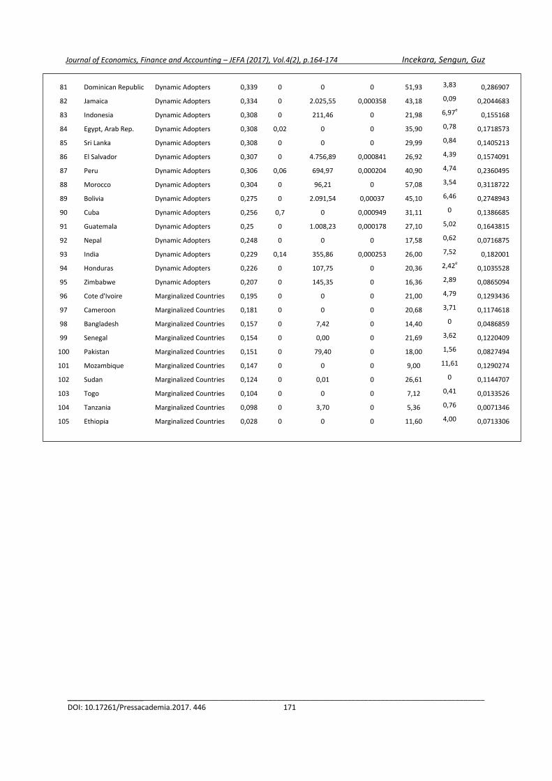
Journal of Economics, Finance and Accounting – JEFA (2017), Vol.4(2), p.164-174 Incekara, Sengun, Guz
_________________________________________________________________________________________________
DOI: 10.17261/Pressacademia.2017. 446 171
81 Dominican Republic Dynamic Adopters 0,339 0 0 0
51,93 3,83 0,286907
82 Jamaica Dynamic Adopters 0,334 0 2.025,55 0,000358 43,18 0,09 0,2044683
83 Indonesia Dynamic Adopters 0,308 0 211,46 0 21,98 6,97e
0,155168
84 Egypt, Arab Rep. Dynamic Adopters 0,308 0,02 0 0 35,90 0,78 0,1718573
85 Sri Lanka Dynamic Adopters 0,308 0 0 0 29,99 0,84 0,1405213
86 El Salvador Dynamic Adopters 0,307 0 4.756,89 0,000841 26,92 4,39 0,1574091
87 Peru Dynamic Adopters 0,306 0,06 694,97 0,000204 40,90 4,74 0,2360495
88 Morocco Dynamic Adopters 0,304 0 96,21 0 57,08 3,54 0,3118722
89 Bolivia Dynamic Adopters 0,275 0 2.091,54 0,00037 45,10 6,46 0,2748943
90 Cuba Dynamic Adopters 0,256 0,7 0 0,000949 31,11 0 0,1386685
91 Guatemala Dynamic Adopters 0,25 0 1.008,23 0,000178 27,10 5,02 0,1643815
92 Nepal Dynamic Adopters 0,248 0 0 0 17,58 0,62 0,0716875
93 India Dynamic Adopters 0,229 0,14 355,86 0,000253 26,00 7,52 0,182001
94 Honduras Dynamic Adopters 0,226 0 107,75 0 20,36 2,42e
0,1035528
95 Zimbabwe Dynamic Adopters 0,207 0 145,35 0 16,36 2,89 0,0865094
96 Cote d'Ivoire Marginalized Countries 0,195 0 0 0 21,00 4,79 0,1293436
97 Cameroon Marginalized Countries 0,181 0 0 0 20,68 3,71 0,1174618
98 Bangladesh Marginalized Countries 0,157 0 7,42 0 14,40 0 0,0486859
99 Senegal Marginalized Countries 0,154 0 0,00 0 21,69 3,62 0,1220409
100 Pakistan Marginalized Countries 0,151 0 79,40 0 18,00 1,56 0,0827494
101 Mozambique Marginalized Countries 0,147 0 0 0 9,00 11,61 0,1290274
102 Sudan Marginalized Countries 0,124 0 0,01 0 26,61 0 0,1144707
103 Togo Marginalized Countries 0,104 0 0 0 7,12 0,41 0,0133526
104 Tanzania Marginalized Countries 0,098 0 3,70 0 5,36 0,76 0,0071346
105 Ethiopia Marginalized Countries 0,028 0 0 0 11,60 4,00 0,0713306

Journal of Economics, Finance and Accounting – JEFA (2017), Vol.4(2), p.164-174 Incekara, Sengun, Guz
_________________________________________________________________________________________________
DOI: 10.17261/Pressacademia.2017. 446 172
TAI Rank Country Category TAI 2016
Diffusion of Old İnnovations(DOI) Development of Human Skills
Telephone (mainlines + cellular per 1000 people)f
Electricity consumption (kwh per capita)g
DOI Index
Mean years of
schoolingh
Gross enrolment
ratio, tertiary (%of tertiary school-age
population)k DHS Index
1 Switzerland Leaders 0,813 1867,2 7.807,31 0,983406
12,8 57.229j 0,73
2 Luxembourg Leaders 0,766 1994,8 14.193,17 1 11,7 19.407l 0,51
3 Netherlands Leaders 0,745 1648,1 6.821,06 0,969789 11,9 78.501l 0,78
4 Sweden Leaders 0,685 1670,5 13.870,39 1 12,1 62.353j 0,72
5 Ireland Leaders 0,682 1445,8 5.701,90 0,918054 12,2 77.626j 0,79
6 Singapore Leaders 0,673 1824,1 8.839,71 0,995928 10,6 69,811l 0,68
7 Denmark Leaders 0,666 1582,6 6.039,61 0,957419 12,7 81.516j 0,83
8 Korea, Rep. Leaders 0,661 1765,2 10.427,89 1 11,9 95.345 0,86
9 Germany Leaders 0,658 1716,4 7.019,01 0,972674 13,1 68.265 0,79
10 United States Leaders 0,635 1559,9 12.988,26 0,994535 12,9 85.796 0,86
11 Finland Leaders 0,633 1452,9 15.509,73 0,968154 10,3 87.289 0,75
12 Norway Leaders 0,626 1294,9 23.325,75 0,925412 12,6 76.696 0,81
13 France Leaders 0,622 1625,2 7.373,98 0,977648 11,1 64.390j 0,68
14 Japan Leaders 0,619 1767,7 7.835,60 0,983771 11,5 63.362j 0,7
15 Austria Leaders 0,617 1995,9 8.513,01 0,992131 10,8 81.540 0,75
16 Australia Leaders 0,616 1707,5 10.133,86 1 13 90.306 0,89
17 Belgium Leaders 0,604 1558,3 7.966,69 0,979597 11,3 73.318j 0,73
18 Israel Leaders 0,597 1765,5 6.558,72 0,965835 12,5 66.181j 0,76
19 New Zealand Leaders 0,596 1620,8 9.084,22 0,998679 12,5 80.882j 0,82
20 Malta Leaders 0,589 1826,9 4.735,77 0,932999 10,3 46.973 0,57
21 Iceland Leaders 0,582 1639,5 54.799,17 1 10,6 81,26l 0,4
22 Estonia Leaders 0,576 1789,7 6.664,66 0,96745 12,5 69.550 0,77
23 Kazakhstan Leaders 0,575 1816,1 4.892,50 0,936282 11,4 46.039 0,61
24 Russian Federation Leaders 0,563 1849,7 6.539,21 0,965534 12 78.653j 0,79
25 Greece Leaders 0,562 1602,3 5.029,00 0,939057 10,3 113.871j 0,87
26 Czech Republic Leaders 0,557 1407,2 6.284,79 0,917822 12,3 66.017j 0,75
27 Slovenia Leaders 0,556 1494,4 6.833,17 0,948577 11,9 82.926j 0,8
28 Hong Kong SAR, China Leaders 0,549 2879,1 5.933,63 0,955736 11,2 68.475 0,71
29 United Kingdom Leaders 0,546 1761,5 5.407,29 0,94637 13,1 61n 0,48
30 Malaysia Leaders 0,536 1585,4 4.511,97 0,928118 10 26.074 0,46
31 Lithuania Leaders 0,535 1582,6 3.663,67 0,907017 12,4 68.531j 0,76
32 Spain Leaders 0,534 1497,2 5.401,05 0,925557 9,6 89.670 0,73
33 Latvia Leaders 0,531 1450,3 3.472,54 0,869205 11,5 67.039j 0,71
34 Slovak Republic Leaders 0,526 1381,9 5.202,47 0,89203 12,2 52.923j 0,68
35 Poland Leaders 0,522 1663,8 3.937,65 0,91439 11,8 71.158l 0,75
Table 1: Technology Achievement Index 2016

Journal of Economics, Finance and Accounting – JEFA (2017), Vol.4(2), p.164-174 Incekara, Sengun, Guz
_________________________________________________________________________________________________
DOI: 10.17261/Pressacademia.2017. 446 173
36 Belarus Leaders 0,521 1726,8 3.648,32 0,906695
12 87.940 0,83
37 Hungary Leaders 0,516 1501,3 3.890,29 0,89349 11,6 50.862 0,64
38 Italy Leaders 0,507 1751,7 5.159,18 0,941634 10,1 63.095j 0,63
39 Argentina Leaders 0,506 1706 3.093,35 0,890057 9,8 82.917j 0,71
40 Canada Leaders 0,506 1265 15.519,34 0,91674 13 60m 0,48
41 Croatia Potential leaders 0,499 1384,7 3.754,27 0,859886 11 69.544j 0,7
42 Chile Potential leaders 0,499 1486,9 3.878,91 0,889616 9,8 88.577 0,73
43 Ukraine Potential leaders 0,496 1656,4 3.600,23 0,905357 11,3 82.305j 0,77
44 Bulgaria Potential leaders 0,492 1525,4 4.639,71 0,917165 10,6 73.934 0,7
45 Bahrain Potential leaders 0,491 2058,6 18.216,62 1 9,4 37.375 0,48
46 Cyprus Potential leaders 0,482 1231,9 3.594,79 0,812101 11,6 60.101 0,69
47 Saudi Arabia Potential leaders 0,478 1891,2 8.741,42 0,994801 8,7 63.066 0,56
48 Qatar Potential leaders 0,47 1767,2 15.470,99 1 9,1 17.219 0,37
49 Serbia Potential leaders 0,468 1569,9 4.444,22 0,9235 10,5 58.287 0,63
50 Portugal Potential leaders 0,467 1545,5 4.685,05 0,923005 8,2 65.607j 0,55
51 Brunei Darussalam Potential leaders 0,458 1170,9 9.703,55 0,888042 8,8 30.844 0,42
52 Costa Rica Potential leaders 0,451 1678,4 1.954,56 0,843767 8,4 53.629 0,51
53 Philippines Potential leaders 0,443 1189,2 692,06 0,63288 8,9 35.753j 0,45
54 Kuwait Potential leaders 0,442 2451,6 14.910,58 1 7,2 27.027l 0,33
55 Oman Potential leaders 0,439 1703,2 5.981,45 0,956545 8 31.922 0,39
56 Georgia Potential leaders 0,437 1510,2 2.459,75 0,849461 12,1 43.419 0,63
57 Romania Potential leaders 0,436 1269,3 2.494,53 0,786363 10,8 53.220 0,62
58 Brazil Potential leaders 0,426 1480,4 2.529,30 0,844874 7,7 49.279j 0,45
59 Azerbaijan Potential leaders 0,424 1299,6 2.092,54 0,777403 11,2 25.483 0,51
60 Armenia Potential leaders 0,423 1343,3 1.870,20 0,778355 10,9 44.309 0,58
61 Thailand Potential leaders 0,422 1606,1 2.470,77 0,867398 7,3 48.857 0,43
62 China Potential leaders 0,419 1086,6 3.762,08 0,770094 7,5 43.392 0,42
63 Jordan Potential leaders 0,416 1842,3 2.103,86 0,85119 9,9 44.869 0,54
64 Macedonia, FYR Potential leaders 0,414 1163,7 3.556,50 0,789877 9,3 39.594j 0,49
65 South Africa Potential leaders 0,413 1722,3 4.325,52 0,923863 9,9 19.375j 0,42
66 Turkey Potential leaders 0,412 1110,1 2.744,84 0,746251 7,6 86.309j 0,62
67 Albania Potential leaders 0,41 1134,7 2.531,89 0,746246 9,3 58.109 0,57
68 Moldova Potential leaders 0,407 1430,3 1.352,79 0,768996 11,2 41.213 0,58
69 Kyrgyz Republic Potential leaders 0,404 1399,5 1.887,02 0,794473 10,6 45.917j 0,57
70 Vietnam Potential leaders 0,402 1369,6 1.305,58 0,749315 7,5 28.835 0,35
71 Uruguay Potential leaders 0,401 1924,7 2.985,06 0,886464 8,5 0 0,27
72 Panama Potential leaders 0,394 1897,5 2.038,00 0,847983 9,3 38.739 0,48
73 Lebanon Potential leaders 0,392 1122 3.194,07 0,765493 7,9 38.484 0,42
74 Colombia Potential leaders 0,386 1300,9 1.177,11 0,719765 7,3 55.589 0,46
75 Mauritius Potential leaders 0,385 1708,9 2.148,33 0,853298 8,5 36.667 0,43
76 Mexico Potential leaders 0,377 1018,7 2.056,96 0,685264 8,5 29.940j 0,4
77 Mongolia Potential leaders 0,365 1137,1 1.908,94 0,718554 9,3 68.567 0,62
78 Tunisia Potential leaders 0,35 1383,1 1.434,62 0,76246 6,8 34.606 0,35

Journal of Economics, Finance and Accounting – JEFA (2017), Vol.4(2), p.164-174 Incekara, Sengun, Guz
_________________________________________________________________________________________________
DOI: 10.17261/Pressacademia.2017. 446 174
79 Bosnia and Herzegovina Dynamic Adopters 0,342 1103,8 3.219,01 0,760206
8,3 38n 0,26
80 Botswana Dynamic Adopters 0,34 1768 1.563,51 0,821259
8,9 27.513j 0,41
81 Dominican Republic Dynamic Adopters 0,339 948,4 1.516,52 0,627983
7,6 47.515j 0,44
82 Jamaica Dynamic Adopters 0,334 1205 1.126,47 0,686903
9,7 27.220 0,45
83 Indonesia Dynamiz Adopters 0,308 1411 787,68 0,709421
7,6 31.102j 0,37
84 Egypt, Arab Rep. Dynamic Adopters 0,308 1183,5 1.697,47 0,721564
6,5 36.228 0,34
85 Sri Lanka Dynamic Adopters 0,308 1258 525,88 0,626073
10,8 19.796 0,47
86 El Salvador Dynamic Adopters 0,307 1599,5 915,00 0,767238
6,5 28.852j 0,31
87 Peru Dynamic Adopters 0,306 1192,1 1.269,77 0,69498
9 0 0,29
88 Morocco Dynamic Adopters 0,304 1334,2 866,24 0,698229
4,4 28.143 0,2
89 Bolivia Dynamic Adopters 0,275 1001,7 705,29 0,571091
8,2 0 0,25
90 Cuba Dynamic Adopters 0,256 411,7 1.425,48 0,31194
11,5 36.280 0,57
91 Guatemala Dynamic Adopters 0,25 1220,5 555,04 0,62028
5,6 18.325l 0,22
92 Nepal Dynamic Adopters 0,248 997,3 128,15 0,828465
3,3 14.940 0,09
93 India Dynamic Adopters 0,229 800,5 765,00 0,496045
5,4 25.535j 0,24
94 Honduras Dynamic Adopters 0,226 1014,4 720,98 0,577986
5,5 21.184j 0,22
95 Zimbabwe Dynamic Adopters 0,207 870,1 531,75 0,490323
7,3 8.433 0,25
96 Cote d'Ivoire Marginalized Countries 0,195 1206,1 252,38 0,536408
4,3 9.155 0,11
97 Cameroon Marginalized Countries 0,181 763,6 278,06 0,37648
6 17.478 0,23
98 Bangladesh Marginalized Countries 0,157 824,4 293,02 0,410208
5,1 13.440j 0,17
99 Senegal Marginalized Countries 0,154 1019,6 219,25 0,459859
2,5 10.386 0,04
100 Pakistan Marginalized Countries 0,151 688 449,97 0,386309
4,7 9.927 0,14
101 Mozambique Marginalized Countries 0,147 745,7 435,60 0,412935
3,2 5.974j 0,05
102 Sudan Marginalized Countries 0,124 708,3 158,66 0,291998
3,1 16.320j 0,09
103 Togo Marginalized Countries 0,104 684,4 147,50 0,271903
4,5 10.625 0,13
104 Tanzania Marginalized Countries 0,098 761,3 89,48 0,261036
5,1 3.647 0,13
105 Ethiopia Marginalized Countries 0,028 436,6 64,62 0,021795
2,4 8.126j 0,02
Notes: a Related to the year of 2015 data is obtained from European Patent Office b Data on patents and royalties are missing for these countries. Lack of data for these countries generally indicates little formal innovation occurring. Therefore, a value ‘0’ for the missing indicates has been used for these countries in the present study. Related to the year of 2015 data is derived from World Bank Database c Related to the year of 2015 data is derived from World Bank Database. d In TAI-02 (Desai et al.2002), data of high and medium technology exports as percentage of manufactured export was used. However, in spite of extensive internet search data for medium tecnology exports could not be traced. Related to the year of 2015 data is derived from World Bank Database. e For purposes of calculating the TAI, the nearest available data of year 2014 was used for countries for which no data were available. Related to the year of 2014 is derived from World Bank Database f Related to the year of 2015 derived from International Telecommunication Union (ITU). For purposes of calculating the TAI, the weighted average value for OECD countries (1583,034) was used. g For purposes of calculating the TAI, the nearest available data of year 2013 was used for countries, and the weighted average value for OECD countries (9204) was used. Related to the year of 2013 is derived from World Bank Database h Related to the year of 2014 derived from United Nation Devolepment Programme (UNDP). j Related to the year of 2014 derived from International Telecommunication Union (ITU). k Related to the year of 2015 derived from International Telecommunication Union (ITU). l Related to the year of 2013 derived from International Telecommunication Union (ITU). m The nearest available data of the year 2011 was used. Tha data derived from 2014 Human Devolopment Report. n The nearest available data of the year 2012 was used. Tha data derived from 2014 Human Devolopment Report.

Journal of Economics, Finance and Accounting – JEFA (2017), Vol.4(2), p-175-183 Cavus
_________________________________________________________________________________________________
DOI: 10.17261/Pressacademia.2017.447 175
A NEW APPROACH ON OCCUPATIONAL HEALTH AND SAFETY: FINANCIAL STATE SUPPORT FOR EMPLOYER
DOI: 10.17261/Pressacademia.2017.447
JEFA- V.4-ISS.2-2017(12)-p.175-183
O. Hakan Cavus1
1Manisa Celal Bayar University, Manisa, Turkey. [email protected]
To cite this document Cavus, O.H., (2017). A new approach on occupational health and safety: financial state support for employer. Journal of Economics, Finance and Accounting (JEFA), V.4, Iss.2, p.175-183. Permemant link to this document: http://doi.org/10.17261/Pressacademia.2017.447 Copyright: Published by PressAcademia and limited licenced re-use rights only.
ABSTRACT Purpose- Thanks to the Law on Occupational Health and Safety No.6331, which came into force on 30.06.2012, it has become compulsory
to employ occupational safety professionals and health professionals in the workplaces in order to carry out the services of occupational
health and safety. Within this framework, the purpose of this study is to analyse the principles of financial State support designed for the
purpose of refunding from the Social Security Institution (SSI) budget some amount of the money that was paid by employers for the
services of occupational health and safety to the employers of the private enterprises which are classified as very dangerous and
dangerous and which have workers less than 10 people.
Methodology- We conducted our research by making use of existing literature, and we also examined the financial support provided for
employers in terms of legal aspects by considering regulations and notices.
Findings- It was observed that the financial support in question did not become widespread. The reasons for this can be listed as: (i) the
bulk of unregistered employers, (ii) the amount of financial support’s being lower, and (iii) the employers’ not having enough information
regarding the issue. Conclusion- In order to make the financial support in question, it is necessary to (i) increase the amount of the so-called financial support, (ii) terminate the authorized Community Health Center (CHCs) responsibilities for providing occupational health and safety services, and (iii) eliminate the contradiction between the Law numbered 6331 and by-laws in determining the companies that will benefit from the support.
Keywords: Law on occupational health and safety, occupational health and safety professionals, financial state support. JEL Codes: I19, K32
1. INTRODUCTION
The Occupational Health and Safety Act No. 6331 which was published in the Official Gazette dated 30th
June 2012 (OHSA) has included all employees and employers with a few exceptions. The OHSA has aimed at preventing occupational accidents and occupational diseases, recording these accidents and diseases; besides it has initiated a significant transformation in terms of extending the occupational safety culture in working life. This law has brought along many obligations to employers, employees and the government in thearea of occupational health and safety (Kılkış, 2016). With making regulations such as carrying out risk analysis at workplaces, establishing occupational health and safety board, selection of employee representative, implementation of health surveillance, obligating enforcement of occupational health and safety trainings as well as enforcement of employing occupational physicians, occupational safety experts and health personnel; enterprises in Turkey have started to provide a safe working environment (Bilir, 2016).
Journal of Economics, Finance and Accounting – (JEFA), ISSN: 2148-6697, http://www.pressacademia.org/journals/jefa
Year: 2017 Volume: 4 Issue: 2

Journal of Economics, Finance and Accounting – JEFA (2017), Vol.4(2), p-175-183 Cavus
_________________________________________________________________________________________________
DOI: 10.17261/Pressacademia.2017.447 176
Within the scope of the obligation to provide occupa tional health and safety services which are regulated among the significant responsibilities of the employer in the OHSA, By-law on Occupational Health and Safety Services (ROHSS) which was published in the Official Gazette dated 29
th December 2012 and the By-Law on Occupational Health and Safety Services
by Employer and Representative of the Employer in Workplaces (OHSSEREW) which was published in the Official Gazette dated 29
th June 2015 have entered into force. Within the scope of carrying out occupational health and safety services, By-
Law on the Duties, Authorities, Responsibilities and Trainings of Occupational Safety Specialists of 29 December 2012 on the duties, powers, responsibilities and education of occupational safety specialists (DARTOSS) and By-Law on the Duties, Authorities, Responsibilities and Trainings of the Occupational Physician and Other Health Personnel of 20 July 2013 on education, duties, powers and responsibilities of occupational physicians and other health personnel (DARTOPOHP) which were published in the Official Gazette have entered into force.
In terms of the OHSA, employers have employed occupational health and safety specialist, occupational physician and other health care staff in different ways. For instance, in case employer or representative of employer who has enterprises classified as less hazardous employing fewer than ten workers complete the required training and receive certificate (OHSSEREW, Article 9), they can carry out duties- except health surveillance and occupational environment control- which are assigned to occupational health and safety specialist or occupational physician by allocating ten minutes at least (OHSSEREW, Article 5). The employer may also appoint an occupational physician and occupational health and safety specialist who has received training and certifications from among the employees in order to provide the occupational health and safety services. The employer who has enterprise classified as very hazardous employing ten and more than ten workers may also appoint other health care staff. In addition, employers who receive the required training and certification can take on occupational health and safety services themselves with considering hazard class and the number of employees (ROHSS Article 5/1). However, in case the employer does not undertake the duty of carrying out the occupational health and safety services himself or in the absence of suitable personnel from the workplace employees, the employer shall establish a workplace health and safety unit (WHSU) with appointing at least one occupational physician and at least one safety specialists who have required qualifications and certificate which is appropriate for hazard class of the workplace. In this unit, the employer may also appoint other health care staff (ROHSS, Article 10/1). Again, the employer may provide occupational health and safety services by means of outsourced service procurement.
In this context, the employer may get services from public institutions and organizations, organized industrial zones and joint health and safety unit (JHSU) is any unit which is established by public institutions and organizations, organized industrial zones and companies operating under the Turkish Code of Commerce No. 6102 in order to provide occupational health and safety services to workplaces, with required equipment and personnel and which is authorized by the Ministry (ROHSS Article 4/f). In order to be able to establish the JHSU, there is at least one worker in the JHSU within the full-time employment contract; occupational physician, occupational safety specialist and other health care staff are obliged to be employed (ROHSS, Article 12/1).
Another unit that the employer can provide occupational health and safety services other than the OHSA is the Community Health Centers (CHCs) affiliated to the Ministry of Health Turkish Public Health Institution of Turkey. Regarding the CHCs, Regulation on Community Health Center and Affiliated Units (CHCAU) published in the Official Gazette dated 5
th February
2015 was regulated. With the aim of protecting and improving community health in its region, CHC is health institution which determines risks and problems related to health, carries out corrective and preventive activities, coordinates and ensures to efficiently serve primary care preventive, curative and rehabilitative health services and monitors, assesses, support these services, ensures coordination between health institutions in the region and other institutions and organizations (CHCAU Article 4/n). At the same time, CHC has been also defined as a community health center affiliated unit authorized by the Ministry of Labor and Social Security to carry out occupational health and safety services (CHCAU, Article 4 / p).
When it is evaluated in general, primary duties of CHCs can be defined as to carry out studies in cooperation with related institutions in order to supply occupational health and safety services; to meet this unit’s requirements in accordance with the applicable legislation; to follow its region in terms of occupational diseases, work-related diseases and occupational accidents; by making cooperation with the relevant institutions and organizations, demand necessary measures from workplaces where an incident happened that is important for public health; within the scope of primary health services, recording the units, in case it supplies services such as laboratory, radiography, respiratory function test, hearing test… etc. in occupational health and safety units and joint health and safety units of its region(CHCAU Article 26). CHCs also have duties related to occupational health and safety services besides their duties on public health. CHCs conduct their activities within the framework of Directive on Rules and Principles about Occupational Health and Safety Services in Community Health Centers (DRPOHSSCHC) dated 31
st Jan 2014.
Fulfillment of occupational health and safety services brings about significant financial burden for the employers. This burden may not cause an increase in operating cost for large and institutional workplaces, but when it is considered that

Journal of Economics, Finance and Accounting – JEFA (2017), Vol.4(2), p-175-183 Cavus
_________________________________________________________________________________________________
DOI: 10.17261/Pressacademia.2017.447 177
the 99.8% of the workplaces in Turkey are small and medium sized and have low profit margins, it is obvious that fulfillment of occupational health and safety services causes very heavy financial burdens for small sized enterprises. Within this context, a new subsidy has been provided for small and medium-sized enterprises (Kosgeb, 2015) which constitute 74.2% of the total employment in Turkey, while providing utilization of subsidies provided as a means to carry out occupational health and safety services and security services through outsourcing service (OHSA, Article 7). Occupational health and safety are covered by the subsidies as much as the amount that is determined to cover by state for the workplaces in subsidy program. In this context, By-Law on Financial State Support for Occupational Health and Safety Services (FSSOHSS) was published in Official Gazette dated 24 December 2013. In addition, relevant procedures and principles about reimbursement of subsidies were specified with Notification on Financial State Support for Occupational Health and Safety Services (NFSSSOHS) was published in Official Gazette dated 03
rd March 2014 and it has entered into
force.
Within the framework of comparing the costs of occupational health and safety services; we first focused on the legal regulations related to employers’ responsibility of employing occupational health and safety professionals and then dealt in detail with the implementation stages of financial State support to be provided by SSI for the employers fulfilling the services of occupational health and safety at their own workplaces.
2. THE EMPLOYERS’ OBLIGATION TO EMPLOY OCCUPATIONAL SAFETY SPECIALIST, OCCUPATIONAL PHYSICIAN AND OTHER HEALTH CARE STAFF
The OHSA has brought about many new obligations to the employer. One of the most important obligations is the obligation to employ an occupational health and safety specialist, occupational physician and other health personnel who are also called as health professionals in terms of the occupational health and safety services. These health professionals work in the workplaces during the period which is scheduled in accordance with the legislation. According to our legislation, occupational health and safety specialist is any engineer, architect or technician who are authorized by the Ministry to work in the field of occupational health and safety and who have occupational health and safety expertise certificate (OHSA Article 4/f, DARTOSS, Article.4/f); occupational physician is any physician who is authorized by the Ministry to work in the field of occupational health and safety and who has occupational medicine certificate (OHSA Article 4/1, DARTOPOHP, Article.4/g); and other health care staff any nurse/health technician who is authorized to perform the nursing profession who has the occupational nurse’s certificate issued by the Ministry in order to work in the field of occupational health and safety; health officer, technicians any person with the title of emergency medical technician, environmental health technician who has diploma and certificate issued by the Ministry in order to work in the field of occupational health and safety (DARTOPOHP, Article.4/b)
Occupational health and safety specialists carry out their duties in the periods specified below. In this context (DARTOSS, Article 12; Narter, 2014):
a) At least 10 minutes per month per employee in less hazardous working area,
b) At least 20 minutes per month per employee in hazardous working area
c) At least 40 minutes per month per employee, taking place in a very hazardous working area.
Furthermore, at least one full time occupational health and safety specialist is employed for each 1000 employees in the workplaces which have 1000 and more employees and classified as less hazardous. For a workplace which consists of 500 and more employees and classified as hazardous, at least one full time occupational health and safety specialist is employed for each 500 employees. And at least one full time occupational health and safety specialist will be employed for each 250 employees in the workplaces which include 250 and more employees and classified as very hazardous.
As another health professionals, occupational physicians perform their duties at workplaces for the following periods. According to this (DARTOPOHP, Article.12; Yamakoğlu, 2016):
a) At least 5 minutes per month per employee, in workplaces classified as less hazardous
b) At least 10 minutes per month per employee in workplaces classified as hazardous
c) At least 15 minutes per month per employee, in workplaces classified as very hazardous.
Again, at least one full time occupational physician is employed for each 1000 employees in the workplaces which have 2000 and more employees and classified as less hazardous. For a workplace which consists of 1000 and more employees and classified as hazardous, at least one full time occupational physician is employed for each 1000 employees. And at least one full time occupational physician is employed for each 750 employees in the workplaces which include 750 and more employees and classified as very hazardous.

Journal of Economics, Finance and Accounting – JEFA (2017), Vol.4(2), p-175-183 Cavus
_________________________________________________________________________________________________
DOI: 10.17261/Pressacademia.2017.447 178
Duty period of other health personnel has been scheduled as follows (DARTOPOHP, Article.19):
a) At least 10 minutes per month per employee in workplaces which have10 to 49 employees and classified in a very hazardous class
b) At least 15 minutes per month per employee in workplaces which have 50 to 249 employees and classified in very hazardous class.
c) At least 20 minutes per month per employee in workplaces which have 250 and more employees and classified in a very hazardous class.
In the workplaces where the full-time occupational physician is assigned, appointing other health care staff is not required.
As can be seen, the higher the hazard class of workplaces, the longer duty period of health professionals. The increase in duty period means that the employer purchases for these services with higher cost.
3. GENERAL FEATURES OF FİNANCİAL STATE SUPPORTS TO THE OCCUPATIONAL HEALTH AND SAFETY SERVICES
According to the OHSA, this support may be provided to enterprises employing fewer than ten workers except for public bodies and organizations provided that the enterprise is classified as 'very hazardous' and 'hazardous'. However, the Council of Ministers may decide that the Ministry may also provide subsidies to enterprises employing fewer than ten workers and classified as 'less hazardous'. However, state subsidies to occupational health and safety services have not yet been provided to enterprises are classified as less hazardous. Social Security Institution (SSI) shall cover expenses by allocating resources out of premiums collected under the short-term insurance program including occupational accidents and occupational diseases (OHSA Article 7/b). In order to be able to give financial state support to the state, two important workplace conditions have to be fulfilled. Accordingly, the workplace must first be registered in the Occupational Health and Safety Record, Follow-up and Monitoring Program (OHS-KATİP)(OHS-REFMP), which is used for the registration, follow-up and monitoring of the occupational health and safety services in the General Directorate of Occupational Health and Safety. In addition, a contract must be signed between the workplace and the person, institution or organization (service provider) that provides the occupational health and safety service authorized by the General Directorate Occupational Health and Safety.
3.1. Workplaces That Will Not Benefit From Financial State Support
The OHSA has covered all workplaces in public and private sector in general. However, some activities and individuals have been excluded from the scope of the OHSA (Süzek, 2015). According to this; this Law shall not be applicable to the following activities and persons: a) Activities of the Turkish Armed Forces, the police and the Undersecretary of National Intelligence Organization except for those employed in workplaces such as factories, maintenance centers, sewing workshops and the like b) intervention activities of disaster and emergency units c) domestic services ç) Persons producing goods and services in their own name and on their own account without employing workers d) Prison workshop, training, security and vocational course activities within the framework of improvements carried out throughout the enforcement services for convicts and inmates (OHSA Article 2/2). In addition, public institutions and workplaces which have less than 50 employees and are involved in the less hazardous class will not be able to benefit from the state subsidy as they do not carry the conditions for benefiting from state subsidy both in terms of employee number and workplace’s hazard class.
3.2. Workplaces That Can Benefit From Financial State Support
The financial state support for occupational health and safety services has been implemented from 01st
Jan.2014 (OHSSEREW, Article 4/2) for employers of workplaces which are classified as hazardous and very dangerous with fewer than ten employees in Turkey, excluding public institutions and organizations. It is necessary to emphasize an important point here. It has been stipulated that the number of the employees of the employer working in all the establishments in Turkey should has less than the number of the employees of the same employer in order to benefit from state subsidy by arranging the OSHA in a restrictive manner in the OHSSEREW.
The conditions to be sought in determining whether the number of employees is less than ten in the workplaces that will benefit from the state subsidy are also determined. Accordingly, (OHSSEREW, Article 4/2):
a) If the same employer has more than one registered workplace in Turkey, the total number of insured employed by the same employer in workplaces in hazardous and very hazardous class throughout Turkey within the scope of Social Insurance and General Health Insurance Law No. 5510 No. 4 / a shall be taken as basis.

Journal of Economics, Finance and Accounting – JEFA (2017), Vol.4(2), p-175-183 Cavus
_________________________________________________________________________________________________
DOI: 10.17261/Pressacademia.2017.447 179
b) The insured employed by employers who are employed by the employer shall be included in the total number of employees who have not worked in the workplace for several reasons during the month and who have not paid wages and those who entered or paid out during the month.
c) The number of insured persons registered in the cancellation qualified monthly premiums and service documents given to SSI and the candidates specified in the Vocational Education Law No. 3308 are not taken into consideration in determining the number of employees who are receiving vocational training in apprenticeship and apprenticeship.
It should also be noted that the insured real person as employer or legal personality shareholder of employer (self-employed persons) in accordance with Law No. 5510 4/b is not taken into account as insured employees under 4/b in determining the number of employees.
4. PRINCIPLES OF IMPLEMENTING THE SUPPORT
4.1. Determination and Calculation of Occupational Health and Safety Service Financial State Support
The fees of occupational health and safety services given to the enterprises employing fewer than 10 employees are determined separately for each workplace, based on the hazard class of the enterprise, the number of the workers notified to SSI, and the number of days that the personnel have worked. The fees of occupational health and safety services that are subject to the support are determined as 1.4% of the daily average of the minimum incomes taken as the basis for the premium in hazardous enterprises, and 1.6% of the daily average of the minimum incomes taken as the basis for the premium in very hazardous enterprises. The amount for the fee of the occupational health and safety services to be provided is determined by multiplying these percentages by the number of days of premium payment reported in the monthly premiums and service documents of the enterprises (OHSSEREW, Article 5). When a sample calculation is done; for the period of 01.01.2017-31.12.2017, the daily gross minimum wage is TL 59.25. The amount of support for a worker in 2017 is 59.25x1.4% = 82.95 TL for the enterprises in hazardous class and 59.25x1.6% = 94.80 TL for the enterprises in very hazardous class.
The amount that the employers will pay for occupational health and safety services received from the Joint Health and Safety Unit (JHSU) will always be more than the amount they will pay for the services to be received from the authorized CHCs. However, the obligation to employ occupational health and safety professionals, whichever way they are met and how low-cost they are, brings a certain bureaucratic workload and cost to the employers that have small businesses (Akyiğit, 2013). In addition, authorized CHCs provide both public health services and OHS services. Since the primary task of the CHC is to provide public health services, their abilities of providing occupational health and safety services remains as of secondary importance. This made it impossible for authorized CHCs to meet market demands for occupational health and safety services due to their current organization. However, when occupational health and safety services are purchased from authorized CHCs, occupational health and safety services will be much cheaper and almost all of the service costs will be covered by the support provided to the employer. For this reason, receiving occupational health and safety services from authorized CHCs has become more advantageous for medium and small-sized enterprises.
4.2. The Method for Applying and Funding of the Financial State Support
It is necessary for the enterprises, which are included in the scope of the support, to apply to the SSI to benefit from the support provided. In order to implement the occupational health and safety support, the General Directorate of Occupational Health and Safety has given authority to the SSI to access the OHS-REFMP in order to ensure the identification of the enterprises that have signed a contract and are within the scope of the support. SSI will check through the OHS-REFMP that which of the enterprises that have applied to benefit from the support are covered, and whether these enterprises have duly contracted with a service provider (OHSSEREW, Article 6/1).
In order to benefit from the support, the application to be made to SSI is determined to be in a certain procedure. Accordingly, employers of the enterprises in hazardous and very hazardous classes will apply to SSI units, where their enterprises are registered, in order to benefit from occupational health and safety support. In the situation that the same employer has more than one registered enterprises in Turkey, the application will be made to the units where the employer's head office is registered, with the enterprises in hazardous and very hazardous classifications separately stated in the application form (OHSSEREW, Article 4/1). Apart from the enterprises stated by the employer in the application, the other enterprises belonging to the same employer in Turkey, separately for the classes of hazardous and very hazardous, and whether these enterprises are included in the scope of the support are identified by SSI units. As a result of the examination to be carried out by SSI, the processes are carried out taking the number of workers notified by the enterprises determined by SSI units into account. The numbers of the apprentices, apprentice candidates, and the students receiving vocational training in the workplace, who are in the status of student under the Law of Higher Education and the number of part-time OHS professionals whose services are outsourced, are not included in the determined number of the workers (OHSSEREW, Article 4/3).

Journal of Economics, Finance and Accounting – JEFA (2017), Vol.4(2), p-175-183 Cavus
_________________________________________________________________________________________________
DOI: 10.17261/Pressacademia.2017.447 180
Application deadlines have also been set for applications for support payments. According to this, the applications are made until the end of;
a) April, for the months of January, February and March,
b) July, for the months of April, May and June,
c) October, for the months of July, August and September,
d) January of the following year, for the months of October, November and December.
The SSI calculates the cost of the service provided to the employers, which have contracted with the General Directorate of Occupational Health and Safety and which are within the scope of the payment, in quarterly periods; and the amounts calculated at the end of each period are paid to the employer at the end of the following second month (OHSSEREW, Article 4/4).
Payments under support are subject to certain conditions. According to this; it is required that the monthly premium and service documents of the workers are delivered to the SSI by the employer within its regulated deadline and that there is no debts related to premiums in overall Turkey as of the date of the support payment's being processed. For the employers meeting these two conditions:
a)The support payment of the first term is processed at the end of May, for the months of January, February and March,
b)The support payment of the second term is processed at the end of August, for the months of April, May and June,
c)The support payment of the third term is processed at the end of November, for the months of July, August and September,
d)The support payment of the fourth term is processed at the end of February of the following year, for the months of October, November and December (OHSSEREW, Article 4/4).
The final procedure for employers to receive the support is related to issuing invoices. Employers are obliged to submit invoices to the SSI in the form of occupational health and safety service fees under the name of the reflection invoice. In the reflection invoices, the daily amount of support to be paid for each worker will be determined by recording hazardous and very hazardous enterprises separately, and by applying 1.4% rate for hazardous, and 1.6% for very hazardous enterprises in daily average of the minimum incomes taken as the basis for the premium, for each month that is within the scope of the payment periods. For each month covered by the payment periods, the amount of the support to be paid will be determined over the number of days of premium payment notified by the monthly premium and service document to SSI (OHSSEREW, Article 7-8).
5. CEASING THE FINANCIAL STATE SUPPORT AND REFUNDING
The financial assistance provided under the support may be ceased in certain cases and for a certain period of time. The interruption of the support and the refunding has generally been due to the detection of unregistered workers by SSI. According to the regulation on the subject; the enterprises which are detected to be employing unregistered workers by the SSI Supervisors or SSI Inspectors, who are the authorized officials of SSI for supervising and inspecting, by the inspectors of the other public institutions as the result of the investigations, audits and inspection that they carry out according to their own regulations, or by the documents obtained from banks, working capital enterprises, public administrations, and other institutions established by law, or by the authorizations of the courts; will not be able to receive support funds for three years starting from the next month of date of the determination, and the payments that were processed starting from the employment of the unregistered worker will be refunded by the enterprise together with its legal rate of interest to SSI (OHSSEREW, Article 9/1, Akyiğit, 2013)
Furthermore, in case of determining that there are unregistered (uninsured) employees in the enterprises belonging to the employers with more than one enterprise, the employer will not be able to receive support funds for three years starting from the next month of date of the determination, and the payments that were processed for either of the detected and other enterprises of the employer starting from the employment of the unregistered worker will be refunded by the enterprise together with its legal interest to SSI (OHSSEREW, Article 9/2).
6. THE EFFECTIVENESS OF THE FINANCIAL SUPPORT REGARDING THE OCCUPATIONAL HEALTH AND SAFETY SERVICES, AND THE DIMENSIONS OF THE FINANCIAL BURDEN OF THE SUPPORT
The main purpose of providing financial support/incentives in the context of occupational health and safety activities is to encourage the preparation of a healthy and a safe workplace environment, in particular to reduce occupational accidents and occupational diseases by applying proactive measures and to spread the work safety culture. According to the research

Journal of Economics, Finance and Accounting – JEFA (2017), Vol.4(2), p-175-183 Cavus
_________________________________________________________________________________________________
DOI: 10.17261/Pressacademia.2017.447 181
carried out, 1 Euro spent under the financial incentive/support has returned as 4.5 EURO. Apart from these; financial supports have further increased the sense of responsibility in large enterprises and reduced the social insurance costs, and have increased the occupational health and safety activities in small and medium-sized enterprises over time. Particularly in the scope of the occupational health and safety strategies implemented by the European Union in the period of 2007-2012, financial supports have mostly been used. During this period; there has been a 28% reduction in occupational accidents in the meat processing sector in Germany through financial subsidies/incentives used to expand occupational health and safety services. The Italian Workers' Insurance Agency has provided credits with reduced interest rates for medium and small sized businesses within the scope of occupational health and safety, resulting in reductions between 13% and 25% in occupational accidents (Elsler and Taylor, 2010).In a study carried out to investigate the effectiveness of these financial supports, the reasons for diminishing the effectiveness of financial support in small and medium-sized establishments have been grouped under the following topics (Alper et al, 2015):
1)The employers of small businesses, who want to stay out of registration, do not request for support by avoiding their enterprises from being under multi-dimensional registration and supervision and being accessible and visible to public institutions, despite the financial support provided to them.
2) Small businesses have insufficient knowledge of the support provided.
3) They do not have sufficient time and the manpower to perform bureaucratic procedures related to the application process in order to benefit from the financial support provided.
4) When the financial support provided is low, it makes the application unnecessary and meaningless for the employer.
5) Employers believe that, despite all the information and high level of penalties, the practice will loosen over time and the enterprises will be outside the scope of the controls.
In addition, according to another application, which can be regarded as another way of financial support in Turkey; with the directive dated 31.01.2014; the service fees of authorized CHCs, which can be called as a kind of public JHSU, was determined far below the market level, taking small businesses into account. However, the practice has shown that, at least until today, authorized CHCs cannot meet the demands for occupational health and safety services. It has been difficult to find occupational safety specialists, workplace physicians and other health personnel to work in authorized CHCs. In addition, the facts that they have had compulsory service due to the received education, they have been obliged perform the tasks that have been assigned by the CHCs other than the tasks related to the occupational health and safety subjects in the spare times, the financial contribution of these duties, which were to be carried out in addition to their own duties, have been lower than expected, and finally the service is risky; the occupational health and safety professional’s desire to work in these authorized CHCs have been perished (Alper et al. 2015).
A calculation has been made based on SSI's April 2014 statistics for enterprises in hazardous and very hazardous classifications regarding the potential burden of financial support for small businesses to our social security system. According to the calculation based on the assumption that all businesses are in hazardous class, SSI needs to allocate 70% of the premium income collected for short-term insurance branches to support occupational health and safety services. When the premium income, collected from all insured workers on behalf of the short term insurance branches, is taken into account, the amount to be spent for the support will be 20.45% of the total premium incomes. The result of the same calculation made under the assumption that all enterprises are in hazardous class and that all businesses and insured workers will benefit from this support, the amount of support provided by the SSI will be 80% of the total premium incomes of the short term insurance branches. When all of the workers covered by the support are taken into consideration, the ratio of the support provided will be 23.4% of the total premium incomes of the short term insurance branches. When a calculation is made based on the SSI's total budget for 2014, the SSI's cost of support for health and safety services will only be about 0.0004 % of the total premium incomes and about 0.0003% of the expenditures. These financial support amounts mean that their cost to the SSI at a level that can be affordable (Alper et al.2015).
Supports or incentives for occupational health and safety services are of vital importance for medium and small sized businesses. Enterprises, where occupational accidents and occupational diseases occur at the highest level, are the small businesses. In addition to the limited financing opportunities of small business employers, who will bear the costs regarding the measures to ensure occupational health and safety services, employers see the expenditures with this purpose as unnecessary costs. Especially in times of economic crises, small businesses give up on spending for occupational health and safety. Another problem which appears is that the machines and equipment used are old technology products (Alli, 2008 , Gökbayrak, 2014).
7. CONCLUSION
The main aim of OHSA is to create healthy and safe working environments and to prevent occupational accidents and occupational diseases with pro-active methods. For this purpose, OHSA has brought important obligations to employers,

Journal of Economics, Finance and Accounting – JEFA (2017), Vol.4(2), p-175-183 Cavus
_________________________________________________________________________________________________
DOI: 10.17261/Pressacademia.2017.447 182
employees and the state by including private and public enterprises in Turkey except for some exceptions. The obligation of the employer to provide occupational health and safety has been defined as performing every necessary measures. Within the scope of occupational health and safety services, the financial burden of the employer in the scope of the new obligations has increased seriously. Considering that 98.2% of the enterprises in Turkey are small and medium sized workplaces; it has been seen that, sometimes these financial burdens become non-surmountable, and therefore, the employers become unable to meet the requirements. For this reason, as in other countries, in the case of employers' occupational health and safety services are provided by JHSUs or authorized CHCs, as of 01.01.2014, for enterprises with fewer than ten employees in very hazardous and hazardous classes, with the exception of public institutions and organizations in the presence of certain conditions, providing financial state support has become legally possible. However, since financial support has not received enough attention, the spread of occupational health and safety services has not been achieved. First of all, the amount of financial support in question needs to be increased and workplaces in the less dangerous class should also be included in the financial support. In this context, arrangements should be made to organize them as a professional organization, for example as the Chamber of Occupational Health and Safety Professionals, in order to ensure that health and safety professionals are able to provide more effective services by enabling their independence. It would also be an appropriate policy to terminate the tasks for providing occupational health and safety services, given to CHCs, which are already inadequate to provide these services. Another important problem is the violation between the Law and the Regulation in the determination of the enterprises belonging to the employers who will benefit from the financial support. From this point, it is seen that the condition of having fewer than 10 workers that is sought in the determination of the establishments that will benefit from the support according to the OHSA, has been sought within the framework of the concept of the workplaces. However, OHSSEREW is based on the concept of the employer rather than the workplace, and in order to benefit from the incentive, less than ten employers are required to be found in the total workplaces of the employer in Turkey. For this reason, the restrictive provision of the Regulation must be turned into a compatible one with the Law.
REFERENCES
Akyiğit, E. 2013, “İş Sağlığı ve Güvenliği Hizmetlerinde Devlet Desteği, MESS, Yıl:8, Sayı:29, pp.45-48
Alli, O. 2008, “Fundemantal Principles of Occupational Health and Safety”, ILO, Geneva. http://www.ilo.org/wcmsp5/groups/public/@dgreports/@dcomm/@publ/documents/publication/wcms_093550.pdf. (10.12.2016)
Alper, Y., Kılkış, İ., Engin T. 2015, “The Importance and Effectiveness of Financial Support for Small Enterprises within the Framework of Law no.6331”, Business and Economics Research Journal, Volume 6, Number 3, pp. 69-86, http://www.berjournal.com/tr/6331-sayili-kanun-cercevesinde-kucuk-isyerlerine-yonelik-maddi-destegin-onemi-ve-etkinligi (10.12.2016)
Bilir, N. 2016, İş Sağlığı ve Güvenliği, Güneş Tıp Kitapevleri, s.10-12
Elsler, D., Taylor, N. T. 2010, “A Review of Case Studies Evaluating Economic Incentives to Promote Occupational Safety and Health, Scand J Work Environ Health 2010; 36(4):289–298, http://www.astri.nl/media/uploads/files/review-case-studies-econ-incentives3.pdf. (10.12.2016)
Elsler D., Taylor T.N. (Editors), 2010 “Economic Incentives to Improve Occupational Safety and Health: A Review From the European Perspective. Luxembourg: Publications Office of the European Union; In press, http://www.astri.nl/media/uploads/files/review-case-studies-econ-incentives3.pdf. (01.05.2015)
Gökbayrak, Ş. 2014, “Küçük ve Orta Ölçekli İşletmelerde Risk Gruplarına Yönelik Sosyal Politikalar”, http://www.isguvenligi.net/kucuk-ve-orta-olcekli-isletmelerde-riskgruplarına-yonelik-sosyal-politikalar. (01.05.2015)
Kılkış, İ. 2016, “İş Sağlığı ve Güvenliği”, Dora Yayınları, s. 120-125
Küçük ve Orta Ölçekli İşletmeleri Geliştirme ve Destekleme İdaresi Başkanlığı (Kosgeb). 2015, “2015 Yılı Faaliyet Raporu” http://www.kosgeb.gov.tr/Content/Upload/Dosya/Mali%20Tablolar/Faaliyet%20Raporlar%C4%B1/KOSGEB_2015_Y%C4%B1l%C4%B1_Faaliyet_Raporu.pdf . (15.01.2017)
Narter, S. 2015, “İşkazası ve Meslek Hastalığında Hukuki ve Cezai Sorumluluk, Adalet Yayınevi, s. 130-132
Süzek, S. 2015, “İş Hukuku”, Beta Yayıncılık, s.610-612
Yamakoğlu, E. 2016, “İşverenin, İşyeri Hekimi ve İş Güvenliği Uzmanı Çalıştırma Yükümlülüğü”, Seçkin Yayıncılık, s. 120-123
5510 sayılı Sosyal Sigortalar ve Genel Sağlık Sigortası Kanunu,
http://www.mevzuat.gov.tr/Metin1.Aspx?MevzuatKod=1.5.5510&MevzuatIliski=0&sourceXmlSearch=&Tur=1&Tertip=5&No=5510. (10.10.206)

Journal of Economics, Finance and Accounting – JEFA (2017), Vol.4(2), p-175-183 Cavus
_________________________________________________________________________________________________
DOI: 10.17261/Pressacademia.2017.447 183
6331 sayılı İş Sağlığı ve Güvenliği Kanunu, http://www.mevzuat.gov.tr/Metin1.Aspx?MevzuatKod=1.5.6331&MevzuatIliski=0&sourceXmlSearch=&Tur=1&Tertip=5&No=6331. (10.10.2016)
İş Sağlığı ve Güvenliği Hizmetleri Yönetmeliği, 2012, http://www.mevzuat.gov.tr/Metin.Aspx?MevzuatKod=7.5.16924&MevzuatIliski=0&sourceXmlSearch=i%C5%9F%20sa%C4%9Fl%C4%B1%C4%9F%C4%B1. (10.10.2016)
İşyerlerinde İşveren ve İşveren Vekili Tarafından Yürütülecek İş Sağlığı ve Güvenliği Hizmetlerine İlişkin Yönetmelik, 2015, http://www.mevzuat.gov.tr/Metin.Aspx?MevzuatKod=7.5.20857&MevzuatIliski=0&sourceXmlSearch=i%C5%9F%20sa%C4%9Fl%C4%B1%C4%9F%C4%B1. (10.10.2016)
İş Güvenliği Uzmanlarının Görev, Yetki, Sorumluluk ve Eğitimleri Hakkında Yönetmelik, 2012, http://www.mevzuat.gov.tr/Metin.Aspx?MevzuatKod=7.5.16923&MevzuatIliski=0&sourceXmlSearch=i%C5%9F%20g%C3%BCvenli%C4%9Fi. (10.10.2016)
İşyeri Hekimi ve Diğer Sağlık Personelinin Görev, Yetki, Sorumluluk ve Eğitimleri Hakkında Yönetmelik, 2013, http://www.mevzuat.gov.tr/Metin.Aspx?MevzuatKod=7.5.18615&MevzuatIliski=0&sourceXmlSearch=i%C5%9Fyeri%20hekimi. (10.10.2016)
Toplum Sağlığı Merkezi ve Bağlı Birimler Yönetmeliği, 2015, http://www.mevzuat.gov.tr/Metin.Aspx?MevzuatKod=7.5.20507&MevzuatIliski=0&sourceXmlSearch=toplum%20sa%C4%9Fl%C4%B1%C4%9F%C4%B1%20merkezi. (10.10.2016)
İş Sağlığı ve Güvenliği Hizmetlerinin Desteklenmesi Hakkında Yönetmelik, 2013, http://www.mevzuat.gov.tr/Metin.Aspx?MevzuatKod=7.5.19151&MevzuatIliski=0&sourceXmlSearch=i%C5%9F%20sa%C4%9Fl%C4%B1%C4%9F%C4%B1. (10.10.2016)
İş Sağlığı ve Güvenliği Hizmetlerinin Desteklenmesi Hakkında Tebliğ, 2014, http://www.mevzuat.gov.tr/Metin.Aspx?MevzuatKod=9.5.19644&MevzuatIliski=0&sourceXmlSearch=i%C5%9F%20sa%C4%9Fl%C4%B1%C4%9F%C4%B1. (10.10.2016)
Toplum Sağlığı Merkezlerinde Yürütülecek İş Sağlığı ve Güvenliği Hizmetlerinin Usul ve Esasları Hakkında Yönerge, 2014, http://thsk.saglik.gov.tr/Dosya/mevzuat/yonergeler/CCI07022014.pdf. (10.10.2016)

Journal of Economics, Finance and Accounting – JEFA (2017), Vol.4(2), p.184-191 Ozdogan, Gacar, Aktas
_________________________________________________________________________________________________
DOI: 10.17261/Pressacademia.2017.448 184
DIGITAL AGRICULTURE PRACTICES IN THE CONTEXT OF AGRICULTURE 4.0
DOI: 10.17261/Pressacademia.2017.448
JEFA- V.4-ISS.2-2017(13)-p.184-191
Burak Ozdogan1, Anıl Gacar
2, Huseyin Aktas
3
1 Manisa Celal Bayar University. Manisa, Turkey. [email protected] 2 Manisa Celal Bayar University. Manisa, Turkey. [email protected] 3 Manisa Celal Bayar University. Manisa, Turkey. [email protected]
To cite this document Ozdogan. B., A. Gacar and H. Aktas, (2017). Digital agriculture practices in the context of agriculture 4.0.. Journal of Economics, Finance and Accounting (JEFA), V.4, Iss.2, p.184-191. Permanent link to this document: http://doi.org/10.17261/Pressacademia.2017.448 Copyright: Published by PressAcademia and limited licenced re-use rights only.
ABSTRACT Purpose- Agricultural production is under heavy pressure based upon increasing world population and significant changes in the climate. In
this study, the concept of digital agriculture practices and their effects on agricultural productivity is discussed. An evaluation of current
circumstance is made through the cases of Doktar Inc. and Tarla.io which are digital agriculture companies located in Turkey.
Methodology- This study has utilized case method to evaluate the current circumstance of digital agriculture applications in Turkey. Since
digital agriculture is an area that is still in early development stage in Turkey, case method is one of the most suitable methods. 11 open-
ended questions and subsequent interviews sent to Doktor Inc and Tarla.io General Managers via e-mail and answers are evaluated with
other collected data.
Findings- Digital agriculture applications are in the early development stage in Turkey. The companies that are discussed in the paper have
made meaningful progress regarding raising awareness of farmers and other involved parts of agriculture sector in Turkey. While the
penetration of the two companies is currently not enough both as volume and quantity, the applications used for digital agriculture by
them are parallel with the applications in developed countries.
Conclusion- Digital agriculture practices in Turkey have yet to be implemented in very limited, but there are steps to be taken to
acceleration. To develop digital farming in Turkey, supports of government have strategic priorities. In this context, the development of a
digital agriculture action plan and supporting of this strategy with related policies and implementations, like in the EU countries and USA,
will enable the expansion of agricultural production vision in Turkey. Technopolis and incubation centers of universities will be able to
transform the accumulated scientific knowledge into initiatives and create a digital agriculture-focused ecosystem.
Keywords: Digital agriculture, big data, innovation, IoT, cloud computing.
JEL Codes: Q16, O31, M13
1. INTRODUCTION
Turkey is located on a geographical position hosted to various civilizations throughout history (Assyrian, Hittite, Byzantine, Seljuk, Ottoman Empire). Because of different climate characteristics according to the regions and Anatolia had also been a world trade center, these civilizations mostly performed agricultural activities in many areas and species (Doğan, Arslan ve Berkman, 2015: 32).
Journal of Economics, Finance and Accounting – (JEFA), ISSN: 2148-6697, http://www.pressacademia.org/journals/jefa
Year: 2017 Volume: 4 Issue: 2

Journal of Economics, Finance and Accounting – JEFA (2017), Vol.4(2), p.184-191 Ozdogan, Gacar, Aktas
_________________________________________________________________________________________________
DOI: 10.17261/Pressacademia.2017.448 185
The report published by Turkish Union of Chambers and Commodity Exchanges (TOBB in Turkish, 2013) states that Turkey, in agricultural production, is among the top 10, with the growing many such as hazelnut or cherry. However, the report shows that Turkey lags behind the world about total factor productivity and Turkey’s technical activity has been decreased.
Examining the total of the world on the other hand, the population of the world is expected to reach 9,2 billion by the year 2050. The United Nations Food and Agriculture Organisation (FAO) foresees that farmers should produce 70% more to satisfy this demand when comparing the year 2006 (WBCSD 2008). According to the OECD (2012) report, water used in agriculture activities for about 70% of world’s total water usage while according to WBCSD (2009) report, water usage of many developing countries causes to over %90 water consumption.
All these developments require producers to use new generation farming models instead of traditional farming methods in order to preserve sustainability in agriculture. In recent years, with the developments in communication technologies, the sectors that have had no or very limited relationships, seem to feed each other recently and these interactions have resulted in high added value.
Byerlee et.al. (2009) states that globalization affects the agriculture sector and that situation leads to usage of new technologies in their work. They also emphasized that developing countries such as India and Brazil are introducing high value-added agricultural products to the market. In this case, the agricultural export amount of developed countries is mainly composed of products with high added value while innovation makes possible to get products with high added value products.
Innovation is considered as an important way of achieving much more with fewer resources and effort (Avşar and Avşar, 2014: 380). Juma (2015) states that enriching raw material by innovation in accordance with world’s changing economic, politic and ecologic conditions, contributes to the processing, packaging, storage, distribution, and safety of food after the production. Tüylüoğlu and Saraç (2012) also reached the conclusion that tending to innovation in agriculture by ensuring the efficiency of production with the whole processes, increases to the economic growth.
The agricultural sector has been following technological developments and benefiting from these developments for many years. Developments in satellite, GPS (Global Positioning System), GIS (Geographic Information System) and other mobile communication technologies have provided to an emergence of precision agriculture implementations (López-Riquelme et al. 2016). Especially in recent years, developments in communication technologies such as cloud computing and internet of things have combined with other developments such as artificial intelligence, robotic technologies, and big data analysis allows starting the fourth revolution, in other words, digital agriculture, for the agricultural sector (Dong et al. 2013; Tan 2016).
The theoretical basis of digital agriculture is covered and two cases of digital agriculture applications from Turkey is evaluated in the further sections. Suggestions for the faster development of digital agriculture applications in Turkey are made in the conclusion.
2. DIGITAL AGRICULTURE
As expected, agriculture technology sector has been changing like as other sectors and progressing towards becoming a knowledge-intensive enterprise. With this change, traditional production systems have been transforming into modern, productive and innovative systems (Andrade-SanchezandHeun 2010). Recently, the farmers have experienced that managerial activities also turn new paradigms besides production and this situation require more interaction with environmental factors (Sørensenet al., 2010). The concept of agriculture in recent times and in the near future means; the agriculture with water saving, intelligent agriculture, high-quality, high-efficiency, non-polluting agriculture. Digital agriculture is the most effective and necessary approach to realize all these transformations (Yane 2010).
Shen et al. (2010) describe digital agriculture as an implementation of the concept “digital world” proposed in the 90’s and the concept “precision agriculture” emphasizes agricultural production processes. Digital agriculture means the using of computer and communication technologies to increase profitability and sustainability in agriculture.
Digital agriculture brings together new opportunities, along with the widespread use of advanced, related, and data-intensive computer technologies, also called the industry 4.0 revolution, to the agriculture. With the digital agricultural tools, which can be used in all agricultural and livestock systems, optimization, high precision, real-time and customized information usage becomes possible of the management of resources, and that creates leverage effect in agricultural implementations (van ES et al. 2016; Deichman et al. 2016). Report written by GIFS (2015) claims that less than 20% of agricultural lands of the whole world are managed using digital agriculture technologies.
The Digital agriculture, also known as information-based agriculture model, places the processes of providing processing and interpreting digital data based on the agricultural production and management systems (Liang et al. 2002; Zhang 2011).

Journal of Economics, Finance and Accounting – JEFA (2017), Vol.4(2), p.184-191 Ozdogan, Gacar, Aktas
_________________________________________________________________________________________________
DOI: 10.17261/Pressacademia.2017.448 186
Computerized systems and communication technologies need to be interactively benefitted to realize digital agriculture transformation. The components of digital agriculture are shown in Fig.1.
Figure 1: Components of Digital Agriculture
While providing seamless data storage and real-time reporting in the value chain, cloud computing, or cloud can be integrated into the agricultural process where objects can be directly derived from different sources with the Internet of Things (IoT), robotic technologies and drones. Finally, big data analysis is combining large amounts of synchronous and big data from all these different sources into meaningful information (van ES et al., 2016).
2.1. Big Data and Cloud Computing in Agriculture
Big data technologies play a vital role in the digital agriculture revolution. In digital agriculture period, while machines are equipped with all kinds of sensors to gauge data in their around, deep learning algorithms and machine behaviors can be generated as a result of analysis of these data. Hashem et.al (2015) defines big data as complements of techniques that require integration forms to distinguish unrecognized values from large scale, various and complex data sets. Big data enables farmers to view all production parameters of real-time operations and improve decision-making processes (IDEAGRO 2015). Data from internal sources have a leverage effect when integrated with data from external big data sources such as market data or competitors (Sun et al., 2013; Wolfert et al., 2017). Data production process is consisting 3 stages: process oriented data from traditional operating systems, data from IoT-based machines, and human-derived data (UNECE 2013):
• Process Mediated: Process-driven data, also known as data from traditional operating systems, is related to the activities of an enterprise, its customers, and of its operations (IRMA 2016).
• Machine Generated: Data derived from the internet of machines or objects, obtained from many sensors and intelligent machines used to record and measure agricultural activities. It ranges from simple sensor records to complex computer logs (Hashem 2015).
• Human Sourced: Human-derived data consists of personal experiences that interpreted subjectively. Social media data, personal blogs, and comments, pictures and videos are accepted in this category (Devlin 2013).
More accessible agricultural information makes it compulsory to collect more data and allows deeper insight. This cycle has come through the accumulation of more data and the development of more intensive agricultural knowledge over the years we have been. In recent years, analytic possibilities of agricultural data and sensor data have expanded with the use of multivariate statistical methods and "machine learning" artificial intelligence (Weltzien 2016).
Cloud computing is the basic infrastructure that enables intelligent farming implementations such as scalable calculations, software, data access and storage services (Kaloxylos et al., 2012; Lakshmisudha et al. 2016). Through cloud computing, large-scale data can be stored with low investment cost and instant access to this data becomes possible (Chavali 2014).
Cloud computing contributes to the agriculture sector with a wide range of implementations;
Big Data Analysis
Internet of
Things
Cloud Computing
Robotics and UAV

Journal of Economics, Finance and Accounting – JEFA (2017), Vol.4(2), p.184-191 Ozdogan, Gacar, Aktas
_________________________________________________________________________________________________
DOI: 10.17261/Pressacademia.2017.448 187
• Real-time monitoring and guidance in agricultural production: Through cloud computing, agricultural production processes can be instantaneously viewed, controlled, and intervened immediately in the production process if required (Zhu et al. 2013).
• Farm management system: Cloud-based farm management systems enable farmers to enter data into the system time and space independently which enables managerial decisions to be up to date all time (Patel & Patel 2013; Ault 2013).
• Data flow from external sources: Cloud computing enables instantaneous acquisition of information for weather and other climatic conditions that may be needed during the agricultural activities and can be used directly in decision-making through interrelated devices (Goraya & Kaur 2015).
2.2. Internet of Things and Drones in Agriculture
Porter and Heppelmann (2014) claims that smart and connected devices will enable companies to face with the new competitive opportunities and threats by changing nature of the industry and the nature of competition. Smart and connected devices will lead many enterprises to ask the question "What are we doing?". According to O’Halloran and Kvochko (2015), over the next 10 years, IoT revolution will dramatically change sectors such as production, energy, agriculture, transportation and other industrial sectors that generate two-thirds of global GDP, when considered together.
Using IoT in agriculture will improve the functionality of existing tools by making the physical world a part of the information system through advanced networked innovative systems. By bringing together information from different sensors and RFID tags, IoT has unlimited potential application areas from monitoring of greenhouses to animals and agricultural machinery (Kaloxylos et al. 2012).
Through sensor networks, agriculture can be established regardless of geographical differences between scientists, farmers, and crops by linking to the Internet of Things. IoT technology enables efficient use of resources by allowing producers to make timely and appropriate decisions with real-time and accurate data (Savale et al., 2015; Balamurugan et al., 2016).
IoT supports agricultural enterprises with enough data to calculate how much wheat can be produced in a specific area in a given amount of seed, fertilizer, water and soil chemistry and weather. Agricultural enterprises can prepare sensitive production mixes to increase harvest yields through interconnected intelligent machines and cloud computing-based on big data analysis software (O'Halloran & Kvochko 2015).
Within the framework of sensitive agriculture implementations, satellites and air vehicles are used to provide information about agricultural areas for a long time. As result of developments in drone technology, the use of these tools for agricultural purposes has become widespread and it has become possible for farmers to access the images they need instantly or by remote control of activities such as pesticide applications at low cost (Malveaux et al 2014; Tripicchio et al). Drones that specially developed for agricultural applications, has sensitive sensors and imaging systems to detect pests and plant diseases (Doyle, van der Wal et al.2015).
3. DATA AND METHODOLOGY
The aim of this study is to examine the leading companies of Turkey, Doktar A.Ş, and Tarla.io, in the field of "digital agriculture" with the help case method. According to Yin (1994), the case method asks "why" and "how" to the managers, preventing the manager from manipulating the research questions. In this direction, the data used in the research are obtained by analyzing the written and visual data from the internet environment with 11 open-ended questions and subsequent interviews sent to Doktor Inc and Tarla.io General Managers Tanzer Bilgen and Erdem Erikci via e-mail.
The reason for the use of case method analysis, which is a qualitative research method in the study, is due to the limited time for the research and that the mentioned issue is an area that is still developing in Turkey. With the growing number of companies interested in digital agriculture, qualitative and quantitative methods can be used together and the related literature can be expanded.
Another reason for using the case method in the study is the need for evaluating this subject in more holistic, objective and detailed manner in order not to have any preconceptions about the subject (Sönmez and Alacapınar, 2014: 91). The questions directed to the general manager of Doktar Inc. were sent in the electronic environment on 09.02.2017 and the answers were obtained on 17.03.2017. On the other hand, the General Manager of Tarla.io, Erdem Erikçi, was directed on 07.03.2017 and the answers were obtained on 09.03.2017. The answers and other collected data were evaluated together to reveal the sample application part of the study.
3.1. Doktar Inc Company Profile
Doktar was founded in 2012 with the aim of producing digital solutions that will provide higher productivity and lower cost to Turkish farmers. With the services of Doktar projects, developed with various supports of The Scientific and

Journal of Economics, Finance and Accounting – JEFA (2017), Vol.4(2), p.184-191 Ozdogan, Gacar, Aktas
_________________________________________________________________________________________________
DOI: 10.17261/Pressacademia.2017.448 188
Technological Research Council of Turkey (TUBITAK); farmers start to benefit from the experts and information technology in the structure of Doktar to solve production problems, produce with modern and accurate techniques and informed about market demand throughout the season. Defined itself as a company of agricultural technology, Doktar provides farmers agricultural technical information with technology especially to small and medium scale farmers to solve problems in sector applications. The company received 75% of the grant for two projects with a budget of TL 650.000 within the scope of support program of TUBITAK until this time. The company delivers products and services developed specifically for farmers through many business partnerships and today more than 130.000 farmers use their services.
3.2. Tarla.io Company Profile
Tarla.io was established in Bilkent University Technopolis in Ankara at 2014 to design the digital state of agriculture in Turkey and in the world and to present it to the service of the farmers. Tarla.io, which was founded with the support of KOSGEB, has also received TUBITAK support after the establishment, has a foundation philosophy which is using the possibilities of information technology to ensure that people and nature can exist in harmony. Electronical Engineering Inc. parent company of Tarla.io identifies itself as a knowledge project focusing on sensitive agricultural technologies, is an innovation-focused company operating in the aerospace and meteorological fields.
4. FINDINGS AND DISCUSSIONS
4.1. Mobile Services Offered by Doktar Inc.
The Doktar was established in the Technopolis of Ege University to provide the technical information by utilizing various digital agriculture technologies that farmers need. The service called "Agriculture Doctor" in other words, the company's most comprehensive service currently available is offering personalized agricultural consulting service to farmers from planting to harvesting, agricultural spraying calendar to watering calendar, based on field and product.
To deliver the service to farmers throughout Turkey, Doktar has been in partnership with Turkcell which is the largest GSM operator in Turkey. Both the Agriculture Doctor Service and the Agricultural Consultancy Services of Doktar are provided to farmers by this partnership. “Doktar Phenology Engine” by Doktar Inc developed after the R&D project, would become a special algorithm that can simulate plant development. Within the scope of this project, 117 plants cultivated in Turkey are simulated and given information about when fertilization will take place from the time of sowing until the time of harvest and when to apply disinfectant, and how to be effective on agricultural revenues. In achieving the agricultural output, phenology plays a role in determining the first date of occurrence of natural events annually. By recording the times of these natural events, Doktar helps farmers to produce products based on more scientific registered data rather than observation. The Phenology Engine is used for farmers who subscribe to the service offered by the Doktor. On the other side, the company also has cloud computing and IoT applications.
4.2. Usage of Cloud, Big Data, and Internet of Things in the Services of Doktar Inc.
Doktor Inc. as a company focused on digital agriculture, offers all products and services to farmers through the cloud. Thanks to cloud computing, Doktor Inc. can instantly analyze farmers’ fields and crop data increases the efficiency by keeping all its systems on the cloud. Cloud computing will ensure that the services currently offered via mobile GSM operators can be offered over all devices that can be connected to the Internet in the short term.
Big data analysis is one of the services that the company plans to offer in the short term. Currently, the necessary infrastructure is being established both in terms of technological sense and in terms of access to big data. Services of the company, which are based on big data analysis, are expected to operationalize within 3 years. In this scope, Doktar who continues the work on the use of IoT technologies develops the product named "Mathematics of the Flavor". Based on the Connected Agriculture method; "Mathematics of the Flavor” is based on three basic sources. First is an implementation given to the agricultural engineer, to collect what farmer does and match with the phenological development. Second, agricultural sensors; third is the satellite. Doktar benefits from technologies that try to mathematize differences between farmers who receive different crops under the same conditions. With the application of the Mathematics of the Flavor, the aim can be sampling in a microclimate place in Turkey to sow a product that does not grow in Turkey but grows in Argentina for example. Within this scope, Doktar performs temperature measurements in 8000 different points of Turkey.
4.3. Mobile Services Offered by Tarla.io
Tarla.io has the interpretation of measurements made from meteorological stations for each coordinate. Thus, even if there is no measuring station in the region, it still can make the most accurate estimate. In Tarla.io, decision support systems are created by including current or archival meteorological data, information about the biology of plants and soil characteristics. For example, by monitoring the temperature accumulation in a specific region, fertilizer recommendations can be made for the farm by estimating that the wheat is in the bolting phonology. Tarla.io benefits from mobile

Journal of Economics, Finance and Accounting – JEFA (2017), Vol.4(2), p.184-191 Ozdogan, Gacar, Aktas
_________________________________________________________________________________________________
DOI: 10.17261/Pressacademia.2017.448 189
communication technologies to present this analysis to farmers. This service, called TARLA.IO SMS, which is offered to farmers via mobile subscription.
Another reformed mobile service "Toros Çiftçi", has a special model for decomposing of organic matter and chemical fertilizers in the soil, estimating the movements in a soil, and optimizes the plant feed to reduce the environmental pollution caused by fertilization.
4.4. Usage of Cloud Computing, Big Data, and Internet of Things
Tarla.io benefits from cloud computing infrastructure, all products and services are provided with its own infrastructure. Besides the data obtained from the installed sensors, the storage and calculation of all data from other sources are carried out via cloud computing systems. Field management system “TARLA.IO ADMIN”, that designed to manage the operations of large food companies or agricultural firms, is supporting production planning of its users by presenting plant, weather and soil information in live stream. Service is currently being used by Konya Seker Coop. to manage operations involving 200.000 farmers and 100.000 farms. Operation infrastructure is carried out by entirely cloud computing.
“TARLA.IO RISK” is another service developed by the company for the use of agricultural credit and insurance institutions. It is a system that quantitatively determines the risk involved in agricultural applications by making use of archival meteorological and land data of a specific land. The system, which is designed to work entirely on the cloud computing infrastructure, enables forecasting of the profit that the funds spent on the field will be able to predict in advance and optimize credit and insurance decisions.
Although Tarla.io is a very busy data-driven enterprise, the size of the data it has just received, does not reach the size required for big data analysis. However, all the services of the enterprise which is required to have big data analysis capabilities as the number of users benefiting from products and services increases in the near future, are designed to perform these analyses. When the big data analysis process starts, the efficiency of the products and services offered by Tarla.io will reach a higher level.
"Nooli", an object of Internet of Things, developed within the scope of the project supported by TÜBİTAK, is a special sensor that sends the data from the field obtained by measuring the temperature and relative humidity of the air to the center of Tarla.io, thus provides the option of irrigation and spraying to the farmer on this point. The storage and calculation of data from Nooli are also carried out via the cloud system. Nooli sensor allows controlling the situation of fields in real time.
5. CONCLUSION
Turkey, which has approximately 23 million hectares of agricultural land, grows field crops in 66% of this area and grows fruit and vegetables in approximately 20%.
1. In recent years, the agriculture sector in Turkey has not been able to grow
economically and has faced problems such as productivity and efficiency.2 Digital agriculture practices in Turkey have yet to
be implemented in very limited and there are steps to be taken to accelerate the transformation process.
Tanzer Bilgen, the founding partner of Doktar Inc, claims that the average age of farmers in Turkey is between 50-55, while the use of mobile and smart devices that are the basis of digital agriculture practices is also decreasing in this age group. It is especially important that young farmers have competence in agricultural technologies and digital agriculture applications, which are considered as sources of agricultural productivity and economic value added.
To develop digital farming in Turkey, supports of government have strategic importance. In this context, the development of a digital agriculture action plan and supporting of this strategy with related policies and implementations, like in the EU countries and USA, will enable the expansion of agricultural production vision in Turkey. It is important to support the establishment and research infrastructures of enterprises aiming to develop domestic digital agriculture practices and to encourage these enterprises like Doktar Inc and Tarla.io. Increasing the number of micro or large scale hybrid initiatives that combine data-oriented informatics expertise with agronomic expertise will open the way for innovative agricultural implementations.
Technopolises and incubation centers of universities will be able to transform the accumulated scientific knowledge into enterprises and create a digital agriculture-focused ecosystem. In this context, Doktar and Tarla.io, both Technopolis companies, are important exemplary enterprises. Besides, the enrichment of higher education curriculum and other educational options, to increase the competence of young farmers in digital farming applications, which will start to increase in the sector in the next few years, can speed up digital conversion.
1http://www.tarim.gov.tr/sgb/Belgeler/SagMenuVeriler/BUGEM.pdf 2 https://ekonomi.isbank.com.tr/UserFiles/pdf/tarimsektoru.pdf

Journal of Economics, Finance and Accounting – JEFA (2017), Vol.4(2), p.184-191 Ozdogan, Gacar, Aktas
_________________________________________________________________________________________________
DOI: 10.17261/Pressacademia.2017.448 190
REFERENCES
Andrade-Sanchez, P., & Heun, J. T. (2010), Understanding Technical Terms and Acronyms Used in Precision Agriculture, The University of Arizona, Arizona Cooperative Extension Bulletin AZ1534.
Ault, A., Krogmeier, J., & Buckmaster, D. (2013, July), Mobile, Cloud-Based Farm Management: A Case Study with Trello on My Farm, In 2013 ASABE Annual International Meeting, https://elibrary.asabe.org/abstract.asp?aid=43733&t=2&redir=&redirType=, Accessed: 11.02.2017.
Avşar, D. & Avşar, G. (2014), Yeni Tarım Düzeninin Tarımsal Üretim Üzerindeki Etkileri ve Türkiye’deki Uygulamalar, Akademik Platform, 379-385.
Balamurugan S., Divyabharathi, N., Jayashruthi, K., Bowiya, M., Shermy, R. P. &Shanker, R., (2016), Internet of Agriculture: Applying IoT to Improve Food and Farming Technology, International Research Journal of Engineering and Technology (IRJET), 3(10), 713-719.
Byerlee, D., de Janvry, A. ve Sadoulet, E. (2009), Agriculture for Development: Toward a New Paradigm, Annual Review of Resource Economics, 1, 15-31.
Chavali, L. N. (2014), Cloud Computing in Agriculture. In Agricultural Bioinformatics, 189-213, Springer India.
Deichmann, U., Goyal, A., & Mishra, D. (2016), Will Digital Technologies Transform Agriculture in Developing Countries?, Agricultural Economics, 47(S1), 21-33.
Devlin, B. (2013), Business UnIntelligence: Insight and Innovation Beyond Analytics and Big Data, Technics Publications, New Jersey, p.151.
Doğan, Z., Arslan, S. ve Berkman, A.N. (2015), Türkiye’de Tarım Sektörünün İktisadi Gelişimi ve Sorunları: Tarihsel Bir Bakış, Niğde Üniversitesi İktisadi ve İdari Bilimler Fakültesi Dergisi, Ocak, 8(1). 29-4.
Dong, X., Vuran, M. C., & Irmak, S. (2013), Autonomous Precision Agriculture Through İntegration of Wireless Underground Sensor Networks with Center Pivot Irrigation Systems, Ad Hoc Networks, 11(7), 1975-1987.
Doyle, M., How the Internet of Things Helps Grow our Food, Product Lifecycle Report, http://www.ptc.com/product-lifecycle-report/how-the-internet-of-things-helps-grow-our-food, Accessed: 11.02.2017.
Faulkner, A., Cebul, K., (2014), Agriculture Gets Smart: The Rise of Data and Robotics, Cleantech Agriculture Report, http://info.cleantech.com/Ag-Get-Smart-Report-Submit.html, Accessed: 09.02.2017.
GIFS, Global Institute for Food Security (2015), Digital and Computational Agriculture, 2014-2015 Annual Report, http://gifs.ca/wp-content/uploads/2015/08/GIFS-2014-15-Annual-Report-final.pdf, Accessed: 11.02.2017.
Goraya, M. S., Kaur, H., (2015), Cloud Computing in Agriculture, HCTL Open International Journal of Technology Innovations and Research (IJTIR), 16, 1-5.
Hashem, I. A. T., Yaqoob, I., Anuar, N. B., Mokhtar, S., Gani, A., & Khan, S. U. (2015), The Rise of “Big Data” on Cloud Computing: Review and Open Research Issues, Information Systems, 47, 98-115.
IDEAGRO (2015), The Era of Digital Agriculture, http://www.ideagro.es/index.php/noticias/89-the-era-of-digital-agriculture, Accessed: 11.02.2017.
IRMA, Information Resources Management Association (2016), Big Data: Concepts, Methodologies, Tools, and Applications, IGI Global Publishing, Hershey, p.279.
Juma, C. (2015), The New Harvest: Agricultural Innovation in Africa. Oxford University Press.
Kaloxylos, A., Eigenmann, R., Teye, F., Politopoulou, Z., Wolfert, S., Shrank, C., Dilinger, M., Lampropoulou, I., Antoniou E., Pesonen, L. & Nicole, H. (2012), Farm Management Systems and The Future Internet Era, Computers and Electronics in Agriculture, 89, 130-144.
Lakshmisudha, K., Hegde, S., Kale, N., Iyer, S., (2016), Smart Precision Based Agriculture Using Sensors, International Journal of Computer Applications, 146(11), 36-38.
Liang, Y., Lu, X. S., Zhang, D. G., & Liang, F. (2002). The Main Content, Technical Support and Enforcement Strategy of Digital Agriculture, Geo-Spatial Information Science, 5(1), 68-73.
López-Riquelme, J. A., Pavón-Pulido, N., Navarro-Hellín, H., Soto-Valles, F., & Torres-Sánchez, R. (2016), A Software Architecture Based on FIWARE Cloud for Precision Agriculture, Agricultural Water Management, http://dx.doi.org/10.1016/j.agwat.2016.10.020
Malveaux, C., Hall, S. G., & Price, R. (2014), Using Drones in Agriculture: Unmanned Aerial Systems for Agricultural Remote Sensing Applications, In 2014 Montreal, Quebec Canada July 13–July 16, 2014, American Society of Agricultural and Biological Engineers.
O’Halloran, D., & Kvochko, E. (2015), Industrial Internet of Things: Unleashing the Potential of Connected Products and Services, In World Economic Forum (p. 40).
OECD (2012), OECD Environmental Outlook to 2050, OECD Publishing, http://dx.doi.org/ 10.1787/9789264122246-en

Journal of Economics, Finance and Accounting – JEFA (2017), Vol.4(2), p.184-191 Ozdogan, Gacar, Aktas
_________________________________________________________________________________________________
DOI: 10.17261/Pressacademia.2017.448 191
Patel, R., Patel, M. (2013), Application of Cloud Computing in Agricultural Development of Rural India, International Journal of Computer Science and Information Technologies, 4(6), 922-926.
Porter, M. E., & Heppelmann, J. E. (2014), How Smart, Connected Products are Transforming Competition. Harvard Business Review, 92(11), 64-88.
Savale, O., Managave, A., Ambekar, D., & Sathe, S., (2015), Internet of Things in Precision Agriculture using Wireless Sensor Networks, International Journal of Advanced Engineering & Innovative Technology, 2(3), 1-5.
Shen, S., Basist, A., & Howard, A. (2010), Structure of a Digital Agriculture System and Agricultural Risks Due to Climate Changes, Agriculture and Agricultural Science Procedia, 1, 42-51.
Sørensen, C. G., Fountas, S., Nash, E., Pesonen, L., Bochtis, D., Pedersen, S. M., Basso, B. & Blackmore, S. B. (2010), Conceptual Model of a Future Farm Management Information System, Computers and Electronics in Agriculture, 72(1), 37-47.
Sönmez, V. ve Alacapınar, F.G (2014). Örneklendirilmiş Bilimsel Araştırma Yöntemleri. Genişletilmiş 3. Baskı. Ankara
Sun, Z. F., Du, K. M., & Zhang, F. X. (2013), Perspectives of Research and Application of Big Data on Smart Agriculture. J. Agric. Sci. Technol, 15(6), 63-71.
Tan, L. (2016), Cloud-based Decision Support and Automation for Precision Agriculture in Orchards, IFAC-PapersOnLine, 49(16), 330-335.
TOBB (2013), Türkiye Tarım Sektörü Raporu 2013, TOBB Yayınları, https://www.tobb.org.tr/Documents/yayinlar/2014/turkiye_tarim_meclisi_sektor_raporu_2013_int.pdf, Acceessed: 12.02.2017.
Tripicchio, P., Satler, M., Dabisias, G., Ruffaldi, E. & Avizzano, C. A. (2015), Towards Smart Farming and Sustainable Agriculture with Drones, In 2015 International Conference on Intelligent Environements, 140-143. IEEE.
Tüylüoğlu, Ş. & Saraç, Ş. (2012), Gelişmiş ve Gelişmekte Olan Ülkelerde İnovasyonun Belirleyicileri: Ampirik Bir Analiz, Eskişehir Osmangazi Üniversitesi İİBF Dergisi, 7(1), 39-74.
UNECE, (2013), Classification of Types of Big Data, Big Data in Official Statistics, http://www1.unece.org/stat/platform/display/bigdata/Classification+of+Types+of+Big+Data, Accessed: 10.02.2017.
van der Wal, T., Kooistra, L., & Poppe, K. J. (2015), The Role of New Data Sources in Greening Growth: The Case of Drones, In 2015 OECD Green Growth and Sustainable Development Forum, Paris, 14.12.2015.
van Es, H.M., J.D. Woodard, M. Glos, L.V. Chiu, T. Dutta, and A. Ristow. 2016. Digital Agriculture in New York State: Report and Recommendations. Cornell University, Ithaca, NY.
WBCSD (2008), Agricultural Ecosystems: Facts and Trends, WBCSD Publishing, http://www.wbcsd.org/Projects/Climate-Smart-Agriculture/Resources/Agricultural-Ecosystems-Facts-and-trends ,Accessed: 12.02.2017
WBCSD (2009), Water Facts and Trends, WBCSD Publishing, http://www.unwater.org/downloads/Water_facts_and_trends.pdf, Accessed: 12.02.2017
Weltzien C., (2016), Digital Agriculture or Why Agriculture 4.0 Still Offers Only Modest Returns, Landtechnik, 71(2), 66–68.
Wolfert, S., Ge, L., Verdouw, C., & Bogaardt, M. J. (2017), Big Data in Smart Farming–A Review, Agricultural Systems, 153, 69-80.
Yane, D. (2010, October), Research and Analysis about System of Digital Agriculture Based on a Network Platform, In International Conference on Computer and Computing Technologies in Agriculture (pp. 274-282). Springer Berlin Heidelberg.
Yin, R. K. (1994). Case Study Research. Design and Methods, Applied Social Research Methods Series, 5, (ed. Sage Publications).
Zhang, Y. (2011, February), Design of The Node System of Wireless Sensor Network and Its Application in Digital Agriculture, Computer Distributed Control and Intelligent Environmental Monitoring (CDCIEM), 2011 International Conference on (pp. 29-35). IEEE.
Zhu, Y., Wu, D., & Li, S. (2013), Cloud Computing and Agricultural Development of China: Theory and Practice, International Journal of Computer Science Issues, 10(1), 7-12.

Journal of Economics, Finance and Accounting – JEFA (2017), Vol.4(2), p.192-200 Oztaysi, Onar, Kahraman
_________________________________________________________________________________________________
DOI: 10.17261/Pressacademia.2017. 449 192
SELECTION AMONG INNOVATIVE PROJECT PROPOSALS USING A HESITANT FUZZY MULTIPLE CRITERIA DECISION MAKING METHOD
DOI: 10.17261/Pressacademia.2017.449
JEFA-V.4-ISS.2-2017(14)-p.192-200
Basar Oztaysi 1
, Sezi Cevik Onar2, Cengiz Kahraman
3
1 Istanbul Technical University, Industrial Engineering Department, Istanbul, Turkey. [email protected] 2 Istanbul Technical University, Industrial Engineering Department, Istanbul, Turkey. [email protected] 3 Istanbul Technical University, Industrial Engineering Department, Istanbul, Turkey. [email protected]
To cite this document Oztaysi, B., S.C. Onar and C. Kahraman, (2017). Selection amaong innovative project proposals using a hesitant fuzzy multiple criteria decision making method. Journal of Economics, Finance and Accounting (JEFA), V.4, Iss.2, p.192-200. Permemant link to this document: http://doi.org/10.17261/Pressacademia.2017.449 Copyright: Published by PressAcademia and limited licenced re-use rights only.
ABSTRACT Purpose- In recent decades, innovation and desearch and development (R&D) has been the key component for growth and economic
competitiveness for companies and countries.
Methodology- Since innovation Project require considerable funds and contain risk, it is important to evaluate their potantial performance
and return on investment to make proper decision.
Findings- The objective of this study is to develop a decision model for innovative Project selection using multicriteria decision making
model (MCDM) and Hesitant Fuzzy sets. By using MCDM approach, various perspectives on project evaluation can be integrated into
decision making model.
Conclusion- Employing hesitant fuzzy sets enable a better representation of decision makers’ inguistic evaluations and thus provide better results.
Keywords: Innovative projects, hesitant fuzzy sets, multiple criteria, decision making.
JEL Codes: D82, M19, O32
1. INTRODUCTION
In today’s competitive, globalized markets, generating competitive advantage through the continuous introduction of new products, services and processes has become a vital challenge (Meuer et al., 2015). OECD (2015) claim that innovation supports economic growth and can play a critical for providnig sustainable growth. However, still there is no structured methodology for innovation activities, studies show that upto 90% of innovative initiations fail to realize its goals depending on category (Gourville, 2006). Thus, innovation projects are evaluated as uncertain attempts to long term success. This leads the problem of innovative project assessment and selection.
After their review on quantitative models used for R&D project selection Heidenberger and Stummer (1999) propose five groups: first group is benefit measurement methods which use mainly economic models for project selection. Second group is mathematical programming which use linear and non-linear models for project selection. Third group is artificial intelligence which use expert systems and fuzzy sets. Fourth group is simulation and heuristic approaches. The last group is decision theory which uses decision analysis and multicriteria decision making (MCDM) approach in project selection. This study can be classified in the last group since it uses MCDM approach. MCDM deals with problems that takes place in discrete decision space and the alternatives are predetermined. Innovative project selection can be modeled as a MCDM problem since it brings the flexibility to handle various conflicting criteria in the decision model.MCDM problems have
Journal of Economics, Finance and Accounting – (JEFA), ISSN: 2148-6697, http://www.pressacademia.org/journals/jefa
Year: 2017 Volume: 4 Issue: 2

Journal of Economics, Finance and Accounting – JEFA (2017), Vol.4(2), p.192-200 Oztaysi, Onar, Kahraman
_________________________________________________________________________________________________
DOI: 10.17261/Pressacademia.2017. 449 193
already been recenty used in both innovative project selection studies (Oztaysi et al. 2017, Morton et al., 2016) as well as other specific project selection Read et al., 2017, Rouhani, 2017, Oztaysi et al. 2016, Stojcetovic et al. 2016, Oztaysi, 2015, Mousavi et al. 2015)
In the conventional MCDM methods, decision makers’ evaluations are the key for problem definition and they are generally represented using numerical numbers. However in many real world problems collecting and using numerical values may be unrealistic. In order to deal with these kind of situations fuzzy set theory is developed (Zadeh, 1965). Using fuzzy sets, imprecision and uncertainty can be better handled in decision making problems. In set theory an item either blongs to a set or not, fuzzy set theory extend this with the concept of membership degree. Membership degree gets a value between 0 and 1, and show the degree of membership to a set. In addition to ordinary fuzzy sets, new extensions of fuzzy sets are proposed. The term Hesitant fuzzy set (HFS) is proposed by Torra (2010) for cases where the membership value of an item to a specific set can take more than one value. With this unique property HFS enables to model hesitancy of decision makers into the decision model.
The originality of this paper comes from using hessitant fuzzy sets in innovative project selection problem for the first time. The rest of the paper is as follows. Section 2 presents a brief literature review of innovative project selection studies. Section 3 provides the decision model, steps of the methodology and numerical application. The results of the methodology is discussed in Section 4. In the last section, suggestions on future studies are given.
2. LITERATURE REVIEW
Innovation and R&D has been in close connection since R&D is one of the main sources of sucessfull innovation initiatives. A brief survey on Scopus database containing the R&D, innovation, and project selection revelas that the academic studies on the topic goes back to 1962. Since then, a increasing trend can be observed, especially after 2000 (Figure 1.).
In the recent years, studies on the topic has increased. Liu et al. (2017) propose an R&D project selection based on evidential reasoning rule based model integrating experts’ weights and reliabilities into the decision process. In another study, Caglar & Gurel (2017) focus on project portfolio selection considering cancellation probabilities, using mixed-integer linear programming and dynamic programming algorithm. Karaveg et al. (2016) investigate the criteria of R&D commercialization capability after applying a survey on enterpreneurs and researchers. Mohagheghi et al. (2015) propose a model using interval type-2 fuzzy sets to assessing R&D projects. Using fuzzy sets and a new proposed, risk-return index the evaluation is first introduced. This model includes a new risk-return index. The model is also extended in project portfolio selection and a case study is applied to energy industry.
Heydari et al. (2016) integrate project portfolio selection problem with scheduling. The proposed model is constructed to form bi-objective non-linear problem. Ater, the authors use goal programming technique to solve the model to find the optimal portfolio and their schedule. Cluze et al. (2016) propose a novel process based on the eco-design strategy. The first step of the process is generating potential eco-innovative R&D projects, then the proposed projects are analyzed and assessed using multicriteria approach. They are then analyzed and assessed using an appropriate multi-criteria grid Karasakal and Aker (2015) propose a R&D project ranking method using data envelopment analysis (DEA) and Interval Analytic Hierarchy Process. Interval Analytic Hierarchy Process is used to obtain the weights of the criteria. The authors also propose treshold estimation and assignment models for sorting the alternative projects.
Figure 1: Academic studies on innovative project selection
1 0
2
4
6
8
10
12
14
1950 1960 1970 1980 1990 2000 2010 2020

Journal of Economics, Finance and Accounting – JEFA (2017), Vol.4(2), p.192-200 Oztaysi, Onar, Kahraman
_________________________________________________________________________________________________
DOI: 10.17261/Pressacademia.2017. 449 194
Hassanzadeh et al. (2014) propose using multiobjective binary integer programming model for R&D project portfolio selection. The authors construct the model with uncertain constraints and objective functions. In the study, robust optimization is used to handle uncertainty and while and an interactive procedure is eployed for making tradeoffs among the multiple objectives. Silva et al (2014) proposes a novel hybrid process analytics approach to decompose the complex reviewer assignment for R&D projects. The authors apply data-driven decision models with process analytics with the aim of achieving high operational efficiencies and high-quality assignment. Binneman and Steyn (2014) introduce an appropriate project selection criteria and gate review-point criteria for innovative project selection. The authors obtain the criteria as a resut of Delphi survey with seven experts. The resulting criteria contains fourteen selection criteria with their weight and forty relevant gate reviewing criteria. Güemes-Castorena and Uscanga-Castillo (2014) focus project selection problem of technology transfer offices based on expert experiences, feedbacks of applicants and evaluators to identify the relevance of the evaluation tool as well as to improve the performance and its impact. The paper also comprise the problems associated with applying the tool and interpreting the results. Zhao et al. (2012) propose using three main criteria, namely technical capability, satisfactory degree of project benefit and the crossing similarity, to evaluate alternative R&D projects. The authors also propose three different fuzzy approaches to quantify these indicators. In the study, a multi-objective trade-off model is constructed and solved using heurtics.
3. DATA AND METHODOLOGY
3.1. Hesitant Fuzzy Sets
Hesitant Fuzzy Sets (HFSs) are introduced by (Torra, 2010) to deal with cases where membership degree of an element cannot be determined, or different experts define different values. In such cases HFSs can handle the situation without any loss of information.
Let X be a fixed set, a hesitant fuzzy set (HFS) on X is in terms of a function that when applied to X returns a subset of [0, 1] (Torra,2010). Mathematical expression for HFS is as follows:
𝐸 = {< 𝑥, ℎ𝐸(𝑥) > | 𝑥𝜖 𝑋 }, (1)
Here, ℎ𝐸(𝑥) is a set of some values in [0, 1], denoting the possible membership degrees of the element 𝑥𝜖 𝑋 to the set.
The basic set operations and arithmetic operations on hesistant fuzzy sets are defined by Zhang and Wei, (2013) as follows:
ℎ𝜆 = ∪𝛾∈ℎ {𝛾𝜆}; (2)
𝜆ℎ = ∪𝛾∈ℎ {1 − (1 − 𝛾)𝜆}; (3)
ℎ1⋃ℎ2 = ∪𝛾1∈ℎ1,𝛾2∈ℎ2, 𝑚𝑎𝑥{𝛾1, 𝛾2}; (4)
ℎ1 ∩ ℎ2 = ∪𝛾1∈ℎ1,𝛾2∈ℎ2, 𝑚𝑖𝑛{𝛾1, 𝛾2}; (5)
ℎ1⨁ℎ2 = ∪𝛾1∈ℎ1,𝛾2∈ℎ2, {𝛾1 + 𝛾2 − 𝛾1𝛾2}; (6)
ℎ1⨂ℎ2 = ∪𝛾1∈ℎ1,𝛾2∈ℎ2, { 𝛾1𝛾2}; (7)
Hesitant fuzzy sets are has the potential to represent inguistic variables. For this purpose, hesitant fuzzy linguistic term sets (HFLTS) are introduced by Rodríguez et al. (2012). When experts or decision makers cannot agree on a single linguistic term, they need to represent the hesitancy into the decision model. HFLTSs offer flexibility to elicit comparative linguistic expressions by using context-free grammars that formalize the generation of flexible linguistic expressions.
Ordered weighted average (OWA) operator of dimension n provide a mapping OWA: 𝑅𝑛 → 𝑅, so that
𝑂𝑊𝐴(𝑎1, 𝑎2, … , 𝑎𝑛) = ∑ 𝑤𝑗𝑏𝑗𝑛𝑗=1 (8)
where 𝑏𝑗 is the jth largest of the aggregated arguments 𝑎1, 𝑎2, … , 𝑎𝑛, and 𝑊 = (𝑤1, 𝑤2, … , 𝑤𝑛)𝑇 is the associated weighting
vector satisfying wi ∈ [0,1], i = 1,2,… , n and ∑ wi = 1ni=1 .
A triangular fuzzy membership function ��=(a, b, c) is used as the representation of the comparative linguistic expressions
based on HFLTS HS, the definition domain of �� should be the same as the linguistic terms {si, . . . , sj} ∈ HS. The min and the
max operators are used to compute a and c.
si = (𝑎𝑙𝑖 , 𝑎𝑚
𝑖 , 𝑎𝑢𝑖 )
𝑎 = 𝑚𝑖𝑛{𝑎𝑙𝑖 , 𝑎𝑚
𝑖 , 𝑎𝑙𝑖+1, … , 𝑎𝑚
𝑗, 𝑎𝑢𝑗} = 𝑎𝑙
𝑖 (9)
𝑐 = 𝑚𝑎𝑥{𝑎𝑙𝑖 , 𝑎𝑚
𝑖 , 𝑎𝑙𝑖+1, … , 𝑎𝑚
𝑗, 𝑎𝑢
𝑗} = 𝑎𝑢
𝑗 (10)

Journal of Economics, Finance and Accounting – JEFA (2017), Vol.4(2), p.192-200 Oztaysi, Onar, Kahraman
_________________________________________________________________________________________________
DOI: 10.17261/Pressacademia.2017. 449 195
The remaining elements 𝑎𝑚𝑖 , 𝑎𝑚
𝑖+1, … , 𝑎𝑚 𝑗∈ 𝑇 should contribute to the computation of the parameter b. The aggregation
operator OWA will be used to aggregate them:
𝑏 = 𝑂𝑊𝐴𝑊𝑆(𝑎𝑚𝑖 , 𝑎𝑚
𝑖+1, … , 𝑎𝑚 𝑗) (11)
3.2. Hesitant Fuzzy AHP
Based on the definitions given in the previous sub-section, Analytic Hierarchy Process method is extended to process hesitanat fuzzy sets (Oztaysi et al. 2015, Kahraman et. al, 2016). The steps of the Hesitant Fuzzy AHP method are given in the following:
Step 1. Pairwise comparison matrices are formed based on the decision hierarchy and decision makers fill the matrices using linguistic terms given in Table 1.
Step 2. The linguistic terms are transform fuzzy nubers using Table 1.
Table 1: Linguistic Scale for Hesitant Fuzzy AHP
Linguistic Term Abb. Triangular Fuzzy Number
s10 Absolutely High Importance
(AHI) (7,9,9)
s9 Very High Importance (VHI) (5,7,9)
s8 Essentially High Importance
(ESHI) (3,5,7)
s7 Weakly High Importance (WHI) (1,3,5)
s6 Equally High Importance (EHI) (1,1,3)
s5 Exactly Equal (EE) (1,1,1)
s4 Equally Low Importance (ELI) (0.33,1,1)
s3 Weakly Low Importance (WLI) (0.2,0.33,1)
S2 Essentially Low Importance
(ESLI) (0.14,0.2,0.33)
s1 Very Low Importance (VLI) (0.11,0.14,0.2)
s0 Absolutely Low Importance
(ALI) (0.11,0.11,0.14)
Experts’ compromised evaluations may also be composed of the linked linguistic evaluations such as between EHI and WHI, or between ESLI and WLI.
Let �� be a pairwise comparison matrix and ��𝑖𝑗 be its element. In cases where the decision makers cannot agree on the
same linguistic term then ��𝑖𝑗 is defined as linked linguistic evaluation such as between EHI and WHI, or between ESLI and
WLI. The pairwise comparison matrix is given by;
�� = |
��11 ��12 … ��1𝑛��21 ��22 … ��2𝑛⋮ ⋮ … ⋮��𝑛1 ��𝑛2 … ��𝑛𝑛
| (12)
where (��𝑖𝑗) represents the compromised fuzzy set evaluation on comparison of ith element to jth element.

Journal of Economics, Finance and Accounting – JEFA (2017), Vol.4(2), p.192-200 Oztaysi, Onar, Kahraman
_________________________________________________________________________________________________
DOI: 10.17261/Pressacademia.2017. 449 196
Step 2. The consistency of compromised fuzzy pairwise comparison matrix is cheked. If the pairwise comparisons are not consistent, experts must reevaluate the compromised pairwise comparison matrix.
Step 3: The linked evaluations are transformed into numerical values using envelope method by Liu and Rodriguez (2014). The result of this operation is in the form of trapezoidal fuzzy numbers. In the following the operations are summarized.
Assume the experts’ compromised evaluations vary between two terms i.e. 𝑠𝑖 and 𝑠𝑗 . Then 𝑠0 ≤ 𝑠𝑖 < 𝑠𝑗 ≤ 𝑠10. The
parameters a and d of the trapezoidal fuzzy membership function (a, b, c, d) are computed as
𝑎 = 𝑚𝑖𝑛{𝑎𝑙𝑖 , 𝑎𝑚
𝑖 , 𝑎𝑙𝑖+1, … , 𝑎𝑚
𝑗, 𝑎𝑢𝑗} = 𝑎𝑙
𝑖 (13)
𝑑 = 𝑚𝑎𝑥{𝑎𝑙𝑖 , 𝑎𝑚
𝑖 , 𝑎𝑙𝑖+1, … , 𝑎𝑚
𝑗, 𝑎𝑢
𝑗} = 𝑎𝑢
𝑗 (14)
𝑏 =
{
𝑎𝑚𝑖 , 𝑖𝑓 𝑖 + 1 = 𝑗
𝑂𝑊𝐴𝑤2 (𝑎𝑚𝑖 , . . , 𝑎𝑚
𝑖+𝑗
2 ) , 𝑖𝑓 𝑖 + 𝑗 𝑖𝑠 𝑒𝑣𝑒𝑛
𝑂𝑊𝐴𝑤2 (𝑎𝑚𝑖 , … , 𝑎𝑚
𝑖+𝑗−1
2 ) , 𝑖𝑓 𝑖 + 𝑗 𝑖𝑠 𝑜𝑑𝑑
(15)
𝑐 =
{
𝑎𝑚𝑖+1 , 𝑖𝑓 𝑖 + 1 = 𝑗
𝑂𝑊𝐴𝑤1 (𝑎𝑚𝑗, 𝑎𝑚𝑗−1, . . . , 𝑎𝑚
𝑖+𝑗
2 ) , 𝑖𝑓 𝑖 + 𝑗 𝑖𝑠 𝑒𝑣𝑒𝑛
𝑂𝑊𝐴𝑤1 (𝑎𝑚𝑗, 𝑎𝑚
𝑗−1, . . . , 𝑎𝑚
𝑖+𝑗+1
2 ) , 𝑖𝑓 𝑖 + 𝑗 𝑖𝑠 𝑜𝑑𝑑
(16)
OWA weights required by the formula are calculated as defined in Filev and Yager (1998).
Step 4: numerical pairwise comparison matrix (��) is formed.
�� = |
(1,1,1,1)��21⋮��𝑛1
��12(1,1,1,1)
⋮��𝑛2
……⋮⋮⋮…
��1𝑛��2𝑛⋮
(1,1,1,1)
|
(27)
where ��𝑖𝑗 = (𝑐𝑖𝑗𝑙, 𝑐𝑖𝑗𝑚1
, 𝑐𝑖𝑗𝑚2, 𝑐𝑖𝑗𝑢
) and
��𝑗𝑖 = (1
𝑐𝑖𝑗𝑢,
1
𝑐𝑖𝑗𝑚2,
1
𝑐𝑖𝑗𝑚1,1
𝑐𝑖𝑗𝑙)
Step 5: Fuzzy geometric mean for each row (��𝑖) is computed using Eq. 17.
��𝑖 = (��𝑖1 ⨂��𝑖2…⨂��𝑖𝑛)1/𝑛 (17)
Step 6: The fuzzy weight (��𝑖) of each attribute (or alternative) is calculated using (��𝑖) values as follows:
��𝑖 = ��𝑖 ⨂(��1⊕ ��2…⊕ ��𝑛)−1 (18)
Step 7: In order to find the crisp results the trapezoidal fuzzy numbers are defuzzified using Eq. 19.
𝐷 = 𝑐𝑙+ 2𝑐𝑚1 + 2𝑐𝑚2+ 𝑐𝑢
6 (19)
Step 8: The next step is to calculate the performance scores of each alternative. To this end, the steps 1 – 7 are repeated for each pairwise comparison matrix. The overall weights and alternative priorities are calculated by multiplying the local value with the parent’s weights.
Step 9: The alternative with the highest defuzzified value is selected as the best alternative.

Journal of Economics, Finance and Accounting – JEFA (2017), Vol.4(2), p.192-200 Oztaysi, Onar, Kahraman
_________________________________________________________________________________________________
DOI: 10.17261/Pressacademia.2017. 449 197
4. FINDINGS AND DISCUSSIONS
In this sub section, criteria for innovative project selection is introduced, then numerical application.
4.1. Criteria for Innovative Project Selection
The hierarchy for innovative project selection has four criteria and twelve subcriteria as shown in Figure 2.
Figure 2: Hierarchy and Crieria for Innovative Project Selection
The first criterion of the decision model is Innovativeness which defines the originality of the project, significance of the potential outcome and risk of the projet. The second criterion is Feasibility which is analyzed by total cost of the project, planned duration of the project and possibility of commercialization. The third criterion is Competence which deals with the integration of the project with the company. It contains sub-criteria such as project size, human resources and technological resources. The last criterion is Enviromental Factors which focus on the contribution of the potential outcome to company’s strategies, competitive power and operations.
4.2. Results of Hesitant AHP
The application of the method starts with comparing the criteria with respect to the main goal. The decision makers compared each criterion with others. Table 2 shows the results of the comparison by the decision making team.
Table 2: Pairwise comparison of criteria with respect to the goal
Innovativeness Feasibility Competence Environmental
Innovativeness EE
Betweeen WHI and ESHI EE
Betweeen EE and EHI
Feasibility EE EE
Betweeen WLI and ELI
Competence EE ELI
Environmental EE
After applying step 2 and step 3, numerical pairwise comparison matrix is obtained as shown in Table 3.

Journal of Economics, Finance and Accounting – JEFA (2017), Vol.4(2), p.192-200 Oztaysi, Onar, Kahraman
_________________________________________________________________________________________________
DOI: 10.17261/Pressacademia.2017. 449 198
Table 3: Numerical Pairwise Comparison Matrix with Respect to the Goal
Innovativeness Feasibility Competence Environmental
Innovativeness (1,1,1,1) (1,3,5,7) (1,1,1,1) (1,1,1,3) Feasibility (0.143,0.2,0.333,1) (1,1,1,1) (1,1,1,1) (0.2,0.333,1,1) Competence (1,1,1,1) (1,1,1,1) (1,1,1,1) (0.333,1,1,1) Environmental (0.333,1,1,1) (1,1,3,5) (1,1,1,3) (1,1,1,1)
Then geometric means are calculated, later hesitant fuzzt weights are obtained and these weights are defuzzified to findthe crisp weights. These values are shown in Table 4.
Table 4: Geometric Means and Weights
Geometric Means Hesitant Fuzzy Weights Crisp Weights
Innovativeness (1,1.316,1.495,2.140) (0.164,0.288,0.391,0.73) 0.342
Feasibility (0.411,0.508,0.759,1) (0.067,0.111,0.199,0.341) 0.156
Competence (0.759,1,1,1) (0.124,0.219,0.261,0.341) 0.206
Environmental (0.759,1,1.316,1.967) (0.124,0.219,0.344,0.671) 0.296
The same steps are later applied to subcriteria. In other words, each sub-criterion of a criterion is pairwise compared with the other subcriteria under same criterion. Table 5 shows the results of the sub-criteria comparisons. Local weights are the weights of the sub-criterion under the related criterion, and global weights show overall weight of the subcriterion.
Table 5: Weights of the Sub-Criteria
Sub-Criterion Hessitan Fuzzy Weight Local Weight Global Weight
Orginality (SC1) (0.162,0.332,0.916,1) 0.475 0.162
Significance (SC2) (0.049,0.093,0.258,0.547) 0.187 0.064
Risk (SC3) (0.085,0.194,0.441,1) 0.339 0.116
Cost (SC4) (0.129,0.377,0.489,0.794) 0.394 0.061
Duration (SC5) (0.051,0.089,0.116,0.288) 0.12 0.019
Commercialization (SC6) (0.269,0.447,0.489,1) 0.486 0.076
Project Size (SC7) (0.151,0.291,0.371,0.732) 0.321 0.066
Human Resources (SC8) (0.151,0.291,0.535,0.867) 0.383 0.079
Technological Sources (SC9) (0.127,0.201,0.371,0.732) 0.297 0.061
Project Size (SC10) (0.151,0.291,0.371,0.732) 0.321 0.095
Human Resources (SC11) (0.151,0.291,0.535,0.867) 0.383 0.113
Technological Sources (SC12) (0.127,0.201,0.371,0.732) 0.297 0.088
The next step is to form pairwise comparisons for the alternatives with respect to each criterion. To this end twelve pairwise comparison matrices are formed and filled by the decision makers. The results are shown in Table 6.
The last step is to find the weighted sum of alternative scores to find the overall priorities.
Table 6: Results of Evaluations of the Alternatives
SC1 SC2 SC3 SC4 SC5 SC6 SC7 SC8 SC9 SC10 SC11 SC12 Wght. Sum
Weights 0.162 0.064 0.116 0.061 0.019 0.076 0.066 0.079 0.061 0.095 0.113 0.088
Alt.1 0.320 0.219 0.409 0.320 0.233 0.313 0.354 0.198 0.385 0.388 0.219 0.386 0.319
Alt.2 0.226 0.262 0.143 0.226 0.267 0.221 0.201 0.254 0.173 0.205 0.262 0.203 0.216
Alt.3 0.219 0.228 0.206 0.219 0.267 0.279 0.214 0.287 0.207 0.209 0.228 0.241 0.230
Alt.4 0.235 0.292 0.243 0.235 0.233 0.187 0.231 0.261 0.234 0.199 0.292 0.169 0.235

Journal of Economics, Finance and Accounting – JEFA (2017), Vol.4(2), p.192-200 Oztaysi, Onar, Kahraman
_________________________________________________________________________________________________
DOI: 10.17261/Pressacademia.2017. 449 199
The results reveal that Alternative 1 has the highest priority and it is followed by Alternative 4, Alternative 3 and Alternative 2.
5. CONCLUSION
Innovation projects are the source of economic growth but they require considerable investments and bear lots of risks. Thus selection of the right project is very important for companies. In this paper innovative Project project selection is modeled as a MCDM problem and hesitant AHP is applied in a numerical case study.
In the case study a decision model with four criteria and twelve sub-criteria and three alternatives is built. The criteria are determined after a literature survey and with the help of decision making team’s comments. The results reveal that the most important criterion is Innovativeness which is followed by Environmental Factors . Among the sub Criteria, the most important ones are found to be Orginality, Risk and Human Resources. Finally, Alternative 4 is selected as the best alternative.
In thisstudy, by using hesitant fuzzy sets, the hesitancy of the decision makers are integrated into the calculations, in tother words, evaluations of the decision makers are better represented in the model, without information loss. One of the limitation of the study is that, as the number of alternatives increase, the number of pairwise comparisons increase exponantially. For the future studies, the decision model can be extended with TOPSIS or VIKOR Method so that the results are found based on idela solutions, instead of pairwise comparisons. Another suggestion for further studies is to extend the method to work with incomlete pairwise comparisons.
REFERENCES
Meuer, J., Rupietta, C., Backes-Gellner, U. 2015. “Layers of co-existing innovation systems”. Research Policy, 44(4), 888-910.
Gourville, J. 2006, “Eager seller and stony buyers: understanding the psychology of new-product adaptation”. Harvard Business Review, 84(6), 98-106.
Mohagheghi V., Mousavi S.M., Siadat A. 2015, "A new approach in considering vagueness and lack of knowledge for selecting sustainable portfolio of production projects" In: IEEE conference on industrial engineering and engineering management (IEEM), pp 1732–1736.
Heydari, T., Seyed Hosseini, S.-M., Makui, A. 2016, “Developing and solving an one-zero non-linear goal programming model to R and D portfolio project selection with interactions between projects”, International Business Management, 10(19), pp. 4516-4521.
OECD, 2015. The OECD Innovation Strategy – 2015, http://www.oecd.org/innovation/innovation-imperative.htm, last accessed: 02.03.2017.
Heidenberger K. Stummer C. 1999, “Research and development project selection and resource allocation: a review of quantitative modelling approaches”, International Jurnal of Management Reviews, Volume 1, Issue 2, Pages 197–224.
Oztaysi, B., Onar, S.C., Goztepe, K., Kahraman C. 2017 “Evaluation of research proposals for grant funding using interval-valued intuitionistic fuzzy sets”, Soft Computing, Volume 21, Issue 5, pp 1203–1218.
Morton A., Keiser J.M., Salo A. 2016. “Multicriteria Portfolio Decision Analysis for Project Selection, Multiple Criteria Decision Analysis”, Volume 233 of the series International Series in Operations Research & Management Science pp 1269-1298.
Read L., Madani K., Mokhtari S., Hanks C. 2017, “Stakeholder-driven multi-attribute analysis for energy project selection under uncertainty”, Energy, Volume 119, Pages 744-753.
Rouhani S.2017 “A fuzzy superiority and inferiority ranking based approach for IT service management software selection”, Kybernetes, Vol. 46 Issue: 4, pp.728-746, (2017).
Oztaysi B., Cevik Onar B., Kahraman C. 2016 “Fuzzy multicriteria prioritization of Urban transformation projects for Istanbul”, Journal of Int. & Fuzzy Systems 30 (4), 2459-2474i
Stojcetovic B., Nikolic D., Velinov V., Bogdanovic D. 2016, “Application of integrated strengths, weaknesses, opportunities, and threats and analytic hierarchy process methodology to renewable energy project selection in Serbia”, Journal of Renewable and Sustainable Energy, 8.
Oztaysi, B. 2015. “A Group Decision Making Approach Using Interval Type-2 Fuzzy AHP for Enterprise Information Systems Project Selection”, Journal of Multiple-Valued Logic and Soft Computing, Volume: 24 Issue: 5-6 Pages: 475-500.
Mousavi, S. M., Vahdani, B., Hashemi, H., Ebrahimnejad, S. 2015. “An Artificial Intelligence Model-Based Locally Linear Neuro-Fuzzy for Construction Project Selection”, Journal of Multiple-Valued Logic & Soft Computing, Vol. 25 Issue 6, p589-604.
Zadeh L.A. 1965, “Fuzzy sets”, Information and Control 8 (3) 338–353.
Torra V. 2010, “Hesitant fuzzy sets”, Inernational Journal of Intelligent Systems, Volume 25, Issue 6, Pages 529–539.

Journal of Economics, Finance and Accounting – JEFA (2017), Vol.4(2), p.192-200 Oztaysi, Onar, Kahraman
_________________________________________________________________________________________________
DOI: 10.17261/Pressacademia.2017. 449 200
Liu, F., Zhu, W.D., Chen, Y.W., Xu, D.L., Yang, J.B. 2017, “Evaluation, ranking and selection of R&D projects by multiple experts: an evidential reasoning rule based approach”, Scientometrics, pp. 1-19.
Çağlar, M., Gürel, S. 2017, “Public R&D project portfolio selection problem with cancellations”, OR Spectrum,pp. 1-29
Karaveg, C., Thawesaengskulthai, N., Chandrachai, A. 2016, “R&D commercialization capability criteria: implications for project selection”, Journal of Management Development 35(3), pp. 304-325.
Mohagheghi, V., Mousavi, S.M., Vahdani, B., Shahriari, M.R. 2016, “R&D project evaluation and project portfolio selection by a new interval type-2 fuzzy optimization approach”, Neural Computing and Applications, pp. 1-20.
Heydari, T., Seyed Hosseini, S.M., Makui, A., 2016, “Developing and solving an one-zero non-linear goal programming model to R and D portfolio project selection with interactions between projects”, International Business Management, 10(19), pp. 4516-4521.
Cluzel, F., Yannou, B., Millet, D., Leroy, Y. 2016. “Eco-ideation and eco-selection of R&D projects portfolio in complex systems industries”, Journal of Cleaner Production, 112, pp. 4329-4343.
Zhao, X., Yang, Y., Wu, G., Yang, J., Xue, X., 2012. “A dynamic and fuzzy modeling approach for multi-objective R & D project portfolio selection”, Journal of Convergence Information Technology, 7(1), pp. 36-44.
Zhang, N., and Wei G. 2013, Extension of VIKOR method for decision making problem based on hesitant fuzzy set, Applied Mathematical Modelling, 37(7), 4938-4947.
Rodriguez R.M., Martinez L. and Herrera F. 2012, “Hesitant Fuzzy linguistic term sets for decision making”, IEEE Transactions on Fuzzy Systems 20(1), 109–19.
Öztaysi B., Cevik Onar S., Boltürk E., Kahraman C., 2015, “Hesitant fuzzy analytic hierarchy process”, Fuzzy Systems (FUZZ-IEEE), 2015 IEEE International Conference on, 1-7
Kahraman C., Boltürk E., Cevik Onar S., Öztayşi B., 2016, “Multi-Attribute Warehouse Location Selection In Humanitarian Logistics Using Hesitant Fuzzy”, International Journal of the Analytic Hierarchy Process 8 (2), 271-298.
Filev D., Yager R.R., 1998, “On the issue of obtaining OWA operator weights”, Fuzzy sets and systems 94 (2), 157-169.
Cluzel, F., Yannou, B., Millet, D., Leroy, Y. 2016, “Eco-ideation and eco-selection of R&D projects portfolio in complex systems industries”, Journal of Cleaner Production, 112, pp. 4329-4343.
Karasakal, E., Aker, P. 2015, “A multicriteria sorting approach based on data envelopment analysis for R&D project selection problem”, Omega.
Hassanzadeh, F., Nemati, H., Sun, M. 2014, “Robust optimization for interactive multiobjective programming with imprecise information applied to R&D project portfolio selection”, European Journal of Operational Research, 238(1), pp. 41-53.
Binneman, B., Steyn, H. 2014, “Criteria for selection and gate reviews of technology innovation projects”, South African Journal of Industrial Engineering, 25(1), pp. 117-130
Güemes-Castorena, D., Uscanga-Castillo, G.I. 2014, “Evaluation tool for technological project selection in the early stage of innovation: Experiences from the development of the application in a technology transfer office”, PICMET 2014 - Portland International Center for Management of Engineering and Technology, Proceedings: Infrastructure and Service Integration, pp. 2836-2842.
Silva, T., Jian, M., Chen, Y. 2014, “Process analytics approach for R&D project selection”, ACM Transactions on Management Information Systems, 5(4),21

Journal of Economics, Finance and Accounting – JEFA (2017), Vol.4(2), p-203-208 Sener, Hacioglu, Akdemir
_________________________________________________________________________________________________
DOI: 10.17261/Pressacademia.2017.450 203
INVENTION AND INNOVATION IN ECONOMIC CHANGE
DOI: 10.17261/Pressacademia.2017.450
JEFA-V.4-ISS.2-2017(15)-p.203-208
Sefer Sener1, Volkan Hacioglu
2, Ali Akdemir
3
1 Istanbul University, Faculty of Economics, Istanbul, Turkey. [email protected] 2 Istanbul University, Faculty of Economics, Istanbul, Turkey. [email protected] 3 İstanbul ArelÜniversitesi, Istanbul, [email protected]
To cite this document Sener, S., V. Hacioglu and A. Akdemir.(2017). Invention and innovation in economic change.Journal of Economics, Finance and Accounting (JEFA), V.4, Iss.2, p.203-208. Permemant link to this document:http://doi.org/10.17261/Pressacademia.2017.450 Copyright: Published by PressAcademia and limited licenced re-use rights only.
ABSTRACT Purpose- In this paper we investigate the difference between invention and innovation. Since theories of invention are rare in the
literature, this subject deserves the appropriation of proper attention. In the economics of competitive market, there is an important
distinction between invention and innovation.
Methodology- We use qualitative and historical-narrative methodology. An invention is devoid of economic value unless it is put into
practical use and consumption. An abstract idea may be an important invention. But it takes an entrepreneur to transform the abstract
invention into a marketable product. By “getting things done,” the entrepreneur produces economic value and thereby utility.
Findings- The entrepreneur produces utilities by arranging, designing or re-organizing things in a new way that were not done before. On
the other hand, the inventor creates ideas to produce something new that was inexistent beforehand.
Conclusion- The task of inventor may seem more essential at first. However, as far as competitive economy is concerned, the function of
innovative entrepreneur is determinant in economic change and development. An inventor becomes entrepreneur if endeavor in invention
is transformed into labor in entrepreneurship.
Keywords:Invention, innovation, economic change, development, entrepreneur.
JEL Codes: O32, O33
1. INTRODUCTION
The process of invention and innovation shapes the structure and mechanism of economic change. A clear-cut definition of invention and innovation is only possible by the thorough study of theories that surround those concepts. The origins of invention and innovation also require historical categorization of both terms technically. Many researchers pointed out the difficulties of defining the concept of invention. There are broad and narrow definitions each of which has its own pros and cons.
Besides, social, cultural and psychological aspects of invention and innovation urge multidimensional approaches. In the broadest sense, an invention is an idea that is ‘new’, ‘different’ and ‘better’ as compared to the existing ideas. Indeed, “the term invention can be used to include all human creative activity, from composing a poem to developing a chemical process” Nelson (1959, p. 103).
Journal of Economics, Finance and Accounting – (JEFA), ISSN: 2148-6697, http://www.pressacademia.org/journals/jefa
Year: 2017 Volume: 4 Issue: 2

Journal of Economics, Finance and Accounting – JEFA (2017), Vol.4(2), p-203-208 Sener, Hacioglu, Akdemir
_________________________________________________________________________________________________
DOI: 10.17261/Pressacademia.2017.450 204
This study outlines the process of invention and innovation in terms of economic change from the historical and theoretical perspective. The economic conditions under which inventions are turned from abstract ideas into physical products differ between societies. In every economy there is a social process which produces invention and inventor on the one hand, and innovation and innovator on the other hand.
Plan of the paper is as follows. Section 2 deals with creative action and innovation expectations from the contemporary world view. Section 3 stresses upon the practical distinction between invention and innovation. The theoretical definition of invention and innovation is traced in Section 4. The theories of invention and innovation are analyzed in Section 5. Subsection 5.1 gets into the details of Usher’s Theory of Strategic Invention. In Subsection 5.2, a comparison is made between Usher and Schumpeter on invention and innovation. Section 6 concludes with remarks on the relevant literature.
2. CREATIVE ACTION AND INNOVATION EXPECTATIONS
The modus operandi of economic life is not designed as mechanical as a machinery process. It changes with the wind of animal spirits. Sunspot expectations are in play more than ever as a self-fulfilling prophecy or what Popper (1957) called it as ‘Oedipus Effect’ of modern times. Innovation expectations are also a kind of sunspot expectations as an extrinsic random variable that affects the fluctuations out of economic fundamentals. The trend of globalization is also a source of destabilization. We are living in a more uncertain world than ever before. Every novelty comes with new opportunities and challenges.
People in our age are more aware of psychological factors that drive them to consume, save and invest if possible. They don’t behave as if their propensity to consume increase or decrease along their consumption function. They don’t enter into the labor market to sell their labor in quantity units. They don’t make accurate calculations and dive into cost considerations to maximize their expected utilities.
If rationality is one of the determinant factors of productivity, irrationality is also a determinant factor of creativity. Most of the innovations come after emotional creative spurts and most individuals believe that they work better with creative spurts than routine periods of employment. Without the element of creativity, marginal productivity will gradually decrease in time and eventually cease to exist or be on a very low level in the long run. The element of creativity always comes with the entrepreneurial spirit. This is so in all arts and sciences. In order to investigate the nature of creativity as an element of innovation that causes economic development and change, we need to understand the concept of entrepreneurship.
The entrepreneur is he who invents new ways of doing things to open new vistas for efficient production. As Schumpeter states “a study of creative response in business becomes coterminous with a study of entrepreneurship. The mechanisms of economic change in capitalist society pivot on entrepreneurial activity” (Schumpeter, 1947, p. 150). Of course the entrepreneurial activity is not restricted to the capitalist society. But Schumpeter singles out capitalist entrepreneurship as a sufficiently distinct phenomenon that is at the heart of economic change.
3. THE DISTINCTION BETWEEN INVENTION AND INNOVATION
In a capitalist society, there is an important distinction between invention and innovation. An invention is devoid of economic value unless it is put into practical use and consumption. An abstract idea may be an important invention. But it takes an entrepreneur to transform the abstract invention into a marketable product. By “getting things done,” the entrepreneur produces economic value and thereby utility.
The inventor and the entrepreneur may or may not be the same person. Telephone was invented by Graham Bell. At the outset, Bell was trying to help people whose hearings are impaired, and one of them was his mother. This was not at all an economic motive. Bell was an outright inventor. Today telephones are evolved into a technological miracle. As a capitalist entrepreneur, Steve Jobs’ handy design of iPhones was an absolute innovation which added considerable amount of economic value to the original invention. It created great amount of marketable value and utility by revolutionizing the uses and functions of telephone in many ways. Perfect competition renders perfect price and profit opportunities.
An invention may remain dormant for years until an entrepreneur comes up with an innovation that is apt to mass production. When inventions are properly adopted in the production process, they become innovations for they contribute to the productivity of resources (Rosenberg, 1974). Innovation adoption capacity of entrepreneurs closely related with the diffusion process of new ideas in the society. Schmookler (1966) deals with inventive activity in economic terms. Since he considers demand-side economics, Schmookler (1966) does not make any difference and clarification between invention and innovation. As far as the economic consequences of inventive activity are concerned, the difference between invention and innovation is important.

Journal of Economics, Finance and Accounting – JEFA (2017), Vol.4(2), p-203-208 Sener, Hacioglu, Akdemir
_________________________________________________________________________________________________
DOI: 10.17261/Pressacademia.2017.450 205
If ‘marketableness’ is the keyword for an innovative product to become successful, then ‘profitableness’ is another root that always comes under the former. Profit opportunity in a business enterprise attracts the attention and drives the labor of capitalist entrepreneur whereas an inventor may be moved by the motives other than profit seeking as in the case of Bell. This entrepreneurial instinct inspected as the psychology of making money versus the altruistic instinct of devotion to contrivance by Taussing (1915).
4. THE THEORETICAL DEFINITIONS OF INVENTION AND INNOVATION
The theoretical definitions of invention and innovation require getting into the details of modus operandi in the ordinary course of economic life. One of the broad definitions of invention can be found in Schumpeter’s concept of creative response. According to this approach, a change in the “mechanisms” of getting things done in a better and more efficient way that is different from the manner that has hitherto been done can be thought as invention (Schumpeter, 1947).
The very early form of creative response falls into the general category of invention. Schumpeter (1947) classifies three important properties for creative economic activity. The first point is of unpredictability. This quality of creative activity makes the difference between ex-ante and ex-post in the event of invention. From the standpoint of the observer, an invention is almost always out of perfect foresight. This corresponds contradictorily to the hypothesis of rational expectations. So how and under which historical and social conditions an invention happens are crucial questions to be investigated in the field of economic science.
Second property is concerned with the very nature of creative action and reaction. Creative action operates through creative destruction which is another Schumpeterian concept. Creative response changes the existing social and economic structures, infrastructures and superstructures sometimes with a single strike and sometimes with waves of subsequent strikes. The impact of creative response has its full effect upon the secular growth trend in the economy. Creative action causes a sea-change in the economy and this is different from which economists tend to call “transitions.” For this reason, creative response is an historical process as opposed to a strict theoretical setting in which the final outcome is determined by the initial data (Schumpeter, 1947).
Third property is related with the quality of human capital in a society. Since the human quality in a certain society at a particular time is homogeneous, it is important to distinguish relative qualities in different field of activity. The human quality required in the agricultural sector will be well different from that of high-tech industries. Sophistication and education of personnel among the layers of society provide qualified entrepreneurial power for economic change.
When we move from the broad definition of invention to a more specific one, we arrive at an approach that puts innovation on the basis of cultural change: “any thought, behavior, or thing that is new because it is qualitatively different from existing forms. Strictly speaking, every invention is an idea, or constellation of ideas; but some inventions by their nature must remain mental organizations only, whereas others may be given overt and tangible expression” (Barnett, 1953, p. 7).
From this definition, another classification arises. Every invention is born out of an abstract idea in human mind. And some of them are realized in a concrete form. Hence an inventor is not necessarily an entrepreneur. There is a difference between creating a new idea and “getting things done.” Economical organization and arrangement of material things to produce utility are far beyond to create a novel idea. Schumpeter (1947) gives some examples of this distinction. For instance, although Greek science had all that is necessary to build a steam engine, the imagination of Greek people did not create a steam engine in antiquity. This shows that the material progress of the society is cumulative and comprehensive.
The order of concepts follows the natural course: imitation precedes invention (imitation of flight of birds preceded the invention of the plane), invention precedes innovation (invention of the plane preceded the innovations in aircraft industry), and innovation precedes implementation. Every phase requires specific cultural and economic conditions. In some cultures, inventions precede innovations with a long lag or inventions exist without innovations. In China, printing press was invented but never implemented at a large scale. Likewise, in Egypt papyrus was invented but it was not manufactured as a mass production. However, when cause and effect connection is considered, inventions always come before innovations and the former is seen as a requisite precondition for the latter (Baumol, 2002, pp. 9-10). Another definition of invention and innovation takes the above practical difference in consideration. From this perspective, the innovation is defined as “the production of new technical knowledge” (Elster, 1983, p. 93). Accordingly, the invention is defined as an activity for “the generation of some scientific idea, theory or concept that may lead to an innovation when applied to a process of production” (Elster, 1983, p. 93).
5. THE THEORIES OF INVENTION AND INNOVATION
Theories of invention and innovation can be grouped into three categories. In the first category, neo-classical theories of growth take place. In this framework, invention and innovation are embedded in the term of technology. Technology is integrated into the growth models of production. But the role of entrepreneur is rather blurred in this context. When we

Journal of Economics, Finance and Accounting – JEFA (2017), Vol.4(2), p-203-208 Sener, Hacioglu, Akdemir
_________________________________________________________________________________________________
DOI: 10.17261/Pressacademia.2017.450 206
recall from Schumpeter that the invention and innovation are mere entrepreneurial activities, it is hard to exaggerate the role of entrepreneur in economic growth.
In the second category, there is Schumpeterian Theory of Entrepreneur. According to Schumpeter (1912) technological change has three phases each of which creates conditions sufficient for economic development:
(i.) Invention as a creation of new ideas which are systematically turned into technologies; (ii.) Innovation as commercialization of invented ideas into marketable forms of production; (iii.) Diffusion as disseminating new ways of “getting things done” through the different layers of production.
In the third category, the theory of evolutionary economy sets up. In evolutionary conception, the invention is seen as a process rather than a separate occasion. In this respect, “the transcendentalist approach, which attributes the emergence of invention to the inspiration of the occasional genius who from time to time achieves a direct knowledge of essential truth through the exercise of intuition, is rejected as unhistorical” (Ruttan, 1959, p. 600). Schumpeterian theory of entrepreneur is developed into the theory of invention by early American writers such as Ogburn (1922), Usher (1929), Kaempffert (1930) and Gilfillan (1935). This was a reaction chiefly to the Great Man Theory of Transcendentalism (Arthur, 2007, p. 247).
5.1. Usher’s Theory of Strategic Invention: The Cumulative Synthesis Approach
Abbott Payson Usher’s (1929) Theory of Strategic Invention is based upon Gestalt experiments of Wolfgang Köhler (1926). It is a rejection of both the transcendentalist and the mechanistic theories of invention. Usher formulates the cumulative synthesis approach as an alternative to the transcendentalist and mechanistic process theories of invention (Ruttan, 1959). According to Usher’s Theory of Strategic Invention, a kind of Keynesian animal spirit is at play. Inventive activity under amenable conditions flourishes as an act of insight:
“Acts of skill include all learned activities whether the process of learning is an achievement of an isolated adult individual or a response to instructions by other individuals. Inventive acts of insight are unlearned activities that result in new organizations of prior knowledge and experience. . .” (Usher, p .526).
This act of individual insight is carried out in four moves as follows:
(i.) Perception of the Problem.—The first move is the drive to act upon the perception of a problem. The problem is perceived because it creates distress as incompleteness or dissatisfaction for the fullness of life. The true nature of the problem is of a desire that is not fulfilled.
(ii.) Setting the Stage.—The second move is the setting of the stage which depends upon pure chance. At this move, the individual acts upon haphazard happening of events or wayward thoughts. The individual learns from trial and error experiment and the shadow teaches the wanderer its lesson. The individual as an ‘economic actor’ collects the elements, material things and knowledge, and manipulate them with its skill to find solution.
(iii.) The Act of Insight.—The third move is the acting out of the configurations for which the individual prepared during the setting of the stage. By this move, the individual verifies that it found a solution to the problem. Here the element of uncertainty enters into the scene. The uncertainties of the environment—vicissitudes of particular time and particular place—are the most important factors that affect the outcome.
(iv.) Critical Revision.—The fourth and final move is time for the individual to critically revise its course of action during previous moves. The individual makes sure that the solution is practical in its detail and can be used as a technique at a later date. The old adage holds at this step: practice makes perfect!
Usher’s Theory of Strategic Invention concentrates on the cumulative synthesis of collective individual inventions which are observed frequently in the ordinary business of life. “Such acts of insight frequently emerge in the course of performing acts of skill, though characteristically the act of insight is induced by the conscious perception of an unsatisfactory gap in knowledge or mode of action” (Usher, 1955, p. 523).
5.2. Usher and Schumpeter on Invention and Innovation
Ruttan (1959) attempts to clarify the meaning of the concepts of invention and innovation with a comparison of Schumpeter’s theory of innovative entrepreneurship in the process of economic development to Usher’s theory on the emergence of strategic inventions. Goddin (2008) discusses in detail the theories on invention and innovation in a Project on the Intellectual History of Innovation. Schumpeter (1912), by borrowing from Ricardo, theoretically classifies innovation in five categories:
(i.) Introduction of new products by which “new utilities” come into existence. (ii.) Finding new ways—techniques and methods—of production for existing products. (iii.) Opening up of new markets or networks of markets.

Journal of Economics, Finance and Accounting – JEFA (2017), Vol.4(2), p-203-208 Sener, Hacioglu, Akdemir
_________________________________________________________________________________________________
DOI: 10.17261/Pressacademia.2017.450 207
(iv.) Discovery of new sources of supplies. Implementation of new forms of industrial and institutional organization that will improve efficiency in production.
In this classification, ‘invention’ and ‘discovery’ are used synonymously. According to Schumpeter “innovation is possible without anything we should identify as invention and invention does not necessarily induce innovation, but produce of itself no economically relevant effect at all” (Schumpeter, 1939, p. 84).
The theoretical distinction between invention and innovation made by Schumpeter is criticized as artificial (Solo, 1951). It was difficult to maintain such a distinction which explains the relation between inventors, innovators and entrepreneurs as “merely a change of coincidence” (Ruttan, 1959). The relation between inventors, innovators and entrepreneurs are systematically analyzed as an industrial process (Maclaurin, 1950).
The advantage of the Usher’s theory is its focus on conscious and deliberate efforts—rather than transcendentalist approach of obscure occasions which are subconscious by their very nature—to control the speed and direction of inventions and innovations. The process of cumulative synthesis comprises individual elements of novelty that cluster around the new synthesis. The control factor of cumulative process concentrates in setting the stage and critical revision steps. The individual sets the stage in a manner that the element of chance is minimized though not eliminated outright. Also, Usher’s theory overcomes the difficulty in the artificial distinction between the process of invention and the process of innovation in Schumpeterian approach.
6. CONCLUDING REMARKS
Every new era requires its own novelty. Inventions and innovations also evolve over time and they are subject to change. The distinction between invention and innovation ranges from one field to another. The creative process spans over wide area of knowledge. There is an increasing attention on the invention and innovation in economics. The importance of human factor as an innovative entrepreneur makes its way out of standard definitions of rational producers and consumers that are sketched in economic mind.
The process of invention and innovation is one of the most complicated subjects in the fields of economic science. For this reason, in modeling innovative human behavior, both theoretical and historical perspectives are needed. Schumpeter introduced the innovative entrepreneur into the theory of economic development. The most decisive difference between invention and innovation is economical. An invention of abstract idea has no economical value. Inventions in mathematics are examples for these kinds of discoveries. The abstract idea needs to be turned into a physical product that produces utilities and thereby satisfies human wants. A marketable new product includes innovation as a value added.
The historical course of events follows natural evolutions. Thereby the order of economic change begins with imitation, and then comes invention, and subsequently innovation. Schumpeter defines invention as a creative response. There are three important properties of creative response in a socio-economic condition. First is the unpredictability of inventive activity. Inventions cannot be forecasted by deterministic ways of empiricism. Second, inventions are part of creative destruction. Third property concerns with the quality of human capital in a society.
In neo-classical theories of growth, technology was exogenous. The entrepreneur was absent and the process of invention and innovation was a black box. Endogenous growth models integrated the element of technology into the neo-classical models. But they did not shed light on the dark and deep realms of innovative entrepreneurship. Schumpeterian theory of entrepreneur opened the black box. However, Schumpeter’s conception of innovative entrepreneur was not a theory of invention and innovation. Even today, theories of invention are relatively scarce in literature.
Usher’s Theory of Strategic Invention developed a cumulative synthesis approach. It was a rejection of both transcendentalist and mechanistic process theories of invention. This theory is an inquiry into the individual inventive acts of insight. According to Usher, social process of invention and innovation consists of acts of insight. This analysis focuses on the insights into individual mental and social processes provided by Gestalt psychology. Novelty emerges in the individual act of insight on four steps which is a synthesis of familiar items: (1) perception of problem or an incomplete pattern in Gestalt terminology; (2) the setting of the stage on which the individual act of insight is formed or configured; (3) the performance of the act of insight; (4) critical revision to master the new pattern.
In order to understand the mechanism of economic development, economists should work interdisciplinary. History and sociology provide ample experiments than those in isolated laboratories with unrealistic assumptions. The innovative entrepreneur was an elf bottled out by Schumpeter. Now it is time to investigate the potential powers of this intangible engine to conduct it more efficiently and effectively than ever before. Because the power without control is of no avail.

Journal of Economics, Finance and Accounting – JEFA (2017), Vol.4(2), p-203-208 Sener, Hacioglu, Akdemir
_________________________________________________________________________________________________
DOI: 10.17261/Pressacademia.2017.450 208
REFERENCES
Arthur, W. B. (2007). “The Structure of Invention,” Research Policy, Vol. 36, pp. 274-287.
Barnett, H. G. (1953). Innovation: The Basis of Cultural Change, New York: McGraw-Hill.
Baumol, W. J. (2002). The Free-Market Innovation Machine: Analyzing the Growth Miracle of Capitalism, New Jersey: Princeton University Press.
Elster, J. (1983). Explaining Technical Change: A Case Study in the Philosophy of Science, Cambridge: Cambridge University Press.
Gilfillan, S. C. (1935). The Sociology of Invention, Cambridge: Follett.
Goddin, B. (2008). “Innovation: the History of a Category,” Project on the Intellectual History of Innovation, Working Paper No. 1.
Kaempffert, W. (1930).Invention and Society, Chicago: American Library Association.
Köhler, W. (1926).The Mentality of Apes, London: Harcourt, Brace.
Maclaurin, W. R. (1950). “The Process of Technological Innovation: The Launching of a New Scientific Industry,”American Economic Review, Vol. 60, pp. 90-112.
Nelson, R. R. (1959). “The Economics of Invention: A Survey of the Literature,” The Journal of Business, Vol. 32, pp. 101-127.
Ogburn, W. F. (1922). Social Change with Respect to Culture and Original Nature, New York: B. W. Huebsch, Inc.
Rosenberg, N. (1974). “Science, Invention and Economic Growth,” The Economic Journal, Vol. 84, No. 333, pp. 90-108.
Ruttan, V. W. (1959). “Usher and Schumpeter on Invention, Innovation, and Technological Change,” The Quarterly Journal of Economics, Vol. 73(4), pp. 596-606.
Schumpeter, J.A. (1939).Business Cycles: A Theoretical, Historical, and Statistical Analysis of the Capitalist Process, New York: McGraw-Hill.
Schumpeter, J. A. (1947). “The Creative Response in Economic History,”The Journal of Economic History, Vol. 7, No. 2, pp. 149-159.
Schumpeter, J.A. (1912), The Theory of Economic Development: An Inquiry into Profits, Capital, Credit, Interest, and the Business Cycle, Cambridge: Harvard University Press.
Schmookler, J. (1966). Invention and Economic Growth, Cambridge: Harvard University Press.
Solo, C. S. (1951). “Innovation in the Capitalist Process: A Critique of the Schumpeterian Theory,” The Quarterly Journal of Economics, Vol. 65, pp. 417-28.
Taussing, F. W. (1915). Inventors and Money-Makers. New York: The Macmillan Company.
Usher, A. P. (1929). A History of Mechanical Inventions, New York: Dover.
Usher, A. P. (1955). “Technical Change and Capital Formation” in Capital Formation and Economic Growth, National Bureau Committee for Economic Research, Princeton: Princeton University Press.

Journal of Economics, Finance and Accounting – JEFA (2017), Vol.4(2), p.207-214 Bayraktar, Ozyilmaz, Toprak
_________________________________________________________________________________________________
DOI: 10.17261/Pressacademia.2017.451 207
REGIONAL ANALYSIS OF IMPACT OF EMPLOYMENT ON INEQUALITY AND GROWTH IN INFORMATION AND TECHNOLOGY INTENSIVE SECTORS
DOI: 10.17261/Pressacademia.2017.451
JEFA-V.4-ISS.2-2017(16)-p.207-214
Yuksel Bayraktar1, Ayfer Ozyilmaz
2, Metin Toprak
3
1 Istanbul University, Istanbul, Turkey. [email protected] 2 Gumushane University, Gumushane, Turkey. [email protected] 3 Istanbul University, Istanbul, Turkey. [email protected]
To cite this document Bayraktar, Y.,A. Ozyilmaz and M. Toprak (2017). Regional analysis of impact of employment on inequality and growth in information and technology intensive sectors. Journal of Economics, Finance and Accounting (JEFA), V.4, Iss.2, p.207-214. Permemant link to this document: http://doi.org/10.17261/Pressacademia.2017.451 Copyright: Published by PressAcademia and limited licenced re-use rights only.
ABSTRACT Purpose- The aim of this study is to analyse the impact of qualified labour force in information and technology intensive sectors both on
inequality and growth at the regional level.
Methodology- The impact of employment in the knowledge and technology intensive sectors on regional growth and regional inequality is
analysed with fixed effect model. Data range is between 2008 and 2015 at level 1 for Turkey
Findings- According to the results of the analysis, technology-oriented human capital is positively influencing growth. In addition, there is a
positive correlation between public spending and employment rates and growth. There is no significant relationship between migration,
import-export data and growth. In relation to human capital and inequality, human capital increases regional inequalities. But public
expenditures reduce regional disparities. On the other hand there is no statistically significant relation between export and import data and
regional inequality.
Conclusion- The results of the study show that qualified labour force in the information and technology intensive sectors increases both
regional growth and regional inequality.
Keywords: Technology, human capital, qualified labour force, regional ınequality, regional growth.
JEL Codes: O33, J24, R11
1. INTRODUCTION
The influence of the human capital on the economy has become more and more important in recent years, albeit understood in the old centuries. The human capital emphasis that began with the adage of Alfred Marshall in 1890 that "the most valuable asset of the entire capital is investment in human capital" continued with Benjamin Franklin putting education investments at the forefront and deepened with Gary Becker’s book that emphasized the importance of investment in education in 1964 (Bergheim, 2005: 6), and later on handled in a number of studies including Frank (1960), Arrow (1962), Nelson and Phelps (1966), and Mincer (1984).
In these studies, the role of human capital and technology on economic growth were emphasized until the 1980s, and technology and human capital were accepted as exogenous variables. In contrast to the classical growth theories, the endogenous growth theories developed since the 1980s have considered human capital and technology as endogenous
Journal of Economics, Finance and Accounting – (JEFA), ISSN: 2148-6697, http://www.pressacademia.org/journals/jefa
Year: 2017 Volume: 4 Issue: 2

Journal of Economics, Finance and Accounting – JEFA (2017), Vol.4(2), p.207-214 Bayraktar, Ozyilmaz, Toprak
_________________________________________________________________________________________________
DOI: 10.17261/Pressacademia.2017.451 208
variables. Importance of human capital in economic growth was increased after Romer (1990) saw technological development as endogenous variable and Lucas (1988) put forward human capital in economic growth. And this emphasis put forth by many researchers including mainly by Romer (1986, 1990), Lucas (1993), Becker et al. (1990), and Barro (1992, 1998).
Human capital, which plays an important role in modern growth theories, is at the centre of the growth process at macroeconomic context, and plays a decisive role in income distribution by causing wage differentials at the microeconomic context. Human capital, which plays a key role in sustainable development, is seen not only being a cause in the economic growth process, but also as a consequence of the developments brought by economic growth (Mincer, 1996: 29). The impact of human capital on economic growth is explained by two channels in the context of relationship between human capital and economic growth.
The first is the direct effect of the human capital that allows technological development. According to the direct impact channel if there are no incentives to generate new ideas, innovative activities will not take place or will occur at a slow pace. In the second channel, human capital directly affects production. In this transmission channel, human capital increases production by physical capital function. Technological developments that have a positive effect on the qualified labour force bring about economic growth by increasing total factor productivity (Fedderke, 2005: 2).
When we look at the relationship between human capital and inequality, one of the most important factors in determining income inequalities is human capital (Mahmood and Noor, 2014: 40), and the most significant transmission channel of human capital on inequality is technological developments. In the early stages of technological development, inequality increases as several high-income persons monopolize technologically advanced sectors. In the process, inequality decreases with the increase in participation in technology-intensive sectors and the inclusion of more labour in technology (Barro, 1999: 9). The widespread and rising qualified labour force also brings innovation together, and this process cyclically increases the need for qualified labour force (Eicher and Penalosa; 2011: 174).
When human capital is analysed at the regional level, there are great differences in educational opportunities between rural and urban areas. In many countries, urban education standards are far above the educational standards in the rural areas (Spagat, 2002: 28). This brings human capital inequality between regions. Human capital inequality negatively affects the growth performance of countries by causing growth differences between regions.
In this study, the impact of the qualified labour force on growth and inequality is analysed at the regional level. The mutual relationship between these variables is examined separately because the human capital has different impacts on economic growth and inequality. The impact of the qualified labour force in the information and technology intensive sectors on growth and inequality is analysed by panel data econometrics. This study is based on the data at level 1 in the period of 2008-2015, and the variable of regional Gini is taken as the dependent variable in the relationship of human capital and inequality. And the dependent variable is the regional GDP variable per capita in the relationship of the human capital and growth.
2. LITERATURE REVIEW
Ojha et al. (2013) analysed the effect of human capital and technology on growth and inequality using the computable general equilibrium (cge) models in India in 2004-2030. According to the results of the study, physical capital is at the forefront in economic growth and income inequality in the short term while human capital plays a more effective role in the long term growth but increases the inequalities even more. In addition, the simultaneous use of physical and human capital, including technology, has a more widespread effect on growth.
Woźniak and Jabłoński (2012) studied the relationship between human capital, economic growth and inequality with the fixed effect regression model in OECD countries between 1994 and 2008; and found that there is a positive relationship between human capital and economic growth. On the other hand, in the study that groups social inequalities, they found that the impact of human capital on inequalities differs from group to group. Fleisher et al. (2010) analysed the relationship between human capital, technology, inequality and growth by the fixed effect method in the Chinese economy in 1983-2001. According to the study, human capital positively influences economic growth by increasing productivity per worker and total factor productivity. Another finding of the study is that human capital is an effective factor in reducing regional disparities.
Fleisher (2005) analysed the relationship between foreign direct investment, factor productivity, human capital and inequality using the least squares method in 1949-1989 in China. According to the results of the analysis, human capital positively affects the total factor productivity. In addition, technology is spreading from rich regions to poor regions, so that inequality tends to decrease. Galor and Tsiddon (1997) tested the relationship between technology, inequality, and economic growth in the US economy by Cohort analysis. According to the study, inequality increases in the early periods of technological development.

Journal of Economics, Finance and Accounting – JEFA (2017), Vol.4(2), p.207-214 Bayraktar, Ozyilmaz, Toprak
_________________________________________________________________________________________________
DOI: 10.17261/Pressacademia.2017.451 209
Technological developments stimulate technology and growth by increasing labour force mobility and via this process increase the quantity of labour force in technology intensive sectors. However, as technology becomes more accessible over time, mobility of human capital reduces and this process leads to a reduction of inequalities. On the other hand, this slows down the pace of technological development and negatively affects economic growth. In addition, decreasing of the density of human capital in technology-intensive sectors slows economic growth by reducing major technological breakthroughs. In addition to the studies addressing the relationship between human capital, growth and inequality, there are many studies that separately address the relationship between these variables.
When we look at studies analysing the human capital-growth relationship, human capital has positive impacts on economic growth in the studies by Ghulam et al.(2017, 12 Asian countries), Su and Liu (2016, China), Teixeira and Queirós (2016, mainly OECD and Central Europe and Mediterranean countries), Li and Wang (2016, China), Pelinescu (2015, EU countries), Mgadmi and Rachdi (2014, Tunisia), Banerjee and Roy (2014, India), Dias and Tebaldib (2012, 61 countries), Zhang and Zhuang (2011, China), Ding and Knight (2011, China), Cuaresma et al. (2009, Europe 255 regions), Digdowiseiso (2009, Indonesia), Kar and Ağır (2006, Turkey), Mingyong et al. (2006, China), Fuente and Doménech (2006, 21 OECD countries), and Perotti (1996, 67 countries). Čadil et al. (2014) have not found any impact of human capital on growth in their work on level 2 regions in EU countries.
When we look at studies that deal with the relation between human capital and inequality; human capital reduces inequality in the studies by Qin et al. (2016, China), Shahpari and Davoudi (2014, Iran), Jiang et al. (2011, China), and Digdowiseiso (2009, Indonesia). Human capital increases inequality in the studies by Rodríguez and Tselios (2009, 102 regions in the EU), and Checchi (2001, 113 countries).
3. METHODOLOGY
3.1. Data and Method
In this study, the impact of qualified labour force in the knowledge and technology intensive sectors on inequality and growth is analysed at the level 1 between 2008-2015 in Turkey by using panel data method. The analysis is categorized as Model 1 and Model 2. In Model 1, human capital-growth relationship is analysed, while in Model 2, human capital-inequality relation is analysed. In the analysis, fixed and random effects models are estimated first and Hausman test is used to determine which model to use. Eviews and Stata package programs are used in the analyses.
In model 1, GDP per capita is given in regional terms to represent growth as a dependent variable. As independent variables, qualified labour force in knowledge and technology intensive sectors, received and given internal migrations, export and import figures per capita, public investment expenditures as representative to public expenditure (total of expenditures of health, education, etc.) and employment data are used.
In Model 2, regional Gini data are used to express inequality as a dependent variable. As independent variables, the qualified labour force in the knowledge and technology intensive sectors, received and given internal migration, per capita export and import data, and public investment expenditures as representative to public expenditures (total of expenditures of health, education, etc.) are used.
In Model 1 and Model 2, two models are estimated as fixed effect model (FEM) and random effect model (REM) in panel data analysis and Hausman test is used to determine which model to use. According to Hausman test result, fixed effect model (FEM) is decided in Model 1 and Model 2. Relevant variables were obtained from TURKSTAT regional data and the Ministry of Development.
Model 1 and Model 2 for the variables used in the panel regression analysis are shown below.
Model 1: Model used to measure regional growth (FEM)
𝐿𝐺𝐷𝑃𝑖𝑡 = 𝛼𝑖 + 𝛽1𝐿𝑀𝐼𝐺𝑂𝑖𝑡 + 𝛽2𝐿𝑀𝐼𝐺𝐼𝑖𝑡+𝛽3𝐿𝐻𝐶𝑖𝑡+𝛽4𝐿𝐺𝑉𝑖𝑡+𝛽5𝐿𝐸𝑋İ𝑡 + 𝛽6𝐿𝐼𝑀𝑖𝑡++𝛽7𝐸𝑀𝑃𝑖𝑡+𝑢𝑖𝑡
𝐿𝐺𝐷𝑃𝑖𝑡 = regional growth 𝐿𝑀𝐼𝐺𝑂𝑖𝑡 = receiving internal migration variable 𝐿𝑀𝐼𝐺𝐼𝑖𝑡 = sending internal migration variable 𝐿𝐻𝐶𝑖𝑡 = qualified labour force variable in information and technology intensive sectors 𝐿𝐺𝑉𝑖𝑡 = public expenditures 𝐿𝐸𝑋𝑖𝑡 = export variable 𝐿𝐼𝑀𝑖𝑡 = import variable 𝐸𝑀𝑃𝑖𝑡 = employment rate

Journal of Economics, Finance and Accounting – JEFA (2017), Vol.4(2), p.207-214 Bayraktar, Ozyilmaz, Toprak
_________________________________________________________________________________________________
DOI: 10.17261/Pressacademia.2017.451 210
Model 2: Model used to measure regional inequality (FEM Model)
𝐿𝐺𝑁𝑖𝑡 = 𝛼𝑖 + 𝛽1𝐿𝑀𝐼𝐺𝐼𝑖𝑡 + 𝛽2𝐿𝑀𝐼𝐺𝑂𝑖𝑡+𝛽3𝐿𝐻𝐶𝑖𝑡+𝛽4𝐿𝐺𝑉𝑖𝑡+𝛽5𝐿𝐸𝑋İ𝑡 + 𝛽6𝐿𝐼𝑀𝑖𝑡+𝑢𝑖𝑡 𝐿𝐺𝑁𝑖𝑡 = 𝑟𝑒𝑔𝑖𝑜𝑛𝑎𝑙 𝑔𝑖𝑛𝑖 𝑖𝑛𝑑𝑒𝑥 𝐿𝑀𝐼𝐺𝐼𝑖𝑡 = receiving internal migration variable 𝐿𝑀𝐼𝐺𝑂𝑖𝑡= sending internal migration variable 𝐿𝐻𝐶𝑖𝑡 = qualified labor force variable in information and technology intensive sectors 𝐿𝐺𝑉𝑖𝑡 = public expenditures 𝐿𝐸𝑋𝑖𝑡 = export variable 𝐿𝐼𝑀𝑖𝑡 = import variable
Note: L in the model expresses the logarithm of the corresponding variable.
3.2. Descriptive Statistics
Descriptive statistics in model 1 and model 2 are included separately in the study. Table 1 shows descriptive statistics between qualified labour force and growth in information and technology intensive sectors, and Table 2 shows descriptive statistics on the relationship between qualified labour force and regional inequality in information and technology intensive sectors.
When Table 1 is examined, per capita GDP representing regional growth is the highest in Istanbul (2014) and the lowest in Southeast Anatolia (2008). Employment in the information and technology intensive sectors is highest in Istanbul (2014) and lowest in northeastern Anatolia (2008). The lowest internal immigration region is Northeast Anatolia (2008) and the highest internal immigration region is İstanbul (2015).
When we look at internal emigration rates, the least emigrant region is West Marmara (2008), while the region with the highest emigration is Istanbul (2014). Eastern Marmara (2008) is the region with the highest exports per capita and Istanbul (2009) is the region with the lowest exports per capita. While Istanbul (2013) is the first place in import per capita, Middle Eastern Anatolia (2008) is at the last place. Public investment expenditures are highest in Western Anatolia (2014) and lowest in Northeastern Anatolia (2009). The region with the highest employment is the Eastern Black Sea region (2008) and the region with the lowest employment is the Southeast Anatolia (2009) region.
Table 1: Model 1 Descriptive Statistics
LNGDP LNHC LNINMIG LNOUTMIG LNEX LNIMP LNGOV EMP
Mean 9.619879 5.728519 11.91097 11.96207 6.545079 6.364444 14.22372 45.22857
Median 9.607197 5.554697 11.87159 12.00802 6.544443 6.510989 14.20628 45.70000
Maximum 10.68384 7.345042 13.01799 12.95905 8.663715 9.228082 15.53330 57.60000
Minimum 8.784264 4.371976 10.95102 11.24443 4.290459 3.332205 12.79367 30.00000
Std. Dev. 0.439538 0.792021 0.485042 0.369222 1.094060 1.492715 0.591936 6.099290
Table 2 analyses the relationship between qualified labour force and regional inequality in information and technology intensive sectors. When Table 2 is examined, it is seen that the region with the highest inequality is the Mediterranean and the region with the lowest inequality is the East Marmara. The descriptive statistics of the other independent variables have the same values as in Model 1.
Table 2: Model 2 Descriptive Statistics
LNGINI LNINMIG LNOUTMIGR LNHC LNGOV LNEX LNIMP
Mean -1.003626 11.91097 11.96207 5.728519 14.22372 6.545079 6.364444
Median -0.994252 11.87159 12.00802 5.554697 14.20628 6.544443 6.510989
Maximum -0.835013 13.01799 12.95905 7.345042 15.53330 8.663715 9.228082
Minimum -1.130164 10.95102 11.24443 4.371976 12.79367 4.290459 3.332205
Std. Dev. 0.061927 0.485042 0.369222 0.792021 0.591936 1.094060 1.492715
Table 3 shows the correlation matrix covering the relationship between human capital and regional growth. According to the table results, there is a positive relationship between growth and qualified labour force, migration rates, per capita imports, public expenditures and employment. There is a negative relationship between growth and exports.

Journal of Economics, Finance and Accounting – JEFA (2017), Vol.4(2), p.207-214 Bayraktar, Ozyilmaz, Toprak
_________________________________________________________________________________________________
DOI: 10.17261/Pressacademia.2017.451 211
Table 3: Model 1 Correlation Matrix
The correlation matrix analysing the relationship between human capital and regional inequality is given in Table 4. When Table 4 is examined, it is seen that there is a positive relationship between regional inequality and qualified labour force and migration. There is a negative relationship between regional inequality and immigration, public expenditure, and exports and imports.
Table 4: Model 2 Correlation Matrix
LNGINI LNINMIGR LNOUTMIGR LNHC LNGOV LNEX LNIMP
LNGINI 1
LNINMIGR -0.069429 1
LNOUTMIGR 0.060095 0.866036 1
LNHM 0.006241 0.954294 0.788566 1
LNGOV -0.073589 0.721074 0.730532 0.711319 1
LNEX -0.212407 -0.109167 -0.127229 -0.055069 -0.055143 1
LNIMP -0.126541 0.912088 0.738311 0.915574 0.628302 0.063709 1
4. FINDINGS
Firstly, the Hausman test is used to determine which of the random effects or fixed effects models to use in the model. In the Hausman test to determine whether the model is a random effect model or a fixed effect model, hypotheses are:
𝐻0 = There are random effects
𝐻1 = No random effects
Table 5: Hausman Test Statistics Results
Test Result Chi Square Statistics Probability Model to Use
Cross-Section Random Effects (Model 1)
37.32 0.00 Fixed effects model
Cross-Section Random Effects (Model 2)
41.19 0.00 Fixed effects model
In the Hausman test, when the probability values of Model 1 and Model 2 are examined, it is seen that p≤0.05. Accordingly, in both models, the 𝐻0hypothesis is rejected at the 1% significance level and the result is that the fixed effect method should be used. After the model was determined, autocorrelation and heteroscedasticity problems were encountered in the tests performed to determine whether autocorrelation and heteroscedasticity existed in the series. After autocorrelation and heteroscedasticity removed from series the results are shown in Table 6 and Table 7.
Table 6: Model 1 Analysis Results
Variable Coefficient Standard error t-statistics Probability
LNHC 0.4430655 0.1613295 2.75 0.006
LNINMIG 0.1228272 0.1840213 0.67 0.504
LNOUTMIGR 0.0030185 0.1899093 0.02 0.987
LNEX 0.1070056 0.0700773 1.53 0.127
LNIMP -0.0491092 0.0918441 -0.53 0.593
LNGOV 0.235461 0.0779742 3.02 0.003
EMP 0.020835 0.0082276 2.53 0.011
LNGDP LNHC LNINMIGR LNOUTMIG LNEX LNIMP LNGOV EMP
LNGDP 1
LNHM 0.789295 1
LNINMIGR 0.733364 0.954294 1
LNOUTMIG 0.484362 0.788566 0.866036 1
LNEX -0.065680 -0.055069 -0.109167 -0.127229 1
LNIMP 0.746514 0.915574 0.912088 0.738311 0.063709 1
LNGOV 0.607006 0.711319 0.721074 0.730532 -0.055143 0.628302 1
EMP 0.354149 -0.028766 -0.088272 -0.248665 0.047793 -0.093082 -0.103954 1

Journal of Economics, Finance and Accounting – JEFA (2017), Vol.4(2), p.207-214 Bayraktar, Ozyilmaz, Toprak
_________________________________________________________________________________________________
DOI: 10.17261/Pressacademia.2017.451 212
C 0.9033937 3.207856 0.28 0.778
observations 84
Number of groups 12
F-statistics (probability)
0.00
Table 6, where the relationship between skilled labour force and growth is analysed, appears to have a total of 84 observations of 12 regions at level 1 bases. When the F-statistics results are examined, it is concluded that the probability value is equal to zero, i.e. the model is meaningful as a whole. When the model is analysed, a positive and statistically significant relationship is found between the qualified labour force and growth in information and technology intensive sectors at the level of 1%. In other words, technology-oriented human capital is positively influencing growth. In addition, there is a positive correlation between public spending and employment rates and growth at the level of 5% significance. There is no significant relationship between migration, import-export data and growth.
Table 7: Model 2 Analysis Results
Variable Coefficient Standard error t-statistics Probability
LNINMIGR -0.0633959 0.0521249 -1.22 0.224
LOUTNMIGR 0.0923928 0.0487756 1.89 0.058
LNEX -0.0079275 0.0099508 -0.80 0.426
LNIMP -0.0245218 0.0222648 -1.10 0.271
LNHC 0.0666584 0.0383719 1.74 0.082
LNGOV -0.0471579 0.0114543 -4.12 0.000
C -0.8568686 0.5356984 -1.60 0.110
observations 84
Number of groups 12
F-statistics (probability)
0.00
Table 7, where regional inequality and qualified labour force are analysed, shows that there are 84 observations belonging to 12 regions based on level 1. According to the results of the analysis, a statistically significant and positive relationship is found between the qualified labour force in the information and technology intensive sectors and regional inequality at the level of 10% significance. In other words, human capital increases regional inequalities. There is a positive relationship between emigration and regional inequality at the level of 10% significance, but no relation between immigration and inequality is found. On the other hand, there is no statistically significant relation between export and import data and regional inequality. Public expenditures are meaningful and negative on regional inequality at the level of 1% significance. In other words, public expenditures reduce regional disparities.
5. CONCLUSION
The effect of the human capital on economic growth and inequality is realized through two channels. The first of these is education and expenditure on education, which has a decisive role in human capital. Education increases the quality of the labour force and the qualified labour force leads to productivity increases. Increased productivity, on the one hand, increases the income inequality between qualified and unqualified labour force, on the other hand it plays a fast-moving role in economic growth. The second transmission channel is technological development. When human capital is evaluated from a technology perspective, the need for qualified labour force increases with technological development; the need for a qualified workforce is increasing wage inequalities in the first stages of technological development, where demand growth is more than supply growth. However, with the widespread use of technology, inequalities decline due to the supply increase in the qualified labour market. On the other hand, human capital increases by increasing of quality of the labour force. Increased human capital stock plays a crucial role in economic growth with increases in productivity and production.
In this study, the impact of qualified labour force in knowledge and technology intensive sectors on regional growth and regional inequality is analysed by panel data method within the scope of Level 1 regions (12 regions) in Turkey between 2008 and 2015. According to the results of the study in which the fixed effects model is used, the technology-focused human capital increases both economic growth and inequality. When the findings for the effect of technology-oriented human capital on regional inequality are examined, it is seen that the results are parallel to the literature due to the short term is taken as basis.

Journal of Economics, Finance and Accounting – JEFA (2017), Vol.4(2), p.207-214 Bayraktar, Ozyilmaz, Toprak
_________________________________________________________________________________________________
DOI: 10.17261/Pressacademia.2017.451 213
REFERENCES
Angel de la F. & Doménech, R. (2006), ‘‘Human Capital in Growth Regressions: How Much Difference Does Data Quality Make?’’, Journal of the European Economic Association, 4(1), 1-36.
Arrow. K. J. (1962), ‘‘The Economic Implications of Learning by Doing’’, The Review of Economic Studies, 29, 155-123, doi: 10.2307/2295952.
Banerjee, R., & Roy, S. S. (2014), ‘‘ Human Capital, Technological Progress and Trade: What Explains India's Long Run Growth?’’, Journal of Asian Economics, 30, 15-31.
Barro, R. J. (1992), ‘‘Human Capital and Economic Growth’’, Proceedings, Federal Reserve Bank of Kansas City, 199-230.
Barro, R. J. (1998), ‘‘Human Capital and Growth in Cross-Country Regressions’’, http://www.sofofa.cl/eventos/2002/enero-junio/barro7.5.B.pdf
Barro, R. J. (1999), ‘‘Inequality, Growth, and Investment’’, Working Paper No: 7038, http://www.nber.org/papers/w7038.pdf
Becker, G. S., Murphy, K. M., & Tamura, R. (1990), ‘‘Human Capital, Fertility, and Economic Growth’’, Journal of Political Economy, 98(5): 12-37.
Benhabib, J., & Spiegel, M. M. (2002), ‘‘Human Capital and Technology Diffusion’’, FRBSF Working Paper, 935-966.
Bergheim, S. (2005), ‘‘Human Capital is the key to Growth-Success Stories and Policies for 2020’’, http://129.35.230.60/PROD/CIB_INTERNET_EN-PROD/PROD0000000000190080.pdf
Čadil, J., Petkovová, L., & Blatná, D. (2014), ‘‘Human Capital, Economic Structure and Growth’’, Procedia Economics and Finance, 12, 85-92.
Checchi, D. (2001), Education, inequality and income inequality: Distributional Analysis Research Programme Discussion Paper No: 52.
Crespo-Cuaresma, J., Foster, N., & Stehrer, R. (2009), Determinants of Regional Economic Growth by Quantile, Working Papers No: 54, http://www.wiiw.ac.at/the-determinants-of-regional-economic-growth-by-quantile-dlp-1956.pdf
Dias, J., & Tebaldi, E. (2012), ‘‘Institutions, Human Capital and Growth: The Institutional Mechanism’’, Structural Change and Economic Dynamics, 23(3), 300-312.
Digdowiseiso, K. (2009), Education inequality, economic growth, and income inequality: Evidence from Indonesia, 1996-2005, MPRA Paper no: 17792
Ding, S., & Knight, J. (2011), ‘‘Why has China Grown so Fast? The role of Physical and Human Capital Formation. Oxford Bulletin of Economics and Statistics, 73(2), 141-174.
Eicher, T. S., & Garcıa-Peñalosa, C. (2001), ‘‘Inequality and Growth: The Dual Role of Human Capital in Development’’, Journal of Development Economics, 66(1), 173-197.
Fedderke, J. W. (2005), ‘‘Technology, Human Capital and Growth’’, Economic Research Southern Africa, Working Paper No: 27
Fleisher, B. (2005), ‘‘Regional Inequality and Productivity Growth in China: The Role of Foreign Direct Investment, Infrastructure, and Human Capital, Doctoral dissertation, Ohio State University Columbus.
Fleisher, B., Li, H., & Zhao, M. Q. (2010). Human capital, economic growth, and regional inequality in China. Journal of development economics, 92(2), 215-231.
Frank, A. G. (1960), ‘‘Human Capital and Economic Growth’’, Economic Development and Cultural Change, 8(2), 170-173.
Galor, O., & Tsiddon, D. (1997), ‘‘Technological Progress, Mobility, and Economic Growth’’, The American Economic Review, 87(3): 363-382.
Ghulam M., Marian Rizov, & David Kernohan (2017), ‘‘Growth, Human Development, and Trade: The Asian Experience’’, Economic Modelling, 61: 93-101.
Jiang, Y., Shi, X., Zhang, S., & Ji, J. (2011), ‘‘The Threshold Effect of High-Level Human Capital Investment on China's Urban-Rural Income Gap’’, China Agricultural Economic Review, 3(3): 297-320.
Kar, M. & Ağır, H. (2006), ‘‘The Relationship Between Human Capital and Economic Growth in Turkey: Causality Test by Cointegration Approach, 1926-1994, (in Turkish), Sosyal Ekonomik Araştırmalar Dergisi, 1(11): 50-68.
Li, T., & Wang, Y. (2016), ‘‘Growth Channels of Human Capital: A Chinese Panel Data Study’’, China Economic Review, http://www.sciencedirect.com/science/article/pii/S1043951X16301407
Lucas Jr, R. E. (1993), ‘‘Making a Miracle. Econometrica’’, Journal of the Econometric Society, 251-272.
Lucas, R. E. (1988), ‘‘On the Mechanics of Economic Development’’, Journal of Monetary Economics, 22(1): 3-42.

Journal of Economics, Finance and Accounting – JEFA (2017), Vol.4(2), p.207-214 Bayraktar, Ozyilmaz, Toprak
_________________________________________________________________________________________________
DOI: 10.17261/Pressacademia.2017.451 214
Mahmood, S., & Noor, Z. M. (2014), ‘‘Human Capital and Income Inequality in Developing Countries: New Evidence Using the Gini Coefficient’’, Journal of Entrepreneurship and Business, 2(1), 40-48.
Mgadmi, N., & Rachdi, H. (2014), The Impact of Human Capital on Economic Growth: Evidence from Tunisia Using Star and Stecm Models’’, The Economics and Finance Letters, 1(5): 30-38.
Mincer, J. (1984), ‘‘Human Capital and Economic Growth’’, Economics of Education Review, 3(3): 195-205.
Mincer, J. (1996), ‘‘Economic Development, Growth of Human Capital, and the Dynamics of the Wage Structure’’, Journal of Economic Growth, 1(1): 29-48.
Mingyong, L., Shuijun, P., & Qun, B. (2006), ‘‘Technology Spillovers, Absorptive Capacity and Economic Growth’’, China Economic Review, 17(3): 300-320.
Nelson, Richard R. and Edmund S. Phelps (1966), “Investment in Humans, Technological Diffusion, and Economic Growth,” American Economic Review, 56, 69-75.
Ojha, V. P., Pradhan, B. K., & Ghosh, J. (2013), ‘‘Growth, Inequality and Innovation: A CGE Analysis of India’’, Journal of Policy Modeling, 35(6): 909-927.
Pelinescu, E. (2015), ‘‘The Impact Of Human Capital on Economic Growth’2, Procedia Economics and Finance, 22: 184-190.
Perotti, R. (1996), ‘‘Growth, Income Redistribution, and Democracy: What the Data Say’’, Journal of Economic Growth, 1: 149-187.
Qin, X., Wang, T., & Zhuang, C. C. (2016), ‘‘Intergenerational Transfer of Human Capital and Its Impact on Income Mobility: Evidence from China’’, China Economic Review, 38(2016): 306-321.
Rodríguez‐Pose, A., & Tselios, V. (2009), ‘‘Education and Income Inequality in the Regions of the European Union’’, Journal of Regional Science, 49(3): 411-437.
Romer, P.M. (1986), “Increasing Returns and Long Run Growth”, Journal of Political Economy, 94 (5): 1002-1037.
Romer, P.M. (1990), “Endogenous Technological Change”, Journal of Political Economy, 98 (5), 71-102
Shahpari, G., & Davoudi, P. (2014), ‘‘Studying Effects of Human Capital on Income Inequality in Iran’’, Procedia-Social and Behavioral Sciences, 109, 1386-1389.
Spagat, M. (2002), ‘‘Human Capital, Growth and Inequality in Transition Economies’’, William Davidson Working Paper Number 499.
Su, Y., & Liu, Z. (2016), ‘‘The impact of Foreign Direct Investment and Human Capital on Economic Growth: Evidence from Chinese Cities’’, China Economic Review, 37: 97-109.
Teixeira, A. A., & Queirós, A. S. (2016), ‘‘Economic Growth, Human Capital and Structural Change: A Dynamic Panel Data Analysis’’,Research Policy, 45(8): 1636-1648
Woźniak, M. G., & Jabłoński, Ł. (2012), ‘‘Social Inequality, Human Capital and Economic Growth in OECD Countries: Synthesis’’, Nierówności Społeczne a Wzrost Gospodarczy/Uniwersytet Rzeszowski, 28, 24-40.
Zhang, C. and L. Zhuang (2011), ‘‘The Composition of Human Capital and Economic Growth: Evidence from China Using Dynamic Panel Data Analysis’’, China Economic Review, 22(1): 165–171.