
Journal of Computer Science December 2013
108
International Journal of Computer Science & Information Security © IJCSIS PUBLICATION 2013 IJCSIS Vol. 11 No. 12, December 2013 ISSN 1947-5500
-
Upload
independent -
Category
Documents
-
view
1 -
download
0
Transcript of Journal of Computer Science December 2013

International Journal of Computer Science
& Information Security
© IJCSIS PUBLICATION 2013
IJCSIS Vol. 11 No. 12, December 2013 ISSN 1947-5500


IJCSIS
ISSN (online): 1947-5500
Please consider to contribute to and/or forward to the appropriate groups the following opportunity to submit and publish original scientific results. CALL FOR PAPERS International Journal of Computer Science and Information Security (IJCSIS) January-December 2014 Issues The topics suggested by this issue can be discussed in term of concepts, surveys, state of the art, research, standards, implementations, running experiments, applications, and industrial case studies. Authors are invited to submit complete unpublished papers, which are not under review in any other conference or journal in the following, but not limited to, topic areas. See authors guide for manuscript preparation and submission guidelines. Indexed by Google Scholar, DBLP, CiteSeerX, Directory for Open Access Journal (DOAJ), Bielefeld Academic Search Engine (BASE), SCIRUS, Scopus Database, Cornell University Library, ScientificCommons, ProQuest, EBSCO and more.
Deadline: see web site Notification: see web siteRevision: see web sitePublication: see web site
For more topics, please see web site https://sites.google.com/site/ijcsis/
For more information, please visit the journal website (https://sites.google.com/site/ijcsis/)
Context-aware systems Networking technologies Security in network, systems, and applications Evolutionary computation Industrial systems Evolutionary computation Autonomic and autonomous systems Bio-technologies Knowledge data systems Mobile and distance education Intelligent techniques, logics and systems Knowledge processing Information technologies Internet and web technologies Digital information processing Cognitive science and knowledge
Agent-based systems Mobility and multimedia systems Systems performance Networking and telecommunications Software development and deployment Knowledge virtualization Systems and networks on the chip Knowledge for global defense Information Systems [IS] IPv6 Today - Technology and deployment Modeling Software Engineering Optimization Complexity Natural Language Processing Speech Synthesis Data Mining

Editorial Message from Managing Editor
International Journal of Computer Science and Information Security (IJCSIS – established since May 2009), is a global venue to promote research and development results of high significance in the theory, design, implementation, analysis, and application of computing and security. As a scholarly open access peer-reviewed international journal, the main objective is to provide the academic community and industry a forum for dissemination of original research related to Computer Science and Security. High caliber authors regularly contribute to this journal by submitting articles that illustrate research results, projects, surveying works and industrial experiences relevant to latest advances in the Computer Science & Information Security.
IJCSIS archives all publications in major academic/scientific databases; abstracting/indexing, editorial board and other important information are available online on homepage. Indexed by the following International agencies and institutions: Google Scholar, Bielefeld Academic Search Engine (BASE), CiteSeerX, SCIRUS, Cornell’s University Library EI, Scopus, DBLP, DOI, ProQuest, EBSCO. Google Scholar reported increased in number cited papers published in IJCSIS. IJCSIS supports the Open Access policy of distribution of published manuscripts, ensuring "free availability on the public Internet, permitting any users to read, download, copy, distribute, print, search, or link to the full texts of [published] articles". IJCSIS editorial board ensures a rigorous peer-reviewing process and consisting of international experts. IJCSIS solicits your contribution with your research papers. IJCSIS is grateful for all the insights and advice from authors & reviewers. We look forward to your collaboration. Get in touch with us. For further questions please do not hesitate to contact us at [email protected]. A complete list of journals can be found at: http://sites.google.com/site/ijcsis/
IJCSIS Vol. 11, No. 12, December 2013 Edition
ISSN 1947-5500 © IJCSIS, USA.
Journal Indexed by (among others):

IJCSIS EDITORIAL BOARD Dr. Yong Li School of Electronic and Information Engineering, Beijing Jiaotong University, P. R. China Prof. Hamid Reza Naji Department of Computer Enigneering, Shahid Beheshti University, Tehran, Iran Dr. Sanjay Jasola Professor and Dean, School of Information and Communication Technology, Gautam Buddha University Dr Riktesh Srivastava Assistant Professor, Information Systems, Skyline University College, University City of Sharjah, Sharjah, PO 1797, UAE Dr. Siddhivinayak Kulkarni University of Ballarat, Ballarat, Victoria, Australia Professor (Dr) Mokhtar Beldjehem Sainte-Anne University, Halifax, NS, Canada Dr. Alex Pappachen James (Research Fellow) Queensland Micro-nanotechnology center, Griffith University, Australia Dr. T. C. Manjunath HKBK College of Engg., Bangalore, India.
Prof. Elboukhari Mohamed Department of Computer Science, University Mohammed First, Oujda, Morocco

TABLE OF CONTENTS
1. Paper 30111332: A Robust Kernel Descriptor for Finger Spelling Recognition based on RGB-D Information (pp. 1-7) Karla Otiniano-Rodrıguez, Guillermo Camara-Chavez Department of Computer Science (DECOM), Federal University of Ouro Preto, Ouro Preto-MG-Brazil Abstract — Systems of communication based on sign language and finger spelling are used by deaf people. Finger spelling is a system where each letter of the alphabet is represented by a unique and discrete movement of the hand. Intensity and depth images can be used to characterize hand shapes corresponding to letters of the alphabet. The advantage of depth sensors over color cameras for sign language recognition is that depth maps provide 3D information of the hand. In this paper, we propose a robust model for finger spelling recognition based on RGB-D information using a kernel descriptor. In the first stage, motivated by the performance of kernel based features, we decided to use the gradient kernel descriptor for feature extraction from depth and intensity images. Then, in the second stage, the Bag-of-Visual-Words approach is used to search semantic information. Finally, the features obtained are used as input of our Support Vector Machine (SVM) classifier. The performance of this approach is quantitatively and qualitatively evaluated on a dataset of real images of the American Sign Language (ASL) finger spelling. This dataset is composed of 120,000 images. Different experiments were performed using a combination of intensity and depth information. Our approach achieved a high recognition rate with a small number of training samples. With 10% of samples, we achieved an accuracy rate of 88.54% and with 50% of samples, we achieved a 96.77%; outperforming other state-of-the-art methods, proving its robustness. 2. Paper 30111304: A Novel Non-Shannon Edge Detection Algorithm for Noisy Images (pp. 8-13) El-Owny, Hassan Badry Mohamed A. Department of Mathematics, Faculty of Science ,Aswan University , 81528 Aswan, Egypt. Current: CIT College, Taif University, 21974 Taif, KSA. Abstract— Edge detection is an important preprocessing step in image analysis. Successful results of image analysis extremely depend on edge detection. Up to now several edge detection methods have been developed such as Prewitt, Sobel, Zerocrossing, Canny, etc. But, they are sensitive to noise. This paper proposes a novel edge detection algorithm for images corrupted with noise. The algorithm finds the edges by eliminating the noise from the image so that the correct edges are determined. The edges of the noise image are determined using non-Shannon measures of entropy. The proposed method is tested under noisy conditions on several images and also compared with conventional edge detectors such as Sobel and Canny edge detector. Experimental results reveal that the proposed method exhibits better performance and may efficiently be used for the detection of edges in images corrupted by Salt-and-Pepper noise. Keywords -Non-Shannon Entropy; Edge Detection; Threshold Value; Noisy images. 3. Paper 30111308: Influence of Stimuli Color and Comparison of SVM and ANN classifier Models for BCI based Applications using SSVEPs (pp. 14-22) Rajesh Singla, Department of Instrumentation and Control Engineering, Dr. B. R. Ambedkar National Institute of Technology Jalandhar, Punjab-144011, India Arun Khosla, Department of Electronics and Communication Engineering, Dr. B. R. Ambedkar National Institute of Technology Jalandhar, Punjab-144011, India Rameshwar Jha, Director General, IET Bhaddal, Distt.- Ropar, Punjab-140108 ,India
Abstract - In recent years, Brain Computer Interface (BCI) systems based on Steady-State Visual Evoked Potential (SSVEP) have received much attentions. In this study four different flickering frequencies in low frequency region were used to elicit the SSVEPs and were displayed on a Liquid Crystal Display (LCD) monitor using LabVIEW. Four stimuli colors, green, blue, red and violet were used in this study to investigate the color influence in SSVEPs. The Electroencephalogram (EEG) signals recorded from the occipital region were segmented into 1 second window and features were extracted by using Fast Fourier Transform (FFT). This study tries to develop a classifier, which can provide higher classification accuracy for multiclass SSVEP data. Support Vector Machines (SVM) is a powerful approach for classification and hence widely used in BCI applications. One-Against-All (OAA), a popular strategy for multiclass SVM is compared with Artificial Neural Network (ANN) models on the basis of SSVEP classifier accuracies. Based on this study, it is found that OAA based SVM classifier can provide a better results than ANN. In color comparison SSVEP with violet color showed higher accuracy than that with other stimuli. Keywords- Steady-State Visual Evoked Potential; Brain Computer Interface; Support Vector Machines; ANN. 4. Paper 30111311: Comparative Study of Person Identification System with Facial Images Using PCA and KPCA Computing Techniques (pp. 23-27) Md. Kamal Uddin, Abul Kalam Azad, Md. Amran Hossen Bhuiyan Department of Computer Science & Telecommunication Engineering, Noakhali Science & Technology University, Noakhali-3814, Bangladesh Abstract — Face recognition is one of the most successful areas of research in computer vision for the application of image analysis and understanding. It has received a considerable attention in recent years both from the industry and the research community. But face recognition is susceptible to variations in pose, light intensity, expression, etc. In this paper, a comparative study of linear (PCA) and nonlinear (KPCA) based approaches for person identification has been explored. The Principal Component Analysis (PCA) is one of the most well-recognized feature extraction tools used in face recognition. The Kernel Principal Component analysis (KPCA) was proposed as a nonlinear extension of a PCA. The basic idea of KPCA is to maps the input space into a feature space via nonlinear mapping and then computes the principal components in that feature space. In this paper, facial images have been classified using Euclidean distance and performance has been analysed for both feature extraction tools. Keywords—Face recognition; Eigenface; Principal component analysis; Kernel principal component analysis. 5. Paper 30111312: Color Image Enhancement of Face Images with Directional Filtering Approach Using Bayer’s Pattern Array (pp. 28-34) Dr. S. Pannirselvam, Research Supervisor & Head, Department of Computer Science, Erode Arts & Science College (Autonomous), Erode, Tamil Nadu, India S. Prasath, Ph.D (Research Scholar), Department of Computer Science, Erode Arts & Science College (Autonomous), Erode, Tamil Nadu, India Abstract - Today, image processing penetrates into various fields, but till it is struggling in quality issues. Hence, image enhancement came into existence as an essential task for all kinds of image processings. Various methods are been presented for color image enhancement, especially for face image. In this paper various filters are used for face image enhancement. In order to improve of the image quality directional filtering approach using Bayer’s pattern are has been applied. In this method the color image are get decomposed into three color component array, then the Bayer’s pattern array is applied to enhance those color component and interpolate the three colors into a single RGB color image. The experimental result shows that this method provides better enhancement in term of quality when compared with the existing methods such as Bilinear Method, Gaussian Filter and Vector Median Filter. The peak Signal Noise Ratio (PSNR) and Mean Square Error (MSE) are been used for similarity measures. Keywords- VMF, GF, BM, PBPM, RGB, YbCr , PSNR, MSE
6. Paper 30111314: An Agent-Based Framework for Virtual Machine Migration in Cloud Computing (pp. 35-39) Somayeh Soltan Baghshahi, Computer Engineering Department, Islamic of Azad University, North Tehran Branch, Tehran, Iran Sam Jabbehdari, Computer Engineering Department, Islamic of Azad University, North Tehran Branch Tehran, Iran Sahar Adabi, Computer Engineering Department, Islamic of Azad University, North Tehran Branch Abstract — Cloud computing is a model for large-scale distributed computing, which services to customers be done through a dynamic virtual resources with high computational power of using the Internet. The cloud service providers use different methods to manage virtual resources, that to use of autonomous nature of the intelligent agents, it can improve quality of service in a cloud distributed environment. In this paper, we design a framework by using of the multiple intelligent agents, which these agent interactions with together and they manage to provide the service. Also, In this framework, an agent is designed to improve the migration technique of virtual machines. Keywords- Cloud Computing; Virtualizaion; Virtual Machine Migration; Agent-Based Framework 7. Paper 30111315: Migration of Virtual Clusters with Using Weighted Fair Queuing Method in Cloud Computing (pp. 40-44) Leila Soltan Baghshahi, Computer Engineering Department, Islamic of Azad University, South Tehran Branch, Tehran, Iran Ahmad Khademzadeh, Education and National International Scientific Cooperation Department, Research Institute for ICT(ITRC), Tehran, Iran Sam Jabbehdari, Computer Engineering Department, Islamic of Azad University, North Tehran Branch, Tehran, Iran Abstract— Load Balancing, Failure Recovery and Quality of Services, portability are some of the advantages in virtualization technology and cloud computing environment. In this environment, with uses the feature of Encapsulation, virtual machines together is considered as a cluster, that these clusters are able to provide the service in cloud environments. In this paper, multiple virtual machines are considered as a cluster. These clusters are migrated from a data center to another data center with using weighted fair queuing. This method is simulated in CloudSim tools in Eclipse and Java programming language. Simulation results show that the bandwidth parameter plays an important role for the virtual machine migration. Keywords-Cloud Computing; Virtualizaion; Virtual Cluster; Live Migration 8. Paper 30111317: Fisher’s Linear Discriminant and Echo State Neural Networks for Identification of Emotions (pp. 45-49) Devi Arumugam, Research Scholar, Department of Computer Science, Mother Teresa Women’s University, Kodaikanal, India. Dr. S. Purushothaman, Professor, PET Engineering College, Vallioor, India-627117. Abstract — Identifying the emotions from facial expression is a fundamental and critical task in human-computer vision. Here expressions like anger, happy, fear, sad, surprise and disgust are identified by Echo State Neural Network. Based on a threshold, the presence of an expression is concluded followed by separation of expression. In each frame, complete face is extracted. The complete face is from top of head to bottom of chin and left ear to right ear. Features are extracted from a face using Fisher’s Linear Discriminant function. The features are extracted from a face is considered as a pattern. If 20 frames belonging to a video are considered, then 20 patterns are created. All 20 patterns are labeled as (1/2/3/4/5/6) according to the labelling decided. The labelling is done as anger=1, fear=2, happy=3, sad=4, surprise=5 and disgust=6. If 20 frames from each video is obtained then number of patterns available for training the proposed Echo State neural Networks are 6 videos x 20 frames= 120 frames. Hence, 120

patterns are formed which are used for training ESNN to obtain final weights. This process is called during the testing of ESNN. In testing of ESNN, FLD features are presented to the input layer of ESNN. The output obtained in the output layer of ANN is compared with threshold to decide the type of expression. For ESNN, the expression identification is highest. Keywords- Video frames; Facial tracking; Eigen Value and eigen vector; Fisher’s Linear Discriminant (FLD); Echo State Neural Network (ESNN); 9. Paper 30111321: A New Current-Mode Multifunction Inverse Filter Using CDBAs (pp. 50-52) Anisur Rehman Nasir, Syed Naseem Ahmad Dept. of Electronics and Communication Engg. Jamia Millia Islamia, New Delhi-110025, India Abstract - A novel current-mode multifunction inverse filter configuration using current differencing buffered amplifiers (CDBAs) is presented. The proposed filter employs two CDBAs and passive components. The proposed circuit realizes inverse lowpass, inverse bandpass and inverse highpass filter functions with proper selection of admittances. The feasibility of the proposed multifunction inverse filter has been tested by simulation program. Simulation results agree well with the theoretical results. Keywords: CDBA, multifunction, inverse filter 10. Paper 30111324: Assessment of Customer Credit through Combined Clustering of Artificial Neural Networks, Genetics Algorithm and Bayesian Probabilities (pp. 53-57) Reza Mortezapour, Department of Electronic And Computer, Islamic Azad University, Zanjan, Iran Mehdi Afzali, Department of Electronic And Computer, Islamic Azad University, Zanjan, Iran Abstract — Today, with respect to the increasing growth of demand to get credit from the customers of banks and finance and credit institutions, using an effective and efficient method to decrease the risk of non-repayment of credit given is very necessary. Assessment of customers' credit is one of the most important and the most essential duties of banks and institutions, and if an error occurs in this field, it would leads to the great losses for banks and institutions. Thus, using the predicting computer systems has been significantly progressed in recent decades. The data that are provided to the credit institutions' managers help them to make a straight decision for giving the credit or not-giving it. In this paper, we will assess the customer credit through a combined classification using artificial neural networks, genetics algorithm and Bayesian probabilities simultaneously, and the results obtained from three methods mentioned above would be used to achieve an appropriate and final result. We use the K_folds cross validation test in order to assess the method and finally, we compare the proposed method with the methods such as Clustering-Launched Classification (CLC), Support Vector Machine (SVM) as well as GA+SVM where the genetics algorithm has been used to improve them. Keywords - Data classification; Combined Clustring; Artificial Neural Networks; Genetics Algorithm; Bayesian Probabilities. 11. Paper 30111327: A Cross Layer UDP-IP protocol for Efficient Congestion Control in Wireless Networks (pp. 58-68) Uma S V, K S Gurumurthy Department of ECE, University Visveswaraya College of Engineering, Bangalore University, Bangalore, India Abstract — Unlike static wired networks, mobile wireless networks present a big challenge to congestion and flow control algorithms as wireless links are in a constant competition to access the shared radio medium. The transport layer along with IP layer plays a major role in Congestion control applications in all such networks. In this research, a twofold approach is used for more efficient Congestion Control. First, a Dual bit Congestion Control Protocol
(DBCC) that uses two ECN bits in the IP header of a pair of packets as feedback is used. This approach differentiates between the error and congestion-caused losses, and is therefore capable of operating in all wireless environments including encrypted wireless networks. Secondly, for better QoS and fairshare of bandwidth in mobile multimedia wireless networks, a combined mechanism, called the Proportional and Derivative algorithm [PDA] is proposed at the transport layer for UDP traffic congestion control. This approach relies on the buffer occupancy to compute the supported rate by a router on the connection path, carries back this information to the traffic source to adapt its actual transmission rate to the network conditions. The PDA algorithm can be implemented at the transport layer of the base station in order to ensure a fair share of the 802.11 bandwidth between the different UDP-based flows. We demonstrate the performance improvements of the cross layer approach as compared to DPCP and VCP through simulation and also the effectiveness of the combined strategy in reducing Network Congestion. Keywords — congestion; explicit congestion bits [ECN]; transport layer; Internet Protocol [IP]; transmission rate; 12. Paper 30111331: The Development of Educational Quality Administration: a Case of Technical College in Southern Thailand (pp. 69-72) Bangsuk Jantawan, Department of Tropical Agriculture and International Cooperation, National Pingtung University of Science and Technology, Pingtung, Taiwan Cheng-Fa Tsai, Department of Management Information Systems, National Pingtung University of Science and Technology, Pingtung, Taiwan Abstract— The purpose of this research were: to survey the needs of using the information system for educational quality administration; to develop Information System for Educational quality Administration (ISEs) in accordance with quality assessment standard; to study the qualification of ISEs; and to study satisfaction level of ISEs user. Subsequently, the tools of study have been employed that there were the collection of 47 questionnaires and 5 interviews to specialist by responsible officers for Information center of Technical colleges and Vocational colleges in Southern Thailand. The analysis of quantitative data has employed descriptive statistics using mean and standard deviation as the tool of measurement. Hence, the result was found that most users required software to search information rapidly (82.89%), software for collecting data (80.85%) and required Information system which could print document rapidly and ready for use (78.72%). The ISEs was created and developed by using Microsoft Access 2007 and Visual Basic. The ISEs was at good level with the average of 4.49 and SD at 0.5. Users’ satisfaction of this software was at good level with the average of 4.36 and SD at 0.58. Keywords- Educational Quality Assurance; Educational Quality Administration; Information System; 13. Paper 31101306: Performance Evaluation Of Data Compression Techniques Versus Different Types Of Data (pp. 73-78) Doa'a Saad El-Shora, Faculty of Computers and Informatics, Zagazig University, Zagazig, Egypt Ehab Rushdy Mohamed, Faculty of Computers and Informatics, Zagazig University, Zagazig, Egypt Nabil Aly Lashin, Faculty of Computers and Informatics, Zagazig University, Zagazig, Egypt Ibrahim Mahmoud El- Henawy, Faculty of Computers and Informatics, Zagazig University, Zagazig, Egypt Abstract — Data Compression plays an important role in the age of information technology. It is now very important a part of everyday life. Data compression has an important application in the areas of file storage and distributed systems. Because real world files usually are quit redundant, compression can often reduce the file sizes considerably, this in turn reduces the needed storage size and transfer channel capacity. This paper surveys a variety of data compression techniques spanning almost fifty years of research. This work illustrates how the performance of data compression techniques is varied when applying on different types of data. In this work the data compression techniques: Huffman, Adaptive Huffman and arithmetic, LZ77, LZW, LZSS, LZHUF, LZARI and PPM are tested against different types of data with different sizes. A framework for evaluation the performance is constructed and applied to these data compression techniques.
(IJCSIS) International Journal of Computer Science and Information Security,Vol. 11, No. 12, December 2013
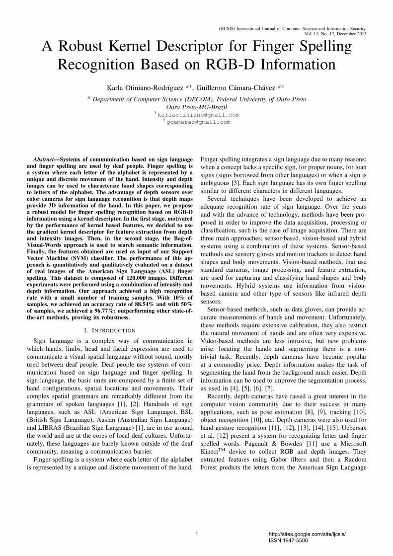
A Robust Kernel Descriptor for Finger SpellingRecognition Based on RGB-D Information
Karla Otiniano-Rodrıguez #1, Guillermo Camara-Chavez #2
# Department of Computer Science (DECOM), Federal University of Ouro PretoOuro Preto-MG-Brazil
1 [email protected] [email protected]
Abstract—Systems of communication based on sign languageand finger spelling are used by deaf people. Finger spelling isa system where each letter of the alphabet is represented by aunique and discrete movement of the hand. Intensity and depthimages can be used to characterize hand shapes correspondingto letters of the alphabet. The advantage of depth sensors overcolor cameras for sign language recognition is that depth mapsprovide 3D information of the hand. In this paper, we proposea robust model for finger spelling recognition based on RGB-Dinformation using a kernel descriptor. In the first stage, motivatedby the performance of kernel based features, we decided to usethe gradient kernel descriptor for feature extraction from depthand intensity images. Then, in the second stage, the Bag-of-Visual-Words approach is used to search semantic information.Finally, the features obtained are used as input of our SupportVector Machine (SVM) classifier. The performance of this ap-proach is quantitatively and qualitatively evaluated on a datasetof real images of the American Sign Language (ASL) fingerspelling. This dataset is composed of 120,000 images. Differentexperiments were performed using a combination of intensity anddepth information. Our approach achieved a high recognitionrate with a small number of training samples. With 10% ofsamples, we achieved an accuracy rate of 88.54% and with 50%of samples, we achieved a 96.77%; outperforming other state-of-the-art methods, proving its robustness.
I. INTRODUCTION
Sign language is a complex way of communication inwhich hands, limbs, head and facial expression are used tocommunicate a visual-spatial language without sound, mostlyused between deaf people. Deaf people use systems of com-munication based on sign language and finger spelling. Insign language, the basic units are composed by a finite set ofhand configurations, spatial locations and movements. Theircomplex spatial grammars are remarkably different from thegrammars of spoken languages [1], [2]. Hundreds of signlanguages, such as ASL (American Sign Language), BSL(British Sign Language), Auslan (Australian Sign Language)and LIBRAS (Brazilian Sign Language) [1], are in use aroundthe world and are at the cores of local deaf cultures. Unfortu-nately, these languages are barely known outside of the deafcommunity, meaning a communication barrier.
Finger spelling is a system where each letter of the alphabetis represented by a unique and discrete movement of the hand.
Finger spelling integrates a sign language due to many reasons:when a concept lacks a specific sign, for proper nouns, for loansigns (signs borrowed from other languages) or when a sign isambiguous [3]. Each sign language has its own finger spellingsimilar to different characters in different languages.
Several techniques have been developed to achieve anadequate recognition rate of sign language. Over the yearsand with the advance of technology, methods have been pro-posed in order to improve the data acquisition, processing orclassification, such is the case of image acquisition. There arethree main approaches: sensor-based, vision-based and hybridsystems using a combination of these systems. Sensor-basedmethods use sensory gloves and motion trackers to detect handshapes and body movements. Vision-based methods, that usestandard cameras, image processing, and feature extraction,are used for capturing and classifying hand shapes and bodymovements. Hybrid systems use information from vision-based camera and other type of sensors like infrared depthsensors.
Sensor-based methods, such as data gloves, can provide ac-curate measurements of hands and movement. Unfortunately,these methods require extensive calibration, they also restrictthe natural movement of hands and are often very expensive.Video-based methods are less intrusive, but new problemsarise: locating the hands and segmenting them is a non-trivial task. Recently, depth cameras have become popularat a commodity price. Depth information makes the task ofsegmenting the hand from the background much easier. Depthinformation can be used to improve the segmentation process,as used in [4], [5], [6], [7].
Recently, depth cameras have raised a great interest in thecomputer vision community due to their success in manyapplications, such as pose estimation [8], [9], tracking [10],object recognition [10], etc. Depth cameras were also used forhand gesture recognition [11], [12], [13], [14], [15]. Uebersaxet al. [12] present a system for recognizing letter and fingerspelled words. Pugeault & Bowden [11] use a MicrosoftKinectTM device to collect RGB and depth images. Theyextracted features using Gabor filters and then a RandomForest predicts the letters from the American Sign Language
1 http://sites.google.com/site/ijcsis/ ISSN 1947-5500
(IJCSIS) International Journal of Computer Science and Information Security,Vol. 11, No. 12, December 2013
(ASL) finger spelling alphabet. Issacs & Foo [16] proposedan ASL finger spelling recognition system based on neuralnetworks applied to wavelets features. Bergh & Van Gool [17]propose a method based on a concatenation of depth and color-segmented images, using a combination of Haar wavelets andneural networks for 6 hand poses recognition of a single user.
In this paper, we propose a framework for finger spellingrecognition using intensity and depth images. Motivated bythe performance of kernel based features, due to its simplicityand the ability to turn any type of pixel attribute into patch-level features, we decided to use the gradient kernel descriptor[18]. The experiments are performed using a public databasecomposed of 120,000 images stating 24 symbols classes [19].The obtained results show that the accuracy obtained by ourmethod, using intensity and depth images, is greater thanonly using intensity or depth images separately. Moreover, theaccuracy obtained by the proposed method performs betterthan the methods proposed in [11], [15]. The results showthat our method is promising.
The remainder of this paper is organized as follows. InSection II, our proposed method is introduced and detailed.The experiments are presented in Section III, where theresults are discussed. Finally, conclusion and future work arepresented in Section IV.
II. PROPOSED MODEL
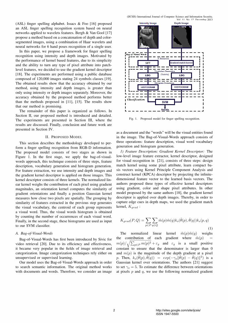
This section describes the methodology developed to per-form a finger spelling recognition from RGB-D information.The proposed model consists of two stages as shown inFigure 1. In the first stage, we apply the bag-of-visual-words approach, this technique consists of three steps, featuredescription, vocabulary generation and histogram generation.For feature extraction, we use intensity and depth images andthe gradient kernel descriptor is applied on those images. Thiskernel descriptor consists of three kernels. The normalized lin-ear kernel weighs the contribution of each pixel using gradientmagnitudes, an orientation kernel computes the similarity ofgradient orientations and finally a position Gaussian kernelmeasures how close two pixels are spatially. The grouping bysimilarity of features extracted in the previous step generatesthe visual vocabulary, the centroid of each group representsa visual word. Thus, the visual words histogram is obtainedby counting the number of occurrences of each visual word.Finally, in the second stage, these histograms are used as inputto our SVM classifier.
A. Bag-of-Visual-Words
Bag-of-Visual-Words has first been introduced by Sivic forvideo retrieval [20]. Due to its efficiency and effectiveness,it became very popular in the fields of image retrieval andcategorization. Image categorization techniques rely either onunsupervised or supervised learning.
Our model uses the Bag-of-Visual-Words approach in orderto search semantic information. The original method workswith documents and words. Therefore, we consider an image
Fig. 1. Proposed model for finger spelling recognition.
as a document and the ”words” will be the visual entities foundin the image. The Bag-of-Visual-Words approach consists ofthree operations: feature description, visual word vocabularygeneration and histogram generation.
1) Feature Description: Gradient Kernel Descriptor: Thelow-level image feature extractor, kernel descriptor, designedfor visual recognition in [21], consists of three steps: designmatch kernel using some pixel attribute, learn compact ba-sis vectors using Kernel Principle Component Analysis andconstruct kernel (KPCA) descriptor by projecting the infinite-dimensional feature vector to the learned basis vectors. Theauthors proposed three types of effective kernel descriptorsusing gradient, color and shape pixel attributes. In othermodel proposed by the same authors [18], the gradient kerneldescriptor is applied over depth images. Thereby, in order tocapture edge cues in depth maps, we used the gradient matchkernel, Kgrad :
Kgrad(P,Q) =∑p∈P
∑q∈Q
m(p)m(q)ko(θ(p), θ(q))ks(p, q)
(1)The normalized linear kernel m(p)m(q) weighs
the contribution of each gradient where m(p) =
m(p)/√∑
p∈P m(p)2 + εg and εg is a small positiveconstant to ensure that the denominator is larger than 0and m(p) is the magnitude of the depth gradient at a pixelp. Then, ko(θ(p), θ(q)) = exp(−γo‖θ(p) − θ(q)‖2) is aGaussian kernel over orientations. The authors [21] suggestto set γo = 5. To estimate the difference between orientationsat pixels p and q, we use the following normalized gradient
2 http://sites.google.com/site/ijcsis/ ISSN 1947-5500

(IJCSIS) International Journal of Computer Science and Information Security,Vol. 11, No. 12, December 2013
vectors in the kernel function ko:
θ(p) = [sin(θ(p))cos(θ(p))]
θ(q) = [sin(θ(q))cos(θ(q))]
where θ(p) is the orientation of the depth gradient at a pixelp. Gaussian position kernel ks(p, q) = exp(−γs‖p − q‖2)with p denoting the 2D position of a pixel in an imagepatch (normalized to [0,1]), measures how close two pixelsare spatially. The value suggest for γs is 3.
To summarize, the gradient match kernel Kgrad consists ofthree kernels: the normalized linear kernel weighs the contri-bution of each pixel using gradient magnitudes; the orientationkernel ko computes the similarity of gradient orientations; andthe position Gaussian kernel ks measures how close two pixelsare spatially.
Match kernels provide a principled way to measure thesimilarity of image patches, but evaluating kernels can becomputationally expensive when image patch are large [21].The corresponding kernel descriptor can be extracted from thismatch kernel by projecting the infinite-dimensional featurevector to a set of finite basis vectors, which are the edgefeatures that we use in the next steps. For more details, theapproach that extracts the compact low-dimensional featuresfrom match kernels is found in [21].
2) Vocabulary Generation: Then, a visual word vocabularyis generated from the feature vectors;s each visual word(codeword) represents a group of several similar features.The visual word vocabulary (codebook) defines a space ofall entities occurring in the image.
3) Histogram Generation: Finally, a histogram of visualwords is created by counting the occurrence of each codeword.These occurrences are counted and arranged in a vector. Eachvector represents the features for an image.
B. Classification
Support vector machines, introduced as a machine learningmethod by Cortes and Vapnik [22], are a useful classificationmethod. Furthermore, SVMs have been successfully appliedin many real world problems and in several areas: text cate-gorization, handwritten digit recognition, object recognition,etc. The SVMs have been developed as a robust tool forclassification and regression in noisy and complex domains.SVM can be used to extract valuable information from datasets and construct fast classification algorithms for massivedata.
An important characteristic of the SVM classifier is to allowa non-linear classification without requiring explicitly a non-linear algorithm thanks to kernel theory.
In kernel framework data points may be mapped into ahigher dimensional feature space, where a separating hyper-plane can be found. We can avoid to explicitly computingthe mapping using the kernel trick which evaluate similar-ities between data K(dt, ds) in the input space. Commonkernel functions are: linear, polynomial, Radial Basis Function(RBF), χ2 distance and triangular.
Fig. 3. Most conflictive similar signs in the dataset.
III. EXPERIMENTS
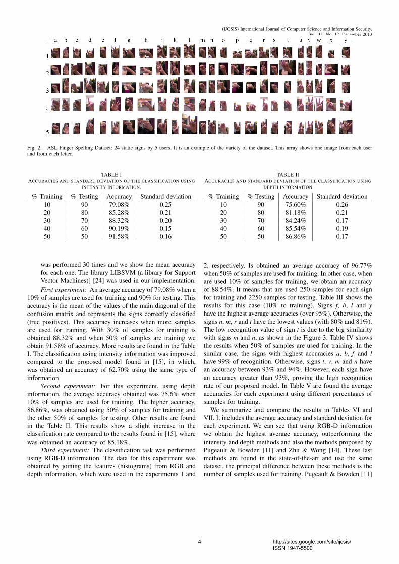
The ASL Finger Spelling Dataset [19] contains 500 samplesfor each of 24 signs, recorded from 5 different persons (non-native to sign language), amounting to a total of 60,000samples. Each sample has a RGB image and a depth image,making a total of 120,000 images. The sign J and Z arenot used, because these signs have motion and the proposedmodel only works with static signs. The dataset has varietyof background and viewing angles. Figure 2 shows someexamples and there is possible to see the variety in size,background and orientation.
Due to the variety in the orientation when the signal isperformed, signs became strongly similar. Figure 3 shows themost similar signs a, e, m, n, s and t. The examples are takenfrom the same user. It is easy to identify the similarity betweenthese signs, all are represented by a closed fist, and differonly by the thumb position, leading to higher confusion levels.Therefore, these signs are the most difficult to differentiate inthe classification task.
In order to validate our technique, we conduct three experi-ments. In the first, a classification of the signs was performedusing different percentages of samples for training and testingfrom intensity information. In the second, a classification wasalso performed from depth information varying the percent-ages of training and testing. Finally, a classification of thesigns was performed using different percentages of samplesfor training and testing from both information (RGB-D).
For each experiment, we have some specifications:• To extract all low level features using gradient kernel
descriptor, are used approximately 12x13 patches overdense regular grid with spacing of 8 pixel (images arenot of uniform size), each patch has a size of 16x16.
• In order to produce the visual word vocabulary, the LBG(Linde-Buzo-Gray) [23] algorithm was used to detect onehundred clusters by taking a sample of 30% from the totalfeatures.
• Moreover, in the classification stage, we use a RBFkernel, whose values for g (gamma) and c (cost) are 0.25and 5, respectively. We also use different percentages ofsamples for training and testing. For example, we use10% of samples for training and the other 90% is used totesting, and this percentage varies up to 50% for training.In order to obtain more precise results, each experiment
3 http://sites.google.com/site/ijcsis/ ISSN 1947-5500
(IJCSIS) International Journal of Computer Science and Information Security,Vol. 11, No. 12, December 2013
Fig. 2. ASL Finger Spelling Dataset: 24 static signs by 5 users. It is an example of the variety of the dataset. This array shows one image from each userand from each letter.
TABLE IACCURACIES AND STANDARD DEVIATION OF THE CLASSIFICATION USING
INTENSITY INFORMATION.
% Training % Testing Accuracy Standard deviation10 90 79.08% 0.2520 80 85.28% 0.2130 70 88.32% 0.2040 60 90.19% 0.1550 50 91.58% 0.16
was performed 30 times and we show the mean accuracyfor each one. The library LIBSVM (a library for SupportVector Machines)] [24] was used in our implementation.First experiment: An average accuracy of 79.08% when a
10% of samples are used for training and 90% for testing. Thisaccuracy is the mean of the values of the main diagonal of theconfusion matrix and represents the signs correctly classified(true positives). This accuracy increases when more samplesare used for training. With 30% of samples for training isobtained 88.32% and when 50% of samples are training weobtain 91.58% of accuracy. More results are found in the TableI. The classification using intensity information was improvedcompared to the proposed model found in [15], in which,was obtained an accuracy of 62.70% using the same type ofinformation.
Second experiment: For this experiment, using depthinformation, the average accuracy obtained was 75.6% when10% of samples are used for training. The higher accuracy,86.86%, was obtained using 50% of samples for training andthe other 50% of samples for testing. Other results are foundin the Table II. This results show a slight increase in theclassification rate compared to the results found in [15], wherewas obtained an accuracy of 85.18%.
Third experiment: The classification task was performedusing RGB-D information. The data for this experiment wasobtained by joining the features (histograms) from RGB anddepth information, which were used in the experiments 1 and
TABLE IIACCURACIES AND STANDARD DEVIATION OF THE CLASSIFICATION USING
DEPTH INFORMATION
% Training % Testing Accuracy Standard deviation10 90 75.60% 0.2620 80 81.18% 0.2130 70 84.24% 0.1740 60 85.54% 0.1950 50 86.86% 0.17
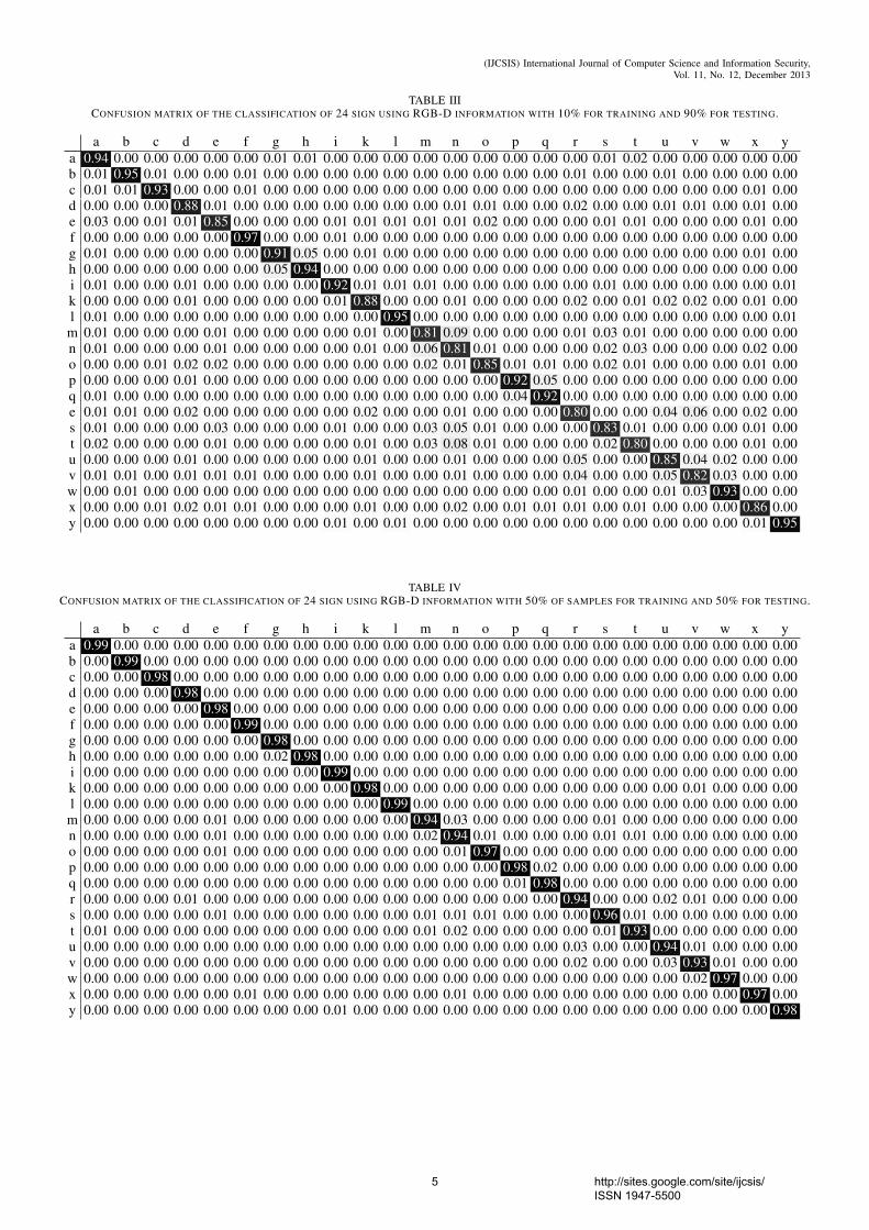
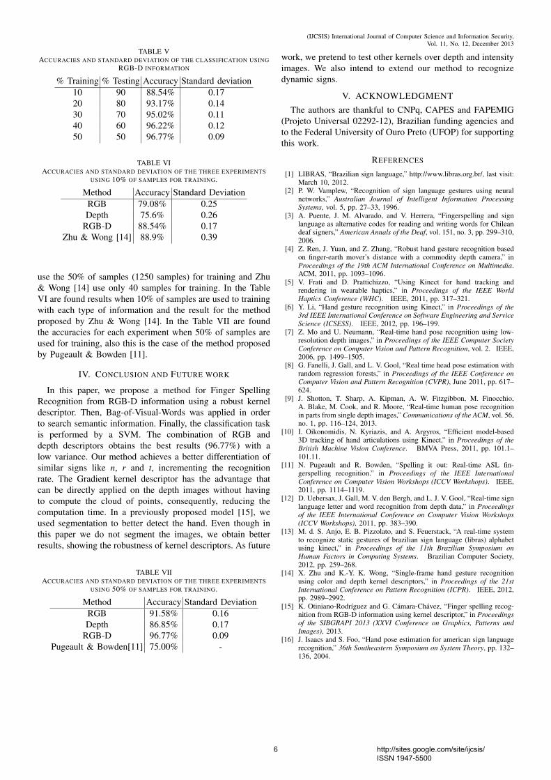
2, respectively. Is obtained an average accuracy of 96.77%when 50% of samples are used for training. In other case, whenare used 10% of samples for training, we obtain an accuracyof 88.54%. It means that are used 250 samples for each signfor training and 2250 samples for testing. Table III shows theresults for this case (10% to training). Signs f, b, l and yhave the highest average accuracies (over 95%). Otherwise, thesigns n, m, r and t have the lowest values (with 80% and 81%).The low recognition value of sign t is due to the big similaritywith signs m and n, as shown in the Figure 3. Table IV showsthe results when 50% of samples are used for training. In thesimilar case, the signs with highest accuracies a, b, f and lhave 99% of recognition. Otherwise, signs t, v, m and n havean accuracy between 93% and 94%. However, each sign havean accuracy greater than 93%, proving the high recognitionrate of our proposed model. In Table V are found the averageaccuracies for each experiment using different percentages ofsamples for training.
We summarize and compare the results in Tables VI andVII. It includes the average accuracy and standard deviation foreach experiment. We can see that using RGB-D informationwe obtain the highest average accuracy, outperforming theintensity and depth methods and also the methods proposed byPugeault & Bowden [11] and Zhu & Wong [14]. These lastmethods are found in the state-of-the-art and use the samedataset, the principal difference between these methods is thenumber of samples used for training. Pugeault & Bowden [11]
4 http://sites.google.com/site/ijcsis/ ISSN 1947-5500
(IJCSIS) International Journal of Computer Science and Information Security,Vol. 11, No. 12, December 2013
TABLE IIICONFUSION MATRIX OF THE CLASSIFICATION OF 24 SIGN USING RGB-D INFORMATION WITH 10% FOR TRAINING AND 90% FOR TESTING.
a b c d e f g h i k l m n o p q r s t u v w x ya 0.94 0.00 0.00 0.00 0.00 0.00 0.01 0.01 0.00 0.00 0.00 0.00 0.00 0.00 0.00 0.00 0.00 0.01 0.02 0.00 0.00 0.00 0.00 0.00b 0.01 0.95 0.01 0.00 0.00 0.01 0.00 0.00 0.00 0.00 0.00 0.00 0.00 0.00 0.00 0.00 0.01 0.00 0.00 0.01 0.00 0.00 0.00 0.00c 0.01 0.01 0.93 0.00 0.00 0.01 0.00 0.00 0.00 0.00 0.00 0.00 0.00 0.00 0.00 0.00 0.00 0.00 0.00 0.00 0.00 0.00 0.01 0.00d 0.00 0.00 0.00 0.88 0.01 0.00 0.00 0.00 0.00 0.00 0.00 0.00 0.01 0.01 0.00 0.00 0.02 0.00 0.00 0.01 0.01 0.00 0.01 0.00e 0.03 0.00 0.01 0.01 0.85 0.00 0.00 0.00 0.01 0.01 0.01 0.01 0.01 0.02 0.00 0.00 0.00 0.01 0.01 0.00 0.00 0.00 0.01 0.00f 0.00 0.00 0.00 0.00 0.00 0.97 0.00 0.00 0.01 0.00 0.00 0.00 0.00 0.00 0.00 0.00 0.00 0.00 0.00 0.00 0.00 0.00 0.00 0.00g 0.01 0.00 0.00 0.00 0.00 0.00 0.91 0.05 0.00 0.01 0.00 0.00 0.00 0.00 0.00 0.00 0.00 0.00 0.00 0.00 0.00 0.00 0.01 0.00h 0.00 0.00 0.00 0.00 0.00 0.00 0.05 0.94 0.00 0.00 0.00 0.00 0.00 0.00 0.00 0.00 0.00 0.00 0.00 0.00 0.00 0.00 0.00 0.00i 0.01 0.00 0.00 0.01 0.00 0.00 0.00 0.00 0.92 0.01 0.01 0.01 0.00 0.00 0.00 0.00 0.00 0.01 0.00 0.00 0.00 0.00 0.00 0.01k 0.00 0.00 0.00 0.01 0.00 0.00 0.00 0.00 0.01 0.88 0.00 0.00 0.01 0.00 0.00 0.00 0.02 0.00 0.01 0.02 0.02 0.00 0.01 0.00l 0.01 0.00 0.00 0.00 0.00 0.00 0.00 0.00 0.00 0.00 0.95 0.00 0.00 0.00 0.00 0.00 0.00 0.00 0.00 0.00 0.00 0.00 0.00 0.01
m 0.01 0.00 0.00 0.00 0.01 0.00 0.00 0.00 0.00 0.01 0.00 0.81 0.09 0.00 0.00 0.00 0.01 0.03 0.01 0.00 0.00 0.00 0.00 0.00n 0.01 0.00 0.00 0.00 0.01 0.00 0.00 0.00 0.00 0.01 0.00 0.06 0.81 0.01 0.00 0.00 0.00 0.02 0.03 0.00 0.00 0.00 0.02 0.00o 0.00 0.00 0.01 0.02 0.02 0.00 0.00 0.00 0.00 0.00 0.00 0.02 0.01 0.85 0.01 0.01 0.00 0.02 0.01 0.00 0.00 0.00 0.01 0.00p 0.00 0.00 0.00 0.01 0.00 0.00 0.00 0.00 0.00 0.00 0.00 0.00 0.00 0.00 0.92 0.05 0.00 0.00 0.00 0.00 0.00 0.00 0.00 0.00q 0.01 0.00 0.00 0.00 0.00 0.00 0.00 0.00 0.00 0.00 0.00 0.00 0.00 0.00 0.04 0.92 0.00 0.00 0.00 0.00 0.00 0.00 0.00 0.00e 0.01 0.01 0.00 0.02 0.00 0.00 0.00 0.00 0.00 0.02 0.00 0.00 0.01 0.00 0.00 0.00 0.80 0.00 0.00 0.04 0.06 0.00 0.02 0.00s 0.01 0.00 0.00 0.00 0.03 0.00 0.00 0.00 0.01 0.00 0.00 0.03 0.05 0.01 0.00 0.00 0.00 0.83 0.01 0.00 0.00 0.00 0.01 0.00t 0.02 0.00 0.00 0.00 0.01 0.00 0.00 0.00 0.00 0.01 0.00 0.03 0.08 0.01 0.00 0.00 0.00 0.02 0.80 0.00 0.00 0.00 0.01 0.00u 0.00 0.00 0.00 0.01 0.00 0.00 0.00 0.00 0.00 0.01 0.00 0.00 0.01 0.00 0.00 0.00 0.05 0.00 0.00 0.85 0.04 0.02 0.00 0.00v 0.01 0.01 0.00 0.01 0.01 0.01 0.00 0.00 0.00 0.01 0.00 0.00 0.01 0.00 0.00 0.00 0.04 0.00 0.00 0.05 0.82 0.03 0.00 0.00w 0.00 0.01 0.00 0.00 0.00 0.00 0.00 0.00 0.00 0.00 0.00 0.00 0.00 0.00 0.00 0.00 0.01 0.00 0.00 0.01 0.03 0.93 0.00 0.00x 0.00 0.00 0.01 0.02 0.01 0.01 0.00 0.00 0.00 0.01 0.00 0.00 0.02 0.00 0.01 0.01 0.01 0.00 0.01 0.00 0.00 0.00 0.86 0.00y 0.00 0.00 0.00 0.00 0.00 0.00 0.00 0.00 0.01 0.00 0.01 0.00 0.00 0.00 0.00 0.00 0.00 0.00 0.00 0.00 0.00 0.00 0.01 0.95
TABLE IVCONFUSION MATRIX OF THE CLASSIFICATION OF 24 SIGN USING RGB-D INFORMATION WITH 50% OF SAMPLES FOR TRAINING AND 50% FOR TESTING.
a b c d e f g h i k l m n o p q r s t u v w x ya 0.99 0.00 0.00 0.00 0.00 0.00 0.00 0.00 0.00 0.00 0.00 0.00 0.00 0.00 0.00 0.00 0.00 0.00 0.00 0.00 0.00 0.00 0.00 0.00b 0.00 0.99 0.00 0.00 0.00 0.00 0.00 0.00 0.00 0.00 0.00 0.00 0.00 0.00 0.00 0.00 0.00 0.00 0.00 0.00 0.00 0.00 0.00 0.00c 0.00 0.00 0.98 0.00 0.00 0.00 0.00 0.00 0.00 0.00 0.00 0.00 0.00 0.00 0.00 0.00 0.00 0.00 0.00 0.00 0.00 0.00 0.00 0.00d 0.00 0.00 0.00 0.98 0.00 0.00 0.00 0.00 0.00 0.00 0.00 0.00 0.00 0.00 0.00 0.00 0.00 0.00 0.00 0.00 0.00 0.00 0.00 0.00e 0.00 0.00 0.00 0.00 0.98 0.00 0.00 0.00 0.00 0.00 0.00 0.00 0.00 0.00 0.00 0.00 0.00 0.00 0.00 0.00 0.00 0.00 0.00 0.00f 0.00 0.00 0.00 0.00 0.00 0.99 0.00 0.00 0.00 0.00 0.00 0.00 0.00 0.00 0.00 0.00 0.00 0.00 0.00 0.00 0.00 0.00 0.00 0.00g 0.00 0.00 0.00 0.00 0.00 0.00 0.98 0.00 0.00 0.00 0.00 0.00 0.00 0.00 0.00 0.00 0.00 0.00 0.00 0.00 0.00 0.00 0.00 0.00h 0.00 0.00 0.00 0.00 0.00 0.00 0.02 0.98 0.00 0.00 0.00 0.00 0.00 0.00 0.00 0.00 0.00 0.00 0.00 0.00 0.00 0.00 0.00 0.00i 0.00 0.00 0.00 0.00 0.00 0.00 0.00 0.00 0.99 0.00 0.00 0.00 0.00 0.00 0.00 0.00 0.00 0.00 0.00 0.00 0.00 0.00 0.00 0.00k 0.00 0.00 0.00 0.00 0.00 0.00 0.00 0.00 0.00 0.98 0.00 0.00 0.00 0.00 0.00 0.00 0.00 0.00 0.00 0.00 0.01 0.00 0.00 0.00l 0.00 0.00 0.00 0.00 0.00 0.00 0.00 0.00 0.00 0.00 0.99 0.00 0.00 0.00 0.00 0.00 0.00 0.00 0.00 0.00 0.00 0.00 0.00 0.00
m 0.00 0.00 0.00 0.00 0.01 0.00 0.00 0.00 0.00 0.00 0.00 0.94 0.03 0.00 0.00 0.00 0.00 0.01 0.00 0.00 0.00 0.00 0.00 0.00n 0.00 0.00 0.00 0.00 0.01 0.00 0.00 0.00 0.00 0.00 0.00 0.02 0.94 0.01 0.00 0.00 0.00 0.01 0.01 0.00 0.00 0.00 0.00 0.00o 0.00 0.00 0.00 0.00 0.01 0.00 0.00 0.00 0.00 0.00 0.00 0.00 0.01 0.97 0.00 0.00 0.00 0.00 0.00 0.00 0.00 0.00 0.00 0.00p 0.00 0.00 0.00 0.00 0.00 0.00 0.00 0.00 0.00 0.00 0.00 0.00 0.00 0.00 0.98 0.02 0.00 0.00 0.00 0.00 0.00 0.00 0.00 0.00q 0.00 0.00 0.00 0.00 0.00 0.00 0.00 0.00 0.00 0.00 0.00 0.00 0.00 0.00 0.01 0.98 0.00 0.00 0.00 0.00 0.00 0.00 0.00 0.00r 0.00 0.00 0.00 0.01 0.00 0.00 0.00 0.00 0.00 0.00 0.00 0.00 0.00 0.00 0.00 0.00 0.94 0.00 0.00 0.02 0.01 0.00 0.00 0.00s 0.00 0.00 0.00 0.00 0.01 0.00 0.00 0.00 0.00 0.00 0.00 0.01 0.01 0.01 0.00 0.00 0.00 0.96 0.01 0.00 0.00 0.00 0.00 0.00t 0.01 0.00 0.00 0.00 0.00 0.00 0.00 0.00 0.00 0.00 0.00 0.01 0.02 0.00 0.00 0.00 0.00 0.01 0.93 0.00 0.00 0.00 0.00 0.00u 0.00 0.00 0.00 0.00 0.00 0.00 0.00 0.00 0.00 0.00 0.00 0.00 0.00 0.00 0.00 0.00 0.03 0.00 0.00 0.94 0.01 0.00 0.00 0.00v 0.00 0.00 0.00 0.00 0.00 0.00 0.00 0.00 0.00 0.00 0.00 0.00 0.00 0.00 0.00 0.00 0.02 0.00 0.00 0.03 0.93 0.01 0.00 0.00w 0.00 0.00 0.00 0.00 0.00 0.00 0.00 0.00 0.00 0.00 0.00 0.00 0.00 0.00 0.00 0.00 0.00 0.00 0.00 0.00 0.02 0.97 0.00 0.00x 0.00 0.00 0.00 0.00 0.00 0.01 0.00 0.00 0.00 0.00 0.00 0.00 0.01 0.00 0.00 0.00 0.00 0.00 0.00 0.00 0.00 0.00 0.97 0.00y 0.00 0.00 0.00 0.00 0.00 0.00 0.00 0.00 0.01 0.00 0.00 0.00 0.00 0.00 0.00 0.00 0.00 0.00 0.00 0.00 0.00 0.00 0.00 0.98
5 http://sites.google.com/site/ijcsis/ ISSN 1947-5500
(IJCSIS) International Journal of Computer Science and Information Security,Vol. 11, No. 12, December 2013
TABLE VACCURACIES AND STANDARD DEVIATION OF THE CLASSIFICATION USING
RGB-D INFORMATION
% Training % Testing Accuracy Standard deviation10 90 88.54% 0.1720 80 93.17% 0.1430 70 95.02% 0.1140 60 96.22% 0.1250 50 96.77% 0.09
TABLE VIACCURACIES AND STANDARD DEVIATION OF THE THREE EXPERIMENTS
USING 10% OF SAMPLES FOR TRAINING.
Method Accuracy Standard DeviationRGB 79.08% 0.25Depth 75.6% 0.26
RGB-D 88.54% 0.17Zhu & Wong [14] 88.9% 0.39
use the 50% of samples (1250 samples) for training and Zhu& Wong [14] use only 40 samples for training. In the TableVI are found results when 10% of samples are used to trainingwith each type of information and the result for the methodproposed by Zhu & Wong [14]. In the Table VII are foundthe accuracies for each experiment when 50% of samples areused for training, also this is the case of the method proposedby Pugeault & Bowden [11].
IV. CONCLUSION AND FUTURE WORK
In this paper, we propose a method for Finger SpellingRecognition from RGB-D information using a robust kerneldescriptor. Then, Bag-of-Visual-Words was applied in orderto search semantic information. Finally, the classification taskis performed by a SVM. The combination of RGB anddepth descriptors obtains the best results (96.77%) with alow variance. Our method achieves a better differentiation ofsimilar signs like n, r and t, incrementing the recognitionrate. The Gradient kernel descriptor has the advantage thatcan be directly applied on the depth images without havingto compute the cloud of points, consequently, reducing thecomputation time. In a previously proposed model [15], weused segmentation to better detect the hand. Even though inthis paper we do not segment the images, we obtain betterresults, showing the robustness of kernel descriptors. As future
TABLE VIIACCURACIES AND STANDARD DEVIATION OF THE THREE EXPERIMENTS
USING 50% OF SAMPLES FOR TRAINING.
Method Accuracy Standard DeviationRGB 91.58% 0.16Depth 86.85% 0.17
RGB-D 96.77% 0.09Pugeault & Bowden[11] 75.00% -
work, we pretend to test other kernels over depth and intensityimages. We also intend to extend our method to recognizedynamic signs.
V. ACKNOWLEDGMENTThe authors are thankful to CNPq, CAPES and FAPEMIG
(Projeto Universal 02292-12), Brazilian funding agencies andto the Federal University of Ouro Preto (UFOP) for supportingthis work.
REFERENCES
[1] LIBRAS, “Brazilian sign language,” http://www.libras.org.br/, last visit:March 10, 2012.
[2] P. W. Vamplew, “Recognition of sign language gestures using neuralnetworks,” Australian Journal of Intelligent Information ProcessingSystems, vol. 5, pp. 27–33, 1996.
[3] A. Puente, J. M. Alvarado, and V. Herrera, “Fingerspelling and signlanguage as alternative codes for reading and writing words for Chileandeaf signers,” American Annals of the Deaf, vol. 151, no. 3, pp. 299–310,2006.
[4] Z. Ren, J. Yuan, and Z. Zhang, “Robust hand gesture recognition basedon finger-earth mover’s distance with a commodity depth camera,” inProceedings of the 19th ACM International Conference on Multimedia.ACM, 2011, pp. 1093–1096.
[5] V. Frati and D. Prattichizzo, “Using Kinect for hand tracking andrendering in wearable haptics,” in Proceedings of the IEEE WorldHaptics Conference (WHC). IEEE, 2011, pp. 317–321.
[6] Y. Li, “Hand gesture recognition using Kinect,” in Proceedings of the3rd IEEE International Conference on Software Engineering and ServiceScience (ICSESS). IEEE, 2012, pp. 196–199.
[7] Z. Mo and U. Neumann, “Real-time hand pose recognition using low-resolution depth images,” in Proceedings of the IEEE Computer SocietyConference on Computer Vision and Pattern Recognition, vol. 2. IEEE,2006, pp. 1499–1505.
[8] G. Fanelli, J. Gall, and L. V. Gool, “Real time head pose estimation withrandom regression forests,” in Proceedings of the IEEE Conference onComputer Vision and Pattern Recognition (CVPR), June 2011, pp. 617–624.
[9] J. Shotton, T. Sharp, A. Kipman, A. W. Fitzgibbon, M. Finocchio,A. Blake, M. Cook, and R. Moore, “Real-time human pose recognitionin parts from single depth images,” Communications of the ACM, vol. 56,no. 1, pp. 116–124, 2013.
[10] I. Oikonomidis, N. Kyriazis, and A. Argyros, “Efficient model-based3D tracking of hand articulations using Kinect,” in Proceedings of theBritish Machine Vision Conference. BMVA Press, 2011, pp. 101.1–101.11.
[11] N. Pugeault and R. Bowden, “Spelling it out: Real-time ASL fin-gerspelling recognition.” in Proceedings of the IEEE InternationalConference on Computer Vision Workshops (ICCV Workshops). IEEE,2011, pp. 1114–1119.
[12] D. Uebersax, J. Gall, M. V. den Bergh, and L. J. V. Gool, “Real-time signlanguage letter and word recognition from depth data,” in Proceedingsof the IEEE International Conference on Computer Vision Workshops(ICCV Workshops), 2011, pp. 383–390.
[13] M. d. S. Anjo, E. B. Pizzolato, and S. Feuerstack, “A real-time systemto recognize static gestures of brazilian sign language (libras) alphabetusing kinect,” in Proceedings of the 11th Brazilian Symposium onHuman Factors in Computing Systems. Brazilian Computer Society,2012, pp. 259–268.
[14] X. Zhu and K.-Y. K. Wong, “Single-frame hand gesture recognitionusing color and depth kernel descriptors,” in Proceedings of the 21stInternational Conference on Pattern Recognition (ICPR). IEEE, 2012,pp. 2989–2992.
[15] K. Otiniano-Rodrıguez and G. Camara-Chavez, “Finger spelling recog-nition from RGB-D information using kernel descriptor,” in Proceedingsof the SIBGRAPI 2013 (XXVI Conference on Graphics, Patterns andImages), 2013.
[16] J. Isaacs and S. Foo, “Hand pose estimation for american sign languagerecognition,” 36th Southeastern Symposium on System Theory, pp. 132–136, 2004.
6 http://sites.google.com/site/ijcsis/ ISSN 1947-5500
(IJCSIS) International Journal of Computer Science and Information Security,Vol. 11, No. 12, December 2013
[17] M. Van den Bergh and L. Van Gool, “Combining RGB and ToF camerasfor real-time 3D hand gesture interaction,” in Proceedings of the IEEEWorkshop on Applications of Computer Vision (WACV), ser. WACV ’11.Washington, DC, USA: IEEE Computer Society, 2011, pp. 66–72.
[18] L. Bo, X. Ren, and D. Fox, “Depth kernel descriptors for objectrecognition,” in Proceedings of the IEEE International Conference onIntelligent Robots and Systems (IROS). IEEE, 2011, pp. 821–826.
[19] R. B. Nicolas Pugeault, “ASL finger spelling dataset,”http://personal.ee.surrey.ac.uk/Personal/N.Pugeault/index.php, lastvisit: April 29, 2013.
[20] J. Sivic and A. Zisserman, “Video google: A text retrieval approachto object matching in videos,” in Proceedings of the Ninth IEEEInternational Conference on Computer Vision. IEEE, 2003, pp. 1470–1477.
[21] L. Bo, X. Ren, and D. Fox, “Kernel descriptors for visual recognition,”Advances in Neural Information Processing Systems, vol. 7, 2010.
[22] C. Cortes and V. Vapnik, “Support-vector networks,” Machine Learning,vol. 20, no. 3, pp. 273–297, 1995.
[23] Y. Linde, A. Buzo, and R. Gray, “An algorithm for vector quantizerdesign,” IEEE Transactions on Communications, vol. 28, no. 1, pp. 84–95, 1980.
[24] C.-C. Chang and C.-J. Lin, “LIBSVM: A library for supportvector machines,” ACM Transactions on Intelligent Systems andTechnology, vol. 2, no. 3, pp. 1–27, 2011, software available athttp://www.csie.ntu.edu.tw/ cjlin/libsvm.
7 http://sites.google.com/site/ijcsis/ ISSN 1947-5500

(IJCSIS) International Journal of Computer Science and Information Security, Vol. 11, No. 12, 2013
A novel non-Shannon edge detection algorithm for noisy images
El-Owny, Hassan Badry Mohamed A.
Department of Mathematics, Faculty of Science ,Aswan University , 81528 Aswan, Egypt. Current: CIT College, Taif University, 21974 Taif, KSA.
.
Abstract— Edge detection is an important preprocessing step in image analysis. Successful results of image analysis extremely depend on edge detection. Up to now several edge detection methods have been developed such as Prewitt, Sobel, Zero-crossing, Canny, etc. But, they are sensitive to noise. This paper proposes a novel edge detection algorithm for images corrupted with noise. The algorithm finds the edges by eliminating the noise from the image so that the correct edges are determined. The edges of the noise image are determined using non-Shannon measures of entropy. The proposed method is tested under noisy conditions on several images and also compared with conventional edge detectors such as Sobel and Canny edge detector. Experimental results reveal that the proposed method exhibits better performance and may efficiently be used for the detection of edges in images corrupted by Salt-and-Pepper noise. Keywords -Non-Shannon Entropy ; Edge Detection; Threshold Value ; Noisy images.
I. INTRODUCTION
Edge detection has been used extensively in areas related to image and signal processing. Its use includes pattern recognition, image segmentation, and scene analysis. The edges are also use to locate the objects in an image and measure their geometrical features. Hence, edge detection is an important identification and classification tool in computer vision. This topic has attracted many researchers and several achievements have been made to investigate new and more robust techniques .
Natural images are prone to noise and artifacts. Salt and pepper noise is a form of noise typically seen on images. It is typically manifested as randomly occurring white and black pixels. Salt and pepper noise creeps into images in situations where quick transients, such as faulty switching, take place. On the other hand, White noise is additive in nature where the each pixel in the image is modified via the addition of a value drawn from a Gaussian distribution. To test the generality of the results, the proposed edge detection algorithm was tested on images containing both these types of noise.
A large number of studies have been published in the field of image edge detection[1-16], which attests to its importance within the field of image processing. Many edge detection algorithms have been proposed, each of which has its own strengths and weaknesses; for this reason, hitherto there does not appear to be a single "best" edge detector. A good edge
detector should be able to detect the edge for any type of image and should show higher resistance to noise.
Examples of approaches to edge detection include algorithms such as the Sobel and Prewitt edge detectors which are based on the first order derivative of the pixel intensities[1]. The Laplacian-of-Gaussian (LoG) edge detector is another popular technique, using instead the second order differential operators to detect the location of edges [2,17,18]. However, all of these algorithms tend to be sensitive to noise, which is an intrinsically high frequency phenomenon. To solve this problem the Canny edge detector was proposed, which combines a smoothing function with zero crossing based edge detection [3]. Although it is more resilient to noise than the previously mentioned algorithms, its performance is still not satisfactory when the noise level is high. There are many situations where sharp changes in color intensity do not correspond to object boundaries like surface marking, recording noise and uneven lighting conditions [4-7,19-22]
In this paper we present a new approach to detect edges of gray scale noisy images based on information theory, which is entropy based thresholding. The proposed method is decrease the computation time as possible as can and the results were very good compared with the other methods.
The paper is organized as follows: Section 2 describes in brief the basic concepts of Shannon and non-Shannon entropies. Section 3 is devoted to the proposed method of edge detection. In Section 4, the details of the edge detection algorithm is described. In Section 5, some particular images will be analyzed using proposed method based algorithm and moreover, a comparison with some existing methods will be provided for these images. Finally, conclusions will be drawn in Section 6.
II. BASIC CONCEPT OF ENTROPY
Physically Entropy can be associated with the amount of disorder in a physical system. In[23] Shannon redefined the entropy concept of Boltzmann/Gibbs as a measure of uncertainty regarding the information content of a system. He defined an expression for measuring quantitatively the amount of information produced by a process.
In accordance with this definition, a random event that occurs with probability is said to contain ln 1⁄ ln units of information. The amount
is called the self-information of event . The amount of
8 http://sites.google.com/site/ijcsis/ ISSN 1947-5500
(IJCSIS) International Journal of Computer Science and Information Security, Vol. 11, No. 12, 2013
self information of the event is inversely proportional to its probability. If 1, then 0 and no information is attributed to it. In this case, uncertainty associated with the event is zero. Thus, if the event always occurs, then no information would be transferred by communicating that the event has occurred. If 0.8 , then some information would be transferred by communicating that the event has occurred[24].
The basic concept of entropy in information theory has to do with how much randomness is in a signal or in a random event. An alternative way to look at this is to talk about how much information is carried by the signal [25]. Entropy is a measure of randomness.
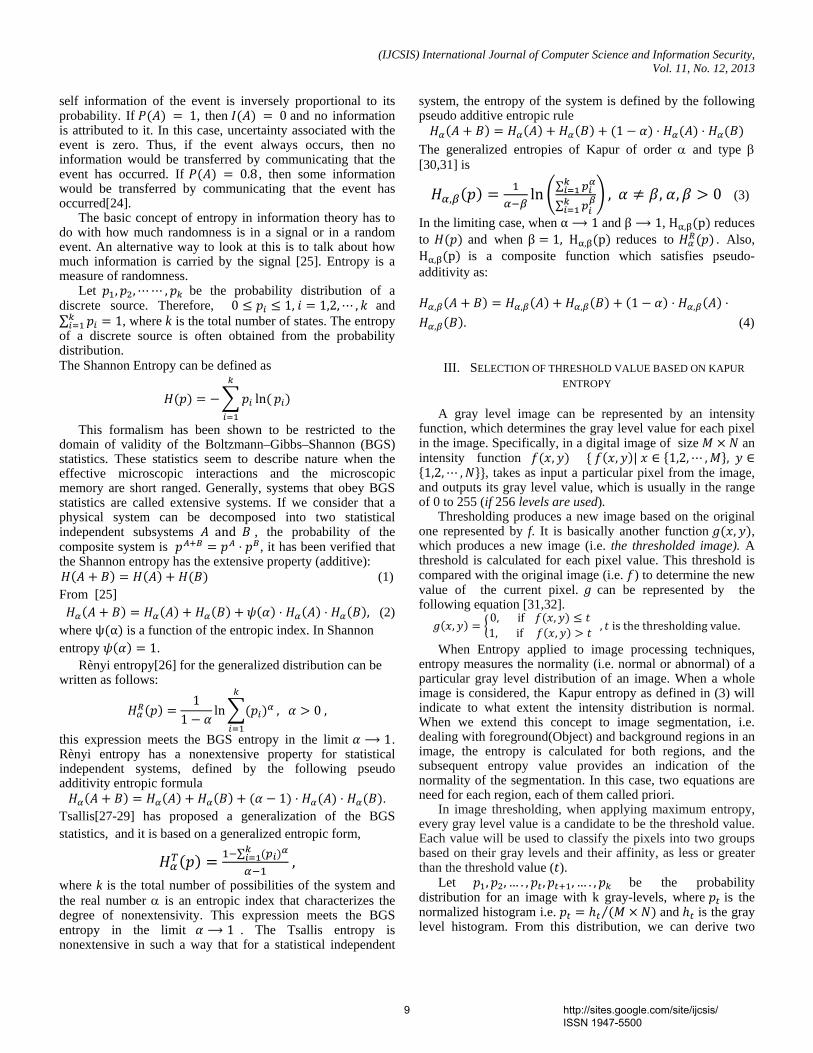
Let , , , be the probability distribution of a discrete source. Therefore, 0 1, 1,2, , and ∑ 1, where k is the total number of states. The entropy of a discrete source is often obtained from the probability distribution. The Shannon Entropy can be defined as
ln
This formalism has been shown to be restricted to the domain of validity of the Boltzmann–Gibbs–Shannon (BGS) statistics. These statistics seem to describe nature when the effective microscopic interactions and the microscopic memory are short ranged. Generally, systems that obey BGS statistics are called extensive systems. If we consider that a physical system can be decomposed into two statistical independent subsystems and , the probability of the composite system is , it has been verified that the Shannon entropy has the extensive property (additive):
(1) From [25] , (2) where ψ α is a function of the entropic index. In Shannon entropy 1.
Rènyi entropy[26] for the generalized distribution can be written as follows:
11
ln , 0 ,
this expression meets the BGS entropy in the limit 1. Rènyi entropy has a nonextensive property for statistical independent systems, defined by the following pseudo additivity entropic formula
1 . Tsallis[27-29] has proposed a generalization of the BGS statistics, and it is based on a generalized entropic form,
∑ , where k is the total number of possibilities of the system and the real number α is an entropic index that characterizes the degree of nonextensivity. This expression meets the BGS entropy in the limit 1 . The Tsallis entropy is nonextensive in such a way that for a statistical independent
system, the entropy of the system is defined by the following pseudo additive entropic rule
1
The generalized entropies of Kapur of order α and type β [30,31] is
, ln ∑
∑, , , 0 (3)
In the limiting case, when α 1 and β 1, H , p reduces to and when β 1, H , p reduces to . Also, H , p is a composite function which satisfies pseudo-additivity as:
, , , 1 ,
, . (4)
III. SELECTION OF THRESHOLD VALUE BASED ON KAPUR
ENTROPY
A gray level image can be represented by an intensity function, which determines the gray level value for each pixel in the image. Specifically, in a digital image of size an intensity function , , | 1,2, , , 1,2, , , takes as input a particular pixel from the image,
and outputs its gray level value, which is usually in the range of 0 to 255 (if 256 levels are used).
Thresholding produces a new image based on the original one represented by f. It is basically another function , , which produces a new image (i.e. the thresholded image). A threshold is calculated for each pixel value. This threshold is compared with the original image (i.e. ) to determine the new value of the current pixel. can be represented by the following equation [31,32].
,0, if ,1, if , , is the thresholding value.
When Entropy applied to image processing techniques, entropy measures the normality (i.e. normal or abnormal) of a particular gray level distribution of an image. When a whole image is considered, the Kapur entropy as defined in (3) will indicate to what extent the intensity distribution is normal. When we extend this concept to image segmentation, i.e. dealing with foreground(Object) and background regions in an image, the entropy is calculated for both regions, and the subsequent entropy value provides an indication of the normality of the segmentation. In this case, two equations are need for each region, each of them called priori.
In image thresholding, when applying maximum entropy, every gray level value is a candidate to be the threshold value. Each value will be used to classify the pixels into two groups based on their gray levels and their affinity, as less or greater than the threshold value ( ).
Let , , … . , , , … . , be the probability distribution for an image with k gray-levels, where is the normalized histogram i.e. ⁄ and is the gray level histogram. From this distribution, we can derive two
9 http://sites.google.com/site/ijcsis/ ISSN 1947-5500
(IJCSIS) International Journal of Computer Science and Information Security, Vol. 11, No. 12, 2013
probability distributions, one for the object (class A) and the other for the background (class B), are shown as follows:
: , , … . . , ,
(5)
: , , … . . , ,
where ∑ , ∑ , t is the threshold value. (6)
In terms of the definition of Kapur entropy of order and type , the entropy of Object pixels and the entropy
of background pixels can be defined as follows:
,1
ln∑
∑, , , 0
(7)
,1
ln∑
∑, , , 0 .
The Kapur entropy , is parametrically dependent upon the threshold value for the object and background. It is formulated as the sum each entropy, allowing the pseudo-additive property for statistically independent systems, as defined in (4). We try to maximize the information measure between the two classes (object and background). When
, is maximized, the luminance level that maximizes the function is considered to be the optimum threshold value. This can be achieved with a cheap computational effort.
Argmax , , 1 · , · , . (8) When 1 and 1 , the threshold value in (4),
equals to the same value found by Shannon Entropy. Thus this proposed method includes Shannon’s method as a special case. The following expression can be used as a criterion function to obtain the optimal threshold at 1 and 1.
Argmax , , . (9)
Now, we can describe the Kapur Threshold algorithm to determine a suitable threshold value and α and β as follows:
II. if 0 1 and 0 1 then
Apply Equation (8) to calculate optimum threshold value .
else Apply Equation (9) to calculate optimum threshold value .
end-if 5. Output: The suitable threshold value of I, FOR
, 0,
IV. PROPOSED ALGORITHM FOR EDGE DETECTION
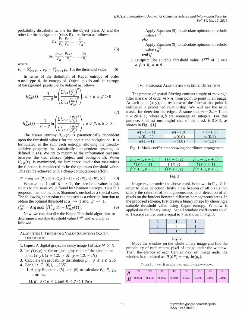
The process of spatial filtering consists simply of moving a filter mask w of order from point to point in an image. At each point , , the response of the filter at that point is calculated a predefined relationship. We will use the usual masks for detection the edges. Assume that 2 1 and
2 1 , where , are nonnegative integers. For this purpose, smallest meaningful size of the mask is 3 3 , as shown in Fig. 1[1].
1, 1 1,0 1, 10, 1 0,0 0,11, 1 1,0 1,1
Fig. 1: Mask coefficients showing coordinate arrangement
1, 1 1, 1, 1 , 1 , , 11, 1 1, 1, 1
Fig. 2
Image region under the above mask is shown in Fig. 2. In order to edge detection, firstly classification of all pixels that satisfy the criterion of homogeneousness, and detection of all pixels on the borders between different homogeneous areas. In the proposed scheme, first create a binary image by choosing a suitable threshold value using Kapur entropy. Window is applied on the binary image. Set all window coefficients equal to 1 except centre, centre equal to × as shown in Fig. 3.
1 1 1 1 × 1 1 1 1
Fig. 3 Move the window on the whole binary image and find the
probability of each central pixel of image under the window. Then, the entropy of each Central Pixel of image under the window is calculated as ln .
TABLE I . P AND H OF CENTRAL PIXEL UNDER WINDOW. 1/9 2/9 3/9 4/9 5/9 6/9 7/9 8/9
0.2441 0.3342 0.3662 0.3604 0.3265 0.2703 0.1955 0.1047
ALGORITHM 1: THRESHOLD VALUE SELECTION (KAPUR
THRESHOLD)
1. Input: A digital grayscale noisy image I of size . 2. Let , be the original gray value of the pixel at the
point , , 1,2, , , 1,2, , 3. Calculate the probability distribution , 0 255 4. For all 0,1, … ,255 ,
I. Apply Equations (5) and (6) to calculate , , and
10 http://sites.google.com/site/ijcsis/ ISSN 1947-5500
(IJCSIS) International Journal of Computer Science and Information Security, Vol. 11, No. 12, 2013
where, is the probability of central pixel of binary image under the window. When the probability of central pixel
1 then the entropy of this pixel is zero. Thus, if the gray level of all pixels under the window homogeneous, then
1 and 0. In this case, the central pixel is not an edge pixel. Other possibilities of entropy of central pixel under window are shown in Table 1.
In cases 8/9, and 7/9, the diversity for gray level of pixels under the window is low. So, in these cases, central pixel is not an edge pixel. In remaining cases, 6/9, the diversity for gray level of pixels under the window is high. So, for these cases, central pixel is an edge pixel. Thus, the central pixel with entropy greater than and equal to 0.2441 is an edge pixel, otherwise not.
The following Algorithm summarize the proposed technique for calculating the optimal threshold values and the edge detector.
The steps of our proposed technique are as follows: Step 1: Find global threshold value ( ) using Kapur entropy .
The image is segmented by into two parts, the object (Part1) and the background (Part2).
Step 2: By using Kapur entropy, we can select the locals threshold values ( ) and ( ) for Part1 and Part2, respectively.
Step 3: Applying Edge Detection Procedure with threshold values , and . Step 4: Merge the resultant images of step 3 in final output
edge image. In order to reduce the run time of the proposed algorithm,
we make the following steps: Firstly, the run time of arithmetic operations is very much on the big digital image, I , and its two separated regions, Part1 and Part2. We are use the linear array (probability distribution) rather than I , for segmentation operation, and threshold values computation , and . Secondly, rather than we are create many binary matrices and apply the edge detector procedure for each region individually, then merge the resultant images into one. We are create one binary matrix according to
threshold values , and together, then apply the edge detector procedure one time. This modifications will reduce the run time of computations.
V. EXPERIMENTAL RESULTS
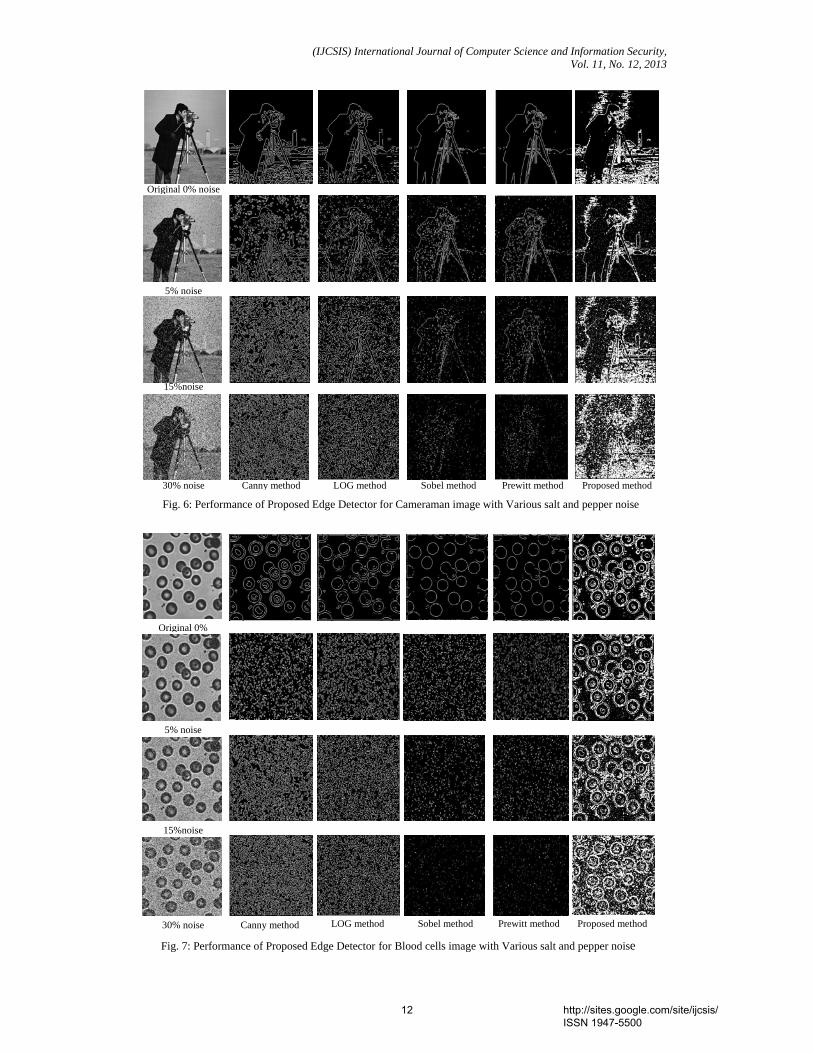
To demonstrate the efficiency of the proposed approach, the algorithm is tested over a number of different grayscale images and compared with traditional operators. The performance of the method is tested under noisy condition (Salt & Pepper noise) on test images. The images are corrupted by Salt & Pepper noise with 5%, 15% and 30% noise density before processing. The images detected by Canny, LOG, Sobel, Prewitt and the proposed method, respectively. All the concerned experiments were implemented on Intel® Core™ i3 2.10GHz with 4 GB RAM using MATLAB R2007b. As the algorithm has two main phases – global and local enhancement phase of the threshold values and detection phase, we present the results of implementation on these images separately.
The proposed scheme used the good characters of Kapur entropy, to calculate the global and local threshold values. Hence, we ensure that the proposed scheme done better than the traditional methods.
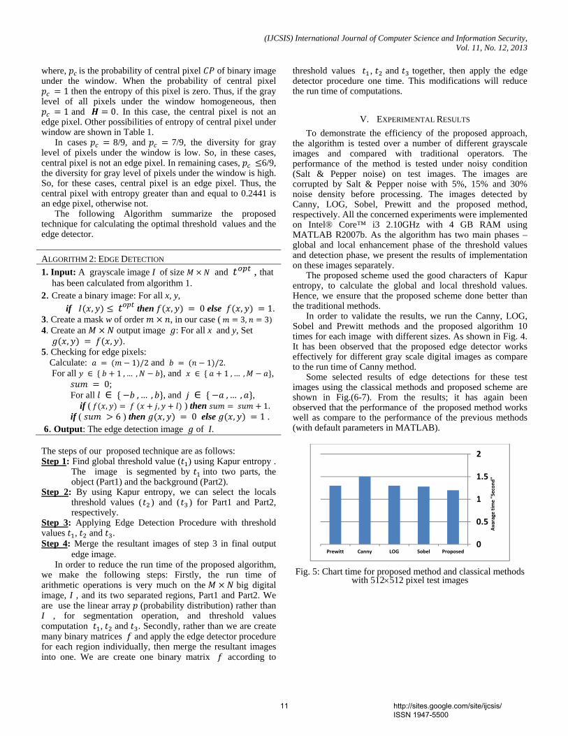
In order to validate the results, we run the Canny, LOG, Sobel and Prewitt methods and the proposed algorithm 10 times for each image with different sizes. As shown in Fig. 4. It has been observed that the proposed edge detector works effectively for different gray scale digital images as compare to the run time of Canny method.
Some selected results of edge detections for these test images using the classical methods and proposed scheme are shown in Fig.(6-7). From the results; it has again been observed that the performance of the proposed method works well as compare to the performance of the previous methods (with default parameters in MATLAB).
Fig. 5: Chart time for proposed method and classical methods with 512×512 pixel test images
0
0.5
1
1.5
2
ProposedSobelLOGCannyPrewitt
Avarage tim
e "Secon
d"
ALGORITHM 2: EDGE DETECTION
1. Input: A grayscale image I of size and , that has been calculated from algorithm 1.
2. Create a binary image: For all x, y,
if , then , 0 else , 1. 3. Create a mask w of order , in our case ( 3, 3) 4. Create an output image : For all x and y, Set
, , . 5. Checking for edge pixels:
Calculate: 1 /2 and 1 /2. For all 1 , … , , and 1 , … , , 0; For all , … , , and , … , , if ( , , ) then 1. if ( 6 ) then , 0 else , 1 .
6. Output: The edge detection image of I.
11 http://sites.google.com/site/ijcsis/ ISSN 1947-5500
(IJCSIS) International Journal of Computer Science and Information Security, Vol. 11, No. 12, 2013
Original 0% noise
5% noise
15%noise
30% noise Canny method LOG method Sobel method Prewitt method Proposed method
Fig. 6: Performance of Proposed Edge Detector for Cameraman image with Various salt and pepper noise
Original 0%
5% noise
15%noise
30% noise Canny method LOG method Sobel method Prewitt method Proposed method
Fig. 7: Performance of Proposed Edge Detector for Blood cells image with Various salt and pepper noise
12 http://sites.google.com/site/ijcsis/ ISSN 1947-5500
(IJCSIS) International Journal of Computer Science and Information Security, Vol. 11, No. 12, 2013
VI. CONCLUSION
An efficient approach using Kapur entropy for detection of edges in grayscale images is presented in this paper. The proposed method is compared with traditional edge detectors. On the basis of visual perception and edgel counts of edge maps of various grayscale images it is proved that our algorithm is able to detect highest edge pixels in images. The proposed method is decrease the computation time as possible as can with generate high quality of edge detection. Also it gives smooth and thin edges without distorting the shape of images. Another benefit comes from easy implementation of this method.
REFERENCES
[1] R. C. Gonzalez and R.E. Woods, "Digital Image Processing.", 3rd Edn., Prentice Hall, New Jersey, USA. ISBN: 9780131687288, 2008.
[2] F. Ulupinar and G. Medioni, “Refining Edges Detected by a LoG operator”, Computer vision, Graphics and Image Processing, 51, 1990, 275-298.
[3] J. Canny, "A Computational Approach to Edge Detect", IEEE Trans. on Pattern Analysis and Machine Intelligence, Vol.PAMI-8, No.6, 1986, 679-698.
[4] Dong Hoon Lim, "Robust edge detection in noisy images", Computational Statistics & Data Analysis,50, 2006, pp. 803-812.
[5] Amiya Halder, etl., " Edge Detection: A statistical Approach", 3rd International Conference on Electronics Computer Technology (ICECT 2011).8-10April-2011 Kanyakumari, India
[6] Kaustubha Mendhurwar, etl., " Edge Detection in Noisy Images Using Independent Component Analysis", ISRN Signal Processing , Volume 2011, Article ID672353, 9 pages.
[7] Bijay Neupane, etl., " A New Image Edge Detection Method using Quality-based Clustering", Technical Report DNA#2012-01, April2012, Abu Dhabi, UAE.
[8] A. El-Zaart, "A Novel Method for Edge Detection Using 2 Dimensional Gamma Distribution", Journal of Computer Science 6 (2), 2010 , pp. 199-204.
[9] R. M. Haralick, “Digital Step Edges from Zero Crossing of Second Directional Derivatives”, IEEE Trans. on Pattern Analysis and Machine Intelligence, Vol. PAMI-6, No1, Jan, 1984, 58-68.
[10] V. S. Nallwa and T. O. Binford, “On Detecting Edges”, IEEE Trans. on Pattern Analysis and Machine Intelligence, Vol. PAMI-8, No.6, Nov, 1986, 699-714 .
[11] V. Torre and T. A. Poggio, “On Edge Detection”, IEEE Trans. on Pattern Analysis and Machine Intelligenc, Vol. PAMI-8, No.2, Mar. 1985, 147-163.
[12] D. J. Willians and M. Shan, “Edge Contours Using Multiple Scales”, Computer Vision, Graphics and Image Processing, 51, 1990, pp. 256-274.
[13] A. Goshtasby, “On Edge Focusing”, Image and Vision Computing, Vol. 12, No.4, May, 1994, 247-256 .
[14] A. Huertas and G. Medioni, “Detection of Intensity Changes with Subpixel Accuracy Using Laplacian-Gaussian Masks”, IEEE Trans. on Pattern Analysis and Machine Intelligence, Vol. PAMI-8, No.5, Sep.1986, 651-664 .
[15] H. D. Cheng and Muyi Cu, “Mass Lesion Detection with a Fuzzy Neural Network”, J. Pattern Recognition, 37, pp.1189-1200, 2004.
[16] Jun Xu and Jinshan Tang, “Detection of Clustered Micro calcifications using an Improved Texture based Approach for Computer Aided Breast Cancer Diagnosis System”, J. CSI Communications, vol. 31, no. 10, 2008, pp. 17-20.
[17] M. Basu, "A Gaussian derivative model for edge enhancement.", Patt. Recog., 27:1451-1461, 1994.
[18] C. Kang, and W. Wang, "A novel edge detection method based on the maximizing objective function.", Pattern. Recog., 40, 2007, pp. 609-618.
[19] M. Roushdy, "Comparative Study of Edge Detection Algorithms Applying on the Grayscale Noisy Image Using Morphological Filter", GVIP, Special Issue on Edge Detection, 2007, pp. 51-59.
[20] B. Mitra, "Gaussian Based Edge Detection Methods- A Survey ". IEEE Trans. on Systems, Manand Cybernetics , 32, 2002, pp. 252-260.
[21] F. Luthon, M. Lievin and F. Faux, "On the use of entropy power for threshold selection." Int. J. Signal Proc., 84, 2004, pp. 1789-1804.
[22] M.Sonka, V.Hlavac, and R.Boyle, "Image Processing, Analysis, and Machine Vision" Second Edition, ITP, 1999.
[23] Shannon, C.E., “A mathematical Theory of Communication”, Int. J. Bell. Syst. Technical, vol.27, pp. 379-423, 1948.
[24] Baljit Singh and Amar Partap Singh, “Edge Detection in Gray Level Images based on the Shannon Entropy”, J. Computer Science, vol.4, no.3, 2008, pp.186-191.
[25] Landsberg, P.T. and Vedral, V. Distributions and channel capacities in generalized statistical mechanics. Physics Letters A, 247, (3), 1998, pp. 211-217.
[26] Alfréd Rényi , On measures of entropy and information, Pro ceeding of fourth Berkeley Symposium on Mathematical statistics and Probability, Vol. 1, 1961, pp. 547-561.
[27] M. P. de Albuquerque, I. A. Esquef , A.R. Gesualdi Mello, "Image Thresholding Using Tsallis Entropy." Pattern Recognition Letters 25, 2004, pp. 1059–1065.
[28] C. Tsallis, Non-extensive Statistical Mechanics and Themodynamics, Historical Background and Present Status. In: Abe, S. , Okamoto, Y. (eds.) Nonextensive Statistical Mechanics and Its Applications, Springer-Verlag Heidelberg, 2001.
[29] C. Tsallis, , Possible generalization of Boltzmann-Gibbs statistics, Journal of Statistical Physics, 52,, 1988, pp. 479-487.
[30] J. N. Kapur, H. K. Kesavan, Entropy optimisation Principles with Applications, Academic Press, Boston,1994.
[31] J. N. Kapur, Generalization entropy of order α and type β, The mathematical seminar, 4 , 1967, pp 78-84.
13 http://sites.google.com/site/ijcsis/ ISSN 1947-5500
(IJCSIS) International Journal of Computer Science and Information Security,
Vol. 11, No. 12, December 2013
Influence of Stimuli Color and Comparison of SVM
and ANN classifier Models for BCI based
Applications using SSVEPs
Rajesh Singla Department of Instrumentation and Control
Engineering,
Dr. B. R. Ambedkar National Institute of Technology
Jalandhar, Punjab-144011, India
Arun Khosla
Department of Electronics and Communication
Engineering,
Dr. B. R. Ambedkar National Institute of Technology
Jalandhar, Punjab-144011, India
Rameshwar Jha Director General, IET Bhaddal,
Distt.- Ropar, Punjab-140108 ,India
Abstract—— In recent years, Brain Computer Interface (BCI)
systems based on Steady-State Visual Evoked Potential
(SSVEP) have received much attentions. In this study four
different flickering frequencies in low frequency region were
used to elicit the SSVEPs and were displayed on a Liquid
Crystal Display (LCD) monitor using LabVIEW. Four stimuli
colors, green, blue, red and violet were used in this study to
investigate the color influence in SSVEPs. The
Electroencephalogram (EEG) signals recorded from the
occipital region were segmented into 1 second window and
features were extracted by using Fast Fourier Transform
(FFT). This study tries to develop a classifier, which can
provide higher classification accuracy for multiclass SSVEP
data. Support Vector Machines (SVM) is a powerful approach
for classification and hence widely used in BCI applications.
One-Against-All (OAA), a popular strategy for multiclass SVM
is compared with Artificial Neural Network (ANN) models on
the basis of SSVEP classifier accuracies. Based on this study, it
is found that OAA based SVM classifier can provide a better
results than ANN. In color comparison SSVEP with violet
color showed higher accuracy than that with other stimuli .
Keywords- Steady-State Visual Evoked Potential; Brain
Computer Interface; Support Vector Machines; ANN.
I. INTRODUCTION
The Brain Computer Interface (BCI) system provides a direct communication channel between human brain and the computer without using brain‟s normal output pathways of peripheral nerves and muscles [1]. By acquiring and translating the brain signals that are modified according to the intentions, a BCI system can provide an alternative,
augmentative communication and control options for individuals with severe neuromuscular disorders, such as spinal cord injury, brain stem stroke and Amyotrophic Lateral Sclerosis (ALS).
Electroencephalography (EEG) is a non-invasive way of acquiring brain signals from the surface of human scalp, which is widely accepted due to its simple and safe approach. The brain activity commonly utilized by EEG based BCI systems are Event Related Potentials (ERPs), Slow Cortical Potentials (SCPs), P300 potentials, Steady-State Visual Evoked Potentials (SSVEPs) etc. Among them SSVEPs are attracted due to its advantages of requiring less or no training, high Information Transfer Rate (ITR) and ease of use [1, 2, 3].
SSVEPs are oscillatory electrical potential that are elicited in the brain when the person is visually focusing his/her attention on a stimulus that is flickering at frequency 6Hz or above [4]. These signals are strong in occipital region of the brain and are nearly sinusoidal waveform having the same fundamental frequency as the stimulus and including some of its harmonics. By matching the fundamental frequency of the SSVEP to one of the stimulus frequencies presented, it is possible to detect the target selected by the user. Considering the amplitudes of SSVEPs induced, the stimuli frequencies are categorized into three ranges, centered at 15 Hz low frequency, 31 Hz medium frequency and 41 Hz high frequency respectively [5].
There are many research groups that are designing SSVEP based BCI systems. Lalor et al. [6] developed the
14 http://sites.google.com/site/ijcsis/ ISSN 1947-5500
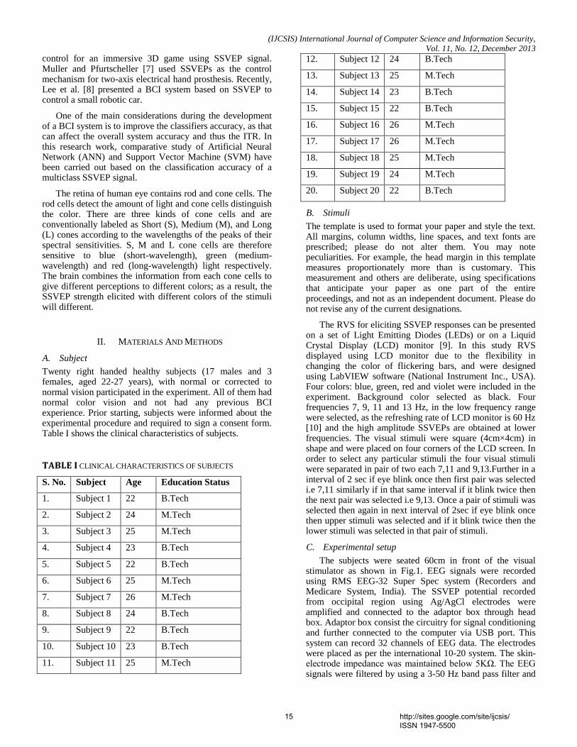
(IJCSIS) International Journal of Computer Science and Information Security,
Vol. 11, No. 12, December 2013
control for an immersive 3D game using SSVEP signal. Muller and Pfurtscheller [7] used SSVEPs as the control mechanism for two-axis electrical hand prosthesis. Recently, Lee et al. [8] presented a BCI system based on SSVEP to control a small robotic car.
One of the main considerations during the development of a BCI system is to improve the classifiers accuracy, as that can affect the overall system accuracy and thus the ITR. In this research work, comparative study of Artificial Neural Network (ANN) and Support Vector Machine (SVM) have been carried out based on the classification accuracy of a multiclass SSVEP signal.
The retina of human eye contains rod and cone cells. The rod cells detect the amount of light and cone cells distinguish the color. There are three kinds of cone cells and are conventionally labeled as Short (S), Medium (M), and Long (L) cones according to the wavelengths of the peaks of their spectral sensitivities. S, M and L cone cells are therefore sensitive to blue (short-wavelength), green (medium-wavelength) and red (long-wavelength) light respectively. The brain combines the information from each cone cells to give different perceptions to different colors; as a result, the SSVEP strength elicited with different colors of the stimuli will different.
II. MATERIALS AND METHODS
A. Subject
Twenty right handed healthy subjects (17 males and 3 females, aged 22-27 years), with normal or corrected to normal vision participated in the experiment. All of them had normal color vision and not had any previous BCI experience. Prior starting, subjects were informed about the experimental procedure and required to sign a consent form. Table I shows the clinical characteristics of subjects.
CLINICAL CHARACTERISTICS OF SUBJECTS
S. No. Subject Age Education Status
1. Subject 1 22 B.Tech
2. Subject 2 24 M.Tech
3. Subject 3 25 M.Tech
4. Subject 4 23 B.Tech
5. Subject 5 22 B.Tech
6. Subject 6 25 M.Tech
7. Subject 7 26 M.Tech
8. Subject 8 24 B.Tech
9. Subject 9 22 B.Tech
10. Subject 10 23 B.Tech
11. Subject 11 25 M.Tech
12. Subject 12 24 B.Tech
13. Subject 13 25 M.Tech
14. Subject 14 23 B.Tech
15. Subject 15 22 B.Tech
16. Subject 16 26 M.Tech
17. Subject 17 26 M.Tech
18. Subject 18 25 M.Tech
19. Subject 19 24 M.Tech
20. Subject 20 22 B.Tech
B. Stimuli
The template is used to format your paper and style the text. All margins, column widths, line spaces, and text fonts are prescribed; please do not alter them. You may note peculiarities. For example, the head margin in this template measures proportionately more than is customary. This measurement and others are deliberate, using specifications that anticipate your paper as one part of the entire proceedings, and not as an independent document. Please do not revise any of the current designations.
The RVS for eliciting SSVEP responses can be presented on a set of Light Emitting Diodes (LEDs) or on a Liquid Crystal Display (LCD) monitor [9]. In this study RVS displayed using LCD monitor due to the flexibility in changing the color of flickering bars, and were designed using LabVIEW software (National Instrument Inc., USA). Four colors: blue, green, red and violet were included in the experiment. Background color selected as black. Four frequencies 7, 9, 11 and 13 Hz, in the low frequency range were selected, as the refreshing rate of LCD monitor is 60 Hz [10] and the high amplitude SSVEPs are obtained at lower frequencies. The visual stimuli were square (4cm×4cm) in shape and were placed on four corners of the LCD screen. In order to select any particular stimuli the four visual stimuli were separated in pair of two each 7,11 and 9,13.Further in a interval of 2 sec if eye blink once then first pair was selected i.e 7,11 similarly if in that same interval if it blink twice then the next pair was selected i.e 9,13. Once a pair of stimuli was selected then again in next interval of 2sec if eye blink once then upper stimuli was selected and if it blink twice then the lower stimuli was selected in that pair of stimuli.
C. Experimental setup
The subjects were seated 60cm in front of the visual stimulator as shown in Fig.1. EEG signals were recorded using RMS EEG-32 Super Spec system (Recorders and Medicare System, India). The SSVEP potential recorded from occipital region using Ag/AgCl electrodes were amplified and connected to the adaptor box through head box. Adaptor box consist the circuitry for signal conditioning and further connected to the computer via USB port. This system can record 32 channels of EEG data. The electrodes were placed as per the international 10-20 system. The skin-electrode impedance was maintained below 5KΩ. The EEG signals were filtered by using a 3-50 Hz band pass filter and
15 http://sites.google.com/site/ijcsis/ ISSN 1947-5500
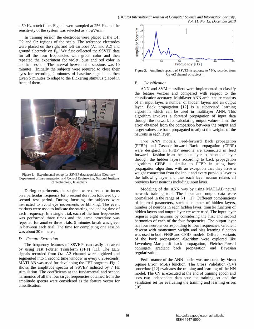
(IJCSIS) International Journal of Computer Science and Information Security,
Vol. 11, No. 12, December 2013
a 50 Hz notch filter. Signals were sampled at 256 Hz and the sensitivity of the system was selected as 7.5µV/mm.
In training session the electrodes were placed at the O1, O2 and Oz regions of the scalp. The reference electrodes were placed on the right and left earlobes (A1 and A2) and ground electrode on Fpz. We first collected the SSVEP data for all the four frequencies with green color and then repeated the experiment for violet, blue and red color in another session. The interval between the sessions was 10 minutes. Initially the subjects were required to close their eyes for recording 2 minutes of baseline signal and then given 5 minutes to adapt to the flickering stimulus placed in front of them.
Figure 1. Experimental set up for SSVEP data acquisition (Courtesy-
Department of Instrumentation and Control Engineering, National Institute of Technology, Jalandhar)
During experiments, the subjects were directed to focus on a particular frequency for 5 second duration followed by 5 second rest period. During focusing the subjects were instructed to avoid eye movements or blinking. The event markers were used to indicate the starting and ending time of each frequency. In a single trial, each of the four frequencies was performed three times and the same procedure was repeated for another three trials. 5 minutes break was given in between each trial. The time for completing one session was about 30 minutes.
D. Feature Extraction
The frequency features of SSVEPs can easily extracted by using Fast Fourier Transform (FFT) [11]. The EEG signals recorded from Oz -A2 channel were digitized and segmented into 1 second time window in every 0.25seconds. MATLAB was used for developing the FFT program. Fig. 2 shows the amplitude spectra of SSVEP induced by 7 Hz stimulation. The coefficients at the fundamental and second harmonics of all the four target frequencies obtained from the amplitude spectra were considered as the feature vector for classification.
Figure 2. Amplitude spectra of SSVEP in response to 7 Hz, recorded from
Oz -A2 channel of subject 4.
E. Classification
ANN and SVM classifiers were implemented to classify the feature vectors and compared with respect to the classification accuracy. Multilayer ANN architecture consists of an input layer, a number of hidden layers and an output layer. Back propagation [12] is a supervised learning algorithm which can be used in multilayer ANN. This algorithm involves a forward propagation of input data through the network for calculating output values. Then the error obtained from the comparison between the output and target values are back propagated to adjust the weights of the neurons in each layer.
Two ANN models, Feed-forward Back propagation (FFBP) and Cascade-forward Back propagation (CFBP) were designed. In FFBP neurons are connected in feed forward fashion from the input layer to the output layer through the hidden layers according to back propagation algorithm. CFBP is similar to FFBP in using back propagation algorithm, with an exception that they have a weight connection from the input and every previous layer to the following layer and thus each layer neuron relates all previous layer neurons including input layer.
Modeling of the ANN was by using MATLAB neural network training tool. The input and output data were normalized in the range of [-1, +1]. Different combinations of internal parameters, such as number of hidden layers, number of neurons in each hidden layer, transfer function of hidden layers and output layer etc were tried. The input layer requires eight neurons by considering the first and second harmonics of each of the four frequencies. The output layer has four neurons corresponding to four frequencies. Gradient descent with momentum weight and bias learning function was used in both FFBP and CFBP models. Different variants of the back propagation algorithm were explored like Levenberg-Marquardt back propagation, Fletcher-Powell conjugate gradient back propagation and Bayesian regularization.
Performance of the ANN model was measured by Mean Square Error (MSE) function. The Cross Validation (CV) procedure [12] evaluates the training and learning of the NN model. The CV is executed at the end of training epoch and uses two independent data sets: the training set and the validation set for evaluating the training and learning errors [16].
16 http://sites.google.com/site/ijcsis/ ISSN 1947-5500
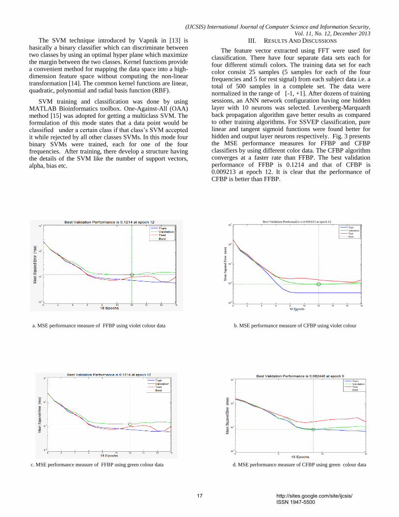
(IJCSIS) International Journal of Computer Science and Information Security,
Vol. 11, No. 12, December 2013
The SVM technique introduced by Vapnik in [13] is basically a binary classifier which can discriminate between two classes by using an optimal hyper plane which maximize the margin between the two classes. Kernel functions provide a convenient method for mapping the data space into a high-dimension feature space without computing the non-linear transformation [14]. The common kernel functions are linear, quadratic, polynomial and radial basis function (RBF).
SVM training and classification was done by using MATLAB Bioinformatics toolbox. One-Against-All (OAA) method [15] was adopted for getting a multiclass SVM. The formulation of this mode states that a data point would be classified under a certain class if that class‟s SVM accepted it while rejected by all other classes SVMs. In this mode four binary SVMs were trained, each for one of the four frequencies. After training, there develop a structure having the details of the SVM like the number of support vectors, alpha, bias etc.
III. RESULTS AND DISCUSSIONS
The feature vector extracted using FFT were used for classification. There have four separate data sets each for four different stimuli colors. The training data set for each color consist 25 samples (5 samples for each of the four frequencies and 5 for rest signal) from each subject data i.e. a total of 500 samples in a complete set. The data were normalized in the range of [-1, +1]. After dozens of training sessions, an ANN network configuration having one hidden layer with 10 neurons was selected. Levenberg-Marquardt back propagation algorithm gave better results as compared to other training algorithms. For SSVEP classification, pure linear and tangent sigmoid functions were found better for hidden and output layer neurons respectively. Fig. 3 presents the MSE performance measures for FFBP and CFBP classifiers by using different color data. The CFBP algorithm converges at a faster rate than FFBP. The best validation performance of FFBP is 0.1214 and that of CFBP is 0.009213 at epoch 12. It is clear that the performance of CFBP is better than FFBP.
a. MSE performance measure of FFBP using violet colour data b. MSE performance measure of CFBP using violet colour
c. MSE performance measure of FFBP using green colour data d. MSE performance measure of CFBP using green colour data
17 http://sites.google.com/site/ijcsis/ ISSN 1947-5500
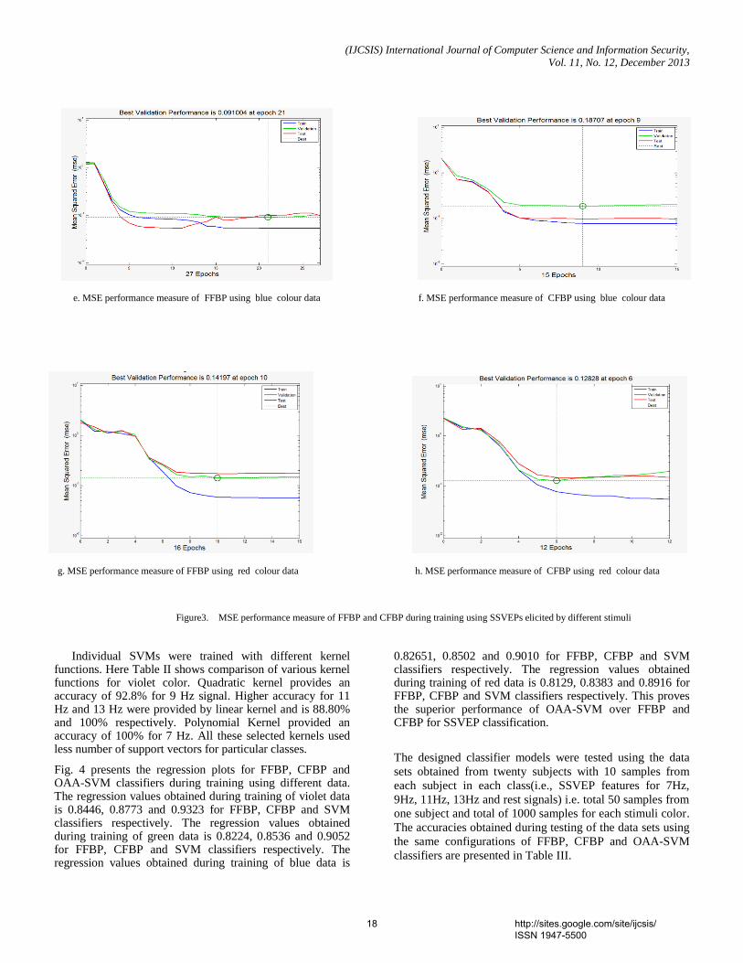
(IJCSIS) International Journal of Computer Science and Information Security,
Vol. 11, No. 12, December 2013
e. MSE performance measure of FFBP using blue colour data f. MSE performance measure of CFBP using blue colour data
g. MSE performance measure of FFBP using red colour data h. MSE performance measure of CFBP using red colour data
Figure3. MSE performance measure of FFBP and CFBP during training using SSVEPs elicited by different stimuli
Individual SVMs were trained with different kernel
functions. Here Table II shows comparison of various kernel functions for violet color. Quadratic kernel provides an accuracy of 92.8% for 9 Hz signal. Higher accuracy for 11 Hz and 13 Hz were provided by linear kernel and is 88.80% and 100% respectively. Polynomial Kernel provided an accuracy of 100% for 7 Hz. All these selected kernels used less number of support vectors for particular classes.
Fig. 4 presents the regression plots for FFBP, CFBP and OAA-SVM classifiers during training using different data. The regression values obtained during training of violet data is 0.8446, 0.8773 and 0.9323 for FFBP, CFBP and SVM classifiers respectively. The regression values obtained during training of green data is 0.8224, 0.8536 and 0.9052 for FFBP, CFBP and SVM classifiers respectively. The regression values obtained during training of blue data is
0.82651, 0.8502 and 0.9010 for FFBP, CFBP and SVM classifiers respectively. The regression values obtained during training of red data is 0.8129, 0.8383 and 0.8916 for FFBP, CFBP and SVM classifiers respectively. This proves the superior performance of OAA-SVM over FFBP and CFBP for SSVEP classification.
The designed classifier models were tested using the data
sets obtained from twenty subjects with 10 samples from
each subject in each class(i.e., SSVEP features for 7Hz,
9Hz, 11Hz, 13Hz and rest signals) i.e. total 50 samples from
one subject and total of 1000 samples for each stimuli color.
The accuracies obtained during testing of the data sets using
the same configurations of FFBP, CFBP and OAA-SVM
classifiers are presented in Table III.
18 http://sites.google.com/site/ijcsis/ ISSN 1947-5500
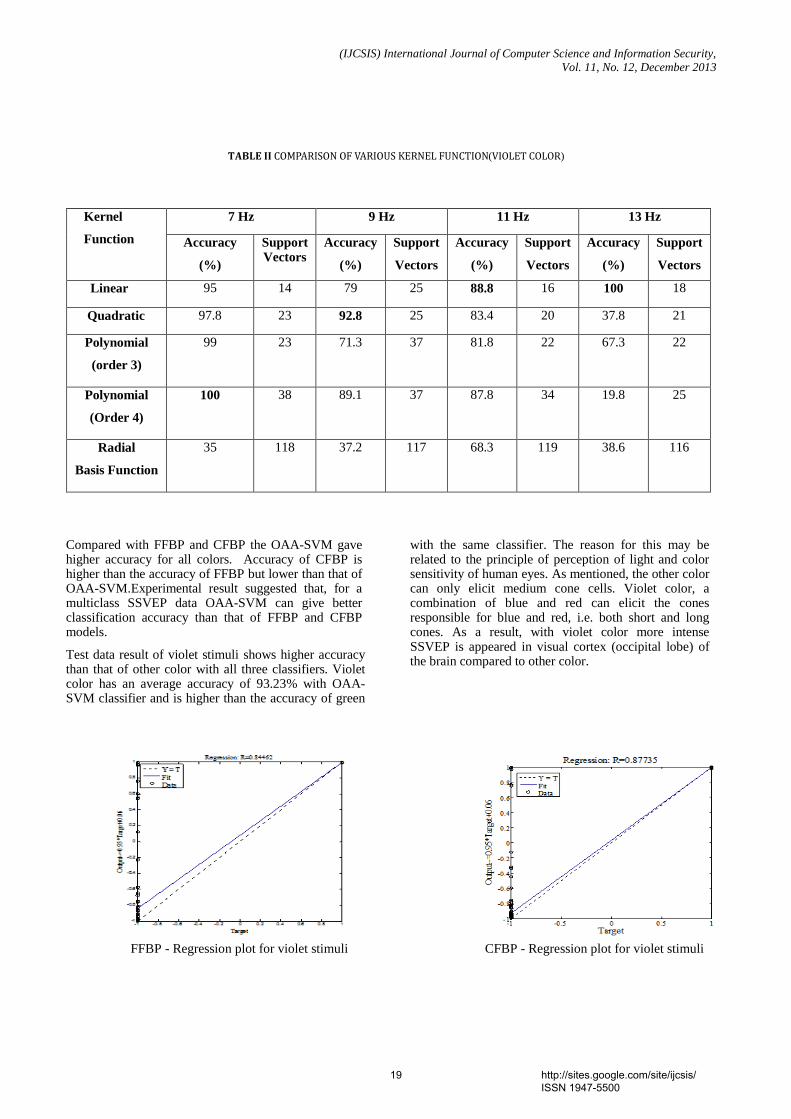
(IJCSIS) International Journal of Computer Science and Information Security,
Vol. 11, No. 12, December 2013
(VIOLET COLOR)
Kernel
Function
7 Hz 9 Hz 11 Hz 13 Hz
Accuracy
(%)
Support Vectors
Accuracy
(%)
Support
Vectors
Accuracy
(%)
Support
Vectors
Accuracy
(%)
Support
Vectors
Linear 95 14 79 25 88.8 16 100 18
Quadratic 97.8 23 92.8 25 83.4 20 37.8 21
Polynomial
(order 3)
99 23 71.3 37 81.8 22 67.3 22
Polynomial
(Order 4)
100 38 89.1 37 87.8 34 19.8 25
Radial
Basis Function
35 118 37.2 117 68.3 119 38.6 116
Compared with FFBP and CFBP the OAA-SVM gave higher accuracy for all colors. Accuracy of CFBP is higher than the accuracy of FFBP but lower than that of OAA-SVM.Experimental result suggested that, for a multiclass SSVEP data OAA-SVM can give better classification accuracy than that of FFBP and CFBP models.
Test data result of violet stimuli shows higher accuracy than that of other color with all three classifiers. Violet color has an average accuracy of 93.23% with OAA-SVM classifier and is higher than the accuracy of green
with the same classifier. The reason for this may be related to the principle of perception of light and color sensitivity of human eyes. As mentioned, the other color can only elicit medium cone cells. Violet color, a combination of blue and red can elicit the cones responsible for blue and red, i.e. both short and long cones. As a result, with violet color more intense SSVEP is appeared in visual cortex (occipital lobe) of the brain compared to other color.
FFBP - Regression plot for violet stimuli CFBP - Regression plot for violet stimuli
19 http://sites.google.com/site/ijcsis/ ISSN 1947-5500
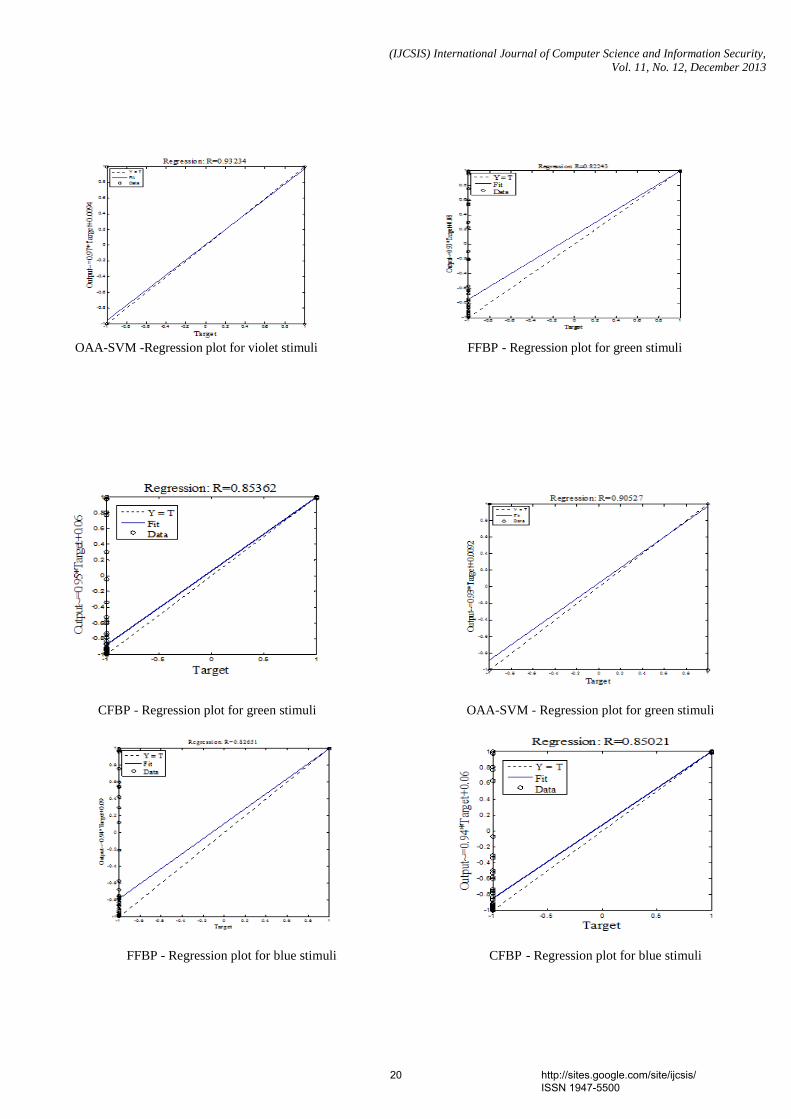
(IJCSIS) International Journal of Computer Science and Information Security,
Vol. 11, No. 12, December 2013
OAA-SVM -Regression plot for violet stimuli FFBP - Regression plot for green stimuli
O
CFBP - Regression plot for green stimuli OAA-SVM - Regression plot for green stimuli
FFBP - Regression plot for blue stimuli CFBP - Regression plot for blue stimuli
20 http://sites.google.com/site/ijcsis/ ISSN 1947-5500
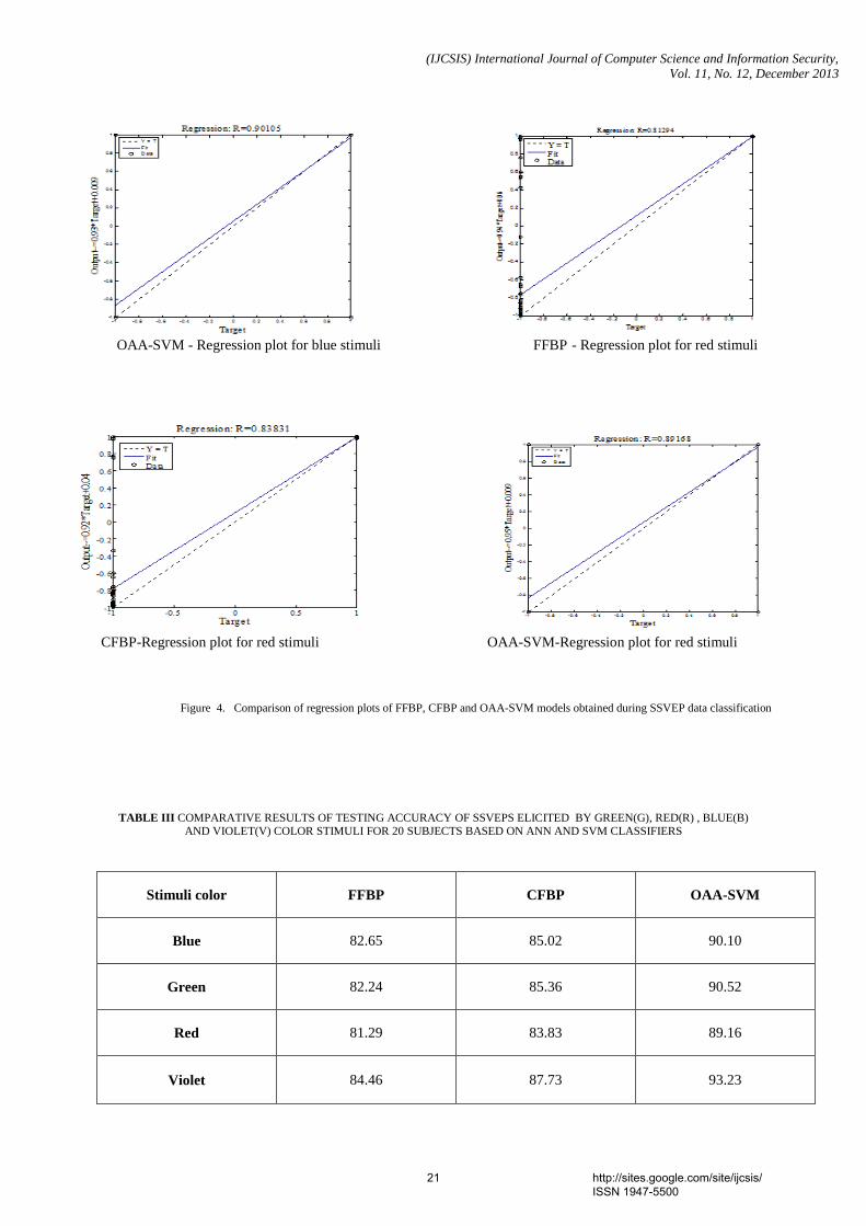
(IJCSIS) International Journal of Computer Science and Information Security,
Vol. 11, No. 12, December 2013
OAA-SVM - Regression plot for blue stimuli FFBP - Regression plot for red stimuli
CFBP-Regression plot for red stimuli OAA-SVM-Regression plot for red stimuli
Figure 4. Comparison of regression plots of FFBP, CFBP and OAA-SVM models obtained during SSVEP data classification
TABLE III COMPARATIVE RESULTS OF TESTING ACCURACY OF SSVEPS ELICITED BY GREEN(G), RED(R) , BLUE(B) AND VIOLET(V) COLOR STIMULI FOR 20 SUBJECTS BASED ON ANN AND SVM CLASSIFIERS
Stimuli color FFBP CFBP OAA-SVM
Blue 82.65 85.02 90.10
Green 82.24 85.36 90.52
Red 81.29 83.83 89.16
Violet 84.46 87.73 93.23
21 http://sites.google.com/site/ijcsis/ ISSN 1947-5500
(IJCSIS) International Journal of Computer Science and Information Security,
Vol. 11, No. 12, December 2013
IV. CONCLUSIONS
In this research three classifier models (FFBP, CFBP and OAA-SVM) were constructed for SSVEP data classification. The motivation of this work is to improve the accuracy of SSVEP based BCI system by improving the classification accuracy. EEG signals were recorded by using RMS EEG-32 Super Spec system and SSVEP features extracted using FFT. SSVEPs were elicited using four different frequencies. Four different stimuli color, green, red, blue, and violet were compared to get better performance. The amplitudes of first and second harmonics of SSVEP data were successfully used as the feature vector to train the classifier models. The experimental result shows that OAA-SVM yields superior classification accuracy compared against FFBP and CFBP for SSVEP data. The result also showed that SSVEPs with violet stimuli is better than that with other stimuli.
The future work may include the development of a SSVEP based BCI application system that can provide higher accuracy by using OAA-SVM classifier.
ACKNOWLEDGMENT
The authors would like to thank the subjects who
participated in the EEG recording session.
REFERENCES
[1] J. R. Wolpaw, N. Birbaumer, W. J. Heetderks, D. J.
McFarland, P. H. Peckham, G. Schalk, E. Donchin, L. A.
Quatrano, C. J. Robinson, and T. M. Vaughan, “Brain Computer Interface technology: - a review of the first
international meeting,” IEEE Trans. Rehab. Eng. vol. 8,
pp. 164-173, June 2000. [2] R. Singla, B. Chambayil, A. Khosla, J. Santosh
“Comparison of SVM and ANN for classification of eye
events in EEG,” Journal of Biomedical Sciences and engineering (JBISE), Vol 4, No 2, January 2011, pg (62-
69). Scientific Research Publishing, USA
[3] T. W. Berger, J. K. Chapin, G. A. Gerhardt, et. al., “International assessment of research and development in
brain-computer interfaces: report of the world technology
evaluation center,” Berlin: Springer, 2007. [4] M. Cheng, X.R. Gao, S.K. Gao, and D. xu, “Design and
implementation of a brain computer interface with high
transfer rates,” IEEE Trans Biomed Eng., 2002, vol. 49. No. 10, pp. 1181-1186
[5] Y. J. Wang, R. P. Wang, X. R. Gao, B. Hong, and S. K.
Gao, “A Practical VEP-based brain-computer interface,” IEEE Trans. Neural Syst. Rehabil. Eng., vol. 14, no. 2, pp.
234-240, June 2006.
[6] E. C. Lalor, S. P. Kelly, C. Finucane, R. Burke, R. Smith,
R. B. Reilly, and G. McDarby, „„Steady-state VEP-based
brain-computer interface control in an immersive 3D gaming environment,” EURASIP J. Appl. Signal Process.,
vol. 2005, no. 19, pp. 3156–3164, 2005.
[7] G. R. Muller-Putz and G. Pfurtscheller, “Control of an electrical prosthesis with an SSVEP-based BCI,” IEEE
Trans. Biomed. Eng., vol. 55, no. 1, pp. 361–364, 2008.
[8] P. L. Lee, H. C. Chang, T. Y. Hsieh et.al., “A brain wave
actuated small robot car using ensemble empiricalmode
decomposition based approach,” IEEE Trans. Sys. Man
and cyber.part A: Systems and humans, vol. 42, no. 5, pp
1053-1064, sept. 2012. [9] D. H. Zhu, J. Bieger, G. G. Molina, and R. M. Aarts, “A
Survey of Stimulation Methods Used in SSVEP-Based
BCI system,” Comput. Intell. Neurosci., pp. 702357, 2010. [10] Y. Wang, Y. –T. Wang, and T. –P. Jung, “Visual stimulus
design for high-rate SSVEP BCI,” Electron. Lett., vol 46,
No. 15, pp. 1057-1058, 2010. [11] G. R. Muller-Putz, R. Scherer, C. Brauneis, and G.
Pfurtscheller, “Steady-State Visual Evoked Potential
(SSVEP)-based Communication: Impact of Harmonic Frequency Components,” J. Neural Eng., vol. 2, no. 4, pp.
123-130,2005.
[12] S. Haykin, “Neural Networks:A Comprehensive Foundation,”1998, Prentice Hall.
[13] V. Vapnik., “Statistical Learning Theory,” John Wiley and
Sons, Chichester, 1998. [14] X. Song-yun, W. Peng-wei, Z. Hai-jun, Z. Hai-tao,
“Research on the classification of Brain function based on
SVM,” The 2nd International Conference on Bioinformatics and Biomedical Engineering, ICBBE 2008,
p1931 – p1934, 2008.
[15] B. Chambayil, R. Singla, R. Jha, “Virtual keyboard BCI using eyeblinks in EEG,” IEEE 6th int. conf. on wireless
and mobile computing, networking and communication, pp 466-470, 2010
[16] Vijay Khare, Jayashree Santosh, Sneh Anand and Manvir
Bhatia “Classification of five mental tasks based on two methods of neural network”. International Journal of
Computer science and information security ,pp 86-92,
Vol8 No.3, 2010 AUTHORS PROFILE
Rajesh Singla was born in Punjab , India in 1975. He obtained B.E Degree from Thapar University in 1997, M.Tech degree froom IIT-Roorkee in 2006. Currentely he is pursuing Ph.D degree from National Institute of Technology Jalandhar, Punjab, India. His area of interest is Brain Computer Interface, Rehabilation Engineering, and Process Control.
He is working as an Associate Professor in National Institute of Technology Jalandhar, India.
Dr Arun Khosla was born in Punjab, India. He received the BE degree from Thapar University, India, M.Tech from NIT Kurukshetra, Ph.D. from Kurukshetra University, India. His research areas include Artificial Intelligence and Bio-Medical Instrumentation.
He is working as an Associate Professor in the Department of Electronics and Communication Engineering, NIT Jalandhar. He is also Head of the Department since 2010.
Dr R. Jha was born in Bihar, India in 1945. He received his
BSc (Engineering Electrical)from Bhagalpur University in 1965, his MTech From IIT-Delhi in 1970 and his PhD degree from
Punjab University-Chandigarh, India, in 1980. He worked as a
Lecturer in the Johrat Engineering Collage-Johrat, (1965–1972) and as an Assistant Professor at the Punjab Engineering College
Chandigarh, (1972–1986). In 1986, he joined REC-Hamirpur, as
a Professor and rose to be its Principal in 1990. He joined NIT-Jalandhar as professor and Head of the Instrumentation &
Control Engineering Department (1994–2010). His area of
interest is computer-aided analysis and design of control systems and fuzzy systems.
He is working as the Director- Principal of the Institute of
Engineering and Technology-Bhaddal, India.
22 http://sites.google.com/site/ijcsis/ ISSN 1947-5500
(IJCSIS) International Journal of Computer Science and Information Security, Vol. 11, No. 12, December 2013
Comparative Study of Person Identification System with Facial Images Using PCA and KPCA
Computing Techniques
Md. Kamal Uddin, Abul Kalam Azad, Md.Amran Hossen Bhuiyan Department of Computer Science & Telecommunication Engineering, Noakhali Science & Technology University
Noakhali-3814, Bangladesh
Abstract— Face recognition is one of the most successful areas of research in computer vision for the application of image analysis and understanding. It has received a considerable attention in recent years both from the industry and the research community. But face recognition is susceptible to variations in pose, light intensity, expression, etc. In this paper, a comparative study of linear (PCA) and nonlinear (KPCA) based approaches for person identification has been explored. The Principal Component Analysis (PCA) is one of the most well-recognized feature extraction tools used in face recognition. The Kernel Principal Component analysis (KPCA) was proposed as a nonlinear extension of a PCA. The basic idea of KPCA is to maps the input space into a feature space via nonlinear mapping and then computes the principal components in that feature space. In this paper, facial images have been classified using Euclidean distance and performance has been analysed for both feature extraction tools. Keywords—Face recognition; Eigenface; Principal component analysis; Kernel principal component analysis.
I. INTORDUCTION
Modern civilization heavily depends on person authentication for several purposes. Face recognition has always a major focus of research because of its non-invasive nature and because it is people’s primary method of person identification. The identification of a person interacting with computers represents an important task for automatic systems in the area of information retrieval, automatic banking and control of access to security areas and so on. Here, a tiny effort has been carried out to develop the person identification systems with facial image by using Principal Component Analysis (PCA) and Kernel Principal Component Analysis (KPCA) computing techniques. And finally the performance has been compared with both computing techniques.
II. RELATED WORKS Face recognition is an active area of research with applications ranging from static, controlled mug-shot verification to dynamic, uncontrolled face identification in a cluttered
background [1]. In the context of personal identification, face recognition usually refers to static, controlled full-frontal portrait recognition [10]. By static, it means that the facial portraits used by the face recognition system are still facial images (intensity or range). By controlled, it means that the type of background, illumination, resolution of the acquisition devices, and the distance between the acquisition devices and faces, etc. are essentially fixed during the image acquisition process. Obviously, in such a controlled situation, the segmentation task is relatively simple and the intra-class variations are small.
Over the past three decades, a substantial amount of research effort has been devoted to face recognition [1], [10]. In the1970s, face recognition was mainly based on measured facial attributes such as eyes, eyebrows, nose, and lips, chin shape, etc. [1]. Due to the lack of computational resources and brittleness of feature extraction algorithms, only a very limited number of tests were conducted and the recognition performance of face recognition systems was far from desirable [1]. After the dormant 1980s, there was resurgence in face recognition research in the early 1990s. In addition to continuing efforts on attribute based techniques [11], a number of new face recognition techniques were proposed, including:
Principal Component Analysis(PCA) [1], [11], [12] Linear Discriminant Analysis(LDA) [13] A variety of neural network based techniques [14] Kernel Principal Component Analysis(KPCA)[15]
III. FACE FEATURE EXTRACTION PCA is powerful technique for extracting a structure from potentially high-dimensional data sets, which corresponds to extracting the eigenvectors that are associated with the largest eigenvalues from the input distribution. For faster computation of the eigenvectors and eigenvalues, singular value decomposition (SVD) is used. This eigenvector analysis has already been widely used in face processing [1], [2]. A kernel
23 http://sites.google.com/site/ijcsis/ ISSN 1947-5500
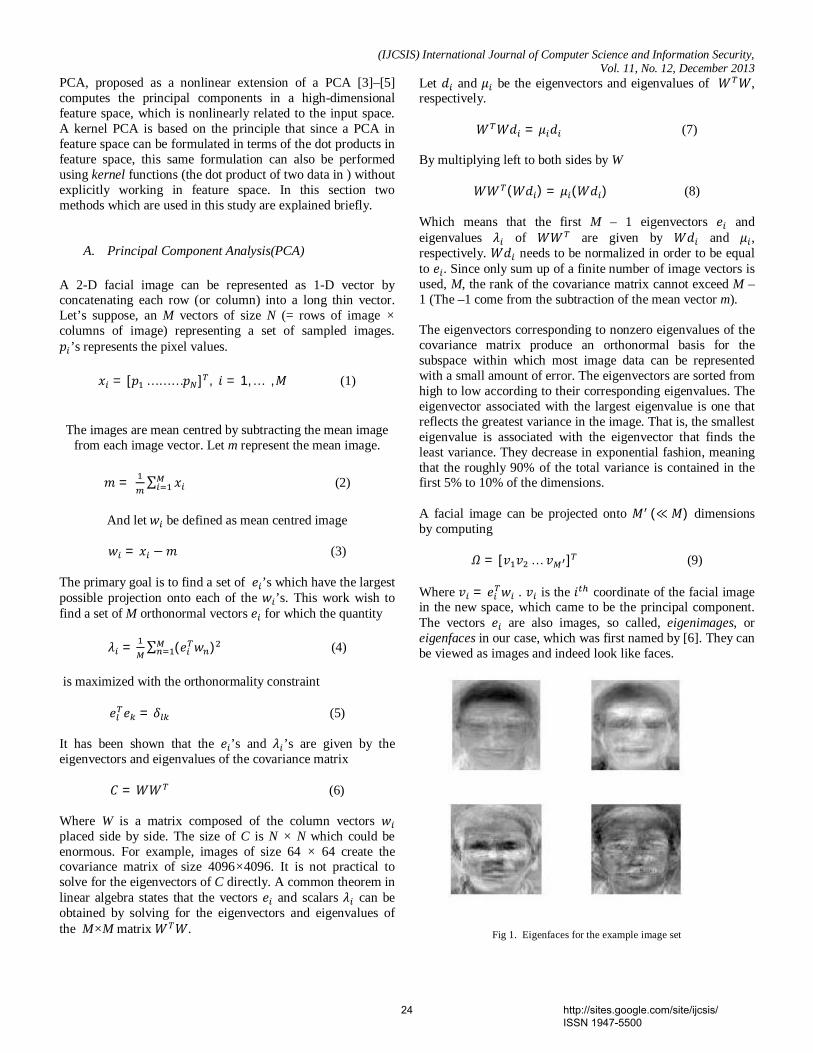
(IJCSIS) International Journal of Computer Science and Information Security, Vol. 11, No. 12, December 2013
PCA, proposed as a nonlinear extension of a PCA [3]–[5] computes the principal components in a high-dimensional feature space, which is nonlinearly related to the input space. A kernel PCA is based on the principle that since a PCA in feature space can be formulated in terms of the dot products in feature space, this same formulation can also be performed using kernel functions (the dot product of two data in ) without explicitly working in feature space. In this section two methods which are used in this study are explained briefly.
A. Principal Component Analysis(PCA)
A 2-D facial image can be represented as 1-D vector by concatenating each row (or column) into a long thin vector. Let’s suppose, an M vectors of size N (= rows of image × columns of image) representing a set of sampled images. 푝 ’s represents the pixel values.
푥 = [푝 … … …푝 ] , 푖 = 1, … ,푀 (1)
The images are mean centred by subtracting the mean image
from each image vector. Let m represent the mean image.
푚 = ∑ 푥 (2)
And let 푤 be defined as mean centred image
푤 = 푥 −푚 (3)
The primary goal is to find a set of 푒 ’s which have the largest possible projection onto each of the 푤 ’s. This work wish to find a set of M orthonormal vectors 푒 for which the quantity
휆 = ∑ (푒 푤 ) (4)
is maximized with the orthonormality constraint
푒 푒 = 훿 (5) It has been shown that the 푒 ’s and 휆 ’s are given by the eigenvectors and eigenvalues of the covariance matrix
퐶 = 푊푊 (6)
Where W is a matrix composed of the column vectors 푤 placed side by side. The size of C is N × N which could be enormous. For example, images of size 64 × 64 create the covariance matrix of size 4096×4096. It is not practical to solve for the eigenvectors of C directly. A common theorem in linear algebra states that the vectors 푒 and scalars 휆 can be obtained by solving for the eigenvectors and eigenvalues of the M×M matrix 푊 푊.
Let 푑 and 휇 be the eigenvectors and eigenvalues of 푊 푊, respectively.
푊 푊푑 = 휇 푑 (7)
By multiplying left to both sides by W
푊푊 (푊푑 ) = 휇 (푊푑 ) (8) Which means that the first M – 1 eigenvectors 푒 and eigenvalues 휆 of 푊푊 are given by 푊푑 and 휇 , respectively. 푊푑 needs to be normalized in order to be equal to 푒 . Since only sum up of a finite number of image vectors is used, M, the rank of the covariance matrix cannot exceed M – 1 (The –1 come from the subtraction of the mean vector m). The eigenvectors corresponding to nonzero eigenvalues of the covariance matrix produce an orthonormal basis for the subspace within which most image data can be represented with a small amount of error. The eigenvectors are sorted from high to low according to their corresponding eigenvalues. The eigenvector associated with the largest eigenvalue is one that reflects the greatest variance in the image. That is, the smallest eigenvalue is associated with the eigenvector that finds the least variance. They decrease in exponential fashion, meaning that the roughly 90% of the total variance is contained in the first 5% to 10% of the dimensions. A facial image can be projected onto 푀 (≪푀) dimensions by computing
훺 = [푣 푣 … 푣 ] (9) Where 푣 = 푒 푤 . 푣 is the 푖 coordinate of the facial image in the new space, which came to be the principal component. The vectors 푒 are also images, so called, eigenimages, or eigenfaces in our case, which was first named by [6]. They can be viewed as images and indeed look like faces.
Fig 1. Eigenfaces for the example image set
24 http://sites.google.com/site/ijcsis/ ISSN 1947-5500
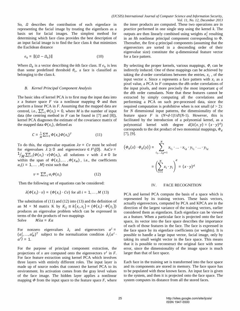
(IJCSIS) International Journal of Computer Science and Information Security, Vol. 11, No. 12, December 2013
So, 훺 describes the contribution of each eigenface in representing the facial image by treating the eigenfaces as a basis set for facial images. The simplest method for determining which face class provides the best description of an input facial image is to find the face class 푘 that minimizes the Euclidean distance 휖 = ‖(훺 −훺 )‖ (10) Where 훺 is a vector describing the kth face class. If 휖 is less than some predefined threshold 휃 , a face is classified as belonging to the class k.
B. Kernel Principal Component Analysis The basic idea of kernel PCA is to first map the input data into x a feature space F via a nonlinear mapping Φ and then perform a linear PCA in F. Assuming that the mapped data are centred, i.e., ∑ 훷(푥 ) = 0, where M is the number of input data (the centring method in F can be found in [7] and [8]), kernel PCA diagnoses the estimate of the covariance matrix of the mapped data 훷(푥 ), defined as
퐶 = ∑ 훷(푥 )훷(푥 ) (11) To do this, the eigenvalue equation 휆푣 = 퐶푣 must be solved for eigenvalues 휆 ≥ 0 and eigenvector푣 ∈ 퐹0. As퐶푣 =1푀∑ (훷(푥 ) ∙ 푣)훷(푥 ), all solutions v with 휆 ≠ 0 lie
within the span of 훷(푥 ), … ,훷(푥 ), i.e., the coefficients 훼 (푖 = 1, … ,푀) exist such that
푣 = ∑ 훼 훷(푥 ) (12) Then the following set of equations can be considered:
휆(훷(푥 ) ∙ 푣) = (훷(푥 ) ∙ 퐶푣) for all 푖 = 1, … ,푀 (13) The substitution of (11) and (12) into (13) and the definition of an M × M matrix K by 퐾 ≡ 푘 푥 ,푥 = (훷(푥 ) ∙ 훷 푥 ) produces an eigenvalue problem which can be expressed in terms of the dot products of two mappings Solve 푀휆훼 = 퐾훼 For nonzero eigenvalues 휆 and eigenvectors 훼 =(훼 , … ,훼 ) subject to the normalization condition 휆 (훼 ∙훼 ) = 1. For the purpose of principal component extraction, the projections of x are computed onto the eigenvectors 푣 in F. For face feature extraction using kernel PCA which involves three layers with entirely different roles. The input layer is made up of source nodes that connect the kernel PCA to its environment. Its activation comes from the gray level values of the face image. The hidden layer applies a nonlinear mapping Φ from the input space to the feature space F, where
the inner products are computed. These two operations are in practice performed in one single step using the kernel k. The outputs are then linearly combined using weights 훼 resulting in an lth nonlinear principal component corresponding to Φ. Thereafter, the first q principal components (assuming that the eigenvectors are sorted in a descending order of their eigenvalue size) constitute the q-dimensional feature vector for a face pattern. By selecting the proper kernels, various mappings, Φ, can be indirectly induced. One of these mappings can be achieved by taking the d-order correlations between the entries, 푥 , of the input vector x. Since x represents a face pattern with 푥 as a pixel value, a PCA in F computes the dth order correlations of the input pixels, and more precisely the most important q of the dth order cumulants. Note that these features cannot be extracted by simply computing all the correlations and performing a PCA on such pre-processed data, since the required computation is prohibitive when is not small (d ˃ 2): for N dimensional input patterns, the dimensionality of the feature space F is (N+d-1)!/d!(N-1). However, this is facilitated by the introduction of a polynomial kernel, as a polynomial kernel with degree 푑(푘(푥, 푦) = (푥 ∙ 푦) ) corresponds to the dot product of two monomial mappings, 훷 [7], [9].
훷 (푥) ∙ 훷 (푦) = 푥 ∙. ..∙ 푥 ∙ 푦 ∙… ∙ 푦,…,
= 푥 ∙ 푦 = (푥 ∙ 푦)
IV. FACE RECOGNITION
PCA and kernel PCA compute the basis of a space which is represented by its training vectors. These basis vectors, actually eigenvectors, computed by PCA and KPCA are in the direction of the largest variance of the training vectors, earlier considered them as eigenfaces. Each eigenface can be viewed as a feature. When a particular face is projected onto the face space, its vector into the face space describes the importance of each of those features in the face. The face is expressed in the face space by its eigenface coefficients (or weights). It is possible to handle a large input vector, facial image, only by taking its small weight vector in the face space. This means that it is possible to reconstruct the original face with some error, since the dimensionality of the image space is much larger than that of face space. Each face in the training set is transformed into the face space and its components are stored in memory. The face space has to be populated with these known faces. An input face is given to the system, and then it is projected onto the face space. The system computes its distance from all the stored faces.
25 http://sites.google.com/site/ijcsis/ ISSN 1947-5500
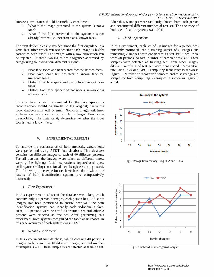
(IJCSIS) International Journal of Computer Science and Information Security, Vol. 11, No. 12, December 2013
However, two issues should be carefully considered: 1. What if the image presented to the system is not a
face? 2. What if the face presented to the system has not
already learned, i.e., not stored as a known face? The first defect is easily avoided since the first eigenface is a good face filter which can test whether each image is highly correlated with itself. The images with a low correlation can be rejected. Or these two issues are altogether addressed by categorizing following four different regions:
1. Near face space and near stored face => known faces 2. Near face space but not near a known face =>
unknown faces 3. Distant from face space and near a face class => non-
faces 4. Distant from face space and not near a known class
=> non-faces Since a face is well represented by the face space, its reconstruction should be similar to the original; hence the reconstruction error will be small. Non-face images will have a large reconstruction error which is larger than some threshold 휃 . The distance ∈ determines whether the input face is near a known face.
V. EXPERIMENTAL RESULTS To analyse the performance of both methods, experiments were performed using AT&T face database. This database contains ten different images of each of 40 different persons. For all persons, the images were taken at different times, varying the lighting, facial expressions (open/closed eyes, smiling/not smiling) and facial details (glasses/ no glasses). The following three experiments have been done where the results of both identification systems are comparatively discussed:
A. First Experiment: In this experiment, a subset of the database was taken, which contains only 12 person’s images, each person has 10 distinct images, has been performed to ensure how well the both identification systems can identify each individual’s face. Here, 10 persons were selected as training set and other 2 persons were selected as test set. After performing this experiment, both systems recognized the faces as unknown. In this case accuracy of both systems was 100%.
B. Second Experiment
In this experiment face database, which contains 40 person’s images, each person has 10 different images, so total number of samples is 400. These samples were selected as training set.
After this, 5 images were randomly chosen from each person and constructed different number of test set. The accuracy of both identification systems was 100%.
C. Third Experiment
In this experiment, each set of 10 images for a person was randomly portioned into a training subset of 8 images and remaining 2 images were considered as test set. Since, there were 40 persons, so total number of samples was 320. These samples were selected as training set. From other images, different numbers of test set were constructed. Recognition rate using PCA and KPCA computing techniques is shown in Figure 2. Number of recognized samples and false recognized sample for both computing techniques is shown in Figure 3 and 4.
Fig 2. Recognition accuracy using PCA and KPCA
Fig 3. Number of false recognized samples
26 http://sites.google.com/site/ijcsis/ ISSN 1947-5500
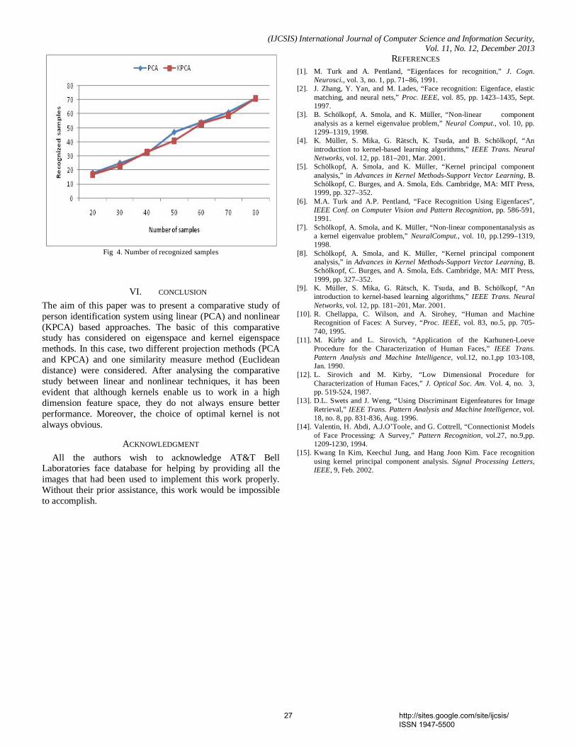
(IJCSIS) International Journal of Computer Science and Information Security, Vol. 11, No. 12, December 2013
Fig 4. Number of recognized samples
VI. CONCLUSION The aim of this paper was to present a comparative study of person identification system using linear (PCA) and nonlinear (KPCA) based approaches. The basic of this comparative study has considered on eigenspace and kernel eigenspace methods. In this case, two different projection methods (PCA and KPCA) and one similarity measure method (Euclidean distance) were considered. After analysing the comparative study between linear and nonlinear techniques, it has been evident that although kernels enable us to work in a high dimension feature space, they do not always ensure better performance. Moreover, the choice of optimal kernel is not always obvious.
ACKNOWLEDGMENT All the authors wish to acknowledge AT&T Bell
Laboratories face database for helping by providing all the images that had been used to implement this work properly. Without their prior assistance, this work would be impossible to accomplish.
REFERENCES [1]. M. Turk and A. Pentland, “Eigenfaces for recognition,” J. Cogn.
Neurosci., vol. 3, no. 1, pp. 71–86, 1991. [2]. J. Zhang, Y. Yan, and M. Lades, “Face recognition: Eigenface, elastic
matching, and neural nets,” Proc. IEEE, vol. 85, pp. 1423–1435, Sept. 1997.
[3]. B. Schölkopf, A. Smola, and K. Müller, “Non-linear component analysis as a kernel eigenvalue problem,” Neural Comput., vol. 10, pp. 1299–1319, 1998.
[4]. K. Müller, S. Mika, G. Rätsch, K. Tsuda, and B. Schölkopf, “An introduction to kernel-based learning algorithms,” IEEE Trans. Neural Networks, vol. 12, pp. 181–201, Mar. 2001.
[5]. Schölkopf, A. Smola, and K. Müller, “Kernel principal component analysis,” in Advances in Kernel Methods-Support Vector Learning, B. Schölkopf, C. Burges, and A. Smola, Eds. Cambridge, MA: MIT Press, 1999, pp. 327–352.
[6]. M.A. Turk and A.P. Pentland, “Face Recognition Using Eigenfaces”, IEEE Conf. on Computer Vision and Pattern Recognition, pp. 586-591, 1991.
[7]. Schölkopf, A. Smola, and K. Müller, “Non-linear componentanalysis as a kernel eigenvalue problem,” NeuralComput., vol. 10, pp.1299–1319, 1998.
[8]. Schölkopf, A. Smola, and K. Müller, “Kernel principal component analysis,” in Advances in Kernel Methods-Support Vector Learning, B. Schölkopf, C. Burges, and A. Smola, Eds. Cambridge, MA: MIT Press, 1999, pp. 327–352.
[9]. K. Müller, S. Mika, G. Rätsch, K. Tsuda, and B. Schölkopf, “An introduction to kernel-based learning algorithms,” IEEE Trans. Neural Networks, vol. 12, pp. 181–201, Mar. 2001.
[10]. R. Chellappa, C. Wilson, and A. Sirohey, “Human and Machine Recognition of Faces: A Survey, “Proc. IEEE, vol. 83, no.5, pp. 705-740, 1995.
[11]. M. Kirby and L. Sirovich, “Application of the Karhunen-Loeve Procedure for the Characterization of Human Faces,” IEEE Trans. Pattern Analysis and Machine Intelligence, vol.12, no.1,pp 103-108, Jan. 1990.
[12]. L. Sirovich and M. Kirby, “Low Dimensional Procedure for Characterization of Human Faces,” J. Optical Soc. Am. Vol. 4, no. 3, pp. 519-524, 1987.
[13]. D.L. Swets and J. Weng, “Using Discriminant Eigenfeatures for Image Retrieval,” IEEE Trans. Pattern Analysis and Machine Intelligence, vol. 18, no. 8, pp. 831-836, Aug. 1996.
[14]. Valentin, H. Abdi, A.J.O’Toole, and G. Cottrell, “Connectionist Models of Face Processing: A Survey,” Pattern Recognition, vol.27, no.9,pp. 1209-1230, 1994.
[15]. Kwang In Kim, Keechul Jung, and Hang Joon Kim. Face recognition using kernel principal component analysis. Signal Processing Letters, IEEE, 9, Feb. 2002.
27 http://sites.google.com/site/ijcsis/ ISSN 1947-5500
(IJCSIS) International Journal of Computer Science and Information Security, Vol. 11, No. 12, 2013
COLOR IMAGE ENHANCEMENT OF FACE IMAGES WITH DIRECTIONAL FILTERING APPROACH USING BAYER’S PATTERN
ARRAY Dr. S. Pannirselvam Research Supervisor & Head Department of Computer Science,
Erode Arts & Science College (Autonomous), Erode, Tamil Nadu, India .
S. Prasath Ph.D (Research Scholar) Department of Computer Science,
Erode Arts & Science College (Autonomous), Erode, Tamil Nadu, India .
ABSTRACT - Today, image processing penetrates into various fields, but till it is struggling in quality issues. Hence, image enhancement came into existence as an essential task for all kinds of image processings. Various methods are been presented for color image enhancement, especially for face image. In this paper various filters are used for face image enhancement. In order to improve of the image quality directional filtering approach using Bayer’s pattern are has been applied. In this method the color image are get decomposed into three color component array, then the Bayer’s pattern array is applied to enhance those color component and interpolate the three colors into a single RGB color image. The experimental result shows that this method provides better enhancement in term of quality when compared with the existing methods such as Bilinear Method, Gaussian Filter and Vector Median Filter. The peak Signal Noise Ratio (PSNR) and Mean Square Error (MSE) are been used for similarity measures. Keywords- VMF, GF, BM, PBPM, RGB, YbCr , PSNR, MSE
1. INTRODUCTION In the computer era there is a rapid growth in the field
of information technology and the security system was suffering from various issues. Today, criminals have been entered into the field of information technology called cyber crime. Lot of security systems has emerged to solve the various security issues such as password, username, secret codes, but failed due to cyber attacks. In order to overcome such security issues the biometric system has been emerged with various features such as face recognition, fingerprints recognition, gait, palm print, voice, signatures etc.
Every human being can identify a faces in a scene with no effort, with an automated system such objectives are the very challenging one due to various factors which affects the quality of the image. Hence, face recognition system has been used to verify the identity of an individual. It can be accomplished by matching process using various methods and features such as geometric, statistical, low-level features which are derived from face images. The demosaicking process plays a crucial role in the image enhancement with good quality. Naive, single channel, demosaicking schemes such as nearest neighbor replication, bilinear interpolation and cubic spline interpolation are usually provides less image quality. In this directional filtering approach using Bayer’s pattern array method the image are been decomposed. After interpolating the green channel, the algorithms are used to estimate the red and blue components under the assumption that the color of neighboring pixels is
similar. Minimizing differences in the RGB ratios between neighboring pixels usually does the estimation. Other algorithms interpolate color differences and not color ratios. They are able to compute the gradient for the green channel correctly (or for the red and blue channels). Presently digital cameras carry out color demosaicking process prior to compression, apparently due to the considerations of easy user interface and device compatibility. Color demosaicking triples the amount of raw data by generating R, G and B bands via color interpolation. Demosaicking process is used to reconstruct the R, G and B bands. This relieves the camera from the tasks of color demosaicking and color decorrelation and reduces the amount of input data to compression codec. The new workflow can potentially reduce on-camera computing power and input/output bandwidth. More importantly, the new design allows lossless or near-lossless compression of raw mosaic data, which is the main theme of the preprocessing. In recent research in color demosaicking indicates that more sophisticated color demosaicking algorithms than those implemented on camera, provided that original mosaic data are available, can obtain superior image quality. Furthermore, other image and video applications, such as super-resolution imaging and motion analysis should also benefits from lossless compression of color mosaic data, in which even sub pixel precision is much desired. The noise is characterized by its pattern and its probabilistic characteristics. There is a wide variety of noise types such as Gaussian noise, salt and pepper noise, poison noise, impulse noise, speckle noise. 2. RELATED WORK
An adaptive iterative histogram matching (AIHM) algorithm [1] for chromosome contrast enhancement especially in banding patterns. The reference histogram, with which the initial image needs to be matched, is created based on some processes on the initial image histogram.
An image enhancement algorithm [2] of video analysis and the CI value is used as the evaluation function which can provide a reference to the degree of enhancement. The video image enhancement algorithm based on the point analysis method of multi-dimensional biomimetic informatics and it works well based on the point analysis method of multi-dimensional biomimetic algorithm.
28 http://sites.google.com/site/ijcsis/ ISSN 1947-5500
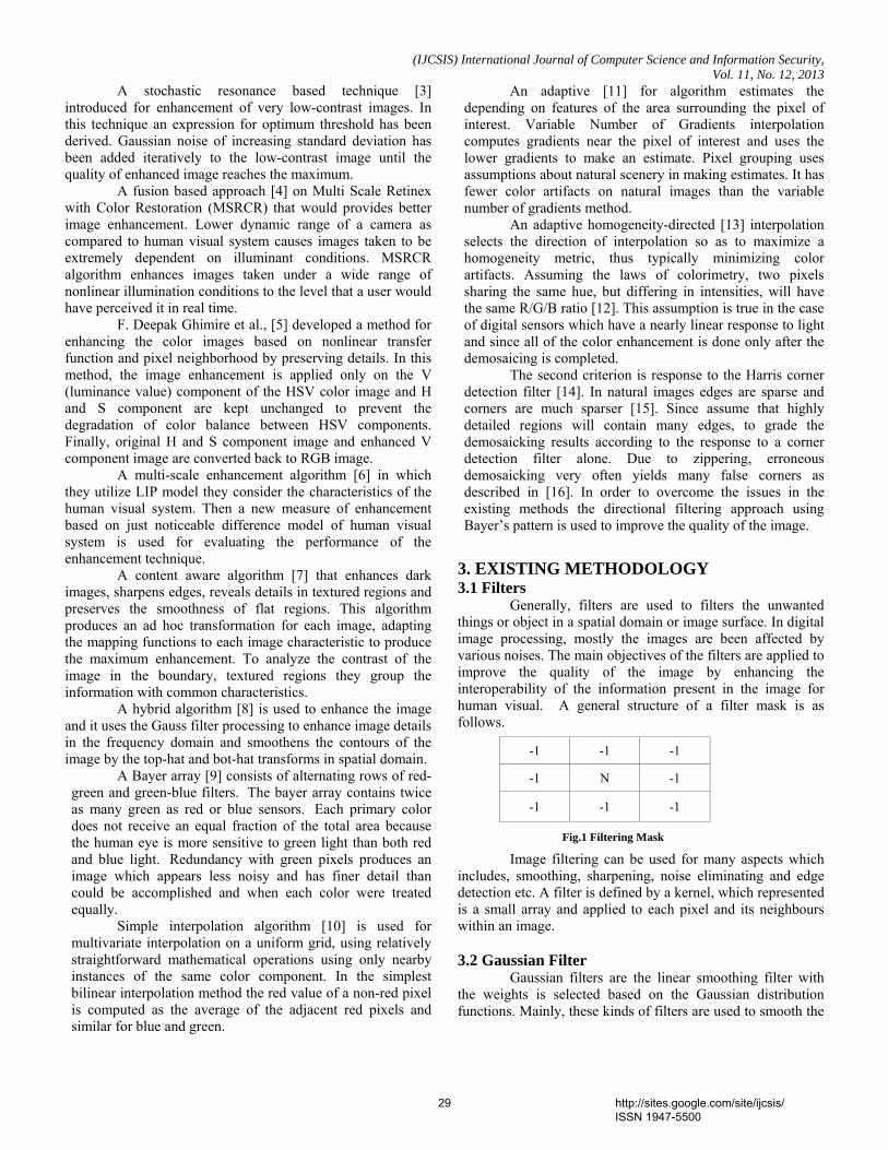
(IJCSIS) International Journal of Computer Science and Information Security, Vol. 11, No. 12, 2013
A stochastic resonance based technique [3] introduced for enhancement of very low-contrast images. In this technique an expression for optimum threshold has been derived. Gaussian noise of increasing standard deviation has been added iteratively to the low-contrast image until the quality of enhanced image reaches the maximum.
A fusion based approach [4] on Multi Scale Retinex with Color Restoration (MSRCR) that would provides better image enhancement. Lower dynamic range of a camera as compared to human visual system causes images taken to be extremely dependent on illuminant conditions. MSRCR algorithm enhances images taken under a wide range of nonlinear illumination conditions to the level that a user would have perceived it in real time.
F. Deepak Ghimire et al., [5] developed a method for enhancing the color images based on nonlinear transfer function and pixel neighborhood by preserving details. In this method, the image enhancement is applied only on the V (luminance value) component of the HSV color image and H and S component are kept unchanged to prevent the degradation of color balance between HSV components. Finally, original H and S component image and enhanced V component image are converted back to RGB image.
A multi-scale enhancement algorithm [6] in which they utilize LIP model they consider the characteristics of the human visual system. Then a new measure of enhancement based on just noticeable difference model of human visual system is used for evaluating the performance of the enhancement technique.
A content aware algorithm [7] that enhances dark images, sharpens edges, reveals details in textured regions and preserves the smoothness of flat regions. This algorithm produces an ad hoc transformation for each image, adapting the mapping functions to each image characteristic to produce the maximum enhancement. To analyze the contrast of the image in the boundary, textured regions they group the information with common characteristics.
A hybrid algorithm [8] is used to enhance the image and it uses the Gauss filter processing to enhance image details in the frequency domain and smoothens the contours of the image by the top-hat and bot-hat transforms in spatial domain.
A Bayer array [9] consists of alternating rows of red-green and green-blue filters. The bayer array contains twice as many green as red or blue sensors. Each primary color does not receive an equal fraction of the total area because the human eye is more sensitive to green light than both red and blue light. Redundancy with green pixels produces an image which appears less noisy and has finer detail than could be accomplished and when each color were treated equally.
Simple interpolation algorithm [10] is used for multivariate interpolation on a uniform grid, using relatively straightforward mathematical operations using only nearby instances of the same color component. In the simplest bilinear interpolation method the red value of a non-red pixel is computed as the average of the adjacent red pixels and similar for blue and green.
An adaptive [11] for algorithm estimates the depending on features of the area surrounding the pixel of interest. Variable Number of Gradients interpolation computes gradients near the pixel of interest and uses the lower gradients to make an estimate. Pixel grouping uses assumptions about natural scenery in making estimates. It has fewer color artifacts on natural images than the variable number of gradients method.
An adaptive homogeneity-directed [13] interpolation selects the direction of interpolation so as to maximize a homogeneity metric, thus typically minimizing color artifacts. Assuming the laws of colorimetry, two pixels sharing the same hue, but differing in intensities, will have the same R/G/B ratio [12]. This assumption is true in the case of digital sensors which have a nearly linear response to light and since all of the color enhancement is done only after the demosaicing is completed.
The second criterion is response to the Harris corner detection filter [14]. In natural images edges are sparse and corners are much sparser [15]. Since assume that highly detailed regions will contain many edges, to grade the demosaicking results according to the response to a corner detection filter alone. Due to zippering, erroneous demosaicking very often yields many false corners as described in [16]. In order to overcome the issues in the existing methods the directional filtering approach using Bayer’s pattern is used to improve the quality of the image.
3. EXISTING METHODOLOGY 3.1 Filters
Generally, filters are used to filters the unwanted things or object in a spatial domain or image surface. In digital image processing, mostly the images are been affected by various noises. The main objectives of the filters are applied to improve the quality of the image by enhancing the interoperability of the information present in the image for human visual. A general structure of a filter mask is as follows.
Fig.1 Filtering Mask
Image filtering can be used for many aspects which includes, smoothing, sharpening, noise eliminating and edge detection etc. A filter is defined by a kernel, which represented is a small array and applied to each pixel and its neighbours within an image.
3.2 Gaussian Filter
Gaussian filters are the linear smoothing filter with the weights is selected based on the Gaussian distribution functions. Mainly, these kinds of filters are used to smooth the
-1 -1 -1
-1 N -1
-1 -1 -1
29 http://sites.google.com/site/ijcsis/ ISSN 1947-5500
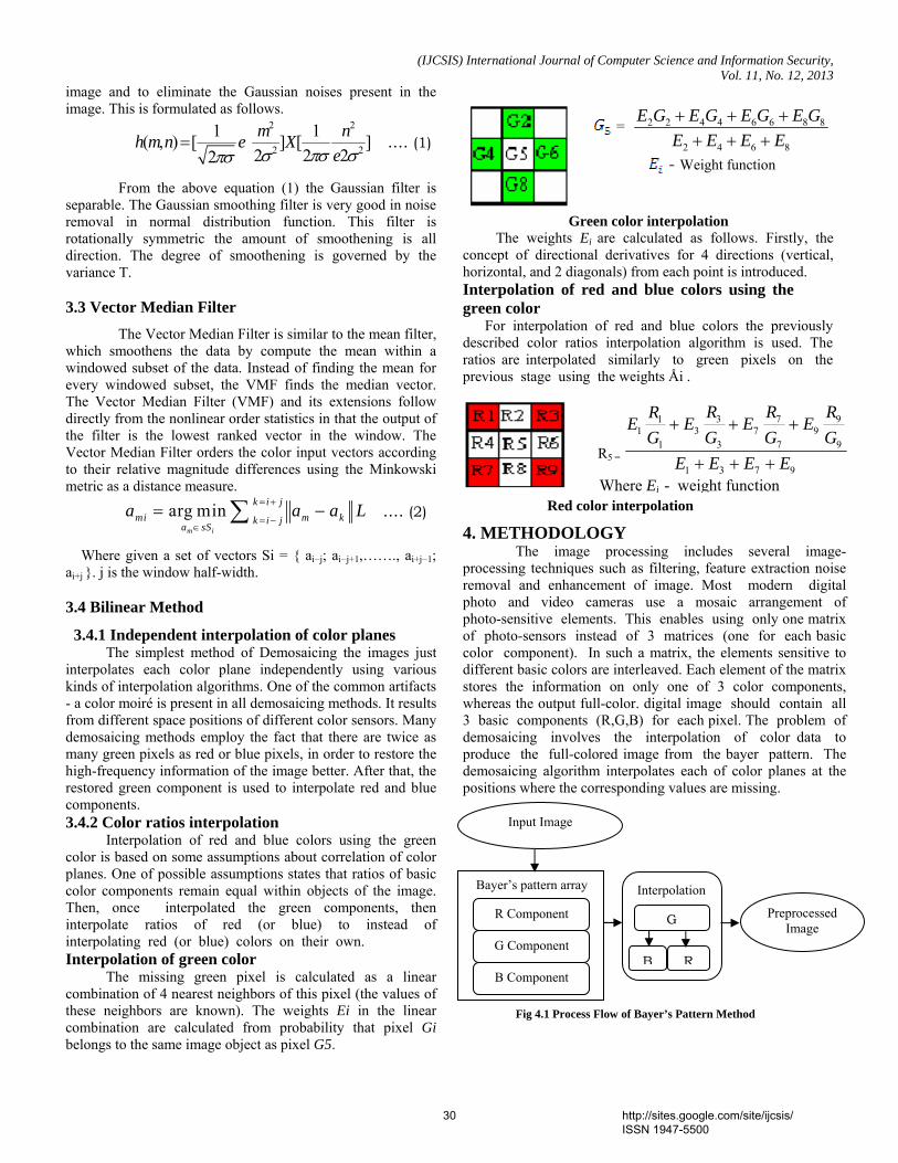
(IJCSIS) International Journal of Computer Science and Information Security, Vol. 11, No. 12, 2013
image and to eliminate the Gaussian noises present in the image. This is formulated as follows.
2 2
2 2
1 1( , ) [ ] [ ]2 2 22m nh m n e X
eσ πσ σπσ= .... (1)
From the above equation (1) the Gaussian filter is separable. The Gaussian smoothing filter is very good in noise removal in normal distribution function. This filter is rotationally symmetric the amount of smoothening is all direction. The degree of smoothening is governed by the variance T.
3.3 Vector Median Filter
The Vector Median Filter is similar to the mean filter, which smoothens the data by compute the mean within a windowed subset of the data. Instead of finding the mean for every windowed subset, the VMF finds the median vector. The Vector Median Filter (VMF) and its extensions follow directly from the nonlinear order statistics in that the output of the filter is the lowest ranked vector in the window. The Vector Median Filter orders the color input vectors according to their relative magnitude differences using the Minkowski metric as a distance measure.
arg minm i
k i jmi m kk i ja sS
a a a L= +
= −∈
= −∑ .... (2)
Where given a set of vectors Si = ai−j; ai−j+1,……., ai+j−1; ai+j . j is the window half-width. 3.4 Bilinear Method
3.4.1 Independent interpolation of color planes The simplest method of Demosaicing the images just interpolates each color plane independently using various kinds of interpolation algorithms. One of the common artifacts - a color moiré is present in all demosaicing methods. It results from different space positions of different color sensors. Many demosaicing methods employ the fact that there are twice as many green pixels as red or blue pixels, in order to restore the high-frequency information of the image better. After that, the restored green component is used to interpolate red and blue components. 3.4.2 Color ratios interpolation Interpolation of red and blue colors using the green color is based on some assumptions about correlation of color planes. One of possible assumptions states that ratios of basic color components remain equal within objects of the image. Then, once interpolated the green components, then interpolate ratios of red (or blue) to instead of interpolating red (or blue) colors on their own. Interpolation of green color The missing green pixel is calculated as a linear combination of 4 nearest neighbors of this pixel (the values of these neighbors are known). The weights Ei in the linear combination are calculated from probability that pixel Gi belongs to the same image object as pixel G5.
Green color interpolation
The weights Ei are calculated as follows. Firstly, the concept of directional derivatives for 4 directions (vertical, horizontal, and 2 diagonals) from each point is introduced. Interpolation of red and blue colors using the green color For interpolation of red and blue colors the previously described color ratios interpolation algorithm is used. The ratios are interpolated similarly to green pixels on the previous stage using the weights Åi .
Red color interpolation
4. METHODOLOGY The image processing includes several image-
processing techniques such as filtering, feature extraction noise removal and enhancement of image. Most modern digital photo and video cameras use a mosaic arrangement of photo-sensitive elements. This enables using only one matrix of photo-sensors instead of 3 matrices (one for each basic color component). In such a matrix, the elements sensitive to different basic colors are interleaved. Each element of the matrix stores the information on only one of 3 color components, whereas the output full-color. digital image should contain all 3 basic components (R,G,B) for each pixel. The problem of demosaicing involves the interpolation of color data to produce the full-colored image from the bayer pattern. The demosaicing algorithm interpolates each of color planes at the positions where the corresponding values are missing.
Fig 4.1 Process Flow of Bayer’s Pattern Method
= 2 2 4 4 6 6 8 8
2 4 6 8
E G E G E G E GE E E E+ + ++ + +
- Weight function
R5 =
3 7 911 3 7 9
1 3 7 9
1 3 7 9
R R RRE E E E
G G G GE E E E
+ + +
+ + +
Where Ei - weight function
Input Image
Preprocessed Image
Bayer’s pattern array
Interpolation
R Component G
B R G Component
B Component
30 http://sites.google.com/site/ijcsis/ ISSN 1947-5500
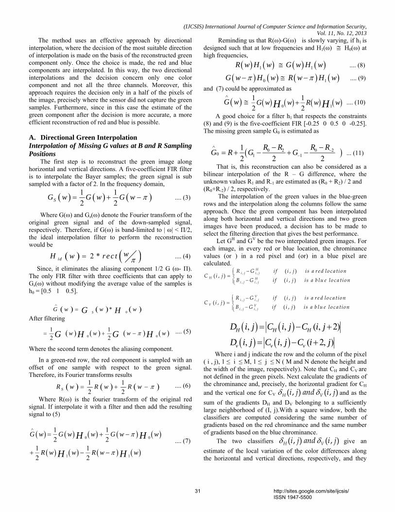
(IJCSIS) International Journal of Computer Science and Information Security, Vol. 11, No. 12, 2013
The method uses an effective approach by directional interpolation, where the decision of the most suitable direction of interpolation is made on the basis of the reconstructed green component only. Once the choice is made, the red and blue components are interpolated. In this way, the two directional interpolations and the decision concern only one color component and not all the three channels. Moreover, this approach requires the decision only in a half of the pixels of the image, precisely where the sensor did not capture the green samples. Furthermore, since in this case the estimate of the green component after the decision is more accurate, a more efficient reconstruction of red and blue is possible.
A. Directional Green Interpolation Interpolation of Missing G values at B and R Sampling Positions The first step is to reconstruct the green image along horizontal and vertical directions. A five-coefficient FIR filter is to interpolate the Bayer samples; the green signal is sub sampled with a factor of 2. In the frequency domain,
( ) ( ) ( )1 12 2SG w G w G w π= + − .... (3)
Where G(ω) and Gs(ω) denote the Fourier transform of the original green signal and of the down-sampled signal, respectively. Therefore, if G(ω) is band-limited to | ω| < П/2, the ideal interpolation filter to perform the reconstruction would be
( ) ( )2 *idwH w re c t π= .... (4)
Since, it eliminates the aliasing component 1/2 G (ω- П). The only FIR filter with three coefficients that can apply to Gs(ω) without modifying the average value of the samples is h0 = [0.5 1 0.5].
( ) ( ) ( )0*SG w w wHG∧
= After filtering
( ) ( ) ( ) ( )0 0
1 12 2
w w w wG GH Hπ= + − .... (5)
Where the second term denotes the aliasing component.
In a green-red row, the red component is sampled with an offset of one sample with respect to the green signal. Therefore, its Fourier transforms results
( ) ( ) ( )1 12 2SR w R w R w π= + − .... (6)
Where R(ω) is the fourier transform of the original red signal. If interpolate it with a filter and then add the resulting signal to (5)
( ) ( ) ( ) ( ) ( )
( ) ( ) ( ) ( )
0 0
1 1
1 12 2
1 12 2
G w G w w G w w
R w w R w w
H H
H H
π
π
∧
= + −
+ − −
.... (7)
Reminding us that R(ω)-G(ω) is slowly varying, if h1 is designed such that at low frequencies and H1(ω) ≅ H0(ω) at high frequencies, ( ) ( )1R w H w ≅ ( ) ( )1G w H w .... (8)
( ) ( )0G w H wπ− ≅ ( ) ( )1R w H wπ− .... (9)and (7) could be approximated as
( )G w∧
≅ ( ) ( ) ( ) ( )0 1
1 12 2
G w w R w wH H+ .... (10)
A good choice for a filter h1 that respects the constraints
(8) and (9) is the five-coefficient FIR [-0.25 0 0.5 0 -0.25]. The missing green sample G0 is estimated as
( )0 2 0 20 1 1
12 2 2
R R R RG R G G∧
−−
− −= + − + − ... (11)
That is, this reconstruction can also be considered as a bilinear interpolation of the R – G difference, where the unknown values R1 and R-1 are estimated as (R0 + R2) / 2 and (R0+R-2) / 2, respectively. The interpolation of the green values in the blue-green rows and the interpolation along the columns follow the same approach. Once the green component has been interpolated along both horizontal and vertical directions and two green images have been produced, a decision has to be made to select the filtering direction that gives the best performance. Let GH and GV be the two interpolated green images. For each image, in every red or blue location, the chrominance values (or ) in a red pixel and (or) in a blue pixel are calculated.
⎧⎪⎨⎪⎩
⎧⎪⎨⎪⎩
−=
−
−=
−
, ,
, ,
, ,
, ,
( , )( , )
( , )
( , )( , )
( , )
Hi j i j
H Hi j i j
Vi j i j
V Vi j i j
R G if i j is a r ed lo c a t ionC i j
B G if i j is a b lu e lo c a t ion
R G if i j is a r ed lo c a tionC i j
B G if i j is a b lu e lo c a tion
( ) ( )( ) ( )
, , ( , 2)
, , ( 2, )H H H
v v v
D i j C i j C i j
D i j C i j C i j
= − +
= − +
Where i and j indicate the row and the column of the pixel ( i , j), 1 ≤ i ≤ M, 1 ≤ j ≤ N ( M and N denote the height and the width of the image, respectively). Note that CH and CV are not defined in the green pixels. Next calculate the gradients of the chrominance and, precisely, the horizontal gradient for CH and the vertical one for CV ( , ) ( , )H Vi j and i jδ δ and as the sum of the gradients DH and DV belonging to a sufficiently large neighborhood of (I, j).With a square window, both the classifiers are computed considering the same number of gradients based on the red chrominance and the same number of gradients based on the blue chrominance. The two classifiers ( , ) ( , )H Vi j and i jδ δ give an estimate of the local variation of the color differences along the horizontal and vertical directions, respectively, and they
31 http://sites.google.com/site/ijcsis/ ISSN 1947-5500
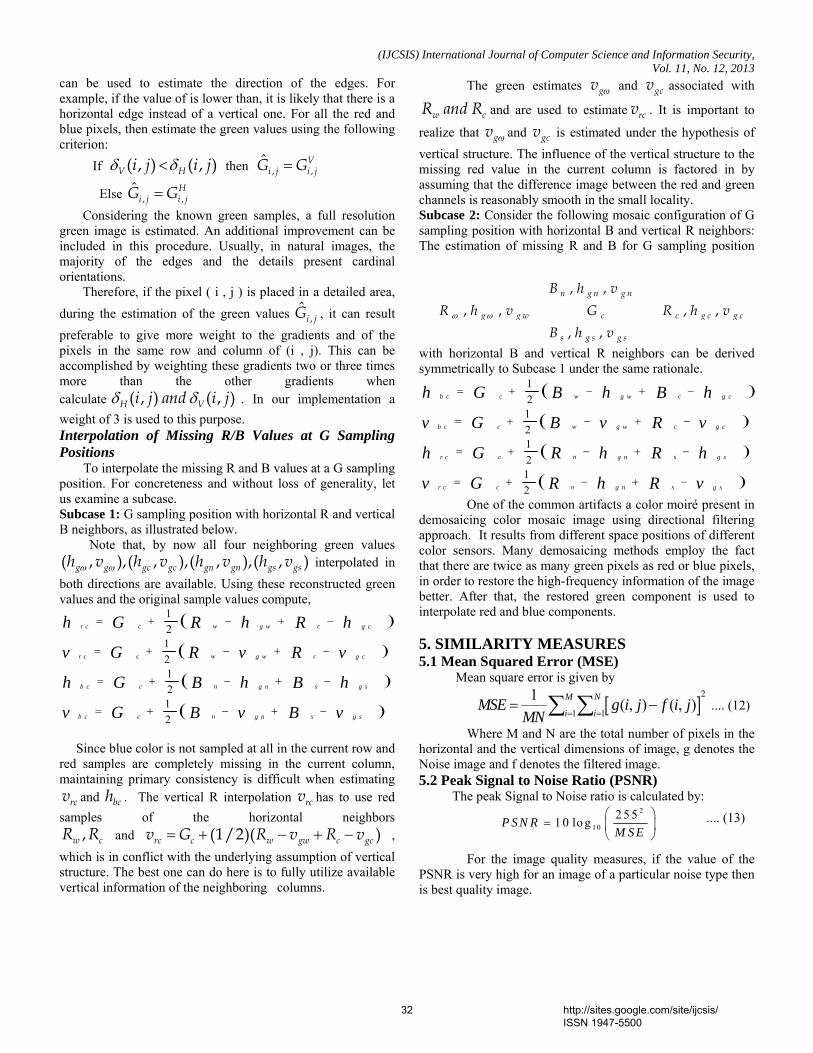
(IJCSIS) International Journal of Computer Science and Information Security, Vol. 11, No. 12, 2013
can be used to estimate the direction of the edges. For example, if the value of is lower than, it is likely that there is a horizontal edge instead of a vertical one. For all the red and blue pixels, then estimate the green values using the following criterion: If ( , ) ( , )V Hi j i jδ δ< then , ,
ˆ Vi j i jG G=
Else , ,ˆ Hi j i jG G=
Considering the known green samples, a full resolution green image is estimated. An additional improvement can be included in this procedure. Usually, in natural images, the majority of the edges and the details present cardinal orientations. Therefore, if the pixel ( i , j ) is placed in a detailed area, during the estimation of the green values ,
ˆi jG , it can result
preferable to give more weight to the gradients and of the pixels in the same row and column of (i , j). This can be accomplished by weighting these gradients two or three times more than the other gradients when calculate ( , ) ( , )H Vi j and i jδ δ . In our implementation a weight of 3 is used to this purpose. Interpolation of Missing R/B Values at G Sampling Positions
To interpolate the missing R and B values at a G sampling position. For concreteness and without loss of generality, let us examine a subcase. Subcase 1: G sampling position with horizontal R and vertical B neighbors, as illustrated below. Note that, by now all four neighboring green values ( , ),( , ),( , ),( , )g g gc gc gn gn gs gsh v h v h v h vω ω interpolated in both directions are available. Using these reconstructed green values and the original sample values compute,
( )
( )
( )
( )
12121212
w cr c c g w g c
w cr c c g w g c
n sb c c g n g s
n sb c c g n g s
h G h hR R
v G v vR R
h G h hB B
v G v vB B
= + − + −
= + − + −
= + − + −
= + − + −
Since blue color is not sampled at all in the current row and red samples are completely missing in the current column, maintaining primary consistency is difficult when estimating
rcv and bch . The vertical R interpolation rcv has to use red samples of the horizontal neighbors
,w cR R and (1/2)( )rc c w gw c gcv G R v R v= + − + − , which is in conflict with the underlying assumption of vertical structure. The best one can do here is to fully utilize available vertical information of the neighboring columns.
The green estimates gv ω and gcv associated with
w cR and R and are used to estimate rcv . It is important to
realize that gv ω and gcv is estimated under the hypothesis of vertical structure. The influence of the vertical structure to the missing red value in the current column is factored in by assuming that the difference image between the red and green channels is reasonably smooth in the small locality. Subcase 2: Consider the following mosaic configuration of G sampling position with horizontal B and vertical R neighbors: The estimation of missing R and B for G sampling position
with horizontal B and vertical R neighbors can be derived symmetrically to Subcase 1 under the same rationale.
( )
( )
( )
( )
12121212
w cb c c g w g c
w cb c c g w g c
n sr c c g n g s
n sr c c g n g s
h G h hB B
v G v vB R
h G h hR R
v G h vR R
= + − + −
= + − + −
= + − + −
= + − + −
One of the common artifacts a color moiré present in demosaicing color mosaic image using directional filtering approach. It results from different space positions of different color sensors. Many demosaicing methods employ the fact that there are twice as many green pixels as red or blue pixels, in order to restore the high-frequency information of the image better. After that, the restored green component is used to interpolate red and blue components. 5. SIMILARITY MEASURES 5.1 Mean Squared Error (MSE) Mean square error is given by
[ ]2
1 1
1 ( , ) ( , )M N
i iMSE g i j f i j
MN = == −∑ ∑ .... (12)
Where M and N are the total number of pixels in the horizontal and the vertical dimensions of image, g denotes the Noise image and f denotes the filtered image. 5.2 Peak Signal to Noise Ratio (PSNR) The peak Signal to Noise ratio is calculated by:
2
1 02 5 51 0 lo gP S N RM S E
⎛ ⎞= ⎜ ⎟
⎝ ⎠ .... (13)
For the image quality measures, if the value of the PSNR is very high for an image of a particular noise type then is best quality image.
ω ω
, ,, , , ,
, ,
n g n g n
g g w c c g c g c
s g s g s
B h vR h v G R h v
B h v
32 http://sites.google.com/site/ijcsis/ ISSN 1947-5500
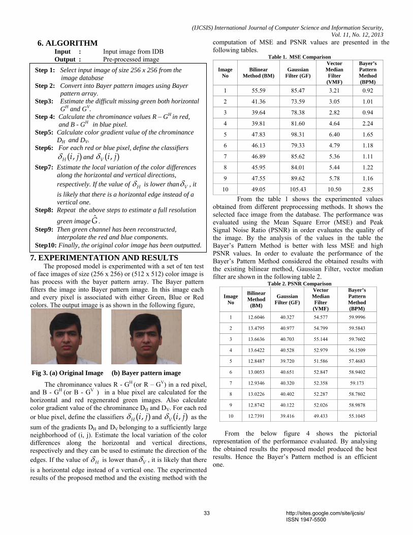
(IJCSIS) International Journal of Computer Science and Information Security, Vol. 11, No. 12, 2013
6. ALGORITHM Input : Input image from IDB Output : Pre-processed image
7. EXPERIMENTATION AND RESULTS The proposed model is experimented with a set of ten test of face images of size (256 x 256) or (512 x 512) color image is has process with the bayer pattern array. The Bayer pattern filters the image into Bayer pattern image. In this image each and every pixel is associated with either Green, Blue or Red colors. The output image is as shown in the following figure,
Fig 3. (a) Original Image (b) Bayer pattern image
The chrominance values R - GH (or R – GV) in a red pixel, and B - GH (or B - GV ) in a blue pixel are calculated for the horizontal and red regenerated green images. Also calculate color gradient value of the chrominance DH and DV. For each red or blue pixel, define the classifiers ( , )H i jδ and ( , )V i jδ as the sum of the gradients DH and DV belonging to a sufficiently large neighborhood of (i, j). Estimate the local variation of the color differences along the horizontal and vertical directions, respectively and they can be used to estimate the direction of the edges. If the value of Hδ is lower than Vδ , it is likely that there is a horizontal edge instead of a vertical one. The experimented results of the proposed method and the existing method with the
computation of MSE and PSNR values are presented in the following tables.
Table 1. MSE Comparison
Image No
Bilinear Method (BM)
Gaussian Filter (GF)
Vector Median Filter
(VMF)
Bayer’s Pattern Method (BPM)
1 55.59 85.47 3.21 0.92
2 41.36 73.59 3.05 1.01
3 39.64 78.38 2.82 0.94
4 39.81 81.60 4.64 2.24
5 47.83 98.31 6.40 1.65
6 46.13 79.33 4.79 1.18
7 46.89 85.62 5.36 1.11
8 45.95 84.01 5.44 1.22
9 47.55 89.62 5.78 1.16
10 49.05 105.43 10.50 2.85 From the table 1 shows the experimented values
obtained from different preprocessing methods. It shows the selected face image from the database. The performance was evaluated using the Mean Square Error (MSE) and Peak Signal Noise Ratio (PSNR) in order evaluates the quality of the image. By the analysis of the values in the table the Bayer’s Pattern Method is better with less MSE and high PSNR values. In order to evaluate the performance of the Bayer’s Pattern Method considered the obtained results with the existing bilinear method, Gaussian Filter, vector median filter are shown in the following table 2.
Table 2. PSNR Comparison
Image No
Bilinear Method
(BM)
Gaussian Filter (GF)
Vector Median Filter
(VMF)
Bayer’s Pattern Method (BPM)
1 12.6046 40.327 54.577 59.9996
2 13.4795 40.977 54.799 59.5843
3 13.6636 40.703 55.144 59.7602
4 13.6422 40.528 52.979 56.1509
5 12.8487 39.720 51.586 57.4683
6 13.0053 40.651 52.847 58.9402
7 12.9346 40.320 52.358 59.173
8 13.0226 40.402 52.287 58.7802
9 12.8742 40.122 52.026 58.9878
10 12.7391 39.416 49.433 55.1045
From the below figure 4 shows the pictorial representation of the performance evaluated. By analysing the obtained results the proposed model produced the best results. Hence the Bayer’s Pattern method is an efficient one.
Step 1: Select input image of size 256 x 256 from the image database
Step 2: Convert into Bayer pattern images using Bayer pattern array. Step3: Estimate the difficult missing green both horizontal GH and GV. Step 4: Calculate the chrominance values R – GH in red, and B - GH in blue pixel. Step5: Calculate color gradient value of the chrominance DH and DV. Step6: For each red or blue pixel, define the classifiers ( , )H i jδ and ( , )V i jδ Step7: Estimate the local variation of the color differences along the horizontal and vertical directions, respectively. If the value of Hδ is lower than Vδ , it is likely that there is a horizontal edge instead of a vertical one. Step8: Repeat the above steps to estimate a full resolution
green image G . Step9: Then green channel has been reconstructed, interpolate the red and blue components. Step10: Finally, the original color image has been outputted.
33 http://sites.google.com/site/ijcsis/ ISSN 1947-5500
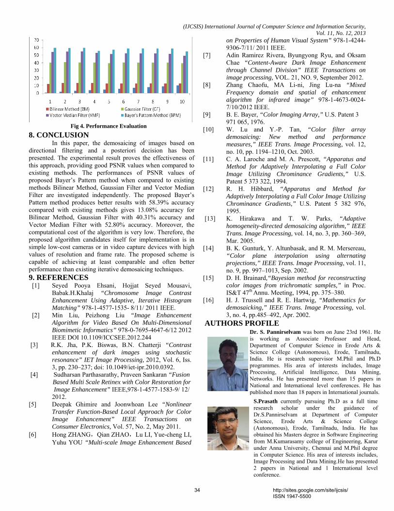
(IJCSIS) International Journal of Computer Science and Information Security, Vol. 11, No. 12, 2013
Fig 4. Performance Evaluation
8. CONCLUSION In this paper, the demosaicing of images based on directional filtering and a posteriori decision has been presented. The experimental result proves the effectiveness of this approach, providing good PSNR values when compared to existing methods. The performances of PSNR values of proposed Bayer’s Pattern method when compared to existing methods Bilinear Method, Gaussian Filter and Vector Median Filter are investigated independently. The proposed Bayer’s Pattern method produces better results with 58.39% accuracy compared with existing methods gives 13.08% accuracy for Bilinear Method, Gaussian Filter with 40.31% accuracy and Vector Median Filter with 52.80% accuracy. Moreover, the computational cost of the algorithm is very low. Therefore, the proposed algorithm candidates itself for implementation is in simple low-cost cameras or in video capture devices with high values of resolution and frame rate. The proposed scheme is capable of achieving at least comparable and often better performance than existing iterative demosaicing techniques. 9. REFERENCES [1] Seyed Pooya Ehsani, Hojjat Seyed Mousavi,
Babak.H.Khalaj “Chromosome Image Contrast Enhancement Using Adaptive, Iterative Histogram Matching” 978-1-4577-1535- 8/11/ 2011 IEEE.
[2] Min Liu, Peizhong Liu “Image Enhancement Algorithm for Video Based On Multi-Dimensional Biomimetic Informatics” 978-0-7695-4647-6/12 2012 IEEE DOI 10.1109/ICCSEE.2012.244
[3] R.K. Jha, P.K. Biswas, B.N. Chatterji “Contrast enhancement of dark images using stochastic resonance” IET Image Processing, 2012, Vol. 6, Iss. 3, pp. 230–237; doi: 10.1049/iet-ipr.2010.0392.
[4] Sudharsan Parthasarathy, Praveen Sankaran “Fusion Based Multi Scale Retinex with Color Restoration for Image Enhancement” IEEE,978-1-4577-1583-9/ 12/
2012. [5] Deepak Ghimire and Joonwhoan Lee “Nonlinear
Transfer Function-Based Local Approach for Color Image Enhancement” IEEE Transactions on Consumer Electronics, Vol. 57, No. 2, May 2011.
[6] Hong ZHANG,Qian ZHAO,Lu LI, Yue-cheng LI, Yuhu YOU “Multi-scale Image Enhancement Based
on Properties of Human Visual System” 978-1-4244-9306-7/11/ 2011 IEEE.
[7] Adin Ramirez Rivera, Byungyong Ryu, and Oksam Chae “Content-Aware Dark Image Enhancement through Channel Division” IEEE Transactions on image processing, VOL. 21, NO. 9, September 2012.
[8] Zhang Chaofu, MA Li-ni, Jing Lu-na “Mixed Frequency domain and spatial of enhancement algorithm for infrared image” 978-1-4673-0024-7/10/2012 IEEE.
[9] B. E. Bayer, “Color Imaging Array,” U.S. Patent 3 971 065, 1976.
[10] W. Lu and Y.-P. Tan, “Color filter array demosaicing: New method and performance measures,” IEEE Trans. Image Processing, vol. 12, no. 10, pp. 1194–1210, Oct. 2003.
[11] C. A. Laroche and M. A. Prescott, “Apparatus and Method for Adaptively Interpolating a Full Color Image Utilizing Chrominance Gradients,” U.S. Patent 5 373 322, 1994.
[12] R. H. Hibbard, “Apparatus and Method for Adaptively Interpolating a Full Color Image Utilizing Chrominance Gradients,” U.S. Patent 5 382 976, 1995.
[13] K. Hirakawa and T. W. Parks, “Adaptive homogeneity-directed demosaicing algorithm,” IEEE Trans. Image Processing, vol. 14, no. 3, pp. 360–369, Mar. 2005.
[14] B. K. Gunturk, Y. Altunbasak, and R. M. Mersereau, “Color plane interpolation using alternating projections,” IEEE Trans. Image Processing, vol. 11, no. 9, pp. 997–1013, Sep. 2002.
[15] D. H. Brainard,“Bayesian method for reconstructing color images from trichromatic samples,” in Proc. IS&T 47th Annu. Meeting, 1994, pp. 375–380.
[16] H. J. Trussell and R. E. Hartwig, “Mathematics for demosaicking,” IEEE Trans. Image Processing, vol. 3, no. 4, pp.485–492, Apr. 2002.
AUTHORS PROFILE
Dr. S. Pannirselvam was born on June 23rd 1961. He is working as Associate Professor and Head, Department of Computer Science in Erode Arts & Science College (Autonomous), Erode, Tamilnadu, India. He is research supervisor M.Phil and Ph.D programmes. His area of interests includes, Image Processing, Artificial Intelligence, Data Mining, Networks. He has presented more than 15 papers in National and International level conferences. He has published more than 18 papers in International journals.
S.Prasath currently pursuing Ph.D as a full time research scholar under the guidance of Dr.S.Pannirselvam at Department of Computer Science, Erode Arts & Science College (Autonomous), Erode, Tamilnadu, India. He has obtained his Masters degree in Software Engineering from M.Kumarasamy college of Engineering, Karur under Anna University, Chennai and M.Phil degree in Computer Science. His area of interests includes, Image Processing and Data Mining.He has presented 2 papers in National and 1 International level conference.
34 http://sites.google.com/site/ijcsis/ ISSN 1947-5500
(IJCSIS) International Journal of Computer Science and Information Security,
Vol. 11, No. 12, December 2013
An Agent-Based Framework for Virtual Machine
Migration in Cloud Computing
Somayeh Soltan Baghshahi *
Computer Engineering Department
Islamic Azad University, North Tehran Branch
Tehran, Iran
Sam Jabbehdari
Computer Engineering Department
Islamic Azad University, North Tehran Branch
Tehran, Iran
Sahar Adabi
Computer Engineering Department
Islamic Azad University, North Tehran Branch
Abstract— Cloud computing is a model for large-scale distributed
computing, which services to customers be done through a
dynamic virtual resources with high computational power of
using the Internet. The cloud service providers use different
methods to manage virtual resources, that to use of autonomous
nature of the intelligent agents, it can improve quality of service
in a cloud distributed environment.
In this paper, we design a framework by using of the multiple
intelligent agents, which these agent interactions with together
and they manage to provide the service. Also, In this framework,
an agent is designed to improve the migration technique of
virtual machines.
Keywords- Cloud Computing; Virtualizaion; Virtual Machine
Migration; Agent-Based Framework
I. INTRODUCTION
Cloud computing is an emerging new paradigm for hosting
services over the internet. Cloud computing offers
infrastructure as a service, platform as a service and storage as
a service to the cloud users. Cloud users are charged based on
their service usage. The cloud computing services are available
at anywhere, anytime, only we have to need internet
connectivity. To improve the utilization of cloud resources we
use virtual machines. The virtual machine is a software
implementation of a computing environment in which
operating system or program can be installed and run [1].
Cloud computing [2] has currently attracted considerable
attention from both the industrial community and the academic
community. Virtualization provides an abstraction of hardware
resources enabling multiple instantiations of operating systems
to run simultaneously on a single physical machine. Another prominent advantage of the Virtualization is the
live migration technique [3,5] which refers to the act of migrating a virtual machine from one physical machine to another even as the virtual machine continues to execute. Currently, live migration has become a key ingredient behind the management activities of cloud computing system to achieve the goals of load balancing, energy saving, failure recovery, and system maintenance [4].
II. RELATED WORK
Virtualization is the key technology that enables the emerging
cloud computing paradigm [8][9][10], because it allows
resources to be allocated to different applications on demand
and hides the complexity of resource sharing from cloud users.
VMs are generally employed in different types of cloud
systems as containers for hosting application execution
environments and provisioning resources. For example, in
Infrastructure-as-a-Service (IaaS) clouds [3], VMs are directly
exposed to users to deliver a full computer infrastructure over
the internet; In Platform-as-a-Service (PaaS) clouds [13], VMs
are also used by the clouds internally to manage resources
across the application execution platforms delivered to users.
VM migration is a unique capability of system Virtualization
which allows an application to be transparently moved from
one physical host to another and to continue its execution after
migration without any loss of progress. It is generally done by
transferring the application along with its VM’s entire system
* Corresponding author
35 http://sites.google.com/site/ijcsis/ ISSN 1947-5500
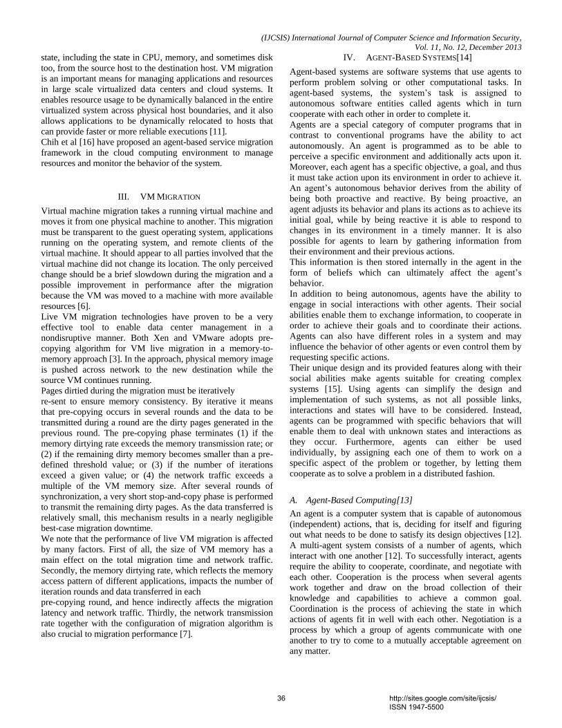
(IJCSIS) International Journal of Computer Science and Information Security,
Vol. 11, No. 12, December 2013
state, including the state in CPU, memory, and sometimes disk
too, from the source host to the destination host. VM migration
is an important means for managing applications and resources
in large scale virtualized data centers and cloud systems. It
enables resource usage to be dynamically balanced in the entire
virtualized system across physical host boundaries, and it also
allows applications to be dynamically relocated to hosts that
can provide faster or more reliable executions [11].
Chih et al [16] have proposed an agent-based service migration
framework in the cloud computing environment to manage
resources and monitor the behavior of the system.
III. VM MIGRATION
Virtual machine migration takes a running virtual machine and
moves it from one physical machine to another. This migration
must be transparent to the guest operating system, applications
running on the operating system, and remote clients of the
virtual machine. It should appear to all parties involved that the
virtual machine did not change its location. The only perceived
change should be a brief slowdown during the migration and a
possible improvement in performance after the migration
because the VM was moved to a machine with more available
resources [6].
Live VM migration technologies have proven to be a very
effective tool to enable data center management in a
nondisruptive manner. Both Xen and VMware adopts pre-
copying algorithm for VM live migration in a memory-to-
memory approach [3]. In the approach, physical memory image
is pushed across network to the new destination while the
source VM continues running.
Pages dirtied during the migration must be iteratively
re-sent to ensure memory consistency. By iterative it means
that pre-copying occurs in several rounds and the data to be
transmitted during a round are the dirty pages generated in the
previous round. The pre-copying phase terminates (1) if the
memory dirtying rate exceeds the memory transmission rate; or
(2) if the remaining dirty memory becomes smaller than a pre-
defined threshold value; or (3) if the number of iterations
exceed a given value; or (4) the network traffic exceeds a
multiple of the VM memory size. After several rounds of
synchronization, a very short stop-and-copy phase is performed
to transmit the remaining dirty pages. As the data transferred is
relatively small, this mechanism results in a nearly negligible
best-case migration downtime.
We note that the performance of live VM migration is affected
by many factors. First of all, the size of VM memory has a
main effect on the total migration time and network traffic.
Secondly, the memory dirtying rate, which reflects the memory
access pattern of different applications, impacts the number of
iteration rounds and data transferred in each
pre-copying round, and hence indirectly affects the migration
latency and network traffic. Thirdly, the network transmission
rate together with the configuration of migration algorithm is
also crucial to migration performance [7].
IV. AGENT-BASED SYSTEMS[14]
Agent-based systems are software systems that use agents to
perform problem solving or other computational tasks. In
agent-based systems, the system’s task is assigned to
autonomous software entities called agents which in turn
cooperate with each other in order to complete it.
Agents are a special category of computer programs that in
contrast to conventional programs have the ability to act
autonomously. An agent is programmed as to be able to
perceive a specific environment and additionally acts upon it.
Moreover, each agent has a specific objective, a goal, and thus
it must take action upon its environment in order to achieve it.
An agent’s autonomous behavior derives from the ability of
being both proactive and reactive. By being proactive, an
agent adjusts its behavior and plans its actions as to achieve its
initial goal, while by being reactive it is able to respond to
changes in its environment in a timely manner. It is also
possible for agents to learn by gathering information from
their environment and their previous actions.
This information is then stored internally in the agent in the
form of beliefs which can ultimately affect the agent’s
behavior.
In addition to being autonomous, agents have the ability to
engage in social interactions with other agents. Their social
abilities enable them to exchange information, to cooperate in
order to achieve their goals and to coordinate their actions.
Agents can also have different roles in a system and may
influence the behavior of other agents or even control them by
requesting specific actions.
Their unique design and its provided features along with their
social abilities make agents suitable for creating complex
systems [15]. Using agents can simplify the design and
implementation of such systems, as not all possible links,
interactions and states will have to be considered. Instead,
agents can be programmed with specific behaviors that will
enable them to deal with unknown states and interactions as
they occur. Furthermore, agents can either be used
individually, by assigning each one of them to work on a
specific aspect of the problem or together, by letting them
cooperate as to solve a problem in a distributed fashion.
A. Agent-Based Computing[13]
An agent is a computer system that is capable of autonomous
(independent) actions, that is, deciding for itself and figuring
out what needs to be done to satisfy its design objectives [12].
A multi-agent system consists of a number of agents, which
interact with one another [12]. To successfully interact, agents
require the ability to cooperate, coordinate, and negotiate with
each other. Cooperation is the process when several agents
work together and draw on the broad collection of their
knowledge and capabilities to achieve a common goal.
Coordination is the process of achieving the state in which
actions of agents fit in well with each other. Negotiation is a
process by which a group of agents communicate with one
another to try to come to a mutually acceptable agreement on
any matter.
36 http://sites.google.com/site/ijcsis/ ISSN 1947-5500
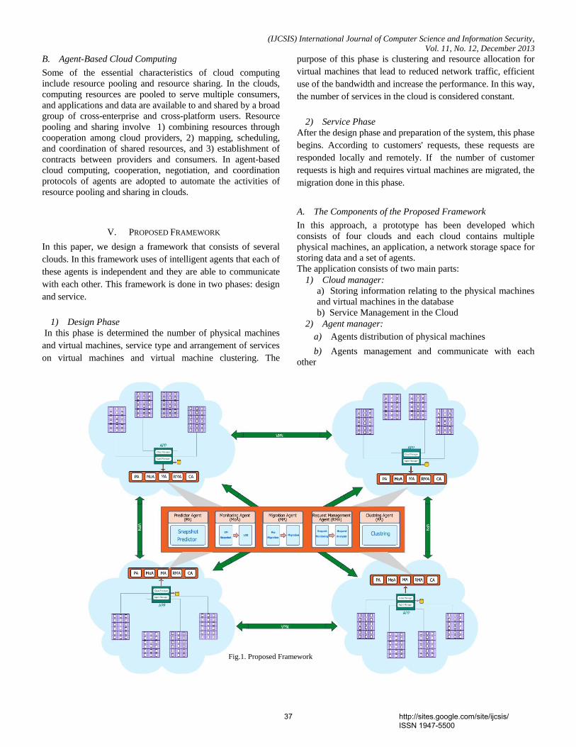
(IJCSIS) International Journal of Computer Science and Information Security,
Vol. 11, No. 12, December 2013
B. Agent-Based Cloud Computing
Some of the essential characteristics of cloud computing
include resource pooling and resource sharing. In the clouds,
computing resources are pooled to serve multiple consumers,
and applications and data are available to and shared by a broad
group of cross-enterprise and cross-platform users. Resource
pooling and sharing involve 1) combining resources through
cooperation among cloud providers, 2) mapping, scheduling,
and coordination of shared resources, and 3) establishment of
contracts between providers and consumers. In agent-based
cloud computing, cooperation, negotiation, and coordination
protocols of agents are adopted to automate the activities of
resource pooling and sharing in clouds.
V. PROPOSED FRAMEWORK
In this paper, we design a framework that consists of several
clouds. In this framework uses of intelligent agents that each of
these agents is independent and they are able to communicate
with each other. This framework is done in two phases: design
and service.
1) Design Phase
In this phase is determined the number of physical machines
and virtual machines, service type and arrangement of services
on virtual machines and virtual machine clustering. The
purpose of this phase is clustering and resource allocation for
virtual machines that lead to reduced network traffic, efficient
use of the bandwidth and increase the performance. In this way,
the number of services in the cloud is considered constant.
2) Service Phase
After the design phase and preparation of the system, this phase
begins. According to customers' requests, these requests are
responded locally and remotely. If the number of customer
requests is high and requires virtual machines are migrated, the
migration done in this phase.
A. The Components of the Proposed Framework
In this approach, a prototype has been developed which
consists of four clouds and each cloud contains multiple
physical machines, an application, a network storage space for
storing data and a set of agents.
The application consists of two main parts:
1) Cloud manager:
a) Storing information relating to the physical machines
and virtual machines in the database
b) Service Management in the Cloud
2) Agent manager:
a) Agents distribution of physical machines
b) Agents management and communicate with each
other
Fig.1. Proposed Framework
37 http://sites.google.com/site/ijcsis/ ISSN 1947-5500
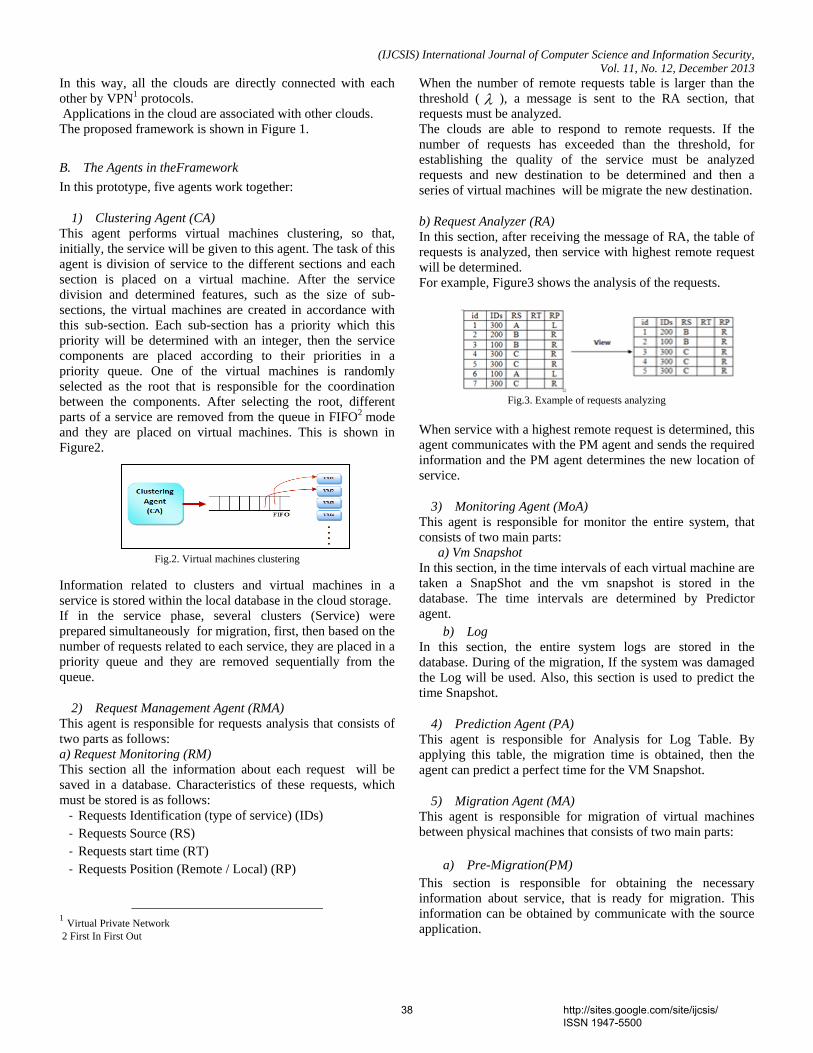
(IJCSIS) International Journal of Computer Science and Information Security,
Vol. 11, No. 12, December 2013
In this way, all the clouds are directly connected with each
other by VPN1 protocols.
Applications in the cloud are associated with other clouds.
The proposed framework is shown in Figure 1.
B. The Agents in theFramework
In this prototype, five agents work together:
1) Clustering Agent (CA) This agent performs virtual machines clustering, so that,
initially, the service will be given to this agent. The task of this
agent is division of service to the different sections and each
section is placed on a virtual machine. After the service
division and determined features, such as the size of sub-
sections, the virtual machines are created in accordance with
this sub-section. Each sub-section has a priority which this
priority will be determined with an integer, then the service
components are placed according to their priorities in a
priority queue. One of the virtual machines is randomly
selected as the root that is responsible for the coordination
between the components. After selecting the root, different
parts of a service are removed from the queue in FIFO2 mode
and they are placed on virtual machines. This is shown in
Figure2.
Fig.2. Virtual machines clustering
Information related to clusters and virtual machines in a
service is stored within the local database in the cloud storage.
If in the service phase, several clusters (Service) were
prepared simultaneously for migration, first, then based on the
number of requests related to each service, they are placed in a
priority queue and they are removed sequentially from the
queue.
2) Request Management Agent (RMA) This agent is responsible for requests analysis that consists of
two parts as follows:
a) Request Monitoring (RM)
This section all the information about each request will be
saved in a database. Characteristics of these requests, which
must be stored is as follows:
- Requests Identification (type of service) (IDs)
- Requests Source (RS)
- Requests start time (RT)
- Requests Position (Remote / Local) (RP)
1 Virtual Private Network 2 First In First Out
When the number of remote requests table is larger than the
threshold ( ), a message is sent to the RA section, that
requests must be analyzed.
The clouds are able to respond to remote requests. If the
number of requests has exceeded than the threshold, for
establishing the quality of the service must be analyzed
requests and new destination to be determined and then a
series of virtual machines will be migrate the new destination.
b) Request Analyzer (RA) In this section, after receiving the message of RA, the table of
requests is analyzed, then service with highest remote request
will be determined.
For example, Figure3 shows the analysis of the requests.
Fig.3. Example of requests analyzing
When service with a highest remote request is determined, this
agent communicates with the PM agent and sends the required
information and the PM agent determines the new location of
service.
3) Monitoring Agent (MoA)
This agent is responsible for monitor the entire system, that
consists of two main parts:
a) Vm Snapshot
In this section, in the time intervals of each virtual machine are
taken a SnapShot and the vm snapshot is stored in the
database. The time intervals are determined by Predictor
agent.
b) Log
In this section, the entire system logs are stored in the
database. During of the migration, If the system was damaged
the Log will be used. Also, this section is used to predict the
time Snapshot.
4) Prediction Agent (PA) This agent is responsible for Analysis for Log Table. By
applying this table, the migration time is obtained, then the
agent can predict a perfect time for the VM Snapshot.
5) Migration Agent (MA) This agent is responsible for migration of virtual machines
between physical machines that consists of two main parts:
a) Pre-Migration(PM)
This section is responsible for obtaining the necessary
information about service, that is ready for migration. This
information can be obtained by communicate with the source
application.
38 http://sites.google.com/site/ijcsis/ ISSN 1947-5500
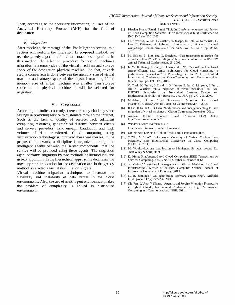
(IJCSIS) International Journal of Computer Science and Information Security,
Vol. 11, No. 12, December 2013
Then, according to the necessary information, it uses of the
Analytical Hierarchy Process (AHP) for the find of
destination.
b) Migration
After receiving the message of the Pre-Migration section, this
section will perform the migration. In proposed method, we
use the greedy algorithm for virtual machines migration. In
this method, the selection procedure for virtual machines
migration is memory size of the virtual machines and storage
space of the destination physical machine. So that, at each
step, a comparison is done between the memory size of virtual
machine and storage space of the physical machine, If the
memory size of virtual machine was smaller than storage
space of the physical machine, it will be selected for
migration.
VI. CONCLUSION
According to studies, currently, there are many challenges and
failings in providing service to customers through the internet,
Such as the lack of quality of service, lack sufficient
computing resources, geographical distance between clients
and service providers, lack enough bandwidth and high
volume of data transferred. Cloud computing using
virtualization technology is improved these weaknesses. In the
proposed framework, a discipline is organized through the
intelligent agents between the server components, that the
service will be provided using these agents. The migration
agent performs migration by two methods of hierarchical and
greedy algorithm. In the hierarchical approach is determine the
most appropriate location for the destination and in the greedy
method is selected a virtual machine for migrate.
Virtual machine migration techniques to increase the
flexibility and scalability of data center in the cloud
environments. Also, the use of multi-agent environment makes
the problem of complexity is solved in distributed
environment.
REFERENCES
[1] Bhaskar Prasad Rimal, Eunni Choi, Ian Lumb “a taxonomy and Survey of Cloud Computing Systems” 2Fifth International Joint Conference on INC, IMS and IDC 2009.
[2] M. Armbrust, A. Fox, R. Griffith, A. Joseph, R. Katz, A. Konwinski, G. Lee, D. Patterson, A. Rabkin, I. Stoica, et al., “A view of cloud computing,” Communications of the ACM, vol. 53, no. 4, pp. 50–58, 2010.
[3] M. Nelson, B. Lim, and G. Hutchins, “Fast transparent migration for virtual machines,” in Proceedings of the annual conference on USENIX Annual Technical Conference, p. 25, 2005.
[4] K. Ye, D. Huang, X. Jiang, H. Chen, and S. Wu, “Virtual machine based energy-efficient data center architecture for Cloud computing: a performance perspective,” in Proceedings of the 2010 IEEE/ACM International Conference on GreenComputing and Communications (GreenCom), pp. 171– 178, 2010.
C. Clark, K. Fraser, S. Hand, J. G. Hansen, E. Jul, C. Limpach, I. Pratt, and A. Warfield, “Live migration of virtual machines,” in Proc. USENIX Symposium on Networked Systems Design and Implementation (NSDI’05), Berkeley, CA, USA, pp. 273–286, 2005.
[5] M.Nelson, B.Lim, “Fast Transparent Migration for Virtual Machines,”USENIX Annual Technical Conference,April – 2005.
[6] H.Lio, H.Jin, h.Xu, X.Liao, “Performance and energy modeling for live migration of virtual machines ,” Cluster Computing,December- 2011.
[7] Amazon Elastic Compute Cloud (Amazon EC2), URL: http://aws.amazon.com/ec2/.
[8] Windows Azure Platform, URL:
http://www.microsoft.com/windowsazure/.
[9] Google App Engine, URL:http://code.google.com/appengine/.
[10] Y.WU, M.Zaho,“ Performance Modeling of Virtual Machine Live Migration,”IEEE International Conference on Cloud Computing (CLOUD), 2011.
[11] M. Wooldridge, An Introduction to Multiagent Systems, second Ed. John Wiley & Sons, 2009.
[12] K. Mong Sim,”Agent-Based Cloud Computing”,IEEE Transactions on Services Computing, Vol. 5, No. 4, October-December 2012.
[13] A. Vichos,”Agent-based management of Virtual Machines for Cloud infrastructure”, Master of science, Computer Science, School of Informatics University of Edinburgh,2011.
[14] N. R. Jennings,” On agent-based software engineering”, Artificial Intelligence, 117(2):277–296, 2000.
[15] Ch. Fan, W.Ang, Y.Chang, “Agent-based Service Migration Framework in Hybrid Cloud”, International Conference on High Performance Computing and Communications, IEEE, 2011.
39 http://sites.google.com/site/ijcsis/ ISSN 1947-5500
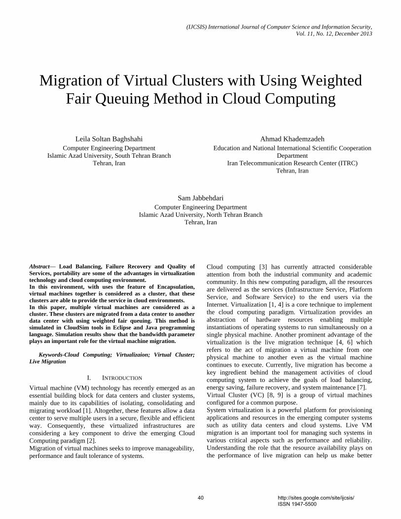
(IJCSIS) International Journal of Computer Science and Information Security,
Vol. 11, No. 12, December 2013
Migration of Virtual Clusters with Using Weighted
Fair Queuing Method in Cloud Computing
Leila Soltan Baghshahi
Computer Engineering Department
Islamic Azad University, South Tehran Branch
Tehran, Iran
Ahmad Khademzadeh
Education and National International Scientific Cooperation
Department
Iran Telecommunication Research Center (ITRC)
Tehran, Iran
Sam Jabbehdari
Computer Engineering Department
Islamic Azad University, North Tehran Branch
Tehran, Iran
Abstract— Load Balancing, Failure Recovery and Quality of
Services, portability are some of the advantages in virtualization
technology and cloud computing environment.
In this environment, with uses the feature of Encapsulation,
virtual machines together is considered as a cluster, that these
clusters are able to provide the service in cloud environments.
In this paper, multiple virtual machines are considered as a
cluster. These clusters are migrated from a data center to another
data center with using weighted fair queuing. This method is
simulated in CloudSim tools in Eclipse and Java programming
language. Simulation results show that the bandwidth parameter
plays an important role for the virtual machine migration.
Keywords-Cloud Computing; Virtualizaion; Virtual Cluster;
Live Migration
I. INTRODUCTION
Virtual machine (VM) technology has recently emerged as an
essential building block for data centers and cluster systems,
mainly due to its capabilities of isolating, consolidating and
migrating workload [1]. Altogether, these features allow a data
center to serve multiple users in a secure, flexible and efficient
way. Consequently, these virtualized infrastructures are
considering a key component to drive the emerging Cloud
Computing paradigm [2].
Migration of virtual machines seeks to improve manageability,
performance and fault tolerance of systems.
Cloud computing [3] has currently attracted considerable
attention from both the industrial community and academic
community. In this new computing paradigm, all the resources
are delivered as the services (Infrastructure Service, Platform
Service, and Software Service) to the end users via the
Internet. Virtualization [1, 4] is a core technique to implement
the cloud computing paradigm. Virtualization provides an
abstraction of hardware resources enabling multiple
instantiations of operating systems to run simultaneously on a
single physical machine. Another prominent advantage of the
virtualization is the live migration technique [4, 6] which
refers to the act of migration a virtual machine from one
physical machine to another even as the virtual machine
continues to execute. Currently, live migration has become a
key ingredient behind the management activities of cloud
computing system to achieve the goals of load balancing,
energy saving, failure recovery, and system maintenance [7].
Virtual Cluster (VC) [8, 9] is a group of virtual machines
configured for a common purpose.
System virtualization is a powerful platform for provisioning
applications and resources in the emerging computer systems
such as utility data centers and cloud systems. Live VM
migration is an important tool for managing such systems in
various critical aspects such as performance and reliability.
Understanding the role that the resource availability plays on
the performance of live migration can help us make better
40 http://sites.google.com/site/ijcsis/ ISSN 1947-5500
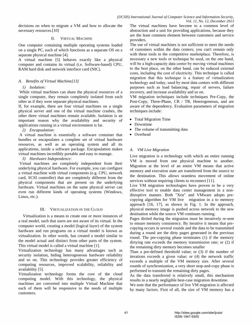
(IJCSIS) International Journal of Computer Science and Information Security,
Vol. 11, No. 12, December 2013
decisions on when to migrate a VM and how to allocate the
necessary resources.[10]
II. VIRTUAL MACHINE
One computer containing multiple operating systems loaded
on a single PC, each of which functions as a separate OS on a
separate physical machine [4].
A virtual machine [5] behaves exactly like a physical
computer and contains its virtual (i.e. Software-based) CPU,
RAM hard disk and network interface card (NIC).
A. Benefits of Virtual Machine[13]
1) Isolation:
While virtual machines can share the physical resources of a
single computer, they remain completely isolated from each
other as if they were separate physical machines.
If, for example, there are four virtual machines on a single
physical server and one of the virtual machine crashes, the
other three virtual machines remain available. Isolation is an
important reason why the availability and security of
applications running in a virtual environment is far.
2) Encapsulation:
A virtual machine is essentially a software container that
bundles or encapsulates a complete set of virtual hardware
resources, as well as an operating system and all its
applications, inside a software package. Encapsulation makes
virtual machines incredibly portable and easy to manage.
3) Hardware Independence:
Virtual machines are completely independent from their
underlying physical hardware. For example, you can configure
a virtual machine with virtual components (e.g. CPU, network
card, SCSI controller) that are completely different from the
physical components that are present on the underlying
hardware. Virtual machines on the same physical server can
even run different kinds of operating systems (Windows,
Linux, etc.).
III. VIRTUALIZATION IN THE CLOUD
Virtualization is a means to create one or more instances of
a real model, such that users are not aware of its virtual. In the
computer world, creating a model (logical layer) of the system
hardware and run programs on a virtual model is known as
virtualization. In other words, has created a model similar to
the model actual and distinct from other parts of the system.
This virtual model is called a virtual machine [1].
Virtualization technology has many advantages such as
security isolation, hiding heterogeneous hardware reliability
and so on. This technology provides greater efficiency of
computing resources, improved scalability, reliability and
availability [5].
Virtualization technology forms the core of the cloud
computing model. With this technology, the physical
machines are converted into multiple Virtual Machine that
each of them will be responsive to the needs of multiple
customers.
The virtual machines have become to a common level of
abstraction and a unit for providing applications, because they
are the least common element between customers and service
providers.
The use of virtual machines is not sufficient to meet the needs
of customers within the data centers; you can't remain only
with these tools in the competitive market . Theref
-
. This technique is c
purposes such as load balancing, repair of servers, failure
recovery, and increase availability and so on.
VM migration techniques include techniques Pre-Copy, the
Post-Copy, Three-Phase, CR / TR, Heterogeneous, and are
aware of the dependency. Evaluation parameters of migration
techniques include:
Total Migration Time
Downtime
The volume of transmitting data
Overhead
A. VM Live Migration
Live migration is a technology with which an entire running
VM is moved from one physical machine to another.
Migration at the level of an entire VM means that active
memory and execution state are transferred from the source to
the destination. This allows seamless movement of online
services without requiring clients to reconnect [11].
Live VM migration technologies have proven to be a very
effective tool to enable data center management in a non-
disruptive manner. Both "Xen" and VMware adopts pre-
copying algorithm for VM live migration in a to memory
approach [16, 17], as shown in Fig. 1. In the approach,
physical memory image is pushed across network to the new
destination while the source VM continues running.
Pages dirtied during the migration must be iteratively re-sent
to ensure memory consistency. By iterative it means that pre-
copying occurs in several rounds and the data to be transmitted
during a round are the dirty pages generated in the previous
round. The pre-copying phase terminates (1) if the memory
dirtying rate exceeds the memory transmission rate; or (2) if
the remaining dirty memory becomes smaller
Than a pre-defined threshold value; or (3) if the number of
iterations exceeds a given value; or (4) the network traffic
exceeds a multiple of the VM memory size. After several
rounds of synchronization, a very short stop-and-copy phase is
performed to transmit the remaining dirty pages.
As the data transferred is relatively small, this mechanism
results in a nearly negligible best-case migration downtime.
We note that the performance of live VM migration is affected
by many factors. First of all, the size of VM memory has a
41 http://sites.google.com/site/ijcsis/ ISSN 1947-5500
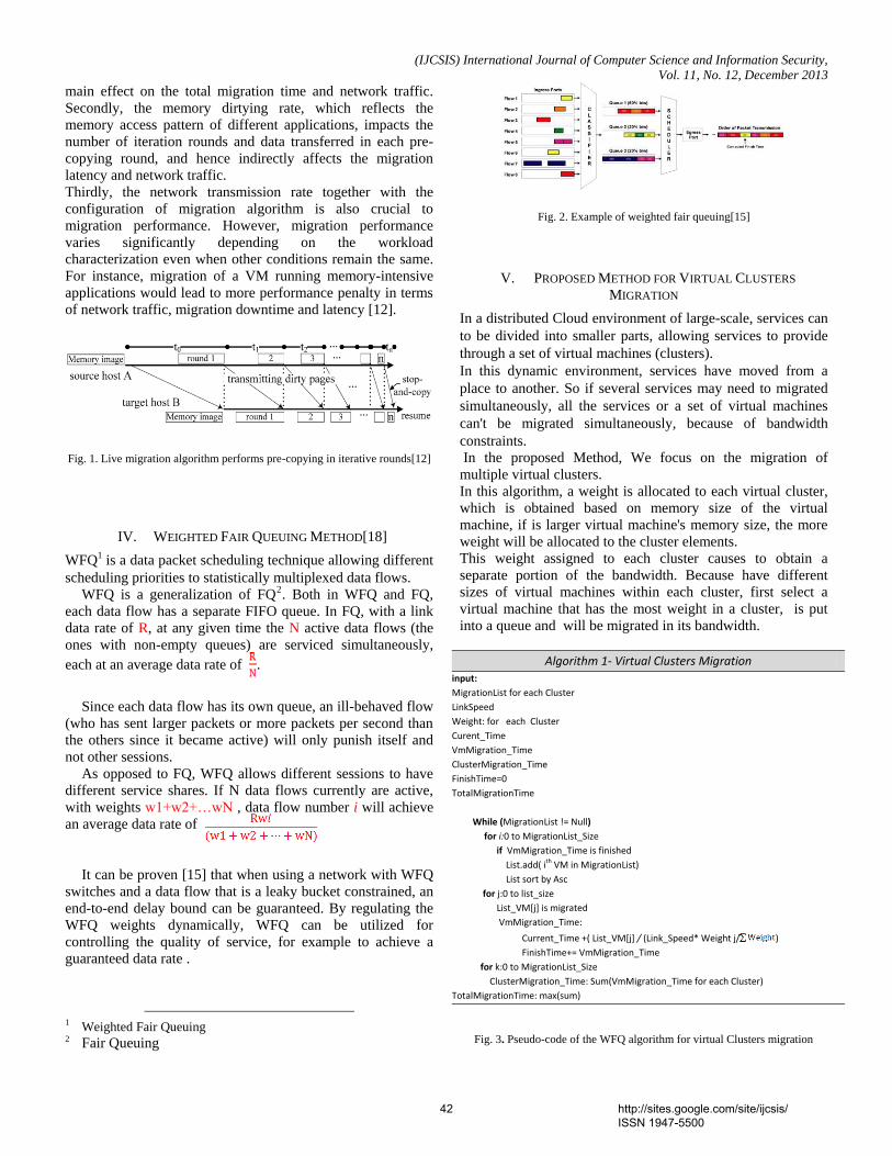
(IJCSIS) International Journal of Computer Science and Information Security,
Vol. 11, No. 12, December 2013
main effect on the total migration time and network traffic.
Secondly, the memory dirtying rate, which reflects the
memory access pattern of different applications, impacts the
number of iteration rounds and data transferred in each pre-
copying round, and hence indirectly affects the migration
latency and network traffic.
Thirdly, the network transmission rate together with the
configuration of migration algorithm is also crucial to
migration performance. However, migration performance
varies significantly depending on the workload
characterization even when other conditions remain the same.
For instance, migration of a VM running memory-intensive
applications would lead to more performance penalty in terms
of network traffic, migration downtime and latency [12].
Fig. 1. Live migration algorithm performs pre-copying in iterative rounds[12]
IV. WEIGHTED FAIR QUEUING METHOD[18]
WFQ1 is a data packet scheduling technique allowing different
scheduling priorities to statistically multiplexed data flows.
WFQ is a generalization of FQ2. Both in WFQ and FQ,
each data flow has a separate FIFO queue. In FQ, with a link
data rate of R, at any given time the N active data flows (the
ones with non-empty queues) are serviced simultaneously,
each at an average data rate of .
Since each data flow has its own queue, an ill-behaved flow
(who has sent larger packets or more packets per second than
the others since it became active) will only punish itself and
not other sessions.
As opposed to FQ, WFQ allows different sessions to have
different service shares. If N data flows currently are active,
with weights 1+ 2+… N , data flow number i will achieve
an average data rate of
It can be proven [15] that when using a network with WFQ
switches and a data flow that is a leaky bucket constrained, an
end-to-end delay bound can be guaranteed. By regulating the
WFQ weights dynamically, WFQ can be utilized for
controlling the quality of service, for example to achieve a
guaranteed data rate .
1 Weighted Fair Queuing 2 Fair Queuing
Fig. 2. Example of weighted fair queuing[15]
V. PROPOSED METHOD FOR VIRTUAL CLUSTERS
MIGRATION
In a distributed Cloud environment of large-scale, services can
to be divided into smaller parts, allowing services to provide
through a set of virtual machines (clusters).
In this dynamic environment, services have moved from a
place to another. So if several services may need to migrated
simultaneously, all the services or a set of virtual machines
can't be migrated simultaneously, because of bandwidth
constraints.
In the proposed Method, We focus on the migration of
multiple virtual clusters.
In this algorithm, a weight is allocated to each virtual cluster,
which is obtained based on memory size of the virtual
machine, if is larger virtual machine's memory size, the more
weight will be allocated to the cluster elements.
This weight assigned to each cluster causes to obtain a
separate portion of the bandwidth. Because have different
sizes of virtual machines within each cluster, first select a
virtual machine that has the most weight in a cluster, is put
into a queue and will be migrated in its bandwidth.
Algorithm 1- Virtual Clusters Migration input:
MigrationList for each Cluster
LinkSpeed
Weight: for each Cluster
Curent_Time
VmMigration_Time
ClusterMigration_Time
FinishTime=0
TotalMigrationTime
While (MigrationList != Null)
for i:0 to MigrationList_Size
if VmMigration_Time is finished
List.add( ith VM in MigrationList)
List sort by Asc
for j:0 to list_size
List_VM[j] is migrated
VmMigration_Time:
Current_Time +( List_VM[j] / (Link_Speed* Weight j/ )
FinishTime+= VmMigration_Time
for k:0 to MigrationList_Size
ClusterMigration_Time: Sum(VmMigration_Time for each Cluster)
TotalMigrationTime: max(sum)
Fig. 3. Pseudo-code of the WFQ algorithm for virtual Clusters migration
42 http://sites.google.com/site/ijcsis/ ISSN 1947-5500
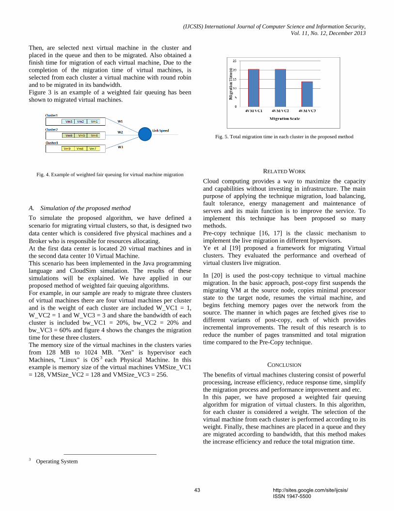
(IJCSIS) International Journal of Computer Science and Information Security,
Vol. 11, No. 12, December 2013
Then, are selected next virtual machine in the cluster and
placed in the queue and then to be migrated. Also obtained a
finish time for migration of each virtual machine, Due to the
completion of the migration time of virtual machines, is
selected from each cluster a virtual machine with round robin
and to be migrated in its bandwidth.
Figure 3 is an example of a weighted fair queuing has been
shown to migrated virtual machines.
Fig. 4. Example of weighted fair queuing for virtual machine migration
A. Simulation of the proposed method
To simulate the proposed algorithm, we have defined a
scenario for migrating virtual clusters, so that, is designed two
data center which is considered five physical machines and a
Broker who is responsible for resources allocating.
At the first data center is located 20 virtual machines and in
the second data center 10 Virtual Machine.
This scenario has been implemented in the Java programming
language and CloudSim simulation. The results of these
simulations will be explained. We have applied in our
proposed method of weighted fair queuing algorithms.
For example, in our sample are ready to migrate three clusters
of virtual machines there are four virtual machines per cluster
and is the weight of each cluster are included W_VC1 = 1,
W_VC2 = 1 and W_VC3 = 3 and share the bandwidth of each
cluster is included bw_VC1 = 20%, bw_VC2 = 20% and
bw_VC3 = 60% and figure 4 shows the changes the migration
time for these three clusters.
The memory size of the virtual machines in the clusters varies
from 128 MB to 1024 MB. "Xen" is hypervisor each
Machines, "Linux" is OS 3 each Physical Machine. In this
example is memory size of the virtual machines VMSize_VC1
= 128, VMSize_VC2 = 128 and VMSize_VC3 = 256.
3 Operating System
Fig. 5. Total migration time in each cluster in the proposed method
RELATED WORK
Cloud computing provides a way to maximize the capacity
and capabilities without investing in infrastructure. The main
purpose of applying the technique migration, load balancing,
fault tolerance, energy management and maintenance of
servers and its main function is to improve the service. To
implement this technique has been proposed so many
methods.
Pre-copy technique [16, 17] is the classic mechanism to
implement the live migration in different hypervisors.
Ye et al [19] proposed a framework for migrating Virtual
clusters. They evaluated the performance and overhead of
virtual clusters live migration.
In [20] is used the post-copy technique to virtual machine
migration. In the basic approach, post-copy first suspends the
migrating VM at the source node, copies minimal processor
state to the target node, resumes the virtual machine, and
begins fetching memory pages over the network from the
source. The manner in which pages are fetched gives rise to
different variants of post-copy, each of which provides
incremental improvements. The result of this research is to
reduce the number of pages transmitted and total migration
time compared to the Pre-Copy technique.
CONCLUSION
The benefits of virtual machines clustering consist of powerful
processing, increase efficiency, reduce response time, simplify
the migration process and performance improvement and etc.
In this paper, we have proposed a weighted fair queuing
algorithm for migration of virtual clusters. In this algorithm,
for each cluster is considered a weight. The selection of the
virtual machine from each cluster is performed according to its
weight. Finally, these machines are placed in a queue and they
are migrated according to bandwidth, that this method makes
the increase efficiency and reduce the total migration time.
43 http://sites.google.com/site/ijcsis/ ISSN 1947-5500
(IJCSIS) International Journal of Computer Science and Information Security,
Vol. 11, No. 12, December 2013
REFERENCES
[1] P. Barham, B. Dragovic, K. Fraser, S. Hand, T. Harris, A. Ho, R.
N I. P A. W “X of ” P ACM Symposium on Operating Systems Principles, p. 177, 2003.
[2] R. Buyya, C. Yeo, S.Venugopal, J.Broberg., I.Brandic, “Cloud computing and emerging IT platforms” Future Generation Computer Systems 25 pp.599–616, 2003.
[3] M. Armbrust, A. Fox, R. Griffith, A. Joseph, R. Katz, A. Konwinski, G. Lee, D. Patterson, A. Rabkin, I. Stoica, . “A ” C ACM, vol. 53, no. 4, pp. 50–58, 2010.
[4] C. W “M VM ESX ” ACM SIGOPS Operating Systems Review, vol. 36, no. SI, p. 194, 2002.
[5] E.P.Zaw, N.L.Thein, “I L VM M U LRU S T A ”, International journal of Compute Science and Telecommunications, Volume 3, Issue 3, 2012.
[6] M. N B. L G. H “F migration for ” Proceedings of the annual conference on USENIX Annual Technical Conference, p. 25, 2005.
[7] K. Y D. H X. J H. C S. W “V machine based energy-efficient data center architecture for cloud computing: a ” Proceedings of the 2010 IEEE/ACM International Conference on Green Computing and Communications, pp. 171–178, 2010.
[8] K. Y X. J S. C D. H B. W “A and modeling the performance in Xen-based virtual cluster ” 2010 12th IEEE International Conference on High Performance Computing and Communications (HPCC), pp. 273–280, 2010.
[9] M. F. M V. U O. K J. X “V for high- ” SIGOPS O . Syst. Rev., vol. 40, no. 2, pp. 8–11, 2006.
[10] Y.W M.Z ”P M V M L M ” International Conference on Cloud Computing (CLOUD), IEEE , PP. 492-499, 2011.
[11] S.Ak R.S A.R A. .M A.H “Predicting The Performance Of Vir M M ” in Modeling, Analysis & Simulation of Computer and Telecommunication Systems (MASCOTS), IEEE International Symposium on , pp. 37 – 46, , 2010.
[12] H.Liu, H.Jin, C-Z.Xu, X.Liao, “Performance and energy modeling for live migration of virtual ”, Springer Science+Business Media, LLC 2011.
[13] A.Agarwal, S.Raina, Live Migration of Virtual Machines in Cloud, International Journal of Scientific and Research Publications, Vol.2, Issue 6, June 2012.
[14] D. S A. V “L -rate servers: a general model for ” IEEE/ACM T Networking, 1998.
[15] P. Bertsekas ” T B r and Queuing in a QOS Environment” Department of Electrical Engineering M.I.T, OPNET Technologises, 2002.
[16] C. Clark, K. Fraser, S. Hand, J.G Hansen, E. Jul, C. Limpach, I. Pratt, A. Warfield, “Live migration of virtual machines. In:Proceedings of Second S N k S D I (NSDI’05) ”, pp. 273–286, 2005.
[17] M. N B.H. L G. H “Fast transparent migration for virtual machines. In: Proceedings of USENIX Annual Technical Conference (USENIX’05)” Anaheim, California, USA, pp. 391–394, 2005.
[18] http://en.wikipedia.org/wiki/Weighted_fair_queuing
[19] K. Ye, x. Jiang, R.Ma, F.Yan, "VC-Migration: Live Migration of Virtual Clusters in the Cloud", ACM/IEEE 13th International Conference on Grid Computing, PP. 209-218, 2012.
[20] M.R.Hines, U.Eshpande, K.Gopalan, "Post-Copy Live Migration of Virtualization of Virtual Machine" International Conference on Virtual Execution Environment (VEE), pp. 14-26, March 2009.
44 http://sites.google.com/site/ijcsis/ ISSN 1947-5500
Fisher’s Linear Discriminant and Echo State Neural Networks for Identification of Emotions
Devi Arumugam and Purushothaman S.,
1Devi Arumugam Research Scholar, Department of Computer Science,
Mother Teresa Women’s University, Kodaikanal, India-624102.
2Dr. S. Purushothaman Professor, PET Engineering College,
Vallioor, India-627117
Abstract— Identifying the emotions from facial expression is a fundamental and critical task in human-computer vision. Here expressions like anger, happy, fear, sad, surprise and disgust are identified by Echo State Neural Network. Based on a threshold, the presence of an expression is concluded followed by separation of expression. In each frame, complete face is extracted. The complete face is from top of head to bottom of chin and left ear to right ear. Features are extracted from a face using Fisher’s Linear Discriminant function. The features are extracted from a face is considered as a pattern. If 20 frames belonging to a video are considered, then 20 patterns are created. All 20 patterns are labeled as (1/2/3/4/5/6) according to the labelling decided. The labelling is done as anger=1, fear=2, happy=3, sad=4, surprise=5 and disgust=6. If 20 frames from each video is obtained then number of patterns available for training the proposed Echo State neural Networks are 6 videos x 20 frames= 120 frames. Hence, 120 patterns are formed which are used for training ESNN to obtain final weights. This process is called during the testing of ESNN. In testing of ESNN, FLD features are presented to the input layer of ESNN. The output obtained in the output layer of ANN is compared with threshold to decide the type of expression. For ESNN, the expression identification is highest.
Keywords- Video frames; Facial tracking; Eigen Value and eigen vector; Fisher’s Linear Discriminant (FLD); Echo State Neural Network (ESNN);
I. INTRODUCTION The development of modern human computer interface
system requires computers to closely understand the biometrics of human system. Some of the biometrics is face, iris, fingerprint, GAIT. Biometrics through face, eyes place an important role in activating icons on the TV screen, computer screen. Hence, a technique of detection of expressions from face helps in various applications.
From the video images acquired from built-in cameras, and from speech waveforms collected from on-board microphones, this information can be used to teach computers to recognize human emotions. Computers may learn to recognize gestures, postures, facial expressions, eye contact.
The term “Emotional expression” means any outward expression that arises as a response to some stimulus event.
II. RESEARCH WORK Emotion recognition through the computer-based of facial
expression has been an active and interesting area of research in the literature survey for a long time.
Paul Ekman 1978, as reported by Ekman, anger and disgust are commonly confused in judgment studies. Also, fear and surprise are commonly confused. Because of sharing the similar facial actions, these confusions are occurred.
Bassili, 1979, compare several facial expression recognition algorithms. The author states that these algorithms perform well compared to trained human recognition of about 87%.
Paul Ekman 1994, and his colleagues have performed wide studies of human facial expressions. They found proof to support universality in facial expressions. These “universal facial expressions” are happiness, sadness, anger, fear, surprise, and disgust. They studied facial expressions in various cultures, with preliterate cultures, and found much unity in the expression and recognition of emotions on the face.
Essa, 1997, to extract motion blobs from image sequences, the spatial and temporal filtering together with thresholding is used. Turk 1991, to detect the presence of a face, the blobs are then evaluated using the eigen faces method Essa, 1997, extended their face detection approach to extract the positions of prominent facial features using Eigen features.
Chaudhury et al., 2003, described that instead of a fixed threshold value to initialize the face tracker, used two face probability maps. One used for frontal views and another one for profiles.
Boccignone et al., 2005, Li et al., 2006, proposed that before tracking a face, one should choose the features to track. The exploitation of color is one of the common choices because it is invariant to facial expressions, scale, and poses changes.
Arnaud et al., 2005; Zhiwei Zhu et al., 2005; Yan tong et al., 2007, described facial features extraction from eyes, nose and mouth.
(IJCSIS) International Journal of Computer Science and Information Security, Vol. 11, No. 12, December 2013
45 http://sites.google.com/site/ijcsis/ ISSN 1947-5500
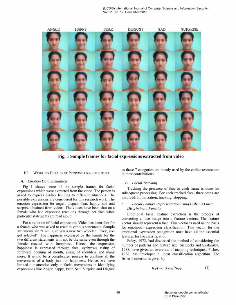
Fig. 1 Sample frames for facial expressions extracted from video
III. WORKING DETAILS OF PROPOSED ARCHITECTURE
A. Emotion Data Simulation Fig 1 shows some of the sample frames for facial
expressions which were extracted from the video. The person is asked to express his/her feelings to different situations. The possible expressions are considered for this research work. The emotion expression for anger, disgust, fear, happy, sad and surprise obtained from videos. The videos have been shot on a female who had expressed reactions through her face when particular statements are read aloud.
For simulation of facial expression, Video has been shot for a female who was asked to react to various statements. Sample statements are “I will give you a new two wheeler”, “hey, you got selected”. The happiness expressed by the female for the two different statements will not be the same even through the female reacted with happiness. Hence, the expression happiness is expressed through face, eyebrows, rising of forehead, opening of mouth, rising of shoulders and many more. It would be a complicated process to combine all the movements of a body just for happiness. Hence, we have limited our attention only to facial movements in identifying expressions like Anger, happy, Fear, Sad, Surprise and Disgust
as these 7 categories are mostly used by the earlier researchers in their contributions.
B. Facial Tracking Tracking the presence of face in each frame is done for
subsequent processing. For each tracked face, three steps are involved: Initialization, tracking, stopping.
C. Facial Feature Representation using Fisher’s Linear Discriminant Function Emotional facial feature extraction is the process of
converting a face image into a feature vectors. The feature vector should represent a face. This vector is used as the basis for emotional expression classification. This vector for the emotional expression recognition must have all the essential features for the classification.
Foley, 1972, had discussed the method of considering the number of patterns and feature size. Siedlecki and Skalansky, 1988, have given an overview of mapping techniques. Fisher, 1936, has developed a linear classification algorithm. The fisher’s criterion is given by
(1) J() =TSb/TSW
(IJCSIS) International Journal of Computer Science and Information Security, Vol. 11, No. 12, December 2013
46 http://sites.google.com/site/ijcsis/ ISSN 1947-5500
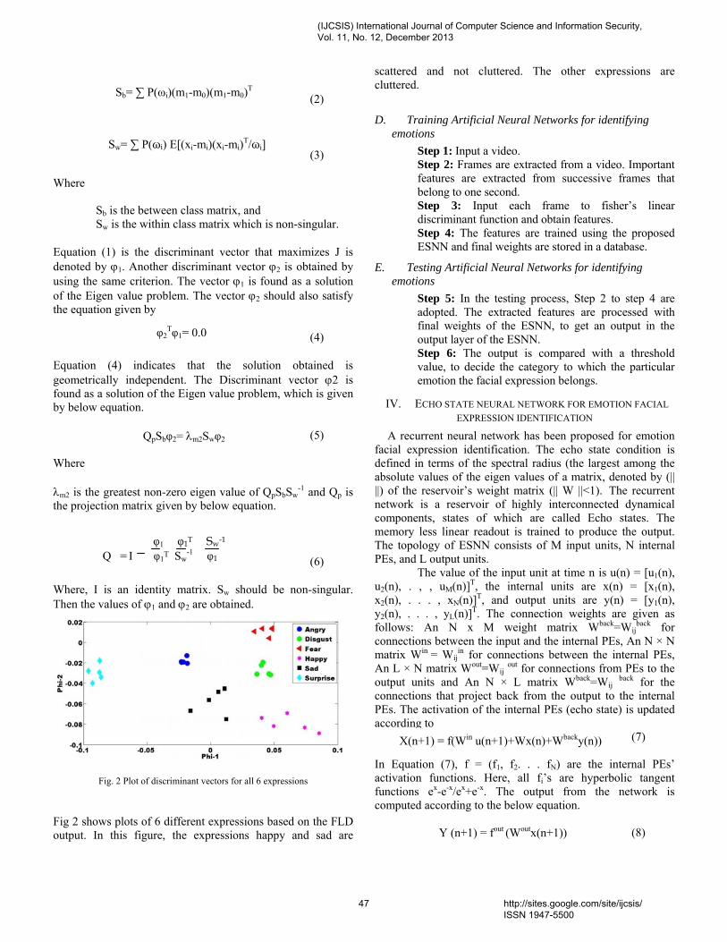
(2)
(3)
Where
Sb is the between class matrix, and Sw is the within class matrix which is non-singular.
Equation (1) is the discriminant vector that maximizes J is denoted by ϕ1. Another discriminant vector ϕ2 is obtained by using the same criterion. The vector ϕ1 is found as a solution of the Eigen value problem. The vector ϕ2 should also satisfy the equation given by
(4)
Equation (4) indicates that the solution obtained is geometrically independent. The Discriminant vector ϕ2 is found as a solution of the Eigen value problem, which is given by below equation.
(5)
Where
λm2 is the greatest non-zero eigen value of QpSbSw-1 and Qp is
the projection matrix given by below equation.
(6)
Where, I is an identity matrix. Sw should be non-singular. Then the values of ϕ1 and ϕ2 are obtained.
Fig. 2 Plot of discriminant vectors for all 6 expressions
Fig 2 shows plots of 6 different expressions based on the FLD output. In this figure, the expressions happy and sad are
scattered and not cluttered. The other expressions are cluttered.
D. Training Artificial Neural Networks for identifying emotions
Step 1: Input a video. Step 2: Frames are extracted from a video. Important features are extracted from successive frames that belong to one second. Step 3: Input each frame to fisher’s linear discriminant function and obtain features. Step 4: The features are trained using the proposed ESNN and final weights are stored in a database.
E. Testing Artificial Neural Networks for identifying emotions
Step 5: In the testing process, Step 2 to step 4 are adopted. The extracted features are processed with final weights of the ESNN, to get an output in the output layer of the ESNN. Step 6: The output is compared with a threshold value, to decide the category to which the particular emotion the facial expression belongs.
IV. ECHO STATE NEURAL NETWORK FOR EMOTION FACIAL EXPRESSION IDENTIFICATION
A recurrent neural network has been proposed for emotion facial expression identification. The echo state condition is defined in terms of the spectral radius (the largest among the absolute values of the eigen values of a matrix, denoted by (|| ||) of the reservoir’s weight matrix (|| W ||<1). The recurrent network is a reservoir of highly interconnected dynamical components, states of which are called Echo states. The memory less linear readout is trained to produce the output. The topology of ESNN consists of M input units, N internal PEs, and L output units.
The value of the input unit at time n is u(n) = [u1(n), u2(n), . , , uM(n)]T, the internal units are x(n) = [x1(n), x2(n), . . . , xN(n)]T, and output units are y(n) = [y1(n), y2(n), . . . , yL(n)]T. The connection weights are given as follows: An N x M weight matrix Wback=Wij
back for connections between the input and the internal PEs, An N × N matrix Win = Wij
in for connections between the internal PEs, An L × N matrix Wout=Wij out for connections from PEs to the output units and An N × L matrix Wback=Wij back for the connections that project back from the output to the internal PEs. The activation of the internal PEs (echo state) is updated according to
(7)
In Equation (7), f = (f1, f2. . . fN) are the internal PEs’ activation functions. Here, all fi’s are hyperbolic tangent functions ex-e-x/ex+e-x. The output from the network is computed according to the below equation. (8)
Sb= ∑ P(ωi)(m1-m0)(m1-m0)T
Sw= ∑ P(ωi) E[(xi-mi)(xi-mi)T/ωi]
2T1= 0.0
QpSb2= λm2Sw2
1 1T Sw-1
Q = I 1T Sw-1 1
X(n+1) = f(Win u(n+1)+Wx(n)+Wbacky(n))
Y (n+1) = fout (Woutx(n+1))
(IJCSIS) International Journal of Computer Science and Information Security, Vol. 11, No. 12, December 2013
47 http://sites.google.com/site/ijcsis/ ISSN 1947-5500
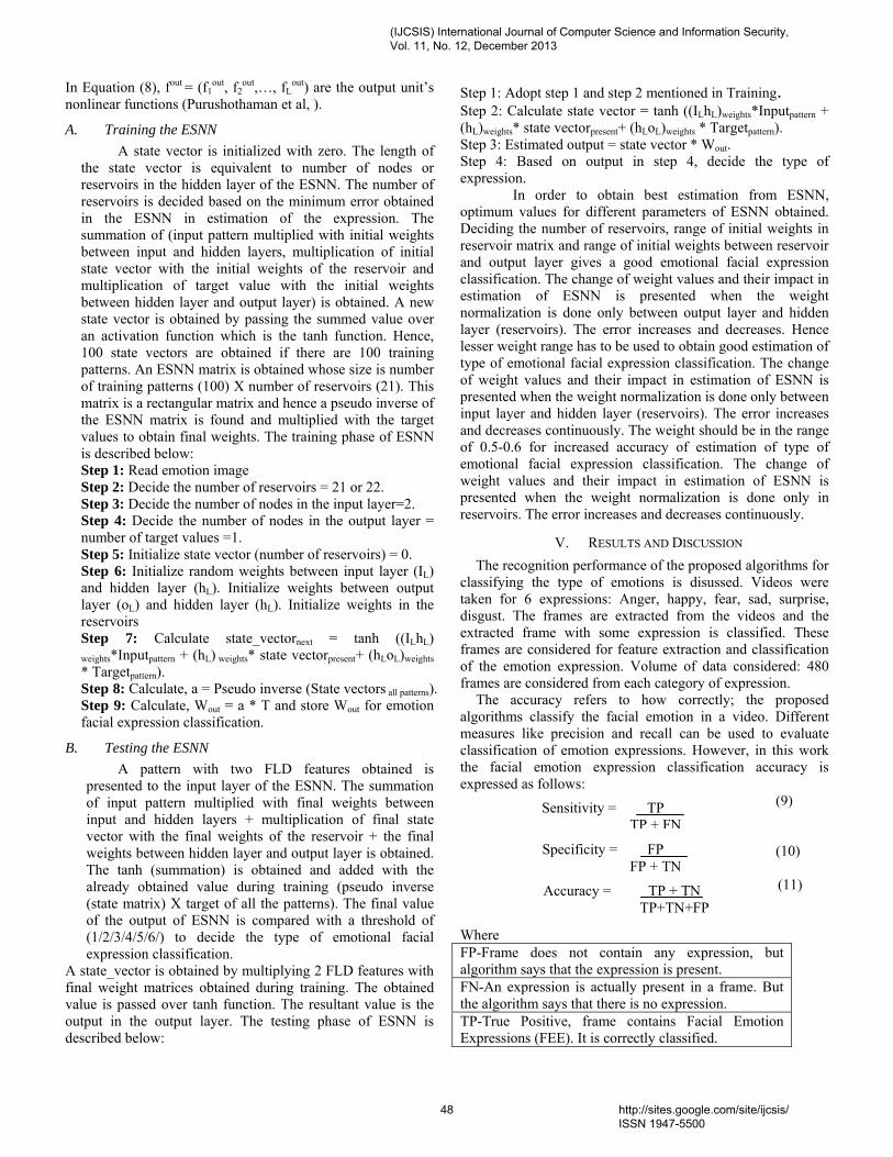
In Equation (8), fout = (f1out, f2
out,…, fLout) are the output unit’s
nonlinear functions (Purushothaman et al, ).
A. Training the ESNN A state vector is initialized with zero. The length of
the state vector is equivalent to number of nodes or reservoirs in the hidden layer of the ESNN. The number of reservoirs is decided based on the minimum error obtained in the ESNN in estimation of the expression. The summation of (input pattern multiplied with initial weights between input and hidden layers, multiplication of initial state vector with the initial weights of the reservoir and multiplication of target value with the initial weights between hidden layer and output layer) is obtained. A new state vector is obtained by passing the summed value over an activation function which is the tanh function. Hence, 100 state vectors are obtained if there are 100 training patterns. An ESNN matrix is obtained whose size is number of training patterns (100) X number of reservoirs (21). This matrix is a rectangular matrix and hence a pseudo inverse of the ESNN matrix is found and multiplied with the target values to obtain final weights. The training phase of ESNN is described below: Step 1: Read emotion image Step 2: Decide the number of reservoirs = 21 or 22. Step 3: Decide the number of nodes in the input layer=2. Step 4: Decide the number of nodes in the output layer = number of target values =1. Step 5: Initialize state vector (number of reservoirs) = 0. Step 6: Initialize random weights between input layer (IL) and hidden layer (hL). Initialize weights between output layer (oL) and hidden layer (hL). Initialize weights in the reservoirs Step 7: Calculate state_vectornext = tanh ((ILhL)
weights*Inputpattern + (hL) weights* state vectorpresent+ (hLoL)weights * Targetpattern). Step 8: Calculate, a = Pseudo inverse (State vectors all patterns). Step 9: Calculate, Wout = a * T and store Wout for emotion facial expression classification.
B. Testing the ESNN A pattern with two FLD features obtained is
presented to the input layer of the ESNN. The summation of input pattern multiplied with final weights between input and hidden layers + multiplication of final state vector with the final weights of the reservoir + the final weights between hidden layer and output layer is obtained. The tanh (summation) is obtained and added with the already obtained value during training (pseudo inverse (state matrix) X target of all the patterns). The final value of the output of ESNN is compared with a threshold of (1/2/3/4/5/6/) to decide the type of emotional facial expression classification.
A state_vector is obtained by multiplying 2 FLD features with final weight matrices obtained during training. The obtained value is passed over tanh function. The resultant value is the output in the output layer. The testing phase of ESNN is described below:
Step 1: Adopt step 1 and step 2 mentioned in Training. Step 2: Calculate state vector = tanh ((ILhL)weights*Inputpattern + (hL)weights* state vectorpresent+ (hLoL)weights * Targetpattern). Step 3: Estimated output = state vector * Wout. Step 4: Based on output in step 4, decide the type of expression.
In order to obtain best estimation from ESNN, optimum values for different parameters of ESNN obtained. Deciding the number of reservoirs, range of initial weights in reservoir matrix and range of initial weights between reservoir and output layer gives a good emotional facial expression classification. The change of weight values and their impact in estimation of ESNN is presented when the weight normalization is done only between output layer and hidden layer (reservoirs). The error increases and decreases. Hence lesser weight range has to be used to obtain good estimation of type of emotional facial expression classification. The change of weight values and their impact in estimation of ESNN is presented when the weight normalization is done only between input layer and hidden layer (reservoirs). The error increases and decreases continuously. The weight should be in the range of 0.5-0.6 for increased accuracy of estimation of type of emotional facial expression classification. The change of weight values and their impact in estimation of ESNN is presented when the weight normalization is done only in reservoirs. The error increases and decreases continuously.
V. RESULTS AND DISCUSSION The recognition performance of the proposed algorithms for
classifying the type of emotions is disussed. Videos were taken for 6 expressions: Anger, happy, fear, sad, surprise, disgust. The frames are extracted from the videos and the extracted frame with some expression is classified. These frames are considered for feature extraction and classification of the emotion expression. Volume of data considered: 480 frames are considered from each category of expression.
The accuracy refers to how correctly; the proposed algorithms classify the facial emotion in a video. Different measures like precision and recall can be used to evaluate classification of emotion expressions. However, in this work the facial emotion expression classification accuracy is expressed as follows:
(9)
(10)
(11)
Where FP-Frame does not contain any expression, but algorithm says that the expression is present. FN-An expression is actually present in a frame. But the algorithm says that there is no expression. TP-True Positive, frame contains Facial Emotion Expressions (FEE). It is correctly classified.
Sensitivity = TP TP + FN
Specificity = FP FP + TN
Accuracy = TP + TN TP+TN+FP
(IJCSIS) International Journal of Computer Science and Information Security, Vol. 11, No. 12, December 2013
48 http://sites.google.com/site/ijcsis/ ISSN 1947-5500
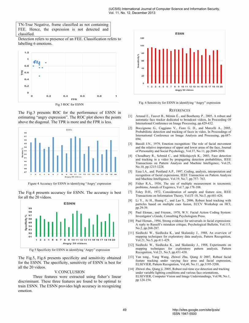
TN-True Negative, frame classified as not containing FEE. Hence, the expression is not detected and classified. Detection refers to presence of an FEE. Classification refers to labelling 6 emotions.
Fig 3 ROC for ESNN
The Fig.3 presents ROC for the performance of ESNN in estimating “angry expression”. The ROC plot shows the points above the diagonal. The TPR is more and the FPR is less.
Figure 4 Accuracy for ESNN in identifying “Angry’ expression
The Fig.4 presents accuracy for ESNN. The accuracy is best for all the 20 videos.
Fig 5 Specificity for ESNN in identifying ‘Angry” expression
The Fig.5, Fig.6 presents specificity and sensitivity obtained for the ESNN. The specificity, sensitivity of ESNN is best for all the 20 videos.
V.CONCLUSION Three features were extracted using fisher’s linear
discriminant. These three features are found to be optimal to train ESNN. The ESNN provides high accuracy in recognizing emotion.
Fig. 6 Sensitivity for ESNN in identifying “Angry” expression
REFERENCES [1] Arnaud E., Fauvet B., Mémin É., and Bouthemy P., 2005, A robust and
automatic face tracker dedicated to broadcast videos, In Proceeding Of International Conference on Image Processing, pp.429-432.
[2] Boccignone G., Caggiano V., Fiore G. D., and Marcelli A., 2005, Probabilistic detection and tracking of faces in video, In Proceedings of International Conference on Image Analysis and Processing, pp.687-694.
[3] Bassili J.N., 1979, Emotion recognition: The role of facial movement and the relative importance of upper and lower areas of the face, Journal of Personality and Social Psychology, Vol.37, No.11, pp.2049-2058.
[4] Choudhury R., Schmid C., and Mikolajczyk K., 2003, Face detection and tracking in a video by propagating detection probabilities, IEEE Transactions on Pattern Analysis and Machine Intelligence, Vol.25, No.10, pp.1215-1228.
[5] Essa I.A., and. Pentland A.P., 1997, Coding, analysis, interpretation and recognition of facial expressions, IEEE Transaction on Pattern Analysis and Machine Intelligence, Vol.19, No.7, pp.757- 763.
[6] Fisher R.A., 1936, The use of multiple measurement in taxonomic problems, Annals of Eugenics, Vol.7, pp.178-188.
[7] Foley D.H., 1972, Consideration of sample and feature size, IEEE Transactions on Information Theory, Vol.IT-18, No.5, pp.681-626.
[8] Li Y., Ai H., Huang C., and Lao S., 2006, Robust head tracking with particles based on multiple cues fusion, ECCV Workshop on HCI, pp.29-39.
[9] Paul Ekman., and Friesen., 1978, W.V. Facial Action Coding System: Investigator’s Guide, Consulting Psychologists Press.
[10] Paul Ekman., 1994, Strong evidence for universals in facial expressions: A reply to Russell’s mistaken critique, Psychological Bulletin, Vol.115, No.2, pp.268-287.
[11] Siedlecki W., Siedlecka K., and Skalansky J., 1988, An overview of mapping techniques for exploratory data analysis, Pattern Recognition, Vol.21, No.5, pp.411-429.
[12] Siedlecki W., Siedlecka K., and Skalansky J., 1988, Experiments on mapping techniques for exploratory pattern analysis, Pattern Recognition, Vol.21, No.5, pp.431-438.
[13] Yan tong., Yang Wang, Zhiwei Zhu, Qiang Ji, 2007, Robust facial feature tracking under varying face pose and facial expression, ELSEVIER, Pattern Recognition, Vol.40, No.11, pp.3195-3208.
[14] Zhiwei zhu, Qiang ji, 2005, Robust real-time eye detection and tracking under variable lighting conditions and various face orientations, ELSEVIER, Computer Vision and Image Understandings, Vol.98, No.1, pp 124-154.
(IJCSIS) International Journal of Computer Science and Information Security, Vol. 11, No. 12, December 2013
49 http://sites.google.com/site/ijcsis/ ISSN 1947-5500
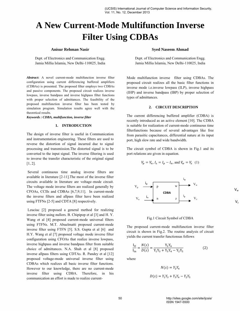
A New Current-Mode Multifunction Inverse Filter Using CDBAs
Anisur Rehman Nasir Syed Naseem Ahmad
Dept. of Electronics and Communication Engg. Jamia Millia Islamia, New Delhi-110025, India
Abstract: A novel current-mode multifunction inverse filter configuration using current differencing buffered amplifiers (CDBAs) is presented. The proposed filter employs two CDBAs and passive components. The proposed circuit realizes inverse lowpass, inverse bandpass and inverse highpass filter functions with proper selection of admittances. The feasibility of the proposed multifunction inverse filter has been tested by simulation program. Simulation results agree well with the theoretical results. Keywords : CDBA, multifunction, inverse filter
1. INTRODUCTION
The design of inverse filter is useful in Communication and instrumentation engineering. These filters are used to reverse the distortion of signal incurred due to signal processing and transmission.The distorted signal is to be converted to the input signal. The inverse filtering is used to inverse the transfer characteristic of the original signal [1, 2].
Several continuous time analog inverse filters are available in literature [2-11].The most of the inverse filter circuits available in literature are voltage–mode circuit. The voltage mode inverse filters are realized generally by CFOAs, CCIIs and CDBAs [6,7,9,11]. In current-mode the inverse filters and allpass filter have been realized using FTFNs [2-5] and CDTA [8] respectively.
Leuciuc [2] proposed a general method for realizing inverse filter using nullors. B. Chipipop et al [3] and H. Y. Wang et al [4] proposed current-mode universal filters using FTFNs. M.T. Abuelmatti proposed current-mode inverse filter using FTFN [5]. S.S. Gupta et al [6] and H.Y. Wang et al [7] proposed voltage mode inverse filter configuration using CFOAs that realize inverse lowpass, inverse highpass and inverse bandpass filter from suitable choice of admittances. N.A. Shah et al [8] proposed inverse allpass filters using CDTAs. R. Pandey et al [12] proposed voltage-mode universal inverse filter using CDBAs which realizes all basic inverse filter functions. However to our knowledge, there are no current-mode inverse filter using CDBA. Therefore, in his communication an effort is made to realize current-
Dept. of Electronics and Communication Engg. Jamia Millia Islamia, New Delhi-110025, India
Mode multifunction inverse filter using CDBAs. The proposed circuit realizes all the basic filter functions in inverse mode i.e.inverse lowpass (ILP), inverse highpass (IHP) and inverse bandpass (IBP) by proper selection of types of admittances.
2. CIRCUIT DESCRIPTION
The current differencing buffered amplifier (CDBA) is recently introduced as an active element [10]. The CDBA is suitable for realization of current-mode continuous time filterfunctions because of several advantages like free from parasitic capacitances, differential nature at its input port, high slew rate and wide bandwidth.
The circuit symbol of CDBA is shown in Fig.1 and its port relations are given in equation.
, , and (1)
Fig.1 Circuit Symbol of CDBA
The proposed current-mode multifunction inverse filter circuit is shown in Fig.2. The routine analysis of circuit yields the current transfer functionsas follows
IOI
Y YY Y Y Y Y Y 2
where
n
w
z
ip
in
Vp
Vn
Vw
Vz
p Vw
Vz
CDBA
iw
ip
(IJCSIS) International Journal of Computer Science and Information Security, Vol. 11, No. 12, December 2013
50 http://sites.google.com/site/ijcsis/ ISSN 1947-5500
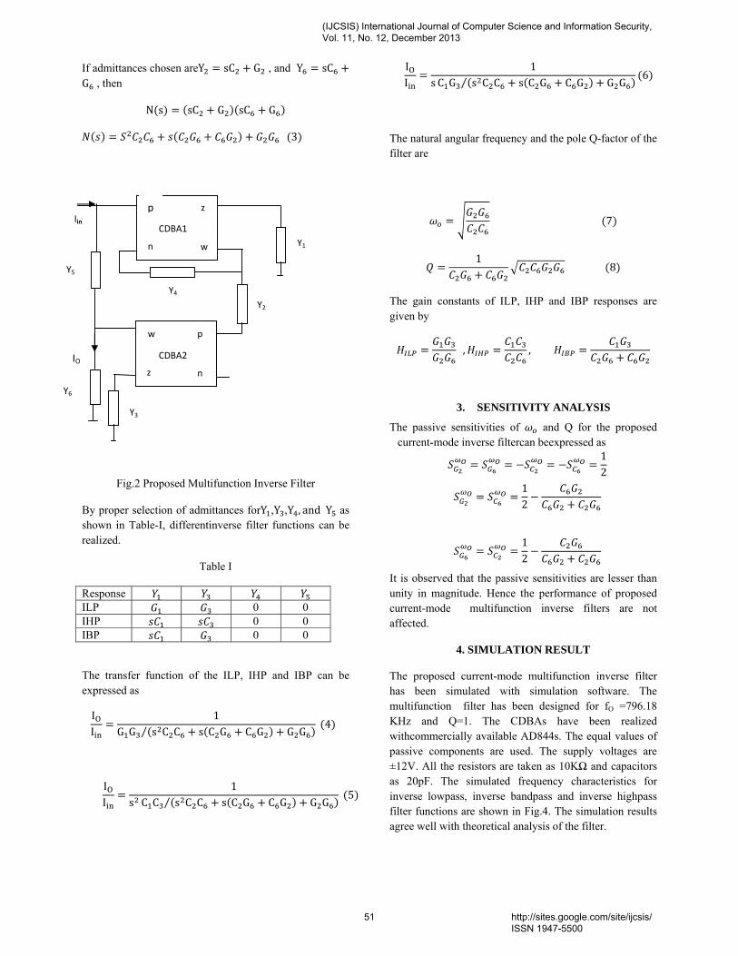
If admittances chosen areY sC G , and Y sCG , then
N s sC G sC G
3
Fig.2 Proposed Multifunction Inverse Filter
By proper selection of admittances forY ,Y ,Y , and Y as shown in Table-I, differentinverse filter functions can be realized.
Table I
Response ILP 0 0 IHP 0 0 IBP 0 0
The transfer function of the ILP, IHP and IBP can be expressed as
IOI
1G G s C C s C G C G G G⁄ 4
IOI
1s C C s C C s C G C G G G⁄ 5
IOI
1s C G s C C s C G C G G G⁄ 6
The natural angular frequency and the pole Q-factor of the filter are
7
1 8
The gain constants of ILP, IHP and IBP responses are given by
, ,
3. SENSITIVITY ANALYSIS
The passive sensitivities of and Q for the proposed current-mode inverse filtercan beexpressed as
12
12
12
It is observed that the passive sensitivities are lesser than unity in magnitude. Hence the performance of proposed current-mode multifunction inverse filters are not affected.
4. SIMULATION RESULT
The proposed current-mode multifunction inverse filter has been simulated with simulation software. The multifunction filter has been designed for fO =796.18 KHz and Q=1. The CDBAs have been realized withcommercially available AD844s. The equal values of passive components are used. The supply voltages are ±12V. All the resistors are taken as 10KΩ and capacitors as 20pF. The simulated frequency characteristics for inverse lowpass, inverse bandpass and inverse highpass filter functions are shown in Fig.4. The simulation results agree well with theoretical analysis of the filter.
p
n
z
w
n
p w
z
Iin
Y1
Y4 Y2
Y5
Y6
Y3
IO
CDBA1
CDBA2
(IJCSIS) International Journal of Computer Science and Information Security, Vol. 11, No. 12, December 2013
51 http://sites.google.com/site/ijcsis/ ISSN 1947-5500
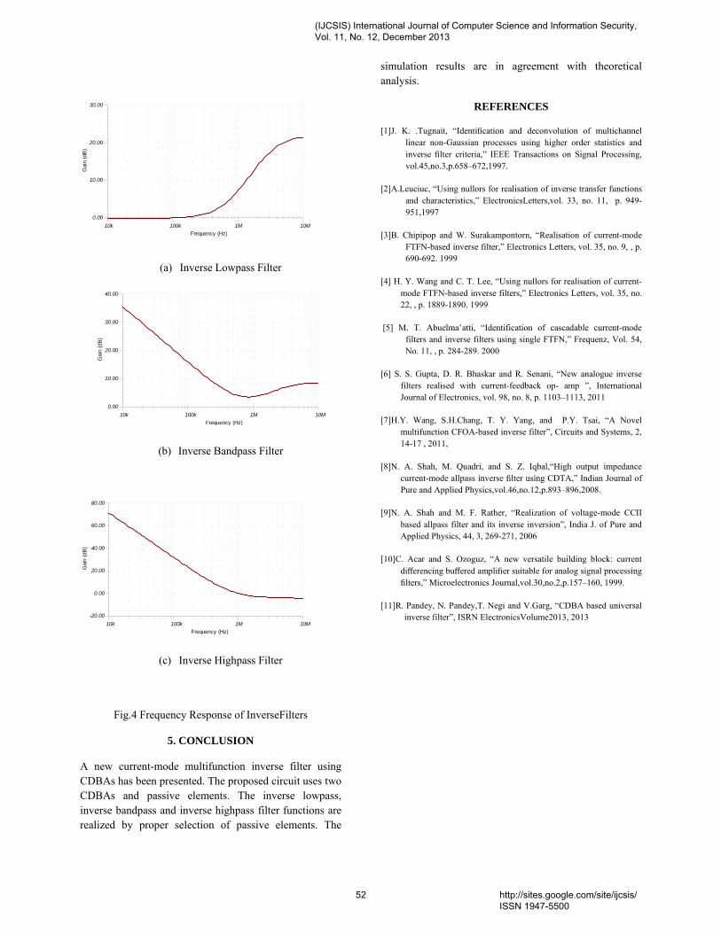
(a) Inverse Lowpass Filter
(b) Inverse Bandpass Filter
(c) Inverse Highpass Filter
Fig.4 Frequency Response of InverseFilters
5. CONCLUSION
A new current-mode multifunction inverse filter using CDBAs has been presented. The proposed circuit uses two CDBAs and passive elements. The inverse lowpass, inverse bandpass and inverse highpass filter functions are realized by proper selection of passive elements. The
simulation results are in agreement with theoretical analysis.
REFERENCES
[1]J. K. .Tugnait, “Identification and deconvolution of multichannel linear non-Gaussian processes using higher order statistics and inverse filter criteria,” IEEE Transactions on Signal Processing, vol.45,no.3,p.658–672,1997.
[2]A.Leuciuc, “Using nullors for realisation of inverse transfer functions and characteristics,” ElectronicsLetters,vol. 33, no. 11, p. 949-951,1997
[3]B. Chipipop and W. Surakampontorn, “Realisation of current-mode FTFN-based inverse filter,” Electronics Letters, vol. 35, no. 9, , p. 690-692. 1999
[4] H. Y. Wang and C. T. Lee, “Using nullors for realisation of current-mode FTFN-based inverse filters,” Electronics Letters, vol. 35, no. 22, , p. 1889-1890. 1999
[5] M. T. Abuelma’atti, “Identification of cascadable current-mode filters and inverse filters using single FTFN,” Frequenz, Vol. 54, No. 11, , p. 284-289. 2000
[6] S. S. Gupta, D. R. Bhaskar and R. Senani, “New analogue inverse filters realised with current-feedback op- amp ”, International Journal of Electronics, vol. 98, no. 8, p. 1103–1113, 2011
[7]H.Y. Wang, S.H.Chang, T. Y. Yang, and P.Y. Tsai, “A Novel multifunction CFOA-based inverse filter”, Circuits and Systems, 2, 14-17 , 2011,
[8]N. A. Shah, M. Quadri, and S. Z. Iqbal,“High output impedance current-mode allpass inverse filter using CDTA,” Indian Journal of Pure and Applied Physics,vol.46,no.12,p.893–896,2008.
[9]N. A. Shah and M. F. Rather, “Realization of voltage-mode CCII based allpass filter and its inverse inversion”, India J. of Pure and Applied Physics, 44, 3, 269-271, 2006
[10]C. Acar and S. Ozoguz, “A new versatile building block: current differencing buffered amplifier suitable for analog signal processing filters,” Microelectronics Journal,vol.30,no.2,p.157–160, 1999.
[11]R. Pandey, N. Pandey,T. Negi and V.Garg, “CDBA based universal inverse filter”, ISRN ElectronicsVolume2013, 2013
T
Frequency (Hz)10k 100k 1M 10M
Gai
n (d
B)
0.00
10.00
20.00
30.00
T
Frequency (Hz)10k 100k 1M 10M
Gai
n (d
B)
0.00
10.00
20.00
30.00
40.00
T
Frequency (Hz)10k 100k 1M 10M
Gai
n (d
B)
-20.00
0.00
20.00
40.00
60.00
80.00
(IJCSIS) International Journal of Computer Science and Information Security, Vol. 11, No. 12, December 2013
52 http://sites.google.com/site/ijcsis/ ISSN 1947-5500
(IJCSIS) International Journal of Computer Science and Information Security, Vol. 11, No. 12, 2013
Assessment of Customer Credit through Combined Clustering of Artificial Neural
Networks, Genetics Algorithm and Bayesian Probabilities
Reza Mortezapour Department of Electronic And Computer
Islamic Azad University Zanjan, Iran
Mehdi Afzali Department of Electronic And Computer
Islamic Azad University Zanjan, Iran
Abstract—Today, with respect to the increasing growth of demand to get credit from the customers of banks and finance and credit institutions, using an effective and efficient method to decrease the risk of non-repayment of credit given is very necessary. Assessment of customers' credit is one of the most important and the most essential duties of banks and institutions, and if an error occurs in this field, it would leads to the great losses for banks and institutions. Thus, using the predicting computer systems has been significantly progressed in recent decades. The data that are provided to the credit institutions' managers help them to make a straight decision for giving the credit or not-giving it. In this paper, we will assess the customer credit through a combined classification using artificial neural networks, genetics algorithm and Bayesian probabilities simultaneously, and the results obtained from three methods mentioned above would be used to achieve an appropriate and final result. We use the K_folds cross validation test in order to assess the method and finally, we compare the proposed method with the methods such as Clustering-Launched Classification (CLC), Support Vector Machine (SVM) as well as GA+SVM where the genetics algorithm has been used to improve them.
Keywords- Data classification; Combined Clustring; Artificial Neural Networks; Genetics Algorithm; Bayyesian Probabilities.
I. INTRODUCTION
Today, with respect to the development of database systems and large amount of data saved in these systems, we need an instrument to process the data saved and to provide the users with the information resulted from the process. Data analysis is one of the most important methods that it provides the users and the analysts with some useful models of data with at least intervention of known users in order to make critical and important decisions of organizations according to them. Classification is one of the most common duties of data analysis. In fact, classification has been defined as evaluation of the characteristics of data set and then to allocate them to a set of groups predefined. Data analysis can be used to create a model or a view of a group based on data characteristics by
using historical data. Then, we can use the predefined model in order to classify new data sets. Also, we can use it for the future predictions by determining a view that is correspondent with it. Commercial issues such as regression analysis, risk management and case targeting are involved in the classification. In order to overcome the financial problems of credit, organizations and institutions have considered several sections as the credits management. The purpose of the company credits management is to determine policies and to observe strategies that are correspondent with the company's functional aspect in terms of risk and efficiency. If the customers observe the previsions of credit contracts and pay the cash of goods purchased on credit, the company efficiency would be increased. Risk or hazard is a probability that the company credit not be receipted or in order to receipt previous credits, the company would be incurred additional costs.
II. PREVIOUS RESEARCHES
In the past, many researchers provided traditional statistical methods to credit accounts by using Linear Discriminant Analysis (IDA) and Logistic Regression and it has been used two common statistical methods in the structure of credit rating models. Nevertheless, Krles, Prakash, Reichert and Wagner cho suggested that usually because of considering the classification nature of credit data, IDA is be needed and this fact has been challenged that it seems unlikely to be the covariance matrix of bad and good credit groups. In addition to IDA method, logistic regression is usually another method for the credit rating. Logistic regression is a model that would be used to predict the probability of an event occurring. This method allows us to use different predictor variables which may be numerical or classified. Basically, the logistic regression model has initially been used as a method to predict binary outcomes. The logistic regression model doesn't need to the normal multi-variables hypothesis, but it depends on various access of perfect linear relationship between the independent variables for powering the logistic function.
53 http://sites.google.com/site/ijcsis/ ISSN 1947-5500
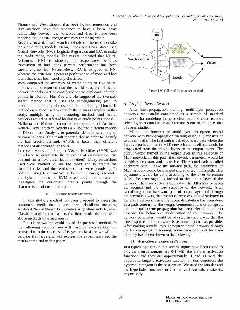
(IJCSIS) International Journal of Computer Science and Information Security, Vol. 11, No. 12, 2013
Thomas and West showed that both logistic regression and IDA methods have this tendency to have a linear basic relationship between the variables and thus, it have been reported that it hasn't enough accuracy for rating credit. Recently, new database search methods can be used to make the credit rating models. Desai, Crook and Over Street used Neural Networks (NW), Logistic Regression and IDA to make the credit rating models. The results indicated that Neural Networks (NN) is showing the expectancy, whereas assessment of bad loans percent performance has been carefully classified. Nevertheless, IRA is as good as NN, whereas the criterion is percent performance of good and bad loans that it has been carefully classified. West compared the accuracy of credit points of five neural models and he reported that the hybrid structure of neural network models must be considered for the applicants of credit points. In addition, Hu, Kuo and Ho suggested the two-step search method that it uses the self-organizing plan to determine the number of clusters and then the algorithm of K methods would be used to classify the clusters samples. In this study, multiple using of clustering methods and neural networks would be affected by design of credit points' model. Malhotra and Malhotra compared the operation of Artificial Neural-Fuzzy Interface System (ANFIS) and different models of Discriminant Analysis to potential defaults screening of customer's loans. This result reported that in order to identify the bad credits demand, ANFIS is better than different methods of discriminant analysis. In recent years, the Support Vector Machine (SVM) was introduced to investigate the problems of classification (the demand for a new classification method). Many researchers used SVM method to rate the credit and to predict the financial risks, and the results obtained were promising. In addition, Hung, Chen and Wang chose three strategies to make the hybrid models of SVM-based credit points and to investigate the customer's credits points through the characteristics of customer input.
III. THE PROPOSED METHOD
In this study, a method has been proposed to assess the customer's credit that it uses three classifiers including Artificial Neural Networks, Genetics Algorithm and Bayesian Classifier, and then it extracts the final result obtained from above methods by a mechanism.
Fig. (1) shows the workflow of the proposed method. In the following sections, we will describe each section. Of course, due to the clearness of Bayesian classifier, we will not describe this issue and will express the experiments and the results at the end of this paper.
Figure.1 Workflow of the proposed method.
A. Artificial Neural Network After back-propagation training, multi-layer perceptron
networks are usually considered as a sample of standard networks for modeling the prediction and the classification: selecting an optimal MLP architecture is one of the areas that has been studied.
Method of function of multi-layer perceptron neural network with back-propagation training essentially consists of two main paths. The first path is called forward path where the input vector is applied to MLP network and its effects would be propagated from the middle layers to the output layers. The output vector formed in the output layer is true response of MLP network. In this path, the network parameters would be considered constant and invariable. The second path is called backward path. Unlike the forward path, the parameters of MLP network would be changed and adjusted in this path. This adjustment would be done according to the error correction code. The error signal is formed in the output layer of the network. The error vector is defined as the difference between the optimal and the true response of the network. After calculating in the backward path of output layer and through the networks layers, the amount of error would be distributed in the entire network. Since the recent distribution has been done in a path contrary to the weight communications of synapses, the term back error propagation has been selected in order to describe the behavioral modification of the network. The network parameters would be adjusted in such a way that the true response of the network is as more optimal as possible. After making a multi-layer perceptron neural network through the back-propagation training, some decisions must be made that they have been shown in the following.
1) Activation Function of Neurons In a typical application that several inputs have been coded as 0-1, the neuron outputs are 0-1 with the annular activation functions and they are approximately -1 and +1 with the hyperbolic tangent activation function. In this condition, the hyperbolic tangent is the best option. We used the annular and the hyperbolic functions in German and Australian datasets, respectively.
54 http://sites.google.com/site/ijcsis/ ISSN 1947-5500
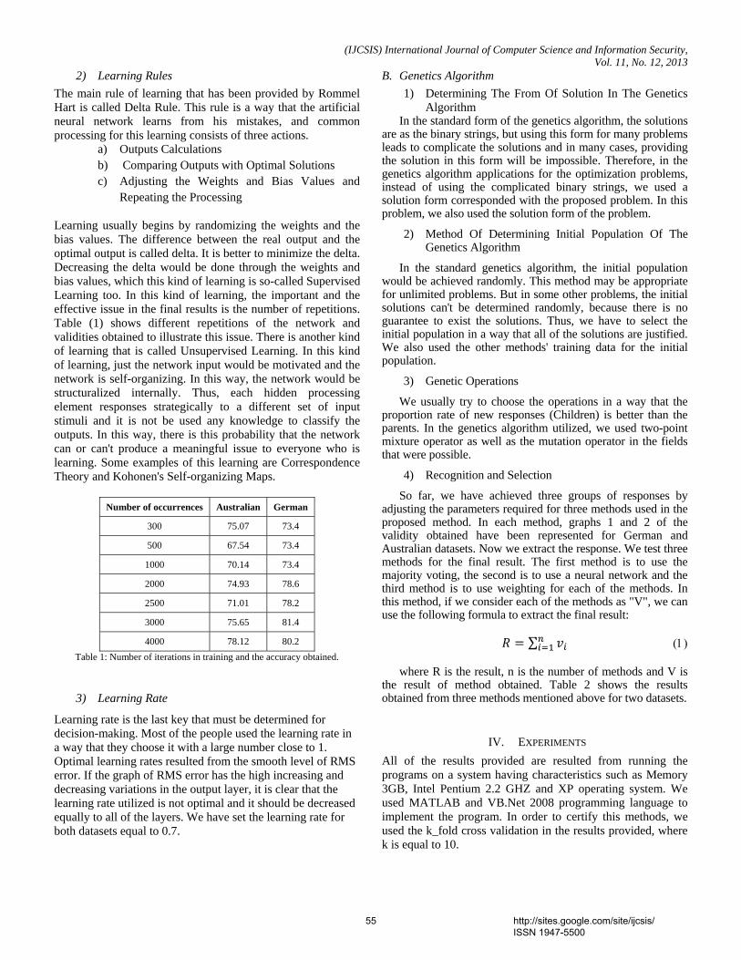
(IJCSIS) International Journal of Computer Science and Information Security, Vol. 11, No. 12, 2013
2) Learning Rules The main rule of learning that has been provided by Rommel Hart is called Delta Rule. This rule is a way that the artificial neural network learns from his mistakes, and common processing for this learning consists of three actions.
a) Outputs Calculations b) Comparing Outputs with Optimal Solutions c) Adjusting the Weights and Bias Values and
Repeating the Processing
Learning usually begins by randomizing the weights and the bias values. The difference between the real output and the optimal output is called delta. It is better to minimize the delta. Decreasing the delta would be done through the weights and bias values, which this kind of learning is so-called Supervised Learning too. In this kind of learning, the important and the effective issue in the final results is the number of repetitions. Table (1) shows different repetitions of the network and validities obtained to illustrate this issue. There is another kind of learning that is called Unsupervised Learning. In this kind of learning, just the network input would be motivated and the network is self-organizing. In this way, the network would be structuralized internally. Thus, each hidden processing element responses strategically to a different set of input stimuli and it is not be used any knowledge to classify the outputs. In this way, there is this probability that the network can or can't produce a meaningful issue to everyone who is learning. Some examples of this learning are Correspondence Theory and Kohonen's Self-organizing Maps.
Number of occurrences Australian German
300 75.07 73.4
500 67.54 73.4
1000 70.14 73.4
2000 74.93 78.6
2500 71.01 78.2
3000 75.65 81.4
4000 78.12 80.2
Table 1: Number of iterations in training and the accuracy obtained.
3) Learning Rate
Learning rate is the last key that must be determined for decision-making. Most of the people used the learning rate in a way that they choose it with a large number close to 1. Optimal learning rates resulted from the smooth level of RMS error. If the graph of RMS error has the high increasing and decreasing variations in the output layer, it is clear that the learning rate utilized is not optimal and it should be decreased equally to all of the layers. We have set the learning rate for both datasets equal to 0.7.
B. Genetics Algorithm 1) Determining The From Of Solution In The Genetics
Algorithm In the standard form of the genetics algorithm, the solutions
are as the binary strings, but using this form for many problems leads to complicate the solutions and in many cases, providing the solution in this form will be impossible. Therefore, in the genetics algorithm applications for the optimization problems, instead of using the complicated binary strings, we used a solution form corresponded with the proposed problem. In this problem, we also used the solution form of the problem.
2) Method Of Determining Initial Population Of The Genetics Algorithm
In the standard genetics algorithm, the initial population would be achieved randomly. This method may be appropriate for unlimited problems. But in some other problems, the initial solutions can't be determined randomly, because there is no guarantee to exist the solutions. Thus, we have to select the initial population in a way that all of the solutions are justified. We also used the other methods' training data for the initial population.
3) Genetic Operations
We usually try to choose the operations in a way that the proportion rate of new responses (Children) is better than the parents. In the genetics algorithm utilized, we used two-point mixture operator as well as the mutation operator in the fields that were possible.
4) Recognition and Selection
So far, we have achieved three groups of responses by adjusting the parameters required for three methods used in the proposed method. In each method, graphs 1 and 2 of the validity obtained have been represented for German and Australian datasets. Now we extract the response. We test three methods for the final result. The first method is to use the majority voting, the second is to use a neural network and the third method is to use weighting for each of the methods. In this method, if we consider each of the methods as "V", we can use the following formula to extract the final result:
∑ (1)
where R is the result, n is the number of methods and V is the result of method obtained. Table 2 shows the results obtained from three methods mentioned above for two datasets.
IV. EXPERIMENTS
All of the results provided are resulted from running the programs on a system having characteristics such as Memory 3GB, Intel Pentium 2.2 GHZ and XP operating system. We used MATLAB and VB.Net 2008 programming language to implement the program. In order to certify this methods, we used the k_fold cross validation in the results provided, where k is equal to 10.
55 http://sites.google.com/site/ijcsis/ ISSN 1947-5500
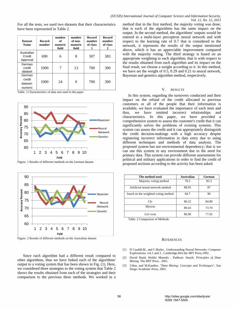
(IJCSIS) International Journal of Computer Science and Information Security, Vol. 11, No. 12, 2013
For all the tests, we used two datasets that their characteristics have been represented in Table 2.
Dataset Name
Record number
number of
numeric field
number of non-
numeric field
Record number of class
1
Record number of class
2 Australian
Credit Approval
690 6 8 307 383
German credit
dataset 1000 7 13 700 300
German credit
dataset-numeric
1000 24 0 700 300
Table. 2 Characteristics of data sets used in the paper
Figure. 1 Results of different methods on the German dataset
Figure. 2 Results of different methods on the Australian dataset
Since each algorithm had a different result compared to other algorithms, thus we have linked each of the algorithms' output to a voting system that has been shown in Fig. (1). Here, we considered three strategies to the voting system that Table 2 shows the results obtained from each of the strategies and their comparison to the previous three methods. We worked in a
method that in the first method, the majority voting was done; that is each of the algorithms has the same impact on the output. In the second method, the algorithms' outputs would be entered in a multi-layer perceptron neural network and with respect to the learning rate of 0.7 that is considered to the network, it represents the results of the output mentioned above, which it has an appreciable improvement compared with the majority voting. The third strategy is based on an appropriate weighting to each algorithm; that is with respect to the results obtained from each algorithm and its impact on the final result, we choose a weight according to it. In this method, we have set the weight of 0.5, 0.29 and 0.21 to neural network, Bayesian and genetics algorithm method, respectively.
V. RESULTS
In this system, regarding the turnovers conducted and their impact on the refund of the credit allocated to previous customers or all of the people that their information is available, we have evaluated the importance of each item and thus, we have omitted incorrect relationships and characteristics. In this paper, we have provided a comprehensive system to assess the customer's credit that it can significantly solves the problems of existing systems. This system can assess the credit and it can appropriately distinguish the credit decision-makings with a high accuracy despite registering incorrect information in data entry due to using different techniques and methods of data analysis. The proposed system has not environmental dependency; that is we can use this system in any environment due to the need for primary data. This system can provide different assessments for political and military applications in order to find the credit of proposed sections according to the activity has been asked.
German Australian The method used 83.3 78.2 Majority voting method
87 88.95 Artificial neural network method
90 84.7 based on the weighted voting method
84.80 86.52 Clc
73.70 80.43 Mysvm
77.92 86.90 GA+svm
Table. 2 Comparison of Methods
REFERENCES
[1] D Caudill,M., and C.Butler , Understanding Neural Networks: Computer
Explorations, vol.1 and 2 , Cambridge,MA:the MIT Press,1992.
[2] David Hand, Heikki Mannila , Padhraic Smyth. Principles of Data Mining. The MIT Press . 2001.
[3] J.Han, and M.Kamber, "Data Mining: Concepts and Techniques", San Diego Academic Press, 2001.
60
65
70
75
80
85
90
1 2 3 4 5 6 7 8 9 10
Accuracy Pe
rcen
t
Fold
Bayesian:
Neural Network:Genetic:
60
65
70
75
80
85
90
1 2 3 4 5 6 7 8 9 10
Accuracy Pe
rcen
t
Fold
Bayesian:
Neural Network:Genetic:
56 http://sites.google.com/site/ijcsis/ ISSN 1947-5500
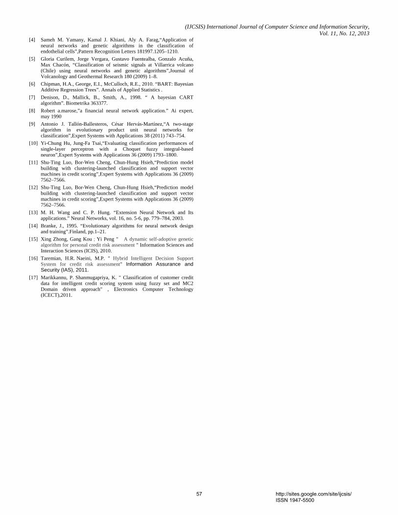
(IJCSIS) International Journal of Computer Science and Information Security, Vol. 11, No. 12, 2013
[4] Sameh M. Yamany, Kamal J. Khiani, Aly A. Farag,“Application of neural networks and genetic algorithms in the classification of endothelial cells”,Pattern Recognition Letters 181997.1205–1210.
[5] Gloria Curilem, Jorge Vergara, Gustavo Fuentealba, Gonzalo Acuña, Max Chacón, “Classification of seismic signals at Villarrica volcano (Chile) using neural networks and genetic algorithms”,Journal of Volcanology and Geothermal Research 180 (2009) 1–8.
[6] Chipman, H.A., George, E.I., McCulloch, R.E., 2010. “BART: Bayesian Additive Regression Trees”. Annals of Applied Statistics .
[7] Denison, D., Mallick, B., Smith, A., 1998. “ A bayesian CART algorithm”. Biometrika 363377.
[8] Robert a.marose,”a financial neural network application.” Ai expert, may 1990
[9] Antonio J. Tallón-Ballesteros, César Hervás-Martínez,“A two-stage algorithm in evolutionary product unit neural networks for classification”,Expert Systems with Applications 38 (2011) 743–754.
[10] Yi-Chung Hu, Jung-Fa Tsai,“Evaluating classification performances of single-layer perceptron with a Choquet fuzzy integral-based neuron”,Expert Systems with Applications 36 (2009) 1793–1800.
[11] Shu-Ting Luo, Bor-Wen Cheng, Chun-Hung Hsieh,“Prediction model building with clustering-launched classification and support vector machines in credit scoring”,Expert Systems with Applications 36 (2009) 7562–7566.
[12] Shu-Ting Luo, Bor-Wen Cheng, Chun-Hung Hsieh,“Prediction model building with clustering-launched classification and support vector machines in credit scoring”,Expert Systems with Applications 36 (2009) 7562–7566.
[13] M. H. Wang and C. P. Hung. “Extension Neural Network and Its applications.” Neural Networks, vol. 16, no. 5-6, pp. 779–784, 2003.
[14] Branke, J., 1995. “Evolutionary algorithms for neural network design and training”.Finland, pp.1–21.
[15] Xing Zhong, Gang Kou ; Yi Peng " A dynamic self-adoptive genetic algorithm for personal credit risk assessment " Information Sciences and Interaction Sciences (ICIS), 2010.
[16] Taremian, H.R. Naeini, M.P. " Hybrid Intelligent Decision Support System for credit risk assessment" Information Assurance and Security (IAS), 2011.
[17] Marikkannu, P. Shanmugapriya, K. " Classification of customer credit data for intelligent credit scoring system using fuzzy set and MC2 Domain driven approach" , Electronics Computer Technology (ICECT),2011.
57 http://sites.google.com/site/ijcsis/ ISSN 1947-5500
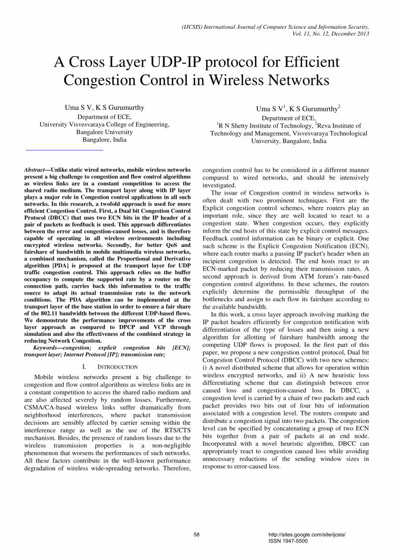
(IJCSIS) International Journal of Computer Science and Information Security,
Vol. 11, No. 12, December 2013
A Cross Layer UDP-IP protocol for Efficient
Congestion Control in Wireless Networks
Uma S V, K S Gurumurthy
Department of ECE,
University Visvesvaraya College of Engineering,
Bangalore University
Bangalore, India
Uma S V1, K S Gurumurthy
2
Department of ECE, 1R N Shetty Institute of Technology,
2Reva Institute of
Technology and Management, Visvesvaraya Technological
University, Bangalore, India
Abstract—Unlike static wired networks, mobile wireless networks
present a big challenge to congestion and flow control algorithms
as wireless links are in a constant competition to access the
shared radio medium. The transport layer along with IP layer
plays a major role in Congestion control applications in all such
networks. In this research, a twofold approach is used for more
efficient Congestion Control. First, a Dual bit Congestion Control
Protocol (DBCC) that uses two ECN bits in the IP header of a
pair of packets as feedback is used. This approach differentiates
between the error and congestion-caused losses, and is therefore
capable of operating in all wireless environments including
encrypted wireless networks. Secondly, for better QoS and
fairshare of bandwidth in mobile multimedia wireless networks,
a combined mechanism, called the Proportional and Derivative
algorithm [PDA] is proposed at the transport layer for UDP
traffic congestion control. This approach relies on the buffer
occupancy to compute the supported rate by a router on the
connection path, carries back this information to the traffic
source to adapt its actual transmission rate to the network
conditions. The PDA algorithm can be implemented at the
transport layer of the base station in order to ensure a fair share
of the 802.11 bandwidth between the different UDP-based flows.
We demonstrate the performance improvements of the cross
layer approach as compared to DPCP and VCP through
simulation and also the effectiveness of the combined strategy in
reducing Network Congestion.
Keywords—congestion; explicit congestion bits [ECN];
transport layer; Internet Protocol [IP]; transmission rate;
I. INTRODUCTION
Mobile wireless networks present a big challenge to
congestion and flow control algorithms as wireless links are in
a constant competition to access the shared radio medium and
are also affected severely by random losses. Furthermore,
CSMA/CA-based wireless links suffer dramatically from
neighborhood interferences, where packet transmission
decisions are sensibly affected by carrier sensing within the
interference range as well as the use of the RTS/CTS
mechanism. Besides, the presence of random losses due to the
wireless transmission properties is a non-negligible
phenomenon that worsens the performances of such networks.
All these factors contribute in the well-known performance
degradation of wireless wide-spreading networks. Therefore,
congestion control has to be considered in a different manner
compared to wired networks, and should be intensively
investigated.
The issue of Congestion control in wireless networks is
often dealt with two prominent techniques. First are the
Explicit congestion control schemes, where routers play an
important role, since they are well located to react to a
congestion state. When congestion occurs, they explicitly
inform the end hosts of this state by explicit control messages.
Feedback control information can be binary or explicit. One
such scheme is the Explicit Congestion Notification (ECN),
where each router marks a passing IP packet's header when an
incipient congestion is detected. The end hosts react to an
ECN-marked packet by reducing their transmission rates. A
second approach is derived from ATM forum’s rate-based
congestion control algorithms. In these schemes, the routers
explicitly determine the permissible throughput of the
bottlenecks and assign to each flow its fairshare according to
the available bandwidth.
In this work, a cross layer approach involving marking the
IP packet headers efficiently for congestion notification with
differentiation of the type of losses and then using a new
algorithm for allotting of fairshare bandwidth among the
competing UDP flows is proposed. In the first part of this
paper, we propose a new congestion control protocol, Dual bit
Congestion Control Protocol (DBCC) with two new schemes:
i) A novel distributed scheme that allows for operation within
wireless encrypted networks, and ii) A new heuristic loss
differentiating scheme that can distinguish between error
caused loss and congestion-caused loss. In DBCC, a
congestion level is carried by a chain of two packets and each
packet provides two bits out of four bits of information
associated with a congestion level. The routers compute and
distribute a congestion signal into two packets. The congestion
level can be specified by concatenating a group of two ECN
bits together from a pair of packets at an end node.
Incorporated with a novel heuristic algorithm, DBCC can
appropriately react to congestion caused loss while avoiding
unnecessary reductions of the sending window sizes in
response to error-caused loss.
58 http://sites.google.com/site/ijcsis/ ISSN 1947-5500

(IJCSIS) International Journal of Computer Science and Information Security,
Vol. 11, No. 12, December 2013
In the second part of this paper a new router based
congestion control algorithm, the Proportional and Derivative
algorithm (PDA) is proposed. This PDA monitors the level of
network congestion through the occupancy of the buffer which
is maintained with the control target. Based on the difference
between the present and target occupancy, the PDA controller
associated with each link computes periodically a fair rate)
and forwards the result to the next gateways till the
destination. Using a feedback scheme, the destination supplies
the source with the minimal received fairshare. In their turn,
sources have to adapt their transmission rate according to
received fair rate.
We show in this paper through simulation results that the
Combined DBCC and PDA algorithms guarantee efficiency
and fairness simultaneously reducing the Network congestion
effectively. Besides, through analysis, choice of control gain
leading to system stability in term of traffic transmission rate
has been made. The paper is structured as follows: Section II
presents the related work, Section III discusses the proposed
cross layer approach for congestion control. In Section IV, we
present the implementation and simulation results. Section V
concludes the paper.
II. RELATED WORK
The two issues addressed in this work have been addressed
individually in the past. Over the last few years, abundant
techniques have been developed to improve the efficiency and
fairness of TCP. A network explicit feedback mechanism
based on link throughput measurement was developed in [1].
Another explicit call admission control scheme, called
EXACT is proposed in [2]. If the proposed explicit congestion
control schemes succeed to reach efficiency and fairness, none
of them is dealing with the stability criterion, which is one of
the most important issues in highly dynamic wireless
networks.
Examples include the works of [3], [4], [5] using
algorithms to adaptively adjust the sending window size, and
[6], [7], [8], [9] employing alternative congestion signals.
However, due to their integrated controller design, these
techniques often fail to achieve both efficiency and fairness
[10]. By decoupling efficiency control from fairness, eXplicit
Congestion-control Protocol (XCP) [11] and Variable-
structure Congestion-control Protocol (VCP) [12] can achieve
high utilization, low persistent queue length, insignificant
packet loss rate, and sound fairness depending on the
heterogeneity characteristics of a network. While XCP
requires the use of a large number of IP packet header bits to
relay congestion information thereby introducing significant
deployment obstacles, VCP only uses the two existing ECN
bits in the IP header to encapsulate three congestion levels
hence presenting a more practical alternative of deployment
than XCP. However, VCP can only deliver limited feedback to
end hosts since two bits can at most represent four levels of
congestion. In order to avoid sudden bursts, VCP has to
control the growth of transmission rates by setting artificial
bounds. This yields slow convergence speeds and high
transition times. Moreover, due to the use of fixed parameters
for fairness control, VCP exhibits poor fairness characteristics
in high delay networks. Very recently, several works have
attempted addressing the problem associated with VCP
limitations by increasing the amount of feedback. While the
work in MLCP [13] proposes using 3 bits to represent the
Load Factor (LF), the UNO framework [14] proposes another
alternative to increase the amount of feedback by passively
utilizing information in IP Identification (IPID) field. In
contrast, DPCP [15] proposes a distributed framework that
allows for using no more than 2 ECN-bits to deliver a 4-bit
representation of the LF. That said, DPCP needs to access
partial information in the TCP header in order to be able to
efficiently distribute and reassemble the LF. However, in
encrypted networks protected by IPSec, TCP header
information is lost when crossing encryption boundaries.
Thus, DPCP cannot operate in such encrypted networks.
Furthermore, wireless networks are characterized by fading
related error-caused loss in addition to queuing related
congestion-caused loss. Experiments have shown that the
performance of any congestion control protocols relies on
appropriate reaction to loss according to its source. Like VCP,
DPCP reacts to loss without differentiating between the
sources of loss and thus performs inefficiently over wireless
networks.
Considering the issue of fair share, it has been proven in
[16] and [17] that TFRC does not always meet its fair share
when the network conditions are dynamic and may present
TCP-unfriendliness behavior. In [18], the TFRC performance
degradation in wireless environment is highlighted and found
to be due to the so-called RTS/CTS congestion induced
problem. Previous research in TCP and TFRC performance
improvement over wireless networks includes investigating
loss discrimination algorithms (LDA) in order to distinguish
losses due to congestion from those caused by random
wireless errors [19, 20, 21, 22, 23, 24, 25, 26]. Moreover,
several other adaptive RTP-based congestion control schemes
use a similar approach to react to a loss situation in the
network. A first set try to investigate the correlation between
the ROTT (Relative One-way Trip Time) and a congestion
loss. Extensive experimental results conducted in [19, 20]
show that spike-trains observed in a ROTT-graph are only
related to congestion losses and not to random losses.
Congestion control Schemes like PASTRA [27] and VTP [28]
take profit of the ROTT loss discrimination algorithm to find
congestion signals. Another approach, called the inter-arrival
scheme, uses the time between the arrivals of two consecutive
packets as a congestion indication [19, 20]. In [29], Vicente et
al. present the design of LDA+, a loss-delay based congestion
algorithm, based on the inter-arrival scheme. An improvement
of the Datagram Congestion Control Protocol (DCCP) is also
considered in [30] showing that the bandwidth utilization is
improved by more than 30% and up to 50% in significant
setups. The PDA has previously been adapted to ABR flows
59 http://sites.google.com/site/ijcsis/ ISSN 1947-5500
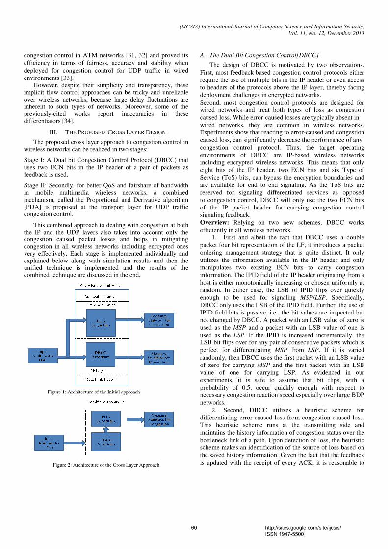
congestion control in ATM networks [31, 3
efficiency in terms of fairness, accuracy and
deployed for congestion control for UDP traffic
environments [33]. However, despite their simplicity and transparency, these
implicit flow control approaches can be tricky and unreliable over wireless networks, because large delay fluctuations are inherent to such types of networks. Moreover, some of the previously-cited works report inaccuracies in these differentiators [34].
III. THE PROPOSED CROSS LAYER
The proposed cross layer approach to congestion control in wireless networks can be realized in two stages:
Stage I: A Dual bit Congestion Control Protocol (DBCC) that uses two ECN bits in the IP header of a pair of packets as feedback is used.
Stage II: Secondly, for better QoS and fairshain mobile multimedia wireless networks, a combined mechanism, called the Proportional and Derivative algorithm [PDA] is proposed at the transport layer for UDP traffic congestion control.
This combined approach to dealing with congestion atthe IP and the UDP layers also takes into account only the congestion caused packet losses and helps in mitigating congestion in all wireless networks including encrypted ones very effectively. Each stage is implemented individually and explained below along with simulation results and then unified technique is implemented and the results of the combined technique are discussed in the end.
Figure 1: Architecture of the Initial approach
Figure 2: Architecture of the Cross Layer Approach
(IJCSIS) International Journal of Computer Science and Information Security,
32] and proved its
ency in terms of fairness, accuracy and stability when
deployed for congestion control for UDP traffic in wired
However, despite their simplicity and transparency, these can be tricky and unreliable large delay fluctuations are
Moreover, some of the inaccuracies in these
AYER DESIGN
o congestion control in wireless networks can be realized in two stages:
Dual bit Congestion Control Protocol (DBCC) that uses two ECN bits in the IP header of a pair of packets as
Secondly, for better QoS and fairshare of bandwidth mobile multimedia wireless networks, a combined
mechanism, called the Proportional and Derivative algorithm [PDA] is proposed at the transport layer for UDP traffic
This combined approach to dealing with congestion at both the IP and the UDP layers also takes into account only the congestion caused packet losses and helps in mitigating congestion in all wireless networks including encrypted ones
implemented individually and ow along with simulation results and then the
the results of the combined technique are discussed in the end.
Approach
A. The Dual Bit Congestion Control[DBCC]
The design of DBCC is motivated by
First, most feedback based congestion control
require the use of multiple bits in the IP
to headers of the protocols above the IP
deployment challenges in encrypted networks.
Second, most congestion control protocols are designed
wired networks and treat both types of loss as congestion
caused loss. While error-caused losses are typically absent in
wired networks, they are common in wireless networks.
Experiments show that reacting to error
caused loss, can significantly decrease the performance of any
congestion control protocol. Thus, the target operating
environments of DBCC are IP
including encrypted wireless networks.
eight bits of the IP header, two ECN bits and six Type of
Service (ToS) bits, can bypass
are available for end to end signaling.
reserved for signaling differentiated
to congestion control, DBCC will only
of the IP packet header for carrying congestion
signaling feedback.
Overview: Relying on two new schemes,
efficiently in all wireless networks.
1. First and albeit the fact that D
packet four bit representation of the LF, it introduces a packet
ordering management strategy that is quite distinct.
utilizes the information available in the IP header and only
manipulates two existing ECN bits to c
information. The IPID field of the IP header originating from a
host is either monotonically increasing or chosen uniformly at
random. In either case, the LSB of IPID flips over quickly
enough to be used for signaling
DBCC only uses the LSB of the IPID field. Further, the use of
IPID field bits is passive, i.e., the bit values are inspected but
not changed by DBCC. A packet with an LSB value of zero is
used as the MSP and a packet with an LSB value of one is
used as the LSP. If the IPID is increased incrementally, the
LSB bit flips over for any pair of consecutive packets which is
perfect for differentiating MSP
randomly, then DBCC uses the first packet with an LSB value
of zero for carrying MSP and the first packet with an LSB
value of one for carrying LSP. As evidenced in our
experiments, it is safe to assume that bit flips, with a
probability of 0.5, occur quickly enough with respect to
necessary congestion reaction speed especially over larg
networks.
2. Second, DBCC utilizes a heuristic scheme for
differentiating error-caused loss
This heuristic scheme runs at the
maintains the history information of congestion
bottleneck link of a path. Upon detection
scheme makes an identification of the
the saved history information. Given the fact that the feedback
is updated with the receipt of every ACK, it is reasonable to
International Journal of Computer Science and Information Security,
Vol. 11, No. 12, December 2013
Dual Bit Congestion Control[DBCC]
is motivated by two observations.
First, most feedback based congestion control protocols either
require the use of multiple bits in the IP header or even access
to headers of the protocols above the IP layer, thereby facing
deployment challenges in encrypted networks.
Second, most congestion control protocols are designed for
wired networks and treat both types of loss as congestion
caused losses are typically absent in
tworks, they are common in wireless networks.
show that reacting to error-caused and congestion
loss, can significantly decrease the performance of any
congestion control protocol. Thus, the target operating
are IP-based wireless networks
including encrypted wireless networks. This means that only
two ECN bits and six Type of
Service (ToS) bits, can bypass the encryption boundaries and
are available for end to end signaling. As the ToS bits are
reserved for signaling differentiated services as opposed
will only use the two ECN bits
of the IP packet header for carrying congestion control
Relying on two new schemes, DBCC works
wireless networks.
e fact that DBCC uses a double
of the LF, it introduces a packet
ordering management strategy that is quite distinct. It only
information available in the IP header and only
existing ECN bits to carry congestion
information. The IPID field of the IP header originating from a
is either monotonically increasing or chosen uniformly at
random. In either case, the LSB of IPID flips over quickly
to be used for signaling MSP/LSP. Specifically,
only uses the LSB of the IPID field. Further, the use of
field bits is passive, i.e., the bit values are inspected but
packet with an LSB value of zero is
and a packet with an LSB value of one is
. If the IPID is increased incrementally, the
any pair of consecutive packets which is
MSP from LSP. If it is varied
randomly, then DBCC uses the first packet with an LSB value
and the first packet with an LSB
of one for carrying LSP. As evidenced in our
is safe to assume that bit flips, with a
quickly enough with respect to
speed especially over large BDP
utilizes a heuristic scheme for
caused loss from congestion-caused loss.
This heuristic scheme runs at the transmitting side and
maintains the history information of congestion status over the
link of a path. Upon detection of loss, the heuristic
scheme makes an identification of the source of loss based on
Given the fact that the feedback
the receipt of every ACK, it is reasonable to
60 http://sites.google.com/site/ijcsis/ ISSN 1947-5500
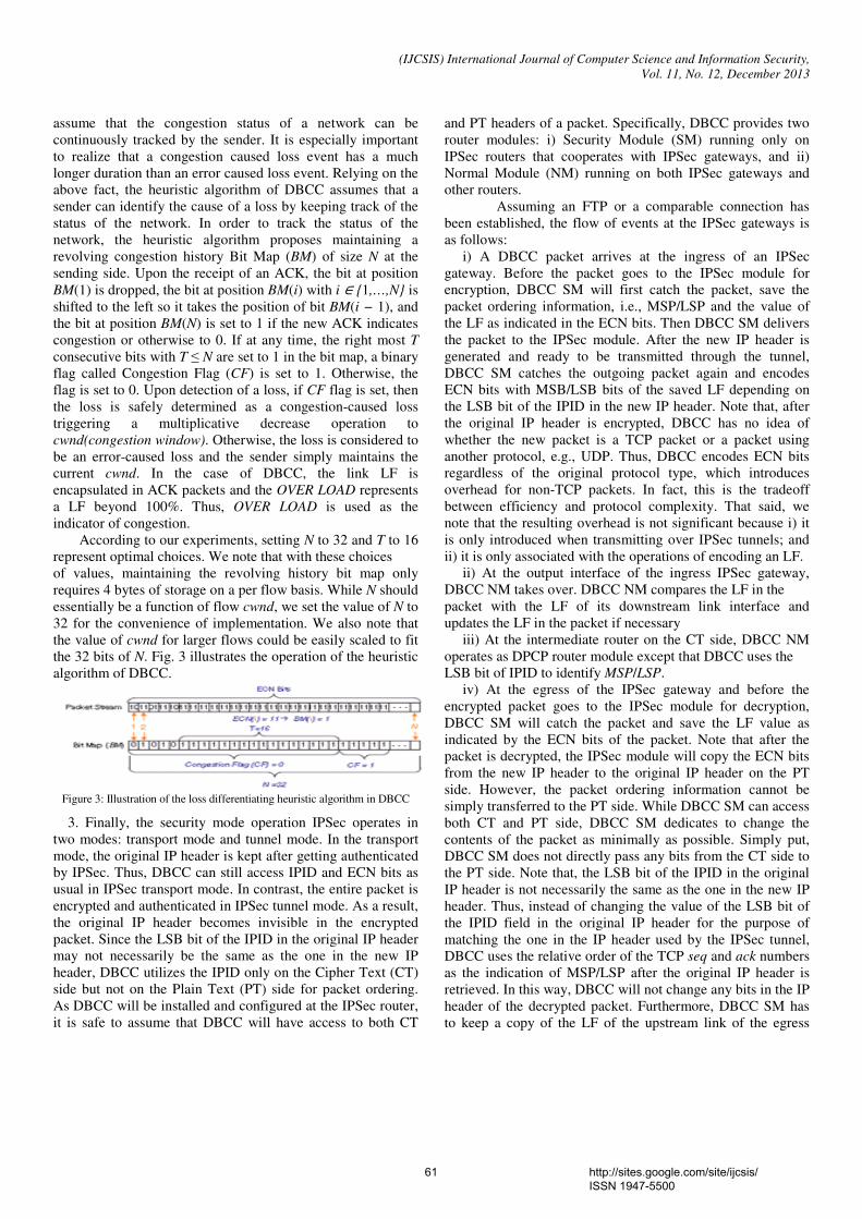
(IJCSIS) International Journal of Computer Science and Information Security,
Vol. 11, No. 12, December 2013
assume that the congestion status of a network can be
continuously tracked by the sender. It is especially important
to realize that a congestion caused loss event has a much
longer duration than an error caused loss event. Relying on the
above fact, the heuristic algorithm of DBCC assumes that a
sender can identify the cause of a loss by keeping track of the
status of the network. In order to track the status of the
network, the heuristic algorithm proposes maintaining a
revolving congestion history Bit Map (BM) of size N at the
sending side. Upon the receipt of an ACK, the bit at position
BM(1) is dropped, the bit at position BM(i) with i ∈ 1,…,N is
shifted to the left so it takes the position of bit BM(i − 1), and
the bit at position BM(N) is set to 1 if the new ACK indicates
congestion or otherwise to 0. If at any time, the right most T
consecutive bits with T ≤ N are set to 1 in the bit map, a binary
flag called Congestion Flag (CF) is set to 1. Otherwise, the
flag is set to 0. Upon detection of a loss, if CF flag is set, then
the loss is safely determined as a congestion-caused loss
triggering a multiplicative decrease operation to
cwnd(congestion window). Otherwise, the loss is considered to
be an error-caused loss and the sender simply maintains the
current cwnd. In the case of DBCC, the link LF is
encapsulated in ACK packets and the OVER LOAD represents
a LF beyond 100%. Thus, OVER LOAD is used as the
indicator of congestion.
According to our experiments, setting N to 32 and T to 16
represent optimal choices. We note that with these choices
of values, maintaining the revolving history bit map only
requires 4 bytes of storage on a per flow basis. While N should
essentially be a function of flow cwnd, we set the value of N to
32 for the convenience of implementation. We also note that
the value of cwnd for larger flows could be easily scaled to fit
the 32 bits of N. Fig. 3 illustrates the operation of the heuristic
algorithm of DBCC.
Figure 3: Illustration of the loss differentiating heuristic algorithm in DBCC
3. Finally, the security mode operation IPSec operates in
two modes: transport mode and tunnel mode. In the transport
mode, the original IP header is kept after getting authenticated
by IPSec. Thus, DBCC can still access IPID and ECN bits as
usual in IPSec transport mode. In contrast, the entire packet is
encrypted and authenticated in IPSec tunnel mode. As a result,
the original IP header becomes invisible in the encrypted
packet. Since the LSB bit of the IPID in the original IP header
may not necessarily be the same as the one in the new IP
header, DBCC utilizes the IPID only on the Cipher Text (CT)
side but not on the Plain Text (PT) side for packet ordering.
As DBCC will be installed and configured at the IPSec router,
it is safe to assume that DBCC will have access to both CT
and PT headers of a packet. Specifically, DBCC provides two
router modules: i) Security Module (SM) running only on
IPSec routers that cooperates with IPSec gateways, and ii)
Normal Module (NM) running on both IPSec gateways and
other routers.
Assuming an FTP or a comparable connection has
been established, the flow of events at the IPSec gateways is
as follows:
i) A DBCC packet arrives at the ingress of an IPSec
gateway. Before the packet goes to the IPSec module for
encryption, DBCC SM will first catch the packet, save the
packet ordering information, i.e., MSP/LSP and the value of
the LF as indicated in the ECN bits. Then DBCC SM delivers
the packet to the IPSec module. After the new IP header is
generated and ready to be transmitted through the tunnel,
DBCC SM catches the outgoing packet again and encodes
ECN bits with MSB/LSB bits of the saved LF depending on
the LSB bit of the IPID in the new IP header. Note that, after
the original IP header is encrypted, DBCC has no idea of
whether the new packet is a TCP packet or a packet using
another protocol, e.g., UDP. Thus, DBCC encodes ECN bits
regardless of the original protocol type, which introduces
overhead for non-TCP packets. In fact, this is the tradeoff
between efficiency and protocol complexity. That said, we
note that the resulting overhead is not significant because i) it
is only introduced when transmitting over IPSec tunnels; and
ii) it is only associated with the operations of encoding an LF.
ii) At the output interface of the ingress IPSec gateway,
DBCC NM takes over. DBCC NM compares the LF in the
packet with the LF of its downstream link interface and
updates the LF in the packet if necessary
iii) At the intermediate router on the CT side, DBCC NM
operates as DPCP router module except that DBCC uses the
LSB bit of IPID to identify MSP/LSP.
iv) At the egress of the IPSec gateway and before the
encrypted packet goes to the IPSec module for decryption,
DBCC SM will catch the packet and save the LF value as
indicated by the ECN bits of the packet. Note that after the
packet is decrypted, the IPSec module will copy the ECN bits
from the new IP header to the original IP header on the PT
side. However, the packet ordering information cannot be
simply transferred to the PT side. While DBCC SM can access
both CT and PT side, DBCC SM dedicates to change the
contents of the packet as minimally as possible. Simply put,
DBCC SM does not directly pass any bits from the CT side to
the PT side. Note that, the LSB bit of the IPID in the original
IP header is not necessarily the same as the one in the new IP
header. Thus, instead of changing the value of the LSB bit of
the IPID field in the original IP header for the purpose of
matching the one in the IP header used by the IPSec tunnel,
DBCC uses the relative order of the TCP seq and ack numbers
as the indication of MSP/LSP after the original IP header is
retrieved. In this way, DBCC will not change any bits in the IP
header of the decrypted packet. Furthermore, DBCC SM has
to keep a copy of the LF of the upstream link of the egress
61 http://sites.google.com/site/ijcsis/ ISSN 1947-5500
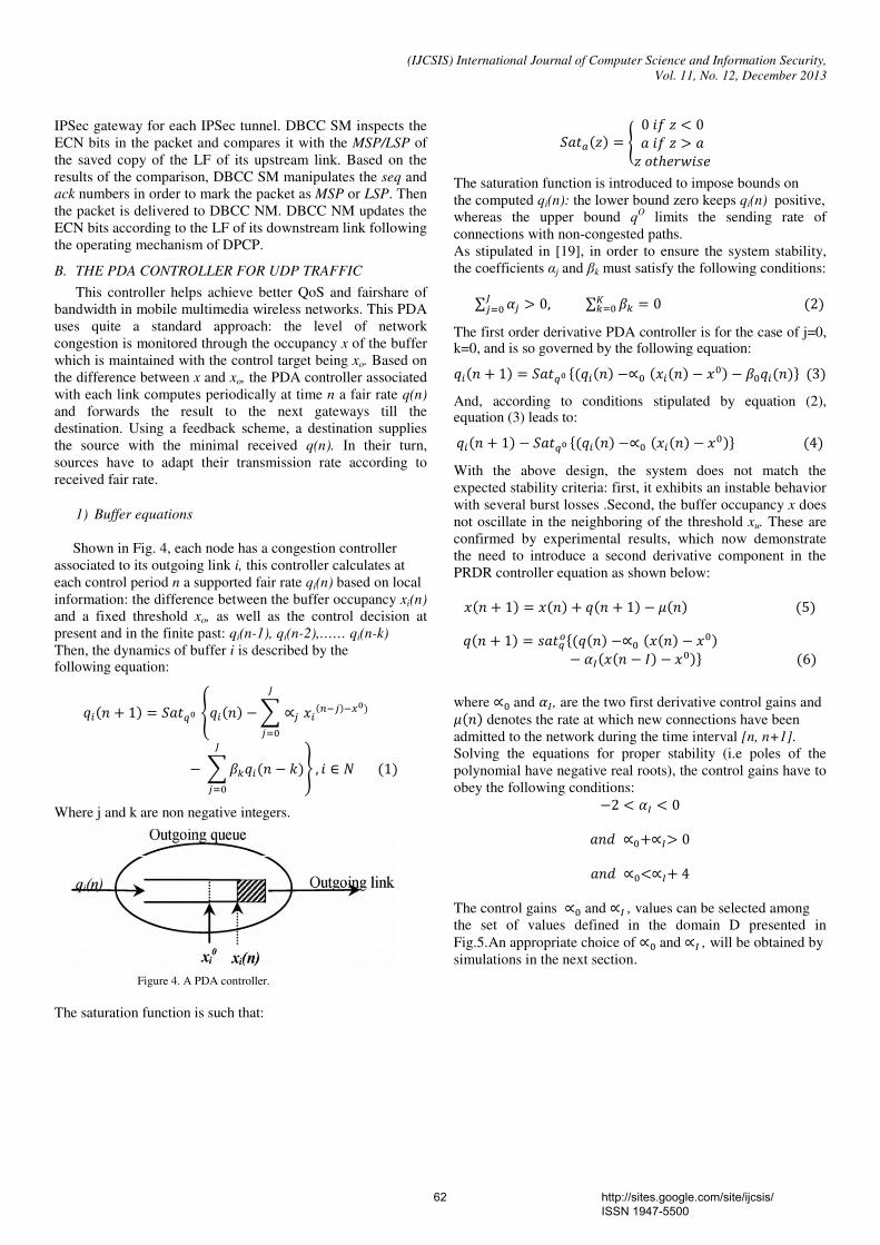
(IJCSIS) International Journal of Computer Science and Information Security,
Vol. 11, No. 12, December 2013
IPSec gateway for each IPSec tunnel. DBCC SM inspects the
ECN bits in the packet and compares it with the MSP/LSP of
the saved copy of the LF of its upstream link. Based on the
results of the comparison, DBCC SM manipulates the seq and
ack numbers in order to mark the packet as MSP or LSP. Then
the packet is delivered to DBCC NM. DBCC NM updates the
ECN bits according to the LF of its downstream link following
the operating mechanism of DPCP.
B. THE PDA CONTROLLER FOR UDP TRAFFIC
This controller helps achieve better QoS and fairshare of
bandwidth in mobile multimedia wireless networks. This PDA
uses quite a standard approach: the level of network
congestion is monitored through the occupancy x of the buffer
which is maintained with the control target being xo. Based on
the difference between x and xo, the PDA controller associated
with each link computes periodically at time n a fair rate q(n)
and forwards the result to the next gateways till the
destination. Using a feedback scheme, a destination supplies
the source with the minimal received q(n). In their turn,
sources have to adapt their transmission rate according to
received fair rate.
1) Buffer equations
Shown in Fig. 4, each node has a congestion controller
associated to its outgoing link i, this controller calculates at
each control period n a supported fair rate qi(n) based on local
information: the difference between the buffer occupancy xi(n)
and a fixed threshold xo, as well as the control decision at
present and in the finite past: qi(n-1), qi(n-2),…… qi(n-k)
Then, the dynamics of buffer i is described by the following equation:
+ 1 = − ∝
− −
, ! ∈ " 1
Where j and k are non negative integers.
Figure 4. A PDA controller.
The saturation function is such that:
#$ = % 0 !' $ < 0 !' $ > $ *ℎ,-.!/,0 The saturation function is introduced to impose bounds on
the computed qi(n): the lower bound zero keeps qi(n) positive,
whereas the upper bound qO limits the sending rate of
connections with non-congested paths.
As stipulated in [19], in order to ensure the system stability,
the coefficients αj and βk must satisfy the following conditions:
∑ 2 > 0, ∑ = 03 2
The first order derivative PDA controller is for the case of j=0, k=0, and is so governed by the following equation: + 1 = 5 −∝ − − 6 3
And, according to conditions stipulated by equation (2), equation (3) leads to: + 1 − 5 −∝ − 6 4
With the above design, the system does not match the
expected stability criteria: first, it exhibits an instable behavior
with several burst losses .Second, the buffer occupancy x does
not oscillate in the neighboring of the threshold xu. These are
confirmed by experimental results, which now demonstrate
the need to introduce a second derivative component in the
PRDR controller equation as shown below:
+ 1 = + + 1 − 9 5
+ 1 = / ;5 −∝ − − 2< − = − 6 6
where ∝ and 2<, are the two first derivative control gains and 9 denotes the rate at which new connections have been
admitted to the network during the time interval [n, n+1].
Solving the equations for proper stability (i.e poles of the
polynomial have negative real roots), the control gains have to
obey the following conditions: −2 < 2< < 0
? ∝+∝<> 0
? ∝<∝<+ 4
The control gains ∝ and ∝< , values can be selected among
the set of values defined in the domain D presented in
Fig.5.An appropriate choice of ∝ and ∝< , will be obtained by
simulations in the next section.
62 http://sites.google.com/site/ijcsis/ ISSN 1947-5500
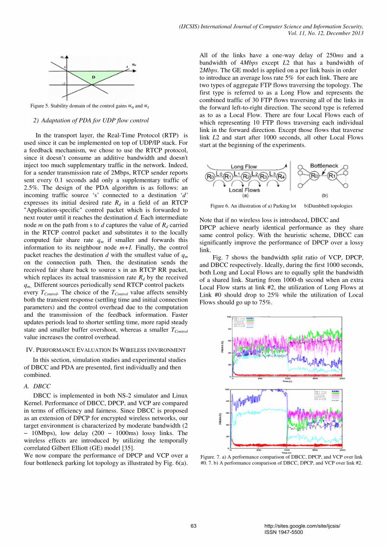
(IJCSIS) International Journal of Computer Science and Information Security,
Vol. 11, No. 12, December 2013
Figure 5. Stability domain of the control gains ∝ and ∝<
2) Adaptation of PDA for UDP flow control
In the transport layer, the Real-Time Protocol (RTP) is
used since it can be implemented on top of UDP/IP stack. For
a feedback mechanism, we chose to use the RTCP protocol,
since it doesn’t consume an additive bandwidth and doesn't
inject too much supplementary traffic in the network. Indeed,
for a sender transmission rate of 2Mbps, RTCP sender reports
sent every 0.1 seconds add only a supplementary traffic of
2.5%. The design of the PDA algorithm is as follows: an
incoming traffic source ‘s’ connected to a destination ‘d’
expresses its initial desired rate Rd in a field of an RTCP
"Application-specific" control packet which is forwarded to
next router until it reaches the destination d. Each intermediate
node m on the path from s to d captures the value of Rd carried
in the RTCP control packet and substitutes it to the locally
computed fair share rate qm if smaller and forwards this
information to its neighbour node m+I. Finally, the control
packet reaches the destination d with the smallest value of qm
on the connection path. Then, the destination sends the
received fair share back to source s in an RTCP RR packet,
which replaces its actual transmission rate Rd by the received
qm.. Different sources periodically send RTCP control packets
every TControl. The choice of the TControl value affects sensibly
both the transient response (settling time and initial connection
parameters) and the control overhead due to the computation
and the transmission of the feedback information. Faster
updates periods lead to shorter settling time, more rapid steady
state and smaller buffer overshoot, whereas a smaller TControl
value increases the control overhead.
IV . PERFORMANCE EVALUATION IN WIRELESS ENVIRONMENT
In this section, simulation studies and experimental studies
of DBCC and PDA are presented, first individually and then
combined.
A. DBCC
DBCC is implemented in both NS-2 simulator and Linux
Kernel. Performance of DBCC, DPCP, and VCP are compared
in terms of efficiency and fairness. Since DBCC is proposed
as an extension of DPCP for encrypted wireless networks, our
target environment is characterized by moderate bandwidth (2
− 10Mbps), low delay (200 − 1000ms) lossy links. The
wireless effects are introduced by utilizing the temporally
correlated Gilbert Elliott (GE) model [35].
We now compare the performance of DPCP and VCP over a
four bottleneck parking lot topology as illustrated by Fig. 6(a).
All of the links have a one-way delay of 250ms and a
bandwidth of 4Mbps except L2 that has a bandwidth of
2Mbps. The GE model is applied on a per link basis in order
to introduce an average loss rate 5% for each link. There are
two types of aggregate FTP flows traversing the topology. The
first type is referred to as a Long Flow and represents the
combined traffic of 30 FTP flows traversing all of the links in
the forward left-to-right direction. The second type is referred
as to as a Local Flow. There are four Local Flows each of
which representing 10 FTP flows traversing each individual
link in the forward direction. Except those flows that traverse
link L2 and start after 1000 seconds, all other Local Flows
start at the beginning of the experiments.
Figure 6. An illustration of a) Parking lot b)Dumbbell topologies
Note that if no wireless loss is introduced, DBCC and
DPCP achieve nearly identical performance as they share
same control policy. With the heuristic scheme, DBCC can
significantly improve the performance of DPCP over a lossy
link.
Fig. 7 shows the bandwidth split ratio of VCP, DPCP,
and DBCC respectively. Ideally, during the first 1000 seconds,
both Long and Local Flows are to equally split the bandwidth
of a shared link. Starting from 1000-th second when an extra
Local Flow starts at link #2, the utilization of Long Flows at
Link #0 should drop to 25% while the utilization of Local
Flows should go up to 75%.
Figure. 7. a) A performance comparison of DBCC, DPCP, and VCP over link
#0. 7. b) A performance comparison of DBCC, DPCP, and VCP over link #2.
63 http://sites.google.com/site/ijcsis/ ISSN 1947-5500
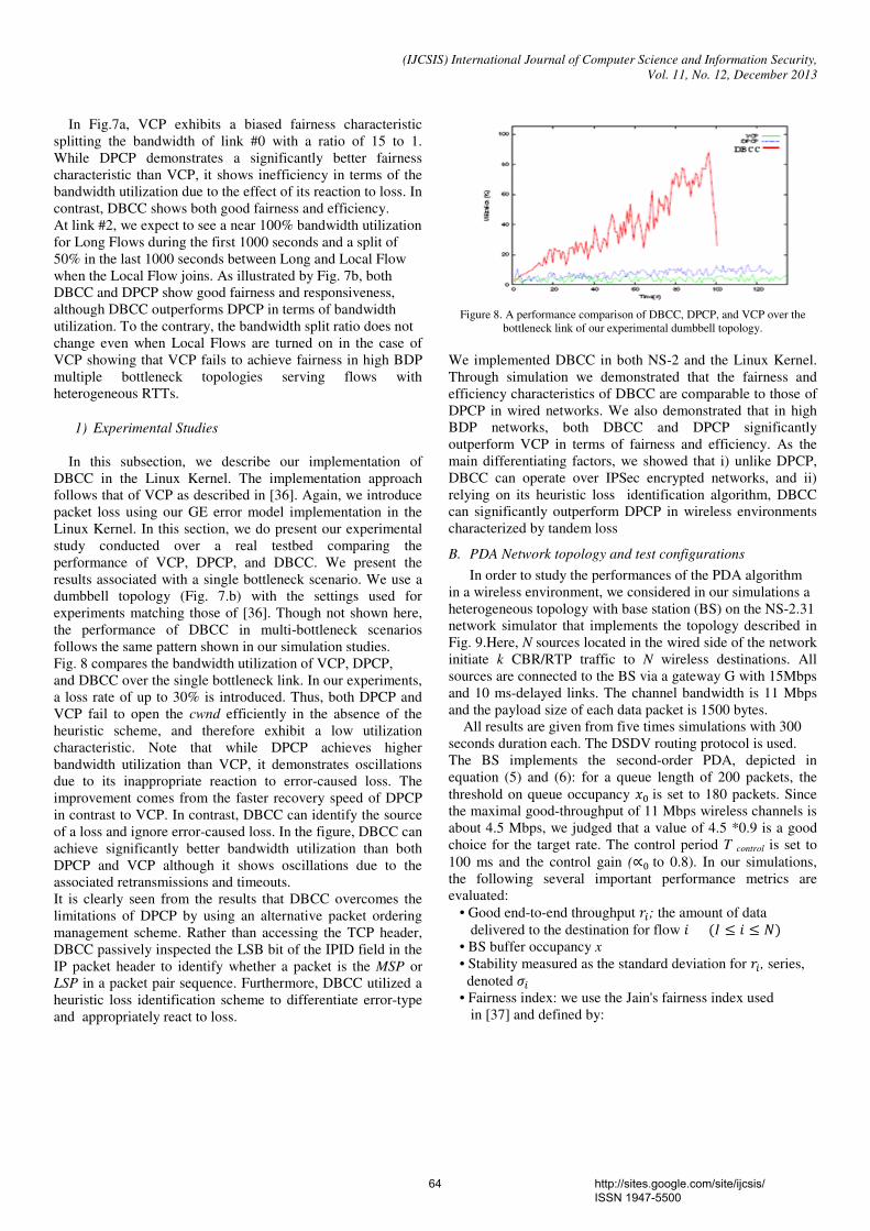
(IJCSIS) International Journal of Computer Science and Information Security,
Vol. 11, No. 12, December 2013
In Fig.7a, VCP exhibits a biased fairness characteristic
splitting the bandwidth of link #0 with a ratio of 15 to 1.
While DPCP demonstrates a significantly better fairness
characteristic than VCP, it shows inefficiency in terms of the
bandwidth utilization due to the effect of its reaction to loss. In
contrast, DBCC shows both good fairness and efficiency.
At link #2, we expect to see a near 100% bandwidth utilization
for Long Flows during the first 1000 seconds and a split of
50% in the last 1000 seconds between Long and Local Flow
when the Local Flow joins. As illustrated by Fig. 7b, both
DBCC and DPCP show good fairness and responsiveness,
although DBCC outperforms DPCP in terms of bandwidth
utilization. To the contrary, the bandwidth split ratio does not
change even when Local Flows are turned on in the case of
VCP showing that VCP fails to achieve fairness in high BDP
multiple bottleneck topologies serving flows with
heterogeneous RTTs.
1) Experimental Studies
In this subsection, we describe our implementation of
DBCC in the Linux Kernel. The implementation approach
follows that of VCP as described in [36]. Again, we introduce
packet loss using our GE error model implementation in the
Linux Kernel. In this section, we do present our experimental
study conducted over a real testbed comparing the
performance of VCP, DPCP, and DBCC. We present the
results associated with a single bottleneck scenario. We use a
dumbbell topology (Fig. 7.b) with the settings used for
experiments matching those of [36]. Though not shown here,
the performance of DBCC in multi-bottleneck scenarios
follows the same pattern shown in our simulation studies.
Fig. 8 compares the bandwidth utilization of VCP, DPCP,
and DBCC over the single bottleneck link. In our experiments,
a loss rate of up to 30% is introduced. Thus, both DPCP and
VCP fail to open the cwnd efficiently in the absence of the
heuristic scheme, and therefore exhibit a low utilization
characteristic. Note that while DPCP achieves higher
bandwidth utilization than VCP, it demonstrates oscillations
due to its inappropriate reaction to error-caused loss. The
improvement comes from the faster recovery speed of DPCP
in contrast to VCP. In contrast, DBCC can identify the source
of a loss and ignore error-caused loss. In the figure, DBCC can
achieve significantly better bandwidth utilization than both
DPCP and VCP although it shows oscillations due to the
associated retransmissions and timeouts.
It is clearly seen from the results that DBCC overcomes the
limitations of DPCP by using an alternative packet ordering
management scheme. Rather than accessing the TCP header,
DBCC passively inspected the LSB bit of the IPID field in the
IP packet header to identify whether a packet is the MSP or
LSP in a packet pair sequence. Furthermore, DBCC utilized a
heuristic loss identification scheme to differentiate error-type
and appropriately react to loss.
Figure 8. A performance comparison of DBCC, DPCP, and VCP over the
bottleneck link of our experimental dumbbell topology.
We implemented DBCC in both NS-2 and the Linux Kernel.
Through simulation we demonstrated that the fairness and
efficiency characteristics of DBCC are comparable to those of
DPCP in wired networks. We also demonstrated that in high
BDP networks, both DBCC and DPCP significantly
outperform VCP in terms of fairness and efficiency. As the
main differentiating factors, we showed that i) unlike DPCP,
DBCC can operate over IPSec encrypted networks, and ii)
relying on its heuristic loss identification algorithm, DBCC
can significantly outperform DPCP in wireless environments
characterized by tandem loss
B. PDA Network topology and test configurations
In order to study the performances of the PDA algorithm
in a wireless environment, we considered in our simulations a
heterogeneous topology with base station (BS) on the NS-2.31
network simulator that implements the topology described in
Fig. 9.Here, N sources located in the wired side of the network
initiate k CBR/RTP traffic to N wireless destinations. All
sources are connected to the BS via a gateway G with 15Mbps
and 10 ms-delayed links. The channel bandwidth is 11 Mbps
and the payload size of each data packet is 1500 bytes.
All results are given from five times simulations with 300
seconds duration each. The DSDV routing protocol is used.
The BS implements the second-order PDA, depicted in
equation (5) and (6): for a queue length of 200 packets, the
threshold on queue occupancy is set to 180 packets. Since
the maximal good-throughput of 11 Mbps wireless channels is
about 4.5 Mbps, we judged that a value of 4.5 *0.9 is a good
choice for the target rate. The control period T control is set to
100 ms and the control gain (∝ to 0.8). In our simulations,
the following several important performance metrics are
evaluated:
• Good end-to-end throughput -; the amount of data
delivered to the destination for flow ! = ≤ ! ≤ "
• BS buffer occupancy x
• Stability measured as the standard deviation for -, series,
denoted A • Fairness index: we use the Jain's fairness index used
in [37] and defined by:
64 http://sites.google.com/site/ijcsis/ ISSN 1947-5500
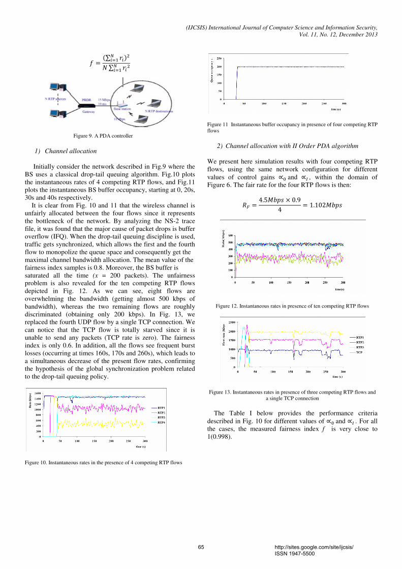
(IJCSIS) International Journal of Computer Science and Information Security,
Vol. 11, No. 12, December 2013
' = ∑ -BC D" ∑ -DBC
Figure 9. A PDA controller
1) Channel allocation
Initially consider the network described in Fig.9 where the
BS uses a classical drop-tail queuing algorithm. Fig.10 plots
the instantaneous rates of 4 competing RTP flows, and Fig.11
plots the instantaneous BS buffer occupancy, starting at 0, 20s,
30s and 40s respectively.
It is clear from Fig. 10 and 11 that the wireless channel is
unfairly allocated between the four flows since it represents
the bottleneck of the network. By analyzing the NS-2 trace
file, it was found that the major cause of packet drops is buffer
overflow (IFQ). When the drop-tail queuing discipline is used,
traffic gets synchronized, which allows the first and the fourth
flow to monopolize the queue space and consequently get the
maximal channel bandwidth allocation. The mean value of the
fairness index samples is 0.8. Moreover, the BS buffer is
saturated all the time (x = 200 packets). The unfairness
problem is also revealed for the ten competing RTP flows
depicted in Fig. 12. As we can see, eight flows are
overwhelming the bandwidth (getting almost 500 kbps of
bandwidth), whereas the two remaining flows are roughly
discriminated (obtaining only 200 kbps). In Fig. 13, we
replaced the fourth UDP flow by a single TCP connection. We
can notice that the TCP flow is totally starved since it is
unable to send any packets (TCP rate is zero). The fairness
index is only 0.6. In addition, all the flows see frequent burst
losses (occurring at times 160s, 170s and 260s), which leads to
a simultaneous decrease of the present flow rates, confirming
the hypothesis of the global synchronization problem related
to the drop-tail queuing policy.
Figure 10. Instantaneous rates in the presence of 4 competing RTP flows
Figure 11 Instantaneous buffer occupancy in presence of four competing RTP
flows
2) Channel allocation with II Order PDA algorithm
We present here simulation results with four competing RTP
flows, using the same network configuration for different
values of control gains ∝ and ∝< , within the domain of
Figure 6. The fair rate for the four RTP flows is then:
EF = 4.5HIJ/ × 0.94 = 1.102HIJ/
Figure 12. Instantaneous rates in presence of ten competing RTP flows
Figure 13. Instantaneous rates in presence of three competing RTP flows and
a single TCP connection
The Table I below provides the performance criteria
described in Fig. 10 for different values of ∝ and ∝< . For all
the cases, the measured fairness index f is very close to
1(0.998).
65 http://sites.google.com/site/ijcsis/ ISSN 1947-5500
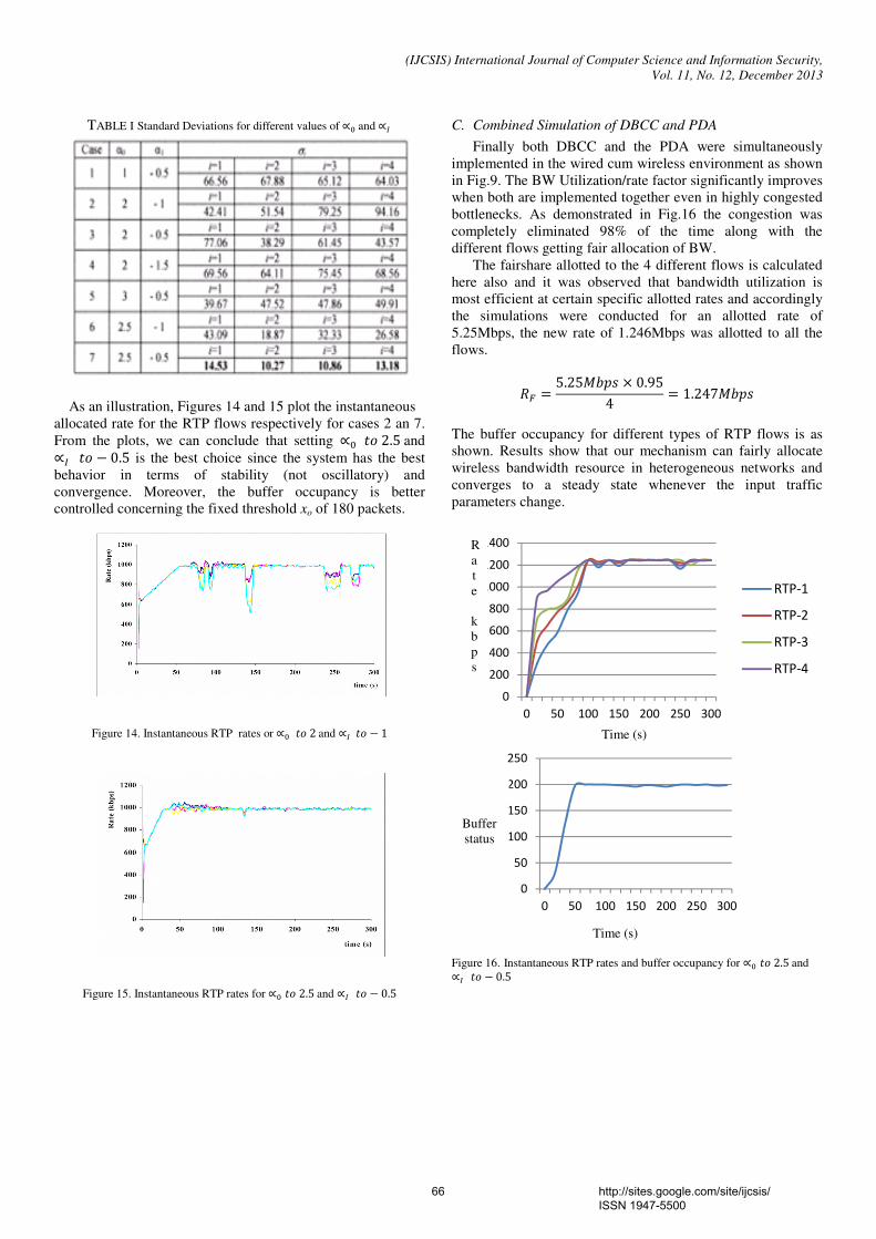
(IJCSIS) International Journal of Computer Science and Information Security,
Vol. 11, No. 12, December 2013
TABLE I Standard Deviations for different values of ∝ and ∝<
As an illustration, Figures 14 and 15 plot the instantaneous
allocated rate for the RTP flows respectively for cases 2 an 7.
From the plots, we can conclude that setting ∝ * 2.5 and ∝< * − 0.5 is the best choice since the system has the best
behavior in terms of stability (not oscillatory) and
convergence. Moreover, the buffer occupancy is better
controlled concerning the fixed threshold xo of 180 packets.
Figure 14. Instantaneous RTP rates or ∝ * 2 and ∝< * − 1
Figure 15. Instantaneous RTP rates for ∝ * 2.5 and ∝< * − 0.5
C. Combined Simulation of DBCC and PDA
Finally both DBCC and the PDA were simultaneously
implemented in the wired cum wireless environment as shown
in Fig.9. The BW Utilization/rate factor significantly improves
when both are implemented together even in highly congested
bottlenecks. As demonstrated in Fig.16 the congestion was
completely eliminated 98% of the time along with the
different flows getting fair allocation of BW.
The fairshare allotted to the 4 different flows is calculated
here also and it was observed that bandwidth utilization is
most efficient at certain specific allotted rates and accordingly
the simulations were conducted for an allotted rate of
5.25Mbps, the new rate of 1.246Mbps was allotted to all the
flows.
EF = 5.25HIJ/ × 0.954 = 1.247HIJ/
The buffer occupancy for different types of RTP flows is as
shown. Results show that our mechanism can fairly allocate
wireless bandwidth resource in heterogeneous networks and
converges to a steady state whenever the input traffic
parameters change.
Figure 16. Instantaneous RTP rates and buffer occupancy for ∝ * 2.5 and ∝< * − 0.5
0
200
400
600
800
1000
1200
1400
0 50 100 150 200 250 300
RTP-1
RTP-2
RTP-3
RTP-4
0
50
100
150
200
250
0 50 100 150 200 250 300
Time (s)
R
a
t
e
k
b
p
s
Buffer
status
Time (s)
66 http://sites.google.com/site/ijcsis/ ISSN 1947-5500
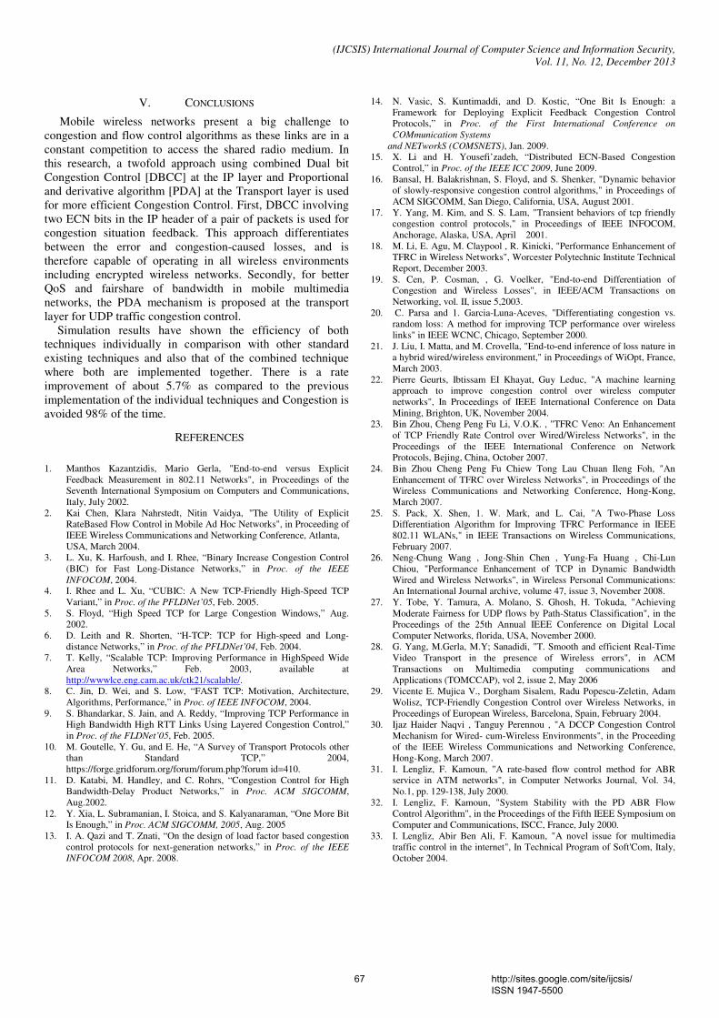
(IJCSIS) International Journal of Computer Science and Information Security,
Vol. 11, No. 12, December 2013
V. CONCLUSIONS
Mobile wireless networks present a big challenge to
congestion and flow control algorithms as these links are in a
constant competition to access the shared radio medium. In
this research, a twofold approach using combined Dual bit
Congestion Control [DBCC] at the IP layer and Proportional
and derivative algorithm [PDA] at the Transport layer is used
for more efficient Congestion Control. First, DBCC involving
two ECN bits in the IP header of a pair of packets is used for
congestion situation feedback. This approach differentiates
between the error and congestion-caused losses, and is
therefore capable of operating in all wireless environments
including encrypted wireless networks. Secondly, for better
QoS and fairshare of bandwidth in mobile multimedia
networks, the PDA mechanism is proposed at the transport
layer for UDP traffic congestion control.
Simulation results have shown the efficiency of both
techniques individually in comparison with other standard
existing techniques and also that of the combined technique
where both are implemented together. There is a rate
improvement of about 5.7% as compared to the previous
implementation of the individual techniques and Congestion is
avoided 98% of the time.
REFERENCES
1. Manthos Kazantzidis, Mario Gerla, "End-to-end versus Explicit
Feedback Measurement in 802.11 Networks", in Proceedings of the
Seventh International Symposium on Computers and Communications,
Italy, July 2002.
2. Kai Chen, Klara Nahrstedt, Nitin Vaidya, "The Utility of Explicit
RateBased Flow Control in Mobile Ad Hoc Networks", in Proceeding of
IEEE Wireless Communications and Networking Conference, Atlanta,
USA, March 2004.
3. L. Xu, K. Harfoush, and I. Rhee, “Binary Increase Congestion Control
(BIC) for Fast Long-Distance Networks,” in Proc. of the IEEE
INFOCOM, 2004.
4. I. Rhee and L. Xu, “CUBIC: A New TCP-Friendly High-Speed TCP
Variant,” in Proc. of the PFLDNet’05, Feb. 2005.
5. S. Floyd, “High Speed TCP for Large Congestion Windows,” Aug.
2002.
6. D. Leith and R. Shorten, “H-TCP: TCP for High-speed and Long-
distance Networks,” in Proc. of the PFLDNet’04, Feb. 2004.
7. T. Kelly, “Scalable TCP: Improving Performance in HighSpeed Wide
Area Networks,” Feb. 2003, available at
http://wwwlce.eng.cam.ac.uk/ctk21/scalable/.
8. C. Jin, D. Wei, and S. Low, “FAST TCP: Motivation, Architecture,
Algorithms, Performance,” in Proc. of IEEE INFOCOM, 2004.
9. S. Bhandarkar, S. Jain, and A. Reddy, “Improving TCP Performance in
High Bandwidth High RTT Links Using Layered Congestion Control,”
in Proc. of the FLDNet’05, Feb. 2005.
10. M. Goutelle, Y. Gu, and E. He, “A Survey of Transport Protocols other
than Standard TCP,” 2004,
https://forge.gridforum.org/forum/forum.php?forum id=410.
11. D. Katabi, M. Handley, and C. Rohrs, “Congestion Control for High
Bandwidth-Delay Product Networks,” in Proc. ACM SIGCOMM,
Aug.2002.
12. Y. Xia, L. Subramanian, I. Stoica, and S. Kalyanaraman, “One More Bit
Is Enough,” in Proc. ACM SIGCOMM, 2005, Aug. 2005
13. I. A. Qazi and T. Znati, “On the design of load factor based congestion
control protocols for next-generation networks,” in Proc. of the IEEE
INFOCOM 2008, Apr. 2008.
14. N. Vasic, S. Kuntimaddi, and D. Kostic, “One Bit Is Enough: a
Framework for Deploying Explicit Feedback Congestion Control
Protocols,” in Proc. of the First International Conference on
COMmunication Systems
and NETworkS (COMSNETS), Jan. 2009.
15. X. Li and H. Yousefi’zadeh, “Distributed ECN-Based Congestion
Control,” in Proc. of the IEEE ICC 2009, June 2009.
16. Bansal, H. Balakrishnan, S. Floyd, and S. Shenker, "Dynamic behavior
of slowly-responsive congestion control algorithms," in Proceedings of
ACM SIGCOMM, San Diego, California, USA, August 2001.
17. Y. Yang, M. Kim, and S. S. Lam, "Transient behaviors of tcp friendly
congestion control protocols," in Proceedings of IEEE INFOCOM,
Anchorage, Alaska, USA, April 2001.
18. M. Li, E. Agu, M. Claypool , R. Kinicki, "Performance Enhancement of
TFRC in Wireless Networks", Worcester Polytechnic Institute Technical
Report, December 2003.
19. S. Cen, P. Cosman, , G. Voelker, "End-to-end Differentiation of
Congestion and Wireless Losses", in IEEE/ACM Transactions on
Networking, vol. II, issue 5,2003.
20. C. Parsa and 1. Garcia-Luna-Aceves, "Differentiating congestion vs.
random loss: A method for improving TCP performance over wireless
links" in IEEE WCNC, Chicago, September 2000.
21. J. Liu, I. Matta, and M. Crovella, "End-to-end inference of loss nature in
a hybrid wired/wireless environment," in Proceedings of WiOpt, France,
March 2003.
22. Pierre Geurts, Ibtissam EI Khayat, Guy Leduc, "A machine learning
approach to improve congestion control over wireless computer
networks", In Proceedings of IEEE International Conference on Data
Mining, Brighton, UK, November 2004.
23. Bin Zhou, Cheng Peng Fu Li, V.O.K. , "TFRC Veno: An Enhancement
of TCP Friendly Rate Control over Wired/Wireless Networks", in the
Proceedings of the IEEE International Conference on Network
Protocols, Bejing, China, October 2007.
24. Bin Zhou Cheng Peng Fu Chiew Tong Lau Chuan Ileng Foh, "An
Enhancement of TFRC over Wireless Networks", in Proceedings of the
Wireless Communications and Networking Conference, Hong-Kong,
March 2007.
25. S. Pack, X. Shen, 1. W. Mark, and L. Cai, "A Two-Phase Loss
Differentiation Algorithm for Improving TFRC Performance in IEEE
802.11 WLANs," in IEEE Transactions on Wireless Communications,
February 2007.
26. Neng-Chung Wang , Jong-Shin Chen , Yung-Fa Huang , Chi-Lun
Chiou, "Performance Enhancement of TCP in Dynamic Bandwidth
Wired and Wireless Networks", in Wireless Personal Communications:
An International Journal archive, volume 47, issue 3, November 2008.
27. Y. Tobe, Y. Tamura, A. Molano, S. Ghosh, H. Tokuda, "Achieving
Moderate Fairness for UDP flows by Path-Status Classification", in the
Proceedings of the 25th Annual IEEE Conference on Digital Local
Computer Networks, florida, USA, November 2000.
28. G. Yang, M.Gerla, M.Y; Sanadidi, "T. Smooth and efficient Real-Time
Video Transport in the presence of Wireless errors", in ACM
Transactions on Multimedia computing communications and
Applications (TOMCCAP), vol 2, issue 2, May 2006
29. Vicente E. Mujica V., Dorgham Sisalem, Radu Popescu-Zeletin, Adam
Wolisz, TCP-Friendly Congestion Control over Wireless Networks, in
Proceedings of European Wireless, Barcelona, Spain, February 2004.
30. Ijaz Haider Naqvi , Tanguy Perennou , "A DCCP Congestion Control
Mechanism for Wired- cum-Wireless Environments", in the Proceeding
of the IEEE Wireless Communications and Networking Conference,
Hong-Kong, March 2007.
31. I. Lengliz, F. Kamoun, "A rate-based flow control method for ABR
service in ATM networks", in Computer Networks Journal, Vol. 34,
No.1, pp. 129-138, July 2000.
32. I. Lengliz, F. Kamoun, "System Stability with the PD ABR Flow
Control Algorithm", in the Proceedings of the Fifth IEEE Symposium on
Computer and Communications, ISCC, France, July 2000.
33. I. Lengliz, Abir Ben Ali, F. Kamoun, "A novel issue for multimedia
traffic control in the internet", In Technical Program of Soft'Com, Italy,
October 2004.
67 http://sites.google.com/site/ijcsis/ ISSN 1947-5500
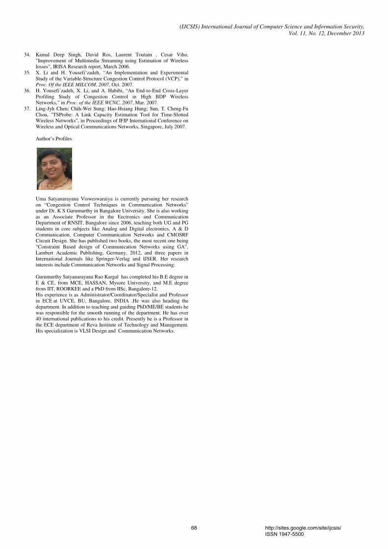
(IJCSIS) International Journal of Computer Science and Information Security,
Vol. 11, No. 12, December 2013
34. Kamal Deep Singh, David Ros, Laurent Toutain , Cesar Viho,
"Improvement of Multimedia Streaming using Estimation of Wireless
losses", IRISA Research report, March 2006.
35. X. Li and H. Yousefi’zadeh, “An Implementation and Experimental
Study of the Variable-Structure Congestion Control Protocol (VCP),” in
Proc. Of the IEEE MILCOM, 2007, Oct. 2007.
36. H. Yousefi’zadeh, X. Li, and A. Habibi, “An End-to-End Cross-Layer
Profiling Study of Congestion Control in High BDP Wireless
Networks,” in Proc. of the IEEE WCNC, 2007, Mar. 2007.
37. Ling-Jyh Chen; Chih-Wei Sung; Hao-Hsiang Hung; Sun, T. Cheng-Fu
Chou, "TSProbe: A Link Capacity Estimation Tool for Time-Slotted
Wireless Networks", in Proceedings of IFIP International Conference on
Wireless and Optical Communications Networks, Singapore, July 2007.
Author’s Profiles
Uma Satyanarayana Visweswaraiya is currently pursuing her research
on “Congestion Control Techniques in Communication Networks”
under Dr. K S Gurumurthy in Bangalore University. She is also working
as an Associate Professor in the Eectronics and Communication
Department of RNSIT, Bangalore since 2006, teaching both UG and PG
students in core subjects like Analog and Digital electronics, A & D
Communication, Computer Communication Networks and CMOSRF
Circuit Design. She has published two books, the most recent one being
“Constraint Based design of Communication Networks using GA”,
Lambert Academic Publishing, Germany, 2012, and three papers in
International Journals like Springer-Verlag and IJSER. Her research
interests include Communication Networks and Signal Processing.
Gurumurthy Satyanarayana Rao Kargal has completed his B.E degree in
E & CE, from MCE, HASSAN, Mysore University, and M.E degree
from IIT, ROORKEE and a PhD from IISc, Bangalore-12.
His experience is as Administrator/Coordinator/Specialist and Professor
in ECE at UVCE, BU, Bangalore, INDIA .He was also heading the
department. In addition to teaching and guiding PhD/ME/BE students he
was responsible for the smooth running of the department. He has over
40 international publications to his credit. Presently he is a Professor in
the ECE department of Reva Institute of Technology and Management.
His specialization is VLSI Design and Communication Networks.
68 http://sites.google.com/site/ijcsis/ ISSN 1947-5500

(IJCSIS) International Journal of Computer Science and Information Security, Vol. 11, No. 12, December 2013
The Development of Educational Quality
Administration: a Case of Technical College in
Southern Thailand
Bangsuk Jantawan
Department of Tropical Agriculture and International
Cooperation
National Pingtung University of Science and Technology
Pingtung, Taiwan
Cheng-Fa Tsai
Department of Management Information Systems
National Pingtung University of Science and Technology
Pingtung, Taiwan
Abstract— The purpose of this research were: to survey the
needs of using the information system for educational quality
administration; to develop Information System for Educational
quality Administration (ISEs) in accordance with quality
assessment standard; to study the qualification of ISEs; and to
study satisfaction level of ISEs user. Subsequently, the tools of
study have been employed that there were the collection of 47
questionnaires and 5 interviews to specialist by responsible
officers for Information center of Technical colleges and
Vocational colleges in Southern Thailand. The analysis of
quantitative data has employed descriptive statistics using
mean and standard deviation as the tool of measurement.
Hence, the result was found that most users required software
to search information rapidly (82.89%), software for collecting
data (80.85%) and required Information system which could
print document rapidly and ready for use (78.72%). The ISEs
was created and developed by using Microsoft Access 2007 and
Visual Basic. The ISEs was at good level with the average of
4.49 and SD at 0.5. Users’ satisfaction of this software was at good level with the average of 4.36 and SD at 0.58.
Keywords- Educational Quality Assurance; Educational
Quality Administration; Information System;
I. INTRODUCTION
A. Background
According to the National Education Act (1999) and Vocational Education Act, 2008, the educational institution in Thailand had been changed in various aspect and also called for education reform. Education reform has been caused by social currents of globalization and knowledge. Not only Thailand, but also other countries around the world have focused on the teaching and learning process to students for holistic development. The concept of learning has made personnel of cultural, social, economic and technology for their continuous and timely global trends. The process of teaching and learning quality is important to make a difference. This process must be continuous and consistent with the concept of quality assurance to build up the confidence of students, parents, community and Thai society. Therefore, school administrators along with the teaching methods should confidently make standard ability
of students and the impact on the development of Thailand [1], [2].
The section 47 in the National Education Act (1999) requires the development of quality assurance standards for all educational levels. It includes internal quality assurance and external quality assurance. In the section 48 requires the internal quality assurance as part of a process of the educational institutions continuously. In addition, the section 49 also requires that all educational institutions must obtain external assessment at least once in every five years since the last assessment. The assessment outcomes will be duly submitted to the concerned agencies and the public. Then, educational institutions must prepare to support implementation of the various sections [1],
Hence, researcher interests in development of information management system for administration of educational quality by collecting the data that related with the quality assurance standards. The Technical College and Vocational College in Southern Thailand have to improve a quality of information system and need to collect the data consistently in order to make the decision-maker efficiently. It can identify the weaknesses or problems effectively as well. The remedial measures are needed so as to facilitate subsequent planning and actions required to achieve the goals effectively [3].
B. Research Objectives
The overall objective of this study was to obtain information on the development of educational quality administration for the technical college in southern Thailand. There were four specific objectives of this study following: (1) to survey the needs of using information system for educational quality administration of colleges in southern Thailand; (2) to improve information system for educational quality administration of technical colleges in southern Thailand; (3) to study the quality of information system for educational quality administration of technical colleges in southern Thailand; and (4) to study satisfaction level of information system for educational quality administration of technical colleges in southern Thailand. Actions required achieving the goals effectively [3].
69 http://sites.google.com/site/ijcsis/ ISSN 1947-5500
(IJCSIS) International Journal of Computer Science and Information Security, Vol. 11, No. 12, December 2013
C. Research Hypotheses
This study was based on the hypotheses, which consists of the following three parts: (1) ISEs has appropriated in educational quality management of technical colleges in southern Thailand and good level; (2) ISEs has been developed and has a good quality; and (3) the users of ISEs have a satisfaction in the information system for educational quality management at a high level.
D. Research Scope
As the population, this study was created and develops ISEs of technical colleges in southern Thailand of 47 institutions. Purposive samplings composed of 47 responsible officers for information center of technical colleges and industrial and community colleges in southern Thailand.
As the specialist, there were 3 specialists of quality assessment information system for educational quality management. The details below were the specialist qualifications: (1) the graduate master's degree or higher than that of related fields; (2) the bachelor’s degree or related work in the educational standards of technical colleges and vocational college; and (3) the working-related information and expertise in computer data base of not less than five years, including both sides of eight persons.
E. Research Tools
The tools of study enclosed of four parts: the first tool was the requirement questionnaire of ISEs software. The questionnaire divided was five episodes: (Episode 1) the general data of respondents were multiple choice questions; (Episode 2) the condition used information system in college was multiple choice questions; (Episode 3) the problem of used information system in college was multiple choice questions; (Episode 4) the need of used information system in college was multiple choice questions, and (Episode 5) the opinion and suggestion about needed in used information system program in college; the second tool was the ISEs software; the third tool was the quality evaluate of ISEs; and the fourth tool was the satisfaction questionnaire in used ISEs. It was divided were two parts: (Episode 1) the general data of respondents were multiple choice questions, and (Episode 2) the opinion about used information system was multiple choice questions.
F. Definition Terminology
There were 3 key terminologies of study. Firstly, the technical college in southern regional office of vocational commission: means the institutions technical college and vocational college kind within the technical college in southern regional office of vocational commission in the area south of 47 colleges. Secondly, the user information system: means the personal responsibility information center of technical college in southern regional office of vocational commission. Thirdly, the information system development: means the process of developing software with Microsoft Access and Visual Basic programming a standby Standalone
to be able to store data, Process data and report data According to the information system.
II. METHODOLOGY
A. Data Collection
The process in this study consisted of the information following: (1) the data from questionnaires and the needs of using information system for educational quality administration of colleges in southern regional office of vocational education commission composed of 47 responsible officers; (2) the data from specialists of quality assurance standards, internal quality assurance, and overview information systems composed of eight specialists; and (3) the data from the technical college and vocational college in southern regional office of vocational commission composed of 47 institutions.
B. Data Analysis
1) Create questionnaire needed in used information
system for education quality administration; First step, there were 4 parts: (1) study the principle to
create questionnaire for book document journal related
research, (2) design and create survey of problem and needed to divide issues, (3) take the needed survey of used
information system for education quality administration
draft sent to chief advisor and chief advisor check it and
Edit for suitable, (3) improve and edit needed survey used of
information system for educational quality management of
technical colleges in southern regional office of vocational
education commission, and (4) take need survey in
information system for education quality administration to
use.
2) Development for education quality administration
development information system for education quality
administration to create by procedure; Second step, there were 6 parts: (1) preliminary
investigation, (2) systems analysis, (3) evaluate the consistency of the standard data items, (4) file and database
design (file and database design, program structure design,
and input and output design), (5) system development
(programming, and documentation), and (6) system
implementation.
3) Creating evaluate for education quality
administration have the procedure; Third step, there were 6 parts: (1) study the document ad
related research to education quality administration, (2)
research analysis form objective of research for approach in
used evaluate for comprehensive objective of research, (3)
create evaluate quality of system was evaluation scale 5
levels Likert scale for comments of the specialist of check
system standard and tests information system before to use, (4) take standard evaluate sent to chiefs advisor to check and
suggestion for suitable content, (5) improve and edit
standard evaluate both side according suggestion, and (6)
take quality evaluate of system to sent to the specialist 3
person quality evaluate.
70 http://sites.google.com/site/ijcsis/ ISSN 1947-5500
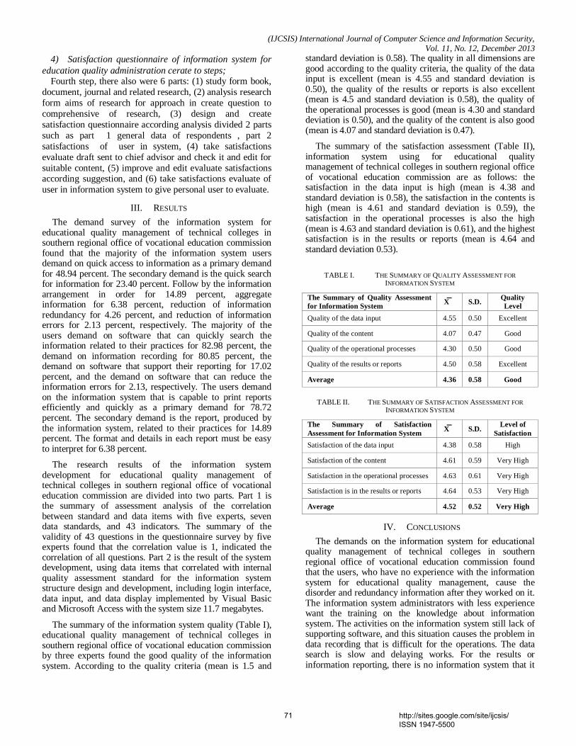
(IJCSIS) International Journal of Computer Science and Information Security, Vol. 11, No. 12, December 2013
4) Satisfaction questionnaire of information system for
education quality administration cerate to steps; Fourth step, there also were 6 parts: (1) study form book,
document, journal and related research, (2) analysis research
form aims of research for approach in create question to
comprehensive of research, (3) design and create
satisfaction questionnaire according analysis divided 2 parts
such as part 1 general data of respondents , part 2
satisfactions of user in system, (4) take satisfactions
evaluate draft sent to chief advisor and check it and edit for
suitable content, (5) improve and edit evaluate satisfactions according suggestion, and (6) take satisfactions evaluate of
user in information system to give personal user to evaluate.
III. RESULTS
The demand survey of the information system for educational quality management of technical colleges in southern regional office of vocational education commission found that the majority of the information system users demand on quick access to information as a primary demand for 48.94 percent. The secondary demand is the quick search for information for 23.40 percent. Follow by the information arrangement in order for 14.89 percent, aggregate information for 6.38 percent, reduction of information redundancy for 4.26 percent, and reduction of information errors for 2.13 percent, respectively. The majority of the users demand on software that can quickly search the information related to their practices for 82.98 percent, the demand on information recording for 80.85 percent, the demand on software that support their reporting for 17.02 percent, and the demand on software that can reduce the information errors for 2.13, respectively. The users demand on the information system that is capable to print reports efficiently and quickly as a primary demand for 78.72 percent. The secondary demand is the report, produced by the information system, related to their practices for 14.89 percent. The format and details in each report must be easy to interpret for 6.38 percent.
The research results of the information system development for educational quality management of technical colleges in southern regional office of vocational education commission are divided into two parts. Part 1 is the summary of assessment analysis of the correlation between standard and data items with five experts, seven data standards, and 43 indicators. The summary of the validity of 43 questions in the questionnaire survey by five experts found that the correlation value is 1, indicated the correlation of all questions. Part 2 is the result of the system development, using data items that correlated with internal quality assessment standard for the information system structure design and development, including login interface, data input, and data display implemented by Visual Basic and Microsoft Access with the system size 11.7 megabytes.
The summary of the information system quality (Table I), educational quality management of technical colleges in southern regional office of vocational education commission by three experts found the good quality of the information system. According to the quality criteria (mean is 1.5 and
standard deviation is 0.58). The quality in all dimensions are good according to the quality criteria, the quality of the data input is excellent (mean is 4.55 and standard deviation is 0.50), the quality of the results or reports is also excellent (mean is 4.5 and standard deviation is 0.58), the quality of the operational processes is good (mean is 4.30 and standard deviation is 0.50), and the quality of the content is also good (mean is 4.07 and standard deviation is 0.47).
The summary of the satisfaction assessment (Table II), information system using for educational quality management of technical colleges in southern regional office of vocational education commission are as follows: the satisfaction in the data input is high (mean is 4.38 and standard deviation is 0.58), the satisfaction in the contents is high (mean is 4.61 and standard deviation is 0.59), the satisfaction in the operational processes is also the high (mean is 4.63 and standard deviation is 0.61), and the highest satisfaction is in the results or reports (mean is 4.64 and standard deviation 0.53).
TABLE I. THE SUMMARY OF QUALITY ASSESSMENT FOR
INFORMATION SYSTEM
The Summary of Quality Assessment
for Information System X S.D.
Quality
Level
Quality of the data input 4.55 0.50 Excellent
Quality of the content 4.07 0.47 Good
Quality of the operational processes 4.30 0.50 Good
Quality of the results or reports 4.50 0.58 Excellent
Average 4.36 0.58 Good
TABLE II. THE SUMMARY OF SATISFACTION ASSESSMENT FOR
INFORMATION SYSTEM
The Summary of Satisfaction
Assessment for Information System X S.D.
Level of
Satisfaction
Satisfaction of the data input 4.38 0.58 High
Satisfaction of the content 4.61 0.59 Very High
Satisfaction in the operational processes 4.63 0.61 Very High
Satisfaction is in the results or reports 4.64 0.53 Very High
Average 4.52 0.52 Very High
IV. CONCLUSIONS
The demands on the information system for educational quality management of technical colleges in southern regional office of vocational education commission found that the users, who have no experience with the information system for educational quality management, cause the disorder and redundancy information after they worked on it. The information system administrators with less experience want the training on the knowledge about information system. The activities on the information system still lack of supporting software, and this situation causes the problem in data recording that is difficult for the operations. The data search is slow and delaying works. For the results or information reporting, there is no information system that it
71 http://sites.google.com/site/ijcsis/ ISSN 1947-5500
(IJCSIS) International Journal of Computer Science and Information Security, Vol. 11, No. 12, December 2013
can print out to quickly and approved for users’ demand. The college that has complete, efficient, and up-to-date information system to serve the demands can improve the quality of that college efficiently. This development is based on the principles, evidences, and facts that can be proved by the scientific analyses and assessments, logics and causality because the information is required in planning and decision-making that leads to the development of concepts and alternative ways of operation [4].
The development of the information system for educational quality management of technical colleges in southern regional office of vocational education commission found that the correlation can be differentiated into seven dimensions as follows: learners and technical graduates, curriculum and study planning, learner development activities, professional services for publics, research & development, leadership and management, and the standard for the internal quality assurance. Generally, data items are correlated with the standard and the indicators in the internal educational quality assessment.
The information system users’ satisfaction assessment for educational quality management of technical colleges in southern regional office of vocational education commission found that the highest satisfaction of the users is in the results or reports from the information system, high satisfaction in operational processes, contents, and data input.
The suggestions in this study consisted of the following items: Firstly, this study should have a management of information system, quality of education available online, not limited to only one computer at any computer to find information, and access data, anytime, anywhere; and Finally, database and information system of the college should be simple and easy to use, and actions required achieving the goals effectively and efficiently. Responsible officers should be maintaining the database and information system to effective and up date.
V. SUGGESTIONS FOR FURTHER RESEARCH
Further work should be study the behavior of information systems personnel to use information system of the educational quality management of technical colleges in southern regional office of vocational education commission. The research with a similar format should be developing databases on information, report information, and software packages to more easily, such as MySQL database program or on-line system.
ACKNOWLEDGMENT
B. Jantawan would like to express thanks Dr. Cheng-Fa Tsai, professor of the Management Information Systems Department, the Department of Tropical Agriculture and International Cooperation, National Pingtung University of Science and Technology in Taiwan for supporting the outstanding scholarship, and highly appreciates to the Technical College in Southern Thailand for giving the information.
REFERENCES
[1] Office of the National Education Commission. (n.d.). National Education Act of B.E. 2542 (1999). Retrieved November 26, 2011,
from http://www.onec.go.th/Act/5/english/act27.pdf
[2] Vocational Education Act, 2008, Retrieved November 30, 2011, from http://www.ratchakitcha.soc.go.th/DATA/PDF
/2551/A/043/1.PDF
[3] Pinthong, C., 2010, Internal quality assurance standards for the College, and Community Colleges, Department typography Min Buri
School.
[4] Boonreang, K., 1999, Statistical research1, Print No. 7, Bangkok: P.N, printing.
72 http://sites.google.com/site/ijcsis/ ISSN 1947-5500
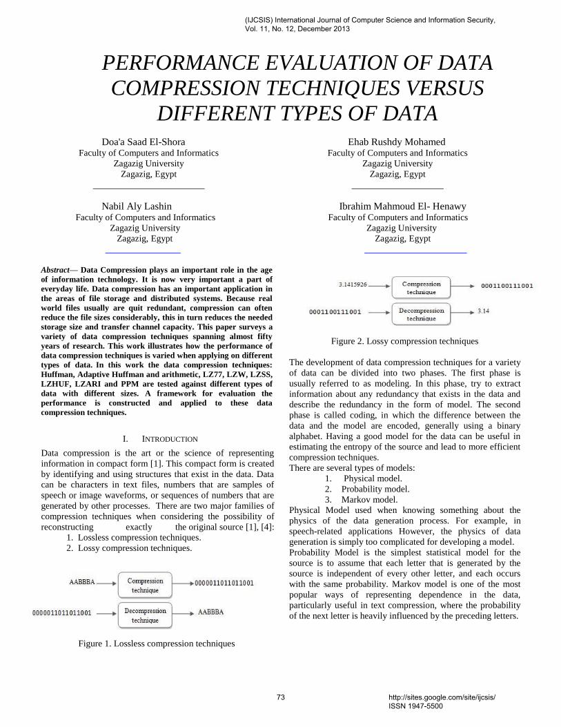
PERFORMANCE EVALUATION OF DATA
COMPRESSION TECHNIQUES VERSUS
DIFFERENT TYPES OF DATA
Doa'a Saad El-Shora
Faculty of Computers and Informatics
Zagazig University
Zagazig, Egypt
Nabil Aly Lashin
Ehab Rushdy Mohamed
Faculty of Computers and Informatics
Zagazig University
Zagazig, Egypt
Ibrahim Mahmoud El- Henawy Faculty of Computers and Informatics Faculty of Computers and Informatics
Zagazig University Zagazig University
Zagazig, Egypt Zagazig, Egypt
Abstract— Data Compression plays an important role in the age
of information technology. It is now very important a part of
everyday life. Data compression has an important application in
the areas of file storage and distributed systems. Because real
world files usually are quit redundant, compression can often
reduce the file sizes considerably, this in turn reduces the needed
storage size and transfer channel capacity. This paper surveys a
variety of data compression techniques spanning almost fifty
years of research. This work illustrates how the performance of
data compression techniques is varied when applying on different
types of data. In this work the data compression techniques:
Huffman, Adaptive Huffman and arithmetic, LZ77, LZW, LZSS,
LZHUF, LZARI and PPM are tested against different types of
data with different sizes. A framework for evaluation the
performance is constructed and applied to these data
compression techniques.
I. INTRODUCTION
Data compression is the art or the science of representing
information in compact form [1]. This compact form is created
by identifying and using structures that exist in the data. Data
can be characters in text files, numbers that are samples of
speech or image waveforms, or sequences of numbers that are
generated by other processes. There are two major families of
compression techniques when considering the possibility of
reconstructing exactly the original source [1], [4]:
1. Lossless compression techniques.
2. Lossy compression techniques.
Figure 1. Lossless compression techniques
Figure 2. Lossy compression techniques
The development of data compression techniques for a variety
of data can be divided into two phases. The first phase is
usually referred to as modeling. In this phase, try to extract
information about any redundancy that exists in the data and
describe the redundancy in the form of model. The second
phase is called coding, in which the difference between the
data and the model are encoded, generally using a binary
alphabet. Having a good model for the data can be useful in
estimating the entropy of the source and lead to more efficient
compression techniques.
There are several types of models:
1. Physical model.
2. Probability model.
3. Markov model.
Physical Model used when knowing something about the
physics of the data generation process. For example, in
speech-related applications However, the physics of data
generation is simply too complicated for developing a model.
Probability Model is the simplest statistical model for the
source is to assume that each letter that is generated by the
source is independent of every other letter, and each occurs
with the same probability. Markov model is one of the most
popular ways of representing dependence in the data,
particularly useful in text compression, where the probability
of the next letter is heavily influenced by the preceding letters.
(IJCSIS) International Journal of Computer Science and Information Security, Vol. 11, No. 12, December 2013
73 http://sites.google.com/site/ijcsis/ ISSN 1947-5500
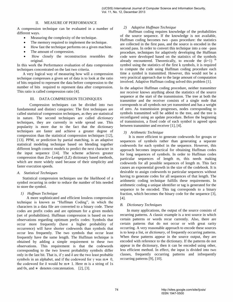
II. MEASURE OF PERFORMANCE
A compression technique can be evaluated in a number of
different ways.
Measuring the complexity of the technique.
The memory required to implement the technique.
How fast the technique performs on a given machine.
The amount of compression.
How closely the reconstruction resembles the
original.
In this work the Performance evaluation of data compression
techniques concentrated on the last two criteria.
A very logical way of measuring how will a compression
technique compresses a given set of data is to look at the ratio
of bits required to represent the data before compression to the
number of bits required to represent data after compression.
This ratio is called compression ratio [4].
III. DATA COMPRESSION TECHNIQUES
Compression techniques can be divided into two
fundamental and distinct categories: The first techniques are
called statistical compression techniques, as they are statistical
in nature. The second techniques are called dictionary
techniques, they are currently in wide spread use. This
popularity is more due to the fact that the dictionary
techniques are faster and achieve a greater degree of
compression than the statistical compression techniques [12],
[13]. PPM, or prediction by partial matching, is an adaptive
statistical modeling technique based on blending together
different length context models to predict the next character in
the input sequence [14]. The scheme achieves greater
compression than Ziv-Lempel (LZ) dictionary based methods,
which are more widely used because of their simplicity and
faster execution speeds.
A. Statistical Techniques
Statistical compression techniques use the likelihood of a symbol recurring in order to reduce the number of bits needed to store the symbol.
1) Huffman Technique
A more sophisticated and efficient lossless compression
technique is known as “Huffman Coding”, in which the
characters in a data file are converted to a binary code. These
codes are prefix codes and are optimum for a given models
(set of probabilities). Huffman compression is based on two
observations regarding optimum prefix codes: Symbols that
occur more frequently (have a higher probability of
occurrence) will have shorter codewords than symbols that
occur less frequently. The two symbols that occur least
frequently have the same length. The Huffman technique is
obtained by adding a simple requirement to these two
observations. This requirement is that the codewords
corresponding to the two lowest probability symbols differ
only in the last bit. That is, if γ and δ are the two least probable
symbols in an alphabet, and if the codeword for γ was m 0,
the codeword for δ would be m 1. Here m is a string of 1s
and 0s, and denotes concatenation. [2], [3].
2) Adaptive Huffman Technique Huffman coding requires knowledge of the probabilities of the source sequence. If the knowledge is not available, Huffman coding becomes two –pass procedure: the statistics are collected in the first pass, and the source is encoded in the second pass. In order to convert this technique into a one –pass procedure, techniques for adaptively developing the Huffman code were developed based on the statistics of the symbols already encountered. Theoretically, to encode the (k+1)
th
symbol using the statistics of the first k symbols, it is required to compute the code using Huffman coding procedure each time a symbol is transmitted. However, this would not be a very practical approach due to the large amount of computation involved. Adaptive Huffman coding solved this problem [1].
In the adaptive Huffman coding procedure, neither transmitter nor receiver knows anything about the statistics of the source sequence at the start of the transmission. The tree at both the transmitter and the receiver consists of a single node that corresponds to all symbols not yet transmitted and has a weight of zero. As transmission progresses, nodes corresponding to symbols transmitted will be added to the tree, and the tree is reconfigured using an update procedure. Before the beginning of transmission, a fixed code of each symbol is agreed upon between transmitter and receiver [1], [4].
3) Arithmetic Technique
It is more efficient to generate codewords for groups or
sequences of symbols rather than generating a separate
codewords for each symbol in the sequence. However, this
approach becomes impractical for obtaining Huffman codes
for long sequences of symbols. In order to Huffman codes
particular sequences of length m, this needs making
codewords for all possible sequences of length m. This fact
causes an exponential growth in the size of the codebook. It is
desirable to assign codewords to particular sequences without
having to generate codes for all sequences of that length. The
arithmetic coding technique fulfills these requirements. In
arithmetic coding a unique identifier or tag is generated for the
sequence to be encoded. This tag corresponds to a binary
fraction, which becomes the binary code for the sequence [3],
[4].
B. Dictionary Techniques
In many applications, the output of the source consists of
recurring patterns. A classic example is a text source in which
certain patterns or words recur currently. Also, there are
certain patterns that do not occur or with great rarity
occurring. A very reasonable approach to encode these sources
is to keep a list, or dictionary, of frequently occurring patterns.
When these patterns appear in the source output, they are
encoded with reference to the dictionary. If the patterns do not
appear in the dictionary, then it can be encoded using other,
less efficient method. In effect, the input is divided into two
classes, frequently occurring patterns and infrequently
occurring patterns [9], [10].
(IJCSIS) International Journal of Computer Science and Information Security, Vol. 11, No. 12, December 2013
74 http://sites.google.com/site/ijcsis/ ISSN 1947-5500
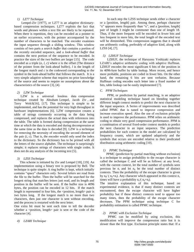
1) LZ77 Technique
Lempel-Ziv [1977], or LZ77 is an adaptive dictionary-
based compression techniques. LZ77 exploits the fact that
words and phrases within a text file are likely to be repeated.
When there is repetition, they can be encoded as a pointer to
an earlier occurrence, with the pointer accompanied by the
number of characters to be matched. The encoder examines
the input sequence through a sliding window. This window
consists of two parts a search buffer that contains a portion of
the recently encoded sequence, and a look-ahead buffer that
contains the next portion of the sequence to be encoded. In
practice the sizes of the two buffers are larger [15]. The code
encoded as a triple (o, l, c) where o is the offset (The distance
of the pointer from the look-ahead buffer), l is the length of
the longest match and c is the codeword corresponding to the
symbol in the look-ahead buffer that follows the match. It is a
very simple adaptive scheme that requires no prior knowledge
of the source and seems to require no assumptions about the
characteristics of the source [3], [4].
2) LZW Technique
LZW is a universal lossless data compression
technique created by Abraham Lempel, Jacob Ziv , and
Terry Welch[16], [17]. This technique is simple to be
implemented, and has the potential for very high throughput in
hardware implementations [6]. LZW compression creates a
table of strings commonly occurring in the data being
compressed, and replaces the actual data with references into
the table. The table is formed during compression at the same
time at which the data is encoded and during decompression at
the same time as the data is decoded [9]. LZW is a technique
for removing the necessity of encoding the second element of
the pair (i, c). That is, the encoder would only send the index
to the dictionary. So the dictionary has to be primed with all
the letters of the source alphabet. The technique is surprisingly
simple; it replaces strings of characters with single codes. It
does not do any analysis of the incoming text [5].
3) LZSS Technique
This scheme is initiated by Ziv and Lempel [18], [19]. An
implementation using a binary tree is proposed by Bell. The
technique is quite simple: A ring buffer is kept, which initially
contains “space” characters only. Several letters are read from
the file to the buffer. Then the buffer will be searched for the
longest string that matches letters just read, and its length and
position in the buffer will be sent. If the buffer size is 4096
bytes, the position can be encoded in 12 bits. If the match
length is represented in four bits, the <position, length> pair is
two bytes long. If the longest match is no more than two
characters, then just one character is sent without encoding,
and the process is restarted with the next letter.
One extra bit must be sent each time to tell the decoder
whether a <position, length> pair is sent or the code of the
character [4].
4) LZARI Technique
In each step the LZSS technique sends either a character
or a [position, length] pair. Among these, perhaps character
“e” appears more frequently than “x”, and a [position, length]
pair of length 3 might be commoner than one of length 18.
Thus, if the more frequent will be encoded in fewer bits and
less frequent in more bits, the total length of the encoded text
will be diminished. This compression suggests that it should
use arithmetic coding, preferably of adaptive kind, along with
LZSS [4], [7].
5) LZHUF Technique
LZHUF, the technique of Haruyasu Yoshizaki replaces
LZARI’s adaptive arithmetic coding with adaptive Huffman.
LZHUF encodes the most significant 6 bits of the position in
its 4096-byte buffer by table lookup. More recent, and hence
more probable, positions are coded in fewer bits. On the other
hand, the remaining 6 bits are sent verbatim. Because
Huffman coding encodes each letter into a fixed number of
bits, table lookup can be easily implemented [7].
C. PPM Techniques
PPM, or prediction by partial matching, is an adaptive
statistical modeling technique based on blending together
different length context models to predict the next character in
the input sequence. A Series of improvements was described
called PPMC that is tuned to improve compression and
increase execution speed. Also the use of exclusion principle
is used to improve the performance. PPM relies on arithmetic
coding to obtain very good compression performance. PPM is
a combination of several fixed-order context models to predict
the next character in an input sequence. The prediction
probabilities for each context in the model are calculated by
frequency counts, which are updated adaptively and the
symbols that occurs are encoded relative to their predicated
distribution using arithmetic coding [10].
1) PPMC Technique
PPMC (prediction by partial matching without exclusion)
is a technique to assign probability to the escape character is
called the technique C and will be as follows: at any level,
with the current context, let the total number of symbols seen
previous be nt and let nd be the total number of distinct
contexts. Then the probability of the escape character is given
by nd/ ( nd+nt). Any character which appeared in this context nc
times will have a probability nc/( nd+nt).
The intuitive explanation of this technique, based on
experimental evidence, is that if many distinct contexts are
encountered, then the escape character will have higher
probability but if these distinct contexts tend to appear too
many times, then the probability of the escape character
decreases. The PPM technique using technique C for
probability estimation is called PPMC technique.
2) PPMC with Exclusion Technique
PPMC can be modified by using exclusion, this
modification will improve the compression ratio but it is
slower than the first type. Exclusion principle states that: If a
(IJCSIS) International Journal of Computer Science and Information Security, Vol. 11, No. 12, December 2013
75 http://sites.google.com/site/ijcsis/ ISSN 1947-5500
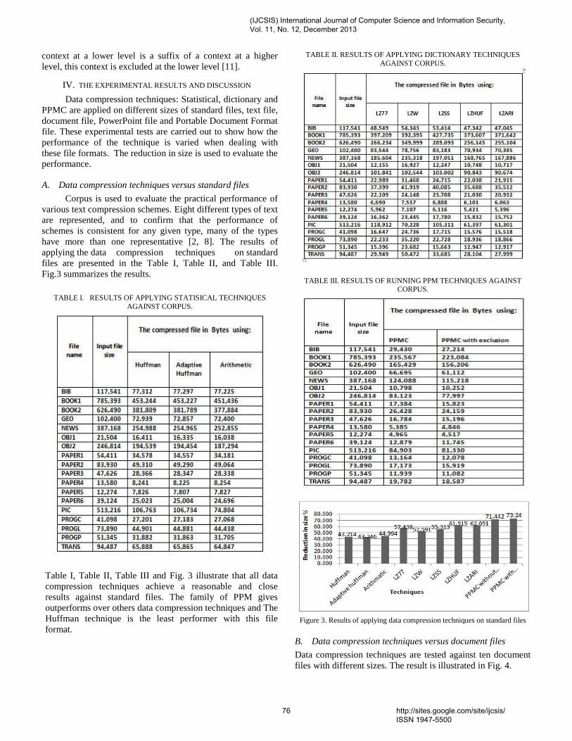
context at a lower level is a suffix of a context at a higher
level, this context is excluded at the lower level [11].
IV. THE EXPERIMENTAL RESULTS AND DISCUSSION
Data compression techniques: Statistical, dictionary and
PPMC are applied on different sizes of standard files, text file,
document file, PowerPoint file and Portable Document Format
file. These experimental tests are carried out to show how the
performance of the technique is varied when dealing with
these file formats. The reduction in size is used to evaluate the
performance.
A. Data compression techniques versus standard files
Corpus is used to evaluate the practical performance of
various text compression schemes. Eight different types of text
are represented, and to confirm that the performance of
schemes is consistent for any given type, many of the types
have more than one representative [2, 8]. The results of
applying the data compression techniques on standard
files are presented in the Table I, Table II, and Table III.
Fig.3 summarizes the results.
TABLE I. RESULTS OF APPLYING STATISICAL TECHNIQUES
AGAINST CORPUS.
Table I, Table II, Table III and Fig. 3 illustrate that all data
compression techniques achieve a reasonable and close
results against standard files. The family of PPM gives
outperforms over others data compression techniques and The
Huffman technique is the least performer with this file
format.
TABLE II. RESULTS OF APPLYING DICTIONARY TECHNIQUES
AGAINST CORPUS.
TABLE III. RESULTS OF RUNNING PPM TECHNIQUES AGAINST CORPUS.
Figure 3. Results of applying data compression techniques on standard files
B. Data compression techniques versus document files
Data compression techniques are tested against ten document
files with different sizes. The result is illustrated in Fig. 4.
(IJCSIS) International Journal of Computer Science and Information Security, Vol. 11, No. 12, December 2013
76 http://sites.google.com/site/ijcsis/ ISSN 1947-5500
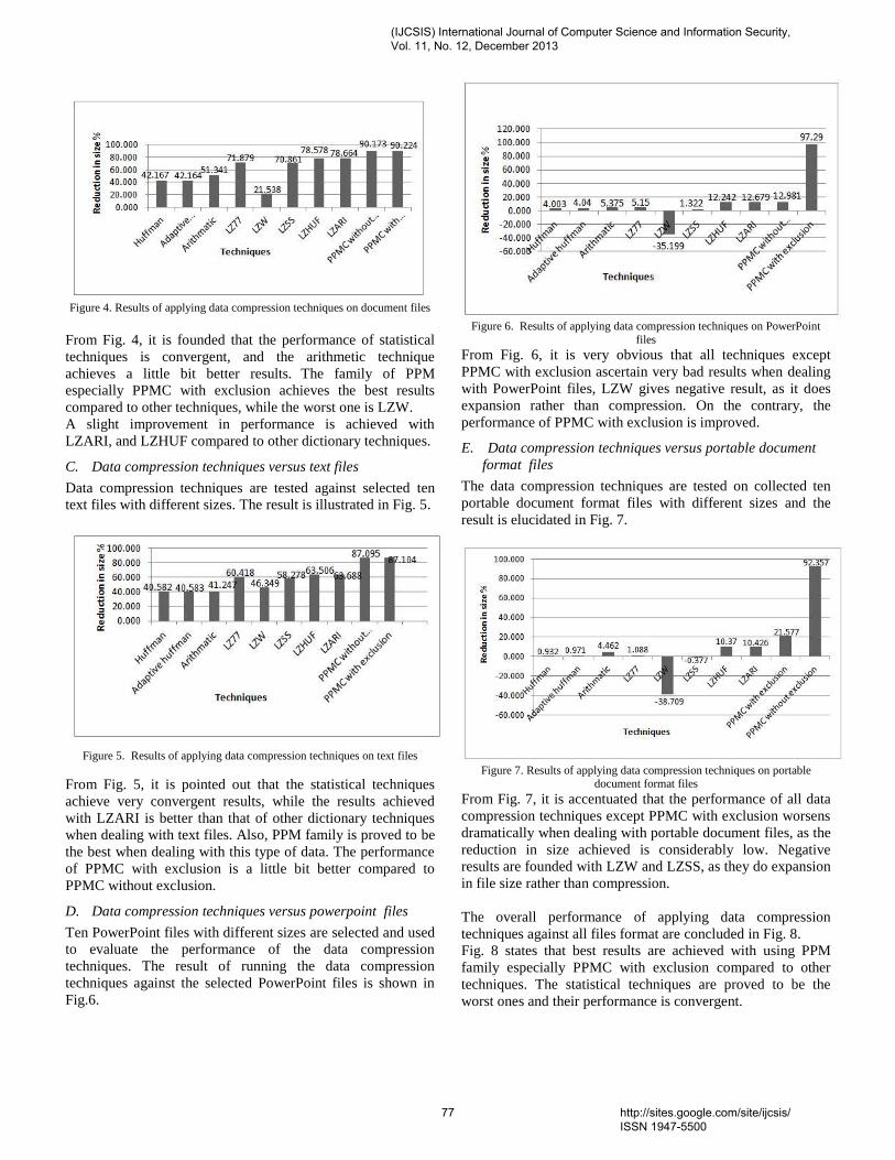
Figure 4. Results of applying data compression techniques on document files
From Fig. 4, it is founded that the performance of statistical
techniques is convergent, and the arithmetic technique
achieves a little bit better results. The family of PPM
especially PPMC with exclusion achieves the best results
compared to other techniques, while the worst one is LZW.
A slight improvement in performance is achieved with
LZARI, and LZHUF compared to other dictionary techniques.
C. Data compression techniques versus text files
Data compression techniques are tested against selected ten
text files with different sizes. The result is illustrated in Fig. 5.
Figure 5. Results of applying data compression techniques on text files
From Fig. 5, it is pointed out that the statistical techniques
achieve very convergent results, while the results achieved
with LZARI is better than that of other dictionary techniques
when dealing with text files. Also, PPM family is proved to be
the best when dealing with this type of data. The performance
of PPMC with exclusion is a little bit better compared to
PPMC without exclusion.
D. Data compression techniques versus powerpoint files
Ten PowerPoint files with different sizes are selected and used
to evaluate the performance of the data compression
techniques. The result of running the data compression
techniques against the selected PowerPoint files is shown in
Fig.6.
Figure 6. Results of applying data compression techniques on PowerPoint
files
From Fig. 6, it is very obvious that all techniques except
PPMC with exclusion ascertain very bad results when dealing
with PowerPoint files, LZW gives negative result, as it does
expansion rather than compression. On the contrary, the
performance of PPMC with exclusion is improved.
E. Data compression techniques versus portable document
format files
The data compression techniques are tested on collected ten
portable document format files with different sizes and the
result is elucidated in Fig. 7.
Figure 7. Results of applying data compression techniques on portable
document format files
From Fig. 7, it is accentuated that the performance of all data
compression techniques except PPMC with exclusion worsens
dramatically when dealing with portable document files, as the
reduction in size achieved is considerably low. Negative
results are founded with LZW and LZSS, as they do expansion
in file size rather than compression.
The overall performance of applying data compression
techniques against all files format are concluded in Fig. 8.
Fig. 8 states that best results are achieved with using PPM
family especially PPMC with exclusion compared to other
techniques. The statistical techniques are proved to be the
worst ones and their performance is convergent.
(IJCSIS) International Journal of Computer Science and Information Security, Vol. 11, No. 12, December 2013
77 http://sites.google.com/site/ijcsis/ ISSN 1947-5500
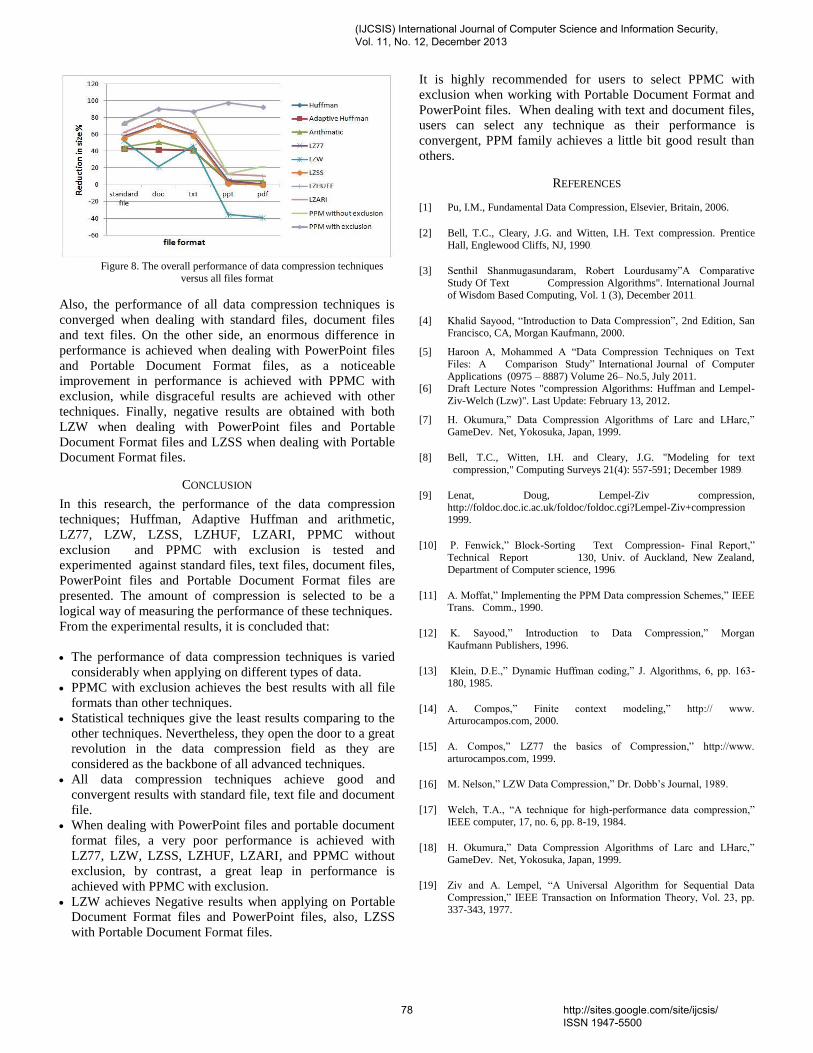
Figure 8. The overall performance of data compression techniques
versus all files format
Also, the performance of all data compression techniques is
converged when dealing with standard files, document files
and text files. On the other side, an enormous difference in
performance is achieved when dealing with PowerPoint files
and Portable Document Format files, as a noticeable
improvement in performance is achieved with PPMC with
exclusion, while disgraceful results are achieved with other
techniques. Finally, negative results are obtained with both
LZW when dealing with PowerPoint files and Portable
Document Format files and LZSS when dealing with Portable
Document Format files.
CONCLUSION
In this research, the performance of the data compression
techniques; Huffman, Adaptive Huffman and arithmetic,
LZ77, LZW, LZSS, LZHUF, LZARI, PPMC without
exclusion and PPMC with exclusion is tested and
experimented against standard files, text files, document files,
PowerPoint files and Portable Document Format files are
presented. The amount of compression is selected to be a
logical way of measuring the performance of these techniques.
From the experimental results, it is concluded that:
The performance of data compression techniques is varied
considerably when applying on different types of data.
PPMC with exclusion achieves the best results with all file
formats than other techniques.
Statistical techniques give the least results comparing to the
other techniques. Nevertheless, they open the door to a great
revolution in the data compression field as they are
considered as the backbone of all advanced techniques. All data compression techniques achieve good and
convergent results with standard file, text file and document
file.
When dealing with PowerPoint files and portable document
format files, a very poor performance is achieved with
LZ77, LZW, LZSS, LZHUF, LZARI, and PPMC without
exclusion, by contrast, a great leap in performance is
achieved with PPMC with exclusion.
LZW achieves Negative results when applying on Portable
Document Format files and PowerPoint files, also, LZSS
with Portable Document Format files.
It is highly recommended for users to select PPMC with
exclusion when working with Portable Document Format and
PowerPoint files. When dealing with text and document files,
users can select any technique as their performance is
convergent, PPM family achieves a little bit good result than
others.
REFERENCES
[1] Pu, I.M., Fundamental Data Compression, Elsevier, Britain, 2006.
[2] Bell, T.C., Cleary, J.G. and Witten, I.H. Text compression. Prentice Hall, Englewood Cliffs, NJ, 1990.
[3] Senthil Shanmugasundaram, Robert Lourdusamy”A Comparative
Study Of Text Compression Algorithms". International Journal of Wisdom Based Computing, Vol. 1 (3), December 2011.
[4] Khalid Sayood, “Introduction to Data Compression”, 2nd Edition, San
Francisco, CA, Morgan Kaufmann, 2000.
[5] Haroon A, Mohammed A “Data Compression Techniques on Text
Files: A Comparison Study” International Journal of Computer
Applications (0975 – 8887) Volume 26– No.5, July 2011. [6] Draft Lecture Notes "compression Algorithms: Huffman and Lempel-
Ziv-Welch (Lzw)". Last Update: February 13, 2012.
[7] H. Okumura,” Data Compression Algorithms of Larc and LHarc,” GameDev. Net, Yokosuka, Japan, 1999.
[8] Bell, T.C., Witten, I.H. and Cleary, J.G. "Modeling for text
compression," Computing Surveys 21(4): 557-591; December 1989.
[9] Lenat, Doug, Lempel-Ziv compression, http://foldoc.doc.ic.ac.uk/foldoc/foldoc.cgi?Lempel-Ziv+compression
1999.
[10] P. Fenwick,” Block-Sorting Text Compression- Final Report,”
Technical Report 130, Univ. of Auckland, New Zealand, Department of Computer science, 1996.
[11] A. Moffat,” Implementing the PPM Data compression Schemes,” IEEE Trans. Comm., 1990.
[12] K. Sayood,” Introduction to Data Compression,” Morgan
Kaufmann Publishers, 1996.
[13] Klein, D.E.,” Dynamic Huffman coding,” J. Algorithms, 6, pp. 163-180, 1985.
[14] A. Compos,” Finite context modeling,” http:// www. Arturocampos.com, 2000.
[15] A. Compos,” LZ77 the basics of Compression,” http://www.
arturocampos.com, 1999.
[16] M. Nelson,” LZW Data Compression,” Dr. Dobb’s Journal, 1989.
[17] Welch, T.A., “A technique for high-performance data compression,” IEEE computer, 17, no. 6, pp. 8-19, 1984.
[18] H. Okumura,” Data Compression Algorithms of Larc and LHarc,” GameDev. Net, Yokosuka, Japan, 1999.
[19] Ziv and A. Lempel, “A Universal Algorithm for Sequential Data
Compression,” IEEE Transaction on Information Theory, Vol. 23, pp. 337-343, 1977.
(IJCSIS) International Journal of Computer Science and Information Security, Vol. 11, No. 12, December 2013
78 http://sites.google.com/site/ijcsis/ ISSN 1947-5500

(IJCSIS) International Journal of Computer Science and Information Security, Vol. 11 No. 12, December 2013
IJCSIS AUTHORS’ & REVIEWERS’ LIST Assist Prof (Dr.) M. Emre Celebi, Louisiana State University in Shreveport, USA
Dr. Lam Hong Lee, Universiti Tunku Abdul Rahman, Malaysia
Dr. Shimon K. Modi, Director of Research BSPA Labs, Purdue University, USA
Dr. Jianguo Ding, Norwegian University of Science and Technology (NTNU), Norway
Assoc. Prof. N. Jaisankar, VIT University, Vellore,Tamilnadu, India
Dr. Amogh Kavimandan, The Mathworks Inc., USA
Dr. Ramasamy Mariappan, Vinayaka Missions University, India
Dr. Yong Li, School of Electronic and Information Engineering, Beijing Jiaotong University, P.R. China
Assist. Prof. Sugam Sharma, NIET, India / Iowa State University, USA
Dr. Jorge A. Ruiz-Vanoye, Universidad Autónoma del Estado de Morelos, Mexico
Dr. Neeraj Kumar, SMVD University, Katra (J&K), India
Dr Genge Bela, "Petru Maior" University of Targu Mures, Romania
Dr. Junjie Peng, Shanghai University, P. R. China
Dr. Ilhem LENGLIZ, HANA Group - CRISTAL Laboratory, Tunisia
Prof. Dr. Durgesh Kumar Mishra, Acropolis Institute of Technology and Research, Indore, MP, India
Jorge L. Hernández-Ardieta, University Carlos III of Madrid, Spain
Prof. Dr.C.Suresh Gnana Dhas, Anna University, India
Mrs Li Fang, Nanyang Technological University, Singapore
Prof. Pijush Biswas, RCC Institute of Information Technology, India
Dr. Siddhivinayak Kulkarni, University of Ballarat, Ballarat, Victoria, Australia
Dr. A. Arul Lawrence, Royal College of Engineering & Technology, India
Mr. Wongyos Keardsri, Chulalongkorn University, Bangkok, Thailand
Mr. Somesh Kumar Dewangan, CSVTU Bhilai (C.G.)/ Dimat Raipur, India
Mr. Hayder N. Jasem, University Putra Malaysia, Malaysia
Mr. A.V.Senthil Kumar, C. M. S. College of Science and Commerce, India
Mr. R. S. Karthik, C. M. S. College of Science and Commerce, India
Mr. P. Vasant, University Technology Petronas, Malaysia
Mr. Wong Kok Seng, Soongsil University, Seoul, South Korea
Mr. Praveen Ranjan Srivastava, BITS PILANI, India
Mr. Kong Sang Kelvin, Leong, The Hong Kong Polytechnic University, Hong Kong
Mr. Mohd Nazri Ismail, Universiti Kuala Lumpur, Malaysia
Dr. Rami J. Matarneh, Al-isra Private University, Amman, Jordan
Dr Ojesanmi Olusegun Ayodeji, Ajayi Crowther University, Oyo, Nigeria
Dr. Riktesh Srivastava, Skyline University, UAE
Dr. Oras F. Baker, UCSI University - Kuala Lumpur, Malaysia
Dr. Ahmed S. Ghiduk, Faculty of Science, Beni-Suef University, Egypt
and Department of Computer science, Taif University, Saudi Arabia
Mr. Tirthankar Gayen, IIT Kharagpur, India
Ms. Huei-Ru Tseng, National Chiao Tung University, Taiwan
(IJCSIS) International Journal of Computer Science and Information Security, Vol. 11 No. 12, December 2013
Prof. Ning Xu, Wuhan University of Technology, China
Mr Mohammed Salem Binwahlan, Hadhramout University of Science and Technology, Yemen
& Universiti Teknologi Malaysia, Malaysia.
Dr. Aruna Ranganath, Bhoj Reddy Engineering College for Women, India
Mr. Hafeezullah Amin, Institute of Information Technology, KUST, Kohat, Pakistan
Prof. Syed S. Rizvi, University of Bridgeport, USA
Mr. Shahbaz Pervez Chattha, University of Engineering and Technology Taxila, Pakistan
Dr. Shishir Kumar, Jaypee University of Information Technology, Wakanaghat (HP), India
Mr. Shahid Mumtaz, Portugal Telecommunication, Instituto de Telecomunicações (IT) , Aveiro, Portugal
Mr. Rajesh K Shukla, Corporate Institute of Science & Technology Bhopal M P
Dr. Poonam Garg, Institute of Management Technology, India
Mr. S. Mehta, Inha University, Korea
Mr. Dilip Kumar S.M, University Visvesvaraya College of Engineering (UVCE), Bangalore University,
Bangalore
Prof. Malik Sikander Hayat Khiyal, Fatima Jinnah Women University, Rawalpindi, Pakistan
Dr. Virendra Gomase , Department of Bioinformatics, Padmashree Dr. D.Y. Patil University
Dr. Irraivan Elamvazuthi, University Technology PETRONAS, Malaysia
Mr. Saqib Saeed, University of Siegen, Germany
Mr. Pavan Kumar Gorakavi, IPMA-USA [YC]
Dr. Ahmed Nabih Zaki Rashed, Menoufia University, Egypt
Prof. Shishir K. Shandilya, Rukmani Devi Institute of Science & Technology, India
Mrs.J.Komala Lakshmi, SNR Sons College, Computer Science, India
Mr. Muhammad Sohail, KUST, Pakistan
Dr. Manjaiah D.H, Mangalore University, India
Dr. S Santhosh Baboo, D.G.Vaishnav College, Chennai, India
Prof. Dr. Mokhtar Beldjehem, Sainte-Anne University, Halifax, NS, Canada
Dr. Deepak Laxmi Narasimha, Faculty of Computer Science and Information Technology, University of
Malaya, Malaysia
Prof. Dr. Arunkumar Thangavelu, Vellore Institute Of Technology, India
Mr. M. Azath, Anna University, India
Mr. Md. Rabiul Islam, Rajshahi University of Engineering & Technology (RUET), Bangladesh
Mr. Aos Alaa Zaidan Ansaef, Multimedia University, Malaysia
Dr Suresh Jain, Professor (on leave), Institute of Engineering & Technology, Devi Ahilya University, Indore
(MP) India,
Dr. Mohammed M. Kadhum, Universiti Utara Malaysia
Mr. Hanumanthappa. J. University of Mysore, India
Mr. Syed Ishtiaque Ahmed, Bangladesh University of Engineering and Technology (BUET)
Mr Akinola Solomon Olalekan, University of Ibadan, Ibadan, Nigeria
Mr. Santosh K. Pandey, Department of Information Technology, The Institute of Chartered Accountants of
India
Dr. P. Vasant, Power Control Optimization, Malaysia
Dr. Petr Ivankov, Automatika - S, Russian Federation
(IJCSIS) International Journal of Computer Science and Information Security, Vol. 11 No. 12, December 2013
Dr. Utkarsh Seetha, Data Infosys Limited, India
Mrs. Priti Maheshwary, Maulana Azad National Institute of Technology, Bhopal
Dr. (Mrs) Padmavathi Ganapathi, Avinashilingam University for Women, Coimbatore
Assist. Prof. A. Neela madheswari, Anna university, India
Prof. Ganesan Ramachandra Rao, PSG College of Arts and Science, India
Mr. Kamanashis Biswas, Daffodil International University, Bangladesh
Dr. Atul Gonsai, Saurashtra University, Gujarat, India
Mr. Angkoon Phinyomark, Prince of Songkla University, Thailand
Mrs. G. Nalini Priya, Anna University, Chennai
Dr. P. Subashini, Avinashilingam University for Women, India
Assoc. Prof. Vijay Kumar Chakka, Dhirubhai Ambani IICT, Gandhinagar ,Gujarat
Mr Jitendra Agrawal, : Rajiv Gandhi Proudyogiki Vishwavidyalaya, Bhopal
Mr. Vishal Goyal, Department of Computer Science, Punjabi University, India
Dr. R. Baskaran, Department of Computer Science and Engineering, Anna University, Chennai
Assist. Prof, Kanwalvir Singh Dhindsa, B.B.S.B.Engg.College, Fatehgarh Sahib (Punjab), India
Dr. Jamal Ahmad Dargham, School of Engineering and Information Technology, Universiti Malaysia Sabah
Mr. Nitin Bhatia, DAV College, India
Dr. Dhavachelvan Ponnurangam, Pondicherry Central University, India
Dr. Mohd Faizal Abdollah, University of Technical Malaysia, Malaysia
Assist. Prof. Sonal Chawla, Panjab University, India
Dr. Abdul Wahid, AKG Engg. College, Ghaziabad, India
Mr. Arash Habibi Lashkari, University of Malaya (UM), Malaysia
Mr. Md. Rajibul Islam, Ibnu Sina Institute, University Technology Malaysia
Professor Dr. Sabu M. Thampi, .B.S Institute of Technology for Women, Kerala University, India
Mr. Noor Muhammed Nayeem, Université Lumière Lyon 2, 69007 Lyon, France
Dr. Himanshu Aggarwal, Department of Computer Engineering, Punjabi University, India
Prof R. Naidoo, Dept of Mathematics/Center for Advanced Computer Modelling, Durban University of
Technology, Durban,South Africa
Prof. Mydhili K Nair, M S Ramaiah Institute of Technology(M.S.R.I.T), Affliliated to Visweswaraiah
Technological University, Bangalore, India
M. Prabu, Adhiyamaan College of Engineering/Anna University, India
Mr. Swakkhar Shatabda, Department of Computer Science and Engineering, United International University,
Bangladesh
Dr. Abdur Rashid Khan, ICIT, Gomal University, Dera Ismail Khan, Pakistan
Mr. H. Abdul Shabeer, I-Nautix Technologies,Chennai, India
Dr. M. Aramudhan, Perunthalaivar Kamarajar Institute of Engineering and Technology, India
Dr. M. P. Thapliyal, Department of Computer Science, HNB Garhwal University (Central University), India
Dr. Shahaboddin Shamshirband, Islamic Azad University, Iran
Mr. Zeashan Hameed Khan, : Université de Grenoble, France
Prof. Anil K Ahlawat, Ajay Kumar Garg Engineering College, Ghaziabad, UP Technical University, Lucknow
Mr. Longe Olumide Babatope, University Of Ibadan, Nigeria
Associate Prof. Raman Maini, University College of Engineering, Punjabi University, India

(IJCSIS) International Journal of Computer Science and Information Security, Vol. 11 No. 12, December 2013
Dr. Maslin Masrom, University Technology Malaysia, Malaysia
Sudipta Chattopadhyay, Jadavpur University, Kolkata, India
Dr. Dang Tuan NGUYEN, University of Information Technology, Vietnam National University - Ho Chi Minh
City
Dr. Mary Lourde R., BITS-PILANI Dubai , UAE
Dr. Abdul Aziz, University of Central Punjab, Pakistan
Mr. Karan Singh, Gautam Budtha University, India
Mr. Avinash Pokhriyal, Uttar Pradesh Technical University, Lucknow, India
Associate Prof Dr Zuraini Ismail, University Technology Malaysia, Malaysia
Assistant Prof. Yasser M. Alginahi, College of Computer Science and Engineering, Taibah University,
Madinah Munawwarrah, KSA
Mr. Dakshina Ranjan Kisku, West Bengal University of Technology, India
Mr. Raman Kumar, Dr B R Ambedkar National Institute of Technology, Jalandhar, Punjab, India
Associate Prof. Samir B. Patel, Institute of Technology, Nirma University, India
Dr. M.Munir Ahamed Rabbani, B. S. Abdur Rahman University, India
Asst. Prof. Koushik Majumder, West Bengal University of Technology, India
Dr. Alex Pappachen James, Queensland Micro-nanotechnology center, Griffith University, Australia
Assistant Prof. S. Hariharan, B.S. Abdur Rahman University, India
Asst Prof. Jasmine. K. S, R.V.College of Engineering, India
Mr Naushad Ali Mamode Khan, Ministry of Education and Human Resources, Mauritius
Prof. Mahesh Goyani, G H Patel Collge of Engg. & Tech, V.V.N, Anand, Gujarat, India
Dr. Mana Mohammed, University of Tlemcen, Algeria
Prof. Jatinder Singh, Universal Institutiion of Engg. & Tech. CHD, India
Mrs. M. Anandhavalli Gauthaman, Sikkim Manipal Institute of Technology, Majitar, East Sikkim
Dr. Bin Guo, Institute Telecom SudParis, France
Mrs. Maleika Mehr Nigar Mohamed Heenaye-Mamode Khan, University of Mauritius
Prof. Pijush Biswas, RCC Institute of Information Technology, India
Mr. V. Bala Dhandayuthapani, Mekelle University, Ethiopia
Dr. Irfan Syamsuddin, State Polytechnic of Ujung Pandang, Indonesia
Mr. Kavi Kumar Khedo, University of Mauritius, Mauritius
Mr. Ravi Chandiran, Zagro Singapore Pte Ltd. Singapore
Mr. Milindkumar V. Sarode, Jawaharlal Darda Institute of Engineering and Technology, India
Dr. Shamimul Qamar, KSJ Institute of Engineering & Technology, India
Dr. C. Arun, Anna University, India
Assist. Prof. M.N.Birje, Basaveshwar Engineering College, India
Prof. Hamid Reza Naji, Department of Computer Enigneering, Shahid Beheshti University, Tehran, Iran
Assist. Prof. Debasis Giri, Department of Computer Science and Engineering, Haldia Institute of Technology
Subhabrata Barman, Haldia Institute of Technology, West Bengal
Mr. M. I. Lali, COMSATS Institute of Information Technology, Islamabad, Pakistan
Dr. Feroz Khan, Central Institute of Medicinal and Aromatic Plants, Lucknow, India
Mr. R. Nagendran, Institute of Technology, Coimbatore, Tamilnadu, India
Mr. Amnach Khawne, King Mongkut’s Institute of Technology Ladkrabang, Ladkrabang, Bangkok, Thailand
(IJCSIS) International Journal of Computer Science and Information Security, Vol. 11 No. 12, December 2013
Dr. P. Chakrabarti, Sir Padampat Singhania University, Udaipur, India
Mr. Nafiz Imtiaz Bin Hamid, Islamic University of Technology (IUT), Bangladesh.
Shahab-A. Shamshirband, Islamic Azad University, Chalous, Iran
Prof. B. Priestly Shan, Anna Univeristy, Tamilnadu, India
Venkatramreddy Velma, Dept. of Bioinformatics, University of Mississippi Medical Center, Jackson MS USA
Akshi Kumar, Dept. of Computer Engineering, Delhi Technological University, India
Dr. Umesh Kumar Singh, Vikram University, Ujjain, India
Mr. Serguei A. Mokhov, Concordia University, Canada
Mr. Lai Khin Wee, Universiti Teknologi Malaysia, Malaysia
Dr. Awadhesh Kumar Sharma, Madan Mohan Malviya Engineering College, India
Mr. Syed R. Rizvi, Analytical Services & Materials, Inc., USA
Dr. S. Karthik, SNS Collegeof Technology, India
Mr. Syed Qasim Bukhari, CIMET (Universidad de Granada), Spain
Mr. A.D.Potgantwar, Pune University, India
Dr. Himanshu Aggarwal, Punjabi University, India
Mr. Rajesh Ramachandran, Naipunya Institute of Management and Information Technology, India
Dr. K.L. Shunmuganathan, R.M.K Engg College , Kavaraipettai ,Chennai
Dr. Prasant Kumar Pattnaik, KIST, India.
Dr. Ch. Aswani Kumar, VIT University, India
Mr. Ijaz Ali Shoukat, King Saud University, Riyadh KSA
Mr. Arun Kumar, Sir Padam Pat Singhania University, Udaipur, Rajasthan
Mr. Muhammad Imran Khan, Universiti Teknologi PETRONAS, Malaysia
Dr. Natarajan Meghanathan, Jackson State University, Jackson, MS, USA
Mr. Mohd Zaki Bin Mas'ud, Universiti Teknikal Malaysia Melaka (UTeM), Malaysia
Prof. Dr. R. Geetharamani, Dept. of Computer Science and Eng., Rajalakshmi Engineering College, India
Dr. Smita Rajpal, Institute of Technology and Management, Gurgaon, India
Dr. S. Abdul Khader Jilani, University of Tabuk, Tabuk, Saudi Arabia
Mr. Syed Jamal Haider Zaidi, Bahria University, Pakistan
Dr. N. Devarajan, Government College of Technology,Coimbatore, Tamilnadu, INDIA
Mr. R. Jagadeesh Kannan, RMK Engineering College, India
Mr. Deo Prakash, Shri Mata Vaishno Devi University, India
Mr. Mohammad Abu Naser, Dept. of EEE, IUT, Gazipur, Bangladesh
Assist. Prof. Prasun Ghosal, Bengal Engineering and Science University, India
Mr. Md. Golam Kaosar, School of Engineering and Science, Victoria University, Melbourne City, Australia
Mr. R. Mahammad Shafi, Madanapalle Institute of Technology & Science, India
Dr. F.Sagayaraj Francis, Pondicherry Engineering College,India
Dr. Ajay Goel, HIET , Kaithal, India
Mr. Nayak Sunil Kashibarao, Bahirji Smarak Mahavidyalaya, India
Mr. Suhas J Manangi, Microsoft India
Dr. Kalyankar N. V., Yeshwant Mahavidyalaya, Nanded , India
Dr. K.D. Verma, S.V. College of Post graduate studies & Research, India
Dr. Amjad Rehman, University Technology Malaysia, Malaysia

(IJCSIS) International Journal of Computer Science and Information Security, Vol. 11 No. 12, December 2013
Mr. Rachit Garg, L K College, Jalandhar, Punjab
Mr. J. William, M.A.M college of Engineering, Trichy, Tamilnadu,India
Prof. Jue-Sam Chou, Nanhua University, College of Science and Technology, Taiwan
Dr. Thorat S.B., Institute of Technology and Management, India
Mr. Ajay Prasad, Sir Padampat Singhania University, Udaipur, India
Dr. Kamaljit I. Lakhtaria, Atmiya Institute of Technology & Science, India
Mr. Syed Rafiul Hussain, Ahsanullah University of Science and Technology, Bangladesh
Mrs Fazeela Tunnisa, Najran University, Kingdom of Saudi Arabia
Mrs Kavita Taneja, Maharishi Markandeshwar University, Haryana, India
Mr. Maniyar Shiraz Ahmed, Najran University, Najran, KSA
Mr. Anand Kumar, AMC Engineering College, Bangalore
Dr. Rakesh Chandra Gangwar, Beant College of Engg. & Tech., Gurdaspur (Punjab) India
Dr. V V Rama Prasad, Sree Vidyanikethan Engineering College, India
Assist. Prof. Neetesh Kumar Gupta, Technocrats Institute of Technology, Bhopal (M.P.), India
Mr. Ashish Seth, Uttar Pradesh Technical University, Lucknow ,UP India
Dr. V V S S S Balaram, Sreenidhi Institute of Science and Technology, India
Mr Rahul Bhatia, Lingaya's Institute of Management and Technology, India
Prof. Niranjan Reddy. P, KITS , Warangal, India
Prof. Rakesh. Lingappa, Vijetha Institute of Technology, Bangalore, India
Dr. Mohammed Ali Hussain, Nimra College of Engineering & Technology, Vijayawada, A.P., India
Dr. A.Srinivasan, MNM Jain Engineering College, Rajiv Gandhi Salai, Thorapakkam, Chennai
Mr. Rakesh Kumar, M.M. University, Mullana, Ambala, India
Dr. Lena Khaled, Zarqa Private University, Aman, Jordon
Ms. Supriya Kapoor, Patni/Lingaya's Institute of Management and Tech., India
Dr. Tossapon Boongoen , Aberystwyth University, UK
Dr . Bilal Alatas, Firat University, Turkey
Assist. Prof. Jyoti Praaksh Singh , Academy of Technology, India
Dr. Ritu Soni, GNG College, India
Dr . Mahendra Kumar , Sagar Institute of Research & Technology, Bhopal, India.
Dr. Binod Kumar, Lakshmi Narayan College of Tech.(LNCT)Bhopal India
Dr. Muzhir Shaban Al-Ani, Amman Arab University Amman – Jordan
Dr. T.C. Manjunath , ATRIA Institute of Tech, India
Mr. Muhammad Zakarya, COMSATS Institute of Information Technology (CIIT), Pakistan
Assist. Prof. Harmunish Taneja, M. M. University, India
Dr. Chitra Dhawale , SICSR, Model Colony, Pune, India
Mrs Sankari Muthukaruppan, Nehru Institute of Engineering and Technology, Anna University, India
Mr. Aaqif Afzaal Abbasi, National University Of Sciences And Technology, Islamabad
Prof. Ashutosh Kumar Dubey, Trinity Institute of Technology and Research Bhopal, India
Mr. G. Appasami, Dr. Pauls Engineering College, India
Mr. M Yasin, National University of Science and Tech, karachi (NUST), Pakistan
Mr. Yaser Miaji, University Utara Malaysia, Malaysia
Mr. Shah Ahsanul Haque, International Islamic University Chittagong (IIUC), Bangladesh
(IJCSIS) International Journal of Computer Science and Information Security, Vol. 11 No. 12, December 2013
Prof. (Dr) Syed Abdul Sattar, Royal Institute of Technology & Science, India
Dr. S. Sasikumar, Roever Engineering College
Assist. Prof. Monit Kapoor, Maharishi Markandeshwar University, India
Mr. Nwaocha Vivian O, National Open University of Nigeria
Dr. M. S. Vijaya, GR Govindarajulu School of Applied Computer Technology, India
Assist. Prof. Chakresh Kumar, Manav Rachna International University, India
Mr. Kunal Chadha , R&D Software Engineer, Gemalto, Singapore
Mr. Mueen Uddin, Universiti Teknologi Malaysia, UTM , Malaysia
Dr. Dhuha Basheer abdullah, Mosul university, Iraq
Mr. S. Audithan, Annamalai University, India
Prof. Vijay K Chaudhari, Technocrats Institute of Technology , India
Associate Prof. Mohd Ilyas Khan, Technocrats Institute of Technology , India
Dr. Vu Thanh Nguyen, University of Information Technology, HoChiMinh City, VietNam
Assist. Prof. Anand Sharma, MITS, Lakshmangarh, Sikar, Rajasthan, India
Prof. T V Narayana Rao, HITAM Engineering college, Hyderabad
Mr. Deepak Gour, Sir Padampat Singhania University, India
Assist. Prof. Amutharaj Joyson, Kalasalingam University, India
Mr. Ali Balador, Islamic Azad University, Iran
Mr. Mohit Jain, Maharaja Surajmal Institute of Technology, India
Mr. Dilip Kumar Sharma, GLA Institute of Technology & Management, India
Dr. Debojyoti Mitra, Sir padampat Singhania University, India
Dr. Ali Dehghantanha, Asia-Pacific University College of Technology and Innovation, Malaysia
Mr. Zhao Zhang, City University of Hong Kong, China
Prof. S.P. Setty, A.U. College of Engineering, India
Prof. Patel Rakeshkumar Kantilal, Sankalchand Patel College of Engineering, India
Mr. Biswajit Bhowmik, Bengal College of Engineering & Technology, India
Mr. Manoj Gupta, Apex Institute of Engineering & Technology, India
Assist. Prof. Ajay Sharma, Raj Kumar Goel Institute Of Technology, India
Assist. Prof. Ramveer Singh, Raj Kumar Goel Institute of Technology, India
Dr. Hanan Elazhary, Electronics Research Institute, Egypt
Dr. Hosam I. Faiq, USM, Malaysia
Prof. Dipti D. Patil, MAEER’s MIT College of Engg. & Tech, Pune, India
Assist. Prof. Devendra Chack, BCT Kumaon engineering College Dwarahat Almora, India
Prof. Manpreet Singh, M. M. Engg. College, M. M. University, India
Assist. Prof. M. Sadiq ali Khan, University of Karachi, Pakistan
Mr. Prasad S. Halgaonkar, MIT - College of Engineering, Pune, India
Dr. Imran Ghani, Universiti Teknologi Malaysia, Malaysia
Prof. Varun Kumar Kakar, Kumaon Engineering College, Dwarahat, India
Assist. Prof. Nisheeth Joshi, Apaji Institute, Banasthali University, Rajasthan, India
Associate Prof. Kunwar S. Vaisla, VCT Kumaon Engineering College, India
Prof Anupam Choudhary, Bhilai School Of Engg.,Bhilai (C.G.),India
Mr. Divya Prakash Shrivastava, Al Jabal Al garbi University, Zawya, Libya

(IJCSIS) International Journal of Computer Science and Information Security, Vol. 11 No. 12, December 2013
Associate Prof. Dr. V. Radha, Avinashilingam Deemed university for women, Coimbatore.
Dr. Kasarapu Ramani, JNT University, Anantapur, India
Dr. Anuraag Awasthi, Jayoti Vidyapeeth Womens University, India
Dr. C G Ravichandran, R V S College of Engineering and Technology, India
Dr. Mohamed A. Deriche, King Fahd University of Petroleum and Minerals, Saudi Arabia
Mr. Abbas Karimi, Universiti Putra Malaysia, Malaysia
Mr. Amit Kumar, Jaypee University of Engg. and Tech., India
Dr. Nikolai Stoianov, Defense Institute, Bulgaria
Assist. Prof. S. Ranichandra, KSR College of Arts and Science, Tiruchencode
Mr. T.K.P. Rajagopal, Diamond Horse International Pvt Ltd, India
Dr. Md. Ekramul Hamid, Rajshahi University, Bangladesh
Mr. Hemanta Kumar Kalita , TATA Consultancy Services (TCS), India
Dr. Messaouda Azzouzi, Ziane Achour University of Djelfa, Algeria
Prof. (Dr.) Juan Jose Martinez Castillo, "Gran Mariscal de Ayacucho" University and Acantelys research
Group, Venezuela
Dr. Jatinderkumar R. Saini, Narmada College of Computer Application, India
Dr. Babak Bashari Rad, University Technology of Malaysia, Malaysia
Dr. Nighat Mir, Effat University, Saudi Arabia
Prof. (Dr.) G.M.Nasira, Sasurie College of Engineering, India
Mr. Varun Mittal, Gemalto Pte Ltd, Singapore
Assist. Prof. Mrs P. Banumathi, Kathir College Of Engineering, Coimbatore
Assist. Prof. Quan Yuan, University of Wisconsin-Stevens Point, US
Dr. Pranam Paul, Narula Institute of Technology, Agarpara, West Bengal, India
Assist. Prof. J. Ramkumar, V.L.B Janakiammal college of Arts & Science, India
Mr. P. Sivakumar, Anna university, Chennai, India
Mr. Md. Humayun Kabir Biswas, King Khalid University, Kingdom of Saudi Arabia
Mr. Mayank Singh, J.P. Institute of Engg & Technology, Meerut, India
HJ. Kamaruzaman Jusoff, Universiti Putra Malaysia
Mr. Nikhil Patrick Lobo, CADES, India
Dr. Amit Wason, Rayat-Bahra Institute of Engineering & Boi-Technology, India
Dr. Rajesh Shrivastava, Govt. Benazir Science & Commerce College, Bhopal, India
Assist. Prof. Vishal Bharti, DCE, Gurgaon
Mrs. Sunita Bansal, Birla Institute of Technology & Science, India
Dr. R. Sudhakar, Dr.Mahalingam college of Engineering and Technology, India
Dr. Amit Kumar Garg, Shri Mata Vaishno Devi University, Katra(J&K), India
Assist. Prof. Raj Gaurang Tiwari, AZAD Institute of Engineering and Technology, India
Mr. Hamed Taherdoost, Tehran, Iran
Mr. Amin Daneshmand Malayeri, YRC, IAU, Malayer Branch, Iran
Mr. Shantanu Pal, University of Calcutta, India
Dr. Terry H. Walcott, E-Promag Consultancy Group, United Kingdom
Dr. Ezekiel U OKIKE, University of Ibadan, Nigeria
Mr. P. Mahalingam, Caledonian College of Engineering, Oman
(IJCSIS) International Journal of Computer Science and Information Security, Vol. 11 No. 12, December 2013
Dr. Mahmoud M. A. Abd Ellatif, Mansoura University, Egypt
Prof. Kunwar S. Vaisla, BCT Kumaon Engineering College, India
Prof. Mahesh H. Panchal, Kalol Institute of Technology & Research Centre, India
Mr. Muhammad Asad, Technical University of Munich, Germany
Mr. AliReza Shams Shafigh, Azad Islamic university, Iran
Prof. S. V. Nagaraj, RMK Engineering College, India
Mr. Ashikali M Hasan, Senior Researcher, CelNet security, India
Dr. Adnan Shahid Khan, University Technology Malaysia, Malaysia
Mr. Prakash Gajanan Burade, Nagpur University/ITM college of engg, Nagpur, India
Dr. Jagdish B.Helonde, Nagpur University/ITM college of engg, Nagpur, India
Professor, Doctor BOUHORMA Mohammed, Univertsity Abdelmalek Essaadi, Morocco
Mr. K. Thirumalaivasan, Pondicherry Engg. College, India
Mr. Umbarkar Anantkumar Janardan, Walchand College of Engineering, India
Mr. Ashish Chaurasia, Gyan Ganga Institute of Technology & Sciences, India
Mr. Sunil Taneja, Kurukshetra University, India
Mr. Fauzi Adi Rafrastara, Dian Nuswantoro University, Indonesia
Dr. Yaduvir Singh, Thapar University, India
Dr. Ioannis V. Koskosas, University of Western Macedonia, Greece
Dr. Vasantha Kalyani David, Avinashilingam University for women, Coimbatore
Dr. Ahmed Mansour Manasrah, Universiti Sains Malaysia, Malaysia
Miss. Nazanin Sadat Kazazi, University Technology Malaysia, Malaysia
Mr. Saeed Rasouli Heikalabad, Islamic Azad University - Tabriz Branch, Iran
Assoc. Prof. Dhirendra Mishra, SVKM's NMIMS University, India
Prof. Shapoor Zarei, UAE Inventors Association, UAE
Prof. B.Raja Sarath Kumar, Lenora College of Engineering, India
Dr. Bashir Alam, Jamia millia Islamia, Delhi, India
Prof. Anant J Umbarkar, Walchand College of Engg., India
Assist. Prof. B. Bharathi, Sathyabama University, India
Dr. Fokrul Alom Mazarbhuiya, King Khalid University, Saudi Arabia
Prof. T.S.Jeyali Laseeth, Anna University of Technology, Tirunelveli, India
Dr. M. Balraju, Jawahar Lal Nehru Technological University Hyderabad, India
Dr. Vijayalakshmi M. N., R.V.College of Engineering, Bangalore
Prof. Walid Moudani, Lebanese University, Lebanon
Dr. Saurabh Pal, VBS Purvanchal University, Jaunpur, India
Associate Prof. Suneet Chaudhary, Dehradun Institute of Technology, India
Associate Prof. Dr. Manuj Darbari, BBD University, India
Ms. Prema Selvaraj, K.S.R College of Arts and Science, India
Assist. Prof. Ms.S.Sasikala, KSR College of Arts & Science, India
Mr. Sukhvinder Singh Deora, NC Institute of Computer Sciences, India
Dr. Abhay Bansal, Amity School of Engineering & Technology, India
Ms. Sumita Mishra, Amity School of Engineering and Technology, India
Professor S. Viswanadha Raju, JNT University Hyderabad, India
(IJCSIS) International Journal of Computer Science and Information Security, Vol. 11 No. 12, December 2013
Mr. Asghar Shahrzad Khashandarag, Islamic Azad University Tabriz Branch, India
Mr. Manoj Sharma, Panipat Institute of Engg. & Technology, India
Mr. Shakeel Ahmed, King Faisal University, Saudi Arabia
Dr. Mohamed Ali Mahjoub, Institute of Engineer of Monastir, Tunisia
Mr. Adri Jovin J.J., SriGuru Institute of Technology, India
Dr. Sukumar Senthilkumar, Universiti Sains Malaysia, Malaysia
Mr. Rakesh Bharati, Dehradun Institute of Technology Dehradun, India
Mr. Shervan Fekri Ershad, Shiraz International University, Iran
Mr. Md. Safiqul Islam, Daffodil International University, Bangladesh
Mr. Mahmudul Hasan, Daffodil International University, Bangladesh
Prof. Mandakini Tayade, UIT, RGTU, Bhopal, India
Ms. Sarla More, UIT, RGTU, Bhopal, India
Mr. Tushar Hrishikesh Jaware, R.C. Patel Institute of Technology, Shirpur, India
Ms. C. Divya, Dr G R Damodaran College of Science, Coimbatore, India
Mr. Fahimuddin Shaik, Annamacharya Institute of Technology & Sciences, India
Dr. M. N. Giri Prasad, JNTUCE,Pulivendula, A.P., India
Assist. Prof. Chintan M Bhatt, Charotar University of Science And Technology, India
Prof. Sahista Machchhar, Marwadi Education Foundation's Group of institutions, India
Assist. Prof. Navnish Goel, S. D. College Of Enginnering & Technology, India
Mr. Khaja Kamaluddin, Sirt University, Sirt, Libya
Mr. Mohammad Zaidul Karim, Daffodil International, Bangladesh
Mr. M. Vijayakumar, KSR College of Engineering, Tiruchengode, India
Mr. S. A. Ahsan Rajon, Khulna University, Bangladesh
Dr. Muhammad Mohsin Nazir, LCW University Lahore, Pakistan
Mr. Mohammad Asadul Hoque, University of Alabama, USA
Mr. P.V.Sarathchand, Indur Institute of Engineering and Technology, India
Mr. Durgesh Samadhiya, Chung Hua University, Taiwan
Dr Venu Kuthadi, University of Johannesburg, Johannesburg, RSA
Dr. (Er) Jasvir Singh, Guru Nanak Dev University, Amritsar, Punjab, India
Mr. Jasmin Cosic, Min. of the Interior of Una-sana canton, B&H, Bosnia and Herzegovina
Dr S. Rajalakshmi, Botho College, South Africa
Dr. Mohamed Sarrab, De Montfort University, UK
Mr. Basappa B. Kodada, Canara Engineering College, India
Assist. Prof. K. Ramana, Annamacharya Institute of Technology and Sciences, India
Dr. Ashu Gupta, Apeejay Institute of Management, Jalandhar, India
Assist. Prof. Shaik Rasool, Shadan College of Engineering & Technology, India
Assist. Prof. K. Suresh, Annamacharya Institute of Tech & Sci. Rajampet, AP, India
Dr . G. Singaravel, K.S.R. College of Engineering, India
Dr B. G. Geetha, K.S.R. College of Engineering, India
Assist. Prof. Kavita Choudhary, ITM University, Gurgaon
Dr. Mehrdad Jalali, Azad University, Mashhad, Iran
Megha Goel, Shamli Institute of Engineering and Technology, Shamli, India

(IJCSIS) International Journal of Computer Science and Information Security, Vol. 11 No. 12, December 2013
Mr. Chi-Hua Chen, Institute of Information Management, National Chiao-Tung University, Taiwan (R.O.C.)
Assoc. Prof. A. Rajendran, RVS College of Engineering and Technology, India
Assist. Prof. S. Jaganathan, RVS College of Engineering and Technology, India
Assoc. Prof. (Dr.) A S N Chakravarthy, JNTUK University College of Engineering Vizianagaram (State
University)
Assist. Prof. Deepshikha Patel, Technocrat Institute of Technology, India
Assist. Prof. Maram Balajee, GMRIT, India
Assist. Prof. Monika Bhatnagar, TIT, India
Prof. Gaurang Panchal, Charotar University of Science & Technology, India
Prof. Anand K. Tripathi, Computer Society of India
Prof. Jyoti Chaudhary, High Performance Computing Research Lab, India
Assist. Prof. Supriya Raheja, ITM University, India
Dr. Pankaj Gupta, Microsoft Corporation, U.S.A.
Assist. Prof. Panchamukesh Chandaka, Hyderabad Institute of Tech. & Management, India
Prof. Mohan H.S, SJB Institute Of Technology, India
Mr. Hossein Malekinezhad, Islamic Azad University, Iran
Mr. Zatin Gupta, Universti Malaysia, Malaysia
Assist. Prof. Amit Chauhan, Phonics Group of Institutions, India
Assist. Prof. Ajal A. J., METS School Of Engineering, India
Mrs. Omowunmi Omobola Adeyemo, University of Ibadan, Nigeria
Dr. Bharat Bhushan Agarwal, I.F.T.M. University, India
Md. Nazrul Islam, University of Western Ontario, Canada
Tushar Kanti, L.N.C.T, Bhopal, India
Er. Aumreesh Kumar Saxena, SIRTs College Bhopal, India
Mr. Mohammad Monirul Islam, Daffodil International University, Bangladesh
Dr. Kashif Nisar, University Utara Malaysia, Malaysia
Dr. Wei Zheng, Rutgers Univ/ A10 Networks, USA
Associate Prof. Rituraj Jain, Vyas Institute of Engg & Tech, Jodhpur – Rajasthan
Assist. Prof. Apoorvi Sood, I.T.M. University, India
Dr. Kayhan Zrar Ghafoor, University Technology Malaysia, Malaysia
Mr. Swapnil Soner, Truba Institute College of Engineering & Technology, Indore, India
Ms. Yogita Gigras, I.T.M. University, India
Associate Prof. Neelima Sadineni, Pydha Engineering College, India Pydha Engineering College
Assist. Prof. K. Deepika Rani, HITAM, Hyderabad
Ms. Shikha Maheshwari, Jaipur Engineering College & Research Centre, India
Prof. Dr V S Giridhar Akula, Avanthi's Scientific Tech. & Research Academy, Hyderabad
Prof. Dr.S.Saravanan, Muthayammal Engineering College, India
Mr. Mehdi Golsorkhatabar Amiri, Islamic Azad University, Iran
Prof. Amit Sadanand Savyanavar, MITCOE, Pune, India
Assist. Prof. P.Oliver Jayaprakash, Anna University,Chennai
Assist. Prof. Ms. Sujata, ITM University, Gurgaon, India
Dr. Asoke Nath, St. Xavier's College, India
(IJCSIS) International Journal of Computer Science and Information Security, Vol. 11 No. 12, December 2013
Mr. Masoud Rafighi, Islamic Azad University, Iran
Assist. Prof. RamBabu Pemula, NIMRA College of Engineering & Technology, India
Assist. Prof. Ms Rita Chhikara, ITM University, Gurgaon, India
Mr. Sandeep Maan, Government Post Graduate College, India
Prof. Dr. S. Muralidharan, Mepco Schlenk Engineering College, India
Associate Prof. T.V.Sai Krishna, QIS College of Engineering and Technology, India
Mr. R. Balu, Bharathiar University, Coimbatore, India
Assist. Prof. Shekhar. R, Dr.SM College of Engineering, India
Prof. P. Senthilkumar, Vivekanandha Institue of Engineering and Techology for Woman, India
Mr. M. Kamarajan, PSNA College of Engineering & Technology, India
Dr. Angajala Srinivasa Rao, Jawaharlal Nehru Technical University, India
Assist. Prof. C. Venkatesh, A.I.T.S, Rajampet, India
Mr. Afshin Rezakhani Roozbahani, Ayatollah Boroujerdi University, Iran
Mr. Laxmi chand, SCTL, Noida, India
Dr. Dr. Abdul Hannan, Vivekanand College, Aurangabad
Prof. Mahesh Panchal, KITRC, Gujarat
Dr. A. Subramani, K.S.R. College of Engineering, Tiruchengode
Assist. Prof. Prakash M, Rajalakshmi Engineering College, Chennai, India
Assist. Prof. Akhilesh K Sharma, Sir Padampat Singhania University, India
Ms. Varsha Sahni, Guru Nanak Dev Engineering College, Ludhiana, India
Associate Prof. Trilochan Rout, NM Institute of Engineering and Technlogy, India
Mr. Srikanta Kumar Mohapatra, NMIET, Orissa, India
Mr. Waqas Haider Bangyal, Iqra University Islamabad, Pakistan
Dr. S. Vijayaragavan, Christ College of Engineering and Technology, Pondicherry, India
Prof. Elboukhari Mohamed, University Mohammed First, Oujda, Morocco
Dr. Muhammad Asif Khan, King Faisal University, Saudi Arabia
Dr. Nagy Ramadan Darwish Omran, Cairo University, Egypt.
Assistant Prof. Anand Nayyar, KCL Institute of Management and Technology, India
Mr. G. Premsankar, Ericcson, India
Assist. Prof. T. Hemalatha, VELS University, India
Prof. Tejaswini Apte, University of Pune, India
Dr. Edmund Ng Giap Weng, Universiti Malaysia Sarawak, Malaysia
Mr. Mahdi Nouri, Iran University of Science and Technology, Iran
Associate Prof. S. Asif Hussain, Annamacharya Institute of technology & Sciences, India
Mrs. Kavita Pabreja, Maharaja Surajmal Institute (an affiliate of GGSIP University), India
Mr. Vorugunti Chandra Sekhar, DA-IICT, India
Mr. Muhammad Najmi Ahmad Zabidi, Universiti Teknologi Malaysia, Malaysia
Dr. Aderemi A. Atayero, Covenant University, Nigeria
Assist. Prof. Osama Sohaib, Balochistan University of Information Technology, Pakistan
Assist. Prof. K. Suresh, Annamacharya Institute of Technology and Sciences, India
Mr. Hassen Mohammed Abduallah Alsafi, International Islamic University Malaysia (IIUM) Malaysia
Mr. Robail Yasrab, Virtual University of Pakistan, Pakistan
(IJCSIS) International Journal of Computer Science and Information Security, Vol. 11 No. 12, December 2013
Mr. R. Balu, Bharathiar University, Coimbatore, India
Prof. Anand Nayyar, KCL Institute of Management and Technology, Jalandhar
Assoc. Prof. Vivek S Deshpande, MIT College of Engineering, India
Prof. K. Saravanan, Anna university Coimbatore, India
Dr. Ravendra Singh, MJP Rohilkhand University, Bareilly, India
Mr. V. Mathivanan, IBRA College of Technology, Sultanate of OMAN
Assoc. Prof. S. Asif Hussain, AITS, India
Assist. Prof. C. Venkatesh, AITS, India
Mr. Sami Ulhaq, SZABIST Islamabad, Pakistan
Dr. B. Justus Rabi, Institute of Science & Technology, India
Mr. Anuj Kumar Yadav, Dehradun Institute of technology, India
Mr. Alejandro Mosquera, University of Alicante, Spain
Assist. Prof. Arjun Singh, Sir Padampat Singhania University (SPSU), Udaipur, India
Dr. Smriti Agrawal, JB Institute of Engineering and Technology, Hyderabad
Assist. Prof. Swathi Sambangi, Visakha Institute of Engineering and Technology, India
Ms. Prabhjot Kaur, Guru Gobind Singh Indraprastha University, India
Mrs. Samaher AL-Hothali, Yanbu University College, Saudi Arabia
Prof. Rajneeshkaur Bedi, MIT College of Engineering, Pune, India
Mr. Hassen Mohammed Abduallah Alsafi, International Islamic University Malaysia (IIUM)
Dr. Wei Zhang, Amazon.com, Seattle, WA, USA
Mr. B. Santhosh Kumar, C S I College of Engineering, Tamil Nadu
Dr. K. Reji Kumar, , N S S College, Pandalam, India
Assoc. Prof. K. Seshadri Sastry, EIILM University, India
Mr. Kai Pan, UNC Charlotte, USA
Mr. Ruikar Sachin, SGGSIET, India
Prof. (Dr.) Vinodani Katiyar, Sri Ramswaroop Memorial University, India
Assoc. Prof., M. Giri, Sreenivasa Institute of Technology and Management Studies, India
Assoc. Prof. Labib Francis Gergis, Misr Academy for Engineering and Technology (MET), Egypt
Assist. Prof. Amanpreet Kaur, ITM University, India
Assist. Prof. Anand Singh Rajawat, Shri Vaishnav Institute of Technology & Science, Indore
Mrs. Hadeel Saleh Haj Aliwi, Universiti Sains Malaysia (USM), Malaysia
Dr. Abhay Bansal, Amity University, India
Dr. Mohammad A. Mezher, Fahad Bin Sultan University, KSA
Assist. Prof. Nidhi Arora, M.C.A. Institute, India
Prof. Dr. P. Suresh, Karpagam College of Engineering, Coimbatore, India
Dr. Kannan Balasubramanian, Mepco Schlenk Engineering College, India
Dr. S. Sankara Gomathi, Panimalar Engineering college, India
Prof. Anil kumar Suthar, Gujarat Technological University, L.C. Institute of Technology, India
Assist. Prof. R. Hubert Rajan, NOORUL ISLAM UNIVERSITY, India
Assist. Prof. Dr. Jyoti Mahajan, College of Engineering & Technology
Assist. Prof. Homam Reda El-Taj, College of Network Engineering, Saudi Arabia & Malaysia
Mr. Bijan Paul, Shahjalal University of Science & Technology, Bangladesh
(IJCSIS) International Journal of Computer Science and Information Security, Vol. 11 No. 12, December 2013
Assoc. Prof. Dr. Ch V Phani Krishna, KL University, India
Dr. Vishal Bhatnagar, Ambedkar Institute of Advanced Communication Technologies & Research, India
Dr. Lamri LAOUAMER, Al Qassim University, Dept. Info. Systems & European University of Brittany, Dept.
Computer Science, UBO, Brest, France
Prof. Ashish Babanrao Sasankar, G.H.Raisoni Institute Of Information Technology, India
Prof. Pawan Kumar Goel, Shamli Institute of Engineering and Technology, India
Mr. Ram Kumar Singh, S.V Subharti University, India
Assistant Prof. Sunish Kumar O S, Amaljyothi College of Engineering, India
Dr Sanjay Bhargava, Banasthali University, India
Mr. Pankaj S. Kulkarni, AVEW's Shatabdi Institute of Technology, India
Mr. Roohollah Etemadi, Islamic Azad University, Iran
Mr. Oloruntoyin Sefiu Taiwo, Emmanuel Alayande College Of Education, Nigeria
Mr. Sumit Goyal, National Dairy Research Institute, India
Mr Jaswinder Singh Dilawari, Geeta Engineering College, India
Prof. Raghuraj Singh, Harcourt Butler Technological Institute, Kanpur
Dr. S.K. Mahendran, Anna University, Chennai, India
Dr. Amit Wason, Hindustan Institute of Technology & Management, Punjab
Dr. Ashu Gupta, Apeejay Institute of Management, India
Assist. Prof. D. Asir Antony Gnana Singh, M.I.E.T Engineering College, India
Mrs Mina Farmanbar, Eastern Mediterranean University, Famagusta, North Cyprus
Mr. Maram Balajee, GMR Institute of Technology, India
Mr. Moiz S. Ansari, Isra University, Hyderabad, Pakistan
Mr. Adebayo, Olawale Surajudeen, Federal University of Technology Minna, Nigeria
Mr. Jasvir Singh, University College Of Engg., India
Mr. Vivek Tiwari, MANIT, Bhopal, India
Assoc. Prof. R. Navaneethakrishnan, Bharathiyar College of Engineering and Technology, India
Mr. Somdip Dey, St. Xavier's College, Kolkata, India
Mr. Souleymane Balla-Arabé, Xi’an University of Electronic Science and Technology, China
Mr. Mahabub Alam, Rajshahi University of Engineering and Technology, Bangladesh
Mr. Sathyapraksh P., S.K.P Engineering College, India
Dr. N. Karthikeyan, SNS College of Engineering, Anna University, India
Dr. Binod Kumar, JSPM's, Jayawant Technical Campus, Pune, India
Assoc. Prof. Dinesh Goyal, Suresh Gyan Vihar University, India
Mr. Md. Abdul Ahad, K L University, India
Mr. Vikas Bajpai, The LNM IIT, India
Dr. Manish Kumar Anand, Salesforce (R & D Analytics), San Francisco, USA
Assist. Prof. Dheeraj Murari, Kumaon Engineering College, India
Assoc. Prof. Dr. A. Muthukumaravel, VELS University, Chennai
Mr. A. Siles Balasingh, St.Joseph University in Tanzania, Tanzania
Mr. Ravindra Daga Badgujar, R C Patel Institute of Technology, India
Dr. Preeti Khanna, SVKM’s NMIMS, School of Business Management, India
Mr. Kumar Dayanand, Cambridge Institute of Technology, India
(IJCSIS) International Journal of Computer Science and Information Security, Vol. 11 No. 12, December 2013
Dr. Syed Asif Ali, SMI University Karachi, Pakistan
Prof. Pallvi Pandit, Himachal Pradeh University, India
Mr. Ricardo Verschueren, University of Gloucestershire, UK
Assist. Prof. Mamta Juneja, University Institute of Engineering and Technology, Panjab University, India
Assoc. Prof. P. Surendra Varma, NRI Institute of Technology, JNTU Kakinada, India
Assist. Prof. Gaurav Shrivastava, RGPV / SVITS Indore, India
Dr. S. Sumathi, Anna University, India
Assist. Prof. Ankita M. Kapadia, Charotar University of Science and Technology, India
Mr. Deepak Kumar, Indian Institute of Technology (BHU), India
Dr. Dr. Rajan Gupta, GGSIP University, New Delhi, India
Assist. Prof M. Anand Kumar, Karpagam University, Coimbatore, India
Mr. Mr Arshad Mansoor, Pakistan Aeronautical Complex
Mr. Kapil Kumar Gupta, Ansal Institute of Technology and Management, India
Dr. Neeraj Tomer, SINE International Institute of Technology, Jaipur, India
Assist. Prof. Trunal J. Patel, C.G.Patel Institute of Technology, Uka Tarsadia University, Bardoli, Surat
Mr. Sivakumar, Codework solutions, India
Mr. Mohammad Sadegh Mirzaei, PGNR Company, Iran
Dr. Gerard G. Dumancas, Oklahoma Medical Research Foundation, USA
Mr. Varadala Sridhar, Varadhaman College Engineering College, Affiliated To JNTU, Hyderabad
Assist. Prof. Manoj Dhawan, SVITS, Indore
Assoc. Prof. Chitreshh Banerjee, Suresh Gyan Vihar University, Jaipur, India
Dr. S. Santhi, SCSVMV University, India
Mr. Davood Mohammadi Souran, Ministry of Energy of Iran, Iran
Mr. Shamim Ahmed, Bangladesh University of Business and Technology, Bangladesh
Mr. Sandeep Reddivari, Mississippi State University, USA
Assoc. Prof. Ousmane Thiare, Gaston Berger University, Senegal
Dr. Hazra Imran, Athabasca University, Canada
Dr. Setu Kumar Chaturvedi, Technocrats Institute of Technology, Bhopal, India
Mr. Mohd Dilshad Ansari, Jaypee University of Information Technology, India
Ms. Jaspreet Kaur, Distance Education LPU, India
Dr. D. Nagarajan, Salalah College of Technology, Sultanate of Oman
Dr. K.V.N.R.Sai Krishna, S.V.R.M. College, India
Mr. Himanshu Pareek, Center for Development of Advanced Computing (CDAC), India
Mr. Khaldi Amine, Badji Mokhtar University, Algeria
Mr. Mohammad Sadegh Mirzaei, Scientific Applied University, Iran
Assist. Prof. Khyati Chaudhary, Ram-eesh Institute of Engg. & Technology, India
Mr. Sanjay Agal, Pacific College of Engineering Udaipur, India
Mr. Abdul Mateen Ansari, King Khalid University, Saudi Arabia
Dr. H.S. Behera, Veer Surendra Sai University of Technology (VSSUT), India
Dr. Shrikant Tiwari, Shri Shankaracharya Group of Institutions (SSGI), India
Prof. Ganesh B. Regulwar, Shri Shankarprasad Agnihotri College of Engg, India
Prof. Pinnamaneni Bhanu Prasad, Matrix vision GmbH, Germany

(IJCSIS) International Journal of Computer Science and Information Security, Vol. 11 No. 12, December 2013
Dr. Shrikant Tiwari, Shri Shankaracharya Technical Campus (SSTC), India
Dr. Siddesh G.K., : Dayananada Sagar College of Engineering, Bangalore, India
Mr. Nadir Bouchama, CERIST Research Center, Algeria
Dr. R. Sathishkumar, Sri Venkateswara College of Engineering, India
Assistant Prof (Dr.) Mohamed Moussaoui, Abdelmalek Essaadi University, Morocco
Dr. S. Malathi, Panimalar Engineering College, Chennai, India
Dr. V. Subedha, Panimalar Institute of Technology, Chennai, India
Dr. Prashant Panse, Swami Vivekanand College of Engineering, Indore, India
Dr. Hamza Aldabbas, Al-Balqa’a Applied University, Jordan
Dr. G. Rasitha Banu, Vel's University, Chennai
Dr. V. D. Ambeth Kumar, Panimalar Engineering College, Chennai
Prof. Anuranjan Misra, Bhagwant Institute of Technology, Ghaziabad, India
Ms. U. Sinthuja, PSG college of arts &science, India
Mr. Ehsan Saradar Torshizi, Urmia University, Iran
Mr. Shamneesh Sharma, APG Shimla University, Shimla (H.P.), India

CALL FOR PAPERS International Journal of Computer Science and Information Security
IJCSIS 2014 ISSN: 1947-5500
http://sites.google.com/site/ijcsis/ International Journal Computer Science and Information Security, IJCSIS, is the premier scholarly venue in the areas of computer science and security issues. IJCSIS 2011 will provide a high profile, leading edge platform for researchers and engineers alike to publish state-of-the-art research in the respective fields of information technology and communication security. The journal will feature a diverse mixture of publication articles including core and applied computer science related topics. Authors are solicited to contribute to the special issue by submitting articles that illustrate research results, projects, surveying works and industrial experiences that describe significant advances in the following areas, but are not limited to. Submissions may span a broad range of topics, e.g.: Track A: Security Access control, Anonymity, Audit and audit reduction & Authentication and authorization, Applied cryptography, Cryptanalysis, Digital Signatures, Biometric security, Boundary control devices, Certification and accreditation, Cross-layer design for security, Security & Network Management, Data and system integrity, Database security, Defensive information warfare, Denial of service protection, Intrusion Detection, Anti-malware, Distributed systems security, Electronic commerce, E-mail security, Spam, Phishing, E-mail fraud, Virus, worms, Trojan Protection, Grid security, Information hiding and watermarking & Information survivability, Insider threat protection, Integrity Intellectual property protection, Internet/Intranet Security, Key management and key recovery, Language-based security, Mobile and wireless security, Mobile, Ad Hoc and Sensor Network Security, Monitoring and surveillance, Multimedia security ,Operating system security, Peer-to-peer security, Performance Evaluations of Protocols & Security Application, Privacy and data protection, Product evaluation criteria and compliance, Risk evaluation and security certification, Risk/vulnerability assessment, Security & Network Management, Security Models & protocols, Security threats & countermeasures (DDoS, MiM, Session Hijacking, Replay attack etc,), Trusted computing, Ubiquitous Computing Security, Virtualization security, VoIP security, Web 2.0 security, Submission Procedures, Active Defense Systems, Adaptive Defense Systems, Benchmark, Analysis and Evaluation of Security Systems, Distributed Access Control and Trust Management, Distributed Attack Systems and Mechanisms, Distributed Intrusion Detection/Prevention Systems, Denial-of-Service Attacks and Countermeasures, High Performance Security Systems, Identity Management and Authentication, Implementation, Deployment and Management of Security Systems, Intelligent Defense Systems, Internet and Network Forensics, Large-scale Attacks and Defense, RFID Security and Privacy, Security Architectures in Distributed Network Systems, Security for Critical Infrastructures, Security for P2P systems and Grid Systems, Security in E-Commerce, Security and Privacy in Wireless Networks, Secure Mobile Agents and Mobile Code, Security Protocols, Security Simulation and Tools, Security Theory and Tools, Standards and Assurance Methods, Trusted Computing, Viruses, Worms, and Other Malicious Code, World Wide Web Security, Novel and emerging secure architecture, Study of attack strategies, attack modeling, Case studies and analysis of actual attacks, Continuity of Operations during an attack, Key management, Trust management, Intrusion detection techniques, Intrusion response, alarm management, and correlation analysis, Study of tradeoffs between security and system performance, Intrusion tolerance systems, Secure protocols, Security in wireless networks (e.g. mesh networks, sensor networks, etc.), Cryptography and Secure Communications, Computer Forensics, Recovery and Healing, Security Visualization, Formal Methods in Security, Principles for Designing a Secure Computing System, Autonomic Security, Internet Security, Security in Health Care Systems, Security Solutions Using Reconfigurable Computing, Adaptive and Intelligent Defense Systems, Authentication and Access control, Denial of service attacks and countermeasures, Identity, Route and
Location Anonymity schemes, Intrusion detection and prevention techniques, Cryptography, encryption algorithms and Key management schemes, Secure routing schemes, Secure neighbor discovery and localization, Trust establishment and maintenance, Confidentiality and data integrity, Security architectures, deployments and solutions, Emerging threats to cloud-based services, Security model for new services, Cloud-aware web service security, Information hiding in Cloud Computing, Securing distributed data storage in cloud, Security, privacy and trust in mobile computing systems and applications, Middleware security & Security features: middleware software is an asset on its own and has to be protected, interaction between security-specific and other middleware features, e.g., context-awareness, Middleware-level security monitoring and measurement: metrics and mechanisms for quantification and evaluation of security enforced by the middleware, Security co-design: trade-off and co-design between application-based and middleware-based security, Policy-based management: innovative support for policy-based definition and enforcement of security concerns, Identification and authentication mechanisms: Means to capture application specific constraints in defining and enforcing access control rules, Middleware-oriented security patterns: identification of patterns for sound, reusable security, Security in aspect-based middleware: mechanisms for isolating and enforcing security aspects, Security in agent-based platforms: protection for mobile code and platforms, Smart Devices: Biometrics, National ID cards, Embedded Systems Security and TPMs, RFID Systems Security, Smart Card Security, Pervasive Systems: Digital Rights Management (DRM) in pervasive environments, Intrusion Detection and Information Filtering, Localization Systems Security (Tracking of People and Goods), Mobile Commerce Security, Privacy Enhancing Technologies, Security Protocols (for Identification and Authentication, Confidentiality and Privacy, and Integrity), Ubiquitous Networks: Ad Hoc Networks Security, Delay-Tolerant Network Security, Domestic Network Security, Peer-to-Peer Networks Security, Security Issues in Mobile and Ubiquitous Networks, Security of GSM/GPRS/UMTS Systems, Sensor Networks Security, Vehicular Network Security, Wireless Communication Security: Bluetooth, NFC, WiFi, WiMAX, WiMedia, others This Track will emphasize the design, implementation, management and applications of computer communications, networks and services. Topics of mostly theoretical nature are also welcome, provided there is clear practical potential in applying the results of such work. Track B: Computer Science Broadband wireless technologies: LTE, WiMAX, WiRAN, HSDPA, HSUPA, Resource allocation and interference management, Quality of service and scheduling methods, Capacity planning and dimensioning, Cross-layer design and Physical layer based issue, Interworking architecture and interoperability, Relay assisted and cooperative communications, Location and provisioning and mobility management, Call admission and flow/congestion control, Performance optimization, Channel capacity modeling and analysis, Middleware Issues: Event-based, publish/subscribe, and message-oriented middleware, Reconfigurable, adaptable, and reflective middleware approaches, Middleware solutions for reliability, fault tolerance, and quality-of-service, Scalability of middleware, Context-aware middleware, Autonomic and self-managing middleware, Evaluation techniques for middleware solutions, Formal methods and tools for designing, verifying, and evaluating, middleware, Software engineering techniques for middleware, Service oriented middleware, Agent-based middleware, Security middleware, Network Applications: Network-based automation, Cloud applications, Ubiquitous and pervasive applications, Collaborative applications, RFID and sensor network applications, Mobile applications, Smart home applications, Infrastructure monitoring and control applications, Remote health monitoring, GPS and location-based applications, Networked vehicles applications, Alert applications, Embeded Computer System, Advanced Control Systems, and Intelligent Control : Advanced control and measurement, computer and microprocessor-based control, signal processing, estimation and identification techniques, application specific IC’s, nonlinear and adaptive control, optimal and robot control, intelligent control, evolutionary computing, and intelligent systems, instrumentation subject to critical conditions, automotive, marine and aero-space control and all other control applications, Intelligent Control System, Wiring/Wireless Sensor, Signal Control System. Sensors, Actuators and Systems Integration : Intelligent sensors and actuators, multisensor fusion, sensor array and multi-channel processing, micro/nano technology, microsensors and microactuators, instrumentation electronics, MEMS and system integration, wireless sensor, Network Sensor, Hybrid
Sensor, Distributed Sensor Networks. Signal and Image Processing : Digital signal processing theory, methods, DSP implementation, speech processing, image and multidimensional signal processing, Image analysis and processing, Image and Multimedia applications, Real-time multimedia signal processing, Computer vision, Emerging signal processing areas, Remote Sensing, Signal processing in education. Industrial Informatics: Industrial applications of neural networks, fuzzy algorithms, Neuro-Fuzzy application, bioInformatics, real-time computer control, real-time information systems, human-machine interfaces, CAD/CAM/CAT/CIM, virtual reality, industrial communications, flexible manufacturing systems, industrial automated process, Data Storage Management, Harddisk control, Supply Chain Management, Logistics applications, Power plant automation, Drives automation. Information Technology, Management of Information System : Management information systems, Information Management, Nursing information management, Information System, Information Technology and their application, Data retrieval, Data Base Management, Decision analysis methods, Information processing, Operations research, E-Business, E-Commerce, E-Government, Computer Business, Security and risk management, Medical imaging, Biotechnology, Bio-Medicine, Computer-based information systems in health care, Changing Access to Patient Information, Healthcare Management Information Technology. Communication/Computer Network, Transportation Application : On-board diagnostics, Active safety systems, Communication systems, Wireless technology, Communication application, Navigation and Guidance, Vision-based applications, Speech interface, Sensor fusion, Networking theory and technologies, Transportation information, Autonomous vehicle, Vehicle application of affective computing, Advance Computing technology and their application : Broadband and intelligent networks, Data Mining, Data fusion, Computational intelligence, Information and data security, Information indexing and retrieval, Information processing, Information systems and applications, Internet applications and performances, Knowledge based systems, Knowledge management, Software Engineering, Decision making, Mobile networks and services, Network management and services, Neural Network, Fuzzy logics, Neuro-Fuzzy, Expert approaches, Innovation Technology and Management : Innovation and product development, Emerging advances in business and its applications, Creativity in Internet management and retailing, B2B and B2C management, Electronic transceiver device for Retail Marketing Industries, Facilities planning and management, Innovative pervasive computing applications, Programming paradigms for pervasive systems, Software evolution and maintenance in pervasive systems, Middleware services and agent technologies, Adaptive, autonomic and context-aware computing, Mobile/Wireless computing systems and services in pervasive computing, Energy-efficient and green pervasive computing, Communication architectures for pervasive computing, Ad hoc networks for pervasive communications, Pervasive opportunistic communications and applications, Enabling technologies for pervasive systems (e.g., wireless BAN, PAN), Positioning and tracking technologies, Sensors and RFID in pervasive systems, Multimodal sensing and context for pervasive applications, Pervasive sensing, perception and semantic interpretation, Smart devices and intelligent environments, Trust, security and privacy issues in pervasive systems, User interfaces and interaction models, Virtual immersive communications, Wearable computers, Standards and interfaces for pervasive computing environments, Social and economic models for pervasive systems, Active and Programmable Networks, Ad Hoc & Sensor Network, Congestion and/or Flow Control, Content Distribution, Grid Networking, High-speed Network Architectures, Internet Services and Applications, Optical Networks, Mobile and Wireless Networks, Network Modeling and Simulation, Multicast, Multimedia Communications, Network Control and Management, Network Protocols, Network Performance, Network Measurement, Peer to Peer and Overlay Networks, Quality of Service and Quality of Experience, Ubiquitous Networks, Crosscutting Themes – Internet Technologies, Infrastructure, Services and Applications; Open Source Tools, Open Models and Architectures; Security, Privacy and Trust; Navigation Systems, Location Based Services; Social Networks and Online Communities; ICT Convergence, Digital Economy and Digital Divide, Neural Networks, Pattern Recognition, Computer Vision, Advanced Computing Architectures and New Programming Models, Visualization and Virtual Reality as Applied to Computational Science, Computer Architecture and Embedded Systems, Technology in Education, Theoretical Computer Science, Computing Ethics, Computing Practices & Applications Authors are invited to submit papers through e-mail [email protected]. Submissions must be original and should not have been published previously or be under consideration for publication while being evaluated by IJCSIS. Before submission authors should carefully read over the journal's Author Guidelines, which are located at http://sites.google.com/site/ijcsis/authors-notes .

© IJCSIS PUBLICATION 2013 ISSN 1947 5500
http://sites.google.com/site/ijcsis/