first break volume 19.8 August 2001

453

© 2000 EAGE

technical article

Joint 3D inversion of SWD and surfaceseismic data1

Giuliana Rossi2, Piero Corubolo2, Gualtiero Böhm2, Enrico Ceraggioli3,Paolo Dell�Aversana3, Sergio Morandi3, Flavio Poletto2 and Aldo Vesnaver2

the geological formations. Often the only way for dealingwith such phenomena is approximating the Earth complexi-ties by a few equivalent layers (Backus 1962; MacBeth 1995).In practice, this is what also happens in our approach. Weapproximate the Earth by a blocky medium, and in eachblock (or �voxel�) the velocity field is assumed to be constant.When the ray paths sample a voxel at different angles but weestimate a single velocity value in it, we actually build an iso-tropic equivalent medium, which best fits the available data.

In this paper, we present some results obtained in Italy, ina region characterized by complex geological structures. Wejointly inverted direct and reflected arrivals of a SWD survey.Since the depth coverage of such data only ranged from 3224to 5040 m, we also used a seismic profile passing about100 m away from the well. The joint inversion of surface andwell records required matching signals with different charac-teristics: most of their energy is contained in the frequencybands 20�100 and 14�50 Hz, respectively. The proposed ap-proach provides two important benefits: first, the local resolu-tion and reliability increases in the whole illuminated area;secondly, the error sensitivity in the reflector depth is smallerthan in the interval velocity field of the adjacent layer. In thisway, we get a better estimate of the lithologic properties in therocks around the well.

The improved estimate of the velocity field in the depthdomain is particularly useful for later possible processingsteps, such as pre-stack depth migration, the estimation ofacoustic impedance and the lateral extrapolation of the de-tailed information of well logs. These important aspects arenot described here for brevity. However, we got encouragingresults by this approach in these further applications: we referthe interested reader to other recent papers (Vesnaver et al.1999, 2000).

Recording geometry and inversionreliability

The local resolution and reliability of the tomographic inver-sion depends strongly on the ray path distribution in the cho-sen model. Therefore, the location of sources and receivers iscritical, and should be adapted to the target depth and theoverburden features. This analysis can be done partly �a pri-

1 Based on a paper presented at the 60th EAGE Conference �Geophysical Division, June 1998.2 OGS, PO Box 2011, 34016 Trieste, Italy.3 Enterprise Oil Italiana, Via Due Macelli 66, 00187 Rome, Italy.

Introduction

The data obtained from well logs and surface seismic profileshave opposite but complementary characteristics. The firstare very precise in depth, but they measure only the localphysical properties; the second have a lower resolution, butsample a much larger rock volume. A Vertical Seismic Profile(VSP) is the natural bridge between the two data types: its re-solving power is intermediate, and it is recorded in time atwell-known depths. Thus, it can directly check the conversionbetween the time domain of surface profiles and the depthdomain of well logs.

Seismic-While-Drilling (SWD) is a recent technology thatuses the drilling bit as a seismic source (Rocca et al. 1990;Rector & Marion 1991; Rector 1992; Miranda et al. 1996). Itproduces a reverse VSP, whose characteristics closely resem-ble the direct VSP acquired by conventional sources placed atthe surface. A major advantage of the new approach is that itis not necessary to stop the drilling operations to lower thereceivers into the well. The estimated P-wave velocity dependson the elastic parameters of the rocks, which can be character-ized in the whole volume covered by the available ray paths.When both direct and reflected arrivals are used, this volumeincludes layers below the current well total depth. Of course,the signal-to-noise ratio of reflected arrivals is not always ad-equate. In most cases, however, SWD technology provides in-formation about the major lithologic changes ahead of thebit, including possible overpressured fluids in the pore space.In this way, one can choose the optimal bit type or change thedensity of the drilling mud in due time.

In principle, there are no differences in the traveltime in-version when dealing with the travel times from surface orwell data. However, it is a quite common experience to meas-ure �vertical velocities� in the boreholes that do not matchthose obtained from surface seismic (Miller & Chapman1991). The latter are called �horizontal velocities� in some pa-pers (Al-Chalabi 1994; Andrea et al. 1997). Common reasonsfor this mismatch are fine layering or intrinsic anisotropy in

first break volume 19.8 August 2001

© 2000 EAGE

454

technical article

ori� and partly �a posteriori�, i.e. before and after the data re-cording and basic processing. In this section we discuss someaspects of the acquisition planning.

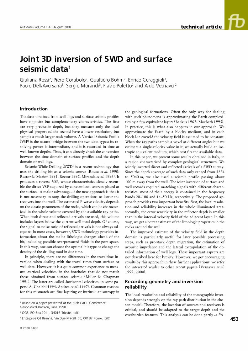
When a well is being drilled, a seismic profile is at the mini-mum usually available. Thus we have at least a rough macro-model in depth, obtained, for example, by using stackingvelocities and the Dix formula, plus some geological con-straint. Figure 1 shows such a model for an area in SouthernItaly, where an SWD recording and its tomographic inversionwere planned. The model is composed of a few horizontal lay-ers. The actual area is certainly much more complex, i.e. char-acterized by dipping fault blocks, but at present its 3Dgeometry is not well known.

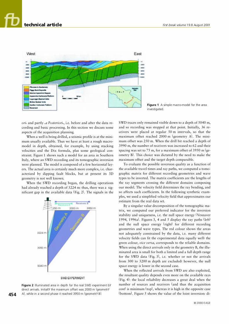
When the SWD recording began, the drilling operationshad already reached a depth of 3224 m: thus, there was a sig-nificant gap in the available data (Fig. 2). The signals in the

SWD traces only remained visible down to a depth of 5040 m,and so recording was stopped at that point. Initially, 36 re-ceivers were placed at regular 50 m intervals, so that themaximum offset reached 2000 m (geometry A). The mini-mum offset was 250 m. When the drill bit reached a depth of3990 m, the number of receivers was increased to 62 and theirspacing was set to 75 m, for a maximum offset of 3950 m (ge-ometry B). This choice was dictated by the need to make themaximum offset and the target depth comparable.

To evaluate the possible inversion quality as a function ofthe available travel times and ray paths, we computed a tomo-graphic matrix for different recording geometries and wavetypes to be inverted. The matrix coefficients are the lengths ofthe ray segments crossing the different domains composingour model. The velocity field determines the ray bending, andso affects such coefficients. In the following synthetic exam-ples, we used a simplified velocity field that approximates ourestimate from the real data set.

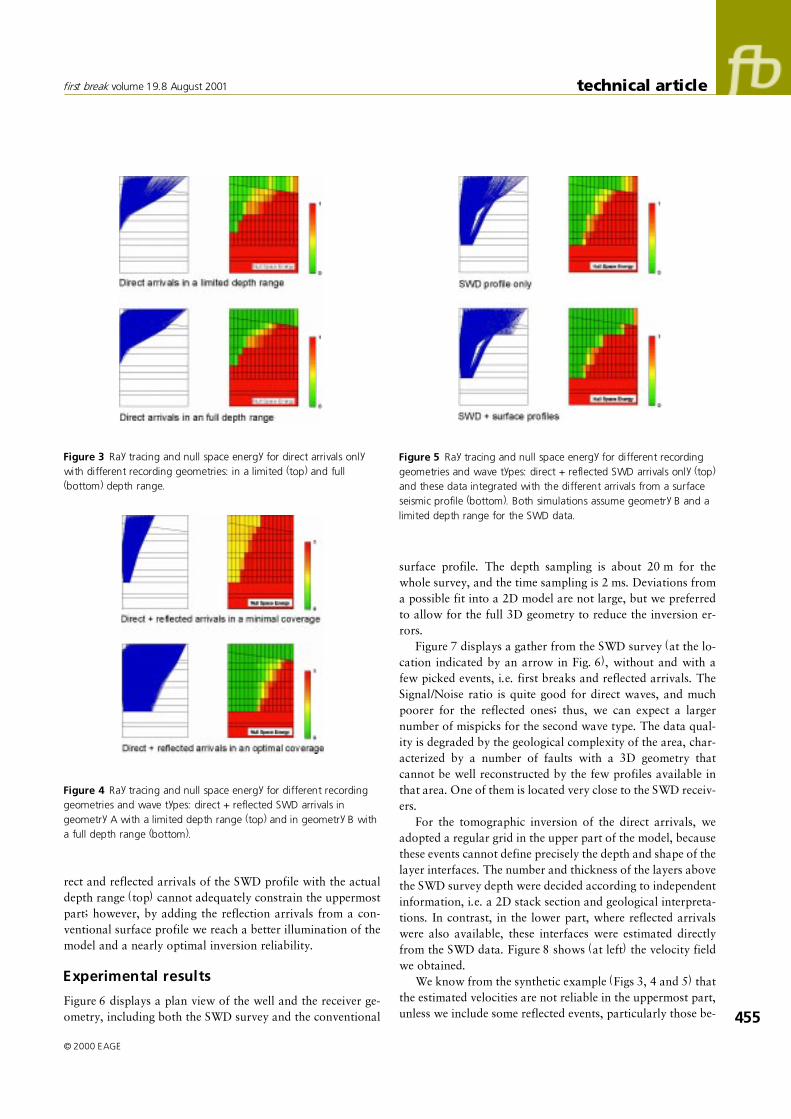
By a singular value decomposition of the tomographic ma-trix, we computed our preferred indicator for the inversionstability and uniqueness, i.e. the null space energy (Vesnaver1994, 1996a). Figures 3, 4 and 5 display the ray paths (left)and the null space energy (right) for different recordinggeometries and wave types. The red colour shows the areasnot adequately constrained by the data, i.e. many differentvelocity fields can fit the experimental data equally well; thegreen colour, vice versa, corresponds to the reliable domains.When using the direct arrivals only in the geometry B, the illu-minated area is small for both a limited and a full depth rangefor the SWD data (Fig. 3), i.e. whether or not the arrivalsfrom 300 to 3200 m depth are excluded; however, the nullspace energy is lower in the second case.

When the reflected arrivals from SWD are also exploited,the resultant quality depends even more on the available rays(Fig. 4): the local reliability decreases a great deal when thenumber of sources and receivers (and thus the acquisitioncost) is minimum (top), whereas it is high in the opposite case(bottom). Figure 5 shows the value of the joint inversion: di-

Figure 1 A simple macro-model for the areainvestigated.

Figure 2 Illuminated area in depth for the real SWD experiment bydirect arrivals. Initially the maximum offset was 2000 m (geometryA), while in a second phase it reached 3950 m (geometry B).

first break volume 19.8 August 2001

455

© 2000 EAGE

technical article

surface profile. The depth sampling is about 20 m for thewhole survey, and the time sampling is 2 ms. Deviations froma possible fit into a 2D model are not large, but we preferredto allow for the full 3D geometry to reduce the inversion er-rors.

Figure 7 displays a gather from the SWD survey (at the lo-cation indicated by an arrow in Fig. 6), without and with afew picked events, i.e. first breaks and reflected arrivals. TheSignal/Noise ratio is quite good for direct waves, and muchpoorer for the reflected ones; thus, we can expect a largernumber of mispicks for the second wave type. The data qual-ity is degraded by the geological complexity of the area, char-acterized by a number of faults with a 3D geometry thatcannot be well reconstructed by the few profiles available inthat area. One of them is located very close to the SWD receiv-ers.

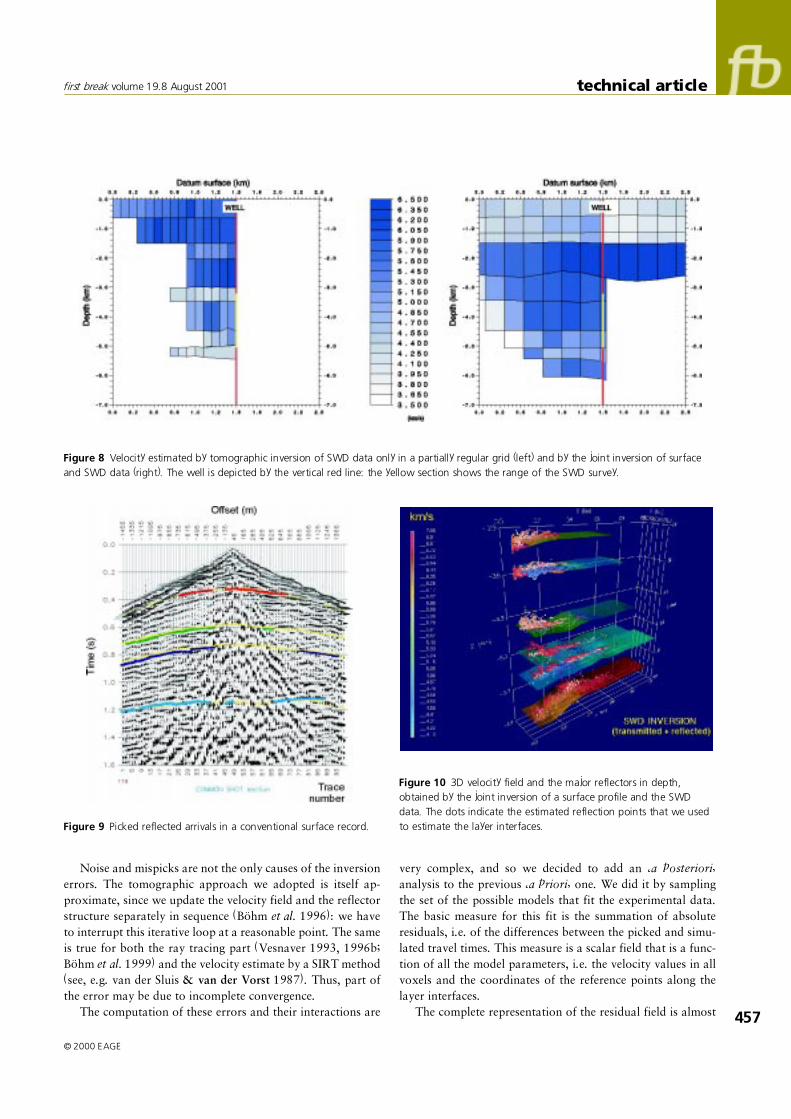
For the tomographic inversion of the direct arrivals, weadopted a regular grid in the upper part of the model, becausethese events cannot define precisely the depth and shape of thelayer interfaces. The number and thickness of the layers abovethe SWD survey depth were decided according to independentinformation, i.e. a 2D stack section and geological interpreta-tions. In contrast, in the lower part, where reflected arrivalswere also available, these interfaces were estimated directlyfrom the SWD data. Figure 8 shows (at left) the velocity fieldwe obtained.

We know from the synthetic example (Figs 3, 4 and 5) thatthe estimated velocities are not reliable in the uppermost part,unless we include some reflected events, particularly those be-

Figure 3 Ray tracing and null space energy for direct arrivals onlywith different recording geometries: in a limited (top) and full(bottom) depth range.

Figure 4 Ray tracing and null space energy for different recordinggeometries and wave types: direct + reflected SWD arrivals ingeometry A with a limited depth range (top) and in geometry B witha full depth range (bottom).

Figure 5 Ray tracing and null space energy for different recordinggeometries and wave types: direct + reflected SWD arrivals only (top)and these data integrated with the different arrivals from a surfaceseismic profile (bottom). Both simulations assume geometry B and alimited depth range for the SWD data.

rect and reflected arrivals of the SWD profile with the actualdepth range (top) cannot adequately constrain the uppermostpart; however, by adding the reflection arrivals from a con-ventional surface profile we reach a better illumination of themodel and a nearly optimal inversion reliability.

Experimental results

Figure 6 displays a plan view of the well and the receiver ge-ometry, including both the SWD survey and the conventional

first break volume 19.8 August 2001

© 2000 EAGE

456

technical article

tween the Earth�s surface and the uppermost level for theSWD recording. Thus, we picked the reflected arrivals of thesurface profile depicted in Fig. 6. The seismic source here isdynamite; the source and receiver interval are about 30 m.The shots are mostly recorded in a split-spread geometry,with 96 channels. The estimated velocity (Fig. 8, right) is nowmuch more extended in space. One can notice the differentdiscretization in the uppermost part, where the layer inter-faces have now a space-variant depth, estimated by reflectiontomography. There are significant differences in the velocityfield, especially in the upper part.

Figure 9 shows the picked arrivals in a record from the sur-face profile. The sampling rate is 4 ms, and the picking erroris of this order of magnitude. We may assume that the traveltime errors are Gaussian, if they are mainly due to interferingnoise or random interpretation errors. In this case, their effecton our estimated interfaces and velocity anomalies will besmall if the number of available rays is large: the adopted in-version algorithm can average out the white noise.

The joint inversion of SWD and surface data required afull 3D approach, due to the spatial geometry of the two sur-veys, which cannot be contained all in one plane. On theother hand, the limited azimuth coverage and spatial distribu-tion of sources and receivers did not provide an ideal ray pathdistribution. Therefore we adapted the local resolution byminimizing the null space energy, i.e. by increasing the voxelsize in the areas where the ray coverage is poor (Böhm &Vesnaver 1999). Figure 10 displays a 3D view of the velocityfield and the major interfaces so obtained. We notice that thedispersion of the estimated reflection points is significant: it is

certainly due to the drawbacks we mentioned above, i.e. thenoise and the 3D geometry of the actual geological structures.

A posteriori validation

In our initial analysis, we computed the null space energy fordifferent ray path distributions, in order to decide the modelcomplexity that can be supported by the available data. Im-plicitly, we supposed that no noise or mispicks affect the data,since we obtained it from a numerical simulation. Of course,this is not true for the real data set, especially for the reflectedevents in the SWD survey, where the Signal/Noise ratio israther poor at large depths.

Figure 6 Plan view of the recording geometry for the real SWDexperiment and the surface seismic profile used for the jointinversion.

Figure 7 Picked direct (top) and reflected arrivals (bottom) in someSWD records.

first break volume 19.8 August 2001

457

© 2000 EAGE

technical article

Noise and mispicks are not the only causes of the inversionerrors. The tomographic approach we adopted is itself ap-proximate, since we update the velocity field and the reflectorstructure separately in sequence (Böhm et al. 1996): we haveto interrupt this iterative loop at a reasonable point. The sameis true for both the ray tracing part (Vesnaver 1993, 1996b;Böhm et al. 1999) and the velocity estimate by a SIRT method(see, e.g. van der Sluis & van der Vorst 1987). Thus, part ofthe error may be due to incomplete convergence.

The computation of these errors and their interactions are

very complex, and so we decided to add an �a posteriori�analysis to the previous �a priori� one. We did it by samplingthe set of the possible models that fit the experimental data.The basic measure for this fit is the summation of absoluteresiduals, i.e. of the differences between the picked and simu-lated travel times. This measure is a scalar field that is a func-tion of all the model parameters, i.e. the velocity values in allvoxels and the coordinates of the reference points along thelayer interfaces.

The complete representation of the residual field is almost

Figure 8 Velocity estimated by tomographic inversion of SWD data only in a partially regular grid (left) and by the joint inversion of surfaceand SWD data (right). The well is depicted by the vertical red line: the yellow section shows the range of the SWD survey.

Figure 9 Picked reflected arrivals in a conventional surface record.

Figure 10 3D velocity field and the major reflectors in depth,obtained by the joint inversion of a surface profile and the SWDdata. The dots indicate the estimated reflection points that we usedto estimate the layer interfaces.

first break volume 19.8 August 2001

© 2000 EAGE

458

technical article

impossible, because it may depend on hundreds of variables.However, Fig. 11 can give us a flavour of the inversion stabil-ity. In the plot, the x and y axes represent, respectively, theaverage velocity in the deepest estimated layer and its averagedepth, while the z coordinate shows the average depth error.The inversion procedure produces samples of this field as aspin-off of its iterations: at each inversion step, we evaluatethe time residuals, converted into depth, for the present modelconfiguration. We contour the residual sum and obtain a sur-face interpolating them: if we see a deep absolute minimum inthis surface, our parameter set is well constrained and its esti-mation does not depend a lot on the initial model. Of course,if we carry out a multiple inversion test by starting with differ-ent initial models (as we did), we get a finer sampling of thetime residual function, and so a finer �a posteriori� analysis ofthe inversion process.

Figure 11 shows a long narrow valley, nearly parallel tothe velocity axis, whose length exceeds an interval of 1000 m/s, centred at about 6300 m/s. This means that the error in theestimated velocity at a depth of 6200 m may reach 16%. Theerror in the depth is much smaller, since the valley width doesnot exceed 200 m, which is only about 3% of the expecteddepth. In the figure, dots coded by the same colour corre-spond to samples of the solution space obtained at the inter-mediate stages within a single inversion run.

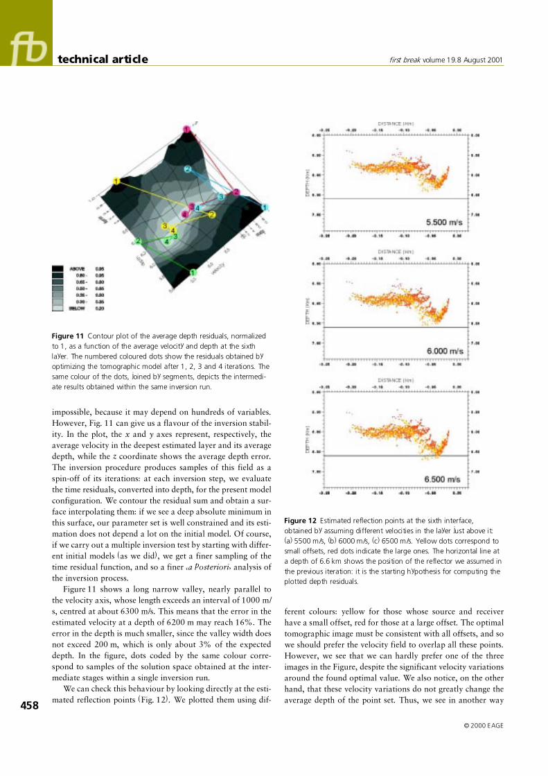
We can check this behaviour by looking directly at the esti-mated reflection points (Fig. 12). We plotted them using dif-

ferent colours: yellow for those whose source and receiverhave a small offset, red for those at a large offset. The optimaltomographic image must be consistent with all offsets, and sowe should prefer the velocity field to overlap all these points.However, we see that we can hardly prefer one of the threeimages in the Figure, despite the significant velocity variationsaround the found optimal value. We also notice, on the otherhand, that these velocity variations do not greatly change theaverage depth of the point set. Thus, we see in another way

Figure 12 Estimated reflection points at the sixth interface,obtained by assuming different velocities in the layer just above it:(a) 5500 m/s, (b) 6000 m/s, (c) 6500 m/s. Yellow dots correspond tosmall offsets, red dots indicate the large ones. The horizontal line ata depth of 6.6 km shows the position of the reflector we assumed inthe previous iteration: it is the starting hypothesis for computing theplotted depth residuals.

Figure 11 Contour plot of the average depth residuals, normalizedto 1, as a function of the average velocity and depth at the sixthlayer. The numbered coloured dots show the residuals obtained byoptimizing the tomographic model after 1, 2, 3 and 4 iterations. Thesame colour of the dots, joined by segments, depicts the intermedi-ate results obtained within the same inversion run.

first break volume 19.8 August 2001

459

© 2000 EAGE

technical article

the different sensitivity to velocity and depth error in this par-ticular case, i.e. with this recording geometry and in this partof the model. In our case, this was the target area.

Conclusions

The joint inversion of direct and reflected arrivals provides areliable tomographic image in a walk-away VSP, in the depthinterval where the ray paths of both wave types intersect thewell. In a SWD survey, this information can be used to predictmajor lithological changes ahead of the bit.

In the depth range where the SWD survey is missing orpartial, we can improve the resolution and reliability of theestimated depth model by jointly inverting the SWD data andsome conventional surface profile. The reflected arrivals arenecessary for deciding the interfaces structure, and increasealso the illuminated area. The null space energy, obtainedfrom the singular value analysis of the tomographic matrix, isa minimum when all available wave types are inverted to-gether.

We processed a real SWD and a surface profile fromSouthern Italy. To get a quantitative estimate of the velocity-depth errors, we carried out an �a posteriori� evaluation of thetomographic image. We found that the errors in the reflectordepths are smaller than those in the velocity field, because ofthe averaging approach we adopted for estimating the layerinterfaces.

Acknowledgements

We thank Enterprise Oil Italiana, Fina Italiana, Mobil Oiland UTP for their support and for permission to publish thispaper. The OGS contribution was partially supported also bythe European Commission in the Thermie Programme (con-tract no. OG/132/95).

References

Al-Chalabi M. [1994] Seismic velocity � a critique. First Break 12,589�596.

Andrea, M., Sams, M.S., Worthington, M.H. and King, M.S.[1997] Predicting horizontal velocities from well data. GeophysicalProspecting 45, 593�609.

Backus, G.E. [1962] Long-wave elastic anisotropy by horizontallayering. Journal of Geophysical Research 67, 4427�4440.

Böhm, G., Rossi, G. and Vesnaver, A. [1996] 3D reflectiontomography by adaptive irregular grids. 58th EAGE Meeting,Amsterdam, The Netherlands, Expanded Abstracts, paper C056.

Böhm, G., Rossi, G. and Vesnaver, A. [1999] Minimum time raytracing for 3D irregular grids. Journal of Seismic Exploration 8,117�131.

Böhm, G. and Vesnaver, A. [1999] In quest of the grid. Geophysics64, 1116�1125.

MacBeth, C. [1995] How can anisotropy be used for reservoircharacterisation? First Break 13, 31�37.

Miller, D.E. and Chapman, C.H. [1991] Incontrovertible evidenceof anisotropy in crosshole data. 61st SEG Meeting, Houston, USA,Expanded Abstract. SB1.4, 825�828.

Miranda, F., Aleotti, L., Abramo, F., Poletto, F., Craglietto, A.,Persoglia, S. and Rocca, F. [1996] Impact of the Seismic WhileDrilling technique on the exploration wells. First Break 14, 55�68.

Rector, J.W. [1992] Noise characterisation and attenuation in drillbit recordings. Journal of Seismic Exploration 1, 379�393.

Rector, J.W. and Marion, B.P. [1991] The use of drill-bit energy asa downhole seismic source. Geophysics 56, 628�634.

Rocca, F., Persoglia, S., Poletto, F. and Craglietto, A. [1990] Use ofdrilling noises to generate a reciprocal VSP. Final Report CEC,Contract DG XVII/TH-0113-87.

van der Sluis, A. and van der Vorst, H.A. [1987] Numericalsolution of large, sparse linear algebraic systems arising fromtomographic problems. In: Seismic Tomography with Applicationsin Global Seismology and Exploration Geophysics (ed. G. Nolet).D. Reidel Publishing Co.

Vesnaver, A. [1993] Minimum time ray tracing of reflected,refracted and diffracted waves in irregular grids. 55th EAGEMeeting, Stavanger, Norway, Expanded Abstracts, paper P059.

Vesnaver, A. [1994] Towards the uniqueness of tomographicinversion solutions. Journal of Seismic Exploration 3, 323�334.

Vesnaver, A. [1996a] The contribution of reflected, refracted andtransmitted waves to seismic tomography: a tutorial. First Break 14,159�168.

Vesnaver, A. [1996b] Ray tracing based on Fermat�s principle inirregular grids. Geophysical Prospecting 44, 741�760.

Vesnaver, A., Böhm, G., Madrussani, G., Petersen, S. and Rossi, G.[1999] Tomographic imaging by reflected and refracted arrivals atthe North Sea. Geophysics 64, 1852�1862.

Vesnaver, A., Böhm, G., Madrussani, G., Rossi, G. and Granser, H.[2000] Depth imaging and velocity calibration by 3D adaptivetomography. First Break 7, 303�312.

MS received June 1999