Joining and Deformation Processes with Corrosion Resistance

Grant Brandal

Submitted in partial fulfillment of the

requirements for the degree of

Doctor of Philosophy

in the Graduate School of Arts and Sciences

COLUMBIA UNIVERSITY

2017

© 2016

Grant Brandal

All rights reserved

ABSTRACT

Joining and Deformation Processes with Corrosion Resistance

Grant Brandal

Dissimilar metal joining was performed with the main goal being maximization of the strength of

the joined samples, but because of some potential applications of the dissimilar joints, analyzing

their corrosion behavior also becomes crucial. Starting with materials that initially have suitable

corrosion resistance, ensuring that the laser processing does not diminish this property is

necessary. Conversely, the laser shock peening processing was implemented with a complete

focus on improving the corrosion behavior of the workpiece. Thus, many commonalities occur

between these two manufacturing processes, and this thesis goes on to analyze the thermal and

mechanical influence of laser processing on materials’ corrosion resistances.

Brittle intermetallic phases can form at the interfaces of dissimilar metal joints. A process called

autogenous laser brazing has been explored as a method to minimize the brittle intermetallic

formation and therefore increase the fracture strength of joints. In particular, joining of nickel

titanium to stainless steel wires is performed with a cup/cone interfacial geometry. This

geometry provides beneficial mechanical effects at the interface to increase the fracture strength

and also enables high-speed rotation of the wires during irradiation, providing temperature

uniformity throughout the depth of the wires. Energy dispersive X-ray spectroscopy, tensile

testing, and a numerical thermal modelling are used for the analysis.

The material pair of nickel titanium and stainless steel have many applications in implantable

medical devices, owing to nickel titanium’s special properties of shape memory and

superelasticity. In order for an implantable medical device to be used in the body, it must be

ensured that upon exposure to body fluid it does not corrode in harmful ways. The effect that

laser autogenous brazing has on the biocompatibility of dissimilar joined nickel titanium to

stainless steel samples is thus explored. While initially both of these materials are considered to

be biocompatible on their own, the laser treatment may change much of the behavior. Thermally

induced changes in the oxide layers, grain refinement, and galvanic effects all influence the

biocompatibility. Nickel release rate, polarization, hemolysis, and cytotoxicity tests are used to

help quantify the changes and ascertain the biocompatibility of the joints.

To directly exert a beneficial influence on materials’ corrosion properties laser shock peening

(LSP) is performed, with a particular focus on the stress corrosion cracking (SCC) behavior.

Resulting from the combination of an applied load on a susceptible material exposed to a

corrosive environment, SCC can cause sudden material failure. Stainless steel, high strength

steel, and brass are subjected to LSP and their differing corrosion responses are determined via

cathodic charging, hardness, mechanical U-bend, Kelvin Probe Force Microscopy, and SEM

imaging. A description accounting for the differing behavior of each material is provided as well

as considerations for improving the effectiveness of the process.

SCC can occur by several different physical processes, and to fully encapsulate the ways in

which LSP provides mitigation, the interaction of microstructure changes induced by LSP on

SCC mechanisms is determined. Hydrogen absorbed from the corrosive environment can cause

phase changes to the material. Cathodic charging and subsequent X-ray diffraction is used to

analyze the phase change of sample with and without LSP processing. Lattice dislocations play

an important role, and transmission electron microscopy helps to aid in the analysis. A finite

element model providing spatially resolved dislocation densities from LSP processing is

performed.

i

Table of Contents

List of Figures…………………………………………………………………………………....vi

Chapter 1: Introduction

1.1 Laser Manufacturing Processes ........................................................................................ 1

1.2 Dissimilar Material Joining .............................................................................................. 2

1.2.1 Nickel Titanium ........................................................................................................ 3

1.2.2 Biocompatibility ....................................................................................................... 8

1.2.3 Autogenous Laser Brazing ........................................................................................ 9

1.3 Mitigation of Stress Corrosion Cracking ....................................................................... 12

1.3.1 Introduction to SCC ................................................................................................ 12

1.3.2 Failure Mechanisms ................................................................................................ 15

1.3.3 Prevention Techniques ............................................................................................ 20

1.3.4 Laser Shock Peening ............................................................................................... 22

1.4 Organization and Objectives of Dissertation ................................................................. 26

Chapter 2: Beneficial Interface Geometry for Laser Joining of NiTi to Stainless Steel

Wires

2.1 Introduction .................................................................................................................... 29

2.2 Background .................................................................................................................... 32

2.2.1 Ternary Phase Diagram and Brittle Intermetallics .................................................. 32

2.2.2 Geometrical Considerations .................................................................................... 34

ii

2.2.3 Stress Intensity Formulation ................................................................................... 36

2.2.4 Process .................................................................................................................... 38

2.2.5 Thermal Modeling ................................................................................................. 38

2.3 Procedure ........................................................................................................................ 40

2.4 Results & Discussion ..................................................................................................... 41

2.4.1 Temperature Profile ................................................................................................ 41

2.4.2 Joint Morphology .................................................................................................... 44

2.4.3 Composition ............................................................................................................ 46

2.4.4 Joint Strength .......................................................................................................... 49

2.4.5 Fracture Surfaces .................................................................................................... 55

2.5 Conclusion ...................................................................................................................... 57

Chapter 3: Biocompatibility and Corrosion Response of Laser Joined NiTi to Stainless

Steel Wires

3.1 Introduction .................................................................................................................... 59

3.2 Background .................................................................................................................... 61

3.2.1 Laser Autogenous Brazing ...................................................................................... 61

3.2.2 Biocompatibility Concerns ..................................................................................... 62

3.2.3 Divergence From Base Material Response ............................................................. 64

3.2.4 Polarization Tests .................................................................................................... 65

3.2.5 Numerical Modeling ............................................................................................... 67

3.2.6 Microbiology Testing.............................................................................................. 68

iii

3.3 Experimental Procedure ................................................................................................. 69

3.4 Results ............................................................................................................................ 71

3.4.1 Polarization Tests .................................................................................................... 71

3.4.2 Corrosion Current Modeling ................................................................................... 72

3.4.3 Nickel Release Tests ............................................................................................... 75

3.4.4 Morphology & Thermally Induced Changes .......................................................... 77

3.4.5 Cytotoxicity and Hemolysis .................................................................................... 85

3.5 Conclusion ...................................................................................................................... 87

Chapter 4: Material Influence on Mitigation of Stress Corrosion Cracking via Laser Shock

Peening

4.1 Introduction .................................................................................................................... 88

4.2 Background .................................................................................................................... 90

Mechanisms of Stress Corrosion Cracking ............................................................. 90

Laser Shock Peening ............................................................................................... 92

Dislocation Generation ........................................................................................... 93

Work Function and Corrosion Potential ................................................................. 94

Processing Concerns ............................................................................................... 95

4.3 Experimental Procedure ................................................................................................. 96

4.4 Results & Discussion ..................................................................................................... 97

Surface Morphology ............................................................................................... 97

Cathodic Charging and Hardness Increases ............................................................ 99

iv

U-Bend SCC Testing ............................................................................................ 102

Kelvin Probe Force Microscopy ........................................................................... 108

4.5 Conclusion .................................................................................................................... 113

Chapter 5: Laser Shock Peening for Suppression of Hydrogen Induced Martensitic

Transformation in Stress Corrosion Cracking

5.1 Introduction .................................................................................................................. 114

5.2 Background .................................................................................................................. 116

5.2.1 Hydrogen induced martensitic transformation ...................................................... 116

5.2.2 Hydrogen enhanced localized plasticity ............................................................... 118

5.2.3 Laser Shock Peening and Lattice Changes ........................................................... 119

5.2.4 Numerical Modelling ............................................................................................ 121

5.3 Experimental Setup ...................................................................................................... 122

5.4 Results & Discussion ................................................................................................... 123

5.4.1 Detection of Martensite Formation ....................................................................... 123

5.4.2 Mechanism of SCC Mitigation ............................................................................. 128

5.4.3 Imaging Analysis .................................................................................................. 133

5.5 Conclusion .................................................................................................................... 141

Chapter 6: Conclusion

6.1 Autogenous Laser Brazing of Wires ............................................................................ 142

6.2 Biocompatibility of Autogenously Brazed Wires ........................................................ 143

6.3 Laser Shock Peening for Stress Corrosion Cracking Mitigation ................................. 144

v

6.4 LSP Suppression of Hydrogen Induced Martensite ..................................................... 146

6.5 Future Work ................................................................................................................. 147

References………………………………………………………………...……………………151

Appendix……………………………………………………………………………………….166

vi

List of Figures:

Chapter 1:

Figure 1 Process of shape memory by the martensite transformation in NiTi [4]. The

deformation step occurs via detwinning to allow for recovery of the initial shape.

Figure 2 NiTi used as a guidewire for orthodontic braces [9]. The constant force exerted by the

NiTi over a large range of strain provides good performance.

Figure 3 Autogenous laser brazing experimental setup.

Figure 4 Increase of the amount of hydrogen absorbed with decreasing applied potentials [20].

Figure 5 Mechanism of failure for hydride formation in SCC [22].

Figure 6 Hydrogen enhanced decohesion mechanism of SCC [22], which weakens the atomic

bonding and makes the material become more brittle and weak.

Figure 7 Experimental evidence obtained from TEM measurements of hydrogen increasing the

mobility of dislocations [24], leading to the mechanism of hydrogen enhanced localized

plasticity.

Figure 8 Description of dislocations behaving as trapping sites to hydrogen diffusion by forming

deep wells of potential energy [25].

Figure 9 Thermal desorption spectroscopy measurements of hydrogen desorption for four

different amounts of drawing reductions [27]. At high deformation, additional trapping

sites are formed which require higher amounts of energy (temperature) to release the

hydrogen.

Figure 10 Schematic of the physical process for laser shock peening [35].

Figure 11 Physical setup of for the LSP experiments

Chapter 2:

Figure 1 Ternary phase diagram for Fe-Ni-Ti at 1173 K [13]

Figure 2 Schematic diagram describing the geometry used. Point 1 is at the apex of the cone,

point 2 is on the outside edge.

vii

Figure 3 Mode I stress intensity (KI) and Mode II stress intensity (KII) versus angle of interface,

for a constant uniaxial load. The interfacial area is superimposed over-top, indicating that

as the cones become sharper, the area increase results in a decrease of stress intensity.

Figure 4 Longitudinal sectioned time snapshot of thermal accumulation in 90° cones.

Corresponding times are: (a) 1s, (b) 4s, (c) 6.8s (laser has shut off). Laser location

indicated by white dotted line. Power: 15W, Angular velocity: 3000°/s

Figure 5 Uniformity along line segment 1-2 on the interface. As the angular velocity is

increased, the thermal distribution becomes more even and the average temperature rises.

Figure 6 Time history of points 1 and 2 along the interface from Figure 2, compared to points at

the top and bottom of the interface of wires with flat interfaces. Temperature difference

between the 2 points on the rotated wires throughout the laser scan is minimal. Laser

power is 15 W for the rotated wires, and 35W for the flat interfaces.

Figure 7 Images of four different combinations of power and cone angle. The outer surface near

the joint of the 90° wires experienced more deformation. Rotational velocity is held

constant at 3000°/s.

Figure 8 Longitudinal section image of a 120° cone processed at a power of 15W. The arrows

indicate the paths of EDX line scans.

Figure 9 Longitudinal section image of a 120° cone processed at a power of 17W. Excessive

melting and deformation is present on the outer surface.

Figure 10 EDX line scan across line II, indicating the mixing occurring in the joint. Sample

irradiated at 13W.

Figure 11 EDX line scan across region II indicated in Figure 8. Gradual decrease of

concentration across the width of the interface is indicative of diffusion. Sample

irradiated at 15W.

Figure 12 EDX compositional map, corresponding to the longitudinal sectioned image of Figure

8, showing iron (red), nickel (green), and titanium (blue). Laser power is 15W. A mixing

region is observed along the interface, the width of which decreases towards the center of

the wire. This indicates that the lighter colored regions along the interface of the

longitudinal sectioned images are indeed the mixed regions.

Figure 13 Increase of load at fracture with increasing laser power input. Standard error for each

level is indicated. Note that the 90° wires are stronger than the 120° wires at every power

except for 17W.

Figure 14 Stress at fracture over a range of power levels. The 90° wires are consistently stronger

than the 120° wires, which is consistent with predictions. .

viii

Figure 15 Comparison of fracture strength between two different angles. The percentage scale

on the left is how much stronger the 90° joint is compared to the 120° joint, for given

power and angular velocities. As the power is increased, the difference between the two

geometries reduces. This graph does not indicate which parameters gave the best overall

results, but simply indicates the difference between the two angles.

Figure 16 Maximum average strength at fracture achieved for each wire geometry. Standard

error is indicated. The 180° samples are the non-rotated, flat interfaces. Both of the

conical wires have much higher fracture strengths.

Figure 17 Fracture surface indicating brittle transgranular fracture. 90° interface, 17 W, 3000°/s.

Fractured at 200 MPa, along a surface not corresponding to the material interface.

Figure 18 Fracture surface of a sample that broke at 393 MPa, which was the highest strength

achieved. The original cup and cone geometry was intact after fracture. Quasi-cleavage is

apparent, indicating a better joint than Figure 17.

Chapter 3:

Figure 1 Schematic diagram illustrating the autogenous laser brazing setup. The wires are

rotated, while the laser simultaneously scans towards the interface, but is turned off before

crossing over to the stainless steel side. The angle θ corresponds to the apex angle of the

cup/cone configuration.

Figure 2 Visual description of the numerical model used for prediction of the galvanic current.

Laplace’s equation is solved in the electrolyte PBS. Material properties are taken into

account as the relevant boundary conditions along the bottom border. The function fi(φ) is

the polarization response for the respective material.

Figure 3 Polarization response of metal samples in PBS solution. The solid lines indicate

measurements, while the dashed lines are approximations. The more electronegative

equilibrium potential of the NiTi will cause it to experience anodic effects, while the

stainless steel is cathodic. When the transition from the base materials goes through the

two intermediary phases, the corrosion current gets significantly reduced. This data was

used for fi(φ) in Figure 2.

Figure 4 Numerical simulation results for the distribution of the electric potential in the PBS

solution. The gradient of this field gives the direction of electron flow, and is denoted via

the arrows. At either extreme along the bottom boundary, the potential approaches the

equilibrium potential of the respective material nearby.

ix

Figure 5 Distribution of electron flow along the lower boundary of Figure 4, corresponding to the

corrosion current. The dotted lines are for a electrolytic conductivity that is only 10% that

of the solid lines, causing a more non-uniform distribution.

Figure 6 Total amount of nickel released from joined samples as a function of time. The two

different processing parameters of low and high energy inputs have similar profiles, but

are noticeably higher than the base NiTi. This NiTi has undergone a previous heat

treatment; non-treated NiTi has a release profile higher than the treated samples in here in

our case.

Figure 7 Optical images comparing the interface regions for two different laser power levels.

Both underwent a rotational speed of 3000°/sec, (a) had a laser power of 15 W while (b)

was irradiated at 13W. The HAZ of the NiTi progresses through several regions before

the material starts to bow out at the interface.

Figure 8 SEM image of the outside interface for a joined sample. Roughness and non-uniformity

is evident in this region, making it susceptible to effects such as pitting and crevice

corrosion.

Figure 9 Surface corrosion at the mixed interface region after 6 days (a) and 15 days (b) of

exposure to the simulated body fluid. Both samples were joined at 17 W and 1500°/sec.

Rather uniform texture is seen in (a), but this surface becomes much rougher as corrosion

proceeds, as evidenced by the sharper regions found in (b).

Figure 10 Optical micrograph at the interface of a longitudinally sectioned sample. Distinct

grains are clearly visible in the NiTi on the left hand side, with size increasing nearer to

the interface. The inset shows an enlarged image near the outer edge, where the

combination of stress and elevated temperatures resulted in dynamic recrystallization.

This is a region that recrystallized without having reached the melting temperature.

Figure 11 EBSD unique grain map in a region of NiTi far from the interface. The rather small

grain size may be an effect of previous cold working. When compared with the sizes of

Figure 10, it is clear that the thermal accumulation of the interface results in significant

grain growth.

Figure 12 EBSD phase map in a HAZ of the stainless steel. At elevated temperatures, stainless

steel may become sensitized by precipitation of chromium along grain boundaries. This is

a representative image of the whole region, and chromium precipitation was never

detected. Thus, the biocompatibility of the stainless steel is not harmed by the laser

joining process.

Figure 13 Images of the border of the heat affected zone and base material in the NiTi, as

indicated by the inset region of Figure 1. More corrosion is evident in the lower power

sample of (a) than for the higher power of (b). This is evidence that more intermetallic

formation at the interface may act as an electrical resistance, effectively reducing the flow

of the galvanic current.

x

Figure 14 Hemolysis testing for two different laser processing parameters. Slightly more

hemolytic properties are found in the sample irradiated with higher energy, but both are

well within the biocompatible, safe zone. Error bars indicate standard error.

Chapter 4:

Figure 1 LSP indentation profile of a stainless steel sample irradiated at 250 mJ with a spot size

of 0.9 mm. The two lines are traces across perpindicular directions.

Figure 2 Indentation profile of brass LSP processed at 250 mJ. More surface roughening effects

are visible than on the stainless steel sample.

Figure 3 Morphology of a patterned brass sample after LSP processing. Individual indentations

are still visible because of the 0% overlap condition.

Figure 4 Hardness increases after cathodic charging on stainless steel samples, caused by

increased hydrogen absorption into the lattice. The values on the abscissa correspond to

the amount of overlapping between adjacent LSP pulses, and 2X indicates that the surface

was treated with two passes. As the level of LSP processing increases, the amount of

hardness changes via hydrogen decreases.

Figure 5 Hardness increases of AISI 4140 steel after cathodic charging. The level of LSP

processing causes the hydrogen effects to be lessened, indicating mitigation to hydrogen

embrittlement. The percent increases are lesser than for the stainless steel show.

Figure 6 SEM micrograph of the side of an untreated stainless steel U-bend specimens after 1 hr

of exposure to boiling magnesium chloride.

Figure 7 Untreated (a) and LSP treated (b) images showing the edge of stainless steel U-bend

samples, where the bottom part of these images is the outer surface. LSP prevents cracks

from propagating onto the outer surface in (b).

Figure 8 Outer U-bent face for untreated stainless steel samples. Indicated by the arrow,

cracking has occurred for the untreated sample, but was been prevented from occurring on

the LSP treated sample

Figure 9 Optical micrographs of etched stainless steel samples exposed to 1 hr of boiling

magnesium chloride. (a) has not been LSP treated, and shows a combination of

transgranular and intergranular fracture. (b) has been LSP treated, where the fracture

mechanism is now dominated by intergranular fracture. The effects of increased hydrogen

penetrating the lattice in (a) may cause the transgranular failure.

Figure 10 Multiple cracks found in an AISI 4140 U-bend sample LSP three times at 300 mJ.

Unlike the stainless steel, the high strength steel fails by many parallel cracks rather than

one major failure.

Figure 11 Mises stress in Pascals overlaid on the final deformed shape of a U-bend specimen

from FEM simulation.

xi

Figure 12 Tension on a path along the long direction in the center of the U-bend samples. The

peak stress is higher for the brass.

Figure 13 Work function measurements for brass, stainless steel, and high strength steel. The

center of the LSP pulse is at 0 um, and each material changes differently in response to the

incident shockwave. Brass experiences work function decreases from LSP, while the high

strength steel experiences an increased work function. The scale on the high strength steel

figure covers a wider range than the other two, indicating an increased response to the

shockwave processing.

Figure 14 Rate of change of dislocation density, on the vertical axis for, varying amounts of

plastic deformation. The three materials generate dislocations at varying rates. But since

the yield strength of high strength steel is the largest, it will have lower dislocation

generation for a given amount of deformation

Figure 15 Rate of change of dislocation density for high strength steel with three different types

of heat treatments. As such, the downward slope of the annealed sample above 350 MPa

does not indicate decreasing dislocation density but rather that dislocations are being

generated at a slower rate.

Chapter 5:

Figure 1 Free energy diagram showing the suitable conditions for the formation of deformation

induced martensite [19].

Figure 2XRD measurements of lattice changes from cathodic charging a specimen without LSP

treatment. Prior to cathodic charging, the material is fully austenitic (a). After 24 hours (b),

the absorbed hydrogen has caused the formation of a martensite peak, (c) with further

increases after 48 hours

Figure 3 Hydrogen induced lattice expansion for 24 and 48 hours of cathodic charging.

Figure 4 XRD measurements of a selected region of the spectrum for samples after LSP processing

(a), and then subjected to 24 hours (b) and 48 hours (c) of cathodic charging. The initially

austenitic peaks experience broadening after 24 hours, but no martensite formation occurs,

illustrating the effectiveness of LSP processing as a mitigation tool. Some martensite does

eventually form after 48 hours.

Figure 5 (a) Untreated stainless steel sample after cathodic charging 24 hours showing large

amounts of martensite formation, seen as the grains with platelet like structure. (b) Samples

which were subject to LSP prior to cathodic charging have considerably fewer martensitic

grains.

Figure 6 Magnified images after etching the samples of Figure 5, for an untreated sample (a) and

LSP treated (b) both after cathodic charging.

xii

Figure 7 Increases to the dislocation density after LSP processing at 1.6 GPa, which act as an

impediment to hydrogen induced martensite formation. The largest increase is seen upon

the initial incident pulse.

Figure 8 Decrease in the diffusion coefficient after various levels of incident pressure from LSP

processing. The dotted line of dislocation density shows its inverse relationship to the

diffusion coefficient.

Figure 9 Distribution of dislocation cell size after 3 LSP impacts. Symmetry is used along the

boundary at the left side.

Figure 10 Dislocation cell size for increasing number of incident LSP pulses at 4 depths.

Figure 11 Asymptotic increase of the ratio of dislocation density in cell walls to cell interior.

Figure 12 (a) Untreated sample showing lower densities of dislocations. (b) Increase of

dislocation density after 3 LSP impacts at 2.5 GW cm-2

Figure 13 Pile ups of dislocations at the grain boundary. Regions of twinning, indicated by the

arrow and letter “T” are also found, with the inset a diffraction image indicative of lattice

twinning.

Figure 14 (a) Dislocation cell formation, with the inset diffraction image indicating no grain

misorientation. (b) Dislocation subgrain structure, where the formation of within individual

grains ends at the grain boundaries.

Figure 15 High magnification TEM showing resolved lattice structure

xiii

Acknowledgement

Completion of this thesis was made possible by the assistance and contributions of many people,

both within Columbia University and outside. The contribution of my thesis advisor Professor

Y. Lawrence Yao goes beyond providing me financial support and a position in his lab. During

our discussions throughout my time in the Advanced Manufacturing Lab, the suggestions,

questions, and sometimes even criticisms from Dr. Yao resulted in increases to the quality of my

research work, as well as gaining an understanding of how to frame projects for my future career.

The discussions with Professor Sinisa Vukelic, regarding both technical aspects and general

advice on navigating through the doctoral program, are greatly appreciated. Many thanks also to

the researchers that were willing to allow me to share their expertise and resources of their

laboratories, including Professor Jeff Kysar, Dr. Irina Chernyshova, and Dr. Tong Wang. Also,

the expertise from Professor James Im for my thesis committee is appreciated.

The members of the Advanced Manufacturing Lab are very deserving of acknowledgement for

completion of this thesis. Particularly, Dr. Gen Satoh taught me many invaluable lessons of how

to perform quality research, and helped to set me up for success.

Lastly, and far from least, the incredible support from my family allowed me to complete the

program, and it undoubtedly would not have been possible without them.

1

Chapter 1: Introduction

1.1 Laser Manufacturing Processes

Lasers are a versatile tool for implementation of advanced manufacturing processes. While the

main method by which lasers impact materials is through transfer of thermal energy, the high

controllability and precision of this heat input can be taken advantage of to achieve complex, and

often surprising results. Perhaps the most commonly known laser manufacturing processes are

cutting and welding. Fields such as the automotive industry have made extensive use of large

scale laser welding. In contrast, laser welding of integrated circuits has benefited from the small

scale benefits and precision, thus illustrating the versatility of laser applications. Other laser

manufacturing process include engraving, forming, material deposition, and annealing. This thesis

will explore two different manufacturing processes, dissimilar material joining and laser shock

processing, with a focus on the corrosion implications of the processing.

In order to fully appreciate the versatility of laser manufacturing processes, differences in

characteristics amongst lasers themselves must first be highlighted. Distinctions are drawn

between continuous wave and pulsed lasers. A constant beam of energy is emitted from continuous

wave lasers, whereas pulsed lasers emit individual bursts of incident photons. In cases where

uniform heating of a component is desired continuous wave lasers may be more applicable.

Alternatively, higher intensities are often achievable by use of pulsed lasers and may be more

suitable in applications such as ablation. The response that a material has to an incident laser beam

is a complex thermal problem, and cannot be completely prescribed via the consideration of only

one parameter. While laser power is often the most commonly discussed parameter of continuous

2

wave lasers, other parameters including the wavelength and interaction time will be likewise

influential. For manufacturing processes, the lasers wavelength is most crucial regarding the

absorption into the material, so even if keeping all other parameters constant, changing the target

material in a manufacturing process may result in the entire process having to be re-evaluated

simply on the basis that different amounts of energy will be absorbed. In effect, the wavelength

dependent absorption is coupled to the power of the laser. The pulse length also significantly

affects the results in pulsed laser applications, and the time scale of pulse lengths for different

processes can vary of several orders of magnitude, where widespread use has been made of both

nanosecond (10-9 s-1) length pulses all the way down to femtosecond (10-15 s-1) pulses.

The result is that many different types of lasers are required in order to realize the wide range of

laser manufacturing applications, and the choice of which type of laser to use is not arbitrary, but

rather it naturally becomes quite explicitly defined simply by the nature of the desired application.

Carefully matching the right laser for each application must also be performed with consideration

of the target material. Once all of the parameters have been correctly identified, laser

manufacturing processes are found to be a versatile tool capable of achieving many results that

cannot be attained via traditional processes.

1.2 Dissimilar Material Joining

Joining of dissimilar materials is an effective method for exploiting beneficial characteristics of

particular materials in different regions of a component, including toughness, corrosion, wear

resistance, and flexibility. Cost reduction can also be achieved by only implementing certain

materials in crucial regions, and by the same means weight reduction is also attainable. This can

3

be implemented on both large scales, including aerospace, or on small scales like implantable

medical devices.

Various different types of products have been greatly improved by joining of dissimilar material.

One example is pacemakers, where platinum is required to be joined onto stainless steel wires.

The platinum acts as an electrode for efficient current transfer, but because of its extremely high

cost it is joined onto stainless steel in less crucial areas. Another example is golf clubs – a field

where the manufacturers are in constant, heated competition to create the highest performing

products to directly benefit the consumer. The golf club face (the region which impacts the ball)

requires hard, wear resistant surfaces [1], while weight reduction is more important in the other

regions. Exploiting more subtle types of properties can also become essential, particularly for

some medical devices. Stents are placed inside of blood vessels to prevent blockages. Since this

is internal of the human body, radiopacity is required in order to detect the device with imaging

techniques. Precise placement of the stent is required for success of the procedure, but some stent

materials are not radiopaque and therefore cannot be clearly seen with X-ray imaging. To alleviate

this problem, joining a dissimilar, radiopaque material onto the stent will provide markers for clear

identification and locating of the device [2].

1.2.1 Nickel Titanium

1.2.1.1 SHAPE MEMORY AND SUPERELASTICITY

Nickel titanium (NiTi) is a very unique material which possess shape memory and superelastic

properties, both of which are enabled by the microstructure. NiTi was originally known as Nitinol,

a portmanteau of NiTi and the place of its discovery the Naval Ordnance Lab (NOL). After

4

deformation, subsequent heating of NiTi causes the material to return to its initial, undeformed

shape – this is the shape memory effect. Superelasticity allows for the material to experience

extensive amounts of extension without sustaining any permanent deformation. The difference of

which of these phenemonon occurs is dependent on the temperature at which the deformation

occurs. At low temperatures the material is in the martensite phase, but at elevated temperatures

the material becomes austenitic. NiTi that is deformed while in the martensite phase will be

capable of experiencing shape memory, while that which is deformed while in the austenitic phase

will undergo superelasticity.

With the phase transformation guiding the mechanical behavior, four transition temperatures

become important: martensite start (Ms) and finish (Mf) temperatures and the austenite start (As)

and finish (Af) temperature. For a material initially in the low temperature martensite phase, upon

heating a transformation to austenite will begin at the austenitic start temperature. The transition

will complete, resulting in full austenite, once the austenite finish temperature is reached.

Similarly, upon cooling of the material the transition to martensite will begin at the martensitic

start temperature and complete once the martensitic finish temperature has been reached. Typical

values of these transition temperatures are Ms=37 °C, Mf=21 °C, As=58 °C, and Af=70 °C [3].

These temperatures can be tailored based on variations to the ratio of nickel to titanium, so that

whichever phase is desired for particular applications can be obtained. Of particular note is that

these transition temperatures are across the range of room temperature. As opposed to some other

metallurgical processes that require temperature extremes, NiTi experiences phase changes at

reasonable temperatures that would be expected to be reached for numerous types of consumer

applications as well is internal to the human body.

5

Figure 1 Process of shape memory by the martensite transformation in NiTi [4]. The

deformation step occurs via detwinning to allow for recovery of the initial shape.

Figure 1 illustrates the mechanics of the shape memory process which is dependent on the self-

accommodation of the martensite phase. After starting with an initial shape in the austenitic phase

in (a), cooling below the martensite transition temperature forms twinned martensite. Self –

accommodation refers to the fact that twin boundaries form on invariant planes of the

microstructure, but the overall macroscopic shape of the material remains the same as the initial

austenite. Deformation occurs by detwinning of the martensite phase, producing a shape that is

different from the original. Recovery of the initial shape is then achieved by heating the detwinned

and deformed martensite above the austenite transition temperature, as seen in the completion of

the loop from (c) to (a). This process is a one-way shape memory effect since the shape of the

deformed structure is forgotten upon heating. By a slightly different process, a two way shape

memory effect can be attained, so that thermally cycling between high and low temperatures results

6

in the material flipping between two prescribed shapes. Training of the material is required for

the two way effect, which involves additional deformation to the deformed martensite phase to

generate lattice dislocations [5]. The dislocations remain in the microstructure during heating, and

their presence thereby remembers the initial shape of the material. Heat treating of the material

allows for alteration of the transition temperatures, so that by localized heating of specific areas

the shape memory response will become non-homogenous, so that complex motion can further be

achieved.

Superelasticity is similarly dependent on the phase transformations, but for the NiTi to exhibit this

property it must be deformed while in the austenitic phase. The applied stress causes martensite

to become stable at temperatures above the initial transition temperature, as described by the

Clausius-Clapeyron equation. Once this stress induced martensite has formed, additional elastic

deformation of the material is accommodated via detwinning, which enables recoverable

deformation of levels up to 11%.

1.2.1.2 DEVICE APPLICATIONS

Exploitation of shape memory and superelasticity enables devices with unique and important

functionality. The two-way shape memory effect can be used for micro-actuators [6], in such

applications as robotics. Separation nuts in aerospace applications have also made use of NiTi as

an actuator to aid in automated release of payloads [7]. Superelasticity has been used in eyeglasses

so that the wire frames do not permanently bend when they get accidentally deformed. Additional

advanced applications are also being developed, such as utilizing the shape memory effect to create

7

morphing structures to change the shape of aerodynamic components on airplane wings and

engines during flight [8].

Figure 2 NiTi used as a guidewire for orthodontic braces [9]. The constant force exerted by the

NiTi over a large range of strain provides good performance.

Biomedical implementation of shape memory and superelasticity have become widespread. The

deformation induced phase transformation which enables superelasticity occurs at a constant

stress, creating a plateau on a stress-strain curve. Guidewires for orthodontic braces, as seen in

Figure 2, have been used for applying a constant load over large ranges of strains along this plateau.

Endoscopy rods consisting of grippers or scissors can be created and controlled on small scales

[10] helping to increase the capabilities of laparoscopic surgical procedures. Numerous forms of

stents made from NiTi have also been created. The superelasticity has been utilized to recover the

8

initial, expanded shape upon implantation in the artery. Orthopedic applications of NiTi have also

been developed, including spinal rods, medical staples, bone plates for repairing fractures, and

knee replacement components [11].

1.2.2 Biocompatibility

The use of NiTi for implantable medical devices requires that the material does not have

detrimental interactions with the body. Many complex biological interactions occur by the body

when it is exposed to external materials, especially for extended time periods, and materials which

do not cause harmful effects are considered as biocompatible. Williams et al. have framed the

situation as such, “The biocompatibility of a long term implantable medical device refers to the

ability of the device to perform its intended function, with the desired degree of incorporation in

the host, without eliciting any undesirable local or systemic effects in that host” [12]. Distinctions

in the biocompatibility requirements then naturally arise based on the different applications and

durations of exposure for various implantable medical devices. Material factors including

mechanical behavior, porosity, topography, crystallinity, and corrosive products all must be

considered and properly matched before implementation. In this thesis, biocompatibility will

focus on the released corrosive products as well as the microbiological influence rather than on

finding suitable mechanical parameters for the materials that match the body’s natural components.

The biocompatibility of different elements can widely vary. One half of NiTi’s composition is

nickel, which is one of the elements most known for causing biocompatibility concerns. Despite

the fact that nickel is an essential nutrient, elevated levels of nickel have serious consequences.

Nickel concentrations in serum as low as 13 µg/L have been found to cause nausea, headache,

9

cough, shortness of breath, and even potential hospitalization [13]. Additionally, nickel can

become carcinogenic at prolonged and elevated exposure levels [14]. So in order to use equiatomic

NiTi for implantable medical devices an understanding of why the nickel will not have deleterious

effects must be provided. Titanium is more reactive with air, and forms a protective titanium oxide

layer encasing the material, thus preventing leaching of nickel ions into the body. Numerous

studies have reported the amount of nickel that is released from NiTi in corrosion studies, and the

values have widely varied, a possible result of the sensitivity of the oxide layer to manufacturing

conditions, particularly heat treatment history and surface roughness. Ensuring uniformity of

oxide layer thickness helps to minimize the nickel release rate [15]. By comparing NiTi wires

with identical compositions, Shabalovskaya et al. found a nearly 2 order of magnitude difference

in the nickel release rate based on the dies used for the wire drawing [16]. Thus all steps of the

manufacturing process must be carefully considered. Control over the oxide layer and its

composition can be achieved via heat treating, as reported by Firstov et al. [17], with oxidation at

temperatures above 500 °C providing the best results. The sensitivity of NiTi’s biocompatibility

to oxide composition, and its response to heat treatment, introduce processing concerns for laser

joining. Even if the laser processing results in mechanically strong joints, destruction or alteration

of the oxide layer that can reduce the material’s biocompatibility would restrict the implementation

of the joining technology.

1.2.3 Autogenous Laser Brazing

Metallurgical complications create difficulties for dissimilar material joining. When components

from the two materials mix together they can form brittle intermetallic phases. Such phases easily

fracture, resulting in poor durability of the joint. Stainless steel is a common material used in

10

medical device applications. The study of joining NiTi to stainless steel is carried out in this thesis,

but this material pair readily forms several different types of brittle intermetallic phases. To

achieve dissimilar metal joining, a process called autogenous laser brazing has been developed.

The name is derived from the fact that mixing of the two base materials is prevented, as in brazing,

and the absence of an additional interlayer makes it an autogenous process. In this, thermal

accumulation at the interface is used to minimize the amount of melting which occurs, and

subsequently preventing large regions of intermetallics [18]. For joining of wires, temperature

uniformity throughout the radial direction is crucial so that the entire interface reaches the joining

temperature simultaneously. Previous implementation of autogenous laser brazing used thin wire,

but for applications requiring thicker diameters the process must be tailored. A thermal model

describing this situation is provided in Chapter 2, but the most important aspect regarding the

physical implementation is that rotation of the wires during irradiation achieves this desired

uniformity throughout the wire’s thickness. The laser spot size is the same as the diameter of the

wires, and the scan starts a set distance away from the interface. Simultaneous rotation and linear

motion towards the interface results effective uniform heating throughout the wires.

11

Figure 3 Autogenous laser brazing experimental setup.

The experimental setup for performing autogenous laser brazing is shown in Figure 3. A rotary

motion stage is fixed to a vertical positioning stage, which is then mounted onto an X-Y positioning

system. One of the wires is clamped into the rotary stage, and then other is allowed to freely rotate.

The sliding stage on the left hand side of the image is weight loaded and provides an axial force,

pressing the two wires together. Since the wire on the left side is mounted with a low-friction ball

bearing, the friction at the interface enables it to rotate in synchronization with the rotary stage. A

benefit of using this passive system, rather than affixing both wires to rotary stages, is that precise

synchronization between the two rotary stages would be required, as any slight differences in

rotation speed or start/stop time would tear apart the newly formed joints. Argon gas is flowed

across the wires during irradiation to limit the effects of oxidation, and is supplied from the rubber

tubes seen in Figure 3.

Rotary stage

XY motion stage Z positioning stage

Laser focusing lens

Argon gas

Wires to be joined

Sliding rail

12

1.3 Mitigation of Stress Corrosion Cracking

1.3.1 Introduction to SCC

The performance of a product can be harmfully impacted if it is exposed to corrosive environments.

Material properties of its components will be degraded. If the material is also simultaneously

undergoing mechanical loading, the effects will be exaggerated. This is known as environmentally

induced cracking. Environmentally induced cracking is composed of three subcategories: stress

corrosion cracking (SCC), corrosion fatigue cracking (CFC), and hydrogen embrittlement. Each

one of these classifications share similar traits, with the root mechanisms being very similar.

Sometimes differentiations between the three cannot be made.

From the corrosive environment, the hydrogen concentration is generally the preeminent factor. It

is hydrogen that interacts most readily with the metallic materials. Stress corrosion cracking is the

most common, and it is exactly as the name suggests: cracking in the presence of both an applied

stress and a corrosive fluid. The applied stress could also be the result of a residual stress from

previous manufacturing processes. It results in a brittle failure, normal to the direction of loading.

Either transgranular or intergranular fracture is possible, where transgranular is more likely to

occur in planes that have low miller indices. From a design perspective, the biggest problem is

that stress corrosion cracking is difficult to make conclusive predictions of when and where it will

occur. It is highly dependent on the specific material/environment pair. Failure can occur at levels

below the material’s yield strength, sometimes as low as 5% that of the ultimate tensile strength.

Corrosion fatigue cracking is caused when the applied stress in an SCC configuration fluctuates.

Being less dependent on the corrosive environment than SCC, CFC also has blunter crack tips that

are usually transgranular. The third classification of environmentally induced cracking is

13

hydrogen embrittlement. This occurs when hydrogen is able to penetrate into a crystal lattice,

detrimentally affecting its structural integrity. If it is detected early enough, the effects of hydrogen

embrittlement can be reversed by low temperature baking.

Instances where environmentally induced cracking are of concern are wide ranging, and detailed

analysis of the system of interest must be made for full understanding. Even if during the operation

of a machine it has been determined that environmentally induced cracking should not occur,

differences in the temperatures and stress levels during startup/shutdown procedures may be

enough to have detrimental effects. Often these additional considerations go unaccounted for.

Welded zones are inherently susceptible, as they have initial cracks and pores the corrosive

medium can easily penetrate into [19]. Alloys are generally more prone than pure elements are,

as less homogeneity and more impurities in their crystal structure may increase adsorption and

diffusion of harmful elemental atoms. In addition, the corrosive environment does not even need

to be very caustic, even moist air can be harmful.

Since SCC, CFC, and hydrogen embrittlement are all rather similar, the physical mechanisms

causing these processes can be described together. Traditional corrosion is a result of chemical

reactions taking place that are minimizing the free energy of surfaces contacted with an electrolytic

material, e.g. steel forming rust when exposed to water. The material erodes away, resulting in

mass loss. Environmentally induced cracking is different in that very little material is eroded away,

as evidenced by matching opposing sides of fracture surfaces. It is sudden failure. This makes

inspections very difficult, as the onset of environmentally induced cracking is hard to detect.

14

Figure 4 Increase of the amount of hydrogen absorbed with decreasing applied potentials [20].

Within crevices on a material’s surface, hydrolysis may acidify the electrolyte. Thus, the pH

within the crevices does not match the pH of the bulk solution. This causes an increase in the

surface’s anodic reactions. In this case, the applied stress works to open up and expose more

surface crevices. Often the areas attacked are along the grain boundaries, where it is more difficult

for passive oxide layers to form. Since pH is simply a measurement of the activity of the hydrogen

ions in the electrolyte, it is clear the hydrogen concentration plays a major role in environmentally

induced cracking. Cathodic polarization is a common method to prevent corrosion. In this,

additional electrons are provided to the metallic surface to reduce the rate of the anodic reaction.

But as seen in Figure 4, increase of hydrogen adsorption occurs with increasing cathodic

polarization (decreasing applied potential) for NiTi in NaCl. This process increases the evolution

of hydrogen atoms from the acidity in the electrolyte, subsequently increasing the concern of

15

hydrogen damage, whose mechanisms will be discussed later. Hydrogen has a very high

diffusivity, especially in steel, and can penetrate deep into a material. When a material is being

stressed, and the crystal lattice is stretched, hydrogen’s diffusivity becomes even more

exaggerated. The additional hydrogen atoms within the already stressed lattice may push the

material over its threshold by weakening the atomic bonding, and result in failure. Ferritic iron is

most susceptible, while austenitic iron is rather resistant because of its FCC structure.

1.3.2 Failure Mechanisms

As previously indicated, hydrogen is generally considered as having the most significant effect in

environmentally induced cracking. These effects can be accounted for as hydride formation,

hydrogen enhanced decohesion, hydrogen enhanced localized plasticity, or adsorption-induced

dislocation emission.[21]. Despite all being caused by hydrogen, different physical processes are

occurring for each classification. Sometimes, the net result will be a combination of multiple

processes, which increases the complexity of identifying susceptible material/environment pairs.

Figure 5 Mechanism of failure for hydride formation in SCC [22].

Hydrogen has high diffusivity in most metals, and sometimes it can diffuse to regions ahead of a

crack tip. In these regions hydride phases will form, which are less fracture resistant the base

16

materials. Hydrides occur when hydrogen bonds with a metal, forming a new molecule. Examples

are aluminum hydride, titanium (IV) hydride, or iron (I) hydride. In materials that do not form

hydrides, a very similar failure mechanism can occur. Particularly in stainless steel, large

hydrogen concentrations can induce a phase change to martensite [23], which is similarly brittle

to hydrides, so much so that it is occasionally referred to as a pseudo-hydride in these cases. The

crack will then be able to easily propagate through these brittle regions.

Figure 6 Hydrogen enhanced decohesion mechanism of SCC [22], which weakens the atomic

bonding and makes the material become more brittle and weak.

Hydrogen enhanced decohesion occurs when the presence of hydrogen weakens the atomic

bonding of the metal by donating an electron to make individual atoms more stable. In iron, for

example, hydrogen will give its electron to iron to help fill the incomplete 3d orbit. This will

weaken the bonding between iron atoms, making the material more susceptible to cracking.

17

Figure 7 Experimental evidence obtained from TEM measurements of hydrogen increasing the

mobility of dislocations [24], leading to the mechanism of hydrogen enhanced localized

plasticity.

A third type of mechanism is hydrogen enhanced localized plasticity (HELP). The mechanical

behavior of materials is heavily determined by the number and distribution of dislocations in its

crystal lattice. In some situations, solute hydrogen is able to increase the diffusion of such

dislocations within the lattice by shielding elastic interactions [21]. Figure 7 was generated by

tracking the movement of individual dislocation in transmission electron microscopy by Ferreira

et al. [24]. The numbers 1-7 correspond to particular dislocations linearly arranged approaching a

grain boundary. Hydrogen was then pumped into the chamber at various pressures, while a

constant load was also applied in situ. The distance moved on the vertical axis is measured in the

same direction, towards the grain boundary, for all of the dislocations. So at sufficient hydrogen

18

levels of pressures near 95 torr, the repulsive forces between dislocations are reduced. If a crack

tip happened to be present in such a hydrogen rich region, the locally the flow stress of the material

is reduced because of the increased dislocation mobility. Localized plastic failure subsequently

occurs at levels below the material’s initial failure threshold.

Figure 8 Description of dislocations behaving as trapping sites to hydrogen diffusion by forming

deep wells of potential energy [25].

But the HELP mechanism is particularly intriguing since experimental evidence showing that

instead, dislocations act as trapping sites and prevent hydrogen diffusion also exists. Rectification

of the interaction between hydrogen and dislocations is thus necessary in order to elucidate how

LSP can mitigate HELP. Within the material’s lattice, dislocations provide innocuous places for

the hydrogen to reside, that are lower energy than interstitial regions, as numerically derived by

Oriani et al. [26], and illustrated in Figure 8. Kumnick et al. (1980) estimated that after being

heavily deformed the trapping density of annealed iron increased by a factor of 1000. During

plastic deformation dislocation generation occurs. Using thermal desorption spectroscopy (TDS),

Nagumo et al. detected the temperatures of hydrogen release peaks for several amounts of plastic

19

deformation [27]. The percentages labelling each line in Figure 9 correspond to the drawing

reductions, so that 0% has significantly fewer dislocations than 85%. In TDS, the workpiece is

gradually heated, and once the thermal energy equals the trapping energy the hydrogen is released

and diffuses out through the surface. Only 1 peak is evident in the 0% line that was not plastically

deformed, but at 85% drawing reduction a clear second peak becomes evident. Since this peak is

at a higher temperature, it indicates that greater trapping strength.

Figure 9 Thermal desorption spectroscopy measurements of hydrogen desorption for four

different amounts of drawing reductions [27]. At high deformation, additional trapping sites are

formed which require higher amounts of energy (temperature) to release the hydrogen.

Hydrogen is usually considered to be the most prominent culprit in environmentally induced

cracking, but other effects may also be responsible. Rupture of the passive oxide film could cause

20

premature material failure, and this rupture may be a result of the applied stresses. This rupture

would be essential for initiation, but it is not clear how it relates to crack propagation. One

proposed description is called film induced cleavage. A crack that is propagating through a brittle

oxide film will penetrate into the base material if it has enough momentum. While most films are

thin enough there is not sufficient distance for suitable momentum to build up, application of an

external anodic current may increase the likelihood. Atoms other than hydrogen could diffuse into

the lattice, resulting in similar effects. Areas with broken passive layers become anodically

softened, but plastic deformation is confined by the surrounding areas where no film breakdown

has occurred. Materials with high strain hardenability are the most susceptible.

1.3.3 Prevention Techniques

Several surface treatments have been proposed in order to prevent environmentally induced

cracking from occurring. It has been shown that introducing a compressive residual stress on the

surface will be beneficial to a material’s corrosive response [28]. One common method for this is

shot peening. Similarly, laser shock peening (LSP) is also known as a way to introduce

compressive residual stresses at the surface. Both of these are promising because they are purely

mechanical processes, no thermal effects are incurred in the materials (if an ablative layer for LSP

is used).

First experiments on using LSP to modify corrosion responses were done in Japan by Sano et al.

[29]. They were concerned with SCC in 304 stainless steel when exposed to high temperature

water, as is the case in nuclear power plants. Building off of this work, Peyre & Fabbro et al.

continued to apply LSP for corrosion experiments, focusing especially on the effect it has on pitting

21

corrosion. Both shot peening and LSP will increase the rest potentials of a steel surface [30]. Rest

potential is a very important characteristic when predicting the corrosive behavior of a material.

Lower potentials indicate that a material is more active and likely to experience oxidation,

especially when galvanically coupled with another material [31]. Peyre et al. attributed the rest

potential increase to modifications of the passive film. But the passive film on non-treated samples

is much more stable. In multiple tests, it was found that over time the rest potential will actually

decay towards the untreated behavior. It is clear how damaging the oxide layer by a surface

treatment could cause the rest potential to become more active with time, but a clear explanation

of the initial increase in rest potential was not given. Some other groups continued to explore

different material/electrolyte solutions and how they respond to LSP. Kalainathan et al. explored

corrosive behavior of 316L stainless steel that is laser shock processed without the use of an

interlayer [32]. They found an increase in the rest potential, but the corrosion current also

increased with increasing laser power.

More specific to environmentally induced cracking, using LSP to prevent stress corrosion

cracking has been explored. In magnesium alloys, SCC decreases with an increasing laser power

of LSP [33]. The grain structure is refined by the laser impacts, and the residual compressive

stress acts to prevent crack propagation. Since steels are also susceptible to SCC, the response of

304 stainless steel was explored by Lu et al. [34]. Rest potentials became more passive, but their

time dependence and stability were not explored.

22

1.3.4 Laser Shock Peening

Laser shock peening (LSP) is a unique application of laser material processing. Rather than

utilizing thermally induced changes in the target material, LSP induces purely mechanical

deformation, which imparts a compressive residual stress. A schematic of the physical

configuration for achieving this is shown below in Figure 10:

Figure 10 Schematic of the physical process for laser shock peening [35].

The workpiece is first coated with an ablator or confining layer. Various different ablator materials

have been used effectively, including aluminum foil, black paint, and electrical tape. This thesis

uses black electrical tape because it ensures that a uniform thickness will be achieved throughout

all of the samples. A confining medium, which is transparent to the laser wavelength, is then

placed on top of the ablator. Again, various materials can be implemented as the confining medium

(water, glass acrylic). Upon irradiation, the laser beam passes through the confining medium and

is absorbed in the ablator, which is vaporized and then experiences ionization because of the high

laser intensity. The plasma which is formed naturally tries to rapidly expand, but the confining

23

medium is in place to restrict the expansion. A shockwave is thus generated which travels down

into the target material inducing plasticity and resulting in the compressive residual stress. The

pressure exerted by the plasma is expressed as [36]:

𝑃 = 𝐴 (𝛼

2𝛼+3)1/2

𝑍1/2𝐼1/2 (1)

where P is pressure, I is the laser intensity, Z is the reduced shock impedance between the target

and confining layer, and constant α≈0.1. To increase the induced pressure, and therefore also the

compressive residual stress, Equation 1 indicates that several aspects of the physical configuration

can be tuned. Increasing laser intensity causes increases scaled to the square root, but the

maximum laser intensity is limited by the ionization threshold of air. More rigid confining layers

increase the shock impedance, such that using glass nearly doubles the pressure. But brittle

materials such as glass are more difficult to implement because the shockwave causes internal

cracking, making each confining layer one-time-use only, as opposed to water which allows the

workpiece to be submerged.

Figure 11 shows the physical setup used in this work. A clamping fixture was mounted onto an

X-Y motion stage. Milling out a window from a sheet of steel allowed for clamping of an acrylic

confining layer around the edges with an even pressure distribution. For treating large areas, the

laser is scanned across the sample. The black cylinder along the top in the center of the image

contains the focusing lens, with a focal length of 150 mm. While scanning, keeping constant

spacing between neighboring pulses is crucial to ensure uniformity of the final surface. With the

laser firing at a constant repetition rate this constant spacing is easily achieved by the motion stage

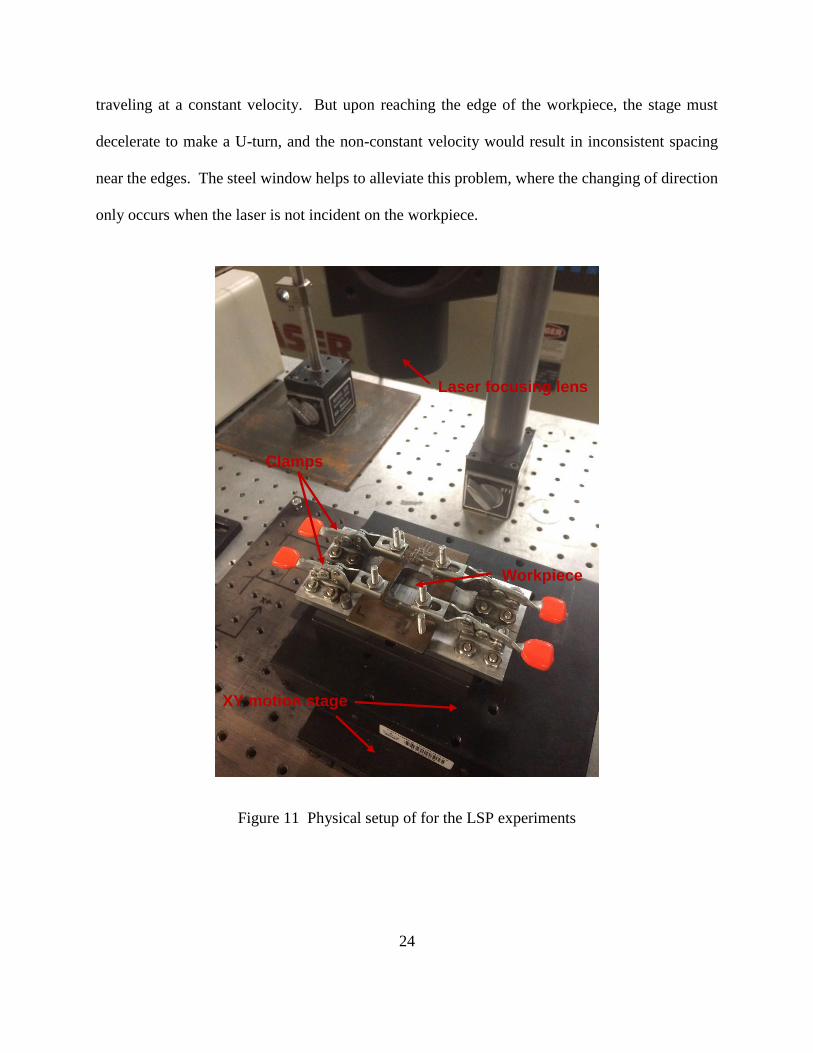
24

traveling at a constant velocity. But upon reaching the edge of the workpiece, the stage must

decelerate to make a U-turn, and the non-constant velocity would result in inconsistent spacing

near the edges. The steel window helps to alleviate this problem, where the changing of direction

only occurs when the laser is not incident on the workpiece.

Figure 11 Physical setup of for the LSP experiments

Laser focusing lens

XY motion stage

Workpiece

Clamps

25

LSP has traditionally been investigated and implemented as a tool for extending the fatigue lives

of materials. The compressive stress prevents surface micro cracks from propagating and

extending through the material, resulting in fatigue life improvements of about 3x, and as great

as 40x in specific configurations have been reported [37]. Compared to shot peening (which also

imparts compressive residual stresses on components), greater depths of affected regions are

attained and less surface damage is induced by LSP. One of the most influential applications on

which this has been performed is to extend the lifetimes of turbine blades in aircraft engines.

Since deformation in LSP occurs from the shockwave propagation, the material characterization

and analysis of deformation mechanisms has warranted intensive investigations. In the past, the

Manufacturing Research Lab at Columbia University has been a significant contributor to the

field, particularly regarding micro scale LSP. The defining feature of micro-LSP is that the

beam spot size is roughly the same size as the individual grains of the material [38], where in

conventional LSP spot sizes on the order of millimeters are often used, so that grain orientation

and anisotropy becomes of focus. Precision for LSP processing of micro-devices can thus be

achieved, but many additional mechanical and metallurgical areas of consideration arise.

Spatially resolved measurement of residual stress and dislocation distribution was achieved by

Chen et al., which required the use of a synchrotron light source in order to generate the large

amount of X-rays required for X-ray diffraction at the microscale [39]. A finite element

technique was developed by Fan et al., and modelling of the material as a hydrodynamic

substance was required in order to accurately describe the deformation and high strain rates

incurred by the shock waves [35]. In the model, the effects of shock waves propagating from

both the top and bottom of the work piece (dual sided LSP) was analyzed, and the phase

difference between the opposing shockwave greatly impacted the resulting stress distribution.

26

Vukelíc et al. analyzed the response of a bi-crystal that was hit with an incident LSP impact on

its grain boundary in terms of lattice rotation [40].

With the establishment that LSP is beneficial for fatigue life improvement, new applications of

the process are now being explored. The ability of LSP to prevent SCC has been identified as an

area of increasing significance, and this becomes the focus of the latter part of this thesis.

Various researchers have shown an improvement to stress corrosion cracking resistance after

LSP treatment [41][34], but an understanding of the underlying reasons why and how the

improvement occurred has not been fully developed. Since SCC is a complex phenomenon, the

many different forms that it can take may account for a lack of understanding because no

unifying theory as to the mechanism of mitigation can be found. Instead, the details regarding

microstructural changes by LSP, and how they interact with each different form of SCC,

becomes necessary in order to understand each scenario.

1.4 Organization and Objectives of Dissertation

Increasing the strength of joints formed via autogenous laser brazing is presented in Chapter 2. By

shaping the interface into a cup/cone geometry, where the tip of the stainless steel protrudes into

the cone shaped end of a NiTi wire. The interfacial surface area is thereby increased, resulting in

decreases to the stress intensity factor. Additionally, the cup/cone geometry ensures that proper

alignment is maintained during rotation of the wires, where the rotation provides a uniform heat

input to minimize the temperature gradient throughout the thickness of the wires. A thermal model

is developed to determine the temperatures reached at the interface and to thus help guide the

selection of processing conditions. The widths of the mixed interfacial regions are analyzed with

energy dispersive X-ray spectroscopy. Quantification of the joint strength is carried out by tensile

27

testing the specimens to fracture. While both the incident laser power and rotation speed are found

to significantly influence the fracture strength, samples with sharper angles (and therefore larger

interfacial areas) are found to consistently be stronger.

The material pair of NiTi and stainless steel have many potential biomedical applications, and as

such, the biocompatibility of joined samples is investigated in Chapter 3. Using the cup/cone

autogenous laser brazing process, polarization testing, electron microscopy, nickel release rate,

hemolysis, and cytotoxicity testing are subsequently performed. The polarization testing enables

the individual material behavior in a corrosive environment to be quantified and input as

parameters into a finite element model that predicts the corrosion currents formed. Dissimilar

materials form galvanic couples when placed in a corrosive environment, causing one of the

materials to preferentially corrode, and this behavior is captured in the model. Another concern is

that the laser heating may damage the protective oxide layer of the NiTi. But since autogenous

laser brazing is capable of precise control over the heat input, the biocompatibility of the joined

samples is found to be nearly as safe as the base material.

In the second portion of this thesis, using lasers to directly reduce stress corrosion cracking

susceptibility is performed. Chapter 4 presents laser shock peening on stainless steel, high strength

steel, and brass to analyze their various responses, and to identify to material properties which

govern the behavior. Cathodic charging of the samples is performed to accelerate the rate of

hydrogen absorption, for which absorbed hydrogen is the root cause of several SCC failure

mechanisms. Once hydrogen has been absorbed, it can stress the lattice causing increases in the

hardness. Comparison of the hardness changes of untreated samples to treated samples shows that

the LSP process does indeed reduce the amount of hydrogen damage. Using mechanical U-bend

28

testing, confirmation of the benefit was found, where LSP treating increased the time to failure of

U-bend samples when exposed to corrosive environments. Work function measurements by

Kelvin Probe Force Microscopy and a discussion of dislocation generation describe the reasons

for the behavior.

Chapter 5 continues the mitigation of stress corrosion cracking onto a microscale level,

determining the changes to the microstructure that influence the corrosion resistance. In stainless

steel, sufficient concentrations of absorbed hydrogen can induce a phase change from austenite to

martensite, resulting in weakening of the material to SCC. X-ray diffraction measurements are

performed to detect this phase transformation on cathodically charged samples. LSP processing

is found to restrict the formation of martensite. Transmission electron microscopy of the stainless

steel then illustrates the microstructure changes accounting for the mitigation, particularly the

generation of dislocations and their arrangement into dislocation cell structure. Finite element

modelling of the shockwave deformation process is coupled to dislocation generation, providing

spatially resolved data of the dislocation densities.

29

Chapter 2: Beneficial Interface Geometry for

Laser Joining of NiTi to Stainless Steel Wires

2.1 Introduction

In order to exploit specific material properties in different places of products, it is often

beneficial to join dissimilar materials. Joining dissimilar materials can help to optimize toughness,

wear resistance, chemical resistance, thermal properties, hardness, flexibility, etc. Many types of

dissimilar materials can be joined (ceramics, composites, polymers), but this paper will focus on

the joining of dissimilar metals.

Due to some of its unique properties, nickel titanium (NiTi) is receiving increasing use,

especially in such devices. NiTi has good biocompatibility, which makes it ideal for implantable

medical devices. NiTi can allow for less invasive procedures because of its shape memory effect

and superelasticity. Some examples of current NiTi applications are stents, Simon vena cava vein

filters, and atrial Septal defect occlusion systems [1]. Obviously, implantable medical devices are

not made simply out of a single material, which is why techniques for joining NiTi to other

materials must be explored. A common pair is joining nickel titanium to stainless steel (SS), using

stainless steel where NiTi is unnecessary. Using stainless steel in places where shape memory and

superelasticity are not required can help to reduce the part cost, as well as exploit some of the

properties of the stainless steel where desired.

The process chosen for joining a dissimilar material pair is heavily dependent on the

composition of the materials of interest, and also on the specifications for the finished product [2].

Possibly the simplest way to join dissimilar materials is by using adhesives. Adhesives are

sensitive to temperature, and their strength heavily relies on the amount of moisture that is

absorbed [3,4]. Clearly this is not viable for implantable medical devices. When heating processes

30

are used for joining, many dissimilar metal pairs have a tendency to form brittle intermetallic

phases [5]. In response, several different methods to minimize the amount of intermetallic

formation have been reported. One proposed method is to use friction stir welding. This process

reaches lower temperatures, and thus may help minimize intermetallic formation [6]. Friction stir

welding of magnesium and aluminum has been shown to be possible, but it was found that the

hardness across the joint became twice that of the base materials [7]. Fracture occurred at the point

with the highest hardness gradient. Significantly changing the material properties is undesirable,

and it was also found that there was a very narrow range for working parameters (rotation speed,

weld speed). Also, friction stir welding is not easily applied to the wire geometry currently of

interest. Another method is to melt a filler material that is placed between the two materials, and

never directly melt the base materials. When choosing a filler material, it is important that its

thermal expansion properties are similar to the materials being joined, otherwise large residual

stresses will form. Nickel-chromium filler materials are often used when joining stainless steels,

since they have comparable thermal properties [2]. Using zinc as a filler, Mathieu was able to

achieve tensile strengths of 240 MPa when joining aluminum to stainless steel [8]. But, it is also

possible to take advantage of the large difference of melting temperature between these materials.

Stainless steel has a much higher melting temperature than aluminum. By laser irradiating the

stainless steel side, the heat will conduct across the interface and melt the aluminum [5]. This

eliminates the need for a filler material, but is restricted to material pairs with large melting

temperature differences.

The dissimilar metal pair of NiTi and stainless steel, which is of interest to the medical

world, does not have a very large melting temperature difference. With the use of an 80 µm wide

copper filler material between NiTi and stainless steel wires, Li et al. was able to achieve a tensile

31

fracture strength of 521 MPa [9]. But without the use of a filler material, they only reached a

maximum strength of 187 MPa. Since the addition of filler materials is undesirable because it

causes additional biocompatibility concerns, increasing the strength of joints without using filler

materials is preferred. A process for joining nickel titanium and stainless steel wires together,

without using a filler material, was proposed by Satoh et al.[10]. As noted by Bao et al., when

scanning a laser across a material, temperature spikes will occur as the laser approaches the trailing

edge [11]. At the edges of the material, the heat cannot be conducted away by surrounding

material. This spatial isolation of temperature peaks is the driving force behind Satoh’s method.

Their process, however, is limited in that it is difficult to apply uniform heating at the interface for

larger diameter wires. This paper will introduce a method that can be applied to thicker wires. In

joining processes, the interface geometry can be altered to maximize the effectiveness of the

process being used. For example, including an extra lip of material along the top of a seam to be

electron beam welded can provide material to fill any gaps that form [12]. To evenly heat the

thicker wires currently of interest, they will be rotated during laser irradiation. A cup and cone

interfacial geometry was proposed by the authors in a previous work [13], and will be investigated

here. This will help to keep the wires aligned during rotation, and also increase the surface area

of the interface, resulting in higher strength. The tip of the stainless steel wire is shaped into a

point, and the nickel titanium is shaped as an inverted cone, whereby the stainless steel can fit into

it. This results in a net increase of surface area of the interface, without increasing the outside

diameter of the joint. Cones with different apex angles were analyzed. To allow for even heat

distribution, the wires were rotated while being irradiated. The effect that different laser power

levels had on each of these angles is presented.

32

2.2 BACKGROUND

2.2.1 Ternary Phase Diagram and Brittle Intermetallics

Two of the most useful properties of nickel titanium are its superelasticity and shape

memory effect. The superelasticity is due to a diffusionless martensitic transformation that occurs

under large strains. This transformation is from austenitic BCC B2 into an HCP B19 crystal

structure. The Clausius-Clapeyron relation indicates how, under an induced stress, martensite can

form at temperatures higher than the martensite start temperature Ms [14]. During the

transformation, detwinning of the martensite accommodates extensive deformation at a uniform

stress. When nickel titanium has been deformed in its martensitic (low temperature) phase, heating

to the austenitic phase will cause it to recover its original shape; this is the shape memory effect.

Figure 1 Ternary phase diagram for Fe-Ni-Ti at 1173 K [13]

One of the biggest concerns when joining dissimilar metals is the formation of brittle

intermetallic phases. Intermetallics form in very specific proportions, and have crystal structures

that differ from the original base materials. Electrical, mechanical, magnetic, and chemical

33

properties may be different from the base materials as well [15]. The specific ratios they form in

makes it possible to identify phases present in a sample by using EDX analysis. Many

intermetallics are subject to brittle fracture and suffer from a low crack tolerance. Their complex

crystal structures have large Burgers’ vectors, so it often requires less energy for fracture than for

dislocation movement. A ternary phase diagram for titanium, iron, and nickel is shown in Figure

1 [16]. This is at 1173 K, about 400 K below melting temperature for the NiTi. For simplification,

we neglect the effects of the chromium that is present in the stainless steel. Chromium behaves

similarly to the titanium, and there is much less of it than the other three materials [17]. Fe2Ti is a

Laves phase, and has some unique magnetic properties [18]. But, its C14 hexagonal structure is

quite brittle [19]. The other common intermetallic formed is FeTi. Large regions of FeTi have

been shown to decrease the tensile strength of the joint [20]. Nickel titanium and stainless steel

have different thermal expansion coefficients, and van der Eijk et al. concluded that this difference

could result in residual stresses and initial cracks within the intermetallic layer [21]. Using a nickel

interface layer may help to lessen the amount of brittle intermetallics formed, but it will not

completely prevent their formation [21]. Shortening the time period that the base materials are at

or above melting temperature will limit intermetallic formation as well. Borrisutthekul et al. found

that placing a heat sink with a large thermal conductivity next to the joint lowered the amount of

intermetallics formed when joining steel to aluminum [22]. If over-melting occurs at the interface,

iron from the stainless steel can substitute for the nickel in the NiTi’s austenitic phase, lowering

the martensitic start temperature Ms and allowing for the formation of an R phase [23]. This

lowered Ms and decrease of nickel concentration will also result in the superelastic plateau

occurring at a higher stress [14].

34

Phase change is not limited to the interface. The heat affected zone of the base materials

will also undergo some changes. Precipitates in the base NiTi will increase, which also results in

lowering the Ms temperature [24]. Once the NiTi has recrystallized, the thermodynamic

parameters will remain nearly constant though [25]. Overall, to increase the fracture strength of

the NiTi to stainless steel joints, it is necessary to minimize the amount of brittle intermetallic

phases that form [26].

2.2.2 Geometrical Considerations

Characterization of the quality of each joint is based on its tensile testing results. Since the

dissimilar material pair has different Young’s Moduli, the stress-strain response does not have a

clear, direct interpretation. Thus, the most important characteristic is the load at fracture for each

joint. The fracture strength of joints can be increased by distributing the load over a larger surface

area. Different interface geometries can be used to increase the contact area, without increasing

the overall size of the part. Increasing the surface area will decrease the stress concentration on

the interface, but sharper angles may have detrimental effects on surface wetting [27]. This places

a limitation on the geometries in that they must not be too complex. One possibility is to make a

U slot, and slide one piece around the other. Vaidya et al. used this method for butt welding plates

of aluminum AA6605 and titanium Ti6Al4V [28]. Fracture occurred in a heat affected zone, and

not at the interface itself. The simplest way to increase the interface surface area for wires is to

cut the ends at an angle, in the fashion of a scarf joint. This will result in an increase of surface

area, given by 𝐴 =𝐴𝑜

cos(𝜑), where Ao is the cross sectional area of the wires, and φ is the angle

between the normal of the surface and the longitudinal axis of the wire. This is a viable option to

be applied to the 381µm diameter wires that Satoh explored [29]. But, the wires of current interest

have twice that diameter. Getting the heat to conduct through thicker wires and evenly melt the

35

interface is not viable. Overheating must be avoided. As simply melting the base NiTi, without

any mixing or intermetallic formation occurring, can decrease the tensile strength of the wire by

as much as 30% [30]. One solution is to use multiple lasers, and simultaneously irradiate the top

and bottom of the sample [28]. But due to the rotational symmetry of the wires, an alternative

method is to use a single laser source while simultaneously rotating both of the wires during the

laser scan. This paper will make use of this wire rotation.

Figure 2 Schematic diagram describing the geometry used. Point 1 is at the apex of the cone,

point 2 is on the outside edge.

To increase the interfacial surface area, a cup and cone geometry is proposed, as shown in

Figure 2. In a way, this is like an axisymmetric scarf joint about the longitudinal axis of the wires.

The stainless steel will be shaped into a point, while the end of the NiTi is drilled out in the shape

of a cone. An angle θ is defined as the apex angle of the cone. Two different apex angles will be

analyzed (90° and 120°) and their strengths compared to wires without the conical interfaces. The

90° cones will have an interface area of 0.645 mm2 while the 120° cones will be 0.527 mm2, which

are 41% and 16% larger than a flat interface, respectively. Of course, this increased surface area

is not normal to the direction of loading. As such, we do not expect the effect due to this increased

surface are to be equal to this same percentage increase. An additional benefit of the conical

interfaces is that they help to keep the wires aligned during rotation.

36

2.2.3 Stress Intensity Formulation

Stress intensity in uniaxial tension along a crack, away from the free edges, oriented at an

angle is given by [31]:

𝐾𝐼 = 𝜎√𝜋𝑎 ∗ 𝑠𝑖𝑛2𝜃

2

𝐾𝐼𝐼 = 𝜎√𝜋𝑎 ∗ 𝑠𝑖𝑛𝜃

2𝑐𝑜𝑠

𝜃

2

(1)

where σ is the applied stress, a is crack length, 𝜃

2 is the angle between the applied load and the

crack. We assume that the cracks formed will be in areas that did not melt along the interface, and

also that the fracture will propagate along the joint interface within the intermetallic layer.

Therefore, the cracks will be oriented 𝜃

2 degrees from the direction of loading as well. Figure 3

shows these K values for various interfacial angles. For an ideally brittle material, 𝐾𝐼𝐼𝐶

𝐾𝐼𝐶= 1.2 [32],

where KIIC is mode II fracture toughness and KIC is mode I fracture toughness. From the graph we

see that as the angle decreases (sharper cones on the wires), both KI and KII decrease. This effect

is due to the increase of surface area on the interface. In order to exploit the higher KII value, it is

preferable to introduce some shear component along the joint. Figure 3 indicates that the lowest

stress intensity, and therefore the strongest joints, is a result of having smaller apex angles. But,

as the cone becomes sharper, heating along the interface will become less uniform, and complete

joining may not be possible.

37

Figure 3 Mode I stress intensity (KI) and Mode II stress intensity (KII) versus angle of interface,

for a constant uniaxial load. The interfacial area is superimposed over-top, indicating that as the

cones become sharper, the area increase results in a decrease of stress intensity.

Stress singularities will form at the traction free edges of dissimilar material joints [33] and

are dependent on the joining angles as well as the difference of material properties (i.e. Poisson’s

ratio and Young’s Modulus). For a 2D plane stress situation with dissimilar materials bonded at

an angle α (corresponding to ∝= 90° −𝜃

2, for θ defined in Figure 2) under uniaxial tension σo, the

stress components along the interface can be expressed as [34]:

𝜎𝜃 = 4𝐴(

𝛾2

𝑠𝑖𝑛2(𝛼))𝜒1(𝑧, 𝛼, 𝜅)𝑒

−2𝛾𝑧∗cot(𝛼) + 𝜎𝑜𝑠𝑖𝑛2(𝛼)(𝑛𝑜𝑟𝑚𝑎𝑙)

𝜏𝑟𝜃 = 4𝐵 (𝛾2

𝑠𝑖𝑛2(𝛼))𝜒2(𝑧, 𝛼, 𝜅)𝑒

−2𝛾𝑧∗cot(𝛼) − 𝜎𝑜𝑠𝑖𝑛(𝛼) cos(𝛼)(𝑠ℎ𝑒𝑎𝑟)

(2)

where A,B are constants, 𝑧 =𝑟

𝑤∗sin(𝛼), γ are roots of a characteristic equation, χi are oscillating

functions, and 𝜅 =−𝛾∗sin(𝛾)

cos(𝛾). The significance of these equations is that the first term of both the

normal and shear stresses contains an exponential decaying with distance from the free corner.

Thus, away from the edges in the bulk of the material, the shear and normal stress components are

constant for each respective interface angle. It has been shown [34] that even for very sharp angles,

38

the stress singularity will not result in more than a 7% deviation from the uniform stress in the

bulk of the material. This increase of stress at the free edge may result in failure initiating there,

but due to the relatively small magnitude the benefit of introducing a shear component outweighs

this effect.

2.2.4 Process

The NiTi is the material that will be irradiated, since it has a lower melting temperature

than the stainless steel. Starting the laser a fixed distance away, and then scanning at a constant

velocity towards the interface will result in heat accumulation along the interface. Once the NiTi

reaches its’ melting temperature and joins onto the stainless steel side, the thermal conduction

across the interface increases. A rapid cooling rate is desired for joining NiTi to stainless steel

[29]. Since the stainless steel is at much lower temperatures than the NiTi, this desirable rapid

cooling will occur. At the same time, both the wires are spun at a constant angular velocity, helping

to ensure uniform heating. Along joint interfaces, the irradiated material will contract as it is

cooled [12]. Since the conical portion of the NiTi encases the stainless steel, as this contraction

occurs the NiTi will squeeze onto the stainless steel wire.

2.2.5 Thermal Modeling

Heat input from the laser is the only parameter we can control during the joining process,

thus 3D thermal modeling was performed to help choose parameters. The heat flux of the laser

was modeled as a Gaussian distribution with a spot size of 800 µm. At the interface, the initial

thermal resistance is large, which results in thermal accumulation. But once the interface has

melted, this resistance decreases significantly. To simulate this changing conductance across the

interface, a thin thermally resistive layer was placed between the NiTi and stainless steel. By

39

equating the heat flow in the definitions of convection and conduction heat transfer, we can get the

relationship

ℎ = −𝑘

∆𝑥. (3)

where h is the heat transfer coefficient per area, k is the thermal conductivity, and ∆x is the width

of the resistive layer. The non-melted NiTi-SS interface has h=79 W/m2K [35]. Values for k and

∆x were set to give this initial ratio. A temperature dependent step function was associated with

∆x, so that once each node of the interface reached its melting temperature, the value of ∆x would

decrease, thus increasing the conductance. According to the Hagen-Ruben Relation, laser

absorption can be calculated as:

𝐴 = √8𝜀𝑜𝜔𝜌 (4)

where εo is the permittivity of free space, ω is the angular frequency of incident radiation, and ρ is

the electrical resistivity of the material [36]. Electrical resistivity is proportional to temperature,

and thus absorptivity increases as the temperature is increased. The most dramatic increase of

absorptivity is when the material changes from a solid to a liquid. Since in this process melting is

limited to the interface, we make the simplification of using a constant resistivity. An electrical

resistivity of 5.48E-7 Ω m was used, which is the value for titanium at 333K [37]. The value for

titanium is applicable since the titanium oxide layer that forms on the surface of the NiTi is similar

to the surface of titanium. A laser with wavelength of 1064 nm was used, resulting in an

absorptivity of 26%. Convective cooling from the argon flow is present on the outside surface of

the wires. The convective heat transfer coefficient was calculated using the Zhukauskas

Correlation [38]:

𝑁𝑢𝐷 = 𝐶𝑅𝑒𝐷𝑚𝑃𝑟𝑛 (

𝑃𝑟

𝑃𝑟𝑠)14

(5)

40

ℎ = 𝑁𝑢𝐷𝑘

𝐷

(6)

where 𝑁𝑢𝐷 is the average Nusselt number, 𝑅𝑒𝐷 is the Reynolds number, Pr is the Prandtle number,

k is thermal conductivity, D is the wire diameter, and C & m are constants determined from the

Reynolds number. Using a kinematic viscosity for argon of 1.41E-4 m2/s [39], the Reynolds

number was calculated as 0.92, resulting in ℎ = 12.7𝑊/𝑚2𝐾. The 3D heat equation was

implemented in COMSOL. Although the temperature distribution was not directly measured, the

trends predicted by this thermal model will be shown to be consistent with experimental results.

2.3 Procedure

For this study, NiTi and hard tempered SS304 wires of diameter 762 µm were used. The

NiTi wires had a composition of 54 at% titanium and 46 at% nickel. Initially in the austenitic

phase at room temperature, the NiTi undergoes a stress induced phase transformation at 480 MPa.

The angles of the points analyzed on the stainless steel samples were 90° and 120°, with

corresponding values for the NiTi. In order to create the cones on the ends of the stainless steel

wires, they were placed into an angled block, and then spun at 5000 rpm against 320 grit silicon

carbide abrasive paper. To create the cups in the ends of the NiTi, 1143 µm diameter spot drills

were used, with corresponding tip angles. After shaping, the wires were washed with acetone in

an ultrasonic bath.

The NiTi wires were fastened into a rotary stage, while the stainless steel wires were placed

in an un-driven ball bearing fastened onto a sliding linear stage. An axial load of 2 Newtons was

applied to the linear stage. Argon was flowed into a chamber surrounding the wires at 10 scfh. A

SPI redENERGY G4 fiber laser operating in CW mode at a wavelength of 1064 nm was used.

41

Power levels of 13-17 W were analyzed in single watt increments. Laser spot size was 738 µm.

The wires were rotated at angular velocities of 3000°/sec, 2500°/sec, and 2000°/sec. The laser

spot started 1.6 mm away from the interface, underwent 18,000° of total rotation, and stopped 0.1

mm short of the interface. This corresponds to laser irradiation times of 6 s, 7.2 s, and 9 s for

3000°/sec, 2500°/sec, and 2000°/sec rotations, respectively.

Tensile testing was carried out according to ASTM E8-11 standards [40]. An Hitachi-

S4700 SEM with energy dispersive X-ray spectroscopy (EDX) attachment was used for the

compositional analysis.

2.4 Results & Discussion

2.4.1 Temperature Profile

Figure 4 Longitudinal sectioned time snapshot of thermal accumulation in 90° cones.

Corresponding times are: (a) 1s, (b) 4s, (c) 6.8s (laser has shut off). Laser location indicated by

white dotted line. Power: 15W, Angular velocity: 3000°/s

In Figure 4, a longitudinal section view of the wires is plotted displaying temperature at

three different times during the laser scan. As the NiTi wire begins to heat up, the interfacial

resistance causes thermal accumulation. This indicates that most of the melting should be limited

to the interface, which is desirable. If excessive melting occurred along the whole path of the laser

scan, the wire would lose its structural integrity and deform. The rotation of the

42

wires allows the hot temperature to be able to reach the extents of the NiTi cone, both points 1 and

2. Had the wires not been rotated during irradiation, insufficient heat would have been able to

conduct to the apex. Once the interface has melted, the NiTi wets onto the stainless steel side, and

the thermal resistivity across the interface decreases. The third time snapshot is after wetting has

occurred, and the stainless steel wire is seen to heat up.

Figure 5 Uniformity along line segment 1-2 on the interface. As the angular velocity is

increased, the thermal distribution becomes more even and the average temperature rises.

An even temperature distribution along the interface is desired, since this will allow for

uniform melting. Figure 5 displays the temperature distribution along the line segment from points

1 to 2 at the moment the laser has completed its scan. Of the three different angular velocities,

3000°/s has the flattest temperature distribution. It is also apparent that increasing the angular

velocity increases the average temperature of the interface, despite having a shorter interaction

time with the wire. As the wire is being spun faster, the input heat flux from the laser beam behaves

more like a uniform ring of heat around the circumference of the wire, as opposed to a single point

source. The overall power from the laser is the same, but the uniform heating may decrease the

43

temperature gradient in the vertical direction, resulting in less heat being conducted away. Figure

6 displays the time history for points 1 and 2, and for points on the top and bottom of the interface

of wires with flat interfaces that were not rotated during irradiation.

Figure 6 Time history of points 1 and 2 along the interface from Figure 2, compared to points at

the top and bottom of the interface of wires with flat interfaces. Temperature difference between

the 2 points on the rotated wires throughout the laser scan is minimal. Laser power is 15 W for

the rotated wires, and 35W for the flat interfaces.

We are looking for the maximum temperature difference along each wire’s interface. From

the symmetry, the largest temperature difference on the rotated wires is between the outside point

2 and the apex point 1. For the non-rotated wires, the largest difference is between points at the

top and bottom of the interface. At 1.5 seconds, the top of the flat wires is nearly 1700 K, while

the bottom is only 1400 K. By examining longitudinally sectioned samples that were not rotated,

we see that often the top is overmelted, while no melting occurs at the bottom. This is consistent

with the predictions of the thermal model. If laser power is increased to allow for the bottom point

to reach melting temperature, the top point will reach excessive temperatures. The temperatures

44

at the two points on the interface that was rotated reach the melting temperature at nearly the same

time, which will results in good uniformity of the joint.

2.4.2 Joint Morphology

Figure 7 Images of four different combinations of power and cone angle. The outer surface near the joint of the 90°

wires experienced more deformation. Rotational velocity is held constant at 3000°/s.

45

Outside images of four of the joints are presented in the Figure 7. Most apparent is the

effect of thermal accumulation, in that the majority of the melting occurs in the NiTi near the

interface. More melting is evident in both of the wires that are at 15 W. The interface for this

power level tends to bulge out more than it does at 13 W. But for their respective power levels,

the 90° wires tend to have a larger belled region than the 120° wires do. The cone is deeper in the

90° wires, so the walls near the end of the NiTi are much thinner for a longer distance. It takes

very little heat to melt these thin walls, which may result in the apparently larger melted region of

the 90° wires.

Figure 8 Longitudinal section image of a 120° cone processed at a power of 15W. The arrows

indicate the paths of EDX line scans.

Longitudinal section images of samples from 15 W and 17 W are presented in Figures 8

and 9. In both of the images, the cup and cone geometry is still intact. Along the angles of the

interface, a possibly mixed region is visible. These regions will be analyzed via EDX. In the 15

W wire, joining is apparent throughout the center of the wire. But within the mixed region, two

46

large circular defects are present. Also, joining is not apparent at the apex of the cone. This region

will act as an initial crack during tensile testing, resulting in a lower fracture strength. The apex

of the 17 W wire also does not appear to have complete joining, yet excessive deformation occurred

on the outside. Therefore, continuing to increase the power will not result full joining of the

interface. Alternatively, varying other parameters, such as angular velocity, could help to achieve

more melting at the apex.

Figure 9 Longitudinal section image of a 120° cone processed at a power of 17W. Excessive

melting and deformation is present on the outer surface.

2.4.3 Composition

The width of the mixed region, where brittle intermetallics will form, is critical to the

fracture strength of each joint. Typical results for wires irradiated at 13 W and 15 W are analyzed.

EDX line profiles were acquired along arrows I, II, and III indicated in Figure 8. The distance

between scan points is 0.34μm. Electron beam parameters were adjusted so that a detection rate

of 1500 counts/sec was achieved. A line profile for II is displayed in Figure 10. The region from

37 µm to 65 µm is where mixing of the NiTi and stainless steel occurred. All of the scans along

II and III for both power levels had very similar shape, with just the width of this mixing layer

47

being the only difference. An abrupt transition happens between the mixed region and the base

materials. To determine which phases are forming, we compare the compositions to the ternary

phase diagram of Figure 1. Since it does not appear on the phase diagram, the amount of chromium

is neglected, which will slightly increase the concentrations from those displayed on the line scan.

Two peaks stand out: one where titanium reaches nearly 50% and the other where nickel reaches

nearly 50%. For both of these, the iron level is between 10-20%. Comparison with the phase

diagram indicates that these are regions of (Fe,Ni)Ti.

Figure 10 EDX line scan across line II, indicating the mixing occurring in the joint. Sample

irradiated at 13W.

The widest mixing zone occurred on II for the wire processed at 15 W shown in Figure 11,

with a width of 33 µm. Instead of having a flat trend along the length, this joint has more of a slow

transition from the NiTi to the stainless steel. This is evidence that diffusion of the materials has

taken place. The thinnest mixing zone occurred on II for the wire processed at 13 W, with a width

of only 18 µm. Analysis on I for both samples showed no mixing zone, indicating that joining did

not occur at the centers. As is expected, the mixing for the 13 W sample is consistently lower than

that of the 15 W.

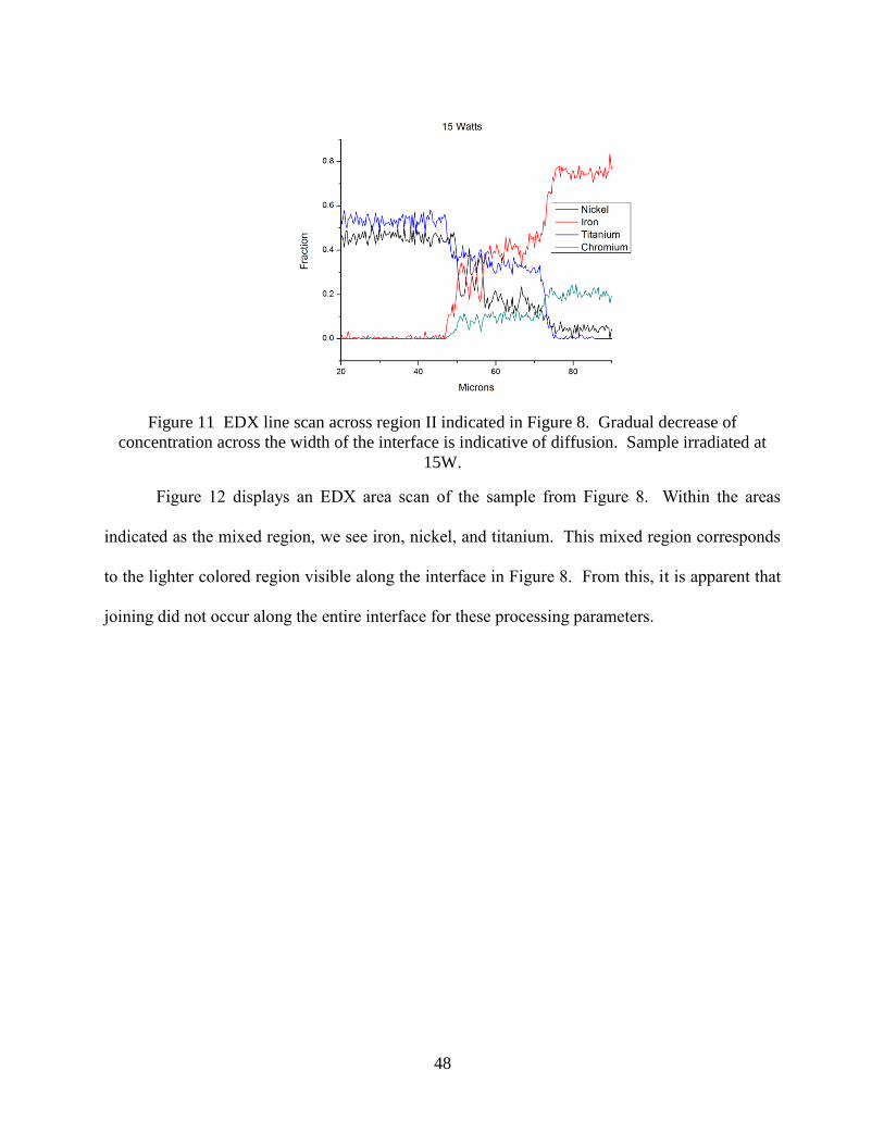
48

Figure 11 EDX line scan across region II indicated in Figure 8. Gradual decrease of

concentration across the width of the interface is indicative of diffusion. Sample irradiated at

15W.

Figure 12 displays an EDX area scan of the sample from Figure 8. Within the areas

indicated as the mixed region, we see iron, nickel, and titanium. This mixed region corresponds

to the lighter colored region visible along the interface in Figure 8. From this, it is apparent that

joining did not occur along the entire interface for these processing parameters.

49

Figure 12 EDX compositional map, corresponding to the longitudinal sectioned image of Figure

8, showing iron (red), nickel (green), and titanium (blue). Laser power is 15W. A mixing region

is observed along the interface, the width of which decreases towards the center of the wire.

This indicates that the lighter colored regions along the interface of the longitudinal sectioned

images are indeed the mixed regions.

2.4.4 Joint Strength

Different rotation speeds have different laser interaction times, so slower rotations allow

for more heat input. But at the same time, slower rotation speeds also allow for more heat to be

conducted away, resulting in lower interface temperatures. Characterizing the laser parameters by

the total amount of energy input (power x time), is unable to capture both of these effects [41]. As

such, strengths for different rotation speeds are plotted separately as a function of power. The

average load at fracture for a sample of wires processed at a rotation speed of 3000°/sec is

presented in Figure 13. For both the 90° and 120° wires, an upward trend with power is evident.

Also, as the power increases the variance in tensile strength decreases. This higher consistency is

50

attributed to the excess melting that occurs under the higher powers. When the wires are being

rotated under the laser, there is some slight unavoidable alignment error. At 17 W, the large melt

pool is able to fill in the gaps that are not perfectly aligned. This does not occur at the lower power

levels, and thus they will be more sensitive to the alignment. For 13 W through 16 W, the 90°

angle wires have higher average fracture strength than the 120° angle wires. This is consistent

with the idea that increasing the interface surface area will allow for higher fracture loads. But, at

17 W, the 120° wires have a higher average load. It is possible that at this higher power, the

increased surface area allowed for more formation of brittle intermetallic phases.

Figure 13 Increase of load at fracture with increasing laser power input. Standard error for each

level is indicated. Note that the 90° wires are stronger than the 120° wires at every power except

for 17W.

The axial load causes the cross sectional area of the joint to increase during processing.

This effect may cause some misinterpretation of Fig 13. The loads at fracture for various rotation

speeds have been normalized by the cross sectional area of the fracture, and are plotted in Figure

14. Here we see that the fracture strength will actually decrease with overheating. This is evidence

that too much mixing occurs at the higher power levels, and therefore large amounts of brittle

intermetallics are forming. At 3000°/sec and 14 W, the 90° wires have an average strength of about

51

310 MPa, which is the highest level reached for this rotation speed. The highest strength of 270

MPa for the 120° wires occurs at 15 W. The ideal power level is where a minimum yet sufficient

amount of melting occurs. With their sharper angle, the 90° wires overlap more than the 120°

wires, resulting in better contact. The amount of melting at 14 W may be ideal to join the 90°

wires together, but the 120° wires need slightly more melting in order to overcome some small

misalignment effects.

In Figure 14, the difference in strength between the 90° and 120° interfaces rotated at the

slower velocities is much more pronounced than the wires irradiated at 3000°/sec. From the

thermal model, we know that the wires at higher rotation speeds reach higher temperatures. Thus,

the strength results indicate that the samples at 3000°/sec overmelt, mix, and negate the effect of

the different interface angles. For the 2500°/sec samples, the 90° wires irradiated at 14 W had an

average fracture strength of 374 MPa, which is the highest level achieved. The highest level

achieved for the 2000°/sec samples of 342 MPa occurred at 15 W. The additional power necessary

to reach the peak for the samples processed at slower rotational speeds is again consistent with the

thermal model results presented in Figure 5. Since the strongest samples fractured at levels below

the lowest possible superelastic plateau of 480 MPa, no complex stress distributions are occurring

at the interface from a phase transformation. The wires rotated at 2000 DPS have the longest

interaction time with the laser. While the wires rotated at 3000 DPS have the fastest processing

time, therefore less time for heat dissipation from conduction to occur. Yet, it is the 2500 DPS

rotation that gives the strongest result, suggesting that at this rotation speed, the effects of total

heat input and heat dissipation counteract each other in a beneficial way.

52

Figure 14 Stress at fracture over a range of power levels. The 90° wires are consistently stronger

than the 120° wires, which is consistent with predictions.

53

For all power levels, aside from 13 W at 3000°/sec, the 90° wires have the higher of the two

strengths. This chart is normalized to cross sectional area, but the overall interface area of the 90°

wires is still larger, indicating that increasing surface area due to different joint geometry can

increase the fracture strength of these wire joints. It is noted that standard stainless steel 304 yields

at 205 MPa. Clearly, the samples ran at 13-17 W are above this yield strength.

Figure 15 Comparison of fracture strength between two different angles. The percentage scale

on the left is how much stronger the 90° joint is compared to the 120° joint, for given power and

angular velocities. As the power is increased, the difference between the two geometries

reduces. This graph does not indicate which parameters gave the best overall results, but simply

indicates the difference between the two angles.

To compare the relative strengths between the two different apex angles, the percentage

increase in strength from the 120° wires to the 90° wires, at each respective power level and

rotation speed, has been plotted in Figure 15. As previously indicated, the overmelting that occurs

when the wires are rotated at 3000°/sec dominates over the joint angle, resulting in minimal, if

any, strength increase. The most pronounced difference in strength of the two geometries occurs

at the lower powers. Since the percentage increase of fracture strength is significantly higher than

the predicted difference in fracture toughnesses, clearly some other mechanisms are involved. The

sharper angles on the 90° cones allow for the wires to slide deeper into each other with more

54

overlap. Thus, upon rotation and before irradiation, the sharper angles stay in much better

alignment. At the low powers, where melting is minimal, alignment plays a huge role in the

strength of the joint. Any part of the interface that is not in contact with the other wire will not

join. As the power is increased, the strength difference of the two geometries rapidly converges to

zero. The overall strongest joint achieved (90° interface, 2500°/s rotation, 14 W) is about 150%

stronger than the corresponding parameter for the 120° cone.

Figure 16 Maximum average strength at fracture achieved for each wire geometry. Standard

error is indicated. The 180° samples are the non-rotated, flat interfaces. Both of the conical

wires have much higher fracture strengths.

For comparison, the fracture strength of wires of the same diameter with a simple flat

interface was also tested. These wires were held stationary, and irradiated at a power of 35W as

the laser was scanned towards the interface. Rotation of wires with flat interfaces was not viable,

since the centrifugal force felt by the wires causes them to separate away from each other at the

interface. As previously shown in the thermal model, rotation of the wires allows for more heating

across the depth of the wires. Since the flat wires were not spun, more power input was required

in order to achieve melting across the entire interface. The results are displayed in Figure 16, with

180° corresponding to the flat interfaces. The rotated wires were spun at 2500°/sec. We see that

the wires that had the cup and cone geometry, and were rotated during irradiation, are indeed

55

stronger than the non-rotated flat tests. The error for the rotated wires is also much smaller as well.

During processing of the flat interfaces, the high laser power required to melt the bottom of the

interface results in excessive melting of the top surface.

2.4.5 Fracture Surfaces

To better understand the differences of fracture strengths for various processing parameters,

the fracture surfaces of a set of samples was analyzed via SEM. These images are presented in

Figures 17 and 18. Combining high laser power with fast rotation of the wires results in large

amounts of melting at the interface, and thus a quite brittle joint. In Figure 17 we see a large region

of transgranular cleavage, with locally smooth fracture surfaces, which are indicative of brittle

fracture. The fracture surface of this sample did not occur along the initial cup/cone geometry, but

instead it occurred on a plane nearly perpendicular to the axis of loading. Overheating of this

sample results in a large width of the interface. This wide interface gives a crack more opportunity

to propagate through grains that are preferentially oriented to allow for low energy brittle fracture.

Figure 18 is a sample irradiated at a lower power, but higher rotational speed. With fracture

occurring at 393MPa, this was the strongest of all the samples.

56

Figure 17 Fracture surface indicating brittle transgranular fracture. 90° interface, 17 W,

3000°/s. Fractured at 200 MPa, along a surface not corresponding to the material interface.

When overheating does not occur, minimal changes are made to the base materials and thus

fracture will be restricted to the brittle intermetallic interface. As is expected, fracture occurred

along the conical geometry. Within this narrower interface, there will be a lower probability of a

grain being preferentially oriented for low energy fracture. The majority of Figure 18 is indicative

of quasi-cleavage, which has characteristics of both brittle and ductile fracture. Some parabolic

dimples are present in the lower right corner of the image, whose elongated shape is a result of the

shear component along the interface.

57

Figure 18 Fracture surface of a sample that broke at 393 MPa, which was the highest strength

achieved. The original cup and cone geometry was intact after fracture. Quasi-cleavage is

apparent, indicating a better joint than Figure 17.

2.5 Conclusion

The effect of using a cup and cone interfacial geometry for joining of NiTi-SS wires has

been explored. Rotation of the wires during laser irradiation was used. This rotation produced

much more uniform heating of the interface. Joints that had a 90° apex angle of the cone were

found to consistently have higher fracture strengths than the 120° cones. The optimal laser

power level for the 90° wires was 14W, while 15W for the 120° wires produced the strongest

joints. Overmelting of the interface tended to negate the effects of the interfacial geometry.

When overmelting did not occur, fracture was along the conical geometry. EDX analysis

indicated (Fe,Ni)Ti formation in a thin region along the interface with a decreasing width

towards the center of the wire. Even for the samples where excessive melting of the outside

surface occurred, the apex of the cone in the center of the wires did not sufficiently melt. Thus,

the effects on fracture strength that rotational velocity has was also explored. It was found that

increasing the rotational speed resulted in increased melting. Even though cones with sharp apex

angles are desirable with respect to the stress intensity formulation, limitations do exist for how

58

small of apex angles can be used. Temperature uniformity will decrease as the apex angle is

decreased. Also, the wall thickness of the NiTi cupped wires will decrease with sharper angles.

These thin walls will be more sensitive to overheating, and also may fracture from shear loads

that may be applied.

59

Chapter 3: Biocompatibility and Corrosion

Response of laser Joined NiTi to Stainless Steel

Wires

3.1 Introduction

Nickel titanium (NiTi) is a special material in that it is a shape memory alloy and exhibits

superelasticity. For shape memory, after the material has been deformed, heating above a

threshold temperature will cause the NiTi to return to its original shape. Superelasticity is the

capability of the material to withstand large amounts of strain, via a diffusionless phase

transformation.

These two properties have been found to be especially useful for developing medical

devices. For example, a stent made of NiTi can be compressed to fit inside a catheter, moved

into the desired position in the body, and then upon removal of the catheter the NiTi will spring

back into its original shape because of its superelasticity. NiTi can also be used for bone staples

and Simon vena cava vein filters [1]. The shape memory effect can be exploited by positioning

the NiTi as an actuator on the end of a wire, acting as scissors or graspers. In this type of setup,

the NiTi must be joined to a second material, to act as a foundation for movement. Stainless

steel (SS) is a common material to pair with nickel titanium. Joining can be accomplished via

adhesives, mechanical joints, or thermal processes such as welding or brazing. Cost reduction

can also be achieved by joining dissimilar materials.

For implantable medical devices, mechanical joints are too bulky, and adhesives will not

last in the corrosive environment of the body. Thermal joining processes often end up being the

preferred method. But electric spot welding of NiTi to NiTi has been shown to significantly

60

increase cytotoxicity [2]. Safer joining methods must be established. Further complicating

things, metallurgical issues arise when NiTi and stainless steel are joined. The phases formed by

mixtures of these two materials are brittle intermetallics [3]. Since one of the main reasons for

using NiTi is its flexibility, brittle joints are inadequate. Utilizing laser joining technology is a

common way to make effective NiTi-SS joints, as will be described later. Since these joints are

being placed in the body, it is important to ensure that they possess good biocompatibility.

Numerous studies determining the biocompatibility of the base nickel titanium and stainless steel

materials have been reported [4–6]. In general, both of these materials are considered as

biocompatible.

Most of the proposed methods of laser joining NiTi to stainless steel require using an

interlayer of a third material, which suppresses brittle intermetallics formation. The corrosion

response of samples using a copper interlayer was reported by Zhang et al. [7]. Commonly,

nickel is used as an interlayer as well. This can give good mechanical strength [8], but

introducing a third material (especially pure Ni) is undesirable because it will add more

biocompatibility concerns. If the polarization response of the interlayer is more active than the

other materials, galvanic concerns will be greatly enhanced from surface area considerations.

Investigations of the biocompatibility of NiTi laser joined directly to stainless steel to date have

not been reported. Previous publications by the authors described a process to increase the

tensile fracture strength of laser joined NiTi-SS joints [9,10] without the use of an interlayer, and

is referred to as “autogenous laser brazing”. Now, this paper will explore the biocompatibility

and corrosion response of this type of joint. Investigations into the nickel release rate,

cytotoxicity, hemolytic response, and corrosion morphology are made.

61

3.2 Background

3.2.1 Laser Autogenous Brazing

Nickel titanium is nearly equiatomic, and iron is the most prevalent element in stainless

steel. A Ti-Ni-Fe ternary phase diagram can thus be used to determine which phases are formed

when these three elements are melted and brought into contact with each other [11]. All of the

potential phases that form (NiTi2, FeTi, Fe2Ti, and Ni3Ti) are brittle intermetallics. Excessive

amounts of these brittle phases will decrease the fracture strength of the weld. Using lasers as

the input heat source can help to limit the formation of these phases by preventing overmelting.

Figure 1 shows a schematic diagram of the autogenous laser brazing setup. The laser starts a

fixed distance away, and is scanned at a constant velocity towards the interface. Simultaneously,

the wires are rotated, to ensure radially uniform heating. Thermal accumulation occurs at the

interface since there is a thermal resistance between the two wires. The thermal accumulation

results in a high localization of heating, so that only a very limited amount of the NiTi will melt

and then wet onto the stainless steel wire. Thus, a narrower region of intermetallics forms,

resulting in increased fracture strengths. For additional strength, the wires have been fashioned

into a cup and cone geometry, which provides mechanical benefits [9].

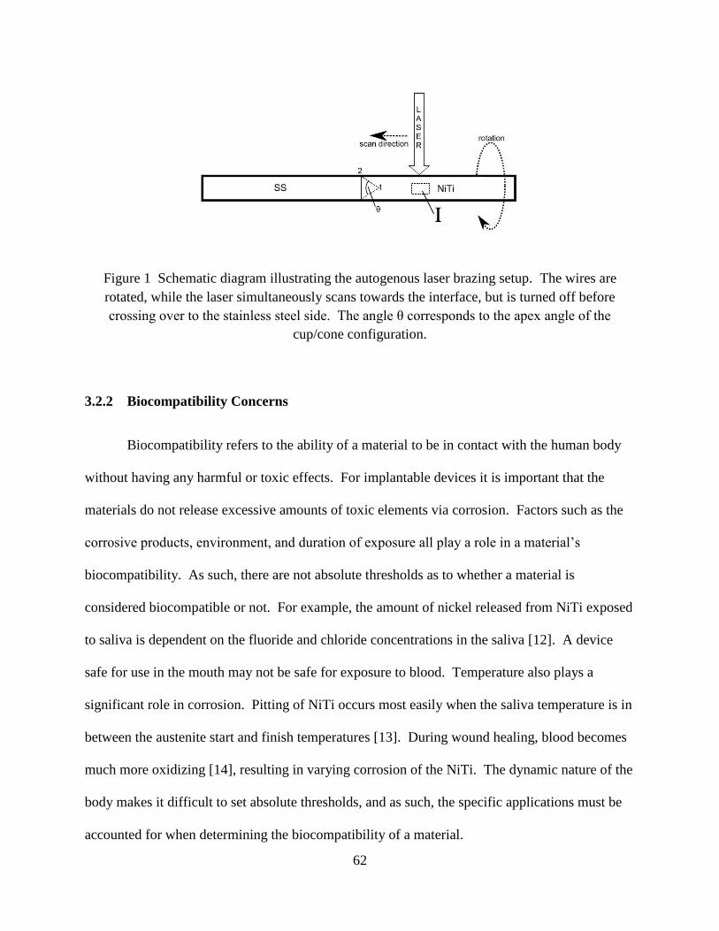
62

Figure 1 Schematic diagram illustrating the autogenous laser brazing setup. The wires are

rotated, while the laser simultaneously scans towards the interface, but is turned off before

crossing over to the stainless steel side. The angle θ corresponds to the apex angle of the

cup/cone configuration.

3.2.2 Biocompatibility Concerns

Biocompatibility refers to the ability of a material to be in contact with the human body

without having any harmful or toxic effects. For implantable devices it is important that the

materials do not release excessive amounts of toxic elements via corrosion. Factors such as the

corrosive products, environment, and duration of exposure all play a role in a material’s

biocompatibility. As such, there are not absolute thresholds as to whether a material is

considered biocompatible or not. For example, the amount of nickel released from NiTi exposed

to saliva is dependent on the fluoride and chloride concentrations in the saliva [12]. A device

safe for use in the mouth may not be safe for exposure to blood. Temperature also plays a

significant role in corrosion. Pitting of NiTi occurs most easily when the saliva temperature is in

between the austenite start and finish temperatures [13]. During wound healing, blood becomes

much more oxidizing [14], resulting in varying corrosion of the NiTi. The dynamic nature of the

body makes it difficult to set absolute thresholds, and as such, the specific applications must be

accounted for when determining the biocompatibility of a material.

63

In the material pair we are working with, NiTi is of the most concern, as it is composed

of nearly 50% nickel. The human body is allergic to very small nickel concentrations, with some

people being hypersensitive. Even though some small amounts of nickel are necessary for

nutrition and healthy metabolism, direct release of nickel into the body from an implanted device

is of great concern. The amount of nickel present in foods that actually gets absorbed by the

body is in the range of 1-20% [15]. Subsequently, devices that are implanted directly into the

bloodstream, such as stents, must be scrutinized even more closely than those for oral

applications. Blood platelets may become activated when contacted by nickel, causing thrombus

formation in the blood stream [16]. Nickel also may activate monocytes, a type of white blood

cell, which will lead to inflammation [17].

Despite its high nickel concentration, NiTi is generally considered biocompatible because

it forms a passive titanium oxide layer on its entire outer surface. As a result, the high nickel

concentration is not too detrimental to the biocompatibility of NiTi. Oxide layer depth is limited

by the distance that electrons from the metal can tunnel through the oxide layer to reach the

electrolyte solution [18]. Michiardi et al. found optimal parameters for thermal treating NiTi,

and achieved an oxide layer that was 63 µm thick, approximately ten times thicker than the oxide

of a mechanically polished sample [19]. Plasma source ion implantation can be used to

introduce additional oxygen, increasing the corrosion resistance of NiTi [20]. Uniformity of this

layer plays an important role, and as such, any regions where the oxide layer is damaged or

thinned will be detrimental [21].

The oxide layer formed on NiTi is capable of withstanding large deformations [22]. This

allows for the superelasticity of NiTi to be used in medical devices. Since implementations of

NiTi usually involve high levels of strain, having an oxide layer sensitive to deformation would

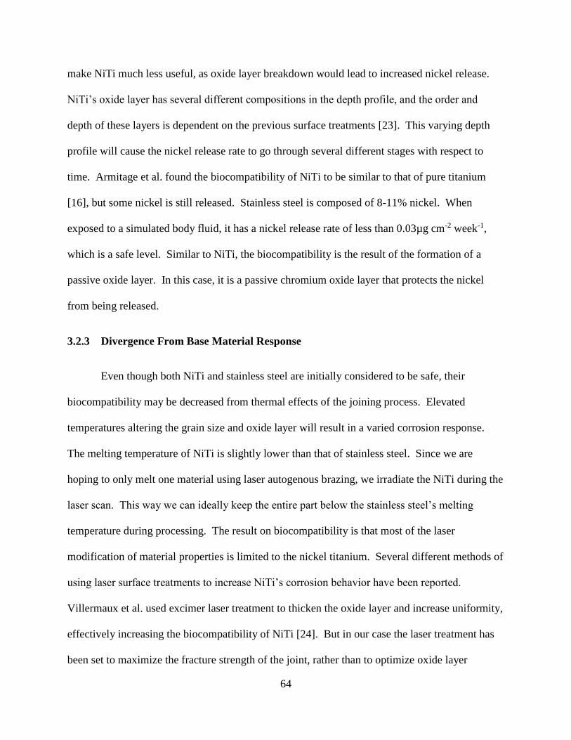
64

make NiTi much less useful, as oxide layer breakdown would lead to increased nickel release.

NiTi’s oxide layer has several different compositions in the depth profile, and the order and

depth of these layers is dependent on the previous surface treatments [23]. This varying depth

profile will cause the nickel release rate to go through several different stages with respect to

time. Armitage et al. found the biocompatibility of NiTi to be similar to that of pure titanium

[16], but some nickel is still released. Stainless steel is composed of 8-11% nickel. When

exposed to a simulated body fluid, it has a nickel release rate of less than 0.03µg cm-2 week-1,

which is a safe level. Similar to NiTi, the biocompatibility is the result of the formation of a

passive oxide layer. In this case, it is a passive chromium oxide layer that protects the nickel

from being released.

3.2.3 Divergence From Base Material Response

Even though both NiTi and stainless steel are initially considered to be safe, their

biocompatibility may be decreased from thermal effects of the joining process. Elevated

temperatures altering the grain size and oxide layer will result in a varied corrosion response.

The melting temperature of NiTi is slightly lower than that of stainless steel. Since we are

hoping to only melt one material using laser autogenous brazing, we irradiate the NiTi during the

laser scan. This way we can ideally keep the entire part below the stainless steel’s melting

temperature during processing. The result on biocompatibility is that most of the laser

modification of material properties is limited to the nickel titanium. Several different methods of

using laser surface treatments to increase NiTi’s corrosion behavior have been reported.

Villermaux et al. used excimer laser treatment to thicken the oxide layer and increase uniformity,

effectively increasing the biocompatibility of NiTi [24]. But in our case the laser treatment has

been set to maximize the fracture strength of the joint, rather than to optimize oxide layer

65

growth. As the NiTi is heated, TiNi3 may precipitate out at the grain boundaries [25]. A

homogenous passive oxide layer will not form across multi phase surfaces, and the corrosion

resistance will therefore be decreased if excessive TiNi3 is formed [26].

3.2.4 Polarization Tests

When placed in an electrolyte, a material will have an equilibrium electric potential that it

will naturally reach. Any deviation from this potential will cause changes in the corrosion

current from the material. This current is electrons that are released from the surface, and for

NiTi, accompanying Ni+ ions will also be introduced to the body. The response a material has to

deviations from its equilibrium potential is described by the Butler-Volmer Equation [27]:

𝑖 = 𝑖𝑜𝑒(

𝛼𝑛𝐹𝑅𝑇

𝜂) − 𝑖𝑜𝑒(−

(1−𝛼)𝑛𝐹𝑅𝑇

𝜂)

(1)

where i is the current density, α is the charge transfer coefficient, n is the number of electrons for

the reaction, R is the gas constant, T is temperature, and η is the overpotential (difference from

equilibrium). When the material is held at a potential much greater than its equilibrium, η

becomes large in the positive direction, and the first exponential term will dominate, and vice

versa for negative values of η. In these limits, Equation (1) can be rearranged to give the Tafel

Equations as [28]:

𝜂𝑐 = 𝛽𝑐𝑙𝑜𝑔 (

𝑖𝑐

𝑖𝑜)

(2)

𝜂𝑎 = 𝛽𝑎𝑙𝑜𝑔 (

𝑎

𝑖𝑜)

(3)

66

where c and a represent the cathode and the anode, and β accounts for the activation polarization.

Joining dissimilar metals results in a galvanic couple, in which one of the metals is

preferentially corroded. Plotting the polarization curves of the materials on the same graph can

predict how large the galvanic corrosive effect will be, where the corrosion potential and current

for the joined part will be the point on the graph where the polarization curves intersect.

Mixed potential theory, as described above, is a method to roughly estimate the corrosion

current of a joined sample. But, it is restrictive in that it does not take into account the

geometrical features and spatial distribution of the part. The regions far from the dissimilar

interface will have the same behavior as the base material response, indicating the corrosion

current will decay as we move towards the outer regions. A way to determine the anisotropy of

current along the part is by calculating the Wagner Parameter. The Wagner Parameter is defined

as [29]:

𝑊 = [𝜌

𝑑𝑖

𝑑𝐸]

−1

= 𝜎𝑅𝑝 (4)

where ρ and σ are the resistivity and conductivity of the solution, respectively, di/dE is the slope

from the polarization curve, and Rp is the polarization resistance. Physically, the Wagner

Parameter is the ratio of the resistance of the metal over the resistance of the electrolyte. As this

number gets large, the spatial distribution of current will become more uniform along the metal,

and vice versa.

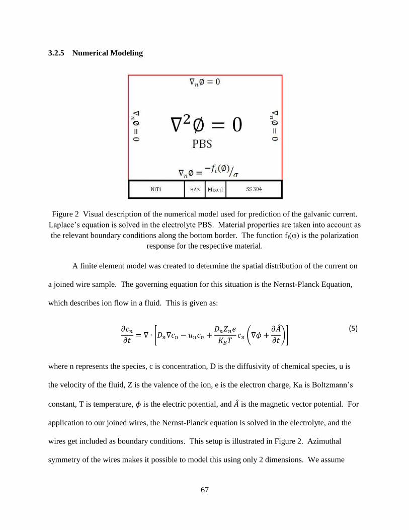
67

3.2.5 Numerical Modeling

Figure 2 Visual description of the numerical model used for prediction of the galvanic current.

Laplace’s equation is solved in the electrolyte PBS. Material properties are taken into account as

the relevant boundary conditions along the bottom border. The function fi(φ) is the polarization

response for the respective material.

A finite element model was created to determine the spatial distribution of the current on

a joined wire sample. The governing equation for this situation is the Nernst-Planck Equation,

which describes ion flow in a fluid. This is given as:

𝜕𝑐𝑛

𝜕𝑡= ∇ ∙ [𝐷𝑛∇𝑐𝑛 − 𝑢𝑛𝑐𝑛 +

𝐷𝑛𝑍𝑛𝑒

𝐾𝐵𝑇𝑐𝑛 (∇𝜙 +

𝜕��

𝜕𝑡)]

(5)

where n represents the species, c is concentration, D is the diffusivity of chemical species, u is

the velocity of the fluid, Z is the valence of the ion, e is the electron charge, KB is Boltzmann’s

constant, T is temperature, 𝜙 is the electric potential, and �� is the magnetic vector potential. For

application to our joined wires, the Nernst-Planck equation is solved in the electrolyte, and the

wires get included as boundary conditions. This setup is illustrated in Figure 2. Azimuthal

symmetry of the wires makes it possible to model this using only 2 dimensions. We assume

68

there is no magnetic field present and that the electrolyte is stationary, electroneutral, and well-

mixed. The well-mixed electrolyte leads to having no concentration gradient, i.e. ∇𝑐𝑛 = 0.

These simplifications reduce Equation (5) to Laplace’s Equation:

∇2𝜙 = 0 (6)

Using the results of the polarization tests now allows for inclusion of the stainless steel

and NiTi material properties. Let 𝐼𝑁𝑖𝑇𝑖(𝜙) and 𝐼𝑆𝑆(𝜙) be the respective polarization curves.

Dividing these by the conductivity of the electrolyte, σ, gives the Neumann boundary conditions

as [30]:

∇𝜙 =

−𝐼(𝜙)

𝜎

(7)

The laser irradiated region and the actual joint do not contain enough surface area to explicitly

measure the polarization response by traditional methods. But it is known that the polarization

response of the mixed region of the joint lies in between the responses of the base materials [31].

Therefore, 𝐼𝑁𝑖𝑇𝑖(𝜙) and 𝐼𝑆𝑆(𝜙) were averaged to produce 𝐼𝑚𝑖𝑥𝑒𝑑(𝜙). In addition, a fourth region

simulating the heat affected zone (HAZ) of the NiTi was also used. The equilibrium potential of

laser surface treated NiTi lies slightly more noble than that of the base NiTi [32]. Shifting the

NiTi curve gives us the response of the HAZ of NiTi. This setup was solved using COMSOL.

3.2.6 Microbiology Testing

Electrochemical techniques that determine the rate of corrosion are an indirect way of

determining biocompatibility, since assumptions on the effect of the ions released from corrosion

69

must be made. A direct approach is to do hemolysis and cytotoxicity testing. These are both

microbiological tests that measure the interaction of the sample with various biological cells.

Oftentimes implantable medical devices will be exposed directly to blood, as would be the case

for a stent. The amount of red blood cells destroyed from contact with the sample is determined

via hemolysis testing. Samples are exposed to a serum for 72 hours, and then brought into

contact with rabbit blood samples. When red blood cells are destroyed, they release hemoglobin,

and the hemoglobin concentration is measured using a spectrophotometer [33]. The percentage

of cells destroyed gets reported as the hemolytic index, where indexes ranging from 0-2 are

considered to be safe, while anything above 5 is considered as hemolytic and non-biocompatible.

Similarly, cytotoxicity tests are used to measure cell death. The wire samples are

exposed to a serum, then this serum is extracted and placed into contact with a cell culture

obtained from mice. On a scale of zero to four, the amount of cell destruction is qualitatively

determined as either non-toxic or toxic [34].

3.3 Experimental Procedure

Nickel titanium and stainless steel 304 wires with 762 µm diameters were used. The

composition of the NiTi is 54 at% Ti and 46 at% Ni, with the austenitic finish temperature below

room temperature. A conical apex angle of 90° was used for all the joints. Rotation of 5000 rpm

against 320 grit silicon carbide abrasive paper formed the cones on the end of the stainless steel

wires. The nickel titanium wires were first flattened on the ends using the same type of abrasive

paper. Then a 1143 µm diameter spot drill was used to form the cup-like shape. Laser joining

was achieved via an SPI redENERGY G4 fiber laser, with a wavelength of 1064 nm and

operating in continuous wave mode. Laser powers ranging from 13-17 W were used, and the

rotation speeds ranged from 1500°/s to 3000°/s. The laser started 1.6 mm away from the

70

interface, on the NiTi side, and then scanned towards the interface at a linear velocity, stopping

0.1 mm before it reached the stainless steel.

Phosphate buffered saline (PBS) was used as the electrolyte for the corrosion tests. As

the end product is implantable medical devices, the PBS acted as a simulated body fluid to

mimic the environment of the body. The PBS was 1X concentration, whose components are

0.138 M NaCl and 0.0027 M KCl. The polarization responses of the nickel titanium and

stainless steel were obtained following the methods of ASTM G5 [35]. All potentials are with

respect to a Saturated Calomel Electrode (SCE). Degradation testing was performed in vials

containing 22 mL of PBS at 37°C. Laser power was 17 W, and this time rotational speeds of

1500°/sec and 2500°/sec were analyzed. Three wire joints were placed in each vial, and 5

duplicate vials were made. Joints were removed in progressive intervals, at 1, 3, 6, 10, and 15

days. The leftover fluid, with corroded materials, was used for nickel concentration analysis via

Inductively Coupled Plasma Atomic Emission Spectroscopy (ICPAES), following protocol of

EPA 200.7 Rv. 4.4 [36]. Imaging of the corroded wires was carried out on a Hitachi-S47 00

SEM. Grain size and phase determination was achieved using electron backscatter diffraction

(EBSD). For the microbiology tests of hemolysis and cytotoxicity, ASTM756 and ISO 10993-5

were used, respectively. Cell line L929 was implemented for the cytotoxicity tests.

71

3.4 Results

3.4.1 Polarization Tests

Figure 3 Polarization response of metal samples in PBS solution. The solid lines indicate

measurements, while the dashed lines are approximations. The more electronegative equilibrium

potential of the NiTi will cause it to experience anodic effects, while the stainless steel is

cathodic. When the transition from the base materials goes through the two intermediary phases,

the corrosion current gets significantly reduced. This data was used for fi(φ) in Figure 2.

The results of the polarization tests are presented in Figure 3, where the solid lines are

measured quantities and the dotted lines represent estimations. Since the equilibrium potential of

NiTi is lower than that of stainless steel, it is clear that the NiTi will act as the anode for the

galvanic couple, resulting in more nickel ions being released into the electrolyte. Mixed-

potential theory suggests that the corrosion of the joined wires will increase by at least a factor of

ten compared to the base materials. When the potential of the stainless steel rises above 0.2 V,

the oxide layer breaks down, and the corrosion current rapidly increases. The breakdown

72

potential of NiTi is not shown on the plot, but at some higher potential it would have similar

behavior. The polarization resistance for each material is extracted from Figure 3, and plugged

into Equation (5) to determine the respective Wagner Parameters. PBS has a conductivity of

15,000 µmhos/cm. This results in WNiTi = 43.5 m and Wstainless = 22.5 m. Both of these numbers

are rather large, suggesting a somewhat uniform current distribution. Although, the stainless will

have a slightly less uniform response traveling away from the interface.

Figure 4 Numerical simulation results for the distribution of the electric potential in the PBS

solution. The gradient of this field gives the direction of electron flow, and is denoted via the

arrows. At either extreme along the bottom boundary, the potential approaches the equilibrium

potential of the respective material nearby.

3.4.2 Corrosion Current Modeling

The electric potential of the PBS electrolyte is plotted in Figure 4, with the arrows

indicating the gradient of this field, representative of the direction of current flow. Using the

results from the polarization tests, the spatial distribution of the electron current density was

73

determined across the wires. This distribution is displayed in Figure 5. The solid lines are the

currents for corrosion in PBS, while the dotted lines are for comparison to the corrosion response

in an electrolyte with 1

10 the conductivity of PBS. Blood has a very similar nominal conductivity

to that of PBS. But, the orientation of the erythrocytes will greatly impact the conductivity. This

orientation could be dependent on whether the blood is flowing or stationary. Blood flowing at

high velocity can have a conductivity as low as 1

10 that of stationary blood [37], corresponding to

the dashed lines in Figure 5. Regions with positive values of electron flow are anodic, that is,

these are the regions attacked by the galvanic couple, while the regions with negative current

density are not releasing ions into the electrolyte and therefore are being galvanically protected.

Both of the intermediary regions have lengths of 1 mm, corresponding to length of the laser

interaction.

74

Figure 5 Distribution of electron flow along the lower boundary of Figure 4, corresponding to

the corrosion current. The dotted lines are for a electrolytic conductivity that is only 10% that of

the solid lines, causing a more non-uniform distribution.

As is predicted by Wagner Parameter analysis, lowering the conductivity of the

electrolyte results in a more non-uniform distribution of current density. On the NiTi, the current

adjacent to the HAZ is nearly 50% larger than that towards the end of the wire. Since it has a

smaller polarization resistance, the stainless steel is even more non-uniform, with the current

across the segment varying by almost 100%.

Current densities for the PBS simulated model are more uniform, again consistent with

the Wagner parameter. We see that the stainless has more non-uniformity than the NiTi though.

The NiTi lies slightly above 3x10-7 A/cm2, which is a rather low current. This is desirable, and

suggests that this galvanic pair is likely to have good biocompatibility properties, since the

amount of nickel released into the electrolyte is not going to be excessive. In a way, the HAZ

NiTi and the mixed region act as stepping stones for the galvanic couple, effectively lowering the

75

predicted current. Figure 3 suggests that if the NiTi was coupled directly to the stainless steel,

the corrosion current would be on the order of 10-6.5 A/cm2, about 30% higher than the currents

calculated using the numeric model. In reality, the transition from the base NiTi to the HAZ is

continuous (corresponding to the temperature gradient formed from thermal accumulation),

rather than the step function that was defined in the model. But, since we are unable to measure

this transition using potentiostat testing, the simplified configuration was used.

3.4.3 Nickel Release Tests

Figure 6 Total amount of nickel released from joined samples as a function of time. The two

different processing parameters of low and high energy inputs have similar profiles, but are

noticeably higher than the base NiTi. This NiTi has undergone a previous heat treatment; non-

treated NiTi has a release profile higher than the treated samples in here in our case.

For reasons previously described, the release of nickel from corroding NiTi is of the most

concern. Titanium ions will be released as well, but these are of much less biological concern,

and the relative quantity of titanium released is known to be much less than that of nickel [38].

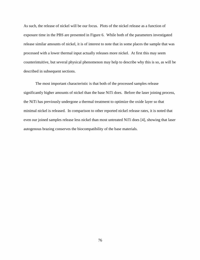
76

As such, the release of nickel will be our focus. Plots of the nickel release as a function of

exposure time in the PBS are presented in Figure 6. While both of the parameters investigated

release similar amounts of nickel, it is of interest to note that in some places the sample that was

processed with a lower thermal input actually releases more nickel. At first this may seem

counterintuitive, but several physical phenomenon may help to describe why this is so, as will be

described in subsequent sections.

The most important characteristic is that both of the processed samples release

significantly higher amounts of nickel than the base NiTi does. Before the laser joining process,

the NiTi has previously undergone a thermal treatment to optimize the oxide layer so that

minimal nickel is released. In comparison to other reported nickel release rates, it is noted that

even our joined samples release less nickel than most untreated NiTi does [4], showing that laser

autogenous brazing conserves the biocompatibility of the base materials.

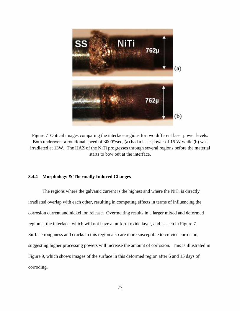
77

Figure 7 Optical images comparing the interface regions for two different laser power levels.

Both underwent a rotational speed of 3000°/sec, (a) had a laser power of 15 W while (b) was

irradiated at 13W. The HAZ of the NiTi progresses through several regions before the material

starts to bow out at the interface.

3.4.4 Morphology & Thermally Induced Changes

The regions where the galvanic current is the highest and where the NiTi is directly

irradiated overlap with each other, resulting in competing effects in terms of influencing the

corrosion current and nickel ion release. Overmelting results in a larger mixed and deformed

region at the interface, which will not have a uniform oxide layer, and is seen in Figure 7.

Surface roughness and cracks in this region also are more susceptible to crevice corrosion,

suggesting higher processing powers will increase the amount of corrosion. This is illustrated in

Figure 9, which shows images of the surface in this deformed region after 6 and 15 days of

corroding.

78

Figure 8 SEM image of the outside interface for a joined sample. Roughness and non-

uniformity is evident in this region, making it susceptible to effects such as pitting and crevice

corrosion.

79

Figure 9 Surface corrosion at the mixed interface region after 6 days (a) and 15 days (b) of

exposure to the simulated body fluid. Both samples were joined at 17 W and 1500°/sec. Rather

uniform texture is seen in (a), but this surface becomes much rougher as corrosion proceeds, as

evidenced by the sharper regions found in (b).

An optical micrograph of a longitudinally sectioned joint is presented in Figure 10. Only

the bottom half of the wires is represented, as the top half is symmetric. Many different regions

are seen on the nickel titanium side. Colloidal silica was used in the final polishing step for this

80

sample, which acts as a mild etchant to help identify grain distribution and size. The grains

nearest to the interface are the largest, which can be attributed to the thermal accumulation

occurring in this region. As discussed by Satoh [39], the grain size will gradually decrease as we

move away from the interface. In the non-HAZ regions of the NiTi, the grains are too small to

see using optical microscopy. Electron microscopy can be used to increase the resolution and

magnification. Figure 11 is an EBSD map illustrating the grain size and distribution of the NiTi

in a region further removed from the interface. Each color represents a unique grain. Many of

these grains have diameters less than 200 nm. Pretreating the material and cold-working is used

to refine the grain size to this small value, as described by Crone [40], which is done for

mechanical property considerations. The corrosion current will increase as the grain size is

decreased, which can be expressed as [41]:

𝑖𝑐𝑜𝑟𝑟𝑜𝑠𝑖𝑜𝑛 = 𝐴 +

𝐵

√𝑔𝑟𝑎𝑖𝑛 𝑠𝑖𝑧𝑒

(8)

where both A and B are material constants. This relationship arises from the fact that grain

boundaries are weaker, and more susceptible to releasing ions into the electrolyte. Higher

temperatures reached during processing will result in larger grains being formed. Thus from a

grain size argument, wires processed with higher laser input will have lower corrosion currents.

Amorphous NiTi is even more corrosion resistant and has a higher pitting potential, because it

lacks grain boundaries [42]. But, amorphous NiTi is much harder and is difficult to shape or

machine into complex parts.

81

Figure 10 Optical micrograph at the interface of a longitudinally sectioned sample. Distinct

grains are clearly visible in the NiTi on the left hand side, with size increasing nearer to the

interface. The inset shows an enlarged image near the outer edge, where the combination of

stress and elevated temperatures resulted in dynamic recrystallization. This is a region that

recrystallized without having reached the melting temperature.

Figure 11 EBSD unique grain map in a region of NiTi far from the interface. The rather small

grain size may be an effect of previous cold working. When compared with the sizes of Figure

10, it is clear that the thermal accumulation of the interface results in significant grain growth.

This phenomenon means that we will have competing effects for the corrosion current

that flows. The effect of the galvanic couple is that the corrosion current near the interface will

be increased, but the larger grains in this region will try to resist this increase in corrosion. The

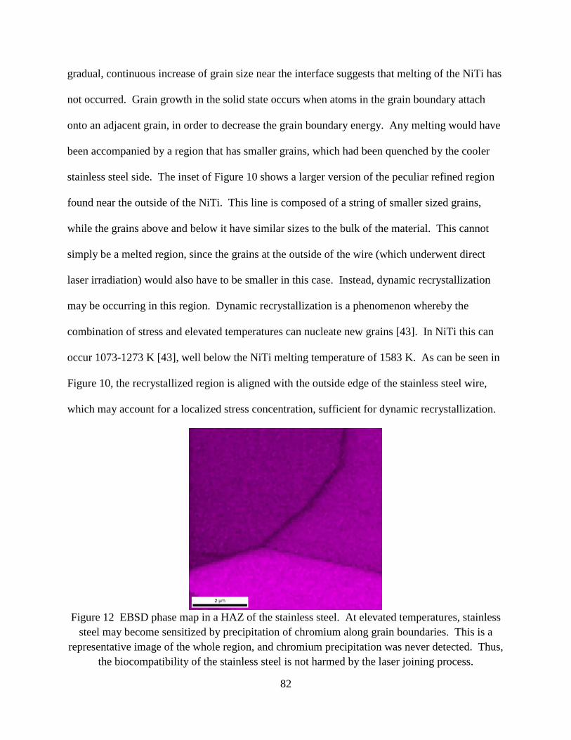
82

gradual, continuous increase of grain size near the interface suggests that melting of the NiTi has

not occurred. Grain growth in the solid state occurs when atoms in the grain boundary attach

onto an adjacent grain, in order to decrease the grain boundary energy. Any melting would have

been accompanied by a region that has smaller grains, which had been quenched by the cooler

stainless steel side. The inset of Figure 10 shows a larger version of the peculiar refined region

found near the outside of the NiTi. This line is composed of a string of smaller sized grains,

while the grains above and below it have similar sizes to the bulk of the material. This cannot

simply be a melted region, since the grains at the outside of the wire (which underwent direct

laser irradiation) would also have to be smaller in this case. Instead, dynamic recrystallization

may be occurring in this region. Dynamic recrystallization is a phenomenon whereby the

combination of stress and elevated temperatures can nucleate new grains [43]. In NiTi this can

occur 1073-1273 K [43], well below the NiTi melting temperature of 1583 K. As can be seen in

Figure 10, the recrystallized region is aligned with the outside edge of the stainless steel wire,

which may account for a localized stress concentration, sufficient for dynamic recrystallization.

Figure 12 EBSD phase map in a HAZ of the stainless steel. At elevated temperatures, stainless

steel may become sensitized by precipitation of chromium along grain boundaries. This is a

representative image of the whole region, and chromium precipitation was never detected. Thus,

the biocompatibility of the stainless steel is not harmed by the laser joining process.

83

On the right hand side of Figure 10 is the stainless steel, which has a rather uniform

morphology. That is, the thermal input from the laser appears to change very little of the

structure. Since the laser never directly irradiates the stainless steel side, it is clear that minimal

heat affected zones should be present in the stainless steel. Even if the laser happened to cross

over the interface, it would not be much of a concern for the corrosion response of the stainless

steel since it is known that laser surface melting of stainless steel helps to increase its corrosion

resistance [44]. But the reason that irradiation of the stainless steel is avoided is that keeping the

stainless steel below its melting temperature prevents mixing and brittle intermetallic formation,

subsequently decreasing the mechanical strength of the joint. The region near the interface along

the bottom appears to have melted and resolidified into a smaller grain structure.

Grain growth is not the only thermal effect that could occur in the materials. Elevated

temperatures may result in some of the materials’ components precipitating out, and thus altering

the corrosion behavior. In stainless steels, chromium is insoluble in iron from 425°C to 815°C,

so chromium carbide will precipitate out at the grain boundaries resulting in depleted regions

[28]. These chromium depleted regions (along the grain boundaries) will be more susceptible to

corrosion, with this process being referred to as “sensitization.” Microgalvanic corrosion then

occurs, because the regions with less chromium are more active in the electrolyte. Detection of

this can be done via EBSD. Figure 12 shows an EBSD phase detection map in one of the most

heat affected zones of the sample from Figure 10. No chromium precipitates are detected.

Multiple scans were performed across several different samples, and evidence of chromium

precipitation was never detected. This suggests that the stainless steel does not stay at the

elevated temperature for a sufficient time for precipitation to occur, indicating again that the

84

autogenous laser brazing process does indeed input only the minimum amount of energy

necessary for joining. Similarly, the NiTi may undergo thermally induced precipitation as well.

EBSD analysis was also performed on regions of the NiTi side, looking for precipitate formation,

as seen in Figure 11. But, no evidence of precipitates were formed in the NiTi either, which is

beneficial for keeping the material properties of the processed wires as similar to those of the

base material as possible. The small initial grain size may act as a barrier to precipitation

forming, especially of Ni4Ti3 [45].

Figure 13 Images of the border of the heat affected zone and base material in the NiTi, as

indicated by the inset region of Figure 1. More corrosion is evident in the lower power sample

of (a) than for the higher power of (b). This is evidence that more intermetallic formation at the

interface may act as an electrical resistance, effectively reducing the flow of the galvanic current.

85

Even though no precipitates are formed in the heat affected zone of the NiTi wire, this

region still has an altered corrosion response to the PBS electrolyte. Since the temperature

distribution is very uniform in the axial direction, because of the high rotational velocity, the heat

affected zone on the surface of the wires is essentially one dimensional. SEM images of the

border of the heat affected zone with the base material of two samples are presented in Figure 13.

Both of these samples underwent corrosion for 15 days, with (a) being processed with more laser

energy than (b). It is clearly evident that the lower energy sample undergoes more corrosion in

this case, which agrees with the results found via the nickel release tests. But, it is interesting to

note that this occurs on both sides of the HAZ boundary. At higher heat inputs, the width of the

mixed interface will become wider than that of lower powers. The presence of additional new

material phases, such as TiFe2 and TiFe, may act as electrical insulators. With respect to mixed

potential theory, a resistance will shift the corrosion current to the left of the intersection in

Figure 3, effectively decreasing the amount of galvanic current that flows. Additionally, this

could also be attributed to the larger grains in the more heated sample.

3.4.5 Cytotoxicity and Hemolysis

Two different processing parameters were tested for their biocompatibility using

cytotoxicity and hemolysis testing. The largest difference in laser effects on the wires was

desired, while still having joints that were mechanically strong. Both sets were rotated at

3000°/sec during laser irradiation, but the power was 13 W for the low end and 17 W for the

high.

For the cytotoxicity, both the low and high power samples returned toxicity grades of

zero, indicating they are both non-toxic. At first this may seem unenlightening, but it does lead

86

to an important realization. A window containing the processing parameters that result in good

tensile strengths has been reported by the authors in a previous work [9]. The parameters used in

these microbiology tests fall on the low and high ends of this window, indicating that the range

of parameters useful for achieving high strengths corresponds to a non-cytotoxic range. If a

significant trade-off between strength and biocompatibility was found, this would be detrimental

to the applications of the autogenous laser brazing process.

Figure 14 Hemolysis testing for two different laser processing parameters. Slightly more

hemolytic properties are found in the sample irradiated with higher energy, but both are well

within the biocompatible, safe zone. Error bars indicate standard error.

Hemolysis testing is more sensitive than cytotoxicity, and is capable of detecting

differences between the samples’ processing parameters. As seen in Figure 14, samples

irradiated at 13 W were found to have a hemolytic index of 1.6, while the samples irradiated at

17 W had a hemolytic index of 1.8. The standard error is 0.9, so the difference of the two

parameters lies slightly outside of this uncertainty. Having a hemolytic index of less than 2 is

considered to be non-hemolytic, so both of the parameters are within this safe zone. But the 17

87

W wires are approaching this upper limit. The base materials of unprocessed NiTi and stainless

steel are known to have hemolytic indexes in the range of 0.2 to 0.4 [16].

3.5 Conclusion

The range of processing parameters investigated here has been shown in a previous study

by the authors to have drastic effects on mechanical strength [9]. But the biocompatibility across

this range is found to be quite similar. This is beneficial for the application of autogenous laser

brazing. If the parameters giving the strongest mechanical strength were different from those

that provide good biocompatibility, implementation of the autogenous laser brazing process for

manufacture of implantable medical devices would be restricted. We have found that many

different factors influence the biocompatibility of the joined samples. Fortunately though, the

differing effects appear to counter act with each other, and the end result is that the joined

samples are slightly less biocompatible than unprocessed NiTi, but still lie within a safe range for

implantation into the body.

88

Chapter 4: Material Influence on Mitigation of

Stress Corrosion Cracking via Laser Shock

Peening

4.1 Introduction

When choosing which materials to implement into engineering designs what may often go

overlooked is how mechanical stress influences corrosion behavior. Stress corrosion cracking

(SCC) is a phenomenon where a corrosive environment effectively lowers the fracture strength of

a material. Rather than traditional failure by corrosion, which is evident by a slow dissolution of

the material, SCC occurs without warning. This lack of visual clues is what makes SCC of

concern; its sudden cracking can lead to unpredictable, catastrophic failure of integral parts. The

biggest problem from a design perspective is that stress corrosion cracking is difficult to make

conclusive predictions of when and where it will occur. It is highly dependent on the specific

material/environment pair, where a material that is resistant in one environment may become

dangerously susceptible to SCC in other environments.

The stress required for SCC can either be externally applied or be a residual stress from

previous manufacturing processes. Some situations where this occurs are pipe taps and fittings,

nuclear reactors, pressure vessels, or high strength pipeline steels. Brass is machinable and

generally considered as corrosion resistant, but it is still susceptible to SCC, and when this does

occur it can cause excessive damage. Small concentrations of ammonia are found to be the main

cause for brass’s failure by SCC, where even the low concentrations found in drinking water can

be problematic [1]. Residual stresses caused during installation --such as tightening of threaded

components-- can cause material failure. Other residual stresses, most prominently those caused

89

by welding, can make a material susceptible to SCC. Many of the pipelines found in chemical

processing plants are at risk, as are pipelines for distribution of gases. Recently, a natural gas

pipeline rupture was attributed to SCC, where a combination of the internal pressure and corrosive

gas as well as the external soil moisture and movement combined to cause failure [2]. Another

critical example of SCC’s concern is in nuclear reactors, where susceptibility and cracking has

been extensively documented [3]. Additionally, the elevated temperatures and exposure to

radiation compound the concern for premature failure of reactors.

With the identification of SCC’s potentially catastrophic effects, the question arises as how

to prevent this phenomenon from occurring. While proper selection of materials does help,

sometimes further enhancement of a material’s SCC resistance must be provided by surface

processing treatments. Shot peening has been identified as potentially beneficial, attributed to

imparting a compressive residual stress upon the surface of the material [4]. But the macroscopic

morphological changes caused by this process may be undesirable, and the precision unsuitable

for small parts. Another method is heat treating the final piece to relieve residual stresses, but this

is not always practical, especially on large parts such as nuclear reactor cores. Furthermore, the

additional effects of heat treating (grain refinement, oxide or precipitate formation) may be

undesirable.

Laser shock peening (LSP) is a surface treatment process that has the potential for helping

to mitigate the effects of SCC without damaging other characteristics of the material. While

originally developed for increasing the fatigue life of materials, LSP uses laser generated shock

waves to impart compressive residual stresses onto the surface [5], with affected regions as deep

as 1 mm into the metal, much deeper than traditional shot peening. Another benefit of LSP over

other processes is that it maintains minimal changes on overall feature morphology and metallurgy,

90

thus avoiding the requirement of modifications to the design. The capability of LSP to prevent

SCC has previously been investigated by several researchers. For example, LSP treatment of

stainless steel has been found to increase the time-to-failure in boiling MgCl2 solutions of U-bend

specimens, where the improved behavior was attributed to the residual compressive stress

counteracting the applied load [6]. While this is a simple explanation of beneficial effects, it does

not capture the overall phenomenon, namely, the electrochemical effects are not taken into

consideration. Even though LSP does not impart any thermal effects on the surface, it still causes

significant changes to the surface chemistry and microstructure. As proof, multiple researchers

have shown that LSP treatment increases the rest potential of metals during polarization testing

[7]. Increased rest potentials are indicative of more inert surfaces, but in most cases it was found

that over time the rest potential decayed back towards the initial, untreated level.

Across these previous investigations it is clear that LSP has the potential to effectively

reduce the effects of stress corrosion cracking. But the mechanism driving the SCC resistance

improvement has yet to be fully understood, where achieving this understanding could lead to

identification of scenarios that would benefit the most as well as optimization of the process. In

this paper we work to provide a further description of the mitigation effects imparted by LSP, not

just including stress analysis but also by providing a discussion of the microstructural and

electrochemical changes that make LSP a valuable tool for SCC mitigation, as well as differences

caused by material characteristics.

4.2 Background

Mechanisms of Stress Corrosion Cracking

Several different failure mechanisms have been proposed to explain the occurrence of SCC,

but no definitive consensus has been reached. This may be a result of different mechanisms

91

dominating under different circumstances. Some of these theories are hydride formation,

hydrogen enhanced decohesion, hydrogen enhanced localized plasticity, and adsorption-induced

dislocation emission [8]. In many cases the most preeminent factor and common theme is the

effect of hydrogen. Hydrogen present in the corrosive environment can have negative effects by

penetrating into the microstructure of the metal, known as hydrogen embrittlement. When a

material is stressed in tension, and the crystal lattice is elongated, hydrogen’s diffusivity becomes

even more exaggerated. The additional hydrogen atoms within the already stressed lattice may

push the material over its threshold by weakening the atomic bonding, and result in failure. But

developing a simple relationship between applied stress and SCC occurrence cannot be achieved

[9], illustrating the unpredictable nature of the phenomenon.

Once it has penetrated the metallic surface, the distribution and location of hydrogen

throughout the lattice is important. Grain boundaries act as high diffusivity paths, allowing for

deep penetration of hydrogen [10]. Cold working generates dislocations within the lattice

structure, and these dislocations act as hydrogen trapping sites. It is most likely that the hydrogen

atoms will be found in the trapping sites rather than interstitial locations [11], and as a result the

solubility of hydrogen raises with increasing dislocation density. With excessive amounts of

hydrogen present, a material’s lattice becomes stressed and subsequently its hardness is increased

[12]. This enables measuring hardness increases in materials exposed to hydrogen containing

environments to be used as an indicator of the amount of hydrogen that has penetrated into the

lattice.

92

Laser Shock Peening

The physical configuration for LSP processing consists of an ablative layer placed in

between a target surface and a confining layer [13]. Since the confining layer is transparent to the

laser’s wavelength, upon irradiation the laser beam passes through this layer and is absorbed into

the ablative layer. Using a sufficiently intense laser beam instantly vaporizes the ablative layer

causing it to expand. But the confining layer restricts the expansion, and thus a shock wave is

generated and travels into the material resulting in a compressive residual stress [14]. The metallic

surface does not undergo any thermal effects, as all of the laser energy is absorbed by the ablative

layer.

An important characteristic of materials’ corrosion responses is the formation of a surface

oxide layer. This layer can help to passivate the material, preventing the occurrence of further

corrosion. Stainless steel, for example, achieves its corrosion resistance from the formation of a

chromium oxide layer, which encases and protects the iron. Thickness and uniformity of such

oxide layers are very important, and therefore, any surface processing treatment has the potential

to negatively impact the oxide layer. Additionally, the stress state on the surface influences the

formation of oxide layers as well [15]. Surface roughness also plays an important role in the

initiation of stress corrosion cracking. Within crevices on a material’s surface, hydrolysis may

acidify the electrolyte so that the pH within the crevices does not match the pH of the bulk solution.

This causes an increase in the surface’s anodic reactions. In this case, the applied stress works to

open up and expose more surface crevices.

93

Dislocation Generation

During LSP processing, the material experiences extremely high strain rates as the shock

wave propagates through it, reaching levels as high as 106 s-1. This causes plastic deformation [16]

as well as the formation of many lattice dislocations. As stated above, dislocations act as trapping

sites for hydrogen, whereby LSP can be used to alter the hydrogen behavior and distribution within

the lattice. Hydrogen’s solubility increases with dislocation density and subsequently its

diffusivity decreases as described by the following equation [17]:

𝐷 = 𝐷𝐿𝐶𝐿

𝐶𝐿+𝐶𝑥(1−𝜃𝑥) (1)

where D is the effective diffusivity, DL is the normal (defect free) diffusivity, CL and Cx are the

concentrations in the lattice and trapping sites, and θ is the population fraction of available trapping

sites.

Upon plastic deformation, the rate at which dislocation density increases will vary for

different materials. Dislocation generation by plasticity has three stages: easy glide, dislocation

multiplication by tangling, and dynamic recovery. Each one of these stages can be numerically

described in terms of the rate of change of dislocation density ϱ vs. shear strain γ, as derived in

Malygin et al. [18]. For easy glide:

(𝑑𝜚

𝑑𝛾)

𝑚= 𝜒𝑚 = (𝑏𝜆𝑚)−1 = 𝛿𝑚𝑏−1 (2)

where b is the Burgers vector and λ is the average distance between dislocations and obstacles such as grain

boundaries. The second stage is described by:

(𝑑𝜚

𝑑𝛾)

𝑓= 𝜒𝑓𝜚

𝑓

12⁄

𝜒𝑓 ≈ 10−2𝑏 (3)

The third and final stage, dynamic recovery is when dislocation annihilation occurs, by dislocations of opposite

signs coming into contact or by grain refinement:

94

(𝑑𝜚

𝑑𝛾)

𝑎= −𝜒𝑎𝜚 𝜒𝑎 =

𝜔𝑠

52⁄

𝜇

24𝜋2𝛼𝜏𝑐= 𝑏−1𝛿𝑎 𝜔𝑠 ≈ 0.5 (4)

where μ is the shear modulus, α is a dislocation interaction constant, and τc is the critical resolved

shear stress. Summation of the combined effects and rearrangement of variables yields:

𝑑𝜚

𝑑𝛾 ~ (𝜎 − 𝜎𝑠)𝜃 =

1

2𝑚3(𝛼𝜇𝑏)2 [𝜒𝑚 + 𝜒𝑓 (

𝜎−𝜎𝑠

𝑚𝛼𝜇𝑏) − 𝜒𝑎 (

𝜎−𝜎𝑠

𝑚𝛼𝜇𝑏)

2

] (5)

where θ is the work hardening coefficient, σ is stress, and σs is the yield stress. Thus, by use of

Equation 5 the rate of change of dislocation density versus strain (deformation) can be estimated

based on material characteristics.

Work Function and Corrosion Potential

It is evident that the corrosive response of metals is dependent on surface characteristics,

which leads one to desire ways to characterize the surface’s electrochemical behavior as it may

lead to additional insights regarding SCC behavior. One such characterization is to analyze the

work function. By definition, the work function is the amount of energy required to remove an

electron from the surface, as expressed by the equation:

𝑊 = −𝑒∅ − 𝐸𝑓 (6)

where e is the elementary charge, ∅ is the vacuum electrostatic potential, and Ef is the Fermi Level.

Oftentimes the work function is discussed regarding photoelectric devices, but it can also be

applied to corrosion analyses, particularly as related to the open circuit potential during

polarization testing. A linear relationship between increasing work functions and increasing rest

potentials has been reported, thus providing an empirical basis [19,20]. Examinations of the

validity of this relationship have been made on iron surfaces exposed to humid environments,

95

where it has been concluded that work function analysis is an effective method for corrosion

characterization [21].

Multiple factors can affect the work function, particularly stress, both applied and residual.

The Fermi level depends upon electron density, leading some researchers to develop relationships

between elastic stress and work function changes. Based on density functional theory, Wang et

al. have modeled the distribution of atoms in Cu(100) and how applied loads affect their density

and thus work function [22]. They found that tensile strains decrease work function, while

compressive strains cause work function increases. While this provides a good basis, the plastic

deformation caused by LSP further complicates the discussion. Dislocations are lattice

imperfections, regions where electrons may be more easily ejected from the surface. Increasing

the amount of plastic strain in copper samples results in both decreased work function and

decreased corrosion potential [23]. The competing effects elastic and plastic strain have on work

function is a trade-off that must be understood in order to fully maximize the benefits LSP has on

SCC.

Processing Concerns

With many different factors contributing to LSP’s influence on corrosion response, it is of

concern that focusing on improving one aspect could actually result in harming another one. This

leads to concerns that overprocessing of the metallic samples will start to undo any beneficial

effects that had been imparted. For example, while initially austenitic, stainless steel can

experience martensite formation upon excessive deformation. The corrosion response of

martensitic phases differs from austenitic ones, thereby destroying the material’s homogeneity and

thus decreasing the corrosion resistance. Increased strain rates also cause more martensitic

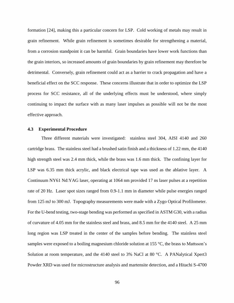
96

formation [24], making this a particular concern for LSP. Cold working of metals may result in

grain refinement. While grain refinement is sometimes desirable for strengthening a material,

from a corrosion standpoint it can be harmful. Grain boundaries have lower work functions than

the grain interiors, so increased amounts of grain boundaries by grain refinement may therefore be

detrimental. Conversely, grain refinement could act as a barrier to crack propagation and have a

beneficial effect on the SCC response. These concerns illustrate that in order to optimize the LSP

process for SCC resistance, all of the underlying effects must be understood, where simply

continuing to impact the surface with as many laser impulses as possible will not be the most

effective approach.

4.3 Experimental Procedure

Three different materials were investigated: stainless steel 304, AISI 4140 and 260

cartridge brass. The stainless steel had a brushed satin finish and a thickness of 1.22 mm, the 4140

high strength steel was 2.4 mm thick, while the brass was 1.6 mm thick. The confining layer for

LSP was 6.35 mm thick acrylic, and black electrical tape was used as the ablative layer. A

Continuum NY61 Nd:YAG laser, operating at 1064 nm provided 17 ns laser pulses at a repetition

rate of 20 Hz. Laser spot sizes ranged from 0.9-1.1 mm in diameter while pulse energies ranged

from 125 mJ to 300 mJ. Topography measurements were made with a Zygo Optical Profilometer.

For the U-bend testing, two-stage bending was performed as specified in ASTM G30, with a radius

of curvature of 4.05 mm for the stainless steel and brass, and 8.5 mm for the 4140 steel. A 25 mm

long region was LSP treated in the center of the samples before bending. The stainless steel

samples were exposed to a boiling magnesium chloride solution at 155 °C, the brass to Mattsson’s

Solution at room temperature, and the 4140 steel to 3% NaCl at 80 °C. A PANalytical Xpert3

Powder XRD was used for microstructure analysis and martensite detection, and a Hitachi S-4700

97

Scanning Electron Microscope (SEM) was used for imaging. Cathodic charging was performed

in 1M sulfuric acid at a current density of 800 mA/cm2 for 30 minutes. Work function

measurements were made on a Bruker Dimension FastScan AFM operating in Peak Force KPFM

mode and using PFQNE-AL probes. The FEM model was implemented in ABAQUS.

4.4 Results & Discussion

Surface Morphology

Characterization of the surface morphology is first performed to understand the impact the

LSP treating had on the surfaces. Figures 1 & 2 show optical profilometer measurements across

LSP indentations, where the two lines are measured in perpendicular directions. Figure 1 is a

stainless steel sample irradiated at 250 mJ showing indentation depth of slightly over 3 µm. As

compared to the stainless steel sample, a brass sample processed with the same parameters has a

similar depth, but it is clear that the roughness within the indentation is much higher on the brass.

Much more surface deformation has occurred, such as the emergence of large slip bands, and this

result could be potentially harmful to the brass. Increased surface roughness provides the corrosive

environment more cracks and crevices to penetrate into, and as such, smoother surfaces are

generally more corrosion resistant. But it is important to keep in mind the scale of this roughening.

The indentations on the stainless are large and smooth enough that they should not cause any

detrimental effects such as crevice corrosion or local acidification of the electrolyte. As the laser

scans across the surface it creates a uniform array of indentations, of which a 3D topographical

map is shown in Figure 3 for a brass sample. This pattern is for 0% overlapping between adjacent

pulses, and good uniformity of the surface indentations is seen across the samples.

98

Figure 1 LSP indentation profile of a stainless steel sample irradiated at 250 mJ with a spot size of 0.9 mm. The

two lines are traces across perpindicular directions.

Figure 2 Indentation profile of brass LSP processed at 250 mJ. More surface roughening effects are visible than on

the stainless steel sample.

The occurrence of any phase transformations was investigated with XRD. Stainless steel

samples were processed at 250 mJ, and then in attempts to induce excessive deformation, the

samples were reprocessed one and two more times. This gave three samples with either one pass,

two passes, or three passes, where retreating the LSP sample compounds the shockwave’s effects.

Austenitic stainless steel has large 2θ diffraction peaks at 43.58°, 50.79°, 74.70°, and 90.69°. The

presence of martensite would cause the emergence of new diffraction peaks, because of the

different lattice spacing of the martensite phase. Although other researchers have found

deformation induced martensite in LSP treated stainless steel samples, we detected no martensite

phases in any of our samples. In terms of corrosion, this is a positive result, as martensite’s

presence would be detrimental to the corrosion resistance.

99

Figure 3 Morphology of a patterned brass sample after LSP processing. Individual indentations are still visible

because of the 0% overlap condition.

Cathodic Charging and Hardness Increases

While LSP is known to increase the surface hardness of metallic samples, the absorption

of hydrogen also can cause increases in hardness levels near the surface [25]. Cathodic charging

is thus an effective way for performing accelerated testing of hydrogen uptake in metallic samples.

The excess electrons provided by the power supply react with the acidity of the corrosive

environment to produce hydrogen molecules. As the hydrogen permeates into the metal it locally

stresses the lattice, resulting in the measured hardness increase. Thus, the hardness changes are

an indicator of the amount of hydrogen influence that each sample has experienced.

Figure 4 Hardness increases after cathodic charging on stainless steel samples, caused by increased hydrogen

absorption into the lattice. The values on the abscissa correspond to the amount of overlapping between adjacent

LSP pulses, and 2X indicates that the surface was treated with two passes. As the level of LSP processing increases,

the amount of hardness changes via hydrogen decreases.

100

Hardness increases induced by cathodic charging of stainless steel samples and 4140 high

strength steel are plotted in Figures 4 & 5, respectively. Vickers hardness (HV) is determined by

the equation:

𝐻𝑉 = 0.0018544 × 𝐿𝑑2⁄ (7)

where L is the applied indenter load in grams, and d is the observed diagonal length. Based on

this relationship, and using our applied load of 100 gf, we can estimate that for HV=300 the

indentation reached about 5 µm into the sample, indicating that by using the low indenter load we

are measuring in the near surface regions that would experience the LSP effect. Five different

processing conditions are shown where the hardness for each respective treatment level is plotted

before and after cathodic charging. With increasing amounts of laser processing there is a clear

decrease in the amount of hardness increase by cathodic charging. For untreated stainless steel

samples cathodic charging caused nearly 30% hardness increases, while all of the LSP treated

samples underwent less than 10% increases, with the increase becoming statistically insignificant

for the samples processed at 20% and two passes. The high strength steel shown in Figure 5

underwent lower percent increases from both LSP and cathodic charging, but shows the same trend

as for stainless steel. As this material is much less ductile than stainless steel, the 10% hardness

increase in the untreated sample could still have significant detrimental effects.

101

Figure 5 Hardness increases of AISI 4140 steel after cathodic charging. The level of LSP processing causes the

hydrogen effects to be lessened, indicating mitigation to hydrogen embrittlement. The percent increases are lesser

than for the stainless steel show.

LSP processing can influence the hydrogen behavior in various ways. First, it may act to

prevent the initial entry of hydrogen into the surface. But once the hydrogen has entered the lattice,

the dislocations generated from LSP will further prevent the hydrogen from diffusing deeper into

the metal, where dislocations act as trapping sites for hydrogen. If there is insufficient energy to

remove hydrogen from trapping sites, diffusion will be prevented, causing the hydrogen to remain

near the surface. While a hydrogen enriched region is of some concern, the potential it has for

decreasing the total amount of hydrogen that gets into the metal could be a strength of LSP for

preventing SCC.

102

U-Bend SCC Testing

The U-bend tests provide the most definitive proof for the effectiveness of LSP processing

on preventing stress corrosion cracking, as summarized in Table 1. Stainless steel samples with

no LSP processing fractured after 97±22 minutes, while samples LSP treated at 250 mJ and 3

surface passes fractured after 160±7 minutes. Failure time was defined as when crack propagation

was observed which penetrated completely across the outer face of the sample. This significant

increase in fracture time is the result of several beneficial factors imparted on the stainless steel

via LSP treating, as will be discussed. For all of the samples, no evidence of general corrosion

was visible. That is, aside from close inspection to detect the cracks, the samples appeared as if

they were not suffering at all from corrosion. It is this aspect of SCC which makes it of great

interest: its ability to cause catastrophic failure on apparently non-corroded parts.

Material Corrosive

Environment

Time to Failure

(untreated)

hours

Time to Failure

(with LSP

treatment)

Percent Increase

Stainless Steel

304

155 °C

Magnesium

Chloride

1.62 ± 0.37 2.67 ± 0.12 65%

Figure 6 SEM micrograph of the side of an untreated stainless steel U-bend specimens after 1 hr of exposure to boiling

magnesium chloride.

103

High Strength

Steel

AISI 4140

80 °C

3% NaCl 114 ± 33 160 ± 15 40%

260 Brass

20 °C

Mattssons

Solution

20 20 0%

Table 1 Summary of U-bend stress corrosion testing. The corrosive environments have been to chosen to

provide the most susceptibility to SCC for each material.

An image of the fractured surface of an untreated stainless steel sample is shown in Figure

6. In this, the samples were exposed to a boiling magnesium chloride solution for precisely 1 hour,

and then removed regardless of observing failure or not. In this way, comparisons can be made

showing the benefits of LSP at a snapshot in time. A dominant large crack can be seen in the

center of Figure 6, nearly propagating through the entire thickness. Two other minor cracks are

also evident. The large cracking did not occur on LSP treated samples after the 1 hour MgCl2

exposure, but some smaller crack initiation was found. While the sides of the specimens were not

LSP treated, the cracking appears to initiate on the outer surface (bottom edge of images) which is

the side that LSP processing was executed and also where the highest levels of tensile stress occur.

At the edge of the sample, if the crack begins propagating across the outer surface, catastrophic

failure will be inevitable.

(a) (b)

Figure 7 Untreated (a) and LSP treated (b) images showing the edge of stainless steel U-bend samples, where the bottom

part of these images is the outer surface. LSP prevents cracks from propagating onto the outer surface in (b).

104

On the untreated sample in Figure 7a it is clear the propagation does occur in both

directions, as this figure is taken at an angle showing both the side and the outer face of the sample.

In the treated samples, as seen in 7b, the crack is prevented from propagating down the front, LSP

treated surface. This effect of preventing existing cracks from propagating onto the LSP treated

surface is most likely the result of the compressive stress induced by the processing. Even though

these samples are in tension because of the U-bending, having an initial compressive stress lowers

the amount of tensile stress found in the final form [6]. Furthermore, not only does LSP treating

prevent crack propagation, but it also prevents the formation of cracking, as illustrated in Figure

8. This image is of the outer surface of an untreated sample, showing that after 1 hour of

magnesium chloride exposure cracks begin to form. Conversely, no initiation was found on the

LSP treated samples. While the mechanical compressive stress definitely plays a role, other factors

to be discussed later become nearly as significant.

Etching the fractured surface enables examination of the failure type differences between

the untreated and treated samples, which can be seen in Figure 9. The untreated samples have both

large intergranular cracking and many smaller branches with transgranular failure characteristics.

Figure 8 Outer U-bent face for untreated stainless steel samples. Indicated by the arrow, cracking has occurred for the

untreated sample, but was been prevented from occurring on the LSP treated sample.

105

Conversely, the treated samples showed only intergranular failure without the occurrence of

branching. The differences in fracture mode should be considered while remembering that

hardness increases suggest the presence of more hydrogen in the untreated samples than the treated

ones. Hydrogen’s presence within the grains may effectively reduce their fracture toughness, via

hydrogen enhanced decohesion, allowing cracks to propagate directly through these weakened

grains. Processing by LSP has also been shown to increase the grain size uniformity [26]. Since

non-uniformity will result in the stress not being evenly distributed across grains, certain grains in

non-LSP treated samples may be at increased risk to failure, and thus suffer from transgranular

failure.

LSP processing was also found to increase the time to failure of AISI 4140 high strength

steel in U-bends exposed to 3% NaCl at 80 °C, simulating conditions found in certain marine

environments. Untreated samples experienced failure after 114±33 hours, while LSP treated

samples lasted 160±15 hours. The LSP samples were treated with three passes at 300 mJ pulse

energies with a 1 mm spot size and zero overlap of adjacent pulses. As opposed to the stainless

steel failing by a single catastrophic crack propagating, many adjacent cracks formed

Figure 9 Optical micrographs of etched stainless steel samples exposed to 1 hr of boiling magnesium chloride. (a) has

not been LSP treated, and shows a combination of transgranular and intergranular fracture. (b) has been LSP treated,

where the fracture mechanism is now dominated by intergranular fracture. The effects of increased hydrogen

penetrating the lattice in (a) may cause the transgranular failure.

106

simultaneously in the high strength steel samples, as seen in Figure 10. The different SCC

mechanisms can be attributed with this variation. Passive layer breakdown is often cited as a cause

of SCC failure in stainless steel. Once a particular location fails in the stainless steel, it is

reasonable that sudden, localized failure will occur in the region, particularly if the underlying

lattice has been weakened by hydrogen absorption. Conversely, the high strength steel does not

have the protective oxide layer, which is why simultaneous failure may occur across larger regions.

U-bend testing of the brass samples found significantly different results than for stainless

and high strength steel samples. Namely, no increase of time to failure was observed on the brass

samples that were LSP treated. All of the tested specimens --ranging from untreated to 4 different

laser processing parameters-- fractured at nearly the same time after approximately 20 hours

exposure to Mattsson’s Solution. Stress corrosion cracking can occur via different mechanisms,

and this suggests that the mechanism present in stainless steel differs from that of the brass. Also,

material factors may further influence the cracking behavior, as discussed regarding work function

changes in the following section.

Figure 10 Multiple cracks found in an AISI 4140 U-bend sample LSP three times at 300 mJ. Unlike the stainless steel,

the high strength steel fails by many parallel cracks rather than one major failure.

107

Figure 11 Mises stress in Pascals overlaid on the final deformed shape of a U-bend specimen from FEM simulation.

A finite element model was used for estimating the levels of stress in each of the U-bend

samples. Even though the bend geometry is the same for the stainless steel and brass (4 mm radius

of curvature), their yield strengths and strain hardening result in differences. Figure 11 shows a

3D representation of the final geometry of a bent specimen, with a color overlay of Mises stress,

showing that the highest stress magnitudes occur at the bottom and along the sides. Tensile stress

causes SCC, and a plot showing the tension on a path along the center of the outside (bottom) face

is shown in Figure 12. The peak stress experienced by the brass samples is nearly 100 MPa higher

than that of the stainless steels, owing to the higher ductility of the stainless steel, and subsequently

more plasticity occurring in the brass. Since both of these levels are above the material’s yield

strengths, dislocation generation from forming the U-bend does occur, potentially interacting with

LSP’s effects and increasing the total amount of dislocations available for hydrogen trapping. This

suggest that U-bend samples with lower induced stress would see even larger relative mitigation

improvement from LSP processing.

108

Figure 12 Tension on a path along the long direction in the center of the U-bend samples. The peak stress is higher

for the brass.

Kelvin Probe Force Microscopy

For each of the three materials tested, the effect on work function from LSP processing is

shown in Figure 13, where the x-axis plots the radial distance outward from the center of a single

incident laser pulse. The incident laser has a radius of about 500 μm, where beyond this the

material is considered as untreated. Since increases in work function are associated with

increases in corrosion rest potentials, ideally there would be increased work functions in the

processed areas. But upon initial inspection of the figure it is clear that each of the materials

behave differently. High strength steel does show an increase in work function, suggesting

improved corrosion resistance, which corresponds to the improvement found in the U-bend

testing. But brass actually decreases in the laser processed area while the stainless steel shows

essentially no change in work function. These different responses can be explained by exploring

fundamental differences of the three materials.

109

Figure 13 Work function measurements for brass, stainless steel, and high strength steel. The center of the LSP pulse

is at 0 um, and each material changes differently in response to the incident shockwave. Brass experiences work

function decreases from LSP, while the high strength steel experiences an increased work function. The scale on the

high strength steel figure covers a wider range than the other two, indicating an increased response to the shockwave

processing.

While dislocations have beneficial effects in terms of hydrogen trapping, they can

simultaneously have detrimental effects by reducing the work function, and subsequently the

corrosion resistance. By modelling the work function as a summation of individual coulomb

forces acting on an electron from each positive atomic nuclei in the lattice, it can be shown that

the electrons will reside in potential wells that exist between the lattice sites [23]. Since the work

function is the energy required to remove an electron, it is analogous to the depth of these

potential wells and can be expressed as:

𝜙 ≈ ∑𝑧𝑒2

4𝜋𝜀0|𝑥𝑖−𝑥𝑒𝑛|𝑛 (8)

110

where 𝜙 is the work function, z is the effective nuclear charge of the lattice atoms, e is the

elementary charge, and |xi-xen| is the distance from the equilibrium position (bottom of the well)

to each lattice site. Below an edge dislocation, where the lattice experiences tension, the distance

to the lattice atoms increases, and the summation indicates that this causes the work function to

decrease. Above the dislocation the lattice experiences compression, and this causes an increase

in the potential depth. But this does not have an increase on the work function because the work

function simply corresponds to the energy required to remove an electron from the shallowest

well. With dislocations having the effect of decreased work function, it must be reconciled as to

how LSP processing --which increases the number of dislocations-- can increase the work

function of some materials. This comes down to a competing effect between the compressive

residual stress and the dislocation density of the processed material.

Plotting Equation 5 for our three materials of interest is shown in Figure 14. The values

on the ordinate axis are proportional to the dislocation density, showing how the two types of

steel initially behave similarly and the brass is distinctly different. Upon plastic deformation the

high strength steel develops dislocations at a much faster rate than the brass. But for given

deformations, the high strength steel actually will have fewer dislocations because of its much

higher yield strength (675 MPa vs. 360 MPa). Laser shock peening imparts a compressive

residual stress in the materials, and in order for the high strength steel to be capable of having an

increased work function, this compressive stress must outweigh the detrimental effects of

increased dislocation density. Contrasting this is the brass, where the lower yield stress allows

for more plastic deformation, and thus larger increases in dislocation density. Prior heat

treatments will also affect the rate at which dislocations are generated in a material. Figure 15

shows the rate of dislocation generation for annealed, normalized, and quenched high strength

111

steel. It can be seen that annealing, resulting in the highest ductility, results in the slowest rate of

dislocation generation. For implementing LSP to mitigate SCC, it is thus important to take the

thermal history of the target material into account.

Figure 14 Rate of change of dislocation density, on the vertical axis for, varying amounts of plastic deformation.

The three materials generate dislocations at varying rates. But since the yield strength of high strength steel is the

largest, it will have lower dislocation generation for a given amount of deformation.

Figure 15 Rate of change of dislocation density for high strength steel with three different types of heat treatments.

As such, the downward slope of the annealed sample above 350 MPa does not indicate decreasing dislocation

density but rather that dislocations are being generated at a slower rate.

112

The above analysis shows the variation in material parameters and their effect, but does

not incorporate strain rate effects, which can reach very high levels in LSP processing. The

plasma formation causes shock waves to propagate through the target material, and the

shockwave itself is what can cause dislocation generation. At sufficiently high pressures

homogenous generation of perfect dislocations at the wave front can occur if the shear stress

reaches sufficient values, as expressed by [27]:

𝜏 = 0.054𝜇 (9)

The maximum shear stress at the front of a shockwave of pressure p is:

𝜏𝑚𝑎𝑥 =3(1−2𝜈)

2(1+𝜐)∗ 𝑃 (10)

for Poisson’s ratio υ, and by substitution this gives the expression defining the required pressure

for dislocation generation:

𝑃𝑚𝑖𝑛 =0.036(1+𝜐)

(1−2𝜈)𝜇 (11)

For brass 260, this gives a minimum necessary pressure of 6.5 GPa, stainless steel 304 is

10.1 GPa, while the value for AISI 4140 is 8.9 GPa for generation of perfect dislocations. These

numbers are higher than the Hugoniot elastic limits (HEL) for each material, where the HEL of

brass is 0.217-0.243 GPa [28] and of SS304 is 0.35 [29], but this is a result of Shockley partial

dislocations being accounted for in the HEL. Nevertheless, Equation 11 provides a clear

relationship of the increasing pressure requirements as being dependent on the shear modulus.

The results from KPFM analysis, of decreasing work function for the brass, may thus be an

effect of it experiencing much more plastic deformation than the other materials because of its

lower threshold for dislocation generation.

113

Even though the dislocation generation in stainless steel is expected to be similar to the

high strength steel, Figure 12b show no change in the work function as a result of LSP. As for

the brass, the activation of slip systems and dislocation generation that occurs for the stainless

also occurs, but the major factor contributing to stainless that is absent from the brass is the

presence of a thick surface oxide layer. Stainless’s chromium oxide layer greatly impacts the

work function, so any of the reduced work function regions in the bulk of the material may be

concealed by the oxide layer. Compressive stresses also promote oxide layer growth, another

benefit of the LSP process. In this way, LSP processing of the stainless steel may exhibit only

the beneficial effects because the oxide layer works to suppress any detrimental material

imperfections.

4.5 Conclusion

Our results have helped to identify the mechanism by which LSP processing of metallic

samples is capable of improving their corrosion resistance, and how it varies for different

materials. While the compressive residual stress is beneficial, microstructural effects within the

crystal lattice also play large roles. It has been highlighted that this process cannot be arbitrarily

applied; each situation must be fully understood to ensure that negative effects do not occur.

Additional analysis, particularly regarding dislocation generation and the role it plays in hydrogen

trapping and diffusion, will help lead to developing the process further.

114

Chapter 5: Laser shock peening for

suppression of hydrogen induced martensitic

transformation in stress corrosion cracking

5.1 Introduction

Material failure by corrosion can often be prevented because corrosive products, such as rust,

indicate that the integrity of the material has been compromised. But a special case of corrosion

called Stress Corrosion Cracking (SCC) behaves quite differently from conventional corrosion.

SCC occurs when a susceptible material in a suitable corrosive environment experiences a tensile

stress. The required stress can be either externally applied or residual stress from a previous

manufacturing process, and levels as low as 20% of the material’s yield strength have been shown

to cause failure [1]. Of most concern with SCC is that it causes sudden and catastrophic material

failure. Additionally, materials generally thought of as being resistant to corrosion are susceptible

to SCC failure in certain environments and furthermore it is quite difficult to predict when the

onset of SCC is going to occur.

Many different industrial applications are prone to experiencing SCC. Considerable attention has

been paid to the occurrence of SCC in the boiling water reactors found in nuclear power plants [2],

where any failures could result in extremely dangerous situations. Pressure vessels and gas

pipelines have been found to be at risk [3,4], as are various types of implantable medical

devices [5].

Several physical descriptions exist for explaining the mechanisms of SCC, but they often are

related to deleterious effects of hydrogen atoms absorbed from the corrosive environment. In this

case, the term hydrogen embrittlement is used. Hydrogen has a high diffusivity in metals, and it

115

is highly reactive with the material’s lattice. Processes such as electroplating, pickling, or various

types of surface cleaning can further increase the levels of absorbed hydrogen within the lattice.

Details on the physical changes to the material’s lattice and structure will be provided in the

following section.

To prevent material failure by SCC, several different mitigation techniques exist. Coating and

plasma nitriding of the material can prevent surface reactions and limit the amount of hydrogen

that penetrates into the lattice [6,7], but in harsh environments coatings will eventually degrade,

crack, or delaminate, since they are not as tough as the metal, leaving the material vulnerable to

SCC. A different approach to mitigation is to actually modify the material itself, by imparting a

compressive residual stress on the material’s surface. One such technique is laser shock peening

(LSP), which uses incident laser pulses to generate shockwaves on a material’s surface. While

originally developed for increasing the fatigue life of metallic components [8], recent studies have

shown that LSP processing helps to prevent the onset of SCC [9,10]. The improvement has mostly

been attributed to the compressive stress counteracting the necessary tensile stress for SCC

initiation, but this cannot be solely attributable, as evidenced by the fact that LSP processing can

decrease the corrosion current of 4140 steel [11], an electrochemical effect. LSP causes many

forms of microstructural changes to the material, including the generation of lattice dislocations

and sub grain dislocation cell formation [12]. Lattice dislocations act as hydrogen trapping sites

and will influence the absorption and diffusion of hydrogen [13], and structural changes to the

lattice symmetry will further influence SCC occurrence. In this paper we identify the underlying

microstructural changes to stainless steel 304 induced by LSP that allow for it to be a beneficial

mitigation process against SCC, particularly regarding two main failure mechanisms: martensitic

phase change and hydrogen enhanced localized plasticity.

116

5.2 Background

5.2.1 Hydrogen induced martensitic transformation

Of particular concern for SCC in stainless steels is the formation of martensite, a phase that is

brittle and susceptible to fracture and corrosion [14]. The fracture surfaces of initially austenitic

stainless steel that has failed by SCC show that brittle failure has occurred, which is most often

accompanied by the presence of martensite on the fracture surface [15,16]. Even materials that

initially are fully austenitic can form martensite through various environmental processes, thereby

embrittling the material [17]. Martensite is characterized as a phase that forms via a diffusionless

transformation, in that long range movement of atoms does not occur, and the materials

composition remains constant. In the case of stainless steel, the initially FCC austenite transforms

into martensite which can be of either BCC or HCP crystal systems. Fewer slip systems and a

more complex crystal structure result in the martensite being a quite brittle phase. In carbon steel

systems, this transformation occurs upon rapid cooling from elevated temperatures. This does not

allow time for carbon to diffuse, and the remaining carbon atoms sit in interstitial lattice sites,

causing distortions and subsequently the phase change. In corrosive environments, the same type

of lattice transformation from austenite to martensite occurs, except that it is now hydrogen atoms

causing the lattice distortions and internal stress. During exposure to the corrosive environment,

once this transformation has occurred, even locally, the likelihood of brittle failure is greatly

enhanced. Therefore, prevention of the martensitic transformation would be a powerful method

for mitigation of SCC failure in austenitic stainless steels.

Olson and Cohen described the initiation sites for martensite as the intersection of shear bands and

identified which lattice planes the transformation will occur on [18]. As hydrogen from the

corrosive environment diffuses into austenite, it causes expansion and an internal stress that acts

117

as a driving force for the formation of martensite. This strain energy increases the free energy of

the austenite, subsequently making the martensite phase more stable. Plots of the free energy of

the respective phases are shown vs. temperature in Figure 1, where ΔGch is the difference in

chemical free energy of the two phases.

Figure 1 Free energy diagram showing the suitable conditions for the formation of deformation induced martensite

[19].

In stainless steels, the addition of alloying elements promotes the formation of austenite, so that in

Figure 1 T0 can be below room temperature. For the stress induced martensitic transformation to

occur, the internal strain energy must be equal to ΔGcrit-ΔGch. Martensite becomes the lower

energy phase with increasing amounts of absorbed hydrogen because the BCC and HCP lattices

provide more interstitial spaces for the hydrogen to reside [20], but this is also accompanied by a

volumetric expansion of nearly 4% when the hydrogen to metal atomic ratio approaches 20% [21].

Since the martensitic transformation requires significant levels of hydrogen to reach the required

strain energy, accelerated testing by cathodically charging the workpiece is often performed. X-

Ray Diffraction, which measures lattice spacing, is a preferred method for detecting phases present

in a metallic sample. Narita et al. have used this method to identify the formation of martensite,

as well as relating lattice shifts of the austenite peaks to expansion caused by absorbed hydrogen

118

[22]. Prevention of this phase transformation is therefore crucial to SCC mitigation, and this can

be accomplished by generating lattice dislocations, as described in the Results & Discussion

Section.

5.2.2 Hydrogen enhanced localized plasticity

While various explanations have been proposed which describe the process of stress corrosion

cracking, one of the leading theories involves hydrogen influencing the behavior of lattice

dislocations, and is called hydrogen enhanced localized plasticity (HELP). In this, hydrogen can

shield the interactions between dislocations, reducing repulsive forces and thereby allowing for

increased dislocation motion [23]. In regions of a crack tip the localized flow stress thus decreases

significantly, allowing for small scale ductile fracture to occur at the propagating crack tip and low

stresses, while macroscopically the part retains the appearance of brittle failure. Analyses of

fracture surfaces have shown that microscopic ductile failure can occur in SCC, providing

evidence of the existence of HELP. Additionally, TEM imaging in hydrogen environments has

shown an increase to dislocation mobility, albeit the samples have been restricted to low densities

of dislocations [24].

Numerical analyses have also been developed to describe the process of hydrogen influencing

dislocation mobility, based on elasticity [25], finite element crack propagation [26], and atomistic

approaches [27]. While the previous approaches found increases to hydrogen’s mobility in the

lattice in the presence of hydrogen, other researchers have concluded that hydrogen does not have

an influence on dislocation mobility [28]. But in order for HELP to occur, ease of dislocation

interactions must be provided. As such, prohibiting the mobility of dislocations will result in

mitigation against HELP and SCC material failure, and the following section will describe how

119

lattice changes resulting from shockwave processing can provide this beneficial effect.

Dislocations can be of different form, and the discrepancy of whether hydrogen increases mobility

may be dependent on the type of dislocation [29]. Additionally the shielding effects have been

described for dislocations with similar orientations, so that when large dislocation densities occur,

as is the case for laser shock peening, the shielding effects may disappear.

5.2.3 Laser Shock Peening and Lattice Changes

Generating shockwaves on the surface of a metallic sample causes plastic deformation and a

residual compressive stress. While this can be performed with processes such as mechanical shot

peening, a more effective method which provides effects deeper into the surface is laser shock

peening (LSP). In LSP, the workpiece is coated with an ablative layer and then a confining

medium transparent to the laser is placed on top. Upon laser irradiation, the ablative layer is

ionized and a plasma cloud forms. This tries to expand, but the confining medium restricts the

expansion and thus a shockwave is generated that propagates down into the material, resulting in

a residual compressive stress within the material. Since the laser is completely absorbed in the

ablative layer, no thermal effects are caused in the workpiece, which is especially important for

SCC considerations because any heat affected zone (HAZ) in the material could negatively affect

its corrosion resistance. Rastering the laser beam across the workpiece allows large areas to be

processed.

Upon LSP processing, many lattice changes are induced within the workpiece, altering the

behavior and effect of absorbed hydrogen within the lattice, and can be responsible for the SCC

mitigation performance of LSP. Plastic deformation is accompanied with the generation of lattice

dislocations, where LSP has been shown to cause large increases in dislocation density. Hydrogen

120

diffusing through a crystal lattice gets stuck in the dislocations, known as hydrogen trapping. This

effectively reduces the diffusivity of hydrogen within the material while also increasing its

solubility by providing low energy places for the hydrogen to reside.

A unique feature of dislocations is the way that they will interact and tangle with each other. With

increasing amounts of deformation, this tangling will result in the formation of dislocation cells

[30]. Elastic energy is minimized via the cell configuration, and as such acts as the driving force

of formation. The periodic dislocation cell structure has walls of high dislocation density and

interiors of lower densities, and these cells are present within individual grains of the polycrystals.

The nonhomogeneous dislocation density results in cell walls that have larger flow stresses than

the cell interiors, resulting in alternating strain states. Dislocation cell formation has been

experimentally detected using micro-XRD measurements that provide micron level spatial

resolution [12], as well as TEM imaging showing the cellular structure [31].

LSP processing introduces additional considerations for the theory of dislocation generation,

because it causes incredibly high strain rates. Since dislocation multiplication is often considered

as the result of tangling dislocations (such as Frank-Read sources), it cannot account for the whole

phenemonon of LSP dislocation generation because it would require dislocations within the lattice

to be traveling at speeds higher than physically possible in order to keep up with the wave front.

To rectify this, Meyers and Murr proposed [32] a mechanism of homogenous dislocation

generation which does not require dislocation motion to keep up with the wave front for generation.

When the shear stress from the shock wave reaches sufficient value in a cubic lattice, dislocations

are homogenously generated, as expressed in the empirical relationship of Equation 1:

𝜏ℎ = 0.054𝐺 (1)

121

where 𝜏ℎ is the shear stress required for homogeneous generation, and G is the material’s shear

modulus. At the wave front high shear stresses do form, and by this equation it is indicated this

additional mechanism for dislocation generation will result in high dislocation densities from LSP,

restricting hydrogen induced martensite formation as well as causing dislocation tangling to

restrict their mobility.

5.2.4 Numerical Modelling

Using finite element methods, a numerical model was implemented for obtaining the dislocation

density, homogenous generation, and cell size induced by various levels of LSP processing. The

high strain rates in LSP require that the material be analyzed with hydrodynamic considerations

[33]. Rather than the usual Hooke’s law governing deformation, the Mie-Gruneisen equation of

state has been implemented, relating energy to internal pressure as:

𝑝 − 𝑝𝐻 = Γ𝑜𝜌𝑜(𝐸𝑚 − 𝐸𝐻) (2)

where p is pressure, 𝑝𝐻 is the Hugoniot pressure, EH is the Hugoniot energy, 𝜌𝑜 is the reference

density, and Γ𝑜 is a material constant. Combining this with the Hugoniot jump conditions results

in [34]:

𝑝 =𝜌𝑜𝑐𝑜

2𝜂

(1−𝑠𝜂)2(1 −

Γ𝑜𝜂

2) + Γ𝑜𝜌𝑜𝐸𝑚 (3)

for co and s the Hugoniot parameters and 𝜂 = 1 − 𝜌𝑜/𝜌. The incident laser pulse was simulated

as a spatio-temporal pressure on the top surface, with the value calculated by [8]:

𝑃 = 𝐴 (𝛼

2𝛼+3)

1/2

√𝑍 ∗ 𝐼 (4)

122

Where P is the exerted pressure from the shock wave, A is a constant, α ≈ 0.1, Z is the shock

impedance, and I is the laser intensity. As discussed in the preceding section, during deformation

the generation of dislocations and their subsequent arrangement into cellular structures will

influence the behavior of hydrogen within the lattice. Toth et al. derived equations for the rate of

dislocation generation with deformation as [35]:

𝑑𝜌𝑤

𝑑𝑡=

6𝛽∗��𝑐(1−𝑓)2 3⁄

𝑏𝑑𝑓+

√3𝛽∗��𝑐(1−𝑓)√𝜌𝑤

𝑓𝑏− 𝑘𝑜��𝑤𝜌𝑤 (

��𝑤

��𝑜)

−1 𝑛⁄

(5)

𝑑𝜌𝑐

𝑑𝑡= 𝛼∗ ��𝑤√𝜌𝑤

𝑏√3− 𝛽∗ 6��𝑐

𝑏𝑑(1−𝑓)1 3⁄ − 𝑘𝑜��𝑐𝜌𝑐 (��𝑐

��𝑜)

−1 𝑛⁄

(6)

where ρ is the dislocation density with subscript w for cell walls and c for cell interior, α* and β*

are constants, f is the volume fraction of the cell walls vs. cell interior, b is burgers vector, d is the

lattice spacing, and γ is the shear strain rate. These equations are incrementally solved using the

Euler Method during shock wave propagation and relaxation to determine the distribution and

density of dislocations and cells, the relationship 𝜌 = 𝑓𝜌𝑤 + (1 − 𝑓)𝜌𝑐 is used to determine the

total dislocation density.

5.3 Experimental Setup

AISI 304 stainless steel samples were used as the workpieces. A Continuum NY61 pulsed

Nd:YAG laser with a wavelength of 1064 nm, pulse energies ranging from 125 – 300 µJ, spot size

of 1 mm, and pulse lengths of 17 ns was used for the LSP processing. In the experimental

configuration, the ablative layer was black electrical tape and the confining medium of clear acrylic

was clamped on top. For the TEM imaging, a FEI Talos F200X S/TEM was used. Specimen

preparation for the TEM was performed on a FEI Helios NanoLab 660 SEM/FIB using the lift-out

technique. Cathodic charging of the samples in 1M sulfuric acid at a current density of 50 mA/cm2

123

for up to 48 hours was also performed, and lattice spacing and phase detection was carried out in

a PANAlytical XPert3 Powder XRD. The finite element analysis was implemented in ABAQUS.

5.4 Results & Discussion

5.4.1 Detection of Martensite Formation

Characterization of the microstructural changes induced by absorbed hydrogen within the lattice

have been performed by making XRD measurements on stainless steel samples that underwent

cathodic charging. The bottom line of Figure 2 shows a selected portion of the XRD spectrum of

the AISI 304 prior to any cathodic charging, and is thus our reference state. The two peaks present

at 43.45° and 50.68° are both austenitic and correspond to the (111) and (200) orientations,

respectively [36]. Full spectrum scans for 2θ values up to 110° were performed to ensure that the

material is fully austenitic, but only the selected spectrum of 42° to 53° is presented in the figures

because this is the region where most of the induced changes are found to occur. After 24 hours

of cathodic charging distinct microstructural changes occurred in the sample, as seen in Figure 2.

A new peak at 45.98° is present, which corresponds to (110) α’-martensite. As no thermal or

mechanical processes have been used, this phase transformation is strictly a result of the cathodic

charging and subsequent hydrogen absorption. Once this transformation has occurred, the

stainless steel’s susceptibility to premature failure by SCC is greatly increased. Hydrogen

diffusion is also higher in martensite than it is in austenite, so the SCC mechanisms that are

dependent on hydrogen will be exaggerated upon martensitic formation as well. The top line of

Figure 2 shows the same sample after 48 hours of total cathodic charging time, and the martensite

peak has become even more prominent. This increasing amount of martensite within the lattice

simply further increases the material’s SCC susceptibility.

124

Figure 2 XRD measurements of lattice changes from cathodic charging a specimen without LSP treatment. Prior to

cathodic charging, the material is fully austenitic (a). After 24 hours (b), the absorbed hydrogen has caused the

formation of a martensite peak, (c) with further increases after 48 hours

Figure 3 Hydrogen induced lattice expansion for 24 and 48 hours of cathodic charging.

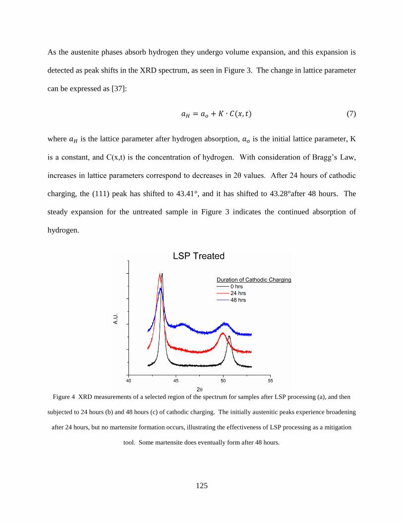
125

As the austenite phases absorb hydrogen they undergo volume expansion, and this expansion is

detected as peak shifts in the XRD spectrum, as seen in Figure 3. The change in lattice parameter

can be expressed as [37]:

𝑎𝐻 = 𝑎𝑜 + 𝐾 ∙ 𝐶(𝑥, 𝑡) (7)

where 𝑎𝐻 is the lattice parameter after hydrogen absorption, 𝑎𝑜 is the initial lattice parameter, K

is a constant, and C(x,t) is the concentration of hydrogen. With consideration of Bragg’s Law,

increases in lattice parameters correspond to decreases in 2θ values. After 24 hours of cathodic

charging, the (111) peak has shifted to 43.41°, and it has shifted to 43.28°after 48 hours. The

steady expansion for the untreated sample in Figure 3 indicates the continued absorption of

hydrogen.

Figure 4 XRD measurements of a selected region of the spectrum for samples after LSP processing (a), and then

subjected to 24 hours (b) and 48 hours (c) of cathodic charging. The initially austenitic peaks experience broadening

after 24 hours, but no martensite formation occurs, illustrating the effectiveness of LSP processing as a mitigation

tool. Some martensite does eventually form after 48 hours.

126

For analysis of the mechanism whereby SCC and hydrogen embrittlement can be mitigated, LSP

treated samples were exposed to the same amount of cathodic charging, as presented in Figure 4.

While it is possible for plastic deformation from the LSP processing to induce martensite, Figure

4 confirms that this transformation has not occurred during our processing. In order to generate

deformation induced martensite in LSP, a threshold of induced pressure from the plasma must be

reached, which for stainless steel has been reported to be around 5 GPa [38]. Using Equation 4,

the induced pressure in our configuration is 2.25 GPa. Although the samples were processed 3

times, keeping the induced pressure below the martensite formation threshold has prevented its

formation. After 24 hours of cathodic charging, shown in the middle line of Figure 4, the austenite

peaks have slightly broadened (a result of distortions to the lattice), but no martensite peak has

formed. This is in direct contrast to Figure 2, and demonstrates that LSP processing suppresses

martensite formation and thereby limits the stainless steel from SCC susceptibility. But, from

Figure 3, the (111) peak has undergone greater expansion compared to the untreated sample after

24 hours. This is because no martensite is available in the LSP treated sample to accommodate

hydrogen. The microstructural changes from LSP that provide this mitigation will be discussed in

the following section. After continued cathodic charging for 48 hours of the LSP treated sample,

martensite eventually does begin to form, as shown in the top line of Figure 4. But this figure is

similar to the shape of the untreated sample charged for 24 hours in Figure 2. So even once

martensite does begin to form in the LSP treated sample, the amount is still less than that of an

untreated sample, and therefore also less likely to suffer premature failure. In Figure 3 the lattice

expansion of (111) has now significantly decreased from the value at 24 hours, indicative of how

the deformed austenite no longer needs to retain as large of amounts of hydrogen and can thus

relax.

127

The rearrangement of the lattice during martensite formation enables the visual detection of its

presence. Polished samples after cathodic charging are imaged using differential interface contrast

(DIC) optical microscopy, and presented in Figure 5, with the sample of (a) being untreated and

(b) being LSP treated prior to the hydrogen exposure..

(a) (b)

Figure 5 (a) Untreated stainless steel sample after cathodic charging 24 hours showing large amounts of martensite

formation, seen as the grains with platelet like structure. (b) Samples which were subject to LSP prior to cathodic

charging have considerably fewer martensitic grains.

The large majority of Figure 5a is indicative of martensite, while only a few martensitic grains are

found in 5b. Since no etchant was used to obtain these images, and the samples were initially

polished to a mirror like finish, the surface deformation is the sole result of hydrogen effects. But

to detect the structure of the grain interiors, SEM imaging was also performed on the same samples

after etching, and is shown in Figure 6. Martensite structure is clearly seen throughout the entirety

of the grain from the untreated sample in Figure 6a. In contrast, the grain of the LSP treated sample

in Figure 6b has a small region of martensite formation, indicated by the arrow, but the phase

transformation has been prevented from propagating throughout the entirety of the grain. This is

the result of the increased dislocation density from the LSP processing resisting the transformation,

confirming the results of the numerical model and Equation 8 below.

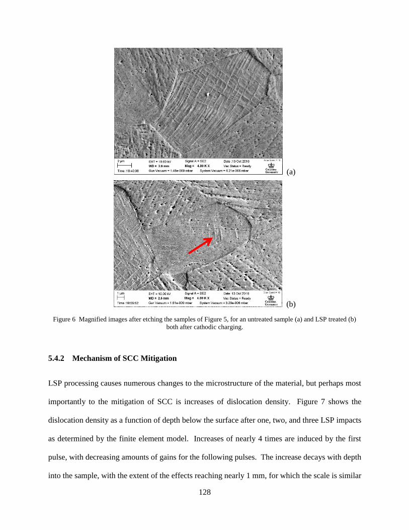
128

(a)

(b)

Figure 6 Magnified images after etching the samples of Figure 5, for an untreated sample (a) and LSP treated (b)

both after cathodic charging.

5.4.2 Mechanism of SCC Mitigation

LSP processing causes numerous changes to the microstructure of the material, but perhaps most

importantly to the mitigation of SCC is increases of dislocation density. Figure 7 shows the

dislocation density as a function of depth below the surface after one, two, and three LSP impacts

as determined by the finite element model. Increases of nearly 4 times are induced by the first

pulse, with decreasing amounts of gains for the following pulses. The increase decays with depth

into the sample, with the extent of the effects reaching nearly 1 mm, for which the scale is similar

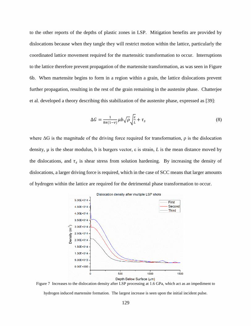
129

to the other reports of the depths of plastic zones in LSP. Mitigation benefits are provided by

dislocations because when they tangle they will restrict motion within the lattice, particularly the

coordinated lattice movement required for the martensitic transformation to occur. Interruptions

to the lattice therefore prevent propagation of the martensite transformation, as was seen in Figure

6b. When martensite begins to form in a region within a grain, the lattice dislocations prevent

further propagation, resulting in the rest of the grain remaining in the austenite phase. Chatterjee

et al. developed a theory describing this stabilization of the austenite phase, expressed as [39]:

∆𝐺 =1

8𝜋(1−𝜈)𝜇𝑏√𝜌√

𝜀

𝐿+ 𝜏𝑠 (8)

where ΔG is the magnitude of the driving force required for transformation, ρ is the dislocation

density, µ is the shear modulus, b is burgers vector, ε is strain, L is the mean distance moved by

the dislocations, and 𝜏𝑠 is shear stress from solution hardening. By increasing the density of

dislocations, a larger driving force is required, which in the case of SCC means that larger amounts

of hydrogen within the lattice are required for the detrimental phase transformation to occur.

Figure 7 Increases to the dislocation density after LSP processing at 1.6 GPa, which act as an impediment to

hydrogen induced martensite formation. The largest increase is seen upon the initial incident pulse.

130

A second effect caused by the increase of dislocation density is a result of dislocations behaving

as hydrogen trapping sites, altering both the diffusivity and solubility of hydrogen within the

material’s lattice. Decreasing the diffusivity will result in the hydrogen not being able to penetrate

deep into the material and restrict any hydrogen induced changes to the near surface level.

Additionally, hydrogen residing in trapping sites will cause less internal stress within the lattice

and therefore be less likely to cause brittle failure. The influence of dislocation density on the

hydrogen diffusion coefficient is expressed as:

𝐷

𝐷𝑜= [1 +

𝑁𝑥𝑁𝐿𝐾

(𝑁𝐿+𝐾𝑐𝐿)2]−1

(9)

where D is the material’s hydrogen diffusion coefficient after LSP, DL is the initial hydrogen

diffusion coefficient, Nx is the number of trapping sites (determined by dislocation density), NL is

the number of interstitial lattice sites, K the equilibrium constant of the reaction defined as K=exp(-

ΔEx/RT), ΔEx is the energy difference between the lattice site and trapping site, and CL is the

hydrogen concentration. Implementation of Equation 9 into the dislocation density results of the

FEM model provide the percentage decrease in hydrogen diffusion coefficient, as shown in Figure

8. Different types of trapping sites can form, with varying strengths of trapping, and this is

represented by larger values of ΔEx and subsequently larger K values. The decrease of diffusivity

is much more dramatic for stronger trapping sites.

131

Figure 8 Decrease in the diffusion coefficient after various levels of incident pressure from LSP processing. The

dotted line of dislocation density shows its inverse relationship to the diffusion coefficient.

The formation of dislocation cells by LSP processing can provide further restrictions to martensitic

formation. Figure 9 shows a 2D cross section of the dislocation cell size after 3 incident LSP

pulses, with symmetry being used along the left hand boundary. An initial distribution of a cellular

arrangement is required for the model, but this is set to 1.8 µm which is large enough that it can

nearly be considered to be the grain size. Again since the hydrogen induced martensitic

transformation requires coordinated lattice movement, microstructural disruptions can prevent the

transformation. The martensitic transformation will not propagate across grain boundaries, and in

the same way dislocation cells may prevent propagation as well. Along grain boundaries

misorientation creates high diffusivity paths for hydrogen to penetrate, but dislocation cells are not

associated with misorientation, and therefore dislocation cells may be further advantageous over

grain boundaries.

132

Figure 9 Distribution of dislocation cell size after 3 LSP impacts. Symmetry is used along the boundary at the left

side.

Figure 10 presents the dislocation cell size at various depths below the surface for increasing

numbers of LSP impacts. Shock pressure governs the size of the dislocation cells formed, while

the pulse duration determines the definition between walls and cell interiors [32]. Similar to the

dislocation density, the greatest change in cell size are caused by the first laser pulse, especially

near the surface. But at 450 µm deep, the cell size continues to decrease after the second and

third pulses. This suggests that further increases to the number of incident pulses will help to

cause deeper effects of cell formation, but a minimum cell size will be eventually attained.

Figure 10 Dislocation cell size for increasing number of incident LSP pulses at 4 depths.

133

The induced pressure from the LSP impact will significantly influence the formation and

structure of the dislocation cells. In Figure 11, the ratio of the dislocation densities of cell walls

to the cell interiors are plotted as a function of increasing incident pressure for a single impact.

Below 1 GPa insufficient deformation occurred to plastically deform the material. But as the

pressure increased, the ratio asymptotically increases as well, approaching a ratio of 8 as the

pressure nears 5 GPa. As mentioned in a previous section, stainless steel will experience

deformation induced martensite from the shockwave at pressures above 5 GPa. Therefore,

significant microstructural changes are occurring which were not captured in the basis for this

numerical model, and therefore place an upper limit on our modelled pressure range. But since

martensite is to be avoided for providing SCC mitigation, the higher incident pulse pressures

should be avoided regardless.

Figure 11 Asymptotic increase of the ratio of dislocation density in cell walls to cell interior.

5.4.3 Imaging Analysis

TEM imaging of the stainless steel samples at various magnifications in order to analyze and

interpret microstructural changes induced by LSP was performed, and also to relate these

134

microstructures to SCC mitigation. Figure 12a shows the structure of an untreated sample, in the

as-received condition. Even before LSP treating, low concentrations of dislocations are present in

the samples with a loosely aligned structure corresponding to the assumption of an initial

concentration that was used for defining the FEM model. Annealing of the samples would provide

further reductions in the initial dislocation density if desired. Little restriction to the motion of

hydrogen and dislocations is provided, since long free paths are present without the effects of

tangling. Hydrogen can freely diffuse through this structure, and upon the initiation of a hydrogen

induced martensitic transformation, large regions of coordinated lattice shifting will occur without

obstruction, spreading the amount of martensite and increasing the material’s SCC susceptibility.

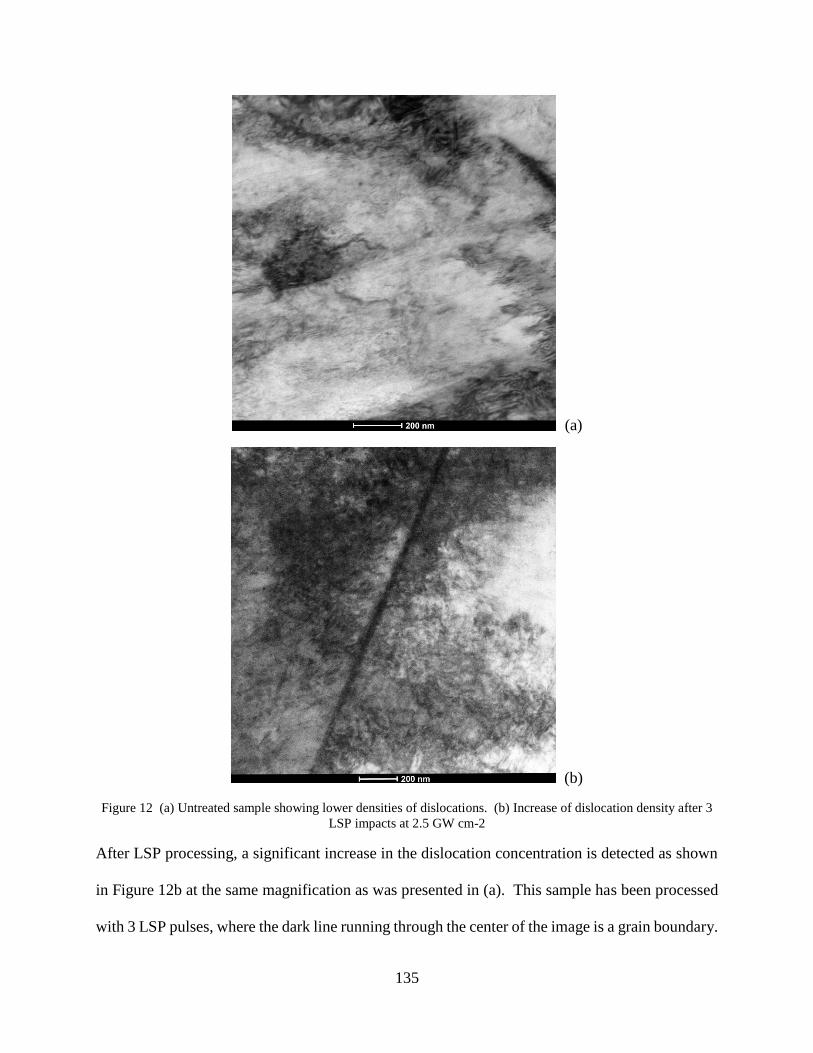
135

(a)

(b)

Figure 12 (a) Untreated sample showing lower densities of dislocations. (b) Increase of dislocation density after 3

LSP impacts at 2.5 GW cm-2

After LSP processing, a significant increase in the dislocation concentration is detected as shown

in Figure 12b at the same magnification as was presented in (a). This sample has been processed

with 3 LSP pulses, where the dark line running through the center of the image is a grain boundary.

136

The darker regions of the image correspond to dense dislocation tangling, and some regions with

low dislocation densities are found on the right hand side. Tangling of dislocations is much more

apparent than in the untreated sample, which will prevent long range dislocation diffusion from

occurring. Stainless steel has a low stacking fault energy (SFE), resulting in screw dislocations

often decomposing into partial dislocations, as well as the formation of twinning.

Dislocation behavior between neighboring grains may be significantly different because the

dislocations will not diffuse across the grain boundary and since the grains have different rotational

orientation to the direction of loading, the slip systems that have become activated will not be the

same. Dislocations in Figure 13 can clearly be seen accumulating near the grain boundary, with

discontinuities in density across the boundary. Behavior at the grain boundary is important to

SCC, since the misorientation along grain boundaries can act as high diffusivity regions for the

hydrogen. Regions with twinning formation are also found along the top portion of the image,

indicated with the arrow, where the mirror like appearance of adjacent diffraction spots in the TEM

image indicates this as well. Twinning can be an intermediate step in the formation of deformation

induced martensite, but the low amounts formed from this LSP processing appear to not have

detrimental effects.

137

Figure 13 Pile ups of dislocations at the grain boundary. Regions of twinning, indicated by the arrow and letter “T”

are also found, with the inset a diffraction image indicative of lattice twinning.

In other regions of the sample, periodic structure formation can be found, as presented in Figure

14a. These dislocation cells effectively partition the inner regions of the grain, helping to prevent

the propagation of any martensitic transformation. Once martensite formation has begun to occur

in a region, in order for it to propagate coordinated lattice motion is required. But the cell walls

disrupt this transformation, limiting the amount of hydrogen induced martensite, which in turn

results in less susceptibility to material failure by SCC. Dislocation cells can also provide for

effective mitigation against the HELP mechanism. Mobile dislocations will become tangled at the

walls [40,41], and by preventing their motion localized decreases to flow stress will be avoided.

Figure 14b also shows the formation of dislocation cells, where it is clear that they are subgrain

structures. Although grain boundaries would also provide barriers to dislocation movement, it is

important to note that dislocation cells occur within individual grains, because the high levels of

misorientation occurring at the grain boundaries actually can allow for increased amounts of

hydrogen diffusion. At high levels of deformation, it is possible for LSP to induce grain

T

138

refinement, where the increased grain boundaries with high amounts of misorientation will provide

high diffusivity paths for the hydrogen to deeply penetrate the lattice. The inset of Figure 14a

shows a TEM diffraction pattern obtained in the region of apparent cell formation. For

polycrystalline regions, the diffraction pattern would show concentric rings indicative of the

various orientations of each lattice structure [31]. But the singular alignment of the diffraction

pattern indicates that there is not any misalignment across the boundaries, thereby ensuring that

high hydrogen diffusivity paths are not formed.

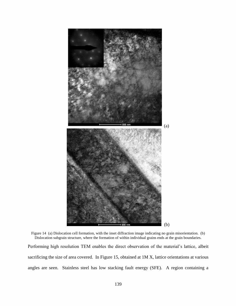
139

(a)

(b)

Figure 14 (a) Dislocation cell formation, with the inset diffraction image indicating no grain misorientation. (b)

Dislocation subgrain structure, where the formation of within individual grains ends at the grain boundaries.

Performing high resolution TEM enables the direct observation of the material’s lattice, albeit

sacrificing the size of area covered. In Figure 15, obtained at 1M X, lattice orientations at various

angles are seen. Stainless steel has low stacking fault energy (SFE). A region containing a

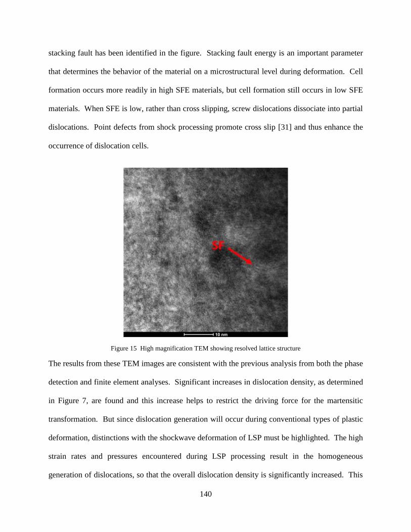
140

stacking fault has been identified in the figure. Stacking fault energy is an important parameter

that determines the behavior of the material on a microstructural level during deformation. Cell

formation occurs more readily in high SFE materials, but cell formation still occurs in low SFE

materials. When SFE is low, rather than cross slipping, screw dislocations dissociate into partial

dislocations. Point defects from shock processing promote cross slip [31] and thus enhance the

occurrence of dislocation cells.

Figure 15 High magnification TEM showing resolved lattice structure

The results from these TEM images are consistent with the previous analysis from both the phase

detection and finite element analyses. Significant increases in dislocation density, as determined

in Figure 7, are found and this increase helps to restrict the driving force for the martensitic

transformation. But since dislocation generation will occur during conventional types of plastic

deformation, distinctions with the shockwave deformation of LSP must be highlighted. The high

strain rates and pressures encountered during LSP processing result in the homogeneous

generation of dislocations, so that the overall dislocation density is significantly increased. This

141

allows for more dislocation tangling and pinning to occur at lower amounts of macroscopic

deformation than would be required in a conventional cold working process of the material.

Furthermore, by performing LSP at conditions below the threshold for deformation induced

martensite and grain refinement, as done in our experiments, increased amounts of beneficial

effects towards mitigation of SCC can be provided.

5.5 Conclusion

The microstructural effects of how LSP provides mitigation for stainless steel against stress

corrosion cracking has been explored with regards to two of the SCC failure mechanisms:

hydrogen induced phase changes and hydrogen enhanced localized plasticity. As hydrogen from

a corrosive environment penetrates into the lattice of stainless steel, it can induce a phase change

of the material from austenite to martensite, resulting in increases to the material’s susceptibility

to failure by SCC. We have shown that laser shock peening is an effective process for preventing

this transformation, and thus improving stainless steel’s resistance to SCC. Cathodic charging

induced martensite in untreated samples within 24 hours, while 48 hours were required to detect

martensite in samples that had undergone LSP. The increases to dislocation density and cell

formation induced by LSP processing restrict the driving force of the transformation, so that larger

amounts of hydrogen are required to cause the detrimental phase change. TEM imaging confirmed

the dislocation increase and arrangement. Likewise, these microstructural changes also promote

tangling of mobile dislocations, which in turn helps prevent premature failure from HELP. As

HELP is prevalent in regions of low dislocation density, increasing the density reduces the ability

of hydrogen to shield the elastic interactions between dislocations. SCC mitigation by delaying

the onset of material failure can thus be achieved, but complete resistance to SCC can not, since

even after LSP treating martensite does eventually form.

142

Chapter 6: Conclusion

In conclusion, two different laser manufacturing processes have been investigated. In each, the

influence on the corrosion behavior of the metallic samples is of concern. While the joining

process required that the initial corrosion behavior of the base materials not be destroyed, the

surface shockwave processing has been carried out with the intention of directly increasing

corrosion resistance. Thus many concerns regarding microstructure and thermally induced

changes from the incident laser beam become common across the two processes. Major

contributions achieved during each of the projects are now summarized below.

6.1 Autogenous Laser Brazing of Wires

Joining of dissimilar metals is traditionally negatively affected by the formation of brittle

intermetallics at the interface. Restricting melting to only one of the materials will limit material

mixing, but crucially, the melting temperatures of NiTi and stainless steel are quite similar. The

process of laser autogenous brazing is a technique for achieving precise control over the heat

input, thereby minimizing the amount of mixing which occurs at the interface and subsequently

provides high strength joints. Thermal resistance at the dissimilar interface results in thermal

accumulation and therefore localized melting at the end of the NiTi. Scanning the laser towards

the interface helps to prevent melting from occurring directly under the incident laser, since the

laser spot size is much larger than the ideal mixed/melted region. While evidence of some

surface melting away from the interface is seen, the continual grain growth detected with

decreasing distance to the interface is evidence that the majority of the melting is restricted to the

actual interface. A cup and cone geometry at the interface has been investigated here for joining

of NiTi to stainless steel. This provides twofold mechanical benefits for further strength

143

increases. First, an increase to the interfacial surface area causes decreases to the stress intensity

factor. Second, the mode II fracture toughness of ideally brittle materials is 20% higher than the

mode I, so by shifting some of the loading into a shear component orientation this increased

strength can be utilized. Uniform temperature throughout the depth of the wires is essential for

quality results, thus rotation of the wires during irradiation has been performed.

Differences between 90° and 120° interfacial angles of the cup and cone geometry were

explored, where 90° are a sharper apex angle. The 90° wires had consistently higher fracture

strengths than the flatter interfacial angled wires, with a difference of 150% for optimal

parameters. In addition to the mechanical benefits of the sharper angle, the alignment during

high speed rotation of the 90° tubes was superior due to the deeper penetration of the sharper

cup-cone configuration. Any potential misalignment has the capacity to prevent complete

joining at the interface from occurring. Rotational speed influences the thermal distribution, and

numerical modeling of the thermal distribution helped to determine the range of parameters to

use as well as providing insight into the differences between parameters. Higher rotational

speeds achieved both higher temperatures and increased temperature uniformity at the interface.

While changes to the laser power can subsequently be accommodated by increases or decreases

to the laser power, temperature uniformity at the interface is most crucial to the autogenous laser

brazing process.

6.2 Biocompatibility of Autogenously Brazed Wires

Since the dissimilar metal pair of NiTi and stainless steel have many applications in the biomedical

field the biocompatibility of the resulting joined samples from autogenous laser brazing is

investigated. Biocompatibility is the capability of an external material to be exposed to the body

without resulting in harmful or toxic effects. Even though the base materials are initially

144

considered biocompatible, thermal effects induced by the laser processing may detrimentally alter

the behavior. Oxide layers, in both materials, are responsible for much of the corrosion resistance.

In particular, a protective titanium oxide layer forms on the outside of NiTi to prevent nickel from

being released, since nickel is of particular biocompatibility concern. Electrochemical, corrosion,

and microbiological testing were all performed to ensure the safety of the autogenous laser brazing

process for use in implantable medical devices.

Polarization testing was carried out on each of the base materials to quantify the amount of

corrosion current flowing at different prescribed electric potentials in a simulated body fluid. The

resulting data was input into a numerical model based on the Nernst-Planck equation to determine

the corrosion current in the NiTi, heat affected zone, mixed region, and stainless steel, where the

corrosion current flowing from the NiTi can release nickel ions. Exposing joined samples to the

simulated body fluid for periods up to 15 days allows for this release to take place, and then the

concentration of nickel ions present in the fluid was measured by use of inductively coupled

plasma atomic emission spectroscopy. Increases to the amount of nickel released compared to the

base material were found, but the level was still below guideline upper limits of the safe amount.

The concentration of only nickel corroded into the simulated body fluid was measured, since nickel

has the most biocompatibility concerns of the materials’ components. While other ions, such as

Fe will also be released, the hemolysis and cytotoxicity tests confirming the biocompatibility do

account for all of the potentially released materials. But still, direct measurement of the amount

of other metallic ions released during corrosion would be informative. Grain growth of the base

materials near the interface occurs from the laser heat input, helping to add to the corrosion

resistance since corrosion current decreases as grain size is increased. Galvanic effects will be

most prominent near the interface, but the larger grains help to counteract this effect, as well as

145

the influence on the oxide layer. The precise amount of heat input during the autogenous laser

brazing process is thus suitable for providing biocompatibility of NiTi and stainless steel.

Therefore, this joining technique has the potential to be used as a manufacturing process for various

types of medical devices.

6.3 Laser Shock Peening for Stress Corrosion Cracking Mitigation

Now, the use of lasers for directly improving the corrosion resistance of materials was investigated,

particularly with regards to stress corrosion cracking (SCC). Laser shock peening (LSP) is a

process which uses laser induced shockwaves to plastically deform a target workpiece. The

response of three materials, stainless steel, high strength streel, and brass, to LSP and subsequent

corrosion testing was compared and differences in their respective behavior was justified in regards

to various material properties. Mechanical fracture, cathodic charging, hardness, analytical,

fractography, and Kelvin Probe Force Microscopy (KPFM) experiments were used for

explanation. Many of the failure mechanisms of SCC are dependent on the behavior of absorbed

hydrogen within the lattice, and its interaction with lattice dislocations induced by the LSP was

explored as a reason for the beneficial effect of surface processing.

Cathodic charging supplies an overvoltage to the workpiece resulting in increased amounts of

hydrogen absorption and is an effective technique to perform accelerated tests. As hydrogen is

absorbed during cathodic charging for 30 minutes, the hardness of untreated stainless steel

increased by nearly 30%. But cathodic charging at various LSP parameters reduced this to values

of less than 5%, thus indicating how LSP prevents the hydrogen from having large detrimental

effects on the material. High strength steel samples showed the same trend. Mechanical U-bend

testing provided definitive proof of the benefits of LSP; stainless steel samples had a 65% increase

in time to failure and the high strength steels had a 40%. In comparison, no increases for the brass

146

samples treated by LSP were found. To account for the material differences, numerical models

comparing the rate of dislocation generation under plastic deformation were simulated. Upon

yielding, each material generated dislocations at differing rates, within a particular material the

heat treatment history further influences the generation.

Two mechanisms of dislocations are then evaluated in terms of corrosion response, their behavior

as hydrogen trapping sites and their influence on the material’s work function. By trapping

hydrogen, large accumulation within the lattice does not occur and thus helps to prevent SCC, but

dislocations also reduce the work function of the material. Work function has been directly

correlated with corrosion resistance, where decreases to work function decrease resistance. By

using KPFM, the work function of high strength steel increased from LSP processing (accounted

for by the compressive residual stress), but the work function of brass decreased. Since brass

yields at lower levels, inducing the same amount of LSP shockwave pressure causes much higher

dislocation densities, which effectively decreases the corrosion resistance. This is illustrative of

how, even though LSP does provide SCC mitigation, the process must be controlled so that over

deformation of the target material does not occur. Performing the U-bend fracture tests for varying

incident LSP pressures would help to establish the optimal parameters, as well as the upper limit

to where increasing amounts of deformation will become detrimental to the SCC resistance. Since

LSP can directly induce the martensite transformation in stainless steel at levels above 5 GPa this

likely create an upper limit, but confirmation of this as well as investigation into the other materials

will help to further elucidate. Since for the chosen parameters used on the brass samples no benefit

was detected, it is thus also possible that mitigation for the brass could be provided by decreasing

the incident LSP pressure.

147

6.4 LSP Suppression of Hydrogen Induced Martensite

For stainless steels, one of the mechanisms of SCC is a phase change from austenite to martensite

induced by absorbed hydrogen. Similar to the way quenching of steels traps carbon in interstitial

sites resulting in lattice deformation, large concentrations of hydrogen will also cause this

transformation. Martensite is more susceptible to SCC than austenite, and thus prevention of this

phase change will provide increased mitigation against the SCC mechanism. Again, dislocations

from LSP processing play an integral role, but this time dislocations counteract the driving force

of martensite transformation.

Phase detection is performed via X-ray diffraction (XRD). Upon cathodic charging, for

accelerated uptake of hydrogen, martensite is detected in untreated stainless steel samples after 24

hours. Further cathodic charging to 48 hours results in a larger amounts of martensite within the

material. But samples that were pre-treated with LSP prior to cathodic charging were found to

have no hydrogen induced martensite after 24 hours of cathodic charging. Direct evidence of LSP

mitigating this SCC mechanism is thus highlighted. Observation of dislocations is achieved via

transmission electron microscopy (TEM), and this technique is performed on untreated and LSP

treated samples to detect microstructural changes that account for the mitigation. Large increases

to dislocation density are found after LSP processing and some arrangement into a sub grain

dislocation cell formation is also seen. Another mechanism of SCC is hydrogen enhanced

localized plasticity (HELP), where in some cases the presence of hydrogen can cause increases to

dislocation mobility, allowing for lowered flow stress in areas near crack tips. The dislocation

structures from LSP processing can promote tangling of mobile dislocations and thus prevent the

increased mobility. By its nature, TEM provides imaging in localized regions. A finite element

model providing a spatially resolved distribution of dislocation density and cell formation is thus

148

provided for comparison with the TEM imaging and to calculate the resulting structure across

larger areas. Since the phase change to martensite requires a coordinated lattice shift, the presence

of dislocations disrupts this movement and prevents martensite formation.

6.5 Future Work

While significant contributions to these two laser based manufacturing processes has been

described above, continued work is identified in order to further develop and improve the

processes. For autogenous laser brazing, additional interfacial geometries can be explored.

Joining of wires is very conducive to the cup and cone geometry, but other configurations such as

lap joints would require a new configuration. The sharp angle formed at the tip of the cone is

subject to stress concentrations and complications regarding uniform heat flow. As such, rounding

of the interface could be compared to the current configuration.

To increase potential applications, autogenous laser brazing of material pairs other than NiTi and

stainless steel should be investigated. Adapting the equations of the thermal finite element model

into dimensionless form would enable efficient selection of the processing parameters for different

materials. Particularly regarding the biocompatibility response, other materials may have different

reactions to the process that are not as favorable as the current materials. Similarly, after exposure

to a corrosive environment, quantification of any decreases to the fracture strength of the joints

would be suitable for investigation, particular for ensuring extended lifetimes of implantable

medical devices that may make use of autogenous laser brazing.

The dynamic behavior of the body will also influence the corrosion response of joined samples.

As highlighted in Chapter 3, the velocity of blood will change its conductivity, as well as providing

the potential for erosion of the joint to occur if crevices are present. Analysis in simulated dynamic

environments may yield different results. The nickel release testing performed in this work was

149

across a duration of 15 days, but for implantable devices the biocompatibility for extended

lifetimes much longer than this must be confirmed. Regarding nickel released from the oxide

layer, the thermal changes increase the amount of nickel which is present, and is often detected as

an initial spike in released nickel. Once the additional nickel region has been depleted, the nickel

released should begin to decay, forming a plateau in Figure 6 of Chapter 3. For applications of the

autogenous laser brazing process, confirmation of this plateau is essential, and can be attained by

performing extended durations of the decay experiments.

Similarly, investigation of the lifetime of the mitigation benefits to SCC provided by LSP

processing is warranted. Each of the corrosion tests performed in this thesis have been under

accelerated conditions, but many applications, such as nuclear reactors, will require extended

lifetimes of the beneficial effects. Additionally, elevated temperature adds another level of

consideration that must be accounted for when determining how long the improvement will last.

Creep and stress relaxation may result in increased SCC susceptibility, so the way that the

dislocation structure evolves with time will determine the material’s behavior. But time

constraints for how long testing can be performed do exist, simply because it is not feasible to

perform real time testing on products that may be expected to be in service for 50 years or more.

As such, determination of the validity and accuracy of extrapolating the results of accelerated tests

to longer lifetimes should be achieved.

Further understanding of the role that dislocations play as hydrogen trapping sites would help to

clarify the extent of SCC mechanisms that can be mitigated by LSP. In particular, measuring

changes to the hydrogen diffusivity caused by LSP will provide valuable insight. The Devanathan-

Stachurski cell is a potential method to do so. The sample workpiece is placed as a membrane

separating two electrochemical cells. By use of a potentiostat, in one of the cells the workpiece is

150

held at a cathodic potential and on the other cell the workpiece is anodic. This induces hydrogen

generation on the cathodic side and diffusion through the sample to the anodic side to occur that

is detected as a current flow in the oxidation cell. Choosing the thickness of the workpiece is

crucial; too thick and minimal amounts of hydrogen will penetrate, but too thin of sample

workpieces will be dominated by surface effects. To promote hydrogen uptake, by preventing

passivated layers from forming, in particular for stainless steel, coating of the surface post-LSP

with a thin palladium layer may be beneficial. Thus, direct measurement of the change to hydrogen

diffusivity caused by LSP can be obtained.

During the cathodic charging measurements of hardness increase and martensitic transformation,

a constant charging current was set, but the actual amount of hydrogen absorbed for each sample

was not determined. The Devanathan-Stachurski cell would be able to provide information about

the rate of hydrogen absorption, and how it will be affected by LSP processing. Furthermore, the

use of thermal desorption spectroscopy to measure subsequent hydrogen release after cathodic

charging would provide data about the amount of hydrogen absorbed.

151

References

Chapter 1:

[1] Gilbert, P. “Golf Club Head.” U.S. Patent: 8128510, March 16, 2011.

[2] Mackiewicz, D., Fitzgerald, K., and Anukhin, B.“Radiopaque markers for medical

devices.” U.S. Patent Application: 20050060025, September 12, 2003.

[3] Kok, M., Dagdelen, F., Aydogdu, A., and Aydogdu, Y., 2016, “The change of

transformation temperature on NiTi shape memory alloy by pressure and thermal ageing,”

J Phys. Conf. Ser., 667(1).

[4] Wayman, C., and Duerig, T., 1990, “An Introduction to Martensite and Shape Memory,”

Engineering Aspects of Shape Memory Alloys, T. Duerig, K. Melton, D. Stockel, and C.

Wayman, eds., Butterworth-Heinemann, Boston, pp. 3–20.

[5] Liu, Y., Liu, Y., and Humbeeck, J. V. A. N., 1999, “Two-Way shape memory effect

developed by martensite deformation in NiTi,” Acta mater., 47(1), pp. 199–209.

[6] Stoeckel, D., and Waram, T., 1991, “Use of NiTi Shape Memory Alloys for Thermal Sensor

‐ Actuators,” Mater Des, 11, pp. 302–307.

[7] Lucy, M. H., Hardy, R. C., Kist, E. H., Watson, J. J., and Wise, S. A., 1996, “Report on

Alternative Devices to Pyrotechnics on Spacecraft,” AISS/USU Cionference on Small

Satellites, Logan, UT.

[8] Oehler, S., Hartl, D., Lopez, R., Malak, R., and Lagoudas, D., 2012, “Design optimization

and uncertainty analysis of SMA morphing structures,” Smart Mater. Struct., 21, p. 090416.

[9] Petrini, L., and Migliavacca, F., 2011, “Biomedical Applications of Shape Memory Alloys,”

J. Metall., 2011(Figure 1), pp. 1–15.

[10] Duerig, T., Pelton, A., and Stöckel, D., 1999, “An Overview of Nitinol Medical

Applications,” Mater. Sci. Eng. A, A273(275), pp. 149–160.

[11] Bahraminasab, M., and Sahari, B. Bin, 2013, “NiTi Shape Memory Alloys , Promising

Materials in Orthopedic Applications.”

[12] Williams, D. F., 2008, “On the mechanisms of biocompatibility,” Biomaterials, 29, pp.

2941–2953.

152

[13] Sunderman, F. W., Dingle, B., Hopfer, S. M., and Swift, T., 1988, “Acute Nickel Toxicity

in Electroplating Workers Who Accidently Ingested a Solution of Nickel Sulfate and Nickel

Chloride,” 266, pp. 257–266.

[14] Shen, M., and Zhang, Q. F., 1994, “Risk Assessment of Nickel Carcinogenicity and

Occupational Lung Cancer,” 102, pp. 275–282.

[15] Trépanier, C., Tabrizian, M., Yahia, L. H., Bilodeau, L., and Piron, D. L., 1998, “Effect of

Modification of Oxide Layer on NiTi Stent Corrosion Resistance,” J. Biomed. Mater. Res.,

43(4), pp. 433–40.

[16] Shabalovskaya, S. a, Tian, H., Anderegg, J. W., Schryvers, D. U., Carroll, W. U., and Van

Humbeeck, J., 2009, “The influence of surface oxides on the distribution and release of

nickel from Nitinol wires.,” Biomaterials, 30(4), pp. 468–77.

[17] Firstov, G. S., Vitchev, R. G., Kumar, H., Blanpain, B., and Van Humbeeck, J., 2002,

“Surface oxidation of NiTi shape memory alloy.,” Biomaterials, 23(24), pp. 4863–71.

[18] Satoh, G., Qiu, C., Naveed, S., and Lawrence Yao, Y., 2014, “Strength and Phase

Identification of Autogenous Laser Brazed Dissimilar Metal Microjoints,” J. Manuf. Sci.

Eng., 137(1), p. 011012.

[19] Lu, B. T., Chen, Z. K., Luo, J. L., Patchett, B. M., and Xu, Z. H., 2005, “Pitting and stress

corrosion cracking behavior in welded austenitic stainless steel,” 50, pp. 1391–1403.

[20] Ota, A., Yazaki, Y., Yokoyama, K., and Sakai, J., 2009, “Hydrogen Absorption and

Thermal Desorption Behavior of Ni-Ti Superelastic Alloy Immersed in Neutral NaCl and

NaF Solutions under Applied Potential,” 50(7), pp. 1843–1849.

[21] Birnbaum, H. K., and Sofronis, P., 1994, “Hydrogen-enhanced localized plasticity—a

mechanism for hydrogen-related fracture,” Mater. Sci. Eng. A, 176(1-2), pp. 191–202.

[22] Lynch, S., 2012, “Hydrogen embrittlement phenomena and mechanisms,” Corros Rev, 30,

pp. 105–123.

[23] Yang, Q., and Luo, J. L., 2000, “Martensite transformation and surface cracking of

hydrogen charged and outgassed type 304 stainless steel,” 288, pp. 75–83.

[24] Ferreira, P., Robertson, I. M., and Birnbaum, H. K., 1998, “Hydrogen Effects on the

Interaction Between Dislocations,” Acta mater., 46(5), pp. 1749–1757.

[25] Izumi, T., and Itoh, G., 2011, “Thermal Desorption Spectroscopy Study on the Hydrogen

Trapping States in a Pure Aluminum,” 52(2), pp. 130–134.

153

[26] Oriani, R. A., 1970, “The diffusion and trapping of hydrogen in steel,” Acta Mater., 18, pp.

147–157.

[27] Nagumo, M., Takai, K., and Okuda, N., 1999, “Nature of hydrogen trapping sites in steels

induced by plastic deformation,” J. Alloys Compd., 293, pp. 310–316.

[28] Obata, M., Sudo, A., and Matsumoto, J., 1996, “The effect of shot peening on residual stress

and stress corrosion cracking for austenitic stainless steel,” Proceedings of 6th International

conference on Shot Peening, pp. 24–33.

[29] Sano, Y., Mukai, N., Okazaki, K., and Obata, M., 1997, “Residual stress improvement in

metal surface by underwater laser irradiation,” Nucl. Instruments Methods Phys. Res. B,

21(I 997), pp. 432–436.

[30] Peyre, P., Scherpereel, X., Berthe, L., Carboni, C., Fabbro, R., Béranger, G., and Lemaitre,

C., 2000, “Surface modifications induced in 316L steel by laser peening and shot-peening.

Influence on pitting corrosion resistance,” Mater. Sci. Eng. A, 280(2), pp. 294–302.

[31] Oldfield, J. W., 1988, “Galvanic Corrosion,” Galvanic Corrosion, H.P. Hack, ed., ASTM,

Philadelphia, PA, pp. 5–22.

[32] Kalainathan, S., Sathyajith, S., and Swaroop, S., 2012, “Effect of laser shot peening without

coating on the surface properties and corrosion behavior of 316L steel,” Opt. Lasers Eng.,

50(12), pp. 1740–1745.

[33] Zhang, Y., You, J., Lu, J., Cui, C., Jiang, Y., and Ren, X., 2010, “Effects of laser shock

processing on stress corrosion cracking susceptibility of AZ31B magnesium alloy,” Surf.

Coatings Technol., 204(24), pp. 3947–3953.

[34] Lu, J. Z., Qi, H., Luo, K. Y., Luo, M., and Cheng, X. N., 2014, “Corrosion behaviour of

AISI 304 stainless steel subjected to massive laser shock peening impacts with different

pulse energies,” Corros. Sci., 80, pp. 53–59.

[35] Fan, Y., Wang, Y., Vukelic, S., and Yao, Y. L., 2007, “Numerical Investigation of Opposing

Dual Sided Microscale Laser Shock Peening,” J. Manuf. Sci. Eng., 129(2), p. 256.

[36] Peyre, P., and Fabbro, R., 1995, “Laser shock processing : a review of the physics and

applications,” Opt. Quantum Electron., 27, pp. 1213–1229.

[37] Clauer, A., 1996, “Laser Shock Peening for Fatigue Resistance,” Surface Performance of

Titanium, J. Gregory, H. Rack, and D. Eylon, eds., TMS, Warrendale, PA, pp. 217–230.

[38] Zhang, W., and Yao, Y. L., 2002, “Micro Scale Laser Shock Processing of Metallic

154

Components,” J. Manuf. Sci. Eng., 124(2), p. 369.

[39] Chen, H., Yao, Y. L., and Kysar, J. W., 2004, “Spatially Resolved Characterization of

Residual Stress Induced by Micro Scale Laser Shock Peening,” J. Manuf. Sci. Eng., 126(2),

p. 226.

[40] Vukelic, S., Kysar, J. W., and Yao, Y. L., “Grain boundary response of aluminum bicrystal

under micro scale laser shock peening.”

[41] Zhang, Y., Lu, J., and Luo, K., 2013, “Stress Corrosion Cracking Resistance of AISI 304

SS Subjected to Laser Shock Processing,” Laser Shock Processing of FCC Metals, Springer,

Berlin, Germany, pp. 137–152.

Chapter 2:

[1] Duerig T., Pelton A., and Stöckel D., 1999, “An Overview of Nitinol Medical

Applications,” Materials Science and Engineering: A, 273-275, pp. 149–160.

[2] Avery R. E., 1991, “Pay Attention to Dissimilar-metal Welds: Guidelines for Welding

Dissimilar Metals,” Chemical Engineering Progress, 4550(May), pp. 1168–1177.

[3] Mubashar A., Ashcroft I. a., Critchlow G. W., and Crocombe A. D., 2011, “Strength

Prediction of Adhesive Joints After Cyclic Moisture Conditioning Using a Cohesive Zone

Model,” Engineering Fracture Mechanics, 78(16), pp. 2746–2760.

[4] Hand H. M., Arah C. O., McNamara D. K., and Mecklenburg M. F., 1991, “Effects of

Environmental Exposure on Adhesively Bonded Joints,” International Journal of

Adhesion and Adhesives, 11(1), pp. 15–23.

[5] Schubert E., Zerner D. I., and Sepold P. G., “Laser Beam Joining of Material

Combinations for Automotive Applications,” SPIE, 3097, pp. 212–221.

[6] Yamamoto N., Liao J., Watanabe S., and Nakata K., 2009, “Effect of Intermetallic

Compound Layer on Tensile Strength of Dissimilar Friction-Stir Weld of a High Strength

Mg Alloy and Al Alloy,” Materials Transactions, 50(12), pp. 2833–2838.

[7] Yan Y., Zhang D., Qiu C., and Zhang W., 2010, “Dissimilar Friction Stir Welding

Between 5052 Aluminum Alloy and AZ31 Magnesium Alloy,” Transactions of

Nonferrous Metals Society of China, 20, pp. s619–s623.

[8] Mathieu A., Shabadi R., Deschamps A., Suery M., Matteï S., Grevey D., and Cicala E.,

2007, “Dissimilar Material Joining Using Laser (Aluminum to Steel Using Zinc-based

Filler Wire),” Optics & Laser Technology, 39(3), pp. 652–661.

155

[9] Li H., Sun D., Gu X., Dong P., and Lv Z., 2013, “Effects of the Thickness of Cu Filler

Metal on the Microstructure and Properties of Laser-welded TiNi Alloy and Dtainless

Steel Joint,” Materials & Design, 50, pp. 342–350.

[10] Satoh G., and Yao Y. L., 2011, “Laser Autogenous Brazing - A New Method for Joining

Dissimilar Metals,” Proc. of the 30th International Congress on the Applications of Lasers

and Electro-Optics, Lake Buena Vista, FL, pp. 315–324.

[11] Bao J., and Yao Y. L., 2001, “Analysis and Prediction of Edge Effects in Laser Bending,”

Journal of Manufacturing Science and Engineering, 123(1), pp. 53–61.

[12] Schwartz M., 1979, Metals Joining Manual, McGraw-Hill, New York.

[13] Brandal G. B., Satoh G., Yao Y. L., and Naveed S., 2013, “Effects of Interfacial Geometry

on Laser Joining of Dissimilar NiTi to Stainless Steel Wires,” Proc. of MSEC 2013,

Madison, WI.

[14] Otsuka K., and Ren X., 2005, “Physical Metallurgy of Ti–Ni-Based Shape Memory

Alloys,” Progress in Materials Science, 50(5), pp. 511–678.

[15] Westbrook J. H., 1967, “Historical Sketch,” Intermetallic Compounds, J.H. Westbrook,

ed., Robert E. Krieger Publishing Co., Inc., New York, pp. 3–14.

[16] Keyzer J. De, “Thermodynamic Modeling of the Fe-Ni-Ti system: A Multiple Sublattice

Approach,” University of Leuven.

[17] Vannod J., 2011, “Laser Welding of Nickel-Titanium and Stainless Steel Wires:

Processing, Metallurgy and Properties,” Ecole Polytechnique Federale De Lausanne.

[18] Sauthoff G., 1995, “Intermetallics,” VCH Publishers, New York.

[19] Martins T. B., and Rechenberg H. R., 2006, “Antiferromagnetic TiFe2 in Applied Fields:

Experiment and Simulation,” Hyperfine Interactions, 169, pp. 1273–1277.

[20] Ghosh M., and Chatterjee S., 2002, “Characterization of Transition Joints of

Commercially Pure Titanium to 304 Stainless Steel,” Materials Characterization, 48(5),

pp. 393–399.

[21] Eijk C. Van Der, Fostervoll H., Sallom Z. K., and Akselsen O. M., 2003, “Plasma

Welding of NiTi to NiTi , Stainless Steel and Hastelloy C276,” ASM Materials Solutions

2003 Conference, Pittsburgh. PA.

[22] Borrisutthekul R., Yachi T., Miyashita Y., and Mutoh Y., 2007, “Suppression of

Intermetallic Reaction Layer Formation by Controlling Heat Flow in Dissimilar Joining of

Steel and Aluminum Alloy,” Materials Science and Engineering A, 467, pp. 108–113.

156

[23] Cacciamani G., Keyzer J. De, Ferro R., Klotz U. E., Lacaze J., and Wollants P., 2006,

“Critical Evaluation of the Fe–Ni, Fe–Ti and Fe–Ni–Ti Alloy Systems,” Intermetallics,

14(10-11), pp. 1312–1325.

[24] Ortega A. M., Tyber J., Frick C. P., Gall K., and Maier H. J., 2005, “Cast NiTi Shape-

Memory Alloys,” Advanced Engineering Materials, 7(6), pp. 492–507.

[25] Liu Y., and McCormick P. G., 1994, “Thermodynamic Analysis of the Martensitic

Transformation in NiTi - Effect of Heat Treatment on Transformation Behaviour,” Acta

metall. mater, 42(7), pp. 2401–2406.

[26] Satoh G., Brandal G. B., Naveed S., and Yao Y. L., 2013, “Laser Autogenous Brazing of

Biocompatible, Dissimilar Metals in Tubular Geometries,” Proc. of North American

Manufacturing Research Institution/SME, Vol. 41, Madison, WI.

[27] Vaidya W. V., Horstmann M., Ventzke V., Petrovski B., Koçak M., Kocik R., and

Tempus G., 2010, “Improving Interfacial Properties of a Laser Beam Welded Dissimilar

Joint of Aluminium AA6056 and Titanium Ti6Al4V for Aeronautical Applications,”

Journal of Materials Science, 45(22), pp. 6242–6254.

[28] Vaidya W. V., Horstmann M., Ventzke V., Petrovski B., Koçak M., Kocik R., and

Tempus G., 2009, “Structure-property Investigations on A Laser Beam Welded Dissimilar

Joint of Aluminium AA6056 and Titanium Ti6Al4V for Aeronautical Applications Part I:

Local Gradients in Microstructure, Hardness and Strength,” Materialwissenschaft und

Werkstofftechnik, 40(8), pp. 623–633.

[29] Satoh G., Yao Y. L., and Qiu C., 2013, “Strength and microstructure of laser fusion-

welded Ti–SS dissimilar material pair,” The International Journal of Advanced

Manufacturing Technology, 66(1-4), pp. 469–479.

[30] Ogata Y., Takatugu M., Kunimasa T., Uenishi K., and Kobayashi K. F., 2004, “Tensile

Strength and Pseudo-elasticity of YAG Laser Spot Melted Ti-Ni Shape Memory Alloy

Wires,” Materials Transactions, 45(4), pp. 1070–1076.

[31] Hertzberg R. W., 1996, Deformation and Fracture Mechanics of Engineering Materials,

John wiley & Sons, Inc., New York.

[32] Awaji H., and Kato T., 1999, “Awaji - Criterion for combined mode I-II brittle

fracture.pdf,” Materials Transactions, 40(9), pp. 972–979.

[33] Munz D., and Yang Y. Y., 1992, “Stress Singularities at the Interface in Bonded

Dissimilar Materials Under Mechanical and Thermal Loading,” Journal of Applied

Mathematics, 59(December), pp. 857–861.

[34] Wah T., 1975, “Plane stress analysis of a scarf joint,” 491(December).

157

[35] Ifflander R., 2001, Solid-State Lasers for Materials Processing, Springer-Verlag, New

York.

[36] Xie J., Kar A., Rothenflue J. A., and Latham W. P., 1997, “Temperature-Dependent

Absorptivity and Cutting Capability of CO 2 , Nd: YAG and Chemical Oxygen-iodine

Lasers,” Journal of Laser Applications, 9, pp. 77–85.

[37] Bel’skaya E. A., 2005, “An Experimental Investigation of the Electrical Resistivity of

Titanium in the Temperature Range from 77 to 1600 K,” High Temperature, 43(4), pp.

546–553.

[38] Incropera F. P., and DeWitt D. P., 2002, Fundamentals of Heat and Mass Transfer, John

wiley & Sons, Inc., Hoboken, NJ.

[39] Younglove B. A., and Hanley J. M., 1986, “The Viscosity and Thermal Conductivity

Coefficients of Gaseous and Liquid Argon,” Journal of Physical and Chemical Reference

Data, 15(4), pp. 1323–1337.

[40] “ASTM Standard E8, 2011, ‘Standard Test Methods for Tension Testing of Metallic

Materials,’ ASTM International, West Conshohocken, PA, 2003.”

[41] Li W., and Yao Y. L., 2001, “Laser Forming with Constant Line Energy,” The

International Journal of Advanced Manufacturing Technology, 17(3), pp. 196–203.

Chapter 3:

[1] Duerig T., Pelton A., and Stöckel D., 1999, “An Overview of Nitinol Medical

Applications,” Mater. Sci. Eng. A, A273(275), pp. 149–160.

[2] Dos Santos R. L., Pithon M. M., Nascimento L. E. A. G., Martins F. O., Teresa M.,

Romanos V., and Nojima L. I., 2011, “Cytotoxicity of electric spot welding : an in vitro

study,” Dent. Press J Orthod., 16(3), pp. 1–6.

[3] Vannod J., 2011, “Laser Welding of Nickel-Titanium and Stainless Steel Wires:

Processing, Metallurgy and Properties,” Ecole Polytechnique Federale De Lausanne.

[4] Cui Z. D., Man H. C., and Yang X. J., 2005, “The Corrosion and Nickel Release Behavior

of Laser Surface-melted NiTi Shape Memory Alloy in Hanks’ Solution,” Surf. Coatings

Technol., 192(2-3), pp. 347–353.

[5] Surmenev R. a, Ryabtseva M. a, Shesterikov E. V, Pichugin V. F., Peitsch T., and Epple

M., 2010, “The Release of Nickel from Nickel-Titanium (NiTi) is Strongly Reduced by a

Sub-micrometer Thin Layer of Calcium Phosphate Deposited by rf-Magnetron

Sputtering.,” J. Mater. Sci. Mater. Med., 21(4), pp. 1233–9.

158

[6] Hang R., Ma S., Ji V., and Chu P. K., 2010, “Corrosion Behavior of NiTi Alloy in Fetal

Bovine Serum,” Electrochim. Acta, 55(20), pp. 5551–5560.

[7] Zhang C., Sun X., Zhao S., Yu W., and Sun D., 2014, “Susceptibility to Corrosion and In

Vitro Biocompatibility of a Laser-Welded Composite Orthodontic Arch Wire.,” Ann.

Biomed. Eng., 42(1), pp. 222–230.

[8] Li H. M., Sun D. Q., Cai X. L., Dong P., and Wang W. Q., 2012, “Laser Welding of TiNi

Shape Memory Alloy and Stainless Steel Using Ni Interlayer,” Mater. Des., 39, pp. 285–

293.

[9] Brandal G., Satoh G., Yao Y. L., and Naveed S., 2013, “Beneficial Interface Geometry for

Laser Joining of NiTi to Stainless Steel Wires,” J. Manuf. Sci. Eng., 135(6).

[10] Satoh G., and Yao Y. L., 2011, “Laser Autogenous Brazing - A New Method for Joining

Dissimilar Metals,” Proceedings of the 30th International Congress on the Applications of

Lasers and Elecro-Optics, Lake Buena Vista, FL, pp. 315–324.

[11] Cacciamani G., De Keyzer J., Ferro R., Klotz U. E., Lacaze J., and Wollants P., 2006,

“Critical evaluation of the Fe–Ni, Fe–Ti and Fe–Ni–Ti alloy systems,” Intermetallics,

14(10-11), pp. 1312–1325.

[12] Li X., Wang J., Han E., and Ke W., 2007, “Influence of Fluoride and Chloride on

Corrosion Behavior of NiTi Orthodontic Wires,” Acta Biomater., 3(5), pp. 807–15.

[13] Wang J., Li N., Han E., and Ke W., 2006, “Effect of pH, Temperature and Cl-

concentration on Electrochemical Behavior of NiTi Shape Memory Alloy in Artificial

Saliva,” J. Mater. Sci. Mater. Med., 17(10), pp. 885–90.

[14] Petro R., and Schlesinger M., 2013, Applications of Electrochemistry in Medicine,

Springer US, Boston, MA.

[15] 2003, “Risk Assessment: Nickel,” Expert Gr. Vitam. Miner., pp. 225–231.

[16] Armitage D. a, Parker T. L., and Grant D. M., 2003, “Biocompatibility and

Hemocompatibility of Surface-Modified NiTi Alloys.,” J. Biomed. Mater. Res. A, 66(1),

pp. 129–137.

[17] Wataha J. C., Lockwood P. E., Marek M., and Ghazi M., 1999, “Ability of Ni-containing

Biomedical Alloys to Activate Monocytes and Endothelial Cells in Vitro.,” J. Biomed.

Mater. Res., 45(3), pp. 251–257.

[18] Fehlner F., and Graham M., 2002, “Thin Oxide Film Formation on Metals,” Corrosion

Mechanisms in Theory and Practice, P. Marcus, ed., Marcel Dekker, New York, NY, pp.

171–187.

159

[19] Michiardi A., Aparicio C., Planell J. a, and Gil F. J., 2006, “New Oxidation treatment of

NiTi Shape Memory Alloys to Obtain Ni-free Surfaces and to Improve

Biocompatibility.,” J. Biomed. Mater. Res. B. Appl. Biomater., 77(2), pp. 249–56.

[20] Tan L., 2003, “Corrosion and Wear-Corrosion Behavior of NiTi Modified by Plasma

Source Ion Implantation,” Biomaterials, 24(22), pp. 3931–3939.

[21] Trépanier C., Tabrizian M., Yahia L. H., Bilodeau L., and Piron D. L., 1998, “Effect of

Modification of Oxide Layer on NiTi Stent Corrosion Resistance,” J. Biomed. Mater.

Res., 43(4), pp. 433–40.

[22] Sohmura T., 1988, “Improvement in Corrosion Resistance in Ti-Ni Shape Memory Alloy

for Implant by Oxide Film Coating,” World Biomaterial Congress Proceedings, Kyoto,

Japan, p. 574.

[23] Undisz A., Schrempel F., Wesch W., and Rettenmayr M., 2012, “Mechanism of Oxide

Layer Growth During Annealing of NiTi,” J. Biomed. Mater. Res. A, 100(7), pp. 1743–

1750.

[24] Villermaux F., Tabrizian M., Yahia L., Meunier M., and Piron D. L., 1997, “Excimer

Laser Treatment of NiTi Shape Memory Alloy Biomaterials,” Appl. Surf. Sci., 109-110,

pp. 62–66.

[25] Nishida M., Wayman C. M., and Honma T., 1986, “Precipitation Processes in Near-

Equiatomic TiNi Shape Memory Alloys,” Metall. Trans. A, 17(9), pp. 1505–1515.

[26] Verdian M. M., Raeissi K., Salehi M., and Sabooni S., 2011, “Characterization and

Corrosion Behavior of NiTi–Ti2Ni–Ni3Ti Multiphase Intermetallics Produced by Vacuum

Sintering,” Vacuum, 86(1), pp. 91–95.

[27] Landolt D., 2002, “Introduction to Surface Reactions: Electrochemical Basis of

Corrosion,” Corrosion Mechanisms in Theory and Practice, P. Marcus, ed., Marcel

Dekker, New York, NY, pp. 1–17.

[28] Jones D. A., 1992, Principles and Prevention of Corrosion, MacMillan, New York.

[29] Oldfield J. W., 1988, Galvanic Corrosion, ASTM, Philadelphia, PA.

[30] Deshpande K. B., 2011, “Numerical Modeling of Micro-Galvanic Corrosion,”

Electrochim. Acta, 56(4), pp. 1737–1745.

[31] Chan C. W., Man H. C., and Yue T. M., 2012, “Susceptibility to Stress Corrosion

Cracking of NiTi Laser Weldment in Hanks’ Solution,” Corros. Sci., 57, pp. 260–269.

160

[32] Yan X.-J., and Yang D.-Z., 2006, “Corrosion Resistance of a Laser Spot-Welded Joint of

NiTi Wire in Simulated Human Body Fluids,” J. Biomed. Mater. Res. A, 77(1), pp. 97–

102.

[33] F756-08 A., 2013, “Standard Practice for Assessment of Hemolytic Properties of

Materials,” pp. 1–5.

[34] 10993-5 I., 2009, Biological evaluation of medical devices - Part 5: Tests for in vitro

cytotoxicity.

[35] ASTM, 2013, “Standard Reference Test Method for Making Potentiostatic and

Potentiodynamic Anodic,” 94(Reapproved 2011), pp. 1–13.

[36] 200.7 E., 1994, “Determination of Metals and Trace Elements in Water and Wastes by

Inductively Coupled Plasma-Atomic Emission Spectrometry,” 4, pp. 1–58.

[37] Visser K. R., 1989, “Electric Conductivity of Stationary and Flowing Human Blood at

Low Frequencies,” IEEE Engineering in Medicine & Biology Society 11th Annual

International Conference, pp. 1540–1542.

[38] McMahon R. E., Ma J., Verkhoturov S. V, Munoz-Pinto D., Karaman I., Rubitschek F.,

Maier H. J., and Hahn M. S., 2012, “A Comparative Study of the Cytotoxicity and

Corrosion Resistance of Nickel-Titanium and Titanium-Niobium Shape Memory Alloys.,”

Acta Biomater., 8(7), pp. 2863–70.

[39] Satoh G., 2013, “Modification and Integration of Shape Memory Alloys through Thermal

Treatments and Dissimilar Metal Joining,” Columbia University.

[40] Crone W. C., Yahya A. n., and Perepezko J. H., 2001, “Influence of Grain Refinement on

Superelasticty in NiTi,” Proceedings of the SEM Annual Conference on Experimental

Mechanics, Portland, OR, pp. 510–513.

[41] Ralston K. D., Birbilis N., and Davies C. H. J., 2010, “Revealing the Relationship

Between Grain Size and Corrosion Rate of Metals,” Scr. Mater., 63(12), pp. 1201–1204.

[42] Shih C. C., Lin S. J., Chung K. H., Chen Y. L., and Su Y. Y., 2000, “Increased Corrosion

Resistance of Stent Materials by Converting Current Surface Film of Polycrystalline

Oxide into Amorphous Oxide.,” J. Biomed. Mater. Res., 52(2), pp. 323–332.

[43] Zhang Y., Jiang S., Liang Y., and Hu L., 2013, “Simulation of Dynamic Recrystallization

of NiTi Shape Memory Alloy During Hot Compression Deformation Based on Cellular

Automaton,” Comput. Mater. Sci., 71, pp. 124–134.

[44] Akgun O. V., Urgen M., and Cakir A. F., 1995, “The Effect of Heat Treatment on

Corrosion Behavior of Laser Surface Melted 304L Stainless Steel,” Mater. Sci. Eng. A,

203, pp. 324–331.

161

[45] Prokofiev E., Burow J., Payton E., Zarnetta R., Frenzel J., Gunderov D. V., Valiev R. Z.,

and Eggeler G., 2010, “Suppression of Ni4Ti3 Precipitation by Grain Size Refinement in

Ni-Rich NiTi Shape Memory Alloys,” Adv. Eng. Mater., 12(8), pp. 747–753.

Chapter 4:

[1] Brandl, E., Malke, R., Beck, T., Wanner, a., and Hack, T., 2009, “Stress corrosion cracking

and selective corrosion of copper-zinc alloys for the drinking water installation,” Mater.

Corros., 60(4), pp. 251–258.

[2] Rice, S., 2015, “Epic Energy finds gas pipeline rupture was caused by stress corrosion

cracking,” Advert.

[3] Cox, B., 1990, “Environmentally-induced cracking of zirconium alloys - a review,” J. Nucl.

Mater., 170, pp. 1–23.

[4] Obata, M., Sudo, A., and Matsumoto, J., 1996, “The effect of shot peening on residual stress

and stress corrosion cracking for austenitic stainless steel,” Proceedings of 6th International

conference on Shot Peening, pp. 24–33.

[5] Chen, H., Yao, Y. L., and Kysar, J. W., 2004, “Spatially Resolved Characterization of

Residual Stress Induced by Micro Scale Laser Shock Peening,” J. Manuf. Sci. Eng., 126(2),

p. 226.

[6] Zhang, Y., Lu, J., and Luo, K., 2013, “Stress Corrosion Cracking Resistance of AISI 304

SS Subjected to Laser Shock Processing,” Laser Shock Processing of FCC Metals, Springer,

Berlin, Germany, pp. 137–152.

[7] Peyre, P., Braham, C., Ledion, J., Berthe, L., and Fabbro, R., 2000, “Corrosion Reactivity

of Laser-Peened Steel Surfaces,” 9(December), pp. 656–662.

[8] Birnbaum, H. K., and Sofronis, P., 1994, “Hydrogen-enhanced localized plasticity—a

mechanism for hydrogen-related fracture,” Mater. Sci. Eng. A, 176(1-2), pp. 191–202.

[9] Akid, R., and Dmytrakh, I., 1998, “Influence of Surface Deformation and Electrochemical

Variables on Corrosion and Corrosion Fatigue Crack Development,” Fatigue Fract. Eng.

Mater. Struct., 21, pp. 903–911.

[10] Shewmon, P., 1989, Diffusion in Solids, The Minerals, Metals, and Materials Society,

Warrendale, PA.

[11] Hirth, J. P., 1980, “Effects of Hydrogen on the properties of Iron and steel,” Metall. Trans.

A, 11, pp. 861–890.

[12] Kamoutsi, H., Haidemenopoulos, G. N., Bontozoglou, V., and Pantelakis, S., 2006,

“Corrosion-induced hydrogen embrittlement in aluminum alloy 2024,” Corros. Sci., 48(5),

pp. 1209–1224.

[13] Peyre, P., and Fabbro, R., 1995, “Laser shock processing : a review of the physics and

applications,” Opt. Quantum Electron., 27, pp. 1213–1229.

162

[14] Fan, Y., Wang, Y., Vukelic, S., and Yao, Y. L., 2005, “Wave-solid interactions in laser-

shock-induced deformation processes,” J. Appl. Phys., 98(10), p. 104904.

[15] Navai, F., 1995, “Effects of tensile and compressive stresses on the passive layers formed

on a type 302 stainless steel in a normal sulphuric acid bath,” J Mat Sci, 30, pp. 1166–1172.

[16] Chen, H., Kysar, J. W., and Yao, Y. L., 2004, “Characterization of Plastic Deformation

Induced by Microscale Laser Shock Peening,” J. Appl. Mech., 71(5), p. 713.

[17] Krom, A. H. M., and Bakker, A., 2000, “Hydrogen trapping models in steel,” Metall. Mater.

Trans. B, 31(6), pp. 1475–1482.

[18] Malygin, G. A., 1990, “Dislocation Density Evolution Equation and Strain Hardening of

f.c.c. Crystals,” Phys. Status Solidi, 119(2), pp. 423–436.

[19] Druffner, C., Schumaker, E., and Sathish, S., 2004, “Scanning Probe Microscopy :,”

Nondestructive Materials Characterization, N.G.H. Meyendorf, ed., Springer-Verlag, pp.

323–355.

[20] Schmutz, P., and Frankel, G. S., 1998, “Characterization of AA2024-T3 by Scanning Kelvin

Probe Force Microscopy,” J. Electrochem. Soc., 145(7), pp. 2285–2295.

[21] Stratmann, M., and Streckel, H., 1990, “On the atmospheric corrosion of metals which are

covered with thin electrolyte layers. Verification of the experimental technique,” Corros.

Sci., 30(6-7), pp. 681–696.

[22] Wang, X. F., Li, W., Lin, J. G., and Xiao, Y., 2010, “Electronic work function of the Cu

(100) surface under different strain states,” Europhys. Lett., 89(6), p. 66004.

[23] Li, W., and Li, D. Y., 2005, “Variations of work function and corrosion behaviors of

deformed copper surfaces,” Appl. Surf. Sci., 240(1-4), pp. 388–395.

[24] Meyers, M., and Murr, L., 1981, Shock Waves and High Strain Rate Phenomena in Metals,

Plenum Press, New York.

[25] Al Duheisat, S., 2014, “An Investigation of Mechanical Degradation of Pure Copper by

Hydrogen,” Contemp. Eng. Sci., 7(4), pp. 165–178.

[26] Zhang, W., Yao, Y. L., Engineering, M., and York, N., 2001, “Microscale Laser Shock

Processing — Modeling , Testing , and Microstructure Characterization,” 3(2), pp. 128–

143.

[27] Meyers, M. A., Jarmakani, H., Bringa, E. M., and Remington, B. A., 2009, “Dislocations in

Shock Compression and Release,” Dislocations in Solids, J.P. Hirth, and L. Kubin, eds.,

Elsevier, pp. 91–197.

[28] Nahme, H., Worswick, M., Nahme, H., and Dynamic, M. W., 1994, “Dynamic properties

and spall plane formation of brass,” J. Phys. IV, 04(C8), pp. 707–712.

[29] Duffy, T. S., Ahrens, T. J., and Samples, a, 1997, “Dynamic compression of an Fe – Cr –

Ni alloy to 80 GPa,” 82(1997), pp. 4259–4269.

163

Chapter 5:

[1] Lijie, Q., Wuyang, C., Huijun, M., Jimei, X., and Peixin, G., 1993, “Hydrogen-facilitated

corrosion and stress corrosion cracking of austenitic stainless steel of type 310,” MetTrans

A, 24, pp. 959–962.

[2] Was, G. S., and Andresen, P., 2007, “Stress Corrosion Cracking Behavior of Alloys in

Aggressive Nuclear Reactor Core Environments,” Corrosion, 63(1), pp. 19–45.

[3] Manfredi, C., and Otegui, J. ., 2002, “Failures by SCC in buried pipelines,” Eng. Fail.

Anal., 9(5), pp. 495–509.

[4] Kane, R. D., Sridhar, N., Brongers, M. P., Beavers, J. A., Agrawal, A. K., and Klein, L. J.,

2005, “Stress corrosion cracking in fuel ethanol: a recently recognized phenomenon,”

Mater. Perform., (12), pp. 50–55.

[5] Manivasagam, G., Dhinasekaran, D., and Rajamanickam, A., 2010, “Biomedical Implants:

Corrosion and its Prevention - A Review,” Recent Patents Corros. Sci., 2(1), pp. 40–54.

[6] Ensinger, W., 1996, “Ion-beam sputter coating of tantalum tube inner walls for protection

against hydrogen embrittlement,” Surf. Coatings Technol., 84(1–3), pp. 434–438.

[7] Michler, T., 2008, “Influence of plasma nitriding on hydrogen environment embrittlement

of 1.4301 austenitic stainless steel,” Surf. Coatings Technol., 202, pp. 1688–1695.

[8] Peyre, P., and Fabbro, R., 1995, “Laser shock processing : a review of the physics and

applications,” Opt. Quantum Electron., 27, pp. 1213–1229.

[9] Zhang, Y., Lu, J., and Luo, K., 2013, “Stress Corrosion Cracking Resistance of AISI 304

SS Subjected to Laser Shock Processing,” Laser Shock Processing of FCC Metals,

Springer, Berlin, Germany, pp. 137–152.

[10] Brandal, G., and Yao, Y. L., 2015, “Microstructural Effects Induced by Laser Shock

Peening for Mitigation of Stress Corrosion Cracking,” ICALEO, Atlanta, GA.

[11] Peyre, P., Braham, C., Ledion, J., Berthe, L., and Fabbro, R., 2000, “Corrosion Reactivity

of Laser-Peened Steel Surfaces,” 9(December), pp. 656–662.

[12] Chen, H., Yao, Y. L., and Kysar, J. W., 2004, “Spatially Resolved Characterization of

Residual Stress Induced by Micro Scale Laser Shock Peening,” J. Manuf. Sci. Eng., 126(2),

p. 226.

[13] Hirth, J. P., 1980, “Effects of Hydrogen on the properties of Iron and steel,” Metall. Trans.

A, 11, pp. 861–890.

[14] Ozgowicz, W., Kurc-lisiecka, A., and Grajcar, A., 2012, “Corrosion Behaviour of Cold-

Deformed Austenitic Alloys.”

164

[15] Zinbi, A., and Bouchou, A., 2010, “Delayed cracking in 301 austenitic steel after bending

process : Martensitic transformation and hydrogen embrittlement analysis,” 17, pp. 1028–

1037.

[16] Liu, R., Narita, N., Alstetter, C., Birnbaum, H., and Pugh, E. N., 1980, “Studies of the

Orientations of Fracture Surfaces Produced in Austenitic Stainless Steels By Stress-

Corrosion Cracking and Hydrogen Embrittlement,” Metall. Trans. A, 11(September), pp.

1563–1574.

[17] Solomon, N., and Solomon, I., 2010, “Deformation induced martensite in AISI 316

stainless steel,” 46(13), pp. 121–128.

[18] Olson, G. B., and Cohen, M., 1972, “A mechanism for the strain-induced martensitic

transformations,” J. Less-Common Met., 28(1), pp. 107–118.

[19] Shin, H. C., Ha, T. K., and Chang, Y. W., 2001, “Kinetics of deformation induced

martensitic transformation in a 304 stainless steel,” 45, pp. 823–829.

[20] Vakhney, A. G., Yaresko, A. N., Antonov, V. N., and Nemoshkalenko, V. V, 1998, “The

effect of hydrogen on the electronic structure and phase stability of iron-based alloys doped

with chromium and nickel,” 10, pp. 6987–6994.

[21] Hoelzel, M., Danilkin, S. A., Ehrenberg, H., Toebbens, D. M., Udovic, T. J., Fuess, H., and

Wipf, H., 2004, “Effects of high-pressure hydrogen charging on the structure of austenitic

stainless steels,” 384, pp. 255–261.

[22] Narita, N., Altstetter, C. J., and Birnbaum, H. K., 1982, “Hydrogen-related phase

transformations in austenitic stainless steels,” Metall. Trans. A, 13(8), pp. 1355–1365.

[23] Ćwiek, J., 2009, “Hydrogen degradation of high-strength steels,” 37(2), pp. 193–212.

[24] Ferreira, P., Robertson, I. M., and Birnbaum, H. K., 1998, “Hydrogen Effects on the

Interaction Between Dislocations,” Acta mater., 46(5), pp. 1749–1757.

[25] Birnbaum, H. K., and Sofronis, P., 1994, “Hydrogen-enhanced localized plasticity—a

mechanism for hydrogen-related fracture,” Mater. Sci. Eng. A, 176(1–2), pp. 191–202.

[26] Sofronis, D. C. A. P., and Jr, R. D., 2007, “Modeling of hydrogen-assisted ductile crack

propagation in metals and alloys,” pp. 135–157.

[27] Pezold, J. Von, and Lymperakis, L., 2011, “Hydrogen-enhanced local plasticity at dilute

bulk H concentrations : The role of H – H interactions and the formation of local hydrides,”

59, pp. 2969–2980.

[28] Song, J., and Curtin, W. A., 2014, “Mechanisms of hydrogen-enhanced localized

plasticity : An atomistic study using a -Fe as a model system,” Acta mater., 68, pp. 61–69.

[29] Lynch, S. P., 2011, “Hydrogen embrittlement (HE) phenomena and mechanisms,” Stress

Corrosion Cracking: Theory and Practice, V.S. Raja, and T. Shoji, eds., Woodhead

Publishing, Cambridge, UK, pp. 90–130.

165

[30] Holt, D. L., 1970, “Dislocation cell formation in metals,” J. Appl. Phys., 41(8), pp. 3197–

3201.

[31] Mordyuk, B. N., Milman, Y. V., Iefimov, M. O., Prokopenko, G. I., Silberschmidt, V. V.,

Danylenko, M. I., and Kotko, a. V., 2008, “Characterization of ultrasonically peened and

laser-shock peened surface layers of AISI 321 stainless steel,” Surf. Coatings Technol.,

202(19), pp. 4875–4883.

[32] Meyers, M., and Murr, L., 1981, Shock Waves and High Strain Rate Phenomena in Metals,

Plenum Press, New York.

[33] Fan, Y., Wang, Y., Vukelic, S., and Yao, Y. L., 2007, “Numerical Investigation of

Opposing Dual Sided Microscale Laser Shock Peening,” J. Manuf. Sci. Eng., 129(2), p.

256.

[34] Simulia, 6AD, “Abaqus Analysis User’s Guide.”

[35] Toth, L. S., Molinari, A., and Estrin, Y., 2002, “Strain Hardening at Large Strains as

Predicted by Dislocation Based Polycrystal Plasticity Model,” J. Eng. Mater. Technol.,

124(1), p. 71.

[36] Bentley, A. P., and Smith, G. C., 1986, “Phase-Transformation of Austenitic Stainless-

Steels As a Result of Cathodic Hydrogen Charging,” Metall. Trans. a-Physical Metall.

Mater. Sci., 17(9), pp. 1593–1600.

[37] Rozenak, P., and Bergman, R., 2006, “X-ray phase analysis of martensitic transformations

in austenitic stainless steels electrochemically charged with hydrogen,” 437, pp. 366–378.

[38] Ye, C., Suslov, S., Lin, D., and Cheng, G. J., 2012, “Deformation-induced martensite and

nanotwins by cryogenic laser shock peening of AISI 304 stainless steel and the effects on

mechanical properties,” Philos. Mag., 92(11), pp. 1369–1389.

[39] Chatterjee, S., Wang, H., Yang, J. R., and Bhadeshia, H. K. D. H., 2006, “Mechanical

stabilisation of austenite,” 22(6), pp. 641–644.

[40] Shin, D. H., Kim, I., Kim, J., and Park, K., 2001, “Grain Refinement Mechanism During

Equal-Channel Angular Pressing of a Low-Carbon Steel,” Acta MAter., 49, pp. 1285–

1292.

[41] Takai, K., and Kitamura, M., 2013, “Hydrogen Dragging by Moving Dislocation and

Enhanced Lattice Defect Formation in 316L and 304 Stainless Steels,” Proc. of the ASME

2013 Pressure Vessels and Piping Conference, pp. 1–7.

166

Appendix This appendix section works in conjunction with the archived files, and is for the purpose of

describing the attached data as well as the practical requirements in order to run the numeric

simulations that were developed for this thesis. A folder corresponding to each body chapter has

been created: autogenous laser brazing for joining of dissimilar materials is found in “\Chapter 2,”

biocompatibility analysis of the dissimilar joined NiTi and stainless steel samples is in

“\Chapter 3”, material differences accounting for the mitigation of stress corrosion cracking via

laser shock peening is found in “\Chapter 4,” and finally the microstructure changes accounting

for the improved mitigation from LSP is in “\Chapter 5.” Relevant information for each chapter,

as well as some additional data which was not included in the described results, will now be

individually provided. Furthermore, slides for the corresponding presentations of each chapter are

found in “\Presentations,” as well as the Thesis Defense presentation slides.

Chapter 2: Beneficial Interface Geometry for Laser Joining of NiTi to Stainless Steel Wires

The file “Parameter Key.pdf” contains the numeric code used for identification of the parameters

used for each sample. A progression of several configurations is included, starting with flat

interfaces without rotation, then going all the way through the best results of rotation with conical

interfaces. Sample number, laser power, rotational velocity, total degrees of rotation, longitudinal

(linear scan) velocity, scan length, as well as relevant notes for each piece is recorded. The sample

numbers can then be used to identify the data in the folder “\Tensile Test Data,” which contains

both raw data and some compiled charts from the MTS testing. Calculation of the amount of

overlap during rotation, dependent on the scan length, total rotational degrees, and beam radius is

found using “Laser Rotation Overlap.xlsx.” Changing these parameters in cells B1 and F1 will

167

automatically produce the amount of overlap in column B, as a function of various total rotational

degrees. Additional optical imaging of cross sectioned samples is contained in the folder “\Cross

Section Images.”

Thermal modelling of the temperature distribution during the joining process was performed in

COMSOL. The file “Thermal3dWires.mph” is used for running the simulation, where in this, the

heat equation is solved in three dimensions. To simulate rotation of the wires, the heat flux

representing the incident laser spot is rotated while the wires remain stationary in the simulation.

Numerous parameters are required to implement this type of motion on the heat flux, and are first

defined in the Model Builder under Global Definitions Parameters. Many of the definitions are

self-explanatory, such as power and beam radius. “Laser Rotation Overlap.xslx” is used for choice

of TotalDegrees. stopDistance is the distance short of the interface at which the laser source is

turned off. Simulation of the thermal resistance and then subsequent joining and wetting uses a

step function for the conductivity at the interface, set by the two values initialInterface and

meltedInterface, which are the limits for the DefinitionVariables 1 Interface Conductance.

Geometrical arguments are made to determine LaserFlux, which is the rotating heat source. Upon

completion of the laser scan simulation, spatially resolved 3D data of temperature are thus

provided, from which time history and temperature path data can be extracted.

Chapter 3: Biocompatibility and Corrosion Response of Laser Joined NiTi to Stainless Steel

Wires

Several folders containing files for the different measurements performed to determine the

biocompatibility of autogenously brazed wires are found in the “\Chapter 3” folder. Images of the

cross section of joined samples are in “\Cross Section Images” for two orthogonal cutting

168

directions. The sub folders labelled with Conductive Epoxy indicate that a CCC (conductive

carbon cement) Carbon Adhesive was used for mounting of the samples, to prevent electron

charging within the SEM of the epoxy region and thus enabling clearer imaging near the edges of

the wires. Corresponding to these samples, raw data for energy dispersive X-ray spectroscopy

(EDX) for measurement of the composition near the joined interfaces is presented in “\Cross

Section EDX.” The *.oim files of the “EBSD” folder are the raw data used for phase detection of

any precipitate formation.

Optical imaging of corrosion in the PBS is presented in “\Interface Corrosion,” where the exposure

time is labelled on the file names. Hemolysis and cytotoxicity testing was performed by Boston

Scientific. The certified test reports provided by their microbiology lab are contained in the

“\Microbiology Tests” folder. Similarly, nickel concentration released by joined samples into the

PBS was performed by Elemental Analysis, Inc., where the certified results with the labelled

corresponding standards used are in “\Nickel Release.”

Experimental polarization testing of the NiTi and stainless steel was implemented on a potentiostat

with the raw data available in the “\Polarization Tests” folder. The estimation of the responses of

the heat affected zone and the mixed region are done in the spreadsheet file “4 Material (HAZ)

Complete Polarization Data.xlsx.”

COMSOL is used for calculation of the corrosion currents from the Galvanic configuration of the

joined, dissimilar materials upon exposure to a simulated body fluid. The file

“FourMaterialGalvanicCorrosionModel.mph” contains the model. By several assumptions

described in Chapter 3, the Nernst-Planck Equation is simplified down to Laplace’s Equation of

the electric potential. In COMSOL, a PDE module is used as to enable precise definition of the

169

desired parameters. Poisson’s Equation is selected, but the source term f is set to 0 to give us

Laplace’s Equation. The rectangular modelled region is the PBS area, and is where this equation

is solved, and the material data from the polarization testing is provided as Neumann boundary

conditions along the bottom edge. Within DefinitionsModel Builder, each of the four regions

(base NiTi, HAZ NiTi, mixed region, base stainless steel) are individually defined by inputting the

tabulated data from “\Polarization Tests.” The bottom edge is then cut into for segments

corresponding to the length of each of these regions, and the boundary fluxes are defined in Model

1Poisson’s Equation. The two sides and upper boundary are defined to have zero flux. Upon

running of the model, the electric potential within the PBS is provided in a 2D plot, but to

determine the corrosion current the data of a path along the bottom edge is extracted.

Chapter 4: Material Influence on Mitigation and Stress Corrosion Cracking via Laser Shock

Peening

Files corresponding to material differences and their effect on the mitigation to SCC provided by

LSP are found in the “\Chapter 4” folder. As U-bend testing was performed to determine the

extension of lifetime, images of crack propagation for the stainless steel, high strength steel, and

brass are all found in “\U-bend fracture.” The labels of treated and untreated correspond to samples

with and without LSP processing, respectively. Optical profilometer data at various

magnifications and incident laser pulse energies are in “\Optical Profilometer.” Raw data of the

work function measurements is provided in “\KPFM.”

The equations for rate of change of dislocation density as a function of plastic deformation are

numerically solved in Matlab. The material data used are found in the references provide in

Chapter 4. The Burgers vectors used are the values from pure materials, and each material is

170

assumed to start with a uniform grain size. An array is created for each of the parameters, where

the first column corresponds to stainless steel, the second to high strength steel, and the third to

brass. This allows for efficient calculations and coding in the Plotting section. The array tensile

is the ultimate tensile strength of each material, and thus provides a maximum amount of

deformation to be modelled. In the first “Plotting” section, a for loop for each of the materials is

created to incrementally solve the dislocation generation equation. The parameter sigma is

scanned from the yield strength up to the ultimate tensile strength, which covers a different range

for each material. Resulting rates of dislocation density are then overlaid on the same plot using

Matlab’s hold feature. Next, the same process is repeated, but this time instead of different

materials, high strength steel samples with three different thermal heat treating histories are

modelled. The for loops are labelled corresponding to annealed, normalized, and quenched, where

the yield strength is different each one. Subsequent overlaid plotting on a new figure is then

provided.

The stresses reached during the U-bend formation are simulated with an Abaqus finite element

model. Within “\Abaqus U-bend model” the file “bend.cae” is used for running the simulation.

In this, a rigid die with a curved end corresponding to the desired radius of curvature of the final

U-bend is created. Then, the workpiece is bent around this die by applying a pressure load. The

pressure is incrementally increased across five steps to provide for improved convergence behavior

of the model. A minimal amount of boundary conditions are included to allow for realistic

deformation of the material, which for the workpiece simply results in defining a single coincident

point between the workpiece and the die at the center of the model, which is BC-2. The other

boundary condition (BC-3) is a stationary reference point for the die, to ensure that it does not

171

begin to move when the pressure is applied. Several plots are then also provided in “\U-Bend

Abaqus Data.”

Chapter 5: Laser Shock Peening for Suppression of Hydrogen Induced Martensitic

Transformation in Stress Corrosion Cracking

The microstructure changes to the stainless steel from LSP which result in SCC mitigation are

assisted by the included files in “\Chapter 5.” Raw XRD data for various cathodic charging times

and LSP processing are identified in their filenames within the “\XRD” folder. Visualization of

the hydrogen induced martensitic transformation is presented in “\Optical Microscopy” for LSP

and non-LSP treated samples, as indicated by the respective file names. A large number of TEM

images were generated during the research process, and additional images which were not included

in the writing are found in “\TEM Images.” All of the samples that are in folders labelled as dates

have undergone LSP treating, while alternatively, the untreated samples are so labelled. Integral

to the TEM imaging is sample preparation. The lift-out technique using a FIB-SEM was

implemented on a machine at City University New York’s Advanced Science Research Center,

and instructions for instrument operation are in “FEI Helios NanoLab 660 Dualbeam FIB.docx,”

as well as some user generated images in the “\CUNY FIB” folder.

Spatially resolved modelling of dislocation density and cell size is implemented in a two step

model combining Abaqus Standard and Explicit. The hydrodynamic modelling of strain rate from

Fan’s model of reference [33] from Chapter 5 is the starting point, onto which dislocation

modelling is implemented. The initial, high deformation of the incident shock wave is modelled

using Abaqus Explicit, and after a set amount of elapsed time the results are imported into Abaqus

Standard to model the relaxation. Both of these models are created in the same “shock.cae” file.

172

The dislocation calculations are performed using the subroutine “Vdload.for,” which must be run

in conjunction with “exp.inp,” which is the input file written from “shock.cae” for the explicit step.

In addition to dislocations, the subroutine is also used to simulate the LSP pulse by inputting a

Gaussian spatial pressure along the top of the workpiece. The parameters set in “Vdload.for” are

labelled according to the equations of Chapter 5. State variables SDV1 and SDV2 correspond to

the dislocation densities in the walls and cell interiors, respectively. For each time increment, the

strain rate is calculated and saved as “SHEAR” which is then input into the differential equations

and solved by use of the Euler Method. Additional state variables for total dislocation density

(SDV4) and cell size (SDV5) are labelled. Upon each iteration, the subroutine updates the state

variables using the stateNew command, and incrementally adds it to the previous value which is

referenced as stateOld.

Upon successful completion of the explicit step, the data must be imported into the Abaqus

standard model of “relax.inp.” The field variables, such as stress and strain, are imported using

the Abaqus Command Line prompt of “oldJob=exp.” But an additional step is required to transfer

the results of the dislocation densities saved as state variables. The state variables must be

extracted from the .ODB file of the explicit step, and saved as a .CSV file. An included example

is the file “SDV4.csv.” When running “relax.inp” the subroutine “USDFLD.for” must therefore

be run in conjunction. All of these files must also reside in the same directory. The first thing this

subroutine does is opens the “SDV4.csv” file and writes the state variable information from the

last step of the explicit step as the initial condition for the standard step. Once this is complete,

the same dislocation generation equations as in “Vdload.for” are solved for each increment.

173

Publications Under Candidature

Brandal, G. and Yao, YL. Laser Shock Peening for Suppression of Hydrogen Induced

Martensitic Transformation in Stress Corrosion Cracking. Journal of Manufacturing Science

and Engineering, submitted.

Brandal, G., Ardelean, J., O’Gara, S., Chen, H., and Yao, YL. Mechanical vs. Thermal

Removal Mechanisms in Glass-side Laser Scribing of Thin Film Solar Cells. Manufacturing

Letters, submitted.

Bucher, T., Brandal, G., Chen, H., and Yao, YL. Quantifying the Heat Affected Zone in Laser

Scribing of Thin film Solar Cells. Manufacturing Letters, to be submitted.

Brandal, G., Bucher, T., Chen, H., Yao, YL. Shunt Loss and Thermally Induced Material

Changes in Laser Scribing of Thin Film Solar Cells. To be presented, Proceedings of the 35th

International Congress on Applications of Lasers & Electro-Optics. San Diego, CA, Oct 16-20,

2016. Paper #136.

Satoh, G., Brandal, G., Yao, YL, Naveed, S. Laser Autogenous Brazing of Biocompatible,

Dissimilar Materials in Tubular Geometries. Journal of Manufacturing Science and

Engineering, revised paper under review.

Also, Transactions of the North American Manufacturing Research Institution of SME.

Madison, WI, June 10-14, 2013; Vol. 41.

Brandal, G. and Yao, YL. Dislocation Generation and Cell Formation as a Mechanism for

Stress Corrosion Cracking Mitigation. To be presented, Proceedings of the 35th International

Congress on Applications of Lasers & Electro-Optics. San Diego, CA, Oct 16-20, 2016.

Paper #2105.

Brandal, G. and Yao, YL. Material Influence on Mitigation of Stress Corrosion Cracking Via

Laser Shock Peening. Journal of Manufacturing Science and Engineering. January 2017;

139(1), pp. 011002-1 to 10.

Zhang, M., Chen, CJ., Brandal, G., Bian, D., Yao, YL. Experimental and Numerical

Investigation of Laser Forming of Closed-Cell Aluminum Foam. Journal of Manufacturing

Science and Engineering. February 2016;138(2), pp. 021006-1 to 8.

Also, Proceedings of the 33rd International Congress on Applications of Lasers & Electro-

Optics. San Diego, CA, Oct 19-23, 2014. Paper #803.

Brandal, G. and Yao, YL. Microstructural Effects Induced by Laser Shock Peening for

Mitigation of Stress Corrosion Cracking. Proceedings of the 34th International Congress on

Applications of Lasers & Electro-Optics. Atlanta, GA, Oct 18-22, 2015. Paper #202.

Brandal, G., Ardelean, J., O’Gara, S., Chen, H., Yao, YL. Comparative Study of Laser Scribing

of SnO2:F Thin Films Using Gaussian and Top-Hat Beams. Proceedings of the 34th

International Congress on Applications of Lasers & Electro-Optics. Atlanta, GA, Oct 18-22,

2015. Paper #M603.

174

Kongsuwan, P., Brandal, G., Yao, YL. Laser Induced Porosity and Crystallinity Modification

of a Bioactive Glass Coating on Titanium Substrates. Journal of Manufacturing Science and

Engineering. June 2015;137(3), pp. 031004-1 to 12.

Brandal, G., Yao, YL., Naveed, S. Biocompatibility and Corrosion Response of Laser Joined

NiTi to Stainless Steel Wires. Journal of Manufacturing Science and Engineering. June

2015;137(3), pp. 031015-1 to 10.

Also, Proceedings of the 33rd International Congress on Applications of Lasers & Electro-

Optics. San Diego, CA, Oct 19-23, 2014. Paper #P176.

Chen, CJ., Zhang, M., Kongsuwan, P., Brandal, G., Bian, D., Yao, YL. Effects of Laser

Radiation on the Wetting and Diffusion Characteristics of Kovar Alloy on Borosilicate Glass.

Proceedings of the 33rd International Congress on Applications of Lasers & Electro-Optics. San

Diego, CA, Oct 19-23, 2014. Paper #153.

Brandal, G., Satoh, G., Yao, YL., Naveed, S. Beneficial Interface Geometry for Laser Joining

of NiTi to Stainless Steel Wires. Journal of Manufacturing Science and Engineering. December

2013;135(6), pp. 061006-1 to 10.

Brandal, G., Satoh, G., Yao, YL., Naveed, S. Effects of Interfacial Geometry on Laser Joining

of Dissimilar NiTi to Stainless Steel Wires. Proceedings of the ASME 2013 International

Manufacturing Science and Engineering Conference. Madison, WI, June 10-14, 2013.

Paper #1204.