ORIGINAL ARTICLE

Dissimilar metal joining of stainless steel and titanium usingcopper as transition metal

Gonçalo Pardal1 & Supriyo Ganguly1 & Stewart Williams1 & Jay Vaja2

Received: 27 September 2015 /Accepted: 12 November 2015# The Author(s) 2016. This article is published with open access at Springerlink.com

Abstract Joining of stainless steel and titanium dissimilar met-

al combination has a specific interest in the nuclear industry.

Due to the metallurgical incompatibility, it has been very diffi-

cult to produce reliable joints between these metals due to the

formation of FeTi and Fe2Ti types of intermetallic compounds.

The metallurgical incompatibility between both materials is

enhanced by the time–temperature profile of the welding pro-

cess used. Brittle intermetallics (IMCs) are formed during Fe–

Ti welding (FeTi and Fe2Ti). The present study uses the low

thermal heat input process cold metal transfer (CMT), when

compared with conventional GMAW, to deposit a copper

(Cu) bead between Ti and stainless steel. Cu is compatible with

Fe, and it has a lower melting point than the two base materials.

The welds were produced between AMS 4911L (Ti-6Al-4V)

and AISI 316L stainless steel using a CuSi-3 welding wire. The

joints produced revealed two IM layers located near the parent

metals/weld interfaces. The hardness of these layers is higher

than the remainder of the weld bead. Tensile tests were carried

out with a maximum strength of 200 MPa, but the interfacial

failure could not be avoided. Ti atomic migration was observed

during experimental trials; however, the IMC formed are less

brittle than FeTi, inducing higher mechanical properties.

Keywords Titanium . Stainless steel . Intermetallic .

Dissimilar welding

1 Introduction

The main challenge when joining dissimilar metals is the met-

allurgical incompatibility of the metals used. This is applica-

ble to the dissimilar joint of titanium (Ti) and stainless steel

(Fe). This incompatibility is reflected by the formation of in-

termetallic (IMC) phases formed during the welding of these

materials. Binary phase diagrams show the different IMC

phases formed during equilibrium conditions for a particular

combination of materials. In Fig. 1, the phase diagram be-

tween Fe and Ti [1] is shown.

The Fe–Ti binary phase diagram depicts also the absence of

solid solubility between Fe and Ti.

IMC formation is also dependent on the time–temperature

profile that both metals are subjected. As the IMC formation is

dependant of diffusion and reaction between the parent

metals, an increase in the time–temperature cycles increases

the mobility of the metals and, consequently, the formation of

different IMC phases. To avoid the formation of brittle IMCs,

there are two different routes or a combination of the two that

can be followed:

& Welding process control (low heat input).

& Weld metal engineering (use of other metals to change the

weld pool composition).

1.1 Welding process control

This route uses physical principles to deter the IMC formation.

As the IMC formation is mainly controlled by diffusion and

* Gonçalo Pardal

g.n.pardalrodrigues@cranfield.ac.uk

Supriyo Ganguly

s.ganguly@cranfield.ac.uk

Stewart Williams

s.williams@cranfield.ac.uk

Jay Vaja

Jay.Vaja@awe.co.uk

1 Cranfield University–Welding Engineering and Laser Processing

Centre, Bedford MK43 0Al, UK

2 AWE–Aldermaston Reading, Berkshire RG7 4PR, UK

Int J Adv Manuf Technol

DOI 10.1007/s00170-015-8110-2

reaction processes if the heat input and the interaction time are

lowered, they will induce lower IMCs. Several studies were

made to join stainless steel and Ti using low thermal input

processes as diffusion bonding [2, 3] and friction stir welding

[4]. In the first study, D. Poddar used diffusion bonding to join

commercially pure (CP) titanium to precipitation hardening

stainless steel. D. Poddar verified that a temperature of

950 °C with a holding time of 3600 s and with a loading of

4 to 6 E−3 MPa could achieve the best joint conditions. This

joint had a reaction layer of 79.9 μm but had a tensile strength

of 344.3 MPa and an elongation of 12.8 %. S. Kundu et al.

also used diffusion bonding to join CP titanium and

microduplex stainless steel obtaining also a reaction layer

and joint properties of 306 MPa of tensile strength with duc-

tility of 6.9 %. M. Fazel-Najafabadi et al. used friction stir

welding to lap weld CP Ti with 304 stainless steel using a

double shoulder tool. The presence of Ti–Fe IMC compounds

was detected, but the strength of the sample was attributed to

the bimetallic vortices that contributed to a mechanical inter-

lock. The samples obtained had maximum shear strength of

119 MPa. Explosive welding was also used to joint titanium

and stainless steel; these joints were defect free and no IMCs

were detected at the joint interface [5], but the flexibility of

explosion welding is very low when compared with the fusion

welding processes. To allow more flexibility to the welding

process, laser in key-hole mode was also studied [6]; however,

even with high cooling rates obtained by this process, it was

not possible to make any sound joint.

1.2 Weld metal engineering

The second route is to control the reaction between the

two alloys by adding a third metal that inhibits IMC for-

mation or that modifies the IMC composition suitably to

make it tougher. Silver and silver alloys have been studied

due to its low melting point and high compatibility to-

wards Fe. In [7], J. Lee et al. used an Ag interlayer of

20 and 40 μm to braze titanium and stainless steel. The

brazing material remained in the centre of the weld and

prevented the formation of the brittle Fe–Ti IMCs and

substitute them to AgTi IMCs which improved the joint

strength considerably. Other metal researched on joining

of Ti and stainless steel is Ni, the melting temperature is

higher than Ag, but it is also very compatible with Fe. R

Shiue et al. [8] used a commercial silver alloy (BAg-8) to

braze Ti-6Al-4V to 17-4PH stainless steel coated with a

10 μm Ni barrier layer. Using the Ni Ag combination,

they managed to avoid the formation of Fe–Ti IMCs. Cu

Fig. 1 Fe–Ti binary phase

diagram

Table 1 Parent material atomic composition (%wt)

Material C Si Mn P S Cr Ni Mo N Fe Pb Al Cu V Y H O

Stainless steel 316L 0.020 0.45 1.73 0.032 0.01 17.2 10.0 2.07 0.054 Bal – – – – – – –

AMS 4911L 0.08 – – – – – – – 0.5 0.3 – 5.5 –6.75 – 3.5–4.5 0.005 0.0125 0.2

CuSi-3 – 3.0 1.1 – – – – – – 0.1 0.01 0.03 Bal – – – –

Int J Adv Manuf Technol

was also studied as a barrier for the IMC formation. T.

Wang et al. [9] investigated electron beam welding with a

thick interlayer of 1 mm, but the formation of IMC could

not be avoided as dispersive distribution of TiFe2 IMCs,

and Ti–Cu and Ti–Cu–Fe IM compounds were observed.

Electron beam welding and pulsed laser welding were

investigated by I. Tomashchuck et al. [10] using a 0.5 mm

pure Cu interlayer. The tensile strength of the joints was

limited by the different Ti–Cu IMC present. S. Kundu

et al. [11] used diffusion bonding and a 300 μm Cu inter-

layer obtaining a maximum tensile strength of 318 MPa and

a ductility of 8.5 %

The present investigation reported a combination of

these two main strategies to improve the mechanical

properties of Ti to stainless steel welding. Cu was select-

ed as a transition metal due to its lower melting temper-

ature vs mechanical properties relationship when com-

pared to other possible transition metals like Ag and Ni.

Cu is compatible with Fe, and the IMC phases produced

with Ti are tougher than the Fe–Ti IMC. It also used a

low heat input cold metal transfer (CMT) welding process

when compared with conventional GMAW welding.

CMT relies in wire control and surface tension to detach

the molten metal and deposit it. This reduces the time–

temperature cycle, decreasing diffusion and IMC forma-

tion. A copper backing bar was used to quickly extract

the heat generated during the welding process. CMT was

chosen not only for its low heat input, but also by its

flexibility (does not need a furnace, can be used for dif-

ferent types of joints, can adapt to several joint designs

and or paths, etc.) when compared with some of the join-

ing processes mentioned before (infrared brazing, explo-

sion welding, etc.)

2 Experimental procedure and materials

Titanium AMS4911L plates of dimensions 150 (L)×100

(W)×1.7 mm (T) were joined with 316L stainless steel of

identical length and width but with 2 mm in thickness.

The chemical composition of the alloys and the filler

wires used in the experiments is given in Table 1.

Each plate was manually ground and linished prior to

the welding–brazing process with particular attention to

the surfaces that form the gap brazed by the CuSi-3

welding wire (vertical faces). The plates were joined in

butt welding configuration with 1.7 mm gap. This gap

was obtained by controlled experimentation in an attempt

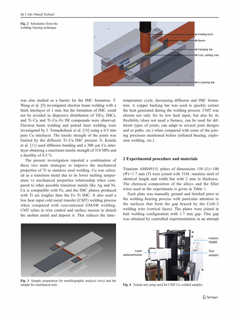
Fig. 2 Schematics from the

welding–brazing technique

Fig. 3 Sample preparation for metallographic analysis (two) and the

sample for mechanical tests Fig. 4 Tensile test setup used for CMT Cu welded samples

Int J Adv Manuf Technol

to empirically optimise the welding process. A narrower

gap would result in lack of fusion type defect near the

root by improper wetting by the copper alloy while larger

gap would cause underfilling. A 1 mm diameter CuSi-3

welding wire was deposited between the Ti and stainless

steel plates using CMT welding process (Fig. 2).

After the welding process, three different specimens were

produced as shown in Fig. 3, one for mechanical tests and two

for metallographic analysis.

Metallographic specimens were prepared by mounting

them on conductive resin for electron microscopy, ground

using silicon carbide paper and polished using diamond

paste and colloidal silicon suspension mixed with oxalic

acid. They were analysed by optical microscopy, scanning

electron microscopy and electron-dispersive spectroscopy

(SEM/EDS). Hardness mapping of the specimen was car-

ried out by a Zwick microhardness machine, with the

following parameters: HV0.1/10 [12]. Each sample ex-

tracted to mechanical tests was tested using the 100 kN

INSTRON 5500R tensile test machine. The tensile test

was performed at a constant speed of 1 mm per second;

the load and displacement were acquired by a National

Instruments system attached to a laser extensometer

(Fig. 4). The gauge length used during the experiments

was 50 mm.

3 Welding parameters

The experiments were carried out using constant welding pa-

rameters (travel speed - 0.5 m/min, contact tip to work piece

distance - 13.5 mm and CMT mode - 1183), except the wire

feed speed that was varied as shown in Table 2. As CMT is a

synergic process changing the wire feed speed, it would

change the current and voltage, translating to a heat input

variation that is shown by the following expression:

HI ¼ ηV :I

TSð1Þ

where HI is the heat input,V is the voltage, I is the intensity,

TS is the travel speed and η is the welding process efficiency

that for a MIG process has CMT is stipulated as 0.85 [13].

The welding wire was positioned towards the stainless steel

plate to enhance the melting of stainless steel and avoid Ti

melting. This will prevent the diffusion of Ti into the weld

pool and avoid the formation of Fe–Ti intermetallics.

Figure 5 depicts the experimental setup and the different po-

sitioning of the welding wire in relation to the central line of

the gap between the parent metals.

Fig. 5 Welding wire positioning during the welding–brazing

experiments

Table 2 CMTwelding-brazing parameters for the welding-brazing experiments

Sample Offset (mm) Wire feed speed (m/min) Heat input (J/mm) Fracture location

CMT 1 0.50 5.00 110.76 Stainless

CMT 2 0.50 6.00 118.40 Stainless

CMT 3 0.50 7.00 140.75 Stainless

CMT 4 0.50 8.00 157.67 Stainless

CMT 5 0.50 9.00 154.99 Ti

CMT 6 0.85 5.00 101.83 Stainless

CMT 7 0.85 6.00 116.51 Stainless

CMT 8 0.85 7.00 135.01 Stainless

CMT 9 0.85 8.00 149.91 Stainless

CMT 10 0.85 9.00 171.44 Ti

CMT 11 1.20 5.00 115.47 Stainless

CMT 12 1.20 6.00 108.89 Stainless

CMT 13 1.20 7.00 138.44 Stainless

CMT 14 1.20 8.00 152.99 Cu bead

CMT 15 1.20 9.00 152.59 Ti

Int J Adv Manuf Technol

Table 2 contains the experimental points used during these

experimental trials.

The remainder constant parameters not shown in Table 2

are as follows:

& Contact tip to work distance (CTWD)—13 mm

& Shielding gas flows

○ CMT torch—22 l/min

○ Back shielding—2 l/min

○ Trailing shield—62.5 l/min

& Torch angle 0° perpendicular to the parent metals

4 Results

4.1 Weld bead geometry

Similar weld bead geometry was obtained, as shown in Fig. 6,

from all the different experimental trials listed in Table 2.

The top surface (Fig. 6a) showed traces of oxidation

even though a trailing shield was used; however, the weld

root was successfully shielded with no apparent sign of

oxidation (Fig. 6b).

After macroscopic analysis, it is possible to verify that

the weld bead geometry is very similar for all of the

welded samples. The welding wire positioning does not

influence the weld bead geometry (Fig. 7 (I, II and III)).

However, the geometry is slightly different when the heat

input is increased (Fig. 7a–c).

Samples with low heat input, i.e. with lower wire

feed speeds as shown in Fig. 7a (I, II and III), do not

wet correctly the stainless steel plate. A clear undercut

can be seen at the Fe–Cu interface; this is due to a low

heat input and a fast solidification of the melt pool

when in contact with the stainless steel plate. As the

heat input is increased in samples in Fig. 7b, c, a better

wetting of the stainless steel plate is achieved. However,

the contribution of the parent metals in the Cu bead is

more noticeable (higher melting of parent metals).

With the microscopic examination, it is also possible

to identify three different areas in each joined sample:

two different reaction layers between the parent metals

Fig. 6 Weld bead stability and oxidation from sample CMT 11: a top surface and b weld root

Fig. 7 Selected sample macrographs. I—0.5 mm, II—0.85 mm, III—1.20 mm, a–c increasing the wire feed speed

Int J Adv Manuf Technol

and the Cu bead and also the Cu bead with several dis-

persed phases.

4.2 Hardness evaluation

As stated in Sect. 1, this metallic combination (Fe–Cu–Ti)

can generate IMC phases, and so, to identify their loca-

tion, microhardness testing was carried out.

Three samples were selected for these tests, CMT 2, 4

and 5 (Table 2). The three samples selected were made at

the same welding wire positioning (0.5 mm from the cen-

tre of the gap and towards the stainless steel) and have

increasing heat inputs. CMT 2 and 4 have failed at the

Fe–Cu interface whilst sample CMT 5 has failed at the

Cu–Ti interface.

Figure 8 shows the hardness mapping results for the three

selected samples (Fig. 7a–c (I)).

All of the specimens tested showed similar hardness

profiles with the bulk of the Cu deposited bead being

the softer part of the joint and as expected; the higher

hardness values are concentrated at the interfaces be-

tween the Cu bead and the stainless steel and Ti plates,

at previously observed reaction layers.

Sample CMT 2 has the lower average hardness due to

the lower heat input used in this weld. This lower heat

input induces a lower melting of the parent metals,

Fig. 8 Hardness mapping and corresponding optical macrographs for samples: a CMT 2, b CMT 4 and c CMT 5

Fig. 9 aCu deposited weld bead macrograph and distinctive areas. bBackscattered SEM image. c EDSmapping showing the main elements present on

the sample

Int J Adv Manuf Technol

reducing the diffusion/reaction between intervening Fe, Ti

and Cu.

On the contrary, samples CMT 4 and 5 have higher

average hardness particularly at the Fe–Cu and Ti–Cu

interfaces. This can be justified by the higher heat input

and, consequently, the increase in the melting of the par-

ent metals that will originate higher interdiffusion. The

higher hardness values for both these samples are located

at the Cu–Fe interface with values close to 1000 HV.

However, the facture location of both of these samples

is located in different parts of the sample. For CMT 4,

the fracture location is at the Fe–Cu interface that coin-

cides with the location of the hardest IMC phases whilst,

for sample CMT 5, the location is at the Ti–Cu interface.

This indicates not only that the IMC hardness is the major

contributing factor for the failure of this joint, but also

that the IMC volume plays a role in failure location. As

the time–temperature profile increases with the increase of

the heat input, the Ti–Cu IMC layer volume increases,

increasing the probability of the failure being located at

this interface.

4.3 SEM/EDS analysis

To identify the nature of the possible IMC phases formed at

these samples, the three previously identified areas were sub-

jected to SEM/EDS analysis (Fig. 9).

The first layer to be analysed was the stainless steel–Cu

interlayer. This layer is discontinuous in nature, and naturally,

it results from the reaction between the stainless steel and the

deposited Cu bead.

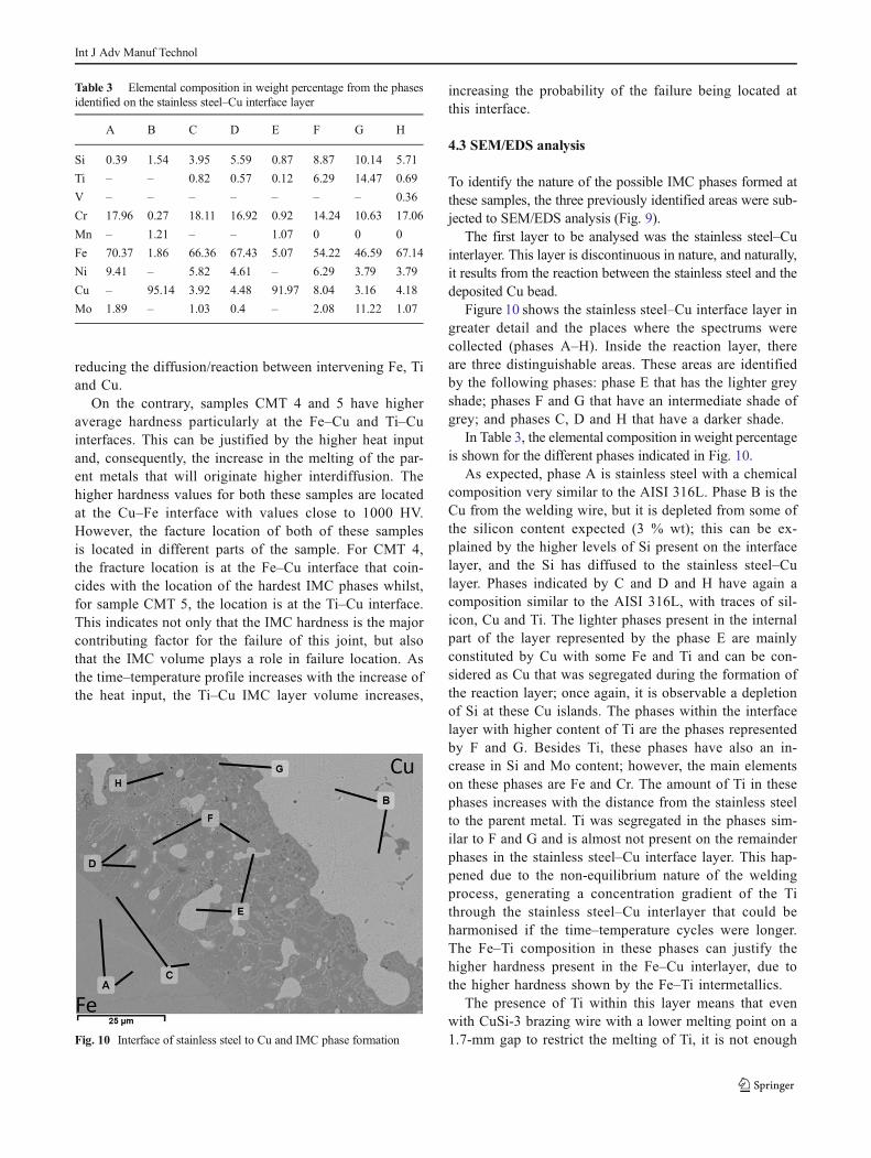
Figure 10 shows the stainless steel–Cu interface layer in

greater detail and the places where the spectrums were

collected (phases A–H). Inside the reaction layer, there

are three distinguishable areas. These areas are identified

by the following phases: phase E that has the lighter grey

shade; phases F and G that have an intermediate shade of

grey; and phases C, D and H that have a darker shade.

In Table 3, the elemental composition in weight percentage

is shown for the different phases indicated in Fig. 10.

As expected, phase A is stainless steel with a chemical

composition very similar to the AISI 316L. Phase B is the

Cu from the welding wire, but it is depleted from some of

the silicon content expected (3 % wt); this can be ex-

plained by the higher levels of Si present on the interface

layer, and the Si has diffused to the stainless steel–Cu

layer. Phases indicated by C and D and H have again a

composition similar to the AISI 316L, with traces of sil-

icon, Cu and Ti. The lighter phases present in the internal

part of the layer represented by the phase E are mainly

constituted by Cu with some Fe and Ti and can be con-

sidered as Cu that was segregated during the formation of

the reaction layer; once again, it is observable a depletion

of Si at these Cu islands. The phases within the interface

layer with higher content of Ti are the phases represented

by F and G. Besides Ti, these phases have also an in-

crease in Si and Mo content; however, the main elements

on these phases are Fe and Cr. The amount of Ti in these

phases increases with the distance from the stainless steel

to the parent metal. Ti was segregated in the phases sim-

ilar to F and G and is almost not present on the remainder

phases in the stainless steel–Cu interface layer. This hap-

pened due to the non-equilibrium nature of the welding

process, generating a concentration gradient of the Ti

through the stainless steel–Cu interlayer that could be

harmonised if the time–temperature cycles were longer.

The Fe–Ti composition in these phases can justify the

higher hardness present in the Fe–Cu interlayer, due to

the higher hardness shown by the Fe–Ti intermetallics.

The presence of Ti within this layer means that even

with CuSi-3 brazing wire with a lower melting point on a

1.7-mm gap to restrict the melting of Ti, it is not enoughFig. 10 Interface of stainless steel to Cu and IMC phase formation

Table 3 Elemental composition in weight percentage from the phases

identified on the stainless steel–Cu interface layer

A B C D E F G H

Si 0.39 1.54 3.95 5.59 0.87 8.87 10.14 5.71

Ti – – 0.82 0.57 0.12 6.29 14.47 0.69

V – – – – – – – 0.36

Cr 17.96 0.27 18.11 16.92 0.92 14.24 10.63 17.06

Mn – 1.21 – – 1.07 0 0 0

Fe 70.37 1.86 66.36 67.43 5.07 54.22 46.59 67.14

Ni 9.41 – 5.82 4.61 – 6.29 3.79 3.79

Cu – 95.14 3.92 4.48 91.97 8.04 3.16 4.18

Mo 1.89 – 1.03 0.4 – 2.08 11.22 1.07

Int J Adv Manuf Technol

to prevent Ti diffusion within the Cu weld bead. Ti dif-

fuses across the deposited CuSi-3 weld bead and interacts

with Fe at the Fe–Cu interface (the backscattered EDS

images taken from the Cu–Ti interface layer are shown

in Fig. 11).

Each of the phases was identified by a letter, and mul-

tiple spectrums were analysed for each sample. The spec-

trum locations were identified by the lines shown in

Fig. 11.

Phase A is the Ti base plate with the same distribution of Ti,

Al and V as the parent material (Ti-6Al-4V).

Phase B is mainly composed of Ti (67.90 %) and Cu

(18.43 %). Phase B is a continuous layer between the base

metal (Ti) and the main Ti–Cu reaction layer. The identi-

fication of this layer can be done using the Cu–Ti phase

diagram due to the low values of Si, Fe and Cr present.

This IMC is a dual-phased IMC composed of CuTi2 and α

Ti (Fig. 12a).

Phase C that appears in black on the SEM backscattered

image is mainly composed of Si and Ti, and the ratio be-

tween these elements is very close to Ti5Si3 phase on the

Ti–Si (Fig. 12b) phase diagram. This phase has 20 % wt

content while the CuSi-3 wire only has 3 %; this shows

once again that the silicon content of the wire was segre-

gated to particular areas of the joint, producing IMC phases

with higher contents of silicon.

Phases D and E compose almost all of the Cu–Ti

interface layer. Phase D has a cellular structure, and

phase E has an intercellular space structure. These two

phases are similar; however, from the Fe atomic

Fig. 11 Cu–Ti interface layer SEM backscattered image and phases investigated: a IMC layer close to the Ti parent metal and b transition between the

IMC layer and the beginning of the Cu weld bead

Fig. 12 Cu–Ti phase diagram with phase B indicated by an orange line: a Si–Ti phase diagram with phase C represented by a blue line [1]

Int J Adv Manuf Technol

proportion present, phase D can be estimated to the

closest stoichiometric composition being a ternary IM

compound, whilst phase E can be estimated to be a

binary IMC. And so, phase D can be evaluated by a

ternary Cu–Fe–Ti phase diagram [14] and phase E can

be evaluated by a Fe–Cu phase diagram (Fig. 12).

Phase D points to a binary phase compound of FeTi

and Ti2Cu, and phase E has a ratio between Ti and Cu

very close to Ti2Cu. F, G and H can be considered

external to the Cu–Ti reaction layer due to the higher

discontinuity of these phases and the lower values of Ti

when compared with the previous phases. Phases F and

H are mainly composed of Cu, Ti and Fe, whilst phase

G is only composed of Cu and Ti. These phases were

also evaluated using the Cu–Fe–Ti. When plotted on the

Cu–Fe–Ti phase diagram, phase F is a dual-phased IMC

composed of FeTi and Ti2Cu, but much closer to FeTi

composition than phase D, showing a much bigger pres-

ence of Fe, due to being out of the IMC layer and in the area

with higher Fe concentrations shown in Fig. 13. Phase G

points to a dual-phased τ2 and TiCu4 IMC phase in solid

solution with Cu, and finally, phase H indicates to be also a

dual-phased IMC of τ2 + τ4 (Ti37Cu67-xFex, x=5–7)

After the Cu–Ti interface layer and towards the Cu

bead, another phase was observed at the backscattered

EDS imaging (Fig. 11b). The main elements composing

phase I (Fig. 10b) are Ti, Fe, Cu, Si and Cr, and their

distribution is shown in Table 4. As this phase is manly

composed of five components, it was impossible to

identify it against a dual or ternary phase diagram.

The final area to be investigated was the area of

dispersed IMC phases within the Cu bead. Two different

areas inside the Cu bead were analysed. One was closer

to the stainless steel and other close to the Ti. These

two different areas were analysed to verify if the prox-

imity to the different parent metals has an influence on

the IMC formation and composition. Figure 14 shows

the two different IMC areas and the corresponding

phases selected.

The correspondent elemental distribution in weight

percent is shown in Table 5. The IMCs identified are

mainly composed of Fe, Cr, Si, Ti and Cu. The correct

identification of the stoichiometric composition of the

IMC phases was not possible, due to the multiplicity

of important elements present within these phases.

Due to the high cooling rate, it is possible to observe coring

on the IMC formed closer to the stainless steel, with the pres-

ence of different elemental concentration values in the same

Fig. 13 Cu–Fe–Ti phase diagram isothermal section at 849 °C with phase D plotted (a) [14]. Cu–Ti phase diagram with phase E plotted (b) [1]

Table 4 Elemental composition in weight percentage from the phases

identified on the Cu–Ti interface layer

A B C D E F G H I

Al 5.83 4.97 0.26 3.54 2.68 1.35 1.35 0.86 0.12

Si – 0.40 19.79 0.76 0.61 1.14 – 0.11 8.97

S – – – – – 0.09 – – –

Ti 90.07 67.90 66.62 49.43 56.92 41.43 8.21 31.93 33.01

V 4.10 5.39 5.37 3.70 – – – – 2.97

Cr – – 1.22 1.41 – 1.64 – 1.28 7.16

Mn – – – 0.10 – – 0.71 0.32 1.25

Fe – 2.69 0.87 6.52 – 15.47 0.91 8.59 29.86

Ni – 0.22 – 0.41 – 1.85 – 1.70 2.11

Cu – 18.43 5.88 34.13 39.80 37.05 88.83 55.24 14.54

Int J Adv Manuf Technol

intermetallic phase. This reveals the non-equilibrium condi-

tions experienced during the welding process. The morpholo-

gy of the IMC phases is also different with the phases closer to

Ti being more angular in shape while the phases closer to the

stainless steel are more circular or spherical.

Phases C and D IMC phases have higher levels of Ti

when compared with the IMCs close to the stainless steel

(phases A and B), showing that the IMC composition

changes with the distance to the parent metals. This also

reveals a gradient of Ti and stainless steel present inside

the Cu bead.

4.4 Mechanical strength

To evaluate the success of using Cu as a transition metal

between Ti and stainless steel, mechanical tests were also

carried out and the results are shown in Fig. 15.

The ultimate tensile strength of each sample was cal-

culated using the thickest value for the cross-sectional

area of each sample and the maximum thickness of the

sample; this includes the reinforcement and root pene-

tration curves introduced by the CuSi-3 brazed metal.

This way, a conservative calculation of the tensile load

for each sample was achieved.

The welded samples show an increase of tensile

strength with the increase of the heat input. However,

the welding wire positioning does not seem to be a

controlling parameter of this welding process. This char-

acteristic denotes that the welding process is tolerant to

the positioning of the wire in relation to the parent

metals. This will facilitate the alignment of the welding

process making the welding technique more relevant to

industry application.

The samples with higher tensile load also have the

maximum strain with the maximum present on the sam-

ple CMT 4 with a strain close to 2 %. The mechanical

test results show a clear increase not only on tensile

strength but also in ductility of these specimens, with

the heat input. This indicates that this process can be

further improved, by a further increase. As the IMC

formation is time–temperature dependant, there is criti-

cal value where an increase in heat input and, conse-

quently, an increase in the time–temperature cycle will

have a negative effect in the tensile strength of the

joint. However, this point was not achieved during this

work. From that value of heat input, a further increase

of energy will always result in a loss of mechanical

properties of the welded joint.

The tensile test results can be compared with studies

done in infrared brazing of Ti and stainless steel using Cu

as an interlayer [11] and the study done using electron

beam welding to join the same parent metals using Cu

as an interlayer [9]. The mechanical properties reported

by this study are a maximum tensile strength of

318 MPa with a ductility of 8.5 % and 234 MPa with a

Fig. 14 Scattered IMCs close to stainless steel SEM backscattered image and phases investigated (a) and scattered IMC phases close to Ti (b)

Table 5 Elemental composition in weight percentage from the phases

identified in Fig. 14

Si Ti V Cr Fe Ni Cu Mo

A 10.34 6.48 0.00 17.19 56.03 3.56 6.42 0.00

B 11.27 16.54 1.19 8.87 43.91 2.70 9.87 5.65

C 11.85 27.95 1.43 7.04 39.56 3.49 8.24 0.44

D 11.50 21.04 0.55 8.92 46.86 3.09 6.89 1.17

The IMCs identified are mainly composed of Fe, Cr, Si, Ti and Cu. The

correct identification of the stoichiometric composition of the IMC phases

was not possible, due to the multiplicity of important elements present

within these phases

Int J Adv Manuf Technol

3.6 % elongation, respectively. These results exceed me-

chanical strength of the results presented in this work;

however, the added flexibility of this joining process

when compared with infrared brazing and electron beam

welding can result on easier and cost-effective application

in industry.

5 Conclusions

It was possible to join stainless steel and Ti using CuSi-3

welding wire.

The heat input revealed to be the dominant parameter

during the study developed. The maximum tensile prop-

erties were obtained for the samples brazed with higher

heat input. Samples with the lowest heat input did not

wet properly the parent metals, resulting in the lowest

mechanical properties.

The IM phase formation was not avoided, but the IMCs

formed are more ductile in nature when compared with the

Fe–Ti IMCs. The phases identified are and the maximum

hardness measured was of 1000 HV0.1.

The IMC phases identified are mainly located at the inter-

faces between the parent metals and the Cu. However,

scattered IMC phases are present at the Cu bead.

Acknowledgments Supriyo Ganguly acknowledges the support re-

ceived vide EPSRC (Engineering and Physical Sciences Research Coun-

cil) project no. EP/J017086/1. Enquiries for access to the data referred to

this article should be directed to researchdata@cranfield.ac.uk.

Open Access This article is distributed under the terms of the Creative

Commons At t r ibut ion 4 .0 In te rna t ional License (h t tp : / /

creativecommons.org/licenses/by/4.0/), which permits unrestricted use,

distribution, and reproduction in any medium, provided you give

appropriate credit to the original author(s) and the source, provide a link

to the Creative Commons license, and indicate if changes were made.

References

1. ASM International (1992) ASM handbook: alloy phase diagrams v.

3. ASM International

2. Poddar D (2009) Solid-state diffusion bonding of commercially

pure titanium and precipitation hardening stainless steel. Int J

Recent Trends Eng 1:93–99

3. Kundu S, Chatterjee S (2008) Diffusion bonding between

commercially pure titanium and micro-duplex stainless steel.

Mater Sci Eng A 480:316–322. doi:10.1016/j.msea.2007.07.

033

4. Fazel-Najafabadi M, Kashani-Bozorg SF, Zarei-Hanzaki a (2011)

Dissimilar lap joining of 304 stainless steel to CP-Ti employing

friction stir welding. Mater Des 32:1824–1832. doi:10.1016/j.

matdes.2010.12.026

5. Kahraman N, Gulenc B, Findik F (2005) Joining of titanium/

stainless steel by explosive welding and effect on interface. J

Mater Process Technol 169:127–133. doi:10.1016/j.jmatprotec.

2005.06.045

6. Shanmugarajan B, Padmanabham G (2012) Fusion welding studies

using laser on Ti–SS dissimilar combination. Opt Lasers Eng 50:

1621–1627. doi:10.1016/j.optlaseng.2012.05.008

7. Lee JG, Hong SJ, LeeMK, Rhee CK (2009) High strength bonding

of titanium to stainless steel using an Ag interlayer. J Nucl Mater

395:145–149. doi:10.1016/j.jnucmat.2009.10.045

8. Shiue RK, Wu SK, Chan CH, Huang CS (2006) Infrared

brazing of Ti-6Al-4V and 17-4 PH stainless steel with a

nickel barrier layer. Metall Mater Trans A 37:2207–2217.

doi:10.1007/BF02586140

9. Wang T, Zhang B, Chen G et al (2010) Electron beam welding of

Ti-15-3 titanium alloy to 304 stainless steel with copper interlayer

sheet. Trans Nonferrous Met Soc China 20:1829–1834. doi:10.

1016/S1003-6326(09)60381-2

10. Tomashchuk I, Sallamand P, Andrzejewski H, Grevey D (2011)

The formation of intermetallics in dissimilar Ti6Al4V/copper/

Fig. 15 Ultimate tensile strength vs heat input for all welded samples (a) and stress strain curves for samples CMT 2 and 4 (b)

Int J Adv Manuf Technol

AISI 316 L electron beam and Nd:YAG laser joints. Intermetallics

19:1466–1473. doi:10.1016/j.intermet.2011.05.016

11. Kundu S, Ghosh M, Laik a et al (2005) Diffusion bonding of com-

mercially pure titanium to 304 stainless steel using copper interlay-

er. Mater Sci Eng A 407:154–160. doi:10.1016/j.msea.2005.07.010

12. BS EN ISO 6507–1 (2005) Metallic materials—Vickers hardness

test—part 1: test method. Br Stand 20

13. Pépe N, Egerland S, Colegrove P a et al (2011) Measuring the

process efficiency of controlled gas metal arc welding processes.

Sci Technol Weld Join 16:412–417. doi:10.1179/1362171810Y.

0000000029

14. Raghavan V (2002) Cu-Fe-Ti (copper-iron-titanium). J Phase

Equilibria 23:172–174. doi:10.1361/1054971023604152

Int J Adv Manuf Technol