Joana Filipa Garrido Nogueira

Um

inho |

2019

Joana F

ilipa G

arr

ido N

ogueira

Fre

sh

wa

ter

bio

div

ers

ity a

sse

ssm

en

t in

are

as w

ith

an

d w

ith

ou

t p

rote

cti

on

Freshwater biodiversity assessment in areas with and

without protection

October 2019

University of Minho

School of Sciences

Joana Filipa Garrido Nogueira

Freshwater biodiversity assessment in

areas with and without protection

October 2019

Master thesis in Ecology

Work made under supervision of:

Professor Doutor Ronaldo Sousa

Professor Doutor Amílcar Teixeira

Universidade do Minho

Escola de Ciências

iii

Acknowledgments

Many thanks to CBMA-Centre of Molecular and Environmental Biology, Department of Biology, and

University of Minho for the logistics support.

To my supervisor, Prof. Dr. Ronaldo Sousa for all the knowledge, the confidence and the patience

transmitted. Thank you for all the opportunities given and for inspiring me to pursue in the field of

Ecology/Conservation.

To my co-supervisor, Prof. Dr. Amílcar Teixeira and to Prof. Dr. Simone Varandas for the

tremendous help in the field as well as for the valuable scientific discussions.

To Fernando Miranda for all the help during the field surveys and the special care devoted to brown

trouts.

To my master classmates, lab and field partners for all the friendship, laughs and support.

To my dear friends Pedro, Cristina and Rita for always cheering me up throughout the last five

years.

To my best friends, Mariana, Diana and Sandrinha, that always made sure that I did not forget my

focus and strength.

To my siblings Miguel and his wife Joana, Rodrigo and Margarida for the help with sorting the

macroinvertebrates and for supporting me along the way.

To my nephews Guilherme, Inês, Michael, Francisca and Vasco for inspiring me to be the best

version of myself.

Finally, to my parents that always believed in me and gave me the right guidance throughout the

years, without whom this work would not be possible. You are the lighthouse in the storm.

It’s our choices that show what we truly are, far more than our abilities.

-J. K. Rowling

iv

STATEMENT OF INTEGRITY

I hereby declare having conducted this academic work with integrity. I confirm that I have not used

plagiarism or any form of undue use of information or falsification of results along the process

leading to its elaboration.

I further declare that I have fully acknowledged the Code of Ethical Conduct of the University of

Minho.

v

Avaliação da biodiversidade em água-doce de áreas com e sem proteção

Resumo

Os ecossistemas de água-doce são essenciais para o bem-estar humano, sendo consideradas

áreas com grande biodiversidade. No entanto, esta tem sofrido uma diminuição enorme devido à

expansão das atividades humanas. As áreas protegidas são essenciais para a conservação da

biodiversidade e já provaram ser bem-sucedidas em travar a extirpação de espécies quando são

bem geridas. Infelizmente, são maioritariamente focadas na biodiversidade terrestre, ignorando

muitas vezes os ecossistemas de água-doce. O principal objetivo deste trabalho foi determinar a

influência do Parque Natural de Montesinho (PNM), que foi projetado para proteger a fauna

terrestre, na biodiversidade de água-doce presente nos Rios Mente, Rabaçal, Tuela e Sabor. Assim

sendo, foram amostrados dois grupos faunísticos: peixes e invertebrados (bivalves e outros

macroinvertebrados) dentro, na periferia e fora do PNM. Com estes dados foram calculados índices

de diversidade (riqueza, abundância, diversidade de Shannon-Wiener e equitabilidade de Pielou) e

índices de qualidade de água (IBMWP, IASPT e %EPT). Seria expectável que os resultados

indicassem uma melhor condição abiótica e biológica dentro do parque. Contudo, este não foi o

caso pois os resultados mostraram que a área protegida não afeta positivamente nem a qualidade

de água nem nenhum dos dois grupos faunísticos monitorizado. As comunidades de

macroinvertebrados e a abundância de Margaritifera margaritifera não foram influenciadas pela

área protegida e apenas os comprimentos de M. margaritifera foram significativamente menores

dentro do PNM. No que diz respeito às comunidades de peixes, a riqueza e a abundância foram

significativamente maiores fora da área protegida. Assim sendo, concluímos que o PNM não

garante a proteção de espécies aquáticas e dos seus ecossistemas. Este trabalho reforça a visão

de que as áreas protegidas têm que ser desenhadas e geridas tendo também em conta a

diversidade aquática se tencionam ser eficazes na sua proteção. O controlo de espécies não-

nativas, a redução de fontes localizadas de poluição, a regulação das pescas e a melhoria da

conectividade dos rios são algumas das medidas mais importantes a tomar pelo governo, pela

população local e por outras partes interessadas de modo a alcançar uma proteção adequada dos

ecossistemas de água-doce e impedir a extirpação de espécies com importância de conservação.

Palavras-chave: áreas protegidas, biodiversidade, conservação, ecossistemas de água-doce.

vi

Freshwater biodiversity assessment in areas with and without protection

Abstract

Freshwater ecosystems are essential to human well-being and are considered areas of high

biodiversity. However, this biodiversity has been suffering severe declines due to the expansion of

human activities. Protected areas are essential for biodiversity conservation and have proven to be

successful in stopping species extirpation, when managed properly. Unfortunately, they are usually

focused on terrestrial biodiversity, leaving many times freshwater ecosystems aside. The main goal

of this study was to determine the influence that the Montesinho Natural Park (MNP), mainly

designed to protect terrestrial biodiversity, has on freshwater biodiversity present in Mente,

Rabaçal, Tuela and Sabor Rivers. Therefore, we sampled two aquatic faunal groups: fishes and

invertebrates (bivalves and other macroinvertebrates) inside, in the periphery and outside the MNP.

Biodiversity (richness, abundance, Shannon-Wiener diversity and Pielou’s evenness) and water

quality (IBMWP, IASPT and %EPT) indices were calculated. It would be expected that results

indicated better abiotic and biological conditions inside the park. However, this was not the case,

with results showing that the protected area does not affect positively neither water quality nor the

two faunal groups monitored. The macroinvertebrate communities and Margaritifera margaritifera

abundance were not influenced by the protected area and only M. margaritifera length was

significantly lower inside the MNP. For the fish communities, richness and abundance were

significantly higher outside the protected area. Given these results, we conclude that MNP does

not guarantee protection for the aquatic biodiversity and its ecosystems. This work highlights the

view that protected areas need to be designed and managed for aquatic biodiversity if they intend

to be successful in their conservation. Control of non-native species, reduction of point source

pollution, regulation of fisheries and improvement of rivers connectivity are some of the most

important actions that need to be taken by governmental, local population and stakeholders in

order to achieve a proper protection of freshwater ecosystems and prevent the extirpation of

species with conservation importance.

Keywords: biodiversity, conservation, protected areas, freshwater ecosystems.

vii

List of contents

Freshwater biodiversity assessment in areas with and without protection

ACKNOWLEDGMENTS………………………………………………………………. iii

RESUMO………………………………………………………………………………… v

ABSTRACT……………………………………………………………………………… vi

LIST OF FIGURES ……………………………………………………………………. viii

LIST OF TABLES ……………………………………………………………………… xi

1. INTRODUCTION……………………………………………………………….1

1.1 Importance of freshwater ecosystems…………………………...1

1.2 Freshwater Protected Areas…………………………………………3

1.3 Statement of the problem and main objectives……………......7

2. MATERIAL AND METHODS………………………………………………..10

2.1 Study area………………………………………………………………..10

2.2 Sampling strategies............................................................13

2.3 Data analysis…………………………………………………………….16

3. RESULTS……………………………………………………………………….19

3.1 Abiotic characterization……………………………………………..19

3.2 Macroinvertebrate communities…………………………………..20

3.3 Fish communities……………………………………………………….28

4. DISCUSSION………………………………………………………………….35

4.1 Abiotic characterization……………………………………………..36

4.2 Macroinvertebrate communities…………………………………..37

4.3 Fish communities……………………………………………………….39

4.4 Conservation implications and future directions……………..41

5. CONCLUSION ………………………………………………………………..44

6. LITERATURE CITED………………………………………………………...47

7. ANNEX…………………………………………………………………………..55

viii

List of Figures

Figure 1 – Diagram with the five major threats to freshwater biodiversity.

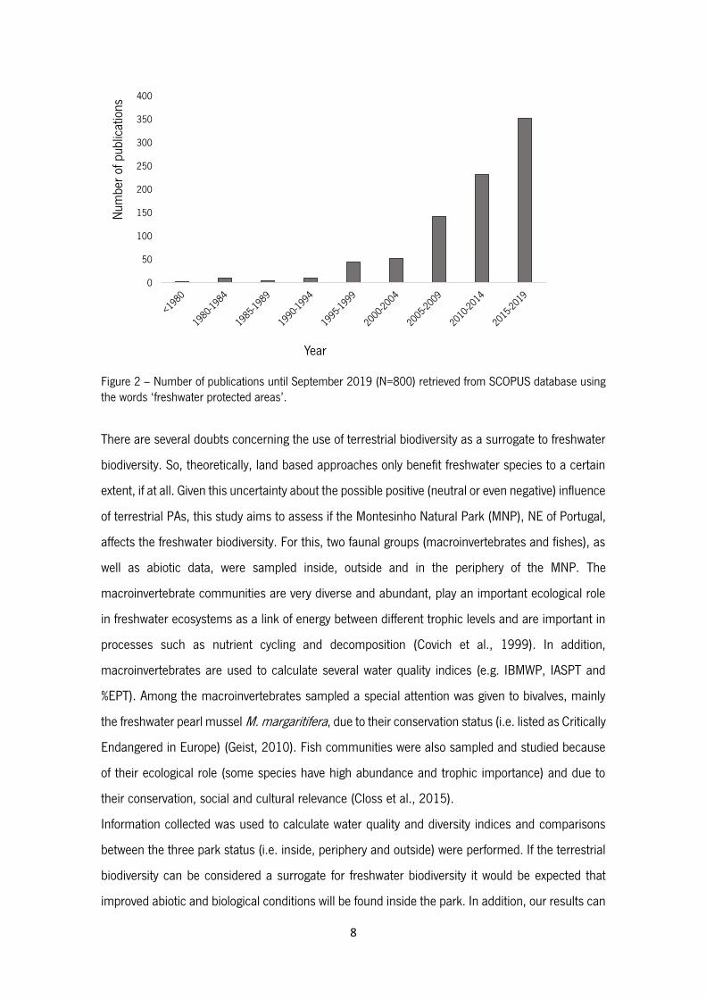
Figure 2 – Number of publications until September 2019 (N=800) retrieved from SCOPUS

database using the words ‘freshwater protected areas’.

Figure 3 – Examples of faunal diversity found in Montesinho Natural Park and surrounding areas:

brown trout Salmo trutta (A); pearl mussel Margaritifera margaritifera (B); dragonfly Macromia

splendens (C); Louisiana red swamp crayfish Procambarus clarkii (D). Courtesy of Ronaldo Sousa.

Figure 4 – Rivers surveyed in this study: Mente (A), Rabaçal (B), Tuela (C) and Sabor (D). Courtesy

of Ronaldo Sousa.

Figure 5 – Map of the surveyed area showing the location of the 24 sampling sites in Mente (M),

Rabaçal (R), Tuela (T) and Sabor (S) Rivers.

Figure 6 – Measurement of abiotic variables with a multi-parameter probe (A) and hand net used

to collect the macroinvertebrates (B). Courtesy of Ronaldo Sousa.

Figure 7 – Divers surveying freshwater mussels by snorkelling.

Figure 8 – Measurement of a brown trout Salmo trutta in the field.

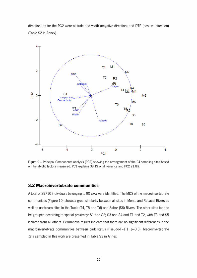
Figure 9 – Principal Components Analysis (PCA) showing the arrangement of the 24 sampling

sites based on the abiotic factors measured. PC1 explains 38.1% of all variance and PC2 21.8%.

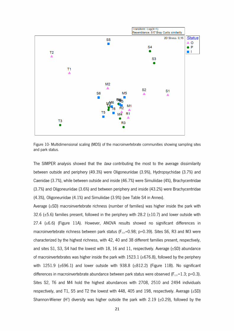
Figure 10 - Multidimensional scaling (MDS) of the macroinvertebrate communities showing

sampling sites and park status.

Figure 11 – Richness (A), Abundance (B), Shannon-Wiener diversity (C) and Pielou’s evenness

(D) of the macroinvertebrate communities outside (pink), periphery (green) and inside (blue) the

park. White circles represent the average values. Boxplots show median values (central line), the

range from the 25th to 75th percentile (box) and the largest and lowest value within 1.5 times

interquartile range below and above the 25th and 75th percentile (whiskers) and dots represent

extreme values.

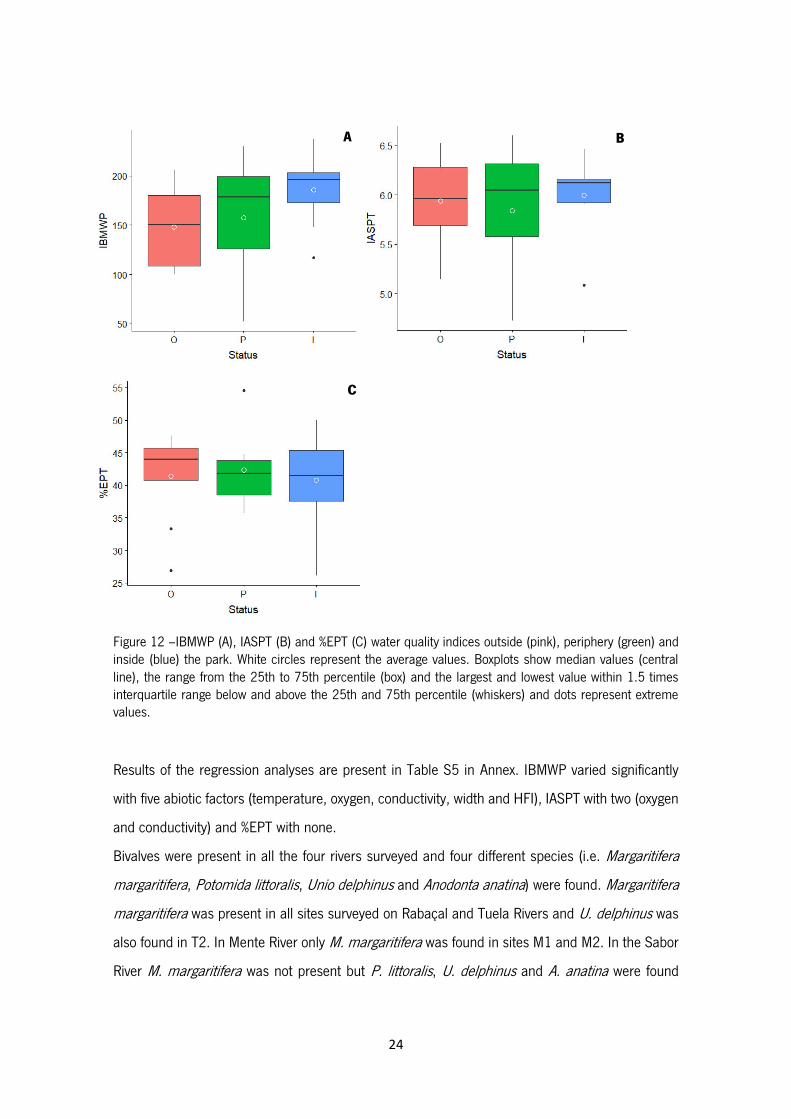
Figure 12 –IBMWP (A), IASPT (B) and %EPT (C) water quality indices outside (pink), periphery

(green) and inside (blue) the park. White circles represent the average values. Boxplots show

median values (central line), the range from the 25th to 75th percentile (box) and the largest and

ix

lowest value within 1.5 times interquartile range below and above the 25th and 75th percentile

(whiskers) and dots represent extreme values.

Figure 13 – Abundance (ind. CPUE) of pearl mussel Margaritifera margaritifera outside (pink),

periphery (green) and inside (blue) the park. White circles represent the average values. Boxplots

show median values (central line), the range from the 25th to 75th percentile (box) and the largest

and lowest value within 1.5 times interquartile range below and above the 25th and 75th percentile

(whiskers) and dots represent extreme values.

Figure 14 – Abundance (ind.CPUE) of the pearl mussel Margaritifera margaritifera on Mente (A),

Rabaçal (B) and Tuela (C) Rivers in each site outside (pink), in the periphery (green) and inside

(blue) the park. White circles represent the average values. Boxplots show median values (central

line), the range from the 25th to 75th percentile (box) and the largest and lowest value within 1.5

times interquartile range below and above the 25th and 75th percentile (whiskers) and dots

represent extreme values. Different letters indicate significant differences among status.

Figure 15 - Length (mm) of the pearl mussel Margaritifera margaritifera outside (pink), periphery

(green) and inside (blue) the park. White circles represent the average values. Boxplots show

median values (central line), the range from the 25th to 75th percentile (box) and the largest and

lowest value within 1.5 times interquartile range below and above the 25th and 75th percentile

(whiskers) and dots represent extreme values. Different letters indicate significant differences

among status.

Figure 16 - Length (mm) of Margaritifera margaritifera in Rabaçal (A) and Tuela (B) Rivers in each

site outside (pink), in the periphery (green) and inside (blue) the park. White circles represent the

average values. Boxplots show median values (central line), the range from the 25th to 75th

percentile (box) and the largest and lowest value within 1.5 times interquartile range below and

above the 25th and 75th percentile (whiskers) and dots represent extreme values. Different letters

indicate significant differences among status.

Figure 17 - Multidimensional scaling (MDS) of the fish communities showing sampling sites and

park status.

Figure 18 - Richness (A), Abundance (B), Shannon-Wiener diversity (C) and Pielou’s evenness (D)

of the fish communities outside (pink), periphery (green) and inside (blue) the park. White circles

represent the average values. Boxplots show median values (central line), the range from the 25th

to 75th percentile (box) and the largest and lowest value within 1.5 times interquartile range below

x

and above the 25th and 75th percentile (whiskers) and dots represent extreme values. Different

letters indicate significant differences among status.

Figure 19 – Abundance (ind.CPUE) of Salmo trutta (A), Squalius alburnoides (B), Luciobarbus

bocagei (C), Squalius carolitertii (D), Pseudochondrostoma duriense (E), Cobitis calderoni (F) and

Cobitis paludica (G) outside (pink), in the periphery (green) and inside (blue) the park. White circles

represent the average values. Boxplots show median values (central line), the range from the 25th

to 75th percentile (box) and the largest and lowest value within 1.5 times interquartile range below

and above the 25th and 75th percentile (whiskers) and dots represent extreme values. Different

letters indicate significant differences among status.

Figure 20 – Length (cm) of Salmo trutta (A), Squalius alburnoides (B), Luciobarbus bocagei (C),

Squalius carolitertii (D), Pseudochondrostoma duriense (E), Cobitis calderoni (F) and Cobitis

paludica (G) outside (pink), in the periphery (green) and inside (blue) the park. White circles

represent the average values. Boxplots show median values (central line), the range from the 25th

to 75th percentile (box) and the largest and lowest value within 1.5 times interquartile range below

and above the 25th and 75th percentile (whiskers) and dots represent extreme values. Different

letters indicate significant differences among status.

Figure 21 – Before (2012) (A) and after (2017) (B, C) the construction of a weir with the goal of

creating an artificial beach for visitors inside Montesinho Natural Park. Courtesy of Ronaldo Sousa.

Figure 22 – Macroinvertebrates and fish richness outside (pink), in the periphery (green) and

inside (blue) the park. The size of the circles is proportional to the value of richness.

Figure 23 – Species of conservation importance (Vulnerable, Endangered or Critically

Endangered) in each site for all the rivers studied, outside (pink), in the periphery (green) and inside

(blue) the park. The size of the circles is proportional to the number of species.

xi

List of Tables

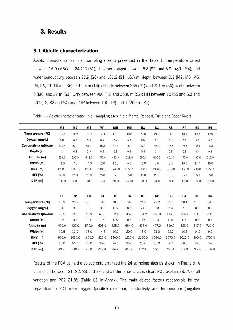
Table 1 – Abiotic characterization in all sampling sites in the Mente, Rabaçal, Tuela and Sabor

Rivers.

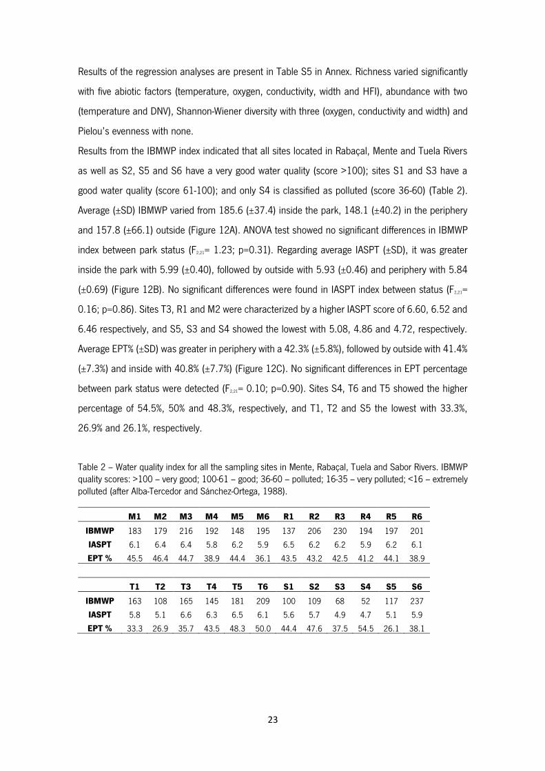
Table 2 – Water quality index for all the sampling sites in Mente, Rabaçal, Tuela and Sabor Rivers.

IBMWP quality scores: >100 – very good; 100-61 – good; 36-60 – polluted; 16-35 – very polluted;

<16 – extremely polluted (after Alba-Tercedor and Sánchez-Ortega, 1988).

Table S1 - Results of the Principal Components Analysis based on the abiotic data.

Table S2 – Contribution of the abiotic variables to each of the first three PCA axis.

Table S3 – Abundance of macroinvertebrates taxa in Mente, Rabaçal, Tuela and Sabor Rivers.

Table S4 – SIMPER analysis results showing the macroinvertebrate taxa contributing the most to

the average dissimilarity between status (outside, in the periphery and inside the park).

Table S5 – Results of the linear regressions between abiotic factors and macroinvertebrates

richness (S), abundance (N), Shannon-Wiener diversity (H’), Pielou’s evenness (J’), and IBMWP,

IASPT and %EPT water quality indices. ns – non significant; * - statistically significant.

Table S6 – Abundance (ind.CPUE) of Margaritifera margaritifera in Mente, Rabaçal and Tuela

Rivers.

Table S7 –Fish species abundance (ind.CPUE) in Mente, Rabaçal, Tuela and Sabor Rivers.

Table S8 – Results of the PERMANOVA analysis on fish communities along park status (outside,

in the periphery and inside the park) and overall results of the pairwise tests.

Table S9 - SIMPER analysis results showing the fish species contributing the most to the average

dissimilarity between status (outside, in the periphery and inside the park).

Table S10 – Results of the linear regressions between abiotic factors and fish richness (S),

abundance (N), Shannon-Wiener diversity (H’) and Pielou’s evenness (J’). ns – non significant; * -

statistically significant.

1

1. Introduction

1.1 Importance of freshwater ecosystems

Freshwater ecosystems are essential to environmental health, economic wealth and human well-

being (Grill et al., 2019). The integrity of freshwater ecosystems is of vital importance, as the fresh

water supply stands in the top ten (listed as fourth) of the most pressing concerns for human

survival (WEF, 2019). Humans use freshwater ecosystems for drinking and irrigation purposes,

waste disposal, transportation, energy production, fisheries, and for harvesting plants and minerals

(Strayer and Dudgeon, 2010). All these services provided by freshwater ecosystems have high

economic value.

Covering approximately 1% of Earth’s surface, lakes and rivers host 9.5% of all animal species

(Dudgeon et al., 2006; He et al., in press) turning freshwater ecosystems areas of high biodiversity.

Still, this biodiversity faces numerous threats responsible for large declines in abundance and

spatial distribution of many species. For example, 44% of freshwater mussels, 37% of fish, 23% of

amphibians, 19% of reptiles, 15% of mammals and dragonflies, 13% of birds, 9% of butterflies and

7% of aquatic plants are threatened in Europe (Freyhof and Brooks, 2011). According with the

2018 World Wide Fund for Nature and its Living Planet Index, freshwater vertebrates (one-third of

all vertebrates) declined in their abundance and spatial distribution by 83% compared to 1970

data. This is particularly alarming if compared to the declines reported for marine and terrestrial

ecosystems with values around 36% and 38%, respectively (He et al., in press; Reid et al., 2019).

Several freshwater species suffered pronounced range contractions, like the European sturgeon

(Acipenser sturio) that was extirpated from all major European rivers, and is now confined to the

Garrone River in France. Other species such as the baiji (Lipotes vexillifer) and the Chinese

paddlefish (Psephurus gladius) are considered extinct due to human activities and intrinsic factors

(e.g. long life cycle and lower fecundity) of their biology (He et al., in press). Besides human

activities, many freshwater species are restricted to small isolated areas and this situation is

responsible for high rates of endemism and increased risk of extinction (Abell et al., 2008; Dudgeon

et al., 2006). Given the remarkable biodiversity, the vulnerability and the level of endemism present

in freshwater ecosystems these areas should, in theory, be considered a conservation priority.

Unfortunately that is not the case since, for example, conservation literature tends to be biased

towards terrestrial systems with 81% of research articles focused on these ecosystems (Di Marco

et al., 2017).

2

Under the current biodiversity crisis, species are declining at an alarming rate (Olson et al., 2001)

primarily due to human activities and global consumption of natural resources (Garcia-Moreno et

al., 2014). This has led to chemical, physical and biological alterations in all ecosystems, being

freshwater ecosystems no exception (Carpenter et al., 2011). Human well-being is the priority when

it comes to decision making and policy, resulting in loss of biodiversity that supports some of these

same priorities (Cowx and Portocarrero-Aya, 2011; Darwall et al., 2018). The biggest threats to

freshwater ecosystems are related to overexploitation, climate change, introduction of non-native

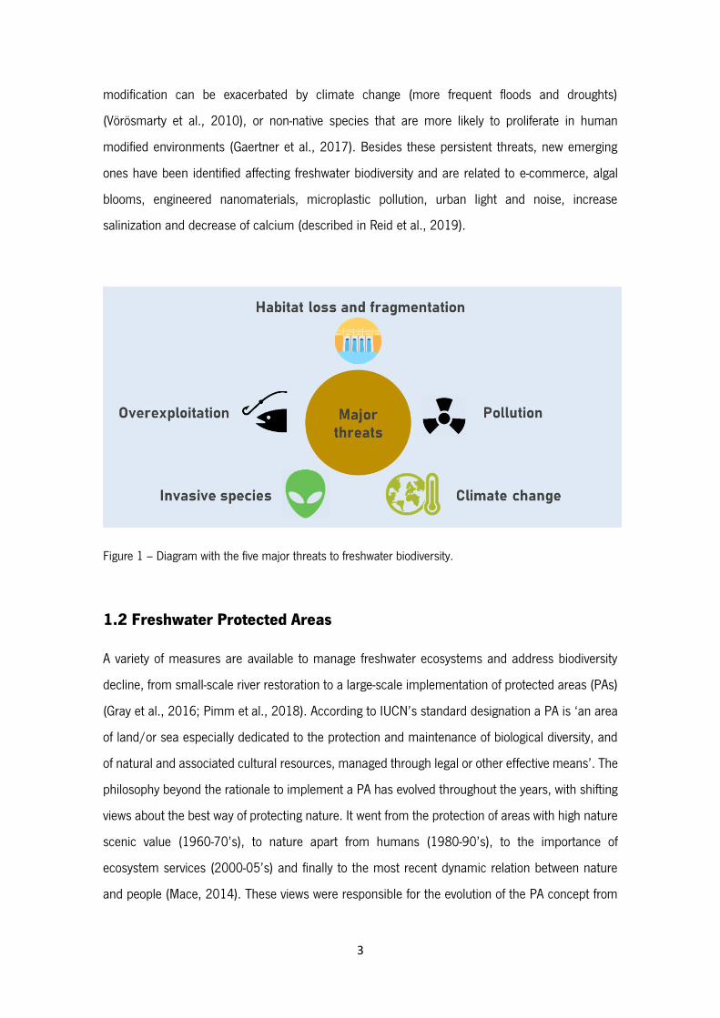
species, pollution, changes in water flow and destruction and fragmentation of habitats (Figure 1)

(Carpenter et al., 2011; Dudgeon et al., 2006). Overexploitation is mostly affecting fishes

(overfishing), amphibians and reptiles (Naylor et al., 2000), but even macroinvertebrates can be

highly explored (see for example some freshwater bivalves in Lopes-Lima et al., 2017 and Zieritz

et al., 2018). The increasing water temperature related with the higher global atmospheric

temperature causes the depletion of dissolved oxygen in water, affects the physiology, phenology

and distribution of many species (Carpenter et al., 2011; Mohseni et al., 2003) and can even

cause direct mortality (Nogueira et al., in press). Freshwater ecosystems are also heavily impacted

by the introduction of non-native species (Sala et al., 2000; Strayer, 2010), affecting ecosystems

structure and functioning as well as their biotic and abiotic interactions (Sousa et al., 2009; Sousa

et al., 2019). Even though some species have been introduced accidentally, many have been

deliberately introduced by humans to serve their needs (e.g. aquaculture, sport fishing and pest

control) (Carpenter et al., 2011; Sousa et al., 2014). Changes in the land use of riparian areas and

watersheds (mostly due to agricultural expansion) alters de input of water, sediments, nutrients

and other chemicals leading to eutrophication and pollution that affects natural communities, alters

biogeochemical cycles and disturbs the habitat for many species (Dudgeon et al., 2006; Quinton

et al., 2010; Strayer and Dudgeon, 2010). As fresh water is not evenly available in time and space,

there is a need to control water reserves (mostly to agriculture, industry and domestic use) through

the construction of dams and levees. These physical obstacles alter the connectivity of rivers,

capture about 25% of global sediment load (Vörösmarty and Sahagian, 2000), can heavily change

the natural river flow, impair fish (and other species) migration and exacerbate the occurrence of

infectious diseases caused by standing-water related parasites (Carpenter et al., 2011). Globally,

there is close to 2.8 million dams (reservoir area >1000 m2) fragmenting rivers and altering their

courses and this number will rise in the next years in areas such as Amazon, Mekong, Congo and

the Balkans basins (Grill et al., 2019). All these threats may operate synergistically, as flow

3

modification can be exacerbated by climate change (more frequent floods and droughts)

(Vörösmarty et al., 2010), or non-native species that are more likely to proliferate in human

modified environments (Gaertner et al., 2017). Besides these persistent threats, new emerging

ones have been identified affecting freshwater biodiversity and are related to e-commerce, algal

blooms, engineered nanomaterials, microplastic pollution, urban light and noise, increase

salinization and decrease of calcium (described in Reid et al., 2019).

Figure 1 – Diagram with the five major threats to freshwater biodiversity.

1.2 Freshwater Protected Areas

A variety of measures are available to manage freshwater ecosystems and address biodiversity

decline, from small-scale river restoration to a large-scale implementation of protected areas (PAs)

(Gray et al., 2016; Pimm et al., 2018). According to IUCN’s standard designation a PA is ‘an area

of land/or sea especially dedicated to the protection and maintenance of biological diversity, and

of natural and associated cultural resources, managed through legal or other effective means’. The

philosophy beyond the rationale to implement a PA has evolved throughout the years, with shifting

views about the best way of protecting nature. It went from the protection of areas with high nature

scenic value (1960-70’s), to nature apart from humans (1980-90’s), to the importance of

ecosystem services (2000-05’s) and finally to the most recent dynamic relation between nature

and people (Mace, 2014). These views were responsible for the evolution of the PA concept from

4

the protection of terrestrial biodiversity islands surrounded by human disturbed areas to the current

emphasis on the importance of socioecological systems (Palomo et al., 2014).

Since we cannot protect all regions with some biological importance, the selection of priority areas

is fundamental. This can be made using species data through two main methodologies: one is

based on scoring the sites according to criteria of species vulnerability, rareness and richness

(Margules and Usher, 1981); the other, more recent, is based on systematic conservation planning

(Margules and Pressey, 2000). Systematic conservation planning aims to represent a maximum of

species in a priority area, in the most cost-effective way, which is done by identifying the

conservation goals (e.g. target species and area) and available resources (e.g. socioeconomic cost).

Systematic conservation planning uses the concept of complementarity, which is defined as the

gain in representativeness in biodiversity when a site is added to an area (Hermoso et al., 2016).

Ideally, a PA should be designed with the intent of protecting all faunal groups, but due to limited

biological data and resources, some species (usually defined as surrogate species) are used as

proxy to the presence of others (Caro, 2010). However, this approach can be misleading and can

disregard rare and spatially restricted species, as demonstrated by Stewart et al., (2018) when

these authors found limited congruence of priority watersheds for 72 species of freshwater fish,

amphibians, reptiles and mussels. The effectiveness of a PA can be measured by its

representativeness and persistence, meaning that reserves must include a full range of biodiversity

items (e.g. genetic, taxonomic and ecosystems) and that this biodiversity has the capacity to

survive, maintain natural processes and populations, as well as withstand threats (Margules and

Pressey, 2000).

Given the potential role of PAs in preserving biodiversity, freshwater ecosystems have been also a

target of worldwide conservation efforts. Examples include the USA’s National Wild and Scenic

Rivers, developed for protecting freshwater systems (209 rivers designated, including the

Mississippi River) due to their aesthetic value; United Kingdom’s Special Areas of Conservation,

developed to protect rare and vulnerable species such as the Borgie River in Scotland or the Avon

River in England, that use surrogate species like the pearl mussel Margaritifera margaritifera, plants

such as Ranunculus sp. or fish such as the Atlantic salmon Salmo salar; or the Canadian Heritage

Rivers System that include, among others, the longest protected river, Fraser River, with 1375 km.

There are also examples of Ramsar Sites designated with the goal of protecting wetlands, such as

the Lake Baikal in Russia, or the Danube Delta in Romania (Saunders et al., 2002). More recently,

the concept of Key Biodiversity Areas (KBAs) developed by IUCN, uses a standard criterion to

5

identify freshwater regions capable of maintaining endangered species (but see Butchart et al.,

2015).

Despite this increasing interest in conserving freshwater ecosystems there is still a high discrepancy

between the protected area coverage in terrestrial, marine and freshwater systems, with 57%, 37%

and 6%, respectively (Di Marco et al., 2017). Currently, 15.4% of terrestrial land surface is covered

by PAs, and CBD’s Aichi Biodiversity Target 11 has the goal to protect at least 17% (including inland

waters) by 2020 (CBD; Convention on Biological Diversity 2010; Pimm et al., 2018). This

expansion should be planned towards a more balanced distribution in terrestrial, marine and

freshwater ecosystems. Since the CBD report joined both terrestrial and aquatic systems it is

difficult to differentiate between them, and assess the increased coverage for each one. Abell et al.

(2011) proposed a method that prioritizes possible PAs by overlapping areas that host rare and

endemic species from both the terrestrial and freshwater domains. This pragmatic approach is of

major importance since funds for conservation are scarce and besides being frequent in marine

and terrestrial planning, freshwater systems are lacking in spatial prioritisation (Abell et al., 2007;

Juffe-Bignoli et al., 2016). For example, in Europe, Natura 2000 represents the most important

conservation network and PAs are based on Birds and Habitats Directives (Natura 2000:

http://ec.europa.eu). Although their primary goal is to protect biodiversity, the efficiency in

protecting freshwater habitats and species has been questioned (Hermoso et al., 2015), as we

cannot simply expect that they will be accidentally included in terrestrial PAs (Abell et al., 2011).

For example, Carrizo et al. (2017) showed a great mismatch between the existing PAs and areas

of critical importance to freshwater biodiversity, with 84% of threatened freshwater megafauna

falling outside the reserves, proving the lack of representativeness of aquatic biodiversity when

planning a PA.

Despite that legal protection may enhance the diversity and abundance of some species there are

several examples of decline and loss of freshwater biodiversity inside PAs. Examples include the

disappearance of amphibians due to the chytrid fungus infection (Skerratt et al., 2007) or the

extirpation of native fish and mollusks due to the stocking of non-native fish in Banff National Park

in Canada (Schindler, 2000). In addition, the implementation of management measures is much

more developed in terrestrial and marine counterparts (Collier, 2011), turning more difficult the

implementation of a PA in a freshwater ecosystem (Hermoso et al., 2016). These difficulties to

conserve freshwater biodiversity are generally exacerbated by the intricate complexity of river

connections, the high spatial and temporal variability, the lack of control of external processes and

6

threats (Roux et al., 2008; Collier, 2011) and patchy information on freshwater species (Abell et

al., 2011). For example, IUCN Red List assessment lacks information on many freshwater species,

and the knowledge of fish migration routes and spawning grounds is also limited (He et al., in

press). If some of this basic information is lacking for a faunal group such as migratory fish, we

may think that the level of ignorance for basic biological features in macroinvertebrates is even

higher. In addition, and although rivers are often chosen as ecologic corridors, many times these

same rivers inside PAs are used as simple administrative boundaries (Hermoso et al., 2015). For

example, in Portugal the Peneda Gerês National Park and International Tejo Natural Park are two

important PAs and the Cávado and Tejo Rivers function in several kilometres as the border of the

two parks, respectively. Finally, the hydrological connectivity in a river (longitudinal, lateral and

vertical) also poses a great challenge for the design and management of PAs, and so, traditional

ideas used in terrestrial ecosystems are not adequate for freshwater protection (Abell et al., 2007).

Longitudinal connectivity is crucial to maintain ecological processes such as species migration,

their reproduction, long-term population dynamics and gene flow; lateral connectivity allows the

exchange of matter and energy between rivers and floodplains or other habitats (e.g. lakes); and

vertical connectivity links the surface and groundwater systems (Hermoso et al., 2011). Spatial-

temporal connectivity also maintains important ecological processes like the periodic migrations or

the dispersal to refuge areas (Hermoso et al., 2016). All these details turn the implementation of

an effective freshwater PA much more difficult when compared to terrestrial or marine PAs.

Ideally, and for a freshwater PA be really effective, it should cover the whole watershed (Abell et

al., 2017; Rodriguez-Olarte et al., 2011) and take in account that possible disruptive factors

(pollution, flow alteration and introduction of non-native species) propagate along the rivers

(Hermoso et al., 2015). Mitigation of point source pollution, the management of fisheries and non-

native invasive species, the restriction of human activities and land use around the watershed (e.g.

riparian vegetation and floodplain), as well as restoration of the normal water flow and connectivity

are essential to achieve a proper protection of aquatic biodiversity (Abell et al., 2011; Dudgeon et

al., 2006; Nel et al., 2007; Saunders et al., 2002). However, the reality is that many of the world’s

rivers are barely protected in their upland areas, being that only 11% of rivers (by length) benefit

from integrated management (Abell et al., 2017). Therefore, and as a more realistic management

tool, sub-catchments (contributing catchment around a river segment) are often considered spatial

planning units in freshwater conservation (Reis et al., 2019).

7

Designing a freshwater PA has also socioeconomic and political constrains. Areas with/around

water bodies are frequently disputed for industrial (e.g. construction of dams), commercial (e.g.

extraction of natural resources) or housing purposes, and so new reserves are often chosen in

remote or low productivity areas for convenience. This situation usually does not contribute for a

well representation of their biodiversity. Anyway, a few studies have already started to use a

systematic conservation planning approach for freshwater ecosystems (e.g. Abell et al., 2007;

Lawrence et al., 2011) and, for example, Hermoso et al. (2011) used a well-known conservation

planning software package – MARXAN – to penalize management measures that do not include

upstream catchments.

Finally, and as the interest about ecosystems services is growing, freshwater conservation could

enhance several important functions and services such as water supply, nutrient cycling and water

regulation (Palomo et al., 2014). Thus, a framework for freshwater conservation planning is

urgently needed, and an increase in the exchange of information between science, policy and

management would strongly benefit freshwater ecosystems (Darwall et al., 2018).

1.3 Statement of the problem and main objectives

Previous studies have shown that some PAs have a positive influence on freshwater biodiversity.

For example, fish population structure tends to improve (i.e. higher fish length and biomass) inside

protected areas where fishing is regulated/prohibited (Baird and Flaherty, 2005; Cucherousset et

al., 2007; Keppler et al., 2017; Sanyanga et al., 1995). On the other hand, other studies showed

no differences in biodiversity patterns for macroinvertebrates and fish outside and inside PAs

(Heino et al., 2009; Srinoparatwatana and Hyndes, 2011) or even a negative effect on freshwater

turtles inside Brazilian PAs (Fagundes et al., 2016). To the best of our knowledge there is no such

an assessment in Portugal, and very few worldwide. In fact, and although 800 studies were

retrieved in our search in the SCOPUS database using the words ‘freshwater protected areas’

(Figure 2), the reality is that very few of these studies really assess the effectiveness of protected

areas in freshwater ecosystems.

8

Figure 2 – Number of publications until September 2019 (N=800) retrieved from SCOPUS database using the words ‘freshwater protected areas’.

There are several doubts concerning the use of terrestrial biodiversity as a surrogate to freshwater

biodiversity. So, theoretically, land based approaches only benefit freshwater species to a certain

extent, if at all. Given this uncertainty about the possible positive (neutral or even negative) influence

of terrestrial PAs, this study aims to assess if the Montesinho Natural Park (MNP), NE of Portugal,

affects the freshwater biodiversity. For this, two faunal groups (macroinvertebrates and fishes), as

well as abiotic data, were sampled inside, outside and in the periphery of the MNP. The

macroinvertebrate communities are very diverse and abundant, play an important ecological role

in freshwater ecosystems as a link of energy between different trophic levels and are important in

processes such as nutrient cycling and decomposition (Covich et al., 1999). In addition,

macroinvertebrates are used to calculate several water quality indices (e.g. IBMWP, IASPT and

%EPT). Among the macroinvertebrates sampled a special attention was given to bivalves, mainly

the freshwater pearl mussel M. margaritifera, due to their conservation status (i.e. listed as Critically

Endangered in Europe) (Geist, 2010). Fish communities were also sampled and studied because

of their ecological role (some species have high abundance and trophic importance) and due to

their conservation, social and cultural relevance (Closs et al., 2015).

Information collected was used to calculate water quality and diversity indices and comparisons

between the three park status (i.e. inside, periphery and outside) were performed. If the terrestrial

biodiversity can be considered a surrogate for freshwater biodiversity it would be expected that

improved abiotic and biological conditions will be found inside the park. In addition, our results can

0

50

100

150

200

250

300

350

400

Num

ber

of p

ublic

atio

ns

Year

9

function as a reference of the abiotic and biological conditions of the study area. This information

can be used for future comparisons and help politicians, managers and stakeholders to make

better decisions (e.g. define areas that are not currently included in the park but could be in the

future) concerning the conservation of the freshwater biodiversity present in the MNP and

surrounding areas.

10

2. Material and methods

2.1 Study area

Montesinho Natural Park was created in 1979 and is located in northeast Portugal (Trás-os-Montes

region), which includes Vinhais and Bragança counties. The park is located from 41º 43’47’’ to

41º 59’ 24’’ N and 6º 30’ 53’’ to 7º 12’ 9’’ W, and is a category V in the IUCN assessment. By

definition a Category V protected area is ‘where the interaction of people and nature over time has

produced an area of distinct character with significant ecological, biological, cultural and scenic

value: and where safeguarding the integrity of this interaction is vital to protecting and sustaining

the area and its associated nature conservation and other values’. MNP was designed with the

focus on birds, terrestrial vertebrates and plants. There is a significant biodiversity, however much

lower than in the past, having suffered a tremendous lost in the amount of native forest, a drastic

reduction of wolf abundance, and the disappearance of bear and lynx (ICNF, 2019).

Climate is Mediterranean with influence from the Atlantic Ocean (Oliveira et al., 2012), where the

medium annual temperatures vary between 8.5 and 12.8ºC. Annual average precipitation is 1000-

1600 mm, with highest values in winter and an almost absence of precipitation in the summer.

Floods may occur in winter/early spring and droughts in summer/early autumn (Sousa et al.,

2015).

The geology of the park and surrounding area is very complex, dominated by schist, granite,

amphibolite and migmatite, and also the occurrence of basic and ultrabasic rock formations (e.g.

peridotites and serpentines). Its geomorphology is characterized by the existence of mountains and

plateaux cut by deep river valleys, where altitude range between 438 and 1481 m, being the

highest values registered in Montesinho and Coroa mountains.

The vegetation of the study area is very diverse, mostly influenced by its geographic

location/climate and complex geology, and include species such as the oak Quercus pyrenaica,

the chestnut Castanea sativa and the holm oak Quercus rotundifolia. The scrubland is composed

of heather Erica australis and Erica umbellate, the rockrose Cistus ladanifer or Genista

tridentata and meadows with ryegrass Lolium rigidum, among many other species. Riparian

vegetation includes the alder Alnus glutinosa, the ash Fraxinus sp. and the willow Salix sp. Species

of conservation value include matgrass Nardus stricta, the crossleaf heath Erica tetralix and the

needle furze Genista anglica.

11

A significant presence of birds is noted in MNP, constituting a nesting place for 125 of the 150

species described in this protected area. Rare species like the eagle Aquila chrysaetos, the black

stork Ciconia nigra or the red-backed shrike Lanius collurio can be found. Terrestrial mammals like

the wild boar Sus scorfa, the Iberian wolf Canis lupus signatus, the deer Cervus elaphus and roe

deer Capreolus capreolus can also be found, as well as aquatic mammals like the water desman

Galemys pyrenaicus and the otter Lutra lutra. The rivers that cross the park are important habitats

for the brown trout Salmo trutta (Figure 3A) and Iberian endemic cyprinids such as

Pseudochondrostoma duriense, Achondrostoma arcasii, Squalius carolitertii, Squalius alburnoides

and Luciobarbus bocagei.

Some species with conservation importance also find a refuge in the MNP and surrounding areas,

including Iberian endemic species such as the water lizard Lacerta schreiberi or the frog Rana

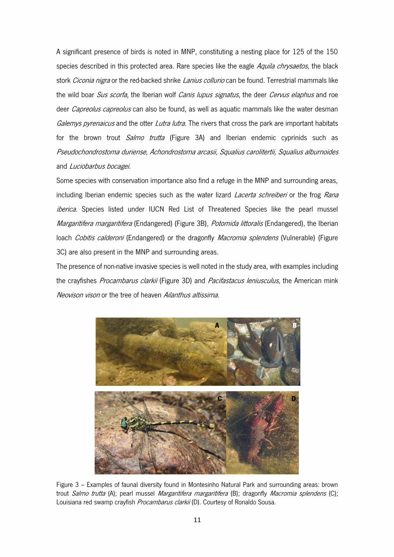
iberica. Species listed under IUCN Red List of Threatened Species like the pearl mussel

Margaritifera margaritifera (Endangered) (Figure 3B), Potomida littoralis (Endangered), the Iberian

loach Cobitis calderoni (Endangered) or the dragonfly Macromia splendens (Vulnerable) (Figure

3C) are also present in the MNP and surrounding areas.

The presence of non-native invasive species is well noted in the study area, with examples including

the crayfishes Procambarus clarkii (Figure 3D) and Pacifastacus leniusculus, the American mink

Neovison vison or the tree of heaven Ailanthus altissima.

Figure 3 – Examples of faunal diversity found in Montesinho Natural Park and surrounding areas: brown trout Salmo trutta (A); pearl mussel Margaritifera margaritifera (B); dragonfly Macromia splendens (C); Louisiana red swamp crayfish Procambarus clarkii (D). Courtesy of Ronaldo Sousa.

A B

C D

12

The human pressure within the MNP is low, with a total area of 75 000 hectares and a population

under 9000 inhabitants throughout 88 villages that tends to decline due to the ageing population

and the abandonment of rural areas. Human occupation is mostly related to subsistence

agriculture, associated with the cultivation of potatoes, chestnut, rye and permanent grassland.

Rivers surveyed in this study are included in the Tua: Mente (Fig. 4A), Rabaçal (Fig. 4B) and Tuela

(Fig. 4C) Rivers and Sabor basins: Sabor River (Fig. 4D). Mente is a tributary of Rabaçal, which in

turn is connected to Tuela to form the Tua River just upstream of the city of Mirandela. All the four

rivers are born in Spain with extensions of 120 km, 57 km, 88 km and 102 km respectively (Oliveira

et al., 2012). All rivers belong to the Douro basin, being Sabor and Tua Rivers (in addition to

Tâmega River) the most important tributaries in the right side of the basin in Portuguese territory.

Areas around the four rivers have very low human pressure, being all rivers quite undisturbed

(Sousa et al., 2012, 2015, 2018). In the study area, Rabaçal (Rebordelo and Sonim) and Tuela

(Nunes and Trutas) Rivers have two small small hydropower plants each and the Sabor River

(Gimonde) just one.

Figure 4 – Rivers surveyed in this study: Mente (A), Rabaçal (B), Tuela (C) and Sabor (D). Courtesy of Ronaldo Sousa.

A B

C D

13

2.2 Sampling strategies

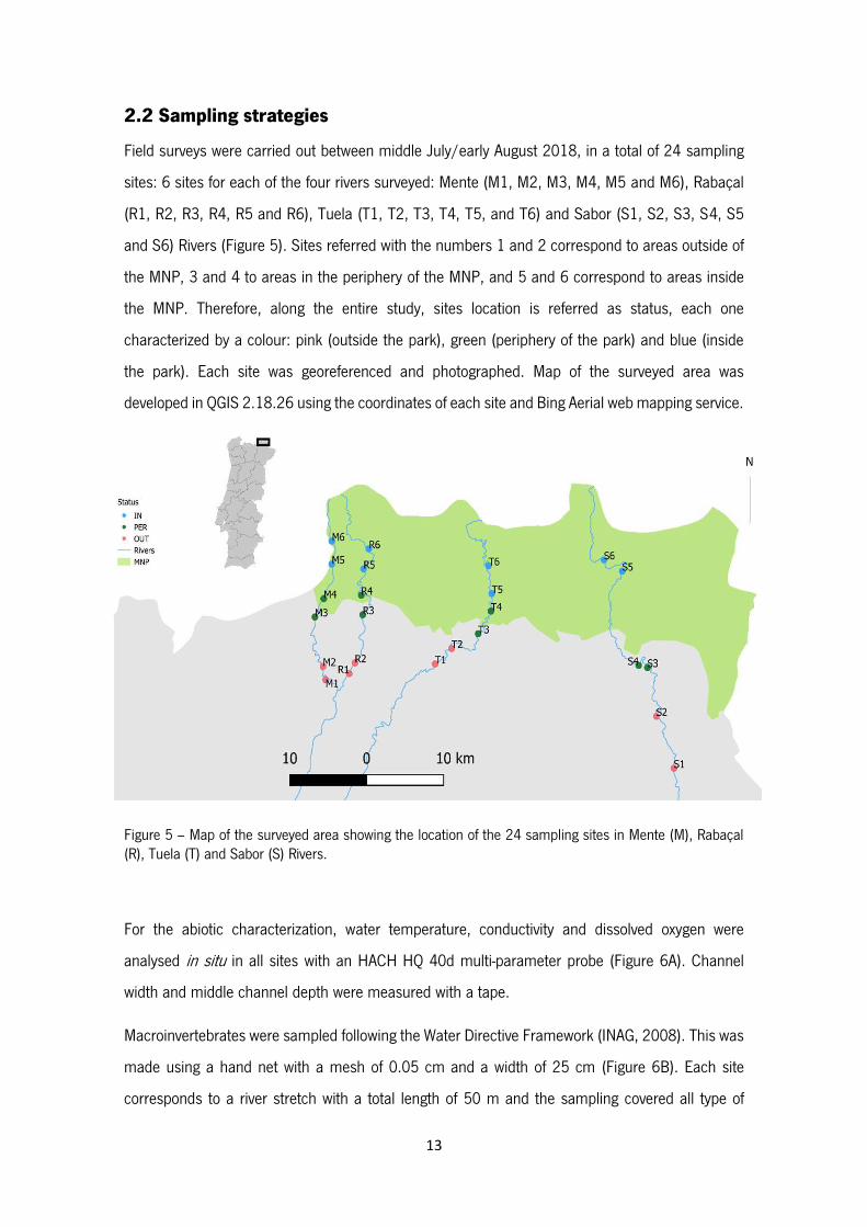
Field surveys were carried out between middle July/early August 2018, in a total of 24 sampling

sites: 6 sites for each of the four rivers surveyed: Mente (M1, M2, M3, M4, M5 and M6), Rabaçal

(R1, R2, R3, R4, R5 and R6), Tuela (T1, T2, T3, T4, T5, and T6) and Sabor (S1, S2, S3, S4, S5

and S6) Rivers (Figure 5). Sites referred with the numbers 1 and 2 correspond to areas outside of

the MNP, 3 and 4 to areas in the periphery of the MNP, and 5 and 6 correspond to areas inside

the MNP. Therefore, along the entire study, sites location is referred as status, each one

characterized by a colour: pink (outside the park), green (periphery of the park) and blue (inside

the park). Each site was georeferenced and photographed. Map of the surveyed area was

developed in QGIS 2.18.26 using the coordinates of each site and Bing Aerial web mapping service.

Figure 5 – Map of the surveyed area showing the location of the 24 sampling sites in Mente (M), Rabaçal (R), Tuela (T) and Sabor (S) Rivers.

For the abiotic characterization, water temperature, conductivity and dissolved oxygen were

analysed in situ in all sites with an HACH HQ 40d multi-parameter probe (Figure 6A). Channel

width and middle channel depth were measured with a tape.

Macroinvertebrates were sampled following the Water Directive Framework (INAG, 2008). This was

made using a hand net with a mesh of 0.05 cm and a width of 25 cm (Figure 6B). Each site

corresponds to a river stretch with a total length of 50 m and the sampling covered all type of

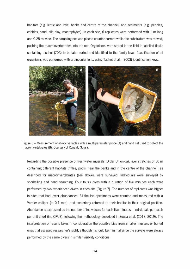
14

habitats (e.g. lentic and lotic, banks and centre of the channel) and sediments (e.g. pebbles,

cobbles, sand, silt, clay, macrophytes). In each site, 6 replicates were performed with 1 m long

and 0.25 m wide. The sampling net was placed counter-current while the substratum was moved,

pushing the macroinvertebrates into the net. Organisms were stored in the field in labelled flasks

containing alcohol (70%) to be later sorted and identified to the family level. Classification of all

organisms was performed with a binocular lens, using Tachet et al., (2003) identification keys.

Figure 6 – Measurement of abiotic variables with a multi-parameter probe (A) and hand net used to collect the macroinvertebrates (B). Courtesy of Ronaldo Sousa.

Regarding the possible presence of freshwater mussels (Order Unionida), river stretches of 50 m

containing different habitats (riffles, pools, near the banks and in the centre of the channel), as

described for macroinvertebrates (see above), were surveyed. Individuals were surveyed by

snorkelling and hand searching. Four to six dives with a duration of five minutes each were

performed by two experienced divers in each site (Figure 7). The number of replicates was higher

in sites that had lower abundances. All the live specimens were counted and measured with a

Vernier calliper (to 0.1 mm), and posteriorly returned to their habitat in their original position.

Abundance is expressed as the number of individuals for each five minutes – individuals per catch

per unit effort (ind.CPUE), following the methodology described in Sousa et al. (2018, 2019). The

interpretation of results takes in consideration the possible bias from smaller mussels or buried

ones that escaped researcher’s sight, although it should be minimal since the surveys were always

performed by the same divers in similar visibility conditions.

A B

15

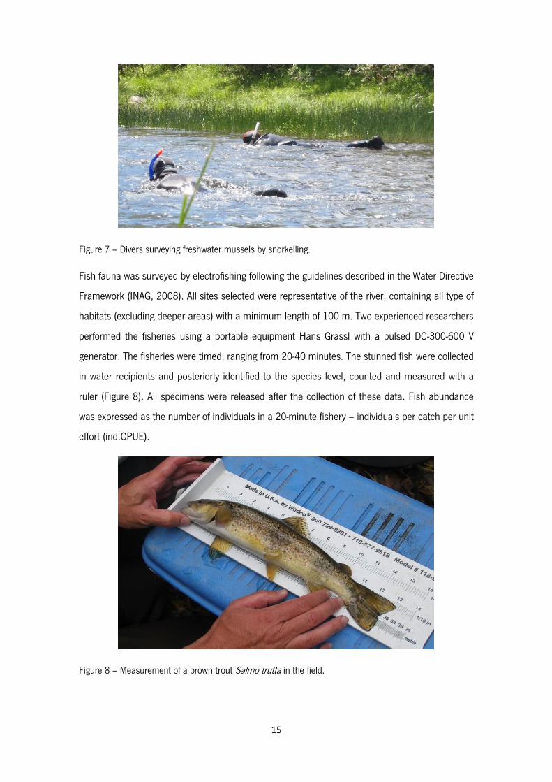
Figure 7 – Divers surveying freshwater mussels by snorkelling.

Fish fauna was surveyed by electrofishing following the guidelines described in the Water Directive

Framework (INAG, 2008). All sites selected were representative of the river, containing all type of

habitats (excluding deeper areas) with a minimum length of 100 m. Two experienced researchers

performed the fisheries using a portable equipment Hans Grassl with a pulsed DC-300-600 V

generator. The fisheries were timed, ranging from 20-40 minutes. The stunned fish were collected

in water recipients and posteriorly identified to the species level, counted and measured with a

ruler (Figure 8). All specimens were released after the collection of these data. Fish abundance

was expressed as the number of individuals in a 20-minute fishery – individuals per catch per unit

effort (ind.CPUE).

Figure 8 – Measurement of a brown trout Salmo trutta in the field.

16

2.3 Data analysis

Abiotic characterization consisted on the analysis of nine variables including water temperature,

conductivity, dissolved oxygen and river width and depth (as described above) plus altitude,

distance to the nearest village (DNV), distance to the limits of the park (DTP) and Human Footprint

Index (HFI). Altitude and DNV were calculated using Google Earth, being that DNV was considered

to be the minimum distance in a straight line from the sampling site to the nearest village. The

DTP was calculated using QGIS (2.18.26) measuring tool, being the distance from sampling sites

to the nearest limit of MNP, in which positive values relate to sites outside the park, and negative

ones to sites inside the park. As for the HFI, it measures the human pressure compiling information

of population density, human land use and infrastructure (e.g. built-up areas, crop land, pasture

and night-time lights) and human access (e.g. roads, railroads, and navigable waterways). HFI is

expressed as percentage and is available at ArcGIS (https:// arcgis.com). In the particular case of

this study, we used the average percentage value described for each sampling site. All abiotic data

was normalised and used to perform a Principal Component Analysis (PCA). This multivariate

analysis allowed to sort the different sites according to the variables in study and was performed

on Primer 6 (version 1.0.3, Primer-E Ltd, Plymouth).

The macroinvertebrate communities were analysed with a Multidimensional scaling (MDS), in

which the data was previously log transformed and used to make a similarity matrix using the Bray-

Curtis distance. To evaluate the influence of the park status on the macroinvertebrate communities

in the 24 sites, a one-way PERMANOVA was designed with status (3 factors: outside, periphery and

inside) as a fixed factor. The test considered 9999 permutations, but when the number was lower

than 150 the Monte Carlo test p-value was considered. A similarity percentage (SIMPER) analysis

was performed (cut-off 90%) to assess the taxa contributing to the dissimilarity between the tree

different park status. Richness (number of families; S), abundance (N), and diversity indices

Shannon-Wiener (H’) and Pielou’s evenness (J’) were calculated using DIVERSE function. All the

analyses mentioned above were computed on Primer 6 (version 1.0.3, Primer-E Ltd, Plymouth).

Also, regression analyses were performed with dependent variables: S, N, H’, J’, IBMWP, IASPT

and %EPT against independent predictor variables: temperature, oxygen, conductivity, depth,

altitude, width, HFI, DNV and DTP using Minitab 14. Water quality indices were also determined,

including the IBMWP (Iberian Biological Monitoring Working Party) (Alba-Tercedor and Sánchez-

Ortega, 1988), the IASPT (Iberian Average Score Per Taxa) (Alba-Tercedor, 2000) and the %EPT

(percentage of Ephemeroptera, Plecoptera and Tricoptera families). A one-way ANOVA was

17

performed to test possible differences in richness, abundance, H’ index, J’ index, IBMWP, IASPT

and %EPT between the different park status.

Abundance and length of the pearl mussel M. margaritifera were analysed compiling all three rivers

in which the species is present (Mente, Rabaçal and Tuela Rivers) and also each river individually

for a more detailed assessment. A one-way ANOVA was carried out in order to assess possible

differences in abundance and length between park status. A Tukey test was performed with length

data to detect where the differences exist. Regarding the analyses on each river, a one-way ANOVA

was performed to compare pearl mussel’s abundance in the different park status for the Rabaçal

and Tuela Rivers. For this, data was previously transformed (square root) to achieve

homoscedasticity. A multiple comparison test (Tukey) was conducted in the Tuela River. In Mente

River, pearl mussels were only found outside the park (see results section) and so no further

statistical analysis was performed. A one-way ANOVA was also performed to check possible

differences in pearl mussel’s length between park status for Rabaçal and Tuela Rivers, as well as

a Tukey test. All these statistical analyses were performed with R Studio (version 1.1.463). Finally,

a linear regression tested a possible relation between pearl mussel abundance and its fish host (i.e

Salmo trutta) abundance on Minitab 14.

Fish communities were analysed with a MDS, in which the data was previously log transformed

and used to make a similarity matrix using the Bray-Curtis distance. A one-way PERMANOVA test

(9999 permutations) was designed to evaluate the influence of the park status (3 factors: outside,

periphery and inside) in the fish communities, followed by pair-wise comparison tests. The test

considered 9999 permutations, but when the number was lower than 150 the Monte Carlo test p-

value was considered. A similarity percentage (SIMPER) analysis was performed (cut-off 90%) to

assess the species contributing to the dissimilarity between the tree park status. Richness (number

of species; S), abundance (N), Shannon-Wiener diversity (H’) and Pielou’s evenness (J’) indices

were calculated as described above. All the analyses mentioned above were computed on Primer

6 (version 1.0.3, Primer-E Ltd, Plymouth). In addition, a one-way ANOVA was used to test possible

differences in richness, H’ and J’ indices between the park status in the four studied rivers. A non-

parametric Kruskall-Wallis rank test was used to analyse possible differences in abundance

between park status since normality was not achieved even after several transformations. Multiple

comparison tests were performed with richness (Tukey test) and abundance (Kruskall-Wallis

multiple comparison test). These statistical analyses were performed with R Studio (version

1.1.463). Also, regression analyses were performed with dependent variables: S, N, H’ and J’

18

against independent predictor variables: temperature, oxygen, conductivity, depth, altitude, width,

HFI, DNV and DTP on Minitab 14.

A more detailed assessment was made for each fish species individually. For that, a one-way

ANOVA was performed to analyse possible differences in Salmo trutta and Squalius carolitertii

abundance between park status, with data being previously log transformed. Since Squalius

alburnoides, Luciobarbus bocagei and Pseudochondrostoma duriense abundance data departed

from normality and had heteroscedasticity (even after several transformations), a Kruskall-Wallis

test was performed to compare possible differences in abundance between park status. For Cobitis

calderoni and Cobitis paludica abundance, a Wilcox test was performed. Whenever relevant, a

multiple comparison test was conducted. Length data of each fish species was also used to assess

possible differences between park status. Salmo trutta, Squalius carolitertii and

Pseudochondrostoma duriense length data was analysed with a one-way ANOVA, Squalius

alburnoides and Luciobarbus bocagei with Kruskall-Wallis test (due to heteroscedasticity) and

Cobitis calderoni and Cobitis paludica with a t test. Whenever relevant, a multiple comparison test

was conducted. All these statistical analyses were performed with R Studio (version 1.1.463).

Finally, it was constructed a diagram using macroinvertebrates and fish richness, discriminating

each site and park status for all the studied rivers. The same was made for the number of species

with conservation importance, listed under IUCN Red List of Threatened Species as Vulnerable

(VU), Endangered (EN) or Critically Endangered (CR). Species include macroinvertebrates:

Macromia splendens (VU), Margaritifera margaritifera (EN), Potomida littoralis (EN) and fishes:

Pseudochondrostoma duriense (VU), Squalius alburnoides (VU), Cobitis calderoni (EN), Cobitis

paludica (VU).

19

3. Results

3.1 Abiotic characterization

Abiotic characterization in all sampling sites is presented in the Table 1. Temperature varied

between 16.9 (M3) and 24.2ºC (S1); dissolved oxygen between 6.8 (S2) and 8.9 mg/L (M4); and

water conductivity between 38.9 (S6) and 161.2 (S1) µS/cm; depth between 0.3 (M2, M5, M6,

R4, R6, T1, T6 and S6) and 1.5 m (T4); altitude between 385 (R1) and 721 m (S6); width between

6 (M6) and 22 m (S3); DNV between 900 (T1) and 3580 m (S2); HFI between 15 (S5 and S6) and

50% (T2, S2 and S4) and DTP between 100 (T3) and 12200 m (S1).

Table 1 – Abiotic characterization in all sampling sites in the Mente, Rabaçal, Tuela and Sabor Rivers.

M1 M2 M3 M4 M5 M6 R1 R2 R3 R4 R5 R6

Temperature (ºC) 18.9 18.9 16.9 17.4 17.3 18.2 22.0 21.0 21.0 18.3 19.7 19.0

Oxygen (mg/L) 8.5 8.8 8.5 8.9 8.7 8.6 8.0 8.7 8.2 8.6 8.5 8.7

Conductivity (µS/cm) 52.9 53.7 61.1 55.8 54.7 46.1 47.7 48.0 46.8 40.3 40.9 43.3

Depth (m) 1 0.3 0.5 0.4 0.3 0.3 0.8 0.4 0.5 0.3 0.4 0.3

Altitude (m) 389.0 396.0 442.0 455.0 491.0 529.0 385.0 410.0 452.0 477.0 487.0 525.0

Width (m) 11.0 7.0 14.0 12.0 12.5 6.0 16.0 7.0 8.0 10.0 11.0 16.0

DNV (m) 1250.0 1100.0 1250.0 1400.0 1700.0 1050.0 3400.0 2350.0 1600.0 1150.0 980.0 1850.0

HFI (%) 35.0 25.0 25.0 25.0 25.0 25.0 35.0 25.0 35.0 35.0 35.0 25.0

DTP (m) 10600 8600 100 -1300 -5000 -8200 10000 8800 1800 -1200 -2800 -6000

T1 T2 T3 T4 T5 T6 S1 S2 S3 S4 S5 S6

Temperature (ºC) 20.9 20.9 20.1 19.8 18.7 19.6 24.2 22.2 22.1 20.1 21.3 19.3

Oxygen (mg/L) 8.6 8.6 8.6 8.8 8.5 8.7 7.8 6.8 7.4 7.9 8.6 8.5

Conductivity (µS/cm) 76.5 76.5 53.9 61.3 52.4 46.8 161.2 116.0 115.0 134.4 50.3 38.9

Depth (m) 0.3 0.8 0.5 1.5 0.5 0.3 0.5 0.5 0.4 0.5 0.6 0.3

Altitude (m) 409.0 429.0 579.0 608.0 625.0 654.0 418.0 497.0 519.0 523.0 647.0 721.0

Width (m) 12.5 12.0 16.0 14.5 16.0 20.0 15.0 21.0 22.0 16.5 14.0 9.0

DNV (m) 900.0 1450.0 1650.0 920.0 1400.0 1220.0 2220.0 3580.0 1570.0 1020.0 990.0 1700.0

HFI (%) 25.0 50.0 35.0 35.0 35.0 25.0 25.0 25.0 50.0 50.0 15.0 15.0

DTP (m) 4900 2100 -500 -2000 -3400 -8900 12200 5500 2700 1800 -9500 -11400

Results of the PCA using the abiotic data arranged the 24 sampling sites as shown in Figure 9. A

distinction between S1, S2, S3 and S4 and all the other sites is clear. PC1 explain 38.1% of all

variation and PC2 21.8% (Table S1 in Annex). The main abiotic factors responsible for the

separation in PC1 were oxygen (positive direction), conductivity and temperature (negative

20

direction) as for the PC2 were altitude and width (negative direction) and DTP (positive direction)

(Table S2 in Annex).

Figure 9 – Principal Components Analysis (PCA) showing the arrangement of the 24 sampling sites based on the abiotic factors measured. PC1 explains 38.1% of all variance and PC2 21.8%.

3.2 Macroinvertebrate communities

A total of 29710 individuals belonging to 90 taxa were identified. The MDS of the macroinvertebrate

communities (Figure 10) shows a great similarity between all sites in Mente and Rabaçal Rivers as

well as upstream sites in the Tuela (T4, T5 and T6) and Sabor (S6) Rivers. The other sites tend to

be grouped according to spatial proximity: S1 and S2; S3 and S4 and T1 and T2, with T3 and S5

isolated from all others. Permanova results indicate that there are no significant differences in the

macroinvertebrate communities between park status (Pseudo-F=1.1; p=0.3). Macroinvertebrate

taxa sampled in this work are presented in Table S3 in Annex.

21

Figure 10- Multidimensional scaling (MDS) of the macroinvertebrate communities showing sampling sites and park status.

The SIMPER analysis showed that the taxa contributing the most to the average dissimilarity

between outside and periphery (49.3%) were Oligoneuriidae (3.9%), Hydropsychidae (3.7%) and

Caenidae (3.7%), while between outside and inside (46.7%) were Simuliidae (4%), Brachycentridae

(3.7%) and Oligoneuriidae (3.6%) and between periphery and inside (43.2%) were Brachycentridae

(4.3%), Oligoneuriidae (4.1%) and Simuliidae (3.9%) (see Table S4 in Annex).

Average (±SD) macroinvertebrate richness (number of families) was higher inside the park with

32.6 (±5.6) families present, followed in the periphery with 28.2 (±10.7) and lower outside with

27.4 (±6.6) (Figure 11A). However, ANOVA results showed no significant differences in

macroinvertebrate richness between park status (F2,21=0.98; p=0.39). Sites S6, R3 and M3 were

characterized by the highest richness, with 42, 40 and 38 different families present, respectively,

and sites S1, S3, S4 had the lowest with 18, 16 and 11, respectively. Average (±SD) abundance

of macroinvertebrates was higher inside the park with 1523.1 (±676.8), followed by the periphery

with 1251.9 (±696.1) and lower outside with 938.8 (±812.2) (Figure 11B). No significant

differences in macroinvertebrate abundance between park status were observed (F2,21=1.3; p=0.3).

Sites S2, T6 and M4 hold the highest abundances with 2708, 2510 and 2494 individuals

respectively, and T1, S5 and T2 the lowest with 448, 405 and 198, respectively. Average (±SD)

Shannon-Wiener (H’) diversity was higher outside the park with 2.19 (±0.29), followed by the

22

periphery with 2.14 (±0.38) and lower inside with 2.06 (±0.34) (Figure 11C). No significant

differences in H’ index between park status were detected (F2,21=0.29; p=0.75). Sites M2, R2 and

M3 hold the highest Shannon-Wiener diversity of macroinvertebrates with values of 2.57, 2.56 and

2.53 respectively, and M5, S3 and S4 the lowest with 1.65, 1.61 and 1.50, respectively. Average

(±SD) Pielou’s evenness varied between 0.67 (±0.06) outside the park, followed by its periphery

with 0.66 (±0.06) and inside with 0.59 (±0.09) (Figure 11D). Again, results of the ANOVA test

showed no significant differences between park status (F2,21= 2.15; p=0.14). Sites M2, T4 and T2

had the greatest evenness values with 0.78, 0.76 and 0.71 respectively, and M5, T5 with 0.49

and S6 with 0.45 had the lowest values.

Figure 11 – Richness (A), Abundance (B), Shannon-Wiener diversity (C) and Pielou’s evenness (D) of the macroinvertebrate communities outside (pink), periphery (green) and inside (blue) the park. White circles represent the average values. Boxplots show median values (central line), the range from the 25th to 75th percentile (box) and the largest and lowest value within 1.5 times interquartile range below and above the 25th and 75th percentile (whiskers) and dots represent extreme values.

A B

C D

23

Results of the regression analyses are present in Table S5 in Annex. Richness varied significantly

with five abiotic factors (temperature, oxygen, conductivity, width and HFI), abundance with two

(temperature and DNV), Shannon-Wiener diversity with three (oxygen, conductivity and width) and

Pielou’s evenness with none.

Results from the IBMWP index indicated that all sites located in Rabaçal, Mente and Tuela Rivers

as well as S2, S5 and S6 have a very good water quality (score >100); sites S1 and S3 have a

good water quality (score 61-100); and only S4 is classified as polluted (score 36-60) (Table 2).

Average (±SD) IBMWP varied from 185.6 (±37.4) inside the park, 148.1 (±40.2) in the periphery

and 157.8 (±66.1) outside (Figure 12A). ANOVA test showed no significant differences in IBMWP

index between park status (F2,21= 1.23; p=0.31). Regarding average IASPT (±SD), it was greater

inside the park with 5.99 (±0.40), followed by outside with 5.93 (±0.46) and periphery with 5.84

(±0.69) (Figure 12B). No significant differences were found in IASPT index between status (F2,21=

0.16; p=0.86). Sites T3, R1 and M2 were characterized by a higher IASPT score of 6.60, 6.52 and

6.46 respectively, and S5, S3 and S4 showed the lowest with 5.08, 4.86 and 4.72, respectively.

Average EPT% (±SD) was greater in periphery with a 42.3% (±5.8%), followed by outside with 41.4%

(±7.3%) and inside with 40.8% (±7.7%) (Figure 12C). No significant differences in EPT percentage

between park status were detected (F2,21= 0.10; p=0.90). Sites S4, T6 and T5 showed the higher

percentage of 54.5%, 50% and 48.3%, respectively, and T1, T2 and S5 the lowest with 33.3%,

26.9% and 26.1%, respectively.

Table 2 – Water quality index for all the sampling sites in Mente, Rabaçal, Tuela and Sabor Rivers. IBMWP quality scores: >100 – very good; 100-61 – good; 36-60 – polluted; 16-35 – very polluted; <16 – extremely polluted (after Alba-Tercedor and Sánchez-Ortega, 1988).

M1 M2 M3 M4 M5 M6 R1 R2 R3 R4 R5 R6

IBMWP 183 179 216 192 148 195 137 206 230 194 197 201

IASPT 6.1 6.4 6.4 5.8 6.2 5.9 6.5 6.2 6.2 5.9 6.2 6.1

EPT % 45.5 46.4 44.7 38.9 44.4 36.1 43.5 43.2 42.5 41.2 44.1 38.9

T1 T2 T3 T4 T5 T6 S1 S2 S3 S4 S5 S6

IBMWP 163 108 165 145 181 209 100 109 68 52 117 237

IASPT 5.8 5.1 6.6 6.3 6.5 6.1 5.6 5.7 4.9 4.7 5.1 5.9

EPT % 33.3 26.9 35.7 43.5 48.3 50.0 44.4 47.6 37.5 54.5 26.1 38.1

24

Figure 12 –IBMWP (A), IASPT (B) and %EPT (C) water quality indices outside (pink), periphery (green) and inside (blue) the park. White circles represent the average values. Boxplots show median values (central line), the range from the 25th to 75th percentile (box) and the largest and lowest value within 1.5 times interquartile range below and above the 25th and 75th percentile (whiskers) and dots represent extreme values.

Results of the regression analyses are present in Table S5 in Annex. IBMWP varied significantly

with five abiotic factors (temperature, oxygen, conductivity, width and HFI), IASPT with two (oxygen

and conductivity) and %EPT with none.

Bivalves were present in all the four rivers surveyed and four different species (i.e. Margaritifera

margaritifera, Potomida littoralis, Unio delphinus and Anodonta anatina) were found. Margaritifera

margaritifera was present in all sites surveyed on Rabaçal and Tuela Rivers and U. delphinus was

also found in T2. In Mente River only M. margaritifera was found in sites M1 and M2. In the Sabor

River M. margaritifera was not present but P. littoralis, U. delphinus and A. anatina were found

A B

C

25

exclusively in S1. A total of 94 freshwater mussels were found in S1, being 87 U. delphinus, 4 P.

littoralis and 2 A. anatina.

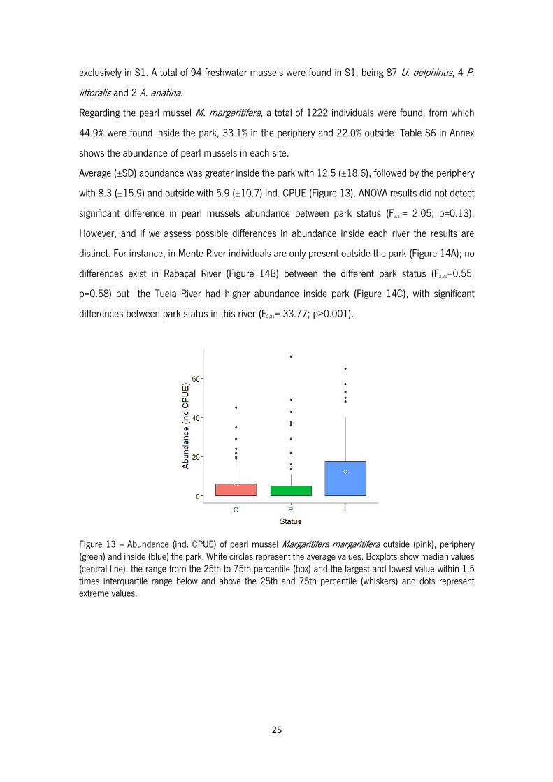
Regarding the pearl mussel M. margaritifera, a total of 1222 individuals were found, from which

44.9% were found inside the park, 33.1% in the periphery and 22.0% outside. Table S6 in Annex

shows the abundance of pearl mussels in each site.

Average (±SD) abundance was greater inside the park with 12.5 (±18.6), followed by the periphery

with 8.3 (±15.9) and outside with 5.9 (±10.7) ind. CPUE (Figure 13). ANOVA results did not detect

significant difference in pearl mussels abundance between park status (F2,21= 2.05; p=0.13).

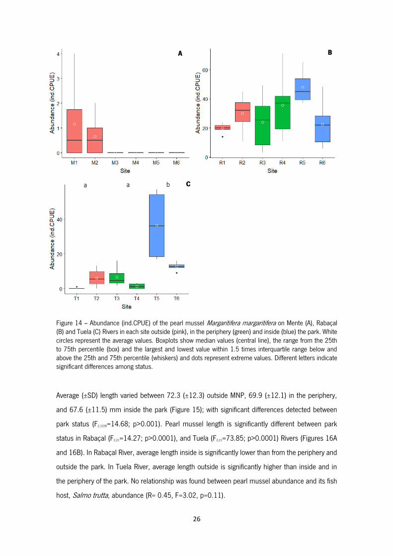
However, and if we assess possible differences in abundance inside each river the results are

distinct. For instance, in Mente River individuals are only present outside the park (Figure 14A); no

differences exist in Rabaçal River (Figure 14B) between the different park status (F2,21=0.55,

p=0.58) but the Tuela River had higher abundance inside park (Figure 14C), with significant

differences between park status in this river (F2,21= 33.77; p>0.001).

Figure 13 – Abundance (ind. CPUE) of pearl mussel Margaritifera margaritifera outside (pink), periphery (green) and inside (blue) the park. White circles represent the average values. Boxplots show median values (central line), the range from the 25th to 75th percentile (box) and the largest and lowest value within 1.5 times interquartile range below and above the 25th and 75th percentile (whiskers) and dots represent extreme values.

26

Figure 14 – Abundance (ind.CPUE) of the pearl mussel Margaritifera margaritifera on Mente (A), Rabaçal (B) and Tuela (C) Rivers in each site outside (pink), in the periphery (green) and inside (blue) the park. White circles represent the average values. Boxplots show median values (central line), the range from the 25th to 75th percentile (box) and the largest and lowest value within 1.5 times interquartile range below and above the 25th and 75th percentile (whiskers) and dots represent extreme values. Different letters indicate significant differences among status.

Average (±SD) length varied between 72.3 (±12.3) outside MNP, 69.9 (±12.1) in the periphery,

and 67.6 (±11.5) mm inside the park (Figure 15); with significant differences detected between

park status (F2,1228=14.68; p>0.001). Pearl mussel length is significantly different between park

status in Rabaçal (F2,21=14.27; p>0.0001), and Tuela (F2,21=73.85; p>0.0001) Rivers (Figures 16A

and 16B). In Rabaçal River, average length inside is significantly lower than from the periphery and

outside the park. In Tuela River, average length outside is significantly higher than inside and in

the periphery of the park. No relationship was found between pearl mussel abundance and its fish

host, Salmo trutta, abundance (R= 0.45, F=3.02, p=0.11).

A B

C b a a

27

Figure 15 - Length (mm) of the pearl mussel Margaritifera margaritifera outside (pink), periphery (green) and inside (blue) the park. White circles represent the average values. Boxplots show median values (central line), the range from the 25th to 75th percentile (box) and the largest and lowest value within 1.5 times interquartile range below and above the 25th and 75th percentile (whiskers) and dots represent extreme values. Different letters indicate significant differences among status.

Figure 16 - Length (mm) of Margaritifera margaritifera in Rabaçal (A) and Tuela (B) Rivers in each site outside (pink), in the periphery (green) and inside (blue) the park. White circles represent the average values. Boxplots show median values (central line), the range from the 25th to 75th percentile (box) and the largest and lowest value within 1.5 times interquartile range below and above the 25th and 75th percentile (whiskers) and dots represent extreme values. Different letters indicate significant differences among status.

A B

a b c

b a a a b b

28

3.3 Fish communities

A total of 2043 individuals belonging to seven species were surveyed in this study, of which 11.8%

were present inside the park, 46.6% in its periphery and 41.6% outside. The seven fish species

were Salmo trutta, Squalius carolitertii, Pseudochondrostoma duriense, Squalius alburnoides,

Luciobarbus bocagei, Cobitis calderoni and Cobitis paludica. Salmo trutta was found in all sites

except M1, R1, S1 and S2; Squalius carolitertii was present in all sites, with exception of T1 and

M6; Pseudochondrostoma duriense was found in all sites excluding R6 and S6; Squalius

alburnoides was found in T1 and T2, M1, M2, M3 and M4, R1 and R2 and S1, S2, S3 and S4;

Luciobarbus bocagei was found in T1 and T2, M1, M2 and M4, R1, R4, R5 and R6 and S1, S2,

S3 and S4; Cobitis calderoni was present in M1, M2, R2 and R5; Cobitis paludica was found in

S1, S3 and S4. Fish species abundance are presented in Table S7 in Annex.

The MDS of the fish communities is shown in Figure 17. Permanova results indicate that there are

significant differences in fish assemblages between park status (Pseudo-F=8.3; p=0.0001), being

that all status differs significantly from each other (Table S8 in Annex).

Figure 17 - Multidimensional scaling (MDS) of the fish communities showing sampling sites and park status.

29

The SIMPER analysis showed that the species contributing the most to the average dissimilarity

between outside and periphery (44.4%) were S. alburnoides (28 %), S. carolitertii (17%) and L.

bocagei (16.9%), while between outside and inside (66.3%) were S. alburnoides (31.8%), P.

duriense (16.1 %) and L. bocagei (15.2%) and between periphery and inside (48.1%) were P.

duriense (26%), S. alburnoides (22.4%) and S. carolitertii (20.6%) (see Table S9 in Annex).

Regarding diversity indices, average (±SD) species richness was highest outside with 4.75 (±0.7),

followed by periphery with 4.25 (±1.3) and inside with 3 (±0.9) species (Figure 18A). Significant

differences in fish richness between park status were found (F2,21=6.5; p=0.006), being outside

significantly higher than inside MNP. Sites M2, S3 and S4 had the highest richness with 6 species,

and M6 and S6 the lowest with only 2 species found. Concerning fish abundance, the periphery

had the highest average (±SD) values of 119.04 (±150.3), followed by outside with 106.07 (±84.2)

and inside with 30.25 (±28.1) ind. CPUE (Figure 18B). Kruskal-Wallis analyses showed significant

differences in fish abundance between park status (χ2=7.7; p=0.02), in which the abundance

outside the park is significantly higher than inside MNP. Sites S3, S2 and S4 had the highest

abundance with 445, 287 and 240 ind. CPUE, and R3, M6 and M5 the lowest with only 11, 10.7

and 4 ind. CPUE respectively. Average (±SD) Shannon-Wiener diversity was highest in the periphery

with 1.06 (± 0.2), followed by outside with 1.01 (±0.4) and inside with 0.82 (±0.3) (Figure 18C).

No differences in Shannon-Wiener diversity were found between park status (F2,21= 1.42; p=0.26).

Sites S4, S3 and S1 hold the highest Shannon-Wiener diversity with values of 1.42, 1.38 and 1.36,

respectively, and R1, M1 and M6 the lowest with 0.47, 0.46 and 0.38. Average (±SD) Pielou’s

evenness varied between 0.78 (±0.2) inside, 0.76 (±0.1) in the periphery and 0.65 (±0.23) outside

the park (Figure 18D). No significant differences in J’ index between the park status were found

(F2,21= 1; p=0.38). Sites S6, R3 and M5 showed the highest evenness values with 0.99, 0.97 and

0.94, respectively, and S5, R1 and M1 the lowest with 0.46, 0.34 and 0.29, respectively.

30

Figure 18 - Richness (A), Abundance (B), Shannon-Wiener diversity (C) and Pielou’s evenness (D) of the fish communities outside (pink), periphery (green) and inside (blue) the park. White circles represent the average values. Boxplots show median values (central line), the range from the 25th to 75th percentile (box) and the largest and lowest value within 1.5 times interquartile range below and above the 25th and 75th percentile (whiskers) and dots represent extreme values. Different letters indicate significant differences among status.

Results of the regression analyses are present in Table S10 in Annex. Richness varied significantly

with four abiotic factors (conductivity, altitude, HFI and DTP), abundance with four (oxygen,

conductivity, width and HFI), Shannon-Wiener diversity with one (conductivity) and Pielou’s

evenness with one (DNV).

Analysing each species abundance (±SD) individually we can observe that S. trutta abundance

ranged from 7.2 (±3) inside the park, 5.4 (±4.7) in the periphery and 1.3 (±2) ind. CPUE outside

(Figure 19A). Results indicate that S. trutta abundance differs significantly between park status

(F2,21= 7.37; p=0.003), being significantly lower outside when compared to inside and periphery.

A B

C D

a ab b a ab b

31

Average (±SD) abundance of S. alburnoides varied from 53.9 (±48.5) outside, 42.6 (±58.6 in the

periphery to 0 ind. CPUE inside the park (Figure 19B). Squalius alburnoides abundance is

significantly distinct between park status (χ2=11.9; p=0.002), being significantly higher outside

than inside the park. Average (±SD) abundance of L. bocagei average varied between 12.1 (±16.3)

outside, 3 (±5.8) in the periphery and 2.5 (±5.6) ind. CPUE inside the park (Figure 19C). No

significant differences in L. bocagei abundance between park status were found (χ2=5.7; p=0.06).

Average (±SD) abundance of S. carolitertii varied between 32 (±41.6) in the periphery, 22 (±44)

outside and 18.1 (±20.7) ind. CPUE inside the park (Figure 19D). No significant differences in S.

carolitertii abundance between park status were found (F2,21= 0.39; p=0.69). Average (±SD)

abundance of P. duriense varied between 27.5 (±42) in the periphery, 12.8 (±9.3) outside and 1.4

(±1.9) ind. CPUE inside the park (Figure 19E). Pseudochondrostoma duriense abundance differs

significantly between park status (χ2=13.38; p=0.001), being values inside of the park significantly

lower than outside and in the periphery. Average (±SD) abundance of C. calderoni ranged between1

(±2.8) inside, 0.89 (±1.4) outside and 0 ind. CPUE in the periphery of the park (Figure 19F). No

significant differences in C. calderoni abundance between park status were found (W=3.59;

p=0.16). Average (±SD) abundance of C. paludica ranged from 8.5 (±17) in the periphery, 3.1 (±9)

outside and 0 ind. CPUE inside the park (Figure 19G), with no significant differences in abundance

found between park status (W=2.18; p=0.34).

A B a b b a ab b

32

Figure 19 – Abundance (ind.CPUE) of Salmo trutta (A), Squalius alburnoides (B), Luciobarbus bocagei (C), Squalius carolitertii (D), Pseudochondrostoma duriense (E), Cobitis calderoni (F) and Cobitis paludica (G) outside (pink), in the periphery (green) and inside (blue) the park. White circles represent the average values. Boxplots show median values (central line), the range from the 25th to 75th percentile (box) and the largest and lowest value within 1.5 times interquartile range below and above the 25th and 75th percentile (whiskers) and dots represent extreme values. Different letters indicate significant differences among status.

C D

E F

G

a a b

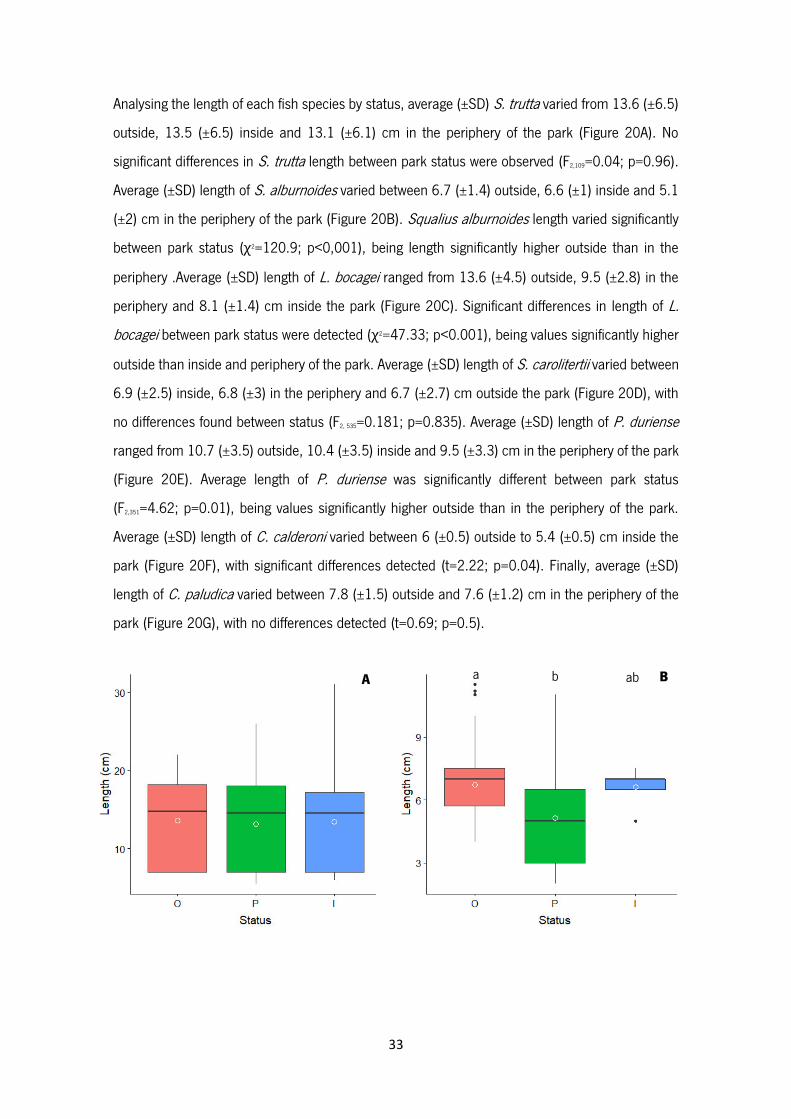
33

Analysing the length of each fish species by status, average (±SD) S. trutta varied from 13.6 (±6.5)

outside, 13.5 (±6.5) inside and 13.1 (±6.1) cm in the periphery of the park (Figure 20A). No

significant differences in S. trutta length between park status were observed (F2,109=0.04; p=0.96).

Average (±SD) length of S. alburnoides varied between 6.7 (±1.4) outside, 6.6 (±1) inside and 5.1

(±2) cm in the periphery of the park (Figure 20B). Squalius alburnoides length varied significantly

between park status (χ2=120.9; p<0,001), being length significantly higher outside than in the

periphery .Average (±SD) length of L. bocagei ranged from 13.6 (±4.5) outside, 9.5 (±2.8) in the

periphery and 8.1 (±1.4) cm inside the park (Figure 20C). Significant differences in length of L.

bocagei between park status were detected (χ2=47.33; p<0.001), being values significantly higher

outside than inside and periphery of the park. Average (±SD) length of S. carolitertii varied between

6.9 (±2.5) inside, 6.8 (±3) in the periphery and 6.7 (±2.7) cm outside the park (Figure 20D), with

no differences found between status (F2, 535=0.181; p=0.835). Average (±SD) length of P. duriense

ranged from 10.7 (±3.5) outside, 10.4 (±3.5) inside and 9.5 (±3.3) cm in the periphery of the park

(Figure 20E). Average length of P. duriense was significantly different between park status

(F2,351=4.62; p=0.01), being values significantly higher outside than in the periphery of the park.

Average (±SD) length of C. calderoni varied between 6 (±0.5) outside to 5.4 (±0.5) cm inside the

park (Figure 20F), with significant differences detected (t=2.22; p=0.04). Finally, average (±SD)

length of C. paludica varied between 7.8 (±1.5) outside and 7.6 (±1.2) cm in the periphery of the

park (Figure 20G), with no differences detected (t=0.69; p=0.5).

A B a b ab

34

Figure 20 – Length (cm) of Salmo trutta (A), Squalius alburnoides (B), Luciobarbus bocagei (C), Squalius carolitertii (D), Pseudochondrostoma duriense (E), Cobitis calderoni (F) and Cobitis paludica (G) outside (pink), in the periphery (green) and inside (blue) the park. White circles represent the average values. Boxplots show median values (central line), the range from the 25th to 75th percentile (box) and the largest and lowest value within 1.5 times interquartile range below and above the 25th and 75th percentile (whiskers) and dots represent extreme values. Different letters indicate significant differences among status.

C D

E F

G

a b b

a b ab

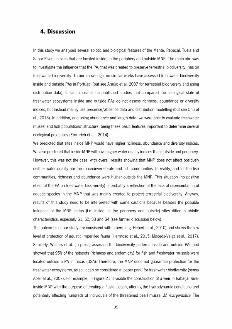
35

4. Discussion

In this study we analysed several abiotic and biological features of the Mente, Rabaçal, Tuela and

Sabor Rivers in sites that are located inside, in the periphery and outside MNP. The main aim was

to investigate the influence that the PA, that was created to preserve terrestrial biodiversity, has on

freshwater biodiversity. To our knowledge, no similar works have assessed freshwater biodiversity

inside and outside PAs in Portugal (but see Araújo et al. 2007 for terrestrial biodiversity and using

distribution data). In fact, most of the published studies that compared the ecological state of

freshwater ecosystems inside and outside PAs do not assess richness, abundance or diversity

indices, but instead mainly use presence/absence data and distribution modelling (but see Chu et

al., 2018). In addition, and using abundance and length data, we were able to evaluate freshwater

mussel and fish populations’ structure, being these basic features important to determine several

ecological processes (Emmrich et al., 2014).

We predicted that sites inside MNP would have higher richness, abundance and diversity indices.

We also predicted that inside MNP will have higher water quality indices than outside and periphery.

However, this was not the case, with overall results showing that MNP does not affect positively

neither water quality nor the macroinvertebrate and fish communities. In reality, and for the fish

communities, richness and abundance were higher outside the MNP. This situation (no positive

effect of the PA on freshwater biodiversity) is probably a reflection of the lack of representation of

aquatic species in the MNP that was mainly created to protect terrestrial biodiversity. Anyway,

results of this study need to be interpreted with some cautions because besides the possible

influence of the MNP status (i.e. inside, in the periphery and outside) sites differ in abiotic

characteristics, especially S1, S2, S3 and S4 (see further discussion below).

The outcomes of our study are consistent with others (e.g. Hebert et al., 2010) and shows the low

level of protection of aquatic imperilled fauna (Hermoso et al., 2015; Maceda-Veiga et al., 2017).

Similarly, Walters et al. (in press) assessed the biodiversity patterns inside and outside PAs and

showed that 95% of the hotspots (richness and endemicity) for fish and freshwater mussels were

located outside a PA in Texas (USA). Therefore, the MNP does not guarantee protection for the

freshwater ecosystems, as so, it can be considered a ‘paper park’ for freshwater biodiversity (sensu

Abell et al., 2007). For example, in Figure 21 is visible the construction of a weir in Rabaçal River

inside MNP with the purpose of creating a fluvial beach, altering the hydrodynamic conditions and

potentially affecting hundreds of individuals of the threatened pearl mussel M. margaritifera. The

36

construction of this weir is just one example of the lack of attention devoted to the conservation of

freshwater species in MNP.

Figure 21 – Before (2012) (A) and after (2017) (B, C) the construction of a weir with the goal of creating an artificial river beach for visitors inside Montesinho Natural Park. Courtesy of Ronaldo Sousa.

4.1 Abiotic characterization

Sites S1, S2, S3 and S4 were different abiotically from all other sites. This may be related to a

more Mediterranean climate influence in the middle and lower parts of the Sabor River, translated

in higher water temperature and conductivity, and lower dissolved oxygen. Also, these four sites

represent wider channels and are subject to higher HFI due to the proximity of roads, denser

human populations and higher agriculture activity. The remaining sites differentiate themselves

mostly due to altitude, width and distance to the park limit. Sites R1, M1, T1, R2, M2, T2 and R3

A

B C

37

are located more downstream, have lower altitudes and have higher channel widths and distance

to the park limit when compared to sites T3, T5, T6, M5, R6, S5 and S6 that are located more

upstream and inside or very near the park limit, and are characterized by higher altitudes and

smaller channel width. Sites R4, R5, M3, M4, M6 and T4 correspond to sites with intermediate

characteristics of the parameters mentioned above. Anyway, some of these differences should be

interpreted with caution since some of the variables may change seasonally and the values

collected can only give a glimpse of the summer conditions. In addition, important abiotic variables

were not measured (e.g. sediments, river flow) and may be also responsible for important spatial

differences. Although not quantitatively evaluated, all rivers have very similar sedimentological

conditions since most of the sites are characterized by coarse sediments that are typical from

mountainous rivers. In addition, all rivers have similar river flow (with possible smaller values in

the Mente River) and with marked seasonal differences (i.e. high flows during winter and spring

and low flows during summer and early autumn conditions). It is also important to mention that all

sites in Mente and Rabaçal are subjected to natural flow conditions because no dams exist in the

sites surveyed. On the other hand, T1 and T2 and S1 to S4 have small dams upstream that are

responsible for a non-natural river flow.

4.2 Macroinvertebrate communities

The macroinvertebrates communities were not influenced by the MNP, as there were no significant

differences regarding richness, abundance, diversity indices and water quality inside, in the

periphery and outside the park. Human disturbance is relatively small in the study area due to low

human population density. In reality, this is a highly overaged and depopulated rural region with

an agricultural sector still dominated by low intensity farming, a relatively high forest cover, and

low fragmentation (Sousa et al., 2018, 2019). Also, almost all the sites surveyed in this study have

high heterogeneity of habitats and hydrological conditions, being all these charcteristics important

for the presence of an exceptional freshwater biodiversity and most of the times for an excellent

water quality (Muotka et al., 2002). Heino et al. (2009) also found no differences in

macroinvertebrates richness and communities’ composition between protected and unprotected

areas in Finland. These authors reported that the lack of differences was due to very similar water

chemistry in both areas.

There was no relation between the predictor variable distance to the park (DTP) and richness,

abundance and diversity and water quality indices, which demonstrates the lack of influence of the

38

MNP on the macroinvertebrate communities. On the other hand, there was a positive relation

between dissolved oxygen and richness, Shannon-Wiener diversity, IBMWP and IASPT. For the

contrary, there was a negative relation between water conductivity and richness, H’, IBMWP and

IASPT; between water temperature and richness, abundance and IMBWP; between width and

richness and H’; as well as between HFI, richness and IBMWP. Even though there were no

significant differences, the MDS analyses show that Sabor River sites (except S6) and downstream

sites in Tuela River (T1, T2 and T3) depart from all other sites. Sites in Sabor River (except S6)

have lower values in richness and H’, as well as water quality indices with lower IBMWP and IASPT

values, than the other sites. The reason for that is that sites more upstream in Mente, Rabaçal and

Tuela Rivers have oligotrophic conditions (higher dissolved oxygen, lower temperature and

conductivity and very clear waters) while sites in the Sabor River (mainly from S1 to S4) have higher

anthropogenic disturbance (higher HFI) and are more nutrient-enriched. The negative influence of

human activities on freshwater macroinvertebrate communities is well known in the literature and

sites more disturbed by organic pollution (e.g. due to agriculture activities) are characterized by a

loss of sensitive taxa, that are replaced by pollution tolerant and generalist species (Lenat and

Crawford, 1994; Sonneman et al., 2001). For example, from S6 to S4 there is a substitution of

more sensitive taxa like Aphelocheiridae, Brachycentridae or Perlidae by the prevalence of more

tolerant ones like Chironomidae, Gerridae or Oligochaeta.

Overall, the macroinvertebrate communities and the water quality assessed in this work were more

influenced by the degree of human alteration in the catchment than by the protected area status.

Similar results were described for macroinvertebrate communities in Italian rivers by Mancini et al.

(2005). These authors, and sampling in 19 Italian PAs with a different size and subject to a very

distinct land use, also found that the biological quality (assessed using macroinvertebrate

communities) of the sites was similar inside and outside the PAs. The authors also found that the

size of the PAs have no effect in the biological quality but did reflect the land use. Therefore, our

study and others (e.g. Heino et al., 2009; Mancini et al. 2005) showed that the presence of PAs

per se does not influence the macroinvertebrate communities and that land use may have a major

impact on the macroinvertebrate communities and water quality.

With respect to M. margaritifera assessment, even though there were more individuals present

inside the MNP, overall differences were not significant. However, differences exist if rivers are

analysed separately. In Mente River there was only individuals outside the park, and this situation

is possibly due to the lack of suitable habitat and hydrological stability in upstream sites (Sousa et

39

al., 2015). In Rabaçal River there were no differences in abundance between the different park

status, and M. margaritifera appears to present suitable conditions and excellent habitats along

the six sites surveyed (Sousa et al., 2015). As for Tuela River, we found more individuals inside the

park, which is possibly related to the fact that downstream sites are more disturbed (e.g. T2 has a

HFI of 50%) by agriculture effluents, causing the enrichment of nutrients in the water column,

mainly during spring and summer conditions, which may affect the reproduction and survival of M.

margaritifera juveniles (Geist, 2010).

Pearl mussel length varied with protection status, being that average length was smaller inside the

park, both in Rabaçal and Tuela Rivers. We found more juveniles inside the park, and consequently

higher recruitment, and this situation is probably related to the higher number of individuals

reproducing in upstream areas. In fact, areas with higher pearl mussel density produce more larva

(glochidia) and increases the chances of salmonids infestation (Arvidsson et al., 2012). Pearl

mussels proliferate in cool, nutrient-poor oxygenated waters, and so upstream sites are generally

more suitable for juvenile recruitment and survival (Sousa et al., 2013). Also, knowing that Salmo

trutta is the unique host of pearl mussels in the study area, and the abundance of this fish was

higher inside the park, this situation may result in higher glochidia infestation and overall higher

recruitment and consequent increase in juveniles. Although it was not statistically significant,

mainly due to the low number of sites surveyed, there was a positive relation between M.

margaritifera and S. trutta abundances. Previous works have shown the positive relation between

the presence of pearl mussels, including juveniles, and fish hosts (Arvidsson et al., 2012).

We found no other works that assessed abundance and population structure of pearl mussels

inside and outside PA, which impair us of further comparisons. Anyway, Dobler et al. (2019)

modelled the distribution of M. margaritifera and Unio crassus in Germany and found that suitable

habitat for both species is not adequately represented in PAs.

4.3 Fish communities

Fish communities were influenced by park status and, contrary to expected, richness and

abundance were higher outside and in the periphery when compared to sites inside MNP. Our

results are concordant with Chessman (2013) where he analysed fish abundance and richness in

Darling, Murray and Murrumbidgee Rivers (Australia) inside and outside PAs. However, other

studies found no differences in fish richness inside and outside PAs (Chu et al., 2018; Penha et

al., 2014; Silvano et al., 2009) or found significantly higher richness inside PAs (Abraham and

40

Kelkar, 2012). We found no significant differences in Shannon-Wiener diversity between park

status, which is concordant with the findings by Chu et al. (2018) for fish communities in Canadian

Lakes.

Fish communities’ composition depended greatly on abiotic factors and human land use (Esselman

and Allan, 2010). There was a positive relationship between water conductivity and richness,

abundance and H’; between width and abundance; between HFI and richness and abundance;

between DNV and Pielou’s evenness; and between DTP and richness. Overall, these relationships

showed that sites located outside the MNP possessed higher richness and abundance. In the same

vein, abundance varied negatively with dissolved oxygen, as well as richness with altitude, meaning

that upstream sites (inside the MNP) harbour lower fish abundance and richness. Similar results

have been described by Rahel and Hubert (1991) where fish abundance was positively associated

to stream size and position, and negatively to altitude, showing a longitudinal river gradient in fish

diversity. This gradient is responsible for a higher fish diversity in downstream compared to

upstream areas, and this situation is related to a higher availability and quality of resources as well

as by greater habitat and flow stability in downstream areas (Grossman et al., 2010). Therefore,

the higher abundance and richness in the fish communities in this study reflect much more the

intrinsic abiotic features of the study area than the possible contribution made by the MNP. In fact,

and regarding each species abundance, S. trutta was the only fish species that was significantly

more abundant inside MNP. It is so because these mountain rivers of northern Portugal are typically

salmonid streams, dominated by the presence of wild brown trout (S. trutta), being this species

well adapted to the harsh conditions (i.e. low content of nutrients, high discharge, low temperature)

normally observed (Kottelat and Freyhof, 2007).

It must be referred that in lower stretches of salmonid streams, S. trutta cohabit with endemic

cyprinids. Squalius alburnoides and P. duriense abundance is significantly higher outside than

inside the park, due to the longitudinal river gradient described above. For instance, P. duriense

feeds on small invertebrates but also on detritus and organic matter, the last two less abundant in

upstream sites subjected to very oligotrophic conditions, being this species mostly present in

middle parts of rivers (Kottelat and Freyhof, 2007). Cobitis paludica was not found inside the park,

as it has been described to prefer middle to lower reaches of rivers where it feeds on detritus,

chironomid larva and ostracods (Winfield and Nelson, 2012).

When analysing each species length, all cyprinids (except S. carolitertii) were, in average, bigger

outside the park, which could be related to a higher availability of resources that allows higher

41

growth rates. Cobitis calderoni were larger outside the park, but as few individuals were caught,

further discussion will be speculative. Future assessments of the basic ecology (e.g. abundance,

population structure and reproduction) of this endangered species are necessary.

Overall, the analyses of the fish communities demonstrate an almost complete lack of protection

by MNP since most fish species are preferentially distributed outside the park. As so, our results

highlight the importance of considering the differences in the distribution and habitat preferences

of fishes when designing a PA, as terrestrial diversity is not a valid surrogate for this faunal group.

4.4 Conservation implications and future directions

In light of the discussions on future scenarios for conservation and in order to achieve the Aichi

Biodiversity Targets, some authors and stakeholders defend the need to protect half of the Earth

to ensure the protection of 85% of all species (Wilson, 2016). The use of established PAs and

programs for their upgrade and upsize have been discussed as a potential measure to achieve

those goals (Pringle, 2017). In Portugal, 22.9% of the territory is currently under protection (World

Database on Protected Areas: https://www.protectedplanet.net), still leaving much space to fulfil

the 50% goal. If there is an opportunity (or need) to expand the MNP we propose an extension of

its southern limits in order to protect species of conservation importance, such as Macromia

splendens and several fish species. In the particular case of MNP priority should be given to the

downstream areas in the Mente, Rabaçal and Tuela Rivers since they present high species richness

(some of conservation importance as mentioned above), almost pristine habitats and, more

important, an almost absence of human disturbance when compared to the downstream areas of

Sabor River. In fact, downstream areas of the Sabor River are more affected by invasive species,

and have a denser human population and agricultural activity, which may turn the extension of the

park more problematic. Anyway, a possible increase in the area cover by the MNP would be more

cost-effective (compared to establish a new reserve) and would, in theory, improve the conservation

status of several freshwater species.

There are other forms of protection rather that the classical implementation (or enlargement) of a

PA as described above. Examples include ‘no-take’ reserves that are areas where no extractive

activity (e.g. fishing or mining) is allowed, that proven to be a success in freshwater ecosystems,

especially for fish fauna (Cucherousset et al. 2007; Baird and Flaherty, 2005; Sanyanga et al.,

1995) or even ‘no-go’ areas where no people are allowed to enter except researchers (Graham et

al., 2010). Also, a management plan that combines different levels of protection, with full protected

42

areas (‘no-take’ and ‘no-go’ areas), partially protected areas (some form of non-intensive extractive

activity is allowed) and buffer areas (for non-intrusive recreational activities) have also proven to be

successful in marine reserves (Costa et al., 2013). Williams et al. (2011) proposed a long-term

conservation plan, the “native fish conservation areas”, that seeks to conserve native aquatic

species at whole watershed-scale. From the alternatives mentioned above, the last one cannot be

applied to the study area due to the extension of the river basins and to political constraints (e.g.

all rivers share their basins with Spain).

There is an exceptional aquatic biodiversity both inside and surrounding areas of MNP, as so, a set

of management measures need to be implemented in order to have a positive impact on freshwater

biodiversity, particularly in threatened species. Most pressing disturbing factors in the study area

include agriculture within the watershed, introduction of non-native invasive species, sport fisheries,

disturbance of the riparian vegetation (including the recent disease described in alder trees), loss

and fragmentation of habitats due to the presence of dams, weirs and other physical obstacles and

climate change.

Agricultural practices should adopt strategies that minimize its impacts (e.g. riparian buffers to

decrease sediment and organic run-off) and control point source pollution (Saunders, 2002). Public

partnerships with the surrounding land owners and subsidy awards could help to enhance

environmental-friendly agricultural practices in MNP and surrounding areas (Abell et al., 2006; Nel

et al., 2009b).

Given the growing number of non-native species introductions in Portuguese freshwater

ecosystems (Anastácio et al., 2019; Ribeiro et al., 2009), including on the study area (Meira et al.,

2019; Sousa et al, 2019), it is crucial to actively prevent their arrival by prohibiting practices such

as introducing non-native fish, the use of live bait or the release of pets. Education programs in

local schools and hunting and fishing associations will increase public awareness. Programs for

early detection of non-native species is also critical, and could be made by intensive monitoring

with the help of local citizens and/or using molecular tools such as environmental DNA (Jerde et

al., 2011; Strand et al., 2019). Already present non-native species should be eradicated, or if not

possible, their abundance should be controlled and their dispersal contained. In this way, the

spread of invasive predators like the crayfish Pacifastacus leniusculus that is a major threat to the

conservation of M. margaritifera (Sousa et al., 2019), could be limited.

Stricter regulation and closer inspection of fisheries (e.g. obligatory devolution or increase of

minimal capture length) could help improve fish stocks. Education programs especially devoted to

43

sport fishermen should be implemented to increase awareness about the importance of conserving

several Iberian endemisms.

A recent plague of diseases affecting the alders in MNP (since 2016) caused by a pathogenic

fungus Phytophthora alni needs to be further studied as alders are responsible for important

functions (e.g. nutrient cycling, shade, bank stabilization and habitat; Bjelke et al., 2016). Studies

that include the spread of the disease and assessment of major ecological impacts should be

performed.

The presence of small dams in the study area changes the physical habitat (temperature,

sediments and flow) for many aquatic species, including M. margaritifera (Ferreira, 2018).

Improvement of river connectivity could be achieved by the removal of obsolete physical barriers,

better management of the dam operations in order to restore more natural river flows and provision

of fish passages (Schilt, 2007). Lateral connectivity can be increased though the management of

surrounding terrestrial areas as described above. As for vertical connectivity, mapping groundwater

recharge and discharge could help control activities such as water abstraction or maintain natural

vegetation cover and prevent the establishment of non-native invasive plants with high water

demands (Nel et al., 2009a).

Projected climate scenarios indicate that extreme climatic events (e.g. droughts, floods and heat

waves) are going to increase in frequency, magnitude and intensity (Rammig and Mahecha, 2015).

In response, species can alter their spatial distribution, phenology and physiology and in extreme

cases face extirpation (Maxwell et al., 2019). In the summer of 2017, an extreme drought caused

a decline in the number of individuals of M. margaritifera in Rabaçal (27.6%) and Tuela (38.7%)

Rivers in the study area (Nogueira et al., in press). Research on habitat suitability models using

future climate scenarios (following Bolotov et al., 2018; Santos et al., 2015) and that take in

account connectivity, should be conducted since they may help the implementation of future

management actions devoted to pearl mussel (and other species) conservation. As aquatic species

have their dispersal limited to river boundaries, it is crucial to maintain connectivity (along the main

river and between tributaries), suitable habitat and refuges. The future role of MNP in protecting

freshwater biodiversity will be to maintain dispersal pathways and minimize human disturbances

(Markovic et al., 2014).

Finally, and as mentioned before, there are serious knowledge gaps on the ecology, population

status and distribution of many aquatic species, and so more studies are highly needed to help

conservation planning for this region. Collecting data on threatened species like M. margaritifera is

44

of major conservation importance since its facing population declines of 90% in Europe since the

20th century (Sousa et al., 2015; Lopes-Lima et al., 2017). Although, the populations surveyed in

this study still present healthy conditions they face many threats (see Sousa et al., 2015, 2018,

2019 and discussion above) and so a special attention should be devoted to this species. For

example, information on reproduction (e.g. definition of exact time of the year of the glochidia

release) and recruitment of juveniles (e.g. microhabitat conditions and growth) are highly needed

and will for sure help the conservation of pearl mussels in MNP and surrounding areas. Also, some

of the fish species have conservation importance due to their restricted distribution, being Iberian

endemisms, and are listed as Vulnerable (Pseudochondrostoma duriense, Squalius alburnoides

and Cobitis paludica) or even Endangered (Cobitis calderoni) by the IUCN Red List. As so, research

on basic ecology (e.g. feeding habitats, distribution, microhabitat, reproduction, migration patterns)

and genetics of these species would help their conservation. Salmo trutta and M. margaritifera

populations need to be monitored in order to better understand their current distribution and

population’s structure, being that fishing activities should be prohibited in areas where both brown

trout and pearl mussels are present. New technologies could be applied to fill these knowledge

gaps, such as remote-sensing (Tansey et al., 2009) or environmental DNA that have the advantage

of being real-time assessment (Thomsen et al., 2012). Ecological and genetic information could

also be critical to develop ex-situ reproduction programs and posterior release for imperilled aquatic

species.

5. Conclusion

No spatial overlap between macroinvertebrates and fish richness was observed in this study (Figure

22). For instance, the higher values of macroinvertebrates richness were in S6 and R3, while for

fish richness were in M2, S3 and S4. Our results are in accordance with previous works that shown

little congruence between macroinvertebrates and fish diversity (Orme et al., 2005; Walters et al.,

in press). Regarding threatened species (listed as Vulnerable, Endangered or Critically Endangered

by IUCN Red List) more species were found outside the MNP (Figure 23). The patterns of richness

and threat level depicted here are of significant importance for the conservation of freshwater

biodiversity in this region, showing a lack of their representativeness inside the MNP. It is likely that

MNP is more efficient in protecting species that are more reliant on oligotrophic and high current

conditions such as M. margaritifera and S. trutta, than for cyprinid fish species that preferentially

colonize more downstream and stable areas.

45

Figure 22 - Macroinvertebrates and fish richness in each site for all the rivers studied, outside (pink), in the periphery (green) and inside (blue) the park. The size of the circles is proportional to the value of richness.

Figure 23 – Species of conservation importance (Vulnerable, Endangered or Critically Endangered) in each site for all the rivers studied, outside (pink), in the periphery (green) and inside (blue) the park. The size of the circles is proportional to the number of species.

46

Building on this assessment, future works could use the information gathered here and assess

other PAs in Portugal using the same or other (e.g. mammals, reptiles, amphibians, plants)

biological groups. This study can also be seen as a current reference of the state of the biological

communities in this region and used in future comparisons. Also interesting, would be the

evaluation of the terrestrial fauna and flora inside, outside and in the periphery of the MNP and

assess if the park is really protecting the terrestrial diversity. Such an approach will eventually show

the effectiveness of the protection generated by the park or confirm this as a ‘paper park’, even for

the terrestrial biodiversity.

Increase awareness of the unique regional biodiversity (not only megafauna) by local population

could, in theory, make people celebrate iconic freshwater species present in the MNP, boost their

sense of pride and joy, which ultimately could lead to a stronger local protection. Example of these

flagship species could be the pearl mussel M. margaritifera, the damselfly M. splendens, the

Iberian loach C. calderoni or the brown trout S. trutta. Due to the close proximity of Spain and

being that all rivers surveyed are born there, a better transboundary collaboration between Spain

and Portugal would be more efficient than independent management, as natural systems knows

no political frontiers. All these measures require strong leadership, expertise, collaboration and

funding (Pringle, 2017; Williams et al., 2011).

Legal protection of habitats and species will not automatically lead neither to a better ecological

state nor to the conservation of imperilled endemic species. As so, much work remains to be done

in order to achieve a proper system of freshwater PAs in Portugal (Hermoso et al., 2015) and the

world (Abell et al., 2007). As clearly demonstrated here, the presence of a PA mainly thought to

protect terrestrial habitats and species, does not guarantee the effective protection of freshwater

biodiversity. Anyway, information collected may have great implications for freshwater conservation

in the study area, highlighting the importance of abiotic and biological data to implement future

management decisions in order to conserve one of the most beautiful and less human disturbed

Portuguese regions.

47

6. Literature cited

Abell, R., Allan, J. D., & Lehner, B. (2007). Unlocking the potential of protected areas for freshwaters. Biological Conservation, 134, 48-63.

Abell, R., Lehner, B., Thieme, M., & Linke, S. (2017). Looking beyond the fenceline: Assessing protection gaps for the world's rivers. Conservation Letters, 10, 384-394.

Abell, R., Thieme, M. L., Revenga, C., Bryer, M., Kottelat, M., Bogutskaya, N., ... & Petry, P. (2008). Freshwater ecoregions of the world: a new map of biogeographic units for freshwater biodiversity conservation. BioScience, 58, 403-414.

Abell, R., Thieme, M., Ricketts, T. H., Olwero, N., Ng, R., Petry, P., ... & Hoekstra, J. (2011). Concordance of freshwater and terrestrial biodiversity. Conservation Letters, 4, 127-136.

Abraham, R.K., & Kelkar, N. (2012). Do terrestrial protected areas conserve freshwater fish diversity? Results from the Western Ghats of India. Oryx , 46, 544–553.

Anastácio, P.M., Ribeiro, F., Capinha, C., Banha, F., Gama, M., Filipe, A.F., … & Sousa, R. (2019). Non-native freshwater fauna in Portugal: a review. Science of the Total Environment, 650, 1923 - 1934.

Araújo, M. B., Lobo, J. M., & Moreno, J. C. (2007). The effectiveness of Iberian protected areas in conserving terrestrial biodiversity. Conservation Biology, 21, 1423-1432.

Arvidsson, B. L., Karlsson, J., & Österling, M. E. (2012). Recruitment of the threatened mussel Margaritifera margaritifera in relation to mussel population size, mussel density and host density. Aquatic Conservation: Marine and Freshwater Ecosystems, 22, 526-532.

Baird, I.G., & Flaherty, M.S. (2005). Mekong River fish conservation zones in southern Laos: assessing effectiveness using local ecological knowledge. Environmental Management, 36, 439–454. Bjelke, U., Boberg, J., Oliva, J., Tattersdill, K., & McKie, B. G. (2016). Dieback of riparian alder caused by the Phytophthora alni complex: projected consequences for stream ecosystems. Freshwater biology, 61, 565-579. Bolotov, I. N., Makhrov, A. A., Gofarov, M. Y., Aksenova, O. V., Aspholm, P. E., Bespalaya, Y. V., ... & Ostrovsky, A. N. (2018). Climate warming as a possible trigger of Keystone Mussel population decline in Oligotrophic Rivers at the continental scale. Scientific Reports, 8, 35. Butchart, S. H., Clarke, M., Smith, R. J., Sykes, R. E., Scharlemann, J. P., Harfoot, M., ... & Brooks, T. M. (2015). Shortfalls and solutions for meeting national and global conservation area targets. Conservation Letters, 8, 329-337.

Carpenter, S. R., Stanley, E. H., & Vander Zanden, M. J. (2011). State of the world's freshwater ecosystems: physical, chemical, and biological changes. Annual Review of Environment and Resources, 36, 75-99.

Caro, T. (2010). Conservation by proxy: indicator, umbrella, keystone, flagship, and other surrogate species. Island Press.

48

Carrizo, S. F., Lengyel, S., Kapusi, F., Szabolcs, M., Kasperidus, H. D., Scholz, M., ... & Darwall, W. (2017). Critical catchments for freshwater biodiversity conservation in Europe: identification, prioritisation and gap analysis. Journal of Applied Ecology, 54, 1209-1218.

Chessman, B.C. (2013). Do protected areas benefit freshwater species? A broad-scale assessment for fish in Australia’s Murray–Darling Basin. Journal of Applied Ecology, 50,969–976.

Chu, C., Ellis, L., & de Kerckhove, D. T. (2018). Effectiveness of terrestrial protected areas for conservation of lake fish communities. Conservation Biology, 32, 607-618.

Closs, G., Krkosek, M., & Olden, J. (2015). Conservation of freshwater fishes (Conservation Biology). Cambrige University Press.

Collier, K. J. (2011). The rapid rise of streams and rivers in conservation assessment. Aquatic Conservation: Marine and Freshwater Ecosystems, 21, 397-400.

Costa, B. H., Erzini, K., Caselle, J. E., Folhas, H., & Gonçalves, E. J. (2013). ‘Reserve effect’ within a temperate marine protected area in the north-eastern Atlantic (Arrábida Marine Park, Portugal). Marine Ecology Progress Series, 481, 11-24.

Covich, A. P., Palmer, M. A., & Crowl, T. A. (1999). The role of benthic invertebrate species in freshwater ecosystems: zoobenthic species influence energy flows and nutrient cycling. BioScience, 49, 119-127.

Cowx, I. G., & Portocarrero-Aya, M. (2011). Paradigm shifts in fish conservation: Moving to the ecosystem services concept. Journal of Fish Biology, 79, 1663–1680.

Cucherousset, J., Paillisson, J.-M., Carpentier, A., Thoby, V., Damien, J.-P., Eybert, M.-C., ...& Robinet, T. (2007). Freshwater protected areas: an effective measure to reconcile conservation and exploitation of the threatened European eels (Anguilla anguilla)? Ecology of Freshwater Fish, 16, 528–538. Darwall, W., Bremerich, V., De Wever, A., Dell, A. I., Freyhof, J., Gessner, M. O., …& Weyl, O. (2018). The alliance for freshwater life: A global call to unite efforts for freshwater biodiversity science and conservation. Aquatic Conservation: Marine and Freshwater Ecosystems, 28, 1015–1022.

Di Marco, M., Chapman, S., Althor, G., Kearney, S., Besancon, C., Butt, N., ... & Watson, J. E. (2017). Changing trends and persisting biases in three decades of conservation science. Global Ecology and Conservation, 10, 32-42.

Dobler, A. H., Geist, J., Stoeckl, K., & Inoue, K. (2019). A spatially explicit approach to prioritize protection areas for endangered freshwater mussels. Aquatic Conservation: Marine and Freshwater Ecosystems, 29, 12-23.

Dudgeon, D., Arthington, A. H., Gessner, M. O., Kawabata, Z. I., Knowler, D. J., Lévêque, C., ... & Sullivan, C. A. (2006). Freshwater biodiversity: importance, threats, status and conservation challenges. Biological Reviews, 81, 163-182.

Emmrich, M., Pédron, S., Brucet, S., Winfield, I. J., Jeppesen, E., Volta, P., ... & Mehner, T. (2014). Geographical patterns in the body‐size structure of European lake fish assemblages along abiotic

and biotic gradients. Journal of Biogeography, 41, 2221-2233.

49

Esselman, P. C., & Allan, J. D. (2010). Relative influences of catchment and reach‐scale abiotic

factors on freshwater fish communities in rivers of northeastern Mesoamerica. Ecology of Freshwater Fish, 19, 439-454.

Fagundes, C. K., Vogt, R. C., & De Marco Júnior, P. (2016). Testing the efficiency of protected areas in the Amazon for conserving freshwater turtles. Diversity and Distributions, 22, 123-135.

Ferreira, A. (2018). Margaritifera margaritifera em Portugal: Principais ameaças à sua conservação. Master thesis, University of Minho.

Freyhof, J., & Brooks, E. (2011). European Red List of Freshwater Fishes. Luxembourg: Publications Office of the European Union.

Gaertner, M., Wilson, J. R., Cadotte, M. W., MacIvor, J. S., Zenni, R. D., & Richardson, D. M. (2017). Non-native species in urban environments: patterns, processes, impacts and challenges. Biological Invasions, 19, 3461-3469.

Garcia‐Moreno, J., Harrison, I. J., Dudgeon, D., Clausnitzer, V., Darwall, W., Farrell, T., … & Tubbs,

N. (2014). Sustaining freshwater biodiversity in the Anthropocene. In J. Bogardi, A. Bhadurim, J. Leentvaar, & S. Marx (Eds.). The global water system in the Anthropocene: Challenges for science and governance (pp. 247–270). Switzerland: Springer. Geist, J. (2010). Stategies for the conservation of endangered pearl mussels (Margaritifera margaritifera L.): a synthesis of conservation genetics and ecology. Hydrobiologia, 644, 69-88. Graham, N. A., Spalding, M. D., & Sheppard, C. R. (2010). Reef shark declines in remote atolls highlight the need for multi‐faceted conservation action. Aquatic Conservation: marine and freshwater ecosystems, 20, 543-548. Gray, C. L., Hill, S. L., Newbold, T., Hudson, L. N., Börger, L., Contu, S., ... & Scharlemann, J. P. (2016). Local biodiversity is higher inside than outside terrestrial protected areas worldwide. Nature Communications, 7, 12306. Grill, G., Lehner, B., Thieme, M., Geenen, B., Tickner, D., Antonelli, F., ... & Macedo, H. E. (2019). Mapping the world’s free-flowing rivers. Nature, 569, 215. Grossman, G. D., Ratajczak, R. E., Farr, M. D., Wagner, C. M., & Petty, J. T. (2010). Why there are fewer fish upstream. American Fisheries Society Symposium, 73, 63-81. He, F., Zarfl, C., Bremerich, V., David, J. N. W., Hogan, Z., Kalinkat, G., … & Jähnig, S. C. (in press).The global decline of freshwater megafauna. Global Change Biology.

Heino, J., Ilmonen, J., Kotanen, J., Mykrä, H., Paasivirta, L., Soininen, J., & Virtanen, R. (2009). Surveying biodiversity in protected and managed areas: algae, macrophytes and macroinvertebrates in boreal forest streams. Ecological Indicators, 9, 1179-1187.

Herbert, M. E., Mcintyre, P. B., Doran, P. J., Allan, J. D., & Abell, R. (2010). Terrestrial reserve networks do not adequately represent aquatic ecosystems. Conservation Biology, 24, 1002-1011.

Hermoso, V., Abell, R., Linke, S., & Boon, P. (2016). The role of protected areas for freshwater biodiversity conservation: challenges and opportunities in a rapidly changing world. Aquatic Conservation: Marine and Freshwater Ecosystems, 26, 3-11.

50

Hermoso, V., Linke, S., Prenda, J., & Possingham, H. P. (2011). Addressing longitudinal connectivity in the systematic conservation planning of fresh waters. Freshwater Biology, 56, 57-70.

Hermoso, V., Filipe, A. F., Segurado, P., & Beja, P. (2015). Filling gaps in a large reserve network to address freshwater conservation needs. Journal of Environmental Management, 161, 358-365.

INAG, I.P.2008. Manual para a avaliação biológica da qualidade de água de sistemas fluviais segundo a Diretiva Quadro da Água Protocolo de amostragem e análise para os macroinvertebrados bentónicos. Ministério do Ambiente, Ordenamento do Território e do Desenvolvimento Regional. Instituto da Água, I.P.

INAG, I.P.2008. Manual para a avaliação biológicada qualidade da água em sistemas fluviais segundo a Directiva Quadro da Água Protocolo de amostragem e análise para a fauna piscícola. Ministério do Ambiente, do Ordenamento do Território e do Desenvolvimento Regional. Instituto da Água, I.P.

Jerde, C. L., Mahon, A. R., Chadderton, W. L., & Lodge, D. M. (2011). “Sight‐unseen” detection of rare aquatic species using environmental DNA. Conservation Letters, 4, 150-157.

Juffe-Bignoli, D., Brooks, T. M., Butchart, S. H., Jenkins, R. B., Boe, K., Hoffmann, M., ... & Carpenter, K. E. (2016). Assessing the cost of global biodiversity and conservation knowledge. PLoS One, 11, e0160640.

Keppler, F. W., Hallwass, G., & Silvano, R. A. M. (2017). Influence of protected areas on fish assemblages and fisheries in a large tropical river. Oryx, 51, 268-279.

Kottelat, M., & Freyhof, J. (2007). Handbook of European freshwater fishes. Publications Kottelat.

Lawrence, D. J., Larson, E. R., Liermann, C. A. R., Mims, M. C., Pool, T. K., & Olden, J. D. (2011). National parks as protected areas for US freshwater fish diversity. Conservation Letters, 4, 364-371.

Lenat, D. R., & Crawford, J. K. (1994). Effects of land use on water quality and aquatic biota of three North Carolina Piedmont streams. Hydrobiologia, 294, 185-199.

Lopes‐Lima, M., Sousa, R., Geist, J., Aldridge, D. C., Araujo, R., Bergengren, J., ... & Douda, K.

(2017). Conservation status of freshwater mussels in Europe: state of the art and future challenges. Biological Reviews, 92, 572-607.

Mace, G. M. (2014). Whose conservation? Science, 345, 1558-1560.

Maceda-Veiga, A., Baselga, A., Sousa, R., Vilà, M., Doadrio, I., & de Sostoa, A. (2017). Fine-scale determinants of conservation value of river reaches in a hotspot of native and non-native species diversity. Science of the Total Environment, 574, 455-466.

Mancini, L., Formichetti, P., Anselmo, A., Tancioni, L., Marchini, S., & Sorace, A. (2005). Biological quality of running waters in protected areas: the influence of size and land use. Biodiversity & Conservation, 14, 351-364.

Margules, C. R., & Pressey, R. L. (2000). Systematic conservation planning. Nature, 405, 243.

Margules, C., & Usher, M. B. (1981). Criteria used in assessing wildlife conservation potential: a review. Biological Conservation, 21, 79-109.

51

Markovic, D., Carrizo, S., Freyhof, J., Cid, N., Lengyel, S., Scholz, M., ... & Darwall, W. (2014). Europe's freshwater biodiversity under climate change: distribution shifts and conservation needs. Diversity and Distributions, 20, 1097-1107.

Maxwell, S. L., Butt, N., Maron, M., McAlpine, C. A., Chapman, S., Ullmann, A., ... & Watson, J. E. (2019). Conservation implications of ecological responses to extreme weather and climate events. Diversity and Distributions, 25, 613-625.

Meira, A., Lopes-Lima, M., Varandas, S., Teixeira, A., Arenas, F., & Sousa, R. (2019). Invasive crayfishes as a threat to freshwater bivalves: Interspecific differences and conservation implications. Science of the Total Environment, 649, 938-948.

Mohseni, O., Stefan, H. G., & Eaton, J. G. (2003). Global warming and potential changes in fish habitat in US streams. Climatic Change, 59, 389-409.

Muotka, T., Paavola, R., Haapala, A., Novikmec, M., & Laasonen, P. (2002). Long-term recovery of stream habitat structure and benthic invertebrate communities from in-stream restoration. Biological Conservation, 105, 243–253.

Naylor, R. L., Goldburg, R. J., Primavera, J. H., Kautsky, N., Beveridge, M. C. M., Clay, J., …& Troell, M. (2000). Effect of aquaculture on world fish supplies. Nature, 405, 1017-1024.

Nel, D.C., Marais, C., Blignaut, J.M. (2009a) Water neutrality: a first quantitative framework for investing in water in South Africa. Conservation Letters, 2, 11–18. Nel, J. L., Roux, D. J., Abell, R., Ashton, P. J., Cowling, R. M., Higgins, J. V., ... & Viers, J. H. (2009b). Progress and challenges in freshwater conservation planning. Aquatic Conservation: Marine and Freshwater Ecosystems, 19, 474-485. Nel, J. L., Roux, D. J., Maree, G., Kleynhans, C. J., Moolman, J., Reyers, B., ... & Cowling, R. M. (2007). Rivers in peril inside and outside protected areas: a systematic approach to conservation assessment of river ecosystems. Diversity and Distributions, 13, 341-352. Nogueira, J.G., Lopes-Lima, M., Varandas, S., Teixeira, A., & Sousa, R. (in press). Effects of an extreme drought on the endangered pearl mussel Margaritifera margaritifera: a before/after assessment. Hydrobiology.

Oliveira, J.M., Segurado, P., Santos, J.M., Teixeira, A., Ferreira, M.T., & Cortes, R.V. (2012). Modelling stream-fish functional traits in reference conditions: regional and local environmental correlates. PLoS One 9, e4578.

Olson, D. M., Dinerstein, E., Wikramanayake, E. D., Burgess, N. D., Powell, G. V., Underwood, E. C., ... & Loucks, C. J. (2001). Terrestrial Ecoregions of the World: A New Map of Life on Earth: A new global map of terrestrial ecoregions provides an innovative tool for conserving biodiversity. BioScience, 51, 933-938.

Orme, C. D. L., Davies, R. G., Burgess, M., Eigenbrod, F., Pickup, N., Olson, V. A., ... & Stattersfield, A. J. (2005). Global hotspots of species richness are not congruent with endemism or threat. Nature, 436, 1016-1019.

Palomo, I., Montes, C., Martin-Lopez, B., González, J. A., Garcia-Llorente, M., Alcorlo, P., & Mora, M. R. G. (2014). Incorporating the social–ecological approach in protected areas in the Anthropocene. BioScience, 64, 181-191.

52

Penha, J., Fernandes, I.M., Suarez, Y.R., Silveira, R.M., Florentino, A.C., Mateus, L. (2014). Assessing the potential of a protected area for fish conservation in a neotropical wetland. Biodiversity and Conservation, 23, 3185–3198.

Pimm, S. L., Jenkins, C. N., & Li, B. V. (2018). How to protect half of Earth to ensure it protects sufficient biodiversity. Science Advances, 4, eaat2616.

Pringle, R. M. (2017). Upgrading protected areas to conserve wild biodiversity. Nature, 546, 91-99.

Quinton, J. N., Govers, G., Van Oost, K., & Bardgett, R. D. (2010). The impact of agricultural soil erosion on biogeochemical cycling. Nature Geoscience, 3, 311.

Rahel, F. J., & Hubert, W. A. (1991). Fish assemblages and habitat gradients in a Rocky Mountain–Great Plains stream: biotic zonation and additive patterns of community change. Transactions of the American Fisheries Society, 120, 319-332.

Rammig, A., & Mahecha, M. D. (2015). Ecosystem responses to climatic extremes. Nature 527, 315-316.

Reis, V., Hermoso, V., Hamilton, S. K., Bunn, S. E., & Linke, S. (2019). Conservation planning for river-wetland mosaics: A flexible spatial approach to integrate floodplain and upstream catchment connectivity. Biological Conservation, 236, 356-365.

Reid, A. J., Carlson, A. K., Creed, I. F., Eliason, E. J., Gell, P. A., Johnson, P. T., ... & Cooke, S. J. (2019). Emerging threats and persistent conservation challenges for freshwater biodiversity. Biological Reviews, 94, 849-873.

Ribeiro, F., Collares-Pereira, M. J., & Moyla, P. B. (2009). Non-native fish in the fresh waters of Portugal, Azores and Madeira Islands: a growing threat to aquatic biodiversity. Fisheries Management and Ecology, 16, 255–264.

Rodríguez-Olarte, D., Taphorn, D. C., & Lobón-Cerviá, J. (2011). Do protected areas conserve neotropical freshwater fishes? A case study of a biogeographic province in Venezuela. Animal Biodiversity and Conservation, 34, 273-285.

Roux, D. J., Ashton, P. J., Nel, J. L., & MacKay, H. M. (2008). Improving cross‐sector policy

integration and cooperation in support of freshwater conservation. Conservation Biology, 22, 1382-1387.

Sala, O. E., Chapin, F. F., Armesto, J. J., Berlow, R., Bloomfield, J., Dirzo, R., .... & Wall, D. H. (2000). Global biodiversity scenarios for the year 2100. Science, 287, 1770–1774.

Santos, R.M.B., Sanches Fernandes, L.F., Varandas, S.G.P., Pereira, M. G., Sousa, R., Teixeira, A., … & Pacheco, F.A.L. (2015) - Impacts of climate change and land-use scenarios on Margaritifera margaritifera, an environmental indicator and endangered species. Science of the Total Environment, 511, 477-488.

Sanyanga, R.A., Machena, C., & Kautsky, N. (1995) Abundance and distribution of inshore fish in fished and protected areas in Lake Kariba, Zimbabwe. Hydrobiologia, 306, 67–78. Saunders, D. L., Meeuwig, J. J., & Vincent, A. C. J. (2002). Freshwater protected areas: strategies for conservation. Conservation Biology, 16, 30-41.

53

Saunders, D. L., Meeuwig, J. J., & Vincent, A. C. J. (2002). Freshwater protected areas: strategies for conservation. Conservation Biology, 16, 30-41.

Schilt, C.R. (2007). Developing fish passage and protection at hydropower dams. Applied Animal Behaviour Science, 104, 295–325.

Schindler, D. W. (2000). Aquatic problems caused by human activities in Banff National Park, Alberta, Canada. Ambio, 29, 401-408.

Silvano, R. A., Ramires, M., & Zuanon, J. (2009). Effects of fisheries management on fish communities in the floodplain lakes of a Brazilian Amazonian Reserve. Ecology of Freshwater Fish, 18, 156-166.

Skerratt, L. F., Berger, L., Speare, R., Cashins, S., McDonald, K. R., Phillott, A. D., ... & Kenyon, N. (2007). Spread of chytridiomycosis has caused the rapid global decline and extinction of frogs. EcoHealth, 4, 125-134.

Sonneman, J. A., Walsh, C. J., Breen, P. F., & Sharpe, A. K. (2001). Effects of urbanization on streams of the Melbourne region, Victoria, Australia. II. Benthic diatom communities. Freshwater Biology, 46, 553-565.

Sousa, R., Amorim, Â., Froufe, E., Varandas, S., Teixeira, A., & Lopes-Lima, M. (2015). Conservation status of the freshwater pearl mussel Margaritifera margaritifera in Portugal. Limnologica, 50, 4-10.

Sousa, R., Amorim, A., Sobral, C., Froufe, E., Varandas, S., Teixeira, A. & Lopes-Lima, M. (2013). Ecological status of a Margaritifera margaritifera (Linnaeus, 1758) population at the southern edge of its distribution (River Paiva, Portugal). Environmental Management, 52, 1230-1238.

Sousa, R., Ferreira, A., Carvalho, F., Lopes‐Lima, M., Varandas, S., & Teixeira, A. (2018). Die‐offs

of the endangered pearl mussel Margaritifera margaritifera during an extreme drought. Aquatic Conservation: Marine and Freshwater Ecosystems, 28, 1244-1248.

Sousa, R., Gutiérrez, J. L., & Aldridge, D. C. (2009). Non-indigenous invasive bivalves as ecosystem engineers. Biological Invasions, 11, 2367-2385.

Sousa, R., Nogueira, J. G., Ferreira, A., Carvalho, F., Lopes-Lima, M., Varandas, S., & Teixeira, A. (2019). A tale of shells and claws: The signal crayfish as a threat to the pearl mussel Margaritifera margaritifera in Europe. Science of the Total Environment, 665, 329-337.

Sousa, R., Novais, A., Costa, R., & Strayer, D. L. (2014). Invasive bivalves in fresh waters: impacts from individuals to ecosystems and possible control strategies. Hydrobiologia, 735, 233-251.

Sousa, R., Varandas, S., Cortes, R., Teixeira, A., Lopes-Lima, M., Machado, J., & Guilhermino, L., (2012). Massive die-offs of freshwater bivalves as resource pulses. Annales Limnology—International Journal of Limnology 48, 105–112.

Srinoparatwatana, C., & Hyndes, G. (2011) Inconsistent benefits of a freshwater protected area for artisanal fisheries and biodiversity in a Southeast Asian wetland. Marine and Freshwater Research, 62, 462–470. Stewart, D. R., Underwood, Z. E., Rahel, F. J., & Walters, A. W. (2018). The effectiveness of surrogate taxa to conserve freshwater biodiversity. Conservation Biology, 32, 183-194.

54

Strand, D. A., Johnsen, S. I., Rusch, J. C., Agersnap, S., Larsen, W. B., Knudsen, S. W., ... & Vrålstad, T. (2019). Monitoring a Norwegian freshwater crayfish tragedy: eDNA snapshots of invasion, infection and extinction. Journal of Applied Ecology, 56, 1661-1673.

Strayer, D. L. (2010). Alien species in fresh waters: ecological effects, interactions with other stressors, and prospects for the future. Freshwater Biology, 55, 152-174.

Strayer, D.L., & Dudgeon, D. (2010). Freshwater biodiversity conservation: recent progress and future challenges. Journal of the North American Benthological Society, 29, 344–358.

Tachet, H., Richoux, P., Bournaud, M., & Usseglio-Polatera, P. (2003). Invertébrés d'eau douce: systématique, biologie, écologie (Vol. 15). Paris: CNRS éditions.

Tansey, K., Chambers, I., Anstee, A., Denniss, A., & Lamb, A. (2009). Object-oriented classification of very high resolution airborne imagery for the extraction of hedgerows and field margin cover in agricultural areas. Applied Geography, 29, 145-157.

Thomsen, P. F., Kielgast, J. O. S., Iversen, L. L., Wiuf, C., Rasmussen, M., Gilbert, M. T. P., ... & Willerslev, E. (2012). Monitoring endangered freshwater biodiversity using environmental DNA. Molecular Ecology, 21, 2565-2573.

Vörösmarty, C. J., Green, P., Salisbury, J., & Lammers, R. B. (2010). Global water resources: vulnerability from climate change and population growth. Science, 289, 284-288.

Vörösmarty, C. J., & Sahagian, D. (2000). Anthropogenic disturbance of the terrestrial water cycle. Bioscience, 50, 753-765.

Walters, A. D., Brown, M. A., Cerbie, G. M., Williams, M. G., Banta, J. A., Williams, L. R., ... & Berg, D. J. (in press). Do hotspots fall within protected areas? A Geographic Approach to Planning analysis of regional freshwater biodiversity. Freshwater Biology.

Williams, J. E., Williams, R. N., Thurow, R. F., Elwell, L., Philipp, D. P., Harris, F. A., ... & Frissell, C. A. (2011). Native fish conservation areas: a vision for large-scale conservation of native fish communities. Fisheries, 36, 267-277.

Wilson, E. O. (2016) Half-Earth: Our Planet’s Fight for Life. Norton & Company.

Winfield, I. J., & Nelson, J. S. (2012). Cyprinid fishes: systematics, biology and exploitation (Vol. 3). Springer.

World Economic Forum (WEF) (2019). The global risk report. Geneva: World Economic Forum.

World Wide Fund for Nature (WWF) (2018). Living Planet Report 2018: Aiming Higher (Eds M. Grooten and R. E. A. Almond). WWF International, Gland, Switzerland.

Zieritz, A., Bogan, A.E., Froufe, E., Klishko, O., Kondo, T., Kovitvadhi, U., …. & Zanatta, D.T. (2018). Diversity, biogeography and conservation of freshwater mussels (Bivalvia: Unionida) in East and Southeast Asia. Hydrobiologia 810, 29-44.

55

7. Annex

Table S1 - Results of the Principal Components Analysis based on the abiotic data.

PC Eigenvalues %Variation Cumulative %Variation

1 3.43 38.1 38.1 2 1.96 21.8 59.9 3 1.38 15.4 75.3

56

Table S2 – Contribution of the abiotic variables to each of the three PCA axis.

Variable PC1 PC2 PC3

Temperature -0.415 -0.015 -0.01

Oxygen 0.47 0.19 0.055

Conductivity -0.467 -0.082 0.018

Depth -0.092 0.243 0.567

Altitude 0.182 -0.576 0.312

Width -0.288 -0.429 0.312

HFI -0.231 0.23 0.524

DNV -0.29 -0.318 -0.416

DTP -0.355 0.477 -0.18

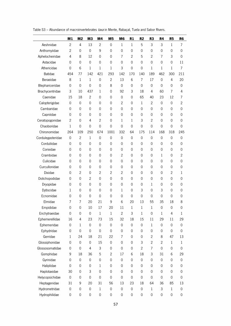
57

Table S3 – Abundance of macroinvertebrates taxa in Mente, Rabaçal, Tuela and Sabor Rivers.

M1 M2 M3 M4 M5 M6 R1 R2 R3 R4 R5 R6

Aeshnidae 2 4 13 2 0 1 1 5 3 3 1 7

Anthomyiidae 2 0 0 9 0 0 0 0 0 0 0 0

Aphelocheiridae 4 8 12 0 0 7 2 5 2 7 3 0

Astacidae 0 0 0 0 0 0 0 0 0 0 0 11

Athericidae 0 6 1 1 1 3 0 0 1 1 1 7

Batidae 454 77 142 421 293 142 170 140 189 462 300 211

Beraeidae 8 1 1 0 2 13 6 7 17 0 4 20

Blephariceridae 0 0 0 0 8 0 0 0 0 0 0 0

Brachycentridae 3 10 437 1 0 92 3 18 4 60 7 4

Caenidae 15 18 2 0 0 0 0 65 40 23 12 7

Calopterigidae 0 0 0 0 0 2 0 1 2 0 0 2

Cambaridae 0 0 0 0 0 0 0 0 0 0 0 0

Capniidae 0 0 0 0 0 0 0 0 0 0 0 0

Ceratopogonidae 2 0 4 2 0 1 1 3 2 0 0 0

Chaoboridae 1 0 0 0 0 0 0 0 0 0 0 0

Chironomidae 264 109 250 674 1001 332 64 175 114 168 318 245

Cordulegasteridae 0 2 1 0 0 0 0 0 0 0 0 0

Corduliidae 0 0 0 0 0 0 0 0 0 0 0 0

Corixidae 0 0 0 0 0 0 0 0 0 0 0 0

Crambidae 0 0 0 0 0 2 0 0 0 1 0 2

Culicidae 0 0 0 0 0 0 0 0 0 0 0 0

Curcullonidae 0 0 0 0 0 0 0 0 0 0 0 0

Dixidae 0 2 0 2 2 2 0 0 0 0 2 1

Dolichopodidae 0 0 2 0 0 0 0 0 0 0 0 0

Dryopidae 0 0 0 0 0 0 0 0 1 0 0 0

Dytiscidae 1 0 0 0 0 1 0 3 0 3 0 0

Ecnomidae 0 0 0 0 0 0 0 0 0 0 0 0

Elmidae 7 7 20 21 9 6 20 13 55 35 18 8

Empididae 0 0 10 17 20 11 1 1 1 0 0 0

Enchytraeidae 0 0 0 1 1 2 3 1 0 1 4 1

Ephemerellidae 16 4 23 73 15 32 18 15 11 29 11 29

Ephemeridae 0 1 0 0 0 0 0 0 1 0 0 0

Ephydridae 0 0 0 0 0 0 0 0 0 0 0 0

Gerridae 1 24 18 21 22 7 0 0 2 8 47 13

Glossiphonidae 0 0 0 15 0 0 0 3 2 2 1 1

Glossosomatidae 0 0 4 3 0 0 0 2 7 0 0 0

Gomphidae 9 18 36 5 2 17 6 18 3 31 6 29

Gyrinidae 0 0 0 0 0 0 0 0 0 0 0 0

Haliplidae 0 0 0 1 0 0 0 0 0 0 0 0

Haplotaxidae 30 0 3 0 0 0 0 0 0 0 0 0

Helycopsichidae 0 0 0 0 0 0 0 0 0 0 0 0

Heptagenidae 31 9 20 31 56 13 23 18 64 36 85 13

Hydrometridae 0 0 0 1 0 0 0 0 1 3 1 0

Hydrophilidae 0 0 0 0 0 0 0 0 0 0 0 0

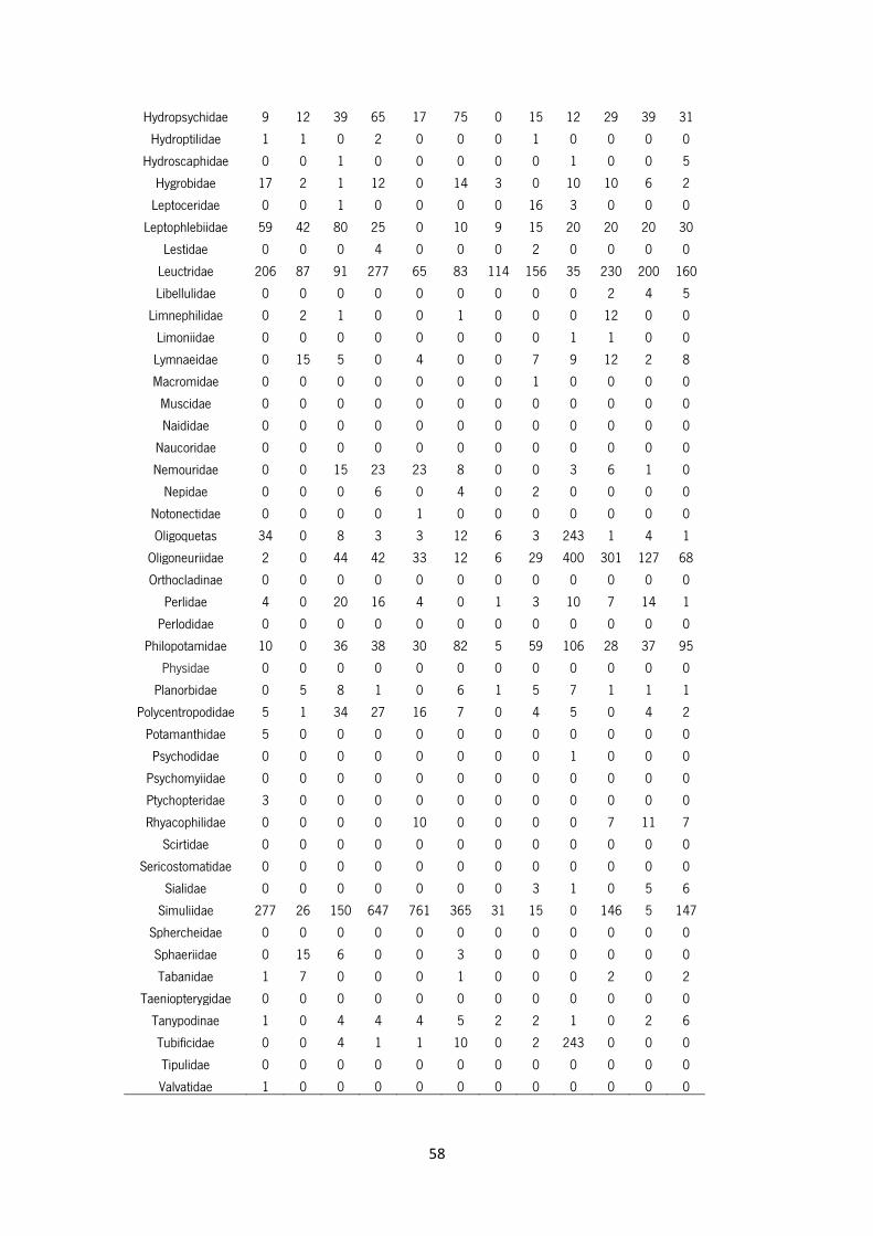
58

Hydropsychidae 9 12 39 65 17 75 0 15 12 29 39 31

Hydroptilidae 1 1 0 2 0 0 0 1 0 0 0 0

Hydroscaphidae 0 0 1 0 0 0 0 0 1 0 0 5

Hygrobidae 17 2 1 12 0 14 3 0 10 10 6 2

Leptoceridae 0 0 1 0 0 0 0 16 3 0 0 0

Leptophlebiidae 59 42 80 25 0 10 9 15 20 20 20 30

Lestidae 0 0 0 4 0 0 0 2 0 0 0 0

Leuctridae 206 87 91 277 65 83 114 156 35 230 200 160

Libellulidae 0 0 0 0 0 0 0 0 0 2 4 5

Limnephilidae 0 2 1 0 0 1 0 0 0 12 0 0

Limoniidae 0 0 0 0 0 0 0 0 1 1 0 0

Lymnaeidae 0 15 5 0 4 0 0 7 9 12 2 8

Macromidae 0 0 0 0 0 0 0 1 0 0 0 0

Muscidae 0 0 0 0 0 0 0 0 0 0 0 0

Naididae 0 0 0 0 0 0 0 0 0 0 0 0

Naucoridae 0 0 0 0 0 0 0 0 0 0 0 0

Nemouridae 0 0 15 23 23 8 0 0 3 6 1 0

Nepidae 0 0 0 6 0 4 0 2 0 0 0 0

Notonectidae 0 0 0 0 1 0 0 0 0 0 0 0

Oligoquetas 34 0 8 3 3 12 6 3 243 1 4 1

Oligoneuriidae 2 0 44 42 33 12 6 29 400 301 127 68

Orthocladinae 0 0 0 0 0 0 0 0 0 0 0 0

Perlidae 4 0 20 16 4 0 1 3 10 7 14 1

Perlodidae 0 0 0 0 0 0 0 0 0 0 0 0

Philopotamidae 10 0 36 38 30 82 5 59 106 28 37 95

Physidae 0 0 0 0 0 0 0 0 0 0 0 0

Planorbidae 0 5 8 1 0 6 1 5 7 1 1 1

Polycentropodidae 5 1 34 27 16 7 0 4 5 0 4 2

Potamanthidae 5 0 0 0 0 0 0 0 0 0 0 0

Psychodidae 0 0 0 0 0 0 0 0 1 0 0 0

Psychomyiidae 0 0 0 0 0 0 0 0 0 0 0 0

Ptychopteridae 3 0 0 0 0 0 0 0 0 0 0 0

Rhyacophilidae 0 0 0 0 10 0 0 0 0 7 11 7

Scirtidae 0 0 0 0 0 0 0 0 0 0 0 0

Sericostomatidae 0 0 0 0 0 0 0 0 0 0 0 0

Sialidae 0 0 0 0 0 0 0 3 1 0 5 6

Simuliidae 277 26 150 647 761 365 31 15 0 146 5 147

Sphercheidae 0 0 0 0 0 0 0 0 0 0 0 0

Sphaeriidae 0 15 6 0 0 3 0 0 0 0 0 0

Tabanidae 1 7 0 0 0 1 0 0 0 2 0 2

Taeniopterygidae 0 0 0 0 0 0 0 0 0 0 0 0

Tanypodinae 1 0 4 4 4 5 2 2 1 0 2 6

Tubificidae 0 0 4 1 1 10 0 2 243 0 0 0

Tipulidae 0 0 0 0 0 0 0 0 0 0 0 0

Valvatidae 1 0 0 0 0 0 0 0 0 0 0 0

59

T1 T2 T3 T4 T5 T6 S1 S2 S3 S4 S5 S6

Aeshnidae 1 0 15 7 7 3 2 1 0 0 0 13

Anthomyiidae 2 1 0 0 1 1 0 0 0 0 0 0

Aphelocheiridae 1 0 5 9 5 9 0 0 0 0 0 1

Astacidae 0 0 0 0 0 0 0 0 2 0 0 0

Athericidae 3 0 1 1 1 8 0 0 0 0 2 10

Batidae 1 0 15 45 69 434 329 665 233 162 120 190

Beraeidae 8 0 0 0 0 0 0 0 0 0 0 0

Blephariceridae 0 0 0 0 0 0 0 0 0 0 0 0

Brachycentridae 31 6 37 62 555 220 0 0 0 0 0 1

Caenidae 0 2 1 0 2 2 50 462 95 36 80 2

Calopterigidae 0 0 6 0 0 0 1 0 0 0 0 2

Cambaridae 0 0 0 0 0 0 0 2 1 0 0 0

Capniidae 0 1 4 0 0 0 0 0 0 0 0 0

Ceratopogonidae 0 0 0 0 0 1 0 1 0 0 0 0

Chaoboridae 0 0 0 0 0 0 0 0 0 0 0 0

Chironomidae 130 83 164 207 623 812 0 320 30 125 80 123

Cordulegasteridae 0 0 0 0 0 0 0 0 0 0 2 2

Corduliidae 0 0 1 0 0 0 0 0 0 0 0 0

Corixidae 0 0 0 0 0 0 0 0 0 0 2 0

Crambidae 0 0 0 0 0 0 0 0 0 0 0 2

Culicidae 1 0 0 0 0 0 0 0 0 0 0 0

Curcullonidae 0 2 0 0 0 0 0 0 0 0 0 0

Dixidae 0 2 3 0 2 2 0 0 0 0 0 3

Dolichopodidae 1 1 0 0 0 0 0 0 0 0 0 0

Dryopidae 0 0 0 0 0 0 0 0 0 0 0 0

Dytiscidae 2 3 0 0 0 0 0 0 0 1 12 0

Ecnomidae 0 0 1 0 0 0 0 0 0 0 0 0

Elmidae 5 4 1 21 9 13 37 8 1 0 7 30

Empididae 3 1 1 0 0 0 0 0 0 0 0 0

Enchytraeidae 1 1 0 0 0 0 0 5 1 0 0 1

Ephemerellidae 2 0 38 30 136 142 0 0 1 0 0 31

Ephemeridae 0 0 1 0 0 0 0 0 0 0 0 0

Ephydridae 0 0 0 0 1 0 0 0 0 0 0 0

Gerridae 11 19 48 10 1 0 1 0 13 50 32 3

Glossiphonidae 0 0 0 0 0 0 0 0 0 0 0 2

Glossosomatidae 0 0 0 0 0 1 0 0 0 0 0 0

Gomphidae 0 0 5 15 12 26 0 4 0 0 6 9

Gyrinidae 0 0 0 0 0 0 0 0 0 0 0 2

Haliplidae 0 0 0 0 0 3 0 0 0 0 0 0

Haplotaxidae 4 2 0 0 0 0 0 0 0 0 0 0

Helycopsichidae 0 0 0 0 0 1 0 0 0 0 0 0

Heptagenidae 6 7 0 48 3 31 1 1 0 0 9 19

Hydrometridae 0 0 0 0 0 0 1 0 0 0 0 2

Hydrophilidae 0 0 0 0 0 0 0 0 0 0 0 1

Hydropsychidae 4 0 0 27 24 101 116 520 112 1 8 10

60

Hydroptilidae 0 0 0 0 0 0 0 0 0 0 0 1

Hydroscaphidae 0 0 29 0 0 0 0 0 0 0 0 5

Hygrobidae 0 4 0 0 5 10 0 0 0 0 1 16

Leptoceridae 1 0 22 0 13 3 0 0 0 0 0 4

Leptophlebiidae 5 4 0 0 1 0 20 14 0 0 0 1

Lestidae 0 0 0 0 0 0 0 0 0 0 1 0

Leuctridae 0 0 1 63 74 193 80 50 15 8 0 20

Libellulidae 0 0 0 0 0 0 0 0 0 0 0 0

Limnephilidae 9 0 0 0 0 0 0 0 0 0 0 3

Limoniidae 0 0 0 0 0 0 0 0 0 0 0 1

Lymnaeidae 4 8 0 1 0 5 1 1 0 0 5 0

Macromidae 0 0 0 0 0 0 0 0 0 0 0 0

Muscidae 13 0 0 0 0 0 0 0 0 0 0 0

Naididae 5 5 0 0 0 0 0 0 0 0 0 0

Naucoridae 0 0 1 0 0 0 15 0 0 0 0 0

Nemouridae 0 0 0 0 0 0 0 0 0 0 0 16

Nepidae 0 0 0 0 0 0 0 0 0 0 4 0

Notonectidae 0 0 0 0 0 0 0 0 0 0 1 5

Oligoquetas 27 17 0 0 0 5 1 5 1 2 0 2

Oligoneuriidae 0 0 0 20 1 119 0 2 0 0 0 0

Orthocladinae 0 7 18 0 0 0 0 0 0 0 0 0

Perlidae 0 0 0 1 2 3 0 0 0 0 8 2

Perlodidae 0 0 0 0 1 0 0 0 0 0 0 0

Philopotamidae 1 0 0 43 10 72 25 27 0 0 0 0

Physidae 0 0 0 0 0 0 6 0 0 0 0 0

Planorbidae 9 11 0 3 1 10 0 12 3 0 2 4

Polycentropodidae 0 2 1 2 3 3 1 1 0 4 0 7

Potamanthidae 0 1 0 0 0 0 0 0 0 0 0 0

Psychodidae 0 0 0 0 0 0 0 0 0 0 0 0

Psychomyiidae 0 0 0 0 0 2 0 0 0 1 0 0

Ptychopteridae 0 0 0 0 0 0 0 0 0 0 0 0

Rhyacophilidae 3 0 0 0 0 1 0 1 1 0 15 10

Scirtidae 0 0 0 0 0 0 0 0 0 0 0 4

Sericostomatidae 0 0 0 0 0 0 0 0 0 0 0 2

Sialidae 0 0 0 0 0 0 0 0 0 0 0 0

Simuliidae 141 0 102 24 40 268 140 606 300 282 0 819

Sphercheidae 0 0 0 0 3 0 0 0 0 0 0 0

Sphaeriidae 9 0 2 1 0 4 0 0 0 0 4 0

Tabanidae 0 2 0 3 1 1 0 0 1 0 2 2

Taeniopterygidae 0 0 0 0 0 1 0 0 0 0 0 0

Tanypodinae 0 0 3 0 0 0 0 0 0 0 0 0

Tubificidae 3 2 0 0 0 0 0 0 0 0 0 0

Tipulidae 1 0 1 1 0 0 0 0 0 0 2 2

Valvatidae 0 0 0 0 0 0 0 0 0 0 0 0

61

Table S4 – SIMPER analysis results showing the macroinvertebrate taxa contributing the most to the average

dissimilarity between status (outside, in the periphery and inside the park).

Outside vs. Periphery Outside vs. Inside Periphery vs. Inside

Taxa % contribution Taxa

%

contribution Taxa

%

contribution

Oligoneuriidae 3.86 Simuliidae 4.04 Brachycentridae 4.29

Hydropsychidae 3.73 Brachycentridae 3.68 Oligoneuriidae 4.11

Caenidae 3.69 Oligoneuriidae 3.62 Simuliidae 3.88

Leuctridae 3.56 Ephemerellidae 3.6 Philopotamidae 3.49

Simuliidae 3.52 Caenidae 3.51 Caenidae 3.24

Brachycentridae 3.47 Philopotamidae 3.27 Leuctridae 3.21

Batidae 3.43 Hydropsychidae 3.27 Heptagenidae 3.19

Leptophlebiidae 3.4 Leuctridae 3.21 Ephemerellidae 2.95

Philopotamidae 3.29 Batidae 3.08 Leptophlebiidae 2.75

Gerridae 3.17 Leptophlebiidae 3.06 Hydropsychidae 2.58

Ephemerellidae 3.11 Chironomidae 2.84 Rhyacophilidae 2.54

Heptagenidae 3.07 Gerridae 2.75 Elmidae 2.42

Oligoquetas 2.82 Rhyacophilidae 2.5 Gomphidae 2.34

Elmidae 2.51 Gomphidae 2.29 Hygrobidae 2.3

Gomphidae 2.43 Oligoquetas 2.25 Gerridae 2.28

Chironomidae 2.33 Hygrobidae 2.11 Nemouridae 2.21

Lymnaeidae 1.99 Heptagenidae 2.1 Perlidae 2.15

Perlidae 1.92 Beraeidae 1.97 Oligoquetas 2.13

Planorbidae 1.92 Athericidae 1.96 Polycentropodidae 2.02

Beraeidae 1.91 Perlidae 1.9 Chironomidae 1.95

Polycentropodidae 1.89 Planorbidae 1.76 Aeshnidae 1.93

Hygrobidae 1.88 Nemouridae 1.75 Aphelocheiridae 1.83

Aphelocheiridae 1.8 Lymnaeidae 1.74 Lymnaeidae 1.83

Aeshnidae 1.75 Polycentropodidae 1.69 Beraeidae 1.82

Tubificidae 1.69 Aphelocheiridae 1.59 Empididae 1.75

Nemouridae 1.57 Aeshnidae 1.51 Tubificidae 1.68

Sphaeriidae 1.41 Sphaeriidae 1.51 Leptoceridae 1.68

Leptoceridae 1.4 Empididae 1.46 Batidae 1.6

Empididae 1.33 Leptoceridae 1.44 Athericidae 1.51

Haplotaxidae 1.3 Dytiscidae 1.29 Planorbidae 1.47

Athericidae 1.08 Tanypodinae 1.27 Hydroscaphidae 1.41

Tanypodinae 1.08 Dixidae 1.21 Tanypodinae 1.38

Limnephilidae 1.06 Haplotaxidae 1.2 Dixidae 1.32

Tabanidae 1.06 Tabanidae 1.13 Sphaeriidae 1.22

Orthocladinae 1.04 Elmidae 1.06 Glossiphonidae 1.05

Enchytraeidae 1.02 Enchytraeidae 1.05 Dytiscidae 1.04

Hydroscaphidae 1.01 Tubificidae 1.04 Tabanidae 1.01

Dytiscidae 1 Limnephilidae 0.9 Calopterigidae 0.97

Glossiphonidae 0.96 Sialidae 0.84 Glossosomatidae 0.93

Ceratopogonidae 0.95 Nepidae 0.8 Nepidae 0.92

Glossosomatidae 0.93 Naididae 0.78 Enchytraeidae 0.87

Anthomyiidae 0.87 Ceratopogonidae 0.74 Limnephilidae 0.84

Naididae 0.82 Calopterigidae 0.71 Sialidae 0.8

Rhyacophilidae 0.8 Hydroscaphidae 0.68 Libellulidae 0.77

Calopterigidae 0.78 Notonectidae 0.67 Ceratopogonidae 0.75

Naucoridae 0.77 Anthomyiidae 0.65 Astacidae 0.7

Libellulidae 0.65 Notonectidae 0.69

Naucoridae 0.63 Crambidae 0.68

Crambidae 0.62 Glossiphonidae 0.62

62

Table S5 – Results of the linear regressions between abiotic factors and macroinvertebrates richness (S). abundance (N). Shannon-Wiener diversity (H’). Pielou’s evenness (J’) and IBMWP. IASPT and %EPT water quality indices. ns – non significant; * - statistically significant.

S N H' J' IBMWP IASPT %EPT

Temperature F= 8.9; R= -5.4% * F= 4.7; R= -4.2% * ns ns F= 9.8; R= -5.6% * ns ns

Oxygen F= 10.7; R= 5.7% * ns F= 8.9; R= 5.4%

* ns F= 11.3; R= 5.8% * F= 4.3; R= 4% * ns

Conductivity F= 29.2; R= -7.6% * ns F= 8.3; R= -

5.2% * ns F= 35.3; R= -7.8% * F= 13.5; R= -6.2% * ns

Depth ns ns ns ns ns ns ns

Altitude ns ns ns ns ns ns ns

Width F= 9.91; R= -5.6% * ns F= 6.8; R= -

4.9% * ns F= 8.8; R= -5.3% * ns ns

HFI F=6.7; R= -4.8% * ns ns ns F= 7.7; R= -5.1% * ns ns

DNV ns F= 4.8; R= 4.2% * ns ns ns ns ns

DTP ns ns ns ns ns ns ns

63

Table S6 – Abundance (ind.CPUE) of Margaritifera margaritifera in Mente. Rabaçal and Tuela Rivers.

Site Abundance (ind.CPUE)

T1 0.17

T2 6.17

T3 6.67

T4 1.33

T5 36.50

T6 12.67

M1 1.17

M2 0.67

R1 19.80

R2 30.00

R3 24.00

R4 35.50

R5 48.00

R6 22.50

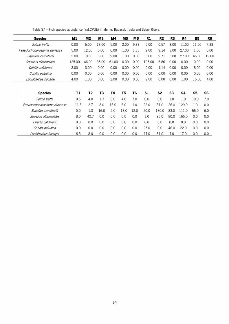
64

Table S7 – Fish species abundance (ind.CPUE) in Mente. Rabaçal. Tuela and Sabor Rivers.

Species M1 M2 M3 M4 M5 M6 R1 R2 R3 R4 R5 R6

Salmo trutta 0.00 5.00 13.00 5.00 2.00 9.33 0.00 0.57 3.00 11.00 11.00 7.33

Pseudochondrostoma duriense 5.00 12.00 5.00 6.00 1.00 1.33 9.00 9.14 3.00 27.00 1.00 0.00

Squalius carolitertii 2.00 10.00 3.00 9.00 1.00 0.00 3.00 9.71 5.00 27.00 46.00 12.00

Squalius alburnoides 125.00 46.00 35.00 61.00 0.00 0.00 105.00 6.86 0.00 0.00 0.00 0.00

Cobitis calderoni 3.00 3.00 0.00 0.00 0.00 0.00 0.00 1.14 0.00 0.00 8.00 0.00

Cobitis paludica 0.00 0.00 0.00 0.00 0.00 0.00 0.00 0.00 0.00 0.00 0.00 0.00

Luciobarbus bocagei 4.00 1.00 0.00 2.00 0.00 0.00 2.00 0.00 0.00 1.00 16.00 4.00

Species T1 T2 T3 T4 T5 T6 S1 S2 S3 S4 S5 S6

Salmo trutta 0.5 4.0 1.3 8.0 4.0 7.0 0.0 0.0 1.0 1.0 10.0 7.0

Pseudochondrostoma duriense 11.5 2.7 8.0 16.0 6.0 1.0 22.0 31.0 26.0 129.0 1.0 0.0

Squalius carolitertii 0.0 1.3 16.0 2.0 13.0 12.0 20.0 130.0 83.0 111.0 55.0 6.0

Squalius alburnoides 8.0 42.7 0.0 0.0 0.0 0.0 3.0 95.0 80.0 165.0 0.0 0.0

Cobitis calderoni 0.0 0.0 0.0 0.0 0.0 0.0 0.0 0.0 0.0 0.0 0.0 0.0

Cobitis paludica 0.0 0.0 0.0 0.0 0.0 0.0 25.0 0.0 46.0 22.0 0.0 0.0

Luciobarbus bocagei 6.5 8.0 0.0 0.0 0.0 0.0 44.0 31.0 4.0 17.0 0.0 0.0

65

Table S8 – Results of the PERMANOVA analysis on fish communities along park status (outside. in the periphery and inside the park) and overall results of the pairwise tests.

Source Degrees of freedom SS MS Pseudo-F P(perm) Permutations P(MC)

Status 2 13594 6797.2 8.3374 0.0001 9957 0.0001

Residuals 21 17121 815.27

Total 23 30715

Groups t P(perm) Permutations P(MC)

O. P 1.8884 0.0253 5053 0.0271

O. I 4.2017 0.0003 5062 0.0002

P. I 2.2235 0.0041 5073 0.0077

66

Table S9 - SIMPER analysis results showing the fish species contributing the most to the average dissimilarity between status (outside. in the periphery and inside the park).

Outside vs. Periphery Outside vs. Inside Periphery vs. Inside

Taxa % contribution Taxa % contribution Taxa % contribution

Squalius alburnoides 28.04 Squalius alburnoides 31.78 Pseudochondrostoma

duriense 25.95

Squalius carolitertii 16.95 Pseudochondrostoma

duriense 16.07 Squalius alburnoides 22.42

Luciobarbus bocagei 16.85 Luciobarbus bocagei 15.16 Squalius carolitertii 20.55

Salmo trutta 14.27 Squalius carolitertii 14.59 Salmo trutta 10.62 Pseudochondrostoma

duriense 10.06 Salmo trutta 14.12 Luciobarbus bocagei 10.61

Cobitis paludica 8.92

67

Table S10 – Results of the linear regressions between abiotic factors and fish richness (S), abundance (N), Shannon-Wiener diversity (H’), and Pielou’s evenness (J’). ns – non significant; * - statistically significant.

S N H' J'

Temperature ns ns ns ns

Oxygen ns F= 24.3; R= -7.2% * ns ns

Conductivity F= 7.6; R= 5.1% * F= 22.1; R= 7.1% * F= 10.8; R= 5.7 * ns

Depth ns ns ns ns

Altitude F= 13.4; R= -6.2% * ns ns ns

Width ns F= 5.9; R= 4.6% * ns ns

HFI F= 7.5; R= 5% * F= 6.9; R=4.9% * ns ns

DNV ns ns ns F= 6; R= 4.6% *

DTP F= 12.9; R= 6.1% * ns ns ns