Javier,Pagaduan,Punsalang ECOMETV26

Estimating the Demand for Philippine Exports of Top Trading Partners per Region : An Iterative Seemingly Unrelated

Regression and Panel Data Analysis

A Research Paper Presented to the Economics Department

De La Salle University

In partial fulfillment of the requirements in ECOMET2

Submitted by: JAVIER, Katrina Joy PAGADUAN, Jesson PUNSALANG, Gio

V26

Submitted to: Dr. Cesar Rufino

2

TABLE OF CONTENTS

I. Introduction A. Background of the Study B. Statement of the Problem C. Statement of the Objectives D. Scope and Limitations II. Review of Related Literature III. Theoretical Framework A. Theory of Consumer Demand B. Income and Substitution Effects C. The Mundell-‐Flemming Model D. Gravity Model of World Trade E. Marshall-‐Lerner Condition IV. OPERATIONAL FRAMEWORK

A. Data B. Variables and A-‐Priori Expectations

V. PER COUNTRY DEMAND ESTIMATION

A. Time Series OLS estimation vs. Seemingly Unrelated Regression B. Model Specification C. Iterated Seemingly Unrelated Regression (ISUR) D. The Breusch-‐Pagan Test E. Regression Analyses

E.1. Statistical Tests E.2. Time series OLS estimation E.3. Iterative Seemingly Unrelated Regression (ISUR) regression E.4. Individual OLS estimation vs. ISUR regression

F. Interpretations F.1.USA F.2. Japan F.3. Australia F.4. Germany F.5. Singapore

VI. Aggregate Export Demand Estimation

A. Fixed Effects Models (FEM) vs. Random Effects Model (REM) vs. Naïve Model vs. Within-‐Group (WG) Model

B. Definition of Panel Data Models B.1. Naive Model B.2. Fixed Effects Models (FEM) B.3. Within-‐Group (WG) Model

3

B.4. Random Effects Model (REM) C. Tests

C.1. Wald’s Test: Naïve vs. LSDV1 C.2. Wald’s Test: Naïve vs. LSDV2 C.3. Wald’s Test: Naïve vs. LSDV3 C.4. Wald’s Test: LSDV1 vs. LSDV3 C.5. Wald’s Test: LSDV2 vs. LSDV3 C.6. Breusch-‐Pagan Test: Naïve vs. REM C.7. Hausman Test: REM vs. FEM

D. Regression Analyses & Statistical Testing D.1. General Comments D.2. Interpretations of REM Results D.3. Interpretations of LSDV3 Results

VII. Policy Recommendations And Conclusion VIII. References IX. Appendix

4

I. INTRODUCTION A. Background of the Study

In the recent years, the Philippines has been considered a newly industrialized and an emerging-‐market economy. According to the World Bank, the Philippines’ almost P200-‐billion GDP in 2010, the fourth largest in Southeast Asia, is predominantly accounted for by the service sector with a whopping 50% share, followed by the industry sector with 33% and the agricultural sector with 17% industry-‐to-‐GDP share. The increasing productivity of these sectors translate to greater prospects for the Philippine export industry as one of its key drivers of growth.

Despite numerous severe economic fluctuations in the recent decades, the

Philippine export industry showed signs of resiliency – as evidenced by the surge in trade volumes in light of the crises. The US and Japan have remained the country's two largest export markets together with fast-‐growing China and ASEAN countries. Other top export markets also include Hong Kong, Germany, Netherlands, South Korea, France and India. Nevertheless, the Philippines has continuously been trading with countries from all the six inhabitable continents of the world.

According to Economy Watch, Philippine exports totaled US$50.72 billion during the

year 2010, with the primary export commodities being semiconductors and electronic products, transport equipment, garments, copper products, petroleum products, coconut oil and fruits. The industry contributed up to around 35% of the country’s total GDP – making it one of the biggest earning sectors for the country (The World Bank, 2012).

The trade statistics presented earlier reveal the relative importance of the exports

industry for the Philippines’ economic performance. In lieu with this, vital questions have been raised in order to safeguard the industry and prevent massive disruptions as they may pose to be major risks for the country’s aggregate output. Among these are as follows:

“What characterizes trade between the Philippines and its trading partners?”

“What factors determine the volume of trade between the Philippines and its international export markets?” “What policies should the government employ in order to sustain the growth of the Philippine exports industry?”

Although these questions may appear to be very much pronounced in the country

today, a comprehensive empirical analysis has yet to be conducted in answering these. This research aims to answer these three key questions associated with the Philippine exports industry via estimating two sets of demand functions of the Philippines’ top export markets per region – an aggregated estimation and a per-‐country analysis – using various econometric modeling techniques. Moreover, a comprehensive analysis will be facilitated using International Trade and Macroeconomic Theories.

5

B. Statement of the Problem In order to characterize the demand for Philippine goods, how do we estimate using available data the export demand equations of the top five trading partners of the Philippines which are US, Japan, China, Singapore, and Hong Kong? Also, what are the factors that influence demand for Philippine goods? Finally, how responsive are consumers to changes in these factors? C. Statement of the Objectives The objectives of the study are as follows:

1. To estimate the Philippine export demand equations of USA, Australia, Germany, Japan and Singapore, all of which represent the top trading partners of the Philippines per region.

2. To estimate an aggregated export demand equation for the five countries aforementioned.

3. To identify significant factors that influence demand for Philippine goods and services

4. To determine the responsive of foreign consumers to these factors. D. Scope and Limitations This paper studies the demand for Philippine goods, capturing exports as the dependent variable. However, this study has several limitations. First, we limited our study to the top five major trading partners of the Philippines which are US, Japan, China, Singapore, and Hong Kong. Second, we limited the factors affecting Philippine exports to only the real exchange rate, Gross Domestic Product (GDP), and distance of these five countries. Next, our data is limited to information gathered annually from 1980-‐2011. Lastly, we used Iterative Seemingly Unrelated Regressions (ISUR) to estimate the demand for Philippine goods.

6

II. REVIEW OF RELATED LITERATURE

During the 1960s and 1970s, many economists believed that participation in international trade and improvement in export performance could provide the much needed motivation for economic growth in the developing economies.

There are many arguments which favor the export-‐led development strategy. First,

trade expansion will bring improved productivity through increased economies of scale in the export sector, positive externalities on non-‐exports and through increased capacity utilization. Second, exports may affect productivity through encouraging better allocation of resources driven by specialization and increased in efficiency, which in turn generate dynamic comparative advantage via reduction in costs for a country that facilitates exports (Mahadevan, 2007). Third, through encounters with international markets, trade will facilitate more diffusion of knowledge and more efficient management techniques which will have a net positive effect on the rest of economy and enhance overall economic productivity. Fourth, export growth also promotes capital accumulation and accumulation of foreign exchange and thus enables the importation of capital and intermediate inputs necessary in the production of goods exports. Thus, growth has been analyzed as the engine of economic growth (Bhagwati and Srinivasan, 1978; Krueger,1978; Kavoussi, 1984).

In the empirical literature on export demand, the most influential work is Senhadji

and Montenegro (1999). They used Phillips Hansen's method to estimate export demand equations for developing and developed countries. They found that African countries face the lowest income elasticities for their exports, while Asian countries have the highest income and price elasticities. However, Senhadji and Montenegro did not include exchange rate in the relative price variable. Following Rao and Singh (2007), this could result in obtaining bias income and price elasticities.

Arize (2001) finds that for Singapore economy, there is a long run and stable

equilibrium relationship among exports and its determinants. Guisan and Cancelo (2002) estimated the export demand function considering the supply side determinants such as domestic gross domestic product, domestic private consumption and human capital in addition to foreign income and relative export price. Lately, Kumar (2009a) finds that there is a structural break in the export demand function of the Philippines and assert that there is a cointegrating relationship between real exports, real income and relative prices. In another study, Kumar (2009b) estimated export demand function for China and find significant long-‐run income and relative price elasticities.

The export-‐led growth policies have played an important role in promoting exports

and hence the output growth in the Asian countries. Many studies have tested the export-‐led growth hypothesis for various countries using alternative estimation techniques, and results vary considerably from country to country with some supportive and some opposing evidence.

7

This paper is organized as follows. The next section discusses the theoretical framework, followed by the model specification and results of the empirical study. The final section concludes. III. THEORETICAL FRAMEWORK A. Theory of Consumer Demand

The theory of demand is about the behavior of consumers in the market place. Its purpose is to explain the process by which consumers make choices from among the alternative commodities available to them at any point in time. The consumer in this theory is an individual whose objective is to maximize the satisfaction from selecting the best possible combination of commodities he can afford. With the presence of a principle of diminishing marginal utility, it is possible to identify the particular group of commodities that would yield the highest utility. Hence, it shows that for any given consumer there is a unique collection of commodities which maximized his/her satisfaction or utility. A rise (fall) in the price of a good would decrease (increase) the amount purchased, other things being held constant.

The Neoclassical theory of consumer demand states there is a negative relationship between the quantity demanded for a product and that product's price. As prices for goods decline, consumers purchase more of those goods and purchase less as the prices increase. The level to which consumers vary their demand for a particular good in response to a price change reflects elasticity of demand. If consumer demand for a good drops sharply in response to a price increase, then demand for that good is said to be highly elastic. If consumer demand changes little or not at all, even in response to a sharp price increase, then demand is said to be inelastic. B. Income and Substitution Effects

Income effect is the impact that a change in the price of a good has on the quantity demanded of that good due strictly to the resulting change in real income or purchasing power while substitution effect is the impact that a change in the price of a good has on the quantity demanded of that good, which is due to the resulting change in relative prices (Px/Py).

There are two definitions of Substitution effects given by Eugene Slutsky and Sir

John R. Hicks. The Slutsky Substitution effect is the effect on consumer choice of changing the price ratio, leaving his/her initial utility unchanged while the Hicks Substitution effect is the effect on consumer choice of changing the price ratio, leaving the consumer just able to afford his/her initial bundle.

Indifference curve analysis is used to illustrate the two effects. An indifference curve represents the preferences of a consumer between two goods. Its slope, the marginal rate of substitution, shows how willing the consumer is to switch between the goods. The

8

budget constraint shows the line of available opportunities when the consumer allocates her entire budget between the two goods. Its slope is the relative price of the two goods. The consumer is assumed to maximize overall satisfaction (utility) while spending her entire budget on the two goods where the indifference curve and budget constraint are tangent to one another.

Income and substitution effects change demand differently with different types of

goods. Total effect is composed of both Income and substitution effects. When X is a normal good, with a decrease in the price of good X, the quantity of X demanded decrease (total effect). The income effect increases and so is the substitution effect, so the decrease in the price of good X leads to an increase in the quantity demanded. When X is an inferior good, with a decrease in the price of good X, the quantity of X demanded increases (total effect). The substitution effect exceeds the income effect, so the decrease in the price of good X leads to an increase in the quantity demanded. When X is a giffen good, with a decrease in the price of good X, the quantity of X demanded decrease (total effect). The income effect exceeds the substitution effect, so the decrease in the price of good X leads to a decrease in the quantity demanded. C. The Mundell-‐Flemming Model

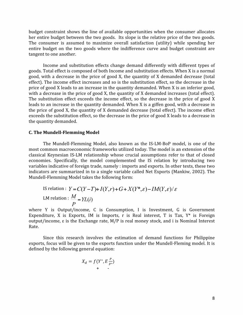
The Mundell-‐Flemming Model, also known as the IS-‐LM-‐BoP model, is one of the most common macroeconomic frameworks utilized today. The model is an extension of the classical Keynesian IS-‐LM relationship whose crucial assumptions refer to that of closed economies. Specifically, the model complemented the IS relation by introducing two variables indicative of foreign trade, namely : imports and exports. In other texts, these two indicators are summarized in to a single variable called Net Exports (Mankiw, 2002). The Mundell-‐Flemming Model takes the following form:

IS relation :

LM relation :

where Y is Output/income, C is Consumption, I is Investment, G is Government Expenditure, X is Exports, IM is Imports, r is Real interest, T is Tax, Y* is Foreign output/income, ε is the Exchange rate, M/P is real money stock, and i is Nominal Interest Rate. Since this research involves the estimation of demand functions for Philippine exports, focus will be given to the exports function under the Mundell-‐Fleming model. It is defined by the following general equation: 𝑋! = 𝑓(𝑌∗,𝐸 !

!∗)

+ -‐

( ) ( , ) ( *, ) ( , )/Y C Y T I Y r G X Y IM Yε ε ε= − + + + −

( )M YL iP=

9

where Xd is foreign demand for a country’s goods, Y* is foreign output, P is local price index, P* is foreign price index, and E is the nominal exchange rate. Exports represent the demand for local goods of foreign countries. One of the determinants of exports suggested by the Mundell-‐Flemming Model is foreign income. Higher foreign income leads to higher demand for local goods, thus inducing additional volume on the part of exporters. Another determinant of exports in the model is real exchange rate, which is computed by multiplying the nominal exchange rate to the relative price of local goods to foreign goods. If local prices are higher relative to that of foreign prices, foreign countries are more likely to opt for goods from another country. Hence, in the case of a currency appreciation (or valuation), exports decrease. (Blanchard, 2011) D. Gravity Model of World Trade

The Gravity Model of World Trade is an important tool used in analyzing international trade relations. Its basic foundations refer to that of Newton’s Law of Gravity. According to Krugman, Obstfeld & Melitz (2012), the international economics variant of the Gravity Theory takes the form of:

𝑇!,! = 𝐴 ∗ 𝑌!! ∗ 𝑌!!/𝐷!"! where 𝑇!,! is the value of trade between country i and j, A is a constant term, 𝑌!! is the GDP of country i , 𝑌!! is the GDP of country j and 𝐷!"! is the distance between country i and j. In this model, the total value of trade (value of imports plus exports) between two countries is determined by three things, namely: the two GDPs of trading countries and the distance between them. Both the GDPs of trading countries have a positive effect on bilateral trade flows because of the higher incomes of large economies and their tendency to spend more on imported goods. In addition, these larger economies have a more diversified product line, hence drawing more transactions to supply foreign need. The distance on the other hand has a negative relationship due to logistical costs. Distance greatly affects both time and transportation costs. Although typically the product of the two GDPs and the distance between them are proportional and inversely proportional respectively, economists estimate the elasticity of each of these variables in correspondence to the data at hand (Krugman, Obstfeld , & Melitz, 2012). These elasticities are represented by the a, b and c superscripts. E. Marshall-‐Lerner Condition The Marshall-‐Lerner Condition (also called the Marshall-‐Lerner-‐Robinson) is at the heart of the elasticities approach to the balance of payments. This condition answers when a real devaluation in fixed exchange rates or in floating exchange rates of the currency improve the current-‐account balance of a country.

10

This condition states that a real devaluation or real depreciation of the currency will improve the trade balance if the sum of elasticities (in absolute values) of the demand for imports and exports with respect to the real exchange rate is greater than one, (ɛ+ɛ*=1).

For the trade balance to improve following depreciation, exports must increase enough and imports must decrease enough to compensate for the increase in the price of imports (Blanchard, 2011). IV. OPERATIONAL FRAMEWORK A. Data

In estimating the demand for Philippine goods and services, this research will make use of quarterly data from 1985Q1-‐2011Q4. The sources of data are as follows: Data Source Indicator Direction of Trade Statistics, IMF Philippine Exports per country International Finance Statistics, IMF Real Effective Exchange Rate (Consumer

Price Index) International Finance Statistics, IMF Real Gross Domestic Product TimeandDate.Com Distance

B. Variables and A-‐Priori Expectations The theories mentioned in the preceding section provide key variables that may be considered as factors of exports demand in an economy. This research will make use of the determinants supported by the Gravity Model and the Mundell-‐Flemming Model as independent variables. On the other hand, the value of Philippine exports to selected countries will be the dependent variable of the study. Exports represent the total value of the outflow of goods from the domestic economy to the international market. Since this research aims to estimate demand for Philippine goods both on a per country and aggregated basis, data on the direction of trade of Philippine goods and services (as of 2011) will be utilized. According to the Department of Trade and Industry, these top trading partners are as follows: Region Top Trading Partner ASEAN Singapore Oceania Australia Europe Germany Americas USA Asia Japan

11

Note that the value of exports is originally expressed in terms of PHP but was later converted by the IMF to USD using period average exchange rates. The Real Effective Exchange Rate (REER) is defined by The World Bank as “the nominal effective exchange rate divided by a price deflator or index of costs” (The World Bank, 2012). The nominal effective exchange rate used in the computation of this dataset contains the value of Philippine Peso against a weighted average of different foreign currencies. The base year used by The World Bank is 2005 (2005=100). In essence, the Real Effective Exchange Rate represents the relative price of domestic goods in comparison to the weighted average prices of foreign goods. It is considered as a proxy variable for the variable Price typically found in demand equations. This study will make use of three REER indices. First, the Philippines’ REER is used to measure the response of the importing nation to price changes in the local Philippine market and currency appreciation (depreciation) of the Philippine Peso. Second, China’s REER will be used as a proxy for the competitor’s REER. The theory of consumer demand postulates that price changes of a competitor influences the demand for a firm’s goods . The same principles applies in the case of Philippine exports – wherein China, an export powerhouse in the East Asian Region, may be considered as the biggest competitor of Philippine goods and services. Lastly, the REER of the importing country will be used in order to evaluate the impact of price changes in their respective economies. The Gross Domestic Product (GDP) represents the total income of an economy and the total expenditure on the production of goods and services both from the private and public sector (Mankiw, 2002). The Real GDP data of Australia, Germany, Japan, Singapore and the US employed in this research was sourced from the International Financial Statistics of the IMF. Real stands for the adjustment of the nominal GDP to price changes brought about by inflation. For consistency purposes, Real GDP figures have the same base year at 2005. It is considered as a proxy variable for the variable Income normally found in demand equations.

The data on distance used in this paper is defined by the source TimeandDate.Com as “the theoretical air distance (great circle distance)”. Theoretical air distance is different from that of airport-‐to-‐airport distance due to the varying routes chosen by air carriers (Time and Date AS, 2012). For the sake of uniformity, the distance between capital cities will be measured – Manila-‐Washington DC, Manila-‐Tokyo, Manila-‐Canberra, Manila-‐Singapore and Manila-‐Berlin. All figures are expressed in terms of kilometers. Note however that variable distance will only be used in the aggregated export demand estimation and not in the per-‐country demand estimation. Distance is time invariant, hence, it would not make sense to include it as a variable in the individual export demand equation estimation. The table below summarizes the A-‐Priori expectations on the aforementioned variables.

12

Variable Code A-‐Priori Explanation Real Effective Exchange Rate (Consumer Price Index) -‐ Philippines

lnPHLREERCPIi -‐ As supported by the Mundell-‐Flemming Model and the Marshall Lerner Condition, an appreciation will decrease foreign demand on local goods, hence lower exports.

Real Effective Exchange Rate (Consumer Price Index) – China

lnCHIREERCPIi + As supported by the Mundell-‐Flemming Model and the Theory of Consumer Demand, an appreciation (revaluation) will decrease foreign demand on local goods, hence lower exports. Since China is considered an export-‐industry competitor, an appreciation of the Chinese currency will lead to an increase in the demand for Philippine goods and services.

Real Effective Exchange Rate (Consumer Price Index) – Importing Country

lnCCDREERCPIi + As supported by the Mundell-‐Flemming Model and the Marshall Lerner Condition, an appreciation of the importing country’s currency will lead to an increase in exports. This is due to Philippine goods and services being cheaper in comparison to the importing country’s.

Gross Domestic Product (foreign)

lnCCDGDPi + As supported by the Mundell-‐Flemming and Gravity Model of Trade, an increase in GDP of foreign economies will lead to higher demand for local goods, hence higher exports.

Gross Domestic Product (local)

lnCCDGDPj + As supported by the Gravity Model of Trade, an increase in GDP of the local economy will lead to an increase in the volume of trade between two nations.

Distance lnDISTCCDi -‐ As supported by the Gravity Model, the bigger the distance between two countries (capital), the higher the logistical costs.

Exports to country i

lnEXPCCDi Dependent Variable

*CCD stands for the three-‐letter country codes (AUS,GER,JPN,SGP,USA,PHL)

13

IV. PER COUNTRY DEMAND ESTIMATION A. Time Series OLS estimation vs. Seemingly Unrelated Regression In facilitating the demand estimation on a per country basis, we will run two econometric models -‐ the simple Time-‐series Classical Linear Regression Model (CLRM) estimated using the Ordinary Least Squares (OLS) procedure and the Iterative Seemingly Unrelated Regression (ISUR) using the Feasible Generalized Least Squares (FGLS) method. In return, the results of these two regression analyses will be compared and the more appropriate modeling technique will be determined thereafter. The estimates of both models will be presented in the succeeding sections. B. Model Specification This study will employ the basic specification in estimating export equations by Rao and Singh (2005). In their model, exports is estimated using the two determinants suggested by the Mundell-‐Flemming Model – Foreign Income (GDP) and the Real Exchange Rate. Having said, the researchers would further complement this by adding the variable local GDP which was derived from the Gravity Theory Model. The variable distance is omitted in this per-‐country demand estimation because it is time-‐invariant. This may be considered as a fixed influence importers from each of the five countries to be estimated have to deal with in their trading activities. Since this study involves the estimation of demand for Philippine exports of Australia, Germany, Japan, Singapore, and USA, there will be five equations in the analysis. The general form of each equation will be as follows:

𝑙𝑛𝐸𝑋𝑃𝐶𝐶𝐷! = 𝛽! + 𝛽!𝑙𝑛𝐶𝐶𝐷𝐺𝐷𝑃! + 𝛽!𝑙𝑛𝑃𝐻𝐿𝐺𝐷𝑃! + 𝛽!𝑙𝑛𝑃𝐻𝐿𝑅𝐸𝐸𝑅𝐶𝑃𝐼! + 𝛽!𝑙𝑛𝐶𝐻𝐼𝑅𝐸𝐸𝑅𝐶𝑃𝐼! + 𝛽!𝑙𝑛𝐶𝐶𝐷𝑅𝐸𝐸𝑅𝐶𝑃𝐼! + 𝑢!

where CCD is the three letter country code (AUS, GER, JPN, SGP, USA) of the importing country and 𝑢! is the stochastic disturbance term (which may be contemporaneously correlated between the five equations). C. Iterated Seemingly Unrelated Regression (ISUR) The primary objective of this research is to estimate the per country demand functions for Philippine Exports. In doing so, problem arises if it is to be found out that the error terms of each equation are contemporaneously correlated with each other. In the context of the research topic of this study, it is very likely that the five demand functions to be estimated have correlated errors. The Error Term/ Residual Term is also known as the variable which captures all of the factors not specified as under one of the regressors of the model. Since the research talks about exports demand in the Philippines on a per country basis, certain common influences affecting the demand of each of the five countries to Philippine goods is very much apparent. Among these are ease of transacting business proceedings, export incentives, political stability, overall perception of Philippine-‐

14

manufacturing quality and etc.

In such case, Zellner’s Iterated Seemingly Unrelated Regression (ISUR) will yield more efficient estimates over separate ordinary least squares estimation for each equation (Salman, 2011). According to Salman (2011), the ISUR technique “provides parameter estimates that converge to unique maximum likelihood parameter estimates and take into account any possible contemporaneous correlation between the equations”.

Generally, the Seemingly Unrelated Regression Model (SUR) is used in a system of equations wherein all variables in the right hand side are exogenous and that their errors are contemporaneously correlated. The estimates gain efficiency by taking into account this relationship between the errors. The Breusch – Pagan test is employed in order to test for the contemporaneous correlation of residuals. The Null Hypothesis of the said test indicates that 𝐸 𝑢!𝑢� = 0 (no contemporaneous correlation – not SUR) and the Alternative Hypothesis states that 𝐸 𝑢!𝑢! ≠ 0 (there exists contemporaneous correlation – use SUR).

SUR models jointly estimate a system of equations. Hence, the first step in SUR

estimation is the “stacking” of the equations together. It takes the following form in matrix format:

𝑌 = 𝑋𝛽 + 𝑢

where Y is an mx1 vector of the dependent variables, X is an mxk matrix of indepentent variables, 𝛽 is a kx1 vector of coefficients and 𝑢 is an mx1 vector of residuals. Before the SUR procedure is laid out, it is first important to note that in the case of contemporaneous correlation in the error terms, where 𝐸 𝑢!𝑢! = 𝜎!" ≠ 0, the covariance matrix of the stacked error term is non-‐scalar. Hence, the general SUR follows a three-‐step approach:

Step 1. Individually estimate each equation using OLS. The residuals must then be computed.

Step 2. Using the generated residuals in Step 1, estimate 𝜎!". The estimated 𝜎!" are the covariances in the variance-‐covariance matrix.

Step 3. Use Feasible Generalized Least Squares (FGLS) in estimating 𝛽.

This procedure may be iterated due to the fact that the matrix of coefficients estimated using the FGLS procedure is more efficient than that which is estimated through OLS. With this in mind, the main difference between using the conventional Seemingly Unrelated Regression Model (SUR) and the Iterated version (ISUR) is that ISUR repetitively estimates 𝜎!" based on the coefficient matrix estimated using FGLS. Steps 2 and 3 are then repeated until the elements of the variance-‐covariance matrix no longer changes from one iteration to another.

15

D. The Breusch-‐Pagan Test

The Breusch-‐Pagan test for contemporaneous correlation will be used in determining whether or not the equations to be estimated are apt for the SUR method. One of the focuses of this research is to conduct an exposition of the Seemingly Unrelated Regression analysis. Hence, the result of the Breusch-‐Pagan test will be vital in ensuring that the data and equations at hand are appropriate for the desired econometric technique to be carried out. The Null and Alternative Hypothesis of the test are as follows:

Ho : E(UiUj) = 0

HA : E(UiUj) ≠0

Acceptance of the null hypothesis will affirm that the proper econometric model is NOT SUR. It indicates that the error terms Ui and Uj are not statically correlated. Therefore, individual estimation of each of the equations should be carried out. Joint estimation using the SUR approach will be appropriate if the alternative hypothesis is accepted. Such a scenario denotes cross-‐sectional correlation between the residual terms Ui and Uj. The result of the Breusch-‐Pagan Test is shown in the initial regression portion in the succeeding section of the research.

E. Regression Analyses

After establishing the a-‐priori expectations and definitions of the variables in our model specification, we now run two regressions in estimating the per-‐country demand functions of Philippine exports. First, each of the five equations will be estimated individually using the simple time series OLS estimation procedure. Second, the five equations aforementioned will be jointly estimated using the ISUR approach.

E.1. Statistical Tests

Statistical Tests were conducted to check for key CLRM violations and to determine the most appropriate regression model in line with our research goal. The tests to conducted in this research follows that of Dycaico, Gamboa, Surbano & Tan (2012). Their study involved a similar per-‐country estimation of the demand for Philippine tourism – hence, making their tests applicable for the purposes of this research. The authors tested for multicollinearity, autocorrelation and the existence of a unit root. Also, the Breusch-‐Pagan test was used to prove which estimation procedure is more appropriate for our data. The software Stata was used for all testing procedures. All of the computer-‐generated results are in the Appendix section of this research.

It is important to note that despite the non-‐stationarity of the variables in Dycaico et al., (2012), the authors still proceeded with the ISUR estimation of their tourism demand equations. In line with this, we followed the same procedure in our regression analysis. This was further supplemented by conducting Augmented Dickey-‐Fuller Tests (for Unit Root Testing) and Johansen’s Cointegration Test. The results from the two tests show that despite the non-‐stationarity of the variables, cointegrating parameters were present in

16

each equation.

The Variance Inflation Factors (VIF) test was used to test for multicollinearity. The results show that the GDP of the Philippines and its trading partners are slightly collinear above normal levels. This may be an indicator of the interdependence of economies in the international arena. Although this may be the case, omitting one of the GDP variables to solve the multicollinearity issue will violate the stipulations of the Gravity Theory of World Trade. It will neglect the importance of the size of the trading countries’ economies. Hence, this research moves forward with the same set of theoretically-‐backed variables in the estimation procedure.

Heteroscedasticity, or the scenario of a non-‐constant variance of the residuals, is rampant in cross-‐sectional data. Since each of the equations involve time-‐series data, testing for heteroscedasticity was no longer carried out. Instead, autocorrelation testing was facilitated using the Breusch-‐Pagan-‐Godfrey test. Autocorrelation is endemic in time-‐series data. It basically states that the error terms are correlated overtime. The results show that the data is indeed suffering from autocorrelation. To rectify this, the Prais-‐Winsten estimation procedure was carried out on each of the five equations. This procedure takes into account the correlation structure of the residuals by improving Cochrane-‐Orcutt algorithm (Gujarati, 2004). On the other hand, FGLS estimation, which was used for the ISUR model, already takes into account the correlation structure of the error terms. This sidelines the need for any corrective measures.

Ramsey’s RESET was used to estimate for model specification bias. Due to the nature of this research, it is expected that the models may be subject to specification errors. Although GDP and Exchange Rate variables may well represent income and prices in a typical demand function, other influences that are not readily observable using statistical data also affect volume of trade between countries. These influences include free trade agreements, political ties, historical relationship, natural calamities and etc. Note however that the specification of the equations used in this study were derived from related literature such as that of Singh & Rao (2005).

E.2. Time series OLS estimation

As mentioned earlier, the Prais-‐Winsten estimation procedure was used to correct for autocorrelation in each of the five equations. The individual estimation of each equation yielded the following coefficients:

Dependent Variable : lnEXPCCD Variable / Country USA Japan Australia Germany Singapore lnCCDGDP 2.092 *** 3.291 *** 1.3153 *** 3.930*** 2.201 *** lnPHLGDP -‐0.046 0.206 ** 0.711 *** 0.156 -‐0.327 lnPHLREERCPI -‐0.154 -‐0.411 -‐0.595 * -‐0.200 0.271 lnCHIREERCPI 0.487 ** 0.159 -‐0.029 0.169 -‐0.163 lnCCDREERCPI -‐0.745 0.113 -‐0.013 0.407 1.077 constant 0.003 -‐8.192 ** -‐1.859 -‐14.659 *** -‐7.665

17

*** -‐ significant at 1% ** -‐ significant at 5% * -‐ significant at 10% CCD = Country Code of Importing Country (AUS,JPN,SGP,GER,USA)

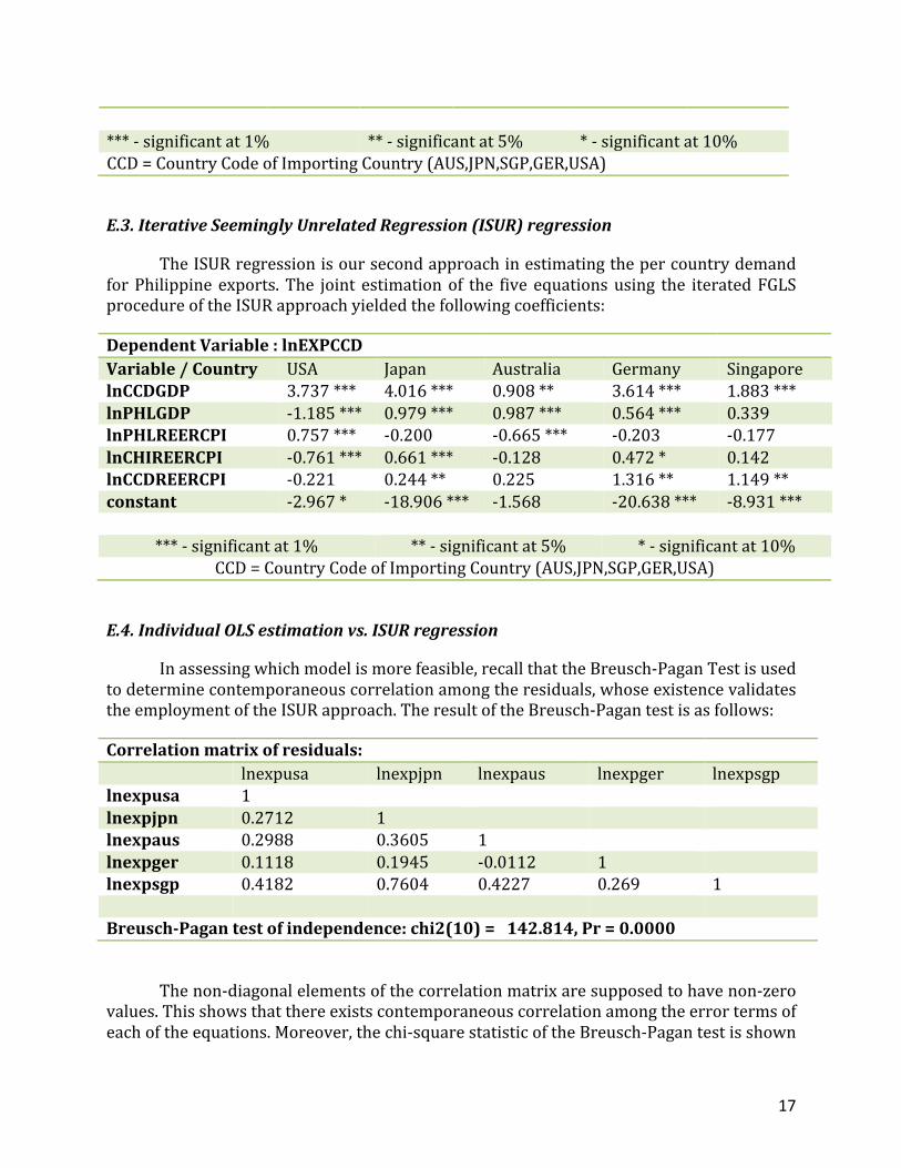
E.3. Iterative Seemingly Unrelated Regression (ISUR) regression

The ISUR regression is our second approach in estimating the per country demand for Philippine exports. The joint estimation of the five equations using the iterated FGLS procedure of the ISUR approach yielded the following coefficients:

Dependent Variable : lnEXPCCD Variable / Country USA Japan Australia Germany Singapore lnCCDGDP 3.737 *** 4.016 *** 0.908 ** 3.614 *** 1.883 *** lnPHLGDP -‐1.185 *** 0.979 *** 0.987 *** 0.564 *** 0.339 lnPHLREERCPI 0.757 *** -‐0.200 -‐0.665 *** -‐0.203 -‐0.177 lnCHIREERCPI -‐0.761 *** 0.661 *** -‐0.128 0.472 * 0.142 lnCCDREERCPI -‐0.221 0.244 ** 0.225 1.316 ** 1.149 ** constant -‐2.967 * -‐18.906 *** -‐1.568 -‐20.638 *** -‐8.931 ***


E.4. Individual OLS estimation vs. ISUR regression

In assessing which model is more feasible, recall that the Breusch-‐Pagan Test is used to determine contemporaneous correlation among the residuals, whose existence validates the employment of the ISUR approach. The result of the Breusch-‐Pagan test is as follows:

Correlation matrix of residuals: lnexpusa lnexpjpn lnexpaus lnexpger lnexpsgp lnexpusa 1 lnexpjpn 0.2712 1 lnexpaus 0.2988 0.3605 1 lnexpger 0.1118 0.1945 -‐0.0112 1 lnexpsgp 0.4182 0.7604 0.4227 0.269 1 Breusch-‐Pagan test of independence: chi2(10) = 142.814, Pr = 0.0000

The non-‐diagonal elements of the correlation matrix are supposed to have non-‐zero values. This shows that there exists contemporaneous correlation among the error terms of each of the equations. Moreover, the chi-‐square statistic of the Breusch-‐Pagan test is shown

18

to be significant up to the 99% confidence interval. Ergo, the null hypothesis indicating Ho : E(UiUj) = 0 is rejected. The errors are statically correlated. The ISUR is the more appropriate modeling technique in the estimation of the per-‐country demand functions for Philippine exports.

The ISUR approach is also known to yield more efficient coefficients (Salman, 2011). This means that its standard errors must be smaller in comparison to the individual OLS estimation procedure. The table below shows the standard errors of the coefficients from each of the estimation procedures:

Variable Std. Err. ISUR

Std. Err. OLS

Variable Std. Err. ISUR

Std. Err. OLS

Dependent Variable : lnexpusa Dependent Variable : lnexpger lnusagdp 0.431 0.747 lngergdp 0.388 0.418 lnphlgdp 0.291 0.121 lnphlgdp 0.168 0.146 lnphlreercpi 0.184 0.302 lnphlreercpi 0.202 0.288 lnchireercpi 0.170 0.228 lnchireercpi 0.243 0.262 lnusareercpi 0.287 0.481 lngerreercpi 0.619 0.825 constant 1.606 4.212 constant 4.118 5.456 Dependent Variable : lnexpjpn Dependent Variable : lnexpsgp lnjpngdp 0.317 0.678 lnsgpgdp 0.266 0.276 lnphlgdp 0.108 0.100 lnphlgdp 0.410 0.229 lnphlreercpi 0.146 0.274 lnphlreercpi 0.390 0.542 lnchireercpi 0.148 0.178 lnchireercpi 0.243 0.340 lnjpnreercpi 0.114 0.211 lnsgpreercpi 0.544 1.123 constant 1.971 3.917 constant 2.654 4.798 Dependent Variable : lnexpaus lnausgdp 0.383 0.342 lnchireercpi 0.145 0.226 lnphlgdp 0.336 0.255 lnausreercpi 0.232 0.341 lnphlreercpi 0.196 0.314 constant 1.333 2.035

As shown above, majority of the standard errors of the coefficients jointly estimated using ISUR had smaller values compared to those individually estimated using OLS. This further affirms that there is an efficiency-‐gain from employing the ISUR procedure. This is attributable to the ability of the ISUR model to take into account the contemporaneous correlation of the error terms in the estimation procedure.

It is also important to note that the ISUR approach yielded more significant estimates. Initally, almost all estimates for the Real Exchange Rate coefficients of derived from the individual OLS estimation were insignificant. After using the ISUR approach, the Real Exchange Rate variables became significant – signifying that the price distortions in individual economies only become meaningful for trade volume if the influences affecting

19

trade with other partners are also taken into account. It also confirms the multi-‐dimensional, highly competitive mechanism of the international market wherein the decision of firms and individuals are not solely based on the economic fundamentals of a single trading partner but also to that of itself and the other countries which may also be able to provide them with their needs.

The result of the Breusch-‐Pagan test, the smaller standard errors, and the more significant coefficients are all in favor of the joint estimation of each of the demand equations. Having this in mind, this study will conduct analyses and interpretations using the estimates of the ISUR approach.

F. Interpretations

Note that since this study involves a multivariate regression model such as the ISUR, it is assumed that all other factors besides the one being interpreted are held constant. The ISUR coefficient estimates presented earlier are again as follows:

Dependent Variable : lnEXPCCD Variable / Country USA Japan Australia Germany Singapore lnCCDGDP 3.737 *** 4.016 *** 0.908 ** 3.614 *** 1.883 *** lnPHLGDP -‐1.185 *** 0.979 *** 0.987 *** 0.564 *** 0.339 lnPHLREERCPI 0.757 *** -‐0.200 -‐0.665 *** -‐0.203 -‐0.177 lnCHIREERCPI -‐0.761 *** 0.661 *** -‐0.128 0.472 * 0.142 lnCCDREERCPI -‐0.221 0.244 ** 0.225 1.316 ** 1.149 ** constant -‐2.967 * -‐18.906 *** -‐1.568 -‐20.638 *** -‐8.931 ***


F.1.USA

The United States has been one of the top markets for Philippine exports in the

recent decades. It is a well-‐known fact that its large economy is consumption-‐driven – meaning to say, consumers in the United States tend to demand more due to their very high per capita incomes. In fact, according to The World Bank (2012), the US has one of the highest per capita income among developed nations at $48,442 (PPP at current US$) in 2011. This massive consumer demand of the US is clearly evident in the ISUR estimates.

In the analysis, it was shown that a one percent increase in the Real GDP index of the

USA will cause a 3.737% percent increase in the volume of Philippine exports to the US. This finding is statistically significant up to the 99% confidence interval and shows that the demand of the US is very elastic in correspondence to fluctuations in prevailing income levels (GDP). On the other hand, a one percent increase in the Real GDP index of the Philippines will cause a decrease in Philippine Exports to the US by 1.185% -‐-‐ suggesting a negative relationship between the Philippine Economy and its exports to the US. This

20

result, although seemingly atypical, is also significant up to the 99% confidence interval. The constant term, although statistically significant, will be disregarded as it may be considered a nuisance parameter due to its negative intercept value.

As per the real exchange rate of the Philippines, an appreciation of the peso index by one percent will cause an increase in the exports to the US by 0.757% and is significant at the 99% confidence interval. On the other hand, the a one percent increase in China’s real exchange rate causes a reduction in Philippine exports volume by 0.761%. These two findings may be considered peculiar as the Marshall-‐Lerner Condition dictates that a currency appreciation leads to a decrease in net exports. This may be attributable to the ability of the US to import more expensive goods in exchange for quality improvement. The Price level increases in the economy stem from increasing input costs such as wages, raw materials and investment in new technology. Heavy spending on these inputs causes firms to increase their prices. More often than not, the spill-‐over effect of this is the improved quality of goods being produced. Hence, for the considerably highly educated American population, cheaper may not necessarily be better.

F.2. Japan

Japan has also been one of the largest trading partner of the Philippines. Currently, it is the largest export market of the Philippines in the Asian continent. This may be due to the strong governmental linkages between the two countries and the relative proximity of the Philippines.

As shown in the table above, a one percent increase in the GDP of Japan increases their demand for Philippine goods and services by 4.016%. This finding, significant at the 99% confidence interval, emphasizes that the Japanese display high income elasticity in their importation from the Philippines. Likewise , an increase in the Philippine GDP by one percent increases the importation of the Japanese of Philippine products and services by 0.979% which is also significant at the 99% confidence interval. This idea is supported by the theretical underpinning of the Gravity Model of World Trade wherein the size of the trading partners have positive effects in the volume of trade between them.

A one percent increase in the Real Exchange Rate of China will increase the demand for Philippine exports by 0.661% and is significant at the 99% confidence interval. This affirms the negative relationship between the price of a competitor and demand for local exports. An increase in the Real Exchange Rate of Japan will also cause a positive effect of 0.244% and is significant at the 95% confidence interval. This evidences that an increase in price of Japanese goods and services will cause them to outsource more of their needs from foreign countries such as the Philippines. The constant term is also considered as a nuisance parameter due to its negative intercept value.

F.3. Australia

Australia has been the biggest export market of the Philippines in the Oceania. Although data suggests that the volume of exports in this region is not that high compared

21

to others, Australia has had a substantial share in the Philippine exports across time.

A one percent increase in the GDP of Australia increases their demand for Philippine exports by 0.908% and is significant at the 95% confidence interval. Likewise, an increase in the GDP of the Philippines by one percent increases exports to Australia by 0.987. Meanwhile, if the real exchange rate index of the Philippines increases by one percent, exports to Australia decreases by 0.665% -‐-‐ indicating that the increase in the relative price of Philippine commodities and services puts off Australians to import from the Philippines. These findings are both significant at the 99% confidence interval.

F.4. Germany

Germany is known as one of the export powerhouses in the world. They are also known to import large amounts of raw materials. With this in mind, Germany has been the largest of the two large European export market of the Philippines, the other one being the Netherlands. This indicates the reliance of these highly developed nations on intermediate goods from the country.

A one percent increase in the GDP of Germany increases their demand for Philippine exports by 3.614%. This positive relationship exhibits the importance of income fluctuations in the demand of Germans to import from the Philippines. Similarly, a one percent increase in Philippine GDP increases exports to Germany by 0.564%. These two elasticities are both significant at the 99% confidence interval.

In case of a one percent real currency appreciation in China, German demand for Philippine exports increases by 0.472. This is, however, weakly significant as the p-‐value is only within the 90% confidence interval. On the other hand, a one percent increase in the real exchange rate of Germany increases their demand for exports by 1.316%, which is significant at the 95% confidence interval. Similar to the findings for USA and Japan, the constant term is considered a nuisance parameter despite its significance.

F.5. Singapore

Singapore, together with the Philippines, is a member of the Association of the Southeast Asian Nations. Throughout the recent years, the ASEAN leaders have been working on policies towards regional integration. Part of this is the ASEAN Free Trade Agreement – a trade bloc intended to make ASEAN a competitive production base in the international market through the elimination of tariffs and trade barriers (International Enterprise Singapore, 2012). In addition, Singapore’s economy is heavily reliant in international trade. Its small geographical size limits it from producing its own agricultural produce. In fact, Blanchard (2011) states that exports make up around 243% of Singapore’s GDP. The ASEAN free trade agreement and the structure of the Singaporean economy may be able to explain the massive volume of Philippine exports to their country.

A one percent increase in the GDP of Singapore increases their demand for Philippine goods and services by 1.883% and is significant at the 99% confidence interval. In comparison to the US, Japan, and Germany, the income elasticity of Singapore is

22

relatively lower because no matter the current state of their economy, the existence of a Free Trade Agreement allows for some degree of trade resiliency in cases of economic distortions and business cycle fluctuations. Furthermore, a one percent increase in the real exchange rate index of Singapore will cause a 1.149% increase in their Philippine export demand. The constant term is also considered a nuisance parameter in the case of Singapore.

23

VI. AGGREGATE EXPORT DEMAND ESTIMATION A. Fixed Effects Models (FEM) vs. Random Effects Model (REM) vs. Naïve Model vs. Within-‐Group (WG) Model In estimating the aggregate export demand function of the Philippines, we employ different econometric models – FEM, REM, Naïve, and Within-‐Group, and see which provides better and more efficient results. We then perform statistical tests in order to further extract the desired results. B. Definition of Panel Data Models Panel data models are appropriate in this study because panel data have certain advantages over cross-‐section or time-‐series data. First, they take into account the unobserved heterogeneity of cross section and time-‐series nature of observations. Second, they provide more information in the estimation procedure which facilitates better modeling. They are also used to study the dynamics of change such as unemployment behavior, turnovers, and labor mobility. Lastly, panel data mitigates the risk of committing aggregation bias (Gujarati & Porter, 2009). Hence, in this section we differentiate each type of panel data models to have a better grasp of how each model generates results. B.1. Naive Model Also called as the Pooled OLS regression, this model is the most basic among the panel data models. It assumes that all parameters are time and space invariant. Naïve model is estimated through OLS. By pooling together all the observations, it does not consider the unobserved heterogeneity of the cross-‐sectional entities. It is highly possible that the error term is correlated with some of the regressors, thus running the risks of producing biased and inconsistent estimates. B.2. Fixed Effects Models (FEM) Unlike the Naïve model which posits that all parameters are time and space invariant, FEM assumes that parameters are unknown fixed values. Under FEM, there are four sub-‐models. However, for the purposes of this study, we limit the scope to three. These are the Least-‐Squares Dummy Variable (LSDV) models 1 to 3. LSDV-‐M1, the default FEM, assumes that intercepts are time invariant and slope coefficients fixed. The unobserved heterogeneity among cross-‐sectional entities is estimated using dummy variables. As OLS is the best linear, unbiased estimator (BLUE) under this model, this solves the problems of micronumerousity and heterogeneity. LSDV-‐M2, on the other hand, assumes that slope coefficients are fixed and intercepts are space-‐invariant. This model explicitly takes into account the dynamics of change by considering the unobserved heterogeneity of time. This is estimated using an instrument or proxy. Using OLS as its estimation procedure, LSDV-‐M2 prevents omitted variable bias and the problem of micronumerousity.

24

The last model under FEM is LSDV-‐M3, which posits that intercepts are both time and space varying. It takes into account the unobserved heterogeneity of spatial entities, as well as the dynamics of change or the uniqueness of time period. OLS is BLUE under this model. B.3. Within-‐Group (WG) Model The WG estimator eliminates the fixed effect of the intercept by expressing the values of the dependent and independent variables for each cross-‐sectional entity as deviations from their respective means (Gujarati & Porter, 2009). This is done for all the cross-‐sectional units, then all the mean-‐corrected values are pooled and estimated using OLS. This model takes into account the unobserved heterogeneity by eliminating it through differencing sample observations around their sample means. B.4. Random Effects Model (REM) Also called as the Error Components Model, REM assumes that the intercept, unlike FEM which treats it as fixed, is a random variable which represents the mean value of all the intercepts of the cross-‐sectional units. The individual differences in the intercept values of spatial units are captured by the error term. The composite error term captures the random effect of each cross-‐sectional entity and the individual error which varies across time and space, i.e., the idiosyncratic term. C. Tests We use various tests in order to identify the best model for our study. First, we use Wald’s test to know whether to pool observations or not, that is, whether to use the Naïve or FEM (LSDV-‐M1 to M3). Under the Wald’s test, the null hypothesis states that the restricted model is better while it is the unrestricted model under the alternative hypothesis. Hence, for a 95% confidence, we reject the null hypothesis if the p-‐value is less than 0.05; we accept it otherwise. C.1. Wald’s Test: Naïve vs. LSDV1 The result is as follows: . quietly xi: reg lnexpccd lnccdgdp lnphlgdp lnphlreercpi lnchireercpi lnccdree > rcpi lndistccd i.country . test _Icountry_2 _Icountry_3 _Icountry_4 _Icountry_5 ( 1) _Icountry_2 = 0 ( 2) _Icountry_3 = 0 ( 3) _Icountry_4 = 0 ( 4) _Icountry_5 = 0 Constraint 3 dropped F( 3, 528) = 1863.09

25

Prob > F = 0.0000

Since the p-‐value is less than 0.05, we reject the null hypothesis that the restricted model, Naïve, is better than the unrestricted, LSDV1. Therefore, LSDV1 is better than Naïve. C.2. Wald’s Test: Naïve vs. LSDV2 The result is as follows:

F(104, 427) = 0.16

Prob > F = 1.0000

Since the p-‐value is more than 0.05, we accept the null hypothesis that the restricted model, Naïve, is better than the unrestricted, LSDV2. Therefore, Naïve is better than LSDV2. C.3. Wald’s Test: Naïve vs. LSDV3 The result is as follows: F(107, 424) = 73.01 Prob > F = 0.0000

Since the p-‐value is less than 0.05, we reject the null hypothesis that the restricted model, Naïve, is better than the unrestricted, LSDV3. Therefore, LSDV3 is better than Naive. C.4. Wald’s Test: LSDV1 vs. LSDV3 The result is as follows: F(104, 424) = 2.76 Prob > F = 0.0000

Since the p-‐value is less than 0.05, we reject the null hypothesis that the restricted model, LSDV1, is better than the unrestricted, LSDV3. Therefore, LSDV3 is better than LSDV1. C.5. Wald’s Test: LSDV2 vs. LSDV3 The result is as follows: F( 3, 424) = 2501.12 Prob > F = 0.0000

Since the p-‐value is less than 0.05, we reject the null hypothesis that the restricted model, LSDV2, is better than the unrestricted, LSDV3. Therefore, LSDV3 is better than LSDV2.

26

Therefore, since LSDV3 > Naïve, LSDV1, & LSDV2, then it follows that the best model among Naïve and FEM is LSDV3. C.6. Breusch-‐Pagan Test: Naïve vs. REM To determine which is better between Naïve and REM, we use the Breusch-‐Pagan Lagrange Multiplier Test. Under this test, the null hypothesis states that there are no random effects, meaning, Naïve is better. The alternative hypothesis, on the other hand, posits that there are random effects, hence REM is better than Naïve. Therefore, for a 95% confidence, we reject the null hypothesis if the p-‐value is less than 0.05; we accept it otherwise. The result is as follows: . xttest0 Breusch and Pagan Lagrangian multiplier test for random effects lnexpccd[country,t] = Xb + u[country] + e[country,t] Estimated results: | Var sd = sqrt(Var) ---------+----------------------------- lnexpccd | 2.010476 1.417913 e | .1088459 .3299181 u | 0 0 Test: Var(u) = 0 chi2(1) = 19147.89 Prob > chi2 = 0.0000

Since the p-‐value is less than 0.05, we reject the null hypothesis that there are no random effects. Hence, REM is better than Naïve. As shown in the previous subsection, LSDV3 is better than Naïve. It is also the best model among FEM. In this subsection, it is shown that REM is also better than Naïve. The question now boils down to which is better between LSDV3 and REM. This is answered by the Hausman test. C.7. Hausman Test: REM vs. FEM Another test that allows us whether to use REM or not is the Hausman test. Under the Hausman test, the null hypothesis states that the random effects are not correlated with one or more regressors. Hence, REM is better. However, as the alternative hypothesis asserts, when there is a correlation between the random effects and one or more regressors, FEM is better than REM. Therefore, for a 95% confidence, we reject the null hypothesis if the p-‐value is less than 0.05; we accept it otherwise. The result is as follows:

27

. hausman fixed random ---- Coefficients ---- | (b) (B) (b-B) sqrt(diag(V_b-V_B)) | fixed random Difference S.E. -------------+---------------------------------------------------------------- lnccdgdp | 1.092438 1.230835 -.1383968 . lnphlgdp | .6311058 1.191862 -.5607566 . lnphlreercpi | -1.39517 -.2893485 -1.105822 .2495744 lnchireercpi | .1771066 -.341649 .5187556 . lnccdreercpi | .0869852 3.731582 -3.644597 . lndistccd | -1.929546 .2713164 -2.200863 . ------------------------------------------------------------------------------ b = consistent under Ho and Ha; obtained from regress B = inconsistent under Ha, efficient under Ho; obtained from xtreg Test: Ho: difference in coefficients not systematic chi2(6) = (b-B)'[(V_b-V_B)^(-1)](b-B) = -1458.20 chi2<0 ==> model fitted on these data fails to meet the asymptotic assumptions of the Hausman test; see suest for a generalized test

This result may seem trivial as the Hausman test is supposed to identify which model is better between REM and LSDV3. This may also justify the need to employ the SUR estimation procedure as the result suggests. For the purposes of this study, we consider the results generated by LSDV3 and REM since they appear to be the best models among the set of panel data models. D. Regression Analyses & Statistical Testing

Dependent Variable : lnEXPCCD Variable / Model Naïve LSDV-‐M1 LSDV-‐M2 LSDV-‐M3 REM WG lnCCDGDP 1.230835*** 1.499196*** .9432642*** 1.092438*** 1.230835*** 1.230835 lnPHLGDP 1.191862*** .9730339*** .7268734 .6311058*** 1.191862*** 1.191862*** lnPHLREERCPI -‐.2893485 .1354118 -‐1.736064 -‐1.39517*** -‐.2893485 -‐.2893485 lnCHIREERCPI -‐.341649 -‐.3881461*** .1641852 .1771066 -‐.341649 -‐.341649 lnCCDREERCPI 3.731582*** .0170378 3.920288*** .0869852 3.731582*** 3.731582*** lnDISTCCD .2713164*** -‐2.014405*** .2975777*** -‐1.929546*** .2713164*** .2713164*** constant -‐21.40541*** 11.86913*** .9432642 18.66535*** -‐21.40541*** -‐.0031217 *** -‐ significant at 1% ** -‐ significant at 5% * -‐ significant at 10% CCD = Country Code of Importing Country (AUS,JPN,SGP,GER,USA)

D.1. General Comments As the results generated vary across each type of panel data model. Some variables are highly significant in some models, while some are not. Most of the variables are significant at 1% confidence. A-‐priori expectations are met most of the explanatory

28

variables. Naïve and WG produce virtually similar results. This is because the two models are identical mathematically (Gujarati & Porter, 2009). Only, the WG estimator produces consistent slope coefficients vis-‐à-‐vis Naïve. Albeit consistent, WG coefficients are inefficient compared to Naïve. As noted in the previous sub-‐section, we consider both REM and LSDV3 as the best models in this study. Hence, in interpreting the results of the regression analysis, we focus only on the results under the two models. D.2. Interpretations of REM Results The export demand function therefore is as follows: 𝑙𝑛𝐸𝑋𝑃𝐶𝐶𝐷!" = −21.41+ 1.23𝑙𝑛𝐶𝐶𝐷𝐺𝐷𝑃!" + 1.19𝑙𝑛𝑃𝐻𝐿𝐺𝐷𝑃!" − 0.29𝑙𝑛𝑃𝐻𝐿𝑅𝐸𝐸𝑅𝐶𝑃𝐼!"

− 0.34𝑙𝑛𝐶𝐻𝐼𝑅𝐸𝐸𝑅𝐶𝑃𝐼!" + 3.73𝑙𝑛𝐶𝐶𝐷𝑅𝐸𝐸𝑅𝐶𝑃𝐼!" + 0.27𝑙𝑛𝐷𝐼𝑆𝑇𝐶𝐶𝐷!" + 𝑤!" The average intercept value of the five countries is -‐21.41. Since this is a double log model, the slope coefficients represent demand elasticities. Ceteris paribus, a 1%-‐increase in the GDP of the foreign country leads to a 1.23%-‐increase in Philippine exports. This analysis is sound and valid because as foreign GDP increases, holding all else equal, demand for goods increases and so exports rise. A 1%-‐increase in Philippine GDP yields a 1.19% increase in Philippine exports, holding other factors equal. As the Gravity Model of Trade posits, local GDP increases result to larger volume of trade with other economies. Al though insignificant, real effective exchange rate of the Philippines meets the a-‐priori expectation. It is negative because as supported by the Mundell-‐Fleming model and the Marshall-‐Lerner condition, appreciation decreases foreign demand on local goods, thereby decreasing exports. When appreciation takes place, local goods are more expensive relative to competitors’ goods. A 1% appreciation of Philippine peso decreases exports by 0.29%, ceteris paribus. Real effective exchange rate of China appears to be statistically insignificant. More so, it fails to meet the a-‐priori expectation. It is supposed to be positive because being an export powerhouse in the world, an appreciation of Chinese currency makes Chinese exports more expensive relative to Philippine goods, hence the increase in demand for Philippine exports. This claim is supported by the Mundell-‐Fleming model and the Marshall-‐Lerner condition. Real effective exchange rate of importing country asserts that a 1% increase in the importing country’s exchange rate increases Philippine exports by 3.73%. This is because as Mundell-‐Fleming model & Marshall-‐Lerner condition suggest, appreciation of importing country’s currency leads to increases in imports. Philippine goods are cheaper after the appreciation, hence the increase in exports. However, albeit statistically significant, result for the distance variable suggests that a 1% increase in distance between Philippines and trading partner results to a 0.27% rise in Philippine exports. This is counterintuitive because as distance between two countries gets bigger, more costs are incurred such as

29

logistical and transactional costs, hence lower exports. This claim is supported by the Gravity Model of Trade. The parameter sigma_u represents the standard deviation of the idiosyncratic term, which is the combined time-‐series and cross-‐section error component. Parameter sigma_e, on the other hand, is the standard deviation of the cross-‐section error component. Rho represents the correlation between the two parameters. Since rho equals 0, it indicates that the usual assumption of REM that the individual error components are not correlated with each other and that they are not autocorrelated across both cross-‐section and time-‐series units is met. D.3. Interpretations of LSDV3 Results lnexpccd Coef. Std. Err. t P>t [95% Conf. Interval] lnccdgdp 1.092438 0.0894028 12.22 0 0.91671 1.268166 lnphlgdp 0.6311058 0.1995966 3.16 0.002 0.2387837 1.023428 lnphlreercpi -‐1.39517 0.4938742 -‐2.82 0.005 -‐2.365917 -‐0.4244235 lnchireercpi 0.1771066 0.2394166 0.74 0.46 -‐0.2934847 0.6476979 lnccdreercpi 0.0869852 0.1356696 0.64 0.522 -‐0.1796835 0.3536539 lndistccd -‐1.929546 0.0505063 -‐38.2 0 -‐2.02882 -‐1.830273 _Icountry_2 2.187057 0.054638 40.03 0 2.079662 2.294452 _Icountry_3 1.225323 0.0434708 28.19 0 1.139877 1.310768 _Icountry_4 (dropped) _Icountry_5 4.80188 0.0688752 69.72 0 4.666501 4.93726 _Idate_101 -‐0.0827771 0.1778875 -‐0.47 0.642 -‐0.4324283 0.2668741 _Idate_102 0.0074338 0.1812164 0.04 0.967 -‐0.3487605 0.3636281 _Idate_103 -‐0.2880011 0.1637112 -‐1.76 0.079 -‐0.6097877 0.0337855 _Idate_104 -‐0.4317798 0.1780583 -‐2.42 0.016 -‐0.7817668 -‐0.0817929 _Idate_105 -‐0.4794739 0.1802614 -‐2.66 0.008 -‐0.8337911 -‐0.1251567 _Idate_106 -‐0.4795251 0.1852641 -‐2.59 0.01 -‐0.8436755 -‐0.1153747 _Idate_107 -‐0.5268312 0.1702456 -‐3.09 0.002 -‐0.8614617 -‐0.1922007 _Idate_108 -‐0.5263516 0.1872323 -‐2.81 0.005 -‐0.8943708 -‐0.1583325 _Idate_109 -‐0.4384971 0.1800552 -‐2.44 0.015 -‐0.792409 -‐0.0845852 _Idate_110 -‐0.356788 0.1811875 -‐1.97 0.05 -‐0.7129256 -‐0.0006505 _Idate_111 -‐0.4528926 0.179876 -‐2.52 0.012 -‐0.8064523 -‐0.0993329 _Idate_112 -‐0.4633241 0.1927452 -‐2.4 0.017 -‐0.8421792 -‐0.084469 _Idate_113 -‐0.4029907 0.1880808 -‐2.14 0.033 -‐0.7726775 -‐0.0333039 _Idate_114 -‐0.2953184 0.1923149 -‐1.54 0.125 -‐0.6733277 0.0826909 _Idate_115 -‐0.5125602 0.1890651 -‐2.71 0.007 -‐0.8841818 -‐0.1409387 _Idate_116 -‐0.4096025 0.2000043 -‐2.05 0.041 -‐0.8027259 -‐0.016479 _Idate_117 -‐0.3040247 0.1917315 -‐1.59 0.114 -‐0.6808872 0.0728378 _Idate_118 -‐0.2686231 0.1875223 -‐1.43 0.153 -‐0.6372123 0.099966 _Idate_119 -‐0.4668688 0.163206 -‐2.86 0.004 -‐0.7876624 -‐0.1460752 _Idate_120 -‐0.3717031 0.1604046 -‐2.32 0.021 -‐0.6869903 -‐0.0564158 _Idate_121 -‐0.349676 0.1576698 -‐2.22 0.027 -‐0.6595879 -‐0.0397642 _Idate_122 -‐0.3668136 0.1732097 -‐2.12 0.035 -‐0.7072702 -‐0.0263571 _Idate_123 -‐0.6223289 0.1821876 -‐3.42 0.001 -‐0.9804322 -‐0.2642257 _Idate_124 -‐0.5036988 0.1834937 -‐2.75 0.006 -‐0.8643694 -‐0.1430283

30

_Idate_125 -‐0.3833121 0.1667978 -‐2.3 0.022 -‐0.7111656 -‐0.0554587 _Idate_126 -‐0.2913863 0.1628741 -‐1.79 0.074 -‐0.6115276 0.0287549 _Idate_127 -‐0.3459289 0.151445 -‐2.28 0.023 -‐0.6436054 -‐0.0482525 _Idate_128 -‐0.2888037 0.1592973 -‐1.81 0.071 -‐0.6019145 0.0243071 _Idate_129 -‐0.2307336 0.1583511 -‐1.46 0.146 -‐0.5419845 0.0805173 _Idate_130 -‐0.0531197 0.1605311 -‐0.33 0.741 -‐0.3686556 0.2624162 _Idate_131 -‐0.1440095 0.1548465 -‐0.93 0.353 -‐0.4483718 0.1603528 _Idate_132 -‐0.1275677 0.1569173 -‐0.81 0.417 -‐0.4360004 0.180865 _Idate_133 -‐0.0926396 0.1557152 -‐0.59 0.552 -‐0.3987095 0.2134302 _Idate_134 -‐0.0572849 0.1576217 -‐0.36 0.716 -‐0.3671022 0.2525324 _Idate_135 -‐0.2369226 0.1466987 -‐1.62 0.107 -‐0.5252699 0.0514248 _Idate_136 (dropped) _Idate_137 0.0907526 0.1773526 0.51 0.609 -‐0.2578472 0.4393524 _Idate_138 0.2541768 0.1746725 1.46 0.146 -‐0.089155 0.5975086 _Idate_139 0.3057696 0.1799929 1.7 0.09 -‐0.04802 0.6595592 _Idate_140 0.269248 0.1714082 1.57 0.117 -‐0.0676676 0.6061637 _Idate_141 0.239548 0.1641308 1.46 0.145 -‐0.0830633 0.5621593 _Idate_142 0.3742542 0.1674914 2.23 0.026 0.0450373 0.7034712 _Idate_143 0.3242676 0.1701595 1.91 0.057 -‐0.0101936 0.6587287 _Idate_144 0.4402913 0.1723598 2.55 0.011 0.1015053 0.7790773 _Idate_145 0.5550385 0.1734889 3.2 0.001 0.2140331 0.896044 _Idate_146 0.5440756 0.1737649 3.13 0.002 0.2025278 0.8856235 _Idate_147 0.476557 0.1797322 2.65 0.008 0.1232799 0.829834 _Idate_148 0.6471358 0.1816946 3.56 0 0.2900015 1.00427 _Idate_149 0.7291515 0.1857473 3.93 0 0.3640512 1.094252 _Idate_150 0.6777282 0.1601487 4.23 0 0.3629439 0.9925125 _Idate_151 0.4234714 0.1446011 2.93 0.004 0.1392471 0.7076957 _Idate_152 0.3598038 0.1471388 2.45 0.015 0.0705915 0.6490162 _Idate_153 0.4336218 0.1437616 3.02 0.003 0.1510477 0.7161959 _Idate_154 0.3717057 0.146762 2.53 0.012 0.083234 0.6601773 _Idate_155 0.3009804 0.1431975 2.1 0.036 0.0195151 0.5824457 _Idate_156 0.4940188 0.146465 3.37 0.001 0.206131 0.7819066 _Idate_157 0.6318511 0.1495551 4.22 0 0.3378894 0.9258128 _Idate_158 0.6470661 0.1460947 4.43 0 0.3599061 0.9342261 _Idate_159 0.5142671 0.1447633 3.55 0 0.229724 0.7988103 _Idate_160 0.5138136 0.1454404 3.53 0 0.2279397 0.7996875 _Idate_161 0.4508826 0.1585199 2.84 0.005 0.1392999 0.7624654 _Idate_162 0.4328898 0.1643254 2.63 0.009 0.109896 0.7558836 _Idate_163 0.4056743 0.1584365 2.56 0.011 0.0942555 0.7170932 _Idate_164 0.2243693 0.1518757 1.48 0.14 -‐0.0741537 0.5228923 _Idate_165 0.3210937 0.1590949 2.02 0.044 0.0083809 0.6338066 _Idate_166 0.1630714 0.1571412 1.04 0.3 -‐0.1458015 0.4719443 _Idate_167 0.1255417 0.1624958 0.77 0.44 -‐0.1938559 0.4449392 _Idate_168 0.0899119 0.155414 0.58 0.563 -‐0.2155658 0.3953896 _Idate_169 0.2651778 0.1507665 1.76 0.079 -‐0.0311651 0.5615206 _Idate_170 0.3185734 0.1583167 2.01 0.045 0.00739 0.6297567 _Idate_171 0.2206063 0.1587188 1.39 0.165 -‐0.0913674 0.53258 _Idate_172 0.130401 0.1666824 0.78 0.434 -‐0.1972258 0.4580277 _Idate_173 0.0404307 0.1596496 0.25 0.8 -‐0.2733725 0.3542338 _Idate_174 0.0135447 0.1668039 0.08 0.935 -‐0.3143208 0.3414103 _Idate_175 -‐0.0838941 0.1718025 -‐0.49 0.626 -‐0.4215848 0.2537966 _Idate_176 (dropped)

31

_Idate_177 0.0604585 0.1736064 0.35 0.728 -‐0.2807779 0.4016948 _Idate_178 0.1154491 0.1697217 0.68 0.497 -‐0.2181516 0.4490499 _Idate_179 -‐0.0614072 0.1705514 -‐0.36 0.719 -‐0.3966387 0.2738243 _Idate_180 -‐0.1129987 0.162877 -‐0.69 0.488 -‐0.4331456 0.2071481 _Idate_181 -‐0.0004861 0.1613225 0 0.998 -‐0.3175775 0.3166053 _Idate_182 0.0279364 0.1634859 0.17 0.864 -‐0.2934075 0.3492802 _Idate_183 0.0963058 0.1587699 0.61 0.544 -‐0.2157683 0.4083799 _Idate_184 0.205833 0.1511459 1.36 0.174 -‐0.0912555 0.5029215 _Idate_185 0.1909913 0.1537574 1.24 0.215 -‐0.1112303 0.4932129 _Idate_186 0.2868993 0.152076 1.89 0.06 -‐0.0120174 0.5858161 _Idate_187 0.208086 0.1614202 1.29 0.198 -‐0.1091974 0.5253694 _Idate_188 0.1559579 0.1541569 1.01 0.312 -‐0.1470491 0.4589649 _Idate_189 0.2533142 0.1612736 1.57 0.117 -‐0.063681 0.5703095 _Idate_190 0.2951541 0.159025 1.86 0.064 -‐0.0174214 0.6077296 _Idate_191 0.3389975 0.177246 1.91 0.056 -‐0.0093926 0.6873877 _Idate_192 0.378768 0.1592354 2.38 0.018 0.0657789 0.6917571 _Idate_193 0.3805616 0.158232 2.41 0.017 0.0695449 0.6915784 _Idate_194 0.3642746 0.1540897 2.36 0.019 0.0613998 0.6671494 _Idate_195 0.0036886 0.1612919 0.02 0.982 -‐0.3133428 0.3207199 _Idate_196 -‐0.0916577 0.1521694 -‐0.6 0.547 -‐0.390758 0.2074425 _Idate_197 0.2092177 0.1570087 1.33 0.183 -‐0.0993946 0.5178301 _Idate_198 0.1423034 0.1531268 0.93 0.353 -‐0.1586787 0.4432855 _Idate_199 0.2079116 0.1631342 1.27 0.203 -‐0.1127407 0.528564 _Idate_200 0.3412617 0.1588744 2.15 0.032 0.0289823 0.6535412 _Idate_201 0.3585178 0.1702546 2.11 0.036 0.0238697 0.6931659 _Idate_202 0.4924102 0.1638253 3.01 0.003 0.1703994 0.814421 _Idate_203 0.2865127 0.1761123 1.63 0.105 -‐0.0596492 0.6326746 _Idate_204 0.296034 0.1657394 1.79 0.075 -‐0.0297393 0.6218072 _Idate_205 0.2099692 0.1727097 1.22 0.225 -‐0.1295047 0.5494431 _Idate_206 0.203075 0.1673548 1.21 0.226 -‐0.1258734 0.5320235 _Idate_207 (dropped) _cons 18.66535 2.592947 7.2 0 13.56872 23.76199

Since individual heterogeneity and time variety are captured by dummy variables in the LSDV3 model, each trading partner has its own corresponding intercept every year. This may be interpreted as the autonomous demand for Philippine exports of each trading partner on a year-‐to-‐year basis. The base category for this analysis is Australia’s export demand at 1985Q1. In addition, since the software Stata dropped the variable representing Singapore, analysis will be centered on the differences of autonomous demand of Japan, US, and Germany against that of the base category.

The LSDV3 model employed is of the log-‐log specification. Therefore, the slope

coefficients represent the elasticities of Philippine exports in response to certain changes in the independent variables. Note, however, that these coefficients measure the aggregated responsiveness of the five trading partners across the observation period in our study. As stated earlier, individual heterogeneity and the dynamics of change are both already captured by the dummy variables of the LSDV3 model. Additionally, interpretations on each of the estimated coefficients assume that all other factors besides the country and quarter being observed are held constant.

32

A one percent increase in the GDP of the importing nation triggers a 1.092% increase in Philippine exports to its regional principal markets and is statistically significant at the 99% confidence interval. Meanwhile, a 0.631% increase is caused by a one percent increase in the GDP of the Philippines. These claims are supported by the Mundell-‐Flemming Model and the Gravity Theory of World Trade wherein foreign GDP upturns lead to positive growth in exports and that local GDP improvements lead to increase in trade volume.

In case of a one percent increase in the real exchange rate index of the Philippines, a

-‐1.396% change is likely for the volume of Philippine exports to Australia, Germany, Japan, Singapore and the US. This finding is strongly significant at 1% confidence and is also backed by economic theory. The Marshall Lerner Condition dictates that a real currency appreciation will lead to negative changes in net exports – which is clearly the case in the regression analysis.

Distance variability is also strongly significant at 1% confidence. Trading partners

who are farther by one percent of the average will lead to a 1.930% reduction in the volume of Philippine exports. The Gravity Model may also be accountable for such phenomena.

In general, Germany (ICountry_2) has a higher average aggregate export of 2.187

million USD primarily because of their need to export the intermediate goods of the Philippines. Japan (ICountry_3), on the other hand, has a higher average aggregate export of 1.225 million USD because Japan has, throughout the recent decades, been one of the largest markets for Philippine exports. This may also be because of the strong political linkages between them. Like Japan, USA’s (ICountry_5) sheer economic size and consumer demand lead to a higher average aggregate export of 4.802 million USD.

In 1985Q2 (Idate_101), autonomous demand of Germany was 20.76963 million

USD. Japan and the US had 19.8079 million USD and 23.38445 million USD, respectively. During 2011Q3 (Idate_206), average autonomous demand of the importing nations increased by 0.203075 million USD. In the long run, from 1985Q1-‐2011Q3, the autonomous demand for Philippine exports of Germany, Japan and USA is increasing.

The European Union (EU) was formally assembled in 1993Q4 (Idate_135). During

that time, the aggregate export demand of Germany was 20.62235 million USD. Aggregate demand of Japan was 19.65375 million USD and the aggregate export demand of USA was 23.23031 million USA. Because there is a single market in EU, regulatory policies are responsible for antitrust issues, approving mergers, breaking up cartels, working for economic liberalization and preventing state aid to protect its competitiveness.

It was during 1990s when high income countries like USA, Japan and Germany,

institutions, companies and organizations were prosperous and experienced steady economic growth. On 1990Q1 (Idate_120), autonomous demand of Germany, Japan and US have amounted to 20.480, 19.51897 and 23.09553 million USD respectively. The growth persisted until 1999Q4 (Idate_159), wherein the average aggregate demand of importing

33

countries increased by 0.5142671 million USD. The 90s was considered a time of prosperity in the United States under the administration of former US President Bill Clinton. The U.S economy experienced its longest period of peace time economic expansion wherein personal incomes increased sharply. It also marked the reunification of the once-‐split West and East Germany.

During the fourth quarter of 1985(Idate_103), the average autonomous demand of

the importing nations decreased by .288 million USD. This disruption may be attributed to the political instabilities of the Marcos administration. According to World Bank, there was a sharp contraction in the production of the manufacturing sector by a massive 7.9 percent in 1985 and the incentive system was not conducive to a broad-‐based export expansion.

Before 1997, exports were the growth engines for Asian countries. A combination of

inexpensive and well-‐educated labor, export orientated economies, and falling barriers to international trade turned the region into an export powerhouse. In 1997Q1 (Idate_148), the average autonomous demand of the importing nations increased by 0.6471358. The investments grew which lead to higher imports thus, increasing the deficit of balance of payments. Exports started to decline during the Asian Financial Crisis which started in 1997Q3 (Idate_151) which not only affected Asia but also the America and some European Countries. With this, the autonomous demand of Germany decreased to 21.27588 million USD. Japan and USA had 20.31414 million USD and 23.8907 million USD respectively.

The 9/11 attack happened in the USA on September 11, 2001. At 2001Q2

(Idate_166), the average autonomous demand of these 3 countries were 21.01548 million USD, 20.05374 million USD and 23.6303 million USD, respectively. 911 attack increased the average aggregate demand of importing nations by 0.0899119 million USD during 2001Q4 (Idate_168).

The world food crisis, which lasted from 2007Q1 (Idate_188) to 2008Q2 (Idate_193)

caused a high rise in the cost of food especially staple commodities such as rice, wheat, and corn. Hunger prevailed in many developing countries during this time. During 2007Q1 (Idate_188), average autonomous demand of the importing nations increased by 0.1559579 million USD. And the average autonomous demand of the importing nations during 2008Q2 is higher by 0.3805616. Albeit the unfortunate circumstance, this crisis did not affect the export demand behavior of Germany, Japan and USA primarily because these are developed countries.

The Global Financial Crisis of 2008/09 shocked the US economy with world stock

market collapses and financial institution breakdowns. Its economic impacts started during the 2007Q3 (Idate_190). Global financial meltdown may affect the livelihoods of almost everyone in an increasingly inter-‐connected world. It brought an effect to exports because exports declined sharply. Germany had an autonomous demand of 21.14756 million USD, Japan had 20.18583 million USD and USA had 23.76238 million USD.

European debt crisis started because the global financial crisis brought the

unsustainable fiscal policies of countries in Europe. When growth slows, so do tax revenues

34

making unsustainable high budget deficits. This crises started during the 2009Q4 (Idate_199). The average autonomous demand of the importing nations increased by 0.2079116 million USD. The crisis didn’t have a negative effect to exports because many countries still think that it is Greece who suffered much from this said crisis.

The Japanese earthquake crisis, which created a nuclear damage during the 2011Q1

(Idate_204), also created an impact on Japan’s import. Before the earthquake, Japan’s aggregate export demand was 20.18671. But after the earthquake, Japan’s aggregate export demand in 2011Q2-‐Q3 (Idate_205-‐206) was 20.10064 million USD and 20.09375 million USD respectively. This is because Japan gave priority to their domestic goods in parts struck by the calamity.

It was also during 2011Q1 ((Idate_204)were crisis and uprisings in the Middle East

and North Africa started and these countries possess large crude oil reserves. The average aggregate demand of the importing nations increased by 0.203075 million USD on 2011Q3 (Idate_206) because Germany, Japan and USA were not affected by the said crisis.

Another crisis which transpired during 2011 was known as the United States debt-‐ceiling crisis. It started as a debate in the United States Congress about increasing the debt ceiling. The US Congress must approve the expenditure for the federal government to pay for it. The only way to pay for the budget deficit is by borrowing the shortfall amount through debt instruments and the amount that the government can borrow is limited by the debt ceiling. The aggregate demand of US was 23.76326 million USD. The failure to raise the debt ceiling would lead to a decrease in government spending, thus to a fall in aggregate demand.

35

VII. POLICY RECOMMENDATIONS AND CONCLUSION

As a developing country, the growth of the export industry in the Philippines will be instrumental towards achieving a full-‐fledged economic take-‐off. The expansion of export industries in the recent decades had been considered a key driver towards development. The cases of Japan, China and Germany are perfect examples to attest to this. Moreover, an increasing share of exports in the GDP of an economy is an indicator of productivity gains through investments in technology, human capital and physical capital. It reflects the competitiveness of local products in the international arena. It may also be considered as an indicator of trade openness, which according to international economic theory, brings forth mutual gains in each of the trading partners. (Krugman, Obstfeld, & Melitz, 2012).

As evidenced by the regression analyses presented in the preceding sections, the

economic circumstances of the importing country, which is reflected by its GDP, has been shown to be a significant factor in determining the volume of Philippine exports. In fact, in the per country demand estimation, the variable representing foreign GDP has been consistently significant across all observations. Furthermore, the GDP of the Philippines has been shown to have a significant positive effect in exports in most of the observed countries.

It can be inferred from these results that international cooperation is beneficial for

the Philippines. It also mirrors increasingly interdependence of economies worldwide. By improving economic ties with other countries, GDP growth and export industry expansion will be realized. The Japan-‐Philippines Economic Partnership Agreement (JPEPA) is an example of a well-‐established linkage with another nation. Active participation in such kinds of agreements should be upheld by policymakers in the country.

Furthermore, the significant negative relationship between distance and export

volume highlights the importance of regional cooperation towards the development of the export industry. Since there is more incentive for nearby countries to trade with the Philippines, potential benefits must be harnessed. Strengthening connections with ASEAN countries through bilateral trade agreements, open skies policy, enhancement of free trade initiatives and etcetera will greatly develop the trade sector of the country.

Meanwhile, the statistically significant estimates of real exchange rates in the

regression analyses reveal the relative importance of monetary and exchange rate policy in determining the volume of Philippine exports. The classical macroeconomic goal of price stability may also lead to the stabilization of trade volumes. Price distortions, more specifically a currency appreciation in the domestic market, deters trade relations between trading partners. In such case, the need for sound fiscal and monetary policies is accentuated. Effective usage of policy tools such as taxation, government expenditure and the Bangko Sentral’s Open Market Operations (OMO) will lead to a more conducive environment for international trade relations.

36

This research has tackled key determinants of the volume of Philippine exports to its major trading partners across different regions. Economic theories such as the Mundell-‐Flemming Model, the Marshall-‐Lerner Condition, the Gravity Theory of World Trade and the Theory of Consumer Demand were used to back the selection of variables used in the study. A review of related literature was also conducted to help facilitate the flow of ideas in this research. Subsequently, demand estimation for Philippine exports was conducted in a per country and aggregated basis using different econometric techniques. The results revealed the significant impacts of real exchange rates and the size of the trading partners in the volume of Philippine exports. Moreover, the distance between the Philippines and its trading partner was also seen to be a determinant of trade volumes in the panel data regressions.

Overall, although this study was able to estimate demand equations for Philippine

exports, a more detailed and comprehensive analysis involving all of its trading partners may provide additional room for research in the future. Other estimation techniques may also be utilized thereafter.

37

VIII. REFERENCES Arize, A.C. (2001). Traditional export demand relation and parameter instability: an empirical investigation. Journal of Economic Studies, Vol. 28 No.6, pp.378-‐98. Bhagwati, J.N. and Srinivasan, T.N. (1978). Trade policy and development. In R.

Dornbusch and F.A. Frenkel (eds.) International Economic Policy: Theory and Evidence. Baltimore, MD: Johns Hopkins University Press.

Blanchard, O. (2011). Macroeconomics. Singapore: Pearson Education Inc. Clarkson, G. (1962). The Theory of Consumer Demand: A Critical Appraisal. Massachusetts Institute of Technology. Dycaico, A., Gamboa, J., Surbano, E., & Tan, F. (2012). Estimating the International Demand

for Philippine Tourism of China, Japan, Korea, and United States of America . Manila: De La Salle University.

Department of Trade and Industry. (2011). Department of Trade and Industry -‐

International Trade -‐ Statistics. Retrieved November 5, 2012, from Department of Trade and Industry Website: http://www.dti.gov.ph/dti/index.php?p=697

Guisan, M.C., Cancelo, M.T. (2002). Econometric models of foreign trade in OECD countries.

Applied Econometrics and International Development, Vol. 2 pp.65-‐81. Gujarati, D. (2004). Basic Econometrics (Fourth ed.). New York: The McGraw-‐Hill

Companies. International Enterprise Singapore. (2012, April 26). Welcome to Singapore FTA Network.

Retrieved December 9, 2012, from International Enterpise Singapore Website: http://www.fta.gov.sg/fta_afta.asp?hl=1

Kavoussi, R.M. (1984). Export expansion and economic growth: Further empirical evidence. Journal of Development Economics, 14, 241-‐50. Krueger, A. O. (1978). Foreign Trade Regimes and Economic Development: Liberalization

Attempts and Consequences. Cambridge, MA: Ballinger. Krugman, P. R., Obstfeld, M., & Melitz, M. J. (2012). International Economics Theory and

Policy (Ninth ed.). Boston : Pearson Education Inc. Kumar, S. (2009a). An empirical evaluation of export demand in China. Journal of Chinese

Economic and Foreign Trade Studies, Vol. 2 pp.100-‐9.

38

Kumar, S. (2009b). A re-‐examination of private consumption in Fiji. Pacific Economic Bulletin, Vol. 24 pp.70-‐81.

Mahadevan, R. (2007). New Evidence on the Export-‐led Growth Nexus: A Case Study of

Malaysia. World Economy, 30 (7), 1069-‐1083. Mankiw, N. G. (2002). Macroeconomics. New York: Worth Publishers;. Rao, B. Bhaskara & Singh, Rup, 2007. Effects of Trade Openness on the Steady State Growth

Rates of Selected Asian Countries with an Extended Exogenous Growth Model. MPRA Paper 5851, University Library of Munich, Germany.

Salman, A. K. (2011). Using the SUR Model of Tourism Demand for Neighbouring Regions in

Sweden and Norway. Advances in Econometrics-‐Theory and Applications , 97-‐115. Senhadji, A. and C. Montenegro, 1999. Time series analysis of structural export demand

equations: A cross country analysis. IMF Staff Papers, 46: 259-‐273. Singh, R., & Rao, B. (2005). ESTIMATING EXPORT EQUATIONS. Fiji: University of the South

Pacific, Suva . Time and Date AS. (2012). Distance . Retrieved November 5, 2012, from TimeandDate.Com:

http://www.timeanddate.com/worldclock/distance.html The World Bank. (2012). Exports of goods and services (% of GDP). Retrieved December 12,

2012, from The World Bank : http://data.worldbank.org/indicator/NE.EXP.GNFS.ZS The World Bank. (2012). GDP per capita (current US$). Retrieved November 28, 2012, from

The World Bank: http://data.worldbank.org/indicator/NY.GDP.PCAP.CD?order=wbapi_data_value_2011+wbapi_data_value+wbapi_data_value-‐last&sort=desc

The World Bank. (2012). GDP per Capita, PPP (at Current US$). Retrieved December 9,

2012, from The World Bank Data: http://data.worldbank.org/indicator/NY.GDP.PCAP.PP.CD?order=wbapi_data_value_2011+wbapi_data_value+wbapi_data_value-‐last&sort=desc

The World Bank. (2012). Real effective exchange rate index (2005 = 100). Retrieved

November 5, 2012, from The World Bank Data: http://data.worldbank.org/indicator/PX.REX.REER

Velasco, M.S. (2011). Microeconomics: Income and Substitution Effects. Retrieved from

http://www.slideshare.net/salasvelasco/microeconomics-‐income-‐andsubstitution-‐effects.

39

IX. APPENDIX A. Per Country Demand Estimation and Statistical Testing A.1 Individual OLS estimation . reg lnexpusa lnusagdp lnphlgdp lnphlreercpi lnchireercpi lnusareercpi Source | SS df MS Number of obs = 108 -------------+------------------------------ F( 5, 102) = 139.98 Model | 31.2400282 5 6.24800564 Prob > F = 0.0000 Residual | 4.55288811 102 .044636158 R-squared = 0.8728 -------------+------------------------------ Adj R-squared = 0.8666 Total | 35.7929163 107 .334513237 Root MSE = .21127 ------------------------------------------------------------------------------ lnexpusa | Coef. Std. Err. t P>|t| [95% Conf. Interval] -------------+---------------------------------------------------------------- lnusagdp | 4.440781 .4331461 10.25 0.000 3.581638 5.299925 lnphlgdp | -1.589062 .293221 -5.42 0.000 -2.170665 -1.00746 lnphlreercpi | .8551294 .183018 4.67 0.000 .492114 1.218145 lnchireercpi | -.8425798 .1741067 -4.84 0.000 -1.18792 -.4972399 lnusareercpi | .3204752 .311509 1.03 0.306 -.2974015 .9383518 _cons | -6.855061 1.647331 -4.16 0.000 -10.12253 -3.587587 ------------------------------------------------------------------------------ . vif Variable | VIF 1/VIF -------------+---------------------- lnusagdp | 21.70 0.046089 lnphlgdp | 21.39 0.046742 lnchireercpi | 2.35 0.426292 lnusareercpi | 2.18 0.458669 lnphlreercpi | 1.30 0.770828 -------------+---------------------- Mean VIF | 9.78 . bgodfrey Breusch-Godfrey LM test for autocorrelation --------------------------------------------------------------------------- lags(p) | chi2 df Prob > chi2 -------------+------------------------------------------------------------- 1 | 25.200 1 0.0000 --------------------------------------------------------------------------- H0: no serial correlation . ovtest Ramsey RESET test using powers of the fitted values of lnexpusa Ho: model has no omitted variables F(3, 99) = 4.81 Prob > F = 0.0036 . prais lnexpusa lnusagdp lnphlgdp lnphlreercpi lnchireercpi lnusareercpi Iteration 0: rho = 0.0000 Iteration 1: rho = 0.4543 Iteration 2: rho = 0.7925 Iteration 3: rho = 0.9298

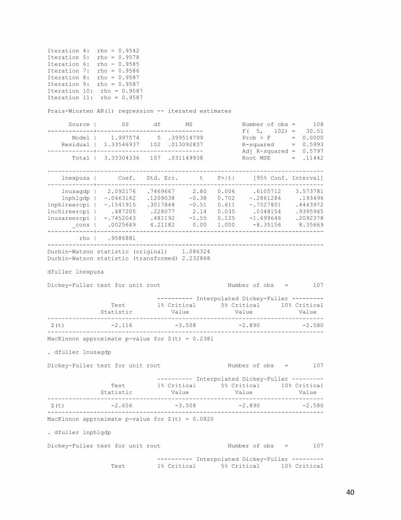
40

Iteration 4: rho = 0.9542 Iteration 5: rho = 0.9578 Iteration 6: rho = 0.9585 Iteration 7: rho = 0.9586 Iteration 8: rho = 0.9587 Iteration 9: rho = 0.9587 Iteration 10: rho = 0.9587 Iteration 11: rho = 0.9587 Prais-Winsten AR(1) regression -- iterated estimates Source | SS df MS Number of obs = 108 -------------+------------------------------ F( 5, 102) = 30.51 Model | 1.997574 5 .399514799 Prob > F = 0.0000 Residual | 1.33546937 102 .013092837 R-squared = 0.5993 -------------+------------------------------ Adj R-squared = 0.5797 Total | 3.33304336 107 .031149938 Root MSE = .11442 ------------------------------------------------------------------------------ lnexpusa | Coef. Std. Err. t P>|t| [95% Conf. Interval] -------------+---------------------------------------------------------------- lnusagdp | 2.092176 .7469667 2.80 0.006 .6105712 3.573781 lnphlgdp | -.0463162 .1209038 -0.38 0.702 -.2861284 .193496 lnphlreercpi | -.1541915 .3017848 -0.51 0.611 -.7527801 .4443972 lnchireercpi | .487205 .228077 2.14 0.035 .0348154 .9395945 lnusareercpi | -.7452043 .481192 -1.55 0.125 -1.699646 .2092378 _cons | .0025649 4.21182 0.00 1.000 -8.35156 8.35669 -------------+---------------------------------------------------------------- rho | .9586881 ------------------------------------------------------------------------------ Durbin-Watson statistic (original) 1.086324 Durbin-Watson statistic (transformed) 2.232868 dfuller lnexpusa Dickey-Fuller test for unit root Number of obs = 107 ---------- Interpolated Dickey-Fuller --------- Test 1% Critical 5% Critical 10% Critical Statistic Value Value Value ------------------------------------------------------------------------------ Z(t) -2.116 -3.508 -2.890 -2.580 ------------------------------------------------------------------------------ MacKinnon approximate p-value for Z(t) = 0.2381 . dfuller lnusagdp Dickey-Fuller test for unit root Number of obs = 107 ---------- Interpolated Dickey-Fuller --------- Test 1% Critical 5% Critical 10% Critical Statistic Value Value Value ------------------------------------------------------------------------------ Z(t) -2.656 -3.508 -2.890 -2.580 ------------------------------------------------------------------------------ MacKinnon approximate p-value for Z(t) = 0.0820 . dfuller lnphlgdp Dickey-Fuller test for unit root Number of obs = 107 ---------- Interpolated Dickey-Fuller --------- Test 1% Critical 5% Critical 10% Critical

41

Statistic Value Value Value ------------------------------------------------------------------------------ Z(t) -1.436 -3.508 -2.890 -2.580 ------------------------------------------------------------------------------ MacKinnon approximate p-value for Z(t) = 0.5651 . dfuller lnphlreercpi Dickey-Fuller test for unit root Number of obs = 107 ---------- Interpolated Dickey-Fuller --------- Test 1% Critical 5% Critical 10% Critical Statistic Value Value Value ------------------------------------------------------------------------------ Z(t) -2.773 -3.508 -2.890 -2.580 ------------------------------------------------------------------------------ MacKinnon approximate p-value for Z(t) = 0.0622 . dfuller lnchireercpi Dickey-Fuller test for unit root Number of obs = 107 ---------- Interpolated Dickey-Fuller --------- Test 1% Critical 5% Critical 10% Critical Statistic Value Value Value ------------------------------------------------------------------------------ Z(t) -3.669 -3.508 -2.890 -2.580 ------------------------------------------------------------------------------ MacKinnon approximate p-value for Z(t) = 0.0046 . dfuller lnusareercpi Dickey-Fuller test for unit root Number of obs = 107 ---------- Interpolated Dickey-Fuller --------- Test 1% Critical 5% Critical 10% Critical Statistic Value Value Value ------------------------------------------------------------------------------ Z(t) -3.811 -3.508 -2.890 -2.580 ------------------------------------------------------------------------------ MacKinnon approximate p-value for Z(t) = 0.0028 . vecrank lnexpusa lnusagdp lnphlgdp lnphlreercpi lnchireercpi lnusareercpi Johansen tests for cointegration Trend: constant Number of obs = 106 Sample: 102 - 207 Lags = 2 ------------------------------------------------------------------------------- 5% maximum trace critical rank parms LL eigenvalue statistic value 0 42 1266.8027 . 148.1696 94.15 1 53 1299.9256 0.46472 81.9239 68.52 2 62 1319.9169 0.31422 41.9412* 47.21 3 69 1330.6985 0.18407 20.3780 29.68 4 74 1334.7923 0.07433 12.1905 15.41 5 77 1338.5921 0.06919 4.5907 3.76 6 78 1340.8875 0.04238 ------------------------------------------------------------------------------- . reg lnexpjpn lnjpngdp lnphlgdp lnphlreercpi lnchireercpi lnjpnreercpi Source | SS df MS Number of obs = 108

42

-------------+------------------------------ F( 5, 102) = 372.14 Model | 58.0865896 5 11.6173179 Prob > F = 0.0000 Residual | 3.18420595 102 .031217705 R-squared = 0.9480 -------------+------------------------------ Adj R-squared = 0.9455 Total | 61.2707955 107 .572624257 Root MSE = .17669 ------------------------------------------------------------------------------ lnexpjpn | Coef. Std. Err. t P>|t| [95% Conf. Interval] -------------+---------------------------------------------------------------- lnjpngdp | 4.347422 .4320063 10.06 0.000 3.490539 5.204304 lnphlgdp | .9309317 .1415678 6.58 0.000 .6501327 1.211731 lnphlreercpi | -.2255432 .150485 -1.50 0.137 -.5240296 .0729431 lnchireercpi | .8440003 .1774347 4.76 0.000 .4920593 1.195941 lnjpnreercpi | .481435 .1727204 2.79 0.006 .1388449 .8240251 _cons | -22.03884 2.521285 -8.74 0.000 -27.03979 -17.03788 ------------------------------------------------------------------------------ . vif Variable | VIF 1/VIF -------------+---------------------- lnjpngdp | 9.93 0.100668 lnphlgdp | 7.13 0.140245 lnchireercpi | 3.48 0.287062 lnjpnreercpi | 1.66 0.601858 lnphlreercpi | 1.25 0.797394 -------------+---------------------- Mean VIF | 4.69 . bgodfrey Breusch-Godfrey LM test for autocorrelation --------------------------------------------------------------------------- lags(p) | chi2 df Prob > chi2 -------------+------------------------------------------------------------- 1 | 54.359 1 0.0000 --------------------------------------------------------------------------- H0: no serial correlation . prais lnexpjpn lnjpngdp lnphlgdp lnphlreercpi lnchireercpi lnjpnreercpi Iteration 0: rho = 0.0000 Iteration 1: rho = 0.7013 Iteration 2: rho = 0.8537 Iteration 3: rho = 0.9156 Iteration 4: rho = 0.9464 Iteration 5: rho = 0.9598 Iteration 6: rho = 0.9645 Iteration 7: rho = 0.9659 Iteration 8: rho = 0.9663 Iteration 9: rho = 0.9664 Iteration 10: rho = 0.9664 Iteration 11: rho = 0.9665 Iteration 12: rho = 0.9665 Iteration 13: rho = 0.9665 Prais-Winsten AR(1) regression -- iterated estimates Source | SS df MS Number of obs = 108 -------------+------------------------------ F( 5, 102) = 33.03 Model | 1.54632185 5 .309264371 Prob > F = 0.0000 Residual | .955033879 102 .009363077 R-squared = 0.6182 -------------+------------------------------ Adj R-squared = 0.5995

43

Total | 2.50135573 107 .023377156 Root MSE = .09676 ------------------------------------------------------------------------------ lnexpjpn | Coef. Std. Err. t P>|t| [95% Conf. Interval] -------------+---------------------------------------------------------------- lnjpngdp | 3.291441 .6775613 4.86 0.000 1.947502 4.635381 lnphlgdp | .2056949 .0996229 2.06 0.041 .0080933 .4032965 lnphlreercpi | -.4115695 .2737127 -1.50 0.136 -.9544774 .1313384 lnchireercpi | .1589114 .1776699 0.89 0.373 -.193496 .5113187 lnjpnreercpi | .1134338 .21128 0.54 0.593 -.3056391 .5325068 _cons | -8.192268 3.917299 -2.09 0.039 -15.96221 -.4223251 -------------+---------------------------------------------------------------- rho | .9664559 ------------------------------------------------------------------------------ Durbin-Watson statistic (original) 0.564195 Durbin-Watson statistic (transformed) 2.386512 . dfuller lnexpjpn Dickey-Fuller test for unit root Number of obs = 107 ---------- Interpolated Dickey-Fuller --------- Test 1% Critical 5% Critical 10% Critical Statistic Value Value Value ------------------------------------------------------------------------------ Z(t) -1.156 -3.508 -2.890 -2.580 ------------------------------------------------------------------------------ MacKinnon approximate p-value for Z(t) = 0.6920 . dfuller lnjpngdp Dickey-Fuller test for unit root Number of obs = 107 ---------- Interpolated Dickey-Fuller --------- Test 1% Critical 5% Critical 10% Critical Statistic Value Value Value ------------------------------------------------------------------------------ Z(t) -4.004 -3.508 -2.890 -2.580 ------------------------------------------------------------------------------ MacKinnon approximate p-value for Z(t) = 0.0014 . dfuller lnjpnreercpi Dickey-Fuller test for unit root Number of obs = 107 ---------- Interpolated Dickey-Fuller --------- Test 1% Critical 5% Critical 10% Critical Statistic Value Value Value ------------------------------------------------------------------------------ Z(t) -2.776 -3.508 -2.890 -2.580 ------------------------------------------------------------------------------ MacKinnon approximate p-value for Z(t) = 0.0617 . vecrank lnexpjpn lnjpngdp lnphlgdp lnphlreercpi lnchireercpi lnjpnreercpi Johansen tests for cointegration Trend: constant Number of obs = 106 Sample: 102 - 207 Lags = 2 ------------------------------------------------------------------------------- 5% maximum trace critical rank parms LL eigenvalue statistic value 0 42 1109.0846 . 97.2993 94.15

44

1 53 1127.2127 0.28968 61.0430* 68.52 2 62 1138.6788 0.19454 38.1109 47.21 3 69 1147.066 0.14636 21.3363 29.68 4 74 1153.7072 0.11777 8.0540 15.41 5 77 1157.1413 0.06274 1.1858 3.76 6 78 1157.7342 0.01112 ------------------------------------------------------------------------------- reg lnexpaus lnausgdp lnphlgdp lnphlreercpi lnchireercpi lnausreercpi Source | SS df MS Number of obs = 108 -------------+------------------------------ F( 5, 102) = 154.14 Model | 40.9687022 5 8.19374045 Prob > F = 0.0000 Residual | 5.42196102 102 .053156481 R-squared = 0.8831 -------------+------------------------------ Adj R-squared = 0.8774 Total | 46.3906633 107 .4335576 Root MSE = .23056 ------------------------------------------------------------------------------ lnexpaus | Coef. Std. Err. t P>|t| [95% Conf. Interval] -------------+---------------------------------------------------------------- lnausgdp | 1.341272 .413319 3.25 0.002 .5214558 2.161088 lnphlgdp | .7745117 .3649037 2.12 0.036 .050727 1.498296 lnphlreercpi | -.5995187 .2001081 -3.00 0.003 -.9964321 -.2026053 lnchireercpi | .0305902 .1498386 0.20 0.839 -.2666141 .3277944 lnausreercpi | -.3211978 .2628706 -1.22 0.225 -.8426004 .2002047 _cons | -1.114773 1.38302 -0.81 0.422 -3.857986 1.628439 ------------------------------------------------------------------------------ . vif Variable | VIF 1/VIF -------------+---------------------- lnphlgdp | 27.82 0.035943 lnausgdp | 24.20 0.041318 lnausreercpi | 1.97 0.508638 lnchireercpi | 1.46 0.685426 lnphlreercpi | 1.30 0.767866 -------------+---------------------- Mean VIF | 11.35 . bgodfrey Breusch-Godfrey LM test for autocorrelation --------------------------------------------------------------------------- lags(p) | chi2 df Prob > chi2 -------------+------------------------------------------------------------- 1 | 28.153 1 0.0000 --------------------------------------------------------------------------- H0: no serial correlation . ovtest Ramsey RESET test using powers of the fitted values of lnexpaus Ho: model has no omitted variables F(3, 99) = 6.95 Prob > F = 0.0003 . prais lnexpaus lnausgdp lnphlgdp lnphlreercpi lnchireercpi lnausreercpi Iteration 0: rho = 0.0000 Iteration 1: rho = 0.4893 Iteration 2: rho = 0.5086

45

Iteration 3: rho = 0.5108 Iteration 4: rho = 0.5110 Iteration 5: rho = 0.5111 Iteration 6: rho = 0.5111 Iteration 7: rho = 0.5111 Prais-Winsten AR(1) regression -- iterated estimates Source | SS df MS Number of obs = 108 -------------+------------------------------ F( 5, 102) = 48.61 Model | 9.77321267 5 1.95464253 Prob > F = 0.0000 Residual | 4.10128449 102 .040208672 R-squared = 0.7044 -------------+------------------------------ Adj R-squared = 0.6899 Total | 13.8744972 107 .129668198 Root MSE = .20052 ------------------------------------------------------------------------------ lnexpaus | Coef. Std. Err. t P>|t| [95% Conf. Interval] -------------+---------------------------------------------------------------- lnausgdp | 1.314853 .341956 3.85 0.000 .6365849 1.993121 lnphlgdp | .7113366 .254693 2.79 0.006 .2061542 1.216519 lnphlreercpi | -.5950249 .3136 -1.90 0.061 -1.217049 .0269991 lnchireercpi | -.0291428 .2256739 -0.13 0.898 -.4767659 .4184802 lnausreercpi | -.0134474 .3410127 -0.04 0.969 -.6898445 .6629498 _cons | -1.859263 2.034991 -0.91 0.363 -5.895657 2.177131 -------------+---------------------------------------------------------------- rho | .5110701 ------------------------------------------------------------------------------ Durbin-Watson statistic (original) 1.016248 Durbin-Watson statistic (transformed) 2.035768 . dfuller lnexpaus Dickey-Fuller test for unit root Number of obs = 107 ---------- Interpolated Dickey-Fuller --------- Test 1% Critical 5% Critical 10% Critical Statistic Value Value Value ------------------------------------------------------------------------------ Z(t) -2.127 -3.508 -2.890 -2.580 ------------------------------------------------------------------------------ MacKinnon approximate p-value for Z(t) = 0.2337 . dfuller lnausgdp Dickey-Fuller test for unit root Number of obs = 107 ---------- Interpolated Dickey-Fuller --------- Test 1% Critical 5% Critical 10% Critical Statistic Value Value Value ------------------------------------------------------------------------------ Z(t) -0.849 -3.508 -2.890 -2.580 ------------------------------------------------------------------------------ MacKinnon approximate p-value for Z(t) = 0.8044 . dfuller lnausreercpi Dickey-Fuller test for unit root Number of obs = 107 ---------- Interpolated Dickey-Fuller --------- Test 1% Critical 5% Critical 10% Critical Statistic Value Value Value ------------------------------------------------------------------------------ Z(t) -1.501 -3.508 -2.890 -2.580

46

------------------------------------------------------------------------------ MacKinnon approximate p-value for Z(t) = 0.5332 . vecrank lnexpaus lnausgdp lnphlgdp lnphlreercpi lnchireercpi lnausreercpi Johansen tests for cointegration Trend: constant Number of obs = 106 Sample: 102 - 207 Lags = 2 ------------------------------------------------------------------------------- 5% maximum trace critical rank parms LL eigenvalue statistic value 0 42 1077.7161 . 134.4420 94.15 1 53 1108.9732 0.44554 71.9279 68.52 2 62 1125.2833 0.26489 39.3077* 47.21 3 69 1136.813 0.19551 16.2482 29.68 4 74 1140.3929 0.06531 9.0885 15.41 5 77 1143.774 0.06180 2.3263 3.76 6 78 1144.9371 0.02171 ------------------------------------------------------------------------------- . reg lnexpger lngergdp lnphlgdp lnphlreercpi lnchireercpi lngerreercpi Source | SS df MS Number of obs = 108 -------------+------------------------------ F( 5, 102) = 349.57 Model | 59.9999701 5 11.999994 Prob > F = 0.0000 Residual | 3.50146203 102 .034328059 R-squared = 0.9449 -------------+------------------------------ Adj R-squared = 0.9422 Total | 63.5014321 107 .593471328 Root MSE = .18528 ------------------------------------------------------------------------------ lnexpger | Coef. Std. Err. t P>|t| [95% Conf. Interval] -------------+---------------------------------------------------------------- lngergdp | 3.733187 .4062575 9.19 0.000 2.927378 4.538997 lnphlgdp | .4774458 .1735043 2.75 0.007 .1333009 .8215907 lnphlreercpi | -.1402453 .2085831 -0.67 0.503 -.5539688 .2734783 lnchireercpi | .3981397 .2540646 1.57 0.120 -.1057963 .9020757 lngerreercpi | .779026 .6383623 1.22 0.225 -.4871624 2.045215 _cons | -18.25515 4.287978 -4.26 0.000 -26.76034 -9.749968 ------------------------------------------------------------------------------ . vif Variable | VIF 1/VIF -------------+---------------------- lngergdp | 15.46 0.064677 lnphlgdp | 9.74 0.102670 lnchireercpi | 6.50 0.153962 lngerreercpi | 3.31 0.302079 lnphlreercpi | 2.19 0.456404 -------------+---------------------- Mean VIF | 7.44 . bgodfrey Breusch-Godfrey LM test for autocorrelation --------------------------------------------------------------------------- lags(p) | chi2 df Prob > chi2 -------------+------------------------------------------------------------- 1 | 46.295 1 0.0000 --------------------------------------------------------------------------- H0: no serial correlation

47

. ovtest Ramsey RESET test using powers of the fitted values of lnexpger Ho: model has no omitted variables F(3, 99) = 15.24 Prob > F = 0.0000 . prais lnexpger lngergdp lnphlgdp lnphlreercpi lnchireercpi lngerreercpi Iteration 0: rho = 0.0000 Iteration 1: rho = 0.6729 Iteration 2: rho = 0.7270 Iteration 3: rho = 0.7362 Iteration 4: rho = 0.7381 Iteration 5: rho = 0.7384 Iteration 6: rho = 0.7385 Iteration 7: rho = 0.7385 Iteration 8: rho = 0.7385 Iteration 9: rho = 0.7385 Prais-Winsten AR(1) regression -- iterated estimates Source | SS df MS Number of obs = 108 -------------+------------------------------ F( 5, 102) = 45.75 Model | 4.15093052 5 .830186104 Prob > F = 0.0000 Residual | 1.85082896 102 .018145382 R-squared = 0.6916 -------------+------------------------------ Adj R-squared = 0.6765 Total | 6.00175948 107 .05609121 Root MSE = .1347 ------------------------------------------------------------------------------ lnexpger | Coef. Std. Err. t P>|t| [95% Conf. Interval] -------------+---------------------------------------------------------------- lngergdp | 3.930186 .4179565 9.40 0.000 3.101171 4.7592 lnphlgdp | .1559933 .1459956 1.07 0.288 -.1335884 .445575 lnphlreercpi | -.2002994 .2884751 -0.69 0.489 -.7724883 .3718896 lnchireercpi | .1693972 .2623594 0.65 0.520 -.3509914 .6897859 lngerreercpi | .4068769 .8248277 0.49 0.623 -1.229165 2.042919 _cons | -14.65888 5.455675 -2.69 0.008 -25.48019 -3.837576 -------------+---------------------------------------------------------------- rho | .7385487 ------------------------------------------------------------------------------ Durbin-Watson statistic (original) 0.653092 Durbin-Watson statistic (transformed) 2.070282 . dfuller lnexpger Dickey-Fuller test for unit root Number of obs = 107 ---------- Interpolated Dickey-Fuller --------- Test 1% Critical 5% Critical 10% Critical Statistic Value Value Value ------------------------------------------------------------------------------ Z(t) -2.253 -3.508 -2.890 -2.580 ------------------------------------------------------------------------------ MacKinnon approximate p-value for Z(t) = 0.1875 . dfuller lngergdp Dickey-Fuller test for unit root Number of obs = 107 ---------- Interpolated Dickey-Fuller --------- Test 1% Critical 5% Critical 10% Critical Statistic Value Value Value

48

------------------------------------------------------------------------------ Z(t) -2.298 -3.508 -2.890 -2.580 ------------------------------------------------------------------------------ MacKinnon approximate p-value for Z(t) = 0.1725 . dfuller lngerreercpi Dickey-Fuller test for unit root Number of obs = 107 ---------- Interpolated Dickey-Fuller --------- Test 1% Critical 5% Critical 10% Critical Statistic Value Value Value ------------------------------------------------------------------------------ Z(t) -1.621 -3.508 -2.890 -2.580 ------------------------------------------------------------------------------ MacKinnon approximate p-value for Z(t) = 0.4725 . vecrank lnexpger lngergdp lnphlgdp lnphlreercpi lnchireercpi lngerreercpi Johansen tests for cointegration Trend: constant Number of obs = 106 Sample: 102 - 207 Lags = 2 ------------------------------------------------------------------------------- 5% maximum trace critical rank parms LL eigenvalue statistic value 0 42 1186.6934 . 95.7303 94.15 1 53 1203.504 0.27180 62.1091* 68.52 2 62 1217.696 0.23492 33.7251 47.21 3 69 1227.2986 0.16572 14.5200 29.68 4 74 1231.0485 0.06831 7.0200 15.41 5 77 1233.9321 0.05295 1.2529 3.76 6 78 1234.5585 0.01175 ------------------------------------------------------------------------------- . reg lnexpsgp lnsgpgdp lnphlgdp lnphlreercpi lnchireercpi lnsgpreercpi Source | SS df MS Number of obs = 106 -------------+------------------------------ F( 5, 100) = 229.10 Model | 137.269231 5 27.4538462 Prob > F = 0.0000 Residual | 11.9834599 100 .119834599 R-squared = 0.9197 -------------+------------------------------ Adj R-squared = 0.9157 Total | 149.252691 105 1.4214542 Root MSE = .34617 ------------------------------------------------------------------------------ lnexpsgp | Coef. Std. Err. t P>|t| [95% Conf. Interval] -------------+---------------------------------------------------------------- lnsgpgdp | 3.162931 .3507633 9.02 0.000 2.467027 3.858835 lnphlgdp | -1.647687 .5209874 -3.16 0.002 -2.681311 -.6140625 lnphlreercpi | -1.009721 .4556371 -2.22 0.029 -1.913692 -.1057504 lnchireercpi | .7813671 .2461618 3.17 0.002 .292989 1.269745 lnsgpreercpi | 1.710129 .8528928 2.01 0.048 .0180136 3.402243 _cons | -7.246746 3.321707 -2.18 0.031 -13.83692 -.6565746 ------------------------------------------------------------------------------ . vif Variable | VIF 1/VIF -------------+---------------------- lnsgpgdp | 29.08 0.034382 lnphlgdp | 25.16 0.039750 lnsgpreercpi | 3.20 0.312554 lnphlreercpi | 2.98 0.335215

49

lnchireercpi | 1.74 0.573460 -------------+---------------------- Mean VIF | 12.43 . bgodfrey Number of gaps in sample: 1 Breusch-Godfrey LM test for autocorrelation --------------------------------------------------------------------------- lags(p) | chi2 df Prob > chi2 -------------+------------------------------------------------------------- 1 | 60.294 1 0.0000 --------------------------------------------------------------------------- H0: no serial correlation . ovtest Ramsey RESET test using powers of the fitted values of lnexpsgp Ho: model has no omitted variables F(3, 97) = 20.73 Prob > F = 0.0000 . prais lnexpsgp lnsgpgdp lnphlgdp lnphlreercpi lnchireercpi lnsgpreercpi Number of gaps in sample: 1 (note: computations for rho restarted at each gap) Iteration 0: rho = 0.0000 Iteration 1: rho = 0.7483 Iteration 2: rho = 0.8472 Iteration 3: rho = 0.8588 Iteration 4: rho = 0.8606 Iteration 5: rho = 0.8609 Iteration 6: rho = 0.8610 Iteration 7: rho = 0.8610 Iteration 8: rho = 0.8610 Iteration 9: rho = 0.8610 Prais-Winsten AR(1) regression -- iterated estimates Source | SS df MS Number of obs = 106 -------------+------------------------------ F( 5, 100) = 61.37 Model | 12.0703962 5 2.41407924 Prob > F = 0.0000 Residual | 3.93393455 100 .039339345 R-squared = 0.7542 -------------+------------------------------ Adj R-squared = 0.7419 Total | 16.0043308 105 .152422198 Root MSE = .19834 ------------------------------------------------------------------------------ lnexpsgp | Coef. Std. Err. t P>|t| [95% Conf. Interval] -------------+---------------------------------------------------------------- lnsgpgdp | 2.20139 .2758917 7.98 0.000 1.654029 2.748751 lnphlgdp | -.3273763 .2290017 -1.43 0.156 -.781709 .1269565 lnphlreercpi | .2708753 .541996 0.50 0.618 -.8044293 1.34618 lnchireercpi | -.1629528 .3401852 -0.48 0.633 -.8378706 .5119649 lnsgpreercpi | 1.07676 1.122981 0.96 0.340 -1.151202 3.304723 _cons | -7.665134 4.797791 -1.60 0.113 -17.18381 1.853547 -------------+---------------------------------------------------------------- rho | .860967 ------------------------------------------------------------------------------ Durbin-Watson statistic (original) 0.492724 Durbin-Watson statistic (transformed) 2.078993

50

. dfuller lnexpsgp Dickey-Fuller test for unit root Number of obs = 107 ---------- Interpolated Dickey-Fuller --------- Test 1% Critical 5% Critical 10% Critical Statistic Value Value Value ------------------------------------------------------------------------------ Z(t) -0.986 -3.508 -2.890 -2.580 ------------------------------------------------------------------------------ MacKinnon approximate p-value for Z(t) = 0.7585 . dfuller lnsgpgdp Dickey-Fuller test for unit root Number of obs = 104 ---------- Interpolated Dickey-Fuller --------- Test 1% Critical 5% Critical 10% Critical Statistic Value Value Value ------------------------------------------------------------------------------ Z(t) -0.927 -3.509 -2.890 -2.580 ------------------------------------------------------------------------------ MacKinnon approximate p-value for Z(t) = 0.7791 . dfuller lnsgpreercpi Dickey-Fuller test for unit root Number of obs = 107 ---------- Interpolated Dickey-Fuller --------- Test 1% Critical 5% Critical 10% Critical Statistic Value Value Value ------------------------------------------------------------------------------ Z(t) -1.742 -3.508 -2.890 -2.580 ------------------------------------------------------------------------------ MacKinnon approximate p-value for Z(t) = 0.4094

A.2 Iterative Seemingly Unrelated Regression Estimation . sureg ( lnexpusa lnusagdp lnphlgdp lnphlreercpi lnchireercpi lnusareercpi ) ( > lnexpjpn lnjpngdp lnphlgdp lnphlreercpi lnchireercpi lnjpnreercpi ) ( lnexpau > s lnausgdp lnphlgdp lnphlreercpi lnchireercpi lnausreercpi ) ( lnexpger lnger > gdp lnphlgdp lnphlreercpi lnchireercpi lngerreercpi) (lnexpsgp lnsgpgdp lnphl > gdp lnphlreercpi lnchireercpi lnsgpreercpi), isure corr Iteration 1: tolerance = .4970968 Iteration 2: tolerance = .2611744 Iteration 3: tolerance = .132951 Iteration 4: tolerance = .06860112 Iteration 5: tolerance = .0484983 Iteration 6: tolerance = .03394877 Iteration 7: tolerance = .02355572 Iteration 8: tolerance = .01623574 Iteration 9: tolerance = .01113815 Iteration 10: tolerance = .00761691 Iteration 11: tolerance = .00519801 Iteration 12: tolerance = .00354245 Iteration 13: tolerance = .00241207 Iteration 14: tolerance = .00164148 Iteration 15: tolerance = .00111667 Iteration 16: tolerance = .00075949

51

Iteration 17: tolerance = .00051648 Iteration 18: tolerance = .0003512 Iteration 19: tolerance = .0002388 Iteration 20: tolerance = .00016237 Iteration 21: tolerance = .0001104 Iteration 22: tolerance = .00007506 Iteration 23: tolerance = .00005104 Iteration 24: tolerance = .0000347 Iteration 25: tolerance = .00002359 Iteration 26: tolerance = .00001604 Iteration 27: tolerance = .00001091 Iteration 28: tolerance = 7.416e-06 Iteration 29: tolerance = 5.042e-06 Iteration 30: tolerance = 3.428e-06 Iteration 31: tolerance = 2.331e-06 Iteration 32: tolerance = 1.585e-06 Iteration 33: tolerance = 1.078e-06 Iteration 34: tolerance = 7.327e-07 Seemingly unrelated regression, iterated ---------------------------------------------------------------------- Equation Obs Parms RMSE "R-sq" chi2 P ---------------------------------------------------------------------- lnexpusa 106 5 .2137442 0.8604 619.06 0.0000 lnexpjpn 106 5 .1722317 0.9483 2004.03 0.0000 lnexpaus 106 5 .2266519 0.8812 784.28 0.0000 lnexpger 106 5 .1817142 0.9446 1802.50 0.0000 lnexpsgp 106 5 .3696638 0.9029 966.37 0.0000 ---------------------------------------------------------------------- ------------------------------------------------------------------------------ | Coef. Std. Err. z P>|z| [95% Conf. Interval] -------------+---------------------------------------------------------------- lnexpusa | lnusagdp | 3.737308 .4305005 8.68 0.000 2.893542 4.581073 lnphlgdp | -1.184815 .2910271 -4.07 0.000 -1.755218 -.6144125 lnphlreercpi | .756933 .1844686 4.10 0.000 .3953812 1.118485 lnchireercpi | -.7607292 .1700094 -4.47 0.000 -1.093941 -.4275169 lnusareercpi | -.2214597 .2873938 -0.77 0.441 -.7847412 .3418218 _cons | -2.966956 1.605988 -1.85 0.065 -6.114634 .1807227 -------------+---------------------------------------------------------------- lnexpjpn | lnjpngdp | 4.015987 .3171508 12.66 0.000 3.394383 4.637591 lnphlgdp | .9789134 .1075803 9.10 0.000 .7680599 1.189767 lnphlreercpi | -.1997339 .1463203 -1.37 0.172 -.4865165 .0870486 lnchireercpi | .6605603 .1477798 4.47 0.000 .3709172 .9502035 lnjpnreercpi | .243806 .1143679 2.13 0.033 .0196491 .467963 _cons | -18.9063 1.970579 -9.59 0.000 -22.76856 -15.04404 -------------+---------------------------------------------------------------- lnexpaus | lnausgdp | .9077916 .3829845 2.37 0.018 .1571558 1.658427 lnphlgdp | .986719 .3357314 2.94 0.003 .3286976 1.64474 lnphlreercpi | -.6654825 .1957897 -3.40 0.001 -1.049223 -.2817416 lnchireercpi | -.1279328 .144682 -0.88 0.377 -.4115042 .1556387 lnausreercpi | .2246224 .2318863 0.97 0.333 -.2298664 .6791111 _cons | -1.567565 1.333435 -1.18 0.240 -4.181048 1.045919 -------------+---------------------------------------------------------------- lnexpger | lngergdp | 3.614423 .3880253 9.31 0.000 2.853907 4.374938 lnphlgdp | .5640603 .1678519 3.36 0.001 .2350766 .893044 lnphlreercpi | -.2026392 .2015727 -1.01 0.315 -.5977143 .192436 lnchireercpi | .4722141 .2431931 1.94 0.052 -.0044357 .9488639 lngerreercpi | 1.316129 .619298 2.13 0.034 .1023269 2.529931

52

_cons | -20.63824 4.117675 -5.01 0.000 -28.70874 -12.56775 -------------+---------------------------------------------------------------- lnexpsgp | lnsgpgdp | 1.882597 .2657358 7.08 0.000 1.361764 2.403429 lnphlgdp | .3390013 .4101702 0.83 0.409 -.4649174 1.14292 lnphlreercpi | -.1773434 .3895274 -0.46 0.649 -.940803 .5861162 lnchireercpi | .141651 .2429522 0.58 0.560 -.3345266 .6178286 lnsgpreercpi | 1.148796 .5443499 2.11 0.035 .0818896 2.215702 _cons | -8.930588 2.654142 -3.36 0.001 -14.13261 -3.728566 ------------------------------------------------------------------------------ Correlation matrix of residuals: lnexpusa lnexpjpn lnexpaus lnexpger lnexpsgp lnexpusa 1.0000 lnexpjpn 0.2712 1.0000 lnexpaus 0.2988 0.3605 1.0000 lnexpger 0.1118 0.1945 -0.0112 1.0000 lnexpsgp 0.4182 0.7604 0.4227 0.2690 1.0000 Breusch-Pagan test of independence: chi2(10) = 142.814, Pr = 0.0000

B. Aggregated Export Demand Estimation B.1. Naïve Model . reg lnexpccd lnccdgdp lnphlgdp lnphlreercpi lnchireercpi lnccdreercpi lndistc > cd Source | SS df MS Number of obs = 538 -------------+------------------------------ F( 6, 531) = 55.00 Model | 413.785259 6 68.9642098 Prob > F = 0.0000 Residual | 665.840309 531 1.25393655 R-squared = 0.3833 -------------+------------------------------ Adj R-squared = 0.3763 Total | 1079.62557 537 2.01047592 Root MSE = 1.1198 ------------------------------------------------------------------------------ lnexpccd | Coef. Std. Err. t P>|t| [95% Conf. Interval] -------------+---------------------------------------------------------------- lnccdgdp | 1.230835 .2621193 4.70 0.000 .7159167 1.745753 lnphlgdp | 1.191862 .2564039 4.65 0.000 .6881719 1.695553 lnphlreercpi | -.2893485 .426174 -0.68 0.497 -1.126542 .5478454 lnchireercpi | -.341649 .2994596 -1.14 0.254 -.9299199 .2466218 lnccdreercpi | 3.731582 .4709234 7.92 0.000 2.806481 4.656684 lndistccd | .2713164 .0782548 3.47 0.001 .1175895 .4250433 _cons | -21.40541 3.432038 -6.24 0.000 -28.14745 -14.66337 ------------------------------------------------------------------------------

B.2. LSDV Models 1,2,3 . xi: reg lnexpccd lnccdgdp lnphlgdp lnphlreercpi lnchireercpi lnccdreercpi lnd > istccd i.country i.country _Icountry_1-5 (naturally coded; _Icountry_1 omitted) Source | SS df MS Number of obs = 538 -------------+------------------------------ F( 9, 528) = 1043.43 Model | 1022.15491 9 113.572768 Prob > F = 0.0000 Residual | 57.4706551 528 .108845938 R-squared = 0.9468 -------------+------------------------------ Adj R-squared = 0.9459

53

Total | 1079.62557 537 2.01047592 Root MSE = .32992 ------------------------------------------------------------------------------ lnexpccd | Coef. Std. Err. t P>|t| [95% Conf. Interval] -------------+---------------------------------------------------------------- lnccdgdp | 1.499196 .0958929 15.63 0.000 1.310818 1.687575 lnphlgdp | .9730339 .0863864 11.26 0.000 .8033306 1.142737 lnphlreercpi | .1354118 .1258592 1.08 0.282 -.1118344 .382658 lnchireercpi | -.3881461 .0892599 -4.35 0.000 -.5634941 -.212798 lnccdreercpi | .0170378 .1531657 0.11 0.911 -.2838512 .3179267 lndistccd | -2.014405 .0574819 -35.04 0.000 -2.127326 -1.901483 _Icountry_2 | 2.179898 .063166 34.51 0.000 2.055811 2.303986 _Icountry_3 | 1.113805 .049231 22.62 0.000 1.017092 1.210517 _Icountry_4 | (dropped) _Icountry_5 | 4.865774 .079207 61.43 0.000 4.710174 5.021373 _cons | 11.86913 1.200006 9.89 0.000 9.511755 14.2265 ------------------------------------------------------------------------------ . xi: reg lnexpccd lnccdgdp lnphlgdp lnphlreercpi lnchireercpi lnccdreercpi lnd > istccd i.date i.date _Idate_100-207 (naturally coded; _Idate_100 omitted) Source | SS df MS Number of obs = 538 -------------+------------------------------ F(110, 427) = 2.66 Model | 438.777328 110 3.9888848 Prob > F = 0.0000 Residual | 640.84824 427 1.50081555 R-squared = 0.4064 -------------+------------------------------ Adj R-squared = 0.2535 Total | 1079.62557 537 2.01047592 Root MSE = 1.2251 ------------------------------------------------------------------------------ lnexpccd | Coef. Std. Err. t P>|t| [95% Conf. Interval] -------------+---------------------------------------------------------------- lnccdgdp | .9432642 .3018962 3.12 0.002 .3498765 1.536652 lnphlgdp | .7268734 .8447132 0.86 0.390 -.93344 2.387187 lnphlreercpi | -1.736064 2.127745 -0.82 0.415 -5.918221 2.446093 lnchireercpi | .1641852 1.030702 0.16 0.874 -1.861695 2.190066 lnccdreercpi | 3.920288 .5263513 7.45 0.000 2.885726 4.95485 lndistccd | .2975777 .0861375 3.45 0.001 .1282715 .4668839 _Idate_101 | .0420419 .7664253 0.05 0.956 -1.464394 1.548478 _Idate_102 | .1518583 .7805629 0.19 0.846 -1.382365 1.686082 _Idate_103 | -.1722209 .7051624 -0.24 0.807 -1.558242 1.213801 _Idate_104 | -.3320811 .7671509 -0.43 0.665 -1.839943 1.175781 _Idate_105 | -.3786894 .7764222 -0.49 0.626 -1.904775 1.147396 _Idate_106 | -.3011038 .7981047 -0.38 0.706 -1.869807 1.267599 _Idate_107 | -.3766627 .7329111 -0.51 0.608 -1.817225 1.0639 _Idate_108 | -.3511651 .8064869 -0.44 0.663 -1.936344 1.234013 _Idate_109 | -.2900829 .7753355 -0.37 0.708 -1.814032 1.233866 _Idate_110 | -.1965008 .7805426 -0.25 0.801 -1.730685 1.337683 _Idate_111 | -.2625654 .7745773 -0.34 0.735 -1.785024 1.259894 _Idate_112 | -.2716682 .8303325 -0.33 0.744 -1.903716 1.360379 _Idate_113 | -.252221 .8102149 -0.31 0.756 -1.844727 1.340285 _Idate_114 | -.1869719 .8286044 -0.23 0.822 -1.815623 1.441679 _Idate_115 | -.4405204 .814207 -0.54 0.589 -2.040873 1.159832 _Idate_116 | -.3344947 .8617543 -0.39 0.698 -2.028303 1.359314 _Idate_117 | -.1819319 .8260856 -0.22 0.826 -1.805632 1.441768 _Idate_118 | -.1048308 .8078819 -0.13 0.897 -1.692751 1.48309 _Idate_119 | -.3165343 .7028049 -0.45 0.653 -1.697922 1.064853 _Idate_120 | -.1838197 .6910144 -0.27 0.790 -1.542033 1.174393 _Idate_121 | -.1253346 .6792036 -0.18 0.854 -1.460333 1.209664 _Idate_122 | -.1702761 .7462105 -0.23 0.820 -1.636979 1.296427 _Idate_123 | -.4838189 .7843244 -0.62 0.538 -2.025436 1.057798 _Idate_124 | -.3250029 .7905421 -0.41 0.681 -1.878841 1.228835 _Idate_125 | -.2328848 .7186255 -0.32 0.746 -1.645368 1.179599

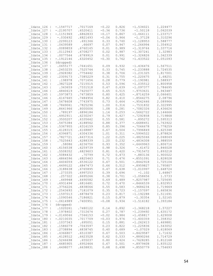
54

_Idate_126 | -.1547717 .7017169 -0.22 0.826 -1.534021 1.224477 _Idate_127 | -.2195707 .6520411 -0.34 0.736 -1.50118 1.062039 _Idate_128 | -.1151969 .6862833 -0.17 0.867 -1.464111 1.233717 _Idate_129 | -.030492 .6821493 -0.04 0.964 -1.37128 1.310296 _Idate_130 | .2299123 .691346 0.33 0.740 -1.128953 1.588777 _Idate_131 | .0439589 .66697 0.07 0.947 -1.266994 1.354912 _Idate_132 | .0089859 .6760145 0.01 0.989 -1.319744 1.337716 _Idate_133 | .0112943 .6708277 0.02 0.987 -1.307241 1.32983 _Idate_134 | .0077564 .6789919 0.01 0.991 -1.326826 1.342339 _Idate_135 | -.1912146 .6320452 -0.30 0.762 -1.433522 1.051093 _Idate_136 | (dropped) _Idate_137 | .0655177 .7641651 0.09 0.932 -1.436476 1.567511 _Idate_138 | .2453235 .7525744 0.33 0.745 -1.233888 1.724535 _Idate_139 | .2928382 .7754442 0.38 0.706 -1.231325 1.817001 _Idate_140 | .2309173 .7385229 0.31 0.755 -1.220675 1.68251 _Idate_141 | .198978 .7071656 0.28 0.779 -1.190981 1.588937 _Idate_142 | .3827228 .7215515 0.53 0.596 -1.035512 1.800958 _Idate_143 | .343659 .7331518 0.47 0.639 -1.097377 1.784695 _Idate_144 | .4840619 .7425077 0.65 0.515 -.9753631 1.943487 _Idate_145 | .5973873 .7473859 0.80 0.425 -.8716259 2.066401 _Idate_146 | .6167665 .7484954 0.82 0.410 -.8544275 2.08796 _Idate_147 | .5678608 .7743975 0.73 0.464 -.9542446 2.089966 _Idate_148 | .7849061 .7825296 1.00 0.316 -.7531832 2.322995 _Idate_149 | .8641966 .8000006 1.08 0.281 -.7082326 2.436626 _Idate_150 | .789197 .6896184 1.14 0.253 -.5662722 2.144666 _Idate_151 | .4952911 .6230247 0.79 0.427 -.7292858 1.719868 _Idate_152 | .3500207 .6335642 0.55 0.581 -.895272 1.595313 _Idate_153 | .5475384 .6188562 0.88 0.377 -.6688451 1.763922 _Idate_154 | .5367955 .6316159 0.85 0.396 -.7046678 1.778259 _Idate_155 | .4128315 .6168887 0.67 0.504 -.7996849 1.625348 _Idate_156 | .6396871 .6304336 1.01 0.311 -.5994522 1.878826 _Idate_157 | .7827721 .6437314 1.22 0.225 -.4825046 2.048049 _Idate_158 | .7525643 .6288339 1.20 0.232 -.4834308 1.988559 _Idate_159 | .58086 .6236756 0.93 0.352 -.6449963 1.806716 _Idate_160 | .6156538 .6259739 0.98 0.326 -.61472 1.846028 _Idate_161 | .5508352 .6829603 0.81 0.420 -.7915472 1.893218 _Idate_162 | .5084432 .70799 0.72 0.473 -.883136 1.900022 _Idate_163 | .4864596 .6825463 0.71 0.476 -.8551091 1.828028 _Idate_164 | .4404059 .6536122 0.67 0.501 -.8442918 1.725104 _Idate_165 | .4499122 .6847473 0.66 0.512 -.8959827 1.795807 _Idate_166 | .3188638 .6765895 0.47 0.638 -1.010997 1.648724 _Idate_167 | .273335 .6997253 0.39 0.696 -1.102 1.64867 _Idate_168 | .257322 .6695266 0.38 0.701 -1.058656 1.5733 _Idate_169 | .449948 .6490582 0.69 0.489 -.8257987 1.725695 _Idate_170 | .4931494 .6816481 0.72 0.470 -.8466539 1.832953 _Idate_171 | .3756226 .6838066 0.55 0.583 -.9684234 1.719669 _Idate_172 | .2543693 .7181079 0.35 0.723 -1.157097 1.665836 _Idate_173 | .1597013 .6878479 0.23 0.817 -1.192288 1.511691 _Idate_174 | .1090546 .7186821 0.15 0.879 -1.30354 1.52165 _Idate_175 | -.0614989 .7400951 -0.08 0.934 -1.516182 1.393184 _Idate_176 | (dropped) _Idate_177 | .1020261 .7480122 0.14 0.892 -1.368218 1.57227 _Idate_178 | .1978402 .7312674 0.27 0.787 -1.239492 1.635172 _Idate_179 | -.0149046 .7346153 -0.02 0.984 -1.458817 1.429008 _Idate_180 | -.0210035 .7017709 -0.03 0.976 -1.400359 1.358352 _Idate_181 | .1037343 .695051 0.15 0.881 -1.262413 1.469881 _Idate_182 | .1586079 .7043597 0.23 0.822 -1.225836 1.543052 _Idate_183 | .2738894 .6838745 0.40 0.689 -1.07029 1.618069 _Idate_184 | .4366807 .6510387 0.67 0.503 -.8429587 1.71632 _Idate_185 | .4128512 .6623528 0.62 0.533 -.8890266 1.714729 _Idate_186 | .5246698 .655037 0.80 0.424 -.7628285 1.812168 _Idate_187 | .4685905 .6952464 0.67 0.501 -.8979408 1.835122 _Idate_188 | .4498077 .6638831 0.68 0.498 -.8550779 1.754693

55

_Idate_189 | .5603188 .6946143 0.81 0.420 -.80497 1.925608 _Idate_190 | .6157967 .6848094 0.90 0.369 -.7302203 1.961814 _Idate_191 | .6394588 .7634246 0.84 0.403 -.861079 2.139997 _Idate_192 | .6835821 .685042 1.00 0.319 -.662892 2.030056 _Idate_193 | .6421532 .6813218 0.94 0.346 -.6970088 1.981315 _Idate_194 | .6517843 .6632381 0.98 0.326 -.6518334 1.955402 _Idate_195 | .2243136 .6948217 0.32 0.747 -1.141383 1.59001 _Idate_196 | .0852431 .6552732 0.13 0.897 -1.202719 1.373206 _Idate_197 | .3864095 .6763609 0.57 0.568 -.9430016 1.715821 _Idate_198 | .278139 .6595455 0.42 0.673 -1.018221 1.574499 _Idate_199 | .2990944 .702873 0.43 0.671 -1.082427 1.680616 _Idate_200 | .4584937 .6843344 0.67 0.503 -.8865897 1.803577 _Idate_201 | .4746061 .7334875 0.65 0.518 -.9670893 1.916301 _Idate_202 | .574136 .7056668 0.81 0.416 -.8128769 1.961149 _Idate_203 | .3265809 .7588185 0.43 0.667 -1.164904 1.818065 _Idate_204 | .3481893 .7139471 0.49 0.626 -1.055099 1.751477 _Idate_205 | .2487755 .7441422 0.33 0.738 -1.213862 1.711413 _Idate_206 | .2207875 .7208907 0.31 0.760 -1.196148 1.637723 _Idate_207 | (dropped) _cons | -14.87173 10.91169 -1.36 0.174 -36.31904 6.575579 ------------------------------------------------------------------------------ . xi: reg lnexpccd lnccdgdp lnphlgdp lnphlreercpi lnchireercpi lnccdreercpi lnd > istccd i.country i.date i.country _Icountry_1-5 (naturally coded; _Icountry_1 omitted) i.date _Idate_100-207 (naturally coded; _Idate_100 omitted) Source | SS df MS Number of obs = 538 -------------+------------------------------ F(113, 424) = 114.43 Model | 1045.34943 113 9.25087989 Prob > F = 0.0000 Residual | 34.2761399 424 .080839953 R-squared = 0.9683 -------------+------------------------------ Adj R-squared = 0.9598 Total | 1079.62557 537 2.01047592 Root MSE = .28432 ------------------------------------------------------------------------------ lnexpccd | Coef. Std. Err. t P>|t| [95% Conf. Interval] -------------+---------------------------------------------------------------- lnccdgdp | 1.092438 .0894028 12.22 0.000 .91671 1.268166 lnphlgdp | .6311058 .1995966 3.16 0.002 .2387837 1.023428 lnphlreercpi | -1.39517 .4938742 -2.82 0.005 -2.365917 -.4244235 lnchireercpi | .1771066 .2394166 0.74 0.460 -.2934847 .6476979 lnccdreercpi | .0869852 .1356696 0.64 0.522 -.1796835 .3536539 lndistccd | -1.929546 .0505063 -38.20 0.000 -2.02882 -1.830273 _Icountry_2 | 2.187057 .054638 40.03 0.000 2.079662 2.294452 _Icountry_3 | 1.225323 .0434708 28.19 0.000 1.139877 1.310768 _Icountry_4 | (dropped) _Icountry_5 | 4.80188 .0688752 69.72 0.000 4.666501 4.93726 _Idate_101 | -.0827771 .1778875 -0.47 0.642 -.4324283 .2668741 _Idate_102 | .0074338 .1812164 0.04 0.967 -.3487605 .3636281 _Idate_103 | -.2880011 .1637112 -1.76 0.079 -.6097877 .0337855 _Idate_104 | -.4317798 .1780583 -2.42 0.016 -.7817668 -.0817929 _Idate_105 | -.4794739 .1802614 -2.66 0.008 -.8337911 -.1251567 _Idate_106 | -.4795251 .1852641 -2.59 0.010 -.8436755 -.1153747 _Idate_107 | -.5268312 .1702456 -3.09 0.002 -.8614617 -.1922007 _Idate_108 | -.5263516 .1872323 -2.81 0.005 -.8943708 -.1583325 _Idate_109 | -.4384971 .1800552 -2.44 0.015 -.792409 -.0845852 _Idate_110 | -.356788 .1811875 -1.97 0.050 -.7129256 -.0006505 _Idate_111 | -.4528926 .179876 -2.52 0.012 -.8064523 -.0993329 _Idate_112 | -.4633241 .1927452 -2.40 0.017 -.8421792 -.084469 _Idate_113 | -.4029907 .1880808 -2.14 0.033 -.7726775 -.0333039 _Idate_114 | -.2953184 .1923149 -1.54 0.125 -.6733277 .0826909 _Idate_115 | -.5125602 .1890651 -2.71 0.007 -.8841818 -.1409387 _Idate_116 | -.4096025 .2000043 -2.05 0.041 -.8027259 -.016479

56

_Idate_117 | -.3040247 .1917315 -1.59 0.114 -.6808872 .0728378 _Idate_118 | -.2686231 .1875223 -1.43 0.153 -.6372123 .099966 _Idate_119 | -.4668688 .163206 -2.86 0.004 -.7876624 -.1460752 _Idate_120 | -.3717031 .1604046 -2.32 0.021 -.6869903 -.0564158 _Idate_121 | -.349676 .1576698 -2.22 0.027 -.6595879 -.0397642 _Idate_122 | -.3668136 .1732097 -2.12 0.035 -.7072702 -.0263571 _Idate_123 | -.6223289 .1821876 -3.42 0.001 -.9804322 -.2642257 _Idate_124 | -.5036988 .1834937 -2.75 0.006 -.8643694 -.1430283 _Idate_125 | -.3833121 .1667978 -2.30 0.022 -.7111656 -.0554587 _Idate_126 | -.2913863 .1628741 -1.79 0.074 -.6115276 .0287549 _Idate_127 | -.3459289 .151445 -2.28 0.023 -.6436054 -.0482525 _Idate_128 | -.2888037 .1592973 -1.81 0.071 -.6019145 .0243071 _Idate_129 | -.2307336 .1583511 -1.46 0.146 -.5419845 .0805173 _Idate_130 | -.0531197 .1605311 -0.33 0.741 -.3686556 .2624162 _Idate_131 | -.1440095 .1548465 -0.93 0.353 -.4483718 .1603528 _Idate_132 | -.1275677 .1569173 -0.81 0.417 -.4360004 .180865 _Idate_133 | -.0926396 .1557152 -0.59 0.552 -.3987095 .2134302 _Idate_134 | -.0572849 .1576217 -0.36 0.716 -.3671022 .2525324 _Idate_135 | -.2369226 .1466987 -1.62 0.107 -.5252699 .0514248 _Idate_136 | (dropped) _Idate_137 | .0907526 .1773526 0.51 0.609 -.2578472 .4393524 _Idate_138 | .2541768 .1746725 1.46 0.146 -.089155 .5975086 _Idate_139 | .3057696 .1799929 1.70 0.090 -.04802 .6595592 _Idate_140 | .269248 .1714082 1.57 0.117 -.0676676 .6061637 _Idate_141 | .239548 .1641308 1.46 0.145 -.0830633 .5621593 _Idate_142 | .3742542 .1674914 2.23 0.026 .0450373 .7034712 _Idate_143 | .3242676 .1701595 1.91 0.057 -.0101936 .6587287 _Idate_144 | .4402913 .1723598 2.55 0.011 .1015053 .7790773 _Idate_145 | .5550385 .1734889 3.20 0.001 .2140331 .896044 _Idate_146 | .5440756 .1737649 3.13 0.002 .2025278 .8856235 _Idate_147 | .476557 .1797322 2.65 0.008 .1232799 .829834 _Idate_148 | .6471358 .1816946 3.56 0.000 .2900015 1.00427 _Idate_149 | .7291515 .1857473 3.93 0.000 .3640512 1.094252 _Idate_150 | .6777282 .1601487 4.23 0.000 .3629439 .9925125 _Idate_151 | .4234714 .1446011 2.93 0.004 .1392471 .7076957 _Idate_152 | .3598038 .1471388 2.45 0.015 .0705915 .6490162 _Idate_153 | .4336218 .1437616 3.02 0.003 .1510477 .7161959 _Idate_154 | .3717057 .146762 2.53 0.012 .083234 .6601773 _Idate_155 | .3009804 .1431975 2.10 0.036 .0195151 .5824457 _Idate_156 | .4940188 .146465 3.37 0.001 .206131 .7819066 _Idate_157 | .6318511 .1495551 4.22 0.000 .3378894 .9258128 _Idate_158 | .6470661 .1460947 4.43 0.000 .3599061 .9342261 _Idate_159 | .5142671 .1447633 3.55 0.000 .229724 .7988103 _Idate_160 | .5138136 .1454404 3.53 0.000 .2279397 .7996875 _Idate_161 | .4508826 .1585199 2.84 0.005 .1392999 .7624654 _Idate_162 | .4328898 .1643254 2.63 0.009 .109896 .7558836 _Idate_163 | .4056743 .1584365 2.56 0.011 .0942555 .7170932 _Idate_164 | .2243693 .1518757 1.48 0.140 -.0741537 .5228923 _Idate_165 | .3210937 .1590949 2.02 0.044 .0083809 .6338066 _Idate_166 | .1630714 .1571412 1.04 0.300 -.1458015 .4719443 _Idate_167 | .1255417 .1624958 0.77 0.440 -.1938559 .4449392 _Idate_168 | .0899119 .155414 0.58 0.563 -.2155658 .3953896 _Idate_169 | .2651778 .1507665 1.76 0.079 -.0311651 .5615206 _Idate_170 | .3185734 .1583167 2.01 0.045 .00739 .6297567 _Idate_171 | .2206063 .1587188 1.39 0.165 -.0913674 .53258 _Idate_172 | .130401 .1666824 0.78 0.434 -.1972258 .4580277 _Idate_173 | .0404307 .1596496 0.25 0.800 -.2733725 .3542338 _Idate_174 | .0135447 .1668039 0.08 0.935 -.3143208 .3414103 _Idate_175 | -.0838941 .1718025 -0.49 0.626 -.4215848 .2537966 _Idate_176 | (dropped) _Idate_177 | .0604585 .1736064 0.35 0.728 -.2807779 .4016948 _Idate_178 | .1154491 .1697217 0.68 0.497 -.2181516 .4490499 _Idate_179 | -.0614072 .1705514 -0.36 0.719 -.3966387 .2738243

57

_Idate_180 | -.1129987 .162877 -0.69 0.488 -.4331456 .2071481 _Idate_181 | -.0004861 .1613225 -0.00 0.998 -.3175775 .3166053 _Idate_182 | .0279364 .1634859 0.17 0.864 -.2934075 .3492802 _Idate_183 | .0963058 .1587699 0.61 0.544 -.2157683 .4083799 _Idate_184 | .205833 .1511459 1.36 0.174 -.0912555 .5029215 _Idate_185 | .1909913 .1537574 1.24 0.215 -.1112303 .4932129 _Idate_186 | .2868993 .152076 1.89 0.060 -.0120174 .5858161 _Idate_187 | .208086 .1614202 1.29 0.198 -.1091974 .5253694 _Idate_188 | .1559579 .1541569 1.01 0.312 -.1470491 .4589649 _Idate_189 | .2533142 .1612736 1.57 0.117 -.063681 .5703095 _Idate_190 | .2951541 .159025 1.86 0.064 -.0174214 .6077296 _Idate_191 | .3389975 .177246 1.91 0.056 -.0093926 .6873877 _Idate_192 | .378768 .1592354 2.38 0.018 .0657789 .6917571 _Idate_193 | .3805616 .158232 2.41 0.017 .0695449 .6915784 _Idate_194 | .3642746 .1540897 2.36 0.019 .0613998 .6671494 _Idate_195 | .0036886 .1612919 0.02 0.982 -.3133428 .3207199 _Idate_196 | -.0916577 .1521694 -0.60 0.547 -.390758 .2074425 _Idate_197 | .2092177 .1570087 1.33 0.183 -.0993946 .5178301 _Idate_198 | .1423034 .1531268 0.93 0.353 -.1586787 .4432855 _Idate_199 | .2079116 .1631342 1.27 0.203 -.1127407 .528564 _Idate_200 | .3412617 .1588744 2.15 0.032 .0289823 .6535412 _Idate_201 | .3585178 .1702546 2.11 0.036 .0238697 .6931659 _Idate_202 | .4924102 .1638253 3.01 0.003 .1703994 .814421 _Idate_203 | .2865127 .1761123 1.63 0.105 -.0596492 .6326746 _Idate_204 | .296034 .1657394 1.79 0.075 -.0297393 .6218072 _Idate_205 | .2099692 .1727097 1.22 0.225 -.1295047 .5494431 _Idate_206 | .203075 .1673548 1.21 0.226 -.1258734 .5320235 _Idate_207 | (dropped) _cons | 18.66535 2.592947 7.20 0.000 13.56872 23.76199 ------------------------------------------------------------------------------

B.3. Wald’s Tests . quietly xi: reg lnexpccd lnccdgdp lnphlgdp lnphlreercpi lnchireercpi lnccdree > rcpi lndistccd i.country . test _Icountry_2 _Icountry_3 _Icountry_4 _Icountry_5 ( 1) _Icountry_2 = 0 ( 2) _Icountry_3 = 0 ( 3) _Icountry_4 = 0 ( 4) _Icountry_5 = 0 Constraint 3 dropped F( 3, 528) = 1863.09 Prob > F = 0.0000 quietly xi: reg lnexpccd lnccdgdp lnphlgdp lnphlreercpi lnchireercpi lnccdree > rcpi lndistccd i.date . . test _Idate_101 _Idate_101 _Idate_102 _Idate_103 _Idate_104 _Idate_105 _Idate > _106 _Idate_107 _Idate_108 _Idate_109 _Idate_110 _Idate_111 _Idate_112 _Idate > _113 _Idate_114 _Idate_115 _Idate_116 _Idate_117 _Idate_118 _Idate_119 _Idate > _120 _Idate_121 _Idate_122 _Idate_123 _Idate_124 _Idate_125 _Idate_126 _Idate > _127 _Idate_128 _Idate_129 _Idate_130 _Idate_131 _Idate_132 _Idate_133 _Idate > _134 _Idate_135 _Idate_136 _Idate_137 _Idate_138 _Idate_139 _Idate_140 _Idate > _141 _Idate_142 _Idate_143 _Idate_144 _Idate_145 _Idate_146 _Idate_147 _Idate > _148 _Idate_149 _Idate_150 _Idate_151 _Idate_152 _Idate_153 _Idate_154 _Idate > _155 _Idate_156 _Idate_157 _Idate_158 _Idate_159 _Idate_160 _Idate_161 _Idate > _162 _Idate_163 _Idate_164 _Idate_165 _Idate_166 _Idate_167 _Idate_168 _Idate > _169 _Idate_170 _Idate_171 _Idate_172 _Idate_173 _Idate_174 _Idate_175 _Idate > _176 _Idate_177 _Idate_178 _Idate_179 _Idate_180 _Idate_181 _Idate_182 _Idate > _183 _Idate_184 _Idate_185 _Idate_186 _Idate_187 _Idate_188 _Idate_189 _Idate

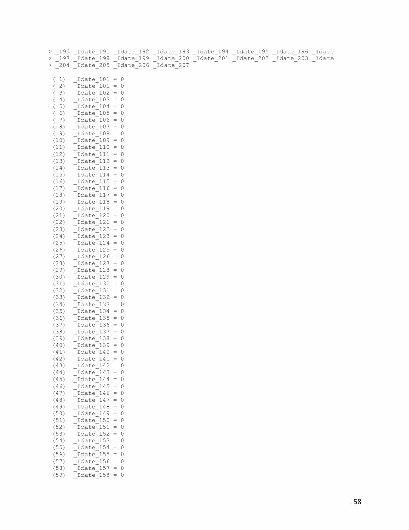
58

> _190 _Idate_191 _Idate_192 _Idate_193 _Idate_194 _Idate_195 _Idate_196 _Idate > _197 _Idate_198 _Idate_199 _Idate_200 _Idate_201 _Idate_202 _Idate_203 _Idate > _204 _Idate_205 _Idate_206 _Idate_207 ( 1) _Idate_101 = 0 ( 2) _Idate_101 = 0 ( 3) _Idate_102 = 0 ( 4) _Idate_103 = 0 ( 5) _Idate_104 = 0 ( 6) _Idate_105 = 0 ( 7) _Idate_106 = 0 ( 8) _Idate_107 = 0 ( 9) _Idate_108 = 0 (10) _Idate_109 = 0 (11) _Idate_110 = 0 (12) _Idate_111 = 0 (13) _Idate_112 = 0 (14) _Idate_113 = 0 (15) _Idate_114 = 0 (16) _Idate_115 = 0 (17) _Idate_116 = 0 (18) _Idate_117 = 0 (19) _Idate_118 = 0 (20) _Idate_119 = 0 (21) _Idate_120 = 0 (22) _Idate_121 = 0 (23) _Idate_122 = 0 (24) _Idate_123 = 0 (25) _Idate_124 = 0 (26) _Idate_125 = 0 (27) _Idate_126 = 0 (28) _Idate_127 = 0 (29) _Idate_128 = 0 (30) _Idate_129 = 0 (31) _Idate_130 = 0 (32) _Idate_131 = 0 (33) _Idate_132 = 0 (34) _Idate_133 = 0 (35) _Idate_134 = 0 (36) _Idate_135 = 0 (37) _Idate_136 = 0 (38) _Idate_137 = 0 (39) _Idate_138 = 0 (40) _Idate_139 = 0 (41) _Idate_140 = 0 (42) _Idate_141 = 0 (43) _Idate_142 = 0 (44) _Idate_143 = 0 (45) _Idate_144 = 0 (46) _Idate_145 = 0 (47) _Idate_146 = 0 (48) _Idate_147 = 0 (49) _Idate_148 = 0 (50) _Idate_149 = 0 (51) _Idate_150 = 0 (52) _Idate_151 = 0 (53) _Idate_152 = 0 (54) _Idate_153 = 0 (55) _Idate_154 = 0 (56) _Idate_155 = 0 (57) _Idate_156 = 0 (58) _Idate_157 = 0 (59) _Idate_158 = 0

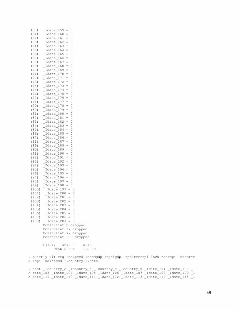
59

(60) _Idate_159 = 0 (61) _Idate_160 = 0 (62) _Idate_161 = 0 (63) _Idate_162 = 0 (64) _Idate_163 = 0 (65) _Idate_164 = 0 (66) _Idate_165 = 0 (67) _Idate_166 = 0 (68) _Idate_167 = 0 (69) _Idate_168 = 0 (70) _Idate_169 = 0 (71) _Idate_170 = 0 (72) _Idate_171 = 0 (73) _Idate_172 = 0 (74) _Idate_173 = 0 (75) _Idate_174 = 0 (76) _Idate_175 = 0 (77) _Idate_176 = 0 (78) _Idate_177 = 0 (79) _Idate_178 = 0 (80) _Idate_179 = 0 (81) _Idate_180 = 0 (82) _Idate_181 = 0 (83) _Idate_182 = 0 (84) _Idate_183 = 0 (85) _Idate_184 = 0 (86) _Idate_185 = 0 (87) _Idate_186 = 0 (88) _Idate_187 = 0 (89) _Idate_188 = 0 (90) _Idate_189 = 0 (91) _Idate_190 = 0 (92) _Idate_191 = 0 (93) _Idate_192 = 0 (94) _Idate_193 = 0 (95) _Idate_194 = 0 (96) _Idate_195 = 0 (97) _Idate_196 = 0 (98) _Idate_197 = 0 (99) _Idate_198 = 0 (100) _Idate_199 = 0 (101) _Idate_200 = 0 (102) _Idate_201 = 0 (103) _Idate_202 = 0 (104) _Idate_203 = 0 (105) _Idate_204 = 0 (106) _Idate_205 = 0 (107) _Idate_206 = 0 (108) _Idate_207 = 0 Constraint 2 dropped Constraint 37 dropped Constraint 77 dropped Constraint 108 dropped F(104, 427) = 0.16 Prob > F = 1.0000 . quietly xi: reg lnexpccd lnccdgdp lnphlgdp lnphlreercpi lnchireercpi lnccdree > rcpi lndistccd i.country i.date . test _Icountry_2 _Icountry_3 _Icountry_4 _Icountry_5 _Idate_101 _Idate_102 _I > date_103 _Idate_104 _Idate_105 _Idate_106 _Idate_107 _Idate_108 _Idate_109 _I > date_110 _Idate_110 _Idate_111 _Idate_112 _Idate_113 _Idate_114 _Idate_115 _I

60

> date_116 _Idate_117 _Idate_118 _Idate_119 _Idate_120 _Idate_121 _Idate_122 _I > date_123 _Idate_124 _Idate_125 _Idate_126 _Idate_127 _Idate_128 _Idate_129 _I > date_130 _Idate_131 _Idate_132 _Idate_133 _Idate_134 _Idate_135 _Idate_136 _I > date_137 _Idate_138 _Idate_139 _Idate_140 _Idate_141 _Idate_142 _Idate_143 _I > date_144 _Idate_145 _Idate_146 _Idate_147 _Idate_148 _Idate_149 _Idate_150 _I > date_151 _Idate_152 _Idate_153 _Idate_154 _Idate_155 _Idate_156 _Idate_157 _I > date_158 _Idate_159 _Idate_160 _Idate_161 _Idate_162 _Idate_163 _Idate_164 _I > date_165 _Idate_166 _Idate_167 _Idate_168 _Idate_169 _Idate_170 _Idate_171 _I > date_172 _Idate_173 _Idate_174 _Idate_175 _Idate_176 _Idate_177 _Idate_178 _I > date_179 _Idate_180 _Idate_181 _Idate_182 _Idate_183 _Idate_184 _Idate_185 _I > date_186 _Idate_187 _Idate_188 _Idate_189 _Idate_190 _Idate_191 _Idate_192 _I > date_193 _Idate_194 _Idate_195 _Idate_196 _Idate_197 _Idate_198 _Idate_199 _I > date_200 _Idate_201 _Idate_202 _Idate_203 _Idate_204 _Idate_205 _Idate_206 _I > date_207 ( 1) _Icountry_2 = 0 ( 2) _Icountry_3 = 0 ( 3) _Icountry_4 = 0 ( 4) _Icountry_5 = 0 ( 5) _Idate_101 = 0 ( 6) _Idate_102 = 0 ( 7) _Idate_103 = 0 ( 8) _Idate_104 = 0 ( 9) _Idate_105 = 0 (10) _Idate_106 = 0 (11) _Idate_107 = 0 (12) _Idate_108 = 0 (13) _Idate_109 = 0 (14) _Idate_110 = 0 (15) _Idate_110 = 0 (16) _Idate_111 = 0 (17) _Idate_112 = 0 (18) _Idate_113 = 0 (19) _Idate_114 = 0 (20) _Idate_115 = 0 (21) _Idate_116 = 0 (22) _Idate_117 = 0 (23) _Idate_118 = 0 (24) _Idate_119 = 0 (25) _Idate_120 = 0 (26) _Idate_121 = 0 (27) _Idate_122 = 0 (28) _Idate_123 = 0 (29) _Idate_124 = 0 (30) _Idate_125 = 0 (31) _Idate_126 = 0 (32) _Idate_127 = 0 (33) _Idate_128 = 0 (34) _Idate_129 = 0 (35) _Idate_130 = 0 (36) _Idate_131 = 0 (37) _Idate_132 = 0 (38) _Idate_133 = 0 (39) _Idate_134 = 0 (40) _Idate_135 = 0 (41) _Idate_136 = 0 (42) _Idate_137 = 0 (43) _Idate_138 = 0 (44) _Idate_139 = 0 (45) _Idate_140 = 0 (46) _Idate_141 = 0 (47) _Idate_142 = 0 (48) _Idate_143 = 0

61

(49) _Idate_144 = 0 (50) _Idate_145 = 0 (51) _Idate_146 = 0 (52) _Idate_147 = 0 (53) _Idate_148 = 0 (54) _Idate_149 = 0 (55) _Idate_150 = 0 (56) _Idate_151 = 0 (57) _Idate_152 = 0 (58) _Idate_153 = 0 (59) _Idate_154 = 0 (60) _Idate_155 = 0 (61) _Idate_156 = 0 (62) _Idate_157 = 0 (63) _Idate_158 = 0 (64) _Idate_159 = 0 (65) _Idate_160 = 0 (66) _Idate_161 = 0 (67) _Idate_162 = 0 (68) _Idate_163 = 0 (69) _Idate_164 = 0 (70) _Idate_165 = 0 (71) _Idate_166 = 0 (72) _Idate_167 = 0 (73) _Idate_168 = 0 (74) _Idate_169 = 0 (75) _Idate_170 = 0 (76) _Idate_171 = 0 (77) _Idate_172 = 0 (78) _Idate_173 = 0 (79) _Idate_174 = 0 (80) _Idate_175 = 0 (81) _Idate_176 = 0 (82) _Idate_177 = 0 (83) _Idate_178 = 0 (84) _Idate_179 = 0 (85) _Idate_180 = 0 (86) _Idate_181 = 0 (87) _Idate_182 = 0 (88) _Idate_183 = 0 (89) _Idate_184 = 0 (90) _Idate_185 = 0 (91) _Idate_186 = 0 (92) _Idate_187 = 0 (93) _Idate_188 = 0 (94) _Idate_189 = 0 (95) _Idate_190 = 0 (96) _Idate_191 = 0 (97) _Idate_192 = 0 (98) _Idate_193 = 0 (99) _Idate_194 = 0 (100) _Idate_195 = 0 (101) _Idate_196 = 0 (102) _Idate_197 = 0 (103) _Idate_198 = 0 (104) _Idate_199 = 0 (105) _Idate_200 = 0 (106) _Idate_201 = 0 (107) _Idate_202 = 0 (108) _Idate_203 = 0 (109) _Idate_204 = 0 (110) _Idate_205 = 0 (111) _Idate_206 = 0

62

(112) _Idate_207 = 0 Constraint 3 dropped Constraint 15 dropped Constraint 41 dropped Constraint 81 dropped Constraint 112 dropped F(107, 424) = 73.01 Prob > F = 0.0000 . quietly xi: reg lnexpccd lnccdgdp lnphlgdp lnphlreercpi lnchireercpi lnccdree > rcpi lndistccd i.country i.date . . test _Idate_101 _Idate_101 _Idate_102 _Idate_103 _Idate_104 _Idate_105 _Idate > _106 _Idate_107 _Idate_108 _Idate_109 _Idate_110 _Idate_111 _Idate_112 _Idate > _113 _Idate_114 _Idate_115 _Idate_116 _Idate_117 _Idate_118 _Idate_119 _Idate > _120 _Idate_121 _Idate_122 _Idate_123 _Idate_124 _Idate_125 _Idate_126 _Idate > _127 _Idate_128 _Idate_129 _Idate_130 _Idate_131 _Idate_132 _Idate_133 _Idate > _134 _Idate_135 _Idate_136 _Idate_137 _Idate_138 _Idate_139 _Idate_140 _Idate > _141 _Idate_142 _Idate_143 _Idate_144 _Idate_145 _Idate_146 _Idate_147 _Idate > _148 _Idate_149 _Idate_150 _Idate_151 _Idate_152 _Idate_153 _Idate_154 _Idate > _155 _Idate_156 _Idate_157 _Idate_158 _Idate_159 _Idate_160 _Idate_161 _Idate > _162 _Idate_163 _Idate_164 _Idate_165 _Idate_166 _Idate_167 _Idate_168 _Idate > _169 _Idate_170 _Idate_171 _Idate_172 _Idate_173 _Idate_174 _Idate_175 _Idate > _176 _Idate_177 _Idate_178 _Idate_179 _Idate_180 _Idate_181 _Idate_182 _Idate > _183 _Idate_184 _Idate_185 _Idate_186 _Idate_187 _Idate_188 _Idate_189 _Idate > _190 _Idate_191 _Idate_192 _Idate_193 _Idate_194 _Idate_195 _Idate_196 _Idate > _197 _Idate_198 _Idate_199 _Idate_200 _Idate_201 _Idate_202 _Idate_203 _Idate > _204 _Idate_205 _Idate_206 _Idate_207 ( 1) _Idate_101 = 0 ( 2) _Idate_101 = 0 ( 3) _Idate_102 = 0 ( 4) _Idate_103 = 0 ( 5) _Idate_104 = 0 ( 6) _Idate_105 = 0 ( 7) _Idate_106 = 0 ( 8) _Idate_107 = 0 ( 9) _Idate_108 = 0 (10) _Idate_109 = 0 (11) _Idate_110 = 0 (12) _Idate_111 = 0 (13) _Idate_112 = 0 (14) _Idate_113 = 0 (15) _Idate_114 = 0 (16) _Idate_115 = 0 (17) _Idate_116 = 0 (18) _Idate_117 = 0 (19) _Idate_118 = 0 (20) _Idate_119 = 0 (21) _Idate_120 = 0 (22) _Idate_121 = 0 (23) _Idate_122 = 0 (24) _Idate_123 = 0 (25) _Idate_124 = 0 (26) _Idate_125 = 0 (27) _Idate_126 = 0 (28) _Idate_127 = 0 (29) _Idate_128 = 0 (30) _Idate_129 = 0 (31) _Idate_130 = 0 (32) _Idate_131 = 0

63

(33) _Idate_132 = 0 (34) _Idate_133 = 0 (35) _Idate_134 = 0 (36) _Idate_135 = 0 (37) _Idate_136 = 0 (38) _Idate_137 = 0 (39) _Idate_138 = 0 (40) _Idate_139 = 0 (41) _Idate_140 = 0 (42) _Idate_141 = 0 (43) _Idate_142 = 0 (44) _Idate_143 = 0 (45) _Idate_144 = 0 (46) _Idate_145 = 0 (47) _Idate_146 = 0 (48) _Idate_147 = 0 (49) _Idate_148 = 0 (50) _Idate_149 = 0 (51) _Idate_150 = 0 (52) _Idate_151 = 0 (53) _Idate_152 = 0 (54) _Idate_153 = 0 (55) _Idate_154 = 0 (56) _Idate_155 = 0 (57) _Idate_156 = 0 (58) _Idate_157 = 0 (59) _Idate_158 = 0 (60) _Idate_159 = 0 (61) _Idate_160 = 0 (62) _Idate_161 = 0 (63) _Idate_162 = 0 (64) _Idate_163 = 0 (65) _Idate_164 = 0 (66) _Idate_165 = 0 (67) _Idate_166 = 0 (68) _Idate_167 = 0 (69) _Idate_168 = 0 (70) _Idate_169 = 0 (71) _Idate_170 = 0 (72) _Idate_171 = 0 (73) _Idate_172 = 0 (74) _Idate_173 = 0 (75) _Idate_174 = 0 (76) _Idate_175 = 0 (77) _Idate_176 = 0 (78) _Idate_177 = 0 (79) _Idate_178 = 0 (80) _Idate_179 = 0 (81) _Idate_180 = 0 (82) _Idate_181 = 0 (83) _Idate_182 = 0 (84) _Idate_183 = 0 (85) _Idate_184 = 0 (86) _Idate_185 = 0 (87) _Idate_186 = 0 (88) _Idate_187 = 0 (89) _Idate_188 = 0 (90) _Idate_189 = 0 (91) _Idate_190 = 0 (92) _Idate_191 = 0 (93) _Idate_192 = 0 (94) _Idate_193 = 0 (95) _Idate_194 = 0

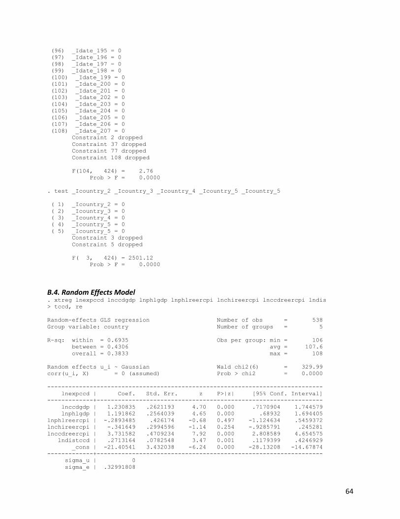
64

(96) _Idate_195 = 0 (97) _Idate_196 = 0 (98) _Idate_197 = 0 (99) _Idate_198 = 0 (100) _Idate_199 = 0 (101) _Idate_200 = 0 (102) _Idate_201 = 0 (103) _Idate_202 = 0 (104) _Idate_203 = 0 (105) _Idate_204 = 0 (106) _Idate_205 = 0 (107) _Idate_206 = 0 (108) _Idate_207 = 0 Constraint 2 dropped Constraint 37 dropped Constraint 77 dropped Constraint 108 dropped F(104, 424) = 2.76 Prob > F = 0.0000 . test _Icountry_2 _Icountry_3 _Icountry_4 _Icountry_5 _Icountry_5 ( 1) _Icountry_2 = 0 ( 2) _Icountry_3 = 0 ( 3) _Icountry_4 = 0 ( 4) _Icountry_5 = 0 ( 5) _Icountry_5 = 0 Constraint 3 dropped Constraint 5 dropped F( 3, 424) = 2501.12 Prob > F = 0.0000

B.4. Random Effects Model . xtreg lnexpccd lnccdgdp lnphlgdp lnphlreercpi lnchireercpi lnccdreercpi lndis > tccd, re Random-effects GLS regression Number of obs = 538 Group variable: country Number of groups = 5 R-sq: within = 0.6935 Obs per group: min = 106 between = 0.4306 avg = 107.6 overall = 0.3833 max = 108 Random effects u_i ~ Gaussian Wald chi2(6) = 329.99 corr(u_i, X) = 0 (assumed) Prob > chi2 = 0.0000 ------------------------------------------------------------------------------ lnexpccd | Coef. Std. Err. z P>|z| [95% Conf. Interval] -------------+---------------------------------------------------------------- lnccdgdp | 1.230835 .2621193 4.70 0.000 .7170904 1.744579 lnphlgdp | 1.191862 .2564039 4.65 0.000 .68932 1.694405 lnphlreercpi | -.2893485 .426174 -0.68 0.497 -1.124634 .5459372 lnchireercpi | -.341649 .2994596 -1.14 0.254 -.9285791 .245281 lnccdreercpi | 3.731582 .4709234 7.92 0.000 2.808589 4.654575 lndistccd | .2713164 .0782548 3.47 0.001 .1179399 .4246929 _cons | -21.40541 3.432038 -6.24 0.000 -28.13208 -14.67874 -------------+---------------------------------------------------------------- sigma_u | 0 sigma_e | .32991808

65

rho | 0 (fraction of variance due to u_i) ------------------------------------------------------------------------------ B.5. Breusch Pagan Test for Random Effects . xttest0 Breusch and Pagan Lagrangian multiplier test for random effects lnexpccd[country,t] = Xb + u[country] + e[country,t] Estimated results: | Var sd = sqrt(Var) ---------+----------------------------- lnexpccd | 2.010476 1.417913 e | .1088459 .3299181 u | 0 0 Test: Var(u) = 0 chi2(1) = 19147.89 Prob > chi2 = 0.0000

B.6. Hausman Test . quietly xi: reg lnexpccd lnccdgdp lnphlgdp lnphlreercpi lnchireercpi lnccdree > rcpi lndistccd i.country i.date . . est store fixed . quietly xtreg lnexpccd lnccdgdp lnphlgdp lnphlreercpi lnchireercpi lnccdreerc > pi lndistccd ,re . . est store random . hausman fixed random ---- Coefficients ---- | (b) (B) (b-B) sqrt(diag(V_b-V_B)) | fixed random Difference S.E. -------------+---------------------------------------------------------------- lnccdgdp | 1.092438 1.230835 -.1383968 . lnphlgdp | .6311058 1.191862 -.5607566 . lnphlreercpi | -1.39517 -.2893485 -1.105822 .2495744 lnchireercpi | .1771066 -.341649 .5187556 . lnccdreercpi | .0869852 3.731582 -3.644597 . lndistccd | -1.929546 .2713164 -2.200863 . ------------------------------------------------------------------------------ b = consistent under Ho and Ha; obtained from regress B = inconsistent under Ha, efficient under Ho; obtained from xtreg Test: Ho: difference in coefficients not systematic chi2(6) = (b-B)'[(V_b-V_B)^(-1)](b-B) = -1458.20 chi2<0 ==> model fitted on these data fails to meet the asymptotic assumptions of the Hausman test; see suest for a generalized test

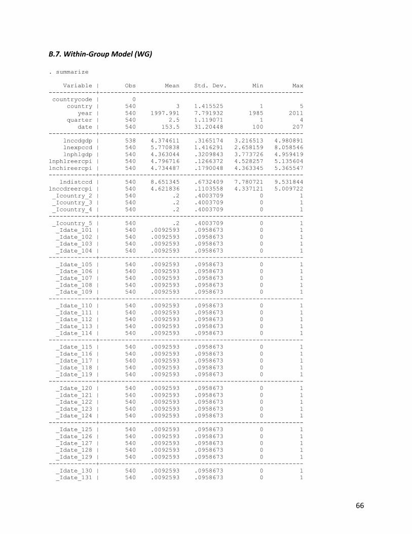
66

B.7. Within-‐Group Model (WG) . summarize Variable | Obs Mean Std. Dev. Min Max -------------+-------------------------------------------------------- countrycode | 0 country | 540 3 1.415525 1 5 year | 540 1997.991 7.791932 1985 2011 quarter | 540 2.5 1.119071 1 4 date | 540 153.5 31.20448 100 207 -------------+-------------------------------------------------------- lnccdgdp | 538 4.374611 .3165174 3.216513 4.980891 lnexpccd | 540 5.770838 1.416291 2.658159 8.058546 lnphlgdp | 540 4.363044 .3209843 3.773726 4.959419 lnphlreercpi | 540 4.796716 .1266372 4.528257 5.135604 lnchireercpi | 540 4.734487 .1790048 4.363345 5.365547 -------------+-------------------------------------------------------- lndistccd | 540 8.651345 .6732409 7.780721 9.531844 lnccdreercpi | 540 4.621836 .1103558 4.337121 5.009722 _Icountry_2 | 540 .2 .4003709 0 1 _Icountry_3 | 540 .2 .4003709 0 1 _Icountry_4 | 540 .2 .4003709 0 1 -------------+-------------------------------------------------------- _Icountry_5 | 540 .2 .4003709 0 1 _Idate_101 | 540 .0092593 .0958673 0 1 _Idate_102 | 540 .0092593 .0958673 0 1 _Idate_103 | 540 .0092593 .0958673 0 1 _Idate_104 | 540 .0092593 .0958673 0 1 -------------+-------------------------------------------------------- _Idate_105 | 540 .0092593 .0958673 0 1 _Idate_106 | 540 .0092593 .0958673 0 1 _Idate_107 | 540 .0092593 .0958673 0 1 _Idate_108 | 540 .0092593 .0958673 0 1 _Idate_109 | 540 .0092593 .0958673 0 1 -------------+-------------------------------------------------------- _Idate_110 | 540 .0092593 .0958673 0 1 _Idate_111 | 540 .0092593 .0958673 0 1 _Idate_112 | 540 .0092593 .0958673 0 1 _Idate_113 | 540 .0092593 .0958673 0 1 _Idate_114 | 540 .0092593 .0958673 0 1 -------------+-------------------------------------------------------- _Idate_115 | 540 .0092593 .0958673 0 1 _Idate_116 | 540 .0092593 .0958673 0 1 _Idate_117 | 540 .0092593 .0958673 0 1 _Idate_118 | 540 .0092593 .0958673 0 1 _Idate_119 | 540 .0092593 .0958673 0 1 -------------+-------------------------------------------------------- _Idate_120 | 540 .0092593 .0958673 0 1 _Idate_121 | 540 .0092593 .0958673 0 1 _Idate_122 | 540 .0092593 .0958673 0 1 _Idate_123 | 540 .0092593 .0958673 0 1 _Idate_124 | 540 .0092593 .0958673 0 1 -------------+-------------------------------------------------------- _Idate_125 | 540 .0092593 .0958673 0 1 _Idate_126 | 540 .0092593 .0958673 0 1 _Idate_127 | 540 .0092593 .0958673 0 1 _Idate_128 | 540 .0092593 .0958673 0 1 _Idate_129 | 540 .0092593 .0958673 0 1 -------------+-------------------------------------------------------- _Idate_130 | 540 .0092593 .0958673 0 1 _Idate_131 | 540 .0092593 .0958673 0 1

67

_Idate_132 | 540 .0092593 .0958673 0 1 _Idate_133 | 540 .0092593 .0958673 0 1 _Idate_134 | 540 .0092593 .0958673 0 1 -------------+-------------------------------------------------------- _Idate_135 | 540 .0092593 .0958673 0 1 _Idate_136 | 540 .0092593 .0958673 0 1 _Idate_137 | 540 .0092593 .0958673 0 1 _Idate_138 | 540 .0092593 .0958673 0 1 _Idate_139 | 540 .0092593 .0958673 0 1 -------------+-------------------------------------------------------- _Idate_140 | 540 .0092593 .0958673 0 1 _Idate_141 | 540 .0092593 .0958673 0 1 _Idate_142 | 540 .0092593 .0958673 0 1 _Idate_143 | 540 .0092593 .0958673 0 1 _Idate_144 | 540 .0092593 .0958673 0 1 -------------+-------------------------------------------------------- _Idate_145 | 540 .0092593 .0958673 0 1 _Idate_146 | 540 .0092593 .0958673 0 1 _Idate_147 | 540 .0092593 .0958673 0 1 _Idate_148 | 540 .0092593 .0958673 0 1 _Idate_149 | 540 .0092593 .0958673 0 1 -------------+-------------------------------------------------------- _Idate_150 | 540 .0092593 .0958673 0 1 _Idate_151 | 540 .0092593 .0958673 0 1 _Idate_152 | 540 .0092593 .0958673 0 1 _Idate_153 | 540 .0092593 .0958673 0 1 _Idate_154 | 540 .0092593 .0958673 0 1 -------------+-------------------------------------------------------- _Idate_155 | 540 .0092593 .0958673 0 1 _Idate_156 | 540 .0092593 .0958673 0 1 _Idate_157 | 540 .0092593 .0958673 0 1 _Idate_158 | 540 .0092593 .0958673 0 1 _Idate_159 | 540 .0092593 .0958673 0 1 -------------+-------------------------------------------------------- _Idate_160 | 540 .0092593 .0958673 0 1 _Idate_161 | 540 .0092593 .0958673 0 1 _Idate_162 | 540 .0092593 .0958673 0 1 _Idate_163 | 540 .0092593 .0958673 0 1 _Idate_164 | 540 .0092593 .0958673 0 1 -------------+-------------------------------------------------------- _Idate_165 | 540 .0092593 .0958673 0 1 _Idate_166 | 540 .0092593 .0958673 0 1 _Idate_167 | 540 .0092593 .0958673 0 1 _Idate_168 | 540 .0092593 .0958673 0 1 _Idate_169 | 540 .0092593 .0958673 0 1 -------------+-------------------------------------------------------- _Idate_170 | 540 .0092593 .0958673 0 1 _Idate_171 | 540 .0092593 .0958673 0 1 _Idate_172 | 540 .0092593 .0958673 0 1 _Idate_173 | 540 .0092593 .0958673 0 1 _Idate_174 | 540 .0092593 .0958673 0 1 -------------+-------------------------------------------------------- _Idate_175 | 540 .0092593 .0958673 0 1 _Idate_176 | 540 .0092593 .0958673 0 1 _Idate_177 | 540 .0092593 .0958673 0 1 _Idate_178 | 540 .0092593 .0958673 0 1 _Idate_179 | 540 .0092593 .0958673 0 1 -------------+-------------------------------------------------------- _Idate_180 | 540 .0092593 .0958673 0 1 _Idate_181 | 540 .0092593 .0958673 0 1 _Idate_182 | 540 .0092593 .0958673 0 1 _Idate_183 | 540 .0092593 .0958673 0 1 _Idate_184 | 540 .0092593 .0958673 0 1

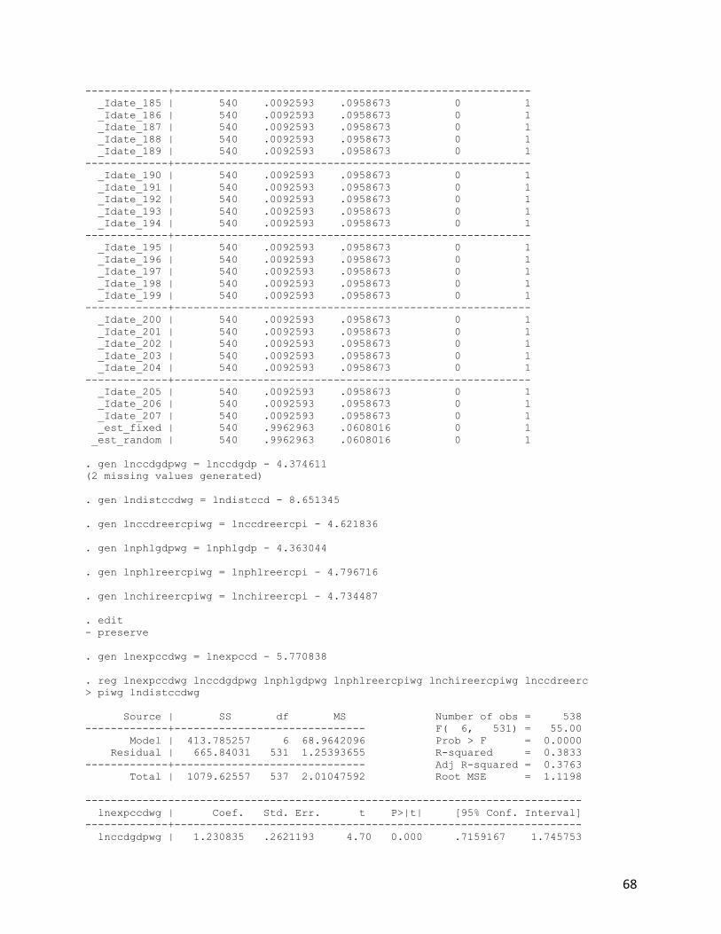
68

-------------+-------------------------------------------------------- _Idate_185 | 540 .0092593 .0958673 0 1 _Idate_186 | 540 .0092593 .0958673 0 1 _Idate_187 | 540 .0092593 .0958673 0 1 _Idate_188 | 540 .0092593 .0958673 0 1 _Idate_189 | 540 .0092593 .0958673 0 1 -------------+-------------------------------------------------------- _Idate_190 | 540 .0092593 .0958673 0 1 _Idate_191 | 540 .0092593 .0958673 0 1 _Idate_192 | 540 .0092593 .0958673 0 1 _Idate_193 | 540 .0092593 .0958673 0 1 _Idate_194 | 540 .0092593 .0958673 0 1 -------------+-------------------------------------------------------- _Idate_195 | 540 .0092593 .0958673 0 1 _Idate_196 | 540 .0092593 .0958673 0 1 _Idate_197 | 540 .0092593 .0958673 0 1 _Idate_198 | 540 .0092593 .0958673 0 1 _Idate_199 | 540 .0092593 .0958673 0 1 -------------+-------------------------------------------------------- _Idate_200 | 540 .0092593 .0958673 0 1 _Idate_201 | 540 .0092593 .0958673 0 1 _Idate_202 | 540 .0092593 .0958673 0 1 _Idate_203 | 540 .0092593 .0958673 0 1 _Idate_204 | 540 .0092593 .0958673 0 1 -------------+-------------------------------------------------------- _Idate_205 | 540 .0092593 .0958673 0 1 _Idate_206 | 540 .0092593 .0958673 0 1 _Idate_207 | 540 .0092593 .0958673 0 1 _est_fixed | 540 .9962963 .0608016 0 1 _est_random | 540 .9962963 .0608016 0 1 . gen lnccdgdpwg = lnccdgdp - 4.374611 (2 missing values generated) . gen lndistccdwg = lndistccd - 8.651345 . gen lnccdreercpiwg = lnccdreercpi - 4.621836 . gen lnphlgdpwg = lnphlgdp - 4.363044 . gen lnphlreercpiwg = lnphlreercpi - 4.796716 . gen lnchireercpiwg = lnchireercpi - 4.734487 . edit - preserve . gen lnexpccdwg = lnexpccd - 5.770838 . reg lnexpccdwg lnccdgdpwg lnphlgdpwg lnphlreercpiwg lnchireercpiwg lnccdreerc > piwg lndistccdwg Source | SS df MS Number of obs = 538 -------------+------------------------------ F( 6, 531) = 55.00 Model | 413.785257 6 68.9642096 Prob > F = 0.0000 Residual | 665.84031 531 1.25393655 R-squared = 0.3833 -------------+------------------------------ Adj R-squared = 0.3763 Total | 1079.62557 537 2.01047592 Root MSE = 1.1198 ------------------------------------------------------------------------------ lnexpccdwg | Coef. Std. Err. t P>|t| [95% Conf. Interval] -------------+---------------------------------------------------------------- lnccdgdpwg | 1.230835 .2621193 4.70 0.000 .7159167 1.745753

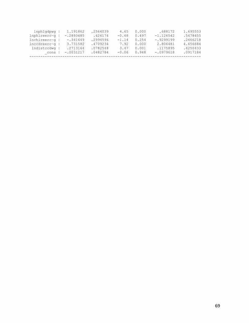
69

lnphlgdpwg | 1.191862 .2564039 4.65 0.000 .688172 1.695553 lnphlreerc~g | -.2893485 .426174 -0.68 0.497 -1.126542 .5478455 lnchireerc~g | -.341649 .2994596 -1.14 0.254 -.9299199 .2466218 lnccdreerc~g | 3.731582 .4709234 7.92 0.000 2.806481 4.656684 lndistccdwg | .2713164 .0782548 3.47 0.001 .1175895 .4250433 _cons | -.0031217 .0482784 -0.06 0.948 -.0979618 .0917184 ------------------------------------------------------------------------------

Javier,Pagaduan,Punsalang ECOMETV26

Documents

Transcript of Javier,Pagaduan,Punsalang ECOMETV26