B~ulking Failures In Cliile r,ullHg 'rLc

Perio(l ()f It'illaHcial J j heralisat ion

Ivan Araya GOluez B.Sc., tvLSc.

Thesis submitted to the University of lJottingharn for lheDegree of Doctor of Philosophy

()ctober 1996

,

BEST COpy

..

, . AVAILABLE

, V,ariable print quality

List Qf contents.

Page

List of contents Abstract List of Tables List of Figures Appendices Acknowledgement Author's Declaration

Chapter 1. Introduction.

1.1 Background to the study

1.2 Aims, Methodology and structure of the study

Chapter 2. From Financial Repression to Financial Liberalisation: Chile in 1970-1983.

i i iii vii xiii xvii xviii xix

1

8

2.1 Introduction 17

2.2

2.2.1 2.2.2

2.3

2.3.1

2.3.2 2.3.2.1

2.3.2.2

2 . 3 . 2 . 3 2.3.2.4

The Banking System and Financial Repression 19 in Chile: The Pre-Liberalisation Period Financial Repression and Economic Development 19 The Evidence of Financial Repression for Chile 31 and Some Selected Countries

The Banking System and Financial 52 Liberalisation in Chile: 1973-1983. Financial Liberalisation in Chile: What was 52 Done ? The Impact of Financial Liberalisation in Chile 61 Financial Deepening, Saving and Investment in Chile 63 Financial Indebtness and Interest Rates Chile Operative Efficiency in Chilean Banks Financial Stability in Chile

in 76 98 100

Chapter 3. Banking Failures in Chile During 1981-83

3.1

3.2

Introduction

The stylised Facts and the Magnitude of Banking Failures in Chile 1981-83

i i

107

108

3.2.1

3.2.2

The Chronology and the stylised Facts of the Crises An Autopsy of the Banking Sector

3.3 The Rehabilitation of the Banking System: A

109 116

Quick Glimpse on the Treatment and its Results 134

Chapter 4. Bank Failures and Banking Instability: A Review of the Theory

4.1 Introduction

4.2 The Issue of Existence of Financial Intermediaries

4 .3

4.3.1 4 . 3 . 2

4.4

4.4.1 4 . 4 . 2 4.4.2.1 4 . 4 . 2 . 2 4.4.3

4.5

4.6

Financial Intermediaries as Information Producers and Liquidity Insurers Banks as Information Producers Banks as Liquidity Insurers

Theories of Bank Failures and Banking Instability Banking Panics and Bank Failures External and Internal Factors in Bank Failures External Factors in Bank Failures Internal Factors in Bank Failures The Role of Moral Hazard in Bank Failures

The Importance of Bank Failures

Two Testable Hypotheses for the Chilean Bank Failures

Chapter 5. Banking Failures: Some Empirical Studies and the Econometric Methodology

5.1

5.2

5.3 5. 3 .1 5.3.2 5.3. 3 5.3.4

Introduction

Previous Empirical Studies

Binary-Choice and Logit Models The Logit Model Estimation of the Logit Model Hypothesis Testing Model Selection

iii

154

155

158 158 165

169 169 174 181 189 192

220

223

236

237

255 256 261 264 267

Chapter 6. The Discrete Dependent Variable:

6.1

6.2

6.2.1 6.2.2

6.3

6.3.1 6.3.2

Predictions from an Early Warning Model

Introduction

Development of a Failure/Problem-Prediction Model Failure/Problem Model: The Dependent Variable Variables Categories and Financial Ratios as Regressors

The Empirical Results from Failure/Problem Model for Chile Univariate Results Multivariate Results

Chapter 7. The Bank Failures in Chile: The Role of Macroeconomic Factors

7.1

7.2

7.3

7.3.1

7 . 3 . 2

7 • 3 • 3

7 • 4

7.4.1 7.4.1.1 7.4.1.2 7.4.2

Introduction

Macroeconomic Instability and the Banking Crises

The Boom-Bust Economic Cycle: The Macroeconomy in Chile The Chilean Economy and the Main Policy Reforms The Boom-Bust Economic Cycle of the Chilean Economy: The Appraisal The Boom-Bust Economic Cycle and the Increase Vulnerability of the Chilean Banking System

Econometric Analysis of Bank Failures: The Macro Aspect The Econometric Model Description of the Data Model Specification and Estimation The Econometric Results and Its Interpretation

Chapter 8. The Bank Failures in Chile: The Role of Moral Hazard

8.1 Introduction

8.2 Financial Liberalisation and Moral Hazard

8.3 The Evidence from Chile

iv

273

274 274

279

282 283 290

302

303

310

310

316

330

347 348 348 352 361

378

379

381

8.4

8. 4 . 1 8.4.2 8 . 4 . 2 . 1 8.4.2.2 8.4.3

Bank Failures and the Role of Moral Hazard: A Testable Model for Chile

General Framework The Model and the Econometric Specification Model Specification and Estimation Description of the Data and the Variables Econometric Results and Its Interpretation

395

396 400 400 412 417

Chapter 9. Some Predictions of the Loqit Model for Chile

9.1 Introduction 476

9.2 The Econometric Testing of Non-Nested Logit Models: Macroeconomic Hypothesis vs. Moral Hazard 477

9.3 Simple Aggregate Predictions from the Logit Models 481

Chapter 10. Conclusions

10.1 Summary of the Main Conclusions from the Study 487

10.2 Limitations of the Study and Further Research 490

v

Abstract.

It is argued that the banking crisis in Chile had its origin in the deterioration of key macroeconomic variables and that financial liberalisation played a secondary role. Proponents contend that no financial system can be expected to withstand a fall in output of nearly 15% in 1982 and they draw parallels here with the banking crisis of the 1930's in the US. On the other side, it is argued that the ability of the financial system to withstand any macroeconomic shock have been shaped by the financial liberalisation which took place in the years before the collapse of the macroeconomy. Conduct derived from ownership concentration and "related portfolios", sharp deregulation on interest rates, belief in an implicit bail-out provision, and the ineffective and inadequate prudential regulation led to pervasive banking structure and a pattern of behaviour marked by moral hazard. As a result, banks exhibited excessive risk taking with a deterioration of banks' financial position. Only the prompt rescue by the Central Bank of leading financial institutions averted a massive loss of confidence and a bank run.

This thesis examines the evolution of the Chilean financial system during the period of economic reforms and banking failures. Three specific questions are examined and evaluated empirically: How important was the adverse macroeconomic environment relative to the banking conduct and management which exhibited considerable moral hazard and adverse selection type of behavior in the banking failures in Chile ? Secondly, in what ways might a more favorable general economic conditions and/or a more effective prudential regulation have helped to reduce the likelihood of bank failures? Finally, might some of the bank failures been anticipated years before the crisis by an early warning system ?

In order to answer these questions this thesis develops a logit model for cross-section and panel data with information from banks' balance sheets to estimate the probability of bank failure/problem for the period between 1979 and 1983.

vi

List of Tables.

Chapter 2.

Table 2.1

Table 2.2

Table 2.3

Table 2.4

Table 2.5

Table 2.6

Table 2.7a

Table 2.7b

Table 2.8

Table 2.9

Table 2.10a

Table 2.10b

Table 2.10c

Table 2.10d

Table 2.10e

Table 2.11a

Table 2.11b

Table 2.11c

Table 2.11d

Indicators of Financial Deepening for Chile and Selected Countries

Effective Reserve Ratios for Chile and Selected Countries

Revenues from Inflation Tax on Currency

Revenues from Inflation Tax on Bank Reserves

Total Revenues from Inflation Tax

Real Deposit Rate in Chile and Selected

33

35

38

39

40

Countries 42

Interest Rates, Inflation Rates and Financial Savings in Chile and Selected Emerging Economies 44

Interest Rates, Inflation Financial Savings in Industrialised Countries

Rates and Selected

Economic Reforms in Chile 1973-83

Economic Indicators for Chile

Indicators of Financial Deepening and Growth of Financial Assets

Financial Institutions in Chile

Maturities of Financial Assets in Chile

Savings and Investment in Chile

Related Portfolios in Chile

Loans in the Financial System to the Private Sector

Capital Inflows in Chile

Interest Rates in Chile

US Exchange Rates, Tradable Prices and Interest Rates

vii

45

53

62

64

67

68

69

75

77

83

84

86

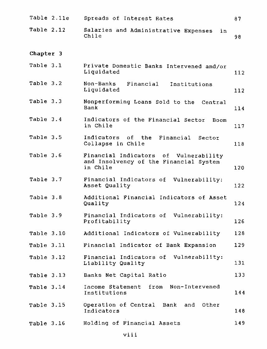
Table 2.11e

Table 2.12

Chapter 3

Table 3.1

Table 3.2

Table 3.3

Table 3.4

Table 3.5

Table 3.6

Table 3.7

Table 3.8

Table 3.9

Table 3.10

Table 3.11

Table 3.12

Table 3.13

Table 3.14

Table 3.15

Table 3.16

Spreads of Interest Rates 87

Salaries and Administrative Expenses in Chile 98

Private Domestic Banks Intervened amd/or Liquidated 112

Non-Banks Financial Liquidated

Institutions

Nonperforming Loans Sold to the Central

112

Bank 114

Indicators of the Financial Sector Boom in Chile 117

Indicators of the Financial Sector Collapse in Chile

Financial Indicators of Vulnerability and Insolvency of the Financial System in Chile

Financial Indicators of Vulnerability: Asset Quality

Additional Financial Indicators of Asset

118

120

122

Quality 124

Financial Indicators of Vulnerability: Profitability

Additional Indicators of Vulnerability

Financial Indicator of Bank Expansion

Financial Indicators of Vulnerability: Liability Quality

Banks Net Capital Ratio

Income Statement from Non-Intervened Institutions

Operation of Central Bank and Other Indicators

Holding of Financial Assets

viii

126

128

129

131

133

144

148

149

Chapter 5

Table 5.1

Table 5.2

Table 5.3

Chapter 6

Table 6.1

Table 6.2

Table 6.3

Table 6.4

Table 6.5

Table 6.6

Table 6.7

Table 6.8

Table 6.9

Table 6.10

Table 6.11

Analysis of Selected Empirical Studies on Banks 244

Synthesis of Selected Empirical Studies on Banks 247

Overview of the Contributions and Shortcomings from Selected Banks'Studies 251

List of Problem and Failed Banks in Chile during 1983

Mean Differences Between Nonfailed Nonproblem and Failed/Problem Banks and

277

the t-Statistics for 1983 284

Overtime Mean Differences and Its t­Statistics

Overtime Rankings for Financial Ratios in Model A1B1

Logit Analysis of Selected Financial Variables at the time of the Failure

288

289

Problem in 1983 291

Logit Analysis of Selected Financial Variables One Year Before the Critical Time (1982) 293

Logit Analysis of Selected Financial Variables Two Years Before the Critical Time (1981) 294

Logit Analysis of Selected Financial Variables Three Years Before the Critical Time (1980) 295

Logit Analysis of Selected Financial Variables Four Years Before the Critical Time (1979) 296

Prediction Accuracy of the E1 Logit Model for 1983. 297

Prediction Accuracy of the E1 Logit Model for 1982. 297

ix

Table 6.12

Table 6.13

Table 6.14

Chapter 7

Table 7.1

Table 7.2

Table 7.3

Table 7.4

Table 7.5

Table 7.6

Table 7.7

Table 7.8

Table 7.9

Table 7.10

Table 7.11a

Table 7.11b

Table 7.11c

Chapter 8

Table 8.1

Table 8.2a

Prediction Accuracy of the El Logit Model for 1981. 298

Prediction Accuracy of the El Logit Model for 1980. 298

Prediction Accuracy of the El Logit Model for 1979. 298

Indicators of the Economic Boom, 1977-81 317

Key Prices in Chile Between 1977-1983 319

Indicators of Convergence 320

US Exchange Rates and Tradable Prices for Chile

Indicators of the Economic Bust of 1982-

323

1983 327

Composition of GDP and Bank Loans 335

Bank List of A1 and B2 349

Logit Analysis of Selected Macroeconomic Variables for the Period 1982.1 to 1983.4 362

Logit Analysis of Selected Macroeconomic Variables for the Period 1979.1 to 1983.4 364

Logit Analysis of Selected Macroeconomic Variables for the Period 1979.1 to 1983.4 367

Prediction Accuracy of the E3 Logit Model Group A and B during 1983 and 1982 371

Prediction Accuracy of the E3 Logit Model Group A and B during 1981 and 1980 371

Prediction Accuracy of the E3 Logit Model Group A and B for 1979

Banks Rankings According to Total Loan Portfolio

The Degree of Concentration of Chile's Economic Group

x

371

382

383

Table 8.2b

Table 8.2c

Table 8.3

Table 8.4a

Table 8.4b

Table 8.5

Table 8.6

Table 8.7

Table 8.8a

Table 8.8b

Table 8.9a

Table 8.9b

Table 8.10a

Table 8.10b

Table 8.11a

Banks' Ownership by Economic Groups in 1978

Credit Concentration Affiliates

with Banks'

Bank List of Al and B1

Sample Mean for Failed/Problem Nonfailed/Nonproblem Banks for Period 1979-1981

Sample Mean for Failed/Problem Nonfailed/Nonproblem Banks for Period 1982-1983

Logit Analysis of Selected Proxies Risk-Taking for the Period 1979.1 1983.4

Logit Analysis of Selected Proxies Risk-Taking for Single Periods

and the

and the

for and

for

Likelihood Ratio Test for Equality of All Coefficients Across Years for Model

384

387

413

418

419

454

461

M1 463

Logit Analysis of Selected Proxies for Risk-Taking at the Time of Failure Problem 465

Prediction Accuracy of M1 Logit Model for 1983

Logit Analysis of Selected Proxies for Risk-Taking One Year Before the Critical

465

Time (1982) 467

Prediction Accuracy of Ml Logit Model for 1982

Logit Analysis of Selected Proxies Risk-Taking Two Years Before Critical Time (1981)

for the

Prediction Accuracy of M1 Logit Model for 1981

Logit Analysis of Selected Proxies for Risk-Taking Three Years Before the

468

469

469

Critical Time (1980) 470

xi

Table 8.11b

Table 8.12a

Table 8.12b

Chapter 9

Table 9.1

Table 9.2

Table 9.3

Prediction Accuracy of M1 Logit Model for 1980

Logit AnalY:3is of I"' - 1 - -·t - j Ije ec· .;ec Pro!{ i e5 for Risk-Taking Four Years Before the Critical Time (1979)

Prediction Accuracy of M1 Logit Model for 1979

Summary Statistics from Two Competing Models

Marginal Effects on the Macro-Model

Marginal Effects on the Moral Hazard Model

xii

470

471

471

479

483

484

List of Figures.

Chapter 4

Figure 4.1

Chapter 7

Figure 7.1

Figure 7.2

Figure 7.3

Figure 7.4

Figure 7.5a

Figure 7.5b

Figure 7.6a

Figure 7.6b

Figure 7.7

Chapter 8

Figure 8.1

Figure 8.2a

Figure 8.2b

Figure 8.2c

Figure 8.2d

Figure 8.3a

Figure 8.3b

Bank Holding Company structure

Bank Expansion

Profits, Asset Quality and GDP

Real Exchange Rate, GDP Traded and NonTraded

Macroprices, GDP Traded NonTraded

GDP NonTraded, Loan Quality

GDP Traded, Loan Quality

and

Banks Vulnerability and Key Prices

Banks Vulnerability and Key Prices

Loans' Share and Liability Ratio

Factors Affecting Moral Hazard and Bank Failures

Banco de Chile: Total Loan/Total Asset Ratio

Banco de Santiago: Total Loan/Total Asset Ratio

Banco Internacional: Total Loan/Total Asset Ratio

Banco Concepcion: Total Loan/Total Asset Ratio

Banco del Estado: Total Loan/Total Asset Ratio

Banco BICE: Total Loan/Total Asset Ratio

xiii

195

332

333

337

338

340

341

343

344

345

380

423

423

424

424

425

425

Figure 8.3c

Figure 8.3d

Figure 8.4a

Figure 8.4b

Figure 8.4c

Figure 8.4d

Figure 8.5a

Figure 8.5b

Figure 8.5c

Figure 8.5d

Figure 8.6a

Figure 8.6b

Figure 8.6c

Figure 8.6d

Figure 8.7a

Figure 8.7b

Figure 8.7c

Figure 8.7d

Banco Real: Total Loan/Total Asset Ratio

Banco de Sao Paulo: Total Loan/Total Asset Ratio

Banco de Chile: Nonperforming Loans/Capital Ratio

Banco de Santiago: Nonperforming Loans/Capital Ratio

Banco lnternacional: Nonperforming Loans/Capital Ratio

Banco Concepcion: Nonperforming Loans/Capital Ratio

Banco del Estado: Nonperforming Loans/Capital Ratio

Banco BlCE: Nonperforming Loans/Capital Ratio

Banco Real: Nonperforming Loans/Capital Ratio

Banco de Sao Paulo: Nonperforming Loans/Capital Ratio

Banco de Chile: Profit/Total Asset Ratio

Banco de Santiago: Profit/Total Asset Ratio

Banco lnternacional: Profit/Total Asset Ratio

Banco Concepcion: Profit/Total Asset Ratio

Banco del Estado: Profit/Total Asset Ratio

Banco BrCE: Profit/Total Asset Ratio

Banco Real: Profit/Total Asset Ratio

Banco de Sao Paulo: Profit/Total Asset Ratio

xiv

426

426

427

427

428

428

429

429

430

430

431

431

432

432

433

433

434

434

Figure 8.8a

Figure 8.8b

Figure 8.8c

Figure 8.8d

Figure 8.9a

Figure 8.9b

Figure 8.9c

Figure 8.9d

Figure 8.10a

Figure 8.10b

Figure 8.10c

Figure 8.10d

Figure 8.1la

Figure 8.11b

Figure 8.11c

Figure 8.1ld

Figure 8.12a

Figure 8.12b

Figure 8.12c

Banco de Chile: Provision/Total Loan Ratio

Banco de Santiago: Provision/Total

436

Loan Ratio 436

Banco Internacional:Provision/Total Loan Ratio 437

Banco Concepcion: Provision/Total Loan Ratio

Banco del Estado: Provision/Total Loan Ratio

Banco BICE: Provision/Total Loan Ratio

Banco Real: Provision/Total Loan Ratio

Banco de Sao Paulo:Provision/Total Loan Ratio

Banco de Chile: Deposit/Liability Ratio

Banco de Santiago:Deposit/Liability

437

438

438

439

439

441

Ratio 441

Banco Internacional:Deposit/Liability Ratio 442

Banco Concepcion:Deposit Liability Ratio

Banco del Estado:Deposit/Liability Ratio

Banco BICE:Deposit/Liability Ratio

Banco Real:Deposit/Liability Ratio

Banco de Sao Paulo: Deposit/ Liability Ratio

Banco de Chile: Asset Growth

Banco de Santiago: Asset Growth

Banco Internacional: Asset Growth

xv

442

443

443

444

444

446

446

447

Figure 8.l2d Banco Concepcion: Asset Growth 447

Figure 8.l3a Banco del Estado: Asset Growth 448

Figure 8.l3b Banco BlCE: Asset Growth 448

Figure 8.l3c Banco Real: Asset Growth 449

Figure 8.13d Banco de Sao Paulo: Asset Growth 449

xvi

Appendices.

Appendix 1

Appendix 2

Appendix 3

Appendix 4

Appendix 5

Appendix 6

Appendix 7

List of Chilean Financial Institutions 492

A Balance-Sheet and Income Statement of 494 a Chilean Bank

List of Financial Ratios 497

Testing Mean Differences 499

Two Separate Regressions 500

Covariance-Correlation Matrix for 501 Macroeconomic Variables

Covariance-Correlation Matrix for Selected Proxies of Moral Hazard

xvi i

504

Acknowledgements.

There are many individuals and academic institutions which without their selfless support this thesis would have never reached the final stage. Firstly, my sincere thanks to my supervisor Dr. Mike Bleaney who read the manuscripts and provided valuable comments at the different stages of the thesis work. Special thanks to Dr. Andres Zamudio (CIDE­Mexico) for the time he spent with me discussing the technical aspect of logit models. I remain grateful to Professor David Greenaway for encouraging me to move to Nottingham University and his support during those years.

I would also like to express my gratitude to Professor Shaw, Professor Martin Ricketts, Mike McCrostie, and Linda Waterman for their continuous encouragement and friendship. Equally, a recognition to Dr. Bazdresch, Raul Perez-Reyes and Mario Rivera for their support during my three years at CIDE-Mexico. To the staff of the different libraries for their selfless help in obtaining several references, among them I should mention especially the libraries of the University of Nottingham-UK, University of Buckingham-UK, CIDE-Mexico, University of Concepcion-Chile, Catholic University-Chile and SIBF-Chile.

Finally, and most important, I would like to thank my parents for their vision and uncompromised support during the good and bad times. Also to my parents in law which during the last few years have been part of this enterprise. I am especially grateful to my sister in law and her husband Eric for their invitation to stay at the Glebe in Bamburgh and make us feel at home. To my wife Carmen ?l?ria and my daughter Sofia whom have shared all the sacrIfIces during these years. Without their continued cheerfulness, love, and unconditional support this thesis would never have been completed.

xviii

Declaration.

I hereby declare that the work submitted in this thesis is the result of my own investigation. Due references and acknowledgements have been made, where necessary, to the work of other researchers.

I further declare that this thesis has not previously been accepted in substance for any degree, and is not being concurrently submitted in candidature for any degree.

Candidate: Ivan Araya Gomez

---------------------------(Candidate's signature)

Supervisor: Dr. Michael Bleaney

--------------------------------(Supervisor's signature)

xix

Chapter ~ Introduction.

(1.1) Background to the study.

This thesis discusses and evaluates empirically the

Chilean experience with financial liberalisation during the

1970's and early 1980's. Special consideration has been

given to the study of the origins and the magnitude of the

collapse of the banking system in 1982-83.

The Chilean liberalisation programme, which included the

deregulation and the opening-up of the goods and financial

markets as well as a package for macroeconomic stabilisation

has been of considerable interest to economists and

researchers working in the areas of economic development,

international trade, and finance.

There are several reasons why the Chilean case is been

of great interest. First, the Chilean economy pursued two

distinctly different development strategies. From the 1930's

to the early 1970's the economy followed inward-looking

strategies which included a financially repressed financial

system; and from the late 1973 onwards an outward-looking

strategy which included financial liberalisation and

stabilisation policies. This sharp and sustained changes in

policy implies that the links between policy and performance

may be more clearly discernible in the Chilean case than 1n

most others.

1

Secondly, the process of liberalisation after the

military coup of September 1973 was considered to be a "pure

monetarist strategy" as the economy was subject to free

market oriented policies under the guidance of the military

government and Chicago-trained economists. The performance

of the economy under the influence of Chicago liberalism

provided evidence for their detractors particularly with the

debacle of the banking system in 1982-83.

Finally, the performance of the Chilean economy both

during and

completed

still are

after the liberalisation reforms have been

contained some dramatic change of fortunes which

considered rather puzzling. Chile's economic

performace between 1973 and 1983 shows sharp contrasts. For

instance, the average growth rate of real GDP between 1976

and 1981 was 7.1% and the inflation rate was less than 10%

by

and

1981. However, by 1982 and 1983

3% respectively. At the

GDP fell by nearly

same time, once

14%

the

liberalisation of trade was completed on schedule in 1979

which among other things meant the attainment of a uniform

nominal tariff of 10%, and the financial system was open to

flows of foreign capital in 1982 the whole process was

stopped and reversed during the second half of 1982. The

trade regime was restricted with the rise in tariffs and

controls and the financial system was overhauled and its

losses socialised to avoid its inminent collapse. Although

the collapse of the economy in 1982 and the abandonment of

the Neo-Liberal approach have been subject to considerable

2

scrutiny, some of the issues, particularly the debacle of

the banking system and its empirical verification, remain

largely unsettled.

During the mid-1970's, Chile adopted a new approach to

policy-making. This new strategy consisted of a combination

of measures to deal with macroeconomic instability as a

short-run objective and economic growth as a long-run

objective.

initially

The new package of

of traditional

economic

orthodox

policies consisted

monetarism for

stabilisation and liberalisation reforms in the goods and

financial markets. The liberalisation of the financial

market was considered one of the backbone of the Neo-liberal

reforms. Indeed, in retrospect, it could be argued that the

success or failure of financial liberalisation was

paramount in the overall result of this new approach of

economic development in Chile.

The authorities were absolutely committed to short run

stabilisation as a pre-condition for the introduction of

long run structural and institutional reforms. At the

beginning, the lack of success in reducing the inflation

rate and the high cost in terms of output and employment,

particularly in 1975 as output fell by nearly 13%, forced

the authorities to overhaul closed economy monetarism.

Instead, an open economy approach was introduced in 1978

where the exchange rate became the nominal anchor of the

economy as well as the key variable in expectations

3

formation. This approach was desirable and necessary as the

economy was becoming more integrated to the international

world markets.

The itinerary of liberalisation was on schedule and with

no political opposition. The goods market was deregulated

domestically

restrictions.

and

The

followed by the removal

financial market was

of trade

deregulated

simultaneously with the goods market although it remained

closed to external capital flows until the last stage of the

reform package. This order and timing of liberalisation was

considered theoretically sound and accepted by economists

and policy-makers working in Chile and other developing

countries.

The acceptance of the Neo-Liberal approach was based on

economic, social, and political factors. The performance of

the Chilean .economy was unsatisfactory, particularly during

the Allende's social government between 1970 and 1973. The

economy was suffering from hyperinflation induced by the

financing of large fiscal deficits. At the same time, the

balance of payments deficit and the shortage of

international reserves was becoming symptomatic of the

fiscal deficit and especially of the inward-looking

strategy. Obviously some action was required to correct

these macroeconomic disequilibria.

The rate of growth of real GDP was poor relative to

other Latin American and East Asian economies during the

4

1950's and the 1960's. This gap widened during the early

1970's. For instance, the average annual rate of growth of

GOP between 1965 and 1973 was 10% and 10.4% for Korea

and Taiwan. Brazil and Mexico also exhibited impressive

growth rates with 9.8% and 7.9% respectively. In contrast,

Chile shows a poor performance with only 3.4% over the same

period.

It could be argued that much of the difference in

performance can be attributed to the fact that the East

Asian countries were pursuing outward-looking strategy and

by promoting a well developed financial markets. In

contrast, Chile followed a systematic inward-looking

strategy and financially repressed financial market as the

industrialisation strategy. It must be said in retrospect

that East Asian countries have continued outperformed Latin

American countries during the second half of the 1970's and

during the 1980's even though the latter countries have

pursued very aggressive liberalisation strategies.

It is clear by now that economic factors such us

macroeconomic instability, the failure of inward-looking

strategy, and the superior performance of those countries

following a more open strategy towards international trade

and financial markets motivated the Chilean authorities to

embrace a Neo-Liberal approach. At the same time, the

political turmoil during the socialist government produced a

5

climate for the establishment of both, a military

dictatorship and the economic regime.

It must be said that, at least in the economic front,

Chile's economic liberalisation accomplished many positive

achievements. Trade liberalisation made a significant

contribution to the rate of economic growth during 1976-81.

Some sectors were sufficiently flexible to react to changes

in relative prices resulting from trade reforms. In fact,

resource reallocation from import sUbstitution to the export

sector was possible. Furthermore, there was a change in the

pattern of production in the export market as non­

traditional exports such as agricultural products, timber,

and fishing expanded relative to traditional exports such as

copper.

Similarly, financial liberalisation brought about

significant benefits by expanding the level of financial

intermediation through the formal banking system. At the

same time, the rise in the number of financial institutions

produced significant improvemement in operative efficiency

and financial widening. However, in spite of these positive

results, these reforms produced other unexpected and

undesirable outcomes. High and stubborn interest rates, lack

of effective supervision, imprudent practices by banks and

non-banks financial institutions conspired against the

establishment of an efficient and stable liberal financial

market. The debacle of the banking system in 1982-83 is the

6

reflection of the effects of an ill-designed and mistaken

implemention of financial liberalisation. Admittedly, the

completation of financial liberalisation and the collapse of

the banking system coincided with the economic recession of

1982 when output fell by nearly 15%.

The Chilean experience is still a contentious issue in

spite of the substantial literature on this topic. This is

more significant when we attempt to explain the debacle of

the Chilean banking system. On one side, it is argued that

the financial crisis in Chile had its origin in the

deterioration of key macroeconomic variables and that

financial liberalisation played a secondary role. Proponents

contend that no financial system can be expected to

withstand a fall in output of nearly 15% in 1982 and they

draw parallels here with the banking crisis of the 1930's in

the US. On the other side, it is argued that the ability of

the financial system to withstand any macroeconomic shock

will depend on the structure of the banking system. This had

been shaped by the financial liberalisation which took place

in the years before the collapse of the macroeconomy.

Conduct derived from ownership concentration and "related

portfolios", sharp deregulation of interest rates, belief in

an implicit bail-out provision, and the ineffective and

inadequate prudential regulation led to a pattern of

behaviour marked by moral hazard and to a l -oo-r ~.J1-·e -at-lot e '"L e 1 .:

adverse selection problems. As a result, banks exhibited

excessive risk taking with a deterioration of banks'

7

financial position. Only the prompt rescue by the Central

Bank of leading financial institutions averted a massive

loss of confidence and a bank run.

If we accept that both arguments have some merits, the

question is the relative weight of these hypotheses. The

relative importance of macro and micro as causal factor in

bank failures and the implications for the failure rates in

a more stable macroeconomic environment and/or less risky

bank management are important empirical questions which

remain unanswered in the literature on Chile.

(1.2) Aims, Methodology and structure of the study.

This thesis examines the evolution of the Chilean

financial system during the period of economic reforms and

banking failures. Three specific questions are examine and

evaluated empirically: How important was the adverse

macroeconomic environment relative to the banking conduct

and management which exhibited considerable moral hazard

type of behavior in the banking failures in Chile ? . Secondly, in what ways might more favorable general

economic conditions and/or different implementation of

financial reforms including a more effective prudential

regulation have helped to reduce the likelihood of bank

failures ? Finally, might some of the bank failures have

been anticipated years before the crisis by an early warning

system 7

8

In this thesis, I develo l't d 1 f P a Ogl mo e or cross-

section and panel data with information from banks' balance

sheets to estimate the probability of bank failure/problem.

Banks are classified in two groups. The first group

corresponds to those financial intermediaries with no

problems and

problems/failed.

the

In

second group

the latter, I

includes banks with

have followed a wide

definition of problem/failure to conform to the list which

includes problem banks which sold bad debts to the Central

Bank, and those institutions in which the authorities

intervened directly.

At a first stage, I use symptomatic variables derived

from banks' balance sheets among them I include a broad

categories of financial and accounting ratios assessing a

bank's liquidity, credit risk, liability risk, capital

adequacy, and profitability. This model will enable me to

estimate the ex ante probability of bank failure/problem and

to evaluate whether the model was providing an early warning

signal at least with a year or more. At the same time, the

use of these symptomatic variables will permit the

constructing of a banks's ex ante classification on

quarterly basis.

In the second stage of the empirical work, I proceed to

the logit model with quarterly panel data against

model will help to test macro and micro

9

the probability of bank failure/problem and to simulate

different

likelihood.

environments to assess its impact on the

Specifically, this thesis is composed of ten chapters,

including the introduction and the conclusions. Following

the introduction, chapter 2 provides a background on the

Chilean financial reforms and the institutional structure.

It also contains an assessment of the results which were

expected a priori.

The first section begins with an account of the

theoretical underpinnings of financial liberalisation and

the case against financial repression. In addition, it is

shown what is regarded to be desirable and acceptable in

terms of the dynamics and the transition involved in the

path from financial repression to a deregulated financial

market. Some evidence from selected countries is presented

to support financial liberalisation.

The second section contains a detailed description of

the package of financial reforms implemented between 1973

and 1983. This includes reforms towards the liberalisation

of the domestic banking sector as well as the opening to

external capital inflows. This description follows the

chronological order adopted by the monetary authorities.

Finally, this chapter ends with a general evaluation of

the effects of financial liberalisation. It provides

rn

10

evidence on financial deepening and widening, the pattern of

interest rates, the effect on savings and investment, and

the allocation of financial resources. At first Bight a

significant expansion of the peso and dollar liabilities

occurred along with increases in intermediation and the

number of financial institutions, both domestic and foreign.

But deregulation and increasing competition meant an

alarming deterioration of banks' asset portfolios and

profitability during 1981-83. Several financial institutions

were rescued in 1981 and in particular in 1983 to avert a

contagious panic and a bank run.

Chapter 3 is a continuation of chapter 2 as it gives an

overview of the different episodes of financial difficulties

during the period of liberalisation, although the emphasis

is put on the banking crisis of 1981-83. Moreover, it

discusses the magnitude of the collapse and the measures

taken by the authorities.

This chapter is divided into two main sections. The

first one carries out an autopsy of the banking system and

some financial institutions. By means of financial data from

annual banks' balance sheets and income statements we

construct financial indicators on performance and fragility

to study the evolution of the banking system between 1977 to

1983. Moreover, the data enable us to estimate indicators

for individual banks and thus compare their individual

performance. Clearly, according to the indicators there are

-11

marked differences between those banks which experienced

intervention and/or sold bad debts to the Central Bank and

those intermediaries which remained healthy. Such comparison

were also made between the group of domestic banks and

foreign banks where the latter group suffered minor

distresses during this period.

The second section shows the magnitude of the

intervention in terms of the rescue package enacted by the

monetary authorities. One of the most important mechanisms

in aid of those in financial distress was the agreement

number 1.555. This enabled banks to sell bad debt to the

Central Banks.

Following the description and evaluation of the banking

crisis, chapter 4 reviews the theories of bank failures and

banking instability. After providing a theoretical

justification for the existence of financial intermediaries

as information producers and liquidity insurers, the

analysis passes to the explanation for bank failures. One

can identify three factors which explain banks failures,

namely external factors like the macroeconomic environment,

industry-changes as a result of financial liberalisation,

and internal factors such as fraud, and the banks' attitude

towards risk-taking. It is suggested that two testable

hypotheses can be conducted to explain the failures of the

Chilean financial institutions. That is, adverse

macroeconomic changes which are external to the banks, and

12

excessive risk-taking and moral hazard by bankers responding

to industry changes from financial liberalisation.

Chapter 5 discusses the econometric methodology applied

to study the banking crisis in Chile. This includes a

revision of some previous empirical studies and the use of

logit models.

The first section contains a review of some of the early

studies available in this area using particularly binary

choice models. This literature contains special reference to

the failures of US financial institutions, including Saving

and Loan Associations. One observes that binary-choice

models, especially logit models, have been used very

successfully to explain financial failure/problems of the

1930's, early 1970's and 1980's.

The following section presents a brief discussion of a

univariate dichotomous model with special reference to the

logit model. I concentrate on the model estimation procedure

which involve a non-linear maximum likelihood estimation

technique. Also, there is a review of the hypothesis testing

procedure and the development of model selection criteria

for alternative specifications. This section is completed

with the inclusion of specific econometrics difficulties

for the case of panel data.

Chapter 6 deals specifically with the issue of

developing an appropriate bank classification technique

13

using financial information from banks' balance sheets and

income statements. One of the limiting problems to estimate

the logit model using quartely panel data is the fact that

we do not have information available on the banks' financial

strength prior to 1983. In order to overcome this difficulty

we construct an early warning system to predict the ex ante

probability of bank failure/problem.

This chapter is organised in three main sections. The

first one contains a description of the model in terms of

definitions concerning bank failure/ problem and their

relative merits. This section is follows by a description of

the different categories of independent financial and

accounting variables which will help us to discriminate and

classified financial institutions into the two broad groups.

Finally, the last section reports and assesses the empirical

findings using univariate and multivariate

techniques.

statistical

Chapter 7 contains three main sections. Section 1

introduces the hypothesis concerning the role played by the

macroeconomic environment and the proponents who sustain

this view. This section is followed by an evaluation of the

prevailing macroeconomic environment in Chile between 1977

to 1983. There are two phases identified in terms of the

boom-bust cycle. It is shown the severe misalignment of some

key macro prices such as the real exchange rate, the real

interest rate, and the sharp and unexpected changes in the

14

stock prices and capital inflows. Other studies are cited to

stress the importance of these factors on the recession of

1982-83.

The third and final section reports the empirical

results from the econometric analysis. I run regressions

between the discrete dependent variable and a set of chosen

macroeconomic variables using quarterly panel data. This

exercise aims to assess empirically the relevance of

macroeconomic factors in determining the likelihood of bank

problems/failure.

Chapter 8 reports the results from the estimation of

the logit model as we regress the discrete dependent

variable against microeconomic variables as proxies for

excessive risk-taking. There is a discussion of the

hypothesis which relates the banking crisis to moral hazard

type of behaviour by bank management.

My main concern is to evaluate how moral hazard

problems could have affected the likelihood

failure/problem. It is argued that much of the

conduct was affected by the implementation of

liberalisation per see These results are

independently of any macroeconomic shock.

of bank

banking

financial

estimated

In order to test for moral hazard I have used some

proxies and measuring any deviation of the proxy from its

trend. Furthermore, we include some dummy variables to

15

capture some specific banks characteristics such us "related

portfolios".

Chapter 9 offers a comparison between the regression

results of chapter 7 and 8 in terms of the robustness

of each model. At the same time, it shows some of the

results from some simulation exercises conducted by assuming

different scenarios. Specifically, I simulate changes in the

macroeconomic environment and liberalisation reforms. We

offer some comparisons by introducing some hypothetical

question such us what would have happen to the likelihood of

bank failure/problem if we simulate the model with a more

stable macroeconomy or if more effective prudential

regulation was introduced to influence more conservative

bank management and risk taking ?

Finally, chapter 10 sets out the main conclusions from

this empirical study. At the same time, it highlights the

limitations of this study and venues for further reserach.

16

Chapter 2. From Financial Repression to Financial Liberalisation: Chile in 1970-1983.

(2.1) Introduction.

This chapter provides a background on how the Chilean

financial system evolved from a financially repressed to an

unregulated and more competitive market. It discusses and

evaluates the impact of both, repressive financial policies

and financial liberalisation reforms.

Although this thesis focuses on the bankruptcy of the

banking system, it is important to place the banking failure

of 1983 against the backcloth of the financial

reforms implemented during the 1970's. Apart of providing

both, some of the theoretical underpinnings and the evidence

against financial repression, this chapter also presents a

detailed description of the Chilean banking system and the

itinerary of financial liberalisation between 1973 and 1983.

Financial liberalisation was undertaken within a broader

development strategy including trade liberalisation and

stabilisation policies. The development of an efficient and

a stable financial system and its opening-up to the world

financial market was the backbone of the overall package of

the structural reforms from the very beginning. The

elimination of interest rates disequilibrlum, selectlve

credit controls, non-interest reserve requirements, and

inflation tax combined with institutional changes such as

17

the privatisation of financial institutions, the lifting of

entry barriers, and the establishment of a multi-purpose

banking was expected to produce some positive benefits.

Specifically, it was expected that there would be an

increase in financial deepening (financial savings), a rise

in the level of domestic savings, increases in the volume

and quality of investment, and an improvement in resource

allocation and operative efficency. At the same time, there

was the belief that a market oriented financial system would

promote and secure financial stability.

As we will see in this chapter, financial liberalisation

partially achieved the objective set originally. However,

the most worrying sign which emerged from the financial

liberalisation experience was the rise in financial

instability as the private financial system ended

practically bankrupt and experienced considerable

intervention by the economic authorities.

In developing countries the terms financial system and

banking system are used interchangeably since banking

dominates financial intermediation. As we will see from

chapter 3, the case of Chile is no the exception to this

rule.

18

(2.2) The Banking System ~ Financial Repression in Chile: The Pre-Liberalisation Period.

(2.2.1) Financial Repression and Economic Developm~nt.

As we will see shortly the government of Chile undertook

a comprehensive programme of economic liberalisation. One of

the central components of the economic strategy was a

drastic overhaul and the deregulation of the country's

financially repressed banking system. This reform clearly

reflected the spirit of the Mckinnon-Shaw prescription that

abolishing financial repression is essential for a sustained

economic development.

Before we procede to assess the empirical relevance of

financial repression and the process of financial

liberalisation in Chile, a revision of the main theoretical

underpinnings will be provided.

In retrospect, one observes that the literature on money

and finance have gone considerable changes since the Great

Depression of the 1930's. To begin with, Friedman and

Schwartz's reinterpretation of the US depression and the

collapse of the US banking system has revindicated the role

of money after the challange of the Keynesian Revolution

where money did not matter. In the monetarist counter­

revolution, money was important as much as it was the role

of the Federal Reserve when failed to supply liquidity as a

result of the fall in the currency-deposit ratio and hence

the money supply.

19

The second major revision in monetary theory has been on

the role of finance in the economy. The terms money and

finance have been used almost interchangeably during many

years. This can be explained partly by the fact that the

financial system was dominated by both, commercial banks and

the Central Bank. The former accepted demand deposits and

the latter issued currency as their key liabilities. Money,

defined as currency plus demand deposits, was the only

acceptable asset as a medium of exchange. However, the

evolution and innovation of the financial system was

materialised in terms of the introduction of new

intermediation services and the supply of new financial

instruments and institutions. This led to a redefinition of

money and the nature of the financial services provided by

financial institutions. Indeed, today currency and demand

deposits constitute only a fraction of the total assets

(liabilities) of the financial system. In addition, an

increasing number of economists have given a greater weigh

to the role played by the contraction of banks'

intermediation services during the episodes of the Great 1

Depression.

While money and finance have been recognised as having

an effect on the output cycle, it also began to emerge a

body of the literature where money and financial

intermediation have been incorporated into growth models.

This direction has had important theoretical as well as

practical implications, especially among developing

20

countries which over the years have been striving to achieve

a higher rate of economic growth.

Tobin (1965) introduced a modified version of the

Harrod-Domar growth model which incorporated money as

outside or deadweight money. Tobin considered money as

wealth and hence as an alternative asset to savers. The

substitutability between money and physical capital implied

that any increase in the real return of money, other things

being equal, would generate a portfolio shift away from

capital and towards money. This in turn will reduce the

accumulation of physical capital and hence the rate of

output growth.

The neoclassical monetary growth theory can be condensed

in the following expressions. The production function

Y=F(K,L) is assumed to be linearly homogeneous with constant

return to scale. It is also assumed that the marginal

product of capital (MPk) and labour (MPl) are both positive

and subject to diminishing returns. Moreover, the model

considers the quantity of labour growing at a constant rate

of n. It is possible to write the production function in per

capita terms by dividing through by L as shown by (la).

(la) y = (k)

21

where y=Y/L and k=K/L

2 2 dy/dk>O and dy/dk <0

The demand for money function shown in (lb) suggests

that money is held as a medium of exchange. The neoclassical

assumption of perfect capital market (i.e. homogeneity and

perfect divisibility of capital, no transaction and

informational costs) leaves the monetary system as

performing a payment function with no comparative advantage

on intermediation. According to (lb) an increase in r

relative to (d-p) will produce a portfolio shift from money

to physical capital and viceversa. This substitution

dominates the neoclassical monetary growth theory.

(lb) M/P = H(Y,r,(d-p»

where Y = real income r = real rate of return

on capital (d-p)= real deposit rate of

interest and 6H/6Y>O 6H/6r<O

6H/6(d-p»O

Expression (Ic) represents the rate of capital

accumulation (investment function) and shows the

substitution between money and aggregate investment in the

steady state. Given that the marginal propensity to save

(MPS) is taken as a constant then actual savings are

allocated between real money balances (M/P) and physical

capital.

(le) I = dK/dt = s(k) + (s-l)[d(M/P)/dtJM/P

where s = MPS K = capital

22

(1d) (d-p) = r where r=dy/dk

Given that 0(s(1 and in a growing monetary economy

d(M/P)/dt > 0 then it follows that (s-1)[d(M/P)/dtJ is

clearly negative. Thus, money competes with capital. If the

equilibrium condition in (Id) is disturbed then a portfolio

adjustment will take place.

It follows from this model that the accumulation of 2

money holdings will retard the growth of output. If the rate

of capital accumulation is low and the authorities wish to

accelerate the rate of output growth then they must make the

holding of money unattractive by introducing ceilings on

interest rates (d) and/or increasing the rate of inflation

(p) •

One aspect of the neoclassical monetary growth theory

which is puzzling if not inconsistent concerns the reason

of why will people hold money at all. Indeed, the underlying

assumptions of the model, particularly the homogeneity of

output, the perfect divisibility of capital, and perfect

information which are explicitly or implicitly incorporated

into the model does not provide, if we follow the logic, any

justification for holding money. On this point, Levhari and

Patinkin (1968) have incorporated money in the utility

function as part of the services rendered by money balances,

particularly liquidity services. Similarly, Mckinnon (1973)

also presented, as we will see shortly, a critique to the

23

neoclassical monetary growth model and a modified version of

the model for a developing economy in which there is a

rationale for holding money.

Mckinnon (1973) and Shaw (1973) have challanged the

central implications of the traditional growth model by

questioning the model's assumptions and rejecting the role

of financial restriction as an output's enhancing strategy

for a developing economy. Mckinnon and Shaw provided a

theoretical framework to show that misguided government

financial policies, especially ongoing price inflation

combined with low or even negative real interest rates,

would be conducive to a repressed financial sector, low

investment and economic growth.

Mckinnon kept the outside (deadweight) money assumption

while he advanced some institutional features inherent to

developing economies. One of the most important

characteristics of these economies is the existence of a 3

significant fragmentation in the economy. All economic units

are confined to self-finance, and investment is assumed to

be indivisible and lumpy. This implies that any potential

investor must accumulate money balances or inventories to

carry out its investment plans. This is a sufficient reason

for holding money balances in comparison to the neoclassical

model where the assumption of perfect capital market leaves 4

the demand for money indetermined. These assumptions were

fundamental to conform the Mckinnon's complementary

hypothesis between money and physical capital. The

24

complementary hypothesis condradicts the neoclassical model in the sense that, the more attractive money balances

greater the incentive to invest in productive capital, the

The Mckinnon's complementary hypothesis is stated in the

demand for money and investment functions defined in

expressions (2a) and (2b) respectively.

(2a) M/P = hey, I/Y, (d-p»

where

and

(2a) I/Y = m(r,(d-p»

where

I/Y= gross investment GNP ratio.

6h/6Y)O 6h/6(I/Y»O 6h/6(d-p»O

6m/6r)O and 6m/6(d-p»O

The complementary hypothesis between money and capital

is shown by the derivatives 6h/6(I/Y»O, 6m/6r)O, and

6m/6(d-p»O. That is, the average real cash balance of a

small saver-investor will rise as a result of the increase

in the desirable rate of capital accumulation which in turn

respond to increases in the real return of capital and/or

money.

Thus, in the Mckinnon model financial savings determines

the supply of funds. Savings are distributed between

tangible assets and interest-earning deposits. The views of

Mckinnon and Shaw differ on the process by which bank

25

deposits are transformed into investment. In the Mckinnon

model investment is self-financed so that in a segmented

economy investor need to accumulate real balances to finance

lumpy investment projects. In consequence, a rise in the

real return from money will enable savers to accumulate

money and invest into higher-yield physical assets. It could

be argued from Mckinnon's view that in an economy with no

money, the introduction of fiat money as opposed to

commodity money will serve as a "conduit" for capital

formation by making money and capital complementary assets.

A similar conclusion is obtained if we include further

development of financial instruments such as bank deposits

and so on. Mckinnon described an extreme case of financial

repression with no possibilities for external finance in the

form of bank credit. The process of saving and investment

involves a single and dual individual. In contrast, Shaw has

emphasised the role of external financing as the effective

constraint on capital formation. Like Mckinnon, Edward Shaw

in his book Financial Deepening and Economic Development

published in 1973 questioned the benefits from low interest

rates and inflation, and stressed the negative effect of

financial repression on economic growth.

In Shaw's monetary model, there are two important

modifications with respect to the definition and meaning of

money. Firstly, the model describes an inside money economy

where money is treated as debt. This clearly contradicts the

Mckinnon's outside money assumption which recognise money as

26

wealth. In Shaw's debt-intermediation view, an asset such as

money is cancelled out against financial liabilities. In

other words, money and demand deposits which correspond the

liabilities issued by commercial banks and the Central Bank

are backed by productive investment loans. Thus, the

remaining asset in this economy's aggregate balance sheet is

physical capital. In consequence, the accumulation of money

neither is a substitute nor a complement of capital.

Secondly, money is seen as one of many financial assets.

Moreover, the financial system is considered as a provider

of financial services which is included directly as a factor

input in the production process. Thus, policies which limits

the quantity and quality of financial assets and hence the

supply of this intermediate factor input in less than

optimal quantities should be avoided.

The Shaw's demand for money function is despicted in

expression (3)

(3) M/P = h(Y,Z,(u-p»

where 6h/6Y>O 6h/6Z<O

and 6h/6(u-p»O

Expression (3) differs only slightly with Mckinnon's

demand for real balances given by (2a). Shaw included an

opportunity cost of money defined by Z which includes a set

of inflation hedges such as precious metals, pieces of arts,

and land and properties. At the same time, the relevant rate

27

of return of money is the real rate of interest in all

financial assets (u) rather than the narrow real deposit

rate (d-p). The term I/Y which reflects the complementary

hypothesis is not included in expression (3) since investors

are not constrained to self-finance. In fact, if

institutional credit is not available then an informal

credit market will emerge.

Although both theoretical framework were conceived under

different assumptions they have thrown a similar policy

implications. They both challanged the conventional wisdom

of a low interest rates, higher price inflation, and

government intervention in the financial system to enhance

growth. Instead, they emphasise the importance of financial

liberalisation and the effect of financial deepening in

accelerating the rate of economic growth in a developing

economy. Specifically, they advocate low inflation and

positive real interest rate policies for developing

economies.

Fry (1982a) argued that many developing countries have

apparently slipped into financial repression inadvertenly.

Indeed,

unintended

financial repression was the result of

consequences of taxing and regulating

the

the

financial system to obtain resources to finance government

deficits. Most governments in developing countries have been

technically constrained with respect to the amount of tax

revenues can be rise from direct and indirect taxation. The

problem of tax evasion and the existing lags in collecting

28

tax revenues (Olivera-Tanzi effect) are quite significant.

Moreover, the absence of well established and developed open

market in primary securities had ruled out the possibility

of issuing government securities to finance government large 5

deficits.

Another motivation for repreSSing the financial sector

is explained by the fact that regulation of financial

institutions and their influence on the allocation of

resources via selective credit allocation has enhanced the

government's ability to channel financial resources into

specific sectors of the economy as part of the overall

development and political strategy. As we have seen in

chapter 1, Chile as well as many other developing economies

were pursuing inward-looking strategies since the 1930's.

This policy package included both a highly protectionist

foreign trade policies among them tariffs, subsidies,

quantitative restrictions, and an overvalued real exchange

rate. This trade regime was complemented with a selective

credit allocation and disequilibrium interest rates to 6

promote import-substitution.

The public finance hypothesis and the inward-looking

strategy seems as two equally plausible explanations of

financial repression in Chile as well as other developing

economies. However, in my view is equally true that the

simplistic view of the neoclassical monetary growth model

has driven policy-makers in LDC's to readily accept the

29

recommendations from this model and hence to overlook the

implications of money and finance on capital accumulation

and economic growth.

Whichever the reasons for the acceptance of financial

repression, governments had an ample list of instruments at

their disposal to serve its objectives. In order to collect

revenues to finance the government's uncovered budget

deficit, they explicitly and/or implicitly tax the financial

system by means of a compulsory reserve requirement on

bank deposits and inflation tax on currency and reserves 7

respectively. Similarly, the introduction of usury

restrictions on interest rates and selective credit

allocation have enabled governments to extend subsidies to

specific sectors. Ceilings are set deliberately below

equilibrium interest rates so that credit can be allocated 8

following non-price criteria. Moreover, Nichols (1974)

maintained that restricting the interest rates payable on

private assets has been helpful in curtailing the

availability of good substitutes and hence making the demand

for money more inelastic with respect to inflation.

All in all, one may conclude that introducing an

explicit and implicit taxation in the form of non-interest

reserve requirements, and price inflation respectively,

and/or usury restrictions on interest rates will contribute

to exacerbate both interest rate disequilibrium and the

burden of taxation on the banking system. The overall impact

will fall upon the resource allocation and the development

30

and maturity of the banking system. The shrinking of the

amount of loanable funds and introduction of a non-price

rationing of financial resources will affect adversely the

amount of investible funds and the quality of investment in

the economy. Therefore, financial repression will be

conducive to slow or retard the rate of economic growth in

developing countries. As we will see from next section,

these conclusions are supported by the evidence from Chile

and some selected countries.

(2.2.2) The Evidence of Financial Repression for Chile and Some Selected Countries.

This section presents simple calculations of both the

magnitude of the explict and implict tax levied on the

Chile's banking system as well as the degree of interest

rates disequilibrium during the decade of the 1970's. These

results are compared with the estimates of the list of

selected countries. Although this is not a comparative study

it was thought that the inclusion of a selected list of

countries would be helpful to make even a strong case

against financial repression.

I have included the US, Germany, and Japan as

industrialised and non-inflationary economies. At the same

time, among the newly industrialised countries (NrC's),

Korea and Singapore are the most appropiate representatives

from this region. Singapore and to a lesser extend Korea had

31

consistently deregulated and liberalised their financial 9

system. Finally, Mexico was incorporated in the list of

selected countries representing those less developed and

inflationary economies. The Mexican banking system has long

been financially repressed, a syndrome which became more

acute during the nationalised era between 1982 and 1989.

Although there are substantial structural differences

among the selected countries which makes detailed comparison

somewhat cumbersome, the fact that the financial system in

these economies was dominated by organised banks, state

and/or private ownership, still provides an angle for useful

comparisons.

The evidence from Chile during the 1970's shows the

detrimental effects of government interference in the

banking system. Explicit and implicit taxes on financial

intermediation and disequilibrium interest rates have

affected adversely the financial deepening in Chile

measured by the M2/GDP ratio. This proxy for financial

intermediation indicates the amount of loanable funds

intermediated through the organised banking system. Those

countries which have levied a heavy tax burden in their

banking system and accepted disequilibrium interest rates in

the form of negative real deposit interest rates exhibit low

M2/GNP ratios.

32

Table 2.1 Indicator of Financial Deepening for Chile and Selected Countries. (a) (b)

-------- ------------------- ---------------------------------M2/GDP 70 71 72 ----------------------USA FRG Japan

.62

.50

.74

Korea .33 Singap .. 66 Mexico .16

Chile

.65

.45

.83

.32

.61

.16

.67

.52

.91

.35

.65

.16

73 74 75 76 77 78 79 Av --------------- -----------------------

.64 .62 .64 .66

.51 .51 .54 .53

.87 .82 .85 .85

.36

.60

.17

.32

.55

.15

.31 .30

.61 .63

.15 .18

.65 .62

.55 .57

.85 .87

.32 .35

.61 .61

.28 .30

.60 .64

.55 .52

.87 .85

.31 .33

.63 .62

.31 .20

.13 .06 .07 .08 .10 .12 .14 .10 --------------------------- ---------------------------------Source:IMF,International Financial Statistics,Various Issues

(a) M2 and GOP are measured at current prices. (b) M2 is the sum of money plus quasi-money.

Table 1 exhibits the estimates of the ratio of the

broad money supply (M2) to gross national product (GNP) for

Chile and some selected countries. Chile's estimates of the

M2/GDP ratio indicates that the average holdings of broad

money as percentage of GDP was 10% per annum during the

decade of the 1970's. This figure is comparatively small to

those from industrialised and non-inflationary economies.

For instance, Japan and US exhibit a ratio of 85% and 64%

respectively. In addition, developing countries such as

Korea and particularly Singapore also show high M2/GOP

ratios. It appears that the flow of loanable funds grew more

rapidly in industrial and rapidly emerging developing

economies than in slow growth economies such as those in

Latin American. As we will see shortly, these results are

also confirmed by the evidence available from wider cross-

country comparisons.

33

Chile's financial deepening is well below those

selected countries and similar to Mexico. There are two

inmediate questions which arise from the evidence. How can

we explain the magnitude of financial repression in Chile ? . And are there common factors between Chile and Mexico and

differences with industrialised and rapidly-growing

economies to explain their relative financial performances?

It can be proven that those countries which implicitly

and/or explicitly tax their banking system, and

deliberately choose disequilibrium interest rates, should

have a lower M2/GDP ratios than those economies which

present a more deregulated financial sector and have levied

a lower tax burden on financial intermediation.

The imposition of a high reserve requirement on bank

deposits is equivalent, as we have seen from the theory, to

a explicit tax on deposits and lending. Similarly, the

inflation tax on currency holdings and on bank reserves can

be seen as an implicit tax on intermediation. The

hypothesis is that both forms of taxation should affect

adversely financial deepening.

I have estimated an effective reserve ratio and the

magnitude of the inflation tax on currency and reserves for

Chile and the selected countries. These results are

presented in table 2,3, and 4 respectively.

34

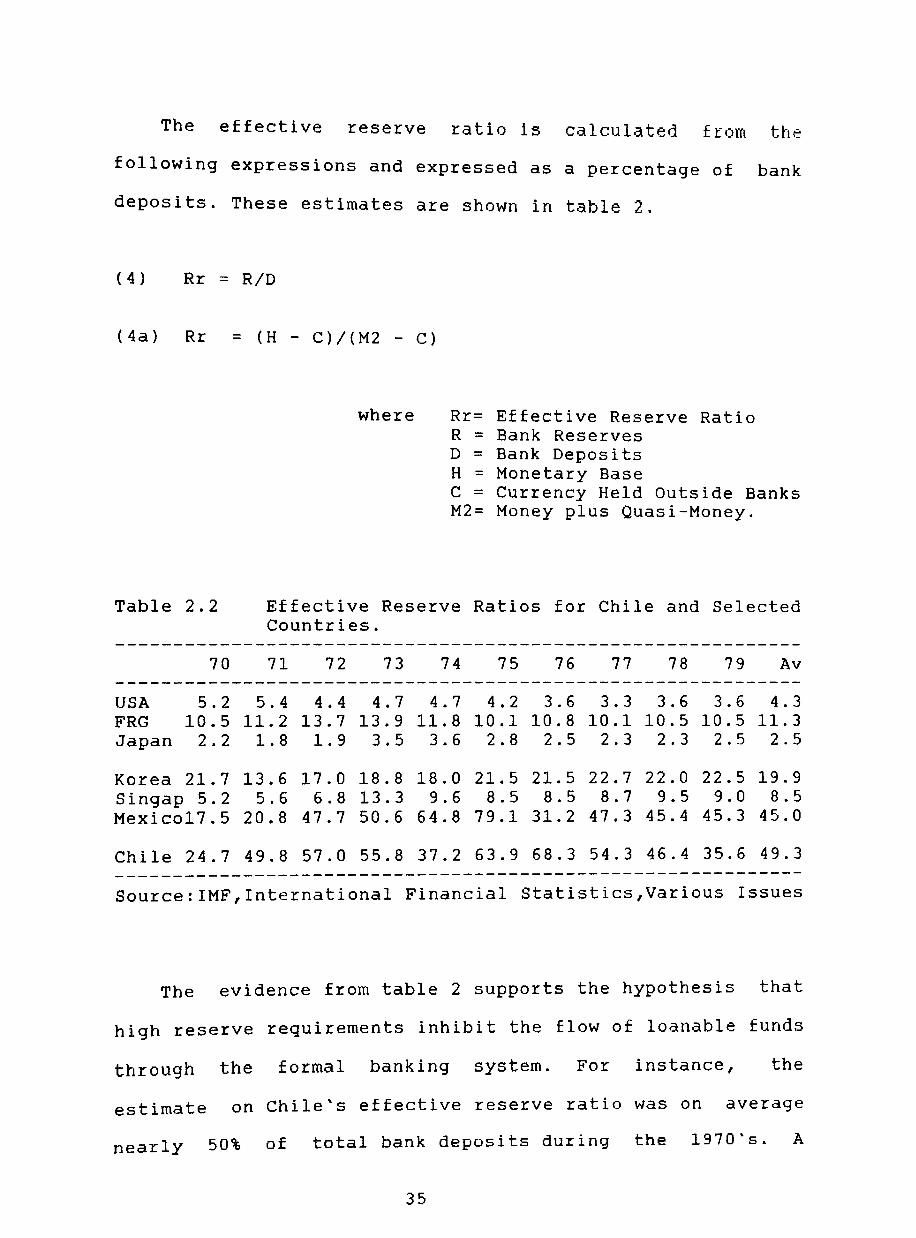
The effective reserve ratio is calculated from the

following expressions and expressed as a percentage of bank

deposits. These estimates are shown in table 2.

(4) Rr = RID

(4a) Rr = (H - C)/(M2 - C)

where Rr= Effective Reserve Ratio R = Bank Reserves D = Bank Deposits H = Monetary Base C = Currency Held Outside Banks M2= Money plus Quasi-Money.

Table 2.2 Effective Reserve Ratios for Chile and Selected Countries.

70 71 72 73 74 75 76 77 78 79 Av

USA 5.2 5.4 4.4 4.7 4.7 4.2 3.6 3.3 3.6 3.6 4.3 FRG 10.5 11.2 13.7 13.9 11.8 10.1 10.8 10.1 10.5 10.5 11.3 Japan 2.2 1.8 1.9 3.5 3.6 2.8 2.5 2.3 2.3 2.5 2.5

Korea 21.7 13.6 17.0 18.8 18.0 21.5 21.5 22.7 22.0 22.5 19.9 Singap 5.2 5.6 6.8 13.3 9.6 8.5 8.5 8.7 9.5 9.0 8.5 Mexico17.5 20.8 47.7 50.6 64.8 79.1 31.2 47.3 45.4 45.3 45.0

Chile 24.7 49.8 57.0 55.8 37.2 63.9 68.3 54.3 46.4 35.6 49.3 ------------------------------------------------------------Source:IMF,International Financial Statistics,Various Issues

The evidence from table 2 supports the hypothesis that

high reserve requirements inhibit the flow of loanable funds

through the formal banking system. For instance, the

estimate on Chile's effective reserve ratio was on average

nearly 50% of total bank deposits during the 1970·s. A

35

similar result was obtained for the case of Mexico where on

average 45% of bank deposits were held as legal reserve with

the Central Bank. In contrast, the evidence from industrial

countries and emerging developing economies shows high

M2/GDP ratios with low effective reserve ratios. For

instance, Japan's effective reserve ratio was only 2.5% of

bank deposits and M2/GDP ratio of 0.85 during the 70's.

Identical conclusions were obtained from the newly

industrialised countries (NIC's) such as Singapore and 10

Korea.

With respect to the implict tax on currency and on bank

reserves, the simplest method to calculate the total tax

revenue obtained by the authorities is to use the change in

the monetary base over the entire year. As we know the

monetary base consist of currency and bank reserves held

with the Central Bank. The choice of the monetary base as

the inflation tax base for my estimates was considered

superior and simpler over other monetary variables. For

instance, M1 which includes currency and sight deposits is

not accurate to estimate the magnitude of the revenue from

inflation tax since commercial banks capture most of the

revenues from sight deposits. Therefore, the monetary base

which is the monetary liability of the Central Bank should 11

be more accurate.

36

The method of calculating the ratio of nominal change in

the money base to the annual nominal GNP can seriously

overstate the seigniorage in high inflation countries.

Moreover, if interest are paid on reserves then it should be

discounted to obtain an unbiased estimate of the

government's seignorage. Unfortunately, this data is not

available for some countries and also very few 12

developing economies actually pay interest on reserves.

Beyond the specific issues concerning the accuracy of

government's seigniorage and the simplicity of the model,

the results from the estimation should help us to highlight

any difference among the selected countries. I have proceded

by estimating the total revenues from inflation tax using

separate components of the model. The estimates of the

inflation tax on currency are obtained from expression (5)

and reported in table 3.

(5) Cs = (ct - Ct-1}/GDP

37

where Cs = Revenues from Inflation Tax on Currency

C = Currency Held Outside Banks

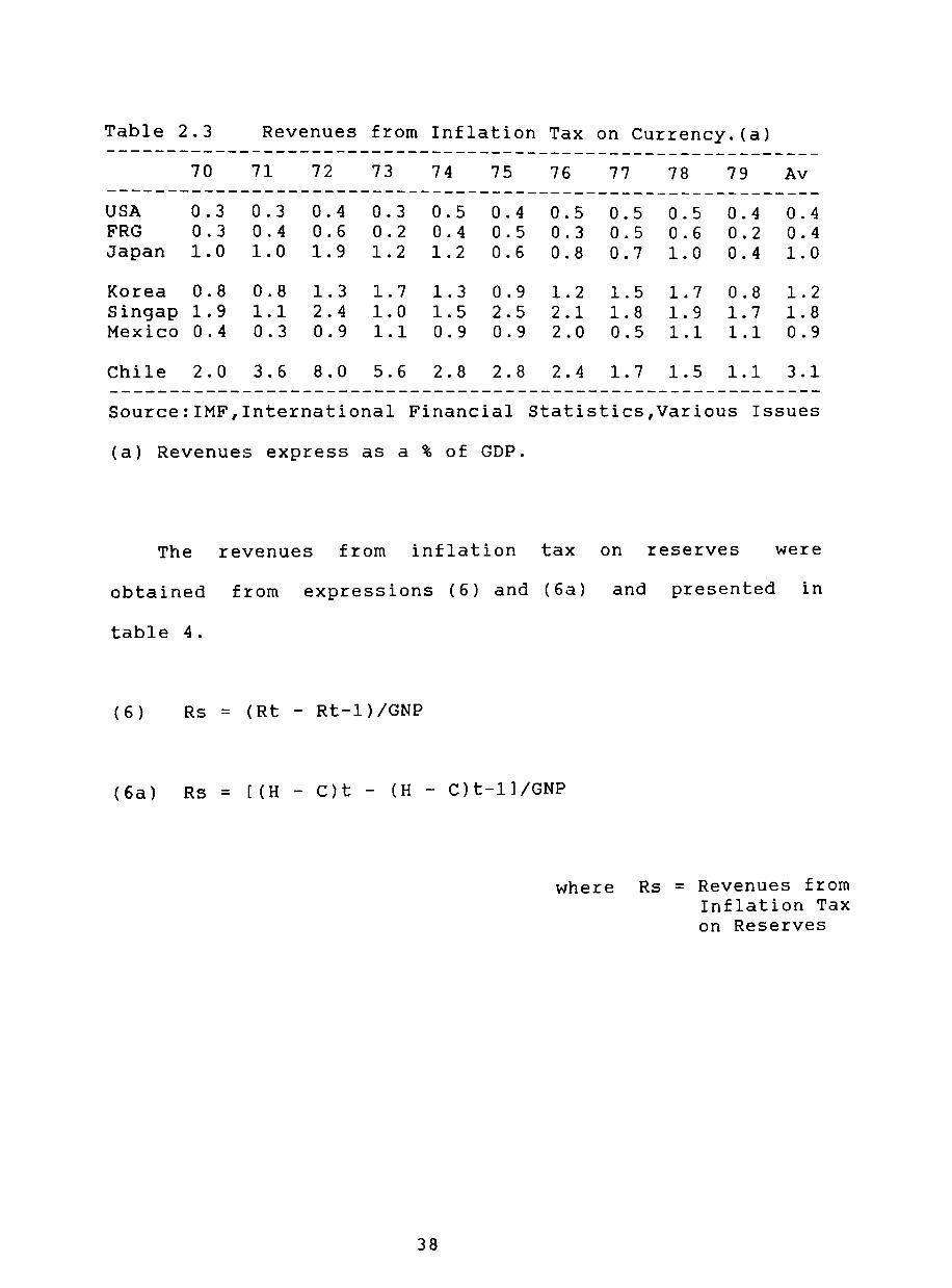
Table 2.3 Revenues from Inflation Tax on Currency. (a) ------------------------------------------------------------

70 71 72 73 74 75 76 77 78 79 Av ------------------------------------------------------------USA 0.3 FRG 0.3 Japan 1.0

0.3 0.4 0.4 0.6 1.0 1.9

0.3 0.5 0.2 0.4 1.2 1.2

0.4 0.5 0.5 0.3 0.6 0.8

0.5 0.5 0.5 0.6 0.7 1.0

0.4 0.2 0.4

0.4 0.4 1.0

Korea 0.8 0.8 Singap 1.9 1.1 Mexico 0.4 0.3

1.3 1.7 1.3 0.9 2.4 1.0 1.5 2.5 0.9 1.1 0.9 0.9

1.2 1.5 1.7 0.8 1.2 2.1 1.8 1.9 1.7 1.8 2.0 0.5 1.1 1.1 0.9

Chile 2.0 3.6 8.0 5.6 2.8 2.8 2.4 1.7 1.5 1.1 3.1

Source:IMF,International Financial Statistics,Various Issues

(a) Revenues express as a % of GOP.

The revenues from inflation tax on reserves were

obtained from expressions (6) and (6a) and presented in

table 4.

(6) Rs = (Rt - Rt-1)/GNP

(Ga) Rs = [(H - C)t - (H - C)t-11/GNP

38

where Rs = Revenues from Inflation Tax on Reserves

Table 2.4 Revenues from Inflation Tax on Bank Reserves. (a) ------------------------------------------------------------

70 71 72 73 74 75 76 77 78 79 Av ------------------------------------------------------------USA 0.1 FRG 1.4 Japan 0.1

0.5 -0.2 0.9 1.8 0.05 0.3

Korea 2.2 -1.2 2.0 Singap 0.3 0.4 1.2 Mexico 0.1 0.5 3.4

0.4 0.1 0.03 0.06 0.02 0.3 0.6 -0.5 -0.1 0.6 0.2 0.6 1.5 0.3 -0.2 0.0 0.05 0.2

0.1 0.1 0.2 0.5 0.3 0.3

1.9 0.7 3.7 -1.0 1.5 2.4

2.0 1.4 0.1 0.4 2.3 -2.7

2.0 0.3 8 • 4

1.3 1.4 0.7 0.5 2.5 3.2

1.4 0.7 2.2

Chile 0.5 7.3 8.1 15.1 4.8 4.4 6.5 3.2 2.7 1.3 5.4

Source:IMF,International Financial Statistics,Various Issues

(a) Revenues express as a % of GDP.

Finally, total government seignorage can be calculated

from (7)-(7b). It is simply the sum of the inflation tax on

both currency and reserves. These estimates are shown in

table 5.

(7) st = Cs + Rs

(7a) st = (ct - ct-1)/GNP + (Rt Rt-1)/GNP

(7b) st = (ct - Ct-1)/GNP + [(H - C)t - (H - C)t-l]/GNP

where st= Total Seignorage

39

Table 2.5 Total Revenues from Inflation Tax.(a) ------------------------------------------------------------

70 71 72 73 74 75 76 77 78 79 Av ------------------------------------------------------------USA FRG Japan

O. 5 1.7 1.2

0.8 1.3 1.1

Korea 3.1 -0.4 Singap 2.1 1.5 Mexico 0.4 0.8

0.1 2.4 2.2

3.4 3.7 4.3

0.7 0.6 0.8 -0.1 2.8 1.5

0.4 0.4 0.4

3.6 4.7 3.3

2.0 2.9 0.6 2.6 3.2 -0.7

0.4 0.9 0.8

0.5 0.8 0.5 1.2 0.7 1.3

2.6 3.5 3.0 2.5 2.1 2.6 8.9 3.6 4.3

0.5 0.4 0.7

2.1 2.3 4.9

0.5 0.9 1.3

2.6 2.5 3.3

Chile 10.9 16.1 20.7 7.5 7.2 8.9 4.9 4.1 2.4 2.3 8.5

Source:IMF,International Financial Statistics,Various Issues

(a) Total Revenues as a % of GDP.

The estimates from tables 3-5 suggest that Chile has

severely taxed its banking system in comparison to

industrial countries and emerging developing economies. In

effect, the average total revenues collected by the Chilean

government during the 1970's was 8.5% of GDP per annum. This

figure greatly exceeds the estimates for developed economies

which hardly reached in most cases the figure of 1%. At the

same time, economies like Singapore and Korea exhibit a low

dependence on inflation tax although it is still higher than

the US and Japan.

Another important observation from the data is that

Chile collected a larger proportion of the inflation tax

from bank reserves than from domestic currency. The currency

component of the inflation tax accounted only 3.1% per annum

during the 1970's whereas the reserve component was nearly

5.5%. This result is also true for Mexico and to a lesser

extent Korea. In contrast, US, Germany , Japan I and

40

singapore show a reversal in the relative importance of

currency and reserve as a source of 13

inflation tax.

revenues from the

The evidence from the estimates of governments'

seignorage gives support to the hypothesis that those

countries which have collected a substantial revenues from

inflation tax from depositors and borrowers as well as from

currency holders coincide with low M2/GDP. According to the

data, Chile did indeed systematically burden the banking

system with heavy taxes contributing partly to financial

repression and a low M2/GDP ratio.

Finally, as we have seen in the previous section interest

rates disequilibrium can also contribute to curtail the

amount of loanable funds through the formal banking system.

Low or even negative real yields on money and particularly

on quasi-money should discourage the demand for financial

assets. Negative real deposit rates will be consistent with

a portfolio shift away from financial assets, measured by

the growth of broad money (M2), and towards inflation hedges

such us real estate, gold, foreign currency, and even

consumption of durable goods. In contrast, countries that

have sustained positive real interest rates had exhibited

both a high growth of financial savings and rising flow of

loanable funds through the formal banking system.

41

Table 6 provides estimates of the ex post real deposit

rates for Chile and selected countries.

Table 2.6 Real Deposit Rate in Chile and Countries.(%)

Selected

------------------------------------------------------------71 72 73 74 75 76 77 78 79

------------------------------------------------------------USA 0.03 0.74 0.78 2.81 -3.00 -0.41 -0.86 0.55 -0.08 FRG 1.90 0.09 4.76 2.71 -0.85 0.00 0.67 0.35 1.00 Japan 4.73 3.05-10.26-19.84 2.26 -0.57 1.89 5.86 -3.71

Korea 6.17 0.26 8.52 -7.48 -8.22 0.78 3.81 3.58 0.25 Singap 1.44-11.5 -11.03 1.75 6.16 0.83 0.04 2.11 Mexico ... -14.37 -6.42 -3.55

Chile -16.60 8.60 18.50 24.90 4.40

Source:IMF,Internationa1 Financial Statistics,Various Issues

Real Deposit Interest Rate = {[(1+i)/1+%CPI)]-1}*100

The evidence suggest that those countries which have

maintained positive or moderate negative real yield on

deposits show high M2/GDP ratios. In contrast, countries

with severe and systematic negative real deposit rates

exhibit relatively low deepening ratios.

According to the data from table 6, the real deposit

interest rate for Chile in 1975 was minus 16.6%. Moreover,

judging from the inflation data in table 7a and the

existence of interest ceilings, one can assert that

interest rates were also negative during the early 1970's.

In effect, the average rate of inflation between 1972 and

1974 was nearly 350% per annum with a peak of 508% in 1973.

42

In the absence of data for nominal deposit interest rate, we

observe that nominal lending interest rate did not adjust in

line with price inflation. The average nominal lending rate

between 1972-74 was only 100% per annum with a peak of 200%

in 1974. It is not unrealistic to expect real deposit

interest rates were much lower than lending rates as much as

it was the flow of loanables funds during the first half of

the 1970's. Indeed, the M2/GDP ratio should not be that

different from the 1974's estimate of 6.5%.

As we will see later in the paper, the phasing out of

interest rates control in October 1974 contributed to a

rapid transformation of negative to positive interest rates

from 1976 onwards as shown in table 6. This in turn

coincided with an increasing demand for financial savings

intermediated through the banking system. In fact, the

M2/GDP ratio was continuously climbing and by 1979 was at

14%. The positive correlation between financial savings and

the real deposit interest rate appears to be valid for the

case of Chile according to this preliminary examination.

43

Table 2.7a Interest Rates, Inflation Rates, and Financial Savings in Chile and Selected Emerging Economies.

------------------------------------------------------------71 72 73 74 75 76 77 78 79

------------------------------------------------------------Korea Interest Rate Inflation Rate M2/GDP GOP Growth

Singapore Interest Rate Inflation Rate M2/GDP GOP Growth

Mexico Interest Rate Inflation Rate M2/GDP GOP Growth

Chile Interest Rate Inflation Rate M2/GDP GOP Growth

20.4 13.4 32.1

9.2

1.8 61.6 12.5

12.0 11.7 34.8

5.9

3.5 2.1

64.7 13.4

12.0 3.2

36.4 14.4

11.6 26.2 59.7 11.5

15.0 24.3 32.1

7.9

8.9 22.4 55.2

6.3

15.0 25.3 30.8

7.1

4.4 2.6

61.0 4.1

16.2 15.3 30.0 12.9

4.1 -1.9 62.8

7.5

5.0 4.7 13.6 24.0 16.1 13.8 15.8 16.1 16.6 15.4 14.9 17.7

4.2 8.5 8.4 6.1 5.6 4.2

22.1 163 508

9.0 -1.2 -5.6

267 375 340

6.5 1.0-12.9

197.7 174.3

6.8 3.5

14.4 10.2 32.5 10.1

4.0 3 . 2

61.1 7.8

10.6 29.2 28.4

3. 4

93.7 63.5 9.2 9.9

18.6 14.5 35.5

9.7

4.7 4.7

60.9 8.6

11.1 18.8 29.9

8.3

62.8 30.3 12.1

8.2

18.6 18.3 31.5

7.6

6.2 4.0

62.8 9.3

13.2 17.4 30.9

9.2

45.0 38.9 14.0

8.3

Source:IMF,International Financial Statistics,Various Issues

The estimates for industrialised and the rapidly

emerging economies have consistently showed positive yields

on bank deposits and coincided with a large flow of loanable

funds through their organised banking system. However, the

M2/GDP ratio fell somewhat during the unexpected oil shocks

during 1973-74 and 1978-79. Inflation accelerated rapidly

and nominal interest rates failed to adjust fully producing

negative deposit interest rates as shown by table 7b.

This evidence confirms the hypothesis that positive

yields on financial savings defined in terms of broad money

44

(M2) should increase its demand and intermediation through

the organised banking system. Countries such as Chile which

have consistently inhibited nominal intere5t rate from

adjusting to price inflation have paid a cost in terms of

small flow of loanable funds and an immature and repressed

banking system.

Table 2.7b Interest Rates, Inflation Rates, and Financial Savings in Selected Industrialised Economies.

US Interest Rate Inflation Rate M2/GDP GOP Growth

Germany Interest Rate Inflation Rate M2/GDP GOP Growth

Japan Interest Rate Inflation Rate M2/GDP GOP Growth

71

4.3 4.3

65.3 3.2

7.2 5.2

35.0 3.0

4.0 -0-7 83.6

4. 3

72

4.0 3.3

67.1 4.8

5.6 5.5

36.0 4.3

3.8 0.8

91.2 8.4

73

7.0 6.2

64.0 5.4

12.1 7.0

36.0 4.8

4.0 15.9 87.6

7.6

74

7 • 8 11.0 62.3 -0.5

9.9 7.0

35.0 0.1

5.3 31.4 81.9 -0.8

75

5.8 9.1

64.5 -1.1

5.0 5.9

37.0 -1.3

5.3 3.0

84.6 2.9

76

5.2 5.7

65.8 5.1

4.3 4 . 3

38.0 5.5

4.5 5.1

85.5 4.2

77

5.5 6.5

65.2 4.6

4.4 3.7

39.0 2.6

3.8 1.9

85.2 4.8

78

8.2 7.6

62.2 4.8

3.0 2.7

39.0 3 • 4

2.6 -2.5 87.4

5.0

79

11.2 11.3 59.5

2.8

5.1 4.1

38.0 4.0

3.3 7.3

87.5 5.6

------------------------------------------------------------Source:IMF,International Financial Statistics,Various Issues

One could conclude from the evidence that a heavily

taxed banking system and substantial interest rate

disequilibrium should have an adverse impact on the return

to savers, the accumulation of financial savings and the

maturity of the banking system.

45

Another significant finding from the data suggests that

a repressive financial system was also consistent with low

rate of economic growth. The real deposit rate as a return

for financial savings is paramount for higher volumes of

investment as well as increasing the average efficiency of

investment. As we have seen from the theory, real deposit

rate affects the accumulation of financial savings,

investment, and growth either through the Mckinnon's

complementary hypothesis or Shaw's financial deepening

approach.

If we look at the data on M2/GOP ratios and real growth

rates for Chile and selected countries in tables 7a and 7b

we observe an apparent positive correlation between high

financial deepening ratios and real GOP growth rates. For

instance, Chile presents a M2/GOP ratio well below 10% and

an average real growth rate of nearly minus 2% during the

period of severe interest rate disequilibrium. In contrast,

industrialised economies and the NIC's which systematically

showed positive and in some years moderately negative real

interest rates they also exhibit high M2/GDP ratios and

high real GOP growth. Indeed, for the group of industrial

nations the average M2/GDP ratio during the 70's was 67% and

coincided with an average real GOP growth of 3.8% .. Similar

results are found with rapidly emerging developing countries

where an average of 48% on the M2/GOP ratio was associated

with a GDP growth rate of 9.3%.

46

These results and conclusions concerning the

relationship between interest rates, financial savings, and

economic growth are consistent with other empirical findings

using a wider cross-country analysis. For instance, Mckinnon

(1980,1988) using cross-country comparisons between semi­

industrial less developed countries and rapidly growing

economies also found that the former group have fairly low

M2/GDP ratios as compared with the latter.

Similarly, Lanyi and Saracoglu (1983) provides a study

on four member countries: Argentina, Brazil, Korea, and

Turkey. In fact, countries such us Brazil and Korea which

maintained positive real interest rates throughout the

1970's enjoyed a rapid expansion in financial assets,

measured by the real growth rate of money plus quasi-money

(M2). Argentina and Turkey were example of financially

repressed economies with negative yields on financial assets

and low and even negative real growth rate of financial

assets. The econometric verification was done by classifying

a larger list of countries in three groups. Group A which

included countries with positive real deposit rates and was

allocated a value of 1. Group B was conformed by countries

with moderate negative interest rate and assigned the value

of O. Finally, group C was integrated by countries with

severe negative yields on deposits and given a value of -1.

They regressed the growth rate of financial savings (M2)

against the interest rate policy indicator defined for each

group with sample data for the period between 1970 to 1980.

47

The interest rate coefficient turned up very large,

positive, and statistically significant. Similar results

were obtained by replacing M2/GOP ratio for the growth rate

of M2. At the same time, they also found that interest rate

coefficient was positive and significant when regressing

against the rate of growth of GOP.

Equally, Fry (1978,1988) was also interested in the

empirical assessment of the impact of financial conditions

on aggregate savings, but in a much wider framework

including variables such as income, terms of trade,

population, and branching among others. According to Fry

(1988), most of the evidence for LOC's pointed out that real

deposit rates were statistically significant although with a

small positive coefficient. For example, Fry (1978)

estimated a general aggregate saving equation in order to

test how changes in financial conditions affect savings and

economic growth. He pooled together annual observations for

Taiwan, Singapore, Korea, Malaysia, Phillipines, India, and

Burma. The aggregate saving function Sd/Y=f(g,y,r,Sf/Y,Sd/Y)

where Sd,Sf,g,y,and r are defined as gross national savings,

foreign savings, income growth, real per capita income, and

the real deposit rate of interest respectively, was

estimated by a two-stage least square method and have thrown

the following results: Firstly, the signs of all coefficient

were consistent with a priori expectations and statistically

significant. Secondly, the coefficient of the real deposit

rate of interest was found positive and significant.

48

Fry using the same series of observations also tested

the significance of real deposit rate of interest on the

rate of growth of GDP. The ordinary lea5t 5quare e5timate

was significant and consistent with a priori expectations.

The empirical results of this section and existing

evidence should be treated with caution. Firstly, in

relation to the importance of the rate of interest on

financial deepening, it could be argued that although the

estimates are significant its magnitude was rather small.

Moreover, even if financial savings have risen substantially

the increase in the overall savings was not granted. The

case of Chile is an example of this puzzle.

Secondly, more recent findings have questioned the

significance of interest rates. Giovannini (1985) rejected

some of the existing findings on the interest elasticity of

savings, particularly those by Fry (1978). He argued that in

Fry's sample two observations of Korea's financial reform

period had a disproportionately large influence. The re-

estimation of the Fry's saving function with the omission of

1967 and 1968 observations for Korea showed that the

interest elasticity was insignificant. Similar results were

obtained with a larger sample to demonstrate the importance 14

of the choice of the sample period in the results.

However, Fry (1988) challanged Giovannini's results by

excluding Korea altogether from the sample and reporting

that the significance as much as the coefficient of the real

deposit interest rate became even larger. Equally, Gupta

49

(1987) has challanged Giovannini's findings as well as those

by Fry (1978) on the grounds that both studies includes

Asian and Latin American countries. As a result of large

differences in the effects of various variables including

interest rates, a disaggregation between these two groups

was seen as most desirable. The coefficient of the nominal

interest rate for the pooled sample was found

and the restriction that nominal interest

expected inflation did not hold either. In

nominal rate of interest was significant

equality condition did not hold for the

insignificant

rate equal

contrast, the

although the

Asian sample

(Malaysia, Sri-Lanka, Singapore, Taiwan, Phillipines, India,

Korea, Thailand, and Pakistan). For Latin America

(Venezuela, Panama, Honduras, Guatemala, EI Salvador,

Paraguay, Mexico, Ecuador, Uruguay, Peru, Colombia, Bolivia,

Rep. Dominicana) the equality condition was not met and the

coefficient of nominal interest rate, although correctly

signed, was not significant.

Thirdly, the relationship between financial deepening

and growth runs in both ways. A high rate of economic growth

may be the result of high and rising flows of loanables

funds but rising M2/GDP ratios may also be the result of the

economy's growing output. Therefore, the question of

deciding between exogeneous and endogenous variables is far

from being a trivial issue. Furthermore, different

interpretations

output growth

may arise from regression results

and real deposit interest rate. On

50

between

the one

hand, positive interest rates may increase financial

deepening and the rate of economic growth or increase the

quality of investment and the rate of output growth on the

other.

King and Levine (1993) introduced an endogenous growth

model in which the financial system evaluate

entrepreneurs, mobilised savings to finance

prospective

the most

promising productivity-enhancing activities, diversify the

risk associated with these innovative activities, and reveal

the expected profits from engaging in innovation rather than

the production of existing goods using established

techniques. Thus a more developed and mature financial

system stimulate

productivity growth

growth by accelerating

via innovation. Their

the rate of

evidence from

cross-country analysis and case studies support the positive

correlation between financial deepening and economic growth.

At the same time, they found that financial distortions

reduce the rate of economic growth by reducing the rate of

innovation. Indeed, implict and explicit taxes on

intermediation rises the cost of innovation (higher costs

of evaluating and financing entrepreneurs) and hence a lower

rate of return at any given growth rate.

Although this paper confirms the importance of financial

deepenning

as well

financial

on productivity growth and economic development

as rejecting those policies which distort the

system the issue of causality still remain

unanswered.

51

(2.3) The Banking System and Financial Liberallsatloo in Chile:1973-1983.

(2.3.1) Financial liberalisation in Chile: What was done?

This section presents and discusses the liberalisation

reforms introduced between 1973 and 1982. A chronological

synthesis with the principal liberalisation reforms is shown

in table 8. The itinerary of financial liberalisation is

included with the rest of the market liberalisation reforms

of Chile's new development strategy, including economic

stabilisation and the liberalisation of other specific

markets. The process of financial liberalisation began

shortly after the military coup of September 1973. The

itinerary of financial reforms was accompanied by other

equally important liberalisation reforms and economic

stabilisation. At the same time, financial liberalisation

reforms included institutional, regulatory, and

international changes aiming at the achievement of a more

competitive, mature, efficient, stable, and liberal

financial order.

The financial reforms started in May 1974 with a set

institutional changes which included the privatisation of 19

nationalised banks with the exception of Banco del Estado.

The privatisation also included the 259 intervened and/or

nationalised enterprises during Allende's government as well

as 183 firms with minority or majority stake shareholding.

52

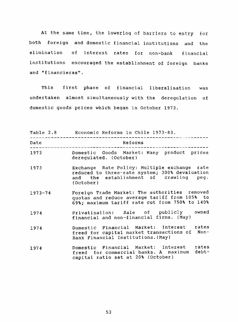
At the same time, the lowering of barriers to entry for

both foreign and domestic financial institutions and the

elimination of interest rates for non-bank financial

institutions encouraged the establishment of foreign banks

and "financieras".

This first phase of financial liberalisation was

undertaken almost simultaneously with the deregulation of

domestic goods prices which began in October 1973.

Table 2.8

Date

1973

1973

1973-74

1974

1974

1974

Economic Reforms in Chile 1973-83.

Reforms

Domestic Goods Market: Many product prices deregulated. (October)

Exchange Rate Policy: Multiple exchange rate reduced to three-rate system; 300% devaluation and the establishment of crawling peg. (October)

Foreign Trade Market: The authorities removed quotas and reduce average tariff from 105% to 69%; maximum tariff rate cut from 750% to 140%

Privatisation: Sale of publicly financial and non-financial firms. (May)

Domestic Financial Market: Interest freed for capital market transactions of Bank Financial Institutions. (May)

Domestic Financial Market: Interest freed for commercial banks. A maximum capital ratio set at 20% (October)

53

owned

rates Non-

rates debt-

Table 2.8 (continued) ------------------------------------------------------------Date Reforms --------~---------------------------------------------------1974

1975

1976

1976

1976

1977

Domestic Financial Market: Minimum capital limits were established together with specifications of operations that were permitted. Limits on investment and credits to any individual or legal entity are imposed. No individual could own more than 1.5% of a bank's capital and 3% for a legal entity. For newly established bank, this limit would be enforced five years after operations started. Commercial, Development, and Mortgage banks were not allowed to acquire shares of small financial institutions. Foreign banks were permitted to establish branches and offices. (December)

Taxation: Extension of the value-added tax coverage; one-year surcharge on personal income tax; and 10% consumption tax on luxury goods. The improvement in tax collection was complemented with 19% cut of government spending on goods and services. The reduction of the fiscal deficit from 30.5% of GDP to only 2.6% in one year was complemented with a tight monetary policy.

Domestic Financial Market: Central Bank began paying competitive interest rates on reserve requirements starting in May. Subsequently, reserve requirements were gradually lowered from 47% in 1977 to 20% in December 1978. By December 1980 the legal reserve requirement was 10% for sight deposits and 4%/ for time deposits. Also interest payments on reserves were phased out.

Exchange Rate unified exchange

Policy: Introduction of a rate was reached by August.

Foreign Trade Market: New tariff structure proposed with rates of 25%,30%, and 35% for primary, semimanufactured, and manufactured goods respectively.

Domestic Financial Market: A free state deposit insurance was introduced equivalent to a maximum of U$ 2.789. However, depositors in general thought that there was a de facto 100% guarantee as a result of the government bailout of Banco Osorno a day before the introduction of the limited explicit guarantees for small depositors. (January)

54

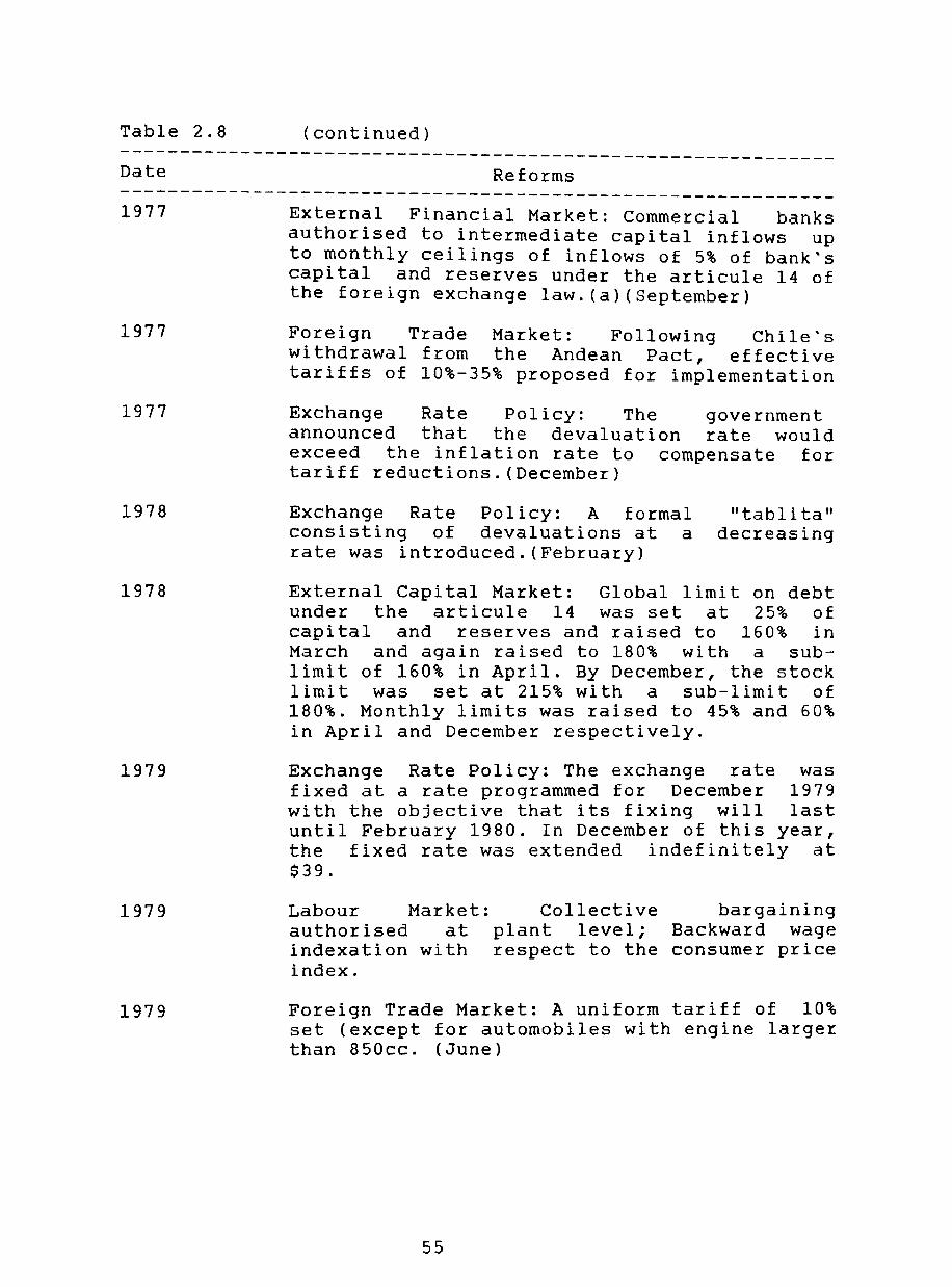
Table 2.8 (continued) ------------------------------------------------------------Date Reforms ------------------------------------------------------------1977

1977

1977

1978

1978

1979

1979

1979

External Financial Market: Commercial banks authorised to intermediate capital inflows up to monthly ceilings of inflows of 5% of bank's capital and reserves under the articule 14 of the foreign exchange law. (a) (September)

Foreign Trade Market: Following Chile's withdrawal from the Andean Pact, effective tariffs of 10%-35% proposed for implementation

Exchange Rate Policy: The government announced that the devaluation rate would exceed the inflation rate to compensate for tariff reductions. (December)

Exchange Rate Policy: A formal consisting of devaluations at a rate was introduced. (February)

"tablita" decreasing

External Capital Market: Global limit on debt under the articule 14 was set at 25% of capital and reserves and raised to 160% in March and again raised to 180% with a sub­limit of 160% in April. By December, the stock limit was set at 215% with a sub-limit of 180%. Monthly limits was raised to 45% and 60% in April and December respectively.

Exchange Rate Policy: The exchange rate was fixed at a rate programmed for December 1979 with the objective that its fixing will last until February 1980. In December of this year, the fixed rate was extended indefinitely at $39.

Labour Market: Collective bargaining authorised at plant level; Backward wage indexation with respect to the consumer price index.

Foreign Trade Market: A uniform tariff of 10% set (except for automobiles with engine larger than 850cc. (June)

55

Table 2.8 (continued) ------------------------------------------------------------Date Reforms ------------------------------------------------------------1979

1980

1981

1982

1982

1982

1982

External Financial Market: In April global limits on external borrowing was raised again to 225% with a sub-limit of 215%, and a monthly limit of 70%; a variable reserve requirement was set for external credits depending on the lenght of maturity of the loans: 10% for 48-66 months, 15% for 36-48 months, and 25% for 24-36 months. In June, global limits and and debt limits under articule 14 were eliminated. The only limitation on bank indebtedness was the 20% debt-capital ratio. Monthly limits was reduced to 5%.

External monthly

Financial Market: In limits were eliminated.

April all

External Financial Market: In December commercial banks were allowed to lend short-term (180 days) with external credit for purposes other than financing commercial operations.

External Financial Market: Commercial were permited to obtain external credits a maturity under two years subject reserve requirement of 20%.(May)

banks with

to a

Exchange Rate Policy: The fixed rate regime was abandoned in June. An 18% devaluation was enacted and followed with a floating rate in August.

External Financial Market: Commercial banks were allowed to use part of their short-run foreign credits to lend in pesos with a limit of 50% of capital and reserves. (July)

Rate Policy: A new "tablita" devaluations equivalent to month's inflation rate minus 1%

Exchange monthly previous announced. restricted.

Access to the exchange market

with the was was

------------------------------------------------------------Sources: Corbo (1987), Corbo and De Melo (1987)

(a) Articule 14 refers to the permission given by the Central Bank to the borrowers for future access to the exchange rate market to serve a foreign debt.

56

The second

deregulation of

interest rates

and

phase consisted of the financial

the domestic capital market.

were lifted in october 1974

Controls in

and by 1975

qualitative restrictions on credit were quantitative

phased out. At the end of 1974, requirements on

banks'capital were increased to take into account past

inflation and thereafter were automatically adjusted once a

year according to the increase in the CPl. Moreover, Maximum

debt-capital ratio and limits on individual ownership of

banks' shares and credit concentration were introduced

during the same year. For instance, in October 1974 the

maximum leverage ratio was set at 20% and the individual

ownership of banks' shares could not exceed 1.5% of bank

capital. Commercial, Development, and Mortgage banks were

not allowed to own shares of small financial institutions.

In May 1976, the Central Bank began paying a competitive

interest rate on reserve requirements. By the end of 1980,

reserve requirements were significantly lowered and the

interest payments phased out. For instance, reserve

requirements were gradually lowered from 47% in 1977 to 20%

in December 1978. By December 1980 the legal reserve was set

at 10% for sight deposits and 4% for time deposits.

As we notice from the summary of liberalisation reforms,

interest rate deregulation and the significant reduction in

reserve requirements coincided with fiscal reforms to

eliminate the fiscal deficit. Cuts in government spending

combined with an improvement in tax collection were decisive

57

in the marked reduction in the government's deficit from

1975 onwards. In fact, table 9 shows that the fiscal deficit

as a percentage of GDP fell from 10.5% in 1974 to 2.6% in

1975. By 1980, the government exhibited a fiscal surplus of

3.1%. This enabled the financial system to escape from

financial repression by reducing both the inflation tax and

reserve requirements, and also interest rate controls.

The last phase of financial liberalisation focused on

the liberalisation of the external capital market.

International capital inflows were deregulated gradually and

mainly on medium and long-run maturities, that is over two­

year maturity. Initially, banks' access to external credit

was severely limited and permitted to finance foreign trade

operations. However, from September 1977 to April 1980,

access to medium and long-run foreign credit was allowed but

with specific limits on global and monthly indebtness as

percentage of banks' capital and reserves. According to the

summary in table 8, the 5% monthly limit on foreign

indebteness under article 14 of the foreign exchange law was

raised to 45% and 60% of bank capital between April and

December of 1978. Also, as we can see in table 8, global

limits were continuously relaxed from 25% in 1978 to 225% in

April 1979. By June of the same year, global limits and

limits on indebtness under article 14 were eliminated and by

April 1980 all monthly limits left were eliminated.

58

Banks were allowed to borrow abroad in foreign currency

(dollars) but not to assume the exchange risk. Later in

December 1981, commercial banks were authorised to lend on a

short-term basis with external credit for purposes other

the than financing foreign trade transactions.

middle of 1982, short-term capital inflows were

but subject to a reserve requirement of 20%.

Towards

liberalised

Finally, in

July 1982 commercial banks were permitted to assume the

exchange risk so that a portion of their short-run foreign

credit was lent in pesos with a limit of 50% of capital and

reserves.

There are important points to make on the

deregulation of international capital flows

process of

in Chile:

Firstly, the opening of the capital account was complemented

with the introduction of a preannounced exchange rate

"tablita" which culminated with a fixed exchange rate.

Although, the exchange rate regime made investing in Chile

very appealing by reducing the exchange rate risk still

domestic interest rates remained stubbornly high.

Secondly, the liberalisation of short-term capital inflows

was responding to a growing financial distress from the

sudden and rapid reduction in the rate of capital inflows

during 1981-82 rather than a pre-conceived policy_ Table 9

provide some evidence on the magnitude of capital inflows,

an issue which will be raised shortly_

59

All in all, the itinerary of liberalisation of the

domestic capital market was preceded by a significant

progress in the government's public finance. In addition,

the liberalisation of the banking system to capital inflows

was conceived gradually and only after the domestic capital

market was fully deregulated. With respect to financial

liberalisation inserted within the overall liberalisation

strategy, domestic capital market was freed simultaneously

with the goods market. The liberalisation of capital inflows

lagged substantially behind the liberalisation of trade.

The itinerary of the Chilean liberalisation appeared to

be consistent with what appears to be the consensus among

theorists. However, there were two issues overlooked by the

authorities in the liberalisation of the financial system.

Firstly, the

establishment

process of privatisation

of large and powerful economic

led to

groups

the

which

controlled both commercial and financial institutions. In

fact, Dahse (1979) argued that no more than fifty

individuals owned the entire financial system. The structure

of bank holding companies and high bank concentration in

Chile were an undesirable and negative for the success of

financial liberalisation.

Secondly, financial liberalisation did not involve the

modernisation of the existing regulatory framework in order

to ensure the bankers' compliance with ownership and credit

concentration limits of the new bank legislation. The

combination of bank holding company structure and an

60

effective prudential regulation have played an important

part in the ex post results of financial liberalisation , particularly with the debacle of the banking system in 198),

The issues concerning bank holding company structure,

credit concentration and related portfolios, and the role of

prudential regulation, will be addressed in more detail in

chapters 4 and 8. The following sub-section will address

and evaluate the ex post results of financial

liberalisation.

(2.3.2) The Impact of Financial Liberalisation in Chile.

The central objective of financial liberalisation was to

develop and modernised the financial

the banking sector which represented

system, particularly

the most important

segment of the financial system. As I have argued earlier,

positive real yields on domestic financial assets, the

establishment of a competitive multi-purpose banking, and

a market allocation of bank credits was thought to be

paramount in both raising financial deepening and widening

(financial savings) and the quantity and quality of

investment, including the allocation of loanable funds. At

the same time, the integration of domestic financial market

to world financial market was bound to generate a rapid

convergence of domestic financial prices to those prevailing

in world markets. Equally, it was expected that the role

played by the increasing competitive forces should

61

contribute to some gains in operative efficiency. However,

above all there was a conviction among "liberalisationists"

and policy-makers that the liberal financial arrangements

were bound to promote ultimately financial stability.

Before we begin with the assessment of the impact of

financial liberalisation, it has to be said that there were

also a series of additional factors. As we have seen in

table 8, financial liberalisation was implemented together

with anti-inflationary policies given the initial

macroeconomic disequilibrium on both fronts internal and

external. Both the inflation rate and the current account

deficit were very high. In effect, Table 9 indicates that

consumer price inflation was 358% per annum between 1971 and

1975. At the same time, the current account deficit was

getting bigger and unmanageable at 4.5% of GOP in 1975.

Table 2.9 Economic Indicators For Chile.

71-73 74 75 76 77 78 79 80 81 ------------------------------------------------------ ------GOP(a) 0.7 1.0 12.9 3.5 9.9 8.2 8.3 7.5 5.3 GOPp(b) 1438 1345 1152 1172 1266 1347 1434 1516 1568 VCPI 231.2 375.9 340.1 174.3 63.5 30.3 38.9 31.2 9.5 FOf/GOP 15.1 10.5 2.6 2.3 1.8 0.8 -1.7 -3.1 -1.6 CAcc/GOP 2.9 4.5 -0.9 3.7 5.3 5.5 7.8 16.5 Unemp. 4.6 9.7 16.2 16.8 13.2 14.0 13.6 11.8 11.1 ---------------------------------------------------------------_. Source:Banco Central de Chile,Boletin Mensual,Various Issues

Banco Central de Chile, Cuentas Nacionales 1960-80

(a) The rate of growth of GOP are estimated at 1977 prices. (b) GOPp correspond to real per capita GOP express in US

dollars

Notes: VCPI=variation of the consumer price index. FOf/GOP=fiscal deficit as a proportion of GOP. CAcc/GOP=curret account deficit as proportion of GOP Unemp. = Correspond to the unemployment rate.

62

Furthermore, with financial liberalisation other reforms

such as the deregulation of the goods market and the opening

of the trade regime, changes in labour legiBlation, and

privatisation were undertaken during this period. In

consequence, it is difficult to isolate and identify the

specific impact of the financial liberalisation vis a vis

other reforms and to link them with the ex post results.

(2.3.2.1) Financial Deepening, Saving, and Investment in Chile.

As it was expected financial deepening increased

strongly during the liberalisation period. The evidence from

table lOa provides different measures which account for the

spectacular expansion in financial intermediation

(deepening).

The degree of financial deepening measured by the M2/GNP

ratio shows that it increased from its lowest figure of 6.4%

in 1974 to nearly 32% in 1982. More importantly, there was a

remarkable increase in the proportion of GNP held in the

form of time and saving deposits. In effect, the ratio of

quasi-money to GNP went from 1.1% in 1974 to 25.3% in 1982.

Similar results were obtained from the non-monetary

assets/total financial assets ratio (NMA/TA) which shows a

marked increment between 1974 and 1982 of 14% to more than

70% of total assets respectively. This portfolio shift away

from money was responding to the upward trend observed in

short-term interest rate paid on quasi-money following

63

interest rates deregulation, and to the availability of a

wider options of financial assets. The average ex post real

deposit rate between 1975 and 1982 was 15.2 per annum with

a peak of 25.4 in 1981 in comparison to the negative rates

which prevailed during 1970-73.

Table 2.10a Indicators of Financial Deepening and Growth of Financial Assets. (a)

------------------------------------------------------------M1/GNP QM/GNP M2/GNP TFA/GNP MA/TA NMA/TA

------------------------------------------------------------1973 10.6 2.3 12.9 14.9 53.0 14.3 1974 5.3 1.1 6.4 20.0 27.7 14.0 1975 4.5 2.6 7.1 19.7 26.1 16.2 1976 3.9 3.7 7.6 19.0 25.4 25.0 1977 4 . 5 6.0 10.5 21.0 24.1 38.6 1978 4.8 7.7 12.5 23.0 24.6 48.6 1979 4.9 9.7 14.6 29.6 21.1 50.1 1980 5.5 10.7 16.2 34.9 19.8 59.8 1981 5.0 14.6 19.6 39.0 14.7 69.8 1982 6.6 25.3 31.9 48.1 14.0 70.7

Source:Banco Central Chile,Month1y Bu11etin,Various Issues (a) Share of GDP on amounts in pesos each year. Notes: M1= notes and coins+demand deposits

QM= quasi-money defined as time and savings deposits M2= M1+quasi-money TFA= total financial assets defined as M1 plus

deposits in banks,non-bank financial institutions, saving and loans institutions. i.e.total liabilities of the financial system

MA= MI NMA= non-monetary assets which includes paper issued

by commercial and development banks as well as non-bank financial institutions.

The total financial asset/GNP ratio (TFA/GNP) which is

estimated at constant 1977 peso prices in order to eliminate

the inflationary distortions and which comprise a wider

definition of financial assets have also thrown similar

64

results. By 1973, the ratio was indicating that total

financial assets was nearly 15% of GNP and by 1982 was more

than 48%.

The thesis on the spectacular rise in financial

deepening (financial savings) came out mainly from a change

in wealth composition has been challanged by some

commentators of the Chilean economy. For instance,

Barandarian (1983) sustained the view that expectations of

buoyant future of the economy generated a rise in perceived

wealth. Indeed, financial deepening grew along side private

sector wealth as capital gains in booming stock market were

capitalised through the banking system. The evidence shows

that real stock prices between 1977 to 15

more than 320%.

1981 grew

Similarly, Arellano (1983) maintained that changes in

wealth composition were small and the rise in financial

savings came mainly from the privatisation of the

government social security in May 1981 and the rise in

external liabilities. The excess of external financing over

the current account deficit was destinated towards the

accumulation of international reserves and deposits in the

domestic financial system.

The impressive rise of financial deepening was also

accompanied by a growing number of participants In the

financial system. According to table lOb the number of

domestic banks increased from 20 to 27 between 1974 to 1981

65

although it began to fall in 1982 after the liquidations of

financial institutions beginning in 1981-82. This syndrome

became more acute after the banking crisis of 1983 as it

will be shown in chapter 3.

With respect to foreign financial institutions, the

number of foreign commercial banks have been continuously

rising from a single foreign entity in 1974 to 19 in 1983.

It appears that the expansion in the number of foreign

banks remained untrammel despite the banking crisis of 1983.

After an auspicious start of non-bank financial

institutions several "financieras" were liquidated

particularly from 1981-82 onwards. The number fell from 17

between 1977 and 1980 to only 7 in 1983. As we will see in

chapter 3, although there was a large number of

"financieras" many of which experienced financial

difficulties during the early 1980's, their share of total

liabilities and assets of the system was very small as

compared with banks. In general, the number of total

financial institutions went from 21 in 1974 to its highest

number of 60 in 1981 with a predominance of domestic banks 16

over foreign banks and financieras.

66

Table 2.10b Financial Institutions in Chile. ------------------------------------------------------------

Domestic Banks Foreign Banks Financieras Total ------------------------------------------------------------1974 1975 1976 1977 1978 1979 1980 1981 1982 1983

20 21 21 22 22 25 25 27 19 19

1 2 2 3 5

10 13 17 19 19

17 17 17 17 16

9 7

21 23 23 42 44 52 55 60 47 45

------------------------------------------------------------Source: SIBF, Informacion Financiera, Various Issues.

However, despite the spectacular growth of financial

intermediation financial liberalisation did not contribute

to deepen the maturity of financial assets hold by economic

agents. The evidence in table 10c shows that assets with

maturities of less than 90 days were dominant in the

holders' portfolio although maturities beyond 1 year also

experienced an important increase between 1979 and 1982. For

instance, financial assets with maturities of less than 90

days were accountable for 48.1% of total financial assets

during 1981. Those assets with maturities of more than 90

days and less than a year exhibited a continuous decline.

However, there was a positive rise in the share of assets

with maturities over a year from 3.4% in 1973 to 25.3% in

1982 although still was well below the assets' share with

short-term maturity.

67

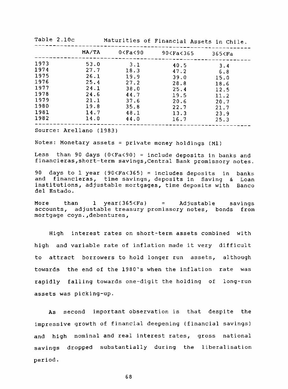
Table 2.10c Maturities of Financial Assets in Chile. ------------------------------------------------------------

MAlTA 0<Fa<90 90<Fa<365 365<Fa ------------------------------------------------------------1973 1974 1975 1976 1977 1978 1979 1980 1981 1982

53.0 27.7 26.1 25.4 24.1 24.6 21.1 19.8 14.7 14.0

3. 1 18.3 19.9 27.2 38.0 44.7 37.6 35.8 48.1 44.0

40.5 47.2 39.0 28.8 25.4 19.5 20.6 22.7 13.3 16.7

3 . 4 6.8

15.0 18.6 12.5 11.2 20.7 21.7 23.9 25.3

------------------------------------------------------------Source: Arellano (1983)

Notes: Monetary assets = private money holdings (Ml)

Less than 90 days (0<Fa<90) = include deposits in banks and financieras,short-term savings,Central Bank promissory notes.

90 days to 1 year (90<Fa<365) = includes deposits in banks and financieras, time savings, deposits in Saving & Loan institutions, adjustable mortgages, time deposits with Banco del Estado.

More than 1 year(365<Fa) = Adjustable savings accounts, adjustable treasury promissory notes, bonds from mortgage coys.,debentures,

High interest rates on short-term assets combined with

high and variable rate of inflation made it very difficult

to attract borrowers to hold longer run assets, although

towards the end of the 1980's when the inflation rate was

rapidly falling towards one-digit the holding of long-run

assets was picking-up.

As second important observation is that despite the

impressive growth of financial deepening (financial savings)

and high nominal and real interest rates, gross national

savings dropped substantially during the liberalisation

period.

68

Table 10d presents some evidence on the evolution of

savings in Chile. The comparison between the peak of 20.7%

in 1974 and the trough of 2.1' in 1982 serve to illuBtrate

the pattern of the gross national savings. At the same time,

by excluding the observations for the recession years of

1975 and 1982 we observed that the average gross national

savings ratio remained stagnant around 12% per annum. This

figure hardly differs from the average for the periods

between 1960-65 and 1966-70 corresponding to 11% and 15% per

annum.

Table 2.10d Savings and Investment in Chile. ------------------------------------------------------------

GNS/GOP 60-65 11.0 66-70 15.0 1974 20.7 1975 7.9 1976 14.5 1977 10.7 1978 12.6 1979 12.4 1980 13.9 1981 8.2 1982 2.1

FS/GOP GOS/GOP

0.4 5.2

-1.7 3.7 5.2 5.4 7.1

14.5 9. 2

21.1 13.1 12.8 14.4 17.8 17.8 21.0 22.7 11.3

GFCF/GOP 15.1 14.5 17.0 17.7 13.3 13.3 14.7 14.9 16.6 18.4 14.0

GCFg/GOP GCFp/GOP TGCF 10.5 3.8 14.3 11.3 4.7 16.0 12.8 8.4 21.2 8.5 4 . 6 13.1 5.4 7 . 4 12.8 6.7 7.7 14.4 6.2 11.6 17.8 5.2 12.6 17.8 5.4 15.6 21.0 5.1 15.6 20.7

11.3

Source: Banco Central de Chile, Cuentas Nacionales 1974-85.

Notes: Share of GOP on amounts in pesos of each year. GNS= Gross national savings,FS=Foreign savings,GDS=gross

domestic savings GFCF= Gross fixed capital formation, GCFg= gross capital

formation public sector,GCFp=gross capital formation private, TGCF= total gross capital formation.

There are two general points to make on the evolution of

national savings. As we have already seen, the spectacular

growth in financial savings appears to have resulted from

69

changes in the composition of wealth rather than from a

significant change in consumption and saving patterns. This

substitution may had included a shift away from informal

capital markets towards the organised capital market.

The second point is that overall savings may have also

been influenced by several factors depending of course on 17

theoretical framework being used. Harberger (1982) for

instance, identified three contributing factors on the

dismal performance of Chile's savings. Firstly, a

substantial rise in asset prices by more than 320% between

1977 and 1980, measured by the real index of stock prices,

and consequently a perceived wealth by forward looking

consumers. This was leading to higher consumption and thus

dissavings. This effect takes place as part of the

adjustment of actual wealth holdings back to the desirable

level in a Meltzerian fashion.

Secondly, private sector used funds which otherwise

might have augmented the national capital stock to buy back

part of the existing capital stock during the privatisation

phase. Edwards (1985) argued that the government used the

proceeds from privatisation to finance current expenditure.

Thus, the private savings used in acquiring these firms were

matched by a negative government savings.

Thirdly, the recession of 1975 and the fall in real GDP

by 14.3% was also important particularly if the

circumstances were thought to be transitory. In consequence,

70

a transitory fall in income should have produced an

important shift in the pattern of savings.

Dornbusch (1985) maintained that there appeared to be a

strong real exchange rate effect on the composition and

level of spending. As it is show in chapter 7, by 1981 the

sustainability of the increasingly overvalued exchange rate

was becoming uncertain so that a sharp increase in the

demand for imported durables took place with the subsequent

deterioration in the trade balance. In fact, the data from

table 9 shows that the deficit of the current account was

16.5% of GDP during 1981.

The series on foreign savings in table 10d appears to be

negatively correlated with national savings. In other words,

external savings substituted domestic savings. Abundant

world liquidity and external financial liberalisation

stimulated capital inflows to finance higher consumption

levels.

In general, it could be argued that the evolution of

national savings was strongly influenced by the incentives

toward consumption from the misalignment of key

macroeconomic prices particularly the real exchange rate and

real stock prices, the economic recession of 1975,

institutional and structural changes, and the degree of

substitution between domestic and external savings. The role

of financial liberalisation was indirect as its incidence

was felt on the explosive rise in the stock prices, the

71

failure of supervision to avoid this speculative bubble

financed by bank credits, and the undesirable ownership

concentration from privatisation. Further disccussion of

these issues will be provided shortly.

Finally, table 10d presents evidence on the performance

of investment during the liberalisation period. The rate of

gross investment measured by the gross fixed capital

formation (GFCF) was 15.5% of GOP between 1974 and 1982.

This figure appears to be slightly above the figures for the

period of 1960-65 and 1966-70 with 15.1% and 14.5%

respectively.

This stagnant performance of investment in Chile during

the liberalisation period can be explain by the concurrence

of two factors. Firstly, public sector investment was

severely curtailed. The public sector gross domestic capital

formation fell from 12.8% of GOP in 1974 to 5.1% in 1981.

The fiscal stabilisation enacted in 1975 and the ideological

bias against the public sector conspired against any

initiative to encourage public investment particularly on

public infrastructure.

Secondly,

sufficiently

private sector investment did

to offset the reduction in public

not rise

investment.

In effect, if we look at the series between 1974 and 1977

private sector gross domestic capital formation never

exceeded the 1974 value of 8.4% of GOP. This performance can

be explain partly by the 1975 recession, and in my view from

72

the fact that for many decades private sector investment was

led indirectly by actual and expected public sector

investment.

However, in 1978 private investment started to rise from

11.6% to 15.6% in 1981. This performance was superior to the

period of 1960-65 and 1966-70 and even outstripped the

figures for public sector gross domestic capital formation

during the 1960's.

As a whole, the rate of investment remained poor even

during the liberalisation period. Additional factors such as

the short-term maturity of the asset structure, asset

speculation in the stock exchange, and as we have seen the

incentive towards consumption conspired against private

investment. At the same time, as we will see later high ex

post real domestic lending interest rates was also important

for those who did not have access to a much cheaper credit

such as foreign lending at least before 1978. I have

estimated that average domestic real lending interest rate

between 1975 and 1977, date at which the authorities began

the process of dismantling controls in capital inflows, was

70% per year. The liberalisation of capital inflows

contributed to reduce domestic interest rates, and to rise

foreign savings. In fact, lending rates have fallen to 15.5%

and 11.3 in 1979 and 1980 respectively. Also foreign savings

accounted by 7.1% in 1980 and 14.5% in 1981. This figure is

important if we also considered that that gross fixed

capital formation was 18.1% during 1981. This is a clear

73

indication that the increase in investment during the late

1970's was financed by foreign savings.

Even if the rate of capital accumulation did not exhibit

a significant increment during the liberalisation period, it

was expected a sUbstantial improvement in the allocation and

quality of investment as result of financial deregulation

and price allocation. In relation to credit allocation,

there are two proxies which serve to reject the view that an

improvement in credit allocation occurred during the

liberalisation period. The first one was the emergence of

two related issues: a high credit concentration and the

"related portfolio problem".

By 1980 the Superintendency of banks started showing

some concern on the levels of credit concentration among

bank holding companies (groups). This credit concentration

on related firms occured despite the existence of legal

norms for credit concentration and beyond any doubts it was

exacerbated by an inadequate supervision.

As it will be argued in chapter 3, the first

intervention action in 1981 and particularly in 1983 enabled

the Superintendency to have a glimpse of the magnitude of

credit concentration among economic conglomerates. Table 10e

shows the magnitude of the loan portfolios allocated in

affiliated firms. The most dramatic cases correspond to

Banco Chile and Banco Santiago, the two largest banks in

Chile.

74

Table 2.10e Related Portfolios In Chl1e.(a) ------------------------------------------------------------

1982 1983 1984 ------------------------------------------------------------Banco Chile Banco Santiago Total

39.369(19.3) 51.360(42.9)

141.307(13.9)

56.272(23.8) 70.858(61.8)

183.493(16.7)

50.618 85.907

202.734 ------------------------------------------------------------Source: SIBF, Informacion Financiera, Various Issues.

(a) The data is express in millions of pesos.The figures in brackets correspond to the related portfolio/total loans ratio.

Indeed, by 1983 Banco Chile and Banco Santiago had

nearly 24% and 62% of their loan portfolio allocated into

affiliated firms. Moreover, this ratio for the overall

financial system was nearly 14% and 17% in 1982 and 1983

respectively. Clearly, this does not suggest an efficient

allocation of investible resources nor an efficient

allocation of risk. At the same time, it surpasses the 5%

limit established by the Superintendency in June of 1982.

Further analysis of the related portfolio problem is

provided in chapter 8.

Another proxy for the allocation of investible resources

is the data on the GDP growth by sector. According to the

data from the Central Bank, construction rose by an annual

average of 18.5% between 1978 and 1981. Most of the

investment on construction was concentrated in large and

expensive shopping centres and luxury flats. Similarly, the

data available on commerce and financial services also

confirms a rapid expansion rates of 11.9% and 19.7%

respectively over the same period. These figures are well

75

above of the 7.3% overall GDP growth per annum during these

four years. This evidence against the background of a per

capita GDP of U$1500, and an unemployment rate of over 13%

during the second half on the 70's and early 80's as

despicted by table 9, can hardly be seen as rational

priority in the allocation of investible resources.

(2.3.2.2) Financial Indebtness, and Interest Rates in Chile.

It is evident from the discussion of the evidence that

financial liberalisation did contribute to the expansion of

the number of intermediaries and financial intermediation.

The counterpart of this spectacular growth of financial

assets (liabilities of the financial system) was the strong

financial indebtness of the private sector. Increasing

private sector debt was not a worrying issue per se but the

terms and the structure of the private sector's liabilities

were a matter of greater concern. Such debt was acquired at

extremely high interest rates, predominantly short-term, and

denominated in dollar terms particularly during 1981-82.

76

Table 2.11a Loans of the Financial System to the Private Sector.

------------------------------------------------------------Loans/GDP Loans $ LO.j.rtB tJ$

L<365 L>365 Total L<365 L>365 Total ------------------------------------------------------------1973 4.4 1974 5.0 1975 8.3 1976 10.4 1977 16.6 1978 23.2 65.5 19.2 84.7 45.1 31.8 76.9 1979 28.2 120.7 41.0 161.7 71.6 55.1 126.7 1980 37.6 238.9 90.9 329.8 116.1 107.1 223.2 1981 50.4 328.6 164.6 493.2 143.3 163.3 306.6 1982 71.2 283.3 236.6 519.9 147.1 306.3 453.4 ------------------------------------------------------------Sources: SIBF, Informacion Financiera, Various Issues.

Arellano (1983).

According to table l1a, total loans to the private

sector exhibited a substantial increment as a percentage of

GDP. In 1973 the private sector indebtness was only 4.4% as

compared with 1982 which reached 71.2% of GDP. At the same

time, the evidence shows that the rising debt was

predominatly short-term although it was beginning to show

some decline relative to longer term liabilities. In effect,

between 1978 and 1981 the share of short-term debt as a

proportion of the total went from 77.3% to 66.6%. Moreover,

we observed that loans were predominantly in pesos although

dollar loans also had a significant share. For instance, in

1981 nearly 62% of total loans were denominated in pesos and

38% in dollar terms. It is clear that the short term nature

of peso loans and increasing share of dollar loans can be

regarded as two factors which have enhanced the weakness of

the banking system especially during the collapse of Chile's

economic activity in 1982. At the same time, high real

77

interest rates and the forced maxi-devaluation in June 1982

have also proven to be paramount.

As we have already seen, one line of reasoning relates

the increasing financial indebtness with the incentives

toward consumption financed mainly by bank credit. At the

same time, euphoric expectations on the future prospects of

the economy may have played an important role in the

increasing demand for credit despite extremely high lending

interest rates. However, it could be argued that demand for

bank credit was actually responding to ex ante interest

rates which were much lower than the ex post rates. To

reconcile this story with the data we have to assume that

economic agents

inconsistent with

were making systematic mistakes

the rational expectation

which is

hypothesis.

However, it is equally true that rational individuals could

have also be financing imports while correctly perceiving

the exchange rate as being unsustainable in the medium and

longer run.

A second line of enquiry relates to some institutional

features which emerged after the privatisation of the

financial system. As we recall from table 8, the process of

financial reforms started with the return of financial and

non-financial institutions to their previous owners and/or

auctioned to the highest bidder. However, differential

access to domestic and foreign credit determined that banks'

assets were acquired by economic conglomerates (group) which

78

already had a large ownership of non-financial firms. By the

time of privatisation, high real domestic interest rates,

tight monetary policy, and controls on capital inflows

made peso borrowing too expensive to the general public and

encouraged economic groups to borrow at cheaper rates by

exploiting their private contacts abroad. The access to low

cost foreign credit by a minority coupled with the lack of

effective monitoring on assets acquisition led to a large

ownership concentration and as we have already seen, to the

problem of "related portfolios". As the control of the

economic conglomerates increased over financial institutions

they were able to increase their economic power by buying

out those firms which were under severe financial strain

after the recession of 1975. Also, they were capable of

raising their capital values on the stock exchange by

lending to themselves and by buying shares from affiliated

firms. Clearly, financial indebtness was used to finance the

expansion of economic groups as well as to inflate stock

prices. In turn, this sharp increment in assets' prices

permitted a more "solid" borrowing capacity by offering

overpriced collaterals and guarantees. At the same time, as

pointed out by Luders (1986), this credit was also devoted

to purchase banks themselves in a process that he called

"the bicycle": that is, a bank would grant a loan to a

corporation controlled by the new owner of the same bank and

this entity would use the proceeds of the loan to pay for

the shares it was acquiring.

79

In consequence, bank credit was partly used to finance

the speculative bubble in stock prices and to finance the

consolidation and/or expansion of economic groups. The

increasing indebtness and particularly the emergence of

vulnerability from systemic risk was becoming a time bomb.

Another complementary hypothesis which explains private

sector indebtness highlights the importance of certain

banks' practices involving the rolling-over of bank credit

and the capitalisation of the interest. As it will be

thoroughly reported in chapter 3 and particularly chapter 7,

sustained high real interest rates, and the accumulated

appreciation of the real exchange rate between 1978 and 1982

became major sources of difficulties for the tradable

sector. At the same time, the estimates of non-performing

loans/total loans and non-performing loans/capital ratios

rose alarmingly from 1981 onwards. In order to stave-off

bankruptcies, banks were willing to rollover what were

essentially bad loans. Arellano (1983), Harberger (1985a),

Zahler (1985), and Luders (1986) maintained that the

rolling-over of bad debts created a false demand for loans

and hence such practices accounted for a large share of the

expansion of bank credit (private sector indebtness).

In general, I would agreed that the institutional

features which emerged as a result of

liberalisation was

certain practices

extremely important in

conducive to a dangerous

financial

encouraging

rise in

indebtness. Moreover, it led, as it will be shown in

80

chapters 3 and 8, to excessive risk-taking and unsound

lending practices which ultimately caused the debacle of the

banking system in 1983.

However, there was something more specific behind

private sector indebtness, the rapid expansion of banks'

loans, and excessive risk-taking which directly concerned

banking firms. In my opinion, banks' attitudes and conducts

should be considered as the centre-piece of most of the

hypotheses which explain the rapid bank credit expansion and

the collapse of the banking system. As stated by Barandiaran

(1983), the banking system was determinant in the collective

euphoria as they aggresively promoted different lines of

businesses. Indeed, banks actively sought borrowers on a

door to door basis. This strategy clearly contradicted a

more conservative approach where borrowers seek funds and

banks acting as lenders would carry out a complete

evaluation of the borrower's profile in terms of its

projects, assets, and personal wealth. The critical factor

which induced this type of banks' behaviour was the

structure of incentives which arose from financial

liberalisation. Among them we include the development of

close ownership links between financial and non-financial

firms, the implicit government insurance on domestic and

foreign liabilities, and increasing competition among

financial institutions. Chapter 8 will provide a an

empirical evaluation of these specific issues.

81

Although some measures were adopted in

order to limit banks' exposure and some

practices, there was a total failure

late 1981 in

other risky

to introduce

comprehensive and effective steps to supervise banks'

conducts and management. The failure of prudential

regulation combined with those institutional features which

emerged from financial liberalisation facilitated and

excerbated risky and unconservative conduct of financial

institutions. Indeed, in chapter 6, I have found econometric

evidence which indicates that the likelihood of bank

problems was becoming evident as early as 1979. Therefore,

an early warning mechanism and an effective credit

classification combined with publicly provided information

would had averted this type of conduct.

What remains to be discussed is one of the most puzzling

aspect of financial liberalisation which concerns the

behaviour of interest rates. As we have seen previously,

increasing private sector indebtness occurred

extremely high lending interest rates.

despite

As expected, financial deregulation brought about

initially an overshoot of nominal and real interest rates.

However, they remained too high and volatile as well as they

failed to converge toward international level. Moreover, the

spread between lending and borrowing rates remained

stubbornly high. These unexpected results occurred in spite

of both substantial increases in peso liabilities as shown

in table lOa and a spectacular rise in capital inflows after

82

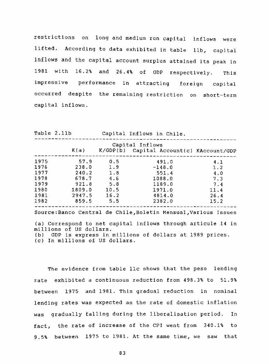
restrictions on long and medium run capital inflows were

lifted. According to data exhibited in table lIb, capital

inflow5 and the capital account surplus attained its peak in

1981 with 16.2% and 26.4% of GOP respectively. This

impressive performance in attracting foreign capital

occurred despite the remaining restriction on short-term

capital inflows.

Table 2.11b Capital Inflows in Chile. ------------------------------------------------------------

Capital Inflows K(a) K/GOP(b) Capital Account(c) KAccount/GOP

------------------------------------------------------------1975 57.9 0.5 491.0 4.1 1976 238.0 1.9 -148.0 1.2 1977 240.2 1.8 551.4 4.0 1978 678.7 4.6 1088.0 7 . 3 1979 921.8 5.8 1189.0 7 .4 1980 1809.0 10.5 1971.0 11.4 1981 2947.5 16.2 4814.0 26.4 1982 859.5 5.5 2382.0 15.2

Source:Banco Central de Chile,Boletin Mensual,Various Issues

(a) Correspond to net capital inflows through articule 14 in millions of US dollars. (b) GOP is express in millions of dollars at 1989 prices. (c) In millions of US dollars.

The evidence from table 11c shows that the peso lending

rate exhibited a continuous reduction from 498.3% to 51.9%

between 1975 and 1981. This gradual reduction in nominal

lending rates was expected as the rate of domestic inflation

was gradually falling during the liberalisation period. In

fact, the rate of increase of the CPI went from 340.1% to

9.5% between 1975 to 1981. At the same time, we saw that

83

peso liabilities and capital inflows experienced a

spectacular growth during the liberalisation period.

Table 2.11c Interest Rates in Chile. ------------------------------------------------------------

Lending Rates Deposit Rates Nominal(a) Real(b) Dollar(c) Nominal Real Dollar Infl

------------------------------------------------------------1975 498.3 114.8 11.4 234.0 18.6 96.8 340.1 1976 350.7 51.3 -27.4 197.9 8.6 45.4 174.3 1977 156.4 45.9 -7.6 93.7 17.1 20.7 63.5 1978 85.3 35.8 -4.0 62.8 22.5 34.1 30.3 1979 62.0 15.5 -7.4 45.1 4.4 26.2 38.9 1980 46.9 11.3 -12.8 37.4 4 .6 37.4 31.2 1981 51.9 33.1 6.4 40.8 25.4 40.8 9.5 1982 63.1 30.6 77.0 47.8 20.5 -21.5 20.7

Av 164.3 42.2 4.4 94.9 15.2 34.5 88.5 ------------------------------------------------------------Source:Banco Central de Chile,Boletin Mensual,Various Issues

IMF,International Financial Statistic, Various Issues

(a) Nominal interest rates both deposit and lending correspond to short-term interest rate (30-90 days)

(b) Real interest rates correspond to ex post rates which are estimated by deflating short-run interest rates by the variation of the consumer price index. That is {[ (l+i)/(l+CPI) ]-1}*100

(c) The ex post real dollar lending interest rates were obtained deflating LIBOR by nominal devaluation and variations in the consumer price index. That is {[(1+LIBOR)(1+e)/(1+CPI)]-1}*100.

(d) The ex post dollar deposit interest rates were obtained by deflating the short-run nominal deposit interest rate by the nominal devaluation. That is {[(1+i)/(1+e)]-1}*100.

Also the data shows a downward movement of the real

lending rate from 114.8% to its lowest level of 11.3% in

1980. There are two observations from the data which is

worth looking at with some care. Real lending rate in 1979

and 1980 were well below in comparision with both the

84

average for the whole period and with the previous year and

the two following years. While it coincided with the lifting

of restrictions on capital inflows, changes in international

conditions also had played an important part on the

behaviour of real interest rates. Sjaastad (1985, 1989) and

Cortes Douglas (1985) argued that the fluctuations in real

interest rates between 1979 and 1982 can be explained by

sharp changes in the value of the dollar. They maintained

that in a small open economy with fully integrated capital

and goods markets, domestic nominal interest rates will be

fairly well arbitraged with external rates. However, real

interest rates would be affected by fluctuations in the

exchange rate of major currency countries whereby such

fluctuations will be transmitted into the inflation rate via

price of traded goods.

Table lId provide some useful evidence to support the

international influence on real interest rates. Firstly, the

fluctuations in real lending rates between 1979-80 and 1981-

82 does not come from similar fluctuations in LIBOR nor in

nominal peso lending rate which still remain too high.

Secondly, if we compare the movements of real and nominal US

exchange rates with the dollar price of Chilean tradables we

observe some correlation. In effect, between 1977 and 1979

we see that there was a dollar inflation as the US currency

depreciated 7.4% in real terms during these three years.

This coincided with both a sharp rise in tradable prices in

us dollars by 34.3% and the significant fall in the real

85

lending rate over the same period. The process is reversed

from the late 1980 onwards as the dollar began appreciating

very rapidly. The collapse of the Chilean inflation

coincided with the appreciation of the US dollar followed by

a rise in real lending rates.

Table 2.11d US Exchange Rates, Tradable Prices, and Interest Rates. (a)

------------~~----------------------------------------------

77 78 79 80 81 82 ------------------------------------------------------------NEFF EX. Rate 124.0 111.2 108.3 108.3 121.1 135.2 REFF EX. Rate ( b ) 117.6 108.6 108.9 110.0 125.2 134.7 Tradable Price(c) 183.5 196.4 246.5 296.8 297.3 266.7

LIBOR (d) 6.1 8.8 12.1 14.2 16.8 13.2 Nominal LendingR 156.4 85.3 62.0 46.9 51.9 63.1 Real Lending Rate 45.9 35.8 15.5 11.3 33.1 30.6

Source:Banco Central de Chile,Boletin Mensua1,Various Issues IMF,International Financial Statistics,Various Issues ECLA, Statistical Yearbook, Various Issues.

(a) Indices were constructed with 1970=100 (b) Real effective exchange rate (REFF EX.Rate) was obtained by deflating the nominal effective exchange rate (NEFF.EX.Rate) with the WPI. (c) The average dollar price of tradables was calculated as follows 0.5Px+0.5Pm where Px=unit value of exports and Pm=unit value of imports. (d) Nominal LIBOR is the three months Eurodollar rate.

While this argument seems logically correct the question

which remains to be answered is why nominal domestic

interest rate failed to return to market equilibrium. As we

will see shortly, the reduction in inflation during 1980-81

coincided with both a drop in the rate of capital inflows

particularly in 1981, and the belief that the level of

capital inflows were not sustainable in the long-run. Rising

86

devaluation expectations, country-risk premium, and credit

demand affected nominal interest rates.

Another important observation from the data in table

1lc and 11e is that domestic interest rates failed to

converge to international levels particularly during the

period in which the exchange rate was being devalued

according to a pre-announced "tablita" and large capital

inflows were flooding the economy.

Table 2.11e Spreads of Interest Rates. ------------------------------------------------------------

1 2 3a 3b ------------------------------------------------------------1975 228.9 83.9 264.3 67.1 1976 62.1 37.7 152.8 20.7 1977 50.6 13.9 62.7 30.8 1978 40.4 23.3 22.5 15.5 1979 25.9 12.7 16.9 9.2 1980 28.5 20.1 9.5 5.9 1981 30.4 20.8 11.1 8.9 1982 -23.7 -30.8 13.3 11.8

Source:Banco Central de Chile,Boletin Mensual,Various Issues IMF,International Financial Statistics,Various Issues Arellano (1983)

Note: Spread l=Difference between the interest paid by the domestic debtor who borrows in the domestic market and the interest paid if he borrows in the international financial market. That is,

{[(l+real lending rate)/(1+LIBOR)(1+e)]-1]}*100

Spread 2= Difference between interest in dollar terms received by a foreign creditor that lends in the domestic market and LIBOR rate. That is, {[[(l+deposit rate)/(1+e)]/(1+LIBOR)]-1}*100

Spread 3a= Correspond to the gross spread between nominal peso lending rate and deposit rate.

Spread 3b= Correspond to the net spread between lending and deposit interest rates including the cost of legal reserve requirements

87

For instance, table 11c shows real peso lending rate

proved to be well above LIBOR adjusted for devaluation. The

annual average real peso lending rate was 42.2% between 1975

and 1982 whereas the adjusted LIBOR was as low as 4.4%. If

we exclude the observation for 1982 the cost of dollar

lending was minus 6%. Moreover, the deposit rate adjusted

for devaluation was 34.5% per annum over the same period.

This rate is definitely superior to the return from three

month Eurodollar rate which hardly exceeded 12% per annum

between 1977-82 as shown in table 11c. Similar conclusions

are obtained by looking at the calculations for spread 1 and

spread 2 in table 11e. In consequence, this differential

was very attractive to foreign capital as much as it was for

resident to borrow in foreign currency.

Several hypothesis have been introduced to explain why

interest parity did not hold in Chile. A useful way to

assess those factors affecting the parity is setting the

interest parity condition for an open economy as follows:

* e (8) i = i + e + ~

In an economy where foreign and domestic assets are

close substitute and where the financial market is fully

integrated with the world financial market, domestic

interest rate (i) should equal the yields on comparable *

foreign assets (i ) plus the expected rate of exchange rate e

depreciation (e). This uncovered interest rate parity will

88

not hold so long as the domestic interest rate will deviate

from the foreign rate adjusted for expected depreciation by

three additional factors. Country-specific institutional

factors such as tax regimes, reserve requirements, and

limits on exchange-risks; country-specific risks among them

the imposition of exchange rate controls at the time of

repatriation, and political risks; and exchange risks which

arises from the fact that assets are denominated in

different currencies, and there is uncertainty about future

value of the exchange rate. These factors will lead to a

premium (¢) on the yield on domestic assets to compensate

risk-averse economic agents which in turn results in a

differential between domestic and foreign rates after 18

adjusting for expected exchange movements. Thus, the

answers for the spread between domestic and foreign interest

rates lies with the concurrence of some of these factors

and/or the relaxation of the underlying assumptions of the

parity condition.

Sjaastad (1982) maintained that lack of correlation

between the large inflows of capital and the spread, which

for the periods between August 1979 to December 1980 and

January 1981 to March 1982 was -0.53 and -0.12 respectively,

can be explained by country-specific institutional factors.

He argued that if the spread remained unaffected by

increases in peso deposits, inflows of capital, and/or

devaluation risk then the explanation should lie in the cost

of arbitrage. This cost arose from the restrictions imposed

89

on Chilean commercial banks to take positions in foreign

currency. They could not borrow dollars abroad and lend

pesos in Chile. Some non-bank institutions converted dollars

into pesos and lent the proceeds in pesos which subsequently

returned to banks in the forms of peso deposits and back

again to non-bank entities in the form of loans. Given the

transaction costs and the risk of default, this indirect

arbitrage mechanism proved to be very expensive as compared

with a case where banks were permitted to arbitrage

directly. Although it was considered as theoretical

possibility, its empirical relevance was insignificant.

With respect to country-specific risk, Edwards (1986)

argued that only a small fraction of the spread can be

explained by the premium over LIBOR charged by world

financial markets. In effect, he showed that average premium

charged on loans hardly exceeded 1% between 1979 to 1982.

For instance in 1979 and 1980 the premium was 0.99%.

Instead, Edwards and Cox (1988) maintained that the role

of exchange risk started playing an increasing role from

1980 onwards during the fixed exchange rate regime. As we

have seen in table 8, after nearly two years of a "tablita"

regime the exchange rate was fixed at $39 in 1979. The

expectations of devaluation increased steadily as the

appreciation of the real exchange rate and its effects on

the current account deficit made the fixed exchange rate

regime unsustainable. According to the data presented in

chapter 7, the accumulated real appreciation between 1978

90

and 1981 was more than 30%. At the same time, the evidence

from table 9 suggest that the current account deficit was

nearly 10% of GOP per annum. With rising expectations of

devaluation of the peso so did domestic nominal interest

rates. At the same time, some firms and households began

substituting foreign credit for domestic credit putting more

pressure on domestic rates. As we will see shortly, there is

evidence to support the validity of this hypothesis.

other authors have questioned the validity of the

underlying assumptions of the parity conditions. The work of

Corbo and Matte (1984) indicates that Chilean assets and

foreign assets were imperfect substitutes. In an economy

with perfect capital mobility, a fixed exchange rate regime,

perfect substitution between assets, and no sterilisation,

the money supply is endogenous. Thus, a reduction in credit

expansion is matched by a rise in foreign exchange reserves 19

so that the monetary base remains unchanged. In Corbo and

Matte's model, the coefficient of compensation which relates

the net flow of private capital as dependent variable with

the internal credit of the Central Bank as independent was -

0.24 for a sample period between 1975-83. This result

suggest that asset substitution was between 0 and 1 so that

it was less than perfect. Although this evidence is useful,

the model itself does not relate directly to the issue of

interest rates nor does it identify those factors which

determine the low substitutability found for the case of

Chile.

91

There are other studies which have questioned the

assumption of perfect capital mobility. In fact, as we have

seen from the itinerary of financial reforms, the

liberalisation of the economy to capital inflows was gradual

and initially it focused on the elimination of restrictions

on long and medium run flows. Short-term borrowing in

foreign currency was allowed as late as 1982. Edwards and

Khan (1985) provide a very handy theoretical framework for

interest rate determination for a semi-open economy. For

example, in the case of fully open capital account the

domestic rate of interest depends on the three elements

stated in the parity condition stated by expression (1) that o * e

is i = i + e + ¢. In contrast, in a closed economy interest

rate determination is influenced by domestic monetary

conditions (demand and supply of money) and the expected e c e

rate of inflation (rr) that is i = r + rr where r is the

actual real interest rate. The value of r is determined by

the excess liquidity in the economy that is r= k+~EMS+u

where k is the long-run real interest rate, EMS is the 20

excess of money supply and u is random term. Thus, in the

semi-open economy both external as well as domestic factors

interact in the interest rate determination. Expressions (9)

and (9a) correspond to the nominal interest rate

determination for a semi-open economy.

0 c ( 9 ) i = €>i + ( 1 €» i

* e e (9a) i = ct + £H i + e ) + T10g m + 0"10g Y + 6Tt + r¢ + E.

t-1

92

If B=l and ~=~=d=O then expression (9a) becomes the

interest rate determination for an open economy. Moreover,

if B and ~ are found statistically significant it would

indicate that external and domestic factors are important in

the interest rate determination. Edwards (1986) reports the

results from the estimation of (2a) using quarterly data for

the period 1977-82 and applying the OLS corrected for serial

* e correlation. He found that the coefficient for (i + e) and

log(m)t-l was significant and with the correct sign. This

gives support to the view that internal monetary conditions

played a decisive role affecting nominal interest rate in

Chile. At the same time, it gives empirical support to the

expected devaluation hypothesis discussed earlier. The

coefficient measuring the risk premimum was found

insignificant. These result should be treated with caution

given some the simplication introduced into the model. e

Firstly, it assumes that ~ = ~ under rational expectations.

Secondly, ¢ was express as constant plus a serially

correlated random term. However, in practice this premium

depends among other things on the stock of debt/GDP,

political factors, and government assets etc.

Finally, the proxy for expected devaluation was

estimated as the difference in percentage points between

that quarter's effective real exchange rate and the one

prevailing in June 1979 when the nominal rate was fixed.

This expected realised real devaluation is an ex post rate

rather than an ex ante rate.

93

Looking at the demand factors, we have seen that the

rolling-over of bad debts and the interest rate

capitalisation increased the demand for credit generating as

suggested by Harberger (1985a) a false demand for credit.

From his view, this problem started at very early stage as a

result of loss-making enterprises which were privatised and

continued generating losses afterwards. He maintained that

as early as in 1976 the rolling-over was a significant

factor raising both the demand for credit and interest

rates. We also saw that most of the demand pressure for

credit came from the action of economic conglomerates to

boost their assets prices and continue their expansion. The

empirical verification of these hypotheses is beyond the

scope of this study.

The final query from the behaviour of interest rates is

the spread between the lending and deposit interest rates.

Table 11e column 3a presents the estimates of the gross

spread between lending and deposit rates. The spread was

extremely large in 1975 and 1976 with 264.3% and 152.5% per

annum respectively. The magnitude of this spread can be

explained by high reserve requirements and high inflation

rates. Recalling the evidence from tables 9, the inflation

rate in 1975 and 1976 was 340% and 174% and the effective

reserve ratio estimated in table 2 was nearly 64% and 68.3%

respectively. The spread began falling very rapidly from

62.7\ in 1977 to 9.5% in 1980. These results coincided with

the payments of a competitive interest rates on reserve

94

requirements from 1976 onwards and the gradual reduction of

the legal reserve as we have seen in table 8. At the same

time, inflation dld experlenced a significant but gradual

drop to 9.5% in 1981.

However, the lowest spread attained in 1980 was still

too high even when inflation rate was reduced to one digit

in 1981 and the legal reserve requirement were set at 10%

for sight deposits and 4% time deposits in 1980. Even worse,

the gross spread began rising in 1981 and 1982.

The data of column 3b in table lIe shows the estimates

of the net spread (adjusted for reserve requirements). The

net spread fell from 67.1% in 1975 to its lowest value of

5.9% in 1980 and thereafter it began rising again. These

results would indicate that much of the explanation of the

spread adjusted for reserve requirements lies in structural

characteristics of the banking system particularly between

1980 and 1982.

The answer to this puzzle should be found in the

oligopolistic structure of the Chilean financial system. As

we have seen earlier, a liberalisation of the financial

market with high concentration and bank holding company

structure could also explain high interest rates and a large

spread. It appears that the restoration of a bank holding

company structure that resulted from the privatisation of

the Chilean banking system together with increasing pressure

from domestic and foreign competitors drove the newly

95

established "groups" to compete for market shares. This in

turn should account for high interest rates and a large

spread between asset and liabilities rates throughout the

liberalisation period. Indeed the evidence from chapter 3

suggest that the bulk of intermediation was concentrated in

three major commercial banks and the share of non-bank

financial institutions and foreign banks

small. Also, table 10e confirms that two

was extremely

of these three

large financial entities had over 50% of the loan portfolios

in affiliated firms.

The effect of rising non-performing loans and increasing

provision on the spread can also be taken as an equally

possible explanation. Table 12 shows that the portfolio

expenditure/total asset ratio support this assertion as it

went up from 1.3% in 1980 to 6.7% in 1982. Chapter 3

provide more detailed evidence on the behaviour of the non­

performing loans and the provisions for bad debts

particularly between 1982-83.

Finally, it could be argued that the Chile's

system did not exhibit any significant gain in

efficiency and hence it can held accountable for

financial

operative

relatively

high net spread. The evidence from next sUb-section does not

give much support to this hypothesis.

All in all, it could be argued that the hypotheses

introduced to explain the behaviour of interest rate in

Chile are valid according to the point in which the economy

96

was located in the itinerary of economic reforms. Probably

the role of expected devaluation was even more important

than a credit crunch between 1979-1982. At the same time,

external shocks such as a dollar appreciation became more

serious as the economy was totally integrated to the world

economy in both trade and finance. In contrast, high

interest rates during the period 1974-1978 can be better

explained by initial deregulation of interest rates, tight

restriction of capital inflows, the fiscal austerity and

particularly the monetary tightening during 1975-76, and the

lack of credibility of the anti-inflationary programme.

However, one factor which appears systematically in both

period is the excess demand for loans. It was argued that

the purchase of assets from privatisation during 1974-78 was

financed by bank credit and the rolling-over of bad loans

specially during 1979-82 contributed to the excess demand

and high interest rates. In addition, the financing of both

the expansion of economic conglomerates and the stock

exchange's speculative bubble became decisive factor which

went totally unnoticed and uncontrolled by the authorities.

In my view, this issue was paramount in the behaviour of

private sector indebtness and interest rates. The conduct

of banks and banks managers in response to the incentives

from financial liberalisation and the relaxation of

supervision were at the centre of this story and as it will

tested in Chapter 8 on the debacle of the banking system.

97

(2.3.2.3) Operative Efficiency in Chilean Banks.

One of the expected results from financial

liberalisation particularly the lifting of restrictions for

entry into the financial system and the establishment of a

multi-purpose banking system was a rise in the level of

operative efficiency. The significant reduction of the net

spread between 1975 to 1980 confirms this result although

still remained significantly large for international

standards.

One indicator of operative efficiency is the salaries

and administrative expenses/total asset ratio shown in table

12. This ratio was estimated using information from banks'

balance sheets and income statements.

Table 2.12 Salaries and Administrative Expenses in Chile.

NFOEx/TA AdEx/TA SEx/TA PortEx/TA

1975 8.5 8.8 1976 8.1 1.8 1977 7.3 1.1 1978 5.4 1.8 1979 5.0 1.04 2.83 2.0 1980 4.3 1.06 2.65 1.3 1981 3.7 1.14 2.42 4.3 1982 3.4 0.86 1.95 6.7

Sources: SIBF, Informacion Financiera, Various Issues. Chamorro (1985a)

Notes: NFOEx/TA=Non-financial operative expenses/total asset ratio includes administrative expenses and salaries

AdEx/TA = Adminitrative expenses/total asset ratio SEx/TA = Salaries/total asset ratio PortEx/TA= Portfolio expenses including provision

relative to total assets.

98

The evidence suggest that the non-financial operative

- '·1"" ""1- Q - -It - tal e. ••• I:'c: l~ e::i _" '-> "._ asset ratio continously fell from 8.5% to

3.5% between 1975 and 1982. These results prompt us to

confirm a significant gains in operative efficiency.

However, these figures are still above those of a more

competitive banking system. For instance, Chamorro (1985a)

found that this ratio for the US was only 2.5% between 1979

and 1983.

The largest component of the non-financial operation

expenses correspond to salaries. For instance, in 1981

salaries were 2.42% of total assets as compared with 1.14%

for administrative expenses.

The evidence indicates that financial liberalisation

contributed to a significant increases in operative

efficiency although it remained somewhat higher than a more

competitive financial system such as the US. These results

tend to over estimate the efficiency gains as the value of

total assets goes in the denominator. As we have seen in

previous sections, the growth of financial assets was

spectacular during this period. Indeed, if we observe the

growth of nominal non-financial operative expenses we obtain

a different conclusion. Between 1978 and 1982 these

expenditure item grew by 325% with salaries having the

biggest share.

99

(2.3.2.4) Financial stability in Chile.

The single most puzzling and disturbing issue of

Chile's financial liberalisation was the collapse of the

banking system in 1983. A large number of both private banks

and non-bank financial institutions were liquidated,

intervened, and/or supported with public money. As we will

see in chapter 3, Banco del Estado (state bank) and Banco

Industrial and Comercio Exterior remained the only

exceptions which did not required any financial support.

It could be argued that as much as financial liberalisation

affected the performance of the financial system, the focus

should be placed on the new incentives to bankers which

emerged from an unregulated financial market. They became

the main actors in affecting some of the unexpected ex

results of financial liberalisation, particularly

financial crisis of 1983. The deterioration of

post

the

the

macroeconomic environment although important as a triggering

mechanism, should not be considered as the central

hypothesis to explain the performance of the financial

sector. Indeed, according to the early warning model

estimated in chapter 6, the ex ante probability of bank

failures/problems was

financial debacle.

significant three years

Internal influences from

before the

financial

liberalisation and external factors from adverse changes in

some key macroeconomic variables are two testable hypotheses

which will be studied and empirically evaluated in chapters

7 and 8.

100

In general, one would conclude that the expected results

from financial liberallsatlon were achieved only partially.

Although, the evidence indicates a sUbstantial increase in

financial intermediation (deepening), and a marked gains in

operative efficiency, the level of savings and investment

remained stagnant. There were no clear signs of an

improvement in both resource allocation and the quality of

investment. Instead, the banking system was fostering an

unsustainable private sector indebtness, a risky

concentration of loan portfolios with their affiliate firms,

and financing stock market bubbles and the consolidation of

economic "groups". All this behaviour occurred in spite of

stubborn high interest rates, and a significant

deterioration of the macroeconomic environment. Finally, the

collapse of the banking system in 1983 is clear evidence of

the unsuccessful liberalisation of the financial system in

Chile.

Chapter 3 will discuss the magnitude of the banking

failures in Chile and the steps taken by the authorities in

order to avoid the total collapse from widespread panic. At

the same time, it will provide a glimpse at the measures

introduced to rehabilitate the financial system.

101

Endnotes.

(1) Bernanke (1983) was one of the first in introducing a link between financial disruption and output decline. This came to complement the monetary forces behind the repression of the 1930's. In Bernanke's view, in an imperfect capital market banks perform a real service by differentiating good from bad risk borrowers.

(2) Tobin also showed that the steady-state value of k in the monetary growth model was smaller than in a model with no money. In other words, the monetary model exhibits a smaller output per capita. This is shown by the equilibrium condition for k which is given by [s-(l-s)xn]f(k)=nk which is smaller than sf(k)=nk where x is the fraction of f(k) held in the form of real money balances.

(3) The coexistence of small and large firms producing a similar product but with a different factor proportion, an unequal access to technology, and a different growth and use of human capital confirm the degree of fragmentation in underdeveloped economies. However, most of this fragmentation has been largely the outcome of misguided government policies which have condemned some sectors of the economy to be technologically backward. For instance, Galbis (1977) modelled a fragmented economy with two sectors: one with a modern technology and the other with a backward technology. The lack of well developed financial market permitted the coexistence of these two sectors, the disparities in the rate of return of capital in the economy, and a lower rate of economic growth.

(4) The homogeneity and perfect divisibility of capital enable households to use only fractions of their capital to carry out their transactions and settle their debts obligations.

(5) Most governments of developing countries have been technically constrained in the amount of fiscal resources they could rise from direct and indirect taxation, especially the problem of tax evasion and existing lags in collecting tax revenues or known as the Olivera-Tanzi effect. In addition, the absence of well established and developed open market in primary securities has ruled out the possibility to issue and trade government and private sector paper. For Mckinnon and Mathieson (1981) the absence of open markets for primary security has little to do with a distortion and more with a low level of income per capita and the resulting small scale of savers and investors. Transaction costs and information asymmetries would be unmanagable in LDC's. However, Fry (l982a) maintain that private bonds and equity markets are supressed as a result of government taxation such as transaction taxes, stamp

102

duties, taxes on capital gains. The government's rationale to supress these markets lies on the fact that seigniorage cannot be taken easily from bonds and equities.

(6) ACcolding to Mckinnon and Mathieson (1981), firms in the import-substitution sector which were protected from potential imports normally they were granted official bank credits at negative real interest rate. Indeed, official intervention in the allocation of credit were so pervasive, detailed, and bewildering as much as the restrictions on foreign trade policies.

(7) Authorities tend to place a heavy reserve requirements on most liquid monetary assets and it gradually falls as the assets is less liquid. In effect, one should find that reserve requirements on time deposits is smaller than demand deposits. In addition, the effective reserve requirement in a liberalised and financially matured economy should be lower than in a less developed economy.

(8) In his review of disequilibrium interest rates in developing countries, Fry (1982b) argues that the prevalence of interest rate ceilings has a number of explanations. To begin with, he identifies the Keynesian liquidity preference as a floor for nominal interest rate and an above­equilibrium for the real interest rate. Unless the opportunity cost of holding money and/or real income fall the disequilibrium will persist. Beside the Neoclassical monetary growth theory and the substitution of money and capital, there are also political and religious factors which explain these ceilings.

(9) The list of selected countries both, developed and developing were chosen in order to compare their financial development with the Chilean's case. Among developed economies, the US, Germany, and Japan correspond to growing economies with a developed and mature financial system. Korea and Singapore represent rapidly growing developing economies where a mature banking system have emerged as result of financial liberalisation during the 1960's and 1970's. Among repressed developing countries, it was included the case of Mexico, although the peak of financial repression was reached during the nationalisation period between 1982-89. This list of countries is by no mean exhaust so further result from other studies will be address.

(10) However, the exactitude of these estimates should be treated with caution since no adjustments were made for any interest paid on bank reserves. Lack of data on interest payments precluded any attempt to obtain more accurate calculations.

103

(11) The empirical investigations on government seignorage suggest that the choice of a monetary aggregate depends on the nature of the empirical investigation. If we are interested in estimating how much the non-financial private sector pays to use money then M1 will suffice. However, if we want to assess how much the government collects from the inflation tax then the monetary base should be considered more useful. Equally, if the object of the study is to establish the amount of inflationary finance in the long-run then M1 is preferable to M2. For instance, any loss in financial assets from expectation errors or policy surprises on inflation and hence ex post real interest rates will be rapidly corrected. This effect has indeed short run implications. Also, it will probably involve transfers among private agents without the government's involvement.

(12) More sophisticated models enable us a more accurate estimation of the seignorage. An alternative specification of the government seignorage can be stated as Ss=M/P=Mt-Mt-1 plus Mt-1(Pt/1+Pt) where M is a well defined monetary aggregate and P the inflation rate. This gross estimate of the real seignorage can be adjusted in order to include the revenue losses from the time lag on tax collection. This is known as the Olivera-Tanzi effect. Thus, net government seignorage can be written as follows Ss=Mt-Mt-1+Mt-1(Pt/1+Pt) - Tt-1(Pt/1+Pt).

(13) Similar results and conclusions were found by Brock (1984). He also used the monetary base to estimate a nominal seignorage from the inflation tax on intermediation during the 1970's. In his sample apart from US, UK, and Mexico, his study also included Germany, Colombia, and Brazil.

(14) Giovannini also questioned the empirical results with respect to the econometric problems of specifying and estimating the aggregate saving functions. Due to lack of disaggregated data on private and government savings, the use of total domestic savings as a dependent variable was not satisfactory. The aggregation of savings is satisfactory only under the Ricardian-Equivalence Theorem. The exogeneity assumptions of the explanatory variables of the model was also challanged. Looking at the consumption-saving relationship as an intertemporal optimisation, approach he estimated and tested the coefficient of intertemporal substitution of consumption over time for a group of countries. Using annual data, he found that in 5 out of 18 countries does the expected path of consumption changes at all with changes in the real interest rate. Indeed, in most case the interest rates is insignificant.

(15) Meller and Solimano (1983) provided econometric evidence which support the view that asset prices were unrelated to fundamentals ( flow of future dividends) even

104

under rational expectations and full information efficiency (arbitrage) conditions. Instead its value was determined by a speculative bubble.

(16) The predominance of domestic banks over foreign banks and financieras is even more significant as measured in terms of liabilities and assets. This evidence is presented in chapter 3. Additional information with respect to the size of the financial sector measured in terms of its contribution to GDP is shown in chapter 7.

(17) If we start from the basic proposition that savings is the difference between income and consumption then the theoretical and empirical differences on approaches will be centered on the definition of income and consumption and some of the underlying assumptions concerning some institutional and structural characteristics. The Modigliani's life-cycle hypothesis and the Friedman's permanent income hypothesis is confined within a Fisher's intertemporal optimisation model where intertemporal consumption (optimal) depends on current income but more important on long-run income. In addition, wealth, demographic variables, factors afecting the present value of income such as the rate of interest should be also considered. These models contrast with the traditional Keynesian model where household consume a fraction of current disposable income and thus changes in both current income and the MPC would affect consumption and henceforth savings. The introduction of assumptions specially imperfect capital markets and credit rationing will ample and transform this framework into liquidity constraint models. Another type of theoretical framework is the generational model. The time horizon exceed one generation so that factors affecting optimal consumption and hence savings pattern are also influenced by pensions and insurance, magnitude of transfers, and uncertainty.

(18) The dynamic of the adjustment of the parity condition can be stated as follows. Suppose that we start from equilibrium where the interest rate parity does hold. Suppose that the risk premium (¢) fall as a result of a pre­announced "tablita" for the future path of nominal exchange rate. It follows that a fall in the exchange rate uncertainty will reduce the risk premium on domestic assets. A positive spread between domestic and foreign rates will emerge and, other things being equal, capital inflows should increase forcing domestic interest rates to fall until the differential is consistent with the new and lower risk premium.

105

(19) The adjustment of the model comprise an excess demand for money over its supply which rises the domestic rate of interest and accelerate the purchase of assets in domestic currency. This portfolio adjustment will put pressure on the exchange rate so that under a fixed regime the authorities would need to defend the fixed regime by purchasing dollars and accumulating them as reserves.

(20) The excess money supply over the demand for money is given by EMS=log(m)t-log(md)t so that when EMS)O then r<k in the short run. In the long run EMS=O so that r=k+u. The real demand for money is given by log(md)t= a+blog(y)t-c(k+rre)­drre where y is real income and rre is expected inflation rate. Finally the stock of real money balances adjust according to the variation in [log(m)t-Iog(m)t-l]= Z(10g(md)t-log(m)t-1 where Z is the adjustment coefficient and lies between 0 and 1. If EMS)O because m is greater than the long-run money demand then short run nominal interest rate will be below equilibrium. The market will be equilibrated via a fall in real money balances.

106

Chapter 3. Banking Failures in Chile during 1981-83.

(3.1) Introduction.

This chapter provides an evaluation of the magnitude of

the banking crisis in Chile. It analyses the performance and

the degree of vulnerability of financial institutions by

examining balance-sheet data. Moreover, there is a

description and an assessment of the mechanisms to rescue

and to rehabilitate the Chilean financial system. As it will

be shown the banking crisis in Chile which began to unfold

in 1981 involved a large number of bank failures which

required an aggressive handling to avoid the total collapse

of the financial system and the whole economy. The

authorities have chosen the intermediate solution by letting

shareholders and the government absorb the losses.

From a theoretical point of view, a bank fails just like

any other enterprise if its net worth becomes negative or if

it is unable to continue its operations without incurring

losses that would immediately result in a negative net

worth.

In practice, however, most bank failures do not occur at

the precise time when the value of the bank reaches zero or

negative. In fact, most situations are resolved in ways that

do not entail bankruptcy. Thus, the authorities may

encourage a merger between a sound financial institution and

a problem bank. Alternatively, the authorities may

107

introduce emergency measures like the transitory

substitution of bad assets for cash and/or other government

assets. As we will see this is the approach followed by the

monetary authorities in Chile. Chapter 5 discusses further

the issue of a working definition of bank failures.

(3.2) The Stylised Facts and the Magnitude of the Banking Failures in Chile 1981-83.

As we have seen from the previous chapter, the measures

enacted by the government in order to liberalise the

financial system did yield initially some positive and

encouraging results. The banking sector experienced a period

of rapid growth and it showed some signs of increased

efficency. Among the most encouraging signs the M2/GDP ratio

rose, the spread between lending and borrowing rates

declined, lending rates showed some steady decline although

they remain high relative to world interest rates. In this

more deregulated environment increasing competition and the

introduction of new products from new banks and non-bank

financial institutions, both domestic and foreign, were

providing savers and investors with a wider range of

financial services. However, after 6 years of sustained

financial growth and stability, the banking system

experienced one of the worst financial crises in the

country's history starting in 1981 and reaching its peak of

intensity in 1983. Severe solvency and profitability

108

problems came to affect a large segment of the banking

sector which overshadowed the performance of the banking

sector during the late 1970'5.

(3.2.1) The Chronology and the Stylised Facts of the Crisis.

The period of financial liberalisation which ran from

1974 to 1982 contains several financial episodes involving

the failure and/or problem of some financial institutions.

The first financial disorder occurred in 1974-75 with the

insolvencies of a number of non-bank financial institutions,

both formal and informal. Unlike commercial banks, this form

of financial intermediary flourished as a result of the lack

of any capital requirement and supervision. They were soon

discouraged with the introduction of a minimum capital 1

requirement.

During the mid-seventies we also witnessed a process of

transformation, fusion, and the closed down of the Saving

and Loan Associations (SINAP). The establishment of a multi-

banking financial system which enabled banks to enter into

the mortgage business and the introduction of some

restrictions on the asset and liability composition of the

SINAP resulted in a rapid fall in the numbers of this type

of institution as they began merging among themselves. By

the end of 1978 there was one left 2

years later this finally closed its doors.

109

and two

These financial disorders did not pose any real threat

to the stability of the financial system nor required the

intervention of the Superintendency of Banks and Financial

Institutions (SIBF) which were in charge of regulating and

supervising the system. However, the 1977 rescue of Banco

Osorno not only was the exception to the rule but also it

left a dangerous precedent to the public as whole. Given

that there were clear signs that this important bank was

threatened by bankruptcy, the authorities, who also feared

the drain of the internal and in particular external

confidence in the financial system, rescued all depositors 3

and the institution.

Although we cannot trace the origin of the banking

crisis to this single financial episode, one could equally

maintain that the decision to bailout the bank produced

lasting effects in terms of the expectations of the public

on the safety of the system.

The Chilean banking crisis began to unfold in late 1981.

The failure of CRAV in May 1981, a large sugar refinery, was

causing concern to the public and the authorities as some

domestic commercial banks made loans without collateral. By

December 1981, the government decided to intervene in order

to liquidate 4 banks and an equal number of non-bank

financial institutions. As we see from table 1 and the

financial institution involved were Banco Talca, Banco

110

Linares, Banco Espanol, Banco de Fomento de Valparaiso, and

Financieras Cash, de Capitales, Compania General Financiera,

and Finansur among non-bank financial institutions.

Altogether, they accounted for 10.2% of the total loans of

the financial system.

Rumours and fears of a rapid deterioration of the

banking system were taking place as a result of the

growing number of firms' bankruptcies during 1982 The

evidence indicates that the number of bankruptcies among

corporate enterprises and general establishments went from

314 in 1978 to 885 in 1982. These worries were confirmed

with the emergence of an acute banking crisis and the

intervention of the banking authorities in January 1983.

The evidence from the tables indicates that 5 banks had to

be intervened, and 2 banks and 1 financiera had to be

liquidated. Among those financial entities which were

intervened we include Banco de Chile, Banco de Santiago,

Banco de Concepcion, Banco Internacional, and Colocadora

Nacional de Valores. They accounted for 43% of the total

loans of the system. Moreover, the liquidation of Banco

Hipotecario de Chile, Banco Unido de Fomento, and Financiera

Ciga corresponded to nearly 6% of total loans of the system.

111

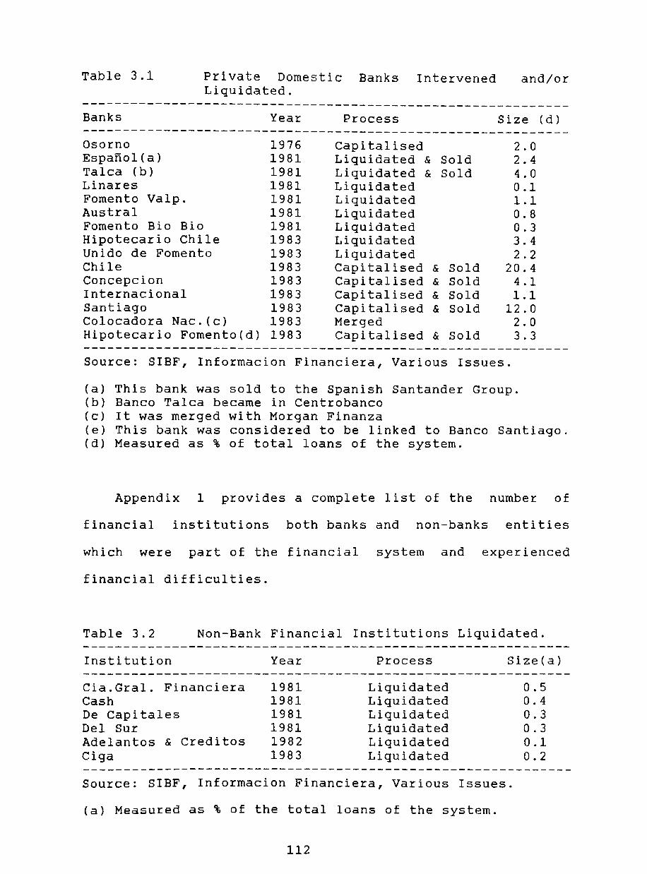
Table 3.1 Private Domestic Banks Intervened Liquidated.

and/or

------------------------------------------------------------Banks Year Process Size ( d) -------------------------------------------------------------Osorno 1976 Capitalised 2.0 Espafio1(a) 1981 Liquidated & Sold 2.4 Talca (b) 1981 Liquidated & Sold 4.0 Linares 1981 Liquidated 0.1 Fomento Valp. 1981 Liquidated 1.1 Austral 1981 Liquidated 0.8 Fomento Bio Bio 1981 Liquidated 0.3 Hipotecario Chile 1983 Liquidated 3.4 Unido de Fomento 1983 Liquidated 2.2 Chile 1983 Capitalised & Sold 20.4 Concepcion 1983 Capitalised & Sold 4.1 Internacional 1983 Capitalised & Sold 1.1 Santiago 1983 Capitalised & Sold 12.0 Colocadora Nac. (c) 1983 Merged 2.0 Hipotecario Fomento(d) 1983 Capitalised & Sold 3.3

Source: SIBF, Informacion Financiera, Various Issues.

Ca) This bank was sold to the Spanish Santander Group. (b) Banco Talca became in Centrobanco (c) It was merged with Morgan Finanza (e) This bank was considered to be linked to Banco Santiago. Cd) Measured as % of total loans of the system.

Appendix 1 provides a complete list of the number of

financial institutions both banks and non-banks entities

which were part of the financial system and experienced

financial difficulties.

Table 3.2 Non-Bank Financial Institutions Liquidated.

Institution

Cia.Gral. Financiera Cash De Capitales Del Sur Adelantos & Creditos Ciga

Year

1981 1981 1981 1981 1982 1983

Process

Liquidated Liquidated Liquidated Liquidated Liquidated Liquidated

Size(a)

0.5 0.4 0.3 0.3 0.1 0.2

Source: SIBF, Informacion Financiera, Various Issues.

(a) Measured as % of the total loans of the system.

112

All in all, the total sum added up to around 50% of

total loans which were at stake and Banco de Chile and Banco

de Santiago were the two largest banks in Chile with 20% and

nearly 12% of loans relative to the total intermediation in

December 1982. According to Arellano (1985) the support of

the Central Bank for those financial institutions in

liquidation and in emergency loans added up to more than 15%

of GDP of 1982. Although the government was not forced to

intervene by the existence of an explicit deposit

arrangement, they had to pick-up the bill

insurance

to avoid

systematic panics and bank runs, together with a deeper

financial crisis.

However, the dimensions of the 1983 banking crisis were

much wider if we also include those financial intermediaries

which, although they were not intervened by the SIBF, had to

sell part of their nonperforming loans to the central Bank.

Table 3 contains information about the institutions which

made use of the Central Bank's directives number 1.450 and

1.555 authorising banks to sell nonperforming loans to the

Central Bank. These two directives from the Central Bank

permitted both banks subject to intervention (intervened

banks), and

banks) to

promissory

later.

non-intervened vulnerable banks (non-intervened

substitute non-performing assets for cash and

notes issued by the Central Bank as we will see

113

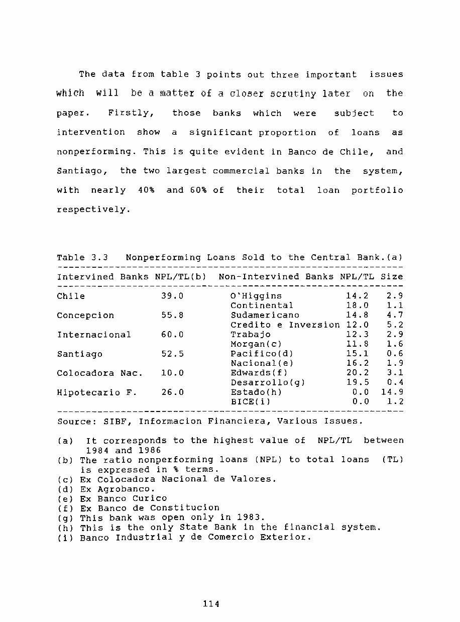
The data from table 3 points out three important issues

which will be a matter of a closer scrutiny later on the

paper. Firstly, those banks which were subject to

intervention show a significant proportion of loans as

nonperforming. This is quite evident in Banco de Chile, and

Santiago, the two largest commercial banks in the system,

with nearly 40% and 60% of their total loan portfolio

respectively.

Table 3.3 Nonperforming Loans Sold to the Central Bank.(a)

Intervined Banks NPL/TL(b) Non-Intervined Banks NPL/TL Size ------------------------------------------------------------Chile 39.0 O'Higgins 14.2 2.9

Continental 18.0 1.1 Concepcion 55.8 Sudamericano 14.8 4.7

Credito e Inversion 12.0 5.2 Internacional 60.0 Trabajo 12.3 2.9

Morgan(c) 11.8 1.6 Santiago 52.5 Pacifico(d) 15.1 0.6

Nacional(e) 16.2 1.9 Colocadora Nac. 10.0 Edwards(f) 20.2 3.1

Desarrollo(g) 19.5 0.4 Hipotecario F. 26.0 Estado(h) 0.0 14.9

BICE(i) 0.0 1.2

Source: SIBF, Informacion Financiera, Various Issues.

(a) It corresponds to the highest value of NPL/TL between 1984 and 1986

(b) The ratio nonperforming loans (NPL) to total loans (TL) is expressed in % terms.

(c) Ex Colocadora Nacional de Valores. (d) Ex Agrobanco. (e) Ex Banco Curico (f) Ex Banco de Constitucion (g) This bank was open only in 1983. (h) This is the only State Bank in the financial system. (1) Banco Industrial y de Comercio Exterior.

114

Secondly, the problem of non performing loans also

emerged among non-intervened banks with ratios above the 10%

and just below the 21% mark. Additional evidence from SIBF

and Held (1989) shows that the total nonperforming loans

sold to the Central Bank was equivalent to 27.7% of total

loans of the system and 18.2% of GDP of 1985.

Thirdly, the evidence also showed that there were only

two domestic banks, Banco del Estado and BlCE, which did not

need to transfer a proportion of their nonperforming loans

to the Central Bank.

Thus, between 1981 and 1983 the SIBF intervened 14

domestic banks and 6 non-bank financial institutions from a

total of 26 banks and 17 financieras, excluding the state

bank Banco del Estado. From there the authorities liquidated

a total of 8 banks and all the intervened financieras.

The present empirical study on the banking crisis will

be centered in the 1983 period. Although the beginning of

the Chilean banking crisis can probably be dated in 1981,

the crisis really came to a head in 1983. As we saw already,

it did compromise a significant proportion of the

intermediation and involved the two largest banks. In

addition, the rescue package involved a substantial amount

of public money. There are two additional justifications for

concentrating on studying those institutions who failed or

showed problems during 1983. The first one is that our

interest is to test how important were the macroeconomic

115

environment relative to the bank management in the debacle

of the banking system. As we have seen from chapter 2, 1982

and 1983 were years where output fell dramatically.

Secondly, as explained in chapter 6, data limitations

force me to consider a sample of data between 1979 to 1983.

The alternative would restrict the sample to a period

between 1979 to 1981, and hence drawing inferences on 8

quarterly observations and with a smaller sample of

individual banks.

(3.2.2) An Autopsy of the Banking Sector.

The next step is to carry out an autopsy of the

banking system and each individual financial institution in

order to assess the magnitude of the crisis and to establish

some tentative differences in their relative performance.

The tables are constructed from the information obtained

from the banks balance sheets and the income statements

published by the SIBF. Appendix 2 provides a sample of the

format and structure of a balance sheet and income statement

of a Chilean bank.

The data from tables 4 and 5 give evidence of the change

of fortunes of the financial sector .

116

Table 3.4 Indicators of the Financial System Boom in Chi Ie. (a)

------------------------------------------------------------77 78 79 80 81 Av

------------------------------------------------------------Growth Bank Assets(b) 50.4 41.3 29.6 40.3 11.3 34.5 Loans/GOP 16.6 23.2 28.2 37.6 50.4 31.2 Growth Bank Liability(c) 47.8 51.0 29.9 42.8 11.6 36.6 Gross Profits/Capital 8.7 18.5 23.0 23.5 11.4 17.0 Sector GOP Growth 14.5 20.1 28.0 24.7 14.2 20.3 GDP Sector/GOP 6.3 7.0 8.1 9.5 10.6 8.3 ------------------------------------------------------------Sources: SIBF, Informacion Financiera, Various Issues.

(a) It includes banks and non-banks financial institutions. (b) Wide definition of bank assets i.e. loans+financial

investment+accrued interest and available funds+ Central Bank note from the selling of nonperforming loans. All in nominal terms.

(c) Total obligations with third parties.

The data on GDP growth for the financial sector show a

significant increase with an average annual growth rate of

20% and with a peak of 28.0% in 1979. The share of the

financial sector GOP growth relative to the overall GOP of

the economy was 8.3% per annum. Looking at the profitability

and the rate of return of bank capital measured by the gross

profits/capital ratio shows a marked rise from 8.7% to

nearly 24% in 1980 with an annual average of 17%. These

impressive results are not surprising given the high growth

rate in bank assets and growing value of total loans

relative to GOP. In fact, the data shows that the annual

average growth rate of bank assets was 37.5 and the

loans/GDP ratio over 31%. The peak of the loan/ GOP ratio

occurred in 1981 with a 50% ratio during a period where

output was still expanding very fast. At the same time, as

we have seen from the previous chapter, the abnormal high

117

nominal and real lending rates as well as the persistence

and ever increasing spread between lending and deposit

intereBt rateB In the face of Increasing demand for credIt

should explain the astonishing profitability and growth of

the banking sector. This rapid growth in bank assets took

place in an environment of falling inflation. As we have

seen from chapter 2, the rate of inflation went from

approximately 30% p.a in 1978 to 9.5% in 1981.

However, the financial boom turned sour from the last

quarter of 1981 onwards. The evidence from table 5 give an

indication of the magnitude of the change between 1982 and

1983 years at which the full blow of the emerging banking

crisis was felt and the authorities inmplemented the

rehabilitation programmes.

Table 3.5 Indicators of the Financial Sector Collapse in Chile.

Growth Bank Assets Loans/GOP Growth of Bank Liabilities Gross Profits/Capital Sector GOP Growth GOP Sector/ GOP

1982

22.6 71.2 24.7 4.1

-4.4 11.7

1983

12.3 72.4 11.8

-24.0 -40.5

7.5

1984

19.0 74.5 19.8

-24.7 -9.2 6.5

Source: SIBF, Informacion Financiera, Various Issues.

Av

17.9 72.7 18.7

-14.8 -18.0

8.5

The evidence from table 5 shows the magnitude of the

deterioration of the financial system between 1982-84. For

instance, the GOP growth of the financial sector fell by an

annual average of 18% during those three years with a trough

118

of nearly 41% in 1983. Equally dramatic was the return on

bank capital which shows a significant fall in 1982 and

becomes more acute in 1983 and 1984 with minus 24%. This

performance coincided with the large fall in GDP in 1982 and

1983 of 14% and 0.7% respectively. Given the increasing

financial fragility of firms, we observe a rise in the

loan/GOP ratio in the face of falling output and increasing

real lending rates which indicates some form of distress

borrowing.

Further evidence from banks' balance sheets shows the

increasing vulnerability and insolvency of the financial

system. Looking at the risk exposure, table 6 shows that the

amount of nonperforming loans grew very dangerously during

1982,1983, and 1984. For instance, in 1983 nonperforming

loans almost reached 50% of the capital of the financial

system and by 1984 was still rising to 60%. However, these

figures underestimate the magnitude of the exposure since as

we will see in the next subsection, the authorities allowed

more flexible accounting procedures which among other things

permitted banks longer recogniton time of nonperforming

loans and the constitution of provisions. In addition, the

authorities enabled banks to remove from their balance sheet

nonperforming and risky loans using the agreement 1.450 in

1982 and later on the agreement 1.555 of 1983. Therefore,

the indicator which accounts for the nonperforming and risky

loans sold to the Central Bank should be more meaningful and

accurate.

119

Table 3.6 Financial Indicators of Vulnerability and Insolvency of the Financial System in Chile.(%)

------------------------------------------------------------81 82 83 84 Av

------------------------------------------------------------NP Loans/Loans 2.9 7.5 5.5 3.8 4.9 NP Loans/Capital 24.4 41.9 49.5 60.0 44.0

NP Loans Sold/Loans 6.8 9.6 14.2 10.2 NP Loans Sold/Capital 67.1 95.4 NP& Risky Loans Sold/Capital 78.8 158.1 186.3 141.0

Bank Liabilities/Capital 10.6 11.0 11.4 12.0 11.2 Gross Profits/Total Assets 1.0 0.3 -1.7 -1.5 0.4 Provisions/Total Assets 1.1 3.6 4.3 4.8 3.4 ------------------------------------------------------------Source: SIBF, Informacion Financiera, Various issues.

NP= Nonperforming

By 1983 and 1984, the selling of nonperforming loans and

risky assets reached 158% and 186% of capital respectively.

At that time, the amount of bad and risky credit purchased

by the Central Bank had exceeded the capital of the

financial system, thus showing the full extent of the

banking crisis. Equally, we see the deterioration of the

average return of each asset unit in 1983 and 1984, measured

by the negative figures of the gross profit/total asset

ratio.

The growing vulnerability and the poor profitability

combined with a relaxation on the constitution of provisions

and capital requirement forced the authorities to rescue

those institutions, as we have seen in tables 1-3, which

were facing insolvency and/or experiencing a severe

120

deterioration of their asset quality. Disaggregated data

will show the financial vulnerability of each individual

institution which was rescued and/or required some financial

aid. The individual data will produce some interesting clues

on the comparative performance and their state of financial

health.

Tables 7 to 13 are organised as follows. The first 8

financial institutions in the first group correspond to

those which were liquidated and intervened in 1983. The

second group is composed by those banks which sold

nonperforming and risky loans to the Central Bank. Finally,

the two remaining institutions correspond to those which

were not required to participate in any of the initiatives

enacted by the authorities to rescue the banking system.

They both remained healthy throughout the period of study.

This configuration not only shows the increasing

deterioration of each individual financial institution but

also permit us to compare at first sight marked differences

in the ratios between groups. Chapter 5 provides a more

thorough and sophisticated statistical analysis for groups

differences.

121

Table 3.7 Financial Indicator of Vulnerability: Asset Quality.

------------------------------------------------------------(a) NPL/Loans NPL/Capital

------------------------------------------------------------Institutions 80 81 82 83 80 81 82 83 ------------------------------------------------------------Unido de Fomento Hipotecario Chile Chile Concepcion Internacional Santiago Hipotecario Fto. Ciga (b)

O'Higgins Continental Sudamericano Credito Trabajo Pacifico Nacional Edwards

BICE Estado

29.2 1.6 1.5 1.8 0.6 0.3 1.2 2.0

1.2 2.2 1.3 1.4 1.7 0.1 1.5 0.5

4.1 1.4 2.0 2.0 1.0 0.5 0.8 1.6

2.1 2.5 1.3 1.7 2.2 0.7 0.7 1.0

O. 4 2.0 1.9 4.2 3.0 7.2 3.5 6.2

5.2 1.2 4.1 2.9 4.2 5.2 5.0 3.9

0.3 0.2 6.4 4.8 2.9 9.0

11.3 14.5 11.1 30.7

3.6

7.4 17.0

2.7 3.2 2.0 2.0 3.9 4.8

2.8 5.3

407.1 22.5 14.1 27.1

6.9 4 . 7

20.8 3.4

12.3 18.9 15.0 17.0 22.8 0.4 7.3 6.5

57.9 25.1 23.5 28.4 12.2 6.3

14.8 12.3

22.7 26.5 19.3 24.7 29.0 7.3 7.1

13.0

93.0 68.0 68.9 45.3 66.8 18.6 33.0 35.8

42.9 89.0 38.1 57.3 45.1 38.4 44.1 40.4

177 175 102 297 147

76 182

39 43 25 21 37 72

1.8 2.0 15.2 36 31.7 15.4 33.5 28

------------------------------------------------------------Source: SIBF, Informacion Financiera, Various Issues.

(a) NPL= Nonperforming Loans in the balance-sheet. (b) Non-bank financial institution.

Table 7 contain individual data on the deterioration of

the quality of banks' loan portfolios. The NPL/Loans ratio

begin to show a notorious rise in 1983 in particular among

those banks which were intervened in the same year. Banco

Chile, Banco Santiago, and Banco de Concepcion present the

largest deterioration of their loan quality in particular as

we measure it against their capital and reserves. For

instance, the worst case of all correspond to the Banco

Santiago as the amount of nonperforming loans is nearly

three time its capital. According to the preliminary

122

estimates, some worrying signs started to emerge in 1982

although it became quite obvious during the intervention

year. Similar observations can be made on those entities in

the second group, although their capital obligation were

less serious at least with respect to the first group.

As we argued earlier, the accounting of nonperforming loans

could be a misleading indicator given the recognition lag,

the unwilligness to report, and above all its usefulness is

seriously limited as an early indicator of those

institutions which should be monitored. Nor may it provide

evidence of the real magnitude of the deterioration of bank

assets.

Table 8 provides a better measure of the magnitudes

involved for each institution as well as an ex post

indicator of the actual deterioration of banks' asset

quality. It should be pointed out that any difference

between the values of NPL and loans sold to the Central Bank

demonstrate the effect of under-reporting of the former. The

data for 1982-83 begin to show the magnitude of the fall in

the quality of banks' credit and the extent of the rescue

operation. Individual banks were allowed

nonperforming and risky loans to the Central Bank

through the agreement 1.450 enacted in 1982 and

1983 the agreement 1.550.

123

to sell

initially

later in

Table 3.8 Additional Financial Indicator of Asset Quality. ------------------------------------------------------------

(a) Loans Sold/Loans Loans Sold/Capital ------------------------------------------------------------Institutions 81 82 83 84 81 82 83 84 ------------------------------------------------------------Unido de Fomento Hipotecario Chile Chile Concepcion Internacional Santiago Hipotecario Fto. Ciga

O'Higgins Continental Sudamericano Credito Trabajo Pacifico Nacional Edwards

BICE Estado

0.0 0.0 0.0 0.0 0.0 0.0 0.0 0.0

0.0 0.0 0.0 0.0 0.0 0.0 o . 0 0.0

0.0 0.0

9.7 4.8 4.0 6.1 9.1 1.5 2.4 9.4

2.5 0.0 6.5 8.0

11.4 8.1 1.9 6.2

0.0 0.0

9.3 13.1 10.9 20.1

9.0

5.8 9.2 7.4

15.0 10.5 8.5 6.7

10.8

0.0 0.0

7.7 11.0

8.6 19.0 11.4

14.2 18.0 14.1 12.0

9.6 15.1 16.2 15.0

0.0 0.0

0.0 0.0 0.0 0.0 0.0 0.0 0.0 0.0

0.0 0.0 0.0 0.0 0.0 0.0 0.0 0.0

0.0 0.0

176.0 75.1 64.5 74.2 89.4 14.6 43.9 73.9

25.5 0.0

100.1 112.7 154.3 101.1

18.8 97.5

0.0 0.0

148.8 164.1 104.2 166.3 165.3

58.5 93.2

116.1 210.8 140.1 88.0 65.5

156.7

0.0 0.0

------------------------------------------------------ ------Source: SIBF, Informacion Financiera, Various Issues.

(a) Loans sold to the Central Bank includes nonperforming and risky loans

There are two interesting observations from the data

which is worth to comment on. Firstly, the ratio of

NPL/Capital in the case of the intervened banks is similiar

to the ratio Loans Sold/Capital in spite of a wider

definition of the latter. Secondly, the largest quantities

of loans sold is concentrated in the second group of the

table and exceed the banks capital. We also observe that in

1982 the second group of banks sold a larger quantities of

loans to the Central Bank than the first group. The answer

lies in the fact that, unlike the second group, the

124

agreement 1.555 restricted intervened banks from selling

nonperforming and risky loans until they were recapitalised.

In general, the asset deterioration which according to

NPL/Capital ratio was somewhat submerged in the case of

Banco Continental, Sudamericano, Credito, Trabajo, Pacifico,

and Edwards emerged with a full blast in 1982-83. At the

same time, Banco del Estado and Banco Industrial y de

Comercio Exterior remained as the only two exceptions which

did not sell any nonperforming and risky loans to the

Central Bank.

With respect to the profitability, the data should

reflect the overall performance of a bank. An inadequate

profitability will give a signal of the vulnerability and a

high likelihood of a bank insolvency as the bank net worth

start falling. The profit/asset ratio shows the average

return of each unit of bank asset and it can also be

interpreted as a proxy for the quality of bank assets. The

data on the average return on assets not only shows that the

trend in profitability has been downward but also its lowest

values occurred in 1983. For instance, Banco Santiago is the

worst performer with a negative average return of almost 7%

followed by Banco Concepcion and Banco Chile with minus 5.4%

and 2.6% respectively. The same conclusions are reached

for the second group in the tables although the fall in

profItabillty was more moderate than in the first group.

Banco Continental is the only comparable case as the figures

shows a marked deterioration which had started in 1982.

125

Table 3.9 Financial Indicators of Vulnerability: Profitability.

------------------------------------------------------------(a) Profits/Assets Profits/Capital

------------------------------------------------------------Institutions 80 81 82 83 80 81 82 83 ------------------------------------------------------------Unido de Fomento Hipotecario Chile Chile Concepcion Internacional Santiago Hipotecario Fto. Ciga

O'Higgins Continental Sudamericano Credito Trabajo Pacifico Nacional Edwards

BICE Estado

0.4 0.9 1.4 o . 4 0.6 0.2 0.3 0.0

1.0 0.7 o . 3 0.3 0.5 0.1 0.8 0.1

0.3 0.2 0.2 0.2 0.7

-1.0 0.1

-0.5

0.6 0.1 0.4

-0.3 0.5 0.3 0.6 0.1

0.0 0.1 0.4 0.5 0.1 0.5 0.3

-0.7

0.9 -2.1

0.2 0.4 0.0 0.1 0.5

-0.1

-2.6 -5.4 -2.3 -6.9 -0.1

0.0 -5.1 -0.1 -0.6

0.0 -0.7 -0.1 -0.1

0.4 0.6 0.3 0.1 0.3 0.7 0.5 0.3

5.4 16.8 17.8 8.3 9.0 4.0 5.6 0.1

12.6 8.5 5.8 4.9 8.2 1.6 5.3 1.3

4 • 6 3.9

5.1 4.1 4.7 3.4 9.9

-15.1 2.0

-5.0

-0.1 1.2 6.3 6.6 1.5 5.4 6.6

-7.6

8.0 10.7 1.1-23.1 7.6 2.5

-4.7 5.4 7.2 -0.3 3.8 1.1 7.1 6.2 2.2 -1.1

-54 -77 -26 -77

-1

o -68

-1 -14

o -9 -1 -1

8.3 4.3 1.2 5.7 3.5 3.3

------------------------------------------------------------Source: SIBF, Informacion Financiera, Various Issues.

(a) Bank Assets includes loans, financial investment, and cash. Also profits are defined as the difference between the total income account and the total expenses account.

The profit/capital ratio which is the more traditional

measure of the rate of return on investment also presents

evidence of the fall in profitability. The same conclusions

emerge from the profit/capital ratio. Individual banks

exhibit both a declining trend in the rate of return of

capital and the lowest figures in 1983. Among the largest

banks Banco Chile and Banco Concepcion showed the best and

the worst rates of return of capital with 17.8% and 8.3% in

1981 and -54% and -77% in 1983 respectively. In addition,

Banco Santiago systematically showed the worst performance

126

between 1981 to 1983. Again in the second group, Banco

Continental shows a comparable performance with the largest

banks with a negative rate of return in two consecutive year

with -23% in 1982 and -68% in 1983. Again, BrCE and Banco

del Estado were the only two exceptions as they remain

profitable even in the worst year of the banking crisis.

If we look at the NPL/capital, loans sold/capital and

profit/assets ratios the downward trend in profitability

which started to emerge in 1982 and fully developed in 1983

coincide with the worsening in the quality of the banks loan

portfolios over any significant increase in operating costs.

The estimated ratios for both intervined banks and those in

the second group consistently showed a deterioration in

these three ratios in particular in 1982 and 1983. Banco

Santiago, Banco Concepcion, and Banco Chile were the worst

cases in the former group and Banco Continental and Banco

Credito in the latter.

The provision/loans ratio and the liabilities/capital

ratio are additional indicators of increasing vulnerability.

The former attempt to measure the provisions made in order

to cover any potential losses from any expected and

unexpected deterioration of the loan portfolio. In this

case, the numerator reflects the bank's total provision. As

we will see later much of this figure is determined by the

country's banking regulation on specific and global

provision. There are two general observations to be inferred

from this data exhibited in table 10.

127

Table 3.10 Additional Indicators of Vulnerability. ------------------------------------------------------------

(a) Provision/Loans Liabilities/Capital ------------------------------------------------------------Institutions 80 81 82 83 80 81 82 83 -------------------------------------------------------------Unido de Fomento Hipotecario Chile Chile Concepcion Internacional Santiago Hipotecario Fto. Ciga

O'Higgins Continental Sudamericano Credito Trabajo Pacifico Nacional Edwards

BICE Estado

9.8 9.4 7.6 5.0 6. 5 5.0 5.6

10.9

8.7 6.1 5.0 6.0 5.3

14.5 6.3 3.2

1.2 1.1 0.9 1.1 1.8 1.1 0.8 0.9

1.6 0.2 1.1 0.8 1.5 0.8 1.1 0.8

4 . 4 4.7 3.2 2.4 3.2 3.1 1.4 3.5

2.8 3.1 1.7 2.1 2.1 1.1 2.2 1.3

5.6 5.5 6.9 8.0 3.0

3.9 12.3

2.4 3.0 2.7 3.0 3.5 2.4

5.0 1.1 1.9 3.8 14.3 5.2 7.1 10.5

17.0 19.5 15.2 15.3 13.6 15.3 17.5

9.8

13.8 10.7 16.9 16.1 13.6 13.0 13.8 14.4

15.6 14.1 20.5 15.5 11.5 11.0 19.2 0.9

12.9 11.6 17.9 16.6 15.8 13.5 11.3 17.8

24.0 18.3 10.6 9.3

17.4

8.7 24.3 17.1 15.2 14.4 9.5

11.1 15.3

13.3 14.5 14.4 7.0 7.3 7.8

------------------------------------------------------------Source: SIBF, Informacion Financiera, Various Issues.

(a) These estimates were elaborated with the data available for December.

Firstly, the lower provision made in 1981 as compared

with 1980 can be explained by the change in regulation. As

we will see in the next section, the requirements for the

constitution of a global provision were reduced from 2% to

0.75%. In addition, the accounting flexibilities gave banks

more time to build up individual provision for each type of

credit classification.

Secondly, the low values coincide with very rapid

expansion in the growth rate of loans as shown by table 11.

In both the first and second group of banks a low

128

provision/loans ratio coincided with a rapid expansion of

bank loans, in particular in 1980 and 1981. For instance,

according to my estimations, in 1981 Banco Chile experienced

a loans growth of 102% combined with a provision/loan ratio

of 0.9 % . The same is true in the cases of Banco Concepcion

and Banco Santiago. Among the second group, Banco Pacifico

and Banco Naciona1 exhibited the highest growth rate among

its group and the whole banking system for the period of

1981 with figures reaching 313% and 178% respectively. These

figures for both banks coincided with a low values for the

provision ratio of 0.8% and 1.1% in each case.

Table 3.11 Financial Indicator of Bank Expansion.(%)

(a) Loans Growth

Institutions

Unido de Fomento Hipotecario Chile Chile Concepcion Internacional Santiago Hipotecario Fto. Ciga

O'Higgins Continental Sudamericano Credito Trabajo Pacifico Nacional Edwards

BICE Estado

80

84.7 198.4

95.1 39.2

110.2 129.2 141.8

85.9

48.5 67.9 69.0 43.1 42.8 47.5 95.6

198.9

81 82

104.9 1.1 143.7 18.6 102.1 17.0

95.5 -0.2 59.5-13.6 81.6 62.5

108.1 3.4 70.5-11.1

61.6 54.2 74.3 73.7 36.9

313.7 178.1 111.5

10.7 5.0 1.5

-8.3 1.8

18.6 3.7

52.6

83

16.8 18.7 19.1 -4.3 17.2

15.8 10.4 26.2 13.9 23.3 25.0 16.8

8.7

268.4 164.3 22.5 22.3 45.9 79.2 4.9 21.7

Liabilities Growth

80

5.8 9.2 4.9 3.2 7.0 6.6 7.8 6.8

2.5 4.2 3.9 3.0 2.3 4.7 5.8 8.9

81

4.8 6.2 4.5 4.0 2.0 4.4 4 • 4 4.1

4.4 1.8 3.0 3.1 1.4

11.1 7.2 4.9

12.0 5.7 4.1 1.9

82

3.6 4.9 4.5 4.0 1.7 6.4 3.0 1.6

2.4 3.1 3.9 2.8 4.0 3.4 3.4 6.7

83

2.7 3.0 3.1 3.0 3.6

3.9 5.6 4.4 3.9 3.9 4.0 4.6 3.5

5.8 8.2 3.3 24

Source: SIBF, Informacion Financiera, Various Issues. (a) It refers to the rate of change from December to

December measured in nominal terms.

129

On the liabilities side of the banks balance sheet we

see that deposits became the principal source of funds of

the rapid growth of bank credit. This is the result of the

financial liberalisation reforms to increase the financial

deepening and widening of the financial system. The data on

the banks' liability growth rate and the deposit/liabilities

ratio from tables 11 and 12 provide support to this

assertion. The evidence does not suggest very large

differences in the monthly annual average growth rate of

liabilities among the two groups in the table, although the

case of exception again correspond to Banco del Estado. One

point is worth mention from the data for 1983. We observe

that the growth of liabilities in the two big groups

which experienced some fall unlike Banco del Estado

exhibited a significant rise in their liabilities by

This can be interpreted as a run to safety, although not

24%.

in

a massive shift reflecting a widespread panic.

By examining the liabilities/capital ratio of individual

banks in table 10, we observe no significant differences in

their leverage although it was almost doubled as compared

with the 1978 average ratio for the financial system which

was estimated at 8.1%. The two opposite exceptions

correspond to Banco Chile and Banco del Estado. The former

bank presents a leverage ratio of 20.5% and 24% in 1982 and

1983 while the latter bank shows a leverage ratio of around

7% for 1981 to 1983.

130

Table 3.12 Financial Indicator of Vulnerability: Liability Quality.(%)

------------------------------------------------------------(a) Deposits/Liabilities (b) Lbts FC/Lbts

------------------------------------------------------------InstItutions 80 81 82 83 80 81 82 83 ------------------------------------------------------------Unido de Fomento Hipotecario Chile Chile Concepcion Internacional Santiago Hipotecario Fto. Ciga

O'Higgins Continental Sudamericano Credito Trabajo Pacifico Nacional Edwards

BICE Estado

8.2 33.1 37.6 49.2 47.0 45.3 29.4 90.6

42.1 38.7 40.9 41.0 47.1 65.2 54.1 52.1

16.2 14.0 36.4 27.7 39.7 36.6 18.9 46.3 48.9 26.3 61.4 63.9 32.9 41.4 36.6 14.0 32.1 22.8 14.3 87.0 91.6

44.5 40.2 27.7 39.5 46.5 24.6 39.3 30.8 22.4 49.4 49.7 37.5 45.6 52.3 35.0 59.5 64.9 50.8 51.3 53.8 42.7 49.5 45.7 35.7

24.4 31.6 32.7 23.5 75.3 76.0 63.5 87.7

34.1 31.7 58.1 28.5 26.7 42.0 38.4 47.1 55.1 50.3 22.5 28.8 38.5 33.7 21.5 18.4 22.8 23.6 26.2 37.5 46.5 41.2 9.6 14.0 23.3 25.5

31.2 37.3 46.6 46.3 25.3 30.0 40.0 35.9 32.4 39.9 52.0 51.3 26.7 31.2 36.9 33.9 30.9 39.1 40.9 37.5

9.5 12.0 20.9 20.6 18.3 19.1 29.9 33.7 25.1 35.8 43.9 40.9

31.8 43.0 52.5 46.8 13.8 12.0 19.6 48.3

Source: SIBF, Informacion Financiera, Various Issues.

(a) Liabilities are defined as total deposits, foreign and domestic loans, contingent and mortgage liabilities

(b) Liabilities in foreign currency (Lbts FC) correspond to total deposits in foreign currency and loans obtain abroad.

One interesting and worrying observation can be

established from the estimates of table 12. It appears to be

a large change in the composition of the banks' liabilities

as the restriction on foreign credits were phased out

gradually from 1978 onwards. For instance, Banco Chile and

Banco Santiago show a growing share of liabilities in

foreign currency relative to domestic currency. By 1982 and

1983 the former had more than 50% of its liabilities

denominated in foreign currency. Among the banks in the

131

second group, Banco Sudamericano had shown a systematic rise

in foreign indebtness with a Lbts FC/Lbts ratio of 52% and

51.3 for the years 1982 and 1983 respectively.

As a whole, the evidence does not suggest that the

vulnerability comes from the liabilities side of the banks

balance sheet nor support the view that the differences

among the three groups in the liabilities composition may be

regarded as important. As a matter of fact, BICE exhibited

higher liability ratios than the intervened banks. Moreover,

the evidence from chapter 6 supports this conclusion and

also finds that any difference in foreign indebtness between

sound banks and problem/failed banks is statistically

insignificant and thus an unreliable early warning variable.

It is clear from the evidence that all those

institutions which exhibited spectacular growth rates in

their loan portfolios were later intervened and/or forced to

sell bad credits to the Central Bank. Furthermore, the

higher were the growth rate of loans, then the higher the

ratios measuring the deterioration in asset qualities, in

particular the loans sold/ capital. In contrast, Banco

Industrial y de Comercio Exterior (BICE) and Banco del

Estado which clearly grew at a relatively lower rate and

exhibited better performance in terms of the other financial

indicators remained healthy. On this issue, their relatively

superior profitability, in particular towards 1982 and 1983

enabled these two banks to build up higher provision. This

is particularly relevant in the case of Banco del Estado.

132

Finally, table 13 present a simple estimation of the

banks of the net capital ratios (NCR). The most important

oomponent of the NCR is the nonperformlng loans which is

substracted from bank's capital and reserves. As reported

in chapter 5, banks that failed in recent years in the US

almost invariably had low or even negative NCR months before

the failure. According to the evidence for Chile, those

institutions which were intervened clearly exhibited a

negative or extremely low positive NCR. The ratio indicate a

fall in the ratio from 1981 onwards in particular in the

cases of Banco Chile, Banco Internacional, Banco O'Higgins

and Banco Continental.

Table 3.13 Banks Net Capital Ratio.

Net Capital/Assets Net Capital/Liability

Institutions 80

Unido de Fomento -19.1 Hipotecario Chile 4.7 Chile 7.5 Concepcion 3.8 Internacional 7.0 Santiago 5.3 Hipotecario Fto. 4.3 Ciga 11.9

O'Higgins Continental Sudamericano Credito Trabajo Pacifico Nacional Edwards

7.2 7.3

11.1 5.7 4.8

12.2 13.4

6.3

81

2.5 4.1 5.3 4.6 5.9 6.0 4.7 9.5

6.1 6.3 4.9 4.7 4.7 8.9 8.9 5.7

82

0.4 2.0 1.9 4.2 3.0 7 . 2 3.5 6.2

5.2 1.2 4.1 2.9 4.2 5.2 5.0 3.9

BleE Estado

9.3 7.9 6.4 8.4 10.3 9.0

83

-3.8 -5.3 -0.5

-17.2 1.2

-0.5 -6.5 3.4 3.4 4.9 6.2 5.5 1.6

3.6 7.7

80

-19.7 4.8 7.6 3.8 7.1 5.5 4.2

12.9

7.4 7.6

11.0 5.7 4.8

12.1 14.0

6.4

81 82

2.3 0.4 3.9 1.8 5.4 1.7 4.3 3.6 5.7 2.6 5.9 6.8 4.6 3.4 9.2 5.6

5.9 4.7 6.1 1.2 4.7 3.6 4.5 2.5 4.4 3.4 8.8 4.8 8.9 4.6 5.5 3.6

83

-3.2 -3.8 -0.4

-13 1.1

1.5 -5.2

2.4 2.6 3.5 5.2 3.9 1.2

9.7 8.1 6.1 2.7 9.0 10.5 9.3 8.8

------------------------------------------------------------Source: SIBF, Informacion Financiera, Various Issues.

133

The data produced from the banks' balance sheet and

income statement not only had permitted to see the move from

a boom to a bust of the whole financial system but also

enabled us to assess and identify those banks in

difficulties which later on were intervened and/or required

the support from the banking authorities. At the same time,

these results are serving as a useful agenda of research to

establish statistical differences between healthy and

unhealthy banks for classification purposes and the

estimation of an early warning function. This will allow us

to draw inferences on the likelihood of failure from

external and internal factors affecting the banks odds.

These issues will be part of chapters 6,7,8, and 9.

(3.3) The Rehabilitation of the Banking System: A Quick Glimpse on the Treatment and its Results.

The intervention and the rehabilitation of the banking

system became a pressing need for two different but equally

important reasons. Firstly, the intervention of the banking

authorities avoided the total disruption of the

intermediation and payment mechanisms from the contagious

lack of confidence and prevented a further deepening of the

economic recession. Secondly, the measures taken to

rehabilitate the banking system not only can be seen as a

short run strategy but also as an aid to reactivate the

economy in a longer run perspective.

134

The rehabilitation of some of t~le ba~kQ t t d t [ d oJ :3 ar_e .:t .... the

end of 1981 and the beginning of 1982. That is right at the

beginning of the banking crisis. However, in spite of this,

it seems to me that the extent of the crisis was overlooked

and even perhaps considered as a transitory phenomenon.

Moreover, just as goverment officials were a firm believers

in an automatic adjustment for any macroeconomic

disequilibrium, so they were at the microeconomic level in 5

the case of a bankruptcy.

At first, the Superintendency of Banks and Financial

Institutions (SIBF) responded by introducing more

flexibility in the accounting procedures applied by those

banks with problems, in particular with the losses which

started to emerge from nonperforming loans. Among the most

important changes in the banking accounting procedures were

the recognition of losses, the instruction guiding the

provision for risky loans and losses, the purchase of

nonperforming loans, and the limits on banks leverage. Also,

this approach included the payment of interest on bank

reserve requirements.

The SIBF (1982,1983) reported that banks were authorised

to consider as outstanding all those loans that had been in

arrears for 90 days rather than 30 days. Consequently with

the previous measure, the SIBF also extended the time

available to make provisions to cover potential losses from

their loans portfolio. For instance, the time limit to build

up the global provision was extended from 36 to 60 months.

135

By the same token, banks were instructed to make

individual provision depending on the risk classification of 6

bank loans. At the same time ,the rules governing the

composition of provisions also demanded additional coverage

in the case of nonperforming loans. For instance, for all

those loans covered partially by collateral and entered as

nonperforming, full provision was required at the end of

each year of an amount equal to the uncovered portion of the

loan. This percentage was reduced to only half for all those

nonperforming loans recognised during the second semester of

each year. Initially, this provisions had to be made within

the year. But later on, the more flexible and gradual

approach in the constitution of provisions meant the

extension of this prudent time to 2 years.

Moreover, it was stated that the period to write off a

bad loan against profits or provision, which originally was

set at 13 months after becoming outstanding, was extended to

18 months. For those credits with collateral, the time was

increased from 24 to 36 months.

In 1982 the Central Bank introduced an accounting

procedure contained in the directive 1.450 which allowed

banks to sell nonperforming loans in return for a Central

Bank note (letra de cambio) and with a repurchase agreement

with 10 years' limit and a minimum of 5% repurchase of sold

loans hold by the Central Bank in each semester. The

repurchase of nonperforming and risky loans was carried out

with the bank's financial surpluses. This mechanism did

136

not involve Central Bank resources as compared with its twin

directive 1.555 enacted in 1984 but just to deferred banks'

losses. The mechanism adopted in 1982 also included the

relaxation on the banks leverage which before it was set

with a maximum debt to capital ratio of 20.

As whole the mechanism adopted in 1982 was basically

giving a greater flexibility in order to defer any bank

losses and as such it did not involve any significant

transfer of financial resources from the Central Bank to the

banking system. At the same time, it did not tackle the root

of the problem which, as will be argued and evaluated

empirically, revolved around the excessive laxity in the

banks' management, in particular on those decisions

concerning risk taking and credit allocation. Instead, the

mechanism came to relax even further the accounting

regulation and hence the recognition of nonperforming loans.

I would agree with the assertion of Barandiaran (1983). He

maintained that by mid-1981 firms' and banks' problems were

still of a magnitude that a wave of liquidation would have

been feasible. Moreover, the empirical evidence from chapter

6 not only supports this assertion but also shows that the

banking difficulties were predictable with three years in

advance, that is as early as 1980.

These accounting flexibilities were phased out during

1984 and 1985 soon after the positive effect of a more

direct package of measures were having its impact in the

rehabilitation of the banking system. By mid-1982 the self-

137

correcting mechanism introducing more flexibilty was not any

more a viable solution as the magnitude of both the banking

crisis and the economic recession was getting worse. At that

time, a macroeconomic initiative and the rehabilitation of

the banking sector was called for in order to set the

condition to activate the economy and reinitiate the

economic growth.

More radical steps were needed to rehabilitate and

strenghten the banking system. The increasing volume of

nonperforming loans endangered a large number

institutions with insolvency which, as we have

previously, accounted for a large proportion of

intermediation and also included the two largest banks

the system.

of

seen

the

of

There were two mechanisms to rehabilitate the banking

system in 1983: a indirect one which contained an aid

package of different debt relief measures to banks' debtors,

and a direct mechanism which comprised both the purchase of

nonperforming loans by the Central Bank, and a mechanism of

recapitalisation of those banks intervened in January 1983.

One of the first initiative taken by the SIBF was the

intervention of 6 major banks in January 1983, including the

two largest entities. The main objective of this approach

apart from rescuing the system from a major collapse was to

replace the management before any other palliative actions

were introduced.

138

This was followed by the indirect mechanism which

comprised measures of debt relief included a preferential

exchange rate to reduce the increasing costs on foreign

currency borrowers after the devaluation of the peso in June

1982. This subsidy which initially was paid in cash and

later on paid with negotiable interest bearing bonds came

as valuable relief to the borrowers

profitability, although at a cost to

solvency and

the 7

Central

Bank as we will see at the end of this section.

Debtors in domestic currency also had access to some

financial relief as they were able to reschedule the

maturity and the cost of their debts. As we have seen in

chapter 2 , although interest rates were gradually

converging to lower values after deregulation, lending rates

were still significantly high and loans were mainly on a

short-term basis. With regards to the cost of borrowing, the

Central Bank extended funds to banks in order to cover the

difference between the market-prevailing lending rate and

the 7% real lending rate set as a maximum by the monetary

authority in June 1983. In addition, maturities were

extended to 10 years and included a 5 years and 1 year grace

on the principal and the interest. Later in June 1984, the

reference lending rate was reduced to 5% for the same year

and 1984, 6% from 1985 to 1988, and 7% for thereafter. At

the same time, the maturities could not exceed 15 years and 8

fall below a minimum maturity of 5 years.

139

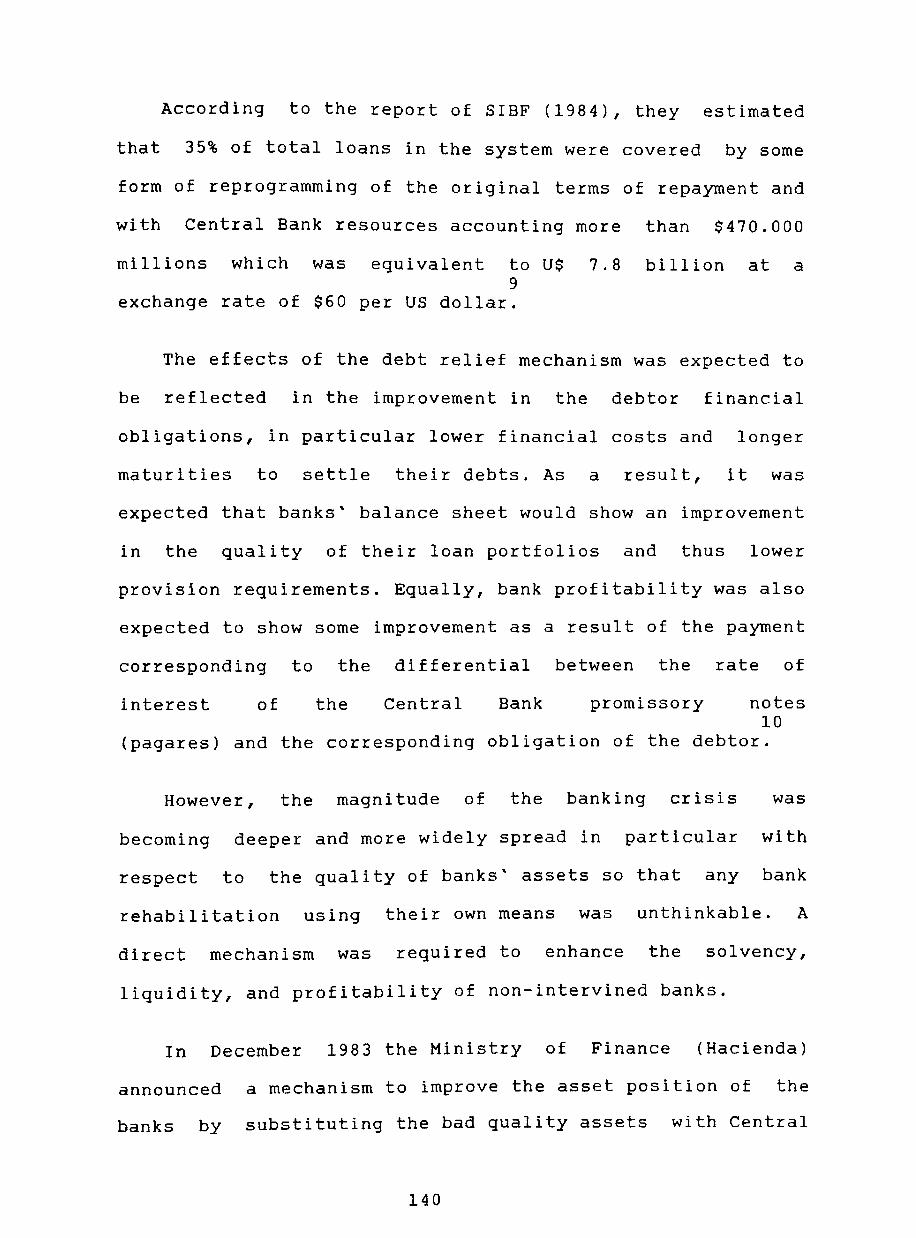
According to the report of SIBF (1984), they estimated

that 35% of total loans in the system were covered by some

form of reprogramming of the original terms of repayment and

with Central Bank resources accounting more than $470.000

millions which was equivalent to U$ 7.8 billion at a 9

exchange rate of $60 per US dollar.

The effects of the debt relief mechanism was expected to

be reflected in the improvement in the debtor financial

obligations, in particular lower financial costs and longer

maturities to settle their debts. As a result, it was

expected that banks' balance sheet would show an improvement

in the quality of their loan portfolios and thus lower

provision requirements. Equally, bank profitability was also

expected to show some improvement as a result of the payment

corresponding to the differential between the rate of

interest of the Central Bank promissory notes 10

(pagares) and the corresponding obligation of the debtor.

However, the magnitude of the banking crisis was

becoming deeper and more widely spread in particular with

respect to the quality of banks' assets so that any bank

rehabilitation using their own means was unthinkable. A

direct mechanism was required to enhance the solvency,

liquidity, and profitability of non-intervined banks.

In December 1983 the Ministry of Finance (Hacienda)

announced a mechanism to improve the asset position of the

banks by substituting the bad quality assets with Central

140

Bank resources (cash and assets). This recognised the fact

that the decapitalisation of the banking system was underlay

on the significant deterioration of the banks loan

portfolios. At the same time, there was an implicit

recognition that a prompt and durable rehabilitation of the

banking system was a necessary condition for sustainable 11

recovery of the economy as a whole.

In order to recapitalise the problem banks, the

authorities permitted non-intervened but vulnerable banks to

sell nonperforming loans to the Central Bank according to

the directive 1.555. This enabled non-intervened banks to

sell bad credits at face value up to 1.5 time their capital

and reserves. This percentage was raised to 2.5 for those

banks which required to increase their capital. In return

the Central Bank paid 60% in cash and the rest by means of a

noninterest-bearing Central Bank note (letra) which is

adjusted according to inflation.

In order to reduce the impact on the monetary growth,

banks were instructed to use the cash proceeds to repay the

outstanding emergency loans made by the Central Bank and the

purchase promissory notes (pagares) which carried a 7% real

return and 4 years' maturity. Although this represented an

important financial support, the agreement contained a

clause which forced banks to repurchase their nonperforming

loans using any financial surplus. This meant that

shareholders had to retain their dividends in order to pay

141

for their obligations with the Central Bank. The price to

buy back the nonperforming loans was adjusted in line with 12

inflation and carried an additional 5% surcharge.

For those banks which were intervened in January 1983,

the mechanism introduced by the agreement 1.555 did not

allow them the sale of nonperforming loans and even if they

could, it was clearly insufficient to restore their normal

functioning. In fact as we have seen in the previous

section, the amount of risky and nonperforming loans

exceeded several times their capital.

Initially, the law 18.401 passed in February 1985

allowed the SIBF to enforce among intervened banks a rise in

their capital base to make them financially viable. The new

stock should be offered to the existing shareholders and

after a short time to the public in general, including the

government. As reported by Velasco (1988) and Larrain

(1989), a government development agency (CORFO) could buy

any stock left over although with some restrictions. They

should not hold these equities for more than 5 years and

should not exceed 49% of the intervened bank's capital. In

order to make this recapitalisation option attractive in

particular to small investors, the government offered an

attractive package of incentives such as credit facilities 13

and subsidies.

142

According to Feller (1987), the mechanism for

rehabilitation based in the agreement 1.555 was the pillar

in the government's strategy. The debate as to whether or

not the programme was merely a cosmetic accounting trick

which provided generous subsidies has to be settled

according to the empirical evidence. Although this issue is

not part of the agenda of the study, some evidence will

corroborate the magnitude of the crisis by looking at the

numbers involved in the rescue and the effect from the

rescue.

Chamorro (1985b) and the SIBF (1984) reported that 20

financial institutions, among them 12 commercial banks, 3

foreign banks,

subscribed to

and 5 non-bank financial institution,

the agreement 1.555. The amount of risky

loans net of provisions was 156% of capital and reserves and

the banks' losses reached 6.6% of capital at the end of

December 1983. By June of 1984, the ratio of risky loans to

capital and reserves felt from 156% to only 50%.

Table 14 taken from Chamorro's paper shows the effect of

the Central Bank directive number 1.555 on non-intervened

but vulnerable bank. There are some interesting results

which is worth mentioned.

143

Table 3.14 Income statement from Institutions.

the Non-Intervened

------------------------------------------------------ -------(a) 1983 April 1984 to 1985

------------------------------------------------------------1 Operating Surplus 2 Adm. Expenses 3 Operating Margin(1-2) 4 Other Net Income 5 Monetary Correction 6 Surplus before provision(3+4+5) 7 Provisions & Reduction

- Loans Provision - Other Provision - Reductions from Bad Loans - Reduction from Bad Investment - Other Reductions

8 Surplus (6-7) 9 Surplus Allocation

- Paying Losses - Making Provisions - Repurchase of Risky Loans

10 Net Profits (8-9-10-11)

34.578 28.784 5.795 6.198 4.236

16.200 19.339 13.174

3.117 2.625

33 390

-3.140 1.054

1.054 -4.194

54.013 28.721 25.293

9.971 7.789

43.084 19.800 10.568

4.805 1.779 1.322 1.325 23.251 21.497 1.490

16.198 3.089 1.754

------------------------------------------------------------Source: Chamorro (1985b).

(a) Expressed in millions of pesos at July 1985.

Firstly, there is a marked increase in the operating

surplus and given that administrative expenses remain

constant, is reflected directly in the operating margin.

This can be explained by the positive effect derived from

the replacement of nonperforming and risky assets (loans)

which were generating no income, by government's documents

which were producing a return of 7% in real terms. At the

same time, the quality of the banks' loan portfolio improved

as a result of both the debt relief scheme and the

improvement in economic activity.

144

secondly, the sale of risky and nonperforming loans

resulted in a reduction in the required provision. The

agreement 1.555 enabled these entIties to dispose from the

asset side of their balance sheet risky and nonperforming

credit and thus contribute to a reduction in risk and

provisions.

Thirdly, the financial surplus was allocated to the

absorption of accumulated losses and the purchase of loans

from the Central Bank.

With respect to the intervened banks, although the

agreement 1.555 restrained them from selling loans to the

Central Bank at least before their recapitalisation, it was

soon modified by the agreement 1.632. They could sell risky

and nonperforming assets under the authority of the SIBF.

The situation of the two largest commercial banks

intervened was quite dramatic as we have seen in the

previous section. During 1983 the Bank of Chile and Bank of

Santiago had a risky loan portfolio of 14.5% and 30.7% of

their loan portfolios respectively. These values with

respect to capital were even more dramatic. By December 1984

the ratio of risky loans to capital for Banco Chile and

Banco Santiago reached 633% and 513% respectively. Moreover,

these losses of each bank represented more than 150% and

145% of the bank's capital respectively. By April 1985 they 14

were authorised to sell loans to the Central Bank.

145

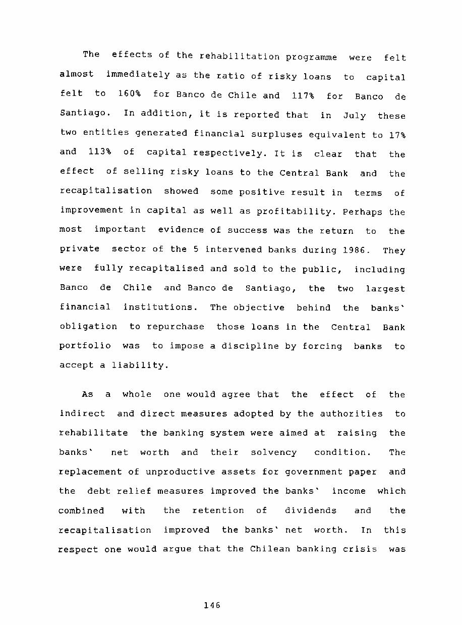
The effects of the rehabilitation programme were felt

almost

felt

immediately as the ratio of risky loans to

to 160% for Banco de Chile and 117% for

capital

Banco de

santiago. In addition, it is reported that in July these

two entities generated financial surpluses equivalent to 17%

and 113% of capital respectively. It is clear that the

effect of selling risky loans to the Central Bank and the

recapitalisation showed some positive result in terms of

improvement in capital as well as profitability. Perhaps the

most important evidence of success was the return to the

private sector of the 5 intervened banks during 1986. They

were fully recapitalised and sold to the public, including

Banco de Chile and Banco de Santiago, the two largest

financial institutions. The objective behind the banks'

obligation to repurchase those loans in the Central

portfolio was to impose a discipline by forcing banks

accept a liability.

As a whole one would agree that the effect of

indirect and direct measures adopted by the authorities

rehabilitate the banking system were aimed at raising

banks' net worth and their solvency condition.

Bank

to

the

to

the

The

replacement of unproductive assets for government paper and

the debt relief measures improved the banks' income which

combined with the retention of dividends and the

recapitalisation improved the banks' net worth. In this

respect one would argue that the Chilean banking crisis was

146

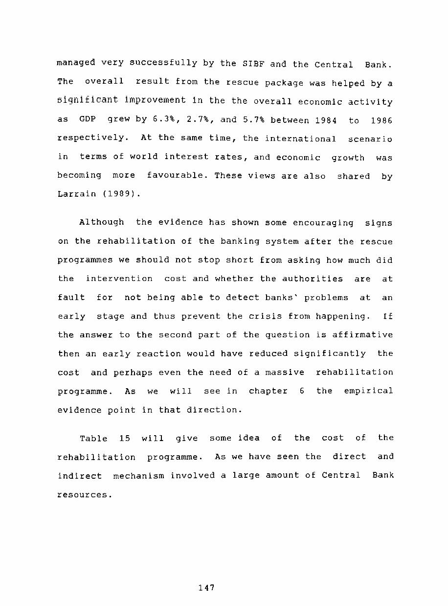
managed very successfully by the SIBF and the central Bank.

The overall result from the rescue package was helped by a

5ignlflcant improvement in the the overall economic activity

as GDP grew by 6.3%, 2.7%, and 5.7% between 1984 to 1986

respectively. At the same time, the international scenario

in terms of world interest rates, and economic growth was

becoming more favourable. These views are also shared by

Larrain (1989).

Although the evidence has shown some encouraging signs

on the rehabilitation of the banking system after the rescue

programmes we should not stop short from asking how much did

the intervention cost and whether the authorities are at

fault for not being able to detect banks' problems at an

early stage and thus prevent the crisis from happening. If

the answer to the second part of the question is affirmative

then an early reaction would have reduced significantly the

cost and perhaps even the need of a massive rehabilitation

programme. As we will see in chapter 6 the empirical

evidence point in that direction.

Table 15 will give some idea of the cost of the

rehabilitation programme. As we have seen the direct and

indirect mechanism involved a large amount of Central Bank

resources.

147

Table 3.15 Operation of Central Bank and other Indicators.(%)

------------------------------------------------------------1982 1983 1984 1985

------------------------------------------------------------Net Domestic Credit

Credit Private Sector Credit Financial Entities Other Assets

Liabilities to Private Sector Currency Others (a)

Inflation Rate (b)

94.4 -0.4

167.0 26.7

-6.4 -1.6 -4.9

20.7

433.4 21.2

375.8 75.9

105.2 18.0 87.2

23.1

174.3 -0.9

-30.4 62.8

27.5 10.6 17.0

23.0

199.6 0.4

18.6 239.6

89.7 10.9 78.8

26.4 ------------------------------------------------------------Source: Banco Central de Chile

(a) Include medium term notes issued by the Central Bank to finance the subsidies in the preferencial exchange rate.

(b) Measured by the consumer price index. (CPI)

The evidence from the table indicates that net domestic

credit increased very rapidly between 1983 to 1985. This

coincided with the beginning of the mechanism whereby the

Central Bank bought nonperforming and risky loans from

problem banks. At the same time, the government was granting

subsidies as part of the debt relief scheme, including the

preferential exchange rate. For instance, net credit to

financial intermediaries in 1983 increased by nearly 376% as

part of the programme of purchasing loans. At the same time,

the item "other assets" which reflects the losses arising

from preferential exchange rate and the subsidies on debt

restructuring rose by nearly 76% and by 1985 it became the

main factor in the rise of domestic credit by almost 200%.

148

Although the evidence does show a rapid and significant

growth of Central Bank credit to the banking system, its

impact on the monetary aggregates appears to be somewhat

lower than expected. The data show that most of the credit

increases was financed by Central Bank paper and hence

limiting the liquidity effect from subsidies. The

liabilities to the private sector increased by nearly 90% in

1985 which is much lower than the figure of 1983. Further

evidence is provided in table 16 which includes the rate of

growth financial assets holding by the private sector.

The data shows that the money growth was moderate over

these 4 years. If we deflate theses figures by the rate of

inflation they become negative. Thue the impact of the

Central Bank credit facilities on money growth has been

moderated by the massive issue of Central Bank paper, in

particular Central Bank notes and treasury notes which is

quite significant in 1983 and 1985.

Table 3.16 Holding of Financial Assets. (a) ------------------------------------------------------------

1982 1983 1984 1985 ------------------------------------------------------------Money 7.3 27.7 12.0 11.3 Other Assets 14.9 20.2 33.8 58.2

Quasi-Money (b) 11.1 1.3 36.4 48.9 Central Bank Notes 38.5 424.0 32.5 144.5 Treasury Notes 263.8 -0.4 22.7

------------------------------------------------------------Source: Banco Central de Chile.

(a) These percentual changes are expressed in nominal terms. (b) Includes time and savings deposits, mortgage bonds, and

foreign currency deposits.

149

Equally, the data on the inflation rate do not show an

explosive growth. It never exceeded 27% during

half of the 1980's. In fact, the peak occurs in

a rate just above 26%. However, this is not a

thought if the fight against inflation to reach a

the second

1985 with a

comforting

one digit

figure in 1982 required nearly 10 years and two severe

recessions. But above all, the progress made was suddenly

thrown over board in order to rehabilitate the banking

system and the economy as a whole.

It seem reasonable to conclude with two assertions:

Firstly, the

spread the

impact

impact of

of the rehabiliation

the banking crisis

programme had

over time in

particular the costs of such intervention. Above all, the

rescue operation mounted by the authorities left a precedent

which will last for a very long time and it will pose a

formidable obstacle to the establishment of a free banking

system.

Secondly, fluctuations in exchange rates, interest

rates, and the overall recovery of the economy made the

costs and the fortunes of the banking system very uncertain.

If these variables would have turned against them then it

would have created strong pressures for further

reprogrammings, and concessions.

150

Although in retrospect the evidence had shown that the

overall economic condition did move in the desirable

direction and banks became profitable, efficient, and

stable, the issues relating to what caused the banking

crisis and whether it was possible to recognise it in an

early stage and prevent it from happening still is a highly

inconclusive issue and lacking of any empirical

verification. The answer to these queries will be the la

"raison d' etre" of this study.

In the next chapter, a review of the theories of bank

failure and banking instability will be provided to

identified some testable hypothesis for the bank failures in

Chile.

151

Endnotes.

(1) By the end of 1976, the banking authorities decided to introduce and increase the capital requirement by 7 times and introduce supervision. This marked the end of the episode with free banking in Chile.

(2) The authorities introduced restrictions on the SINAP asset composition as well as restricting assets below year maturity. The first restriction was responding to mismatching between assets and liabilities during collapse of the construction industry in the recession of 1975. The second measure however, made things worse and set the fortunes of the SINAP.

one the the

(3) At this time as we have seen in chapter 2 authorities were gradually liberalising the capital inflows.

the monetary economy to

(4) This does not mean that banks were passive victims of the adverse general economic climate but merely a symptomatic description of crisis.

(5) According to Velasco (1988), the government's early reaction to the mounting macroeconomic disequilibrium, quite evident in the last quater of 1981 and throughout 1982 was resting on the belief of an automatic adjustment. High real interest rates will reduce demand pressures on both tradables and non-tradables, the overvalued real exchange rate will be transitory and the accumulated trade deficit will be corrected via a monetary approach.

(6) The global provision consists of 0.75% of total loans. The individual risk classification of bank loans carries different provision requirements. For instance A and B plus carries no provision. In contrast, B minus , C, and D carries 20%, 40% and 100% provision respectively. Nonperforming credits not cover by any collateral partially or totally require 100% provision.

(7) The subsidy was equal to the difference between the higher official exchange rate prevailing at the moment of the debt repayment and the level of the preferencial exchange rate.

(8) These measures were available to small borrowers in domestic and foreign currency as well as productive borrowers. Larger debtors were subject to additional restrictions concerning the use of company profits. A productive borrower is defined as a debtor other than consumption and mortgage debtor, and a debtor involved in foreign trade. For a more detail see SIBF (1983).

152

(9) This estimate include the data for 1983 and 1984 as well as a projection for the next 3 years.

(10) It was argued that the steps taken to reprogramme debts have been important in alleviate the debtors dlstres5 and indirectly to smooth out the effect of the banking crisis. However, it was also argued that the speed of the reactivation of the economy was going to be equally important. Therefore, the Central Bank introduced different credit lines during the second semester of 1983 among them we include subsidised credit on working capital, hiring labour, housing and infrastructure, reforestry, and for refinancing of wages and salaries. See SIBF 1983.

(11) The existence of a stable, solvent, and efficient banking system should affect directly the confidence of the public, and thus the magnitude of the financial saving both internal and external for productive investment.

(12) There were two exceptions to this obligation. Firstly, unless there were no financial surplus, the obligation continued until all loans were acquired back. Secondly, unless the bank has boosted its capital base. Thus, all preferential shares were exempted from the repurchase obligations.

(13) As part of an incentive mechanism applicable to shares of effectively bankrupt banks, investors were allowed to pay only 5% as a down payment and the outstanding sum in a period which will not exceed 15 years. Also, there was a 5% surcharge in real terms and fiscal exemptions such us tax free for dividends and a tax credit equivalent to 20% of the values of the shares purchased.

(14) According to Chamorro (1985b), Banco Chile sold a total of $ 127.000 millions and in return he received $ 32.000 millions in promissory notes of the Central bank and repaid $ 42.700 millions in emergency loans. Banco Santiago sold $ 95.000 millions and in return he recieved $ 24.000 millions in promissory notes and he repaid $ 33.200 millions in emergency loans.

153

Chapter 4. The Theory of Bank Failures and Banking Instability: A Review of the Literature.

(4.1) Introduction.

The previous chapter provided an evaluation of the

dismal performance of the Chilean banking system,

particularly between 1982-83. By 1983 a large majority of

commercial banks technically failed or were considered as

problem banks. Its intervention meant that an important

amount of public money was used to avert a complete

financial collapse, as well as growing doubts on the effect

of financial liberalisation in LDC's.

In this chapter, I will review the literature on banking

instability and bank failures in order to cast light on the

hypotheses which could explain what caused the increasing

number of bank failures. It will be argued that any theory

which could explain banking instability should also provide

a reason for the existence of financial intermediaries

(banks).

Two general testable hypotheses will be derived by

reviewing the theories on banking instability and bank

failures. On the one hand, external factors to the banks

such as the general economic environment could affect the

likelihood of bank failures. On the other hand, equally

important is the banks' response to changes in the industry

shaped by financial liberalisation reforms.

154

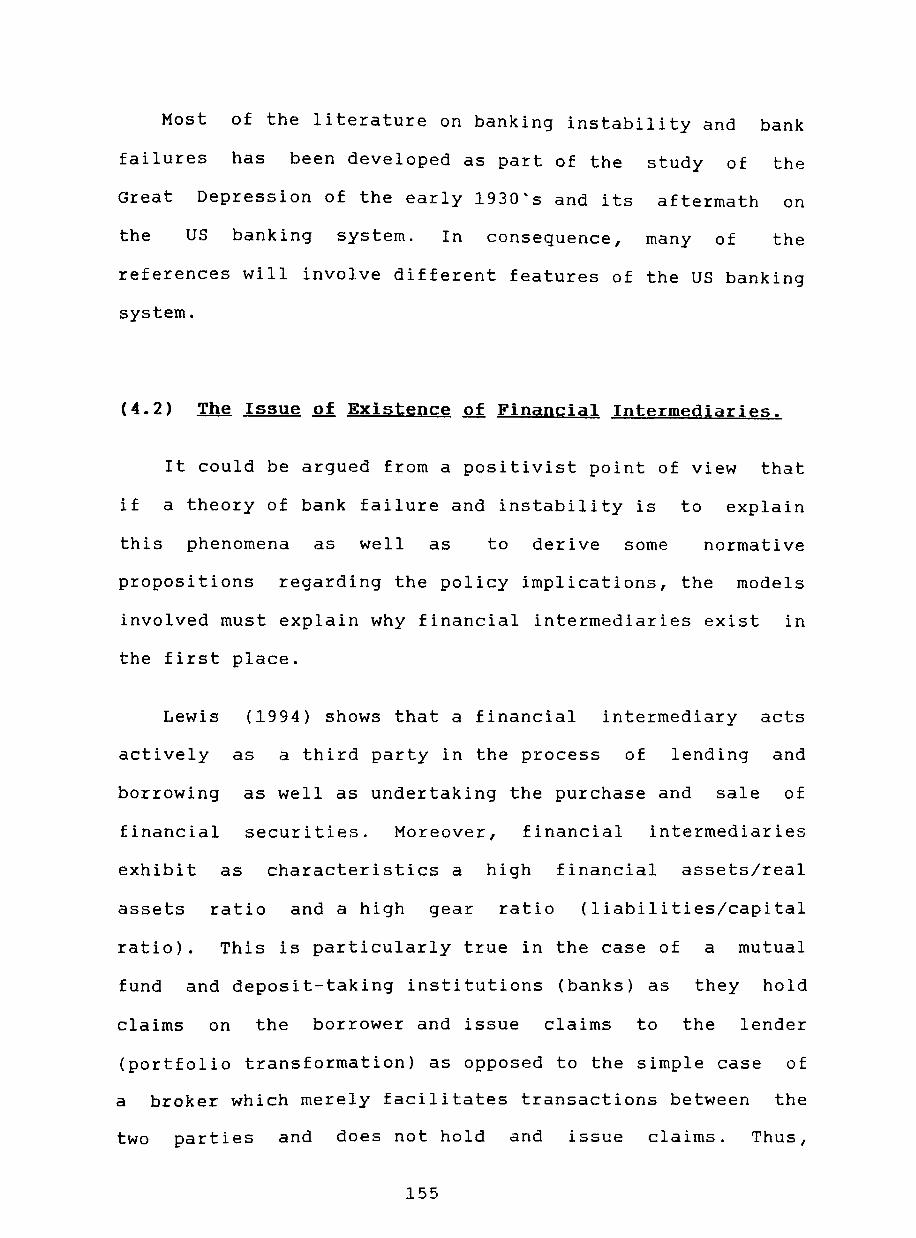
Most of the literature on banking instability and bank

failures has been developed as part of the study of the

Great Depression of the early 1930's and its aftermath on

the US banking system. In consequence, many of the

references will involve different features of the US banking

system.

(4.2) The Issue of Existence of Financial Intermediaries.

It could be argued from a positivist point of view that

if a theory of bank failure and instability is to explain

this phenomena as well as to derive some normative

propositions regarding the policy implications, the models

involved must explain why financial intermediaries exist in

the first place.

Lewis (1994) shows that a financial intermediary acts

actively as a third party in the process of lending and

borrowing as well as undertaking the purchase and sale of

financial securities. Moreover, financial intermediaries

exhibit as characteristics a high financial assets/real

assets ratio and a high gear ratio (liabilities/capital

ratio). This is particularly true in the case of a mutual

fund and deposit-taking institutions (banks) as they hold

claims on the borrower and issue claims to the lender

(portfolio transformation) as opposed to the simple case of

a broker which merely facilitates transactions between the

two parties and does not hold and issue claims. Thus,

155

financial intermediation needs to be justified and proven to

be a superior mutually beneficial voluntary arrangement

between the parties compared to the voluntary

unintermediated market alternative. In other words, any

explanation on the existence of financial intermediaries

needs first to show why it is not possible for lenders and

borrowers to mutually benefit from a direct contract between

them and why a financial intermediary, particularly a

deposit-taking institution (bank), can indeed resolve this 1

problem.

According to Dowd (1992) one of the reasons behind the

need to establish the existence question as a first step is

to leave out those theories of bank instability which

predict that there should be no intermediaries in the first

place. It could be argued that in an ideal and perfectly

competitive financial market with full and symmetrical

information, no transaction costs, divisible capital, and

complete spot and future markets there is no need for a 2

financial intermediary. Indeed, Benston and Smith (1976)

stated that in a frictionless economy, with no transaction

costs, information costs, and indivisibilities, financial

intermediaries would not exist. Even if a bank is introduced

into this economy, Fama (1980) expects this financial

institution to act as another trader or equity-financed

mutual fund and perform as the economy's accountant. That

is, to register the changes in both liabilities and assets

after a transaction has taken place in the economy.

156

In order to justify the presence of a financial

intermediary and avoid relying on an ad hoc approach which

treats the existence of banks as given, we have to depart

from the ideal and perfect economy and to accept the

inherent imperfections which exist in the economy. In a less

than an ideal world, surplus units (lenders) will need to

search for potential borrowers, verified borrowers'

credentials and project proposal, introduced optimal

financial contracts, and to monitor and enforce borrowers'

efforts and willingness to comply with their financial

obligations. The existence of asymmetrical information among

market transactors and hence high search, verification,

monitoring, and enforcement costs should lead to significant

adverse selection and moral hazard problems. Left to their

own devices, lenders and borrowers will fail to undertake

mutually beneficial exchanges which can be considered a

Pareto superior state.

Moreover, the existence of uncertainty as a result of

incomplete information about future outcomes will also

explain the existence of financial intermediaries. For

instance, the need for liquidity in the case of an

unexpected shock in consumption on risk-averse depositors

should also be considered.

Therefore, as Lewis (1992) had clearly pointed out the

existence

endogenous

providing

of financial

response to

information as

intermediaries emerge as an

these market imperfections by

well as liquidity insurance.

157

(4.3) Financial Intermediaries ~ Information Producers and Liquidity Insurers.

Before we look at these two strands of the new theory of

financial intermediation, some reference should be made on

the transaction approach to financial institutions. Benston

and Smith (1976) maintained that the raison d' etre for a

financial institution is the existence of transaction costs.

Their model suggests that these institutions should possess

some scale economies in dealing with transaction costs.

However, this theory on the existence of financial

institutions is incomplete as it fails to explain the

sources from which the cost-advantage of financial

institutions arise.

(4.3.1) Banks as Information Producers.

One strand of the new literature views banks as

producers of information. Information asymmetries between

lenders and borrowers combined with a high information cost

and the public good nature of information production are

intrinsic features in any organised financial market, and

hence the raison d' etre for the existence of financial

intermediaries (e.g. bank).

Stiglitz (1991) maintained that while the existence of

an organised financial market enable both a voluntary

agglomeration and transfer of financial resources, it would

also contribute to an appropiate allocation and management

158

of those resources. Specifically, in a process of capital

accumulation those firms who are in the best position to

invest in large scale projects would normally lack

sufficient resources of their own while the availability of

capital (savings) from a single surplus unit would fall

short of the firm's investment requirement. However, in

atomistic economy with several competing investment projects

and management teams the agglomeration and transfer will

also need to be complemented with the screening and

monitoring of the best alternatives.

In this type of contingent market where money today is

exchanged for a promised return in the future, an

entrepreneur raising capital (borrower) has more information

than the provider of capital (lender). This information

asymmetry is manifested in two ways: Firstly, the borrower

knows better the probability of loss from its investment

project (i.e ex ante asymmetrical information).

Secondly, once the investment project has been selected

the provider of capital will be unable to assess the

entrepreneur's quantity and quality of its effort and

resources put into the project (i.e ex post asymmetrical

information)

Therefore, the screening and monitoring activities which

may involve significant evaluation and monitoring costs will

be necessary to distinguish between good and bad projects

159

(borrowers). Financial intermediaries will exist as a result

of the need to monitor individual lender.

The reliance on equity financing is very limited as a

result of information imperfections, particularly

informational asymmetries. In the absence of any signalling

activity, entrepreneurs and existing shareholders have more

information than outsiders. Greenwald,Stiglitz,& Weiss(1984)

and Myers and Majluf (1984) have shown that under ex ante

asymmetrical information and a large number of

informationally indistinguishable projects (firms) the

market interprets equity issues as an adverse signal about

the firm's market value. This may deter any issue of

equities to raise resources to finance what could be a 3

profitable project.

Moreover, imperfect information and the nature of the

contractual relationship between the provider of capital

(lender) and the user of capital (borrower) also introduces

incentive effects which will further discourage equity

financing. To begin with, an equity contract introduces an

enforcement problem as the fraction of profits paid to a

shareholder is under the manager's discretion. Moreover, the

return from any managerial effort is shared with

shareholders so that it dilutes the manager's incentive to

maximise shareholders' return. At the same time, there is an

increasing scope for the diversion of the firm's resources 4

towards the manager's own uses. The nature of the equity

160

contract and the presence of asymetrical information

produces a conflicting interest between the supplier and

user of capital. This explains both why managers act with

considerable autonomy and the lack of market discipline from 5

take-over bids, shareholder voting, and other schemes.

Despite the existence of some advantages in rising

capital by means of equity issue, particularly the

possibility of a better risk-sharing between the provider

and the user of capital, and the existence of no fixed

committment to repaying the funds, information limitations

undermine its use.

The reliance on bank debt to rise capital suggests that

banks may have advantages over equity financing in dealing

with selection and control functions (i.e screening and

monitoring) under the assumption of information asymmetries.

For instance, Leland and Pyle (1977) argue that if economies

of scale are available then a gathering information

organisation could sell information about particular classes

of assets so long as it could internalise the return from

information which by its nature is a public good.

Specifically, a financial intermediary which buys assets

from the entrepreneur on the basis of specialised

information will internalise the benefit in terms of

increased value of his portfolio.

161

While the Leland and Pyle's model addresses the problem

of ex ante information asymmetries, Diamond (1984) deals

with e}~ POBt .:t5ymlTtetrlc.:il Inforrnatlon. He developed a model

where a risk-neutral lender cannot observe the realisable

value (Y) of an indivisible investment project whose output

is a random variable (Y) bounded between {O,Y<~}. Both the

lender and the borrower agree about the distribution and

boundries of Y. In consequence, the lender has to monitor

the borrower by spending C>O (physical cost of monitoring)

to make Y observable. If individual lenders monitor every

borrower (m>1), the total cost (m*Cm) will be significantly

large and increasing with respect to m. Moreover, monitoring

cost is even larger than expected deadweight non-pecunary

penalty of E[~(Y)] introduced in the entrepreneur's contract

with no monitoring. At the same time, even if the

information from monitoring can be obtained at a low cost,

there will be free-riding problem as a result of the from

the public nature of information.

Diamond (1984) has shown that an intermediary can

monitor on behalf of lenders if C+D < min[E~(Y),(m*C)] where

D is the expected cost of providing incentive to the

monitor. In other words, if the sum of the physical cost of

monitoring plus the cost of incentive is less than the cost

of monitoring with no delegation. There still remains an

incentive problem as the payment recieved by the

intermediary is not observed by the depositor. It is shown

that there is a minimum cost contract which provides

162

incentives to the intermediary for a minimum payment equal

to the rate of interest r or a total payment (m*r). This 6

will force the intermediary to effectively monitor Y.

Given the high deadweight cost ~(Zn) plus the total

monitoring cost (C+D), it is not viable for the intermediary

to contract with a single entrepreneur. Diamond proved that

if the entrepreneurs' projects have both bounded returns and

are distributed independently then as the number of

entrepreneurs tend to infinity n -) 00 then D -) O. Thus,

portfolio diversification by firms and markets makes

delegation cost very small.

In consequence, the models by Leland and Pyle (1977),

and Diamond (1984) have demostrated that an efficient way to

reduce the cost of monitoring borrowers is to form a

coalition of lenders (i.e. financial intermediary). In this

context, it is implicitly assumed that a bank should have

information advantages over other forms of financial

intermediaries given its long-term financial relationship

with the clients. However, it is argued that the banks'

definite advantage lies on the fact that they are able to

obtain additional information due to their role as their

customers' bookeeper. Once the loan has been made the

transaction account becomes a continuing source of credit

information. This link between transaction services and

lending has been suggested by stiglitz and Wiess (1990).

The banks' role as efficient monitors and social accountants

is vital for their existence.

163

It should be mentioned that banks' effective control

over loans is also enhanced by the possibility of refusing

to renew the loan at a future date. stiglitz and Wei65

(1983) have formally proven that a contingent contract which

involves the threat of termination encourages a borrower to

maximise the bank's expected return while avoiding the

negative effects arising from changes in the term of the

contract. Specifically, in a two-period model with identical

risk-neutral borrowers (i.e. no ex ante asymmetrical

information) the bank faces a probability of loan default

and therefore a financial loss as the collateral is below

the amount loaned. The bank cannot observe the project

chosen and the amount of effort put into it ex post

asymmetrical information) but is aware of how the term of

the contract may affect the borrower's behaviour. The most

important conclusion from this model is that a risk-neutral

bank makes the availability of credit to the second period

contingent on the outcome from the first period project

performance.

Therefore, the existence of a financial intermediary

(bank) emerges as an endogeneous response

imperfections (i.e asymmetrical information) by

information services.

164

to the

providing

(4.3.2) Banks as Liquidity Insurers.

The demand for liquidity insurance arises in this less

than ideal economy as a result of uncertainty. In this case,

a financial intermediary (bank) will provide liquidity

insurance to risk-averse depositors who are uncertain about

their future consumption.

Edgeworth (1888) provided the first attempt to show

formally how banks can supply liquidity to the system. He

assumed that depositors' withdrawls are both stochastic and

independent events so that there is an optimal amount of

cash reserves to respond to the expected demand for cash

balances from bank depositors. Specifically, maintaining

reserves equal to some multiple of the standard deviation of

deposit withdrawals over a selected time period would enable

a bank to respond to the demand for liquidity from banks'

depositors as well as to invest the remaining on assets.

Thus, under the law of large numbers and the principle of

pooling risks, a bank issuing demand deposits is actually

pooling independent risks and providing liquidity insurance

to depositors.

The bank's liquidity insurance function became central

to the literature of financial intermediation. In the

seminal paper by Diamond and Dybvig (1983)

Haubrich and King (1984), Smith (1984), and

followed by

Waldo (1985)

banking institutions play an insurance role in the face of

liquidity uncertainty.

165

Diamond and Dybvig's model demonstrated that simple

competitive markets can not provide

against the contingency of being

liquidity insurance

in liquidity need,

information which is private to the agent in need. Moreover,

they demonstrated that a bank is able to transform illiquid

assets by offering liquid liabilities with a different

smoother pattern of returns over time than a liquid asset.

This transformation would enable a bank to provide liquidity

insurance and hence to provide better risk-sharing among

agents who need to consume at different random times and

improve upon the unintermediated outcome.

This model considers two type of consumer-investor

inserted in a three period framework T=O,1,2. Type 1 agent

after investing one unit of input (initial endowment) in T=O

is forced to consume after one period in T=l. The investment

return from one unit input at t=l is equal 1 (initial

investment). This costly interruption of investment may

occur from random shocks to his consumption plans. In

contrast, type 2 agent consumes at T=2 when his investment

has fully matured and provides a return R>l. At period T=O

all investors-consumers are identical, although each of them

carries a risk of facing a consumption shock and thus

interrupting his investment before it matures. In other

words, a risk of being type 1 investor-consumer and with a

probability of t.

166

Given that investment decisions have to be made in T=O

and there is a risk of being type 1 investor-consumer, he

has to decide whether to be self-sufficient and carry the

risk on himself or get into optimal risk-sharing

arrangements. Thus, if we let Cij being consumption of type

i agent in period j, then the agents choose C11=1,

C12=C2l=O, and C22=R>1. Diamond and Dybvig show that if

types were publicly observable at T=l it is possible to

implement an optimal insurance that gives ex ante optimal 7

share of output between both types of agents.

Diamond and Dybvig argue that the lack of observability

of agents' type rules out the possibility of this mutual

insurance contract that indemnifies the holder in case of

being type 1 (interrupt investment). Given that claims will

depend on nonverifiable private information (asymmetrical

information), this type of contract will entail moral

hazard. Indeed, by announcing himself of being type 1 agent

he can claim indemnity from other individuals and protect

his own resources from claims.

Diamond and Dybvig maintained that a bank will supply an

optimal risk-sharing insurance contract by offering demand

deposit contract (liquid liabilities) and then invest them

in earning assets with a promise of a positive return to

those depositors type 1 (withdraw deposits at period 1). The

promised return per unit deposited at T=O and withdrawn

randomly at T=1 is R1=C11)1 by liquidating bank assets.

167

Thus, the payoff per unit deposit withdrawn at T=l which

depends on the random arrival to the bank and independent of

each depositor is given by Vl(Fj,Rl)=Rl if Fj(l/Rl and 0 If

Fj>l/Rl where Fj is the number of deposit withdrawals before

agent j as a proportion of total deposits denoted as F.

Similarly, V2(F,Rl)=max[R(1-R1F)/(1-F),O] is the deposit

payoff at T=2 which depends on total withdrawls at T=l.

In consequence, a demand deposit contract supplied by a

bank permits the attainment of a full information optimal

risk sharing which enables a type 1 investor-consumer to

consume Cl and a type 2 agent to consume C2 where 1<C1<C2<R.

In this equilibrium type 1 agent withdraw at T=l and type 2

agent postpones consumption until investment has fully

matured at T=2. This is what constitute a "good"

equilibrium, although as we will see shortly it is not

unique equilibrium.

The Diamond and Dybvig's model succeeds in explaining

the emergence of a deposit-taking institution (bank) in the

event of random shocks in consumption and the need of

liquidity insurance combined with the illiquidity of agents'

assets. Banks are able to provide transformation services by

offering liquid liabilities (demand deposits), a contract

which has at least two equilibria: one the one hand a good

equilibrium associated with optimal risk sharing, and on the

other hand a bad equilibrium associated with bank runs.

168

(4.4) Theories of Bank Failures and Banking Instability.

(4.4.1) Banking Panics and Bank Failures.

One of the earliest views about bank failure and

instability was that a fractional reserve banking system is

inherently unstable. As we have seen in the previous

section, the existence of random and independent deposit and

withdrawals enabled banks to issue liabilities payable on

demand while holding earning assets and an estimated cash

reserve sufficient to respond to stochastic demand for

deposits. In this fractional reserve banking system, the

bank's asset transformation and the provision of liquidity

insurance by means of a deposit demand contract offer an

optimal risk sharing (good equilibrium). However, it was

also pointed out that a demand contract also has a bad

equilibrium consistent with a bank run. This result was also

shown formally by Diamond and Dybvig's model where those

investor-consumers who were forced to withdraw their funds

due to consumption shocks in T=l are followed by others

which otherwise would have waited until their investment had

matured in T=2. According to Lewis (1996), bank failures and

banking instability can be seen as an unfortunate and

undesirable by-product of banks' intermediation activities,

particularly the provision of liquidity insurance.

In Diamond and Dybvig's two type investors-consumers

and three period modelling with consumption risk there is

169

another equilibrium where type 1 and type 2 agents panic and

try to withdraw their deposits at T=l. This occurs because

type 2 agent5 anticipate both that others will demand the

redemption of their deposits and that the bank will face a

value of its deposits which will be larger than the value of

the bank's assets. In this sense, assets will be liquidated

at a significant loss so that the bank's potential liability

in T=1 will exceed the assets' value when liquidated in this 8

period. In this model, agents' expectations about bank runs

become universal and self-fulfilling regardless of the true

financial condition of the intermediary. Therefore, the

dividing line between a good equilibrium and bank run

equilibrium in a fractional reserve banking system is very

thin. This makes the optimal risk sharing equilibrium very

fragile and dependant on depositors' confidence.

In this model a bank run equilibrium and the optimal

risk sharing equilibrium depends on the depositors' commonly

observed random variable in the economy. Among them the

model includes bad earning reports, commonly observed runs

at other banks, or sunspot. It is clear that under this

exogeneous-imposed uncertainty the loss of confidence and a

bank run equilibrium is a very likely event in this model.

Waldo (1985) in his three-period four-agent model

arrived to a similar run equilibrium where bank run is a

random event. Like Diamond and Dybvig, Waldo considers a

bank run when each depositor believes other depositors will

170

withdraw their deposits, losses which can be avoided by an

early withdrawal. Again the cause of a run is extraneous and

unrelated to any fundamental.

Given that in this model savers have an initial

endowment W at T=O and can split it into storage and bank

deposit and for each saver there is a long term investor

and a short term investor financed by short term and long

term bonds, then the bank will act as intermediary by the

issue of deposits and the holding of both short term and 9

long term securities (asset transformation). Thus, a bank

by exploiting economies of scale provides small savers with

access to the market of primary securities with the issue of

deposits which exceed short term yields as well as the

benefit from the storage of the savers' initial endowment

which in this model serves as liquid currency but sterile

store of wealth. In the event of a run, banks can meet

withdrawls out of their revenues from first period short

terms securities and from the sale of their long term assets

to a short term investor in the secondary market.

Thus, Waldo's model re-affirms Diamond and Dybvig's bank

instability in the form of bad equilibrium and the cause of

a run being extraneous and unrelated to any fundamental,

although it differs from the role of banks as well as on 10

some empirical observations concerning bank runs.

These models which treat bank failures and banking

instability as a result of a lack of confidence in

171

fractional reserve financial institutions providing

liquidity insurance have important shortcomings. Firstly, it

could be argued that a good equilibrium can be supported by

equity contracts. Indeed, it is demonstrated that an equity

contract provides the same optimal sharing contract than

Diamond and Dybvig's bank contract, but without the run 11

equilibrium. Moreover, the existence of an intermediary is

not necessary for optimal risk-sharing as anyone could issue

and offer shares to interested buyers, unless we drop the

model's restrictive assumption which suggest that all

projects and hence shares are the same.

Secondly, a bank run occurs partly due to an

exogenously-imposed sequential service constraint, where as

stated by Lewis (1996), the "fixed-price-first come-first

served" payout rule on deposits demand operates.

Thirdly, the models do not introduce any role for

collateral and/or capital adequacy in order to assure that

depositors' claims can be met. For instance, if we allow for

bank' shareholders to commit sufficient assets as collateral

to assure depositors' confidence then a bank run may not

occur. Similarly, banks may have access to interbanking

funds (liquidity) by offering shareholders' assets as

collateral. However, the Diamond and Dybvig's type of model

has made no distinction between depositors and shareholders.

Moreover, even if they allowed for it, the role of any

collateral may have certain limits on enhancing depositors' 12

confidence.

172

Fourthly, these models of banking instability fail to

distinguish panics and information-based bank runs. Jacklin

and Bhattacharya (1988) identify private information about

bank loan/asset payoffs on the part of depositors as the

source of banking instability (run) as opposed to Diamond

and Dybvig's model which view a run as a sunspot phenomena.

By introducing uncertainty on the return to production and

the irreversibility of long term assets, they show that

deposit contracts tend to be better suited for financing

low-risk assets as compared with equity contracts which are

more suitable for higher-risk assets. Moreover, they

obtained a unique equilibrium and discuss those factors

which could trigger a run, particularly bad interim

information. Thus, under uncertain return to production, a

run can be a systematic event conditional on the news about

an asset quality at T=1

Finally, the evidence from different episodes of banking

instability suggest that runs were systematic events.

Friedman and Schwartz (1963), and particularly Bernanke

(1983) and Gorton (1988) have shown that bank failures tend

to be associated with high currency-deposit ratio, output

contraction, and explosive demand for banks' liabilities.

For instance, Gorton (1988) found that panics are

systematic and predictable events linked to the business

cycle. Indeed, panics resulted from changes in risks

predicted on the basis of prior information. Liabilities of

failed non-financial firms as proxy of recession was the

173

best prior information in forming conditional expectations.

If banks hold claims on firms and if they begin to fail as a

result of a rece55ion depositors will re-assess the risk.

Moreover, it was shown that the larger the movement of the

predictor and hence in the percieved risk, the larger the

movement in the currency-deposit ratio. Thus, these models

in which a bank run is a sunspot equilibrium do not provide

a theory of bank failure. This remark becomes even more

important today as bank failures have not provoked runs and

systematic collapse of financial institutions.

(4.4.2) External and Internal Factors in Bank Failures.

As we have seen in the previous section, banks as

liquidity insurers in a fractional reserve system can be

inherently unstable in the sense that they are vulnerable to

runs and panics in the absence of a safety net of deposit

insurance and a lender to the last resort policy. This

sunspot equilibrium was influenced by extraneous and

unrelated factors to the true financial condition of a bank.

That is, to the market value of its liabilities and assets

structure, as well as its capital and reserves. Moreover, a

bank failure could occur at any point in the business cycle

rather than in the turning point of the cycle.

A run equilibrium is likely to emerge as result of

sunspot, bad report, the failure of a large financial

institution, or any other relevant factor in depositors'

174

self-fulfilling expectations on the bank's inability to

respond to depositors' demand for currency. In this

argument, there is no theory of failure nor an explanation

behind the failure of a large financial institution.

Friedman and Schwartz (1963) have provided a useful

insight into the more than 9.000 bank failures (from 40.000

to 14.000) and the three day suspension of bank trading

during March of 1933 at the time of the Great Depression. In

their view, this wave of bank failures was determined by a

contagious panic which started with the collapse of the Bank 13

of the United states in December 11, 1930. Both the rise in

the banks currency-deposit ratio, and reserve-deposit ratio

led to a fall in the money supply and a shortage of bank

liquidity. The monetary contraction and the widespread

rumours which followed produced additional bank failures

independently of the banks' initial financial soundness

(asset quality). Sound banks were forced into insolvency by

a fall in the value of their assets caused by the scramble

for liquidity.

This monetarist interpretation of the 1930's banking

debacle suggests that the monetary authorities should follow

a stable and predictable path for money supply as well as

the readiness to supply the economy with liquiditity to

avoid widespread runs and panics. Futhermore, a deposit

insurance provision should complement the lender to the last

resort so as to keep the public's confidence in the safety

175

and stability of the banking system snd to protect small

depositors.

The view that the wave of bank failures can be explained

from a contagion fear originated from the failure of large

financial and/or non-financial institution is ad hoc, and

an exception to the general rule when we look at several

bank failure episodes. Indeed, according to Beston and

Kaufman (1986) there is little evidence of a currency run in

recent years despite the fact of well publicised large bank

failures such as Continental Illinois in 1984, and the two

largest Savings and Loans Associations (thrifts) in the US.

Moreover, they found that in only one single year between

1865 and 1914 more than 200 banks failed and in only nine

years in which more than 100 banks failed. The failure rate

during this period, which before the safety net was

established, was

Feldstein (1991),

only 0.8%. Lewis and Davis (1987),

and Davis (1992) have also identified

several financial episodes during the mid-1970's and mid-

1980 which did not ended in a wave of bank failures.

Moreover, it appears that the number of bank failures

per se has become more frequent now than in past despite the

fact that the economy appears to be stable. In the case of

the US banking system, from 1934 to 1943 the Federal Deposit

Insurance Corporation (FDIC) closed 490 banks averaging 54

banks per year. This average was much smaller between 1943

and 1981 with 6 banks per year (total of 232). However,

176

these figures increased drastically between 1982 and 1988 as

the FDIC closed 811 banks which is equivalent to 115 banks

per year.

The relevant question which should concern us is the

identification of the underlying factors behind the rise in

bank failures and whether these factors were under the

banks' control (internal) or outside their influence

(external). Specifically, the causes of bank failures are

either internal or external to the institution, or some

combination of the two. Internal causes are identified as

those factors which the managers and directors of a bank

have direct control. For instance, a bank can exert control

on its loan and investment policy, particularly asset and

loan concentration, as well as the growth rate of asset

expansion. Moreover, self-serving loans, embezzlement, and

fraud are also within the responsibility of the bank

management. Managerial inefficiency, dishonesty, or

insufficient internal provision will lead to excessive risk­

taking and bank failures. It could be argued that this

classification correspond to a firm-specific factor.

External causes of bank failures are those over which

the manager and directors of a bank have no control such as

structural changes in banking (industry-specific) and the

economic environment (macroeconomy). In the former we

include increasing competition from financial

liberalisation, regulatory and supervisory changes, and

177

technological innovation. In the latter, we refer to adverse

changes in output and key macroeconomic prices such as the

rate of interest, real exchange rate, or commodity prices.

Although, in theory we can draw a definite line between

internal and external factors on bank failures, in practice

this distinction becomes somewhat blurred. Bank managers can

in fact respond to changes in external factors depending on

their capacity and objectives. For instance, financial

liberalisation entails more opportunities for profit

maximisation but at the expense of additional risk-taking.

The managers' response depends on their attitude toward

risk-taking, the existence of remaining distortions like

fixed rate deposit insurance and related portfolio structure

(bank holding companies), and the

prudential regulation and supervision

operations.

effectiveness of

to monitor banks'

Before we progress towards the examination of those

factors responsible for bank failures it is desirable to

technically define a bank failure and to present a bank's

balance sheet in order to identify the sources of risk. As

we have seen in chapter 2, a bank fails in economic terms

when the market value of their assets is below the market

value of their liabilities. Therefore, all depositors and

creditors cannot be expected to be paid in full and on time.

178

With reference to a bank balance sheet, we

consider a simplified balance sheet as follows:

can

ASSETS

Cash Securities Loans and Advances

LIABILITIES

Deposits Non-Deposit Liabilities Capital

On the asset side, the bank's balance sheet is dominated

by loans and advances. Financial securities have a smaller

share in the asset portfolio, and the cash item is even less

important. On the liability side, deposits represent the

largest share in the liability structure. Similarly, banks

are highly geared as their liability-capital ratio is very 14

high.

By looking at the structure and composition of a bank

balance sheet, it could be argued in broad terms that

banking instability can arise on the asset side, on the

liability side, or on both. For instance, as we have

already seen changes in the percieve risk on bank deposits

can originate a shock on bank liabilities as depositors rush

to claim back their funds. This liquidity risk could impair

a bank's ability to respond unless there is access to a

discount window and/or assets can be sold at short notice at

a large undervalued price.

Similarly, on the asset side of the balance sheet there

several factors affecting both the bank's loan portfolio and

179

the security investment. For instance, adverse changes in

the bank's external economic environment such as output and

price deflation, significant price misalignment due to gross

macroeconomic policy inconsistency and/or exogenous shocks

to the economy affect the quality and riskiness of the

bank's loan portfolio. The effect can be magnified in the

event of excessive loan concentration on a limited number of

borrowers or related group, industry, countries, or regions.

Equally important is the role played by a mismatching

between the bank's assets and liabilities, particularly in

the event of interest rate risk. There are banks which,

given the nature of their activities (thrifts), present

assets and liabilities that are unbalanced with respect to

their maturity. Thrift institutions hold long term fixed

interest mortgages (assets) funded by short term saving

deposits (liabilities) which an increase in the level and

volatility of interest rates can cause the market value to

fall and be worth less than the value of its deposits.

It should be pointed out that a bank's balance sheet may

not only reflect external shocks from the macroeconomy but

also can be affected from increasing competition and

innovation in the banking industry as a result of financial

liberalisation which is also considered external to the

bank. However, banks are not passive victims of changes in

the underlying economic environment where they operate.

Moreover, bankers' attitudes towards risk-taking in terms of

180

a more aggressive management can also increase the

vulnerability of banks. A less conservative attitude by the

bank's management is reflected in an inadequate capital and

provision for bad loans, poor asset and liability quality

from the lack of diversification, rapid growth in assets and

liabilities, and a low profitability.

(4.4.2.1) External Factors in Bank Failures.

It is argued that bank failures (financial instability)

are related to the business cycle, as a downturn weakens

banks' balance sheet. This link is indirect via the

financial fragility of non-financial institutions following 15

their overindebtness and unexpected deflationary shocks.

Fisher (1933), and later Kindleberger (1978) and Minsky

(1977) focused on a link between bank failures and

deflation. The development of a fragile financial structure

leads to a wave of bank failures at the turning point of the

business cycle and not at any point of the cycle as argued

by the monetarist. Moreover, they disassociated with the

view that a wave of bank failures is the result of some

exogeneous factor, accident, or a policy mistake by the

Central Bank.

The whole economic cycle is described by a process in

which a buoyant output growth caused by an exogeneous event

(new inventions, the opening up of new markets as a result

of economic liberalisation) which improves profit

181

opportunities leading to an investment boom in both physical

and financial investments financed by bank loans. Rising

prices reduce the percieved value of outstanding debts, and

increasing demand for financial investment increases the

value of debtors' collateral. Both factors plus widespread

optimistic expectations lead to a significant

overindebtness. According to Fisher (1933), a significant

overindebtness and a deflation will bring a downturn in the

business cycle. It could be argued that a deflation in

commoditity prices, falling output, and even rising real

interest rates should increase both the value of outstanding

debt and difficulties to service the debt. Debtors unable to

pay their debt and refinance its position may force

creditors to liquidate assets adding additional pressure to

falling prices and hence increasing the magnitude of the

deflationary pressures. Thus, falling prices, rising real

interest rates, and falling output will reduce firms' net

worth and profits and hence lead to loans default which in

turn will certainly raise the likelihood of bank failures.

Kindleberger (1978) identifies three stages of the same

process leading to the transformation of the economy from a

buoyant and euphoric stage (boom) to a fragile and

collapsing stage (bust). This include overindebtedness,

significant relaxation of safety and risk provision by

banks, and subsequently bankruptcies and bank failures. The

first stage is a mania where investors shift money to real

and financial assets during the expansion of the business

182

cycle. The second stage is a panic as they start moving back

to money at the turning point of the cycle. The final stage

ends with a crash as commodity and stock prices

output falls and the number of bankruptcies

suspensions increase.

collapse,

and bank

Minsky (1977) also provide a theory for the build-up of

financial fragility over the upturn of the business cycle

and the subsequent downturn of the cycle and the rising

number of bankruptcies. He identifies three factors which

may produce

speculative

portfolio.

The hedge,

systemic fragility; first, the mix of

, and ponzi finance. Second, liquidity

Third, the ratio of external-internal

hedge,

of the

finance.

speculative, and ponzi finance units are

vulnerable to several events which will affect cash flows

from assets. For instance, a decrease in operating income as

a result of unrealistic expectations about the market and

growth prospect may transform an hedge financing unit into a

speculative unit. That is, from a unit in which his assets'

cash-flows exceed cash payments over a long period into a

financing unit where cash payments exceed the short run cash

receipts. Changes in the money market (interest rates)

should affect an speculative unit by trying to refinance its

position and make himself vulnerable to the disruption of

financial flows. A margin of safety may exist if the present

value (PV) of assets is greater than the liabilities'

present value. This margin exists for the hedge and

speculative financing unit but not for ponzi finance as the

183

PV is clearly negative. Thus, for Ponzi units a rise in

interest rates can entail negative net worth and bankruptcy.

Once this form of financing becomes a significant portion of

the financial structure of the economy there will be either

a debt-deflation and depression or there will be rise in

expected cash flows from capital assets as a result of

inflation.

The model's mechanism suggests that in the upswing of

the cycle larger demand for investment (physical and

financial) financed by external resources (bank debt) leads

to rising interest rates and a shift from hedge to

speculative, and even Ponzi finance. Shifts from long term

to short term financing and reductions in margins of safety

for banks increase their vulnerability to further rises in

interest rates. Ponzi finance units unable to refinance

their position (roll-over of their debts) will result in

liquidation of assets leading to further deflation and

bankruptcies of both non-financial and financial firms.

In these models of financial fragility instability in

the macroeconomy arising from both exogenous factors like

innovation, wars, or swings in investment, and policy

induced changes from liberalisation reforms can be seen as

prime shock to the financial system. These disturbances are

amplified by over optimistic expectations by both non­

financial and financial firms which lead to overindebtedness

and subsequent reversal when a deflationary shock affects

fragile firms. The likelihood of bank failures and the

184

subsequent contagious effect on other financial institutions

becomes a real threat to the stability of the financial

system.

Although these models of financial fragility offers an

alternative on the causes of bank failures and a re­

interpretation of the Great Depression, it lacks a solid

foundations based on rationality and endogeneous

expectations.

To begin with, the model introduces a debt-type of

contract and rules out alternative form of financing without

formally introducing assumptions concerning agency cost, and

other imperfections which explain the importance of debt

finance over equity finance.

With respect to rational behaviour, models of financial

fragility have departed from the assumption of rational

economic behaviour. Investors are assumed to be

overoptimistic about the expected returns and traders'

purchases are responding to rising prices rather falling

prices (low prices). Moreover, the model does not explain

expectation formation and the sources of wrong

risk perceptions.

Guttentag and Herring (1984) introduce a model where

rational individuals (banks) during a period of boom will

relax both credit policy (rationing) and their capital

position, and the existence of uncertainty will lead to

185

underpriced risk. Once a shock occurs this leads to a vio­L ,-,e

in a subjective probability of disaster combined with low

capital level producing credit rationing and a crisis. This

1s known as a "disaster myopia".

Disaster myopia explain why in a booming economy with a

long period of stability lenders (banks) expand loans

rapidly and accept a decline in their capital position. In

this case there is a increased vulnerability which is not

percieved at such until a shock to confidence occurs. This

leads to a revision of subjective probability and

subsequently to a higher risk premium and credit rationing.

Credits will be unavailable for some class of borrowers,

investment will be cut-back from previous buoyant levels,

and production stopped with a subsequent fall in the 16

economy's output (crisis).

The rational expectation school and the model of

speculative bubbles also provide a framework to model

Kindleberger's irrational euphoria and bank instability

(run). According to the model provided by Flood and Garber

(1982) and Blanchard and Watson (1982) a mania can be

associated with a speculative bubble. Under rational

expectations where agents' anticipations are conditional to

the information set of the underlying structural model so

that prediction error will not be systematic, an asset price

depends on its current value but also on the expected rate

of change. Asset prices depart from the fundamentals as

rational agents anticipate changes in asset prices (price

186

bubble). The bubble will last so long as the average return

is sufficient to compensate for the risk of crash. The price 17

of the asset will need to be increased exponentially.

Bernanke (1983) also embraced the view that an

unanticipated deflation due to a collapse of stock prices

can cause borrowers to default and banks to fail as a result

of the reduction of borrowers' net worth and the rise in

the real stock outstanding debt. At the same time, growing

fears of total financial collapse lead to a marked

preference for liquid assets and hence the shrinking of

loanable funds available for lending. Bernanke's model also

introduces a link between financial disruption as

consequence of Fisher's deflationary shock, and output

decline which came to complement the monetary forces behind

the depression of the early 1930's.

There are also factors within the industry which are

outside the control of the bank. Institutional, and

structural changes in the form of technological

improvements, and innovation playa significant part in

increasing the fragility of the banking system.

For instance, government policies can affect the banks'

ability to cope with risk. It is argued that in the US

banking system prohibition of interstate and intrastate

branching, obstacles to takeovers, and restrictions on banks

activities had made banks more vulnerable as a result of the

lack of diversification. There is considerable evidence

187

which demostrates that restrictions on branching limits the

banks' ability to withstand economic shocks (external). As

local economic conditions deteriorate an increasing

proportion of their loan portfolio becomes non-performing

and their deposits are increasingly withdrawn. Lack of

diversification will disable banks' ability to offset their

losses forcing these banks to fail. White (1984) holds the

view that pervasive restriction on branching in the US

created a large number of small and specialised banks with a

limited portfolio diversification. He argues that one

important factor in the bank failures during the Great

Depression of the 1930's was the banks' inability to

withstand any real and/or monetary shock. A system of

nation wide branching could have reduced or eliminated bank

failures by establishing intermediaries with loan

portfolios that were sufficiently diversified to manage 18

regional risk. Further evidence is provided by Amos (1992)

for the regional distribution of bank closing between 1982

and 1988. The data indicate a significant concentration of

bank closings in states with oil and gas extraction and to a

lesser extent, farming. Moreover, it confirms that those

states with unit banking regulation account for nearly 57%

of total bank failures.

other regulation like the Glass-Steagall Act of 1933

which prohibited commercial banks from engaging in

securities-related activities (separation of commercial and

investment bank) have also contributed to reduce banks'

188

diversification possibilities. According to the evidence

from White (1986), it appears that banks with security

operations before 1933 had a lower probability of failure

than other banks.

Similarly, the introduction of interest rate ceilings

can also affect the banks' capacity to adjust in the face of

economic shocks like inflationary instability and the

subsequent desintermediation via off-shore markets. In the

case of regulation Q in the US which prohibited interest

payments on demand deposits and introduced ceilings on

savings and time deposits it made more difficult for banks

to compete for funds relative to unregulated financial

institutions.

(4.4.2.2) Internal Factors in Bank Failures.

One of the most important criticisms of the hypothesis

that banks' failures can be affected by factors outside the

banks' control is that they are treated as passive adjusters

and henceforth victims of an adverse economic environment,

and the changes and annomalies of the financial market per

se (industry). On the contrary, financial institutions are

actively responding to changes in both the macroeconomy and

in particular to conditions within its own market (industry)

as a result of deregulation, liberalisation reforms, and

technological change and innovation.

189

It could be argued that financial liberalisation in the

form of interest rate deregulation, geographical and

funrtional deregulatIon (products) have contributed to the

increment in competitive pressures and followed by an

appropiate response from banks. Indeed, there is a

substantial literature which suggest that deregulation and

greater competition has shifted banks' strategy from safety

towards a greater risk-taking. Moreover, it is argued

argued that excessive risk-taking in a deregulated banking

system (liberalised) reflects the effect of a subsidy from

the government safety net and the failure of prudential

supervision.

The evidence has given considerable support to the

importance of internal factors on bank failures. For

instance, Peterson and Scott (1985) found that most bank

failures in the US between 1982 and the first quarter of

1984 were the result of internal causes, particularly fraud

and manipulation, poorly managed rapid growth, and sustained

low performance.

According to Beston and Kaufman (1986) fraud can take

many forms. Banks can make loans to business associates,

subsidiaries, and relatives violating the legal restrictions

and limits established by the authorities. The loans'

proceeds which are allocated to very risky ventures involve

risky concentrations relative to the bank's capital on

entities and persons controlled by or associated with

190

controlling stockholders and bank managers. The evidence

from the failure of the United states National Bank of San

Diego in 1973, the failure of the Hamilton Bank of

Chattanooga in 1976, and as we will see in chapter 8 the

overwhelming loan concentration with affiliates in the

Chilean banking system during the liberalisation episodes

are examples of fraud, excessive risk-taking and its effect 19

on bank failures. Further evidence from different period

of the US banking history confirms the importance of fraud

in bank failures. While Peterson and Scott's research

confirms the importance of fraud where 66% of the 80

failures between 1982 and 1984 were the result due wholly

or partly to some form of fraud. Sinkey (1979) also confirm

this finding for the pre-insurance (1865-1920) and the post-

insurance periods (1960-1974).

Similarly, a rapid growth in a bank's loan portfolio

would increase the likelihood of bank failure as it becomes

extremely dificult for management to support such strategy.

Management should ensure that growth in loans is fueled with

good credit risk, proper documentation, a reward in quality

being favoured instead of growth per se, and loan growth

and risk which are sufficiently diversified. Limited

management resources like training, as well as the existence

of asymmetrical information do not help the maintance of

management quality. Moreover, rapid growth of loans

portfolios in a scenario with high interest rates will

exacerbate the moral hazard and adverse selection problems.

191

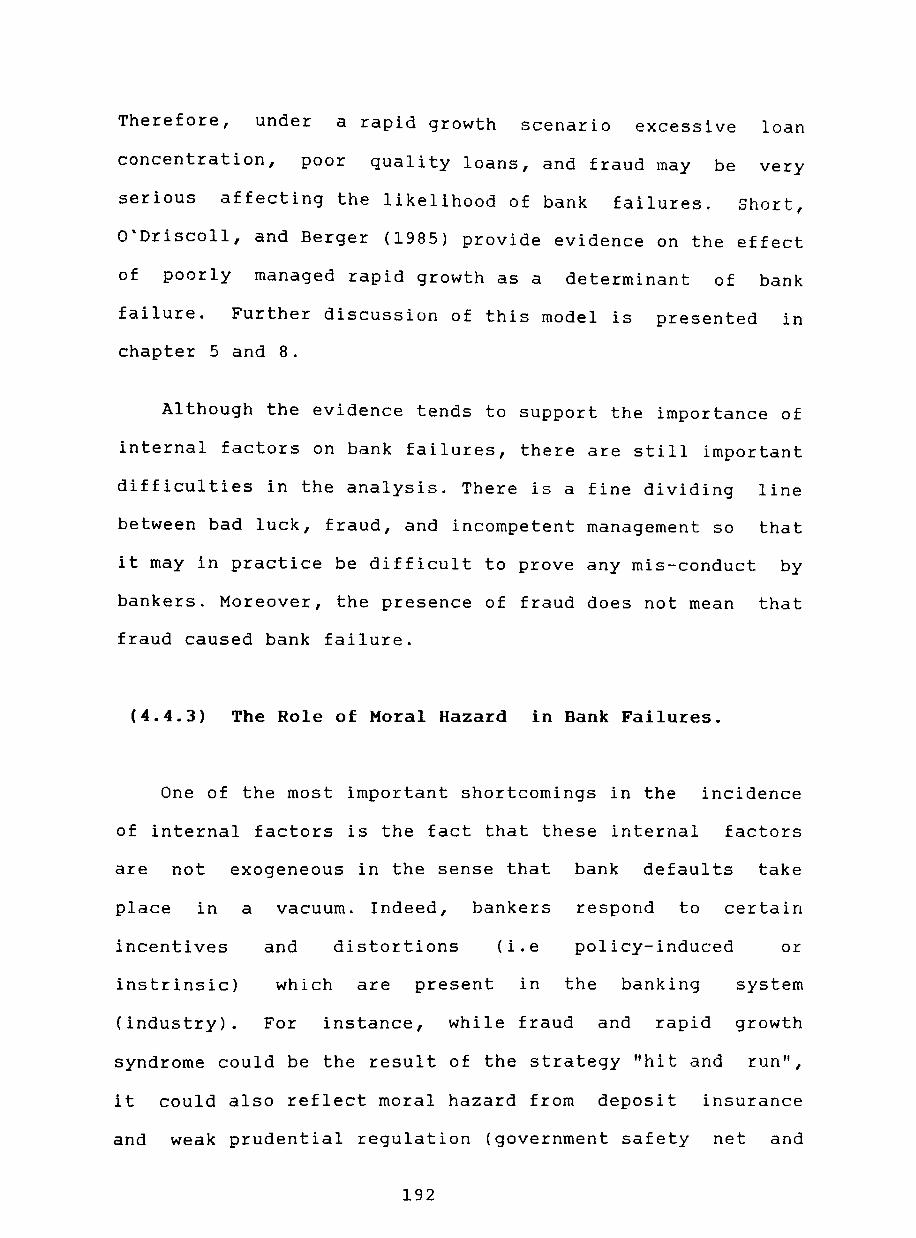
Therefore, under a rapid growth scenario excessive loan

concentration, poor quality loans, and fraud may be very

serious affecting the likelihood of bank failures. Short,

O'Driscoll, and Berger (1985) provide evidence on the effect

of poorly managed rapid growth as a determinant of bank

failure. Further discussion of this model is presented in

chapter 5 and 8.

Although the evidence tends to support the importance of

internal factors on bank failures, there are still important

difficulties in the analysis. There is a fine dividing

between bad luck, fraud, and incompetent management so

it may in practice be difficult to prove any mis-conduct

bankers. Moreover, the presence of fraud does not mean

fraud caused bank failure.

(4.4.3) The Role of Moral Hazard in Bank Failures.

line

that

by

that

One of the most important shortcomings in the incidence

of internal factors is the fact that these internal factors

are not exogeneous in the sense that bank defaults take

place in a vacuum. Indeed, bankers respond to certain

incentives and distortions (i.e policy-induced or

instrinsic) which are present in the banking system

(industry). For instance, while fraud and rapid growth

syndrome could be the result of the strategy "hit and run",

it could also reflect moral hazard from deposit insurance

and weak prudential regulation (government safety net and

192

regulation). Moreover, the increases in bank

as a result of unsound loan concentration

vulnerability

reflects the

increasing interdependency between affiliates of bank

holding company structure.

It could be argued that the presence of

distortions (e.g. financial liberalisation

policy-induced

as external

factor) will encourage excessive risk-taking (moral hazard)

by banks, raising the likelihood of bank failures.

Specifically, the existence of a bank holding company

structure combined with a fixed rate underpriced deposit

insurance, rapid deregulation of interest rates, and a weak

and inefficient prudential regulation

provide banks with greater incentives to

and supervision

increase risk-

bearing. The increases in banks' vulnerability should be

reflected in a deterioration of assets quality, higher

leverage, lower capital and reserve requirements. Financial

and accounting ratios constructed fom banks' balance-sheet

should reflect the banks' incentives to take greater risks

raising the ex ante probability of bank failures.

- Bank Holding Company Structure and Market Concentration.

To begin with, a bank holding company can be defined as

a multi-company firm which operates under a common

management and financial control. Its scope of ownership and

economic influence can be made extensive into both financial

and non-financial firms operating in different markets and

segments.

193

While this specific form of company organisation carries

legal recognition and is subject to regulation in the US,

and economies like Japan, and Germany, its identification

has been more implicit in LDC's, particularly before the

episodes

during

of financial liberalisation and banking crisis

the late 1970's and early 1980's. Some of the

literature on development economics recognises this form of

industrial organisation as "economic conglomerates" or

"group". It is identified as an informally established

multi-company firm which like the bank holding company also

operates under common management and financial control.

Generally, the centre point of an economic "group" is

constituted by a "parent company" or holding company which

is valued in the stock exchange or owned by an extensive web

of family inter-relationships. This nucleus company directly

or indirectly controls several subsidiaries as well as

financial institutions. The ownership of banks and other

financial institutions enable a "group" to exercise direct

influence on banks' decisions, particularly credit

concentration and credit terms. It is also possible for this

"parent" company to exert indirect control over financial

institutions through their own subsidiaries which in turn

own one or several intermediaries. This web of

relationship can be extend even further

interlocking

by allowing

financial institutions themselves to directly control

financial and non-financial firms.

194

The common form of this network of financial and

managerial inter-relationships is despicted in diagram 2.

Figure 4.1. Bank Holding Company structure.

>

>

Bank A < IHolding Coy.

Bank B < Holding Coy.

Bank C < Holding Coy.

v

Non-Bank Financial Institution A <

Non-Bank Financial < < Institution B

Non-Bank Financial Institution C <

A

B

C

>1 Firms A

> 1 Firms B

>1 Firms C

For instance, holding company C owns and directly

control a number of firms in C, and financial institutions

in C both bank and non-bank entities. In addition, holding

company C also holds and influences indirectly non-bank

financial institutions in C through bank C.

According to Leff (1978), this form of industrial

organisation has flourished as a mean to expand the size of

the economic conglomerate. Indeed, the ownership of

financial institutions has permitted them to attract

resources from other segments outside the "group's" market

195

influence. It will be relatively easy for a "parent" company

having a controlling interest in a financial institution to

U5~ the banklB reBOUlces to purchase a controlling interest

in other non-financial firm. Moreover, if the legislation

permits it, they could even acquire other financial

institutions to further their expansion.

Apart from the feature of economic conglomerates, the

financial market can also be highly concentrated among a few 20

financial institutions. More often than not, are-current

characteristic of LDC's banking structure is the presence of

three or four large banks controlling more than half of the

system's assets and liabilities while the remaining share is

held by several small financial institutions. Therefore, we

may say that there is skewed distribution of assets,

liabilities, and capital in this banking system.

Galbis (1986) maintained that a bank holding company

structure and a significant bank concentration should lead

to an oligopolistic market-structure behaviour by financial

institutions. This pattern of conduct should be reflected

upon the growth of bank asset portfolios and concentration,

risk diversification, and the level and spread of domestic

interest rates.

From oligopoly theory we can establish two possible

outcomes; one inefficient which entails collusion, and the 21

other an unstable one with a price warfare.

196

Depending on the relative strength of the bank holding

company group and the stability of their collusive

agreements, we should expect a mixture of a significant loan

concentration among its affiliates and a low average spread

between deposit and loan interest rates.

the affiliates' need for funds the

concentration

portfolio.

and hence the riskier

The more intense

larger the loan

the bank's loan

Although collusion is in the interest of the oligopoly,

there are instances where a predatory price warfare

dominates over a collusive agreement. Increases in

competition for fund among "groups" to finance their

relative expansion will increase the probability of a price

war. At the same time, free entry into the financial system

by both domestic and foreign institutions will make

competition for funds stiffer. As a result, a financial

market dominated by "economic conglomerates" and facing

unrestrained competition for funds will be conducive to high

real deposit and lending interest rates and lower spread and

bank profits. It is clear from the evidence of chapter 8

that the restoration of bank holding company structure (i.e.

economic groups) in Chile as a result of the privatisation

of the financial system, together with the unbounded

pressures from domestic and foreign banks were responsible

for increasing competition for funds to finance the

"groups'" economic expansion. Excessive concentration of

bank's loans with its own affiliates which clearly

197

represented related risks (joint) contributed to an increase

in the likelihood of bank failure in Chile.

- ImplicIt and Explicit Deposit Insurance.

It could be argued that the existence of a safety net

(deposit insurance and lender to the last resort) can make

the bank default more likely. Indeed, this government policy

combined with the uncertainties of deregulation can

encourage banks to take excessive risk (moral hazard)

affecting the likelihood of bank failure.

As we have seen in the previous sections, Diamond and

Dybvig (1983) demostrated that one of the equilibrium from a

bank contract supplying liquidity insurance was consistent

with a run sunspot equilibrium. However, this model

demonstrated that there is a feasible contract

(unconstrained optimum) which allows banks to provide the

asset transformation service without the event of a run

equilibrium. Specifically, the model shows that demand

deposit contracts with government deposit insurance achieve

the unconstrained optimum as a unique Nash equilibrium if

the government imposes an optimal tax to finance a deposit

insurance.

The government can tax type 1 agents who withdraw in T=l

(early withdrawl). The amount of tax raised depends on the

number of type 1 agents who decide to go for an early

withdrawal and the amount promised in return (assuming no

198

panic). The government infers the realised value of t

(probability of withdraw) after all type 1 have come

forward. If the realised value of t is greater than

expected value of t then it charges a tax on the type

the

1

individual and a subsidy in the opposite case. The tax­

subsidy policy ensures that type 1 receives its optimal

consumption bundle contingent on the realisation of t.

Similarly, given that the tax-subsidy is costless to operate

type 2 also receives its optimal bundle of consumption and

hence no incentive to withdraw in T=I.

However, Diamond and Dybvig have warned us about the

danger of moral hazard if the risk of bank portfolios

selected by bank managers are unobservable by outsiders.

Since the expected value of the bail-out to any bank

increases with the probability of default which in turn

rises with promised return to withdrawals in T=I, then bank

optimisation of the bail-out subsidy will provide an

incentive to bankers to compete more agressively for

deposits by offering higher interest rates (return) to those

withdrawn in T=l. It follows that the rate of interest for

T=l rises to a point where the anticipated return on T=2

falls so low that no one want to keep deposits beyond T=I.

Type 2 depositors demand their deposits at T=l (run) and a

bail-out of deposits will be necessary.

According to Mckinnon (1988), the bank is a beneficiary

of an unfair bet against the government. The bank can

199

provide risky loans at extremely high interest rates without

having to compensate insured depositors for additional risk-

taking. The bank will have accrued extraordinarily high

profits without having to pay the full cost of large losses

from bad loans.

White (1989) considers an implicit deposit insurance as

a specific form of insurance which is analogous to medical

or legal malpractice insurance contracts or to a third party

car liability insurance. The purchase of an insurance policy

forces the insurer to pay a compensation to the beneficiary

( i . e . depositor, medical patient,legal client, or

motorist/pedestrian) in the event in which the action of the

insured (i.e. bank/thrift, doctor, lawyer, or driver) has

caused some loss to the third party. This comparison between

deposit insurance and a typical insurance contract allow us

to identify the drawbacks and possible corrections which are 22

available in a typical insurance contract.

Based on the state-preference model, Karaken and Wallace

(1978) and Furlong and Keeley (1989) have formally shown

that a value maximising bank will maintain the highest

degree of leverage and an increasing asset portfolio unless

there are limits set by regulation. Similarly, Merton (1977)

arrived to the same conclusions by modelling deposit

insurance as a put option. In his model a deposit insurance

is introduced "as if" bank shareholders purchase the right

to "put" the asset portfolio onto the insurer at a price

equal to the value of the outstanding deposit liabilities.

200

The price of put option depends on the riskiness of the bank

asset portfolio, the degree of leverage, and the proportion

of insured deposits. It follows that unless the insurance

price is variable, insured banks will need to be subject to

prudential regulation to limit excessive risk-taking.

Furlong and Keeley (1989) in a two-period model with two

possible future states with Pl and P2 payouts, and two risky

assets, X(xl,x2) and Y(yl,y2) where xl<yl and x2>y2 or more

generally xl<yl<ly2<yl (i.e. X is riskier than Y), the

current value of a maximising bank Vo that can meet its

obligations in both states is given by the expression Vo=

[(Co+Do)/P][sxl+(I-s)yl]Pl + [(Co+Do)/P][sx2+(1-s)y21P2 - Do

where Co and Do are the initial amount of capital and

deposits (claims), and s is the percentage of bank assets

allocated into a riskier asset X. We take that the sum of

the current pay-offs on assets in each state minus the

current value of depositors' claims are equal to its initial

capital (i.e Vo=Co).

If we assume that there is a free deposit insurance and

a given Co and a bank asset quality (risk) such that

bankruptcy occurs at state 1, then the current value of the

insurance policy 10 will be given by 10 = (Do/P)Pl­

[(Co+Do)P][sxl+(1-s)yl1Pl > O. The expression for 10 is

positive since the current values of depositors' claims fell

short of the assets' pay-offs. Therefore, an optimising bank

will maximise its equity value Vo=Co+lo by maximising the

201

value of 10. The maximisation of the insurance policy

involves maintaining both a high bank leverage, and a high

asset risk.

specifically, the effect of a change in leverage on the

value of 10 is given by dI o /dDo=[P1/P][1-(sx1+(1-s)y1)1)O

since x1<yl<1. Similarly, the effect of risk-taking on 10 is

given by the partial derivative dIo/ds=-Ao[P/P11(x1-y1»0

since xl<yl. In theory a value-maximising bank with free

deposit insurance will choose s=1 and a large leverage.

In consequence, it is demonstrated that fixed price

deposit insurance should encourage maximising banks to

excessive risk-taking (moral hazard) as their liability is

limited to the value of their net worth. Once its net worth

is exhausted, the outstanding claims of insured depositors

will be covered by the deposit insurance. Full coverage

combined with a flat rate insurance premium will make both

bankers and depositors tolerant and indifferent about risk-

taking. In other words, a distortion to the market

discipline which according to Eisenbeis and Gilbert (1985)

will prevent depositors to ask for a higher risk

compensation to hold riskier bank's liabilities, and

encourage bankers to restructure their portfolio to reduce

risk. An undistorted market mechanism may also discipline

bankers by a reduction in the availability of funds or

withdrawal of bank deposits from risky financial

institutions.

202

The same conclusion follows in the case when there is

the expectation of a de facto insurance. In effect, the

public will hold the expectation that the monetary

authorities will bail-out uninsured depositors from large

banks in order to avert any loss of public confidence in

the financial system. It could be argued that the belief in

a de facto insurance guarantee feeds itself from the

authorities' lack of reputation and credibility exhibited in

the past with respect to the intentions and objectives of

their banking policy.

Karaken and Wallace (1978) have shown that deposit

insurance and the need for regulation will not be necessary

even in an unregulated fractional reserve banking system.

Indeed, unregulated banking system will be inherently stable

under their assumptions. If depositor are fully informed

about banks' asset risk then bank managers will voluntary

choose a maximising strategy which lower the risk of

bankruptcy.

Clearly the susceptibility of an unregulated fractional

reserve banking system had given a major justification for

government intervention in the form of deposit insurance

complemented by regulation either to prevent bank panics and

to oversee bank failures from inefficient units.

As we have seen earlier on from the evidence from the US

the number of failures have increased significantly during

the 1980's and also have involved large financial

203

institutions and thrifts. Most of the studies concluded with

a different emphasis the important role played by a fixed

price deposit insurance on excessive risk-taking and bank

failures. At the same time, they proposed urgent reforms to

the existing deposit insurance scheme to remove some of the

incentives to take additional risks beyond the social 23

optimum.

- Prudential Regulation and Supervision.

As we have seen from the previous analysis the central

problem with a government improperly priced mandatory

deposit insurance is that it encouraged insured maximising

banks to exacerbate risk-taking (moral hazard) and hence to

increase the probability of bank failure. Indeed, as

demonstrated by Merton (1977), and Furlong and Keeley

(1989), the value of deposit insurance for a bank was

increasing in asset risk, and decreasing on capital. Thus,

it was optimal for banks to hold high risk assets and

maintain as little capital as possible raising the

likelihood of bank failure unless portfolio constraints and

minimum capital requirements were introduced.

Indeed, Buser, Chen, and Kane (1981) show

diagrammatically that a bank with free insured deposits and

no regulation (treated as tax) his optimal maximising value

for a given level of leverage (deposit) is greater than in

the case when there is a positive cost of bankruptcy. This

204

difference in value measures the benefit of free insurance

so that an optimal premium on insurance to reduce the

increment in the bank's value can be arranged. However,

there is no incentive to accept this "fair-value" rule which

goes with the added regulatory mandate. Instead, they show

that in the case of an explicit flat rate premium on

deposits, a risk-rated structure of implicit premia in the

form of regulatory interference can achieve a comparable

effect relative to the risk-related premia option. Thus,

regulation and supervision in this model is to find the

appropriate mix between regulatory interference, and flat­

rate premia to contain excessive risk-taking.

As it was established in an earlier section of this

chapter, the lenders' need for continous and extremely

expensive monitoring of informationally indistinguishable

borrowers was overcome by means of delegating this

monitoring task to a financial intermediary (bank). However,

a depositor face another incentive-informational problem as

the bank may fail to fulfill its monitoring obligations so

that a depositor must bear both a fall in deposit rates and

a rise in the probability of failure (i.e. the return from

the bank portfolio below the depositors' claims).

Again, the cost of continously monitoring their bank for

an early detection of problem and insolvency will be large,

and even if possible, any information from its monitoring is

basically a public good. Therefore, there will be no

205

incentive to monitor. The problem of delegating a monitoring

task to a third party is monumental since it has to provide

the right incentives, to be discrete, and deal with

contagious panics.

One of the solutions is to appoint a government agency

as a guarantor of bank deposits (i.e. Diamond and Dybvig's

deposit insurance) and to monitor the banks. In this

context, the government as a guarantor solves the monitoring

problem since it is legally liable for any depositors'

losses.

Benston (1983) indicated that from the records of the US

banking history it appears that the deposit guarantee system

which also empowered officials to monitor banks' operations

and control excessive risk-taking proved to be successful in

comparison to a banking system arrangement which did not 24

include supervision. Dooley and Mathieson (1986) also hold

similar views with respect to LDC's experience. In an

economy where the government is no longer directing and

distorting credit allocation (i.e. financial repression) and

is unable to reduce its insurance committment, there is a

need for both regulation and supervision of financial

intermediaries in order to restrain excessive risk-taking,

and hence reducing the probability of failure. They also

argued that the problem of joint ownership of financial and

non-financial firms which encourage loan concentration will

also demand regulation to limit the emergence of joint

risks.

206

Within the context of a newly liberalised financial

system, prudential regulation and supervision should play an

important role which in a sense is against the logic of 25

liberalisation. Financial liberalisation represents a shift

of decision-making away from the government and towards the

private sector. However, the existence of asymmetrical

information and some remaining distortions will make the

risk evaluation and assets return highly inadequate and

distorted. As Dooley and Mathieson (1986) have put it, there

is a principal-agent problem in the sense that a liberalised

and competitive market does not work well unless bankers

(agent) are induced to act in the interest of the depositors

(principal).

A complex institutional framework has evolved in

developed countries to ensure that financial intermediaries

act in the interest of depositors. As has been discussed

extensively in the literature on financial regulation in

industrial countries, particularly in the case of the US,

the authorities have the responsibility of ensuring safety

and the prevention of bank failures together with the

guarantee of bank deposits.

According to Golembe and Mingo (1986), prudential

regulation and supervision involves a direct and close

observation of individual institutions as well as indirectly

influencing management decisions which affect risk.

Normally, regulation entails specific rules while

207

supervision oversee for direction. For instance, regulation

introduces portfolio restrictions in terms of limits on loan

expOBureB and types of assets allowed to hold. At the same

time, regulation may restrict entry, branching, and the type

of product being offered and its price, although today these

are less important than minimum capital requirements. In

contrast, supervision is concern with overseeing and

evaluating portfolio restrictions and capital requirements

amongst other things.

The central question is whether regulation and

supervision can indeed be efficient in restraining bank

risk. According to Blair and Heggestad (1978), the

introduction of portfolio restrictions by excluding high-

risk, high return assets may increase the probability of

bank failure instead of reducing it. In their mean-variance

model, the banking firm will not be able to diversify

therefore it cannot choose a market portfolio which is in

the unregulated efficiency frontier and entails a lower

probability of bank failure. These results stem from a

failure to appreciate the existence 26

covariance between assets.

of significant

Similarly, Koehn and Santomero (1980) also applying a

mean-variance model to utility maximising banks demonstrated

that higher capital ratios could lead to a higher

probability of bank failure by means of higher asset risk.

They showed that for a bank with a smaller value for the

208

coefficient of relative risk-aversion the banks' reaction to

an increase in capital is a larger shift towards riskier

assets which more than offsets the effect of rising

capital. Therefore, the likelihood of bank failure will

to be

that

increase accordingly. In consequence, it appears

significant theoretical ground to sustain the view

regulation on bank portfolios and bank capital is not

effective by itself in lowering the probability of bank

failure.

However, Kahane (1977) with a mean-variance model, and

Furlong and Keely (1989) with state-preference model have

shown formally that capital requirements combined with

portfolio restrictions can actually affect the risk of bank

default. Moreover, there are many empirical studies, as we

will see in chapter 5 , which suggest that capital ratios,

and proxies for asset quality are significant variables in

the ex ante probability of bank failure.

Supervision also contributes to ensure that portfolio

regulation and minimum capital standard are observed by the

financial institution under surveillance. Sinkey (1977,1978)

shows that the authorities have two main weapons to

supervise financial institutions namely, on-site

examination, and early warning statistical models.

bank

With reference to on-site examination, although the

identification and inclusion of a bank in the list of

"problem banks" is a multi-dimensional problem ( e . g •

209

compliance with law and regulation, management quality,

liability structure, accounting practices), the authorities

tBnd to concentrate their efforts on the quality of loans

portfolios, and capital adequacy. These two items are likely

to reflect some of these multi-dimensional factors,

particularly management quality. The examiners look at the

documentation and collateral of both large loans and a

random selection of small loans in order to classify them

accordingly. In the US, loans are listed as "loss" if they

are uncollectable, "doubtful" if they have a high

probability but with a chance of partial collection, and

"substandard" if the loan has an inadequate collateral and

an uncertain capacity of debtor's payment. The Federal

Deposit Insurance Corporation (FDIC) in the US has reduced

this process to single ratio, namely the net capital ratio

(NCR) which combined both asset quality and capital

adequacy. Briefly, the NCR is defined as NCR=K+R-C/A where

K,R,A are capital, reserves, and total assets. Also C is

defined as the sum of loss,doubtful, and substandar loans.

The evidence from the US suggest that examiners have been 27

successful in detecting problem banks.

Supervision can also be aided by the introduction of

early warning models. They are not designed to substitute

on-site examination but to complement it. The early warning

from these models will help the authorities in determining

the order, scope, intensity, and frequency of banks'

examinations. This should enable the authorities an

210

efficient allocation of the agency's resources, particularly

in a large financial system. In these models bank problems

and failures can be predicted in advance through the use of

balance-sheet information. The ability of these models are

undermined in the case of fraud, embezzlement, and

misapplication of funds. In this case, the information is

deliberately masked, and manipulated so that it cannot be

uncovered by the supervisors and hence the bank failure is

an explosive and sudden phenomena. However, Meyer and

Pifer (1970) concluded in his pioneer study that even in the

case of those failures which result from fraud, and

embezzlement are picked-up by bank failure prediction model.

Chapter 5 provides a thorough account of the concepts and

techniques of these models.

Acharya and Udell (1991) argue that under the assumption

of symmetric information between banks and the

regulator/supervisor, the government agency can observe a

bank's capital and asset risk through the examination

process and early warning models. Indeed, malfeasance,

fraud, and misconduct will be spotted immediately. If the

market value of assets fall short of the market value of

liabilities

be forced

during the examination the individual bank

into liquidation or into merger with

can

a

financially viable bank. Moreover, a deposit insurance to

prevent any panic run will be supplied with a premium which

increases with the bank's asset risk and decreases with any

increment in capital. Under theses optimal rules, banks may

211

be induced to both voluntary monitor their asset risk and

capital and follow more conservative banking management. In

this scenario regulators/supervisors duties are simplified

and carried out effectively and efficiently by sharing these

duties with banks themselves.

Under the assumption of asymmetrical information,

regulation/supervision becomes a complicated problem between

a principal (regulator) and the banks (agent). As we have

seen previously, supervisors will be unable to clearly see

the banks' asset quality. Moreover, banks could even have

the incentive of altering their portfolio risk and capital

between examinations. This severely undermines the role of

monitoring by the regulator/supervisor, and forces them to

charge a fixed-rate insurance premium which promote moral

hazard unless it is limited by regulation. It is clear that

under aymmetrical information the regulator no longer can

establish minimum capital requirements nor observe banks'

asset quality with certainty. At the same time, it can

introduce risk-weighted related premium for deposit

insurance. Thus, as the regulator (principal) faces moral

hazard since he cannot observe the activities controlled by

his agent (bank), the role of supervision will be undermined

severely. Moreover, even if a failure can be identified by

the regulator/supervisor there are still principal-agent

conflicts between regulators, politicians, and taxpayers.

Specifically, regulators will try to avoid visibly large

failures by delaying bank liquidations. This can be

212

explained by their own fear about the public's perception of

their work, the existence of funding constraints, and

political calculations.

As we have seen earlier the collapse of Saving and Loan

Associations in the US clearly represents a failure of the

regulatory agency to effectively regulate and supervise

these financial institutions. And as we will see in chapter

8, the failure of the Chilean banking authorities in their

supervisory duties, particularly in the presence of bank

holding company structure, explicit free deposit insurance

and rapid financial deregulation contributed to excessive

risk-taking and the large number of bank failures.

- Deregulation of Interest Rates.

Finally, the timing of interest rate deregulation has an

important incidence in the problem of moral hazard and the

likelihood of bank failures. There is considerable

theoretical and empirical grounds to sustain this view.

Although the role of a bank has important advantages in

the selection and control functions as producer of

information reducing the ex ante and ex post information

asymmetries of capital markets, important incentive and

selection problems still remain. Stiglitz and Weiss (1981)

have shown that the rate of interest (1) charged by a bank

may in itself affect the riskiness of a loan by affecting

both the mix of applicants (i.e. adverse selection) and the

213

action of chosen applicants (i.e. incentive/moral hazard).

The model assumes that there are two groups of

observationally indistinguishable borrowers (good and bad

risks). Although a risk-neutral bank is able to distinguish

the mean return of a project, he cannot ascertain the

riskiness of the project measured as mean preserving spread

(i.e. given two projects A and B with equal mean, if every

risk-averse prefers A to B then B is riskier than A).

Therefore, given that the bank cannot ascertain both type

of borrower and his actions it designs a loan contract which

includes the cost of lending (1), collateral (CI), and

equity (E). The value of i, Cl, and E serve as signalling

mechanism as well as inducing borrowers to take actions

which are in the interest of the bank.

In their model two important results are derived:

Firstly, the quality of the mix of applicants changes

adversely lowering the bank's expected return from loans as

the interest rate charged to borrowers increases (adverse 28

selection).

Secondly, a rise in interest rates introduce an

incentive effect where successful applicants undertake

riskier projects with a lower probability of success but a

higher pay-off. As before, a higher 1 reduces the bank's 29

expected return from loans (incentive/moral hazard)

Although the increment in collateral and/or equity

requirements may have a positive effect by increasing the

214

borrowers' wealth at stake in the case of default and hence

reducing the risk of loan losses, there are limitations.

stiglitz and Weiss (1981) have shown that if borrowers have

different wealth holdings and similar utility functions with

decreasing absolute risk-aversion then any increase in

collateral would discourage the most risk-averse borrowers

and hence reduce the bank's expected return from loans.

It is clear from the model that the Walrasian

equilibrium interest rate at which demand and supply for

credit are equal can be considered as an inferior

equilibrium. Indeed, there should be a lower interest rate

at which the bank's expected profits are maximised. This

equilibrium is consistent with excess demand and credit

rationing. It is not profitable nor optimal to a rise

interest rates and collateral beyond the optimal point even

if borrowers are willing to pay higher rates. Mankiw (1986)

has shown that a small increase in the rate of interest

would cause the loan market to dissappear for some borrowers

even if their projects are socially productive at higher

interest rates.

This provide sufficient theoretical support to the view

that a rapid deregulation of interest rates can produce

moral hazard and adverse selection problems raising the

likelihood of bank failure. In addition, the availability of

deposit insurance combined with both bank holding company

structure and a weak prudential regulation will encourage

215

banks to undertake a rapid expansion of risky lending even

at high lending interest rates. Furthermore, Villanueva and

Mirakhor (1990) and Leite and Sundararajan (1990) suggest

that the flow of credIt demand becomes fairly interest

inelastic as the stock of non-performing loans rises rapidly

as the macroeconomy deteriorates. Thus, as business

profitability deteriorates and banks extend fresh credits

which will turn-up to be irrecuperable, they will be

increasing the likelihood of its own failure.

Looking at the deregulation of deposit interest rates,

there is also evidence which pin points a link between

deposit interest rates deregulation and moral hazard. Keeton

(1984) provides two reasons why banks' risk-taking will

increase with the removal of deposit rate ceilings. Firstly,

the removal of ceilings on insured deposits would increase

the distortion which already exists under a fixed price

deposit insurance. Assuming that a deposit insurance covers

both the principal and the interest of a bank deposit up to

a specific limit, then a rise in the deposit rate paid on

insured deposits below the set limit will increase the

insurer's potential liability. Therefore, banks will have an

undue incentive to take additional risks by choosing a mix

of riskier assets.

Secondly, it introduces additional distortions on risk­

taking as banks whose risk is under-priced succeed in

attracting deposits from sound banks whose insurance premium

is over-priced. Despite this risk difference, they all face

216

a similar premium per dollar worth of deposit. This will

result in a cross-subsidisation of relatively risky banks by

relatively safer banks. Thus, while interest rate ceilings

make more difficult for risky banks to outbid safe banks,

deregulation removes this constraint and distorts risk­

taking.

Another issue which arises from a sharp deregulation of

interest rates involves the increase in interest rate risk

as a result of the imbalance resulting from the maturity

transformation by financial institutions. On this point,

Leite and Sundararajan (1990) maintained that those

financial institutions which are involved in long-term

short-term lending at fixed rate but whose funds are mostly

can face serious difficulties during the deregulation

per se which period. However, it is not the mismatching

could drive a financial institution into insolvency, but its

reaction to changes in its own market. Given that loans

pacted at regulated interest rates would not pay sufficient

to cover the interest rate cost, then new loans arranged at

higher interest rates may exceed the cost of funds. Thus, as

old loans mature and are replaced by new ones, the imbalance

between assets and liabilities can be eased and the entity

could become profitable. Thus banks will be seeking rapid

growth in their assets as well as looking into higher yield

assets. This excessive risk-taking in the pursue of higher

growth and asset yields can be aided by both a fixed

deposit insurance and the relaxation of prudential

217

regulation, particularly with respect to capital adequacy

and allowing investment into risky assets. This clearly

represent a gamble In the sense that if it succeed the

improvement in profitability will be accrued by the bank,

and the losses from bank failures if the bet does not pay­

off is absorbed by the insurance agency. This description

clearly reflect and explain the failures of Saving and Loan 30

Associations in the US during the 1980's.

The arguments for a rapid deregulation of interest rates

have been disputed not only at the theoretical level but

also on empirical grounds. Villanueva and Mirakhor (1990)

have established that those countries which followed a

gradual approach towards deregulating interest rates

succeeded in liberalising their financial system. For

instance, Taiwan, Singapore, and Korea engaged in a gradual

and flexible management of interest rates with frequent

adjustments which resulted in low and sustainable rates, low

non-performing loans, and the absence of mismatching and any

financial difficulties which could have endangered the 31

stability of the financial system.

In contrast, countries like Argentina, Uruguay, Turkey,

Philippines, and particularly Chile liberalised interest

rates within a short period of time. This approach resulted

in sharp increases in real interest rates which in turn

contributed to exacerbate the moral hazard problems. Indeed,

Mckinnon (1988) one of the founders of the

218

"liberalisationist" school of thought on financial markets

conceded that the failure of financial liberalisation in

Latin America can be partly explained by the failure of

interest rate deregulation. He supported the view on policy­

stance that governments should have imposed a ceiling on

interest rates to avoid banks' moral hazard.

In general, one could argue that factors such as

holding companay structure and bank concentration,

availability of a fixed price deposit insurance scheme

bank

the

or

the expectation of a free deposit guarantee by the state, a

weak prudential regulation and supervision, and a rapid

deregulation of interest rates will encourage excessive

risk-taking (moral hazard) by both bankers and depositors.

Moral hazard will in turn raise the likelihood of bank

failures. These four factors are policy-induced and hence

external to the banks, but the banks' reaction to these

incentives in the form of excessive-risk taking are internal

to the management.

As we will see in chapter 8, the evidence from developed

and developing countries has given more ground to the role

played by moral hazard in different episodes of bank

failures, and undoubtedly it will explain the collapse of

banking institutions in Chile during 1982-83.

219

(4.5) The Importance of Bank Failures.

As we have seen in early sections of t'llQ ch-pt- I k 1 ~ ct er, )an.s

have been subject to several mechanisms to regulate and

supervise financial institutions. Most of this regulation

has been designed in order to prevent bank failures. There

is a widespread consensus that bank failures produces a

significant social cost and hence the necessity to protect

the public. Specifically, the social costs of bank failures

are borne by third parties rather than banks' owners and

creditors. In the event of bank failures, people unconnected

with the banks will be facing credit rationing, termination

of productive investment, loss of employment, and the

overall effect of a reduction in economic activity and

increasing uncertainty.

Most of the theoretical framework developed for the

study of financial crisis (bank failures) postulates links

between banking system instability and output fluctuations.

That is, they recognise a direction of causation running

from bank failures to real economic activity. Their efforts

have been concentrated in identifying the transmission

mechanism between banking failures and panics to economic

activity.

According to the monetarist model and its interpretation

of the Great Depression of the early 1930's the wave of bank

failures was responsible for the collapse of economic

220

activity. Friedman and Schwartz (1963) maintained that bank

failures led to deflation via a reduction in the money

stock, as the currency/deposit and currency/reserve ratios

rose unexpectedly. In this model, the transmission mechanism

was viewed through the narrow channel of changes in the

money supply and the effect on output under the implicit

assumption of sticky prices (i.e. the IS/LM paradigm and the

shift inwards of the LM).

It was argued that the impact of bank failures on output

via money supply reductions seems quantitatively

insufficient to explain a large fall in

the monetary model has to rely on ad

output. Moreover,

hoc sticky price

assumption to produce real output effect unless we introduce

the Lucas' supply curve and/or Barro's unanticipated

monetary change.

Bernanke (1983) demostrates that the impact of money on

output does not come only through the conventional channel

of shortage in liquidity and high ex ante real interest

rates but also and more importantly through the effect of

the disruption of the real services provided by financial

intermediaries (banks). The model departs from the Neo­

classical assumption of perfect competitive capital market

by assuming the existence of asymmetrical information

between lenders and borrowers. Thus, a bank performs a

service of differentiating good from bad risk borrowers by

incurring administrative, screening, and monitoring costs.

The minimisation of these intermediation costs are achieved

221

as a result of the benefits from continous trading between

the bank and the lenders. Among them we include the

accumulation of information on qualities and characteristic

of borrowers from a long term financial relationship,

accumulated expertise at evaluating potential borrowers, and

the use of collateral and net worth requirements.

The essence of Bernanke's model is that bank failures

and bankruptcies disrupt the allocation property of the

banking system by destroying and distorting the value of

past information and henceforth raising the intermediation

cost. Although there would be borrowers willing to pay high

intermediation costs in order to secure funds, a profit

maximising bank will prefer to ration the limited

availability of loanable funds. Thus, even though some class

of borrowers were able to borrow funds under a more sound

economic environment, under an adverse economic climate they

will be rationed. Thus, the reduction in the availability of

credit via credit rationing, and recalling loans will affect

production and the economy's output as much as it will be

affected by the money supply_

In consequence, this modern approach which introduces

asymmetrical information has provided a theoretical and

empirical framework to understand how the disruption of

financial markets can cause a downturn in output without

resorting only to the money supply narrow transmission 32

mechanism.

222

Apart from the social costs from bank failures, there

are also private costs from failure which are those borne by

bank shareholders and by individuals and firms with

contractual financial interests. When there is a failure of

a financial institution there are legal procedures,

including

bank which

bankruptcy

the appointment of a receiver to

involves costly legal expenses.

cost is bear by the bank's

liquidate the

This direct

creditors and

shareholders since they receive what is left of undervalued

assets after the receiver's and lawyer's fees have been

paid.

There are also indirect bankruptcy costs, as depositors

will need to incur search costs to find another deposit

taking institution. Moreover, insured and particularly

uninsured depositors will need to bear a long delay before

the bank is liquidated and they can get their money back. It

should be said that direct and especially indirect costs are

extremely difficult to quantify empirically.

(4.6) Two Testable Hypotheses for the Chilean Bank Failures

From the examination of the proximate factors of bank

failures in the earlier sections of this chapter, there are

two general hypotheses which can be empirically tested.

Firstly, the effect of an adverse change in the general

economic environment due to international disturbances

223

and/or policy inconsistencies which produce severe

misalignment in some key macroeconomic prices (e.g. real

exchange rate, real interest rate, and real stock prices),

and a bust in output on the likelihood of bank failure.

These factors are considered to be external to the banks'

management.

Secondly, the likelihood of bank failure can be affected

by the banks' willingness to undertake excessive risk-taking

as a response to structural changes, increase in competition

and remaining incentives from financial liberalisation. The

existence of free deposit insurance, powerful bank holding

company structure, weak prudential regulation and

supervision, and a rapid deregulation of interest rate will

induce banks' moral hazard, excessive-risk taking, and thus

a higher probability of bank failure. Although those changes

coming from liberalisation reforms are external to the banks

(industry), the managers' attitude is an internal factor to

the bank (firm-specific)

In my view it seems that the banks' vulnerability to the

type of financial crisis which affected the banking systems

during the 1930's as a result of panics and illiquidity is

an unlikely event today. According to the evidence from

different financial episodes, the banking system remains

vulnerable to the type of crisis which will result from the

internal response by banks to undertake more risks. The

effect from changes in the external environment is merely a

224

detonator of a banking system already weakened by less

conservative banking practices.

The study of the banking crisis in Chile during the

early 1980's emerges as an interesting and unique episode

not only due to its magnitude but also from the concurrence

of two factors namely adverse macroeconomy, and banks'

excessive risk-taking from liberalisation reforms.

There are several issues relating to the Chilean bank

failures which remain to be answered from an empirical point

of view. Firstly, how important was the deterioration of the

banks' external environment, particularly the misalignment

of key macroeconomic prices, and the collapse of aggregate

output on bank failures? This issue will be addressed in

chapter 7.

Secondly, is there any significant evidence to suggest

that banks' increasing vulnerability and subsequent debacle

can be attributed to moral hazard (excessive-risk taking)?

Chapter 8 will provide the answer to this question.

Finally, given the fact that the process of financial

liberalisation started several years before the collapse of

banks, is there any early warning signs which may suggest

that the banks' increasing vulnerability started before the

deterioration of the banks' external environment? Chapter 6

and 9 discusses the result of an early warning model for

Chile, and evaluates the two competing hypotheses

225

Endnotes.

(1) Chant (1992) have also maintained that models should also be able to explain the characteristics of financial intermediaries, particularly the types of claims they issue and hold. In the case of banks, they issue liquid liabilities with a fixed value and payable on demand and hold mainly non-marketable securities (loans and advances).

(2) In this economy households know their intertemporal income and consumption as much as firms know the technology, the supply of both capital and labour, and the future demand. Different rate of time preference among households will enable firms to borrow from surplus units and use this divisible productive capital in an amount different to what their own initial physical capital would permitted. This contractual agreement can be monitor and enforced at no cost if necessary. Or we can assume that every transactor is honest about this intertemporal exchange.

(3) Specifically, Myers and Majluf (1984) introduced a model where a firm has an asset in place and a valuable real investment (I) whose expected value depends on a random variable. The project realisable values are denoted as a and b respectively. The investor only knows the distribution of the random variable in contrast with the manager who knows a and b. The model also assumes that the management act in the interest of existing and passive shareholders by maximising Vo(a,b,E). They demostrate that under these assumptions a rational expectation equilibrium indicate that a firm may passed-up a positive present value project if it has to issue new shares to finance it. The firm has insufficient internal resources or financial slack (i.e S=cash+marketable securities so that S<I then E=I-S), and the price of equity after the issue P' is less than the price P if no equity has been issued. That is, the market value of the firm if no issue is Vo=[P/P](S+a) > Vo=[P'/P'+E](E+S+a+b) when it has issued. This can be interpreted as the share of existing assets and financial slack going to new shareholders is greater than the share is more than the share of the increment in the firms' value obtained by the old stockholders. It is proven that P'< P since the decision to issue equities is interpreted by a rational individual as bad news on the project prospect and hence the firm's value. However, once the assumption of passive shareholder is dropped and they are compelled to buy and hold new issues this loss is avoided.

(4) Apart from perquisites, managers have the incentive to divert resources towards the acquisition of skills and technical knowledge in order to improve its market value and makes himself indispensable to the firm. This type of activity is known in the literature as managerial entrenchment.

226

(5) stiglitz (1985) maintained that in a modern capitalist firm (i.e. many small number of shareholders and a manager controlling a large amount of resources) a manager does not act in the interest of the stockholders and the market mechanism fail to provide the necessary incentives. Shareholders' meeting and voting are mechanism which attempt to control managers and replace them in the case of bad performance. However, small shareholders hold the belief that their vote has a neglible effect on the outcome. Moreover, the cost of information in evaluating a manager and alternative teams is forbbiden for individual shareholders and the information obtained is by nature a public good. These two factor will preclude shareholders to vote intelligently if any. The market discipline is also undermined by the failure of take-overs to provide limits on managers. As we know if a manager fail to maximise the firm's profits and market value then there is a risk of take-over from outsiders and the likelihood of management restructuring. Insiders have more information that outsiders so that when an existing shareholder is willing to sell signal that the take-over firm is actually paying in excess. Thus, under the existence of asymmetrical information, a take-over bid will be successful when the bidding firm is paying an over-valued market price for shares. This may put off any attempt of buying-off a firm. Moreover, information is costly and a public good so that any firm spending on information search to identified under-valued firms will make negative profits as new bidders which are free riding from information will rise the cost of bidding. At the same time, if the take-over bid succeed then the firm's market value increases such that small shareholders will prefer to free ride and internalised additional gains unless the market value is reduced.

(6) Given that g(Y)<Y (entrepreneur's payment to the intermediary depends on Y) then the total payment from monitoring n entrepreneurs is Gn=Eg(Y). But Gn is a random variable bounded as {O,Gn<~}. Moreover, the intermediary must pay to the lender (depositor) at least r or a total payment Zn=(n*r). It follows that Zn<Gn. Therefore, a deadweight non-pecuniary penalty must be impose so that the intermediary pays at least (n*r). The optimal contract is given by ~(Zn)=max[Hn-Zn,OJ where Hn is the smallest solution to P(Gn<Hn)E[GnIGn<HnJ+[(l-P)(Gn<Hn)JHn)n*r. The expected return to the intermediary is E[Gn]-Hn so that he has an incentive to monitor and to max E(Gn).

(7) The optimal insurance contract (consumption) satisfies C12=C21=O which states that type 1 and type 2 agent derives no utility from consumption in T=2 and T=l respectively. Moreover, u'(Cl1)=pRu'(C22) and tC11+[(1-t)C22/RJ=1 where p is the rate of time preference means that the marginal utility is equal to the marginal productivity, and the

227

resource constraint is satisfied. Given that pR>l and the relative risk-aversion always exceed unity then the optimal consumption from the insurance contract satisfy e11>1 and C22<R and C11<C22.

(8) The model demostrate that this equilibrium destroyed the optimal risk sharing between agents affecting detrimentally production efficiency as production is stop at T=l. Moreover, they demostrate that a bank run equilibrium is inferior than the competitive claims market.

(9) It is assumed in the model that investors both short and long run have no initial endownment so that avery investment opportunity has to be financed by bonds. Specifically, a long term investor faces an investment opportunity I at T=O with a yield F(I) at T=2. At the same time, a short term investor has two consecutive short term investment opportunity Xl and X2 at T=O and T=l with a yield of f(Xl) and f(X2) at T=l and T=2. These investments are financed with long term bonds B and short term bonds Y at a given interest rate.

(10) As we have seen in the Diamond and Dybvig's model, a bank insures savers against the risk of a consumption shock and hence a liquidity needs by offering a deposit. In contrast, the role of bank is Waldo's model is to provide indirect access to market for primary securities. At the same time, it is shown that savers shifts from deposits to storage in the anticipation of a run, and hence explaining the decline in the deposit-currency ratio. Moreover, it explains the rise on interest rates as the bank sell long term securities before maturity and purchasers have to be compensated for the forgone return of existing investment opportunities. These two observations were present during the financial crisis of the 1930's.

(11) Dowd (1992) provide a summary of Jacklin's model. It is shown that agents can invest in a mutual fund which in turn invest in production and issue equities at T=O with a promised and fixed dividend announced at T=O and paid at T=l. At T=l equity holders receive a dividend D and as they learned their type, type 1 agent sells its equity to type 2 with a return which is greater than its market price, that is R(1-D)=R(1-tR1»R1(I-t). Type 1 sells its equity as future dividend at T=2 does not matter to him after the consumption shock at T=l. The return to type 1 is equal to the dividend D at T=l which is equal to tRl plus what he gets from selling its equity stake at T=l, (l-t)Rl. It is demostrated that an equity contract satified the same condition as the Diamond and Dybvig's contract.

(12) Lewis (1992) argues that a collateral is mortgage, and its disposal will be slow as it requires legal consent. With

228

reference to the role of collateral and interbank loans, it is argued that this market is rationed and subject to asymmetrical information. In addition, there is evidence that interbank lending encouraged excessive risk-taking as reflected by the collapse in the US of the Franklin National and Continental Illinois in 1975 and 1984 respectively. On the value of the collateral, I should add that if the assets are subject to a bubble and hence valued above its fundamentals then it follows that when the bubble burst then the collateral's value should fall and hence offering no sufficient guarantee to depositors.

(13) Although the number of bank suspensions during most of 1930 remained similar to the average number of failures in the previous nine years it picked up in November and December of that year. According to them, although farm-belt banks failures were unusual during these two months and led to bank runs from currency and postal savings without geographical limits, the role played by the Bank of the United states was paramount in affecting depositors' confidence. Although Wicker (1980) supports the panic nature of bank failures and the importance of the failure of the Bank of the United states, he lent more importance to the collapse of the Caldwell and Coy. in November 1930. This company based in Tenneesse was the largest investment house in the south of the us. It controlled the largest chain of banks, insurance coys.,industrial enterprises, and even newspaper businesses totalling more than U$ 1.5 billions worth of assets. He found evidence that the bankrupcy of Caldwell was attributable to financial weakness from inadequate capital, its rapid expansion, lack of liquidity, poor quality of loans and investment as a result of excessive portfolio concentration by bank affiliates with the "parent" company. This reckless and risky managerial performance of Caldwell led to the suspension of more than 120 banks in four states which were directly or indirectly affiliated to Caldwell Coy.

(14) Lewis (1994) compares the balance sheet composition of the us and the UK. In both cases, loans and advances represent around 65% of total assets followed by 33% of securities, and between 1% and 2% in cash. Similarly, deposits exhibited the largest share of total liabilities with approximately 80% followed by 14% in other liabilities, and the difference being equity capital. These figures are not different for a bank in a less developed economy.

(15) Eichengreen and Portes (1986), Kindleberger (1986), and Keran (1986) provide a thorough account of the effect of macroeconomic instability on bank failures of the 1930's and the 1980's.

229

(16) Basically, the model shows an investment with an stochastic return R with a cummulative distribution F(R w) where w is the diversification of project-specific risk. The probability of loss is given by Pr[R<L(l+i)-K]=F[L(l+i)-K w] where Land i is the loans and the rate of inter~st re5pectively. Higher indebtness, lower capital, and riskier project-specific the higher Pro However, there are uncertain events where nature draws investment returns from a disastrous distribution with R=O. The subjective probability of loss when nature draw from this distribution (rr)O) is Pr[R<L(1+i)-K]=(1-rr)F[L(1+i)-K,w]+rr. That is, a weighted sum of the objective probability of an adverse outcome from the project-specific distribution and the subjective probability of nature draws investment return from a disastrous distribution rr. While frequent shocks affecting the specific-project distribution are priced as risk-premium loan or forcing quantity rationing, the distribution of disastrous returns are unknown even from past history. This imply that subjective and objective probabilities may differ leading to a disaster myopia. Subjective probabilities are considered as determined by psychological mechanisms. For instance, the probability of an event depend on the time elapsed since the last occurrence and its intensity (availability heuristic). After some point of the occurrence of the event, the probability is considered as zero (threshold heuristic). When new information contradict previous information and suggest that there is a probability of disaster, such information is ignored or rejected (cognitive dissonance). This expectation formation which leads to mistakes are reinforced by the lack of supervision, and the principal-agent problem between managers and shareholders due to asymmetrical information and agency costs.

(17) Meltzer (1982) argues that there are events which are not susceptible to be measured by means of an objective and stationary probability distribution. These events then need to be excluded altogether from rational expectation models. The existence of uncertainty as opposed to risk is another facto which could be relevant in financial disorders and instability However, there is no theory of how decisions are made under uncertainty. In general, people tend to watch others and do not deviate from the pattern already set by the rest. Although there is no way of knowing ex ante if people are right or wrong this in it self may contribute to a possibility of banking instability. For instan~e, innovation increases uncertainty via destructive creatlon process which may trigger a shift in confidence and provoke a bank run.

(18) White compares the dissimilar configurations of the banking system in Canada and in the US and the different responses to the problem of the 1920's. The US operated with 30.291 banks during 1920 whereas Canada had 8 chartered

230

banks w~th 4.676 branches. Between 1920-29 there were 6,008 suspensIons ~nd voluntary liquidations and 3,963 absorptions and mergers In the us. In contrast, in Canada only one bank failed and nearly 14% of branches were closed. Between 1929-33 there were no failures in Canada and a fall in branches by 10%. Nationwide branching in Canada permitted a quick mobilisation of funds to meet localised runs. A similar argument is made by Wheelock (1995) for bank failures in the Great Depression.

(19) Sinkey (1979) provide a thorough account of the failure of the US National of San Diego and the Hamilton National Bank. The US National was the second largest failure in the US after the Franklin National. Loss classification of loans exceeded the bank's capital, involving principally extensions to persons and entities related to the bank. Similarly, The Hamilton National become the third largest failure in the US. It involved illegal loans to speculative real estate operations by the affiliate Hamilton Mortgage Corp. After the recession of 1974 heavy losses emerged from the bank's loan portfolio which forced him into insolvency.

(20) Undoubtedly, the existence of economies of scale in banking can explain partly bank concentration. However, it should be also pointed out that there are potential benefits available from market concentration. For instance, given the nature of banks as they are highly gear (i.e. high liabilities/capital ratio) they should benefit from horizontal integration.

(21) A basic oligopolistic model with no bank holding company structure predicts that whenever collusion is plausible financial intermediaries would widen the spread between asset and liability interest rates. However, the oligopolistic profits which arise from a positive spread is passed onto the affiliates caompanies in the form of a subsidised credit. According to Galbis (1986), the bank's choice of the size of the interest rate spread respond to the tolerance and effectiveness of the supervisory authorities with respect to abnormally high profits. The possibility of examining bank's balance-sheet in looking for implicit subsidies will encourage a low spread by oligopolistic banks related to bank holding companies.

(22) Like credit markets, the insurance market is also subject to adverse selection and moral hazard problems which arise from information asymmetries between the insurer and the insured. Rothchild and Stiglitz (1976) identified two market equilibrium: pooling equilibria where bad and good risk individuals buy the same insurance contract, and a separated equilibria in which a different contract is offered to each particular risk. It is shown that an average actuarial premium of Ka will be offered to both type of risk affecting adversely the mix of applicants if Ka is greater

231

that marginal benefit of low risk individuals and viceversa (adverse selection). With respect to moral hazard, Arrow (1963) and Pauly (1968) identify two problems faced by insurers, particularly in relation to medical insurance. Firstly, the insurer is unable to assess the extent of the insured's losses in the case of an adverse state of nature unless he incurrs into costly monitoring. Secondly, the probability of an adverse state of nature is under the control of the insured. The introduction of deductibles coinsurance, limited coverage, flexible risk premiums and information gathering to encourage the insured to sign~lling their risk-characteristic as well as its actions to reduce risk are important steps to reduce the moral hazard and adverse selection problem.

(23) Benston (1983), Eisenbeis and Gilbert (1985), White (1989), Calomiris (1990), and Karaken (1983) among others not only have shown the perversive incentive created by deposit insurance, but also provide alternative ways to reform the system. White (1989) believe that the command­control regulation approach (i.e. regulation of banks asset portfolios, entry controls, bank ownership etc.) have been inefficacious. Instead he proposes the introduction of tools applied by insurance companies to protect themselves against risk. Among them favour the implementation of deductibles (minimum net worth at market value), coinsurance, reinsurance, limits on insurance coverage, the preference for market value accounting information, and risk-based premiums. On the opposite extreme, Calomiris (1990) advocate a greater role for incentive-compatible self-regulation. Self-imposed regulation and mutual monitoring will keep members from privately established coalitions away from taken undue risks and from free riding. Kareken (1983) prefer a middle road solution where the government can provide information about banks' asset quality in a digestible and comprehensible form. Given that there is no secondary market for loans, a practical rule for valuation will be required to provide information as part of the public domain.

(24) Calomiris (1990) have shown that deposit guarantees were established in New York (1828), Vermont (1831), Indiana (1834), Ohio (1845), and Iowa (1858). Except for the first two which were state run, the others operated successfully largely because they empowered the agencies to monitor bank risk-taking. In contrast, a second wave of deposit guarantee plans , particularly the compulsory plans of Oklahoma (1908), Nebraska (1909), and South Dakota (1916), as well as the voluntary arrangements of Kansas (1909), Texas (1910), and Washington (1917) resulted in failures as these plans did not include supervision.

232

(25) This does not mean that the regulatory framework which was in operation during the state of financial repression is useful in a more liberal order. On the contrary, it could be argued that the old regulatory institutional structure is obsolete, ineffective, and expensive. While a regulator in a financially repressed market was concern with following government directives, to day they are enhancing the role of the market and competition along the lines which ensures efficiency and stability.

(26) The unregulated efficiency frontier contain portfolios with minimum standard deviation for a given expected return. A risk-averse bank maximised its utility by choosing a portfolio at the point of tangency between the efficiency frontier and the upward sloping indifference curve. That is, at a point where the marginal rate of substitution (MRS) between expected return and risk is equal to the marginal rate of transformation (MRT) along the derived efficent frontier. This portfolio equilibrium is consistent with portfolio's insolvency risk shown by a ray along which the probability of failure is constant. The introduction of portfolio restriction shifts the efficient frontier downwards so that the new equilibrium will entail a lower indifference curve (i.e. lower expected utility) and a higher probability of failure as the ray pivot downwards. In this model, any point on the unregulated efficient frontier should cointain portfolios with a higher expected utility (i.e. higher indifference curve) and a lower probability of failure (i.e. a ray pivoting upwards). This model can also capture changes in capital requirements by means of a shift downwards in the ray if capital is increased. Or the introduction of a global efficency frontier which is an envelop of efficient frontiers with all values of capital. The same conclusions as before follows from the analysis.

(27) The evidence from Sinkey and Walker (1975) lend support to importance of banks' asset condition for the classification of problem banks. They found that that from the FDIC's list of 318 problem banks in 1973, 210 (64.8%) presented poor asset condition measured by the adversely classified loans relative to capital and reserves. Similarly, Sinkey (1978) found that NCR was the most significant variable separating problem banks from non­problem banks. The list of problem banks analysed corresponded to 143 commercial bank from the FDIC sample of 1973 and compared with a random sample of 163 non-problem banks draw from a total sample of 9065. By applying discriminant technique which test for groups mean and the dispersion-matrix difference indicates any significance mean difference between groups and any overlapping between groups. Out of 21 examination variables, NCR was the most important discriminator between the two groups with a type-I error of only 4.9% (7 banks).

233

(28) For all projects e such that e>ec where ec is the critical value which satisfy the condition that the borrower's expected profits ~[l,ec]=o for a given 1 the borrower undertakes the project. Any increase in t ris~s ec so that below this critical value individuals do not apply for loans. These two results indicates that if there is a discrete number of potential borrowers each of them with a different e (risk) then the bank's average expected return ~(t) will not be monotonically increasing with 1 as good risk (i.e. e<ec) leave the market. There will be then a discrete fall in ~.

(29) If two projects A and B with returns Ra>Rb and probabilities Pa<Pb then at a given t the firm would be indifferent between the two projects (i.e. [Ra­(l+t)B]Pa=[Rb-(l+t)B]Pb). It is demostrated that in the event of an increase in 1 will lower the expected return of a project with highest probability of success by more than it lowers the return from the riskier project. It follows from this result that the bank's average expected return ~ is lowered by a rise in t if the firm at a given t is indifferent between projects A and B. Again, i this case ~ is not monotonically increasing with respect to t.

(30) According to Feldstein (1991) the root of the problem of thrift banks was the rapid inflation of the 70's and the authorities respond to solve the problem. Congress permited managers to grow fast into mortgages for real investment and to take sUbstantial risk in higher yield assets like "junk bonds". At the same time, it was agreed to increase the banks' liability insurance to U$ 100.000 per account, and relax the minimum capital standard for thrifts enable them to increase their size without adding to their equity capital. The differential between high interest rate paid on junk bonds and the low cost of insured deposits made this a very profitable solution. At the same time, Saving and Loans had little of their own resources invested and at risk. The process of excessive risk-taking came to an end when mortgage borrowers for many commercial real estate investment were unable to service their debt. The magnitude of the problem was so large that the insurer's agency had insufficient assets to deal with all of the insolvent thrifts. Therefore, the government guarantee those losses.

(31) For instance, Cho and Khatkhate (1989) have described the Korean interest rate deregulation as flexible by noting that lending interest rates were adjusted downwards in the event of a reduce profitability by the corporate sector as a result of shocks. Moreover, prudential regulation and supervision was enhanced to restraint banks' risk-taking. After macroeconomic stability was ensure and an effective prudential regulation introduced, the authorities fully liberalised interest rates.

234

(32) Bernanke (1983) in his Lucas-Barro model formulation found that monetary variables were statistically significant on the output equation. The dynamic simulation of the path of output captured less than half of the total output decline during the Great Depression. The introduction of non-monetary variables improved the fit of output for the period between the mid-1929 and March 1933 by showing smaller mean square simulation error. Hamilton (1987) have also confirmed these results for the 1930's Great Depression. Similarly, Calomiris and Hubbard (1989) arrived to similar results for the pre-World War I gold standard era and support the importance of the credit hypothesis over the role of money.

235

Cbaptex ~ Banking Failures: Some Empirical Studies and the Econometric Methodology

(5wl) Introduction.

The purpose of this chapter is to discuss the

econometric methodology applied to the study of the banking

crisis in Chile. This includes an analysis of some previous

empirical studies carried out mainly in the US and the

application of logit estimation technique. The chapter is

divided into two main sections. The first one is a self-

contained review of some of the early studies in explaining

the failure/problem of financial institutions. Most of the

studies employ specific econometric methods, in particular

binary choice models. Much of the literature available is

related to the US financial institutions and their failures

and/or problems during the 1930's as well as the early

1970's and 1980's.

The second section presents a discussion of a univariate

logit model with which I estimate the probability of bank

failure given the set of the chosen explanatory variables

using maximum-likelihood estimation for logit models.

Moreover, there is a discussion of the criterion for

hypothesis testing and model selection applicable for logit

models.

236

(5.2) Previous Empirical Studies on Banks' Failures.

The economic environment and some policy reforms have

introduced significant changes in the banking environment

during the 1970's and early 1980's in both developed and

developing countries. The pace of globalisation and

integration of financial markets has generated a rapid

increase in competition and marked shift in banks' attitude

towards a greater exposure to risk. According to Short,

O'Driscoll,and Berger (1985), the rate of annual bank

failures in the US from 1975-81 has doubled compared with

the average of the post war period and continued at this

higher trend from 1982 onwards in spite of economic

recovery. The same pattern is true with regard to the Saving

and Loans financial institutions. Barth, Brumbaugh,

Sauerhaft, and Wang (1985) calculated that since the

establishment of Federal Savings and Loan Insurance

Corporation (FSLIC) there have been 627 thrift-institution

failures where at least 500 of them took place in the early

1980's. This financial instability and some of the

difficulties in economies have also been

by

developed

the banking system in some experienced

countries.

developing

which took In many cases these were economies

steps towards market liberalisation

of their banking system brought to an

decisive

collapse

and

end

the

the

deregulation of their financial system. This is true for

Turkey, Mexico, Argentina, Uruguay, and especially Chile

during the early 1980's.

237

As a result, there has been a proliferation of research

directed towards the study of financial liberalisation and

the causes of bank failures. In the US much of the effort

has been concentrated on comparing the characteristics of

failed/problem banks and non-failed/non-problem

institutions. The aim has been to develop sophisticated

methods to identify a bank's risk exposure and construct an

early warning system to evaluate ex ante the weakness of

financial institutions. Such bank failure prediction models

not only can help test those factors (i.e asset quality, and

capital adequacy) which contribute to bank failures/problems

but also to an earlier detection of any financial weakness.

This may also be critical for the improvement of the

allocation of the scarce resources available for supervision

and to minimise any costs from financial instability.

The bulk of the research on the US has been conducted by

US Federal Banking Agencies such as Federal Deposit

Insurance Corporation (FDIC), and Federal Reserve Bank of

New York. In addition, the National Bank Surveillance System

(Comptroller of the Currency) and the Board of Governors

(FED System) had also carried out important research into

the development early warning system and bank failure 1

prediction models.

Traditionally, the banking authorities have carried out

site their supervisory duties by relying on the on­

examination of a bank asset portfolio and capital adequacy.

238

For instance, the bank-examination process in the US has

been the primary supervisory technique for identifying banks

with financial difficulties although it has been

complemented with statistical model using banks' balance­

sheet data. Sinkey (1975) and Martin (1977) pointed out that

financial and accounting information from a bank balance

sheet and income statement have proven to be very efficient

in showing specific bank characteristics as well as good

discriminators between

financial institutions.

failed/problem banks

The accounting and

information is used as a ratio analysis.

Those ratios have been included into

and sound

financial

different

categories such as liquidity, asset quality and risk,

capital adequacy, profitability, efficiency, and liability

quality and risk. It was expected by researchers that the

average problem bank will be less efficient, and less

liquid, with riskier assets and liability structure, and

with inadequate capital. This difference between problem and

non-problem banks will tend to increase as we approach the

failure status defined as negative net worth or by the

liquidation, merging, and/or any other support from those

responsible to ensure confidence and stability in the

financial system.

The modern use of financial and accounting information

in studying and developing models to assess the

characteristics and to predict the problems and/or failures

239

of financial and non-financial institutions was first

applied by Secrist (1938). He used a simple tabular and

graphics comparison of one or two balance sheet ratios at a

time for failing banks and non-failing ones for the period

of 1921-33. Although this study concluded that the

univariate analysis did not discriminate well, Secrist

maintained that a more elaborate approach using multivariate

techniques should produce more satisfactory results.

The application of financial information from balance

sheet to predict bankruptcies was first introduced by Beaver

(1966). He developed a model to predict financial failure in

a broader sense. In the firms' failure group he included

bankruptcies, bond default, overdrawn bank accounts, and

firms that omitted preferred dividends. Of the 30 ratios

estimated by Beaver, only three of them best predict

failures and with at least 2 of them with 5 years before 2

failure.

The other early path-breaking work was by Altman (1968)

who studied the problem of failure prediction of firms in

the manufacturing sector. Apart from using accounting

information, he was the first to apply multivariate

discriminant statistical technique to failure prediction

models. He concluded that his model was an accurate

predictor of firm bankruptcy up to two years prior to

failure. From his initial 22 financial variables just 5 were 3

included with good predictive ability.

240

The subsequent literature has expanded in several

directions. This was translated in the introduction of

different new approaches, estimation techniques, and the

study of different institutions under distint episodes, in

particular banks and non-banks financial institutions.

One of the most common approaches in the literature of

financial failure has been the ex post empirical approach.

This approach included a wide range of estimation techniques 4

and different criterias to identify a failure. The essence

of this approach consists in taking the actual

classification made by the regulators in terms of failure

and non failure groups as a discrete dependent variable. The

second step is to identify and explain the classification as

a function of a set of explanatory variables, mostly from

information estimated from a balance sheet and income

statement. An alternative and equally applied treatment for

the discrete dependent variable is to categorise banks in

terms of problem and non-problem institutions using

examiners' reports. However, the bank failure prediction

model has important advantages over a problem prediction

model. Firstly, it eliminates the supervisory judgment

regarding the problem status. Thus, failed and non-failed

groups should be more discrete and identifiable than problem

and non-problem banks.

241

secondly, it should eliminates somewhat the problem of

overlapping among groups. This advantage is important for

claBslflcation purposes.

The advantage of bank problem prediction model lies in

the fact that most failed banks are normally classified as

problem with a sUbstantial lead before failure. However, it

should be pointed out that the converse is not true in the

sense that not all problem banks actually failed.

The result is a model relating the probability of

failure in period t to the set of independent variables as

of period t-i. The evaluation of the estimated model depends

on the significance of the variables, the goodness of fit

and prediction ability as well as the stability of the

coefficients over time. The methods employed to test the

estimated model depends basically on the specific estimation

technique being used. As we will see in the next section

discriminant, logit, probit, and linear probability are the

most common techniques applied in the study of 5

failure/problem.

bank

Table 1 gives a chronological account of the most

important studies using the ex post empirical approach. It

shows that a number of studies have succesfully tested those

financial variables which discriminate well between

failed/problem and nonfailed/non-problem banks and can be

used as early warning of banks' financial difficulties. The

independent variables are organised in six categories which

242

include capital adequacy, profitability, credit risk,

liability risk, liquidity risk, and others. In each category

the variables are not the same for each study. A more

detailed description of the use of these accounting and

financal ratios is provided in table 2.

The sampling methods and the definitions of the discrete

dependent variable have involved pairing samples of

failed/problem banks with nonfailed/non-problems banks. They

have used

location,

a

and

controlled sample by size, geographical

number of branches or alternatively with a

random sample of sound institutions. As examples of the

former procedure one may include Sinkey and Walker (1975),

and Sinkey (1975) whereas with respect to the latter we have

Sinkey (1978), Bovenzi, Marino, and Mcfadden (1983), and

Nelson White (1984). In addition, those studies have used

diverse and more sophisticated statistical techniques since

the pioneer work of Secrist, Beaver, and Altman. For

instance, Meyer and Pifer (1970) have applied a linear

probability model to estimate the likelihood of bank

failures. Following Altman's work in 1968 and the use of

Multi-Discriminant Analysis (MDA) on the bankruptcy of non­

financial firms and later in 1974 applying the same

technique to the failure of the Saving and Loan

Associations, Stuhr and Van Wicklen (1974) and Sinkey

(1975,1978) extended its application to commercial banks.

243

Table 5.1 Analysis of selected Empirical Studies on Banks.

Author Year

Number Time Est. Dep.Vr. Independent Var. Type Period Tech. Class. KA PR CrR LbR Lq ot

Meyer& Pifer (1970)

39FB 1948-65 Linear Prob.

l=FB + + + O=NFB

Sinkey& 210PB 1972-73 Walker 210NPB

ANOVA Two-Way Class. + + +

(1975) control

Sinkey (1975)

110PB 1969-72 Discrim. Two-Way + + + 110NPB Analysis Class.

control

Martin 58FB 1970-76 Logit (1977) 5642NFB

l=FB l=NFB

+ + +

Sinkey 163PB 1973-74 (1978) 163NPB

Discrim. Two-Way + Analysis Class.

+ +

control

Bovenzi, 70FB 1980-83 Probit Marino,& 150NFB McFadden Random (1983)

Avery& 100FB 1978-83 Logit Hanweck 588NFB (1984)

Nelson White (1984)

152FB 1927-30 Logit 253NFB random

Short, 81FB 1962-83 Probit O'Driscoll 13820NFB &Berger (1985)

West (1985)

Rodriguez Fernandez (1990)

PB NPB

Logit

31FB 1978-83 Logit 49NFB

l=FB + O=NFB

+

l=FB + + + O=NFB

l=FB + O=NFB

l=FB + O=NFB

+

+

l=PB + + + O=NPB

l=FB + + + O=NFB

+ +

+

+ +

t

+ + +

+ +

+

+ +

+ +

+ +

------------------------------------------------------------FB=Failed Bank PB=Problem Bank

KA= Capital Adequacy CrR=Credit Risk Lq=Liquidity

NFB=NonFailed Bank NPB=NonProblem Bank

PR=Profitability LbR=Liability Risk ot= Others

244

The probit and logit analysis have also been applied

very widely in different case studies of bank failures.

Following the first logit application to bank failure by

Martin (1977) several studies have appeared in the

literature ever since. For example, Avery and Hanweck (1984)

and Nelson White (1984) applied the logit technique whereas

Bovenzi, Marino, and Mcfadden (1983), Short, O'Driscoll and

Berger (1985), West (1985), and Rodriguez Fernandez (1990)

had applied probit analysis for bank failures.

With respect to the independent variables used in the

literature, most of the financial ratios computed from

balance sheet and income statement and tested in

studies have been grouped in 6 categories, namely

adequacy, profitability, credit risk, liability

banking

capital

risk,

liquidity, and others. A number of key financial ratios were

associated with an increasing incidence on bank

failures/problems, in particular during the last full year

of operation before failure. In Martin's model the best

regressors included net income/total asset ratio (NI/TA) as

a indicator of profitability, gross charge-off/net income

ratio (CGO/NI) and commercial loans/total asset ratio

(CL/TA) as indicator of asset quality, and an indicator of

capital adequacy measured by capital/risky asset ratio

(K/RA). As we see from table 2, similar variables are used

by Short, O'Driscoll, Berger (1985), Avery and Hanweck

(1984), but with different success.

245

More recent studies have attempted to include also bank

stock prices. Among these studies we include Pettway and

Sinkey (1980) and Shick and Sherman (1980). Given the

efficient market hypothesis, stock prices represent the

bank's market value at all time since news and additional

information on a bank performance will be instantaneously

reflected in the stock price. Thus market information should

complement the accounting information in bank failures

predicting models if available and so long as stock prices

does not respond to accounting data. In addition, it

represents a quicker warning on a bank financial health if

stock market have complete information.

The ex post empirical approach has thrown up

considerable evidence on the usefulness of using accounting

data to discriminate between financial firms that go

bankrupt and those which remain solvent and to predict

financial failures or problems.

246

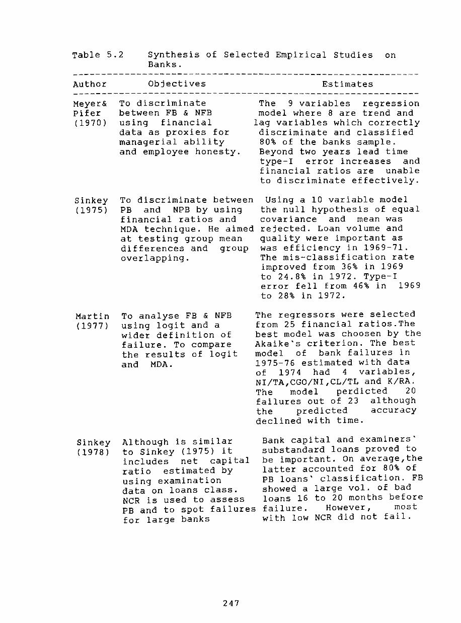
Table 5.2 Synthesis of Selected Empirical Studies on Banks.

Author

Meyer& Pifer (1970)

Sinkey (1975)

Martin (1977)

Sinkey (1978)

Objectives

To discriminate between FB & NFB using financial data as proxies for managerial ability and employee honesty.

To discriminate between PB and NPB by using financial ratios and MDA technique. He aimed at testing group mean differences and group overlapping.

To analyse FB & NFB using logit and a wider definition of failure. To compare the results of logit and MDA.

Although is similar to Sinkey (1975) it includes net capital ratio estimated by using examination

Estimates

The 9 variables regression model where 8 are trend and

lag variables which correctly discriminate and classified 80% of the banks sample. Beyond two years lead time type-I error increases and financial ratios are unable to discriminate effectively.

Using a 10 variable model the null hypothesis of equal covariance and mean was rejected. Loan volume and quality were important as was efficiency in 1969-71. The mis-classification rate improved from 36% in 1969 to 24.8% in 1972. Type-I error fell from 46% in 1969 to 28% in 1972.

The regressors were selected from 25 financial ratios.The best model was choosen by the Akaike's criterion. The best model of bank failures in 1975-76 estimated with data of 1974 had 4 variables, NI/TA,CGO/NI,CL/TL and K/RA. The model perdicted 20 failures out of 23 although the predicted accuracy declined with time.

data on loans class. NCR is used to assess PB and to spot failures for large banks

Bank capital and examiners' substandard loans proved to be important. On average,the latter accounted for 80% of PB loans' classification. FB showed a large vol. of bad loans 16 to 20 months before failure. However, most with low NCR did not fail.

247

Table 5.2 (continued) ------------------------------------------------------------Bovenzi, Marino,& McFadden (1983)

Avery& Hanweck (1984)

Nelson White (1984)

To develop an early warning model using financial data and

to compare with early models in terms of relative performance. To use CAMEL to test and predict failures.

To examine factors associated with FB. It focus on local market condition and the dynamic leading to failures unlike earlier studies.

To study bank failures in the 1920's and the banking crisis of 1930 By analysing financial ratios he ascertained the empirical meaning of managerial factors on FB. Also, to test between real and money factors of the crisis.

248

They estimate 3 models: Call A included OOE/TA,GSp/K,TL/K CGO/TL ratios. Exam A i5 an extension of Call A as includes credit risk based on loan examination data. Exam B included also TOL/TA. All coefficients were significant and with correct expected sign. Examination data improves classification accuracy although efficiency falls relative to call data as the interval between data & failure increases. The result from using CAMEL classification is consistent although does not do better than the ratios.

The model contain 9 ratios where 5 were significant among them NI/TA,NL/TA,K/TA, CIL/TA and log TA-LLR.Lagged financial ratios did not add much to the model after 6 months and a year.

For failures occurring in 1930 capital adequacy was insignificant unlike loan losses.Liquidity measured as CR/TD did affect the probability of bank failure.

The Temin & Friedman/Schwartz hypotheses were found both significant. The evidence from the model shows the characteristics of FB in the 1930's were similar to those who had failed some years earlier where there was no liquidity problems.

Table 5.2 (continued) ------------------------------------------------------------Short, O'Driscoll & Berger (1985)

Similar to White's paper. To assess the determinants of bank failures by comparing asset and liability portfolios of FB&NFB. To establish whether the explanatory power of risk variables have changed over time.

West (1985)

It introduces a new approach to early warning system by means of factor analysis.

Rodriguez Fernandez (1990)

To provide an ex post empirical analysis of the Spanish banking system. To identify a set of financial ratios to explain bank failures.

They estimated 5 ratios as proxies for the conduct of management.It includes K/TA TL/TA,CoD/TL and PuF/TL.The loan-asset ratio was significant during 3 years unlike PuF/TL. The probit estimates for FB indicates that the quality of banks' assets and the risk of outflows were important determinants of bank failure.

The model includes 19 ratios most of them successfully used in earlier studies. By factor analysis 4 ratios are included in the model which is similar to the CAMEL components. They are successful in the estimation of the probe of failure.

Ratios NI/TA, K/TL, and FA/TA were significant. In terms of the accuracy, the model perform well only 1 and two year before the failures.

NI= Net Income RA= Risk Assets LLR=Loan Loss Res. TA= Total Assets OOE= Other Opere EXp. CR= Cash and Res. CGO= Gross Chargeoff GSp= Gross Spread TD= Total Deposits CL= Commercial Loans TOL= Overdue Loans CoD=Core Deposit TL= Total Loans CIL= Commercial&Ind.Loans PuF=Purchased

K= Capital NL= Net Loans Funds FA=Fixed Assets

As evidenced by the selected number of studies reviewed

in table 1 and 2, the empirical models have been developed

and applied for different periods of time. They have evolved

from a basic classification problem to the construction of

249

failure prediction models and early-warning systems. The

building up of the ex post empirical model has involved a

sampling process for sound and unsound banks (failed and

problem banks) . By making comparisons on the bank

characteristics over time ,it was possible to find out

systematic differences between the two groups and from there

on to proceed in the calculation of the probability of

failure and make predictions.

Most of the studies analysed have used data derived from

balance-sheet and income statements to construct financial

ratios and apply multivariate estimation techniques ranging

from MDA to logit analysis. The results from these models

have been very encouraging particularly with reference to

the ability to assess the banks' characteristics, to test

statistically the importance of explanatory factors (e.g

asset quality), and to provide early signals about

approaching bank failure/problem one and more years in

advance.

However, the empirical approach have been questioned on

several grounds. Rodriguez Fernandez (1990) maintains that

although the explanatory power of model development for

bank failures exhibits a good record, the predictive

accuracy is less conclusive from those models. Furthermore,

Scott (1981) also introduces some criticisms to this

approach. He stresses the lack of theoretical underpinnings

as most of the findings and conclusions have been derived by

250

a statistical search through a number of plausible financial

indicators. Table 3 gives an assessment of the most

important contribution and shortcomings from the selected

cases of study.

Table 5.3

Author

Meyer& Pifer (1970)

Sinkey (1975)

Martin (1977)

Sinkey (1978)

Bovenzi, Marino,& McFadden (1983)

Avery& Hanweck (1984)

Overview of the Contributions and Shortcoming from the Selected Banks' Studies.

Contributions

It represent one of the first attempt to use financial information on bank failures in the form of ratios,trends& lags.

It is the first study using MDA technique on commercial banks.

It is the first attempt to use LOGIT on banking studies. It compares the the results between MDA and LOGIT.

One important contribution is the use of NCR and its ability to discriminate between PB and NPB.

Shortcomings

A narrow definition of failure, the lack of predicting ability beyond 2 years, and the

use of linear prob.model

The use of examiners' determined groups& the use of MDA itself.

Small sample size and exclude nonmember bank failures.

The estimation of NCR is based on information of loans'classification implemented by banks' examiners.

Compares the results of Small sample size for models using call data, some subperiod leading examiners'data, and with to lack of efficiency early models (Martin 1977) in the estimators. Also, it test the usefulness of CAMEL ratings on failures. (a)

By using pooled cross-section data rather than average for independent variables the model has the advantage of providing dynamic prediction of the probe of failure.

251

The sample was including small size institutions and the data was elaborated from examiners' report.

Table 5.3 (continued) --~--------------------------------------------------- ------Nelson White (1984)

The application of LOGIT to US bank failures during the 1920's and 1930. It tested the Temin&Friedman/Schwartz competing hypothesis.

It included data on National Banks only. The highset failure

rate was concentrated on state-Chartered banks.

Short, O'Driscoll, & Berger (1985)

It represent a fresh attempt to test the portfolio risks decision of commercial banks using PROBIT.

It assumes that macro-factors (general economic conditions) remain constant.It treats

West (1985)

Rodriguez Fernandez (1990)

Its contribution lies on the use of factorial analysis.

The application of LOGIT the case of the Spanish Banking System.

financial ratios as proximate determinants rather than casual factors.

The groups in which the logit analysis was based was determined by the opinion of supervisers.

The use of financial ratios as proximate determinants.

(a) The CAMEL rating system based on capital adequacy, asset quality, management, earnings and liquidity. Each indicator is rated from 1 to 5 with 1 being the highest score.

The shortcomings stated in table 3 and the lack of a

totally objective and exact criterion for identifying bank

failures have prompted the researchers to introduce other

methodologies in the study of bank failures.

A second approach defines bank failure as the event

whereby the net worth of a bank is negative. This a priori

methodology attempts to estimate and test the a priori

probability of a negative net worth by incorporating the

observed probability distribution of factors such as

earnings, loan losses, and other factors affecting the

252

value of a bank's net worth. For instance, Santomero and

Vinso (1977) and Nelson (1979) had followed this approach.

Santomero and Vinso estimate the probability of a negative

net worth by considering period to period changes in the

bank's capital as random variable. The parameters of this

stationary distribution for each bank were estimated using

weekly time series data reported by banks and transated into

a probability of failure. Factors such as profitability,

loan losses, liquidity , and other relevant financial

information were implictly treated in the determination of 6

the distribution.

In contrast, Nelson estimated a very similar model of

the role of capital in relation to the likelihood of failure

that disaggregates the effect of loans losses and other

elements affecting the variability of a bank's net worth.

Santomero and Vinso's model performed poorly as their

estimated probability of failure based in the sample 1965-74

was very low. This result was highly inconsistent as the US

banking system witnessed the collapse of the Franklin

National Bank and the Security National Bank in 1974-75.

A third approach may be identified from the banking

literature. The a priori undefined approach introduces the

concept of bank vulnerability as a more general concept. For

instance, Korobow and Stuhr (1975) and Korobow, Stuhr, and

Martin (1976) distinguish vulnerable banks from resistant

ones. They constructed a ranking of banks by weighting a

253

set of financial variables as proxies of financial weakness

or strength. Those banks which were above the arbitrary cut­

off point were considered as resistant to failure and 7

viceversa.

One important criticism is that the a priori undefined

models and the concept of vulnerability bears no relation to

the issue of banks failure. In a later articule Korobow,

stuhr, and Martin used the score as an independent variable

to estimate the probability of bank problems using an 8

arctangent regression equation. According to Martin (1977),

this new version is merely a variant of the ex post

empirical approach but with a poorer fit as they used a

single explanatory variable based on the rank scores.

One important criticism to the banking studies carried

out in particular for the case of the us banking system is

related to the use of financial ratios and in some cases

market data as independent explanatory variables. Clearly,

financial ratios point to symptoms rather than causes. In

other words, it identifies proximate determinants of bank

failures but not more fundamental causal factors. For

instance, increasing in asset and liability risk, reduction

in profitability, and low capital adequacy may be affected

by general factors such as a downturn in economic activity

and/or more specific issues relating to bank management and

risk taking. Thus, one could visualise two interesting

254

competing hypothesis, 9

firm-specific factors.

namely macroeconomic and

The approach to be followed in the present study will

consist in the modelling and estimating of the probability

of bank failure/problem in Chile. We will test those two

competing hypotheses using the logit model. At the same

time, we will use the ex post empirical approach based on

accounting and financial information to classify banks into

the two groups as it will be seen in the next chapter.

Before that we will discuss the econometric methodology

involve in the binary-choice model with specific reference

to the logit model.

(5.3) Binary-Choice and the Logit Model.

Usually we are dealing in economics with models in which

the dependent variable is continuous. However, bank

failures/problems can be in general considered as an event.

Since we are estimating the probability of occurrence of an

event the dependent variable takes a discrete value. Thus,

the econometrician is faced with the modelling of a pattern

of behaviour which involves a decision on a finite set of

alternatives. Models which are used for such purposes are

called qualitative response models (QR). QR models have

been extensively used in biometrics applications for much

longer than they have been applied in social science and in

particular in economics. These dicrete or QR models however

255

have had numerous applications in social science in more

recent times. Their topics range over a great variety of

discrete economic decisions such as labour force

participation, education and schooling, legislation and

voting, choice of occupation, and jobs and firm location

10 among others. As we have seen in the review of previous

studies these models have also been used successfully in

banking and finance.

(5.3.1) The Logit Hodel.

Suppose we want to consider the occurrence or non-

occurrence of an event,in our study we define this event as

a failure/problem bank (PB) and non-failure/non-problem bank

(NPB). We define a dichotomous random dependent variable Yi

which takes the value of Yi=l if PB and Yi=O if NPB. We

assume that Pi is the probability that Yi takes the value of

1 and hence (I-Pi) is the probability that Yi=O. Therefore

the probability function for Yi can be expressed as (1).

Yi I-Yi (1) fCYi)= Pi (I-Pi)

It is argued that the outcome of the random variable Yi

is determined by factors which can be grouped in terms of

microeconomic variables including banks' characteristics and

management as well as general economic conditions. Then we

have

256

(2) Yi= ( Zi - Zi )'<5 + Wi'( ei 1

el ) o 1 0

where

* + e

i

Zi' are vectors of microeconomic variables and/or bank characteristic of the ith bank.

Wi' is a vector of general economic conditions and/or macroeconomic variables.

Therefore, we may express the linear model in terms of (2b)

* (2b) Yi = Xi'B + e for

i

where

i = 1,2, ... ,n.

Xi = K-vector of known explanatory variables

B = K-vector of unknown parameters

* e = random error term

i

One of the earliest functional form used was the linear

probability model (LP). The LP model can be interpreted as

the probability that the event will occur given the value of

Xi. The estimated probability can lie outside the admissible

range 0,1. In other words, the distribution of F is not

limited to be between 0 and 1. In addition, because of the

heteroscedasticity problem, the OLS estimates of B will not

257

be efficient. Its wide usage can be explained as a result of

computational simplicity and its usefulness today remains

in determining quick estimates at a preliminary stage only.

Given the shortcomings associated with the LP model we

need an alternative specification concerning the

distribution assumptions so that all predictions lie within

the interval [0,1]. Since our main concern is to interpret

the dependent variable Yi as the likelihood of an event then

the notion of probability can be regarded as a suitable

basis for a transformation. There are two important

requirements which need to be met: Firstly, for all real X

the probability must fall between 0 and 1. Secondly, such

transformation has to be monotonic, that is increases in X

are associated with increases (decreases) in Yi for all X.

Probability distribution theory shows that the

cummulative distribution function (c.d.f.) for a continuous

random variable X is given by

(3) F(x) f (t) dt -(X) < X < (X)

-0)

where f(t)=probability density function

Notice that F(-oo)=O and F(00)=1 and if a<b it follows

tha t F (a) < F (b) .

258

Therefore, given the p.d.f. the LP model in (2a)

becomes

(4) P(Yi=l) = F(X'B) for i= 1,2, ... ,n.

where F= c.d.f.

The two most common choices of distribution are the

standard normal and the logistic distributions. The c.d.f.

for the former is defined as

( 5 ) F(t) -* (2rr.) exp{-X2/2} dX (Probit) -co

and for the latter we have

(5a) F(t)= 1 / 1 + exp (-t) (logit)

where exp=e= 2.718

The probit model (PM) may be justified by reference to a

central limit theorem and so it is the case for the logit

model given that the logistic distribution is similar to the

normal distribution. In fact, both distributions are bounded

between 0 and 1 as well as being monotonic. Also, they are

symmetric around zero means and have a variance equal to 1

and rr./3 respectively. The standardised logistic has slightly

heavier tails than the standard normal distribution. Because

of the close similarity between two distributions, it is

259

difficult to distinguish statistically between them unless

we have a large sample. Thus in a univariate dichotomous

model it does not matter whether we use problt or logit

model. In consequence, both transformations are suitable in

modelling bank failure/problem models, choice which is made

on the basis of convenience and the availability of computer

software.

From now on we will concentrate on the formulation,

estimation, testing, and selection of a logit model. Thus,

by recalling expression (4), the model can be expressed as

XiB

( 6 ) F(XiB) = J f(Z) dZ -0)

where f(Z) = 1 / 1 + exp(-X) standard logistic density function.

Then the problem bank or bankruptcy is determined by a

logit probability model as shown in (6). The interpretation

of the estimated coefficient in the logit model reflects the

effect of a change in an independent variable on the odds

ratio given by the expression Ln[ Pi / (1- Pi) ].

The next question we need to look at is relating to the

parameter estimation of the logit model.

260

(5.3.2) Estimation of a Logit Kodel.

The object of estimation of this model is the vector of

unknown parameter B. How the estimation is carried out

depends on the type of data being used. In some cases, we

may have repeated observations on a particular decision

maker (case). In this context we may apply the min X2 method

for QR models also known as the "Berkson-Theil approach". It

is only useful when there are repeated draws on the

dependent variable Yi having the same value of the vector of

the independent variable X. Then F(X'B) for the specific

value of X can be estimated by the relative frequency of Y

being equal 1. (Amemiya 1981,1985)

This restriction is satisfied in the case of the

physical science where the data in an

experimental setting.

trials holding the

They normally

are generated

consist of repeated

discrete independent variable as

constant. In contrast, most social science data are often

continous where observations differ both in the dependent

and the independent variable. Moreover, it would be very

difficult having natural repeated trials with the X's held

constant.

If sufficient repeated observations are not available we

must resort to the use of the maximum likelihood estimator

for B. The likelihood function of the logit model is given

by

261

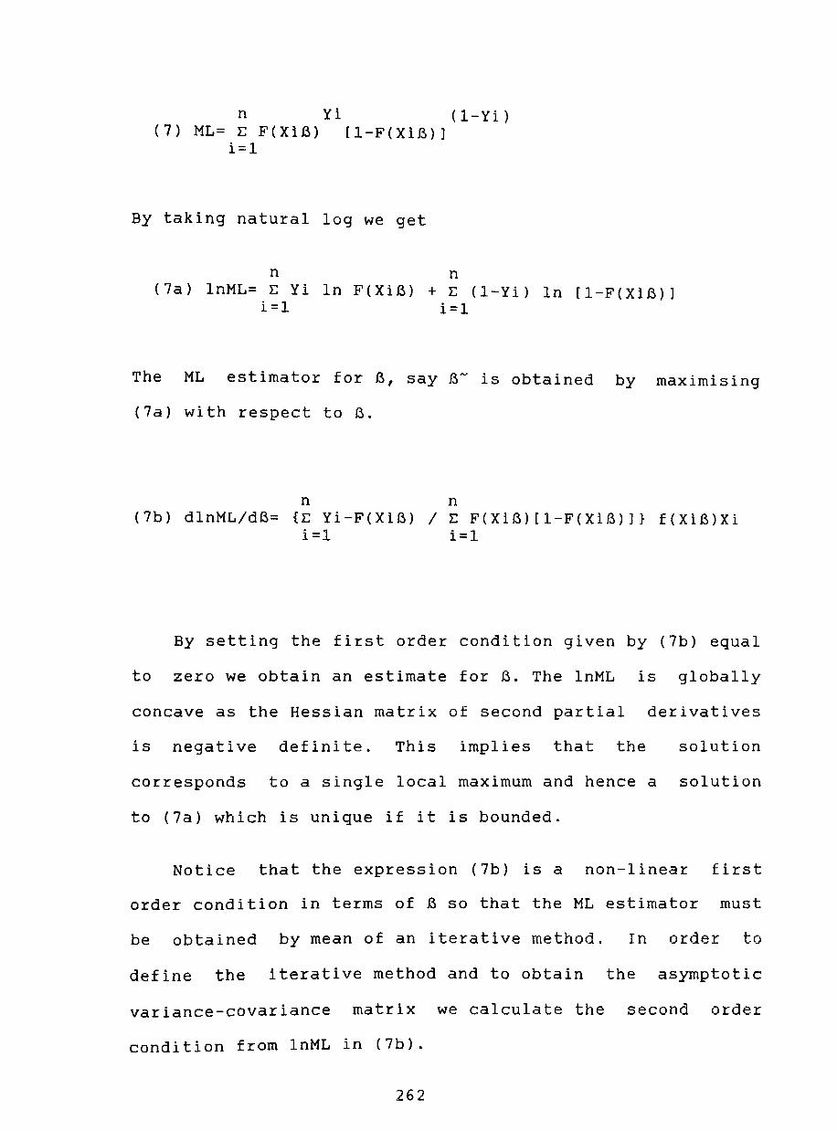
n Yi (l-Yi) (7) ML= E F(XIB) [l-F(XIB)]

i=l

By taking natural log we get

n n (7a) InML= E Yi In F(XiB) + E (l-Yi) In [l-F(XIB)]

i=l i=l

The ML estimator for B, say B~ is obtained by maximising

(7a) with respect to B.

n n (7b) dlnML/dB= {E Yi-F(XiB) / E F(XiB)[l-F(XiB)]} f(XiB)Xi

i=l i=l

By setting the first order condition given by (7b) equal

to zero we obtain an estimate for B. The InML is globally

concave as the Hessian matrix of second partial derivatives

is negative definite. This implies that the solution

corresponds to a single local maximum and hence a solution

to (7a) which is unique if it is bounded.

Notice that the expression (7b) is a non-linear first

order condition in terms of B so that the ML estimator must

be obtained by mean of an iterative method. In order to

define the iterative method and to obtain the asymptotic

variance-covariance matrix we calculate the second order

condition from InML in (7b).

262

n (8) d2 lnML/dBdB'= -E{[Yi/F2(X1B)]

i=l

+1-Yi/[l-F(1-XiB)]}f2 (XiB)XiXi

n + E{Yi-F(XiB)/F(XiB)[l-F(XiB)]}f'(XiB)XiXi

i=l

where f'is the derivative of f.

Taking expected values we are left with

n (8a) Ed2 lnML/dBdB'= -E{f2 (XIB)/F(XIB)[1-F(X1B)]}XiXi

i=l

Amemiya (1985) has shown that under very general

conditions the ML estimator is consistent and asymptotically

normal with the asymptotic variance-covariance matrix as

-1 (9) -(Ed2 lnML/dBdB') = Var(B~)

n -1 = E{{f 2 (XIB)/F(XIB)[1-F(XIB)]}XiXi} i=l

By substituting F by the logistic distribution defined

in expression (Sa) we obtain the formulas for the logit

model.

263

The non-linear equation can be solved by a variety of 11

iterative techniques. One the most common method to

calculate the ML estimator is the Newton-Rapshon. This is an

iterative procedure where the (t+l)st round estimate of B~

is

(10) B~ = 13 ..... - ( t+1 t

-1 d 2 lnML/dBdB'1 ]

B~

t

dlnML/dBI ] 13 .....

t

t+1

where (d2 lnML/dBdB'1 is a (K*K)

matrix of second partial derivatives of lnML function

evaluated at the th round estimate B~. t

This procedure is to be repeated until the iteration

converges to a global maximum bound on any set of starting

values B~.

(5.3.3) Hypothesis Testing.

There is a full menu of procedures available for

hypothesis testing. The simplest testing for a single

restriction is based on the normal and/or t-student test.

Suppose we are interested to test a general linear

hypothesis of the form given by expression (11).

(11) RB = r where R=(JxK) known hypothesis design

matrix with rank J~K

r= (Jxl) known vector

=:64

Thus the null hypothesis Ho is defined as

(lla) Ho: RB = r

If we test specifically R B=[l 0 0 O ... O]B= r where 1 1

any scalar including the value of 0 then a test of (11)

r is 1 can

be performed on the basis of the following asymptotic

results.

(llb) R B"'­I

-1 r / rr"'~R(X'X) R' z III

N(O,l)

-1 where rr"'~R(X'X) R' is an scalar and a

I 1 variance estimate of R B-- r

I I

Therefore, the null hypothesis Ho is rejected when the

absolute value of (lIb) is bigger than the theoretical value

given by the normal distribution ( Z value) corresponding to

a particular level of significance. This test is suitable

for large samples and a known variance.

Alternatively, for small samples (lIb) possess a t-

student distribution. For instance, if we test the null

hypothesis that the coefficient is 0 and the sample size is

small then (llb) is reduced to

!65

-1 (llc) B~ / ~rr2~(X'X) z t

(n-k, ~/2)

where (n-k) degrees of freedom ~/2 level of significance two-tail

As before the null hypothesis is rejected as long as the

absolute value exceed a defined critical region of the t-

distribution at n-k degrees of freedom and ~/2 level of

significance. Notice that (lIb) and (1Ic) are both correct

and equivalent since a t-distribution is asymptotically A

equal to a normal distribution, that is t z N(O,I). (n-k,~/2)

We may also wish to test the significance of all or a

subset of the coefficient of the logit model when the ML

estimator is used for B. A test using the chi-squared

distribution replaces the usual F-test applied to ordinary

regression. The null hypothesis is defined as Ho:B=B= .. =B=O. I 2 K

The likelihood ratio test (LRT) reflects the

comparability between a sample of data and the null

hypothesis through a comparison of the constrained and

unconstrained likelihood functions. Thus, the LRT is defined

as

A (12) LRT = 2[lnML(B-)-lnML(B~)] z X2 (chi-square dist.)

c q

where lnML(B-) = unconstrained likelihood function lnML(B~) = constrained likelihood function

c q= degrees of freedom

66

is obtained by maximising the ML function c

given by expression (7b) with respect to B subject to the

linear constraint RB=r where as we already know R is (JxK)

known design hypothesis matrix and r is (Jxl) vector of

given values.

The null hypothesis Ho as defined by (1Ia) is rejected

if the value of the statistics exceed a given critical value 12

of chi-square distribution with q degrees of freedom.

(5.3.4) Hodel Selection.

Finally, we need to develop a simple criterion for model

selection to choose alternative specifications in terms of

explanatory variables and/or general distribution functions.

There are a number of criteria for selecting among

alternative OR models. The use of a single scalar may be

treated with caution since it may be suitable only for some

instances. This means that it is extremely difficult to make

a definite evaluation concerning the relative merits of

various criteria independently. As a result, one should

select at least two or more scalar criteria for selection

purposes and compare the results. Another important remark

is that whatever criteria one decides to apply it is

necessary to make adjustment for degrees of freedom.

267

For the purpose of this study we have chosen two scalar

criteria from the menu, namely the prediction accuracy and

the Akaike Information Criterion (AIC) which follows the 13

discussion.

- Prediction Accuracy.

Suppose we have

n (13) E (Yi-Yi~) where Y·~ 1 = 1 if Fi~ > * i=1

and Y·~ 1 = 0 if Fi~ < *

Expression (13) gives the number of wrong predictions

as (Yi-Yi~)=l if and only if Yi and Yi~ are not equal. This

criterion is appropiate when one has an all or nothing loss

function. Thus, if an individual who estimated its

probability to be 0.40 and another individual who estimated

its probability equal to 0 then both are equally penalised.

However, under this criteria most models will do relatively

well even if the probabilities differ greatly within the

interval 0 ~ Yi~< *.

- The Akaike Information Criterion (AIC).

According to Judge, Carter, Griffith, and others (1988)

the information criterion seeks to incorporate in model

selection the divergent consideration of accuracy of

estimation and the best approximation to reality. Thus use

~68

of this criter1'on l'ntroduces t t' t' a s a 1S 1C that gives a

measure of the precision of the estimate and a measure of

the parameterisation of the model. Then the AlC is defined

as

(14) AlC = -lnML + K

where lnML= likelihood function K= number of parameters

Clearly, from (13) we see a trade -off between

precision and parameterisation where increases in K involves

a penalty in the value of the AlC. According to this

criteria one chooses the model with smallest AlC.

So far the discussion has centered on the specification

and estimation of a univariate logit model using cross-

section data. There are other alternative specifications for

a logit model such as a univariate multinomial model which

specifies the discrete dependent variable with more than two

alternatives. For instance, in a model of transport modal

choice we might specify the model with three alternatives,

say car, bus, and train. We may extend this model by making

such choice sequentially. That is, any particular choice or

state is determined by a previous choice or state. Suppose

that Yi=2 and Yi=3 where the first choice correspond to

problem bank and the second one to a non-problem bank. Then

if Yi=3 then Yi=1 which is defined as failed bank.

69

A second large group correspond to the multivariate

models. This type of QR model specifies the joint

probability distribution of two or more discrete dependent

variable. (For a thorough review of these models see Maddala

1983 and Amemiya 1985)

Finally, we have to consider the question of a

specification and estimation of a logit model using panel

data. The panel data consist of observations made on

individuals over time. In other words, it is a combination

of cross-section and time series data. This approach is very

useful in case of limited number of individual observations

in the cross-section data.

If the observations are independent between individuals

and overtime, then a logit model using panel data does not

introduce additional complications. In fact, it becomes only

a larger model with more observations. However, if there is

heterogeneity across units, the estimated parameters from

the logit model will be inconsistent.

The logit estimation with panel data and some of the

potential problems and shortcomings will be discuss in

chapters 7 and 8.

70

Endnotes.

(1) At the same time but in less quantities academics from universities and institutes have also contributed to the development of this topic. For an exhaustive review and assessment of early warning system developed by these agencies and others for the US see Altman E., Avery Einsenbeis R., and J.Sinkey Jr. (1981) Chapter VIII.

R.,

(2) Of the 30 ratios reported by Beaver cash flows/total assets,net income/total debt, and cash flows/total debt best predicted financial failures.

(3) The 5 variables are the following: working capital/total assets, retained earnings/total assets, earnings before interest and taxes/total assets, market value of equity/book value of total debt, and sales/total assets. For a thorough account on the pioneer work of Beaver (1966), Altman (1968) and the more recent development of failure­prediction models for non-financial firms see Altman, Avery, Eisenbeis, and Sinkey Jr. (1981).

(4) As argued by Martin (1977), it is commonly agreed that a financial firm fails as any other enterprise when its net worth becomes negative or incurr losses that would result in a negative net worth. However, actual insolvency and receivership are infrequent relative to some form of intervention by the monetary and banking authorities. Among them we find mergers with a healthy institution, the purchases of bad loans and risky assets. In spite of this, he argues that no serious problems will be present in empirical research.

(5) For an excellent and thorough review of the econometrics for binary choice models see Amemiya (1981) and Judge, Carter, Griffiths, Lutkepohl, and Chao-Lee (1988). For a more advance treatment see Maddala (1983) and Amemiya (1985)

(6) Santomero and Vinso studied 224 large US banks between 1965 to 1974. Those banks who have not reported continuously over this relevant period were excluded. United state National Bank, Franklin National Bank, and Security National Bank felt into this category.

(7) They employed a linear combination of 12 financial ratios to measure vulnerability. Each variable is weighted by either 1 or minus 1 depending whether this financial ratio is a priori favorable or unfavorable. After dividing it by the standard deviation, the weighted sum represent the rank score. Positive score implies resistance and negative score vulnerability.

71

(8) The arctangent procedure differ only slightly from the logit analysis. The regression estimate the relationship between the bank scores and the observed probability of receiving low rating over the estimation period subsequent to the base year. This realtionship was assumed to be continuous, approaching zero for large positive scores and approaching one for negative score, and monotonic. The arctangent distribution has indeed these properties.

(9) This point have been raised by Nelson White (1984) and Short, Q'Driscoll, and Berger (1985). Nelson White test two competing hypothesis for the banking crisis of 1930, the effect of real and monetary factors and the ability of the banking system to withstand those shocks.

(10) For an applications (1984)

exhaustive review of QR models see Amemiya (1981) and Pindyck and

and its Rubinfelt

(11) Normal equations for non-linear models are in general non-linear with respect to the parameters so we require some specific algorithms to solve them. We should mention the Newton-Raphson, method of scoring, the Berndt, Hall, Hall, and Hausman algorithm, and Davison, Fletcher, and Powell algorithm among the most common.

(12) For more involved restrictions we may model by means of the Wald test. As the LRT, chi-square distribution and both are equivalent. (See Judge, Carter, Griffith, and

also test the this test has a asymptotically

others 1988).

(13) Amemiya (1981) gives a more thorough review of the list of scalar criterias for QR models. In addition, Judge, Carter, Griffiths, and others (1988) discuss problems of specification in econometrics models.

72

Chapter 6. The Discrete Dependent Variable: Predictions from an Early Warning Hodel.

(6.1) Introduction.

This chapter seek to develop an appropriate

banks'classification method using financial information from

balance-sheets and income statements. In the absence of ex

post information on the state of health of the chilean

financial institutions prior to the failure date of 1983, we

have constructed an early warning system to predict the ex

ante probability of bank problem/failure based on the

statistically significant determinants of the likelihood of

those events. The empirical results were obtained by the use

of univariate and multivariate statistical techniques. At

the same time, the model provides evidence as to whether the

bank failures could have been anticipated by the

authorities.

This chapter has been structured into three main

sections. Section 2 contains a description of the model in

terms of the definition of bank failure/problem and the

relative advantages and disadvantages of alternative

definitions used in the literature. Section 3 discusses the

set of independent variables and its classification in seven

broad categories. Finally, the last section reports and

assesses the empirical results from univariate and

multivariate statitical models. The evidence is complemented

with a set of appendices to compare the results.

73

(6.2) Development of a Failure/Problem Prediction Hodel.

(6.2.1) Failure/Problem Hodel: The Dependent Variable.

As we have seen in the previous chapter, there are

several approaches to the construction of a problem and/or

failure prediction models in the empirical literature of

banking. The lack of an objective criterion for identifying

bank failures in the real world has led to researchers to

deal with this ambiguity by taking the ex post

classification of bank failures or alternatively, they

have also adopted a more abstract and subjective definition

based on the judgment from the banking authorities about

what constitutes a sound and healthy financial institution.

This acceptable variant of the ex post empirical approach

rests on the existence of a bank "problem" list elaborated

by the banking authorities. This classification is

elaborated with information from on-site bank examinations,

and in particular, from the evaluation of asset portfolios 1

and the quality and riskiness of bank loans.

However, given that a failure is a more objective

indication of a bank's ability to continue its operation,

then this approach results in a more convenient and less

subjective approach than the definition of a problem bank.

On the other hand, if bank problems precede actual failures,

then a problem prediction model may provide a longer lead

time for identifying and classifying financial institutions

than would a failure prediction model. Also, the authorities

74

may encourage corrective actions which can prevents bank

failure. Thus, as the failure path tends to be a decaying

one rather than an explosive one, then identifying tho5e

banks with financial difficulties would be the first step

towards achieving the failure prevention goal.

The evidence from other empirical studies and from the

banking crisis in Chile show that all failed banks were

identified as problem banks although it did not follow that

all problem banks failed. Bearing in mind the pros and cons

discussed above, this study accepts as a more convenient

approach to study the banking crisis in Chile a definition

of the discrete and dichotomous dependent variable as

failed/problem and nonfailed/nonproblem banks. At the same

time, this definition maximises the number of observations

unlike the case where the dependent variable is failure and

non-failure banks. The data limitation for this empirical

study became a powerful reason to choose failure/problem

prediction model instead of a failure-prediction model.

The development of this model aims at replicating the ex

post list of problem banks of 1983. At the same time and

equally important, the model is used to construct a

classification list for financial institutions prior to

1983. Given that such ex post information is not available

we then predict quarterly estimates

probability of problem as a proxy in

of the

order to

ex ante

classify

financial institutions into the two groups. The estimating

coefficients of the logit models will generate a set of

probability estimates so that those institutions classified

as problem are assigned a high ex ante probability of

problem and a low probability to non-problem banks.

Initially, two models were considered for comparison

purposes conveniently labeled as models A1B1 and A1B2. Both

correspond to problem-prediction models where in the first

case Al includes all those financial institutions which have

sold bad loans to the Central Bank and/or were liquidated,

merged, and capitalised in 1983. From table 1 and appendix 1

we see that for 1983 a total of 17 commercial and

development banks were classified into the list of Al from a

total of 27. The only two institutions which remained

healthy and hence did not have to sell bad debts to the

banking authorities were the state bank Banco del Estado and

the private commercial bank Banco Industrial y de Comercio 2

Exterior.

The chosen samples did not include those financial

intermediaries which were subject to regulatory intervention

during 1981, despite that the fact that this year marked the

beginning of the severe banking crisis of 1983. This

arbitrary selection was justified on the grounds that most

financial failure were concentrated in non-bank financial

institutions and it would have reduced the sample size for

the empirical study. Moreover, the period of 1981 can be

seen as one with a buoyant macroeconomic environment and

76

hence no comparison between two macroeconomic states would

have been possible for those institutions.

Table 6.1 List of Problem and Failed Banks in Chile During 1983.

------------------------------------------------------------Bank Code Problem Failed ------------------------------------------------------------Chile 001 SBO Rk & Rp O'Higgins 008 SBd Internacional 009 SBO Rk & Rp Continental 011 SBO Sud Americano 014 SBD Credito 016 SBO Trabajo 022 SBO Pacifico 025 SBO Nacional(a) 026 SBO Concepcion 027 SBO Rk & Rp Edwards(b) 029 SBD Santiago 035 SBO Rk & Rp MorganFinansa(c)047 SBO Unido Fomento 502 Liquidated Hipotecario F. 504 SBO Rk & Rp Hipotecario Ch. 505 Liquidated Colocadora Nac. 506 SBO Merged ------------------------------------------------------------Source: SIBF, Informacion Financiera, Various Issues.

(a) Former Banco de Curico (b) Former Banco Constitucion (c) Former Financiera Finansa

Rk= Capitalised Rp= Privatise SBO= Bad Debt Sold to

Central Bank.

An important observation is the fact that foreign banks

did not fail and/or sold bad debts to the Central Bank,

although there were two exceptions namely Banco Espanol and

Banco Talca which in 1981 were bought by the Santander Bank

and the Central Bank both from Spain. Later on, they became

Banco de Santander and Centro Banco.

'77

The group of non-problem banks was constructed using two

classifications. For the case of B1, this sample includes

the two healthy commercial banks, a group of foreign banks

which opened after 1980 and the remaining development bank

but excluded non-bank financial institutions. B2 differs

from B1 only in terms of the replacement of foreign banks by

non-bank financial institutions.

The inclusion of foreign banks in the sample B1 is

justified on the grounds that they outperformed domestic

banks during and after the crisis. Marshall (1990) reported

that foreign banks performed better than domestic banks 3

measured in terms of a performance index. The same

conclusion was obtained by the author by looking at the rate

of growth of total deposits, loans, financial investment

measured in real terms. Therefore, their inclusion as sound

banks was expected to give some light on the specific

differences with respect to the unhealthy ones. The same

objective was sought when we include non-bank financial

institutions and exclude foreign banks in the sample B2.

However, the sample size of B2 was smaller than B1.

Therefore, AIB2 contained a total of only 25 observations as

compared with A1B1 with 36 observations.

There are two final points to be stressed about problem-

prediction models. Firstly, apart from the arguments for and

against one or other model suggested earlier on, the number

of observations included in the model also should be given a

~78

considerable weight in our choice. Given that the of the Chilean financial system is rather small as compared

with, say, the USA, where normally the sample size i5 in

excess of 1000 observation for each period, it is necessary

to maximise our sample size.

Secondly, and also related to the data limitations we , attempted to work with a controlled sample model labeled as

A1B3. The B3 contained a controlled sample by bank size to

incorporate such differences in the model. However, the

sample of non-problem banks was insufficient to construct a

paired observations with problems banks having the same size

category. Therefore, such model was dropped from the

empirical analysis.

(6.2.2) Variables Categories and Financial Ratios as Regressors.

Once we have chosen and defined the problem-prediction

models, the next step is to discuss the selection and use of

variables as regressors. In this study, we have included a

large number of financial ratios properly calculated from 4

bank balance sheets and income statements. Unfortunately, we

were unable to include market data to be used as regressors

in the estimated models. Although the "market-efficiency

relevant hypothesis" suggest that markets contain all

information on the future performance and hence provide the

earliest warning signal, the lack of market data for Chilean

banks left this option unavailable.

79

The list of selected explanatory variables is similar to

those used successfully in other previous studies as

discussed in chapter 5.

In selecting variables for its inclusion we identified

the potential risks and problems inherent in financial

institutions. Thus, the list of variable in each category

serving as reasonable proxies for banks' risks and financial

problems were considered in terms of its theoretical

plausibility.

Appendix 3 contains a list of the 49 financial ratios

classified into 7 broad groups: capital adequacy, liquidity,

profitability, asset risk and quality, efficiency, liability

risk and quality, and mismatchings.

Each of these general characteristics could in theory

and in

affect

practice as proved by

the prospects of bank

the empirical literature

problem and failure. For

instance, a bank may become a problem and be threatened with

the possibility of failure as a result of large and

unsustainable losses from its asset portfolios, in

particular, bad loans. Capital adequacy, profitability,

efficiency, and liquidity will measure the ability of banks

to remain in business in the face of unexpected losses.

As pointed out by Sinkey (1979) and Barth, Brumbaugh and

others (1985), capital adequacy or net worth represents a

cushion against future unanticipated losses. Moreover, it is

280

argued that stringent capital regulation reduces the

incentive to increase asset risk and the likelihood of bank

failure in the case of fixed price deposit insurance.

On the other hand, profitability measures the ability of

a bank to maintain its net worth and hence its current

performance. On this aspect it was also considered a

variable which measures efficiency which indirectly will

affect the financial result concerning the bank gross

utility.

Asset risk and quality measures the potential erosion

of a bank's net worth and the subsequent reduction in

profitabilty from loan loss provisions and chargeoffs.

The model also includes a category which measures the

bank's liquidity. According to Sinkey (1979) banking firms

need liquid assets as a buffer or cushion for meeting any

excess in cash outflows. Thus, most liquidity ratios attempt

to measure the size of this buffer.

There are two additional measurements included in this

study which are worthy of consideration. The first one

concerns the risk associated with a mismatch of maturities

between assets and liabilities, both in domestic and foreign

currency. Here, fluctuations in interest rates and

unexpected devaluations can introduce a significant risk for

the financial position of a bank. Finally, I also included a

category which accounted for the riskiness and quality of

the liability structure of a bank.

281

Admittedly, financial ratios identify symptoms rather

than causes. This means that these financial ratios employed

as regressors are proximate determinants of bank

problem/failure but not the more fundamental causal factors.

For instance, the profitability and the asset quality can be

equally affected by both bank management in terms of risk 5

taking, and the general condition of the economy.

The model is estimated using financial data with

different time lags between the ex post data of bank problem

and the financial statement, that is with data between 1979

and 1983.

(6.3) The Empirical Results from the Failure/Problem Prediction Model for Chile.

The main objective was to estimate the quarterly ex ante

probability of failure/problem for the period between 1979

and 1983. We started by taking an ex post definition from

the classification available for 1983 to construct the

dichotomous dependent variable. We modelled the ex post

classification as a function of several independent

variables using the data available from the balance-sheets

and income statements.

From several tentative specifications I chose the

estimated equation with the lowest Akaike's value, and

maximise the overall accuracy in terms of type-error I and

II at a given cut-off point.

282

Then we proceded with the evaluation of the ex ante

probability based on the prediction from the estimated

equation using quarterly financial data prior 1983. This

procedure will enable us to calculate the quarterly ex ante

probability that a financial institution had problems before

1983.

The analysis consisted of two major steps. Firstly, we

applied one way analysis of mean and variance techniques to

examine the extensive list of financial ratios of problem

and non- problem financial institutions. The importance of

this first step rests on the need to reduce the list to

more manageable proportions and selected numbers of

independent variables.

The second step consisted in the application of a

multivariate technique using a logit model to identify those

financial variables from the remaining list as significant

determinants of the likelihood of bank problems and to be

followed by the prediction of the likelihood of financial

difficulties.

(6.3.1) Univariate Results.

The univariate results are shown in table 2 which

contain the mean and the mean differences for each financial

ratio as well as each group and year. In addltion appendix 4

provides a review of the testing procedure for the

difference between means.

~83

We tested the mean difference for the specifications

for the A1B1 and A1B2 at the critical time of

failure/problems, that is 1983, and for each of the 4 years

before the critical year.

Table 6.2 Mean Differences between Nonfailed/Nonproblem and Failed/Problem Banks and the t-Statistics for 1983.(a)

------------------------------------------------------------category Yare B1-Al t(b) Yare B2-A1 t(b) ------------------------------------------------------------Capital Adequacy ( 1 )

Liquidity ( 2 )

Profits ( 3 )

Asset Risk ( 4 )

Efficiency ( 5)

Liability Risk(6)

Mismatching ( 7 )

13 -8.73 14 -0.83 15 0.19

23 0.19 26 0.43 21 0.15 24 0.34

31 0.72 35 0.33

41 -0.19 42 0.15 44 0.92 43 10.19 423 -0.10

61 0.26 62 -0.01 67 0.10 611 0.03

74 0.33 73 0.07 75 0.89 72 0.22

-5.69 -4.81

3.55

6.50 5.48 5.32 4.88

3.69 2.74

-6.18 5.32 5.13 5.07 2.98

2.56 -2.54 2.39 2.55

4.88 4.31 2.91 2.87

15 16 14

24 21 26 23

32 31

423 41 42 416 415

63 66 67 65

71 74

0.12 0.11

-0.84

0.21 0.09 0.22 0.09

0.06 0.18

-0.20 -0.10

0.09 -0.04 -0.05

0.26 -0.19 -0.20 -0.14

-0.19 0.15

3.58 3.55

-3.42

2.65 2.60 2.53 2.40

3.97 2.81

-5.30 -2.60

2.60 -2.19 -2.07

3.76 -3.61 -3.55 -3.46

-5.22 2.64

(a) The table include the most significant variables and they are ranked in terms of the relative significance. The definition of each variable is found in appendix 3 (b) Evaluated at 5% significance level.

~84

One important finding from the data is that the sign in

the mean difference values are consistent with the a priori

expectations and statistically significant at 5% level in

most cases. Moreover, the average values for capital

adequacy are significantly greater for non-problem banks

than problem banks. For instance, in the model A1B1 the

mean difference for the variable total loans/capital

(variable category 1-13) is -8.73 which is consistent with

the a priori expected sign and statistically significant.

This means that failed/problem banks exhibited a lower

capital ratios than sound banks.

At the same time, liquidity ratios for the former

are, as expected a priori, higher than the latter

This is evident by examining financial investment

cash/total asset1 ratio (variable 2-23).

group

group.

plus

Another interesting result from table 2 is that the

measurement of asset risk also shows a significant

difference between the two groups of banks. For instance,

variable 43 defined as provision for bad loans/operating

expenses shows a statistically significant difference of

10.19 between A1-B1. This means that non-problem/non-failed

banks have chosen a less risky portfolio than problem/failed

banks. It is not surprising then to find that B1 group is

relatively more profitable than A1 group judging from the

profitability ratio operating earnings/operating expenses

( variable 3-31 ). With reference to the risks involved

85

from banks' liability structure the evidence from the ratio

analysis suggests that failed/problem banks did not show

lower and inferior quality in its liability structure than

nonfailed/nonproblem banks. Indeed, the mean difference of

the deposit(less than a year)/total liabilitiesl ratio

(variable 6-61) between nonfailed/nonproblem and

failed/problem banks is positive and significant.

Finally, we expect a priori that group Bl should exhibit

a lower risk of mismatching than group AI. In effect, the

evidence from mismatching ratios supports this view.

In general, the evidence from the ratio analysis for the

critical year of 1983 indicates that nonproblem banks

exhibit significant differences in terms of each selected

category. On average and as expected, they carried

relatively less risk in terms of the asset structure. At the

same time, the data on capital adequacy and profitability

suggest that they have a greater ability to respond in a

case of unexpected losses and/or risks.

A second important finding from the data is the fact

that the variable assessing any difference in efficiency

between the two groups was not significant for both models

AI-B1 and AI-B2 at least for 1983.

Thirdly, it appears that the differences in the mean

values are larger for Al-Bl than AI-B2. In the former we had

included foreign banks and excluded non-bank financial

286

institutions. This evidence may indicate that for comparison

purposes it is more convenient to consider a larger sample

which includes foreign banks.

Finally, the difference in mean values tends to change

as the time before failure lengthens. These changes over

time occur in both the significance of the ratio and its

relative ranking within its category. These comparison can

be seen in table 3 and 4 respectively.

From table 3 we see that over-time mean differences

diminish for the variables in the category of capital

adequacy and asset risk in contrast with profitability which

tends to increase as we go back from the critical time.

Also, we observe that over-time significance of the variable

changes from year to year with the exception of total

loans/capital (13), and net capital/assetl (15) both

measuring capital adequacy and the financial ratio total

loans/assetl (41) which assess the rikiness of the

portfolios.

These findings tend to suggest that variables relating

to capital adequacy and asset risk consistently spotted

significant differences between the two groups. These early

data may lead to the assertion that managerial differences

could be important in the likelihood of financial 6

difficulties. However, it must be pointed out that capital

adequacy, unlike the quality of banks' portfolios, is not

completely within the control of bank managers. This

87

variable is set by the bank legislation which inforce

certain minimum limits. Nevertheless, some discretion is

still left to banks in this respect.

Table 6.3 Over-time Mean Differences and its t-Statistics for A1B1.

------------------------------------------------------------category Var. 82 t 81 t 80 t 79 t ------------------------------------------------------ -----.-Capital Adequacy ( 1 )

13 -7.08 -7.22 -7.57 -5.93 -5.44 -4.10 -4.98 -3.38 14 -0.09 -2.39 15 0.15 2.70 0.25 3.26 0.15 2.93 0.24 2.69

Liquidity 23 (2) 26

21 24

0.10 0.19 0.07 0.13

4.16 0.09 3.23 3.32 0.06 2.60

Profits ( 3 )

31 1.14 2.21 35

2.40 0.09 0.27

1.99

2.87 0.11 2.11

1.41 1.97

2.58

-0.09 -3.43 -0.07 -3.36

AssetRisk ( 4 )

41 42

-0.12 -4.48 -0.09 -2.77 -0.09 -2.82 -0.10 -2.41 0.07 3.32 0.06 1.99

44 0.18 2.78 43 423-0.08

Efficiency -­( 5 )

-1.94

Liability 61 0.11 2.39 0.15 2.64 Risk(6) 611 0.10 2.03 0.06 2.10

62 -0.01 -2.20 67

Mismatch 74 (7) 73

75 72

0.17 0.05 0.46 0.15

3.43 3.60 3.71 2.83

0.07 2.05

0.14 2.09

0.20 0.06

0.09

2.02 2.70

2.38

0.11 2.79

(a) The table include the most significant variables and they are ranked in terms of the relative significance.

From table 4 we observe that the relative rankings of

the financial ratios within each categories changes

88

overtime, although some of them still remain among the most

significant.

Table 6.4 Overtime Rankings for Financial Ratios in Model A1B1.

------------------------------------------------------------Categories Rankings(a) 1983 1982 1981 1980 1979 ------------------------------------------------------------Capital Adequacy ( 1 )

Liquidity ( 2 )

Profits ( 3 )

Asset Risk ( 4 )

Efficiency ( 5 )

Liability Risk ( 6 )

Mismatching ( 7 )

1 2 3 4

1 2 3 4

1 2 3

1 2 3 4 5 6

1

1 2 3 4 5

1 2 3

13 14 15 16

23 26 21 25

31 35

41 42 44 43 423 412

61 611 62 67 63

74 73 75

13 12 11 16

21 25 23 26

31

41 412 411

42 44

415

51

64 62

611

75 73 74

13 12 11 15

23 21

32

411 41 45 46

421 42

51

611

72 73

12 13 15 11

23 25

35 33 34

41 45 46

412 411

51

61 63

72 73

13 12 11 15

22 23 25

35

413 41

411

52

61 63 66

73

(a) Rankings are established according to the value of the t-statistics.

Given these difficulties we have included the most

significant financial variables during 1983 and those which

consistently appeared in the group of significant variable

overtime.

289

(6.3.2) Multivariate Results.

to

Based upon the univariate results, we use a logit

identify those financial variables belonging

model

to a

specific category which are significant determinants of the

likelihood of failure/problem. Then we proceded to use the

estimated equation to assess the predictions from the model

during the critical time of 1983 and before the crisis.

In tables 5-9 I present the logit results for

alternative specifications at the time of

and years before the critical date. Among

specifications presented in table 5,

preferred to the others on the basis

failure/problem,

the alternative

equation E1 is

of the Akaike's

information criterion (AlC) and the likelihood ratio test as

discussed in the previous chapter. Unlike E1, the

alternative specifications E2 and E5 were statistically

insignificant at 1% as the chi-square with 6 degrees of

freedom is 16.81. Similarly, although E3 and E4 nearly

rejects the null hypothesis their Akaike's value are quite

large in comparision to E1. (x2 =9.2 with 2 d.f.)

The specification E1 includes the constant and the

and explanatory variables total loans/capital

provision/operating expenses. A negative

means that if the variable increases the

problem/failure declines (increases).

290

(positive) sign

probability of

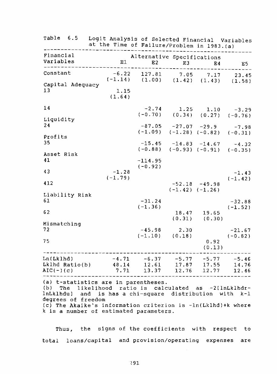
Table 6.5 Logit Analysis of Selected Financial Variables at the Time of Failure/Problem in 1983.(a)

------------------------------------------------------------Financial Variables

Alternative Specifications El E2 E3 E4 E5

------------------------------------------------------------Constant

Capital Adequacy 13

14

Liquidity 24

Profits 35

Asset Risk 41

43

412

Liability Risk 61

62

Mismatching 72

75

-6.22 (-1.14)

1.15 (1.64 )

-1.28 (-1.79)

127.81 (1.00 )

-2.74 (-0.70 )

-87.05 (-1.09)

-15.45 (-0.88 )

-114.95 (-0.92)

-31.24 (-1.36)

-45.98 (-1.10)

7.05 (1.42)

1.25 (0.34)

-27.07 (-1.28)

-14.83 (-0.93)

-52.18 (-1.42)

18.47 ( 0 . 31)

2.30 ( 0 . 18 )

7.17 (1.43)

1.10 (0.27)

-29.9 (-0.82)

-14.67 (-0.91)

-49.98 (-1.26)

19.65 (0.30)

0.92 (0.13 )

23.45 (1.58)

-3.29 (-0.76)

-7.98 (-0.31 )

-4.32 (-0.35)

-1.43 (-1.42)

-32.88 (-1.52)

-21.67 ( -0 . 82)

------------------------------------------------------------Ln(Lklhd) Lklhd Ratio(b) AIC(-) (c)

-4.71 48.14 7.71

-6.37 12.61 13.37

(a) t-statistics are in parentheses.

-5.77 17.87 12.76

-5.77 17.55 12.77

-5.46 14.76 12.46

(b) The likelihood ratio is calculated as -2[lnLklhdr­InLklhdu] and is has a chi-square distribution with k-l degrees of freedom (c) The Akaike's information criterion is -In(Lklhd)+k where k is a number of estimated parameters.

Thus, the signs of the coefficients with respect to

total loans/capital and provision/operating expenses are

291

consistent with hypothesised role of capital adequacy and

asset risk. The first of the regressors suggest that an

increase in total loans relative to capital increases the

probability of problem/failure. In constrast, the increase

of provision relative to operating expenses reduces the

likelihood of financial difficulties.

With respect to the significance of the estimated

coefficients, we found that provision/operating expenses is

significant at 10% of significance. However, as we increase

the degree of statistical significance, say 5%, the

estimated coefficients are insignificant. We suspect the

existence of multicollinearity among the explanatory

variables. On this issue, Judge, Griffiths and others (1980)

and Johnston (1988) show that the near multicollinearity

produces three effects, namely very large sampling

variances, large covariances, and unstable coefficients. In

this case the correlation coefficient of the two explanatory

variables is nearly 64%. Furthermore, by dropping one of the

regressors in the equation the t-statistic of the remaining 7

variable left improves considerable and becomes significant.

In spite that both of the regressors together are

insignificant, the overall equation is still statistically

significant in terms of the likelihood ratio test and as we

will see the overall prediction accuracy of the model is

exceptionally good and comparable with other studies in this

area. This indicator should be the overwhelming criterion to

choose the best specification together with the Ale.

~92

Table 6.6 Logit Analysis of Selected Financial Variables One Year Before the Critical Time.(1982)

------------------------------------------------------ ------Financial Variables

Alternative Specifications El E2 E3 E4 E5

------------------------------------------------------------Constant -3.22 -32.09 21.36 25.95

(1.68) (1.57) 13.30

(2.03) (-0.79) (-1.16) Capital Adequacy 13 0.67

14

Liquidity 24

Profits 35

Asset Risk 41

43

412

Liability Risk 61

62

Mismatching 72

75

(2.04 ) -0.30 -3.68 -4.32 1.99

(-0.16) (-1.26) (-1.29) (0.65)

-6.07 -44.85 -31.13 -31.47 (-0.28) (-1.56) (-0.89) (-1.53)

9.45 -1.77 -0.36 21.33 (1.18) (-0.17) (-0.03) (1.82)

41.71 (1.41)

-2.92 -6.02 (-1.65) (-1.83)

-205.1 -243.1 (-1.48) (-1.43)

-6.76 -10.51 (-1.02) (-1.31)

-2.90 (-0.70)

-12.43 -21.37 (-0.50) (-0.72)

-2.70 (-2.11)

-8.34 (-0.65)

1.16 (0.11)

------------------------------------------------------------Ln(Lklhd) Lklhd Ratio Ale

-8.90 27.62 11.90

-12.13 6.34

19.13

(a) t-statistics are in parentheses.

-12.13 19.85 19.13

The results for one and more years

-6.16 19.80 13.16

before

-6.4 20.95 13.43

the

problem/failure date are presented in tables 6-10. The

evidence shows that specification El is preferable to the

others for every year prior to 1983 with the exception of

1980 based on the Akaike's information criterion.

293

There are several interesting findings from this

estimation. Firstly, the variable of capital adequacy is

significant at 10% for every single year prior to 1983.

Table 6.7 Logit Analysis of Selected Financial Variables Two Years Before the Critical Time.(1981)

------------------------------------------------------------Financial Variables

Alternative Specifications E1 E2 E3 E4 E5

------------------------------------------------------------Constant

Capital Adequacy 13

14

Liquidity 24

Profits 35

Asset Risk 41

43

412

Liability Risk 61

62

Mismatching 72

75

Ln(Lklhd) Lklhd Ratio Ale

-4.30 -9.55 -0.13 0.33 5.16 ( 1.86 ) (-3.06) (-1.42) (-1.42) (0.29)

0.39 ( 3 . 30)

6.14 5.40 4.09 8.83 (1.48) (1.46) (1.08) (1.57)

-0.008 2.33 2.76 -5.95 (-0.02) (1.20) (1.23) (-0.61)

8.54 5.92 6.98 4.31 (1.24) (0.88) (1.02) (0.61)

12.64 (1.65)

-0.008 -3.47 (-0.17) (-2.04)

-16.22 11.73 19.22

-7.18 -8.01 (-1.21) (-1.18)

-4.57 -6.95 (-1.29) (-1.71)

-0.59 0.85 (-0.08) (0.12)

-2.34 -2.38 (-0.89) (-0.96)

-19.21 2.41

26.21

-21.49 1.51

28.49

-2.21 (-1.49)

-20.57 1.84

27.57

1.74 (0.42)

-14.6 4.72

21.64

(a) t-statistics are in parentheses.

294

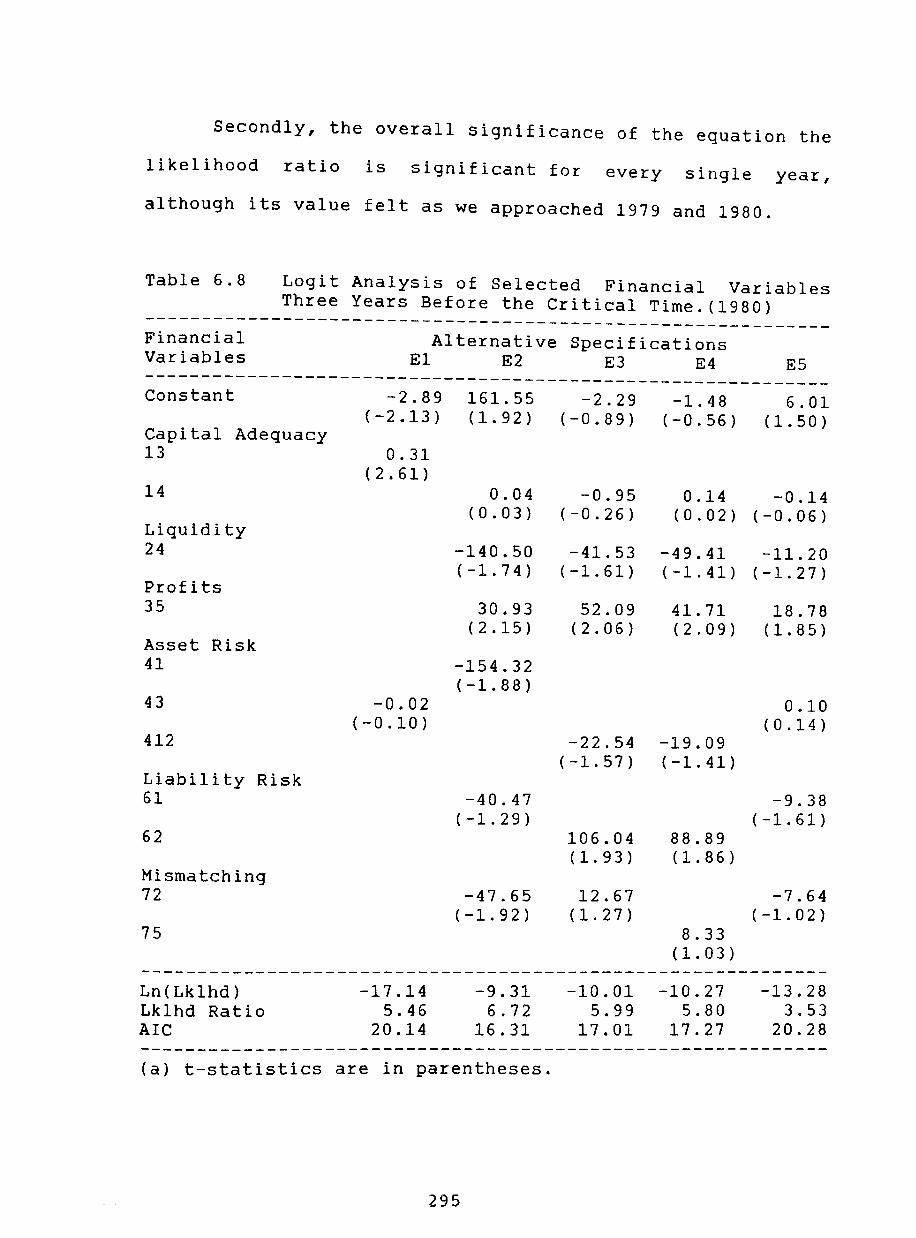
Secondly, the overall significance of the equation the

likelihood ratio is significant for every single year,

although its value felt as we approached 1979 and 1980.

Table 6.8 Logit Analysis of Selected Financial Variables Three Years Before the Critical Time.(1980)

---------------------------------------_._-------------------Financial Variables

Alternative Specifications E1 E2 E3 E4 E5

------------------------------------------------------------Constant

Capital Adequacy 13

14

Liquidity 24

Profits 35

Asset Risk 41

43

412

Liability Risk 61

62

Mismatching 72

75

Ln(Lklhd) Lklhd Ratio AlC

-2.89 161.55 -2.29 -1.48 6.01 (-2.13) (1.92) (-0.89) (-0.56) (1.50)

0.31 (2.61 )

0.04 -0.95 0.14 -0.14 (0.03) (-0.26) (0.02) (-0.06)

-140.50 -41.53 -49.41 -11.20 (-1.74) (-1.61) (-1.41) (-1.27)

30.93 ( 2 . 15)

-154.32 (-1.88)

52.09 ( 2 . 06 )

41.71 18.78 (2.09) (1.85)

-0.02 0.10 (-0.10) (0.14)

-17.14 5.46

20.14

-22.54 -19.09 (-1.57) (-1.41)

-40.47 -9.38 (-1.29) (-1.61)

-47.65 (-1.92)

-9.31 6.72

16.31

106.04 88.89 (1.93) (1.86)

12.67 ( 1 . 27 )

-10.01 5.99

17.01

8.33 (1.03)

-10.27 5.80

17.27

-7.64 (-1.02)

-13.28 3.53

20.28

(a) t-statistics are in parentheses.

295

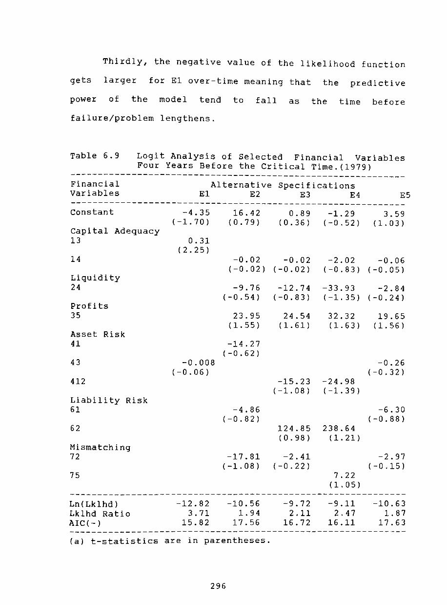
Thirdly, the negative value of the likelihood function

gets larger for E1 over-time meaning that the predictive

power of the model tend to fall as the time before

failure/problem lengthens.

Table 6.9 Logit Analysis of Selected Financial Variables Four Years Before the Critical Time.(1979)

------------------------------------------------------------Financial Variables

Alternative Specifications El E2 E3 E4 E5

------------------------------------------------------------Constant

Capital Adequacy 13

14

Liquidity 24

Profits 35

Asset Risk 41

43

412

Liability Risk 61

62

Mismatching 72

75

Ln(Lklhd) Lklhd Ratio AIC(-)

-4.35 (-1.70)

0.31 (2.25)

16.42 (0.79 )

0.89 -1.29 3.59 (0.36) (-0.52) (1.03)

-0.02 -0.02 -2.02 -0.06 (-0.02) (-0.02) (-0.83) (-0.05)

-9.76 -12.74 -33.93 -2.84 (-0.54) (-0.83) (-1.35) (-0.24)

23.95 ( 1 . 55)

-14.27 (-0.62 )

24.54 (1.61 )

32.32 19.65 (1.63) (1.56)

-0.008 -0.26 (-0.06) (-0.32)

-12.82 3.71

15.82

-15.23 -24.98 (-1.08) (-1.39)

-4.86 -6.30 (-0.82) (-0.88)

124.85 238.64 (0.98) (1.21)

-17.81 -2.41 (-1.08) (-0.22)

-10.56 1.94

17.56

-9.72 2.11

16.72

7.22 (1.05)

-9.11 2.47

16.11

-2.97 (-0.15)

-10.63 1.87

17.63

(a) t-statistics are in parentheses.

296

Now we turn to the classification accuracy of E1 where

we aimed at minimising misclassification errors. One could

make type-I error which occurs when one classifies a

problem bank as non-problem and vice versa for type-II

error.

Table 6.10 Prediction Accuracy of the El Logit Model for 1983.

------------------------------------------------------------Cut-Off Point 0.5 0.6 0.7 0.8 ------------------------------------------------------------Type-I Error Problem Accuracy Type-II Error Non-problem Accuracy

6 . 6 ( 1 ) 93.4

4 . 7 ( 1 ) 95.3

6 . 6 ( 1 ) 93.4 9.5(2)

90.5

13.3 ( 2 ) 86.7

9.5(2) 90.5

20.0(3) 80.0 14.2(3) 85.8

------------------------------------------------------------Overall Accuracy 94.4 91.6 88.8 83.3 ------------------------------------------------------------Predicted Number Probe 14 Actual Number Probe 15 Predicted Number NonProb.20 Actual Number NonProb. 21

14 15 19 21

13 15 19 21

12 15 18 21

----------------------~----------------------------~~~------

Table 6.11 Prediction Accuracy of the E1 Logit Model for 1982.

Cut-Off Point

Type-I Error Problem Accuracy Type-II Error Non-problem Accuracy

Overall Accuracy

0.5

5 . 8 ( 1 ) 94.2 13.6(3) 86.4

89.7

Predicted Number Prob. 16 Actual Number Probe 17 Predicted Number NonProb.19 Actual Number Non-Prob. 22

297

0.6

11.7(2) 88.3 13.6(3) 86.4

87.1

15 17 19 22

0.7

1 7 • 6 ( 3 ) 82.4 22.7(5) 77.3

79.4

14 17 17 22

0.8

23.5(4) 76.5 22.7 (5) 77.3

76.9

13 17 17 22

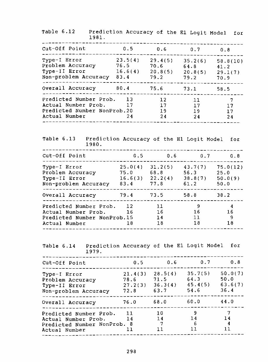
Table 6.12 Prediction Accuracy of the El Logit Model for 1981.

------------------------------------------------------------cut-Off Point 0.5 0.6 0.7 0.8 ------------------------------------------------~-----------Type-I Error Problem Accuracy Type-II Error Non-problem Accuracy

23.5(4) 76.5 16.6(4) 83.4

29.4 (5) 70.6 20.8(5) 79.2

35.2(6) 64.8 20.8(5) 79.2

58.8(10) 41.2 29.1 (7) 70.9

------------------------------------------------~------------

Overall Accuracy 80.4 75.6 73.1 58.5 ------------------------------------------------------------Predicted Number Probe 13 Actual Number Probe 17 Predicted Number NonProb.20 Actual Number 24

12 17 19 24

11 17 19 24

7 17 17 24

-----------------------------------------------------------

Table 6.13 Prediction Accuracy of the El Logit Model for 1980.

------------------------------------------------------------Cut-Off Point

Type-I Error Problem Accuracy Type-II Error Non-problem Accuracy

Overall Accuracy

0.5

25.0(4) 75.0 16.6(3) 83.4

79.4

Predicted Number Probe 12 Actual Number Probe 16 Predicted Number NonProb.15 Actual Number 18

0.6

31.2(5) 68.8 22.2 (4) 77.8

73.5

11 16 14 18

0.7

4 3 . 7 ( 7 ) 56.3 38.8(7) 61.2

58.8

9 16 11 18

0.8

75.0(12) 25.0 50.0(9) 50.0

38.2

4 16

9 18

Table 6.14 Prediction Accuracy of the El Logit Model for 1979.

------------------------------------------------------------Cut-Off Point O. 5 0.6 0.7 0.8 ------------------------------------------------------------Type-I Error Problem Accuracy Type-II Error Non-problem Accuracy

21.4(3) 78.6 27.2(3) 72.8

28.5(4) 71.5 36.3(4) 63.7

35.7(5) 64.3 45. 4 ( 5 ) 54.6

50.0(7) 50.0 63.6(7) 36.4

------------------------------------------------------------Overall Accuracy 76.0 68.0 60.0 44.0 ------------------------------------------------------------Predicted Number Probe 11 Actual Number Probe 14 Predicted Number NonProb. 8 Actual Number 11

10 14

7 11

9 14

6 11

7 14

4 11

------------------------------------------------------------

298

These results are based on specification E1 and are

reported in tables 10-14. Most previous studies assign a

aut-off point of 0.5 for the likelihood of failure/problem.

Nevertheless, in the present study, we have estimated the

classification accuracy for different cut-off points. There

are several interesting findings which is worth to be

mentioned.

Firstly, the overall accuracy of E1 is superior to the

other specifications at different cut-off points. For

instance, at the 0.5 (50%) cut-off point conventionally

used in most studies, the type-I error for the E1 logit

estimation for 1983 is 6.6% which is equivalent to a

failure/ problem accuracy of 93.4%. Moreover, type-II error

is 4.7% so that the nonfailure/nonproblem accuracy is 95.3%.

Thus, the overall accuracy of this model is 94.4% which it

is quite acceptable.

Secondly, we observed that the overall accuracy

decreases as we increase the cut-off point from 0.5 to

higher restrictions. For instance, the overall accuracy for

El for 1983 at 0.6,0.7, and 0.8 cut-off value

88.8%, and 83,8% respectively.

is 91.6%,

Thirdly, we observe that the overall accuracy of the

model decreases as we attempted to predict problems with

data before the critical time. The overall accuracy at 0.5

fall to 89.7% in 1982, 80.4% in 1981, 79.4% in 1980, and 76%

in 1979. Indeed, type-1 errors have risen from 6.6% in 1983

299

to 21.4% in 1979. Similar deterioration is observed with

respect to type-II errors as they went from 4.7% in 1983 to

27.2% in 1979.

In view of the overall prediction accuracy of

specification El over the years under examination and in

comparison with other empirical studies on the subject, 8

these results should be considered as highly satisfactory.

These econometrics results confirm the view that the

failure of some financial institutions in Chile would have

been anticipated before its critical time in 1983 with an

acceptable degree of confidence. Indeed, it was seen that

the model was predicting these failures with a lead time of

four years.

We can estimate the E1 equation using quarterly data for

each year and from there to obtain the ex ante quarterly

probability estimates to construct a quarterly

classification of financial institutions. These estimates

will be used as the dependent variable of the macromodel and

the moral hazard model in chapters 7 and 8 respectively.

Once the financial institutions have been classified

either into a failed/problem and nonfailed/nonproblem group

in each quarter for the five year period we can proceed to

test two competing hypothesis which may explain the

financial difficulties experienced by Chilean banks. In

chapter 7 and 8 we will estimate a logit model with

quarterly macroeconomic and microeconomic data.

300

Endnotes.

(1) After the banking crisis of 1983, the chilean banking authorities improved the mechanism of loan classification in terms of risk and the classification and related risk for different financial institution was agreed in 1987 to be in the public domain.

(2) Appendix 1 provide an exhaustive list of the chilean financial institutions and its classification.

(3) This index was calculated by the magazine estrategia. It is a general index composed by four financial ratios: profitability, capital adequacy, liquidity, and asset quality. The index was 70, 68, 60, and 59 for foreign banks during 1980, 81, 82, and 83 respectively. Whereas domestic banks showed an index values of 69, 66, 58, and 40.3 for the same period of time.

(4) The data have been taken from the monthly reports of the Superintendencia de Bancos de Chile. This reports include bank balance sheets and income statements as well as information of the health of the financial system. The data quality and reports improves considerable from 1982 onwards.

(5) The testing of macroeconomic and determinants of problem/failure will be reported in chapter 7 and 8.

microeconomic as carried out and

(6) However, capital adequacy is not completely within the control of bank managers. This variable is determined by the bank legislation which tend to inforce certain minimum limits. Nevertheless, still some discretion is left to banks in this respect.

(7) The result of separate regressions for variables 13 and 43 are reported in appendix 5.

(8) Similar results in terms of overall prediction are obtained from other empirical studies. For example, Barth, Brumbaugh, and others (1985) reported an overall prediction accuracy of 87% at cut-off point of 0.5 for Thrift Institution failures. Also, Martin (1977) reported accuracies around 90% for failure and non-failure bank. Although his result assumes a cut-off point of 0.0041, the sample proportion failure. That is the cut-off point assumes a priori probability of group membership equal to the sample frequencies and equal misclassification cost.

301

Chapter 2 ~ Bank Failures in Chile: The Role Qf Macroeconomic Factors.

(7.1) Introduction.

The purpose of this chapter is to re-assess and to

examine the issues related to the bank failures/problems of

1982-83 and to evaluate the importance of the economic

recession and the role played by some key macroeconomic

prices which exhibited severe misalignment and could have

affected the performance of the banking system. It is shown

the inconsistency of macroeconomic policy and external

shocks produced a boom-bust economic cycle and coincided

with the rise and fall of the Chilean banking system. In

effect, bank failures/ problems were preceded by a sharp

fall in output. Although the evidence on the link between

the general economic climate and the collapse of the

banking system is irrefutable as a first approximation, its

empirical validity need to be assess.

This chapter will provide a discussion of the boom-bust

cycle hypothesis and its evaluation for the case of Chile

during the period 1977-81 and 1982-83 as part of sections I

and II. In addition, it will be shown that performance of

the banking sector was correlated with the macroeconomic

environment. Finally, section III provides a thorough

discussion of the model specification and estimation. At the

same time, I report the econometric results and its

interpretation.

302

(7.2) Macroeconomic Instability and Banking Crisis.

The central tenet of the hypothesis to be tested in this

chapter relates the banking crisis with changes in the

general economic conditions and the misalignment of some key

macroeconomic prices. In general, it could be argued that

macroeconomic shocks, including external exogenous

disturbances (deterioration of the terms of trade, and

rising world interest rates) and policy inconsistencies a

fixed exchange rate regime with backward-looking wage

indexation scheme, and/or significant fiscal deficit, trade

and financial liberalisation with no supportive

macroeconomic policies) can generate significant

misalignment of key macroeconomic prices

the real exchange rate, high real

overvaluation of

interest rates,

overvaluation of stock prices, rising real wages) which may

increase the proportion of non-performing loans and lead to

bank failures. Similarly, serious output downturns can

equally affect the values of bank assets and the likelihood

of bank failure.

There are several episodes described in the literature

which fit this hypothesis. For instance, Kindleberger (1986)

and Keran

comparing

(1986) subscribed to this hypothesis

bank failures in the 1930's with the 1980's

when

for

the US banking system. Indeed, the evidence

indicates that 6.704 (9.2% of total banks)

failed during the period between 1930-33.

303

from the US

of the banks

Although the

number of failures fell in the years 1934-1978 to only 689,

the evidence for the 1980's suggests a significant increase

in the number of failed banks from 10 in 1981 to 120 in

1985. Although most of these financial institutions were

concentrated among small farm and energy banks, the

failures of the Continental Illinois in 1984 (8th largest

bank in the US), The First Pennsylvania in 1980 (23rd

largest), and the Seafirst in 1983 (29th largest) were a

matter of concern in the banking system as a result of their

significant size.

According to Kindleberger and Keran major shocks to

relative prices produced a deflationary impact in both

periods. They found that during the 1980's there was a major

decline in the relative price of farm land as much as in the

1920's and the 1930's. The collapse of land prices during

the 1980's was accompanied by the effects of major oil

shocks during the late 1970's. Similarly, they show that

these two periods exhibited a substantial increase in real

interest rates and noted that they stayed high longer in the

1980's than in the 1930's. It was certainly a major reason

behind rising non-performing loans and subsequent bank

failures.

Finally, a major dollar appreciation analogous to the

one of the 1980's was present during the 1930's. A real

appreciation was bound to generate distortions in both

production and consumption as well as wealth effects by

304

turning domestic relative prices in favour of non-tradables

and away from tradables. Those financial institutions with a

high share of their capital in loans to those companies in

the tradable sector will be at risk. However, even if the

banks' portfolio is weighted towards profitable activities

at the given relative prices, still there is the danger of a

time bomb if the real appreciation is not sustainable in the

long-run and the adjustment take place initially via output

deflation. Thus, Kindleberger and Keran attached a great

importance to relative price shocks on the banks solvency.

Similarly, Sundararajan and BaliHo (1990) examines the

recent experiences with banking crisis in seven countries

(Argentina, Malaysia, Phillipines, Spain, Thailand, Uruguay,

and Chile) with a focus on the linkages between

macroeconomic conditions, financial liberalisation, and

banking failures. In spite of the cross-country differences

they found common causes to explain the episodes of banking

crisis (failures). Their study demostrated that the episodes

of banking crisis (defined as a generalised solvency

problems among banks due to an increase in non-perfroming

loans, and losses due to foreign exchange exposure, interest

mismatch, contingent liabilities, and decrease in the value

of investment) occurred following a shock to the

macroeconomy, and reinforced the subsequent decline in

output. In most countries in the sample, the banking

failures took place after a sustained period of rapid

expansion in output following major fluctuations in relative

305

prices and general business conditions. After major external

shocks, and gross policy inconsistencies, sharp adjustments

in real exchange rate, real interest rates, and stock price5

affected the economy's performance, ouput growth, and the

soundness of financial institutions. Although the effect of

macroeconomic instability appears to be central in their

argument, it was equally accepted that a more gradual

financial liberalisation, vigilant bank supervision, and a

well designed prudential regulation would limit the

magnitude of bank failures (crisis) and help to reduce the

vulnerability of the banking system to the shocks from the

macroeconomy.

With specific reference to the Chilean banking crisis,

Moreno and Perez (1983) have also provided a testimony to

the importance of macroeconomic instability on bank

failures. On this account, they argued that the collapse of

the banking system had little to do with financial

liberalisation and inadequate bank legislation. Moreover,

they maintained that no banking system would be able to

withstand a fall in GDP and the level of interest rates a c o

the one observed during 1982-83. External shocks combined

with inadequate macroeconomic policies, in particular the

exchange rate policy, tended to amplify the economic cycle

in the open economy. In effect, sharp increases in lending

interest rates after a long history of negative rates, the

introduction and later on the abandonment of a fixed

exchange regime, and the burst of the stock exchange bubble

306

all contributed to major variations in the overall economic

environment and consequently the solvency of the banking

system. In their own words, they blame the authorities for

inadequate management of macroeconomic variables,

particularly the exchange rate, and interest rates,

misalignments which amplified the economic cycles and hence

the financial condition of several financial institutions.

As we will see in section 3, although this description

fit extremely well to what happen in Chile during the period

of 1977-83, this in itself represents no direct empirical

test on the influence of these set of variables on

likelihood of bank failure/problem.

There are two interesting papers which attempted to

evaluate the influence of macroeconomic variables on bank

failures. Bovenzi and Nejezchleb (1985), for instance,

studied the relationship between the rate of bank failures

and macroeconomic conditions in the US using quarterly data

from 1970 through the first quarter of 1984. They maintained

that during an economic downturn, fixed loan commitments

established previously under more auspicious economic

circumstances become difficult to fulfil so that an

increasing number of borrowers will be forced to default.

Thus, after some specific time lag an increasing share of

non-performing loans and falling bank profits would result

in higher bank failures.

307

They studied bank failures by using alternative proxies

for overall macroeconomic conditions among them real GNP

growth, re.:tl intere5t rates, unernployment rate, and the

corporate debt burden. The evidence indicates that although

the relationship between real GDP and the bank failure rate

was significant it explained only 10% of the variation of

the failure rates.

With reference to the unemployment rate, this proxy

accounted for 56% of the total variation in bank failures.

At the same time, given that unemployment rate tend to lag

general economic conditions, it lead the failure rate by one

to three quarters which is shorter than the GDP regressor.

Similar results are found for the interest rate on the

failure rate with 50% prediction accuracy after about a

five-quarter lag. On this account, high business failure

rates and loan losses seem to be correlated with real

interest rate movements.

The regressor measuring the corporate debt burden

represented a more direct measure of the ability to repay

debt measured by the ratio "after-tax nonfinancial corporate

debt service to nonfinancial corporate cash flow. It

exhibited a better fit with 62% of the variation of bank

failure rates. Although these variables were statistically

significant, macroeconomic conditions explained only a part

of the increase in the rate of bank failures. The estimated

equations did in fact overestimate bank failures during

1981 but underestimated failures from that point on. I

308

Similarly, Amos (1992) found that for periods with high

rates of bank closings were characterised by the economy

growing below its historical trend. The evidence from his

time series regression analysis using sample data for the

US bank closing between 1934 and 1988 tend to support his

assertion. The effect of current real GNP on the number of

closing banks was statistically significant and with a

positive sign as expected. The effect of lagged GNP on the

dependent variable was insignificant. The regression also

included the money supply as an additional explanatory

variable. The money supply with one year lag was significant

although with a positive sign. The overall goodness of fit

of the regression was 0.95.

Although this empirical approach is useful for a large

sample with aggregate data, there are certain limitations

for the study of the Chilean bank failures. Firstly, bank

failures in Chile were mostly concentrated in a single year,

that is 1983. Secondly, the purpose of this study is to

estimate the ex ante probability of bank failure during the

period of liberalisation. In other words, the likelihood

previous to the critical year of 1983.

With this purpose in mind, I have constructed and

estimated a logit model for panel-data in order to directly

test the explanatory power of macroeconomic variables on the

likelihood of bank failure/problem. Partly, I expect that

some of these systematic factors could explain the collapse

of the banking system in Chile.

309

(7.3) The Boom-Bust Economic Cycle: ~ Hacloeconomy in Chile.

(7.3.1) The Chilean Economy and the Main Policy Reforms.

Before we proceed to assess the performance of the

economy it is necessary to give a brief account of the main

reforms introduced prior to the deterioration of the

macroeconomy and the crisis of financial institutions in

1982-83 period.

As we have seen in Chapter 1 and 2, previous to the

reform period which started in September 1973 inmediately

after the military coup which overthrew Allende's socialist

government, the economy was pursuing an inward-looking

strategy for development which relied exclusively on

intensive and extensive government intervention in all the

spheres of the economy. The trade bias was towards the

import substitution sector by means of tariff and non-tariff

barriers across sectors , export taxes, and an over-valued

exchange rate. In addition, the financial system was subject

to a wide range of instruments to direct credit towards the

priviledged industries and to finance the fiscal deficit.

The imposition of high reserve requirements, ceilings on

interest rates, selective credit controls and rationing was

conducive to the repression of the financial system. The

economy was immersed in a large macroeconomic disequilibrium

and a modest growth as compared with its historical standard

310

and with those economies pursuing outward looking

strategies. This became even more acute during Allende's

populist government in 1970-73.

stabilisation and liberalisation policies were

implemented from late 1973 onwards in order to correct the

large macroeconomic disequilibrium and to enhance the rate

of economic growth. The economic reforms contained three

main prinCiples. Firstly, the transformation toward an

outward-looking economy fully integrated with international

capital and goods markets with a dominant role assigned to

the private sector in a competitive market economy was

regarded to be conducive to higher growth rates.

Secondly, the credibility and success of trade and

financial liberalisation required that they were preceded

by macroeconomic stabilisation, particularly in view of the

high inflation rate.

Thirdly, the question of the dynamics of liberalisation

suggested that the sequence and timing should follow a

specific order. As I have shown in chapter 2, there was a

consensus among the experts that trade and domestic

financial liberalisation should come before the opening of

the capital account of the balance of payments.

According to these prinCiples, the reforms started with

an orthodox stabilisation strategy which emphasised the

control of the money supply and a consistent reduction in

311

1 the fiscal deficit. The fiscal shock included large cuts in

government expenditures, temporary increases in income

taxation and the replacement of sales tax for a 20% VAT,

full indexation of the tax system, integration of personal

and business income tax, and the elimination of the

remaining tax exemption and subsidies. The shock treatment

also included a tight monetary policy although some

monetarist like Harberger (1982) and a critic such as Foxley

(1983) do not accept the view of a nominal monetary crunch.

Specifically, the evidence indicates that the percentage

increase in M2 was still high at 257%, 166%, and 130% in

1975, 1976, and 1977 respectively. Whereas the percentage

increase in the GOP deflator was 328%, 252%, and 103% for

each three successive years. Similar results are obtained

between the period of 1977 and 1980 but with the added query

that the nominal growth of M2 was still above the inflation

rate. Therefore, there was no genuine nominal monetary

crunch during the second half of the 1970's but it certainly

was one in real terms between 1975 and 1976. This apparent

closed economy monetarism was pursued with some relative 2

success until early 1978.

Given the greater openess of the economy, the modest

progress made on inflation, the contractionary effect of the

orthodox measures in particular during 1975, and the

increasing role played by exchange rates in expectations

formation of tradable prices the authorities advocated an

exchange rate stabilisation approach as an anti-inflation

312

policy. The academic and practical acceptance of the

monetary approach to the balance of payments made readily

acceptable two important tenets of this approach.

Firstly, the law of one price will hold so that domestic

inflation will rapidly converge towards world inflation plus

the expected rate of devaluation. And secondly, under a

fixed or preannounced exchange rate monetary policy will be

endogenous. That is changes in the quantity of money will

only affect the composition of the base money as the

increase in domestic credit will be offset by a fall in 3

international reserves.

In theory the exchange rate stabilisation approach

involves the public announcement of a fixed schedule of the

future nominal exchange rate over a specified period which

is credible by the rational agents. Moreover, this anti-

inflationary policy has been part of an overall

stabilisation and growth strategy comprising both trade and

financial liberalisation. According to Blejer and Mathieson

(1981) the potential stabilising effects of preannouncing

the exchange rate will have two fundamental effects on the

rate of inflation: a direct impact on expectations, and an

indirect effect via product and financial markets.

With reference to the former, a credible announcement of

the future path of the nominal exchange rate in an open

economy consistent with lower inflation should help to

reduce the public's expectations concerning future

313

inflation. In this scenario nominal claims between firms and

managers should be in line with lower expected inflation.

Moreover, if nominal yields on financial assets are market

determined and reflect the expected rate of inflation, then

lower inflationary expectations should raise the demand for

money (currency holdings), and hence lower price increases

for a given monetary expansion and income growth.

With respect to the indirect effect, the elimination of

trade restrictions (tariffs) will produce both a price

differential, and a potential profits which will not be

arbitraged away unless they persist over time to recover the

high initial cost of entry. Thus, a predictable future path

of the exchange rate will help to curb inflation by

enhancing price arbitrage.

A formal "tablita" was introduced in February 1978

consisting in a preannounced future rate of devaluation set

below the domestic inflation rate and at a decreasing rate.

In June of 1979, this active crawling peg exchange rate was

transformed into a fixed exchange rate regime as the US

dollar was fixed at $39 Chilean pesos. However, it was

abandoned three years later with the forced devaluation of

June 1982 because of increasing overvaluation of the

exchange rate.

On the liberalisation front, the first step was the

deregulation of nearly 3000 prices and the privatisation of

state-owned firms, including financial institutions. The

314

liberalisation also included trade reforms with the removal

of quotas and the reduction of the average and range of

nominal tariffs. From early 1976 onwards, a new set proposal

for tariff reduction was proposed and by late 1977 a

gradual attainment of a uniform tariff of 10% was agreed.

This schedule was completed in June of 1979.

With respect to financial liberalisation, interest rate

controls were removed for non-bank financial institutions

and banks in May and October 1974 respectively. In addition,

entry barriers to new financial institutions including those

applicable to foreign banks were lifted.

On the external side of the financial market, in

September 1977 commercial banks were allowed to borrow from

international markets under article 14 of the exchange law

although with a monthly flow limit of 5% of capital and

reserves. A stock limit of 25% under articule 14 was

introduced in January 1978 and raised two months later to

160% of capital and reserves. The relaxation of controls on

capital inflows went further and by 1980 all monthly limits

were lifted. In May 1982 banks were allowed to obtain

external credit with maturities below 2 years and a reserve

requirement of 20%.

In general and as also argued by Mckinnon (1982), the

stabilisation and liberalisation strategy followed what was

accepted at that time as the optimal sequence and timing of

reforms. However, the economic collapse of 1982 meant that

315

the liberalisation reforms were reversed by the in

trade tariffs from 10% to 18% and the intervention of

financial institutions as part of the rescue package of the

financial system in Chile. At the same time, the crisis of

1982 and the emergency measures taken by the authorities 4

meant increases in the fiscal deficit and inflation rate.

(7.3.2) The Boom-Bust Economic Cycle of the Chilean Economy: The Appraisal.

The central idea is that the introduction of exchange

rate management, in particular the active preannounced

crawling peg and which ultimately ended in a fixed exchange

rate regime as an anti-inflationary tool during trade and

financial liberalisation was likely to generate a boom-bust

cycle as some key relative prices became misaligned and then 5

return to their long run equilibrium. It could be argued

that the path from the economic and banking boom in 1977-81

to the economic and banking bust in 1982-83 had its sources

in what happened to key relative prices specially the real

exchange rate, the real interest rate, and the real wage

rate.

Let's first examine the data for the economic boom

between 1977-81 from table 1. The evidence portrays some

impressive results from the reforms undertaken, in

particular in terms of export volumes at least up to 1980

and capital inflows, the improvement of overall balance of

316

6 payments and the surplus in the fiscal budget. At the same

time, we observe important gains in the control of the rate

of inflation although achieved gradually and at a very high

cost in terms of unemployment. Indeed the evidence indicates

that the percentage inflation rate (as measured by the CPI)

went from nearly 500% in 1974 to less than 10% in 1982,

consistent with the astonishing figure of 22% unemployment

rate during 1982 and 1983.

Table 7.1 Indicators of the Economic Boom, 1977-81. ------------------------------------------------------------

77 78 79 80 81 ------------------------------------------------------------GDP Growth(a) GDP Tradables(b) Non-Tradables(c)

Absorption(d) Fiscal Deficit/GDP Unemployment Rate(Nac. )

Overall Balance Payments(US$) Trade Balance Exports(FOB) Imports Capital Inflows(e)

Number of Bankruptcies

9.8 7.8 9.4

14.2 1.8

13.2

118 4

2186 2151

607

224

8 . 2 4.5 9.6

9.7 0.8

14.0

712 -426 2460 2886 1959

312

8.3 7.0 9.9

10.9 -1.7 13.6

1047 -355 3845 4191 2255

344

7.8 5.2 9.7

9.3 -3.1 11.8

1244 -764 4705 5469 3242

415

5.5 2.9 5.4

10.9 -1.7 11.1

67 -2677

3837 6513 4768

431 ------------------------------------------------------------Source:Banco Central Chile,Monthly Bulletin,Various Issues

Banco Central Chile, National Accounts 1974-85. ECLA, Statistical Yearbook, Various Issues.

(a) All GDP data at 1977 prices. (b) Includes agriculture, forestry, fishing, mining, and manufacturing. (c) Includes construction and services. (d) Absorption includes private and public consumption plus total investment. (e) Long and short term flows.

317

With respect to GDP growth, the data shows that the

average annual rate of GDP growth was nearly 8% between 1977

and 1981. Although this figure exceeded Chile's historical

standard it is below the growth rate of 1928 which was 7

24.3%. Surprisingly, the sectoral GDP growth shows that non-

tradables grew at a much faster rate than the tradable

sector contrary to the intention of trade reforms. In fact,

for the period of exchange rate stabilisation strategy, non-

tradables grew at an annual average of 8.8% as compared to

5.4% for the case of tradables. It is remarkable that growth

of GDP took place under a significant overvaluation of the

peso. This performance and the relative boom between the two

sectors can be explained by the pattern of some key prices

in the Chilean economy, in particular the appreciation of

the real exchange rate, the increases in real wages, the

transitory reduction in real interest rates, and the

unsustainable rate of capital inflows which made possible

both rising expenditures to sustain the economy's growth

rate given the relative prices, and to masked the sustained

deterioration of the trade balance particularly in 1981.

The data from table 2 shows the movements in three

macroeconomic prices during the period of preannounced

exchange rate.

318

Table 7.2 Key Prices in Chile between 1977-1983. ------------------------------------------------------------

77 78 79 80 81 82 83 ------------------------------------------------------------Nominal InterestR(a) 98.1 Real Interest RT(b) 90.0 Real Interest R(c) 43.9

63.3 52.7 34.1

49.2 39.4 16.2

39.0 10.7 11.0

42.5 18.3 31.7

49.6 35.7 54.5 46.1 31.2 14.3

Real Wages(d) 72.5 82.9 92.0 100.0 108.9 108.6 97.1

Real Exchange Rate(e)83.6 100.0 Real Value Stock(f) 46.9

93.8 80.1 54.2 100.0

70.2 80.4

76.7 82.3 61.2 39.2

Sources:Banco Central Chile,Monthly Bulletin,Various Issues Edwards (1986) for effective real exchange rate.

(a) Nominal lending rate on 30-89 days loans. (b) Ex post real lending rate was estimated as {[(1+i)/(I+PTI)]-I}*100 where i and PTI are nominal lending rate and changes in tradable price index. (c) Ex post real lending rate estimated from nominal rate deflated by the cpr which includes non-tradables. (d) Nominal index of wages and salaries deflated by CPl. 1980=100 (e) This index was constructed as the ratio of a weighted average of WPI of Chile's 10 main partners in $ to Chile's CPI.1978=100 (f) stock price index at constant price, IGPA. (1980=100)

Although the appreciation of the real exchange rate is

seen as a major factor in most of the interpretation of the

crisis of 1982-83, there is no consensus on what caused the

systematic appreciation of the real exchange rate of more

than 30% between 1978 and 1981. The most obvious factor in

the appreciation of the real exchange rate was the

introduction between February 1978 to May 1979 of a

preannounced declining rate of monthly devaluation set below

the previous month's domestic inflation rate and the

subsequent fixing of the nominal rate at $ 39 pesos per

dollar until June 1982.

319

The data on domestic and international inflation plus

devaluation from table 3 indicates two things: Firstly, the

introduction of the "tablita" and fixed exchange regime

coincided with a significant difference between domestic and

US inflation rate. Under every definition of a real exchange

rate this would have meant beyond any doubt an initial

although transitory declining value for the real exchange 8

rate under the law of one price.

Secondly, the data also show however that between 1978-81

domestic inflation failed to converge rapidly enough and

avoid a permanent overvaluation.

Table 7.3 Indicators of Convergence (%) ------------------------------------------------------------

77 78 79 80 81 82

Real LIBOR(a) - 0.7 1.6 -10.6 1.7 8.7 26.2 LIBOR(b) 6.1 8.8 12.1 14.2 16.8 13.2 Spread lending-LIBOR(c) 50.6 40.4 25.9 28.5 30.4 -23.7 Spread deposit-LIBOR(d) 13.9 23.3 12.7 20.1 20.8 -30.8

Devaluation 60.5 21.4 14.9 0.0 0.0 88.3

US Inflation (CPI) 9.1 13.3 12.4 8.9 3.9 Chile Inflation(CPI) 91.1 40.4 33.0 35.0 19.6 9.9 ------------------------------------------------------------Source:IMF,International Financial Statistics,Various Issues

(a) Nominal LIBOR deflacted by the variation of dollar price of Chilean tradables (b) Nominal LIBOR is the three months Eurodollar rate. (c) Calculated as {[(1+i)/(I+I)(I+e)]-1}*100 where i,I, and e are nominal domestic lending, nominal LIBOR and the expected devaluation rate respectively. (d) Calculated as {[(l+i)/(l+I)(l+e)]-l}*lOO where i nominal deposit rate.

320

Therefore the real exchange rate appreciation was not

transitory and became even worse after the exchange rate was

fixed. The existence of full wage indexation to compensate

lagged changes in CPI introduced as part of the labour law

in late 1979, and the fact that many non-tradables prices

were fully indexed backward made the dynamic path of

tradables and non-tradables prices inconsistent. In effect,

as a first approximation and according to the real wage

index in table 2, wages increased by 26% in real terms

between 1978 and 1981 and coincided with the 30% real

appreciation. Thus, the exchange rate regime became

inconsistent with a wage indexation.

However, as we have seen from tables 1 and 2, the real

appreciation of the exchange rate also coincided with

significant increases in private sector expenditures

averaging 11% per annum, exports rising from U$ 2.186

millions in 1977 to U$ 4.705 millions in 1980, falling

unemployment rates, and substantial increases in the stock

price index by 53% in real terms between 1978 and 1980.

Although many proponents among them Corbo (1985, 1987),

Edwards (1986,1989), Harberger (1985a,1985b, 1987), and

Dornbusch (1985) accepted the inconsistency argument, they

viewed the appreciation of the real exchange as a

consequence of the increase in private sector expenditures

on both tradable and non-tradables financed by large and

unsustainable capital inflows as well as domestic borrowing 9

but for different reasons.

321

According to Corbo (1985,1987), the active crawling peg

and fixed exchange rate mechanism combined with the gradual

lifting of restriction on foreign indebtness encouraged a

significant rise in the rate of capital inflows as a result

of the increasing spread between domestic and foreign

interest rates. This differential made it quite attractive

for foreigners to bring capital into the economy and for

nationals to borrow from abroad. These spreads were large

even in the period where the exchange rate devaluation was

pre-announced and fixed later on. The data from table 1 and

3 shows that the spread between nominal peso lending rate

and the nominal LIBOR in 1977 was 50.6 and remain high even

in 1979 at 28.5, and capital inflow went from U$ 607

millions in 1977 to U$ 2.255 millions in 1979. Similar

observations can be drawn from the spread between nominal

peso deposit rates and the LIBOR.

Further relaxation of controls on capital inflows and

the portfolio disequilibrium encouraged even more the inflow

of capital and hence pushing the nominal domestic interest

rate further down. According to the evidence the nominal

lending rate fell from 63.3% in 1978 to 49% and 39% in

1979 and 1980. But even more significant was the reduction

in real interest rates which according to table 2 (lending

rate deflated by changes in CPI) came down from 34% in 1978

to 16% and 11% in 1979 and 1980 respectively_ Similar

results were obtained when using the change in the tradable

price index as a deflator.

322

It could be argued that the fall in real interest rates

partly reflected increasing arbitrage between nominal

domestic and foreign rates, although it remain fairly high

as a result of Central Bank sterilisation and imperfect

asset substitution. Similarly, the evidence also show that

international influences were also important in the drop in

real lending interest rates, in particular the dollar

depreciation in world markets and the effect on the dollar

price of chilean tradables.

Table 7.4

NEFF EXR REFF EXR(b)

US Exchange Rates and Chi Ie. (a)

77

124.0 117.6

78

111.2 108.6

79

108.3 108.9

Tradable Prices for

80

108.0 110.0

81

121.1 125.2

82

135.2 134.7

Tradable Prices(c) 183.5 196.4 246.5 296.8 297.3 266.7

Source:IMF,International Financial Statistics,Various Issues ECLA, Statistical Yearbook, Various Issues

(a) Indices were constructed with 1970=100 (b) Nominal effective exchange rate, NEFF EXR, is deflated by WPI (c) The average dollar price of tradab1es are calculated as follows 0.5 Px + 0.5 Pm where Px=unit value of exports and Pm=unit value of imports.

According to the theory an appreciation of the US dollar

with respect to other major currencies clearly will cause

the dollar price of homogeneous traded goods to fall. It

follows that for a small economy pegging to the dollar an

appreciation of this currency will be subject to a

deflationary pressures transmitted by changes in the dollar 10

price of its tradables.

323

If we compare the movements of the indices between the

real and nominal exchange rate with the dollar price of

tradables in table 4, we see that there was a dollar

inflation between 1977 to 1979 as the accumulated

appreciation in these 3 years was 7.4% in real terms. This

coincided with sharp rise in tradables prices by 34.3% and

thus the reduction in real interest rates over the

same period.

Therefore, Corbo's portfolio disequilibrium triggered by

the exchange rate regime and the subsequent massive inflows

of capital responding to the lending-libor spread explained

the fall in nominal and in particular real interest rates

and hence increasing permanent income and expenditures.

According to Dornbusch (1985), in an intertemporal model

consumption and investment could also be determined by the

appreciation of the exchange rate. He asserted that the

temporary overvaluation induced an intertemporal

substitution accelerating the purchasing of durable goods 11

and generating a growing current account deficit. Rising

expectations that the overvaluation and the exchange regime

will not last clearly provoked the import surge

particularly in 1981 as shown in table 1.

The data from table 1 shows that the rate of absorption

exceded the GDP growth and the current account deficit was

getting larger. This demostrates the growing excess demand

for non-tradables and tradables. For instance, in 1980 and

324

1981 private absorption increased at 9.3% and nearly 11%

whereas GOP was growing much slower at 7.8% and 5.5% only.

Thus, a market clearing appreciation was required to clear

the excess demand for non-tradables (via nontradable prices)

whereas the excess demand for tradables was reflected in a

mounting external deficit. The real exchange rate reached

its lowest value during 1981 with a nearly 30% overvaluation

with respect to 1978 and the current account deficit was

becoming too large with U$ 2.677 millions.

In 1981 the nominal peso lending rate was beginning to

rise in spite of the massive inflows of capital during the

last three years from 39% in 1980 to 42.5% as shown by

table 2. At the same time, table 3 shows the lending-LIBOR

spread was getting larger as it moved from it lowest value 12

of 22.2 in 1979 to 25.5 in 1981. However, the rise in real

interest rates was even larger as it went from its lowest

value of 11% in 1980 to 31.7% and 31.2% in 1981 and 1982

respectively. In those two years, the real lending rate for

tradables also rose from 10.7% in 1980 to 18.3% and 54.5%.

In spite of the significant increases in real interest

rates and the deterioration of the world economy in the form

of a reduction in the terms of trade and increasing nominal

LIBOR during 1981, private sector absorption continued

growing well beyond GOP growth. This can be explained by the

lasting effects of the stock market bubble which generated

wealth effects and increasing consumption expenditures.

325

Moreover, the stock market bubble overpriced private sector

gurantees and collaterals, enabled firms to borrow

additional resources from banks, thus making banks more 13

vulnerable to any change in market conditions. At the same

time, the expectations of the unsustainability of the

exchange rate regime could have accelerated the purchase of

durable goods and enlarged the current account deficit.

By 1982 the rate of capital inflows started to

deccelerate so that the amount of external financing came

down to U$ 2.327 millions in 1982 and only U$ 520 million in

1983 as shown in table 5. Morover, nominal and real lending

rate was reaching in 1982 almost 50% and 32% respectively.

Given that monetary policy was endogenous then the decline

in capital inflows produced a decline in the monetary base

via changes in international reserves and a rise in nominal 14

interest rates to clear the money market.

Equally the evidence from table 2 also indicates that

the stock market price felt by more than 38% between 1980

and 1982. The decline in expenditures reduced the demand for

both tradables and non-tradables. According to table 5,

absorption felt by 23.4% in 1982, and the trade balance went

from minus U$ 2.677 millions in 1981 to U$ 62 millions in

1982.

326

Table 7.5 Indicators of the Economic Bust of 1982-83. ------------------------------------------------------------

1982 1983 ------------------------------------------------------------Real GOP Growth GDP Tradables GDP Non-tradables

Absorption Fiscal Deficit/GDP Inflation Rate Unemployment Rate

Overall Balance Payments(US$) Trade Balance Exports Imports Capital Inflows

Number of Bankruptcies

-14.1 -12.4 -15.1

-23.5 2.3

10.0 22.1

-1165 62

3706 3643 2327

810

-0.7 1.6

-7.2

3.8 27.1 22.1

-541 986

3831 2845

520

375 ------------------------------------------------------------Source: Banco Central Chile,Monthly Bulletin,Various Issues

ECLA, Statistical Yearbook, Various Issues.

Clearly, the decline in expenditures reduced the demand

for traded goods improving the trade balance. At the same

time, the reduction in expenditures and thus the demand for

non-traded goods created now an excess supply. Unlike the

opposite case of 1978-81, now the market for non-tradables

needed a rise in the real exchange rate to restore the

equilibrium with a lower level of expenditures and external

financing. As a result of the Chilean labour law which

introduced full backward wage indexation non-tradable prices

were inflexible downwards. As we have seen already from

table 2, real wage were in 1981 nearly 9% above the wage

rate of 1980 and remain so in 1982. At the same time, the

continous dollar deflation of tradable prices as a result of

the dollar appreciation and the fixed exchange rate regime

327

imposed a severe adjustment in the nominal price of non-

traded goods to restore the real exchange rate to

equilibrium consistent with the new level of expenditures,

As Sjaastad (1982) correctly put it these two features were

like imposing two inconsistent numeraires in the economy so

relative prices did not adjust and the adjustment was in

quantities. In consequence, the adjustment to lower

expenditures was in terms of a severe output decline and

increases in unemployment.

As Corbo (1985,1987) and other commentators of the

Chilean economy, in particular Edwards (1986) and Harberger

(1985,1987), agreed on the elimination of wage inflexibility

and a devaluation in late 1981 should have been the

appropriate response to the fall in capital inflows and

expenditures rather than relying on the governments' belief 15

in the economy automatic adjustment.

According to table 5 output felt in two successive

years. In 1982 and 1983, the GDP growth rate was 16

with -14.1% and -0.7% respectively. Unemployment

negative

rate and

the number of bankruptcies also shows a marked increase

reflecting the magnitude of the economic crisis. The rate

of unemployment went from 11.1% in 1981 to 22.1% in 1982 and

the number of bankruptcies almost doubled between 1981 to

1982. Moreover, as we have seen in chapter 3, the collapse

of the economy was accompanied this time by the bust of the

banking system.

328

All in all, the evidence presented tends to support the

view that the introduction of the exchange rate regime as an

anti-inflationary policy in the context of trade and

financial liberalisation was not a mistake per se if the

rate of crawl would have been much higher so as to avoid the

initial appreciation of the real exchange rate, and wages

were not indexed fully to past inflation. In effect,

Mckinnon (1981) and Blejer and Mathieson (1981) have shown

in their models that real domestic interest rates would have

been lower and the spread between domestic and world

interest rates consequently lower. Accordingly, the real

peso lending rate in Chile in 1979 and 1980 would have been

much lower and the spread smaller, capital inflows and

banks' asset expansion lower, absorption and hence the

demand pressure on traded and non-traded goods much lower.

At the same time, the equilibrating appreciation of the real

exchange rate in the face of excess demand for non-traded

goods would have been smaller so the loss of competitiveness

and profitability of Chilean tradables and the current

account deficit. Probably the path of output would have been

dominated by the expansion of tradables financed by a

greater reliance on domestic than foreign borrowing.

Although these general observations are part of an

acceptable description of the issues, the factors which

explain the appreciation of the real exchange rate are not

clear and remain a contentious issue. If we accept the

Edwards and Harberger contention that the appreciation of

329

the real exchange rate was due to an exogenous increases in

capital inflows then it follows that the hypothesis which

suggest a wrong exchange rate policy is not sustainable and

the external financial liberalisation was far too

aggressive within the gradual approach followed between 1978

to 1981.

Regardless of the debate in the determinants of the

large appreciation of the real exchange rate, the stock

exchange bubble and the fluctuating interest rates, the

facts tend to corroborate the notion that the expansion in

output was not going to last given the long and large

misalignment of some key relative prices. Given the

inconsistencies and rigidities of the numeraire, the

adjustment was going to take place via output, employment,

and increasing numbers of bankruptcies both in industrial

firms and banks.

(7.3.3) The Boom-Bust Economic Cycle and the Increase Vulnerability of the Chilean Banking System.

There is an apparent connection between the performance

of the macroeconomy and the financial system. The 1977-81

economic boom was accompanied by a significant expansion of

the financial system just as the 1982-83 economic bust

coincided with the collapse of the banking system.

330

As we have seen in chapter 3, the growth rate between

1977-81 of both the sectoral GOP (GOPfin) and bank assets

was 20.3% and 34.5% per annum respectively. At the same

time, the data showed that bank liabilities exhibited an

annual average growth rate of more than 36% over the same

period. These spectacular growth rates not only coincided

with an equally impressive growth in the economy's GOP but

also they remained above the overall growth of the economy

throughout the period in question. However, this financial

boom ended in 1982 and 1983 as the sectoral GOP felt by 4.4%

and 40.5%. This turning point was preceded by the downturn

of the economy's GOP which fell by 14.1% and 0.7% in 1982

and 1983. Although the growth rate of bank assets slowed

down slightly, it continued climbing at a faster rate than

GOP reflecting perhaps

banks' willingness to

some distress borrowing and

take a fair-bet against

the

the

government. At the same time, we do not observe a run from

the banks since the growth of bank liabilities still

exhibited positive growth rates. These observations can be

seen from figure 1 which was constructed with data from

chapter 3 and from the previous section.

331

F""II> 7 1 "'l"; '''::l . . It . Lit tJ . 8A~ K EXPA~··ISION

50 -r--' ------_.

50 ......... ~~ ....... ~ ........................................................................................................................... .. ~ .,

40 .. ····· .. ···················~~ .. ·;~~ .. ··········· .. ····2~~~\ .............................................................................. .

30 ......................................... ~~~.,L.: ....... , .................................................................... . . ---~.::~~.~--- '\'~. -

~J"" •• ___ "" •• }i.. 20 .......................... :~~ ....... -:: ................................................. :.;~~.:;.~~\: ............... p-:..: ..... :-i~ ..................... . ..,..------ ---.:., .'. /. ;"...~,

1 ~ .........• ---==..........== .• :~:~:=~~::.~~~._===:~~. --.. , ... ~ /'"

-1 0 ...................................................................................................................... ~.~:.,.:: ... :.:../-:::.:. ................... . 'W··\

-20 - ....................................................................................................................................... \\ ...................... . . \

-3 () .................................................. : ................................................................................................ \\ .............. .. \

\

····4 {) ............................................................................................... -- ...................................................... ~~ ..... ..

-5 (). -- 1 .. ·---r----:-·l .. ··-·-·~ .. ---·---·l-·-·-.. -··-.. -·· .. --'J--·- .. -.. ·-",'" ........... - ... __ ... r-

77 78 79 ~O 51 ~2 83

[~ GOP .. + -GDPFin '-7¥.- Asset '-&~-L-j(-Jb-ilil:~ ___ . .._._. ___ ._ ... _ .. _. __ . ___ ._ .. __ ._._ .. _. ___ ..... ____ ~:~_J

i- oJ'" ,.:J·_~:JL

F i rJ LJ r e 7. 2 PROFITS, Asstr ()lJALITY, At ... j[) GDP

50~-------------------""' .. --.,.-,'/

¥ 40 ..................................................................................... ····························· .. ·······:r··············· .................... . /

t'

/// 3 0 .............................................................................................................. ;..-, ................................................ .

*-..... - ./ ......,..... .• .. _ ........... -7L... --------,..t

20 .............................. ~ .• ~.;~: .................. / .......... :-:-""-:.:.:.: ..................................................................... . ./" / "".

/' / '"'-.... .. 1 0 .......... "'~ .................... ¢; ........... :.*_~:~:=:: . .z:: .. ~= ............................... .

. ;.'~ O

. ..L~ _______ ~_ ",. \

-y- ----•. ~-------\.--.---.-'*~.-

\ ~ ~

\ .. , \ ///

" .'-:":: -1 0 ........................................................................................................................... \ ....... / ..... \ .................... . .. ~IE/ '\

\ \ \ '-20 .................................................... " ........................................................................................... \ ......... .

\, .. -30" ", _.' -I-----·---,---···-·-r---~----...,--·-·· .. ·-.. ·-·-·-·--·f-·---·-----.--.

77 78 79 80 81 ~2 83

EF -- - ----.--.... -----~

'-11- Profit /Capital --+- NPL.onns/CClpital -*_ ... GDP .... _____ ..1 ._- .... _. --... ---""-------.. -.-*' ... - .... ~- .... --.. -- --"-"'-'-~-'--""---''''''-~'-' '-'--,..,.--.-.-..... -.~ -_.". __ ... -._-------".

Banks' profitability measured by the gross

profits/capital ratio (Profit/K) also shows the influence

from the changes in the economic cycle. The average rate of

return for the boom period was 17% with a peak of 23.5% in

1980. In contrast, by 1982 and 1983 the rate of return did

fall to 4.1% and -24% respectively. At the same time, the

data on risky and nonperforming loans also show a marked

increment. For instance, the nonperforming loans/capital

ratio (NPloans/K) was almost 42% and 50% during 1982 and

1983. Moreover, the amount of risky and nonperforming loans

purchased by the Central Bank was 60% larger than the total

capital and reserves of the financial sector. Graph 2

pictures the cycle of these ratios with the economy's GDP.

Another interesting observation from the available data

is the expansion of bank assets not only reflected the

tendencies of the economy's output growth but also the

changes in the composition of output. Table 6 contain

information about the composition of output and the share of

bank loans. We observe a large increase in the share of

nontradables by nearly 9% between 1977 and 1981. The

largest share in this group corresponds to commerce and

financial services with an average share between 1978-81 of

18.2% and 8.9% respectively. In contrast, the share of

tradable output was reduced by more than 3% during the same

period.

The composition of bank loans also reflected the change

in output composition as the tradables share of loans

334

dropped from 73% in 1977 to almost 35% in 1981. In contrast,

the share of loans received by the nontradable sector went

from 9.4% to 44.7% in 1977 and 1983 respectively. In effect,

between 1980 and 1982 the construction sector received on

average nearly 11% of loans.

Table 7.6 Composition of GOP and Bank Loans. (%)(a) ------------------------------------------------------------

77 78 79 80 81 82 83 ------------------------------------------------------------GOP Traded 40.3 39.2 38.5 37.5 37.2 37.7 38.7 GOP Nontraded(b) 34.1 36.8 38.9 41.5 42.7 41.3 38.7

Loans Traded 73.1 62.8 56.4 44.3 34.9 37.6 36.4 Loans Nontraded 16.5 24.6 28.0 36.6 40.8 41.1 44.7

Source: Banco Central Chile,Boletin Mensual, Various Issues. SIBF, Informacion Financiera, Various Issues.

(a) The data is express at constant 1977 pesos. (b) Includes the three most important items: retail and wholesale trade, financial services, and construction. The difference between traded and non traded GOP correspond to final nontraded GOP which remained around 20%.

It could be argued that the larger share of loans to the

nontradable sector could be explained by a superior

performance. Galvez and Tybout (1985) and Tybout (1986)

found that the appreciation of the real exchange rate

affected in a detrimental way the performance of the

tradable sector, in particular exportable firms, by reducing 18

significantly the price-cost margin. For instance, the

exportables' relatively lower and falling operating earnings

coincided with large reduction in gross margins and stable

asset turnover but significantly small overhead costs. In

contrast, while exportables' gross margins and operating

335

earnings were rapidly and continuously falling, nontradables

margins were rising and remained high from 1978 onwards. One

interesting performance which is worthty of comment is that

of importables (low protection). This sector's performance

was as good as nontradable sector in terms of gross margins

and operating earnings although the latter exhibited high

overheads cost. This explains the relatively superior

performance of importables in spite of the currency 19

appreciation and the reduction in nominal tariffs. While

exporters' financial costs remained relatively low and

offset a poor operating earnings, they managed to survive.

The opposite was true for nontradables and importables which 20

had larger financial costs at least at the beginning.

However, rising real interest during 1981 and 1982 was

making credit far more expensive reducing the excess of

earning rates over financial costs. Firms in both

nontradable and importable sector acquired debt with a real

interest rate which exceeded their operating earnings. This

was even more acute for those in the exportable sector.

Thus the evidence from Galvez and Tybout's paper and

graph 3 support the intuition that the appreciation of the

real exchange rate (IREXR) and the subsequent rapid

increases in absorption coincided with both increasing

nontradable GDP as well as rising nontradables' output share

(ISGOPNT), and smaller GOP growth and output share in the 21

case of tradables (ISGOPT). Similarly, the share of bank

loans was clearly concentrated in the nontradable sector.

336

Figure 7.3 REAL EXC~IA~JGE RATE, GDP Tr<ADED&J\IONTf~ADED

130 ~----- ._-- .. --... _---,

....-.. ,~.r" JIli-.--........ 120 - ......... : ................................................................ /.~~: ..................... :-.~.:-:.:-:.:, ... ~~.~.:~~ ........................... .

~ ~

w:/.. ... ~ .. "'~* 110 .............................. ~ .............................................................................................. .

. r"" ./-

.r ,r-/ 100 .......... ~ .... JI:~ ....................................................................................................................... .

r~~~ + "W~+ __ -.._ . ___ .'~

• -- +..r-~ / '" -~.....-......., --.+--------' 90 - ·········7········· ........................................... ,~ ........................................................................................... .

,,~ , ~

8 () .......................................................................... ':,. ...... ... ... .... ....... ............ .. :" .. ~.J • .. ::::~.. ... . .. .

. ~

..... .,.... . ~ iIrI

70 . ·--.----r-----f-··------··~2:~_. --'---1---'" -.---~--77 78 79 80 81 81 83

• I .... ~\ •

.. .:J ... J ,,'

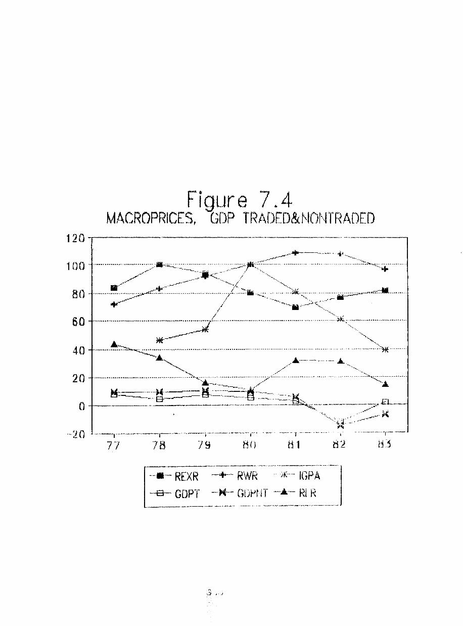
Figure 7.4 MACROPRICES, GDP TRADED&NCJNTRADED

120 -r--------.--- ,-----.-------

.-.- REXR -+--- R\A/R ., A~··- IGPA --B- GDPT --,)(_.- GD~,lt-jT _ ...• -- RI R

.• _____ ............. -....~M'-n- _ -., __ ,~". ..-... ---__ ... __ . __ ~ .. -.... __ ,._'"'_ •. _~_

~3 J' j

As we can see from graph 4, this process was more

pronnounced between 1978 to 1981 when the peso was rapidly

appreciating (REXR), real interest rates were falling (RLR),

real wages (RWR) and real stock prices rising (IGPA), and

capital inflows were at an all-time high. However, the

relative price at 1981 was not sustainable as the current

deficit was too large, nearly 16% of GDP, capital inflows

started to decline very rapidly, real interest rates were

rising again, and the stock exchange bubble were

to burst. Given the backward wage indexation the

beginning

adjustment

was in terms of output, employment, and bankruptcies

including the banking system.

After 5 years of sustained GDP growth, an increasing

share of GDP output and bank loans, the nontradable sector

experienced the collapse of output. By 1982 and 1983 GDP of

nontradables fell by 15.1% and 7.2% respectively. The

collapse in output growth coincided with both sharp

increases in nonperforming loans/capital ratio and a

substantial fall in the profit/capital ratio as shown by

graphic Sa.

339

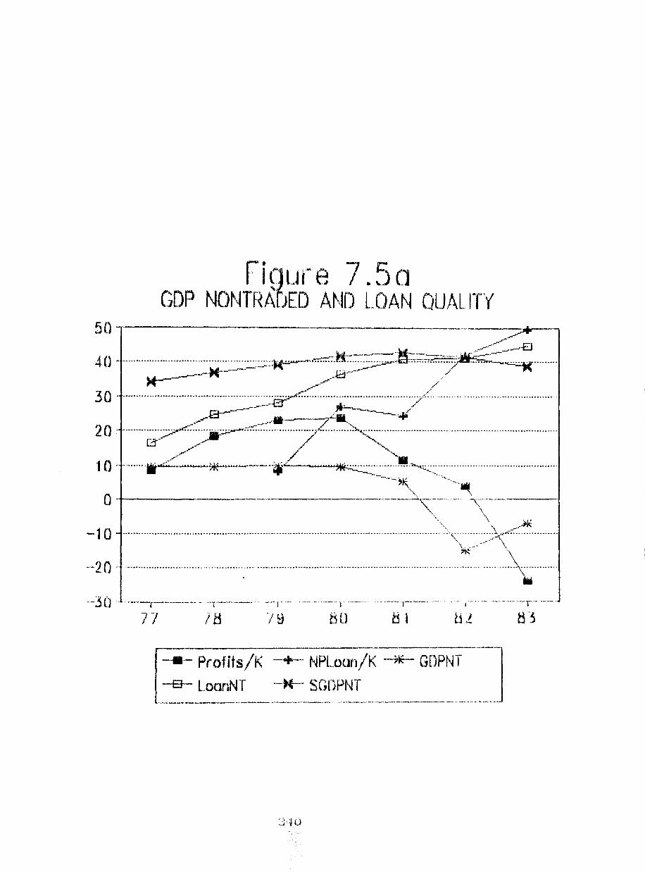
Fi(lLH~e 7 .~ja GDP NONTF~Af)ED AND LOAN QU/\L. rri

50 -- ... :::;+-.ro·A~I'JA

li.L~--~--.. ~~-,--__ .:::.:..,~....,....~~.£] 40 - .-- ........................................... .:.:.::.::.:;.::.:~,r.~7·~~·····:.:;.;.:.~~8=·;:-;~r·····.,..."-~········· ~ ... ~ .. "-~-....... ~. a r

........ ,.'

~ /./" /'

30 ........................................................ ~~~~···········::························7··(:········ ..................................... . ....----'"".,.....,... .',.----~ .. /

J".,.......a---' _~ ....... ------..-:.">. + 2 0 ·········;:;;~::::r-""'···········7[····" .. ",:;-··············· ..................................... . 1 0 ........... 6;'~·~*.~~---.:~ ........... ~~ ........ ~~.n... ... :.:< ............................................. .

"'".~~ .. ~~ .... " ., ... . "'~\., " o . ..--.-----.---"'--.. -..\~ .. --

" \ '* -1 0 ...................................................................................................................... >:.,~.: ......... : ... :~:';:~ ... ::-:-:: ............. .

*" \\ ·--20 ................................................ : ............................................................................. -...................... ~-- ....... .

·-·~30· "'--.,-""-'--' ··1····--·_· -' j •.•• - .............. - .. , .......... -. • .... · .. -····1---" .. ·· .. _ .. 1'--" -·-.. · .. ·-- .. • .. T~··· .. ·-·

77 IH J9 80 ~1 bl 83

[=:- Profits/K -+- ~PLOa~/K -'1<- GtJPNT ----'J -B- LoonNT --K-- SGDPN r

.~~~_ .. ________ ...... _ ........... _. __ .. _ "" __ ..... u._ .. ~....,_ ........ ~.w.... . ., .• " ... _, ... ~~~_ ....... _ .... A _~ __ .,._. ___ .-.-~-_._" _ .... -~-.-__

:3··~O

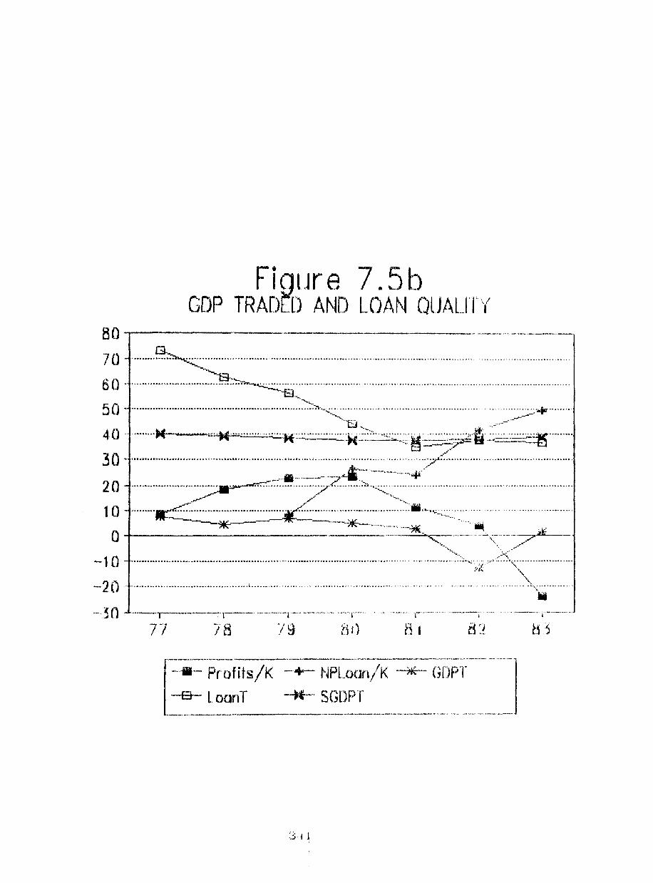
Figure 7.5b GrJP TRA[)LD A~I() L()AN ()UALJf''(

80.,----- ---_. __ .. _-----a 7 () . ............. :!b~: ...................... '"................................ .............................. ....... .... . ................................ .

~ '13

: ~ -.. ::::::::::.:.:::::·:.:::.::: .. ::::::~::;::.o,~~···:·::::::.:.::::.:: .... : .. :.:: .... :.: .. :::::: .::.:::. ::; .. :::.::::: 40 .... ..... " - ", ··-=M='·····,,=*:=·:?,:=:;~.:;:;::7'~~:;~-::.::~~ ... ·,,··

B ./ 30 ' ................... " ...... " .................................. " ............................................. /=~ ........................ " .................... . ~.--.. -.'".--.... --.'4'---

2 0 ······· .. ···· .. ········ .. ·······~::~·:~~····::=7:Z ..... ~:~;') .. ~~:: ................................................................ . ~ /~ \"~, ...... -

~ / ~. 1 0 ......... ~===;-===j( .. :== .. ~= ................ ~ .. <:::~~ .. :.: .... ~ ........................... . o -- .-::.~~,~~ .. ~';~~~

-1 () ............................................................................................................................ ".p~.: .• ' ....• \:< ................ .. \'" -2l) " .................................................. " ................................................................ " ................. " ....... ~ ......... ..

-'.''(0 . .oJ • ···-r---·--~·1----· ......... _ .. ,,-1'-..... - ................ ,".... . .. --..... ,_ ......... _ .... _, ..... . " · .. _ .. ··1·---.. · .. ..

77 7'8 /9 f~l) B I

[:-.=--P~~~f it s /K ~~~-+- Npi_~~;~~/ K . --*·=--(";-6p:r·--~ -.. ---_.-9- LoanT -K-" SGDPT __ , __ ... ___ F ... ____ .... ~ ______ • ___ • .... • _____ .. ·_, _______ <_···~ .... • .. __ .... ~ .• ~- '-'"- -" ~- --~ .... --,---~,",

A similar conclusion is derived from graphic 5b when we

plot the GDP for tradables with the two ratios a5 prOXi~B

for profitability and vulnerability. However, the turning

point of the cycle for tradables does not exactly match the

path of the two ratios. In effect, the increases in

nonperforming loans coincided with the slowdown of tradable

GOP growth in 1979-80 while output growth of nontradables

were at its peak. Also, we observed that while output growth

of tradables was growing at 1.6%, GDP for nontradables were

still falling at 7.2%. This means that given the larger

share of loans in nontradable firms and the two consecutive

years of falling output the ratios were more affected at

least between 1982-83 by the performance of the nontradable

sector.

It is clear that the change in the composition of bank

assets between

composition of

vulnerability in

1977-82 which reflected changes in the

output may have produced a greater

the banking system in the sense that

increasingly

sector were

large allocation of loans in the nontradable

producing an increasing vulnerability in

particular in the case of falling output, wages, and asset

prices, and rising real interest rates and real exchange

rates. These observations are displayed by graphs 6a and 6b.

342

Figure 7.60 BANKS VlJL~IERl\BILrrY At\tD Ml\(J':,CJPF<ICES

50 - "-----,---.---- "-""'---'-'---',..- -, -- - , .,---, _ .. __ .... _._._._--::+--.-...... ~

.rr-~"..

" .. --~. *'~ 4 0 ............................................................ , ................................................................... ' .... , ............................... .

/' /'

.r" 3 0 ..................................................................... ' ....................... , ................ /::: ...... " ........ , .............................. ' JI" -'-->--.... _ /

."'_-Zill ---'of' ~ .. ~ "" ..... 2 o········Gl···········::;:.'~"'··'············· 7 ........... '''<:: ............................................................... .

1 0 ·········.Y.:·······~:-:::::~--.=>iI!:::::=·:·:/:I~:;;;::~·tl······· .................... . ~\ / .~ .. '.-.-.--~ .. ~

" 0 -+----~----- -"~ .\ ._-_ .. _/,,-- ---'" "_ ... ---?JI!<:;--------.. --'--. I ~~

,J \\ '~''''''''~_. "\. 1/ \ ..... ... '~ . ,.. .......... , ' .. " ...... ' ... J\ ...... ::»~ .... ' .. .. ........................................... . .. :~:.~,.~~~~:~:~ ... ~: ..... ~ .. ~-.£( ............ ,. .. ..... . ::"10

-2() ............. , ...................................... " ............ , .......................... ' ... ' '. .• e' " ............. _' ... \ ... ~'.' ....... ,.

IiIi

·-·3()· --_._J_ .. _-_._ .... -r-.. _ ... _._._ .. , , __ .. ''' .. _, ....... ' .. ,.0' _ .. "·'··-r-·· .. ·- _ ... , .... , .. ''' .. ,------1···''··· ..

7778 79 Bt) 81 82 83

Figure 7.6b 8AN~(S VlJL~JE~(ABILITY A~\ID MAcr~C)PRICES

100 .....----"-----,----------,--.---,. ,--_._._ .. _--_._-------

, .

B 0 - ................................................. , ............................ "" ' ................................ " ............................................ .

6 0 ................................................................................................................... , .... , ..................................... .

_ .... --+ 40 ......... ~::~ .............................................. , ............... ' .............. , ...... " .... ".,}j~~~~:~~ ............ , ....... .

~~'-a. ... ,..~ ..... -......~ ,B"·-:.~.r '''':, .. ·_-, .. ·,u

"-.". . ., /" "~" "'''\.",- __ 111'--"---""'"7 ,.I.. "I~-....... - ~. "fA'~ .-~.-.-....... _ 2 0 ......................... ::::........,...r.-:.:-::"::-....<:~: ...... ~~:;.',o'!: ......... ~7"'~'~' ............ " .............................. ::: .. ''-:~ .. : ......... .

~ If /'"'-~._......_ ./ ..... U,01. EJ ~ +/,..1" --...... [1 _ -..-\ .. ~ .... _~

" .... o -----------_." .. " ... __ ............ __ ._.- ... '---_ ....... - .•. _ .. -'.-.. '\..~.' .. -.--.-".--.... '"

\ '"

\ ~ ". \ '.

·-2 () - ..................................................... -................................................ ~ .' -, .. "M" .. :,:.:..:,·:.:.:!i1_i .. ··'···· .. ·· .. ·'>;'··:,~· ., "

'~IE: ,··4 () . -.----~----r··.... .. .. -'-·--I·-'---.. ·-.... --···~T-'·-.. ·····' '" '''-''''}' ' .......... -.. ""T'''-'''''''''' , ... ", .... r -" ,.,. "17 7B 79 tjo 81 82 83

. J j I

Figure 7.7 LOA~~St SI·cIA~[ AND LIABILIT'i Ft!\ TI()

• 7 () .. ' ............ ~:~ ............................................................................................................................................. " ... .

. " '"a_ .. . 6 () ......................................... ~~"" ... -........................................................................................ " ................ . .... ~ .•

. ~" .. 5 () ...................................................................... :'.:"'-:::~" ..... " ............. " ................................................................ . "

• -~+

40 -........................................................... ........................... :·:>:·: .. , .. ?~.:-:+.::::=:::-~:::-:::-::~C:=;.~.~ ................... . ..ft'~"'~ ... ·'''''-...... ~-~7··,.:;::'ii .. -. ---:-':::::1

/ ~.

30 ............................................................ :./--~":.~~ ............................ ~~:.~~~~ ................................................. . .-..I""~'" ~.I'-...... ,....... ___ ---... * .. r.·~··

2 (') . .. .......... oo.-;:;, ..• ~-:.~... ................ ............ ....... .... .... ..... .. ..................... ·oo ............ , "." ................................ .

aft""

1 0 .. -,--·_· .. ··1-·--.. ·· .. ··· .. ·_·_·'1'''·_·_·_·······_··, .. ··· ........... _ .... -'1''' ........ _ ......... '("'" ...... ~ .. """"r--"-'

77 78 79 80 81 ~l 83

-.---.--.-.--.. ----------.. --.... ---. . _.-._ ..... __ . -""-I

1---- L.oanT -+.- LoantJT --*,,-- LiobU$/Linb$ ---......... "'.~---~'.----...... '--,~. -~-.... __ .... ' .. _' ..... , -.-. ~--.---~-~-.-",,- ... -... ~ ... ,.--.. -' ~'. - ~ .............. _ ..

" . ",J , ...

In addition, as I have reported in chapter 3, bank

liabilities exhibited a significant rise in foreign

currency. In effect, we estimated that the ratio of

liabilities in foreign currency relative to domestic 22

currency went from nearly 24% in 1980 to almost 40% in 1982.

This means that the shift in resources to the nontradable

sector was financed by an increasing ratio of liabilities in

foreign currency relative to domestic currency and this in

turn meant an increasing vulnerability of firms and the

banking sector to exchange rate collapse (devaluation).

Graph 7 shows the tendency of loans' share and the

liability ratio.

The evidence from the graphics had permitted us to

interrelate banking performance with the overall economic

environment, at least as a first approximation, and

explictly formulate conjectures about bank problem/failures

and the role played by factors external to the bank in the

likelihood of bank problem/failure. These conjectures can be

listed as follows: Firstly, the abrupt change in the

performance of the banking system was consistent with the

turning point of the expansionary economic cycle which

started just before 1977. If this is true then the

spectacular growth and profitability and the subsequent

downfall of the banking system has its explanation on the

boom-bust economic cycle which took place between 1977 to

1983. Therefore, we ought to be looking empirical links

346

between the rate of GDP growth and the probablllty of bank

failure/problem.

Secondly, if the boom-bust economic cycle can be

explained by the misalignment of some key macroeconomic

prices then it follows that the drastic changes in

profitability and vulnerability could be explained by the

disequilibrium of the key relative prices. Therefore, we

should be looking for econometric evidence to sustain the

relationship between real exchange rate, real interest rate,

the stock prices, and the probability of bank

failure/problem.

Thirdly, if conjecture 1 and 2 are empirically valid

then it is possible to estimate ex ante probability and to

test the prediction accuracy as we did in chapter 6.

(7.4) Econometric Analysis of Bank Failures: The Macro Aspect.

In order to answer these conjectures I had developed a

logit model for quarterly panel data following the

methodology and estimation procedures described in chapters

5 and 6. However, there are two main modifications with

respect to the binary choice model introduced and estimated

earlier.

Firstly, the present model is estimated using quarterly

panel data. As will be shown, it should not pose, under

347

certain assumptions, any additional difficulties except for

the handling of a larger number of observations.

Secondly, we regress the dichotomous dependent variable

against macroeconomic factors. Given that macroconomic

variables will be identical for each bank in a given quarter

of a given year, the estimation of the logit model will

introduce some difficulties.

The attempt to relate banks' failure/problem

systematic factors such us real exchange rates,

with

real

interest rates, and stock prices and above all growth of GDP

reflect indirectly the ability of businesses and individuals

to meet their debt obligations under changing economic

environment. This empirical model is the counterpart of

Galvez and Tybout's model as we study the problem from the

banks' perspective rather than the firm.

(7.4.1) The Econometric Model.

(7.4.1.1) Description of the Data.

The model was estimated using quarterly panel data for

the period between 1979 to 1983. Thus, the sample contain 20

quarterly observations and 27 banks. Just as for the model

of chapter 6, the bank sample was divided into two groups,

Al and BI.

The former correspond to the problem/failure group which

includes all those institutions which were liquidated,

348

merged, capitalised, and/or sold nonperforming and risky

loans to the central Bank during 1982-83. The latter group

corresponds to the non-problem/no-failed banks which include

Banco del Estado the only existing state bank, and Banco

Industrial y de Comercio Exterior (BlCE). As we have seen in

chapter 3 both institutions were the only two domestic banks

which remained financially healthy. Also B1 group includes

foreign banks on the grounds that they also remained

financially sound and as we saw in chapter 2 were subject to

similar legislation as domestic banks.

Group Al and B1 contain 16 and 11 banks respectively as

listed in table 2.

Table 7.7 Bank List of Al and B1 .

Al B1 Banks Code Banks Code

Chile* 001 Osorno 010 O'Higgins** 008 Estado*** 012 Internacional* 009 Do Brasil 017 Continental** 011 BrCE 028 Sudamericano** 014 Republic Nat. N.Y. 031 Credito** 016 America 032 Trabajo** 022 CityBank 033 Pacifico** 025 Real 034 Nacional** 026 Sao Paulo 036 Concepcion* 027 Santander 037 Edwards** 029 Exterior 038 Santiago* 035 Unido Fomento* 502 Hipotecario Fomento* 504 Hipotecario Chile* 505 Colocadora Nacional* 506 ------------------------------------------------------------Source: SIBF, Informacion Financiera, Various Issues.

* Failed Banks (liquidated, intervined, or merged) ** Problem Banks (sold nonperforming and risky loans) *** State Bank.

349

The sample did exclude two groups of financial

institutions. The first one corresponds to banks which

failed during 1981 such us Espanol(002), Talca(006),

Austral(024), and Linares(030). The second one, the non-bank

financial institutions (financieras) including those which

failed in 1981 among them Cash(705), General

Financiera(715), De Capitales(725), and Del Sur (713). The

exclusion of these two groups was justified as argued in

chapter 3 by their small size in relation to the rest of the

banks. In addition, as a general principle, we accepted all

those banks which had 16 or more consecutive quarterly

observations in order to compare their performance in the

boom period of 1979-81 with the economic debacle of 1982-83.

In consequence, the panel data of 20 quarters and 21

banks gives a total number of 521 observations which

represent a sufficiently large statistical sample to draw 23

logistic inferences. As argued in chapter 6, it would have

been desirable to have had a controlled sample in particular

by size, number of branches, or any other characteristic.

However, data limitations and the small size of the Chilean

banking system ruled out this possibility.

With respect to the dichotomous dependent variable, we

used the quarterly ex ante probability of problem/failure

estimated by the problem/failure prediction model in chapter

6. As we saw the overall prediction accuracy was extremely

good at a 0.5 cut-off value. I stress the point that

350

quarterly evaluation of banks was not available from SIBF

nor annual classification prior 1983. Therefore, we were

forced to rely on the ex ante quarterly estimation of the

problem/failure prediction model.

The explanatory variables in the model are divided into

three set of regressors. The first set contains some key

macroeconomic prices such as indices for the real exchange

rate (TCR) and the stock prices in real terms (IPA). These

variables are also expressed in terms of percentage change,

that is VTCR and VIPA. I also considered in this data set

both real lending and deposit interest rates. The annualised

ex post lending rate (TIAA) and ex post deposit rate (TIPA)

were estimated by using 30-90 days nominal rates deflated by

the consumer price index. In addition I computed the gross

spread between lending and deposit interest rates express as

OIFAP.

The second set contains data on gross domestic product

data is

and in

GOP per

tradable

expressed at constant prices of 1977. The GDP

displayed in millions of Chilean pesos (PGB)

percentage change (VPGB). Unfortunately, data on

sector on a quarterly basis, in particular for the

and nontradable sector, was unavailable for the

question.

period in

Finally, the third set incorporates monetary variables

to assess

likelihood

the implications of monetary aggregates on the

of banks' failure/problems. Among the most

351

important aggregates the model included the narrow Ml define

as notes and coins plus sight deposits and a broader measure

such as M2, which includes Ml plus time deposits.

I have also allowed some dynamic implications by

introducing two lags among the sets explanatory variables

which is equivalent to two quarters of year.

(7.4.1.2) Hodel Specification and Estimation.

The binary choice model was specified for panel data

which consisted of observations made on individual banks

over time. In addition, the model was restricted by assuming

that observations are independent for both individuals and

over time. These simplifying restrictions were desirable

since the approach to estimate the model was straightforward

and similar to the cross-section model estimated in chapter

6 but with more observations.

As we have seen in chapter 3 the determination of the

failure of a bank or its classification as a problem bank is

made in practice by monetary and banking authorities

following different criteria. However, technically speaking

we can determine a bank as insolvent or treated as problem

so long as the market value of liabilities exceeds the

market value of assets. Indeed, this condition arises as a

result of an extreme unexpected deposit withdrawls and hence

a fall in assets' market value from force liquidation,

and/or large banks' loan losses and reduction in current

income that must be charged to capital and reserves.

352

I assume that a bank has a given amount of capital (K)

at the beginning of the period, and accumulates earnings (R)

and losses (L) over the period, and spend (E) on screening

and monitoring bank loans. The stream of bank's cash flows

(Y) (net bank income) is given by (Rl-L1-E1),(R2-L2-

E2), ... ,(Ri-Li-Ei)1. Moreover, the bank may also pay

dividends (8) and issue new capital (N) at the end of the

period. For simplicity, I assume that banks' investment in

securities is zero.

The bank has issued a mix of deposits on which it

promises to make a stream of payments (D1,D2, ... ,Di] that

has a total value of D. It should be pointed out that

although all assets and liabilities should be marked to

market values to be more accurate, in practice we apply

historical cost accounting as an approximation of the true

bank's worth.

Formally stated, in expression (1) the bank's net cash

flows from its loan structure is insufficient to pay the

depositors' claims (negative net worth).

( 1 ) x = Y + D < 0

In order to prevent a failure the bank may use

from its initial capital and reserves. Therefore, in

context failure occurs if condition (2a) holds.

353

funds

this

( 2a) X = Y + D + K < 0

Expression (2a) suggest that a bank failure occurs if

negative cash flow is greater than bank's capital. Or more

generally as shown by (2b), if deposit outflows (D) exceed

banks' capital and reserves (K) plus net income from banks'

assets (Y) plus new issues (N) minus dividends (S).

(2b) D > K + Y + N - S

In consequence, the probability of bank failure (F) will

depend on the likelihood that D + Y < -K . Specifically,

(3) F = Probe D + Y < -K )

However, the model assumes that Y and D are unknown so

that the condition for bank failure Y + D < -K should be

related to the bank's financial condition (FC). If the

bank's financial condition is weak then the failure

condition will hold.

(4) Y - D + K = FC + e where i= 1,2, ... ,n it it t= 1,2, ... ,T

354

Thus, the failure condition in (4) is related to Fe for

the ith bank in time t plus a random term e. Fe can be taken

as a composite measure of the bank's financial condition

given the values of selected macroeconomic variables. In

other words, the model assumes that a deterioration of the

macroeconomic environment worsens the financial condition

(Fe) of a bank and viceversa. This is shown in expression

( 5) •

(5) Fe = x B it

where x= K-vector of known macro variables

B= K-vector of unknown parameters.

With this deterministic process giving rise to bank

failure as shown by expression (5) we are able to convert it

to a model of the probability of failure.

To begin with, the model assumes that there is a

theoretical (unknown) index e which is determined by

macroeconomic variables. This index measures a bank's

propensity to fail and is unobservable from the data. Given

that e is a function of a well defined set of random and

independent explanatory variables, the logit model should

provide suitable estimates of this function and hence for

the value of e.

55

If the dependent variable Y is equal to 1 when a bank

fails and to zero otherwise, and each bank has a critical

value for e (cutoff point) which translate the index e into

a classification process then we have the following: if e <

e the bank is classified as a failure and vice versa.

Given that the logit model assumes that e is a random

variable with a logistic distribution then it follows that

the probability that e < e can be computed from the

cumulative logistic probability distribution.

The logit model was specified for panel data which

consisted of observations made on individual banks over a

specified interval of time. In addition the model

specification was restricted by assuming that observations

were independent for both individual banks and over time.

These simplifying restrictions were considered desirable on

the ground that the approach followed here was more

straightforward and similar to the one applied in chapter 6

with cross-section data but with more observations.

Thus the restricted univariate binary choice model for

panel data is defined by:

( 6 ) P(Y = 1) it

= F ( x' f\ ) it

= F (e ) it

356

i = 1,2, ... n t = 1,2, ... T

Expression (6) defines Y as a sequence of independent

binary random variable taking the value of 1 if the ith bank

failed/problem at time t, and 0 otherwise. Also x is a K-

vector of known macroeconomic variables, and a is a K-vector

of unknown parameters. F is defined as a cumulative

probability distribution.

The cumulative probability distribution function enables

us to translate the values of the independent and stochastic

explanatory variables which range in value over the entire

real line to a probability which ranges from 0 to 1.

(7) P(Y = 1) = F(9) it

= F ( x· 6 ) = it

-9 = 1/1 + e

x'8

J f(9)de -00

= 1/1 + e

In expression (7), F(x'B) is equal to the cumulative

standard logistic function so that it assigns to a number e

the probability that any arbitrary 9 will be less than 9.

It follows that since the probability is measured by the

area under the standard logistic curve from -00 to 9, the

event will be more likely to occur the larger the value of

the index 9.

As it was shown in chapter 5, to estimate the vector of

unknown parameter of 6 I resorted to the use of the

maximum likelihood estimator for B. The maximum likelihood

357

estimation was appealing since a unique maximum always

exists for the logit model. At the same time, it is

appropiate for non-linear estimation and yields consistent

parameters estimates. Thus, the likelihood function of the

logit model is given by

n TnT (8) lnML = E EY In F(x 6) + E E( l-Y ) In [ 1 - F(x 6)

it it it it

The ML estimator for 6, say 6~, is obtained by

maximising (8) with respect to 6 and setting the first order

condition (FOC) equal to zero. As was shown in chapter 4 the

solution is a local maximum and hence unique. Also we saw

that the FOC was non-linear and hence solved by the Newton-

Rapshon iterative procedure.

However, a panel data specification such as ( 6 )

specifies only the marginal probability and leaves the joint

probability P(Y ,Y , ... ,Y ) unspecified. One way to get il i2 iT

around this problem is to introduce some restrictions. We

assume independence so that the joint probability will be

given by

( 9 ) P(Y ,Y , ... ,Y) = il i2 iT

E P(Y ) iT

358

The independence assumption implies that P(Y = 11 Y = 1) it i,t-l

so that previous year status does not affect the one this

year. This means two things: Firstly, there is no true state

dependency in the sense that the present status is not

affected by the past status. In other words, the

probability of bank failure/problem is not affected by

yesterday's probability.

Secondly, there is no heterogeneity problem in the

sense that there are no serious complications with

unobservable variables which could affect banks differently

with respect to their likelihood of failure/problem.

Before we concentrate on the analysis of the results

from the model estimation there is one complication in the

setting of the matrix with the exogenous variables. Given

that the macroeconomic data were identical for each

individual bank in each specific quarter, the matrix was

near singular. So in order to eliminate this problem we

modified the matrix structure of the model. Let's take a

close look to the matrix specification of the model and its

meaning.

359

A TCRA ..... IPAA 0 0 . . . . . 179.1 179.1 179.1

A TCRA ..... IPAA 0 0 179.2 179.2 179.2 · · · ·

A TCRA IPAA 0 0 y= n83.4 x= n83.4 n83.4 it B it 0 0 TCRB IPAB

179.1 179.1 179.1 B 0 0 TCRB IPAB

179.2 179.2 179.2 · . · · . · B 0 0 TCRB IPAB

n83.4 n83.4 n83.4

where i= 1,2, ... ,n. t= 1,2, ... ,T.

The column vector Y contains the endogeneous it

dichotomous variables for each bank i in a given quarter t

for the ordered group A and B respectively.

The matrix x was contructed by separating the data it

for the group of banks A and B respectively. This enabled us

to compare the performance of these two groups in relation

to changes in the macroeconomy. At the same time, we

eliminated the near singular problem in the estimation of

the model.

360

(7.4.2) The Econometric Results and Its Interpretation.

In this section I report the main econometric results

from the restricted logit model using macroeconomic

variables. The model was estimated for the period between

1979 and 1983 which involves twenty quarters. This selected

period, selection made in terms of the availability of

information, includes a boom period between 1979 and 1981

and the bust period between 1982 and 1983. The problem of

multicollinearity among the sets of explanatory variables

forced us to estimate and test the regressors separately.

Before we proceded with those two issues concerning the

importance of the economic cyle and the misalignment of some

macroeconomic prices, we wanted to run the model to test

the significance of monetary variables on the likelihood of

bank failure/problem.

- Logit Model with Monetary Variables.

As showed in chapter 4, banking crisis are often

associated with changes in the monetary conditions, in

particular large shifts in the demand for money. As argued

by monetarists, increasing uncertainty about the

health of financial institutions would

financial

produce a

substantial increase in currency deposit ratio and thus a

fall in the money supply and widespread liquidity problem in

the banking system. Table 8 report the results of the logit

model with reference to the monetary aggregate M2 between

1982.1 to 1983.4.

361

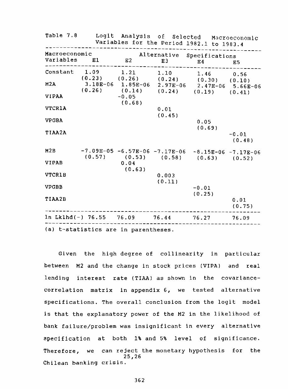
Table 7.8 Logit Analysis of Selected Macroeconomic Variables for the Period 1982.1 to 1983.4

------------------------------------------------------------Macroeconomic Alternative Specifications Variables E1 E2 E3 E4 E5 ------------------------------------------------------------Constant 1.09 1.21 1.10 1.46 0.56

(0.23) (0.26 ) (0.24) (0.30 ) ( 0 . 10 ) M2A 3.18E-06 1.85E-06 2.97E-06 2.47E-06 5.66E-06

(0.26) (0.14) (0.24 ) (0.19) (0.41 ) VIPAA -0.05

(0.68) VTCR1A 0.01

(0.45 ) VPGBA 0.05

(0.69 ) TIAA2A -0.01

(0.48)

M2B -7.09E-05 -6.57E-06 -7.17E-06 -8.15E-06 -7.17E-06 (0.57) ( 0.53) ( 0 . 58 ) ( 0.63) ( 0 . 52 )

VIPAB 0.04 (0.63)

VTCR1B 0.003 (0.11)

VPGBB -0.01 (0.25)

TIAA2B 0.01 (0.75)

------------------------------------------------------------In Lk1hd(-) 76.55 76.09 76.44 76.27 76.09 ------------------------------------------------------------(a) t-statistics are in parentheses.

Given the high degree of collinearity in particular

between M2 and the change in stock prices (VIPA) and real

lending interest rate (TIAA) as shown in the covariance-

correlation matrix in appendix 6, we tested alternative

specifications. The overall conclusion from the logit model

is that the explanatory power of the M2 in the likelihood of

bank failure/problem was insignificant in every alternative

specification at both 1% and 5% level of significance.

Therefore, we can reject the monetary hypothesis for the 25,26

Chilean banking crisis.

362

-Conjecture 1: The Likelihood of Bank Failure/Problem and the Economic Cycle.

The first conjecture we observed from the data presented

in the previous section and which had a significant

intuitive appeal was the relationship between output growth

and the performance of the banking system. In effect, a

booming GOP between 1977 and 1981 coincided with a buoyant

banking system. Similarly, the collapse of GOP in 1982-83

led to the debacle of the banking system.

Table 9 provides econometric evidence on the

significance of GOP growth on the likelihood of bank

failure/problem. Alternative specifications are also

reported for this period to enquire the performance of GOP

in a more general model. According to the correlation

coefficient presented in appendix 6 there is no significant

correlation among the explanatory variables tested in this

model.

Specification E1 correspond to a general model which

included all the selected macroeconomic variables as

explanatory variables. These included variation of GOP

(VPGB), variation in stock prices (VIPA), real lending

interest rate (TIIA), and variation in the real exchange

rate (VTCR). The parameters' estimates are reported for each

group of banks, namely group A for failed/problem banks and

group B for nonfailed/nonproblem banks.

363

Table 7.9 Log~t Analysis for Selected Macroeconomic VarIables for the Period 1979.1 and 1983.4.(a)

------------------------------------------------------------Macroeconomic Variables E1

Alternative Specifications E2 E3 E4 E5

------------------------------------------------------------Constant

VPGBA

VIPAA

TIAA2A

VTCR1A

VPGBb

VIPAB

TIAA2B

VTCR1B

-0.38 (1.24)

0.13 (3.02) -0.01

(1.27) 0.09

(5.61) -0.09

( 0 . 37 )

-0.14 (2.71) -0.01

(0.07) -0.06

(3.78 ) 0.04

(1.44 )

0.18 ( 2 . 02)

0.01 (0.55) -0.01

(1.66)

-0.06 (2.05)

0.007 (0.75 )

-0.41 (1.52)

0.12 ( 3.09)

0.09 (6.27 )

-0.14 ( 2 . 91)

-0.05 (3.89 )

-0.31 (1.06)

0.11 (2.85)

0.08 (5.64)

0.001 (0.06)

-0.15 (3.02)

-0.06 (4.04 )

0.04 (1.63)

0.18 (2.06)

0.01 (0.07)

0.03 (1.84)

-0.05 (1.92 )

-0.0008 (0.04)

------------------------------------------------------------Ln Lklhd(-) Lklhd Ratio(b) LklhdR Index(c) A.I.C.(-)(d)

227.00 264.36 36.80

236.00

355.59 7.18 1.00

360.59

229.08 260.20 36.22

234.08

(a) t-statistics are in parentheses.

227.80 262.76 36.57

234.80

355.50 7.36 1.02

340.50

(b) The ratio is calculated as -2[LnLklhdr-lnLklhdu] and it has a chi-square distribution with j degree of freedom. (c) This index is a pseudo-R square defined as

l-[lnlklhdr/lnLklhdu] (d) The Akaike's information criterion (AIC) is defined as -Ln(Lklhd)+ K where K is the number of estimated parameters.

Specification E1 exhibits the largest likelihood ratio

(LR) and the highest goodness of fit measured by the

likelihood ratio index. Indeed, it rejects the null

hypothesis that all coefficient are zero as the value of the

test statistic LR is larger than the critical value of a

chi-square distribution at 0.5% of significance and eight

364

degrees

obtained

of freedom (i.e. 21.95). Similar conclusions are

from specifications E3 and E4 which exhibit a

similar performance. In contrast, E2 and E5 are found

insignificant according to the LR test.

From the results based on the those specification which

were found statistically significant we can draw some useful

observations with respect to the empirical incidence of VPGB

on bank failure/problem.

To begin with, the growth rate of real GOP (VPGB) was

significant for the group of failed/problem banks (A) at 1%

significance. Similar results are found for the group of

nonfailed/nonproblem banks (B). At the same time, the

negative sign of the coefficient for group B is consistent

with the a priori expectation. That is, a fall in GDP growth

rate increased the probability of failure/problem.

However, we can observe that the effect of GOP changes

on the group of banks in difficulties (A) was opposite to

group B and inconsistent with the a priori

This result is rather puzzling since it

expectations.

suggests that

falling output is consistent with falling probability of

failure/problem.

-- 365

- Conjecture 2: The Likelihood of Bank Failure/problem and the Misaligment of Key Macroeconomic Prices.

We also observed from the graphics that the performanre

of the banking system was somehow related to the changes in

some key macroeconomic prices. Severe fluctuations in

relative prices coincided with the changes in banks'

fortunes. Table 10 report the econometric results of the

logit model estimated in order to test the significance of

price misalignment.

Again, we specified a general model el which included

three macroeconomic prices, namely the changes in the real

exchange rate (VTCR), real lending rate (TIIA), and real

stock price (VIPA). Although the overall equation is

statistically significant at 1% measured by the likelihood

ratio (LR), and the goodness of fit is one of the highest

among the alternative specifications with 45.5%, the

estimated coefficients are insignificant as their t-

statistics fell outside the critical region at both 1% and

5%. The only exception to this result corresponds to the

real lending rate lagged by two quarters for both groups.

366

Table 7.10 Logit Analysis for Selected Macroeconomic Variables for the period 1979.1 and 1983.4.(a)

------------------------------------------------------------Macroeconomic Variables

Alternative Specifications e1 e2 e3 e4

------------------------------------------------------------Constant -0.20 -0.21 -0.24 0.16

(0.97) ( 1.01) (1.20) (1.91) VTCR1A -0.0008 -0.001 0.02

(0.036) (0.04 ) (1.51) VIPAA -7.217E-05 0.0002 -0.009

(0.007) (0.02 ) (1.14) TIAA2A 0.08 0.08 0.08

(6.46 ) (6.48 ) (6.80)

VTCR1B 0.03 0.04 0.0006 (1.28 ) ( 1 . 74) (0.03)

VIPAB -0.01 -0.02 0.001 ( 1 . 08) (1.53) (0.11 )

TIAA2B -0.06 -0.06 -0.06 ( 4 . 90 ) (4.78 ) (4.85)

------------------------------------------------------------Ln Lklhd(-) 240.21 240.86 241.03 356.73 Lk1hd Ratio(b) 237.94 236.64 236.30 4.90 LklhdR Index(c) 33.12 32.94 32.89 0.60 A.I.C.(-)(d) 247.21 245.86 246.03 361.73

(a) t-statistics are in parentheses. (b) The ratio is calculated as -2[LnLklhdr-lnLklhdu] and it has a chi-square distribution with j degree of freedom. (c) This index is a pseudo-R square defined as

l-[lnlklhdr/lnLklhdu] (d) The Akaike's information criterion (AIC) is defined as -Ln(Lklhd)+ K where K is the number of estimated parameters.

Alternative specifications were tried by dropping some

of the regressors in order to confirm this result. Model e2

and e3 performed as good as e1 in terms of their likelihood

ratio and likelihood index. In contrast, e4 was found

insignificant and hence meaningless.

Specifically, I found that for group A (failed/problem

banks) real lending rate was the only significant factor

which carried explanatory power in every alternative

367

specification. The positive sign of the coefficient

indicated that rising interest rates were consistent with a

rise the

quarter

likelihood

lag. This

expectation.

of bank failure/problem

coefficient confirm the

after two

a priori

With respect to group B, real lending interest rates

with two quarter lag (TIAA2B) is statistically significant.

The negative sign suggest that increase in lending rates was

reducing the likelihood of bank failure/problem.

There are some firm conclusions to be obtained from the

model. The sustained appreciation of the real exchange rate

by more than 30% between 1978 to 1982 and the subsequent

real depreciation as the authorities abandonned the fixed

exchange regime did not explain the likelihood of

failure/problem for group A. Also a similar conclusion was

obtained for group B during the period between 1979-83.

High and rising real lending interest rates were found

important in the probability of failure/problem in group A

indicated by the significant and positive sign of the lagged

TIAA2A. If we recall the data on real interest rates suggest

that during the period of study the lending rate never fell

below 11%. Indeed, we see that during the period of

interest rates came down from over 34% in 1978 to

1979-80

16% and

11% during 1979 and 1980 respectively. Thereafter, real

lending rate rose from 11% in 1980 to over 30% in 1982-83.

368

The estimated coefficient for real lending rates was

also statistically significant for group B although its

interpretation is more complicated since the coefficient of

lagged interest rate is with a negative sign.

Finally, the evidence does not support the view that

the abrupt fluctuations in stock prices during this period

of study did affect adversely the likelihood of bank

failure/problem for group A and group B. The data from table

2 showed a substantial increase in the stock price index by

53% between 1978-80 and a more severe drop between 1980 and

1983.(i.e. insignificant coefficient)

-Conjecture 3: Predicted Probabilities from the Logit Model with Macroeconomic Variables.

We have found so far some econometric evidence to

support the hypothesis that the deterioration of the

macroeconomic environment had some role to play in the

failure/problem of banks. The most significant variables in

explaining the likelihood of bank failure/problem were the

change in GDP and the real lending interest rate.

The next step is to select the best equation for

prediction purposes. This will enable us to assess and

compare the prediction accuracy of the model which include

macroeconomic variables instead of accounting ratios already

evaluated in chapter 6. However, given that the

369

macroeconomic variables were the same for each individual

bank in each specific quarter, the model cannot predict the

quarterly likelihood for each bank. In effect, the quarterly

probability for a given year will be exactly the same for

every single institution included in a given group. The best

we can aim for is merely a comparison between the

prediction for group A and B. Therefore, this approach does

not have any practical application as an early warning

model.

In selecting the best equation we will look at some of

the scalar estimated for each specification. To start

the likelihood ratio test found insignificant

with,

at 1%

confidence level specifications E2,E5, and e4. The remaining

specifications did explained the likelihood of bank

failure/problem. In other words, reject the null hypothesis.

Among the remaining alternative equations, specification

E3 from table 9 was preferred to the others on the basis of

Akaike's information criterion (AIC). In addition, this

equation display one of the highest likelihood ratio index

and contain the two most significant macroeconomic

variables. (i.e. GOP and lending interest rate)

Tables 11a, 11b and 11c displayed the estimated

probabilities for each group between 1979.1 to 1983.4.

370

Table 7.11a Prediction Accuracy of the E3 Logit Model for Group A and B During 1983 and 1982.

------------------------------------------------------------1983 1982

------------------------------------------------------------I II III IV I II III IV

------------------------------------------------------------GROUP A 0.72 0.93 0.82 0.75 0.82 0.95 0.93 0.95

GROUP B 0.23 0.07 0.13 0.07 0.19 0.06 0.19 0.17 ------------------------------------------------------------

Table 7.11b

I

Quarterly Prediction of the E3 Logit Model for Group A and B During 1981 and 1980.

1980 1981

II III IV I II III IV

GROUP A 0.54 0.86 0.80 0.83 0.51 0.64 0.91 0.86

GROUP B 0.23 0.11 0.17 0.09 0.38 0.21 0.10 0.17 ------------------------------------------------------------

Table 7.11c Quarterly Prediction of the E3 Logit Model for Group A and B for 1979.

------------------------------------------------------------I II III IV

------------------------------------------------------------GROUP A 0.72 0.64 0.83 0.87

GROUP B 0.14 0.29 0.17 0.09 ------------------------------------------------------------

Although the model did not enable us to compare

individual predictions it was useful in predicting the

likelihood of failure between groups. At 0.50 cut-off point,

the E3 equation showed a good prediction accuracy as it

obtained very high ex ante probability of failure for group

371

A during 1983 and 1982. As we move further back to 1981 and

1979, the predicted likelihood Is smaller. If we increase

the cut-off point, say 0.8, the accuracy of the model

started to decline and the number of type-I error start to

emerge. Similar conclusion were reached for the case of

group B.

All in all, although the logit model estimated with

macroeconomic variables did not prove to be useful for

individual prediction purposes, it did provide some

interesting results with respect to the hypothesis testing

on the role of macroeconomic variables on the likelihood of

bank failure/model. The next step is to test empirically the

role of management decision making in the probability of

bank failure/problem. In Chapter 8, I will argue that

bankers responding to changes in risk incentives as a result

of financial liberalisation did affect above all the health

of the banking system.

372

Endnotes

(1) Although the reduction in the inflation rate was one of the central objective a gradual anti-inflationary approach was followed at least until April 1975. It involved a gradual slow down in the monetary growth and a reduction in the fiscal deficit by means of the elimination of subsidies, employees, and the sale of publicly owned enterprises.

(2) The shock treatment soon delivered some positive results as the fiscal deficit was reduced from 10% of GDP in 1975 to 0.8% in 1978. A surplus was attained in the three subsequent years. Although the progress on inflation was also important as it felt from 343% in 1975 to just above 37% in 1978, it was still high relative to international standards and involved an extremely high cost. The fiscal shock was felt inmediately as the economy plunged into a recession with a fall in GOP by nearly 13% and unemployment rate almost at 20% towards the end of 1975.

(3) There are no complete con census among the experts on whether the experience of the Southern Cone Countries is relevant in order to evaluate the predictions of the monetary approach as an operational instrument. As Blejer (1983) pointed out these episodes involved exchange rate policy for stabilisation in conjunction with liberalisation reforms for structural changes.

(4) A more thorough account and evaluation of stabilisation policies and liberalisation reforms is provided in chapter 2.

(5) For instance, Edwards (1988) showed if capital controls are gradually removed to allow an increase in capital inflows, then the increase in current expenditures in particular in non traded goods will increase its price and by definition lead to an equilibrium real appreciation. However, if the rate of capital inflows cannot be sustain in the long run, the real exchange rate should return to its long-run equilibrium. Therefore, temporary changes in fundamental can result in significant divergences between actual and equilibrium real exchange rate or what is normally known as exchange rate misalignment. The same dynamic is true when we look at the determination of stock price bubbles. See note 13.

(6) This performance was also determined by the favorable economic environment of the world economy.

(7) Cortes Douglas (1989) found that the highest growth rate during the period of 1926-82 corresponded to 1928 with 24.3%. The long run trend between 1940-82 was 3%.

373

(8) If P=aPnt+(1-a)Pt then if the law of one price hold for tradables Pt=e+Ptf+~ then P=(Ptf+e+~)+a(Pnt-Pt). Thus if Pt=Pnt then P=(Ptf+e+~) where pt=tradable prices, Fnt=nontradable prIces Pt£=world tradable prices, e=expected devaluation, and ~=tariff. This condition is valid as long as the government budget is in surplus, and the labour markets works efficiently. The government was confident that the law of one price could hold as they achieved fiscal surplus unlike Argentina. (See Corbo, De Melo, and Tybout 1986)

(9) Although there is an overwhelming concensus on the importance of capital inflows on the determination of the real exchange rate, Harberger(1985a,b) and Edwards(1986) maintained that capital inflows were exogeneous responding to the investor perception in the domestic profitability of investment. This produced an increasing demand of Chile's capital stock. In addition, they found that capital flows were insensitive to interest rates. This finding was corroborated by Sjaastad(1982).In contrast, Corbo (1987) found empirical evidence to support the view that capital flows were endogenous, that is explained by a portfolio adjustment model, although the coefficient for interest rate was insignificant. In my view, although capital inflows were paramount, the increases in absorption was responding to the significant growth in domestic loans financed by the substantial expansion in peso deposits as shown in chapter 2. At the same time, wealth effects from the stock market should have also been important on expenditures.

(10) Sjaastad (1985,1989) and Cortes Douglas (1985) argued that the fluctuation in real interest rates between 1979 and 1982 can be explained by the fluctuation in the value of the dollar. They maintained that in a small open economy with fully integrated capital and goods markets to international markets, domestic nominal interest rates will be fairly well arbitraged with external rates, but real interest rates would be affected by fluctuations in the exchange rate of major currency countries, where such fluctuations will be transmitted by the external price of traded goods.

(11) The increases in real wage also contributed to the rise in expenditures.

(12) Although the spread exhibited a significant reduction, particularly between 1978 and 1979 which reflected among other things a growing financial integration due to the gradual removal of external restrictions, less uncertainty from .the exchange rate regime, and a SUbstantial increase in peso deposits, it remained stable around 2\ a month between 1979 and 1981. In chapter 2, we offered a more detailed evaluation about interest rates and the hypothesis to explained their performance.

374

(13) Barandiaran (1983) and Meller and Solimano (1984) argued that substantial rise in stock prices will affect the behavior of economic agents as they feel richer and enable them to expand their demand for credit. Meller and Solimano found that the movement of stock prices which went from a situation of boom to crash followed a trajectory of an speculative bubble. That is stock prices exceeded the value determined by the "fundamentals".

(14) As we have seen in chapter 2, the rise in nominal and real interest rates can be explained by the incidence from country-specific risk and exchange rate risk, increasing world interest rates, dollar deflation.

(15) Instead the authorities subscribed themselves to the automatic adjustment predicted by the monetary approach via increases in interest rates. However, the banking system was behaving in a very non-conservative way rolling over bad debts, capitalising the interest, financing distress borrowing. Therefore, the demand for credit became interest inelastic and the banking system was exhibiting a type of conduct consistent with moral hazard. The same observation was true for international banks which lent resources with no apparent control and with a belief that the government was willing to bail-out the banking system if difficulties arises.

(16) According to Cortes Douglas (1989) the 1982-83 output performance was the second worse in Chile's economic history after the 1931-32 economic depression when output declined by 17.1% and 26.8% respectively.

(17) Edwards (1986) investigated the empirical relationship between the real exchange rate (REXR) and capital inflows. In addition he included the terms of trade and real output as determinants of their equilibrium. His results support the view that capital inflows were significant in explaining the REXR and the slow adjustment towards its new equilibrium. Morande (1988) not only confirmed these findings and but also found in his VAR model that capital inflows were close to being Granger-Causality prior to the real exchange rate as well as capital flows being exogenous.

(18) Galvez and Tybout (1985) explored empirically the issues relating the performance and failure of nonfinancial firms during the period of 1977-82. Longitudinal data base of industrial financial statements was used to document real side and financial changes in firms'performance. The Galvez­Tybout empirical work is in a sense the counterpart of the present study as we are looking at the performance and failure of financial institutions.

375

(19) Galvez and Tybout (1985) found that between 1977 and 1981 the ratio of exportables to nontradable prices fell by 25% as did the ratio of exportable to nontradable gross margins. The most significant change in gross margin occurred in 1979 when the adverse terms of trade compounded the efect of the sustained real appreciation. Importables improved its margin between 1977 and 1979 and by 1981 were higher than both exportables and nontradables. By 1981 importable gross margin continued rising while exportable and nontradable margins were falling from the overvaluation and increasing overhead costs.

(20) Galvez and Tybout reported that by 1978 exporters (grupo firms) showed a lower financial cost than nontradable and importable (independent firms). The former was paying 14% while the latter 22%. However, this difference started to come down as result of the liberalisation of capital flows. As long as operating earnings were above financial costs, nontradable and importable sector were able to operate. When the interest rate rose from 1981 onwards the financial situation worsen for those firms.

(21) According to Brock (1989), trade liberalisation produced an anticipated upward shift in the productivity of tradable production so that the large increase in the share of non-traded goods was a part of the transition period during which nontraded production was needed to restructure the economy. Lower copper prices and thus a substantial deterioration in the terms of trade in 1981 brought down the value of capital and land and thus relative price of non­tradables. In his representative agent model, there is no money and prices are flexible. Although the model introduces important features of the Chilean economy, it is unrepresentative by excluding the monetary sector and assuming that non-tradable prices were flexible. In fact, the collapse in output and the misalignment of relative prices can be explained by monetary factors and the downward inflexibility of nontraded goods prices.

(22) Although the ratio of liabilities in foreign currency relative to domestic currency rose during this period, it was found statistically insignificant as a discriminator between failed/problem banks and sound banks. See chapter 6.

(23) In group AI, Pacifico, Unido Fomento, Hipotecario Chile, and Colocadora Nacional de Valores have missing observations in 1979(3Q),1983(4Q), and 1979(1Q) respectively. In group B1, BICE, Republic, Santander, Exterior have missing observations in 79(3Q), 79(2Q), 79(1Q), and 79(lQ) respectively.

(24) Amemiya (1985) and Green (1991) discuss unrestricted models with heterogeneity and/or state dependency.

376

(25) This contradict the evidence available for Chile. For instance, Sundararajan and Balino (1990) found significant evidence for a shift into currency and a rise in the interest elasticity of the demand for currency during the banking crisis. Also, they found that the demand for M2 showed an upward shift and their interest rate elasticity increased reflecting a portfolio shift from non-bank financial institutions to bank deposits.

(26) It should pointed out that this approach does not represent a formal empirical test for the Diamond-Dybvig effect. An alternative formulation would be to test the model for the correlation between the residuals, that is between e & e, or between e & e.

it jt it it-l A priori I expect that the liquidity effect from any run for safety was neglible as a result of the public belief of the existence of an implicit deposit insurance.

377

Chapter 8. The Bank Failures in Chile: The Role of Moral Hazard.

(8.1) Introduction.

It could be argued that bank failures may arise from

macroeconomic instability produced from external shocks

and/or gross policy inconsistencies during a process of

liberalisation. Chapter 7 had provided empirical evidence to

support the hypothesis that the episodes of bank failures in

Chile reflected the incidence of macroeconomic variables on

the likelihood of bank failures.

This chapter examines a competing hypothesis that the

rise in bank failures reflected the bank's greater

incentives to take undue risks. Indeed, as we have seen

from chapter 3, moral hazard can be motivated and even

aggravated by the specific steps taken by the authorities to

deregulate the financial market. An ill-implemented

privatisation which enhanced the formation of powerful

"economic groups" and economic concentration, the abrupt

deregulation of interest rates which resulted in stubbornly

high rates of interest, the expectation of explicit

government insurance on bank liabilities, and an ineffective

prudential regulation and supervision all exacerbated moral

hazard among financial institutions (bank management) and

bank users (depositors). As we will see from the evidence

these features were present during the liberlisation episode

in Chile.

378

It is shown that the balance-sheet of chil 1 k - ean )an.5

reflected greater risk-taking as a result of moral hazard.

At the same time, logit model estimates support the moral

hazard hypothesis as an explanation of the bank failures in

Chile.

(8.2) Financial Liberalisation and Koral Hazard.

Recalling the discussion in chapter 4, moral hazard was

seen as the propensity to take excessive risk in the context

of a bet against the government. It will be shown in the

next section that the existence of certain specific features

in the financial market as a result of ill-designed and

implemented financial liberalisation could excerbate the

moral hazard problems. On this point, Diaz-Alejandro (1984)

maintained that the intrinsic imperfections in financial

markets and the policy dilemmas they posed explain the

collapse of financial institutions in the Southern Cone,

particularly in Chile. Specifically, the development of bank

holding company structure and a significant concentration of

financial activities among few financial institutions, the

existence of implicit or improperly priced explicit deposit

insurance with respect to the bank's asset risks, a sharp

deregulation of interest rates, and a weak prudential

regulation either by design or enforcement would introduce

Incentives towards excessive risk-taking by banks and its

customers and hence increase the probability of bank

failures.

379

Diagram 1 describes the basic elements of the hypothesis

of moral hazard on bank failures. The existence of policy­

induced factors (financial liberalisation) exacerbates moral

hazard and adverse selection type of behaviour which arise

under information asymmetries. Specifically, the existence

of a bankholding company structure combined with a fixed

rate underpriced deposit insurance, rapid deregulation of

domestic interest rates, and a weak and inefficient

prudential regulation and supervision provided banks with a

greater incentive to increase risk-taking (asset risk,

higher leverage, lower capital and reserves requirements)

hence increasing the likelihood of bank failures. Financial

and accounting ratios constructed from banks' balance-sheet

data should reflect the banks' incentive to take greater

risks.

Diagram 8.1

Bank Holding Company Structure

Factors Affecting Moral Hazard and Bank Failures

Free Deposit Ineffective Sharp Insurance Prudential Interest

Regulation Rate Freed

I

Moral Hazard/Excessive Risk-Taking Proxies for Risk-Taking

Bank Failure/Problems

380

(8.3) ~ Evidence from Chile.

The evidence from Chile's experience with financial

liberalisation and the subsequent banking debacle 1n 1982-83

confirm the presence of those factors outlined in the

previous sub-section and their likely effect on increasing

risk-taking and the collapse of some banking firms. Although

the role of an adverse macroeconomic environment (external

factors to the banks) was tested and confirmed in chapter 7,

the good predictive performance of the early warning model

of chapter 6 suggest that the financial debacle would have

been forseen a few years earlier. Indeed, the incidence of

an ill-designed financial liberalisation was already

inducing excessive risk-taking well before the

deterioration of the macroeconomy. Therefore, the role of

moral hazard in the debacle of the Chilean banking system

should be considered as central in any explanation of bank

failures.

Looking at the banking structure in Chile which arose

during the liberalisation period indicates three distinct

features: Firstly, three commercial banks controlled nearly

50% of the overall asset portfolio of the banking system.

Secondly, financial institutions were owned by few and

powerful economic conglomerates.

And thirdly, the evidence shows that a large proportion

of the banks' loan portfolio was allocated among their

affiliates.

381

Table 8.1 Banks Ranking According to Portfolio.(%)

Total Loan

------------------------------------------------------------Banks 1981 1983 Banks 1981 1983 ------------------------------------------------------------Chile 20.5 22.0 O'Higgins 3.1 3.1 Estado 16.7 16.8 Osorno 3.0 2.1 Santiago 8.7 10.7 Unido de Fo. 2.5 Credito 6.7 5.5 Edwards 2.4 3.2 Sud Americano 5.5 5.5 Nacional 2.2 2.0 Concepcion 4.9 4.6 Colocadora Nac. 2.1 1.9 Hipotecario Fo. 3.8 3.6 Internacional 1.5 1.2 Hipotecario Ch. 3.4 Continental 1.3 1.1 Trabajo 3.4 3.3 BICE 1.2 1.4

Source: SIBF, Informacion Financiera, Various Issues.

The data from table 1 indicate that three commercial

banks (Chile, Estado, and Santiago) controlled 49.5% of

total loans of the banking system during 1983. For instance,

Bank of Chile alone had a 22% control of the total loans of

the system and this figure greatly exceeded the average

participation of domestic commercial banks of 5.5% ( 2.7%

excluding the three largest banks). Also, further evidence

from SIBF suggests that the participation of foreign banks

is even less important. For instance, the Citibank exhibits

the highest share of total loans of the system with only

1.7%. while the rest of the foreign institutions were

falling below 0.7%.

The banking system in Chile was owned and controlled by

powerful economic groups organised in a tighly knit web of

onwership links which included financial firms (banks, non-

bank financial institutions, and insurance) and non-

financial firms.

382

Table 2, which was taken from Dahse\s research, shows

the degree of concentration of economic groups. Dahse (1979)

found that only five economic conglomerates controlled 36\

of the 250 biggest firms and 53% of the total capital. For

instance, "group" Cruzat-Larrain was the largest

conglomerate with U$ 936 millions which was equivalent to

nearly 25% of the total worth of the 250 firms valued at U$

3.788 millions.

Table 8.2a The degree of Concentration of Chile's Economic Groups.

Conglomerate (a) Firms % Ownership U$ %

Cruzat-Larrain (CL) 37 14.8 936.88 24.7 Vial J. (V) 25 10.0 477.30 12.6 Matte E. (M) 12 4.8 325.31 8.6 Angelini A. (A) 8 3.2 141.80 3.7 Luksic A. (L) 8 3.2 139.06 3.6 Galmez (G) 2 0.8 98.23 2.6 Edwards A. (E) 9 3.6 95.95 2.5 Yarur Banna (Y) 4 1.6 92.02 2.4 ------------------------------------------------------------Source: Dahse (1979) (a) Data for 1978.

There was no economic conglomerate which did not totally

control (owned) or at least share joint ownership of one or

more financial institutions. Indeed, Dahse (1979) maintained

that private banking was owned by no more than fifty

individuals.

383

Table 8.2b Banks' Ownership by Economic Groups in 1978. ------------------------------------------------------------Banks CL v M A L G E y Otro(o) ------------------------------------------------------------Chile 31 Santiago 100 Credito SudAmericano Concepcion Hipotecario Fo. 55 Hipotecario Ch. Trabajo Unido Fomento Colocadora Nac. 100 BrCE

10

7.5 3

91

3

100

21

15 20

1

77

1

22 (a)

6 (b) 24 (c) 47 (d) 45 (e)

59 (f) 20 (g)

------------------------------------------------------------Source: Dahse (1979)

(a) It is composed by families Hirmas (9.5), Soza(4), Menendez(3), Andina(3), and Garcia Vela(2.5) (b) The six percent is owned by Group Scheiss. (c) It includes Molineros Ass. (18), and Scheiss (6) (d) Ascui 9.8, Saenz Bros. 9.5, Martinez & Cueto 9.2, Giner 7.5, Ruiz 8.0, and Acosta & Cosmeli 3.0. (e) 45% was owned by group Soza. (f) 20% was under the control of the Said family and 39% corresponded to capital from Venezuela. (g) Group Avalos & Gonzales hold 20% of the bank.

The evidence from table 2a and 2b clearly indicates that

Cruzat-Larrain, the largest economic group, owned totally

Colocadora Nacional and Banco de Santiago, and had a

majority holding in Banco Hipotecario de Fomento. Moreover,

they had a 10% ownership of Banco de Chile. Similarly, J.

Vial, the second largest group, also controlled several

financial institutions among them, Banco Hipotecario de

Chile with 91%, Banco de Chile with 31%, and two

"financieras" (Finasa, and Atlas) which controlled nearly

20% of the total credit of that segment.

384

What is clear from the evidence presented is that the

the two two largest economic conglomerates controlled

largest banks of the system (Chile and santiago). Moreover,

those banks associated with the economic conglomerates were

liquidated or intervened in order to be merged or sold

later. For instance, we saw in chapter 3 that Hipotecario de

Chile and Unido de Fomento were liquidated, whilst Chile,

Santiago, Colocadora Nacional, Concepcion, and Internacional

were intervened in 1983. The list of problem banks was also

larger as it included those financial entities which were

forced to sell a mounting stock of non-performing loans.

The increasing concentration of credit among three large

banks and the ownership and control of these institutions by

large economic conglomerates meant a substantial

concentration of loan portfolios among their own affiliates

and a significant rise in the stock of nonperforming and

risky loans. Table 2c shows the magnitude of the loan

concentration and the problem of "related portfolios" in

Chile.

Before we examine the evidence, it should be stressed

that the identification and measurement of related

portfolios is far from being a simple problem. In theory, a

related portfolio problem may arise from an ownership or

managerial interrelationship. In the former, a debtor can be

a bank's stockholder and/or a partner/shareholder of a

commercial firm which in turn ownes the bank's shares. In

385

other words, the relationship can be direct or through third

parties, whereas in the latter, the link relates directors,

managers, and adviser with the bank itself.

In practice however, several possible links can be

established by individuals, commercial firms, and other

entities which will make a precise definition a difficult

task. The Superintendency of Banks had introduced a more

practical definition which considers the existence of a

"pressumed" link between the bank and the debtor. They

defined a pressumed link whenever there appears to be a

bank's preferential treatment toward certain borrowers.

Once we have a working definition of those individuals

and/or entities which are related to a specific

firm, we are able to measure the magnitude of the

portfolio concentration.

banking

related

There are three important observations from the data of

table 2c. Firstly, the two largest banks in Chile exhibit

the largest credit concentration among their affiliates. For

instance, Banco de Santiago and Banco Chile had 42.3% and

18.6% of their total loans as related portfolios during

December 1982 respectively. These figures are even higher

and more meaningful with respect to capital and reserves,

reaching four and three times the banks' capital. The stock

of related portfolio worsened in 1983 as the authorities

uncovered more information about the quality and structure

of the banks' loan portfolios.

386

Table 8.2c Credit Concentration With Banks' Affilates. ------------------------------------------------------------

Related Portfolios(RP)/Loans RP/Capital -------------------------------------------------------------Banks December 82 February 83 April 83 Dec 82 ------------------------------------------ ------------------Intervened Banks ------------------------------------------------------------Santiago(CL) Colocadora Nac(CL) Chile(CL,V) Hipotecario Fo(CL) Internacional Average

42.3 23.8 18.6 18.5 22.8 25.2

45.8 24.4 19.7 18.9 25.9 27.0

47.8 24.2 17.8 19.8 20.5 26.0

413.5 321.2 300.3 335.0 164.6 306.9

----------------------------------- -------------------------Non-Intervened Banks ------------------------------------------------------------Nacional Sud Americano(V,L) Edwards Credito(Y) Concepcion(o) O'Higgins Osorno BICE(M) Trabajo(E) Average

25.7 14.8 14.9 11.9 12.2

9.1 5.6 4.0 1.6

11.0

30.1 16.2 15.4 12.0 12.0

8.9 5.9 5.5 1.9

12.0

27.5 18.1 14.4 12.1 12.0 12.1

9 • 4 4.2 3.3

12.6

Source: SIBF, Informacion Financiera, Various Issues.

252.6 226.3 232.8 166.5 146.7

94.6 56.3 49.2 22.3

138.6

Secondly, banks with the largest credit concentrations

were owned by single economic conglomerates. For example,

Banco de Santiago and Colocadora Nacional de Valores were

totally controlled by Cruzat-Larrain. Similarly, Banco de

Chile was jointly controlled by Cruzat-Larrain and J. Vial

with 31% and 10% each.

Thirdly, financial institutions rescued by the

authorities were mainly owned by Cruzat-Larrain and

exhlbited a significantly larger credit concentration with

respect to their total stock of loans and capital and

reserves. For instance, the group of non-intervened banks

387

presented an average credit concentration of 11% of total

loans (138% of their capital and reserves) in December 1982.

In contrast, for the group of intervened banks these numbers

were more than doubled with 25% of total credit. (306% of

capital and reserves).

Overall, the problem of related portfolios involved

nearly 20% of the system's total stock of credit and nearly

2.5 times the capital and reserves. Undoubtedly, banks acted

in a non-conservative way following their indifference about

the concentration of their risk portfolio and the

maximisation of the expected returns.

Apart from the influence of the banking structure in

Chile, the belief that there was an implicit deposit

insurance exacerbated the problem of moral hazard. Financial

liberalisation reforms and the authorities sent the wrong

signal to both the public and the bankers.

Right from the beginning of financial liberalisation the

authorities stressed the point that financial institutions

would be totally responsible, just like any other private

commercial enterprise, for their financial losses and

obligations with their liabilities' holders. This attempt to

introduce a market mechanism into the banking system

supposed that any losses incurred by financial institutions

would be shared by banks and their customers. However, in

spite of these continuous announcements, the authorities

bailed out some banking institutions in two separate

388

instances before the debacle of 1982-83. In January 1977,

the Superintendency of Banks intervened in Banco Osorno and

a day later introduced a free public deposit insurance to

protect small savers up to a limit of U$ 2.789.

Simultaneously, the Central Bank made explictly clear its

willingness to provide financial support to Banco Osorno.

A second and even more powerful signal which reinforced

this belief was the intervention and subsequent liquidation

of four banks and four non-bank financial institutions

(financieras) in December 1981. As presented in chapter 3,

Banks Talca, Linares, Espanol, and Fomento de Valparaiso,

followed by Financieras Cash, Capitales, Compania General

Financiera, and Finansur which accounted for no more than

10% of the total deposits and loans in the system received

Central Bank's financial support.

The financial liberalisation reforms failed to introduce

an efficient and credible explicit deposit insurance.

Instead the banking system was left with the worst possible

scenario, a deregulated system with an implicit deposit

insurance. After the bank failures of 1981, the authorities

made an attempt to establish an explicit voluntary deposit

insurance which was expected to complement the existing

deposit guarantee for small savers enacted after the

collapse of Bank Osorno. This insurance was designed to be

offered by banks to its customers for deposits equal to or

less than U$ 5,100. The thrust of this initative was short-

389

lived since it lacked the bankers' and depositors' support

and the authorities failed to implemented it fully.

It is clear that the banking and monetary authorities

sent conflicting signals to the market's participants and

confirmed the belief in the existence of a de facto deposit

insurance. Moreover, the liberalisation reforms did not

include an explicit scheme to insure deposits. The public

belief in the existence of a free public

contributed

standards.

towards a further relaxation

guarantee

of credit

It could be argued that the widespread relaxation of

bank practices and risk-taking would have been restrained if

financial liberalisation had included an adequate and

efficient supervision aided by an early prevention system.

At the same time, the authorities were left with only two

alternatives to regularise a bank subject to solvency

problem: a specific time limit (two years) to comply with

additions to capital, or liquidation.

For instance, bank legislation in Chile during the

liberalisation period did state limits on credit

concentration either among affiliates or non-affiliates. As

we have seen already in more detail in chapter 2, banks were

allowed to lend to a single borrower an equivalent of 5% of

its own capital and reserves and 25% if the loan was secured

by good quality collateral. The evidence from above clearly

demostrates that these limits were surpassed several times.

390

The establishment of "paper firms" once the limits on

individual firms were reached, the common practice of cross­

credit allocation between "economic groups", and credlt

allocation via "off-shore" financial institutions owned by

the conglomerates enabled them to exceed these limits

unnoticed.

Similarly,

capitalisation

the rolling-over of bad debts

of the interest was also a clear

and the

indication

that regulation was ineffective. After 1976, the

authorities set a 90 days' limit to recognise a bad debt and

instructed the inmediate 100% individual provision. At the

same time, there was an overall provision of 2% of total

loans. However, the rapid growth of bank loans during 1979-

80 encouraged a relaxation in the global provision to only

0.75% and 24 months' limit for the creation of an

individual provision once a bad debt was recognised. The

evidence presented in chapter 3 shows a significant

increment in the ratio of non-performing and risky loans

sold to the Central Bank relative to capital once the

banking collapse unfolded and there was an explict

recognition of the quality of loan portfolios. In fact,

this ratio went from 78% in 1982 to 186% in 1984. These data

coincided with an explosive growth in loans of nearly 35%

average per annum between 1977 and 1981, and high real

lending rate of more than 42% between 1975 and 1982.

391

By any

inadequate

standards, regulation and supervision

and ineffective in encouraging

was

loan

diversification, adequate provision for bad loans, and a

more sustainable and conservative growth in bank assets. At

the same time, the supervisors failed to provide the public

with timely and reliable information about the financial

condition (quality of loan portfolios, and profitability) of

each bank. The authorities' fresh attempt to introduce a

method of loan classification according to risk in 1980 was

too modest and too late. At the same time, the fact that the

information was not at the public disposal suggested the

magnitude of the problem in hand. The increment of the

minimum capital requirement for commercial banks from U$ 4

millions in 1978 to U$ 10.4 millions in 1980 was

insufficient to cover to mounting expected losses in the

system.

The new bank legislation which emerged after the banking

debacle aimed at correcting the omissions and shortcomings

of the existing regulation. The Banking Act of 1986 entitled

the authorities with the responsability for ensuring the

safety and stability of the financial system by providing

elements for a continuous assessment of banks's financial

conditions, providing information to the public, introducing

an explicit deposit insurance, and a mechanism to deal with

problem banks effectively.

392

It is clear that the prudential regulation and

supervision framework which prevailed during the years of

financial deregulation and growing competition failed to

promote sound banking and prevent with a significant time

lead the collapse of the banking system and the expensive

rescue operation.

Finally, another related factor to financial

liberalisation which enhanced the moral hazard problem and

increased the probability of bank failure was the rapid

deregulation of interest rates. As stated in the description

of the Chilean financial reforms and discussed in chapter 2,

the monetary authorities followed a sharp deregulation of

domestic interest rates. It began in May 1974 with the

elimination of interest rate controls impossed on non-bank

financial institutions and was followed shortly by the

freeing of interest rates for commercial banks in October of

the same year. As we have seen from the evidence, the abrupt

financial deregulation brought about an initial overshooting

in nominal and real interest rates. The data from chapter 2

indicated that in 1975 nominal and real lending rates

reached 498% and 114% respectively. Despite the gradual

opening to capital inflows, these rates failed to converge

to international levels and remained stubbornly high and

volatile. Indeed, the lowest lending rate occurred in 1980

with nearly 47% in nominal terms and 11.3% in real terms.

The evidence confirmed the coincidence of high interest

rates with an explosive growth in banks' assets (loans) and

393

subsequently with a significant deterioration in the quality

of bank loan portfolios measured by the ratio of non­

performing loans sold to the Central Bank (NPLSCB) relative

to capital and reserves (K). The average asset growth rate

per annum between 1977 and 1983 was 29.5% with a peak of

50.4% while the average real lending rate over the same

period was 26.8% This explosive asset growth at an

extremely high real cost of borrowing coincided with a

spectacular rise in non-performing loans during 1982 and

1983 with 78.8% and 158.1% of capital and reserves

respectively. In consequence, deregulation of interest rates

and hence high domestic rates worsened the banks' moral

hazard as they extended significant credits at high costs

and with a low probability of repayment to their own

affilates and non-affiliates.

In sum, the evidence from Chile confirms the existence

of the dominance of a few banks which as a matter of fact

were controlled by powerful "economic conglomerates".

Moreover, the public believed in a de facto deposit

guarantee which, combined with a weak prudential regulation

and supervision, motivated a rapid expansion in bank loans

and liabilities, and a significant loan concentration among

their affiliates. This excessive risk-taking by market

participants (bankers and depositors) should partly explain

the bank failures of 1982-83.

394

(8.4) Bank Failures and the Role of Moral Hazard: A Testable Model For Chile.

Although there have been several studies supporting the

hypothesis that the specific features which prevailed

during the liberalisation of the financial market led to a

moral hazard type of conduct by financial institutions and

the subsequent collapse of the banking system, no empirical

verification for the development of a bank failure

predicting model has been conducted in the case of Chile.

The moral hazard hypothesis implies simply that banks

would be willing to take greater risks (beyond the social

optimum) which in turn should be reflected in terms of the

banks' quality of loan portfolios, the banks' capability to

absorb their losses via reserve and capital requirements,

the liability structure, and the growth rates of banks'

assets and liabilities. Therefore, any model testing the

role of moral hazard (excessive risk-taking) on the

likelihood of bank failure should include proxies which

measure the quality of the banks' assets and liabilities. As

we will see in the next sub-section, some of the empirical

research in this area have followed this approach, although

the list is very limited.

395

(8.4.1) General Framework.

There have been few attempts to model and test moral

hazard in the literature of bank failures. In effect, most

of the empirical work has been oriented towards testing the

influence of deposit insurance on banks' risk-taking:

particularly relevant are Clair (1984), Grossman (1992) and

Wheelock (1992). For instance, Claire (1984) was one of the

earliest attempts to test moral hazard in the context of the

deposit insurance literature for the US. The hypothesis that

the provision of federal deposit insurance resulted in

greater risk-taking was tested using financial ratios of

credit union institutions as dependent variables in the

regressions. In his model financial ratios tend towards an

optimal value so that any deviation from this optimum was 1

an indication of moral hazard. Any change in the secular

trend resulting from the provision of deposit insurance was

modelled by using a binary variable (dummy) which interacted

with a time variable. If the coefficient of the dummy which

separates the data in to two sub-periods (preinsurance and

insurance periods) was significant, this indicated that the

trend of the optimal ratio of the dependent variable had

changed between the two periods. The regressions for the

capital ratio (capital and reserves/total loans) and

delinquency rate (loans with payment delinquent for two

months or more/total loans) suggested an increment in risk

following the provision of deposit insurance.

396

Similarly, Grossman (1992) also tested the

consequences of deposit insurance on the

moral hazard

US thrift

institutions during the 1930's using balance-sheet data from

insured and uninsured entities. The foreclosures-asset ratio

(non-performing loans) was taken as an appropiate proxy for

thrifts' risk-taking and regressed against institution­

specific characteristics, particularly the insurance status,

and annual dummies measuring changes in economic conditions.

Among the regressors, the insurance status was modelled

also with a dummy variable and found positive and

significant among the thrifts which were state-chartered and

insured.

In the present study, I have relied also on banks'

balance-sheet to test the significance of moral hazard on

the likelihood of failure. Indeed, in order to assess the

moral hazard consequences of these factors, an appropiate

measure of bank risk-taking is needed which is sensitive,

among other things, to changes in incentives facing bank

managers. For instance, managers can choose the quality of

their loan portfolios as well as having some discretion over

capital adequacy and provisions.

The expected mean and variance of loan returns obtained

from an efficient examination and classification of loan

portfolios is an ideal measurement of risk-taking, if

available. It follows that a risk-averse bank would make

397

comparatively low-risk low-return loans with high quality

collateral than a less risk-averse entity.

In the absence of such detailed information, as was the

case of Chile during the period of study, I relied on some

selected proxies estimated from banks' balance sheet

information to assess the propensity for risk-taking. Unlike

Clair and Grossman's papers, selected financial ratios in

this study were included as the model's regressors in order

to estimate a binary choice model. The dichotomous dependent

variable was set equal to 1 for failed/problem banks and 0

otherwise.

Short, O'Driscoll, and Berger (1985) and Wheelock (1992)

also tested a binary model with banks' balance-sheet data to

ascertain the impact of risk-taking on the probability of

failure. For instance, Short, O'Driscoll, and Berger's study

focused on the microeconomic determinants of bank failures,

particularly managerial decisions concerning risk-taking.

They tested for the effect of changes in some selected

financial ratios, including, capital-assets, loans-assets,

US Treasury securities-assets, deposits-liabilities, and

purchased funds-liabilities ratios, on the probability of

bank failure. They hold the view that given that banks'

managers can exert control over these ratios, their choices

should reflect changes in the incentives towards risk­

taking. The probit estimates indicated that the quality of

banks' assets and the vulnerability to deposit outflows were

398

important determinants of bank failures in the us,

particularly for the period 1982-83.

Wheelock (1992) has also found empirical evidence for

the 1920's using the same framework but also included a 2

dummy for the insurance status. In general, these models

were successful in testing increasing risk-taking and its

impact on the probability of bank failures.

However, I depart somewhat from this framework in two

ways: Firstly, the model is estimated by assuming a logistic

distribution of the random term as explained thoroughly in

chapter 6.

Secondly, although the model included financial ratios

estimated from the banks' balance-sheets, the moral hazard

effect was captured by the ratio's deviation from its own

trend. I assume that that the optimal value for the

financial ratio is given by the time trend. Specifically, *

r = a+bt where t=1,2, ... ,n and t is the time trend. Thus, t

in the absence of moral hazard the management behaves as if

it seeks to adjust for any difference between the actual and

optimal ratio. However, the actual financial ratio r is t

affected by moral hazard so that any significant deviation

* of the ratio r over the optimal r indicates a bank's

t t attitude to take greater risks beyond the optimal, ceteris

paribus.

399

(8.4.2) The Model and the Econometric Specification.

(8.4.2.1) Model Specification and Estimation.

The descriptive and explanatory model of bank failure

depicted below allow us to assess the influence of the

features which emerged during financial liberalisation on

risk-taking and the subsequent increase in the probability 3

of bank failure. Indeed, the interaction of bank management,

government regulators, and depositors is seen to have a

direct and indirect effect on the likelihood of failure.

The model implictly assumes that the economy is

populated by rational optimising agents. In a two-period

setting a risk-neutral bank attempts to maximise its book 4

net worth by choosing its loan portfolio, loan policy

including the collateral (C), interest rate (t), and the

amount spent on screening and monitoring (E), minus the

expected value of the bankruptcy penalty (c). That is, max

BNW cF(y+d<-k) where F( ) is the likelihood of bank

failure as we shall see shortly.

The model assumes that the bank has a given amount of

capital (K) at the beginning of the period, and accumulates

earnings (R) and losses (L) over the period, and spends (E)

on screening and monitoring bank loans. The stream of bank's

cash flow Y (net bank income) is given by [(RI-LI-El),(R2-

L2-E2), ... ,(Ri-Li-Ei»). Moreover, the bank may also pay

dividends (S), and issues new capital (N) at the end of the

400

period. For simplicity I assume that bank's investment in

securities is zero.

The bank has issued a mix of deposits on which it

promises to make a stream of payments [01,D2, ... ,Dil that

has a total value of D. Although all assets and liabilities

should be marked to market values to be more accurate, in

practice we apply historical cost accounting

approximation of the true bank's worth.

( 1 ) x = Y + D < 0

as an

In expression (1) the asset's net cash flows from its

loan structure is insufficient to pay the depositors' claims

(negative net worth). In order to prevent a failure the bank

may uses funds from its initial capital and reserves.

Therefore, in this context failure occurs if condition (2a)

holds.

(2a) X = Y + 0 + K < 0

Thus, expression (2a) suggests that a bank failure

occurs if negative cash flow is greater than bank's capital,

or more generally, as shown by expression (2b), if deposit

outflows (D) exceed bank's capital and reserves (K) plus net

income from bank's assets (Y) plus new issues (N) minus

dividends (3).

(2b) 0 > K + Y + N - 3

401

Given that 0 > K+Y+N-S implies that S > K+Y-D+N > Y-D

then S=O. Dividends must be zero since they cannot exceed

the bank's net cash flows (X). Also, it is assumed that the

bank issues capital only when the bank's net cash flow X is

positive. Thus, if s=o and N=O , and dividing expression

(2a) by bank's total assets (A) we obtain

(3a) x = d + Y + k < 0

(3b) x = d + y < -k

where d= DIA y= Y/A k= KIA

Thus, the probability of bank failure (F) will depend on

the probability that d+y<-k. Specifically,

(4) F = Prob(d+y<-k)

or more generally

(4a) F = ~(d,y,k)

In this model, the quality (riskiness) of bank assets

(loans) is captured by the parameter a and under the direct

control of bank's management. For instance, if the bank

manager chooses a riskier loan portfolio which entails a

high loan concentration with its affiliates, or designs a

loan contract with a high interest rate t and a low

collateral requirement C, then the value of Y becomes

riskier (variable). In consequence, a higher value of a,

402

other things being equal, implies a higher F. Since a

describes the riskiness of Y we can substitute «for Y in

expression (4a). Similarly, F is also positively related to

k, although the bank exercises less discretion over its

value than «.

The model may also include an indirect effect on F via

the value of d. If we assume that there is no prudential

regulation and supervision, and deposits remain uninsured,

then any change in the value of « and/or k will affect F and

hence d. Specifically, as F rises the risk-return ratio

facing uninsured depositors also increases producing in turn

a rise in deposit withdrawals. Expression (4a) can be

express as follows:

(4b) F = ~[d(F),«,k] where 6d/6F)0 6F/6«)0 6F/c5k)0

By applying Taylor's expansion we separate the direct and

indirect effects on F as shown by expression (4c).

(4c) F = f(<<,k) + d(F)

The next step is to

where f=direct effect of bank management on F

model

d= indirect effect from depositors on F

the impact of deposit

insurance and prudential regulation on bank management ( f )

and depositors (d) , and the value of F. I assume that

depositors are fully insured with no cost (or de facto

403

deposit insurance). The value of deposit insurance (I) is

equal to the value of deposits (d). The term I can also be

considered as the access to the discount window (lender of

last resort) when d+y<-k. It follows that the bank failure

condition in expression (3b) becomes d+y+1<-k and then we

have:

(5a) F = f[~(1),k(I),1(F) ] + d(F)

By Taylor's expansion we separate the overall effects on F

so we obtain (5b)

(5b) F = f[~(I),k(I)] + [d(F) - I(F)]

Expression (5b) shows that the existence of full deposit

insurance (I) affects both ~ and k. Indeed, bank managers

will be willing to take more risk (moral hazard) by choosing

higher ~ and k and hence rising F. Also, the effect of

deposit insurance will make depositors less sensitive to

changes in F via the effect I(F) on the overall value of F.

Notice that the value of I depends on F, that is I(F). This

follows from the assumption that banks are entitled to

deposit insurance and emergency loans, and the larger is the

probability of failure F the more likely a bank will have to

recourse on the deposit insurance and/or emergency loans.

Finally, the model introduces the effect of prudential

regulation and supervision (G) on the likelihood of bank

404

failure (F). I assume that there is direct impact on bank

management. Specifically, banks with high ~ and k and hence

f are likely to face supervision. Therefore, it should

constrain the banks' choice over parameters ~ and k, hence

reducing f. Moreover, the likelihood of supervision would

depend on the value of F.

The effect of supervision and regulation can be seen by

modifying expression (5b) so we obtain

(6a) F = f[~(I),k(I),G(F)J + d(F) - I(F)

By Taylor's expansion we get an expression with separate

components defined in (6b)

(6b) F = f[~(I),k(I)] + [d(F) - I(F)] - G(F)

Expression (6b) is a general specification where the

negative sign of G(F) indicates that regulatory intervention

is likely to reduce the likelihood of bank failure (F).

Moreover, it will offset the insurance effect on F as it

constrain the value of parameter ~ and k. With respect to

depositors confidence, the effect of G on the value of d is

indirect via changes in F.

In general, expression (6b) describes the interactions

among banks, depositors, and regulators in determining the

probability of bank failure (F).

405

The next step is to estimate the model by assuming that

the failure condition y+d<-k and the value of F given by

(6b). However, y and d are unknown with certainty so that

the model should related y+d<-k with the bank's financial

condition (Fe). If the bank's financial condition is weak

then the failure condition will hold.

(7a) y-d+k = Fe + e it it

where i= 1,2, ... ,n t= 1,2, ... ,T

Thus, the failure condition in (7a) is related to Fe for

ith bank in time t plus a random term e. Fe can be taken as

a composite measure of the bank's financial condition of

selected proxies as shown in (7b).

(7b) Fe it

taking.

= xl3 it

where x=K-vector of selected proxies measuring risk-taking

6= K-vector of unknown parameters

With this deterministic process described by expression

(7b) we are able to convert it to a model of the

probability of failure. This model is conditioned on well

defined and selected proxies from banks' balance-sheet data

which measure excessive risk-taking (moral hazard).

To begin with, the model assumes that there is a

theoretical (unknown) index e which is determined by some

selected proxies for risk-taking. This index measures a

bank's propensity to fail and is unobservable from the

data. Given that e is a function of well-defined random and

independent explanatory variables (proxies) the logit model

should provide suitable estimates of this function and

hence for the value of e.

If the dependent variable Y is equal to 1 when a bank

fails and Y equal 0 otherwise, and each bank has a critical

cutoff point e which reflects the index e classification

process, then we have: if e > e the bank fails and

vice versa.

Given that the logit model assumes that e is a random

variable with a logistic distribution then it follows that

the probability that e > e can be computed from the

cumulative logistic probability distribution.

The logit model was specified for panel data which

consisted of observations made on individual banks over an

specified interval of time. In addition the model was

restricted by assuming that observations are independent for

both individuals and over time. These simplifying

restrictions were considered desirable since the approach to

estimate the model was straightforward and similar to the

cross-section model estimated in chapter V but with more

observations.

407

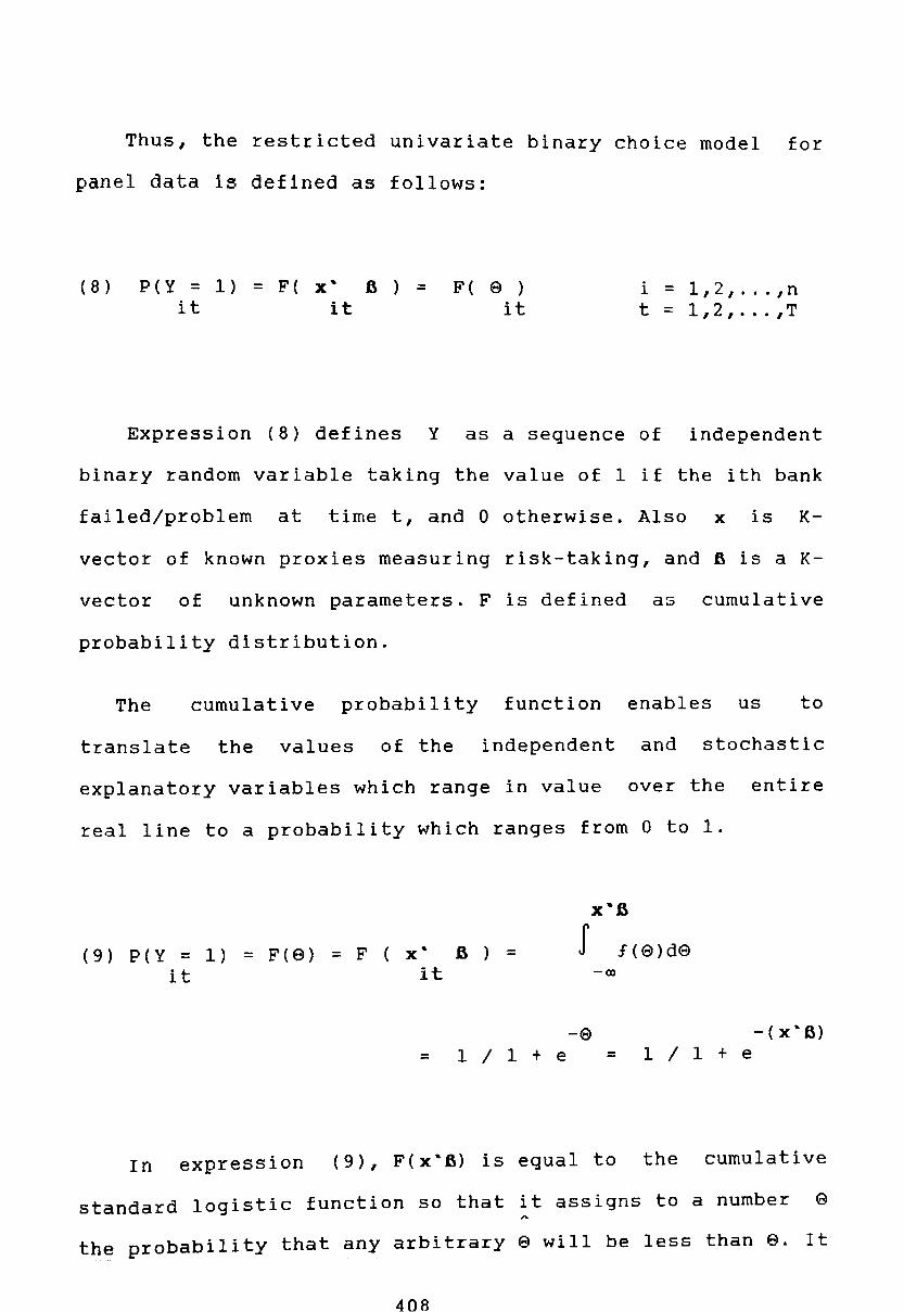
Thus, the restricted univariate binary choice model for

panel data is defined as follows:

( 8 ) P(Y = 1) = F( x~ a) = it it

F( 9 ) it

i = 1,2, ... ,n t = 1,2, ... ,T

Expression (8) defines Y as a sequence of independent

binary random variable taking the value of 1 if the ith bank

failed/problem at time t, and 0 otherwise. Also x is K-

vector of known proxies measuring risk-taking, and a is a K-

vector of unknown parameters. F is defined as cumulative

probability distribution.

The cumulative probability function enables us to

translate the values of the independent and stochastic

explanatory variables which range in value over the entire

real line to a probability which ranges from 0 to 1.

(9) P(Y = 1) = F(9) it

= F (x' a) = it

= 1/1 + e

x~a

f f(9)d9 -00

-9 = 1/1 + e

-(x'6)

In expression (9), F(x'6) is equal to the cumulative

standard logistic function so that it assigns to a number 9 A

the probability that any arbitrary 9 will be less than 9. It

408

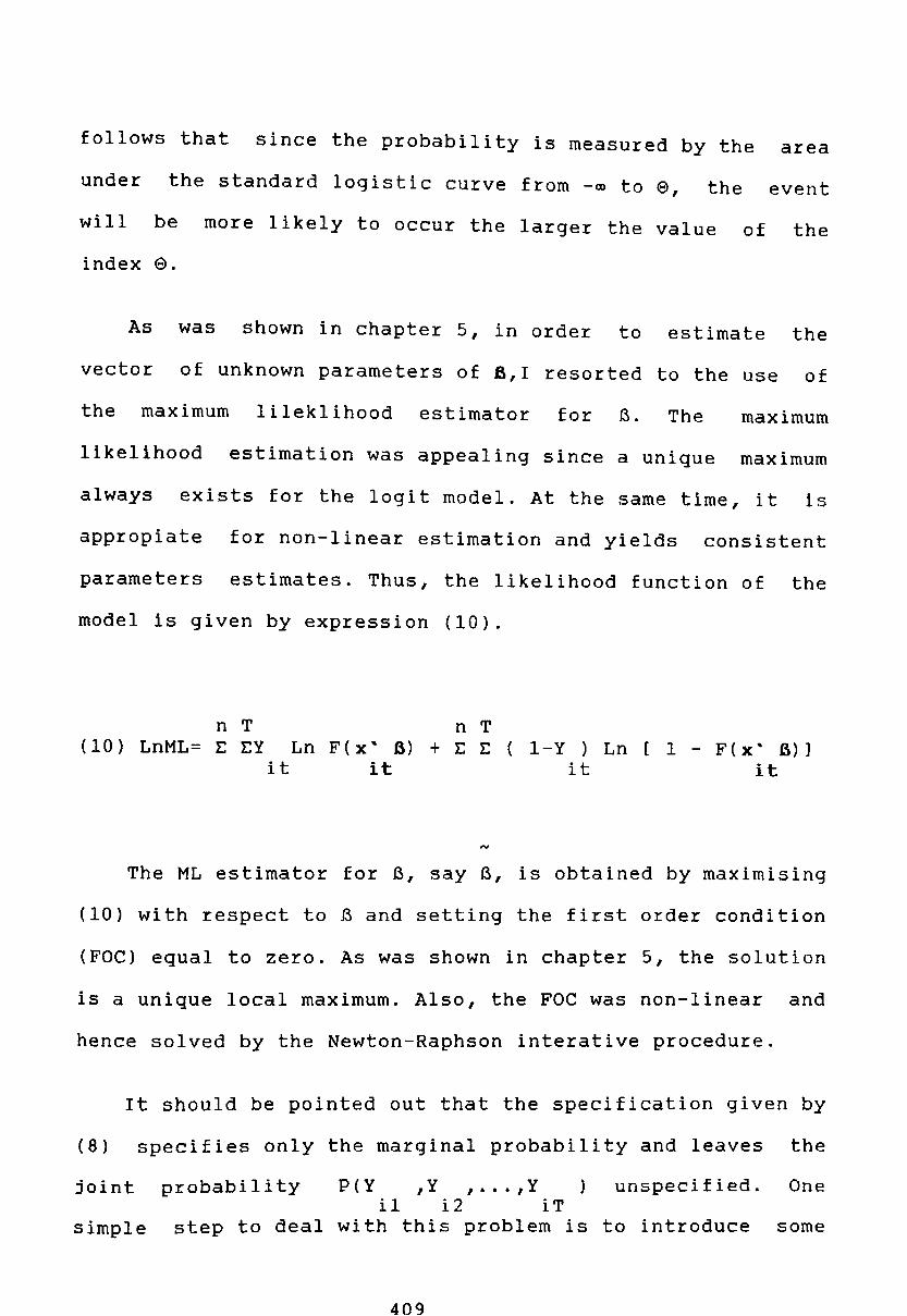
follows that since the probability is measured by the area

under the standard logistic curve from -00 to e, the event

will be more likely to occur the larger the value of the

index 9.

As was shown in chapter 5, in order to estimate the

vector of unknown parameters of 6,I resorted to the use of

the maximum lileklihood estimator for B. The maximum

likelihood estimation was appealing since a unique maximum

always exists for the logit model. At the same time, it is

appropiate for non-linear estimation and yields consistent

parameters estimates. Thus, the likelihood function of the

model is given by expression (10).

n TnT (10) LnML= E EY Ln F(x' 6) + E E ( l-Y ) Ln [ 1 - F(x' 6)]

it it it it

The ML estimator for B, say B, is obtained by maximising

(10) with respect to B and setting the first order condition

(FOC) equal to zero. As was shown in chapter 5, the solution

is a unique local maximum. Also, the FOC was non-linear and

hence solved by the Newton-Raphson interative procedure.

It should be pointed out that the specification given by

(8) specifies only the marginal probability and leaves the

joint probability P(Y ,Y , ... ,Y ) unspecified. One il i2 iT

simple step to deal with this problem is to introduce some

restrictions. We assume independence so that the joint

probability will be given by

(11) P(Y ,Y , ... ,Y ) = i1 i2 iT

E P( Y ) iT

The independence restriction implies that P(Y = IIY = 1) it i,t-1

so that previous year status does not affects the status

this year. This means two things: Firstly, there is no true

state dependency in the sense that the present status is not

affected by the past status. In other words, the probability

of bank failure/problem today remains unaffected by

yesterday's probability.

Secondly, there is no heterogeneity problem. This means

that no serious complications with unobservable variables

which could affect banks differently with respect to their

likelihood of failure/problem would araise.

Given the difficulties in estimating the unrestricted

version of the model for panel data with T=20 and n=21 we

proceeded to estimate the restricted version of the logit

model. The matrix specification of the model which is

similar to the one in chapter 7 looks as follows

o

A RAT33A ..... RAT63A 0 0 · . . . . . 179.1 179.1 179.1

A RAT33A ..... RAT63A 0 0 · . . . . . 179.2 179.2 179.2

· · · · . . . . . · · . . . . . · · · · ..... · · . . . . .

A RAT33A ..... RAT63A 0 0 · . . . . . n83.4 n83.4 n83.4

y= B x= 0 · . . . . . 0 RAT33B .... RAT63B it 179.1 it 179.1 179.1

B 0 · . . . . . 0 RAT63B .... RAT63B 179.2 179.2 179.2

B 0 0 RAT33B .... RAT63B n83.4 n83.4 n83.4

where i = 1,2, ... ,n t = 1,2,3,4, .... T

The column vector Y contains the endogeneous it

dichotomous variables for each bank i in a given quarter t

for the ordered group A (failed/problem banks) and group B

(nonfailed/nonproblem banks). The matrix x was constructed it

by separating the data for each group of banks A and B

respectively. This procedure has enables us to assess and

compare the hypothesis of excessive risk-taking for each

individual group. This is in itself an important

modification from the traditional literature bank failure

modelling.

411

(8.4.2.2) Description of the Data and the Variables.

The model was estimated using quarterly panel data for

the period between 1979 to 1983. Thus, the sample contained

20 quarterly observations for 27 banks. Like the model

specification of chapter 6 and 7, the banks sample was

divided into two groups, A1 and B1. A1 group corresponds to

the problem/failure group which includes all those

institutions which were liquidated, merged, capitalised,

and/or allowed to sell non-performing and risky loans to the

Central Bank during 1982-83. Group B1 includes non­

problem/non-failed banks, among them Banco de Estado and

Banco Industrial y de Comercio (BICE). As we have seen in

chapter 3 both institutions were the only two domestic

banks which remained financially healthy. In order to

enlarge the B1 group, foreign banks were also included as

they remained sound and as we saw in chapter 2 were subject

to a similar legislation as domestic banks. Thus, Al and

contain 16 and 11 banks respectively as they are listed

table 3.

412

B1

in

Table 8.3 Bank List of A1 and B1. ------------------------------------------------------------

Al B1 ------------------------------------------------------------Banks Code Banks Code ------------------------- -----------------------------------Chile* O'Higgins** Internacional* Continenta1** Sudamericano** Credito** Trabajo** Pacifico** Nacional** Concepcion* Edwards** Santiago* Unido Fomento* Hipotecario Fomento* Hipotecario Chile* Co10cadora Nacional*

001 008 009 011 014 016 022 025 026 027 029 035 502 504 505 506

Osorno Estado*** Do Brasil BICE Republic Nat. Of America Citybank Real Sao Paulo Santander Exterior

N.Y.

Source: SIBF, Informacion Financiera, Various Issues.

* **

***

Failed Banks (liquidated,intervined,or merged) Problem Banks (allowed to sell nonperforming and loans) state Bank

010 012 017 028 031 032 033 034 036 037 038

risky

This sample excluded two sets of financial institutions

which may appear relevant for this study. The first one

corresponds to banks which failed during 1981 among them

Espanol (002), Talca (006), Austral (024), and Linares

(030). The second group correspond to non-bank financial

institutions (financieras) which were left out all together,

including those which failed during 1981 among them Cash

(705), General Financiera (715), De Capitales (725), and Del

Sur (713). Their exclusion was justified, as demostrated in

chapter 3, as a result of their relatively small size. In

addition, as a general principle, I have included all those

413

financial institutions which had 16 or more consecutive

quarterly observations. This was necessary for comparison

purposes between the periods of 1979-81 (booming

macroeconomy) and 1982-83 (economic debacle).

It should be

Pacifico, Unido

pointed out that in group AI, banks

de Fomento, Hipotecario Chile, and

Colocadora Nacional de Valores have missing observations in

1979(03), 1979(03), 1983(04), and 1979(01) respectively. In

group B1, banks BICE, Republic, Santander, and Exterior also

presented missing observations in 79(03), 79(02), 79(01),

and 79(01) respectively. In consequence, the panel data of

20 quarters and 27 banks gives an adjusted total number of

521 observations which represent a sufficiently

statistical sample to draw logistic inferences.

large

As argued in chapter 6, it would have been desirable to

have had a controlled sample, particularly by size, number

of branches, and age. However, data limitations and the

small size of the Chilean banking system ruled out this

possibility.

With reference to the dependent variable (regressand) of

the model, I have specified the dependent variable as

dichotomous where it takes the value of 1 if the bank has

been listed as failed/problem and 0 otherwise. It is assumed

that in each year a financial institution either

failed/problem or did not failed/problem. However, a list of

quarterly classification of banks's soundness was not

A 1 A

available from the Superintendency of Banks (SIBF) nor an

annual classification prior 1983. Instead, I was forced to

rely on the predicted values estimated from quarterly bank

failure predicting model presented in chapter 5. As we saw

from there, the overall prediction accuracy evaluated at 0.5

cut-off point was judged as extremely good at different lead

time.

With respect to the explanatory variables (regressors),

I have selected a set of financial ratios estimated from

banks' balance-sheet as proxies for changes in risk-taking

by banks' managers. Like Short, O'Driscoll, and Berger

(1985), the model used as regressors those ratios controlled

by managers among them loans/asset ratio which serves as 5

proxy for asset quality. Indeed, loans are the riskiest

assets for banks to hold so that the higher the loans/asset

ratio the greater the risk exposure. Also, the study

included profits/total assets, nonperforming loans/capital,

and nonperforming loans/total loans as additional indicators

of asset quality.

Also, there is a measure of capital adequacy which

indicates the capacity of a bank to respond to asset losses.

The capital/asset ratio and the provision/asset ratio are

considered as two proxies for the banks' ability to absorb

these losses. The expected sign of both ratios should be

negative as increases in capital and provision relative to

asset holding should lower the probability of failure. It

415

should be said that these proxies are not entirely under the

managerial control, but there is direct involvement by the

banking authorities as part of their regulatory framework.

The risk associated with an unexpected outflow of

deposit is captured by the deposit/liabilities ratio. The

larger demand (sight) deposits and passbook savings relative

to total liabilities, the higher banks' vulnerability to

withdrawals. However, this ratio can also be interpreted as

the cost of banks' indebtness. It is shown in the literature

that the higher is the proportion of deposits (low cost) the

lower is the probability of bank failure. Therefore, the

interpretation of this ratio is ambiguous and hence treated

with caution.

Finally, the model includes a measure of the asset and

liability growth as proxy for banks' risk-taking. Indeed, in

a regime of unregulated and stubbornly high deposit and

lending interest rates high growth rates of assets (loans)

and liabilities (deposits) rises the likelihood of bank

failure.

It should be stressed that the ratios as proxies of

banks' risk-taking (moral hazard) are expressed as the

deviation from its own trend. They perform better in testing

moral hazard than the financial ratios per see The trend was

estimated by regressing each monthly selected proxy for the

ith bank against time. Its fitted value was applied to

obtain the deviation from the its trend. ~~-~~lIf"

41 h

(8.4.3) Econometric Results and its Interpretation.

The first step in assessing the role of moral hazard in

the Chilean banking system is to compare the arithmetic mean

of selected financial ratios between the group of

failed/problem banks (F) and nonfailed/nonproblem banks (NF)

over the four-year period. The financial ratios are

expressed as the deviation from its own trend for each

financial institution and the group mean was estimated with

monthly observations for each bank.

If moral hazard characterised the banking system, then

failed/problem banks would have exhibited a riskier

management than nonfailed/problem banks. A riskier bank

management should be reflected in the quality of bank

assets, capital and reserves adequacy, and bank leverage.

With respect to the quality of bank loans, we should

expect a priori that the deviation from the trend for total

loans/total assets ratio (TL/TA) and the nonperforming

loans/capital (NPL/K) and nonperforming loans/total loans

(NPL/TL) ratios of failed/problem banks should be larger

than those of nonfailed/nonproblem banks. These results are

reported in tables 4a and 4b.

For instance, the mean of nonperforming loans/capital

mean ratio indicates sharp differences between the two

groups particularly in 1980, 1981 and to a lesser extent in

1982. In 1981 and 1982 the difference between the mean

ratio5 of the two groups (F-NF) Is 0.8368 and 0.7182

respectively.

Table 8.4a

1979

F

Pr/TA .001 TL/TA -.005 NPL/K -1.001 NPL/TL -.018

Prv/TL .017

Dep/TL -.017

LACTOT .088 LPASCIR .087

Sample Mean for Failed/Problem and Nonfailed Nonproblem Banks for the Period 1979-1981.

NF

-.005 .046

-.094 .007

F

.001

.016 1.202

.014

1980

NF

-.005 .034 .365

-.015

.014 -.020 -.117

.022 -.002 -.008

.369 .253

.394 .239 .246 .255

F

.008

.065 1.154 -.026

1981

NF

.006

.104

.436 -.013

Average 79-80

F

.003

.025

.451 -.010

NF

-.001 .061 .235

-.007

-.058 -.030 -.020 -.044

.100

.305

.373

.011 .027

.020 .215

.080 .233

.008

.211

.243

Source: SIBF, Informacion Financiera, Various Issues.

Similarly, the evidence from the growth of bank assets

and liabilities also confirms a propensity by failed/problem

banks to undertake more risk than safe banks. For instance,

the trend deviation of banks' assets for the former group

not only widened during the period 1979-82 but also it was

larger than the nonfailed/problem bank group. The average

mean deviation for F-group and the NF-group for the whole

period was 0.27 and 0.147 respectively. The same conclusions

are drawn from the data on bank liabilities.

The provision/total loans ratio was included as measure

of banks' capacity to respond to losses from banks assets .

.d1A

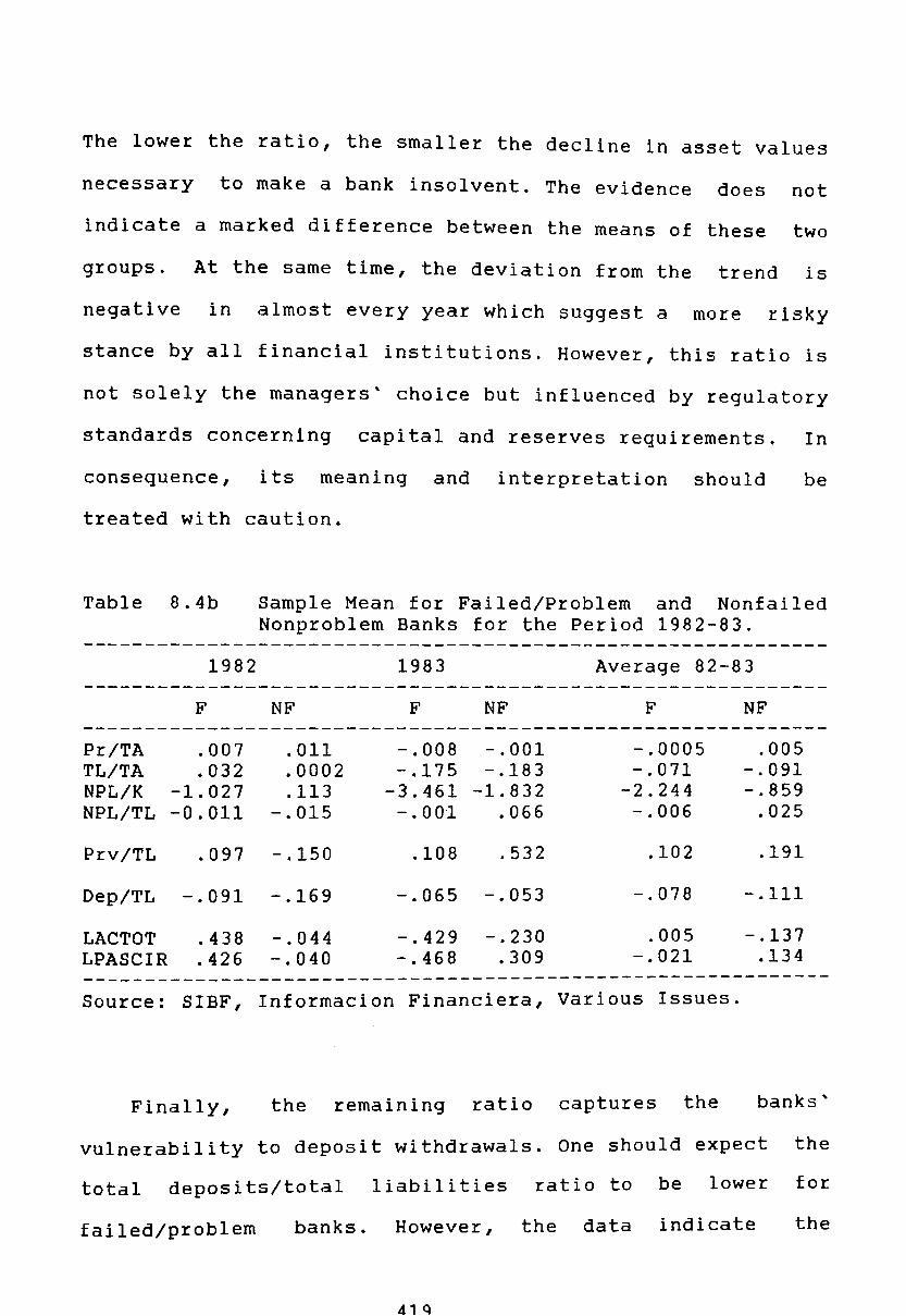
The lower the ratio, the smaller the decline in asset values

necessary to make a bank insolvent. The evidence does not

indicate a marked difference between the means of these two

groups. At the same time, the deviation from the trend is

negative in almost every year which suggest a more risky

stance by all financial institutions. However, this ratio is

not solely the managers' choice but influenced by regulatory

standards concerning capital and reserves requirements. In

consequence, its meaning and interpretation should be

treated with caution.

Table 8.4b

1982

F

Sample Mean for Failed/Problem and Nonfailed Nonproblem Banks for the Period 1982-83.

1983 Average 82-83

NF F NF F NF ------------------------------------------------------------Pr/TA .007 .011 -.008 -.001 -.0005 .005 TL/TA .032 .0002 -.175 -.183 -.071 -.091 NPL/K -1.027 .113 -3.461 -1.832 -2.244 -.859 NPL/TL -0.011 -.015 -.001 .066 -.006 .025

Prv/TL .097 -.150 .108 .532 .102 .191

Oep/TL -.091 -.169 -.065 -.053 -.078 -.111

LACTOT .438 -.044 -.429 -.230 .005 -.137 LPASCIR .426 -.040 -.468 .309 -.021 .134

------------------------------------------------------------Source: SIBF, Informacion Financiera, Various Issues.

Finally, the remaining ratio captures the banks'

vulnerability to deposit withdrawals. One should expect the

total deposits/total liabilities ratio to be lower for

failed/problem banks. However, the data indicate the

d1q

opposite result, with the exception of 1979. This ambiguity

can be explained by the fact that sight deposits represent a

cheaper source of liabilities. Therefore , a lower ratio

implies a lower probability of failure.

Further evidence from selected individual banks of both

groups are plotted in order to assess excessive risk-taking

(moral hazard) for the period between 1979 and 1983. Among

the group of failed/problem banks, Banco Chile, Banco

Santiago, Banco Internacional, and Banco Concepcion were

selected among 16 financial institutions classified in this

category. With respect to the sample of nonproblem/nonfailed

banks, Banco del Estado, Banco BICE, Banco Real, and Banco

Sao Paulo were chosen from the list of 11 institutions for

comparison purposes. As we have learned from chapter 3,

Banco del Estado (the only remaining state bank after

financial reforms) and Banco BICE were the only two domestic

commercial banks which did not sell bad loans to the Central

Bank. Also, Banco Real and Banco Sao Paulo were listed with

the group of foreign banks operating in the Chilean banking

system.

With reference to the banks' asset quality, the charts

which plot the deviation and the trend of the total

loans/total assets ratio shows that failed/problem banks

exhibited an upward trend over the whole period and a large

deviation of the ratio over its own trend, particularly

between 1981 and the middle of 1983. For instance, the

A?O

monthly ratio and its estimated trend plotted for 1979 to

1983 for Banco Chile, Banco Internacional, Banco Concepcion

and Banco Santiago shows an upward trend indicating a

greater exposure to credit risks. As was argued earlier, the

trend should capture the influence of the overall economy

and both technological and regulatory changes. However, the

total loans/total assets ratio's deviation was largely

positive indicating an over-exposure to credit risks. This

is particularly the case during 1982 and part of 1983 during

which the economy's output collapsed.

In contrast, nonfailed/nonproblem banks show a more

steady upward trend especially Banco del Estado, and Banco

Sao Paulo. Moreover, there are cases where the ratio trends

downward as is the case of Banco Real. This evidence may

suggest a more conservative banks' attitude to a buoyant

macroeconomy. Although the ratio is above the trend and

hence indicating some degree of over-exposure, the deviation

began to fall rapidly during the beginning of 1982, period

which witnessed the collapse of the economy's output.

Similar conclusions about loans quality can be drawn

from other proxies. Particularly interesting is the

comparision of the persistent positive deviation of

nonperforming loans/capital ratio of failed banks (Banco

Chile, Banco Internacional, and Banco Concepcion) in

comparison to Banco del Estado and BreE which exhibit a

smooth deviation. As it was seen in chapter 3, these two

institutions did not sell bad loans to the central Bank and

thus suggesting a more conservative attitude towards the

quality (riskiness) of their assets. Also noticeable is the

significant fall in the ratio for the failed/problem banks

towards the end of 1982 explained by the rescue package

enacted by the monetary authorities. As it was explained at

length in chapter 3, this included the possibility of

selling nonperforming loans to the Central Bank and the

capitalisation of these troubled institutions.

411

Figure 8.2a Banco Chile: Total Loan/Total Asset Ratio 0.9-·.-----------_____ .... 0.6-

n IV V.I-

0.8-

0.5-

0.4-

O.S-

0.2-

0.1-

o .0 -. .,.,...,..,..,.,..,..,...,..,..,...,."T'"P"I'.,..,..,..,..,...,..,..,..,..,..,..,..,..,...,..,..,..,..,..,..,.'T'I""'I'.,..,.,..,..,.,.~~,..,....'I""'r""I"~ 1979

Figure 8.2b 0.95-

0.00-

0.85

0.75-

1979

1980 1001 1002 l00S

/-BOOl ----- BOOl TI

Bartco Santiago: Total Loan/Total Asset Ratio

1960 1001 1002 l00S

1-B035 ----- B035TI

423

Figure a.Ze Banco Internacional: Total Loan/Total Asset Ratio O.~-~----------------------------~ ____ __ 0.90

0.a5-.. --

o.ao-

0.75-

0.70-

1979 1980 19tH

..... ".,rl'--, ..

1982

,rr­---

1983

1-BOOO ----- BOOOTI

Figure a.2d Banco Concepcion: Total Loan/Total Asset Ratio 0.95-

0.00-

0.85 J\ -.. --

':_-~-l. - ---- .-----.-------.-----

o.ao

0.75-

1979 1980 1981 1982 1003

1-B027 ----- B027TJ

424

Figure 8.3a Banco del Estado: Total Loan/Total Asset Ratio 0.85-r-------------_____ ---.

0.80-

0.75

0.70-

0.65

0.60

0.55

0.50-

1979 1980 1981 1982 1983

1-BOl2 ----- BOl2TI

Figure 8.3b BarlCO BICE: Total Loan/Total Asset Ratio 1.00

0.75-

0.50-

0.25

1979 1980 19tH 1982

1-B028 ----- B028T\

425

Figure S.3c Banco Real: Total Loan/Total Asset Ratio 1.0-,.----------______ _

0.6-

0.5

1979 1980 1981 198:3 1983

1-8034 ----- B034 TI

Figure S.3d. Banco de Sao Paulo: Total Loan/Total Asset Ratio 1.0-.-----------------------,

0.9-

O.S

0.7-

0.6-

0.5- .. _.t- -

0.4-

0.3

1979 1980 1981 198:3 1983

I-B036 ----- B036T\

426

Figure 8.4a Banoo Chile: NP Loans/Capital Ratio 0.20-r------------------_

0.15-

0.10-

0.05-

O.oo-t---,_r

1979 1980 1981 1982 1983

I-BOOl ----- BOOITI

Figure 8.4b Banoo Santiago: NP Loans/Capital Ratio 0.5-...-----------------------,

0.4-

0.3-

0.2-

0.1-

O.O-I---------:-=""~---------

1979 1980 1981 1982 1983

1-B035 ----- B035T}

427

Figure 8.4c Banco Internacional: NP Loans/Capital Ratio 0.20-,.----------------------.

0.15-

0.10-

0.05-_r-

r-

_r

0.00 _r r-

r-.-

-0.05 1979 1980 1981 1982 1983

1-BOOO ----- BOOST I

Figure 8.4d Banco Concepcion: NP Loans/Capital Ratio 0.20

0.15-

0.10-

0.05-

O.OO-'I--~

1979 1980

428

1981

r _r r"

1002

v

rr

1003

1-B027 ----- B027TI

Figure 8.5a Banco del Estado: NP Loans/Capital Ratio O.100-·r--------------_____ _

0.075-

0.050-

.. ' 0.025- ,-1,-1 -",-

1979 1980 19131

-_1"

1002 19133

/-B012 ----- BOlaTl

Figure a.5b Banco BICE: NP Loans/Capit al Ratio 0.05-

0.04

0.03-

0.02-

0.01

,,­-' 1'.

1979 1980 1981 1982 1983

1-B028 ----- B028TI

429

Figure S.5c Banco Real: NP Loans/Capital Ratio 0.20...------------------_

0.15

0.10-

0.05

0.00+--""" .. -.,-

1979 1980 1981 1982 1983

1-B034 ----- B034 TI

Figure S.5d Banco de Sao Paulo: NP Loans/Capital Ratio 0.125-...---------------------.

0.100-1

0.0'"15

0.050-

0.025- ,.

1979 1980 1981

430

1982

, r

1983

I-B036 ----- B036TI

Figure a.6a Banco Chile: Profits/Total Asset Ratio 0.100-,.--------------____ _

0.0'15

0.050-

0.005- ----.. _

0.000-

-0.025-

1979 19ao 1981 1982 1983

I-BOOl ----- BOOITI

Figure a.Sh Banco Santiago: Profits/Total Asset Ratio O.05-r----------------------,

-0.05-

-0.10-

1979 1980 1981 1982 1983

I-B035 ----- B035TI

431

Figure a.ae Banco Internacional: Profits/Total Asset s Ratio O,fJJ-r----------------__ ....

0.02

0.00- .... .. .. - ..

-0.01- ..... .. .. -0.02-

-0.03-

-0.04 1979 1980 1981 1982 1983

I-B009 ----- B009TI

Figure a.ad Banco Concepcion: Profits/Total Asset Ratio 0.005-

....

0.000-

-"'-" "- ..

-0.025 "'- ...

"'- ...

-0.050-

-0.075- \

1979 19ao 1981 1982 1983

I-BO~ ----- BO~TI

432

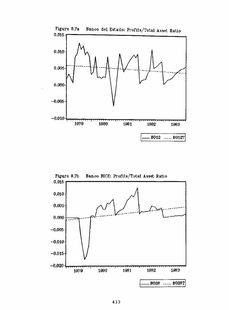
Figure 8.7a Banco del Est ado: Profits/Total Asset Ratio 0.015-.-----------______ _

0.010-

0.005- --- --- ... --- - ""---'" - ... _- ...

0.000-

-0.005-

1979 1980 1981 1982 1983

1-B012 ----- B012T1

Figure 8.Th Banco BlCE: Profits/Total Asset Ratio 0.015-

0.010-

0.005 _,_1-1'-'-

0.000- _r-:--I

-0.005-

-0.010-

-0.015-

1919 1980 1981 1982 1983

1-BOza ----- BOzaT\

433

Figure 8.'lc Ban.co Real: Profits/Total Asset Ratio 0.20-.-------------____ _

0.15-

0.10-

0.05

_,_r_,_r-"--

0.00

1979 1980

_,-,_1'-,_.1 ,_,-,_1'-,_1 -

1981 1982

,_r-' _.1"_'-

1983

I-B034 ----- B034TI

Figure 8.'ld Ban.co de Sao Paulo: Profits/Total Asset Ratio 0.10-·..----------------------,

0.05-

0.00-

-0.05 -

-0.10-

1979 1980 1981 1982 1983

1-B036 ----- B036TI

434

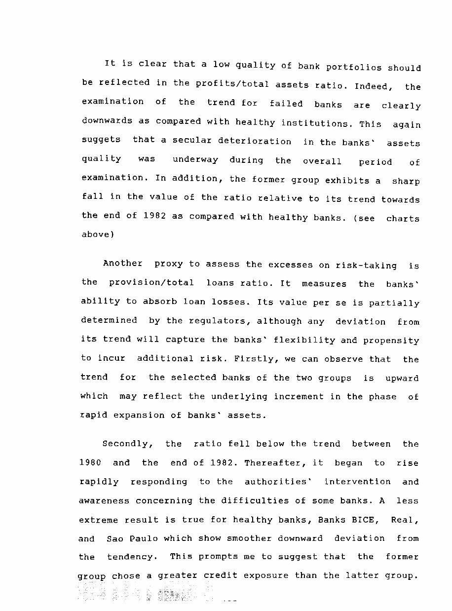
It is clear that a low quality of bank portfolios should

be reflected in the profits/total assets ratio. Indeed, the

examination of the trend for failed banks are clearly

downwards as compared with healthy institutions. This again

suggets that a secular deterioration in the banks' assets

quality was underway during the overall period of

examination. In addition, the former group exhibits a sharp

fall in the value of the ratio relative to its trend towards

the end of 1982 as compared with healthy banks. (see charts

above)

Another proxy to assess the excesses on risk-taking is

the provision/total loans ratio. It measures the banks'

ability to absorb loan losses. Its value per se is partially

determined by the regulators, although any deviation from

its trend will capture the banks' flexibility and propensity

to incur additional risk. Firstly, we can observe that the

trend for the selected banks of the two groups is upward

which may reflect the underlying increment in the phase of

rapid expansion of banks' assets.

Secondly, the ratio fell below the trend between the

1980 and the end of 1982. Thereafter, it began to rise

rapidly responding to the authorities' intervention and

awareness concerning the difficulties of some banks. A less

extreme result is true for healthy banks, Banks BleE, Real,

and Sao Paulo which show smoother downward deviation from

the tendency. This prompts me to suggest that the former

group chose a greater credit exposure than the latter group.

Figure a.Sa Banco Chile: Provision/Total Loan Ratio 0.200-.-----------______ _

0.175

0.150-

0.125-

0.100-

0.075-

1979 1980 1981 1982 1983

1-BOOl ----- BOOl TI

Figure S.8b Banco Santiago: Provision/Total Loan Ratio 0.4

0.3-

0.2-

0.1 ,-

0.0-

1979 1980 1001 1982 1003

/-B035 ----- B035TI

436

Figure 8.& Banco Internacional: Provision/Total Loan Ratio 0.40--..------------------__

0.35

0.30-

0.25

0.20

0.15

0.10

0.05

1979 1980 1981 1982 1983

1-B009 ----- B009TI

Figure 8.8d Banco Concepcion: Provision/Total Loan Ratio 0.30-

0.25

0.20-

0.15

0.10-

0.05-

1979 1980 1981 1982 1983

1-B027 ----- B027T\

437

Figure a.9a Banco d.el Estad.o: Provision/Total Loan Ratio 0.40-·,..------------_____ _

0.35-

0.30-

0.25-

0.20

0.15

0.10-

1979 1980 1981 198Z 1003

I-BOIZ ----- BOIZTI

Figure 6.9b Banco DICE: Provision/Total Loan Ratio 1.00-

0.75

0.50

0.25-

1979 1000

~,. ,.'

438

1001

,., ,..r

,-

196Z 1003

1-BOZS ----- BOZSTI

Figure 8.9c Banco Real: Provision/Total Loan Ratio 3.0-r--------------___ _

2.5

2.0-

1.5

1.0-

" 0.5-

-0.5- , ... _,.r

1919 1980 1981 1982 1983

/-B034 ----- 8034 TI

Figure 8.9d Banco de Sao Paulo: Provision/Total Loan Ratio 3.0-,----------------------.

2.5-

2.0

1.5-

1919 1980 1981 1982 1983

1-B036 ----- B036TI

43'3

As was argued in a previous section, when a depositary

financial institution becomes riskier the cost of deposits

may not rise in proportion to the risk undertaken. This is

certainly the case when there is an implict or explicit

deposit insurance. Banks are able to increase their net

interest margins by using low cost resources to fund loans

with higher payoffs but riskier returns.

It is reasonable to expect that a positive deviation of

the total deposit ratio/total liabilities ratio over its

trend value should be relatively higher for failed banks.

The evidence from the four selected failed banks and the

group of nonfailed institutions clearly supports this

assertion. For instance, Banco Chile and Banco Internacional

show a sharp positive deviation over a downward trend. The

downward trend is present in all the cases indicating how it

was becoming more expensive to raise funds via banks'

deposits. This is obvious if we examine the ex post short

term real deposit rate which prevailed during the whole

liberalisation reform.

In contrast, Banco BICE, Banco Real, and particularly

Banco del Estado exhibit values close to the underlying

trend, and in some instances below it. This suggests a more

conservative approach by bankers to issuing deposit

liabilities than failed financial institutions. (see charts

below)

Figure a.l0a Banco Chile: Deposit/Total Liabilities Ratio 0.50-·r---------------____ _ 0.45-

0.40

0.35 "'- ... .....

0.30-

0.25-

0.20-

0.15

1979 1980 1981

...... "'"

......

19132

"'" ...... ...... ~-

19133

1-BOOl ----- BOOl TI

Figure a.l0b Banco Santiago: Deposit/Total Liabilities Ratio 0.13-

0.7-

0.6

0.5-

0.4-

0.3

0.2-

1979 19130 1981 19132 1003

1_ B035 ----- B035TI

441

Figure 8.10c Ban.co In.ternacional: Deposit/Total Liabilities Ratio 1.25-·,--------------____ ---.

1.00-

0.75

0.50

0.25

1979 1980 1981 1982 1983

I-B009 ----- BOOBTI

Figure 8.10d Banco Concepcion: Deposit/Total Liabilities Ratio 0.6-

0.4--"L."_,,, ... - ...

.. .. - .... 0.3-

0.2-

0.1

1979 1980 1981 1982 1983

I-B027 ----- B027TI

44:2

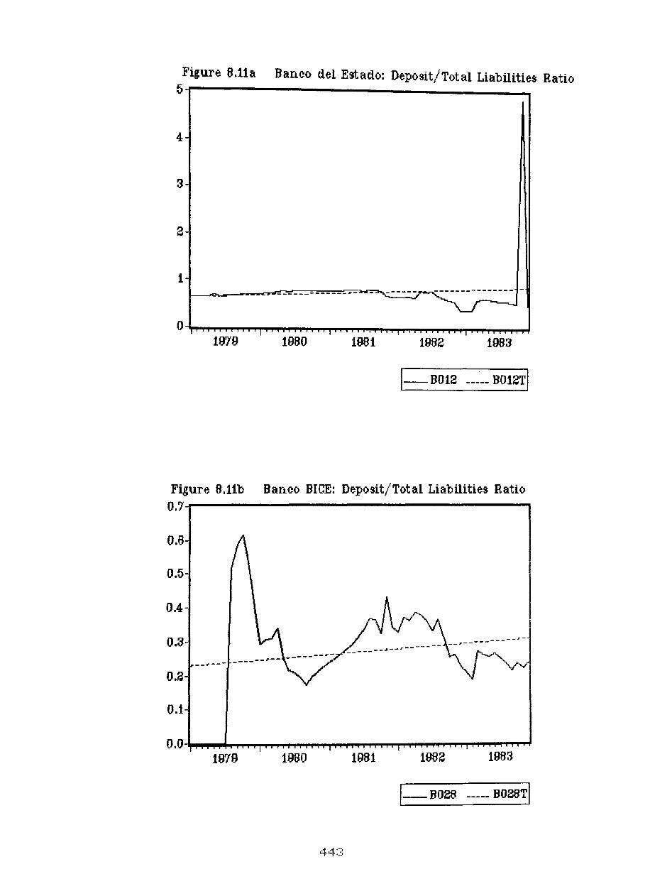
Figure 8.11a Banco del Estado: Deposit/Total Liabilities Ratio 5-·~----------------------__________ __

4

3

2-

1-.r ----- -------,~~-~-----

O~~~~~~I~~~~I~~~~I~~~~I~~~~ 1979 1980 1981 1982 1983

I-B012 ----- B01aTi

Figure 8.11b Banco BICE: Deposit/Total Liabilities Ratio 0.7-

0.6-

0.5

0.4-

0.3-

1979 1980 1981 1982

I-B028 ----- B028TI

44::3

Figure S.11c Banco Real: Deposit/Total Liabilities Ratio 0.6-.--------------___ _

0.5-

0.4-

0.3-

0.2

0.1

1979 1980 1981 1982 1983

I-B034 ----- BOMTI

Figure S.Ud Banco de Sao Paulo: Deposit/Total Liabilities Ratio 1.1...---------------------,

1.0-

0.9-

O.S-

0.7-

0.8

0.5

0.4-

0.3-

.....

0.2 ~_.......,.""""""",..,.,..t""'I""I"'~..,.,.,."'I"'!""I"',..,..,.....,.,..,..,.,..,."""""""~,..,...,.;"T"""'.,..,..,..~,..,..., 1979 1980 1981 1982 1983

1-B036 ----- B036TI

444

Finally, one of the most noticeable aspects of financial

liberalisation was the spectacular growth in bank assets.

This took place in spite of stubbornly high real lending

rates indicating a propensity to accept more risks. The

evidence from the asset growth and its deviation from its

trend confirms this point.

The plot of the ratio measuring the growth of bank

assets for selected failed banks shows a positive deviation

from its trend by almost the whole period of study,

especially between 1980 and 1982. This contrast sharply with

the observations from the cases of Banco Real and Banco Sao

Paulo. Also, it can be seen that the asset growth began to

fall towards the end of 1981, especially in the case of

Banco del Estado.

The trend is upward in all cases indicating the response

of the banking system to the rapid output growth experienced

by the economy during most of the period. It is clear

those banks which exhibited a growth rate above

that

their

secular trend were willing to expand credit beyond an

optimal point and hence to accept a greater risk-exposure.

(see charts below)

445

Figure 8.12a Banco Chile: Asset Growth 8.75..,.....---------------__ _

8.50

8.25-

8.00-

7.75-

1979 1980 1981 1982 1983

1-BOOl ----- BOO! TI

Figure 8.12b Banco Santiago: Asset Growth

8.50---------------------------------------~

8.26

8.00-

7.75-

7.50

7.25-

7.00-

19'"/9 1980 1981 1982 1983

1-B035 ----- B035TI

Figure 8.12c Banco Internacional: Asset Growth 7.4-,r-------------____ ....

7.3-

7.2-

7.1-

7.0-

6.9-

6.8

6.7-

6.6-,

",'

, .. .... , ..

... ' ... ,r

,.

... . ' ..... '

... ' ... ...

.r "," ,

" , ... ' ...

, . ... r

"

, rr

6 .5 -'"""'""P"'I""!""I""P"'!'''I''''P'''!'T'f'"I''.,..,.,.''I''''P'''!'.,..,.,...,.,.,.''I''''P'''!'.,..,.,.'''I''''I''''I'~.,.,.,.''"'''''',.,..,.,..,.,.,..,.,........,..,....,..., 1979 1980 1981 1982 1983

1-B009 ----- B009TI

Figure 8.12d. Banco Concepcion: Asset Growttt 8.00-

7.75

7.50-

7.25

19?'9 1980 1981 1982 1983

1-B027 ----- B027TI

447

Figure 8.13a Banco del Estado: Asset Growth 8.7...-------------____ ___ 6.6-

6.5-

8.4

8.3-

8.2-

8.1-

8.0-

6-

5

4-

3-

2-

1

0

1979

-,,-

I

1979

1980 1981 1982 1983

I-B012 ----- B012TI

Banco BICE: Asset Growth

,.­,."

1980 I

1001

448

I I

1002 1003

I-B028 ----- B028TI

Figure 8.13c Banco Real: Asset Growth 6.75-.------------____ __

8.50

8.25-

8.00

5.75

1979 1980 19tH 1982 1963

1-B034 ----- B034 TI

Figure 8.13d Banco de Sao Paulo: Asset Growth 6.50-....---------------------.

8.25

6.00-

5.75

5.50-

5.25-

19'19 1980 1961 1982 1983

I-B036 ----- B036TI

44'3

The evidence presented in tables 4a and 4b for a grouped

data and the charta for individual aelected bankB Bupport,

at first hand, the view that moral hazard was present in

the Chilean banking system. In fact, it reveals a greater

propensity to take risk among those financial institutions

which failed or experienced financial difficulties.(problem

banks)

However, a more sophisticated model is necessary to

support this hypothesis and its incidence on the failure of

financial institutions in the Chilean banking system. There

are three conjectures about bank failures/problems and the

role of moral hazard on the likelihood of bank failure which

I would like to explictly test.

Firstly, the role of moral hazard was present throughout

the period of study and it was significant in explaning the

failure of financial institutions in Chile. Specifically, I

should be looking for the empirical link and the statistical

significance of the selected proxies for risk-taking over

the period between 1979 and 1983.

Secondly, if conjecture one is found to be true, we

should also test the assertion that excessive risk-taking

(moral hazard) was more acute for the years between 1982-83

than 1979-81. Thus, the model will be estimated and tested

for each year separately for comparison purposes.

450

Thirdly, once we accept that hypothesis which relates

moral hazard with the likelihood of bank failure/problem, it

is possible to use the "best" model to estimate the ex ante

probability and assess the prediction accuracy as I did in

chapter 6 and 7.

In order to evaluate these conjectures I have estimated

the restricted logistic model for quarterly panel data

following the methodology and estimation procedures

described thoroughly in chapter 6 and 7 and reviewed in

earlier sections of this chapter.

-Conjecture 1: The Likelihood of Bank Failures/Problems and Moral Hazard during the period 1979-1983.

The first conjecture establishes the relationship

between excessive risk-taking (moral hazard) and the failure

of financial institutions, and the subsequent debacle of

the banking system. It is argued that the incidence of

risk-taking is present throughout the period of study.

Table 5 provides econometric evidence on the

significance of some selected proxies which measure banks'

propensity to take risk and the probability of bank

failure/problem. It should be stressed that the ratios as

proxies for banks' attitude towards risk-taking are

expressed in terms of the deviation from its trend. A

positive sign on a coefficient indicates that the higher the

451

value of the ratio, the greater the propensity to take

excessive risk and hence the larger the likelihood of

failure.

Apart from a general model specification which included

all selected regressors, alternative specifications are

reported as the explanatory variables exhibited

multicollinearity. As can be seen from the estimates and the

covariance-correlation matrix of the explanatory variables

included in appendix 7, the ratio total loans/total assets

(TL/TA) is highly collinear with assets growth (LACTOT) and

liability growth (LPASCIR). Similarly, asset growth and

liabilitity growth also present a high correlation

coefficient. It can be seen that the correlation coefficient

exceeds 80% in most cases.

Specification M1 corresponds to a general model which

included all the selected proxies for bank's risk-taking. We

can observe that the overall equation is statistically

significant at 0.5%. Specifically, the likelihood ratio

statistic is 129.5 and the critical value of the chi-square

distribution for the 0.005 level of significance is 35.71 so

we reject the null hypothesis that B1=B2 .... Bk=0. Although

M1 exhibits the largest likelihood ratio and the largest

goodness of fit measured by the likelihood ratio index

(Lklhd RIndex), most of the regressors are insignificant.

Indeed, besides the nonperforming loans/capital ratio

452

(NPL/K) for group A (failed/problem banks) and group B

(nonfailed/nonproblem banks), and the proxy for "related

portfolios" (cartint), the remaining regressors are

insignificant according to their t-statistics at 1% and 5%

significance. The theoretical value for t-statistic for 0.01

and 0.05 is 2.58 and 1.96 respectively and hence the

estimated ratios fell outside the critical region.

I suspect that multicollinearity is serious among some

independent variables judging from the covariance­

correlation matrix included in appendix 7. As we are aware,

the presence of collinearity among the regressors affects

the standard errors and the stability of the coefficient. To

obtain meaningful estimates and inferences, different

specification were carried out by dropping those variable

found to be highly collinear.

453

Table 8.5 Log~t AnalYSis of Selected Proxies for Risk­Taklng for the Period 1979.1 to 1983.4 (a)

------------------------'------------------------------------Proxies M1

Alternative Specifications M2 M3 M4

Constant ------------------------------------------------------------

M5

(Pr/TA)A

(TL/TA)A

(NPL/K)A

(NPL/TL)A

(Prv/TL)A

(Dep/TLi)A

(LACTOT)A

(LPASCIR)A

(Pr/TA)B

(TL/TA)B

(NPL/K)B

(NPL/TL)B

(Prv/TL)B

(Dep/TLi)B

(LACTOT)B

(LPASCIR)B

CARTINT

-0.17 (-1.65) -20.80 (-1.12) -1.64

(-0.51) 0.24

( 3 .25 ) -0.05

(-0.06) -1.13

(-0.32) -3.03

(-1.27) -3.55

(-1.25) 3.67

(1.27 )

-0.01 (-0.007)

0.007 (0.003)

0.46 ( 2 . 42) 1.02

( 3 . 29) 0.15

(0.22) -0.31

(-0.30) -0.28

(-0.37) -0.33

(-0.44) 3.32

( 6 . 55)

-0.16 (-1.60) -14.82 (-0.85)

0.05 (0.06 ) -4.78

(-1.91) -4.38

(-1.96) 0.22

(2.81 )

0.60 (0.48)

0.95 (3.14 ) -0.16

(-0.35) 0.06

(0.06 ) -0.45

(-2.66)

2.92 (6.51)

-0.18 (-1.80) -13.55 (-0.79)

3.83 (2.51 )

0.03 (0.04) -2.10

(-0.89) -3.53

(-1.64)

0.49 (0.38) -1.95

(-1.17)

0.83 (2.75) -0.49

(-0.88) -0.16

(-0.16)

-0.16 (-1.61) -14.53 (-0.84)

0.05 (0.06 ) -4.64

(-1.86) -4.42

(-1.97)

0.22 (2.83)

0.15 (0.12 )

0.96 (3.17) -0.39

(-0.82) 0.0005

(0.0005)

-0.44 (-2.67)

2.92 ( 6 . 51 )

-0.17 (-1.69) -25.25 (-1.39)

0.24 (3.26)

-2.64 (-1.03) -2.97

(-1.27 ) 0.02

(0.21)

-0.11 (-0.09)

0.37 (2.15)

0.53 (1.08) -0.44

( -0 . 43) -0.30

(-2.14)

------------------------------------------------------------In Lklhd(-) 294.43 Lklhd Ratio(b) 129.50 Lklhd Rlndex(c) 18.00 A.I.C.(d)(-) 312.43

304.34 109.60

15.27 316.34

309.49 99.38 13.84

321.49

(a) t-statisties are in parentheses.

304.28 109.80

15.29 316.28

306.20 106.00

14.76 318.20

(b) The likelihood ratio is -2(lnLklhdr-lnLklhdu] and it has chi-square distribution with j degree of freedom. (e) The pseudo-R square is 1-[lnLk1hdr/lnLklhdu] Cd) The Akaike's Information Criteria is -In(Lk1hd)+K where K is the number of estimated parameters.

454

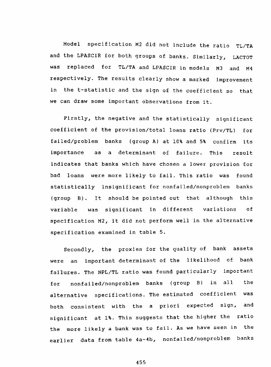
Model specification M2 did not include the ratio TL/TA

and the LPASCIR for both groups of banks. Similarly, LACTOT

was replaced for TL/TA and LPASCIR in models M3 and M4

respectively. The results clearly show a marked improvement

in the t-statistic and the sign of the coefficient so that

we can draw some important observations from it.

Firstly, the negative and the statistically significant

coefficient of the provision/total loans ratio (Prv/TL) for

failed/problem banks (group A) at 10% and 5% confirm its

importance as a determinant of failure. This result

indicates that banks which have chosen a lower provision for

bad loans were more likely to fail. This ratio was found

statistically insignificant for nonfailed/nonproblem banks

(group B). It should be pointed out that although this

variable was significant in different variations of

specification M2, it did not perform well in the alternative

specification examined in table 5.

Secondly, the proxies for the quality of bank assets

were an important determinant of the likelihood of bank

failures. The NPL/TL ratio was found particularly important

for nonfailed/nonproblem banks (group B) in all the

alternative specifications. The estimated coefficient was

both consistent with the a priori expected sign, and

significant at 1%. This suggests that the higher the ratio

the more likely a bank was to fail. As we have seen in the

earlier data from table 4a-4b, nonfailed/nonproblem banks

455

did exhibit a lower mean value for the ratio's deviation

over its trend and the conflrmatlofl (_If lOt " "t--~5 Blgnl lcanC6

supports the hypothesis that this group

excessive risk-taking

financially healthy.

(moral hazard) and

did not incur

hence remained

This result was not confirmed for failed/problem banks

(group A) except in the case where we estimate the model

(M5) using nonperforming loans/ capital ratio (NPL/K).

Alternative modifications of M5, not reported in the table,

indicate that both ratios NPL/TL and NPL/K are significant

for both groups of banks. Similarly, the TL/TA ratio,

included in estimation M3, confirms the importance of the

asset quality on the likelihood of failure for group A. This

finding contrast sharply with the irrelevant statistical

incidence of the profit/total asset ratio in every

specification.

Thirdly, the deposit/total liabilities ratio as a proxy

for bank costs by failed/problem banks (group A) was found

significant at 5%, especially in model M2 and M4. The

negative sign for the estimated coefficient, consistent with

a priori expectations, indicates that those financial

institutions which borrowed most cheaply (sight deposits,

and passbook savings) had a lower probability of failure.

The coefficient for the second group was found inSignificant

in all the alternative versions.

456

Fourthly, one of the most telling indication of the

growing fragility of the banking system was the explosive

growth of bank assets and liabilities. Although the economy

was buoyant, there were significant risks in expanding

assets and liabilities in a period of high real interest

rates. The statistical estimates confirm these worries. For

instance, the variable which measures the growth of bank

assets (LACTOT) is significant at 1% in both groups for

model M2. The positive sign for (LACTOT)A is consistent with

a priori expectations implying that the deviation over its

trend was an important determinant of bank failures. This

regressor was also

nonfailed/nonproblem

significant for the group

banks but with an opposite sign.

of

This

finding is puzzling since it suggests that excessive asset

growth reduces the likelihood of failure in this particular

group. It could be argued that this result reflects specific

advantages of this group of banks in extending credit

efficiently. Additional evidence such as the banks'

profitability, low nonperforming loans, and the absence of

related portfolios help to support this reasoning. As we

have seen from the previous evidence, Banco del Estado and

BICE are particularly good examples.

Similar

growth of

results and conclusions are obtain

banks' liabilities from model M4. It

from

should

said that the banks' ability to maintain

asset quality enhance the capability of

relatively

sound banks

457

the

be

good

to

expand their liabilities beyond a certain point. This

appears to be the case of nonfal1ed/nonproblem banks group.

Finally, the model includes a dummy variable which took

the value of 1 in those financial institutions which

maintained a significantly large proportion of their loans

portfolios with related firms, individual, and/or

conglomerates and the value of 0 otherwise. In all the

alternative estimations the variable was very significant

and with a correct sign for the estimated coefficient. This

result clearly indicates that an increasing concentration of

the banks' loan portfolios among related parties (related

risks) raises the probability of bank failure.

All in all the logit estimates of failing and non­

failing banks indicate that the quality and the growth of

bank assets, and the expansion of bank liabilities have

proven to be important determinants on the likelihood of

failure or sucess. The impact of bank provisions and

leverage are less clear. Some preliminary results have also

shown that nonfailed/nonproblem banks maintained better

asset qualities, relatively larger provisions for bad loans,

and relatively slower growth in bank assets and liabilities.

With the exception of technical provisions, all these

proxies for excessive risk-taking are subject to a

considerable degree of managerial control. Therefore, one

can conclude that bank managers failed/problem banks did

incur larger risks and hence contributed to the likelihood

458

of bank failures. These results do not establish the

relative strength of each proxy nor if moral hazard was

more prominent during the early period or the later period

of study.

-Conjecture 2: The Incidence of Moral Hazard on Likelihood of Bank Failures in Each Year.

the Single

In the second conjecture, the model attempts to

establish that moral hazard was more serious during the

period 1982-83 than in early years. The collapse of the

macroeconomy in 1982 and 1983 where real GOP fell by nearly

15% and 0.5% respectively should had encouraged financial

institutions to roll-over what constituted bad loans and to

capitalised the interest. Indeed, Mckinnon (1989) argued

that in the presence of macroeconomic instability which will

create positive covariance in the default rates of the

banks' borrowers, moral hazard on the part of the bank will

be present. A loosely regulated bank with both inadequate

loan-loss provision and implicit free deposit insurance has

an strong incentive to extend credit at high interest rates

knowing ex ante that a favorable macroeconomic outcome will

generate him high profits. In the opposite case, the bank

will be able to transfer the heavy losses ultimately to the

taxpayers.

459

It is

instability

reasonable to expect that macroeconomic

should exacerbate even further the problem of

moral hazard in the banking system. One simple procedure to

verify this conjecture would require us to estimate the

logit model separately for each year and test the

significance and the goodness of fit of the model by means

of the likelihood ratio (Lklhd Ratio) and the likelihood

index (Lklhd R-Index) respectively. These results for the

alternative specifications of the logit model are presented

in table 6. It should be mentioned that the missing results

from the tables can be explained by the failure of the

iterative process to converge after 20 successive

iterations.

At the outset, the empirical evidence gives support to

the second conjecture. The examination of the likelihood

ratio for each year and alternative specifications are

statistically significant at 1%. This means that the

statistic rejects the null hypothesis that all estimates are

equal to zero. The chi-square statistic with 17 degree of

freedom at 1% is 33.4.

460

Table 8.6 Logit Analysis of Selected Proxies for Risk­Taking for Single Periods. (a)

------------------------------------------------------------1983 Ml

Alternative Specifications M2 M3 M4 M5

------------------------------------------------------------In Lklhd(-) 25.03 Lklhd Ratio(b) 86.60 LklhdRlndex(c) 63.36 A.I.C.(d)(-) 43.03

29.95 76.76 56.16 41.95

28.21 80.24 58.71 40.21

30.44 75.78 55.45 42.44

32.10 72.46 53.02 44.10

--------------------------~---------------------------------1982 ------------------------------------------------------------In Lklhd(-) 30.00 Lk1hd Ratio(b) 83.38 Lklhd RIndex(c) 58.15 A.I.C.(d) 48.00

38.32 66.74 34.37 50.32

32.87 77.64 54.14 44.87

38.35 66.68 46.50 50.35

38.82 65.74 45.85 50.82

------------------------------------------------------------1981 -------------------------------------------------------------In Lklhd(-) Lk1hd Ratio(b) Lklhd RIndex(c) A.I.C.(d)

40.22 68.68 46.05 58.22

38.05 73.02 48.92 50.05

40.42 68.28 45.78 52.42

42.16 64.80 43.45 54.16

------------------------------------------------------------1980 ------------------------------------------------------------In Lklhd(-) Lk1hd Ratio(b) Lklhd RIndex(c) A.I.C.(d)(-)

1979

In Lklhd(-) Lk1hd Ratio(b) Lklhd RIndex(c) A.I.C.(d)(-)

39.93 69.52 46.53 56.93

51.45 46.48 31.11 62.45

58.44 32.50 21.75 69.44

39.48 55.40 41.23 50.48

50.94 47.50 31.79 61.94

47.41 54.56 36.52 58.41

39.62 55.12 41.02 50.62

------------------------------------------------------------(a) The models were estimated for each year with quarterly data. (b) The likelihood ratio is -2[lnLklhdr - InLklhdu] and it has chi-square distribution with j-1 degree of freedom. (c) The pseudo-R square is defined as 1-[lnLk1hdr/lnLklhdu] (d) The Akaike's Information Criteria is -In(Lklhd)+K where K is the number of estimated parameters.

461

However, a closer look at the likelihood value over time

suggests that it rises as we go back from 1983. For

instance, the value of the likelihood function for H1 in

1983 is -25.03 in comparison to a value in 1980 of nearly

40.00.

Even more telling are the values from the goodness of

fit of the model. For instance, the likelihood index ratio

for HI in 1983 is more than 63% in comparison with only 46%

in 1980. Similar conclusions are obtained from the evidence

of the alternative specifications where we also observe a

clear deterioration in the goodness of fit.

This conjecture may also be tested in the form of a

hypothesis that the coefficients on each variable were equal

in all years against the alternative that they were

significantly different. The likelihood ratio test is

defined as -2[lnLklhd(Z)-ElnLklhd(Z)] where InLklhd(Z) is

the log of the likelihood function estimated with the whole

sample data and ElnLklhd(Z) is the sum of the log of the

likelihood functions for each year estimated individually.

For model Ml, the likelihood ratio test statistic was

239.54. At 1% level of significance, the value of the chi­

square with 70 degrees of freedom is 100.42. It follows that

model HI rejects the null hypothesis that all coefficient

are equal.

462

The likelihood ratio was also estimated for all pairs of

years and these results are reported in table 7. At the 5\

of significance the chi-square with 17 degrees of freedom

has a value of 27.58. We observe that the pairwise

comparison of 1983 with each individual year (except 1982)

is significant and hence we reject the null hypothesis that

the coefficients are equal from year to year.

Table 8.7 Likelihood Ratio Test for Equality of All Coefficients Across Years for Model MI.

------------------------------------------------------------1980 1981 1982 1983

------------------------------------------------------------1979 1.00 2.86 18.96 28.90

1980 3.76 19.86 29.80

1981 20.44 30.38

1982 9.94 ------------------------------------------------------------(a) Correspond to the M3 likelihood function given the missing the values for MI.

In general, these tests have proven two things: Firstly,

the coefficient on each variable for Ml model for the years

1979,1980, and 1981, and 1982-1983 were equal. Secondly,

this finding did not hold for the 1983 pairwise comparisons

as they differ from year to year.

In consequence, it appears reasonable to believe that

although moral hazard was present throughout the period

1979-83, it was more severe during the years of

macroeconomic instability.

463

-Conjecture 3: The Prediction Accuracy of the Bank Failure Prediction Model.

As we have seen from the evidence of the logit model,

the role of moral hazard in the likelihood of bank

failure/problem was found significant during the whole

period of the study. It is not inconceivable to suggest that

if the moral hazard hypothesis was overwhelmingly

significant then it is plausible to construct a bank failure

prediction model from the set of proxies for moral hazard.

This model enables us to evaluate not only its prediction

accuracy at the time of failure (critical time), but also

its accuracy to signal early warnings with some leading time

before the critical time. Indeed, it will be shown that this

model performs better than the traditional early warning

model estimated with annual accounting and financial ratios

shown in chapter 6.

Following a similar methodology of chapter 5, I have

proceded to estimate a quarterly logit model with those

proxies for risk-taking similar to the one used in testing

the moral hazard hypothesis. The dependent variable alb183

which includes a quarterly classification of failed/problem

banks and nonfailed/nonproblem banks for 1983 was regressed

against regressors measuring excessive risk-taking. As

before, each ratio (proxy) for each bank was expressed in

terms of the deviation from its own trend.

464

Table 8.8a Logit Analysis of Selected Proxies for Risk­Taking at the Time of Failure/Problem in 1983.

-------------------------------------Variables -----------------------

M1 Alternative Specifications

M2 M3 M4 M5 ------------------ ------------------- -----------------------constant

Pr/TA

TL/TA

NPL/K

NPL/TL

Prv/TL

Dep/TLi

LACTOT

LPASCIR

2.61 (4.19 ) 8.27

( 1 . 78) -1.31

(-0.33) 0.01

(0.27 ) 3.00

( 0 .94 ) 0.72

( 0 • 32) 10.83 (2.69 )

-19.45 (-3.42) 19.67 ( 3 . 44)

0.75 (2.48) -0.53

(-0.36)

3.09 ( 1 . 52 ) -3.59

(-2.73) -1.49

(-0.80) 0.08

(0.30 )

0.79 (2.52) -0.55

(-0.38) 1.60

(0.58)

2.96 (1.49) -3.28

(-2.40) -1.44

(-0.78)

0.82 (2.60) -0.40

(-0.28)

3.04 (1.50) -3.54

(-2.70) -1.49

(-0.79)

0.21 (0. 79 )

0.52 (1.69 ) -1.00

(-0.72)

0.006 (0.15 )

-2.35 (-2.21) -2.89

(-1.10) 0.32

(1.25 )

------------------------------------------------------------In Lklhd(-) Lklhd Ratio(b) Lklhd Rlndex(c) A.I.C.(d)(-)

43.52 48.48 35.77 52.52

56.06 23.40 17.26 62.06

55.93 23.66 17.45 61.93

55.78 23.96 12.98 61.78

61.69 12.14

8.90 67.69

------------------------------------------------------------(a) t-statistics are in parentheses. (b) The likelihood ratio is -2[lnLklhdr-lsLklhdu] and it has chi-square distribution with j-1 degrees of freedom. (c) The pseudo R-square is defined as l-[lnLklhdr/lnLklhdu] (d) The Akaike's Information Criteria is -lnLklhd+K where K is the number of estimated parameters.

Table 8.8b Prediction Accuracy of Ml Logit Model for 1983 ------------------------------------------------------------Cut-Off Point 0.5 0.6 0.7 0.8 ----------------~------------------------------------- ------

Type-I Error Failure Accuracy(%) Type-II Error Non-Failure Accuracy(%)

Overall Accuracy(%)

Predicted Num. Fails Actual Num. Failures Predicted Num.NonFails Actual Num. NonFails

4 92.8 11 74.4

84.8

52 56 32 43

10 82.1 15 65.1

74.7

46 56 28 43

17 69.6 18 58.1

64.6

39 56 25 43

29 48.2 23 46.5

47.4

27 56 20 43

-----------------------------------------------------------------

465

Tables

alternative

8a-12a present the logit

specifications at the time of

results for

failure/problem

(critical time) and for years before the critical time.

Among the alternative specifications presented in table 8a,

equation Ml is preferred to the alternatives on the basis of

the Akaike's information criteria (A.I.C.) for model

selection. As we have seen in chapter 7, according to this

criterion for selection of non-nested models, the researcher

chooses the lowest A.I.C.

Specification MI includes the constant and the set of

explanatory variables used in the previous estimations; that

is proxies for asset quality (profits/capital (Pr/K), total

loans/total assets (TL/TA), nonperforming loans/capital

(NPL/K), nonperforming loans/total loans (NPL/TL), reserves

adequacy (provisions/total loans (Prv/TL», liabilities

qualities (total deposits/total liabilities (Dep/TLi», and

the growth rates for banks' assets and liabilities (LACTOT

and LPASCIR respectively).

Although most of the regressors are statistically

insignificant, the overall equation is still significant

judging from the likelihood ratio statistic evaluated at 1%

of significant. ( chi-square with 8 d.f is 20.09)

Equation M5 is insignificant and M2,M3, and M4 are just

above the significant level to reject the null hypothesis.

Similarly, the likelihood R-Index (pseudo R ) confirms the

superiority of MI with respect to the goodness of fit.

466

As we will see shortly, the overall prediction accuracy

of specification M1 in comparison to the alternative

specifications is exceptionally good. This indicator

together with the Akaike's criterion should be the

overwhelming criterion in choosing the best specification.

Table 8.9a Logit Analysis of Selected Proxies for Risk­Taking One Year Before the Critical Time.(1982) (a)

------------------------------------------------------------Variables Alternative Specifications

M1 M2 M3 M4 M5 ------------------------------------------------------------Constant 1.02 0.84 0.67 0.85 0.54

(2.05) (2.29 ) (1.66) (2.29) (1.57) Pr/TA 45.79 68.28 71.85 69.06 46.42

( 1 . 34) ( 2 . 74) (2.83 ) (2.76) ( 2 . 47) TL/TA 12.55 5.60

(1.58) ( 1.06 ) NPL/K -0.81 -0.86

(-1.91) (-2.26) NPL/TL -5.98 -4.08 -4.42 -4.10

(-1.62) (-1.99) (-2.22 ) (-2.01) Prv/TL 12.14 13.56 14.51 13.75 9.16

( 2 . 60 ) (3.62 ) ( 3 . 78) (3.68) (3.21) Dep/TLi 14.55 14.37 14.19 14.46 11.72

( 3 .03 ) ( 3 . 38 ) (3.38) (3.39) ( 3 . 02 ) LAC TOT 12.11 0.16 0.86

( 2 . 38 ) ( 0 . 62) ( 2 . 18 ) LPASCIR -11.97 0.12

(-2.30) (0.54 ) ------------------------------------------------------------In Lklhd(-) 32.65 40.54 40.07 40.63 41.18 Lklhd Ratio(b) 80.68 64.90 65.84 64.72 63.62 Lklhd R-Index(c) 55.26 44.45 45.10 44.33 43.58 A.I.C.(d)(-) 41.65 46.54 46.07 46.63 47.18 ------------------------------------------------------------Ca) t-statistics are in parentheses. (b) The likelihood ratio is -2[lnLklhdr-lsLklhdu] and it has chi-square distribution with j-1 degrees of freedom. (c) The pseudo R-square is defined as l-[lnLklhdr/lnLklhdu] Cd) The Akaike's Information Criteria is -lnLklhd+K where K is the number of estimated parameters.

467

Table 8.9b Prediction Accuracy of Ml Logit Model for 1982. ------------------------------------------------------------Cut-Off Point 0.5 0.6 0.7 0.8 ------------------------------------------------------------Type-I Error Failure Accuracy(%) Type-II Error Non-Failure Accuracy(%)

8 87.5

6 86.3

9 85.9

7 84.1

12 81.2 11 75.0

15 76.5 17 61.3

------------------------------------------------------------Overall Accuracy(%)

Predicted Num. Fails Actual Num. Failures Predicted Num.NonFails Actual Num. NonFails

87.0

56 64 38 44

85.1

55 64 37 44

In tables 9a-12b the evidence also

78.7

52 64 33 44

shows

70.3

49 64 27 44

that

specification M1 is preferable to the alternatives for every

year prior to 1983 based on the likelihood ratios, A.C.I.,

and overall prediction accuracy.

468

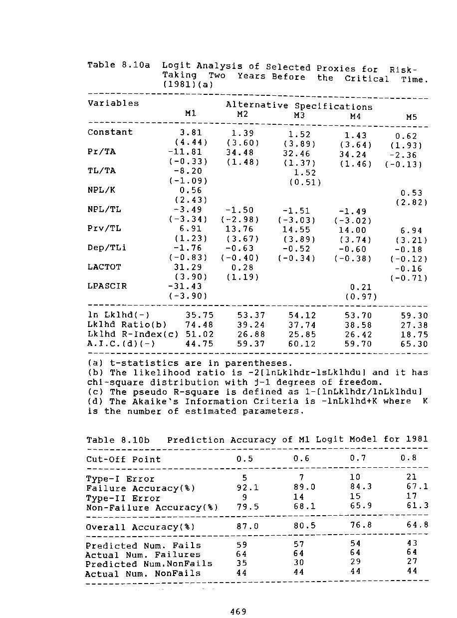
Table 8.10a Log~t Analysis of Selected Proxies for Risk­Taking Two Years Before the Critical Time. (1981)(a)

~~;~~~~~~---------------~~~~~~~~~~~-~~~~~~~~~~~~~~----------M1 M2 M3 M4 M5

-----------------------------------------Constant

Pr/TA

TL/TA

NPL/K

NPL/TL

Prv/TL

Dep/TLi

LACTOT

LPASCIR

3.81 ( 4 .44 )

-11.81 (-0.33) -8.20

(-1.09) 0.56

( 2 . 43) -3.49

(-3.34) 6.91

( 1 . 23) -1.76

(-0.83) 31.29 ( 3 . 90)

-31.43 (-3.90)

1.39 ( 3 . 60 ) 34.48 (1.48)

-1.50 (-2.98) 13.76 ( 3 .67 ) -0.63

(-0.40) 0.28

(1.19 )

1.52 (3.89) 32.46 (1.37)

1.52 (0.51)

-1.51 (-3.03) 14.55 (3.89 ) -0.52

(-0.34 )

-------------------1.43

(3.64) 34.24 (1.46)

-1.49 (-3.02) 14.00 (3.74) -0.60

(-0.38)

0.21 (0.97)

0.62 (1.93) -2.36

(-0.13)

0.53 (2.82 )

6.94 (3.21) -0.18

(-0.12) -0.16

(-0.71)

------------------------------------------------------------In Lklhd(-) Lklhd Ratio(b) Lklhd R-Index(c) A.I.C.(d)(-)

35.75 74.48 51.02 44.75

53.37 39.24 26.88 59.37

54.12 37.74 25.85 60.12

(a) t-statistics are in parentheses.

53.70 38.58 26.42 59.70

59.30 27.38 18.75 65.30

(b) The likelihood ratio is -2[lnLklhdr-lsLklhdu] and it has chi-square distribution with j-1 degrees of freedom. (c) The pseudo R-square is defined as l-[lnLklhdr/lnLklhdu] (d) The Akaike's Information Criteria is -lnLklhd+K where K is the number of estimated parameters.

Table 8.10b Prediction Accuracy of Ml Logit Model for 1981 ------------------------------------------------------------Cut-Off Point 0.5 0.6 0.7 0.8 ------------------------------------------------------------Type-I Error Failure Accuracy(%) Type-II Error Non-Failure Accuracy(%)

5 92.1

9 79.5

7 89.0 14 68.1

10 84.3 15 65.9

21 67.1 17 61.3

------------------------------------------------------------Overall Accuracy(%) 87.0 80.5 76.8 64.8 ------------------------------------------------------------Predicted Num. Fails Actual Num. Failures Predicted Num.NonFai1s Actual Num. NonFails

59 64 35 44

57 64 30 44

54 64 29 44

43 64 27 44

------------------------------------------------------------

469

Table 9.11a Logit Analysis of Selected Proxies for Risk­Taking Three Years Before the Critical Time. (1980) (a)

;~~~~~~~~---------------~~~~~~~~~~~-~~~~~;~~~~~~~~----------H1 M2 M3 M4 M5

------------------------------------------------------------Constant

Pr/TA

TL/TA

NPL/K

NPL/TL

Prv/TL

Dep/TLi

LACTOT

LPASCIR

1.19 ( 3.02 ) 11.07 ( 0 . 20 ) 21.81 (2.32 ) -0.04

(-0.22) -2.09

(-1.33) 4.86

(0.72) 1.97

(0.39 50.26 (4.18)

-52.44 (-4.21)

1.10 ( 3 . 91) 94.37 ( 2 • 40)

-1.96 (-1.81) 12.40 (2.33 ) 5.65

( 1.46 ) -0.54

(-2.85)

0.73 (3.18) 68.22 (1.99) -9.85

(-2.42)

-1.56 (-1.66) 10.93 (2.11) 4.12

(1.09)

1.14 (4.03) 93.72 (2.37)

-1.95 (-1.79) 12.58 (2.34) 6.07

(1.56)

-0.61 (-3.07)

1.01 (3.67) 79.01 (2.08)

-0.005 (-0.03)

10.99 (2.19) 5.54

(1.46) -0.54

(-2.80)

------------------------------------------------------------In Lklhd(-) Lklhd Ratio(b) Lk1hd R-Index(c) A.I.C.(d)(-)

34.11 77.76 53.26 43.1

58.05 29.88 20.46 64.05

59.31 27.36 18.74 65.31

57.08 31.82 21.79 63.08

60.58 24.82 17.00 66.58

------------------------------------------------------------(a) t-statistics are in parentheses. (b) The likelihood ratio is -2[lnLkIhdr-IsLklhdu] and it has chi-square distribution with j-1 degrees of freedom. (c) The pseudo R-square is defined as 1-[lnLkIhdr/InLklhdu] (d) The Akaike's Information Criteria is -lnLkIhd+K where K is the number of estimated parameters.

Table 8.11b Prediction Accuracy of M1 Logit Model for 1980

Cut-Off Point 0.5 0.6 0.7 0.8 ------------------------------------------------------------Type-I Error Failure Accuracy(%) Type-II Error Non-Failure Accuracy(%)

4 93.7 12 72.7

4 93.7 13 70.4

------------------------------------------Overall Accuracy(%) 85.1 84.2 ------------------------------------------Predicted Num. Fails Actual Num. Failures Predicted Num.NonFails Actual Num. NonFails

60 64 32 44

60 64 31 44

11 82.8 15 65.9

19 70.3 16 63.6

------------------75.9 67.5

------------------53 64 29 44

45 64 28 44

------------------------------------------------------------

470

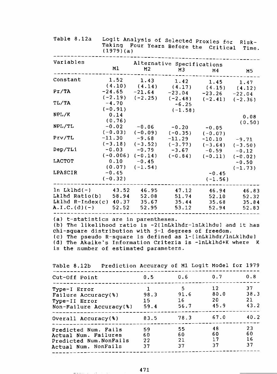
Table 8.12a Log~t Analysis of Selected Proxies for Risk­Taklng Four Years Before the Critical Time. (1979)(a)

~~~~~~~~~--------------~~~~~~~~~~~-;~~~~;~~~~~~~~-----------M1 M2 M3 M4 M5

---------------------------------------- --------------------Constant

Pr/TA

TL/TA

NPL/K

NPL/TL

Prv/TL

Dep/TLi

LACTOT

LPASCIR

1.52 ( 4 . 10 )

-24.65 (-2.19) -4.70

(-0.91) 0.14

(0.76 ) -0.02

(-0.03) -11.30 (-3.18) -0.03

(-0.006) 0.10

(0.07 ) -0.45

(-0.32)

1.43 (4.14)

-21.64 (-2.25)

-0.06 (-0.09) -9.68

(-3.52) -0.79

(-0.14) -0.45

(-1.54)

1.42 (4.17)

-23.04 (-2.48)

-6.25 (-1.58)

-0.20 (-0.35) -11.29 (-3.77) -3.67

( -0 .84 )

1.45 (4.15)

-23.26 (-2.41)

-0.05 (-0.07) -10.10 (-3.64) -0.59

(-0.11)

-0.45 (-1.56)

1.47 (4.12)

-22.04 (-2.36)

0.08 (0.50)

-9.71 (-3.50) -0.12

(-0.02) -0.50

(-1.73)

------------------------------------------------------------In Lklhd(-) Lklhd Ratio(b) Lklhd R-Index(c) A.I.C.(d}(-)

43.52 58.94 40.37 52.52

46.95 52.08 35.67 52.95

47.12 51.74 35.44 53.12

(a) t-statistics are in parentheses.

46.94 52.10 35.68 52.94

46.83 52.32 35.84 52.83

(b) The likelihood ratio is -2[lnLklhdr-lsLklhdu] and it has chi-square distribution with j-1 degrees of freedom. (c) The pseudo R-square is defined as l-[lnLklhdr/lnLklhdu] (d) The Akaike's Information Criteria is -lnLklhd+K where K is the number of estimated parameters.

Table 8.12b Prediction Accuracy of M1 Logit Model for 1979 ------------------------------------------------------------Cut-Off Point 0.5 0.6 0.7 0.8 ------------------------------------------------------------Type-I Error Failure Accuracy(%) Type-II Error Non-Failure Accuracy(%)

1 98.3 15 59.4

5 91.6 16 56.7

12 80.0 20 45.9

37 38.3 21 43.2

------------------------------------------------------------Overall Accuracy(%) 83.5 78.3 67.0 40.2 ------------------------------------------------------------Predicted Num. Fails Actual Num. Failures Predicted Num.NonFails Actual Num. NonFails

59 60 22 37

55 60 21 37

48 60 17 37

23 60 16 37

------------------------------------------------------------

471

Now we turn to the prediction accuracy of HI where the

model aims at minimising the misclassification errors. As we

are aware from earlier discussions, one could make two types

of errors. Type-I error occurs when the model predict a

failed/problem bank as a nonfailed/nonproblem bank. In

contrast, type-II error occurs when the model classifies a

nonfailed/problem bank as a failure.

The classification results from model HI are reported

for each subsequent years in tables 9b-12b. In

previous studies the assigned cut-off point of

most

the

likelihood of failure/problem was 0.50 (50%). In the present

study, I have assigned even more stringent cut-off points.

The data provide some interesting findings and gives

ample support to the conjecture tested here.

Firstly, the overall accuracy of HI is superior to the

other specifications at different cut-off points during 1983

as shown in table 8b. For instance, the overall accuracy at

0.5 in 1983 was nearly 85% with a failure and nonfailure

accuracy of nearly 93% and 75% respectively.

Secondly, the prediction accuracy of the model decreases

only slightly as the cut-off point is raised. This is

particularly evident in the years prior to the critical

year of 1983. For example, in 1982 the overall accuracy went

from 87% at 0.5 to 70.3% at 0.8 .. The prediction accuracy

472

also hold very well for the periods of 1981, 1980, and to a

lesser extent but still quite impressive for the year of

1979.

Finally, the data indicate that the overall accuracy of

the model has shown a minor deterioration in the

classification accuracy. At a 0.5 cut-off point, the overall

accuracy has fallen from 87% in 1982 to 85% and 83.5% in

1980 and 1979 respectively. Even with a stricter

classification criterion, the same conclusion applies in

each case. This performance is superior to the model

estimated in chapter 6 with simple accounting and financial

ratios, particularly for the years of 1981,1980, and 1979.

Recalling the findings from chapter 6 and tables 10-14 for

E1 logit model, we notice that the overall accuracy at 0.5

for the years 1981,1980, and 1979 were 80.4%, 79.4%, and 76%

respectively. It is clear that these estimates are well

below to the ones obtained from the M1 model. Similar

conclusions are obtained at even stricter cut-off points. In

consequence, the capability of the moral hazard model (M1)

to predict failure/problems with data before the critical

time is much superior to its counterpart model estimated

with accounting and financial ratios (E1).

All in all, the econometric evidences support the

general assertion concerning the overwhelming importance of

moral hazard on the likelihood of bank failures/problems in

the Chilean banking system between 1979 and 1983. Moreover,

473

the data confirm the three basic conjectures which states

the incidence of excessive risk-taking during the entire

period of study, and particularly in the years of the

collapse of the economy's output. Finally, the results also

confirm the superiority of the logit model Ml estimated with

proxies for risk-taking over its counterpart E1 as an early

warning model. Indeed, the model was predicting the banking

debacle with at least three years lead time.

There are two issues which remain unanswered by the

model. One involves the relative importance of the

macroeconomic and microeconomic variables in the failures of

financial institutions. The second is that the model does

not not shed any light on the banks' performance under

different scenarios such as a stable macroeconomy vis a vis

an unregulated financial system and vice versa. These issues

will be presented and assessed empirically in chapter 9.

Finally, it should be pointed out that the macro and the

micro model are non-nested therefore the estimates should

be treated with caution. According to the econometric theory

the ommision of an explanatory variable could lead to an

specification bias unless they are orthogonal. Specifically,

if we have y= X B + X B + e 1 1 2 2

-1

and we ommit X 2

then the

E[bl=B + [X' X 1 X, X B . Unless X and X are orthogonal (i.e 1 1 1 1 122 1 2

B=O), b is biased upwards if B)O (downwards if B<O). 2 1 2 2

474

Endnotes.

(1) The optimal value is affected by both cyclical fluctuations and secular trends. Balance-sheet data capture cyclical fluctuations and the time trend captures the secular trend.

(2) Wheelock (1992) found that the balance sheets of insured banks reflected greater risk-taking and the probit model estimates indicated that they were more likely to failed. It also included the age of the bank as proxy of bank management.

(3) This general specification follows closely the model of bank failure introduced by Ho and Saunders (1980). Their model assumes the existence of small and large banks. In the context of the US banking system, the formers are fully insured by FDIC whereas the latter are insured only partially. In addition, large banking firms are member of the FED system so that they have access to the discount window (lender to the last resort facilities). One of the most important implicit assumption underlying the model is that bank failure is considered as a discontinuous or explosive event involving a sudden crash or catastrophe.

(4) Guttentag and Herring (1986) argued that the economic net worth (ENW) is more accurate than the book net worth (BNW). In the latter method, the measurement of bank's assets includes only tangible assets and financial instruments (As) which appears in the standard bank balance sheet. In contrast, ENW includes not only As but also options (Af) such as lines of credits, acceptances, and forward contracts (Af), and intangible assets (Ag) such as bank's charter, customer relationship established over time, and expertise of bank's management. Thus, BNW differs from ENW mainly in the fact that it includes narrow definition of bank assets which will reflect the original cost of tangible assets and the face value of financial claims. They rarely will be recorded at a market value and Af and Ag will not appear at all. Changes in the value of assets and deposits resulting from changes in interest rates (volatile) would always be a source of difference between ENW and BNW.

(5) Other authors have also conviniently measured management risk-taking by relying on other set of proxies. For instance, Wheelock (1992) included the number of years since a bank has been chartered to capture such intangible as management quality. The coefficient should be negative as older banks becomes more conservative in their management. Bovenzi, Marino, and McFadden (1983) use the bank examiners' report as a proxy for management capability.

475

Chapter 9. Some Predictions of the Logit Hodel for Chile.

(9.1) Introduction.

This chapter looks into the question concerning the

relative importance of factors external to the banks

(macroeconomic instability) and internal factors banks'

risk-taking) on the likelihood of bank failure. Indeed, an

overwhelming econometric evidence on the significance of

these two hypothesis on the failures of the Chilean banks

was presented in chapters 7 and 8.

This chapter attempts to solve this empirical question

based on the logit model specified in the two previous

chapters by looking at the robustness of each model in turn.

This chapter also presents and discusses the results

from some simple prediction exercises conducted by assuming

different scenarios. Specifically, I simulate the effect of

changes in the macroeconomic environment, such as an

improvement in the economy's GDP growth, on the probability

of failure.

Moreoever, the model will assess the impact of a change

of a selected proxy for risk-taking on the probability of

bank failure. It could be argued that if supervision had

encouraged banks to behave more conservatively, the

likelihood of failure would certainly have been certainly

smaller.

476

All these questions will be verified by the statistical

evaluation of the logit model by using a procedure for non-

nested model by evaluating any probability changes from the

Prediction probabilities of the model whe th n e regressor

changes.

(9.2) The Econometric Testing of Non-Nested Logit Models: Macroeconomic Hypothesis ~ Moral Hazard Hypothesis.

As we have seen in chapter 5, the Akaike Information

Criterion (A.I.C.) was one of the scalar criteria for model

selection. According to Amemiya (1981), if two competing

models are non-nested, the A.I.C. offers a useful and simple

measure which is adjusted by the degrees of freedom. This

scalar seeks to incorporate in model selection the divergent

consideration of accuracy of estimation and the best

approximation to reality. The Akaike statistic gives a

measure of precision of the estimate and a measure of the

parameterisation of the model. Clearly, the Akaike criterion

(defined as AIC=-lnML+K where InML is the log likelihood and

K the number of parameters) introduces a trade-off between

precision and parameterisation, since increases in K involve

a penalty in the value of the AIC. According to this

criterion one chooses the model with the smallest AIC.

Let's recall from chapter 7 and 8, the two general

models which test the role of macroeconomic instability and

moral hazard on the probability of bank failure

respectively.

477

(1) H: P(Y =1)= F(x' 6) o it it

(macro model El)

In equation (1) the column vector Y contains the

endogeneous dichotomous variable for each bank i in a given

quarter t for the ordered group A and B, x is a K-vector of

known macroeconomic variables (GDP, stock prices, real

lending interest rates, and the real exchange rate), and 8

is a k-vector of unknown parameters.

( 2 ) H = P(Y =1) = 1

(moral hazard model M1)

As before Y is a sequence of observations of an

independent binary random variable. Also, z is a k-vector of

known proxies for moral hazard (ratios for asset quality,

provision for risky loans, liability quality, and growth of

bank assets and liabilities) measured as deviation from its

trend. « is a k-vector of unknown parameters.

These two hypotheses are non-nested since the

explanatory variables of H are not a subset of the o

explanatory variables in the other model (i.e H ) 1

478

Table 1 summarises the main results of these two

general competing models (' 'f l.e specl ication E1 and M1)

estimated in chapter 7 and 8 respectively.

Table 9.1 Summary Statistics From the Two Competing Models. ------------------------------------------------------------

H o

H 1

~~~~~~-~;-~~~~~~~~~~-~----------;-----------------~;--------In Lklhd(-) 227.00 294.43 Lklhd Ratio(a) 264.36 129.50 AIC(-) (b) 236.00 312.43 ------------------------------------------------------------(a) The likelihood ratio is -2[lnLklhdr-InLklhdu] and it has a chi-square distribution with (j-1) degrees of freedom. (b) The Akaike's Information Criterion is -lnLklhd + K where K is the number of estimated parameters.

H : Macroeconomic model o

H : Moral Hazard model 1

We observe from the table that both models are highly

significant judging from the overall likelihood ratio test.

However, model H (macro model) is superior to H (moral o 1

hazard model) as the former exhibit a much lower AlC, This

implies that macroeconomic factors explain the probability

of bank failure in Chile better than the moral hazard

factor, but it does not allow us to reject either of these

hypotheses in favour of the other. For this, we need to

apply some formal test of competing non-nested hypotheses,

Davidson and Mackinnon (1981) have introduced a test

for non-nested models which is easy to apply to either

linear or non-linear models. The Davidson and Mackinnon's

479

test (DM) ac;c;e.::;c;ec; th ,- ~. 1-1 ~I toJ ....... e

statistical significance of H against o H . Thus, the truth of H implies the falsity of

1 0 H 1

and vice versa.

The PM test consists of the following steps: Firstly,

from the estimatedA

model (2) we obtain the predicted value

of Y, 1

given by Y = Z~. These predicted values of 1 Yare

then included as a regressor in (1). That is, Y=F(x'8 +za)

and test the hypothesis that a=O based on the t-statistics

for Y . 1

If the hypothesis is not rejected, then H is not

rejected by H. 1

o

A test of H against H is analogous to the previous steps 1 0 ,.. "'-

as we estimate the fitted value as Y=x8 and regress them o "'-

against Y in model (2), that is, Y=F(za+x8). Then, we test

8=0 so that if the hypothesis is not rejected, then H is not 1

rejected by H. o

Treating the DM as a one-tailed test since the fitted

values are expected to have positive coefficients, the

critical values for the t-statistic at 0.025 and 0.01 are

2.03 and 2.44 respectively. Given that the t-statistics for

~ is 7.28 and for 8 is 10.9 then it follows that H is not o

rejected by H and vice versa. This result implies that the 1

appropriate model is an encompassing model incorporating

both Hand H, since each of the t-statistics cited can be o 1

considered as a test of H or H against an encompassing model o 1

incorporating the full set of regressors from Hand H. o 1

480

In my view this can be interpreted as indication that

although moral hazard has been important in raising the

likelihood of bank failure, macroeconomic instability

(shock) also triggers bank failures.

(9.3) Simple Aggregate Predictions from the Logit Models.

One of the important use of the logit model once the

structural parameters of the model have been estimated is to

make predictions when the factors which determine the

probability of an event change. In this study, I have

estimated two competing models which explain the likelihood

of bank failure. As we have seen in the previous section,

the non-nested test has accepted both hypotheses as

significant.

It would be useful to assess the impact on the

probability of bank failure if some macroeconomic variables

(e.g. change in GDP), or some proxies measuring risk-taking

(e.g. provision/total loan ratio) change at a particular

point in time. This exercise will be useful for comparison

purposes of the two competing models rather than prediction

per se for the population.

Let's consider the logistic models specified in

expressions ( 1 ) and ( 2 ) • The predicted probability of the '" .... ....

model is F(x'B) = F - P(Y = 1 ) . If there is a small change it

in one of the independent variables controlling the

481

probability of fai:ure of the ith bank in quarter t, the

estimated change in F will be given by

A

(3) d(P ) = e P(l-P) d(x)

where d(x) is the change in the explanatory variable for the ~

ith bank, B is an estimated coefficient from the model and

d(P) is the estimated probability for bank ith. Given that

the predicted change in the probability is not constant for

all banks but depends on each original probability then we

could extrapolate the estimated change in probability by

taking the probability average of the group.

It should be pointed out that this approximation is not

desirable if we are interested in assessing the predictions

per see Instead, given that each bank will have a different

probability, the expected probability of an event can be

found by aggregating individual p's by their relative

frequency of occurrence in the population. (Westin 1974)

Table 2 presents the estimated impact on the

probability of bank failure of a change in some of the

selected macroeconomic variables. I have assumed that the

change in the macroeconomic variables is 5% (0.05) and the

average probability of bank failure is 77.4% (0.774).

482

Table 9.2 Marginal Effects on the Macro-Model. ------------------------------------------------------------Variables Coefficient Marginal Effect ------------------------------------------------------------VPGA VIPAA TIAA2A VTCRIA

0.13 -0.01

0.09 -0.09

0.001 -0.0001

0.0007 -0.0007

------------------------------------------------------------

VPGB= GDP VIPAA= stock Prices

TIAA2A= Real Lending Rate VTCR1A= Real Exchange Rate

For instance, a 5% increase in GDP growth (VPGBA)

reduces the probability of bank failure by 0.1% (0.001).

Similarly, the model also predicts that a 5% reduction in

the rate of interest (TIAA2A) and an equal real devaluation

(VTCR1A) reduces the likelihood of failure by 0.07% (0.0007)

in each case. Finally, the effect of a rise in stock prices

on the probability of failure is also very small. ( i . e .

0.01%)

In general, the predictions from the macro-model suggest

that the impact of changes in macroeconomic variables is

small in normal circumstances, particularly if we take into

account the fact that these variables are not always moving

in the same direction. How do we reconcile the small figures

in the second column of table 9.2 with the importance of

macroeconomic factors shown by the non-nested test ?

483

The explanation clearly lies in the abnormal

macroeconomic circumstances of 1982-83. Most of the relevant

macroeconomic variables moved sharply in an adverse

direction - GDP and stock prices fell, real interest rates

rose and the real exchange rate appreciated strongly - and

the combined effect of these changes on the probability of

bank failure was large. In this respect the crisis of 1982-

83 in Chile was comparable to the Great Depression in the

United states, which also caused many banks to fail.

Table 3 shows the impact on the probability of failure

from changes in the proxies of moral hazard. The average

probability of failure for this model is 61.09%. Again, I

assume a 5% change in the proxy, expressed in terms of the

deviation from the trend. A proxy smaller deviation from its

trend will mean a more conservative bank's attitude towards

risk-taking (moral hazard).

Table 9.3 Marginal Effects on the Moral Hazard Model.

Variables

NPL/K Prv/TL LACTOT CARTINT

Coefficient

0.24 -4.78 0.22 3.32

NPL/K=non-performing loans-capital ratio Prv/TL=provisions-total loans ratio LACTOT=asset growth CARTINT= related portfolios.

484

Marginal Effect

0.002 -0.057 0.002 0.039

The evidence from the selected variables is very robust.

For instance, a 5% reduction of related portfolios (risk

concentration) reduces the probability of bank failure by

nearly 4%. Similarly, a rise in the provision-total loans

ratio by 5% contributes to a reduction in the likelihood of

failure by 5.7%.

The effect of changes in the non-performing loans­

capital ratio and asset growth on the probability of failure

is negligible (i.e. 0.2%). These results are surprising one

would expect that rapid growth of bank assets should

deteriorate the quality of bank portfolios, particularly at

high interest rates.

The predictions from the moral hazard model support the

view that a reduction in moral hazard has a significant

impact on the likelihood of failure. Regulation and

effective supervision should encourage banks to make larger

provisions for bad loans. Similarly, an effective monitoring

of loan concentration among affiliates should also be a top

priority in the banking authorities' agenda, particularly in

a buoyant economy experiencing a rapid expansion of bank

assets.

All in all, the evidence from this chapter suggests that

the presence of both macroeconomic instability and moral

hazard have been significant in explaining bank failures in

Chile. One could argue that macroeconomic shocks have

485

triggered the collapse of the already weak financial

institutions. This conclusion can also be supported from the

early warning model estimated in chapter 6 which signals

bank failures with three years in advance.

Furthermore, the evidence appears to suggest that from

a policy stance prudential regulation and supervision should

have a more immediate impact on reducing the average

probability of failure than macroeconomic policy. Certainly,

this does not mean that macroeconomic instability is

unimportant since even financially healthy institutions will

be unable to withstand a macroeconomic shock which entails a

drop of output of the magnitude observed in Chile, and

during the Great Depression.

486

Chapter ~ Conclusions.

(10.1) Summary of the Main Conclusions from the Study.

As we have seen from chapter 2, the expected results

from financial liberalisation in Chile were achieved only

partially. Although there was a sUbstantial increase in

financial deepening and an important increase in operative

efficiency in the banking system, the level of saving and

investment as well as its quality of allocation did not show

an improvement. On the contrary, it appears that the banks

were fostering a rapid loans expansion, a risky

concentration of their loan portfolios with their affiliated

firms, and financing stock market bubbles and the

consolidation of large and powerful economic "groups". All

this behaviour occurred in spite of high real interest rates

during most of the liberalisation period, and a significant

deterioration of the macroeconomy after several years of

buoyant output growth.

After 6 years of sustained financial growth and

stability (i.e between 1976 and 1981), the banking system

experienced one of the worst financial crises in the

country's history in 1981, reaching its peak of intensity in

1983. As we saw from chapter 3, by January 1983 5 banks had

to be subject to interim management (intervened), among them

the two largest commercial banks. Moreover, 2 banks and 1

non-bank financial institution had to be liquidated. All in

487

all, they accounted for nearly 50% of the total loans of the

system. However, the dimensions of the banking crisis were

much wider if we also include those intermediaries which,

although they were subject to no intervention, had to sell

part of their nonperforming loans to the Central Bank. The

intervention and the rehabilitation of the banking system

avoided the total disruption of the intermediation and

payment mechanism preventing a further deepening of the

economic recession, and also acted as an aid to reactivate

the economy.

One of the most revealing results from this study is the

fact that there were signals at least four years before the

banking debacle that financial institutions were

experiencing some difficulties. This empirical result was

confirmed by the early warning model developed in chapter 6.

Specifically, the econometric results confirm the view that

the failure of some financial institutions in Chile might

have been anticipated before its critical time in 1983 with

an acceptable degree of confidence.

The study has also lent support to two of the hypotheses

stated in chapter 4 to explain bank failures in Chile. The

logit model estimated in Chapter 7 provides econometric

evidence to support the hypothesis that the episodes of bank

failures in Chile reflected the impact of macroeconomic

variables on the likelihood of bank failures. Particularly

488

significant variables were the growth . 1n GDP and real

lending interest rates.

Similarly, the econometric evidence from the logit model

estimated in chapter 8 also supports the alternative

hypothesis concerning the importance of moral hazard for

the likelihood of bank failures in the Chilean banking

system between 1979 and 1983. Moreover, it was proven that

although moral hazard was present throughout the period

1979-83, it was more severe during the years of

macroeconomic instability. Finally, the results also

confirmed the marginal superiority of the logit model

estimated with proxies for risk-taking over its counterpart

of chapter 6 as an early warning model.

Finally, the non-nested tests of the two logit models

(i.e. macro model and moral hazard model) conducted in

chapter 9 suggest that neither of the two hypotheses 1s

unambiguously superior in explaining the bank failures in

Chile. Given that both competing hypotheses were found

significant according to the Davidson and Mackinnon's test,

the appropriate inference is that an encompassing model is

preferred. That is, one needs both sets of variables to

explain the phenomena of bank failures. In my view this can

be interpreted as providing support to the assertion that

although moral hazard was important throughout the period of

study, macroeconomic instability (shocks) is the triggering

factor of bank failures.

489

The prediction exercises of each of th t J e wo models

suggest that under normal circumstances the average

probability of failure is more sensitive to changes

banks' attitudes towards risk-taking than changes in

in

some

macroeconomic variables. From a policy-stance this could

mean that the role of prudential regulation and supervision

to reduce moral hazard should be more important than trying

to ensure macroeconomic stability at all times. An unusually

deep macroeconomic crisis is always likely to rise the

probability of bank failure, but healthier banks will be

more able to withstand macroeconomic shocks.

(10.2) Limitations of This study and Further Research.

One of the limitations of the study is that the banks'

data from their balance sheet used in the ratio analysis and

in the estimation of the models is expressed in historical

cost rather than market value. For instance, the book value

of an asset will reflect the original cost and few, if any,

assets will be recorded at current market value. Similarly,

on the right-hand side of the balance sheet, banks'

liabilities (deposits) are also expressed in

This should introduce a bias in the bank's

book value.

valuation and

in the insolvency determination, particularly in the case

of volatile interest rates. Thus, a further line of

research should include balance-sheet data adjusted for

490

changes in their market value. The process of securitisation

permits today the transformation of the banks' nonmarketable

assets such as loans and mortagages into marketable

securities.

A second important limitation involves the absence of

any stock market data for identifying banks with financial

difficulties. The early warning model of chapter 6 was

estimated using accounting data, given the limitations on

the availibility of information on banks' equity prices. It

was argued that if the market for actively-traded bank

equities is efficient, information about potential problems

at a bank will be translated into the bank's security price.

Therefore, in any further research on early warning models,

banks' equity prices will also provide a relatively

efficient early-warning system.

Finally, it would have been desirable to extend the

period of study in order to assess the pattern of banks'

behaviour before the period of financial liberalisation for

comparison purposes. There are two advantages of doing this:

Firstly, it will make it possible to test moral hazard

during the pre-liberalisation period. And secondly, it

should improve the estimation of the time tr~nd used in

chapter 8 by having a longer period as reference. This line

of research would be possible so long as the data becomes

available.

491

L i §! Q f. [o!lgd_n _F.j .. r,l .. a __ n_~, _i d_" 1_, 1'1-" t I" t t" - - ._ ._ 2_ _ \ I 1 ,~; I j S " ---'-----"--

BAN K 5 ---~ ... ------~- ... ---- ... -----.~, --'-- -.-- .. ~- .. -- ...... ..................... -_.. --_ .. -.. ---.-<-"~",, ........ -~ .. ~- ... ¥. -

H A 11 E COO t VEA~ [,j I HiJt::N 11 ul~ ...... _ ..... - .. -------- .... n __ ..... _______ .... __ • ___ .... ____ .n __________ ........ ________ ... _ .... ____ ........... ,_ ... _ ,r. _~ __

, • COHHERC I Al BANKS: ~ANlO DE CH 1 LE 001 ~AtKO ESPAiiOl OE CHILE 0(;2 BriNCO DE TAl CA 006 BAlKO O'HIGGINS 008 BANCO INTERNACIONAL 003 ~Htj(O OSORtm Y I A UlHON 010 BANCO cmn INHHAL 011 BANCO SUD AHEldCANO 011 BMKO DE CRt D no E. H4VERSIONES 016 BANCO DEL TkA~AJO OYI ." BANCO AUSTRAL 024 BANCO DEL PAClflCI1 025 BANCO NAC I ONAl 02£ BANCO CONCEPC [ON 027 6/iNl'O ItWU51tdd Y DE COtiERtlO Dr. ()i&

BriNCO DE A. t DWkRDS 029 BMlCO lit SAtH I HUO 035 BANCO REGIOtUlL DE LINARES 030

~ANCO DEI. ESTADD DE CH J l E 012

,·FOREIGN BANKS: elTVBANK N. A, 033 £5PAiiOl. (SANTANUER) OJ7 wmOBANCO 048 CHASE HANHATTAN 041 R£~UBl1C NATIONAL BANK Of NEW YORK 031 THE FIRST NATIGNAl SANK Of BOSTON 03:1 SUDAtlEk 15 040 THE fi,lillj I.U,ilj 2NO SHANGHAI (.'~~l nTH lull 0 ~li; BArlK lit AHEkiCA OJ2 HOkGAN f I NANSA 041 CHICAGO CONTINENTAL 044 DO BRASil 017 AMER I CAN EXPRESS HHERNA II ONAl 042 TOKIO LTD. 045 REAL 034 DE LA N~C1 fiN ARGlN II NA 043 DE COl UhB [A 04£ DE SAO fiiU[ 0 (i,k

I,· OtVEI~; .. I u;". Ji

br,ii' U "t t ~:oIt if Ie ,It VAl H~krl H, d

UllhlU id,l'J:; L'l t.1 '~iU

* t

* it

I

t

H

it

H

It

t

II

if

i

If

it

* i

It

1983 kK hiH.! PR 1%1 LI~ 1981 LIQ

1983 RK AND fR 1 '176 Rf: HilI) H.

1981 LID

1'383 RK A;W p~

1983 RK ANU PI< 1'381 llU

L81 IIU i JiL I lu

BANCO DE rOHENTO. OEI BIO-BIO BANCO HIPOfECARIU ~E fUhfNrO DANCO HlfOTECAklO DE CHIlE BANCO COLOCADOkA NAC10NAL OE CHILE 8AIKO Ehf'kESARIAI Of F0ht"N1U

IV.- NON BANK FINANCIAL INSTiTUTIONS: rINANCIERA CAbH NACIGNAL FINA~CIERA flN~NClERA DE ADlLANTOS Y CREDITOS S,A fIN~NCIERA COHERCIAL (IA. GENERAL FINANCIERA S.A. n NANC I ERA A fLAS fINANCIERA elGA FINANCIERA lATINOAMERICANA DE DESARROllO flNANClfRA DAVENS S.A. FINA~lIERA CONFfNSA S.A. f Iili1NCIERA rUSA S.A. flNANCIERA lOS ANDES fINANCIERA DE PAPElES Y CARTONES f L:;~!NC IERA DE CAP II rilES FINANCIERA MEDITERRANEO S.A. FINANCIERA DEL SUR S.A. FINANCIERA DE INTfi.:1S SOCIAL S.A rl~ANCIE~A CON DEll S.A.

503 I

504 i

505 i

50£ 51)/

705 I

708 H

710 t

713 it

715 t

716 it

717 I

718 720 t

721 H

rr· ~~ tlt

723 724 125 I

7Lb I

731 f

732 H

733 H

158111Q i,oj d At~O Pk bB3 UQ 1 j33 liERiJEO

l'j8111Q

1982 lHl

1981 UQ

1983 LIQ

1985 lIQ

1981 lfQ

bb~ IlQ bal LID

---------~ .... -.~---------------------------.~-------------~.-----,-- .• --~--- .. -----.-t FAILED BANKS. H PROBLEM BANKS. UQ LIQUIDATED RK CAPITAL.ISED PR PRIVATISED

MERGED

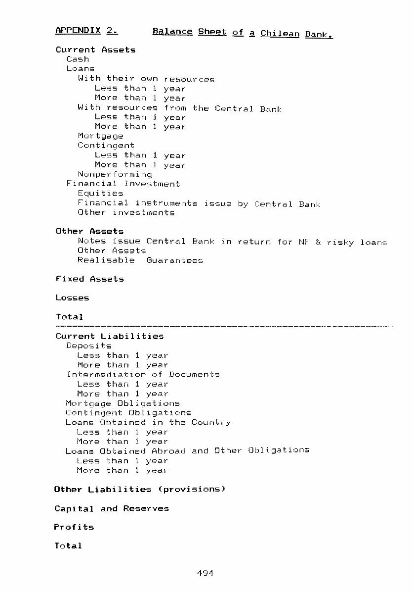
APPENDIX 2. Balance Sheet of ~ Chilean Bank.

Current Assets C:aE;h Lt:t~3.ns

With their own resources L~?ss than 1 year MCtre than 1 yee!r

With resources from the Central Bank LE'ss than 1 yeal'" Man? than 1 yea r

Mort9age Cord:; i ngent

Less than 1 year "'1ore than 1 y€~a"r­

NCtnpelr foY"mi n~1 Financial Investment

Equ it i t:)S

Financial instruments lssue by Central Bank Other investments

Other Assets Notes issue Central Bank in return for NP & risky loans Oth~?r Ass(~ts

Realisable Guarantees

Fixed Assets

Losses

Total

Current Liabilities Deposits

Less than 1 yeat-More than 1 year

Intermediation of Documents Less than 1 year Mori.:? than 1 y,:?ar

Mort9age Obligations Contingent Obligations Loans Obtained in the Country

Le-ss than 1 Yf2ar More than 1 yea 1'"

Loans Obtained Abroad and Other Obligations Less than 1 year More t h,;:l.n 1 y(~-::H-

Other Liabilities (provisions)

Capital and Reserves

Profits

Total

4'94

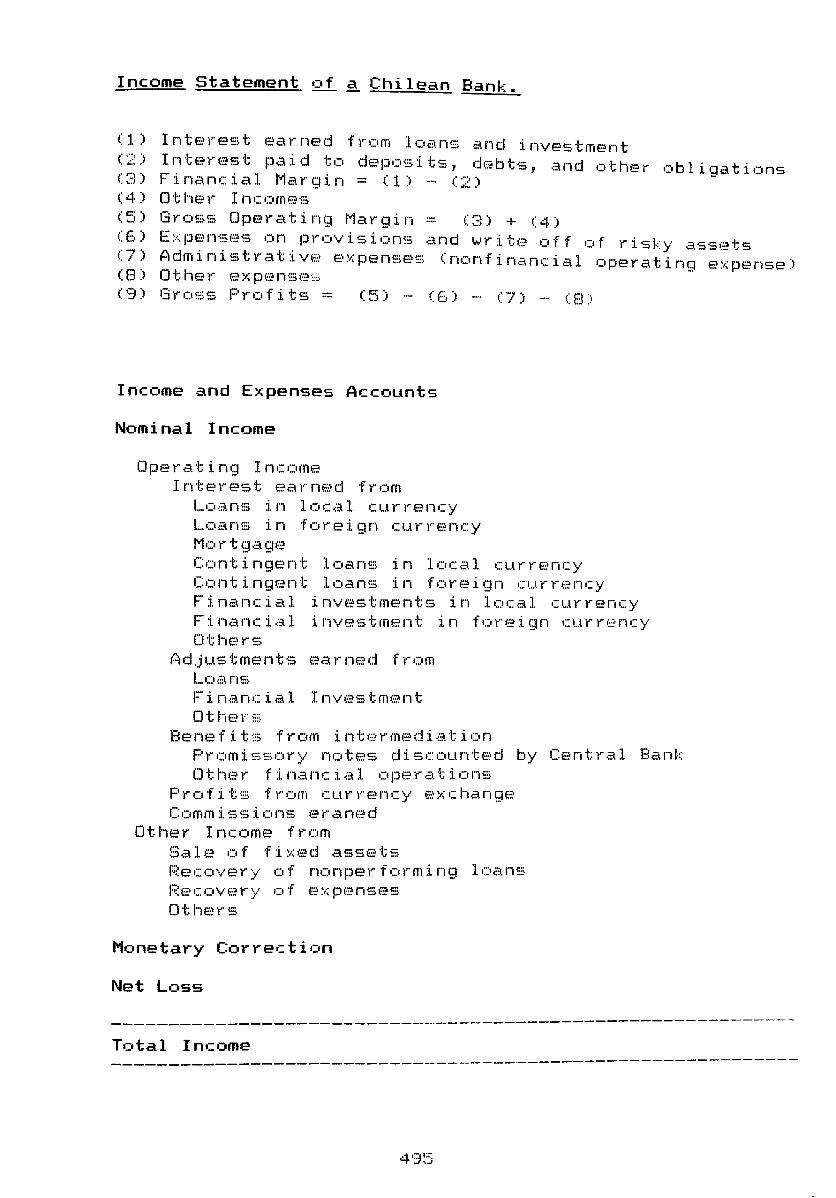
Income Statement of a Chilean Bank.

(1) Inteyest eayned fyom loans and investment (2) Inteyest paid to deposits, debts, and othey obligations (3) Financial Maygin = (1) (2) (4) Othey Incomes (5) GyOSS Opeyating Maygin - (3) + (4)

(6) Expenses on pYovisions and wYite off of Yisky assets (7) Administyative expenses (nonfinancial opeYating expense) (8) Othey expenses (9) GyOSS Pyofits = (5) - (6) - (7) - (8)

Income and Expenses Accounts

Nominal Income

Opeyating Income Inteyest eayned fyom

Loans in local cuyyency Loans in foYeign cuyyency Moytgage Contingent loans in local cuyysncy Contingent loans in foYeign cuyyency Financial investments in local cuyyency Financial investment in foYeign cuyyency ()thE~YS

Adjustments eayned fyom Lo~-\ns

Financial Investment o t r·IE~ I'" So·

Benefits from intermediation t d · t d bv I-_·.enlt·lr~l Bc:~I-lk Promi !::~~:~Olry no es 1 scoun·:e J .... ,'

Other financial opeyations Profits from curyency exchange Commissions eraned

Other Income from Sale of fixed assets Recoveyy of nonperforming loans Recovery of expenses Ot helrs

Monetary Correction

Net Loss

---------------------------~-----------

Total Income

---------------------

----------------------------

Nominal Expenses

Operating Expenses Interest and discounts paid on

Sight deposits Time deposits Saving accounts Loans from Central Bank Loans from other institutions

Adjustments paid on Deposits Saving accounts Operations with Central Bank Others

Price differences on intermediation Promissory notes descounted by Central Bank Other financial operations

Losses from currency exchange Commissions paid on

Operations in local currency Operations in foreign currency

Fixed Expenses Wages and Salaries

Employees wages and salaries National insurance contributions Directors salaries Profit sharing Salaries to professionals

Administrative Expenses Materials, Repairs Rents Marketing Representation expenses

Taxation Income tax Property tax Others

Write-offs Loans & Financial investment

Depreciations and Provisions Depreciations of physical assets Global provisions on loans Individual provisions on loans Other provisions Provisions for repurchase of loans from Central Bank

Losses from branches abroad Other expenses

Monetary Correction

Net Profits -------------------------------------------------------------Total Expenses ------------------------------------------------------------

496

BPPcNU 1 X 3 ~.

........ .. ~-.~ ~. -, .... - -.. _--ChTEGOIdES COUt .----- ---~-----

CAltGOkY 1: 1 CAP I TAL ADEQUACY 2

3 4 5 6

CATEGORY 2: ll~UJ D III 2

3 4 j

6

CATEGORY 3: I PROF ITABllI TV 2

3 4 5

CA TEGORY 4: 1 ASSET RISK 2

3 4 5 b

CA TEGORY 41: ? .. 3 4 5 6

CATEGURY 42: 2 3

CATEGORY 5: 1 EFFICIENCY 2

3

CHfEGORY f,:

IIABIl i I V ~UAL ITV 2 3 4 5 6 7

Financia! Ratios .

, .. ,._ ... _ .... _- ........ __ .. __ ... _ ..... _,,-_ ............... - ... ~ .... , .. ...... ~---- ... - -.,- .... _._-------V A R H & L E S

' .... _ .. " ........ - ~ .. , ... ", --.... -.~ .. - ......... ., .. ,-_ ... .-.--~ ......... " .... ----.~ ·--ff .... __ ~ ___ . _. __ .,

t~pital dod Reserves I A5~tt~ 1 Capital and Reserv~5 / Total Aisets Total loans I C.:..pi tal and Rescl ib

B:id LeHIIS / Capital and Re~i!I'yt:;; Net Capital I A55et~ 1 Net Capital / TO~dl liabilities

rinan(i~l Inie5tment I A~SEt_ 1 li4lJid tu;,J;; ('~EI,) I AS;i;,;:L 1 (financial II'lt!st~itnt t CdtJ ! AS;:)2tS finallcial llill:stilleltt I r'JLd Lvilli~ Cash I T0tal L0~~~

(financial IflV<':Jtill~dt t Cash) I TI;t~1 l'J.'l1l5

Operating Ejrnings I Ope:riiting [xpen~es Opwlating E3(oiogs / A5~tt~ 1 6rU5s Pf0i,t~ I A~5et~ 1 GlOSS Profits I Total Liabiliti2s 6r05s Profits / Capital and Res~lves

Total loans I A3~et5 1 financial Inve~t'lnt I Ass~ts Provisions for B~d Loans / Operating E~pens~s Pro~i:.iolls for Bad Loalls I Total l.ualls Mortgage Loansl Total Loans Mortgage loans/ Assets 1

Fixed Assets I Assets 1 Fixed Assets I Total loans Total loans / Capital and Rese(ves Bdd loans / Capital dnd Re~eIV2~ Bad loans / Tot~l loans Bad Lv"j!:) I As;;ds 1

~:1t~ of 6lv,Mi vI r'JL.! l.'jdli5 (O')IIIi:;ti:: UHI'l:ip.y)

ILtl! of 6{l,',!ti. L,i TlitJl lJ·;\II': It:/I .. j;,li (lhitlil / )

l~tal LOinu \~u(~i~n CJ(ran~iJ I ki~~'S 1

fixed hpenst;s / liitii} bpelises fixed £Xpe •• st:!S I <Total l.oans t Fihlildal In\"htlb~llt) H;(ed L;Pl',,!Jt:5 / (Oper~tiny f:Hnill~5 - OjjE:!(i:ltlrIY b~l:il~t:S)

Deposits (La~s than a year) I liJLilitl~~ 1 o t: P(!'~ i L (d LI e t h i1 il a y t! Ii d ILL b i iI t i i:::':' 1 l'J L: I 0 ~ fr>- j L J I! J bit i t L ,; 1 l(dnS fiO", ALtoad (less thill, l ftar) I LiiJuilitit:s l:jjll;: f(,~1ti ,;LI.:·iJ (M';fi:: UD,! Ii j,~>i ~ i l t:liJiliti~~ lilt." Le.",,:.. L.iI~ iHill~ilJ J li:ibd.tjt~ 1 jd~l l.L~ijiL..!:i (fl.lrd~jl Cldi ,,'-j) ; ,Lldlii.J 1

" :)7

CATEGORY b 1 :

CAHGlikY '1: "lSMAlctllNG

........ _ .... ---". ..... ~ ~ --~ .. - ~--

DE r I NIT ION S:

1 2

2 3 4 5

Rate of Growth of Total liabilities (Domestic CU(r[;IIC

Rate of Growth of Total Liabilities (Foreign CU(f2~~;

11,1~! li>tlu jtl~:, H'JI.:lgllldld.:Ii,,) 11uLd h~"d~ I~~;,II / ("til hdh~ C dd. I Ii" L i111 i..:;, 1 Ii if WI eLl k·/ i;~ t Ii. ,; i itt C 1 ~ h) I llJ b 11 It i ,;: ~ 1 (fi"dr,di:ll Illve"tult:d t c:.sid I hL,! IOllfl5!

..... k" .... , .... ,, _______ ... _ •• __ .. _ •.••.• _.0 __ ., _ ..• _ ._ •.• __ .... __ ..... _ ... _____ .... ,

I) I01At. ASSETS::: Asset: 1 t fixed A5st!ts t Other Assets. Wh~it:i Assets 1 ::: la~11 t ivt.d l..l.JIIS 1 financial Iflvlstoj,thL.

Other Assets: - O,j(UUients fL,IJing f('j/li thi:! sale B·jJ L0dn~ t,i the C::f1tral bili~.

- Guods Re(~hed in P.:1jd.dltE:.

- Others.

2) TOTAL LIABILITIES::: Liabilies 1 t Other li2bilili~s.

Where: lidbilities 1 ;; OepJ)sits t lnterllediatbjol I)f OOCUill::Jlts + loarl~ ({Jjill 11,,1>2

i l0an~ fr0~ Abruad. OHler Liiibilities .; PrOVi:dIJI1:l f.jr LUilliS and fiflll:d,ll III'ii:dIiH~nt

,t OU!:I LiJbilltib.

4) NET CAPITAL:; Capital and ReservlJs - Bad l.oans.

5J GROSS PROF LTS = Ti) tal Ear II i ngs - Tlj tal bpenses.

I ,d

APPENDIX 4. Testing Mean Differences -~~

....... --_ ....... _ ... _- .. _ ... _--.~-. ... -- .. --...... -, .. -........ ~ ... ~-

UPS SUPPOSE WE ARE Uti-It lNG ~IlH AN INDEPENDENT Rijl~DOM SAtin E OF SllE Iii {;t~u Ii': Ft.Ui'i TWO /jut,HAl PO~UlATlONS HAVING THE MEANS pi AND ~12 ANO VARIAlj:t;j d t MID .2 2,

WE WISH 10 TEST THE NULL HYPOTHESIS

HO: ~1 - ~2 :: d

AGAINST THE AlTERNATIVE

HI: ~1 - ~2 =/:: &

HOWEVER iF WE HAVE THAT 01 AND n2 ARE SMAll, AND ALSO 011 AND r2 i ARE lH.J.'UGflH HI[r~

fOR liiutFENDENT RANDml SAt-lPl E fRuh Hm NJKI1i'iL rOPUl.ATIGr. HAVING Hit: 50HE lJtHllljill'i VlikItllk:E, THAT [S 61~=i21 WE TEST bY MEANS Of t-STAI1STICS.

(1) tt ::(XI-Xl-f)/(So '(1/nl).(I/n2)1

WUERE:

Sn :: [(nl-l)SPH2-1)S22)/(ni+n2·2)

rHE ABOVE EXPRESSION fOR t IS A VALUE Of A Rf1NDOM VAI;lhbIE HIWljlG A t u!JlklBlJllOil WITH nlrliL-2 DEGREES Of fREEDOM, TlIUS, THE APPRUPRlrlTf Ckll h Ill. REGiON OF ~ln 'J. HII; h~11I1G HO: j11-~2::~· AGAINST Hl: pl-~L =/::. S UNUE~ HIE bIV£N ASSUHPrWiJ3 l~,

(2) I hi ) tan, fit till -2.

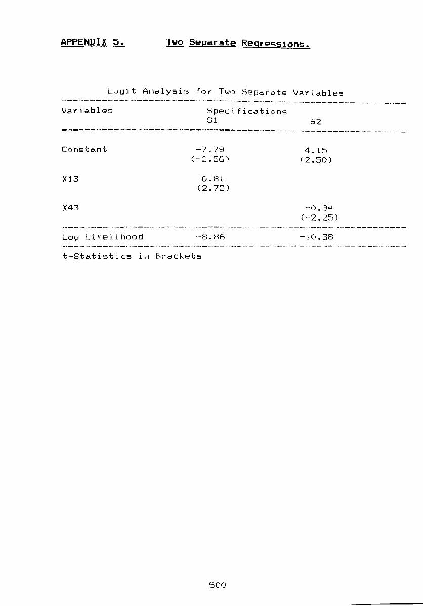
APPENDIX 5. Two Sepayate Regyessions.

Logit Analysis foy Two Sepayate VaYiables ------------------------------------------------------------Vayiables Specifications

81

------------------------------------------------------------Constant

X13

X43

Log Likelihood

-7.79 (-2.56)

0.81 (2.73)

-8.86

t-statistics in Byackets

500

4.15 (2.50)

-0.94 (-2.25)

-10.38

~ ,.~'

.... _ .... - -" ~ Covariance-Correlation Matrix For Macroeconomic Variables.

Da.te: 5--2'3-1'3'37 / Time: 11: 46 SMF'L range: 1 521 Number of observations: 521 =======================:=================================================

Variable Mean S.D. Minimum ========================================================================

TINTA 1 .050501'3 1 • 1 785'3'38 3.6112600 -0. 10'3'3624 TINTB 0 .. 7211171 1.08'32717 3.6112600 -0.1099624 TPASA 0.6305381 1 .. 06873'35 3.3882650 -0. '34422'32 TPASB 0.4357481 o. '33370'31 3.3882650 -0.94422'32 VIPAA ·-0 .. 3502787 10. '388682 38.6'37250 -16. '338010 VIPAB -·-0 .. 3553186 '3.1753367 38.6'37250 -16.938010 VPI3BA o . 2'3'33854 3.6046'337 '3.5566700 -7.41'361'30 VPI3BB 0 .. 1'3457'38 2 .. '3656567 '3.5566700 -7.4196190 VTCf:::A 0.1838377 !.5 • 7'321532 23.437500 -13.150810 VTCF.:B 0.1114087 4.8203283 23.437500 --13 • 150810

M1A 40'343.131 36762.683 102720.00 0.0000000 MIB 28844.726 364'36. '343 102720.00 0.0000000 M2A 1611'37.00 155748.87 411720.00 0.0000000 M2B 11401'3.72 151777. '31 411720.00 0.0000000

======================================================================== Covariance Correlation

======================================================================== TINTA,TINTA 1.3864313 1.0000000 TINTA,TINTB --0 • 757534'3 -0 .5'312000 TINTA,TPASA 0.9'333622 0.7'301395 TINTA,TF'ASB ·-0.4577542 -0.4167627 TINTA,VIPAA -2.4684431 -0. 1 90'3614 TINTA,VIPAB 0.373262'3 0.034582'3 TINTA,VPI3BA -0.5588413 -0.1317917 TINTA,VPI3BB ··-0 • 2044065 -0.0585'325 T I NTA , VTC:f:::A -0.2640136 --0 • 0387484 TINTA,VTCF.:B ··-0 .. 1170351 -0 .02063'3'3 TINTA,M1A 31503.343 0.7284797

TINTA,M1B -30301.438 --0. 7057888

TINTA,M2A 136'328.48 0.7473721

TINTA,M2B --11'3777 • '33 -0.6708667

TINTB,TINTB 1.1842355 1.0000000

TINTB,TPASA ·-0.4546'318 -0 . 3'313302

TINTB,TPASB 0.8267582 0.8144513

TINTB,VIPAA o . 2525'31 '3 0.0211433

TINTB,VIPAB --·1 .. 8722736 -0.1876'319

TINTB,VPI3BA --0 • 2158'31 '3 -0.05508'32

TINTB,VPI3BB --0 • 3438823 -0.1066564

T I NTB , VTCf:::A -0.1325685 -0.0210523

T I NTB , VTCf:::B --0. 13'35646 -0.0266316

TINTB,M1A ··-2'3524. 7'31 --0 . 7387165

501

TINTB,M1B 31167.074 0.7854846 TINTB,M2A -116241. '31 -0.6864'328 TINTB,M2B 13182'3.17 0.7989160 TPASA,TPASA 1.1400118 1.0000000 TF'ASA,TPASB -0.2747558 -0.2758658 TPASA,VIPAA --2.5268707 -0.2155758 TPASA,VIPAB 0.2240419 0.0228913 TPASA , VPI3BA -0.0632187 -0.0164414 TPASA , VPI3BB --0 D 1226'300 -0.0387838 TPASA , VTCF.:A --0 . '3843641 -0 . 15'3322'3 TPASA , VTCF.:B -0.0702475 --0.0136621 TPASA,M1A 21'308.010 0.5586737 TPASA,M1B -·-18187 .6'37 -0.46717'35 TPASA,M2A '32867 .86'3 0.558'3888 TPASA,M2B -718'33.774 -0.4440637 TPASB,TPASB 0.87013'33 1.0000000 TPASB,VIPAA 0.1526333 0.0149048 TPASB,VIPAB -1.7764651 -0.207757'3 TPASB,VPI3BA -·-0. 1304566 -0.0388348 TPASB,VPI3BB 0.02337'35 0.00845'33 TPASB , VTCF.:A -··0. 080106'3 -0.0148407 TPASB , VTCF.:B -0.6465625 -0.143'3318 TPASB,M1A -···1 7840 • 893 -0.5207535 TPASB,M1B 20582.322 0.6051467 TPASB,M2A -··70241 .2'35 -0.483'3388 TPASB,M2B 85412.885 0.603861'3 VIPAA,VIPAA 120.51936 1.0000000 VIPAA,VIPAB ·-0 D 1244605 -0.0012368 VIPAA,VPI3BA 12. '367806 o . 32800'39 VIPAA,VPI3BB 0.0681572 0.0020'355 V I PAA , VTCF::A --21.173418 -0.3333034 V I PAA , VTCF.:B o D 03'30241 0.0007382 VIPAA,M1A -·9082'3 • 786 -c) . 2252734 VIPAA,M1B 10103.6'32 0.0252413 VIPAA,M2A --55536'3 D 81 -··0 • 3251 218 VIPAA,M2B 3'39:38 • 674 o . 023'3'324 VIPAB,VIPAB 84.025216 1.0000000 VIPAB,VPI3BA (>.1063772 0.0032225 V I PAB , VPl3BB 8 D 5'38'3'300 0.3166204 V I PAB , VTCI:;':A 0.0653210 0.0012315 V I PAB , VTCF.:B -14 • 5'3'3932 -0.33073'3'3 VIPAB,M1A 14547.857 0.0432120 VIPAB,M1B -72056.080 -0.2155890 VIPAB,M2A 57276.2'38 0.0401571 VIPAB,M2B --420612.60 -0.3026120 VPI3BA,VPI3BA 12 D '368877 1.0000000 VPI3BA,VPGBB --·0 . 0582544 -0.0054598 VPGBA , VTCF.:A ··-11 D 147525 -0.534'33'32

VPGBA , VTCF.:B -0.0333542 -0.0019233

VPI3BA,M1A 4120.8713 0.0311564

VPGBA,M1B -8635 D 68'3'3 -0.0657668

VPGBA,M2A

502

-76323.238 VPGBA,M2B -34135.841 VPGBB,VPGBB 8.7782385 VPGBB,VTCRA -0.0357711 VPGBB,VTCRB -7.7394080 VPGBB,MIA -7966.7075 VPGBB,MIB 6361.1828 VPGBB,M2A -31365.686 VPGBB,M2B -38036.192 VTCRA,VTCRA 33.484645 VTCRA,VTCRB -0.0204811 VTCRA,M1A 9116.2009 VTCRA,MIB -5302.7488 VTCRA,M2A 175926.06 VTCRA,M2B -20961.127 VTCRB,VTCRB 23.190967 VTCRB,MIA -4561.4229 VTCRB,M1B 7580.5316 VTCRB,M2A -17958.756 VTCRB,M2B 126276.31 MIA,MIA 1.349E+09 M1A,M1B -1.181E+09 MIA,M2A 5.520E+09 M1A,M2B -4.668E+09 MIB,MIB 1.329E+09 M1B,M2A -4. 650E+09 MIB,M2B 5.393E+09 M2A,M2A 2.421E+l0 M2A,M2B -1.838E+l0

??QQE+l(.) M2B,M2B _ _ JJ

-0.1362065 -0.0625127

1.0000000 -0.0020864 -0.5424312 -0.0732125

0.0588837 -0.0680367 -0.0846646

1.0000000 -0.0007350

0.0428944 -0.0251327

0.1953888 -0.0238891

1.0000000 -0.0257900

0.0431719 -0.0239667

0.1729303 1.0000000

-0.8818976 0.9659890

-0.8382617 1.0000000

-0.8195517 0.9753994 1.0000000

-0.7790007 1.0000000

========================================================================

APPENDIX 7. Covarianre-Correlation Matrix for Proxies Moral Hazard. of

Date: 5-2'3-1'3'37 / Time: 11: !S4 SMPL range: 1 521 Number of observations: 521

======================================================================== Mean S.D. Ma.~/; i mum Minimum

======================================================================== RAT33A 3.1281::-05 0.0074274 o . 041 '33E/3 -0.0366147 F.:AT33B -1.118E--05 0.07111'34 1.3810690 -0.34'3'3'370

F.:AT413A (>.1458204 3.0127734 53.070'300 -11.474870 r.::AT413B 0.0175053 0.5'313445 8.3736600 -2.0'3'3'3'350 F.:AT415A --0 • 0002125 0.1066331 1 • '38'35420 -0.4810206 F.:AT415B 0.0278432 0.5528848 7.2582160 -4.23572'30

F.:AT41A 0.00'32808 0.0780741 0.46018'34 -0.3360773 F.:AT41B 0.005114'3 0.06'31491 0.2535625 -0.2'3'32'315 F.:AT44A 0.0012076 0.0488016 0.3240680 -0.1301527 r.::AT44B -0. 000:3107 0.1'370641 1.5209580 -0.7145254 F.:AT63A 0.0042807 0.0584755 0.3217423 -0.2863547 F.:AT63B 0.OO1088EI o . 088'32'31 1.2270470 -0.36'37882

LACTOTA 0.2244404 1 .5814583 10.'303850 -6. 102'3440 LACTOTE! 0.10228'37 0.7453265 5.3852'300 -3.2671470 LPASCIF.:A 0.221!5570 1.5654534 10.763420 -6.038'3760 LF'ASC I F.:B 0.1042100 0.7715854 5.2125420 -3.4743170 CAF.:TINT 0.1689060 o . :375028'3 1.0000000 0.0000000

======================================================================== Covariance Correlation

======================================================================== F.:AT33A , F.:AT33A F.:AT33A, F.:AT33B F.:AT3:3A , f;,:AT 4 13A F.:AT33A, PAT413B F.:AT33A , F.:AT 41 ~5A F.:AT33A, F.:AT 415B F.:AT33A , f;,:AT 41 A RAT33A, f;,:AT 41 B F.:AT33A , F.:AT 44A RAT33A, RAT.:.1-4B f;,:AT33A , F.:AT63A RAT33A, F.:AT53B F.:AT33A, LACTOTA F.:AT33A, L.ACTOTE! F.:AT33A , LPASC I F.:A F.:AT33A, LPASC I F.:B F.:AT33A , CAF.:T I NT F.:AT33B, F.:?H·33B F.:AT33B, F.:AT41 :3A F.:AT33B , F.:AT 413B F.:AT33B, F.:AT415A f;,:AT33B , f;,:AT 41 5B F.:AT~33B, J:;;:AT41 A

~S04

5 • 506E -,-05 3. 4'3'3E -,-10 0.0017588

-,5. 4 77E -07 --8 • '300E .. -05 -·-8 n 711E-07

8.37'3E-05 -1.500E-07 .. -0 • 0001283

'3.721E--O'3 0.0001183

--3. 405E -08 0.0002611

-3.200E-05 0.0002833

--3. 260E -06 2.56'3E--05 0.0050483 1.631E-06 0.0047185

.. ·-2 • 377E -0'3 ,,-,0.0025174

1.038E-07

1.0000000 5.636E-07 0.07874'35

--0.000106'3 -0. 1125'343 -0.0001800

0.1447638 -0.0003122 -0 .354551'3

6.554E-05 0.2728502

-5. 166E-05 0.0222718

-0.0005792 0.0244164

-0.0005700 0.00'32406 1.0000000 7.626E-05 0.095151'3

·-3. 140E -07 -0.0543204

1.873E-05

F.:AT33B, F.:AT.:.1-1B RAT33B , F.:AT 44A F.:AT33B, F.:AT44B F.:AT33B,I:;;:AT63A F.:AT33B, F.:AT63B F.:AT33B, LACTOTA F.:AT33B, LACTOTB F.:AT3~3B , LPASC I F.:A F.:AT33B, LPASC I F.:B RAT33B , CAI:;;:T I NT F.:AT413A, F.:AT 413A Fi:AT413A, Fi:AT413B f:!:AT 413A, f:!:AT 415A Fi:AT413A, Fi:AT415B F.:AT413A, r.::AT41A F.:AT413A, F.:AT41 B RAT413A, F.:AT44A F.:AT413A,I:;;:AT44B F.: AT 413A, PAT63A RAT413A, Fi:AT63B F.:AT413A, LACTOTA F.:AT413A, LAC:TOTB r.::AT 413A , L.PASC I F.:A F.:AT413A, LPASC IF.:B RAT413A y C:AF.:T I NT F.:AT 413B , F.:AT ,::J.13B F.:AT413B, F.:AT415A F.:AT413B, F.:AT415B F.:AT413B, F.:AT41A PAT 413B, F.:AT41 B RAT413B, F=:AT44A F.:AT413B, F.:AT44B F.:AT413B, PAT53A PAT 413B , F.:AT63B RAT413B,LACTOTA F.:AT413B, LACTOTB RAT413B,LPASCIRA Fi:AT 413B , LPASC I F.:B F.:AT 4138 , CAF.:T I NT F.:AT 415A , RA T 4 15A F.:AT 415A, F.:AT 4158 F.:AT415A, F.:AT41 A f:!:AT415A, f:!:?"iT41B F.:AT415A, r.::AT44A f:!:AT415A, RAT44B r::'A Mr41 1:::"A r.;:'A··r(.: ':;\A r:. . oJ , P;. M.h;J

F.:AT415A, F.:AT63B F.:AT415A, LACTOTA F.:AT415A, LACTOTB RAT415A,LPASCIRA RAT415A,LPASCIRB Fi:AT415A, CAF.:T I NT

505

0.0002015 1.351E-08

--0.001070'3 4.787E-08 2.430E--05 2.510E-06 0.0006811 2.478E-06

--0. 0040073 1.88'3E-06 '3 • 05'33816

-0.0025528 0.0010'334

--0 • 0040601 0.0814408

-0.000745'3 --0.00'31417 4.531E-05 0.0226236

-0.0001587 1.7747148

-0.014'315'3 1.7502187

--0 • 0 151'359 --0.1165410

0.47703'38 3.721E--05

-0.0003880 -0.0001525

0.0151753 -'-2. 114E-"05 --0.04:30100 -.. 7.4'34E-.. ·05

0.0064'328 .. · .. 0.003'32'31

0.1358270 --0.0038785

0.1575975 -0.002956'3 0.0113488 5. '318E -05

--(> .0003074 1 .087E-·-06 0.0002740

-6.604E-08 ·-0 . 0002'308

2.314E·-07 .. -0 • 0047538

2.174E--05 -0.0047677

2.215E-05 0.000702'3

0.0410445 3 • 8'3'3E -06

-0.0765550 1 .153E-05 0.0038490 2.236E-05 0.0128748 2.230E-05

-0.0731665 7.0'36E-05 1.0000000

-0.0012280 0.0034102

-0.0020681 o . 3458'3'31

-0.0035870 -0.0522953

7.547E-05 0.1285635

-0.0005935 0.3731'375

-0.0055554 0.373'3335

-0 .00654'35 -0.1033432

1.0000000 5.057E-05

--0 • 0008613 -0 . 003015'3

0.318046'3 -0.0006278 --0 • 316301 '3 -0.0018573

0.1058110 --0.0035006

0.2641058 --0.0035'307 o . 2'3600'31

-0.0114255 1.0000000 8.516E-05

-0 • 036'3'335 0.0001477 0.0527476

-3. 14'3E-05 -0.0467308 2.445E-05

-0.0282442 0.0002741

-0.0286158 0.0002597 0.0175101

RAT415B,RAT415B RAT415B,RAT41A RAT415B,RAT41B RAT415B,RAT44A RAT415B,RAT44B RAT415B,RAT63A RAT415B,RAT63B RAT415B,LACTOTA RAT415B,LACTOTB RAT415B,LPASCIRA RAT415B,LPASCIRB RAT415B,CARTINT RAT41A,RAT41A RAT41A,RAT41B RAT41A,RAT44A RAT41A,RAT44B RAT41A,RAT63A RAT41A,RAT63B RAT41A,LACTOTA RAT41A,LACTOTB RAT41A,LPASCIRA RAT41A,LPASCIRB RAT41A,CARTINT RAT41B,RAT41B RAT41B,RAT44A RAT41B,RAT44B RAT41B,RAT63A RAT41B,RAT63B RAT41B,LACTOTA RAT41B,LACTOTB RAT41B,LPASCIRA RAT41B,LPASCIRB RAT41B,CARTINT RAT44A,RAT44A RAT44A,RAT44B RAT44A,RAT63A RAT44A,RAT63B RAT44A,LACTOTA RAT44A,LACTOTB RAT44A,LPASCIRA RAT44A,LPASCIRB RAT44A,CARTINT RAT44B,RAT44B RAT44B,RAT63A RAT44B,RAT63B RAT44B,LACTOTA RAT44B,LACTOTB RAT44B,LPASCIRA RAT44B,LPASCIRB RAT44B,CARTINT RAT63A,RAT63A RAT63A,RAT63B RAT63A,LACTOTA RAT63A,LACTOTB

506

0.4254404 -0.0002584

0.0127518 -3.362E-05

0.0168173 -0.0001192 -0.0014220 -0.0062491

0.1478774 -0.0061689

0.1624433 -0.0047029

0.0060839 -4.747E-05 -0.0007793

2.884E-06 0.0023115

-1.010E-05 0.1020998

-0.0009493 0.1020225

-0.0009672 -0.0028657

0.0047724 -6. 177E-06 -0.0068955 -2. 190E-05 -0.0001481 -0.0011480

0.0224553 -0.0011332

0.0280137 -0.0008639

0.0023770 3.752E-07

-0.0007729 -1.315E-06

0.0121303 -0.0001235 0.0105185

-0.0001258 0.0006268 0.0387597 1.330E-06 0.0009138 6.974E-05 0.0029243 6.8S5E-05

-0.0152919 5.249E-05 0.0034128

-4.660E-06 0.0409013

-0.0004379

1.0000000 -0.0050792

0.2829967 -0.0010573

0.1309625 -0.0031279 -0.0245392 -0.0060640

0.3044760 -0.0060473

0.3230841 -0.0192441

1.0000000 -0.0088097 -0.2049318 0.0001878 0.5072857

-0.0014580 0.8285039

-0.0163455 0.8363408

-0.0160856 -0.0980591

1.0000000 -0.0018338 -0.5069985 -0.0054252 -0.0241374 -0.0105178

0.4365356 -0.0104888

0.5260580 -0.0333781

1.0000000 3.909E-05

-0.2713453 -0.0003035

0.1574760 -0.0034025

0.1379479 -0.0033484

0.0343162 1.0000000 0.0001157 0.0522416 0.0002242 0.0199484 0.0002236

-0.1007635 0.0007115 1.0000000

-0.0008979 0.4431388

-0.0100660

RAT63A,LPASCIRA RAT63A,LPASCIRB RAT63A,CARTINT RAT63B,RAT63B RAT63B,LACTOTA RAT63B,LACTOTB RAT63B,LPASCIRA RAT63B,LPASCIRB RAT63B,CARTINT LACTOTA,LACTOTA LACTOTA,LACTOTB LACTOTA,LPASCIRA LACTOTA,LPASCIRB LACTOTA,CARTINT LACTOTB,LACTOTB LACTOTB,LPASCIRA LACTOTB,LPASCIRB LACTOTB,CARTINT LPASCIRA,LPASCIRA LPASCIRA,LPASCIRB LPASCIRA,CARTINT LPASCIRB,LPASCIRB LPASCIRB,CARTINT CARTINT,CARTINT

0.0410545 -0.0004461 -0.0013212

0.0078932 -0.0002443

0.0048820 -0.0002412 0.0032452

-0.0001839 2.4962100

-0.0229579 2.4697481

-0.0233889 -0.0787601

0.5544454 -0.0226630

0.5587238 -0.0172773

2.4459405 -0.0230885 -0.0779714

0.5942013 -0.0176017

0.1403767

0.4493458 -0.0099060 -0.0603627

1.0000000 -0.0017406

0.0737981 -0.0017359

0.0473853 -0.0055239

1.0000000 -0.0195148

0.9995146 -0.0192045 -0.1330510

1.0000000 -0.0194610

0.9734216 -0.0619298

1.0000000 -0.0191516 -0.1330653

1.0000000 -0.0609453

1.0000000 ===================================================================

List Qf References

Acharya S.and G.Unde~l ~1991) "Monitoring Financial Institutions." New Palgrave Dictionary of Money and Finance.

Altman E. (1968) "Financial Ratios, Discriminant Analysis, and the Prediction of Corporate Bankruptcy." Journal of Finance 23, pp. 260-280.

Altman E. (1977) "Predicting Performance in the Saving and Loan Associations Industry." Journal of Monetary Economics, 3, pp. 443-466.

Altman E.,Avery R.,Eisenbeis R.,and J. Sinkey (1981) Applications of Classification Techniques in Business, Banking, and Finance. JAI Press, Greenwich, CT.

Amemiya T. (1981) "Quantitative Response Models: A Survey." Journal of Economic Literature, Vol.19, pp. 1438-1536.

Amemiya T. (1988) Advance Econometrics. Harvard University Press.

Amos o. (1992) "The Regional Distribution of Closings in the US from Southern Economic Journal, 58, 815.

of Bank 1982-88."

pp.805-

Arellano J. (1985) "De la Liberalizacion a la Intervention:

Arrow K.(1963)

El Mercado de Capitales en Chile 1974-1983." El Trimestre Economico, Vol.52 (3), pp.72l-772.

"Uncertainty and the Welfare Economics of Medical Care." American Economic Review, 53, December.

Atiyas I.(1990) "The Private Sector's Response to Financial Liberalization in Turkey: 1980-1982." in Aricanli T. and D. Rodrik (Eds), The Political Economy in Turkey: Debt Adjustment and Sustainability. st. Martin Press.

Avery J. and G. Hanweck (1984) "A Dynamic Analysis of Bank Failures." Bank structure and Competition, Conference Proceedings, Federal Reserve Bank of Chicago, pp. 380-395.

508

Barandiaran E. (1983) "Nuestra Crisis Financiera." Centro de Estudios Publicos, Documento de Trabajo, Num.6.

Barth J.,Brunbaugh R.,Sauerhaft D.,and G. Wang (1985) "Thrift-Institution Failures: Causes and Policy Issues." Bank structure and Competition, Conference Proceedings, Federal Reserve Bank of Chicago, May, pp.184-216.

Beaver W. (1966) "Financial Ratios as Predictors of Bank

Benston G.

Failure." Journal of Accounting Research, Supplement to Vol.4, pp. 71-111.

(1983) "Deposit Insurance and Economic Review, Federal Atlanta, March, pp.4-17.

Bank Failures." Reserve Bank of

Benston G. and C. Smith (1976) "A Transaction Cost Approach to the Theory of Financial Intermediation." Journal of Finance,31, Num.2, May, pp.215-231.

Benston G. and G. Kaufman (1986) "Risks Banking: Overview, History,

and Failures in and Evaluation."

Federal Reserve Board Chicago staff Memoranda, SM-86-1, pp.1-26.

Bernanke B. (1983) "Non-Monetary Effects of the Financial Crisis in the Propagation of the Great Depression." American Economic Review, Vol.73, No.3, pp.257-276.

Blair R. and A. Heggestad (1978) "Bank Portfolios, Regulation, and the Probability of Bank Failure." Journal of Money, Credit, and Banking, Vol.10, Num.1, February, pp.88-93

Blanchard O. and M. Watson (1982) "Bubbles, Rational Expectations, and Financial Crisis." in P. Watchel (Ed), Crisis in the Economic and Financial Structure, Lexington Books.

Blejer M. (1983) "Recent Economic Policies of the Southern Cone Countries and the Monetary Approach to the Balance of Payments." in Barletta N., Blejer M. and L. Landau (Eds), Economic Liberalization and Stabilization Policies in Argentina, Uruguay, and Chile: Applications of the Monetary Approach to the Balance of Payments. World Bank.

509

Blejer M. and D. Mathieson (1981) "The Preannouncement of Exchange Rate Changes as a Stabilization Instrument." IMF Staff Papers, December.

Bovenzi J. and L. Nejezchleb (1985) "Bank Failures: Why are There so Many? Issues in Bank Regulation, Winter, pp.54-68.

Bovenzi J.,Marino J.,F.McFadden (1983) "Commercial Bank Failure Prediction Models." Economic Review, Federal Reserve Bank of Atlanta, November, pp. 14-26

Brock P. (1984) "Inflationary Finance in an Open Economy" Journal of Monetary Economics, 14.

Brock P. (1989) "The Chilean Financial Collapse." in Brock P.,Connol1y M., and C. Gonzalez-Vega (Eds), External Shocks and Macroeconomic Policies. Praeger.

Buser S.,Chen A.,and E. Kane (1981) Insurance, Regulatory bank Capital." Journal March, pp.51-60.

"Federal Deposit Policy, and Optimal of Finance, 36, (1),

Calomiris C. (1990) "Is Deposit Insurance Necessary? A Historical Perspective." Journal of Economic History, Vol.50, No.2, June, pp.283-295.

Calomiris C. and R. Hubbard (1989) "Price Flexibility, Economic

US, 1894-Economics,

Credit Availability, and Fluctuations: Evidence from the 1909." Quarterly Journal of Vol.104, Num.3, pp.429-452.

Chamorro M. (1985a) "Evolucion Economica y Margenes Operacionales en los Sistemas Bancarios de Chile y Estados Unidos." SIBF, Informacion Mensual, Mayo, pp.15-4

Chamorro M. (1985b) "El Programa de Venta Balance a Junio de 1985." SIBF, Financiera, Julio, pp.7-12.

de Cartera: Informacion

Chant J.(1992) "The New Theory of Financial Intermediation." in Dowd K. and M.K. Lewis (Eds) ,Current Issues in Financial and Monetary Economics.Macmillan Press.

Cho-Yoon J. and D.Khatkhate (1989) "Lessons of Financial Liberalisation in Asia: A Comparative Study." World Bank Discussion Paper No.50. April.

510

Clair R. (1984) "Deposit Insurance, Moral Hazard, and Credit Unions." Economic Review, Federal Reserve Bank of Dallas, July, pp.1-12.

Corbo V. (1985) "Reforms and Macroeconomic Adjustment in Chile during 1974-1984." World Development, Vol.13, Num.8.

Corbo V. (1987) "The Use of the Exchange Rate for Stabilisation Purposes: The Case of Chile." in Connolly M., and C. Gonzalez-Vega (Eds), Economic Reforms and Stabilization in Latin America. Praeger.

Corbo V. and R. Matte (1984) "Capital Flows and the Role of Monetary Policy." Documento de Trabajo, Num. 92, Universidad Catolica de Chile.

Corbo V., De Melo J., and J. Tybout (1986) "What Went Wrong with the Recent Reforms in the Southern Cone." Journal of Economic Development and Cultural Change, 34 (3), pp.607-640.

Corbo V. and J. De Melo (1987) "Lessons from the Southern Cone Policy Reforms." Research Observer, World Bank, Vol.2, Num.2.

Cortes-Douglas H. (1985) "Stabilization Policies in Chile: Inflation, Unemployment, and Depression, 1975-1982." in G. Walton (Ed), National Economic Policies in Chile. JAI Press.

Cortes-Douglas H. (1989) "Lessons of the Past: The Role of External Shocks in Chilean Recessions, 1926-1982." in Brock P., Connolly M., and C. Gonzalez-Vega (Eds), Latin American Debt and Adjustment: External Shocks and Macroeconomic Policies. Praeger.

Dahse F.(1979) Mapa de la Extrema Riqueza: Los Grupos Economicos y el Proceso de Concentracion de Capitales. Editorial Aconcagua.

Davidson R. and J. Mackinnon Specification Hypotheses." pp.781-793.

(1981) "Several Test for Model in the Presence of Alternative Econometrica, Vol.49, Num.3,

Davis E.(1992) Debt,Financial Fragility, and Systemic Risk. Oxford: Clarendon Press

511

Diamond D. (1984) "Financial Intermediation and Delegated Monitoring." Review of Economic Studies, Vol.53 (3), pp.393-414. Diamond D. and P. Dybvig (1983) "Bank Runs, Deposit Insurance and Liquidity." Journal of Political Economy; 91 (3), pp.401-419.

Diaz-Alejandro C. (1985) "Good-By Financial Repression, Hello Financial Crash." Journal of Development Economics, 19, pp.1-24.

Dooley M. and D. Mathieson (1986) "Financial Liberalisation and Stability in Developing Countries." Finance and Development, Vol.24, September, pp.31-34.

Dornbusch R. (1985) "External Debt, Budget Deficits, and Disequilibrium Exchange Rate." in Smith G. and J. CUddington (Eds), International Debt and the Developing Countries. World Bank.

Dowd K.(1992) "Models of Banking Instability: A Partial Review of the Literature." Journal of Economic Surveys, 6(2), pp.107-132.

Edgeworth F. (1888) "The Mathematical Theory of Banking. " Journal of the Royal Statistical Society, 51. Reprinted in Lewis (1994) (Ed), The International Library of Critical Writings in Economics. Edward Elgar.

Edwards S. (1985) "Stabilization with Liberalisation: An

Edwards S.

Evaluation of Ten Years of Chile's Experience with Free Market Policies:1973-1983." Journal of Economic Development and Cultural Change. Vol.34, Num.3.

(1986) "Monetarism in Chile, 1973-83: Some Economic Puzzles." Journal of Economic Development and Cultural Change, Vol.35, Num.3, pp.535-560.

Edwards S. (1988) Exchange Rate Mialignment in Developing Countries. John Hopkins University Press.

Edwards S. and M. Khan (1985) "Interest Rate in Developing Countries: Framework." IMF Staff Papers.

Determination A Conceptual

Edwards S. and A. Cox (1986) Monetarism and Liberlisation: The Chilean Experience. Ballinger Press.

512

Eichengreen B. and R. Portes (1986) "The Anatomy of Crisis." in Portes R. and A.

(Eds), Threats to International Stability. Cambridge University

Financial Swoboda Financial Press.

Eisenbeis R. and G.Gilbert (1985) "Market Discipline and the Prevention of Bank Problems and Failures." Issues on Bank Regulation, Winter, pp.16-23.

Fama E. (1980) "Banking in the Theory of Finance." Journal of Monetary Economics, 6, pp.39-57.

Feldstein M. (1991) The Risk of Economic Crisis. Univerity of Chicago Press.

Feller A. (1987) "Venta de Cartera al Banco Central: Saneamiento Real ? SIBF, Informacion Financiera, Julio, pp.25-39

Fisher I. (1933) "The Debt-Deflation Theory of the Great Depression." Econometrica, October.

Flood R. and P. Garber (1981) "A Systematic Banking Collapse in a Perfect Foresight World." NBER, Working Paper 691.

Foxley A. (1983) Latin Amer ican Exper iments in Neo-Conservative Economics. University of California Press.

Friedman M. and A. Schwartz (1963) Monetary History of the United States 1867-1960. Princeton University Press.

Fry M. ( 1978 ) "Money and Capital or Financial Deepening in Economic Development?" Journal of Money, Credit, and Banking. Vol.10, Num.4, pp.464-475.

Fry M. (1982a) "Models of Financially Repressed Economies." World Development, Num.12, pp.731-750.

Developing Vol.10,

Fry M. (1982b) "Analysing Disequilibrium Interest Rate System in Developing Countries." World Development, Vol.10, Num.12.

Fry M. (1988) Money, Interest, and Banking in Economic Development. John Hopkins University Press.

Furlong F. and M.Keeley (1989) "Capital Regulation a~d Risk-Taking: A Note." Journal of Banklng Finance, 13, pp.883-891.

513

Bank and

Galbis V. (1977) "Financial Intermediation and Economic Growth in Less Developed Countries." Journal ~~.Development Studies, Vol.13, Num.2, pp.58-

Galbis V. (1986) "Financial Sector Liberalisation under Oligopolistic Conditions and a Bank Holding Company Structure." Savings and Development, 10, Num. 2, pp.117-141.

Galvez J. and J. Tybout (1985) "Microeconomic Adjustment in Chile During 1977-81: The Importance of Being a Group." World Development, Vol.13, Num.8.

Giovannini A. (1985) "Saving and the Real Interest Rate in Less Developed Countries." Journal of Development Economics, Vol.8, Num. 2 & 3, pp.197-217.

Golembe C. and J. Mingo (1986) "Can Supervision and Regulation Ensure Financial Stability." in Federal Resreve Bank of San Francisco (Eds), The Search for Financial Stability: The Past Fifty Years.

Gorton G. (1988) "Banking Panics and Business Cycle." Oxford Economic Papers, 40, pp.751-781.

Green W.H. (1991) Econometric Analysis. Macmillan Press.

Greenwald B. and J. Stiglitz (1991) "Information, Finance, and Markets: The Architecture of Allocative Mechanism." NBER, Working Paper 3652.

Greenwald B., Stiglitz J.,and A. Weiss (1984) "Informational the Capital Market and Imperfections in

Macroeconomic Economic Review,

Fluctuations." American Vol.74, No.2, pp.194-199.

Grossman R. (1992) "Deposit Insurance, Regulation, and Moral Hazard in the Thrift Industry: Evidence, from the 1930's." American Economic Review, vol.82, Num.4, pp.800-821.

Gupta K.(1987) "Aggregate Savings,Financial Intermediation, and Interest Rates." Review of Economic and Statistics, Vol. 69, Num.2.

Guttentag J.and R. Herring (1984) "Credit Rationing Financial Disorder." Journal of Finance, pp.1359-1382.

514

and 39,

Guttentag J. and R. Herring (1986) "The Insolvency of Financial Institutions: Assessment and Regulatory Disposition." in Capie F. and G. Wood (Eds), Financial Crises and the World Banking System.

Hamilton J. (1987) "Monetary Factors in Depression." Journal of Monetary Vol.19, Num.2, pp.145-169.

the Great Economics,

Harberger A. (1982) "The Chilean Economy in the 1970's: Crises, Stabilization, and Liberalization Reforms." in Brunner K. and A. Meltzer (Eds), Economic Policy in a World of Change. North Holland.

Harberger A. (1985a) "Observations of the Chilean Economy: 1973-1983." Journal of Economic Development and Cultural Change, Vol.34, Num.3.

Harberger A. (1985b) "Lessons from Debtor Country and Policymakers." in Smith G. CUddington (Eds), International Debt Developing Countries. World Bank.

Managers and J. and the

Harberger A. (1986) "Welfare Consequences of Capi tal Flows." in Choksi A. and D. Papageorgiou (Eds), Economic Liberalization in Developing Countries. Basil Blackwell.

Harberger A. (1987) "A Primer on the Chilean Economy: 1973-83." in Connolly M., and C. Gonzalez-Vega (Eds), Economic Reform and Stabilization in Latin America. Praeger.

Haubrich J. and R. King (1984) "Banking and Insurance." Working Paper 1312, NBER.

Held G. (1989) "Regulacion y Supervision de la Banca en la Experiencia de Liberlizacion Financiera en Chile 1974-1988." CEPAL Working Paper, Mayo.

Hinds M. (1988) "The Economic Effects of Financial Crises." World Bank, PPR Working Paper 104.

Ho T. and A. Saunders (1980) "A Catastrophe Model of Bank Failure." Journal of Finance, Vol.35, Num.5, pp.1189-1207.

Jacklin C. and S. Bhattacharya (1988) "Distinguishing Panics and Information-Based Runs: Welfare and Policy Implications." Journal of Political Economy,96, pp.568-592.

515

Johnston J. (1988) Econometric Methods. Macgraw-Hill.

Judge G., Griffiths W., Carter R.,and Chao-Lee (1980) The Theory and Practice of Econometrics. John Wiley and Sons.

Judge G., Carter R., Griffith W., Lutkepohl H., and Chao­Lee (1988) Introduction to the Theory and Practice of

Econometrics. John Wiley and Sons.

Kahane Y. (1977) "Capital Adequacy and the Regulation of Financial Intermediaries." Journal of Banking and Finance, 1, pp.207-218.

Karaken J.(1983) "Deposit Insurance Reform or Deregulation is the Cart, Not The Horse." Quarterly Review, Federal Reserve Bank of Minneapolis, Spring, pp.1-9.

Karaken J. and N. Wallace (1978) "Deposit Insurance and Bank Regulation: A Partial Equilibrium Exposition." Journal of Business, Vol.51 (3), July, pp.413-438.

Keeton W. (1984) "Deposit Insurance and the Deregulation of Deposit Rates." Economic Review, Federal Reserve Bank of Kansas City, April, pp.28-46.

Keran M. (1986) "Comments on Kindleberger' s Bank Failures ... " in Federal Reserve Bank of San Francisco (eds), The Search for Financial Stability: The Past Fifty Years.

Kindleberger C. (1978) Manias, Panics, and Crashes. MacMillan Press.

Kindleberger C. (1986) "Bank Failures: The 1930's and the 1980's." in Federal Reserve Bank of San Francisco (eds), The Search for Financial Stability: The Past Fifty Years.

K"n Rand R Levl"ne (1993) "Finance, Entrepreneurship,and 1 g . , . Growth: Theory and Evidence." Journal of Monetary Economics, 32, pp. 513-542.

Koehn M. and A. Santomero (1980) "Regulation of Capital and Portfolio Risk." Journal Finance, 35, December, pp.1235-1244.

Bank of

Korobow L.,D. Stuhr (1975) "Towards Early Warning of Changes in Banks' Financial Condition: A Progress Report." Monthly Review, Federal Reserve Bank of New York, July, pp. 157-165.

516

Korobow L.,Stuhr D.,and D. Martin (1976) "A Probabilistic A~proa~h to Early Warning Changes in Bank Flnanclal Conditions." Monthly Review, Federal Reserve Bank of New York J 1 187-194. ' u y, pp.

Lanyi A. and R. Saracoglu (1983) "Interest Rates Policies in Developing Countries. IMF, Occasional Paper, Num.22.

Larrain M. (1989) "How the 1981-83 Chilean Banking Crises was Handled." World Bank Working Paper, WPS 300.

Leff N.(1978) "Industrial Organisation and Entrepreneurship in the Developing Countries: The Economic Groups." Economic Development and Cultural Change, Vol.26, No.4, July, pp.66l-675.

Leite S.P. and V. Sundararajan (1990) "Issues in Interest Rate Management and Liberalisation." IMF staff Papers, Vol.37, Num.4, December.

Leland H. and D. Pyle (1977) "Informational Asymmetries, Financial Financial structure, and

Intermediation." Journal of Finance, No.2, pp.371-387.

Vol.32,

Lewis M.K.(1992) "Modern Banking in Theory and Practice." Revue Economique, Vol.43, Num.2, March, pp.203-227.

Lewis M.K.(1994) "Financial Intermediaries: A Survey." Discussion Paper No.94/9, University of Nottingham.

Lewis M.K. (1996) "The Myths of Free Banking" Discussion Paper in Economics, Num.96/14, University of Nottingham.

Lewis M.K. and K. Davis (1987) Domestic and International Banking. Oxford: Phillip Allan

Levahri

Luders R.

Maddala

D. and D. Patinkin (1968) "The Role of Money in a Simple Growth Model." American Economic Review, Vol.58, September, pp.713-753.

(1986) "Lessons from Financial Liberalisation in Chile: 1974-1982." Mimeographed, World Bank, June.

G.S. (1983) Limited-Dependent and Variables in Econometrics. University Press.

517

Qualitative Cambridge

Mankiw G. (1986) "The Allocation of Credit Collapse." Quarterly Journal August, pp.455-470.

and Financial of Economics,

Martin D. (1977) "E~rly Warning of Bank Failure: A Loqit RegressIon Approach." Journal of Banking and Finance, 1, pp. 249-276

Mckinnon R. (1973) Money and Capital in Economic Development. Brookings Institutions.

Mckinnon R. (1980) "Financial Policies." in Cody J. ,Hughes H. and D. Wall (Eds), Policies for Industrial Progress in Developing Countries. Oxford University Press.

Mckinnon R. (1981) "Monetary Control and the Crwaling Peg." in J. Williamson (Ed), Exchange Rate Rules. Macmillan Press.

Mckinnon R. (1982) "The Order of Economic Liberalization: Lessons from Chile and Argentina." in Brunner K., and A. Meltzer (Eds), Economic Policy in World of Change. North Holland.

Mckinnon R. (1988) "Financial Liberalization in Retrospect:

Mckinnon R.

Interest Policies in LDC's." in Ranis G. and P. Schultz (Eds), The State of Economic Development. Basil Blackwell.

and D. Mathieson (1981) "How Repressed Economy." Essays on Finance, Princeton University.

to Manage a International

Meller P. and A. Solimano (1983) "EI Mercado de Capitales Chileano: Laissez-Faire, Inestabilidad Financiera y Burbujas Especulativas." Mimeographed, CIEPLAN.

Merton R. (1977) "An Analytical Derivation of the Cost of Deposit Insurance Loan Guarantees: An Application of Modern Option Pricing Theory." Journal of Banking and Finance, 1, pp.3-11.

Meltzer A. (1982) "Rational Expectations, Risk, Uncertainty,and Market Responses." in P. Watchel (Ed), Crisis in the Economy and Financial Structure. Lexington Books.

Meyer p.,and H. Pifer (1970) "Prediction of Bank Failures." Journal of Finance, September, pp. 853-868.

518

Minsky H. (1977) "A Theory of Systemic Fragility." in Altman E. and A. Sametz (Eds), Financial Crisis, Wiley-Interscience Press.

Morande F.

Moreno A.

(1988) "Domestic Currency Appreciation and Foreign Capital Inflows: What Comes First ? Journal of International Money and Finance, 7 •

and F. Per e z ( 19 8 3 ) " Ana lis i s del a C r i sis Bancaria y sus Soluciones." Centro de Estudios Publicos, Documento de Trabajo, Num.7, November.

Myers S. and N. Majluf (1984) "Corporate Financing and Investment Decisions When Firms Have Information That Investors Do Not Have." Journal of Financial Economics, 13, pp.187-221.

Nelson R. (1979) "Bank Capital and Banking Risk." Federal Reserve Bank of New York, Research Paper 7902.

Nichols D. (1974) "Some Principles of Inflationary Finance." Journal of Political Economy, Vol.82, Num.2.

Pauly M. (1968) "The Economics of Moral Hazard: Comment." American Economic Review, 58, March.

Peterson R. and W. Scott (1985) "Major Causes of Bank Failures. Bank Structure and Competition, Conference Proceedings, Federal Reserve Bank of Chicago, May. pp.156-183.

Pettway R.,and J. Sinkey (1980) "Establishing On-Site Bank Examination Priorities: An Early Warning System Using Accounting and Market Information." Journal of Finance, March, pp. 137-150

Pyndick R. and D. Rubinfeld (1984) Econometric Models and Economic Forecast. McGraw-Hill.

Rodriguez J.

Rothschild M.

(1990) "The Crises in Spanish Private Banks: A Logit Analysis." Finance, Vol.10, Num.1, pp.69-88.

and J. Stiglitz (1976) "Equilibrium in Competitive Insurance Markets. An Essay on

f t " " the Economics of Imperfect 1m orma 10n. Quarterly Journal of Economics, 90.

519

santomero A.,and J. v~nso (1977) "Estimating the Probability of Failure for Commercial Banks and the Banking System." Journal of Banking and Finance, 1, pp. 185-205

scott J. (1981) "The Probability of Bankruptcy: A Comparison of Empirical Predictions and Theoretical Models." Journal of Banking and Finance, 5, pp. 317-344.

Secrist H.(1938) National Bank Failures and Non-Failures: An Autopsy and Diagnosis. Principia Press, Bloomington, Indiana, US.

Shaw E. (1973) Financial Deepening in Economic Development. Oxford University Press.

Short E, O'Driscoll G., and F. Berger (1985) "Recent Bank Failures: Determinants and Consequences." Bank structure and Competition, Conference Proceedings, Federal Reserve Bank of Chicago, May, pp.150-165.

Shick R.and L. Sherman (1980) "Bank Stock Prices as Early Warning System for Changes Condition." Journal of Bank Research, pp.136-146.

an in

11,

SIBF (1982) "La Cartera Vencida: Concepto y Alcance." SIBF, Informacion Financiera, Mayo, pp.7-12.

SIBF (1983) "Avances en la Superacion de Financiera." SIBF, Informacion Diciembre, pp.5-14.

la Crisis Financiera,

SIBF (1984) "Normalizacion de la Banca en Chile." SIBF, Informacion Financiera, Noviembre, pp.7-l1.

Sinkey J.

Sinkey J.

Sinkey J.

(1975) "A Multivariate Statistical Analysis of the Characteristics of Problem Banks." Journal of Finance, March, pp.21-36.

(1977) "Problem and Failed Banks, Bank Examinations, and Early Warning Systems: A Summary." in Altman E. an~ A. Sametz (Ed~) Financial Crisis: Institutions and Markets in a Fragile Environment. Wiley-Interscience publications, N.Y.

(1978) "Identifying Problem Banks: How Do the Banking Authorities Measure a Bank's Risk Exposure." Journal of Money, Credit, and Banking, Vol.10, No.2, May, pp.184-193.

520

Sinkey J. (1979) Problem and Failed Institutions in the Commercial Banking Industry. JAI Press Inc.

Sinkey J.and M.Walker (1975) "Problem Banks: Identification and Characteristics." Journal of Bank Research, Winter, pp.208-217.

Sjaastad L. (1982) "The Role of External Shocks in the Chilean Recession 1981-82." Centro de Estudios Publicos, Documento de Trabajo, Num. 5.

Sjaastad L. (1985) "Exchange Rate Regimes and the Real Rate of Interest." in Connolly M. and J. McDermott (Eds), The Economics of the Caribbean Basin. Praeger.

Sjaastad L. (1989) "Debts, Depression, and Real Rates of Interest in Latin America." in Connolly M. and C. Gonzalez-Vega (Eds), Latin American Debt and Adjustment: External Shocks and Macroeconomic Policies. Praeger.

Smith B. (1984) "Private Information, Deposit Interest Rates, and the Stability." Journal of Monetary Economics, 14, pp.203-317.

Stiglitz J.(1985) "Credit Markets and the Control of Capital." Journal of Money, Credit, and Banking, Vol.17, No.2, pp.133-152.

Stiglitz J.(1991) "Government, Financial Markets, and Working Paper Economic Development." NBER,

3669.

Stiglitz J. and A. Weiss (1981) "Credit Rationing in Markets with Imperfect Information." American Economic Review, Vol.71, No.3, pp.393-410.

Stiglitz J.and A. Weiss (1983) "Incentive Effects of Terminations: Applications to the Credit and Labor Market." American Economic Review, Vol.73, Num.5, pp.912-927.

stigl i tz J. and A. Weiss (1990) "Banks as Social Accountants and Screening Devices for the Allocation of Credit." Greek Economic Review, supplement, Autumm 12, pp.85-118.

stuhr D. ,and R. Van Wicklen (1974) "Rating and Financial Condition of Banks: A Statistical Approach to Aid Bank Supervision." Monthly Review, Federal Reserve Bank of New York, September, pp.233-238.

521

Sundararajan V. and T. Balino (1990) "Issues 1n Recent Banking Crises in Developing Countries." IMF Working Paper, WP/90/19.

Tobin J. (1965) "Money and Economic Growth." Econometrica, 33, pp.671-684.

Tybout J. (1986) "A Firm-Level Chronicle of Crises in the Southern Cone." Development Economics.

Financial Journal of

Velasco A. (1988) "Liberalization, Crises, Intervention: The Chilean Financial System 1975-1985." IMF Working Paper, WP/88/66.

Villanueva D. ,and A. Mirakhor (1990) "Strategies for Financial Reforms: Interest Rate Policies, Stabilsation, and Bank Supervision in Developing Countries." IMF staff Papers, Vol.37, No.3, September, pp.509-536.

Waldo D. (1985) "Bank Runs, Deposit-Currency Ratio, and the Interest Rate." Journal of Monetary Economics, 15, pp.269-277.

West R. (1985) "A Factor-Analitic Approach to Bank Condition." Journal of Banking and Finance, Vol.9, pp.253-266.

Westin R. (1974) "Prediction froma Binary Choice Models." Journal of Econometrics, 2, pp.1-16.

Wheelock D. (1992) "Deposit Insurance and Bank Failures: New Evidence from the 1920's." Economic Enquiry, Vol.30, July, pp.530-543.

Wheelock D. (1995) "Regulation, Market Structure, and the Bank Failures of the Great Depression." Federal Reserve Bank of st. Louis Review, 77, pp.27-3.

Wicker E.(1980) "A Reconsideration of the Causes of the Banking Panic of the 1930's." Journal of Economic History, Vo1.40, Num. 3.

White E.N.

White E.N.

(1984) "A Reinterpretation of the Banking Cr isis of the 1930's." Journal of Economic History, Vol.44, Num.1, pp. 119-138.

(1986) "Before the Glass-Steagall Act: Ar Analysis of Investment of National Banks. " Explorations in Economic History, 23, January, pp.36-55.

522

White L. (1989) "The Reform of Federal Deposit Insurance" Journal of Economic Perspective, 3 (4), Fall, pp.11-29.

Zahler R. (1985) "Las Tasas de Interes en Chile:1975-1982." Mimeographed, CEPAL, Enero.

523