©Copyright JASSS

Luis R. Izquierdo and J. Gary Polhill (2006)

Is Your Model Susceptible to Floating-Point Errors?Journal of Artificial Societies and Social Simulation vol. 9, no. 4

<http://jasss.soc.surrey.ac.uk/9/4/4.html>For information about citing this article, click here

Received: 18-Jan-2006 Accepted: 12-Oct-2006 Published: 31-Oct-2006

Abstract

This paper provides a framework that highlights the features of computer models that makethem especially vulnerable to floating-point errors, and suggests ways in which the impact ofsuch errors can be mitigated. We focus on small floating-point errors because these are mostlikely to occur, whilst still potentially having a major influence on the outcome of the model.The significance of small floating-point errors in computer models can often be reduced byapplying a range of different techniques to different parts of the code. Which technique is mostappropriate depends on the specifics of the particular numerical situation under investigation.We illustrate the framework by applying it to six example agent-based models in the literature.

Keywords:Floating Point Arithmetic, Floating Point Errors, Agent Based Modelling, Computer Modelling,Replication

Introduction

1.1If a model uses floating-point numbers, chances are that it is suffering floating-point errors.However, the important question is not whether there are floating-point errors in the model(which there almost certainly are); neither is it whether these errors occur frequently. Thequestion is not even (necessarily) whether the results obtained from the model are significantlyaffected by floating-point errors. The key question is whether floating-point errors have asubstantial impact on whatever the model is used for. In short, the model might be sufferingfloating-point errors, but … does it really matter?

1.2It is clear that there cannot be a general answer for such a question. The answer not onlydepends on the particular model under consideration but also, and crucially, on the specific usethe researcher makes of it. Since researchers use models for very different purposes, in order toassess whether floating-point errors are something to worry about or not, the best that can beprovided is a framework that assists researchers in finding out the answer for themselves in anyspecific case they might encounter. The aim of this paper is to provide such a framework. Weuse six agent-based models that have formed the basis of several scientific publications toillustrate both the use and the usefulness of the framework. These models are:

. 1 Axelrod's model of metanorms (Axelrod 1986; Galán & Izquierdo 2005).

. 2 The Artificial Stock Market, or ASM (LeBaron et al. 1999; Johnson 2002).

. 3 FEARLUS (Polhill et al. 2001; Gotts et al. 2003).

. 4 BM (Macy & Flache 2002; Flache & Macy 2002).

. 5 CASD (Izquierdo et al. 2004)

. 6 CharityWorld (Polhill et al. 2006).

1.3More specifically, the framework provided here is aimed at assisting the reader in identifyingwhether a particular model might behave significantly differently when run in a floating-pointenvironment versus when run following the rules of real arithmetic. The rationale for studyingsuch a question derives from the observation that many modellers readily assume that theirfloating-point model is behaving as if it was running under real arithmetic. Thus, in broaderterms, this paper is about the extent to which a particular simulation model is an accuraterepresentation of the modeller's intentions or specifications; significant differences in behaviourusing the two arithmetic systems most often imply significant differences between what themodeller believes is happening in a model and what is actually happening.

1.4In this paper, we regard the behaviour of the model in real arithmetic as the correct one becausethe use of real arithmetic ensures the prevalence of several laws (e.g. the associative law ofaddition, the associative law of multiplication, and the distributive law between multiplicationand addition) which are usually considered desirable in modelling real-world systems, andwhich do not necessarily hold in floating-point arithmetic. This, in turn, is one of the reasonswhy most modellers' intent is to run their simulations using real arithmetic.

1.5The relevance of floating-point errors in computer modelling has already been demonstratedby Polhill et al. (2005), who showed how two well known agent-based models can besubstantially affected by these errors (also, see another striking illustration of the importance offloating-point errors in computer models in Appendix B). Following that work, Polhill et al.(2006) conducted a thorough evaluation of a wide range of techniques that can be used tomitigate the impact of floating-point errors, with interval arithmetic being identified as themost promising way forward. However, given the advanced level of programming expertiserequired to put into practice some of the measures proposed by Polhill et al. (2006), it isconceivable that not many computer modellers will actually implement them, particularly if theyare not convinced that floating-point errors are an issue in their models. This paper aims tofacilitate the task of finding out whether a model is significantly affected by floating-pointerrors and, if so, whether it really matters. This is done by providing a framework that (a)highlights the features of models that make them especially vulnerable to floating-point errorsand (b) suggests ways in which floating-point problems can be avoided or mitigated to someextent.

The very basics of floating-point arithmetic

2.1Many of the calculations implemented in formal models involve numbers that are not necessarilyintegers. When these calculations take place in a computer, the standard way of conductingthem is using floating-point arithmetic. The use of floating-point numbers derives from therequirement of working with an infinite and fully connected set of numbers (e.g. the realnumbers) in a machine that can only employ a finite bit string to represent that set. Polhill et al.(2006) provide a brief introduction to how floating-point numbers work; Goldberg (1991) andHigham (2002, ch. 1 and 2) give more advanced and extensive introductions to the topic.Roughly speaking, within a very wide range, the floating-point representation of a number xconsists of the n most significant digits of x in a base b (i.e. the number x written in scientificnotation in base b)[1]. For instance, the closest floating-point number to 7654321 in a decimalfloating-point system with 4 digits of precision would be 7.654·106. Thus, floating-pointsystems have the convenient property that the density of representable numbers in a range isrelated to the magnitude of the numbers in that range (i.e. representable numbers are not

equally spaced): the smaller the magnitude of the numbers in a range, the higher the density offloating-point numbers in that range (Figure 1). As an example, using the types float ordouble in C, roughly half of all representable floating-point numbers are between –1 and 1.

Figure 1. Schematic illustration of the correspondence between the set of real numbers andtheir floating-point representation in a computer. The set of real numbers is fully connected

and unbounded, whereas the set of floating-point numbers in a computer is sparse andbounded

2.2Whilst inexact by nature, floating-point numbers in most computers are impressively accurate.To measure their accuracy, numerical analysts define the unit roundoff u, which is the maximumrelative error in approximating any real number (within the range of the floating-point system)by its closest representable floating-point number. The unit roundoff in double precision IEEE754 standard floating-point numbers (IEEE 1985) is 2–53 ≈ 1·10–16, and the range isapproximately [10–308, 10+308]. Thus, double precision IEEE floating-point numbers givebetween 15-17 significant decimal digits of accuracy. Since floating-point systems in mostmodern processors and platforms follow the IEEE 754 standard, the following discussion willfocus on this standard.

2.3IEEE floating-point arithmetic is also impressively precise. The standard stipulates that (in thedefault rounding mode) all arithmetic operations (+, –, ×, /) should be computed as though theprecision is infinite and the result is rounded to the nearest representable number. This istermed exact rounding (Goldberg 1991). Exact rounding, however, does not guarantee that therelative error after a small number of sequential calculations will be necessarily small. Higham(2002, p. 9) provides some striking (though admittedly extreme) examples where the relativeerror can be as high as 50% after just four simple operations. Note also that exact roundingrefers to operations with floating-point numbers, not with real numbers – e.g. (0.3 / 0.1) doesnot equal 3 in IEEE double precision arithmetic.

2.4What is essential to realise is that if a model uses floating-point numbers, then it is almostcertain that it will suffer floating-point errors. This is so for two reasons:

. 1 The set of floating-point numbers is discrete and bounded, whereas the set of realnumbers is continuous and unbounded. Figure 1 sketches this many(actually infinite)-to-

one function that relates real numbers with their floating-point representation. Thus,most real numbers are not exactly representable in the floating-point systems used incomputers.

. 2 Most modern computers use base 2 in their floating-point number system (Higham 2002,p. 47). This means that any number which is not exactly representable in base 2 will havesome rounding error. In particular, most base 10 decimal fractions will have roundingerrors. As an example, in single or double precision IEEE 754, only 63 of the 999999numbers of the form 0.000001·i (i = 1, 2… 999999) are exactly representable.

Scope of this paper

3.1While acknowledging that floating-point errors can accumulate to a large extent in somemodels, this paper focuses on the impact of small errors. There are three reasons for this:

. 1 As explained above, it is almost certain that every model that uses floating-point numberssuffers floating-point errors. However, there is no reason to believe that these errorsaccumulate to a large extent in general.

. 2 Small errors can have major impacts. Even when errors do not accumulate to a largeextent, the results of a model can be potentially meaningless due to very small floating-point errors. The main reason for this is that, when models have branching statements,even the smallest error can make the model follow the wrong branch, and theconsequences of deviating from the right path are potentially enormous.

. 3 The problems caused by small errors are also present when errors accumulate, so all theissues addressed in this paper are also relevant for models with large errors.

3.2Though the three points above argue for the usefulness of this paper, they also reveal adisturbing fact: in the best possible scenario, the framework provided here will assist indetermining that floating-point errors do not significantly affect any conclusions provided errorsdo not accumulate to a large extent. Unfortunately, there is not a simple rule to avoidaccumulation of floating-point errors. In fact, such a task is sometimes impossible and, evenwhen possible, it is by no means trivial even for experienced numerical analysts. The silverlining is that by investigating the potential impact of small errors in a (sufficiently simple)model, it is likely that we will be able to acquire a reasonable idea of the extent to which errorsaccumulate.

The heart of the framework: Knife-edge thresholds

4.1As mentioned above, one of the main problems we face when using floating-point numbers in amodel is that (a) floating-point errors will almost certainly occur, and (b) even the smallestfloating-point error can make the model follow the wrong path. This means that the differencebetween the correct result and the computed one is potentially massive even if errors do notaccumulate since, quite simply, the model may not be conducting the operations it should. Theproblem of performing the wrong operations due to floating-point errors is created by what wecall knife-edge thresholds. Knife-edge thresholds are branching statements[2] (e.g.IF(condition)–THEN(action)) where the condition part involves a comparison with a floating-pointnumber, and the subsequent action(s) create some kind of discontinuity. As an example,consider the following program, which, using IEEE 754 standard double precision, results in theundue death of an agent:

ENERGY = 0.6;ENERGY = ENERGY – 0.2;ENERGY = ENERGY – 0.4;IF (ENERGY < 0) THEN (AGENT DIES);

4.2Whether or not the undue death of an agent significantly affects any conclusions based on the

model is something that will depend on the type of conclusions being drawn from the model,which is why a framework rather than a more rigorous methodology is the best that can beprovided.

Overview of the framework

5.1The framework consists of a series of actions and recommendations that are intended to assistthe reader in assessing whether the conclusions obtained with a model may be affected byfloating-point errors. For the benefit of the reader, Figure 2 presents the framework as a step-wise methodology. However, we would rather describe our work as a framework for variousreasons:

. 1 Advanced users can sometimes skip various steps in the methodology, since just one or afew steps often suffice to appropriately deal with floating-point issues (which steps aremost useful depends on each particular case).

. 2 There is often more than one step in the methodology that can be applied to solve aspecific floating-point problem, and the one that comes first in the step-wisemethodology is not always necessarily the easiest to implement.

. 3 Undertaking certain actions in the list can enhance the usefulness of previous steps, so itis often useful to iterate through the step-wise methodology.

Figure 2. UML Activity diagram (Booch et al. 1999) of a step-wise methodology to deal withfloating-point errors in a model. This methodology is not meant to be prescriptive; it is offered

only as a guideline. Many possible variants are possible, some of which are indicated usingdotted-dashed arrows. White boxes contained in one single grey box denote actions aimed atachieving one common goal; there is not a fixed execution order for these, and just a few of

them may be sufficient to achieve the goal

5.2The first proposed action is to become familiar with potential floating-point issues in themodel. This requires finding out whether errors are occurring at all and, if so, identifying wherethey are occurring and calculating the approximate magnitude of the error. Several guidelineson how to do this are given in section 6.

5.3Section 7 explains two sets of simple actions aimed at mitigating the impact of floating-pointerrors. These actions can be undertaken before conducting a thorough study of every knife-edge threshold in the model, and they will potentially facilitate the analysis to a great extent.

5.4Section 8 is the core part of the framework. It explains how to identify knife-edge thresholds(identification; section 8.1), what features should be considered to deal with them appropriately(characterisation; section 8.2), what techniques can be applied to make sure that the correctbranch is always selected (securement; section 8.3), and how to assess their impact when theycannot be successfully secured (assessment; section 8.4).

Early identification of potential floating-point issues in the model

Error identification

6.1The first question that needs to be answered is whether the model under investigation issuffering floating-point errors at all. In general, it will be necessary to identify all the floating-point variables in the model (e.g. by using the Unix command grep) and then assess whetherthere is any chance that such variables will be meant to store values that they cannot storeprecisely (e.g. fractions which are not exactly representable in binary with a finite number ofbits, like 0.1). The following techniques can assist in conducting such a task:

If using a platform that fully complies with the IEEE 754 standard (e.g. C, C++, andObjective-C, but not Java at present), it is possible to conduct an automatic detection offloating-point errors at run-time; elsewhere (Polhill and Izquierdo 2005) we explain howto do this automatic check.Run the model and print the value of floating-point variables to many digits. For instance,printing the variable ENERGY to 30 significant digits after each of the first threestatements in the piece of code introduced in section 0 gives the following output:

ENERGY= 0.599999999999999977795539507497ENERGY= 0.399999999999999966693309261245ENERGY= -5.55111512312578270211815834045e-17

Study the behaviour of the model after changing the precision of certain variables (e.g.replace floats with doubles, or vice versa).Check mathematical properties of the model that are known to hold in real arithmetic (e.g.stability of values that should remain constant throughout the simulation, like the numberof shares in the ASM (Polhill and Izquierdo, 2005) or the total wealth in CharityWorld(Polhill et al. 2006)).Investigate the consequences of rearranging expressions in ways that are mathematicallyequivalent but numerically different (Polhill et al. 2005). For instance, replace a · (b + c)with a·b + a·c.

Early estimation of the magnitude of errors

6.2To acquire an approximate idea of the magnitude of the error that may occur in a computation,we provide here a few well-known results on the precision of arithmetic operations (+, –, ×, /).What follows is valid for most computers (Higham 2002) and, in particular, holds for IEEE 754standard arithmetic.

6.3Arithmetic operations with floating-point operands (and also the square root in IEEE 754standard arithmetic) are computed as though the precision is infinite and the result is roundedto the nearest representable number. This means that the relative error in the computed valueof any valid arithmetic operation with floating-point operands is no greater than the unitroundoff u, which is approximately equal to 6·10–8 in IEEE 754 standard single precision and1·10–16 in double precision. Mathematically,

[ x ⊗ y ]f = ( x ⊗ y ) ·(1 + δ) |δ| ≤u

where x and y are two floating point numbers, [z]f denotes the closest representable number toz, ⊗ stands for any arithmetic operation, and δ is the relative error. Note, however, that whenperforming an arithmetic operation (a ⊗ b) with real numbers a and b in a computer, the resultis generally [[a]f ⊗ [b]f]f , which may not coincide with [a ⊗ b]f. This potential discrepancy,illustrated in Figure 3, explains why (0.3 / 0.1) does not equal 3 in IEEE 754 double precisionarithmetic, even though [3]f ≡ 3.

Figure 3. Schematic representation of stages in a floating-point calculation with two realoperands a and b to the floating-point result [[a]f ⊗ [b]f]f. Dotted lines show conversion from anon-representable to a representable number, and hence a potential source of error, whilst the

solid lines indicate the operation

6.4When summing n floating-point numbers {xi}, assuming that no number xi takes part in morethan n–1 additions[3], Higham (2002) shows that the final result is the exact sum of terms xi·(1+ εi) with |εi| ≤ (nu / (1 – nu)). In particular, if all summands have the same sign, then therelative error of the final result is at most nu.

6.5As for multiplication and division, it is worth saying that while over the whole set of floating-point numbers there are just as many exact divisions as there are exact multiplications (ignoringthe number 0 as an operand), such equivalence does not hold within subsets of representablenumbers. For instance, division between members of the set of representable integers is much

more likely to give errors than multiplication (e.g. while every multiplication between integers inthe range [1, 10000] is exact, less than 0.5% of the divisions are).

6.6From now on, we assume that the model under investigation does suffer floating-point errors.The following section outlines two sets of (preliminary) actions that could mitigate the effect ofthese errors: changing the parameter values, and re-arranging mathematical expressions.

Early mitigation of errors

Early mitigation of errors by changing parameter values

7.1There are several computer models which, if run according to the laws of real arithmetic, wouldexhibit the same behaviour for different parameterisations as long as certain relations betweentheir parameters are satisfied. This property is often lost in the realm of floating-pointarithmetic, where some of those parameterisations will cause more errors than others (see astriking illustration of this in Appendix B). This is the case in Axelrod's model of metanorms(henceforth RAEAN[4]), CASD, BM, and CharityWorld.

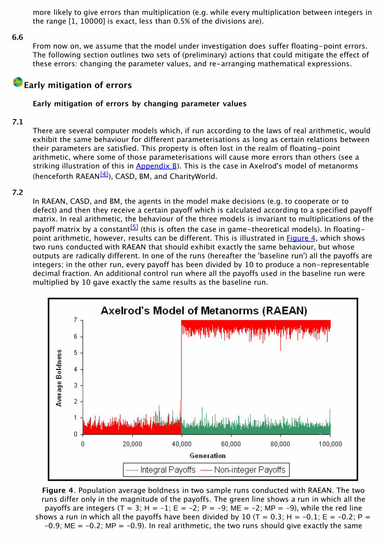
7.2In RAEAN, CASD, and BM, the agents in the model make decisions (e.g. to cooperate or todefect) and then they receive a certain payoff which is calculated according to a specified payoffmatrix. In real arithmetic, the behaviour of the three models is invariant to multiplications of thepayoff matrix by a constant[5] (this is often the case in game-theoretical models). In floating-point arithmetic, however, results can be different. This is illustrated in Figure 4, which showstwo runs conducted with RAEAN that should exhibit exactly the same behaviour, but whoseoutputs are radically different. In one of the runs (hereafter the 'baseline run') all the payoffs areintegers; in the other run, every payoff has been divided by 10 to produce a non-representabledecimal fraction. An additional control run where all the payoffs used in the baseline run weremultiplied by 10 gave exactly the same results as the baseline run.

Figure 4. Population average boldness in two sample runs conducted with RAEAN. The tworuns differ only in the magnitude of the payoffs. The green line shows a run in which all thepayoffs are integers (T = 3; H = –1; E = –2; P = –9; ME = –2; MP = –9), while the red line

shows a run in which all the payoffs have been divided by 10 (T = 0.3; H = –0.1; E = –0.2; P =–0.9; ME = –0.2; MP = –0.9). In real arithmetic, the two runs should give exactly the same

output. The program and all the parameters used in this experiment are available in theSupporting Material

7.3Figure 4 does not show a special case. Out of 1000 pairs of simulations where each member ofthe pair should exhibit exactly the same behaviour (using the same parameters as in Figure 4,but a different random seed for each pair), in 999 cases the simulation results differed. We alsoran 1000 additional control runs where the baseline integral payoffs used in Figure 4 weremultiplied by 10, and no differences were found in any of these 1000 pairs. Thus, it seems clearthat the runs with integral payoffs suffered fewer floating-point errors than the runs conductedwith non-integral payoffs. It is worth mentioning that using IEEE 754 double precision, everyaddition, subtraction, or multiplication using integers in the range [–94906266, 94906266] isexact.

7.4If only integral payoffs are used in CASD, the model behaves exactly as with real arithmetic.Similarly, virtually every version of CharityWorld behaves as with real arithmetic if appropriatecare is taken in choosing the parameters (see Polhill et al. 2006).

7.5Thus, a clear recommendation is, if possible, to use parameter values that minimise the chancesof getting floating-point errors. In particular, when exploring the parameter space of a model, itis advisable to sample parameter values that have few digits in binary[6] rather than simple-looking numbers in base 10. For instance, select multiples of 9.765625·10–4 rather thanmultiples of 0.001. In double precision, the closest representable number to 0.001, i.e. [0.001]f, has 51 significant bits out of the 53 bits of accuracy that the format stipulates; on the otherhand, 9.765625⋅10–4, which is exactly representable, has only one significant bit.

[0.001]f is stored (in binary) as:1.0000011000100100110111010010111100011010100111111100 · 2–10

9.765625·10–4 ≡ [9.765625·10–4]f is stored as: 1.0000000000000000000000000000000000000000000000000000 · 2–10

7.6Thus, the chances of getting an inexact result are higher when using [0.001]f as an operand,rather than [9.765625·10–4]f. The same applies for models that use empirical data: valuesshould be rounded to exactly representable base 2 numbers, instead of simple-looking base 10numbers. Our experience is that inputting numbers that are not exactly representable is veryoften the reason behind the appearance of the first floating-point error in a model. On theother hand, when dealing with representable numbers with few bits (e.g. small integers), it isoften not until a division takes place that the first floating-point error appears.

Early mitigation of errors by re-implementing mathematical expressions

7.7Expressions that are equivalent in real arithmetic may not be equivalent numerically (see astriking illustration of this in Appendix B): much effort in the field of numerical analysis isdevoted to the study of the accuracy and stability of different algorithms that are equivalent inreal arithmetic. Obviously, this paper is by no means a substitute for that, and the interestedreader should refer to the vast literature in numerical analysis. Higham (2002) provides anexcellent introduction to the topic, and gives recommendations for common operations likesummation (pp. 89–90). Chan et al. (1983) offer recommendations on computing the samplevariance, an operation which is commonly performed in computer models (e.g. RAEAN and theASM). Whenever it is possible to pass twice through the data, Chan et al. (1983) recommendusing the following formula to compute the sum of squares of the deviations from the mean in aset of N data points {xi}:

7.8In general, one can sometimes avoid the appearance of errors by rearranging expressions infairly trivial ways. As an example, consider the following condition, which is used in Axelrod'smodel of metanorms (Axelrod 1986, p. 1099) to check whether one particular number xj in a set

of N data points {xi} exceeds the average of the set by at least one standard deviation σ:

(1)

7.9This condition would be naturally implemented as:

(1a)

7.10Implementation [1a] will almost certainly suffer from floating-point errors because of thedivisions and the square root. However, assuming that {xi} are integers, and {xi} and N are nottoo large[7] (both conditions prevail in Axelrod's paper), the following rearrangement willprevent any errors from happening[8]:

(1b)

7.11Similar examples can be found in CharityWorld, where

(2a)

should be substituted by

(2b)

if {xi} are integers.

Knife-edge Thresholds: Identification, Characterisation, Securement andAssessment

Identification of knife-edge thresholds

8.1Potential knife-edge thresholds can be identified conducting an automatic search forcomparison operators. However, note that not every branching statement with a comparisoninvolving a floating-point variable is a knife-edge threshold. For example, the followingimplementation of the absolute value of a floating-point number is not a knife-edge threshold,since there are no discontinuities in the algorithm.

IF (x < 0.0) THEN (x = –x);

8.2Something similar occurs in the ASM. The ASM is an artificial stock market where several sharesof one single asset are repeatedly traded. The market is cleared by iteratively reducing theimbalance between the aggregate demand and the aggregate supply of shares, a task that isperformed by evaluating the traders' reactions to different trial prices. The aggregate demandand supply for a certain price are computed by summing up the desired share holdings ofindividual agents for that price. Since the function that determines each agent's desiredholdings is a continuous function of the price, the whole clearing process lacks knife-edgethresholds. Small errors in the calculation and in the summation of agents' desired holdingsmean small errors in the computation of the clearing price; and conversely, small errors in thecalculation of the price will mean small errors in the actual holding of individual agents: thereare no discontinuities.

8.3By contrast, condition [1] in RAEAN determines how many clones of an agent there should be inthe succeeding generation, which is a discontinuous consequent. Similarly, condition [2a], inCharityWorld, determines whether an agent should donate a fixed amount of money to itsneighbour. Both branching statements are clearly knife-edge thresholds.

8.4Another common type of knife-edge threshold, which is found in many stochastic models (e.g.in all six models investigated here), appears when some action is required to occur with acertain (floating-point) probability:

IF (randomNumber < probability) THENaction; (3)

8.5The last knife-edge threshold we will study in the following sections (let us call it [4]) appears inFEARLUS. To assess the impact of floating-point errors in FEARLUS we replicated everyexperiment conducted by Polhill et al. (2001). In that set of experiments, there was only onebranching statement in the code where the wrong branch could sometimes be followed[9]. InFEARLUS, the agents have to select a land use for every land parcel they hold according to oneselection algorithm. One of such algorithms, called Intelligent Imitation, involves selecting theland use with the highest expected yield for the land parcel under consideration. If more thanone land use provides the highest expected yield, one of them is selected at random. Theexpected yield is a rational number that is sometimes not exactly representable (e.g. 13.1), andthus its computer representation may contain some small error. When that is the case, it wasseen that it is possible in principle that two yields which are equal in real arithmetic areperceived as different due to floating-point errors, and therefore the wrong decision couldpotentially be made: a land use could be selected over another when a random decision betweenthe two should have been made. There are other knife-edge thresholds in FEARLUS (see Polhillet al. 2005), but they can all be avoided by appropriately parameterising the model (as Polhill etal. 2001 and Gotts et al. 2003 did).

8.6Once the knife-edge thresholds in a model are identified, the next steps are to characterisethem, secure them, and/or assess their impact. The following sections explain how to do this. Itis important to emphasise, however, that it is not always necessary to undertake these threeactions on every threshold in a model. The ultimate goal is to determine whether floating-pointerrors may affect the conclusions obtained from a model, so any analysis will be useful only tothe extent that it helps us to achieve such a goal. Sometimes an early assessment (withoutcharacterising or securing the threshold) is sufficient to conclude that floating-point errors willnot affect the conclusions drawn from the model.

8.7As an example, consider the ASM, where every agent uses a Genetic Algorithm (GA) to select the

best forecasting rules to predict future prices in the market. The GA implementation in the ASMabounds in knife-edge thresholds, and it can be easily shown that the selection of forecastingrules conducted by each agent's GA is significantly affected by floating-point errors: some rulesthat would be selected under real arithmetic are not chosen in floating-point arithmetic andvice versa (Polhill and Izquierdo 2005). However, LeBaron et al. (1999) were not interested instudying the specific forecasting rules that each agent selects; they just needed agents thatlearn how to predict prices in the specific market they trade in. The GA finds rules that workwithin the market it is being applied to, floating-point errors included, so the fact that the GAwould produce different answers under real arithmetic is actually unimportant for the studiesconducted by LeBaron et al. (1999). If someone was interested in studying the evolution of thepopulation of forecasting rules in the ASM, then floating-point errors could indeed be an issue.This observation illustrates the point that whether floating-point errors are significant or notstrongly depends on what the model is used for.

Characterisation

8.8The analysis of any knife-edge threshold begins with a characterisation of the set of values thatthe variables involved in its condition part should take under real arithmetic, and of the errorthey may contain in floating-point arithmetic. Ideally, this analysis would include an estimate ofboth the magnitude of the error and whether there is any apparent bias in it. As we will see inthe next section, this characterisation will determine which techniques are most appropriate toprevent the model from following the wrong branch.

8.9As an example, consider threshold [2b] in CharityWorld, where data points {xi} represent thewealth of a set of agents. In most settings of CharityWorld it is easy to see that, under realarithmetic, every xi is an exact multiple of a certain parameter G, i.e. every possible value of xi isseparated from every other possible value by at least a minimum distance dmin = G = min { (xi –xj) ; xi ≠ xj }. Similar examples can be found in RAEAN, FEARLUS, and CASD. This is an importantproperty since, if errors are small compared to dmin, then one can easily identify what thecorrect value of a variable should be. To assess the magnitude of the errors involved, themethods and analytical bounds provided in section 6 may be useful.

8.10There are other properties of the set of possible values {yi} which would appear in the conditionpart of the knife-edge threshold under real arithmetic that are worth assessing, since they willinfluence the selection of the most appropriate technique to use, e.g.:

Whether every possible value yi is rational.Whether there is an upper limit for the number of digits[6] of every possible value yi.Whether the set {yi} is continuous (i.e. is it always possible to find another member of {yi}between any two members of the set?).Whether the set {yi} is bounded.

Securement

8.11This section presents four techniques aimed at securing knife-edge thresholds, i.e. ensuringthat the correct branch of the threshold is followed. Each technique is appropriate for differentcases, and sometimes no technique can guarantee that the model will always follow the rightpath. A summary of the most relevant features of each technique is provided at the end of thissection.

Tolerance windows

8.12As shown in the previous section, many knife-edge thresholds have the convenient property

that the set of possible values that may appear in the condition part is such that, under realarithmetic, every value is separated from every other possible value by a minimum distance dminthat can be easily identified. When dmin is substantial (i.e. greater than the floating-point errorsin the variables involved), if the wrong branch is followed, it is because two numbers thatshould have been equal are detected as different, rather than because two numbers that shouldbe different are detected as equal or because their relative order has been inverted. In thosecases, tolerance windows are particularly useful to ensure that the correct branch is alwaysfollowed.

8.13The use of tolerance windows consists in replacing the comparison operators as shown

x > y → x > [y + ε]fx ≥ y → x ≥ [y – ε]fx < y → x < [y – ε]fx ≤ y → x ≤ [y + ε]fx ≡ y → ( x ≥ [y – ε]f ) ∧ ( x ≤ [y + ε]f )x ≠ y → ( x < [y – ε]f ) ∨ ( x > [y + ε]f )

where ε is a non-negative floating point number[10]. The value of ε should be high enough todetect as equal two different floating-point numbers that would be equal in the absence offloating point errors, but low enough to detect as different two numbers that would indeed bedifferent without such errors. Setting ε = [dmin/3]f– (where [dmin/3]f– denotes the largestfloating-point number no greater than dmin/3) guarantees that the correct branch is alwaysfollowed as long as the absolute error in each number to be compared is less than ε/2 (proof inAppendix A).

8.14The weakness of tolerance windows is that they require calculating (absolute) error bounds toensure correct behaviour. To calculate such bounds the theoretical results given in section 6 canbe useful.

8.15A very simple way of putting this technique into practice in NetLogo (Wilensky 1999) isillustrated in Appendix B. A more sophisticated implementation (written in objective-C) whereevery variable is coded as an object, and every comparison operator (which is a message thatcan be sent to one object, with another object being an argument of such a message) isprogrammed as described above is freely available in the Supporting Material.

Rounding to n significant digits

8.16This technique consists in rounding every floating-point variable to a specified number ofsignificant digits in the working base – most often base 10 – every time the variable changes itsvalue. To round x to n significant digits in base 10, the following formula can be used (within acertain range) in any programming language:

where round(z) returns the closest integer to z and ceil(z) denotes the smallest integer greaterthan or equal to z. An example of this implementation in NetLogo (Wilensky 1999) is providedin Appendix B. In programming languages that allow printing numbers to n significant digits(e.g. C, C++, Objective-C, and Java) a simpler implementation of this technique consists inprinting x to a string with the specified precision, and then read the string back as a floating-point value (Polhill et al. 2006; Supporting Material). As an example, printing values to 5significant decimal digits in the piece of code introduced in section 4 would produce the

following results:

ENERGY = 0.6;ENERGY-FLOAT-BEFORE-PRINTING-TO-STRING = 0.5999999999999999777955395…; ( ≡[0.6]f )ENERGY-STRING = "0.6";ENERGY-FLOAT-AFTER-READING-STRING = 0.5999999999999999777955395…; ( ≡ [0.6]f )ENERGY = ENERGY – 0.2;ENERGY-FLOAT-BEFORE-PRINTING-TO-STRING = 0.3999999999999999666933092…; ( ≠[0.4]f )ENERGY-STRING = "0.4";ENERGY-FLOAT-AFTER-READING-STRING = 0.4000000000000000222044604…; ( ≡ [0.4]f )ENERGY = ENERGY – 0.4;ENERGY-FLOAT-BEFORE-PRINTING-TO-STRING = 0; ( ≡ [0]f )

8.17Thus the problem would be solved (i.e. the agent would not unduly die). Rounding to significantdigits is particularly useful if, in the absence of errors, every number directly or indirectlyinvolved in a knife-edge threshold of the model has only a few digits in the working base (as ithappens in CharityWorld, CASD, and FEARLUS). The fact that every possible value for a certainvariable should only have a limited number of digits implies that all possible values for thatvariable should be separated from each other by a minimum relative distance. That is valuableinformation that this technique can exploit by taking the result of every operation conducted onsuch a variable back to the closest valid number (or, to be precise, back to the floating-pointrepresentation of the closest valid number). Thus, if relative errors are not too large, roundingto n significant digits (i.e. rounding to the floating-point representation of the closest numberwith n significant digits) will reduce the accumulation of errors and their impact.

8.18To describe this formally, let a be the number of significant decimal digits of accuracyguaranteed by the current floating-point environment; a = 6 in IEEE 754 single precision, and a= 15 in double precision (Sun Microsystems 2000, p. 27). If in the absence of errors thenumbers at both sides of a comparison have n or fewer digits in decimal[11], then rounding bothnumbers to n significant figures before comparing them will guarantee a correct comparisonprovided that n ≤ a and the relative error in both numbers is less than 10–n/2. Thus, liketolerance windows, this technique also requires error bounds to ensure correct behaviour. Note,however, that in this case the required bounds concern relative errors, rather than absoluteerrors. One advantage of this technique over tolerance windows is that rounding can preventaccumulation of errors.

8.19There is one exception to the formal analysis of the previous paragraph: it does not necessarilyapply when comparing two numbers that should be both equal to 0. The reason is that roundinga value very close to 0 to any number of significant digits does not take that value back to 0, asone often desires. For the sake of clarity, note that while rounding [1.000002222222]f to 5significant digits produces the value 1 (as intended), rounding [0.000002222222]f to 5significant digits produces the value [2.2222e-06]f. Thus, it is worth considering implementingthis technique so numbers within a small interval around 0 are rounded to 0. Having said that,comparing two numbers that should be both equal to 0 is not always problematic (as illustratedin the code example above).

8.20Finally, note that, in principle, there is no need to round every value every time it changes; it isenough to round those values that are to be compared in a knife-edge threshold, andpotentially only when they are to be compared, as long as the required error bounds are met.This can greatly simplify the implementation of this technique, since it would suffice to re-program only the comparison operators (see an example of how to do this in Appendix B). Thebenefit of rounding values after every change is that errors do not accumulate so much, and

therefore it is easier to guarantee that the required error bounds are met.

8.21An elegant way of putting this technique into full operation is to implement every variable in themodel as an object, and program every mathematical operator – a message that can be sent tothe object – to be followed by an automatic rounding. An implementation of such a class ofobjects (written in objective-C) is freely available in the Supporting Material.

Interval arithmetic

8.22Interval arithmetic consists in defining every constant z in the model as an interval [ [z]f–, [z]f+ ](where [z]f+ denotes the smallest floating-point number no less than z), defining also everyvariable as an interval, and performing every operation in the model according to the rules ofinterval arithmetic. Thus, the correct value of any variable is guaranteed to be within its interval.Comparison operators are implemented so they issue a warning if there is any chance that theyare giving the wrong answer. Therefore, if a model runs without warnings, then it is certain thatit has followed the right path. This is the main strength of interval arithmetic. Polhill et al.(2006) explain how to implement interval arithmetic in floating-point environments. Animplementation in Objective-C is freely available in the Supporting Material.

8.23The distinguishing property of interval arithmetic is that it does not require any assumptionabout the set of values that are to be compared in the model, or about the magnitude of theirerrors. This feature can be very valuable, but it can also be a weakness. It clearly is a worthyproperty if the model runs without warnings. However, the fact that interval arithmetic does notuse any information about the properties of the numbers involved in the comparisons can be aweakness if the model issues warnings and some available information could have beenexploited. As an example, note that the comparison between [0.04]f and [[0. 1]f × [0.4]f]f issuesa warning under interval arithmetic, but can be performed correctly using tolerance windows orstrings under a very wide range of conditions. Another trivial illustration where intervalarithmetic fails (i.e. it issues an unnecessary warning) is the comparison between two non-representable identical values.

8.24Thus, a useful approach is to use interval arithmetic at first to automatically disregard thoseknife-edge thresholds where the right branch was selected (i.e. no warnings issued) and toautomatically calculate error bounds. The second stage would be to deal with each of thethresholds where warnings were issued exploiting specific knowledge about the properties ofthe particular variables involved, and potentially making use of the error bounds provided byinterval arithmetic. This combined approach is often very useful because interval arithmetic isweaker precisely where tolerance windows and rounding to significant n digits are stronger (i.e.when numbers that should be equal are different because of small errors).

8.25In summary, though safe and powerful in many cases, interval arithmetic is weak whencomparing numbers which should be equal but which contain small errors. It also has theadditional disadvantage that it is harder to implement than the previous techniques (Polhill &Izquierdo 2005). On the other hand, interval arithmetic is the only technique presented herethat gives bounds for the error contained in any variable. Kahan (1998), whilst acknowledgingthat interval arithmetic is pessimistic in its estimate of error, nonetheless recommends it on thebasis that it "never lulls its users into a false sense of security" (p. 25).

Rational arithmetic (vs. floating-point arithmetic)

8.26Many computer model specifications do not require the use of irrational numbers (e.g. FEARLUS,CASD, BM, and CharityWorld). Even when they do, it is often the case that they can be re-implemented so only rational numbers are used (see re-implementation [1b] of condition [1a] inRAEAN). In those cases, a simple way of avoiding floating-point errors altogether is to

implement a class of rational numbers. All the problems with floating-point errors in FEARLUS,CASD, BM, and CharityWorld are avoided by using rationals, even if no care is taken to selectappropriate parameterisations. A class of rational numbers (written in objective-C) is availableonline in the Supporting Material.

8.27Using rational numbers we were able to assess how often the wrong branch was followed inknife-edge threshold [4] in FEARLUS, under floating-point arithmetic. Our study consisted of2700 different pairs of runs, each run within each pair differing only in the arithmetic used. Itturned out that the two implementations followed the same branches in all cases. Thus, weconclude here that not only the conclusions, but also the results published by Polhill et al.(2001) and Gotts et al. (2003) using FEARLUS are unaffected by floating-point errors.

Summary of techniques to secure knife-edge thresholds

8.28Table 1 provides a summary of the most relevant features of every technique, and Appendix Cshows their computational requirements in terms of memory and speed.

Table 1: Summary of the most relevant features of every technique

Most usefulwhen: Main advantage(s) Main

disadvantage(s)

Requiredlevel of

programmingexpertise

Tolerancewindows

In the absence oferrors, everypossible value xi inthe threshold isseparated fromevery otherpossible value by asubstantialminimum distancedmin = min { (xi –xj) ; xi ≠ xj }.[12]

Simplicity

It requires(absolute) errorbounds toensure correctbehaviour.

Basic

Roundingto n

significantdigitsbefore

comparing

In the absence oferrors, everypossible value inthe threshold hasonly a few digits inthe workingbase.[12]

Simplicity

It requires(relative) errorbounds toensure correctbehaviour.

Basic

Roundingto n

significantdigitsafterevery

operation

In the absence oferrors, everypossible value inthe threshold hasonly a few digits inthe workingbase.[12]

It can preventaccumulation oferrors.

It requires(relative) errorbounds toensure correctbehaviour.

Intermediate

Intervalarithmetic

Information aboutthe set of valuesinvolved in thethreshold in theabsence of errorsis not readily

It does notrequire anycharacterisationof the set ofvalues involvedin thethreshold.

Weak (i.e. itissuesunneccessarywarnings) whencomparing Advanced

arithmetic available and/orthe magnitude ofthe error they maycontain isunknown.

threshold.It does notrequire errorbounds.It provides safeerror bounds.

numbers thatshould be equalbut containsmall errors.

Rationalarithmetic

Only rationalnumbers are used.

It completely solvesthe problem if onlyrational numbers areused.

Advanced levelof programmingexpertiserequired.

Advanced

Assessment

8.29The last stage of the analysis of knife-edge thresholds consists in evaluating the chances oftaking the wrong branch, and in assessing the consequences of such an undesirable event. Theanalysis of the importance of following the wrong path can be undertaken using 'backward erroranalysis' (Higham 2002): what change in the parameters or in the structure of the model wouldproduce the current (faulty) results under real (exact) arithmetic? i.e. to what changes in theparameters or in the structure of the model are floating-point errors equivalent? If suchchanges are sufficiently unimportant for our conclusions, then floating-point errors do not reallymatter.

Axelrod's knife-edge threshold [1]

8.30As an example, consider Axelrod's knife-edge threshold [1]. This threshold is secured by usingintegral payoffs only and by implementing condition [1b]; these two measures guarantee thatthe correct branch is always followed[13]. Using rational arithmetic and condition [1b] solves theproblem too. Nevertheless, to illustrate the fact that even if the model sometimes follows thewrong branch, the conclusions obtained with it may still be valid, let us assume that we useimplementation [1a] and non-integral payoffs. In Axelrod's paper, each xi in [1a] is the sum offewer than 3000 payoffs (which are parameters in the model). Applying some of the resultsabout the errors in floating-point arithmetic mentioned before, one can see that the error ateither side of [1a] is going to be very small. Thus, the chances of condition [1a] being wronglyevaluated are low, except when the standard deviation σ should equal zero in real arithmetic.Simulation tests have confirmed these results[14]. Fortunately, when σ equals zero in realarithmetic the exact model specifications are similar to (though not the same as) those followedby the faulty model when σ is very close to zero (Galán & Izquierdo 2005).

8.31Thus, we conclude that in a very few occasions some agents which should have been cloned arenot, and vice versa. Because there is also some random mutation of cloned agents in the model,one can argue that the effect of floating-point errors is roughly equivalent to some extramutation which takes effect very rarely. One could even argue that the same changes caused byfloating-point errors could have occurred in an exact model, but due to the random mutation.The question now is whether such extra (and most likely not random) noise is likely to changethe conclusions that the researcher extracts from the model. If that was the case, one shouldbear in mind that the conclusions obtained from the model would then be as sensitive tofloating-point errors as they are to small changes in the mutation process.

8.32Axelrod's model was designed to explore whether a social norm to cooperate would collapse ornot. This type of conclusion refers to an aggregate property of the overall system (which is anergodic Markov chain) and, as such, we conjectured that, most likely, the small random effectsat the individual level caused by floating-point errors (which represent small alterations in thetransition probabilities of the Markov chain) would not affect it. Experiments summarised inFigure 5 confirmed our speculations. Note that we conclude that the overall behaviour of the

system, which can only be explored conducting many runs with different random seeds, is notsignificantly affected by floating-point errors. As we saw before, the dynamics of eachindividual run is indeed significantly affected by floating-point errors, even at the populationlevel.

Figure 5. Proportion of runs (out of 1000 for each line) where the norm collapses in Axelrod'smodel of metanorms. The green line shows runs in which all the payoffs are integers (T = 3; H

= –1; E = –2; P = –9; ME = –2; MP = –9) and condition [1b] was implemented. The red lineshows runs where every payoff has been divided by ten (T = 0.3; H = –0.1; E = –0.2; P = –0.9;ME = –0.2; MP = –0.9), and condition [1a] was used. The two programs and all the parameters

used in this experiment are available in the Supporting Material

Stochastic knife-edge thresholds [3]

8.33Another interesting example, where the techniques presented in section 8.3 are not alwaysuseful, is knife-edge threshold [3] in stochastic models. In contrast to non-stochastic knife-edge thresholds, the important question here is the magnitude of the error in the value ofprobability, rather than its mere appearance. If such an error is small, then floating-point errorsat this threshold will not significantly affect the overall statistical behaviour of the model. This isso because, since the threshold is stochastic, there is no 'wrong branch' in the sense that eachone of them would be followed with very similar probability using either arithmetic (given thatthe error is small by assumption). If the threshold is repeated very frequently in a run, then itwould be necessary to ensure that the error is either very small (e.g. if probability is a non-representable constant), or small and unbiased.

8.34As an example, we study the following knife-edge threshold, which is executed by each agentin BM:

IF(rand < pt) THEN [cooperate] ELSE[defect];

where rand is a random number in the range [0,1] and pt is the agent's probability to cooperatein time-step t. The probability pt is updated every time-step according to one of two possibleformulae. Which formula is used depends on the action (cooperate or defect) undertaken byeach of the two agents in the model in the previous time-step. Because of the simple arithmetic

form of the two updating formulae (see Macy & Flache 2002), the error in pt+1 will be smallgiven any one particular formula. Thus, assuming the same path has been followed in thefloating-point model and in its exact counterpart up to a point, the chances of bothimplementations keep following the same path will be very high. In the unlikely case that thefloating-point model deviates from the 'correct' path at some point, one could always argue thatsuch a deviation could have occurred with extremely similar probability in the correct modelanyway. Thus, we would conclude that floating-point errors do not significantly affect the overallstatistical behaviour of this model.

8.35To be sure, we re-implemented the BM model in both double precision floating-pointarithmetic and exact (rational) arithmetic. We conducted an experiment of 1000 runs, each ofthem consisting of 2000 iterations, and it turned out that the 2·106 decisions made by each ofthe agents in the whole experiment were exactly the same in both implementations. Figure 6shows, for each iteration t, the maximum difference between the values of pt in eachimplementation across the 1000 runs. (For the parameterisation used, the value of pt is thesame for both agents in a given implementation). Figure 6 shows that the error is very small, aswe had conjectured, but has a clear bias at the end of the runs.

Figure 6. Maximum difference across 1000 runs between the value of pt in an exactimplementation of the BM model (Macy & Flache 2002) and the value of pt in an implementationusing IEEE 754 double precision arithmetic. The figure shows data for the Prisoner's Dilemmawith parameters [π = (4,3,1,0), A = 2, l = 0.5, h = 0, pC,1 = 0.5] (see Macy & Flache 2002).

The program used to conduct this experiment is available in the Supporting Material.

8.36To explain such a bias in the error, it is worth noting that the BM model implicitly relies oninfinite precision. It can be analytically proved (Izquierdo et al. 2006) that pt asymptoticallyapproaches its limit value 1 in every run shown in Figure 6. This asymptotic convergence to 1 issomething that could have never been found out for certain using floating-point arithmetic,since there is an infinite set of numbers S (defined as the rational numbers strictly between thelargest representable floating-point number smaller than 1 and the number 1) which pt cannottake in the floating-point implementation but it does take in the exact implementation.

8.37In fact, the mathematical analysis shows that after a sufficiently high number of iterations in real

arithmetic, it is almost certain that pt takes values in S. However, pt cannot take any value in theset S in the floating-point model: it either stops at the largest representable number smallerthan 1 (or at an even smaller number), or rounds up to 1. In fact, the final value of pt in everyrun we conducted with floating-point arithmetic (Figure 6) was 1–2–52. This value is preservedindefinitely due to floating-point errors. That explains the bias of approximate magnitude 2–52 ≈ 2.22045·10–16 shown in Figure 6. In any case, the floating-point model, whilst inexact, isstatistically extremely similar to its exact counterpart.

8.38Thus, we conclude that the overall statistical behaviour of the BM model is not significantlyaffected by floating-point errors. Admittedly, however, its precise long-term behaviour cannotbe adequately studied using floating-point simulations only. Using the parameters shown in thecaption of Figure 6, floating-point simulations lock in to an absorbing state[15], whereas it canbe proved that under exact arithmetic no state can ever be revisited! Then again, the exactmodel does have a limiting state (pt = 1) that lies near the absorbing state of the floating-pointmodel (pt = 1–2–52), and this explains why the macroscopic behaviour of both models turnedout to be identical in the 1000 runs we conducted. Thus, it is clear once again that floating-point errors affect certain types of conclusions, but not others – i.e. the importance of floating-point errors in a model strongly depends on the specific use the researcher makes of it.

Summary

9.1Floating-point arithmetic creates the illusion of working with real numbers, and it does it soeffectively that many computer modellers are unaware of the potentially unpleasant effects thatit can have on their results. If a model uses floating-point numbers, chances are that it issuffering rounding errors. If, in addition, the model contains knife-edge thresholds, then smallfloating-point errors may have a disproportionate impact on its results.

9.2To perform an analysis of the relevance of floating-point errors in a model, the purpose of themodel is paramount, since it is the purpose of the model that determines the acceptablemagnitude and impact of the errors. In this paper, we have provided a framework intended toassist the reader in finding out whether a particular use of a particular model may be affected byfloating-point errors, and what to do about it.

9.3After conducting an early identification of potential floating-point issues, our nextrecommendation is to undertake some preliminary tasks aimed at reducing the magnitude offloating-point errors, e.g. appropriate selection of parameter values and re-implementation ofmathematical formulae. Small errors affect model results through knife-edge thresholds. Thus,the next step is to conduct a thorough analysis of potentially every knife-edge threshold in themodel – interval arithmetic can be very useful at this stage to identify (and dismiss) those knife-edge thresholds where it is certain that the correct branch has been followed, and whichtherefore do not require further attention.

9.4The analysis of each knife-edge threshold begins with a characterisation of the set of valuesinvolved in its condition part. This characterisation determines which techniques are mostuseful to ensure that the correct branch of the code is always selected. In this paper, fourtechniques (tolerance windows, rounding to n significant digits, interval arithmetic, and rationalarithmetic) have been described, and their specific strengths and weaknesses have beenhighlighted.

9.5Unfortunately, sometimes it is impossible to guarantee that the correct branch will be followedin every knife-edge threshold of a model. In those cases, it is necessary to assess the extent towhich following the wrong path affects the conclusions obtained with the model. To do that, wehave shown that backward-error analyses are particularly useful: often the magnitude of the

impact of floating-point errors can be meaningfully formulated in terms of changes inparameters or slight alterations in the structure of the model. This correspondence betweenfloating-point errors and model structure facilitates the task of determining the relevance offloating-point errors in a certain model that is being used for a certain purpose.

Acknowledgements

This work has been funded by the Scottish Executive Environment and Rural Affairs Department.We would like to thank Bruce Edmonds for many helpful comments and discussions, DaleRothman for suggesting the term 'knife-edge', Nick Higham for useful advice at the early stagesof this investigation, and three anonymous referees for their clarifying suggestions.

Notes

1The most common base in floating-point computing systems is base 2.

2Some authors refer to control flow statements, rather than branching statements. By branchingstatement we mean any point in the code of a program where the flow of control may diverge.Some examples are:IF(condition)THEN(action), and DO(action)WHILE(condition).

3It is also assumed that nu < 1.

4RAEAN stands for "Reimplementation of Axelrod's 'Evolutionary Approach to Norms' " (Galán &Izquierdo 2005).

5In the BM model it is necessary to multiply the aspiration level by the same constant too.

6By 'digits of a real number x' in a certain base b we mean the minimum number of digits Xnecessary to write x in base b, according to the format X·X…X · bexp, and without loss ofprecision.

7Even if {xi} were large, one could always subtract an integral estimate of the mean of {xi} fromevery xi, and then apply [1b] to the shifted data.

8Please note that at this stage we are only concerned about the first appearance of floating-point errors, not about the impact of such errors in evaluating the condition. Even if thecondition is evaluated correctly in both implementations, implementation [1b] will help us tofocus on the relevant errors in the model (e.g when doing an automatic detection of all theerrors). The same applies for [2a] and [2b].

9We arrived at this statement using interval arithmetic. Later in the paper we acknowledgeinterval arithmetic as a useful technique to identify those knife-edge thresholds where thecorrect branch of the code has been followed for certain, and which therefore do not require anyfurther attention.

10Knuth (1998, p. 233) also suggests a variation on this approach that takes into considerationthe magnitude of the operands. A brief investigation using CharityWorld did not find thisimproved things much (Polhill et al 2006).

11It is also assumed that both numbers lie within the range of normalised floating-pointnumbers. In double precision that range is: [–1.797…·10308, –2.225…–308] ∪ [2.225…–308,1.797…·10308].

12If errors are not too large, this means that when the wrong branch is followed, it is because

two numbers that should have been equal are detected as different (due to small floating-pointerrors), which is most often the case.

13In our experiments it turned out that using integral parameters was enough to select the rightbranch at the knife-edge threshold every time the condition was evaluated: the 1000 runs weconducted with implementation [1b] and integral payoffs produced exactly the same results asthe 1000 runs we conducted with implementation [1a] and integral payoffs.

14Interestingly, these tests also showed that the error is somewhat biased.

15The value of pt completely determines the state of the system.

Appendix A

The following two theorems provide the theoretical basis to show that using tolerance windowsof magnitude ε = [dmin/3] f– , the correct path in a branching statement is always followed aslong as the absolute error in each number to be compared is less than ε/2.

Theorem 1: Let x, y and ε (ε ≥ 0) be three floating-point numbers and assume that summationand subtraction are exactly rounded (as the IEEE 754 standard stipulates). If |x – y| > 2ε, then xand y will be detected as being different using tolerance windows of magnitude ε.

Proof: Assume for now that x > y. Then |x – y| > 2ε implies that x > y + 2ε. Let D(y + ε) be theerror in computing [y + ε]f, expressed as D(y + ε) = [y + ε]f – (y + ε). It can be easily shown that|D(y + ε)| ≤ ε. Thus,

x > y + 2ε ⇒ x > y + ε + D(y + ε) ⇒ x > [y + ε]f

The proof for the case where x < y is analogous. The 2ε margin is the smallest needed toguarantee that the two numbers will be detected as different, since there are cases where |x – y|= 2ε and the result of this proposition does not apply. ¤

Theorem 2: Let x, y and ε be three floating-point numbers and assume that summation andsubtraction are exactly rounded (as the IEEE 754 standard stipulates). If |x – y| ≤ ε then x and ywill be detected as being equal using tolerance windows of magnitude ε.

Proof: |x – y| ≤ ε ⇔ y – ε ≤ x ≤ y + ε

Since subtraction is exactly rounded, we know that [y – ε]f ≤ x. This is because x is a floatingpoint number that is nearer to y – ε than any floating point number greater than x (since y – ε ≤x ). Similarly, we also know that x ≤ [y + ε]f. Assuming a larger margin for |x – y| would notprovide such a guarantee. Thus, if |x – y| ≤ ε, then [y – ε]f ≤ x ≤ [y + ε]f . ¤

In summary, if summation and subtraction are exactly rounded, then using tolerance windowsof magnitude ε will enable the model to follow the correct branch if:

. i Each pair of numbers that need to be detected as different for the model to follow theright branch are correctly ordered, and their absolute difference is greater than 2[ε]f.

. ii No two numbers that need to be detected as being equal for the model to follow the rightbranch have an absolute difference greater than [ε]f.

It can be easily proved that setting ε = [dmin/3] f– guarantees both (i) and (ii) above as long theabsolute error in each number is less than ε/2.

Appendix B

Appendix B is here.

Appendix C

Appendix C is here.

References

AXELROD R M (1986) An Evolutionary Approach to Norms. American Political Science Review, 80(4). pp. 1095-1111.

BOOCH G, Rumbaugh J, and Jacobson I (1999) The Unified Modeling Language User Guide.Addison-Wesley, Boston, MA.

CHAN T F, Golub G H, and LeVeque R J (1983) Algorithms for Computing the Sample Variance:Analysis and Recommendations. The American Statistician, 37(3). pp. 242-247.

FLACHE A and Macy M W (2002) Stochastic Collusion and the Power Law of Learning. Journal ofConflict Resolution, 46 (5). pp. 629-653.

GALÁN J M and Izquierdo L R (2005) Appearances Can Be Deceiving: Lessons LearnedReimplementing Axelrod's 'Evolutionary Approach to Norms'. Journal of Artificial Societies andSocial Simulation, 8 (3), http://jasss.soc.surrey.ac.uk/8/3/2.html

GOLDBERG D (1991) What every computer scientist should know about floating point arithmetic.ACM Computing Surveys 23 (1). pp. 5-48.

GOTTS N M, Polhill J G, and Law A N R (2003) Aspiration levels in a land use simulation.Cybernetics & Systems 34 (8). pp. 663-683.

HIGHAM N J (2002) Accuracy and Stability of Numerical Algorithms, (second ed.), Philadelphia, USA:SIAM.

IEEE (1985) IEEE Standard for Binary Floating-Point Arithmetic, IEEE 754-1985, New York, NY:Institute of Electrical and Electronics Engineers.

IZQUIERDO L R, Gotts N M, and Polhill J G (2004) Case-Based Reasoning, Social Dilemmas, and aNew Equilibrium Concept. Journal of Artificial Societies and Social Simulation, 7 (3),http://jasss.soc.surrey.ac.uk/7/3/1.html

IZQUIERDO L R, Izquierdo S S, Gotts N M, and Polhill J G (2006) Transient and Long-RunDynamics of Reinforcement Learning in Games. Submitted to Games and Economic Behavior.

JOHNSON P E (2002) Agent-Based Modeling: What I Learned from the Artificial Stock Market.Social Science Computer Review, 20. pp. 174-186.

KAHAN W (1998) "The improbability of probabilistic error analyses for numerical computations".Originally presented at the UCB Statistics Colloquium, 28 February 1996. Revised and updatedversion (version dated 10 June 1998, 12:36 referred to here) is available for download fromhttp://www.cs.berkeley.edu/~wkahan/improber.pdf

KNUTH D E (1998) The Art of Computer Programming Volume 2: Seminumerical Algorithms. ThirdEdition. Boston, MA: Addison-Wesley.

LEBARON B, Arthur W B, and Palmer R (1999) Time series properties of an artificial stock market.Journal of Economic Dynamics & Control, 23. pp. 1487-1516.

MACY M W and Flache A (2002) Learning Dynamics in Social Dilemmas. Proceedings of theNational Academy of Sciences USA, 99, Suppl. 3, pp. 7229-7236.

POLHILL J G, Gotts N M, and Law A N R (2001) Imitative and nonimitative strategies in a land usesimulation. Cybernetics & Systems, 32 (1-2). pp. 285-307.

POLHILL J G and Izquierdo L R (2005) Lessons learned from converting the artificial stock marketto interval arithmetic. Journal of Artificial Societies and Social Simulation, 8 (2),http://jasss.soc.surrey.ac.uk/8/2/2.html

POLHILL J G, Izquierdo L R, and Gotts N M (2005) The ghost in the model (and other effects offloating point arithmetic). Journal of Artificial Societies and Social Simulation, 8 (1),http://jasss.soc.surrey.ac.uk/8/1/5.html

POLHILL J G, Izquierdo L R, and Gotts N M (2006) What every agent based modeller should knowabout floating point arithmetic. Environmental Modelling and Software, 21 (3), March 2006. pp.283-309.

WILENSKY U (1999) NetLogo. http://ccl.northwestern.edu/netlogo/. Center for ConnectedLearning and Computer-Based Modeling, Northwestern University, Evanston, IL.

SUN MICROSYSTEMS (2000) Numerical Computation Guide. Lincoln, NE: iUniverse Inc. Availablefrom http://docs.sun.com/source/806-3568/.

Return to Contents of this issue

© Copyright Journal of Artificial Societies and Social Simulation, [2006]