Is Nonfarm Diversification a Way Out of Poverty for Rural Households? Evidence from Vietnam in...
54
PEP Research Project 1006 Is Nonfarm Diversification a Way Out of Poverty for Rural Households? Evidence from Vietnam in 1993-2006 INTERIM REPORT Pham Thai Hung & Bui Anh Tuan, Dao Le Thanh Abstract Using the four high quality household living standards surveys available to date this paper reveals that Vietnam’s rural labour force has been markedly diversifying toward nonfarm activities in the doi moi (renovation) reform. The employment share of the RNFS has increased from 23 percent to 58 percent between the years 1993 and 2006. At the individual level, the results indicate that participation in the RNFS is determined by a set of individual, household, and community level characteristics. Gender, ethnicity, and educations are reported as main individual-level drivers of nonfarm diversification. Lands as most important physical assets of rural households are found to be negative to nonfarm employment. It is also evident that both physical and institutional infrastructures exert important influences on individual participation in the nonfarm sector. At the household level, a combination of parametric and semi-parametric analysis is adopted to examine whether nonfarm diversification is a poverty exit path for rural households. This paper demonstrates a positive effect of nonfarm diversification on household welfare and this effect is robust to different estimation techniques, measures of nonfarm diversification, and the usage of equivalent scales. However, the poor is reported to benefit less than the non-poor from nonfarm activities. Though promoting a buoyant nonfarm sector is crucial for rural development and poverty reduction, it needs to be associated with enhancing access to nonfarm opportunities for the poor. JEL code: J21, J49 Keywords: rural nonfarm sector, nonfarm diversification, Vietnam First draft: 19 January, 2008 Latest revised: 12 August, 2008 Acknowledgements: This work was carried out with financial and scientific support from the Poverty and Economic Policy (PEP) Research Network, which is financed by the Australian Agency for International Development (AusAID) and the Government of Canada through the International Development Research Centre (IDRC) and the Canadian International Development Agency (CIDA).
-
Upload
independent -
Category
Documents
-
view
1 -
download
0
Transcript of Is Nonfarm Diversification a Way Out of Poverty for Rural Households? Evidence from Vietnam in...
PEP Research Project 1006
Is Nonfarm Diversification a Way Out of Poverty for Rural Households? Evidence from Vietnam in 1993-2006
INTERIM REPORT
Pham Thai Hung &
Bui Anh Tuan, Dao Le Thanh
Abstract
Using the four high quality household living standards surveys available to date this paper reveals that Vietnam’s rural labour force has been markedly diversifying toward nonfarm activities in the doi moi (renovation) reform. The employment share of the RNFS has increased from 23 percent to 58 percent between the years 1993 and 2006. At the individual level, the results indicate that participation in the RNFS is determined by a set of individual, household, and community level characteristics. Gender, ethnicity, and educations are reported as main individual-level drivers of nonfarm diversification. Lands as most important physical assets of rural households are found to be negative to nonfarm employment. It is also evident that both physical and institutional infrastructures exert important influences on individual participation in the nonfarm sector. At the household level, a combination of parametric and semi-parametric analysis is adopted to examine whether nonfarm diversification is a poverty exit path for rural households. This paper demonstrates a positive effect of nonfarm diversification on household welfare and this effect is robust to different estimation techniques, measures of nonfarm diversification, and the usage of equivalent scales. However, the poor is reported to benefit less than the non-poor from nonfarm activities. Though promoting a buoyant nonfarm sector is crucial for rural development and poverty reduction, it needs to be associated with enhancing access to nonfarm opportunities for the poor.
JEL code: J21, J49
Keywords: rural nonfarm sector, nonfarm diversification, Vietnam
First draft: 19 January, 2008 Latest revised: 12 August, 2008
Acknowledgements: This work was carried out with financial and scientific support from the Poverty and Economic Policy (PEP) Research Network, which is financed by the Australian Agency for International Development (AusAID) and the Government of Canada through the International Development Research Centre (IDRC) and the Canadian International Development Agency (CIDA).
2
Table of Contents
1. INTRODUCTION .................................................................................................................................... 3
2. A REVIEW OF RURAL NONFARM SECTOR .............................................................................................. 4
3. RURAL NONFARM SECTOR IN VIETNAM: OVERVIEW ............................................................................. 9
4. EMPIRICAL METHODOLOGY AND DATA .............................................................................................. 13
4.1 Modelling Participation of Individuals into the RNFS ................................................................. 13
4.2 Modelling the Welfare Impact of Nonfarm Diversification on Rural Households.......................... 16
Semi-Parametric Approach: The Propensity Score Matching ............................................................ 18
4.3 Data........................................................................................................................................... 21
5. EMPIRICAL RESULTS .......................................................................................................................... 23
5.1 Empirical Results – Individual Participation into the RNFS ........................................................ 23
5.2 Welfare Effect of Nonfarm Diversification – Empirical Results.................................................... 28
Nonfarm Diversification and Household Welfare: The PSM Results.................................................. 32
6. REMARKS .......................................................................................................................................... 35
REFERENCES ......................................................................................................................................... 37
3
1. Introduction
Vietnam’s renovation process, commonly referred as Doi moi, was officially launched in 1986 and
has undergone for about two decades. The country has transformed from a centrally planned
economy into a dynamic market economy with a GDP growth rate of nearly 7.3 percent (GSO
Statistical Yearbook, various issues). This impressive growth has resulted in an impressive poverty
reduction. The national poverty rate fell almost 3.6 times (from 58 to less than 16 percent) between
1993 and 2006 (using the Vietnam Household Living Standards Surveys from this period).
Although this was associated with substantial structural changes towards industry and services,
agriculture has remained central to the economic growth and poverty reduction during the doi moi.
The decollectivization wave and land reform in the early 1990s (Fforde and Huan, 2001),
promoting private sector (including household businesses) (World Bank, 2001; 2005), removing
barriers to trade and production in agriculture directly benefited the majority of Vietnam’s
population whose livelihoods were closely dependent on small-scale subsistence agriculture in the
rural sector (see, for instance, Benjamin and Brandt, 2004).
However, the gains from correcting previous policy distortions were unsustainable and there have
been concerns that agriculture will not be sufficient to absorb the country’s growing labour force
and continue its contribution to the export growth as it did in the early 1990s. The share of
agriculture in total employment sunk from more than two third in 1990 to around 42 percent in
2006, and the underemployment rate was very high in the rural areas (GSO, 2004 and 2006 record
an average of 25 percent). Vietnam’s agricultural exports, which were behind much of the recent
growth in agriculture, have been faced by worsening external environment due to the collapse of
the world prices for the major agricultural commodities in the late 1990s (World Bank, 2006). The
rural-urban migration started rising at high rates. Official statistics from the most recent population
census reveals a number of 4.35 million internal migrants between 1994 and 1999 (GSO, 2001).
Under this context, there has been a growing pessimism about contribution of agriculture in
employment creation and export expansion in the long term and currently it is widely assumed that
4
increased participation in nonfarm activities is critical to the future growth. In fact, nonfarm
employment has become an increasingly important source of employment for the rural population.
Van de Walle and Cratty (2004) reveal that the incidence of households that involved in at least
one nonfarm activities increased from a quarter up to nearly a half of rural households between
1993 and 1998. Expansion of nonfarm employment is also reported in Hoang et al. (2005) and
Minot et al. (2006) for the Red River Delta, and Northern Uplands, respectively. World Bank
(1998, 2006) highlights an increasing share of the RNFS in rural employment and household
incomes through the incidence of nonfarm employment greatly varies across the country.
The current paper examines that growing importance of nonfarm employment in Vietnam and the
impacts of nonfarm diversification on rural poverty and inequality. The main research questions are
inter alia (i) what are determinants of nonfarm diversification by rural households; and (ii) to what
extent does nonfarm diversification contribute to improve welfare of rural households? The paper
draws on the growing literature on the rural nonfarm sector (RNFS) in developing countries (see
Lanjouw and Lanjouw, 1995; Reardon, 1997; Ellis, 1998; Haggblade et al., 2006 for a review). The
paper use three rounds of the Vietnam’s living standards measurement surveys that spread over the
period 1992-2004 corresponding to radical economic transformation in Vietnam.
The paper is structured as follows. Section two reviews the literature on the RNFS in developing
countries and, particularly, in Vietnam. Section three describes the RNFS in Vietnam and its
evolution over time using the household living standards surveys that cover a period of radical
reforms from 1993 to 2006. The empirical framework and data sources used to implement that
framework is outlined in section four. Empirical results are analyzed in the fifth section. Some
policy implications and suggestions are provided in the final section.
2. A Review of Rural Nonfarm Sector
The significant role of the RNFS has been neglected in development economics until recently. The
old view considers the RNFS as those activities limited at individual household level and/or at
village level by traditional technologies. Hymer and Resnik (1969) developed one of the earliest

5
models on the RNFS, in which farmers were assumed to produce two kinds of goods, food and
some simple non-agricultural products, to serve their own needs; the RNFS was supposed to
consist of the household or village production of handicrafts and services, including some textiles,
garments and food processing for village consumption. However, as the rural economy develops,
alternative uses for rural labour in cash crops and other simple type of nonfarm activities become
available, consumption of goods that are either imported or produced in urban centers is also
possible, the RNFS will, as a consequence, wither away. Ranis and Steward (1993) criticize the
traditional view by arguing that the RNFS also include non-traditional and modernizing production
activities such as non-agricultural processes and/or products. There is also a potential relationship
between the nonfarm and agriculture sector as they can mutually support each other via potential
(backward and forward) linkages (Haggblade et al., 1989). As a result, the RNFS will grow up
(instead of withering away) with the rural development process.
Recent arguments for paying attention to the RNFS generally point out the perceived potential of
the sector in absorbing rural labour force, slowing rural-urban migration, contributing to income
growth, and promoting more equal distribution of income. In an important contribution to the
literature on the RNFS, Lanjouw and Lanjouw (1995) argue that neglecting the RNFS would be
mistaken. In many developing countries, a large proportion of the growing population lives in rural
areas. With limits to cultivable land, it is unlikely that the agriculture sector would be productively
capable in absorbing the growing rural labour force. Given this, they highlight the role of the RNFS
as a contributor to growth, income distribution, and minimizing migration. In supporting this,
Davis and Pearce (2000), Meier and Rauch (2000), Haggblade et al. (2006) emphasize the role of
the RNFS in balancing the process of economic development and absorbing fast-growing and low-
income rural labour forces in developing countries. In the context of transitional economies, Bright
et al. (2000) suggest a key role of the RNFS in the development of rural economies.
The impact of nonfarm diversification on household welfare is a complicated issue. While
participating in nonfarm activities apparently contributes to total household income, there has been
a debate on the interaction between nonfarm diversification and poverty reduction. Lanjouw and
6
Lanjouw (1995) consider the RNFS a combination of both productive and non-productive
activities. While the former is likely to considerably raise living standards of rural households, the
latter is described as ‘residual’ activities by rural households in response to shortfalls of income. In
this regard, the welfare effect of nonfarm diversification depends on whether rural households are
in a ‘pull’ or ‘push’ scenario – using Hart’s (1994) terminology. Some rural households may be
‘pushed’ into nonfarm activities in their struggle to survive, while others may be ‘pulled’ into them
by their desire to accumulate. As the ‘pushed’ scenario is usually referred to poor households and
the ‘pulled’ is more likely associated with the non-poor, the welfare effect of nonfarm
diversification on rural poverty in general is not unequivocal. Ellis (1998) supports this argument
and urges that nonfarm participation may be associated with success at achieving livelihood
security under improving economic conditions as well as with livelihood distress in deteriorating
conditions. According to Von Braun and Pandya-Lorch (1991) rural households seek nonfarm
activities either for ‘good’ or for ‘bad’ reasons. While the latter refers to the pressure on the poor to
diversify as a coping strategy, the former implies the attraction of the RNFS to the better-off.
The growing importance of the RNFS has attracted a large number of empirical studies, which can
be loosely divided into two strands. The first strand investigates the determinants of participation in
the RNFS by rural households and individuals (Reardon, 1997; Berdegue et al. 2001; De Janvry
and Sadoulet 2001; Lanjouw and Lanjouw, 2001; Lanjouw and Shariff, 2002). This generally
demonstrates strong impacts of human capital, demographic characteristics, household assets, and
community-level physical and institutional infrastructures on nonfarm employment decisions. The
studies in the second strand have concentrated on how participation in the RNFS has affected
household income, and thus rural poverty (Reardon et al. 1992; Ellis, 1998; Lanjouw, 1998;
Lanjouw et al. 2001, Lanjouw, 2001).1 While re-affirming the influence of the above factors on the
decision-making process to participate in the RNFS, the second strand commonly shows the
importance of nonfarm income-generating activities in total household income, and thus a
considerable contribution by the RNFS to rural poverty reduction. Unfortunately, this positive
1 Some of the studies listed here discuss both the decision-making process to participate in the RNFS and its impact on income and poverty, for instance Berdegue et al. (2001), Lanjouw and Shariff (2002)
7
effect of nonfarm diversification is not universally observed. There has evidence that the poor do
not benefit from the RNFS as much as the non-poor, and the gains from the RNFS largely depend
on the capacity of individuals and households to react to new opportunities created outside
agriculture.
Given this, the welfare effect of nonfarm diversification largely depends on supply-side availability
and dynamics of RNFSs, and household capacity to participate and take advantages of nonfarm
opportunities. Nonfarm diversification is more welfare-enhancing when it occurs in a dynamic
rural economic base, with improving infrastructure conditions, and/or when households have
certain capacity (i.e. human capital, lands and other assets) to undertake investment into such
opportunities. Therefore, the effect of nonfarm diversification on household welfares depends on
specific context of research and remains largely an empirical question.
In this context, there have been a growing number of empirical studies on this issue. In Japan,
Taiwan, and South Korea, the poorer/landless households experienced a higher percentage of
income from nonfarm activities, and this suggests an equalizing influence and poverty alleviation
role of the RNFS (Lanjouw and Lanjouw, 2001). Ravallion and Datt (2002) find that farm yield
and nonfarm output are all associated with poverty reduction in different states of India. In
Berdegue et al. (2001) and Lanjouw (2001), the poor are found to be engaged in ‘last resort’
nonfarm activities, while the non-poor are active in productive nonfarm activities in El Salvador
and Chile, respectively. By reviewing 18 field studies, Reardon (1997) shows that the share of
nonfarm income in total income is two twice higher in upper third households compared to lower
third households. In general, the existing studies reveal either a U-shaped or a negatively-sloped
relationship between nonfarm income and total household income or assets.
The evidence above has been obtained mainly on the basis of descriptive analysis. There are few
studies that tackle the relationship between nonfarm diversification and household welfare by using
econometric models. The endogeneity concern of diversification to poverty is probably the main
difficulty in establishing a causal relationship between nonfarm diversification and household
welfare. Most of the current empirical studies on the RNFS (as above) focus either on the
8
probability of nonfarm diversification or the determinants of nonfarm incomes or both. To our
knowledge, there are a few exceptions that formally deal with the relationship between nonfarm
diversification and household welfare. These include Reardon et al. (1992), Lanjouw (1998), Van
de Walle and Cratty (2004), Dabalen et al. (2004), De Janvry, Sadoulet, and Zhu (2005), Bezemer
et al. (2005), and Jonasson (2005). These studies are briefly reviewed below.
Reardon et al. (1992) employ a recursive system to examine the interaction between nonfarm
diversification, household income, and consumption expenditures in Burkina Faso and reveal a
positive impact of nonfarm diversification on household income and food consumption. In the case
of Ecuador, Lanjouw (1998) proposes a simple simulation that involves estimating an earnings
regression over the whole population of wage-earners and using the estimates to predict the average
earnings of the poor. Lanjouw found that a shift of the poor out of the traditional sector into non-
agricultural activities would imply a rise in the average income. By estimating the individual
earnings equation and household expenditures, Jonasson (2005) reports a better earnings potential
for rural households in the RNFS in Peru. De Janvry et al. (2005) examine the earnings potential in
the RNFS more thoroughly by simulating a counterfactual of what the welfare outcomes (in terms
of household incomes, poverty, and inequality) would be in the absence of nonfarm activities. De
Janvry et al. then reveal that without nonfarm income sources, rural poverty and income inequality
would be much higher in Hubei province of China. Bezemer et al. (2005) introduce a departure
from the classical regression approaches to apply a Bayesian stochastic frontier approach (though
the OLS is also used) in estimating technical efficiency of households who involved in both
farming and nonfarm activities in Georgia. The results demonstrate that nonfarm diversification has
contributed to higher technical efficiency in agriculture and higher income. In the case of Vietnam,
Van de Walle and Cratty (2004) provide some insights on the relationship between nonfarm
activities and rural poverty by using a ‘common causation’ method. This involves identifying
exogenous variables having the same sign in both welfare and diversification regressions. Although
this study points out variables that jointly influence both living standards and nonfarm
diversification, it does not offer conclusive evidence on the causality. With efforts to tackle the
9
same issue, Dabalen et al. (2004) use a semi-parametric approach, the Propensity Score Matching,
to examine the welfare impact of nonfarm diversification in rural Rwanda. By comparing earnings
of different household groups, they generally conclude that participating in nonfarm activities
produces a positive impact on household welfare.
In the Vietnamese context, the understanding on the RNFS is currently limited. Van de Walle and
Cratty (2004) use the first two living standards measurement surveys in the 1990s to investigate the
welfare impacts of nonfarm diversification. The study reveals that participating in non-farm
employment is a route out of poverty for a considerable proportion of the rural labour force but not
for all. More recently, Hoang et al. (2005) collect information from two villages in the Red River
Delta and reveal an important role of nonfarm activities. World Bank (2005) documents
agricultural diversification and provide some useful descriptive analysis on changes in employment
structures in rural areas. Minot et al. (2006) examine certain aspects of the RNFS when focusing on
agricultural diversification in the Northern Uplands. Pham (2007) provides a good picture on
nonfarm diversification in Vietnam when investigating the effect of trade reform on rural
employment. This paper will add to the existing literature by providing clearer insights on the
driving forces underlying nonfarm diversification into wage employment and self-employment
activities, which have not been examined in previous studies on Vietnam.
3. Rural Nonfarm Sector in Vietnam: Overview
This paper uses data drawn from the four high quality household-level surveys conducted for
Vietnam. These surveys cover a period of radical economic reforms from 1993 to 2006. The
surveys were implemented by the GSO under funding and technical support from UNDP, the
World Bank and other donors. Details of these surveys will be described in section 4. In the
absence of statistical data at the national level, these surveys will be used to develop a overview of
the RNFS in Vietnam.
As “[…] nonfarm means (any) activity outside agriculture and nonfarm employment means (any
types of) employment of the rural household members in these activities” (Reardon et al., 2001, p.
10
396), the scope of nonfarm employment needs to be clearly defined. The RNFS in the current study
consists of all economic activities in the rural areas that are different from farm labour (which is
specified as activities by individual who works on her/his own farm or is hired by the others to
work on their farms as farmer labourer). This definition is essentially similar to the others
suggested in the literature (Reardon, 1997; Barrett and Reardon, 2000). Given this, individuals
might be classified to one of the three employment outcomes according to their primary jobs. The
first outcome refers to working in agriculture, or ‘farm labour’. The second type includes nonfarm
self employment, which includes workers who were self-employed in their household nonfarm
activities. Finally, the third outcome includes the wage employed in rural areas.
Applying the definition of nonfarm activities to the data on rural households interviewed in the
surveys above, Table 1 reports the structure of rural employment in the period 1993-2006. It is
evident that the RNFS has become an increasingly important source of employment in rural areas
(currently account for 74 percent of the country’s total population - GSO, 2006). The employment
share of the RNFS has increased from 23 percent to 58 percent between the initial and terminal
years. More importantly, the expansion of nonfarm diversification was driven with a strong shift of
the rural economy toward wage employment (which has risen threefold). As wage employment can
be reasonably considered as formal sector employment (compared to self employment in
agriculture or the RNFS), this suggest a marked increase in the incidence of the wage labour
market over time. There is a marked difference in the structure of rural employment across the
country. In relative term, this shift in employment structure is most pronounced in the Southeast,
two Delta regions, and Central Highlands.
[Table 1 about here]
Selected basic characteristics of rural workers are summarized in Table 2. It is noTable that female
involvement in the RNFS was substantially improved. In year 1993, farming was the main job of
78 percent of women in rural areas. By year 2004, only 48 percent of women worked in their own
farms, and the remaining half was diversified into the RNFS as their main source of employment
and thus income. There is also a marked shift in employment structure among ethnic minorities
11
toward nonfarm wage employment. In 2006, 58 percent of ethnic labour force is now self-
employed in agriculture (compared to 90 percent in 1993), while the corresponding figures for
nonfarm self employment and wage employment is 10 and 32 percent respectively. This could be a
result of the plethora of policy initiatives to encourage participation by ethnic minorities in the
wage labour market (Pham and Reilly, 2008).
[Table 2 about here]
In terms of age structure, approximately 60 percent of nonfarm workers aged from 20 to 40 years
old. As living standards have been recently increased, young people have had more opportunities to
pursue higher education. As a result, the age pattern has changed over time with a decreasing
proportion of young workers. Though dramatic improvement in average education of rural people
during Doi moi is widely reported (Pham and Reilly, 2007), this does not reflect by figures on
educational attainments of rural workers. Table 3 also demonstrates a considerable difference in
average landholding between farmers and nonfarm workers. On average, the average household
landholdings of nonfarm workers are considerably lower than that of farmers, especially in the
initial and terminal years. In addition, the figures on land endowments are relatively stable over
time as most changes in rural land reallocation already took place in the early of the 1990s
(Ravallion and Van de Walle, 2004).
As the rural economy has been diversified toward an increasingly important RNFS, nonfarm
income has become an increasingly important source of income for rural households. To inform the
relative importance of nonfarm income, we calculate the total (and sources of) net income of rural
households over the past 12 months. The total income is divided in four different sources, including
agricultural income, nonfarm wage income, nonfarm self-employment income, and other non-
labour income sources (e.g. remittances, subsidies, pension, savings etc.). The results reveal that
the share of the nonfarm income source (i.e. wage and self-employment) increased from 32 percent
in 1993 up to nearly 54 percent in 2006. Table 3 represents the share of nonfarm income in
Vietnam and other developing countries. As these figures were reported using different definitions
of nonfarm income sources from the surveys with distinctive scales and techniques, they are thus
12
subject to differences in measurement and should be interpreted with cautions. With an average
share of 44 percent during the period 1993-2006, the share of nonfarm income in Vietnam is as
high as those reported in Africa and Latin America, and higher than the average level of the other
Asian countries (e.g. China, India, Philippines, and Pakistan).
[Table 3 about here]
To provide further insights on the contribution of nonfarm diversification to overall rural poverty
and income inequality, the Shapley approach is employed to decompose the poverty headcount
index and the Gini coefficient by the above income sources.2 Table 4 suggests that while all sources
of income have contributed to the reduction of rural poverty, the nonfarm income sources have
been the most important driver of rural poverty reduction in the early 1990s. This poverty-reducing
effect of nonfarm activities is particularly attributable to the nonfarm self-employment income. As
the share of nonfarm self-employment is basically the same as that of wage employment in the
rural labour market (see Table 1), it can be taken to suggest that the average earnings from nonfarm
self-employed activities are higher than those from wage employment. The relative contribution of
nonfarm activities in rural poverty reduction however declined between 1993 and 1998.3 This is
likely to be explained by the impressive agricultural growth. During the period 1993-1998, the
agricultural sector annually grew at an average rate of 4.5 percent, which is exceptionally high
compared to the average of the developing world (Benjamin and Brandt, 2004). Given this, the
relative contribution of the agricultural income in poverty reduction rose from 32 to 48 percent.4
[Table 4 about here]
The estimated Gini coefficient using income as welfare measure reveals a different picture from the
common understanding on income inequality in rural Vietnam during the 1990s, which is largely
2 Though the framework was originally developed in the theory of cooperative games to estimate the expected marginal contribution of player k to the total surplus, it can be applied in a number of other contexts. In poverty and inequality analysis, the Shapley approach has been recently used to decompose poverty and inequality by different criteria (such as groups or sources). This approach and its application can be found in detail in Shorrocks (1999), Duclos and Araar (2006). 3 The results using the VHLSS 2004 and VHLSS 2006 are subject to further investigation on income data and will be added later. 4 The fact that the source of other non-labour incomes consist of a wide range of incomes prevent any reliable insights on the rationale behind the contribution of this source to rural poverty and income inequality.
13
based on expenditure Gini coefficients.5 For instance, World Bank (2003) reported the Gini
coefficient modestly increased from 0.34 to 0.35 between 1993 and 1998, while the Gini
coefficient in the rural areas actually declined from 0.28 to 0.27 over this five year period. What
suggests by the income Gini coefficient in Table 4 is however a sharp increase in rural income
inequality in the 1990s (i.e. from 0.45 to 0.54 between 1993 and 1998). The decomposition results
using the Shapley approach demonstrate that the nonfarm source of incomes were the main force
underlying such worsening income inequality. Conversely, the agricultural income source is found
to be inequality-balancing. It suggests that while nonfarm diversification has contributed to the
reduction of rural poverty, it has however exerted a negative income distribution effect during the
1990s.6
In summary, the descriptive analysis above demonstrates a vigorous shift of rural employment
toward nonfarm activities. It also suggests a close association between nonfarm diversification and
rural poverty and income inequality, though it does not imply causality. The empirical framework
proposed to examine the determinants of nonfarm diversification and the observed association
between such diversification and household welfare is outlined below.
4. Empirical Methodology and Data
4.1 Modelling Participation of Individuals into the RNFS
The probability models have been most commonly used to examine the participation by individual
and households in the RNFS. Lanjouw (1998), Lanjouw (2001), Berdegue et al. (2001), Deininger
and Olinto (2001) apply a Probit model to examine nonfarm diversification in Ecuador, El
Salvador, Chile, and Columbia, respectively. A Logit model is sometimes employed for instance in
Ruben and Van de Berg (2001). However, these models are limited to the cases where an
individual has only two choices (i.e. whether or not to participate in the RNFS).7 Given the great
5 It is partly due to the convenience in calculating the Gini coefficient using expenditures as these data are provided ready in the released survey datasets from GSO. In addition, it is generally recognized that consumption expenditure provides a better welfare measure than current income (see below). 6 The relative contributions of the income sources to rural poverty and income inequality remain the same when using other indices of poverty (the average normalised poverty gap - FGT(1), and the average squared normalised poverty gap - FGT(2)) and inequality (the generalized entropy indices). 7 In addition, the count data models are sometimes used. Mduma and Wobst (2005), for instance, employ the Negative Binomial and Zero Inflated Poisson (ZIP) models to examine the RNFS in Tanzania.
14
heterogeneity of rural nonfarm activities and the employment classification specified above, a
multiple employment outcome model is probably more appropriate. For instance, Lanjouw and
Shariff (2002) distinguish five occupations in rural India and adopt the Multinomial Logit (MNL)
model to examine the probabilities of participation in each outcome. Escobal (2001) employs the
same model to examine nonfarm employment in Peru. This paper applies the same empirical
strategy to examine the probabilities of individuals to participate in the above employment
outcomes.
Let yij = 1 if the ith individual chooses the jth alternative employment outcome, the probability that
an individual i experiences outcome j is expressed as follows (the individuals subscript i is
suppressed for simplicity)
( )∑
=
== 3
1
'
'
j
j
j
e
ejyPβ
β
h
h
for j = 1, 2, 3 [1]
where P(y=j) with j = 1, 2, 3 represents the probability of an individual being in either farm labour,
nonfarm self employment, or nonfarm wage employment, respectively; h is a (kx1) vector of
characteristics for each individual in the sample (see below); βj is a (kx1) vector of coefficients on h
vector applicable in state j. Applying the Theil normalization to the coefficients of outcome one
(i.e. farm labour or y = 1), equation [1] then reduces to the following:
( )∑
=
+== 3
2
'1
11
j
jeyP
βh
for j = 1 and ( )∑
=
+== 3
2
'
'
1j
j
j
e
ejyPβ
β
h
h for j = 2, 3 [2]
Clearly, the credibility of the empirical results from estimating the reduced form of the expression
[2] largely depends on the ‘quality’ of vector h. Following Reardon (1997), vector h will include
variables at the individual, household, and community level. At the individual level, education
levels are commonly found as one of the most important factors of nonfarm participation (De
Janvry and Sadoulet, 2001; Barret et al. 2001; Lanjouw and Shariff, 2002). In addition, Moser
(1996) argues that age has a considerable influence on the ability to cope with economic
15
difficulties. As men and women have different options and responsibilities in processes of
livelihood generation and these influence the choices they make in taking up income-generating
activities, gender as an important driver of nonfarm diversification is highlighted in Newman and
Canagarajah (2001), Niehof (2004). Beside these, ethnicity and religions are also important factors
as these may raise transaction costs of being employed in the RNFS (Janowski and Bleahu 2001).
At the household level, family size and structure affects the capacity of the household to supply
labor to the RNFS (Behrman and Wolfe, 1984). Household landholding is commonly referred as
having a central role in nonfarm participation, though the net effect of landholding is unequivocal
(Liedholm and Kilby, 1989; Rief and Cochrane, 1990; Walker and Ryan, 1990). In addition to land,
other physical assets also play an important role in the decision-making process of participation in
the RNFS (Reardon, 1997). Physical asset are sometime discussed in relation with access to credit,
which is important to start nonfarm businesses or pay for transaction costs of having nonfarm
employment, especially in the presence of under-developed rural credit market.
At the community level, access to road, communication facilities, and markets are amongst the
most important factors that affect participation in the RNFS (Bright et al. 2000; Lanjouw, 2001;
Lanjouw et al. 2001; Berdegue et al. 2001). Distance to towns and/or cities affects availability and
spatial distribution of nonfarm activities (Jacoby, 2000; Fafchamps and Shilpi, 2001). Lack of
access to formal loans severely affects the involvement in the RNFS by individuals and
households, especially the poor (Diagne et al. 2000; Davis et al. 2002). As a significant proportion
of nonfarm activities can be directly linked to the natural resource base, Wandschneider (2003)
highlight the effect of natural resource endowments on the RNFS. Availability, quality, and
organization of services available to individuals and households, and opportunities created by local,
regional, and national government policies are also supposed as determinants of nonfarm
employment (Bright et al. 2000).
As common in other studies using the MNL setting, it is useful to test whether the MNL model
satisfies the assumption of ‘independence of irrelevant alternatives’ (IIA), which implies that
choices are assumed independent of the introduction of other alternatives. This potential weakness
16
of the MNL models becomes a particular problem when the outcomes are close substitutes for one
another. The test for the IIA assumption involves a test of whether the coefficients of the choice
model are constant when there are changes in the set of alterative outcomes. The literature on
applied econometrics has suggested a number of methods which can be used to test this
assumption. As discussed in Wills (1987), the Small-Hsiao test is preferred compared with other
tests given its reliance on the classical testing tradition. With that consideration, the Small-Hsiao
test is used as a specification testis in this paper (Small and Hsiao, 1985). In addition to the
specification test for the IIA property, another specification test of the MNL model is necessary to
question whether any two outcomes out of the three unordered employment outcomes under
consideration can be combined. This is testable by using a Wald test.
4.2 Modelling the Welfare Impact of Nonfarm Diversification on Rural Households
The above sub-section outlines the empirical framework to investigate participation of individuals
into the RNFS. The approach to examine the welfare impact of such nonfarm diversification on the
welfare rural households is described in this sub-section. This study exploits two methods to
investigate how diversification exerts impacts on household welfare, including (i) the two-stage
least squares (TSLS) method; and (ii) the Propensity Score Matching (PSM) approach. The
application of these two methods is useful as the former is used primarily to examine the causal
relationship between nonfarm diversification and household welfare, as well as the extent to which
diversification has affected household welfare. Meanwhile, the latter provides some straightforward
estimates of welfare gains, or loss, from nonfarm diversification. The natures of these methods as
the framework for empirical estimation are outlined below.
Welfare Effect of Nonfarm Diversification: Two-Stage Least Squares Approach
In common with the previous studies on rural poverty using the Vietnamese household surveys,
household expenditure can be modelled as a function of various regressors at the household level
that reflect characteristics of household heads, demographic features, household assets,
geographical locations, and at the commune level such as socio-economic conditions,
infrastructures etc. (Glewwe et al., 2004; Niimi et al. 2003; Litchfield et al. 2008). In addition, the

17
measure of nonfarm diversification will be included as the regressor of a central interest. Given
this, the most general structural form of the welfare function of household i at time t can be
expressed as
ittittitit unfy ++= 21 '' ββ x [3]
where yi is the consumption expenditure level of the household i at time t; xi is a vector comprising
the household- and community-level characteristics at time t; β1 and β2 are column vectors of
parameters to be estimated, and ui is an i.i.d. error term. Vector xi can be defined similar to the set
of regressors used in [3] excluding individual-level variables. In addition, some further household-
level regressors will also be added.
The problem of endogeneity of nonfarm diversification to welfare reviewed earlier is apparently
reflected in the framework given by equation [3]. The TSLS can be used to replace the problematic
nfit variable in equation [3] by a counterpart variable that is purged of its stochastic component to
ensure that the OLS procedure could be applied. In order to do this a ‘reduced form’ of equation [3]
is specified so that the incidence of nonfarm diversification is a function of all the exogenous
variables and a set of instruments as
ittittititnf µδδ ++= 21 '' zx [4]
where zi is a vector of instrumental variables, which exerts impacts on nonfarm diversification but
not on consumption expenditure. With the predicted value from this OLS-estimated ‘reduced form’
equation, defined as itfnˆ , equation [3] can be reduced to the following:
ittittitit fny ϖ+∂+∂= 21 ''ˆ x [5]
The TSLS approach implicitly assumes that a set of relevant and valid instruments can be
identified. Fortunately, the comprehensive VLSSs provide sufficient information for this relatively
restrictive requirement in this study. We will specify a number of instruments that reflect the
availability of nonfarm opportunities and the demand side of nonfarm labour at the commune level
(see below).
In addition to the endogeneity of the nonfarm diversification variable, some regressors in vector xi,
which was implicitly assumed of having only exogenous variables in the above equations, are also
likely to be endogenous to welfare. For instance, it is well known in the literature that fertility

18
decisions can be endogenous to living standards (Birdsall and Griffin, 1988; Aassve et al., 2005).
In addition, there might be unobservable factors that exert certain effects on both diversification
and household welfare. Entrepreneurial skill of household members, efforts by households,
competitive advantages of local markets are, among others, few examples of these unobservables.
This may also cause the simultaneity problem in equation [5]. Therefore, these issues need to be
resolved before undertaking the empirical analysis.
Using the panel available in this study, the above level regression model can be transformed to a
variant of the ‘differenced’ model type as:
itttititnf ''''' 211 µδδ ++=∆ −*izx [6]
ittittitit fny '''''ˆ211 ϖ+∂+∂∆=∆ −x [7]
where 1−−=∆ ititit yyy and 1−−=∆ ititit nfnfnf .
The use of the initial period (and thus pre-determined) variables in vector xit-1 eliminates the
potential endogeneity of the some household-level characteristics vector xit ( *iz is subject to further
discussions later). In addition, it may also mitigate the simultaneity problem caused by some
unobservables. These initial characteristics have been widely adapted in earlier studies on
household welfare in Vietnam (Glewwe et al., 2004; Litchfield et al., 2008).
Semi-Parametric Approach: The Propensity Score Matching
The use of the initial conditions in a version of the ‘differenced’ TSLS model as a simple (and
effective) solution to the simultaneity problem is however quite restrictive. Another way to
examine welfare effect of nonfarm diversification is to compare the welfare level (consumption
expenditure in this case) of those who diversified into the RNFS and the ‘counterfactual’ level that
these households forgone by that diversification. Unfortunately, the ‘counterfactual’ expenditure is
not observable in our non-experiment situation. Obtaining the differences between the consumption
levels of the diversified and undiversified however results in a biased estimate of returns to
nonfarm activities as the diversified might be systematically different from the undiversified. One
possible solution is to create a diversified group and another undiversified group in a way that
ensures that they are as similar as possible. This involves finding the same observable
characteristics, and then matching each diversified household with another undiversified one based

19
on the similarity of the observables. However, if the vector of the observables is multi-dimensional,
especially when it includes some continuous variables, that matching becomes probably unfeasible.
The Propensity Score Matching (PSM) method provides a well-known solution to this problem.
The framework is outlined below based on Rubin (1997), Rosenbaum and Rubin (1983), Dehejia
and Wahba (1998, 1999).
Let yi1 presents the expenditure level of the diversified household i (also called the treatment) at
time t (the time subscript t is suspended for convenience), and yi0 represents the expenditure level
would be if this household did not participate in the RNFS (also called the control).8 Let di be a
treatment indicator, which is equal to one if the household i is diversified and zero otherwise. Then
the welfare effect of being diversified for a single household would be 01 iii yy −=τ . However, in a
non-experiment context the household i can only either diversifies or not, therefore only one of yi1
or yi0 can be actually observed. As a result, the welfare effect of nonfarm diversification (given
below) cannot be estimated:
( ) ( )11 011=−==
= iiiiddyEdyE
iτ [8]
Rubin (1977) makes a proposition that extends experimental framework to non-experimental
studies. This proposition of selection on observables states that if for each household we observe a
vector of pre-treatment covariates gi (this can be defined as in equation [1]) the assignment to the
treatment is then assumed to be associated only with this pre-treatment vector. Therefore,
conditional to vector gi , the outcomes yi1 or yi0 are orthogonal to the treatment indicator di with all
i. This implies that conditional to the observable gi there is no systematic pre-treatment differences
between the diversified and undiversified group. Therefore, the effect of nonfarm diversification,
now measured as the average treatment effect (ATE), can be expressed as:
( ) ( ){ }10,1,1
==−=== iiiiiiid
ddyEdyEEi
ggτ [9]
where the outer expectation is over the distribution of the pre-treatment variables in the treated
population, 1=ii dg .
8 For simplicity, the treatment group is defined by the diversified and the control group comprises of the undiversified. The definition of the treatment and control group will be changed when undertaking the empirical estimation.
20
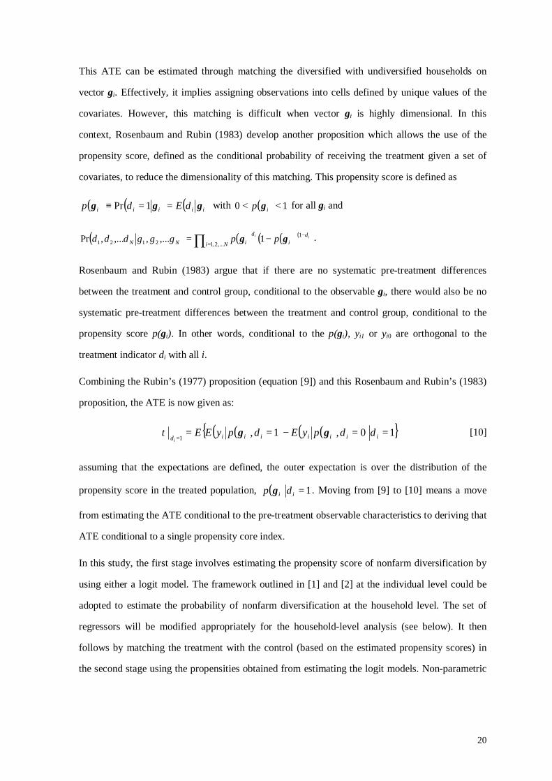
This ATE can be estimated through matching the diversified with undiversified households on
vector gi. Effectively, it implies assigning observations into cells defined by unique values of the
covariates. However, this matching is difficult when vector gi is highly dimensional. In this
context, Rosenbaum and Rubin (1983) develop another proposition which allows the use of the
propensity score, defined as the conditional probability of receiving the treatment given a set of
covariates, to reduce the dimensionality of this matching. This propensity score is defined as
( ) ( ) ( )iiiii dEdp ggg ==≡ 1Pr with ( ) 10 << ip g for all gi and
( ) ( ) ( )( )( )ii di
d
Ni iNN ppgggddd −
=−= ∏ 1
,...2,12121 1,...,,...,Pr gg .
Rosenbaum and Rubin (1983) argue that if there are no systematic pre-treatment differences
between the treatment and control group, conditional to the observable gi, there would also be no
systematic pre-treatment differences between the treatment and control group, conditional to the
propensity score p(gi). In other words, conditional to the p(gi), yi1 or yi0 are orthogonal to the
treatment indicator di with all i.
Combining the Rubin’s (1977) proposition (equation [9]) and this Rosenbaum and Rubin’s (1983)
proposition, the ATE is now given as:
( )( ) ( )( ){ }10,1,1
==−=== iiiiiiid
ddpyEdpyEEi
ggτ [10]
assuming that the expectations are defined, the outer expectation is over the distribution of the
propensity score in the treated population, ( ) 1=ii dp g . Moving from [9] to [10] means a move
from estimating the ATE conditional to the pre-treatment observable characteristics to deriving that
ATE conditional to a single propensity core index.
In this study, the first stage involves estimating the propensity score of nonfarm diversification by
using either a logit model. The framework outlined in [1] and [2] at the individual level could be
adopted to estimate the probability of nonfarm diversification at the household level. The set of
regressors will be modified appropriately for the household-level analysis (see below). It then
follows by matching the treatment with the control (based on the estimated propensity scores) in
the second stage using the propensities obtained from estimating the logit models. Non-parametric
21
matching techniques as explained in Becker and Ichino (2002) or Leuven and Sianesi (2006) can be
used for this second stage.9
In both the parametric and semi-parametric analysis, consumption expenditure (given in natural
logarithm) is used as a welfare measure. Using real per capita expenditure however does not
control for possible differences in consumption behaviours among the household members,
especially between children and adults; male and female (Tedford et al., 1986). This study applies
the WHO’s equivalent scales by which a female adult is given a weight of 0.8 of a male adult, and
a child aged under 15 years counts for a fraction of 0.5 of a male adult.10
4.3 Data
This paper uses data drawn from household-level surveys conducted for Vietnam in the four
separate years during the period 1992-2006. These surveys were implemented by the GSO under
funding and technical support from UNDP, the World Bank and other donors. The Vietnam Living
Standards Surveys (VLSS) of 1992/93 and 1997/98 are multi-topic surveys mirrored the World
Bank’s Living Standard Measurement Surveys with nationally representative samples of 4,800 and
6,000 households respectively (see World Bank, 2000; 2001). These surveys were superseded in
2002, 2004 and 2006 by a new biennial household survey programme known as the Vietnam
Household Living Standards Surveys (VHLSS), which used a rotating core-and-module designed
survey with an expanded sample size. This aims to produce statistics that are representative at the
provincial level (Phung and Nguyen, 2006). However, given the potential presence of non-
sampling errors in the VHLSS 2004 that may have adversely affected the computation of poverty
rates (see Baulch et al. 2008), the later VHLSS 2004 and VHLSS 2006, which surveyed a total of
9,189 households, is the ones used in this study. Though the content of the questionnaire was
modified over time, this still allows for the construction of a set of variables necessary for the
empirical analysis of this paper that is compatible across these surveys.
9 As this is a combination of a parametric approach in the first stage and a non-parametric approach in the second stage, the PSM method is referred to be semi-parametric. See Dabalen et al. (2004) for an example of applying this PSM approach to examine the welfare effect of nonfarm activities in rural Rwanda. 10 This are the most commonly used equivalent scale in earlier studies on Vietnam (see Litchfield et al., 2008 for instance).
22
There are two types of samples used in estimation of this paper. Firstly, the samples of rural
individuals drawn from these surveys consist of the economically active rural labour force, aged
from 15 to 65 years.11 The lower age limit of 15 years old is selected as it is common in the rural
areas that children finish the lower secondary school at an average age of 14 years old and may
start working after that instead of continuing their upper secondary education. Indeed, the surveys
show that more than 90 percent of the rural population aged 15 years and older have had lower
secondary as the highest educational level obtained. This suggests that the majority of rural people
stopped schooling before the upper secondary school, and thus entered the rural labour force at an
average age of 15 years old. The upper age limit of 65 years old is chosen through the retirement
ages in Vietnam are regulated at 60 and 55 years old for males and females, respectively as most
rural people still work either on their own farms or in other self-employed nonfarm activities after
their retirement.12 Individual employment outcomes are then specified on the basis of the most time
consuming job over a period of 12 months. It should be noted that these employment outcomes are
classified on the basis of the primary (most time-consuming) jobs over the past 12 months.
Therefore, these do not take into account any multiple-job activities. This might underestimate the
importance of the RNFS as one important role of nonfarm activities is to provide work in the slack
periods of the agricultural cycle, and hence nonfarm employment can be undertaken in terms of
multiple-job holdings. However, investigating this issue, which requires a considerably more
complicated methodological framework than what proposed in this paper, is not a primary
objective of the current study. Secondly, the samples of rural households drawn from the surveys
are also used to examine the welfare effect of nonfarm diversification using the PSM approach as
described from [8] to [10].
In addition to the two types of cross-sectional samples, there is a panel 4,308 households from the
VLSS 1992/93 and VLSS 1997/98 and another panel of 4,278 households between the VHLSS
11 Ideally, all people in the economically active rural population should be included in the samples. However, the proportion of those who can not find jobs in the seven days preceding the interview was very small. The surveys revealed that those who had no work, or could not find a job, or did not know how and where to look for a job ranges from 1-2% percent in the VHLSSs to about 3% percent in the VLSSs. 12 In fact, the data from the surveys reveal that people aged 60 years and older account for seven percent of the economically active labour force, and the people aged from 60 to 65 years olds are dominant in this share.
23
2004 and VHLSS 2006. However, there is no link between these two panels due to differences in
the sampling procedure between the two waves of VLSSs and VHLSSs. These two panels will be
used to implement the framework outlined from [3] to [7].
5. Empirical Results
This section reports the empirical results obtained from estimating the framework above. The first
sub-section presents the findings on the determinants of nonfarm diversification at the individual
level. The second sub-section focuses on the empirical evidence at the household level on the
impact of nonfarm diversification on the welfare of rural households.
5.1 Empirical Results – Individual Participation into the RNFS
Table A1, reported in the appendix to this paper, provides a description of the variables used in our
analysis and selected summary statistics. The specification test results for the MNL models (as
above) suggest the appropriateness of using this model in our case (see Table A2). The estimates
obtained from this MNL model are expressed in terms of marginal effects for continuous regressors
and impact effects for binary regressors, as reported in Table 5, for a more meaningful
interpretation.
At the individual level, it is firstly notable that men are less likely than women to be engaged in
nonfarm self employment but more likely to be wage-employed in the RNFS. On average and
ceteris paribus, male workers are less likely to be self-employed by between three to 7.5
percentage points than female workers. This gender effect has risen over time (by 4.5 percentage
points), with the absolute t-ratio corresponding to this point estimate computed at a comfortably
significant 2.06. In the rural labour market for the wage employed, men are found to be more likely
to be involved in nonfarm wage employment by ceteris paribus two to 4.5 percentage points. This
advantage of male workers has fallen between the initial and terminal years, with the estimated t-
ratio computed at 2.42 in absolute terms. This finding is somewhat different from existing evidence
elsewhere. Women are found by Lanjouw and Shariff (2002), Lanjouw (2001), Lanjouw et al.
24
(2001) to be less active in the RNFS in India, El Salvador, and Tanzania, respectively. In contrast,
female workers are reported to be more involved in nonfarm activities in Ghana and Uganda as
reported in Newman and Canagarajah (2001). By taking into account differences between self and
wage employment, the current paper provides a new insight on the relative positions of female
workers in the rural Vietnam. Bearing the burden of housework and taking care of children and the
elderly, diversifying into self-employed activities is less time demanding than into wage
employment.
It has been widely found that the ethnic minority groups have benefited less than the Kinh (and
Chinese) majority from the doi moi (see Baulch et al., 2007 for a review). In this case, it is evident
that ethnic minority workers are less likely to be involved in nonfarm self employment than the
majority.13 There is also statistical evidence that the ethnic effect on nonfarm self employment have
widened over time with the absolute t-ratio for a test of the difference between the years 1993 and
2006 computed at a statistically significant 2.34. Having less employment opportunities could be
one reason for an increasing welfare gap between the majority and minority groups as recently
reported in Baulch et al. (2008).
[Table 5 about here]
Predictably, education is of considerable importance to nonfarm diversification in all the cases. The
better-educated individuals are, the more likely they are to be employed in the RNFS. The
education effect is most pronounced for those with upper secondary or higher educational
qualification. Attaining higher education qualifications substantially re-inforce the probability of
being wage-employed (the absolute t-ratio for the test of the difference between the educational
effect on nonfarm self employment and wage employment are comfortably significant in all cases).
This positive effect of education on nonfarm diversification is a widespread finding in the literature
on the RNFS (see for instance Lanjouw, 1998; Newman and Canagarajah, 2001). In Vietnam’s
rural labour market, Van de Walle and Crafty (2003) using the first two surveys report a positive 13 A more disaggregate breakdown of ethnic minority groups (rather than a simple majority-minority distinction) is desirable. However, these groups account for a small proportion of the samples in the two earlier VLSSs, and dividing the ethnic minorities into sub-groups will result in very small size for each groups. Further details on the effect of Doi moi on the ethnic minorities can be found in Baulch et al. (2007).
25
effect of education on nonfarm diversification. Pham and Reilly (2007) suggest monotonically
increasing returns to education during the doi moi.
Other individual-level characteristics also have statistically significant effects on nonfarm
employment. As there is insufficient information from the surveys to compute actual labour force
experience, the age of an individual rather than a potential labour force measure is used to proxy
for labour market experience.14 Compared to the age group of less than 20 year olds, workers in the
other age groups are generally more likely to be involved in nonfarm activities. The positive effect
of age on nonfarm self employment is upheld for all the age groups. In the rural wage-employed
market, workers who aged more than 50 years old would be between three to six percentage points
less likely to find wage-employed jobs. In addition, marital status is revealed as an important
determinant of participation in the RNFS. On average and ceteris paribus, getting married reduces
the probability of employment in nonfarm activities by between two to seven percentage points.
There is also statistical evidence that this negative effect of marriage on nonfarm diversification has
widened over time (|t| = 4.8 and 2.1 for the difference between the marital status effect on nonfarm
self employment and wage employment respectively between the years 1993 and 2006).
We now turn our attention to the household-level characteristics. The literature on labour market
participation in developing countries suggests that size and structure of households have important
influence in employment decisions as these factors affect the ability of the household to supply
labour to the RNFS (Reardon, 1997). With regard to household size, it is expected that absorbing
an extra household member exerts pressure on the family’s expenditures and intensify the impetus
to find work outside the family’s agricultural production (see Reardon et al. 1992 and Clay et al.
(1995) for the case of Burkina Faso and Rwanda, respectively). In the case of Vietnam, the effect
of the household size is also positive and statistically significant. But the effect of household size is
however modest. Regarding the effect of dependency ratios, the literature on the RNFS suggests an
ambiguous effect. While having more children and/or elderly people clearly exerts pressure on
14 Other studies on Vietnam (see Pham and Reilly 2007 for a review) commonly use potential labour force experience, which is obtained using highest educational qualification attained. However, as the information on schooling years is not available (see above), this would introduce measurement error providing a source of bias in the employment equation estimates.
26
adults in seeking income-generating opportunities, this also imposes a time constraints on the
labour supply decision. In this context, it is not surprised as the empirical evidence of this issue has
been mixed (Reardon et al. 1992; Newman and Canagarajah, 2001). This mixed evidence is not
observed in rural Vietnam. The estimates demonstrate that having more children and/or elderly
peoples exerts a negative impact on other members’ participation in the RNFS.
Household landholding is found as the most important household-level determinants of nonfarm
employment in rural Vietnam. Annual crop land, either irrigated or non-irrigated, as the most
important types of agricultural land, exerts a negative effect on participation in the RNFS. The
same effect is found for access to other types of lands. This finding is at odd to the ambiguous
effect of landholding on nonfarm diversification suggested in the literature.15 On the one hand,
landholding may raise the probability of diversification through a wealth effect as land can be used
as collateral for credit. On the other hands, having more lands may also drift households away from
the RNFS as it increases their concentration in agriculture. This negative effect of landholding is
especially relevant for those who diversified into the RNFS as a response to a seasonal shortfall of
income from agriculture. In the case of Vietnam, the latter effect probably outweighed the former
due to the lack of well-functioning land market. Ravallion and van de Walle (2004) demonstrate
that though several land market reforms were initiated during the 1990s, land was not actually
owned and land-use rights were not generally well formalized during the 1990s.
The empirical evidence on the RNFS in developing countries usually reports a spatial effect (see
Lanjouw et al. (2001) and Ruben and van de Berg (2001) for the case of Tanzania and Honduras,
respectively). This spatial effect on nonfarm diversification in rural Vietnam is also revealed by the
estimated impacts of the regional dummies. Compared to the Northern Uplands, individuals
residing in the southern part of the country, especially in the Southeast, are considerably more
likely to be engaged in nonfarm income-generating activities. There is statistical evidence that this
15 The empirical literature tends to suggest mixed evidence. Walker and Ryan (1990), Lanjouw and Shariff (2002) report individuals from households with higher per capita landholding are more likely to be involved in the India. The same result is also documented in the case of Tanzania (Lanjouw et al., 2001; Mduma and Wobst, 2005), Burkina Faso (Reardon et al. 1992). While Liedholm and Kilby (1989), Rief and Cochrane (1990) reveal the opposite in the case of Nigeria and Thailand, respectively.
27
regional effect has risen over time (the absolute t-ratio of the tests for the differences in the regional
effects over times are statistically significant at a conventional 5% level). There is also evident for
seasonality of nonfarm employment. Compared to the first quarter, omitted as the based, rural
workers are more active in nonfarm activities in the other quarter. This could be linked to the New
Year festival (or the Tet) that usually falls at the end of January or beginning of February.
Traditionally, this is the biggest and longest holiday event in the country and its effect usually
prevails well before and after the Tet.
The marginal (and impact) effects of the commune-level variables on rural nonfarm employment
are reported by the end of Table 4. One possible alternative to this set of commune-level
determinants is to use a set of commune dummies to control for the commune fixed effect (see van
de Walle and Cratty, 2004; Baulch et al. 2008). Though it provides an appropriate way to control
for heterogeneity among locations, this method however throws away commune-level attributes
which are potentially critical to off-farm diversification. More importantly, as the set of communes
varies across time, this method does not allow any comparison over time as estimates are obtained
from different set of regressors. Given this, the current paper employs a more desirable set of the
selected commune-level characteristics and type of communes. The same approach is also
employed in some other previous studies on Vietnam, using the same datasets (see Litchfield et al.
2008 for instance).
In common with the empirical literature on the effects of community characteristics on nonfarm
activities, infrastructure conditions are found as important factors of nonfarm diversification.
Individuals with access to infrastructure facilities such as road, public transport, and post office are
more likely to be involved in the RNFS. Controlling for other factors, a commune having a paved
road increases the probability of individuals residing in that commune by between three to five
percentage points. A positive effect of similar ceteris paribus magnitude is also evident for access
to public transport. This effect of infrastructure on nonfarm diversification is widely documented in
the literature on the RNFS. In Tanzania, access to asphalt roads increases the probability of
business sector involvement of the people in the sub-urban areas by about six percentage points
28
(Lanjouw et al. 2001). The case of El Salvador provides another example where proximity to a
paved road significantly improves the likelihood that a family member is engaged in nonfarm
employment (Lanjouw, 2001). Jacoby (2000) and Fafchamps and Shilpi (2001) also report a
positive correlation between access to road and nonfarm activities.
The demand side of the RNFS at the commune level is partially proxied by a dummy for whether
there are factories located within ten kilometres from the commune’s centre. As these provide
sources of nonfarm employment, these variables are expected to positively affect nonfarm
diversification by individuals residing in the commune. Indeed, the presence of factories located in
or nearby the commune exerts a positive and strong impact on nonfarm diversification. On average
and ceteris paribus, having factories located within 10 km from the commune centre improves the
probability of being involved in nonfarm activities by between three to six percentage points.
Distances to town or cities are acknowledged in Reardon (1997) as an important determinant of the
development of the RNFS. Fafchamps and Shilpi (2003) show that proximity to urban economic
centres considerably foster nonfarm activities in Nepal. In this study, distances to commune centre
and district centres are included in the reduced form MNL models. The estimates reveal a negative
relationship between distances to centres and probability of being involved in nonfarm activities in
the majority of cases. This suggests that proximity to centres of commune or districts make it more
likely to be self-employed or wage-employed in the nonfarm sector.
5.2 Welfare Effect of Nonfarm Diversification – Empirical Results
Nonfarm Diversification and Household Welfare: The TSLS results16
In this study, the instruments in vector *iz reflect the change in the availability of nonfarm
opportunities and the change in the demand side of nonfarm labour at the commune level between
1998 and 1993. These include (i) change in commune-level availability of nonfarm income
generating activities was calculated as the ratio of people employed in the RNFS and the total
16 This section reports the results obtained from using the VLSS 1992/93 and VLSS 1997/98. The results using the panel of the two later VHLSSs will be added later due to some adjustments to the panel that has been currently investigated by the GSO staff (at this date of Sept 09, 2008).

29
economically active labour force at each commune. (ii) Change in the number of households
residing at the commune is used to partially capture possible changes in nonfarm labour supply and
general socio-economic conditions. (iii) Four variables that reflect changes in the nonfarm labour
demand condition is proxied by the change in availability of traditional occupations (such as
handicrafts), and factories that located within ten kilometres from the commune centre. The
diagnostic tests demonstrate that the instruments are passed the tests for relevance, validity, and
exogeneity.17 The TSLS estimates obtained from the panel of rural households18 and the test results
are reported in Table 6. It is important to note that the estimates are not sensitive to whether
consumption expenditure is adjusted by household sizes or the equivalent scales. Therefore, the
empirical analysis in this sub-section will concentrate on the estimates obtained from using real
consumption expenditure per capita as the welfare measure.
[Table 6 about here]
The estimates of the initial period variables are not discussed in detail here, though a number of
points worth making about their effects on the change in consumption expenditures. Of the
variables included in vector xit-1, the initial education attainments of household heads exert a strong
and positive influence on the improvement in expenditure between 1993 and 1998. This impact is
also reported in, among others, Glewwe et al. (2004), Niimi et al. (2003). Ethnicity is commonly
found as an important determinant of household welfare in Vietnam (Baulch et al., 2004) and this
study is not an exception. Compared to the ethnic minorities the Kinh and Chinese households
experienced an improvement in expenditure per head that is ceteris paribus five percentage points
17 The F-test statistics for instrument relevance are well above the Stock and Watson’s ‘rule-of-thumb’. The Sargan’s test results verify that the instruments are orthogonal to the error process in the structural welfare equation. The Hausman specification test shows that the null hypothesis of the exogeneity of the problematic regressor is decisively rejected, suggesting the validity of using the TSLS. 18 Van de Walle and Cratty (2004) adopted the method of Fitzgerald et al. (1998) to test for possible bias due to panel attrition (a number of 3494 household were re-interviewed in the VLSS 1997/1998 out of 3,839 original rural households in the VLSS 1992/94). They reported little effect on the significance levels or point estimates when the regression was weighted for attrition. This can be taken to suggest that attrition is not a serious issue that needs to be resolved in this study.
30
higher.19 It is also evident that demographic characteristics have affected household welfare status.
While bigger household size exerts a positive effect on expenditure, a negative impact is reported
for the ratio of children and elderly. The initial access to annual cropland (both irrigated and non-
irrigated) is shown as having a positive effect on expenditure. The strong effect of annual cropland,
which is mainly used for rice cultivation, can be linked to the importance of the rice sector for rural
households (Minot and Goletti, 1998; Benjamin and Brandt, 2004). In addition, transportable road
and public transport are two physical infrastructure conditions that produce a positive effect on
expenditure. Initial access to post office as an institutional infrastructure also exerts a significant
and considerable positive impact on the improvement in expenditure for the households in that
commune between 1993 and 1998.20
We now turn to the effect on nonfarm diversification on household welfare (the first row in Table
5). On average and ceteris paribus, a ten percent increase in the share of household members
(self)employed in the RNFS produced an approximately an eight percentage point improvement in
expenditure between 1993 and 1998. When adjusted for the equivalent scales, such increase in
nonfarm diversification exerts an essentially the same impact on expenditure per AE unit. It implies
that the relationship between consumption expenditure and poverty in rural Vietnam is not
sensitive to whether equivalence scales are used or not. When the incidence of nonfarm
diversification is measured by the share of the nonfarm income source, the same positive effect of
nonfarm activities on consumption expenditure is upheld. Controlling for other factors, a household
with a ten percent increase in the share of nonfarm income experienced an improvement in
expenditure per head that was nearly ceteris paribus five percentage points higher during the period
19 Although a further breakdown of ethnic minorities, as in Van de Walle and Cratty (2004), is desirable, this study does not pursue that as the estimates based on small sized ethnic groups are probably not reliable (the ethnic minority groups accounts for 11 percent in the panel). 20 We also estimated the TSLS model using the commune-fixed effect (instead of having a number of the commune-level regressors). The results reveal little effect on the estimates on the other household-level variables and a considerable improvement in the power of explanation (i.e. adjusted R2). We prefer reporting the estimates using the set of commune-level controls as these provide better insights on the effect of the community-level characteristics on rural poverty. In order to conserve space, the estimates using the commune-fixed effects are omitted here for brevity.
31
1993-1998. And again, it is evident that the welfare effect of nonfarm diversification is not
sensitive to the equivalent scales.21
The reported effect of nonfarm diversification on household welfare is, however, conditional to the
assumption of homoskedasticity. In the presence of heteroscedasticity, the standard TSLS estimates
of the standard errors are inconsistent, preventing valid inference, and the usual forms of the
diagnostic tests for endogeneity and over-identifying restrictions are invalid (Baum et al., 2003).22
Given this, the Hansen’s (1982) two-step efficient generalized method of moments (GMM)
approach is employed to examine the sensitivity of the TSLS estimates to the possible problem of
heteroscedasticity.23 The GMM estimates, which are not reported here for brevity, demonstrate the
same relationship between nonfarm diversification and household welfare as found above. The
estimated impacts of the other pre-determined variables on changes in household expenditure are
broadly the same as those obtained from the TSLS estimation with strong effects of heads’
education attainment levels, household demographic characteristics, and infrastructure conditions.
It suggests that heteroscedasticity is not an issue that needs to be resolved in this case. Given this,
we conclude a strong and positive welfare effect of nonfarm diversification in rural Vietnam. This
effect is robust to the different measures of nonfarm diversification and whether expenditure is
given per head or per AE unit.24
21 Given the geographical heterogeneity among the seven regions and the regional divergence in nonfarm diversification and nonfarm income (see Table 2 and 3), it can be argued that capturing the regional effect on welfare by allowing for intercept shifts might not be sufficient. In order to test for whether that geographical heterogeneity also affects welfare though its effect on nonfarm diversification, we interact the incidence of nonfarm diversification in equation (6) with the regional dummies. However, the estimated coefficients on these interaction terms are not jointly statistically different from zero (using the Wald test). 22 Although the Huber’s heteroscedasticity-consistent or ‘robust’ standard errors in when testing for the relevance of instruments, the usual forms of the tests for endogeneity and over-identifying restrictions are invalid in the presence of heteroscedasticity. 23 By using the efficient two-stage generalized method of moments (GMM) approach, the efficiency gains of this estimator relative to the traditional TSLS ones derive from the use of the optimal weighting matrix, the over-identifying restrictions of the model, and the relaxation of the i.i.d. assumption (Baun et al., 2003). 24 The Amemiya Generalized Least Squares (AGLS) approach can be an alternative for the TSLS procedure in this paper (see Maddala, 1983 for in detail discussions). However, as transforming the dependent variable the welfare function from continuous variable to a discrete alternative in the AGLS model implies also ‘throwing away’ information, we do not apply this model in the current paper.
32
Nonfarm Diversification and Household Welfare: The PSM Results25
The above results were obtained by estimating a version of the ‘differenced’ TSLS model to inform
the effect of the change in the incidence of nonfarm diversification on the improvement in
consumption expenditures between 1993 and 1998 for the households in the panel. This section
adopts the PSM approach to investigate the welfare effect of nonfarm diversification in 1993 and
1998 separately. Rural households are categorized in the three groups on the basis of their primary
employment activities, including (i) farm-only households; (ii) nonfarm-only households; and (iii)
diversified households. The farm-only households, or completely undiversified, are those with all
household members working in farm labour as their main occupations. The nonfarm-only
households are completely diversified into the RNFS and hence none of their members work in
farm labour. In between these two categories, the diversified households allocate their labour
supply for both farm labour and nonfarm activities. Figure A1 in the Appendix represents the
relative position of these three types of households. It shows that nonfarm-only households are
among the richest; it follows by the diversified group. Farm-only households are among the poorest
in rural Vietnam.
The first step of the PSM procedure involves estimating the propensity scores of the treatment and
control group by a logit model.26 The set of regressors used in this stage is similarly defined as
vector xi used in the TSLS approach. This first stage’s estimates are not discussed here for brevity
but it is important to note that the logit models perform reasonably well in this case. Therefore, it is
likely to argue that the set of covariates does capture a good deal of the observables that determine
the probability of a household to be assigned to the treatment. This gives credibility for performing
the matching in the second stage. The matching in this study is performed between (i) the
diversified versus the farm-only; (ii) the nonfarm-only versus the farm-only; and (iii) the nonfarm-
only versus the diversified. In addition, as participation in the RNFS and the resultant outcomes are
likely to be different between the poor and the non-poor (section two), the PMS approach is
separately implemented for the poor and non-poor sub-sample to test this hypothesis.27
25 The PSM results using the VHLSS 2004 and VHLSS 2006 will be added when the 2004-2006 panel is re-adjusted and made available by the GSO staff (which is expected to be ready by the end of Sept, 2008). 26 The first stage of the PSM approach can be implemented by estimating either a probit or a logit model. In our case, the logit estimates are essentially the same as the probit estimates. 27 This separation between the poor and non-poor sample is statistically justified in most of the cases on the basis of the Wald test using the estimated variance-covariance matrices.
33
As the welfare impact of nonfarm diversification is not sensitive to the usage of the equivalent
scales (see above), we focus on real expenditure per head as the welfare measure in the matching
exercise (the ATEs using expenditure per AE unit are largely the same as those obtained from
using expenditure per capita). Expenditure is trimmed at the value of 0.01, implying that one
percent of the treatment observations at which the propensity score density of the control
observations is the lowest will be omitted. In an effort to inform the sensitivity of the ATE
estimates, the matching is implemented by three different matching techniques, including the
nearest matching and two kernel matching functions (Epanechnikow and biweight) (see Becker and
Ichino, 2002; Leuven and Sianesi, 2006 for more details). The estimated ATEs obtained from this
matching are reported in Table 7. Although the estimates slightly reduces with movement from the
nearest to kernel matching techniques, the welfare effect of nonfarm diversification on welfare is in
the same direction. The interpretation below is based on the results from kernel matching functions.
[Table 7 about here]
It is apparent that nonfarm diversification significantly improves consumption expenditure in both
years. On average and ceteris paribus, moving from being a farm-only to nonfarm-only household
improves per capita expenditure by about seven percent in 1993 and nearly ten percents in 1998.28
The incidence of nonfarm diversification also matters. Compared to the farm-only household,
becoming (partially) diversified produces about five percent higher in real expenditure per head in
1993 and eight percent higher in 1998. The welfare improvement of becoming diversified is
smaller than that of becoming nonfarm-only. This difference in the welfare impact by level of
diversification is re-affirmed when the nonfarm-only group is set as the treatment and the
diversified is set as the control. A household is better-off when becoming nonfarm-only than
staying partially diversified (that household experienced ceteris paribus five percent higher in
expenditure in 1993 and 12-13 percent higher in 1998).29 In addition, it is notable that the welfare
effect of nonfarm diversification was on the rise between 1993 and 1998. For instance, compared to
28 It is desirable to compare the welfare gains from this study and those reported for the case of Rwanda in Dabalen et al. (2004) by calculating the percentage of these gains in total household consumption. However, as Dabalen et al. only present welfare outcomes in the domestic currency without reporting the average household consumption expenditure, this comparison is not possible. 29 In an earlier version of this paper, we also distinguished nonfarm diversification by types of employment (i.e. wage employment or self-employment). However, the logit estimates in the first stage (that models the probabilities of being wage-employed or self-employed) suggest a mixed picture and the power of explanation is poor. Therefore, the estimated ATE might not be reliable. For this reason, we omitted these matching results.
34
being farm-only, a household became nonfarm-only in 1998 experienced an improvement in its
consumption expenditure that is ceteris paribus twice higher than it was in 1993. This increasing
welfare effect over time coincides with the growing share of the RNFS in income and employment
between 1993 and 1998 highlighted earlier. This can be taken to suggest an important contribution
of the RNFS to the reduction of rural poverty during the 1990s.
The results also demonstrate that the welfare impact of nonfarm diversification is considerably
higher for the non-poor than for the poor households. In 1998 for instance, a non-poor household
becoming a nonfarm-only household improved its consumption expenditure per head between 15 to
19 percent compared with being farm-only or partially diversified. Though this difference in the
welfare impact of nonfarm diversification between the poor and the non-poor varies across time
and pairs of comparison, it remains the same in all cases that the poor benefit considerably less than
the non-poor from nonfarm activities. As the Vietnamese households are not heavily clustered
around the national poverty lines (Niimi et al., 2003), it is reasonable to argue that the results are
not sensitive to the usage of the national poverty lines. As the non-poor is found to benefit more
than the poor from nonfarm diversification opportunities, nonfarm diversification can be
inequality-increasing.
This effect of nonfarm diversification on inequality is worrying given the increasing trend in
overall inequality in Vietnam has been recently reported (see World Bank, 2003; Glewwe et al.,
2004 for instance). Earlier studies generally link such increasing inequality to income divergence
among regions, between rural and urban areas, or between the majority and ethnic minorities. The
analysis in this study suggests that such increasing inequality is partially attributable to the
development of the RNFS during the 1990s. This is opposite to Lanjouw (1998) who suggests that
“[…] nonfarm employment income may serve to reduce aggregate income inequality” (p.5).
However, Lanjouw acknowledged that it is difficult to comment on whether nonfarm
diversification is income-inequality increasing or decreasing without information on what the
counterfactual situation would have been in the absence of such activities. By using a combination
of the PSM approach and the Shapley approach, this study provides a better insight on impact of
nonfarm diversification on income inequality. Nonetheless, the finding that nonfarm diversification
is more beneficial for the better-off is not surprising as the wealthier rural households are more
likely to be attracted into nonfarm activities, while the poor often seek for nonfarm opportunities as
35
‘residual’ sources of income. This pattern has been found in a number of studies reviewed earlier
and Vietnam is thus not an exception in this regard.
6. Remarks
Vietnam’s rural labour force has been markedly diversifying toward nonfarm activities in the doi
moi. The employment share of the RNFS has increased from 23 percent to 56 percent between the
years 1993 and 2004. As a result, nonfarm income became a major component of total income for
rural households. With an average share of 44 percent during the period 1993-2004, the share of
nonfarm income in Vietnam is as high as those reported in Africa and Latin America, and higher
than the average level of the other Asian countries.
The broad picture which emerges from this paper is that participation by rural individuals and
households in the RNFS is determined by a set of individual, household, and community level
characteristics. Gender, ethnicity, and educations are reported as main individual-level drivers of
nonfarm diversification. Lands as most important physical assets of rural households are found to
be negative to nonfarm employment as greater landholding encourages more concentration in
agriculture. In addition, infrastructures, both physical and institutional, exert important influences
on individual participation in the RNFS. The paper argues that supporting the development of a
buoyant RNFS is crucial for rural transformation and rural poverty reduction. This is important not
only because such diversification contributes to household income, and thus rural poverty
reduction, but also because it can provide a potential solution to problems associated with the
currently high underemployment and the growing rural-urban migration.
To empirically examine whether there is a causality running from nonfarm diversification to
household welfare, this study adopts a combination of a parametric and semi-parametric analysis,
The TSLS procedure is used to instrument the endogenous nonfarm diversification variable in the
welfare function while the PSM approach is proposed to estimate the gap between the actual
expenditure level of a household in a given diversification outcome and the ‘counterfactual’ level
that the household forgone by such diversification.
36
The results suggest a strong and positive welfare effect of nonfarm diversification. Based on the
TSLS estimates for the panel, we find that a ten percentage point increase in the share of household
employment in the RNFS produces approximately eight percentage points higher in the
improvement of expenditure per head between 1993 and 1998, on average and ceteris paribus.
When the incidence of nonfarm diversification is measured by the share of the nonfarm income
source, the same increase in the incidence of diversification improves per capita expenditure by
more than four percentage points. This finding is robust to the usage of the equivalent scales and
possible presence of heteroscedasticity.
The positive effect of nonfarm diversification on household welfare is re-affirmed by the ATE
estimated obtained separately for 1993 and 1998 using the PSM approach. The estimates reveal
that nonfarm diversification does significantly improve household consumption expenditure. It also
evident that the welfare effect of nonfarm diversification tends to increase over time and this trend
coincides with the development of the RNFS. Interestingly, the results suggest that the incidence of
diversification matters as becoming nonfarm-only is found to have the largest improvement in
consumption expenditure. In addition, the welfare gain from nonfarm diversification is found to be
greater for the non-poor than for the poor. It suggests that while nonfarm diversification
significantly improves the living standards in rural Vietnam, it might not be the poverty exit path
for the poor. It also implies that the development of the RNFS partly intensifies income inequality
in the rural areas.
Based on the above findings, we argue that supporting the development of a buoyant RNFS is
crucial for the reduction of rural poverty. Investing in education, health services, and rural
infrastructures are among the priorities to encourage the RNFS. In pursuing this support, enhancing
access to nonfarm diversification opportunities for the poor is necessary to ensure that the benefits
from the nonfarm opportunities are not only limited to the non-poor.
37
References
Aassve A., H. Engelhardt, F. Francavilla, A. Kedir, J. Kim, F. Mealli, L. Mencarini, S. Pudney, and A. Prskawetz, (2005), ‘Poverty and Fertility in Less Developed Countries: A Comparative Analysis’, ISER Working Paper 2005-13, University of Essex.
Barrett, C.B. and T. Reardon (2000), ‘Assets, Activity, and Income Diversification among African Agriculturalists: Some Practical Issues’, mimeo, Land Tenure Centre, University of Wisconsin-Madison.
Barrett, C.B., T. Reardon, and P. Webb (2001), ‘Nonfarm income diversification and household livelihood strategies in rural Africa: concepts, dynamics, and policy implications’, Food Policy, 26, pp. 315–331
Baulch, B., Hung T. Pham, and B. Reilly (2007), ‘Ethnicity and Household Welfare in Vietnam: Empirical Evidence from 1993 to 2004’, mimeo, Institute of Development Studies, University of Sussex.
Baulch, B., Hung T. Pham, and B. Reilly (2008), ‘Increasing Disadvantage and the Ethnic Gap in Rural Vietnam, 1993-2004’ mimeo, Institute of Development Studies, University of Sussex.
Baulch, B., K.T.C. Truong, D. Haughton, and J. Haughton (2004), ‘Ethnic Minority Development in Vietnam: A Socioeconomic Perspective’, in Glewwe et al. (eds), Economic Growth, Poverty, and Household Welfare in Vietnam, World Bank Regional and Sectoral Studies, World Bank, Washington, D.C.
Baum C.F., M.E. Schaffer, and S. Stillman (2003), ‘Instrumental variables and GMM: Estimation and Testing’, Working Paper No. 545, Department of Economics, Boston College.
Becker S.O. and A. Ichino (2002), ‘Estimation of Average Treatment Effects Based on Propensity Score’, The STATA Journal, 2(4), pp. 358-377.
Behrman, J.R. and B.L. Wolfe (1984), ‘Labor Force Participation and Earnings Determinants for Women in the Special Conditions of Developing Countries’, Journal of Development Economics, 15, pp.259-288.
Benjamin, D. and L. Brandt (2004), ‘Agriculture and Income Distribution in Rural Vietnam under Economic Reforms: A Tale of Two Regions’, in Glewwe et al. (eds), Economic Growth, Poverty, and Household Welfare in Vietnam, World Bank Regional and Sectoral Studies, World Bank, Washington, D.C.
Berdegue, J.A.; E. Ramirez; T. Reardon, and G. Escobar (2001), ‘Rural Nonfarm Employment and Incomes in Chile’, World Development, 29(3), 411-425.
Bezemer, D., K. Balcombe, J. Davis, I. Fraser (2005), ‘Is Rural Income Diversity Pro-Growth? Is It Pro-Poor? Evidence from Georgia’, Proceedings of the German Development Economics Conference, Kiel 2005, Research Committee Develoment Economics, Verein Fur Socialpolitik.
Birdsall N.M., C.C. Griffin (1988), ‘Fertility and Poverty in Developing Countries’, Journal of Policy Modeling, 10(1), pp. 29-55.
Bright, H., J. Davis, M. Janowski, A. Low, and D. Pearce (2000), ‘Rural Non-Farm Livelihoods in Central and Eastern Europe and Central Asia and the Reform Process: A Literature Review’, Rural Non-Farm Economy Project Report No. 2633, National Resources Institute.
Clay, D., F. Byiringiro, J. Kangasniemi, T. Reardon, B. Sibomana, L. Uwamariya, and D. Tardif-Douglin, (1995), ‘Promoting food security in Rwanda through sustainable agricultural productivity: Meeting the challenges of population pressure, land degradation, and poverty’, International Development Paper No. 17, Michigan State University.
Dabalen, A., S. Paternostro, and G. Pierre (2004), ‘The Returns to Participation in the Nonfarm Sector in Rural Rwanda’, World Bank Policy Research Working Paper No. 3426, Development Research Group, World Bank, Washington, D.C.
Davis, D., T. Reardon, K. Stamoulis, and P. Winters (2002), Promoting Farm/Non-Farm Linkages for Rural Development - Case Studies from Africa and Latin America, Food and Agricultural Organization, Rome.
Davis, J. and D. Pearce (2000), ‘The rural nonfarm economy in Central and Eastern Europe’, Discussion Paper No. 2000/04, Natural Resources Institute.
38
De Janvry A., E. Sadoulet, N. Zhu (2005), ‘The Role of Non-Farm Income in Reducing Rural Poverty and Inequality in China’, Working Paper Series 1001, Department of Agricultural and Resource Economics, University of California at Berkeley.
De Janvry, A. and E. Sadoulet (2001), ‘Income Strategies among Rural Households in Mexico: The Role of Off-Farm Employment’, World Development, Vol. 29, No. 3, pp. 467-480;
Dehejia, R.H. and S. Wahba (1998), ‘Propensity Score Matching Methods for Non-experimental Causal Studies’, NBER Working Paper No. 6829, National Bureau for Economic Research.
Dehejia, R.H. and S. Wahba (1999), ‘Causal Effects in Nonexperimental Studies: Reevaluating the Evaluation of Training Programs’, Journal of the American Statistical Association, 94 (448), pp. 1053-1062.
Deiningger K. and P. Olinto (2001), ‘Rural Nonfarm Employment and Income Diversification in Colombia’, World Development, Vol. 29, No. 3, pp. 455-465;
Diagne, A., M. Zeller, and M. Sharma (), ‘Empirical measurements of households’ access to credit and credit constraints in developing countries: Methodogical issues and evidence’, Food Consumption and Nutrition Division Discussion Paper No. 90, International Food Policy Research Institute.
Duclos, J. Y. and A. Araar, (2006), Poverty and Equity: Measurement, Policy, and Estimation with DAD, Kluwer Academic Publishers.
Ellis, F. (1998), ‘Household livelihood strategies and rural livelihood diversification’, Journal of Development Studies, 35(1), p.1–38.
Escobal, J. (2001), ‘The Determinant of Income Diversification in Rural Peru’, World Development, 29(3), pp. 497-508.
Fafchamps, M. and F. Shilpi (2001), ‘The Spatial Division of Labour in Nepal’, WB Policy Research Working Paper No. 2845, Development Research Group, World Bank, Washington, D.C.
Ffrode, A. and N.D. Huan (2001), ‘Vietnamese Rural Society and its Institutions: Results of a Study of Cooperative Groups and Cooperatives in three Provinces‘, final research report to Ministry of Agriculture and Rural Development of Vietnam.
Glewwe, P., N. Agrawal, and D. Dollar (eds) (2004), Economic Growth, Poverty, and Household Welfare in Vietnam, World Bank Regional and Sectoral Studies, World Bank, Washington D.C.
GSO (2001), Population and Housing Census in Vietnam in 1999, General Statistical Office, Statistical Publishing House, Hanoi.
GSO (2004), Statistical Yearbook 2002, General Statistical Office, Statistical Publishing House, Hanoi. GSO (2006), Statistical Yearbook 2004, General Statistical Office, Statistical Publishing House, Hanoi. Haggblade, S., P. Hazell, and J.Brown (1989), ‘’Farm-nonfarm linkages in rural subSaharan Africa’, World
Development, 17(8), pp. 1173-1201. Haggblade, S., P. Hazell, and T. Reardon (2006), Transforming the Rural Nonfarm Economy, Johns Hopkins
University Press, Baltimore. Hansen, L.P. (1982), ‘Large Sample Properties of Generalized Method of Moments Estimators’,
Econometrica, 50(4), pp. 1029-1054. Hart, G. (1994), ‘The Dynamics of Diversification in an Asian Rice Region’, in B. Koppel, J. Hawkins, W.
James, and L. Rienner (eds), Development or Deterioration? Work in Rural Asia, Lynne Reiner. Hoang, X. T., N.A. Dang, and C. Tacoli (2005), ‘Livelihood Diversification and Rural-Urban Linkages in
Vietnam’s Red River Delta’, Discussion Paper 193, Food Consumption and Nutrition Division, International Food Policy Research Institute (IFPRI), Washington DC.
Hymer, S and S. Resnik (1969), ‘A Model of an Agrarian Economy with Non-Agricultural Activities’, American Economic Review, 50.
Jacoby, H.G. (2000), ‘Access to Markets and the Benefits of Rural Roads’, Economic Journal, 110(465), pp.713–737.
Janowski, M. and A. Bleahu (2001), ‘Factors affecting household-level involvement in rural non-farm economic activities in two communities in Dolj and Brasov Judete, Romania’, Rural Non-Farm Economy Project Report No. 2638, National Resources Institute.
Lanjouw R. (2001), ‘Nonfarm Employment and Poverty in Rural El Salvador’, World Development, 29(3), pp. 529-547.
39
Lanjouw, J. and P. Lanjouw (1995), ‘Rural Nonfarm Employment: A Survey’, Policy Research Working Paper No. 1463, Development Research Group, World Bank, Washington, D.C.
Lanjouw, J. and P. Lanjouw (2001), ‘The Rural Nonfarm Sector: Issues and Evidence from Developing Countries’, Agricultural Economics, 26, pp.1-26.
Lanjouw, P. (1998), ‘Ecuador’s Rural Nonfarm Sector as a Route Out o Poverty’, Policy Research Working Paper No. 1094, Development Research Group, World Bank, Washington, D.C.
Lanjouw, P. and A. Shariff (2002), ‘Rural Nonfarm Employment in India: Access, Incomes, and Poverty Impact’, NCAER Working Paper No. 81, National Council for Applied Economic Research.
Lanjouw, P., J. Quizon, and R. Sparrow (2001), ‘Non-agricultural Earnings in Peri-Urban Areas of Tanzania: Evidence from Household Survey Data’, Food Policy, 26, pp.385-403.
Leuven E. and B. Sianesi (2003). ‘PSMATCH2: Stata module to perform full Mahalanobis and propensity score matching, common support graphing, and covariate imbalance testing’, [available at http://ideas.repec.org/c/boc/bocode/s432001.html]
Liedholm, C. and P. Kilby (1989), ‘The Role of Nonfarm Activities in the Rural Economy’, in K.J. Arrow, The Balance between Industry and Agriculture in Economic Development: Proceedings of the Eighth World Congress of the International Economic, Volume 1 Basic Issues, Macmillan Press, London.
Litchfield, J., P. Justino, T.H Pham (2008), ‘ Poverty Dynamics Under Trade Reform: Evidence from Vietnam’, (forthcoming in Review of Income and Wealth)
Maddala, G.S. (1983), Limited-Dependent and Qualitative Variables in Econometrics, Cambridge University Press.
Mduma, J.K. and P. Wobst (2005), ‘Determinants of Rural Labor Market Participation in Tanzania’, African Studies Quarterly 8(2): [online version at http://web.africa.ufl.edu/asq/v8/v8i2a2.htm]
Meier, G.M. and J.E. Rauch (2000), Leading Issues in Economic Development (eds), Seventh Edition. New York: Oxford University Press.
Minot, N. and F. Goletti (1998), ‘Export Liberalization and Household Weflare: the Case of Rice in Vietnam’, American Agricultural Economic, 80, pp. 738-749.
Minot, N., M. Epprecht, T.T.A. Tran, and Q.T. Le (2006), ‘Income Diversification and Poverty in the Northern Uplands of Vietnam’, Research Report No. 145, International Food Policy Research Institute.
Moser, C.N. (1996), ‘Confronting crisis: a comparative study of household responses to poverty and vulnerability in four poor urban communities’, Environmentally Sustainable Development Studies and Monographs Series No. 8, World Bank, Washington, D.C.
Newman, C. and S. Canagarajah (2001), ‘Gender, Poverty, and Nonfarm Employment in Uganda and Ghana’, Policy Research Working Paper No. 2367, Development Research Group, World Bank, Washington, D.C.
Niehof, A. (2004), ‘The significance of diversification for rural livelihood systems’, Food Policy, 29, pp.321-338.
Niimi, Y., P. Vasudeta-Dutta, and A. Winters (2003), ‘Trade Liberalization and Poverty Dynamics in Vietnam’, PRUS Working Paper No. 17, Deparment of Economics, University of Sussex.
Pham, T.H. (2007), ‘Trade Liberalization and Rural Nonfarm Employment in Vietnam’, PRUS Working Paper No. 35, Department of Economics, University of Sussex.
Pham, T.H. and B. Reilly (2008), ‘The Ethnic Wage Inequality in Vietnam: Empirical Evidence from 2002’, mimeo, Department of Economics, University of Sussex.
Pham, T.H. and Reilly, R. (2007), ‘Gender Pay Gap in Vietnam in 1993-2002: A Quantile Regression
Approach’, Journal of Asian Economics, Vol. 18, No.5, pp.775-806.
Phung, D.T. and P. Nguyen (2006), ‘Vietnam Household Living Standard Survey (VHLSS), 2002 and 2004: Basic Information’, mimeo, General Statistics Office.
Ranis, G. and F. Steward (1993), ‘Rural Nonagricultural Activities in Development: Theory and Application’, Journal of Development Economics, 40, 75-101.

40
Ravallion, M. and D. Van de Walle (2002), ‘Land Market Adjustment During Economic Transition: A Case Study for Vietnam’, Policy Research Working Paper No. 2951, Development Research Group, World Bank, Washington, D.C.
Reardon, T. (1997), ‘Using Evidence of Household Income Diversification to Inform Study of the Rural Nonfarm Labour Market in Africa’, World Development, 25(5), pp. 735-747.
Reardon, T., C. Delgado, and P. Malton (1992), ‘Determinants and Effects of Income Diversification Amongst Farm Households in Bukina Faso’, Journal of Development Studies, 28(2), pp. 264-296.
Reardon, T., J. Berdegue, G. Escobar (2001), ‘Rural Nonfarm Employment and Incomes in Latin America: Overview and Policy Implications’, World Development, 29(3), pp. 395-411.
Rief, Y.M. and S.H. Cochrane (1990), ‘The Off-Farm Labor Supply of Farmers: The Case of the Chiang Mai Valley of Thailand’, Economic Development and Cultural Change, 38, pp. 683-698
Rosenbaum, P.R. and D.B. Rubin (1983), ‘The Central Role of the Propensity Score in Obervatioal Studies for Causal Effects’, Biometrika, 70(1), pp. 41-55.
Ruben, R. and M. Van Der Berg (2001), ‘Nonfarm Employment and Poverty Alleviation of Rural Farm Households in Honduras’, World Development, 29(3), pp. 549-560.
Rubin, D.B. (1977), ‘Assignment to treatment group on the basis of a covariate’, Journal of Educational Statistics, 2, pp. 1-26.
Shorrocks, A.F. (1999), Decomposition Procedures for Distributional Analysis: A Unified Framework Based on the Shapley Value, unpublished paper, University of Essex and Institute for Fiscal Studies.
Small, K.A and C. Hsiao (1985), ‘Multinomial Logit Specification Tests’, International Economic Review, 26(3), pp. 619-627.
Tedford, J.R., J.O. Capps, and J.J. Havlicek (1986), ‘Adult Equivalent Scales Once More: A Developmental Approach’, American Journal of Agricultural Economics, 68(2), pp.322-333.
Van de Walle, D. and D. Cratty (2003), ‘Is the Emerging Non-Farm Market Economy the Route Out of Poverty in Vietnam?’, Policy Research Working Paper No. 2950, Development Research Group, World Bank, Washington, D.C.
Von Braun, J. and R. Pandya-Lorch (eds.) (1991), ‘Income Sources of Malnourished People in Rural Areas: Microlevel Information and Policy Implications’, Working Papers on Commercialization of Agriculture and Nutrition No. 5, International Food Policy Research Institute.
Walker, T.S. and J.G. Ryan (1990), Village and Household Economies in India's Semi-Arid Tropics, Johns Hopkins, Baltimore.
Wandschneider (2003) Wandschneider, T. (2003), ‘Determinants of access to rural non-farm employment: Evidence from Africa,
South Asia and transition economies’, NRI Report No. 2758, Natural Resource Institute. Wills, H. (1987), ‘A Note on Specification Tests for the Multinomial Logit Model’, Journal of Econometrics,
34, pp. 263-274. World Bank (1998), Vietnam: Advancing Rural Development from Vision to Action, a Report for the
Consultative Group Meeting for Vietnam, World Bank Vietnam Office, Dec. 1998, Hanoi. World Bank (2000), Vietnam Living Standard Survey (VLSS), 1992-93: Basic Information, Poverty and
Human Resources Division, World Bank, Washington, D.C. (updated 2000). World Bank (2001), Vietnam Living Standard Survey (VLSS), 1997-98: Basic Information, Poverty and
Human Resources Division, World Bank, Washington, D.C. World Bank (2003), Vietnam Development Report 2004: Poverty, World Bank Vietnam Office, Hanoi. World Bank (2005), Vietnam Development Report 2006: Business, World Bank Vietnam Office, Hanoi. World Bank (2006), Accelerating Vietnam's rural development: growth, equity and diversification. Volume
1: Overviews, World Bank Vietnam Office, Hanoi.
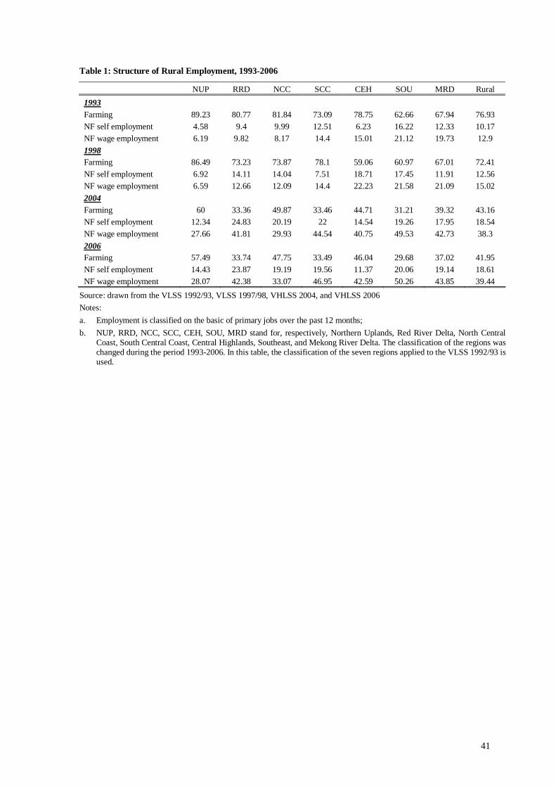
41
Table 1: Structure of Rural Employment, 1993-2006
NUP RRD NCC SCC CEH SOU MRD Rural 1993 Farming 89.23 80.77 81.84 73.09 78.75 62.66 67.94 76.93 NF self employment 4.58 9.4 9.99 12.51 6.23 16.22 12.33 10.17 NF wage employment 6.19 9.82 8.17 14.4 15.01 21.12 19.73 12.9 1998 Farming 86.49 73.23 73.87 78.1 59.06 60.97 67.01 72.41 NF self employment 6.92 14.11 14.04 7.51 18.71 17.45 11.91 12.56 NF wage employment 6.59 12.66 12.09 14.4 22.23 21.58 21.09 15.02 2004 Farming 60 33.36 49.87 33.46 44.71 31.21 39.32 43.16 NF self employment 12.34 24.83 20.19 22 14.54 19.26 17.95 18.54 NF wage employment 27.66 41.81 29.93 44.54 40.75 49.53 42.73 38.3 2006 Farming 57.49 33.74 47.75 33.49 46.04 29.68 37.02 41.95 NF self employment 14.43 23.87 19.19 19.56 11.37 20.06 19.14 18.61 NF wage employment 28.07 42.38 33.07 46.95 42.59 50.26 43.85 39.44
Source: drawn from the VLSS 1992/93, VLSS 1997/98, VHLSS 2004, and VHLSS 2006 Notes: a. Employment is classified on the basic of primary jobs over the past 12 months; b. NUP, RRD, NCC, SCC, CEH, SOU, MRD stand for, respectively, Northern Uplands, Red River Delta, North Central
Coast, South Central Coast, Central Highlands, Southeast, and Mekong River Delta. The classification of the regions was changed during the period 1993-2006. In this table, the classification of the seven regions applied to the VLSS 1992/93 is used.
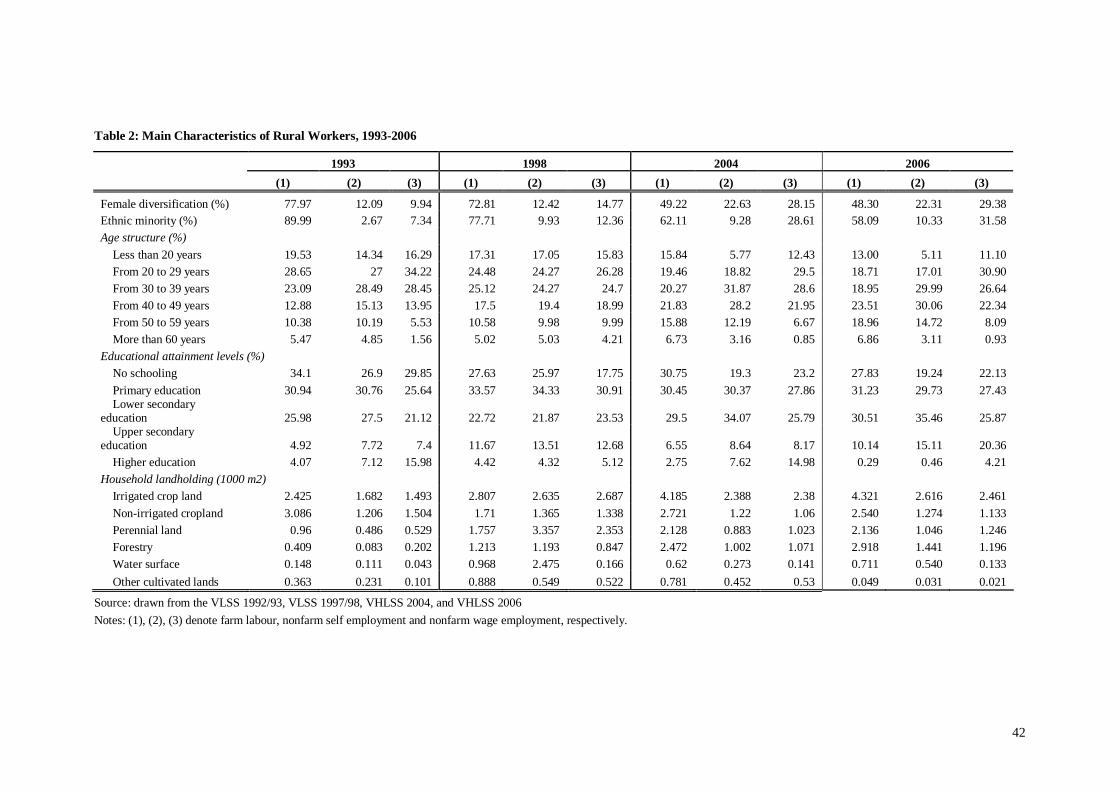
42
Table 2: Main Characteristics of Rural Workers, 1993-2006
1993 1998 2004 2006 (1) (2) (3) (1) (2) (3) (1) (2) (3) (1) (2) (3)
Female diversification (%) 77.97 12.09 9.94 72.81 12.42 14.77 49.22 22.63 28.15 48.30 22.31 29.38 Ethnic minority (%) 89.99 2.67 7.34 77.71 9.93 12.36 62.11 9.28 28.61 58.09 10.33 31.58 Age structure (%)
Less than 20 years 19.53 14.34 16.29 17.31 17.05 15.83 15.84 5.77 12.43 13.00 5.11 11.10 From 20 to 29 years 28.65 27 34.22 24.48 24.27 26.28 19.46 18.82 29.5 18.71 17.01 30.90 From 30 to 39 years 23.09 28.49 28.45 25.12 24.27 24.7 20.27 31.87 28.6 18.95 29.99 26.64 From 40 to 49 years 12.88 15.13 13.95 17.5 19.4 18.99 21.83 28.2 21.95 23.51 30.06 22.34 From 50 to 59 years 10.38 10.19 5.53 10.58 9.98 9.99 15.88 12.19 6.67 18.96 14.72 8.09 More than 60 years 5.47 4.85 1.56 5.02 5.03 4.21 6.73 3.16 0.85 6.86 3.11 0.93
Educational attainment levels (%) No schooling 34.1 26.9 29.85 27.63 25.97 17.75 30.75 19.3 23.2 27.83 19.24 22.13 Primary education 30.94 30.76 25.64 33.57 34.33 30.91 30.45 30.37 27.86 31.23 29.73 27.43 Lower secondary
education 25.98 27.5 21.12 22.72 21.87 23.53 29.5 34.07 25.79 30.51 35.46 25.87 Upper secondary
education 4.92 7.72 7.4 11.67 13.51 12.68 6.55 8.64 8.17 10.14 15.11 20.36 Higher education 4.07 7.12 15.98 4.42 4.32 5.12 2.75 7.62 14.98 0.29 0.46 4.21
Household landholding (1000 m2) Irrigated crop land 2.425 1.682 1.493 2.807 2.635 2.687 4.185 2.388 2.38 4.321 2.616 2.461 Non-irrigated cropland 3.086 1.206 1.504 1.71 1.365 1.338 2.721 1.22 1.06 2.540 1.274 1.133 Perennial land 0.96 0.486 0.529 1.757 3.357 2.353 2.128 0.883 1.023 2.136 1.046 1.246 Forestry 0.409 0.083 0.202 1.213 1.193 0.847 2.472 1.002 1.071 2.918 1.441 1.196 Water surface 0.148 0.111 0.043 0.968 2.475 0.166 0.62 0.273 0.141 0.711 0.540 0.133 Other cultivated lands 0.363 0.231 0.101 0.888 0.549 0.522 0.781 0.452 0.53 0.049 0.031 0.021
Source: drawn from the VLSS 1992/93, VLSS 1997/98, VHLSS 2004, and VHLSS 2006 Notes: (1), (2), (3) denote farm labour, nonfarm self employment and nonfarm wage employment, respectively.

43
Table 3: Share of Nonfarm Income in Vietnam and Other Developing Countries
Country Years Share of nonfarm incomes (%) Africa (average) a (various) 42
Botswana 1 1985-86 77 Burkina Faso 2 1981-84 37 Ethiopia 3 1989-90 36 Kenya (central) 4 1974-75 42 Tanzania 5 1980 25 Uganda (Mbale district) 6 2001 50
Latin America (average) a (various) 40 Chile 7 1990 32 Mexico 8 1992 50 Mexico 8 2004 76 Ecuador 9 1995 41
Asia (average) a (various) 32 Pakistan 10 1988-89 31 India 11 1993-94 34 China (Guangdong) 12 1989 34 Philippines (Mindanao) 12 1984-85 23
Vietnam b 1993-2004 38 Vietnam 1993 32 Vietnam 2004 52 Vietnam 2006c 54
Sources: a average figures: Haggblade, Hazell, and Reardon (2006); 1: Botswana: Valentine (1993); 2: Burkina Faso: Reardon et al. (1992); 3: Ethiopia: Webb and von Braun (1994); 4: Kenya: Collier and Lal (1986); 5: Tanzania: Collier et al. (1990); 6: Uganda: Ellis and Bahiigwa (2003); 7: Chile: Berdegue et al. (2001); 8: Mexico: Verner (2005); 9: Ecuador: Lanjouw and Lanjouw (2001); 10: Pakistan: Adams and He (1995); 11: India: Lanjouw and Shariff (2004); 12: China and Philippines: Delgado and Siamwalla (1997); b: own calculations for Vietnam; c the 2006 figure is rough estimate and subject to further adjustment.
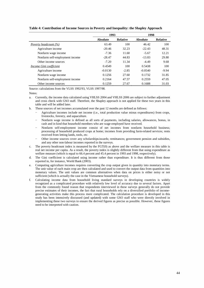
44
Table 4: Contribution of Income Sources in Poverty and Inequality: the Shapley Approach
1993 1998 Absolute Relative Absolute Relative
Poverty headcount (%) 63.49 100 46.42 100 Agriculture income -20.46 32.23 -22.43 48.31 Nonfarm wage income -7.36 11.60 -5.67 12.21 Nonfarm self-employment income -28.47 44.83 -13.83 29.80 Other income sources -7.20 11.34 -4.49 9.68
Income Gini coefficient 0.4549 100 0.5438 100 Agriculture income -0.0130 -2.85 -0.0540 -9.94 Nonfarm wage income 0.1256 27.60 0.1732 31.85 Nonfarm self-employment income 0.2164 47.57 0.2559 47.05 Other income sources 0.1259 27.67 0.1688 31.03
Source: calculations from the VLSS 1992/93, VLSS 1997/98. Notes: a. Currently, the income data calculated using VHLSS 2004 and VHLSS 2006 are subject to further adjustment
and cross check with GSO staff. Therefore, the Shapley approach is not applied for these two years in this table and will be added later.
b. These sources of net incomes accumulated over the past 12 months are defined as follows: − Agriculture incomes include net income (i.e., total production value minus expenditures) from crops,
livestocks, forestry, and aquaculture. − Nonfarm wage income is defined as all sorts of payments, including salaries, allowances, bonus, in
cash and in kind that household members who are wage-employed have received. − Nonfarm self-employment income consist of net incomes from nonfarm household business;
processing of household produced crops at home; incomes from providing farm-related services; rents received from letting lands, tools, etc.
− Other income sources cover any scholarships/awards; remittances; government pension and subsidies, and any other non-labour incomes reported in the surveys.
c. The poverty headcount index is measured by the FGT(0) as above and the welfare measure in this table is real net income per capita. As a result, the poverty index is slightly different from that using expenditure as welfare measure (which is equal to 66.4 percent and 45.4 percent in 1993 and 1998, respectively).
d. The Gini coefficient is calculated using income rather than expenditure. It is thus different from those reported in, for instance, World Bank (2003).
e. Computing agriculture incomes requires converting the crop output given in quantity into monetary terms. The unit value of each main crop are then calculated and used to convert the output data from quantities into monetary values. The unit values are common alternatives when data on prices is either noisy or not sufficient (which is actually the case in the Vietnamese household surveys).
f. Calculating income data from household living standard surveys in developing countries is widely recognized as a complicated procedure with relatively low level of accuracy due to several factors. Apart from the commonly found reason that respondents interviewed in these surveys generally do not provide precise estimates of their incomes, the fact that rural households rely on a diversified portfolio of income-generating activities make this process more complicated. The calculation procedure is developed in this study has been intensively discussed (and updated) with some GSO staff who were directly involved in implementing these two surveys to ensure the derived figures as precise as possible. However, these figures need to be interpreted with caution.
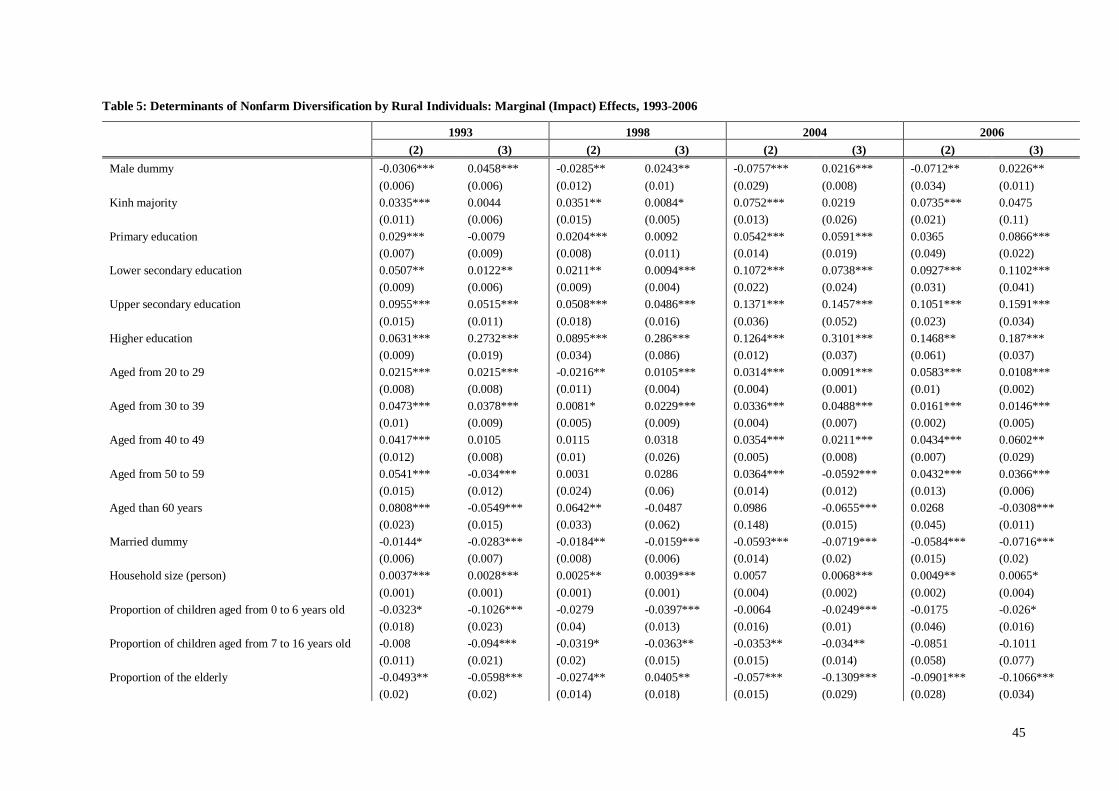
45
Table 5: Determinants of Nonfarm Diversification by Rural Individuals: Marginal (Impact) Effects, 1993-2006
1993 1998 2004 2006 (2) (3) (2) (3) (2) (3) (2) (3) Male dummy -0.0306*** 0.0458*** -0.0285** 0.0243** -0.0757*** 0.0216*** -0.0712** 0.0226** (0.006) (0.006) (0.012) (0.01) (0.029) (0.008) (0.034) (0.011) Kinh majority 0.0335*** 0.0044 0.0351** 0.0084* 0.0752*** 0.0219 0.0735*** 0.0475 (0.011) (0.006) (0.015) (0.005) (0.013) (0.026) (0.021) (0.11) Primary education 0.029*** -0.0079 0.0204*** 0.0092 0.0542*** 0.0591*** 0.0365 0.0866*** (0.007) (0.009) (0.008) (0.011) (0.014) (0.019) (0.049) (0.022) Lower secondary education 0.0507** 0.0122** 0.0211** 0.0094*** 0.1072*** 0.0738*** 0.0927*** 0.1102*** (0.009) (0.006) (0.009) (0.004) (0.022) (0.024) (0.031) (0.041) Upper secondary education 0.0955*** 0.0515*** 0.0508*** 0.0486*** 0.1371*** 0.1457*** 0.1051*** 0.1591*** (0.015) (0.011) (0.018) (0.016) (0.036) (0.052) (0.023) (0.034) Higher education 0.0631*** 0.2732*** 0.0895*** 0.286*** 0.1264*** 0.3101*** 0.1468** 0.187*** (0.009) (0.019) (0.034) (0.086) (0.012) (0.037) (0.061) (0.037) Aged from 20 to 29 0.0215*** 0.0215*** -0.0216** 0.0105*** 0.0314*** 0.0091*** 0.0583*** 0.0108*** (0.008) (0.008) (0.011) (0.004) (0.004) (0.001) (0.01) (0.002) Aged from 30 to 39 0.0473*** 0.0378*** 0.0081* 0.0229*** 0.0336*** 0.0488*** 0.0161*** 0.0146*** (0.01) (0.009) (0.005) (0.009) (0.004) (0.007) (0.002) (0.005) Aged from 40 to 49 0.0417*** 0.0105 0.0115 0.0318 0.0354*** 0.0211*** 0.0434*** 0.0602** (0.012) (0.008) (0.01) (0.026) (0.005) (0.008) (0.007) (0.029) Aged from 50 to 59 0.0541*** -0.034*** 0.0031 0.0286 0.0364*** -0.0592*** 0.0432*** 0.0366*** (0.015) (0.012) (0.024) (0.06) (0.014) (0.012) (0.013) (0.006) Aged than 60 years 0.0808*** -0.0549*** 0.0642** -0.0487 0.0986 -0.0655*** 0.0268 -0.0308*** (0.023) (0.015) (0.033) (0.062) (0.148) (0.015) (0.045) (0.011) Married dummy -0.0144* -0.0283*** -0.0184** -0.0159*** -0.0593*** -0.0719*** -0.0584*** -0.0716*** (0.006) (0.007) (0.008) (0.006) (0.014) (0.02) (0.015) (0.02) Household size (person) 0.0037*** 0.0028*** 0.0025** 0.0039*** 0.0057 0.0068*** 0.0049** 0.0065* (0.001) (0.001) (0.001) (0.001) (0.004) (0.002) (0.002) (0.004) Proportion of children aged from 0 to 6 years old -0.0323* -0.1026*** -0.0279 -0.0397*** -0.0064 -0.0249*** -0.0175 -0.026* (0.018) (0.023) (0.04) (0.013) (0.016) (0.01) (0.046) (0.016) Proportion of children aged from 7 to 16 years old -0.008 -0.094*** -0.0319* -0.0363** -0.0353** -0.034** -0.0851 -0.1011 (0.011) (0.021) (0.02) (0.015) (0.015) (0.014) (0.058) (0.077) Proportion of the elderly -0.0493** -0.0598*** -0.0274** 0.0405** -0.057*** -0.1309*** -0.0901*** -0.1066*** (0.02) (0.02) (0.014) (0.018) (0.015) (0.029) (0.028) (0.034)
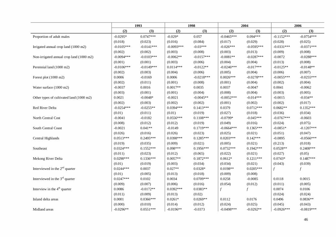
46
1993 1998 2004 2006 (2) (3) (2) (3) (2) (3) (2) (3) Proportion of adult males -0.0295* 0.0747*** -0.029* 0.057 -0.0465*** 0.094*** -0.1152*** -0.0754*** (0.018) (0.023) (0.016) (0.084) (0.017) (0.029) (0.028) (0.025) Irrigated annual crop land (1000 m2) -0.0105*** -0.0141*** -0.0093*** -0.03*** -0.026*** -0.0595*** -0.0331*** -0.0371*** (0.002) (0.002) (0.003) (0.008) (0.003) (0.013) (0.009) (0.008) Non-irrigated annual crop land (1000 m2) -0.0094*** -0.0103*** -0.0062** -0.0157*** -0.0081** -0.0287*** -0.0072 -0.0288*** (0.001) (0.001) (0.003) (0.006) (0.004) (0.004) (0.013) (0.008) Perennial land (1000 m2) -0.0106*** -0.0149*** 0.0114*** -0.0122** -0.0246*** -0.017*** -0.0125** -0.0148** (0.002) (0.003) (0.004) (0.006) (0.005) (0.004) (0.006) (0.007) Forest plot (1000 m2) 0.0006 -0.0169 0.0006 -0.0218*** 0.0026*** -0.0278*** -0.0055*** -0.0255*** (0.002) (0.011) (0.001) (0.008) (0.001) (0.004) (0.002) (0.004) Water surface (1000 m2) -0.0037 0.0016 0.0017** 0.0035 0.0037 -0.0047 0.0041 -0.0062 (0.003) (0.001) (0.001) (0.004) (0.008) (0.004) (0.003) (0.005) Other types of cultivated land (1000 m2) 0.0021 -0.0048* -0.0021 -0.0045** -0.0052*** -0.014*** -0.0015 -0.034** (0.002) (0.003) (0.002) (0.002) (0.001) (0.002) (0.002) (0.017) Red River Delta -0.0254*** -0.0255** 0.0394*** 0.1413*** 0.0379 0.0712*** 0.0682** 0.1352*** (0.01) (0.011) (0.01) (0.019) (0.027) (0.018) (0.036) (0.034) North Central Cost -0.0041 -0.0182 0.0556*** 0.1108*** -0.0799* -0.045*** -0.0767*** -0.0603 (0.008) (0.012) (0.012) (0.019) (0.049) (0.016) (0.024) (0.075) South Central Coast -0.0021 0.041** -0.0149 0.1719*** -0.0664*** 0.1365*** -0.0851* -0.1207*** (0.026) (0.016) (0.026) (0.023) (0.025) (0.021) (0.051) (0.047) Central Highlands 0.0513*** 0.2495*** 0.0398*** 0.1285*** 0.0203*** 0.142*** -0.0895 -0.0566*** (0.019) (0.035) (0.009) (0.021) (0.005) (0.021) (0.213) (0.018) Southeast 0.0324*** 0.1552*** 0.098*** 0.1956*** 0.0732*** 0.1942*** 0.0528** 0.2408*** (0.011) (0.023) (0.012) (0.065) (0.022) (0.021) (0.027) (0.05) Mekong River Delta 0.0298*** 0.1336*** 0.0057** 0.1872*** 0.0612* 0.1211*** 0.0743* 0.1487*** (0.01) (0.019) (0.003) (0.034) (0.034) (0.021) (0.043) (0.039) Interviewed in the 2nd quarter 0.0244*** 0.0037 0.027** 0.0328* 0.0198** 0.0205*** f f (0.01) (0.005) (0.013) (0.018) (0.009) (0.008) Interviewed in the 3rd quarter 0.0247*** 0.0102 0.0034 0.0709*** 0.0258 -0.0085 0.0118 0.0015 (0.009) (0.007) (0.006) (0.016) (0.054) (0.012) (0.011) (0.005) Interview in the 4th quarter 0.0086 -0.0172** 0.0392*** 0.0383** f f 0.0074 0.0106 (0.011) (0.009) (0.013) (0.02) (0.024) (0.024) Inland delta areas 0.0001 0.0366*** 0.0261* 0.0269** 0.0112 0.0176 0.0496 0.0836** (0.000) (0.010) (0.014) (0.012) (0.024) (0.025) (0.045) (0.043) Midland areas -0.0296** 0.0551*** -0.0196** -0.0373 -0.0498*** -0.0292** -0.0926*** -0.0819***
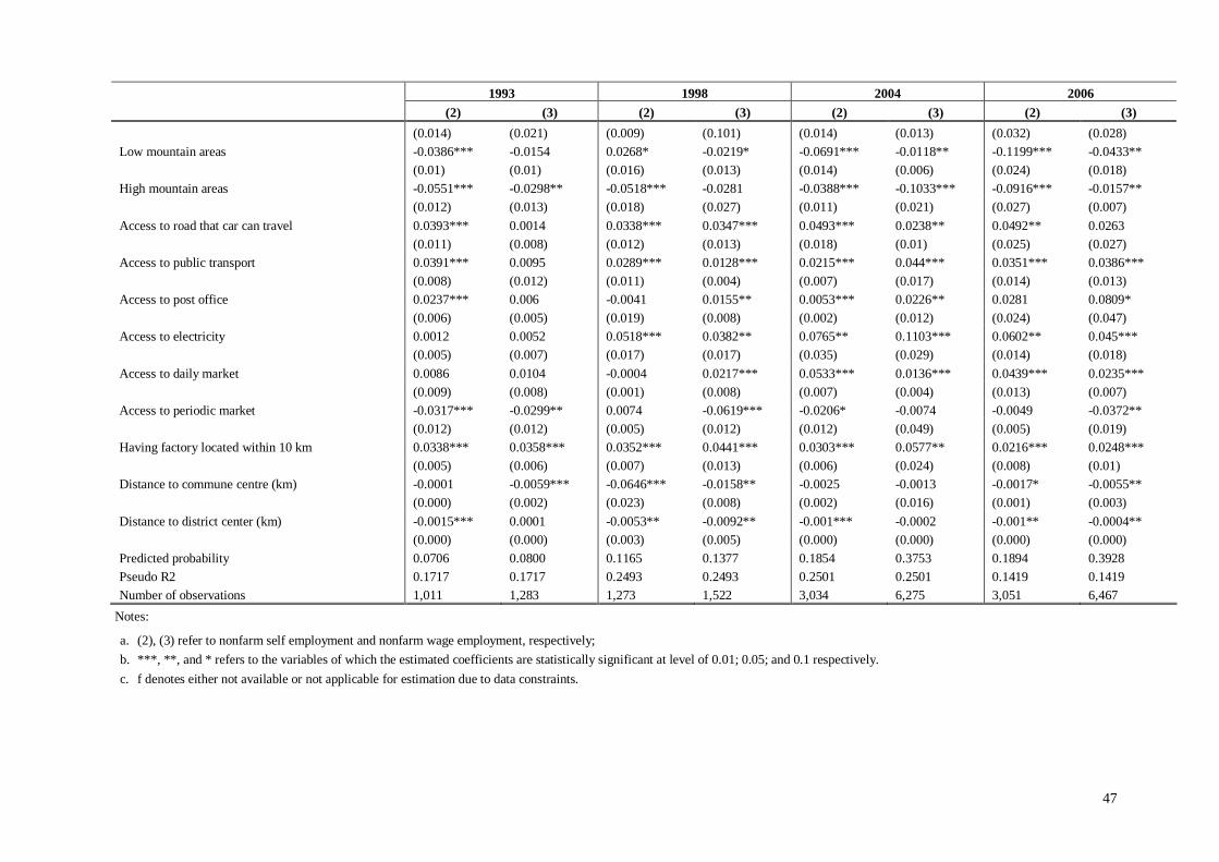
47
1993 1998 2004 2006 (2) (3) (2) (3) (2) (3) (2) (3) (0.014) (0.021) (0.009) (0.101) (0.014) (0.013) (0.032) (0.028) Low mountain areas -0.0386*** -0.0154 0.0268* -0.0219* -0.0691*** -0.0118** -0.1199*** -0.0433** (0.01) (0.01) (0.016) (0.013) (0.014) (0.006) (0.024) (0.018) High mountain areas -0.0551*** -0.0298** -0.0518*** -0.0281 -0.0388*** -0.1033*** -0.0916*** -0.0157** (0.012) (0.013) (0.018) (0.027) (0.011) (0.021) (0.027) (0.007) Access to road that car can travel 0.0393*** 0.0014 0.0338*** 0.0347*** 0.0493*** 0.0238** 0.0492** 0.0263 (0.011) (0.008) (0.012) (0.013) (0.018) (0.01) (0.025) (0.027) Access to public transport 0.0391*** 0.0095 0.0289*** 0.0128*** 0.0215*** 0.044*** 0.0351*** 0.0386*** (0.008) (0.012) (0.011) (0.004) (0.007) (0.017) (0.014) (0.013) Access to post office 0.0237*** 0.006 -0.0041 0.0155** 0.0053*** 0.0226** 0.0281 0.0809* (0.006) (0.005) (0.019) (0.008) (0.002) (0.012) (0.024) (0.047) Access to electricity 0.0012 0.0052 0.0518*** 0.0382** 0.0765** 0.1103*** 0.0602** 0.045*** (0.005) (0.007) (0.017) (0.017) (0.035) (0.029) (0.014) (0.018) Access to daily market 0.0086 0.0104 -0.0004 0.0217*** 0.0533*** 0.0136*** 0.0439*** 0.0235*** (0.009) (0.008) (0.001) (0.008) (0.007) (0.004) (0.013) (0.007) Access to periodic market -0.0317*** -0.0299** 0.0074 -0.0619*** -0.0206* -0.0074 -0.0049 -0.0372** (0.012) (0.012) (0.005) (0.012) (0.012) (0.049) (0.005) (0.019) Having factory located within 10 km 0.0338*** 0.0358*** 0.0352*** 0.0441*** 0.0303*** 0.0577** 0.0216*** 0.0248*** (0.005) (0.006) (0.007) (0.013) (0.006) (0.024) (0.008) (0.01) Distance to commune centre (km) -0.0001 -0.0059*** -0.0646*** -0.0158** -0.0025 -0.0013 -0.0017* -0.0055** (0.000) (0.002) (0.023) (0.008) (0.002) (0.016) (0.001) (0.003) Distance to district center (km) -0.0015*** 0.0001 -0.0053** -0.0092** -0.001*** -0.0002 -0.001** -0.0004** (0.000) (0.000) (0.003) (0.005) (0.000) (0.000) (0.000) (0.000) Predicted probability 0.0706 0.0800 0.1165 0.1377 0.1854 0.3753 0.1894 0.3928 Pseudo R2 0.1717 0.1717 0.2493 0.2493 0.2501 0.2501 0.1419 0.1419 Number of observations 1,011 1,283 1,273 1,522 3,034 6,275 3,051 6,467
Notes:
a. (2), (3) refer to nonfarm self employment and nonfarm wage employment, respectively; b. ***, **, and * refers to the variables of which the estimated coefficients are statistically significant at level of 0.01; 0.05; and 0.1 respectively. c. f denotes either not available or not applicable for estimation due to data constraints.
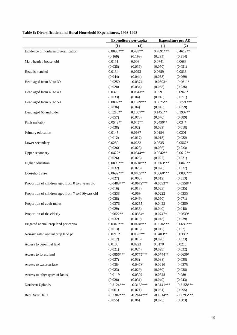
48
Table 6: Diversification and Rural Household Expenditures, 1993-1998
Expenditure per capita Expenditure per AE (1) (2) (1) (2)
Incidence of nonfarm diversification 0.8088*** 0.433** 0.7891*** 0.4612** (0.169) (0.199) (0.235) (0.214) Male headed household 0.0151 0.008 0.0741 0.0688 (0.035) (0.036) (0.050) (0.051) Head is married 0.0134 0.0022 0.0689 0.0838 (0.044) (0.044) (0.068) (0.069) Head aged from 30 to 39 -0.0250 -0.0374 -0.0593* -0.0611* (0.028) (0.034) (0.035) (0.036) Head aged from 40 to 49 0.0325 0.0843** 0.0291 0.0948* (0.033) (0.04) (0.043) (0.051) Head aged from 50 to 59 0.0897** 0.1329*** 0.0825** 0.1721*** (0.036) (0.04) (0.043) (0.059) Head aged 60 and older 0.1216** 0.1657** 0.1451** 0.1907** (0.057) (0.078) (0.076) (0.089) Kinh majority 0.0549** 0.045** 0.0450** 0.034* (0.028) (0.02) (0.023) (0.018) Primary education 0.0145 0.0167 0.0184 0.0201 (0.012) (0.017) (0.015) (0.022) Lower secondary 0.0280 0.0282 0.0535 0.0567* (0.026) (0.028) (0.036) (0.033) Upper secondary 0.0422* 0.0544** 0.0542** 0.0612** (0.026) (0.023) (0.027) (0.031) Higher education 0.0809*** 0.0718*** 0.0663*** 0.0849** (0.032) (0.028) (0.028) (0.037) Household size 0.0692*** 0.0405*** 0.0860*** 0.0885*** (0.027) (0.008) (0.012) (0.013) Proportion of children aged from 0 to 6 years old -0.0483*** -0.0672*** -0.0533** -0.0558** (0.016) (0.018) (0.023) (0.025) Proportion of children aged from 7 to 616years old -0.0538 -0.069 -0.0222 -0.0335 (0.038) (0.049) (0.060) (0.071) Proportion of adult males -0.0376 -0.0255 -0.0423 -0.0259 (0.029) (0.036) (0.040) (0.048) Proportion of the elderly -0.0622** -0.0334* -0.0747* -0.0639* (0.032) (0.019) (0.045) (0.039) Irrigated annual crop land per capita 0.0340*** 0.0478*** 0.0536*** 0.0686*** (0.013) (0.015) (0.017) (0.02) Non-irrigated annual crop land pc. 0.0215* 0.0327** 0.0403** 0.0386* (0.012) (0.016) (0.020) (0.023) Access to perennial land 0.0188 0.0223 0.0170 0.0210 (0.021) (0.024) (0.029) (0.032) Access to forest land -0.0856*** -0.0775*** -0.0744** -0.0639* (0.027) (0.03) (0.038) (0.038) Access to watersurface -0.0354 -0.0478* -0.0210 -0.0375 (0.023) (0.029) (0.030) (0.038) Access to other types of lands -0.0119 -0.0302 -0.0628 -0.0801 (0.028) (0.031) (0.040) (0.043) Northern Uplands -0.3124*** -0.3138*** -0.3141*** -0.3158*** (0.061) (0.071) (0.081) (0.095) Red River Delta -0.2302*** -0.2644*** -0.1914** -0.2295*** (0.055) (0.06) (0.075) (0.083)
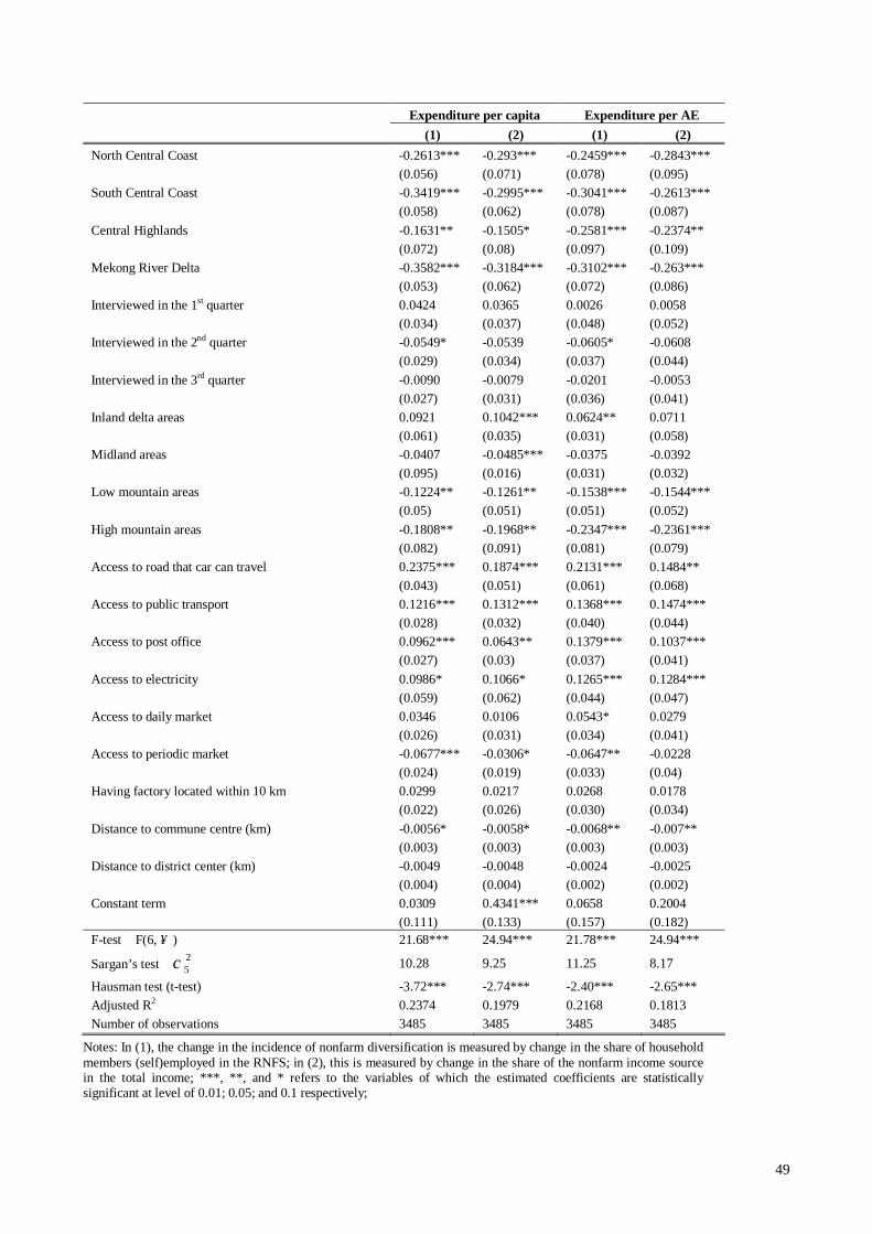
49
Expenditure per capita Expenditure per AE (1) (2) (1) (2)
North Central Coast -0.2613*** -0.293*** -0.2459*** -0.2843*** (0.056) (0.071) (0.078) (0.095) South Central Coast -0.3419*** -0.2995*** -0.3041*** -0.2613*** (0.058) (0.062) (0.078) (0.087) Central Highlands -0.1631** -0.1505* -0.2581*** -0.2374** (0.072) (0.08) (0.097) (0.109) Mekong River Delta -0.3582*** -0.3184*** -0.3102*** -0.263*** (0.053) (0.062) (0.072) (0.086) Interviewed in the 1st quarter 0.0424 0.0365 0.0026 0.0058 (0.034) (0.037) (0.048) (0.052) Interviewed in the 2nd quarter -0.0549* -0.0539 -0.0605* -0.0608 (0.029) (0.034) (0.037) (0.044) Interviewed in the 3rd quarter -0.0090 -0.0079 -0.0201 -0.0053 (0.027) (0.031) (0.036) (0.041) Inland delta areas 0.0921 0.1042*** 0.0624** 0.0711 (0.061) (0.035) (0.031) (0.058) Midland areas -0.0407 -0.0485*** -0.0375 -0.0392 (0.095) (0.016) (0.031) (0.032) Low mountain areas -0.1224** -0.1261** -0.1538*** -0.1544*** (0.05) (0.051) (0.051) (0.052) High mountain areas -0.1808** -0.1968** -0.2347*** -0.2361*** (0.082) (0.091) (0.081) (0.079) Access to road that car can travel 0.2375*** 0.1874*** 0.2131*** 0.1484** (0.043) (0.051) (0.061) (0.068) Access to public transport 0.1216*** 0.1312*** 0.1368*** 0.1474*** (0.028) (0.032) (0.040) (0.044) Access to post office 0.0962*** 0.0643** 0.1379*** 0.1037*** (0.027) (0.03) (0.037) (0.041) Access to electricity 0.0986* 0.1066* 0.1265*** 0.1284*** (0.059) (0.062) (0.044) (0.047) Access to daily market 0.0346 0.0106 0.0543* 0.0279 (0.026) (0.031) (0.034) (0.041) Access to periodic market -0.0677*** -0.0306* -0.0647** -0.0228 (0.024) (0.019) (0.033) (0.04) Having factory located within 10 km 0.0299 0.0217 0.0268 0.0178 (0.022) (0.026) (0.030) (0.034) Distance to commune centre (km) -0.0056* -0.0058* -0.0068** -0.007** (0.003) (0.003) (0.003) (0.003) Distance to district center (km) -0.0049 -0.0048 -0.0024 -0.0025 (0.004) (0.004) (0.002) (0.002) Constant term 0.0309 0.4341*** 0.0658 0.2004 (0.111) (0.133) (0.157) (0.182) F-test ∼ F(6, ∞ ) 21.68*** 24.94*** 21.78*** 24.94***
Sargan’s test ∼ 25χ 10.28 9.25 11.25 8.17
Hausman test (t-test) -3.72*** -2.74*** -2.40*** -2.65*** Adjusted R2 0.2374 0.1979 0.2168 0.1813 Number of observations 3485 3485 3485 3485
Notes: In (1), the change in the incidence of nonfarm diversification is measured by change in the share of household members (self)employed in the RNFS; in (2), this is measured by change in the share of the nonfarm income source in the total income; ***, **, and * refers to the variables of which the estimated coefficients are statistically significant at level of 0.01; 0.05; and 0.1 respectively;
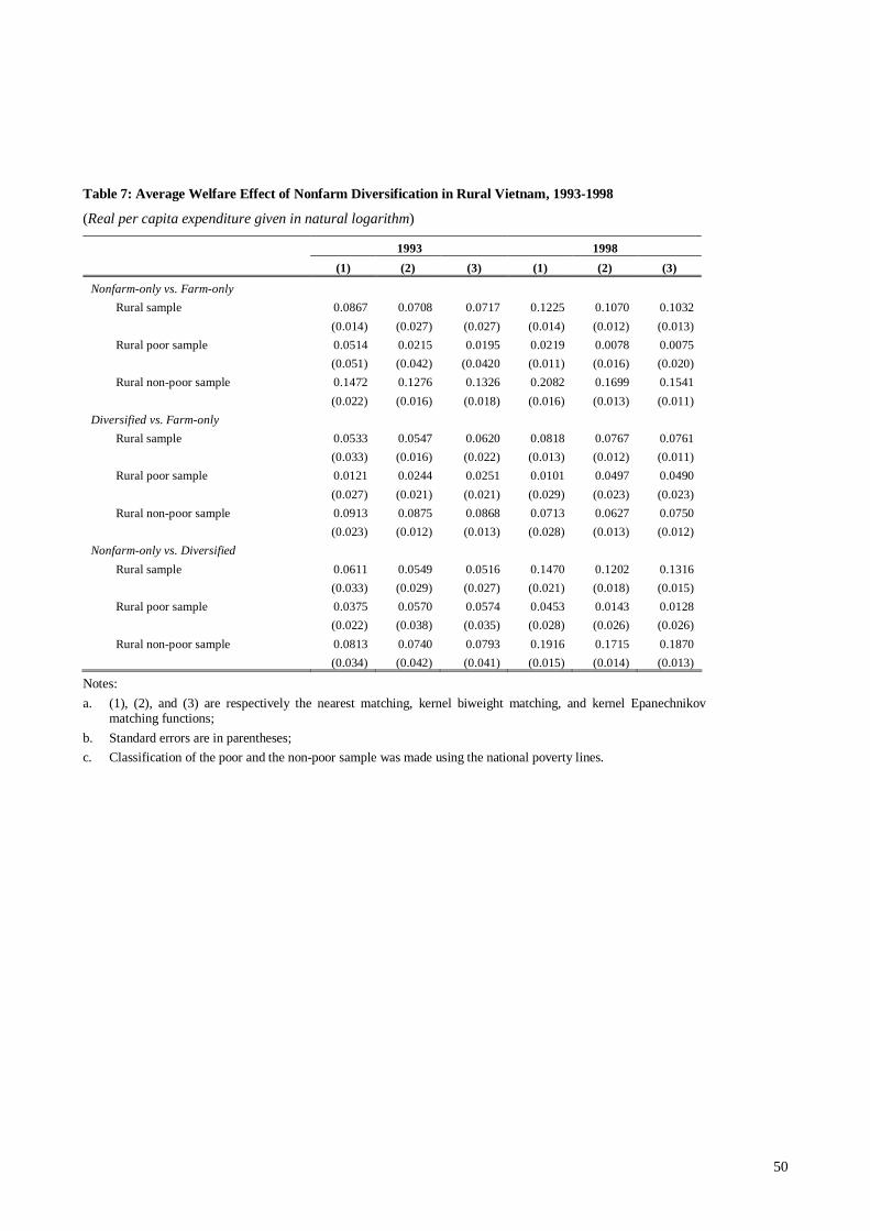
50
Table 7: Average Welfare Effect of Nonfarm Diversification in Rural Vietnam, 1993-1998
(Real per capita expenditure given in natural logarithm)
1993 1998 (1) (2) (3) (1) (2) (3)
Nonfarm-only vs. Farm-only Rural sample 0.0867 0.0708 0.0717 0.1225 0.1070 0.1032
(0.014) (0.027) (0.027) (0.014) (0.012) (0.013) Rural poor sample 0.0514 0.0215 0.0195 0.0219 0.0078 0.0075
(0.051) (0.042) (0.0420 (0.011) (0.016) (0.020) Rural non-poor sample 0.1472 0.1276 0.1326 0.2082 0.1699 0.1541
(0.022) (0.016) (0.018) (0.016) (0.013) (0.011) Diversified vs. Farm-only
Rural sample 0.0533 0.0547 0.0620 0.0818 0.0767 0.0761 (0.033) (0.016) (0.022) (0.013) (0.012) (0.011)
Rural poor sample 0.0121 0.0244 0.0251 0.0101 0.0497 0.0490 (0.027) (0.021) (0.021) (0.029) (0.023) (0.023)
Rural non-poor sample 0.0913 0.0875 0.0868 0.0713 0.0627 0.0750 (0.023) (0.012) (0.013) (0.028) (0.013) (0.012) Nonfarm-only vs. Diversified
Rural sample 0.0611 0.0549 0.0516 0.1470 0.1202 0.1316 (0.033) (0.029) (0.027) (0.021) (0.018) (0.015)
Rural poor sample 0.0375 0.0570 0.0574 0.0453 0.0143 0.0128 (0.022) (0.038) (0.035) (0.028) (0.026) (0.026)
Rural non-poor sample 0.0813 0.0740 0.0793 0.1916 0.1715 0.1870 (0.034) (0.042) (0.041) (0.015) (0.014) (0.013)
Notes: a. (1), (2), and (3) are respectively the nearest matching, kernel biweight matching, and kernel Epanechnikov
matching functions; b. Standard errors are in parentheses; c. Classification of the poor and the non-poor sample was made using the national poverty lines.
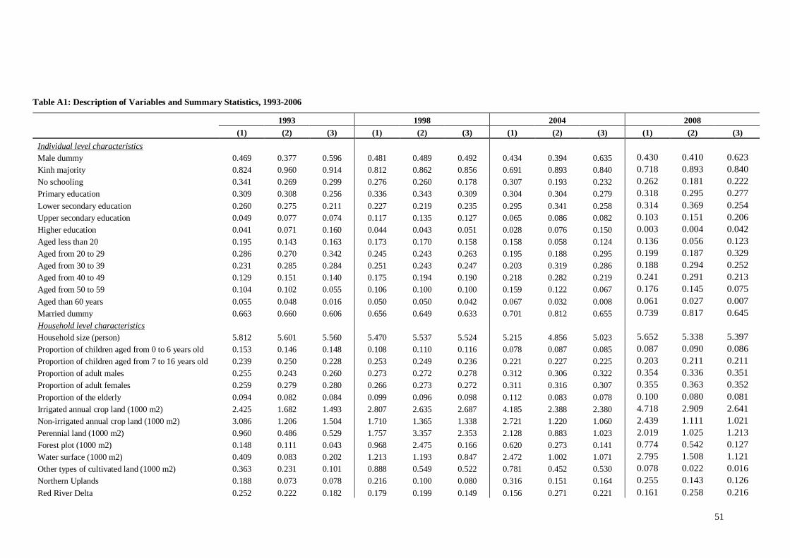
51
Table A1: Description of Variables and Summary Statistics, 1993-2006
1993 1998 2004 2008 (1) (2) (3) (1) (2) (3) (1) (2) (3) (1) (2) (3) Individual level characteristics Male dummy 0.469 0.377 0.596 0.481 0.489 0.492 0.434 0.394 0.635 0.430 0.410 0.623 Kinh majority 0.824 0.960 0.914 0.812 0.862 0.856 0.691 0.893 0.840 0.718 0.893 0.840 No schooling 0.341 0.269 0.299 0.276 0.260 0.178 0.307 0.193 0.232 0.262 0.181 0.222 Primary education 0.309 0.308 0.256 0.336 0.343 0.309 0.304 0.304 0.279 0.318 0.295 0.277 Lower secondary education 0.260 0.275 0.211 0.227 0.219 0.235 0.295 0.341 0.258 0.314 0.369 0.254 Upper secondary education 0.049 0.077 0.074 0.117 0.135 0.127 0.065 0.086 0.082 0.103 0.151 0.206 Higher education 0.041 0.071 0.160 0.044 0.043 0.051 0.028 0.076 0.150 0.003 0.004 0.042 Aged less than 20 0.195 0.143 0.163 0.173 0.170 0.158 0.158 0.058 0.124 0.136 0.056 0.123 Aged from 20 to 29 0.286 0.270 0.342 0.245 0.243 0.263 0.195 0.188 0.295 0.199 0.187 0.329 Aged from 30 to 39 0.231 0.285 0.284 0.251 0.243 0.247 0.203 0.319 0.286 0.188 0.294 0.252 Aged from 40 to 49 0.129 0.151 0.140 0.175 0.194 0.190 0.218 0.282 0.219 0.241 0.291 0.213 Aged from 50 to 59 0.104 0.102 0.055 0.106 0.100 0.100 0.159 0.122 0.067 0.176 0.145 0.075 Aged than 60 years 0.055 0.048 0.016 0.050 0.050 0.042 0.067 0.032 0.008 0.061 0.027 0.007 Married dummy 0.663 0.660 0.606 0.656 0.649 0.633 0.701 0.812 0.655 0.739 0.817 0.645 Household level characteristics Household size (person) 5.812 5.601 5.560 5.470 5.537 5.524 5.215 4.856 5.023 5.652 5.338 5.397 Proportion of children aged from 0 to 6 years old 0.153 0.146 0.148 0.108 0.110 0.116 0.078 0.087 0.085 0.087 0.090 0.086 Proportion of children aged from 7 to 16 years old 0.239 0.250 0.228 0.253 0.249 0.236 0.221 0.227 0.225 0.203 0.211 0.211 Proportion of adult males 0.255 0.243 0.260 0.273 0.272 0.278 0.312 0.306 0.322 0.354 0.336 0.351 Proportion of adult females 0.259 0.279 0.280 0.266 0.273 0.272 0.311 0.316 0.307 0.355 0.363 0.352 Proportion of the elderly 0.094 0.082 0.084 0.099 0.096 0.098 0.112 0.083 0.078 0.100 0.080 0.081 Irrigated annual crop land (1000 m2) 2.425 1.682 1.493 2.807 2.635 2.687 4.185 2.388 2.380 4.718 2.909 2.641 Non-irrigated annual crop land (1000 m2) 3.086 1.206 1.504 1.710 1.365 1.338 2.721 1.220 1.060 2.439 1.111 1.021 Perennial land (1000 m2) 0.960 0.486 0.529 1.757 3.357 2.353 2.128 0.883 1.023 2.019 1.025 1.213 Forest plot (1000 m2) 0.148 0.111 0.043 0.968 2.475 0.166 0.620 0.273 0.141 0.774 0.542 0.127 Water surface (1000 m2) 0.409 0.083 0.202 1.213 1.193 0.847 2.472 1.002 1.071 2.795 1.508 1.121 Other types of cultivated land (1000 m2) 0.363 0.231 0.101 0.888 0.549 0.522 0.781 0.452 0.530 0.078 0.022 0.016 Northern Uplands 0.188 0.073 0.078 0.216 0.100 0.080 0.316 0.151 0.164 0.255 0.143 0.126 Red River Delta 0.252 0.222 0.182 0.179 0.199 0.149 0.156 0.271 0.221 0.161 0.258 0.216
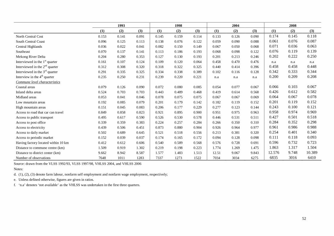
52
1993 1998 2004 2008 (1) (2) (3) (1) (2) (3) (1) (2) (3) (1) (2) (3) North Central Cost 0.153 0.141 0.091 0.145 0.159 0.114 0.133 0.126 0.090 0.174 0.145 0.118 South Central Coast 0.096 0.125 0.113 0.138 0.076 0.122 0.059 0.090 0.088 0.061 0.076 0.087 Central Highlands 0.036 0.022 0.041 0.082 0.150 0.149 0.067 0.050 0.068 0.071 0.036 0.063 Southeast 0.070 0.137 0.141 0.113 0.186 0.193 0.068 0.098 0.122 0.076 0.119 0.139 Mekong River Delta 0.204 0.280 0.353 0.127 0.130 0.193 0.201 0.213 0.246 0.202 0.222 0.250 Interviewed in the 1st quarter 0.161 0.107 0.124 0.109 0.120 0.064 0.458 0.470 0.476 n.a n.a n.a Interviewed in the 2nd quarter 0.312 0.308 0.320 0.318 0.322 0.325 0.440 0.414 0.396 0.458 0.458 0.448 Interviewed in the 3rd quarter 0.291 0.335 0.325 0.334 0.338 0.389 0.102 0.116 0.128 0.342 0.333 0.344 Interview in the 4th quarter 0.235 0.250 0.231 0.239 0.220 0.221 n.a n.a n.a 0.200 0.209 0.208 Commune level characteristics Coastal areas 0.079 0.126 0.090 0.072 0.080 0.085 0.054 0.077 0.067 0.066 0.103 0.067 Inland delta areas 0.524 0.703 0.703 0.443 0.489 0.468 0.419 0.614 0.568 0.426 0.612 0.582 Midland areas 0.053 0.041 0.046 0.078 0.075 0.075 0.067 0.067 0.069 0.064 0.067 0.078 Low mountain areas 0.192 0.085 0.079 0.201 0.179 0.142 0.182 0.119 0.152 0.201 0.119 0.152 High mountain areas 0.151 0.045 0.083 0.206 0.177 0.229 0.277 0.123 0.144 0.243 0.100 0.121 Access to road that car can travel 0.849 0.858 0.823 0.921 0.895 0.900 0.951 0.975 0.963 0.958 0.974 0.969 Access to public transport 0.495 0.617 0.590 0.526 0.530 0.578 0.446 0.531 0.511 0.427 0.501 0.518 Access to post office 0.339 0.359 0.383 0.224 0.257 0.284 0.266 0.350 0.310 0.284 0.352 0.298 Access to electricity 0.439 0.506 0.451 0.873 0.880 0.904 0.926 0.964 0.977 0.961 0.986 0.988 Access to daily market 0.502 0.689 0.645 0.521 0.518 0.556 0.213 0.381 0.320 0.254 0.401 0.340 Access to periodic market 0.152 0.039 0.037 0.174 0.165 0.172 0.094 0.128 0.098 0.111 0.118 0.093 Having factory located within 10 km 0.412 0.612 0.606 0.540 0.589 0.568 0.576 0.728 0.691 0.596 0.732 0.723 Distance to commune centre (km) 1.509 0.919 1.302 0.219 0.198 0.223 1.774 1.269 1.475 1.863 1.317 1.504 Distance to district center (km) 9.662 8.942 8.587 1.577 1.483 1.513 12.51 9.067 9.843 12.576 9.748 10.389 Number of observations 7648 1011 1283 7337 1273 1522 7034 3034 6275 6835 3016 6410
Source: drawn from the VLSS 1992/93, VLSS 1997/98, VHLSS 2004, and VHLSS 2006 Notes: d. (1), (2), (3) denote farm labour, nonfarm self employment and nonfarm wage employment, respectively; e. Unless defined otherwise, figures are given in ratios. f. ‘n.a’ denotes ‘not available’ as the VHLSS was undertaken in the first three quarters.

53
Table A2: Diagnostic Tests of the MNL Models
Small-Hsiao test for IIA assumption (Ho: outcomes are dependent from other alternatives)
Chi-squared P>Chi-squared Decision VLSS 1992/93
− Nonfarm self employment 246χ ∼ 36.92 0.8281 Accept Ho
− Nonfarm wage employment 246χ ∼ 48.46 0.3740 Accept Ho
− Farming 246χ ∼ 55.61 0.1567 Accept Ho
VLSS 1997/98
− Nonfarm self employment 246χ ∼ 31.97 0.9420 Accept Ho
− Nonfarm wage employment 246χ ∼ 44.85 0.5200 Accept Ho
− Farming 246χ ∼ 37.59 0.8070 Accept Ho
VHLSS 2004
− Nonfarm self employment 245χ ∼ 47.87 0.3968 Accept Ho
− Nonfarm wage employment 245χ ∼ 39.03 0.7569 Accept Ho
− Farming 245χ ∼ 54.04 0.1942 Accept Ho
VHLSS 2006
− Nonfarm self employment 245χ ∼ 56.42 0.118 Accept Ho
− Nonfarm wage employment 245χ ∼ 42.53 0.577 Accept Ho
− Farming 245χ ∼ 45.29 0.585 Accept Ho
Wald test for outcome combination (Ho: outcomes can be collapsed)
Chi-squared P>Chi-squared Decision VLSS 1992/93
− Nonfarm Self + Wage 245χ ∼ 367.84 0.0000 Reject Ho
− Nonfarm Self + Farming 245χ ∼ 629.32 0.0000 Reject Ho
− Nonfarm Wage + Farming 245χ ∼ 1141.00 0.0000 Reject Ho
VLSS 1997/98
− Nonfarm Self + Wage 245χ ∼ 162.86 0.0000 Reject Ho
− Nonfarm Self + Farming 245χ ∼ 352.21 0.0000 Reject Ho
− Nonfarm Wage + Farming 245χ ∼ 403.18 0.0000 Reject Ho
VHLSS 2004
− Nonfarm Self + Wage 244χ ∼ 1187.36 0.0000 Reject Ho
− Nonfarm Self + Farming 244χ ∼ 1344.04 0.0000 Reject Ho
− Nonfarm Wage + Farming 244χ ∼ 2501.14 0.0000 Reject Ho
VHLSS 2004
− Nonfarm Self + Wage 244χ ∼ 1251.04 0.0000 Reject Ho
− Nonfarm Self + Farming 244χ ∼ 1113.09 0.0000 Reject Ho
− Nonfarm Wage + Farming 244χ ∼ 2480.80 0.0000 Reject Ho
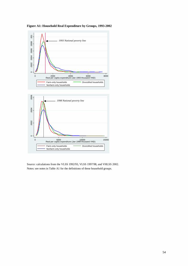
54
Figure A1: Household Real Expenditure by Groups, 1993-2002
0.0
002
.000
4.0
006
.000
8.0
01
0 2000 4000 6000 8000Real per capita expenditure (Jan 1993 thousand VND)
Farm-only households Diversified householdsNonfarm-only households
0.0
002
.000
4.0
006
0 5000 10000 15000Real per capita expenditure (Jan 1998 thousand VND)
Farm-only households Diversified householdsNonfarm-only households
Source: calculations from the VLSS 1992/93, VLSS 1997/98, and VHLSS 2002. Notes: see notes in Table A1 for the definitions of these household groups.
1993 National poverty line
1998 National poverty line